Pronatal Property Rights over Land and Fertility Outcomes · PDF filePronatal Property Rights...

Policy Research Working Paper 7419

Pronatal Property Rights over Land and Fertility Outcomes

Evidence from a Natural Experiment in Ethiopia

Daniel Ayalew AliKlaus Deininger

Niels Kemper

Development Research GroupAgriculture and Rural Development TeamSeptember 2015

WPS7419P

ublic

Dis

clos

ure

Aut

horiz

edP

ublic

Dis

clos

ure

Aut

horiz

edP

ublic

Dis

clos

ure

Aut

horiz

edP

ublic

Dis

clos

ure

Aut

horiz

ed

Produced by the Research Support Team

Abstract

The Policy Research Working Paper Series disseminates the findings of work in progress to encourage the exchange of ideas about development issues. An objective of the series is to get the findings out quickly, even if the presentations are less than fully polished. The papers carry the names of the authors and should be cited accordingly. The findings, interpretations, and conclusions expressed in this paper are entirely those of the authors. They do not necessarily represent the views of the International Bank for Reconstruction and Development/World Bank and its affiliated organizations, or those of the Executive Directors of the World Bank or the governments they represent.

Policy Research Working Paper 7419

This paper is a product of the Agriculture and Rural Development Team, Development Research Group. It is part of a larger effort by the World Bank to provide open access to its research and make a contribution to development policy discussions around the world. Policy Research Working Papers are also posted on the Web at http://econ.worldbank.org. The authors may be contacted at [email protected], [email protected] and [email protected].

This study exploits a natural experiment to investigate the impact of land reform on the fertility outcomes of households in rural Ethiopia. Public policies and customs created a situation where Ethiopian households could influence their usufruct rights to land via a demographic expansion of the family. The study evaluates the impact of the abolishment of these pronatal property rights on fertility outcomes. By matching aggregated census data

before and after the reform with administrative data on the reform, a difference-in-differences approach between reform and non-reform districts is used to assess the impact of the reform on fertility outcomes. The impact appears to be large. The study estimates that women in rural areas reduced their life-time fertility by 1.2 children due to the reform. Robustness checks show that the impact esti-mates are not biased by spillovers or policy endogeneity.

Pronatal Property Rights over Land and Fertility Outcomes: Evidence from a Natural Experiment in Ethiopia¶

Daniel Ayalew Ali*, Klaus Deininger*, Niels Kemper†

*Development Research Group, The World Bank†University of Mannheim, Department of Economics

JEL classification codes: J13, N50

Keywords: Property rights, Fertility, Ethiopia, Natural Experiment

¶ We are indebted to Gebeyehu Belay, Solomon Haile, Zerfu Hailu, Seid Nuru, and Dessalegn Rahmato for in-depth discussions on land reforms in Ethiopia. We thank conference participants at the World Bank's 15th Annual Research Conference on Land and Poverty and the Brown Bag Seminar in Development Economics at the Goethe University in Frankfurt. We thank Alexandra Avdeenko, Albrecht Bohne, Markus Frölich, Dany Jaimovich, Heiner Schumacher, Matthias Schündeln, and Pia Unte for valuable comments.

1 Introduction

“Through marriage or, more accurately, through fathering chil-dren whom he supports, a man thus gains access to a new set ofrights [to land].”(Hoben, 1973: p. 152)

After decades of research, no clear consensus has emerged on whether thenature of the relationship between population growth and economic welfare ispositive, negative or neutral (Birdsall et al., 2003). However, with respect tohuman reproduction, as the main driver of population growth, it can be statedwith somewhat more certainty that fertility is too high to be socially optimalif the social cost of children exceeds their private cost. These externalities mayarise in several situations. The following examples have been widely quoted inthe literature: First, the interrelation between population growth, poverty, andthe degradation of the local natural resource base, which is commonly associatedwith village economies in developing countries, may lead to a situation referredto in the literature as reproductive externalities (Dasgupta, 1993, 1995, 2000).Second, the so called congestion problem can occur if the present value of thecosts of public services, such as education, health, and infrastructure, exceedthe present value of a newborn child’s expected lifetime tax contribution. Thiscreates a condition in which each additional child dilutes the public servicesavailable to the other children (World Bank, 1984; Schultz, 1985). Third, sincechild and adult labor are substitutes, high fertility may lead to a low level wageequilibrium where children work and the wages of adults are depressed (Basuand Van, 1998). While such externalities are hard to observe, the case for policymakers seems to be clear. For instance, in 2013, 37 per cent of the countries inthe world pursued policies to lower the rate of population growth, the majorityof which can be found at the lower tail of the world income distribution (UNDESA, 2013).However, the question whether fertility rates can actually be reduced is still

open. In the long-run, the answer seems to be yes. Historically, fertility rateswere observed to drop as countries began to prosper, urbanize, and structurallychange during industrialization. Apparently, this observation is consistent withthe fact that high fertility rates are now mainly concentrating in sub-SaharanAfrica and South Asia (Maddison, 2006). In the short- and medium-term, publicpolices such as family planning information and services, entitlements, taxes,disincentives, and quota are being employed (Birdsall, 1988).1 In this paper,we draw attention to another domain of public policy, the arrangement andrearrangement of property rights, in influencing fertility rates. We do this inEthiopia, a country which has some of the highest fertility rates in the world.We draw on a natural experiment to evaluate the impact on fertility out-

comes of the abolishment of pronatal property rights. Historically, rules gov-erning access to land in the Amhara region of Ethiopia were pronatal. In thetraditional system of communal land governance, men could claim land on be-

1These programs have, however, mixed effects in lowering fertility rates. See McQueston etal. (2012) for a systematic review of the impact of interventions targeting fertility outcomes.

1

half of the women they were married to. These claims could not be substanti-ated through marriage per se, but the children they had had in the course ofthe marriage (Hoben, 1973). In the wake of a military coup, land governanceshifted from the communal to the state level. In 1974, a nationwide land reformnationalized and redistributed land on the basis of family size. In subsequentyears, family size prevailed as the most important criterion for communal landredistributions (Rahmato, 1994).2 Against this background, we evaluate the im-pact of a land reform implemented in 1997 in the southern part of the Amhararegion, which, surprisingly and unexpectedly, discontinued the historic practiceof primarily redistributing land based on family size. We consider the imple-mentation of the 1997 reform in Amhara as a quasi-experiment during whichthe southern part of the region implemented the 1997 reform, but the northernpart did not. The division of Amhara into reform and non-reform areas fol-lowed a process orthogonal to fertility rates and their determinants. BetweenSeptember 1989 and March 1991 a rebel group who later came into power, theEthiopian People’s Revolutionary Democratic Front (EPRDF), took control ofthe region of Amhara in two temporally distinct military campaigns. After theEPRDF and their allies came to power, the region of Amhara implemented alarge-scale land reform in 1997. However, this reform was only conducted inthe southern part of Amhara, which was conquered by the EPRDF during thesecond military campaign. A political decision was made that the northern partdid not need another land reform as there had been occasional redistributions,using family size as the main criterion, in the areas conquered by the EPRDFduring the first military campaign.We employ a difference-in-differences approach to estimate the impact of

the reform. We use panel data from the 1994 and 2007 Population and Hous-ing Censuses and match it with administrative data from the EnvironmentalProtection, Land Administration and Use Authority of the Amhara RegionalState. For the analysis, data on 2,303,198 individuals in the region of Amhara isaggregated into 212 district—time clusters. We compare the difference betweenthe reform and non-reform districts before and after the 1997 systematic landredistribution in the region. Our key outcome variable is the total fertility rateat the district level. We control for a variety of time varying observables as wellas district level heterogeneity to average out time invariant unobservables.Three assumptions need to be met for our estimates of the policy impact

2We would like to emphasize that the existence of pronatal property rights is not specificto this context. We have found indications for pronatal property rights in various countriesaround the world. In a number of countries in sub-Saharan Africa, a woman’s rights to the useof land are associated with her position as mother and wife. For instance, a woman’s rights toland may increase with the length of her marriage or with having more children. These rightsmay end with divorce, with widowhood, with the failure to have sons (Gray and Kevane, 1999;Guyer, 1986). In addition, it has been argued that in the Punjab, India, the caste systemimproves access to land for farmers with high fertility, especially for those with many sons(Mamdani, 1972). Furthermore, it was argued that granting rights to land on a usufruct basisin Mexican ejidos (agricultural communities) creates pronatal incentives, especially throughland retention, as larger families are less likely to be affected by land redistributions (De Vanyand Sanchez, 1979).

2

to be causal. First, in the absence of the implementation of the land reform,our estimate of the policy impact should be statistically indistinguishable fromzero, i.e., no other systematic factor should explain the change in fertility pat-terns between reform and non-reform districts we observe in the data. Giventhat the division of Amhara into reform and non-reform areas follows a veryspecific geographic pattern, we consider it rather unlikely that our estimatesactually pick up the effect of any other program, even if it was not uniformlyimplemented within the region of Amhara. Second, there is no contamination ofthe non-reform districts by the reform districts, e.g., there should be no change,due to influences from the reform districts, in aggregate fertility behavior at thedistrict level of the districts that were unexposed to the reform. The fact thatthe reform varies at the district level circumvents unobserved heterogeneity infertility behavior at the individual level, i.e., contamination is only an issue ifhouseholds in non-reform districts alter their fertility behavior systematicallyin the same direction because of influences from the exposed districts. As a ro-bustness check, we compare non-reform districts sharing a border with a reformdistrict to non-reform districts not sharing a border with a reform district in aplacebo differences-in-differences specification. Third, policy endogeneity mayaffect the adequacy of non-reform districts as a within-region control group,i.e., the selection of districts into the reform due to unobservable district char-acteristics. While we use fixed effects to average out time-constant unobservedheterogeneity and use the available data from the census to control for timevarying factors at the district level, there may still be a bias in the estimatesdue to time varying unobservables at the district level which are correlated withthe implementation of the reform and fertility rates. As a robustness check,we use the selection-on-observables approach (Altonji et al., 2005; Bellows andMiguel, 2008; Nunn, 2011) to assess whether the potential bias from time vary-ing unobservables drives the selection of districts into the reform.Our findings point towards a substantial effect of the land reform on fertility

outcomes. For the full sample, we estimate a 0.99 reduction in the total fertilityrate, i.e., a reduction of lifetime fertility by one child per woman. This result isclearly driven by the rural rather than the urban sample. For the rural sample,we estimate a 1.2 reduction in the total fertility rate. Looking at age-specificfertility rates, from which the total fertility rate is constructed, we find a clearreduction in fertility for virtually all age groups in the rural sample. The effectis particularly pronounced for women in the most fertile age groups, 25—29 and30—34. With respect to the mechanism at work, we argue that the arrangementof property rights over land before the reform led to a higher economic gainfrom children. It derived from children’s contributing to household wealth inan environment of otherwise weakly defined property rights. More specifically,if land is redistributed according to household size, land holdings and thuswealth depend positively on the number of children. Abolishing the positiverelationship between land and household size leads to a reduction in fertility.Furthermore, through robustness checks, we conclude that our impact estimatesare not downward biased due to spillovers from reform districts into non-reformdistricts. Furthermore, using a selection-on-observables approach, we find no

3

indication of a selection bias from unobservables.Our findings may also contribute to understanding a statistical oddity. The

population count in Amhara was 17.2 million according to the most recent censusin 2007 and clearly fell short of the offi cial government projection of 19.6 millionAmharans for that year. “The 2.5 million missing Amharans”were extensivelycovered in the national media and eventually resulted in fierce debates in theparliament with both opposition and ruling coalition members of parliamentcondemning the census as flawed, calling for a redo of the census, as Ethiopia isa federal state and population size affects the budget of its regions. A panel ofinternational experts reviewed the census, but were not able to spot any mistakesin its design or implementation.3 We conjecture that Ethiopia’s “2.5 millionmissing Amharans”is due to a violation of a crucial assumption underlying thecohort component method, a method commonly used by statistical agencies toproject the total population size for a future date from census data. The methodassumes a constant total fertility for the projection period. However, we finda substantial reduction in the total fertility rate from 4.9 to 3.9 in the reformdistricts, which indicates that the statistical oddity may at least partly be aconsequence of the land reform.The next section discusses the institutional setting and the natural experi-

ment. It also contains some theoretical considerations. Section 3 explains thedata as well as the empirical strategy. Section 4 discusses the findings andSection 5 draws some conclusions.

2 Institutional setting and some theoretical con-siderations

2.1 Pronatal property rights and land tenure in Amhara

In this section, we argue that the rules governing access to land in the Amhararegion were historically pronatal. Having children helped secure access to land inan environment of otherwise weakly defined property rights, no matter whetherland governance was communal or statal. However, pronatal policies for landtenure were surprisingly abolished with the most recent land reform. We hy-pothesize that this policy change might have had a considerable influence onhouseholds’fertility decisions.During the imperial period, a communal system of land governance, known

as rist, was widespread in Amhara.4 The claims of households to land culmi-nated in rist through which they used to acquire usufruct rights to land. Ristrights derived from ancestors who formerly held land in a village.5 Apart from

3See, for instance, The Ethiopian Review, on June 23rd, June 24th and June 26th, 2009.(URL: http://www.ethiopianreview.net, last accessed on May 20th, 2015).

4 It could be found in Gojjam, Gondar, Shoa and Wollo, historic provinces that, by andlarge, form the region of Amhara today.

5The inheritance of rights to land via rist followed cognatic descent rules, which placechildren (regardless of their sex) in the descent category of both their mother and father.

4

direct inheritance, rist land could be obtained through redistributive claimsmade in front of the descent cooperation, a group of village elders. Throughmarriage, a man could claim land with respect to his wife’s rist.6 Interestinglyenough, a man’s right to a wife’s rist did not derive from marriage per se, butthe children they have together in the course of marriage.7

When the Derg, a military junta, came into power by overthrowing the im-perial regime in 1974, land governance moved from the communal to the statelevel. Proclamation No. 31/1975, entitled “A proclamation to provide for thepublic ownership of rural lands,” created a legal basis for a nationwide reformwith a collectivization and redistribution of land. Peasant associations were setup to administer the redistribution down to the village level. It was the firstuniform tenure system ever imposed on Ethiopia as a whole and aimed at a newagrarian order with an egalitarian allocation of wealth and land (Pausewang,1983). The proclamation prohibited private ownership of land by individualsand organizations. Market based mechanisms for land allocation were prohib-ited, and thus the proclamation related usufruct rights to land to the needs ofa family.8 Historic accounts describe how this principle was put into practicein Amharan villages:

“Allotment was made on the basis of family size and the qualityof land. Each household receiving land had a share from both thegood as well as the poor land available for distribution. A minimumceiling of a unit of land (the minimum varied among PAs) was set fora household: and any addition over this was based on the numberof household members. Here too, all shared from the good andthe poor land in the PA land fund. Each additional member of ahousehold had at least two parcels– good and poor quality– to addto the family.”(Rahmato, 1994: p. 47)

It is estimated that the reform effectively redistributed between 1 and 1.5t’emad (approximately one-fourth of a hectare) per household member (Ege,

This is opposed to unilineal descent rules, which placed children (regardless of their sex) inthe descent category of parents of one sex only. Creating overlapping claims to land, the ristsystem led to weakly defined property rights in which usufruct rights to land were commonlycontested. With respect to the situation in Amhara it has been noted: “With cognatic descentthe situation is different. Unless there is some other way in which membership in descentgroups is limited, property rights associated with each group become so widely diffused as tobe meaningless.” (Hoben, 1973: p. 19)

6Hoben (1973: p. 152) states: “From a tactical point of view, the land he may hope toobtain [through marriage] falls into two classes. The first comprises land given to him by hiswife’s kinsmen. The other, and statistically by far the more important, comprises land whichhe may claim in his wife’s name from the descent cooperation.”

7Hoben (1973: p. 136) states: “. . . a man can claim wife’s rist only after his wife has givenhim a child and can keep it as long as he continues to support that child. In other words, aman does not have any rights to rist in virtue of his marriage to his wife but only as trusteeor custodian for the children he has with her. For this reason, wife’s rist is also referred as“children’s rist”.”

8“Without differentiation of the sexes, any person who is willing to personally cultivateland shall be allotted rural land suffi cient for his maintenance and that of his family.”(People’sDemocratic Republic of Ethiopia, 1975: Article 4.1)

5

1997). In the subsequent years, peasant associations were kept busy by cor-recting newly developing inequalities in land holdings through periodic landredistributions and reallocations. While other factors, such as the quantity andquality of the land, were taken into account for the redistribution of land throughpeasant associations, egalitarian norms so that every household should be ableto support its members with the allocated land prevailed (Rahmato, 1994).

2.2 A natural experiment: The abolishment of pronatalproperty rights in land tenure in Amhara

While the 1974 land reform was nationwide, affecting Amhara and the Ethiopia’sother regions alike, the 1997 reform, which is the subject of the empirical analysisin this paper, was specific to the southern half of the Amhara region. We arguethat the implementation of the 1997 reform constitutes in a natural experimentsuitable for assessing the impact of land reform. More specifically, it allows usto causally evaluate the impact of the abolishment of pronatal property rightson households’fertility decisions and other outcomes.First, the implementation of the 1997 reform in the southern half of the

Amhara region discontinued the redistribution of land primarily on the basisof household size as historically practiced in the region and other parts of thecountry. This land reform was initiated by the Ethiopian People’s RevolutionaryDemocratic Front (EPRDF), a rebel group that ended the rule of the Dergin 1991. The 1997 redistribution, with the purpose of strengthening supportfor the EPRDF in rural areas, was implemented after the enactment of the1994 constitution that gave Ethiopia a federal structure. It entailed the 1997land proclamation, which transferred authority over land administration fromthe central to the regional governments. Rather than aiming at an egalitariandistribution of land in terms of household size, observers consider the 1997reform as an attempt to establish a class basis for the regional government inrural areas (Amare, 2002; Ege, 1997, 2002; Gelaye, 1999; Teklu, 2005; Yigremew,1997a, 1997b).9

Second, the change in the land redistribution policy was surprising and unex-pected. Ethnographic accounts show that the Amharans clearly expected a landreform of the type they were historically used to (Ege, 1997).10 Consequently,in the preparation of the land reform, it was observed that many households

9 It separated farmers into birokrasi (bureaucrats) and ch’equm (oppressed). The birokrasiwere those who had held offi ce under the Derg, while the ch’equm had not. Land was re-distributed according to the following benchmarks: First, birokrasi may receive up to fourt’emad of land (roughly one hectare). And, second, ch’equm may receive up to 12 t’emad(roughly three hectares) of land. To implement the reform, households and land holdingswere registered. Then, farmers were separated into birokrasi and ch’equm. Finally, land wasconfiscated and reallocated via lottery, excluding birokrasi from the lottery.10Ege (2002: p. 74) states: “In October 1996 it was announced on the radio that there

would be a land redistribution, and the news spread immediately all over the countryside.Nothing was said about the type of land redistribution to be implemented, but the peasantsclearly expected it to be an updating of the existing land tenure system, an equal distributionof land based on household size, to correct the inequalities that had developed over the years.”

6

tried to game the redistribution process in terms of their expectations about therole of family size.11

Third, the division of Amhara into reform and non-reform areas in 1997followed a process orthogonal to fertility rates and their determinants. BetweenSeptember 1989 and March 1991, the EPRDF took control over the region ofAmhara in two temporally distinct military campaigns, advancing towards thecapital. Infiltrating from the north, the EPRDF managed to conquer NorthWollo, North Shewa, and part of North and South Gondar, between Septemberand December 1989. The EPRDF army then remained in the initially occupiedareas for more than a year. Finally, the remaining areas in Amhara were seizedin two subsequent major military campaigns (i.e., operations Tewodros and DulaBillisuma Welkitima) in February and March 1991. After some years, in early1997, the land reform was implemented only in areas that had been conquered bythe EPRDF during the second military campaign (De Waal, 1991; Ege, 1997).Fourth, the profound change in themodus operandi of the land redistribution

was limited to the southern half of the Amhara region, overlapping with the finalphase of the military campaign of the EPRDF. This raises the question why thereform closely followed this clear distinction and why there was no attempt tocover the entire Amhara region. It appears that the rebel troops, before the fallof the Derg regime, occasionally redistributed land in the northern half of theregion with the objective of ensuring a “fair and equal distribution”of land inthe occupied territories. These redistributions were conducted in the spirit ofthose implemented by the military regime, using family size as the main criterionwith no consideration of earlier political affi liation or involvement of the holderfamily. In 1997, a political decision was made by the ERPDF that no furtherland redistribution was needed in this part of the Amhara region (Adenew andAbdi, 2005; Baye, 2013; Teklu, 2005).12

Figure 1 shows a map of the Amhara region, and the divide between the firstand final waves of the EPRDF military campaigns. The red and green shadedareas show the non-reform and reform districts, respectively. The separationof the two areas coincides with the areas conquered during the two military

11Ege (1997: p. 32) states: “On the basis of previous experience and peasant perception ofjustice, the peasants expected that land would be allocated according to household size, andthey consequently tried to rearrange their households to be in the strongest position possible.Some poor peasants had hired out children as herders, and these were now called home, whichwill have caused strains both in the households losing the herder and in the poor households,for which the herding arrangement had served both to decrease consumption and to earn alittle money. I also heard of a case where a son born outside marriage was asked by his fatherto move to his households, since the father currently had a small household and thereforeexpected to lose land. If the son refused, his father would no more consider him as his child.The same will certainly have happened to many children with divorced parents, who werepulled between the interests of different households.”12 In addition, informants from the North Wollo zone, who participated in the redistribution

process, confirmed that political involvement was not considered at all. Some who were veryactive left their community during the EPRDF military campaign, but the share of theirfamily members who stayed in the community at the time of the redistribution was notaffected. Moreover, they managed to secure some land upon their eventual return to theircommunity.

7

campaigns of the EPRDF.

[Insert Figure 1 about here]

We, therefore, exploit the coincidence of the boundaries between the militarycampaigns and the carrying out of the 1997 land redistribution in the Amhararegion as a natural experiment. This allows us to address endogeneity concerns,since empirically evaluating these effects without any exogenous variation wouldhave made it diffi cult to distinguish the effects of economic change on populationchange from the effects of population change on economic change.

2.3 Some theoretical considerations

We argue that the unanticipated change in the modus operandi of land gover-nance closed down the possibility of getting access to land via family size. Thisaffected fertility decisions. We represent these insights in a simple model. Wepresume that children provide a net economic benefit to a household.13 Das-gupta (1993) argues that such an assumption is more valid in poor than in richcountries because productivity is less tied to human capital. One channel maybe that children earn more than they consume at earlier ages. Other channelsmay be that they provide old-age support or help diversify risk. To illustrate themechanism at work for expositional purposes, we link household size and landownership to household wealth. A household’s wealth W depends on its landholdings, denoted by k, and children, denoted by r, and is given by a continuousfunction W (k, r). We assume that it is strictly increasing and concave in botharguments. Raising children generates economic benefits, but is also costly. Thecost function is given by a strictly convex function, c(r). The objective of thehousehold is thus to choose r in order to maximize the net benefit function

W (k, r)− c(r). (1)

Now assume that land is redistributed according to household size. Landholdings then positively depend on the number of children. Assuming that theyare given by the function k(r), the net benefit function can be re-written as

W (k(r), r)− c(r). (2)

The first-order condition is then

dW

dkk′(r) +

dW

dr= c′(r). (3)

Note that the term dWdk k

′(r) is strictly positive. It captures the fact that anincrease in household size increases landholdings, which ultimately leads to more

13This view departs from the classical literature studying the determinants of fertility, inwhich children generate utility as a consumption good and/or altruism (Barro, 1974; Barroand Becker, 1989; Becker, 1960; Burbidge, 1983; Eckstein and Wolpin, 1985; Razin and Ben-Zion, 1975).

8

wealth. Let r1 be the unique value of r that solves the first-order condition givenin Equation (3). It is straightforward that the existence of a unique solution isguaranteed by the concavity of W in both its arguments. Now consider the casewhere the positive relationship between land and household size is abolished.This implies that k′(r) = 0 and the first-order condition reduces to dW

dr = c′(r).Assuming that r2 is the unique value of r that solves the modified first-ordercondition, the convexity of the cost function ensures that r1 will be greater thanr2, which, in turn, implies that disentangling access to land from children willlead to a reduction in fertility.

3 Data and empirical strategy

3.1 Data and fertility measures

The empirical analysis in this paper employs panel data from the Ethiopian 1994and 2007 Population and Housing Censuses. Census waves were collected by theCentral Statistical Agency of Ethiopia with the technical and financial supportof various international partners, such as the United Nations Fund for Popula-tion Activities (UNFPA), the United Nations Development Fund (UNDP), andthe Department for International Development (DFID). They contain data onthe demographic, economic, and social characteristics of all persons and theirhousing in Ethiopia. In each wave, 20 percent of the census data was collectedwith a long questionnaire, roughly 10 percent of which were accessible to us. Itis a random sample of the full census.We matched the Amhara sub-sample of the census data with administrative

data on the 1997 land reform in the Amhara region from the EnvironmentalProtection, Land Administration and Use Authority. The latter allows us todraw on within-Amhara variation in the empirical analysis. Data from thePopulation and Housing Census is aggregated at the district level, i.e., theadministrative level at which the implementation of the reform varies. We usedthree samples for the empirical analysis: a rural sample, an urban sample,and a full sample, including all data from the rural and urban samples.14 As aconsequence of changes in the administrative boundaries (typically as a result ofsplits), there are more districts in 2007 than in 1994. Thus the data across censuswaves were spatially matched if a 1997 district contains the centroid of a 2007district. We cross-checked the spatial match by comparing whether the districtnames in the two census waves match. In addition, we also cross-validated theadministrative land reform data with independent accounts wherever possible,i.e., there are ethnographic accounts from research operating on the groundduring or shortly after the reform (see, for instance, Abate, 1997a, and Abate,1997b, for the zone of South Wollo; Ege, 1997, for North Shoa; Gelaye, 1999,

14The rural sample was generated by aggregating data on households living in the enu-meration areas classified as rural by the Population and Housing Census. The urban samplewas generated by aggregating data on households living in the enumeration areas classified asurban by the Population and Housing Census. The full sample aggregates all the availabledata.

9

for East Gojam; Yigremew, 1997a, and Yigremew, 1997b, for West Gojam; andGizachew, 2010, for Weg Hemra). For the analysis, data on 2,303,198 individualsin the region of Amhara is aggregated into 212 district-time clusters.Using census data for the research question at hand has two major advan-

tages vis-à-vis the Demographic Health Survey (DHS) for Ethiopia, the mostplausible alternative source of data. First, it allows for a before and after com-parison with a baseline (while the first DHS was collected in 2001, i.e., afterthe land reform in Amhara was implemented). Secondly, the large sample sizeallows us to generate common fertility measures with a relatively better preci-sion at the district level, which is our primary analysis unit. The most commoncohort measure of fertility is the total fertility rate, which gives a point in timeestimate for the average fertility of a population (or a sub-population, such asone Ethiopian district). It is built from age-specific fertility rates and capturesthe average number of children expected to be born by a woman during herchildbearing years (see, for instance, Demeny and McNicoll, 2003).15

[Insert Table 1 about here]

Descriptive statistics of the total and age-specific fertility rates at the districtlevel, which are our key variables of interest, are presented in Table 1. Addi-tional outcome variables focus on labor market participation (the proportionof women in a district who are self-employed, employed, and doing houseworkas main occupation) and marital status (the proportion of women in a districtnever yet married). Two reform indicators capturing the presence and intensityof the land redistribution in 1997, indicating whether at least one peasant asso-ciation (the administrative unit subsidiary to a district) was affected, as well asthe proportion of peasant associations per district being affected by a redistrib-ution are used. Control variables include the district population in a particularage group (the number of district inhabitants in the age groups 12—17, 18—65,and greater than 65), the district population belonging to a particular religion(the number of district inhabitants who are Orthodox, Muslim or Animist) andethnicity (the proportion of the district population being of Amharan ethnicorigin). A precise definition of each variable as well as its source in the censuscan be found in the Appendix.


Table 2 shows the similarity of baseline characteristics for the full, rural andurban samples by regressing the binary reform indicator on either the mainfertility outcomes, additional outcomes, or controls. For all the samples wecannot reject equality, at baseline, in total and age-specific fertility rates, femalelabor market participation indicators, or religion and ethnicity variables. Wefind some differences for the population characteristics, but they seem to be non-

15As compared to period measures of fertility such as the crude birth rate and the generalfertility rate, the total fertility rate has the advantage of being independent of the age structureof the poulation.

10

systematic across age groups. The similarity across pre-reform characteristicsis consistent with a non-selectivity of districts into the reform.

3.2 Empirical strategy

Given the “quasi-experimental”nature of the 1997 Amhara land redistributionand the availability of census data both before and after its implementation, weemploy a difference-in-differences approach to estimate its impact on fertilityand other related outcomes. A simple cross-sectional comparison would notbe appropriate for identifying any causal effects as, even in the absence of theimplementation of the reform, fertility rates between the 1997 reform and non-reform districts might differ as a result of persistent cultural norms (e.g., asto polygyny, the patriarchal system of family and inheritance, early marriages,and the stigmatization of unmarried and divorced women) and environmentalfactors (such as soil quality, land degradation, and climatic conditions). Thesevariables are diffi cult to observe and hence to control for in a cross-sectionalanalysis. In contrast, a difference-in-differences estimation strategy taking intoaccount district level fixed effects wipes out any persistent influences from normsand environmental factors on fertility outcomes at the level of the empiricalanalysis. The difference-in-differences estimation equation, with district levelfixed effects, can be written as

Yjt = β1 + β2AFTERt + β3AFTERt ∗REFORMj +Xjtb+ dj + vjt (4)

where Yjt captures the fertility outcome for district j = 1, ..., 212 at time t =0, 1. AFTERt is a binary indicator equal to one for the time period afterthe implementation of the 1997 reform and zero for the time period before thereform. We use two alternative indicators to capture the land reform representedby REFORMj , in district j. The first one is a binary indicator equal to oneif at least one of the peasant associations belonging to district j implementedthe land reform and zero otherwise. The second one is an indicator for theintensity of the reform, defined as the proportion of peasant associations indistrict j that carried out the 1997 land redistribution. It should be noted thatsince the reform was implemented at the district level, typically almost all thepeasant associations were covered in the areas where the land redistribution wasimplemented.The coeffi cient β3 on the interaction between AFTERt and REFORMj

estimates the average difference-in-differences between the 1997 reform and non-reform districts, Xjt consists of time varying control variables which may becorrelated with fertility outcomes, and dj contains district fixed effects whichabsorb persistent unobserved differences between reform and non-reform areas.The inference is generally based on the standard Huber/White estimator of

the variance matrix. It is valid for the within estimator controlling for cluster-specific fixed effects with data aggregated at the cluster level (Arellano, 1987;Cameron and Miller, 2015). All the main findings are robust to other specifi-cations of the standard errors, such as clustering at the zonal level (the zone

11

is the next administrative unit above districts). Noting that the first entrypoint of the reform was the district administration, we only report results withHuber/White standard errors calculated at the district level.Three assumptions, however, need to be satisfied for the estimate of β3 to

be causal. First, in the absence of the implementation of the land reform, thisestimate should be statistically indistinguishable from zero, i.e., no other sys-tematic factor should explain the change in fertility patterns between reformand non-reform districts. We attribute the empirical findings to the implemen-tation of the land reform in some areas but not in others, but we also consideralternative explanations arising from public action in Amhara. The only ma-jor policy intervention on a scale similar to the 1997 land reform we becameaware of is the Revised Family Code. Updating an earlier Family Code, theRevised Family Code became effective in the year 2000 (Federal DemocraticRepublic of Ethiopia 2000). It changed laws regarding marriage, divorce, in-heritance, paternity, adoption, and child welfare. Aiming at improved access toresources and the removal of restrictions on employment, it may have helped tostrengthen women’s bargaining position within the household and thus decreasefertility. It was a nationwide program even if the start of its implementationvaried by region. In the Amhara region, its implementation commenced in2000 (Hallward-Driemeier and Gajigo, 2013). While we were not able to findany data on the implementation process of the Revised Family Code withinAmhara, we presume that it is plausibly orthogonal to the distinguished imple-mentation pattern of the 1997 land reform. Given that the division of Amharainto reform and non-reform areas follows a very specific geographic pattern, weconsider it rather unlikely that our estimates actually pick-up the effect of anyother program, even if it was not uniformly implemented within the region ofAmhara.Second, there should be no spillover effects from reform to non-reform dis-

tricts, e.g., there should be no change in aggregate fertility behavior at thedistrict level of unexposed districts because of influences from exposed districts.The fact that the reform varies at the district level circumvents unobservedheterogeneity in fertility behavior at the individual level, i.e., contamination isonly an issue if households in non-reform districts alter their fertility behaviorsystematically in the same direction by observing the changes in the reform dis-tricts. As a robustness check, we compare non-reform districts sharing a borderwith a reform district to that of non-reform districts not sharing a border witha reform district in a placebo difference-in-differences specification.Third, policy endogeneity may affect the adequacy of using the non-reform

districts as a within-region control group, i.e., there might exist a selection ofdistricts into the reform along unobservable district characteristics. While weuse fixed effects to average out time-constant unobserved heterogeneity and usethe available data from the census to control for time varying factors at thedistrict level, there may still be a bias in the estimates due to time varyingunobservables at the district level that are correlated with the implementationof the reform and with fertility rates. As a robustness check, we use the selection-on-observables approach to assess whether the potential bias from time varying

12

unobservables drives a selection of districts into the reform.

4 Results

4.1 Unconditional differences in overall means

Table 3 presents a comparison of the means of the total fertility rate (TFR),constructed from the age-specific fertility rates (ASFRs) in 5-year intervals per1000 women in their childbearing years, between the reform and non-reformdistricts and over time. Mean fertility rates from the 1994 and 2007 census datadisaggregated by the 1997 land reform status at the district level are reportedin columns (1) and (2), respectively. The simple differences between the twomeans over time show the trend between census waves for reform and non-reform districts. They are given in column (3). The mean double-differenceand the relative percentage change in TFR are reported in columns (4) and(5), respectively. The latter is calculated comparing the observed difference-in-differences with a counterfactual case assuming that the non-reform districtshad the same trend as the reform districts in the absence of the land reform.The TFR substantially declined from 4.89 in 1994 to 3.96 in 2007 (a decrease

by about 19 percent) in the districts covered by the 1997 land reform while itslightly increased from 4.40 in 1994 to 4.45 in 2007 (an increase by about 1percent) in the non-reform areas. The difference in these differences, -0.989, issignificantly different from zero at conventional levels, suggesting that womenfrom the reform districts reduced their lifetime fertility by roughly one child be-tween the two census waves as compared to those from the non-reform districts.In relative terms, this is equivalent to a decrease in total fertility by about 20percent.


This observed reduction in the TFR can most likely be ascribed to the1997 land reform which was implemented in the southern half of the Amhararegional state. Although this is consistent with the natural experiment providedby the staggered military campaign of the EPRDF forces, it is prudent to becautious as there might be other variables related to fertility rates which couldsystematically vary over time and administrative units. Therefore, we recheckedthese findings in a multivariate regressions framework with additional controlsfor observable characteristics to improve the credibility of a causal inference.

4.2 Graphing means by age group

We descriptively showed that there was a substantial reduction in the TFR inthe reform districts as compared to that of non-reform districts. In Figure 2,we project the difference-in-differences approach into a graphical representation,comparing the ASFR for the reform and non-reform districts. The upper and

13

lower graphs show the ASFRs for the reform and non-reform districts, respec-tively. The bars leaning leftward are the ASFRs for the 1994 census and thoseleaning rightward are the ASFRs for the 2007 census. The ASFRs are orderedtop-to-bottom starting from older to younger age groups. The unit of observa-tion is ASFR per 1000 women in a particular childbearing age group of a 5-yearinterval.As can be seen, the ASFRs are fairly normally distributed across age groups,

with women aged 25—29 being the most fertile age group but women 10—14 aswell as 45—49 being the least fertile age groups. Simple visual observation ofthe top panel of Figure 2 reveals that the ASFR had decreased for virtuallyall age groups in reform districts after the implementation of the reform. Onthe other hand, we do not observe any systematic changes in the ASFRs of thenon-reform districts between the 1994 and 2007 census. If anything, the ASFRshave slightly increased for the most fertile age groups between 20 and 29 yearsof age.

[Insert Figure 2 about here]

These simple observations imply that the reduction in the TFR of the reformdistricts is actually driven by a reduction in the ASFRs across virtually all agegroups of women of childbearing age. These descriptive figures suggest that itis rather unlikely that the observed reduction in the TFR in the reform districtscan be ascribed to other programs, such as the revised family code or familyplanning, which would target particular age groups rather than all women intheir childbearing years.

4.3 Regression-based impact estimates on fertility out-comes

The correlations presented in Table 2 show some differences between the reformand non-reform districts for variables potentially affecting fertility outcomes. Inthis section we present the results of regressions both with and without controlvariables. Including controls improves on the unconditional mean differencesshown above by removing the influence of other observable variables affectingfertility from the estimated impact of the implementation of the reform.Table 4 reports our main regression results for all (columns (1) and (2)) as

well as rural (columns (3) and (4)) and urban (columns (5) and (6) enumerationareas aggregated at the district level. The policy variable of interest is the 1997Amhara land reform, measured by a binary indicator equal to one if the reformwas implemented in at least one of the peasant associations belonging to aparticular district. All regressions include district fixed effects. We have 206observations in the full aggregated data16 , 198 in the rural aggregated data,and 202 in the urban aggregated data. The inference is based on Huber/Whitestandard errors.16Note that the adiministrative data has missing information on three districts. Hence six

cluster-time observations are missing from the analysis.

14

We estimate that the TFR has decreased between 0.965 (without controls)and 0.988 (with controls) in the reform areas. All the estimates are highlysignificant at the 1 percent level. This effect is clearly driven by rural households,for which we estimate that the TFR has decreased between 1.224 and 1.202,depending on the specification. Again, the point estimates are highly significantat the 1 percent level. In turn, looking at the urban data, no significant effectfor the TFR in the reform areas is found.


We repeat the regression set from Table 4, replacing the binary policy indi-cator with the proportion of peasant associations per district implementing thereform as a measure of intensity of the reform. Doing so, we account for the factthat not all peasant associations may have fully implemented the reform. Table5 has the results. We find the same pattern of results, with point estimates fairlyclose to those estimated with the binary policy indicator. For the full data, weestimate a reduction in the TFR between 0.793 and 0.822. Again, this effect isdriven by the rural data, for which we estimate a reduction in the TFR between1.045 and 1.032. All of these point estimates are significant at conventionallevels. For the urban data, we do not find any significant relationship.


The regression results show that there was a pronounced decline in the TFRin the reform districts as compared to the non-reform districts. This effectis driven by the rural data. For the following regressions, we use the samedifference-in-differences specification as before but disaggregate the TFR intothe ASFR used to construct it. We ran eight different regressions for each ASFRfor each age group of women in their childbearing years (in 5-year intervals) forthe full, rural and urban sample, separately. All regressions include districtfixed effects and controls.Table 6 has the results for the full sample. We find a significant reductions

in the ASFRs for age groups between 20 and 24 years of age to 40 and 44 yearsof age. The strongest effect is found for women in the age groups 25—29 and30—34. Again, the effect is clearly driven by the rural sample. Table 7 has theresults. Across virtually all age groups we estimate a reduction in ASFRs forthe reform districts. The effect is particularly pronounced for women in themost fertile age group (25—29), for which the ASFR is estimated to decrease by64.97 per 1000 women, and for those 30—34, for which the ASFR is estimatedto decrease by 59.41. Thus the reduction in the TFR for women in the reformdistricts shown above is driven by a reduction in the ASFRs in age groups wherewomen are unlikely to be giving birth for the first time17 , i.e., fertility seems toreduce at the intensive rather than the extensive margin. For the urban sample,we do not find a systematic relationship between the reform and the ASFRsacross age groups. Table 8 shows the regressions from the urban sample.17According to the Demographic and Health Survey (2000), more than 60 percent of

Ethiopian women gave birth for the first time before age 25.

15




4.4 Regression-based estimates of the impact on otheroutcomes

The available census data allows us to examine the impact of the land reform ontwo other outcomes: female labor market participation and a woman’s decisionas to at what age to get married. For each outcome variable we ran one pluseight different regressions for a particular outcome variable for all women in theirchildbearing years as well as by age group of women in their childbearing years(in 5-year intervals). The regressions follow the same identification strategy asbefore. We focus on the rural sample as we have demonstrated that it is themain driver of our findings.The impact on female labor market participation could be an indirect one. If

women have fewer children, they may have more time to engage in labor marketactivities outside the household. The results are reported in Tables 9, 10 and 11for self-employment, wage employment, and housework, respectively. We findsome evidence for an increase in the proportion of self-employed women in theage groups between 20—25 and 45—49. However, the point estimates for all otherage groups as well as for the full sample of women are not statistically significanteven if they do have a positive sign. We do not find any evidence for an increasein the proportion of women participating in formal wage employment in responseto the land reform. In line with these findings, our results do not show a decreasein the proportion of women reporting housework as their main occupation in thereform relative to the non-reform areas. Nonetheless, it is worth mentioning thatthe time trend is consistently positive for self-employment while it is consistentlynegative for housework, implying, for the whole of Amhara, a continual increasein female self-employment outside the house but a decrease in housework as themain activity over the two census periods.




Furthermore, the land reform may have had a direct effect on the decision toget married. Table 12 has the results for the proportion of unmarried women.

16


We find a considerable change in the proportion of unmarried women be-tween reform and non-reform districts in the 10—14 and 15—19 age groups ofwomen. For these age groups, it is estimated that the proportion of womenwho have never been married increased by 8.1 and 11.4 percent in reform areas.The effect is strong enough to be statistically significant in the regression for allwomen in their childbearing years. The effect is sizeable, but we can only spec-ulate on the reasons. One interpretation would be that the decreasing benefitsfrom childbearing through the reform may have resulted in delayed marriageand thus the postponement of childbearing (having children before marriage isstigmatized in rural areas and thus a rather rare occurrence).

4.5 Robustness checks

4.5.1 Spillovers

Our empirical approach rests on the assumption that there is no contaminationof the non-reform districts through the reform districts, e.g., there should be nochange in aggregate fertility behavior at the district level of unexposed districtsbecause of influences from exposed districts. This may happen, for instance,through peer effects in reproductive decisions. Imitative behavior may influencethe desired family size in such a way that it becomes a function of the averagefamily sizes in relatives’or friends’families (Dasgupta, 1993). If family ties reachacross district borders from areas affected by the reform into areas not affectedby the reform, this may lead to spillovers in fertility outcomes. If this is the case,non-reform districts sharing a border with reform districts should systematicallydiffer in their change in fertility outcomes from non-reform districts which donot share a border with reform districts. If there were spillovers, our impactestimates would be downward biased. We test for this with a placebo difference-in-difference specification in which we set a pseudo-dummy equal to one if anon-reform districts shares a border with a reform district and zero if a non-reform district does not share a border with a reform district. Table 13 has theresults.


We find no statistically significant change for either the full, the rural, or theurban sub-samples. We conclude that there are no systematic differences in theTFR between non-reform districts that share a border with a reform districtand those without a shared border.

4.5.2 Using selection-on-observables to assess the bias from unob-servables

Furthermore, we assume that there is no policy endogeneity, i.e., the selectionof districts into the reform along unobservable district characteristics. While

17

we use fixed effects to average out time-constant unobserved heterogeneity atthe district level and use the available data from the census to control for timevarying factors at the district level, there may still be a bias in the estimates dueto time varying unobservables at the district level correlated with the implemen-tation of the reform and fertility rates. In this section, we assess the likelihoodthat the estimates are biased by time varying unobservables. We follow the ideathat selection from observables can be used to assess the potential bias fromunobservables (Altonji et al., 2005; Bellows and Miguel, 2008; Nunn, 2011), i.e.,how much stronger does selection on unobservables need to be relative to theselection on observables, to explain away the estimated impact.We consider two regressions per outcome variable: one with a full set of

control variables and the other with a restricted set of control variables. Theassessment on the selection of unobservables follows from a comparison of theestimated betas across regressions for the same outcomes, but with differentsets of control variables. We then calculate a ratio with the estimated βfull3

from the model with a full set of controls, relative to the difference betweenthe estimated βs for the restricted and the full model, (βrestrict3 − βfull3 ), i.e.,βfull3 /(βrestrict3 − βfull3 ). The smaller (bigger) the difference between βrestrict3

and βfull3 relative to βfull3 , the lower (higher) the effect of the selection-of-observables on the estimates. Put differently, a large (small) ratio implies a weak(strong) selection-on-unobservables. The ratio tells us how strong the selection-on-unobservables has to be to explain away the estimated reform impact.We use two restricted sets of variables: one that consists of controls for the

demographic composition of the district and another that includes the controlsfor the religious composition of the district. The full set of variables consists ofthe two restricted sets together. Irrespective of the control sets, all regressionsinclude district fixed-effects. The estimated ratios for the TFR in the full, ruraland urban samples are reported in Table 14.


Across all comparisons of control sets, the selection on unobservables wouldneed to be at least eleven times greater than the selection on observables toexplain away the effect. These findings imply that the estimated impact of theimplementation of the reform on fertility is unlikely to be driven by selectiondue to time varying unobservables.

5 Conclusions

We have studied the impact of a land reform on the fertility outcomes of house-holds in rural Ethiopia using a natural experiment. Public policies and cus-toms had created a situation where Ethiopian households could influence theirusufruct rights to land via a demographic expansion of the family. In this paperwe have evaluated the impact on fertility outcomes of the abolishment of thesepronatal property rights. Matching aggregated census data with administrative

18

data on the reform, we compared total fertility rates for districts implementingwith the rates for those not implementing the reform, both before and after thereform.We have estimated a substantial effect of the land reform on fertility out-

comes. For the full sample, we estimated a 0.99 reduction in the total fertilityrate, i.e., a reduction of lifetime fertility by one child per woman, a result clearlydriven by the rural rather than the urban sample: for the rural sample, the es-timated reduction in lifetime fertility rate is about 1.2 children. Looking atage-specific fertility rates, which were used to construct the total fertility rate,we have found a clear reduction in fertility across virtually all age groups in therural sample. The effect is particularly pronounced for women in the most fer-tile age groups, 25—29 and 30—34. Doing robustness checks, we concluded thatour impact estimates are neither biased by spillovers nor by policy endogeneity.

References

[1] Abate, T. (1997a) “Land Redistribution and the Micro-Dynamics of LandAccess and Use in Amhara: The Case of Two Communities in SouthWollo.” In: K. Fukui, E. Kurimoto, and M. Shegeta (Eds.) Ethiopiain Broader Perspective: Papers of the 13th International Conference ofEthiopian Studies, Kyoto: Shokado Booksellers.

[2] Abate, T. (1997b) “Struggle over Policy Loose-Ends: Idioms of Liveli-hood and the Many Ways of Obtaining and Losing Land in South Wollo,Amhara.”Mimeo.

[3] Adenew, B., and F. Abdi (2005) “Research Report 3: Land Registrationin Amhara Region, Ethiopia.”International Institute for Environment andDevelopment: London.

[4] Altonji, J. G., T. E. Elder, and C. Taber (2005) “Selection on Observed andUnobserved Variables: Assessing the Effectiveness of Catholic Schools,”Journal of Political Economy 113(1): 151—84.

[5] Amare, Y. (2002) “Socio-economic dimensions of rural poverty in Ethiopia,a qualitative study of two highland communities in north Shewa,”Journalof Ethiopian Studies 35(2), 112—40.

[6] Arellano, M. (1987) “Computing Robust Standard Errors for Within-GroupEstimators,”Oxford Bulletin of Economics and Statistics 49, 431—34.

[7] Barro, R. J., (1974) “Are government bonds net wealth?” Journal ofPolitical Economy 82(6), 1095—1117.

[8] Barro, R. J., and G. S. Becker (1989) “Fertility choice in a model of eco-nomic growth,”Econometrica 57(2), 481—501.

19

[9] Basu, K., and P. H. Van (1998) “The Economics of Child Labor,” TheAmerican Economic Review 88(3), 412—27.

[10] Baye, G. T. (2013) “Peasants, land reform and property right in Ethiopia:The experience of Gojjam Province, 1974 to 1997,” Journal of AfricanStudies and Development 5(6), 145—56.

[11] Becker, G. S. (1960) “An economic analysis of fertility.” In: G. Roberts(Ed.) Demographic and Economic Change in Developed Countries, Prince-ton University Press.

[12] Becker, G. S., and R. J. Barro (1986) “Altruism and the economic theoryof fertility,”Population Development Review 12, 69—76.

[13] Bellows, J., and E. Miguel (2009) “War and Collective Action in SierraLeone,”Journal of Public Economics 93(11—12), 1144—57.

[14] Birdsall, N. (1988) “Economic approaches to population growth.” In: H.Chenery and T. N. Srinivasan (Eds.), Handbook of Development Economics,Elsevier, Amsterdam.

[15] Birdsall, N., A. Kelley, and S. Sinding (2003) Population Matters: Demo-graphic Change, Economic Growth, and Poverty in the Developing World,Oxford University Press.

[16] Burbidge, J. B. (1983) “Government debt in an overlapping-generationsmodel with bequests and gifts,”American Economic Review 73(1), 222—27.

[17] Cameron, C., and D. L. Miller (2013) “A Practitioner’s Guide to Cluster-Robust Inference,”Journal of Human Resources 50(2), 317—72.

[18] Dasgupta, P. (1993) An Inquiry into Well-Being and Destitution. Claren-don Press: Oxford.

[19] Dasgupta, P. (1995) “The population problem: Theory and evidence,”Journal of Economic Literature 33, 1879—1902.

[20] Dasgupta, P. (2000) “Reproductive Externalities and Fertility Behaviour,”European Economic Review 44, 619—44.

[21] Demeny, P. G., and G. McNicoll (2003) Encyclopedia of Population.Macmillan, London.

[22] De Vany, A., and N. Sanchez (1979) “Land Tenure Structures and Fertilityin Mexico,”The Review of Economics and Statistics 61(1), 67—72.

[23] De Waal, A. (1991) Evil Days: Thirty Years of War and Famine inEthiopia. Human Rights Watch: New York.

20

[24] Eckstein, Z., and K. Wolpin (1985) “Endogenous fertility and optimal pop-ulation size,”Journal of Public Economics 27, 93—106.

[25] Ege, S. (1997) “The Promised Land: The Amhara Land Redistribution of1997.” SMU-rapport 5/97, Norwegian University of Science and Technol-ogy, Centre for Environment and Development, Dragvoll, Norway.

[26] Ege, S. (2002) “Peasant Participation in Land Reform. The Amhara LandRedistribution of 1997.”In: B. Zewde and S. Pausewang (Eds.) Ethiopia–The Challenge of Democracy from Below, Nordiska Afrikainstitutet: Upp-sala, Sweden.

[27] Federal Democratic Republic of Ethiopia (2000) “The Revised Family CodeProclamation No. 213/2000,” Federal Negarit Gazetta of the Federal De-mocratic Republic of Ethiopia, Issue 1/2000.

[28] Gelaye, G. (1999) “Peasant Poetics and State Discourse in Ethiopia:Amharic Oral Poetry as a Response to the 1996—97 Land RedistributionPolicy,”Northeast African Studies 6(1—2), 171—206.

[29] Gizachew, A. (2010) “Development-Induced Displacement and Impoverish-ment to some Affected Villages of Wag Hemra Zone, North East Ethiopia.”Mimeo.

[30] Gray, L., and M. Kevane (1999) “Diminished access, diverted exclusion:Women and land tenure in sub-Saharan Africa,”African Studies Review42(2), 15—39.

[31] Guyer, J. (1986) “Beti Widow Inheritance and Marriage Law: A SocialHistory.” In: B. Potash (Ed.) Widows in African Societies: Choices andConstraints, Stanford University Press: Palo Alto, CA.

[32] Hallward-Driemeier, M., and O. Gajigo (2013) “Strengthening EconomicRights and Women’s Occupational Choice: The Impact of ReformingEthiopia’s Family Law,”World Development 70, 260—73.

[33] Hoben, A. (1973) Land Tenure Among the Amhara of Ethiopia; The Dy-namics of Cognatic Descent. University of Chicago Press: Chicago.

[34] Maddison, A. (2006) The World Economy. A Millennial Perspective (Vol.1). Historical Statistics (Vol. 2), OECD: Paris.

[35] Mamdani, M. (1972). The Myth of Population Control: Family Caste andClass in an Indian Village, Monthly Review Press: New York.

[36] McQueston, K., R. Silverman, and A. Glassman (2012) “Adolescent Fer-tility in Low- and Middle-Income Countries: Effects and Solutions.”CGDWorking Paper 295, Washington, D.C.: Center for Global Development.

[37] Milligan, K. (2005) “Subsidizing the Stork: New Evidence on Tax Incen-tives and Fertility,”The Review of Economics and Statistics 87(3), 539—55.

21

[38] Nunn N., and L. Wantchekon (2011) “The Slave Trade and the Origins ofMistrust in Africa,”American Economic Review 101(7), 3221—52.

[39] Pausewang, S. (1983) Farmers, Land and Society: A Social History of LandReform in Ethiopia, Weltforum Verlag: Munich, Germany.

[40] People’s Democratic Republic of Ethiopa (1975) “Public Ownership ofRural Lands Proclamation No. 31/1975” Federal Negarit Gazetta of theFederal Democratic Republic of Ethiopia, Issue 26/1975.

[41] Rahmato, D. (1994) “Land Tenure and Land Policy in Ethiopia after theDerg.” In: D. Rahmato (Ed.), Proceedings of the Second Workshop of theLand Tenure Project, Trondheim, Centre for Environment and Develop-ment.

[42] Razin, A., and U. Ben-Zion (1975) “An intergenerational model of popula-tion growth,”American Economic Review 65(5), 923—33.

[43] Schultz, T. P. (1985) “School expenditures and enrollment, 1960—1980: Theeffects of income, prices and population growth,”background paper for theWorking Group on Population and Economic Development, Committee onPopulation, National Research Council, Washington, DC.

[44] Teklu, A. (2005) “Research Report 4: Land Registration and Women’sLand Rights in Amhara Region, Ethiopia,”International Institute for En-vironment and Development: London.

[45] The World Bank (1984) Population Change and Development, World De-velopment Report, The World Bank: Washington, D.C.

[46] United Nations Department of Economic and Social Affairs (UN DESA)(2013) World Population Policies, United Nations: New York.

[47] Yigremew, A. (1997a) “Rural Land Holding Readjustment and Rural Orga-nizations in West Gojjam, Amhara Region: A Summary Report.”Mimeo.

[48] Yigremew, A. (1997b) “Rural Land Holding Readjustment in West Gojjam,Amhara Region,”Ethiopian Journal of Development Research 19(2), 57—89.

22

A Appendix

Figure 1: Reform and non-reform districts

Note: Reform districts are colored in green, non-reform districts are coloredin red. Own map produced from administrative data.

23

Figure 2: Age-specific fertility rates by reformand non-reform areas

10 to 14

15 to 19

20 to 24

25 to 29

30 to 34

35 to 39

40 to 44

45 to 49

200 100 200100ASFR per 1000 women

Reform area 1994 Reform area 2007

Source: Ethiopian Population Census 1994 and 2007

10 to 14

15 to 19

20 to 24

25 to 29

30 to 34

35 to 39

40 to 44

45 to 49

200 100 200100ASFR per 1000 women

Nonreform area 1994 Nonreform area 2007

Source: Ethiopian Population Census 1994 and 2007

Note: Difference-in-differences representation of age-specific fertility ratesby reform and non-reform districts.

24

Variable definitions

Variable Variable Description Data sourcename type in census

Total fertility Outcome Constructed by summing age-specific Q29, 2007rate fertility rates in a district multiplied by Q38, 1994

length of age groupsAge-specific Outcome The number of live birth per 1000 Q29, 2007fertility rate women in a district in the past 12 Q38, 1994

months for women aged 10—49grouped into 5-year intervals

Unmarried Additional Proportion of women in a district Q25, 2007Outcome who have never been married Q10, 1994

Self-employed Additional Proportion of women in a district Q24, 2007Outcome who are self-employed as main Q30, 1994

occupationEmployed Additional Proportion of women in a district Q24, 2007

Outcome who are employed as main Q30, 1994occupation

Housework Additional Proportion of women in a district Q24, 2007Outcome who do housework as main Q30, 1994

occupationReform Treatment A binary indicator equal to one Administrative

if at least one peasant dataassociation within a districtimplemented the reform, and

zero otherwiseReform Treatment Proportion of peasant associations Administrativeintensity within a district implementing data

the reformPopulation in Controls Total number of district Q2, 2007age groups 12— population in age group 12—17/ Q14, 199717/18—65/>65 18—65/ older than 65Orthodox/ Controls Total number of district Q7, 2007Animist/ population being Orthodox/ Q19, 1997Muslim Animist/ Muslimpopulation

Notes: Except for administrative data from the Environmental Protection,Land Administration and Use Authority, all data taken from 1994 and 2007Population and Housing Census. Q refers to item in census questionnaire.

25

Table 1: Descriptive statistics

(1) (2) (3) (4) (5)N Mean S.d. Min Max

Outcomes: Fertility measuresTotal fertility rate 212 4.37 1.16 0.93 9.02Age-specific fertility rate (10 to 14) 212 6.66 11.42 0 61.49Age-specific fertility rate (15 to 19) 212 70.16 36.36 0 195.12Age-specific fertility rate (20 to 24) 212 169.20 51.87 11.90 297.62Age-specific fertility rate (25 to 29) 212 191.23 54.75 31.25 375.00Age-specific fertility rate (30 to 34) 212 177.05 62.04 0 347.83Age-specific fertility rate (35 to 39) 212 142.05 59.38 21.28 333.33Age-specific fertility rate (40 to 44) 212 78.37 48.54 0 280.00Age-specific fertility rate (45 to 49) 212 39.06 38.88 0 333.33

Outcomes: Marriage and labor marketUnmarried women (proportion of, 10 to 49) 212 0.34 0.09 0.09 0.61Self-employed women (proportion of, 10 to 49) 212 0.19 0.11 0.05 0.51Employed women (proportion of, 10 to 49) 212 0.03 0 .04 0.00 0.23Women in housework (proportion of, 10 to 49) 212 0.42 0.22 0.01 0.84

Reform indicatorsReform 206 0.70 0.46 0 1.00Reform intense 206 0.66 0.46 0 1.00

ControlsPopulation in age group (log of, 12—17) 212 5.94 0.48 4.53 6.95Population in age group (log of, 18—65) 212 7.10 0.46 5.59 8.05Population in age group (log of, >65) 212 4.44 0.56 2.30 5.75Orthodox population (log of) 212 7.40 1.08 3.33 8.81Animist population (log of) 212 0.15 0.54 0 4.37Muslim population (log of) 212 4.52 2.18 0 8.61Amharan population (log of) 212 7.69 0.66 4.63 8.78

Notes: All variables, except for the reform indicators, are taken from the 1994and 2007 Population and Housing Census. All variables are aggregated at thedistrict level. Note that the proportion of women in the age group 10 to 49being self-employed, employed or in housework as main occupation does notadd up to one due to women still in school, in occupations classified as other

or missing information.

26

Table 2: Comparison of reform and non-reform districts at baseline

(1) (2) (3) (4) (5) (6)Reform Reform Reform Reform Reform Reform

Total fertility 0.0452 0.0500 0.0100rate (0.0457) (0.0443) (0.0212)Age-specific fertility 0.0024 0.0032 0.0022∗

rate (10 to 14) (0.0037) (0.0039) (0.0013)Age-specific fertility 0.0002 0.0002 -0.0004rate (15 to 19) (0.0015) (0.0014) (0.0005)Age-specific fertility -0.0013 -0.0008 0.0005rate (20 to 24) (0.0012) (0.0012) (0.0003)Age-specific fertility 0.0014 0.0017 -0.0002rate (25 to 29) (0.0011) (0.0011) (0.0003)Age-specific fertility 0.0013 0.0006 0.0000rate (30 to 34) (0.0009) (0.0009) (0.0003)Age-specific fertility -0.0004 -0.0004 -0.0008∗

rate (35 to 39) (0.0008) (0.0008) (0.0005)Age-specific fertility 0.0004 0.0005 0.0006∗∗

rate (40 to 44) (0.0011) (0.0010) (0.0003)Age-specific fertility -0.0007 -0.0008 -0.0004rate (45 to 49) (0.0011) (0.0011) (0.0003)Self-employed women -2.4325 -2.1552 -2.1907 -2.2071 -0.0458 -0.2876(proportion of, 10 to 49) (1.6599) (1.7221) (1.6109) (1.6764) (0.4647) (0.4613)Employed women 2.3905 1.9768 -3.2555 -4.6445 0.3970 0.4390(proportion of, 10 to 49) (1.7268) (1.9096) (4.4689) (4.6646) (0.5992) (0.6021)Women in housework -0.0768 -0.1818 0.1270 0.0938 0.5794 0.6986(proportion of, 10 to 49) (0.3980) (0.4180) (0.3947) (0.4210) (0.5751) (0.6002)Unmarried women -0.5943 -0.4653 -1.1086 -0.7910 0.4085 0.5175(proportion of, 10 to 49) (0.7609) (0.8497) (0.7525) (0.8618) (0.4695) (0.4691)Population in age 0.7956∗∗ 0.7915∗∗ 0.9348∗∗∗ 0.8815∗∗∗ 0.9082∗∗∗ 0.9279∗∗∗

group (log of, 12—17) (0.3091) (0.3212) (0.3152) (0.3302) (0.2886) (0.2891)Population in age -0.9307∗∗ -0.9485∗∗ -1.1841∗∗∗ -1.0849∗∗ -1.1437∗∗∗ -1.2083∗∗∗

group (log of, 18—65) (0.4257) (0.4549) (0.4464) (0.4764) (0.3769) (0.3769)Population in age 0.3433∗∗ 0.3313∗ 0.4231∗∗ 0.3855∗∗ 0.3042∗∗ 0.3183∗∗

group (log of, >65) (0.1672) (0.1803) (0.1742) (0.1893) (0.1405) (0.1401)Orthodox -0.0558 -0.0523 -0.0429 -0.0389 -0.0450 -0.0236population (log of) (0.0386) (0.0393) (0.0376) (0.0396) (0.0400) (0.0410)Animist 0.1229 0.1404 0.1512 0.1792∗ 0.1196 0.0672population (log of) (0.0998) (0.1009) (0.0993) (0.1030) (0.0994) (0.1015)Amharan 0.0309 0.0679 -0.0344 -0.0113 0.0849 0.0952population (log of) (0.1254) (0.1309) (0.1254) (0.1315) (0.1255) (0.1267)Sample full full rural rural urban urbanMean (s.d.) LHS 0.6990 0.6990 0.6893 0.6893 0.7087 0.7087variable (0.4609) (0.4609) (0.4650) (0.4650) . (0.4565) (0.4565)Observations 103 103 98 98 101 101R-squared 0.1853 0.2429 0.2244 0.2670 0.1731 0.2808F -test 1.8811 1.4969 2.2618 1.5986 1.6935 1.7790

Notes: Least squares regressions with conventional standard errors inparentheses. LHS variable is reform, a binary indicator equal to one if the landreform was implemented in a district and zero otherwise. Significance level at

90(*), 95(**), 99(***) percent confidence.

27

Table 3: Comparison of reform and non-reform districts over time (full sample)

Mean in Mean in Difference in Difference in Percentage1994 2007 means differences change(1) (2) (2)-(1)

Reform 4.8938 3.9554 -0.9384(1.2667) (0.8779) (0.1816)N = 72 N = 72

No reform 4.3997 4.4500 0.0503 -0.9887 19.99(0.8064) (1.1301) (0.2493) (0.2043)N = 31 N = 31

Notes: Columns (1) and (2) contain means for the total fertility rate by reformand non-reform districts and years. Column (3) shows the difference in meansover time for reform and non-reform districts. Column (4) shows the difference

in these differences. Standard deviations are given in parentheses. Thepercentage change is calculated by dividing the difference-in-differences by thesum of the 1994 reform mean and the 1994 to 2007 difference in means in

non-reform districts (Milligan, 2005).

28

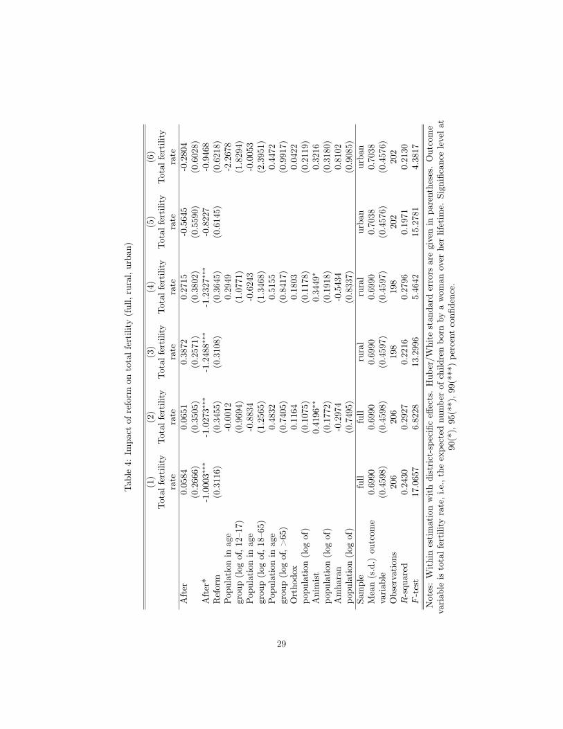
Table4:Impactofreform

ontotalfertility(full,rural,urban)

(1)

(2)

(3)

(4)

(5)

(6)

Totalfertility

Totalfertility

Totalfertility

Totalfertility

Totalfertility

Totalfertility

rate

rate

rate

rate

rate

rate

After

0.0584

0.0651

0.3872

0.2715

-0.5645

-0.2804

(0.2666)

(0.3505)

(0.2571)

(0.3802)

(0.5590)

(0.6028)

After*

-1.0003∗∗∗

-1.0273∗∗∗

-1.2488∗∗∗

-1.2327∗∗∗

-0.8227

-0.9468

Reform

(0.3116)

(0.3455)

(0.3108)

(0.3645)

(0.6145)

(0.6218)

Populationinage

-0.0012

0.2949

-2.2678

group(logof,12—17)

(0.9694)

(1.0771)

(1.8294)

Populationinage

-0.8834

-0.6243

-0.0053


(1.2565)

(1.3468)

(2.3951)

Populationinage

0.4832

0.5155

0.4472

group(logof,>65)

(0.7405)

(0.8417)

(0.9917)

Orthodox

0.1164

0.1803

0.0422

population(logof)

(0.1075)

(0.1178)

(0.2119)

Animist

0.4196∗∗

0.3449∗

0.3216

population(logof)

(0.1772)

(0.1918)

(0.3180)

Amharan

-0.2974

-0.5434

0.8102

population(logof)

(0.7495)

(0.8337)

(0.9085)

Sample

full

full

rural

rural

urban

urban

Mean(s.d.)outcome

0.6990

0.6990

0.6990

0.6990

0.7038

0.7038

variable

(0.4598)

(0.4598)

(0.4597)

(0.4597)

(0.4576)

(0.4576)

Observations

206

206

198

198

202

202

R-squared

0.2430

0.2927

0.2216

0.2796

0.1971

0.2130

F-test

17.0657

6.8228

13.2996

5.4642

15.2781

4.3817

Notes:Withinestimationwithdistrict-specificeffects.Huber/W

hitestandarderrorsaregiveninparentheses.Outcome

variableistotalfertilityrate,i.e.,theexpectednumberofchildrenbornbyawomanoverherlifetime.Significancelevelat

90(*),95(**),99(***)percentconfidence.

29


intensityontotalfertilityrate(full,rural,urban)

(1)

(2)

(3)

(4)

(5)

(6)

Totalfertility

Totalfertility

Totalfertility

Totalfertility

Totalfertility

Totalfertility

rate

rate

rate

rate

rate

rate

After

-0.0899

-0.1009

0.2107

0.0880

-0.6415

-0.3888

(0.2889)

(0.3940)

(0.2959)

(0.4269)

(0.5324)

(0.5909)

After*

-0.8367∗∗

-0.8685∗∗

-1.0625∗∗∗

-1.0577∗∗

-0.7503

-0.8504

Reformintensity

(0.3318)

(0.3798)

(0.3433)

(0.4074)

(0.6072)

(0.6352)

Populationinage

0.2462

0.5714

-2.1098


(1.0002)

(1.1096)

(1.8336)

Populationinage

-0.9726

-0.7396

-0.0538


(1.2448)

(1.3341)

(2.3925)

Populationinage

0.4559

0.4703

0.4367

group(logof,>65)

(0.7464)

(0.8505)

(0.9886)

Orthodox

0.1188

0.1786

0.0415

population(logof)

(0.1113)

(0.1219)

(0.2130)

Animist

0.4136∗∗

0.3356∗

0.3177

population(logof)

(0.1666)

(0.1768)

(0.3152)

Amharan

-0.3658

-0.6261

0.7403

population(logof)

(0.7382)

(0.8177)

(0.9120)

Sample

full

full

rural

rural

urban

urban

Mean(s.d.)outcome

0.6990

0.6990

0.6990

0.6990

0.7038

0.7038

variable

(0.4598)

(0.4598)

(0.4597)

(0.4597)

(0.4576)

(0.4576)

Observations

206

206

198

198

202

202

R-squared

0.2186

0.2712

0.1883

0.2506

0.1937

0.2082

F-test

17.7523

7.6924

12.9289

5.6328

14.6402

4.2064





30


onage-specificfertilityrate(fullsample)

(1)

(2)

(3)

(4)

(5)

(6)

(7)

(8)

Age-specific

Age-specific

Age-specific

Age-specific

Age-specific

Age-specific

Age-specific

Age-specific

fertilityrate

fertilityrate

fertilityrate

fertilityrate

fertilityrate

fertilityrate

fertilityrate

fertilityrate

(10to14)

(15to19)

(20to24)

(25to29)

(30to34)

(35to39)

(40to44)

(45to49)

After

-9.8722∗∗∗

-19.2980

24.9706∗

43.5183∗∗

38.4118∗∗

-13.5470

-7.9584

-43.2103∗∗

(2.7004)

(12.4606)

(13.2018)

(18.7599)

(16.7362)

(18.6428)

(10.5561)

(21.1416)

After*

-2.9611

-15.0950

-28.8320∗∗

-54.9822∗∗∗

-52.6379∗∗∗

-27.2101

-34.9346∗∗∗

11.1994

Reform

(2.9785)

(12.1120)

(14.2484)

(19.3138)

(17.6395)

(17.8758)

(10.8804)

(18.5314)

Populationinage

12.6122

-10.0910

28.1973

-37.4116

-37.4372

42.4558

-23.2999

24.7327


(8.4225)

(32.2034)

(48.5713)

(51.7725)

(58.8545)

(60.7879)

(47.6731)

(43.5474)

Populationinage

6.5978

54.6632

-73.3694

-11.5873

-49.8639

-11.4388

-104.7054∗∗∗

13.0227


(10.3184)

(33.1483)

(63.3193)

(76.4239)

(73.7420)

(57.0747)

(35.1196)

(42.3329)

Populationinage

-13.2738∗∗

-3.7720

0.1887

18.0678

17.3387

-31.7781

57.1484∗∗

52.7122

group(logof,>65)

(6.0038)

(23.7512)

(33.4292)

(39.9518)

(42.2126)

(35.4987)

(26.9270)

(32.2344)

Orthodox

0.3836

1.3617

-2.2496

10.8376∗

7.9477

-1.0095

2.4091

3.6091

population(logof)

(1.1768)

(3.7719)

(4.6046)

(5.7536)

(9.8087)

(5.7206)

(4.7514)

(3.9106)

Animist

-1.0531

4.0435

17.8607∗∗

23.3937∗∗

12.8610

15.8383

-1.2843

12.2669

population(logof)

(2.0550)

(6.2148)

(7.5819)

(9.9298)

(14.5471)

(12.9339)

(8.7156)

(7.6312)

Amhara

-5.9137

-28.1480

-5.1863

9.1168

17.1446

-7.8498

13.9694

-52.6158∗∗

population(logof)

(3.9179)

(18.6745)

(29.9699)

(36.4112)

(61.3746)

(27.6172)

(23.5109)

(23.6026)

Sample

full

full

fulll

full

full

full

full

full

Mean(s.d.)outcome

6.6647

70.158

169.20

191.23

177.05

142.05

78.374

39.056

variable

(11.425)

(36.364)

(51.871)

(54.748)

(62.042)

(59.382)

(48.539)

(38.879)

Observations

206

206

206

206

206

206

206

206

R-squared

0.4582

0.3071

0.1076

0.1494

0.0945

0.2019

0.4113

0.2573

F-test

10.8549

6.9400

2.1051

2.7657

1.8534

3.2304

7.5413

5.4060



variableistheage-specificfertilityrate,i.e.,theannualnumberofbirthsper1000womeninaspecificagegroup.Significance

levelat90(*),95(**),99(***)percentconfidence.

31


onage-specificfertilityrate(ruralsample)

(1)

(2)

(3)

(4)

(5)

(6)

(7)

(8)

Age-specific

Age-specific

Age-specific

Age-specific

Age-specific

Age-specific

Age-specific

Age-specific

fertilityrate

fertilityrate

fertilityrate

fertilityrate

fertilityrate

fertilityrate

fertilityrate

fertilityrate

(10to14)

(15to19)

(20to24)

(25to29)

(30to34)

(35to39)

(40to44)

(45to49)

After

-8.4395∗∗∗

-9.4114

26.4093

50.2109∗∗

52.0566∗∗∗

-13.0570

-10.4176

-33.0504∗

(2.6025)

(14.2969)

(16.3786)

(20.1438)

(16.5222)

(20.5798)

(10.7139)

(18.5722)

After*

-4.6089

-22.3567∗

-29.8026∗

-64.9697∗∗∗

-60.0006∗∗∗

-32.0207

-33.9401∗∗∗

1.1498

Reform

(2.8501)

(13.3374)

(16.3355)

(20.2257)

(18.3218)

(19.5791)

(11.8502)

(16.6678)

Populationinage

14.4071

-14.5838

26.9705

-10.2295

-47.8298

62.9348

15.4496

11.8666


(8.8235)

(35.3106)

(53.6384)

(56.2737)

(61.8442)

(66.6821)

(49.0905)

(41.8120)

Populationinage

6.6420

71.7686∗∗

-72.2661

-7.5503

-28.6253

1.0835

-135.9134∗∗∗

40.0065


(11.0147)

(35.3735)

(66.9144)

(83.2557)

(78.0502)

(61.7619)

(37.7337)

(40.6415)

Populationinage

-15.0081∗∗

-7.0468

28.5759

40.3895

1.8891

-30.4071

45.6164

39.0860

group(logof,>65)

(5.8435)

(28.3350)

(38.4086)

(44.9321)

(44.3216)

(44.6247)

(28.8320)

(32.5977)

Orthodox

0.7140

3.8337

1.4103

14.9881∗∗

11.6709

0.2569

-0.3361

3.5242

population(logof)

(1.2506)

(3.8675)

(4.9417)

(6.1499)

(10.0590)

(6.2770)

(5.3672)

(4.2542)

Animist

-2.0708

5.9241

14.2618

12.6460

11.3581

14.9420

-1.7701

13.6831∗

population(logof)

(2.1759)

(7.8927)

(9.2609)

(11.2959)

(14.1381)

(13.9908)

(11.6892)

(8.0721)

Amhara

-8.2455∗

-23.2289

-12.9384

-11.5641

8.6167

-13.7576

11.6794

-59.2495∗∗

population(logof)

(4.3458)

(19.5788)

(34.6366)

(42.5060)

(65.5084)

(32.1197)

(25.1262)

(26.7855)

Sample

rural

rural

rural

rural

rural

rural

rurall

rural

Mean(s.d.)outcome

6.4655

76.722

181.51

203.47

189.09

150.58

83.213

41.279

variable

(11.114)

(36.723)

(49.128)

(54.699)

(59.867)

(62.701)

(49.937)

(37.708)

Observations

198

198

198

198

198

198

198

198

R-squared

0.4886

0.2388

0.1061

0.2213

0.1125

0.1797

0.4134

0.2418

F-test

10.5345

3.9907

1.8268

3.6739

2.2035

2.5228

8.6332

5.1214





32


onage-specificfertilityrate(urbansample)

(1)

(2)

(3)

(4)

(5)

(6)

(7)

(8)

Age-specific

Age-specific

Age-specific

Age-specific

Age-specific

Age-specific

Age-specific

Age-specific

fertilityrate

fertilityrate

fertilityrate

fertilityrate

fertilityrate

fertilityrate

fertilityrate

fertilityrate

(10to14)

(15to19)

(20to24)

(25to29)

(30to34)

(35to39)

(40to44)

(45to49)

After

-5.7072

-45.0736∗

12.5902

14.0118

-30.7592

21.4320

40.7680

-63.3401

(4.7005)

(26.4971)

(40.5609)

(37.9560)

(37.5287)

(38.1292)

(32.8241)

(65.9322)

After*

-6.1327

11.5107

-63.6041

-36.3273

-11.3057

-46.8859

-79.2994∗

42.6770

Reform

(6.2786)

(26.7274)

(41.1401)

(40.7529)

(39.7578)

(39.0698)

(41.6810)

(57.6150)

Populationinage

6.8324

-10.2361

111.4051

-342.4991∗∗

28.0343

-58.1191

-200.8176

11.8373


(16.1901)

(75.9642)

(137.0856)

(144.7485)

(128.4242)

(107.9666)

(167.7866)

(119.9480)

Populationinage

-20.8171

27.0847

258.8382

187.5902

-176.0041

-36.7655

76.8818

-317.8674∗


(22.7312)

(80.0534)

(200.4982)

(123.4405)

(138.6033)

(106.8076)

(143.2380)

(167.0551)

Populationinage

-0.4295

30.9142

-240.7475∗∗∗

-101.6111

71.9151

39.4161

99.9287

190.0594∗∗

group(logof,>65)

(15.3443)

(38.5134)

(89.6070)

(67.1986)

(94.4578)

(53.3791)

(75.2319)

(89.3293)

Orthodox

-2.7509

-13.6587

-8.1770

10.4224

1.5003

1.4766

-8.8574

28.4790∗

population(logof)

(6.1341)

(9.4889)

(11.3419)

(11.3700)

(14.1481)

(16.5722)

(16.9763)

(16.8451)

Animist

-4.3035

-6.9825

37.5779

91.1155∗∗∗

-30.5795

1.5387

-10.0015

-14.0466

population(logof)

(5.2627)

(13.4510)

(33.8415)

(23.1356)

(23.7582)

(17.1163)

(46.7959)

(13.8846)

Amhara

16.1407

-34.3463

-41.4950

173.4731∗∗∗

128.2623

8.2704

-117.8452

29.5811

population(logof)

(26.5170)

(43.5978)

(68.4956)

(48.2277)

(77.5695)

(47.1729)

(88.3963)

(49.8870)

Sample

urban

urban

urban

urban

urban

urban

urban

urban

Mean(s.d.)outcome

6.5861

35.088

118.34

127.05

108.12

65.229

50.224

31.733

variable

(26.663)

(68.685)

(135.31)

(126.99)

(142.85)

(101.17)

(134.28)

(135.11)

Observations

202

202

202

202

202

202

202

202

R-squared

0.1187

0.1758

0.1289

0.1820

0.0771

0.0417

0.1270

0.0997

F-test

1.5893

2.1873

2.0377

4.3533

1.7697

1.3197

1.2907

1.1554





33

Table9:Reformandshareofself-employedwomen

(1)

(2)

(3)

(4)

(5)

(6)

(7)

(8)

(9)

Self-

Self-

Self-

Self-

Self-

Self-

Self-

Self-

Self-

employ

employ

employ

employ

employ

employ

employ

employ

employ

mentrate

mentrate

mentrate

mentrate

mentrate

mentrate

mentrate

mentrate

mentrate

(10to49)

(10to14)

(15to19)

(20to24)

(25to29)

(30to34)

(35to39)

(40to44)

(45to49)

After

0.1453∗∗∗

0.0976∗∗∗

0.1319∗∗∗

0.1923∗∗∗

0.1674∗∗∗

0.1661∗∗∗

0.1920∗∗∗

0.1476∗∗∗

0.1396∗∗∗

(0.0224)

(0.0164)

(0.0234)

(0.0308)

(0.0283)

(0.0338)

(0.0344)

(0.0321)

(0.0311)

After*

0.0330

0.0061

0.0234

0.0294

0.0591∗∗

0.0361

0.0298

0.0386

0.0676∗∗

Reform

(0.0223)

(0.0162)

(0.0232)

(0.0303)

(0.0293)

(0.0332)

(0.0334)

(0.0321)

(0.0312)

Populationinage

0.0889

0.0581

0.0885

0.0798

0.1565

0.2563∗∗∗

0.0659

0.1204

0.1001


(0.0674)

(0.0552)

(0.0649)

(0.0983)

(0.0948)

(0.0917)

(0.1001)

(0.1039)

(0.1100)

Populationinage

0.1890∗∗

0.1413∗∗

0.1959∗∗

0.2512∗∗

0.1883∗

0.1636

0.1530

0.0984

0.1374


(0.0732)

(0.0681)

(0.0771)

(0.0970)

(0.0983)

(0.1151)

(0.0932)

(0.1196)

(0.1154)

Populationinage

-0.0057

-0.0006

0.0167

-0.0145

-0.0137

-0.0239

0.0304

0.0296

-0.0620

group(logof,>65)

(0.0461)

(0.0384)

(0.0487)

(0.0617)

(0.0647)

(0.0701)

(0.0731)

(0.0680)

(0.0672)

Orthodox

0.0054

0.0058

0.0009

0.0034

0.0065

0.0006

0.0217

0.0158

0.0024

population(logof)

(0.0087)

(0.0062)

(0.0085)

(0.0105)

(0.0110)

(0.0114)

(0.0134)

(0.0131)

(0.0130)

Animist

-0.0141

0.0050

-0.0028

-0.0184

-0.0183

-0.0358

-0.0109

-0.0217

-0.0338

population(logof)

(0.0220)

(0.0147)

(0.0174)

(0.0297)

(0.0322)

(0.0250)

(0.0331)

(0.0271)

(0.0210)

Amhara

-0.1795∗∗∗

-0.1378∗∗∗

-0.2036∗∗∗

-0.2007∗∗∗

-0.1883∗∗∗

-0.2749∗∗∗

-0.2417∗∗∗

-0.0916

-0.0994

population(logof)

(0.0520)

(0.0490)

(0.0415)

(0.0624)

(0.0632)

(0.0817)

(0.0469)

(0.0900)

(0.0771)

Sample

rural

rural

rural

rural

rural

rural

rural

rural

rural

Mean(s.d.)outcome

0.1982

0.0751

0.1339

0.2010

0.2415

0.2661

0.2896

0.3222

0.3430

variable

(0.1214)

(0.0816)

(0.1116)

(0.1516)

(0.1567)

(0.1537)

(0.1583)

(0.1490)

(0.1498)

Observations

198

198

198

198

198

198

198

198

198

R-squared

0.8320

0.7590

0.8051

0.8128

0.8035

0.7855

0.7624

0.7370

0.7051

F-test

66.8649

40.7481

59.9328

56.1947

53.5110

46.2668

58.0638

35.1413

31.3559



variableistheproportionofself-employedwomen,forwomenintheirchildbearingyearsandbyagegroup.Significancelevel

at90(*),95(**),99(***)percentconfidence.

34

Table10:Reformandshareofemployedwomen

(1)

(2)

(3)

(4)

(5)

(6)

(7)

(8)

(9)

Employ-

Employ-

Employ-

Employ-

Employ-

Employ-

Employ-

Employ-

Employ-

mentrate

mentrate

mentrate

mentrate

mentrate

mentrate

mentrate

mentrate

mentrate

(10to49)

(10to14)

(15to19)

(20to24)

(25to29)

(30to34)

(35to39)

(40to44)

(45to49)

After

0.0046

-0.0096∗∗

0.0046

0.0259∗∗∗

0.0071

0.0077

0.0045

0.0115

0.0013

(0.0041)

(0.0039)

(0.0092)

(0.0081)

(0.0059)

(0.0060)

(0.0069)

(0.0135)

(0.0059)

After*

-0.0035

0.0010

-0.0080

-0.0021

0.0016

-0.0092

-0.0013

-0.0179

-0.0108∗

Reform

(0.0036)

(0.0038)

(0.0079)

(0.0076)

(0.0056)

(0.0062)

(0.0066)

(0.0117)

(0.0061)

Populationinage

0.0173∗∗

0.0116

0.0091

0.0356

0.0248∗

0.0383∗∗

0.0137

-0.0048

-0.0033


(0.0086)

(0.0103)

(0.0174)

(0.0219)

(0.0149)

(0.0188)

(0.0169)

(0.0276)

(0.0228)

Populationinage

-0.0124

0.0253∗∗

0.0043

-0.0544∗∗

-0.0556∗∗

-0.0447∗∗∗

-0.0191

0.0351

-0.0114


(0.0103)

(0.0128)

(0.0202)

(0.0242)

(0.0226)

(0.0162)

(0.0219)

(0.0285)

(0.0239)

Populationinage

-0.0047

-0.0071

-0.0054

0.0028

0.0126

-0.0077

-0.0028

-0.0304

-0.0220∗

group(logof,>65)

(0.0072)

(0.0067)

(0.0151)

(0.0157)

(0.0137)

(0.0096)

(0.0128)

(0.0269)

(0.0132)

Orthodox

-0.0001

-0.0022∗

0.0009

0.0011

-0.0017

-0.0015

-0.0004

0.0049∗

0.0016

population(logof)

(0.0012)

(0.0012)

(0.0018)

(0.0025)

(0.0028)

(0.0024)

(0.0024)

(0.0027)

(0.0023)

Animist

0.0011

0.0028

-0.0025

0.0079∗

-0.0010

-0.0007

-0.0029

0.0006

0.0025

population(logof)

(0.0013)

(0.0019)

(0.0030)

(0.0046)

(0.0042)

(0.0035)

(0.0033)

(0.0038)

(0.0028)

Amhara

-0.0040

-0.0195∗∗∗

-0.0094

0.0154

-0.0012

0.0098

0.0075

-0.0299∗

0.0122

population(logof)

(0.0049)

(0.0070)

(0.0082)

(0.0170)

(0.0085)

(0.0099)

(0.0093)

(0.0178)

(0.0085)

Sample

rural

rural

rural

rural

rural

rural

rurall

rural

rural

Mean(s.d.)outcome

0.0177

0.0107

0.0176

0.0299

0.0216

0.0173

0.0150

0.0151

0.0137

variable

(0.0111)

(0.0110)

(0.0176)

(0.0248)

.(0.0209)

(0.0192)

(0.0234)

(0.0238)

(0.0207)

Observations

198

198

198

198

198

198

198

198

198

R-squared

0.5896

0.4433

0.6614

0.2596

0.1190

0.1500

0.0973

0.1316

0.1367

F-test

19.5036

7.5463

25.9183

4.4238

2.2194

3.1340

1.3177

2.0925

2.0270



variableistheproportionofemployedwomen,forwomenintheirchildbearingyearsandbyagegroup.Significancelevelat


35

Table11:Reformandshareofwomeninhouseworkmainoccupation

(1)

(2)

(3)

(4)

(5)

(6)

(7)

(8)

(9)

House-

House-

House-

House-

House-

House-

House-

House-

House-

workrate

workrate

workrate

workrate

workrate

workrate

workrate

workrate

workrate

(10to49)

(10to14)

(15to19)

(20to24)

(25to29)

(30to34)

(35to39)

(40to44)

(45to49)

After

-0.3215∗∗∗

-0.3543∗∗∗

-0.3757∗∗∗

-0.3444∗∗∗

-0.3074∗∗∗

-0.2858∗∗∗

-0.2577∗∗∗

-0.2508∗∗∗

-0.2453∗∗∗

(0.0459)

(0.0402)

(0.0514)

(0.0491)

(0.0464)

(0.0627)

(0.0518)

(0.0677)

(0.0386)

After*

-0.0014

0.0127

-0.0116

0.0179

-0.0097

-0.0019

-0.0282

-0.0028

-0.0139

Reform

(0.0454)

(0.0415)

(0.0497)

(0.0494)

(0.0480)

(0.0593)

(0.0511)

(0.0652)

(0.0409)

Populationinage

-0.1528

-0.2057∗

-0.1639

-0.1711

-0.0856

-0.2799∗

-0.1071

-0.1348

-0.0485


(0.1235)

(0.1090)

(0.1208)

(0.1609)

(0.1452)

(0.1437)

(0.1578)

(0.2044)

(0.1399)

Populationinage

0.2774∗

0.4493∗∗∗

0.1627

0.1693

0.2479

0.3220∗

0.3101∗

0.3196

0.1582


(0.1517)

(0.1543)

(0.1604)

(0.1634)

(0.1696)

(0.1759)

(0.1691)

(0.2334)

(0.1649)

Populationinage

-0.2294∗∗

-0.2329∗∗∗

-0.2453∗∗

-0.1940∗∗

-0.2495∗∗

-0.1909∗

-0.3172∗∗∗

-0.2381∗

-0.1187

group(logof,>65)

(0.0902)

(0.0859)

(0.1011)

(0.0942)

(0.1084)

(0.1141)

(0.1036)

(0.1302)

(0.0851)

Orthodox

0.0118

0.0068

0.0130

0.0230

0.0120

0.0128

0.0092

0.0077

0.0009

population(logof)

(0.0139)

(0.0125)

(0.0134)

(0.0170)

(0.0160)

(0.0169)

(0.0173)

(0.0176)

(0.0154)

Animist

0.0098

0.0140

0.0161

-0.0207

-0.0050

0.0207

0.0141

0.0192

0.0182

population(logof)

(0.0326)

(0.0289)

(0.0292)

(0.0430)

(0.0449)

(0.0365)

(0.0373)

(0.0416)

(0.0265)

Amhara

0.0982

0.0360

0.1642∗∗

0.1250

0.0909

0.1414∗

0.1447∗

0.0534

0.0542

population(logof)

(0.0739)

(0.0827)

(0.0686)

(0.0755)

(0.0772)

(0.0802)

(0.0752)

(0.1141)

(0.0938)

Sample

rural

rural

rural

rural

rural

rural

rurall

rural

rural

Mean(s.d.)outcome

0.4734

0.4269

0.5191

0.5211

0.5052

0.4879

0.4542

0.4214

0.4048

variable

(0.2168)

(0.2219)

(0.2498)

(0.2337)

(0.2301)

(0.2210)

(0.2160)

(0.2072)

(0.1883)

Observations

198

198

198

198

198

198

198

198

198

R-squared

0.8257

0.8541

0.8669

0.7853

0.7587

0.7317

0.7112

0.6240

0.7011

F-test

68.3073

83.1011

91.6994

48.6382

43.6878

45.3139

36.3673

24.5305

28.2777



variableistheproportionofwomenwithhouseworkasmainoccupation,forwomenintheirchildbearingyearsandbyage

group.Significancelevelat90(*),95(**),99(***)percentconfidence.

36

Table12:Reformandshareofwomennevermarried

(1)

(2)

(3)

(4)

(5)

(6)

(7)

(8)

(9)

Never

Never

Never

Never

Never

Never

Never

Never

Never

married

married

married

married

married

married

married

married

married

rate

rate

rate

rate

rate

rate

rate

rate

rate

(10to49)

(10to14)

(15to19)

(20to24)

(25to29)

(30to34)

(35to39)

(40to44)

(45to49)

After

0.0340∗∗∗

0.0189

0.0701∗∗∗

0.0055

0.0034

0.0096

0.0073

-0.0030

0.0008

(0.0117)

(0.0232)

(0.0265)

(0.0166)

(0.0080)

(0.0125)

(0.0076)

(0.0045)

(0.0075)

After*

0.0317∗∗∗

0.0757∗∗∗

0.1083∗∗∗

0.0301∗

0.0058

0.0039

0.0045

0.0072

0.0040

Reform

(0.0120)

(0.0223)

(0.0262)

(0.0173)

(0.0085)

(0.0109)

(0.0074)

(0.0045)

(0.0076)

Populationinage

0.0750∗

-0.3017∗∗∗

0.1010

0.1098∗

-0.0111

-0.0045

-0.0095

-0.0073

-0.0202


(0.0420)

(0.0793)

(0.0855)

(0.0594)

(0.0318)

(0.0320)

(0.0206)

(0.0188)

(0.0211)

Populationinage

-0.0696

0.3146∗∗∗

-0.0755

-0.1335

-0.0124

-0.0097

-0.0139

-0.0056

0.0541∗


(0.0499)

(0.0898)

(0.1087)

(0.0846)

(0.0289)

(0.0289)

(0.0213)

(0.0194)

(0.0300)

Populationinage

0.0312

0.0802

0.0046

-0.0293

0.0126

-0.0152

-0.0009

0.0244∗∗

-0.0083

group(logof,>65)

(0.0320)

(0.0601)

(0.0640)

(0.0466)

(0.0249)

(0.0237)

(0.0125)

(0.0116)

(0.0125)

Orthodox

-0.0040

-0.0089

-0.0145

-0.0090

-0.0039

0.0027

-0.0007

0.0031

0.0010

population(logof)

(0.0043)

(0.0092)

(0.0103)

(0.0062)

(0.0036)

(0.0024)

(0.0021)

(0.0021)

(0.0022)

Animist

-0.0161∗∗

-0.0387∗∗

-0.0302

-0.0170

-0.0012

-0.0037

-0.0023

-0.0012

-0.0012

population(logof)

(0.0081)

(0.0167)

(0.0198)

(0.0112)

(0.0053)

(0.0040)

(0.0042)

(0.0025)

(0.0035)

Amhara

0.0215

-0.0172

0.0964

0.1146∗

0.0427∗∗

0.0319

0.0122

-0.0082

0.0024

population(logof)

(0.0402)

(0.0606)

(0.0885)

(0.0637)

(0.0208)

(0.0195)

(0.0139)

(0.0142)

(0.0197)

Sample

rural

rural

rural

rural

rural

rural

rurall

rural

rural

Mean(s.d.)outcome

0.3133

0.8657

0.4919

0.1556

0.0521

0.0278

0.0172

0.0127

0.0109

variable

(0.0769)

(0.1246)

(0.1825)

(0.0878)

(0.0407)

(0.0312)

(0.0209)

(0.0170)

(0.0194)

Observations

198

198

198

198

198

198

198

198

198

R-squared

0.5896

0.4433

0.6614

0.2596

0.1190

0.1500

0.0973

0.1316

0.1367

F-test

19.5036

7.5463

25.9183

4.4238

2.2194

3.1340

1.3177

2.0925

2.0270



variableistheproportionofwomennevermarried,forwomenintheirchildbearingyearsandbyagegroup.Significancelevel

at90(*),95(**),99(***)percentconfidence.

37

Table13:Comparingnon-reform

districtswithandwithoutaborderwithareform

district

(1)

(2)

(3)

(4)

(5)

(6)

Totalfertility

Totalfertility

Totalfertility

Totalfertility

Totalfertility

Totalfertility

rate

rate

rate

rate

rate

rate

After

-0.0637

-0.6725

0.2776

-1.1215

-1.1737

-0.9468

(0.4110)

(0.8168)

(0.3742)

(0.6948)

(0.8770)

(1.2179)

After*

0.2537

0.6007

0.1732

0.2814

1.6583

2.0223

Reform

(0.5349)

(0.6574)

(0.5104)

(0.4901)

(1.0923)

(1.3967)

Populationinage

3.8149∗

4.9515∗∗

-5.6643


(2.2142)

(2.1534)

(4.4026)

Populationinage

0.0010

0.0308

13.7318


(3.8866)

(4.2768)

(9.0119)

Populationinage

-0.4894

0.3119

1.7938

group(logof,>65)

(1.8738)

(1.4183)

(3.2708)

Orthodox

0.0495

0.3652

0.3475

population(logof)

(0.2921)

(0.2574)

(0.5146)

Animist

0.4540

0.7420

0.4716

population(logof)

(0.5223)

(0.6697)

(1.2404)

Amharan

-2.5158

-1.7464

-10.6304

population(logof)

(3.6092)

(4.7192)

(7.8424)

Sample

full

full

rural

rural

urban

urban

Mean(s.d.)outcome

4.4248

4.4248

4.6854

4.6854

2.7240

2.7240

variable

(0.9739)

(0.9739)

(0.8788)

(0.8788)

(2.0261)

(2.0261)

Observations

6266

5858

6060

R-squared

0.0072

0.1070

0.0638

0.3543

0.0922

0.2124

F-test

0.1659

0.6931

1.1185

2.0565

1.1725

0.5893





38

Table 14: Selection on observables (robustness check)

Controls in Controls in Full Rural Urbanrestricted set full set sample sample sample

none demographic 41.02 13.82 9.23none religious and ethnic 15.74 21.90 36.19none demographic, religious and ethnic 38.11 76.58 7.63demographic demographic, religious and ethnic 20.24 18.09 39.28religious and ethnic demographic, religious and ethnic 25.10 16.25 9.40

Notes: The table reports ratios of estimated coeffi cients from two regressions.One includes the restricted set of controls, the other the unrestricted set ofcontrols. All combinations of control sets are estimated for full, rural and

urban.

39

Pronatal Property Rights over Land and Fertility Outcomes · PDF filePronatal Property Rights...

Documents

Transcript of Pronatal Property Rights over Land and Fertility Outcomes · PDF filePronatal Property Rights...