PROMETHEUS PRESS/PALAEONTOLOGICAL NETWORK …mstiner/pdf/Stiner2004b.pdf · independent of bone...

117

Stiner

Article JTa020. All rights reserved.

A Comparison of Photon Densitometry and Computed Tomography Parameters of Bone

Density in Ungulate Body Part Profiles

Mary C. Stiner* Department of Anthropology, Building 30, University of Arizona, Tucson,

AZ 85721-0030, U.S.A

Journal of Taphonomy 2 (3) (2004), 117-145. Manuscript received 4 October 2004, revised manuscript accepted 15 December 2004.

Biases in ungulate body part representation in archaeofaunas potentially reflect human foraging decisions. However, the signatures of density-mediated attrition of body parts and human selectivity in response to nutritional content can overlap to a significant extent. Zooarchaeologists’ techniques for analyzing skeletal representation for density-dependent biases must either address differential resistance among distinct skeletal macro-tissue classes, or compare skeletal representation within a narrower density range that is widely distributed in the skeleton. This presentation examines the potential comparability of bone density parameters obtained by photon densitometry (PD) and computed tomography (CT) within limb elements and across regions of the whole skeleton. “Unadjusted” parameters obtained by PD and CT techniques are in reasonably good agreement, and these parameters yield similar results when applied to patterns of skeletal representation in Mediterranean faunas generated by Paleolithic humans and Pleistocene spotted hyenas. More significant than the technique for measuring density in modern mammal skeletons is whether the density parameter values have been adjusted, arguably to compensate for problems of shape and the presence of large internal voids in limb bone tubes. The results of systematic comparison of density parameter variation among published sources, and their application to prehistoric cases accumulated by diverse agents, contradict the great preservation differential between spongy and compact bone specimens suggested by certain captive hyena experiments and the Mousterian fauna from Kobeh Cave (Iran). Only the adjustments made to the CT parameters for limb shafts (BMD2) accommodate the latter cases.

Keywords: DENSITY-MEDIATED BONE ATTRITION, TAPHONOMY, ZOOARCHAEOLOGY, VERTEBRATE BODY PART PROFILES, PHOTON DENSITOMETRY, COMPUTED TOMOGRAPHY

Introduction Patterns of prey body part representation are of anthropological interest for what they

may tell us about human foraging decisions, a question that has been explored by a wide range of archaeologists (Binford, 1978; Binford & Bertram, 1977; Brain, 1981;

* E-mail:[email protected]

2004 Journal of Taphonomy

PROMETHEUS PRESS/PALAEONTOLOGICAL NETWORK FOUNDATION (TERUEL)

Available online at www.journaltaphonomy.com

VOLUME 2 (ISSUE 3)

118

Bone density parameters and ungulate body part profiles

Brink, 1997; Lupo, 1995; Lupo & Schmitt, 1997; O’Connell et al., 1988; Todd, 1987; among others). However, bone fragility and associations to food value generally are correlated in animal carcasses (e.g., Grayson, 1989; Lyman, 1984), and thus zooarchaeologists must ask whether the observed biases in body part representation could be explained by in situ attrition mediated by variation in skeletal tissue density. The potential for equifinality among causes of skeletal biases in archaeofaunas can be addressed only in part by comparing the patterns of anatomical representation in archaeofaunas to independent standards (measurements) of bone density in modern taxa. Such analyses require reasonably accurate estimates of density variation within and among skeletal parts. Also significant is how the anatomical data are partitioned in comparisons of parameters to the archaeofaunal patterns.

Much recent debate has focused on the accuracy of bone density parameters that are applied in research on archaeofaunas. Investigators generally accept that body part representation may be compared at several scales—within element, across element, and across bodily regions of the prey anatomy. However, two sources of bulk bone density reference data—those obtained using photon densitometry (PD) and those from computed tomography (CT)—are said to differ significantly with respect to accuracy (Lam et al., 1999, 2003). Of particular concern is how well these standards reflect relative differences in the structural density of compact limb bone shafts and limb epiphyses. These disagreements also have implications for the comparability of limb

density data to other areas of the prey skeleton.

Marean & Kim (1998) and Lam et al. (1999) propose that the density of compact bone in limb elements is so much greater than compact bone tissues elsewhere in the ungulate anatomy that, as a rule, only limb shaft portions should be used to estimate MNE (minimum number of elements) of ungulate limbs in faunal assemblages. Do the PD and CT techniques for measuring bulk density in fresh bone have substantially different consequences in archaeological applications?

This presentation examines potential differences in the predictions of ungulate bone survivorship based on bulk bone density as estimated by PD technique by Lyman (1984, 1994) and Kreutzer (1992) and by CT technique by Lam et al. (1999). In the case of the CT technique, two types of parameters are considered—unadjusted (BMD1) and adjusted (BMD2) types—the latter of which is an attempt to correct for the presence of large internal voids in bone tubes. The comparisons are undertaken at two anatomical scales: within limb elements and across regions of the prey anatomy. Density-mediated attrition and body part profiling Human-modified faunas tend to be highly fragmented, and nowhere is this more evident than in foragers’ middens. Under these conditions, skeletal element counts must be estimated from the frequencies of unique morphologic features that can recognized from partial specimens, such as the head of a femur, the nutrient foramen of

119

Stiner

a humerus, an occipital condyle of a cranium or a prezygopophysis of a lumbar vertebra. Coding systems for identifying fragmented specimens vary and most remain undocumented. In recognition of this fact, this author’s coding system for skeletal elements and portions-of-elements is provided in Appendix 1 and illustrated in a series of figures. The potential resistance of bones and bone fragments to consumers and to post-depositional processes is conditioned partly by the “structural density” of bone tissues (Brain, 1981; Lyman, 1994:235-238). Existing techniques for analyzing body part representation from fragmented faunal material either (1) address the differential survivorship of the full range of structural

density classes in the skeleton, or (2) focus on comparisons of parts that fall within a narrower density range that is well represented in the vertebrate skeleton.

The more common approach to body part profiling emphasizes within-element comparisons of the relative representation of compact and spongy bone macrostructures (Figure 1). There are many variations on the theme, but all within-element comparisons require fairly complete knowledge of structural variation throughout the mammal skeleton. Correlation statistics for bone portion survivorship and independent standards of structural density provide information on the maximum amount of variation that density might explain. Establishing a

Figure 1. Cross-sectioned humerus and femur of artiodactyl ungulate, showing the distribution of compact and spongy macrostructures along the shaft (diaphysis) and ends (epiphyses). Some epiphyses are dominated by spongy bone, but others are dominated by compact bone. The main nutrient foramen is located on the shaft.

120


positive correlation of skeletal survivorship to density is not proof of density-mediated attrition, however, since consumer transport and processing behaviors can produce similar patterns (see Beaver, 2004). Such a correlation merely indicates that density-mediated attrition can be among the potential range of explanations for the patterns observed.

The within-element approach has been very important for research on intensive carcass processing by humans (e.g., Binford, 1978; Brain, 1981; Brink, 1997; Lupo, 1995; Munro, 2004; Stiner, 2003; Todd, 1987). In cases where bone grease extraction is suspected, for example, knowing the fate of all least-dense portions in relation to very dense ones is essential to the success of the study. This treatment of body part representation data does not in itself address questions about body part transport decisions, except with respect to possibility of pre-sectioning of limbs. Cross-element comparisons in body part profiling potentially address questions about human decisions at the level of the complete resource package (often the whole carcass). Cross-element approaches often standardize element counts to the natural abundance of those represented in a complete skeleton (e.g., minimum number of animal units, MAU; Binford, 1978). Some cross-element approaches are distinct for their emphasis on skeletal portions composed of compact bone, a tissue class that is widely distributed in the vertebrate skeleton (Stiner, 1991, 2002). This procedure avoids or reduces the confounding effects of density-mediated bone attrition on estimates of the minimum number of skeletal elements (MNE) by narrowing the tissue density range to those

features that are dominated only by compact bone. The approach is most useful for examining broad biases, or the lack of them, in transport decisions; the risks of misinterpretation with respect of density-mediated attrition are quite different from the first approach and arguably less important (Stiner, 2002).

Rates of differential attrition Bulk, or structural, bone density (sensu Lyman, 1984) is a term more or less unique to zooarchaeological studies. Bulk density desc r ibes d i f fe rences in bone macrostructure—mainly the continuum between compact and spongy bone—because this is what interests zooarchaeologists on account of their reliance on macrostructural features for taxonomic and anatomical identifications. Bulk density does not reflect substantive variation in the material composition (mineral and organic) of bone, nor does it bear a simple linear relation to the strength of bone when loaded against its main axis (Currey, 1984). Bulk density is mainly an expression of variation in concentrated mass of bone specimens that is semi-independent of bone tissue volume and depends foremost on porosity.

Lyman’s (1984, 1991, 1994) comprehensive review of skeletal survivorship in relation to bulk bone density in cultural and paleontological contexts suggests a maximum potential of differential destruction of 1:2 or 1:3 for spongy to compact bone parts. This destruction differential is supported by empirical patterns of skeletal survivorship in other archaeological and paleontological

121

Stiner

sites as well (Lyman, 1991; Stiner, 2002, 2005), and by experiments involving mechanical (Binford & Bertram, 1977; Brain, 1981; Lyman, 1994) and chemical destruction (Margaris, 2004). By contrast, a maximum survivorship differential of 1:8 for spongy to compact bone features is implied by some feeding experiments involving hyenas (Capaldo, 1997; Marean & Spencer, 1991; Marean et al., 1992) and by Marean & Kim’s (1998) refitting study of the Mousterian ungulate fauna from Kobeh Cave in Iran. Interpretation of the latter case assumes that it represents a completely recovered, unsorted collection. The extreme difference in skeletal survivorship found by these authors is supported by the adjustments to CT limb bone parameters published by Lam et al. (1999), but not by the unadjusted CT measurements. Lam et al. (1999, 2003) insist that their adjusted parameters for variation in bulk bone density are more accurate for anticipating density-mediated effects on limb bone survivorship across archaeological and paleontological circumstances.

Comparison of density ranges for limb ends and shafts How different are the predictions for skeletal survivorship from PD and CT parameters of bulk bone density? And how different are the predictions of skeletal survivorship from the unadjusted (BMD1) versus adjusted (BMD2) CT measurements?

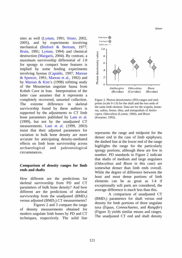
Figures 2 and 3 compare the range of density measurements obtained for modern ungulate limb bones by PD and CT techniques, respectively. The solid line

represents the range and midpoint for the denser end in the case of limb epiphyses; the dashed line at the lower end of the range highlights the range for the particularly spongy portions, although these are few in number. PD standards in Figure 2 indicate that shafts of medium and large ungulates (Odocoileus and Bison in this case) are somewhat denser than limb ends overall. While the degree of difference between the least and most dense portions of limb elements can be as great as 1:4 if exceptionally soft parts are considered, the average difference is much less than this.

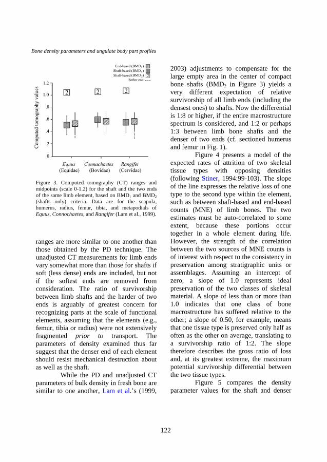
A comparison of unadjusted CT (BMD1) parameters for shaft versus end density for limb portions of three ungulate taxa (Equus, Connochaetes, and Rangifer) (Figure 3) yields similar means and ranges. The unadjusted CT end and shaft density

Figure 2. Photon densitometry (PD) ranges and mid-points (scale 0-1.0) for the shaft and the two ends of the same limb element. Data are for the scapula, hume-rus, radius, femur, tibia, and metapodials of Antilo-capra, Odocoileus (Lyman, 1984), and Bison (Kreutzer, 1992).

122


ranges are more similar to one another than those obtained by the PD technique. The unadjusted CT measurements for limb ends vary somewhat more than those for shafts if soft (less dense) ends are included, but not if the softest ends are removed from consideration. The ratio of survivorship between limb shafts and the harder of two ends is arguably of greatest concern for recognizing parts at the scale of functional elements, assuming that the elements (e.g., femur, tibia or radius) were not extensively fragmented prior to transport. The parameters of density examined thus far suggest that the denser end of each element should resist mechanical destruction about as well as the shaft.

While the PD and unadjusted CT parameters of bulk density in fresh bone are similar to one another, Lam et al.’s (1999,

2003) adjustments to compensate for the large empty area in the center of compact bone shafts (BMD2 in Figure 3) yields a very different expectation of relative survivorship of all limb ends (including the densest ones) to shafts. Now the differential is 1:8 or higher, if the entire macrostructure spectrum is considered, and 1:2 or perhaps 1:3 between limb bone shafts and the denser of two ends (cf. sectioned humerus and femur in Fig. 1).

Figure 4 presents a model of the expected rates of attrition of two skeletal tissue types with opposing densities (following Stiner, 1994:99-103). The slope of the line expresses the relative loss of one type to the second type within the element, such as between shaft-based and end-based counts (MNE) of limb bones. The two estimates must be auto-correlated to some extent, because these portions occur together in a whole element during life. However, the strength of the correlation between the two sources of MNE counts is of interest with respect to the consistency in preservation among stratigraphic units or assemblages. Assuming an intercept of zero, a slope of 1.0 represents ideal preservation of the two classes of skeletal material. A slope of less than or more than 1.0 indicates that one class of bone macrostructure has suffered relative to the other; a slope of 0.50, for example, means that one tissue type is preserved only half as often as the other on average, translating to a survivorship ratio of 1:2. The slope therefore describes the gross ratio of loss and, at its greatest extreme, the maximum potential survivorship differential between the two tissue types.

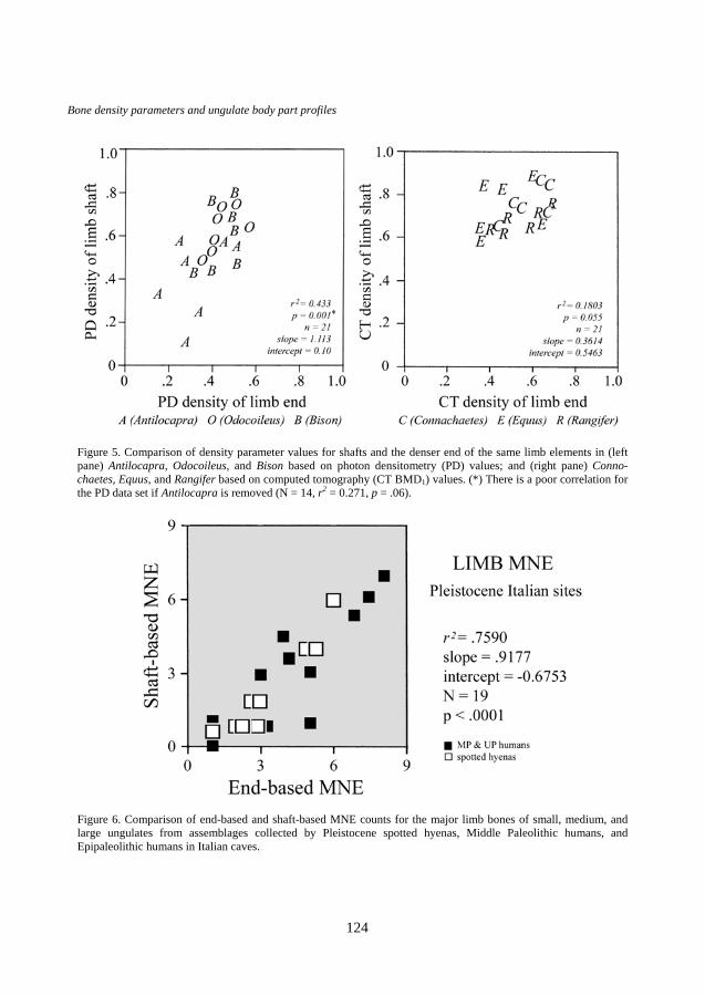
Figure 5 compares the density parameter values for the shaft and denser

Figure 3. Computed tomography (CT) ranges and midpoints (scale 0-1.2) for the shaft and the two ends of the same limb element, based on BMD1 and BMD2 (shafts only) criteria. Data are for the scapula, humerus, radius, femur, tibia, and metapodials of Equus, Connochaetes, and Rangifer (Lam et al., 1999).

123

Stiner

end of each type of limb element obtained by PD and unadjusted CT (BMD1) techniques. Shafts are slightly denser than the ends of these bones according to the PD standards (left), but the slope is close to an ideal value of 1. Some of the values for Antilocapra, the smallest ungulate referent in the PD data set, tend to fall on the lower end of the slope, presumably because the animal possesses a lighter skeletal frame. There is a poor correlation for the data set if Antilocapra is removed (n = 14, r2 = 0.271, slope = 0.904, intercept = 0.218, p = .06). In fact the full set of points for Antilocapra, Odocoileus and Bison form a single tight cluster along the end-density (x) axis, but are more scattered along the shaft-density (y) axis. This finding suggests that end-based counts yield more consistent results among limb elements and among ungulate species when PD standards of density variation are used. Unadjusted CT density standards (right) for medium and large ungulates (Equus, Connochaetes, and Rangifer) are tightly distributed on both axes, indicating that shaft features and the denser ends of each limb type are equally suitable for estimating limb MNE. None of these results supports the idea that shaft-based MNE counts are much more reliable than end-based counts for the construction of body part profiles.

Relative attrition of limb end and shaft features in diverse paleontological and archaeological contexts is also informative in that it can provide a better sense of the natural range of skeletal survivorship (Figure 6). The 19 Pleistocene ungulate assemblages in this comparison are of known origins in Italy, and all of the faunal material was recovered by the excavators and examined systematically (Stiner, 1991,

1994, 2005). The bone collectors and modifiers range from Middle and Upper Paleolithic humans to denning spotted hyenas. MNE counts for shafts and the more common end of each limb element in these shelter faunas indicate no substantive differences. The similarity in representation of limb ends and shafts across agents is all the more striking given the abundant tooth drag marks, salivary rounding, crenellation, and punctures on bones in the hyena-collected assemblages (Stiner, 1994). The gnawing damage by hyenas seems not to have rendered many elements of the head or

Figure 4. Modeled relations of relative attrition of compact (most resistant) versus spongy (least resistant) bone portions of the same element. The slope of the line expresses the rate of relative loss of spongy bone features to compact bone features. The strength of the correlation reflects the consistency in preservation among or within assemblages. Assuming an intercept of zero, a slope of 1.0 corresponds to ideal preservation of these two classes of skeletal material; a slope of less than 1 indicates that spongy bone has suffered relative to compact bone.

124


Figure 5. Comparison of density parameter values for shafts and the denser end of the same limb elements in (left pane) Antilocapra, Odocoileus, and Bison based on photon densitometry (PD) values; and (right pane) Conno-chaetes, Equus, and Rangifer based on computed tomography (CT BMD1) values. (*) There is a poor correlation for the PD data set if Antilocapra is removed (N = 14, r2 = 0.271, p = .06).

Figure 6. Comparison of end-based and shaft-based MNE counts for the major limb bones of small, medium, and large ungulates from assemblages collected by Pleistocene spotted hyenas, Middle Paleolithic humans, and Epipaleolithic humans in Italian caves.

125

Stiner

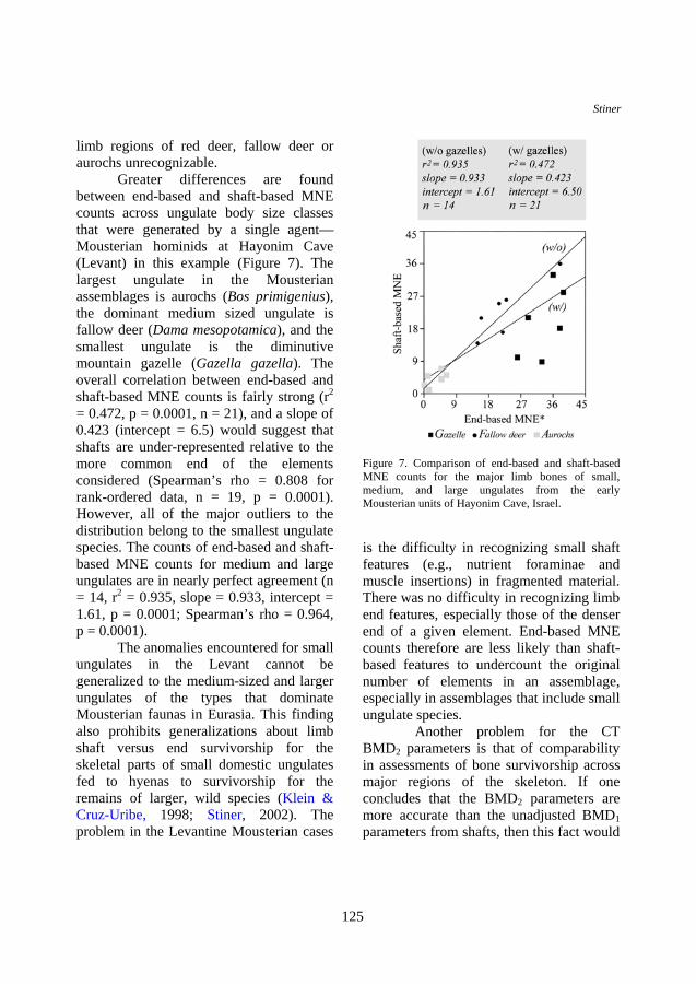
limb regions of red deer, fallow deer or aurochs unrecognizable. Greater differences are found between end-based and shaft-based MNE counts across ungulate body size classes that were generated by a single agent—Mousterian hominids at Hayonim Cave (Levant) in this example (Figure 7). The largest ungulate in the Mousterian assemblages is aurochs (Bos primigenius), the dominant medium sized ungulate is fallow deer (Dama mesopotamica), and the smallest ungulate is the diminutive mountain gazelle (Gazella gazella). The overall correlation between end-based and shaft-based MNE counts is fairly strong (r2 = 0.472, p = 0.0001, n = 21), and a slope of 0.423 (intercept = 6.5) would suggest that shafts are under-represented relative to the more common end of the elements considered (Spearman’s rho = 0.808 for rank-ordered data, n = 19, p = 0.0001). However, all of the major outliers to the distribution belong to the smallest ungulate species. The counts of end-based and shaft-based MNE counts for medium and large ungulates are in nearly perfect agreement (n = 14, r2 = 0.935, slope = 0.933, intercept = 1.61, p = 0.0001; Spearman’s rho = 0.964, p = 0.0001). The anomalies encountered for small ungulates in the Levant cannot be generalized to the medium-sized and larger ungulates of the types that dominate Mousterian faunas in Eurasia. This finding also prohibits generalizations about limb shaft versus end survivorship for the skeletal parts of small domestic ungulates fed to hyenas to survivorship for the remains of larger, wild species (Klein & Cruz-Uribe, 1998; Stiner, 2002). The problem in the Levantine Mousterian cases

is the difficulty in recognizing small shaft features (e.g., nutrient foraminae and muscle insertions) in fragmented material. There was no difficulty in recognizing limb end features, especially those of the denser end of a given element. End-based MNE counts therefore are less likely than shaft-based features to undercount the original number of elements in an assemblage, especially in assemblages that include small ungulate species.

Another problem for the CT BMD2 parameters is that of comparability in assessments of bone survivorship across major regions of the skeleton. If one concludes that the BMD2 parameters are more accurate than the unadjusted BMD1 parameters from shafts, then this fact would

Figure 7. Comparison of end-based and shaft-based MNE counts for the major limb bones of small, medium, and large ungulates from the early Mousterian units of Hayonim Cave, Israel.

126


remove shafts from the list of parts comparable to virtually all other areas of the bony skeleton. Most anthropological questions about prey body part representation concern treatment of the carcass as a whole, and which parts are transported or processed in distinctive ways.

Density range correspondences among anatomical regions The region-based approach to ungulate body part representation pools MNE counts in a way that helps to even-out variation in structural density. The technique is directed to inter-assemblage comparisons from which only the most robust differences in body part representation patterns usually are sought. The minimum number of elements (MNE) is estimated for each skeletal member of a given taxon from the most common morphologically unique “portion” or feature in the assemblage. Some portions will tend to yield higher counts than others, presumably due to their greater inherent resistance to mechanical destruction. Limb end (epiphysis) and shaft features (e.g., foraminae, Figure 8) are considered by this author in estimating MNE (Stiner, 1991, 2002). For the skull, only bony portions are used in the comparisons to post-cranial MNEs, because tooth enamel is so much denser than any kind of bone (Currey, 1984). Small, compact features are favored for counting, and many of these portions coincide with Lyman’s photon densitometry scan sites (1994:234-250; Elkin & Zanchetta, 1991; Kreutzer, 1992; Lyman, 1984; Lyman et al., 1992). The portion-of-element categories

Figure 8. Examples of portion-of-elements representing limb shafts used to count elements (MNE): (a) distal diaphysis of the scapula at its narrowest section; exterior and interior views of nutrient foraminae of (b) humerus, (c) femur, and (d) tibia. Examples are from cervids, but the criteria also apply to wild bovids.

127

Stiner

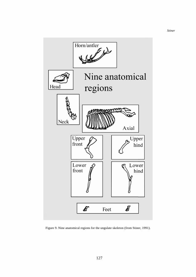
Figure 9. Nine anatomical regions for the ungulate skeleton (from Stiner, 1991).

128


tend to be hierarchical, since fragment size varies and a specimen may contain more than one portion suitable for estimating MNE (e.g., Stiner, 2002).

MNE counts are derived from the most commonly represented portion of each type of element and then condensed into an array of nine anatomical regions (Figure 9): (1) the horn/antler set, (2) head, (3) neck, (4) the rest of the axial column including the ribs and pelvis, (5, 6) upper and lower front limbs, (7, 8) upper and lower rear limbs, and (9) feet (Stiner, 1991). Species-specific identifications are pooled with specimens of the appropriate ungulate body size group to increase sample size and to overcome the fact that some elements and portions of elements are far more diagnostic of taxon than are others.

For the purpose of bar chart comparisons, body part representation can

be standardized against a whole skeleton model (Stiner’s standardized MNE, 1991; equivalent to Binford’s MAU, 1978) by dividing the observed MNE for a skeletal element or group of elements by the expected MNE for the same element or element group in one complete skeleton. If skeletal representation is complete, standardized values for all regions will be equal (and the bars will be of equal height, Figure 10), making major anatomical biases among regions easy to detect. The thickness of compact bone varies among elements, but this variation in bulk density is of a smaller order than between compact bone and the other tissue classes named above. One simply needs to know the locations of compact bone tissues relative to the distribution of the unique morphologic features (“portions”) normally used to estimate the MNE for each kind of element.

Figure 10. Standardized bar chart for the nine anatomical regions of a theoretically complete skeleton (from Stiner, 1991). (1) antler/horn, (2) head, (3) neck, (4) axial, (5) upper front limbs, (6) lower front limbs, (7) upper hind limbs, (8) lower hind limbs, (9) feet. Note that dental elements are not used to calculate the frequencies of head parts. Standardized MNE (observed MNE/expected MNE for one complete skeleton) is equivalent to Binford’s MAU (1978).

129

Stiner

How much variation in the observed MNE values among anatomical regions could be explained by variation in the density of the bone portions used for counting? I begin by considering all of the possible portions (spanning spongy and compact tissue types) in deer (Odocoileus) for which PD density estimates are available (Lyman, 1994:Table 7.6). The comparison is then narrowed to include only those portions most commonly represented in my analyses of diverse Mediterranean faunas from 1985 to the present.

Density value mid-points and ranges in Figure 11, and the pair-wise statistical comparisons of density values in Table 1, indicate that the chances for reduced recognizability of bone portions are

about the same for the head region and various limb regions. An F-ratio statistic indicates that there are no major differences among the pooled cranial, limb, and foot regions (n = 32, r2 = 0.27, p = 0.124). Upper front limbs and foot bones have a somewhat lower probability of preservation than heads and other limb regions, but these differences are minor. The chances for reduced recognizability among cranial and limb regions are closer still for those portions most commonly used by this author to estimate MNE in archaeological assemblages from Mediterranean shelter sites (n = 23, r2 = 0.330; F-ratio = 1.671, p = 0.195) (Table 2). Turning to a more stringent nonparametric version of ANOVA, a Kruskal-Wallis statistic yields basically the same answer as the tests above

Figure 11. Lyman’s (1994) photon densitometry (PD) ranges and midpoints of variation for deer (Odocoileus) across nine anatomical regions of the ungulate skeleton (from Stiner, 2002).

130


(8.393, df = 5, p = 0.136). The conceptual basis for the

profiling technique is well supported by PD estimates of variation in bone structural density. The risks of over-interpretation in this treatment of body part frequencies center on the vertebral column alone (“neck” & “axial”). The question of why vertebral elements are rare in real assemblages must be addressed in other ways.

CT standards are said to be more accurate than the available PD estimates of bone density (Lam et al., 1999). The CT BMD1 standards describe much of the skeleton, including limb ends and shafts. Density values provided by Lam et al. for the skull are confined to the mandible and the petrous bone, the latter of which appears to be exceptionally dense and therefore is omitted from this comparison. The range and average CT BMD1 density values for all skeletal portions of three

a. Mean photon densitometry values for cranial, limb & foot regions:

Anatomical region

N-portions considered

Mean density

S.d.

head 5 0.52 0.09

upper front limb 6 0.38 0.11

lower front limb 6 0.54 0.13

upper hind limb 3 0.42 0.14

lower hind limb 7 0.52 0.18

feet 5 0.36 0.12

b. Pair-wise tests for differences in density among cranial, limb & foot region pairs:

Anatomical region pair

t df p Difference In means

head-upper front limb 2.251 9.0 0.051 0.138

head-lower front limb -0.347 8.7 0.737 -0.023

head-upper hind limb 1.075 2.9 0.362 0.100

head-lower hind limb -0.037 9.3 0.972 -0.003

head-feet 2.292 7.3 0.054 0.158

Table 1. Differences in mean structural density for bony portions of elements by anatomical region based on Lyman’s photon densitometry control data for deer.

131

Stiner

Table 2. Pair-wise mean differences in structural density for (a) all potential bone portions and (b) those portions most commonly used to estimate MNE values in the Mediterranean cave faunas.

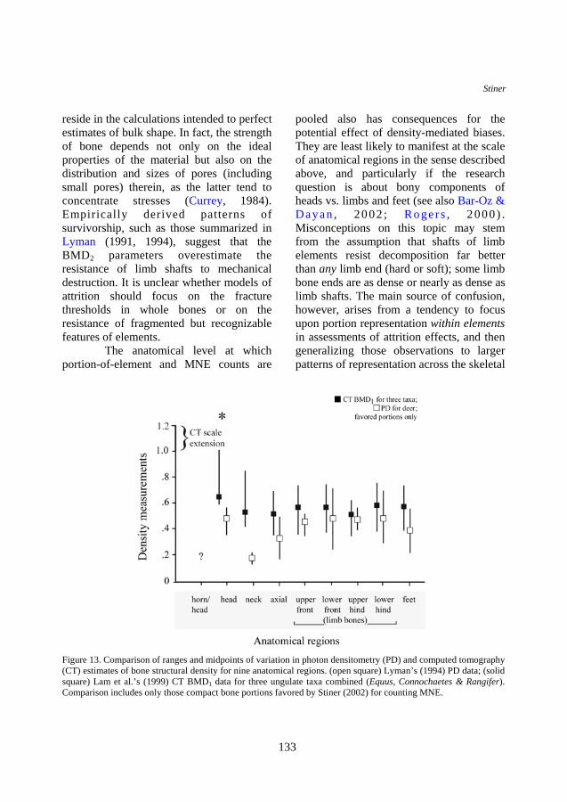
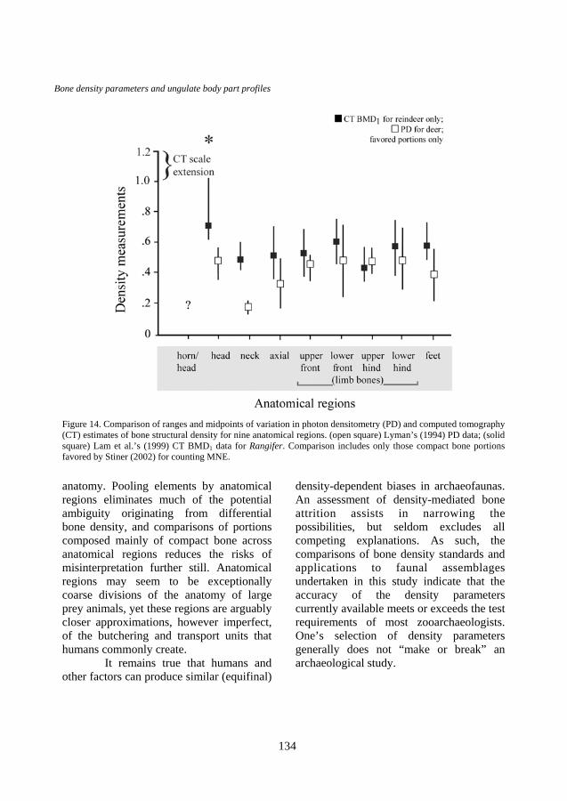
ungulate taxa combined (Equus, Connochaetes, and Rangifer) measured by Lam et al. (Figure 12) are quite similar across body regions—more similar than the patterns seen for PD standards (see Figure 11). The same is true for a narrower range of skeletal portions favored by this author in studies of Mediterranean faunas (Figure 13). Finally, a comparison specific to Rangifer (Figure 14) using the favored portions also indicates similarity in ranges and means among anatomical regions.

Conclusion Many of the components of the skull and limbs have relatively similar chances of resisting mechanical sources of in situ destruction. Macrostructure differences certainly are relevant to understanding the resistance of whole bone elements to a variety of mechanical forces (Currey 1984). Bulk density can also serve as a loose proxy for differences in the resistance of fragmented bone specimens to mechanical

a. All potential portions:

Anatomical region & code

(2) (5) (6) (7) (8) (9)

head (2) —

upper front limb (5) -0.138 —

lower front limb (6) 0.023 0.162 —

upper hind limb (7) -0.100 0.038 -0.123 —

lower hind limb (8) 0.003 0.141 -0.020 0.103 —

feet (9) -0.158 -0.020 -0.181 -0.058 -0.161 —

b. Most commonly used portions:

Anatomical region & code

(2) (5) (6) (7) (8) (9)

head (2) —

upper front limb (5) -0.114 —

lower front limb (6) -0.029 0.085 —

upper hind limb (7) -0.067 0.048 -0.037 —

lower hind limb (8) -0.033 0.082 -0.003 0.034 —

feet (9) -0.195 -0.080 -0.165 -0.128 -0.162 —

132


destruction, despite significant changes in size and shape that arise from breakage.

The assertion that head-dominated patterns, or head-and-foot-dominated patterns, in ungulate remains are likely to be the product of density-mediated attrition (e.g., Marean & Kim, 1998) is not supported by documented variation in structural density in the skeletons of vertebrates, regardless of whether PD or unadjusted CT (BMD1) parameters are used. There are few important differences in the general predictions of skeletal survivorship provided by PD and the unadjusted versions of the CT (BMD1) parameters, especially if minor differences in scaling between the two techniques are taken into account. None of the differences in bone density of head and limb regions obtained by PD or CT (BMD1) techniques is of the order needed to greatly bias MNE

estimates in the region-by-region profiling technique.

T h e o n l y o u t s t a n d i n g contradictions to comparability between PD and CT parameters are the calculation-based adjustments for compact limb shafts represented by Lam et al.’s (1999) BMD2 parameters. These density estimates set limb shafts so far out of range from other parts of the bony skeleton (except the petrous of the cranium) that one may question why or how one should use shafts for body part profiling at all. The BMD2 standards are intended to solve a technical problem posed by the exceptionally large hole within a compact bone tube. The adjusted measurement is taken as a proxy for estimating differential bone strength at the macro-scale. The discrepancy between the adjusted CT (BMD2) parameters and empirical patterns of bone preservation may

Figure 12. Comparison of ranges and midpoints of variation in photon densitometry (PD) and computed tomography (CT) estimates of bone structural density across nine anatomical regions. (open square) Lyman’s (1994) PD data for Odocoileus; (solid square) Lam et al.’s (1999) CT BMD1 data for three ungulate taxa combined (Equus, Connochaetes & Rangifer). Comparison includes all portions of elements for which density was measured.

133

Stiner

reside in the calculations intended to perfect estimates of bulk shape. In fact, the strength of bone depends not only on the ideal properties of the material but also on the distribution and sizes of pores (including small pores) therein, as the latter tend to concentrate stresses (Currey, 1984). Empirically derived patterns of survivorship, such as those summarized in Lyman (1991, 1994), suggest that the BMD2 parameters overestimate the resistance of limb shafts to mechanical destruction. It is unclear whether models of attrition should focus on the fracture thresholds in whole bones or on the resistance of fragmented but recognizable features of elements.

The anatomical level at which portion-of-element and MNE counts are

pooled also has consequences for the potential effect of density-mediated biases. They are least likely to manifest at the scale of anatomical regions in the sense described above, and particularly if the research question is about bony components of heads vs. limbs and feet (see also Bar-Oz & D ayan , 20 02 ; Roge r s , 2 000 ) . Misconceptions on this topic may stem from the assumption that shafts of limb elements resist decomposition far better than any limb end (hard or soft); some limb bone ends are as dense or nearly as dense as limb shafts. The main source of confusion, however, arises from a tendency to focus upon portion representation within elements in assessments of attrition effects, and then generalizing those observations to larger patterns of representation across the skeletal

Figure 13. Comparison of ranges and midpoints of variation in photon densitometry (PD) and computed tomography (CT) estimates of bone structural density for nine anatomical regions. (open square) Lyman’s (1994) PD data; (solid square) Lam et al.’s (1999) CT BMD1 data for three ungulate taxa combined (Equus, Connochaetes & Rangifer). Comparison includes only those compact bone portions favored by Stiner (2002) for counting MNE.

134


anatomy. Pooling elements by anatomical regions eliminates much of the potential ambiguity originating from differential bone density, and comparisons of portions composed mainly of compact bone across anatomical regions reduces the risks of misinterpretation further still. Anatomical regions may seem to be exceptionally coarse divisions of the anatomy of large prey animals, yet these regions are arguably closer approximations, however imperfect, of the butchering and transport units that humans commonly create.

It remains true that humans and other factors can produce similar (equifinal)

density-dependent biases in archaeofaunas. An assessment of density-mediated bone attrition assists in narrowing the possibilities, but seldom excludes all competing explanations. As such, the comparisons of bone density standards and applications to faunal assemblages undertaken in this study indicate that the accuracy of the density parameters currently available meets or exceeds the test requirements of most zooarchaeologists. One’s selection of density parameters generally does not “make or break” an archaeological study.

Figure 14. Comparison of ranges and midpoints of variation in photon densitometry (PD) and computed tomography (CT) estimates of bone structural density for nine anatomical regions. (open square) Lyman’s (1994) PD data; (solid square) Lam et al.’s (1999) CT BMD1 data for Rangifer. Comparison includes only those compact bone portions favored by Stiner (2002) for counting MNE.

135

Stiner

Though less widely discussed, there is at least one more issue that influences the outcomes of research on body part patterns of prey animals. This issue concerns how well any protocol for counting skeletal elements on the basis of recognizable features in fragmented material succeeds in recovering the number of elements originally present in the assemblage. Short of totally reconstructing the skeletal elements from fragments (sensu Marean et al., 1992; Marean & Kim, 1998; Marean & Spencer, 1991), the solution must lie in the level of anatomical detail recognized and recorded. The method for recording portion-of-elements used by this author is much finer grained than any of the published scan site sets (Appendix 1 and Figures 15-26); for example, this protocol treats limb ends as potentially divisible to four subsections; fewer diagnostic shaft features are available, though these portions are apparently among the most dense. Scan sites, instead, tend to represent whole bone cross-sections, whether positioned through limb epiphyses, limb shafts, or other elements. Because the scan sites describe an average density for potentially divisible morphologic subsets, the anatomical data generated by scan site and portion-of-element counts are not altogether compatible. Total refitting of fragments is more consistent with the use of scan site parameters. It is also incredibly costly. By estimating elements from features on fragments, are we missing significant numbers or types of skeletal parts by avoiding the task of complete refitting of bone fragments? A systematic comparison of refitting and portion-based reconstruction has yet to be undertaken. Ideally it should be done on fragmented

material of known history, generated by humans other than archaeologists, and analyzed by diverse zooarchaeologists as a safeguard for replicability. The outcome is unlikely to provide a basis for rejecting existing studies out of hand, but the new information could allow refinements in expectations for certain high-resolution studies of body part representation in archaeofaunas.

Acknowledgments I thank, Natalie Munro and Guy Bar-Oz, the organizers of the Montreal SAA symposium in spring 2004 for providing a stimulating forum in which to develop this study. I also am grateful to Walter Klippel and the vertebrate comparative collection at the University of Tennessee, Knoxville, for access to the Dama dama reference specimen, to Levent Atıcı of Harvard University for access to the Capra aegagrus specimen, and to the Arizona State Museum zooarchaeology comparative collection, Tucson, for access to various taxa, the bones of which are illustrated in Figures 15 through 26. This publication has benefited from comments by Bar-Oz, Munro, and an anonymous reviewer. The research was supported in part by a grant from the National Science Foundation (SBR-9511894). References Bar-Oz, G. & Dayan, T. (2002). “After 20 years”: a

taphonomic re-evaluation of Nahal Hadera V, an Epipalaeolithic site on the Israeli coastal plain. Journal of Archaeological Science, 29: 145-156.

136


Beaver, J. E. (2004). Identifying necessity and sufficiency relationships in skeletal-part representation using fuzzy-set theory. American Antiquity, 69: 131-140.

Binford, L. R. (1978). Nunamiut ethnoarchaeology. Academic Press, New York.

Binford, L. R. & Bertram, J. (1977). Bone frequencies and attritional processes. In (Binford, L. R., ed.) For theory building in archaeology. New York: Academic Press, pp. 77-156.

Brain, C. K. (1981). The hunters or the hunted? An introduction to African cave Taphonomy. University of Chicago Press, Chicago.

Brink, J. W. (1997). Fat content in leg bones of Bison bison, and applications to archaeology. Journal of Archaeological Science, 24: 259-274.

Capaldo, S. D. (1997). Experimental determinations of carcass processing by Plio-Pleistocene hominids and carnivores at FLK 22 (Zinjanthropus), Olduvai Gorge, Tanzania. Journal of Human Evolution, 33: 555-597.

Currey, J. (1984). The mechanical adaptations of bones. Princeton University Press, Princeton.

Elkin, D. C. & Zanchetta, J. R. (1991). Densitometria osea de camélidos—aplicaciones arqueológicas. Actas del X Congreso Nacional de Arqueológia Argentina (Catamarca), 3: 195-204.

Grayson, D. K. (1989). Bone transport, bone destruction, and reverse utility curves. Journal of Archaeological Science, 16: 643-652.

Klein, R. G. & Cruz-Uribe, K. (1998). Comment on Marean & Kim, “Mousterian large-mammal remains from Kobeh Cave: behavioral implications.” Current Anthropology, 39: Supplement 96-97.

Kreutzer, L. A. (1992). Bison and deer bone mineral densities: comparisons and implications for the interpretation of archaeological faunas. Journal of Archaeological Science, 19: 271-294.

Lam, Y. M., Chen, X. & Pearson, O. M. (1999). Intertaxonomic variability in patterns of bone density and the differential representation of bovid, cervid, and equid elements in the archaeological record. American Antiquity, 64 :343-362.

Lam, Y. M., Pearson, O. M., Marean, C. W. & Chen, X. (2003). Bone density studies in zooarchaeology. Journal of Archaeological Science, 30: 1701-1708.

Lupo, K. D. (1995). Hadza bone assemblages and hyena attrition: an ethnographic example of the influence of cooking and mode of discard on the

intensity of scavenger ravaging. Journal of Anthropological Archaeology, 14: 288-314.

Lupo, K. D. & Schmitt, D. N. (1997). Experiments in bone boiling: Nutritional returns and archaeological reflections. Anthropozoologica, 25-26: 137-144.

Lyman, R. L. (1984). Bone density and differential survivorship of fossil classes. Journal of Anthropological Archaeology, 3: 259-299.

Lyman, R. L. (1991). Taphonomic problems with archaeological analyses of animal carcass utilization and transport. In (Purdue, J. R., Klippel, W. E. & Styles, B. W., eds.) Beamers, bobwhites, and blue-points: tributes to the career of Paul W. Parmalee. Springfield: Illinois State Museum Scientific Papers, no. 23, pp. 125-138.

Lyman, R. L. (1994). Vertebrate taphonomy. Cambridge University Press, Cambridge.

Lyman, R. L., Houghton, L. E. & Chambers, A. L. (1992). The effect of structural density on marmot skeletal part representation in archaeological sites. Journal of Archaeological Science, 19: 557-573.

Marean, C. W. & Kim, S. Y. (1998). Mousterian large-mammal remains from Kobeh Cave: behavioral implications. Current Anthropology, 39: Supplement 79-113.

Marean, C. W. & Spencer, L. M. (1991). Impact of carnivore ravaging on zooarchaeological measures of element abundance. American Antiquity, 56: 645-658.

Marean, C. W., Spencer, L. M., Blumenschine, R. J. & Capaldo, S. D. (1992). Captive hyaena bone choice and destruction, the Schlepp Effect and Olduvai archaeofaunas. Journal of Archaeological Science, 19: 101-121.

Margaris, A. V. (2004). Apatite for destruction: differential rates of compact and cancellous bone dissolution. Poster presentation at the 69th Annual Meeting of the Society for American Archaeology Meetings. 31 March 2004, Montreal, Canada.

Munro, N. D. (2004). Zooarchaeological measures of human hunting pressure and site occupation intensity in the Natufian of the southern Levant and the implications for agricultural origins. Current Anthropology, 45 Supplement: 5-33.

O'Connell, J. F., Hawkes. K. & Blurton Jones, N. (1988). Hadza hunting, butchering, and bone transport and their archaeological implications. Journal of Anthropological Research, 44: 113-161.

Rogers, A. (2000). On the value of soft bones in faunal analysis. Journal of Archaeological

137

Stiner

Science, 27: 635-639. Stiner, M. C. (1991). Food procurement and transport

by human and non-human predators. Journal of Archaeological Science, 18: 455-482.

Stiner, M. C. (1994). Honor among thieves: a zooarchaeological study of Neandertal ecology. Princeton University Press, Princeton.

Stiner, M. C. (2003). Zooarchaeological evidence for resource intensification in Algarve, southern Portugal. Promontoria, 1: 27-61.

Stiner, M.C. (2002). On in situ attrition and vertebrate body part profiles. Journal of Archaeological Science, 29: 979-991.

Stiner, M. C. (2005). The faunas of Hayonim Cave (Israel): a 200,000-Year record of Paleolithic diet, demography & society. American School of Prehistoric Research, Peabody Museum Press, Harvard University, Cambridge, Mass.

Todd, L. C. (1987). Analysis of kill-butchering bonebeds and interpretation of Paleoindian hunting. In (Nitecki, M., ed.) The evolution of human hunting. New York: Plenum Press, pp. 225-266.

138


Appendix 1. Stiner’s faunal coding keys for skeletal elements and portions of elements in research on ungulate faunas. Portions can occur singly or in combination with others, and thus the coding system is hierarchical (from Stiner 2002). ELEMENTS PORTIONS-OF-ELEMENTS _________________________________________________________________________ HORN/ANTLER (10s): HORN/ANTLER: 11 horn core 10 rosette (base) 12 antler 11 pedicle-braincase 12 shaft-rosette-pedicle-braincase SKULL (20s): 13 tip/tine (2=shaft fragment; 80=diaphysis section) 21 half cranium, L or R 22 half mandible, L or R CRANIUM & MANDIBLE: 19 hyoid NECK (30s): 20 premaxilla (or “incisive” of anterior mandible) 31 atlas 21 nasal 32 axis 22 zygomatic (mastoid-squamous zone) 33 cervical vertebra 23 maxilla (~complete half) 24 maxilla fragment (241 anterior rim; 242 posterior rim) MAIN AXIAL COLUMN (40s): 25 petrous 40 vertebra, type unknown 26 auditory bulla 41 thoracic vertebra 27 braincase fragment 42 rib 28 occipital (dorsal rim) 43 lumbar vertebra 29 occipital condyle (right or left) 44 sacral vertebra 30 frontal foramen (or anterior foramen of mandible) 45 innominate (1/2 pelvis) 31 orbit lower rim (or gonial angle of mandible) 46 caudal vertebra 32 lacrimal (foramen) 47 sternal segment Other: 16 post margin of mandibular symphysis; 17 basi-cranium; 18 upper orbit FRONT LIMB (50s & 60s): MANDIBLE, BASE MISSING: 51 scapula 33 middle horizontal ramus 52 humerus 34 mid-anterior horizontal ramus 53 coracoid (e.g., birds) 35 anterior horizontal ramus (anterior alvaeolus of LP2) 61 radius 36 mid-posterior horizontal ramus 62 ulna 37 posterior horizontal ramus (dorsal ridge behind LM3) 63 carpal (type unknown) 38 concavity between condyle-coronoid (or base of glenoid process of scapula) 64 metacarpal (bird=carpometacarpus) 39 base of horizontal ramus 65 cuneiform 40 condyloid process 66 magnum 41 coronoid process 67 lunate 42 condyle & coronoid 68 scaphoid 43 ascending ramus (431lingual foramen) 69 unciform MANDIBLE, BASE INTACT: HIND LIMB (70s & 80s): 44 horizontal ramus (whole) 71 femur 45 middle horizontal ramus 81 tibia 46 anterior horizontaontal ramus 82 patella 47 posterior horizontal ramus 83 astragalus 48 mid-anteror horizontal ramus 84 calcaneum 49 mid-posterior horizontal ramus 85 tarsal (type unknown) 86 metatarsal (bird=tarsometatarsus) INNOMINATE: 87 naviculo-cuboid 57 acetabulum fragment 88 external & middle cuneiform 58 acetabulum section—pubic body (581 anterior rim of symphysis; 582 ridge) 89 lateral malleolus 59 acetabulum, complete 60 acetabulum & ilium (~complete) FEET (90s): 61 acetabulum section—iliac body fragment 90 sesamoid 62 acetabulum-iscium (~complete) 91 first phalanx 63 acetabulum section—ischial body fragment 92 second phalanx 64 iliac body (diaphysis) 93 third/terminal phalanx 65 iliac blade (651 dorsal tip; 652 ventral tip)

139

Stiner

66 ilium GENERAL ELEM CATEGORIES: 67 ischial body 1 metapodial (type unknown) 68 ischial blade (681 base or coxae; 682 lateral tuberosity) 2 long bone shaft (type unknown) 69 ischium 3 flat bone (skull or scapula fragment) 4 carpal or tarsal (type unknown) GENERAL ELEM. CAT., cont.: VERTEBRAE: 5 spongy element (axial) 50 epiphysis (501 anterior; 502 posterior) 6 auxiliary third phalanx 51 centrum (body intact) 7 auxiliary second phalanx 52 transverse process 8 auxiliary first phalanx 53 pre-zygopophyses (53-53=intact pair) 9 auxiliary metapodial 54 post-zygopophyses (54-54=intact pair) 55 dorsal spine (also proximal “heel” of ulna olecranon) 56 half TEETH (100s, mammals only): 57 anterior-ventral articulation 9_ _ _deciduous tooth 58 zygopophysis (type unknown) 100 from upper jaw 200 from lower jaw LIMB BONES & RIB (LARGER PORTIONS: 300 dental position unknown 70 proximal (P) epiphysis _10 incisor (type unknown) 71 P epiphysis fragment (see also 91-94) _11 first incisor 72 P < 1/2 _12 second incisor 73 P 1/2 _13 third incisor 74 P > 1/2 _20 canine 75 distal (D) > 1/2 _30 premolar (type unknown) 76 D 1/2 _31 first premolar 77 D < 1/2 _32 second premolar 78 D epiphysis fragment (see also portions 81, 84) _33 third premolar 79 D epiphysis _34 fourth premolar _40 molar (type unknown) LIMB BONE & RIB EPIPHYSIS PORTIONS: _41 first molar 81 medial distal (D) epiphysis _42 second molar 82 lateral D epiphysis _43 third molar 83 anterior D epiphysis 84 posterior D epiphysis 91 anterior proximal (P) epiphysis 92 posterior P epiphysis 93 medial P epiphysis 94 lateral P epiphysis (for calcaneum: 941 tuberosity, 942 tip) LIMB BONE SHAFT & INNOMINATE FEATURES: 990 w/ foramen present 991 w/ proximal rim of attachment scar (radius or ulna) 992 waist (narrowest cross-section or collum) of diaphysis (scapula) 994 anterior "angle" (tibia or scapula) 995 muscle insertion or ligament scar 996 posterior rugosities (tibia or innominate) 997 interior diagonal lattice (humerus) 998 anterior groove (metapodials) 999 posterior groove (metapodials) GENERAL PORTION CODES: 1 complete 2 nearly complete 56 half (561 lateral dimension; 562 vertical) 80 short diaphysis (tube) 85 long diaphysis (for rib, proximal diaphysis with dorsal ridge 86 diaphysis with foramen 90 shaft fragment 95 spongy bone fragment 97 flat bone fragment

140


NOTE: Position and character of a named portion may vary somewhat with taxon such that minor adjustments in definition are needed. This system for classifying and counting distinct morphological features on bones is designed to reconstruct the number of elements represented by fragmented material, and to facilitate simple quantification for body part analysis. Morphologic terms that are unique to a particular element (e.g., processus anconaeus) are avoided in favor of terms that reflect commonalities in shape and orientation (e.g., anterior, posterior; proximal, distal).

Figure 15. Examples of the minimum possible portions-of-elements (code number in italics) for the scapula of Ovis aries as represented in the body part coding system in Appendix 1. Line drawing represents PD and CT scan sites (adapted from Lyman, 1984).

Figure 16. Examples of the minimum possible portions-of-elements (code number in italics) for the humerus of Sus scrofa as represented in the body part coding system in Appendix 1. Line drawing represents PD and CT scan sites (adapted from Lyman, 1984).

141

Stiner

Figure 17. Examples of the minimum possible portions-of-elements (code number in italics) for the radius and ulna of Capra aegagrus as represented in the body part coding system in Appendix 1. Line drawing represents PD and CT scan sites (adapted from Lyman, 1984).

Figure 18. Examples of the minimum possible portions-of-elements (code number in italics) for the femur of Dama dama as represented in the body part coding system in Appendix 1. Line drawing represents PD and CT scan sites (adapted from Lyman, 1984).

142


Figure 19. Examples of the minimum possible portions-of-elements (code number in italics) for the tibia of Ovis canadensis as represented in the body part coding system in Appendix 1. Line drawing represents PD and CT scan sites (adapted from Lyman, 1984).

Figure 20. Examples of the minimum possible portions-of-elements (code number in italics) for the metatarsal of Bos taurus as represented in the body part coding system in Appendix 1. Line drawing represents PD and CT scan sites (adapted from Lyman, 1984).

143

Stiner

Figure 21. Examples of the minimum possible portions-of-elements (code number in italics) for the cranium of Dama dama as represented in the body part coding system in Appendix 1. No scan sites.

Figure 22. Examples of the minimum possible portions-of-elements (code number in italics) for the mandible of Ovis canadensis as represented in the body part coding system in Appendix 1. Line drawing represents PD and CT scan sites (adapted from Lyman, 1984).

144


Figure 23. Examples of the minimum possible portions-of-elements (code number in italics) for various cervical vertebrae of Dama dama as represented in the body part coding system in Appendix 1. Line drawing represents PD and CT scan sites (adapted from Lyman, 1984).

Figure 24. Examples of the minimum possible portions-of-elements (code number in italics) for the thoracic and lumbar vertebrae of Dama dama as represented in the body part coding system in Appendix 1. Line drawing represents PD and CT scan sites (adapted from Lyman, 1984).

145

Stiner

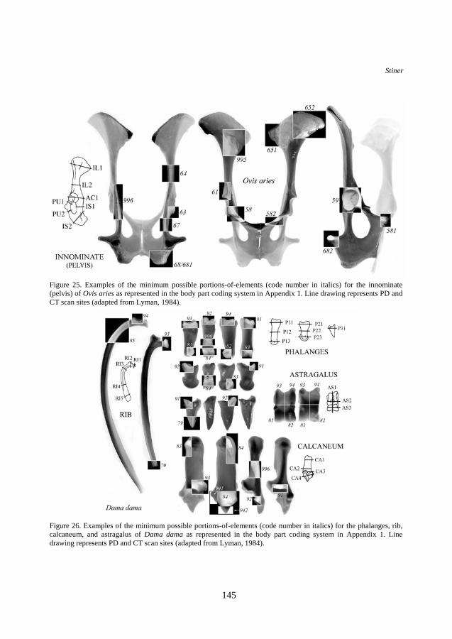
Figure 25. Examples of the minimum possible portions-of-elements (code number in italics) for the innominate (pelvis) of Ovis aries as represented in the body part coding system in Appendix 1. Line drawing represents PD and CT scan sites (adapted from Lyman, 1984).

Figure 26. Examples of the minimum possible portions-of-elements (code number in italics) for the phalanges, rib, calcaneum, and astragalus of Dama dama as represented in the body part coding system in Appendix 1. Line drawing represents PD and CT scan sites (adapted from Lyman, 1984).

146


PROMETHEUS PRESS/PALAEONTOLOGICAL NETWORK …mstiner/pdf/Stiner2004b.pdf · independent of bone...

Documents

Transcript of PROMETHEUS PRESS/PALAEONTOLOGICAL NETWORK …mstiner/pdf/Stiner2004b.pdf · independent of bone...