PROLONGATIONS OF GEOMETRIC OVERDETERMINED
22
PROLONGATIONS OF GEOMETRIC OVERDETERMINED SYSTEMS THOMAS BRANSON, ANDREAS ˇ CAP, MICHAEL EASTWOOD, AND A. ROD GOVER Abstract. We show that a wide class of geometrically defined overdetermined semilinear partial differential equations may be explicitly prolonged to obtain closed systems. As a consequence, in the case of linear equations we extract sharp bounds on the dimension of the solution space. 1. Introduction For ordinary differential equations, it is clear that the n th order equation d n σ dx n = f x, σ, dσ dx ,..., d n-1 σ dx n-1 is equivalent to the system of first order equations dσ dx = σ 1 ,..., dσ k dx = σ k+1 ,..., dσ n-1 dx = f (x, σ, σ 1 ,...,σ n-1 ). This manœuvre is well-known, for example, in reducing the existence and uniqueness of solutions to ordinary differential equations to the case of first order equations. For partial differential equations, however, this na¨ ıve manœuvre fails. Even for overdetermined equations, it is necessary to introduce new dependent variables for certain higher derivatives in order to achieve a first order ‘closed system’—one in which all the first partial derivatives of all the dependent variables are determined in terms of the variables themselves. Example 1.1.2 below is typical in this regard—the original equation is first order but the closed system (1.5) implicitly but necessarily involves second derivatives of the original dependent variables σ a . The introduction of new variables for unknown higher derivatives with the aim of expressing all their derivatives as differential consequences of the original equation is the well-known procedure of ‘prolongation’. Classically, the prolongations of a semilinear differential operator D : E → F between smooth vector bundles E and F on a smooth manifold M are constructed 2000 Mathematics Subject Classification. Primary 35N05; Secondary 17B66, 22E46, 58J70. Key words and phrases. Prolongation, Overdetermined, Semilinear, Partial differential equation. The authors would like to thank the American Institute of Mathematics, the Erwin Schr¨ odinger Institute, the Institute for Mathematical Sciences at the National University of Singapore, and the Banff International Research Station for hospitality during the preparation of this article. This research was also supported by the US NSF (Grant INT-9724781), the Austrian FWF (Project P15747), the Australian Research Council, the Royal Society of New Zealand (Marsden Grant 02- UOA-108), and the New Zealand Institute of Mathematics and its Applications. The authors express their thanks to the referee for suggesting clarifications in the text. 1
Transcript of PROLONGATIONS OF GEOMETRIC OVERDETERMINED

PROLONGATIONS OF GEOMETRIC OVERDETERMINEDSYSTEMS
THOMAS BRANSON, ANDREAS CAP, MICHAEL EASTWOOD, AND A. ROD GOVER
Abstract. We show that a wide class of geometrically defined overdeterminedsemilinear partial differential equations may be explicitly prolonged to obtain closedsystems. As a consequence, in the case of linear equations we extract sharp boundson the dimension of the solution space.
1. Introduction
For ordinary differential equations, it is clear that the nth order equation
dnσ
dxn= f
(x, σ,
dσ
dx, . . . ,
dn−1σ
dxn−1
)is equivalent to the system of first order equations
dσ
dx= σ1, . . . ,
dσk
dx= σk+1, . . . ,
dσn−1
dx= f(x, σ, σ1, . . . , σn−1).
This manœuvre is well-known, for example, in reducing the existence and uniquenessof solutions to ordinary differential equations to the case of first order equations.
For partial differential equations, however, this naıve manœuvre fails. Even foroverdetermined equations, it is necessary to introduce new dependent variables forcertain higher derivatives in order to achieve a first order ‘closed system’—one inwhich all the first partial derivatives of all the dependent variables are determined interms of the variables themselves. Example 1.1.2 below is typical in this regard—theoriginal equation is first order but the closed system (1.5) implicitly but necessarilyinvolves second derivatives of the original dependent variables σa. The introductionof new variables for unknown higher derivatives with the aim of expressing all theirderivatives as differential consequences of the original equation is the well-knownprocedure of ‘prolongation’.
Classically, the prolongations of a semilinear differential operator D : E → Fbetween smooth vector bundles E and F on a smooth manifold M are constructed
2000 Mathematics Subject Classification. Primary 35N05; Secondary 17B66, 22E46, 58J70.Key words and phrases. Prolongation, Overdetermined, Semilinear, Partial differential equation.The authors would like to thank the American Institute of Mathematics, the Erwin Schrodinger
Institute, the Institute for Mathematical Sciences at the National University of Singapore, and theBanff International Research Station for hospitality during the preparation of this article. Thisresearch was also supported by the US NSF (Grant INT-9724781), the Austrian FWF (ProjectP15747), the Australian Research Council, the Royal Society of New Zealand (Marsden Grant 02-UOA-108), and the New Zealand Institute of Mathematics and its Applications. The authors expresstheir thanks to the referee for suggesting clarifications in the text.
1

2 THOMAS BRANSON, ANDREAS CAP, MICHAEL EASTWOOD, AND A. ROD GOVER
from its leading symbol σ(D) :⊙k Λ1 ⊗ E → F where
⊙k Λ1 denotes the bundle ofsymmetric covariant tensors on M of valence k. At any point of M , denoting by Kthe kernel of σ(D), one considers the vector spaces
(1.1) Vi = (⊙i Λ1 ⊗ E) ∩ (
⊙i−k Λ1 ⊗K) for i ≥ k,
declaring the system to be of finite type if Vi = 0 for i sufficiently large [15]. Thesolutions of a system of finite type are determined by finitely many jets at a point.Although there is a general criterion that D be of finite type (namely, that its char-acteristic variety be empty [15, Proposition 1.7.5]) the computation of Vi presents amajor obstacle to further progress.
There are two main points to this article. Firstly, for a wide class of geometricoverdetermined partial differential equations, we explicitly compute Vi (Lemma 3.1
part (4)). The direct sum V =⊕N
i=0 Vi is a vector bundle induced by an irreduciblerepresentation of a reductive Lie algebra so N and its rank can be immediatelyread off. This gives sharp bounds on the jet needed to pin down a solution and,in the linear case, the dimension of the space of solutions. The second point tothis article is motivated by geometric considerations. We can deal with all symbolsof overdetermined invariant operators for an important class of structures includingconformal and quaternionic geometries. Motivated by the machinery of Bernstein-Gelfand-Gelfand sequences [3, 4], we find a uniform procedure to perform the furthersteps necessary explicitly to rewrite the equation in closed form. For the wholedevelopment, representation theory, especially Kostant’s algebraic Hodge theory [11]in Lie algebra cohomology, provides the key to our method.
For readers unfamiliar with overdetermined systems, we begin by discussing someexamples. The reader should be aware, however, that these examples are far toosimple satisfactorily to illustrate the general procedure. In fact, this is inevitable—though our algorithm is explicit, the details in any particular case will generally befearsome. However, for many purposes, the details are unnecessary. For example, wemay deduce without hesitation that, on a Riemannian manifold of dimension n ≥ 3,the space of solutions of the partial differential equation
(1.2) the trace-free part of ∇(a∇bσc) = 0
is finite-dimensional of dimension at most n(n + 2)(n + 4)/3. This bound is sharpand any solution is determined by its 4-jet at one point.
In (1.2) and throughout, we adopt Penrose’s abstract index notation [13]. Thus,indices act as markers to specify the type of a tensor (so σa is a 1-form whilst σa
would be a vector field) and to record symmetries and contractions. Round brackets,as in (1.2), mean that the indices they enclose are symmetrised, square brackets φ[ab]c
take the skew part, and a repeated index φaab denotes contraction. On a Riemannian
manifold, indices may be raised or lowered with the metric in the usual way. Con-nections will be denoted ∇a and on a Riemannian manifold will usually mean theLevi-Civita connection. If ∇a is a torsion-free connection on the tangent bundle, thenits curvature tensor Rab
cd is defined by
(∇a∇b −∇b∇a)Vc = Rab
cdV
d.
PROLONGATIONS OF GEOMETRIC OVERDETERMINED SYSTEMS 3
In particular, ∇b∇aVb = ∇a∇bV
b +RabVb, where Rab = Rca
cb is the Ricci tensor.
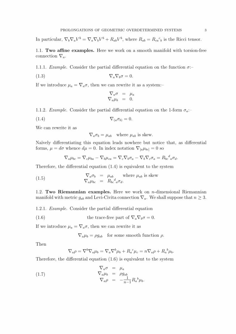
1.1. Two affine examples. Here we work on a smooth manifold with torsion-freeconnection ∇a.
1.1.1. Example. Consider the partial differential equation on the function σ:–
(1.3) ∇a∇bσ = 0.
If we introduce µa = ∇aσ, then we can rewrite it as a system:–
∇aσ = µa
∇aµb = 0.
1.1.2. Example. Consider the partial differential equation on the 1-form σa:–
(1.4) ∇(aσb) = 0.
We can rewrite it as
∇aσb = µab where µab is skew.
Naıvely differentiating this equation leads nowhere but notice that, as differentialforms, µ = dσ whence dµ = 0. In index notation ∇[aµbc] = 0 so
∇aµbc = ∇cµba −∇bµca = ∇c∇bσa −∇b∇cσa = Rbcdaσd.
Therefore, the differential equation (1.4) is equivalent to the system
(1.5)∇aσb = µab where µab is skew∇aµbc = Rbc
daσd.
1.2. Two Riemannian examples. Here we work on n-dimensional Riemannianmanifold with metric gab and Levi-Civita connection∇a. We shall suppose that n ≥ 3.
1.2.1. Example. Consider the partial differential equation
(1.6) the trace-free part of ∇a∇bσ = 0.
If we introduce µa = ∇aσ, then we can rewrite it as
∇aµb = ρgab for some smooth function ρ.
Then
∇aρ = ∇b∇aµb = ∇a∇bµb +Racµc = n∇aρ+Ra
bµb.
Therefore, the differential equation (1.6) is equivalent to the system
(1.7)
∇aσ = µa
∇aµb = ρgab
∇aρ = − 1n−1Ra
bµb.

4 THOMAS BRANSON, ANDREAS CAP, MICHAEL EASTWOOD, AND A. ROD GOVER
1.2.2. Example. Consider the partial differential equation
(1.8) the trace-free part of ∇(aσb) = 0.
Even in this simple case, prolongation is already fairly involved. The details can beomitted on first reading and the main features are described in §1.3 below. We canrewrite (1.8) as
(1.9) ∇aσb = µab + νgab where µab is skew.
Then ∇[aµbc] = 0, so
(1.10)∇aµbc = ∇cµba −∇bµca = ∇c(∇bσa − νgba)−∇b(∇cσa − νgca)
= Rbcdaσd − gab∇cν + gac∇bν.
Tracing over a and b gives
∇bµbc = −Rcdσd − (n− 1)∇cν.
Let us introduce ρc = 1n−1∇
bµbc and rearrange this last equation as
(1.11) ∇aν = −ρa − 1n−1Ra
bσb.
It may be used to eliminate ∇cν from (1.10) to obtain
(1.12) ∇aµbc = gabρc − gacρb +Kabc,
where
(1.13) Kabc = Rbcdaσd + 1
n−1gabRcdσd − 1
n−1gacRbdσd.
Notice that Kabc is totally trace-free. Now apply ∇d to (1.12) and skew over a and dto obtain
Rdaebµce −Rda
ecµbe = ∇dKabc −∇aKdbc + gab∇dρc − gdb∇aρc − gac∇dρb + gdc∇aρb.
Tracing over a and b gives
Rdeµce −Rd
becµbe = −∇bKdbc + (n− 2)∇dρc + gdc∇bρb
but tracing again, over c and d, gives 0 = 2(n− 1)∇bρb. Therefore,
(1.14) ∇aρb = 1n−2
(Ra
cµbc −Racd
bµcd −∇cKabc
).
At this point it is clear that the system has closed: it comprises (1.9), (1.11), (1.12),and in (1.14) one has to expand ∇cKabc using (1.13) and (1.9).
1.3. Discussion. In each of the examples above, we start with a linear differentialoperator D : E → F between vector bundles and the conclusion is that variousauxiliary fields may be introduced so that the equation Dσ = 0 is equivalent to a‘closed system’ in which all the first partial derivatives of all fields are determined aslinear expressions in the fields themselves. It is convenient to regard this system as
a vector bundle V with connection ∇. Thus, the conclusion of Example 1.1.2 is that
∇(aσb) = 0 if and only if ∇Σ = 0

PROLONGATIONS OF GEOMETRIC OVERDETERMINED SYSTEMS 5
where
Σ =
σb
µbc
is a section of the vector bundle V =Λ1
⊕Λ2
and ∇ : V → Λ1 ⊗ V is the connection:–
∇a
σb
µbc
=
∇aσb − µab
∇aµbc −Rbcdaσd
.
Our examples, constructing Σ and ∇ from σ and D, follow the well-known methodof ‘prolongation’. Our aim in this article, however, is to predict the form of a validprolongation for a natural and extensive class of examples without having to carryout the prolongation in detail.
The conclusion of Example 1.2.2 is that (1.8) is equivalent to ∇Σ = 0 where
Σ =
σb
µbc νρb
is a section of the bundle V =
Λ1
Λ2⊕
Λ0
Λ1
and ∇ : V → Λ1 ⊗ V is an explicit connection of the form
(1.15) ∇
σµ ν
ρ
=
∇σ − µ− ν∇µ− ρ−R ./ σ ∇ν − ρ−R ./ σ∇ρ−R ./ µ−R ./ ν − (∇R) ./ σ
,
where each ./ indicates an appropriate linear combination of contractions of itsingredients.
Note that Σ is obtained from σa by application of a linear second order differentialoperator, explicitly
σa 7−→
σa
∇[aσb]1n∇
aσa1
2(n−1)(∇b∇bσa −∇b∇aσb
) .
The equation (1.8) is well-known. It says that the vector field σa is a conformalKilling field—its flow preserves the metric up to scale. From this geometric interpre-tation it follows easily that the space of solutions is bounded by dim so(n+1, 1) sinceso(n+ 1, 1) is the conformal algebra in the flat case. This bound is confirmed by thetechnique of prolongation:–
rankV = 2 rank Λ1 + rank Λ2 + rank Λ0 = 2n+n(n− 1)
2+ 1 =
(n+ 1)(n+ 2)
2.
In [14], Semmelmann uses this technique to establish similar bounds on the dimensionof spaces of conformal Killing forms. Specifically, he finds an explicit connection (alsohaving the form (1.15)) on the bundle
V =
Λp
Λp+1⊕
Λp−1
Λp
with rank
(n+ 2p+ 1
)

6 THOMAS BRANSON, ANDREAS CAP, MICHAEL EASTWOOD, AND A. ROD GOVER
so that conformal Killing p-forms are equivalent to parallel sections of this bundle.The general procedure, to be explained in this article, includes this case and manymore besides.
The corresponding bound for Example 1.1.2 is
rank Λ1 + rank Λ2 = n+n(n− 1)
2=n(n+ 1)
2.
It was pointed out to us by Dan Fox that this is precisely the bound investigated byEisenhart in [8].
1.4. Semilinear variants. Each of the examples discussed so far persists in a semi-linear form. Thus, Example 1.1.1 may be modified as
∇a∇bσ = fab(x, σ,∇cσ)
where fab depends smoothly on its arguments and takes values in symmetric 2-tensors.Evidently, this equation is equivalent to the system
∇aσ = µa
∇aµb = fab(x, σ, µa).
Example 1.1.2 may be modified as
(1.16) ∇(aσb) = fab(x, σc).
The only difficulty in following previous reasoning is that one must be careful as tothe meaning of ∇cfab(x, σd). As it arises, σd is a function of x and so fab may beregarded as a tensor on the manifold and ∇cfab as the usual covariant derivative. Onthe other hand, we may fix σd, regard fab(x, σd) as a function of its first argument,and then take its covariant derivative. We shall use the notation ∂cfab for the resultof this point of view. There is also the partial derivative obtained by fixing x anddifferentiating with respect to σd: let us write δd = ∂/∂σd. Then, by the chain rule,
∇cfab = ∂cfab + (δdfab)∇cσd,
often referred to as expressing ‘total derivative’ in terms of ‘partial derivative’. Theresult of following previous reasoning is that (1.16) is equivalent to the system
∇aσb = µab + fab
∇aµbc = Rbcdaσd + 2∂[bfc]a − 2(δdfa[b)µc]d − 2(δdfa[b)fc]d,
where µab is skew. As a typical nonlinear variant therefore,
∇(aσb) = σaσb + Sab
for an arbitrary given symmetric tensor Sab is equivalent to the closed system
∇aσb = µab + σaσb + Sab
∇aµbc = Rbcdaσd + 2∇[bSc]a − 2σ[bµc]a + 2σaµbc + 2Sa[bσc].
The general semilinear variant of Example 1.2.1 is
∇a∇bσ − 1ngab∇c∇cσ = fab(x, σ,∇cσ),

PROLONGATIONS OF GEOMETRIC OVERDETERMINED SYSTEMS 7
where fab(x, σ, σc) is symmetric and trace-free. If we write δ = ∂/∂σ, then the chainrule for total derivative in terms of partial derivative is
∇cfab = ∂cfab + (δfab)∇cσ + (δdfab)∇cσd
and the closed system generalising (1.7) is
∇aσ = µa
∇aµb = ρgab + fab
∇aρ = − 1n−1Ra
bµb + 1n−1(∂bfab + (δfab)µ
b + (δbfab)ρ+ (δdfab)fbd).
A particular semilinear variant of Example 1.2.2 is
the trace-free part of (∇(aσb) + σaσb + 1n−2Rab) = 0,
where Rab is the Ricci tensor. It is the Einstein-Weyl equation and the correspondingclosed system is derived in [7] by ad hoc methods.
2. Formulation of the main results
Firstly, some generalities on differential operators. As detailed in [15], to everysmooth vector bundle E on a smooth manifold M there are the canonically associatedjet bundles JkE onM and short exact sequences of homomorphisms of vector bundles
0→⊙k Λ1 ⊗ E → JkE → Jk−1E → 0,
where⊙k Λ1 denotes the kth symmetric tensor power of Λ1. A kth order linear
differential operator D : E → F between vector bundles E and F is equivalent to ahomomorphism of vector bundles JkE → F and the symbol σ(D) of D is defined asthe composition
(2.1)⊙k Λ1 ⊗ E ↪→ JkE → F.
A differential operator of the form D1 + D2 where D1 is kth order linear and D2 is(k − 1)st order is called semilinear and its symbol is defined to be σ(D1).
If we now return to the semilinear variants of our affine examples, we see that theform of the equation is independent of the connection. Equation (1.16), for example,says that we have a first order semilinear operator Λ1 →
⊙2 Λ1 whose symbol
Λ1 ⊗ Λ1 −→⊙2 Λ1
is taking the symmetric part. In particular, a change of torsion-free connectionin (1.4) is covered by
∇(aσb) = Γabcσc
as a special case of (1.16).To formulate the semilinear equations on a smooth manifold M to which our pro-
longation procedure will apply, let us regard the tangent bundle as tautologicallyassociated to the frame bundle under the standard representation of GL(n,R) on Rn.Then, an irreducible tensor bundle on M is, by definition, a bundle associated tothe frame bundle under an irreducible representation of GL(n,R). By basic rep-resentation theory, any tensor bundle decomposes into a direct sum of irreducibletensor bundles. In fact, for technical reasons, let us fix a volume form on M . This
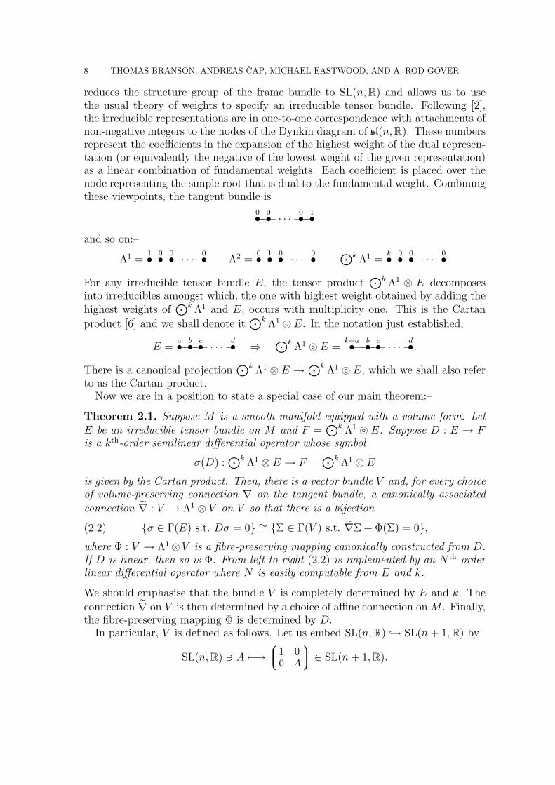
8 THOMAS BRANSON, ANDREAS CAP, MICHAEL EASTWOOD, AND A. ROD GOVER
reduces the structure group of the frame bundle to SL(n,R) and allows us to usethe usual theory of weights to specify an irreducible tensor bundle. Following [2],the irreducible representations are in one-to-one correspondence with attachments ofnon-negative integers to the nodes of the Dynkin diagram of sl(n,R). These numbersrepresent the coefficients in the expansion of the highest weight of the dual represen-tation (or equivalently the negative of the lowest weight of the given representation)as a linear combination of fundamental weights. Each coefficient is placed over thenode representing the simple root that is dual to the fundamental weight. Combiningthese viewpoints, the tangent bundle is
0• 0• · · · 0• 1•
and so on:–
Λ1 =1• 0• 0• · · · 0• Λ2 =
0• 1• 0• · · · 0•⊙k Λ1 =
k• 0• 0• · · · 0•.
For any irreducible tensor bundle E, the tensor product⊙k Λ1 ⊗ E decomposes
into irreducibles amongst which, the one with highest weight obtained by adding thehighest weights of
⊙k Λ1 and E, occurs with multiplicity one. This is the Cartan
product [6] and we shall denote it⊙k Λ1 } E. In the notation just established,
E =a• b• c• · · · d• ⇒
⊙k Λ1 } E =k+a• b• c• · · · d•.
There is a canonical projection⊙k Λ1 ⊗ E →
⊙k Λ1 } E, which we shall also referto as the Cartan product.
Now we are in a position to state a special case of our main theorem:–
Theorem 2.1. Suppose M is a smooth manifold equipped with a volume form. LetE be an irreducible tensor bundle on M and F =
⊙k Λ1 } E. Suppose D : E → Fis a kth-order semilinear differential operator whose symbol
σ(D) :⊙k Λ1 ⊗ E → F =
⊙k Λ1 } E
is given by the Cartan product. Then, there is a vector bundle V and, for every choiceof volume-preserving connection ∇ on the tangent bundle, a canonically associated
connection ∇ : V → Λ1 ⊗ V on V so that there is a bijection
(2.2) {σ ∈ Γ(E) s.t. Dσ = 0} ∼= {Σ ∈ Γ(V ) s.t. ∇Σ + Φ(Σ) = 0},where Φ : V → Λ1⊗V is a fibre-preserving mapping canonically constructed from D.If D is linear, then so is Φ. From left to right (2.2) is implemented by an N th orderlinear differential operator where N is easily computable from E and k.
We should emphasise that the bundle V is completely determined by E and k. The
connection ∇ on V is then determined by a choice of affine connection on M . Finally,the fibre-preserving mapping Φ is determined by D.
In particular, V is defined as follows. Let us embed SL(n,R) ↪→ SL(n+ 1,R) by
SL(n,R) 3 A 7−→1 0
0 A
∈ SL(n+ 1,R).

PROLONGATIONS OF GEOMETRIC OVERDETERMINED SYSTEMS 9
Corresponding to this embedding, the Dynkin diagram of sl(n + 1,R) is obtainedfrom the Dynkin diagram of sl(n,R) by adding a node on the left. Let us denote thefundamental weight of sl(n + 1,R) corresponding to the additional simple root byω0. Any representation of SL(n + 1,R) restricts to a representation of SL(n,R) andhence gives rise to an associated vector bundle on M . Using these two facts, given
E =a• b• c• · · · d• and k ≥ 1, we define V :=
k−1• a• b• c• · · · d•, and it turns out that
N = k − 1 + a+ b+ c+ · · ·+ d. More explicitly, if E is associated to the dual of theirreducible representation of SL(n,R) with highest weight λ, then we consider theirreducible representation of SL(n+ 1,R) with highest weight (k − 1)ω0 + λ, restrictits dual to SL(n,R) and let V be the associated vector bundle. When restricted toSL(n,R), an irreducible representation of SL(n + 1,R) splits into a direct sum ofirreducible representations of SL(n,R). Correspondingly, we obtain a splitting
(2.3) V =k−1• a• b• c• · · · d• =
a• b• c• · · · d• ⊕ · · · .
The representation corresponding to the first summand, which is (isomorphic to) E,can be described as the SL(n,R)–invariant subspace generated by a vector of lowestweight. In particular, there is a canonically defined surjection π : V → E and it isσ = π ◦ Σ that induces the isomorphism (2.2) from right to left.
In the situation of Example 1.1.1, E corresponds to the trivial representation and
k = 2. Thus we obtain V =1• 0• 0• 0• · · · 0•. This corresponds to the representation
R(n+1)∗, which restricted to SL(n,R) splits as R⊕Rn∗. Hence we obtain V = R⊕Λ1
and N = 1.
For Example 1.1.2, we have E = Λ1 and k = 1, which implies V =0• 1• 0• 0• · · · 0•.
The corresponding representation Λ2R(n+1)∗ splits as Rn∗ ⊕ Λ2Rn∗, so V = Λ1 ⊕ Λ2
and again N = 1.For the Riemannian version of Theorem 2.1 we simply replace the embedding of
Lie groups SL(n,R) ↪→ SL(n+ 1,R) by the embedding SO(n) ↪→ SO(n+ 1, 1):–
SO(n) 3 A 7−→
1 0 00 A 00 0 1
∈ SO(n+ 1, 1),
where SO(n + 1, 1) is realised as preserving the quadratic form 2x0xn+1 +∑n
i=1 xi2.
There is a corresponding inclusion of Dynkin diagrams:–
• • �@
· · · • •• ↪→ • • • �@
· · · • ••if n is even and
• • · · · 〉• • ↪→ • • • · · · 〉• •
if n is odd. The irreducible tensor bundles on an oriented Riemannian manifold areassociated to irreducible representations of SO(n). On an oriented spin manifold,we should use Spin(n) ↪→ Spin(n + 1, 1) instead and there are irreducible spinorbundles too, associated to irreducible spin representations. The Riemannian version

10 THOMAS BRANSON, ANDREAS CAP, MICHAEL EASTWOOD, AND A. ROD GOVER
of Theorem 2.1 is obtained by taking F =⊙k
◦ Λ1 } E where⊙
◦ denotes trace-freesymmetric product. Thus, if n is odd for example, then
E =a b c d• • · · · 〉• • ⇒
{F = •
k+a b c d• · · · 〉• • V = •k−1 a b c d• • · · · 〉• •
N = 2(k − 1 + a+ b+ · · ·+ c) + d.
With these replacements, the Riemannian statement is almost identical. The onlysignificant difference is that we may as well use the Levi-Civita connection in the
construction of ∇, which thereby becomes canonical.
2.2. Other geometries. Though the affine and Riemannian cases are perhaps themost significant, there is a more general formulation in terms of certain G-structures,which provides a uniform approach and whose proof is no more difficult. It is thisapproach that we shall adopt for the remainder of this article.
Let G be a Lie group whose Lie algebra g is |1|-graded semisimple:–
g = g−1 ⊕ g0 ⊕ g1
as, for example, discussed in [1, 4, 12]. LetG0 ⊂ G be the subgroup consisting of thoseelements whose adjoint action on g preserves the grading. Its Lie algebra is g0. LetG′
0 be a subgroup of G0 whose Lie algebra is [g0, g0]. It is semisimple and the adjointaction makes g−1 into a G′
0-module. We shall suppose that M is a smooth manifoldendowed with a first order G′
0-structure. More specifically, M should have the samedimension as g−1 and the frame bundle should be reduced under G′
0 → GL(g−1). IfG = SL(n + 1,R), there is a |1|-grading on g = sl(n + 1,R) so that G′
0 = SL(n,R),included into G as in the discussion after Theorem 2.1. This leads to the standardrepresentation of G′
0 on g−1∼= Rn, so the corresponding geometries are n-manifolds
endowed with a volume form. For G = SO(n+1, 1), we may arrange a |1|-grading sothat G′
0 ↪→ G becomes the inclusion of SO(n) described above, and the correspondinggeometries are oriented Riemannian n-manifolds.
For M endowed with a G′0-structure, as above, we may consider vector bundles on
M induced from irreducible representations of G′0. If E is such a representation, we
shall write E for the corresponding vector bundle. In particular, the adjoint actionof G′
0 on g−1 is irreducible and induces the tangent bundle. The Killing form on gcanonically identifies g∗−1 with g1 as G0-modules. Therefore, the G′
0-module g1 gives
rise to the cotangent bundle Λ1 on M . It is convenient to write }kΛ1 } E for thevector bundle associated to the Cartan product }k
g1 } E.A principal G′
0-connection gives rise to connections on all the associated vectorbundles E. Conversely, because the G′
0-action on g−1 is infinitesimally effective, aconnection on the tangent bundle compatible with the G′
0-structure, gives rise to aprincipal connection. Here is the general statement extending Theorem 2.1:–
Theorem 2.3. Let M be a manifold with G′0-structure as above. Suppose E is a
vector bundle on M induced from an irreducible representation of G′0 and fix k ≥ 1.
Then there is a vector bundle V explicitly constructed from E and k and, for everychoice of G′
0-compatible connection ∇ on the tangent bundle, a canonically associated
PROLONGATIONS OF GEOMETRIC OVERDETERMINED SYSTEMS 11
connection ∇ : V → Λ1 ⊗ V on V with the following property. For every kth-ordersemilinear differential operator D : E → F = }kΛ1 } E whose symbol
σ(D) :⊙k Λ1 ⊗ E → F = }kΛ1 } E
is the Cartan product, we have a bijection
(2.4) {σ ∈ Γ(E) s.t. Dσ = 0} ∼= {Σ ∈ Γ(V ) s.t. ∇Σ + Φ(Σ) = 0}(implemented by an N th order linear differential operator in one direction and thenatural projection in the other), where Φ : V → Λ1⊗V is a fibre-preserving mappingcanonically constructed from D. If D is linear, then so is Φ.
The proof will occupy §4 but there is a useful and immediate corollary:–
Corollary 2.4. Any solution of Dσ = 0 is determined by its N-jet. If D : E → F islinear, then the dimension of the space of solutions of Dσ = 0 is bounded by rankV .
Proof. When D is linear Φ is a homomorphism and so ∇ + Φ is a connection on V .According to (2.4), we seek parallel section of V with respect to this connection. �
As in the affine and Riemannian cases, the bundle V is induced from an irreduciblerepresentation V of G. Hence, rankV = dim V and N , which is related to thedecomposition of V as a G′
0-module, can be computed by standard tools from rep-
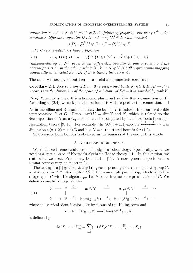
resentation theory [9, 10]. For example, the SO(n + 1, 1)-module1• 1• 0• 0• · · · has
dimension n(n+ 2)(n+ 4)/3 and has N = 4, the stated bounds for (1.2).Sharpness of both bounds is observed in the remarks at the end of this article.
3. Algebraic ingredients
We shall need some results from Lie algebra cohomology. Specifically, what weneed is a special case of Kostant’s algebraic Hodge theory [11]. In this section, westate what we need. Proofs may be found in [11]. A more general exposition in asimilar context may be found in [3].
The setting is a |1|-graded Lie algebra g corresponding to a semisimple Lie group G,as discussed in §2.2. Recall that G′
0 is the semisimple part of G0, which is itself asubgroup of G with Lie algebra g0. Let V be an irreducible representation of G. Wedefine a complex of G0-modules
(3.1)0 −→ V ∂−→ g1 ⊗ V ∂−→ Λ2g1 ⊗ V ∂−→ · · ·
‖ ‖ ‖0 −→ V ∂−→ Hom(g−1,V)
∂−→ Hom(Λ2g−1,V)∂−→ · · ·
where the vertical identifications are by means of the Killing form and
∂ : Hom(Λpg−1,V) −→ Hom(Λp+1g−1,V)
is defined by
∂φ(X0, . . . , Xp) =
p∑i=0
(−1)iXiφ(X0, . . . , Xi, . . . , Xp).

12 THOMAS BRANSON, ANDREAS CAP, MICHAEL EASTWOOD, AND A. ROD GOVER
Since g−1 is Abelian, it is easily verified that ∂2 = 0 and we define the Lie algebracohomology
Hp(g−1,V) =ker ∂ : Λpg1 ⊗ V −→ Λp+1g1 ⊗ Vim ∂ : Λp−1g1 ⊗ V −→ Λpg1 ⊗ V
.
Since ∂ is a homomorphism of G0-modules, Hp(g−1,V) is a G0-module. There is alsoa codifferential
(3.2) 0←− V ∂∗←− g1 ⊗ V ∂∗←− Λ2g1 ⊗ V ∂∗←− · · ·defined by
∂∗(Z0 ∧ · · · ∧ Zp ⊗ v) =
p∑i=0
(−1)i+1Z0 ∧ · · · ∧ Zi ∧ · · · ∧ Zp ⊗ Ziv.
It is also G0-equivariant and satisfies ∂∗2 = 0. There is a ‘Hodge decomposition’:–
(3.3) Λpg1 ⊗ V = im(∂)⊕ (ker(∂) ∩ ker(∂∗))⊕ im(∂∗)
and, in particular, a canonical isomorphism
Hp(g−1,V) ∼= ker(∂) ∩ ker(∂∗) on Λpg1 ⊗ V.The differential ∂ is seen more clearly in the Hodge decomposition
Λpg1 ⊗ V = ker(∂)⊕ im(∂∗)↓ ↙
Λp+1g1 ⊗ V = im(∂)⊕ ker(∂∗)
as an isomorphism ∂ : im(∂∗)→ im(∂). Its inverse is not necessarily ∂∗. Instead, wemay define δ∗ to be this inverse on im(∂) and to annihilate ker(∂∗). We obtain a newG0-equivariant codifferential defining the same Hodge decomposition as does ∂∗ butwith the congenial feature that
(3.4) δ∗∂ = id on im(δ∗) = im(∂∗) and ∂δ∗ = id on im(∂).
Now let us be more specific about the representation V. The description of |1|–gradings is well known: for an appropriate choice of a Cartan subalgebra for thecomplexification of g there is a distinguished simple root α0. This has the propertythat a root space lies in the complexification of gj (j = −1, 0, 1) if and only if j is thecoefficient of α0 in the expansion of the given root into simple roots. In particular, theDynkin diagram of g′0 is obtained by removing in the Dynkin diagram of g the noderepresenting α0 and all edges connected to that node. In the affine and Riemanniancases previously discussed this was the leftmost node. Let ω0 denote the fundamentalweight corresponding to α0. Starting with an irreducible representation E of G′
0, wemay add (k − 1)ω0 to the highest weight of E∗, and define V as the dual of theirreducible representation of G with that highest weight.
The subalgebra g1 ⊂ g is the nilradical of the parabolic g0 ⊕ g1, so Kostant’sversion of the Bott-Borel-Weil Theorem, see [11], describes the cohomology of g1 withcoefficients in an irreducible representation of g. It also follows from Kostant’s theorythat H∗(g1,V∗) is dual (as a representation of g0) to H∗(g−1,V). Since we use highestweights of dual representations as labels, we can directly apply Kostant’s algorithm.
PROLONGATIONS OF GEOMETRIC OVERDETERMINED SYSTEMS 13
This describes the highest weights of irreducible components in the cohomology interms of the actions of the elements of a subset W p of the Weyl group of g.
In particular, H0(g1,V∗) is the irreducible representation of g′0 whose highest weightis the restriction of the highest weight of V∗, whence
(3.5) H0(g−1,V) = E.
In particular, note that E has acquired the structure of a G0-module.To deal with the first cohomology, we have to consider elements of the Weyl group
which have length one, i.e. are reflections corresponding to simple roots. The onlysimple reflection which lies in W p is the one corresponding to α0. This means thatH1(g1,V∗) is an irreducible representation of g′0, and its highest weight is obtainedfrom the highest weight λ of V∗ by subtracting (`+1)α0, where ` is the coefficient ofω0 in the expansion of λ into a linear combination of fundamental weights. But bydefinition, −α0 is the highest weight of g−1 = g∗1, and we obtain
(3.6) H1(g−1,V) = }kg1 } E.
There is a unique element in g whose adjoint action is given by multiplication byj on gj for j = −1, 0, 1, called the grading element. The representation V splits intoeigenspaces for the action of this element, and it is convenient for our purposes towrite this decomposition as
V = V0 ⊕ V1 ⊕ · · · ⊕ VN , in which V0 = E and giVj ⊆ Vi+j.
This is the algebraic source of (2.3) and the number N in Theorems 2.1 and 2.3. Theexplicit formulae for N in §2 may be obtained by observing that N depends linearlyon the coefficients of the fundamental weights in expressing the highest weight andthen verifying our formulae for the fundamental representations. By construction,the homomorphisms ∂ and δ∗ decrease and increase this grading on V, respectively.
Now (3.5) says that Vi∂→ g1 ⊗ Vi−1 is injective ∀i ≥ 1. The module }k
g1 } Eappears with multiplicity one in g1 ⊗ V. Moreover, since g1 increases the grading,
}kg1 } E resides in g1 ⊗ Vk−1. From (3.6), we conclude that
(3.7) Vi∂
↪−→ g1 ⊗ Vi−1∂−→ Λ2g1 ⊗ Vi−2 is exact for 1 ≤ i ≤ k − 1 and i > k.
Now define φ0 : V0 → E as the identity and φi : Vi →⊗i
g1 ⊗ E inductively as thecomposition:–
Vi∂−→ g1 ⊗ Vi−1
id⊗φi−1−−−−→⊗i
g1 ⊗ E.
Also set K = ker :⊙k
g1 ⊗ E→}kg1 } E, the kernel of the Cartan product.
Lemma 3.1. The homomorphism φi : Vi →⊗i
g1 ⊗ E(1) is injective for all i ≥ 0,
(2) has values in⊙i
g1 ⊗ E,
(3) is an isomorphism Vi'−→
⊙ig1 ⊗ E, for 0 ≤ i ≤ k − 1,
(4) is an isomorphism Vi'−→ (
⊙ig1 ⊗ E) ∩ (
⊙i−kg1 ⊗K), for i ≥ k.

14 THOMAS BRANSON, ANDREAS CAP, MICHAEL EASTWOOD, AND A. ROD GOVER
Proof. Statements (1)–(3) immediately follow by induction from (3.7). When i = k,however, the sequence in (3.7) is no longer exact. Rather, (3.6) implies that φk : Vk ↪→⊙k
g1 ⊗ E has }kg1 } E as cokernel. This yields the isomorphism φk : Vk
'−→ K,which is (4) when i = k. For i > k the exactness of (3.7) proves (4) by induction. �
Let us denote by φ−1i :
⊙ig1 ⊗ E→ Vi the inverse of φi for 0 ≤ i ≤ k − 1. Then, by
construction and since δ∗ inverts ∂ on im(δ∗) = V1 ⊕ · · · ⊕ VN , we have:–
Lemma 3.2. Although δ∗ ◦ (id ⊗ φ−1i−1) is defined on g1 ⊗
⊙i−1g1 ⊗ E, it coincides
with φ−1i on
⊙ig1 ⊗ E for 1 ≤ i ≤ k − 1.
We can also be more precise concerning the identification of 1st cohomology in (3.6).From the Hodge decomposition (3.3) and (3.4), the endomorphism π of g1⊗V given byπϕ = ϕ−δ∗∂ϕ−∂δ∗ϕ is projection onto the unique irreducible G0-module isomorphicto }k
g1 } E. To fix this isomorphism, we take
(3.8) }kg1 } E ↪−→ g1 ⊗
⊙k−1g1 ⊗ E
id⊗φ−1k−1−−−−−→ g1 ⊗ Vk−1
π−→ ker(∂) ∩ ker(δ∗).
4. Proof of the main theorem
To prove Theorem 2.3, we shall use the algebra of §3 as follows. Recall thatM is supposed to have a G′
0-structure so any representation of G′0 (and thus any
representation of G0 or G by restriction) induces an associated bundle on M . Ofcourse, E should be the bundle associated to E and we have already observed thatthe bundle associated to g1 is the bundle of 1-forms Λ1. Now we may transfer theconstructions and conclusions of §3 into geometry on M . The G-module V inducesa graded vector bundle
V = V0 ⊕ V1 ⊕ · · · ⊕ VN
on M . The complex (3.1) induces a complex of vector bundle homomorphisms
(4.1) 0 −→ V∂−→ Λ1 ⊗ V ∂−→ Λ2 ⊗ V ∂−→ · · ·
and, similarly, (3.2) induces
(4.2) 0 −→ Vδ∗←− Λ1 ⊗ V δ∗←− Λ2 ⊗ V δ∗←− · · ·
so that E = ker ∂ : V −→ Λ1 ⊗ V and (3.8) induces
(4.3) }kΛ1 } E ∼=ker ∂ : Λ1 ⊗ V −→ Λ2 ⊗ V
im ∂ : V −→ Λ1 ⊗ V= ker(∂) ∩ ker(δ∗).
Lemma 3.1 part (3) yields
φj : Vi'−→
⊙j Λ1 ⊗ E for 0 ≤ j ≤ k − 1.
Lemma 3.1 part (4) identifies Vi with the classical prolongations (1.1) for i ≥ k.
PROLONGATIONS OF GEOMETRIC OVERDETERMINED SYSTEMS 15
A splitting operator. According to the statement of Theorem 2.3 we should choosea connection ∇ on M that is compatible with the G′
0-structure. From this, we obtainconnections on all associated vector bundles, in particular on E and V . Being inducedfrom a principal G′
0-connection, they respect the grading on V and commute with thehomomorphisms in (4.1) and (4.2). We shall denote all of these linear connectionsby ∇.
To prove Theorem 2.3 we shall construct L : E = V0 → V , an N th order lineardifferential operator, so that σ 7→ Lσ induces the isomorphism (2.4). Since theisomorphism in the other direction should simply be given by σ = Σ0, the componentof Σ in V0 = E, the composition σ 7→ (Lσ)0 should be the identity. For this reasonwe refer to L as a ‘splitting operator’. Its definition is
(4.4) Lσ =N∑
i=0
(−1)i(δ∗ ◦ ∇)iσ.
Of course, this an N th order linear differential operator. Moreover, since σ is asection of E = V0, we see that (δ∗ ◦ ∇)iσ is a section of Vi and that a sectionΣ = (Σ0,Σ1, . . . ,ΣN) of V is of the form Lσ if and only if
(4.5) Σ0 = σ and Σi = −δ∗∇Σi−1 for 1 ≤ i ≤ N.
Next, we define the connection ∇ on V as ∇ = ∇ + ∂. So we simply add thealgebraic operator ∂ : V → Λ1 ⊗ V to the component-wise connection ∇. Of course,this defines a linear connection. Note, however, that whilst for a section Σi of Vi, thecovariant derivative ∇Σi is a 1-form with coefficients in Vi, the algebraic term ∂Σi isa 1-form with coefficients in Vi−1. Otherwise put, for a section Σ = (Σ0,Σ1, . . . ,ΣN)
of V the component of ∇Σ taking values in Λ1 ⊗ Vi is ∇Σi + ∂Σi+1 for i < N , whilefor i = N we simply obtain ∇ΣN .
We should now compute the curvature of ∇. The curvatures of all the connections∇ are induced by the same 2-form R, which acts on the sections of any associatedbundle. On the other hand, for the induced connection on TM we also have thetorsion, which we view as a section of Λ2⊗TM . (In the affine and Riemannian caseswe can always choose ∇ to be torsion-free but not with a general G′
0-structure).
Lemma 4.1. Let R be the curvature of the connections ∇ and T the torsion of the
connection ∇ on TM . Let R ∈ Γ(Λ2 ⊗ End(V, V )) be the curvature of ∇. Then forvector fields ξ and η on M and a section Σ = (Σ0, . . . ,ΣN) of V , the Vi-component
of R(ξ, η)Σ is given by
R(ξ, η)Σi + (∂Σi+1)(T (ξ, η)).
In particular, ∇ is flat if and only if ∇ has zero curvature and torsion.
Proof. By definition, ∇ξ∇ηΣ = ∇ξ(∇ηΣ + (∂Σ)(η)). Writing out the first operatoras ∇+ ∂, we obtain
(4.6) ∇ξ∇ηΣ +∇ξ((∂Σ)(η)) + (∂(∇ηΣ))(ξ) + (∂(∂Σ)(η))(ξ).

16 THOMAS BRANSON, ANDREAS CAP, MICHAEL EASTWOOD, AND A. ROD GOVER
To obtain R(ξ, η)Σ we should subtract the same sum with ξ and η exchanged andthen subtract
(4.7) ∇[ξ,η]Σ = ∇[ξ,η]Σ + (∂Σ)([ξ, η]).
On the Lie algebra level (∂v)(Y ) = Y v and thus ∂((∂v)(Y ))(Z) = Z(Y v), which issymmetric in Y and Z since g1 is an Abelian Lie algebra. Hence the last term in(4.6) vanishes after exchange and subtraction. Also, we may write
∇ξ((∂Σ)(η)) = (∇ξ(∂Σ))(η) + (∂Σ)(∇ξη)
and, since ∂ is parallel, rewrite the first summand as (∂(∇ξΣ))(η). But this cancelswith one of the terms from the other summand of the form (4.6). Altogether, we seethat the last three terms in the two summands of the form (4.6) together contribute(∂Σ)(∇ξη − ∇ηξ). Subtracting the last term in (4.7) we obtain (∂Σ)(T (ξ, η)) bydefinition of the torsion. On the other hand, the first terms in the two summands ofthe form (4.6) add up with the remaining term of (4.7) to R(ξ, η)Σ. Now, the resultfollows by splitting into components. �
Having at hand the operators L and ∇, we now define an operator E = V0 → Λ1⊗Vas the composition ∇ ◦ L. From (4.3) we know that F = }kΛ1 } E sits as thesubbundle ker(∂) ∩ ker(δ∗) in Λ1 ⊗ V , and we can use the algebraic Hodge structureto define a projection onto this subbundle. Indeed, in §3 we arranged that thisprojection be explicitly given by ϕ 7→ πϕ ≡ ϕ − δ∗∂ϕ − ∂δ∗ϕ. Using (3.8), we now
define a differential operator D∇ : E → F by D∇ ≡ (−1)k−1(id⊗ φk−1) ◦ π ◦ ∇ ◦ L.The main properties of L and D∇ are collected in:–
Proposition 4.2.
(1) A section Σ = (Σ0, . . . ,ΣN) of V lies in the image of L if and only if δ∗(∇Σ) = 0and, if this is the case, then Σ = L(Σ0).(2) Mapping σ ∈ Γ(E) to the components of Lσ in V0 ⊕ · · · ⊕ Vi induces a vectorbundle homomorphism J iV0 → V0 ⊕ · · · ⊕ Vi, which is an isomorphism for i < k.(3) The differential operator D∇ : E → F is of order k and its symbol is the Cartanproduct.
Proof. (1) Since Vδ∗←− Λ1 ⊗ V inverts ∂ on im(∂), we may easily compute the
components of δ∗(∇Σ). We find that δ∗(∇Σ)0 = 0 and, for 1 ≤ i ≤ N ,
δ∗(∇Σ)i = δ∗((∇Σ)i−1) = δ∗(∇Σi−1 + ∂Σi) = δ∗(∇Σi−1) + Σi
whose vanishing is exactly the criterion (4.5) we already found for Σ = (Σ0, . . .ΣN)to be in the range of L. In (4.5) we also observed that, in this case, Σ = L(Σ0).(2) By construction, mapping σ to the Vi-component of Lσ is a linear differentialoperator of order at most i. Thus, we obtain J iV0 → V0⊕· · ·⊕Vi for all i = 0, . . . , N .We can compute the leading terms of (Lσ)i quite explicitly as follows. Firstly, (Lσ)0
is just σ, a section of V0 = E. Next, from its definition (4.4), we have (Lσ)1 = −δ∗∇σ.Assuming that 1 < k, we see from Lemma 3.2 that δ∗ coincides with φ−1
1 . Therefore,

PROLONGATIONS OF GEOMETRIC OVERDETERMINED SYSTEMS 17
(Lσ)1 = −φ−11 ∇σ, a section of V1. Now ∇(Lσ)1 = −(id⊗φ−1
1 )∇(∇σ), where ∇(∇σ)is a section of Λ1 ⊗ Λ1 ⊗ E. But if we decompose
Λ1 ⊗ Λ1 ⊗ E = (⊙2 Λ1 ⊗ E)⊕ (Λ2 ⊗ E),
then the component∇∧∇σ of∇(∇σ) is a zeroth order operator (made from curvatureand torsion). If 2 < k, then from Lemma 3.2 we conclude that
(Lσ)2 = −δ∗∇(Lσ)1 = δ∗(id⊗ φ−11 )∇(∇σ) = φ−1
2 ∇�∇σ + lots,
where ‘lots’ stands for ‘lower order terms’ (in this case zeroth order). By induction,we claim that
(4.8) (Lσ)i = (−1)iφ−1i ∇�∇� · · · � ∇︸ ︷︷ ︸
i
σ + lots, for 0 ≤ i ≤ k − 1.
For the inductive step, observe that
∇a∇(b∇c · · ·∇d) = ∇(a∇b∇c · · ·∇d) + lots
as differential operators. Therefore,
∇(Lσ)i−1 = ∇((−1)i−1φ−1i−1∇�∇� · · · � ∇︸ ︷︷ ︸
i−1
σ + lots)
= (−1)i−1(id⊗ φ−1i−1)(∇�∇�∇� · · · � ∇︸ ︷︷ ︸
i
σ + lots)
and so, for i < k,
(Lσ)i = −δ∗∇(Lσ)i−1 = (−1)iδ∗(id⊗ φ−1i−1)(∇�∇�∇� · · · � ∇︸ ︷︷ ︸
i
σ + lots)
= (−1)iφ−1i ∇�∇�∇� · · · � ∇︸ ︷︷ ︸
i
σ + lots,
the last equality coming from Lemma 3.2. We have shown (4.8) and, clearly, this issufficient to establish (2).(3) The projection
Λ1 ⊗ E 3 ϕ 7→ πϕ ≡ ϕ− δ∗∂ϕ− ∂δ∗ϕ ∈ ker(∂) ∩ ker(δ∗)
kills im(∂) so D∇σ = (−1)k−1(id⊗φk−1)(π(∇(Lσ)k−1)). From (3.8) and (4.8) we seethat
D∇σ = π(∇(∇�∇� · · · � ∇︸ ︷︷ ︸k−1
σ + lots)),
where now π : Λ1 ⊗⊙k−1 Λ1 ⊗ E → }kΛ1 ⊗ E = F denotes canonical projection
onto this irreducible tensor bundle. It is now clear the D∇ has the Cartan productas its symbol. �

18 THOMAS BRANSON, ANDREAS CAP, MICHAEL EASTWOOD, AND A. ROD GOVER
First step. Now we can perform the first step in rewriting the equation Dσ = 0 onsections of E in terms of sections of V :–
Proposition 4.3. Let D : E → F be a kth order semilinear differential operator asin Theorem 2.3. Then there is a fibre bundle homomorphism A : V0⊕· · ·⊕Vk−1 → Fsuch that σ 7→ Lσ induces a set bijection
{σ ∈ Γ(E) s.t. Dσ = 0} ∼= {Σ ∈ Γ(V ) s.t. ∇Σ + A(Σ) ∈ Γ(im(δ∗))}.
If D is linear, then A is linear, i.e. a vector bundle homomorphism.
Proof. From part (3) of Proposition 4.2 we conclude that the operators D and D∇
have the same symbol. Therefore, we may write Dσ = D∇σ + Ψ(jk−1σ) for somebundle map Ψ : Jk−1E → F . By part (2) of Proposition 4.2 there is a unique fibrebundle map A : V0⊕ · · · ⊕ Vk−1 → F (which we may extend trivially to V ) such thatΨ(jk−1σ) = (−1)k−1A(Lσ) for all σ ∈ Γ(E). Of course, if D is linear, then Ψ is avector bundle homomorphism and hence A is a vector bundle homomorphism too.
Now ∇Lσ is a section of ker(δ∗) by part (1) of Proposition 4.2 and the same is truefor A(Lσ) since, by construction, A even has values in F = ker(∂) ∩ ker(δ∗). Thelast observation even shows that π(A(Lσ)) = A(Lσ) for any σ. Hence, vanishing of
Dσ = (−1)k−1π(∇Lσ+A(Lσ)) is equivalent to ∇Lσ+A(Lσ) being a section of thesubbundle im(δ∗).
Conversely, assume that Σ ∈ Γ(V ) has the property that ∇Σ + A(Σ) is a sectionof im(δ∗). Then, in particular it is a section of ker(δ∗) and since δ∗(A(Σ)) always
vanishes we conclude that δ∗(∇Σ) = 0. By part (1) of Proposition 4.2 this impliesΣ = L(Σ0) and, as above, we see that D(Σ0) = 0. �
Second step. The next step in the procedure is to show that, if ∇Σ + A(Σ) is asection of im(δ∗), then its value can be actually computed. We shall do this in a moregeneral situation than needed for the proof of Theorem 2.3. The motivation for thisis that if A is linear, then it can be absorbed into the connection, so dealing with amore general class of connections is helpful. Notice that any smooth section of thebundle im(δ∗) ⊂ Λ1 ⊗ V can be written as δ∗ψ for some smooth ψ ∈ Γ(Λ2 ⊗ V ).
Proposition 4.4. Let ∇ be a linear connection on V such that for each i = 0, . . . , Nand each smooth section Σ ∈ Γ(V ) that has values in Vi only, the covariant derivative
∇Σ lies in Γ(Λ1 ⊗ (Vi ⊕ · · · ⊕ VN)) and put ∇ = ∇ + ∂. Let A : V → Λ1 ⊗ V bea fibre bundle map such that for v = (v0, v1, . . . , vN) ∈ V the component of A(v) inΛ1 ⊗ Vi depends only on v0, . . . , vi. Then there is a fibre bundle map
B : JNV = JNV0 ⊕ · · · ⊕ JNVN → Λ1 ⊗ V
such that ∇Σ +A(Σ) ∈ Γ(im(δ∗)) is equivalent to ∇Σ +B(jNΣ) = 0. Moreover, thecomponent Bi of B with values in Λ1 ⊗ Vi factors through
J iV0 ⊕ J i−1V1 ⊕ · · · ⊕ J1Vi−1 ⊕ Vi.
If A is linear then B can be chosen to be a vector bundle homomorphism.
PROLONGATIONS OF GEOMETRIC OVERDETERMINED SYSTEMS 19
Proof. Suppose that ∇Σ +A(Σ) + δ∗ψ = 0 for some ψ ∈ Γ(Λ2 ⊗ V ). Recall that the
linear connection ∇ on V extends to an operation de∇ on V -valued forms called the
covariant exterior derivative. For α ∈ Γ(Λ1 ⊗ V ) the covariant exterior derivative isexplicitly given by
de∇α(ξ, η) = ∇ξ(α(η))− ∇η(α(ξ))− α([ξ, η]),
for all vector fields ξ and η on M . Clearly, de∇ is a first order differential operator.
Moreover, if α = ∇Σ for some Σ ∈ Γ(V ), then this definition immediately implies
that de∇∇Σ(ξ, η) = R(ξ, η)(Σ).
Now we define B inductively as follows. We put B0(Σ) ≡ A0(Σ). By assumption,this is algebraic (i.e. of order zero) in Σ and depends only on the component Σ0.
Let R • Σ denote the V -valued 2-form (ξ, η) 7→ R(ξ, η)(Σ). Having defined the
components Bj for j < i, take the component (R •Σ+de∇(Bi−1(Σ)+ · · ·+B0(Σ)))i−1
in Γ(Λ2 ⊗ Vi−1) and define
(4.9) Bi(Σ) ≡ Ai(Σ)− δ∗((R • Σ + d
e∇(Bi−1(Σ) + · · ·+B0(Σ)))i−1 + ∂(Ai(Σ))).
By assumption, A is algebraic in Σ and Ai(Σ) depends only on the components
Σ0, . . . ,Σi. To understand the dependence of R • Σ, note that by assumption on ∇,
the form (∇Σ)j depends only on Σ0, . . . ,Σj+1. Hence the Vj-component of R(ξ, η)(Σ)depends at most on Σ0, . . . ,Σj+2 (since computing curvature needs two derivatives).However, as in the proof of Lemma 4.1, we see that for Σ ∈ Γ(Vj+2) the only contribu-
tion of R(ξ, η)(Σ) in Vj is ∂((∂Σ)(η))(ξ)−∂((∂Σ)(ξ))(η) and we have shown that this
vanishes. Hence, the term (R • Σ)i−1 depends only on Σ0, . . . ,Σi. Assuming induc-tively that for ` ≤ i− 1, the value B`(Σ)(x) depends only on j`
xΣ0, j`−1x Σ1, . . . ,Σ`(x)
for each x ∈ M , we immediately conclude from the fact that de∇ is first order that
Bi(Σ)(x) depends only on jixΣ0, j
i−1x Σ1, . . . ,Σi(x). Hence our components Bi define
a bundle map B whose dependence on jets is exactly as required. Moreover, if A islinear, then obviously B is a vector bundle homomorphism.
Next we show that the equation ∇Σ + B(Σ) = 0 is equivalent to ∇Σ + A(Σ)being a section of im(δ∗). On the one hand, we see from the definition (4.9) that
A(Σ)−B(Σ) is a section of im(δ∗) for any Σ ∈ Γ(V ). Thus ∇Σ +B(Σ) = 0 implies
that ∇Σ + A(Σ) has values in im(δ∗).
Conversely, assume that ∇Σ +A(Σ) + δ∗ψ = 0 for some ψ ∈ Γ(Λ2 ⊗ V ). Then weclaim that A(Σ) + δ∗ψ = B(Σ). Since δ∗ has values in Λ1 ⊗ (V1 ⊕ · · · ⊕ VN) and, bydefinition, B0(Σ) = A0(Σ), this is true for the component in Γ(Λ1 ⊗ V0).
To proceed inductively, we need one more observation concerning de∇. Suppose
that α ∈ Γ(Λ1 ⊗ (Vi ⊕ · · · ⊕ VN)). Then, from the formula for de∇, it is manifest that
de∇α ∈ Γ(Λ2 ⊗ (Vi−1 ⊕ · · · ⊕ VN) and the component (d
e∇α)i−1 is easy to compute:
expanding ∇ = ∇+ ∂ in the above formula, we see that
(de∇α)i−1(ξ, η) = ∂(αi(η))(ξ)− ∂(αi(ξ))(η)
and, looking at the definition of ∂, this means that (de∇α)i−1 = ∂(αi).

20 THOMAS BRANSON, ANDREAS CAP, MICHAEL EASTWOOD, AND A. ROD GOVER
Now suppose inductively that (A(Σ)+δ∗ψ)` = B`(Σ) for ` = 0, . . . , i−1. Denotingby the subscript ≥ i the components with values in Λ1 ⊗ (Vi ⊕ · · · ⊕ VN) we may
rewrite the equation ∇Σ + A(Σ) + δ∗ψ = 0 as
∇Σ +B0(Σ) + · · ·+Bi−1(Σ) + A≥i(Σ) + (δ∗ψ)≥i = 0.
Applying de∇ and looking at the component in Λ2 ⊗ Vi−1 we obtain
0 = (R • Σ + de∇(B0(Σ) + · · ·+Bi−1(Σ)))i−1 + ∂(Ai(Σ)) + ∂(δ∗ψ)i.
Applying δ∗, the last term gives (δ∗ψ)i and from (4.9) we see Ai(Σ)+(δ∗ψ)i = Bi(Σ),which completes the proof. �
Third step. The final reduction is now done by solving component by component:–
Proposition 4.5. Suppose that ∇ is a connection on V satisfying the hypothesis ofProposition 4.4 and
B : JNV = JNV0 ⊕ · · · ⊕ JNVN → Λ1 ⊗ Vis a fibre bundle map such that the component Bi of B in T ∗M ⊗ Vi factors throughJ iV0 ⊕ J i−1V1 ⊕ · · · ⊕ J1Vi−1 ⊕ Vi.
Then there is a fibre bundle map C : V → Λ1 ⊗ V such that ∇Σ + B(Σ) = 0 is
equivalent to ∇Σ + C(Σ) = 0. If B is a vector bundle homomorphism, then also Ccan be chosen to be a vector bundle homomorphism.
Proof. Choosing a connection on TM , we may form iterated covariant derivatives ofsections of V and by the assumptions on B we may write the components of B (withthe obvious meaning of subscripts) as
Bi(Σ) = Bi(Σ≤i, (∇Σ)≤i−1, . . . , (∇iΣ)0).
The component in Λ1⊗ V0 of ∇Σ +B(Σ) is given by (∇Σ)0 +B0(Σ0) and we simply
put C0(Σ) ≡ B0(Σ0). The next component has the form (∇Σ)1 +B1(Σ0,Σ1, (∇Σ)0).
Defining C1(Σ0,Σ1) ≡ B1(Σ0,Σ1,−C0(Σ0)), we see that vanishing of (∇Σ+B(Σ))≤1
is equivalent to vanishing of (∇Σ + C(Σ))≤1, where C = C0 + C1.Let us inductively assume that i > 1 and we have found a fibre bundle map
C : V → Λ1⊗ (V0⊕ · · · ⊕Vi−1) such that vanishing of (∇Σ +B(Σ))≤i−1 is equivalent
to vanishing of (∇Σ + C(Σ))≤i−1 and such that the component Cj(Σ) depends onlyon Σ0, . . . ,Σj for each j < i. Let us also assume that we have derived, for any Σ such
that (∇Σ + C(Σ))≤i−1 = 0, formulae for (∇`Σ)≤i−` as algebraic expressions in Σ≤i.So by assumption we have formulae for all the terms going into Bi as algebraic
operators in Σ≤i and inserting these formulae, we obtain a bundle map Ci with values
in Λ1⊗Vi, which depends only on Σ≤i. By construction, vanishing of (∇Σ+B(Σ))≤i
is equivalent to vanishing of (∇Σ + C(Σ))≤i. Suppose now that Σ satisfies this
equation. By the assumption on ∇, vanishing of (∇Σ + C(Σ))≤i implies vanishing
of (∇`(∇Σ + C(Σ)))≤i−` for each ` = 1, . . . , i. Similarly, (∇`(C(Σ)))≤i−` dependsalgebraically on C(Σ)≤i, to first order on C(Σ)≤i−1 and so on. Hence, expanding
this, it can be written as an expression in Σ≤i, (∇Σ)≤i−1,. . . , (∇`Σ)≤i−` and we have

PROLONGATIONS OF GEOMETRIC OVERDETERMINED SYSTEMS 21
algebraic formulae for all these by inductive hypothesis. Thus we see that vanishing
of (∇`(∇Σ + C(Σ)))≤i−` gives us an algebraic expression for (∇`+1Σ)≤i−` for each` = 1, . . . , i, which completes the inductive step. Of course, linearity is never lost inthis process, so if one starts with a linear operator B, one will end up with a vectorbundle homomorphism C. �
Since the output of each step of our rewriting procedure is a special case of theinput of the next step, this completes the proof of Theorem 2.3.
Remark. As far as the proof of Theorem 2.3 is concerned, the only role that ∂∗ playedwas in constructing δ∗ as a left inverse to ∂. Of course, the definition of ∂∗ and theresulting algebraic Hodge theory is extremely natural but, in defining ∂, only thestructure of V as a g−1-module is needed. It is also important that ∂ respect theG0-action but, as far as δ∗ goes, any other G0-invariant splittings would work just aswell. In practise, there can be considerably simpler ad hoc choices.
Remark. The dimension bound of Corollary 2.4 is sharp. The bound is attained bychoosing a manifold M endowed with a G′
0-structure and a compatible connection,such that all the connections∇ have zero curvature and the connection∇ on TM alsohas zero torsion. Such an example is always provided by the constant G′
0-structureon Rn (where n = dim(g−1)) with the standard flat connection. In this case, let usconsider the equation D∇σ = 0. Then our first step of rewriting simply leads to
∇Σ + δ∗ψ = 0. Applying δ∗de∇, the first term does not give any contribution, since
∇ has zero curvature by Lemma 4.1. This implies that δ∗ψ = 0. Hence the wholerewriting is already finished and we conclude that the differential splitting L : E → Vinduces a bijection between solutions of D∇σ = 0 and sections Σ ∈ Γ(V ) that are
parallel for the flat connection ∇. Locally, a flat connection always has the maximaldimension for its space of parallel sections.
Remark. The flat case also shows that the bound N on the order of the jet of σ at apoint p ∈M needed uniquely to specify a solution of D∇σ = 0 is sharp. To see this,
note that ∇Σ = 0 in the flat case is equivalent to ∇Σi = −∂Σi+1, for all i. Therefore,
Σ|p ∈ (VN)p ⇒ ∇Σ|p ∈ (VN−1 ⊕ VN)p ⇒ · · · ⇒ ∇N−1Σ|p ∈ (V1 ⊕ · · · ⊕ VN)p,
whence ∇N−1σ|p = ∇N−1Σ0|p = 0. But, since ∇ is flat, there is no problem findinga parallel section Σ of V with Σ|p lying in (VN)p.
Remark. In this flat case, the operator D∇ is the first in the so-called ‘Bernstein-Gelfand-Gelfand (BGG) resolution’ and one motivation for our study comes fromanalogues of these first operators on almost Hermitian symmetric manifolds [1] or,more generally, on parabolic geometries [3, 5]. By construction, these analogues areinvariant linear differential operators having the same symbol as in the flat case. TheG′
0-geometries studied in this article cover the almost Hermitian symmetric case soTheorem 2.3 covers the first BGG operators on these geometries. This includes thevarious so-called ‘conformal Killing’ or ‘twistor’ equations in conformal geometry.
Remark. A useful viewpoint on the outcome of Theorem 2.3 is that it restricts thepossible jets of σ that might be specified at a point for a solution of Dσ = 0. In the

22 THOMAS BRANSON, ANDREAS CAP, MICHAEL EASTWOOD, AND A. ROD GOVER
flat case and the equation D∇σ = 0, these jets may be freely specified. In general,there are further constraints, which may be obtained by cross-differentiation of the
closed system ∇Σ + Φ(Σ) = 0.
References
[1] R.J. Baston, Almost Hermitian symmetric manifolds, I: Local twistor theory, Duke Math.Jour. 63 (1991) 81–112.
[2] R.J. Baston and M.G. Eastwood, The Penrose Transform: Its Interaction with RepresentationTheory, Oxford University Press 1989.
[3] D.M.J. Calderbank and T. Diemer, Differential invariants and curved Bernstein-Gelfand-Gelfand sequences, Jour. Reine Angew. Math. 537 (2001) 67–103.
[4] A. Cap, J. Slovak, and V. Soucek, Invariant operators on manifolds with almost Hermitiansymmetric structures, I. Invariant differentiation, Acta Math. Univ. Comenianae 66 (1997)33–69.
[5] A. Cap, J. Slovak, and V. Soucek, Bernstein-Gelfand-Gelfand sequences, Ann. Math. 154(2001) 97–113.
[6] E.B. Dynkin, The maximal subgroups of the classical groups, Amer. Math. Soc. Transl.,Series 2, 6 (1957) 245–378.
[7] M.G. Eastwood and K.P. Tod, Local constraints on Einstein-Weyl geometries, Jour. ReineAngew. Math. 491 (1997) 183–198.
[8] L.P. Eisenhart, Geometries of paths for which the equations of the paths admit n(n + 1)/2independent linear first integrals, Trans. Amer. Math. Soc. 28 (1926) 330–338.
[9] W. Fulton and J. Harris, Representation Theory, a first Course, Springer 1991.[10] J.E. Humphreys, Introduction to Lie Algebras and Representation Theory, Springer 1972.[11] B. Kostant, Lie algebra cohomology and the generalized Borel-Weil theorem, Ann. Math. 74
(1961) 329–387.[12] T. Ochiai, Geometry associated with semisimple flat homogeneous spaces, Trans. Amer. Math.
Soc. 152 (1970) 159–193.[13] R. Penrose and W. Rindler, Spinors and Space-time, vol. 1, Cambridge University Press 1984.[14] U. Semmelmann, Conformal Killing forms on Riemannian manifolds, Math. Zeit., to appear.[15] D.C. Spencer, Overdetermined systems of linear partial differential equations, Bull. Amer.
Math. Soc. 75 (1969) 179–239.
Department of Mathematics, University of Iowa, Iowa City, IA 52242, USAE-mail address: [email protected]
Fakultat fur Mathematik, Universitat Wien, Nordbergstraße 15, A-1090 Wien,AustriaE-mail address: [email protected]
Department of Mathematics, University of Adelaide, South Australia 5005E-mail address: [email protected]
Department of Mathematics, University of Auckland, Private Bag 92019,Auckland, New ZealandE-mail address: [email protected]