Projection, Lifting and Extended Formulation in Integer and

Annals of Operations Research 140, 125–161, 2005c© 2005 Springer Science + Business Media, Inc. Manufactured in The Netherlands.

Projection, Lifting and Extended Formulation in Integerand Combinatorial Optimization∗

EGON BALAS † [email protected] School of Business, Carnegie Mellon University, Pittsburgh, PA 15213

Abstract. This is an overview of the significance and main uses of projection, lifting and extended formu-lation in integer and combinatorial optimization. Its first two sections deal with those basic properties ofprojection that make it such an effective and useful bridge between problem formulations in different spaces,i.e. different sets of variables. They discuss topics like projection and restriction, the integrality-preservingproperty of projection, the dimension of projected polyhedra, conditions for facets of a polyhedron to projectinto facets of its projections, and so on. The next two sections describe the use of projection for comparingthe strength of different formulations of the same problem, and for proving the integrality of polyhedra byusing extended formulations or lifting. Section 5 deals with disjunctive programming, or optimization overunions of polyhedra, whose most important incarnation are mixed 0-1 programs and their partial relaxations.It discusses the compact representation of the convex hull of a union of polyhedra through extended formu-lation, the connection between the projection of the latter and the polar of the convex hull, as well as thesequential convexification of facial disjunctive programs, among them mixed 0-1 programs, with the relatedconcept of disjunctive rank. Section 6 reviews lift-and-project cuts, the construction of cut generating linearprograms, and techniques for lifting and for strengthening disjunctive cuts. Section 7 discusses the recentlydiscovered possibility of solving the higher dimensional cut generating linear program without explicitlyconstructing it, by a sequence of properly chosen pivots in the simplex tableau of the linear programmingrelaxation. Finally, section 8 deals with different ways of combining cuts with branch and bound, and brieflydiscusses computational experience with lift-and-project cuts.

Keywords: disjunctive programming, sequential convexification, 0-1 programming, lift-and-project

1. Basic properties of projection

Most combinatorial optimization problems tend to have several alternative formulations,some of which are easier to handle than others. Projection provides a connection betweendifferent formulations. Since most combinatorial optimization problems are solved bysome combination of polyhedral methods and enumeration, and since the latter typicallyinvolves repeated solution of variants of the problem’s linear programming relaxation, itis crucial to be able to compare the strength of the LP relaxations of different formulationsof the same problem.

∗ This is an updated and extended version of the paper published in LNCS 2241, Springer, 2001 (as given inBalas, 2001).

† Research was supported by the National Science Foundation through grant #DMI-9802773 and by theOffice of Naval Research through contract N00014-97-1-0196.

126 BALAS

Given a polyhedron of the form

Q := {(u, x) ∈ Rp × R

q : Au + Bx ≤ b},

where A, B and b have m rows, the projection of Q onto Rq , or onto the x-space, is

defined as

Projx (Q) := {x ∈ Rq : ∃u ∈ R

p : (u, x) ∈ Q}.

Thus projecting the set Q onto Rq can be viewed as finding a matrix C ∈ R

m×q

and a vector d ∈ Rm such that

Projx (Q) = {x ∈ Rq : Cx ≤ d}.

This task can be accomplished as follows. Call the polyhedral cone

W := {v : vA = 0, v ≥ 0}

the projection cone associated with Projx (Q). Then we have

Theorem 1.1.

Projx (Q) = {x ∈ Rq : (vB)x ≤ vb, v ∈ extr W }

where extr W denotes the set of extreme rays of W .

Proof. W is a pointed cone (since W ⊆ Rm+), hence it is the conical hull of its extreme

rays. Therefore the system of inequalities defining Projx (Q) holds for all x ∈ extr W ifand only if it hold for all x ∈ W .

Now let x ∈ Projx (Q). Then there exists u ∈ Rp such that Au + Bx ≤ b. Premul-

tiplying this system with any v ∈ W , x satisfies (vB)x ≤ vb for all v ∈ W .Conversely, suppose x ∈ R

q satisfies (vB)x ≤ vb for all v ∈ W . Then there existsno v ≥ 0 satisfying vA = 0 and v(Bx − b) > 0. But then, by Farkas’ Lemma, thereexists u satisfying Au ≤ b − Bx , i.e. x ∈ Projx (Q).

Several comments are in order.First, if some of the inequalities defining Q are replaced with equations, the corre-

sponding components of v become unrestricted in sign. In such a case, if the projectioncone W is not pointed, then it is not the convex hull of its extreme rays. Nevertheless,like any polyhedral cone, W is finitely generated, and any finite set W of its generatorscan play the role previously assigned to extr W .

Second, the set Q may be defined, besides the system of inequalities involving thevariables u to be projected out, by any additional constraints—not necessarily linear—not involving u: such constraints will become part of the projection, without any change.

PROJECTION, LIFTING AND EXTENDED FORMULATION 127

In other words, for an arbitrary set S ⊆ Rq , the projection of

Q := {(u, x) ∈ Rp × R

q : Au + Bx ≤ b, x ∈ S}on R

q is

Projx (Q) := {x ∈ Rq : (vB)x ≤ vb for all v ∈ W, x ∈ S}

where W is the projection cone introduced earlier.Third, Projx (Q) as given by Theorem 1.1 may have redundant inequalities, even

when the latter come only from extreme rays of W ; i.e., an extreme ray of W doesnot necessarily give rise to a facet of Projx (Q). It would be nice to be able to iden-tify the extreme rays of W which give rise to facets of Projx (Q), but unfortunately thisin general is not possible: whether an inequality (vB)x ≤ vb is or is not facet defin-ing for Projx (Q) depends on B and b as well as on v. We will return to this questionlater.

Fourth, we have the simple fact following from the definitions, that if x ∈ Rq is an

extreme point of Projx (Q), then there exists u ∈ Rp such that (u, x) is an extreme point

of Q. This has the following important consequence:

Proposition 1.2. If Q is an integral polyhedron, then Projx (Q) is an integralpolyhedron.

Well known special cases

There are two well known algorithms whose iterative steps are special cases of projection:If the matrix A in the definition of Q has a single column a, i.e., if

Q := {(u0, x) : au0 + Bx ≤ b},then

extr W = {vk : ak = 0} ∪ {vi j : ai · a j < 0},where

vk := ek, vi j := ai e j − a j ei ,

with ek the k-th unit vector, and we have one step of Fourier Elimination (see e.g. Stoerand Witzgall, 1970).

If Q is of the form

Q :={

(u, x, x0)

∣∣∣∣

−cu − dx + x0 ≤ 0

A′u + B ′x ≤ b′

}

,

128 BALAS

then

W = {(v0, v) : −v0c + vA′ = 0; v0, v ≥ 0},Proj(x0,x)(Q) :=

{

(x0, x)

∣∣∣∣

x0 + (vB ′ − d)x ≤ vb′, ∀v : (1, v) ∈ extr W

(vB ′)x ≤ vb′, ∀v : (0, v) ∈ extr W

}

and we have the constraint set of the Benders Master Problem (see e.g. Nemhauser andWolsey, 1986).

Projection and restriction

Projection is not to be confused with restriction, another operation that relates a higherdimensional object to one in a subspace. Referring to the same set Q ⊆ R

p × Rq , its

restriction to the subspace defined by u = 0 is

{(u, x) ∈ Q : u = 0} = {x ∈ Rq : (0, x) ∈ Q}.

Notice that, unlike in the case of projection, the restriction of Q “to Rq ,” or “to the

x-space,” is not well defined, since it may mean several things, of which the above is justone. Another one is, for some t ∈ R

p,

{(u, x) ∈ Q : u = t} = {x ∈ Rq : (t, x) ∈ Q}.

Clearly, the restriction of Q through some value assignment to each component of u isalways a subset of Projx (Q).

To illustrate the difference between projection and restriction, consider the setQ := {(x, u) ∈ R

2 : x + u ≥ 1, 0 ≤ x ≤ 2, 0 ≤ u ≤ 1}. Its projection on the x-space is{x ∈ R : 0 ≤ x ≤ 2}, whereas its restriction to the subspace of R

2 defined by u = 0 is{x ∈ R : 1 ≤ x ≤ 2}, as shown in figure 1.

While both projection and restriction map polyhedra from a higher dimensionalspace to a lower dimensional one, sometimes we want to go into the opposite direction.The operation, in a sense reverse to projection, in which one goes from a given polyhedral

Figure 1. (a) Q, (b) Projx Q, and (c) {(x, u) ∈ Q : u = 0}.


formulation of a problem to a higher dimensional one, involving some new variables, iscalled extended formulation. Sometimes going to an extended formulation is referred toas lifting. For instance, many problems defined on graphs that are usually formulated interms of arc variables, can also be formulated in the higher dimensional space of arc-and node-variables; and we will see examples where this is advantageous. Typically,extended formulations are not unique, and it takes some insight to recognize those whichoffer some advantage. One possible advantage might be that the extended formulationgives rise to a polyhedron with desirable properties.

The reverse of restriction of course is relaxation, i.e. the removal of the restrictingconstraint. But this operation becomes less trivial than it sounds when looked at in thefollowing context. Suppose we know a valid inequality, αx ≤ α0, for a polyhedron P ∩ Sthat is a restriction to a subspace of a higher dimensional polyhedron P , and we wouldlike to calculate the strongest (tightest) extension of the inequality, say αx +βy ≤ α0, toP . This is a well defined and important operation called lifting. It consists of calculatingthe missing coefficients β j of the inequality αx + βy ≤ α0 valid for P . There is a wellknown procedure for doing this, called sequential lifting (see e.g. Nemhauser and Wolsey,1986), which calculates the coefficients β j one by one, and under certain conditionsguarantees that if αx ≤ α0 defines a facet of P ∩ S, then αx +βy ≤ α0 defines a facet ofP .

Exercise 1.1 Consider the following variations of Q:

Q1 := {(u, x) ∈ Rp × R

q : Au + Bx = b}Q2 := {(u, x) ∈ R

p × Rq : Au + Bx ≤ b, u ≥ 0}

Q3 = Q with B = ( I0 ), where I is the q × q identity matrix and 0 is the (m − q) × q

zero matrix (assume m > q).

For each Qi , i = 1, 2, 3 write down the projection cone associated with Projx (Qi ).

Exercise 1.2 Prove Proposition 1.2.

2. Dimensional aspects of projection

When we have a polyhedral representation of some combinatorial object, we would likeit to be nonredundant. This makes us interested in identifying among the inequalitiesdefining the polyhedron, say Q, those which are facet inducing, since the latter providea minimal representation. Further, when we project Q onto a subspace, we would like toknow whether the facets of Q project into facets of the projection. To be able to answerthis and similar questions, we need to look at the relationship between the dimension ofa polyhedron and the dimension of its projections. This was done in the paper (Balas andOosten, 1998), on which most of this section is based.

130 BALAS

Consider the polyhedron Q := {(u, x) ∈ Rp × R

q : Au + Bx ≤ b} �= ∅,where A, B and b have m rows, and let us partition (A, B, b) into (A=, B=, b=) and(A≤, B≤, b≤), where A=u + B=x = b= is the equality subsystem of Q, the set ofequations corresponding to the inequalities satisfied at equality by every (u, x) ∈ Q. Letr := rank(A=, B=) = rank(A=, B=, b=), where the last equality follows from Q �= ∅.

Let dim(Q) denote the dimension of Q. It is well known that dim(Q) = p + q − r ,and that Q is full-dimensional, i.e. dim(Q) = p+q, if and only if the equality subsystemis vacuous. When this is the case, then dim(Projx (Q)) = q, for otherwise Projx (Q) has anonempty equality subsystem that must also be valid for Q, contrary to the assumptionthat the latter is full dimensional.

Consider now the general situation, when Q is not necessarily full dimensional.Recall that r = rank(A=, B=), and define r∗ := rank(A=). Clearly, 0 ≤ r∗ ≤ min{r, p}.It can then be shown that

Theorem 2.1 (Balas and Oosten, 1998). dim(Projx (Q)) = dim(Q) − p + r∗.

It follows that dim(Projx (Q)) = dim(Q) if and only if r∗ = p, i.e., the projectionoperation is dimension-preserving if and only if the matrix A= is of full column rank.

When is the projection of a facet a facet of the projection?

We now turn to the question of what happens to the facets of Q under projection. Sincea facet of a polyhedron is itself a polyhedron, the dimension of its projection can bededuced from Theorem 2.1.

Let αu + βx ≤ β0 be a valid inequality for Q, and suppose

F := {(u, x) ∈ Q : αu + βx = β0}

is a facet of Q. Let ( αA )=u + ( β

B )=x = ( β0b )= be the equality subsystem of F , and let rF :=

rank(( αA )=, ( β

B )=). Notice that rF − r = 1, since by assumption dim(F) = dim(Q) − 1.Further, denote r∗

F := rank(( αA )=). We may interpret r∗

F − r∗ as the difference betweenthe number of dimensions “lost” in projecting Q (which is p − r∗) and in projecting F(which is p − r∗

F ). From Theorem 2.1 we then have

Corollary 2.2. dim(Projx (F)) = dim(Projx (Q)) − 1 + (r∗F − r∗).

Indeed, dim(Projx (F)) = dim(F)−p + r∗F = dim(Q)−1−p + r∗

F , and substitutingfor dim(Q) its value given by Theorem 2.1 yields the Corollary.

We are now in a position to state what happens to the facets of Q under projection.

Corollary 2.3. Let F be a facet of Q. Then Projx (F) is a facet of Projx (Q) if and onlyif r∗

F = r∗.


Proof outline. From Corollary 2.2. it is clear that Projx (F) has the dimension of a facetof Projx (Q) if and only if r∗

F = r∗. However, this by itself does not amount to a proof,unless we can guarantee that Projx (F) is a face of Projx (Q), which is far from obvious:in general, the projection of a face need not be a face of the projection. Indeed, thinkof a 3-dimensional pyramid, and its projection on its base: neither the top vertex of thepyramid, nor the 3 edges incident with it, become faces of the projection as a result ofthe operation.

However, if Projx (F) is a set of the form {x ∈ Projx (Q) : βx = β0} for some validinequality βx ≤ β0 for Projx (Q), then clearly Projx (F) is a face of Projx (Q). This is thecase in our situation: since F is a facet of Q, it has a defining inequality αu + βx ≤ β0.Now if r∗

F = r∗, then there exists a vector λ such that α = λA=; hence subtractingλA=u + λB=x = λb= from this defining inequality yields (β − λB=)x ≤ β0 − λb=,which can be written as β ′x ≤ β ′

0. Thus Projx (F) = {x ∈ Projx (Q) : β ′x = β ′0}, i.e.

Projx (F) is a face of Projx (Q); hence a facet.

Another consequence of Theorem 2.1. which is not hard to prove is this:

Corollary 2.4. Let r∗ = p, i.e. let A= be of full column rank, and let 0 ≤ d ≤dim(Q) − 1. Then every d-dimensional face of Q projects into a d-dimensional face ofProjx (Q).

Projection with a minimal system of inequalities

As discussed in Section 1, the inequalities of the system defining Projx (Q) are not nec-essarily facet inducing, even though they are in 1-1 correspondence with the extremerays of the projection cone W . In other words, the system (vB)x ≤ vb, ∀v ∈ extr W , isnot necessarily minimal. In fact, this system often contains a large number of redundantinequalities. It has been shown however (Balas, 1998), that if a certain linear transfor-mation is applied to Q, which replaces the coefficient matrix B of x with the identitymatrix I , the resulting polyhedron Q0 has a projection cone W 0 that is pointed, and theprojection of Q0 is of the form

Projx (Q0) = {x ∈ Rq : vx ≤ v0 for all (v, v0) ∈ R

m+1 such that (v, w, v0) ∈ extr W 0},with Projx (Q0) = Projx (Q). Here w is a set of auxiliary variables generated by the abovetransformation. Furthermore, we have the following

Proposition 2.5 (Balas, 1998). Let Projx (Q) be full dimensional. Then the inequalityvx ≤ v0 defines a facet of Projx (Q) if and only if (v, v0) is an extreme ray of the coneProj(v,v0)(W

0).

The linear transformation that takes Q into Q0 is of low complexity (O(max{m, q}3), where B is m × q). The need to project the cone W 0 onto the subspace (v, v0)

132 BALAS

arises only when B is not of full row rank. In the important case when B is of full rowrank, we have the following stronger result:

Corollary 2.6 (Balas, 1998). Let Projx (Q) be full dimensional and rank(B) = m. Thenthe inequality vx ≤ v0 defines a facet of Projx (Q) if and only if (v, v0) is an extreme rayof W 0.

In many important cases the matrix B is of the form B = ( I0 ), which voids the need

for the transformation discussed above and leads to a projection cone whose extreme raysyield facet inducing inequalities for Projx (Q). This is the case encountered, for instance,in the characterization of the perfectly matchable subgraph polytope of a graph to bediscussed in Section 4; as well as in the projection used in the convex hull characterizationof a disjunctive set discussed in Section 5.

Exercise 2.1 Give an example of a 3-dimensional polyhedron Q and one of its 2-dimensional projections Proj(Q) such that Proj(Q) has (a) fewer facets than Q; (b) morefacets than Q; (c) the same number of facets as Q (visual representation will suffice).

3. Comparing different formulations

Combinatorial optimization problems tend to have several formulations, and choosingthe most convenient one is often a nontrivial exercise. While the number of variablesand constraints in the different formulations do have some importance, the most relevantcriterion of the comparison is the strength of the linear programming relaxation. This isso because most solution procedures involve some branch and bound component, and thebounding usually comes from the LP relaxation: the tighter this relaxation, the strongerthe bound.

Typically the comparisons are made between two problem formulations, say P andQ, such that P is expressed in terms of variables x ∈ R

n , while Q is in terms of variables(x, y) ∈ R

n × Rq . To compare the strength of the two LP relaxations, one has to express

both P and Q in terms of the same variables, and so one uses projection to eliminate yand re-express Q in terms of x , i.e., as Projx (Q). One then compares the LP relaxationof this latter set to that of P .

Before we give several examples of how this can be done, we wish to point outthat projection can be used to compare two different formulations of the same problemeven when they are expressed in completely different (nonoverlapping) sets of variables,provided the two sets are related by an affine transformation. Suppose, for instance, thatwe have two equivalent formulations of a problem whose feasible sets are P and Q:

P := {x ∈ Rn : Ax ≤ a0}, Q := {y ∈ R

q : By ≤ b0}where A is m × n, B is p × q, and

x = T y + c (1)


for some T ⊂ Rn × R

q and c ∈ Rn .

Define

Q+ :={

(x, y) ∈ Rn+q

∣∣∣∣

x − T y = c

By ≤ b0

}

and project Q+ onto Rn . Using the projection cone

W := {(v, w) ∈ Rn+p : −vT + wB = 0, w ≥ 0},

we obtain

Projx (Q+) := {x ∈ Rn : vx ≤ vc + wb0, ∀(v, w) ∈ W }.

Then to compare P with Q, we compare P with Projx (Q+).The affine transformation (1) can also be used to derive a different analytical com-

parison between P and Q that does not make use of projection (Padberg and Sung,1991).

The traveling salesman problem

Consider the constraint set of the TSP defined on the complete digraph G on n +1 nodesin two well known formulations:

Dantzig, Fulkerson, and Johnson (D-F-J) (1954)∑

(xi j : j = 0, . . . , n) = 1 i = 0, . . . , n∑

(xi j : i = 0, . . . , n) = 1 j = 0, . . . , n∑

(xi j : i ∈ S, j ∈ S) ≤ |S| − 1, S ⊆ {0, . . . , n}, 2 ≤ |S| ≤ n + 1

2xi j ∈ {0, 1}, i, j = 0, . . . , n

Miller, Tucker, and Zemlin (M-T-Z) (1960)∑

(xi j : j = 0, . . . , n) = 1 i = 0, . . . , n∑

(xi j : i = 0, . . . , n) = 1 j = 0, . . . , n

ui − u j + nxi j ≤ n − 1 i, j = 1, . . . , n, i �= j

xi j ∈ {0, 1} i, j = 0, . . . , n

The M-T-Z formulation introduces n node variables, but replaces the exponentiallylarge set of subtour elimination constraints by n(n − 1) new constraints that achievethe same goal. However, projecting the constraint set of the M-T-Z formulation into thesubspace of the arc variables by using the cone

W = {v | vA = 0, v ≥ 0}, (2)

134 BALAS

where A is the transpose of the node-arc incidence matrix of G, yields the inequalities

∑(xi j : (i, j) ∈ C) ≤ n − 1

n|C |

for every directed cycle C of G. These inequalities are strictly weaker than the corre-sponding subtour elimination inequalities of the D-F-J formulation, so the latter providesa tighter LP relaxation.

The set covering problem

Consider the set covering problem

min{cx |Ax ≥ e, x ∈ {0, 1}n} (SC)

where e = (1, . . . , 1) and A is a matrix of 0’s and 1’s. Let M and N index the rows andcolumns of A, respectively, and

M j = {i ∈ M |ai j = 1}, j ∈ N , Ni = { j ∈ N |ai j = 1}, i ∈ M.

The following uncapacitated plant location (UPL) problem is known to be equiva-lent to (SC):

min∑

(c j x j : j ∈ N )∑

(ui j : j ∈ Ni ) ≥ 1, i ∈ M

−∑

(ui j : i ∈ M j ) + |M j |x j ≥ 0, j ∈ N

ui j ≥ 0, i ∈ M, j ∈ N ; x j ∈ {0, 1}, j ∈ N

If we now project this constraint set onto the x-space by using the cone

W = {v|vi − v j ≤ 0, j ∈ Ni , i ∈ M : vi ≥ 0, i ∈ M},

we obtain the inequalities

∑(|M j |x j : j ∈ NS) ≥ |S|, ∀S ⊆ M ;

x j ≥ 0, j ∈ N

(where NS := ∪(Ni : i ∈ S), each of which is dominated (strictly if S �= M) by the sumof the inequalities of (SC) indexed by S. Hence the LP relaxation of the UPL formulationis weaker than that of (SC).


If, on the other hand, we use the so called “strong” formulation of the uncapacitatedplant location problem, namely

min∑

(c j x j : j ∈ N )∑

(ui j : j ∈ Ni ) ≥ 1 i ∈ M

− ui j + x j ≥ 0 i ∈ M, j ∈ N ;

ui j ≥ 0, x j ∈ {0, 1}, i ∈ M, j ∈ N ;

then the projected inequalities include∑

(x j : j ∈ Ni ) ≥ 1, i ∈ M ;

x j ≥ 0 j ∈ N

thus yielding the same LP relaxation as that of (SC).

Nonlinear 0-1 programming

Consider the nonlinear inequality∑

j∈N

a j

(

πi∈Q j

xi

)

≤ b, a j > 0, j ∈ N

xi ∈ {0, 1}, i ∈ Q j , j ∈ N

where π denotes product.It is a well known linearization technique due to Fortet (1960) to replace this

inequality by∑

j∈N

a j y j ≤ b

−y j +∑

i∈Q j

xi ≤ |Q j | − 1 j ∈ N

y j − xi ≤ 0 i ∈ Q j , j ∈ N

y j ≥ 0, xi ∈ {0, 1}, i ∈ Q j , j ∈ N

When the number of nonlinear terms is small relative to the number of variables, thisis perfectly satisfactory. However, often the number of terms is a high-degree polynomialin the number of variables, in which case it is desirable to eliminate the new variablesy j , j ∈ N .

The cone needed for projecting the above constraint set onto the x-space has forevery M ⊆ N an extreme direction vector

vM = (1; wM ; 0),

136 BALAS

where 1 is a scalar, 0 is the zero vector with∑

(|Q j | : j ∈ N ) components, and wM ∈ Rn

is defined by

w j ={

a j if j ∈ M

0 if j ∈ N − M.

The corresponding projected inequalities are

∑

i∈QM

(∑

j :i∈Q j

a j

)

xi ≤ b −∑

j∈M

a j (|Q j | − 1), M ⊆ N ,

where QM := ∪(Q j : j ∈ M).But this is precisely the linearization of Balas and Mazzola (1984), arrived at by

other means.

Exercise 3.1 Show that the extreme rays of the cone W defined in (2) are the incidencevectors of the directed cycles of G.

4. Proving the integrality of polyhedra

One of the important uses of projection in combinatorial optimization is to prove theintegrality of certain polyhedra. It often happens that the LP relaxation of a certainformulation, say P , does not satisfy any of the known sufficient conditions for it to havethe integrality property; but there exists a higher dimensional formulation whose LPrelaxation, say Q, satisfies such a condition (for the relevant variables). In such a case allwe need to do is to show that P is the projection of Q onto the subspace of the relevantvariables. It then follows from Proposition 1.2. that P is integral.

We will illustrate the procedure on several examples.

Perfectly matchable subgraphs of a bipartite graph

Let G = (V, E) be a bipartite graph with bipartition V = V1 ∪ V2, let G(W ) denote thesubgraph induced by W ⊆ V , and let X be the set of incidence vectors of vertex sets Wsuch that G(W ) has a perfect matching.

The Perfectly Matchable Subgraph (PMS-) polytope of G is then conv(X ), theconvex hull of X . Its linear characterization (Balas and Pulleyblank, 1983) can be obtainedby projection as follows.

Fact (from the Konig-Hall Theorem)G(W ) has a perfect matching if and only if

|W ∩ V1| = |W ∩ V2|


and for every S ⊆ W ∩ V1

|S| ≤ |N (S)|,

where

N (S) := { j ∈ N |(i, j) ∈ E for some i ∈ S } .

Theorem 4.1 (Balas and Pulleyblank, 1983). The PMS polytope of the bipartite graphG is defined by the system

0 ≤ xi ≤ 1 i ∈ V

x(V1) − x(V2) = 0

x(S) − x(N (S)) ≤ 0 S ⊆ V1.

(3)

If 0 ≤ xi ≤ 1 is replaced by xi ∈ {0, 1}, the theorem is simply a restatement of theKonig-Hall condition in terms of incidence vectors. So the proof of the theorem amountsto showing that the polytope defined by (3) is integral.

Note that the coefficient matrix of (3) is not totally unimodular.To prove the theorem, we restate the constraint set in terms of vertex and edge

variables, xi and ui j , respectively, i.e., in a higher dimensional space. We then obtain thesystem

u(i, N (i)) − xi = 0 i ∈ V1

u(N ( j), j) − x j = 0 j ∈ V2(4)

x(V1) − x(V2) = 0

ui j ≥ 0, (i, j) ∈ E ; 0 ≤ xi ≤ 1, i ∈ V

whose coefficient matrix is totally unimodular. Here u(i, N (i)) := ∑(ui j : j ∈ N (i))

and u(N ( j), j) := ∑(ui j : i ∈ N ( j)). Thus the polyhedron defined by (4) is integral,

and if it can be shown that its projection is the polyhedron defined by (3), this is proofthat the latter is also integral. This is indeed the case (see Balas and Pulleyblank (1983)for a proof). Moreover, the projection yields the system (3) with the condition S ⊆ V1

replaced by

S ⊆ V1 such that G(S ∪ N (S)) and G((K1 \ S) ∪ (K2 \ N (S))) are connected,

where K is the component of G containing S ∪ N (S), and Ki = K ∩ Vi , i = 1, 2.This in turn allows one to weaken the “if” requirement of the Konig-Hall Theorem

to “if |S| ≤ |N (S)| for all S ⊆ V1 such that G(S ∪ N (S)) and G((K1 \ S) ∪ (K2 \ N (S)))are connected.”

138 BALAS

Assignable subgraphs of a digraph

The well known Assignment Problem (AP) asks for assigning n people to n jobs. Whenrepresented on a digraph, an assignment, i.e. a solution to AP, consists of a collectionof arcs spanning G that forms a node-disjoint union of cycles (a cycle decomposition).A digraph G = (V, A) is assignable (admits a cycle decomposition) if the assignmentproblem on G has a solution. The Assignable Subgraph Polytope of a digraph is theconvex hull of incidence vectors of node sets W such that G(W ) is assignable.

Let deg+(v) and deg−(v) denote the outdegree and indegree, respectively, of v andfor S ⊂ V , let �(S) := { j ∈ V |(i, j) ∈ A for some i ∈ S}.

Projection can again be used to prove the following

Theorem 4.3 (Balas, 1987). The Assignable Subgraph Polytope of the digraph G isdefined by the system

0 ≤ xi ≤ 1 i ∈ Vx(S \ �(S)) − x(�(S) \ S) ≤ 0, S ⊆ V .

Path decomposable subgraphs of an acyclic digraph

An acyclic digraph G = (V, A) with two distinguished nodes, s and t , is said to admit ans-t path decomposition if there exists a collection of interior node disjoint s-t paths thatcover all the nodes of G. The s-t Path Decomposable Subgraph Polytope of G is thenthe convex hull of incidence vectors of node sets W ⊆ V −{s, t} such that G(W ∪{s, t})admits an s-t path decomposition.

For S ⊆ V , define

�∗(S) :={

(�(S)\{t}) ∪ �(s) if t ∈ �(S)

�(S) if t �∈ �(S)

Projection can then be used to prove the following

Theorem 4.4 (Balas, 1987). The s-t Path Decomposable Subgraph Polytope of theacyclic digraph G = (V, A) is defined by the system

0 ≤ xi ≤ 1 i ∈ V

x(S \ �∗(S)) − x(�∗(S)\S) ≤ 0 S ⊆ V − {s, t}

Perfectly matchable subgraphs of an arbitrary graph

For an arbitrary undirected graph G = (V, E), the perfectly matchable subgraph(PMS-) polytope, defined as before, can also be characterized by projection, but thisis a considerably more arduous task than in the case of a bipartite graph. The difficulty


partly stems from the fact that the projection cone in this case is not pointed and thusinstead of the extreme rays one has to work with a finite set of generators. On the otherhand, an interesting feature of the technique used in this case is that a complete set ofgenerators did not have to be found; it was sufficient to identify a set of generators thatproduce all facet defining inequalities of the PMS-polytope.

For W ⊂ V , let G(W ) be the subgraph of G induced by W , let c(W ) be the numberof components of G(W ), and let N (W ) be the set of neighbors of W , i.e. N (W ) :={ j ∈ V \W ) : (i, j) ∈ E for some i ∈ W }.

Theorem 4.4 (Balas and Pulleyblank, 1989). The PMS polytope of an arbitrary graphG = (V, E) is defined by the system

0 ≤ xi ≤ 1 i ∈ V

x(S) − x(N (S)) ≤ |S| − c(S) (5)

for all S ⊆ V such that every component of G(S) consists of a single node or else is anonbipartite graph with an odd number of nodes.

For further details and a proof see Balas and Pulleyblank (1989).

Exercise 4.1 Discuss the connection between Theorem 4.4 and Tutte’s condition for agraph to have a perfect matching.

5. Disjunctive programming

Disjunctive programming is optimization over unions of polyhedra. While polyhedra areconvex sets, their unions of course are not. The name reflects the fact that the objectsinvestigated by this theory can be viewed as the solution sets of systems of linear inequal-ities joined by the logical operations of conjunction, negation (taking of complement)and disjunction, where the nonconvexity is due to the presence of disjunctions. Pure andmixed integer programs, in particular pure and mixed 0-1 programs can be viewed asdisjunctive programs; but the same is true of a host of other problems, like for instancethe linear complementarity problem. It is clear that if, for instance, a linear programover a feasible set F is amended with the condition that variable x j has to be an integerbetween 0 and k, which can be written as (x j = 0) ∨ (x j = 1) . . . ∨ (x j = k) (with“∨” the logical “or” symbol), then it becomes an optimization problem over a union ofpolyhedra P0 ∪ P1 ∪ · · · ∪ Pk , where Pi := {x ∈ F : x j = i} for i = 0, 1, . . . , k.The main application of disjunctive programming has so far been to integer and, in par-ticular, 0-1 programming, where it has served as the source of a rich family of cuttingplanes and in the early 90’s has produced a computationally successful variant known aslift-and-project (Balas, Ceria, and Cornuejols, 1993).

The foundations of disjunctive programming were laid in a July 1974 technicalreport, published 24 years later as an invited paper (Balas, 1998) with a foreword. For

140 BALAS

additional work on disjunctive programming in the seventies and eighties see Balas(1979, 1985); Balas and Jeroslow (1980); Balas, Tama, and Tind (1989); Blair (1976,1980); Jeroslow (1977, 1987, 1989); Sherali and Shetty (1980). In particular, Balas(1979) contains a detailed account of the origins of the disjunctive approach and therelationship of disjunctive cuts to Gomory’s mixed integer cut, intersection cuts andothers. Disjunctive programming received a new impetus in the early nineties from thework on matrix cones by Lovasz and Schrijver (1991), see also Sherali and Adams (1990).The version that led to the computational breakthroughs of the nineties is described in thetwo papers by Balas, Ceria, and Cornuejols (1993, 1996), the first of which discusses thecutting plane theory behind the approach, while the second deals with the branch-and-cutimplementation and computational testing. Related recent developments are discussed inBalas et al (1996), Balas (1997), Balas and Perregaard (2003), Beaumont (1990), Ceriaand Pataki (1998), Ceria and Soares (1997, 1999), Letchford (2001), Perregaard andBalas (2001), Stubbs and Mehrotra (1996), Turkay and Grossmann (1996) and Williams(1994).

A disjunctive set, i.e. the constraint set of a disjunctive program, can be expressed inmany different forms, of which the following two extreme ones have special significance.Let

Pi := {x ∈ Rn : Ai x ≥ bi }, i ∈ Q

be convex polyhedra, with Q a finite index set and (Ai , bi ) an mi × (n +1) matrix, i ∈ Q,and let P := {x ∈ R

n : Ax ≥ b} be the polyhedron defined by those inequalities (ifany) common to all Pi , i ∈ Q. Then the disjunctive set

⋃

i∈Q Pi over which we wish tooptimize some linear function can be expressed as

{

x ∈ Rn :

∨

i∈Q

(Ai x ≥ bi )

}

, (6)

which is its disjunctive normal form (a disjunction whose terms do not contain furtherdisjunctions). The same disjunctive set can also be expressed as

{

x ∈ Rn : Ax ≥ b,

∨

h∈Q j

(dh x ≥ dh

0

), j = 1, . . . , t

}

, (7)

which is its conjunctive normal form (a conjunction whose terms do not contain furtherconjunctions). Here (dh, dh

0 ) is a (n + 1)-vector for h ∈ Q j , all j , where each set Q j

contains exactly one inequality of each system Ai x ≥ bi , i ∈ Q, and t is the numberof all sets Q j with this property. Thus the connection between (6) and (7) is that eachterm Ai x ≥ bi of (6) contains Ax ≥ b and exactly one inequality dh x ≥ dh

0 of eachdisjunction of (7) indexed by Q j for j = 1, . . . , t , and that all distinct systems Ai x ≥ bi

with this property are present among the terms of (6).


The lift-and-project approach relies mainly on the following two basic ideas (results)of disjunctive programming, the first one of which is derived from the form (6), whilethe second from the form (7):

1. There is a compact representation of the convex hull of a union of polyhedra in ahigher dimensional space, which in turn can be projected back into the original space.The first step of this operation, i.e. the higher dimensional representation, may beviewed as lifting (or extended formulation), while the second step is projection. As aresult one obtains the convex hull in the original space.

2. A large class of disjunctive sets, called facial, can be convexified sequentially, i.e.their convex hull can be derived by imposing the disjunctions one at a time, generatingeach time the convex hull of the current set.

We will discuss these two ideas in turn.

The convex hull of a union of polyhedra

Theorem 5.1 (Balas, 1998). Given polyhedra Pi := {x ∈ Rn : Ai x ≥ bi } �= ∅, i ∈ Q,

the closed convex hull of⋃

i∈Q Pi is the set of those x ∈ Rn for which there exist vectors

(yi , yi0) ∈ R

n+1, i ∈ Q, satisfying

x −∑

(yi : i ∈ Q) = 0

Ai yi − bi yi0 ≥ 0

yi0 ≥ 0 i ∈ Q

∑ (yi

0 : i ∈ Q) = 1.

(8)

In particular, denoting by PQ := conv(⋃

i∈Q Pi ) the closed convex hull of⋃

i∈Q Pi

and by P the set of vectors (x, {yi , yi0}i∈Q) satisfying (8),

(i) if x∗ is an extreme point of PQ , then (x, {yi , yi0}i∈Q) is an extreme point of P , with

x = x∗, (yk, yk0 ) = (x∗, 1) for some k ∈ Q, and (yi , yi

0) = (0, 0) for i ∈ Q\{k}.(ii) if (x, {yi , yi

0}i∈Q) is an extreme point of P , then yk = x and yk0 = 1 for some k ∈ Q,

(yi , yi0) = (0, 0), i ∈ Q\{k}, and x is an extreme point of PQ .

Note that in this higher dimensional representation of PQ , the number of variablesand constraints is linear in the number |Q| of polyhedra in the union, and so is the numberof facets of P . Note also that in any basic solution of the linear system (8), yi

0 ∈ {0, 1},i ∈ Q, automatically, without imposing this condition explicitly.

If we impose simultaneously all the integrality conditions of a mixed 0-1 programwith p 0-1 variables, we have a disjunction with 2p terms, one for every p-component0-1 point. But if we impose only disjunctions that yield a set Q of manageable size,

142 BALAS

then this representation becomes extremely useful (such an approach is facilitated by thesequential convexifiability of facial disjunctive sets, see below).

In the special case of a disjunction of the form x j ∈ {0, 1}, when |Q| = 2 and

Pj0 := {x ∈ Rn+ : Ax ≥ b, x j = 0},

Pj1 := {x ∈ Rn+ : Ax ≥ b, x j = 1},

PQ := conv(Pj0 ∪ Pj1) is the set of those x ∈ Rn for which there exist vectors (y, y0),

(z, z0) ∈ Rn+1+ such that

x − y − z = 0

Ay − by0 ≥ 0

−y j = 0(8′)

Az − bz0 ≥ 0

z j − z0 = 0

y0 + z0 = 1

Unlike the general system (8), the system (8′), in which |Q| = 2, is of quite manageablesize.

Projection and polarity

In order to generate the convex hull PQ , and more generally, to obtain valid inequalities(cutting planes) in the space of the original variables, we project P onto the x-space:

Theorem 5.2 (Balas, 1998). Projx (P) = {x ∈ Rn : αx ≥ β for all (α, β) ∈ W0},

where

W0 := {(α, β) ∈ Rn+1 : α = ui Ai , β ≤ ui bi for some ui ≥ 0, i ∈ Q}.

Note that W0 is not the standard projection cone of P , introduced in Section 1,which is (assuming each Ai is mi × n)

W := {(α, β, {ui }i∈Q) ∈ Rn × R × R

m1 × · · · × Rm|Q| : α − ui Ai = 0, β − ui bi

≤ 0, ui ≥ 0, i ∈ Q}.

Instead, W0 = Proj(α,β)(W ), i.e. W0 is the projection of W onto the (α, β)-space.In fact, W0 can be shown to be the reverse polar cone P∗

Q of PQ , i.e. the cone of all validinequalities for PQ .


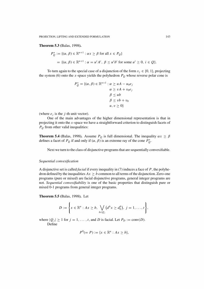
Theorem 5.3 (Balas, 1998).

P∗Q := {(α, β) ∈ R

n+1 : αx ≥ β for all x ∈ PQ}

= {(α, β) ∈ Rn+1 : α = ui Ai , β ≤ ui bi for some ui ≥ 0, i ∈ Q}.

To turn again to the special case of a disjunction of the form x j ∈ {0, 1}, projectingthe system (6) onto the x-space yields the polyhedron PQ whose reverse polar cone is

P∗Q = {(α, β) ∈ R

n+1 : α ≥ u A − u0e j

α ≥ vA + v0e j

β ≤ ub

β ≤ vb + v0

u, v ≥ 0}(where e j is the j-th unit vector).

One of the main advantages of the higher dimensional representation is that inprojecting it onto the x-space we have a straightforward criterion to distinguish facets ofPQ from other valid inequalities:

Theorem 5.4 (Balas, 1998). Assume PQ is full dimensional. The inequality αx ≥ β

defines a facet of PQ if and only if (α, β) is an extreme ray of the cone P∗Q .

Next we turn to the class of disjunctive programs that are sequentially convexifiable.

Sequential convexification

A disjunctive set is called facial if every inequality in (7) induces a face of P , the polyhe-dron defined by the inequalities Ax ≥ b common to all terms of the disjunction. Zero-oneprograms (pure or mixed) are facial disjunctive programs, general integer programs arenot. Sequential convexifiability is one of the basic properties that distinguish pure ormixed 0-1 programs from general integer programs.

Theorem 5.5 (Balas, 1998). Let

D :={

x ∈ Rn : Ax ≥ b,

∨

h∈Q j

(dh x ≥ dh

0

), j = 1, . . . , t

}

,

where |Q j | ≥ 1 for j = 1, . . . , t , and D is facial. Let PD := conv(D).Define

P0(= P) := {x ∈ Rn : Ax ≥ b},

144 BALAS

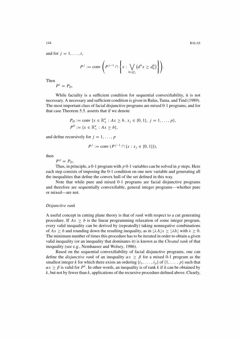
and for j = 1, . . . , t ,

P j := conv

(

P j−1 ∩{

x :∨

h∈Q j

(dh x ≥ dh

0

)})

.

ThenPt = PD.

While faciality is a sufficient condition for sequential convexifiability, it is notnecessary. A necessary and sufficient condition is given in Balas, Tama, and Tind (1989).The most important class of facial disjunctive programs are mixed 0-1 programs, and forthat case Theorem 5.5. asserts that if we denote

PD := conv {x ∈ Rn+ : Ax ≥ b, x j ∈ {0, 1}, j = 1, . . . , p},

P0 := {x ∈ Rn+ : Ax ≥ b},

and define recursively for j = 1, . . . , p

P j := conv (P j−1 ∩ {x : x j ∈ {0, 1}}),then

P p = PD.Thus, in principle, a 0-1 program with p 0-1 variables can be solved in p steps. Here

each step consists of imposing the 0-1 condition on one new variable and generating allthe inequalities that define the convex hull of the set defined in this way.

Note that while pure and mixed 0-1 programs are facial disjunctive programsand therefore are sequentially convexifiable, general integer programs—whether pureor mixed—are not.

Disjunctive rank

A useful concept in cutting plane theory is that of rank with respect to a cut generatingprocedure. If Ax ≥ b is the linear programming relaxation of some integer program,every valid inequality can be derived by (repeatedly) taking nonnegative combinationsof Ax ≥ b and rounding down the resulting inequality, as in �λA�x ≥ �λb� with λ ≥ 0.The minimum number of times this procedure has to be iterated in order to obtain a givenvalid inequality (or an inequality that dominates it) is known as the Chvatal rank of thatinequality (see e.g., Nemhauser and Wolsey, 1986).

Based on the sequential convexifiability of facial disjunctive programs, one candefine the disjunctive rank of an inequality αx ≥ β for a mixed 0-1 program as thesmallest integer k for which there exists an ordering {i1, . . . , i p} of {1, . . . , p} such thatαx ≥ β is valid for Pk . In other words, an inequality is of rank k if it can be obtained byk, but not by fewer than k, applications of the recursive procedure defined above. Clearly,


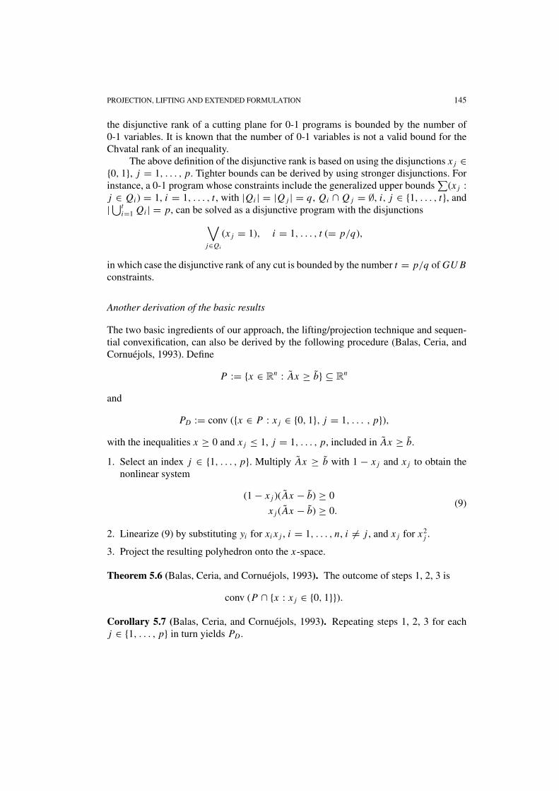
the disjunctive rank of a cutting plane for 0-1 programs is bounded by the number of0-1 variables. It is known that the number of 0-1 variables is not a valid bound for theChvatal rank of an inequality.

The above definition of the disjunctive rank is based on using the disjunctions x j ∈{0, 1}, j = 1, . . . , p. Tighter bounds can be derived by using stronger disjunctions. Forinstance, a 0-1 program whose constraints include the generalized upper bounds

∑(x j :

j ∈ Qi ) = 1, i = 1, . . . , t , with |Qi | = |Q j | = q, Qi ∩ Q j = ∅, i, j ∈ {1, . . . , t}, and| ⋃t

i=1 Qi | = p, can be solved as a disjunctive program with the disjunctions∨

j∈Qi

(x j = 1), i = 1, . . . , t (= p/q),

in which case the disjunctive rank of any cut is bounded by the number t = p/q of GU Bconstraints.

Another derivation of the basic results

The two basic ingredients of our approach, the lifting/projection technique and sequen-tial convexification, can also be derived by the following procedure (Balas, Ceria, andCornuejols, 1993). Define

P := {x ∈ Rn : Ax ≥ b} ⊆ R

n

and

PD := conv ({x ∈ P : x j ∈ {0, 1}, j = 1, . . . , p}),with the inequalities x ≥ 0 and x j ≤ 1, j = 1, . . . , p, included in Ax ≥ b.

1. Select an index j ∈ {1, . . . , p}. Multiply Ax ≥ b with 1 − x j and x j to obtain thenonlinear system

(1 − x j )( Ax − b) ≥ 0

x j ( Ax − b) ≥ 0.(9)

2. Linearize (9) by substituting yi for xi x j , i = 1, . . . , n, i �= j , and x j for x2j .

3. Project the resulting polyhedron onto the x-space.

Theorem 5.6 (Balas, Ceria, and Cornuejols, 1993). The outcome of steps 1, 2, 3 is

conv (P ∩ {x : x j ∈ {0, 1}}).

Corollary 5.7 (Balas, Ceria, and Cornuejols, 1993). Repeating steps 1, 2, 3 for eachj ∈ {1, . . . , p} in turn yields PD.

146 BALAS

The fact that this procedure is isomorphic to the one introduced earlier can be seenby examining the outcome of step 2. In fact, the linearized system resulting from step 2is precisely (8′), the higher dimensional representation of the disjunctive set defined bythe constraint x j ∈ {0, 1} (see Balas, Ceria, and Cornuejols, 1993 for details).

The above 3-step procedure is a streamlined version of the matrix cone procedureof Lovasz and Schrijver (1991). The latter involves in step 1 multiplication with 1 − x j

and x j for every j ∈ {1, . . . , p} rather than just one. While obtaining PD by the Lovasz-Schrijver procedure still involves p iterations of steps 1, 2, 3, the added computationalcost brings a reward: after each iteration, the coefficient matrix of the linearized systemmust be positive semidefinite, a condition that can be used in various ways to derivestrong bounds or cuts (see Lovasz and Schrijver, 1991; Balas et al, 1996).

Another similar procedure, due to Sherali and Adams (1990), is based on multi-plication with every product of the form (π j∈J1 x j )(π j∈J2 (1 − x j )), where J1 and J2 aredisjoint subsets of {1, . . . , p} such that |J1 ∪ J2| = t for some 1 ≤ t ≤ p. Linearizingthe resulting nonlinear system leads to a higher dimensional polyhedron whose strength(tightness) is intermediate between P and PD, depending on the choice of t : for t = p,the polyhedron becomes identical to P defined by the system (8) for a 0-1 polytope.

Disjunctive cuts

Theorem 5.3 describes the set of valid inequalities for a union of polyhedra Pi as definedin Theorem 5.1. If we replace this definition by Pi := {x ∈ R

n+ : Ai x ≥ bi }, then the valid

inequalities for PQ = conv(⋃

i∈Q Pi ) are of the form αx ≥ β, where (α, β) ∈ Rn × R

satisfies

α ≥ ui Ai , β ≤ ui bi , i ∈ Q (10)

for some ui ≥ 0, i ∈ Q.Clearly, every inequality satisfying (10) is dominated by one whose coefficients

satisfy

α j = maxi∈Q

ui aij , β ≤ min

i∈Qui bi (11)

where aij is the j-th column of Ai , i ∈ Q.

Since (10)—or, alternatively, (11)—defines all valid inequalities for a disjunctiveprogram, every valid cutting plane for a disjunctive program can be obtained from (11)by choosing suitable multipliers ui , i ∈ Q. In other words, any cutting plane for acombinatorial optimization problem that can be stated as a disjunctive program, can bebrought to the form (10) or (11). Clearly, the strength of such a cut depends on the choiceof the multipliers ui , i ∈ Q.

We will illustrate this on an example.


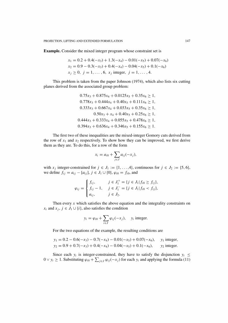
Example. Consider the mixed integer program whose constraint set is

x1 = 0.2 + 0.4(−x3) + 1.3(−x4) − 0.01(−x5) + 0.07(−x6)

x2 = 0.9 − 0.3(−x3) + 0.4(−x4) − 0.04(−x5) + 0.1(−x6)

x j ≥ 0, j = 1, . . . , 6, x j integer, j = 1, . . . , 4.

This problem is taken from the paper Johnson (1974), which also lists six cuttingplanes derived from the associated group problem:

0.75x3 + 0.875x4 + 0.0125x5 + 0.35x6 ≥ 1,

0.778x3 + 0.444x4 + 0.40x5 + 0.111x6 ≥ 1,

0.333x3 + 0.667x4 + 0.033x5 + 0.35x6 ≥ 1,

0.50x3 + x4 + 0.40x5 + 0.25x6 ≥ 1,

0.444x3 + 0.333x4 + 0.055x5 + 0.478x6 ≥ 1,

0.394x3 + 0.636x4 + 0.346x5 + 0.155x6 ≥ 1.

The first two of these inequalities are the mixed-integer Gomory cuts derived fromthe row of x1 and x2 respectively. To show how they can be improved, we first derivethem as they are. To do this, for a row of the form

xi = ai0 +∑

j∈J

ai j (−x j ),

with x j integer-constrained for j ∈ J1 := {1, . . . ,4}, continuous for j ∈ J2 := {5, 6},we define fi j = ai j − [ai j ], j ∈ J1 ∪ {0}, ϕi0 = fi0, and

ϕi j =

fi j , j ∈ J+1 = { j ∈ J1| fi0 ≥ fi j },

fi j − 1, j ∈ J−1 = { j ∈ J1| fi0 < fi j },

ai j , j ∈ J2.

Then every x which satisfies the above equation and the integrality constraints onxi and x j , j ∈ J1 ∪ {i}, also satisfies the condition

yi = ϕi0 +∑

i∈J

ϕi j (−x j ), yi integer.

For the two equations of the example, the resulting conditions are

y1 = 0.2 − 0.6(−x3) − 0.7(−x4) − 0.01(−x5) + 0.07(−x6), y1 integer,

y2 = 0.9 + 0.7(−x3) + 0.4(−x4) − 0.04(−x5) + 0.1(−x6), y2 integer.

Since each yi is integer-constrained, they have to satisfy the disjunction yi ≤0 ∨ yi ≥ 1. Substituting ϕi0 + ∑

j∈J ϕi j (−x j ) for each yi and applying the formula (11)

148 BALAS

with multipliers ui0 = 1/ϕi0 in the first term, and ui

0 = 1/(1 − ϕi0) in the second term ofeach disjunction we obtain for i = 1 and i = 2 the two cuts

0.6

0.8x3 + 0.7

0.8x4 + 0.01

0.8x5 + 0.07

0.2x6 ≥ 1,

and

0.7

0.9x3 + 0.4

0.9x4 + 0.04

0.1x5 + 0.1

0.9x6 ≥ 1.

These are precisely the first two inequalities of the above list. Since all cuts discussedhere are stated in the form ≥1, the smaller the j-th coefficient, the stronger is the cutin the direction j . We would thus like to reduce the size of the coefficients as much aspossible.

Now suppose that instead of y1 ≤ 0 ∨ y1 ≥ 1, we use the disjunction

{y1 ≤ 0} ∨{

y1 ≥ 1

x1 ≥ 0

}

,

which of course is also satisfied by every feasible x .Then, applying formula (11) with multipliers 5, 5 and 15 for y1 ≤ 0, y1 ≥ 1 and

x1 ≥ 0 respectively, we obtain the cut whose coefficients are

max

{5 × (−0.6)

5 × 0.2,

5 × 0.6 + 15 × (−0.4)

5 × 0.8 + 15 × (−0.2)

}

= −3,

max

{5 × (−0.7)

5 × 0.2,

5 × 0.7 + 15 × (−1.3)

5 × 0.8 + 15 × (−0.2)

}

= −3.5,

max

{5 × (−0.01)

5 × 0.2,

5 × 0.01 + 15 × 0.01

5 × 0.8 + 15 × (−0.2)

}

= 0.2,

max

{5 × 0.07

5 × 0.2,

5 × (−0.07) + 15 × (−0.07)

5 × 0.8 + 15 × (−0.2)

}

= 0.35

that is

−3x3 − 3.5x4 + 0.2x5 + 0.35x6 ≥ 1.

The sum of coefficients on the left hand side has been reduced from 1.9875 to −5.95.This strengthening has been obtained by assigning a positive multiplier in (11) to theinequality x1 ≥ 0, which had a zero multiplier in the previous derivation.

Similarly, for the second cut, if instead of y2 ≤ 0 ∨ y2 ≥ 1 we use the disjunction{

y2 ≤ 0

x1 ≥ 0

}

∨ {y2 ≥ 1},


with multipliers 10, 40 and 10 for y2 ≤ 0, x1 ≥ 0 and y2 ≥ 1 respectively, we obtain thecut

−7x2 − 4x4 + 0.4x5 − x6 ≥ 1.

Here the sum of left hand side coefficients has been reduced from 1.733 to −11.6. Again,the effect is obtained by assigning a positive multiplier to x1 ≥ 0, this time on the otherside of the disjunction.

Exercise 5.1 Consider the example at the end of Section 5. Why is it that to improve thefirst cut, we introduce x1 ≥ 0 into the second term of the disjunction (y1 ≤ 0)∨ (y1 ≥ 1),and to improve the second cut, we introduce x1 ≥ 0 into the first term of the disjunction(y2 ≤ 0)∨(y2 ≥ 1)? Why not the other way? Give a necessary and/or sufficient conditionfor an inequality xi ≥ 0 (where xi is a basic variable) to be usable in this role, i.e. toimprove the cut from a given disjunction y1 ≤ 0 ∨ y1 ≥ 1 when included in one of theterms of the disjunction.

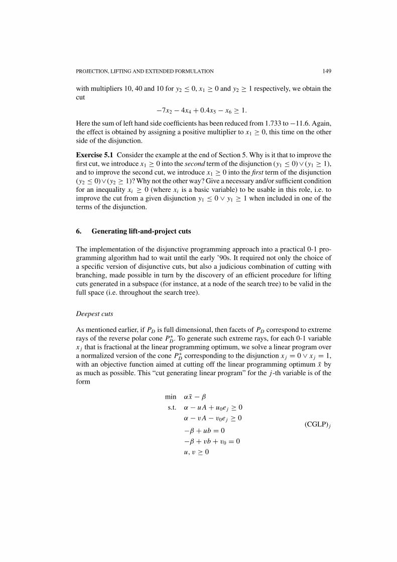
6. Generating lift-and-project cuts

The implementation of the disjunctive programming approach into a practical 0-1 pro-gramming algorithm had to wait until the early ’90s. It required not only the choice ofa specific version of disjunctive cuts, but also a judicious combination of cutting withbranching, made possible in turn by the discovery of an efficient procedure for liftingcuts generated in a subspace (for instance, at a node of the search tree) to be valid in thefull space (i.e. throughout the search tree).

Deepest cuts

As mentioned earlier, if PD is full dimensional, then facets of PD correspond to extremerays of the reverse polar cone P∗

D. To generate such extreme rays, for each 0-1 variablex j that is fractional at the linear programming optimum, we solve a linear program overa normalized version of the cone P∗

D corresponding to the disjunction x j = 0 ∨ x j = 1,with an objective function aimed at cutting off the linear programming optimum x byas much as possible. This “cut generating linear program” for the j-th variable is of theform

min α x − β

s.t. α − u A + u0e j ≥ 0

α − vA − v0e j ≥ 0(CGLP) j−β + ub = 0

−β + vb + v0 = 0

u, v ≥ 0

150 BALAS

and (i) β ∈ {1, −1}, or (ii)∑

j |α j | ≤ 1. For details, see Balas, Ceria, and Cornuejols(1993, 1996).

The normalization constraint (i) or (ii) has the purpose of turning the cone P∗D into a

polyhedron. Several other normalizations have been proposed later, with pro’s and con’sfor each one, and their choice plays an important role in determining the optimum.

Solving (CGLP) j yields a cut αx ≥ β, where

αk ={

max{uak, vak} k ∈ N \ { j}max{ua j − u0, va j + v0} k = j,

(12)

with ak the k-th column of A, and β = min{ub, vb+v0}. This cut maximizes the amountβ − α x by which x is cut off.

Cut lifting

A cutting plane derived at a node of the search tree defined by a subset F0 ∪ F1 of the 0-1variables, where F0 and F1 index those variables fixed at 0 and 1, respectively, is valid atthat node and its descendants in the tree (where the variables in F0 ∪ F1 remain fixed attheir values). Such a cut can in principle be made valid at other nodes of the search tree,where the variables in F0 ∪ F1 are no longer fixed, by calculating appropriate values forthe coefficients of these variables—a procedure called lifting and mentioned in Section 1.However, calculating such coefficients is in general a daunting task, which may requirethe solution of an integer program for every coefficient. One important advantage ofthe cuts discussed here is that the multipliers u, u0, v, v0 obtained along with the cutvector (α, β) by solving (CGLP) j can be used to calculate by closed form expressionsthe coefficients αh of the variables h ∈ F0 ∪ F1.

While this possibility of calculating efficiently the coefficients of variables ab-sent from a given subproblem (i.e. fixed at certain values) is crucial for making itpossible to generate cuts during a branch-and-bound process that are valid through-out the search tree, its significance goes well beyond this aspect. Indeed, most columnsof A corresponding to nonbasic components of x typically play no role in determin-ing the optimal solution of (CGLP) j and can therefore be ignored. In other words, thecuts can be generated in a subspace involving only a subset of the variables, and thenlifted to the full space. This is the procedure followed in Balas, Ceria, and Cornuejols(1993, 1996), where the subspace used is that of the variables indexed by some R ⊂ Nsuch that R includes all the 0-1 variables that are fractional and all the continuous vari-ables that are positive at the LP optimum. The lifting coefficients for the variables notin the subspace, which are all assumed w.l.o.g. to be at their lower bound, are thengiven by

α� := max{ua�, va�}, h ∈ N\R

where u and v are the optimal vectors obtained by solving (CGLP) j .


These coefficients always yield a valid lifted inequality. If normalization (i) is usedin (CGLP) j , the resulting lifted cut is exactly the same as the one that would have beenobtained by applying (CGLP) j to the problem in the full space. If other normalizationsare used, the resulting cut may differ in some coefficients (lifting a cut does not in generalhave a unique outcome).

Cut strengthening

The cut αx ≥ β derived from a disjunction of the form x j ∈ {0, 1} can be strengthenedby using the integrality conditions on variables other than x j , as shown in Balas andJeroslow (1980) (see also Section 7 of Balas, 1979). Indeed, if xk is such a variable, thecoefficient

αk := max{uak, vak}

can be replaced by

α′k := min{uak + u0�mk�, vak − v0�mk�},

where

mk := vak − uak

u0 + v0.

For a proof of this statement, see Balas (1979) or Balas, Ceria, and Cornuejols(1993). The strengthening “works,” i.e. produces an actual change in the coefficient, ifand only if either uak > vak + u0 orvak > uak+v0. Furthermore, the larger the difference|uak − vak |, the more room there is for strengthening the coefficient in question.

This strengthening procedure can also be applied to cuts derived from disjunctionsother than x j ∈ {0, 1}, including disjunctions with more than two terms. In the latter case,however, the closed form expression for the values mk used above has to be replaced bya procedure for calculating those values, whose complexity is linear in the number ofterms in the disjunction (see Balas and Jeroslow, 1980 or Balas, 1979 for details).

The overall cut generating procedure

To summarize briefly the above discussion, the actual cut generating procedure is notjust “lift and project,” but rather RLPLS, an acronym for

• RESTRICT the problem to a subspace defined from the LP optimum, and choose adisjunction;

• LIFT the disjunctive set to describe its convex hull in a higher dimensional space;

152 BALAS

• PROJECT the polyhedron describing the convex hull onto the original (restricted)space, generating cuts;

• LIFT the cuts into the original full space;

• STRENGTHEN the lifted cuts.

Exercise 6.1 Generalize the procedure described in the subsection “Deepest cuts” ofSection 6 to the case where you want to use a stronger disjunction than x j = 0 ∨ x j = 1,namely the one implied by imposing the 0-1 condition on two variables rather than justone: xi ∈ {0, 1}, x j ∈ {0, 1}:

(a) state the resulting (4-term) disjunction,

(b) formulate the corresponding (CGLP)i j ,

(c) given an optimal solution to (CGLP)i j , state the associated cut and derive the expres-sion corresponding to (12).

7. Solving the cut generating linear program in the (LP) simplex tableau

A breakthrough in generating lift-and-project cuts occurred in 2000, when a precisecorrespondence was established in Balas and Perregaard (2003) between feasible basesof the higher dimensional cut generating linear program (CGLP) and (not necessarilyfeasible) bases of the original linear programming relaxation (LP). This correspondencehas made it possible to generate lift-and-project cuts corresponding to an optimal solutionof the (CGLP) without explicitly constructing the latter, by working in the original (LP)tableau. In other words, the correspondence makes it possible to mimic the pivots ofthe (CGLP) through certain pivots of the (LP), and thereby solve the (CGLP) implicitly.Furthermore, as the (CGLP) is by construction highly degenerate, the correspondencebetween the bases of the two linear programs is many-to-one, i.e. many feasible bases ofthe (CGLP) correspond to a basis of the (LP). Thus solving the (CGLP) implicitly savestime not only because (LP) is a smaller linear program than (CGLP), but also becauseone pivot in the (LP) tableau corresponds to several pivots in the (CGLP) tableau.

This correspondence also gives an exact characterization of the connection betweenlift-and-project cuts and earlier cuts in the literature.

Consider the simplex tableau associated with the optimal solution x to (LP), andlet

xk = ako −∑

j∈J

ak j s j (13)

be one of its rows, with xk a 0-1 variable. Here J is the index set of nonbasic variables,|J | = n, and 0 < ak0 < 1. The simple disjunctive cut from the condition xk ≤ 0∨xk ≥ 1


applied to (13) is πsJ ≥ π0 where

π0 = ak0(1 − ak0) and π j = max{ak j (1 − ak0), −ak j ak0} j ∈ J.

If some of the variables s j , say those indexed by J1 ⊆ J , are integer-constrained,this cut can be strengthened to πsJ ≥ π0 through the procedure described in the previoussection, which in this case yields

π j ={

min{(ak j − �ak j�)(1 − ak0), (�ak j� − ak j )ak0} j ∈ J1

π j j ∈ J \ J1

This strengthened simple disjunctive cut is the same (Balas, 1979) as the mixedinteger Gomory cut.

Now consider the cut generating linear program corresponding to variable xk :

min α x − β

α − u A + u0ek = 0

α − v A − v0ek = 0

−β + ub = 0 (CGLP)k

−β + vb + v0 = 0

ue + u0 + ve + v0 = 1

u, u0, v, vo ≥ 0

This formulation differs from the one used in the previous section by the fact thatsurplus variables have been introduced (which accounts for A, b replacing A, b), and adifferent normalization is used (note that A, just like A, has n columns).

It can be shown that in any feasible basic solution to (CGLP)k that yields an in-equality not dominated by the constraints of (LP), u0 and v0 are both positive, and if thebasic components of u and v are indexed by M1 and M2, respectively, then M1 ∩ M2 = ∅,|M1 ∪ M2| = n, and the n × n submatrix A of A whose rows are indexed by M1 ∪ M2 isnonsingular.

Now define J := M1 ∪ M2 and consider the subsystem of Ax ≥ b consisting ofthe constraints indexed by J , written in equality form, i.e. with the surplus variablesexplicitly shown:

Ax − sJ = b

or

x = A−1b + A−1sJ .

The equation corresponding to xk (where k �∈ J ) is then of the form (13), withak0 = ek A−1

k b and ak j = −( A−1)k j , and it can be shown that 0 < ak0 < 1.The following two theorems (Balas and Perregaard, 2003) give the correspondence.

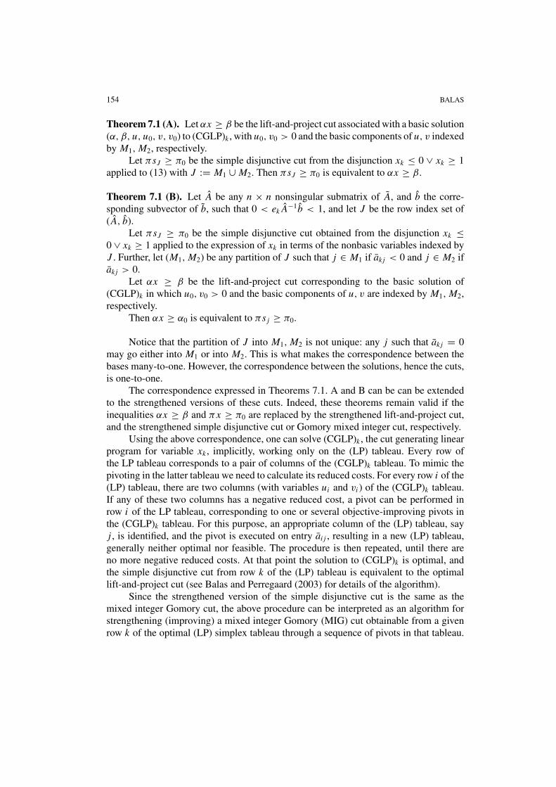
154 BALAS

Theorem 7.1 (A). Let αx ≥ β be the lift-and-project cut associated with a basic solution(α, β, u, u0, v, v0) to (CGLP)k , with u0, v0 > 0 and the basic components of u, v indexedby M1, M2, respectively.

Let πsJ ≥ π0 be the simple disjunctive cut from the disjunction xk ≤ 0 ∨ xk ≥ 1applied to (13) with J := M1 ∪ M2. Then πsJ ≥ π0 is equivalent to αx ≥ β.

Theorem 7.1 (B). Let A be any n × n nonsingular submatrix of A, and b the corre-sponding subvector of b, such that 0 < ek A−1b < 1, and let J be the row index set of( A, b).

Let πsJ ≥ π0 be the simple disjunctive cut obtained from the disjunction xk ≤0 ∨ xk ≥ 1 applied to the expression of xk in terms of the nonbasic variables indexed byJ . Further, let (M1, M2) be any partition of J such that j ∈ M1 if ak j < 0 and j ∈ M2 ifak j > 0.

Let αx ≥ β be the lift-and-project cut corresponding to the basic solution of(CGLP)k in which u0, v0 > 0 and the basic components of u, v are indexed by M1, M2,respectively.

Then αx ≥ α0 is equivalent to πs j ≥ π0.

Notice that the partition of J into M1, M2 is not unique: any j such that ak j = 0may go either into M1 or into M2. This is what makes the correspondence between thebases many-to-one. However, the correspondence between the solutions, hence the cuts,is one-to-one.

The correspondence expressed in Theorems 7.1. A and B can be can be extendedto the strengthened versions of these cuts. Indeed, these theorems remain valid if theinequalities αx ≥ β and πx ≥ π0 are replaced by the strengthened lift-and-project cut,and the strengthened simple disjunctive cut or Gomory mixed integer cut, respectively.

Using the above correspondence, one can solve (CGLP)k , the cut generating linearprogram for variable xk , implicitly, working only on the (LP) tableau. Every row ofthe LP tableau corresponds to a pair of columns of the (CGLP)k tableau. To mimic thepivoting in the latter tableau we need to calculate its reduced costs. For every row i of the(LP) tableau, there are two columns (with variables ui and vi ) of the (CGLP)k tableau.If any of these two columns has a negative reduced cost, a pivot can be performed inrow i of the LP tableau, corresponding to one or several objective-improving pivots inthe (CGLP)k tableau. For this purpose, an appropriate column of the (LP) tableau, sayj , is identified, and the pivot is executed on entry ai j , resulting in a new (LP) tableau,generally neither optimal nor feasible. The procedure is then repeated, until there areno more negative reduced costs. At that point the solution to (CGLP)k is optimal, andthe simple disjunctive cut from row k of the (LP) tableau is equivalent to the optimallift-and-project cut (see Balas and Perregaard (2003) for details of the algorithm).

Since the strengthened version of the simple disjunctive cut is the same as themixed integer Gomory cut, the above procedure can be interpreted as an algorithm forstrengthening (improving) a mixed integer Gomory (MIG) cut obtainable from a givenrow k of the optimal (LP) simplex tableau through a sequence of pivots in that tableau.


The first pivot replaces the source row k for the MIG cut with the source row k of the newtableau resulting from the pivot. This new tableau is in general infeasible, but its row kyields a MIG cut guaranteed to be stronger (more violated by the optimal LP solution x)than the cut from the previous tableau would have been. Each subsequent pivot results inthe replacement of the MIG cut from row k of the current tableau with a MIG cut fromrow k of a new tableau, with a guaranteed improvement of the cut.

8. Branch-and-cut and computational experience

No cutting plane approach known at this time can solve large, hard integer programsjust by itself. Repeated cut generation tends to produce a flattening of the region of thepolyhedron where the cuts are applied, as well as numerical instability which can onlypartly be mitigated by a tightening of the tolerance requirements. Therefore the successfuluse of cutting planes requires their combination with some enumerative scheme. Onepossibility is to generate cutting planes as long as that seems profitable, thereby creating atighter linear programming relaxation than the one given originally, and then to solve theresulting problem by branch and bound. Another possibility, known as branch-and-cut,consists of branching and cutting intermittently; i.e., when the cut generating procedure“runs out of steam,” move elsewhere in the feasible region by branching. This approachdepends crucially on the ability to lift the cuts generated at different nodes of the searchtree so as to make them valid everywhere.

The first successful implementation of lift-and-project for mixed 0-1 programmingin a branch-and-cut framework was the MIPO (Mixed Integer Program Optimizer) codedescribed in Balas, Ceria, and Cornuejols (1996). The procedure it implements can beoutlined as follows.

Nodes of the search tree (subproblems created by branching) are stored along withtheir optimal LP bases and associated bounds. Cuts that are generated are stored in a pool.The cut generation itself involves the RLPLS process described earlier. Furthermore, cutsare not generated at every node, but at every k-th node, where k is a cutting frequencyparameter.

At any given iteration, a subproblem with best (weakest) lower bound is retrievedfrom storage and its optimal LP solution x is recreated. Next, all those cuts in the poolthat are tight for x or violated by it, are added to the constraints and x is updated byreoptimizing the LP.

At this point, a choice is made between generating cuts or skipping that step andgoing instead to branching. The frequency of cutting is dictated by the parameter k thatis problem dependent, and calculated after generating cuts at the root node. Its value is afunction of several variables believed to characterize the usefulness of cutting planes forthe given problem, primarily the average depth of the cuts obtained. In our experiments,the most frequently used value of k was 8.

If cuts are to be generated, this happens according to the RLPLS scheme describedabove. First, a subspace is chosen by retaining all the 0-1 variables fractional and all the

156 BALAS

continuous variables positive at the LP optimum, and removing the remaining variablesalong with their lower and upper bounds. A lift and project cut is then generated fromeach disjunction x j ∈ {0, 1} for j such that 0 < x j < 1 (this is called a round of cuts).Each cut is lifted and strengthened; and if it differs from earlier cuts sufficiently (thedifference between cuts is measured by the angle between their normals), it is added tothe pool; otherwise it is thrown away. After generating a round of cuts, the current LP isreoptimized again.

If cuts are not to be generated (or have already been generated), a fractional variableis chosen for branching on a disjunction of the form x j ∈ {0, 1}; i.e., two new subproblemsare created, their lower bounds are calculated, and they are stored. The branching variableis chosen as the one with largest (in absolute value) cost coefficient among those whoseLP optimal value is closest to 0.5.

Computational results in branch-and-cut mode

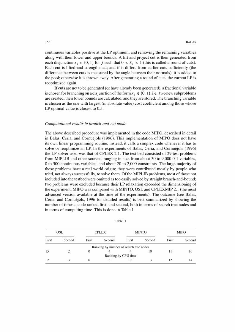
The above described procedure was implemented in the code MIPO, described in detailin Balas, Ceria, and Cornuejols (1996). This implementation of MIPO does not haveits own linear programming routine; instead, it calls a simplex code whenever it has tosolve or reoptimize an LP. In the experiments of Balas, Ceria, and Cornuejols (1996)the LP solver used was that of CPLEX 2.1. The test bed consisted of 29 test problemsfrom MIPLIB and other sources, ranging in size from about 30 to 9,000 0-1 variables,0 to 500 continuous variables, and about 20 to 2,000 constraints. The large majority ofthese problems have a real world origin; they were contributed mostly by people whotried, not always successfully, to solve them. Of the MIPLIB problems, most of those notincluded into the testbed were omitted as too easily solved by straight branch-and-bound;two problems were excluded because their LP relaxation exceeded the dimensioning ofthe experiment. MIPO was compared with MINTO, OSL and CPLEXMIP 2.1 (the mostadvanced version available at the time of the experiments). The outcome (see Balas,Ceria, and Cornuejols, 1996 for detailed results) is best summarized by showing thenumber of times a code ranked first, and second, both in terms of search tree nodes andin terms of computing time. This is done in Table 1.

Table 1

OSL CPLEX MINTO MIPO

First Second First Second First Second First Second

Ranking by number of search tree nodes15 2 0 4 4 10 11 10

Ranking by CPU time2 3 6 6 10 3 12 14


In a sense, MIPO seemed to be the most robust among the four codes: it was theonly one that managed to solve all 29 test problems, and it ranked first or second incomputing time on 26 out of the 29 instances.

Other experiments with lift-and-project in an enumerative framework are reportedon in Thienel (1995), where S. Thienel compares the performance of ABACUS, anobject oriented branch-and-cut code, in two different modes of operation, one using lift-and-project cuts and the other using Gomory cuts; with the outcome that the versionwith lift-and-project cuts is considerably faster on all hard problems, where hard meansrequiring at least 10 minutes.

Little experimentation has taken place so far with cuts derived from stronger dis-junctions than the 0-1 condition on a single variable. In Balas et al (1996) the MIPOprocedure was run on maximum clique problems, where the higher dimensional formu-lation used to generate cuts was the one obtained by multiplying the constraint set withinequalities of the form 1 − ∑

(x j : j ∈ S) ≥ 0, x j ≥ 0, j ∈ S, where S is a stable set.This is the same as the higher dimensional formulation derived from the disjunction

(x j = 0, j ∈ S) ∨ (x j1 = 1, x j = 0, j ∈ S\{ j1}

)

∨ · · · ∨ (x js = 1, x j = 0, j ∈ S\{ js}

),

where s = |S|. As this disjunction is more powerful than the standard one, the cutsobtained were stronger; but they were also more expensive to generate, and without somespecialized code to solve the highly structured cut generating LP’s of this formulation,the trade-off between the strength of the cuts and the cost of generating them favored theweaker cuts from the standard disjunction.

Results in cut-and-branch mode

Bixby et al. (1999) report on their computational experience with a parallel branch-and-bound code, run on 51 test problems after generating several types of cuts at the root node.One of the cut types used was disjunctive or lift-and-project cuts, generated essentiallyas in Balas, Ceria, and Cornuejols (1996) with normalization (ii), but without restrictionto a subspace and without strengthening. Since deriving these cuts in the full space isexpensive, the routine generating them was activated only for 4 of the hardest problems.Their addition to the problem constraints reduced the integrality gap by 58.7%, 94.4%,99.9% and 94.4%, respectively.

In Ceria and Pataki (1998), computational results are reported with a disjunctivecut generator used in tandem with the CPLEX branch and bound code. Namely, thecut generator was used to produce 2 and 5 rounds of cuts from the 0-1 disjunctions forthe 50 most promising variables fractional at the LP optimum, after which the resultingproblem with the tightened LP relaxation was solved by the CPLEX 5.0 MIP code. This“cut-and-branch” procedure was tested on 18 of the hardest MIPLIB problems and theresults were compared to those obtained by using CPLEX 5.0 without the cut generator.

158 BALAS

The outcome of the comparison can be summarized as follows (see Table 2 of Ceria andPataki (1998) for details).

• The total running time of the cut-and-branch procedure was less than the time withoutcuts for 14 of the 18 problems; while the opposite happened for the remaining 4problems.

• Two of the problems solved by cut-and-branch in 8 and 3 minutes respectively couldnot be solved by CPLEX alone in 20 hours.

• For 6 problems the gain in time was more than 4-fold.

Very good results were obtained on two difficult problems outside the above set.One of them, set1ch, could not be solved by CPLEX alone, which after exhausting itsmemory limitations stopped with a solution about 15% away from the optimum. On theother hand, running the cutting plane generator for 10 rounds on this problem produceda lower bound within 1.4% of the integer optimum, and running CPLEX on the resultingtightened formulation solved the problem to optimality in 28 seconds.

The second difficult problem, seymour, was formulated by Paul Seymour in anattempt to find a minimal irreducible configuration in the proof of the four color theorem.It was not solved to optimality until very recently. The value of the LP relaxation is 403.84,and an integer solution of 423.00 was known. The best previously known lower bound of412.76 had been obtained by running a parallel computer with 16 processors for about 60hours, using about 1400 megabytes of memory. The cut-and-branch procedure appliedto this case generated 10 rounds of 50 cuts in about 10.5 hours, and produced a lowerbound of 413.16, using less than 50 megabytes of memory. Running CPLEX for another10 hours on this tightened formulation then raised the bound to 414.20. More recently,using the same lift-and-project cuts but a more powerful computer, the problem wassolved to optimality (Pataki, 2001).

Results when generating lift-and-project cuts from the LP simplex tableau

Early testing on two dozen MIPLIB instances (Balas and Perregaard, 2003) showed thatsolving the (CGLP) implicitly on the (LP) simplex tableau required 7–8 times fewerpivots than doing it directly. A much more thorough testing was performed subsequentlyby M. Perregaard and reported on at the August 2003 International Symposium on Math-ematical Programming held in Copenhagen (Perregaard, 2003). Out of 98 test problemsoriginating in MIPLIB and Hans Mittelmann’s database, 95 were solved within a timelimit of 30 minutes, using both approaches, with cuts generated only at the root node. Theaverage run time per instance was 596 seconds with the original version which solvesthe CGLP explicitly, and 451 seconds with the new version which solves it implicitly,working in the LP simplex tableau. The number of pivots for generating cuts was reduced15–20 times. With the new version, the time spent on cut generation was on the order of5% of the total time to solve the problem by branch and bound.


On the other hand, this experiment also showed that in about 1/4 of all this instances(27 out of 98) pivoting did not improve the cuts, i.e. the MIG cuts turned out to be optimallift-and-project cuts. In the remaining cases, the improvements obtained came from thefirst 8-10 pivots. Over the entire problem set, MIG cuts on the average closed 35.3%of the integrality gap, while lift-and-project cuts closed 38.8%. However, for some hardproblems the difference was much more substantial.

Starting with the 2003C release of XPRESS, the lift-and-project cuts generatedfrom the (LP) simplex tableau are part of the mixed integer solver. The cut generatingmodule uses at most 10 improving pivots per cut, and generates at most 50 lift-and-project cuts per round. The number of rounds is optional, with the understanding thatheavy use of cuts is only recommended on hard problems on which the standard procedurefails.

References

Balas, E. (1998). “Disjunctive Programming: Properties of the Convex Hull of Feasible Points.” Invitedpaper, with a foreword by G. Cornuejols and W. Pulleyblank, Discrete Applied Mathematics 89, 3–44.(Originally MSRR# 348, Carnegie Mellon University, July 1974).

Balas, E. (1979). “Disjunctive Programming.” Annals of Discrete Mathematics 5, 3–51.Balas, E. (1985). “Disjunctive Programming and a Hierarchy of Relaxations for Discrete Optimization

Problems.” SIAM Journal on Algebraic and Discrete Methods 6, 466–485.Balas, E. (1987). “The Assignable Subgraph Polytope of a Directed Graph.” Congressus Numerantium 60,

35–42.Balas, E. (1997). “A Modified Lift-and-Project Procedure.” Mathematical Programming 79, 19–31.Balas, E. (1998). “Projection with a Minimal System of Inequalities.” Computational Optimization and

Applications 10, 189–193.Balas, E. (2001). “Projection and Lifting in Combinatorial Optimization.” In M. Junger and D. Naddef (eds.),

Computational Combinatorial Optimization: Optimal or Provably Near-Optimal Solutions, LNCS 2241,Springer, pp. 26–56.

Balas, E., S. Ceria, and G. Cornuejols. (1993). “A Lift-and-Project Cutting Plane Algorithm for Mixed 0-1Programs.” Mathematical Programming 58, 295–324.

Balas, E., S. Ceria, and G. Cornuejols. (1996). “Mixed 0-1 Programming by Lift-and-Project in a Branch-and-Cut Framework.” Management Science 42, 1229–1246.

Balas, E., S. Ceria, G. Cornuejols, and G. Pataki. (1996). “Polyhedral Methods for the Maximum CliqueProblem.” In D. Johnson and M. Trick (eds.), Clique, Coloring and Satisfiability: The Second DIMACSChallenge. The American Mathematical Society, Providence, RI, pp. 11–27.

Balas, E. and R.G. Jeroslow. (1980). “Strengthening Cuts for Mixed Integer Programs.” European Journalof Operational Research 4, 224–234.

Balas, E. and J.B. Mazzola. (1984). “Nonlinear 0-1 Programming: I. Linearization Techniques, II. DominanceRelations and Algorithms.” Mathematical Programming 30, 1–21 and 22–45.

Balas, E. and M. Oosten. (1998). “On the Dimension of Projected Polyhedra.” Discrete Applied Mathematics87, 1–9.

Balas, E. and M. Oosten. (2000). “The Cycle Polytope of a Directed Graph.” Networks 36, 34–46.Balas, E. and M. Perregaard. (2003). “A Precise Correspondence Between Lift-and-Project Cuts, Simple

Disjunctive Cuts, and Mixed Integer Gomory Cuts for 0-1 Programming.” Mathematical ProgrammingB 94, 221–245.

160 BALAS

Balas, E. and W.R. Pulleyblank. (1983). “The Perfectly Matchable Subgraph Polytope of a Bipartite Graph.”Networks 13, 495–518.

Balas, E. and W.R. Pulleyblank. (1989). “The Perfectly Matchable Subgraph Polytope of an Arbitrary Graph.”Combinatorica 9, 321–337.

Balas, E., J. Tama and J. Tind. (1989). “Sequential Convexification in Reverse Convex and DisjunctiveProgramming.” Mathematical Programming 44, 337–350.

Beaumont, N. (1990). “An Algorithm for Disjunctive Programming.” European Journal of OperationalResearch 48, 362–371.

Bixby, R., W. Cook, A. Cox, and E. Lee. (1999). “Computational Experience with Parallel Mixed IntegerProgramming in a Distributed Environment.” Annals of Operations Research 90, 19–45.

Blair, C. (1976). “Two Rules for Deducing Valid Inequalities for 0-1 Programs.” SIAM Journal of AppliedMathematics 31, 614–617.

Blair, C. (1980). “Facial Disjunctive Programs and Sequences of Cutting Planes.” Discrete Applied Mathe-matics 2, 173–180.

Ceria, S. and G. Pataki. (1998). “Solving Integer and Disjunctive Programs by Lift-and-Project.” In R.E.Bixby, E.A. Boyd, and R.Z. Rios-Mercado (eds.), IPCO VI, Lecture Notes in Computer Science, 1412.Springer, pp. 271–283.

Ceria, S. and J. Soares. (1997). “Disjunctive Cuts for Mixed 0-1 Programming: Duality and Lifting.” GSB,Columbia University.

Ceria, S. and J. Soares. (1999). “Convex Programming for Disjunctive Convex Optimization.” MathematicalProgramming 86, 595–614.

Dantzig, G.B., R.D. Fulkerson, and S.M. Johnson. (1954). “Solution of a Large-Scale Traveling SalesmanProblem.” Operations Research 2, 393–410.

Fortet, R. (1960). “Applications de l’algebre de Boole en recherche operationnelle.” Revue Francaise deRecherche Operationnelle 4, 17–25.

Jeroslow, R.G. (1977). “Cutting Plane Theory: Disjunctive Methods.” Annals of Discrete Mathematics 1,293–330.

Jeroslow, R.G. (1987). “Representability in Mixed Integer Programming I: Characterization Results.” Dis-crete Applied Mathematics 17, 223–243.

Jeroslow, R.G. (1989). “Logic Based Decision Support: Mixed Integer Model Formulation.” Annals ofDiscrete Mathematics 40.

Johnson, E.L. (1974). “The Group Problem for Mixed-Integer Programming.” Mathematical ProgrammingStudy 2, 137–179.

Letchford, A. (2001). “On Disjunctive Cuts for Combinatorial Optimization.” Journal of CombinatorialOptimization 5, 299–317.

Lovasz, L. and A. Schrijver. (1991). “Cones of Matrices and Set Functions and 0-1 Optimization.” SIAMJournal of Optimization 1, 166–190.

Miller, C.E., A.W. Tucker, and R.A. Zemlin. (1960). “Integer Programming Formulations and TravelingSalesman Problems.” Journal of the ACM 7, 326–329.

Nemhauser, G. and L. Wolsey. (1986). Integer and Combinatorial Optimization. Wiley.Padberg, M. and T.-Y. Sung. (1991). “An Analytical Comparison of Different Formulations of the Traveling

Salesman Problem.” Math. Programming 52, 315–357.Pataki, G. (2001). Personal communication, March.Perregaard, M. (2003). “A Practical Implementation of Lift-and-Project Cuts. A computational exploration

of lift-and-project with XPRESS-MP.” Paper presented at the International Symposium on MathematicalProgramming, August, Copenhagen.

Perregaard, M. and E. Balas. (2001). “Generating Cuts from Multiple-Term Disjunctions.” In K. Aardaland B. Gerards (eds.), Integer Programming and Combinatorial Optimization (8th IPCO Conference,Utrecht, 2001), LCNS No. 2081, Springer, pp. 318–360.


Sherali, H. and W. Adams. (1990). “A Hierarchy of Relaxations Between the Continuous and ConvexHull Representations for Zero-One Programming Problems.” SIAM Journal on Discrete Mathematics 3,411–430.

Sherali, H. and C. Shetty. (1980). Optimization with Disjunctive Constraints. Lecture Notes in Economicsand Mathematical Systems, 181, Springer.

Stoer, J. and C. Witzgall. (1970). Convexity and Optimization in Finite Dimensions I. Springer.Stubbs, R.A. and S. Mehrotra. (1996). “A Branch-and-Cut Method for 0-1 Mixed Convex Programming.”

Department of Industrial Engineering, Northwestern University.Thienel, S. (1995). “ABACUS: A Branch-and-Cut System.” Doctoral Dissertation, Faculty of Mathematics

and The Natural Sciences, University of Cologne.Turkay, M. and I.E. Grossmann. (1996). “Disjunctive Programming Techniques for the Optimization of

Process Systems with Discontinuous Investment Costs-Multiple Size Regions.” Industrial EngineeringChemical Research 35, 2611–2623.

Williams, H.P. (1994). “An Alternative Explanation of Disjunctive Formulations.” European Journal ofOperational Research 72, 200–203.

Projection, Lifting and Extended Formulation in Integer and

Documents

Transcript of Projection, Lifting and Extended Formulation in Integer and