Sushant Mehana, PhD StudentRam P. Neupanea, Research AssociateSandeep Kumara, Assistant Professor

aDepartment of Plant Science, SDSU, BrookingsSouth Dakota (SD)-57007

Mehan.Sushant@sdstate.edu

Projecting climate change scenarios on surface hydrology of a small agriculture-dominated watershed

SWAT ConferencePurdue University, West Lafayette

October 15, 2015

Introduction

Knowledge Gap

Objectives

Materials and Methods

Results

Conclusions

Flow of Presentation

Acknowledgements

References

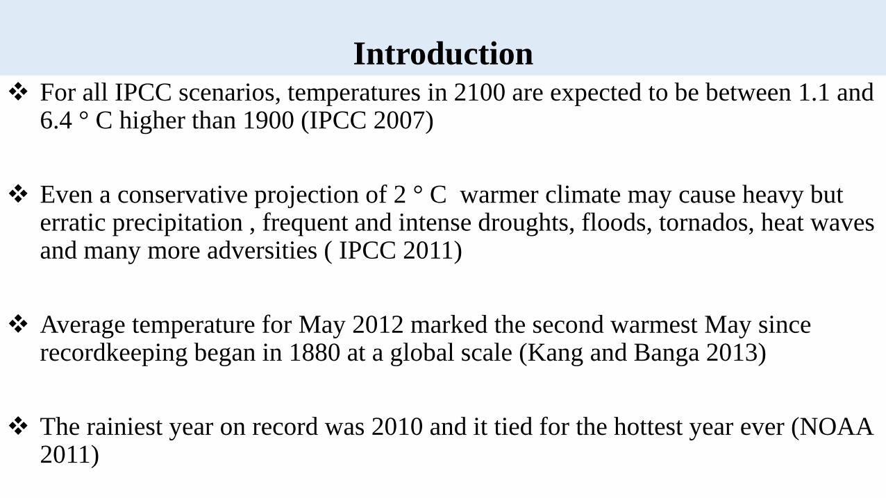
Introduction For all IPCC scenarios, temperatures in 2100 are expected to be between 1.1 and

6.4 ° C higher than 1900 (IPCC 2007)

Even a conservative projection of 2 ° C warmer climate may cause heavy but erratic precipitation , frequent and intense droughts, floods, tornados, heat waves and many more adversities ( IPCC 2011)

Average temperature for May 2012 marked the second warmest May since recordkeeping began in 1880 at a global scale (Kang and Banga 2013)

The rainiest year on record was 2010 and it tied for the hottest year ever (NOAA 2011)

Knowledge Gap

Possible changes in rainfall intensity and seasonal patterns of temperature and precipitation and their implications for the hydrologic cycle are poorly understood (Ficklin et al. 2009)

http://research.uarctic.org/news/2015/8/our-common-future-under-climate-change-outcome-statement/

Objectives Assessing the sensitivity of hydrologic processes to SRES climate change

scenarios for mid- 21st century at monthly time step. The hydrologic processes studied are:

• Percent change in stream discharge generation with respect to baseline scenarios.• Monthly precipitation change• Monthly stream discharge• Monthly soil water storage• Monthly ET change• Monthly percolation• Monthly Runoff• Monthly ground water contribution to streamdischarge• Monthly water yield

MacroscaleHydrologic Models

Large scale GCM climate variables

Hydrologic Model

Hypothetical Scenarios

Statistical downscaling for station variables

Dynamic downscaling for station variables

Hydrologic impacts-stream flow, soil moisture, floods

and, droughts

Large scale hydrologic impacts,

water balances

Projecting hydrologic impacts of climate change

(Mujumdar and Kumar 2012)

Materials and Methods

Study Area

Skunk Creek WatershedWatershed CharacteristicsGeographical Extent of

watershedTopography

S. No. Data type Source and Description

1 Digital Elevation Model (DEM)

10 m × 10 m resolution derived from Geospatial Data Gateway (GDG) to use as topographic data of the study basin.( https://gdg.sc.egov.usda.gov/ )

2 Land Use Map

Obtained in the form of Cropland Data Layer (CDL), a raster dataset with moderate resolution (30 m and 56 m ), created by USDA, National Agricultural Statistics Service ( NASS)

(http://nassgeodata.gmu.edu/cropscape/)

3 Soil Map

Obtained from Soil Survey Geographic Data (SSURGO) collected by National Cooperative Soil Survey (NCSS),USDA and National Resources Conservation Services (NRCS) with scales

ranging from 1:12,000 to 1: 63,360 ( Staff 2011). (http://websoilsurvey.sc.egov.usda.gov/App/WebSoilSurvey.aspx)

4 Weather Data

Daily Temperature and precipitation data were extracted from Daily Surface Weather and Climatological Summaries (DAYMET) Single point Data Extraction ( SPDE) ( Thornton et al

1997; Thornton et al 2012) (http://daymet.ornl.gov/dataaccess). The dataset is available on daily time scale with resolution of 1km × 1 km

5 Stream discharge Stream discharge taken from USGS site no. 06481500 located at Sioux Falls, SD for the study period. (http://waterdata.usgs.gov/nwis/)

Data Collection and Analysis

Time periods for Model Development and Future Scenarios

Baseline time period: 1980-2000Baseline warm up period:1980-1986Baseline calibration period: 1987-1994Baseline validation period: 1995-2000Future scenarios time period: 2046-2065

Bias Corrected Constructed Analog (BCCA) Coupled Model Intercomparison Project Phase-3 (CMIP-3) Climate change

attributes Variables: precipitation; minimum surface air temperature; maximum surface air temperature

Time: 1961-2000; 2046-65; 2081-2100 (daily)

Space:Coverage: North American Land Data Assimilation SystemResolution: 1/8 degree latitude-longitude (~12 km by 12 km)

Maurer, E. P., L. Brekke, T. Pruitt, and P. B. Duffy (2007), 'Fine-resolution climate projections enhance regional climate change impact studies', Eos Trans. AGU, 88(47), 504.

Step 1: Objective function is defined and absolute range of parameters is set

Step 2: Absolute Sensitive analysis is carried, using Latin Hypercube sampling; Objective function is computed

Step 3: Sensitivity Matrix of objective function is calculated. Equivalent of Hessian Matrix is formulated

Step 4: High order derivatives are neglected. Based on Cramer Rao Theorem, an estimate of lower bound of parameter covariance is computed

Step 5: Parameter sensitivity is analyzed using multiple regression

Step 6: Uncertainty measures (p-factor and r-factor) are computed

Algorithm Outputs 95ppu Plots Dotty plots Best_Par.txt Best_Sim.txt Goal.txt New_pars.txt Summary_Stat.txt

Model Calibration and Validation

(Abbaspour et al. 2007)

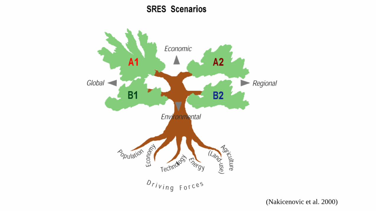
(Nakicenovic et al. 2000)

Results

Hydrographs of Precipitation and Stream discharge on annual basis

0

100

200

300

400

500

600

700

800

900

1000

0

1000

2000

3000

4000

5000

6000

7000

1980 1981 1982 1983 1984 1985 1986 1987 1988 1989 1990 1991 1992 1993 1994 1995 1996 1997 1998 1999 2000

PREC

IPIT

ATIO

N IN

MM

STRE

AM D

ISCH

ARG

E IN

CU

BIC

MET

ER P

ER S

ECO

ND

TIME PERIOD

Streamflow in cubic meter per second Precipitation in mm

StatisticsPre-calibrated Period Calibration Period Validation Period

Daily Monthly Daily Monthly Daily Monthly

NSE† -1.40 0.59 0.56 0.84 0.55 0.76

PBIAS -4.22 -4.64 -9.70 -9.53 -16.30 -5.18

RMSE 1178.38 71.44 411.39 38.67 292.75 22.28

R2 0.18 0.59 0.70 0.84 0.44 0.77

Model Calibration and Validation

January February March April May June July August September October November December2053 171.86 170.28 840.39 90.12 732.16 568.63 23.18 221.19 233.79 353.09 350.08 289.392054 426.06 390.98 704.71 762.46 973.71 880.01 708.23 295.20 385.88 1018.85 1613.36 1186.222055 987.32 1465.90 826.57 1730.08 2961.48 1817.46 1090.83 998.27 786.41 2127.74 1429.33 3306.922056 3165.19 3665.83 5691.41 3442.96 399.12 124.57 199.79 724.26 2471.81 1144.95 2468.16 2583.742057 3207.30 995.12 13117.98 1881.71 1202.79 293.38 756.84 1491.60 796.81 1711.32 238.50 2132.772058 1082.74 1034.44 461.99 941.41 4273.99 1480.94 -4.41 -64.95 -18.37 299.33 721.64 865.672059 841.96 870.87 24.84 -0.87 -38.57 -83.79 -90.55 2.87 79.12 150.48 152.89 177.532060 153.42 106.37 211.22 283.00 384.47 56.08 180.38 244.80 213.98 262.42 412.03 474.85

Impact of climate change scenario A1B on stream discharge in comparison to baseline in percentage

Impact of climate change scenario A2 on stream discharge in comparison to baseline in percentage

January February March April May June July August September October November December2053 180.24 288.82 1014.76 140.65 413.66 1416.22 87.66 288.86 268.76 389.41 398.56 292.612054 463.31 731.70 276.11 717.42 637.63 1702.87 826.94 237.21 400.15 1056.50 1030.78 1065.332055 937.23 1592.02 630.67 1946.62 4871.48 1740.61 936.47 860.53 814.34 2255.88 1465.66 3345.732056 3344.80 2788.38 8356.68 6063.20 899.12 104.44 172.76 908.30 2716.65 1129.20 2457.32 2798.922057 3408.21 991.05 10286.52 1676.90 814.96 123.02 928.73 1428.29 850.15 1628.71 225.80 2186.862058 1099.64 702.32 1245.94 1783.63 4354.94 1232.83 -18.18 -63.78 -15.07 328.50 556.24 997.582059 824.61 881.68 -12.90 -36.01 -13.00 -62.27 -87.26 7.95 95.94 299.00 180.88 267.052060 213.45 162.52 161.90 420.33 543.58 53.16 194.62 285.34 267.06 355.33 476.94 548.21

Impact of climate change scenario B1 on stream discharge in comparison to baseline in percentage

January February March April May June July August September October November December2053 156.90 157.86 690.53 122.57 880.18 1140.90 120.04 277.33 246.47 673.53 479.51 312.572054 510.82 641.33 540.03 1178.68 979.90 2840.25 2157.34 327.80 562.28 1676.98 1107.71 1269.542055 1141.33 1648.70 856.06 1442.86 4516.52 1956.93 1351.16 985.60 783.71 2232.30 1484.61 3359.882056 3247.60 2804.33 8972.95 4705.81 948.77 170.91 310.39 855.18 2747.98 1247.29 3788.46 3069.362057 3942.44 1192.61 17891.01 3366.64 1361.88 326.85 1020.40 1734.18 936.24 2030.98 286.79 2539.822058 1324.97 416.93 1508.02 2428.39 5803.94 1473.37 -15.30 -59.91 -15.18 275.27 521.25 1249.492059 807.57 956.54 -6.57 -28.75 -9.29 -64.71 -80.22 6.44 120.77 178.88 186.06 178.722060 188.65 135.24 245.74 356.75 447.44 205.21 735.80 298.01 330.30 513.25 705.01 579.72

A2 A1B B1 BASELINE

52.72

51.66

55.38

54.47

Monthly Precipitation Change mm

A2 A1B B1 BASELINE

10.9 10.39

12.89

3.83

Monthly Stream discharge m3/s

Impact of climate change scenarios on various hydrologic processes

Impact of climate change scenarios on various hydrologic processes

A2 A1B B1 BASELINE

7.33 6.91

9.98

4.39

Monthly Runoff mm

A2 A1B B1 BASELINE

10.32 9.8910.92

1.18

Monthly GW_Q mm

A2 A1B B1 BASELINE

17.92 17.06

21.18

5.61

Monthly WYLD mm

Impact of climate change scenarios on various hydrologic processes

A2 A1B B1 BASELINE

330.46 321.63 333.33

136.13

Monthly SW mm

A2 A1B B1 BASELINE

34.87 34.92 33.97

50.68

Monthly ET Change mm

A2 A1B B1 BASELINE

10.6210.07

11.57

0.98

Monthly PERC mm

Conclusions The study illustrated changes in water resources in relation to SRES climate

change scenarios for an agricultural watershed The climate change impacts can be witnessed with alternative water surplus

and deficit seasons. Water deficit conditions in terms of negative increase in stream discharge

during crop growth season can adversely affect agricultural productivity in rainfed regions and may progress to agricultural drought.

Impact of climate change scenarios on hydrologic cycle over the study area may be accompanied with a shift in crop growth cycle ( stomatalconductance) due to change in aerothermal regime in producing areas .

There is a need of more extensive assessment of potential climate change impacts on the hydrology and agricultural production in agriculturally dominated watersheds.

Acknowledgement This study was a part of the project supported by the United States

Department of Agriculture- NIFA (Award No. 2014-51130-22593) entitled “Integrated plan for drought preparedness and mitigation, and water conservation at watershed scale.”

Dr. Narayanan Kannan, Ph.D., Associate Research Scientist; Tarleton State University, Texas.

Dr. Suzette Burchkard, Ph.D., P.E., Assistant Department Head, Department of Civil and Environmental Engineering, SDSU, Brookings, SD.

Dr. Rachael McDaniel, Ph.D., Assistant Professor, Department of Agricultural and Biological Engineering, SDSU, Brookings, SD.

Dr. Eric Mbonimpa, Ph.D., Assistant Professor, Air Force Institute of Technology, Ohio.

Dr. Jeppe Kjaersgaard, Minnesota Department of Agriculture, Minnesota.

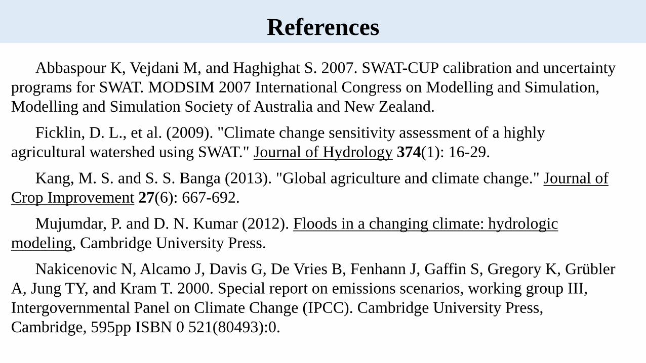
ReferencesAbbaspour K, Vejdani M, and Haghighat S. 2007. SWAT-CUP calibration and uncertainty

programs for SWAT. MODSIM 2007 International Congress on Modelling and Simulation, Modelling and Simulation Society of Australia and New Zealand.

Ficklin, D. L., et al. (2009). "Climate change sensitivity assessment of a highly agricultural watershed using SWAT." Journal of Hydrology 374(1): 16-29.

Kang, M. S. and S. S. Banga (2013). "Global agriculture and climate change." Journal of Crop Improvement 27(6): 667-692.

Mujumdar, P. and D. N. Kumar (2012). Floods in a changing climate: hydrologic modeling, Cambridge University Press.

Nakicenovic N, Alcamo J, Davis G, De Vries B, Fenhann J, Gaffin S, Gregory K, GrüblerA, Jung TY, and Kram T. 2000. Special report on emissions scenarios, working group III, Intergovernmental Panel on Climate Change (IPCC). Cambridge University Press, Cambridge, 595pp ISBN 0 521(80493):0.

THANK YOU !!!

http://www.cnn.com/2009/TECH/science/06/16/climate.change.report/index.html?eref=rss_us