1

RESEARCH REPORT

Contract no. 93/5.10.2011

EXPLORATORY RESEARCH PROJECTS (IDEI)

Project:

The geomagnetic field under the heliospheric forcing. Determination of the

internal structure of the Earth and evaluation of the geophysical hazard

produced by solar eruptive phenomena

Stage IV (2014)

Project Director,

Dr. Crişan Demetrescu Corresponding Member of the Romanian Academy

December, 2014

2

Content

Introduction

Chapter I: Analysis of solar eruptive phenomena and solar wind, responsible for

hazardeous geomagnetic activity (storms with Dst < -150 nT) in solar cycle 23.

Geomagnetic efficiency modelling of eruptive phenomena

1.1. The contribution of solar eruptive phenomena to major geomagnetic storms

in solar cycle 23

1.1.1. Introduction

1.1.2. Event selection

1.1.3. Analysed events

1.1.4. Modelling the geomagnetic efficiency of solar eruptive processes

1.2. The HSS contribution to major geomagnetic storms of the solar cycle 23

1.3. Discussion

Chapter II. New geomagnetic and magneto-telluric measurements in Romania

2.1. Geomagnetic measurements

2.2. Magneto-telluric measurements

2.2.1. The geology and the lithology of the studied area

2.2.2. Processing, modelling, and 1-D inversion of resistivity curves.

Methodology

Chapter III. Magnetic and electric structure of terrestrial litosphere and mantle at

Romanian territory and continental scales. 3D model of the electric resistivity

distribution on the Romanian territory

3.1. Model at the European continental scale, based on analysis of intense

geomagnetic storms in solar cycle no. 23

3.1.1. The principle of the metod and data used

3.1.2. Results

3.2. Model at national territory scale, based on magneto-telluric research carried out

within the frame of the contract

3.2.1. Resistivity litospheric model representative for the East-European

Platform

3.2.2. Resistivity litospheric model representative for the Transylvanian

Depression

3.2.3. Resistivity litospheric model representative for the Pannonian

Depression

3.2.4. Resistivity litospheric model representative for the Moesian Platform

3.2.5. The Carpathian Electric Conductivity Anomaly (CECA) in Romania,

structural peculiarities

Chapter IV. Toward a model for the distribution of the surface geoelectric field

produced by hazardeous geomagnetic variations. Case study – the Romanian territory

4.1. The computing model

4.2. Results

4.2.1. The computer code worked out in the present stage of the contract

4.2.2. The variation of the geoelectric field

Capitolul V. Dissemination of results

3

Introduction

The proposed research aims at achieving an understanding of the space weather

effects on conducting structures inside the Earth and on the surface electric field, with

applications to a better knowledge of the internal structure of the Earth at continental

(Europe) and country scales, on one hand, and to estimating the geophysical hazard of space

weather at midlatitudes, on the other. The main objectives are:

1. To derive the magnetic and electrical properties of the terrestrial lithosphere and

mantle at continental and Romanian territory scales;

2. To analyze solar eruptive processes and solar wind components responsible for

geomagnetic hazardeous activity (geomagnetic storms and substorms) in the time interval

1964-2014;

3. To model the geoelectrical field at the Earth’s surface as produced by various

magnetospheric and ionospheric current systems;

4 To evaluate the geophysical hazard for technological networks associated to

variations of the geoelectric field during geomagnetic disturbances linked to the interaction

of solar coronal mass ejections and high speed streams with the magnetosphere.

The initial contract underwent alterations because of budget cuts, so for 2014,

according to the additional agreement signed with UEFISCDI, the objectives read:

- Analysis of solar eruptive processesand solar wind, responsible for the

hazardeous geomagnetic activity (geomagnetic storms with Dst<-150nT) in the

solar cycle no. 23;

- Determining magnetic and electric structure of terrestrial litosphere and mantle at

Romanian territory and European continental scales;

- Modelling the surface geoelectric field;

- Preparing the research report and dissemination of results.

The research report for the stage 2014 is structured in chapters, according to the work

plan, as follows:

In Chapter I, entitled "Analysis of solar eruptive phenomena and solar wind,

responsible for hazardeous geomagnetic activity (storms with Dst < -150 nT) in solar

cycle 23. Geomagnetic efficiency modelling of eruptive phenomena", the results of two

4

studies, one concerning the geo-effectivity of the coronal mass ejections (CMEs) and of

interplanetary mass ejections (ICMEs), and the other concerning the geo-effectivity of the

high speed streams (HSSs), with a special emphasis on the solar cycle 23, are presented.

In Chapter II, entitled "New geomagnetic and magneto-telluric measurements in

Romania" the geomagnetic measurements carried out in 2014 at the 26 repeat stations of the

National secular variation network and at the Surlari geomagnetic observatory, as well as the

results of two magneto-telluric determinations carried out in the Transylvanian Depression,

are described.

In Chapter III, entitled "Determination magnetic and electric structure of

terrestrial litosphere and mantle at Romanian and continental scales. A 3D model of

the electrical resistivity distribution on the Romanian territory", two models of the

distribution of electric properties of lithosphere and mantle are presented, one for the

European continent, using data from the geomagnetic observatory network and data for a

number of geomagnetic storms, and a second one, for the Romanian territory, using

magneto-telluric measurements. In the first case the magnetic/electromagnetic induction

model, previously devised by research team members. In the second case the electric

structure of the crust on the Romanian territory is presented, as a block model with vertical

variation of the electrical resistivity in each block.

In Chapter IV, entitled ”Toward a model for the surface geoelectric field

produced by hazardeous geomagnetic variations. Case study – the Romanian

territory”, preliminary results on the possible magnitude of the surface geoelectric field that

generates geophysically induced currents in Romania, based on the only geomagnetic

observatory records in Romania, at the Surlari observatory, are presented.

In Chapter V, entitled ”Dissemination of results”, the list of published papers and of

presentations at scientific meetings in 2014 is presented. We mention that the web page of

the project was updated. The address is: http://www.geodin.ro/IDEI2011/engl/index.html.

5

Chapter I: Analysis of solar eruptive phenomena and solar wind, responsible for

hazardeous geomagnetic activity (storms with Dst < -150 nT) in solar cycle 23.

Geomagnetic efficiency modelling of eruptive phenomena

1.1. The contribution of solar eruptive phenomena to major geomagnetic storms in

solar cycle 23

1.1.1. Introduction

The influence of eruptive solar processes over the Earth is a subject of great

importance in present times in the context generated by satellite space missions that study

both the Sun and the heliosphere. The first observation of an eruptive phenomenon – a

strong flare in white light – with geomagnetic consequences was that one made

independently by Carrington (1859) and Hogson (1859). Since then Sun observations

have undergone an immense progress, such that today we benefit of full disk images in

many wavelengths, images of the magnetic configuration of the Sun, as well as many

other measurements, close to Earth, that allow to evaluate the terrestrial magnetic field,

the conditions of the interplanetary magnetic field, and information about the particle flux

that reaches the Earth. All these help us to analyse in detail the influence of solar wind

together with the solar eruptive phenomena.

This study is based on the data provided by the SOHO mission (Solar and

Heliospheric Observatory), mission that is composed of 12 instruments amongst which

LASCO (Large Angle and Spectrometric Coronograph) (Brueckner et al. 1995) that

provides white light images of the solar corona, on the coronal mass ejection catalogue

maintained by CDAW Data Center from NASA and by The Catholic University of

America in cooperation with the Naval Research Laboratory, as well as on the data from

IMP 8, Geotail, Wind and ACE, available through the interface OMNIWEB

(http://omniweb.gsfc.nasa.gov) maintained by Goddard Space Flight Center – NASA.

Interplanetary coronal mass ejections (ICME) are those coronal mass ejections

(CME) that are observed in the interplanetary space. Generally, ICMEs are detected

through a series of characteristic signatures: the sudden increase in speed, the increase of

the magnetic field, the rotation of the magnetic field, the decrease of the density and

temperature of electrons etc. (Zurbuchen and Richardson, 2006). Few of these events

have all the signatures, usually only three signatures are necessary to identify an

interplanetary coronal mass ejection, namely the total pressure perpendicular on the

6

magnetic field in the interplanetary medium close to 1AU, the maximum value of the

intensity of the interplanetary magnetic field, Bmax, and the speed variation, i.e. the

difference between the maximum and minimum speed (ΔV) of the solar wind during that

specific event (Jian et al. 2006). Generally, an ICME is defined as the entire perturbation,

comprising the shock (if it exists), the shield, the region of solar wind compression, “the

driver” or ejecta, and the back of the ejecta or the feet of the coronal mass ejection

(Rouillard, 2011).

1.1.2. Event Selection

Solar cycle 23 (during 1996-2008) had a number of 29 intense storms with a Dst

minimum value less than -150 nT. Using the Richardson and Cane catalogue (available

and updated online) we have identified the interplanetary coronal mass ejections

corresponding to those geomagnetic storms, and we noticed that all geomagnetic intense

storms were triggered by interplanetary coronal mass ejections.

In order to identify the coronal mass ejections responsible for triggering

interplanetary CMEs we used the Richardson & Cane catalogue to which we have added

data obtained by Zhang et al. (2007). Appendix 1 shows a summary table containing all

storms characterised by a minimum Dst value lower than -150 nT and of their connection

to solar eruptive phenomena. Columns show the perturbation date, the beginning and end

of the interplanetary coronal mass ejections, the increase in speed estimated from the

hourly mean values of the solar wind, the ICME speed, the maximum speed recorded in

the solar wind, the mean magnetic field intensity inside the ICME, the association with

magnetic clouds, the minimum value of the Dst index, the mean transit speed at 1 AU

and the solar ejection associated with the corresponding event. Coronal mass ejections

that have been introduced from Zhang et al. (2007) have been marked by ”*”.

From the Richardson and Cane catalogue just two interplanetary coronal mass

ejections are not correlated to coronal mass ejections, that is, the event of October 2,

2001 and the one of September 30, 2002, but Zhang et al. (2007) found their

corresponding CMEs (See Appendix 1.1, events numbers 14 and 20). The properties

specific to these geoeffective CMEs are shown in Table 1.

Out of the 42 coronal mass ejections, only three do not have a linear speed

calculated because of LASCO/SOHO data gaps.

There are 9 coronal mass ejections whose interplanetary speed increases as

magnitude from the distance of 20 solar radii to the distance of 1 AU. All ejections

7

change their speed during their propagation towards the Earth, the majority being

decelerated because of their interaction with the solar wind, other ejections or solar high

speed streams.

Coronal mass ejections of Table 1 are, in their vast majority, of Halo type

(angular width larger than 1200) as seen in the white light images from LASCO/SOHO.

Only 18 CMEs have positive values for the acceleration, which means that most

of them are decelerated after the ejection moment in the Sun vicinity. For the exact

computation of the accelerations, but especially of their variation in time and as a

function of height, one needs data from the lower corona in order to exactly determine its

evolution. Studies carried on by St.Cyr et al. (1999) and Zhang et al. (2001) show that

the acceleration is greater in the lower corona, that there is no deceleration under three

solar radii, despite of gravity. 30% out the coronal mass ejections observed by

LASCO/SOHO are decelerated, a percentage that increases to 54% in our selection.

Table 1: General properties of geo-effective coronal mass ejections

Nr.

Crt. CME Position

Vliniar

(km/s)

V 2nd order

at final

height

(km/s)

V 2nd

order

at 20 Rs

(km/s)

Acce-

leration

(m/s2)

Vtranzit

1 AU

(km/s)

1. 1998/05/02 – 14:06:12 H S17W24 938 697 871 -28.8 1150

2. 1998/05/02 – 05:31:56 H S17W24 542 527 530 -1.4

3. 1998/05/01 – 23:40:09 H S16W12 585 657 627 8

4. 1998/04/29 – 16:58:54 H 1374 1151 1250 -44.8

5. 1998/08/24 – 21:50 N35E09 -- -- -- -- 1260

6. 1998/09/23 – 06:40 N18E09 -- -- -- -- 1020

7. 1999/09/20 – 06:06:05 H S20E01 604 549 357 -14.5 770

8. 1999/10/18 – 00:06:06 PH S26E08 144 263 290 3.5 561

9. 2000/04/04 – 16:32:37 H N18W72 1188 1232 1199 12.8 860

10. 2000/07/14 – 10:54:07 H N17W11 1674 1534 1147 -96.1 1500

11. 2000/08/09 – 16:30:05 H N11W15 703 731 720 2.8 830

12. 2000/09/16 – 05:18:14 H N14W07 1215 1162 1192 -12.3 ...

13. 2000/09/15 – 21:50:07 H 257 285 537 11.2

14. 2000/09/15 –15:26:05 PH N13W00 481 370 335 -10.4

15. 2000/09/15 – 12:06:05 PH N13W00 633 395 0 -64

16. 2000/10/02 – 20:26:05 H S09E04 569 478 483 7.1 756

8

17. 2000/11/03 – 18:26:06 H N23W71 291 475 643 16.4 660

18. 2001/03/28 – 12:50:05 H N17W03 519 582 561 4.4 690

19. 2001/03/29 – 10:26:05 H N13W14 942 965 957 3.5

20. 2001/04/10 – 05:30:00 H S22W20 2411 2876 2974 211.6 1290

21. 2001/04/09 – 15:54:02 H S21W08 1192 1198 1198 1.3

22. 2001/09/29 – 11:54:05 PH N14W01 509 470 150 -12 715

23. 2001/10/19 – 16:50:05 H S14W62 901 895 898 -0.7 870

24. 2001/10/25 – 15:26:05 H S19W26 1092 1080 1087 -1.4 694

25. 2001/10/24 – 06:26:05 S12E14 597 633 653 4.6

26. 2001/11/04 – 16:35:06 H N05W29 1810 1514 1691 -63.4 1250

27. 2001/11/03 – 19:20:05 H N06W14 457 329 299 -9.9

28. 2001/11/22 – 23:30:05 H S18W24 1437 1371 1409 -12.9 1320

29. 2002/09/05 – 16:54:06 H - 1748 1855 1903 43 880

30. 2002/09/26 – 01:31:44 PH - 178 368 331 5.1

31. 2003/10/28 – 11:30:05 H S16E04 2459 2229 2268 -105.2 2185

32. 2003/10/29 – 20:54:05 H S17W10 2029 1670 1519 -146.5 2138

33. 2003/11/18 – 08:50:05 H N03E08 1660 1645 1656 -3.3 886

34. 2004/07/25 – 14:54:05 H N08E35 1333 1366 1359 7 1302

35. 2004/11/04 – 23:30:05 PH - 1055 1037 1050 -1.9 720

36. 2004/11/04 – 09:54:05 H N09E32 653 719 706 6.3

37. 2004/11/07 – 16:54:05 H N09E08 1759 1696 1713 -19.7 830

38. 2004/11/06 – 02:06:05 PH N09E06 1111 1258 1176 18.8

39. 2005/05/13 – 17:12:05 H N12E05 1689 -- -- -- 1270

40. 2005/08/22 – 01:31:48 H S11W54 1194 1086 1127 -17.8 790

41. 2005/08/22 – 17:30:05 H S13W65 2378 2612 2585 108

42. 2006/12/13 – 02:54:04 H - 1774 1622 1573 -61.4 1180

The majority of active regions associated to coronal mass ejection have complex

magnetic structure, like bipolar magnetic regions without a clear distinction between

polarities, formed from several bipolar regions or magnetic regions in which the positive

and negative polarity distribution is so irregular that they cannot be classified as bipolar

regions.

The origin of coronal mass ejections can be located in a rectangle having as

horizontal boundaries the longitudes -35 and 72, and vertical ones the latitudes 35 and -

26.

9

The strongest geoeffective ejections – from October-November 2003 – have been

located close to the centre of the Sun, had very high projected speeds values (1600-2460

km/s), and reached the Earth with high speeds.

1.1.3 Analysed Events

1.1.3.1. November 18, 2003

On November 18, 2003 a halo coronal mass ejection was registered, whose speed,

calculated from the images offered by LASCO was of 1660 km/s. This ejection was

produced by the eruption of a filament (Uralov et al., 2014), but also had a flare

associated. The speed at the height of 20 solar radii was 1656 km/s, just 11 km/s less

than the one registered at the final height of 28 solar radii, with a deceleration of just 3.3

m/s2. The transit speed of this ejection at 1 AU was 886 km/s. The time between

triggering of the ejection and the minimum Dst value moment was 59 hours, a lot longer

than the time estimated using the projected speed – 25 hours.

Figure 1.1.1 shows the evolution of this ejection in LASCO white light images,

superimposed on 195 Å EIT images. In the first frame, the solar flare associated with this

eruptive event is visible in the EUV image. It was an M3.9-class flare above the active

region NOAA 10501 (N03E08), very close to the disk centre. This flare started at 08:12

UT, had its maximum at 08:31 UT and ended at 08:59 UT, as the GOES X-ray data

shows. In the same frame, but in the LASCO image, we can observe a coronal mass

ejection that is still in development, which started ~45 minutes before the one we analyse

here.

The ICME that followed this ejection was observed on November 20, at 08:03 UT

and had a magnetic cloud associated.

10

08:50 UT

09:48 UT

10:24 UT 10:48 UT

Figure 1.1.1 The evolution of the coronal mass ejection of November 18, 2003.

Selected LASCO C2 images superimposed on solar disk 195 Å images provided by EIT.

Composite images worked out with Jhelioviewer (jhelioviewer.org/)

1.1.3.2. November 7, 2004

A halo coronal mass ejection was registered by LASCO on November 7, 2004 at

16:54 UT. GOES registered an X 2.0 flare starting at 15:42 UT that had its maximum

emission in X-ray at 16:06 UT and ended at 16:15 UT.

The flare was ignited in the active region NOAA 10696 situated at N09W22, a

βγδ magnetic-type region. The active region where this flare ignited is shown in Figure

11

1.1.2, in running differences of EIT images on the last row, as compact structures that

represent plasma with higher temperature than the surrounding lower corona.

Figure 1.1.2: Selection of LASCO C2 running differences (first row),

C3 (second row) and EIT (last row) showing the evolution

of the November 7, 2004 CME.

The coronal mass ejection is visible in this Figure in the LASCO C2 images – in

the first row – and those from LASCO C3, shown in the second row. The projected speed

of this ejection was 1759 km/s, the final speed at the distance of 22 solar radii – 1969

km/s, and had a transit speed of 830 km/s. The acceleration for this CME was -19.7 m/s2.

1.1.3.3. August 22, 2005

On August 22, 2005 LASCO detected a Halo coronal mass ejection at 01:31 UT.

The solar flare registered by GOES was an M 2.6-type, whose X-ray flux begun to rise at

00:44 UT, had its maximum at 01:33 UT and came back to background level values at

02:18 UT. The flare was triggered in the active region NOAA 10798 (S11W62) whose

12

magnetic classification was βγ at that date. The location of the flare is visible in the last

frame (lower right) of Figure 1.1.3.

This coronal mass ejection is visible in the Figure below in the LASCO C2

images (first row) and LASCO C3 (second row).

Figure 1.1.3: Running differences of LASCO C2 images (first row),

LASCO C3 (second row first two columns), and EIT (last frame)

showing the evolution of the eruptive phenomena of August 22, 2005.

This ejection was detected as an interplanetary one on August 24 at 02:38 UT and

was accompanied by a magnetic cloud.

1.1.4. Modelling the geomagnetic efficiency of solar eruptive processes

Modelling the efficiency of an eruptive phenomenon is based on establishing

some existing relations between the characteristic measurements of the analysed

phenomena and their geoeffectiveness. It can refer both to the statistical evaluation of the

number of coronal mass ejections and to the probability evaluation of producing a

geomagnetic storm that follow certain coronal mass ejections.

The statistical evaluation of coronal mass ejections that are geoeffective is not

representative in our case, because the number of ejections detected by LASCO is very

13

high (at the solar maximum activity there can be several CMEs/day), but the geomagnetic

storms are much less.

The evaluation of the probability that a certain eruptive phenomenon be

geoeffective is much more important. There are empirical models that evaluate this kind

of probabilities. We chose as relevant data for the solar eruptive phenomena and the

interplanetary coronal mass ejections the projected speed of the ejections at their

detection in the LASCO images, the second order speed at different heights, the

acceleration, the flare position on the solar disk, as well as two parameters of the

interplanetary medium, the total magnetic field intensity and that of the southern

component. However, this probability can give information only as what concerns major

storms. A coronal mass ejection whose speed is not the highest as value, but is

superimposed on an interplanetary magnetic field line whose direction is south, will be

more geoeffective than a strong coronal mass ejection that reaches the Earth while Bz has

negative values.

This study must be continued for the solar cycle 24 in order to benefit from the

propagation speed direction of the coronal mass ejection at its triggering, with the help of

several models based on the new satellite date from STEREO-COR2, relative to the solar

wind direction at the analysed moment. Their positive superimposing will increase the

probability of geoeffectiveness of the solar eruptive phenomenon.

1.2. The HSS contribution to major geomagnetic storms of the solar cycle 23

The solar wind, a continuous flux of plasma from the solar corona, is an

inhomogeneous environment structured according to various parameters (density, plasma

velocity, the heliospheric magnetic field structure). For this reason it is difficult to forecast

its behaviour in the periterrestrial environment. However, certain structures, emitted and

“controlled” by their solar sources, can be forecasted with a sufficient accuracy (70-95 %).

The High Speed Streams (HSS), originating in Coronal Holes (CH) are a repetable structure

and so forecastable. These streams produce, at the impact with the magnetosphere, average

magnitude geomagnetic disturbances, but, in certain favorable circumstances (e. g.,

superposition to a sectorial boundary in the interplanetary space, the interaction with an

ICME), they could produce important geomagnetic storms, they can significantly contribute

to the development of magnetospheric currents at large scale. Their geoeffectivity is directly

dependent on their solar source – the coronal hole – being influenced in the first place by the

heliographic position of the latter. So, it is possible that CHs in the equatorial area or with

14

large extension to the equator produce HSSs with a major effect in the magnetosphere. Such

CHs can be observed at the solar minimum or during the declining phase of the solar cycle.

Also, HSSs emitted by a coronal hole are more geoeffective when the CH is close to the

central meridian and during its passage through the western hemisphere. A HSS propagating

from the solar corona through the interplanetary space interacts with the slow solar wind,

forming at the boundary of the two flowing regimes a compression region, named Corotating

Interaction Region, CIR), that often lives several solar rotations. Such structures appear

because plasma is frozen in the magnetic field and the two streams (rapid and slow) do not

mix, but form a persistent interface in their confluence zone. Consequently the properties of

solar wind plasma and the structure of the interplanetary magnetic field are different in the

two zones separated by the interface.

Table 1.2.1. Geomagnetic storms in the solar cycle 23 with HSS contribution

No Date

mm/dd/hh

Dst min

(nT)

Bz min (nT)/Δt

min

Δt (h)

(Bz<0)

B

(nT) SSC

Solar/Heliospheric Sources

CIR Flare CME/ICME

1999

1 09/22/23 -173 -15,8/-1h 4 h 11 SSC CH2

/ CIR1

C2.8 CME/ICME3

2 10/22/06 -237 -30.7/-1h 8 h 20 SSC CH1

/CIR1

CIR3

CME/ICME

2000

3 04/06/22 -287 -27.3/-1h 7 h 6 gradual CIR1

F2

/C9.7 CME/ICME3

4 10/05/13 -182 -17.5/-2h 3 h 6 SSC CIR1

F2

/ ? CME/ICME3

5 11/06/21 -159 -11.7/-6h 9 h 20 SSC CH2

- CME/MC3

2001

6 10/03/14 -166 -20.9/-2h 9 h 12 SSC CIR1

F2

/M1.8 CME/MC3

1 – Cid, C. et all, 2004, Sol. Physics 223, 231-24

2 – Maris O., Maris G., 2009, HSS Catalog, at: http://www.spacescience.ro/new1/HSS_Catalogue.html

3 – Zhang, J. et all, 2007, JGR 112, A10102, doi: 10.1029/2007JA01321

In Table 1.2.1 the geomagnetic storms of the solar cycle 23 to which HSSs

contributed (as triggering factors and/or as energy sources) are indicated. The date at which

the minimum of the storm occured, the Dst minimum, the Bz minimum / the time difference

between the Bz and Dst minima, respectively the time span (in hours), the scalar B value at

the storm minimum, type of the storm beginning (SSC – sudden commencement – or

gradual) are given. The last three columns give information on the solar and heliospheric

sources of fluxex producing the storm. Under the table references are indicated.

15

One can notice the strong dependence between the negative values of Bz and the

minimum of Dst and the fact that the Bz minimum precedes the Dst minimum. The 3-9 hours

persistance of negative values of Bz ensures an efficient energy transfer and augments the

imporatnce of the geomagnetic storm. All these remarkable storms occured in the maximum

phase of the solar cycle, so the main role in triggering them is of particle fluxes emitted by

solar eruptive phenomena, such as flares and CMEs. This can be seen also from the Table.

In Table 1.2.2 the characteristics of HSSs contributing to geomagnetic storms

included in Table 1.2.1. Data regarding HSSs and geomagnetic storms are taken from The

Complex Catalogue GSs_HSSs for the Solar Cycle 23, worked out within the frame of the

project HELIOTER/PN 2, 2007 – 2010 (Maris O. & Maris, G. 2010, Complex Catalogue:

GSs-HSSs, 1996 – 2008; at: http://www.spacescience.ro/new1/GS_HSS Catalogue.html).

Table 1.2.2. Characteristics of HSS that contributed to major storms of the solar cycle 23 and

of the corresponding storms

HSS Data Geomagnetic Storm Data

Y M D 3-h V0 VMax Dur VM IMF Sol. Sou.

Bz Dst_min t Type

Km/s Km/s days Km/s nT nT mm:dd:hh

1999 9 22 3 355.7 595.0 4.0 239.3 - CH -15.8 -173 09:22:23 SSC

1999 10 20 7 328.0 670.7 7.6 342.7 + CH -30.7 -237 10:22:06 SSC

2000 4 6 4 364.0 615.7 5.5 251.7 - F -27.3 -287 04:06:22 Gradual

2000 10 5 1 367.0 523.0 2.9 156.0 - F -17.5 -182 10:05:13 SSC

2000 11 3 6 334.0 608.0 5.8 274.0 + F -11.7 -159 11:06:21 SSC

2001 9 25 7 373.3 680.3 11.0 307.0 + F -6.4 -102 09:26:01 SSC

2001 9 25 7 -5.5 -55 09:29:21 SSC

2001 9 25 7 -12.7 -148 10:01:08 SSC

2001 9 25 7 -20.9 -166 10:03:14 SSC

For all HSSs the maximum speed of about 600 km/s and velocity jumps, VMax =

VMax – Vo, of 157 km/s - 342 km/s. The streams produced by CHs, as well as the solar

particle fluxes contributing to storms were equally distributed in sectors of the positive or

negative polarityof the heliospheric field (three in each sector). A special case is that of the

HSS of September 25, 2001. During the 11 disturbed days, fluxes of solar plasma from

coronal holes, flares and coronal mass ejections have produced complex disturbances in the

magnetosphere, materialised in a succession of three geomagnetic storms of average

intensity, followed by a major one, as it can be seen from the last four lines of the Table

1.2.2.

16

1.3. Discussion

There is no direct correlation, nor a bijective one, between the characteristic

measures of the CME and the intensity of the geomagnetic storms. The coronal mass

ejection with the greatest linear speed was not followed by the most intense geomagnetic

storm. Nor was the interplanetary coronal mass ejection that reached the Earth with the

highest speed.

Of much more importance is the orientation of the magnetic field that has to be

southward oriented in order to allow the reconnection that triggers the geomagnetic

storms.

A comparative study of speed, direction and positions of the coronal mass ejections,

can provide information about possible effects on Earth. The study will be continued in the

2015 stage of the project.

References

Brueckner G.E., Howard, R.A., Koomen, M.J., Korendyke, C.M., Michels, D.J., Moses, J.D.,

Socker, D. G., Dere, K.P., Lamy, P. L., Llebaria, A., Bout, M. V., Schwenn, R., Simnett, G.

M., Bedford, D. K., Eyles, C. J. (1995), The Large Angle Spectroscopic Coronagraph

(LASCO), Solar Physics, 162 (1-2), 357-402

Carrington, R.: 1859, MNRAS 20, 13

Jian, L.; Russell, C. T.; Luhmann, J. G.; Skoug, R. M. ”Properties of Interplanetary Coronal

Mass Ejections at One AU During 1995 2004” SoPh 239, 393, 2006

Hodgson, R.: 1859, MNRAS 20, 15

Richardson and Cane:”Near-Earth Interplanetary Coronal Mass Ejections During Solar

Cycle 23 (1996--2009): Catalog and Summary of Properties” 2010, Solar Physics

Rouillard, A.P., JASTP 73, 1201, 2011

J. Zhang, I. G. Richardson, D. F.Webb, N. Gopalswamy, E. Huttunen, J. C. Kasper, N. V.

Nitta, W. Poomvises, B. J. Thompson, C.-C. Wu, S. Yashiro, and A. N. Zhukov: ”Solar and

interplanetary sources of major geomagnetic storms (Dst 100 nT) during 1996–2005”, 2007,

Journal of Geophysical Research, 112, A10102

Zurbuchen, Thomas H.; Richardson, Ian G., In-Situ Solar Wind and Magnetic Field

Signatures of Interplanetary Coronal Mass Ejections, Space Science Reviews, 123, 31-43,

2006

17

Chapter II. New geomagnetic and magneto-telluric measurements in Romania

2.1. Geomagnetic measurements

The geomagnetic measurements were carried out at the 26 repeat stations of the so-

called National Network for secular variation, as well as at the Surlari geomagnetic

observatory. The field measurement campaign took place in the time interval 13.08-

2.09.2014. In Fig. 2.1.1 the way the territory has been covered during this campaign is

illustrated. The geographical coordinates of the network stations are given in Table 2.1.1.

Determinations of the horizontal component H, total field intensity F, magnetic

declination D, and magnetic inclination I have been carried out. In parallel with the absolute

measurements, recordings of the field evolution, through the four elements X, Y, Z, and F,

have been carried out. A DI-Flux LEMI 024 theodolite, two QHM magnetometers, a

Geometrics G-856 and a recording LEMI-18 fluxgate magnetometer have been deployed.

The determined values were corrected for the diurnal variation and reduced to the

time of the first reading of the series of determinations stipulated in the measurement

protocol, by means of continuous recordings provided by the Surlari geomagnetic

observatory. Then the values were processed to obtain values for the middle of the year 2013

(the geomagnetic epoch 2013.5), having in view the delay of about one year that affects

observatory annual mean values against which the field data are reduced. In Fig. 2.1.2 the

maps of the geographical distribution of the geomagnetic elements H, Z, D, and F are

presented, reduced to the epoch 2013.5 for which the necessary data from the Surlari

geomagnetic observatory were the definitive ones.

18

Table 2.1.1. Geographic coordinates of repeat stations on the Romanian territory

No. Station Latitude

(degrees)

Longitude

(degrees)

1 Saveni 47.96593 26.88277

2 Livada 47.84867 23.13362

3 Radauti 47.82142 25.94800

4 Somcuta 47.49997 23.43900

5 Vaida 47.25157 21.98520

6 Bistrita 47.19485 24.48570

7 Varatec 47.15150 26.29175

8 Cluj-Faget 46.69750 23.54715

9 Husi 46.67880 28.00265

10 Chisineu-Cris 46.54443 21.53978

11 Bretcu 46.05767 26.35652

12 Lipova 46.05202 21.72387

13 Deva 45.85712 22.91722

14 Dumbravita 45.83292 21.29002

15 Selimbar 45.75188 24.18742

16 Stamora 45.28383 21.24357

17 Gropeni 45.08573 27.86850

18 Mizil 44.99238 26.37497

19 Herculane 44.92215 22.44942

20 Babadag 44.87207 28.76385

21 Costesti 44.65898 24.89332

22 Strehaia 44.61763 23.16890

23 Tonea 44.20200 27.41502

24 Alexandria 43.96683 25.36662

25 Sadova 43.89513 23.93970

26 Negru-Voda 43.82022 28.24305

27 *Surlari Geomagnetic

Observatory (SUA) 44.68000 26.25330

19

Fig. 2.1.1. The way the station network was covered in the time interval 13.08-2.09.2014

Fig. 2.1.2. The geographical distribution on the Romanian territory of the geomagnetic

elements H, D, Z, and F at epoch 2013.5 (measurements carried out in 2014). The repeat

stations of the National secular variation network are marked by symbols

20

2.2. Magneto-telluric measurements

In the second part of September and in the beginning of October 2014, two

magnetotelluric soundings (MTS), located close to Ludus and, respectively, Bazna (Fig.1)

have been carried out in the Transylvanian Depression. In order to obtain very low

frequencies able to investigate the crystalline basement, that is situated in the investigated

area at depths of 7-8 km, the recording time of the EM series (Ex, Ey, Bx, By and Bz) was of

about 10 days. Thus the frequency range used was between 103 Hz and 10

-4 Hz.

1

2

Fig. 2.2.1. Location map for the two mageto-telluric (MT) stations in the Transylvanian

Basin: MTS Luduş (46 : 28; 47.81), altitude 368 m (1); MTS Bazna, (46 : 11; 40.52),

altitude 355 m (2)

2.2.1. The geology and the lithology of the studied area

The Transylvanian Basin is characterized by a sedimentary cover of 1200 - 8000 m,

thinner in the northern part and thicker in the vicinity of the Mures river. The basin includes

the following sedimentary cycles: Upper Cretaceous, Paleogene, Burdigalian-Helvetian,

Tortonian-Buglovian-Sarmatian, Pliocene, and Quaternary.

As regards the crystalline basement of the basin, in its composition there are

epimethamorphic (to East) and mesomethamorphic (to West) schists, that were intercepted

by drillings at various depths, covered by Mesosoic deposits (conglomerates, limestones)

having an epicontinental character (intercepted only in a few places). The tectonic

21

movements at the end of Cretaceous and in Paleogene fragmented the crystalline block in

subunits that, in Lower Paleogene - Miocene, underwent week subsidence and even uplifts.

From the midle Miocene all of them subsided with different intensities. This had some

consequences as regards the level of the basement blocks: three more elevated compartments

may be distinguished (Paucă, 1972, V.Mutihac, 1990): (1) Blaj-Pogăceaua at 3000 m; (2)

Făgăraş–Perşani at 1200 – 3000 m; (3) The Somes – Prisnel up to 2000 m, separated by three

deeper compartments: (i) Turda–Beclean at 6000 m; (ii) Tarnava rivers compartment at 8000

m; (iii) Odorhei–Deva at 6500 m. The Dej tuff was intercepted at the basin margin, with a

thickness of 10-500 m.

2.2.2. Processing, modelling, and 1-D inversion of resistivity curves. Methodology

A multi-channel magnetotelluric system (GMS-06) produced by METRONIX

company, Germany, was used. The central unit ADU-06 has 5 channels at which 4 un-

polarized sensors for electric field recording and 3 magnetic sensors (induction coil) for

magnetic field recording are connected. The frequency range recorded was 103-10

-4 Hz. Data

are stored on the internal “flash disk” or directly on the computer HDD, on which the

MAPROS program is installed. This program operates under Windows 95 and takes the

control over the following operations:

1. Semi-automatic settings in field of the electric and magnetic sensors;

2. Real-time data acquisition and processing;

3. Robust estimation of the magnetotelluric transfer functions Zxy, Zyx and of the

geomagnetic transfer functions Txy ,Tyx;

4. Real-time time series representation for MTS Bazna (Fig. 2.2.2) and for resistivity

and phase curves for MTS Ludus (Fig. 2.2.3) and MTS Bazna (Fig. 2.2.4).

22

Fig. 2.2.2. Magnetotelluric time series: electric components (Ex, Ey) and magnetic

components (Bx, By, Bz) for MTS Bazna

23

Fig. 2.2.3. Resistivity (upper plot) and phase (lower plot) distributions versus frequency for

MTS Ludus

Fig. 2.2.4. Resistivity (upper plot) and phase (lower plot) as a function of frequency for the

MTS Bazna

As regards the vertical distribution of the resistivity obtained for the two MTS, we

have to mention that these were achieved by using a 1-D inversion program. The results are

presented as 1-D models in Fig. 2.2.5 for MTS Ludus and in Fig. 2.2.6 for MTS Bazna.

These results reflect the resistivity distribution from the Earth’s surface down to the

crystalline basement.

The models represent the most probable images as compared to reality, because

between the computed response functions and the experimental values there is a deviation of

at most 2%. According to “Legend” attached to figures, the models for the sedimentary cover

show thicknesses of 6.8 km (MTS Ludus) and 8.5 km (MTS Bazna), and resistivities of

about 2-10 Ωm. The resistivity of crystalline basement is between 700 Ωm and 1000 Ωm.

This information adds to the one obtained previously (Stages 2012 and 2013) based on

magneto-telluric soundings in the data base of the project, contributing the resistivity model

for the main crustal blocks presented in the following.

24

a.

b.

Fig. 2.2.5. 1-D modelling for MTS Ludus. Resistivity and phase curves (a), 1-D model (b) (N-

number of layers, - apparent resistivity, h- thickness of layer , d- depth, S-conductance)

25

a.

b.

Fig. 2.2.6. 1-D modeling for MTS Bazna. Resistivity and phase curves (a), 1-D model (b) (N-

number of layers, - apparent resistivity, h- thickness of layer , d- depth, S-conductance)

26

Chapter III. Magnetic and electric structure of terrestrial litosphere and mantle at

Romanian territory and continental scales. 3D model of the electric resistivity

distribution on the Romanian territory

3.1. Model at the European continental scale, based on analysis of intense geomagnetic

storms in solar cycle no. 23

In the previous stage report (year 2013) we presented an application of the so-called

„magnetic and electromagnetic induction mehod”, previously worked out by the contract

team members, to the case of a major geomagnetic storm (15.05.2005). In the present stage

we extended the study to a number of storms, in order to assess the robustness of the result to

variations of the inducing force.

3.1.1. The principle of the metod and data used

The method used in the present work (see the Phase 2013 report) is based on the

observation that an external variable field induces inside the Earth variable magnetic fields

not only through electromagnetic induction in conductive structures of the crust and mantle,

but also by magnetic induction in rocks above the Curie temperature. In the pure magnetic

induction case, the temporal variation of the field components at a certain observation point

is given by a linear combination of the components of the inducing magnetic force. The

calculated values of the model represent the component of the observed signal produced by

pure magnetic induction, while the residuals contain the information related to the

electromagnetic induction in the Earth at the given point. The model coefficients can be

determined by a least squares procedure and mapped, resulting in images of the lateral

(geographical) distribution of magnetic properties that characterise the rock volume above

the Curie temperature (generaly the crust).

In case of electric properties of crust and mantle, the residual of the induction model

for the vertical component of the field is used. The latter responds to the electromagnetic

induction in the electrically conducting crustal and mantle structures to a greater extent than

the horizontal component. As the induction electromotive force is given by the negative time

derivative of the inducing magnetic field, the latter should correlate with the observed

residual. The working relationship is:

)()()( tZrezRtrezZLtZ sursa ,

27

where sursaZ is the negative time derivative of the vertical component produced by the

inducing source, and Zrez is the residual of the induction model applied to the Z component

recorded at the observation point. L and R, the electrical inductance and, respectively, the

resistance that characterise the crust and mantle under the given observatory, can be

determined for each observatory by means of the least squares method, for the given time

interval. Mapping of the obtained values reflects the lateral distribution of the Earth interior

electric properties. The mapped values are relative, the maps reflecting, as was also the case

of magnetic properties of the crust (the 2012 Report), lateral variations of the parameters L

and R, not real (absolute) values. Also, the obtained information regards a large depth range,

from the surface to mantle depths.

The magnetic storms illustrated by means of the Dst index in Fig. 3.1.1 were used.

For each case the available recordings on the INTERMAGNET site www.intermagnet.org.

(minute values) 12 hours long, including the storm, were downloaded. The external source is

represented by variations of the magnetospheric ring current through the geomagnetic index

Dst (minute values) provided by the site http://geomag.usgs.gov/data. The Dst index

represents the effect of the ring current at the Earth’s surface, in the geomagnetic equatorial

area.

31.03.200111.04.2001 6.11.2001

24.11.2001 30.10.200320.11.2003

7.11.2004

15.05.2005

24.08.2005

Fig. 3.1.1. The variation of the Dst geomagnetic index for the analysed geomagnetic storms

28

3.1.2. Results

In Fig. 3.1.2 we give the results for each of the analysed storms as regards the

electrical resistence (the parameter of interest in modeling the surface electric field produced

by variations of the geomagnetic field). A first observation concerns the fact that the

distribution of observatories providing data is not the same in all cases, making difficult a

correct comparison of results. In Fig. 3.1.3 we show maps with the same distribution of

observatories in all of them. One can see that, in general, the distribution of the electric

resistence is similar, with lower values in the southern and south-western part of the network

than in the north-eastern part. Of course, local differences, still visible, could be put on the

different morphology of the considered geomagnetic variations (an evident case is that of the

31.03.2001 11.04.2001 6.11.2001

24.11.2001 30.10.2003 20.11.2003

7.11.2004 15.05.2005 24.08.2005

Fig. 3.1.2. Maps of the distribution of the electrical resistance at the European continental

scale for the major storms marked on the figure

29

30.10.2003 storm), with consequences in the first place regarding the penetration depth in the

Earth. To elucidate this aspect, we shall tackle in the next stage of the contract the study of

only the main phase of the storm.

31.03.2001 11.04.2001 6.11.2001

24.11.2001 30.10.2003 20.11.2003

7.11.2004 15.05.2005 24.08.2005

Fig. 3.1.3. Maps of the distribution of the electrical resistance at the European continental

scale for the major storms marked on the figure, in case the observatory distribution is the

same in all six maps

3.2. Model at national territory scale, based on magneto-telluric research carried out

within the frame of the contract

In the present phase of the contract we present a quasi-3D model of the resistivity

distribution on the Romanian territory, that follow the geological block structure that form

the terrestrial crust on the study area. Each main block has a stratified electric structure, as

determined by means of the results for the numerous magneto-telluric deep soundings

profiles of the project data base (see Fig. 3.2.1), discussed in previous stages. The following

30

major tectonic units were in view: the East-European Platform, the Transylvanian

Depression, the Pannonian Depression and the Moesian Platform. Models are schematically

presented in the next section. To these, a discussion on the Carpathian Electric Conductivity

Anomaly (CECA) is added.

Fig. 3.2.1. Map of magneto-telluric geotraverses on the Romanian territory (after Stanica et

al., 1999). 1- Scytian Platform; 2 - North Dobrogean Orogen; 3 - Neogene volcanic chain; 4 -

deep fault; 5 - flexure; 6 - overthrust; 7 - CECA; 8 - MT profile

3.2.1. Resistivity litospheric model representative for the East-European Platform

31

3.2.2. Resistivity litospheric model representative for the Transylvanian Depression

3.2.3. Resistivity litospheric model representative for the Pannonian Depression

32

3.2.4. Resistivity litospheric model representative for the Moesian Platform

3.2.5. The Carpathian Electric Conductivity Anomaly (CECA) in Romania, structural

peculiarities

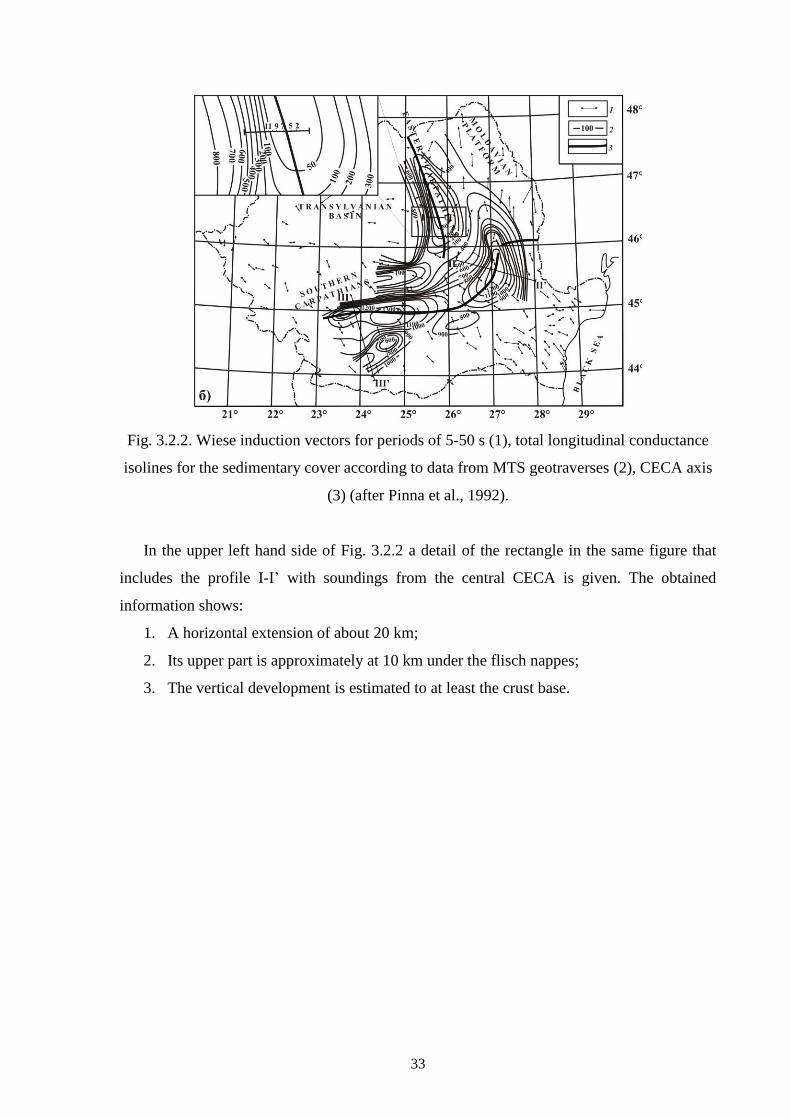
To show the most important electrical conductivity anomaly in Romania, the Wiese

induction vectors map (Pinna et al.1992) and the results of the deep MT soundings (Stănică

et al., 1999) were used. As it may be seen in Fig.3.2.2, CECA may be correlated with the

alignment of the Wiese induction vectors divergence zone. It is developed vertically at the

contact between two types of crust with different thicknesses and electrical properties (East-

European/ Transylvanian) but also within the Moesian crust.

33

Fig. 3.2.2. Wiese induction vectors for periods of 5-50 s (1), total longitudinal conductance

isolines for the sedimentary cover according to data from MTS geotraverses (2), CECA axis

(3) (after Pinna et al., 1992).

In the upper left hand side of Fig. 3.2.2 a detail of the rectangle in the same figure that

includes the profile I-I’ with soundings from the central CECA is given. The obtained

information shows:

1. A horizontal extension of about 20 km;

2. Its upper part is approximately at 10 km under the flisch nappes;

3. The vertical development is estimated to at least the crust base.

34

Fig. 3.2.3. MTS curves for the CECA central zone. Full and dashed colored lines show

perpendicular and, respectively, parallel to CECA resistivities, numbers 2, 5, 6, 7, 8 and 9

correspond MTSs (after Pinna et al., 1992)

In Fig. 3.2.4 a 2-D model for the resistivity distribution is presented for the profile II-II’

of Fig. 3.2.2, located in the bend zone of the Eastern Carpathians were CECA shows:

1. A horizontal extension of about 8 km;

2. Its upper part is at approximately 15 km under the flisch nappes and a part of the

platform sedimentary cover;

3. A vertical development to the crust base (approx. 45 km).

35

Fig. 3.2.4. 2-D Model for the resistivity distribution along the II-II’ profile in the bending

zone of the Eastern Carpathians

In Fig. 3.2.5 a 2-D model is presented for the resistivity along the profile III-III’ of Fig.

3.2.2, crossing the Southern Carpathians, Carpathian foredeep and the northern part of the

Moesian Platform. CECA shows the following characteristics:

1. A horizontal extension of about 6 km;

2. Its upper part is placed approximately 10 km under the flisch nappes and a part of the

platform sedimentary cover;

3. Vertical displacement to the base of crust (approx. 30 km).

Fig. 3.2.5. 2-D Model for the resistivity along profile III-III’

36

References

Mutihac, V., Structura geologică a teritoriului României, Ed. Tehnică, Bucureşti, 1990.

Paucă, M., Etapele genetice ale Depresiunii Transilvaniei, S.C.G.G.G., Geol., XVII, 2. 1972.

Pinna, E., Soare, A., Stanica, D., Stanica, M., Carpathian conductivity anomaly and its

relation to deep structure of the substratum, Acta Geod. Geoph. Mont. Hung. 27(1), pp 35–

45, 1992.

Stanica, M., Stanica, D., Marin-Furnica, C., The Placement of the Trans-European Suture

Zone by Electromagnetic Arguments on the Romanian Territory. Earth, Planets and Space,

51, 1073-1078, 1999.

37

Chapter IV. Toward a model for the distribution of the surface geoelectric field

produced by hazardeous geomagnetic variations. Case study – the Romanian territory

The strong variations of the magnitude and direction of the geomagnetic field during

geomagnetic storms and substorms triggered by the interaction with the magnetosphere and

ionosphere of coronal mass ejections (CMEs), mainly during the maximum solar activity,

and by the high speed streams (HSSs) in the solar wind, especially in the declining phase of

the 11-year solar cycle, induce in the Earth and in the power grid systems certain variable

electric fields that produce, in turn, electric currents known as geophysically induced

currents (GICs). This current type has been studied since the middle of the 19th century,

following observations from communication cables. In the years following the catastrophic

breakdown of the power network in Quebec, Canada, during the severe magnetic storm of

March 13/14, 1989, a special interest has been given to induced currents both in Canada and

in the northern countries (Blais and Metsa, 1994; Boteler and Pirjola, 1998; Viljanen, 1997;

Pirjola and Viljanen, 1998; Beamish et al., 2002), as being most affected by such a

phenomenon because of the proximity of the auroral current system. On the other hand, it

has been shown that the effects of induction could be significant at more southern latitudes

(British Isles, South Africa) (Beamish et al., 2002). At present the European project

EURISGIC is running, that will produce as a prototype the first forecasting service for GICs

in power networks. Principles have been presented, e. g., by Viljanen et al. (2012).

The computation of GIC in a given system of conductors is done in two steps: (1) the

determination of the electric field associated to geomagnetic variations, step that does not

depend on the concrete technological system, and (2) the determination of GIC in the given

technological system. In the present research contract we aimed at tackling the first aspect,

and in the present stage we aimed at approaching, in a first instance, of a study based on

recordings provided by the Surlari geomagnetic observatory, the only observatory in the

Romanian area. In the next phase (2015) we shall approach also the determination of some

quantitative elements regarding the GIC hazard in the national power network.

4.1. The computing model

Generaly, the horizontal electric field (Ex, Ey) produced by the variable magnetic

field is related to the magnetic field (Bx, By) through the impedance Z(ω) of the plane wave

by means of which the propagation of the geomagnetic disturbance is approximated:

38

)()(

)(),()(

)(00

xyyx B

ZEB

ZE (1)

In this relation, ω is the angular frequency of the plane wave, x and y refer to the

North and, respectively East directions, and μₒ is the vacuum permeability.

In case of an Earth viewed as a halfspace with the conductivity σ, and the

propagation of the geomagnetic disturbance in the inside as that of a vertical plane wave, the

surface electric field is described by the relationship (Viljanen and Pirjola, 1989):

duut

ugtE

t

xy

)(1)(

0 (2)

in which gx means the time derivative of the field B.

The integral in eq. (2) is replaced in practice by a sum, and the lower integration limit

by M = 720. That is, in the summation the variations produced in a 12 hours interval before

the first time moment TN, in which the electric field is calculated, are taken into account too.

The geomagnetic recording should appear as minute values, the standard of the

INTERMAGNET network:

)(2

)( 1

0

MNNNN bMRRTE

(3)

N

MNn

nN nNbR1

1 (4)

To solve the problem, a computer code, presented in the next section, was worked

out. By means of this program, calculations for several geomagnetic storms in the solar cycle

23 were done. The results for the Surlari observatory were compared to results for the

Nurmijarvi observatory (Finland), located in the auroral zone, in which the effects of the

geomagnetic variations are stronger.

4.2. Results

4.2.1. The computer code worked out in the present stage of the contract

Based on eqs. (2), (3), and (4) a MATLAB computer code, presented in the

following, was worked out.

39

load data.dat %input parameters Bx=data(:,2); % North geomagnetic element By=data(:,3); % East geomagentic component time=data(:,1); %time interval in minutes mu0=4*pi*10^(-7); %vacuum permeability sigma; %electrical conductivity N=length(SUA); M %time in minutes before the event

%time derivative dBx=diff(Bx); dBy=diff(By); dt=diff(time); gtx=dBx./dt; gty=dBx./dt;

i=(N-M+1):N; Ci=sqrt(i); Citr=transpose(Ci); bxi=(Bx(i)-Bx(i-1))./60; byi=(By(i)-By(i-1))./60; Rx=bxi.*Citr; Ry=byi.*Citr; RNx=sum(Rx); RNy=sum(Ry); bxibef=(Bx(i-1)-Bx(i-2))./60; byibef=(By(i-1)-By(i-2))./60;

Cibefore=sqrt(i+1); Cibef=transpose(Cibefore); Rxbef=bxibef.*Cibef; Rybef=byibef.*Cibef; RNxbef=sum(Rxbef); RNybef=sum(Rybef); Ey=((2/sqrt(pi*mu0*sigma))*((RNxbef- RNx) -(sqrt(M))*bxi(i-M)))*10^(-3); Ex=((2/sqrt(pi*mu0*sigma))*((RNybef- RNy) -(sqrt(M))*byi(i-M)))*10^(-3);

figure(1) subplot(3,1,1), plot(Bx), title('Bx') subplot(3,1,2), plot(gtx), title('dBx/dt') subplot(3,1,3), plot(Ey), title('Ey')

figure(2) subplot(3,1,1), plot(By), title('By') subplot(3,1,2), plot(gty), title('dBy/dt') subplot(3,1,3), plot(Ex), title('Ex')

40

4.2.2. The variation of the geoelectric field

To illustrate the way the code works, we chose the time interval that contains the

geomagnetic storm of November 8, 2004, that had a Dst minimum of -374 nT (Fig. 4.2.1).

To exemplify, we used data from two geomagnetic observatories, namely the national

Fig. 4.2.1. The variation of the Dst index for the geomagnetic storm of November 7, 2004

geomagnetic observatory, Surlari (SUA), located at midlatitude, and the Finish one,

Nurmijarvi (NUR), located under the auroral current system. The geoelectric field was

calculated for both horizontal components, Ex and Ey, based on geomagnetic recordings Bx

and By, using specific electric conductivity for the two locations, of 0.10 Ω-1

m-1

for SUA

and of 1x10-4

Ω-1

m-1

for NUR. The results are presented in Figs. 4.2.2 and 4.2.3.

41

Fig. 4.2.2. The surface geoelectric field for SUA (lower plots). In the same figure the

variation of the components X and Y (upper plots) and their time derivative (middle plots)

are also given

Fig. 4.2.3. The surface geoelectric field for NUR observatory (lower plots). In the same

figure the variation of the components X and Y (upper plots) and their time derivative

(middle plots) are also given

A comparative view of the results for the two observatories shows, even at this stage

of research, the following:

- The more pronounced geoelectric component is directed East-West;

- The amplitude difference is of the order of tens of mV/km in case of SUA, and of

thousands of mV/km in case of NUR;

- The sudden storm commencement (SSC, h=10:57 TU, November 7, 2004) is

more pronounced at SUA latitude than at the NUR latitude and produces a

significant variation of the electric field at SUA when compared with later

variations. The amplitude differences reverse in case of NUR, where the effects

of auroral current dominate.

42

References

Beamish D., Clark TDG., Clarke E., 2002. Thompson AWP.

Blais G., Metsa P., 1994. Solar-Terrestrial Predictions IV, 108-130.

Boteler, D. H. and Pirjola, R. J., The complex-image method for calculating the magnetic

and electric fields produced at the surface of the Earth by the auroral electrojet, Geophys. J.

Int., 132,31–40, 1998.

Pirjola, R. and Viljanen, A., Complex image method for calculating electric and magnetic

fields produced by an auroral electrojet of a finite length, Ann. Geophysicae, 16, 1434–1444,

1998.

Viljanen, A. and Pirjola, R., Statistics on geomagnetically-induced currents in the Finnish

400 kV power system based on recordings of geomagnetic variations. J.Geomagnetism and

Geoelectricity, 41, 411–420, 1989.

Viljanen, A., The relation between geomagnetic variations and their time derivatives and

implications for estimation of induction risks, Geophys. Res. Lett., 24, 631-634, 1997.

Viljanen, A., Pirjola, R., Wik, M., Adam, A., Pracser, E., Sakharov, Y. and Katkalov, J.,

Continental scale modelling of geomagnetically induced currents, J. Space Weather Space

Clim. 2, A17, doi: 10.1051/swsc/2012017, 2012.

43

Chapter IV. Dissemination of results

In the report period 3 papers have been submitted for pubication, namely:

- Beşliu-Ionescu, D., Mariş Muntean, G., Lăcătuș, D.A., Paraschiv, A.R., Mierla,

M., Detailed Analysis of a Geoeffective ICME Triggered by the March 15, 2013

CME, Romanian Geophysical Journal, 2014, accepted.

- Stefan, C., Application of the Radon transform to the study of traveling speeds of

core geomagnetic field features. Case study – The ~80-year variation, Romanian

Geophysical Journal, 2014, accepted.

- Dobrica, V., Demetrescu, C., Mandea, M., Geomagnetic field declination: from

decadal to centennial scales, Journal of Geophysical Research B, 2014, submitted.

Also, during 2014, the team members of the research contract participated at 5

international scientific meetings, with 12 presentations:

- Demetrescu C., Stefan C., Dobrica V., External field noise in main field models at

Earth's surface and at core/mantle boundary, European Geosciences Union

General Assembly, Vienna, Austria, 27 April – 02 May 2014

- Demetrescu C., Stefan C., Dobrica V., Space climate. On geoeffective solar

activity during Maunder and Dalton grand minima, European Geosciences Union

General Assembly, Vienna, Austria, 27 April – 02 May 2014

- Stefan C., Demetrescu C., Dobrica V., On the characteristics of a residual external

signal seen in coefficients of main geomagnetic field models, European

Geosciences Union General Assembly, Vienna, Austria, 27 April – 02 May 2014

- Greculeasa, R., Dobrica, V., Demetrescu, C., The disturbed geomagnetic field at

European observatories. Sources and significance, European Geosciences Union

General Assembly, Vienna, Austria, 27 April – 02 May 2014

- Maris Muntean, G., Besliu-Ionescu, D., Dobrica, V., Lacatus, D.A., Paraschiv,

A.R., Fast Solar Wind and Geomagnetic Variability during the 24th Solar Cycle

(2009 - 2013), European Geosciences Union General Assembly, Vienna, Austria,

27 April – 02 May 2014

- Besliu-Ionescu, D., Lacatus, D.A., Paraschiv, A.R., Mierla, M., Geoeffective

CMEs Associated with Seismically Active Flares, European Geosciences Union

General Assembly, Vienna, Austria, 27 April – 02 May 2014

- Stefan C., Demetrescu C., Dobrica V., A Tentative Reconstruction of the Dst

Index back to 1840, Based on Long Time-Span Models of the Core Magnetic

44

Field, The Sixth Workshop “Solar influences on the magnetosphere, ionosphere

and atmosphere”, Sunny Beach, Bulgaria, 26-30 May 2014

- Maris Muntean, G., Besliu-Ionescu, D., Georgieva, K., Kirov, B., Analysis of the

Geomagnetic Activity during the SC 24 Maximum Phase, The Sixth Workshop

“Solar influences on the magnetosphere, ionosphere and atmosphere”, Sunny

Beach, Bulgaria, 26-30 May 2014

- Demetrescu C., Stefan C., Dobrica V., 400 years of space climate information

from long-term main geomagnetic field models, 11th

Annual Asia Oceania

Geosciences Society (AOGS) Assembly, Sapporo, Japan, 28 July – 01 August

2014

- Mariș Muntean, G., Beșliu-Ionescu, D., Dobrică, V., Lăcătuș, D.A., Paraschiv,

A.R., Sources and Complexity of the Strong Geomagnetic Storms during the

Maximum Phase of Solar Cycle 24, 11th

Annual Asia Oceania Geosciences

Society (AOGS) Assembly, Sapporo, Japan, 28 July – 01 August 2014

- Mariș Muntean, G., Besliu-Ionescu, D., Mierla, M., Detailed analysis of two

intense geomagnetic storms during solar cycle 24, 40th COSPAR Scientific

Assembly, Moscova, Rusia, 2-10 August 2014

- Maris Muntean, G., Besliu-Ionescu, D., Mierla, M., March 2013 ICMEs and their

Geomagnetic Effects, 11th European Space Weather Week, Liege, Belgium,

November 17-21, 2014

To close this report, we mention that the web page of the project,

http://www.geodin.ro/IDEI2011/engl/index.html, was updated.