Project Report - OzCoasts · Estuarine, Coastal and Marine (ECM) National Habitat Mapping Project ....

Estuarine, Coastal and Marine (ECM) National Habitat Mapping Project

Project Report February 2008

Version 1.1

Principal Authors Richard Mount1, 2 and Phillippa Bricher2

1 National Estuarine, Coastal and Marine Information Coordinator, NLWRA 2 Spatial Science Group, School of Geography and Environmental Studies, University of

Tasmania

This project is a component of the Australian “First Pass Coastal Vulnerability Assessment” Project

and is supporting NRM reporting on the ecological integrity of key ECM habitats

Agency Support

Department of Climate Change, Australian Government National Land and Water Resources Audit

School of Geography and Environmental Studies, University of Tasmania

Contents

Executive Summary ...................................................................................... 4

Acronyms................................................................................................ 5

Citation ................................................................................................... 5

1. Agency partners and contributors.............................................................. 6

2. Introduction and Project Objectives........................................................... 7

2.1. Project Scope................................................................................... 9

3. Project Tasks and Activities......................................................................10

3.1. Classification scheme identification and development .........................10

3.2. Data set discovery, access and assessment........................................14

3.3. Data set collation and translation ......................................................16

3.4. Geoprocessing of derived products....................................................17

3.5. QA/QC and data documentation........................................................22

4. ECM National Habitat Map Series components ...........................................23

4.1. ECM Habitat Mapping Inventory........................................................23

4.2. Derived data sets ............................................................................23

4.3. User Guide......................................................................................35

5. Discussion of the ECM National Habitat Map Project...................................36

6. Conclusions ............................................................................................37

Acknowledgements .................................................................................38

References .............................................................................................39

Appendix 1: Data License Usage and Request Letter.......................................41

ACVbio_ProjectReport_v14.doc 30/04/2008 of 43

Executive Summary • This project is designed to produce a nationally consistent set of habitat maps for the

broad habitat classes of seagrass, mangrove, saltmarsh, rocky reef, coral reef, macroalgae, shorelines (beaches), coastal wetlands and estuaries. These habitats were selected as they are likely to change in response to climate change (Voice et al., 2006), are considered key habitats sustaining ecological functioning and are relatively tractable to current mapping methods and effort.

• There are a series of uses for a national estuarine, coastal and marine habitat map. These include supporting the assessment of the vulnerability of Australia’s shores to climate change impacts and, for Natural Resource Management (NRM) purposes, assessing the ecological integrity of key habitats.

• Habitat classification schemes are essential when producing habitat maps. Many of the specified habitat types, including estuaries, wetlands, mangroves and saltmarshes, have existing national classification schemes suitable for mapping purposes. A classification scheme covering beaches and all other shoreline types is being produced by the sister project, Australian Geomorphic and Shoreline Stability Mapping Project.

• However, for the intertidal and subtidal environments, there are a number of habitat classification schemes in use around Australia. These schemes have many characteristics in common, though they are implemented differently to reflect current practise and management needs within each state and territory. Working with key State/NT and Australian government agencies, this project has produced the first National Intertidal/Subtidal Benthic (NISB) Habitat Classification Scheme (Mount, Bricher and Newton, 2007).

• For the first time the bulk of the nation’s ECM habitat mapping data are in one place at one time, potentially making a significant resource for researchers and managers. It is a very large data set with over 700,000 individual map features (polygons) covering more than 5 million Ha (many overlapping data sets). The process of discovering and collating existing mapping data sets was challenging due to data licensing issues, the large number of data sets (over 80) and agencies, the range of varying map classifications schemes and mapping methods, the wide range of map scales, varying temporal coverage, and the large size of some of the data sets.

• The resulting maps are notable for their limited coverage of the Australian intertidal and subtidal zones. The data also did not support the mapping of macroalgae at the national scale, though the class of “sediment” (i.e. sand, silt etc) was added. While the efforts of the marine habitat mappers should be clearly acknowledged, this project has highlighted the very large areas of the coastal and marine environments where the key ecological habitats types are unknown or poorly mapped. This will help direct further mapping efforts.

• More mapping may be required for the following habitat types: high temporal resolution mapping of dune vegetation, coral mapping in the NT, and benthic mapping within the photic zone of the open coast (i.e. the “inner shelf”) in most states/NT. Further development of national habitat classification schemes is needed, especially for wetlands and dunes and dune vegetation.

• In spite of the relatively limited coverage, the resulting maps will assist the process of identifying the vulnerability of ecosystems and habitats for the First Pass Coastal Vulnerability Assessment.



Acronyms AGO Australian Greenhouse Office (now within the DCC) ASDD Australian Spatial Data Directory ASRIS Australian Soil Resource Information System CMA Catchment Management Authority CS Coordinate System CSIRO Commonwealth Scientific and Industrial Research Organisation CVA Coastal Vulnerability Assessment Project DCC Department of Climate Change, Australian Government DEM Digital Elevation Model ECM Estuarine, Coastal and Marine ERIN Environmental Resources Information Network FMP Feature level metadata pointer GIS Geographic Information System GCS Geographic Coordinate System ICAG Intergovernmental Coastal Advisory Group ISB Intertidal/Subtidal Benthic IMCRA Integrated Marine and Coastal Regionalisation of Australia MQ Mixed Quality NISB National Intertidal/Subtidal Benthic NLWRA National Land and Water Resources Audit (Audit) NOO National Oceans Office NRM Natural Resource Management NVIS National Vegetation Information Systetm OSDM Office of Spatial Data Management OSRA Oil Spill Response Atlas SMB Structural Macrobiota WMS Web Mapping Services

Citation Mount, R.E. and P.J. Bricher, 2008. Estuarine, Coastal and Marine (ECM) National

Habitat Map Series Project Report February 2008. Spatial Science Group, School of Geography and Environmental Studies, University of Tasmania. Report to the Department of Climate Change and the National Land and Water Resources Audit, Canberra, ACT. Pp.

1. Agency partners and contributors National: An adjective describing something that is produced or agreed by jurisdictions at all levels including the Australian Government, State/NT Governments, NRM Regions and Local Governments. A very large number of agencies at the national and state level participated in this national project. In terms of the actual data sets, the project was dependent on the goodwill and cooperation of these partners and contributors. Acknowledgements of the individuals involved is covered elsewhere later in this report,; however, we wish to start this report by acknowledging and appreciating the following Agencies: Summary List of Data Custodians For the whole ECM National Habitat Map Series all the following contributors must be acknowledged: Subset of contributors for the National Intertidal/Subtidal (NISB) Habitat Map: Department of Natural Resources, Environment and the Arts, Northern Territory Government of Australia Queensland Department of Primary Industries and Fisheries Queensland Parks and Wildlife Services Environmental Protection Agency Great Barrier Reef Marine Park Authority National Oceans Office Western Australia Department of Environment and Conservation South Australian Department of Environment and Heritage New South Wales Department of Environment and Conservation New South Wales Department of Primary Industries: Fisheries Conservation Commission of the Northern Territory Land Conservation Unit Victorian Department of Primary Industries Parks Victoria Tasmanian Aquaculture and Fisheries Institute Subset of contributors for the Coastal Wetlands Collection: Queensland Environmental Protection Agency Australian Government Department of the Environment and Heritage NSW Department of Planning Subset of contributors for the Estuaries Collection: Geoscience Australia Subset of contributors for the Dune and Dune Vegetation Collection: Australian Government Department of the Environment and Heritage Department of Natural Resources, Environment and the Arts, Northern Territory Government of Australia Queensland Department of Primary Industries and Fisheries WA Department of Industry and Resources WA Department of Minerals and Energy WA Department of Mineral and Petroleum Resources Victorian Department of Primary Industries SA DEH - Natural and Cultural Heritage Queensland Herbarium, Environmental Protection Agency NSW Department of Primary Industries, Mineral Resources NSW Department of Mineral Resources (DMR)


2. Introduction and Project Objectives The Department of Climate Change (DCC; formerly the Australian Greenhouse Office) is working with the States and Territories through the Intergovernmental Coastal Advisory Group (ICAG) to assess Australia’s coastal vulnerability to climate change. An early objective of the Department is to deliver a “First Pass” Coastal Vulnerability Assessment (CVA) of the Australian coast and priority coastal systems (natural and artificial) by June 2008. This will identify risks and priorities and build foundation capacity towards future, more detailed assessments.

A key part of the CVA is the identification and mapping of coastal ecosystems and habitat types that have greater or lesser susceptibility to potential coastal impacts of climate change and sea level rise, such as accelerated erosion and increased marine inundation. These hazards may contribute to impacts including the direct loss of habitats (e.g. seagrass and mangroves), interruptions to biotic and chemical processes (e.g. coral bleaching) and progressive inland migration of ecosystems (e.g. mangrove and saltmarsh). These ecosystems and habitat types have undergone a detailed gap analysis of data and methods via an Australian Greenhouse Office consultancy (Voice et al., 2006).

Assessment of the potential rates and magnitudes with which these hazards may affect particular coastal ecosystems requires detailed measurement and modelling of a range of locally-variable factors (e.g., wave climate & energy, exposure, local bathymetry, littoral drift & sediment budget, and biotic responses). An important initial step is to be able to identify the location of those ecosystems which may be susceptible in some significant degree to such hazards. This, in turn, requires the availability of coastal habitat maps. The maps need to be in a format that enables the rapid and flexible extraction of the required information, such as a well designed GIS spatial database.

At the time this project was initiated, a significant number of coastal habitat maps existed for various discrete sections of the Australian coast. These were prepared for a wide range of purposes, by numerous researchers and agencies, and they existed in a variety of formats, at differing scales and resolutions. Moreover, these maps thematically classified and mapped coastal habitats using a variety of different classification schemes that included a mix of biotic, geomorphic and environmental factors. There was no consistently-classified coastal habitat mapping of the entire Australian coastline, except at scales too coarse to be of practical use in vulnerability assessment.

In order to provide the basis for a First Pass vulnerability assessment of the whole Australian coastline, the DCC has contracted the National Land and Water Resources Audit (Audit) to prepare a national map of the Australian intertidal/subtidal benthic habitats using a nationally-consistent habitat classification that is capable of being readily interrogated to identify habitats that are potentially sensitive to a range of physical hazards related to climate change and sea-level rise. The Audit is involved as it has an interest in compiling national extent and distribution mapping of key estuarine, coastal and marine habitats to support one of the nationally agreed NRM indicators. The seaward boundary of the NRM estuarine, coastal and marine areas is the outer edge of the State Coastal Waters (i.e. 3 nm limits). The indicator will be delivered via the OzCoasts web site managed by Geoscience Australia.

The Audit has in turn coordinated a team of coastal habitat mapping specialists in the Spatial Science Group, School of Geography and Environmental Studies, University of


Tasmania to undertake the bulk of the practical work involved in creating the nationally-consistent coastal classification system and map. The team works through UTAS Innovation Ltd., and is led by Dr Richard Mount (GIS, Remote Sensing and coastal monitoring and mapping specialist and the Audit’s National Estuarine, Coastal and Marine (ECM) Information Coordinator). Via the services of the team, the Audit will produce the following coastal ecosystem and habitat data layers:

beaches (shorelines) mangroves estuaries seagrasses coastal wetlands macroalgae dune vegetation coral reefs saltmarsh rocky reefs

The broad class of “sediment” (i.e. unconsolidated substrates such as sand, silt etc) has been added to the project’s list of classes as it is regularly mapped and is an important habitat type, particularly for the project’s primary objectives.

In practice, a series of information products have been developed to meet the project requirements. The ECM National Habitat Map Series consists of 2 main groups of information products. Firstly, a series of national habitat distribution maps were produced for the habitat types of saltmarsh, mangrove, seagrass, macroalgae, sediment, coral reef and rock substrate including the three following information products:

1. A thematically simplified, high spatial resolution National Intertidal/Subtidal Benthic (NISB) Habitat Map

2. A set of 10 km grid cell ECM Key Habitat Distribution Maps depicting the regional and statewide distribution of each key habitat type

3. A set of 50 km grid cell ECM Key Habitat Distribution Maps depicting the national distribution of each key habitat type

Secondly, four additional information products covering the remaining habitat types of dune vegetation, estuaries, coastal wetlands and shorelines (beaches) are identified as follows:

4. A Dune and Dune Vegetation Map collection

5. A National Estuaries Map collection

6. A National Coastal Wetlands Map collection, and

7. A National Shoreline Map

Together, the information products form the ECM National Habitat Map Series. The coastal ecosystem and habitat layers are as nationally comprehensive and consistent as is practical with current data, that is, legacy data from all States and the Northern Territory. Where appropriately licensed by the data suppliers, these layers are intended to form part of a coastal vulnerability spatial information system that will underpin the national coastal vulnerability assessment process. Where appropriately licensed or permitted by the data suppliers, data will be mapped and are intended to be made available through the proposed OzCoast portal housed at Geoscience Australia. The final nationally-consistent coastal habitat map series produced by this project is intended to be a public domain data set managed by the Australian Government which will ensure full attribution of the various original mapping sources used to build the final map.


2.1. Project Scope

By necessity the project began by defining more closely the scope of the tasks. Many of the tasks for producing the national maps are open ended and given the imperative for a rapid “first pass” assessment, limitations were placed on the project to enable delivery of the products within the required time frame. These constraints are as follows:

• The project was designed to collate existing habitat data sets only

• Existing classification schemes were used when available and, ideally, collected data was translated into nationally consistent schemes. However, where a national scheme was not in place or could not be produced in the time available, we accepted the source data’s classification scheme i.e. created a compilation or collection of data sets consisting of data coded with various schemes rather than translating the data into a single national scheme. Coastal wetlands and dune vegetation are good cases in point. The same applies where significant information would have been lost through the translation process. Estuaries are a good case in point here.

• The Project’s definition of the “coastal zone” includes:

o The marine influenced waters within the State Coastal Waters (i.e. 3 nm limit, which constitutes the seaward boundary for NRM), and

o The land that is either below 10 m elevation (i.e. 10 m above AHD) or within 500 m of the coastline as defined by the mean high water mark. In the low lying areas, this area broadly equates to the distribution of coastal vegetation such as mangroves and, in the environments with more relief than 10 m, this area broadly equates to the extent of habitats subject to a marine influence, for example coastal dunes or coastal cliff habitats. The Shuttle Radar Topography Mission (SRTM) Version 2 digital elevation model (DEM) was used to generate the elevation portion of the coastal zone area.

• Given the technical geographic and cartographic issues that arise when comparing mapped data sets of multiple scales, two derived information products were generated to provide a simplified spatial representation of the distribution of each of the key habitats. These derived products enable the visualisation of the habitat distributions at the regional and national extents. It is extremely important to note that they are definitely NOT able to be used to calculate areas of habitat types. The map format selected for distribution maps is the grid cell format and the two grid cell sizes are 10 km (state and regional) and 50 km (national), respectively.

• In the first instance, data licensing was completed that allowed the First Pass Coastal Vulnerability Assessment project and the production of the NRM Habitat Extent and Distribution Indicator to proceed and, secondly, data licensing is being facilitated that allow further uses of the data, such as open viewing of the derived information products via web mapping services (e.g. OzCoasts) and open access to the data via downloading of the actual data sets.


3. Project Tasks and Activities To achieve the project objectives and the production of the seven information products within the scope of the project, the following tasks were identified and addressed:

1. Identification of classification schemes suitable to support mapping.

2. Development of classification schemes where they are not available.

3. Discovery of data sets with potential value to the project objectives.

4. Accessing and organising data licensing and assessing the quality and suitability of the data sets.

5. Collating the data and translating them into the national classification scheme formats and adding feature level metadata to ensure the source of the data is clear.

6. Geoprocessing data into derived map products including the NISB Habitat Map, the Estuarine Map collection, the Coastal Wetlands Map collection and the 10 km and 50 km NISB Habitat Distribution Maps.

7. Quality assurance and quality control of derived data sets.

8. Documentation of the derived data sets including the production of ANZLIC compliant metadata and ensuring data suppliers are acknowledged.

The following sections summarise the activities and discusses the issues and opportunities that arose with each task.

3.1. Classification scheme identification and development Classification schemes

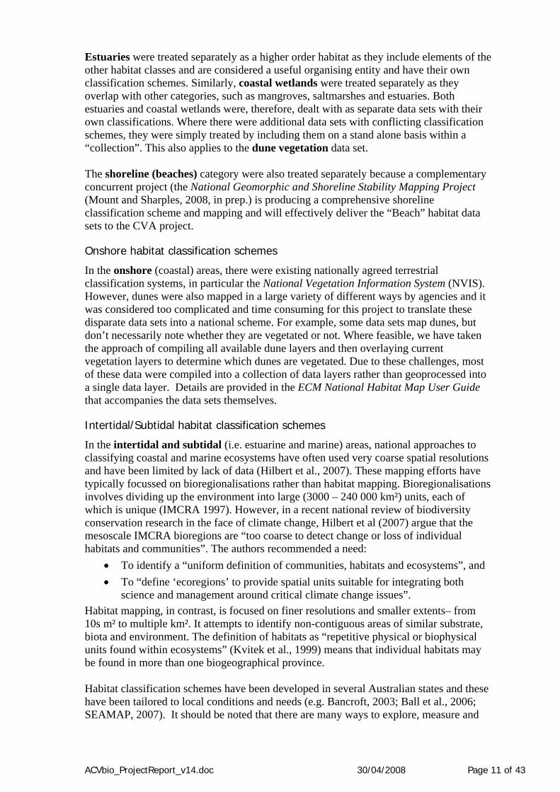
Any method of reporting and assessment that seeks to compare ecological units of interest must address the issue of classification. Classification schemes ideally organise and group information about distinguishable components of ecological systems so that comparisons can be made between the extent and distribution of the components across space and time. In Australia, there are a large number of habitat classification schemes; for example, there are more than 15 schemes for wetland classification systems (including marine and estuarine wetlands). The estuarine, coastal and marine environments are extremely diverse and there is currently no classification scheme that covers all three environments. They must, therefore, be split into areas that have sufficient features in common to enable the application of classification schemes. For the purposes of this map series, the habitats were split into onshore environments (i.e. dunes and dune vegetation) and the subtidal and intertidal environments (i.e. whether estuarine, nearshore or marine) including saltmarsh, mangroves, seagrasses, macroalgae, sediment, rock and coral reef. These classes of habitat types broadly equate to land cover mapping in the terrestrial environment. The intertidal and subtidal habitats did not have a single national classification scheme and it was necessary to produce one during the project. Details of the process for developing the scheme and the resulting scheme are available in the National Intertidal/Subtidal Benthic (NISB) Habitat Classification Scheme Version 1 (Mount, Bricher and Newton, 2007) (see Figure 1 below and Appendix 1 of the User Guide).


Estuaries were treated separately as a higher order habitat as they include elements of the other habitat classes and are considered a useful organising entity and have their own classification schemes. Similarly, coastal wetlands were treated separately as they overlap with other categories, such as mangroves, saltmarshes and estuaries. Both estuaries and coastal wetlands were, therefore, dealt with as separate data sets with their own classifications. Where there were additional data sets with conflicting classification schemes, they were simply treated by including them on a stand alone basis within a “collection”. This also applies to the dune vegetation data set. The shoreline (beaches) category were also treated separately because a complementary concurrent project (the National Geomorphic and Shoreline Stability Mapping Project (Mount and Sharples, 2008, in prep.) is producing a comprehensive shoreline classification scheme and mapping and will effectively deliver the “Beach” habitat data sets to the CVA project.

Onshore habitat classification schemes

In the onshore (coastal) areas, there were existing nationally agreed terrestrial classification systems, in particular the National Vegetation Information System (NVIS). However, dunes were also mapped in a large variety of different ways by agencies and it was considered too complicated and time consuming for this project to translate these disparate data sets into a national scheme. For example, some data sets map dunes, but don’t necessarily note whether they are vegetated or not. Where feasible, we have taken the approach of compiling all available dune layers and then overlaying current vegetation layers to determine which dunes are vegetated. Due to these challenges, most of these data were compiled into a collection of data layers rather than geoprocessed into a single data layer. Details are provided in the ECM National Habitat Map User Guide that accompanies the data sets themselves.

Intertidal/Subtidal habitat classification schemes

In the intertidal and subtidal (i.e. estuarine and marine) areas, national approaches to classifying coastal and marine ecosystems have often used very coarse spatial resolutions and have been limited by lack of data (Hilbert et al., 2007). These mapping efforts have typically focussed on bioregionalisations rather than habitat mapping. Bioregionalisations involves dividing up the environment into large (3000 – 240 000 km²) units, each of which is unique (IMCRA 1997). However, in a recent national review of biodiversity conservation research in the face of climate change, Hilbert et al (2007) argue that the mesoscale IMCRA bioregions are “too coarse to detect change or loss of individual habitats and communities”. The authors recommended a need:

• To identify a “uniform definition of communities, habitats and ecosystems”, and • To “define ‘ecoregions’ to provide spatial units suitable for integrating both

science and management around critical climate change issues”. Habitat mapping, in contrast, is focused on finer resolutions and smaller extents– from 10s m² to multiple km². It attempts to identify non-contiguous areas of similar substrate, biota and environment. The definition of habitats as “repetitive physical or biophysical units found within ecosystems” (Kvitek et al., 1999) means that individual habitats may be found in more than one biogeographical province. Habitat classification schemes have been developed in several Australian states and these have been tailored to local conditions and needs (e.g. Bancroft, 2003; Ball et al., 2006; SEAMAP, 2007). It should be noted that there are many ways to explore, measure and



describe the marine environment, and that there is no single best method for dividing it into homogeneous regions (Butler et al., 2001). One result of the diversity of schemes is that existing habitat maps cannot be easily compared among the states, territory and regions. Given this situation, this project was used as a catalyst for generating a national habitat classification scheme that is consistent with the existing habitat classification schemes, and enables the collation of the existing data into a national habitat map. The habitat classes include: coral reef, rock dominated habitat, sediment dominated habitat, mangroves, saltmarsh, seagrass, macroalgae and filter feeders (e.g. sponges). The scheme is designed to support the development of marine ‘ecoregions’ or bioregional subregions. Details of the process for developing the scheme and the resulting scheme are available in National Intertidal/Subtidal Benthic (NISB) Habitat Classification Scheme Version 1 (Mount, Bricher and Newton, 2007) (see Figure 1 below and Appendix 1 of the User Guide).

The NISB Habitat Classification Scheme supports the DCC/Audit partnership project by providing a nationally consistent map for those habitats that occur between the approximate position of the highest astronomical tide mark (HAT) and the location of the outer limit of the photic benthic zone (approximately at the 50-70 m depth contour). This area is broadly equivalent to the “inner” and “mid-shelf” regions identified by Geoscience Australia. The resulting map data set is known as the NISB Habitat Map and forms a core component of the ECM National Habitat Map Series. Two complementary grid cell data sets were derived from the NISB Habitat Map; the 10 km and 50 km Key ECM Habitat Distribution Maps. These maps are designed to assist with visualising the distribution of the habitats around the continent as the high spatial resolution NISB Habitat Maps are not easy to see when displaying the full extent of a State or Australia. They also serve the purpose of depicting the spread of data availability as the Distribution Map classification scheme includes areas that are unmapped or “unknown”. The scheme classes are “present”, “absent”, “unknown” and “not applicable”. These are defined in detail in the ECM National Habitat Map Series User Guide.

Estuarine classification schemes

There are many estuarine classification schemes in use in Australia (e.g. Roy et al, 2001). However, there is only one national scheme that has been systematically applied to a national mapping database, namely Geoscience Australia’s Conceptual Models of Australia’s Estuaries and Coastal Waterways (Ryan et al., 2003), which documents the approach taken to produce the OzEstuaries estuarine database. This scheme and data set is the key data set for the estuarine habitat types. In addition, the detailed “facies” (i.e. geomorphic units such as flood tide deltas) were translated across to the NISB habitat classification based on a series of defensible assumptions and included in the NISB Habitat Map. Other estuarine data sets were added as separate layers as they typically are sourced from state mapping agency data and are usually at a higher resolution than the OzEstuaries mapping. There are many decisions that go into defining the boundary of estuaries and it is clear a variety of decision rules have been applied to the various data sets resulting in considerable differences in the extent of some estuary polygons. For these reasons, it was considered more useful to collate the estuaries as series of data sets rather than seek to combine them into a single meta-estuarine data set.

30/04/2008 of 43

Figure 1. National Intertidal/Subtidal Benthic (NISB) Habitat Classification Scheme Version 1 (Mount et al, 2007)

1 Consolidated Substrate

1.2 Rock Substrate

1.2.2 Structural Macrobiota (SMB) Dominated

1.2.2.2 Filter Feeder Dominated

1.2.2.1 Macroalgae Dominated

1.2.2.3 Coral Dominated

1.2.2.4 Seagrass Dominated

NISB Habitats

2 Unconsolidated Substrate

1.1 Coral Reef Substrate 2.0 Unconsolidated Substrate

2.0.2 Structural Macrobiota (SMB) Dominated


2.0.2.2 Mangrove Dominated

2.0.2.3 Saltmarsh Dominated



2.0.1 Sediment Dominated

2.0.1.1 Pebble Dominated

2.0.1.2 Gravel Dominated

2.0.1.3 Sand Dominated

2.0.1.4 Silt Dominated

Target classes for the Audit/DCC NISB Habitat map

1.2.1.1 Unbroken Rock Dominated

1.2.1.2 Boulder Dominated

1.2.1.3 Cobble Dominated

1.2.1 Rock Dominated

ACVbio_ProjectReport_v14.doc

Coastal wetland classification schemes

“Coastal” wetlands are defined here to be the wetlands identified in the various data sets that intersect the project’s “coastal zone” (see Section 2.1), that is, where some part of the mapped area of the wetland falls within the coastal zone polygon. The acceptance of the existing classification schemes was necessitated as there are a large number of disparate classification schemes used by a very large number of wetland mapping data sets (over 250) and it was considered impractical to translate the maps to a single national scheme. The extent of the wetland polygons is as provided by the data suppliers and there was not enough information to apply a nationally consistent definition of a wetland. Note that there is a current national project underway to define wetland extent and another seeking to establish a national wetlands classification. Both projects are driven by the Audit.

Shoreline classification schemes

For the shoreline itself, there are some schemes with complete national coverage (e.g. Galloway, 1984 and Short, 1993-2006), though there are thematic and/or resolution limitations. For example, the Galloway mapping is organised into approximately 3 km wide by 10 km long units and Short’s excellent and extensive work is focussed exclusively on sandy beaches. The National Geomorphic and Shoreline Stability Mapping Project is running in parallel to this project and is producing a nationally consistent “smartline” map for all shoreline types that comprehensively maps a large number of shoreline attributes including information about the intertidal zone and the immediate backshore and foreshore. These are considered suitable for defining shoreline habitat types including for example, the location of the sandy beaches suitable for shorebird habitat. Details are provided in the National Geomorphic and Shoreline Stability Map: User Guide (Sharples, in prep) that accompanies that data set.

3.2. Data set discovery, access and assessment Discovery

The process of discovering the data sets with the potential to be included into the ECM National Habitat Map Series was facilitated by the use of the Australian Spatial Data Directory (ASDD), though a surprising number of data sets did not have a record in the directory. The national data repositories operated by Geoscience Australia (GA) and Environmental Resources Information Network (ERIN), Department of Environment, Water, Heritage and the Arts (DEWHA), such as Discover Information Geographically (DIG) were both useful for the freely accessible national data sets such as OzEstuaries. The data custodians for the habitat mapping at the State/NT were largely identified by the NISB Habitat Classification Scheme Reference Group, which consists of key habitat mapping officers from the States and NT (See Appendix A of Mount, Bricher and Newton, 2007). Further data sets were identified through searches of the literature and a series of investigative phone calls to potential leads provided by leading authorities in the field.

Access and data licensing

Data licensing is persistently identified as a significant limitation to accessing national data sets and is posited to be limiting the national effort to innovate (Willibanks, 2007). Given the potential challenges, a strategy was developed in consultation with key data managers from ERIN, DEWR and GA, namely Robyn Gallagher, Damian Woolcombe,


and Brian Burbridge. For this project a two phase strategy was adopted to tackle the anticipated difficulties. Firstly, a standard data license was obtained so that the data sets could be accessed and, at least, evaluated for inclusion as soon as possible and, ideally, geoprocessed to produce, or derive, the required data sets. Almost universally, the data suppliers were readily prepared to contribute to the project. However, mainly due to bureaucratic delays, significant data sets were not received until the last weeks of the project. Recommendation: That future projects with similar data collation intentions allow at least 6 months for data access and licensing. In the second phase, a more detailed data licensing package was produced with the intention of securing the data supplier’s approval for more extensive uses of the derived information products and data sets. In this second phase, legal advice was obtained from a number of sources and, in response, a tiered approach was taken which enabled data suppliers to identify which of a number of increasingly open uses they would allow the supplied data to be put. This approach was intended to clearly communicate the project purposes and, ideally, allow free open access to the ECM National Habitat Mapping Project data sets. It depends on both the data supplier’s view about the degree to which the derived information products contain their intellectual property or copyright and their willingness to see the data sets for which they are responsible, used and distributed in the ways intended by this project. The following are the three proposed tiers of use:

1. That UTAS use the supplied data to produce the ECM Habitat Map Series and provide the derived information products to the DCC via the Audit including:

a. The NISB Habitat Map

b. The 10 km grid cell Key National Habitat Distribution Map

c. The 50 km grid cell Key National Habitat Distribution Map

2. That the DCC and the Audit (representing the Australian Government) publish the resulting information products via simple visual representations of the data, such as hard copy figures in reports and via Web Mapping Services (WMS) including OzCoasts, the web site managed by Geoscience Australia.

3. That the DCC and Audit (representing the Australian Government) distribute the resulting information products via standard Office of Spatial Data Management’s (OSDM) data licenses as used by the AG for other nationally produced data sets, such as the National Vegetation Information System (NVIS), the Australian Soil Resource Information System (ASRIS) and award winning MapConnect.

This tiered approach to data licensing means that some of the data in the ECM National Habitat Map Series may be more accessible to a wider range of users than others. This is an almost inevitable outcome given the complex process of obtaining data licenses for multiple data sets from a wide range of government and research agencies, each operating with their own data licensing policies. Data licenses are stored in the data license folder within each data set folder.

Assessment

Once access was obtained, the data and their associated metadata were assessed and the characteristics of the data evaluated in relation to the project purposes. Where clarification was required, the data producers were contacted.


3.3. Data set collation and translation Collation

The process of collation entailed a number of tasks. For example, data from individual mapping projects and study areas were combined into, typically, a statewide data set. Other tasks included ensuring the coordinate systems were standardised.

Coordinate System (CS)

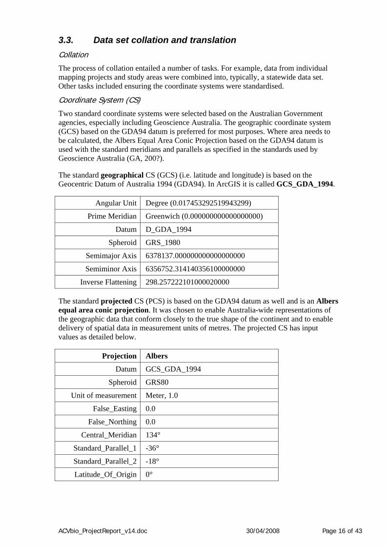
Two standard coordinate systems were selected based on the Australian Government agencies, especially including Geoscience Australia. The geographic coordinate system (GCS) based on the GDA94 datum is preferred for most purposes. Where area needs to be calculated, the Albers Equal Area Conic Projection based on the GDA94 datum is used with the standard meridians and parallels as specified in the standards used by Geoscience Australia (GA, 200?).

The standard geographical CS (GCS) (i.e. latitude and longitude) is based on the Geocentric Datum of Australia 1994 (GDA94). In ArcGIS it is called GCS_GDA_1994.

Angular Unit Degree (0.017453292519943299)

Prime Meridian Greenwich (0.000000000000000000)

Datum D_GDA_1994

Spheroid GRS_1980

Semimajor Axis 6378137.000000000000000000

Semiminor Axis 6356752.314140356100000000

Inverse Flattening 298.257222101000020000

The standard projected CS (PCS) is based on the GDA94 datum as well and is an Albers equal area conic projection. It was chosen to enable Australia-wide representations of the geographic data that conform closely to the true shape of the continent and to enable delivery of spatial data in measurement units of metres. The projected CS has input values as detailed below.

Projection Albers

Datum GCS_GDA_1994

Spheroid GRS80

Unit of measurement Meter, 1.0

False_Easting 0.0

False_Northing 0.0

Central_Meridian 134°

Standard_Parallel_1 -36°

Standard_Parallel_2 -18°

Latitude_Of_Origin 0°


Translation into the NISB Habitat Classification

One of the main tasks of the project was to derive the maps based on the NISB Habitat Classification Scheme (the Scheme) from the various intertidal/subtidal benthic habitat data sets. This required a comprehensive and thorough matching of the source data set attributes with the classes defined by the Scheme. The decision rules defined in the Scheme were also used to establish the destination class to which the source class belonged. Usually there was a considerable simplification of the source data’s classes into the nationally consistent classes. For example, some Victorian data sets had over 90 classes for mapping seagrass. This lower thematic resolution is necessary as it enables a map to be derived that is comparable across the entire continent. Further details of the specific class translations are provided in the ECM National Habitat Map Series User Guide.

3.4. Geoprocessing of derived products Overall, the geoprocessing was minimised to ensure data integrity. Consistent methods were maintained through thorough discussion of each geoprocessing step and a culture of collaboration and openness was encouraged.

Geoprocessing environment

Besides the staff, the geoprocessing environment for the project consists of the software, hardware, reference data sets, standards and security procedures.

Software

ArcGIS 9.2 (ESRI, 2007) Python 2.4 (ref) and Pythonwin (ref) Access 2003 (Microsoft, 2007)

Hardware

A series (4) of Dell Optiplex Windows XP machines were purchased. In addition, over 40 Dell PCs in the PC labs were available for running scripted tasks. A 1.2 Terabyte Server was used with a 1 Terabyte IP Network Drive as primary backup

Reference data sets

A series of reference data sets were available to support the geoprocessing efforts including the Shuttle Radar Topography Mission (SRTM) Digital Elevation Model (DEM) Version 2. This data set was used to derive the coastal zone used in the project. Other data includes the GEOTOPO Version 3 data set. Much of the data collected for the sister project, the Australian Shoreline Geomorphic and Stability Mapping Project, was able to be used to assist the habitat mapping project, all strictly within data license agreements. Note that, when it becomes available in March 2008, the geomorphic mapping information product from that project will be used to derive the shoreline (beach) habitats for this project.

Standards and security

Standard software, hardware and geoprocessing techniques were used wherever possible to ensure accountability. The software packages used are all industry-standard products and actively maintained with Service Packs and Patches. The computers all attain the standard set by the University of Tasmania IT department. The network and IT security is


maintained by the University IT supervisors and the back-up system was designed, implemented and maintained by the School of Geography’s IT Supervisor. Physically, the buildings and rooms are secured by swipe card and keyed doors.

Coastal Zone

The coastal zone is defined in the Project Scope Section of this document (see Section 2.1). The zone is important to define for geoprocessing purposes as many of the spatial data sets classes are not defined with reference to the coastal zone. For example, the NVIS saltmarsh classes extend inland across the continent, well beyond the coastal influence. It was therefore necessary to clip the NVIS saltmarsh layers with the coastal zone polygon defined for this project. On the other hand, the mangrove data sets almost completely fell within the coastal zone polygon. The coastal zone layer is called coastal_buffers_04.shp and is found in the Data_Delivery\Reference_Layers directory.

The NISB Habitat Map

The NISB Habitat Map layers form the primary data sets of the ECM National Habitat Map Series. Following the evaluation and collation tasks, the NISB Habitat data sets were produced for each State/NT through a process of combining the various source data. The data were processed on a state-by-state basis as many characteristics were similar within states but not among states. The user base for many of the data sets was also likely to be grouped on a state-by-state basis. In addition, the production of the 10 km grid cell distribution maps was implemented on a state-by-state basis as they are designed to assist with the extent of a whole state or larger NRM Region. While this approach may bring some minor problems at state boundaries, the advantages were considered to outweigh these. The concept of “quality” is a relative one as the quality of an individual data set will change depending on the purpose for which it is used. In the spatial sciences, assessing the quality of a data set is usually done in the context of the specified purpose and is referred to as assessing the data set’s “fitness-for-purpose”. This is a challenging concept when all the exact purposes are not able to be specified, as is the case here. While a number of purposes are specified (e.g. for the First Pass Coastal Vulnerability Assessment and the NRM Key Habitat Distribution Indicator), there are likely to be many other uses for this data set. The approach taken in this situation is to ensure that the data is labelled according to its known characteristics. This is referred to as a “truth-in-labelling” approach and provides information to those who intend to use the data in the future for currently non-specified purposes. A further NISB Habitat information product was developed as it became clear there were considerable differences in the quality and resolution of the candidate data sets. Criteria were set for deciding whether a data set “qualified” for inclusion in the NISB Habitat Map. In essence and drawing on the NISB Habitat Classification Scheme, the data needed to fall within the accuracy range typically achieved by the leading state mapping agencies. This broadly equates to a resolution that is at least 1:100,000 scale or, preferably, more detailed. Other criteria included an assessment of the data collection methods and coverage. Some data were highly detailed at the quadrat and transect extent, but had very limited coverage. Other data consisted of single samples spaced more than 10 km apart. Some data had little or no field assessment (“ground truthing”) and these were regarded as consisting of lower quality for the purposes of the project.


While the standard NISB Habitat Map consists of the higher quality data, there were significant amounts of information that would be lost if the coarser and lower quality data sets were not included in some way. The approach taken was to add the coarser data to the standard NISB Habitat Map data set and use it for the production of the 10 km and 50 km ECM Key Habitat Distribution grid cell maps. The data are often labelled as “NISB_plus”, indicating that it is the NISB Habitat layer plus other lower quality layers. It is referred to as the NISB Habitat MQ data set, where the “MQ” refers to “Mixed Quality”. Data set name Purpose Quality comment NISB Habitat Map Supporting detailed extent and

distribution mapping at the local, state and regional scale

Scale generally better than 1:100,000 and substantial ground truthing

NISB Habitat MQ data set (“NISB_plus”)

Supporting distribution mapping at the regional and national scale through the production of grid cell distribution maps

Mixed scales including broad coarse scales, sometimes with, limited ground truthing

Geoprocessing methods

The process for geoprocessing each state’s NISB Habitat layer consisted of, firstly, matching the state’s classes with those in the NISB Habitat Classification Scheme. This work was largely completed in Microsoft Access. Once completed the processes layers were spatially combined in ArcGIS as follows:

• The spatial data was CLIPPED to the coastal zone data set. • The highest resolution and best quality layers (e.g. state agency habitat

mapping) were deemed to have a higher spatial priority so they were used to ERASE the lower resolution and quality layers (e.g. the NVIS data).

• This process was repeated as many times as necessary • Finally, all the component layers were combined with the MERGE command. • The legend file was developed and individually applied to each state’s NISB

layer in the Table of Contents then saved as the Milestone_5_NISB_v5.mxd file in the Milestone_5 directory.

Grid Cell Maps

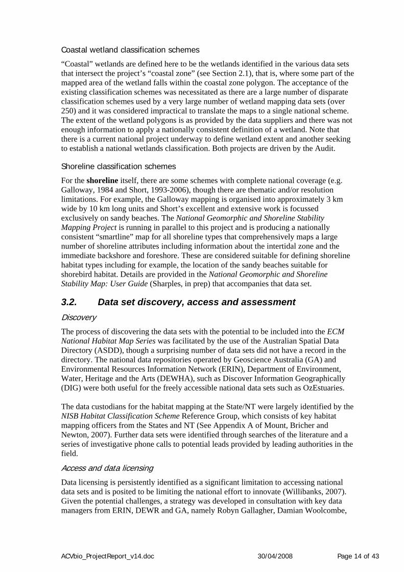
The grid cell maps were produced specifically to assist with visualisation of the data at the regional, state and national scales. The fine, resolution NISB Habitat data is not easily visible when creating maps at these broader coverages. Careful logic was applied to the process as there were concerns that there should neither be an overstatement of the distribution of ECM key habitats leading to misconceptions that the mapping of the continent’s key habitats was competed, nor that the distributions be understated. Firstly, a standard set of grid cells were developed based on the successful use of the 1:100,000 map sheets for a sister weed mapping project within the Audit. Standard 50 km and 10 km cells were produced for the whole of Australia and then subset with the project’s coastal zone polygon. This created the ECM set of grid cells depicted in Figure 2 and Figure 3. The 10 km and 50 km grid cells are precisely nested and have the characteristic of being evenly sized the across the whole continent, both east-west and north-south (See Figure 2 and Figure 3 for an example).


For each key habitat distribution map, each grid cell depicts where the following occurs:

• Firstly, if any of the specified key habitat type occurs, then attribute the cell with “present”

• Secondly, if there is none of the habitat mapped yet the whole area is mapped, mark the cell with “absent”

• Thirdly, if there is none of the habitat mapped and the whole cell is not mapped, then mark the cell as “unknown”.

• Finally, if the entire cell is located in an environment where the habitat could not occur, such as saltmarsh below the high water mark, then mark the cell as “not applicable”.

Clearly, there will be exceptions to these rules and they are completely dependent on the quality of the spatial data, however, they are considered to be robust in a number of ways. Firstly, they are built for the purpose of showing where a habitat has been mapped, no matter how small the patch or the mapping effort. This means the approach will honour the mapper’s observations. Secondly, the method also indicates where further mapping work could be required (i.e. the “unknown” class), thus helping to indicate where significant work remains to be done. It is notable that the classes included in the NISB Habitat Map are drawn from a number of levels within the hierarchy. This is quite acceptable and is regarded as a useful feature of the Classification Scheme, however, when applying the logic described above to a series of nested classes a complex series of logic tests need to be applied. For the purposes of the distribution maps, all coral was lumped together (i.e. both “coral reef substrate” and “coral dominated habitat on a rock substrate” as was all seagrass (i.e. a few seagrasses occur on a rock substrate). It should also be noted that mapping macroalgae via acoustics (i.e. single beam and multi-beam sonar systems) is usually not achievable for technical reasons. This means that, while much of the mapped rock substrate is highly likely to be covered in macroalgae and/or filter feeders, and while it may be reasonable to assume that that is the case, without adequate ground truthing via, for example, a video camera or diver observations, it must be recorded as rock, not macroalgae. This means that the macroalgae mapping is not comprehensive enough to be included in the habitat distribution maps, though with the application of careful assumptions, a reasonable map could be made for particular purposes.

Python scripting and automated processing

Python is a scripting language that can call the ArcGIS geoprocessing modules. The logic used to create the grid cell distribution maps was automated via a Python script. The script was typically applied on a state-by-state-basis. A copy of the script may be obtained by contacting the Project Team leader.


Legend50 km Grid Cells

°

Key ECM Habitat Distribution Maps 50 km grid cells

The national coastal zone grid cell coverage

0 1,000 2,000500Kilometres

Coordinate System - Albers Equal Area Conic, GDA94Map Authors: Richard Mount and Philippa Bricher, UTAS 2008

Figure 2. The 50 km grid cells (here blank) used for displaying the distribution key ECM habitats

Figure 3. An example of the 10 km habitat distribution grid cells nested within the 50 km grid cells.


The National Habitat Map Series Collections

A series of map compilations, or collections, were developed for both the higher level organising entities, such as estuaries and coastal wetlands, and for the less well organised data sets, such as dune vegetation. It is important to note that a different approach was taken to mapping each collection. Firstly, there are a very large number of wetlands spatial databases in Australia. Another Audit project is currently compiling a list of the databases and assessing them for their quality with regard to showing the extent, or area, of Australia’s wetlands. The project is finding that the standards and methodologies for mapping wetlands are very variable. There is also a Wetlands Classification Scheme being developed, again with the assistance of the Audit. As such, it was considered prudent to simply compile the data sets that were available within the project’s time frame and document the remaining data sets. Given the range of approaches to wetland mapping it was considered reasonable to intersect the available data with this project’s coastal zone polygon. This means that if a small part of the wetland falls within the coastal zone the entire wetland is included in the final mapped layer. This approach is based on the assumption that a wetland is usually level and that if any part of the wetland is subject to, for example, inundation or erosion, the whole wetland is potentially affected. The dune vegetation data sets, on the other hand were clipped, or limited, to the extent of the coastal buffer polygon. This decision was based on the assumption that this habitat type is found in non-coastal areas as well as the coastal zone and that, while there is unlikely to be a crisp dividing boundary between coastal and non-coastal areas, it was not possible to accurately delineated this boundary with the evidence to hand. In the absence of higher level evidence, the coastal zone polygon boundary was used.

3.5. QA/QC and data documentation Quality Assurance and Quality Control

The quality of the project tasks was maintained through the application of open communication channels between all members of the UTAS team. The team worked in close proximity and regular discussion took place to establish processing logic, operating procedures and protocols. Feedback is also being sought form the NISB Habitat Classification Scheme Reference Group on the way the Scheme is applied to their data. Domain range and logical tests were applied to the data. More details are available in the ECM National Habitat Map Series User Guide.

ECM National Habitat Map Series User Guide

The User Guide includes the following: • Map Series definition, background and objectives • A brief description of each component and information product • Data Characteristics and Data Dictionary • Data quality information including data set and feature level metadata • The NISB Habitat Classification Scheme (Mount et al, 2007)(see Appendix 1) • Acknowledgements of the Data Suppliers (see Appendix 2) • Summary metadata of the input Data Sources (see Appendix 3)


4. ECM National Habitat Map Series components The following components together comprise the Estuarine, Coastal and Marine National Habitat Map Series:

• The ECM National Habitat Mapping Project Final Report (Mount and Bricher, 2008a)(i.e. this document)

• The derived information products (data sets):

1. The National Intertidal/Subtidal Benthic (NISB) Habitat Map (and associated NISB Habitat MQ (NISB_plus) data set)

2. The National ECM Key Habitat Distribution Map Series (10 km and 50 km grid cell maps)

3. A National Coastal Wetlands Map Collection

4. A National Estuaries Map Collection

5. A National Dune and Dune Vegetation Map Collection, and

6. A National Shoreline Map (derived from the National Geomorphic Shoreline Map or “Smartline” (Sharples and Mount, 2008))

• ECM National Habitat Map Series User Guide (Mount and Bricher, 2008b) including metadata for each product

• The NISB Habitat Classification Scheme Version 1 (Mount et al, 2007) (Appendix 1 of the User Guide)

• Data sources acknowledgement list (Appendix 2 of the User Guide)

• Inventory of habitat mapping data sets (Appendix 3 of the User Guide)

The following sub-sections briefly describe each component and, where applicable, provide examples.

4.1. ECM Habitat Mapping Inventory Over one hundred (100) data sets were located and accessed to support the project. The full list of data sets that were used is presented in Appendix 3 of the User Guide. Each geographic feature in the ECM National Habitat Map Series is attributed with the data supplier’s name and details of the original file and metadata. This both acknowledges the contribution of the source organisation and informs the users of the national map of the various sources of particular features.

4.2. Derived data sets This section focuses on the derived data sets, in particular the National ECM Key Habitat Distribution Map Series. The following 7 figures show the 50 km grid cell series for each of these habitat types:


High level substrate classes

• 1.2 Rock Substrate (i.e. a high level class showing all areas mapped with a predominantly hard substrate that is not coral but including areas also mapped as bare rock, boulders, cobbles, macroalgae and filter feeders (sponges etc))

• Coral (i.e. Includes both 1.1.0.0 Coral Reef Substrate and 1.2.2.3 Coral Dominated Habitat)

• 2.0 Unconsolidated Substrate (i.e. a high level class showing all areas of substrates predominantly consisting of particles of pebble size (<64 mm) or smaller including areas also mapped as seagrass, sediment (sand or silt etc), mangrove or saltmarsh)

Mid level habitat classes

• 2.0.1 Sediment Dominated Habitat (i.e. including all areas dominated by particles of pebble size (<64 mm) or smaller including sands and silts). Note that many mapping agencies do not explicitly map sediments.

• 2.0.2.1 Seagrass Dominated Habitat (i.e. includes areas where seagrasses are the dominant lifeform and have been mapped at least 5% cover (9 m2 reference area).

• 2.0.2.2 Mangrove Dominated Habitat (i.e. includes all areas where mangroves (mangals) are the dominant lifeform)

• 2.0.2.3 Saltmarsh Dominated Habitat (i.e. includes all areas where saltmarsh is the dominant lifeform)

The distribution patterns are a result of both natural ecosystem processes and artefacts of the mapping process. Care should be exercised in distinguishing between the two when using the maps. Firstly, note that the “present” class indicates that a representative of that habitat class has been mapped in the input data sets. This may consist of a single record sometime in the last two to three decades. This means that some of the grid cells depicting presence could be considered to be an overstatement. However, the intention of the maps is to provide a distribution map of known records, NOT a map of abundance, extent, density or condition. Secondly, note the crucial role of the “unknown” class. This class indicates to the user BOTH that there is no mapping of that habitat class in that grid cell AND that the mapping coverage of the area is incomplete. This may be because the mappers of that area did not explicitly target that class (e.g. sediments) or that the mapping effort was not exhaustive (even though it was exhausting, no doubt!). To move a grid cell out of this distribution class requires that further work needs to be completed that produces complete coverage of the grid cell of mapping for that habitat class and shows that the class is either positively present or absent. Another approach would be to identify areas where any particular habitat class could be positively shown to be absent (i.e. could not possibly be present). This could be achieved through judicious application of theoretical and practical knowledge. For example, a national map of the photic zone would produce a significant piece of information that could show deep dark waters where seagrass could not exist. Any “unknown” seagrass grid cells occurring in such areas could be relabelled “not applicable”. It is notable that the distribution maps methodology has produced a paucity of “absent” class grid cells. They only occur in the 10 km grid cells. This result indicates that there



are few cells that are exhaustively mapped. This is a significant insight into the state of habitat mapping around Australia and should be considered in a sober assessment of the need for further habitat mapping. The distribution maps should be read with this thought in mind. Perhaps further information products could be a grid cell map showing the incomplete/completeness status of the grid cells. The final 2 maps show a zoomed in section of the upper Spencer Gulf region. The first map is simply the empty grid cells indicating their relative size and pattern. Note that the 10 km grid cells are nested precisely within the 10 km grid cells. The second map shows the highly detailed NISB Habitat maps and the legend displays the habitat classes. The 10 km grid cells behind the NISB Habitat layer are showing where there is saltmarsh mapped within each cell. If a grid cell is entirely below the high water mark, then it is marked as “N\A”.


ACVbio_ProjectReport_v14.doc

Legend50 km Grid Cells

10 km Grid Cells

°

This map is NOT FOR DISTRIBUTION - it requires further error checking

0 20 4010Kilometres


Acknowledgements and Data SourcesSouth Australian Department of Environment and Heritage

National Intertidal/Subtidal Benthic Habitats

Upper Spencer Gulf Region

Spencer Gulf



LegendNISB_dom02

1.0.0.0 Consolidated

1.1.0.0 Coral Reef

1.2.0.0 Rock Substrate

1.2.1.0 Rock Dominated



2.0.0.0 Unconsolidated

2.0.1.0 Sediment Dominated

2.0.1.1 Pebble Dominated

2.0.1.3 Sand Dominated

2.0.1.4 Silt Dominated

2.0.2.0 Structural Macrobiota Dom


2.0.2.2 Mangrove Dominated

2.0.2.3 Saltmarsh Dominated

3.0.0.0 Unknown

Saltmarsh 10 km Grid CellsPRESENT

ABSENT

UNKNOWN

N\A

°

This map is NOT FOR DISTRIBUTION - it requires further error checking

0 20 4010Kilometres


Acknowledgements and Data SourcesSouth Australian Department of Environment and Heritage

National Intertidal/Subtidal Benthic Habitats

Upper Spencer Gulf Region

4.3. User Guide The ECM National Habitat Map Series User Guide is designed to assist the user to understand the data set. It formally defines the data set via a data dictionary and explains the decisions, assumptions and geoprocessing underpinning the creation of the derived products. It also presents ANZLIC compliant metadata for the various derived products and contains a full inventory of the contributing data sets with contact information. Finally, the NISB Habitat Classification Scheme Version 1 (Mount, Bricher and Newton, 2007) is included to document the class descriptions and decision rules that define the NISB Habitat data set. The User Guide includes the following:

• Map Series definition, background and objectives • A brief description of each component and information product • Data Characteristics and Data Dictionary • Data quality information including data set and feature level metadata • The NISB Habitat Classification Scheme (Mount et al, 2007)(see Appendix 1) • Acknowledgements of the Data Suppliers (see Appendix 2) • Summary metadata of the input Data Sources (see Appendix 3)


5. Discussion of the ECM National Habitat Map Project The ECM National Habitat Map Series has evolved in response to the original project objectives. The original objectives provided a broad direction to the project, which by its very nature had significant unknowns. For example, at the time of drawing up the project there was no national ECM classification scheme. The project team has needed to respond to the situation as it has unfolded. This has included:

• Successfully leading the development of a national habitat classification scheme,

• Developing new geoprocessing techniques, and • Producing new information products to suit the data as it was collated and its

characteristics emerged. The detailed and innovative strategy taken with the data licensing also evolved as the limitations of the standard data licensing approach became more obvious. Excellent goodwill was shown to the project objectives with a strong collaborative ethic emerging as the project proceeded. This indicates that the project is well-founded and is regarded as meeting a need at both the Australian Government and State/NT levels. A number of spin-off tasks and projects are proceeding. For example, there are a series of meetings initiated at the state level for discussing and further developing the NISB habitat Classification Scheme. The NISB Habitat Classification Scheme proved to be robust, though ongoing development of the scheme is important to retain relevance and credibility, particularly with increasing attention and demands being made to produce high quality habitat information products. Recommendation: That there is ongoing development of the NISB Habitat Classification Scheme to support the national habitat mapping effort. An interesting observation arose as the NISB Habitat Classification Scheme process unfolded. It became clear that the habitats as defined in the scheme were very similar to land cover mapping in terrestrial environments except that they were covered, more or less often, with water. Given that legally the benthic marine environment is defined as “land covered by water” (i.e. “subaqueous land” rather than “subaerial land”) it may be useful to consider including the benthic marine environment in national land cover mapping schemes. It would also be valuable to consider how other current marine mapping data sets could contribute to “land use” mapping schemes (e.g. ACLUMP, 2006). For example, aquaculture leases and port areas are all mapped. Recommendation: That the NISB Habitat Map be considered for inclusion into the national land cover mapping data set. It is important to note that Distribution maps are based on the NISB_plus Habitat (or NISB Habitat (Mixed Quality (MQ)) data set. That data set includes as series of data that did not meet the criteria for inclusion in the standard NISB Habitat data set. This was done because there was too much valuable information in those data sets to simply not include them. For example the Great Barrier Reef Marine Park Authority “Dry Reef” data set does not clearly classify the “reef” polygons into type and thus it is impossible to distinguish sandy shoals from coral or rocky reef. An assumption was


made that there is highly likely to be some coral within each 50 km grid cell over the Dry Reef data set, but this is not confirmed. Recommendation: Note the significant difference between the NISB Habitat data set and NISB Habitat MQ (NISB_plus) data set be noted. The ECM National Habitat Map Series information products are designed for some immediate purposes, though it may be anticipated that many other uses will be found for the data sets. For example, the series could be used for updating the Oil Spill Response Atlas (OSRA). It is important then to develop a mechanism for reviewing and updating the data. This is best achieved by developing solid reciprocal relationships with the key data suppliers, in this case, primarily the state/NT ECM mapping agencies. Providing access to high spatial resolution national data sets, such as remote sensing products, would be an excellent way of contributing to the overall national mapping effort. Recommendation: That the national data sets are systematically distributed back to the various data suppliers for review and, if possible, they are supported to enable updating on a regular basis. It became clear that some of the key habitat types were not easily compiled into a single map of habitats – for example seagrass and estuarine mapping. The differences in the characteristics of the habitat types have been referred to throughout the report and will not be repeated here. Suffice to say, that a series of information products needed to be developed to enable logical and comprehensive compilation of the data. A further, complication was provided by the varied nature of the classification schemes used for some habitat groupings – in particular, dune vegetation and wetlands. Further work is warranted in harmonising the schemes and data sets, and it is noted that the Audit is stimulating such work in the wetlands area. Recommendation: That further work is considered for collating and translating national wetlands data sets into a national wetlands classification scheme. The collation of the dune vegetation data sets were particularly challenging. Often there were data sets mapping dunes, but these gave no indication of the vegetation condition. A decision was made to compile the dune mapping that was available within the project time frame and then to use geoprocessing commands to combine it with the NVIS dune vegetation polygons. Again, classification issues made it challenging to collate all the dune vegetation mapping into a single layer. Given its potential for rapid changes through time, this data set would be a good candidate for high temporal resolution mapping and monitoring methods. Recommendation: That dune vegetation is considered as a candidate for further high resolution mapping and monitoring work.

6. Conclusions The objectives of each of the parties in the project partnership were readily aligned. The Audit’s objective for data to support the key ECM habitat extent for NRM purposes is well matched to the DCC’s need for a rapid collation of the key habitat subject to climate change impacts as defined in the Voice et al. (2006) report.


Acknowledgements A large undertaking such as this requires goodwill and commitment from many people. We are very grateful for all the support provided to us by the many partners in this truly national (in the inclusive sense of the word!) project. The NISB Habitat Classification Scheme is the result of the work of many people including those who, over the years, have led the development of habitat mapping in the challenging coastal and marine environments. We would like to particularly acknowledge the following people who have directly contributed to the production of this scheme: David Ball, Victoria; Ewan Buckley, Chris Simpson and Kevin Bancroft, WA; Alan Jordan, NSW; Vanessa Lucieer, Tasmania; Len McKenzie, QLD; David Miller, SA; Elvira Poloczanska, CSIRO; David Ryan, GA; Neil Smit, NT; Rob Thorman, Audit; and Gina Newton. Most of these people were also key contacts in the state agencies who smoothed the way to obtaining access to the data sets and have provided willingly of their time in explaining the detail of their data – many thanks to you all. Daniel Ierodiaconou was very responsive in tight circumstances – thanks Dan. Jo Klemke and Anth Boxshall have also been helpful in Victoria. Stuart Phinn and Mike Ronan look like picking up the classification ball in Queensland and run with it some more and Ewan Buckley is a total gem and doing a similar job in WA. Rob Williams does what he knows best in NSW – map macrophytes. The likes of Matthew Royal, David Miller, Bryan McDonald, Sam Gaylard and Doug Fotheringham have done some great work in SA. Neil Smit and the others in NT managed to come up with some great data sets for the project. At the Audit, Rob Thorman steered the ship skilfully through its many stages and was particularly able in scoping the project in a realistic way. Data licensing gurus including Peter Wilson, Audit, Robyn Gallagher, ERIN (then GA), Damian Woolcombe, ERIN and Brian Burbridge, GA provided excellent advice about how to tackle the minefield that is data licensing. We all dream of whole of government licensing made easy! The UTAS team consists of Richard Mount, Phillippa Bricher, Jenny Newton, Katherine Tattersall and Simon File. They were magnificently supported by the following generous colleagues: Tore Pedersen, Luke Wallace, Dom Jaskierniak, Chris Sharples and Samya Jabbour. The UTAS team would also like to acknowledge the support they have received from the School of Geography, especially Jon Osborn and Elaine Stratford. At UTAS Innovation we would particularly like to appreciate the boundless enthusiasm and enabling approach of Tony Baker and his team, including the legal advice from Richard Atkins.


References

ACLUMP (2006). Guidelines for land use mapping in Australia: principles, procedures and definitions, Australian Government Bureau of Rural Sciences

Ball, D., S. Blake and A. Plummer (2006). Review of Marine Habitat Classification Systems.

No. 26, Parks Victoria. Bancroft, K. P. (2002). A standardised classification scheme for the mapping of shallow-water

marine habitats in Western Australia., Marine Conservation Branch, Department of Conservation and Land Management, WA.

Banks, S. A. and G. A. Skilleter (2002). "Mapping intertidal habitats and an evaluation of their

conservation status in Queensland, Australia.” Ocean and Coastal Management 45: 485-509.

Burrough, P. A. and R. A. McDonnell (1998). Principles of Geographical Information Systems.

Oxford University Press. Butler, A., P. Harris, V. Lyne, A. Heap, V. Passlow and R. Porter-Smith (2001). An Interim

Bioregionalisation for the continental slope and deeper waters of the South-East Marine Region of Australia., National Oceans Office.

Cocito, S. (2004). "Bioconstruction and biodiversity: their mutual influence." Scientia Marina

68(Supplement 1): 137-144. Cowardin, L. M., V. Carter, F.C. Golet and E.T. LaRoe (1979). Classification of wetlands and

deepwater habitats of the United States. Washington, D.C, U.S. Department of the Interior, Fish and Wildlife Service: 79.

Delaney, J. and K. Van Neil (2007). Geographical Information Systems - An Introduction.

Melbourne, Oxford University Press. DEWR (2007). Australia’s Native Vegetation – A Summary of Australia’s Major Vegetation

Groups, 2007. Australian Government Department of the Environment and Water Resources.

Diaz, R. J., M. Solan and R. Valente. (2004). "A review of approaches for classifying benthic

habitats and evaluating habitat quality." Journal of Environmental Management(73): 165-181.

Duarte, C.M. and C.L. Chiscano. (1999) “Seagrass biomass and production: a reassessment”,

Aquatic Botany (65:1): 159-174. Gregorio, A. D. and L. J. M. Jansen (2005). Land Cover Classification System - Classification

concepts and user manual. Rome, Food and Agriculture Organization of the United States.



Hilbert, D. W., L. Hughes, J. Johnson, J. M. Lough, T. Low, R.G. Pearson, R.W. Sutherst and S. Whittaker (2007). Biodiversity conservation research in a changing climate, Australian Government Department of the Environment and Water Resources: 72.

IMCRA (1997). Interim Marine and Coastal Regionalisation for Australia: an ecosystem-based

classification for marine and coastal environments. Version 3.2. Canberra, Environment Australia, Commonwealth Department of the Environment.

Kvitek, R., P. Iampietro, E. Sandoval, M. Castleton, C.Bretz, T. Manouki and A. Green (1999).

Final Report Early Implementation of Nearshore Ecosystem Database Project, Institute for Earth Systems Science and Policy

Lilley, S. E. and D. R. Schiel (2006). "Community effects following the deletion of a habitat-

forming alga from rocky marine shores" Oecologia 148: 672–681 Mount, R., P. Bricher and J. Newton (2007). National Intertidal/Subtidal Benthic (NISB)

Habitat Classification Scheme Version 1. Hobart, University of Tasmania: 29. Mount, R. and P. Bricher (2008). ECM National Habitat Map Series User Guide Version 1.

Hobart, University of Tasmania. Report to the Department of Climate Change and the National Land and Water Resources Audit, Canberra, ACT.: 43.

NOO (2006). Version 4.0 A Guide to the Integrated Marine and Coastal Regionalisation of

Australia, Australian Government Department of the Environment and Heritage: 15.

NOO (2002). Ecosystems - nature's diversity. The South-east Regional Marine Plan

Assessment Reports. Hobart, National Oceans Office: 214. Roy, P. S., Williams, R. J., Jones, A. R., Yassini, R., Gibbs, P. J., Coates, B., West, R. J.,

Scanes, P. R., Hudson, J. P., and Nichol, S., (2001). “Structure and function of southeast Australian estuaries.” Estuarine, Coastal and Shelf Science. 53:351-384.

Rule, M., A. Jordan, et al. (2007). The Marine Environment of Northern New South Wales - A

review of current knowledge and existing datasets, Northern Rivers Catchment Management Authority: 202.

Sharples, C. (2008, in prep.). National Shoreline Geomorphic and Stability Mapping Project:

User Guide. Hobart, School of Geography and Environmental Studies, University of Tasmania. Report to the Department of Climate Change and the National Land and Water Resources Audit, Canberra, ACT.

Sharples, C. and R. Mount (2008, in prep.). National Shoreline Geomorphic and Stability

Mapping Project Report. Hobart, School of Geography and Environmental Studies, University of Tasmania. Report to the Department of Climate Change and the National Land and Water Resources Audit, Canberra, ACT.

Appendix 1: Data License Usage and Request Letter



<Contact name>

<Data Supplier Organisation>

<Address>

National Estuarine, Coastal and Marine (ECM) Habitat Mapping Project A Department of Climate Change /National Land and Water Resources Audit Partnership Project Dear <First name>

We are writing to both inform you, firstly, on the progress and anticipated benefits of the ECM Habitat Mapping Project (the Project) and, secondly, to request confirmation of your understanding of the uses to which it is intended to put the final information products.

Firstly, we are pleased to let you know that the data you have supplied (See Schedule 1) to the project team in the Spatial Science Group at UTAS has supported the production of an Australia-wide enhanced information product that depicts coastal and marine habitat types at a higher spatial resolution than achieved ever before in Australia. The enhanced product is made possible due to the combination of a large number of data sources into a carefully established, nationally-consistent and agreed habitat classification scheme. The data sources, including your own, have been subjected to an assessment process and precision geoprocessing techniques. This has enabled the production of three information products as follows:

8. The national simplified thematic (class) resolution, high spatial resolution ECM Habitat map

9. The national 10 km grid cell map depicting the regional distribution of each key habitat type

10. The national 50 km grid cell map depicting the national distribution of each key habitat type

We are extremely pleased with the high level of cooperation and participation in this project; it is clearly a project that is considered relevant and timely to all parties. The project team is very keen to see the value of the work realised by as many people and agencies as possible. To this end the project outputs are intended to be delivered back to the original data suppliers, or the relevant agency, in each state.

By way of background on the genesis and governance of the project, this work was initiated by the Department of Climate Change (DCC; formerly the Australian Greenhouse Office) and managed by the National Land and Water Resources Audit (Audit). The project forms a part of the wider National Coastal Vulnerability Assessment (CVA), as described in more detail in the attached CVA project background document. The team at UTAS are under contract to produce and deliver the Habitat Map to the DCC via the Audit. The DCC will then conduct further coastal vulnerability assessments of the impacts of climate change on, for example, the built infrastructure and biodiversity, using a range of data inputs including the Habitat Map together with data such as wave climate modelling from CSIRO and BOM. The information products generated from this work will be delivered into the public domain, including via the OzCoasts web site maintained by GA. Both GA and the DCC have clearly documented policies of providing free public access to all their information products under the Australian Government Policy on Spatial Data Access and Pricing (http://www.osdm.gov.au/policy/accessPricing.html).



While the vulnerability of the coast to climate change has provided the impetus for this work, the ECM Habitat Map will be useful for a very large range of other uses. Some of these are listed as follows:

• Support for the development of national key habitat extent and distribution indicators by the National Land and Water Resources Audit (Audit) for reporting on coastal habitats.

• A consistent national input to future marine bioregionalisation processes, particularly supporting the development of IMCRA Bioregion sub-regions (or “ecoregions”)

• Upgraded, nationally consistent Oil Spill Response Atlas (OSRA) habitat mapping for all states

• Enhanced information inputs to coastal planning including the flagging of the location of key coastal habitats at potentially higher risk of impact from development pressures

• An inventory of key habitat natural assets to assist NRM projects and activities

• Underpinning of improved wildlife management requiring detailed habitat type mapping

To enable these uses, the ECM Habitat Map information products are being derived in part from the input data including the data you supplied (this work is now almost complete). Following its production, access will need to be provided to the Habitat Map, preferably as broadly as possible. It is proposed that a tiered approach be taken to the use of, and access to the data, as follows:

4. That UTAS use the supplied data to produce the ECM Habitat Map and provide the derived information products to the DCC via the Audit including:

a. The ECM Habitat map

b. The national 10 km grid cell map

c. The national 50 km grid cell map

5. That the DCC and the Audit (representing the Australian Government) publish the resulting information products via simple visual representations of the data, such as hard copy figures in reports and via Web Mapping Services (WMS) including OzCoasts, the web site managed by Geoscience Australia.

6. That the DCC and Audit (representing the Australian Government) distribute the resulting information products via standard Office of Spatial Data Management’s (OSDM) data licenses as used by the AG for other nationally produced data sets, such as the National Vegetation Information System (NVIS), the Australian Soil Resource Information System (ASRIS) and award winning MapConnect.

While the UTAS team previously informed you of the way in which the data you supplied to us is to be used when we entered into the original data licensing agreements, we want to make sure that these uses are clearly stated and maximise mutual understanding. We would appreciate it if you could advise us that you, or your agency, either

1. Confirm that one or more of the above uses are acceptable, or,

2. Have objections to one or more of the intended uses as defined above.

Your response by letter or email would be appreciated as soon a possible, and at the latest, within a month of receiving this letter.

Please feel free to contact the UTAS team leader, Richard Mount, about any of these matters.

Yours on behalf of the partnership project team

Richard Mount, UTAS Blair Wood, Audit Stefanie Pidcock, DCC

Contact Details:

Dr Richard Mount Phone: (03) 6226 2106 Email: [email protected] Phillippa Bricher Phone: (03) 6226 1981 Email: [email protected]

Postal Address: School of Geography & Environmental Studies (Spatial Science), University of Tasmania, Private Bag 76, Hobart, Tasmania. 7001

mailto:[email protected]

mailto:[email protected]



Schedule 1 <Data set name> <maybe, shapefile name>

Project Report - OzCoasts · Estuarine, Coastal and Marine (ECM) National Habitat Mapping Project ....

Documents

Transcript of Project Report - OzCoasts · Estuarine, Coastal and Marine (ECM) National Habitat Mapping Project ....