Project Number: ME – CF –MO08

MINIATURIZATION OF AN OPTOELECTRONIC HOLOGRAPHIC OTOSCOPE FOR

MEASUREMENT OF NANODISPLACEMENTS IN TYMPANIC MEMBRANES

A Major Qualifying Project Report

Submitted to the Faculty

of the

WORCESTER POLYTECHNIC INSTITUTE

in partial fulfillment of the requirements for the

Degree of Bachelor of Science

in Mechanical Engineering

by

______________________________

Geoffrey Karasic

______________________________

Nathan Largesse

______________________________

Lucas Samuel Lincoln

Date: 30 April, 2009

Keywords:

1. laser interferometry

2. tympanic membrane

3. ray tracing

______________________________

Professor Cosme Furlong

i

Abstract

A first generation optoelectronic holographic otoscope (OEHO) is currently in use in a major

hospital. The OEHO allows for nanometer-displacement measurements of the deformation of

mammalian tympanic membrane (TM) under acoustic stimulation and consists of a laser delivery

system, an optical head, a data acquisition PC, and an acoustic excitation system. The optical head in

the current system is sufficient for laboratory use, but requires improved thermomechanical stability,

depth of field, and focusing ability to be suitable for the clinic. Additionally, the medical doctors

working with the current device have indicated miniaturization and improved ease of use are

necessary for full-scale clinical deployment.

In this project, in order make the improvements required for clinical deployment, the optical

and biomechanical properties of the tympanic membrane are reviewed; design parameters

determined; and a design synthesized with the aid of ray tracing analysis and consideration of optical

characteristics. An optical head is prototyped, the optical performance is quantified and the device is

validated through comparison of measured data with analytical and computational solutions.

Measurements of a post-mortem chinchilla membrane are used to compare the device performance to

the previous generation.

The resulting optical head has an improved depth of field, focusing ability; and reduced size

compared to the previous generation. Drawbacks of the design are discussed and recommendations

are made for future work.

ii

Acknowledgements

The group would like to thank Professor Cosme Furlong for his dedication, guidance, and expertise

throughout the duration of this project. We also would like to acknowledge the graduate and post-

graduate students working beside us in the Center for Holographic Studies and Laser micro-

mechaTronics for their assistance and instruction. We are also thankful for Dr. Rosowski of the

Massachusetts Eye and Ear Infirmary for his time, efforts, and feedback; and to Adriana Hera for her

endless knowledge and support.

Lastly, we are grateful to the Mechanical Engineering Department of Worcester Polytechnic

Institute for the opportunity and privilege to work on a challenging, state-of-the-art project.

iii

Table of Contents

Abstract ................................................................................................................................................... i

Acknowledgements ................................................................................................................................ ii

List of Figures ....................................................................................................................................... vi

List of Tables ......................................................................................................................................viii

1. Introduction ...................................................................................................................................... 9

2. Tympanic Membrane Function, Histology, and Characteristics .................................................... 11

2.1. Function of Tympanic Membrane............................................................................................ 11

2.2. Physical Characteristics of the Tympanic Membrane .............................................................. 12

2.2.1. Young‟s Modulus .............................................................................................................. 14

2.3. Histology of the Tympanic Membrane .................................................................................... 14

2.4. Hearing Capabilities and Vibration Modes .............................................................................. 19

2.5. Techniques for Studying Displacements.................................................................................. 21

2.5.1. Clinical Relevance for Studying Displacements ............................................................... 21

2.5.2. State of the Art .................................................................................................................. 21

2.5.3. Mathematical Models of the Tympanic Membrane .......................................................... 22

2.5.4. Design Requirements for an Optical System .................................................................... 24

2.6. Light Tissue Interactions .......................................................................................................... 24

2.7. Optical Characteristics ............................................................................................................. 25

2.7.1. Reflection Spectra of the Human Tympanic Membrane................................................... 25

2.7.2. Coatings to Increase Reflectivity ...................................................................................... 27

3. Interferometry ................................................................................................................................. 29

3.1. Fundamentals ........................................................................................................................... 29

3.2. Double-exposure holography ................................................................................................... 30

3.3. Time-averaged holography ...................................................................................................... 32

4. Previous Work ................................................................................................................................ 35

4.1. Laser Delivery System ............................................................................................................ 36

4.2. Optical Head ........................................................................................................................... 37

4.3. Image Processing Software ..................................................................................................... 38

4.4. Performance of Previous Generation ...................................................................................... 39

5. Objective ......................................................................................................................................... 40

6. Computer Modeling ........................................................................................................................ 42

6.1. Ray Tracing Principles ............................................................................................................ 43

6.2. Ray Tracing Computational Model......................................................................................... 47

iv

7. Optical Head Configuration ............................................................................................................ 50

8. Realization ...................................................................................................................................... 54

8.1. Building the Prototype ............................................................................................................. 54

8.2. Characterization of Optical Performance ................................................................................. 56

8.2.1. Field of View .................................................................................................................... 56

8.2.2. Magnification .................................................................................................................... 57

8.2.3. Resolution ......................................................................................................................... 59

8.2.4. Depth of Field ................................................................................................................... 60

8.2.5. Image Aberration .............................................................................................................. 63

9. Validation ........................................................................................................................................ 66

9.1. Analytical Validation ............................................................................................................... 66

9.2. Computational Validation ........................................................................................................ 72

9.3. Experimental Validation .......................................................................................................... 74

9.3.1. Experimental Procedure .................................................................................................... 74

9.3.2. Experimental Results ........................................................................................................ 76

9.4. Validation Results Comparison ............................................................................................... 78

10. Testing ........................................................................................................................................... 79

11. Recommendations and Future Work ............................................................................................. 83

12. References ..................................................................................................................................... 85

13. Appendix A. Biology Summary – Human TM. ............................................................................ 88

14. Appendix B. TracePro Model Details. .......................................................................................... 89

14.1. Introduction to TracePro ........................................................................................................ 90

14.1.1. Defining Geometry and Optical Characteristics ............................................................. 90

14.1.2. Light sources and ray trace options................................................................................. 95

14.1.3. Tracing Rays and Analysis Tools ................................................................................. 101

14.2. Otoscope Head Model Details ............................................................................................. 107

14.2.1. GRIN Lens ILW ........................................................................................................... 107

14.2.2. GRIN ROD ................................................................................................................... 108

14.2.3. Imaging Lens Achromat................................................................................................ 111

14.2.4. Beamsplitter Cube ......................................................................................................... 116

14.2.5. Optical Fibers ................................................................................................................ 119

14.2.6. CMOS sensor chip ........................................................................................................ 122

15. Appendix C. Optical Characterization Details. ........................................................................... 123

15.1. Resolution Algorithm ........................................................................................................... 123

15.2. Depth of Field Algorithm ..................................................................................................... 124

v

15.3. Image Aberration Algorithm ................................................................................................ 125

16. Appendix D. Component Specifications. .................................................................................... 128

16.1. GRIN Lens ........................................................................................................................... 129

16.2. 5mm Diameter Imaging Lens .............................................................................................. 131

16.3. 6.35mm Diameter Imaging Lens ......................................................................................... 135

16.4. Beam Splitter ....................................................................................................................... 139

16.5. Patch Cable .......................................................................................................................... 142

16.6. si1280 Camera ..................................................................................................................... 144

vi

List of Figures

Fig. 1. Components of middle ear. ...................................................................................................... 11

Fig. 2. Tympanic membrane to stapes area ratio2. .............................................................................. 12

Fig. 3. Human tympanic membrane showing two parts7. ................................................................... 13

Fig. 4. Relative sizes of mammalian tympanic membranes9. ............................................................. 14

Fig. 5. Two sections of human tympanic membrane. Upper - Pars Flaccida. Lower - Pars Tensa. .. 15

Fig. 6. Artist's conception of the migrating pattern of the epidermis in the tympanic membrane of

humans and guinea pigs11. ................................................................................................................... 17

Fig. 7. A SEM photomicrograph of the outer radial and inner circular fibers and the parabolic fibers

in the fibrous layer of the para tensa11. ................................................................................................ 18

Fig. 8. Artist's conception of the fiber arrangement of the human tympanic membrane. SP: short

process of the malleus; U: umbo; TIR: trigonum interradiale; C: circular fibers; R(1): radial fibers

which attach straight into the annular ring; R(2): a few radial fibers which cross paths; T: transverse

fibers; P: parabolic fibers; SMR: sub-mucous fine radial fibers11. ...................................................... 18

Fig. 9. Calculated Vibration Modes of Human TM at 80 dB SPL8. ................................................... 20

Fig. 10. Common Examples of Sound Pressure Levels. ..................................................................... 20

Fig. 11. Tympanic Membrane Displacement at approximately 0.5kHz; FEM (a) vs. Measured (b)8.

.............................................................................................................................................................. 23

Fig. 12. Reflection spectra of healthy human adult taken in vivo.23 ................................................... 26

Fig. 13. Schematic of the three OEHO subsystems. ........................................................................... 35

Fig. 14. Previously Developed Otoscope Head18. ............................................................................... 37

Fig. 15. Laboratory environment of previous generation. .................................................................. 39

Fig. 16. Existing otoscope form, ......................................................................................................... 41

Fig. 17. Flowchart of design process used. ......................................................................................... 42

Fig. 18. Geometry of ray translation between two reference surfaces. ............................................... 44

Fig. 19. Geometry of refraction at a curved surface3. ......................................................................... 45

Fig. 20. Gaussian distribution through system; showing input, post imaging lens, and output on

CMOS chip. ......................................................................................................................................... 49

Fig. 21. Schematic of the optical head showing object beam and reference beam optical fibers (OB

and RB, respectively), gradient-index rod lens (GRIN), imaging lens achromat (IL), beam combiner

cube (BC) and CMOS camera (CAM). ................................................................................................ 50

Fig. 22. GRIN lens Pitch concept illustration. .................................................................................... 51

Fig. 23. Off-axis performance of achromatic doublet versus plano-convex lens. .............................. 52

Fig. 24. Spectral response of SI-1280 Camera. ................................................................................... 53

Fig. 25. Miniaturized Otoscope Head. ................................................................................................ 54

Fig. 26. Previous Generation Otoscope Head18 (Left); Miniaturized Otoscope Head (Right). .......... 55

Fig. 27. Field of View And Magnification Image. .............................................................................. 57

Fig. 28. 1951 USAF Resolution Target. ............................................................................................. 59

Fig. 29. Depth of Field Test. ............................................................................................................... 61

Fig. 30. Depth of Field Contrast Trace Graph. ................................................................................... 62

Fig. 31. Grid Distortion Target. .......................................................................................................... 63

Fig. 32. Distortion Function. ............................................................................................................... 64

Fig. 33. Prismatic Beam. ..................................................................................................................... 66

Fig. 34. Finite Element Beam. ............................................................................................................ 72

Fig. 35. Cantilever Test Setup. ............................................................................................................ 74

Fig. 36. Nitrile Membrane Test Setup................................................................................................. 79

vii

Fig. 37. (a) Nitrile Membrane at 4.228kHz; (b) Nitrile Membrane at 10.66 kHz; (c) 3-D

Representation of Nitrile Membrane at 10.66kHz. .............................................................................. 80

Fig. 38. Chinchilla Test. ...................................................................................................................... 81

Fig. 39. Time-Averaged Image of Chinchilla ..................................................................................... 81

Fig. 40. Annotated screenshot of TracePro environment. ................................................................... 90

Fig. 41. TracePro: 'View' Menu. ......................................................................................................... 91

Fig. 42. TracePro: 'Insert' toolbar. ....................................................................................................... 91

Fig. 43. TracePro: 'Insert' dialog. ........................................................................................................ 91

Fig. 44. TracePro: Boolean toolbar. .................................................................................................... 92

Fig. 45. TracePro: Example Model Tree............................................................................................. 92

Fig. 46. TracePro: 'Apply Properties' dialog. ...................................................................................... 93

Fig. 47. TracePro: Material Property Editor. ...................................................................................... 94

Fig. 48. TracePro: Menu for editing of property data catalogs. .......................................................... 95

Fig. 49. TracePro: Source Tree. .......................................................................................................... 96

Fig. 50. TracePro: 'Define' menu. ....................................................................................................... 96

Fig. 51. TracePro: Definition of a grid source. ................................................................................... 97

Fig. 52. TracePro: Accessing „Raytrace Options‟. .............................................................................. 98

Fig. 53. TracePro: 'Raytrace Options' Dialog. .................................................................................... 99

Fig. 54. TracePro: Importance Sampling target definition. .............................................................. 101

Fig. 55. TracePro: 'Analysis' Toolbar. .............................................................................................. 101

Fig. 56. TracePro: 'Ray Sorting' Dialog. ........................................................................................... 102

Fig. 57. TracePro: Raytrace with no ray sorting. .............................................................................. 103

Fig. 58. TracePro: Ray trace with ray sorting, 'Selected Surface', enabled. ..................................... 104

Fig. 59. TracePro: Analysis Tool Buttons......................................................................................... 104

Fig. 60. TracePro: Ray table excerpt................................................................................................. 105

Fig. 61. TracePro: Sample Irradiance Map. ...................................................................................... 105

Fig. 62. TracePro: Image of raytrace through ILW component, with characteristic result. ............. 108

Fig. 63. TracePro: Image of raytrace through SRL (ILW and Rod combination) component, with

characteristic result. ........................................................................................................................... 108

Fig. 64. TracePro: 'Apply Properties' dialog for Gradient Index definition. ..................................... 109

Fig. 65. TracePro: Selecting the step size of the gradient index. ...................................................... 110

Fig. 66. Achromat diagram with variable convention. ..................................................................... 111

Fig. 67. TracePro: Image of raytrace through achromatic doublet component, with characteristic

result. .................................................................................................................................................. 112

Fig. 68. TracePro: Building the acromat crown, showing the untrimmed surfaces. ......................... 114

Fig. 69. TracePro: Building the achromat crown, showing the tube used to trim for diameter

specification. ...................................................................................................................................... 115

Fig. 70. TracePro: Resulting achromat crown. ................................................................................. 115

Fig. 71. TracePro: Image of raytrace through beamsplitter component, with characteristic result. . 116

Fig. 72. TracePro: Construction of the BS cube, showing the base block and trimming rectangle .. 117

Fig. 73. TracePro: Beamsplitter prism. ............................................................................................. 117

Fig. 74. TracePro: BS construction image, showing the three bodies required to create the splitter.

............................................................................................................................................................ 118

Fig. 75. TracePro: Distribution plot and raytrace of grid source with Nufern 460HP optical fiber

characteristics. Block for distribution monitoring. ........................................................................... 120

Fig. 76. TracePro: Grid source testing block. ................................................................................... 121

viii

List of Tables

Table 1. Contents of various mammalian tympanic membranes9. ...................................................... 16

Table 2. Hearing Frequency Ranges of Different Mammalian Species. ............................................ 19

Table 3. Illustrative component ray traces and construction notes. ................................................... 48

Table 4. Analytically Determine Natural Frequencies. ....................................................................... 71

Table 5. Finite Element Modes of Cantilever. .................................................................................... 73

Table 6. Experimental Modal Frequencies obtainted with ................................................................. 77

Table 7. Analytical and Computational Percent Error. ....................................................................... 78

Table 8. ILW Tracepro specifications............................................................................................... 107

Table 9. GRIN rod TracePro parameters. ......................................................................................... 108

Table 10. AC050-010-A1 TracePro parameter table. ....................................................................... 112

Table 11. Beamsplitter (BS010) TracePro parameter table. ............................................................. 116

Table 12. Grid Source parameters for Nufern 460HP optical fiber. ................................................. 119

Table 13. SI1280 CMOS sensor parameter table. ............................................................................. 122

9

1. Introduction

The tympanic membrane (TM) is a component of the middle ear which helps transmit sound

energy into psychoacoustic signals to provide the sensation of hearing. Despite its important and

irreplaceable function in human and other mammalian bodies, the current understanding of the

function of the TM leaves much to be desired. Diagnosis of hearing disorders and malfunction are

almost exclusively performed via qualitative investigation of the membrane. The medical

community has desired a tool for the quantitative measurement of the tympanic membrane‟s response

to acoustic stimulus.

This desire was recently answered with the development of an opto-electronic holographic

otoscope1 (OEHO). This tool provides a full-field of view, video rate deformation measurement

system of the tympanic membrane, and has a resolution on the order of nanometers. It is installed at

the Massachusetts Eye and Ear Infirmary (MEEI) and has provided the medical professionals the

ability to gather previously unavailable information on the response of mammalian tympanic

membranes to acoustic stimulation.

This modern tool has proved an invaluable resource to the MEEI laboratory researchers, and

a full scale clinical deployed is desired. The current generation requires a number of improvements

prior to this clinical deployment, primarily a miniaturized size; an increased depth of field; an

intuitive magnification and focusing system; and an increased thermomechanical stability.

The goal of this MQP, and the task described herein, was to redesign the OEHO in order to

address these improvements. Special attention was paid to creating a device which requires little

technical training and can be packaged in a otoscope-like package; while reducing the overall size of

the OEHO and achieving better optical performance.

10

In order to achieve this task, the biology of the tympanic membrane was first investigated to

understand the requirements of the system, as well as what potential difficulties are encountered by

measuring a biological sample and how these can be addressed.

Following this, an optical configuration was developed utilizing existing optical design tools

and auxiliary research. The configuration was designed to meet the constraints of the project as well

as address the improvements indicated above.

Finally, the device was prototyped and evaluated, as well as validated through the

comparison of analytical, computational, and experimental solutions to a known dynamic system.

The device was used by the medical professionals at MEEI to measure the tympanic membrane

deformations of a post-mortem chinchilla and conclusions and further improvements are described.

11

2. Tympanic Membrane Function, Histology, and Characteristics

2.1. Function of Tympanic Membrane

To understand the function and importance of the tympanic membrane, one must have a

general knowledge of how a vibration in the air becomes a sound heard in the human brain. A sound

wave travels into the ear via the auditory canal. It then contacts directly the tympanic membrane. It

is here that the sound energy is transferred from a gas (air) medium to a solid (the tympanic

membrane). This can be related to the opposite of how a loudspeaker functions2. The vibrating air

causes the tympanic membrane to vibrate accordingly, in simple or complex patterns. Attached to

the membrane is a bone, the malleus, which moves precisely as the membrane vibrates. Next, the

energy passes through two additional bones, the incus and then the stapes. See Fig. 1. The energy

moves from the footplate (end) of the stapes to the inner ear, now traveling through a fluid. The

energy is channeled through the cochlea, the auditory input of the inner ear. The sound energy

stimulates hair cells, which produce synaptic activity that evokes action potentials that travel down

the cochlea and to the brain2.

Fig. 1. Components of middle ear3.

12

Hearing requires the transfer of sound from a gaseous medium, to a solid, and finally a fluid,

where it is translated into an electric potential4. If one can imagine listening to someone speak in air

while submerged underwater, one can appreciate the brilliance of how the ear functions. The

primary purpose of the tympanic membrane is to receive the sound energy from air, and then amplify

it through solid tissue and bones. This amplification is possible due to what Katz calls the Areal

relationship4. For the sake of explanation, ignore the malleus and incus bones, as they do little to

affect the sound energy and only link the tympanic membrane to the stapes. The tympanic

membrane has a much greater area (15 to 20 times) than the footplate of the stapes, the bone

responsible for transmitting the sound energy into a fluid5. The sound pressure (PTM) acting on the

TM produces a force (F) equal to the product of the pressure and the TM area (A). This force is

conducted to the stapes footplate, which produces a pressure in the inner ear (PS) equal to the ratio of

the force and the area of the footplate as described by the relationship PS/PTM = ATM/AS. This

transformer process helps overcome the difference in impedance between air and cochlear fluid6,

see Fig. 2.

Fig. 2. Tympanic membrane to stapes area ratio2.

2.2. Physical Characteristics of the Tympanic Membrane

The human tympanic membrane is elliptical in shape. Tympanic membranes of all

mammalian species consist of two parts: the Pars Flaccida and the Pars tensa, see Fig. 3. Although

13

there is variation in shape and size among humans, it is generally accepted that the horizontal axis is

9 to 10mm long and the vertical axis is 8 to 9mm long7. The approximate density of the tympanic

membrane is 1200 kg/m3 8. The pars tensa portion of the tympanic membrane has an approximate

thickness of 34μm and the pars flaccida portion measures approximately 110μm9. Very loud sounds

produce a displacement of the TM up to 1μm4. Changes in pressure due to swallowing can produce

displacements of up to 0.5mm6.

The size and shape of the tympanic membrane varies greatly in other mammalian species, see

Fig. 4. In all species, the pars flaccida is thicker than the pars tensa. There are, however, large

differences between species in regards to size and shape of the pars flaccid relative to the pars tensa9.

Fig. 3. Human tympanic membrane showing two parts7.

14

Fig. 4. Relative sizes of mammalian tympanic membranes9.

2.2.1. Young’s Modulus

In humans, the data suggest that the elastic modulus of the TM lies in the range 0.1–0.3 GPa.

This is unconfirmed, however, as recent experimental studies and mathematical models continue to

produce different results. Mathematical models are based largely off of the known physical

properties of collagen fibers. Experimental studies utilized both tension and bending tests of human

tympanic membrane. The uncertainty in this area would suggest little confidence in the

mathematical models said to represent the tympanic membrane as a whole. This suggests the

usefulness of better tools for measuring deformations in the human tympanic membrane10.

2.3. Histology of the Tympanic Membrane

The ultra-structure of the TM is made up of four primary components: collagen, keratin,

elastin, and mast cells. The pars flaccida and pars tensa of the human tympanic membrane are easily

distinguishable from one another; The pars tensa contains tightly packed, highly ordered collagen

bundles and the pars flaccida contains loose and inhomogeneous bundles. Collagen is a protein and

is generally found in connective tissue in mammals. It exists as long fibers held together, forming a

larger structure. Keratin, another fibrous protein, is found on the surface of both the pars tensa and

pars flaccida. Elastin, a fibrous protein much like collagen, is found throughout the tympanic

membrane in lesser amounts than collagen. Finally, mast cells are found in the pars flaccida and not

15

the pars tensa11. Mast cells are responsible for combating pathogens. A cross section of the human

tympanic membrane is shown in Fig. 5.

Fig. 5. Two sections of human tympanic membrane.

Upper - Pars Flaccida. Lower - Pars Tensa12.

In other mammalian species, amounts and locations of these substances varied greatly. Mast

cells were found in all tympanic membranes, suggesting their importance to the healthy maintenance

of the tympanic membrane. A chart comparing the relative proportions of collagen, mast cells,

keratin, and elastin species-to-species if found in Table 1. By further investigating the individual

properties of these four materials, and also quantifying their amounts in the tympanic membrane, one

could gain insight into mechanical and optical properties of the tympanic membrane in a number of

species9.

16

Table 1. Contents of various mammalian tympanic membranes9.

The tympanic membrane is composed of three distinct layers. The epidermis, mucosal

epithelium, and lamina propria. The epidermis is a common keratinizing epithelium containing no

hair follicles, glands, or other skin appendages. In humans, the epidermis slowly migrates away from

the umbo towards the edges of the tympanic membrane. It is believed that this behavior is a method

17

of self cleaning, see Fig. 6. This is not necessarily the case for other mammalian species, as a

different behavior has been observed in guinea pig tympanic membrane11.

Fig. 6. Artist's conception of the migrating pattern of the epidermis

in the tympanic membrane of humans and guinea pigs11.

The lamina propia is the largest layer of the tympanic membrane. It is largely consisting of

loose connective tissue, collagen and elastic fibers. This layer is where mast cells are located, and it

is responsible for the vascular and nerve supply to the tympanic membrane. Most importantly, the

fibers in the lamina propria are arranged in a very particular way that determine the precise patterns

the tympanic membrane creates when contacted by a sound. These fibers have been studied in a

number of different methods including laser-Doppler-vibrometry and moiré shift interferometry11.

The majority of fibers are categorized as either radial or circular, all centered around the umbo. A

smaller number of transverse and parabolic fibers also are present, See Fig. 7 and Fig. 8 . It has also

been observed that spontaneously healed tympanic membranes are unable to re-create these complex

fiber layer accurately11.

18

Fig. 7. A SEM photomicrograph of the outer radial and inner circular

fibers and the parabolic fibers in the fibrous layer of the pars tensa11.

Fig. 8. Artist's conception of the fiber arrangement of the human

tympanic membrane. SP: short process of the malleus; U: umbo;

TIR: trigonum interradiale; C: circular fibers; R(1): radial fibers

which attach straight into the annular ring; R(2): a few radial

fibers which cross paths; T: transverse fibers; P: parabolic fibers;

SMR: sub-mucous fine radial fibers11.

19

2.4. Hearing Capabilities and Vibration Modes

The human ear is capable of hearing frequencies of 16 to 20,000 Hz13. This range is different

among other mammals, see

Table 2. The threshold for hearing is approximated at 0 dB SPL (sound pressure level). The

maximum SPL for humans is 100 dB, as levels above 120 dB become damaging to the hair cells and

can produce hearing loss5. Typical SPL levels for common situations are shown in Fig. 10.

The natural frequencies of the human tympanic membrane are not confirmed, however

mathematical models have been used to calculate predicted these frequencies. Generally it is

understood that vibration patterns rapidly become more complex at frequencies above 3 kHz14.

Williams and Lesser found using FEA the first six natural frequencies to be 1102.4 Hz, 1125.4 Hz,

1126.7 Hz, 1171.8 Hz, 1174.4 Hz, and 1236.9 Hz13. Examples of calculated natural frequencies and

their respective vibration modes are shown in Fig. 9.

Table 2. Hearing Frequency Ranges of Different Mammalian Species15.

Species Lowest Frequency (Hz) Highest Frequency (Hz)

Human 16 20000

Dog 67 45000

Cat 45 64000

Horse 55 33500

Rabbit 360 42000

Rat 200 76000

Mouse 1000 91000

Gerbil 100 60000

Guinea

Pig 54 50000

Ferret 16 44000

Chinchilla 90 22800

Bat 2000 110000

Elephant 16 12000

20

Fig. 9. Calculated Vibration Modes of Human TM at 80 dB SPL8.

Fig. 10. Common Examples of Sound Pressure Levels16.

0

20

40

60

80

100

120

140

160

Sound Pressure Level (dB SPL)

21

2.5. Techniques for Studying Displacements

2.5.1. Clinical Relevance for Studying Displacements

Each year, doctors conduct tens of thousands of tympanoplasties, in which the tympanic

membrane is reconstructed along with its ossicular connections. These procedures are often effective

in curing and preventing ear disease, however many result in some level of hearing loss.

Tymapnoplasties conducted alongside ossicular reconstructions produce hearing loss greater than 30

dB 50% of the time.

To better study the physical properties of the tympanic membrane and its vibration patterns and

behaviors at different SPL‟s and frequencies, our device studies displacements of the tympanic

membrane17.

2.5.2. State of the Art

Tympanometry has been one means of examining the function of the tympanic membrane. A

sound is applied to the tympanic membrane and a device is used to read the reflected sound. This

sound can be compared against standards to evaluate the function of a specific tympanic membrane

subject. Although this method accomplishes some objectives, it is very limited in close examination

of the tympanic membrane, and provides no information in regards to vibration patterns or actual

measures of displacement.

Laser Doppler Vibrometers (LDVi‟s) are the latest method for studying displacements in the

tympanic membrane. This device measures the velocity of a surface using a laser, and from this data

further information can be obtained. It was believed that this method would eliminate the need to

conduct traditional tympanometry exam. This method is limited because it provides point by point

22

data. Scanning Laser Vibrometers (SLVi‟s) were developed to collect data from multiple points

simultaneously. This test can only be conducted on a small area, however.18

The OEHO device has incredible clinical potential as it obtains quantitative displacement

data of the entire tympanic membrane in real-time, visually demonstrating the vibration patterns and

any other displacement behaviors.

2.5.3. Mathematical Models of the Tympanic Membrane

Mathematical models have been developed for many important components of the human

body. Models make it possible to, with some accuracy, predict how body parts will react to new

scenarios. This is very important for doctors, scientists, and engineers, as it reduces the need for

expensive and time-consuming experimental study. Many body parts, like the tympanic membrane,

are very difficult to study in vivo. It is in these cases that mathematical models are most beneficial,

and also most difficult to correctly develop. There is currently no model of any kind that accurately

and reliably demonstrates the behavior of the tympanic membrane. Improved methods and tools for

taking direct measurements of the tympanic membrane are required. Subjects of interest regarding

the tympanic membrane include displacement measurements, special pressure distributions, and

effects of pathologies8.

An analytical model of the tympanic membrane has been developed. Curviliniear shell

equations were used in addition to the geometry and anisotropic ultrastructure of the tympanic

membrane. Calculated vibration shapes resembled those experimentally acquired in cat tympanic

membrane. This model is limited, however, as many geometric assumptions had to be made to

reduce parameters. Also, because the asymptotic solution is linear, the model cannot be applied to

high sound-pressure levels. Regardless, it is believed that this model can be applied to humans and

other mammals with some accuracy19.

23

A number of studies have been conducted to model the tympanic membrane using the finite

element method with limited success. Differences between the studies include the level of division

of the tympanic membrane, other components of the outer and middle ear included in the model, and

level of technology utilized in the development of the model. Presented in 2001 by Koike et al is a

finite element model taking into account features of the middle ear previously omitted including

ligaments, tendons, cavities, and the external auditory meatus. The tympanic membrane was divided

up into two hundred and thirty-two triangular elements. There was also a focus on including the

tympanic ring in the model, which suspends the membrane in place in the middle ear. This ring was

modeled using linear and torsional springs8. Previously published values for Young‟s modulus and

density were used. It was stated that this model is highly valid, as it accurately simulates the

behavior of the middle ear. When compared with experimental measurements by Tonndorf and

Khanna, it is demonstrated that there are clear differences between model and reality, see Fig. 11.

Fig. 11. Tympanic Membrane Displacement at

approximately 0.5kHz; FEM (a) vs. Measured (b)8.

A mathematical model of the tympanic membrane is critical to advancements in middle-ear

examination, repair, and general understanding. Existing models must be verified and further

developed. An accurate, available tool to better measure displacement of the tympanic membrane is

crucial to achieving these goals.

24

2.5.4. Design Requirements for an Optical System

To measure deformation of the tympanic membrane, the device must be able to measure a

range of displacement of 1μm in depth. In complex vibrations patterns, displacement differentiations

as small as 1nm are important, so the measuring resolution out-of-plane should be on the order of

nanometers.

To view the human tympanic membrane it its entirety, and the vibration patterns, the field of

view of the device should be 10mm x 10mm. This will ensure the full view of membranes regardless

of orientation or variations in shape or size, all of which can differ between human subjects. This

field of view will also accommodate mammals smaller than humans, with the possible exception of

dogs.

How one stimulates the tympanic membrane for testing is very open. For humans,

frequencies should be in the range of 16 to 20,000 Hz12. Vibration patterns will become more

complex at frequencies above 3000 Hz. One should experiment with different sound-pressure levels

to determine what is best for the given test. SPL should not exceed 100 dB. Generally, tests

conducted on human tympanic membrane in other studies utilize between 40 and 100 dB SPL.

2.6. Light Tissue Interactions

Biological tissues are a challenge to study optically due to their in-homogeneity, multilayered

structures, and the anisotropy of their physical characteristics. Strong light scattering is very

common in biological tissues20. The Monte Carlo simulation technique is a method for directly

calculating light distribution in skin or biological tissues. It uses the concept of multiple scattering in

densely packed random media. A skin model was constructed by Tuchin including an epidermis,

dermis, dermis with plexus superficialis, dermis, and finally dermis with plexus profundus. Different

optical properties were used for each type of layer21. It is possible to improve OEHO designs with

25

the limited understanding of the optical characteristics of the tympanic membrane currently available.

Future generations, however, could be produced much more rapidly, and predictably, if Monte Carlo

simulation methods were used and a tympanic membrane model was developed.

2.7. Optical Characteristics

2.7.1. Reflection Spectra of the Human Tympanic Membrane

Identifying the optical characteristics of the tympanic membrane is challenging due to its

thickness of approximately 34μm, complex cellular composition, and deep seated location in the

human body22. Like all biological tissues, the tympanic membrane is naturally an inhomogeneous

light absorbing media. It has been found in reflectivity studies of the tympanic membrane that a

large fraction of light directed at the membrane penetrates through. The reflectivity of the object

behind the tympanic membrane therefore greatly influences measurements if not accounted for23.

A study by Doladov et al counter-screened the tympanic membrane with Indian black ink.

The ink was applied to the middle ear cavity behind the membrane in both cadaveric and healthy

subjects. This produced consistent results in the healthy specimens, shown in Fig. 12.

26

Fig. 12. Reflection spectra of healthy human adult taken in vivo.23

When reflectivity of the tympanic membrane is measured in vivo without consideration for

the material behind the membrane, different results are observed23. Sundberg et al measured

reflectivity in children both healthy and those affected by otitis media, a middle ear infection. It was

shown that affected specimens can be distinguished from healthy specimens. The spectrum obtained

through the study of the healthy tympanic membranes, however, clashed somewhat with the 2001

Doladov study. In this case, the middle ear cavities were reflecting back naturally22.

Considering our device requires reflection of light from the tympanic membrane exclusively,

and not the middle ear cavities behind, we have concluded that the reflectivity spectrum produced by

the Doladov study is more relevant to laser selection. Further, upon study of the Dolodov reflectivity

spectrum, it can be concluded that a laser should be chosen with a wavelength between 600 and 700

nanometers, and as close to 650nm as possible.

27

2.7.2. Coatings to Increase Reflectivity

It has been hypothesized that powder or liquid coatings could be applied to the tympanic

membrane to increase its reflectivity at all or one specific wavelength. Concerns for such a

procedure include damaging the tympanic membrane or affecting the vibration patterns of the

tympanic membrane in some way, invalidating data24.

Dirckx and Decraemer studied bronze powder, white Chinese ink, and magnesium oxide as

coatings on tympanic membrane. Areas of examination included specular reflections, diffuse

reflectivity, intensity distribution, and displacement of the tympanic membrane under static pressure

both with and without coatings. All tests were conducted in vitro. For holographic measurement of

the tympanic membrane, specular reflections should be minimized and diffuse reflection maximized.

The tympanic membrane‟s surface must reflect light24.

White Chinese ink can be applied using a brush, or by spraying, which prevents direct

contact with the sample. A disadvantage to a water-based ink is that it can crack upon drying, and is

difficult to remove after an experiment. The use of white Chinese ink eliminated specular

reflections, narrowed the intensity distribution of reflected light, and increased the mean reflected

intensity by approximately 40%. It was shown that the 7.5μm layer had no measurable effect on the

deformation of 50μm synthetic membrane at a static pressure of 2.5kPa at a resolution of 2.5μm.

White Chinese ink is worthy of further investigation for use on human tympanic membrane24.

Magnesium oxide was applied by burning a wire of magnesium under the sample. The

magnesium oxide smoke produced an opaque coating without touching the subject. It was found that

this coating was easy to remove after the experiment. The magnesium oxide, like the Chinese ink,

eliminated specular reflections, narrowed the intensity distribution of light and increased the mean

reflected intensity by approximately 40%. The layer produced was approximately 17μm in thickness

28

and had no measurable effect on the deformation of the same synthetic membrane at a static pressure

of 2.5kPa. Magnesium oxide also has potential for applications in holography and with the tympanic

membrane24.

The bronze powder was chosen because it was first used by Tonndorf and Khanna in their

historic paper studying the tympanic membrane. It was shown to be inferior to both white Chinese

ink and magnesium oxide. The grain size of the bronze powder used was 1μm and it did eliminate

specular reflections. It did not, however, narrow intensity distribution or increase mean reflected

intensity24.

Due to the definitive results of these tests, it can be concluded that magnesium oxide and

white Chinese ink should be further investigated for use with the OEHO.

29

3. Interferometry

3.1. Fundamentals

Interferometry is a method of measuring displacements, vibrations, temperature, pressure,

and more based on the interference of light. When two light waves depart from the same origin but

take paths of different lengths, they create fringes; or light and dark patterns; when they are

recombined. A fringe represents a change in distance on the objects surface equal to one-half the

wavelengths of the light used.

Classical interferometry required very controlled surfaces, limiting its versatility. When

lasers became available, however, holographic interferometry opened new doors in nondestructive

evaluation methods. In Holographic interferometry, light strikes an object from different locations,

and in then reconstructed with interference. Fringe patterns (due to this interference) show how the

object has moved. In near-ideal conditions, utilizing a highly reflective object and high-resolution

CCD or CMOS camera, measurement resolution can be on the scale of nanometers.

Light, an electromagnetic wave, has two components perpendicular to one another: electric

field and magnetic field. Holography only involves the electric field component, specifically, its

intensity, which is defined

𝐼= 𝜖 v (𝐸2). (3.1)

I represents intensity. 𝜖 represents the electric permittivity of the propagation medium. v is

the velocity, and E2 represents the time-average of the electric field squared. For our purposes, we

only require proportionality between I and E2,

𝐼∝ (𝐸2). (3.2)

30

Interference is generated when any number of waves from the same source interact. This

results in a wave in a new, different direction, shown in Eq. 3.3 as,

E = E1 + E2. (3.3)

The resultant intensity is shown as I,

I = E2 = E12 + E2

2 + 2(E1 ∙ E2). (3.4)

Assuming two waves are polarized linearly in the same direction, electric field vectors for

waves 1 and 2 are calculated using Eq. 3.5 and 3.6.

E1 = A1 cos[𝜔𝑡−𝑘1 ∙ 𝑟] (3.5)

E2 = A2 cos[𝜔𝑡−𝑘2 ∙ 𝑟 + ∅] (3.6)

A represents vector amplitude, 𝜔 represents circular carrier frequency, t represents time, ∅ is

the relative phase between the two waves, and finally, k is the constant wave number (2π)/λ.

Combining Eq. 3.5 and 3.6, the resultant intensity of two overlapping electric fields is

I = A12 + A2

2 + 2A1A2 cos[k2 ∙ r – k1 ∙ r - ∅]. (3.7)

3.2. Double-exposure holography

Mechanical displacement data in double-exposure methods is based on light‟s optical path

change, extracted from the interference patterns of two beams. The object beam, F0 is directed at the

subject, and the reference beam, Fr is directed at the camera. The fields of light belonging to both

beams are:

F0 = A0 exp[i (ø0 + 𝜃n)], (3.8)

Fr = Ar exp[i (ør)]. (3.9)

31

The intensity of the combined wavefronts, recorded by the nth video frame, is expressed in

the Eq. 3.10. This is applicable after the beam splitter and considering phase stepping.

In = (F0 + Fr )(F0 + Fr )*

= A0 exp[j(ø0 + 𝜃n)] + Ar exp[j(ør)]A0 exp[-j(ø0 + 𝜃n)] +

Ar exp(-j ør )]

= |A0|2 + |Ar|

2 + 2A0Ar cos[(ø0 - ør ) + Δθn (3.10)

Amplitudes of objects and reference beams are shown as Ao and Ar respectively. The

randomly changing phase of the object beam is shown as ør, and the phase of the reference beam is

ø0. The known phase step introduced between frames is shown as Δθ. The periodic term from

Eq.3.10 is used to facilitate double exposure investigations. It has been modified to include phase

change due to deformations of the subject under study. The fringe-locas function (Ω) characterizes

this phase change.

Ω (𝑥,) = 2𝜋𝑛 (𝑥,) = [𝑲2 (𝑥,) −𝑲1 (𝑥,𝑦)] ∙ 𝑳(𝑥,𝑦)

=𝑲 (𝑥,) ∙ 𝑳 (𝑥,) (3.11)

The interferometric fringe order at known location (x,y) is shown as n(x,y), K represents the

sensitivity vector, and lastly, L is the displacement vector. Using Eq. 3.11 one can determine that the

intensity In from the deformed object to be,

𝐼𝑛′=𝐼𝑜+𝐼𝑟+2𝐴𝑜𝐴𝑟cos[Δ𝜙+Ω+Δ𝜃𝑛 ]. (3.12)

In Eq. 3.12, Δø represents the random phase difference between fields ø0 and ør. Intensities of

the object (constant) and reference beams are represented by Io and Ir respectively. The mechanical

data is contained in Ω. Video processing software utilizes an algorithm to eliminate Δø from the

32

function by recording four images, or frames, each phase shifted 90 degrees from the prior. The

computer solves two sets of four simultaneous equations. Using intensity modulated by the periodic

function, with Ω as its argument, an image and qualitative data is produced.

To view interference patterns at video frame rates, “display mode” is used, in which the

patterns are modulated by Eq. 3.13. This mode is used specifically for adjusting the system for

qualitative tests.

8A0Ar cos(Ω/2) (3.13)

To obtain quantitative results, “data mode” is used, utilizing Eq. 3.14 and 3.15. These two

results are processed utilizing Eq. 3.16. Because this result is discontinuous, continuous spatial

phase distribution data Ω(x,y) is acquired using phase unwrapping algorithms.

𝐷 = 64𝐴𝑜2𝐴𝑟2cos(Ω) (3.14)

N = 64 A02 Ar

2 sin(Ω) (3.15)

Ω = tan-1 (N/D) (3.16)

3.3. Time-averaged holography

In Time-averaged holography, the subject of study undergoes a continuous vibration as a

single holographic recording is taken. In this method, the fringe locus function Ωt(x,y,t) must be

considered, as it relates to the sinusoidal vibration of the subject. Intensity distribution is calculated:

It (x,y,t) = I0 (x,y) + Ir (x,y) +

2𝐴𝑜 (𝑥,𝑦) 𝐴𝑟 (𝑥,𝑦) cos [Δ𝜙 (𝑥,𝑦) +Ωt (𝑥,𝑦,𝑡) +Δ𝜃𝑛 ]. (3.17)

33

A CCD or CMOS camera reads average intensity at video frame rate of period Δt, therefore

intensity observed is Eq. 3.18. Utilizing phase stepping, intensity distribution for the nth frame is

shown in Eq. 3.19.

𝐼 𝑥, 𝑦 =1

∆𝑡 𝐼𝑡 𝑥, 𝑦, 𝑡 𝑑𝑡

𝑡+∆𝑡

𝑡 (3.18)

Itn (x,y) = I0 (x,y) + Ir (x,y) +

2A0 (x,y) Ar (x,y) cos [Δ𝜙 (𝑥,𝑦) + Δ𝜃n ] 𝑀 [Ωt (𝑥,𝑦)] (3.19)

In Eq. 3.19 the term M[Ω(x,y)] represents the characteristic function that modulates the

interference of the two fields due to the agitation of the subject. The objective here is to determine

Ωt(x,y) which can be related directly to movements in the subject. There are three other variables:

I0, Ir, and Δø, which is eliminated using an algorithm in software. Four frames are obtained to solve

for Ωt(x,y), each one a 90 degree phase shift beyond the prior, Eq. 3.20. By evaluating these

equations, an image is produced with intensity modulated by a periodic function, Ω as the argument.

𝐼𝑡1=𝐼𝑡 + 𝐼𝑟 + 2𝐴𝑜𝐴𝑟 cos (Δ𝜙𝑡 + 0°) 𝑀 (Ω𝑡) (3.20)

𝐼𝑡2=𝐼𝑡 + 𝐼𝑟 + 2𝐴𝑜𝐴𝑟 cos (Δ𝜙𝑡 + 90°) 𝑀 (Ω𝑡)

𝐼𝑡2=𝐼𝑡 + 𝐼𝑟 + 2𝐴𝑜𝐴𝑟 cos (Δ𝜙𝑡 + 180°) 𝑀 (Ω𝑡)

𝐼𝑡2=𝐼𝑡 + 𝐼𝑟 + 2𝐴𝑜𝐴𝑟 cos (Δ𝜙𝑡 + 270°) 𝑀 (Ω𝑡)

Time-averaged holography also has two modes, “display” and “data”. The display

modulation function is shown as Eq. 3.21.

4𝐴𝑜𝐴𝑟 |𝑀 (Ω𝑡)| (3.21)

34

Because time-averaged holography produces an infinite series, each term containing

continuous phase information, it is very difficult to extract qualitative data in “data” mode. For this

reason, Time-averaged holography is generally used for qualitative, image-based observations25.

35

4. Previous Work

The previous generation of this MQP18, in parallel with graduate-level projects, developed

the OEHO to a functional device which was installed at the Massachusetts Eye and Ear Infirmary in

Boston, Massachusetts.

The OEHO consists of three subsystems: The laser delivery system (LDS), the optical head,

and the image processing computer.

Fig. 13. Schematic of the three OEHO subsystems;

Detailed laser delivery system in dashed box.

36

4.1. Laser Delivery System

The laser delivery system is shown in Fig. 13 inside the dashed outline. It consists of a DPSS

laser, acousto-optic modulator, beam splitter cube, piezoelectric phase shifter, and two five-axis fiber

couplers. The basic function of each component will be discussed below in order to provide the

necessary background for an understanding of the project.

The laser is a diode-pumped solid state, 473 nanometer wavelength laser with a 20mW

output.

The acousto-optic modulator, or AOM, is used to strobe the laser light when stroboscopic

illumination is desired. The AOM is contains a quartz element, which the light is passed through,

and a piezo-electric excitation system which passes an acoustic wave through the quartz. The wave

causes localized variations in the refractive index of the quartz, deflecting the beam into several

paths. The angle between these paths is typically measured in micro radians. By aligning the

remaining optics to a particular output it is possible to create a strobing system varied by the acoustic

signal input to the AOM transducer.

A standard 50/50 beam splitter cube is used to separate the beam into the object and reference

paths.

A mirror attached to a stack-type piezo-translator provides the phase shifting of one beam,

which is required to produce the solvable system of equations for optical phase measurements (Refer

to the Interferometry section of this paper for more information).

Two fiber couplers are used to couple the light into single-mode optical fibers, which carry

the light to the optical head.

37

4.2. Optical Head

The optical head is used to illuminate the tympanic membrane, image the reflected light,

recombine the object and reference beams, record the interferograms, and provide an acoustic input

for exciting the sample.

The previous generation optical head is shown in Fig. 14.

Fig. 14. Previously Developed Otoscope Head18.

Note the object and reference beams input via optical fibers from the LDS, as well as the

otoscope speculum located in the bottom right of the figure. The camera for recording the

interferograms is located in the top right of the photo. Nominal dimensions are shown.

38

4.3. Image Processing Software

The third subsystem is the image processing (IP) software, which performs the required

algorithms for recording and displaying the interferograms. The IP also controls the phase shifting

piezoelectric translator, the stroboscopic illumination (via the AOM), and the acoustic signal

generation. The software has several view modes and can perform time-average and double-

exposure measurement.

39

4.4. Performance of Previous Generation

The generation of the OEHO device discussed in this section was installed at the

Massachusetts Eye and Ear Infirmary to allow for measurements of tympanic membrane. The

installation has been overall successful and has allowed for the gathering of data on numerous

tympanic membranes, including normal and pathological samples from various small mammals and

cadaveric humans.

The performance of the system has proved adequate for the laboratory use. The system and

its environment is shown in Fig. 15.

Fig. 15. Laboratory environment of previous generation.

Note the IP software and hardware system located on the left of the image. The LDS and

Optical Head are both located on the optical table at the right of the photo. A sample must be

clamped to the table where the white cloth is located.

40

5. Objective

The ultimate goal of the OEHO project is to install the OEHO in clinics around the country,

providing a standard tool for the measurement and diagnosis of middle ear conditions. The medical

doctors who have used the system in the laboratory environment from Fig. 14 have noted a number

of improvements which must be addressed prior to this clinical deployment. These improvements

are: increased thermomechanical stability; miniaturization; an easier and more intuitive focusing and

magnification system; and increased ergonomics.

The increased thermomechanical stability requirement stems from a tendency for the system

to drift out of a static reference point in the time it takes to take a thorough data set across all phases

of the frequencies of interest.

Miniaturization refers to the size of the optical head. The previous generation is too large to

be comfortably handheld and manipulated to interface with a subject.

An easier and more intuitive focusing and magnification system was requested by the

physicians. Currently, the doctors often focus on the membrane by moving the subject, rather than

using the translator installed in the otoscope head. This is a result of the location of the focusing

system, which makes it unintuitive and difficult.

Increased ergonomics refers primarily to the shape of the device. Clinicians and doctors are

comfortable with existing otoscope devices, an example of which is shown in Fig. 16. Recognizing

that the system will be better received by, and faster incorporated into, the medical community if it

resembles and behaves like the current standard provides inspiration for an overall design form.

41

Fig. 16. Existing otoscope form,

used to qualitatively diagnose hearing26.

As these improvements are focused around the device‟s physical interaction with the

physician, it is proposed that the improvements be addressed by a redesign of the component which

interacts with the physician, the optical head. It was decided that the laser delivery system and image

processing subsystem remain unchanged as the current system provides the functionality required

(full-field of view, nanometer scale, video rate measurements) via phase-shifted laser interferometry.

Therefore, the objective of this MQP is to address the improvements noted above via a

redesign of the otoscope head, while maintaining its function and incorporation with the previous

generation laser delivery and image processing subsystems.

42

6. Computer Modeling

The previous generation‟s optical head was optimized for size and shape given the optical

configuration, meaning that in order to address the size and ergonomic improvements required it was

necessary to synthesize a new optical configuration. This resulted in a ground-up approach for the

design of the otoscope head, where first the required functionality (illumination, imaging,

recombination of beams, and interferogram recording) was assured via the optical design, and

subsequently the configuration‟s miniaturization and ergonomic improvement potential were

evaluated. Fig. 17 shows a flowchart of the design process proposed.

Fig. 17. Flowchart of design process used.

Steps 1-3 are the tasks supported directly with ray tracing CAD software. Step 4 represents

the physical characterization of the system, where it can be verified that the configuration meets the

design requirements in terms of optical performance. Steps 5 and 6 involve experimentation, and

subsequent comparison with the analysis and computational investigations.

43

6.1. Ray Tracing Principles

In order to develop and analyze a new optical system for the otoscope head we explored a

computational technique known as ray tracing. Ray tracing is an optical analysis technique where

light is treated as a finite number of discreet rays which propagate through space. When a ray

encounters an optical component its location and direction are changed via a ray-transfer matrix

(RTM)27:

𝐴 𝐵𝐶 𝐷

𝑦1

𝑉1 =

𝑦2

𝑉2 (6.1)

This matrix describes the effect of the optical component (characterized by A, B, C, and D)

on the input ray (𝑦1 and 𝑉1), the result of which is the output ray position and direction (𝑦2 and 𝑉2 ).

This matrix is capable of describing a combination of translation, refraction, or a combination of

translation and refraction. To illustrate the principle, a translation and refraction matrix will be

derived below:

The basic translation matrix is derived by first considering the geometric solution of a ray

passing through two reference planes, RP1 and RP2.

44

Fig. 18. Geometry of ray translation between two reference surfaces28.

Geometrically;

𝑦2 = 𝑅𝑄 + 𝑄𝑃 (6.2)

= 𝑇𝑆 + 𝑡 ∗ tan 𝑣1 (6.3)

and by a paraxial approximation of rays;

= 𝑦1 + 𝑡 ∗ 𝑣1 (6.4)

Likewise, considering the geometry;

𝑣2 = 𝑣1 (6.5)

Combining these into matrix form provides a simple translation matrix;

45

= 1 𝑇0 1

= 𝐴 𝐵𝐶 𝐷

, (6.6)

Where T is the reduced thickness of the lens;

𝑇 = 𝑡

𝑛 , (6.7)

and the directions V1 and V2 correspond to the angles v1 and v2 via;

𝑉𝑖 = 𝑛 ∗ 𝑣𝑖 , (6.8)

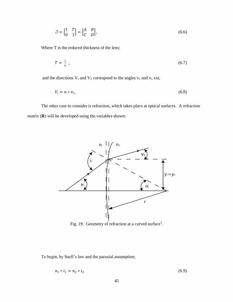
The other case to consider is refraction, which takes place at optical surfaces. A refraction

matrix (R) will be developed using the variables shown:

Fig. 19. Geometry of refraction at a curved surface3.

To begin, by Snell‟s law and the paraxial assumption;

𝑛1 ∗ 𝑖1 = 𝑛2 ∗ 𝑖2 (6.9)

46

Substituting in for angles i1 and i2 provides;

𝑛1 ∗ (𝑣1 +𝑦1

𝑟) = 𝑛2 ∗ (𝑣2 +

𝑦2

𝑟). (6.10)

Or, in matrix form (with the replacements for V and T as noted in the translation matrix

derivation);

= 1 0

−(𝑛2−𝑛1)

𝑟1 =

𝐴 𝐵𝐶 𝐷

. (6.11)

47

6.2. Ray Tracing Computational Model

The RTM method above requires a matrix computation for each ray at each optical interface.

Adding complexity, each optical surface can result in six possible actions, or a combination thereof.

These are: refraction, reflection, absorption, forward scatter, and backward scatter. If a combination

of these actions takes place at an optical surface, a single ray is split into multiple rays, which are

then propagated to more optical surfaces which can result in more ray splitting and more ray matrix

computations. Considering that a raytrace which correctly approximates a physical system can

require hundreds of thousands of starting rays; not to mention the exponential increase due to the

splitting of rays at optical surfaces; it is natural and necessary to extend the RTM method to a

computational system for rapid calculation of ray paths.

Lambda Research‟s TracePro, an existing ray tracing CAD suite, was selected to perform the

required ray tracing for optimization and design iteration of the otoscope head. The system performs

a Monte-Carlo method of probabilistic ray tracing to determine the ray throughput of a system in

three dimensions. ACIS CAD geometry is use to create the volumes and surfaces of an optical

system, and the additional optical characteristics of a volume or surface (such as refraction and

absorption coefficients; and refractive indices) are input and maintained by the TracePro suite.

The system was used to investigate a series of optical components and possible layouts.

Considerations of packaging of the system were paramount, as a small size and otoscope like

appearance were the primary goals of this generation of otoscope head.

The optical elements used in the ray tracing system are illustrated below with a short

description of each element. For further discussion of the benefits of each optical component please

refer to the Optical Head Configuration section of this report. For an in depth tutorial of the

construction of the ray tracing model see Appendix B.

48

Table 3. Illustrative component ray traces and construction notes.

Component and Illustrative Screenshot Notes

Beam Combiners/Splitters

50/50 beam combiner/splitter cube

Constructed from two separate bodies

3 layer AR coating applied to external surfaces

Beamsplitter properties applied to angled, interior

surface.

Validated via equal intensities from each output

beam.

Achromatic Imaging Lenses

Imaging lens achromats where built from their

specified geometries.

Two separate material properties define the different

indices of refraction of the crown and flint.

Validated by verifying focal points with

specifications.

GRIN Imaging Lens (ILW)

GRIN lens built from given geometry.

SELFOC material used to define refractive index

coefficients.

Validated by predicted ray trajectory behavior and

focal point.

GRIN Rod Lenses (SRL)

GRIN lens built from specified length and diameter

SELFOC material used to define refractive index

coefficients.

Validated via faithful recreation of pitch number

given in specifications.

49

In addition to the validations noted in the table, each component; and the system as a whole;

was validated by monitoring the throughput of a Gaussian distribution of light intensity. Laser light

is inherently Gaussian in distribution, and RTM analysis has the ability to faithfully describe the

effect of each optical component on a Gaussian distribution. In order to validate that the components

were modeled correctly, the distribution throughput of each component was investigated.

The distribution behavior throughout the entire system is shown in Fig. 20. Note the faithful

reproduction of the Gaussian intensity. Line profiles are provided through the center of the input and

output intensities for comparison.

Fig. 20. Gaussian distribution through system; showing input, post imaging lens, and output on

CMOS chip.

50

7. Optical Head Configuration

The configuration of the optical head developed is shown in Fig. 21. It consists of 6

components: An object beam (OB), reference beam (RB), Gradient Index (GRIN) rod lens (GRIN),

Imaging Lens (IL), beam combiner (BC), and CMOS digital camera (CAM).

Fig. 21. Schematic of the optical head showing object beam and reference beam optical fibers (OB

and RB, respectively), gradient-index rod lens (GRIN), imaging lens achromat (IL), beam combiner

cube (BC) and CMOS camera (CAM).

The object and reference beams are incorporated via single-mode optical fibers from the laser

delivery system. The object beam is attached via a bare fiber secured in the otoscope packaging.

The distance required between the OB fiber output and the object, given an object beam fiber with a

numerical aperture of 0.1329 and a desired coverage of 12mm x 12mm (increased by 20% to account

for the Gaussian distribution of intensity), is:

12𝑚𝑚∗1.2

tan 2∗0.13 = 54.1𝑚𝑚. (7.1)

51

Likewise, the reference beam is required to provide full illumination across the CMOS chip,

which has a size 6.9 mm x 8.6 mm30. Again, the desired area is increased 20% to account for the

uneven distribution of light from the fiber.

8.6𝑚𝑚∗1.2

tan 2∗0.13 = 3.88𝑚𝑚 (7.2)

A small diameter (2mm) gradient index lens was incorporated into the system for several

reasons. First, the small diameter makes it appropriate for packaging inside an otoscope speculum.

Gradient index lenses are commonly used in endoscopy in order to focus an image in a small

cavity31. Second, the gradient index lens has a numerical aperture (NA) of 0.10032. The small NA

should provide an increased depth of field, as NA and depth of field are inversely proportional33.

The pitch of a gradient index lens refers to the number of cycles of the sinusoidal variation of

light throughout its length. Fig. 22 shows a variety of pitch possibilities when selecting a GRIN rod

lens.

Fig. 22. GRIN lens Pitch concept illustration34.

52

The lens selected has a pitch of 0.50, resulting in the image on the front surface inverted on

the back surface.

The imaging lens (IL) is used to collimate the light from the GRIN back surface. The lens

selected is an achromat of diameter 5mm. An achromat was selected as to reduce any potential

spherical or chromatic aberrations from the imaging lens. Transverse aberrations are also reduced,

and off axis rays are more tightly focused when compared to traditional lens singlets35. See Fig. 23.

Fig. 23. Off-axis performance of achromatic doublet versus plano-convex lens36.

The focal length of the lens is 7.9mm, which is the distance the lens should be placed from

the GRIN lens back surface.

To recombine the two beams, a 50/50 beam splitter cube is used (BC).

53

Two cameras were examined for use with the system, the PixelLink PL-A741 and the

selected camera, a Silicon Imaging SI-1280. The SI-1280 is 1024x1280 pixel, 12bit CMOS type

camera. The pixel size is 6.7microns square. The camera selected for its small size, full-frame

shutter, and active spectral response in the near-infrared range (as a near infrared laser is suggested

for use). It is important to select a camera which captures the maximum amount of light reflected off

the tympanic membrane. Fig. 24 shows the response curve of this camera over a variety of

wavelengths.

Fig. 24. Spectral response of SI-1280 Camera37.

Complete properties of all the optical components selected, including manufacturer‟s part

numbers, can be found in Appendix D.

54

8. Realization

8.1. Building the Prototype

With the otoscope head design optimized theoretically the device was prototyped.

Miniaturization was the primary focus when manufacturing the prototype, while also incorporating

the design considerations from the computer model. The ray tracing analysis determined that stray

light reaching the camera needed to be minimized; therefore all of the components were housed in

enclosures. Fig. 25 shows the otoscope head that was manufactured.

Fig. 25. Miniaturized Otoscope Head.

The nominal dimensions of the otoscope head were significantly reduced when compared to

the previous design. The reduced size of is attributed in large part to the folding of the longest

optical path, as the optical path from the object being imaged to the camera is bent at 90 degrees by

means of a 50/50 beam combiner. Also, the miniaturized design has much fewer adjustable mounts

in comparison to the previous generation, which further reduces the overall size. It should be noted

55

that the rotating translation mount used in the miniaturized design is smaller than the linear

translation mounts used in the previous design. The combination of these features led to a much

more compact design.

A comparison of the nominal dimensions of the miniaturized otoscope head and the previous

generation otoscope head is shown in Fig. 26.

Fig. 26. Previous Generation Otoscope Head18 (Left); Miniaturized Otoscope Head (Right).

The height of the miniaturized otoscope, the dimension into the page in Fig. 26, is only 50mm

compared to the previous generation's 110mm height. This height is limited by the height of the

camera, and could be feasibly reduced to approximately 25mm if the printed circuit board version of

the Silicon Imaging 1280i camera was used. The significant reduction in otoscope head size resulted

in a much more compact, otoscope like design.

56

8.2. Characterization of Optical Performance

Not only was the new otoscope developed intended to be smaller than the previous

generation, but the optical performance required improvement in specific areas. It was necessary to

characterize the optical performance of the miniaturized otoscope head in order to make a

quantitative comparison of it to the prior generation. Unfortunately, a standardized procedure for

characterizing the field of view, magnification, depth of field, resolution and image aberration was

not developed and implemented in the characterization of the prior generation otoscope head.

Therefore, such a procedure with the appropriate targets, image analysis algorithms, and documented

parameters was developed for the characterization of the miniaturized otoscope head.

8.2.1. Field of View

The first characteristic that was determined was the field of view. The background biology

determined the required field of view needed to be 10mm. To determine the distance the object

needed to be away from the optical system to allow a 10mm by 10mm region of it be imaged, a target

comprised of vertical white and black line pairs at a frequency of one line pair per millimeter was

used. A field of view of 10mm was achieved when ten line pairs perfectly fit within the field of

view. At a working distance of 13mm the ten line pairs fit within the field of view. The working

distance for the previous generation otoscope head to get an equivalent field of view was

approximately 90mm. The shorter working distance of the miniaturized otoscope makes

measurement of in vivo tympanic membrane much more feasible, as the device can be more easily

packaged in a design similar to existing otoscopes. Fig. 27 compares the an image of the target used

to determine the field of view at the working distance to a image of the same target scaled to the

actual size.

57

Fig. 27. Field of View And Magnification Image.

8.2.2. Magnification

The magnification shown in Fig. 27 is approximately 0.5, this can be calculated from the

geometry of the system. The CMOS chip used has dimensions of 1280 pixels wide by 1024 pixels

tall. Each pixel is a square with edge length of 6.7µm. The size of the region of interest on the

camera being used is 800 pixels by 800 pixels. Because at a 13mm working distance 10mm fit

within the field of view the magnification can be calculated by finding the ratio of the length of 800

pixels on the CMOS chip to the actual length of the region being imaged:

58

536.010

1

107.61280

1280

800 3

mm

pixel

mmpixels

pixels

pixels

M (8.1)

This means that a 10mm by 10mm region of the object is being imaged on a 5.36mm by 5.36mm

region of the CMOS chip.

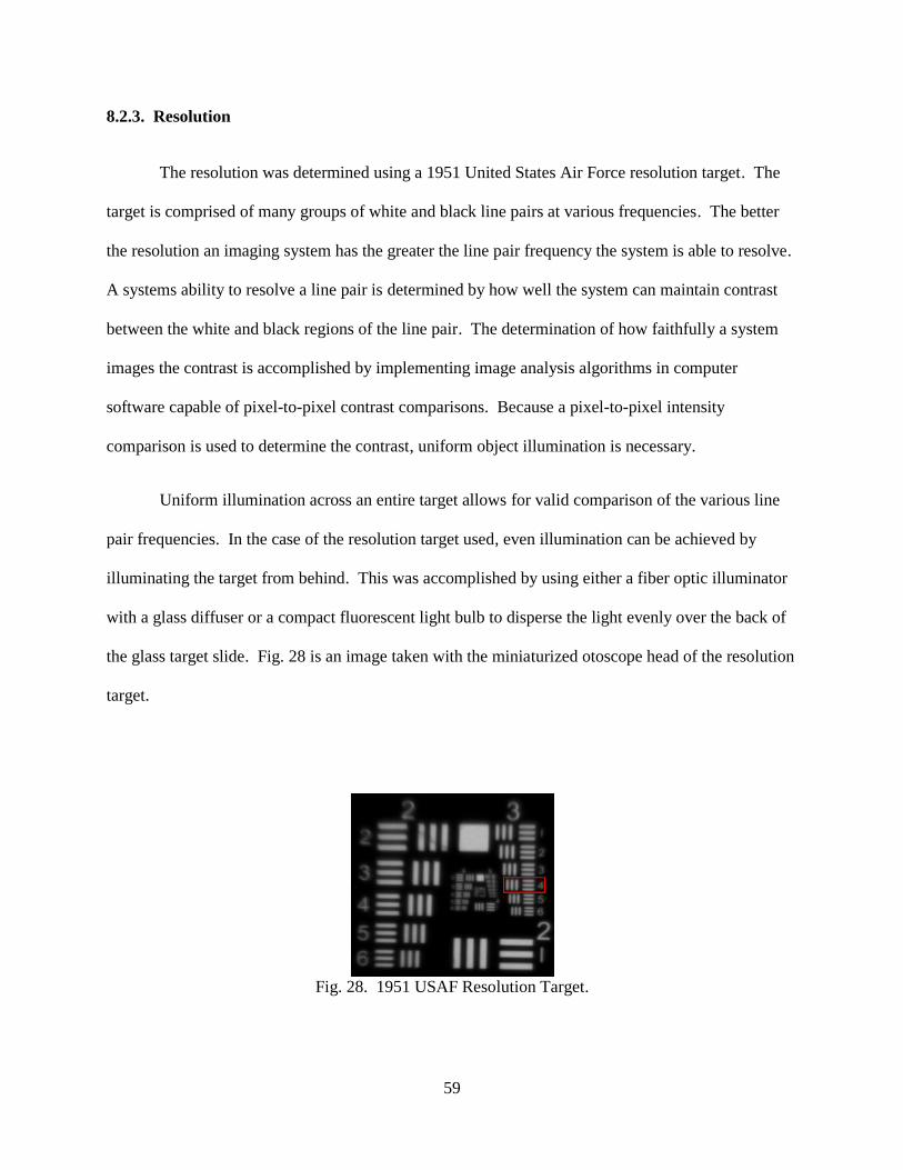
59

8.2.3. Resolution

The resolution was determined using a 1951 United States Air Force resolution target. The

target is comprised of many groups of white and black line pairs at various frequencies. The better

the resolution an imaging system has the greater the line pair frequency the system is able to resolve.

A systems ability to resolve a line pair is determined by how well the system can maintain contrast

between the white and black regions of the line pair. The determination of how faithfully a system

images the contrast is accomplished by implementing image analysis algorithms in computer

software capable of pixel-to-pixel contrast comparisons. Because a pixel-to-pixel intensity

comparison is used to determine the contrast, uniform object illumination is necessary.

Uniform illumination across an entire target allows for valid comparison of the various line

pair frequencies. In the case of the resolution target used, even illumination can be achieved by

illuminating the target from behind. This was accomplished by using either a fiber optic illuminator

with a glass diffuser or a compact fluorescent light bulb to disperse the light evenly over the back of

the glass target slide. Fig. 28 is an image taken with the miniaturized otoscope head of the resolution

target.

Fig. 28. 1951 USAF Resolution Target.

60

By performing a contrast trace across all of the line pair elements on the target, and noting

the maximum and minimum values of the gray scale variation between the white and black lines the

contrast was determined. At a 13mm working distance the miniaturized otoscope head is able to

resolve element 4 of group 3, shown encompassed by a red rectangle in Fig. 28. This correlates to a

line pair per millimeter resolution of 11.3038 at 59% contrast. A more in depth description of the

algorithm used can be found in Appendix C.

8.2.4. Depth of Field

Doctors using the previous generation otoscope requested a larger depth of field to allow for

easier focusing and measurement acquisition. The depth of field of the miniaturized otoscope was

characterized experimentally with a depth of field 45 degree wedge target. The target has horizontal

lines spaced at known intervals that correspond to a distance parallel to the optical axis. A contrast

trace can be performed on the image of the target. The point where the contrast drops below a

certain percentage of the maximum contrast is said to be beyond the depth of field. Further

description of the algorithm used can be found in Appendix C. The test setup used to characterize

the depth of field is shown in Fig. 29.

61

Fig. 29. Depth of Field Test.

The optical head is shown inserted through a bright field/dark field ring illuminator. The

purpose of the ring illuminator is to provide an even light distribution on targets that require front

illumination. The target is positioned at approximately the 13mm away from the GRIN lens. The

depth of field target has multiple groups of line pair frequencies; to perform the characterization of

the miniaturized otoscope head the five line pair per millimeter group was used. Fig. 30 is a graph

generated from the contrast trace of the imaged used to characterize the depth of field.

62

Fig. 30. Depth of Field Contrast Trace Graph.

Each oscillation on the graph corresponds to a white and black line pair. The minimum

contrast level required to be considered „in focus‟ for the depth of field test was 60% of the

maximum contrast oscillation in the image. The maximum contrast in the image is seen at

approximately pixel 340, where the peak gray scale value is 95 and the minimum gray scale value is

approximately 40. The difference of these two values gives the maximum gray scale contrast in the

trace; therefore 60% of 55 is the minimum contrast level to be considered in focus. Thirty-one

oscillations have a contrast of 33 or greater. Because every 5 oscillations correspond to 1 mm, the

depth of field can be calculated as;

mm

mm

lp

lpDoF 2.6

5

31 (8.2)

A depth of field of 6.2mm is attained with the miniaturized optical head when performing a

contrast trace across the 5 line pair per millimeter group at 60% contrast of the 45 degree depth of

field wedge target. The previous generation claimed a depth of field of 5mm39. To make a

quantitative comparison to the new optical head the same methodology described in this section

63

should be used to characterize the depth of field of the previous generation otoscope. It was noted,

qualitatively, that the miniaturized optical head had a noticeably improved depth of field.

8.2.5. Image Aberration

All lenses introduce optical distortions. Depending on a number of parameters the degree to

which the lenses distort the image varies. The optical distortions the miniaturized optical head

introduced were characterized to better understand the degree to which distortions affect image

quality. To characterize the image aberration a fixed frequency grid distortion target was used. This

target is comprised of a grid of evenly spaced black dots on a glass substrate. The entire grid has

dimensions of 25mm by 25mm, and dots are located every 0.25mm. The distortion can be

compensated for by characterizing how the imaged distorted dot positions are shifted from their

original undistorted positions.

The grid target was placed at the working distance of 13mm, and evenly back illuminated.

The image acquired is shown in Fig. 31.

Fig. 31. Grid Distortion Target.

64

Dots lying on the red perpendicular axes labeled X and Y are distorted along the line they lie on. This

one dimensional distortion is the same along both axes. In order to determine the amount of

distortion on said axes an algorithm was developed that utilized centroid analysis techniques.

The algorithm developed to determine the distortion function first labels each dot as a

separate region based on contrast. The centroid of each region is determined and a matrix of the

location of the distorted centroids is created. By comparing the distorted centroid locations to the

undistorted centroid locations the deviation of each centroid is calculated. Fig. 32 shows the plot

generated with the algorithm of the distorted centroid locations versus original centroid locations and

the function fit to the data. Function fitting is built in to the algorithm developed; therefore

iteratively determining the appropriate function is fast and seamless. A more in depth description of

the algorithm used, as well as the code, can be found in Appendix C.

Fig. 32. Distortion Function.

65

The data appears to be linear, which suggests that optics introduce very little distortions to an

image. Despite the appearance of linearity, the better fit for the data is a third-order polynomial.

This was determined by plotting the error and varying the order of the polynomial fit until the error

was approximately zero. The function fit to the data shown in Fig. 32 is given by:

327.0995.010729.310038.4 2638 YYYYYdistorted (8.3)

where Ydistorted, the location of the distorted centroids, is a function of the original centroid location, Y.

The function describing the distortion could now be implemented to calibrate the image processing

software; and the optical distortion the lenses introduce could be removed.

66

9. Validation

The performance of the optical head was validated through the comparison of analytical and

computational solutions of the vibration modes of a cantilever beam to the experimental results. A

cantilever beam was selected as the geometry to evaluate the miniaturized otoscope with because of

its well established analytical and computational models. The copper cantilever modeled and

constructed was a 0.002 inches thick, 0.421 inches long, and 0.176 inches wide. Such dimensions

were chosen via analytical work to ensure the beams first three modes of vibration were within the

audible range for humans, while still fitting approximately in a ten millimeter field of view.

9.1. Analytical Validation

This section describes the analytical process carried out to go from the elementary flexural

theory to determining the modes of vibration of a cantilever beam40. Such analysis is necessary to

understand the phenomena of how the mode shapes of a beam and the frequencies which they occur

at are developed.

It is assumed that the beam being analyzed has a constant cross section and material

properties. A diagram of the theoretical beam is shown in Fig. 33.

Fig. 33. Prismatic Beam.

67

The following derivation is based on the fourth-order ordinary differential equation for the free

transverse vibration of a beam base on,

yx

dxAdxyx

IE2

2

4

4

(9.1)

where;

E is the modulus of elasticity of the material,

I is the area moment of inertia,

is the density of the material,

A is the cross sectional area of the beam.

If we define A

IEa

and substitute it into Eq. 9.1. The equation for the free transverse vibration

of a beam can be written as;

yxa

yx 2

2

24

4 1

. (9.2)

The deflection at any location on a beam varies harmonically with time as the beam vibrates

transversely in a natural mode. The deflection is described by;

tpBtpAXy sincos (9.3)

If we substitute Eq. 9.3 into Eq. 9.2, and take the partial derivatives this yields:

68

tpBtpAXa

ptpBtpAX

x

sincossincos

2

2

4

4

(9.4)

Simplifying this expression yields;

02

2

4

4

Xa

pX

dx

d

.

(9.5)

To make it easier to solve the differential equation we will define2

24

a

pk . Now the fourth-order

differential ordinary differential equation has the form;

04

4

4

XkXdx

d

.

(9.6)

Next the form of the general solution needs to be determined. To satisfy Eq. 9.6 assume nxeX .

Substituting the assumed value of X into Eq. 9.6 and simplifying yields:

044 knenx

. (9.7)

To satisfy Eq. 9.7 n can be equal to: k , k , ki , and ki . So the general solution of the beam in

free transverse vibration is given by;

ikxikxkxkx eFeEeDeCX , (9.8)

which can also be written as:

)cosh()cos()cosh()cos( 21 kxkxCkxkxCX

)sinh()sin()sinh()sin( 43 kxkxCkxkxC

. (9.9)

69

Equation 9.9 describes any beam in transverse vibration. To determine the constants C1, C2,

C3, and C4 for the particular case of the cantilever beam boundary conditions must be applied. C1 can

be solved for by applying the deflection boundary condition at the fixed end of the beam;

00020 43210CCCCX

x

,

Therefore;

01 C (9.10)

C3 can be solved for by applying the slope boundary condition at the fixed end of the beam:

0200 432

0

CkCCXdx

d

x

.

Therefore;

03 C . (9.11)

C2 and C4 cannot be solved for directly, but by applying the final two boundary conditions the

ratio of C2 to C4 is able to be determined. One ratio is found by applying the moment boundary

condition at the free end of the beam;

70

)sinh()sin()cosh()cos(0 2

4

2

22

2

kkkCkkkCXdx

d

x

.

Therefore;

)cosh()cos(

)sinh()sin(

4

2

kk

kk

C

C

.

(9.12)

Applying the shear force boundary condition yields the second ratio;

)cosh()cos()sinh()sin(0 3

4

3

23

3

kkkCkkkCXdx

d

x

.

Therefore;

)sinh()sin(

)cosh()cos(

4

2

kk

kk

C

C

.

(9.13)

Setting Eq. 9.12 equal to Eq. 9.13 and simplifying yields;

)cosh()cos(2)cosh()sinh()cos()sin( 2222 kkkkkk

To simplify further we apply the identities; 1)cos()sin( 22 kk , and 1)sinh()cosh( 22 kk .

This yields the frequency equation;

1)cosh()cos( kk . (9.14)

71

The roots of Eq. 9.14 are used to calculate the fundamental modes of vibration of the cantilever

beam.

The equation that described the frequencies that the fundamental modes of vibration occur at

is;

2

2

kaf

,

(9.15)

Where:

a is defined as A

IE

,

k is the corresponding root of Eq. 9.14,

is the length of the beam.

For the copper beam used to validate the otoscope head the first three natural frequencies with

the corresponding k roots are shown in Table 4.

Table 4. Analytically Determine Natural Frequencies.

Natural Frequency k Root

First Mode 244.3 Hz 1.875

Second Mode 1531.3 Hz 4.694

Third Mode 4287.6 Hz 7.855

72

9.2. Computational Validation

A computational model of the cantilever beam was developed to compliment the analytical

results, as well as help verify the experimental results. The computational work was done with the

ANSYS 11.0, a finite element analysis program. The model was created as an elastic beam element

with a constant cross section and material properties. As with all finite element problems the mesh

size and computation method had to be carefully considered.

Because only the first three dynamic transverse modes were of interest the beam was

analyzed with the Subspace Method in ANSYS. This computational method determines all of the

specified modes for all of the degrees of freedom41. This method yields quite accurate results, but at

the expense of computation time. The computation time was then optimized by determining the

appropriate mesh size.

In this finite element problem the mesh size determined how many discrete elements the

beam would be divided into. Computations were done with a number of different differential

element mesh sizes until a good balance was reached between computation time and accuracy of

results. A beam discretized into one-hundred elements with one end having all of its degrees of

freedom limited yielded relatively fast computation times and modal frequencies within one percent

of the analytical modal frequencies. Fig. 34 is representation of the computational beam developed.

Fig. 34. Finite Element Beam.

73

The beam is seen here divided into one-hundred discrete elements, each with a length of

approximately 107µ-meters. The green arrows on the left of the beam represent the boundary

condition that is fully restraining the left face.

The material properties42 of the beam were defined for a linear elastic isotropic model with

a: Young‟s Modulus of 103GPa, Poison‟s Ratio of 0.34, and density of 8885 kg/m3. The

computational results from the ANSYS43 analysis are shown in Table 4.

Table 5. Finite Element Modes of Cantilever.

Frequency Three Dimensional

Mode Shape

First Mode 244.9 Hz

Second Mode 1534.7 Hz

Third Mode 4297.1 Hz

74

9.3. Experimental Validation

The cantilever beam was constructed in order to determine the experimental modes of

vibration. The beam was cut from copper shim stock to ensure a uniform thickness of 0.002in and a

uniform surface finish. The width of the beam was made to be 0.176in, and the length was left

longer than the 0.421in required for the cantilever so it could be clamped. Because diffuse light

reflecting off of the object is needed to generate good intereferograms, white paint was applied to the

surface of the beam to reduce the amount of specular reflections.

9.3.1. Experimental Procedure

The beam was fixed in a steel clamp so that 0.421in of the beam extended past the clamp.

The clamp was then attached to a piezo shaker. The entire assembly was fixed with the beam located

within the field of view of the otoscope. Using a white light source the otoscope was focused on the

beam. The fixtured cantilever assembly is shown Fig. 35.

Fig. 35. Cantilever Test Setup.

75

With the beam both in the field of view and in focus, the laser light for interferometric

measurements was setup. Due to the small numerical aperture of the system little light is transmitted

from the object to the camera chip. For this reason careful adjustment to the object and reference

beams must be carried out.

The first adjustment to the reference beam should be centering it on the recording medium, in

this case the camera‟s complementary metal-oxide semiconductor (CMOS) chip. Centering the

reference beam in the region of interest on the CMOS chip is accomplished by mounting the fiber

output accurately on the optical axis, so that it illuminates the region of interest evenly. Often this

approach is not feasible due to an inability to control tolerances in the system, such as how accurately

the lenses are mounted or how square the beam combiner is with the optical paths. Therefore in

prototype experimental configurations often the reference beam often must be directed slightly off-

center. When this is the case a kinematic fiber mount is required to precisely position the reference

beam illumination in the region of interest on the CMOS chip. The prototype system developed uses

such a solution.. It should be noted that the likely causes of the image not being perfectly centered

on the CMOS chip in the prototype are the tolerances in the achromatic imaging lens‟s and GRIN

lens‟s mounts.

The object beam is adjusted so that it evenly illuminates the object, while maintaining a

minimal angle between the incident object beam light and the axis of the GRIN lens. Because the

laser light output from the fiber has a divergent Gaussian intensity distribution it is import to not to

place the fiber output to close to the object. When the object fiber output is placed far enough away,

the object will be illuminated evenly. In order to monitor how evenly the object beam is distributed

on the CMOS chip the reference beam should be blocked and the contrast trace tool can be used in

Laser View. By tracing across the region of interest one can ensure there is not a significant change

76

in brightness from one area to another. When the object beam is fixed in its final position, the

reference beam can be unblocked so the beam ratio can be set.

The beam ratio is the ratio of the amount of light from the reference beam to the amount of

light from the object beam reaching the CMOS chip. To adjust the beam ratio the amount of light

being coupled into the optical fiber is adjusted. Due to low amount of light that can be transmitted

through the optical system, the amount of power from object beam is typically maximized; therefore

the beam ratio is determined by coupling and de-coupling the reference beam. A beam ratio between

one and two is recommended. With the reference and object beams fully setup measurements were

taken.

9.3.2. Experimental Results

The piezo shaker was excited via a function generator. The first three modes of vibration

were determined by adjusting the excitation frequency at intervals of 100Hz until a mode shape was

clear in the time averaged intereferograms. When a mode shape was found the frequency and

voltage amplitude to the piezo shaker were adjusted to more accurately determine the frequency of

that particular mode of vibration. The frequencies that corresponded to the first three modes of

vibration were determined, and the optical phase measurements were taken in double exposure mode

with stroboscopic illumination.

The frequency generator, controlled via USB from the image processing computer, had the

output from channel one connected to the piezo shaker and the output from channel two connected to

the AOM driver. A sine wave was input to the piezo shaker, and a pulse wave to the driver.

Measurements were made with a beam ratio of 1.8, 10% duty cycle, and camera exposure time of

25ms. The experimental results for the first three modes of vibration are shown in Table 6.

77

Table 6. Experimental Modal Frequencies obtainted with

OEHO Funtioning in Double-Exposure Stroboscopic Mode.

Frequency Interferogram Piezo Peak-to-peak

Voltage

First Mode 238.5 Hz

5 V

Second Mode 1501.5 Hz

7 V

Third Mode 4092.0 Hz

8 V

78

9.4. Validation Results Comparison

A comparison of the analytical and computational results with respect to the experimental

results is shown in Table 7.

Table 7. Analytical and Computational Percent Error.

First Mode Second Mode Third Mode

Analytical 2.4% 2.0% 4.9%

Computational 2.7% 2.2% 5.0%

The minimal percent error equal to or less than 5% of the analytically and computationally

determined frequencies with respect to the experimentally determined frequencies can be attributed

to assumptions made in the analysis. Small inconsistencies in parameters used in the analysis such as

the material properties, and the geometry of the beam may have introduced the error. Also, it is

possible a user error, such fixing the beam imprecisely, may have introduced the error.

79

10. Testing

Testing of the miniaturized otoscope head was performed on 6mm diameter nitrile membrane

and on a post mortem chinchilla tympanic membrane.

The nitrile membrane was supplied by the doctors at the Massachusetts Eye and Ear

Infirmary to measure because of its resemblance, physically, to a real tympanic membrane in the

capacity that it has a small circular shape and is optically semi-transparent. The membrane was

imaged with the miniaturized otoscope head while being excited acoustically with a speaker. Fig. 36

shows the test setup used to image the membrane.

Fig. 36. Nitrile Membrane Test Setup.

The speaker's input frequency and voltage amplitude were set via a function generator, and the

optical phase images were acquired. The first mode of vibration of the nitrile membrane was found

at 4.228kHz, demonstrating the miniaturized otoscope head's ability to image semi-transparent

membranes. A more complex mode of vibration was acquired at 10.66kHz, the optical phase image

was unwrapped and plotted, demonstrating the system‟s ability to acquire three-dimensional

80

information. The unwrapped optical phase image at 4.228kHz, 10.66kHz and the three-dimensional

plot is shown in Fig. 37.

Fig. 37. (a) Nitrile Membrane at 4.228kHz; (b) Nitrile Membrane at

10.66 kHz; (c) 3-D Representation of Nitrile Membrane at 10.66kHz.

A cadaveric chinchilla was brought to the Center for Holographic Studies and Laser

µmechaTronics to test how the miniaturized otoscope head measured tympanic membranes. The

chinchilla head, with its tympanic membranes exposed, was clamped in a fixture. The tympanic

membrane was excited acoustically over a range of frequencies from 100Hz to 16kHz, and over a

range of sound pressure levels from 92.9dB to 116.1dB. Fig. 38 is shows the test setup used to test

the chinchilla tympanic membrane.

81

Fig. 38. Chinchilla Test.

Doctors from Massachusetts Eye and Ear Infirmary acquired a number of time-average

interferograms and stroboscopic phase images for ordered and complex vibration patterns in the

tympanic membrane. Unfortunately, due to the low speckle per fringe resolution few of the

stroboscope phase images acquired during the testing were able to be unwrapped. A time-averaged

image of a simple mode shape in the chinchilla tympanic membrane demonstrating the large speckle

size is shown in Fig. 39.

Fig. 39. Time-Averaged Image of Chinchilla

Tympanic Membrane at 700 Hz, 102.9dB SPL.

82

The large speckle size was due to two main factors: small diameter optics inherently have a

larger speckle size; and the achromat imaging lens was mounted unparallel to the optical axis. These

issues were dealt with by replacing the 5mm diameter achromat lens with a 6.35mm diameter

achromat lens, as well as getting the achromat lens mounted professionally to ensure its alignment to

the optical axis.

The speckle size was reduced by installing the new 6.35mm diameter achromat imaging lens,

though the miniaturized otoscope head has not yet tested tympanic membrane with the improved

optics.

83

11. Recommendations and Future Work

The feedback from the medical professionals who performed experiments with the otoscope

head provided conclusions and indicated future work regarding the system.

The primary response to the system was positive and in regards to the miniaturized size. The

otoscope head is less than 10% the previous generation in overall volume. Additionally, the more

otoscope-like appearance was indicated as an important improvement over the previous generation as

it will provide a more seamless integration into current clinical practices.

The focusing system, which utilizes a translational tube, was immediately intuitive to all the

professionals who experimented with the system. This is a vast improvement over the previous

system, whose focusing system was often neglected in favor of moving the sample (which the

physicians found simpler despite requiring the unbolting and careful shifting of the sample).

The depth of field has been increased which was beneficial in reducing the time require to set

up and administer a round of experiments.

The device was found to have an insufficient speckle size for the work of the researchers at

MEEI as originally tested. A larger diameter imaging lens was subsequently installed which reduced

the speckle size. Tests with the news lens have yet to be completed by the MEEI researchers but it is

expected the speckle size is reduced to an acceptable size for TM measurement.

Thermomechanical stability was addressed only through the reduction of the degrees of

freedom of the system, and a full-scale investigation into methods to increase the thermomechanical

stability is paramount. Much of the instability of the system stems from having two separate fibers

which transfer light to the optical head. This system should be optimized.

84

A production-type package should be fully designed and manufactured for the optical layout

prototyped. A printed circuit-board camera will allow for numerous packaging options and should be

considered for the next generation.

Finally, an illumination system for the tympanic membrane must be incorporated into the

design and packaging. A bundle of optical fibers to carry light to a ring surrounding the speculum is

suggested for further investigation as current otoscopes utilize this system and it provides even

illumination on the TM.

85

12. References

1 Furlong, C., Rosowski, J.J., Hulli, N. and Ravicz, M.E., Preliminary analyses of tympanic-

membrane motion from holographic measurements, SEM 8th International Symposium Series

on MEMS and Nanotechnology (ISMAN), Springfield, MA, June 2007

2 Schubert, E.D., Hearing: Its Function and Dysfunction, Springer-Verlag, NY, 1980

3 Phon.ox.ac.uk. Home Page. Retrieved 15 December 2008,

http://www.phon.ox.ac.uk/~jcoleman/speaking_hearing.htm

4 Katz, J., Handbook of Clinical Audiology: Fourth Edition, Williams & Wilkins, MD, 1994

5 Standring, S., Gray’s Anatomy: The Anatomical Basis of Clinical Practice, Thirty-Ninth Edition,

Elsevier Ltd., NY, 2005

6 Rowsowski, J., personal communication, March 24, 2009

7 Wajnberg, J. M.D., “The true shape of the tympanic membrane,” The Journal of Laryngology and

Otology, 101:538-541, 1987

8 Koike, T., Wada, H., Kobayashi, T., “Modeling of the human middle ear using the finite-element

method,” J. Acoust. Soc. Am., 111:1306-1317, 2002

9 Chole, R.A., Kodama, K., “Comparative histology of the tympanic membrane and its relationship to

cholesteatoma,” Ann. Otol. Rhinol. Laryngol., 98:761-766, 1989

10 Fay, J., Puria, S., Decraemer, W., Steele, C., “Three approaches for estimating the elastic modulus

of the tympanic membrane,” Journal of Biomechanics, 38:1807-1815 2005

11 Lim, D.J., “Structure and function of the tympanic membrane: a review,” Acta oto-rhino-

laryngologica Belg., 49:101-115, 1995

12 Lim, D.J., “Tympanic Membrane: Electron microscopic observation part I: pars tensa,” Acta oto-

laryngologica, 66:181-198, 1968

13 Haskel, S. and Sygoda, D., Biology, A contemporary Approach, Amsco, NY, 1996

14 Williams, K.R., Lesser, T.H.J., “A finite element analysis of the natural frequencies of vibration of

the human tympanic membrane. Part I.,” British Journal of Audiology, 24:319-327, 1990

15 Deafness in Dogs & Cats. Frequency Hearing Ranges in Dogs and Other Species. Retrieved 20

January 2008, http://www.lsu.edu/deafness/HearingRange.html

16 Tontechnik-Rechner – sengpielaudio. Decibel Table – Comparison Chart. Retrieved 20 January

2008, http://www.sengpielaudio.com/TableOfSoundPressureLevels.htm

86

17 Project proposal. Rosowski, John J.

18 Dywer, B., Maccaferri, M., Wester, C., “Design and Realization of a Laser Holographic

Otoscope,” MQP, WPI-ME, 2008

19 Rabbitt, R.D., Holmes, M.H., “A fibrous dynamic continuum model of the tympanic membrane,”

J. Acoust. Soc. Am., 80:1716-1728, 1986

20 V.V. Tuchin., “Light scattering studies of tissues,” Physics-Uspekhi, 40:495-515, 1997

21 Tuchin, V.V., Utz, S.R., Yaroslavsky, I.V., “Tissue optics, light distribution, and spectroscopy,”

Optical Engineering, 33:3178-3188, 1994

22 Sundberg, M., Peebo, M., Oberg, P.A., Lundquist, P.G., Stromberg, T., “Diffuse reflectance

spectroscopy of the human tympanic membrane in otitis media,” Physiol. Meas., 25:1473-

1483, 2004

23 Doladov, M.Yu., Kazakevich, V.S., Kalashnikov, I.G., Kupaeva, V.V., Shcherbakov, V.A.,

“Optical reflection of the human tympanic membrane,” J. App.Spectroscopy, 66:708-710,

2001

24 Dirckx, J.J.J., Decraemer, W.F.,” Reflective coatings in optical interferometry for in-vitro studies

of the eardrum,” SPIE, 2927:2-10, 1996

25 Hulli, N., “Development of an optoelectronic holographic otoscope system for characterization of

sound-induced displacements in tympanic membranes,” Thesis, WPI-ME, 2008

26 Waldo‟s World “Otoscope” (2009). http://www.waldosworld.org/gallery03/otoscope.jpg

27 Gerrard, Anthony. Matrix Methods in Optics (1975). The Gresham Press, Old Woking, Surrey,

UK.

28 Adapted from 27

29 Nufern.com. “Fiber Details – 460HP” (2004). http://www.nufern.com/fiber_detail.php/95

30 Silicon Imaging. “Silicon Imaging is proud to continue its innovation in ultra” (2009).

http://www.siliconimaging.com/SI-1280CL%20spec.htm

31 GRINTECH.de (2006). http://www.grintech.de/datasheets/grin_endoscope_systems.pdf

32 NSG Europe “Rod Lens Table” (2009). http://www.nsgeurope.com/technology/rodlens.shtml

33 Nikon.com “Nikon MicroscopyU – Concepts and Forumlas” (2009).

http://www.microscopyu.com/articles/formulas/formulasfielddepth.html

34 NSG Europe “Physics of the Selfoc Lens” (2009). http://www.nsgeurope.com/physics.shtml

87

35 Thorlabs.com “Visible Achromat Doublets” (2008).

http://www.thorlabs.com/NewGroupPage9.cfm?ObjectGroup_ID=120&pn=AC050-010-

A1&CFID=34603318&CFTOKEN=89480372

36 Thorlabs.com “Visible Achromat Doublets” (2008).

http://www.thorlabs.com/NewGroupPage9.cfm?ObjectGroup_ID=120&pn=AC050-010-

A1&CFID=34603318&CFTOKEN=89480372

37 Silicon Imaging. “Spectral Response” (2009).

http://www.siliconimaging.com/si1280%20Spectral%20Response.htm

38 EdmundOptics.com. “1951 USAF Glass Resolution Targets.” (2009).

http://www.edmundoptics.com/onlinecatalog/displayproduct.cfm?productID=1790

39 Hernandex-Montes, M. del Socorro, Furlong, C., Rosowski, J. J., Hulli, N., Harrington, E.,

Cheng, T. J., Ravicz, M. E., Santoyo, F. M., “Optoelectronic holographic otoscope for

measurement of nano-displacements in tympanic membranes,” 8

40 Timoshenko, S., Young, D.H., W. Weaver, Jr., Vibration Problems in Engineering: Fourth

Edition, 415-426, 1974

41 Mece.ualberta.ca. “Modal Analysis of Cantilever Beam.” (2009).

http://www.mece.ualberta.ca/tutorials/ansys/IT/Modal/Modal.html

42 Oberg, E., Jones, F.D., Horton, H. L., Ryffel, H. H.. Machinery’s Handbook: 28th Edition,

Industrial Press, NY, 2008

43 Ansys,. V 9.0. Ansys, Inc., Canonsburg, PA, 2007

88

13. Appendix A. Biology Summary – Human TM.

Dimensions: 9-10mm horizontally, 8-9mm vertically

Density: 1200kg/m3

Thickness: 34μm (pars tensa); 110μm (pars flaccida)

Elastic Modulus: Conflicting literature, between 0.1 and 0.3GPa

Max displacement: 1μm

Min displacement: sub-nanometer scale

Audible Freq’s: 16Hz – 20kHz. Complex patterns beginning at 3kHz.

Safe dB SPL’s: 0-100dB

Percent light reflected: 0-17%

Max reflective λ: 620nm – 680nm

Coatings of interest: White Chinese ink, Magnesium oxide (obtained by burning Mg wire)

89

14. Appendix B. TracePro Model Details.

Lambda Research‟s TracePro suite was used for the three dimensional modeling and ray

tracing analysis of the optical configuration. In order for the future of this project to benefit fully

from our work it is important that a working knowledge of TracePro be developed. With knowledge

of the TracePro suite it is possible to understand, analyze and continue the optimization studies of the

configuration developed. The team feels the model is an important contribution to the project and it

should be further investigated.

In this appendix we developed a tutorial which should provide a stable grounds to begin

working in TracePro, as subsequently outline the specifics of the TracePro model created.

90

14.1. Introduction to TracePro

14.1.1. Defining Geometry and Optical Characteristics

TracePro is a three dimensional modeling CAD suite, much like AutoCAD, Solidworks,

Pro/E, and similar applications. As such, it should look and feel familiar to those capable in any

CAD environment. Fig. 40 is a screenshot of the TracePro window.

Fig. 40. Annotated screenshot of TracePro environment.

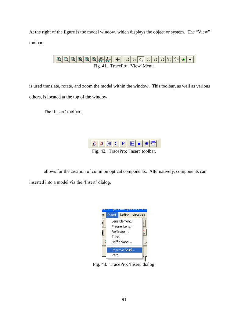
91

At the right of the figure is the model window, which displays the object or system. The “View”

toolbar:

Fig. 41. TracePro: 'View' Menu.

is used translate, rotate, and zoom the model within the window. This toolbar, as well as various

others, is located at the top of the window.

The „Insert‟ toolbar:

Fig. 42. TracePro: 'Insert' toolbar.

allows for the creation of common optical components. Alternatively, components can

inserted into a model via the „Insert‟ dialog.

Fig. 43. TracePro: 'Insert' dialog.

92

The „Primitive Solid‟ selection is used often, and allows you to create common solid objects,

such as cubes, cones, and spheres.

Complex 3d geometries are constructed by inserting overlapping primitive solids and using

the Boolean operations, accessible from the Boolean toolbar:

Fig. 44. TracePro: Boolean toolbar.

Alternatively, these operations can be accessed from the „Edit‟ menu. These operations will become

available for selection after first selecting two objects.

At the left of the image is the Model Tree. In TracePro, solid objects consist of multiple

surfaces (as shown in the tree structure):

Fig. 45. TracePro: Example Model Tree.

93

Properties, for example material properties (such as refractive indices; absorption, reflection, and

transmission coefficients; etc…) and surface properties (such as surface coatings and characteristics)

can be applied to objects or individual surfaces by right clicking and selecting „Properties‟:

Fig. 46. TracePro: 'Apply Properties' dialog.

All characteristics of the TracePro objects and surfaces can be changed and applied via this

dialog. TracePro features data on numerous commercial materials and coatings (see the „Catalog‟

and „Name‟ drop-boxes). To further investigate or alter the properties of a material or coating click

the „View Data‟ button.

94

This produces the Material Property Editor, which provides the mathematical model used for

a particular item, as well as the coefficients which characterize it.

Fig. 47. TracePro: Material Property Editor.

This editor is necessary to input new materials into the system. Occasionally, updated

catalogs are made available at the Lambda Research website (LambdaResearch.com), and can be

imported into the system to provide more up-to-date models of optical components.

All the different catalog property editors can be accessed via the „Define‟ menu.

95

Fig. 48. TracePro: Menu for editing of property data catalogs.

In summary, TracePro is very similar in usage to other geometric CAD software. On top of

the geometry characteristics, however, optical properties can be applied to objects and surfaces by

selecting them in the model tree and choosing „Properties‟.

14.1.2. Light sources and ray trace options

In order to perform a ray trace on the model created its necessary to define a light source.

There are three types of light sources in TracePro: Grid sources, surface sources, and a file sources.

Clicking the tab „Sources‟ in the model tree switches to a source tree view. See Fig. 49.

96

Fig. 49. TracePro: Source Tree.

Sources are defined by the „Define‟ menu.

Fig. 50. TracePro: 'Define' menu.

97

A file source allows you to input a text file with a specific point intensities specified. A

surface source allows you to define a surfaces light emitting properties.

Grid sources are the most versatile sources and the most often used in laser-based

illumination design. The dialog for a grid source is presented below, both „grid‟ and „beam‟ setup

tabs.

Fig. 51. TracePro: Definition of a grid source.

98

Several options are available in the „Grid Setup‟ tab, including origin point, direction, peak

flux, and shape and size. Additionally the input „Rings‟ allows you to define the number of rays

traced from the particular source. Increasing the number of rings in an annular grid will

exponentially increase the number of rays. Computational time will vary between both number of

rays in a source and the specifics of a model, as optical complexity greatly increases the number of

computations the software is required to perform. For much of the work undertaken in this MQP,

30,000 rays was an acceptable starting point.

The „Beam Setup‟ tab allows the definition of the profile of the beam. A Gaussian

distribution, with a specific waist in the x and y directions, can easily be defined here. Note that

selecting a Gaussian spatial distribution negates the pattern selection of the source, as a Gaussian

distribution always uses a random pattern with Gaussian probabilities defining the annular shape.

A divergent beam can be defined via half angle in the „angular profile‟ section of this

window. Note that the combination of a Gaussian spatial distribution and a divergent beam allows

for modeling of the output of laser light from an optical fiber.

With a source (or sources) defined, a raytrace can be performed. Prior to a raytrace, ray

tracing options are available in the „Analysis->Ray Trace Options‟ menu.

Fig. 52. TracePro: Accessing „Raytrace Options‟.

99

The dialog of options is presented:

Fig. 53. TracePro: 'Raytrace Options' Dialog.

Here, ray splitting can be toggled on or off. Ray splitting refers to the behavior of a

ray/surface interaction. With ray splitting on, a ray is split into multiple rays at each surface based on

the absorption, reflection, and transmission coefficients of that surface. For example, if a surface

has a reflection coefficient of .30 and a transmission coefficient of .70, a single ray will be split into

two rays: One transmitted with a power 70% of the initial ray, and one reflected with a power 30% of

the original.

100

Without ray splitting, an interaction instead happens probabilistically. Therefore, in the

example above, the ray will be transmitted 70% of the time, and reflected 30% of the time.

However, the interaction will NOT produce multiple rays.

Removing ray splitting can greatly reduce the computation time of a model, as the number of

rays propagating through space is not exponentially increasing. In the MQP, ray splitting was found

to have little effect on the outcome of the data, while decreasing computation time, and was most

often not in effect.

The raytrace options menu also provides the definition of specific wavelengths, and the

percentage power a ray must reach (compared to its original power) before it is excluded from the

raytrace. Also, „Importance Sampling‟ can be toggled on and off.

Importance Sampling causes TracePro to alter the Monte Carlo probability method used to

favor certain surfaces. In other words, scattered ray directions favor locations indicated in the dialog.

The overall probability is kept faithful by dividing by the amount of weighting used (all done

internally in TracePro). Optimization of the amount of importance sampling allows vastly reduced

computation times by allowing for a reduced total ray count. More information, including a tutorial

for applying importance sampling, can be found in the „Support‟ section of the Lambda Research

website (LambdaResearch.com).

Importance sampling targets are applied from a surface to a point in space through the apply

properties dialog. Each surface can have multiple targets.

101

Fig. 54. TracePro: Importance Sampling target definition.

14.1.3. Tracing Rays and Analysis Tools

Tracing analysis tools are accessible from the „Analysis‟ toolbar, as well as the button to

perform a raytrace.

Fig. 55. TracePro: 'Analysis' Toolbar.

102

The leftmost icon performs a raytrace. The rightmost toggles the display of rays on and off.

Computation times are greatly reduced by disabling the display of rays. The „ ‟ button presents

the sort rays dialog:

Fig. 56. TracePro: 'Ray Sorting' Dialog.

This menu is incredibly useful in reducing the number of rays displayed to a manageable and

informational level. For example, the follow two screenshots (Fig. 57 and Fig. 58) present a model

with a typical number of rays traced, and the same trace where only those rays which collide with the

CMOS surface are displayed:

103

Fig. 57. TracePro: Raytrace with no ray sorting.

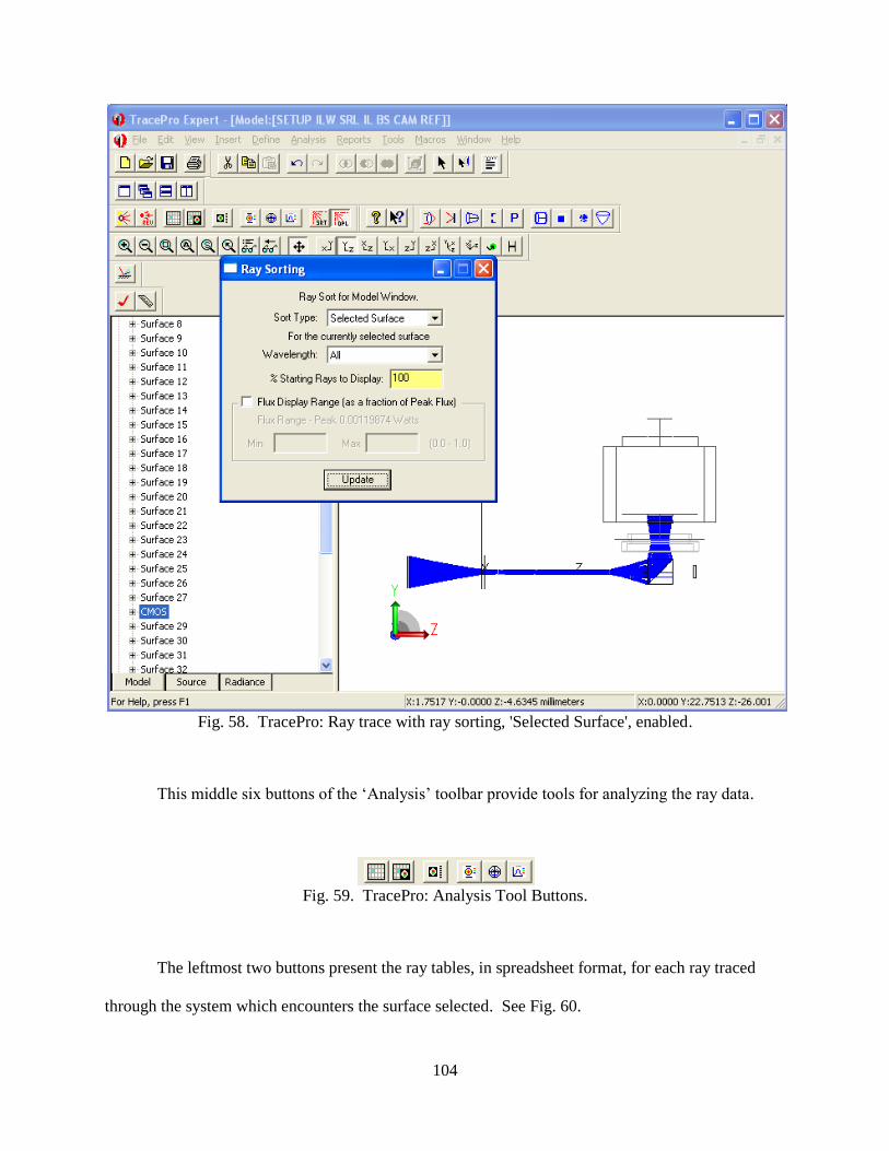
104

Fig. 58. TracePro: Ray trace with ray sorting, 'Selected Surface', enabled.

This middle six buttons of the „Analysis‟ toolbar provide tools for analyzing the ray data.

Fig. 59. TracePro: Analysis Tool Buttons.

The leftmost two buttons present the ray tables, in spreadsheet format, for each ray traced

through the system which encounters the surface selected. See Fig. 60.

105

Fig. 60. TracePro: Ray table excerpt.

Often of more use is the „Irradiance Map‟ selection, which provides a map of the light

intensities experienced on the selected surface.

Fig. 61. TracePro: Sample Irradiance Map.

106

This tool was used above all others to evaluate the performance and function of the optical

system. Options for the irradiance map are accessible by right clicking the map and selecting

„Irradiance/Illuminance options‟. Be sure the normal and up vectors are set appropriately for the

surface under investigation, and note the availability of line profiles, logarithmic plotting, contour

plotting, and various other display options.

Often, an irradiance profile is desired at a location between surfaces. In this case, simply

create a thin block with no material or surface properties at the location of interest. Monitor the

distribution at this plane in space by changing the irradiance map to display incident light (as

opposed to absorbed, via the „Irradiance/Illuminance options‟ dialog) on a surface of this block.

The preceding information, combined with a short time spent experimenting with the

program, should provide an ample understanding for future TracePro computational analysis. More

advance techniques are available in the TracePro suite but require formal training for full utilization.

107

14.2. Otoscope Head Model Details

Details about the modeling of each optical component follow. The final step in each

components modeling was the demonstration of a faithful Gaussian intensity distribution throughput.

For the source of specifications listed as „Manufacture‟s Specification,‟ see Appendix D.

14.2.1. GRIN Lens ILW

The SRL GRIN lens purchased from NSG America has two components, a ILW lens

cemented to the front of a GRIN rod lens. The ILW lens parameters are listed below:

Table 8. ILW Tracepro specifications.

Characteristic Value Source

Diameter 2 mm Manufacturer‟s Specification

Length 6.54 mm Manufacturer‟s Specification

Material and

GRIN

coefficients

SELFOC SLW 300 Material was identified as proprietary, but was identified as

a SELFOC material, by NSG America representative

Walter Boyles. The TracePro catalog contains several

SELFOC materials, SLW300 matched the refractive index

on axis provided from http://www.nsgamerica.com, and

resulted in rays which are focused directly behind the ILW,

as expected by the function of the lens.

108

Fig. 62. TracePro: Image of raytrace through ILW component, with characteristic result.

14.2.2. GRIN ROD

Table 9. GRIN rod TracePro parameters.

Characteristic Value Source

Diameter 2 mm Manufacturer‟s Specification

Length 43.87 mm Inspection Certificate supplied with SRL combination lists

overall length as 50.41mm. 50.41mm less 6.54 mm for

imaging lens equate a rod length of 43.89mm.

Material and

GRIN

coefficients

SELFOC SLW 200 Material was identified as proprietary, but was identified as

a SELFOC material, by NSG America representative

Walter Boyles. The TracePro catalog contains several

SELFOC materials; SLW200 closely matched the pitch

specified with the length specified.

Pitch 0.5 Inspection Certificate supplied with Lens.

Fig. 63. TracePro: Image of raytrace through SRL (ILW and Rod combination) component, with

characteristic result.

109

Notes: The GRIN elements are plano-plano, therefore the geometry can be created simply via

inserting a primitive cylinder.

Ensure that when building a GRIN lens, both „Material‟ and „Gradient Index‟ properties are

applied, and applied as the same type of SELFOC material. Also, the origin and direction (normal

and up vectors) or the index must be specified. See Fig. 64, a screenshot of the apply properties

dialog.

Fig. 64. TracePro: 'Apply Properties' dialog for Gradient Index definition.

The gradient index material is treated as a series of discreet small steps in order to facilitate

the RTM method of raytracing. The size of this step can be selected in the „Ray Trace Options‟

dialog („Analysis‟ > „Raytrace Options‟).

110

Fig. 65. TracePro: Selecting the step size of the gradient index.

111

14.2.3. Imaging Lens Achromat

Fig. 66. Achromat diagram with variable convention1.

1 Source: http://www.thorlabs.com/NewGroupPage9.cfm?ObjectGroup_ID=120&pn=AC050-010-

A1&CFID=34705449&CFTOKEN=15261036

112

Table 10. AC050-010-A1 TracePro parameter table.

Characteristic Value Source

Diameter 5.0 mm Manufacturer‟s Specification

R1 6.55 mm Manufacturer‟s Specification

R2 -4.25 mm Manufacturer‟s Specification

R3 -15.42 mm Manufacturer‟s Specification

Tc1 2.5 mm Manufacturer‟s Specification

Tc2 1.9 mm Manufacturer‟s Specification

Te 3.7 mm Manufacturer‟s Specification

Crown

Material

Schott BAK4 Manufacturer‟s Specification

Flint Material Schott SF5 Manufacturer‟s Specification

Focal Length 10mm Manufacturer‟s Specification

Fig. 67. TracePro: Image of raytrace through achromatic doublet component, with characteristic

result.

Notes: Several achromatic lens doublets were modeled during the course of this project. Some of

the geometries were able to be imported from STEP files available on the Thorlabs, or other

manufacturer, website.

113

The lenses for which a compatible lens file was unavailable were constructed using the

„Insert Lens‟ feature to construct the lenses used in the doublet. For example; the crown consists of

two curved surfaces. Inserting a lens with the appropriate radii of curvature, thickness, and material

(see

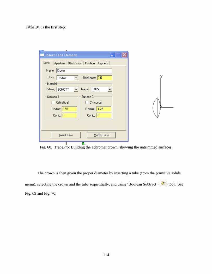
114

Table 10) is the first step:

Fig. 68. TracePro: Building the achromat crown, showing the untrimmed surfaces.

The crown is then given the proper diameter by inserting a tube (from the primitive solids

menu), selecting the crown and the tube sequentially, and using „Boolean Subtract‟ ( ) tool. See

Fig. 69 and Fig. 70.

115

Fig. 69. TracePro: Building the achromat crown, showing the tube used to trim for diameter

specification.

Fig. 70. TracePro: Resulting achromat crown.

This method of lens creation can be repeated for the creation of the flint of an achromatic doublet.

116

14.2.4. Beamsplitter Cube

A Thorlabs BS010 beam splitter is used in the TracePro model. Properties follow:

Table 11. Beamsplitter (BS010) TracePro parameter table.

Characteristic Value Source

Side Length 10 mm Manufacturer‟s Specification

Shape Cube Manufacturer‟s Specification

Fig. 71. TracePro: Image of raytrace through beamsplitter component, with characteristic result.

Notes: The construction of the BS cube was not immediately successful .The construction

method which produced the best results is presented below:

First, create a cube of the appropriate size. Create a larger rectangle, at 45o from the first

cube with one side which passes through the origin and which completely contains one half of the BS

cube:

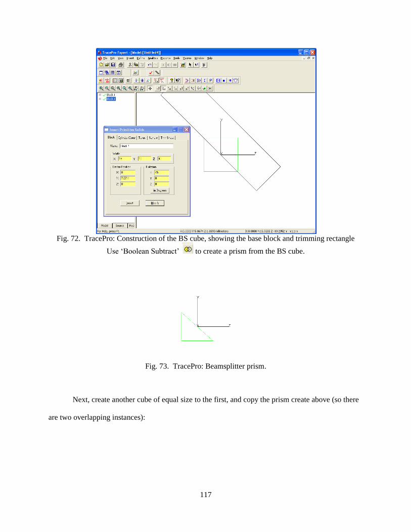
117

Fig. 72. TracePro: Construction of the BS cube, showing the base block and trimming rectangle

Use „Boolean Subtract‟ to create a prism from the BS cube.

Fig. 73. TracePro: Beamsplitter prism.

Next, create another cube of equal size to the first, and copy the prism create above (so there

are two overlapping instances):

118

Fig. 74. TracePro: BS construction image, showing the three bodies required to create the splitter.

Select the copy of the prism, and the cube created, and use „Boolean Subtract‟ to reduce the

cube to a BS prism opposite the first. Apply AR coatings to the outside surfaces, and a Beamsplitter

surface property to the diagonal. The BS should now behave as expected.

119

14.2.5. Optical Fibers

Optical fibers are easily modeled by using a cylinder of the appropriate glass and diameter.

This was verified using the specifications from the 460HP fiber (see appendix D). „Sweep‟ and

„revolve‟ allow for radiused corners and 3d paths for the fibers. Tracing light sources through the

optical fibers was deemed as unnecessary computation time for this particular model, so for the

purposes of the model the optical fibers are not physically modeled, only their light source output is.

The light output was modeled as a grid source with the following properties (see Nufern

460HP specification sheet):

Table 12. Grid Source parameters for Nufern 460HP optical fiber.

Characteristic Value Source

Diameter (1/e^2

Gaussian Waist)

3.5 µm Manufacturer‟s Specification

Beam half angle 7.45 degrees Manufacturer‟s Specification states a NA of 0.13, therefore

the half angle is 7.44 degrees.

Distribution Profile Gaussian Inherent from Laser source.

120

Fig. 75. TracePro: Distribution plot and raytrace of grid source with Nufern 460HP optical fiber

characteristics. Block for distribution monitoring.

121

Notes: The power of a grid source depends both on the number of rays traced and the peak

flux parameters, so as the number of rays is adjusted its necessary to adjust the peak flux to keep the

desired output power.

The easiest way to monitor this and make adjustments is to place a block directly in front of

the fiber which covers the beam completely. Making this a perfect absorber and tracing the source

allows one to read the irradiance map total output power.

Use the check box next to this block in the model tree to remove it from the raytrace once a

power and ray number is settled upon. See Fig. 76.

Fig. 76. TracePro: Grid source testing block.

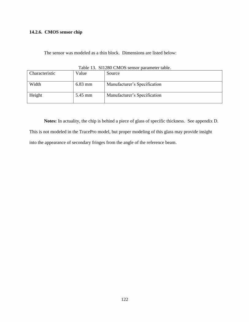
122

14.2.6. CMOS sensor chip

The sensor was modeled as a thin block. Dimensions are listed below:

Table 13. SI1280 CMOS sensor parameter table.

Characteristic Value Source

Width 6.83 mm Manufacturer‟s Specification

Height 5.45 mm Manufacturer‟s Specification

Notes: In actuality, the chip is behind a piece of glass of specific thickness. See appendix D.

This is not modeled in the TracePro model, but proper modeling of this glass may provide insight

into the appearance of secondary fringes from the angle of the reference beam.

123

15. Appendix C. Optical Characterization Details.

15.1. Resolution Algorithm

The code below can be directly put into MATLAB to perform the contrast trace of a resolution target

to determine an optical system‟s resolution.

%% This file will let you determine the line-pairs/millimeter resolution of % the optical system clc; clear; close all; % Input bitmap file type into imread function Image = imread('Resolution_target.bmp'); % Image may be stored as color image, so each color is a repeat. This means % you can strip off the extra layers of the array by allowing the command % below to run. If the image is stored as a one dimensional array comment % out the command below. Image = Image(:,:,1:1); % Show image and choose where to trace % Left click to pick start point of trace and right click to pick end point imshow(Image); improfile %% Determine resolution % Region of interest % Group being measured - % Element being measured - % What is minimum level: dark = input('dark = '); % What is maximum brightness at peak of area interest peak = input('peak = '); % What is minimum brightness in the valley of the area of interest valley = input('valley = '); %Contrast as a percent is: contrast = (peak - valley)/(peak - dark)*100

124

15.2. Depth of Field Algorithm

The code below can be directly put into MATLAB to perform the contrast trace of depth of field

target.

%% This file will let you determine dof of the optical system clc; clear; close all; Image = imread('Depth_of_field_image.bmp'); % Image may be stored as color image, so each color is a repeat. This means % you can strip off the extra layers of the array by allowing the command % below to run. If the image is stored as a one dimensional array comment % out the command below. Image = Image(:,:,1:1); % Show image and choose where to trace % Left click to pick start point of trace and right click to pick end point imshow(Image) % W will be a matrix of the gray scale variation along the trace. This % matrix can be plotted. Depending on what the minimum contrast level % to be considered in focus is, the depth of field can be determined. W = improfile;

125

15.3. Image Aberration Algorithm

The code below can be directly put into MATLAB to determine the optical distortion function. Note

that there are specific options that can be changed in this code depending on the image being

analyzed..

%% Steps to evaluate optical distortions for grid target. clc; clear; close all; %% These steps create a matrix of the distorted positions % The starting image must be cropped, so that only one column of dots is in % the entire image. %Define image as matrix Image = imread('Dot_Grid.bmp'); % Image may be stored as color image, so each color is a repeat. This means % you can strip off the extra layers of the array by allowing the command % below to run. If the image is stored as a one dimensional array comment % out the command below. Image = Image(:,:,1:3); %Determine appropriate gray scale threshold to determine what is white and %what is black. You can either let MATLAB determine what it thinks should %be the threshold by allowing the command below to run graylevel = graythresh(Image); %or you can specify the gray threshold by allowing the command below to %run. It may be necessary to specify the gray threshold if the automatic %command eliminates certain dots. Note: One "graylevel" command lines MUST %be commented out. graylevel = .30;

%Convert image to only black and white (1's and 0's in the matrix) with the %appropriate grayscale threshold BWImage = im2bw(Image,graylevel); %Image may need to be inverted if dots are black and background is white. %To invert image uncomment next line %inv_BWImage = ~BWImage; %fill holes in black/white image filled=imfill(inv_BWImage,'holes'); %Each region must be assigned a different label so the correct number of %centroids are calculated labeled_Image = bwlabel(filled,8);

126

%Filtering out small areas is necessary to ensure that random specs that %are not centroids are not labeled and used in the centroid calculation. A = regionprops(labeled_Image,'Area'); %to adjust the minimum area change what [A.Area] must be greater than in %the next line. idx = find([A.Area] > 8); BW_area_filtered = ismember(labeled_Image,idx); %label image again after filtering labeled_Image2 = bwlabel(BW_area_filtered,8); %A structure is created with all of the centroids of the dot grid struct = regionprops(labeled_Image2,'Centroid'); %Create a matrix with the centroid centers M_Centroid_distort = cat(1,struct.Centroid); %% These next steps create a matrix of the original positions % The matrix of the centroid positions needs to be sorted in ascending % order with respect to the vertical centroid coordinate while maintaining % the horizontal and vertical correlation Sorted_M_Centroid_distort = sortrows(M_Centroid_distort,2); %Length of centroid matrix Length_M_Centroid_distort = size(Sorted_M_Centroid_distort,1); %It is assumed there is no distortion at the center of the principle axes. %This step determines the point all the aberrations are centered around. aberration_center = round(Length_M_Centroid_distort/2); %If the actual distance between the centroids is unknown then you need a %estimate the distance. Estimation is done by taking the average distance %from the aberration center to the centroids immediately above and below %it. % Coordinates of centroids above and below aberration center coordinate_above = Sorted_M_Centroid_distort(round(Length_M_Centroid_distort/2)-1,2); coordinate_below = Sorted_M_Centroid_distort(round(Length_M_Centroid_distort/2)+1,2); Distance = (coordinate_below-coordinate_above)/2; %Build matrix of original centroid locations. This step only changes the %vertical location and keeps the horizontal location from the distorted %image. %make an empty matrix for filling up M_Centroid = zeros(Length_M_Centroid_distort,2); i = 0; while i < Length_M_Centroid_distort - aberration_center; j = i+1;

127

M_Centroid(aberration_center + j,2) = Sorted_M_Centroid_distort(aberration_center,2) + (Distance * j); M_Centroid(aberration_center - i,2) = Sorted_M_Centroid_distort(aberration_center,2) - (Distance * i); M_Centroid(aberration_center + j,1) = Sorted_M_Centroid_distort(aberration_center + i,1); M_Centroid(aberration_center - i,1) = Sorted_M_Centroid_distort(aberration_center - i,1); i = i+1; end %% Plot Centroids on original image % This section can be uncommented to see what the distorted centroid % locations look like plotted on the original image. % imshow(Image) % hold on % plot(M_Centroid(:,1), M_Centroid(:,2), 'b*') % hold off %% Plot aberration % Want to shift plot by coordinate of aberration center aberration = Sorted_M_Centroid_distort(round(Length_M_Centroid_distort/2),2); %make plot plot(M_Centroid(:,2)-aberration,Sorted_M_Centroid_distort(:,2)-aberration, 'bo'); %% Polynomial fitting %Choose polynomial order order = 3; p = polyfit(M_Centroid(:,2)-aberration,Sorted_M_Centroid_distort(:,2)-aberration,order); f = polyval(p,M_Centroid(:,2)-aberration); error=Sorted_M_Centroid_distort(:,2)-aberration-f;

%% Plot fitting results hold on; plot(M_Centroid(:,2)-aberration,f,'g', M_Centroid(:,2)-aberration, error,'r') legend('centroids', 'Y_d_i_s_t_o_r_t_e_d(Y)', 'error') xlabel('Undistorted Centroid Locations (Y)','FontSize',16) ylabel('Distorted Centroid Locations (Y_d_i_s_t_o_r_t_e_d)','FontSize',16)

128

16. Appendix D. Component Specifications.

16.1: GRIN Lens

16.2: 5mm Diameter Imaging Lens

16.3: 6.35mm Diameter Imaging Lens

16.4: Beam Splitter

16.5: Patch Cable

16.6: si1280 Camera

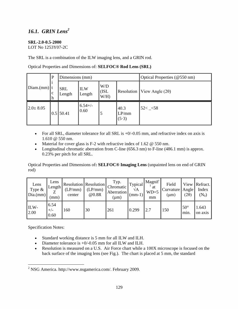
129

16.1. GRIN Lens2

SRL-2.0-0.5-2000

LOT No 1253Y07-2C

The SRL is a combination of the ILW imaging lens, and a GRIN rod.

Optical Properties and Dimensions of: SELFOC® Rod Lens (SRL)

Diam.(mm)

P

i

t

c

h

Dimensions (mm) Optical Properties (@550 nm)

SRL

Length

ILW

Length

W/D

(ISL

W/H)

Resolution View Angle (2θ)

2.0± 8.05

0.5 50.41

6.54+/-0.60

5

40.3

LP/mm

(5·3)

52< _<58

For all SRL, diameter tolerance for all SRL is +0/-0.05 mm, and refractive index on axis is

1.610 @ 550 nm.

Material for cover glass is F-2 with refractive index of 1.62 @ 550 nm.

Longitudinal chromatic aberration from C-line (656.3 nm) to F-line (486.1 mm) is approx. 0.23% per pitch for all SRL.

Optical Properties and Dimensions of: SELFOC® Imaging Lens (unpainted lens on end of GRIN

rod)

Lens

Type &

Dia.(mm)

Lens

Length

Z

(mm)

Resolution

(LP/mm)

center

Resolution

(LP/mm)

@0.8R

Typ.

Chromatic

Aberration

(µm)

Typical

√A

(mm-1)

Magnif-

1 at

WD=5

mm

Field

Curvature

(μm)

View

Angle

(2θ)

Refract.

Index

(N0)

ILW-

2.00

6.54

+/-

0.60

160 30 261 0.299 2.7 150 50°

min.

1.643

on axis

Specification Notes:

Standard working distance is 5 mm for all ILW and ILH.

Diameter tolerance is +0/-0.05 mm for all ILW and ILH.

Resolution is measured on a U.S. Air Force chart while a 100X microscope is focused on the

back surface of the imaging lens (see Fig.). The chart is placed at 5 mm, the standard

2 NSG America. http://www.nsgamerica.com/. February 2009.

130

working distance, away from the lens. Resolution is measured at both lens center and 80% of

the lens radius and normalized by the magnification factor.

Field curvature is the difference in focal positions between the lens center and at 80% of the

lens radius.

End surface is inspected at 20X magnification. No chips and cracks are allowed within 90%

of the lens radius.

Material Toxicity: This product contains components which might be toxic. The user is

advised to pay special attention to such toxicity when using this product in medical devices

for people or animals.

Storage

For extended periods of time, the lenses should be stored in a "dry box" environment. This

entails the use of a desiccant (e.g., silica gel) or a heat source to prevent humidity from

leaching the lens material. This is much more critical for non-coated lenses, since AR

coatings help to protect the lens surfaces from humidity. For short term storage (less than a

month), the plastic box and foam packing in which the lenses are shipped will provide

adequate storage.

In addition to humidity requirement, the lenses need to have sufficient spacing to avoid

potential damage such as chipping and scratching from other lenses. For this reason, NSG

storage boxes have built-in slots in which the lenses are placed, with surrounding packaging

to hold them securely in place.

Handling: After opening the lens boxes, it is important to exercise extra care in lifting the

plastic shield. Particularly with smaller lenses, it is possible that they may cling to the shield

and be lost during removal. Lenses should be handled with stainless steel tweezers,

preferably those with a tapered end. Lenses should be picked up out of their individual

compartments by firmly holding each by its side surface (not the ends).

Cleaning: At times it is necessary to clean the lens surfaces due to the presence of some dust

or film which may impair the image. NSG generally recommends the use of methyl alcohol

as a cleaning solvent. Acetone may also be used, without harm to the lens, but it should be

pure enough to no leave a residue on the lens' surface.

131

16.2. 5mm Diameter Imaging Lens3

AC050-010-A1 - f = 10.0 mm, Ø5 mm Unmounted Visible Achromat, ARC: 400-700 nm

3 Thorlabs. http://www.thorlabs.com/thorProduct.cfm?partNumber=AC050-010-A1. April 2009.

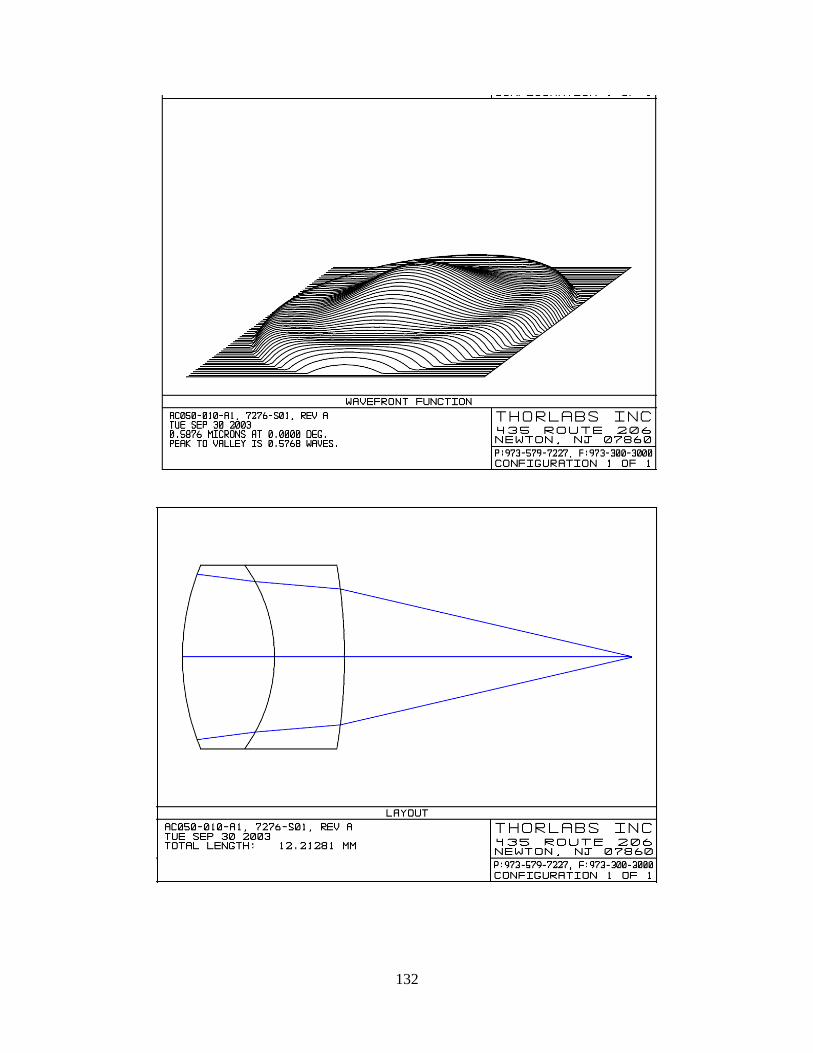
132

133

134

135

16.3. 6.35mm Diameter Imaging Lens4

AC064-013-A1 - f = 12.7 mm, Ø6.35 mm Unmounted Visible Achromat, ARC: 400-700 nm

4 Thorlabs. http://www.thorlabs.com/thorProduct.cfm?partNumber=AC064-013-A1. April 2009.

136

137

138

139

16.4. Beam Splitter5

BS013 - 400-700 nm Broadband Non-Polarizing Beamsplitter Cube, 25.4 mm

5 Thorlabs. http://www.thorlabs.com/thorProduct.cfm?partNumber=BS013. April 2009.

140

141

142

16.5. Patch Cable6

P1-460A-FC-2 - Single Mode Fiber Patch Cable, 2m, 450-600nm, FC/PC

460HP - Single Mode Optical Fiber, 450-600 nm

Source: http://www.thorlabs.com/thorProduct.cfm?partNumber=460HP

6 Thorlabs. http://www.thorlabs.com/thorProduct.cfm?partNumber=P1-460A-FC-2. April 2009.

143

144

16.6. si1280 Camera7

7 Silicon Imaging. http://www.siliconimaging.com/SI-1280CL%20spec.htm. April 2009.

145

146

147

Camera Dimensions

148

CMOS Chip