United International University Dept. Of Electrical & Electronic Engineering (EEE)

EEE 402

Control System Laboratory

ID

Name

Section

Project Name

Date of Submission

Disclaimer: I thereby certify that, this Project is prepared by me only, and I did not

copy any part of this from anybody and did not let other copy any part of my Project.

Sharif Ahmed

Signature of the student

0 2 1 1 2 1 1 1 1

Sharif Ahmed

A

Part-A : Design a pd controller using root locus method and SISOTOOL design tool Part-B : Design a feedback compensator using root locus method and SISO design tool

2 1 . 1 2 . 1 4

Project on:

Part a: Study of PD compensation& Part (b): Study of feedback compensation

Part a: Study of PD compensation

Design requirement:

Given the transfer function )10)(6)(4(

)(

sss

KsG

Design a controller that will yield no more than

25% overshoot and no more than a 2-second

settling time for a step input and zero steady state error for step and ramp inputs.

Calculation:

Before compensation:

i)%OS=25

ii)Ts=2 sec

dominant pole= -2±j4.53324

Procedure:

1. Using SISO Design tool, create the design for a unity negative feedback system with

)10)(6)(4()(

sss

KsG and plot the root locus.

2. From Edit| SISO Tool Preferences window, select Options tab, select Zero/pole/gain

radio button under Compensator Format and click Ok.

3. Right click on the SISO Design Tool window and then click on Grid.

4. Right click on the SISO Design Tool window and then click on Design Constraints| New

from the appeared window. Select Constraint Type as Percent Overshoot, set Percent

Overshoot as 25 and click Ok.

5. Select the closed-loop pole at the intersection of shadowed region and the root locus.

Write down the value obtained in the C(s) text box. Also, write down the closed-loop

poles and damping ratio obtained from View| Closed Loop Poles.

6. Select Analysis| Response to Step Command. Write down the values of percent

overshoot, peak time, settling time and steady state error from the appeared window of

LTI Viewer for SISO Design Tool.

Calculate the imaginary part, d and real part, d of the compensated dominant pole from

the two seconds settling time obtained in Step 6.

7. Find the sum of angles, 𝝨ϴ from the uncompensated system’s poles and zeros to the

desired dominant pole calculated in step 7. Then, calculate the location of compensator

zero, Zc using the formula ωd/(zc – σd) = tan (𝝨ϴ - 180 ̊)

8. Set the Value of the calculated compensated real zero to the root locus using the

window appeared after selecting Compensators| Edit | C, the value of which is obtained

in step 8.

9. Repeat step 6 and discus your findings. This is the end of PD compensation.

10. Set another real zero at -0.001 and a pole at 0 using window appeared after selecting

Compensators| Edit| C.

11. Repeat step 6 and discuss your findings. This is the end of PID compensation.

Before compensation:

For 25% Overshoot:

Dominant pole = - 2.71 ± 6.14i

K = 418

= 0.404

Now,

Kp = 0lims K G(s)

= 0lims

( 4)( 6)( 10)

K

s s s

= 4*6*10

K

= 418

4*6*10 = 1.74

So, Kp = 1.74

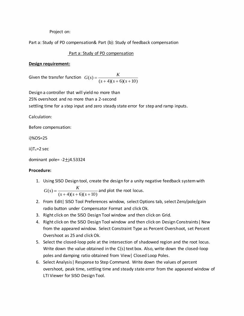
Now, e( ) = 1

1 Kp = 0.364

We found from step response Tp = 0.587 sec

j𝜔

-2.71+ 6.14𝑖

𝜃4 𝜃3 𝜃2

-10 -6 -4 𝜎𝑑

For a closed loop System

T(s) = ( )

1 ( )

KG s

KG s

Now to meet the ideal situation,

1 + KG(s) = 0

KG(s) = -1

= 1 < ± (2n + 1) 180 ̊

Again, |KG(s)| = 1

So, < KG(s) = ± (2n + 1) 180 ̊

𝛴 𝜃 = -𝜃1 - 𝜃2 - 𝜃3 Here, 𝜃1, 𝜃2 , 𝜃3 =angles due to Poles

= ±180 ̊

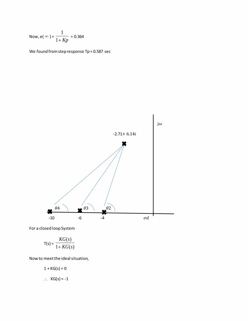
Calculation after compensation:

Percent overshoot % OS = 25 and settling time T’p = 2 sec

And the new dominant Pole = - 𝜎𝑑 ± jωdc

Now,

T’s = 4

dc = 2

Again 𝜃 = 1cos =

1cos (0.404) = 66.17

tan𝜃 =

dc

dc

= 2

dc

dc = 2 * tan = 4.53

New Dominant Pole =- 𝜎𝑑𝑐 ± jωdc = - 2 + 4.53i

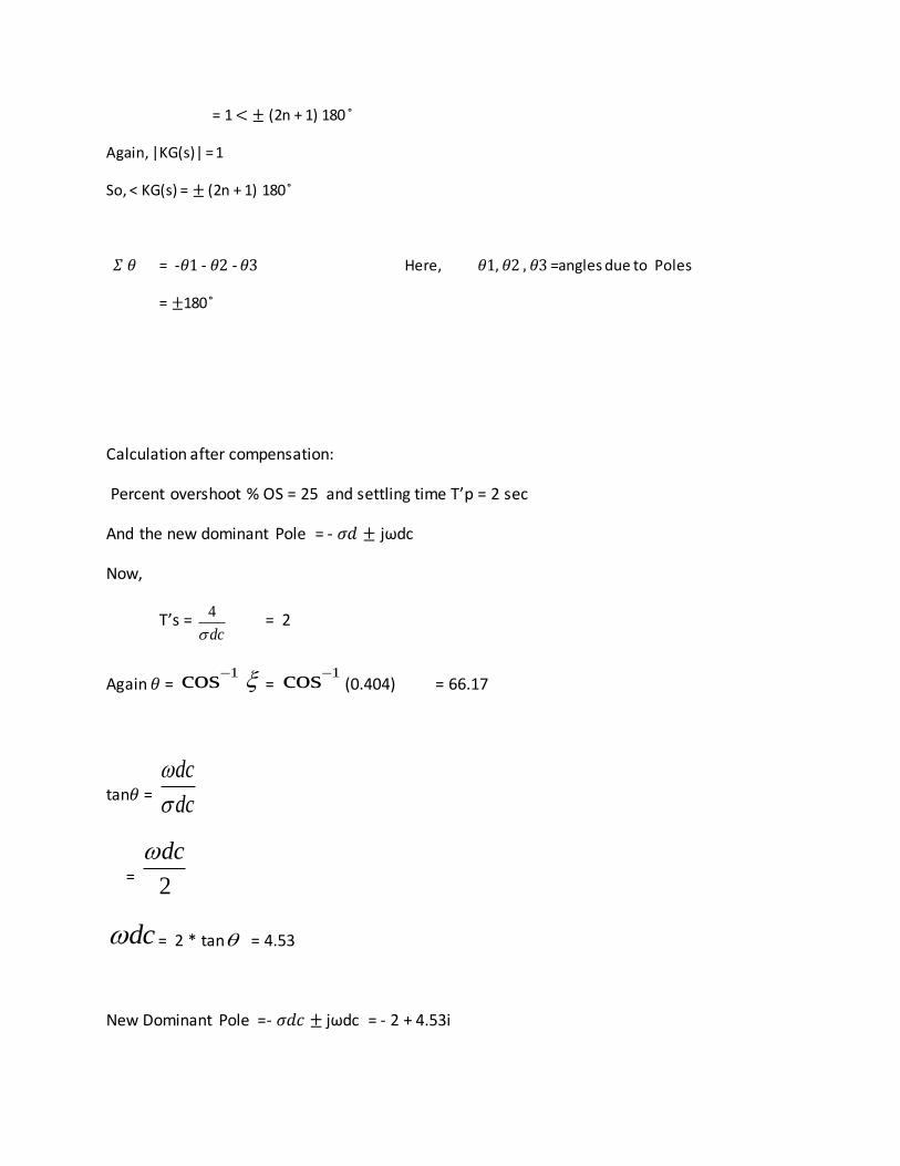
Now, add a pole at the origin to increase system type and drive error to zero for step input.

j𝜔

- 2 + 4.53i

𝜃4 𝜃3 𝜃2 𝜃1

-10 -6 -4 0 𝜎𝑑

𝛴 𝜃 = -𝜃1 - 𝜃2 -𝜃3- 𝜃4 Here, 𝜃1, 𝜃2 , 𝜃3, 𝜃4= angles due to Poles

𝜃1 =180 -1tan 4.53

2=113.821 ̊

𝜃2 = 1tan 4.53

4 2= 66.17 ̊

𝜃3 = 1tan 4.53

6 2= 48.55 ̊

𝜃4 =1tan 4.53

10 2= 29.52 ̊

Now Σ 𝜃 = - 113.821- 66.17 – 48.55 – 29.52

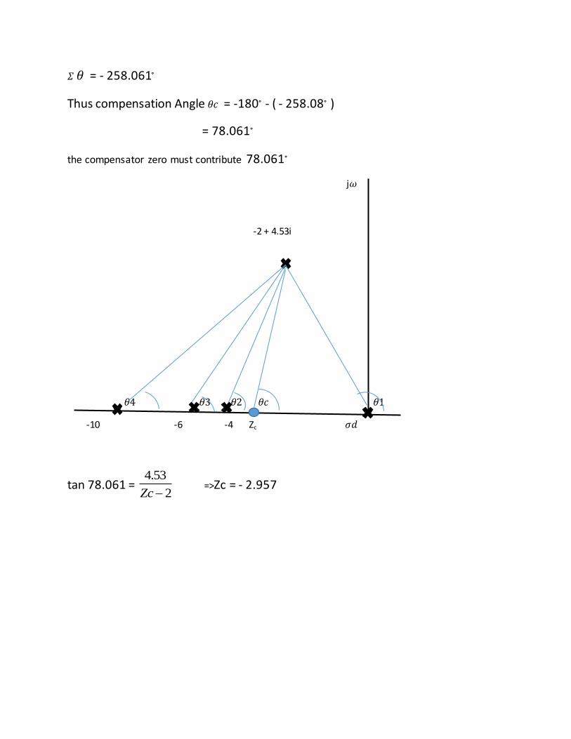
𝛴 𝜃 = - 258.061 ̊

Thus compensation Angle 𝜃𝑐 = -180 ̊ - ( - 258.08 ̊ )

= 78.061 ̊

the compensator zero must contribute 78.061 ̊

j𝜔

-2 + 4.53i

𝜃4 𝜃3 𝜃2 𝜃𝑐 𝜃1

-10 -6 -4 Zc 𝜎𝑑

tan 78.061 = 4.53

2Zc =>Zc = - 2.957

New transfer function G(s) = ( 2.957)

( 4)( 6)( 10)

s

s s s

Uncompensated PD-compensated PID-compensated

Plant and Compensator ( 4)( 6)( 10)

K

s s s

K( 2.957)

s( 4)( 6)( 10)

s

s s s

2

( 2.957)(s 0.001)

s ( 3)( 6)( 10)

s

s s s

Dominant Poles

-2.71±6.14i -2.1±4.51i -2.1 ±4.51i

K 418 291 292

0.404 0.408 0.406

n 6.71 4.93 4.94

%OS 25 25 25

Ts 1.32 1.94 1.76

Tp 0.587 0.235 0.801

Kp& Kv Kp = 1.74 Kv = 13.27 Kp=

Kp=∞ Kv=

e( )

0.364 e( ) for Kv=0.0753 e( )for Kp= 0

Kp=0 Kv=0

Other poles -14.6 -13.3, -2.66 -13.3, -2.66,-0.001

Zeroes none -2.957 -2.957, -0.001

Part b: Study of feedback compensation

a. Design the value ofK1, as well as a in the feedback

path of the minor loop, to yield a settling time of 1

second with 5% overshoot for the step response.

b. Design the value of K to yield a major-loop

response with 10% overshoot for a step input.

c. Use MATLAB or any other computer

program to simulate the step response to the entire closedloop system.

d.

Add a PI compensator to reduce

the major-loop steady-state

error to zero and simulate the step

response using MATLAB or any other

computer program

Procedure:

Minor-loop compensated system:

1. Using SISO Design tool, create the design for the minor loop containing the plant G(s)

with K1 = 1 and the feedback compensator H(s) = s+a and plot the root locus. The value

of Kf will be adjusted to the location of minor-loop poles

2. From Edit| SISO Tool Preferences window, select Options tab, select Zero/pole/gain

radio button under Compensator Format and click Ok.

Right click on the SISO Design Tool window and then click on Grid.

3. Right click on the SISO Design Tool window and then click on Design Constraints| New

from the appeared window. Select Constraint Type as %OS, set Damping it as 5 and click

Ok.

4. Select the closed-loop pole at the intersection of shadowed region and the root locus.

Write down the value obtained in the C(s) text box. This value is equal to Kf. Also, write

down the closed-loop poles and natural frequency obtained from View| Closed Loop

Poles.

5. Select Analysis| Response to Step Command. Write down the values of percent

overshoot, peak time, settling time and steady state error from the appeared window of

LTI Viewer for SISO Design Tool. The performance is tabulated in Table 1.

The entire Closed-loop compensated system:

The closed loop poles and zeros for the minor loop are the open loop poles for the entire unity-

feedback closed-loop system. Henceforth, repeat the steps 1, 4, 5, and 7, complete the

compensation, but this time %OS of 10 for step 4.

This is the end of feedback-compensation using approach 2

Calculation:

Given, settling time, Ts= 1sec

% OS=5%

Now, σd= Ts

4=4

We know, % OS 100)1/( 2

e

= 689.04.3409

2.995

Now, ωn = σd=4

=> ωn= 805.50.689

4

Thus, 2

nd 1 =4.20

Dominant pole dd j =-4±j4.20

4+j4.20

j ωd

𝜃3 𝜃2 𝜃1

-9 -4 0 𝜎𝑑

𝜃1= 180 ̊ - 1tan 4.20

133.64

𝜃2= 90 ̊

𝜃3= 1tan 4.30

40.039 4

Now ∑ 𝜃= -133.6 – 90-40.03=-263.63

So the compensated angle should be, 𝜃𝑐=-180-(-263.63)=83.63.

Since the angle is positive, so we have to add a zero in the transfer function

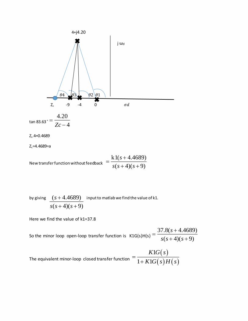
4+j4.20

j ωd

𝜃4 𝜃3 𝜃2 𝜃1

Zc -9 -4 0 𝜎𝑑

tan 83.63 ̊4.20

4Zc

Zc-4=0.4689

Zc=4.4689=a

New transfer function without feedback k1( 4.4689)

( 4)( 9)

s

s s s

by giving ( 4.4689)

( 4)( 9)

s

s s s

input to matlab we find the value of k1.

Here we find the value of k1=37.8

So the minor loop open-loop transfer function is K1G(s)H(s)

37.8( 4.4689)

( 4)( 9)

s

s s s

The equivalent minor-loop closed transfer function

1

1 1

K G s

K G s H s

37.8 1*

( 4)( 9) 37.8( 4.4689)( 4)( 9)

( 4)( 9)

s s s ss s s

s s s

3 2

37.8

13 73.8 168.92s s s

(b):

The major-loop open-loop transfer function is Ge(s)

3 2

37.8

13 73.8 168.92

K

s s s

Drawing the root locus using Ge(s) and searching along the 10% overshoot line (ζ = 0.574) for K

= 0.811.

Now the uncompensated and compensated value table should be like this:

Uncompensated Compensated

Plant and

Compensator 3 2

1

13 36

K

s s s 3 2

37.8

13 73.8 168.92

K

s s s

Dominant Poles -1.56±j1.64 -3.33±j4.53

Gain K1=50.8 K=0.86

0.689 0.592

n 2.27 5.62

% OS 5 5

Ts 2.75 1.1

Tp 2.03 0.927

Kv 1.411 0

e() 0.708

Other poles -9.87 -6.34

Zeroes - -

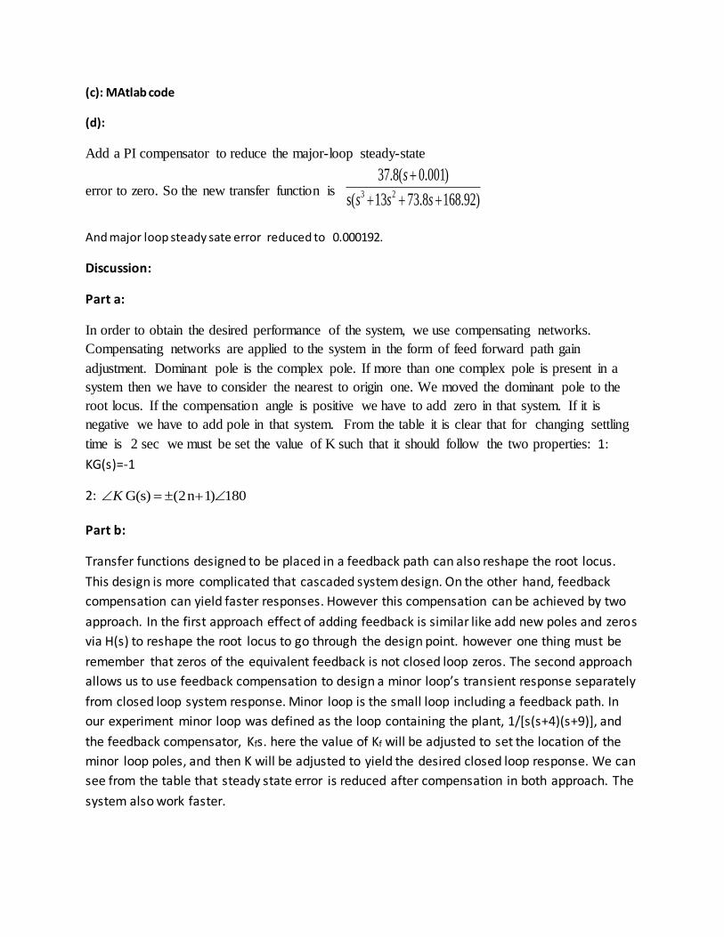
(c): MAtlab code

(d):

Add a PI compensator to reduce the major-loop steady-state

error to zero. So the new transfer function is 3 2

37.8( 0.001)

s( 13 73.8 168.92)

s

s s s

And major loop steady sate error reduced to 0.000192.

Discussion:

Part a:

In order to obtain the desired performance of the system, we use compensating networks.

Compensating networks are applied to the system in the form of feed forward path gain

adjustment. Dominant pole is the complex pole. If more than one complex pole is present in a

system then we have to consider the nearest to origin one. We moved the dominant pole to the

root locus. If the compensation angle is positive we have to add zero in that system. If it is

negative we have to add pole in that system. From the table it is clear that for changing settling

time is 2 sec we must be set the value of K such that it should follow the two properties: 1:

KG(s)=-1

2: G(s) (2n 1) 180K

Part b:

Transfer functions designed to be placed in a feedback path can also reshape the root locus.

This design is more complicated that cascaded system design. On the other hand, feedback

compensation can yield faster responses. However this compensation can be achieved by two

approach. In the first approach effect of adding feedback is similar like add new poles and zeros

via H(s) to reshape the root locus to go through the design point. however one thing must be

remember that zeros of the equivalent feedback is not closed loop zeros. The second approach

allows us to use feedback compensation to design a minor loop’s transient response separately

from closed loop system response. Minor loop is the small loop including a feedback path. In

our experiment minor loop was defined as the loop containing the plant, 1/[s(s+4)(s+9)], and

the feedback compensator, Kfs. here the value of Kf will be adjusted to set the location of the

minor loop poles, and then K will be adjusted to yield the desired closed loop response. We can

see from the table that steady state error is reduced after compensation in both approach. The

system also work faster.