Project AMIGA: The Circumgalactic Medium of Andromeda*

Nicolas Lehner1 , Samantha C. Berek1,2,20, J. Christopher Howk1 , Bart P. Wakker3 , Jason Tumlinson4,5 ,Edward B. Jenkins6 , J. Xavier Prochaska7 , Ramona Augustin4 , Suoqing Ji8 , Claude-André Faucher-Giguère9 ,

Zachary Hafen9 , Molly S. Peeples4,5 , Kat A. Barger10 , Michelle A. Berg1 , Rongmon Bordoloi11 , Thomas M. Brown4 ,Andrew J. Fox12 , Karoline M. Gilbert4,5 , Puragra Guhathakurta7 , Jason S. Kalirai13 , Felix J. Lockman14 ,

John M. O’Meara15 , D. J. Pisano16,17,21, Joseph Ribaudo18 , and Jessica K. Werk191 Department of Physics, University of Notre Dame, Notre Dame, IN 46556, USA

2 Department of Astronomy, Yale University, New Haven, CT 06511, USA3 Department of Astronomy, University of Wisconsin–Madison, WI 53706, USA

4 Space Telescope Science Institute, 3700 San Martin Drive, Baltimore, MD 21218, USA5 Department of Physics & Astronomy, Johns Hopkins University, 3400 N. Charles Street, Baltimore, MD 21218, USA

6 Department of Astrophysical Sciences, Princeton University, Princeton, NJ 08544, USA7 UCO/Lick Observatory, Department of Astronomy & Astrophysics, University of California Santa Cruz, 1156 High Street, Santa Cruz, CA 95064, USA

8 TAPIR, Walter Burke Institute for Theoretical Physics, California Institute of Technology, Pasadena, CA 91125, USA9 CIERA and Department of Physics and Astronomy, Northwestern University, 2145 Sheridan Road, Evanston, IL 60208, USA

10 Department of Physics & Astronomy, Texas Christian University, Fort Worth, TX 76129, USA11 North Carolina State University, Department of Physics, Raleigh, NC 27695-8202, USA

12 AURA for ESA, Space Telescope Science Institute, 3700 San Martin Drive, Baltimore, MD 21218, USA13 Johns Hopkins Applied Physics Laboratory, 11100 Johns Hopkins Road, Laurel, MD 20723, USA

14 Green Bank Observatory, Green Bank, WV 24944, USA15W. M. Keck Observatory 65-1120 Mamalahoa Highway Kamuela, HI 96743, USA

16 Department of Physics & Astronomy, West Virginia University, P.O. Box 6315, Morgantown, WV 26506, USA17 Center for Gravitational Waves and Cosmology, West Virginia University, Chestnut Ridge Research Building, Morgantown, WV 26505, USA

18 Department of Engineering and Physics, Providence College, Providence, RI 02918, USA19 Department of Astronomy, University of Washington, Seattle, WA 98195, USA

Received 2020 February 17; revised 2020 June 26; accepted 2020 June 30; published 2020 August 27

Abstract

Project AMIGA (Absorption Maps In the Gas of Andromeda) is a survey of the circumgalactic medium (CGM) ofAndromeda (M31, Rvir;300 kpc) along 43 QSO sightlines at impact parameters 25 �R�569 kpc (25 atRRvir). We use ultraviolet absorption measurements of Si II, Si III, Si IV, C II, and C IV from the Hubble SpaceTelescope/Cosmic Origins Spectrograph and O VI from the Far Ultraviolet Spectroscopic Explorer to provide anunparalleled look at how the physical conditions and metals are distributed in the CGM of M31. We find that Si IIIand O VI have a covering factor near unity for R1.2 Rvirand 1.9 Rvir, respectively, demonstrating that M31has a very extended ∼104–105.5 K ionized CGM. The metal and baryon masses of the 104–105.5 K CGM gaswithin Rvir are 108 and 4×1010 (Z/0.3 Ze)

−1Me, respectively. There is not much azimuthal variation in thecolumn densities or kinematics, but there is with R. The CGM gas at R0.5 Rviris more dynamic and has morecomplicated, multiphase structures than at larger radii, perhaps a result of more direct impact of galactic feedbackin the inner regions of the CGM. Several absorbers are projected spatially and kinematically close to M31 dwarfsatellites, but we show that those are unlikely to give rise to the observed absorption. Cosmological zoomsimulations of ∼L* galaxies have O VI extending well beyond Rvir as observed for M31 but do not reproduce wellthe radial column density profiles of the lower ions. However, some similar trends are also observed, such as thelower ions showing a larger dispersion in column density and stronger dependence on R than higher ions. Based onour findings, it is likely that the Milky Way has a ∼104–105.5 K CGM as extended as for M31 and their CGM(especially the warm–hot gas probed by O VI) are overlapping.

Unified Astronomy Thesaurus concepts: Circumgalactic medium (1879); Andromeda Galaxy (39); Local Group(929); Quasar absorption line spectroscopy (1317)

Supporting material: figure sets, machine-readable tables

1. Introduction

Over the past 10 yr, in particular since the installation of theCosmic Origins Spectrograph (COS) on the Hubble SpaceTelescope (HST), we have made significant leaps in empiricallycharacterizing the circumgalactic medium (CGM) of galaxies at

low redshift, where a wide range of galaxy masses can bestudied (see recent review by Tumlinson et al. 2017). Weappreciate now that the CGM of typical star-forming orquiescent galaxies has a large share of galactic baryons andmetals in relatively cool gas phases (104–105.5 K; e.g., Stockeet al. 2013; Bordoloi et al. 2014; Liang & Chen 2014; Peepleset al. 2014; Werk et al. 2014; Johnson et al. 2015; Burchett et al.2016; Prochaska et al. 2017b; Chen et al. 2019; Poisson et al.2020). We have come to understand that the CGM of galaxies atz1 is not just filled with metal-enriched gas ejected bysuccessive galaxy outflows, but has also a large amount of

The Astrophysical Journal, 900:9 (44pp), 2020 September 1 https://doi.org/10.3847/1538-4357/aba49c© 2020. The American Astronomical Society. All rights reserved.

* Based on observations made with the NASA/ESA Hubble Space Telescope,obtained from the data archive at the Space Telescope Science Institute. STScIis operated by the Association of Universities for Research in Astronomy, Inc.,under NASA contract NAS 5-26555.20 NSF REU student.21 Adjunct Astronomer, Green Bank Observatory.

1

metal-poor gas (<1%–2% solar) in which little net chemicalenrichment has occurred over several billions of years (e.g.,Ribaudo et al. 2011; Thom et al. 2011; Lehner et al. 2013,2018, 2019; Wotta et al. 2016, 2019; Prochaska et al. 2017b;Kacprzak et al. 2019; Zahedy et al. 2019; Poisson et al. 2020).The photoionized gas around z1 galaxies is very chemicallyinhomogeneous, as shown by large metallicity ranges and thelarge metallicity variations among kinematically distinct com-ponents in a single halo (Lehner et al. 2019; Wotta et al. 2019;see also Crighton et al. 2013; Muzahid et al. 2015, 2016;Rosenwasser et al. 2018). Such a large metallicity variation isobserved not only in the CGM of star-forming galaxies but alsoin the CGM of passive and massive galaxies, where thereappears to be as much cold, bound H I gas as in their star-forming counterparts (e.g., Thom et al. 2012; Tumlinson et al.2013; Berg et al. 2019; Zahedy et al. 2019).

These empirical results have revealed both expected andunexpected properties of the CGM of galaxies, and they allprovide new means to understand the complex relationshipbetween galaxies and their CGM. Prior to these empiricalresults, the theory of galaxy formation and evolution wasmostly left constraining the CGM properties indirectly by theiroutcomes, such as galaxy stellar mass and interstellar medium(ISM) properties. Thus, the balance between outflows, inflows,recycling, and ambient gas—and the free parameters control-ling them—was tuned to match the optical properties ofgalaxies rather than implemented directly as physicallyrigorous and self-consistent models. These indirect constraintssuffer from problems of model uniqueness: it is possible tomatch stellar masses and metallicities with very differenttreatments of feedback physics (e.g., Hummels et al. 2013;Liang et al. 2016). Recent empirical and theoretical advancesoffer a way out of this model degeneracy. New high-resolution,zoom-in simulations employ explicit treatments of the multiplegas-phase nature and feedback from stellar population models(e.g., Hopkins et al. 2014, 2018). It is also becoming clear thathigh resolution not only inside the galaxies but also in theirCGM is required to capture more accurately the complexprocesses in the cool CGM, such as metal mixing (Hummelset al. 2019; Peeples et al. 2019; Suresh et al. 2019; van deVoort et al. 2019; Corlies et al. 2020).

A significant limitation in interpreting the new empiricalresults in the context of new high-resolution zoom simulationsis that only average properties of the CGM are robustly derivedfrom traditional QSO absorption-line techniques for examininghalo gas. In the rare cases where there is a UV-bright QSObehind a given galaxy, the CGM is typically probed along asingle “core sample” through the halo of each galaxy. Thesemeasurements are then aggregated into a statistical map, wheregalaxies with different inclinations, sizes, and environments areblended together and the radial–azimuthal dependence of theCGM is essentially lost. All sorts of biases can result:phenomena that occur strongly in only a subset of galaxiescan be misinterpreted as being weaker but more common, andgenuine trends with mass or star formation rate (SFR) can bemisinterpreted as simply scatter with no real physical meaning(see also Bowen et al. 2016). Simulations also suggest thattime-variable winds, accretion flows, and satellite halos caninduce strong halo-to-halo variability, further complicatinginterpretation (e.g., Hafen et al. 2017; Oppenheimer et al.2018a). Observational studies of single-galaxy CGM with

multiple sightlines are therefore required to gain spatialinformation on the properties of the CGM.Multi-sightline information on the CGM of single galaxies

has been obtained in a few cases from binary or multiple (twoto four) grouped QSOs behind foreground galaxies (e.g.,Bechtold et al. 1994; Martin et al. 2010; Keeney et al. 2013;Bowen et al. 2016), gravitationally lensed quasars (e.g., Smetteet al. 1992; Rauch et al. 2001; Ellison et al. 2004; Lopez et al.2005; Zahedy et al. 2016; Rubin et al. 2018; Kulkarni et al.2019), giant gravitational arcs (e.g., Lopez et al. 2020), orextended bright background objects observed with integral fieldunits (e.g., Péroux et al. 2018). These observations providebetter constraints on the kinematic relationship between theCGM gas and the galaxy and on the size of CGM structures.However, they yield limited information on the gas-phasestructure owing to a narrow range of ionization diagnostics orpoor-quality spectral data. Thus, it remains unclear how tracersof different gas phases vary with projected distance R orazimuth Φ around the galaxy.The CGM that has been pierced the most is that of the Milky

Way (MW), with several hundred QSO sightlines (Wakkeret al. 2003; Shull et al. 2009; Lehner et al. 2012; Putman et al.2012; Richter et al. 2017) through the Galactic halo. However,our position as observers within the MW disk severely limitsthe interpretation of these data (especially for the extendedCGM; see Zheng et al. 2015, 2020) and makes it difficult tocompare with observations of other galaxies.With a virial radius that spans over 23° on the sky, M31 is

the only L* galaxy where we can access more than fivesightlines without awaiting the next generation of UV space-based telescopes (e.g., The LUVOIR Team 2019). With currentUV capabilities, it is the only single galaxy where we can studythe global distribution and properties of metals and baryons insome detail.In our pilot study (Lehner et al. 2015, hereafter LHW15), we

mined the HST/COS G130M/G160M archive available at theBarbara A. Mikulski Archive for Space Telescopes (MAST) forsightlines piercing the M31 halo within a projected distance of∼2 Rvir(where Rvir=300 kpc for M31; see below). Therewere 18 sightlines, but only 7 at projected distance RRvir.Despite the small sample, the results of this study were quiterevealing, demonstrating a high covering factor (6/7) of M31CGM absorption by Si III (and other ions, including, e.g., C IV,Si II) within 1.1 Rvirand a covering factor near zero (1/11)between 1.1 Rvirand 2 Rvir. We found also a drastic change inthe ionization properties, as the gas is more highly ionized atR∼Rvirthan at R<0.2 Rvir. The LHW15 results stronglysuggest that the CGM of M31 as seen in absorption of low ions(C II, Si II) through intermediate (Si III, Si IV) and high ions(C IV, O VI) is very extended out to at least the virial radius.However, owing to the small sample within Rvir, the variationof the column densities (N) and covering factors ( fc) withprojected distances and azimuthal angle remains poorlyconstrained.Our Project Absorption Maps In the Gas of Andromeda

(AMIGA) is a large HST program (PID: 14268; PI: Lehner)that aims to fill the CGM with 18 additional sightlines atvarious R and Φ within 1.1 Rvirof M31 using high-quality COSG130M and G160M observations, yielding a sample of 25background QSOs probing the CGM of M31. We have alsosearched MAST for additional QSOs beyond 1.1 Rvirup toR=569 kpc from M31 (∼1.9 Rvir) to characterize the

2

The Astrophysical Journal, 900:9 (44pp), 2020 September 1 Lehner et al.

extended gas around M31 beyond its virial radius. This archivalsearch yielded 18 suitable QSOs. Our total sample of 43 QSOsprobing the CGM of a single galaxy from 25 to 569 kpc is thefirst to explore simultaneously the azimuthal and radialdependence of the kinematics, ionization level, surfacedensities, and mass of the CGM of a galaxy over its entirevirial radius and beyond. With these observations, we can alsotest how the CGM properties derived from one galaxy usingmultiple sightlines compare with a sample of galaxies withsingle sightline information, and we can directly compare theresults with cosmological zoom-in simulations.

With the COS G130M and G160M wavelength coverage,the key ions in our study are C II, C IV, Si II, Si III, and Si IV(other ions and atoms include Fe II, S II, O I, N I, and N V, butthese are typically not detected, although the limit on O Iconstrains the level of ionization). These species spanionization potentials from <1 to ∼4 ryd and thus trace neutralto highly ionized gas at a wide range of temperatures anddensities. We have also searched the Far Ultraviolet Spectro-scopic Explorer (FUSE) to have coverage of O VI, whichresulted in 11 QSOs in our sample having both COS and FUSEobservations. The H ILyα absorption can unfortunately not beused because the MW dominates the entire Lyα absorption.Instead, we have obtained deep H I 21 cm observations with theRobert C. Byrd Green Bank Telescope (GBT) toward all thetargets in our sample and several additional ones (Howk et al.2017, hereafter Paper I), showing no detection of any H I downto a level of NH I;4×1017 cm−2 (5σ; averaged over an areathat is 2 kpc at the distance of M31). Our nondetections place alimit on the covering factor of such optically thick H I gasaround M31 to fc<0.051 (at 90% confidence level) forRRvir.

This paper is organized as follows. In Section 2, we providemore information about the criteria used to assemble oursample of QSOs and explain the various steps to derive theproperties (velocities and column densities) of the absorption.In that section, we also present the line identification for eachQSO spectrum, which resulted in the identification of 5642lines. In Section 2.5, we explain in detail how we remove theforeground contamination from the Magellanic Stream (MS;e.g., Putman et al. 2003; Nidever et al. 2008; Fox et al. 2014),which extends to the M31 CGM region of the sky with radialvelocities that overlap with those expected from the CGM ofM31. For this work, we have developed a more systematic andautomated methodology than in LHW15 to deal with thiscontamination. In Section 3, we present the sample of the M31dwarf satellite galaxies to which we compare the halo gasmeasurements. In Section 4, we derive the empirical propertiesof the CGM of M31, including how the column densities andvelocities vary with R and Φ, the covering factors of the ionsand how they change with R, and the metal and baryon massesof the CGM of M31. In Section 5, we discuss the resultsderived in Section 4 and compare them to observations fromthe COS-Halos survey (Tumlinson et al. 2013; Werk et al.2014) and to state-of-the-art cosmological zoom-ins from, inparticular, the Feedback in Realistic Environments (FIRE;Hopkins et al. 2020) and the Figuring Out Gas and Galaxies InEnzo (FOGGIE; Peeples et al. 2019) simulation projects. InSection 6, we summarize our main conclusions.

To properly compare to other work and to simulations, wemust estimate a characteristic radius for M31. We use the

radius R200 enclosing a mean overdensity of 200 times thecritical density: R200=(3M200/4πΔ ρcrit)

1/3, where Δ=200and ρcrit is the critical density. For M31, we adopt M200=1.26×1012Me (e.g., Watkins et al. 2010; van der Marel et al.2012), implying R200;230 kpc. For the virial mass and radius(Mvir and Rvir), we use the definition that follows from the top-hat model in an expanding universe with a cosmologicalconstant where Mvir=4π/3 ρvir Rvir

3, where the virial densityρvir=ΔvirΩmρcrit (Klypin et al. 2011; van der Marel et al.2012). The average virial overdensity isΔvir=360 assuming acosmology with h=0.7 and Ωm=0.27 (Klypin et al. 2011).Following, e.g., van der Marel et al. (2012), Mvir;1.2M200;1.5×1012Me and Rvir;1.3R200;300 kpc. The escapevelocity at R200 for M31 is then v200;212 km s−1. A distanceof M31 of dM31=752±27 kpc based on the measurementsof Cepheid variables (Riess et al. 2012) is assumed throughout.We note that this distance is somewhat smaller than the otheroften-adopted distance of M31 of 783 kpc (e.g., Brown et al.2004; McConnachie et al. 2005), but for consistency with ourprevious survey, as well as the original design of ProjectAMIGA, we have adopted dM31=752 kpc. All the projecteddistances were computed using the 3D separation (coordinatesof the target and distance of M31).

2. Data and Analysis

2.1. The Sample

The science goals of our HST large program requireestimating the spatial distributions of the kinematics and metalcolumn densities of the M31 CGM gas within about 1.1 Rvirasa function of azimuthal angle and impact parameter. The searchradius was selected based on our pilot study, where we detectedM31 CGM gas up to ∼1.1 Rvir, but essentially not beyond(LHW15) (a finding that we revisit in this paper with a largerarchival sample; see below). With our HST program, weobserved 18 QSOs at R1.1 Rvirthat were selected to spanthe M31 projected major axis, minor axis, and intermediateorientations. The sightlines do not sample the impact parameterspace or azimuthal distribution at random. Instead, thesightlines were selected to probe the azimuthal variationssystematically. The sample was also limited by a general lackof identified UV-bright active galactic nuclei (AGNs) behindthe northern half of M31’s CGM owing to higher foregroundMW dust extinction near the plane of the MW disk. Combinedwith seven archival QSOs, these sightlines probe the CGM ofM31 in azimuthal sectors spanning the major and minor axeswith a radial sample of 7–10 QSOs in each ∼100 kpc bin in R.In addition to target locations, the 18 QSOs were optimized

to be the brightest available QSOs (to minimize exposure time)and to have the lowest available redshifts (in order to minimizethe contamination from unrelated absorption from high-redshiftabsorbers). For targets with no existing UV spectra prior to ourobservations, we also required that the Galaxy EvolutionExplorer near-UV (NUV) and far-UV (FUV) flux magnitudesare about the same to minimize the likelihood of an interveningLyman limit system (LLS) with optical depth at the Lymanlimit τLL>2. An intervening LLS could absorb more or all ofthe QSO flux we would need to measure foreground absorptionin M31. This strategy successfully kept QSOs with interveningLLS out of the sample.

3

The Astrophysical Journal, 900:9 (44pp), 2020 September 1 Lehner et al.

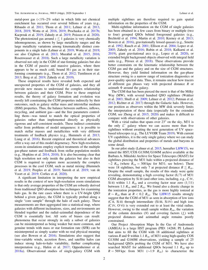
As we discuss below and as detailed by LHW15, the MScrosses through the M31 region of the sky at radial velocitiesthat can overlap with those of M31 (see also Nidever et al.2008; Fox et al. 2014). To understand the extent of MScontamination and the extended gas around M31 beyond thevirial radius, we also searched for targets beyond 1.1 RvirwithCOS G130M and/or G160M data. This search identifiedanother 18 QSOs at 1.1R/Rvir<1.9 that met the dataquality criteria for inclusion in the sample.22 Our final sampleconsists of 43 sightlines probing the CGM of M31 from 25 to569 kpc; 25 of these probe the M31 CGM from 25 to 342 kpc,corresponding to 0.08–1.1 Rvir. Figure 1 shows the locations ofeach QSO in the M31–M33 system (the filled circles beingtargets obtained as part of our HST program PID: 14268 andthe open circles being QSOs with archival HST COS G130M/G160M data), and Table 1 lists the properties of our sampleQSOs ordered by increasing projected distances from M31. Inthis table, we list the redshift of the QSOs (zem), the J2000 rightascension (R.A.) and declination (decl.), the MS coordinate(lMS, bMS; see Nidever et al. 2008 for the definition of thiscoordinate system), the radially (R) and Cartesian (X, Y)projected distances, the program identification of the HSTprogram (PID), the COS grating used for the observations ofthe targets, and the signal-to-noise ratio (S/N) per COSresolution element of the COS spectra near the Si III transition.

2.2. UV Spectroscopic Calibration

To search for M31 CGM absorption and to determine theproperties of the CGM gas, we use ions and atoms that havetheir wavelengths in the UV (see Section 2.4). Any transitionswith λ>1144Å are in the HST COS bandpass. All the targetsin our sample were observed with HST using the COS G130Mgrating (Rλ≈17,000). All the targets observed as part of ournew HST program were also observed with COS G160M, andall the targets but one within R<1.1 Rvirhave both G130Mand G160M wavelength coverage.We also searched for additional archival UV spectra in

MAST, including the FUSE (Rλ≈15,000) archive tocomplement the gas-phase diagnostics from the COS spectrawith information from the O VI absorption. We use the FUSEobservations for 11 targets with adequate S/N near O VI (i.e.,5): RX J0048.3+3941, IRAS F00040+4325, Mrk352, PG0052+251, Mrk335, UGC12163, PG 0026+129, Mrk1502,NGC7469, Mrk304, and PG 2349−014 (only the first sixtargets in this list are at R1.1 Rvir). We did not considerFUSE data for quasars without COS observations because theavailable UV transitions in the FUV spectrum (O VI, C II, C III,Si II, Fe II) are either too weak or too contaminated to allow fora reliable identification of the individual velocity componentsin their absorption profiles.There are also three targets (Mrk335, UGC12163, and

NGC7469) with HST STIS E140M (Rλ;46,500) observa-tions that provide higher-resolution information.23

Figure 1. Locations of the Project AMIGA pointings relative to the M31–M33 system. The axes show the angular separations converted into physical coordinatesrelative to the center of M31. North is up and east to the left. The 18 sightlines from our large HST program are shown with red filled circles; the 25 archival COStargets are shown with open red circles. Plus signs show the GBT H I 21 cm observations described in Paper I. Dotted circles show impact parameters R=100, 200,300, 400, and 500 kpc. Rvir=300 kpc is marked with a thick dashed line. The sizes and orientations of the two galaxies are taken from RC3 (de Vaucouleurset al. 1991) and correspond to the optical R25 values. The light-blue dashed line shows the plane of the MS (bMS=0°) as defined by Nidever et al. (2008). The shadedregion within bMS±20° of the MS midplane is the approximate region where we identify most of the MS absorption components contaminating the M31 CGMabsorption (see Section 2.5).

22 This search found eight additional targets at R>1.6 Rvirthat are notincluded in our sample. SDSSJ021348.53+125951.4, 4C 10.08, andLBQS0052-0038 were excluded because of low S/N in the COS data.NGC7714 has smeared absorption lines. LBQS0107-0232/3/5 lie atzem;0.7–1 and have extremely complex spectra. HS 2154+2228 atzem=1.29 has no G130M wavelength coverage, making the line identificationhighly uncertain.

23 For two targets, we also use COS G225M (3C454.3) and FOS NUV(3C454.3, PG 0044+030) observations to help with the line identification (seeSection 2.3). The data processing follows the same procedure as the other data.

4

The Astrophysical Journal, 900:9 (44pp), 2020 September 1 Lehner et al.

Information on the design and performance of COS, STIS,and FUSE can be found in Green et al. (2012), Woodgate et al.(1998), and Moos et al. (2000), respectively. For the HST data,we use the pipeline-calibrated final data products available inMAST. The HST STIS E140M data have an accuratewavelength calibration, and the various exposure and echelleorders are combined into a single spectrum by interpolatingthe photon counts and errors onto a common grid, adding thephoton counts and converting back to a flux.

The processing of the FUSE data is described in detail byWakker et al. (2003) and Wakker (2006). In short, the spectra

are calibrated using version 2.1 or version 2.4 of the FUSEcalibration pipeline. The wavelength calibration of FUSE cansuffer from stretches and misalignments. To correct for residualwavelength shifts, the central velocities of the MW interstellarlines are determined for each detector segment of eachindividual observation. The FUSE segments are then alignedwith the interstellar velocities implied by the STIS E140Mspectra or with the velocity of the strongest component seen inthe 21 cm H I spectrum. Since the O VI absorption can becontaminated by H2 absorption, we remove this contaminationfollowing the method described in Wakker (2006). This

Table 1Sample Summary

Target zem R.A. Decl. lMS bMS R X Y PID COS Grating S/N(deg) (deg) (deg) (deg) (kpc) (kpc) (kpc)

RX J0048.3+3941 0.134 12.079 39.687 −125.0 24.8 25.0 14.1 −20.7 11632 G130M-G160M 31.5HS 0033+4300 0.120 9.096 43.278 −129.1 22.7 30.5 −15.2 26.5 11632 G130M-G160M 5.9HS 0058+4213 0.190 15.380 42.493 −128.1 27.3 48.6 45.4 17.3 11632 G130M-G160M 8.1RX J0043.6+3725 0.080 10.927 37.422 −122.6 23.7 50.5 2.5 −50.5 14268 G130M-G160M 17.9Zw 535.012 0.048 9.087 45.665 −131.7 22.9 59.7 −14.7 57.8 14268 G130M-G160M 17.8RX J0050.8+3536 0.058 12.711 35.612 −120.5 25.0 77.1 21.6 −74.0 14268 G130M-G160M 18.7IRAS F00040+4325 0.163 1.652 43.708 −130.1 17.4 93.0 −85.5 36.5 14268 G130M-G160M 24.9RXS J0118.8+3836 0.216 19.706 38.606 −123.7 30.7 97.2 92.3 −30.2 14268 G130M-G160M 14.4Mrk352 0.015 14.972 31.827 −116.1 26.5 131.7 48.0 −122.7 14268 G130M-G160M 12.2RX J0028.1+3103 0.500 7.045 31.063 −116.3 19.7 139.1 −41.1 −132.9 14268 G130M-G160M 13.6KAZ 238 0.043 0.242 33.344 −119.7 14.5 150.2 −114.4 −97.3 14268 G130M-G160M 11.5FBS 0150+396 0.212 28.278 39.929 −125.9 37.2 175.5 175.5 0.2 14268 G130M-G160M 10.33C48.0 0.367 24.422 33.160 −117.3 34.6 177.9 150.6 −94.9 14268 G130M-G160M 16.64C 25.01 0.284 4.916 26.048 −111.4 17.0 208.7 −68.6 −197.1 14268 G130M-G160M 18.6PG 0052+251 0.155 13.717 25.427 −109.2 24.7 209.8 36.3 −206.7 14268 G130M-G160M 28.6RXS J0155.6+3115 0.135 28.900 31.255 −115.0 38.4 231.6 203.4 −110.8 14268 G130M-G160M 17.2RBS 2055 0.038 357.970 26.326 −113.2 11.0 238.6 −150.3 −185.4 14268 G130M-G160M 22.33C66A 0.444 35.665 43.035 −131.3 41.9 242.2 235.2 57.9 12612 G130M-G160M 21.4RX J0053.7+2232 0.148 13.442 22.539 −106.2 23.9 246.6 33.9 −244.2 14268 G130M-G160M 14.2Mrk335 0.026 1.581 20.203 −106.3 12.6 292.6 −113.8 −269.6 11524 G130M-G160M 29.8Mrk1148 0.064 12.978 17.433 −100.8 22.5 311.6 29.3 −310.3 14268 G130M-G160M 20.9RBS 2005 0.120 351.476 21.887 −110.5 4.0 328.6 −235.3 −229.5 14268 G130M-G160M 16.2RX J0023.5+1547 0.412 5.877 15.796 −100.8 15.5 335.9 −62.2 −330.1 14071 G130M 6.4Mrk1179 0.038 38.343 27.937 −111.0 46.7 341.0 316.6 −126.6 14268 G130M-G160M 9.5PG 0003+158 0.451 1.497 16.164 −102.3 11.5 342.5 −118.4 −321.4 12038 G130M-G160M 21.4UGC12163 0.025 340.664 29.725 −121.2 −2.5 349.2 −335.9 −95.3 12212 G130M-G160M 9.9SDSSJ011623.06+142940.6 0.394 19.096 14.495 −96.2 27.6 360.7 109.7 −343.6 13774 G130M-G160M 7.7PG 0026+129 0.142 7.307 13.268 −97.9 16.2 365.8 −44.5 −363.1 12569 G130M 16.9Mrk1502 0.061 13.396 12.693 −95.7 21.8 372.4 35.8 −370.7 12569 G130M-G160M 23.2SDSSJ014143.20+134032.0 0.045 25.430 13.676 −93.7 33.4 394.8 192.7 −344.5 12275 G130M 4.6Mrk1501 0.089 2.629 10.975 −96.9 11.2 403.3 −107.4 −388.8 12569 G130M 3.4IRAS 01477+1254 0.147 27.618 13.150 −92.6 35.4 411.6 221.8 −346.7 11727 G130M-G160M 4.9SDSSJ015952.95+134554.3 0.504 29.971 13.765 −92.7 37.7 417.3 251.1 −333.3 12603 G130M 11.23C454.3 0.859 343.491 16.148 −107.5 −5.0 444.1 −345.5 −279.0 13398 G130M-G160M 6.6SDSSJ225738.20+134045.0 0.595 344.409 13.679 −104.9 −5.0 462.5 −339.9 −313.7 11598 G130M-G160M 7.9PG 0044+030 0.623 11.775 3.332 −86.6 17.7 489.0 15.1 −488.8 12275 G130M 8.4NGC7469 0.016 345.815 8.874 −99.9 −5.3 503.9 −331.6 −379.4 12212 G130M-G160M 32.7PHL 1226 0.404 28.617 4.805 −82.5 34.1 512.4 245.4 −449.8 12536 G130M 8.8UM 228 0.098 5.254 0.880 −86.3 10.7 522.8 −75.9 −517.3 13017 G130M-G160M 7.3Mrk304 0.066 334.301 14.239 −109.0 −13.9 533.1 −462.4 −265.2 12569 G130M-G160M 23.9Mrk595 0.027 40.395 7.187 −80.6 46.0 552.4 397.6 −383.5 12275 G130M 11.1PG 2349−014 0.174 357.984 −1.154 −86.6 3.2 562.9 −178.3 −534.0 12569 G130M 27.1Mrk1014 0.163 29.959 0.395 −76.9 33.9 568.7 268.1 −501.5 12569 G130M 24.3

Note.The 18 sightlines from our large HST program have the PID 14268; for the supplemental archival 25 other targets, the HST PID is listed. All the projecteddistances are computed using the 3D separation (coordinates of the target and distance of M31 assumed to be 752 kpc). The coordinates lMS and bMS are the MSlongitudes and latitudes as defined by Nidever et al. (2008). The S/N is given per COS resolution element (assuming R∼17,000) and estimated in the continuumnear Si IIIλ1206.

(This table is available in machine-readable form.)

5

The Astrophysical Journal, 900:9 (44pp), 2020 September 1 Lehner et al.

contamination can be removed fairly accurately with anuncertainty of about ±0.1 dex on the O VI column density(Wakker et al. 2003).

For the COS G130M and G160M spectra, the spectral linesin separate observations of the same target are not alwaysaligned, with misalignments of up to ±40 km s−1 that vary as afunction of wavelength. This is a known issue that has beenreported previously (e.g., Savage et al. 2014; Wakker et al.2015). While the COS team has improved the wavelengthsolution, we find that this problem can still be presentsometimes. Since accurate alignment is critical for studyingmultiple gas phases probed by different ions, and since there isno way to determine a priori which targets are affected, weuniformly apply the Wakker et al. (2015) methodology to co-add the different exposures of the COS data to ensure properalignment of the absorption lines. In short, we identify thevarious strong ISM and intergalactic medium (IGM) weak linesand record the component structures and identify possiblecontamination of the ISM lines by IGM lines. We cross-correlate each line in each exposure, using a ∼3Å wide region,and apply a shift as a function of wavelength to each spectrum.To determine the absolute wavelength calibration, we comparethe velocity centroids of the Gaussian fits to the interstellar UVabsorption lines (higher velocity absorption features beingGaussian fitted separately) and the H I emission observed fromour 9′ GBT H I survey (Paper I) or otherwise from 21 cm datafrom the Leiden/Argentine/Bonn (LAB) survey (Kalberlaet al. 2005) or the Parkes Galactic All Sky Survey (GASS;Kalberla et al. 2010). The alignment is coupled with the lineidentification into an iterative process to simultaneouslydetermine the most accurate alignment and line identification(see Section 2.3). To combine the aligned spectra, we add thetotal counts in each pixel and then convert back to flux, usingthe average flux/count ratio at each wavelength (see also Trippet al. 2011; Tumlinson et al. 2011); the flux error is estimatedfrom the Poisson noise implied by the total count rate.

2.3. Line Identification

We are interested in the velocity range −700 � vLSR �−150 km s−1, where absorption from the M31 CGM may occur(see Section 2.4 for the motivation of this velocity range). It isstraightforward to identify M31 absorption or its absence in thispredefined velocity range, but we must ensure either that thereis no contamination from higher-redshift absorbers or, if thereis, that we can correct for it.

For ions with multiple transitions, it is relatively simple todetermine whether contamination is at play by comparing thecolumn densities and the shapes of the velocity profiles of theavailable transitions. The profiles of atoms or ions with a singletransition can be compared to other detected ions to checkwhether there is some obvious contamination in the singletransition absorption. However, some contamination may stillremain undetected if it directly coincides with the absorptionunder consideration. Furthermore, when only a single ion witha single transition is detected (Si IIIλ1206 being the primeexample), the only method that determines whether it iscontaminated or not is to undertake a complete line identifica-tion of all absorption features in each QSO spectrum.

For the 18 targets in our large HST program, our instrumentsetup ensures that we have the complete wavelength coveragewith no gap between 1140 and 1800Å. As part of our target

selection, we also favor QSOs at low redshift (44% are atzem�0.1, 89% at zem�0.3). This assures that Lyα remains inthe observed wavelength range out to the redshift of the QSO(Lyα redshifts out the long end of the COS band at z=0.48)and greatly reduces the contamination from EUV transitions inthe COS bandpass. The combination of wavelength coverageand low QSO redshift ensures the most accurate lineidentification. At R<351 kpc (i.e., 1.2 Rvir), 93% haveLyα coverage down to z=zemthat remains in the observedwavelength range (one target has only observation of G130M,and another QSO is at z=0.5; see Table 1). On the other hand,for the targets at R>351 kpc, the wavelength coverage is notas complete over 1140–1800Å (55% of the QSOs have onlyone COS grating—all but one have G130M, and four QSOshave zem0.48). We note that the QSOs of 6/10 G130Mobservations have zem<0.17, setting all the Lyα transitionswithin the COS G130M bandpass.The overall line identification process is as follows. First, we

mark all the ISM absorption features (i.e., any absorption thatcould arise from the MW or M31) and the velocity components(which is done as part of the overall alignment of the spectra;see Section 2.2). Local (approximate) continua are fitted nearthe absorption lines to estimate the equivalent widths (Wλ), andtheir ratios for ions with several transitions are checked todetermine whether any are potentially contaminated. Next, wesearch for any absorption features at z=zem, again identifyingany velocity component structures in the absorption. We thenidentify possible Lyα absorption and any other associated lines(other H I transitions and metal transitions) from the redshift ofQSOs down to z=0. In each case, if there are simultaneousdetections of Lyα, Lyβ, and/or Lyγ (and weaker transitions),we check that the equivalent width ratios are consistent. If thereare any transitions left unidentified, we check whether it couldbe O VIλλ1031, 1037, as this doublet can sometimes bedetected without any accompanying H I(Tripp et al. 2008).Finally, we check that the alignment in each absorber withmultiple detected absorption lines is correct, or whether it needssome additional adjustment.In the region R1.1 Rvirand for 84% of the sample at any

R, we believe that the line identifications are reliable andaccurate at the 98% confidence level. In the appendices, weprovide some additional information regarding the lineidentification, in particular for the troublesome cases. We alsomake available in a machine-readable format the full lineidentification for all the targets listed in Table 1 (seeAppendix A).

2.4. Determination of the Properties of the Absorption at−700 �vLSR�−150 km s−1

Our systematic search window for absorption that maybe associated with the CGM of M31 is −700�vLSR�−150 km s−1(LHW15). The −700 km s−1 cutoff correspondsto about −100 km s−1 less than the most negative velocitiesfrom the rotation curve of M31 (∼−600 km s−1; see Cheminet al. 2009). The −150 km s−1 cutoff is set by the MW linesthat dominate the absorption in the velocity range −150 vLSR+50 km s−1. At −100 vLSR−50 km s−1, theabsorption is dominated by low- and intermediate-velocityclouds that are observed in and near the MW disk. Absorptionfrom Galactic high-velocity clouds (HVCs) is seen to velocitiesvLSR∼−150 km s−1 toward distant Galactic halo stars in the

6

The Astrophysical Journal, 900:9 (44pp), 2020 September 1 Lehner et al.

general direction of M31 (Lehner & Howk 2011; Lehner et al.2012, 2015). Since the M31 disk rotation velocities extend toabout −150 km s−1 in the northern tip of M31, there is a smallwindow that is inaccessible for studying the CGM of M31 (seealso Lehner et al. 2015 and Section 3.2).24

To search for M31 CGM gas and determine its properties, weuse the following atomic and ionic transitions: O Iλ1302,C IIλλ1036, 1334, C IVλλ1548, 1550, Si IIλλ1190, 1193,1260, 1304, 1526, Si IIIλ1206, Si IVλλ1393, 1402, O VIλ1031,Fe IIλλ1144, 1608, and Al IIλ1670. We also report results(mostly upper limits on column densities) for N Vλλ1238,1242, N Iλ1199 (N Iλλ1200, 1201 being typically blended inthe velocity range of interest, −700�vLSR�−150 km s−1),P IIλ1301, S IIIλ1190, and S IIλλ1250, 1253, 1259.

To determine the column densities and velocities of theabsorption, we use the apparent optical depth (AOD) method(see Section 2.4.2), but in Appendix D we confront the AODresults with column densities estimated from Voigt profilefitting (PF; see also Section 2.4.3). As much as possible at COSresolution, we derive the properties of the absorption inindividual components. Especially toward M31, this isimportant since along the same line of sight in the velocitywindow −700�vLSR�−150 km s−1, there can be multipleorigins of the gas (including the CGM of M31 or MS; seeFigure 1 and LHW15) as we detail in Section 2.5. However, thefirst step to any analysis of the absorption imprinted on theQSO spectra is to model the QSO’s continuum.

2.4.1. Continuum Placement

To fit the continuum near the ions of interest, we generallyuse the automated continuum fitting method developed for theCOS CGM Compendium (CCC; Lehner et al. 2018). Figure 3in Lehner et al. (2018) shows an example of an automaticcontinuum fit. In short, the continuum is fitted near theabsorption features using Legendre polynomials. A velocityregion of about±1000–2000 km s−1 around the relevantabsorption transition is initially considered for the continuumfit, but this could be changed depending on the complexity ofthe continuum placement in this region. In all cases the intervalfor continuum fitting is never larger than±2000 km s−1 orsmaller than±250 km s−1. Within this predefined region, thespectrum is broken into smaller subsections and then rebinned.The continuum is fitted to all pixels that did not deviate bymore than 2σfrom the median flux, masking pixels from thefitting process that may be associated with small-scaleabsorption or emission lines. Legendre polynomials of orders

between 1 and 5 are fitted to the unmasked pixels, with thegoodness of the fit determining the adopted polynomial order.Typically the adopted polynomials are of orders between 1 and3 owing to the relative simplicity of the QSO continua whenexamined over velocity regions of 500–4000 km s−1. The onlysystematic exception is Si III, where the polynomial order isalways between 2–3 and 5 owing to this line being in the wingof the extended local Lyα absorption profile.This procedure is applied to our predefined set of transitions,

with the continuum defined locally for each. Each continuummodel is visually inspected for quality control. In a few cases,the automatic continuum fitting fails owing to a complexcontinuum (e.g., near the peak of an emission line or wheremany absorption lines were present within the predefinedcontinuum window). In these cases, we first try to adjust thevelocity interval of the spectrum to provide better-constrainedfits; if that still fails, we manually select the continuum regionto be fitted.

2.4.2. Velocity Components and AOD Analysis

The next step of the analysis is to determine the velocitycomponents and integrate them to determine the averagecentral velocities and column densities for each absorptionfeature. In Figure 2, we show an example of the normalizedvelocity profiles. In the online figure set, we provide a similarfigure for each QSO in our sample. Although we system-atically search for absorption in the full velocity range−700�vLSR�−150 km s−1, the most negative velocity ofdetected absorption in our sample is vLSR=−508 km s−1;that is, we do not detect any M31 absorption in the range−700 vLSR−510 km s−1. In Figure 2, MW absorptionat −100 vLSR100 km s−1 is clearly seen in all speciesbut N V. Absorption observed in the −510�vLSR�−150 km s−1 that is not color-coded is produced by higher-redshift absorbers or other MW lines.To estimate the column density in each observed component,

we use the AOD method (Savage & Sembach 1991). In thismethod, the absorption profiles are converted into apparentoptical depth per unit velocity, τa(v)= ln[Fc(v)/Fobs(v)], whereFc(v) and Fobs(v) are the modeled continuum and observed fluxesas a function of velocity. The AOD, τa(v), is related to theapparent column density per unit velocity, Na(v), through therelation Na(v)=3.768 ×1014τa(v)/( fλ (Å)) cm−2 (km s−1)−1,where f is the oscillator strength of the transition and λ is thewavelength in Å. The total column density is obtained byintegrating the profile over the predefined velocity interval, =N

( )ò N v dvv

va

1

2 , where [v1, v2] are the boundaries of the absorption.We estimate the line centroids with the first moment of the AOD

( ) ( )ò òt t=v v v dv v dva a a km s−1. As part of this process, wealso estimate the equivalent widths, which we use mainly todetermine whether the absorption is detected at the �2σ level. Incases where the line is not detected at �2σ significance, we quotea 2σ upper limit on the column density, which is defined as twicethe 1σ error derived for the column density assuming that theabsorption line lies on the linear part of the curve of growth.For features that are detected above the 2σlevel, the

estimated column densities are stored for further analysis.Since we have undertaken a full identification of the absorptionfeatures in each spectrum (see Section 2.3, Appendix A), wecan reliably assess whether a given transition is contaminatedusing in particular the conflict plots described in the appendix(see Appendix B). If there is evidence of some line

24 We note that a small fraction of HVCs near the MW at high galactic latitudes(∣ ∣b >15°–20°) have been detected down to vLSR;−175 km s−1(Lehner &Howk 2011; Lehner et al. 2012). Therefore, absorption in the velocity region−180vLSR−150 km s−1 could represent a mixture of gas from both theCGM of M31 and the MW halo (although the known HVCs in this overalldirection are at vLSR−150 km s−1). While there might be some confusion inthat velocity region, the HVCs associated with the MW halo are typicallydetected in Si II and C II rather than C IV and Si IV (Lehner et al. 2012)). Incontrast, the absorption we find associated with M31 is quite frequently seen inC IV, Si IV, and/or Si III (including sometimes only in these ions), especially atlarger impact parameters (consistent with the properties of the CGM seen at othervelocities as we demonstrate below). Furthermore, in all the cases where gasis observed at −180vLSR−150 km s−1, additional absorption is alsodetected at more negative velocities in the same spectra (i.e., clearly associatedwith M31 rather than the MW); therefore, quantities such as the covering factorwould not change. Only 10% (5/46) of the Si III components fall in the range−180vLSR−150 km s−1, and therefore their impact (if some of thesecomponents are contaminated by the MW) remains quite small.

7

The Astrophysical Journal, 900:9 (44pp), 2020 September 1 Lehner et al.

contamination and several transitions are available for this ion(e.g., Si II, Si IV, C IV), we exclude it from our list.

We find that contamination affects the Si III and C II in thevelocity range −700�vLSR�−150 km s−1 in a few rarecases (six components of Si III and three components ofC IIλ1334).25 For all but one of these contaminated Si IIIcomponents, we can correct the contamination because theinterfering line is a Lyman series line from a higher redshiftand the other H I transitions constrain the equivalent width ofthe contamination. The one case we cannot correct this way isthe −340 km s−1 component toward PHL 1226 (see also

Appendix A), which is associated with the MS. In the footnoteof Table 2, we list the ions that are found to be contaminatedat some level. For any column density that is correctedfor contamination, the typical correction error is about0.05–0.10 dex depending on the level of contamination, aswell as the S/Ns of the spectrum in that region.The last step is to check for any unresolved saturation. When

the absorption is clearly saturated (i.e., the flux level reacheszero flux in the core of the absorption), the line is automaticallymarked as saturated and a lower limit is assigned to the columndensity. In Section 2.5, we will show how we separate the MSfrom the M31 CGM absorption, but we note that only the Si IIIcomponents associated with the MS and the MW have theirabsorption reaching zero-flux level, not the componentsassociated with the CGM of M31.

Figure 2. Example of normalized absorption lines as a function of the LSR velocity toward RX J0043.6+3725 showing the typical atoms and ions probed in oursurvey. High negative velocity components likely associated with M31 are shown in colors, and each color represents a different component identified at the COSG130M-G160M resolution. In this case, significant absorption is observed in the two identified components in C II, Si II, and Si III. Higher ions (Si IV, C IV) areobserved in only one of the components, showing a change in the ionization properties with velocity. Some species are not detected, but their limits can still be usefulin assessing the physical properties of the gas. The MW absorption is indicated between the two vertical dotted lines and is observed in all the species but N V. AtvLSR−100 km s−1, airglow emission lines can contaminate O I, and hence the MW absorption is contaminated, but typically that is not an issue for the surveyedvelocity range −700 �vLSR�−150 km s−1. The complete figure set (43 images) is available in the online journal.

(The complete figure set (43 images) is available.)

25 Toward RX J0048.3+3941, C IIλ1334 is contaminated in the thirdcomponent, but C IIλ1036 is available to correct for it in this case.

8

The Astrophysical Journal, 900:9 (44pp), 2020 September 1 Lehner et al.

When the flux does not reach a zero-flux level, the procedurefor checking saturation depends on the number of transitions fora given ion or atom. We first consider ions with severaltransitions (Si II, C IV, Si IV, sometimes C II) since they canprovide information about the level of saturation for a givenpeak optical depth. For ions with several transitions, we comparethe column densities with different fλ-values to determinewhether there is a systematic decrease in the column density asfλ increases. If there is not, we estimate the average columndensity using all the available measurements and propagate theerrors using a weighted mean. For the Si II transitions,Si IIλ1526 shows no evidence for saturation when detectedbased on the comparison with stronger transitions, whileSi IIλ1260 or λ1193 can be saturated if the peak opticalτa0.9. For doublets (e.g., C IV, Si IV), we systematicallycheck whether the column densities of each transition agreewithin 1σerror; if they do not and the weak transition gives ahigher value (and there is no contamination in the weakertransition), we correct for saturation following the procedurediscussed in Lehner et al. (2018) (and see also Savage &Sembach 1991). For C IV and Si IV, there is rarely any evidencefor saturation (we only correct once for saturation of C IV in thethird component observed in the Mrk352 spectrum; in thatcomponent the peak optical τa∼0.9). For single strongtransitions (in particular Si III and often C II), if the peak opticaldepth is τa�0.9, we conservatively flag the component assaturated and adopt a lower limit for that component. We adoptτa�0.9 as the threshold for saturation based on other ions withmultiple transitions (in particular Si II) where the absorptionstarts to show some saturation at this peak optical depth.

To estimate how the column density of silicon varies with R(which has a direct consequence for the CGM mass estimatesderived from silicon in Sections 4.5 and 4.8), it is useful toassess the level of saturation of Si III, which is the only siliconion that cannot be directly corrected for saturation.26 The lowerlimits of the Si III components associated with the CGM of

M31 are mostly observed at R140 kpc (only two areobserved at R>140 kpc), but they do not reach zero-fluxlevel; these components are conservatively marked as saturatedbecause their peak apparent optical depth is τa>0.9 (notbecause τa?2) and because the comparison between thedifferent Si II transitions shows in some cases evidence forsaturation (see above). Hence, the true values of the columndensities of these saturated components are most likely higherthan the adopted lower-limit values but are very unlikely to beoverestimated by a factor ?3–4. We can estimate how largethe saturation correction for Si III might be using the strong Si IIlines (e.g., Si IIλ1193 or Si IIλ1260) compared to the weakerones (e.g., Si IIλ1526). Going through the eight sightlinesshowing some saturation in the components of Si III associatedwith the CGM of M31 (see Table 2), for all the targets beyond50 kpc, the saturation correction is likely to be small,<0.10–0.15 dex, based on the fact that many show no evidenceof saturation in Si IIλ1260 (when there is no contamination forthis transition) or Si IIλ1193. On the other hand, for the twoinnermost targets, the saturation correction is at least 0.3 dexand possibly as large as 0.6 dex based on the column densitycomparison between saturated Si II and weaker, unsaturatedtransitions. The latter would put NSi;14.5 close to themaximum values derived with photoionization modeling inthe COS-Halos sample (see Section 5.2). Therefore, for thecomponents associated with the CGM of M31 at R>50 kpcwhen we estimate the functional form of NSi with R, we adoptan increase of 0.1 dex of the lower limits. For the two innertargets at R<50 kpc, we explore how an increase of 0.3 and0.6 dex affects the estimation of NSi(R).

2.4.3. High-resolution Spectra and Profile Fitting Analysis

In Appendices C and D we explore the robustness of theAOD results by comparing high- and low-resolution spectraand by comparing to a Voigt PF analysis. There is good overallagreement in the column densities derived from the STIS andCOS data, and our conservative choice of τa∼0.9 as thethreshold for saturation in the COS data is adequate (seeAppendix C). For the PF analysis, we consider the most

Table 2Summary of the Results

Target Ion v1 v2 v σv Nlog s Nlog1 s Nlog

2 fN fMS

(km s−1) (km s−1) (km s−1) (km s−1) [cm−2]

RX J0048.3+3941 Al II −480.0 −320.0 −397.2 19.6 11.92 0.15 0.23 0 −1RX J0048.3+3941 C II −480.0 −320.0 −381.4 1.2 14.15 0.01 0.01 −2 −1RX J0048.3+3941 C IV −480.0 −320.0 −390.8 5.3 13.25 0.05 0.05 0 −1RX J0048.3+3941 Fe II −480.0 −320.0 −432.9 25.2 13.40 0.15 0.23 0 −1RX J0048.3+3941 N I −480.0 −320.0 L L 12.88 0.18 0.30 −1 −1RX J0048.3+3941 N V −480.0 −320.0 L L 12.77 0.18 0.30 −1 −1RX J0048.3+3941 O I −480.0 −320.0 L L 13.47 0.18 0.30 −1 −1RX J0048.3+3941 O VI −480.0 −320.0 −375.5 6.2 13.85 0.05 0.06 0 −1RX J0048.3+3941 S II −480.0 −320.0 L L 13.74 0.18 0.30 −1 −1RX J0048.3+3941 Si II −480.0 −320.0 −374.0 2.4 12.93 0.02 0.02 0 −1RX J0048.3+3941 Si III −480.0 −320.0 −376.0 1.6 13.06 0.02 0.02 −2 −1RX J0048.3+3941 Si IV −480.0 −320.0 L L 12.39 0.18 0.30 −1 −1

Note.The velocities v1 and v2 correspond to the integration of the absorption component. The 1σerrors s Nlog1 and s Nlog

2 are the positive and negative errors,respectively, on the logarithm of the column density. The flag fN has the following definition: 0=detection (not saturated or contaminated); −1=upper limit;−2=lower limit (due to saturation of the line). The flag fMS has the following definition: 0=not contaminated by the MS; −1=contaminated by the MS (seeSection 2.5).

(This table is available in its entirety in machine-readable form.)

26 Some of the Si II transitions (especially Si IIλλ1193, 1260) have evidencefor saturation, but weaker transitions are always available (e.g., Si IIλ1526),and therefore we can determine a robust value of the column density of Si II.

9

The Astrophysical Journal, 900:9 (44pp), 2020 September 1 Lehner et al.

complicated blending of components in our sample anddemonstrate that there are some small systematic differencesbetween the AOD and PF-derived column densities (seeAppendix D). However, these differences are small, and amajority of our sample is not affected by heavy blending.Hence, the AOD results are robust and are adopted for theremaining of the paper.

2.5. Correcting for Magellanic Stream Contamination

Prior to determining the properties of the gas associated withthe CGM of M31, we need to identify that gas and distinguishit from the MW and the MS. We have already removed fromour analysis any contamination from higher-redshift interven-ing absorbers and from the MW (defined as −150vLSR100 km s−1). However, as shown in Figure 1 and discussedin LHW15, the MS is another potentially large source ofcontamination: in the direction of M31, the velocities of the MScan overlap with those expected from the CGM of M31. Thetargets in our sample have MS longitudes and latitudes in therange −132°�lMS�−86° and - + b14 41MS . TheH I 21 cm emission GBT survey by Nidever et al. (2010) findsthat the MS extends to about lMS;−140°. Based on this andprevious H I emission surveys, Nidever et al. (2008, 2010)found a relation between the observed LSR velocities of theMS and lMS that can be used to assess contamination in ourtargeted sightlines based on their MS coordinates. UsingFigure 7 of Nidever et al. (2010), we estimate the upper andlower boundaries of the H I velocity range as a function of lMS,

which we show in Figure 3 by the curved colored area. The MSvelocity decreases with decreasing lMS up to lMS;−120°,where there is an inflection point where the MS LSR velocityincreases. We note that the region beyond lMS−135° isuncertain but cannot be larger than shown in Figure 3 (see alsoNidever et al. 2010); however, this does not affect our surveysince all our data are at lMS−132°.We take a systematic approach to removing the MS

contamination that does not reject entire sightlines based ontheir MS coordinates since not all velocity components may becontaminated even on sightlines close to the MS. In Figure 3,we show LSR velocity of the Si III components as a function ofthe MS longitude. We choose Si III, as this ion is the mostsensitive to detect both weak and strong absorption and isreadily observed in the physical conditions of the MS and M31CGM (Fox et al. 2014; Lehner et al. 2015). We consider theindividual components, as for a given sightline, severalcomponents can be observed falling in or outside the boundaryregion associated with the MS as illustrated in Figure 3. Wefind that 28/74;38% of the detected Si III components arewithin the MS boundary region shown in Figure 3. We notethat changing the upper boundary by ±5 km s−1 would changethis number by about ±3%.To our own sample, we also add data from two different

surveys: the HST/COS MS survey by Fox et al. (2014) and theM31 dwarfs (McConnachie 2012; see also Section 3). For theMS survey, we restrict the sample to −150°�lMS�−20°,i.e., overlapping with our sample but also including higher lMSvalues while still avoiding the Magellanic Clouds region,

Figure 3. LSR velocity of the Si III components (circles) observed in our sample as a function of the MS longitude lMS, color-coded according to the absolute MSlatitude. Shaded regions show the velocities that can be contaminated by the MS and MW (by definition of our search velocity window, any absorption atvLSR>−150 km s−1 was excluded from our sample). We also show the data (squares) from the MS survey from Fox et al. (2014) and the radial velocities of the M31dwarf galaxies (stars).

10

The Astrophysical Journal, 900:9 (44pp), 2020 September 1 Lehner et al.

where conditions may be different. The origin of the sample forthe M31 dwarf galaxies is fully discussed in Section 3. Thelarger galaxy M33 is excluded here from that sample, as itslarge mass is not characteristic. The LSR velocities of the M31dwarfs as a function of lMS are plotted with a star symbol inFigure 3. For the MS survey, we select the LSR velocities ofSi III for the MS survey (note that these are average velocitiesthat can include multiple components), which are shown withsquares in Figure 3. Most (∼90%) of the squares fall betweenthe two curves in Figure 3, confirming the likelihood that thesesightlines probe the MS (although we emphasize that this testwas not initially used by Fox et al. 2014 to determine theassociation with the MS).

The M31 dwarf galaxies are of course not contaminated bythe MS as the gas may be. However, if we assume that thedwarfs’ companions have a similar kinematic distribution, thefrequency with which the dwarfs fall within the velocity rangewhere MS contamination is likely gives us guidance as to howfrequently CGM absorption might be flagged as contaminated.For lMS−132° (the range probed by the background QSOs),only 9% (2/22) of the dwarfs are within the velocity regionwhere MS contamination occurs. If the velocity distributions ofthe M31 dwarfs and M31 CGM gas are similar, this suggeststhat gas components flagged as MS material are highly likely tobe MS gas. We note, however, that two additional dwarfs justmiss being included in the MS velocity region; a small increaseto our MS region would change the frequency of the dwarfsconsistent with MS velocities to 18%.

Observations of H I 21 cm emission toward the QSOsobserved with COS in the MS survey (Fox et al. 2014) andProject AMIGA (Howk et al. 2017) show only H I detectionswithin ∣ ∣ b 11MS . In the region defined by −150°�lMS�−20°, the bulk of the H I 21 cm emission is observedwithin ∣ ∣ b 5MS (Nidever et al. 2010). We therefore expectthe metal ionic column densities to have a strong absorptionwhen ∣ ∣ b 10MS and a weaker absorption as ∣ ∣bMS increases.In Figure 4, we show the total column densities of Si III for thevelocity components from the Project AMIGA sample foundwithin the MS boundary region shown in Figure 3, i.e., weadded the column densities of the components that are likelyassociated with the MS. We also show in the same figure theresults from the Fox et al. (2014) survey. Both data sets showthe same behavior of the total Si III column densities with ∣ ∣bMS ,an overall decrease in NSi III as ∣ ∣bMS increases. Treating thelimits as values, combining the two samples, and using theSpearman rank order, the test confirms the visual impressionthat there is a strong monotonic anticorrelation between NSi III

and ∣ ∣bMS with a correlation coefficient rS=−0.72 and a p-value=0.1%.27 There is a large scatter (about ±0.4 dexaround the dotted line) at any bMS, making it difficult todetermine whether any data points may not be associated withthe MS (e.g., the three very low NSi III at ∣ ∣ < < b12 18MSfrom our sample or the very high value at ∣ ∣ ~ b 27MS from theFox et al. 2014 sample).

In Figure 5, we show the individual column densities ofSi III as a function of the impact parameter from M31 for theProject AMIGA sightlines, where we separate componentsassociated with the MS from those that are not. Looking atFigures 1 and 4, we expect the strongest column densities

associated with the MS to be at ∣ ∣ b 10MS and R300 kpc,which is where they are located on Figure 5. We also expect apositive correlation between NSi III and R for the MScontaminated components, while for uncontaminated compo-nents we expect the opposite (see LHW15). Treating againlimits as values, the Spearman rank order test demonstrates astrong monotonic correlation between NSi III and R (rS=0.68with p=0.1%), while for uncontaminated components thereis a strong monotonic anticorrelation (rS=−0.57 withp=0.1%), in agreement with the expectations. Based onthese results, it is therefore reasonable to consider anyabsorption components observed in the COS spectra withinthe MS boundary region defined in Figure 3 as most likely

Figure 4. Total column density of Si III associated with the MS as a function ofthe absolute MS latitude. We also show the MS survey by Fox et al. (2014)restricted to data with −150°�lMS�−20°. The light-gray squares withdownward-pointing arrows are nondetections in the Fox et al. sample. Thedashed line is a linear fit to the data treating the limits as values. A Spearmanranking correlation test implies a strong anticorrelation with a correlationcoefficient rS=−0.72 and p=0.1%.

Figure 5. Logarithm of the column densities of the individual components forSi III as a function of the projected distances from M31 of the backgroundQSOs, where the separation is made for the components associated or not withthe MS.

27 We note that if we increase the lower limits by 0.15 dex or more andsimilarly decrease the upper limits, the significance of the anticorrelation wouldbe similar.

11

The Astrophysical Journal, 900:9 (44pp), 2020 September 1 Lehner et al.

associated with the MS. We therefore flag any of thesecomponents (28 out of 74 components for Si III) ascontaminated by the MS, and they are not included furtherin our sample.

Finally, we noted above that only a small fraction of thedwarfs are found in the MS contaminated region. While thatfraction is small (9%), this could still suggest that in the MScontaminated region some of the absorption could be a blendbetween both MS and M31 CGM components. However,considering the uncontaminated velocities along sightlines in(29 components) and outside (17 components) the contami-nated regions, with a p-value of 0.74 the Kolmogorov–Smirnov(K-S) comparison of the two samples cannot reject the nullhypothesis that the distributions are the same. This stronglysuggests that the correction from the MS contamination doesnot bias much the velocity distribution associated with theCGM of M31 (assuming that there is no strong change of thevelocity with the azimuth Φ; as we explore this further inSections 3.2 and 4.10, there is, however, no strong evidence ofa velocity dependence with Φ).

3. M31 Dwarf Galaxy Satellites

While Project AMIGA is dedicated to understanding theCGM of M31, our survey also provides a unique probe of the

dwarf galaxies found in the halo of M31. In particular, we havethe opportunity to assess whether the CGM of dwarf satellitesplays an important role in the CGM of the host galaxy, asstudied by cosmological and idealized simulations(e.g.,Anglés-Alcázar et al. 2017; Bustard et al. 2018; Hafen et al.2019, 2020). When considering the dwarf galaxies in ouranalysis, we have two main goals: (1) to determine whether thevelocity distributions of the dwarfs and the absorbers aresimilar, and (2) to assess whether some of the absorptionobserved toward the QSOs could be associated directly withthe dwarfs, either as gas that is gravitationally bound or as gasthat has been recently stripped.The sample for the M31 dwarf galaxies is mostly drawn

from the McConnachie (2012) study of Local Group dwarfs, inwhich the properties of 29 M31 dwarf satellites weresummarized. Four additional dwarfs (Cas II, Cas III, Lac I,Per I) are added from recent discoveries (Collins et al. 2013;Martin et al. 2014, 2016, 2017). M33 is excluded from thatsample, as its large mass is not characteristic of satellites.28

Table 3 summarizes our adopted sample of M31 dwarf galaxies

Table 3Summary of the M31 Dwarf Galaxies

Name Type lMS bMS vLSR Ddwarf R X Y M* M200 R200 v200(deg) (deg) (km s−1) (kpc) (kpc) (kpc) (kpc) (105 Me) (108 Me) (kpc) (km s−1)

M32 cE −126.5 23.8 −194.6 805.0 5.3 −0.1 −5.3 3200.0 852.2 92.8 88.9NGC 205 dE/dSph −127.5 23.4 −241.3 824.0 8.0 −5.8 5.5 3300.0 864.8 93.2 89.3And IX dSph −129.0 25.7 −203.5 766.0 35.3 24.3 25.6 1.5 21.5 27.2 26.1And XVII dSph −130.3 22.9 −246.3 794.0 42.3 −13.2 40.2 2.6 28.0 29.7 28.5And I dSph −123.4 24.2 −372.0 745.0 43.0 7.6 −42.3 39.0 102.7 45.8 43.9And XXVII dSph −131.5 23.1 −534.2 828.0 55.5 −12.2 54.1 1.2 19.3 26.3 25.2And III dSph −121.9 22.0 −341.5 748.0 65.2 −18.9 −62.4 8.3 48.9 35.8 34.3And X dSph −130.8 28.2 −160.0 701.0 73.5 55.4 48.3 1.0 17.4 25.3 24.3And XXV dSph −133.1 21.9 −101.8 813.0 79.0 −28.3 73.8 6.8 44.4 34.7 33.2And XV dSph −123.3 29.8 −336.9 631.0 89.7 81.4 −37.7 4.9 38.0 32.9 31.5NGC 185 dE/dSph −134.7 23.4 −198.0 617.0 93.1 −8.2 92.8 680.0 405.1 72.4 69.4NGC 147 dE/dSph −134.8 22.4 −187.0 676.0 97.5 −20.8 95.3 620.0 387.6 71.4 68.4And XXVI dSph −134.3 20.8 −255.1 762.0 97.8 −41.8 88.4 0.6 13.9 23.5 22.5And XI dSph −118.7 23.9 −416.6 759.0 98.4 9.8 −97.9 0.5 12.6 22.8 21.8And XIX dSph −120.8 18.6 −106.7 933.0 101.2 −62.4 −79.6 4.3 35.7 32.2 30.9And V dSph −134.1 28.6 −398.9 773.0 105.3 60.9 85.9 3.9 34.0 31.7 30.4And XXIV dSph −132.7 30.2 −124.7 600.0 107.7 80.8 71.2 0.9 17.1 25.2 24.2Cas II dSph −136.1 23.0 −133.7 681.0 110.8 −13.1 110.0 1.4 20.8 26.9 25.8And XIII dSph −117.7 24.9 −192.5 912.0 110.9 25.1 −108.1 0.4 11.5 22.1 21.2And XXI dSph −129.3 15.1 −355.1 859.0 118.0 −115.5 23.8 7.6 46.9 35.3 33.8And XX dSph −121.4 16.2 −450.6 802.0 121.1 −94.5 −75.9 0.3 9.8 20.9 20.0And XXIII dSph −124.0 32.7 −236.3 769.0 121.6 118.9 −25.6 11.0 56.0 37.4 35.9And II dSph −117.8 30.1 −192.5 652.0 135.2 92.5 −98.6 76.0 141.5 51.0 48.9Cas III dSph −138.2 22.9 −365.2 772.0 135.7 −13.8 135.0 71.1 137.1 50.5 48.3And XXIX dSph −117.3 13.5 −188.8 731.0 179.7 −123.7 −130.4 1.8 23.5 28.0 26.8And XXII dSph −111.4 32.2 −130.6 794.0 210.1 130.5 −164.7 0.3 10.5 21.5 20.6And VII dSph −138.6 12.1 −299.8 762.0 211.5 −157.1 141.5 95.0 157.5 52.9 50.6IC 10 dIrr −146.6 20.7 −340.0 794.0 240.1 −38.0 237.1 860.0 453.5 75.2 72.0Lac I dSph −131.0 4.6 −188.0 756.0 255.4 −252.4 38.9 40.9 105.1 46.2 44.3And VI dSph −111.6 10.5 −348.8 783.0 258.2 −153.1 −207.9 28.0 87.6 43.5 41.6LGS 3 dIrr/dSph −105.1 26.2 −286.8 769.0 259.8 65.4 −251.4 9.6 52.4 36.6 35.1Per I dSph −132.2 49.4 −328.6 785.0 337.5 331.3 64.4 11.3 56.7 37.6 36.0

Note.Galaxy parameters are from McConnachie (2012), Martin et al. (2014, 2016), and references therein.

(This table is available in machine-readable form.)

28 In Appendix E, we further discuss and present some evidence that the CGMof M33 is unlikely to contribute much to the observed absorption in oursample.

12

The Astrophysical Journal, 900:9 (44pp), 2020 September 1 Lehner et al.

(sorted by increasing projected distance from M31), listingsome of their key properties. As listed in this table, most of theM31 satellite galaxies are dwarf spheroidal (dSph) galaxies,which have been shown to have been stripped of most of theirgas, most likely via ram pressure stripping (Grebel et al. 2003),a caveat that we keep in mind as we associate these galaxieswith absorbers.

3.1. Velocity Transformation

So far we have used LSR velocity to characterize MW andMS contamination of gas in the M31 halo. However, as wenow consider relative motions over 30° on the sky, we cannotsimply subtract M31ʼs systemic radius velocity to place theserelative motions in the correct reference frame. Over such largesky areas, tangential motion must be accounted for because the“systemic” projected radial velocity of the M31 system changeswith sightline. To eliminate the effects of “perspective motion,”we follow Gilbert et al. (2018) (and see also Veljanoski et al.2014) by first transforming the heliocentric velocity (ve) intothe Galactocentric frame, vGal, which removes any effects thesolar motion could have on the kinematic analysis. Weconverted our measured radial velocities from the heliocentricto the Galactocentric frame using the relation from Courteau &van den Bergh (1999) with updated solar motions fromMcMillan (2011) and Schönrich et al. (2010):

( ) ( )( ) ( ) ( ) ( )

= ++ +

v v l bl b b

251.24 sin cos11.1 cos cos 7.25 sin , 1

Gal

where (l, b) are the Galactic longitude and latitude of the object.To remove the bulk motion of M31 along the sightline to eachobject, we use the heliocentric systemic radial velocity for M31of −301 km s−1(van der Marel & Guhathakurta 2008; Cheminet al. 2009), which is vM31,r=−109 km s−1 in the Galacto-centric velocity frame. The systemic transverse velocity of M31is vM31,t=−17 km s−1 in the direction on the sky given by theposition angle θt=287° (van der Marel et al. 2012). Theremoval of M31ʼs motion from the sightline velocities resultingin peculiar line-of-sight velocities for each absorber or dwarf,vM31, is then given by (van der Marel & Guhathakurta 2008)

( )( ) ( ) ( )

rr f q

= -+ -

v v v

v

cos

sin cos , 2t

M31 Gal M31,r

M31,t

where ρ is the angular separation between the center of M31and the QSO or dwarf position and f is the position angle ofthe QSO or dwarf with respect to M31ʼs center. We note thatthe transverse term in Equation (2) is more uncertain (van derMarel & Guhathakurta 2008; Veljanoski et al. 2014), but itseffect is also much smaller, and indeed including it or notwould not quantitatively change the results; we opted toinclude that term in the velocity transformation. We apply thesetransformations to change the LSR velocities to heliocentricvelocities to Galactocentric velocities to peculiar velocities foreach component observed in absorption toward the QSOs andfor each dwarf. With this transformation, an absorber or dwarfwith no peculiar velocity relative to M31ʼs bulk motion hasvM31=0 km s−1, regardless of its position on the sky (Gilbertet al. 2018).

3.2. Velocity Distribution

In Figure 6, we compare the M31 peculiar velocities of theabsorbers using Si III and dwarfs against the projected distance(see Section 3.1). In Figure 6, we also show the expectedescape velocity, vesc, as a function of R for a 1.3×1012Me

point mass. We conservatively divide vesc by 3 in that figureto account for remaining unconstrained projection effects.Nearly all the CGM gas traced by Si III within Rviris found atvelocities consistent with being gravitationally bound, and thisis true even at larger R for most of the absorbers. This findingalso holds for most of the dwarf galaxies, and, as demonstratedby McConnachie (2012), it holds when the galaxies’ 3Ddistances are used (i.e., using the actual distance of the dwarfgalaxies, instead of the projected distances used in this work).Therefore, both the CGM gas and galaxies probed in oursample at both small and large R are consistent with beinggravitationally bound to M31.Figure 6 also informs us that the dwarf satellite and CGM

gas velocities overlap to a high degree but do not followidentical distributions. The mean and standard deviation of theM31 velocities for the dwarfs are +27.1±109.5 and+25.3±67.3 km s−1 for the CGM (Si III) gas. There istherefore a slight asymmetry favoring more positive peculiarmotions. A simple two-sided K-S test of the two samplesrejects the null hypothesis that the distributions are the same at95% level confidence (p=0.04). And indeed, while the twodistributions overlap and the means are similar, the velocitydispersion of the dwarfs is larger than that of the QSOabsorbers.29 For the QSO absorbers, all the componentsbut one have their M31 velocities in the interval −80 �vM31�+160 km s−1, but 9/32 (28%) of the dwarfs are outsidethat range. Four of the dwarfs are in the range +160<vM31�+210 km s−1, a velocity interval that cannot be probedin absorption owing to foreground MW contamination. Theother five dwarfs have vM31<−80 km s−1, while only one out

Figure 6. Left: M31 peculiar velocity (as defined by Equation (2)) against theprojected distances for the observed absorption components associated withM31 (using Si III) and M31 dwarf galaxies. The dotted curves show the escapevelocity divided by 3 to account for the unknown tangential motions of theabsorbers and galaxies. Right: M31 velocity distributions with the same color-coding definition.

29 Considering the dwarf velocities outside the MS region, then we have⟨ ⟩ = v 65.1 102.3M31 km s−1. In that case, the two-sided K-S test of the twosamples rejects the null hypothesis that the distributions are the same at the99.0% level confidence.

13

The Astrophysical Journal, 900:9 (44pp), 2020 September 1 Lehner et al.

of 46 Si III components (2%) have vM31< −80 km s−1. Boththe small fraction of dwarfs at vM31> +160 km s−1 andvM31<−80 km s−1 and the even smaller fraction of absorbersat vM31<−80 km s−1 suggest that there is no importantpopulation of absorbers at the inaccessible velocities vM31>+160 km s−1 (see also Section 2.5).

3.3. The Association of Absorbers with Dwarf Satellites

Using the information from Table 3, we cross-match thesample of dwarf galaxies and QSOs to determine the QSOsightlines that are passing within a dwarf’s R200 radius. Thereare 11 QSOs (with 58 Si III components) within R200 of 16dwarfs. In Table 4, we summarize the results of this cross-match. Figure 7, we show the map of the QSOs and dwarflocations in our survey, where the M31 velocities of the Si IIIcomponents and dwarfs are color-coded on the same scale andthe circles around each dwarf represent their R200

dwarf R200 radius.Table 4 and Figure 7 show that several absorbers can be

found within R200 of several dwarfs when Si III is used as thegas tracer. For example, the two components observed in Si IIItoward Zw 535.012 are found within R200 of six dwarf galaxies.In Table 4, we also list the escape velocity (vesc) at the observedprojected distance of the QSO relative to the dwarf, as well asthe velocity separation between the QSO absorber and thedwarf ( ∣ ∣d º -v v vM31,Si M31,dwarfIII ). So far we have notconsidered the velocity separation δv between the dwarf andthe absorber, but it is likely that if δv?vesc then the observedgas traced by the absorber is unlikely to be bound to the dwarfgalaxy even if Δsep=R/R200<1.

If we set d <v v 3esc , then the sample of componentswould be reduced to 31 instead of 58. The sample is reducedstill further down to 12 if the two most massive dwarfs (M32and NGC 205) are removed from the sample, and down to 6 ifthe most massive dwarfs with Mh>3.9×1010Me areremoved from the sample. Applying a cross-match whereδv<vesc and Δsep<1 can reduce the degeneracy betweendifferent galaxies, especially if one excludes the four mostmassive galaxies. For example, RXS J0118.8+3836 is

located at 0.40R200 and 0.72R200 from Andromeda XV andAndromeda XXIII, but only in the latter case is δv=vesc(and in the former case δv>vesc), making the twocomponents observed toward RXS J0118.8+3836 morelikely associated with Andromeda XXIII.Several sightlines therefore pass within Δsep<1 of a dwarf

galaxy and show a velocity absorption within the escapevelocity. This gas could be gravitationally bound to the dwarf.However, there are also five absorbers where d <v v 3esc ,but the QSO is at 1<Δsep�2 from the dwarf, i.e., thevelocity separation is small, but the spatial projected separationmakes it unlikely to be bound to the dwarf. Here the velocitymatch may be a coincidence or a result of the relative proximityof the dwarfs and QSOs in the CGM of M31 assuming that thegas and dwarfs both follow the same global velocity motion ofthe M31 CGM. As illustrated in Figure 7, there are, however,some dwarfs withΔsep2 with a radial velocity very differentfrom that observed in absorption toward the QSO or vice versa,implying that not all the dwarfs and gas velocities are tightlyconnected.In summary, it is plausible that absorbers with Δsep<1 and

δv=vesc trace gas associated with the CGM of a dwarf, butwe cannot confirm unambiguously this association. Weinspected a number of gas properties (e.g., column densities,ionization levels, kinematics) but did not find any that candifferentiate clearly a dwarf CGM origin from an M31 CGMorigin. Nothing in the properties of the components foundwithin Δsep<1 of a dwarf and having δv=vesc makes themoutliers. This is certainly not surprising since any associationassumes that the dwarf galaxies have a rich gas CGM. Yet allthe satellites listed in the cross-matched Table 4 aredSph galaxies, which are known to be neutral gas poor (Grebelet al. 2003). The dSph galaxies are also likely ionized gasdeficient since the favored mechanism to strip their gas is rampressure, a stripping mechanism efficient on both the neutraland ionized gas (Grebel et al. 2003; Mayer et al. 2006).Therefore, these galaxies are unlikely to have gas-rich CGM,and based on our observations, we do not find any persuasiveevidence that gas associated with M31 satellites causes theabsorption we see in the M31 CGM.

4. Properties of the M31 CGM

We now focus on determining the properties of the CGM ofM31 using only the velocity components that are notcontaminated by the MS (see 2.5). We use the followingatoms and ions to characterize the M31 CGM: O I, Si II, Si III,Si IV, C II, C IV, O VI, and Fe II. O I and Fe II are not commonlydetected, but even so they are useful in assessing the ionizationand depletion levels of the CGM gas. Note that we use theterminology “low ions” for singly ionized species, “inter-mediate ions” for Si III and Si IV, and “high ions” for C IV andO VI. Also note that we adopt here the solar relativeabundances from Asplund et al. (2009).

4.1. Metallicity of the CGM

Radio observations have not detected any H I 21 cm emissiontoward any of the QSO targets in Project AMIGA down to a5σlevel of Nlog H I17.6 (Paper I); many sightlines couldtherefore have Nlog H I=17.6. As a consequence of this, wecannot directly estimate the metallicities of the CGM in oursample. However, we have some weak detections of O I in four

Table 4QSO Absorbers within R200 of M31 Dwarf Galaxies

Dwarf QSO vLSR,Si III Δsep vesc δv(km s−1) (km s−1) (km s−1)

M32 RX J0048.3+3941 −550.4 0.23 187.3 55.1M32 RX J0048.3+3941 −485.4 0.23 187.3 9.9M32 HS 0033+4300 −513.2 0.38 144.3 7.9M32 HS 0058+4213 −535.6 0.55 120.1 42.9M32 HS 0058+4213 −498.7 0.55 120.1 6.0M32 RX J0043.6+3725 −595.9 0.49 127.3 101.9M32 RX J0043.6+3725 −489.1 0.49 127.3 4.9M32 Zw 535.012 −535.4 0.70 106.4 27.8M32 Zw 535.012 −472.6 0.70 106.4 35.0M32 RX J0050.8+3536 −552.3 0.78 100.9 65.1

Note.The match between dwarfs and QSO absorbers was made so that theprojected separation between the dwarf and QSO is within R200

dwarf of the dwarf,i.e., D = r R 1sep 200

dwarf (where r is the projected distance between the QSOand dwarf). Here vesc is the escape velocity of the dwarf at the projecteddistance of the QSO assuming a point-like mass with halo mass listed inTable 3. The velocity separation between the QSO absorber and the dwarf is

∣ ∣d = -v v vM31,Si M31,dwarfIII .

(This table is available in its entirety in machine-readable form.)

14

The Astrophysical Journal, 900:9 (44pp), 2020 September 1 Lehner et al.

components at better than the 3σlevel. Since O I and H I havenearly identical ionization potentials and are strongly coupledthrough charge exchange reactions (Field 1971), O I is anexcellent proxy for H I, requiring no or very small ionizationcorrection as long as the photoionization spectrum is not toohard (e.g., Lehner et al. 2003). Therefore, O I can be compared tothe limit of H I to put a lower limit on the metallicity. The O Ilogarithmic column densities are in the range of 13.3−13.7 dex(see Table 2), with a mean of 13.5 dex. This implies [O I/H I] = ( ) ( )- -N Nlog log O H 0.7O HI I or a metallicityZ 0.2Ze. This lower limit, however, assumes that there is nobeam dilution effect, i.e., we assume that the limit on the H Icolumn density in the 2 kpc beam (at the distance of M31) wouldbe the same as in a pencil beam observed in absorption. Anybeam dilution would increase the limit on H I, and therefore themetallicity limit could be less stringent. We therefore caution thereader not to take this limit as a hard lower limit.

4.2. Relative Abundances

While the metallicity remains quite uncertain, from therelative abundances of detected ions we can assess the level ofionization, dust depletion, and nucleosynthetic history. Forassessing depletions, we can compare refractory elements likeFe to less refractory elements like Si (e.g., Savage &Sembach 1996; Jenkins 2009). Fe II and Si II have similarionization energies (8–16 eV), and their observed ratio shouldbe minimally affected by differential ionization. Hence, theratio [Fe II/Si II]= ( ) ( )-N Nlog log Fe SiFe SiII II traces dustdepletion levels. Unfortunately (but perhaps not surprisingly),Fe II is only detected in the sightline closest to M31, and in thatsightline we derive [Fe II/Si II]=−0.13±0.16. In 10 othersightlines, we place upper limits on that ratio where the twosmallest upper limits imply [Fe II/Si II]0, while all the

others are above 0 dex. While the information is minimal, thisstill demonstrates that there is no evidence for significant dustdepletion in the CGM of M31. As depletions get stronger indenser gas, it is perhaps not surprising that we find littleevidence for it in a sample where the sightlines all have

Nlog H I17.6 and low ions are not commonly detected.While we assume that dust would be the major factor to depleteFe relative to Si, the lack of evidence for depletion of Fe alsopoints to a negligible nucleosynthesis effect on that ratio thatwould produce a nonsolar α-particle (e.g., Si) enhancementrelative to Fe (e.g., Welty et al. 1997).Using ratios of elements with different nucleosynthetic

origins, we can assess the chemical enrichment history of theM31 halo gas by measuring departures from a solar relativeabundance ratio in elements of different nucleosynthetic origin.For instance, the [ ]aC ratio should be sensitive to nucleo-synthesis effects since there is a time lag between theproduction of α-elements and carbon (see, e.g., Cescutti et al.2009; Mattsson 2010). This analysis would be complicated bylarge depletions, but as we have shown above, the Fe/Si ratiosshow little if any evidence of large depletions. As Fe istypically the most depleted element in these conditions (Savage& Sembach 1996; Welty et al. 1999; Jenkins 2009), we canreliably assume that [ ]aC does not suffer large depletions andcan therefore be used as a nucleosynthetic indicator. We useC II/Si II as a proxy for [ ]aC . However, we must also considerionization effects since differential ionization can affect theC II/Si II ratio (C II has a higher ionization energy range[12–25 eV] than Si II [8–16 eV]). To assess this, we use thenine absorbers with detections of both Si II and C II to estimate[C II/Si II]= ( ) ( )-N Nlog log C SiC SiII II . Since this sub-sample includes both detections and lower limits owing tosaturation of C II, we use a survival analysis where the fourcensored lower limits are included (Feigelson & Nelson 1985;

Figure 7. Locations of the QSOs (squares) and dwarfs (circles) relative to M31 (see Figure 1). The data are color-coded according to the relative velocities of thedetected Si III (multiple colors in a symbol indicate multiple detected components) or the dwarfs. The black circles centered on the dwarfs indicate their individualR200. The components associated with the MS have been removed.

15

The Astrophysical Journal, 900:9 (44pp), 2020 September 1 Lehner et al.

Isobe et al. 1986). We find that the mean [C II/Si II]=0.07±0.09 (where the error is the error on the mean from the Kaplan–Meier estimator) and the 1σdispersion is 0.19 dex. This ratio isconsistent with a solar value, i.e., nonsolar nucleosynthesiseffects are negligible. If nondetections of Si II are included, themean rises to [C II/Si II]=0.52±0.11, strongly indicatingthat ionization affects this ratio owing to photons ionizing Si IIinto Si III.

Therefore, based on the relative abundances of Fe and C toSi, there is no evidence for strong dust depletion or nonsolarnucleosynthesis effects in the CGM of M31. We emphasizethat this does not mean that there is no dust in the CGM ofM31, and indeed several studies have shown that the CGM ofgalaxies can have a substantial mass of dust (e.g., Ménard et al.2010; Peek et al. 2015). However, its effect on elementalabundances must be smaller than in the dense regions ofgalaxies. The lack of nucleosynthesis effects on the abundanceof Fe or C relative to Si strongly suggests that the overallmetallicity of the gas is not extremely low, as enhancements ofα-elements are seen in low-metallicity MW halo stars and inlow-metallicity gas in CGM absorbers over a range of redshift.For a sample of H I-selected absorbers with 15 Nlog H I18at 0.2z1, Lehner et al. (2019) found little correlationbetween [ ]aC and the metallicity. However, in stars and H IIregions in the local universe, there is evidence of a trendbetween [ ]aC and the metallicity where [ ]aC ;−0.6 at

- - Z Z2 log 0.5 and [ ]aC ;0 near solar metallici-ties (e.g., Akerman et al. 2004; Fabbian et al. 2010). Therefore,the metallicity of the M31 CGM could still be subsolar, but it isunlikely to be much below 1/3 Ze. This is consistent with therough metallicity estimate set in Section 4.1.

4.3. Ionization Fractions

The ionization fraction of the CGM gas can be estimateddirectly by comparing the column densities of O I to those ofSi II, Si III, and Si IV(e.g., Lehner et al. 2001; Zech et al. 2008).O I is an excellent proxy for neutral gas (see Section 4.1). Si II isfound in both neutral and ionized gas, and Si III and Si IV ariseonly in ionized gas. O and Si are both α-elements with similarnucleosynthetic origins and have similar levels of dust depletionin the diffuse gas (Savage & Sembach 1996; Jenkins 2009).Therefore, if the ratio [O I/Si] = ( ) ( )-N Nlog log O SiO SiI issubsolar, ionization is important in the M31 CGM.

To obtain the total Si column density, we use the individualion columns listed in Table 2. In the case of nondetections ofthe Si ions or O I, we conservatively add the upper limits to thecolumn densities. When there are lower limits present, we addthe column densities using the lower limit values. When bothdetections and nondetections are present, we consider the twoextreme possibilities, where we either set the column density ofthe nondetection to the upper limit value (i.e., the absorption isnearly detected—case 1) or neglect the upper limit (i.e., it is atrue nondetection—case 2). For 28 targets, we can estimate the[O I/Si] ratio. Considering case 1, we find that the mean anddispersion are [O I/Si]<−0.95±0.38 and the full range is[<−1.78, <−0.34], i.e., on average the gas is ionized at the>89% level. In case 2, the mean and dispersion are [O I/Si]<−0.74±0.51, so that the ionization fraction is still>81% on average. These are upper limits because typically O Iis not detected. However, even in the five cases where O I isdetected, four of five are upper limits too because Si III issaturated and hence only a lower limit on the column density of

Si can be derived. In that case, [O I/Si] ranges from <−1.78 to−0.43 (or to <−0.85 if we remove the absorber where the O Iabsorption is just detected at the 2σlevel), i.e., even when O Iis detected to more than 3σ, the gas is still ionized at levels>86%–98%.The combination of Si II, Si III, and Si IV allows us to probe

gas within the ionization energies 8–45 eV, i.e., the bulkof the photoionized CGM of M31. The high ions, C IV andO VI, have ionization energies 48–85 eV and 114–138 eV,respectively, and are not included in the above calculation.The column density of H can be directly estimated in theionization energy 8–45 eV range from the observations via

Nlog H = -N Z Zlog logSi . As we show below, Si variesstrongly with R with values Nlog 13.7Si at R100 kpc and

Nlog 13.3Si at R 100 kpc, which implies NH1.5×1018 (Z/Ze)

−1 cm−2 and 0.6×1018 (Z/Ze)−1 cm−2,

respectively. For the high ions, a ionization correction needsto be added, and, e.g., for O VI, Nlog H = -N Zlog logO VI

-Z flog iO VI

, where f 0.2iO VI

is the ionization fraction ofO VI that peaks around 20% for any ionizing models (e.g., Gnat& Sternberg 2007; Oppenheimer & Schaye 2013a; Lehner et al.2014). As discussed below, there is little variation of NO VI withR, and it is always such that Nlog O VI14.4–14.9 within300 kpc from M31, which implies NH(2.5–8.1)×

( ) -Z Z1018 1 cm−2. Therefore, the CGM of M31 not onlyis mostly ionized (often at levels close to 100%) but alsocontains a substantial fraction of highly ionized gas, with evenhigher column densities than the weakly photoionized gas atR100 kpc.

4.4. Ion Column Densities versus R

In Figure 8, we show the logarithmic (left) and linear (right)values of the total column densities of the componentsassociated with M31 for C II, Si II, Si III, Si IV, C IV, and O VIas a function of the projected distances from M31. Gray datapoints are upper limits, while blue data with upward-pointingarrows are lower limits owing to saturated absorption. Overall,the column densities decrease at higher impact parameter. Asthe ionization potentials of the ions increase, the decrease in thecolumn densities becomes shallower; O VI is almost flat. Theseconclusions were already noted in LHW15, but now that theregion from 50 to 350 kpc is filled with data, these trends areeven more striking. However, our new sample shows also anadditional feature: there is a remarkable change in the quantityand quality of absorption around R200;230 kpc. This changeis especially visible for the low and intermediate ions, wherebyhigh column densities of C II, Si II, Si III, and Si IV are observedsolely at RR200. Low column densities C II, Si II, Si III, andSi IV are observed at all R, but strong absorption is observedonly at RR200. The frequency of strong absorption is alsolarger at R0.6R200 than at larger R for all ions. While thehigher ionization gas traced by C IV and O VI is also weakerbeyond R200, the changes are less extreme. For C II, Si II, Si III,and Si IV, the difference between low and high columndensities is a factor 5–10, while it drops to a factor of 2–4for C IV, and possibly even less for O VI.In Figure 9, we show the logarithmic values of the column

densities derived from the individual components for C II, Si II,Si III, Si IV, C IV, and O VI as a function of the projecteddistances from M31. Similar trends are observed in Figure 8, butFigure 9 additionally shows that (1) more complex velocitystructures (i.e., multiple velocity components) are predominantly

16

The Astrophysical Journal, 900:9 (44pp), 2020 September 1 Lehner et al.

observed at RR200 and (2) factor 2–10 changes in thecolumn densities are observed across multiple velocity compo-nents along a given sightline.

4.5. Silicon Column Densities versus R

With Si II, Si III, and Si IV, we can estimate the total columndensity of Si within the ionization energy range 8–45 eVwithout any ionization modeling. Gas in this range shouldconstitute the bulk of the cool photoionized CGM of M31 (seeSection 4.3). In Figure 10, we show the total column density ofSi (estimated following Section 4.3) against the projecteddistance R from M31. The vertical ticked bars in Figure 10indicate data with some upper limits, and the length of thevertical bar represents the range of NSi values allowed betweencases 1 and 2 (see Section 4.3).

Figure 10 reinforces the conclusions observed from theindividual low ions in Figures 8 and 9. Overall there is adecrease of the column density of Si at larger R. This decreasehas a much stronger gradient in the inner region of the M31CGM between R25 kpc and about R∼100–150 kpc than atR150 kpc. NSi changes by a factor >5–10 between about 25and 150 kpc, while it changes by a factor 2 between 150 and300 kpc. The scatter in NSi is also larger in the inner regions ofthe CGM than beyond 120–150 kpc.To model this overall trend (which is also useful to

determine the baryon and metal content of the CGM; seeSection 4.8), we consider three models, a hyperbolic (H)model, a single power-law (SPL) model, and a Gaussianprocess (GP) model. We refer the reader to Appendix F, wherewe fully explain the modeling process and how lower andupper limits are accounted for in the modeling. Figure 10

Figure 8. Total column densities of the ions as a function of R with overall ionization potential increasing from top to bottom panels. The column densities are shownas logarithmic values (with the same relative vertical scale of about 3 dex in each panel) on the left and in linear units on the right. Blue circles are detections, whilegray circles with downward-pointing arrows are nondetections. A blue circle with an upward-pointing arrow denotes that the absorption is saturated, resulting in alower limit. The components associated with the MS have been removed. The dashed vertical line marks R200. The dotted horizontal line in each panel corresponds tothe threshold column density (Nth) for each ion that separates strong absorbers (mostly observed at RR200) from weak ones (observed at any R; Section 4.6 for moredetail). Note how Si III and O VI are detected at high frequency well beyond R200 and even Rvir.

17

The Astrophysical Journal, 900:9 (44pp), 2020 September 1 Lehner et al.

shows that these three models greatly overlap. The nonpara-metric GP model overlaps more with the SPL model than withthe H model in the range 250 kpcR400 kpc and atR<90 kpc (especially for the high H model; see Figure 10).While there are some differences between these models (andwe will explore in Section 4.8 how these affect the massestimates of the CGM), they all further confirm the strongevolution of the column density of Si with R between 25 and

90–150 kpc and a much shallower evolution with R beyond200 kpc. In Section 4.8, we use these models to constrain themetal and baryon masses of the cool CGM gas probed by Si II,Si III, and Si IV.

4.6. Covering Factors

As noted in Section 4.4, the diagnostic ions behave differentlywith R in a way that reflects the underlying physical conditions.For example, Si II has a high detection rate within R<100 kpc,a sharp drop beyond R>100 kpc, and a total absence atR240 kpc (see Figures 8 and 9). On the other hand, Si III andO VI are detected at all R traced by our survey. The columndensities of Si III, however, fall significantly with R, while O VIremains relatively flat. In this section, we further quantity thedetection rates, or the covering factors, for each ion.To calculate the covering factors of the low and high ions,

we follow the methodology described in Paper I for H I byassuming a binomial distribution. We assess the likelihoodfunction for values of the covering factor given the number ofdetections against the total sample, i.e., the number of targetswithin a given impact parameter range (see Cameron 2011). Asdemonstrated by Cameron (2011), the normalized likelihoodfunction for calculating the Bayesian confidence intervals on abinomial distribution with a noninformative (uniform) priorfollows a β-distribution.In Figure 11, we show the cumulative covering factors ( fc)

for the various ions, where each point represents the coveringfactor for all impact parameters less than the given value ofR. The vertical bars are 68% confidence intervals. As discussedin Sections 4.4 and 4.5, the highest column densities arefound exclusively at R�R200 (and for some ions at R100–150 kpc) for all ions except O VI. For the covering factors,we therefore consider (1) the entire sample (most of the upper

Figure 9. Logarithm of the column densities for the individual components ofvarious ions (low to high ions from top to bottom) as a function of the projecteddistances from M31 of the background QSOs. Blue circles are detections, whilegray circles with downward-pointing arrows are nondetections. A blue circlewith an upward-pointing arrow denotes that the absorption is saturated,resulting in a lower limit. The components associated with the MS have beenremoved. The dashed vertical lines show the R200 location. The same relativevertical scale of about 3 dex is used in each panel for comparison between thedifferent ions.

Figure 10. Total column densities of Si (i.e., NSi=NSi II+NSi III+NSi IV) asa function of the projected distances from M31 of the background QSOs. Thevertical ticked bars show the range of values allowed if the upper limit of agiven Si ion is negligible or not. The lower limits have upward-pointingarrows, and the upper limits are flagged using downward-pointing arrows. Theorange, green, and blue curves are the H-, SPL-, and GP-derived models to thedata, respectively (see text for details regarding how censoring is treated ineach model). The dotted and dashed curves correspond to models where thelower limits at R<50 kpc are increased by 0.3 or 0.6 dex. The blue areascorrespond to the dispersion derived from the GP models (see Appendix F formore details).

18

The Astrophysical Journal, 900:9 (44pp), 2020 September 1 Lehner et al.

limits—nondetections—are at the level of lowest columndensities of a detected absorption, so it is adequate to do that)and (2) the sample where we set a threshold column density(Nth) to be included in the sample. In the left panel of Figure 11we show the first case, while in the right panel we focus on thestrong absorbers only. For the Si ions, we use =Nlog 13;th forthe C ions, =Nlog 13.8;th for O VI, =Nlog 14.6th . Thesethreshold column densities are chosen to separate strongabsorbers that are mostly observed within RR200 from theweaker absorbers that are observed at any R (see Figure 8). Wealso show in the right panel of Figure 11 the results for the H Iemission from Paper I.

These results must be interpreted in light of the fact that theintrinsic strength of the diagnostic lines varies by ion. Theoscillator strengths, fλ, of these transitions are listed in Table 5,along with the solar abundances of these elements. The opticaldepth scales as τ∝fλN (see Section 2.4.2), and fλ is a goodrepresentation of the strength of a given transition and N of theabundance. For the Si ions, Si III has the strongest transition, afactor of 2.7–5.5 stronger than Si IV and a factor of 1.3–5.7stronger than Si II (the weaker Si IIλ1526 is sometimes used tobetter constrain the column density of Si II if the absorption isstrong). Si II and Si IV have more comparable strength, which isalso the case between C II and C IV. Comparing betweendifferent species, ( fλ)Si III;14.4( fλ)O VI, but this is counter-balanced by oxygen being 15 times more abundant than silicon(and a similar conclusion applies comparing Si III with C IIor C IV).

With that in mind, we first consider the left panel ofFigure 11, showing the cumulative covering factors fordetections at any column density. We fitted four low-degreepolynomials to the data: Si III, O VI, and treating in pairsC II+C IV and Si II+Si IV, which follow each other well. ForC II+C IV and Si II+Si IV, we fit the mean covering factors ofeach ionic pair. For O VI, we only fitted data beyond 200 kpcowing to the smaller size sample (there are only three datapoints within 200 kpc and 11 in total; see Figure 8). It isstriking how the cumulative covering factors of Si III and O VI

vary with R quite differently from each other and from the otherions. The cumulative covering factor of Si III appears toincrease with R, but overall it is essentially consistent withabout a unity covering out to 360 kpc, where it starts todecreases. At any R, the covering factor of Si III remains muchhigher than fc of C II+C IV or Si II+Si IV. The cumulativecovering factor of O VI monotonically increases with R up toR∼569 kpc. In contrast, while the cumulative covering factorsof C II+C IV or Si II+Si IV are offset from each other, they bothmonotonically decrease with R.Turning to the right panel of Figure 11, where we show fc

with column density thresholds that change with species (seeabove), the relation between fc and R is quite different. For allthe ions, the cumulative covering factors monotonicallydecrease with increasing R. For C II, C IV, Si II, Si III, andSi IV, the covering factors are essentially the same within 1σ,and the orange line in Figure 11 shows a second-degreepolynomial fit to the mean values of fc between these differentions. Ignoring data at R<200 kpc owing to the small sample

Figure 11. Cumulative covering factors for impact parameters less than R without (left) and with (right) some threshold cut on the column densities (for Si ions, logNth=13; for C ions, =Nlog 13.8;th for O VI, =Nlog 14.6th ; and for H I, =Nlog 17.6th ; see text for more details, and Paper I for H I). A slight artificial offsettinghas been applied in the data points in order to avoid overlapping in the error bars. Confidence intervals (vertical bars) are at the 68% level, and data points are themedian values. On the left panel, the solid lines are polynomial fits to median values of fc for Si III, O VI, C II–C IV, and Si II–Si IV (i.e., taking the mean value of fcbetween these two ions at a given R). On the right panel, the orange line is a polynomial fit to the mean values of fc for C II, C IV, Si II, Si III, and Si IV, while the grayline is a polynomial fit to the median values of fc for O VI.

Table 5Strength and Abundance of Key Ions

Ion fλ [X/H]e

C IIλ1334 171 −3.57C IVλ1550 147 −3.31C IVλ1548 294 −3.57Si IIλ1526 203 −4.49Si IIλ1190 348 −4.49Si IIλ1193 695 −4.49Si IIλ1260 1487 −4.49Si IIIλ1206 1967 −4.49Si IVλ1402 358 −4.49Si IVλ1393 715 −4.49O VIλ1031 137 −3.31

Note.[X/H]e is the solar abundance of the element X, i.e., C, O, or Si (solarabundances from Asplund et al. 2009).

19

The Astrophysical Journal, 900:9 (44pp), 2020 September 1 Lehner et al.

size, O VI has a similar evolution of fc with R, but overall fc istentatively ∼1.5 times larger than for the other ions at any R.

The contrast between the two panels of Figure 11 and insightfrom Figures 8 and 9 strongly suggest that the CGM of M31has three main populations of absorbers: (1) the strongabsorbers that are found mostly at R100–150 kpc (0.3–0.5Rvir) probing the denser regions and multiple gas phase (singlyto highly ionized gas) of the CGM, (2) weak absorbers probingthe diffuse CGM traced principally by Si III (but also observedin higher ions and more rarely in C II) that are found at anysurveyed R but more frequent at RR200, and (3) hotter, morediffuse CGM probed by O VI, O VI having the unique propertycompared to the ions that its column density remains largelyinvariant with the radius of the M31 CGM.

4.7. Ion Ratios and Their Relation with R

In Section 4.3, we show that the ratio of O I to Si ionsprovides a direct estimate of the ionization fraction of the CGMgas of M31. Using ratios of the main ions studied here (C II,C IV, Si II, Si III, Si IV, O VI), we can further constrain theionization and physical conditions in the CGM of M31 andhow they may change with R. To estimate the ionic ratios, weconsider the component analysis of the absorption profiles, i.e.,we compare the column densities estimated over the samevelocity range, noting, however, that coincident velocities donot necessarily mean that they probe the same gas, especially iftheir ionization potentials are quite different (such as for C IIand C IV). In Figure 12, we show the results for several ionratios as a function of R.

4.7.1. The Si II/Si III and Si IV/Si III Ratios

The Si II/Si III and Si IV/Si III ratios are particularly usefulbecause they trace different ionization levels independently ofrelative elemental abundances. The ionization potentials forthese ions are 8.1–16.3 eV for Si II, 16.3–33.5 eV for Si III, and33.5–45.1 eV for Si IV. The top two panels of Figure 12 showthe ratios Si II/Si III and Si IV/Si III as a function of R. In bothpanels, there are many upper limits, and any trends are madedifficult to decipher by the presence of so many limits.However, one trend is clear: all the Si II detections are confinedto RR200 (see also Figure 9).

With so many upper limits, we use the Kaplan–Meierestimator (see Section 4.2) to estimate the mean of these ratios:

( )á ñ = - N Nlog 0.50 0.04 0.23Si SiII III (mean, error onthe mean from the Kaplan–Meier estimator, and standarddeviation) based on 44 data points with 38 upper limits.Similarly, we find ( )á ñ = - N Nlog 0.49 0.07 0.20Si SiIV III

(43 data points with 32 upper limits). There are only 4/44components with N Nlog 0Si SiII III and 8/43 with Nlog Si IV

N 0Si III . In the latter cases, Si IV could trace lower-densityphotoionized gas or hotter, collisionally ionized material thanthe lower ionization states. Among the three Si ions in oursurvey, Si III is the dominant ion at any R from M31 in theionizing energy range 8.1–45.1 eV. Ions (of any element) withionizing energies in the range of 16.3–33.5 eV are thereforeexpected to be dominant ions at least for processes that aredominated by photoionization.

The Si II/Si III ratio has previously been used to constrainthe properties of the photoionized gas. According to photo-ionization modeling produced by Oppenheimer et al. (2018a),an ionic ratio of ( )á ñ = - N Nlog 0.50 0.04 0.23Si SiII III

would imply gas density in the range of −3 nlog H−2.5and a temperature of the gas around 104 K (see Figure 16 inOppenheimer et al. 2018a).

4.7.2. The C II/C IV Ratio

For the C II/C IV ratio the ionizing energy ranges are wellseparated with 11.3–24.3 eV for C II and 47.9–64.4 eV forC IV. In fact, with an ionization potential above the He IIionization edge at 54.4 eV, C IV can also be produced not justby photoionization but also by collisional ionization. Therefore,C II and C IV are unlikely to probe the same ionizationmechanisms or be in a gas with the same density. We note thatC II has ionization energies that overlap with Si III and largerthan those of Si II, which partially explains the presence of C II

Figure 12. Logarithmic column density ratios of different ions as a function ofthe projected distances from M31 of the background QSOs. The columndensities in individual components are compared to estimate the ionic ratios.Blue symbols indicate that both ions in the ratio are detected. Blue downward-or upward-pointing arrows indicate that the absorption is saturated for the ionin the denominator or numerator of the ratio, respectively. Gray symbolsindicate that one of the ions in the ratio is not detected at >2σ. The componentsassociated with the MS have again been removed. The dashed vertical linesmark R200.

20

The Astrophysical Journal, 900:9 (44pp), 2020 September 1 Lehner et al.

beyond R200, where Si II is systematically not detected (see alsoFigure 9).

The third panel of Figure 12 shows the C II/C IV ratios.There is an apparent overall decrease of C II/C IV withincreasing R, but with a large scatter: N Nlog 0C CII IV ismore frequently observed at R<R200 (6/12) than at R>R200

(2/9), consistent with the observation made in Section 4.4 thatthe gas becomes more highly ionized as R increases. With thesurvival analysis (considering the only lower limit as adetection), we find á ñN Nlog C CII IV = ( )- 0.21 0.11 0.40(21 data points with eight upper limits). Considering data atR<R200, we have á ñN Nlog C CII IV = ( )- 0.07 0.10 0.28(12 data points with four upper limits), while at R�R200 wefind á ñN Nlog C CII IV = ( )- 0.33 0.18 0.22 (nine datapoints with four upper limits), confirming again that the gasis more ionized and also more highly ionized at R>R200.

4.7.3. The C IV/Si IV Ratio

For the C IV/Si IV ratio, ions from different elements arecompared, but as we discuss in Section 4.2, the relativeabundances of C and Si are consistent with the solar ratioowing to little evidence of any strong dust depletion ornucleosynthesis effects, i.e., these effects should not impact theobserved ratio of C IV/Si IV. Si IV and C IV have near-adjacentionization energies of 33.5–45.1 eV and 47.9–64.4 eV, respec-tively. Both photoionization and collisional ionization pro-cesses can be important at these ionizing energies. However,for >N Nlog 0C SiIV IV , ionization from hot stars is unim-portant (see Figure 13 in Lehner et al. 2011), which is nearlyalways the case, as illustrated in Figure 12. A harderphotoionizing spectrum or collisional ionization must be atplay to explain the origin of these ions.

Figure 12 suggests a moderate correlation betweenN Nlog C SiIV IV and R. If the two data points beyond 400 kpc

are removed (and treating the limits as actual values), aSpearman rank order implies a monotonic correlation between

N Nlog C SiIV IV and R with a correlation coefficient rS=+0.45and p=0.019 for the gas at R<1.2 Rvir. Considering theentire sample, the Spearman rank test yields rS=0.34 andp=0.07. This is again consistent with our earlier conclusionthat the gas becomes more highly ionized as R increases. Withthe survival analysis (considering the three upper limits asdetections),30 we find á ñN Nlog C SiIV IV = ( )+ 0.87 0.070.24 (29 data points with nine lower limits). This is about afactor of 1.9 larger than the mean derived for the broad C IVand Si IV components in the MW disk and low halo (Lehneret al. 2011), which is about one standard deviation larger.

4.7.4. The C IV/O VI Ratio

Finally, in the last panel of Figure 12, we show the C IV/O VI ratio as a function of R. As for the C IV/Si IV ratio, ionsfrom different elements are compared, and for the samereasons, the relative dust depletion or nucleosynthesis effectsshould be negligible. With 113.9–138.1 eV ionizing energiesneeded to produce O VI, this is the most highly ionized speciesin our survey, and, as we demonstrated in the previous section,the O VI properties (covering factor and column density as afunction of R) are quite unique. Figure 12 does not reveal anyrelation between N Nlog C OIV VI and R.

If we treat the two lower limits as detections, then thesurvival analysis yields á ñN Nlog C OIV VI = ( )- 0.93 0.110.32 (16 data points with six upper limits). The mean and rangeof N Nlog C OIV VI are smaller than observed in the MW diskand low halo, where the full range varies from −1 to +1 dex(see, e.g., Figure 14 of Lehner et al. 2011). This demonstratesthat the highly ionized gas in the 113.9–138.1 eV range is muchmore important than in the 47.9–64.4 eV range at any R of theM31 CGM.

4.8. Metal and Baryon Mass of the M31 CGM

With a better understanding of the column density variationwith R, we can estimate with more confidence the metal andbaryon masses of the M31 CGM than in LHW15, which hadvery little information between 50 and 300 kpc. The metal masscan be directly estimated from the column densities of themetal ions. With the silicon ions, we have information on itsthree dominant ionization stages in the T<7×104 K ionizedgas (ionizing energies in the range of 8–45 eV; see Section 4.5),so we can obtain a direct measured metal mass without anymajor ionization corrections. Following LHW15 (see alsoPeeples et al. 2014), the metal mass of the cool photoionizedCGM is

( )òp m= -M m R N R dR2 ,Zcool

Si1

Si Si

where μSi=0.064 is the solar mass fraction of metals insilicon (i.e., ( )+ =12 log Si H 7.51 and Ze=0.0142 fromAsplund et al. 2009), mSi=28mp, and for NSi(R) we use the H(Equation (F1)), SPL (Equation (F2)), and GP models that wedetermine in Section 4.5 and Appendix F (see Figure 10).A direct method to estimate the total mass is to convert the

total observed column density of Si to total hydrogen columndensity via NH=NH I+NH II=NSi (Si/H)e

−1 (Z/Ze)−1. The

baryonic mass of the CGM of M31 is then

⎜ ⎟⎛⎝

⎞⎠

⎛⎝⎜

⎞⎠⎟ ( )

òp m=

- -

M m fZ

ZR N R dR2

Si

H,g

coolH c

1 1

Si

where μ;1.4 (to correct for the presence of He), mH=1.67×10−24 g is the hydrogen mass, fc is the covering fraction(which is 1 over the considered radii), and ( ) =log Si H-4.49 is the solar abundance of Si. Inserting the values for eachparameter, Mg

cool can be simply written in terms of MZcool:

( ) -M Z Z M10g

cool 2 1Zcool.

In Table 6, we summarize the estimated metal mass overdifferent regions of the CGM for the three models of NSi(R),within R200 (first entry), within Rvir (second entry), within 1/2Rvir(third entry), between 1/2 Rvirand Rvir (fourth entry), andwithin 360 kpc (fifth entry), which corresponds to the radiuswhere at least one of the Si ions is always detected (beyondthat, the number of detections drastically plummets). A keydifference between the H/SPL models and the GP model is thatthe range of values for the H/SPL models is derived using thelow (dotted) and high (dashed) curves in Figure 10, while forthe GP models we actually use the confidence intervals fromthe low and high models (i.e., the top and bottom of the shadedblue curve in Figure 10). Hence, it is not surprising that themass ranges for the GP model are larger. Nevertheless, there isa large overlap between the three models. As the GP resultsoverlap with the other models and provide empirical confidence

30 If these three upper limits are included or excluded from the sample, themeans are essentially the same.

21

The Astrophysical Journal, 900:9 (44pp), 2020 September 1 Lehner et al.

intervals, we adopt them for the remaining of the paper. WithinRvir, the metal and cool gas masses are therefore (2.0±0.5)×107 and 2×109 (Z/Ze)

−1Me, respectively. Owing to the newfunctional form of NSi(R) and how the lower limits are treated,this explains the factor of 1.4 increase in the metal masscompared to that derived in LHW15.

These masses do not include the more highly ionized gastraced by O VI, C IV, or even higher (unobserved) ionizationstates. Even though the sample with O VI is smaller than C IV,we use O VI to probe the higher-ionization gas phase because,as we show above, the properties of O VI (column density andcovering fraction as a function of R) are quite different fromthose of all the lower ions, including C IV, which behaves morelike the other, lower ions. Furthermore, Lehner et al. (2011),using 1.5–3 km s−1 resolution UV spectra, show that C IV canprobe cool and hotter gas, while the profiles of N V and O VIare typically broad and more consistent with hotter gas. SinceO VI is always detected and there is little evidence for variationwith R (see Figure 8), we can simply use the mean columndensity Nlog O VI=14.46±0.10 (error on the mean using thesurvival method for censoring) to estimate the baryon massassuming a spherical distribution:

⎜ ⎟⎛⎝

⎞⎠

⎛⎝⎜

⎞⎠⎟

p m=- -

M r m fN

f

Z

Z

O

H,

igwarm 2

H cO

O

1 1VI

VI

where the O VI ionization fraction is f 0.2iO VI

(seeSection 4.3) and fc=1 for O VI at any R (see Figure 8).Within Rvir, we find Mwarm

g 9.3×109(Z/Ze)−1Me or

M M4.4gwarm

gcool (assuming that the metallicity is about

similar in the cool and warm gas phases). At R200, we find( )´ -M Z Z5.5 10g

warm 9 1 Me. These are lower limitsbecause the fraction of O VI could be much smaller than20% and the metallicity of the cool or warm ionized gas isalso likely to be less than solar (see below). In terms of metalmass in the highly ionized gas phase, this gives Mg

warm

( ) -Z Z M102 1Zwarm and M M4.4Z

warmZcool. Since O VI is

detected out to the maximum surveyed radius of 569 kpc,within that radius (i.e., 1.9 Rvir) we find ´M 34g

warm

( ) -Z Z109 1 Me.By combining both the cool and hot gas-phase masses, we

can find the baryon mass for gas in the temperature range of

∼104–105.5 K within Rvir:

⎛⎝⎜

⎞⎠⎟

= +

´-

M M M

Z

ZM1.1 10 .

g gcool

gwarm

101

Within R200, the total mass Mg7.2×109Me. As the stellarmass of M31 is about 1011Me (e.g., Geehan et al. 2006; Tammet al. 2012), the mass of the diffuse weakly and highly ionizedCGM of M31 within 1 Rviris therefore at least 10% of thestellar mass of M31 and could be significantly larger than 10%.This estimate does not take into account the hot (T106 K)

coronal gas. The diffuse X-ray emission is observed to extend toabout 30–70 kpc around a handful of massive, nonstarburstinggalaxies (Anderson & Bregman 2011; Bregman et al. 2018) or instacked images of galaxies (Anderson et al. 2013; Bregmanet al. 2018), but beyond 50 kpc, the CGM is too diffuse to betraced with X-ray imaging, even though a large mass couldbe present. Using the results summarized recently by Bregmanet al. (2018), the hot gas mass of spiral galaxy halos is in therange (M 1g

hot –10)×109Me within 50 kpc (assuming orestimating metallicities in the range 0.13–0.5Ze). For M31,

= + ´M M M 0.4 10g gcool

gwarm 9 Me within 50 kpc. Extra-

polating the X-ray results to Rvir, Bregman et al. (2018) findmasses of the hot X-ray gas similar to the stellar masses of thesegalaxies in the range (M 1g

hot –10)×1011Me. For the MWhot halo within 1 Rvir, Gupta et al. (2017; but see also Guptaet al. 2012, 2014; Wang & Yao 2012; Henley et al. 2014) derive(3–10)×1010Me, i.e., on the low side of the mass range listedin Bregman et al. (2018). The hot gas could therefore dominatethe mass of the CGM of M31. There are, however, two caveatsto that latter conclusion. First, if fO VI=0.2, then Mwarm

g couldbecome much larger than the lower limits we give. Second, themetallicity of the hot X-ray gas ranges from 0.1 to 0.5Ze with amean metallicity of 0.3Ze (Bregman et al. 2018; Gupta et al.2017), while for the cooler gas we have conservatively adopted asolar abundance. If instead we adopt a 0.3Ze metallicity(consistent with the rough limits set in Sections 4.1, 4.2), thenMg;3.7×1010Me within Rvir, which is now comparable tothe hot halo mass of the MW. If we adopt the average metallicityderived for the X-ray gas, then +M Mg

coolgwarm would be

comparable to the hot gas mass if ~ ´M 5 10ghot 10 Me within

Rvir for M31. Depending on the true metallicities and the actualstate of ionization, the cool and warm gas in the M31 halo couldtherefore contribute to a substantial enhancement of the totalbaryonic mass compared to our conservative assumptions.

4.9. Mapping the Metal Surface Densities in the CGM of M31

Thus far, we have ignored the distribution of the targets inazimuthal angle (Φ) relative to the projected minor and majoraxes of M31, where different physical processes may occur. InFigure 13, we show the distribution of the column densities ofeach ion in the X-Y plane near M31, where the circles representdetections and downward-pointing triangles are nondetections.Multiple colors in a given circle indicate multiple componentsalong that sightline for that ion. We also show the projectedminor and major axes of M31 (dashed lines). The overall trendsthat are readily apparent from Figure 13 are the ones alreadydescribed in the previous sections: (1) overall the columndensity decreases with increasing R, (2) the decrease in N ismuch stronger for low ions than high ions, and (3) Si III and

Table 6Metal Mass of the Cool CGM of M31

Range MZ MZ MZ

H Model SPL Model GP Model(kpc) (107 Me) (107 Me) (107 Me)

5–230 1.5–2.1 1.4–1.7 1.2–2.15–300 2.0–2.6 1.8–2.0 1.5–2.55–150 1.0–1.5 1.0–1.2 0.73–1.4150–300 1.0–1.1 0.77–0.78 0.72–1.15–360 2.5–3.0 2.1–2.3 1.7–2.9

Note.MZ corresponds to the metal mass traced by Si II, Si III, and Si IV. The Hmodel corresponds to the low and high hyperbola models, the SPL modelrepresents the high and low single power-law models, and the GP modelencompasses the range allowed by the errors from the low and high model (seeSection 4.5 and Appendix F).

22

The Astrophysical Journal, 900:9 (44pp), 2020 September 1 Lehner et al.

O VI are observed at all R probed, while singly ionized speciestend to be more frequently observed at small impactparameters. This figure (and Figure 9) also reveals thatabsorption with two or more components is observed morefrequently at R<200 kpc: using Si III, 64%–86% of thesightlines have at least two velocity components at R<200 kpc, while this drops to 14%–31% at R>200 kpc (68%confidence intervals using the Wilson score interval); similarresults are found using the other ions. However, the complexityof the velocity profiles does not change with Φ.

Considering various radius ranges (25–50 kpc, 50–100 kpc,etc.) up to 1 Rvir, there is no indication that the column densitiesdepend strongly on Φ. Considering Si III first, it is equallydetected along the projected major and minor axes and inbetween (wherever there is a sightline), and overall the strengthof the absorption mostly depends on R, not Φ. Considering theother ions, they all show a mixture of detections andnondetections, and the nondetections (which are mostly beyond50 kpc) are not preferentially observed along a certain axis or

one of the regions shown in Figure 13. We therefore find nostrong evidence of an azimuthal dependence in the columndensities.Beyond 1.1 Rvir, the situation is different, with all but one

detection (in C IV and O VI only) being near the southernprojected major axis and about 52° west off near the X=0 kpcaxis. There is detection in this region of Si III, C IV, Si IV, O VI,and also C II. That is the main region where C II is detectedbeyond 200 kpc. In contrast, between the X=0 kpc axis andsouthern projected minor axis, the only region where there areseveral QSOs beyond Rvir, there is no detection in any of theions (excluding O VI because there are no FUSE observationsin these directions). Although that direction is suspiciously inthe direction of the MS, it is very unlikely to be additionalcontamination from the MS because (1) the velocities areinconsistent with the MS expectations in these directions (seeFigure 3 and also Section 4.10), and (2) we see a decrease inthe column densities as ∣ ∣bMS decreases (closer to the core of theMS), the opposite of expectations if the material is associated

Figure 13. Positions of the Project AMIGA targets relative to the M31, where the axes show the physical impact parameter from the center of M31 (north is up, east tothe left). Dotted circles are centered on M31 to mark 100 kpc intervals. The dashed lines represent the projected minor and major axes of M31, and the thin dotted linesare ±45° from the major/minor axes (which by definition of the coordinate systems also correspond to the vertical and horizontal zero axis). Each panel correspondsto a different ion. In each panel, the column densities of each velocity component are shown and color-coded according the vertical color bar. Circles representdetections, while triangles are nondetections. Circles with several colors indicate that the observed absorption along the sightlines has more than one component.

23

The Astrophysical Journal, 900:9 (44pp), 2020 September 1 Lehner et al.

with the MS. Therefore, while at R<Rvirthere is no apparenttrend between N and Φ for any ions (although we keep in mindthat the azimuthal information for O VI is minimal), most of thedetections at R>Rvirare near the southern projected majoraxis and 52° west off of that axis.

The fact that the gas is observed mainly in a specific regionof the CGM beyond Rvir suggests an IGM filament feeding theCGM of M31, as is observed in some cosmological simula-tions. In particular, Nuza et al. (2014) study the gas distributionin simulated recreations of MW and M31 using a constrainedcosmological simulation of the Local Group from theConstrained Local UniversE Simulations (CLUES) project. Intheir Figures 3 and 6, they show different velocity and densityprojection maps where the central galaxy (M31 or MW) isedge-on. They find that some of the gas in the CGM can flow ina filament-like structure, coming from outside the virial radiusall the way down to the galactic disk.

4.10. Mapping the Velocities in the CGM of M31

How the velocity field of the gas is distributed in R and Φbeyond 25–50 kpc is a key diagnostic of accretion and

feedback. However, a statistical survey using one sightlineper galaxy (such as COS-Halos) cannot address this problembecause it observes many galaxies in an essential random mixof orientations and inclinations, which necessarily washes outany coherent velocity structures. An experiment like ProjectAMIGA is needed to access information about large-scaleflows in a sizable sample of lines of sight for a single galaxy.The velocity information remains limited because we have onlythe (projected) radial velocity along pencil beams piercing theCGM at various R and Φ. Nevertheless, as we show below,some trends are apparent thanks to the large size of the sample.We use here the vM31 peculiar velocities as defined byEquation (2). By definition, in the M31 velocity frame, anabsorber with no peculiar velocity relative to M31ʼs bulkmotion has vM31=0 km s−1. In Section 3.2, we show that theM31 peculiar velocities of the absorbers seen toward the QSOsand the velocities of the M31 dwarf satellites largely overlap.We now review how the velocities of the absorbers aredistributed in the CGM of M31 over the entire surveyed rangeof R.In Figures 14 and 15, we show the distribution of the M31

peculiar velocities of the individual components identified for

Figure 14. Similar to Figure 13, but we now show the distribution of the M31 velocities for each component observed for each ion. Circles with several colors indicatethat the observed absorptions along the sightlines have more than one component. By definition, in the M31 velocity frame, an absorber with no peculiar velocityrelative to M31ʼs bulk motion has vM31=0 km s−1.

24

The Astrophysical Journal, 900:9 (44pp), 2020 September 1 Lehner et al.

each ion and the column-density-weighted average velocities ofeach ion, respectively. Circles with several colors againindicate that the observed absorption appears in more thanone component. Both Figures 14 and 15 demonstrate that inmany cases there is some overlap in the velocities betweenlower ions (Si II, C II, Si III) and higher ions (Si IV, C IV, O VI).This strongly implies that the CGM of M31 has multiple gasphases with overlapping kinematics when they are observed inprojection (a property also readily observed from the normal-ized profiles shown in Figure 2 and in the figure set in theonline Journal). There are also some rarer cases where there isno velocity correspondence in the velocities between Si III andhigher ions (see, e.g., near X;−335, Y;−95 kpc), indicat-ing that the observed absorption in each ion is dominated by asingle phase–that is, the components are likely to be distinctsingle-phase objects.

The full range of velocities associated with the CGM ofM31 is −249 �vM31�+175 km s−1 for Si III, but for all theother ions it is −53vM31�+175 km s−1. Furthermore,there is only one absorber/component of Si III that hasvM31=−249 km s−1. We emphasize that the rarity of velocityvM31<−249 km s−1 (corresponding to vLSR<−510 km s−1

in the direction of this sightline) is not an artifact since

velocities below these values are not contaminated by anyforeground gaseous features.We show in Section 3.2 that the M31 dwarf satellites have a

velocity dispersion that is larger (110 km s−1 for the dwarfs vs.68 km s−1 for the Si III absorbers) and the M31 dwarfs havesome velocities in the velocity range contaminated by the MWand MS. While the CGM gas velocity field distribution may notfollow that of the dwarf satellites, it remains plausible thatsome of the absorption from the extended region of the M31CGM could be lost owing to contamination from the MW orMS, i.e., we may not be fully probing the entire velocitydistribution of the M31 CGM. However, as discussed inSection 2.5, there is no evidence that the velocity distributionsof the Si III component in and outside the MS contaminationzone are different (see also Figures 1 and 14), and hence it isquite possible that at least the MS contamination does not affectmuch the velocity distribution of the M31 CGM. With thesecaveats, we now proceed to describe the apparent trends of thevelocity distribution in the CGM of M31.From Figure 14, the first apparent property was already

noted in the previous section: the velocity complexity (andhence full width) of the absorption profiles increases withdecreasing R (see Section 4.9). Within R100 kpc or

Figure 15. Same as Figure 14, but for the average velocities.

25

The Astrophysical Journal, 900:9 (44pp), 2020 September 1 Lehner et al.

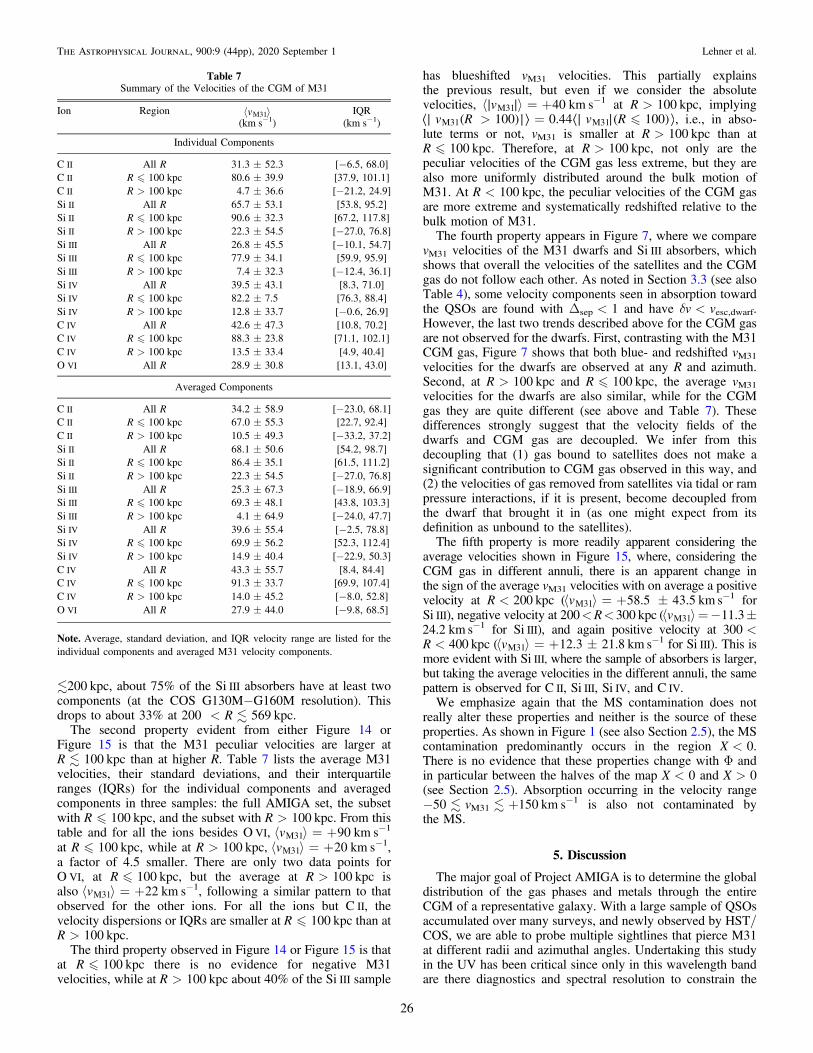
200 kpc, about 75% of the Si III absorbers have at least twocomponents (at the COS G130M−G160M resolution). Thisdrops to about 33% at 200 <R569 kpc.

The second property evident from either Figure 14 orFigure 15 is that the M31 peculiar velocities are larger atR100 kpc than at higher R. Table 7 lists the average M31velocities, their standard deviations, and their interquartileranges (IQRs) for the individual components and averagedcomponents in three samples: the full AMIGA set, the subsetwith R�100 kpc, and the subset with R>100 kpc. From thistable and for all the ions besides O VI, á ñ = +v 90M31 km s−1

at R�100 kpc, while at R>100 kpc, á ñ = +v 20M31 km s−1,a factor of 4.5 smaller. There are only two data points forO VI, at R�100 kpc, but the average at R>100 kpc isalso á ñ = +v 22M31 km s−1, following a similar pattern to thatobserved for the other ions. For all the ions but C II, thevelocity dispersions or IQRs are smaller at R�100 kpc than atR>100 kpc.

The third property observed in Figure 14 or Figure 15 is thatat R�100 kpc there is no evidence for negative M31velocities, while at R>100 kpc about 40% of the Si III sample

has blueshifted vM31 velocities. This partially explainsthe previous result, but even if we consider the absolutevelocities, ∣ ∣á ñ = +v 40M31 km s−1 at R>100 kpc, implying⟨∣ ( )∣⟩ ⟨∣ ∣( )⟩> = v R v R100 0.44 100M31 M31 , i.e., in abso-lute terms or not, vM31 is smaller at R>100 kpc than atR�100 kpc. Therefore, at R>100 kpc, not only are thepeculiar velocities of the CGM gas less extreme, but they arealso more uniformly distributed around the bulk motion ofM31. At R<100 kpc, the peculiar velocities of the CGM gasare more extreme and systematically redshifted relative to thebulk motion of M31.The fourth property appears in Figure 7, where we compare

vM31 velocities of the M31 dwarfs and Si III absorbers, whichshows that overall the velocities of the satellites and the CGMgas do not follow each other. As noted in Section 3.3 (see alsoTable 4), some velocity components seen in absorption towardthe QSOs are found with Δsep<1 and have δv<vesc,dwarf.However, the last two trends described above for the CGM gasare not observed for the dwarfs. First, contrasting with the M31CGM gas, Figure 7 shows that both blue- and redshifted vM31

velocities for the dwarfs are observed at any R and azimuth.Second, at R>100 kpc and R�100 kpc, the average vM31

velocities for the dwarfs are also similar, while for the CGMgas they are quite different (see above and Table 7). Thesedifferences strongly suggest that the velocity fields of thedwarfs and CGM gas are decoupled. We infer from thisdecoupling that (1) gas bound to satellites does not make asignificant contribution to CGM gas observed in this way, and(2) the velocities of gas removed from satellites via tidal or rampressure interactions, if it is present, become decoupled fromthe dwarf that brought it in (as one might expect from itsdefinition as unbound to the satellites).The fifth property is more readily apparent considering the

average velocities shown in Figure 15, where, considering theCGM gas in different annuli, there is an apparent change inthe sign of the average vM31 velocities with on average a positivevelocity at R<200 kpc (á ñ = + v 58.5 43.5M31 km s−1 forSi III), negative velocity at 200<R< 300 kpc (á ñ =- v 11.3M3124.2 km s−1 for Si III), and again positive velocity at 300<R<400 kpc (á ñ = + v 12.3 21.8M31 km s−1 for Si III). This ismore evident with Si III, where the sample of absorbers is larger,but taking the average velocities in the different annuli, the samepattern is observed for C II, Si III, Si IV, and C IV.We emphasize again that the MS contamination does not

really alter these properties and neither is the source of theseproperties. As shown in Figure 1 (see also Section 2.5), the MScontamination predominantly occurs in the region X<0.There is no evidence that these properties change with Φ andin particular between the halves of the map X<0 and X>0(see Section 2.5). Absorption occurring in the velocity range−50vM31+150 km s−1 is also not contaminated bythe MS.

5. Discussion

The major goal of Project AMIGA is to determine the globaldistribution of the gas phases and metals through the entireCGM of a representative galaxy. With a large sample of QSOsaccumulated over many surveys, and newly observed by HST/COS, we are able to probe multiple sightlines that pierce M31at different radii and azimuthal angles. Undertaking this studyin the UV has been critical since only in this wavelength bandare there diagnostics and spectral resolution to constrain the

Table 7Summary of the Velocities of the CGM of M31

Ion Region á ñvM31 IQR(km s−1) (km s−1)

Individual Components

C II All R 31.3±52.3 [−6.5, 68.0]C II R�100 kpc 80.6±39.9 [37.9, 101.1]C II R>100 kpc 4.7±36.6 [−21.2, 24.9]Si II All R 65.7±53.1 [53.8, 95.2]Si II R�100 kpc 90.6±32.3 [67.2, 117.8]Si II R>100 kpc 22.3±54.5 [−27.0, 76.8]Si III All R 26.8±45.5 [−10.1, 54.7]Si III R�100 kpc 77.9±34.1 [59.9, 95.9]Si III R>100 kpc 7.4±32.3 [−12.4, 36.1]Si IV All R 39.5±43.1 [8.3, 71.0]Si IV R�100 kpc 82.2±7.5 [76.3, 88.4]Si IV R>100 kpc 12.8±33.7 [−0.6, 26.9]C IV All R 42.6±47.3 [10.8, 70.2]C IV R�100 kpc 88.3±23.8 [71.1, 102.1]C IV R>100 kpc 13.5±33.4 [4.9, 40.4]O VI All R 28.9±30.8 [13.1, 43.0]

Averaged Components

C II All R 34.2±58.9 [−23.0, 68.1]C II R�100 kpc 67.0±55.3 [22.7, 92.4]C II R>100 kpc 10.5±49.3 [−33.2, 37.2]Si II All R 68.1±50.6 [54.2, 98.7]Si II R�100 kpc 86.4±35.1 [61.5, 111.2]Si II R>100 kpc 22.3±54.5 [−27.0, 76.8]Si III All R 25.3±67.3 [−18.9, 66.9]Si III R�100 kpc 69.3±48.1 [43.8, 103.3]Si III R>100 kpc 4.1±64.9 [−24.0, 47.7]Si IV All R 39.6±55.4 [−2.5, 78.8]Si IV R�100 kpc 69.9±56.2 [52.3, 112.4]Si IV R>100 kpc 14.9±40.4 [−22.9, 50.3]C IV All R 43.3±55.7 [8.4, 84.4]C IV R�100 kpc 91.3±33.7 [69.9, 107.4]C IV R>100 kpc 14.0±45.2 [−8.0, 52.8]O VI All R 27.9±44.0 [−9.8, 68.5]

Note.Average, standard deviation, and IQR velocity range are listed for theindividual components and averaged M31 velocity components.

26

The Astrophysical Journal, 900:9 (44pp), 2020 September 1 Lehner et al.

physical properties of the multiple gas phases existing in theCGM over 104–5.5 K (for z=0, the hottest phase can only beprobed with X-ray observations). With 25 sightlines withinabout 1.1 Rvirand 43 within 569 kpc (1.9 Rvir) of M31, thesize of the sample and the information as a function of R and Φare unparalleled. We will now consider the broad patterns andconclusions we can draw from this unique data set.

5.1. Pervasive Metals in the CGM of M31

A key finding of Project AMIGA is the ubiquitous presenceof metals throughout the CGM of M31. While the search forH I with Nlog H I17.5 in the CGM of M31 toward pointedradio observations has been unsuccessful in the current sample(Paper I and see Figure 1), the covering factor of Si III (29sightlines) is essentially 100% out to 1.2 Rvir, while O VIassociated with M31 is detected toward all 11 sightlines withFUSE data, all the way out to 1.9 Rvir, the maximum radius ofour survey (see Sections 4.4, 4.6). From the ionization rangeprobed by Project AMIGA, we further show that Si III and O VIare key probes of the diffuse gas (see Section 4.7). Withinformation from Si II, Si III, and Si IV, we demonstrate thatSi III is the dominant ion in the ionizing energy range of8–45 eV (see Section 4.7.1). The high covering factors of Si IIIand O VI imply that these ions could be pervasively distributed,but it is quite possible also that small structures could lead tothese large covering factors in projection.

The finding of ubiquitous metals in the CGM of M31 is astrong indication of ongoing and past gas outflows that ejectedmetals well beyond their formation site. Based on a specificSFR of SFR/Må=(5±1)×10−12 yr−1 (using the stellarmass Må and SFR from Geehan et al. 2006; Kang et al. 2009),M31 is not currently in an active star-forming episode. In fact,Williams et al. (2017) show that the bulk of star formationoccurred in the first ∼6 billion years and the last strong episodehappened over ∼2 billion years ago (see also Figure 6 inTelford et al. 2019 for a metal production model of M31). For atypical outflow with gas moving at 100 km s−1, the gas wouldhave traveled about 200 kpc in 2 Gyr, i.e., this is the maximumdistance at which the last burst of star formation could haveimpacted the CGM of M31. Hence, many of the metals seen inthe CGM of M31 must have also been ejected by previous star-forming episodes and/or stripped from its dwarfs and moremassive companions. However, the most distant metals, thosebeyond Rvir (and especially given that they are predominantlyfound along a preferred direction from M31; see Section 4.9),may be supplied from elsewhere. For example, they could haveoriginated in a Local Group medium bearing metals lost fromother galaxies (e.g., the MW or dwarfs) or in a pre-pollutedIGM filament.

In Section 4.8, we estimate that the mass of metalsMcool

Z =(2.0±0.5)×107Me within Rvir for the predomi-nantly photoionized gas probed by Si II, Si III, and Si IV. For thegas probed by O VI, we find that > ´M M4.4 9Z

warmZcool

107 Me within Rvir (this is a lower limit because the ionizationfraction of O VI is an upper limit; see Section 4.8). The sum ofthese two phases yields a lower limit to the CGM metal massbecause the hotter phase probed by X-rays and metals bound indust is not included. If the hot baryon mass of M31 is not toodifferent from that estimated for the MW (see Section 4.8), thenwe expect »M MZ

hotZwarm. The CLUES simulation of the Local

Group estimates that the mass of the hot (>105 K) gas is a

factor of 3 larger than the cooler (<105 K) gas (Nuza et al.2014). The CGM dust mass remains quite uncertain but couldbe at the level of 5×107Me according to estimates around0.1–1L* galaxies (Ménard et al. 2010; Peeples et al. 2014;Peek et al. 2015). Hence, a plausible lower limit on the totalmetal mass of the CGM of M31 out to Rvir is MZ

CGM

´2.5 108 Me, a factor of ∼2 times larger than the cool+warmgas-phase metal mass.The stellar mass of M31 is (1.5±0.2)×1011Me (e.g.,

Williams et al. 2017). Using this result, Telford et al. (2019)estimated that the current metal mass in stars is 3.9×108Me,i.e., about the same amount that is found in the entire CGM ofM31 up to Rvir. Telford et al. (2019) also estimated the metalmass of the gas in the disk of M31 to be around(0.8–3.2)×107Me, while Draine et al. (2014) estimated thedust mass in the disk to be around 5.4×107Me, yielding atotal metal mass in the disk of M31 of about ´M 5Z

disk

108 Me. Therefore, M31 has in its CGM within Rvir at least50% of the present-day metal mass in its disk. As we show inSections 4.4 and 4.8 and discuss above, metals are also foundbeyond Rvir, especially in the more highly ionized phase tracedby O VI (and even higher ions). These metals may have comefrom M31 or from other galaxies in the Local Group such asthe MW or dwarf galaxies.

5.2. Comparison with COS-halos Galaxies

The Project AMIGA experiment is quite different from mostof the surveys of the CGM of galaxies done so far. Outside thelocal universe, surveys of the CGM of galaxies involveassembling samples of CGM gas in aggregate by using onesightline per galaxy (see Section 1), in some nearby cases up tothree to four sightlines (e.g., Bowen et al. 2016; Keeney et al.2017). By assembling a sizable sample of absorbers associatedwith galaxies in a particular subpopulation (e.g., L*, sub-L*,passive or star-forming galaxies), one can then assess how thecolumn densities change with radii around that kind of galaxy,and from this estimate average surface densities, mass budgets,etc., can then be evaluated. By contrast, Project AMIGA hasassembled almost as many sightlines surrounding M31 asCOS-Halos had for its full sample of 44 galaxies. We can nowmake a direct comparison between these two types ofexperiments. For this comparison, we use the COS-Halossurvey of 0.3<L/L*<2 galaxies at z;0.2, which selectedgalaxies within about 160 kpc from the sightline (Tumlinsonet al. 2011, 2013; Werk et al. 2013, 2014). The full mass rangeof the COS-Halos galaxies is quite large, 11.5logM20013.7, but most of the star-forming galaxies are in the range

M11.5 log 12.5200 , and most of the passive quiescentgalaxies have M13.0 log 13.7200 . As a reminder, M31 has

=Mlog 12.1200 (see Section 1).

5.2.1. Column Densities of Si versus R

In Figure 16, we show the total column densities of Si as afunction of R/R200 for the COS-Halos galaxies and M31. Forthe COS-Halos survey, each data point corresponds to anabsorber at some impact parameter from a galaxy, while forM31, each data point is an absorber probing the CGM at adifferent impact parameter from the same galaxy. For COS-Halos, we consider two cases: (1) the column densities of Siestimated in a similar fashion as those for M31, and (2) the

27

The Astrophysical Journal, 900:9 (44pp), 2020 September 1 Lehner et al.

column densities of Si estimated from photoionization model-ing. For case 2 we use the results from Werk et al. (2014; seealso Prochaska et al. 2017b), which were used to determine themetal mass of the CGM of the COS-Halos galaxies in Peepleset al. (2014). For case 1, we use the results from Werk et al.(2013) and follow the procedure in Section 4.5 to estimate NSi

from the column densities of Si II, Si III, and Si IV. We requirethat all three Si ions are available, except in the cases wherethere are only lower limits for two ions (typically Si II andSi III) since in that case the resulting column density is a lowerlimit that encompasses any missing column density from theremaining Si ion (typically Si IV). The sample size in case 1 is35, while in case 2 it is 33, with some overlap between the twosubsamples. In Figure 16, we also show the modeled columndensity of Si as a function of R, in gray for COS-Halos and bluefor M31 (we show the adopted GP model; see Section 4.5).

A striking difference between the COS-Halos and M31 dataimmediately apparent from Figure 16 is that a large number ofvery high Si column densities are observed in COS-Halos atR/R2000.3 that are absent in Project AMIGA. The reasonthat the COS-Halos Si column densities have higher lowerlimits than those of M31 is because the weak transitions of Si IIare saturated in COS-Halos, a situation not observed in M31toward any of the sightlines—the lower limits of Si arise onlybecause Si III is saturated. These high Si column densities also

correspond to the very strong NH I ( Nlog H I18) absorbersobserved in COS-Halos, but again not in M31 (see Figure 5 andSection 4.1 in Paper I). Beam dilution could have affectedsomewhat the comparison between H I column densities fromCOS-Halos (H I absorption) and M31 (H I emission); for themetal ions, this is not an issue. Therefore, the higher frequencyof saturated Si II transitions in COS-Halos compared to M31 isa real effect, not an artifact.Besides this difference, the estimated Si column densities

from the observations in the COS-Halos and Project AMIGAsurveys are distributed with a similar scatter at larger impactparameters (R/R2000.4), where the gas is more ionized (seetop panel in Figure 16). The photoionization-modeled COS-Halos Si displayed in the bottom panel has some higher valuesthan observed in the top panel, but in the impact parameterregion 0.4R/R2000.8 where they are observed, there arealso several lower limits. Beyond R>0.9R200, there are noCOS-Halos observations (owing to the design of the survey).The extrapolated model to the COS-Halos observations shownin gray in Figure 16 is a factor of 2–4 higher than the models ofthe Project AMIGA data shown in blue depending on R/R200.A likely explanation for the higher column density absorbers

is that some of these COS-Halos absorbers could be fully orpartly associated with a galaxy near to the initially targetedCOS-Halos galaxies. In this case the gas would be more likelyto show high columns of neutral and weakly ionized gas.Indeed, while the COS-Halos galaxies were selected to have nobright companions, that selection did not preclude fainternearby companions such as dwarf satellites (see Tumlinsonet al. 2013). Galaxy observation follow-up by Werk et al.(2012) found several L>0.1L* galaxies within 160 kpc of thetargeted COS-Halos galaxy. Comparing the results from othersurveys of galaxies/absorbers at low redshift (Bowen et al.2002; Stocke et al. 2013), Bregman et al. (2018) also noted ahigher preponderance of high H I column density absorbers inthe COS-Halos survey. However, the higher COS-Haloscolumn densities at large radii could also be an effect ofevolution in the typical CGM, as COS-Halos probed a slightlyhigher cosmological redshift. It is also possible that the M31CGM is less rich in neutral gas at these radii than the typical L*

galaxy at z∼0.2, because of its star formation history orenvironment.

5.2.2. CGM Mass Comparison

A key physical parameter of the CGM is its mass, which isobtained from the column density distribution of the gas andassuming a certain geometry of the gas. For M31, we cannotderive the baryonic mass of CGM gas without assuming ametallicity since the H I column density remains largelyunknown and very uncertain toward all the targets in oursample (but see Sections 4.1 and 4.8). However, the metal massof the cool gas probed by Si II, Si III, and Si IV can bestraightforwardly estimated directly from the observationswithout any ionization modeling (see top panel of Figure 16).Even though both Peeples et al. (2014) and Werk et al.

(2014) use the Si column densities derived from photoioniza-tion models, as illustrated in Figure 16, this would notchange the outcome that the metal mass of the cool CGM gasderived from the COS-Halos survey is about a factor of 2–3higher than the metal mass derived in Project AMIGA. This isbecause there are seven COS-Halos Si column densities atR/R200<0.3 that are much higher than seen about M31,

Figure 16. Comparison of the total column densities of Si from M31 and theCOS-Halos galaxies as a function of R/R200. Top panel: NSi are directlyconstrained by the estimates on NSi II, NSi III, and NSi IV from the observationsfor both Project AMIGA and COS-Halos (Werk et al. 2013). The error bars areless than the size of the symbols, and the vertical bars include the range ofpossible values if the nondetections are either near their 2σupper limits or solow as to be negligible. Bottom panel: same as the top panel, but NSi for theCOS-Halos data is derived from CLOUDY photoionization models (Werket al. 2014). The gray dashed line and shaded region represent the best fitbetween NSi and R/R200 and its dispersion using COS-Halos modeled data,respectively. The blue area shows the full range of the GP model of the ProjectAMIGA data (see Section 4.5).

28

The Astrophysical Journal, 900:9 (44pp), 2020 September 1 Lehner et al.

driving the overall model of NSi(R) substantially higher. Thefact that these high NSi values are not found in the CGM ofM31 or lower-redshift galaxies at similar impact parameters(e.g., Bowen et al. 2002; Stocke et al. 2013) suggests a sourceof high column density H I and Si II absorbers in the COS-Halos sample that could be recent outflows, strong accretion/recycling, or gas associated with closer satellites to thesightline. With only five targets within R/R200<0.3 and nonebelow R/R200<0.1 for M31, it would be quite useful to targetmore QSOs in the inner region of the CGM of M31 to betterdetermine how NSi(R) varies with R at small impact parameters.

For the warm–hot gas probed by O VI, the COS-Halos star-forming galaxies have á ñ =N 10O

14.5VI cm−2, a detection rate

close to 100%, and no large variation of NO VI with R(Tumlinson et al. 2011). For M31, we have a similar averageO VI column density, similar hit rate, and little evidence forlarge variation of NO VI with R (see Section 4.8). This impliesthat the masses of the warm–hot CGM of M31 and COS-Halosstar-forming galaxies are similar. M31 has a specific SFR thatis a factor 10 lower than the COS-Halos star-forminggalaxies, but its halo mass is on the higher side of the COS-Halos star-forming galaxies (but lower than the COS-Halosquiescent galaxies). As discussed in Section 5.3.3 in moredetail, M31 and the COS-Halos star-forming galaxies have halomasses in the rangeM200;1011.7–1012.3Me, corresponding toa virial temperature range that overlaps with the temperature atwhich the ionization fraction of O VI peaks, which maynaturally explain some of the properties of the O VI in the CGMof “L*” galaxies (Oppenheimer et al. 2018b). It is also possiblethat some O VI arises in photoionized gas or combinations ofdifferent phases (see Section 5.3.3).

Based on the comparison above, we find that the O VI is lesssubject to the uncertainty in the association of the absorber tothe correct galaxy owing to its column density being lessdependent on R (see also Section 5.3). Therefore, this leads tosimilar metal masses of the CGM of the z∼0.2 COS-Halosgalaxies and M31 for the O VI gas phase. For the lower ions,their column densities are more dependent on R (see alsoSection 5.3). Therefore, the association of the absorber to thecorrect galaxy is more critical to derive an accurate columndensity profile with R and hence derive an accurate CGM metalmass. However, we note that despite these uncertainties, themetal mass of the cool CGM of the COS-Halos galaxies is onlya factor of 2–3 higher than that derived for M31.

5.3. A Changing CGM with Radius

A key discovery from Project AMIGA is that the propertiesof the CGM of M31 change with R. This is reminiscent ofour earlier survey (LHW15), but the increase in the size samplehas transformed some of the tentative results of our earliersurvey into robust findings. In particular, the radius aroundR∼100–150 kpc appears critical in view of several propertieschanging near this threshold radius:

1. For any ions, the frequency of strong absorption is largerat R100–150 kpc than at larger R.

2. The column densities of Si and C ions change by a factor>5–10 between about 25 and 150 kpc, while they changeonly by a factor 2 between 150 and 300 kpc.

3. The detection rate of singly ionized species (C II, Si II) isclose to 100% at R<150 kpc but sharply decreases

beyond (see Figure 9), and therefore the gas has a morecomplex gas-phase structure at R<150 kpc.

4. The peculiar velocities of the CGM gas are more extremeand systematically redshifted relative to the bulk motionof M31 at R100 kpc, while at R100 kpc thepeculiar velocities of the CGM gas are less extreme andmore uniformly distributed around the bulk motionof M31.

There are also two other significant regions: (1) beyondR200;230 kpc the gas is becoming more ionized and morehighly ionized than at lower R (e.g., there is a near total absenceof Si II absorption beyond R200 [see Figure 9], or a higher C II/C IV ratio on average at RR200 than at lower R [seeSection 4.7.2]), and (2) beyond 1.1 Rvirthe gas is not detectedin all the directions away from M31, as it is at smaller radii, butonly in a cone near the southern projected major axis and about52° west of the X=0 kpc axis (see Section 4.9).The overall picture that can be drawn out from these

properties is that the inner regions of the CGM of M31 aremore dynamic and complex, while the more diffuse regions atR0.5 Rvirare more static and “simpler.” Zoom-in cosmo-logical simulations capture in more detail and more accuratelythe structures of the CGM than large-scale cosmologicalsimulations thanks to their higher mass and spatial resolution.Below we use several results from zoom simulations to gainsome insights on these observed changes with R. However, theresults laid out in Section 4 also now provide a new test bed forzoom simulations, so that not only qualitative but alsoquantitative comparison can be undertaken. We note that mostof the zoom simulations discussed here have only a singlemassive halo. However, according to the ELVIS simulations ofLocal Group analogs (Garrison-Kimmel et al. 2014), thereshould be no major difference at least within about Rvir for thedistribution of the gas between isolated and paired galaxies.

5.3.1. Visualization and Origins of the CGM Variation

To help visualize the properties described above and gainsome insights into the possible origins of these trends, we beginby qualitatively examining two zoom simulations. First, weconsider the Local Group zoom simulations from the CLUESproject (Nuza et al. 2014), where the gas distribution aroundMW and M31-like galaxies is studied. Their work does notshow the distribution of the individual ions but examines thetwo main gas phases above and below 105 K in an environmentthat is a constrained analog to the Local Group. Interestingly,considering Figure 3 (simulated M31) or Figure 6 (simulatedMW) in Nuza et al., the region within 100–150 kpc appearsmore complex, with a large covering factor for both cool andhot gas phases and higher velocities than at larger radii. In thesesimulations, this is a result of the combined effects of coolingand supernova heating affecting the closer regions of the CGMof M31. This simulation also provides an explanation for thegas observed beyond 1.1 Rvirthat is preferentially observed in alimited region of the CGM of M31 (see Figure 13 and seemiddle right panel of their Figure 3) whereby the 105 K gasmight be accreting onto the CGM of M31. We also note thatNuza et al. (2014) find a mass for the 105 K CGM gas of1.7×1010Me, broadly consistent with our findings (seeSection 4.8). More quantitative comparisons between theCLUES (or Local Group analog simulations like ELVIS-FIREsimulations; Garrison-Kimmel et al. 2014, 2019) and Project

29

The Astrophysical Journal, 900:9 (44pp), 2020 September 1 Lehner et al.

AMIGA results are beyond the scope of this paper, but theywould be valuable to undertake in the future.

Second, we consider the zoom Eris2 simulation of a massive,star-forming galaxy at z=2.8 presented in Shen et al. (2013).The Eris2 galaxy being z=2.8 and with an SFR of 20 Meyr−1 is nothing like M31, but this paper shows the distributionof the gas around the central galaxy using some of the sameions that are studied in Project AMIGA, specifically Si II, Si IV,C II, C IV, and O VI (see their Figures 3(a) and 4(a), (b)).Because Eris2 is so different from M31, we would naivelyexpect their CGM properties to be different, and yet (1) Eris2 issurrounded by a large diffuse O VI halo with a near-unitycovering factor all the way out to about 3 Rvir; (2) the coveringfactor of absorbing material in the CGM of Eris2 declines lessrapidly with impact parameter for C IV or O VI compared toC II, Si II, or Si IV; and (3) beyond Rvir, the covering factor ofSi II drops more sharply than C II. There are also keydifferences, like the strongest absorption in any of these ionsbeing observed in the bipolar outflows perpendicular to theplane of the disk, which is unsurprisingly not observed in M31since it currently has a low SFR (e.g., Williams et al. 2017).However, the broad pictures of the CGM of M31 and thesimulated Eris2 galaxy are remarkably similar. This impliesthat some of the properties of the CGM may depend more onthe microphysics producing the various gas phases than thelarge-scale physical processes (outflow, accretion) that varysubstantially over time. In fact, the Eris2 simulation shows thatinflows and outflows coexist and are both traced by diffuseO VI; in Eris2, a high covering factor of strong O VI absorbersseems to be the least unambiguous tracer of large-scaleoutflows.

5.3.2. Quantitative Comparison in the CGM Variation betweenObservations and Simulations

Two simulations of M31-like galaxies in different environ-ments at widely separated epochs show some similarity withsome of the observed trends in the CGM of M31. We now takeone step further by quantitatively comparing the columndensity variation of the different ions as a function of R in threedifferent zoom-in cosmological simulations, two being led bymembers of the Project AMIGA team (FIRE and FOGGIEcollaborations), and a zoom-in simulation from the Evolutionand Assembly of GaLaxies and their Environments (EAGLE)simulation project (Crain et al. 2015; Schaye et al. 2015;Oppenheimer et al. 2018a).

(1) Comparison with FIRE-2 Zoom SimulationsWe first compare our observations with column densities

modeled using cosmological zoom-in simulations from theFIRE project.31 Details of the simulation setup and CGMmodeling methods are presented in Ji et al. (2020). Briefly, theoutputs analyzed here are FIRE-2 simulations evolved with theGIZMO code using the meshless finite mass (MFM) solver(Hopkins 2015). The simulations include a detailed model forstellar feedback including core-collapse and Type Ia super-novae, stellar winds from OB and AGB stars, photoionization,and radiation pressure (for details, see Hopkins et al. 2018). Wefocus on the “m12i” FIRE halo, which has a mass Mvir≈1.2M200≈ 1.2× 1012Me at z= 0, which is comparable to thehalo mass of M31. However, neither the SFR history nor thepresent-day SFR is similar. The “m12i” FIRE halo has a factor

of 10–12 higher SFR (see Figure 3 in Hopkins et al. 2020) thanthe present-day SFR of M31 of 0.5Me yr−1 (e.g., Kang et al.2009). We compare Project AMIGA to FIRE-2 simulationswith two different sets of physical ingredients. The “MHD” runincludes magnetic fields, anisotropic thermal conduction, andviscosity, and the “CR” run includes all these processes plusthe “full physics” treatment of stellar cosmic rays (CRs). TheCR simulation assumes a diffusion coefficient ∣∣k = ´3 1029

cm−2 s−1, which was calibrated to be consistent with observa-tional constraints from γ−ray emission of the MW and someother nearby galaxies (Chan et al. 2019; Hopkins et al. 2020). Jiet al. (2020) showed that CRs can potentially provide a large oreven dominant nonthermal fraction of the total pressure supportin the CGM of low-redshift ∼L* galaxies. As a result, in thefiducial CR run analyzed here, the volume-filling CGM ismuch cooler (∼104–105 K) and is thus photoionized in regionswhere in the run without CRs it is filled with hot gas that ismore collisionally ionized.The column densities are generated as discussed in Ji et al.

(2020) using the Trident code (Hummels et al. 2017) to modelthe ion populations and density projections. For the photo-ionization modeling, a hybrid treatment combining the FG09(Faucher-Giguère et al. 2009) and HM12 (Haardt & Madau2012) UV background models is used.32

In Figure 17, we compare the ion column densities fromFIRE-2 simulations with observationally derived total columndensities around M31 as a function of R/R200. The green andorange curves show the median simulated column densities forthe MHD and CR runs, respectively, while the shaded regionsshow the full range of columns for all sightlines at a givenimpact parameter (the lowest values are truncated to match thescales that are adequate for the observations; see Ji et al. 2020for the full range of values). The CR run produces highercolumn densities and better agreement with observations thanthe MHD run for all ions presented. The much higher columndensities of low/intermediate ions (C II, Si II, Si III, and Si IV)in the CR run are due to the more volume-filling and uniformcool phase, which produces higher median values of ioncolumn densities and smaller variations across differentsightlines. In contrast, in the MHD run the cool phase ispressure confined by the hot phase to compact and denseregions, leading to smaller median columns but larger scatterfor the low and intermediate ions. We note, however, that evenin the CR runs the predicted column densities are lower thanobservations at the larger impact parameters R0.5R200. Thismight be due to insufficient resolution to resolve fine-scalestructure in outer halos, or it may indicate that feedback effectsare more important at large radii than in the presentsimulations. This difference is quite notable owing to the factthat the star formation of the “m12i” galaxy has beencontinuous with an SFR in the range of 5–20 Me yr−1

(Hopkins et al. 2020) over the past ∼8 billion years, while M31had only a continuous SFR around 6–8 Me yr−1 over its first 5billion years, while over the past 8 billion years it had only twoshort bursts of star formation about 4 and 2 billion years ago

31 FIRE project website:http://fire.northwestern.edu.

32 We use this mixture because, based on the recent UV background analysisof Faucher-Giguère (2020), the FG09 model is in better agreement with themost up-to-date low-redshift empirical constraints at energies relevant for lowand intermediate ions (C II, Si II, Si III, Si IV, and C IV). However, the HM12model is likely more accurate for high ions such as O VI because the FG09model used a crude AGN spectral model that underpredicted the higher-energypart of the UV/X-ray background. Ji et al. (2020) show how some ion columnsdepend on the assumed UV background model.

30

The Astrophysical Journal, 900:9 (44pp), 2020 September 1 Lehner et al.

(Williams et al. 2017). While there are some clear discrepan-cies, the simulations also follow some similar trends to thoseseen in the empirical results detailed in Section 4: (1) thesimulated column densities of the low ions decrease morerapidly with R than the high ions; (2) OVI is observed beyond1.7R200, where there is no substantial amount of low/intermediate ions; and (3) a larger scatter is observed in thecolumn densities of the low and intermediate ions than in O VI.

In the FIRE-2 simulations, both collisional ionization andphotoionization can contribute significantly to the simulatedO VI columns, typically with an increasing contribution fromphotoionization with increasing impact parameter, driven bydecreasing gas densities. In the MHD run, most of the O VI inthe inner halo (R0.5R200) is produced by collisionalionization, but photoionization can dominate at larger impactparameters. In the CR run, collisional ionization and photo-ionization contribute comparably to the O VI mass at radii50 <R<200 kpc (Ji et al. 2020). The actual origins of theCGM in terms of gas flows in FIRE-2 simulations withoutmagnetic fields or CRs were analyzed in Hafen et al. (2020),although the results are expected to be similar for simulationswith MHD only. In these simulations, O VI exists as part of awell-mixed hot halo, with contributions from all the primarychannels of CGM mass growth: IGM accretion, wind, and

contributions from satellite halos (reminiscent of the Eris2simulations; see above and Shen et al. 2013). The metalsresponsible for O VI absorption originate primarily in winds,but IGM accretion may contribute a large fraction of total gasmass traced by O VI since the halo is well mixed and IGMaccretion contributes 60% of the total CGM mass. In thesimulations, the hot halo gas persists in the CGM for billions ofyears, and the gas that leaves the CGM does so primarily byaccreting onto the central galaxy (Hafen et al. 2019).(2) Comparison with FOGGIE SimulationsWe also compare the observed total column densities to the

MW-mass “Tempest” (M200≈4.2×1011Me) halo from theFOGGIE simulations,33 which has a halo mass of M200≈4.2× 1011Me (Peeples et al. 2019). Again we employ thesoftware Trident (Hummels et al. 2017) to generate the ionpopulations and density projections, limiting potential sourcesof discrepancy. We use the z= 0 output (see Zheng et al. 2020for simulation details), but because of the size differencebetween M31 and the Tempest galaxy, we again scale alldistances by R200 (R200= 159 kpc for the simulated halocompared to 230 kpc for M31). The only “feedback” includedin this FOGGIE run is thermal explosion-driven supernovaoutflows. While this feedback is limited in scope compared toFIRE, FOGGIE achieves higher mass resolution than FIRE-2by using a “forced refinement” scheme that applies a fixedcomputational cell size of ∼381 h−1 pc within a moving cubecentered on the galaxy that is ∼200 h−1 ckpc on a side. Thisrefinement scheme enforces constant spatial resolution on theCGM, resulting in a variable and very small mass resolution inthe low-density gas, with typical cell masses of (1–100 Me).The individual small-scale structures that contribute to theobserved absorption profiles can therefore be resolved. Thesesmall-scale structures that become only apparent in high-resolution simulations are hosts to a significant amount of coolgas, enhancing the column densities in especially the lowionization state of the gas (Peeples et al. 2019; Corlies et al.2020; see also Hummels et al. 2019; Rhodin et al. 2019; van deVoort et al. 2019).As for the FIRE-2 simulations, we compare the Project

AMIGA total column densities to FOGGIE because in thesimulation we do not (yet) separate individual components, butlook at the projected column densities through the halo. Wenote that the CGM is not necessarily self-similar, so somedifferences between the simulation predictions and M31observations at rescaled impact parameter could be due to thehalo mass difference. This is especially so since the halo massrange Mh≈3×1011–1012Me corresponds to the expectedtransition between cold and hot accretion (e.g., Birnboim &Dekel 2003; Keres et al. 2003; Faucher-Giguère et al. 2011;Stern et al. 2020).In Figure 18, we compare the simulated and observed

column densities for each ion probed by our survey. The pinkand green shaded areas are the data points from the simulation(with and without satellite contribution, respectively) and showthe total column density in projection through the halo. Thescatter in the simulated data points comes from variation in thestructures along the mock sightline, and most of the scatter is infact below 1011 cm−2. The peaks in the column densities aredue to small satellites in the halo, which enhance primarily thelow-ion column densities. We show the green points to

Figure 17. Comparison of ion column density profiles between ProjectAMIGA (total column densities) and FIRE-2 simulations, with “MHD” and“CR” runs. Thick curves show median values of an ensemble of sightlinesproduced from simulations, and shaded regions show the full range across allmodel sightlines.

33 FOGGIE project website:http://foggie.science.

31

The Astrophysical Journal, 900:9 (44pp), 2020 September 1 Lehner et al.

highlight the difference between the mock column densitieswith and without satellites. For the high-ionization lines thedifference is negligible, while the difference in the low ions issignificant.

Overall, the metal-line column densities are systematicallylower than in the observations at any R. Only at R0.3R200 isthere some overlap for the singly ionized species between theFOGGIE simulation and observations. However, the discre-pancy is particularly striking for Si III and the high ions. Thiscan be understood by the current feedback implementation inFOGGIE, which does not expel enough metals from the stellardisk into the CGM (Hamilton-Campos et al. 2020) to beconsistent with known galactic metal budgets (Peeples et al.2014). This effect is expected to be stronger for the high ionsthan the low ions, due to the additional heating and ionizationof the CGM that would be expected from stronger feedback,and indeed the discrepancy between the simulation andobservations is larger for the high ions (and Si III) than forthe singly ionized species. However, while the absolute scale ofthe column densities is off, there are also some similaritiesbetween the simulation and observations in the behavior of the

relative scale of the column density profiles with R: (1) thecolumn densities of the low ions drop more rapidly with R thanthe high ions; (2) despite the inadequate feedback in the currentsimulations, the O VI-bearing gas (and C IV to a lesser extent) isobserved well beyond R200; and (3) a larger scatter is observedin the column densities of the low and intermediate ions than inO VI. It is striking that the overall slope of the O VI profileresembles the observations but at significantly lower absolutecolumn density. In the FOGGIE simulation, the low ionstracing mainly dense, cool gas are preferentially found in thedisk or satellites, while the hotter gas traced by the higher ionsis more homogeneously distributed in the halo.(3) Comparison with EAGLE SimulationsFinally, we compare our results with the EAGLE zoom-in

simulations (EAGLE Recal-L025N0752 high-resolution volume)discussed in length in Oppenheimer et al. (2018a). The EAGLEsimulations have successfully reproduced a variety of galaxyobservables (e.g., Crain et al. 2015; Schaye et al. 2015) andachieved “broad but imperfect” agreement with some of theextant CGM observations (e.g., Turner et al. 2016; Oppenheimeret al. 2018a; Rahmati & Oppenheimer 2018; Lehner et al. 2019;Wotta et al. 2019).Oppenheimer et al. (2018a) aimed to directly study the

multiphase CGM traced by low metal ions and to compare withthe COS-Halos survey (see Section 5.2). As such, theyexplored the circumgalactic metal content traced by the sameions explored in Project AMIGA in the CGM galaxies withmasses that comprise that of M31. Overall Oppenheimer et al.find agreement between the simulated and COS-Halos samplesfor Si II, Si III, Si IV, and C II within a factor of two or so andlarger disagreement with O VI, where the column density issystematically lower. With Project AMIGA, we can directlycompare the results with one of the EAGLE galaxies that has amass very close to M31 and also compare the column densitiesbeyond 160 kpc, the maximum radius of the COS-Halos survey(Tumlinson et al. 2013; Werk et al. 2013). We refer the readerto Oppenheimer et al. (2016), Rahmati & Oppenheimer (2018),and Oppenheimer et al. (2018a) for more details on the EAGLEzoom-in simulations, which employ the SpecExBin code(Oppenheimer & Davé 2006) for ion modeling and columndensity projections. We also refer the reader to Figure 1 inOppenheimer et al. (2018a), where in the middle column theyshow the column density map for galaxy halo mass of

=Mlog 12.2200 at z;0.2, which qualitatively shows similartrends described in Section 5.3.1.In Figure 19, we compare the EAGLE and observed column

densities as a function of the impact parameter out to Rvir. As inthe previous two figures, the blue and gray circles aredetections and nondetections in the halo of M31, respectively.The green curve in each panel represents the mean columndensity for each ion as a function of the impact parameter forthe EAGLE galaxy with =Mlog 12.1200 at z=0. In contrastto FIRE-2 or FOGGIE simulations, the EAGLE simulationsappear to produce a better agreement between N and R for lowand intermediate ions (Si II, Si III, Si IV), and C IV out to largerimpact parameters. However, as already noted in Oppenheimeret al. (2018a), this agreement is offset by producing too muchcolumn density for the low and intermediate ions at smallimpact parameters (see, e.g., Si II, which is not affected bylower limits and is clearly overproduced at R80 kpc). Theflat profile of O VI, with very little dependence on R, is similarto the observations and other models, but overall the EAGLE

Figure 18. Comparison of ion column density profiles between ProjectAMIGA (total column densities) and the “Tempest” halo from the FOGGIEsimulations. The pink and green shaded areas are projected total columndensities from the simulated halo with and without galaxy/satellite contribu-tions, respectively, while the rest of the figure is analogous to Figure 8. Thevertical line shows the extent of the forced resolution cube in the FOGGIEsimulation.

32

The Astrophysical Journal, 900:9 (44pp), 2020 September 1 Lehner et al.

O VI column densities are a factor of 0.2–0.6 dex smaller thanobserved. Oppenheimer et al. (2018a) (and also Oppenheimeret al. 2016) already noted that issue from their comparison withthe COS-Halos galaxies (see also Section 5.2), requiringadditional source(s) of ionization for the O VI such as AGNflickering (Oppenheimer & Schaye 2013b; Oppenheimer et al.2018b) or possibly CRs as shown for the FIRE-2 simulations(see Ji et al. 2020 and above). While the results are shown onlyto Rvir, as in the other simulations and M31, O VI is alsoobserved well beyond Rvir in the EAGLE simulations (seeFigure 1 in Oppenheimer et al. 2018a).

5.3.3. Insights from the Observation/Simulation Comparison

The comparison with the simulations shows that the CGM ischanging in zoom-in simulations on length scales roughlysimilar to those observed in M31. The low ions and high ionsfollow substantially different profiles with radius, in both dataand simulations. In the zoom-in simulations described above,the inner regions of the CGM of galaxies are more directlyaffected by large-scale feedback and recycling processesbetween the disk and CGM of galaxies. Therefore, it is notsurprising that the M31 CGM within 100–150 kpc shows alarge variation in column density profiles with R, a more

complex gas-phase structure, and larger peculiar velocitieseven though the current SFR is low. While both accretion andlarge-scale outflow coexist in the CGM and are responsible forthe gas flow properties, stellar feedback is required to produce asubstantial amount of metals in the CGM at large impactparameters (see Figures 17–19). M31 has currently a low SFR,but it had several episodes of bursting star formation in the past(e.g., Williams et al. 2017), likely ejecting a large portion of itsmetals in the CGM during these episodes.Various models simulating different galaxy masses at

different epochs, with distinct SFRs or feedback processes,can reproduce at some level the diffuse O VI observed beyondRvir. All the simulations we have reviewed produce O VIprofiles that are flatter than the low ions and extend to beyondRvir with significant column density. While the galaxy halomasses are different, they are all roughly in the range of about1011.5–1012.3Me, which is a mass range where their virialtemperatures overlap with the temperature at which theionization fraction of O VI peaks (Oppenheimer et al. 2016).Using the EAGLE simulations, Oppenheimer et al. (2016)show that the virial temperature of the galaxy halos can explainthe presence of strong O VI in the CGM of star-forminggalaxies with M200;1011.5–1012.3Me and the absence ofstrong O VI in the CGM of quiescent galaxies that have overallhigher halo masses (M200;1012.5–1013.5Me) and hencehigher virial temperatures, i.e., halo mass, not SFR, largelydrives the presence of strong O VI in the CGM of galaxiesaccording to these simulations (see Section 5.2). Production ofthe O VI in volume-filling virialized gas could explain whyO VI is widely spread in the CGM of simulated galaxies and thereal M31. Additional ionization mechanisms from CRs (Ji et al.2020 and see Figure 17) or fluctuating AGNs (Oppenheimer &Schaye 2013b; Oppenheimer et al. 2018b) can further boost theO VI production, but halo masses with their virial temperaturesclose to the temperature at which the ionization fraction of O VIpeaks appear to provide a natural source for the diffuse,extended O VI in the CGM of L* galaxies. Conversely, anumber of studies have shown that significant O VI can arise inactive outflows, with the outflow column densities varyingstrongly with the degree of feedback (Hummels et al. 2013;Hafen et al. 2020). Right now, no clear observational test candistinguish O VI in warm virialized gas and direct outflows.However, any model that attempts to distinguish them will beconstrained by the flat profile and low scatter seen by ProjectAMIGA.On the other hand, the cooler, diffuse ionized gas probed

predominantly by Si III, as well as low ions (C II, Si II) atsmaller impact parameters, is not well reproduced in thesimulations. In the FIRE-2 and FOGGIE simulations, thecolumn densities of Si III and low ions within 0.3R200 arereasonably matched, but their covering fractions drop sharplyand much more rapidly than observed for M31 whenR>0.3R200. Only near satellite galaxies within 0.3R200 dothe column densities of these ions increase. This is, however,not a fair comparison, as M31 lacks gas-rich satellites withinthis radius. Furthermore, the near-unity covering factor of Si IIIout to 1.65R200 in the CGM of M31 could not be explained bydwarf satellites anyway. For the EAGLE simulation, thisproblem is not as extreme as in the other simulations, butEAGLE does overproduce low and intermediate ions in theinner regions (0.3R200) of the CGM. Possibly maintaining ahigh resolution out to Rvir would be needed to accurately model

Figure 19. Comparison of ion column density profiles between ProjectAMIGA and EAGLE zoom-in simulations of a galaxy with log M200;12.1 atz=0 (from the models presented in Oppenheimer et al. 2018a). For theEAGLE simulation, the mean column densities are shown. Note that here weonly plot the column density profiles out to about Rvir.

33

The Astrophysical Journal, 900:9 (44pp), 2020 September 1 Lehner et al.

the small-scale structures of the cool gas content and preserve itover longer periods of times (Hummels et al. 2019; Peepleset al. 2019; van de Voort et al. 2019).

While the observations of M31 and simulations discussedabove show some discrepancy, there is an overall trend that isuniversally observed: when the ionization energies increasefrom the singly ionized species (Si II, C II) to intermediate ions(Si III, Si IV) to C IV to O VI, the column density dispersionsand dependence on R decrease. While the larger scatter in thelow and intermediate ion column densities compared to O VIwas observed previously (e.g., Werk et al. 2013; Liang et al.2016), that trend with R was not as obvious owing to a largerscatter at any R, in part caused by neighboring galaxies ordifferent galaxy masses (Oppenheimer et al. 2018a). Thisgeneral trend is the primary point of agreement between theobservations and simulations, especially considering that thesimulations were not tuned to match the CGM properties. Thistrend most likely arises from the physical conditions of the gas:in the inner regions of the CGM the gas takes on a density thatfavors the production of the low and intermediate ions. At thesedensities O VI would need to be collisionally ionized ordistributed in pockets of low-density photoionized gas. In theouter regions of the CGM, the overall gas must have a muchlower density where O VI and weak Si III and nearly no singlyionized species can be produced predominantly by photo-ionization processes. This basic structure of the CGM appearsin broad agreement between Project AMIGA, statisticalsampling of many galaxies like COS-Halos, and three differentsuites of simulations.

5.4. Implications for the MW CGM

Based on our findings, it is likely that the MW has not onlyan extended hot CGM (Gupta et al. 2014, 2017; see alsoHenley & Shelton 2010; Miller & Bregman 2013) but also anextended CGM of cool (Si II, Si III, Si IV) and warm–hot (C IV,O VI) gas that extends all the way to about 300 kpc (Rvir), andeven farther away for the O VI. In fact, the MW and M31 O VICGMs most likely already overlap as can be seen, e.g., in theCLUES simulations of the Local Group (Nuza et al. 2014)since the distance between M31 and MW is only 752 kpc.

The multiple gas-phase MW halo has largely been studiedusing HVCs because the velocities of these clouds are highenough to separate them from the disk absorption (e.g., Wakker& van Woerden 1997; Putman et al. 2012; Richter et al. 2017).However, we emphasize that the large majority of HVCs,including the predominantly ionized HVCs, are not at hundredsof kiloparsecs from the MW, but most of them are within15–20 kpc from the Sun (e.g., Wakker 2001; Thom et al. 2008;Wakker et al. 2008; Lehner & Howk 2011; Lehner et al. 2012),i.e., in a radius not even explored by Project AMIGA and manyother surveys of the galaxy CGM at higher redshifts (e.g., Werket al. 2013; Liang & Chen 2014; Borthakur et al. 2016;Burchett et al. 2016). Only the MS allows us to probe theinteraction between the MW and the Magellanic Clouds in theCGM of the MW out to about 50–100 kpc (e.g., D’Onghia &Fox 2016). The results from Project AMIGA strongly suggestthat the CGM of the MW is hidden in the low-velocityabsorption arising from its disk (see also Zheng et al. 2015). Tocomplicate the matter, the column densities of the low ions,intermediate ions, and C IV drop substantially beyond100–150 kpc (see, e.g., Figures 8 and 10). Owing to itsstrength and little dependence on R, O VI is among the best

ultraviolet diagnostics of the extended CGM (see also therecent FOGGIE simulation results by Zheng et al. 2020).

6. Summary

With Project AMIGA, we have surveyed the CGM of asingle galaxy (M31) with an unprecedented number ofbackground targets (43) piercing it at various azimuths andimpact parameters, 25 from 0.08 Rvirto about 1.1 Rvirand theadditional 18 between 1.1<R/Rvir1.9. The 43 QSOs wereall observed with COS G130M/G160M or G130M (providingin particular O I, C II, C IV, Si II, Si III, and Si IV), and 11 werealso observed with FUSE (providing O VI). The resolution ofthe COS G130M/G160M and the S/Ns have been key for thesuccess of this program. All the data were uniformly reducedand analyzed. For the 43 QSOs in our sample, we haveidentified all the absorption features in their spectra todetermine whether any transitions used to probe the CGM ofM31 could be contaminated. We provide the entire lineidentification in Appendix A. While we survey only a singlegalaxy, M31, the uniqueness of our experiment has allowed usto gain a wealth of new information that can be summarized asfollows:

1. Ionized gas traced by Si III and O VI has near-unitycovering factor all the way out to 1.2 Rvirand 1.9 Rvir,respectively. All the other ions have their covering factorsmonotonically decreasing as R increases.

2. We do not find that the properties of the CGM of M31strongly depend on the azimuth with respect to the majorand minor axes, but several properties of the CGMdepend on the projected distance.

3. The gas has a more complex gas-phase structure atR0.5 Rvirwith high covering factors of all the ions. Atlarger R, the gas becomes more highly ionized, with apaucity of singly ionized species. Stronger absorbers arealso observed closer to M31, with the column densities ofall the ions but O VI decreasing sharply as R increases upto R0.5 Rvir; beyond R0.5 Rvirthe columndensities decrease much more mildly with increasing R.

4. The velocity structure of the absorption profiles is morecomplex with R0.5 Rvir,where frequently more thanone velocity component is observed, while at larger R theabsorption profiles predominantly show only one velocitycomponent (at the COS resolution). The peculiarvelocities of the CGM gas are also more extreme andsystematically redshifted by about +90 km s−1 relative tothe bulk motion of M31 at R0.5 Rvir. On the otherhand, at R0.5 Rvir the peculiar velocities are both blue-and redshifted relative to the bulk motion of M31 andonly by 10–20 km s−1 on average.

5. Cosmological zoom-in simulations of ∼L* galaxies(individual galaxies or galaxies in Local Group analogs)show that O VI does extend well beyond Rvir as observedfor M31. On the other hand, cosmological zoom-insimulations do not reproduce well the column densityprofiles of the low ions (Si II, C II) or intermediate ions(Si III, Si IV). All the zoom-in simulations explored in thiswork show some common traits with the observations ofthe CGM of M31: (i) the column densities of O VI do notvary much with R, while those of the lower ions have astrong dependence with R; (ii) the scatter in the columndensities at R is smaller in O VI than any lower ions; and

34

The Astrophysical Journal, 900:9 (44pp), 2020 September 1 Lehner et al.

(iii) O VI is observed at R?Rvir. In other words, thedispersion and the dependence of the column densities onthe impact parameter decline going from singly throughdoubly to highly ionized species.

6. We estimate that the mass of the cool metal mass probedby Si II, Si III, and Si IV of the CGM within Rvir is2×107Me and by O VI is >9×107Me. The totalmetal mass could be as large as 2.5×108Me if thedust and hot X-ray gas are accounted for. Since the totalmetal mass in the disk of M31 is about ´M 5Z

disk

108 Me, the CGM of M31 could have as much as half ofthe present-day metal mass of its disk and possiblymuch more.

7. We estimate that the baryon mass of the ∼104–105.5 Kgas is 3.7×1010(Z/0.3 Ze)

−1Me within Rvir. Thedependence on the largely unknown metallicity of theCGM makes the baryon mass estimate uncertain, but it isbroadly comparable to other recent observational resultsor estimates in zoom-in simulations.

8. We study whether any of the M31 dwarf satellites couldgive rise to some of the observed absorption associatedwith the CGM of M31. We find that several absorbers arewithin close spatial and velocity proximity of the dwarfsand hence could be associated with the CGM of dwarfsif they have a gaseous CGM. However, these aredSph galaxies, which have had their gas stripped viaram pressure and unlikely to have much gas left in theirCGM. And, indeed, none of the properties of theabsorbers in close proximity to these dwarf galaxiesshow any peculiarity that would associate them with theCGM of these satellites rather than the CGM of M31.

9. Based on the Project AMIGA results, it is likely that theMW has similarly a cool and warm–hot ionized CGM,which may extend to similar radii for Si III (R∼320 kpc)and O VI (R∼570 kpc). The signature of the MW CGMgas must be hidden in and blended with the absorptionfrom the MW disk since a large fraction of the high-velocity absorption (HVC) has been observed in the haloof MW at d<10–20 kpc (excluding the MS). Thisimplies that the MW and M31 CGM probed by O VI mustmost likely already overlap and interact with each other.

We thank David Nidever for sharing his original fits of theMS H I emission and Ben Oppenheimer for sharing theEAGLE simulations shown in Figure 19. Support for thisresearch was provided by NASA through grant HST-GO-14268 from the Space Telescope Science Institute, which isoperated by the Association of Universities for Research inAstronomy, Incorporated, under NASA contract NAS5-26555.C.-A.F.-G. and Z.H. were also supported by NSF throughgrants AST-1517491, AST-1715216, and CAREER awardAST-1652522; by NASA through grants NNX15AB22G and17-ATP17-0067; by STScI through grants HST-GO-14681.011and HST-AR-14293.001-A; and by a Cottrell Scholar Awardfrom the Research Corporation for Science Advancement.Based on observations made with the NASA-CNES-CSA FarUltraviolet Spectroscopic Explorer, which was operated forNASA by the Johns Hopkins University under NASA contractNAS5-32985.

Facilities: HST(COS); HST(STIS); FUSE.Software:Astropy (Astropy Collaboration et al. 2018), emcee

(Foreman-Mackey et al. 2013), Matplotlib (Hunter 2007),

PyIGM (Prochaska et al. 2017a), yt (Turk et al. 2011), Trident(Hummels et al. 2017).

Appendix ALine Identification

In Table A1, we provide the line identification for eachabsorption feature detected at about the 2σ level (the line list iscomplete at this level but can also include less significantabsorption). The table is ordered by alphabetical order of theQSO name and for each QSO in order of increasing observedwavelength (second column). In this table, we define thevarious types of absorption features as follows (third column):“ISMLG” is any ISM/CGM/IGM absorption from the LocalGroup environment (mostly the MW and M31); “IGMABS” isany intervening IGM/CGM absorber at Δv>3000 km s−1

from the QSO redshift; “PROXIMATE” is a proximate/associated absorber at 500<Δv<3000 km s−1 from theQSO redshift; “INTRINSIC” is an absorber at Δv<500 km s−1 from the QSO redshift. Any “UNIDENTIFIED”feature at the >2σ level is marked with that denomination.Finally, “OTHER” includes the known fixed-pattern noisefeature (“FPN”), the special case of fixed-pattern noise featureoccurring near the edge of the COS detector (“EDGE”), or the1043Å detector flaw in the FUSE data that causes a fake line(“FLAW”). FPN, EDGE, and FLAW all appear in the fourthcolumn, which is otherwise used to list the atom or iondetected. The fifth column gives the rest wavelength of theatom/ion. The sixth column provides the information regardingthe frame into which the velocity (sixth column) and redshift(seventh column) are defined (“L”: LSR frame—any absorp-tion at ∣ ∣ v 700LSR km s−1; otherwise, “H”: heliocentricframe). Finally, the last two columns give the approximateequivalent widths (Wλ) and errors that are only provided asguidelines, i.e., these should not be used for quantitativescientific purposes since the continuum placement is onlyapproximate. We finally note that the H2 lines are notindividually measured but are based on a model of the H2

absorption (see Wakker 2006), which is the reason for notproviding an error on Wλ.The process for identifying the absorption lines in the COS

spectra is reviewed in Section 2.3. As discussed in this section,some of the QSOs do not have the full FUV wavelengthcoverage, or their redshifts put Lyα beyond the observedwavelength. There are seven such cases that are reviewedbelow:

1. 3C454.3: With zem=0.859, the highest-redshift Lyαabsorber would be at 2259Å. However, there are alsoCOS G225M and FOS G190H/G270H data that helpdisentangle any possible Lyβ from Lyα. In the velocityrange −700�vLSR�−150 km s−1, there is detection ofabsorption in several ions, with all the velocity profiles beingconsistent, suggesting no contamination in the surveyedvelocity range −700 km s−1�vLSR�−150 km s−1.

2. PG 0044+030: With zem=0.623, the highest-redshiftLyα absorber would be at 1973Å. The FOS G190H/G270H data help securely identify Lyβ above 1347Å inthe G130M spectrum. Many lines between 1215 and1347Å are clearly identified as higher-redshift Lymanseries and metal lines, leaving just five absorptionfeatures identified as Lyα, which is about the expectednumber of absorbers given the S/N in the COS spectrum

35

The Astrophysical Journal, 900:9 (44pp), 2020 September 1 Lehner et al.

of this target. In the velocity range −700 �vLSR�−150 km s−1, there is detection in absorption of severalions, with all the velocity profiles and central velocitiesbeing consistent with each other, suggesting no contam-ination in the surveyed velocity range.

3. PHL1226: This target has only COS G130M observa-tions, and since zem=0.404, the highest-redshift Lyαabsorber would be at 1705Å. There are 11 lines that arelisted as Lyα in Table A1, which might be Lyβ.However, some are very unlikely Lyβ, as they are sostrong that Lyγ and/or metal lines would be expectedto be detected and are not. In all the ions but Si III thereis no detection in the velocity range −700�vLSR�−150 km s−1. The absorption feature at −332 km s−1

from Si IIIλ1206 is clearly identified as O Iλ1039associated with the super Lyman limit system atz=0.15974, and therefore there is no detection of M31CGM gas toward this sightline.

4. RX J0023.5+1547: This target has also only COSG130M observations, and since zem=0.412, the high-est-redshift Lyα absorber would be at 1716Å. There areseven lines that are listed as Lyα in Table A1, whichcould be Lyβ. Given the S/N of the COS spectrum, theexpected number of Lyα lines between 1215 and 1460Åis 15, while we identify 13. On the other hand, theexpected number of Lyβ is 4, and only one is identified.This is well within the possible cosmic variance, but it ispossible that two to three lines that are identified as Lyαcould actually be Lyβ. In the velocity range −700�vLSR�−150 km s−1, only Si III is detected; there is noother likely origin for this absorption feature.

5. RX J0028.1+3103: This target has also COS G130M andG160M observations, but since zem=0.500, the highest-redshift Lyα absorber would be at 1823Å. Only one

possible Lyβ identified as Lyα is above the spectrallimit of 1792Å. In the velocity range −700�vLSR�−150 km s−1, two components are detected, with oneobserved in C II, Si III, and Si IV, and a weaker one onlyin Si III. Based on our line identification, there is no otherlikely origin for the weaker Si III-identified absorptionfeature.

6. SDSSJ015952.95+134554.3: This target has also onlyCOS G130M observations, and since zem=0.504, thehighest-redshift Lyα absorber would be at 1828Å. Giventhe S/N of the COS spectrum, we expect about 21 Lyαand 7 Lyβ, while 19 and 2 are listed in Table A1,respectively. So it is possible that two to three linesidentified as Lyα could actually be Lyβ. There is nodetection of Si III (or other ions) in the velocity range−700 �vLSR�−150 km s−1, and hence no contam-ination issue.

7. SDSSJ225738.20+134045.0: This target has COS G130Mand G160M observations, but since zem= 0.595, thehighest-redshift Lyα absorber would be at 1938Å. Thereare three Lyα with no corresponding Lyβthat possiblycould be Lyβ, but it is very unlikely to be the case forthe three identified Lyα. In the velocity range −700�vLSR�−150 km s−1, there is detection of absorption inseveral ions, with all the velocity profiles and centralvelocities being consistent with each other, suggesting nocontamination in the surveyed velocity range.

Appendix BVisually Identifying Contamination

In order to visually assess possible line contamination, aswell as conflicts in independent line identifications, we havedesigned the “conflict plot” that is shown in Figure B1. In this

Table A1Line List Identification

Target λobs Type Ion λrest Frame cz z Wλ s lW(Å) (Å) (km s−1) (mÅ) (mÅ)

3C454.3 1144.95 ISMLG Fe II 1144.9 L 2.0 −0.00002 309.4 96.63C454.3 1146.29 IGMABS H I 1025.7 H 35240.0 0.11758 260.5 71.23C454.3 1152.82 ISMLG P II 1152.8 L −1.0 −0.00002 166.3 38.33C454.3 1153.25 IGMABS O VI 1031.9 H 35246.0 0.11758 155.6 30.33C454.3 1158.39 IGMABS O III 832.9 H 117142.0 0.39074 142.0 28.63C454.3 1159.58 IGMABS O VI 1037.6 H 35239.0 0.11758 93.0 44.33C454.3 1182.72 IGMABS H I 1025.7 H 45885.0 0.15307 63.0 27.33C454.3 1183.43 IGMABS H I 1025.7 H 46094.0 0.15376 548.3 24.03C454.3 1183.77 IGMABS H I 1025.7 H 46192.0 0.15408 296.1 22.13C454.3 1188.85 ISMLG Si II 1190.4 L −393.0 −0.00127 121.2 22.03C454.3 1189.16 ISMLG Si II 1190.4 L −317.0 −0.00106 140.3 26.03C454.3 1190.41 ISMLG Si II 1190.4 L −3.0 −0.00002 412.4 22.7

Note.Definition of the identified types of absorption features: ISMLG: ISM/CGM/IGM absorption from the Local Group environment (mostly the MW and M31);IGMABS: intervening IGM/CGM absorber at Δv>3000 km s−1 from the QSO redshift; PROXIMATE: proximate/associated absorber at 500<Δv<3000 km s−1 from the QSO redshift; INTRINSIC: intrinsic absorber at Δv<500 km s−1 from the QSO redshift; UNIDENTIFIED: unknown origin of theabsorption; OTHER: FPN: fixed-pattern noise feature; OTHER: EDGE: special case of fixed-pattern noise feature occurring near the edge of the COS detector;OTHER: FLAW: refers to the 1043 Å detector flaw in the FUSE data that causes a fake line. In the frame column, “L” stands for LSR frame (any absorption at∣ ∣ v 500LSR km s−1), “H” for heliocentric frame (any absorption at ∣ ∣ >v 500LSR km s−1). Note that the equivalent widths (Wλ) and errors are provided forguidelines and should not be used for quantitative scientific purposes. The H2 lines are not individually measured but are based on a model of the H2 absorption, whichis the reason for not providing an error on Wλ (i.e., in the table it is set to “0.0”).

(This table is available in its entirety in machine-readable form.)

36

The Astrophysical Journal, 900:9 (44pp), 2020 September 1 Lehner et al.

plot, the locations on the x-axis are scaled according to llog obsand the y-axis scale is proportional to ( )+ zlog 1 . The diagonallines represent loci of different transitions and how theirobserved wavelengths change with z. The diagonal lines arecolor-coded depending on whether they trace metal transitions(gray), H2 (green), or H I (blue). We identify some of thetransitions at the top and on the sides of the plot. Anyabsorption feature that is identified in the COS spectrum isidentified by a gray filled circle. Although not shown here, anindependent line identification would be represented with adifferent symbol, immediately identifying the similarities anddifferences between two independent line identifications. Thered horizontal lines represent redshift systems with any line(usually Lyα) that has Wλ�100 mÅ; systems with Lyαhaving strengths below this threshold do not have lines thatstretch across the whole plot, but they can have short linesegments that cover just Lyβ and Lyγ. Some of the commoninterstellar lines appear along the yellow and orange lines thatrepresent a blueshift of −500 and −150 km s−1, respectively(i.e., within the velocity range where we observe M31 CGMgas). For Project AMIGA, we mostly concentrate on transitionsat λ>1145Å that are available in the COS G130M andG160M wavelength bandpass. However, if there are FUSEdata, which provide wavelength coverage λ<1145Å, we alsouse those.

In this figure, potential conflicts are readily detected at theintersection of the horizontal red line, a gray/green/bluesloping line, and the vertical orange/yellow line. If, for one ofthe lines of interest, there is a gray circle at z>0.01 at the one

of the intersection, there is a potential contamination in thevelocity range −700 �vLSR�−150 km s−1 that needs to bechecked. For each sightline in our sample, we have producedthese conflict plots to easily identify any potential contamina-tion of the absorption in the velocity range −700 �vLSR�−150 km s−1.For the specific example shown in Figure B1, there are

two potential conflicts for the components identified in thevelocity range −700 �vLSR�−150 km s−1. One is nearthe N Iλ1134.1 line, where an O VI absorber at z=0.09753is present at 1132.58 Å (shifted by −400 km s−1 relative toN I; see Table A1). However, there is no contaminationnear N Iλ1199.1 in the velocity range −700�vLSR�−150 km s−1, so we know that there is no N I absorption.The second conflict is for C IIλ1334, where Lyα atz=0.09723 contaminates the −140 km s−1C II component.Although there are several weaker Lyman series transitions thatcould have been used to correct for that contamination (whichwe did in some other cases), in this case we have also FUSEobservations that provide C IIλ1036 where the absorption isnot contaminated in this component.

Appendix CComparison between COS G130M/G160M and STIS

E140M Spectra

For three targets (Mrk335, UGC12163, and NGC7469) inour sample we have higher-resolution STIS E140M spectra.Using the same integration velocity ranges that we used for

Figure B1. Example of conflict plot used to determine potential contamination in the velocity range −700 vLSR−150 km s−1. Locations on the x-axis are scaledaccording to llog obs, but the markers show the wavelength. The y-axis scale is proportional to log (1+z), but the markers show z. The diagonal lines represent loci ofdifferent transitions and how their observed wavelengths change with z. The gray lines correspond to metal transitions, while the green ones indicate H2 transitions.Lyman series lines of H I are shown in blue. Some of the transitions are identified near the top and on the sides of the plot. Absorption features identified in the UVspectrum are shown with gray filled circles, with varying sizes proportional to lW . The red horizontal lines represent redshift systems with any line (usually Lyα)that has Wλ�100 mÅ; systems with Lyα having strengths below this threshold do not have lines that stretch across the whole plot, but they do have short linesegments that cover just Lyβ and Lyγ. Most of the lines of interest appear along the yellow and orange lines, which represent a blueshift of −500 and −150 km s−1,respectively. Potential conflicts arise at the intersection of the horizontal red line, a gray/green/blue sloping line, and the vertical orange/yellow line.

37

The Astrophysical Journal, 900:9 (44pp), 2020 September 1 Lehner et al.

COS (which is justified since the spectra were initially allaligned), we estimate the velocities and column densities in theSTIS E140M spectra. The results are summarized in Table C1.In the footnote of this table we also list the S/Ns in the

continuum near C II and Si III since not only resolution but alsoS/Ns can explain some of the differences. The STIS data havesystematically lower S/Ns than the COS spectra. Fox et al.(2005) show that in low-S/N STIS E140M spectra (four tonine per resolution element), the AOD method can over-estimate the apparent column densities by a factor of0.1–0.4 dex, especially when the absorption is weak. As forthe COS spectra, we use the original binning sampling of thedata to estimate the column densities. Binning by 2 or 3 pixelsthe STIS spectra did not change the results in contrast to thestudy of Fox et al. (2005), but in this study the simulatedspectra were affected only by Poisson noise, while the STISE140M are affected by both Poisson and fixed-pattern noises.As illustrated in Figure C1 (see also normalized profiles in

the figure set in the online Journal) with the spectra ofMrk335, where we show for C II and Si III the COS and STISspectra, more components can be revealed in the higher-resolution spectrum and the components appear sharper anddeeper in the higher-resolution spectrum. However, the STISspectrum is also much noisier. For Mrk335, the absorption inall the components is weak, with a peak absorption depth at the20% level in C II and 30%–40% in Si III. Within about the 1σ–2σerrors the column densities between COS and STIS are inagreement even though additional components are revealed inthe STIS spectrum. The column densities derived from theSTIS spectrum are systematically higher, but this effect isconsistent with the lower S/Ns in the STIS data that wereobserved by Fox et al. (2005). For UGC12163, with a peakabsorption depth at 60% in C II and 90% in Si III in thecomponent at −425 km s−1 in the COS spectrum (see theonline figure set), the absorption in these two transitions ismarked as saturated. The STIS Si III reaches zero-flux level,confirming complete saturation in Si III. The STIS apparentcolumn density of C II is 0.09 dex higher than the estimatedlower limit from the COS spectrum, but in agreement withinthe 1σerror, implying that the adopted peak optical depth ofτa>0.9 is about right for saturation in the COS spectra (seeSection 2.4.2). The other components toward UGC12163 areweak, and the STIS upper limits are in agreement with the COSdetection. Toward NGC7469, the most negative absorption isagain the strongest component, and both COS C II and Si IIIwere correctly identified as saturated (even though again thesedo not reach zero-flux levels in the COS spectrum, while theydo in the STIS spectrum). The other two components in thespectra of NGC7469 are very weak. For Si III, the S/N effectis observed with the STIS spectrum having 0.1–0.2 dex higherthan the column densities derived in the very high S/N COSspectrum. On the other hand, the S/N near C II is higher in theSTIS spectrum, and for the component at −251 km s−1, thecolumn densities derived from the COS and STIS spectra are inexcellent agreement (see Table C1).

Table C1Comparison between COS and STIS

Ion/Instrument [v1, v2] v Nlog(km s−1) (km s−1) [cm−2]

Mrk335

C IIλ1334 COS −450, −372 −406.9±3.7 13.22±0.08C IIλ1334 STIS −450, −372 −403.2±4.7 13.34±0.11C IIλ1334 COS −372, −310 −334.6±2.1 13.34±0.06C IIλ1334 STIS −372, −310 −338.8±2.0 13.52±0.06Si IIIλ1206 COS −450, −372 −409.7±1.8 12.49±0.04Si IIIλ1206 STIS −450, −372 −406.5±5.3 12.51±0.13Si IIIλ1206 COS −372, −310 −339.9±0.8 12.75±0.02Si IIIλ1206 STIS −372, −310 −337.8±2.2 12.82±0.07Si IIIλ1206 COS −310, −273 −296.6±0.8 12.40±0.04Si IIIλ1206 STIS −310, −273 −301.8±2.2 12.64±0.17Si IIIλ1206 COS −273, −190 −246.9±3.7 12.28±0.06Si IIIλ1206 STIS −273, −190 L <12.2

UGC12163

C IIλ1334 COS −475, −375 −423.3±3.6 >13.94C IIλ1334 STIS −475, −375 −425.2±5.0 14.05±0.13C IIλ1334 COS −375, −310 −353.0±7.3 13.35±0.20C IIλ1334 STIS −375, −310 L <13.28C IIλ1334 COS −220, −180 −196.6±3.1 13.26±0.18C IIλ1334 STIS −220, −180 −200.8±3.6 -

+13.37 0.260.16

Si IIIλ1206 COS −475, −375 −426.0±2.3 >13.30Si IIIλ1206 STIS −475, −375 −425.5±21.4 >13.45Si IIIλ1206 COS −375, −310 −349.8±6.2 12.43±0.18Si IIIλ1206 STIS −375, −310 L <12.57

NGC7469

C IIλ1334 COS −400, −268 −335.3±0.7 >14.27C IIλ1334 STIS −400, −268 −337.6±0.8 >14.44C IIλ1334 COS −268, −210 −251.4±3.8 13.06±0.09C IIλ1334 STIS −268, −210 −251.1±3.3 13.10±0.08C IIλ1334 COS −202, −150 −176.2±3.4 12.94±0.11C IIλ1334 STIS −202, −150 −184.9±6.8 -

+12.66 0.200.14

Si IIIλ1206 COS −400, −268 −325.2±0.5 >13.57Si IIIλ1206 STIS −400, −268 −332.7±5.9 >13.76Si IIIλ1206 COS −268, −210 −246.9±0.9 12.63±0.02Si IIIλ1206 STIS −268, −210 −250.1±1.7 12.76±0.16Si IIIλ1206 COS −202, −150 −178.8±1.3 12.32±0.04Si IIIλ1206 STIS −202, −150 −174.8±1.2 12.58±0.04

Note.COS stands here for COS G130M and STIS for STIS E140M. The S/Ns(per resolution element) near C II and Si III are, respectively, Mrk335: 36.6,32.2 (COS), 9.5, 4.8 (STIS); UGC12163: 10.7, 10.8 (COS), 5.1, 2.3 (STIS);NGC7469: 37.5, 35.4 (COS), 16.5, 9.0 (STIS).

38

The Astrophysical Journal, 900:9 (44pp), 2020 September 1 Lehner et al.

While the sample with both STIS and COS spectra is small,the comparison shows that (1) there is overall a good agreementin the column densities derived from the STIS and COS dataand (2) our conservative choice of τa∼0.9 as the threshold forsaturation in the COS data is adequate.

Appendix DConfronting the AOD Results with a Line Profile Fitting

Analysis

For the most blended profiles (six targets in our sample), wealso use a Voigt PF analysis to separate the absorption profilesinto individual components with the goal to assess differencesin column density estimates between the PF and AODmethods. With the PF method, we model the absorption profileas individual components using a modified version of thesoftware described in Fitzpatrick & Spitzer (1997; see alsoLehner et al. 2011 for the updates). The best-fit valuesdescribing the gas are determined by comparing the modelprofiles convolved with the COS G130M or G160M (and STISE140M when available) instrumental line-spread function(LSF) of the data. The COS and STIS LSFs are not purely

Gaussian, and we adopt the tabulated COS LSFs from the COSand STIS instrument handbooks (Fischer et al. 2019; Rileyet al. 2019). As the COS LSFs vary with the FUV lifetimepositions, we use the COS LSFs at the appropriate lifetimepositions.34 Three parameters Ni, bi, and vi for each component,i, are input as initial guesses and were subsequently varied tominimize χ2. The fitting process enables us to find the best fitof the component structure using the data from one or moretransitions of the same ionic species simultaneously. However,all the ions are fitted independently (i.e., we did not assume acommon component structure for all the ions a priori). WhenSTIS E140M data are available, we also fit the COS and STISindependently to assess how different these are (see alsoAppendix C). We apply this method to C II, C IV, Si II, Si III,Si IV, and O VI if it is available.We always start each fit with the smallest number of

components that reasonably model the profiles and add more

Figure C1. Example of normalized absorption lines as a function of the LSR velocity toward Mrk335 with a Voigt PF model to the data. The red tick marks show thevelocity centroids. In each panel, the red line shows the resulting PF, while the blue line shows the individual components. The green vertical dotted lines show thevelocity centroids of Si II. When the same ions appear twice (here C II and Si III), the top and bottom panels show the COS and STIS data, respectively. Note that thehigher resolution of STIS E140M shows additional components in C II and Si III, but the low S/N near Si III makes the results very uncertain. The complete figure set(6 images) is available in the online journal.

(The complete figure set (6 images) is available.)

34 For targets obtained at different lifetime positions, we adopt the one with thelongest exposure time, but we note that the results would not changequantitatively if we adopted another lifetime position (less than 0.02–0.04 dexon the column densities).

39

The Astrophysical Journal, 900:9 (44pp), 2020 September 1 Lehner et al.

components as needed. We do not fix any of the inputparameters, i.e., each input parameter is allowed to freely vary.This procedure is repeated for each profile until the best fit isachieved. We finally bear in mind that even though the χ2

goodness of fit may be good, the PF method may still notassess correctly the saturation level, especially since the COSresolution is relatively crude for PF. In a low-S/N orcomplicated profile, a broad component may also be fittedprincipally to reduce the χ2, while several narrower compo-nents could be more adequate and physically more appropriate(see also Lehner et al. 2011). This is a limitation of the PF,especially when the spectral resolution is only ∼17 km s−1

and/or the S/N is low. For C IV and Si IV we fit all thecomponents, including the MW low-velocity components sincethose are not saturated, while for the other ions we only fit thehigh-velocity components since the low-velocity componentsare saturated.

The results from component fitting are provided in Table D1.In Figure C1, we show an example of PF where both COS andSTIS observations are available (in the online figure set, weshow the PFs for the six targets). Considering first the COSdata only, although C II and Si II are fitted independently, thevelocity centroids of C II and Si II match each other. The twocomponents seen in C II and Si II are also observed in Si IIIat the same velocities. However, only the component at−330 km s−1 is observed in C IV (and possibly Si IV). Twoadditional components are observed in Si III but not in C II orSi II. These additional components seen in Si III are alsoobserved in C IV, but shifted in velocity; an additionalcomponent is also observed at −227 km s−1 in only C IV. Thisdemonstrates a clear change in the gas properties with velocity.The STIS E140M observations show additional components,but the results are far more uncertain (especially in the narrowcomponents) owing to the lower S/N of the STIS data (forSTIS column densities with less than 0.15 dex, those are quiteconsistent with the COS-derived column densities). Much ofthese conclusions regarding the velocity structures and how theionization properties change in the different components canbe, however, drawn from the AOD analysis by comparing thevelocity profiles and derived averaged velocities in eachdetermined components.

The six targets that we model with Voigt PFs have the mostcomplex velocity structure in our sample, and therefore acomparison with the AOD results provides a way to assess howsimilar or dissimilar are the results between the AOD and PFanalyses in the worst-case scenarios. For C II, C IV, Si II, Si III,and Si IV, we use the information in Tables 2 and D1 to matchthe component. For 78% (69/88) of the components, we canmatch them directly. For another eight, we co-add twocomponents in the PF or AOD to match the AOD or PFresults, and therefore in total we have 88% matched AOD andPF components. For 3% (3/88) and 9% (8/88) of thecomponents, the PF fits yield extremely narrow (b<4 km s−1) or broad (b45 km s−1) components, respectively;in these cases, the results are deemed uncertain because theyappear in low-S/N spectra and/or complicated profiles (seeabove). In particular, the majority of broad components (7/8)appear in Si III and Si IV, with no counterpart broadcomponents in C IV.For the matched components, the PF and AOD velocity

centroids are in good agreement, with a difference on averageof 0.4–2.8 km s−1 (and dispersion around the mean of3–6 km s−1) depending on the ions. In Figure D1, we showthe comparison of the column densities for the individualcomponents derived from the PF (y-axis) and AOD (x-axis)methods. Within 1σerror, the majority of the data are withinthe 1:1 relationship. There is a slight systematic since

á - ñ + N Nlog log 0.06 0.10PF AOD for C II, Si II, C IV,and S IV; for Si III that difference is somewhat larger with+0.09±0.10 dex, but within 1σdispersion in agreement withthe 1:1 relationship. This systematic can be understood asfollows: (1) in blended absorption some extra absorption can bepresent in the wings of the profiles that is taken into account inthe PF but not necessarily in the AOD method (this effect ismore important for weak absorption features); (2) the width inthe AOD integration is fixed, while in the PF it is a freeparameter, which can increase the column if the width is largerthan used in the AOD. Another systematic observed fromFigure D1 is that the errors in the PF method are on averageabout +0.07±0.15 dex larger than those of the AOD. Severaleffects can explain this systematic: (1) broad shallowcomponents can arise in PF but not in AOD (e.g., for Si IV,

Table D1Summary of the Profile Fit Results

Target Ion Comp. v σv b σb Nlog s Nlog(km s−1) (km s−1) (km s−1) (km s−1) [cm−2]

RX J0048.3+3941 C II 1 −471.4 4.3 13.8 7.7 12.90 0.13RX J0048.3+3941 C II 2 −418.9 4.5 17.5 7.6 13.21 0.13RX J0048.3+3941 C II 3 −373.8 0.9 17.3 1.7 14.07 0.02RX J0048.3+3941 C II 4 −329.1 3.2 14.6 5.1 13.21 0.10RX J0048.3+3941 C II 5 −244.3 0.8 17.3 1.3 13.85 0.02RX J0048.3+3941 C II 6 −177.3 1.0 20.0 1.3 14.25 0.03RX J0048.3+3941 C IV 1 −386.7 4.2 39.2 6.3 13.25 0.05RX J0048.3+3941 C IV 2 −239.0 0.6 21.7 0.9 14.07 0.01RX J0048.3+3941 C IV 3 −183.6 0.8 11.7 1.3 13.59 0.02RX J0048.3+3941 C IV 4 −30.5 4.6 40.0 3.7 13.62 0.07RX J0048.3+3941 C IV 5 −8.8 2.6 11.7 6.0 13.09 0.20RX J0048.3+3941 Si II 1 −374.7 1.3 15.4 2.0 12.83 0.04RX J0048.3+3941 Si II 2 −323.1 5.2 28.5 10.3 12.49 0.10RX J0048.3+3941 Si II 3 −251.8 1.8 13.1 3.2 12.79 0.04

Note.Errors v, b, and N are 1σerrors.

(This table is available in its entirety in machine-readable form.)

40

The Astrophysical Journal, 900:9 (44pp), 2020 September 1 Lehner et al.

removing any components with b>40 km s−1 from thesample would change the error difference from 0.08 to0.04 dex); (2) PF of saturated components (removing Si IIIsaturated components from the sample would change thesystematic from 0.08 to 0.04 dex—as noted above, with theAOD we, however, consider saturated components as lowerlimits only, which is likely to be the case also for the PFresults); (3) in the PF, all the components influence the error ineach component (typically relatively well separated and not tooshallow absorbing components lead to similar errors as, e.g.,C II, Si II, and Si III shown in Figure C1; see Table D1).

In conclusion, while there are some systematic differencesbetween the AOD- and PF-derived column densities, those areon average small (less than 15%). Furthermore, and impor-tantly, the targets considered in this section have the mostcomplicated blending of components in our sample. Since agreat part of this small systematic arises owing to the profilesbeing heavily blended, a majority of our sample is not affectedby those.

Appendix EM33 in the CGM of M31

M33 is separated from M31 by about 190 kpc (see Figure 1)and is the third most massive galaxy in the Local Group, butstill has a mass about 20 times lower than M31 (Corbelli 2003).It is considered a dwarf spiral galaxy, but its stellar mass of(3–6)×109Me (Corbelli 2003) is at least 10 times larger thanthe next two most massive satellites (M32 and NGC205) ofM31 (see Table 3), making M33 quite unique. Kam et al.(2017) show that the halo mass could be as large as5.2×1011Me within a virial radius of 168 kpc, but thiswould imply a very low baryonic mass fraction, suggesting amore plausible M33 virial radius (and hence halo mass) that ismuch smaller.

While M33 appears quite unique as a dwarf spiral galaxy,there are two main reasons that the CGM of M33 is unlikelyto affect much the observed absorption observed toward the

QSOs in our sample. First, the systemic velocity of M33 is−180 km s−1 and the rotation velocity range is from −300to −75 km s−1. Therefore, a large fraction of the M33CGM absorption may actually be lost in the MW HVC anddisk absorption (vLSR>−150 km s−1). Second, checking thecolumn density maps shown in Figure 13, there is no apparenttrend between N and the projected distance from M33, and,furthermore the two closest sightlines to M33 show a lack ofstrong absorption from singly ionized species. To showexplicitly this lack of trend, we plot in Figure E1 the columndensities of the various ions in our sample as a function of the

Figure E1. Logarithm of the total column densities of the detected ions as afunction of RM33 (the projected distance between the QSO sightline and M33).Blue circles are detections, while gray circles with downward-pointing arrowsare nondetections. A blue circle with an upward-pointing arrow denotes that theabsorption is saturated, resulting in a lower limit.

Figure D1. Comparison of the column densities derived using the AOD and PFmethods for the matched components. Black outlined symbols indicate that theabsorption is flagged as saturated using the AOD method.

41

The Astrophysical Journal, 900:9 (44pp), 2020 September 1 Lehner et al.

projected distance from M33 (RM33). Contrary to Figure 8,there is no trend between N and RM33. Furthermore,nondetections and detections are found at any projecteddistances from M33. All these strongly suggest that the CGMof M33 does not contribute significantly to the observedabsorption associated with the CGM of M31.

Appendix FModeling the Column Density of Si as a Function of R

To model the functional form of NSi with R (see Section 4.5),we consider three models: a hyperbolic (H) model, a singlepower-law (SPL) model, and a Gaussian Process (GP) model.Since our sample contains both lower and upper limits, we firstneed to determine how to treat censored points in the fit.Beyond 360 kpc, 8/10 data are upper limits, but there is only 1upper limit at R<360 kpc. Upper limits correspond tonondetection of any Si ions, and hence the value of NSi canonly decrease. We have assessed the effect of these upper limitson the fit by refitting with these values decreased by a factor of2, 4, and 10; the overall effect on the fits is small. We adopt afactor of 10 decrease for all the models. The lower limits aremostly observed at R140 kpc (only two are observed atR>140 kpc; see Figure 10). As discussed in Section 2.4.2,none of the absorption of Si III associated with the CGM ofM31 reaches the zero-flux level in the COS spectra. Based onour discussion in Section 2.4.2, we estimate that the lowerlimits at R>50 kpc should be increased by 0.1 dex, while forthe two inner lower limits the increase is larger, and likely aslarge as 0.3–0.6 dex; we consider these two extrema in the fit.Finally, for data with vertical ticked bars in Figure 10, we takethe mean value between the high and low values.

For the H model, we first use the smaller correction on the innerregion lower limits and consider the two populations of data belowand above Rth=130 kpc and fit each population with a linear fit.We note that Rth can vary between 90 and 130 kpc without varyingthe fit results. We find NSi/(10

14 cm−2) = −1.76×10−2R+1.80 at Rth<130 kpc and NSi/(10

14 cm−2) = −3.25×10−4R+0.204 at Rth�130 kpc. The two lines intersect at R0=92 kpc andN0Si=2.0×1013 cm−2. If stronger correction on the lower limits

is applied, then we find NSi/(1014 cm−2) = −3.43×10−2R+

3.26 at Rth<130 kpc and NSi/(1014 cm−2) = −3.24×10−4R+

0.204 at Rth�130 kpc. The two lines intersect at R0=90 kpc andN0Si=1.7×1013 cm−2. As expected, the effect of the different

corrections on the lower limits is much stronger on the fit atR<130 kpc. The two regimes can then be modeled with a singlehyperbola (e.g., Watts & Bacon 1974):

( ) ( ) ( )[( ) ] ( )

bb d

= + -

+ - +

- -N N R R

R R

10 cm 10 cm

4 , F1Si

14 2Si0 14 2

1 0

2 02 2 0.5

where β1=(α1+α2)/2;−0.0172 (α1,2 being the slopes ofeach straight-line), β2=(α2−α1)/2;+0.0169, and withthe radius of curvature at R=R0 being proportional to δ (anadjustable parameter that allows one to exactly follow the linesright to the intersection point, δ=0, or smoothly merge thetwo asymptotes, δ>0). We adopt δ=30. The dotted anddashed orange curves in Figure 10 show the models where thelower limits at R<50 kpc are increased by a factor of 0.3 or0.6 dex, respectively.

The second model is the SPL, which can be written as

( ) ( )= b -N N R cm , F2Si Si0 2

where =N 10Si0 15.91 cm−2 and β=−1.23 and NSi

0 = 1016.16

cm−2 and β=−1.33 corresponding to lower limits at R<50 kpc being increased by a factor of 0.3 and 0.6 dex,respectively. These two fits are shown in Figure 10 with thedotted and dashed green lines, respectively.Finally, we use the GP model, which is a generic supervised

learning method designed to solve a regression, here betweenlog N and R. The major advantages of this method are that theprediction interpolates the observations in a nonparametric wayand is probabilistic so that empirical confidence intervals canbe computed. We use the Python SCIKIT-LEARN GAUSSIANPROCESS REGRESSION (Pedregosa et al. 2011; Buitinck et al.2013) to model the data with a squared-exponential kernel(with a length scale of 0.1 and lower and upper bounds onlength scale from 0.01 to 130). Changing the length scale haslittle effect on the model, but changing the bounds changes thesmoothness of the model (a small length scale value means thatfunction values can change quickly while large valuescharacterize functions that change only slowly). The use of amore complex kernel like a Matern kernel would yield similarresults when using similar bounds. We treat all the data withthe same weight using an error of 0.3 dex on the columndensity. This is larger than the typical measurements(0.05–0.15 dex) in our sample, except for some of the datawith vertical ticked bars in Figure 10. This error can beunderstood as a prior factor to smooth out the scatter of thedata; empirically, 0.3 dex is the minimal value to make themodel converge.35 The effect of an increase on the error oneach data point would flatten the relationship with a somewhatlarger deviation. The same weight is justified in order to notfavor detections versus upper or lower limits. With theseassumptions, we model the data and show the mean values ofthe predictive distribution from the GP models in Figure 10,with the dotted and dashed blue curves corresponding again tothe cases where the lower limits at R<50 kpc are increased bya factor of 0.3 and 0.6 dex, respectively. The blue area aroundeach curve show the standard deviation determined by the GPmodel.

ORCID iDs

Nicolas Lehner https://orcid.org/0000-0001-9158-0829J. Christopher Howk https://orcid.org/0000-0002-2591-3792Bart P. Wakker https://orcid.org/0000-0002-0507-7096Jason Tumlinson https://orcid.org/0000-0002-7982-412XEdward B. Jenkins https://orcid.org/0000-0003-1892-4423J. Xavier Prochaska https://orcid.org/0000-0002-7738-6875Ramona Augustin https://orcid.org/0000-0001-7472-3824Suoqing Ji https://orcid.org/0000-0001-9658-0588Claude-André Faucher-Giguère https://orcid.org/0000-0002-4900-6628Zachary Hafen https://orcid.org/0000-0001-7326-1736Molly S. Peeples https://orcid.org/0000-0003-1455-8788Kat A. Barger https://orcid.org/0000-0001-5817-0932

35 Including another term in the kernel (e.g., adding another squared-exponential kernel to the original kernel) would produce a similar model witha larger standard deviation; in that case the error on each data point would haveactually no effect on the model.

42

The Astrophysical Journal, 900:9 (44pp), 2020 September 1 Lehner et al.

Michelle A. Berg https://orcid.org/0000-0002-8518-6638Rongmon Bordoloi https://orcid.org/0000-0002-3120-7173Thomas M. Brown https://orcid.org/0000-0002-1793-9968Andrew J. Fox https://orcid.org/0000-0003-0724-4115Karoline M. Gilbert https://orcid.org/0000-0003-0394-8377Puragra Guhathakurta https://orcid.org/0000-0001-8867-4234Jason S. Kalirai https://orcid.org/0000-0001-9690-4159Felix J. Lockman https://orcid.org/0000-0002-6050-2008John M. O’Meara https://orcid.org/0000-0002-7893-1054Joseph Ribaudo https://orcid.org/0000-0003-3381-9795Jessica K. Werk https://orcid.org/0000-0002-0355-0134

References

Akerman, C. J., Carigi, L., Nissen, P. E., Pettini, M., & Asplund, M. 2004,A&A, 414, 931

Anderson, M. E., & Bregman, J. N. 2011, ApJ, 737, 22Anderson, M. E., Bregman, J. N., & Dai, X. 2013, ApJ, 762, 106Anglés-Alcázar, D., Faucher-Giguère, C.-A., Kereš, D., et al. 2017, MNRAS,

470, 4698Asplund, M., Grevesse, N., Sauval, A. J., & Scott, P. 2009, ARA&A, 47, 481Astropy Collaboration, Price-Whelan, A. M., Sipőcz, B. M., et al. 2018, AJ,

156, 123Bechtold, J., Crotts, A. P. S., Duncan, R. C., & Fang, Y. 1994, ApJL, 437, L83Berg, M. A., Howk, J. C., Lehner, N., et al. 2019, ApJ, 883, 5Birnboim, Y., & Dekel, A. 2003, MNRAS, 345, 349Bordoloi, R., Tumlinson, J., Werk, J. K., et al. 2014, ApJ, 796, 136Borthakur, S., Heckman, T., Tumlinson, J., et al. 2016, ApJ, 833, 259Bowen, D. V., Chelouche, D., Jenkins, E. B., et al. 2016, ApJ, 826, 50Bowen, D. V., Pettini, M., & Blades, J. C. 2002, ApJ, 580, 169Bregman, J. N., Anderson, M. E., Miller, M. J., et al. 2018, ApJ, 862, 3Brown, T. M., Ferguson, H. C., Smith, E., et al. 2004, AJ, 127, 2738Buitinck, L., Louppe, G., Blondel, M., et al. 2013, arXiv:1309.0328Burchett, J. N., Tripp, T. M., Bordoloi, R., et al. 2016, ApJ, 832, 124Bustard, C., Pardy, S. A., D’Onghia, E., Zweibel, E. G., & Gallagher, J. S. I.

2018, ApJ, 863, 49Cameron, E. 2011, PASA, 28, 128Cescutti, G., Matteucci, F., McWilliam, A., & Chiappini, C. 2009, A&A,

505, 605Chan, T., Kereš, D., Hopkins, P., et al. 2019, MNRAS, 488, 3716Chemin, L., Carignan, C., & Foster, T. 2009, ApJ, 705, 1395Chen, H.-W., Johnson, S. D., Straka, L. A., et al. 2019, MNRAS, 484, 431Collins, M. L. M., Chapman, S. C., Rich, R. M., et al. 2013, ApJ, 768, 172Corbelli, E. 2003, MNRAS, 342, 199Corlies, L., Peeples, M. S., Tumlinson, J., et al. 2020, ApJ, 896, 125Courteau, S., & van den Bergh, S. 1999, AJ, 118, 337Crain, R. A., Schaye, J., Bower, R. G., et al. 2015, MNRAS, 450, 1937Crighton, N. H. M., Hennawi, J. F., & Prochaska, J. X. 2013, ApJL, 776, L18D’Onghia, E., & Fox, A. J. 2016, ARA&A, 54, 363de Vaucouleurs, G., de Vaucouleurs, A., Corwin, H. G., Jr., et al. 1991, Third

Reference Catalogue of Bright Galaxies (New York: Springer)Draine, B. T., Aniano, G., Krause, O., et al. 2014, ApJ, 780, 172Ellison, S. L., Ibata, R., Pettini, M., et al. 2004, A&A, 414, 79Fabbian, D., Khomenko, E., Moreno-Insertis, F., & Nordlund, Å. 2010, ApJ,

724, 1536Faucher-Giguère, C.-A. 2020, MNRAS, 493, 1614Faucher-Giguère, C.-A., Kereš, D., & Ma, C.-P. 2011, MNRAS, 417, 2982Faucher-Giguère, C.-A., Lidz, A., Zaldarriaga, M., & Hernquist, L. 2009, ApJ,

703, 1416Feigelson, E. D., & Nelson, P. I. 1985, ApJ, 293, 192Field, G. B. 1971, ApJ, 165, 29Fischer, W. J., et al. 2019, Cosmic Origins Spectrograph Instrument Handbook,

v.18.0 (Baltimore, MD: STScI)Fitzpatrick, E. L., & Spitzer, L., Jr. 1997, ApJ, 475, 623Foreman-Mackey, D., Hogg, D. W., Lang, D., & Goodman, J. 2013, PASP,

125, 306Fox, A. J., Savage, B. D., & Wakker, B. P. 2005, AJ, 130, 2418Fox, A. J., Wakker, B. P., Barger, K. A., et al. 2014, ApJ, 787, 147Garrison-Kimmel, S., Boylan-Kolchin, M., Bullock, J. S., & Lee, K. 2014,

MNRAS, 438, 2578Garrison-Kimmel, S., Hopkins, P. F., Wetzel, A., et al. 2019, MNRAS,

487, 1380

Geehan, J. J., Fardal, M. A., Babul, A., & Guhathakurta, P. 2006, MNRAS,366, 996

Gilbert, K. M., Tollerud, E., Beaton, R. L., et al. 2018, ApJ, 852, 128Gnat, O., & Sternberg, A. 2007, ApJS, 168, 213Grebel, E. K., Gallagher, J. S. I., & Harbeck, D. 2003, AJ, 125, 1926Green, J. C., Froning, C. S., Osterman, S., et al. 2012, ApJ, 744, 60Gupta, A., Mathur, S., Galeazzi, M., & Krongold, Y. 2014, Ap&SS, 352, 775Gupta, A., Mathur, S., & Krongold, Y. 2017, ApJ, 836, 243Gupta, A., Mathur, S., Krongold, Y., Nicastro, F., & Galeazzi, M. 2012, ApJL,

756, L8Haardt, F., & Madau, P. 2012, ApJ, 746, 125Hafen, Z., Faucher-Giguère, C.-A., Anglés-Alcázar, D., et al. 2017, MNRAS,

469, 2292Hafen, Z., Faucher-Giguère, C.-A., Anglés-Alcázar, D., et al. 2019, MNRAS,

488, 1248Hafen, Z., Faucher-Giguère, C.-A., Anglés-Alcázar, D., et al. 2020, MNRAS,

494, 3581Hamilton-Campos, K. A., Simons, R., Peeples, M., & Tumlinson, J. 2020,

AAS Meeting, 52, 207.07Henley, D. B., & Shelton, R. L. 2010, ApJS, 187, 388Henley, D. B., Shelton, R. L., & Kwak, K. 2014, ApJ, 791, 41Hopkins, P. F. 2015, MNRAS, 450, 53Hopkins, P. F., Chan, T., Garrison-Kimmel, S., et al. 2020, MNRAS,

492, 3465Hopkins, P. F., Kereš, D., Oñorbe, J., et al. 2014, MNRAS, 445, 581Hopkins, P. F., Wetzel, A., Kereš, D., et al. 2018, MNRAS, 480, 800Howk, J. C., Wotta, C. B., Berg, M. A., et al. 2017, ApJ, 846, 141Hummels, C. B., Bryan, G. L., Smith, B. D., & Turk, M. J. 2013, MNRAS,

430, 1548Hummels, C. B., Smith, B. D., Hopkins, P. F., et al. 2019, ApJ, 882, 156Hummels, C. B., Smith, B. D., & Silvia, D. W. 2017, ApJ, 847, 59Hunter, J. D. 2007, CSE, 9, 90Isobe, T., Feigelson, E. D., & Nelson, P. I. 1986, ApJ, 306, 490Jenkins, E. B. 2009, ApJ, 700, 1299Ji, S., Chan, T., Hummels, C. B., et al. 2020, MNRAS, 496, 4221Johnson, S. D., Chen, H.-W., & Mulchaey, J. S. 2015, MNRAS, 449, 3263Kacprzak, G. G., Pointon, S. K., Nielsen, N. M., et al. 2019, ApJ, 886, 91Kalberla, P. M. W., Burton, W. B., Hartmann, D., et al. 2005, A&A, 440, 775Kalberla, P. M. W., McClure-Griffiths, N. M., Pisano, D. J., et al. 2010, A&A,

521, A17Kam, S. Z., Carignan, C., Chemin, L., et al. 2017, AJ, 154, 41Kang, Y., Bianchi, L., & Rey, S.-C. 2009, ApJ, 703, 614Keeney, B. A., Stocke, J. T., Danforth, C. W., et al. 2017, ApJS, 230, 6Keeney, B. A., Stocke, J. T., Rosenberg, J. L., et al. 2013, ApJ, 765, 27Keres, D., Yun, M. S., & Young, J. S. 2003, ApJ, 582, 659Klypin, A. A., Trujillo-Gomez, S., & Primack, J. 2011, ApJ, 740, 102Kulkarni, V. P., Cashman, F. H., Lopez, S., et al. 2019, ApJ, 886, 83Lehner, N., & Howk, J. C. 2011, Sci, 334, 955Lehner, N., Howk, J. C., Thom, C., et al. 2012, MNRAS, 424, 2896Lehner, N., Howk, J. C., Tripp, T. M., et al. 2013, ApJ, 770, 138Lehner, N., Howk, J. C., & Wakker, B. P. 2015, ApJ, 804, 79Lehner, N., Jenkins, E. B., Gry, C., et al. 2003, ApJ, 595, 858Lehner, N., Keenan, F. P., & Sembach, K. R. 2001, MNRAS, 323, 904Lehner, N., O’Meara, J. M., Fox, A. J., et al. 2014, ApJ, 788, 119Lehner, N., Wotta, C. B., Howk, J. C., et al. 2018, ApJ, 866, 33Lehner, N., Wotta, C. B., Howk, J. C., et al. 2019, ApJ, 887, 5Lehner, N., Zech, W. F., Howk, J. C., & Savage, B. D. 2011, ApJ, 727, 46Liang, C. J., & Chen, H.-W. 2014, MNRAS, 445, 2061Liang, C. J., Kravtsov, A. V., & Agertz, O. 2016, MNRAS, 458, 1164Lopez, S., Reimers, D., Gregg, M. D., et al. 2005, ApJ, 626, 767Lopez, S., Tejos, N., Barrientos, L. F., et al. 2020, MNRAS, 491, 4442Martin, C. L., Scannapieco, E., Ellison, S. L., et al. 2010, ApJ, 721, 174Martin, N. F., Chambers, K. C., Collins, M. L. M., et al. 2014, ApJL, 793, L14Martin, N. F., Ibata, R. A., Lewis, G. F., et al. 2016, ApJ, 833, 167Martin, N. F., Weisz, D. R., Albers, S. M., et al. 2017, ApJ, 850, 16Mattsson, L. 2010, A&A, 515, A68Mayer, L., Mastropietro, C., Wadsley, J., Stadel, J., & Moore, B. 2006,

MNRAS, 369, 1021McConnachie, A. W. 2012, AJ, 144, 4McConnachie, A. W., Irwin, M. J., Ferguson, A. M. N., et al. 2005, MNRAS,

356, 979McMillan, P. J. 2011, MNRAS, 414, 2446Ménard, B., Scranton, R., Fukugita, M., & Richards, G. 2010, MNRAS,

405, 1025Miller, M. J., & Bregman, J. N. 2013, ApJ, 770, 118Moos, H. W., Cash, W. C., Cowie, L. L., et al. 2000, ApJL, 538, L1

43

The Astrophysical Journal, 900:9 (44pp), 2020 September 1 Lehner et al.

Muzahid, S., Kacprzak, G. G., Charlton, J. C., & Churchill, C. W. 2016, ApJ,823, 66

Muzahid, S., Kacprzak, G. G., Churchill, C. W., et al. 2015, ApJ, 811, 132Nidever, D. L., Majewski, S. R., & Butler Burton, W. 2008, ApJ, 679, 432Nidever, D. L., Majewski, S. R., Butler Burton, W., & Nigra, L. 2010, ApJ,

723, 1618Nuza, S. E., Parisi, F., Scannapieco, C., et al. 2014, MNRAS, 441, 2593Oppenheimer, B. D., Crain, R. A., Schaye, J., et al. 2016, MNRAS, 460, 2157Oppenheimer, B. D., & Davé, R. 2006, MNRAS, 373, 1265Oppenheimer, B. D., & Schaye, J. 2013a, MNRAS, 434, 1043Oppenheimer, B. D., & Schaye, J. 2013b, MNRAS, 434, 1063Oppenheimer, B. D., Schaye, J., Crain, R. A., Werk, J. K., & Richings, A. J.

2018a, MNRAS, 481, 835Oppenheimer, B. D., Segers, M., Schaye, J., Richings, A. J., & Crain, R. A.

2018b, MNRAS, 474, 4740Pedregosa, F., Varoquaux, G., Gramfort, A., et al. 2011, Journal of Machine

Learning Research, 12, 2825Peek, J. E. G., Ménard, B., & Corrales, L. 2015, ApJ, 813, 7Peeples, M. S., Corlies, L., Tumlinson, J., et al. 2019, ApJ, 873, 129Peeples, M. S., Werk, J. K., Tumlinson, J., et al. 2014, ApJ, 786, 54Péroux, C., Rahmani, H., Arrigoni Battaia, F., & Augustin, R. 2018, MNRAS,

479, L50Poisson, M., Bustos, C., López Fuentes, M., Mandrini, C. H., &

Cristiani, G. D. 2020, AdSpR, 65, 1629Prochaska, J. X., Tejos, N., Wotta, C. B., et al. 2017a, pyigm/pyigm: Initial

Release for Publications, UCSC, Zenodo, doi:10.5281/zenodo.1045480Prochaska, J. X., Werk, J. K., Worseck, G., et al. 2017b, ApJ, 837, 169Putman, M. E., Peek, J. E. G., & Joung, M. R. 2012, ARA&A, 50, 491Putman, M. E., Staveley-Smith, L., Freeman, K. C., Gibson, B. K., &

Barnes, D. G. 2003, ApJ, 586, 170Rahmati, A., & Oppenheimer, B. D. 2018, MNRAS, 476, 4865Rauch, M., Sargent, W. L. W., Barlow, T. A., & Carswell, R. F. 2001, ApJ,

562, 76Rhodin, N. H. P., Agertz, O., Christensen, L., Renaud, F., & Fynbo, J. P. U.

2019, MNRAS, 488, 3634Ribaudo, J., Lehner, N., Howk, J. C., et al. 2011, ApJ, 743, 207Richter, P., Nuza, S. E., Fox, A. J., et al. 2017, A&A, 607, A48Riess, A. G., Fliri, J., & Valls-Gabaud, D. 2012, ApJ, 745, 156Riley, A., et al. 2019, STIS Instrument Handbook, v.11.0 (Baltimore, MD:

STScI)Rosenwasser, B., Muzahid, S., Charlton, J. C., et al. 2018, MNRAS, 476, 2258Rubin, K. H. R., O’Meara, J. M., Cooksey, K. L., et al. 2018, ApJ, 859, 146Savage, B. D., Kim, T.-S., Wakker, B. P., et al. 2014, ApJS, 212, 8Savage, B. D., & Sembach, K. R. 1991, ApJ, 379, 245Savage, B. D., & Sembach, K. R. 1996, ARA&A, 34, 279Schaye, J., Crain, R. A., Bower, R. G., et al. 2015, MNRAS, 446, 521Schönrich, R., Binney, J., & Dehnen, W. 2010, MNRAS, 403, 1829Shen, S., Madau, P., Guedes, J., et al. 2013, ApJ, 765, 89Shull, J. M., Jones, J. R., Danforth, C. W., & Collins, J. A. 2009, ApJ, 699, 754Smette, A., Surdej, J., Shaver, P. A., et al. 1992, ApJ, 389, 39Stern, J., Fielding, D., Faucher-Giguère, C.-A., & Quataert, E. 2020, MNRAS,

492, 6042

Stocke, J. T., Keeney, B. A., Danforth, C. W., et al. 2013, ApJ, 763, 148Suresh, J., Nelson, D., Genel, S., Rubin, K. H. R., & Hernquist, L. 2019,

MNRAS, 483, 4040Tamm, A., Tempel, E., Tenjes, P., Tihhonova, O., & Tuvikene, T. 2012, A&A,

546, A4Telford, O. G., Werk, J. K., Dalcanton, J. J., & Williams, B. F. 2019, ApJ,

877, 120The LUVOIR Team 2019, ApJ, 877, 120Thom, C., Peek, J. E. G., Putman, M. E., et al. 2008, ApJ, 684, 364Thom, C., Tumlinson, J., Werk, J. K., et al. 2012, ApJL, 758, L41Thom, C., Werk, J. K., Tumlinson, J., et al. 2011, ApJ, 736, 1Tripp, T. M., Meiring, J. D., Prochaska, J. X., et al. 2011, Sci, 334, 952Tripp, T. M., Sembach, K. R., Bowen, D. V., et al. 2008, ApJS, 177, 39Tumlinson, J., Peeples, M. S., & Werk, J. K. 2017, ARA&A, 55, 389Tumlinson, J., Thom, C., Werk, J. K., et al. 2011, Sci, 334, 948Tumlinson, J., Thom, C., Werk, J. K., et al. 2013, ApJ, 777, 59Turk, M. J., Smith, B. D., Oishi, J. S., et al. 2011, ApJS, 192, 9Turner, M. L., Schaye, J., Crain, R. A., Theuns, T., & Wendt, M. 2016,

MNRAS, 462, 2440van de Voort, F., Springel, V., Mandelker, N., van den Bosch, F. C., &

Pakmor, R. 2019, MNRAS, 482, L85van der Marel, R. P., Fardal, M., Besla, G., et al. 2012, ApJ, 753, 8van der Marel, R. P., & Guhathakurta, P. 2008, ApJ, 678, 187Veljanoski, J., Mackey, A. D., Ferguson, A. M. N., et al. 2014, MNRAS,

442, 2929Wakker, B. P. 2001, ApJS, 136, 463Wakker, B. P. 2006, ApJS, 163, 282Wakker, B. P., Hernandez, A. K., French, D. M., et al. 2015, ApJ, 814, 40Wakker, B. P., Savage, B. D., Sembach, K. R., et al. 2003, ApJS, 146, 1Wakker, B. P., & van Woerden, H. 1997, ARA&A, 35, 217Wakker, B. P., York, D. G., Wilhelm, R., et al. 2008, ApJ, 672, 298Wang, Q. D., & Yao, Y. 2012, arXiv:1211.4834Watkins, L. L., Evans, N. W., & An, J. H. 2010, MNRAS, 406, 264Watts, D. G., & Bacon, D. W. 1974, Technometrics, 16, 369Welty, D. E., Hobbs, L. M., Lauroesch, J. T., et al. 1999, ApJS, 124, 465Welty, D. E., Lauroesch, J. T., Blades, J. C., Hobbs, L. M., & York, D. G.

1997, ApJ, 489, 672Werk, J. K., Prochaska, J. X., Thom, C., et al. 2012, ApJS, 198, 3Werk, J. K., Prochaska, J. X., Thom, C., et al. 2013, ApJS, 204, 17Werk, J. K., Prochaska, J. X., Tumlinson, J., et al. 2014, ApJ, 792, 8Williams, B. F., Dolphin, A. E., Dalcanton, J. J., et al. 2017, ApJ, 846, 145Woodgate, B. E., Kimble, R. A., Bowers, C. W., et al. 1998, PASP, 110, 1183Wotta, C. B., Lehner, N., Howk, J. C., et al. 2019, ApJ, 872, 81Wotta, C. B., Lehner, N., Howk, J. C., O’Meara, J. M., & Prochaska, J. X.

2016, ApJ, 831, 95Zahedy, F. S., Chen, H.-W., Johnson, S. D., et al. 2019, MNRAS, 484, 2257Zahedy, F. S., Chen, H.-W., Rauch, M., Wilson, M. L., & Zabludoff, A. 2016,

MNRAS, 458, 2423Zech, W. F., Lehner, N., Howk, J. C., Dixon, W. V. D., & Brown, T. M. 2008,

ApJ, 679, 460Zheng, Y., Peeples, M. S., O’Shea, B. W., et al. 2020, ApJ, 896, 143Zheng, Y., Putman, M. E., Peek, J. E. G., & Joung, M. R. 2015, ApJ, 807, 103

44

The Astrophysical Journal, 900:9 (44pp), 2020 September 1 Lehner et al.