Progress toward multirobot reconnaissance and the - Deep Blue
31
Progress Toward Multi-Robot Reconnaissance and the MAGIC 2010 Competition • • • • • • • • • • • • • • • • • • • • • • • • • • • • • • • • • • • • Edwin Olson, Johannes Strom, Ryan Morton, Andrew Richardson, Pradeep Ranganathan, Robert Goeddel, and Mihai Bulic Department of Computer Science and Engineering, University of Michigan, Ann Arbor, Michigan 48824 e-mail: [email protected], [email protected], [email protected], [email protected], [email protected], [email protected], [email protected] http://april.eecs.umich.edu Jacob Crossman and Bob Marinier Soar Technology, Ann Arbor, Michigan 48105 e-mail: [email protected], [email protected] http://www.soartech.com Received 1 November 2011; accepted 16 March 2012 Tasks like search-and-rescue and urban reconnaissance benefit from large numbers of robots working together, but high levels of autonomy are needed to reduce operator requirements to practical levels. Reducing the re- liance of such systems on human operators presents a number of technical challenges, including automatic task allocation, global state and map estimation, robot perception, path planning, communications, and human- robot interfaces. This paper describes our 14-robot team, which won the MAGIC 2010 competition. It was de- signed to perform urban reconnaissance missions. In the paper, we describe a variety of autonomous systems that require minimal human effort to control a large number of autonomously exploring robots. Maintaining a consistent global map, which is essential for autonomous planning and for giving humans situational aware- ness, required the development of fast loop-closing, map optimization, and communications algorithms. Key to our approach was a decoupled centralized planning architecture that allowed individual robots to execute tasks myopically, but whose behavior was coordinated centrally. We will describe technical contributions throughout our system that played a significant role in its performance. We will also present results from our system both from the competition and from subsequent quantitative evaluations, pointing out areas in which the system performed well and where interesting research problems remain. C 2012 Wiley Periodicals, Inc. 1. INTRODUCTION In 2001, the U.S. Congress mandated that one-third of all ground combat vehicles should be unmanned by 2015. The Defense Advanced Projects Research Agency (DARPA) identified autonomy as a key technology for meeting this challenge. To accelerate the development of these technolo- gies, they sponsored a series of now famous “grand chal- lenges” in which teams built autonomous cars to drive along mountainous desert roads (in 2004 and 2005) and in urban environments (in 2007) (Thrun et al., 2007; Urmson et al., 2008). These grand challenges were successful in developing methods for robot perception, path planning, and vehicle control. In other respects, the impact of these challenges has been less than what was hoped: while robots are cur- rently deployed in military operations, they are almost al- ways teleoperated: virtually everything the robot does is dic- tated by a human using remote control. In hindsight, we see three problems that made it more difficult than expected to Direct correspondence to: Edwin Olson, e-mail: [email protected]. apply the technologies developed for these challenges to the development of practical autonomous robots: • An overreliance on prior data. In the DARPA grand chal- lenges, detailed maps and aerial imagery were available to teams; aside from unexpected (but rare) obstacles, ve- hicle trajectories could largely be planned in advance. Such information is not always available, particularly in- side buildings. GPS, a staple of grand challenge vehicles, can be deliberately jammed or unavailable due to build- ings or natural topographical features. • No humans in-the-loop. In real-world operations, a hu- man commander will often have better insight into how to efficiently complete some components of the mission (incorporating, for example, information from nondigi- tal sources like human scouts). For a robot system to be useful, it must be continually responsive to the comman- der and the evolving situation. This creates significant challenges with regard to communication, human-robot interface, and human-understandable state representa- tion, all of which were absent from the DARPA grand challenges. Journal of Field Robotics 29(5), 762–792 (2012) C 2012 Wiley Periodicals, Inc. View this article online at wileyonlinelibrary.com • DOI: 10.1002/rob.21426
Transcript of Progress toward multirobot reconnaissance and the - Deep Blue

Progress Toward Multi-Robot Reconnaissance and theMAGIC 2010 Competition
• • • • • • • • • • • • • • • • • • • • • • • • • • • • • • • • • • • •
Edwin Olson, Johannes Strom, Ryan Morton, Andrew Richardson, Pradeep Ranganathan, Robert Goeddel,and Mihai BulicDepartment of Computer Science and Engineering, University of Michigan, Ann Arbor, Michigan 48824e-mail: [email protected], [email protected], [email protected], [email protected], [email protected],[email protected], [email protected]://april.eecs.umich.eduJacob Crossman and Bob MarinierSoar Technology, Ann Arbor, Michigan 48105e-mail: [email protected], [email protected]://www.soartech.com
Received 1 November 2011; accepted 16 March 2012
Tasks like search-and-rescue and urban reconnaissance benefit from large numbers of robots working together,but high levels of autonomy are needed to reduce operator requirements to practical levels. Reducing the re-liance of such systems on human operators presents a number of technical challenges, including automatic taskallocation, global state and map estimation, robot perception, path planning, communications, and human-robot interfaces. This paper describes our 14-robot team, which won the MAGIC 2010 competition. It was de-signed to perform urban reconnaissance missions. In the paper, we describe a variety of autonomous systemsthat require minimal human effort to control a large number of autonomously exploring robots. Maintaining aconsistent global map, which is essential for autonomous planning and for giving humans situational aware-ness, required the development of fast loop-closing, map optimization, and communications algorithms. Key toour approach was a decoupled centralized planning architecture that allowed individual robots to execute tasksmyopically, but whose behavior was coordinated centrally. We will describe technical contributions throughoutour system that played a significant role in its performance. We will also present results from our system bothfrom the competition and from subsequent quantitative evaluations, pointing out areas in which the systemperformed well and where interesting research problems remain. C© 2012 Wiley Periodicals, Inc.
1. INTRODUCTION
In 2001, the U.S. Congress mandated that one-third of allground combat vehicles should be unmanned by 2015.The Defense Advanced Projects Research Agency (DARPA)identified autonomy as a key technology for meeting thischallenge. To accelerate the development of these technolo-gies, they sponsored a series of now famous “grand chal-lenges” in which teams built autonomous cars to drivealong mountainous desert roads (in 2004 and 2005) and inurban environments (in 2007) (Thrun et al., 2007; Urmsonet al., 2008).
These grand challenges were successful in developingmethods for robot perception, path planning, and vehiclecontrol. In other respects, the impact of these challengeshas been less than what was hoped: while robots are cur-rently deployed in military operations, they are almost al-ways teleoperated: virtually everything the robot does is dic-tated by a human using remote control. In hindsight, we seethree problems that made it more difficult than expected to
Direct correspondence to: Edwin Olson, e-mail: [email protected].
apply the technologies developed for these challenges tothe development of practical autonomous robots:
• An overreliance on prior data. In the DARPA grand chal-lenges, detailed maps and aerial imagery were availableto teams; aside from unexpected (but rare) obstacles, ve-hicle trajectories could largely be planned in advance.Such information is not always available, particularly in-side buildings. GPS, a staple of grand challenge vehicles,can be deliberately jammed or unavailable due to build-ings or natural topographical features.
• No humans in-the-loop. In real-world operations, a hu-man commander will often have better insight into howto efficiently complete some components of the mission(incorporating, for example, information from nondigi-tal sources like human scouts). For a robot system to beuseful, it must be continually responsive to the comman-der and the evolving situation. This creates significantchallenges with regard to communication, human-robotinterface, and human-understandable state representa-tion, all of which were absent from the DARPA grandchallenges.
Journal of Field Robotics 29(5), 762–792 (2012) C© 2012 Wiley Periodicals, Inc.View this article online at wileyonlinelibrary.com • DOI: 10.1002/rob.21426
Olson et al.: MAGIC 2010—Michigan • 763
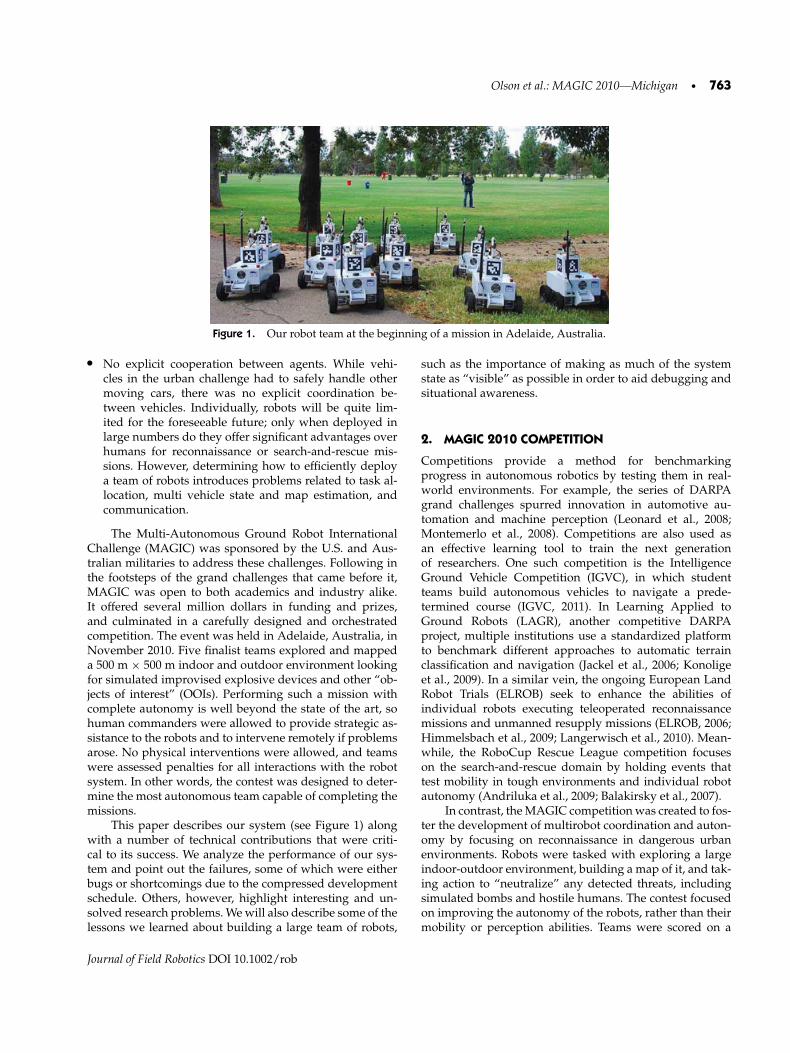
Figure 1. Our robot team at the beginning of a mission in Adelaide, Australia.
• No explicit cooperation between agents. While vehi-cles in the urban challenge had to safely handle othermoving cars, there was no explicit coordination be-tween vehicles. Individually, robots will be quite lim-ited for the foreseeable future; only when deployed inlarge numbers do they offer significant advantages overhumans for reconnaissance or search-and-rescue mis-sions. However, determining how to efficiently deploya team of robots introduces problems related to task al-location, multi vehicle state and map estimation, andcommunication.
The Multi-Autonomous Ground Robot InternationalChallenge (MAGIC) was sponsored by the U.S. and Aus-tralian militaries to address these challenges. Following inthe footsteps of the grand challenges that came before it,MAGIC was open to both academics and industry alike.It offered several million dollars in funding and prizes,and culminated in a carefully designed and orchestratedcompetition. The event was held in Adelaide, Australia, inNovember 2010. Five finalist teams explored and mappeda 500 m × 500 m indoor and outdoor environment lookingfor simulated improvised explosive devices and other “ob-jects of interest” (OOIs). Performing such a mission withcomplete autonomy is well beyond the state of the art, sohuman commanders were allowed to provide strategic as-sistance to the robots and to intervene remotely if problemsarose. No physical interventions were allowed, and teamswere assessed penalties for all interactions with the robotsystem. In other words, the contest was designed to deter-mine the most autonomous team capable of completing themissions.
This paper describes our system (see Figure 1) alongwith a number of technical contributions that were criti-cal to its success. We analyze the performance of our sys-tem and point out the failures, some of which were eitherbugs or shortcomings due to the compressed developmentschedule. Others, however, highlight interesting and un-solved research problems. We will also describe some of thelessons we learned about building a large team of robots,
such as the importance of making as much of the systemstate as “visible” as possible in order to aid debugging andsituational awareness.
2. MAGIC 2010 COMPETITION
Competitions provide a method for benchmarkingprogress in autonomous robotics by testing them in real-world environments. For example, the series of DARPAgrand challenges spurred innovation in automotive au-tomation and machine perception (Leonard et al., 2008;Montemerlo et al., 2008). Competitions are also used asan effective learning tool to train the next generationof researchers. One such competition is the IntelligenceGround Vehicle Competition (IGVC), in which studentteams build autonomous vehicles to navigate a prede-termined course (IGVC, 2011). In Learning Applied toGround Robots (LAGR), another competitive DARPAproject, multiple institutions use a standardized platformto benchmark different approaches to automatic terrainclassification and navigation (Jackel et al., 2006; Konoligeet al., 2009). In a similar vein, the ongoing European LandRobot Trials (ELROB) seek to enhance the abilities ofindividual robots executing teleoperated reconnaissancemissions and unmanned resupply missions (ELROB, 2006;Himmelsbach et al., 2009; Langerwisch et al., 2010). Mean-while, the RoboCup Rescue League competition focuseson the search-and-rescue domain by holding events thattest mobility in tough environments and individual robotautonomy (Andriluka et al., 2009; Balakirsky et al., 2007).
In contrast, the MAGIC competition was created to fos-ter the development of multirobot coordination and auton-omy by focusing on reconnaissance in dangerous urbanenvironments. Robots were tasked with exploring a largeindoor-outdoor environment, building a map of it, and tak-ing action to “neutralize” any detected threats, includingsimulated bombs and hostile humans. The contest focusedon improving the autonomy of the robots, rather than theirmobility or perception abilities. Teams were scored on a
Journal of Field Robotics DOI 10.1002/rob

764 • Journal of Field Robotics—2012
Figure 2. The 500 m × 500 m Adelaide showgrounds weresplit into three phases for the final round of the MAGIC com-petition. The site contained indoor and outdoor portions, anobstacle course, a sand pit, many curbs, chain-link fences, andother interesting terrain topologies.
combination of map quality, number of OOIs neutralized,amount of human interaction, and technical sophistication.
In the MAGIC competition, robots explored the show-grounds in three phases (see Figure 2). The course waslargely unknown to the teams, except for aerial imageryprovided by the organizers and a brief walk-through of thefirst section. In short, the goal was for a team of robots,assisted by two human operators, to explore and map thearea.
The play field simulated a simplified battlefield withbombs, friendly and hostile humans, and other objects suchas cars, doorways, and “toxic vats” (see Figure 3). Picturesof these objects were provided in advance to help partici-pants develop a strategy for detecting them. Ultimately, it
was up to teams to decide how to divide this task betweenrobots and human operators.
In practice, remotely controlled unmanned aerial vehi-cles (UAVs) are widely deployed in these types of searchmissions and are helpful in tracking moving objects (U.S.Army, 2010). Consequently, MAGIC organizers offered adata feed providing position estimates for humans. Thisfeed was implemented using an ultrawideband trackingsystem but was intentionally degraded to mimic the limitedabilities of real-world aircraft: they cannot see through treesor under roofs, and they cannot identify whether targets arefriendly or hostile. Humans could be classified upon visualinspection by the robots based on the color of their jump-suits: red indicated a hostile person, blue indicated a non-combatant. This was a reasonable simplification designedto reduce the difficulty of the perception task.
Simulated bombs and hostile persons were dangerousto robots and civilians. If a robot came within 2.5 m of abomb or hostile human, it would “detonate,” destroying allnearby robots and civilians. Stationary bombs had a lethalrange of 10 m, while hostile humans had a blast range of5 m. In either case, the loss of any civilian resulted in acomplete forfeit of points for that phase; it was thus im-portant to monitor the position of civilians to ensure theirsafety.
Two human operators were allowed to interact withthe system from a remote ground control station (GCS).Teams were allowed to determine when and how the hu-mans would interact remotely with the robots. However,the total interaction time was measured by the contest or-ganizers and used to penalize teams that required greateramounts of human assistance.
Teams were free to use any robot platform or sensorplatform they desired subject to reasonable weight and di-mension constraints. A minimum of three robots had to be
(a) Noncombatant (blue) &mobile OOI (red)
(b) Static OOI through Doorway (c) Toxic Vat
Figure 3. Objects of interest included (a) noncombatants and mobile OOIs, (b) static OOIs and doorways, (c) toxic vats, and cars(not shown).
Journal of Field Robotics DOI 10.1002/rob
Olson et al.: MAGIC 2010—Michigan • 765
used, but teams were free to deploy as many robots as theydesired. In addition, teams designated some robots as “sen-sor” robots (which can collect data about the environment)and “disruptor” robots (which are responsible for neutral-izing bombs and are not allowed to explore). This divisionof responsibilities increased the amount of explicit coordi-nation required between robots: when a bomb was foundby a sensor robot, it would have to coordinate the neutral-ization of that bomb with a second robot. Disruptors neu-tralized bombs by illuminating them with a laser pointerfor 15 s. Hostile humans could also be neutralized, though adifferent type of robot coordination was required: two sen-sor robots had to maintain an unbroken visual lock on thetarget for 30 s.
In the tradition of the previous DARPA challenges,the competition was conducted on a compressed timeline:only 15 months elapsed between the announcement andthe challenge event, which was held in November 2010. Ofthe 23 groups that submitted proposals, only five teams sur-vived the two rounds of down-selection to become finalists.This paper describes the approach of our team, Team Michi-gan, which won first place in the competition.
3. TEAM MICHIGAN OVERVIEW
The MAGIC competition had a structure that favors largeteams of robots because mapping and exploration are of-ten easily parallelizable. A reasonable development strat-egy for such a competition is to start with a relatively smallnumber of robots and, as time progresses and the capabil-ity of those robots improves, to increase the number. Therisk is that early design decisions could ultimately limit thescalability of the system.
Our approach was the opposite: initially we imagineda large team of robots, and then we removed robots as ourunderstanding of the limits of our budget, hardware, and
algorithms improved. The risk is that trade-offs might bemade in the name of scalability that ultimately prove un-necessary if a large team ultimately proves unworkable.Early in our design process, for example, we committed toa low-cost robot design that would allow us to build 16–24 units. Our platform is less capable, in terms of handlingin rough terrain and its sensor payload, than most otherMAGIC teams. However, this approach also drove us to fo-cus on efficient autonomy: neither our radio bandwidth northe cognitive capacities of our human operators would tol-erate robots that require vigilant monitoring or, even worse,frequent interaction.
Our team also wanted to develop a system that couldbe deployed rapidly in an unfamiliar environment. Thiswas not a requirement for the MAGIC competition, butit would be a valuable characteristic for a real-world sys-tem. For example, we aimed to minimize our reliance onprior information (including maps and aerial imagery) andon GPS data. During testing, our system was routinelydeployed in a few minutes from a large van by simplyunloading the robots and turning on the ground controlcomputers.
Our final system was composed of 14 robots and 2 hu-man operators that interacted with the system via the GCS.We deployed twice as many robots as the next largest team,and our robots were the least expensive of any of the final-ists at $11,500 per unit.
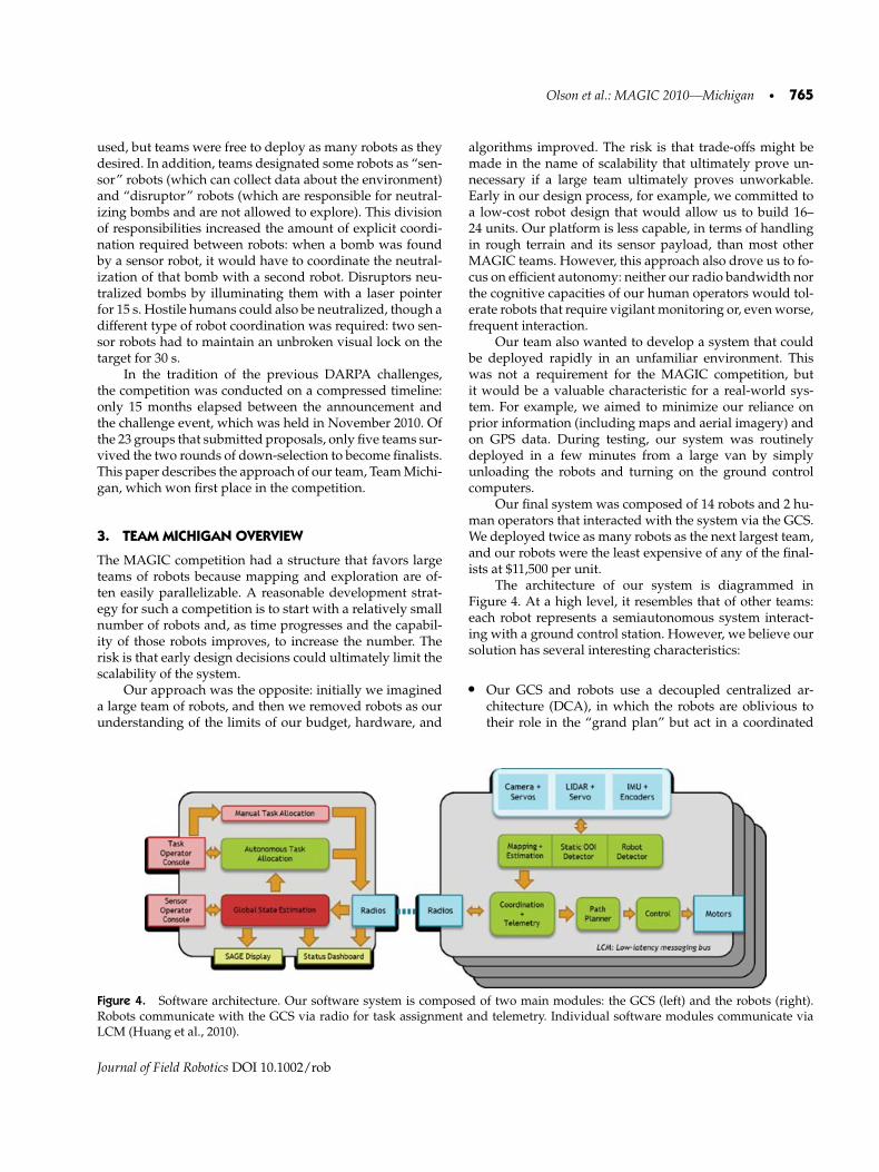
The architecture of our system is diagrammed inFigure 4. At a high level, it resembles that of other teams:each robot represents a semiautonomous system interact-ing with a ground control station. However, we believe oursolution has several interesting characteristics:
• Our GCS and robots use a decoupled centralized ar-chitecture (DCA), in which the robots are oblivious totheir role in the “grand plan” but act in a coordinated
Figure 4. Software architecture. Our software system is composed of two main modules: the GCS (left) and the robots (right).Robots communicate with the GCS via radio for task assignment and telemetry. Individual software modules communicate viaLCM (Huang et al., 2010).
Journal of Field Robotics DOI 10.1002/rob
766 • Journal of Field Robotics—2012
fashion due to the multiagent plans computed on theGCS. Our approach takes this decoupling to an extremedegree: individual robots make no attempt to maintaina consistent coordinate frame.
• The GCS constructs a globally consistent map using acombination of sensing modalities including a visualfiducial system and a new and very fast loop-closingsystem.
• Robots are entrusted with their own safety, includingnot only safe path planning but also autonomous detec-tion and avoidance of hazardous objects.
• The GCS offers a human control of a variety of au-tonomous task-allocation systems via an efficient userinterface.
• We considered the effects of cognitive loading on hu-mans explicitly, which led to the development of a newevent notification and visualization system.
This paper will describe these contributions and pro-vide an overview of our system as a whole. Throughout, wewill describe situations in which new methods were neededand those in which standard algorithms proved sufficient.Our system, while ultimately useful and the winner of theMAGIC competition, was not without shortcomings: wewill describe these and detail our work to uncover the un-derlying causes.
Multirobot systems on the scale of MAGIC are verynew, and there are few well-established evaluation metricsfor such systems. We propose a number of metrics and thecorresponding data for our system in the hope that theywill provide a basis for the evaluation of future systems.
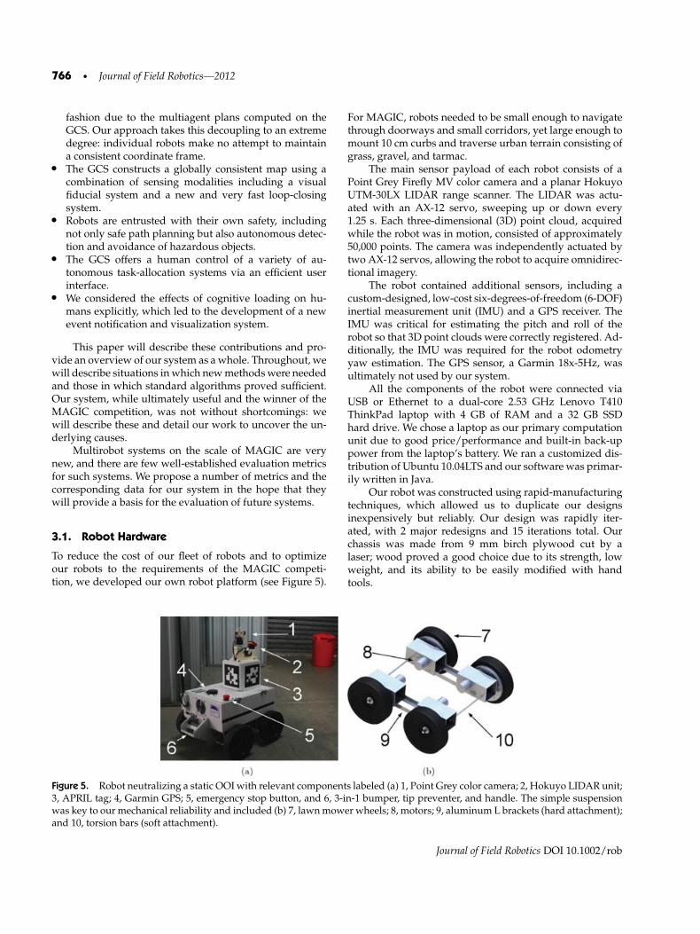
3.1. Robot Hardware
To reduce the cost of our fleet of robots and to optimizeour robots to the requirements of the MAGIC competi-tion, we developed our own robot platform (see Figure 5).
For MAGIC, robots needed to be small enough to navigatethrough doorways and small corridors, yet large enough tomount 10 cm curbs and traverse urban terrain consisting ofgrass, gravel, and tarmac.
The main sensor payload of each robot consists of aPoint Grey Firefly MV color camera and a planar HokuyoUTM-30LX LIDAR range scanner. The LIDAR was actu-ated with an AX-12 servo, sweeping up or down every1.25 s. Each three-dimensional (3D) point cloud, acquiredwhile the robot was in motion, consisted of approximately50,000 points. The camera was independently actuated bytwo AX-12 servos, allowing the robot to acquire omnidirec-tional imagery.
The robot contained additional sensors, including acustom-designed, low-cost six-degrees-of-freedom (6-DOF)inertial measurement unit (IMU) and a GPS receiver. TheIMU was critical for estimating the pitch and roll of therobot so that 3D point clouds were correctly registered. Ad-ditionally, the IMU was required for the robot odometryyaw estimation. The GPS sensor, a Garmin 18x-5Hz, wasultimately not used by our system.
All the components of the robot were connected viaUSB or Ethernet to a dual-core 2.53 GHz Lenovo T410ThinkPad laptop with 4 GB of RAM and a 32 GB SSDhard drive. We chose a laptop as our primary computationunit due to good price/performance and built-in back-uppower from the laptop’s battery. We ran a customized dis-tribution of Ubuntu 10.04LTS and our software was primar-ily written in Java.
Our robot was constructed using rapid-manufacturingtechniques, which allowed us to duplicate our designsinexpensively but reliably. Our design was rapidly iter-ated, with 2 major redesigns and 15 iterations total. Ourchassis was made from 9 mm birch plywood cut by alaser; wood proved a good choice due to its strength, lowweight, and its ability to be easily modified with handtools.
Figure 5. Robot neutralizing a static OOI with relevant components labeled (a) 1, Point Grey color camera; 2, Hokuyo LIDAR unit;3, APRIL tag; 4, Garmin GPS; 5, emergency stop button, and 6, 3-in-1 bumper, tip preventer, and handle. The simple suspensionwas key to our mechanical reliability and included (b) 7, lawn mower wheels; 8, motors; 9, aluminum L brackets (hard attachment);and 10, torsion bars (soft attachment).
Journal of Field Robotics DOI 10.1002/rob
Olson et al.: MAGIC 2010—Michigan • 767
For more complex shapes we used a Dimension 3Dprinter, which “prints” parts by depositing layers of ABSplastic. These included the actuated sensor mount and vari-ous mounting brackets and protective cases. These printersproduce parts that are strong enough to be used directly.Unfortunately, they are also fairly slow: each robot requiredabout 20 h of printing time for a full set of parts.
Each of our robot’s four wheels was independentlypowered and controlled. The gears and wheel assemblyused parts from a popular self-propelled lawn mower;power was transferred to the wheel using a gearway cutinto the inner rim of the wheel. All of the power for therobot, including for the four DC brushed motors, was pro-vided by a 24V 720Wh LiFePO4 battery; our robots had aworst-case run time of around 4 h and a typical run time al-most twice that. This longevity gave as an advantage oversome other teams, which had to swap batteries betweenphases.
4. GLOBAL STATE ESTIMATION: MAPPING ANDLOCALIZATION
Simultaneous localization and mapping (SLAM) is a criti-cal component of our system. For example, our multiagentplanning system relies on a global state estimate to deter-mine what parts of the environment have been seen andto efficiently coordinate the exploration of unseen territory.A good navigation solution is also critical for human-robotinterfaces. A number of challenges must be addressed:
• Consistency: When the same environment is observed atdifferent times, the features of that environment must beregistered correctly. In other words, loop closures musthave a low false negative rate. As with most mappingsystems, the false positive rate must be as close to zeroas possible.
• Global accuracy: While large-scale deformations in amap are acceptable in some applications (Sibley et al.,2009), global accuracy is important when the systemmust coordinate with other systems that use global co-ordinates or when it is desirable to use aerial imagery. Inthe case of MAGIC, global accuracy was also an explicitevaluation criterion.
• Rapid updates: The state estimate must be able toquickly incorporate information as it arrives from therobots.
• Minimal communication requirements: Our system hadlimited bandwidth, which had to support 14 robots innot only mapping but also command/control, telemetry,and periodic image transmission.
• Minimize reliance on a GPS: The robots must operate forlong periods of time indoors, where a GPS is not avail-able. Even outdoors, a GPS (especially with economicalreceivers) is often unreliable.
4.1. Coordinate Frames and the DecoupledCentralized Architecture
Our state estimation system is based on an approach thatwe call a decoupled centralized architecture (DCA). In thisapproach, the global state estimate is computed centrallyand is not shared with the individual robots. Instead, eachrobot operates in its own private coordinate frame that isdecoupled from the global coordinate frame. Within eachrobot’s private coordinate frame, the motion of the robot isestimated through laser- and inertially aided odometry, butno large-scale loop closures are permitted. Because thereare no loop closures, the historical trajectory of the robotis never revised and remains “smooth.” As a result, fu-sion of sensor data is computationally inexpensive: obser-vations can simply be accumulated into (for example) anoccupancy grid.
In contrast, a global state estimate is computed at theGCS. This state includes a global map as well as the rigid-body transformations that relate each robot’s private coor-dinate system to the global coordinate system. Loop clo-sures are computed and result in a constantly changingposterior estimate of the map and, as a consequence, aconstantly changing relationship between the private andglobal coordinate frames. This global map is used on theGCS to support automatic task allocation and user inter-faces, but is not transmitted to the robots, avoiding band-width and synchronization problems. However, critical in-formation, such as the location of dangerous OOIs, can beprojected into each robot’s coordinate system and transmit-ted. This allows a robot to avoid a dangerous object basedon a detection from another robot. (As a matter of imple-mentation, we transmit the location of critical objects inglobal coordinates and the N global-to-private rigid-bodytransformations for each robot; this requires less total band-width than transmitting each critical object N times.)
The basic idea of decoupling navigation and sensingcoordinate frames is not new (Moore et al., 2009), but ourDCA approach extends this to multiple agents. In this mul-tiagent context, it provides a number of benefits:
• It is easy to debug. If robots attempted to maintaintheir own complete state estimates, it could easily de-viate from the one visible to the human operator due toits different histories of communication exchanges withother robots. Such deviations could lead to difficult-to-diagnose behavior.
• It provides a simple sensor fusion scheme for individualrobots, as described above.
• In systems that share submaps, great care must beexercised to ensure that information does not get in-corporated multiple times into the state estimate; thiswould lead to overconfidence (Bahr, 2009; Cunninghamet al., 2010). In our approach, only rigid-body constraints(not submaps) are shared, and duplicates are easilyidentified.
Journal of Field Robotics DOI 10.1002/rob
768 • Journal of Field Robotics—2012
• Low communication requirements. Robots do not needto receive copies of the global map; they receive com-mands directly in their own coordinate frames.
• Little redundant computation. In some systems, robotsshare subgraphs of the map and each robot redundantlycomputes the maximum likelihood map. In our system,this computation is done only at the GCS.
The principal disadvantage of this approach is thatrobots do not have access to the global map nor to the nav-igational corrections computed by the GCS. The most sig-nificant effect is that each robot’s private coordinate frameaccumulates error over time. This eventually leads to in-consistent maps that can interfere with motion planning.To combat this, robots implement a limited sensor memoryof about 15 s, after which observations are discarded. Thelength of this memory is a direct consequence of the rateat which the robot accumulates error; for our skid-steeredvehicles, this error accumulates quickly.
With less information about the world around it, theon-robot motion planner can get mired in local minima (thisis described more in Section 5.4). This limitation is partiallymitigated by the centralized planner, which provides robotswith a series of waypoints that guide it around large obsta-cles. In this way, a robot can benefit from the global mapwithout actually needing access to it.
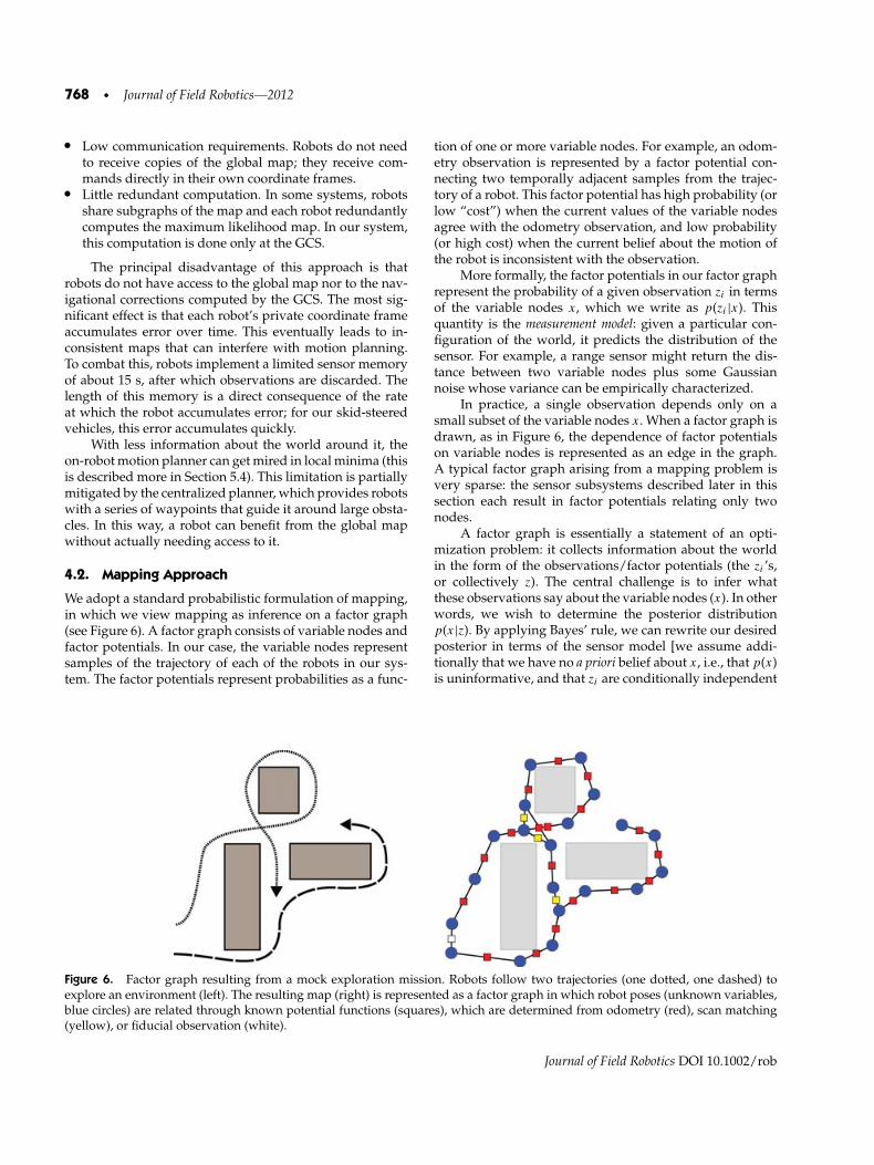
4.2. Mapping Approach
We adopt a standard probabilistic formulation of mapping,in which we view mapping as inference on a factor graph(see Figure 6). A factor graph consists of variable nodes andfactor potentials. In our case, the variable nodes representsamples of the trajectory of each of the robots in our sys-tem. The factor potentials represent probabilities as a func-
tion of one or more variable nodes. For example, an odom-etry observation is represented by a factor potential con-necting two temporally adjacent samples from the trajec-tory of a robot. This factor potential has high probability (orlow “cost”) when the current values of the variable nodesagree with the odometry observation, and low probability(or high cost) when the current belief about the motion ofthe robot is inconsistent with the observation.
More formally, the factor potentials in our factor graphrepresent the probability of a given observation zi in termsof the variable nodes x, which we write as p(zi |x). Thisquantity is the measurement model: given a particular con-figuration of the world, it predicts the distribution of thesensor. For example, a range sensor might return the dis-tance between two variable nodes plus some Gaussiannoise whose variance can be empirically characterized.
In practice, a single observation depends only on asmall subset of the variable nodes x. When a factor graph isdrawn, as in Figure 6, the dependence of factor potentialson variable nodes is represented as an edge in the graph.A typical factor graph arising from a mapping problem isvery sparse: the sensor subsystems described later in thissection each result in factor potentials relating only twonodes.
A factor graph is essentially a statement of an opti-mization problem: it collects information about the worldin the form of the observations/factor potentials (the zi ’s,or collectively z). The central challenge is to infer whatthese observations say about the variable nodes (x). In otherwords, we wish to determine the posterior distributionp(x|z). By applying Bayes’ rule, we can rewrite our desiredposterior in terms of the sensor model [we assume addi-tionally that we have no a priori belief about x, i.e., that p(x)is uninformative, and that zi are conditionally independent
Figure 6. Factor graph resulting from a mock exploration mission. Robots follow two trajectories (one dotted, one dashed) toexplore an environment (left). The resulting map (right) is represented as a factor graph in which robot poses (unknown variables,blue circles) are related through known potential functions (squares), which are determined from odometry (red), scan matching(yellow), or fiducial observation (white).
Journal of Field Robotics DOI 10.1002/rob

Olson et al.: MAGIC 2010—Michigan • 769
given x],
p(x|z) ∝ p(z|x) =∏
i
p(zi |x). (1)
We further assume that each potential is normally dis-tributed, so p(zi |x) ∝ exp{−(x − μ)′�−1(x − μ)}. The stan-dard approach is to find x, which maximizes the probabil-ity of Eq. (1) (or equivalently maximizes the negative logprobability). Taking the log converts
∏p(zi |x) into a sum
of quadratic terms. The maximum (by taking the deriva-tive) can be iteratively computed by solving a series of lin-ear system of the form A�x = b. Typically, only one to twoiterations are required if a good initialization is known.Crucially, the low node degree of the potentials leads toa sparse matrix A. This sparsity is the key to efficient in-ference (Grisetti et al., 2007; Kaess et al., 2007; Olson et al.,2006).
In an online system such as ours, the factor graphis constantly changing. The motion of robots introducesnew variable nodes, and additional sensor readings pro-duce new factor potentials. In other words, we will actuallyconsider a sequence of graphs Gj that tends to grow overtime. For example, robots report their position about onceevery 1.25 s, creating a new variable node that representsthe (unknown) true position of the robot at that time. Sen-sor data collected from that position are compared to previ-ously acquired sensor data; if a match is found, a new factorpotential is added to encode the geometric constraint thatresults from such a match. (This matching process will bedescribed in more detail below.)
The factor graph approach has distinct advantagesover other methods. The memory required by Kalman fil-ter approaches grows quadratically due to the fact thatit explicitly maintains a covariance matrix. Particle filters(Montemerlo, 2003) exhibit even faster growth in mem-ory due to the growth in dimensionality of the state vec-tor; this growth necessitates resampling methods (Grisettiet al., 2005), which introduce approximation errors thatcan cause failures in complex environments. Maximum-likelihood solvers, like ours, do not attempt to explicitly re-cover the posterior covariance. Additionally, factor graphscan be retroactively edited to recover from incorrect loopclosures.
In the following sections, we first describe how sensordata were processed to be incorporated into this graph, in-cluding our methods for filtering false positives. We thendescribe our optimization (inference) strategy in more de-tail, including several improvements to earlier methods.
4.3. Sensing Approach
Our vehicles combine sensor data from three sources: iner-tially aided odometry, visual fiducials, and quasi-3D laserscan matching. As we will describe below, our system canalso make use of GPS data, but generally did not do so.In each case, the processing of the sensor data has the di-
rect goal of producing a rigid-body motion estimate fromone robot pose to another. In the case of odometry, theserigid-body transformations describe the relationship be-tween the ith and (i − 1)th poses of a particular robot. Forscan-matching, these constraints are created irrespective ofwhether the poses are from a single robot or two differ-ent ones. The observation of a visual fiducial necessarilyconcerns two separate robots. While scan-matching con-straints (edges) were computed based on robot laser datasent to the centralized ground station, information aboutinertially guided odometry and visual fiducial observationswere computed locally on each robot and transmitted overthe radio for inclusion in the graph.
Each of the sensing modalities is integrated into thefactor graph in a similar way, namely by introducing anedge that encodes a geometric constraint between twonodes (representing locations). The differences in the qual-ity of data provided by each modality are taken into ac-count during inference by considering the covariance asso-ciated with those edges.
4.3.1. Inertially Aided Odometry
Our robots have four powered wheels in a skid-steer con-figuration. The two rear wheels have magnetic Hall-effectencoders with a resolution of about 0.7 mm per tick. Theseprovide serviceable estimates of forward translation, butdue to the slippage that results from our drive train whenturning, yaw rate estimates are very poor.
To combat this, we developed the PIMU, a “pico”-sized inertial measurement unit (see Figure 7). The PIMUincludes four gyroscope axes (with two axes devoted toyaw for a slightly reduced noise floor), a three-axis ac-celerometer, a magnetometer, and a barometric altimeter. Inour mixed indoor/outdoor settings, we found the magne-tometer to be too unreliable to integrate into our filter anddid not use it. The barometric altimeter was included forevaluation purposes and was also unused.
The PIMU streams data via USB to the host computerwhere filtering is performed. The filtering could have beenperformed on the PIMU (which has an ARM Cortex-M3microprocessor), but performing this filtering on the mainCPU made it easier to modify the algorithm and to re-process logged sensor data as our filtering algorithms im-proved.
Because the PIMU uses low-cost microelectromechan-ical system (MEMS) -based accelerometers and gyro-scopes, online calibration and estimation of bias param-eters becomes important. This is particularly true of thegyroscopes, whose zero-rate output undergoes a large-magnitude random walk. The long operating time of ourrobots (e.g., 3.5 h for competition) necessitates an ongoingrecalibration, as a single calibration at start-up would yieldunacceptable errors by the end of the mission. Similarly,our large number of robots necessitated a simple system
Journal of Field Robotics DOI 10.1002/rob

770 • Journal of Field Robotics—2012
Figure 7. Inertial measurement unit. Left: our open-source PIMU unit combines gyroscopes and accelerometers into a compactUSB-powered device. Right: the orientation of the PIMU can be constrained by integrating the observed acceleration and compar-ing it to the gravity vector; this constrains the gravity vector to lie within a cone centered about the observed gravity vector.
requiring no manual intervention. We also wished to avoidan explicit zero-velocity update system in which the robotwould tell the PIMU that it was stationary; not only wouldit complicate our system architecture (adding a communi-cation path from our on-robot motion planner to the IMU),but such an approach is also error-prone: a robot might bemoving even if it is not being commanded to do so. For ex-ample, the robot could be sliding, teetering on three of itsfour wheels, or it could be bumped by a human or otherrobot.
We implemented automatic zero-velocity updates, inwhich the gyroscopes would detect periods of relative still-ness and automatically recalibrate the zero-rate offset. Inaddition, roll and yaw were stabilized through observa-tions of the gravity vector through the accelerometer. Theresulting inertially aided odometry system was easy touse, requiring no explicit zero-velocity updates or error-prone calibration procedures, and the performance wasquite good considering the simplicity of the online cali-
bration methods (and comparable to commercial MEMS-grade IMUs). The PIMU circuit board and firmware arenow open-source projects and can be manufactured eco-nomically in small quantities for around $250 per unit.
4.3.2. Visual Fiducials
Our robots are fitted with visual fiducials based on theAprilTag visual fiducial system (Olson, 2011) (see Figure 8).These two-dimensional bar codes encode the identity ofeach robot and allow other robots to visually detect thepresence and relative position of another robot. These de-tections are transmitted to the GCS and are used to closeloops by adding more edges to the graph. These fiducialsprovide three significant benefits: 1) they provide accuratedetection and localization, 2) they are robust to lightingand orientation changes, and 3) they include enough er-ror checking that there is essentially no possibility of a falsepositive.
(a) Robot (b) SensorheadFigure 8. One of 24 robots built for the MAGIC 2010 competition, featuring APRIL tag visual fiducials in (a) and a close-up of thesensor package in (b) , consisting of an actuated 2D LIDAR and a pan/tilt color camera.
Journal of Field Robotics DOI 10.1002/rob

Olson et al.: MAGIC 2010—Michigan • 771
Fiducials provide a mechanism for closing loops evenwhen the environment is otherwise devoid of landmarks,and they were particularly useful in initializing the systemwhen the robots were tightly clustered together. These ob-servations only occurred sporadically during normal op-eration of the system because the robots usually stayedspread out to maximize their effectiveness. Each robot hasfour copies of the same fiducial, with one copy on each faceof the robot’s “head,” allowing robots to be detected fromany direction. Each fiducial measures 13.7 cm (excludingthe white border); the relatively large size allowed robotsto detect other robots up to a range of around 5 m.
4.3.3. Laser Scan Matching
The most important type of loop closure information wasbased on matching laser scans from two different robotposes. Our approach is based on a correlative scan match-ing system (Olson, 2009a), in which the motion betweentwo robot poses is computed by searching for a rigid-bodytransformation that maximizes the correlation between twolaser scans. These two poses can come from the same or dif-ferent robots.
Our MAGIC system made several modifications andimprovements over our earlier work. First, our MAGICrobots acquire 3D point clouds rather than the 2D “crosssections” used by our previous approach. While methodsfor directly aligning 3D point clouds have been describedpreviously (Hahnel & Burgard, 2002), these point cloudswould need to be transmitted by radio to make robot-to-robot matches possible. The bandwidth required to supportthis made the approach impractical.
Instead, our approach first collapsed the 3D pointclouds into 2D binary occupancy grids, where occupiedcells correspond to areas in which the point cloud containsan approximately vertical surface. These occupancy gridswere highly repeatable and differed from the terrain clas-sification required for safe path planning (as described inSection 5.3). Additionally, they can be efficiently com-pressed since these maps required radio transmission to theGCS (see Section 4.3.4).
Using this approach, our matching task was to aligntwo binary images by finding a translation and rotation.However, correlation-based scan matching is typically for-mulated in terms of one image and one set of points. We ob-tained a set of points from one of the images by samplingfrom the set pixels. Our previous scan matching methodscould achieve approximately 50 matches per second on a2.4 GHz Intel processor. However, this was not sufficientlyfast for MAGIC: with 14 robots operating simultaneously,the number of potential loop closures is extremely high.While our earlier work used a two-level multiresolutionapproach to achieve a computational speed-up, we gener-alized this approach to use additional levels of resolution.With the ability to attempt matches at lower resolutions,
the scan matcher is able to rule out portions of the searchspace much faster. As a result, matching performance wasimproved to about 500 matches per second with eight res-olution levels. This matching performance was critical tomaintaining a consistent map between all 14 robots.
4.3.4. Lossless Terrain Map Compression
For the GCS to close loops based on laser data, terrainmaps must first be transmitted to the GCS. With each ofthe 14 robots producing a new scan at a rate of almost oneper second, bandwidth quickly becomes an issue. Each ter-rain map consisted of a binary-valued occupancy grid witha cell size of 10 cm; the average size of these images wasabout 150 × 150 pixels.
Initially, we used the ZLib library (the same compres-sion algorithm used by the PNG graphics format), whichcompressed the maps to an average of 378 bytes. This rep-resents a compression ratio of just under 8x, which reflectsthe fact that the terrain maps are very sparse. However, ourlong-distance radios had a theoretical shared bandwidth ofjust 115.2 kbps with even lower real-world performance.The transmission of terrain maps from 14 robots wouldconsume virtually all of the usable bandwidth our systemcould provide.
Recognizing that ZLib is not optimized for this type ofdata, we experimented with a variety of alternative com-pression schemes. Run-length encoding (RLE) performedworse than ZLib, but when RLE and ZLib were combined,the result was modestly better than ZLib alone. Our intu-ition is that ZLib must see a fair amount of data to buildan effective compression dictionary, during which timethe compression rate is relatively poor. By precompressingwith RLE, the underlying structure in the terrain map ismore concisely encoded, which allows ZLib’s dictionary toprovide larger savings more quickly.
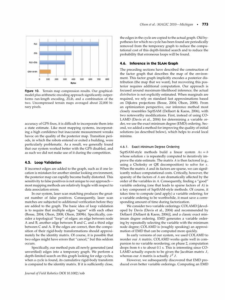
Ultimately, we employed a predictive compressionmethod based on a graphical model that predicts the valueof a pixel given its previously encoded neighbors. Thismodel was combined with an arithmetic encoder (Presset al., 1992). This approach yielded a compression ratio ofjust over 21x, reducing the average message size to 132bytes (see Figure 10).
The graphical model was a simple Bayes net (seeFigure 9), in which the probability of every pixel is as-sumed to be conditionally dependent with its four neigh-bors above and to the left of it. Restricting neighbors tothose above and to the left allows us to treat pixels as acausal stream—no pixels “depend” on pixels that have notyet been decoded.
Once the structure of a model has been specified, wecan train the model quite easily: we use a large corpus ofterrain maps and empirically measure the conditional prob-ability of a pixel in terms of its neighbors. Because we usea binary-valued terrain map, the size of the conditional
Journal of Field Robotics DOI 10.1002/rob

772 • Journal of Field Robotics—2012
Figure 9. Graphical-model-based compression. (Top) When compressing binary-valued terrain maps, the value of every pixelis predicted given four other pixels. For example, given two black pixels to the left and two white pixels above (top left), ourmodel predicts an 85% likelihood that the fifth pixel will be black. If all the surrounding pixels are black (top right), our modelpredicts a 99% likelihood that the fifth pixel will be black. We experimented with four different models that use different sets ofnearby pixels to make predictions (second row); these patterns were designed to capture spatial correlations while making useonly of pixels that would already have been decoded. More complex models required fewer bits to encode a typical terrain map:for example, the 10-neighbor model used only 0.892 times as many bits as the 4-neighbor baseline model. However, this relativelymodest improvement comes at a dramatic cost in model complexity: the 10-neighbor model has 210 = 1,024 parameters that mustbe learned, in contrast to the baseline model’s 24 = 16 parameters. Consequently, our system used the 4-neighbor model.
probability tables that we learn is quite small: a four-neighbor model has just 16 parameters.
We experimented with a variety of model structuresin which the value of a pixel was predicted using 4, 6,9, and 10 earlier pixels (see Figure 9). The number of pa-rameters grows exponentially with the number of neigh-bors, but the compression improved only modestly beyondfour neighbors. Consequently, our approach used a four-neighbor model.
For compression purposes, the graphical model isknown in advance to both the encoder and the decoder.The encoder considers each pixel in the terrain map anduses the model to determine the probability that the pixelis 0 or 1 based on its neighbors (whose values have beenpreviously transmitted). In Figure 9, we see two examplesof this prediction process; in the case of four “0” neighbors,our model predicts a 99% probability that the next pixel willalso be zero. The encoder then passes the probabilities gen-erated by the model and the actual pixel value to an arith-metic encoder.
Arithmetic encoders produce a space-efficient bit-stream by encoding a sequence of probabilistic outcomes(Press et al., 1992). They achieve efficiencies very close tothe Shannon limit. In other words, pixels whose value waspredicted by the model require fewer bits than those thatare “surprising” given the probabilistic model.
On the ground control station, the whole process is re-versed: an arithmetic decoder converts a bitstream into a
sequence of outcomes (pixel values). As each new pixel isdecoded, the values of its previously transmitted neighborsaffect the conditional probabilities of the model.
Our graphical-model-based compression performedmuch better than ZLib, RLE, or our RLE+ZLib hybrid,achieving an average of 132 bytes per terrain map (seeFigure 10). This is only 44% as much data as required bythe next best method, RLE+ZLib, and 35% as much as ZLibalone. In the presence of austere communications limits,this savings was critical in supporting the simultaneous op-eration of 14 robots.
4.4. GPS
Each robot was equipped with a consumer-grade GarminGPS-18x-5 global positioning system receiver, which pro-vided position updates at 5 Hz. Under favorable conditions(outdoors with large amounts of visible sky), these devicesproduce position estimates with only a few meters of error.In more difficult settings, such as outdoors next to a largebuilding, we would occasionally encounter positioning er-rors on the order of 70 m. Upon entering a building, the re-ceiver would produce increasingly poor position fixes untilit eventually (correctly) reported that a fix had been lost.
Unfortunately, these receivers would often outputwildly inaccurate confidence metrics: in particular, theywould occasionally report good fixes when the error wasvery large. Without a reasonable way of estimating the
Journal of Field Robotics DOI 10.1002/rob
Olson et al.: MAGIC 2010—Michigan • 773
Figure 10. Terrain map compression results. Our graphical-model plus arithmetic encoding approach significantly outper-forms run-length encoding, ZLib, and a combination of thetwo. Uncompressed terrain maps averaged about 22,000 bi-nary pixels.
accuracy of GPS fixes, it is difficult to incorporate them intoa state estimate. Like most mapping systems, incorporat-ing a high confidence but inaccurate measurement wreakshavoc on the quality of the posterior map. Transition peri-ods, in which the robots entered or exited a building, wereparticularly problematic. As a result, we generally foundthat our system worked better with the GPS disabled, andas such we did not make use of it during the competition.
4.5. Loop Validation
If incorrect edges are added to the graph, such as if one lo-cation is mistaken for another similar looking environment,the posterior map can rapidly become badly distorted. Thissensitivity to false positives is not unique to our approach—most mapping methods are relatively fragile with respect todata association errors.
In our system, laser scan matching produces the great-est number of false positives. Consequently, laser scanmatches are subjected to additional verification before theyare added to the graph. The basic idea of loop validationis to require that multiple edges “agree” with each other(Bosse, 2004; Olson, 2008; Olson, 2009b). Specifically, con-sider a topological “loop” of edges: an edge between nodeA and B, another edge between B and C, and a third edgebetween C and A. If the edges are correct, then the compo-sition of their rigid-body transformations should approxi-mately be the identity matrix. Of course, it is possible thattwo edges might have errors that “cancel,” but this seldomoccurs.
Specifically, our method puts all newly generated (andunverified) edges into a temporary graph. We perform adepth-limited search on this graph looking for edge cycles;when a cycle is found, its cumulative rigid-body transformis compared to the identity matrix. If it is sufficiently close,
the edges in the cycle are copied to the actual graph. Old hy-potheses for which no cycle has been found are periodicallyremoved from the temporary graph to reduce the compu-tational cost of this depth-limited search and to reduce theprobability that erroneous loops will be found.
4.6. Inference in the SLAM Graph
The preceding sections have described the construction ofthe factor graph that describes the map of the environ-ment. This factor graph implicitly encodes a posterior dis-tribution (the map that we want), but recovering this pos-terior requires additional computation. Our approach isfocused around maximum-likelihood inference; the actualdistribution is not explicitly estimated. When marginals arerequired, we rely on standard fast approximations basedon Dijkstra projections (Bosse, 2004; Olson, 2008). Froman optimization perspective, our inference method mostclosely resembles SqrtSAM (Dellaert & Kaess, 2006), withtwo noteworthy modifications. First, instead of using CO-LAMD (Davis et al., 2004) for determining a variable or-der, we use the exact mininum degree (EMD) ordering. Sec-ond, we added a method for improving the quality of initialsolutions (as described below), which helps to avoid localminima.
4.6.1. Exact Minimum Degree Ordering
SqrtSAM-style methods build a linear system Ax = b
whose solution x is repeatedly computed to iteratively im-prove the state estimate. The matrix A is then factored (e.g.,using a Cholesky or QR decomposition) to solve for x.When the matrix A and its factors are sparse, we can signif-icantly reduce computational costs. Critically, however, thesparsity of the factors of A are dramatically affected by theorder of the variables in A. Consequently, finding a “good”variable ordering (one that leads to sparse factors of A) isa key component of SqrtSAM-style methods. Of course, ittakes time to compute (and apply) a variable ordering; fora variable ordering to be worthwhile, it must save a corre-sponding amount of time during factorization.
We consider two variable orderings: COLAMD [devel-oped by Davis (Davis et al., 2004) and recommended byDellaert (Dellaert & Kaess, 2006)], and a classic exact min-imum degree ordering. EMD generates a variable order-ing by repeatedly selecting the variable with the minimumnode degree; COLAMD is (roughly speaking) an approxi-mation of EMD that can be computed more quickly.
In early versions of our system, we used COLAMD toreorder our A matrix. COLAMD works quite well in com-parsion to no variable reordering; on phase 2, computationdrops from 6 s to about 0.1 s. This is interesting since CO-LAMD actually expects to be given the Jacobian matrix J ,whereas our A matrix is actually JT J .
However, we subsequently discovered that EMD pro-duced even better variable orderings. Computing an EMD
Journal of Field Robotics DOI 10.1002/rob

774 • Journal of Field Robotics—2012
Table I. Effects of variable ordering. While it takes longer to compute the MinDegree ordering, it produces sparser L factors[i.e., it has smaller nonzero (nz) counts], with large impacts on the time needed to solve the system. Note that total time includesadditional costs for constructing the A matrix and thus is slightly larger than the sum of ordering and solve time. Best values areindicated in bold.
Phase Operation EMD COLAMD
Phase 1 (avg. degree 5.7) Ordering Time 0.094 s 0.011 sL nz 517,404 (0.383%) 881,805 (0.652%)
Solve Time 0.597 s 1.298 sTotal Time 0.756 s 1.398 s
Phase 2 (avg. degree 2.96) Ordering Time 0.089 s 0.0069L nz 190,613 (0.116%) 263,460 (0.1609%)
Solve Time 0.118 s 0.165 sTotal Time 0.249 s 0.208 s
Phase 3 (avg. degree 2.68) Ordering Time 0.0025 s 0.0009 sL nz 16,263 (0.317%) 20,034 (0.391%)
Solve Time 0.006 s 0.0146 sTotal Time 0.014 s 0.0281 s
CSW Grid World 3500 (avg. degree 3.2) Ordering Time 0.069 s 0.006 sL nz 183,506 (0.166%) 299,244 (0.271%)
Solve Time 0.096 s 0.214 sTotal Time 0.195 s 0.251 s
ordering is much slower than computing a COLAMD or-dering, but we found that the savings during the Choleskydecomposition typically offset this cost. The performanceof EMD and COLAMD are compared in Table I andFigure 11, measuring the runtime and quality of the or-derings on all three of the MAGIC phases and a standardbenchmark dataset (CSW Grid World 3500). In each case,COLAMD computes an ordering significantly faster thanEMD. However, the quality of the ordering (as measured by
the amount of fill-in in the Cholesky factors) is always bet-ter with EMD; this saves time when solving the system. Thecritical question is whether the total time required to com-pute the ordering and solve the system is reduced by usingEMD. In three of the four cases, EMD results in a net sav-ings in time. These results highlight some of the subtletiesinvolved in selecting a variable ordering method; a moresystematic evaluation (potentially including other variableordering methods) is an interesting area for future work.
Figure 11. EMD vs. COLAMD runtimes. In each case, it is faster to compute the COLAMD ordering than the EMD ordering.However, in all but phase 3 (which had a particularly low node degree), EMD’s better ordering results in lower total computationaltime.
Journal of Field Robotics DOI 10.1002/rob
Olson et al.: MAGIC 2010—Michigan • 775
4.6.2. Initialization
It is well known that least-squares methods are prone todivergence if provided with poor initial estimates (Olson,2008). This problem can be mitigated significantly with agood initial estimate. A popular method is to construct aminimum spanning tree over the graph, setting the initialvalue of each node according to the path from the root ofthe tree to the node’s corresponding leaf.
Initialization is especially important when incorporat-ing global position estimates containing orientation infor-mation because linearization error can inhibit convergenceeven with relatively small errors; 30 or more degrees canbe problematic, 70 degrees is catastrophic. Likewise, a chal-lenge with spanning tree approaches is that two physicallynearby nodes can have very different paths in the spanningtree, leading to significant errors.
Our solution was to construct a minimum-uncertaintyspanning tree from each node with global orientation in-formation. In our system, global alignment could be spec-ified manually at the start of a mission to allow the globalstate to be superimposed on satellite imagery (usually onlyone or two such constraints were needed). Each spanningtree represents a position prediction for every pose rel-ative to some globally referenced point. We then initial-ized each pose with a weighted average of its predictedpositions from the spanning trees. Because multiple span-ning trees were used, discontinuities between nearby nodeswere minimized. This initialization process was very fast: itran in a small fraction of the time required to actually solvethe graph.
4.7. Graph Simplification
While the memory usage of our graph grows roughly lin-early with time, the optimization time grows faster becausethe average node degree increases as more loop closures areidentified. To prevent this, we can consider periodically ap-plying a “simplify” operation that would result in a SLAMgraph with lower average node degree and would there-fore be faster to optimize. The basic challenge in simplify-ing a graph is to find a new graph with fewer edges whoseposterior, p(x|zi ), is similar to the original graph. Both themaximum-likelihood value of the new graph and the co-variance should be as similar as possible.
In the case in which multiple edges connect the sametwo nodes, the edges can be losslessly merged into a sin-gle edge (assuming Gaussian uncertainties and neglectinglinearization effects). In the more general case, lossless sim-plifications of a graph are not usually possible.
Our basic approach is to remove edges that do not pro-vide significantly new information to the graph. Consideran edge e connecting two vertices a and b. If the relativeuncertainty between a and b is much lower when e is in thegraph than without it, then e should remain in the graph.Our approach is to construct a new graph containing all of
the nodes in the original graph, and to add new edges thatreduce the uncertainty between the nodes they connect byat least a factor of α (see Algorithm 1). In practice, we usea Dijkstra projection (Bosse, 2004; Olson, 2008) to computeupper bounds on the uncertainty rather than the exact un-certainty.
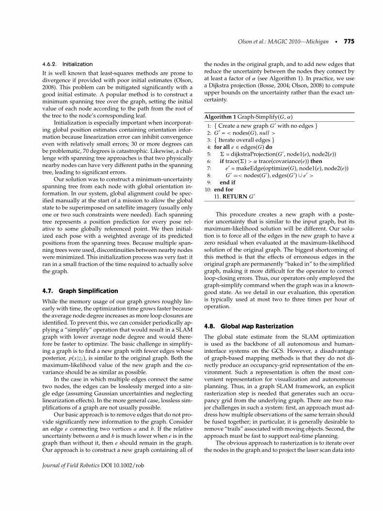
Algorithm 1 Graph-Simplify(G, α)
1: { Create a new graph G′ with no edges }2: G′ = < nodes(G), null >
3: { Iterate overall edges }4: for all e ∈ edges(G) do5: � = dijkstraProjection(G′, node1(e), node2(e))6: if trace(�) > α trace(covariance(e)) then7: e′ = makeEdge(optimize(G), node1(e), node2(e))8: G′ =< nodes(G′), edges(G′) ∪ e′ >
9: end if10: end for
11. RETURN G′
This procedure creates a new graph with a poste-rior uncertainty that is similar to the input graph, but itsmaximum-likelihood solution will be different. Our solu-tion is to force all of the edges in the new graph to have azero residual when evaluated at the maximum-likelihoodsolution of the original graph. The biggest shortcoming ofthis method is that the effects of erroneous edges in theoriginal graph are permanently “baked in” to the simplifiedgraph, making it more difficult for the operator to correctloop-closing errors. Thus, our operators only employed thegraph-simplify command when the graph was in a known-good state. As we detail in our evaluation, this operationis typically used at most two to three times per hour ofoperation.
4.8. Global Map Rasterization
The global state estimate from the SLAM optimizationis used as the backbone of all autonomous and human-interface systems on the GCS. However, a disadvantageof graph-based mapping methods is that they do not di-rectly produce an occupancy-grid representation of the en-vironment. Such a representation is often the most con-venient representation for visualization and autonomousplanning. Thus, in a graph SLAM framework, an explicitrasterization step is needed that generates such an occu-pancy grid from the underlying graph. There are two ma-jor challenges in such a system: first, an approach must ad-dress how multiple observations of the same terrain shouldbe fused together; in particular, it is generally desirable toremove “trails” associated with moving objects. Second, theapproach must be fast to support real-time planning.
The obvious approach to rasterization is to iterate overthe nodes in the graph and to project the laser scan data into
Journal of Field Robotics DOI 10.1002/rob
776 • Journal of Field Robotics—2012
an occupancy grid. This naive approach can remove tran-sient objects through a voting scheme, and is adequatelyfast on small maps (or when used offline). There is littlediscussion of map rasterization in the literature, perhapsdue to the adequacy of this simple approach in these cases.However, when applied to graphs with thousands of nodes(our graph from the first phase of MAGIC had 3,876 nodesand the second had 4,265 nodes), the rasterization timetakes significantly longer than the optimization itself andintroduced unacceptable delays into the planning process.
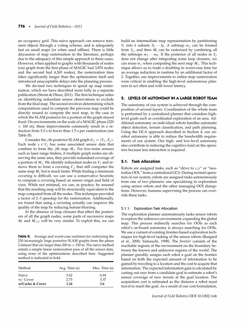
We devised two techniques to speed up map raster-ization, which we have described more fully in a separatepublication (Strom & Olson, 2011). The first technique relieson identifying redundant sensor observations to excludefrom the final map. The second involves determining whichcomputations used to compute the previous map could bedirectly reused to compute the next map, in the case inwhich the SLAM posterior for a portion of the graph stayedfixed. On environments on the scale of a MAGIC phase (220× 160 m), these improvements commonly result in a re-duction from 5.5 s to fewer than 1.5 s per rasterization (seeTable II).
Consider the j th posterior SLAM graph Gj = 〈Vj , Ej 〉.Each node x ∈ Vj has some associated sensor data thatcombine to form the j th map Mj . For low-noise sensorssuch as laser range finders, if multiple graph nodes are ob-serving the same area, they provide redundant coverage ofa portion of Mj . We identify redundant nodes in Vj and re-move them to form a covering Cj that still computes thesame map Mj but is much faster. While finding a minimumcovering is difficult, we can use a conservative heuristicto compute a covering based on sensor origin and field ofview. While not minimal, we can, in practice, be assuredthat the resulting map will be structurally equivalent to themap computed from all the nodes. This technique provideda factor of 2–3 speedup for the rasterization. Additionally,we found that using a covering actually can improve thequality of the map by reducing feature blurring.
In the absence of loop closures that affect the posteri-ors of all the graph nodes, some parts of successive mapsMi and Mi+1 will be very similar. To exploit this, we can
Table II. Average and worst-case runtimes for rasterizing the230 increasingly large posterior SLAM graphs from the phase2 dataset that are larger than 200 m × 150 m. The naive methodentails a simple linear rasterization pass of all the sensor data,using none of the optimizations described here. Suggestedmethod is indicated in bold.
Method Avg. Time (s) Max. Time (s)
Naive 5.62 6.94w/ Cover 2.75 3.37w/Cache & Cover 1.24 3.6
build an intermediate map representation by partitioningVi into k subsets S1 · · · Sk . A submap mj can be formedfrom Sj , and then Mi can be rasterized by combining allthe submaps m1 · · · mk . If the posterior of all nodes in Sj
does not change after integrating some loop closures, wecan reuse mj when computing the next map Mj . This tech-nique allows us to trade a doubling in worst-case time foran average reduction in runtime by an additional factor of2. Together, our improvements to online map rasterizationwere critical in enabling the high-level autonomous plan-ners to act often and with lower latency.
5. LEVELS OF AUTONOMY IN A LARGE ROBOT TEAM
The autonomy of our system is achieved through the com-position of several layers. Coordination of the whole teamis performed by a centralized planner that considers high-level goals such as coordinated exploration of an area. Ad-ditional autonomy on individual robots handles automaticobject detection, terrain classification, and path planning.Using the DCA approach described in Section 4, our on-robot autonomy is able to reduce the bandwidth require-ments of our system. Our high- and low-level autonomyalso contribute to reducing the cognitive load on the opera-tors because less interaction is required.
5.1. Task Allocation
Robots are assigned tasks, such as “drive to x,y” or “neu-tralize OOI,” from a centralized GCS. During normal opera-tion of our system, robots are assigned tasks autonomouslyfrom one of two planners: one specializing in explorationusing sensor robots and the other managing OOI disrup-tions. However, humans supervising the process can over-ride these tasks.
5.1.1. Exploration Task Allocation
The exploration planner autonomously tasks sensor robotsto explore the unknown environment, expanding the globalmap. This process indirectly searches for OOIs as eachrobot’s on-board autonomy is always searching for OOIs.We use a variant of existing frontier-based exploration tech-niques for high-level tasking of the sensor robots (Burgardet al., 2000; Yamauchi, 1998). The frontier consists of thereachable regions of the environment on the boundary be-tween the known and unknown regions of the world. Theplanner greedily assigns each robot a goal on the frontierbased on both the expected amount of information to begained by traveling to a location and the cost to acquire thatinformation. The expected information gain is calculated bycasting out rays from a candidate goal to estimate a robot’ssensor coverage of new terrain at the goal location. Theacquisition cost is estimated as the distance a robot musttravel to reach the goal. As a result of our cost formulation,
Journal of Field Robotics DOI 10.1002/rob
Olson et al.: MAGIC 2010—Michigan • 777
(a) (b) (c) (d)
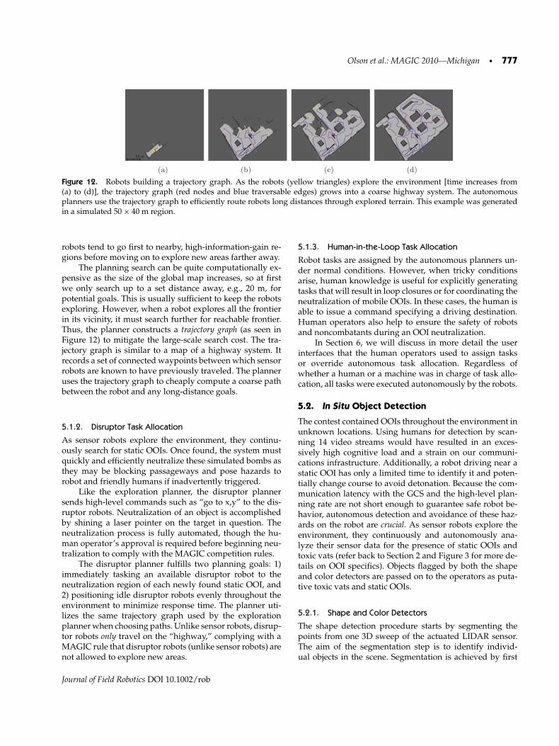
Figure 12. Robots building a trajectory graph. As the robots (yellow triangles) explore the environment [time increases from(a) to (d)], the trajectory graph (red nodes and blue traversable edges) grows into a coarse highway system. The autonomousplanners use the trajectory graph to efficiently route robots long distances through explored terrain. This example was generatedin a simulated 50 × 40 m region.
robots tend to go first to nearby, high-information-gain re-gions before moving on to explore new areas farther away.
The planning search can be quite computationally ex-pensive as the size of the global map increases, so at firstwe only search up to a set distance away, e.g., 20 m, forpotential goals. This is usually sufficient to keep the robotsexploring. However, when a robot explores all the frontierin its vicinity, it must search further for reachable frontier.Thus, the planner constructs a trajectory graph (as seen inFigure 12) to mitigate the large-scale search cost. The tra-jectory graph is similar to a map of a highway system. Itrecords a set of connected waypoints between which sensorrobots are known to have previously traveled. The planneruses the trajectory graph to cheaply compute a coarse pathbetween the robot and any long-distance goals.
5.1.2. Disruptor Task Allocation
As sensor robots explore the environment, they continu-ously search for static OOIs. Once found, the system mustquickly and efficiently neutralize these simulated bombs asthey may be blocking passageways and pose hazards torobot and friendly humans if inadvertently triggered.
Like the exploration planner, the disruptor plannersends high-level commands such as “go to x,y” to the dis-ruptor robots. Neutralization of an object is accomplishedby shining a laser pointer on the target in question. Theneutralization process is fully automated, though the hu-man operator’s approval is required before beginning neu-tralization to comply with the MAGIC competition rules.
The disruptor planner fulfills two planning goals: 1)immediately tasking an available disruptor robot to theneutralization region of each newly found static OOI, and2) positioning idle disruptor robots evenly throughout theenvironment to minimize response time. The planner uti-lizes the same trajectory graph used by the explorationplanner when choosing paths. Unlike sensor robots, disrup-tor robots only travel on the “highway,” complying with aMAGIC rule that disruptor robots (unlike sensor robots) arenot allowed to explore new areas.
5.1.3. Human-in-the-Loop Task Allocation
Robot tasks are assigned by the autonomous planners un-der normal conditions. However, when tricky conditionsarise, human knowledge is useful for explicitly generatingtasks that will result in loop closures or for coordinating theneutralization of mobile OOIs. In these cases, the human isable to issue a command specifying a driving destination.Human operators also help to ensure the safety of robotsand noncombatants during an OOI neutralization.
In Section 6, we will discuss in more detail the userinterfaces that the human operators used to assign tasksor override autonomous task allocation. Regardless ofwhether a human or a machine was in charge of task allo-cation, all tasks were executed autonomously by the robots.
5.2. In Situ Object Detection
The contest contained OOIs throughout the environment inunknown locations. Using humans for detection by scan-ning 14 video streams would have resulted in an exces-sively high cognitive load and a strain on our communi-cations infrastructure. Additionally, a robot driving near astatic OOI has only a limited time to identify it and poten-tially change course to avoid detonation. Because the com-munication latency with the GCS and the high-level plan-ning rate are not short enough to guarantee safe robot be-havior, autonomous detection and avoidance of these haz-ards on the robot are crucial. As sensor robots explore theenvironment, they continuously and autonomously ana-lyze their sensor data for the presence of static OOIs andtoxic vats (refer back to Section 2 and Figure 3 for more de-tails on OOI specifics). Objects flagged by both the shapeand color detectors are passed on to the operators as puta-tive toxic vats and static OOIs.
5.2.1. Shape and Color Detectors
The shape detection procedure starts by segmenting thepoints from one 3D sweep of the actuated LIDAR sensor.The aim of the segmentation step is to identify individ-ual objects in the scene. Segmentation is achieved by first
Journal of Field Robotics DOI 10.1002/rob
778 • Journal of Field Robotics—2012
removing the ground surface from the scene; then, individ-ual points are grouped into cells on a grid; finally, cells withsimilar heights are grouped together as a single object. Thisheight-based segmentation strategy helps to separate ob-jects from walls even if they are very nearby.
After segmentation, we try to identify approximatelycylindrical objects, since both the static OOIs and toxic vatswere approximately cylindrical. First, the length and widthof each object are calculated from the maximally alignedbounding rectangle in the X-Y dimensions. Also, cylindricalobjects presented a semi-circular cross section to the LIDARscanner, and a robust estimate of the radius of each objectwas derived from a RANSAC-based circle fit (Fischler &Bolles, 1981). The circumference of the observed portion ofthis circle was also calculated. Appropriate thresholds onthe values of these four features (length, breadth, radius,circumference) were then learned from a training dataset.Since we did not have access to exact samples of all theobjects that we needed to detect, the thresholds were thenmanually enlarged.
Once candidate objects are detected using shape in-formation, we then apply color criteria. To robustly detectcolor, we used thresholds in YCrCb color space. This colorspace allows us to treat chromaticity information (CrCb)separate from luminance information (Y), thus providinga basic level of lighting invariance. Thresholds on colorand luminance of objects in YCrCb space were then learnedfrom a training set of images that were obtained under var-ious lighting conditions.
To test the color of an object that was detected withthe LIDAR, we must have a camera image that contains theobject. A panoramic camera (or array of cameras) wouldmake this relatively straightforward because color data areacquired in all directions. Our approach was to use a sin-gle actuated camera with a limited field of view instead;this approach allows us to obtain high-resolution images ofcandidate objects while minimizing cost.
A naive camera acquisition strategy would be to pantoward objects once detected by the LIDAR. This operationcould take a second or more, leading to unacceptable ob-ject classification delays. False positives from the LIDARsystem exacerbated the problem because each false positivegenerated a “pan and capture” operation for the camera.
We solve this problem by continuously panning ourcamera and storing the last set of images in memory. Whenthe LIDAR detects a putative object, we retrieve the appro-priate image from memory. As a result, we are able to testthe color of objects without any additional actuation delay.This system is illustrated in Figure 13.
5.3. Terrain Classification
Safe autonomous traversal through the environment re-quires the detection of obstacles and other navigationalhazards. Our approach uses the 3D LIDAR data to ana-lyze the environment in the robot’s vicinity, producing a 2D
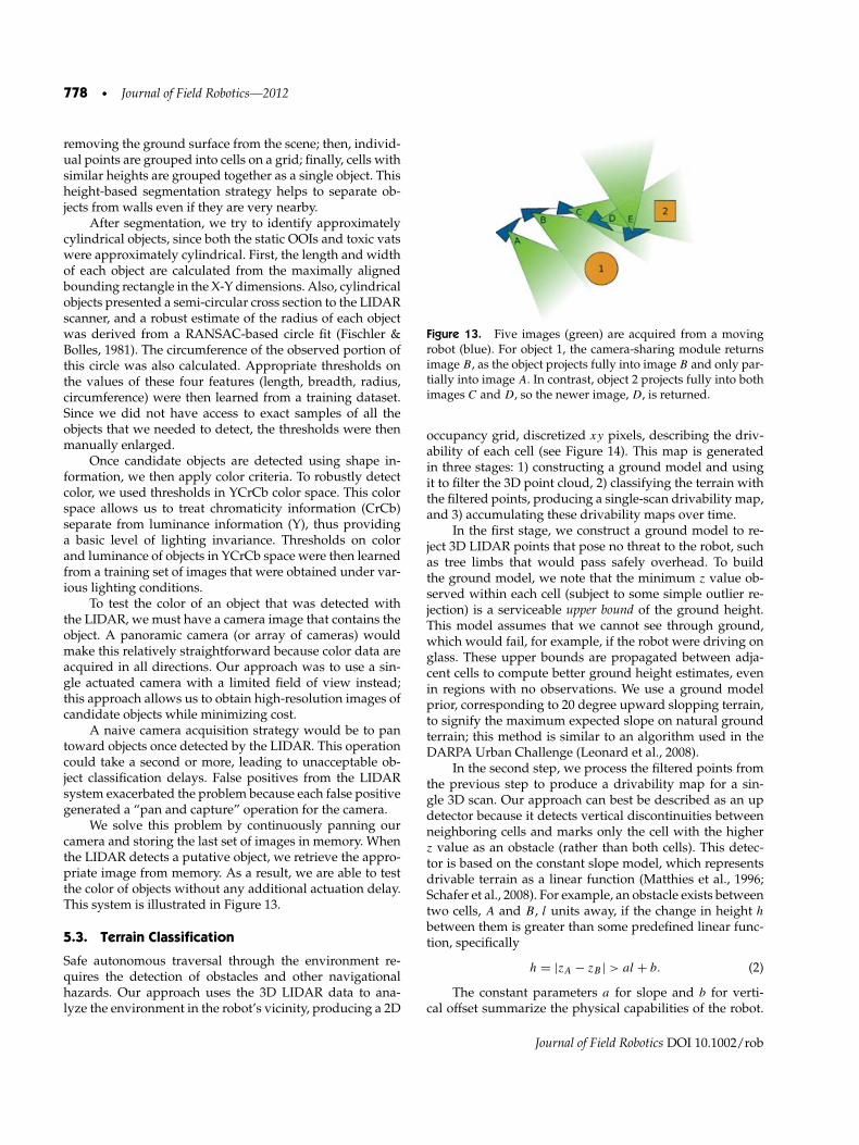
Figure 13. Five images (green) are acquired from a movingrobot (blue). For object 1, the camera-sharing module returnsimage B, as the object projects fully into image B and only par-tially into image A. In contrast, object 2 projects fully into bothimages C and D, so the newer image, D, is returned.
occupancy grid, discretized xy pixels, describing the driv-ability of each cell (see Figure 14). This map is generatedin three stages: 1) constructing a ground model and usingit to filter the 3D point cloud, 2) classifying the terrain withthe filtered points, producing a single-scan drivability map,and 3) accumulating these drivability maps over time.
In the first stage, we construct a ground model to re-ject 3D LIDAR points that pose no threat to the robot, suchas tree limbs that would pass safely overhead. To buildthe ground model, we note that the minimum z value ob-served within each cell (subject to some simple outlier re-jection) is a serviceable upper bound of the ground height.This model assumes that we cannot see through ground,which would fail, for example, if the robot were driving onglass. These upper bounds are propagated between adja-cent cells to compute better ground height estimates, evenin regions with no observations. We use a ground modelprior, corresponding to 20 degree upward slopping terrain,to signify the maximum expected slope on natural groundterrain; this method is similar to an algorithm used in theDARPA Urban Challenge (Leonard et al., 2008).
In the second step, we process the filtered points fromthe previous step to produce a drivability map for a sin-gle 3D scan. Our approach can best be described as an updetector because it detects vertical discontinuities betweenneighboring cells and marks only the cell with the higherz value as an obstacle (rather than both cells). This detec-tor is based on the constant slope model, which representsdrivable terrain as a linear function (Matthies et al., 1996;Schafer et al., 2008). For example, an obstacle exists betweentwo cells, A and B, l units away, if the change in height h
between them is greater than some predefined linear func-tion, specifically
h = |zA − zB | > al + b. (2)
The constant parameters a for slope and b for verti-cal offset summarize the physical capabilities of the robot.
Journal of Field Robotics DOI 10.1002/rob
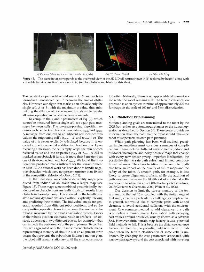
Olson et al.: MAGIC 2010—Michigan • 779
(a) Camera View (not used for terrain analysis) (b) 3D Point Cloud (c) Obstacle Map
Figure 14. The scene in (a) corresponds to the overhead view of the 3D LIDAR return shown in (b) (colored by height) along witha possible terrain classification shown in (c) (red for obstacle and black for drivable).
The constant slope model would mark A, B, and each in-termediate unobserved cell in between the two as obsta-cles. However, our algorithm marks as an obstacle only thesingle cell, A or B, with the maximum z value, thus min-imizing the dilation of obstacles out into drivable terrain,allowing operation in constrained environments.
To compute the h and l parameters of Eq. (2), whichcannot be measured from a single cell, we again pass mes-sages between cells. The message-passing algorithm re-quires each cell to keep track of two values, zmin and zmax.A message from one cell to an adjacent cell includes twovalues: the originating cell’s (zmin − a) and (zmax + a). Thevalue of l is never explicitly calculated because it is en-coded in the incremental addition/subtraction of a. Uponreceiving a message, the cell simply keeps the min of eachreceived value and the respective zmin or zmax. A cell ismarked as an obstacle if its zmin is more than b greater thanone of its 4-connected neighbors’ zmax. We found that twoiterations produced maps sufficient for the terrain presentin MAGIC. Additional work has been done to handle nega-tive obstacles, which were not present (greater than 10 cm)in the competition (Morton & Olson, 2011).
In the final step, we combine drivability maps pro-duced from individual 3D scans into a larger map (seeFigure 15). These maps were combined pessimistically: ev-idence of an obstacle from any individual scan results in anobstacle in the output map. This allowed for the handling ofslow-moving dynamic obstacles without explicitly trackingand predicting their motion. The individual maps are gen-erally acquired from different robot positions, and so thecompositing operation takes into account the motion of therobot as measured by the robot’s navigation system. Errorsin the robot’s position estimates result in artifacts—an ob-stacle appearing in two different places, for example—thatcan impede the performance of the path planner. To combatthis, we aggregated only the 12 most recent obstacle maps,representing a memory of about 15 s. If an alignment erroroccurs that prevents the robot from finding a motion plan,the robot will remain stationary until the erroneous map is
forgotten. Naturally, there is no appreciable alignment er-ror while the robot remains still. The terrain classificationprocess has an in-system runtime of approximately 300 msfor maps on the scale of 400 m2 and 5 cm discretization.
5.4. On-Robot Path Planning
Motion planning goals are transmitted to the robot by theGCS from either an autonomous planner or the human op-erator, as described in Section 5.1. These goals provide noinformation about the path that the robot should take—therobot must perform its own path planning.
While path planning has been well studied, practi-cal implementations must consider a number of compli-cations. These include cluttered environments (indoor andoutdoor), incomplete and noisy obstacle maps that changewith every new sensor sweep, imperfect localization, thepossibility that no safe path exists, and limited computa-tional resources. The characteristics of the computed pathalso have an impact on the quality of future maps and thesafety of the robot. A smooth path, for example, is lesslikely to create alignment artifacts, while the addition ofpath clearance decreases the likelihood of accidental colli-sion due to localization errors (Bhattacharya & Gavrilova,2007; Geraerts & Overmars, 2007; Wein et al., 2008).
Our decision to limit the sensor memory of the ter-rain map to the last 15 s, coupled with the finite range ofthat map, creates a particularly challenging complication.In general, we would like to compute paths with addedclearance to avoid accidental collisions with the environ-ment. One common method to add clearance to a pathis to define a minimum-cost formulation with decayingcost values around obstacles, usually known as a potentialfield. However, finite terrain map history causes potentialfield methods to fail. This is because the distance-clearancetradeoff implied by the potential field is difficult to bal-ance when the terrain classification of some cells is un-known. By changing the cost parameters associated withnarrow passageways and the cost associated with traveling
Journal of Field Robotics DOI 10.1002/rob
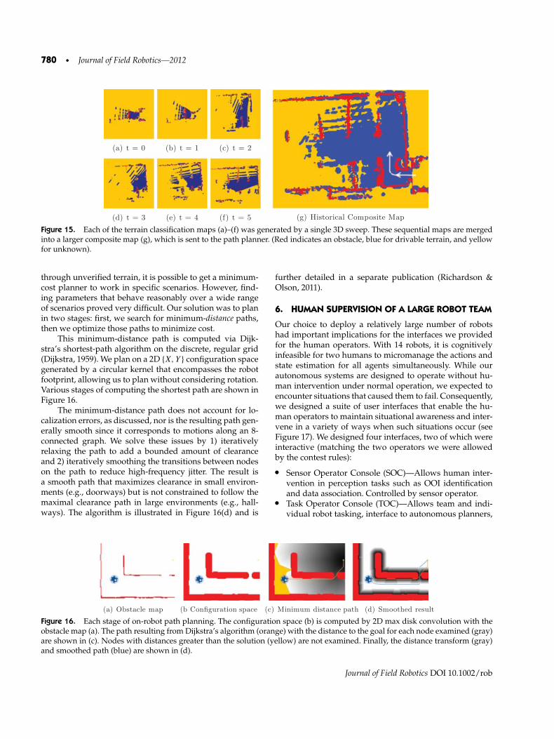
780 • Journal of Field Robotics—2012
(a) t = 0 (b) t = 1 (c) t = 2
(d) t = 3 (e) t = 4 (f) t = 5 (g) Historical Composite Map
Figure 15. Each of the terrain classification maps (a)–(f) was generated by a single 3D sweep. These sequential maps are mergedinto a larger composite map (g), which is sent to the path planner. (Red indicates an obstacle, blue for drivable terrain, and yellowfor unknown).
through unverified terrain, it is possible to get a minimum-cost planner to work in specific scenarios. However, find-ing parameters that behave reasonably over a wide rangeof scenarios proved very difficult. Our solution was to planin two stages: first, we search for minimum-distance paths,then we optimize those paths to minimize cost.
This minimum-distance path is computed via Dijk-stra’s shortest-path algorithm on the discrete, regular grid(Dijkstra, 1959). We plan on a 2D {X, Y } configuration spacegenerated by a circular kernel that encompasses the robotfootprint, allowing us to plan without considering rotation.Various stages of computing the shortest path are shown inFigure 16.
The minimum-distance path does not account for lo-calization errors, as discussed, nor is the resulting path gen-erally smooth since it corresponds to motions along an 8-connected graph. We solve these issues by 1) iterativelyrelaxing the path to add a bounded amount of clearanceand 2) iteratively smoothing the transitions between nodeson the path to reduce high-frequency jitter. The result isa smooth path that maximizes clearance in small environ-ments (e.g., doorways) but is not constrained to follow themaximal clearance path in large environments (e.g., hall-ways). The algorithm is illustrated in Figure 16(d) and is
further detailed in a separate publication (Richardson &Olson, 2011).
6. HUMAN SUPERVISION OF A LARGE ROBOT TEAM
Our choice to deploy a relatively large number of robotshad important implications for the interfaces we providedfor the human operators. With 14 robots, it is cognitivelyinfeasible for two humans to micromanage the actions andstate estimation for all agents simultaneously. While ourautonomous systems are designed to operate without hu-man intervention under normal operation, we expected toencounter situations that caused them to fail. Consequently,we designed a suite of user interfaces that enable the hu-man operators to maintain situational awareness and inter-vene in a variety of ways when such situations occur (seeFigure 17). We designed four interfaces, two of which wereinteractive (matching the two operators we were allowedby the contest rules):
• Sensor Operator Console (SOC)—Allows human inter-vention in perception tasks such as OOI identificationand data association. Controlled by sensor operator.
• Task Operator Console (TOC)—Allows team and indi-vidual robot tasking, interface to autonomous planners,
(a) Obstacle map (b Configuration space (c) Minimum distance path (d) Smoothed result
Figure 16. Each stage of on-robot path planning. The configuration space (b) is computed by 2D max disk convolution with theobstacle map (a). The path resulting from Dijkstra’s algorithm (orange) with the distance to the goal for each node examined (gray)are shown in (c). Nodes with distances greater than the solution (yellow) are not examined. Finally, the distance transform (gray)and smoothed path (blue) are shown in (d).
Journal of Field Robotics DOI 10.1002/rob

Olson et al.: MAGIC 2010—Michigan • 781
Figure 17. Team Michigan’s user interfaces (from left): SOC,Status Dashboard, TOC, and SAGE. These are shown in greaterdetail in Figures 19 and 20.
and provides bird’s-eye view of the environment. Con-trolled by task operator.
• Status Dashboard—Read-only display of each robot’sstatus with indicator lights for various states, batterymeters, and communication throughput that was espe-cially useful for highlighting error states on individualrobots.
• Situation, Actions, Goals, Environment (SAGE)Display—Read-only display with automatic analy-sis of the global state to provide a real-time narration ofthe reconnaissance mission.
6.1. Sensor Operator Console
Online machine perception remains one of the major chal-lenges in autonomous robotics. Automatic object detectionand classification, or loop-closure detection (data associa-tion), has been a topic of considerable research. While weimplemented automatic systems for both of these (see Sec-tions 4 and 5.2), the state-of-the-art still cannot guaranteeerror-free performance for 45 h of combined robot up-timeas demanded by the scope of the competition. Therefore,we dedicated one of our two interactive user interfaces toallowing a human to monitor the perception tasks com-pleted by the system and to intervene when errors occur.
All autonomous detections of OOIs are automaticallyrelayed to the GCS and displayed on the SOC as a thumb-nail on the map. This allows the sensor operator to see allthe object detections currently under consideration by thesystem with a single glance and, if necessary, to modify theclassification. For example, a false detection of a static OOIcan be flagged as such by the sensor operator, causing theautonomous system to abort the deployment of a disruptorrobot already en route for neutralization.
Perceptual errors can also have catastrophic effects onthe global state estimate. Our automatic loop-closure sys-tem described in Section 4 alleviates many of the smallodometry errors typically experienced by the robots. How-ever, our robots occasionally make significant odometry er-rors due to continuous wheel slippage, for example due
to an elevated ridge or drainage ditch. These errors tendnot to be correctable by our automatic loop closer, result-ing in erroneous posteriors and degrading map quality. Se-vere odometry errors can also contribute to erroneous loopclosures, which will cause the SLAM estimate to diverge.Bad loop closures also occur due to perceptual aliasing, acommon occurrence due to the similar structure of manyman-made environments. Thus, human monitoring of theSLAM graph can be used to detect these catastrophic errorsand fix them. Using a SLAM graph as a back-end for ourglobal state estimate makes it straightforward for a humanto understand when an error occurs, simply by visualizingits topology and the evolving posteriors of all the robot tra-jectories. The sensor operator can view the rasterized globalmap to look for artifacts of bad loop closures, or leverageexperience to detect when two robots’ trajectories are mis-aligned (see Figure 18).
We explored several ways in which a human can inter-act with the SLAM graph. We found that high-level controlover the automatic loop closer was the most effective wayfor the human to interact. When the state estimate diverges,the human can revert to automatically added loop closuresthrough a “rewind”-type command. Subsequently, thehuman can suggest that the system find a loop closurethrough two specific robot poses. The system then producesa match confidence score, which the human can use to de-termine if the constraint will alleviate the original problemfaced by the loop closer. When errors occur, the typical se-quence of commands employed by the sensor operator is asfollows: 1) rewind the constraints added by the loop closer,2) suggest an additional constraint be added between tworobot poses in the problem area, and 3) restart the loopcloser. Step 2 is particularly crucial because it provides adifferent prior for the loop closer so it is less likely to makethe same mistake again.
We found these primitives to be an effective way to fixthe global state estimate while still reducing the cognitive
(a) Loop closures lacking (b) With loop closures
Figure 18. Our maps can typically maintain alignment byrunning the automatic loop closer, leading to improvementfrom (a) no loop closures to (b) with loop closures. When theloop closer fails (not shown), misalignment, such as in (a), canprovide a cue to a human operator that intervention may benecessary.
Journal of Field Robotics DOI 10.1002/rob
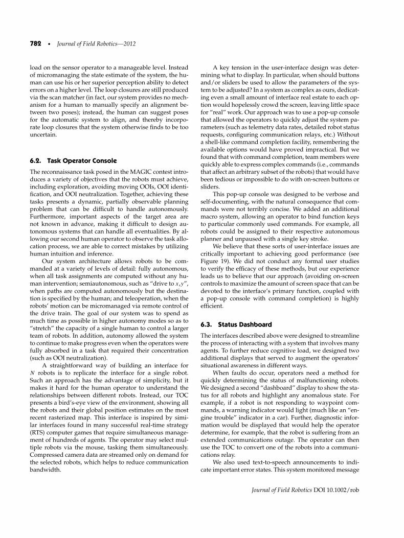
782 • Journal of Field Robotics—2012
load on the sensor operator to a manageable level. Insteadof micromanaging the state estimate of the system, the hu-man can use his or her superior perception ability to detecterrors on a higher level. The loop closures are still producedvia the scan matcher (in fact, our system provides no mech-anism for a human to manually specify an alignment be-tween two poses); instead, the human can suggest posesfor the automatic system to align, and thereby incorpo-rate loop closures that the system otherwise finds to be toouncertain.
6.2. Task Operator Console
The reconnaissance task posed in the MAGIC contest intro-duces a variety of objectives that the robots must achieve,including exploration, avoiding moving OOIs, OOI identi-fication, and OOI neutralization. Together, achieving thesetasks presents a dynamic, partially observable planningproblem that can be difficult to handle autonomously.Furthermore, important aspects of the target area arenot known in advance, making it difficult to design au-tonomous systems that can handle all eventualities. By al-lowing our second human operator to observe the task allo-cation process, we are able to correct mistakes by utilizinghuman intuition and inference.
Our system architecture allows robots to be com-manded at a variety of levels of detail: fully autonomous,when all task assignments are computed without any hu-man intervention; semiautonomous, such as “drive to x,y”,when paths are computed autonomously but the destina-tion is specified by the human; and teleoperation, when therobots’ motion can be micromanaged via remote control ofthe drive train. The goal of our system was to spend asmuch time as possible in higher autonomy modes so as to“stretch” the capacity of a single human to control a largerteam of robots. In addition, autonomy allowed the systemto continue to make progress even when the operators werefully absorbed in a task that required their concentration(such as OOI neutralization).
A straightforward way of building an interface forN robots is to replicate the interface for a single robot.Such an approach has the advantage of simplicity, but itmakes it hard for the human operator to understand therelationships between different robots. Instead, our TOCpresents a bird’s-eye view of the environment, showing allthe robots and their global position estimates on the mostrecent rasterized map. This interface is inspired by simi-lar interfaces found in many successful real-time strategy(RTS) computer games that require simultaneous manage-ment of hundreds of agents. The operator may select mul-tiple robots via the mouse, tasking them simultaneously.Compressed camera data are streamed only on demand forthe selected robots, which helps to reduce communicationbandwidth.
A key tension in the user-interface design was deter-mining what to display. In particular, when should buttonsand/or sliders be used to allow the parameters of the sys-tem to be adjusted? In a system as complex as ours, dedicat-ing even a small amount of interface real estate to each op-tion would hopelessly crowd the screen, leaving little spacefor “real” work. Our approach was to use a pop-up consolethat allowed the operators to quickly adjust the system pa-rameters (such as telemetry data rates, detailed robot statusrequests, configuring communication relays, etc.) Withouta shell-like command completion facility, remembering theavailable options would have proved impractical. But wefound that with command completion, team members werequickly able to express complex commands (i.e., commandsthat affect an arbitrary subset of the robots) that would havebeen tedious or impossible to do with on-screen buttons orsliders.
This pop-up console was designed to be verbose andself-documenting, with the natural consequence that com-mands were not terribly concise. We added an additionalmacro system, allowing an operator to bind function keysto particular commonly used commands. For example, allrobots could be assigned to their respective autonomousplanner and unpaused with a single key stroke.
We believe that these sorts of user-interface issues arecritically important to achieving good performance (seeFigure 19). We did not conduct any formal user studiesto verify the efficacy of these methods, but our experienceleads us to believe that our approach (avoiding on-screencontrols to maximize the amount of screen space that can bedevoted to the interface’s primary function, coupled witha pop-up console with command completion) is highlyefficient.
6.3. Status Dashboard
The interfaces described above were designed to streamlinethe process of interacting with a system that involves manyagents. To further reduce cognitive load, we designed twoadditional displays that served to augment the operators’situational awareness in different ways.
When faults do occur, operators need a method forquickly determining the status of malfunctioning robots.We designed a second “dashboard” display to show the sta-tus for all robots and highlight any anomalous state. Forexample, if a robot is not responding to waypoint com-mands, a warning indicator would light (much like an “en-gine trouble” indicator in a car). Further, diagnostic infor-mation would be displayed that would help the operatordetermine, for example, that the robot is suffering from anextended communications outage. The operator can thenuse the TOC to convert one of the robots into a communi-cations relay.
We also used text-to-speech announcements to indi-cate important error states. This system monitored message
Journal of Field Robotics DOI 10.1002/rob

Olson et al.: MAGIC 2010—Michigan • 783
(a) Sensor Operator Console (SOC) (b) Task Operator Console (TOC)
Figure 19. The two interactive displays used by our human operators. The SOC allowed a human to modify override labeledOOIs and to oversee the progress of the SLAM graph (a). The TOC allowed a human to manage the autonomy of the robots (b).(Best viewed in color.)
rates, battery voltages, memory usage, CPU temperature,etc., and would audibly alert the operators to any anoma-lies. This was an enormous time saver; operators wouldoften be alerted to an anomalous condition before it wasobvious that anything was wrong by merely observing therobots themselves.
6.4. SAGE Display
The Situations, Actions, Goals, and Environment (SAGE)display [see Figure 20(a)] was designed to provide mission-level situation awareness without overwhelming the userwith distracting details. It borrowed from ideas frequentlyused in 3D games. Its default view is an isometric, top-down bird’s-eye view that provided the user with theoverall situation awareness, including robot positions andmission risks. SAGE also detects key events and displayszoomed-in views of the event locality automatically, al-lowing a human operator to maintain global and localsituational awareness without requiring any manual inter-action. SAGE can be thought of as a live “highlights” dis-play, narrating the operation of the system.
6.4.1. Global Situational Awareness
SAGE’s global top-down view uses several design strate-gies to communicate key information to the user at a glance.It automatically computes its view position from the posi-tions of active robots and shifts view positions smoothlywithout distracting the user or requiring intervention.
The most important information presented in thebird’s-eye view is the robot markers. These markers areview-position-invariant so they are always clearly visible.They contain information about the robot’s id, orienta-tion, state, and task. The top-down view also displays in-formation about objects that the robots detect. Most ob-jects are displayed in small sizes and with muted colors,but dangerous objects are highlighted with richly saturatedcolors and rings showing the trigger, blast, and neutraliza-tion distances. Finally, the overhead view provides infor-mation about information quality. Uncertainty about wallsand moving objects is represented as dynamic shifts intransparency, with higher levels of transparency assignedto higher uncertainties. This is especially valuable for mo-bile OOIs, which fade over time so as not to mislead theuser into thinking they are still at a previously sensed
(a) SAGE Display (b) Status Dashboard
Figure 20. The SAGE interface (a) provided a cognitively light-weight system overview by 1) automatically narrating importantevents and showing the entire global state, such as 2) OOIs, 3) unexplored space, and 4) robot positions. Alternatively, the humanoperators could quickly ascertain each robot’s status via its respective row on the status dashboard (b).
Journal of Field Robotics DOI 10.1002/rob

784 • Journal of Field Robotics—2012
location. Unexplored regions are represented using a “fogof war” shading similar to that used in real-time strategygames. Thus the user can see the global state of the robotteam and important mission data at a glance.
6.4.2. Event Detection and Highlight Display
SAGE also draws user attention to important events. SAGEis able to automatically detect several types of events of in-terest to the user using the robots’ status reports and simplerules. For example, SAGE recognizes when new objects aredetected, when robots change to a neutralization task, andwhen civilians are close to dangerous OOIs. Upon recog-nition, SAGE automatically creates a new view that high-lights this event and smoothly animates it to a position atthe right of the display. These highlight windows are color-coded and decorated with key information allowing theuser to quickly see critical information such as the event’sdanger level (e.g., red indicates very dangerous events),type, and associated robot. The view itself is selected to givethe user an appropriate context—an isometric view for newobjects and a third-person view behind the robots for neu-tralization.
To prevent events from overwhelming the user, thesystem prioritizes events and shows only the top fourevents at any time. It also merges similar events and re-moves events over time based on the type and severity ofthe event. The result is that a user has the detailed contextneeded without any need to manipulate interface elements,thus saving time and allowing the user to focus on the high-level tasks.
Highlighting important events enabled the human op-erators to maintain good situational awareness throughoutthe challenge, and contributed to enabling only 2 humanoperators to control 14 robots. The operators leverage thesedisplays to prioritize their intervention in the system. Al-though human intervention was heavily penalized duringthe competition, we were able to leverage the intuition anddomain knowledge of the humans at the appropriate timesto ensure our global state estimate stayed consistent andto handle the complex process of OOI neutralization. Com-bining low human intervention with good state estimationallowed us to address the key goals of the contest and pro-duce a successful system.
7. EVALUATION
We have evaluated our reconnaissance system by analyzingour performance in the MAGIC 2010 contest and throughadditional experiments. Each team was allocated 3.5 h tocomplete all three phases of the competition. We spentroughly 80 min each on phases 1 and 2 and 40 min onthe final phase. Phase 1 consisted largely of an exhibition-style building whose interior was set up very similar to theJune site visits: it contained several 3 m × 3 m obstacles,
in addition to a maze augmented with 15◦ plywood ramps.We successfully neutralized five of the six static OOIs inthis phase. Phase 2 was both topologically and strategi-cally more complex, with many more buildings and inter-nal corridors, as well as mobile OOIs that patrolled outsidealong fixed routes. Our system was successful in neutraliz-ing both of the mobile OOIs, which required complex coor-dination of two sensor robots tracking a moving target at arange of over 10 m for at least 30 s. We were also able to neu-tralize five of the six static OOIs in this phase. Phase 3 wasconsiderably larger in area than phases 1 and 2, althoughthe entrance into the phase was blocked by a tricky com-bination of a patrolling mobile OOI and a noncombatant.Ultimately, this situation proved to be too strategically chal-lenging for our system to handle in the allocated time, high-lighting the need for continued work in real-world, multia-gent robotics.
Our system evaluation focuses on two components:the performance of the mapping system and the amountof human interaction with the system over the course ofthe competition. Our evaluation is made possible by thecomprehensive logs that we collected on each robot and theGCS during all of our testing and at the MAGIC competi-tion. These logs contain all data returned from each of thesensors on every robot and every command issued by theGCS to each robot, as well all the data passed between eachmodule of our system infrastructure. In addition to helpingus quickly develop such a complex software system, we ex-pect that our logging infrastructure enables us to evaluateour performance during the MAGIC competition to a betterdegree than most of our competitors.
7.1. Map Quality
One of the main evaluation criteria for the MAGIC compe-tition was the final quality of the map. The judges, work-ing with the National Institute of Standards and Technol-ogy (NIST), quantitatively evaluated the quality of eachteam’s map. This evaluation was based on fiducial mark-ers whose positions were ground-truthed and manually ex-tracted from each team’s map (Jacoff, 2011). The map wesubmitted for evaluation during the competition can beseen in Figure 21. This map, combined with our OOI detec-tion and neutralization performance, earned us first placeat the competition. Unfortunately, the raw data used by thejudges were not made available to the teams, and so wecannot provide any additional analysis of the errors.
Instead, we have shown the corresponding satellitemap, which shows the rough structure of the venue. Thecontest organizers modified the topology from what isshown in the overhead view by placing artificial barriersto block some hallways and building access points. It is stillapparent that the maps we produced are topologically ac-curate and that all structural elements are present. How-ever, local distortion is evident in some portions of the map.
Journal of Field Robotics DOI 10.1002/rob
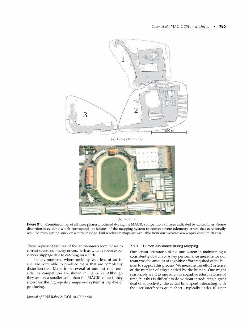
Olson et al.: MAGIC 2010—Michigan • 785
(a) Competition-day
(b) Satellite
Figure 21. Combined map of all three phases produced during the MAGIC competition. (Phases indicated by dotted lines.) Somedistortion is evident, which corresponds to failures of the mapping system to correct severe odometry errors that occasionallyresulted from getting stuck on a curb or ledge. Full resolution maps are available from our website: www.april.eecs.umich.edu
These represent failures of the autonomous loop closer tocorrect severe odometry errors, such as when a robot expe-riences slippage due to catching on a curb.
In environments where mobility was less of an is-sue, we were able to produce maps that are completelydistortion-free. Maps from several of our test runs out-side the competition are shown in Figure 22. Althoughthey are on a smaller scale than the MAGIC contest, theyshowcase the high-quality maps our system is capable ofproducing.
7.1.1. Human Assistance During Mapping
Our sensor operator assisted our system in maintaining aconsistent global map. A key performance measure for ourteam was the amount of cognitive effort required of the hu-man to support this process. We measure this effort in termsof the number of edges added by the human. One mightreasonably want to measure this cognitive effort in terms oftime, but this is difficult to do without introducing a greatdeal of subjectivity: the actual time spent interacting withthe user interface is quite short—typically under 10 s per
Journal of Field Robotics DOI 10.1002/rob
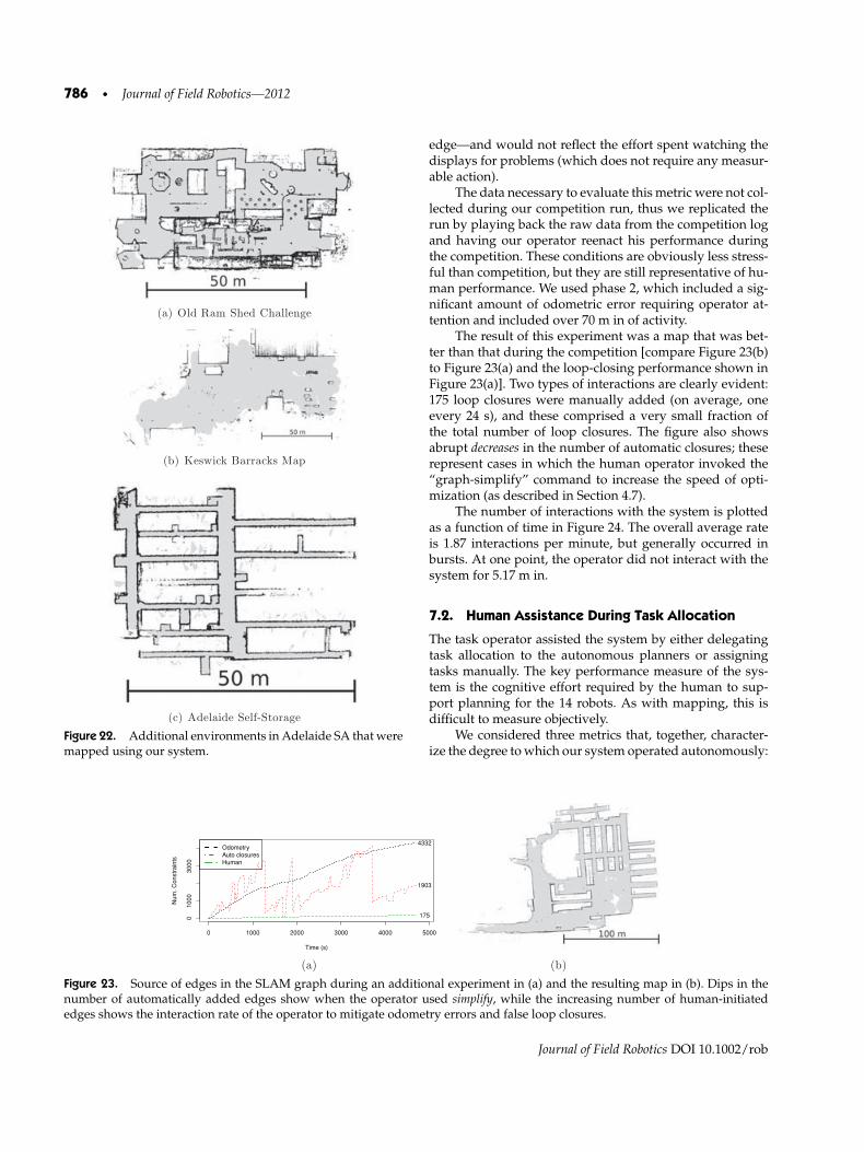
786 • Journal of Field Robotics—2012
(a) Old Ram Shed Challenge
(b) Keswick Barracks Map
(c) Adelaide Self-Storage
Figure 22. Additional environments in Adelaide SA that weremapped using our system.
edge—and would not reflect the effort spent watching thedisplays for problems (which does not require any measur-able action).
The data necessary to evaluate this metric were not col-lected during our competition run, thus we replicated therun by playing back the raw data from the competition logand having our operator reenact his performance duringthe competition. These conditions are obviously less stress-ful than competition, but they are still representative of hu-man performance. We used phase 2, which included a sig-nificant amount of odometric error requiring operator at-tention and included over 70 m in of activity.
The result of this experiment was a map that was bet-ter than that during the competition [compare Figure 23(b)to Figure 23(a) and the loop-closing performance shown inFigure 23(a)]. Two types of interactions are clearly evident:175 loop closures were manually added (on average, oneevery 24 s), and these comprised a very small fraction ofthe total number of loop closures. The figure also showsabrupt decreases in the number of automatic closures; theserepresent cases in which the human operator invoked the“graph-simplify” command to increase the speed of opti-mization (as described in Section 4.7).
The number of interactions with the system is plottedas a function of time in Figure 24. The overall average rateis 1.87 interactions per minute, but generally occurred inbursts. At one point, the operator did not interact with thesystem for 5.17 m in.
7.2. Human Assistance During Task Allocation
The task operator assisted the system by either delegatingtask allocation to the autonomous planners or assigningtasks manually. The key performance measure of the sys-tem is the cognitive effort required by the human to sup-port planning for the 14 robots. As with mapping, this isdifficult to measure objectively.
We considered three metrics that, together, character-ize the degree to which our system operated autonomously:
0 1000 2000 3000 4000 5000
010
0030
00
Time (s)
Num
. Con
stra
ints
175
1903
4332OdometryAuto closuresHuman
(a) (b)
Figure 23. Source of edges in the SLAM graph during an additional experiment in (a) and the resulting map in (b). Dips in thenumber of automatically added edges show when the operator used simplify, while the increasing number of human-initiatededges shows the interaction rate of the operator to mitigate odometry errors and false loop closures.
Journal of Field Robotics DOI 10.1002/rob

Olson et al.: MAGIC 2010—Michigan • 787
0 20 40 60 80
01
23
45
6
Time (min.)
Act
ions
per
Min
ute
Figure 24. Actions per minute for the sensor operator duringan additional experiment. Several extended periods of inactiv-ity show that our mapping system is capable of significant pe-riods of full autonomy.
1) interactions per minute, 2) time spent in fully au-tonomous/semiautonomous/teleoperated mode, and 3)distance traveled in fully autonomous/semiautonomous/teleoperated mode.
A key measure of our system is that we made no useof our teleoperation capability; our system always oper-
ated in either fully autonomous mode (when tasks are as-signed and carried out autonomously) or semiautonomous(when tasks are assigned manually but carried out au-tonomously).
Before presenting results for the three metrics, itis helpful to know how the competition unfolded. InFigure 25, the mode assigned to each robot is plotted overtime. The figure captures the major events in the competi-tion, graphically depicting the number of robots that wereactive at each point in time, and highlighting when prob-lems occurred. For example, the period of time in which allrobots were paused to allow the sensor operator to correctthe global map is readily apparent.
7.2.1. Interactions per Minute
Interactions per minute directly measure the number ofcommands issued by the human operator to the system,and thus represent a measure of how “busy” the hu-man operator was. It is an imperfect measure of cognitive
Figure 25. Robot modes of control during MAGIC with significant events annotation. At the beginning of each phase, operatorsstrategically released robots in waves (A) to provide initial separation. Serious mapping errors occurred in both of the first twophases (B). For example, early in phase 1, a catastrophic odometry error on a single robot caused the global state to diverge, forcingthe operators to pause all of the robots while they fixed the problem. The task operator slowly released robots and manuallyguided them to make important loop closures, bringing the map back under control. In phase 2, the mapping error was causedby an incorrect automatic loop closure, causing the warping near the top of our phase 2 map, as seen in Figure 21. Near theend of phase 1, the autonomous planner proved unable to finish navigating a challenging maze of ramps, causing the operatorsto attempt to semiautonomously navigate several robots through the maze (C). The navigational issues proved design-related(our wheels, excellent for skid steering, had difficulty gripping the smooth ramps) and the operators were unable to completelyexplore the maze. As phases 1 and 2 neared completion, the operators allowed robots to remain idle or paused them (D), seeing noadditional tasks to carry out. (E) denotes robots being disabled by mobile OOIs. At times, operators paused the entire team (F) toprevent robots from wandering too close to these mobile OOIs. In the final phase, we quickly encountered a difficult mobile OOIneutralization (G) that blocked the safe passage to the rest of phase 3. The operators left the team paused in a safe area as theyattempted to position pairs of robots for neutralization, but competition time expired before we were able to neutralize the mobileOOI successfully.
Journal of Field Robotics DOI 10.1002/rob

788 • Journal of Field Robotics—2012
Table III. Number of tasks assigned semiautonomously by type.
Phase Pause Waypoint Assignment Neutralize Static Neutralize Mobile Comm. Relay Mode
1 60 405 7 0 22 68 267 4 9 53 21 142 0 3 0
loading, however, since it does not reflect the effort ex-pended while watching or thinking about what the systemshould do. Conversely, it tends to overcount the number ofsalient interactions; for example, the operator may providea series of waypoints to a robot as a single coherent action,but this would be counted as multiple interactions. Still, themeasure is objective, well-suited to comparisons betweenteams, and reasonably representative of load.
See Figure 26 for the number of interactions per minutefor the task operator during the MAGIC competition. Thetask operator went up to 2 min without interacting with thesystem and averaged 4.25 interactions per minute over theentire competition. The figure shows that the task operatortended to intervene when problems occurred in prolongedbursts, rather than small, quick system adjustments.
The type of human interaction sheds light on the lim-itations of what the autonomous system could not accom-plish on its own. The sensor operator only interacted withthe system to assist in the global state estimate, with thevery occasional OOI confirmation, and thus offers no ad-dition insight. However, the task operator interacted withvarious types of high-level commands, as seen in Table III.Because we did not design mobile OOI tracking or the fi-
Figure 26. Task operator interactions per minute. Plots aredisplayed for each of the phases of MAGIC. Higher peaks inthe plots indicate frequent interactions by the operator. Abruptspikes indicate batch operation such as releasing all agents tothe autonomous planners or pausing the entire team of robots.
Table IV. Ratios of operational time spent in each mode ofcontrol to total time spent in each phase of MAGIC. Though therobots also spent time paused or idle, all tasks were executedcompletely autonomously. Numbers do not sum to 1 due toadditional time spent in either paused or idle states.
Phase Fully autonomous Semiautonomous Teleoperation
1 0.220 0.211 0.02 0.480 0.189 0.03 0.015 0.109 0.0
nal step of static OOI neutralization (i.e., turning on and offthe laser pointer), we expect these tasks to require interven-tion. However, as Table III shows, the task operator inter-vened mostly to give robots movement commands. Thesehuman-directed movement commands were not for explo-ration tasks, but were used to force loop closures and po-sition robots for OOI neutralizations. Had the autonomousplanners explicitly coordinated robots to cause large-scaleloop closures rather than solely exploring new terrain, asignificant amount of task operator interaction would havebeen eliminated.
7.2.2. Time Spent in Autonomous/Semiautonomous Mode
A robot that spends all of its time in fully autonomousmode requires virtually no management effort on the partof the human operator. In contrast, a robot that spends itstime in semiautonomous mode must periodically receivenew tasks from the human operator. The ratio of time spentin these two modes thus measures both the degree of au-tonomy of the system and the load on the operator.
The amount of time spent in our various modes isshown graphically in Figure 27 and in Table IV. These plotsadditionally show time spent in paused and idle, but thekey information is the ratio between semiautonomous andfully autonomous. In phase 1, robots split their time be-tween fully autonomous and semiautonomous. In phase 2,they were in fully autonomous mode (relying on the au-tonomous planners for their task assignments) over 71% ofthe time. In phase 3 the situation was reversed, requiringthe robots to move at very specific times and to strategi-cally chosen locations to avoid being destroyed by a hostile
Journal of Field Robotics DOI 10.1002/rob

Olson et al.: MAGIC 2010—Michigan • 789
Phase 3
Phase 2
Phase 1
0 5000 10000 15000 20000 25000 30000 35000 40000
Summed Time Across Robots (s)
PausedIdle
Semi-AutonomousFully Autonomous
(a) Phase Total
010002000300040005000
2 3 4 5 6 7 8 9 10 11 12 13 14 15
Tim
e (s
)
010002000300040005000
2 3 4 5 6 7 8 9 10 11 12 13 14 15
Tim
e (s
)
0500
1000150020002500
2 3 4 5 6 7 8 9 10 11 12 13 14 15
Tim
e (s
)
Robot ID
(b) Per Robot
Figure 27. Time spent in each robot state during MAGIC. In (a) the combined amount of time robots spent in each mode of controlis shown for each phase, while (b) shows exact times for each individual robot. Shortened bars indicate robots being disabled or,in the case of robot 5, being removed from the competition due to mechanical difficulties.
Phase 3
Phase 2
Phase 1
0 1000 2000 3000 4000 5000 6000 7000Distance (m)
Semi-AutonomousFully Autonomous
(a) Phase Total
0200400600800
10001200
2 3 4 5 6 7 8 9 10 11 12 13 14 15
Dis
tanc
e (m
)
0200400600800
10001200
2 3 4 5 6 7 8 9 10 11 12 13 14 15
Dis
tanc
e (m
)
0200400600800
10001200
2 3 4 5 6 7 8 9 10 11 12 13 14 15
Dis
tanc
e (m
)
Robot ID
(b) Per Robot
Figure 28. Distance traveled in each autonomous mode during MAGIC. (a) shows the combined distance traveled by all robots ineach phase, while (b) shows the distances for individual robots. Teleoperation was omitted from this figure as it was not employedduring MAGIC.
OOI. As a result, they were in fully autonomous mode only12% of the time.
We additionally plot the breakdown on a per-robot ba-sis in Figure 27, which provides additional insight into howthe operator’s time was distributed. What is immediatelyclear is that the ratios are not uniform between robots. In-stead, some robots require more manual task assignmentthan others. This is to be expected: robots in challenging ar-eas require assistance quite frequently. Meanwhile, robotsin relatively straightforward environments make continu-ous progress with virtually no supervision.
7.2.3. Distance traveled in Autonomous/Semiautonomous Mode
This metric is similar to the previous metric, but insteadof tallying the amount of time spent in each mode, it mea-sures the distance traveled in each mode. We use “distancetraveled” as a proxy for “useful work accomplished.” Thisis reasonable because the bulk of the competition relates toexploring the large contest area. The ratio of distance trav-
eled between these two modes measures the effectivenessof the autonomous task allocation and the load on the op-erator.
In the three phases, the distance traveled by the robotsin fully autonomous mode 59.4%, 78.7%, and 15.6% of thetotal distance (see Figure 28 and Table V). These numbersare in rough agreement with the time spent in fullyau-tonomous mode, providing evidence that the autonomoustask allocation is as effective as task allocations by the hu-mans. This is in agreement with our subjective impression
Table V. Ratios of distance traveled for each mode of controlto total distance traveled in each phase of MAGIC.
Phase Fully autonomous Semiautonomous Teleoperation
1 0.594 0.406 0.02 0.787 0.213 0.03 0.156 0.844 0.0
Journal of Field Robotics DOI 10.1002/rob

790 • Journal of Field Robotics—2012
of the system: human intervention is usually required todeal with some sort of problem (a robot stuck on an obsta-cle, for example) rather than to correct a gross inadequacyin the automatically computed task.
8. CONCLUSION
Autonomous urban reconnaissance missions such asMAGIC 2010 present interesting challenges in global stateestimation, multiagent cooperation, human-robot inter-faces, and robot perception. We developed a system of 14robots able to produce metrical maps of large-scale urbanenvironments without relying on prior information such asGPS or satellite imagery, and with only modest human as-sistance.
Our decoupled centralized architecture (DCA) is a keyidea underlying our system design, allowing robots to co-operate but without the communication and global statesynchronization challenges typical of a fully centralizedsystem. Crucial to enabling coordination between robotswas our autonomous global state estimation system, basedon a graph-SLAM approach and an automatic loop closerwith a low false-positive rate. Individual robots navigatedautonomously by analyzing a 3D LIDAR point cloud toidentify drivable terrain and dangerous objects. Robots au-tonomously planned paths through this environment totheir specified goal locations.
Incorporating a human in the loop presents opportu-nities and challenges. A human can provide valuable guid-ance to planning and can assist with sensing and mappingtasks. However, it is challenging to provide a comprehen-sive view of the system’s state without overwhelming theuser. Our system addressed this by allowing humans to fo-cus on different tasks (planning and sensing), and to sup-port them with user interfaces that alerted them to eventsworthy of their attention. These interfaces provided both anaccurate situational awareness of individual robots and theentire team, and the ability to intervene at multiple levelsof autonomy when required.
The MAGIC 2010 competition showcases the progressthat has been made in autonomous, multiagent robotics.However, it also highlights the shortcomings of the currentstate-of-the-art. First, it remains difficult to maintain a con-sistent coordinate frame between a large number of robotsdue to challenges such as wheel slip and perceptual alias-ing. Our system coped with these failures at the expense ofgreater human operator workload. Second, it remains un-clear how to optimally integrate human commanders intoa multirobot system, i.e., how to design user interfaces,manage cognitive workload, and coordinate autonomousand manual tasking at multiple levels of abstraction. Wedemonstrated a workable approach, but a more system-atic study could help to identify general principles. Finally,maintaining reliable communications remains a challenge:
much of our approach was constrained by the performanceof our radio system. Ultimately, we feel that competitionssuch as MAGIC 2010, motivated by real-world problems,are invaluable in identifying important open problems andin promoting solutions to them. These competitions serveas a reminder that there are few truly “solved” problems.
ACKNOWLEDGMENTS
Special thanks go to all our sponsors, including Intel andTexas Instruments, which allowed us to build a large teamof robots. Our robot design greatly benefited from the de-sign and CAD work of Javier Romero. The Oaks Plaza PierHotel and Glenelg Self-Storage in Adelaide, Australia gra-ciously allowed us to operate our robots in their facilities.Many University of Michigan Undergraduate Research Op-portunity Program (UROP) students helped design, build,and test our system. Our host and liaison in Adelaide, ChrisLatham, was both friendly and helpful beyond any reason-able expectation. We also thank our anonymous reviewersfor their helpful suggestions. Finally, our congratulationsto TARDEC and DSTO for successfully organizing such alarge and complex challenge.
REFERENCES
Andriluka, M., Friedmann, M., Kohlbrecher, S., Meyer, J.,Petersen, K., Reinl, C., Schauß, P., Schnitzspan, P., Thomas,D., Vatcheva, A., & Stryk, O. V. (2009). Robocuprescue2009—Robot league team Darmstadt rescue robot team(Germany).
Bahr, A. (2009). Cooperative localization for autonomous un-derwater vehicles. Ph.D. thesis, Massachusetts Institute ofTechnology, Cambridge, MA.
Balakirsky, S., Carpin, S., Kleiner, A., Lewis, M., Visser, A.,Wang, J., & Ziparo, V. A. (2007). Towards heterogeneousrobot teams for disaster mitigation: Results and perfor-mance metrics from robocup rescue. Journal of FieldRobotics, 24(11-12), 943–967.
Bhattacharya, P., & Gavrilova, M. L. (2007). Voronoi diagramin optimal path planning. In International Symposium onVoronoi Diagrams in Science and Engineering (pp. 38–47).Piscataway, NJ: IEEE.
Bosse, M. C. (2004). ATLAS: A framework for large scale au-tomated mapping and localization. Ph.D. thesis, Mas-sachusetts Institute of Technology, Cambridge, MA.
Burgard, W., Moors, M., Fox, D., Simmons, R., & Thrun, S.(2000). Collaborative multi-robot exploration. In Proceed-ings of the IEEE International Conference on Robotics andAutomation (ICRA) (Vol 1, pp. 476–481). Piscataway, NJ,IEEE.
Cunningham, A., Paluri, B., & Dellaert, F. (2010). Ddf-sam:Fully distributed slam using constrained factor graphs. InIROS (pp. 3025–3030). Piscataway, NJ: IEEE.
Davis, T. A., Gilbert, J. R., Larimore, S. I., & Ng, E. G.(2004). A column approximate minimum degree ordering
Journal of Field Robotics DOI 10.1002/rob
Olson et al.: MAGIC 2010—Michigan • 791
algorithm. ACM Transactions on Mathematical Software,30(3), 353–376.
Dellaert, F., & Kaess, M. (2006). Square root SAM: Simulta-neous localization and mapping via square root infor-mation smoothing. International Journal of Robotics Re-search, 25(12), 1181–1203.
Dijkstra, E. W. (1959). A note on two problems in connexionwith graphs. Numerische Mathematik, 1, 269–271.
ELROB (2006). European land robot trials.Fischler, M., & Bolles, R. (1981). Random sample consensus:
A paradigm for model fitting with applications to imageanalysis andd automated cartography. Communicationsof the ACM, 24(6), 381–395.
Geraerts, R., & Overmars, M. H. (2007). Creating high-quality paths for motion planning. International Journalof Robotic Research, 26, 845–863.
Grisetti, G., Stachniss, C., & Burgard, W. (2005). Improvinggrid-based SLAM with Rao-Blackwellized particle filtersby adaptive proposals and selective resampling. In Pro-ceedings of the IEEE International Conference on Roboticsand Automation (ICRA), Barcelona (pp. 2432–2437). Pis-cataway, NJ, IEEE.
Grisetti, G., Stachniss, C., Grzonka, S., & Burgard, W. (2007).A tree parameterization for efficiently computing maxi-mum likelihood maps using gradient descent. In Proceed-ings of robotics: Science and systems (RSS), Atlanta, GA.Cambridge, MA: MIT Press.
Hahnel, D., & Burgard, W. (2002). Probabilistic matching for 3dscan registration. In Proc. of the VDI-Conference Robotik2002 (Robotik). Dusseldorf, Germany: VDI-Verlag.
Himmelsbach, M., von Hundelshausen, F., Luettel, T., Manz,M., Mueller, A., Schneider, S., & Wuensche, H.-J. (2009).Team MuCAR-3 at C-ELROB 2009. In Proceedings of1st Workshop on Field Robotics, Civilian EuropeanLand Robot Trial 2009. Oulu, Finland: University ofOulu.
Huang, A., Olson, E., & Moore, D. (2010). LCM: Lightweightcommunications and marshalling. In Proceedings of theIEEE/RSJ International Conference on Intelligent Robotsand Systems (IROS). Piscataway, NJ: IEEE.
IGVC (2011). Intelligent ground vehicle competition.Jackel, L. D., Krotkov, E., Perschbacher, M., Pippine, J., &
Sullivan, C. (2006). The darpa lagr program: Goals, chal-lenges, methodology, and phase i results. Journal of FieldRobotics, 23(11–12).
Jacoff, A. (2011). Technical adjudication of the magic2010 robotcompetition. Presentation at TARDEC Quarterly RoboticsReview.
Kaess, M., Ranganathan, A., & Dellaert, F. (2007). iSAM: Fastincremental smoothing and mapping with efficient dataassociation. In Proceedings of the IEEE International Con-ference on Robotics and Automation (CRA), Rome, Italy.Piscataway, NJ, IEEE.
Konolige, K., Agrawal, M., Blas, M. R., Bolles, R. C., Gerkey, B.,Sol, J., & Sundaresan, A. (2009). Mapping, navigation, andlearning for off-road traversal. Journal of Field Robotics,26(1).
Langerwisch, M., Reimer, M., Hentschel, M., & Wagner, B.(2010, October). Control of a semi-autonomous ugv us-ing lossy low-bandwidth communication. In The Sec-ond IFAC Symposium on Telematics Applications (TA).Timisoara, Romania.
Leonard, J., How, J., Teller, S., Berger, M., Campbell, S., Fiore,G., Fletcher, L., Frazzoli, E., Huang, A., Karaman, S.,Koch, O., Kuwata, Y., Moore, D., Olson, E., Peters, S.,Teo, J., Truax, R., Walter, M., Barrett, D., Epstein, A.,Maheloni, K., Moyer, K., Jones, T., Buckley, R., Antone,M., Galejs, R., Krishnamurthy, S., & Williams, J. (2008). Aperception-driven autonomous urban vehicle. Journal ofField Robotics, 25(10), 727–774.
Matthies, L., Kelly, A., Litwin, T., & Tharp, G. (1996). Obsta-cle detection for unmanned ground vehicles: A progressreport. In Proceedings of the Intelligent Vehicles’ 95 Sym-posium (pp. 66–71). Piscataway, NJ, IEEE.
Montemerlo, M. (2003). FastSLAM: A factored solution to thesimultaneous localization and mapping problem with un-known data association. Ph.D. thesis, Robotics Institute,Carnegie Mellon University, Pittsburgh, PA.
Montemerlo, M., Becker, J., Bhat, S., Dahlkamp, H.,Dolgov, D., Ettinger, S., Haehnel, D., Hilden, T., Hoff-mann, G., Huhnke, B., Johnston, D., Klumpp, S., Langer,D., Levandowski, A., Levinson, J., Marcil, J., Orenstein,D., Paefgen, J., Penny, I., Petrovskaya, A., Pflueger, M.,Stanek, G., Stavens, D., Vogt, A., & Thrun, S. (2008).Junior: The stanford entry in the urban challenge. Journalof Field Robotics, 25(9), 569–597.
Moore, D. C., Huang, A. S., Walter, M., Olson, E., Fletcher,L., Leonard, J., & Teller, S. (2009). Simultaneous local andglobal state estimation for robotic navigation. In Proceed-ings of the IEEE International Conference on Robotics andAutomation (ICRA). Piscataway, NJ, IEEE.
Morton, R. D., & Olson, E. (2011). Positive and negative obsta-cle detection using the hld classifier. In Proceedings of theIEEE/RSJ International Conference on Intelligent Robotsand Systems (IROS). Piscataway, NJ, IEEE.
Olson, E. (2008). Robust and efficient robotic mapping. Ph.D.thesis, Massachusetts Institute of Technology, Cambridge,MA.
Olson, E. (2009a). Real-time correlative scan matching. In Pro-ceedings of the IEEE International Conference on Roboticsand Automation (ICRA), Kobe, Japan. Piscataway, NJ,IEEE.
Olson, E. (2009b). Recognizing places using spectrally clus-tered local matches. Robotics and Autonomous Systems,57(12), 31 December 2009, 1157–1172.
Olson, E. (2011, May). AprilTag: A robust and flexible multi-purpose fiducial system. In Proceedings of the IEEE Inter-national Conference on Robotics and Automation (ICRA).Shanghai, China.
Olson, E., Leonard, J., & Teller, S. (2006). Fast iterative optimiza-tion of pose graphs with poor initial estimates. In Pro-ceedings of the IEEE International Conference on Roboticsand Automation (ICRA) (pp. 2262–2269). Piscataway, NJ,IEEE.
Journal of Field Robotics DOI 10.1002/rob

792 • Journal of Field Robotics—2012
Press, W., Teukolsky, S., Vetterling, W., & Flannery, B. (1992).Numerical Recipes in C. 2nd ed. Cambridge, UK, Cam-bridge University Press.
Richardson, A., & Olson, E. (2011). Iterative path optimiza-tion for practical robot planning. In Proceedings of theIEEE/RSJ International Conference on Intelligent Robotsand Systems (IROS). Piscataway, NJ, IEEE.
Schafer, H., Hach, A., Proetzsch, M., & Berns, K. (2008). 3dobstacle detection and avoidance in vegetated off-roadterrain. In Proceedings of the IEEE International Confer-ence on Robotics and Automation (ICRA) (pp. 923–928).Piscataway, NJ, IEEE.
Sibley, G., Mei, C., Reid, I., & Newman, P. (2009, June).Adaptive relative bundle adjustment. In Proceedings ofRobotics: Science and Systems, Seattle, WA. Cambridge,MA: MIT Press.
Strom, J., & Olson, E. (2011). Occupancy grid rasterization inlarge environments for teams of robots. In Proceedingsof the IEEE/RSJ International Conference on IntelligentRobots and Systems (IROS). Piscataway, NJ, IEEE.
Thrun, S., Montemerlo, M., Dahlkamp, H., Stavens, D., Aron,A., Diebel, J., Fong, P., Gale, J., Halpenny, M., Hoffmann,G., Lau, K., Oakley, C., Palatucci, M., Pratt, V., Stang,P., Strohband, S., Dupont, C., Jendrossek, L.-E., Koelen,C., Markey, C., Rummel, C., van Niekerk, J., Jensen,E., Alessandrini, P., Bradski, G., Davies, B., Ettinger, S.,
Kaehler, A., Nefian, A., & Mahoney, P. (2007). Stanley:The robot that won the Darpa grand challenge. In The2005 DARPA Grand Challenge. Vol. 36 of Springer Tractsin Advanced Robotics (pp. 1–43). Berlin/Heidelberg,Springer.
Urmson, C., Anhalt, J., Bagnell, D., Baker, C., Bittner, R., Clark,M. N., Dolan, J., Duggins, D., Galatali, T., Geyer, C.,Gittleman, M., Harbaugh, S., Hebert, M., Howard, T. M.,Kolski, S., Kelly, A., Likhachev, M., McNaughton, M.,Miller, N., Peterson, K., Pilnick, B., Rajkumar, R., Rybski,P., Salesky, B., Seo, Y.-W., Singh, S., Snider, J., Stentz, A.,Whittaker, W., Wolkowicki, Z., Ziglar, J., Bae, H., Brown,T., Demitrish, D., Litkouhi, B., Nickolaou, J., Sadekar, V.,Zhang, W., Struble, J., Taylor, M., Darms, M., & Ferguson,D. (2008). Autonomous driving in urban environments:Boss and the urban challenge. Journal of Field Robotics,25(8).
U.S. Army (2010). U.S. army unmanned aircraft systemsroadmap 2010–2035.
Wein, R., Berg, J. P. V. D., & Halperin, D. (2008). Planninghigh-quality paths and corridors amidst obstacles. Inter-national Journal of Robotic Research, 27, 1213–1231.
Yamauchi, B. (1998). Frontier-based exploration using multi-ple robots. In Proceedings of the second international con-ference on autonomous agents, AGENTS ’98 (pp. 47–53).New York, ACM.
Journal of Field Robotics DOI 10.1002/rob