Programmable Seperation of Runout From Profile and Lead ...
6
Programmable Separation of Run,out From Profile and Lead Inspection Data for Gear Teeth With Arbitrary Modifications X'iaogen Su& Dona'id R. Houser Abstract A programmable algorithm is developed to separate out the effect of eccentricity (radiaJ ronout) from elemental gear inspection data, namely, profile and lead data. This algorithm can be coded in gear inspection software to detect the existence, the magnitude and the orientation of the eccentricity without making a separate runout check. A real example shows this algorithm produces good results. Introduction The effect of facti al runout (or eccentricity) on the profile and lead deviation has been noticed for a long time. Gear engineers know that radial ruaout changes the slopes of tlte traces of pro- files and leads. A normal gear inspection usually measures pro- files and leads from three or more teeth, and the average is often taken to compensate for this effect. In 1993, Laskiner al..(Ref, 1) found the analytical equations which describe theinteraction between these element measurements and the radial runout. The equations show the profile and lead traces of all teeth are seg- ments of a sine curve if no profile and lead modifications are imroduced. More recently. Laskin and Lawson (Ref. 2} devel- oped. the method to separate out the effect of runout from these elemental inspection data. They used linear or cubic fitting to get the slope of every elemental inspection curve, Fromthe information given by the slopes. a sine curve is fit, and the effect of the runout represented by the sine curve is removed. The method does not applyto the case where arhitrary modifi.- cations exist, either on the profile or on the lead. However, the method works for partly modified profiles and leads. but the validity of the results is compromised because the fitting processes use only that portion of the profi.le (or the lead) that is free of modifications. If considerable roughness exists on the tooth surfaces, the curvefitting of these short trace segments is net very reliable, This article presents a method that applies to any kind of modification of either profiles or leads. More importantly, only one fitting process that takes into. consideration all the inspec- kP", I,2, ...,n) are the tooth numbers. If we set: tion data is used. The process is non-iterative, and a good result can be expected .. This method only applies to gears witheeeen- tricity (radiallUJl.out). It does not apply to egg-shaped gears or gears with considerable wobble (axial runour), 42 GEAR TECHNOLOGY Extraction of Profile Modification frem the Inspection Data We start our disCllssion wi,th profile inspection d'a,ta. The same procedure applies to the lead inspection data. Referring to Fig. 1, the teeth and the base circlesare plotted. Eq. 1 ill Laskin etal, is cited here, and their symbols are used as well The equa- tion says: where ()eulLEO,ll) is the angle from the eccentricity direction to fhe center of Tooth 1. apB1(LBp,,!l) is the angle extended by the half base tooth thickness. 'I'(21t/teeth number) is the tooth pitch angle, eM(LBOmN) is the roll angle at the measurement point. e is the eccentricity. If no profile modification exists using Eq, 1 and Fig. 2, the prof tie tl'ace.t;" Oil each tooth is a segment of a sine curve hav- ing amplitude e. If an arbitrary profile modification mp(e M ) is applied, the measured profile trace if;, + mp) is the sinusoidal segment superimposed by the profile modification. In rea] measurements, the inspection data may be presented separately or may beoverlaid together and supplemented with a K chart. The final inspection data IIpi is if" + mp) shifted by D (referring to Fig. 2b, c). (2) n is the total number of measured teeth. Dp,2, .... n) are con- stants representing the shifts of profile traces, and they are unknown, Usually. three or four teeth are inspected, and n is either 3 or 4. From Eq. 1, the sinusoidal segment for the Ith mea- sured profile trace is: IP j " (k j - I)~ i .. 1.2 ..... n. (4) (5)
Transcript of Programmable Seperation of Runout From Profile and Lead ...

Programmable Separation ofRun,out From Profile and LeadInspection Data for Gear TeethWith Arbitrary Modifications
X'iaogen Su& Dona'id R. Houser
AbstractA programmable algorithm is developed to separate out the
effect of eccentricity (radiaJ ronout) from elemental gearinspection data, namely, profile and lead data. This algorithmcan be coded in gear inspection software to detect the existence,the magnitude and the orientation of the eccentricity without
making a separate runout check. A real example shows this
algorithm produces good results.Introduction
The effect of facti al runout (or eccentricity) on the profile andlead deviation has been noticed for a long time. Gear engineers
know that radial ruaout changes the slopes of tlte traces of pro-files and leads. A normal gear inspection usually measures pro-files and leads from three or more teeth, and the average is oftentaken to compensate for this effect. In 1993, Laskiner al ..(Ref,1) found the analytical equations which describe theinteractionbetween these element measurements and the radial runout. The
equations show the profile and lead traces of all teeth are seg-ments of a sine curve if no profile and lead modifications areimroduced. More recently. Laskin and Lawson (Ref. 2} devel-oped. the method to separate out the effect of runout from theseelemental inspection data. They used linear or cubic fitting toget the slope of every elemental inspection curve, Fromthe
information given by the slopes. a sine curve is fit, and theeffect of the runout represented by the sine curve is removed.The method does not applyto the case where arhitrary modifi.-cations exist, either on the profile or on the lead. However, themethod works for partly modified profiles and leads. but thevalidity of the results is compromised because the fittingprocesses use only that portion of the profi.le (or the lead) that isfree of modifications. If considerable roughness exists on thetooth surfaces, the curvefitting of these short trace segments isnet very reliable,
This article presents a method that applies to any kind ofmodification of either profiles or leads. More importantly, onlyone fitting process that takes into. consideration all the inspec- kP", I,2, ... ,n) are the tooth numbers. If we set:tion data is used. The process is non-iterative, and a good resultcan be expected ..This method only applies to gears witheeeen-tricity (radiallUJl.out). It does not apply to egg-shaped gears orgears with considerable wobble (axial runour),42 GEAR TECHNOLOGY
Extraction of Profile Modificationfrem the Inspection Data
We start our disCllssion wi,th profile inspection d'a,ta. Thesame procedure applies to the lead inspection data. Referring toFig. 1, the teeth and the base circlesare plotted. Eq. 1 ill Laskinetal, is cited here, and their symbols are used as well The equa-
tion says:
where ()eulLEO,ll) is the angle from the eccentricity direction
to fhe center of Tooth 1. apB1(LBp,,!l) is the angle extended bythe half base tooth thickness. 'I'(21t/teeth number) is the tooth
pitch angle, eM(LBOmN) is the roll angle at the measurementpoint. e is the eccentricity.
If no profile modification exists using Eq, 1 and Fig. 2, theprof tie tl'ace.t;" Oil each tooth is a segment of a sine curve hav-ing amplitude e. If an arbitrary profile modification mp(eM) isapplied, the measured profile trace if;, + mp) is the sinusoidalsegment superimposed by the profile modification.
In rea] measurements, the inspection data may be presentedseparately or may beoverlaid together and supplemented with
a K chart. The final inspection data IIpi is if" + mp) shifted by D(referring to Fig. 2b, c).
(2)
n is the total number of measured teeth. Dp,2, ....n) are con-stants representing the shifts of profile traces, and they areunknown, Usually. three or four teeth are inspected, and n iseither 3 or 4. From Eq. 1, the sinusoidal segment for the Ith mea-sured profile trace is:
IPj" (kj - I)~ i .. 1.2.....n. (4)
(5)

These substitutions simplify Bq. 3 to:
!pi =e sinCE+ ¢j) i ..1.•2, ....n.
Substituting Eq. 6 into Eq. 2 give a new equation for the shift-ed profile traces.
Expanding and rewriting Eq, 7, weget:
It sin(E)cos(¢i) + e cos(e) in(¢,) + mp(EM) .. lip; + D; (8)'i ..I.2....,n.
The profile modification mp' can be solved through any com-bination of three out of these n equations. If ilth, i2 th, i3 th equa-tions are used, we have:
e sin(e)cos(¢rl)'" e cos(e)sin(¢j1) + mp(EM) = vpil + Dn le sin(e)cos{¢i2) + e cos (c) in(¢i2) + m,(EM) '" "pil + Dil 'e sin(E)cOS(¢O) + I! oos(£)sin(~,,) + mp(£M) .. 11,.3+ Dn ,
Taking e sinCE). e cos(e) and mp(£M) as three unknowns, themean profile modification, ITIp(£M)' can be solved.
cos(f1l) -in(¢;l) vprl co (fil) sin(,pjl) DII
cos(tPn) sin{¢a) llpil + costtP,,) sln(q'!h) DIl
cos(4'o) sin(¢o) vpi") 1 I ,005('13) sin(",") DiJmp= _
COS('II) slr:l(i/lrl) I
cos(,p~) it1(~Il) I
cos('iJ) sltl(¢,3) 1This solunon depends onlhe reference of each profile which
dictates the .applied shifts. DiU = W,2,...• n). These shifts areunknown at this stage. But Eq. 10 revealls that the DiS only shiftmp upwards or downwards and do not change nlp's shape.Setting Dj to zero gives rise to:
COS('il) in{~I'l)"p;I
cos(cPa) in(4IIl) Ilpn
COS(¢I3) in(4i13) 1/1"3
fflp= (H)I ;000(';1) sin(cPn) J
COS(IPIl) in(~Il) 1
cos(¢,,) in(~'1) [INormalize nip by making its maximum zero if necessary:
m - max(m ),=> m.p. p p
If we want to make use of all of the inspection data to get abetter result, all different cornbinations (I\. i2• i) out of Upi2•.•• ,in) can be used separately and the ITIpS found can be aver-aged. In other words, if four profiletraces are available. thereare four combinations of these traces that could be used to. getfour mean profile traces that can be further averaged to give ,agloballaver.age.
The extracted profile modification mp not only includesintended profile modifications, such as tip and root relief. butall! 0 inclndes some systematic profile error which shows thesame tendency on each gear tooth. An example of a systematicprofile error cOII,Jd be a pressureangle error (Ref. 4).
,(6)
B
(7)
Touching, Dlrcclionto Measurem.cnt
Eccentric Profile- - ~,~ Concentric
ProfileA
(9) .,'.•.,,
•,,,,,,••
.,,I·•..,
•I.,.,"- ,
'.'~~ ... t" = Me!o:t;/"'!I;iol!lio .,'M-:~"- MtM = profile hlcl /"
"~~~~~~~~-~-.~~--~Mt ',. •...
I·
"I','I,
(10)
Fig. ~ .. Prorate Measurement on. ECCfIlIriC Gear (left nank).
If the inspected teeth are exactly (itn most cases. approxi-mately) evenly spaced aroundlbe gear, the profile modi.ficationcan be calculated simply by averaging the profile deviationsmeasured onall inspected teeth, Thi practice is weU known.and the proof is given here. Summarize Eq. 7 overI = 1,2"",11.
,. n n't 11,,;= t 'tsin (e+ ~i) + n m~(ell/) - 't Di
1'-=1 i=l j-",I.
. '1:""'When the measured teeth are evenly distributed.~· j=1 sin (u ~I)
tends to disappear. Setting D/ to be zero shows that the aver-age profile trace mp(f.M) is a simple average of the individuajprofile tr-aces.
(12)
Separation. of RUDout from ProfLle Inspection Data.After the modificarioa is found, it can be removed from tile
individual profile traces, vpj(i = 1,2•...JI). The re iduals, "'pi -
mp(i = ],2, ...,n). caused by a pure eccentricity are th segmentof a sine curve, A best fit is made to find the sine curve (bothamplitude and pha e) as shown in Eqs. ]3-24.
~ntrod\lcing new variable £1:
£1 = (8"lM - u.pBt) (3)MARCH/APRIL 199B 43

-- -
I \IU.E I - (;10. \\{ (;t-.O\IElin
ParameterNo. of TeethFace WidthNormal Pressure AngleHelix AngleNormal ModuleNormal Tooth ThicknessPilch DiameterBase DiameterTransverse Pre: sure Angle rpM'Transverse Tooth ThicknessHelix LeadHelix. Angle at Base Dia.Angle ,expB1 in Bq..1
Angle a"Ml in Eq. 27
Value Unit25
31.75 :mm23.4541 degree
21.5 degree2.9541 mm4.53 mm79'.37 mm7.1.94 mm
25 degree4.87 mm
633.05 mm19.65 degree5.23 degree
3.52 degree
nUI.E 2 - BEST FIT IU:Sl US !-'IW'\I I'IWFlI.EII~ \n.~\\ I ru \I~ III· H 1\1. I·.e('l-" 11(1("1n
ParameterIntroduced Eccentricity MagnitudeIntroduced Eccentricity OrientationMagnitud.e e Found Out From
Traces of Left FlanksOriemation 8.IM FOlillld Out
From Traces of Left FlanksMagmtude e Found Out
From Traces of Right FlanksOrientation 19"M Found Out
.' rom Traces of Right Flanks
Value Unit0.07118 mm-118.77 degree
'0.0693 mm
-120.3.1 degree
0.0746 mm
-122.48 degree
'1 \BI.I-' .l - BEST FIT IU.SI ITS FI{O\[ I E \11IIn('\-.S\\1r1l \IHUH 1\1 HTI.\I\{ICln
ParameterIntroduced Eccentricity MagnitudeIntroduced Eccentricity OrientationMagnitude e Found Out From
Traces of Left FlanksOrientation 8~1Found Out From
Traces of Left FlanksMagnitude e Found Out From
Traces of Right FlanksOrientation 8.1 Found Out From
Traces of Right Flanks
Value Unit0.0118 mm-121.8 degree
0.0588 mm
128,66 degree
0.0462 mm
128.24 degree--- --- ---------------
I \HI r: ~- HEST HI HI-'SI I I ... I·RO\l I'ROHI ".'11{\n.s" I 1'I\(>l I \IH II·\( 1\1.1·'.('('\ "I'I{I('I n
ParameterEccentricity Magnitude Detected
by Runout CheckEccentricity Orientation Detected
by Runour CheckMagnitude e Found Out From
Traces of Left FlanksOrientation e~lM Found Out
From Traces of Left HanksMagnitude e Found Out From
Traces of Right FlanksOrientation 6i.IM Found Out
From Traces of Right Hanks
Valu.e Unit
Om05 mm
-IM.2 degree
0.0]01 mm
-174.34 d~gree
0.01014 mm
-146.5 degree
44 GEAR TECHNOLOGY
(14)
Eq. 7 becomes:
We have (n + 2) unknowns, Dj(i "" [,2"",'1), e and fl.' Bqs. 15are linearized by introducing:
07)Theil.
t;(E,,) = -Dr + D~..I.cos(£.!l + fli)+ D...1sin{EoI(+ 1/1,) + m,(£,,)- "pi = 0 (1.8)i= 1.2, .... 11.
If p points are measured on each flank, then totally p x fI
equations. exist, We will solve all p x n equation by minimiz-ing F. where
(19)
EMjV = 1..2 .....p) are the roll angles corresponding to the mea-sured point. Setting i1E. (k = l •..•n + 2) to zero give (n +2)
aDklinear equations:
where,
:.{Pi=i. 0 i¢j
i, j '" l.2.....1I•
p= a, _01 = -IooS(EiI/' + ~,,} i = 1.2,.....,
.....- j=1 'I
P= a~...2 = - .1: Sin{EMj + ¢l} j = 1,2, ... ,11
FlP 11
= I I oos1(£ +~)j~1 j~l /II) I
P n
= Q.....l.Ml =.1: .Isin(E/IIJ + ¢)co (Ell) + '¢J'FII=l
p n'"I .I sin2(eM,l + ¢)
j=II=1P
'"-I [\IV) - m(EM·ll i'"' 1.2 .... ,nj=1 Pl1
P n
= .I, .I ["p1(!1 - m{EMj)]ooS(EMj + ';1)J::II=Ip I'!
- .I :I [vp/(,r) - m(Ey)lsin(Ei\()' +I/I~FII=l
The solution is:1(21)
eccentricity magnitude e = " D;..I + D;"2 (22)
DEI '"' arctan ( ~ )
- 1'1+2(23)
eccentricity lecation 8.IM", EI + ups, (24)

The system of Eq. 20 can be very efficiently solved using theGaussian Elimination Method (Ref. 3). It is not necessary toinvert the coefficient matrix A. The profile deviations after theremoval of the effect of runoutare:
""," vpI + Dj - II! sin (E. + Ell + ~i) i ..1.2 ....•".
For the right flank. Eq, 4 in. Laskin et ai. (Ref. I) say:
Similar steps can be followed to. obtain the magnitude and ori-entation of the eccentricity fromthe profiletrace of the .rightflanks.
SepaJ'atioD of Runout from Lead lnspection Data.For spur gears, runout does not affect the lead inspection
data. The separation is applicable only for helical gears.Referring to Fig, 6 in. Laskin et al. (Ref. 1), Eq," (13) of the sinu-soidal curve of lead traces says:
MV'L'" e co (V't.>sin[9.·1 + (,.II. - ap.!l) + (k - 1)1:'+XM i 1 (27)
wherelflbis the base helix angle. 9.1 is the angle from the eccen-tricity direction (0 the center of tooth 1 at the top face. ,I/JMr is thetransverse pressure angle at the measurement diamel:er. apMr isthe angle extended by the half tooth thicknes at (he measure-ment diameter. Lithe helix lead (negative for left handedgears). xM is the ax.ial distance from the top face to the mea-surement point.
E.q. 27 has the same format as Eq. L We first define:
From Eqs, 27-3,].. the lead trace.!; due to the eccentricity can beexpressed as:
lu '"e, in(e+ tp,) i = .,2, ...,11.
If an arbitrary lead modification ml is applied. the measuredlead deviation can be written as:
The mean. lead modification ml can be expressed by the ratio oftwo determinants.
C05(;II) sin(;iI) \lUI
eQS(.,'2) sin(tpa) V/il
C (.,,]) in(tpa} VIiJ
CO (~/I) in(tpll)
co (41'0) sin(tp12)
cos(tpa) sin(!/I;)
Profile Shift inormal Direction
Measured Tooth *1{i (j .. 1,.2..3.... )
(25) k3 k4
(26)Phase
EccentricityLocation
Roll Angle Range of Profile Mea.~urement(Same Por All Measured Teeth)
ajProflle Traces on !I Sineurve
fp/- Without Modification._._. With Modifiea 'on
Tooth 1
(28)Tooth)
(29) Roll Angle Range of Measurement
(30)b) Profile Traces of Four Teeth With and Without Profile Modification
(31)
(32)
(33)
vp4;=JP4+m--D4
1~~~;==i:!!!!!!!!!I&5~~~;::~t~~Phase~p3"iP3+m.--D3
IIpl=jpl+m--Dl
vp2=jp2+m-D2
Roll Angle Range of Measurement
(34)c) Profile Traces of Four Teeth After Shifting
Fig. 2,- Frome Measurements with Arbitrary Mod~catlon.M.~I\CtiIAPI'llL 1 un 45
0.01
E 0E-D·OI~-D.02·§-D.03
-D.04-D05
0.01
E 0E-D·OI~-D.02·§-D.03
-D.04-D.05
0.01
E 0E-D·OI~-D.02·§-D.03
-D.04-D.05
0.2
E 0.1E 0." -D.I::l
-D.2
0.01
E 0E-D·OI~-D.02·§-D.03
-D.04-D.05
0.01
E 0E-DOI~-D.02·§-D.03
-D.04-D.05
20 25 30Roll Angle (deg)
a) Measured Profile Traces
20 25 30Roll Angle (deg)
b) Extracted Mean Profile Modification
20 25 30Roll Angle (deg)
c) Profile Traces After Removal of the Modification
o 50Degree
d) Sine Curve Representing Effect of Runout
20 25 30Roll Angle (deg)
e) Profile Traces After Removal of Effect of Runout
20 25 30Roll Angle (deg)
o Two Possible Worst Profile Traces
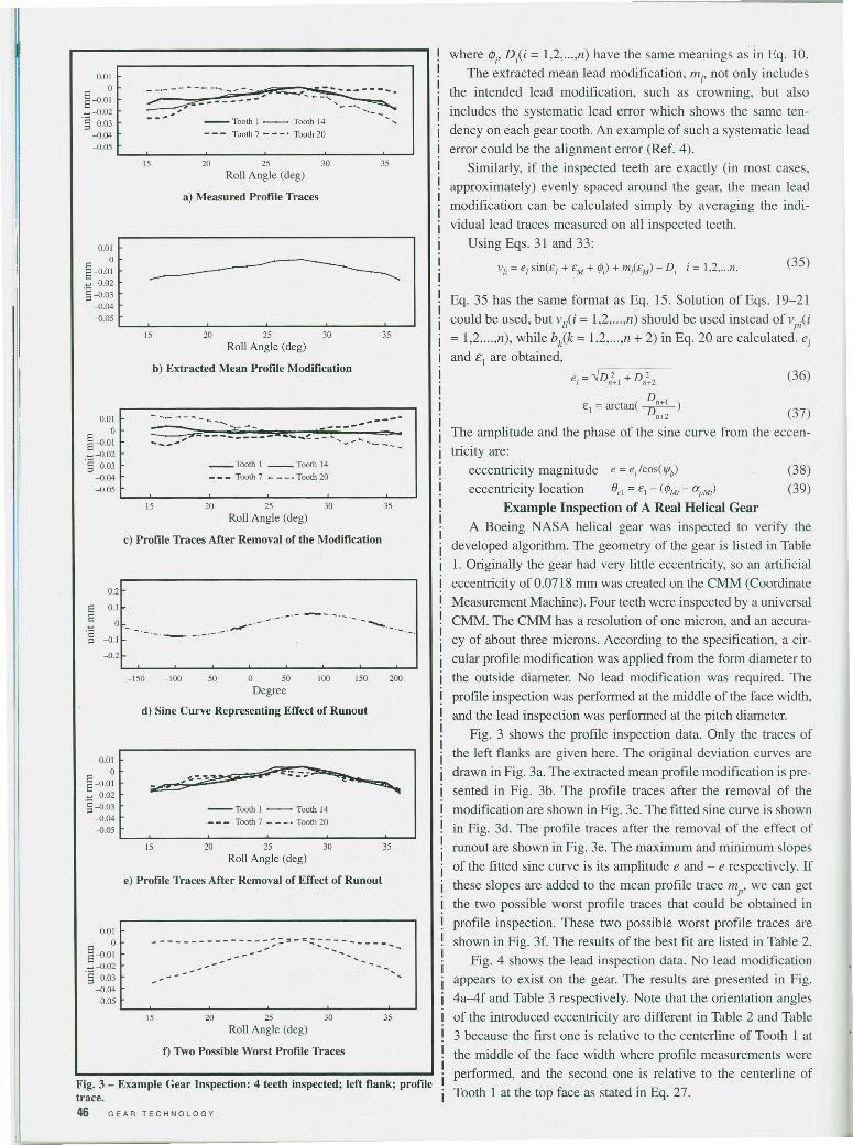
Fig. 3 - Example Gear Inspection: 4 teeth inspected; left flank; profiletrace.46 GEAR TECHNOLOGY
where lfJi, Dp = 1,2,...,n) have the same meanings as in Eq. 10.The extracted mean lead modification, ml' not only includes
the intended lead modification, such as crowning, but alsoincludes the systematic lead error which shows the same ten-dency on each gear tooth. An example of such a systematic leaderror could be the alignment error (Ref. 4).
Similarly, if the inspected teeth are exactly (in most cases,approximately) evenly spaced around the gear, the mean leadmodification can be calculated simply by averaging the indi-vidual lead traces measured on all inspected teeth.
Using Eqs. 31 and 33:
Vii = e/ sin(El + EM + ¢) + m/EM) - D/ i = 1,2, ... n. (35)
Eq. 35 has the same format as Eq. 15. Solution of Eqs. 19-21could be used, but VIP = 1,2, ,n) should be used instead of vpi(i
= 1,2,...,n), while b/k = 1,2, ,n + 2) in Eq. 20 are calculated. ezand £1 are obtained,
D£1 = arctan( ---!!±!..- )
Dn+2 (37)The amplitude and the phase of the sine curve from the eccen-tricity are:
eccentricity magnitude e = e/lcos(ljIb)
eccentricity location eel = EI - (¢Mt- apMt)
Example Inspection of A Real Helical GearA Boeing NASA helical gear was inspected to verify the
developed algorithm. The geometry of the gear is listed in Table1. Originally the gear had very little eccentricity, so an artificialeccentricity of 0.0718 mm was created on the CMM (CoordinateMeasurement Machine). Four teeth were inspected by a universalCMM. The CMM has a resolution of one micron, and an accura-cy of about three microns. According to the specification, a cir-cular profile modification was applied from the form diameter tothe outside diameter. No lead modification was required. Theprofile inspection was performed at the middle of the face width,and the lead inspection was performed at the pitch diameter.
Fig. 3 shows the profile inspection data. Only the traces ofthe left flanks are given here. The original deviation curves aredrawn in Fig. 3a. The extracted mean profile modification is pre-sented in Fig. 3b. The profile traces after the removal of themodification are shown in Fig. 3c. The fitted sine curve is shownin Fig. 3d. The profile traces after the removal of the effect ofronout are shown in Fig. 3e. The maximum and minimum slopesof the fitted sine curve is its amplitude e and - e respectively. Ifthese slopes are added to the mean profile trace mp' we can getthe two possible worst profile traces that could be obtained inprofile inspection. These two possible worst profile traces areshown in Fig. 3f. The results of the best fit are listed in Table 2.
Fig. 4 shows the lead inspection data. No lead modificationappears to exist on the gear. The results are presented in Fig.4a-4f and Table 3 respectively. Note that the orientation anglesof the introduced eccentricity are different in Table 2 and Table3 because the fust one is relative to the centerline of Tooth 1 atthe middle of the face width where profile measurements wereperformed, and the second one is relative to the centerline ofTooth 1 at the top face as stated in Eg. 27.
(38)(39)

Conclusions and CommentsA new programmable algorithm is developed to separate out
the effect of runout from the profile and lead inspection data.The method presented here is more convenient, more reliableand easier to program than that proposed by Laskin and Lawson(Ref. 2). Because the pure radial runout does not contribute tothe noise and vibration of transmissions as much as the real pro-file and lead deviations (Ref. 2), the separation of the effect ofrunout from profile and lead inspection data is significant.
In the Gear Dynamics and Gear Noise Research Laboratory atThe Ohio State University, a CMM is often used to inspect gears.The effect of runout was removed using a two-step inspection,where ronout inspection was performed, a new center was deter-mined; profile and lead inspections were performed based on thenew center. This approach takes more time. The approach present-ed in this paper gives us an alternative way to save inspection time.
In our example, the fitting process from the profile inspec-tion data produces a better result than the fitting process fromthe lead inspection data. It is expected because a regular gearwith non-negligible wobble (axial runout) is used instead of atest gear of very good accuracy as in Laskin and Lawson(Ref.2). In most cases, the profile traces are preferred in theseparation of the effect of runout, particularly when the facewidth of a gear is relatively small compared with its helix lead.In this case, the lead traces are tiny segments (Fig. 4d) of thesine curve, and this makes the fitting process less reliable.Compared with Fig. 3d, the profile traces are longer than thelead traces for our test gear (1.5: 1). The use of lead inspectiondata to separate out the effect of runout should be avoidedunless the helix angle and/or the face width are really large.
The same gear was inspected once more. This time no artificialeccentricity was introduced. Its actual eccentricity was detectedthrough a separate ronout check. The eccentricity was also calcu-lated from the profile traces. The results were listed in Table 4.
The separation of eccentricity based on the profile traces wasvery successful, but the separation of eccentricity based on the leadtraces failed in this case. The reason is the gear has wobble (axialronout) comparable with the eccentricity (radial ronout) that vio-lates the wobble-free assumption from which Eq. 27 was derived.
A more ambitious approach would be to use all the inspectiondata from both flanks to make one sine curve fitting. Take the pro-file inspection data as example. The sine curves represented by Eq.26 (for right flank) and Eq. 1 (for left flank) can be viewed as thesame sine curve (the phase difference can be calculated). We couldthen fit the profile traces of both left and right flanks to one singlesine curve. This approach has not been tried yet by the authors. 0
References:I. Laskin. I. et al. "The Effect of Radial RunoUl on Element Measurement." AGMATechnical Paper 93FTM6. AGMA, Alexandria, VA, 1993.2. Laskin. I & Edward Lawson. "Separation of Runout from Elemental InspectionData." AGMA Technical Paper 95FTM2. AGMA, Alexandria, VA, 1995.3. Taylor, Dean L. Computer-AidedDesign. Addison-Wesley Publishing Co., 1992, pp.80-82.4. AGMA Handbook, Vol. I. AGMA 390.03, March, 1980.
Acknowledgment: The authors would like to thank the sponsors of the Gear Dynamicsand Gear Noise Research wboratory at The Ohio State Universityfor their financialsupport of the research.
Tell Us What You Think ...If you found this article of interest and/or useful, please circle 205.
0.01
E 0E-o·ol~-o.02'§ -003
-0.04-005
0.01
E 0E-o·01~-o.02'§ -0.03
-0.04-0.05
0.01
E 0E-o·01~-o.02'§ -0.03
-0.04-0.05
0.01
E 0E-o·01~-o.02'§ -0.03
-0.04-0.05
0.01
E 0E-oOI~-o.Q2'§ -0.03
-0.04-0.05
::"":O:>;;b:=:C"'"_-_-,-.,,......-=----- •••.•.•.•-.-.-."'."":".-:.~_••._-""'* •• : : :0:::::;:_R :: ~ ~ •••• _
10 15 20Distance to Top Face (mm)
a) Measured Lead Traces
10 15 20 25 30Distance to Top Face (mm)
b) Extracted Mean Lead Modification
o 10 15 20 25 30Distance to Top Face (mm)
a) Lead Traces After Removal of the Mean Modification
-150 -100 -50 0 50 100 150 200Degree
d) Sine Curve Representing Effective of Runout
10 15 20 25 30Distance to Top Face (mm)
e) Lead Traces After Removal of Effective Runout
10 15 20
Distance to Top Face (mm)
f) Two Possible Worst Lead Traces
Xiaogen Su is a graduate student at The Ohio State University whose
principal area of research is gear inspection and reverse engineering. He
worked as an engineer and teacher for seven years before coming to the U.S.
Dr. Donald R. Houser is on the faculty at The Ohio State University.
He is Director of the Gear Dynamics and Gear Noise Research Lab and the
Center for Automotive Research. He has published numerous articles of gear
technology subjects.