Program on « NONEQUILIBRIUM STEADY STATES »Institut Henri Poincaré

10 September - 12 October 2007

Pierre GASPARDCenter for Nonlinear Phenomena and Complex Systems,

Université Libre de Bruxelles,

Brussels, Belgium

1) TRANSPORT AND THE ESCAPE RATE FORMALISM

2) HYDRODYNAMIC MODES AND NONEQUILIBRIUM STEADY STATES

3) AB INITIO DERIVATION OF ENTROPY PRODUCTION

4) TIME ASYMMETRY IN NONEQUILIBRIUM STATISTICAL MECHANICS

TRANSPORT AND THE ESCAPE RATE FORMALISM

Pierre GASPARDBrussels, Belgium

J. R. Dorfman, College Park

G. Nicolis, Brussels

S. A. Rice, Chicago

F. Baras, Dijon

• INTRODUCTION: IRREVERSIBLE PROCESSES

AND THE BREAKING OF TIME-REVERSAL SYMMETRY

• TRANSPORT COEFFICIENTS & THEIR HELFAND MOMENT

• ESCAPE OF HELFAND MOMENTS & FRACTAL REPELLER

• CHAOS-TRANSPORT FORMULAE

• CONCLUSIONS

NONEQUILIBRIUM SYSTEMS

001

011101

111

diffusion electric conduction

between two reservoirs

molecular motor: FoF1-ATPase K. Kinosita and coworkers (2001): F1-ATPase + filament/bead

C. Voss and N. Kruse (1996): NO2/H2/Pt reaction diameter 20 nm

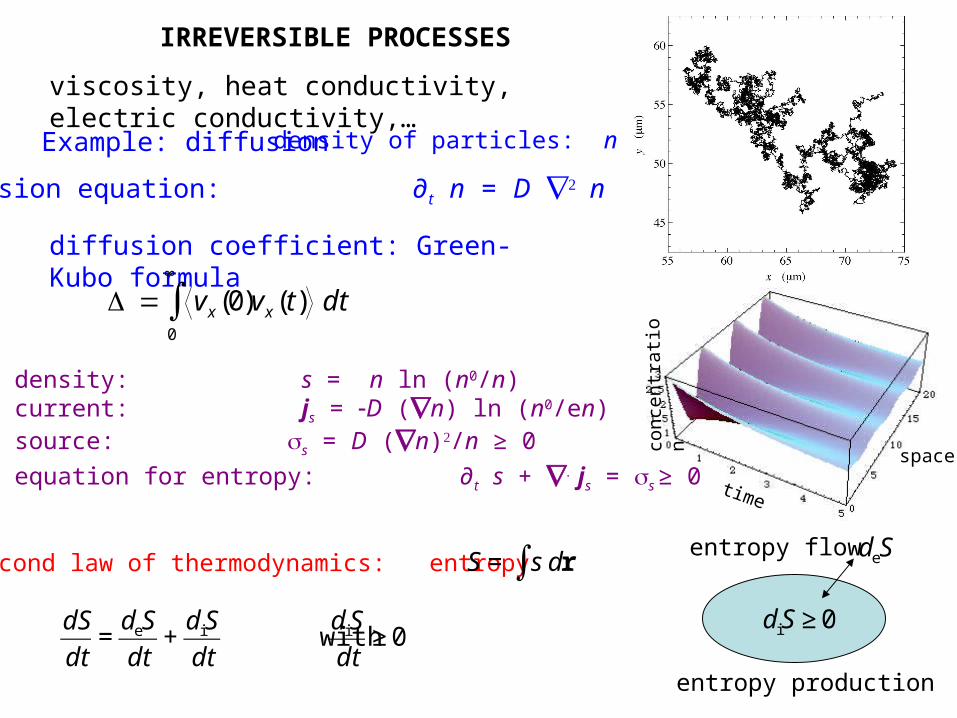
IRREVERSIBLE PROCESSES

Second law of thermodynamics: entropy

€

dS

dt=

deS

dt+

diS

dt with

diS

dt≥ 0

€

deS

€

diS ≥ 0

entropy flow

entropy production

diffusion coefficient: Green-Kubo formula

time

space c

once

ntra

tion

€

D = vx (0)vx (t) 0

∞

∫ dt

Example: diffusion

diffusion equation: ∂t n = D n

entropy density: s = n ln (n0/n)entropy current: js = D (n) ln (n0/en)entropy source: s = D (n)/n ≥ 0

balance equation for entropy: ∂t s + js = s ≥ 0

viscosity, heat conductivity, electric conductivity,…

€

S = s dr∫

density of particles: n

HAMILTONIAN DYNAMICS

€

A system of particles evolves in time according to Hamilton’s equations:

€

dra

dt= +

∂H

∂pa

dpa

dt= −

∂H

∂ra

Determinism: Cauchy’s theorem asserts the unicity of the trajectory issued from initial conditions in the phase space M of the positions ra and momenta pa of the particles:

Hamiltonian function:

€

H =pa

2

2maa=1

N

∑ + U(r1,r2,...,rN )

€

Γ=(r1,p1,r2,p2,...,rN ,pN ) ∈ M dimM = 2Nd

Flow: one-dimensional Abelian group of time evolution:

€

Γ=Φt (Γ0) ∈ M

Time-reversal symmetry:

€

Θ(r1,p1,r2,p2,...,rN ,pN ) = (r1,−p1,r2,−p2,...,rN ,−pN )

Liouville’s theorem: Hamiltonian dynamics preserves the phase-space volumes:

€

dΓ = dr1 dp1 dr2 dp2 ... drN dpN

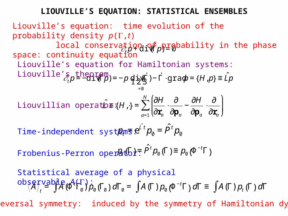
LIOUVILLE’S EQUATION: STATISTICAL ENSEMBLES

€

Statistical average of a physical observable A(Γ):

€

At= A(Φ tΓ0∫ ) p0 Γ0( ) dΓ0 = A(Γ∫ ) p0 Φ−tΓ( ) dΓ ≡ A(Γ∫ ) pt Γ( ) dΓ

€

∂t p + div( ˙ Γ p) = 0

€

ˆ L ≡ H,⋅{ } =∂H

∂ra

⋅∂

∂pa

−∂H

∂pa

⋅∂

∂ra

⎛

⎝ ⎜

⎞

⎠ ⎟

a=1

N

∑

€

pt = eˆ L t p0 = ˆ P t p0

Frobenius-Perron operator:

€

pt Γ( ) = ˆ P t p0 Γ( ) ≡ p0 Φ−tΓ( )

Liouville’s equation: time evolution of the probability density p(Γ,t) local conservation of probability in the phase space: continuity equation

€

∂t p = −div( ˙ Γ p) = −p div( ˙ Γ )=0

1 2 3 − ˙ Γ ⋅grad p = H, p{ } ≡ ˆ L p

Liouville’s equation for Hamiltonian systems: Liouville’s theorem

Liouvillian operator:

Time-independent systems:

Time-reversal symmetry: induced by the symmetry of Hamiltonian dynamics

TIME-REVERSAL SYMMETRY Θ(r,v) = (r,v)

Newton’s fundamental equation of motion for atoms or molecules composing matter is time-reversal symmetric.

velocity v

position r

Phase space:

0

trajectory 1 = Θ (trajectory 2)

time reversal Θ

trajectory 2 = Θ (trajectory 1)

€

md2r

dt 2= F(r)

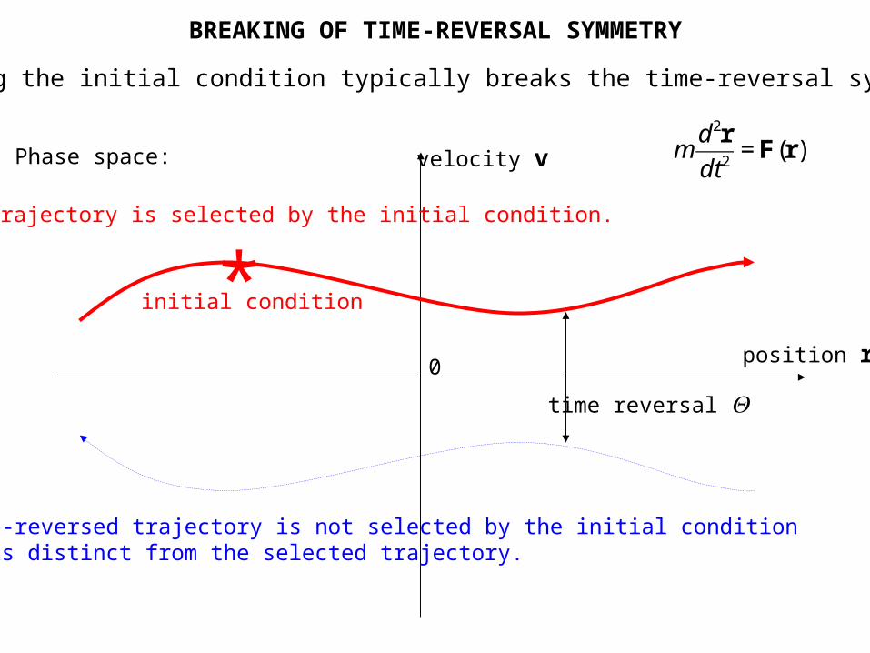
BREAKING OF TIME-REVERSAL SYMMETRY

Selecting the initial condition typically breaks the time-reversal symmetry.

velocity v

position r

Phase space:

0

This trajectory is selected by the initial condition.

time reversal Θ

The time-reversed trajectory is not selected by the initial condition if it is distinct from the selected trajectory.

initial condition* €

md2r

dt 2= F(r)

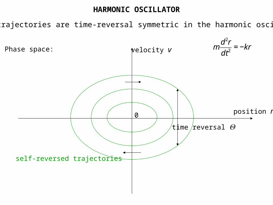
HARMONIC OSCILLATOR

All the trajectories are time-reversal symmetric in the harmonic oscillator.

velocity v

position r

Phase space:

0

time reversal Θ

self-reversed trajectories

€

md2r

dt 2= −kr

FREE PARTICLE

Almost all of the trajectories are distinct from their time reversal.

velocity v

position r

Phase space:

0

time reversal Θ

self-reversed trajectories at zero velocity

€

md2r

dt 2= 0

PENDULUM

The oscillating trajectories are time-reversal symmetric while the rotating trajectories are not.

velocity v

angle

Phase space:

0

time reversal Θ

self-reversed trajectories

unstable direction stable direction

• •

€

d2φ

dt 2= −

g

lsinφ

STATISTICAL MECHANICS

weighting each trajectory with a probability -> invariant probability distribution

velocity v

position

Phase space:

0

time reversal Θ

e.g. nonequilibrium steady state between two reservoirs: breaking of time-reversal symmetry.

res

ervo

ir 1

rese rvo ir 2

STATISTICAL EQUILIBRIUM

The time-reversal symmetry is restored e.g. by ergodicity (detailed balance).

velocity v

position r

Phase space:

0

time reversal Θ

BREAKING OF TIME-REVERSAL SYMMETRY Θ(r,v) = (r,v)

Newton’s equation of mechanics is time-reversal symmetric if the Hamiltonian H is even in the momenta.

Liouville equation of statistical mechanics, ruling the time evolution of the probability density p is also time-reversal symmetric.

The solution of an equation may have a lower symmetry than the equation itself (spontaneous symmetry breaking).

Typical Newtonian trajectories T are different from their time-reversal image Θ T : Θ T ≠ T

Irreversible behavior is obtained by weighting differently the trajectories T and their time-reversal image Θ T with a probability measure.

Spontaneous symmetry breaking: relaxation modes of an autonomous system

Explicit symmetry breaking: nonequilibrium steady state by the boundary conditions

€

∂p

∂t= H, p{ } = ˆ L p

€

∂p

∂t+

∂ ˙ r p( )∂r

+∂ ˙ v p( )

∂v= 0

DYNAMICAL INSTABILITY

€

The possibility to predict the future of the system depends on the stability or instability of the trajectories of Hamilton’s equations.

Most systems are not integrable and presents the property of sensitivity to initial conditions according to which two nearby trajectories tend to separate at an exponential rate.

Lyapunov exponents:

Spectrum of Lyapunov exponents:

Pairing rule for Hamiltonian systems (symplectic character):

Liouville’s theorem:

Prediction limited by the Lyapunov time:

A statistical description is required beyond the Lyapunov time.

€

λi = limt →∞

1

t ln

δΓi(t)

δΓi(0)

€

λ1 = λ max ≥ λ 2 ≥ λ 3 ≥ ...≥ 0 ≥ ...≥ λ 2 f −1 ≥ λ 2 f

€

+λi,−λ i{ }i=1

f

€

λi

i=1

2 f

∑ = 0

€

t < tLyap ≈1

λ max

lnε final

ε initial

CHAOTIC BEHAVIOR IN MOLECULAR DYNAMICS

Hard-sphere gas:

intercollisional time diameter d mean free path l

Perturbation on the velocity angle:

Estimation of the largest Lyapunov exponent: (Krylov 1940’s)

€

δ n ≈ δϕ 0

l

d

⎛

⎝ ⎜

⎞

⎠ ⎟n

≈ δϕ 0 eλ t t ≈ nτ

€

€

λ ≈ 1

τ ln

l

d ≈ 1010 sec−1 (air in the room)

CHAOTIC BEHAVIOR IN MOLECULAR DYNAMICS (cont’d)

Hard-sphere gas: spectrum of Lyapunov exponents

(dynamical system of 33 hard spheres of unit diameter and mass at unit temperature and density 0.001)

€

STATISTICAL AVERAGE: PROBABILITY MEASURE

€

Ergodicity (Boltzmann 1871, 1884): time average = phase-space average

€

limT →∞

1

T A(Φ tΓ0) dt

0

T

∫ = A(Γ∫ ) Ψ0 Γ( ) dΓ = A = A Ψ0

€

pt = ˆ U t p0 = e i ˆ G t p0 ˆ G = i ˆ L

stationary probability density representing the invariant probability measure

€

ˆ G Ψ0 = 0

Spectrum of unitary time evolution:

Ergodicity: The stationary probability density is unique:The eigenvalue is non-degenerate.

€

z = 0

€

Ψ0

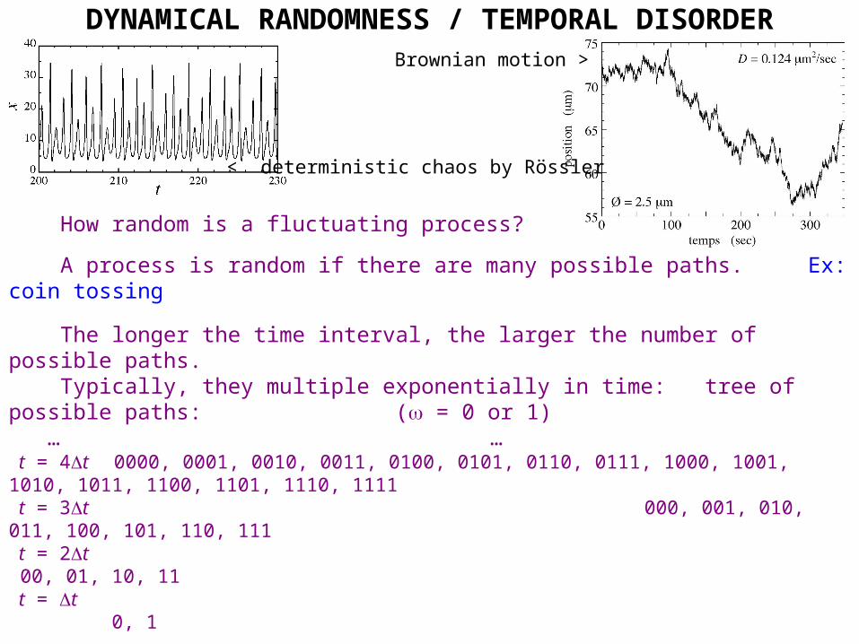
DYNAMICAL RANDOMNESS / TEMPORAL DISORDER

€

How random is a fluctuating process?

A process is random if there are many possible paths. Ex: coin tossing

The longer the time interval, the larger the number of possible paths. Typically, they multiple exponentially in time: tree of possible paths: ( = 0 or 1) … … t = 4t 0000, 0001, 0010, 0011, 0100, 0101, 0110, 0111, 1000, 1001, 1010, 1011, 1100, 1101, 1110, 1111 t = 3t 000, 001, 010, 011, 100, 101, 110, 111 t = 2t 00, 01, 10, 11 t = t 0, 1 Hence, the path probabilities decay exponentially:

(0 1 2 … n1) ~ exp( h t n )

The decay rate h is a measure of dynamical randomness / temporal disorder. h is the so-called entropy per unit time.

< deterministic chaos by Rössler

Brownian motion >

DYNAMICAL RANDOMNESS AND ENTROPIES PER UNIT TIME

€

€

P ={C1,C2,...,CM }

€

()=(0ω1ω2L ωn−1 ) = μ Cω0∩ Φ−τCω1

∩L ∩ Φ−(n−1)τCωn−1( )

€

Φkτ Γ ∈ Cω (k = 0,1,2,...,n −1)

€

h(P ) = lim n →∞

−1

nτμ(ω ) ln μ(ω )

ω

∑ = limn →∞

−1

nτμ(ω0ω1ω2L ωn−1 ) ln μ(ω0ω1ω2L ωn−1 )

ω0ω1ω2L ωn−1

∑

€

hKS = Sup P

h(P )

€

hKS = λ i

λ i >0

∑

Partition of the phase space into domains: coarse-graining

Stroboscopic observation of the system at sampling time :

Multiple-time probability to observe a given path or history:

Entropy per unit time:

Path or history: succession of coarse-grained states

€

=0ω1ω2L ωn−1

Kolmogorov-Sinai entropy per unit time:

closed systems: Pesin’s theorem:

€

(0ω1ω2L ωn−1 ) ≈ exp(−hnτ ) =1

Λ(ω0ω1ω2L ωn−1 )≈

1

exp( λ itλ i >0∑ )

DYNAMICAL RANDOMNESS IN STATISTICAL MECHANICS

€

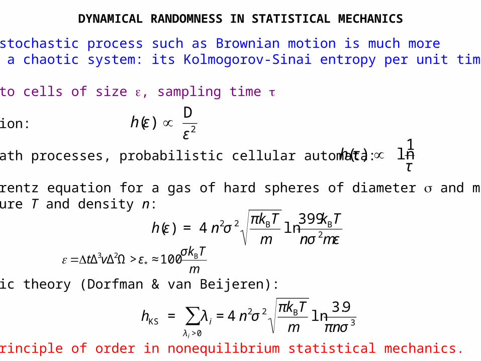
Typically a stochastic process such as Brownian motion is much more random than a chaotic system: its Kolmogorov-Sinai entropy per unit time is infinite.

Partition into cells of size , sampling time

Brownian motion:

Birth-and-death processes, probabilistic cellular automata:

Boltzmann-Lorentz equation for a gas of hard spheres of diameter and mass m at temperature T and density n:

with

Deterministic theory (Dorfman & van Beijeren):

Chaos is a principle of order in nonequilibrium statistical mechanics.

€

h(ε) ∝ D

ε 2

€

h(τ ) ∝ ln1

τ

€

h(ε) = 4 n2σ 2 πkBT

mln

399kBT

nσ 2mε

€

=tΔ3vΔ2Ω > ε* ≈100σkBT

m

€

hKS = λ i

λ i >0

∑ = 4 n2σ 2 πkBT

mln

3.9

πnσ 3

ESCAPE-RATE FORMALISM: DIFFUSION

• diffusion coefficient D = lim t∞ (1/2t) < (xt x0 )

2 >

diffusion equation: ∂t p(x, t) ≈ D ∂x2 p(x, t)

absorbing boundary conditions: p (L, t ) = p (+L , t ) = 0

solution: p(x, t) ~ exp t) cos( x / L )

escape rate: ≈ D ( / L )2

P. Gaspard & G. Nicolis, Phys. Rev. Lett. 65 (1990) 1693; P. Gaspard & F. Baras, Phys. Rev. E 51 (1995) 5332

escape of a particle

out of the diffusive media

Ex: neutron in a reactor

ESCAPE-RATE FORMALISM:THE TRANSPORT COEFFICIENTS & THEIR HELFAND MOMENT

Transport coefficients:

Green-Kubo formula: microscopic current:

Einstein formula: Helfand moment:

Transport property: moment:

self-diffusion:

shear viscosity:

bulk viscosity:

heat conductivity

electric conductivity:

€

J(α ) =dG(α )

dt

€

α = J0(α ) Jt

(α )

0

∞

∫ dt

€

Gt(α ) = G0

(α ) + Jt '(α )

0

t

∫ dt'

€

α =limt →∞

1

2t(Gt

(α ) − G0(α ))2

€

G(D ) = xa

€

G(η ) =1

VkBTxa pay

a=1

N

∑

€

ψ =ζ + 43 η G(ψ ) =

1

VkBTxa pax

a=1

N

∑

€

G(κ ) =1

VkBT 2xa (Ea − Ea )

a=1

N

∑

€

G(η ) =1

VkBTeZa xa

a=1

N

∑

ESCAPE-RATE FORMALISM:ESCAPE OF THE HELFAND MOMENT

Einstein formula:

€

α =limt →∞

1

2t(Gt

(α ) − G0(α ))2

diffusive equation:

€

∂p

∂t= α

∂ 2 p

∂g2 g = Gt

(α )

absorbing boundary conditions:

€

p(g = ±χ /2, t) = 0

€

−χ2

≤ Gt(α ) ≤ +

χ

2

solution of diffusive equation:

€

p(g, t) = a j exp −γ j t( )j=1

∞

∑ sinjπg

χ+

jπ

2

⎛

⎝ ⎜

⎞

⎠ ⎟ γ j = α

jπ

χ

⎛

⎝ ⎜

⎞

⎠ ⎟

2

€

=1 = α π

χ

⎛

⎝ ⎜

⎞

⎠ ⎟

2

for χ → ∞ escape rate:

Diffusion of a Brownian particle Shear viscosity

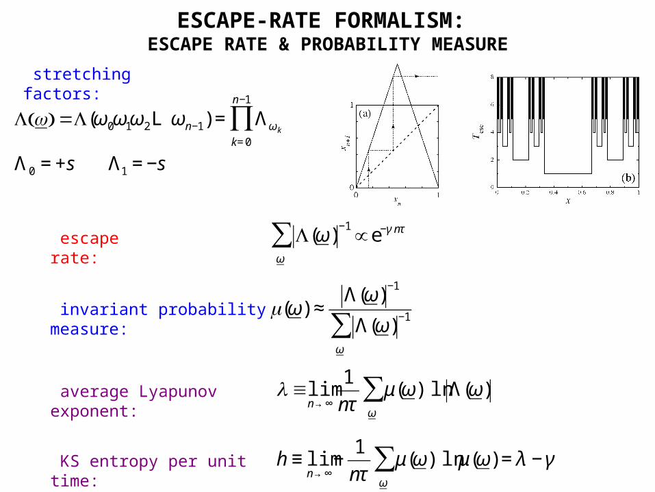
ESCAPE-RATE FORMALISM: ESCAPE RATE & PROBABILITY MEASURE

stretching factors:

invariant probability measure:

€

(ω) ≈Λ(ω)

−1

Λ(ω)−1

ω

∑

escape rate:

€

Λ ( ) =Λ(ω0ω1ω2L ωn−1) = Λωk

k= 0

n−1

∏

Λ0 = +s Λ1 = −s

average Lyapunov exponent:

€

Λ(ω)−1

ω

∑ ∝ e−γ nτ

€

λ ≡limn →∞

1

nτμ(ω) ln Λ(ω)

ω

∑

KS entropy per unit time:

€

h ≡ limn →∞

−1

nτμ(ω) lnμ(ω)

ω

∑ = λ − γ

ESCAPE-RATE FORMALISM: ESCAPE-RATE FORMULA

stretching factors:

€

Λ ( ) =Λ(ω0ω1ω2L ωn−1)

Ruelle topological pressure:

€

P(β ) ≡ limn →∞

1

nτ ln Λ(ω)

−β

ω

∑

€

= λi − hKS

λ i >0

∑ = λ i(1− d1,i)λ i >0

∑

€

(ω)q

l (ω)(q−1)d q

ω

∑ ∝1 l (ω)∝ Λ(ω)-1

€

P q + (1− q) dq[ ] = −q γ

€

=λ−hKS = λ (1− d1)

€

hKS = λ i

λ i >0

∑

generalized fractal dimensions:

escape-rate formula (f = 2):

escape-rate formula (f > 2):

closed system: Pesin’s identity:

escape rate:

€

=−P(1)Lyapunov exponent:

€

λ =λ(1) = −P'(1)

ESCAPE-RATE FORMALISMCHAOS-TRANSPORT FORMULA

Combining the result from transport theory with the escape-rate formula from dynamical systems theory, we obtain the chaos-transport relationship

large-deviation dynamical relationship

P. Gaspard & G. Nicolis, Phys. Rev. Lett. 65 (1990) 1693; J. R. Dorfman, & P. Gaspard, Phys. Rev. E 51 (1995) 28

transport

dynamical instability

∑i λi+

dynamical randomness

hKS

Out of equilibrium, the system has less dynamical randomness than possible by its dynamical instability.

€

α = limχ ,V →∞

χ

π

⎛

⎝ ⎜

⎞

⎠ ⎟2

λ i − hKS

λ i >0

∑ ⎛

⎝ ⎜ ⎜

⎞

⎠ ⎟ ⎟χ

= limχ ,V →∞

χ

π

⎛

⎝ ⎜

⎞

⎠ ⎟2

λ i(1− di)λ i >0

∑χ

ESCAPE-RATE FORMALISM: DIFFUSION

• Helfand moment for diffusion: Gt = xi

diffusion coefficient = lim t∞ (1/2t) < (Gt G0 )

2 >

diffusion equation: ∂t p(x, t) ≈ D ∂x2 p(x, t)

absorbing boundary conditions: p (L, t ) = p (+L , t ) = 0

solution: p(x, t) ~ exp t) cos( x / L )

escape rate: ≈ D ( / L )2

• dynamical systems theory

escape rate (leading Pollicott-Ruelle resonance): λ hKS λ d

chaos-transport relationship: D = lim L∞ ( L / )2 λ dI (L)]

P. Gaspard & G. Nicolis, Phys. Rev. Lett. 65 (1990) 1693; P. Gaspard & F. Baras, Phys. Rev. E 51 (1995) 5332

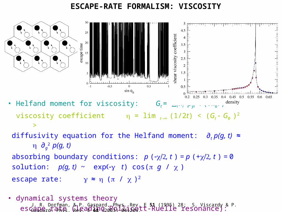
ESCAPE-RATE FORMALISM: VISCOSITY

• Helfand moment for viscosity: Gt = ∑i xi pyi /(VkBT) 1/2

viscosity coefficient = lim t∞ (1/2t) < (Gt G0 )

2 >

diffusivity equation for the Helfand moment: ∂t p(g, t) ≈ ∂g2 p(g, t)

absorbing boundary conditions: p (χ, t ) = p (+χ, t ) = 0

solution: p(g, t) ~ exp t) cos( g / χ )

escape rate: ≈ ( / χ )2

• dynamical systems theory

escape rate (leading Pollicott-Ruelle resonance): ∑i λi hKS λ dI

chaos-transport relationship: = limχ∞ (χ / )2 (∑i λi hKS )χJ. R. Dorfman, & P. Gaspard, Phys. Rev. E 51 (1995) 28; S. Viscardy & P. Gaspard, Phys. Rev. E 68 (2003) 041205.

CONCLUSIONS

Breaking of time-reversal symmetry in the statistical description

€

D /L( )2

≈ γ = λ i

λ i >0

∑ − hKS

⎛

⎝ ⎜ ⎜

⎞

⎠ ⎟ ⎟L

Escape-rate formalism: nonequilibrium transients

fractal repeller

http://homepages.ulb.ac.be/~gaspard

diffusion D : (1990)

viscosity : (1995)

€

/χ( )2

≈ γ = λ i

λ i >0

∑ − hKS

⎛

⎝ ⎜ ⎜

⎞

⎠ ⎟ ⎟L

€

= λi

λ i >0

∑ − hKS = − λ i

λ i <0

∑ − hKS

€

λi

i=1

2 f

∑ = 0Hamiltonian systems: Liouville theorem:

€

=− λi

i=1

2 f

∑ = − λ i

λ i <0

∑ − λ i

λ i >0

∑ = − λ i

λ i <0

∑ − hKS

thermostated systems: no Liouville theorem

volume contraction rate:

€

hKS = λ i

λ i >0

∑Pesin’s identity on the attractor: