Impact of Spillover Effects of Integrated Pest Management ...

1
Program evaluation and spillover effects
M. Angelucci* and V. Di Maro
+
Abstract
This paper is a practical guide for researchers and practitioners who want to
understand spillover effects in program evaluation. It defines spillover effects
and discusses why it is important to measure them. It explains how to design a
field experiment to measure the average effects of the treatment on subjects,
both eligible and ineligible, for the program in the presence of spillover
effects. In addition, it discusses the use of nonexperimental methods for
estimating spillover effects when the experimental design is not a viable
option. Evaluations that account for spillover effects should be designed such
that they explain both the cause of these effects and whom they affect. Such an
evaluation design is necessary to avoid inappropriate policy recommendations
and neglecting important mechanisms through which the program operates.
JEL Classification: C93, C81, D62
Keywords: impact evaluation, spillover effects, field experiments, data collection, Indirect
Treatment Effect, program mechanisms
_________________________ *University of Michigan and IZA. Correspondence address: University of Michigan,
Economics Department, Lorch Hall, 611 Tappan St., Ann Arbor, MI. Email:
Research Group-Development Impact Evaluation (DECIE), The
World Bank. Email: [email protected].
We would like to thank Paul Winters for his extremely useful comments. We also thank
Sarah Strickland and Jorge Olave for their help with the editing of an earlier version. The first
draft of this paper was prepared as part of the Impact Evaluation Guidelines technical notes
(working paper series) of the Office of Strategic Planning and Development Effectiveness at
the Inter-American Development Bank. All remaining errors are our own.
M. Angelucci and V. Di Maro
1. Introduction
This paper is a practical guide to spillover effects: what they are, why it is important to
measure them, and how to design an evaluation to measure the average effects of the
treatment in the presence of spillover effects on subjects both eligible and ineligible for the
program.
Welfare-enhancing interventions often have a specific target population. For example,
conditional cash transfer (CCT) programs in Latin America and elsewhere target the poor,
and other interventions provide incentives to increase schooling for poor children, from
providing equipment to distributing deworming drugs to infected children. However, the
target population is often a subset of the local economy, loosely defined as the geographic
unit or local institution within which the target population lives and operates. In this sense,
we can consider the village, the neighborhood, the city, the municipality, the school district,
or the extended family as the relevant local economy.
The treatment may also affect the local non-target population. For example, the
recipients of CCTs may share resources with or purchase goods and services from ineligible
households who live in the locality, affecting also the ineligibles’ incentives to accumulate
human capital. Children who receive free textbooks and computers may share them with
untreated children (such as relatives, friends, and members of the local church), increasing
enrollment levels in both groups. Supplying deworming drugs to a group of children may
benefit untreated children by reducing disease transmission, lowering infection rates for both
groups. If parasites affect school performance (for example, by reducing emetic iron, causing
weakness and inattention) the treatment may result in both treated and untreated children
learning more. An intervention that improves the supply and quality of water to only some
beneficiary households in a neighborhood is likely to have effects on all residents, ranging
from an increase in property values to a decrease in infection rates. In addition, if the
intervention includes the provision of hygiene information and education campaigns, we
might expect the information to flow from person to person within the community.
While the examples so far describe positive spillover effects, such effects may also be
negative. Introducing genetically modified (GM) crops may contaminate neighboring organic
crops, reducing their value. Similarly, eradicating pests from one farm may cause them to
move to nearby farms, or providing training to a group of people may decrease the
employment likelihood and decrease the wages of close substitutes in production. Examples
of negative spillover effects are also documented in the literature on crime displacement (see,
3
among others, Di Tella and Schargrodsky, 2004 and Yang, 2008).
In some cases, spillover effects are intended. For example, agricultural extension
programs encourage participants to adopt a certain technology and hope that this will induce
further adoption within the community or in neighboring communities. Immunization
campaigns among high-risk populations lower the likelihood of contagion, reducing the
infection rate among low-risk populations. Whether intentionally or not, nonparticipants can
be affected by programs, and these spillover effects should be taken into account when
conducting an impact evaluation. Failure to perform such evaluations results in biased
estimates of program impacts, leading to inappropriate policy recommendations and incorrect
understandings of data-generating models.
For example, suppose that, to study the effect of a deworming drug on school
performance we randomly select half the pupils of a school and treat them with the drug. We
then compare the grades of treated and untreated children. Since the drug is likely to result in
decreased infection rates among both treated and untreated children, it is possible that both
groups’ performances may change. That is, suppose deworming children increases the
average grades of treated pupils by 10 percentage points and of untreated pupils by 4
percentage points. The Average Treatment on the Treated effect1 is 10 percentage points.
However, if we simply compare the grades of treatment and control pupils, we will observe
only a six percentage point increase. In sum, the failure to recognize the possibility that the
drug may affect untreated pupils also and to design the experiment accordingly will result in
a double underestimate of the treatment’s effectiveness. Not only will its effect on the treated
be underestimated, but its effect on the untreated will also remain unmeasured. This may
result in incorrect policy conclusions (for example, a decision to discontinue a program
because it is not cost-effective).
Conversely, when the spillover effects are negative, one overestimates the treatment
effect on the treated and fails to estimate its negative indirect effects. Indirect effects can be
estimated in two ways. At the very least, the evaluation design must select a control group
that is not indirectly affected by the program. This will enable researchers to measure the
program effect on eligible subjects. If possible and relevant, the design should also allow for
the measurement of spillover effects, as these effects are often important policy parameters in
themselves.
To design an evaluation that accounts for the presence of spillover effects, one needs
1The Average Treatment on the Treated effect can be defined as the impact of the program on subjects that are
eligible for it. In our case this is the effect of the deworming intervention on the treated pupils.

M. Angelucci and V. Di Maro
to understand why and how these effects occur. This knowledge would help researchers to
identify the subset of nonparticipants is most likely to be indirectly affected by a particular
treatment. For example, in the case of a deworming drug for children, one has to know how
people become infected (by being in contact with contaminated fecal matter) to understand
which other people are likely to benefit from the deworming (classmates, friends, and
families of dewormed children, who will be less likely to come into contact with
contaminated fecal matter). Importantly, the evaluation must be carefully designed to account
for spillover effects before the program is implemented. Spillover effects cannot be detected
accurately ex post unless the design considers their existence from the start.
The following section describes different types of spillover effects. Section three
explains why it is important for an evaluation design to account for the presence of these
spillover effects. Section four explains how to design an experiment in the presence of
spillover effects. Section five discusses how to use nonexperimental methods when an
experiment is not a viable option. Section six provides a specific example using the
evaluation of the CCT program PROGRESA. Section seven concludes with a summary of the
key recommendations this paper makes to aid the design of evaluations that account for the
presence of spillover effects.
2. Types of spillover effects
In what follows, we describe four types of spillover effects that are particularly
relevant in the development and health economics literature. We call these four types of
spillover effects (1) externalities, (2) social interactions, (3) context equilibrium effects, and
(4) general equilibrium effects.2
Externalities. These effects operate from the treated subjects to the untreated
population. A particularly relevant domain is health. Miguel and Kremer (2004) show that
deworming drugs can have an indirect effect in addition to the direct effect of ingesting the
drug. Supplying deworming drugs to a group of children may benefit untreated children by
reducing disease transmission, lowering infection rates for both groups. If parasites affect
school performance (for example, by reducing emetic iron, causing weakness and
inattention), the treatment may result in both treated and untreated children learning more.
Besides contagion effects in health-related interventions, externalities may arise from
interventions that change the degree of environmental pollution (for example, Lipscomb and
2These labels are somewhat arbitrary, but are a useful way of grouping similar types of spillover effects.

5
Mobarak, 2013) or that introduce GM seeds, which then alter the genetic makeup of non-GM
plants through cross-pollination (for example, Rieben, Kalinina, Schmid, and Zeller 2011).
Social Interactions. The local nontarget population may also be indirectly affected by
the treatment through social and economic interaction with the treated. For example, the
recipients of CCTs may share resources with, and affect the incentives to accumulate human
capital of, ineligible households in treated localities (Angelucci and De Giorgi, 2009).
Recipients of human-capital-enhancing programs who receive free textbooks and computers
may share them with untreated children (such as relatives, friends, and members of the local
church), increasing enrollment for both groups. Similarly, Bobonis and Finan (2009) identify
neighborhood peer effects on children’s school enrollment decisions within the Mexican CCT
PROGRESA program. In particular, they find that peers have considerable influence on the
enrollment decisions of program-ineligible children, and these effects are concentrated
among children from poorer households.
Context equilibrium effects. These spillover effects stem from an intervention that
affects the behavioral or social norms within the contexts (for example, a locality) in which
these interactions are relevant. For example, Avitabile (2012) shows that exogenously
increasing the rate of cervical cancer screening among eligible women in rural Mexico
increases the screening rate for ineligible women, changing the previous social norm by
which husbands prevented women from being screened by male doctors.
General equilibrium effects. These effects stem from interventions that affect
equilibrium prices through changes in supply and demand. They naturally arise in active
labor market programs (for example, Heckman, LaLonde, and Smith, 1999). With few
exceptions (for example, Angelucci and De Giorgi, 2009; Mobarak and Rosenzweig, 2014),
most studies of spillover effects in developing countries focus on the other mechanisms
discussed above. Nevertheless, studying general equilibrium effects has both policy and
economic relevance. At the policy level, such studies determine whether the general
equilibrium effects reinforce or offset the partial equilibrium effect of an intervention. At the
economic level, they provide insights into the local economy and people’s preferences.
Consider the case of PROGRESA. Cash transfers may increase goods prices through
an increase in demand. Price increases would change consumer and producer welfare in
opposite directions, influencing the distribution of benefits and either reinforcing or offsetting
the partial equilibrium effect of the transfer on its recipients, depending on their consumer
and producer mix. The more segmented the local goods market, the stronger the price effects.
The program might also change wages and labor income through two different channels.

M. Angelucci and V. Di Maro
First, the transfers may have an income effect for households that would have sent their
children to school regardless of the program, reducing labor supply. Second, the program
may reduce income for households that would not have sent their children to school in the
absence of the program, increasing their labor supply. The net effect on labor supply, wages,
and labor earnings is unclear a priori.
While one can classify the types of spillover effects, the evaluation designs we will
discuss do not necessarily enable one to distinguish one from the other. One way to
disentangle a specific type of spillover effect is to carefully design survey instruments to
elicit information on the relevant type of unintended response. This highlights once more the
importance of understanding which type of spillover effect might occur and how before
designing the evaluation (and the program).
3. Identification with an experimental design
3.1 Treatment effects in the presence of spillovers
Accounting for spillover effects is necessary for correct identification and estimation of
direct/intended and indirect/unintended treatment effects. Measuring these two effects
enables one to design more effective policies and to learn features of the local economy and
of human behavior.
First, it is useful to define the two parameters of interest. Consider a group of subjects
(for example, individuals, households) who live in areas where a treatment is offered (T=1) or
not offered (T=0). In T=1 areas, some subjects are eligible for the treatment ( 1E ) while
others are not ( 0E ). The variables 0Y and 1Y are potential outcomes in the absence and
presence of the treatment, respectively. The Average Treatment Effect on the Eligibles
( ATE ) is the effect of the treatment on eligible subjects:
1 0( 1 1)ATE E Y Y T E
That is, the ATE identifies the effect of the treatment on subjects that are meant to be
treated.3
While the outcome in the presence of the treatment is the observed outcome for
eligible subjects in the treated area E(Y1|T=1, E=1)=E(Y|T=1, E=1), the potential outcome in
the absence of the treatment, E(Y0|T=1,E=1), is unknown. This missing counterfactual
problem can be solved if the two following non-testable assumptions hold: first, that the
3 If all eligible subjects take up the programme, then this is the average treatment on the treated effect.

7
treatment assignment is independent of the potential outcomes and second, that the treatment
status of any subject does not affect the potential outcomes of other subjects. In statistics,
these assumptions are called the unconfoundedness assumption and the Stable Unit
Treatment Value Assumption (SUTVA).4 Randomizing eligibility ensures that
unconfoundedness holds. Therefore, absent spillover effects in T=1 areas, then E(Y0|T=1,
E=1)=E(Y|T=1, E=0). However, the presence of spillover effects violates the SUTVA.
Therefore, the average observed outcome for the ineligibles in T=1 areas is not the average
potential outcome in the absence of the treatment.
To solve this problem, one can use a double randomization or conduct a partial
population experiment (Moffitt, 2001).5 The idea of double randomization is to first identify
the relevant local economy, that is the socioeconomic unit within which the spillovers occur.
Then, one randomly assigns units (for example, localities, schools) to the treatment (T=1) and
control (T=0) groups. Lastly, one randomly assigns eligibility ( 1E ) in all units.
There are thus three distinct groups defined by treatment and eligibility: eligible and
ineligible subjects in treatment units and (all) subjects in control units. Absent spillover
effects from treatment to control units, if the two randomizations are effective one can
identify the ATE as follows:
ATE=E(Y1-Y0|T=1,E=1)=E(Y|T=1,E=1)-E(Y|T=0) (1)
because unconfoundedness and the SUTVA hold for subjects in control units.
Besides providing unbiased estimates of the ATE, this design enables measurement of
spillover effects. Define the Indirect Treatment Effect as the average effect of the treatment
on ineligible households. If the two previous assumptions hold, one can estimate this
parameter by comparing the observed outcomes of ineligibles in treatment units with subjects
in the control group:
ITE=E(Y1-Y0|T=1,E=0)=E(Y|T=1,E=0)-E(Y|T=0) (2)
While this design solves the problem of the missing counterfactual for the
identification and estimation of the ATE and ITE parameters, it is important to emphasize
that the SUTVA is still violated in treatment units. Indeed, testing that ITE=0 is a test of the
SUTVA violation. In this case, one can think of the estimated ATE as the combination of the
true ATE (the ATE under the SUTVA) and the spillover effect, and both parameters may
depend on the share of the treated unit. Under the additional assumption that these two effects
4 To identify average treatment effects, a weaker assumption than unconfoundedness is required, namely
E(Y0|T=1)= E(Y0|T=0). 5 For example, Bobonis and Finan (2009) follow this approach to estimate education peer effects in
PROGRESA.

M. Angelucci and V. Di Maro
are additive, one can estimate the true ATE by subtracting the estimated ITE from it.
To identify how the spillover effects vary with the proportion of the treated unit, one
must further randomize the share of the treated unit. Crepon, Duflo, Gurgand, Rathelot, and
Zamora (2013) use this type of experimental design to study the displacement effects of labor
market policies. Baird, Bohren, McIntosh, and Ozler (2014) discuss various parameters that
can be identified with this design.
This last point has important policy implications. If the spillover effects are a function
of the share of the local economy that is treated, the estimated ATE will vary as the program
is scaled up (for example, by treating all subjects in one unit). To understand how spillover
effects vary with the share of the treated population, a different design, in which the fraction
of eligible subjects in a given area is treated, is also randomized.
3.2 A numerical example
A numerical example can illustrate the importance of an experimental design that accounts
for the presence of spillover effects. Consider the case in which the treatment is a deworming
drug and the subjects are pupils of a school. The outcome of interest, Y , is the rate of
infection with intestinal parasites. Since pupils in the school study and play together,
providing a group of students with deworming drugs may also affect the infection rate of
pupils that are not directly treated with the drug.
The drug affects infection rates directly—by ingesting the drug, a child becomes
parasite free—and indirectly—worms die off over time, so worm loads naturally decrease in
the absence of reinfection. Therefore, when some pupils take the drug, the re-infection rate
for other children drops, as do the chances of coming into contact with contaminated fecal
matter. At the same time, there is considerable seasonal and inter-annual variation in worm
infection rates and intensity due, for example, to weather variation.
Consider a school in which a group of pupils is offered the deworming drug ( 1E )
and another group is not ( 0E ). The ATE is the average effect of the deworming drug on
the infection rate of eligible pupils, while the ITE is the effect of treating the eligible pupils
on the infection rates of pupils not offered the drug. In this particular example, the ATE will
be some combination of the first and second effects described above (the deworming effect of
the drug and the lowered re-infection rates), while the ITE will be only caused by the
decreased contact with contaminated feces. That is, offering the deworming drug generates a
positive externality: treated children receive a deworming drug, decreasing direct infection
rates and reducing the infection rates of children who do not receive the drug.
9
Suppose that the baseline infection rate was 70 per cent and the rate in the absence of
the treatment was 80 per cent, that is, the infection rate would have increased over time and
this is unknown to the evaluators. Assume that treating a random group of pupils in a school
decreased this rate to 10 per cent for the eligibles and 60 per cent for the ineligibles. In this
case, the ATE and the ITE would be -70 and -20 percentage points. However, the policy
evaluators are unaware of these numbers. To measure this effect, they split the school pupils
into two randomly assigned groups and administer the drug to one group only. The naïve
evaluators compare the infection rates of the two groups of pupils, exploiting the
randomization; that is, they assume that the infection rate for the control group is the same
rate we would observe in the absence of the treatment, or that
060 ( 1 0) ( 1 1)% E Y T E E Y T E .
As mentioned, we know this is untrue. The naïve evaluator would estimate an ATE of -50
percentage points, given by
( 1 1) ( 1 0) 10 60E Y T E E Y T E % % ,
underestimating the true ATE (in absolute value) by 20 percentage points. Moreover, the
evaluator would fail to notice that the ineligibles are also indirectly benefiting from the
deworming drug, as their infection rate has also dropped.
To understand the magnitude of this double underestimation of the program effect and
its negative policy implications, suppose the school has 1,000 pupils and the treatment and
control groups (with pupils assigned randomly to each group) have an equal size of 500
students each. In the absence of the treatment, 800 pupils would have been infected (equally
distributed between treatment and control group). After treating 500 students, only 50 treated
pupils (500x10%) and 300 control pupils (500x60%) are infected, for a total of 650 healthy
children, compared to 200 in the absence of the treatment. However, the naïve evaluator
compares the infection rates of the two groups after administering the drug and erroneously
believes that the drug was successful for 250 pupils in the treatment group and none in the
control group. That is, first the evaluator fails to notice that 100 other students in the
treatment group have benefited from the drug, and then s/he fails to notice that the drug has
also reduced the infection rates for the control group, with only 300 infected pupils rather
than the original 400. In total, 200 more children are not infected compared to the evaluator’s
M. Angelucci and V. Di Maro
estimate.6
Suppose the drug costs US$1 per child and the expected benefits of not having worms
is 1.5. The naïve evaluator would conclude that this treatment is not cost effective, because its
cost of US$500 is higher than its benefit of US$375 (1.5x250). In fact, the drug is cost
effective, because when 500 out of 1,000 pupils are treated, 450 pupils stop being infected,7
for a total benefit of US$675 (1.5x450), exceeding the drug’s cost. The drug would also be
evaluated as cost effective if the evaluator were to properly measure only its ATE, as the
benefits for the treated would be US$525 (1.5x350).
Randomizing treated schools first and then randomly choosing eligible pupils within
the treated schools would have solved this problem, as the infection rate in the control
schools would have been 80 per cent in expectation, providing the evaluators with the right
counterfactual outcome.
To summarize the lessons from this simple example, failing to implement an
evaluation design that accounts for spillover effects results in a double underestimation of the
program’s impact: first, the average effect on the eligible children is underestimated; second,
the effect of the treatment on the ineligible children goes completely unnoticed. This double
underestimation can have result in negative policy implications. Researchers may mistakenly
conclude that the treatment is less effective than it actually is (and that reducing infections is
more costly than it is). Incorrect policy recommendations could be made as a result (for
example, to drop the program, because it is too costly). Importantly, the experiment yields
wrong information, even if the randomization is performed successfully. That is, one cannot
easily infer the existence of spillover effects from data alone. A conceptual framework of
how the treatment may indirectly affect the outcomes for ineligible subjects is essential for
understanding whether and the extent to which spillover effects may occur.
3.3 A different design
In many interventions, eligibility for the program within the unit is decided on the basis of
predetermined criteria (that is, poverty score), meaning that randomization within the unit is
unavailable in these settings. However, it remains possible to measure the spillover effects of
the treatment on ineligible subjects living (or studying, working, and so forth) in treatment
6 Having baseline (t=0) as well as follow-up (t=1) data does not help, as the difference-in-difference estimate of
the naïve ATE is still the same, given that ATE=[E(Y|T=1,E=1,t=1)- E(Y|T=1,E=1,t=0)]- [E(Y|T=1,E=0,t=1)-
E(Y|T=1,E=0,t=0)]= E(Y|T=1,E=1,t=1)- E(Y|T=1,E=0,t=1). 7In principle, it is also possible to define a total treatment effect as the sum of ATE and ITE. In this simple
example this would equal 45 pupils who stopped being infected. However, in practical application it is not
always immediately clear how to define the total treatment effect.

11
units. The only difference in the design is that the second step has a nonrandom assignment.
There are now four distinct groups, depending on unit type and eligibility type: eligible
subjects (E=1) in treatment (T=1) and control (T=0) units and ineligible subjects (E=0) in
treatment (T=1) and control (T=0) units.
Treating the eligible subjects may affect ineligible subjects’ outcomes. Therefore, as
long as we observe outcomes for the four groups we can measure the treatment effect on both
eligible and ineligible subjects:
ATE=E(Y1-Y0|T=1,E=1)=E(Y|T=1,E=1)-E(Y|T=0, E=1) (3)
ITE=E(Y1-Y0|T=1,E=0)=E(Y|T=1,E=0)-E(Y|T=0, E=0) (4)
These comparisons identify the two average treatment effects as long as: (1) the unit
randomization works, that is, there are no ex-ante systematic differences in the characteristics
of eligible subjects in treatment and control units and of ineligible subjects in treatment and
control units; and (2) any spillover effect of the treatment occurs only within the treated unit.
For example, the Kenya deworming project excluded older girls (ages 13 and older)
from deworming due to the risk that the drugs could cause birth defects. To measure spillover
effects, the first step is, as before, to randomly group schools into a treatment and control
group. The second step is to offer the drug to all boys and younger girls in treatment schools.
The four groups are boys and younger girls (E=1) and older girls (E=0) in treatment (T=1)
and control (T=0) schools. There may be spillover effects of the deworming drug among the
older girls attending the treatment school. Therefore, one should collect data on all pupils in
the two groups of schools. In this way, one can measure the effect of offering the drug to
boys and younger girls on the infection rates of both eligible and ineligible students.
In some cases, determining eligibility is more complex and involves the collection of
multiple variables. For example, for conditional cash transfer (CCT) programs, eligibility is
determined by poverty status. In this case the evaluator needs to collect enough data to
compute a continuous poverty indicator for both eligible and ineligible subjects in treatment
and control units. This process of ex-ante data collection for eligible and ineligible subjects,
as well as ex-post collection of information on the outcomes of interest, makes the estimation
of spillover effects more costly and time consuming.
3.4 Understanding the mechanisms
A well-conceived evaluation design should be based on some hypothesis about whether

M. Angelucci and V. Di Maro
spillovers are present and why they exist. After documenting the existence of spillover effects
and measuring their magnitude, it is useful to understand the mechanisms that generate them
and in so doing attempt to verify the initial hypothesis. A clear idea of such mechanisms may
help in the design of effective policies.
Understanding the causes of spillover effects almost always requires more data
collection. For example, consider again the case of treating younger girls and boys with a
course of deworming drugs using the experimental design discussed in the previous section.
Suppose that, after noticing that infection rates among older girls are also lower because of
the treatment, the evaluator wants to understand whether this is caused by a reduction in
contaminated fecal matter or by a change in basic health behavior, such as hand washing. In
that case, the evaluator would need to collect data on these two additional variables,
measuring the contamination rates and the frequency of hand washing.8 If the evaluator were
to find that hand-washing frequency does not differ between older girls in treatment and
control schools, but the level of fecal contamination is lower in treatment schools, the result
would suggest this latter channel is the main cause of the effect.
In this specific example, the additional evidence is, at most, suggestive. If one wanted
to compare the benefits of basic health education to the effects of deworming drugs and the
interaction of the two treatments, the ideal experimental setting would be one in which there
were four random groups of schools. Younger girls and boys in these four groups would
receive respectively: (1) the drug only, (2) the health education only, (3) both the drug and
the health education, and (4) neither. Comparing pupils’ infection rates in each of the first
three groups with the fourth would provide estimates of the effect of each of the three
treatments on eligible pupils, while the comparison for older girls would provide estimates of
the effect of each of the three treatments on the ineligible pupils.
A clear idea of the causes of the spillover effects can also lead to a better
understanding of what ATE and ITE are really capturing, especially in cases in which
different types of spillover effects are coupled with a general equilibrium effect. For example,
an intervention that endows a certain group within the local economy with more resources
might have both a spillover effect in terms of sharing of resources between treated and
untreated subjects (interaction effect) and a general effect on the local economy’s prices
(general equilibrium effect). The setup for estimating the spillover effect will not change,
although knowledge that there is more than one mechanism behind the spillover will help to
8 This is the approach followed in Miguel and Kremer (2004). They collect specific data to show that several
dimensions of worm avoidance behaviour did not change in the treatment group.

13
correctly interpret the estimated ATE and ITE. In this case, the ATE would be the sum of the
direct effect and the general equilibrium effect, and the ITE would be the sum of the indirect
(interaction) effect and the general equilibrium effect.
3.5 Important considerations
As discussed, the key assumptions for the identification and estimation of treatment effects
are that (1) the distribution of characteristics of subjects in treatment and control groups is ex-
ante identical; and (2) any spillover effect of the treatment to ineligible subjects is restricted
to the local economy, that is, the unit of the initial randomization.
Neither of these assumptions is directly testable. However, while one may obtain
indirect evidence that the randomization worked by comparing the means or the distribution
of characteristics of subjects in the treatment and control groups, it is often difficult to test
whether there are no spillover effects between two randomized units. Therefore, it is
extremely important to have a good understanding of how local markets and institutions work
before designing the experiment.
Knowledge of the local economy is crucial for a successful experimental design. For
example, in understanding at what level the deworming drug externalities operate, knowledge
of sanitary habits and facilities in the school and at home is essential. Suppose schools had
high-quality sanitary facilities and monitored pupils’ hand washing, while houses had low-
quality facilities. In this case, the risk of contact with contaminated feces may be higher at
home than at school. Therefore, it is possible that siblings, rather than classmates of treated
children, may benefit indirectly from the treatment. In this case, a double randomization at
the school level may detect no spillover effect, although the drug has actually caused a
reduction in the infection rates of treated children’s siblings.
In sum, a theory regarding the potential causes of spillover effects and knowledge of
local social and economic features and interactions are both essential for increasing
confidence in the experimental design’s suitability to control for or measure spillover effects.
3.6 Design and estimation
An important issue for the experimental design is the optimal share of units and
subjects to randomize. Hahn and Hirano (2010) show that assigning approximately two-thirds
of the units to the treatment group (T=1) and 50 per cent of the subjects in those units to the
eligible group (E=1) provides the most precise estimates of the ATE and ITE.
To discuss estimation issues, we consider the following regression model in which, as

M. Angelucci and V. Di Maro
above, T indicates the treatment status and E the eligibility. The subscripts i and v refer to
the household and the local economy. Xiv is a vector of observable characteristics at the
household and local economy level and iv represents unobserved determinants of the
outcome.
Yiv = α0 + α1Tv + α2Ei + α3TvEi + α4Xiv+ εiv
Under the above assumptions, the parameters 1 3 and 1 identify the ATE and the ITE
when we have eligible and ineligible households.9
Estimation issues can vary depending on the type of data available and the method
used. With an experimental design and no baseline data (that is, the case summarized by the
regression model above) the ATE and ITE can be estimated with a simple OLS. Conditioning
on predetermined determinants of the outcome Y improves estimation precision. In the case
of nonexperimental methods and ex-post data, controls are needed to control for the
differences in treatment and comparison groups.
The availability of baseline data is important to confirm the lack of systematic
differences between treatment and control groups at time 0t in the case of experimental
design (and to check whether randomization was successful), as well as to assess the
differences between treatment and comparison groups in the case of the nonexperimental
designs that we discuss in the next section. In addition, with baseline data, a difference-in-
difference (DID) strategy can be used. The basic idea of DID is to use the difference between
outcome values in the counterfactual group (control or comparison group) before and after
the program (0 1 0 0T t T tY Y ) as an indication of the trend the outcome would have had in the
treatment areas had the program not been in operation. After controlling for this trend, the
remaining difference between treatment and counterfactual group can then be attributed to the
program. This strategy may be especially useful when using nonexperimental methods in
which outcome values are likely to be different at the baseline. A further advantage of using a
DID strategy is that it improves the precision of both the experimental and non-experimental
estimates. In a regression framework, the DID can be written as:
Yivt = α0 + α1Tv + α2t + α3Ei + α4Tvt+ α5 Eit+α6 TvEit+α7Xiv+ εivt
9 The parameter α2 is not identified when eligibility does not vary in the control group.

15
The subscript t takes the value of 0 for the baseline and one for follow-up observations.
In this specification 4 6 estimates the ATE and 6 estimates the ITE. These parameters
are identified under the assumption that, in the absence of the treatment, the trend for
eligibles and ineligibles in the treatment group would have been the same as the observed
trend for eligibles and ineligibles in the control group. This is often called a parallel trend
assumption. When estimating the parameters of both equations, the standard errors should
be clustered at the unit level (Bertrand, Duflo, and Mullainathan, 2004).
3.7 Total effect of the program
One might be interested in calculating the total treatment effect of the program. This
parameter, which we call the TATE (Total Average Treatment Effect), is a weighted average
of the ATE and ITE where the weights, wATE and wITE, are the sample proportion of the E=1
and E=0 groups:
TATE= wATE ATE+ wITE ITE
4. Spillover effects in non-experimental designs
In some cases, a randomized design may not be a viable option. In what follows we focus on
how to correctly estimate spillover effects without randomized control trials.
Without randomization, the main challenge in the evaluation design is to find a group
(defined as the comparison group10
) that can be compared to the treatment group. In the case
of the presence of spillover effects, a further complication is that the outcome for this
comparison group must not be affected by the treatment. Moreover, to estimate the spillover
effects, we must identify the subject group for which spillover effects are likely (the
ineligibles in the local economy) and find a valid comparison group from within local
economies that is not affected by the treatment but is comparable to the treated group.
We follow here the same process as above, that is, we have an intervention offered
only to a subgroup of subjects (E=1) living in the treatment units (T=1) where the program is
active. However, here the assignment of a unit (locality, municipality, and so forth) to
treatment and the assignment of subjects to the program in treatment units are not random
and eligibility is decided according to certain criteria, for example, a poverty score. On one
10
In experimental designs we used the terminology control group but in nonexperimental designs it is more
correct to speak about a comparison group to stress the fact that this group, which can be compared to the
treatment group, was not selected by a random assignment.

M. Angelucci and V. Di Maro
hand, a sample of non-treatment units (T=0) would not necessarily be comparable to a sample
of treatment areas; on the other hand, the group of subjects participating in the program (E=0)
cannot be directly compared to those who are ineligible (E=1), as many observable and
unobservable characteristics might differ.
There are several non-experimental methods that may estimate the program’s impacts
in this case. However, these methods require additional and stronger non-testable
assumptions than the experimental settings. Therefore, non-experimental methods are
generally less credible than experimental methods.
As for the experimental setting, we require samples of four groups: eligibles in
treatment units (T=1, E=1), eligibles in comparison units (T=0, E=1), ineligibles in treatment
units (T=1, E=0) and ineligibles in comparison areas (T=0, E=0) (or just comparable control
units if the eligibility is randomized within the treatment units). Typically, areas excluded
from the program are those that can be used for the comparison groups. The complication in a
nonexperimental setting is that these areas are, by construction, different from treatment
areas. For instance, if the treatment units are the poorest localities (for example, in the design
for the evaluation of the urban component of Mexico’s conditional cash transfer program),
then the units left out (T=0) are, by definition, less poor than those who are included in
(T=1).
4.1 Matching
One nonexperimental design is to employ a matching approach. The key additional
non-testable assumption in this method is that the differences between subjects in the
treatment and comparison units are observed; therefore, conditional on these assumptions, the
treatment assignment is independent of the potential outcomes. This assumption is often
called the Conditional Independence Assumption (CIA).
There are two main empirical issues with this approach. First, researchers must find a
set of observable characteristics such that the CIA holds. We do not know what such
variables are a priori. Researchers have to use their judgment and their knowledge of
economic theory and of the local socioeconomic and institutional features. This assumption
fails if there are characteristics that predict both treatment take up and outcomes but that are
not included in the model. Second, researchers must find a method to match subjects in the
treatment group with similar subjects in the comparison groups. A common method

17
employed is propensity score matching (PSM).11
This method entails predicting participation
in the program with a probit or a logit regression using many predetermined correlates of
program take up. Predictions from these regressions provide a propensity score that can range
between 0 and 1 (which can be thought of as the probability of participating in the program)
for each subject in treatment and comparison units. Researchers then match treated and
untreated subjects in the treatment units with subjects with similar propensity scores in the
comparison units to estimate the ATE and ITE parameters.
Two main differences between the PSM method and a simple linear regression are
that the PSM only imposes minimal parametric restrictions and that the PSM clearly shows
whether there is common support—that is, whether each subject in the treatment units has
matched or comparable subjects in the comparison units.
Following the example above, while treatment (T=1) and comparison (T=0) areas are
different by definition, this would not prevent one from finding households within T=1 that
are comparable (that is, with a similar propensity score) to households in T=0 before the
intervention occurs. Intuitively, a PSM approach estimates the program’s impact comparing
units that have been made more comparable by being matched on the basis of propensity
score.
In our setting, we can estimate the ATE matching those who participate in the
program (E=1) in treatment areas (T=1) with those who were eligible to participate (E=1) in
comparison areas (T=0) and the ITE matching those who were ineligible for the program
(E=0) living in treatment areas (T=1) with those who were ineligible (E=0) in comparison
areas (T=0). Note that in the following equations P(X) is the propensity score:
1 0
1 0
( 1 1 ( )) ( 1 1 ( )) ( 0 1 ( ))
( 1 0 ( )) ( 1 0 ( )) ( 0 0 ( ))
ATE E Y Y T E P X E Y T E P X E Y T E P X
ITE E Y Y T E P X E Y T E P X E Y T E P X
Here, in the absence of randomization, the key assumption is that we can estimate ATE and
ITE, because the CIA holds conditional on the propensity score, P(X).
4.2 Regression discontinuity
A different non-experimental method is the regression discontinuity (RD) approach.12
In the RD approach, programs are often assigned on the basis of a score (for example, a
poverty score or a credit score), and there is a cutoff point above which units (individuals,
11
See, among others, Hendrick, Maffioli, and Vazquez (2010) and Caliendo and Kopeining (2008). 12
See, among others, Chay, Ibarraran, and Villa (2010) and Lee and Lemieux (2009).

M. Angelucci and V. Di Maro
households, localities, and so forth) are eligible for the program and below which they are
not. Intuitively, units that are just above this cutoff would not differ greatly from units that
are just below the cutoff, with the only difference being eligibility for the program. An RD
approach exploits the nontestable assumption that unconfoundedness holds in a small enough
neighborhood of the cutoff point. That is, in this neighborhood treatment assignment is not
systematically related to subjects’ characteristics.
The following example shows how RD can work. We have been assuming that
assignment of areas to treatment is nonrandom. In most cases, this type of targeting implies
that poorer or needier areas are included in the program. Typically, characteristics related to
the relevant targeting objectives are used to compute a score, which is then employed to rank
the areas. A cutoff point is then chosen,13
and only areas with a score below (or above14
) this
cutoff will be included in the program. In our setting, RD can be employed to estimate both
the ATE and the ITE. We would use only areas that are just above and just below the cutoff
point, assuming that these areas have both comparable characteristics and that the only
relevant difference between them is that those just above the cutoff (T=1) receive the
program and those just below (T=0) do not. We can write:
ATE(“just above cutoff”)=E(Y1-Y0|T=1, E=1,“just above cutoff”)=
E(Y | E=1,”just above cutoff”)- E(Y |“just below cutoff”)
and
ITE(“just above cutoff”)=E(Y1-Y0|T=1, E=0,“just above cutoff”)=
E(Y | E=0,“just above cutoff”)- E(Y |“just below cutoff”)
While the identification assumption that unconfoundedness holds around the cutoff
may often seem plausible, the RD approach identifies local parameters, the ATE, and the ITE
for subjects around the cutoff point, which are not necessarily the general population of
interest. RD has a strong internal validity but weak external validity. In our setting, this
means that RD is a powerful way to estimate the direct and indirect impact on the areas
around the cutoff point (high internal validity), but this result cannot be easily extended to the
other areas that are farther from the cutoff point (low external validity). This is even truer if
13
The cutoff point is often chosen according to criteria that are related to the program budget. For example, if
only a certain number of localities can be included due to budgetary restrictions, then the cutoff point can be
chosen accordingly. 14
Inclusion of below or above the cutoff areas depends on the definition of the score. For example, if a higher
value score means that the areas are poorer, and the program wants to include poorer areas, then only areas
above the cutoff will be included.
19
there are reasons to believe that areas around the cutoff are different from areas far from the
cutoff point. This would be the case in our example, as areas just above the cutoff (T=1) are
those units that are only marginally poor and the other areas, substantially above the cutoff,
are by definition poorer.
4.3 Instrumental variables
Another method that could be used to estimate the direct and indirect effects of a
program is the instrumental variables (IV) approach.15
Typically, any nonrandom assignment
to a program creates a bias. For instance, program administrators of a health intervention may
assign localities to a program because those areas are better equipped to provide the health
packages. The comparison of localities with and without the program would then be biased
by definition, since one would be comparing groups that are constructed differently. The
impact of any relevant outcome would then be a sum of the true impact and this bias. One can
control for some of these differences, including many observed characteristics in the model,
but in practice the choice of inclusion in the program would be based on criteria that were not
necessarily observable, such as convenience or political, logistical, or budgetary
considerations.
The IV approach tries to mitigate this bias by means of another variable (an
instrument, Z), which determines the assignment to treatment variable (T) but has no direct
effect on the outcome of interest Y. For example, suppose we want to study the impact of
providing incentives on screening for breast cancer. Eligible women (E=1) in some areas
(T=1) are offered incentives to get screened for breast cancer. Areas with better health
infrastructure are more likely to be assigned to the treatment group (T=1). Therefore, if we
find that the screening rates are higher in the treatment than in the comparison group, we do
not know the extent to which this is due to the better infrastructure vs. the effect of the
incentives.
However, other variables might explain the assignment to treatment but do not
necessarily drive differences in screening for breast cancer. For example, suppose that the
political affiliation of the locality leader or the distance of the locality from the municipality
center affects the likelihood that the locality is treated, but otherwise have no direct effect on
screening rates. Using more formal language, we can say that the instruments Z are correlated
with the treatment variable T, but, conditional on T, are not correlated with the outcome Y.
15
A full treatment of an IV approach can be found in chapter four of Angrist and Pischke’s book (2009).

M. Angelucci and V. Di Maro
An IV approach exploits these variables to estimate the impact of the program16
In our
setting we can employ an IV approach to estimate ATE and ITE as follows:
1 0
1 0
( 1 1) ( ( ) 1 1 ) ( ( ) 0 1 )
( 1 0) ( ( ) 1 0 ) ( ( ) 0 0 )
ATE E Y Y T E E Y T Z E X E Y T Z E X
ITE E Y Y T E E Y T Z E X E Y T Z E X
An intuitive explanation of what IV does in our setting is that it will estimate the impact of
the program for those localities that have different values of T because of changes in Z
(T[Z]=1 vs. T[Z]=0). As in the RD case, this means that the validity of the estimated impact
is only specific to this group of localities, and it cannot be extended to the total universe of
interest (low external validity).17
5. An example: PROGRESA
Consider the case of the Mexican conditional cash transfer (CCT) program, PROGRESA.18
The program’s objectives are to improve education, health, and nutrition for poor households
in rural Mexico. It provides cash transfers to eligible households under the condition that they
send their children to school, have periodic health checks, and participate in informal health
and nutrition classes.
Eligible households in the villages sampled for the policy evaluation receive monthly
grants of about 200 pesos per household, or 32.5 pesos per adult equivalent. This is about 23
per cent and 16 per cent of the average food consumption per adult equivalent for the eligible
and ineligible in control villages.
5.1 Effect of PROGRESA on consumption
Suppose the goal of the evaluator is to measure the effect of PROGRESA on consumption.
As discussed, one of the things to consider when designing the experiment is whether there
may be spillover effects. To determine if there are likely to be spillover effects, it is important
to understand some of the features of rural Mexico. First, the villages that the program targets
are small and marginalized (a combination of financial and geographic isolation), and the
16
In practice, the most difficult part is to find valid instrumental variables. It is always possible to come up with
arguments against the validity of instrumental variables, including those we are using as an example in this
chapter. 17
Following this interpretation, the estimated impacts are only local. We can call them: Local Average
Treatment Effect (LATE) and Local Indirect Treatment Effect (LITE). 18
The following discussion is related to Angelucci and De Giorgi (2009).

21
residents’ income tends to be very volatile. It is conceivable that households may want to
borrow money or buy insurance to ensure their consumption is stable even though their
income varies over time. However, there are no formal credit or insurance institutions such as
banks. Therefore, it is highly likely that these households will resort to informal activities to
stabilize their consumption, consistent with the evidence that consumption is much more
stable over time than income.
One such activity may be to share resources with other households in the village.
Households may share assets or labor, grant each other loans, or give each other gifts.
Abundant evidence suggests that these informal activities are common and frequent among
the poor (for example, Rosenzweig 1988, Townsend 1994, Udry 1995, Fafchamps and Lund
2003, Dubois, Jullien, and Magnac 2008, Fafchamps 2008). In particular, we have reason to
believe that these informal resource sharing networks may be important in the villages in
which PROGRESA is implemented. For example, these villages have very low migration
rates (in 1999, only about 5 per cent of households had at least one member leave in the
previous five years, of which, 20 per cent moved within the same village). Subsequently,
about 80 per cent of households have relatives in the same village. In these villages, groups of
related households (parents’ offspring and siblings, as well as more distant relations) live and
work in close proximity. Therefore, it is highly likely that when one household experiences
high earnings, be it a good harvest or a government transfer, it might share some of those
earnings with extended family members.
This discussion suggests the following: First, to evaluate the effect of PROGRESA on
eligible households, researchers should not compare their consumption with that of ineligible
households living in the same village, but randomly select a group of treatment and control
villages, choosing eligible households in these villages (if one believes these spillover effects
occur mainly at the village level) and collecting data on eligible households in both treatment
and control villages. Second, to measure spillover effects, researchers should also collect
information on ineligible households living in both treatment and control villages.
The design of the experiment is exactly as described. Because of logistical constraints,
the program was started in a limited number of localities and gradually expanded to cover all
targeted localities. The evaluator exploited this gradual phasing in of the program to create
the following experiment. Out of a sample of 506 villages, 320 were randomized to receive
the program from May 1998. The remaining 186 villages started receiving the program at the
end of 1999. A village level census conducted before the randomization ensured there were
data on all households in the 506 villages. Each household was classified as eligible or

M. Angelucci and V. Di Maro
ineligible based on a poverty score computed from observable characteristics (ranging from
education to assets owned to dwelling characteristics). Thus, we have information on eligible
( 1E ) and ineligible ( 0E ) households in treatment ( 1T ) and control ( 0T ) villages,
as shown in Figure 1.
Importantly, there were both eligible and ineligible households in the same extended
family. Thus, for example, it is likely that a woman in a household whose income increased
by 25 per cent because of the PROGRESA grant shared some of it with her sister’s
household. This leads to the formulation of our testable hypotheses.
Hypothesis 1: PROGRESA increases the consumption of eligible households—that is,
the consumption ATE is positive:
1 0( 1 1) 0CATE E C C E T .
Hypothesis 2: PROGRESA has a positive indirect effect on the consumption of
ineligible households—that is, the consumption ITE is positive:
1 0( 0 1) 0CITE E C C E T .
Because of the experimental design, to test these hypotheses one can simply compare the
average consumption of eligibles and ineligibles in treatment and control villages:
( 1 1) ( 1 0)
( 0 1) ( 0 0)
E C E T E C E T
E C E T E C E T
To increase the precision of the estimates, it is common practice to estimate the above
parameters using a regression, adding predetermined determinants of consumption. These are
variables that affect consumption (for example, socioeconomic characteristics), but which are
not correlated with the treatment dummy, because they are measured before the beginning of
the program. That is, one can estimate the following regression in which, as above, T
indicates the treatment status and E the eligibility. The subscripts i and v refer to the
household and the local economy, respectively.
0 1 2 3 4iv v i v i i ivY T E T E X
The parameters 1 3 and 1 identify the ATE and the ITE. The variables ( X ) are:
household poverty index and land size; locality poverty index and number of households; and
the gender, age, and literacy of the head of household and whether he or she speaks an

23
indigenous language. All the X variables are at 1997 values.
However, before estimating average treatment effects it is necessary to check that the
randomization worked—that is, that the characteristics of subjects in treatment and control
villages did not differ systematically, especially in those cases in which randomization was at
the village/local economy level and relevant outcomes were mostly at the
individual/household level. Berhman and Todd (1999) perform this exercise, confirming that
the baseline characteristics are balanced between treatment and control villages.
Table 1 shows the actual data. As hypothesized, both effects are positive and
significant. The consumption ATE is between 24 and 30 pesos, a 15 per cent to 20 per cent
increase in monthly food consumption per adult equivalent, compared to the levels in control
villages (which, by assumption, are not affected by the program’s existence). The
consumption ITE is also positive: PROGRESA causes ineligibles’ monthly food
consumption to increase by about 20 pesos, which is roughly a 10 per cent increase compared
to the consumption level of ineligible households in control villages.
5.2 General equilibrium effects
While we have established the existence of positive spillover effects on consumption,
provided the village randomization was successful and the consumption spillover effects
occurred only within villages, it is not yet clear whether the proposed mechanism (informal
gifts and loans between villagers, especially family members) causes these indirect effects.
Besides working through informal gifts and transfers between relatives and friends, the
program may affect the labor and goods markets as well as savings. Higher goods prices may
increase the incomes of ineligible households if they produce the commodities for which
prices have increased. Similarly, higher wages may increase their labor earnings.
Given the village randomization, we can test the hypothesis that PROGRESA
generates general equilibrium effects by comparing average prices, wages, and income in
control and treatment villages. We observe unit values for 36 food commodities, the
consumption of which accounts for about two-thirds of an eligible household’s nondurable
consumption in control villages. These unit values are observed for the first time in March
1998, right before the distribution of the first transfers, and then again in October 1998 and
May and November 1999, after which the control villages also start to receive cash transfers.
We estimate the parameters of the following equation:

M. Angelucci and V. Di Maro
0 1 2 3 4iv v i v i i ivY T E T E X
Where the variable Y is the log price of the i-th commodity in village v, T is a dummy for
treatment village, and E is a dummy for three data waves after the beginning of the program.
For a robustness check, we also present the estimates of the effect of PROGRESA on prices,
dropping the baseline and using the cross sectional variation only.
Table 2 shows no significant difference in prices by village type, as the coefficient of
the interaction between the village and time dummy is -0.01 and is not statistically
significant. That is, we cannot reject the hypothesis that there are no differential effects on
goods prices by village type, and any effect is likely small (as the standard error is 0.01).
Since grocery stores likely serve clusters of control and treatment villages—only 10 per cent
of purchases of chicken, meat, and medicines and 53 per cent of purchases of staples such as
milk, corn, and flour take place within one’s village of residence—prices may increase in
both control and treatment villages. We would not able to identify this effect.
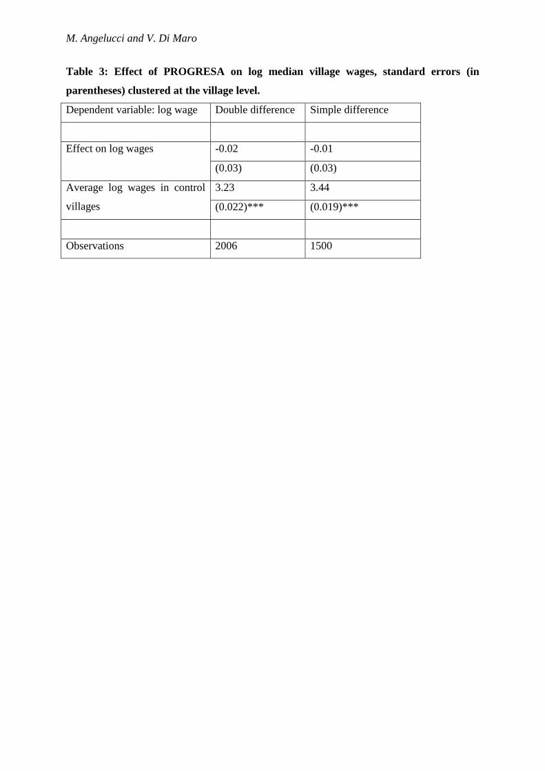
We repeat the analysis for median village wages, the results of which are reported in
Table 3. For prices, the point estimate is -0.02 (small and negative) and the standard error is
0.03. Thus, the effect is not statistically different from zero and is, at most, small.
5.3 Other mechanisms
Having ruled out any sizable general equilibrium effect on prices and wages, it is
useful to provide direct evidence that the increase in consumption for ineligible households is
caused by an increase in the number of loans and gifts received. Angelucci and De Giorgi
(2009) find increases in informal loans and transfers to ineligible households in treatment
villages (and a small decrease in the value of their savings). The implications of these
findings are that failing to account for the program’s spillover effects results in a 12 per cent
underestimation of the effect of PROGRESA on consumption in treatment villages. More
generally, this exercise teaches us how households cope with high levels of income
variability and the absence of formal credit and insurance.
Learning about the causes of spillover effects is useful for at least two additional
reasons. First, it helps us understand what to expect when implementing a program at the
national level. In this case, the findings suggest the program will continue to have sizeable
spillover effects on consumption as long as informal sharing institutions—such as the
extended family—are as important in the rest of Mexico as in the sampled villages. Second,
the findings can help policy makers design more cost effective policies.

25
Suppose one were to find that all village members benefit from the program because
they redistribute the PROGRESA grant in the village regardless of the actual identity of the
households that receive the transfer. This would mean that costly and time consuming
household level targeting may not be required. Geographic targeting, using poverty maps to
identify poor areas, could be a cheaper and faster alternative.
7. Conclusions
Subjects who are ineligible for a particular treatment will often benefit from it indirectly in a
wide variety of interventions. Measuring these spillover effects (or Indirect Treatment
Effects) and understanding the mechanisms that generate them can be crucial to the design of
effective policies. Failing to adopt an evaluation design that accounts for spillover effects can
result in a double underestimation of a program’s impact, as the average effect on eligible
subjects is underestimated and the effect of the treatment on ineligible subjects goes
completely unnoticed. This double underestimation may lead to incorrect policy
recommendations (for example, dropping the program because it does not seem cost
effective).
This paper makes some key recommendations to aid the design of evaluations that
account for the presence of spillover effects. Here is a summary of these recommendations:
1. Develop and/or adopt a theory about what may cause the spillover effects,
who may be affected by them, and how. Knowledge of the local economy and of the
types of interactions among its members is crucial for the design of an evaluation that
at least accounts for the existence of spillover effects. Ideally, the evaluation should
enable researchers to measure the effects and understand why they arise. Having a
hypothesis about spillover effects often means having better assumptions about how
the program works, which should help in the design of better policies.
2. To measure spillover effects effectively, the evaluation design must take them
into account from the start. This often means collecting more data, for instance by
surveying geographical areas that are not affected by the intervention. Evaluation
designs that do not consider these issues from the very beginning are typically unable
to measure spillover effects.

M. Angelucci and V. Di Maro
3. To identify and estimate the average treatment effect on eligible subjects
(ATE) in the presence of spillover effects, researchers should select a control group
that is not affected by the program. Theory will guide in this choice. Consider, for
example, the case in which the indirect effects operate at village level. With an
experimental design, randomize at village level. With a selection-on-observables
design (matching), select treatment and control groups from different villages.
4. To identify and estimate the indirect treatment effect (ITE), that is the effect of
the treatment on individuals who are not directly affected by the treatment, have two
groups of subjects with similar characteristics (the same distribution of characteristics
if there is random assignment) but only one group that is indirectly affected by the
treatment. Consider, for example, the case in which the indirect effects operate at
village level. With an experimental design, conduct a double randomization across
and within villages. With a selection-on-observables design (matching), select
subjects that live in treated villages and who are indirectly affected by the treatment
and compare them with similar subjects from different villages.
5. To understand the mechanisms that cause the spillover effects, think about
potential competing explanations and collect data on relevant outcomes. In many
cases, unveiling the mechanisms behind the spillover effects will lead to a better
understanding of how the program works in general.

27
References
Angelucci, M., and G. De Giorgi. 2009. “Indirect Effects of an Aid Program: How do Cash
Injections Affect Ineligibles’ Consumption?” American Economic Review, 99(1), 486-
508, March.
Angrist, J.D. and J. Pischke. 2009. Mostly Harmless Econometrics. Princeton, NJ, United
States: Princeton University Press.
Avitabile, C., 2012. “Spillover Effects in Healthcare Programs: Evidence of Social Norms
and Information Sharing”. IDB Working Papers Series No. IDB-WP-380, December.
Baird, S., Bohren, J.A, McIntosh, C., and Ozler, B. (2014), “Designing experiments to
measure spillover effects,” PIER working paper
Berhman, J., and P. Todd. 1999. “Randomness in the Experimental Sample of Progresa
(Education, Health, and Nutrition Program)”. International Food Policy Research
Institute Working Paper. Washington DC, United States: IFPRI.
Bertrand, M., Duflo, E., and Mullainathan S. (2004), “How Much Should We Trust
Difference in Differences Estimates?’ The Quarterly Journal of Economics 119(1):
249-275.
Bobonis, G. J., and Finan F. (2009), “Neighborhood Peer Effects in Secondary School
Enrollment Decisions”. The Review of Economics and Statistics 91(4): 695-716
Caliendo, M., and S. Kopeining. 2008. "Some Practical Guidance for the Implementation of
Propensity Score Matching". Journal of Economic Surveys. Blackwell Publishing,
vol. 22(1), pages 31-72, 02.
Chay, K., P. Ibarraran, and J. M. Villa. 2010. "Regression Discontinuity and Impact
Evaluation". Forthcoming in the Inter-American Development Bank-SPD Impact
Evaluation Guidelines series. Washington DC, United States: IDB.
Crepon, B., Duflo, E., Gurgand, M., Ratheot, R., and Zamora, P. (2013), “Do labor market
policies have displacement effects? Evidence from a randomized experiment,” The
Quarterly Journal of Economics, 128(2), 531-80.
Di Tella, Rafael, and Ernesto Schargrodsky, “Do Police Reduce Crime? Estimates Using the
Allocation of Police Forces After a Terrorist Attack,” American Economic Review
94:1 (2004), 115–133.
Dubois, P., Jullien, B., and Magnac, T. (2008) “Formal and Informal Risk Sharing in LDCs:
Theory and Empirical Evidence”, Econometrica 76: 679-725.

M. Angelucci and V. Di Maro
Fafchamps, M. (2008) “Risk Sharing Between Households”, forthcoming Handbook of
Social Economics
Fafchamps, M., and Lund, S. (2003) “Risk-sharing Networks in Rural Philippines”, Journal
of Development Economics 71: 261-87.
Hahn, J. and Hirano, K. (2010), “Design of Randomized Experiments to Measure Social
Interaction Effects," Economics Letters 106(1): 51-53
Hendrick, C., A. Maffioli, and G. Vazquez. 2010. "Guidelines on Matching". Forthcoming in
the Inter-American Development Bank-SPD Impact Evaluation Guidelines series.
Washington DC, United States: IDB.
Heckman, James J. & Lalonde, Robert J. & Smith, Jeffrey A., 1999. "The economics and
econometrics of active labor market programs," Handbook of Labor Economics, in:
O. Ashenfelter & D. Card (ed.), Handbook of Labor Economics, edition 1, volume 3,
chapter 31, pages 1865-2097, Elsevier.
Lee, D., and T. Lemieux. 2009. "Regression Discontinuity Designs in Economics". National
Bureau of Economic Research. Working Paper No. 14723, Feb 2009. Cambridge,
MA, United States: NBER.
Miguel, E., and M. Kremer. 2004. “Worms: Identifying Impacts on Education and Health in
the Presence of Treatment Externalities”. Econometrica 72(1): 159-217.
Moffitt, R. 2001. “Policy Interventions, Low-Level Equilibria, and Social Interactions”. In:
S.N. Durlauf and P. Young, editors. Social Dynamics 45-82. Cambridge, MA, United
States: MIT Press.
Rieben S, Kalinina O, Schmid B, Zeller SL (2011) Gene Flow in Genetically Modified
Wheat. PLoS ONE 6(12): e29730. doi:10.1371/journal.pone.0029730
Rosenzweig, M. (1988), “Risk, Private Information, and the Family,” American Economic
Review, 78(2): 245-50.
Townsend, R., (1994), “Risk and Insurance in Village India”, Econometrica, 62(3): 539-
591.
Yang, D. 2008, “Can Enforcement Backfire? Crime Displacement in the Context of Customs
Reform in the Philippines”. The Review of Economics and Statistics 90(1): 1-14
Udry, C. (1995), “Risk and Saving in Northern Nigeria”, American Economic Review,
85(5): 1287-1300.

29
Figure 1. PROGRESA: Data structure

M. Angelucci and V. Di Maro
Table 1: Average peso monthly food consumption per adult equivalent: levels and
differences
From Angelucci and De Giorgi (2009). Monthly pesos per adult equivalent at Nov. 1998
prices; the exchange rate is roughly 10 pesos per USD. We report the standard deviations of
the means and the standard errors, in brackets, of the treatment effects. The latter are
clustered at village level with *** and ** indicating significance at the 1 per cent and 5 per
cent levels respectively. The set of conditioning variables we add to the regressions in the left
panel are: household poverty index, land size, head of household gender, head of household
age, whether head of household speaks indigenous language, head of household literacy; at
the locality level, poverty index and number of households. All variables are at 1997 values.

31
Table 2: Effect of PROGRESA on log village prices, standard errors (in parentheses)
clustered at the village level.
Dependent variable: log price Double difference Simple difference
Effect on log prices -0.008 0.004
(0.011) (0.006)
Average log prices in control
villages
1.68 1.72
(0.01)*** (0.01)***
Observations 72216 54036
M. Angelucci and V. Di Maro
Table 3: Effect of PROGRESA on log median village wages, standard errors (in
parentheses) clustered at the village level.
Dependent variable: log wage Double difference Simple difference
Effect on log wages -0.02 -0.01
(0.03) (0.03)
Average log wages in control
villages
3.23 3.44
(0.022)*** (0.019)***
Observations 2006 1500