Fondamenti di Informatica

Data abstraction: Vectors

Prof. Emiliano Casalicchio http://www.ce.uniroma2.it/courses/FOI/

1-2

Objectives

This lecture discusses the basic calculations involving rectangular collections of numbers in the form of vectors. For this collections, you will learn how to:

■ Create them ■ Manipulate them ■ Access their elements ■ Perform mathematical and logical operations on

them

1-3

Concept: Using Built-in Functions

  In this chapter we will see the use of some of the functions built into MATLAB.

  At the end of each chapter that uses built-in functions, you will find a summary table listing the function specifications.

  For help on a specific function, you can type the following: >> help <function name>

  For example: >> help sqrt SQRT Square root.

SQRT(X) is the square root of the elements of X. Complex results are produced if X is not positive.

1-4

Concept: Data Collections

This section considers two very common ways to group data: in arrays and in vectors. Data Abstraction allows us to refer to groups of data collectively:

  “all the temperature readings for May” or   “all the purchases from Wal-Mart.”

We can not only move these items around as a group, but also perform mathematical or logical operations on these groups, e.g.:

  compute the average, maximum, or minimum temperatures for a month

A Homogeneous Collection is constrained to accept only items of the same data type – in this case, they will all be numbers

1-5

MATLAB Vectors

Individual items in a vector are usually referred to as its elements. Vector elements have two separate and distinct attributes that make them unique in a specific vector:

  their numerical value and   their position in that vector.

For example, the individual number 66 is the third element in this vector. Its value is 66 and its index is 3. There may be other items in the vector with the value of 66, but no other item will be located in this vector at position 3.

1-6

Vector Manipulation

We consider the following basic operations on vectors:

 Creating a Vector  Determining the size of a Vector  Extracting data from a vector by indexing  Shortening a Vector  Mathematical and logical operations on Vectors

1-7

Creating a Vector – Constant Values

  Entering the values directly, e.g. A = [2, 5, 7, 1, 3]

  Automatically entering values e.g.

 as a range of numbers  as equally distributed in a linear

space  as random, zeros, ones

1-8

Creating a Vector – Entering the values as a range

B = [v1, v2, …, vn]={vi| vmin<=vi<=vmax,vi=vi-1+K, v1=vmin, i=2,..}

K is an integer constant value. E.g.K=3, vmin=1 and vmax=20 B=[1,4,7,10,13,16, 19]

Let’s try defining an algorithm to create the set B

Flow diagram

9

i1, vivmin

read: vmin, vmax , K

vi-1+K > vmax

ii+1

vivi-1+K

End

Start

B = [v1, v2, …, vn]=

{vi| vmin<=vi<=vmax,vi=vi-1+K, v1=vmin, i=2,..}

Pseudocode 1.  read vmin, vmax e K 2.  i1, vivmin

3.  ii+1 4.  if vi-1+K > vmax then exit 5.  else vivi-1+K 6.  go to step 3.

In the following lectures you will learn how to implement in

Matlab this algorithm…and more

No

1-10

Creating a Vector – Entering the values as a range (2)

  In Matlab B = {vi| vmin<=vi<=vmax,vi=vi-1+K, v1=vmin, i=2,..} = = vmin:K:vmax E.g. B = 1:3:20 = [1,4,7,10,13,16, 19]

This syntax is an implementation of the

previous defined algorithm

1-11

Creating a Vector – as equally distributed in a linear space

B = [v1, v2, …, vN]={N equally spaced points between Xmin and Xmax}

e.g. N=11, Xmin=0 e Xmax=20 B=[0 2 4 6 8 10 12 14 16 18 20]

  Matlab offers a built in function to do that C = linspace (Xmin, Xmax, N)

  k is a variable containing

12

k (Xmax-Xmin) / N

i1, vivmin

read: Xmin, Xmax , N

i > N

ii+1

vivi-1+k

End

Start

No

1-13

Creating a Vector - filled with 0, 1, random values

B = [v1, v2, …, vN]; vi=0 for i=1,..,N vi=1 for i=1,..,N vi=xk where xk is a pseudorandom value uniformly or normally distributed

All the cases can use the same algorithm

x = 0 or 1 or Normal() or Uniform()

14

i0

read: N

i > N

ii+1

vix

End

Start

No

x = 0 or 1 or Normal() or Uniform()

1-15

Creating a Vector - filled with 0, 1, random values

Matlab offers built in function implementing the previous algorithm %B = [v1, v2, …, vN]; B=zeros(1,n) %vi=0 for i=1,..,N B=ones(1,n) %vi=1 for i=1,..,N B=rand(1,n) %vi=xk where xk is a pseudorandom value

%uniformly distributed B=randn(1,n) %vi=xk where xk is a pseudorandom value

%normally distributed

1-16

Size of Vectors and Arrays

Problem: we have a vector and we want to know the number of its elements MATLAB provides two functions to determine the size of arrays in general (a vector is an array with one row):

  the function size(A) when applied to the array A returns vector containing two quantities: the number of rows and the number of columns

 The function length(A) returns the maximum value in the size of an array; for a vector, this is its length.

1-17

Indexing a Vector

  The process of extracting values from a vector, or inserting values into a vector

  Syntax:   v(index) returns the

element(s) at the location(s) specified by the vector index.

  v(index) = value replaces the elements at the location(s) specified by the vector index.

  The indexing vector may contain either numerical or logical values

>> A=1:3:12 A = 1 4 7 10 >> A(1) ans = 1 >> B=[2,4] B = 2 4 >> A(B) ans = 4 10

indexing vector

1-18

Numerical Indexing

  The indexing vector may be of any length   It should contain integer (non-fractional) numbers   The values in the indexing vector are constrained by the following rules:

 For reading elements, all index values must be 1 <= element <= length(vector)

 For replacing elements, all index values must be 1 <= element

1-19

Replacement Rules

1.  Either: •  All dimensions of the blocks on

either side of the replacement instruction must be equal, or

•  There must be a single element on the RHS of the replacement

2.  If you replace beyond the end of the existing vector, the vector length is automatically increased.

•  Any element not specifically replaced remains unchanged.

•  Elements beyond the existing length not replaced are set to 0.

>> A=1:3:12 A = 1 4 7 10 >> B=[2,4]; >> A(B)=[0,0] A = 1 0 7 0 >> A(4)=99 A = 1 0 7 99 >> A(7)=99 A = 1 0 7 99 0 0 99

Boolean Algebra

  In mathematics and mathematical logic, Boolean algebra is the subarea of algebra in which the values of the variables are

  the truth values true and false, usually denoted 1 and 0 respectively.

  Instead of elementary algebra where the values of the variables are numbers, and the main operations are addition and multiplication, the main operations of Boolean algebra are

  the conjunction AND, denoted ∧   the disjunction OR, denoted ∨   the negation NOT, denoted ¬

20

Logical operators: NOT, AND, OR

21

AND, & OR, |

NOT, -

1-22

Logical Indexing

  The indexing vector length must be less than or equal to the original vector length

  It must contain logical values (true or false)

  Access to the vector elements is by their relative position in the logical vector   When reading elements, only the

elements corresponding to true index values are returned

  When replacing elements, the elements corresponding to true index values are replaced

  Beware – logical vectors in Matlab echo in the Command window as 1 or 0, but they are not the same thing.

>> a=true a = 1 >> a=false a = 0 >> 13>10 ans = 1 >> mask=[true,false,true,true] mask = 1 0 1 1 >> A(mask) ans = 1 7 99 >> A(mask)=[66,66,66]; >> A A = 66 0 66 66 0 0 99

1-23

Shortening an Array

  Never actually necessary. It is advisable to extract what you want by indexing rather than removing what you don’t want.

 Can lead to logic problems when changing the length of a vector

  Accomplished by assigning the empty vector ([]) to elements of a vector, or to complete rows or columns of an array.

1-24

Operating on Vectors

Three techniques extend directly from operations on scalar values:

■ Arithmetic operations ■ Logical operations ■ Applying library functions

Two techniques are unique to arrays in general, and to vectors in particular:

■ Concatenation ■ Slicing (generalized indexing)

Operators precedence

  Operator description and precedences http://www.mathworks.com/help/techdoc/matlab_prog/f0-40063.html

25

1-26

Arithmetic operations

In the Command window, enter the following: >> A = [2 5 7 1 3]; >> A + 5 ans = 7 10 12 6 8 >> A .* 2 ans = 4 10 14 2 6 >> B = -1:1:3 B = -1 0 1 2 3

1-27

Arithmetic operations (continued)

>> A .* B % element-by-element multiplication ans = -2 0 7 2 9 >> A * B % matrix multiplication!! ??? Error using ==> mtimes Inner matrix dimensions must agree. >> C = [1 2 3] C = 1 2 3 >> A .* C % A and C must have the same length ??? Error using ==> times Matrix dimensions must agree.

1-28

Logical operations

>> A = [2 5 7 1 3]; >> B = [0 6 5 3 2]; >> A >= 5 ans = 0 1 1 0 0 >> A >= B ans = 1 0 1 0 1 >> C = [1 2 3] >> A > C ??? Error using ==> gt

Matrix dimensions must agree.

1-29

Logical operations (continued)

>> A = [true true false false]; >> B = [true false true false]; >> A & B ans = 1 0 0 0 >> A | B ans = 1 1 1 0 >> C = [1 0 0]; % NOT a logical vector >> A(C) % yes, you can index logical vectors, but ... ??? Subscript indices must either be real positive

integers or logicals.

1-30

A Footnote: the find function

  Continuing the code above: >> C = find(B) ans = [1 3]

  The find(...) function consumes a logical vector and returns the numerical indices of the elements of that vector that are true.

1-31

Applying library functions

All MATLAB functions accept vectors of numbers rather than single values and return a vector of the same length. Special Functions: ■ sum(v) and mean(v) consume a vector and return a number ■ min(v) and max(v) return two quantities: the minimum or maximum value in a vector, plus the position in that vector where that value occurred. ■ round(v), ceil(v), floor(v), and fix(v) remove the fractional part of the numbers in a vector by conventional rounding, rounding up, rounding down, and rounding toward zero, respectively.

1-32

Concatenation

  MATLAB lets you construct a new vector by concatenating other vectors:

  A = [B C D ... X Y Z] where the individual items in the brackets may be any vector defined as a constant or variable, and the length of A will be the sum of the lengths of the individual vectors.   A = [1 2 3 42] is a special case where all the component elements are scalar quantities.

1-33

Slicing (generalized indexing)

  A(4) actually creates an anonymous 1 × 1 index vector, 4, and then using it to extract the specified element from the array A.

  In general, B(<rangeB>) = A(<rangeA>)

where <rangeA> and <rangeB> are both index vectors, A is an existing array, and B can be an existing array, a new array, or absent altogether (giving B the name ans). The values in B at the indices in <rangeB> are assigned the values of A from <rangeA> .

1-34

Rules for Slicing

■ Either the dimensions of <rangeB> must be equal to the dimensions of <rangeA> or <rangeA> must be of size 1

■ If B did not exist before this statement was implemented, it is zero filled where assignments were not explicitly made

■ If B did exist before this statement, the values not directly assigned in <rangeB> remain unchanged

1-35

Representing Mathematical Vectors

  An unfortunate clash of names   Vectors in mathematics can be represented by

Matlab vectors   The first, second and third values being the x, y and z

components   Matlab vector addition and subtraction work as

expected.   Matlab magnitude and scaling works as expected.   Dot product is just the sum of A .* B   Cross product has a Matlab function

1-36

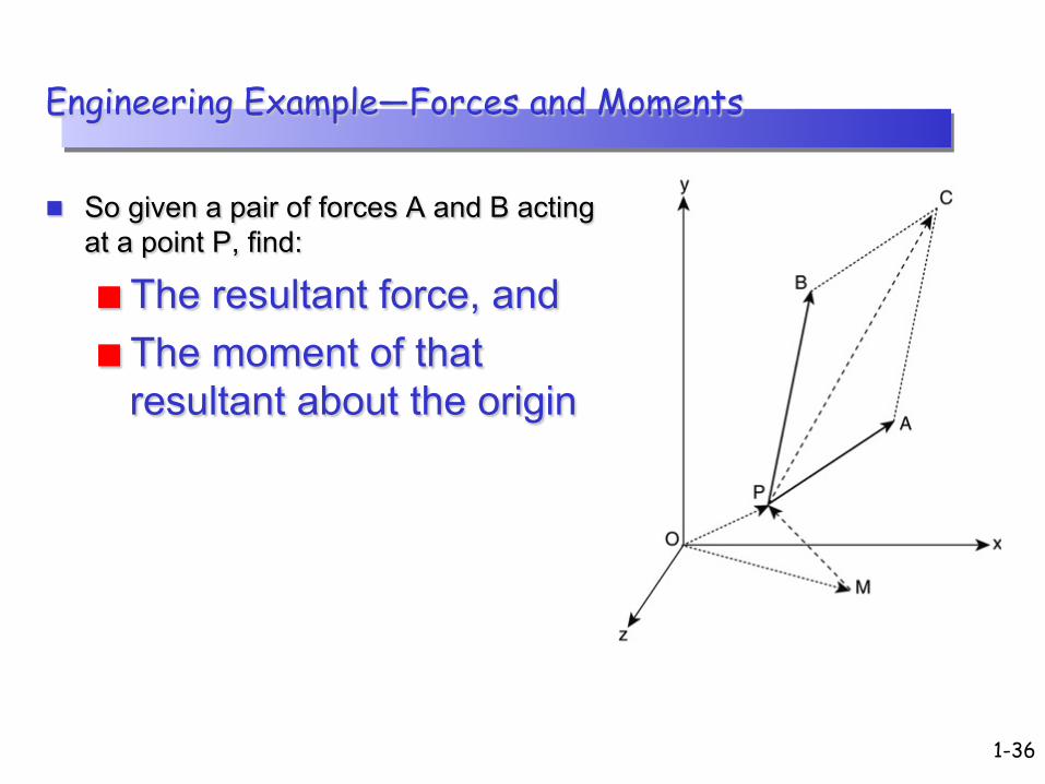
Engineering Example—Forces and Moments

  So given a pair of forces A and B acting at a point P, find:

 The resultant force, and  The moment of that

resultant about the origin

1-37

Vector Solution

clear clc PA = [0 1 1] PB = [1 1 0] P = [2 1 1] M = [4 0 1] % find the resultant of PA and PB PC = PA + PB % find the unit vector in the direction of PC mag = sqrt(sum(PC.^2)) unit_vector = PC/mag % find the moment of the force PC about M % this is the cross product of MP and PC MP = P - M moment = cross( MP, PC )

  Homework

 exercise 3.1 – 3.10 of the book.

38