Productivity Dispersions: Could it simply be technology ...

Productivity Dispersions:

Could it simply be technology choice?∗

Christian Bayer† , Ariel M. Mecikovsky‡, Matthias Meier‡

This version: October 15, 2015

PRELIMINARY VERSION

Abstract

We ask whether differences in micro-level factor productivities should be understood

as a result of frictions in technology choice. Using plant and firm-level data from

Chile, Colombia, Germany, and Indonesia, we document that the bulk of all produc-

tivity differences is persistent even within industries and related to highly persistent

differences in the capital-labor ratio. This suggests a cost of adjusting this ratio. In

fact, a model with such friction in technology choice can explain our findings not

only qualitatively, but also quantitatively. At the same time, the loss in productive

efficiency from this friction is modest in the sense that eliminating it would increase

aggregate productivity by 3-5%.

Keywords: Productivity, Putty-clay, Heterogeneous plants.

JEL Classification Numbers: D2, E2, L1, O3, O4.

∗An earlier version of this paper was titled: Dynamics of Factor Productivity Dispersion. The researchleading to these results has received funding from the European Research Council under the European ResearchCouncil under the European Union’s Seventh Framework Programme (FTP/2007-2013) / ERC Grant agreementno. 282740. Ariel Mecikovsky and Matthias Meier thank the DFG for supporting their research as part of theresearch training group GRK 1707 “Heterogeneity, Risk and Economic Dynamics”. Thanks to financial supportfrom DAAD and DFG, Matthias Meier conducted parts of this paper while visiting NYU, and he would like tothank the department, especially Gianluca Violante, for their hospitality. We are grateful to Jorg Breitung, SimonGilchrist, Matthias Kehrig, Dirk Krueger, Virgiliu Midrigan, Venky Venkateswaran for detailed comments and theparticipants at 4th Ifo Conference Macroeconomics and Survey Data 2013, EEA 2013, CEF 2013, NASM 2013,European Workshop on Efficiency and Productivity Analysis 2013, Warwick Economics PhD Conference 2013,SED 2014, VfS Macroeconomics Meeting 2015 and seminar participants at the Universitat Autonoma Barcelona,Universitat Bonn, Universidad Carlos III Madrid, New York University, and the Universitat Zurich. We thankDeutsche Bundesbank, Instituto Nacional de Estadısticas de Chile, Badan Pusat Statistik and Devesh Raval, forproviding us access to the firm/plant level data from Germany, Chile, Indonesia and Colombia respectively.†CEPR & Department of Economics, Universitat Bonn. Address: Adenauerallee 24-42, 53113 Bonn, Germany.

email: [email protected].‡Department of Economics, Universitat Bonn.

1 Introduction

The allocation of factors to their most productive use is often seen as one of the key

determinants of economic prosperity (Foster et al., 2008). While first-best efficiency

requires that factors produce the same marginal revenue across all production units,

many studies show this condition to be violated in micro data: factor productivities

differ substantially within industries.1

We ask whether these micro-level differences can be understood as a result of frictions

in technology choice; a setup, where firms may in principle choose from a broad set of

technologies, but it is costly to search for them, to install them, and to acquire the

know-how necessary to use them. This leads firms to operate one single technology

which they adjust only occasionally. In between adjustments, production technology is

Leontief. In particular, the capital-labor ratio, the capital intensity, remains fixed. As

the economic environment changes and firms asynchronously adapt their technology in

response, cross-sectional differences in factor productivities and capital intensity emerge.

This, however, is not the only empirical implication of frictional technology choice.

Across all firms, differences in factor productivities and capital intensity should be pre-

dominantly long-lived. Moreover, there must be a trade-off involved. Firms with per-

sistently high productivity in one factor should have a persistently low productivity in

another factor. Further, as long as capital intensity is fixed, i.e. in the short run, labor

and capital productivity can only move in the same direction. Finally, the extent of

competition limits the scope of technologies used in the economy. The more competi-

tive the environment, the larger is the pressure to abandon particularly cost-inefficient

technologies.

To explore whether these implications are borne out empirically, we compute micro-

level labor and capital productivity controlling for industry and time effects, and decom-

pose them into their persistent and transitory components. To have a broad empirical

base, we exploit micro data from Germany (firm-level), Chile, Colombia, and Indonesia

(plant-level). Between 61% and 94% of the cross-sectional variance in labor and capital

productivity is explained by their persistent components. The result is even stronger for

capital intensity where the fraction explained by the persistent component is above 77%

for all countries. Furthermore, the persistent components of labor and capital productiv-

ity are negatively correlated, while their transitory components are positively correlated.

In addition, persistent differences in capital intensity are less dispersed in more compet-

1See Restuccia and Rogerson (2008), Hsieh and Klenow (2009), Peters (2013), Asker et al. (2014),Gopinath et al. (2015), and Restuccia and Santaeulalia-Llopis (2015) to name a few.

1

itive environments, i.e. where markups are persistently lower. Firms/plants in the most

competitive quintile exhibit a 30-50% lower variance of capital intensity than those in

the least competitive quintile. In summary, the data qualitatively supports the idea of

a friction in technology choice driving productivity dispersions.

Next we show that this friction is also able to explain our micro-data findings quan-

titatively. For this purpose, we develop a dynamic partial-equilibrium model which we

calibrate to aggregate targets.

Firms in our model operate a single plant, are subject to monopolistic competition,

face exogenous fluctuations in relative factor prices, and frictions in technology choice

in the spirit of Kaboski (2005). Upon costly adjustment, firms can choose from a broad

set of technologies described by a long-run production function with constant elasticity

of substitution (CES) and constant returns to scale (CRS). This choice pins down a

capital intensity, which remains fixed until next adjustment, but apart from that firms

can freely choose scale, so that the short-run production function is Leontief.

In the calibration of this model, there are two key elements aggregate data needs to

pin down: the process for relative factor prices and the elasticity of substitution in the

long-run production function. For the former, we target the time series behavior of the

aggregate labor income share instead of direct measures of the relative factor price. The

labor share immediately accounts for trends in labor augmenting technological change

and long time series are available in National Accounts. For the elasticity of substitution,

we face the problem that a regression of aggregate capital intensities on relative factor

prices no longer directly identifies the long-run elasticity of substitution, unlike in the

frictionless case. It rather identifies a short-run response of the economy. Still it allows

us to indirectly identify our parameter of interest.

The calibrated model enables us to assess the losses in efficiency and welfare that arise

from the friction in technology choice. We find that they amount to 3% of productivity

and 8% of social welfare. Moreover, we show that less stable relative factor prices are

able to explain the more dispersed productivities in the three developing economies. A

higher volatility of relative factor prices may result from more volatile tax rates, swings

in union power, and shocks to financial markets or real exchange rates. In other words,

a less stable economic environment, as for example in Indonesia, increases misallocation

and the implied welfare losses by more than 50%.

Despite the strong relative differences across countries, our estimated efficiency losses

from misallocation are small compared to the literature. Important for this is our fo-

cus on productive efficiency, i.e. deviations from optimal capital intensity. In contrast,

studies like Hsieh and Klenow (2009) have taken a broader focus including allocative

2

efficiency, i.e. deviations from optimal scale. We disregard those deviations, showing up

as dispersions in markups, for our efficiency calculations for two reasons. First, these dis-

persions might reflect efficient differentiation within industry. For example, they might

stem from alternative strategies on product quality or range (e.g. Bar-Isaac et al., 2012),

think of generics vs. patented pharmaceuticals. Second, there is already a broad set of

theories predicting markup dispersions to which we have little to add. Think models

with price setting frictions a la Calvo (1983), with building a customer base (Gourio

and Rudanko, 2014), or with entry dynamics and innovation as in Peters (2013). All of

these provide explanations of productivity dispersions through heterogeneous markups

as endogenous objects. At the same time, our data suggests that markup dispersions

themselves explain only a minority of all productivity dispersion.

In other words, the friction that explains productivity dispersions needs to produce

differences in capital intensities. Capital adjustment costs in general are such friction

(see Asker et al., 2014). Yet, we show that capital adjustment frictions produce too large

transitory and too small persistent differences in capital intensity. The reason is that

firms respond to short-run shocks by strongly varying their capital intensity if labor is

much more flexible than capital.2

Hence to match the data, it is necessary to assume relatively rigid capital inten-

sities in the short-run. This links our paper to the traditional putty-clay assumption

(Johansen, 1959), which has been advocated to address a broad array of other empiri-

cal phenomena (Gilchrist and Williams, 2000, 2005; Gourio, 2011). Particularly closely

related is Kaboski’s (2005) model of putty-clay technology choice under factor price un-

certainty. An important insight from this paper that carries over to our setup is that

firms underreact to current prices in setting their technology, such that the regression

techniques usually used to identify the long-run elasticity of substitution (see e.g. Raval

(2014) or Oberfield and Raval (2014) for recent contributions or Chirinko (2008) for

an overview) are subject to a downwards bias. In fact, we show that this downwards

bias is likely substantial. Our baseline of the long-run elasticity of substitution is about

five, while the aggregate short-run elasticity being 0.75. This high elasticity not only

has important implications for income-shares (see e.g. Solow, 1956; Piketty, 2011, 2014;

Karabarbounis and Neiman, 2013) but is also key to obtain small productive efficiency

losses from dispersions in capital intensities.

The remainder of this paper is organized as follows: Section 2 describes our tech-

2We conjecture that similar issues are encountered by alternative theories generating productivitydispersions through endogeneous firm-specific shadow-prices of capital, such as through financial frictions(Amaral and Quintin, 2010; Banerjee and Moll, 2010; Buera et al., 2011; Midrigan and Xu, 2013; Moll,2014), imperfect information (David et al., 2013), or contractual incompleteness (Acemoglu et al., 2007).

3

nology choice model in a simplified two-period setup. This allows us to derive the main

qualitative insights that we have sketched in this Introduction and guides our empirical

analysis in Section 3. Section 4 then presents our dynamic model, followed by the quan-

titative results in Section 5. Section 6 compares to an alternative specification of capital

adjustment costs instead of a friction in technology choice and Section 7 concludes. An

Appendix follows.

2 Two-Period Model of Technology Choice

To guide our empirical analysis we start off with a two-period version of our tech-

nology choice model. Assume a mass of firms of measure one. Each firm, i, is endowed

with one plant that has an exogenously given capital intensity ki = KiNi

, where Ki is the

physical amount of capital and Ni is labor. We assume that wages, W , and user costs

of capital, R, are exogenously given, but stochastic.

2.1 Output choice

Each firm has a constant returns to scale production technology and faces monopo-

listic competition for its product, where the elasticity, ξi, of demand for the product, yi,

of firm i is firm-specific and constant, such that prices are given by

pi =1

1− ξizξii y

−ξii ,

where zi is the stochastic market size for firm i’s product. Unit costs of production

depend on the plant’s capital intensity and factor prices, ci = c(ki,W,R). The firm

maximizes profits, and we assume that the firm needs to decide about output before

knowing actual factor prices and demand. The optimal policy will choose output in

order to stabilize the expected markup at its optimal level. The expected gross markup

is constant, 11−ξi > 1. Denoting the expectations operator as E, it is straightforward

to show that the profit maximizing output, y∗i and expected profits under the optimal

policy, π∗, are given by

y∗i =

[Ezξii

Ec(ki, R,W )

]1/ξi

; π∗i =ξi

1− ξiy∗i Ec(ki, R,W ). (1)

4

2.2 Revenue productivities

This implies that firms facing higher demand elasticities, ξi, have on average larger

markups and larger revenue factor productivities. Deviations from expected costs,

Eci/ci, and deviations from expected demand, zξii /Ezξii , lead to additional fluctuations

in realized markups, given by:

piy∗i

WNi +RkiNi=

1

1− ξizξii

Ezξii

Ecici. (2)

Similarly, splitting up this term in two components, these fluctuations move the capital

and labor expenses per value added:

piy∗i

WNi=

1

1− ξizξii

Ezξii

E(W +Rki)

W(3)

piy∗i

RkiNi=

1

1− ξizξii

Ezξii

E(W +Rki)

Rki(4)

On the one hand, (3) and (4) show that firms with higher (target) markups, 11−ξi exhibit

both higher labor and capital productivities. Similarly, positive and unforeseen demand

shocks, zξii /Ezξii , increase both factor productivities. Importantly, in a more general

multi-period setup, these deviations from expectations could only be transitory. On the

other hand, firms with higher capital intensity have a lower capital and higher labor

revenue-productivity, even when these capital intensity differences are expected.

To summarize, productivities differ across firms either because of differences in size

relative to demand (the first two terms) or due to differences in capital intensity and

factor prices (the last term) in (3) and (4).3

2.3 Choice of technology

We assume that in the period preceding production, the firm can opt to replace its

existing plant, setting up a new one with different capital intensity k. In doing so, the

firm compares expected profits with and without technology adjustment to decide the

period preceding production whether to produce with its initially given capital intensity

or to invest in changing the technology. We assume adjustment is costly as it disrupts

production. This disruption summarizes all costs of searching for a technology, installing

3As evident from equation 2, in this environment, adding an additional shock to unit costs (a TFPshock) has the same implications as a demand shock.

5

it and learning to operate it. Upon adjustment the firm forgoes a fraction φi of next

period’s profits, where φi stochastic and drawn from a distribution Φ. The firm draws φi

before it decides about adjustment and hence adjusts capital intensity to k, the capital

intensity that minimizes expected unit costs, whenever

(1− φi)Eπ(k) > Eπ(ki).

This simplifies to

(1− φi) >

(Ec(ki, R,W )

Ec(k, R,W )

) ξi−1

ξi

, (5)

using the expressions in (1) for expected profits.

Since Ec(ki,R,W )

Ec(k,R,W )≥ 1, firms with higher elasticity of demand, ξi, are less likely to adjust

for a given ex ante capital intensity ki. The reason is that firms with high market power

can offload their higher unit costs to consumers and hence have less incentive to invest

in efficient capital intensities. This is reminiscent of Leibenstein’s (1966) X-inefficiency

of monopolies or Bester and Petrakis’s (1993) results for oligopolies.4

As a result, ex-post capital-intensity will be less dispersed within the group of firms

with low markups than among high-markup firms if the ex-ante distribution of capital

intensities is centered around the cost minimizing level k.

2.4 Unit costs

To specify more concretely the relation between capital intensity and unit costs,

we assume that the long-run technology is given by a constant elasticity of substitution

(CES) production function with substitution elasticity σ, such that the output of a plant

with capital intensity ki is given by

yi =

[αk

σ−1σ

i + (1− α)Aσ−1σ

] σσ−1

Ni, (6)

where A captures (Harrod neutral) labor-augmenting technological change, and α is the

distribution parameter.

This implies that realized unit costs, ci = RkiNi+WNiyi

are minimal at capital intensity

4There is, however, one interesting side result of our setup. One can easily show that under thespecific assumption of an isoelastic demand curve and monopolistic competition, producer profits andconsumer rents are equal and therefore, total social surplus of adjustment as well as the social costs ofadjustment need to be scaled by factor two such that the individual optimal adjustment choice is sociallyoptimal.

6

k∗, given by

k∗ =

[α

1− αW

R

]σA1−σ. (7)

Now, to obtain an expression that allows us to relate the cross-sectional average unit

costs to the first two moments of the capital intensity distribution, we use a log second-

order approximation around that minimum:

Ex[log

c(ki, R,W )

c(k∗, R,W )

]≈ 1

2σs∗(1− s∗)

{[Ex(

logkik∗

)]2

+ Vx(log ki)

}, (8)

where s∗ is the capital expenditure share in the cost-minimizing optimum5

s∗ = Rk∗/(W +Rk∗),

and Ex denotes the cross-sectional average and Vx the cross-sectional variance. In words,

the efficiency loss is composed of the average relative difference of capital intensity from

its optimum, Ex log(ki/k∗), and the cross-sectional dispersion of capital intensity across

plants, Vx(log ki). Importantly, the higher the elasticity of substitution between labor

and capital, σ, the lower the efficiency loss from not re-setting capital intensities to their

optimum.

3 Empirics

3.1 Data description

We document factor productivity and capital intensity dispersion in firm-level data

from Germany, and plant-level data from Chile, Colombia and Indonesia. For Germany,

we use the balance sheet data base of the Bundesbank, USTAN, which is a private

sector, annual firm-level data available for 26 years (1973-1998).6 For Chile, Colombia

and Indonesia, we have plant level data from the ENIA survey for 1995-2007, the EAM

census for 1977-1991 and the IBS dataset for 1988-2010, respectively. These datasets

are focused on the manufacturing sector, with the exception of Germany, which provides

information for the entire private non-financial business sector.7

When preparing the data for our analysis, we make sure to treat them in the most

5See Appendix B for details.6See Bachmann and Bayer (2014) for a detailed description.7In particular, private non-financial business sector includes Agriculture, Energy and Mining, Man-

ufacturing, Construction, and Trade.

7

comparable way. From each survey, we use a firm’s/plant’s four-digit industry code,

wage bill, value-added and book or current value of capital stock. In order to obtain

economically consistent capital series for each firm/plant, we re-calculate capital stocks

using the perpetual inventory method when the data set does not include estimates of

the capital stock at current values. When recalculating the capital stock, we exploit

information of capital disaggregated into structures and equipment, which allows us to

control for heterogeneity in capital composition across plants.

Our capital productivity measure requires information on the real interest rate and

economic depreciation. For the latter, we do not rely on the depreciation reported by

plants, that is potentially biased for tax purposes or other reasons, but instead use

economic depreciation rates obtained from National Statistics or external studies if the

former is not available and take the different capital good mixes across firms/plants into

account. Since it is hard to identify the right measure for a real rate for the developing

economies, we instead fix the real rate to 5% for all economies. This implies user costs

of capital Rit = 5%+δit.8 In generating cross-sectional statistics, time variations in user

costs are controlled for by taking out four-digit industry-year fixed effects. The data

treatment and sample selection is described in detail in Appendix A.2.

3.2 Productivities and their transitory and persistent component

We compute average factor productivities for capital and labor per firm and year

using the reported value added per firm/plant at current prices, pityit, labor expenses,

WtNit as reported in the profit and loss statements, and imputed capital expenses,

RitKit. Taking logs, we define revenue productivities of labor and capital

αNit := log(pityit)− log(WtNit); αKit := log(pityit)− log(RitKit). (9)

Using expenditures and value added implicitly controls for quality differences in both

inputs and outputs (c.f. Hsieh and Klenow, 2009). In addition, we construct markups

as value added relative to total expenditures on labor and capital

mcit := log(pityit)− log(RitKit +WtNit). (10)

8The economic depreciation rate of equipment and structures for Germany is obtained from Volk-swirtschaftliche Gesamtrechnung (VGR) while for Chile we obtain time series from Henriquez (2008).Finally, as for Colombia and Indonesia, we consider the average depreciation in Chile for the availableperiod given the absence of national data sources. The depreciation rate values are 15.1% (equipment)and 3.3% (structures) in Germany, while they are on average 10.5% (equipment) and 4.4% (structures)for the rest of the countries.

8

Table 1: Transitory and persistent components of factor productivities

std(αLit) std(αKit ) ρ(αLit, αKit ) std(αLit) std(αKit ) ρ(αLit, α

Kit )

Transitory Component Persistent Component

DE 0.066 0.119 0.352 0.229 0.456 -0.207(0.000) (0.001) (0.002) (0.002) (0.004) (0.004)

CL 0.184 0.281 0.449 0.232 0.577 -0.190(0.006) (0.008) (0.017) (0.009) (0.028) (0.021)

CO 0.144 0.172 0.517 0.257 0.568 -0.234(0.003) (0.004) (0.012) (0.008) (0.023) (0.018)

ID 0.211 0.369 0.343 0.255 0.669 -0.269(0.003) (0.005) (0.007) (0.004) (0.013) (0.009)

Notes: Cross-sectional standard-deviations (std) and correlation (ρ) of transitory and persistentcomponents of labor- and capital productivity, αLit and αKit as in (9). DE: Germany, CL: Chile, CO:Colombia, ID: Indonesia. Transitory and persistent components are obtained by applying a fiveyear moving average filter. Factor productivities are demeaned by 4-digit industry and year, andexpressed in logs. In parentheses: Clustered standard errors at the firm/plant level.

Finally, we calculate the price weighted capital intensity,

κit = log(RitKit)− log(WtNit). (11)

For any of these variables, say xit, we calculate 5-year moving averages, denoted

xit := 15

∑2s=−2 xit+s, to identify the persistent component and deviations thereof, xit =

xit − xit, to identify the transitory component.

We then take out four-digit industry-year fixed effects and calculate dispersions and

correlations between the factor productivities for each component.

3.3 Empirical findings

Table 1 reports standard deviations and correlation for labor and capital productiv-

ity and for all four countries. Three observations stand out: First, capital and labor

productivity are positively correlated in the transitory component (ρ ≈ 40%) while they

are negatively correlated in the persistent component (ρ ≈ −20%). Using the expres-

sions for factor productivities in Section 2, see (3) and (4), deviations from optimal size

9

are more important in the short run, while deviations from optimal capital intensity are

more important in explaining long-run productivity differences. Second, the persistent

components in productivity explain the vast majority of cross-sectional productivity dif-

ferences (between 60% and 92% for labor and between 79% and 94% for capital). Third,

the developing economies show larger productivity dispersions.

As the positive/negative correlation pattern between labor and capital productivity

is a particularly important prediction of technology choice, we check whether this pattern

holds within the four-digit industries. Figure 1 shows that this is the case for the vast

majority of industries.

In light of our results in Section 2, it is useful to look at markup and capital in-

tensity differences, see Table 2. In particular, (8) allows us to relate the latter directly

to increases in unit costs. For all countries, differences in capital intensity are very

persistent. The transitory component makes up only between 4% (Germany) and 17%

(Indonesia) of the total variance. At the same time, persistent differences in capital

intensity are substantially more dispersed in Chile, Colombia, and Indonesia than they

are in Germany with variances being twice as high in Indonesia than in Germany.

On the contrary, the dispersion of persistent cross-sectional markup differences is

strikingly similar across countries, and transitory differences in markups are an im-

portant component of the total cross-sectional variance of markups – at least in the

developing economies (30% in Colombia, 50% in Chile and Indonesia) but less so in

Germany (12%).9

These results along with (3) and (4) suggest that an important component in the

persistent differences in productivity is the choice of capital intensities; deviations in

optimal scale being important but minor.

Using the log approximation in (8), the numbers in Table 2 imply, an increase of

unit-costs between 3.3% for Germany and 6.5% for Indonesia compared to the frictionless

minimum. These numbers assume a unit long-run elasticity of substitution and a capital

share of one third, which yields as cost increase V(κ)/9, ignoring potential differences

in average and static-optimal capital intensities. Note also that these numbers for the

cost increase highly depend on the assumed substitution elasticity and to an important

but lesser extent on the capital share. Decreasing the substitution elasticity to one half

doubles the efficiency loss all else equal. Lowering the capital share to one fifth (e.g. to

account for pure profits) instead decreases the efficiency loss by roughly one third.

9This might relate to the fact that demand is less stable in the developing economies. In fact, thecross-sectional standard deviation of value-added growth is two to four times larger in these economiesthan in Germany.

10

Figure 1: Correlations of factor productivities by four-digit industry

Persistent correlation-1 -0.5 0 0.5 1

Tra

nsi

tory

co

rrel

atio

n

-1

-0.5

0

0.5

1Germany


Tra

nsi

tory

co

rrel

atio

n

-1

-0.5

0

0.5

1Chile


Tra

nsi

tory

co

rrel

atio

n

-1

-0.5

0

0.5

1Colombia


Tra

nsi

tory

co

rrel

atio

n

-1

-0.5

0

0.5

1Indonesia

Notes: Transitory (Persistent) Correlation: Correlation between the transitory (persistent) compo-nent of labor and capital productivity at the firm/plant level, controlling for time-fixed effects.Each circle represents a four digit industry, where the size of a circle reflects aggregate employmentin that industry. For this figure, we restrict industries to include at least 20 firms/plants. The num-ber of industries inside the upper-left quadrant is 99 (out of 125) in Germany, 45 (out of 61) inChile, 62 (out of 73) in Colombia, and 85 (out of 90) in Indonesia.

11

Table 2: Transitory and persistent components of markup and capital intensity

std(mcit) std(κit) ρ(mcit, κit) std(mcit) std(κit) ρ(mcLit, κit)


DE 0.064 0.114 -0.155 0.172 0.551 0.062(0.000) (0.001) (0.002) (0.001) (0.004) (0.004)

CL 0.177 0.258 -0.090 0.184 0.661 -0.085(0.005) (0.009) (0.017) (0.005) (0.029) (0.022)

CO 0.134 0.157 -0.016 0.206 0.676 -0.232(0.003) (0.004) (0.012) (0.005) (0.025) (0.018)

ID 0.203 0.357 -0.120 0.195 0.778 -0.021(0.002) (0.005) (0.007) (0.003) (0.014) (0.010)

Notes: Capital intensities, κit, and markups, mcit, as defined in (10) and (11). See notes of Table 1 forfurther explanation.

To understand to what extent firms actively take these unit cost increases into ac-

count, we split the sample according to firm/plant characteristics – age, size, and im-

portantly a firm’s average markup – and compute again the dispersions of the persistent

component of capital intensity, see Table 3. While there are some differences in these dis-

persions according to age and size, these are neither large nor systematic. What stands

out is splitting the sample according to the average markup. The highest markup quintile

exhibits between 30% and 60% higher capital intensity dispersions (in terms of variances)

than the lowest markup quintile. This is in line with the qualitative predictions of our

model.

In Appendix A.5, we show that our empirical findings are robust to alternative ways

of decomposing into transitory and persistent components, and to alternative measures

of dispersion and correlation. We also find that persistent capital intensity differences

are more dispersed for high-markup firms/plants even when controlling for size and age.

12

Table 3: Persistent component of capital intensity by firm/plant characteristics

std(κit)

Markups Size Age

Bottom Top Bottom TopQuintile Quintile Quintile Quintile Young Old

DE 0.545 0.622 0.610 0.509 n.a. n.a.(0.010) (0.010) (0.009) (0.011)

CL 0.568 0.713 0.749 0.622 n.a. n.a.(0.042) (0.075) (0.068) (0.058)

CO 0.547 0.694 0.763 0.669 0.697 0.699(0.035) (0.061) (0.051) (0.061) (0.100) (0.048)

ID 0.716 0.834 0.830 0.816 0.770 0.801(0.028) (0.035) (0.034) (0.035) (0.058) (0.038)

Notes: Bottom (top) markup quintile: firm/plant average markup below the 20th percentile (above the80th percentile). Old (young): Plant age below 4 years (above 15 years). Bottom (top) size quintile:firm/plant average employment below the 20th percentile (above 80th percentile). The micro data fromGermany and Chile does not include age. See notes of Table 1 and 2 for further explanation.

4 Dynamic Model of Technology Choice

As the qualitative predictions of our simple two-period model of technology choice

are in line with the empirical findings, we explore next whether the model is also quan-

titatively able to produce the observed dispersions. This allows us to assess the welfare

costs arising from a friction in technology choice, too.

4.1 The choice of capital intensity

We remain within the basic setup of our two-period model. Every period, a firm

produces a predetermined output with a given capital intensity, then decides whether

to adjust technology, closing the existing plant and opening a new one, and finally sets

the quantity it wants to produce and sell next period. In case of technology adjustment,

production is disrupted for a fraction φ of a period. We assume φ to be i.i.d. with

13

cumulative distribution function Φ.10

For simplicity, we model all movements of factor prices as changes in the real wage

rate, keeping interest rates constant. We assume a trend growth of the relative wage

and labor productivity, such that we can formulate the model around this trend. This

means, the capital intensity of non-adjusters decreases by a constant factor every period,

denoted by γ.

Along the trend, we assume stochastic fluctuations for the decisive relative factor

costs Wt/Rt, which follows a Gaussian AR-1 process in logs

ωt = log

(Wt

Rt

)= (1− ρω)ω + ρωωt−1 + εωt εωt ∼ N (0, (1− ρ2

ω)σ2ω,

where ρω ∈ (0, 1). Similarly, a firm’s market size zit evolves as

log zit = (1− ρz)µz + ρz log zit−1 + εzt , εzt ∼ N (0, (1− ρ2z)σ

2z),

where ρz ∈ (0, 1). As in Section 2, we assume a firm knows only current market size z and

prices ω as well as the fraction φ of next period’s profit lost in case of adjustment, when

making the decision to adjust technology for the next period. Under these assumptions,

the expected continuation value of a firm that decides to adjust is given by

va(φ, z, ω) = maxk′

{(1− φ)π∗(k′, z, ω) + βEz′,ω′ [v(k′, z′, ω′)]

}, (12)

while the continuation value for a non-adjuster is

vn(k, z, ω) = π∗((1− γ)k, z, ω) + βEz′,ω′ [v((1− γ)k, z′, ω′)]. (13)

In both cases, expected next period’s profits, π∗(k, z, ω), are as given in (1) and β = 11+r

is the discount factor and r is the risk-free real rate.

The expected future value of a firm before knowing adjustment costs, Ez′,ω′ [v], is

given by the upper envelope of va and vn integrating out i.i.d. adjustment costs and

shocks to market size and factor prices

Ez′,ω′ [v(k, z′, ω′)] = Eφ′,z′,ω′[max

{va(φ′, z′, ω′), vn(k, z′, ω′)

}]. (14)

Appendix C shows that the solution to (1), (12), (13), and (14) exists and is unique.

10This i.i.d. assumption follows the literature on lumpy capital adjustment.

14

4.2 Optimal firm policies

The optimal policy is to adjust capital intensity whenever φ < φ(k, z, ω), with the

threshold adjustment cost φ(k, z, ω) defined by va[φ(k, z, ω), z, ω] = vn(k, z, ω). Condi-

tional on adjustment, the optimal new capital intensity is

k(φ, z, ω) = arg maxk′

{(1− φ)π∗(k′, z, ω) + Ez′,ω′ [v(k′, z′, ω′)]

}.

To understand the quantitative results and the calibration strategy, it is useful to

compare the dynamically optimal capital intensity k with the statically optimal one k∗.

Figure 2 displays the adjustment probability Φ(φ), the capital intensity choice k for a a

low and high markup firm, and the statically optimal capital intensity k∗.

A firm will never adjust when current capital intensity and its dynamic target coin-

cide. Left and right of this point on the capital-intensity line, adjustment probabilities

are increasing, see Figure 2(a). As in the two-period setup, firms with high average

markups adjust their capital intensity less often than firms facing elastic prices.

What is new in the dynamic setup is that market power changes a firm’s policy

regarding the intensive margin policies, too. This policy can be intuitively thought

of as minimizing the average distance of the statically optimal and the realized capital

intensity between two adjustments. This has three implications: First, upon adjustment,

firms will overshoot the statically optimal capital intensity k∗t to compensate for the

aggregate trend γ. Second, the dynamically optimal target reacts less to changes in ωt

than k∗t because of mean reversion in ωt. Third, as high-markup firms wait longer until

readjustment both overshooting – see Figure 2 (a) – and underreaction – see Figure 2

(b) – is stronger for firms with more market power.

4.3 Aggregate capital intensity and relative factor prices

Underreaction now has important consequences for the relation of the aggregate

capital intensity and relative factor prices. In a static setup, a regression of the aggregate

capital intensity on the contemporaneous relative factor price ω identifies the long-run

elasticity of substitution σ, see (7). In our frictional dynamic setup, this is no longer the

case.

The estimated regression coefficient, σ, will only recover an average correlation, which

we refer to as aggregate short-run elasticity of substitution. This will be an average of

how current relative factor prices ωt correlate with the various technology vintages of

age s, kt−s, weighted by their share in the economy Γs.

15

Figure 2: Technology adjustment policy

Capital intensity log(k)10.8 11 11.2 11.4 11.6

Exp

ecte

d ad

just

men

t pro

babi

lity

0

0.5

1

1.5

2

2.5

3)(7?(k)) (low markup))(7?(k)) (high markup)

k (low markup)

k (high markup)k$ (static optimum)

(a) extensive margin

!!E!-0.5 0 0.5

log

k(!

)!

log

k(E

!)

-2

-1

0

1

2k (low markup)

k (high markup)k$ (static optimum)k$ (static optimum, CD)

(b) intensive margin

Notes: Subfigure (a) shows the adjustment probabilities, subfigure (b), the chosen capital intensity

conditional on adjustment. The policies are obtained using the parameters of our baseline calibration,

see Section 5. For illustrative purposes, we fix (z) and (k) to their average values and compare firms in

the lowest and highest markup quintile. In subfigure (b), policies are expressed as deviations from its

value at mean relative factor price.

Expressed formally,11 the estimated σ in the dynamic model is

σ ≈ E∞∑s=0

Γs∂kt−s∂ωt−s

corr(ωt−s, ωt). (15)

This estimated coefficient will be substantially smaller than σ. First, underreaction

implies that ∂kt∂ωt

< σ. Second, old vintages only covary with ωt to the extent that factor

prices are persistent, and corr(ωt, ωt−s) = ρsω < 1.

In fact, the difference between the short-run elasticity, σ, and its long-run counter-

part, σ, can be large as the following example shows. Suppose a firm adjusts determin-

istically every S periods. To obtain a closed-form expression, we assume that a firm

adjusting at time t minimizes the expected quadratic loss E∑S

s=0 βs(log kt − log k∗t+s)

2

until the next adjustment. The solution to this sets log kt = 1−β1−βS+1

∑Ss=0 β

sE log k∗t+s.

11We ignore the difference between the log of the average capital intensity and the average overvintages of log capital intensities.

16

Using log k∗t = σωt + c, with c a constant, we obtain

log k − c = σ1− β

1− βSS−1∑s=0

(βρω)s(ωt − ω) = σ1− β

1− βS1− (βρω)S

1− βρω(ωt − ω).

Given S = 10, ρω = 0.8, and β = 0.95, this yields log k∗t −c ≈ 0.49σ(ωt− ω), showing

exactly the type of underreaction depicted in Figure 2, and

σ ≈ 0.49σ

(1

10

1− ρ10ω

1− ρω

)≈ 0.22σ,

which highlights the wedge between short-run and long-run elasticity of substitution.

Despite the relative factor prices being persistent, the short-run elasticity underestimates

the long-run elasticity by almost factor five. Even with more persistent factor prices,

say ρω = 0.9 the two elasticities would remain different by a factor of two.

5 Quantitative Results

5.1 Calibration

Our baseline calibration is for Germany. Starting from this calibration, we ask

whether less stable relative factor prices as reflected in larger fluctuations of the ag-

gregate labor share in the developing economies can explain their larger capital intensity

and factor productivity dispersions.

A first set of parameters is calibrated outside the model – those parameters that can

be observed directly in the data independent of our model: the steady state growth rate

of capital intensity γ and the average relative factor price ω. The latter is given by the

interest rate r, which we set to 5% as in Section 3, the depreciation rate δ, taken as the

average implied depreciation rate in the micro data, and the average salary per employee

W from the micro data. We calibrate to annual frequency in line with the frequency

of the micro data. Details on the aggregate and micro data used for and details of the

calibration can be found in Appendix D.2.

Moreover, we create five groups of firms representing the empirical quintiles of the

observed markups in the micro data. We set the persistence of shocks to market size z

to ρz = 0.9675 in line with Bachmann and Bayer (2013) that uses the same micro data

for Germany. The baseline values of parameters calibrated outside the model is reported

in Table 4.

What remains to be calibrated are the parameters of the production function σ, α

17

Table 4: Parameters calibrated outside the model

Steady state growth rate γ 0.04Interest rate r 0.05Depreciation rate δ 0.09Avg. real wage (in 1,000 DM) W 29.2Demand shifter persistence ρz 0.9675Demand elasticity ξ1 0.19(5 equally ξ2 0.27large groups) ξ3 0.33

ξ4 0.38ξ5 0.48

Notes: Real wage W is expressed in Deutsche Mark(1986), which equals 3/4 Euro (2005).

and A0, the standard deviation and persistence of relative factor prices σω and ρω, the

standard deviation and mean of the demand shifter σz and µz, as well as the adjustment

cost distribution. Of course all parameters are calibrated jointly, but to guide intuition,

we link each parameters to those single data moments most informative for them. We

calculate all model moments as averages from the corresponding moments of 200 model

simulations over 20 periods each (excluding 200 burn-in periods).

To fix µz we target average total costs, while σz is identified by the standard devi-

ation of value added in our firm-level data. We calibrate the CES-production function

parameters A0 and α using transformed capital and labor shares as calibration targets

– a method suggested by Cantore and Levine (2012).12 We define

ψN := (1− s)(EX

N

)σ−1σ

; ψK := s

(EX

K

)σ−1σ

(16)

where N =∑

i,tNi,t, K =∑

i,tKi,t are aggregate labor and capital, respectively, EX =∑i,t(WtNit+RtKit) is aggregate total expenditure, s =

∑i,tRtKitEX is the aggregate share

of capital in total expenditures. Notice that in a frictionless, static version of this model,

ψN and ψK are invariant to relative factor prices and map directly into α and A0 in (6).

To calibrate the factor price process, we let the model match the time series behavior

of the aggregate labor share. We opt for the labor share instead of a direct measures

12We assume the units of measurement being the number of workers and capital measured in con-sumption goods expressed in a money value for a baseline year.

18

of factor prices to control for endogenous reactions of factor prices to shocks to factor

augmenting technological change. For our calibration, we first estimate an AR-1 process

for the labor share using national statistics data.13 We use aggregate data here instead of

the micro data in order to obtain a longer time series. We then replicate this estimation

on simulated data and choose σω and ρω in order to match the empirical labor share

process for Germany. We find substantial fluctuations in the German labor share that

are fairly persistent, see Table 5.

These fluctuations are also closely linked to the substitution elasticity, σ, of the long-

run technology. As explained in Section 4.2, a regression of the aggregate capital intensity

on current factor prices no longer identifies the long-run elasticity of substitution. Still

such measure of the short-run aggregate elasticity – the regression coefficient of aggregate

capital intensity, log(∑

iKit)− log(∑

iNit), on relative factor prices ωt – is informative

for the long-run elasticity. We therefore calibrate σ by matching an aggregate short-run

substitution elasticity of 0.75 which is mid-range of the numbers summarized in Chirinko

(2008). We provide extensive robustness checks with respect to this calibration target.

Finally, we specify the adjustment cost distribution, Φ, as an exponential distribution

described by distribution parameter λφ with E[φ] = 1/λφ. We calibrate λφ by matching

the fraction of plants older than 10 years of 56% as can be obtained from the ELFLOP

data of the German Bureau of Labor (IAB), see (Bachmann et al., 2011). We provide

robustness through an alternative calibration that assumes 25% of old plants have non-

old technology vintages. Put differently, instead of closing a plant and opening a new,

an old plant may be refurbished.

The parameters calibrated inside the model and the matched moments are summa-

rized in Table 5. Our calibration recovers large fluctuations in relative factor prices with

an unconditional standard deviation of 30% (log-scale) and a mild annual persistence of

78%. These numbers are reasonable as the persistence is in line with typical business

cycle persistence and a 32% increase in relative factor costs could for example result

from a typical recession event: a 10% increase in real unit labor costs and a 2 percentage

point decrease in the real interest rate.

The implied long-run elasticity of substitution is 5.1 and hence much higher than

the matched aggregate short-run substitution elasticity of 0.75. This has important

implications both outside our model for the reaction of the labor share to permanent

changes, say in factor supply (see Solow, 1956; Piketty, 2011), and as we will see inside

our model for the efficiency losses from the technology friction and the interpretation of

13Given there is no available information on the labor share in manufacturing at Indonesia fromNational Statistics, we opt to construct aggregate labor share using the micro data.

19

Table 5: Parameters calibrated within the dynamic technology choice model

Calibration targets Data Model

Avg. factor expenditures (in 1,000,000 DM) 7.54 7.38log(VA) std. 1.24 1.24Transformed capital share, ψK 0.15 0.15Transformed labor share, ψN 3659 3636Aggr. labor share std. (in %) 3.30 3.30Aggr. labor share persistence (in %) 88.1 88.8Aggr. (short-run) substitution elasticity 0.75 0.75Share of plants older than 10 years (in %) 56.5 56.9

Calibrated model parameters

CES substitution elasticity σ 5.1CES capital weight (in %) α 15.0CES labor productivity (in 1,000 DM) A0 33.9Relative factor price std. (in %) σω 30.1Relative factor price persistence (in %) ρω 78.4Demand shifter std. σz 1.3Demand shifter mean (in 1,000,000 DM) µz 7.6Avg. adjustment cost draw 1/λψ 2.6

Notes: Calibration targets K/N and WN + RK, and parameters µz and A0 areexpressed in Deutsche Mark (1986), which equals 3/4 Euro (2005). The model issimulated for a set of 200 economies with each 2,000 plants and 20 years. log(VA)std.: Cross-Sectional standard deviation in the log of value added of firms.

dispersions in capital intensities.

5.2 Baseline model

Table 6 presents the cross-sectional standard deviations from the simulated model.

The cross sectional dispersions are obtained as averages over 200 sets of economies where

we simulate 2,000 plants for 20 years.

Overall, the model calibrated primarily to the aggregate time series behavior of the la-

bor share fits the empirical cross-sectional data well. Note that in terms of cross-sectional

moments only the dispersion of persistent markups differences has been targeted.

We obtain that the bulk of productivity differences is persistent, that capital pro-

20

Table 6: Transitory and persistent components of factor productivities, markups, andcapital intensities in the dynamic technology choice model



Kit )

Data 0.07 0.12 0.35 0.23 0.46 -0.21

Model 0.12 0.13 0.97 0.18 0.46 -0.14

std(mcit) std(κKit ) ρ(mcLit, κKit ) std(mcLit) std(κKit ) ρ(mcLit, κ

Kit )

Data 0.06 0.11 -0.16 0.17 0.55 0.06

Model 0.12 0.03 -0.01 0.16 0.52 -0.16

Notes: Cross-sectional standard-deviations (std) and correlation (ρ) of transitory and persistentcomponents of labor- and capital productivity, αLit and αKit as in (9), and capital intensities, κit, andmarkups, mcit, as defined in (10) and (11). All second moments are computed as averages over 200sets of economies simulated with 2,000 plants and for 20 years.

21

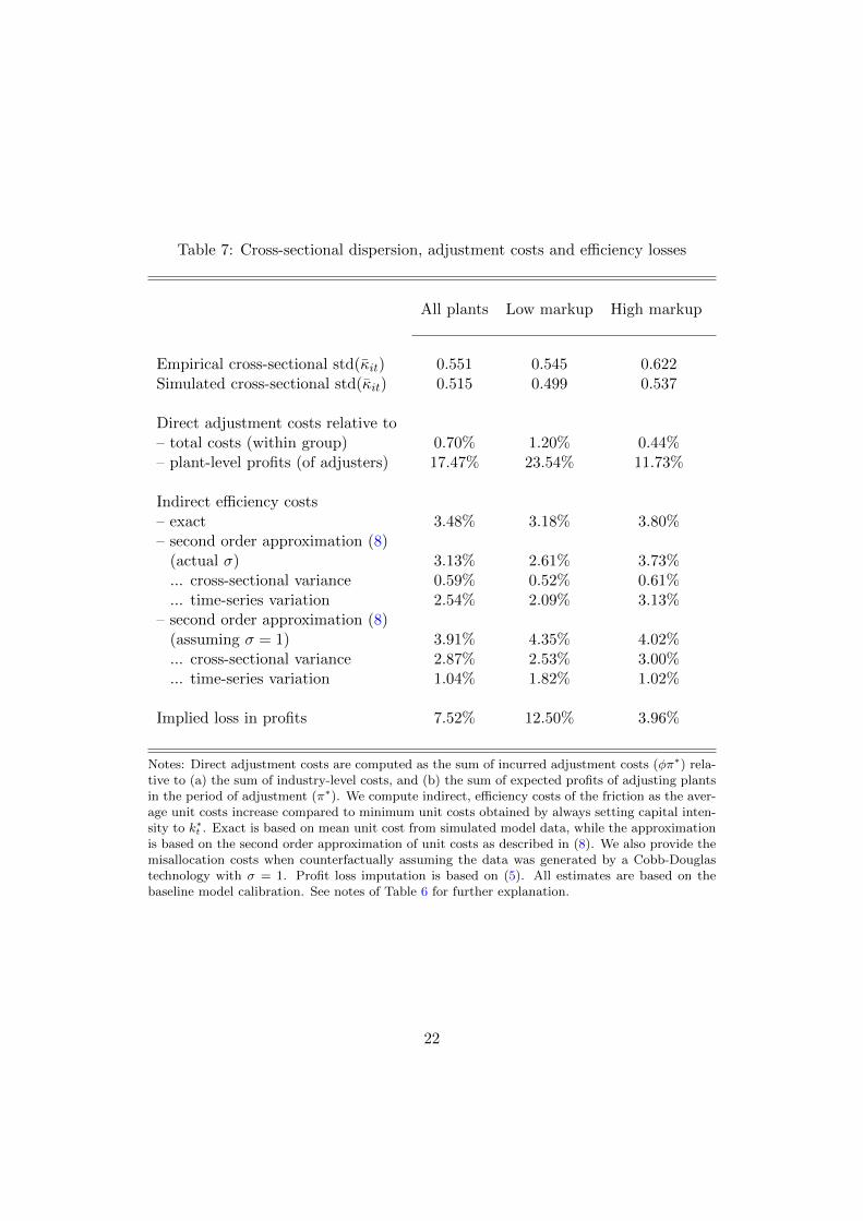
Table 7: Cross-sectional dispersion, adjustment costs and efficiency losses

All plants Low markup High markup

Empirical cross-sectional std(κit) 0.551 0.545 0.622Simulated cross-sectional std(κit) 0.515 0.499 0.537

Direct adjustment costs relative to– total costs (within group) 0.70% 1.20% 0.44%– plant-level profits (of adjusters) 17.47% 23.54% 11.73%

Indirect efficiency costs– exact 3.48% 3.18% 3.80%– second order approximation (8)

(actual σ) 3.13% 2.61% 3.73%... cross-sectional variance 0.59% 0.52% 0.61%... time-series variation 2.54% 2.09% 3.13%

– second order approximation (8)(assuming σ = 1) 3.91% 4.35% 4.02%... cross-sectional variance 2.87% 2.53% 3.00%... time-series variation 1.04% 1.82% 1.02%

Implied loss in profits 7.52% 12.50% 3.96%

Notes: Direct adjustment costs are computed as the sum of incurred adjustment costs (φπ∗) rela-tive to (a) the sum of industry-level costs, and (b) the sum of expected profits of adjusting plantsin the period of adjustment (π∗). We compute indirect, efficiency costs of the friction as the aver-age unit costs increase compared to minimum unit costs obtained by always setting capital inten-sity to k∗t . Exact is based on mean unit cost from simulated model data, while the approximationis based on the second order approximation of unit costs as described in (8). We also provide themisallocation costs when counterfactually assuming the data was generated by a Cobb-Douglastechnology with σ = 1. Profit loss imputation is based on (5). All estimates are based on thebaseline model calibration. See notes of Table 6 for further explanation.

22

ductivity is more disperse than labor productivity and that the persistent component

of labor and capital productivity are negatively correlated. The size of the standard

deviations and correlations is almost perfectly in line with the data.

Table 7 provides information on the implied capital intensity dispersion for the high-

est and lowest markup quintile. Again the simulation results are in line with the data;

albeit the differences across groups somewhat smaller. In the actual data, the differences

between markup groups are roughly 30%, in the numerical model they are about 16%.

In addition, the table reports the implied economic costs of the adjustment friction.

Upon adjustment, firms on average forgo roughly 17% of annual profits –i.e. two months

of disruption. Since adjustment is infrequent, the direct costs of adjustment are small

and well below 1% of total expenditures in the economy.

The indirect, efficiency costs of the friction are, however, larger. On average, unit

costs increase by 3.5% compared to their minimum obtained by always setting capital

intensity to k∗t . In terms of foregone profits, the loss is even larger and amounts to 7.5%.

In our setup with isoelastic demand, the consumer and producer rents are proportional

and hence also the loss due to increased unit costs.

We can use (8) to decompose the efficiency loss into its cross-sectional variance

Vxt log kit and its time-series component (Ext log kit − k∗t )2. The calibrated high long-run

elasticity of substitution decreases the overall costs of misallocation for given deviations

of k from its static optimal value, see (8). At the same time it increases the time

fluctuations in log k∗t . Therefore, the cross-sectional variance term becomes of little

importance. Instead, if one looks at the simulated data through the lens of a Cobb-

Douglas production function, the efficiency loss through the cross sectional dispersion

becomes substantially more and the efficiency loss through the time-series term less

important. A Cobb-Douglas framework has been widely applied, e.g. in Hsieh and

Klenow (2009).

5.3 Robustness checks

Next, we ask how sensitive our results are with respect to the targeted aggregate

short-run elasticity, the assumed trend growth of capital intensity, and equating plant

to technology age. The literature reports a broad range for the former with most esti-

mates falling in the range [0.3, 1.3], see (Chirinko, 2008). If we lower the target aggre-

gate short-run substitution elasticity, the calibration pushes up the long-run elasticity

of substitution but lowers the persistence of factor prices to meet the targets for the

fluctuations in the labor share. The reverse holds true if we lower the target aggregate

23

short-run elasticity of substitution.

Table 8: Model robustness for calibration to Germany

unit coststd(αL

it) std(αKit ) ρ(αL

it, αKit ) std(κit) increase (%)

Data 0.23 0.46 -0.21 0.55 -

Baseline 0.18 0.46 -0.14 0.52 3.48

Short-runelasticity 0.5 0.19 0.49 -0.25 0.57 6.51

Short-runelasticity 1.0 0.17 0.40 0.02 0.43 2.13

Zero balancedgrowth (γ = 0) 0.18 0.35 -0.04 0.40 3.25

Match D.log(VA)dispersion 0.17 0.47 -0.18 0.53 3.48

Refurbishment 0.18 0.38 -0.04 0.43 3.41

Notes: Columns 1-4 show dispersion and correlation of persistent movements in labor pro-ductivity, capital productivity, and capital intensity. Column 5 provides the average per-centage increase in unit costs compared to minimum unit costs obtained in the frictionlessmodel. Baseline reports results for the benchmark model calibration, and below rows pro-vide various robustnesses where we change one calibration target or parameter, and (fully)recalibrate the model. In the third and fourth row, target short-run substitution elasticityis changed to 0.5 and 1.0, respectively. In the fifth row, we impose zero trend in the relativefactor price, and in the sixth row, we match the cross-firm dispersion in first-differenced logvalue added, D.log(VA). The seventh row shows robustness when calibrating the model tomatch 75% as many old plants as observed empirically, which can be thought of as allow-ing for some plant technology refurbishment. See notes of Table 6 for further explanation.

In terms of productivity and capital intensity dispersions, see Table 8, we slightly

overshoot for the lower target elasticity and undershoot the empirical dispersions for the

higher target.

The table also reports the implied dispersion for a variant of the model that sets trend

growth in capital intensity to zero recalibrating all other parameters. The qualitative

results are robust to the trend growth specification, even though dispersions decrease

by 20%, in terms of standard deviations. Finally, the table also shows that the results

are broadly robust when calibrating to the dispersion of valued added growth, and when

allowing technology adjustment through plant refurbishment, that is adjustment without

24

plant closure.

While we recalibrate all other model parameters for the robustness checks above, we

also ask how much the contribution of fluctuations in factor prices and trend growth are

to the resulting cross sectional dispersions in factor productivities. Table 9 shows the

results. Both elements contribute roughly equally to the dispersion of capital intensities

and factor productivities, however, trend growth in capital intensity creates less of the

negative correlation in labor and capital productivity and also produces less productivity

losses – the largest fraction of the productivity losses in the baseline calibration stemming

from surprise time series fluctuations in optimal capital intensities, see Table 7.

Table 9: Model counterfactuals for calibration to Germany

unit coststd(αL


it, αKit ) std(κit) increase (%)

Data 0.23 0.46 -0.21 0.55 -

Baseline 0.17 0.46 -0.14 0.52 3.48

Zero balancedgrowth (γ = 0) 0.17 0.33 0.03 0.37 3.53

No pricefluctuations(σω = 0) 0.17 0.39 0.11 0.41 0.29

Notes: Rows 3 and 4 provide counterfactuals where we change one model parameterwhile keeping all other model parameters unchanged. We counterfactually impose zerotrend in the optimal capital intensity, and assume a deterministic relative factor price,respectively. See notes of Table 6 and 8 for further explanation.

5.4 Developing economies

Next, we ask whether the model is able to explain international differences. For

this, we should expect substantial international differences in the volatility of relative

factor prices. In fact, unconditional standard deviations of labor shares point in this

direction. The labor share is much more volatile in these countries than in Germany, see

the first column of Table 10. For example, this could be the result of political turmoil

and interventions in the labor market or more volatile access to international capital

markets.

25

Table 10: Technology choice model calibrated to Chile, Colombia, and Indonesia

(a) Recalibrate σω

labor share unit coststd (%) std(αL


it, αKit ) std(κit) incr. (%) σω

DE D 3.30 0.23 0.46 -0.21 0.55 – –M 3.30 0.18 0.46 -0.14 0.52 3.48 0.30

CL D 5.22 0.23 0.58 -0.19 0.66 – –M 5.21 0.21 0.52 -0.38 0.63 5.00 0.38

CO D 5.07 0.26 0.57 -0.23 0.68 – –M 5.09 0.21 0.52 -0.37 0.63 4.91 0.37

ID D 5.45 0.26 0.67 -0.27 0.78 – –M 5.44 0.22 0.53 -0.41 0.65 5.14 0.38

(b) Recalibrate σω, σz, α, A0, ξi

labor share unit coststd (%) std(αL


it, αKit ) std(κit) incr. (%) σω

DE D 3.30 0.23 0.46 -0.21 0.55 – –M 3.30 0.18 0.46 -0.14 0.52 3.48 0.30

CL D 5.22 0.23 0.58 -0.19 0.66 – –M 5.15 0.24 0.43 -0.41 0.57 4.54 0.33

CO D 5.07 0.26 0.57 -0.23 0.68 – –M 5.04 0.30 0.42 -0.60 0.65 3.90 0.30

ID D 5.45 0.26 0.67 -0.27 0.78 – –M 5.47 0.21 0.50 -0.47 0.62 3.28 0.30

Notes: The second column specifies D for Data and M for Model. For the three countries CL, CO, IDin Panel (a) we recalibrate the dispersion in the relative factor price, σω, to match the dispersion in thecountries’ labor share, while in Panel (b) we also recalibrate σz, α, A0, and ξi. See notes of Table 6 and8 for further explanation.

We use these differences in labor share volatility to recalibrate the factor price volatil-

ity. Given the shorter available time series for the less developed economies, we assume

26

that their persistence of the labor share is the same as in Germany. In Table 10, we

conduct two different calibration strategies for these countries. In Panel (a), we only

recalibrate σω and fix all other parameters to the German level. Panel (b), by contrast,

shows the results where we also recalibrate the technological parameters and demand

shocks (σz, α, A0, ξi) to match country-specific moments. In (a), the implied increase

in unit costs from misallocation is almost 80% higher in the developing economies, so is

the variance of relative factor prices (standard deviation in last column). In (b), when

adjusting all other technological parameters, the evidence for less table factor prices and

higher efficiency losses vanishes.

6 Capital adjustment frictions

We have seen that frictional technology adjustment is able to produce productivity

and capital intensity dispersions in size close to what we observe empirically, that it can

explain international differences in the persistent component of productivity differences

across plants as well as differences across firms with different markups.

Yet, is it the friction in technology adjustment, or can the observed dispersions be

actually explained by any adjustment friction? Asker et al. (2014) show that capital

adjustment frictions can lead to sizeable productivity dispersions and are able to explain

international differences in capital productivity dispersions as well. However, they do not

split up productivity differences across firms in a persistent and a transitory component

and do not report cross-factor correlations. We therefore adapt our technology choice

model by replacing the technology friction with a capital adjustment friction. As in

Asker et al., we allow for both fixed and convex capital adjustment costs. We provide

more details on model setup and calibration in Appendix E.

Table 11 reports the results of this exercise. As shown in as in Asker et al. (2014),

capital adjustment frictions can explain the overall dispersions in capital productivities

well and in our model account for 88% of the total empirical variance. However, the

model generates long-lived differences in capital productivity that are too small compared

to the data (55% of the variance) and short-lived differences that are too large (330% of

the variance). In addition, the correlations between labor and capital productivity show

the wrong signs when split into transitory and persistent components. This mechanically

implies transitory differences in capital intensity making up a large part (40%) of the

model’s total capital-intensity variance. Again this stands in sharp contrast to the data.

Appendix E shows that these patterns are highly robust to the model calibration.

The reason for this lies in the basic mechanics of any model with different degrees of

27

Table 11: Transitory and persistent components of factor productivities, markups, andcapital intensities in the capital adjustment model



Kit )

Data 0.07 0.12 0.35 0.23 0.46 -0.21

Baseline 0.02 0.25 -0.92 0.15 0.37 0.40


Kit )

Data 0.06 0.11 -0.16 0.17 0.55 0.06

Baseline 0.03 0.27 -0.82 0.15 0.34 -0.38

Notes: Baseline provides model results under the benchmark calibration. See notes of Table 6 and 8for explanations.

flexibility in labor and capital. When one factor is more flexible than the other, a firm

will use the more flexible factor strongly to accommodate shocks to its optimal scale. For

example, as demand z in the capital-adjustment model goes up, the firm wants to raise

production and will do so by hiring more labor on impact and only subsequently adjust

capital. Therefore, capital intensity drops on impact and recovers thereafter. This shows

how idiosyncratic shocks to optimal scale translate directly into transitory idiosyncratic

movements in capital intensity in any model that features different degrees of flexibility

of labor and capital. As discussed before, our calibrated model indeed implies too large

transitory differences in capital intensity relative to persistent ones.

7 Conclusion

This paper asks whether productivity dispersions should be understood as a result of

frictions in technology choice. We have derived qualitative and quantitative implications

of such friction and show that these are borne out empirically.

In line with the existing literature, we find large productivity differences across firms/

plants even within narrowly defined industries. We show that most of the differences

are long lived and related to highly persistent differences in capital intensity. Finally,

28

grouping the sample by average markup we show that the within group cross-sectional

dispersion of capital intensity is largest for the group with the highest markup.

We offer a new explanation to these empirical findings developing a quantitative

dynamic model of technology choice, where adjustment of capital intensity is subject to

a disruption cost. This model, calibrated to the time series behavior of the labor share,

can explain the salient features of the data as well as the cross-country and cross-markup

group differences.

The model also allows us to quantify the efficiency and welfare losses arising from the

technology friction. We focus on losses in productive efficiency and disregard allocative

inefficiency to be conservative in the estimate. Allocative inefficiency in the data shows

up as markup differences, which in our model arise from differences in demand elasticities

and demand shocks. The quantified welfare losses from productive inefficiency and their

differences across countries are modest compared to the literature that includes allocative

inefficiencies.

For future work it would hence be interesting to explore in more detail the reasons for

large differences across countries in cross-sectional markup dispersions – i.e. in allocative

efficiency. Here, the interesting fact is that the cross-sectional markup dispersion is by

and large the same in all countries when looking at persistent markup differences, while

the dispersion of transitory markup differences starkly differ.

References

Acemoglu, D., Antras, P., and Helpman, E. (2007). Contracts and Technology Adoption.

American Economic Review, 97(3):916–943.

Amaral, P. S. and Quintin, E. (2010). Limited Enforcement, Financial Intermediation,

And Economic Development: A Quantitative Assessment. International Economic

Review, 51(3):785–811.

Asker, J., Collard-Wexler, A., and De Loecker, J. (2014). Dynamic inputs and resource

(mis)allocation. Journal of Political Economy, 122(5):1013 – 1063.

Bachmann, R. and Bayer, C. (2013). Wait-and-see business cycles? Journal of Monetary

Economics, 60(6):704 – 719.

Bachmann, R. and Bayer, C. (2014). Investment dispersion and the business cycle.


29

Bachmann, R., Bayer, C., and Seth, S. (2011). Elflop establishment labor flow panel.

Documentation, IAB. Documentation, IAB.

Banerjee, A. V. and Moll, B. (2010). Why Does Misallocation Persist? American

Economic Journal: Macroeconomics, 2(1):189–206.

Bar-Isaac, H., Caruana, G., and Cunat, V. (2012). Search, design, and market structure.


Bester, H. and Petrakis, E. (1993). The incentives for cost reduction in a differentiated

industry. International Journal of Industrial Organization, 11(4):519–534.

Blalock, G. and Gertler, P. J. (2009). How firm capabilities affect who benefits from

foreign technology. Journal of Development Economics, 90(2):192–199.

Buera, F. J., Kaboski, J. P., and Shin, Y. (2011). Finance and Development: A Tale of

Two Sectors. American Economic Review, 101(5):1964–2002.

Calvo, G. (1983). Staggered prices in a utility-maximizing framework. Journal of Mon-

etary Economics, 12(3):383–398.

Cantore, C. and Levine, P. (2012). Getting normalization right: Dealing with ‘dimen-

sional constants’ in macroeconomics. Journal of Economic Dynamics and Control,

36(12):1931–1949.

Chirinko, B. (2008). [sigma]: The long and short of it. Journal of Macroeconomics,

30(2):671–686.

David, J., , Hopenhayn, H. A., and Venkateswaran, V. (2013). The Informativeness of

Stock Prices, Misallocation and Aggregate Productivity. 2013 Meeting Papers 455,

Society for Economic Dynamics.

Foster, L., Haltiwanger, J., and Syverson, C. (2008). Reallocation, Firm Turnover,

and Efficiency: Selection on Productivity or Profitability? The American Economic

Review, 98(1):394–425.

Gilchrist, S. and Williams, J. C. (2000). Putty-Clay and Investment: A Business Cycle

Analysis. Journal of Political Economy, 108(5):928–960.

Gilchrist, S. and Williams, J. C. (2005). Investment, Capacity, and Uncertainty: A

Putty-Clay Approach. Review of Economic Dynamics, 8(1):1–27.

30

Gopinath, G., Kalemli-Ozcan, S., Karabarbounis, L., and Villegas-Sanchez, C. (2015).

Capital allocation and productivity in south europe. Working Paper 21453, National

Bureau of Economic Research.

Gourio, F. (2011). Putty-clay technology and stock market volatility. Journal of Mone-

tary Economics, 58(2):117–131.

Gourio, F. and Rudanko, L. (2014). Customer Capital. Review of Economic Studies,

81(3):1102–1136.

Henriquez, C. (2008). Stock de Capital en Chile (1985-2005): Metodologia y Resultados.

Central Bank of Chile, -:–.

Hsieh, C.-T. and Klenow, P. J. (2009). Misallocation and Manufacturing TFP in China

and India. The Quarterly Journal of Economics, 124(4):1403–1448.

Johansen, L. (1959). Substitution versus Fixed Production Coefficients in the Theory of

Economic Growth: A Synthesis. Econometrica, 27(2):pp. 157–176.

Kaboski, J. P. (2005). Factor price uncertainty, technology choice and investment delay.

Journal of Economic Dynamics and Control, 29(3):509–527.

Karabarbounis, L. and Neiman, B. (2013). The global decline of the labor share. The

Quarterly Journal of Economics.

Leibenstein, H. (1966). Allocative efficiency vs.” x-efficiency”. The American Economic

Review, pages 392–415.

Midrigan, V. and Xu, D. Y. (2013). Finance and Misallocation: Evidence from Plant-

level Data. Forthcoming in American Economic Review, -:–.

Moll, B. (2014). Productivity Losses from Financial Frictions: Can Self-Financing Undo

Capital Misallocation? Forthcoming in American Economic Review.

Oberfield, E. and Raval, D. (2014). Micro Data and Macro Technology. Working paper,

Princeton University.

Peters, M. (2013). Heterogeneous Mark-Ups and Endogenous Misallocation. mimeo,

LSE.

Piketty, T. (2011). On the long-run evolution of inheritance: France 18202050. The

Quarterly Journal of Economics, 126(3):1071–1131.

31

Piketty, T. (2014). Capital in the Twenty-First Century. Harvard University Press.

Raval, D. (2014). The Micro Elasticity of Substitution and Non Neutral Technology.

Working paper, Federal Trade Commission.

Restuccia, D. and Rogerson, R. (2008). Policy Distortions and Aggregate Productivity

with Heterogeneous Plants. Review of Economic Dynamics, 11(4):707–720.

Restuccia, D. and Santaeulalia-Llopis, R. (2015). Land Misallocation and Productivity.

Working Papers tecipa-541, University of Toronto, Department of Economics.

Solow, R. M. (1956). A contribution to the theory of economic growth. The Quarterly

Journal of Economics, 70(1):65–94.

Vial, V. (2006). New Estimates of Total Factor Productivity Growth in Indonesian

Manufacturing. Bulletin of Indonesian Economic Studies, 42(3):357–369.

32

Appendices

A Empirics

A.1 Description of the data

German Firm Data: USTAN (Unternehmensbilanzstatistiken)

USTAN is itself a byproduct of the Bundesbank’s rediscounting and lending activ-

ity. The Bundesbank had to assess the creditworthiness of all parties backing promis-

sory notes or bills of exchange put up for rediscounting (i.e. as collateral for overnight

lending). It implemented this regulation by requiring balance sheet data of all parties

involved, which were then archived and collected, see Bachmann and Bayer (2013) for

details. Our initial sample consists of 1,846,473 firm-year observations. We remove ob-

servations from East German firms to avoid a break of the series in 1990. Finally, we drop

the following sectors: hospitality (hotels and restaurants), financial and insurance insti-

tutions, public health and education sectors. The resulting sample covers roughly 70%

of the West-German real gross value added in the private non-financial business sector.

In particular, it includes Agriculture, Energy and Mining, Manufacturing, Construction,

and Trade.

Chilean Plant Data: ENIA (Encuesta Nacional Industrial Anual)

ENIA is collected by the National Institute of Statistics (Instituto Nacional de Estad-

sticas, INE) and provides plant-level data from 1995 to 2007. ENIA contains information

for all manufacturing plants with total employment of at least ten. For the period under

analysis, we have a sample of 70,217 plant-year observations. According to INE, this

sample covers about 50% of total manufacturing employment.

Colombian Plant Data: EAM (Encuesta Anual Manufacturera)

EAM is a plant-level survey collected by National Institute of Statistics (Departa-

mento Administrativo Nacional de Estaditicas, DANE) for the period 1977 to 1991. The

survey covers information for all manufacturing plants during 1977-1982, while it only

contains data on plants above 10 employees for 1983-1984, and from 1985, small plants

are included in small proportion. This results in 103,011 plant-year observations.

Indonesian Plant Data: IBS (Survei Tahunan Perusahaan Industri Pengolahan)

IBS is the Indonesian Manufacturing Survey of Large and Medium Establishments,

33

provided by the National Institute of Statistics (Badan Pusat Statistik, BPS). The survey

covers all plants with 20 or more employees in the manufacturing sector. Given that the

capital stock is reported since 1988 onwards, we exclude earlier years and focus on the

period 1988-2010, with 485,052 plant-year observations.

A.2 Sample selection

Starting from the raw data set, we concentrate on describing the general cleaning

steps common to all countries, and we provide more information about country-specific

cleaning steps at Table 12.

To begin with, we remove observations where firms or plants report extraordinarily

large depreciation rates (e.g. due to fire or accident). The reason is that our dynamic

model does not capture such cases, and the perpetual inventory method (PIM) will

inaccurately measure the actual capital stock after such incidents occur.14 Next, for

those countries where current values of capital stock is not provided (Germany and

Colombia), we recompute capital stocks using the PIM. In conducting the PIM, we drop

a small amount of outliers, as explained in Section A.4. Further, we do not consider

observations where value-added, capital stock, or employment is non-positive or missing.

Moreover, we do not consider observations where firms/plants have missing values

in the changes of employment (N), real capital (K) and real value-added (VA).15 To

construct capital productivity, we use the lagged value of capital stock, so we effectively

discard the first year of each micro unit. We remove outliers in the levels and in the rela-

tive changes of employment, capital, value-added, and factor shares based on 3 standard

deviations from the industry-year mean. In addition, we drop firm/plant-year obser-

vations whenever the total factor expenditures share is either below 1/3 or above 3/2,

and whenever the firm/plant average total factor expenditure share is above 1. These

two cleaning steps should exclude units from our analysis which report continuously

unreasonably large markups or losses.

Finally, as our empirical results rely on a 5-year moving average filter, we do not

consider firm/plant-year observations that have less than 5 consecutive years.

14At some cases in the ENIA, EAM, and IBS surveys, plants do not report depreciation conditional onpositive capital stock. In order to not loose this observations, we impute the depreciation by capital typeand two-digit industry, estimating a random effect model, using as explanatory variable the log-capitalstock. To discard rare depreciation events, we drop observations whenever the reported depreciationrate in structures (equipment) is above 40% (60%) yearly. Additionally, we do not consider those caseswhere the reported depreciation is below 0.1% (1%) in structures (equipment), yearly.

15To construct measures of real capital stock we consider an index price by each capital type (whenavailable) using the information of gross fixed capital formation at current and constant prices fromNational Accounts, while for for value added we use the GDP price deflator.

34

Table 12: Sample selection

Criterion/Country Germany Chile Colombia Indonesia

Initial sample 1,846,473 70,217 103,006 485,052

East Germany -115,201 – – –Additional cleaning steps – – – -32,618Imputation capital stock – – – +37,341Rare depreciation events -54,280 -8,197 -6,176 -8,775Outliers in PIM -73,784 – -4,280 –Missing values -422,739 -19,589 -29,804 -235,280Outliers in factor variables -176,232 -12,375 -24,651 -86,070Less than 5 consecutive years -312,452 -15,479 -14,264 -84,885

Final sample 689,665 14,307 23,831 74,765

Notes: Missing values denote the sum of missing values at log value added, log capital, factorshares and log changes in employment, capital and value added. Outliers in factor variablesis the sum of all identified outliers at log changes in employment, real capital and real valueadded, and factor shares. For more information with respect to Additional cleaning stepsand Imputation of capital stock in Indonesia, see Section A.3.

A.3 Specific cleaning and imputation steps for IBS

Before proceeding with the general cleaning steps applied to all datasets, we need

to implement some specific corrections in the Indonesia micro data. In doing so, we

closely follow Blalock and Gertler (2009). First, we correct for mistakes due to data

keypunching. If the sum of the capital categories is a multiple of 10n (with n being an

integer) of the total reported capital, we replace the latter with the sum of the categories.

Second, we drop duplicate observations within the year (i.e. observations which have the

same values for all variables in the survey but differ in their plant identification number).

Third, we re-compute value added whenever their values are not consistent with the

formula provided by BPS. Finally, the survey changed their industry classification from

ISIC Rev. 2 in 1998 to ISIC Rev. 3 in 1999 and to ISIC Rev. 4 in 2010. We use United

Nations concordance tables to construct a consistent time series of four digit industry

classification.

Further, the surveys from 1996 and 2006 provides only information on the aggregate

capital stock, yet, not disaggregated by capital type (structure and equipment). To con-

struct an economically reasonable estimate of these variables for these years, we use the

average reported investment share and capital share of capital type in the preceding and

subsequent year, and impute it, multiplying the aggregate capital stock and investment

with the respective share.

35

Finally, we impute capital stock for plants, whenever the survey presents missing val-

ues for this variable in plants which reported information in previous and/or subsequent

years. Following Vial (2006), we impute capital by type (machinery, vehicles, land and

buildings), using the following regression by two-digit sectoral level:

logKit = β0 + β1 logKit−1 + θ lnXit−1 + µi + εit

where Kit is the capital stock of type i, µi plant fixed effects and Xit−1 a set of ex-

planatory variables (total output, input, employees, wages, fuel costs and expenditures

on materials, leasing, industrial services and taxes).16

A.4 Perpetual inventory method

Whenever the dataset does not directly provide information on a firm’s/plant’s cap-

ital stock at current values (USTAN and EAM), we re-calculate capital stocks using the

perpetual inventory method (PIM), in order to obtain economically meaningful capital

series. In doing so, we follow (Bachmann and Bayer, 2014). To begin with, we compute

nominal investment series using the accumulation identity for capital stocks:

pIt Ii,k,t = Kri,k,t+1 −Kr

i,k,t +Dri,k,t,

where Kri,k,t and Dr

i,k,t are firm/plant i’s reported capital stock and depreciation for

capital type k at time t, respectively. Given that capital is reported at historical prices

and does not reflect the productive (real) level of capital stock, we apply the PIM to

construct economic real capital stock at each type of capital:

Ki,k,1 =pI1pIbase

Kai,k,1; Ki,k,t+1 = Ki,k,t(1− δi,k,t) +

pItpIbase

Ii,k,t, ∀t ∈ [0, T ]

where Kai,k,1 is the accounting value of the capital stock of type k for the first period we

observe the unit, ptpbase

Ii,k,t is the real investments in capital k of firm/plant i at time t

and δi,k,t is the reported depreciation rate of capital k by firm/plant i at time t.17

Even though the aforementioned procedure makes sure that values follows a eco-

nomically meaningful real capital stock series from second period onwards, it is not clear

16We evaluate the robustness of the imputation procedure, using linear interpolation as an alternativeapproach. Our empirical findings are robust to this alternative specification.

17The reported depreciation rate is adjusted such that, on average, it coincides with the economicdepreciation rate given by National Accounts. To deflate investment series, we compute an investmentgood price deflator from each country using the information of gross fixed capital formation at currentand constant prices from National Accounts.

36

whether the starting (accounting) input of capital at the unit, Kai,k,t, reflects the produc-

tive real value. To account and adjust the first period value of capital we use an iterative

approach. In specific, we construct a time average factor φk for each type of capital.

It the first iteration step, the adjustment factor takes value of 1 while capital is equal

to its balanced sheet value. That is, Kni,k,t =

pItpIbase

Kai,k,1 for n = 1. For the subsequent

iterations, capital is computed using PIM:

Kni,k,t+1 = Kn

i,k,t(1− δi,k,t) +ptpbase

Ii,k,t,

while the ajdustment factor is constructed using the ratio between the capital of con-

secutive iterations

φnk =1

NT

∑i,t

Kni,k,t

Kn−1i,k,t

.

Finally, the capital stock at the first period we observe the unit is adjusted by the factor

φnk . We apply the procedure iteratively until φk converges18

Kni,k,1 = φn−1

k Kn−1i,k,1.

A.5 Robustness

We conduct four robustness checks. First, we decompose between persistent and

transitory components using either a nine year moving average filter or a HP-Filter

(λ = 6.25). Second, we compute the dispersion and correlations of the persistent and

transitory component (given a five year moving average filter) using the interquantile

range and Spearman’s rho. Third, we compute transitory and persistent dispersions,

weighting by the firm/plant-year log real value added. Finally, we analyze the linear

relation between markups and the persistent component of capital-intensity. To do so,

we apply a two-step OLS regression. In particular, we first remove persistent differences

in capital intensity that can be explained by markups, size, and age characteristics.

Next, we consider the variance of the estimated residual from the first stage, to regress

as a function of markups, size and age.

To summarize, our findings are robust to each specification. Transitory productivity

18We stop whenenever the value of φk is below 1.1. At each iteration step we drop 0.1% from thebottom and the top of the capital distribution. This cleaning step makes sure to not consider episodesof extraordinary depreciation at the plant, which implies that using reported depreciation rate (adjustedto have the same average value from National Accounts) do not reflect the capital stock given by thePIM.

37

differences are positively correlated while persistent differences are negatively correlated.

Moreover, differences in factor productivities and capital intensity are predominantly

long-lived. Further, the estimated effect of markups on the variance in the persistent

component of capital intensity is positive and significant, even after controlling for size

and age. Lastly, and related with the latter finding, given that markups, size, and age

are standarized in the second step from this OLS regression, we can get an idea of the

explanatory importance of each variable. For all countries, markups are at least as

important as size when explaining persistent differences in capital-intensity.

38

Table 13: Robustness: Transitory and persistent components of factor productivities

std(aLit) std(aKit ) ρ(aLit, aKit ) std(aLit) std(aKit ) ρ(aLit, a

Kit )

Transitory Component (9Y MA) Persistent Component (9Y MA)

DE 0.074 0.140 0.350 0.204 0.406 -0.203

CL 0.190 0.313 0.394 0.188 0.482 -0.206

CO 0.153 0.200 0.471 0.218 0.502 -0.242

ID 0.214 0.415 0.274 0.203 0.583 -0.300

Transitory Component (HP) Persistent Component (HP)

DE 0.062 0.113 0.352 0.236 0.471 -0.223

CL 0.169 0.260 0.447 0.231 0.578 -0.191

CO 0.134 0.159 0.516 0.257 0.569 -0.234

ID 0.196 0.343 0.344 0.256 0.670 -0.270

Transitory Component (IQR-SP) Persistent Component (IQR-SP)

DE 0.071 0.129 0.368 0.276 0.556 -0.189

CL 0.209 0.330 0.479 0.297 0.702 -0.161

CO 0.163 0.207 0.487 0.324 0.721 -0.202

ID 0.231 0.419 0.351 0.334 0.856 -0.257

Notes: Labor productivity, aLit, and capital productivity, aKit , as defined in (9). 9YMA: resultsbased on the decomposing between transitory and persistent using a nine year moving averagefilter. HP: results based on the decomposing between transitory and persistent using a HP-filter (λ = 6.25) . IQR-SP: Interquartile range and Spearman’s rank correlation when applyinga five year moving average filter to decompose between frequencies. Factor productivities aredemeaned by 4-digit industry and year and expressed in logs. Standard errors are clusteredstandard errors at the firm/plant level. ρ denotes correlation. DE: Germany, CL: Chile, CO:Colombia, ID: Indonesia.

39

Table 14: Robustness: Transitory and persistent components of markup and capitalintensity

std(mcit) std(κit) ρ(mcit, κit) std(mcit) std(κit) ρ(mcit, κit)


DE 0.073 0.134 -0.184 0.157 0.490 0.089

CL 0.183 0.295 -0.123 0.152 0.552 -0.097

CO 0.145 0.186 -0.066 0.178 0.594 -0.230

ID 0.207 0.412 -0.130 0.160 0.672 -0.027

Transitory Component (HP) Persistent Component (HP)

DE 0.060 0.108 -0.157 0.175 0.572 0.055

CL 0.163 0.238 -0.089 0.184 0.663 -0.088

CO 0.124 0.146 -0.014 0.206 0.677 -0.231

ID 0.189 0.331 -0.123 0.196 0.779 -0.021

Transitory Component (IQR-SP) Persistent Component (IQR-SP)

DE 0.072 0.117 -0.155 0.223 0.665 0.063

CL 0.209 0.277 -0.106 0.258 0.812 -0.087

CO 0.151 0.184 -0.014 0.289 0.854 -0.257

ID 0.226 0.380 -0.119 0.274 0.992 -0.031

Notes: Markups, mcit, and capital intensity, κit, as defined in (10) and (11). 9YMA: resultsbased on the decomposing between transitory and persistent using a nine year moving averagefilter. HP: results based on the decomposing between transitory and persistent using a HP-filter (λ = 6.25) . IQR-SP: Interquartile range and Spearman’s rank correlation when applyinga five year moving average filter to decompose between frequencies. Factor productivities aredemeaned by 4-digit industry and year and expressed in logs. Standard errors are clusteredstandard errors at the firm/plant level. ρ denotes correlation. DE: Germany, CL: Chile, CO:Colombia, ID: Indonesia.

40

Table 15: Robustness: Weighted second moments of factor productivities, markups andcapital intensity at different frequencies


Kit )


DE 0.050 0.101 0.316 0.196 0.457 -0.176

CL 0.187 0.281 0.457 0.239 0.551 -0.205

CO 0.143 0.170 0.520 0.260 0.562 -0.239

ID 0.216 0.370 0.349 0.263 0.672 -0.275

std(mcit) std(κit) ρ(mcit, κit) std(mcit) std(κit) ρ(mcit, κit)


DE 0.052 0.090 -0.161 0.172 0.503 0.067

CL 0.179 0.259 -0.090 0.183 0.645 -0.087

CO 0.133 0.155 -0.016 0.209 0.670 -0.237

ID 0.207 0.356 -0.123 0.198 0.787 -0.021

Notes: abor productivity, aLit, and capital productivity, aKit , as defined in (9). Markups, mcit,and capital intensity, κit, as defined in (10) and (11). Cross-sectional standard-deviations (std)and correlation (ρ) of transitory and persistent components. Transitory and persistent compo-nents are obtained by applying a five year moving average filter (5Y MA). Moments are weightedbased on the value-added of the plant/firm. Variables under interest are demeaned by 4-digitindustry and year and expressed in logs. Standard errors in parentheses are clustered standarderrors at the firm/plant level. DE: Germany, CL: Chile, CO: Colombia, ID: Indonesia.

41

Table 16: Robustness: Regression on the variance in the unexplained persistent compo-nent of capital-intensity

DE CL CO ID

var(εκit)

Log-Markup 0.024 0.069 0.036 0.057(0.003) (0.017) (0.019) (0.011)

Log-Size -0.026 -0.068 -0.057 0.017(0.003) (0.017) (0.024) (0.015)

Log-Age - 0.044 0.009- (0.018) (0.011)

Notes: The results are obtained using a two step OLS regres-sion estimation. First, we regress the persistent component oflog capital intensity (κ) with respect to the demeaned log ofmarkups, size and age. Second, the variance of the estimatedresidual from the first stage (εκit), is regressed as a function ofthe standarized log of markups, size and age. Standard errorsin parentheses are clustered standard errors at the firm/plantlevel. DE: Germany, CL: Chile, CO: Colombia, ID: Indonesia.

42

B Second order approximation of unit costs around k∗

For convenience, let us define the relative factor price by Rt := RtWt

and (physical)

output per worker by

f(kit) :=YitNit

=

[αk

σ−1σ

it + (1− α)Aσ−1σ

t

] σσ−1

.

Subsequently, marginal costs may be expressed as

cit = Wt1 + Rtkitf(kit)

and the first derivative of (log) marginal costs with respect to (log) capital intensity,

∂ log(cit)

∂ log(kit)=

Rtkit

1 + Rtkit− kitf

′(kit)

f(kit)

=(1− α)Rtkit − αk

σ−1σ

it

(1 + Rtkit)(αkσ−1σ

it + (1− α)Aσ−1σ

t )

Let us denote above denominator by D ≡ (1 + Rtkit)(αkσ−1σ

it + (1−α)Aσ−1σ

t ), and obtain

the second derivative as

∂2 log(cit)

∂ log(kit)2=

[(1− α)A

σ−1σ

t Rt − σ−1σ αk

− 1σ

it

]kitD −

[(1− α)A

σ−1σ

t Rtkit − αkσ−1σ

it

]D′kit

D2.

The cost-minimizing capital intensity k∗ implies ∂ log(cit)∂ log(kit) kit=k∗

= 0, and the second

derivative evaluated at kit = k∗, where (1− α)Aσ−1σ

t Rtk∗it = αk

∗σ−1σ

it , is

∂2 log(cit)

∂ log(kit)2 kit=k∗=

(1− α)Aσ−1σ

t Rtk∗it − σ−1

σ αk∗σ−1

σit

D

=(1− α)A

σ−1σ

t1σ Rtk

∗it

(1 + Rtk∗)((1− α)Aσ−1σ

t Rtk∗ + (1− α)Aσ−1σ

t )=

1

σ

Rtk∗

(1 + Rtk∗)2,

43

where the second equation results again from (1−α)Aσ−1σ

t Rtk∗ = αk∗

σ−1σ . The 2nd order

Taylor expansion directly follows as

log(cit)− log(c∗) ≈ σ−1 Rtk∗

(1 + Rtk∗)2

1

2(log(kit)− log(k∗))2.

C Dynamic Planning Problem

C.1 Existence and uniqueness

In the following, we show the existence and uniqueness of the model described by (1),

(12), (13), and (14).

Assumption 1: α ≤ 11+ξ .

Lemma: The function π∗(k, z, ω) is bounded from above and below in k, ∀z, ω.

Proof: Since π∗(k, z, ω) is continuous, it is sufficient to show that limk→∞ |π∗(k, z, ω)| <∞. If this is the case, then π∗(k, z, ω) is bounded for k → ∞ and by the Weierstrass

extreme value theorem, it is bounded for any finite interval [0, c] ∀c ∈ < and hence

bounded everywhere. Defining f(k) := yN =

[αk

σ−1σ + (1− α)A

σ−1σ

] σσ−1

, see (6), and

using (1), we obtain profits as

π∗(k, z, ω) =ξ

1− ξE[zξ]

1ξ

[E[W +Rk]

f(k)

] ξ−1ξ

.

Let us check whether limk→∞ |π∗(k, z, ω)| exists. It suffices to check f(k)E[W+Rk] ; for σ 6= 1:

limk→∞

f(k)

E[W +Rk]

l′Hospital= lim

k→∞

f(k)1σαk−

1σ

E[R]=

α

E[R]limk→∞

[f(k)

k

] 1σ

=α

E[R]limk→∞

[α+ (1− α)A

σ−1σ k−

σ−1σ

] 1σ−1

<∞ (17)

and for σ = 1:

limk→∞

f(k)

W + E[R]k= lim

k→∞

kαA1−α

W + E[R]k=αA1−α

E[R]limk→∞

kα−1 <∞ (18)

Hence, π∗(k, z, ω) is bounded.

Lemma: Let us define the operator T by posing (Tv)(k, z, ω) equal to the right-hand-

side of equation (14). This operator is defined on the set B of all real-valued, bounded and

continuous functions with domain <+×<++×<++. Then T (i) preserves boundedness,

44

(ii) preserves continuity, and (iii) satisfies Blackwell’s sufficient conditions.

Proof: π∗(k, z, ω) is continuous, concave, and bounded in the set of state variables.

(i) Consider u ∈ B bounded below by u and bounded above by u. Then (Tu)(k, z, ω) is

bounded from below and above since π∗(k, z, ω) is bounded as shown before.

(ii) Next, we show that (Tu) is continuous. We note that (Tu) is the maximum of

a constant and a function. Since the function is the sum of two continuous functions

π∗(k, z, ω) and u(k, z, ω), (Tu) is continuous.

(iii) Finally, we need to show that (Tu) satisfies monotonicity and discounting. We note

that if u1, u2 ∈ B and u1(k, z, ω) < u2(k, z, ω) for all k, z and ω, then integrating with

respect to the distributions of z and ω preserves the inequality and hence monotonicity

holds.

We can show discounting since for any u ∈ B and any constant a ∈ <, it holds that

(T [u+ a])(k, z,R) = (Tu)(k, z,R) + βa.

Blackwell’s sufficient conditions for a contraction holds.

Propositon: The model described by (1), (12), (13), and (14) has exactly one solution

(in the metric space B).

Proof: We know from Lemma 2 that T defines a contraction mapping on the metric

space B with modulus β. Existence and uniqueness then follow from the Contraction

Mapping Theorem.

C.2 Computation

To solve the model numerically, we discretize the state space. We apply Tauchen’s

algorithm with 15 grid point to discretize the relative factor price process ω and demand

shocks z. We use 200 grid points for capital intensity, which spans a sufficiently wide

log-spaced grid with grid points not more than 4% distanced from each other, with 4%

being the calibrated annual drift according to the calibration of γ. Adjustment cost

draw φ is discretized into 200 bins. We solve the model using value function iteration.

45

D Further Details: Technology Choice Model

D.1 Dispersions by Markup Quintile

Table 17: Dispersion of persistent movements in capital intensity: Germany

std(κKit ) Q1 Q2 Q3 Q4 Q5

Markup Data 0.545 0.512 0.519 0.539 0.622Model 0.499 0.487 0.493 0.503 0.537

Size Data 0.610 0.525 0.495 0.501 0.509Model 0.504 0.507 0.508 0.501 0.505

Note: Q1-Q5 denote the five quintile groups for markup and size, respectively. We reported dispersionsin persistent capital intensity movements per per quintilie group.

D.2 Further details on calibration

In the baseline model, we obtain and calibrate depreciation rate using the aver-

age depreciation value it the firm-level data in Germany. To do so, we first construct

capital series at each firm using PIM and adjust reported depreciation rate at each

capital type such that it coincides with the economic depreciation rate given by the

Volkswirtschaftliche Gesamtrechnung (VGR).

For γ, we can obtain an estimate using different combinations of the geometric yearly

growth rate of real GDP, manufacturing real output and capital stock relative to popu-

lation, labor force and manufacturing employment. Our estimates go from 2% using real

GDP-Population to 4.3% in Capital stock-Labor Force and 5.8% taking manufacturing

real output-manufacturing Employees. As the bulk of the obtained estimates lies close

to 4%, we use this value as benchmark.19

Further, we calibrate the average demand elasticity ξi for 5 equally large groups

using USTAN data. Next, we construct the average markup at the firm, compute the

average markup in the economy and remove the industry-year fixed effects based on the

four-digit industry classification. Finally, we split the sample in 5 equally large groups

and we compute the average group markup.

19To obtain these estimates we used Penn World Tables (PWT, 8.0), except for the manufacturing-specific series. For the latter, we took National Statistics and ILO Statistics.

46

D.3 Identification

We check whether our model calibration strategy well identifies the model parame-

ters by computing the elasticity of target moments with respect to model parameters.

In particular, we use central finite differences of plus/minus two percent to compute the

gradient. Table 18 shows the matrix containing in rows the elasticity of a given moment

with respect to all parameters. Moments and parameters are sorted corresponding the

discussion in Section 5 relating model parameters to calibration targets. The diagonal

elements of the Jacobian matrix reconfirm our the preceding discussion. E.g. a higher

long-run elasticity of substitution increases the short-run elasticity of substitution. Fur-

thermore, Table 18 shows that our model is (locally) well identified since the Jacobian

matrix has full rank.

Table 18: Elasticity of target moments and parameters

σ λφ σz ρω σω α A0 µz

Short-runsubstitution elasticity 1.63 0.53 -0.02 7.05 1.23 1.99 -1.02 0.00Share ofold plants -0.17 -0.29 -0.09 -0.80 -0.39 -0.87 0.59 0.00Dispersion oflog(VA) 0.00 -0.00 0.98 -0.00 0.01 0.01 -0.09 0.00Labor shareautocorrelation 0.43 0.09 -0.04 1.30 0.27 0.38 -0.20 0.00Labor sharedispersion 1.72 0.35 0.00 4.72 1.79 3.85 -2.29 -0.00Transformed capitalshare -0.00 0.00 -0.00 0.03 -0.01 0.91 -0.62 0.00Transformed laborshare 2.04 -0.01 0.00 -0.06 -0.03 -0.31 0.20 -0.00Averageexpenditures 0.05 0.01 -0.10 0.14 0.08 0.37 1.75 1.00

Notes: This table is based on the baseline calibration for Germany and provides the elasticitiesof the calibration targets with respect to the model parameters.

47

E Further Details: Capital Adjustment Model

E.1 Model setup and calibration

We assume a one-period production lag as an adjustment friction on labor and instead

of the frictional technology choice, we assume a disruption cost of capital adjustment

and convex capital adjustment costs. Analogously to (1), we first define the profit max-

imizing output/employment decision and the corresponding maximal level of expected

next period’s profits

πCA∗(K, z, ω) = maxN ′

Ez′,ω′{z′ξ [y(K,N ′)]1−ξ

1− ξ−WN ′ −RK

},

where output y is given by

y(K,N) =[αK

σ−1σ + (1− α)(AN)

σ−1σ

] σσ−1

.

Given the disruption cost, the firm chooses between adjusting the stock of capital and

staying put every period, the value of which being va and vn, respectively. On the

other side, the convex cost renders large capital adjustments less attractive. The firm’s

dynamic problem is described by the following Bellmann equation.

v(K, z, ω) = βmax{va(K, z, ω), vn(K, z, ω)

}va(K, z, ω) = max

K′

{(1− φF )πCA∗(K ′, z, ω)− φCK

(K ′ −KK

)2

+ Ez′,ω′[v(K ′, z′, ω′)

]}vn(K, z, ω) = πCA∗((1− δ)K, z, ω) + Ez′,ω′

[v((1− δ)K, z′, ω′)

]Our calibration strategy corresponds as closely as possible with the one employed

in the technology adjustment model. We identify the volatility of demand shocks σz

from value added growth fluctuations, we choose the production function parameters to

match ψN,K and to match an aggregate short-run elasticity of 0.75, and we also match the

labor share fluctuations. Again, we simulate five groups of firms with different demand

elasticities to capture persistent markup differences across the five empirical quintiles.

There is one major difference in the calibration strategy: To calibrate fixed and convex

adjustment costs, we target the skewness and kurtosis of gross investment rates for the

German USTAN data as in Bachmann and Bayer (2013).

48

E.2 Robustness

Table 19 shows that the results are robust to alternative calibrations of the capital

adjustment model. That is, to fixing the parameters of the ω-process to the values

calibrated for technology adjustment and to matching the variance of value added growth

instead of value added. Matching value added dispersions, creates substantially larger

shocks to z than matching value added growth dispersions and is closer to Asker et al.’s

calibration and results.

The qualitative results are not altered by any of the considered calibration strategies:

the cross-factor correlations show the wrong sign compared to the data and the transitory

differences in capital intensity explain counterfactually about 40% of the total capital-

intensity variance.

49

Table 19: Robustness of capital adjustment costs model, Germany



Kit )

Data 0.07 0.12 0.35 0.23 0.46 -0.21

Baseline 0.02 0.25 -0.92 0.15 0.37 0.40D.log(VA) 0.01 0.14 -0.91 0.15 0.23 0.74Ela. 0.5 0.01 0.22 -0.86 0.14 0.41 0.62Ela. 1.0 0.03 0.29 -0.92 0.15 0.41 0.3050% σω 0.02 0.31 -0.94 0.15 0.38 0.34


Kit )

Data 0.06 0.11 -0.16 0.17 0.55 0.06

Baseline 0.03 0.27 -0.82 0.15 0.34 -0.38D.log(VA) 0.02 0.15 -0.93 0.15 0.16 -0.31Ela. 0.5 0.02 0.23 -0.85 0.16 0.34 -0.59Ela. 1.0 0.03 0.32 -0.79 0.15 0.39 -0.3650% σω 0.04 0.33 -0.88 0.15 0.35 -0.38

Notes: In the third row, D.log(VA) is as the baseline model but targets the cross sectional dispersion offirst differences of log value added instead of the dispersion in log value added. Ela. 0.5 and 1.0 referto changing the target aggregate short-run substitution elasticity to 0.5 and 1.0, respectively. 50% σωrecalibrates the model with a 50% smaller dispersion in relative factor dispersion. See notes of Table 6and 8 for further explanation.

50

Productivity Dispersions: Could it simply be technology ...

Documents

Transcript of Productivity Dispersions: Could it simply be technology ...