Shape optimization of a microalgal raceway to enhance

productivity

Olivier Bernard a, Liudi Lu b, Jacques Sainte Marie b, Julien Salomon b

aUniversite Nice Cote d’Azur, INRIA Sophia Antipolis Mediterranee, BIOCORE Project-Team, BP93, 06902Sophia-Antipolis Cedex, France

bINRIA Paris, ANGE Project-Team, 75589 Paris Cedex 12, France and Sorbonne Universite, CNRS, LaboratoireJacques-Louis Lions, 75005 Paris, France

Abstract

We consider a coupled physical-biological model describing growth of microalgae in a raceway pond cultivation process,accounting for hydrodynamics. Our approach combines a biological model (based on the Han model) and shallow waterdynamics equations that model the fluid into the raceway pond. We present an optimization procedure dealing with thetopography to maximize the biomass production over one lap or multiple laps with a paddle wheel. On the contrary to awidespread belief in the microalgae field, the results show that a flat topography is optimal in a periodic regime. In otherframeworks, non-trivial topographies can be obtained. We present some of them, e.g., when a mixing device is included in themodel.

Key words: microalgae, hydrodynamic, optimization, han model, shallow water systems

1 Introduction

Numerical design of microalgae production technologies has been for one decade a source of many interesting chal-lenges not only in engineering but also in the area of scientific computing [7,15,20,12]. The potential of these emergingphotosynthetic organisms finds interests for the cosmetics, pharmaceutical fields, feed, food and - in the longer term- green chemistry and energy applications [19]. Outdoor production is mainly carried out in open bioreactors with araceway shape. Algae grow while exposed to solar radiation in such circular basins, where the water is set in motionby a paddle wheel [5] which homogenizes the medium for ensuring an equidistribution of the nutrients and guaranteesthat each cell will have regularly access to light [6]. The algae are periodically harvested, and their concentration ismaintained around an optimal value [17,18]. Light penetration is strongly reduced by the algal biomass, resultingin limited algal concentrations, which stay below 1% [4] of the liquid mass. Above this value, the light extinctionis so high that a large fraction of the population evolves in the dark and does not grow anymore. At low biomassdensity, a fraction of the solar light is not used by the algae and the productivity is suboptimal. Theoretical workshave determined the optimal biomass for maximising productivity [14,10]. Remark that other possibilities exist toimprove the entire photoproduction process in order to optimize its potential. For instance, a non flat topographyshape has been observed to improve the growth rate of the algae in a specific case in [2]. Here, we are going to provethis result, considering different cases. For this we develop a coupled model to describe the growth of algae in araceway pond, accounting for the light that they receive. More precisely, extending the study of [1] by combiningthe Han photosynthesis equations with an hydrodynamic law based on the shallow water equations.

This approach enables us to formulate an optimization problem where the raceway topography is designed tomaximize the productivity. For this problem, we present an adjoint-based optimization scheme which includes the

Email addresses: olivier.bernard@inria.fr (Olivier Bernard), liudi.lu@inria.fr (Liudi Lu),jacques.sainte-marie@inria.fr (Jacques Sainte Marie), julien.salomon@inria.fr (Julien Salomon).

1

arX

iv:2

011.

0491

3v1

[m

ath.

NA

] 9

Nov

202

0

constraints associated to the shallow water regime. On the contrary to a widespread belief, we prove that the flattopography is optimal in a periodic case for productivity in laminar regime. However, non-trivial topographies can beobtained in other contexts, e.g., when an extra mixing strategy is included in the model. Note that in the examplesconsidered in our numerical tests such topographies only slightly improved the biomass production.

The outline of the paper is as follows. In Section 2, we present the biological and hydrodynamic models underlyingour coupled model. In Section 3, we describe the optimization problem and a corresponding numerical optimizationprocedure. Section 4 is devoted to the numerical results obtained with our approach. We conclude in Section 5 withsome perspectives opened by this work.

2 Coupling hydrodynamic and biological models

Our approach is based on a coupling between the hydrodynamic behavior of the particles and the evolution of thephotosystems driven by the light intensity they receive when traveling across the raceway pond.

2.1 Modeling the photosystems dynamics

We consider the Han model [11] which describes the dynamics of the reaction centers. These subunits of the pho-tosynthetic process harvest photons and transfer their energy to the cell to fix CO2. In this compartmental model,the photosystems can be described by three different states: open and ready to harvest a photon (A), closed whileprocessing the absorbed photon energy (B), or inhibited if several photons have been absorbed simultaneously (C).The relation of these three states are presented in Fig. 1.

A B CσI kdσI

τ−1 kr

Photon I Photon I

Fig. 1. Scheme of the Han model, representing the probability of state transition, as a function of the photon flux density.

Their evolution satisfy the following dynamical systemA = −σIA+ B

τ ,

B = σIA− Bτ + krC − kdσIB,

C = −krC + kdσIB.

Here A,B and C are the relative frequencies of the three possible states with

A+B + C = 1, (1)

and I is the photon flux density, a continuous time-varying signal. The other parameters are σ, that stands for thespecific photon absorption, τ which is the turnover rate, kr which represents the photosystem repair rate and kdwhich is the damage rate. As shown in [12], one can use (1), a fast-slow approximation and singular perturbationtheory to reduce this system to a single evolution equation:

C = −α(I)C + β(I), (2)

where α(I) = β(I)+kr,with β(I) = kdτ(σI)2

τσI+1 . The net specific growth rate is obtained by balancing photosynthesisand respiration, which gives

µ(C, I) = −γ(I)C + ζ(I), (3)

2

where ζ(I) = γ(I) − R, with γ(I) = kσIτσI+1 . Here, k is a factor that relates received energy with growth rate. The

term R represents the respiration rate.

In this framework, the dynamics of the biomass X in an open system where a fraction of the biomass is continuouslysampled and is derived from µ:

X = µ(C, I)X −DX, (4)

where D is the dilution rate. The growth rate (3) associated with the steady state, for a constant I is given by

µ(I) = −γ(I)C∗(I) + ζ(I), (5)

where

C∗(I) =β(I)

α(I). (6)

2.2 Steady 1D shallow water equations

The shallow water equations are one of the most popular model for describing geophysical flows, which is derivedfrom the free surface incompressible Navier-Stokes equations (see for instance [8]). In the current study, we focuson the smooth steady state solutions of the shallow water equations in a laminar regime. Such steady states aregoverned by the following partial differential equations:

∂x(hu) = 0, (7)

∂x(hu2 + gh2

2) = −gh∂xzb, (8)

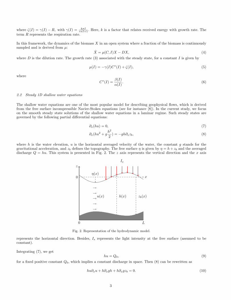
where h is the water elevation, u is the horizontal averaged velocity of the water, the constant g stands for thegravitational acceleration, and zb defines the topography. The free surface η is given by η = h+ zb and the averageddischarge Q = hu. This system is presented in Fig. 2. The z axis represents the vertical direction and the x axis

0 L

z

0 xη(x)

Is

zb(x)h(x)u(x)

Fig. 2. Representation of the hydrodynamic model.

represents the horizontal direction. Besides, Is represents the light intensity at the free surface (assumed to beconstant).

Integrating (7), we gethu = Q0, (9)

for a fixed positive constant Q0, which implies a constant discharge in space. Then (8) can be rewritten as

hu∂xu+ h∂xgh+ h∂xgzb = 0. (10)

3

Let us assume that h is strictly positive. Dividing (10) by h and using (9) to eliminate u, we get

∂x

( Q20

2h2+ g(h+ zb)

)= 0.

This equation corresponds to the Bernoulli’s principle. Now let us consider two fixed constants h(0), zb(0) ∈ R. Forall x ∈ [0, L], we obtain

Q20

2h2+ g(h+ zb) =

Q20

2h2(0)+ g(h(0) + zb(0)) =: M0,

meaning that the topography zb satisfies

zb =M0

g− Q2

0

2gh2− h. (11)

Remark 1 Define the Froude number for the steady state by Fr = u/√gh. The situation Fr < 1 corresponds to

the subcritical case (i.e. the flow regime is fluvial) while Fr > 1 is to the supercritical case (i.e. the flow regime istorrential). In particular, the threshold value of h for Fr = 1 is given by

hc := (Q2

0

g)

13 .

Because of (11), h is the solution of a third order polynomial equation. Given a smooth topography zb, if

hc + zb +Q2

0

2gh2c

− M0

g< 0.

there exists a unique positive smooth solution of (11) which satisfies the subcritical flow condition (see [16, Lemma1]). The velocity u can then be obtained thanks to (9).

2.3 Lagrangian trajectories of the algae and captured light intensity

Let z(t) be the depth of a particle at time t in the raceway pond. We first determine the Lagrangian trajectory ofan algal cell that starts at a given position z(0) at time 0.

From the incompressibility of the flow, we have ∇ · u = 0 with u = (u(x), w(x, z)). Here, w(x, z) is the verticalvelocity. This implies that

∂xu+ ∂zw = 0. (12)

Integrating (12) from zb to z gives:

0 =

∫ z

zb

(∂xu(x) + ∂zw(x, z)

)dz

= ∂x

∫ z

zb

u(x)dz +

∫ z

zb

∂zw(x, z)dz

= ∂x((z − zb)u(x)

)+ w(x, z)− w(x, zb)

= (z − zb)∂xu(x)− u(x)∂xzb + w(x, z),

where we have used the kinematic condition at the bottom (i.e. w(x, zb) = u(x)∂xzb). It then follows from (11) that

w(x, z) = (M0

g− 3u2(x)

2g− z)u′(x).

The Lagrangian trajectory is characterized by the system(x(t)

z(t)

)=

(u(x(t))

w(x(t), z(t))

). (13)

4

Remark 2 Note that a Brownian motion can be included in these equations to take into account the fluid viscosity.In this case, the optimisation procedure required a large set of simulations and an averaging strategy. Such questionsare out of the range of this paper.

Up to now and for the sake of simplicity, we denote by z(x) the depth of a particle at x. From (13), we get

z′ :=z

x= (

M0

g− 3u2

2g− z)u

′

u. (14)

Note that from (9) and (11), we have η = h+ zb = M0

g −u2

2g , which implies η′ = −uu′/g. Multiplying (14) both sides

by u and using the formulation of η, η′ gives

z′u+ zu′ = (η − u2

g)u′

= ηu′ + η′u,

which implies that(u(z − η)

)′= 0. We then obtain

z(x) = η(x) +u(0)

u(x)(z(0)− η(0)). (15)

The computation of trajectories in the shallow water system can be carried out with this formula, where u(0), z(0)and η(0) = h(0) + zb(0) are given as boundary conditions, whereas u(x) can be obtained by (9) and (11). On thecontrary, h(x), hence u(x) will be considered in section 3 as a parameter to be optimized, and (11) will be used to(post-)compute zb(x).

Remark 3 Since Q0 is chosen to be positive, h is necessarily positive and so does u from (9). Moreover, if z(0)belongs to [zb(0), η(0)], then z(x) belongs to [zb(x), η(x)]. In particular, choosing z(0) = zb(0) in (15) and using (9)gives z(x) = zb(x). In the same way, we find that z(x) = η(x) when z(0) = η(0).

To evaluate the light intensity observed on the trajectory z, we assume that the growth process occurs at a muchslower time scale than those of hydrodynamics and is, as such, negligible for one lap over the raceway. As a conse-quence, the turbidity is supposed to be constant over the considered time scale. In this framework, the Beer-Lambertlaw describes how light is attenuated with depth:

I(x, z) = Is exp(− ε(η(x)− z)

). (16)

Here ε is the light extinction coefficient. We assume that the system is perfectly mixed so that the concentration ofthe biomass X in (4) is homogeneous and ε is constant. Combining (16) with (15), we get the following expressionfor the captured light intensity along the trajectory z

I(x, z(x)) = Is exp(− ε u(0)

u(x)(η(0)− z(0))

). (17)

It follows that in this approach, the light intensity I couples the hydrodynamic model and Han model: the trajectoriesof the algae define the received light intensity, which is used in the photosystems dynamics.

We can then derive the equation satisfied by C. Indeed, repeating the reasoning done to get (14) with (2), we finda time-free reformulation, namely

C ′ :=C

x= −α(I)

uC +

β(I)

u, (18)

where all the functions on the right-hand side only depend on x.

5

3 Optimization problem

In this section, we define the optimization problem associated with our biological-hydrodynamic model. We firstintroduce our procedure for a simple problem, and then extend this to other variant cases.

3.1 Optimization functional

The average net specific growth rate over the domain is defined by

µ :=1

L

∫ L

0

1

h(x)

∫ η(x)

zb(x)

µ(C(x, z), I(x, z)

)dzdx. (19)

In order to tackle numerically this optimization problem, let us consider a vertical discretization. Let Nz denotesthe number of particles, and consider a uniform vertical discretization of their initial position:

zi(0) = η(0)−i− 1

2

Nzh(0), i = 1, . . . , Nz.

From (15), we obtain

zi(x)− zi+1(x) =1

Nzh(x), i = 1, . . . , Nz,

meaning that the distribution of particles remains uniform along the trajectories. To simplify notations, we writeIi(x) instead of I(x, zi(x)) hereafter.

Let Ci(x) (resp. Ii(x)) the photo-inhibition state (resp. the light intensity) associated with the trajectories zi(x).Then the semi-discrete average net specific growth rate in the raceway pond can be defined from (19) by

µ∆ : =1

L

∫ L

0

1

h(x)

1

Nzh(x)

Nz∑i=1

µ(Ci(x), Ii(x))dx

=1

LNz

Nz∑i=1

∫ L

0

µ(Ci(x), Ii(x))dx.

(20)

From now on, we focus only on the subcritical case, i.e. Fr < 1, see Remark 1. As we have mentioned in the previoussection, in this regime, a given topography zb corresponds to a unique water height h which verifies this assumption.Note that the volume of our system is simply given by

V =

∫ L

0

h(x)dx. (21)

Therefore, we choose to parameterize h by a vector a := [a1, · · · , aN ] ∈ RN in order to handle the volume of oursystem. This vector will be the variable to be optimized. Once we find the optimum parameter a∗, we can determinatethe associated topography by means of (11).

Remark 4 In usual shallow water solver, equations of type (11) are usually consider to compute h in the simulations.Here, we use this equation in the opposite way, i.e., to recover the topography zb from h.

Our goal is to optimize the topography to maximize µ∆. Up to now, we denote explicitly that the functions dependon a. In the case of one trajectory, we consider the functional

J(a) =1

L

∫ L

0

−γ(I(x; a))C(x) + ζ(I(x; a))

u(x; a)dx,

6

where C satisfies the following parameterized version of (18)

C ′ +α(I(x; a))

u(x; a)C =

β(I(x; a))

u(x; a). (22)

The optimization problem then reads:

Find a∗ solving the maximization problem:

maxa∈RN

J(a). (23)

3.2 Optimality System for maximizing growth rate

In this section, we introduce the optimality system derived from the optimization problem (23) and some of itsvariants. For the sake of simplicity, we first remain in the setting where one single trajectory is considered, and thenextend it to a multiple trajectories system. Next, we analyse the case where C is periodic, and finally, we present amore general case where the volume can also be optimized. For simplicity of notation, we omit x in the notation.

3.2.1 One trajectory problem

Define the Lagrangian of Problem (23) by

L(C, p, a) =1

L

∫ L

0

−γ(I(a))C + ζ(I(a))

u(a)dx

−∫ L

0

p(C ′ +

α(I(a))C − β(I(a))

u(a)

)dx,

where p is the Lagrange multiplier associated with the constraint (22).

The optimality system is obtained by cancelling all the partial derivatives of L. Differentiating L with respect top and equating the resulting expression to zero gives (22). Integrating the terms

∫pC ′dx on the interval [0, L] by

parts and differentiating L with respect to C and C(L) gives rise to

{∂CL = p′ − pα(I(a))

u(a) −1Lγ(I(a))u(a)

∂C(L)L = p(L).(24)

Given a vector a, let us still denote by C, p the corresponding solutions of (22) and (24). The gradient ∇J(a) isobtained by

∇J(a) = ∂aL,

where

∂aL =1

L

∫ L

0

−γ′(I(a))C + ζ ′(I(a))

u(a)∂aI(a)dx

− 1

L

∫ L

0

−γ(I(a))C + ζ(I(a))

u2(a)∂au(a)dx

+

∫ L

0

p−α′(I(a))C + β′(I(a))

u(a)∂aI(a)dx

−∫ L

0

p−α(I(a))C + β(I(a))

u2(a)∂au(a)dx.

(25)

7

3.2.2 Multiple trajectories problem

We now extend the previous framework to deal with multiple trajectories. From (20), the objective functional isdefined by:

µ∆(a) =1

LNz

Nz∑i=1

∫ L

0

−γ(Ii(a))Ci + ζ(Ii(a))

u(a)dx, (26)

where Ci satisfies (22) for the light intensity Ii with i = 1, . . . , Nz. Let us still denote by L the associated Lagrangian.Similar computations as in the previous section give rise to Nz systems similar to (24), where C is replaced by Ci.Denoting by pi the associated Lagrange multipliers, the partial derivative ∂aL (hence the gradient ∇µ∆(a)) is thengiven by

∂aL =1

LNz

Nz∑i=1

∫ L

0

−γ′(Ii(a))Ci + ζ ′(Ii(a))

u(a)∂aIi(a)dx

− 1

LNz

Nz∑i=1

∫ L

0

−γ(Ii(a))Ci + ζ(Ii(a))

u2(a)∂au(a)dx

+

Nz∑i=1

∫ L

0

pi−α′(Ii(a))Ci + β′(Ii(a))

u(a)∂aIi(a)dx

−Nz∑i=1

∫ L

0

pi−α(Ii(a))Ci + β(Ii(a))

u2(a)∂au(a)dx.

3.2.3 Periodic problem

We now consider a variant of our problem, where the photo-inhibition state C is periodic, with a period correspondingto a raceway lap. This situation occurs, e.g., when an appropriate harvest is performed after each lap. To describethe corresponding model, let us first consider a variant of the usual Cauchy problem for (18):

Given I ∈ L2(0, L;R), find (C0, C) ∈ R× C(0, L;R) such that{C ′(x) = −α(I(x))C(x)+β(I(x))

u(x) , x ∈ [0, L]

C(L) = C(0) = C0.(27)

The following theorem gives the existence and uniqueness of a (weak) solution of the problem (27)

Theorem 5 Given I ∈ L2(0, L;R), there exists a unique couple (C0, C) ∈ R× C(0, L;R) satisfying{C(x) = C0 +

∫ x0−α(I(s))C(s)+β(I(s))

u(s) ds ,

C(L) = C0

(28)

for all x ∈ [0, L].

The proof is given in Appendix A. The optimality system is obtained as in the previous sections.

Remark 6 Note that the periodicity of C implies that p is also periodic. Indeed, since C(L) = C(0), then bydifferentiating L with respect to C(L), we have

∂C(L)L = p(L)− p(0).

so that equating the above equation to zero gives the periodicity for p. Similar computations apply for multipletrajectories problem.

8

Next, we state a result for Problem (23) in the case where C is periodic.

Proposition 7 Assume h is of the form

h(x; a) = a0 +

N∑n=1

an sin(2nπx

L), (29)

with a := [a1, . . . , aN ] chosen such that the subcritical condition is satisfied (see Remark 1). Then ∇J(0) = 0.

As a consequence, the flat topography is critical point for Problem (23). Note that the larger N is, the less validis our hydrodynamic model valid, see Section 2.2, where a smooth topography is assumed. Hence, limit situationswhere N → +∞ are not considered in what follows.

PROOF. Let q ∈ [0, 1], consider an initial position by

z(0; a) = η(0; a)− qh(0; a). (30)

Replacing z(0; a) by the previous expression in (17) and using (9), gives

I(a) = Is exp(−εq Q0

u(a)) = Is exp(−εqh(a)). (31)

Introduce a∗ = [0, . . . , 0]. Replacing a by a∗ in (9) and (31), we find that u(a∗) and I(a∗) are both constants withrespect to x. For a given C(0), (22) gives

C(x) = e−α(I(a∗))u(a∗) xC(0) +

β(I(a∗))

α(I(a∗))(1− e−

α(I(a∗))u(a∗) x). (32)

Since C is periodic (i.e. C(L) = C(0)), we get from the previous equation that C(0) = β(I(a∗))α(I(a∗)) . Inserting this value

in (32), we find

C(x) =β(I(a∗))

α(I(a∗)), ∀x ∈ [0, L],

which corresponds to the steady state (6), that we denote by C∗ hereafter. We then compute all the partial derivativesappearing in (25). We get:

∂anu(a) = − Q0

h2(a)∂anh(a),

∂anI(a) = −εqI(a)∂anh(a),

but ∂anh(a) = sin(2nπ xL ), so that the integral from 0 to L of ∂anh(a) is zero. Replacing a by a∗ in (25) , the firstintegral can be computed as

∫ L

0

−γ′(I(a∗))C∗ + ζ ′(I(a∗))

u(a∗)∂anI(a∗)dx

=−γ′(I(a∗))C∗ + ζ ′(I(a∗))

u(a∗)

∫ L

0

∂anI(a∗)dx

=0.

9

and the second integral can be computed as∫ L

0

−γ(I(a∗))C∗ + ζ(I(a∗))

u2(a∗)∂anu(a∗)dx

=−γ(I(a∗))C∗ + ζ(I(a∗))

u2(a∗)

∫ L

0

∂anu(a∗)dx

=0.

Since p is also periodic (see Remark 6), it can be proved in much the same way that the two last terms in (25) alsocancels when a = a∗. The result follows.

Remark 8 Numerically, we observe that the flat topography is actually optimal in the periodic case.

Remark 9 Note that if C is not periodic, (32) implies that C depends also on the space variable x and the compu-tations for the first-two integrals in the proof above will no longer hold. For the same reason, p shall be not constantand the last two integrals in (25), hence the gradient will not cancel in general. In other words, the flat topographyis not an optimum for the case C non periodic, which is confirmed by our numerical tests (see Section 4.3.2).

3.2.4 Non-constant volume problem for maximizing areal productivity

In general, the extinction coefficient is an affine function with respect to the biomass X [13]

ε(X) = α0X + α1, (33)

where α0 > 0 the specific light extinction coefficient of the microalgae specie and α1 the background turbidity thatsummarizes the light absorption and diffusion due to all non-microalgae components. Recall that according to (4),the biomass concentration X depends on the growth rate µ and on the harvesting of the raceway D.

Remark 10 A standard criterion to determine a relevant value of X [14,10], and then an harvesting frequency,consists in regulating it to a value such that the steady-state value of the growth rate µ at the (average) bottom depthzb is 0, i.e.,

µ(Izb) = 0, (34)

where µ(I) is given by (5). Solving (34) provides a value of Izb thus of the extinction coefficient ε(X), and finally ofthe biomass concentration X. This assumption is usually called the compensation condition, for which the growth atthe bottom compensates exactly the respiration.

In this framework, maximizing areal productivity is a relevant target. Productivity per unit of surface for a givenbiomass concentration X is given by:

Π = µXV

S, (35)

where S is the ground surface of the raceway pond and µ is defined in (19). To optimize this objective function, amore general setting where the reactor volume varies can be considered. The total biomass X in a given volume issupposed to satisfy (34) and we assume that it is maintained constant to achieve the compensation conditions, seeRemark 10.

Let us keep the parameterization h given in (29). The volume of the system satisfies V = a0L (see (21)). Moreover,since we consider a 1D framework, we have S = L. The biomass concentration X is chosen to be solution of (34).We have

X(a0)V (a0)

S= α2 − α3a0,

where α2 = 1α0

ln( IsIzb) and α3 = α1

α0, and α0, α1 are given in (33). The detail of the computation is given in Appendix

C. Let us then consider the extended parameter vector a := [a0, a]. For simplicity, we again consider one singletrajectory and optimize the objective function associated with (35) defined by

J(a) =α2 − α3a0

L

∫ L

0

−γ(I(a))C + ζ(I(a))

u(a)dx,

10

where C satisfies (22) with a replacing by a. The corresponding optimization problem reads:

Find a∗ solving the maximization problem:

maxa∈RN+1

J(a). (36)

The Lagrangian of Problem (36) is

L(C, p, a) =α2 − α3a0

L

∫ L

0

−γ(I(a))C + ζ(I(a))

u(a)dx

−∫ L

0

p(C ′ +

α(I(a))C − β(I(a))

u(a)

)dx,

where p is the Lagrangian multiplier associated with the constraint (22) for C. By computations similar to that ofthe previous section, we find as optimality system{

∂CL = p′ − pα(I(a))u(a) −

γ(I(a))u(a)

α2−α3a0

L

∂C(L)L = p(L).

However, there is an extra element in the gradient J(a), namely the derivative with respect to a0, so that ∇J(a) :=

[∂a0L, ∂aL], where

∂a0L =

α2 − α3a0

L

∫ L

0

−γ′(I(a))C + ζ ′(I(a))

u(a)∂a0

I(a)dx

−α2 − α3a0

L

∫ L

0

−γ(I(a))C + ζ(I(a))

u2(a)∂a0

u(a)dx

−α3

L

∫ L

0

−γ(I(a))C + ζ(I(a))

u(a)dx

+

∫ L

0

p−α′(I(a))C + β′(I(a))

u(a)∂a0I(a)dx

−∫ L

0

p−α(I(a))C + β(I(a))

u2(a)∂a0

u(a)dx,

(37)

∂aL =α2 − α3a0

L

∫ L

0

−γ′(I(a))C + ζ ′(I(a))

u(a)∂aI(a)dx

−α2 − α3a0

L

∫ L

0

−γ(I(a))C + ζ(I(a))

u2(a)∂au(a)dx

+

∫ L

0

p−α′(I(a))C + β′(I(a))

u(a)∂aI(a)dx

−∫ L

0

p−α(I(a))C + β(I(a))

u2(a)∂au(a)dx.

(38)

However, we still find that the flat topography is optimal in that case.

Proposition 11 Assume h is of the form (29) and C is periodic, then J(a∗) = 0 with a∗ = [a∗0, 0, · · · , 0].

PROOF. The proof is similar to that of Proposition 7. For a given z(0; a) defined in (30), using the result inAppendix C to replace ε in (31), we have

I(a) = Is exp(− 1

a0ln(

IsIzb

)qh(a)).

11

The two extra partial derivatives appearing in (37) are computed by

∂a0u(a) = − Q0

h2(a)∂a0

h(a),

∂a0I(a) = −(− 1

a20

h(a) +1

a0∂a0

h(a)) ln(IsIzb

)qI(a),

where ∂a0h(a) = 1. The flat topography corresponds to the parameter a∗ = [a∗0, 0, . . . , 0]. Then ∂a0

u(a∗) = − Q0

a∗02

and ∂a0I(a∗) = 0. Hence the first integral and the fourth integral in ∂a0L in (37) are zero. Following a reasoning

similar to that of Proposition 7, we find C∗ is constant. Hence, the last integral in ∂a0L is zero. Finally for

a∗0 =α2

2α3, (39)

the sum of the second and the third integral in ∂a0L is zero.

As for (38), it follows from computations similar to that of the proof of Proposition 7 that this term equals zero,which completes the proof.

4 Numerical Experiments

In this section, we show some optimal topographies obtained in the various previous frameworks.

4.1 Numerical Methods

We start with an algorithm to solve the optimization problem and the numerical solver that we use for our numericaltests.

4.1.1 Gradient Algorithm

We detail now a gradient-based optimization procedure and apply it to Problem (23). The procedure is given inAlgorithm 1.

Algorithm 1 Gradient-based optimization algorithm

1: Input: Tol> 0, ρ > 0.2: Initial guess: a.3: Output: a4: Set err := Tol+1 and define h by (29) using the input data.5: while err >Tol and ‖h‖∞ > hc do6: Compute u by (9) and I by (17).7: Set C as the solution of (22).8: Set p as the solution of (24).9: Compute the gradient ∇J by (25).

10: a = a+ ρ∇J ,11: Set err := ‖∇J‖.12: end while

Note that ‖h‖∞ := maxx∈[0,L] h(x). In addition to a numerical tolerance criterion on the magnitude of the gradient,we need to take into account a constraint on the height h, to guarantee that the simulated flow remains in a subcriticalregime, see Remark 1 (and in the range of industrial constraints, see [5]).

A similar algorithm can be considered to tackle the multiple trajectories Problem (26). Remark that since nointeraction between trajectories is considered, the gradient computation can be partially parallelized when computingIi (hence Ci) and pi.

12

Finally, the optimality system presented in Section 3.2.4 can still be solved with Algorithm 1 by adapting theobjective functional J and the gradient ∇J .

4.1.2 Numerical Solvers

To solve our optimization problem numerically, we introduce a supplementary space discretization with respect tox. In this way, let us take a space increment ∆x, set Nx = [L/∆x] and xnx = nx∆x for nx = 0, . . . , Nx. We chooseto use the Heun’s method for computing C via (22). Following a first-discretize-then-optimize strategy, we get thatthe Lagrange multiplier p is also computed by a Heun’s type scheme. Note that this scheme is still explicit since itsolves a backward dynamics starting from p(L) = 0.

4.2 Parameter settings

We now detail the parameters used in our simulations.

4.2.1 Parameterization of h

As mentioned in Proposition 7, we parameterize h by a truncated Fourier series (29). The parameters to be optimizedwill be the Fourier coefficients a := [a1, . . . , aN ]. Note that we choose to fix a0, since it is related to the volume V ofthe raceway with V = a0L.

4.2.2 Parameter for the models

The spatial increment is set to ∆x = 0.01 m so that the convergence of the numerical scheme has been ensured, and weset the raceway length L = 100 m, the averaged discharge Q0 = 0.04 m2 s−1, the initial value a0(= h(0; a)) = 0.4 mand zb(0) = −0.4 m to stay in standard ranges for a raceway. The free-fall acceleration g = 9.81 m s−2. All thenumerical parameters values for Han’s model are taken from [9] and given in Table 1.

Table 1Parameter values for Han Model.

kr 6.8 10−3 s−1

kd 2.99 10−4 -

τ 0.25 s

σ 0.047 m2 · (µmol)−1

k 8.7 10−6 -

R 1.389 10−7 s−1

In order to determinate the light extinction coefficient ε, let us assume that only 1% of light can be captured bythe cells at the bottom of the raceway, i.e. for z = zb, meaning that Ib = 0.01Is, we choose Is = 2000µmol m−2 s−1

which approximates the maximum light intensity, e.g., at summer in the south of France. Then ε can be computedby

ε = (1/h(0; a)) ln(Is/Ib).

Note that in the case where a0 is also a parameter to be optimized, we take from [13] the specific light extinctioncoefficient of the microalgae specie α0 = 0.2 m2 · gC the background turbidity and α1 = 10 m−1, under these settings,a∗0 defined in (39) is around 0.316 m.

4.3 Numerical results

We now test the influence of various parameters on optimal topographies. In all our experiments, we always observethat the topographies satisfy ‖h‖∞ > hc.

13

4.3.1 Influence of vertical discretization

The first test consists in studying the influence of the vertical discretization number Nz. We choose N = 5 and take100 random initial guesses of a. Note that the choice of a should respect the subcritical condition. Let Nz variesfrom 1 to 100, and we compute the average value of µ∆ for each Nz. The results are shown in Fig. 3. We observe

10 0 10 1 10 2

Nz

0.4

0.5

0.6

0.7

0.8

0.9

1

77"

(d!

1)

Fig. 3. The value of the functional µ∆ for Nz = [1, 100].

numerical convergence when Nz grows, showing the convergence towards the model continuous in space. In view ofthese results, we take hereafter Nz = 50.

4.3.2 Influence of the initial condition

The second test consists in studying the influence of the initial condition C0 on the optimal shape of the racewaypond. We set the numerical tolerance Tol= 10−10, and consider N = 5 terms in the truncated Fourier series asan example to show the shape of the optimal topography. As an initial guess, we consider the flat topography,meaning that a is set to 0. Besides, we compare the optimal topographies obtained with C0 = 0.1 and with C0 = 0.9.The result is shown in Fig. 4. A slight difference between the two optimal topographies is observed. Note that this

0 20 40 60 80 100Length (m)

-0.5

-0.4

-0.3

-0.2

-0.1

0

0.1

Dep

th(m

)

SurfaceBottom

0 20 40 60 80 100Length (m)

-0.6

-0.5

-0.4

-0.3

-0.2

-0.1

0

0.1

Dep

th(m

)

SurfaceBottom

Fig. 4. The optimal topography for C0 = 0.1 (top) and C0 = 0.9 (bottom). The red thick line represents the topography (zb),the blue thick line represents the free surface (η), and all the other curves between represent the different trajectories.

difference remains when the spatial increment ∆x goes to zero.

4.3.3 Influence of Fourier series truncation

The next test is dedicated to the influence of the order of the truncation of the Fourier series used to parameterizethe water elevation h.

14

Set N = [0, 5, 10, 15, 20] and keep all the other parameter values. Table 2 shows the optimal value of the objectivefunction µ∆(a∗) for different order of truncation N of the Fourier series. As expected, the result shows a slight

Table 2The objective function for different order of truncation of the Fourier series.

N Iter µ∆(d−1) log10(‖∇J‖)

0 0 0.94764 −

5 16 0.96942 -10.368944

10 17 0.97509 -10.262891

15 17 0.97734 -10.010322

20 18 0.97851 -10.196963

increase of the optimal value of the objective function µ∆(a∗) when N becomes larger. However, the correspondingvalues of µ∆(a∗) remain close to the one associated with a flat topography.

4.3.4 Simulation with paddle wheel

The last test aims to simulate a more realistic raceway pond situation, where a paddle wheel considered in thesystem. More precisely, we simulate several laps, with a paddle wheel that mix up the algae after each laps. Thepaddle wheel is modelled by a permutation matrix P that rearrange the trajectories at each lap. In our test, P isan anti-diagonal matrix with the entries one. This choice actually corresponds to an optimum and has been shownin [3], where other choices will be investigated.

Meanwhile, this permutation matrix P corresponds to the permutation

π = (1 Nz)(2 Nz − 1)(3 Nz − 2) · · · ,

where we use the standard notation of cycles in the symmetric group. Note that π is of order two. The photo-inhibition state C is then set to be 2-periodic (i.e C1(0) = PC2(L)). The details of the optimization procedure aregiven in Appendix B.

We choose a truncation of order N = 5 in the Fourier series. The initial guess a is still zero. Fig. 5 presents theshape of the optimal topography and the evolution of the photo-inhibition state C for two laps. In particular, weobserve that the state C is actually periodic for each laps. This result is actually proved in [3] in the case of a flattopography.

0 20 40 60 80 100Length (m)

-0.5

-0.4

-0.3

-0.2

-0.1

0

0.1

Dep

th(m

)

SurfaceBottom

Fig. 5. The optimal topography (top) and the evolution of the photo-inhibition state C (bottom) for two laps.

The resulting optimal topography in this case is not flat. However, the increase in the optimal value of the objectivefunction µ∆ compared to a flat topography is around 0.217%, and compare to a flat topography and non permutationcase is around 0.265%, in both cases, the increase remains small.

15

5 CONCLUSIONS AND FUTURE WORKS

A non flat topography slightly enhances the average growth rate. However the gain remains very limited and it isnot clear if the difficulty to design such a pattern could be compensated by the increase in the process productivity.

A flat topography cancels the gradient of the objective functional in many situations where C is assumed to beperiodic. However, including a mixing device gives rise to an optimal non flat topography with a slight gain of theaverage growth rate.

References

[1] Olivier Bernard, Anne-Celine Boulanger, Marie-Odile Bristeau, and Jacques Sainte-Marie. A 2d model for hydrodynamics andbiology coupling applied to algae growth simulations. ESAIM: Mathematical Modelling and Numerical Analysis, 47(5):1387–1412,September 2013.

[2] Olivier Bernard, Liudi Lu, Jacques Sainte Marie, and Julien Salomon. Controlling the bottom topography of a microalgal pond tooptimize productivity. Working paper or Preprint, October 2020.

[3] Olivier Bernard, Liudi Lu, and Julien Salomon. Optimizing microalgal productivity in raceway ponds through a controlled mixingdevice. Working paper or Preprint, October 2020.

[4] Olivier Bernard, Francis Mairet, and Benoıt Chachuat. Modelling of microalgae culture systems with applications to control andoptimization. Microalgae Biotechnology, 153(59-87), 2015.

[5] David Chiaramonti, Matteo Prussi, David Casini, Mario R. Tredici, Liliana Rodolfi, Niccolo Bassi, Graziella Chini Zittelli, and PaoloBondioli. Review of energy balance in raceway ponds for microalgae cultivation: Re-thinking a traditional system is possible. AppliedEnergy, 102:101–111, Feburary 2013.

[6] David Demory, Charlotte Combe, Philipp Hartmann, Amelie Talec, Eric Pruvost, Raouf Hamouda, Fabien Souille, Pierre-OlivierLamare, Marie-Odile Bristeau, Jacques Sainte-Marie, Sophie Rabouille, Francis Mairet, Antoine Sciandra, and Olivier Bernard. Howdo microalgae perceive light in a high-rate pond? towards more realistic lagrangian experiments. The Royal Society, May 2018.

[7] P.H.C. Eilers and J.C.H. Peeters. Dynamic behaviour of a model for photosynthesis and photoinhibition. Ecological Modelling,69(1):113 – 133, 1993.

[8] Jean-Frederic Gerbeau and Benoıt Perthame. Derivation of viscous saint-venant system for laminar shallow water; numericalvalidation. Discrete & Continuous Dynamical Systems - B, 1(1):89–102, Feburary 2001.

[9] Jerome Grenier, F. Lopes, Hubert Bonnefond, and Olivier Bernard. Worldwide perspectives of rotating algal biofilm up-scaling.2020.

[10] Frederic Grognard, Andrei R. Akhmetzhanov, and Olivier Bernard. Optimal strategies for biomass productivity maximization in aphotobioreactor using natural light. Automatica, 50(2):359–368, 2014.

[11] Bo-Ping Han. Photosynthesis–irradiance response at physiological level: A mechanistic model. Journal of theoretical biology,213(2):121–127, November 2001.

[12] Pierre-Olivier Lamare, Nina Aguillon, Jacques Sainte-Marie, Jerome Grenier, Hubert Bonnefond, and Olivier Bernard. Gradient-based optimization of a rotating algal biofilm process. Automatica, 105:80–88, July 2019.

[13] Carlos Martınez, Francis Mairet, and Olivier Bernard. Theory of turbid microalgae cultures. Journal of Theoretical Biology,456:190–200, November 2018.

[14] Pierre Masci, Frederic Grognard, and Olivier Bernard. Microalgal biomass surface productivity optimization based on aphotobioreactor model. IFAC Proceedings Volumes, 43(6):180–185, 2010.

[15] J. Masojıdek, S. Papacek, M. Sergejevova, V. Jirka, J. Cerveny, J. Kunc, J. Korecko, O. Verbovikova, J. Kopecky, D. Stys, andG. Torzillo. A closed solar photobioreactor for cultivation of microalgae under supra-high irradiance: Basic design and performance.Journal of Applied Phycology, 15(2-3):239–248, 2003.

[16] Victor Michel-Dansac, Christophe Berthon, Stephane Clain, and Franoise Foucher. A well-balanced scheme for the shallow-waterequations with topography. Computers and Mathematics with Applications, 72(3):586–593, August 2016.

[17] Rafael Munoz-Tamayo, Francis Mairet, and Olivier Bernard. Optimizing microalgal production in raceway systems. Biotechnologyprogress, 29(2):543–552, 2013.

[18] Clemens Posten and Steven Feng Chen, editors. Microalgae Biotechnology. 153. Springer, 1 edition, 2016.

[19] Rene H. Wijffels and Maria J. Barbosa. An outlook on microalgal biofuels. Science, 329(5993):796–799, August 2010.

[20] Sung Jin Yoo, Se-Kyu Oh, and Jong Min Lee. Design of experiments and sensitivity analysis for microalgal bioreactor systems. InIan David Lockhart Bogle and Michael Fairweather, editors, 22nd European Symposium on Computer Aided Process Engineering,volume 30 of Computer Aided Chemical Engineering, pages 722 – 726. Elsevier, 2012.

16

A Proof for Theorem 5

Let us give the details of the proof for Theorem 5. To prove the existence and uniqueness of (weak) a solution ofthis problem, we need the following result.

Lemma 12 Given Z0 ∈ R, let Z ∈ C(0, L;R) be the weak solution of{Z(x) = −α(I(x))

u(x) Z(x), x ∈ [0, L]

Z(L) = Z0

(A.1)

For x ∈ [0, L]:

‖Z(x)‖2 ≤ e− kr‖u‖∞

x ‖Z0‖2 . (A.2)

PROOF. Let x ∈ [0, L], as a weak solution of (A.1), the function Z is almost everywhere differentiable and a directcalculation gives

d ‖Z(x)‖22dx

= 2 < Z(x),−α(I(x))

u(x)Z(x) >

≤ −2kr‖u‖∞

‖Z(x)‖22 ,(A.3)

where we have used the fact that α(I) = β(I) + kr, β(I) ≥ 0 and 0 < u < ‖u‖∞. Defining f(x) :=d ‖Z(x)‖22

dx+

2 kr‖u‖∞

‖Z(x)‖22 and multiplying both sides by e2 kr‖u‖∞

x, we obtain:

de2 kr‖u‖∞

x ‖Z(x)‖22dx

= e2 kr‖u‖∞

xf(x),

which gives by integration over [0, x]

‖Z(x)‖22 = e−2 kr‖u‖∞

x ‖Z0‖22 +

∫ x

0

e2 kr‖u‖∞

(s−x)f(s)ds.

Because of (A.3), f(x) ≤ 0, this concludes the proof.

Let us now give the proof for Theorem 5.

PROOF. Introduce the mapping Φ : R→ R defined by

Φ(C0) := C(L),

where C is the weak solution of (18). Given C10 ∈ R and C2

0 ∈ R, define Z0 = C20 − C1

0 and Z(x) = C2(x)− C1(x),where C1 and C2 are the weak solutions of (18) with initial conditions C1

0 and C20 , respectively. Subtracting the

corresponding weak representations, we obtain that Z satisfies the assumptions of Lemma 12 so that (A.2) holds.As a consequence, ∥∥C2(L)− C1(L)

∥∥2≤ e−

kr‖u‖∞

L ∥∥C20 − C1

0

∥∥2,

which implies that Φ is a contraction. Applying Banach fixed-point theorem, it follows that there exists a uniqueC0 ∈ R such that Φ(C0) = C0. The corresponding weak solution C of (18) satisfies (28).

17

B System with a paddle-wheel

Let us denote by P the permutation matrix associated with π i.e., 1 as entries on the anti-diagonal. Let us denoteby C1 (resp. C2) the photo-inhibition state for the first (resp. second) lap of the raceway. We then assume that thestate C is 2-periodic, meaning that C1(0) = PC2(L). From (26), we define the objective function by

1

2

2∑j=1

µj∆(a) =

1

2LNz

2∑j=1

Nz∑i=1

∫ L

0

−γ(Ii(a))Cji + ζ(Ii(a))

u(a)dx.

Let us still denote by L the Lagrangian associated with this optimization problem. It can be written

L(C, p,a) =1

2LNz

2∑j=1

Nz∑i=1

∫ L

0

−γ(Ii(a))Cji + ζ(Ii(a))

u(a)dx

−2∑j=1

Nz∑i=1

∫ L

0

pji(Cji′+α(Ii(a))Cji − β(Ii(a))

u(a)

)dx,

where pji is the Lagrangian multiplier associated with the constraint (22) for Cji . Integrating the terms∫pjiC

ji

′dx

on the interval [0, L] by parts, we get

∫ L

0

pjiCji

′dx = −

∫ L

0

pji′Cji dx+ pji (L)Cji (L)− pji (0)Cji (0).

By definition of our paddle wheel model, C2(0) = PC1(L). Differentiating L with respect to C1(L) and C2(L), wefind {

∂C1(L) L = p1(L)− p2(0)P,

∂C2(L) L = p2(L)− p1(0)P.

Then differentiating L with respect to Cji gives the evolution of pji by

∂Cji(L) L = pji

′− pji

α(Ii(a))

u(a)− 1

2LNz

γ(Ii(a))

u(a).

Finally, the partial derivative ∂a L (hence the gradient) is given by

∂aL

=1

2LNz

2∑j=1

Nz∑i=1

∫ L

0

−γ′(Ii(a))Cji + ζ ′(Ii(a))

u(a)∂aIi(a)dx

− 1

2LNz

2∑j=1

Nz∑i=1

∫ L

0

−γ(Ii(a))Cji + ζ(Ii(a))

u2(a)∂au(a)dx

+

2∑j=1

Nz∑i=1

∫ L

0

pji−α′(Ii(a))Cji + β′(Ii(a))

u(a)∂aIi(a)dx

−2∑j=1

Nz∑i=1

∫ L

0

pji−α(Ii(a))Cji + β(Ii(a))

u2(a)∂au(a)dx.

18

C Computation for X

Let us consider a 1D system with vertical light attenuation. We consider the simple configuration of a static growthrate where Han dynamics is considered at equilibrium. The optimal biomass shades light such that, at the pondbottom, we have (34). Replacing α, β, γ, ζ by their own definitions in (5) and (6), we find a second order equationfor I

kdτR(σI)2 + (krτσR− krkσ)I + krR = 0.

Denote by Izb the suitable root of this equation (where 0 < Izb < Is). From (15) and (17), the light intensity at the(averaged) bottom is given by

Izb = Is exp(−ε(X)a0).

This implies

ε(X) =1

a0ln(

IsIzb

).

Recall that ε(X) = α0X + α1, hence we have

X(a0) =

1a0

ln( IsIzb)− α1

α0.

19