Productivity and the Decision to Import and Export: Theory...

Productivity and the Decision to Import and Export: Theory and

Evidence∗

Hiroyuki Kasahara † Beverly Lapham ‡

This version: June 4, 2012

Abstract

This paper develops an open economy model with heterogeneous final goods producers who si-

multaneously choose whether to export their output and whether to use imported intermediates.

Using the theoretical model, we develop and estimate a structural empirical model that incor-

porates heterogeneity in productivity, transport costs, and other costs using Chilean plant-level

data for a set of manufacturing industries. The estimated model is consistent with many key

features of the data regarding productivity, exporting, and importing. We perform a variety of

counterfactual experiments to assess quantitatively the positive and normative effects of barriers

to trade in import and export markets. These experiments suggest that there are substantial

gains in aggregate productivity and welfare due to trade. Furthermore, because of import and

export complementarities, policies which inhibit the importation of foreign intermediates can

have a large adverse effect on the exportation of final goods.

Keywords: exporting, importing, firm heterogeneity, aggregate productivity, resource allocation

JEL Classification Numbers: O40, F12, E23, C23.

∗We thank Martin Boileau, Allen Head, Sam Kortum, Lance Lochner, Ricardo Lopez, Scott Taylor, JohnWhalley, and seminar participants at North American Meeting of Econometric Society, Canadian Macroeco-nomics Study Group, Southern Economic Association, Vienna Macroeconomics Workshop, World Congress ofEconometric Society, Canadian Economics Association, Society for Economic Dynamics, Queen’s University, Uni-versity of Calgary, University of Western Ontario, Universitat de Pompeu Fabra, and Humboldt University. Thiswork was made possible by the facilities of the Shared Hierarchical Academic Research Computing Network(SHARCNET:www.sharcnet.ca). The authors gratefully acknowledge financial support from the Social SciencesHumanities Council of Canada.

†Department of Economics, University of British Columbia, Vancouver, British Columbia, Canada V6T 1Z1;[email protected].

‡Corresponding Author. Department of Economics, Queen’s University, Kingston, Ontario, Canada K7L 3N6;[email protected]; 613-533-2297.

1

1 Introduction

This paper develops and estimates a stochastic industry model of heterogeneous firms which may

export output and import inputs. We use Chilean plant-level data for a set of manufacturing

industries to estimate the model. The estimated models are used to perform counterfactual

experiments regarding different trading regimes to assess the effects of barriers to trade in

import and export markets on prices, productivity, resource allocation, and welfare.

Previous empirical work suggests that there is a substantial degree of resource reallocation

across firms within an industry following trade liberalization and these shifts in resources con-

tribute to productivity growth. Pavcnik (2002) uses Chilean data and finds reallocation and

productivity effects after trade liberalization in that country. Trefler (2004) estimates these

effects in Canadian manufacturing following the U.S.-Canada free trade agreement using plant-

and industry-level data and finds significant increases in productivity among both importers and

exporters.

Empirical evidence also suggests that relatively more productive firms are more likely to

export.1 In this paper we provide empirical evidence consistent with this observation and ad-

ditional evidence suggesting that whether or not a firm is importing intermediates for use in

production is also important for explaining differences in plant performance.2 In particular, our

data suggests that firms which both import intermediates and export their output tend to be

larger and more productive than firms that are active in either market, but not both. Hence, the

impact of trade on resource reallocation across firms which are importing may be as important

as shifts across exporting firms.

Melitz (2003), motivated by the empirical findings regarding exporters described above, de-

velops a monopolistic competition model of exporters with different productivities and examines

the effect of trade liberalization.3 To address simultaneously the empirical regularities concern-

1See, for example, Alvarez and Lopez (2005), Aw, Chung, and Roberts (2000), Bernard and Jensen (1999),Bernard et al. (2003), Clerides, Lack, and Tybout (1998), and Eaton, Kortum, and Kramarz (2004). Otherobservations on firm level exports include: (a) a majority of firms do not export, (b) most exporters only exporta small fraction of their output, and (c) most exporters only export to a small number of countries.

2See also Amiti and Konings (2007), Halpern, Korn, and Szeidl (2006), and Kasahara and Rodrigue (2008) forevidence of a positive relationship between importing inputs and productivity. Few empirical studies simultane-ously examine both exports and imports at the micro-level. A notable exception is Bernard, Jensen, and Schott(2005) who provide empirical evidence regarding both importers and exporters in the U.S.

3Several alternative trade theories with heterogeneous firms have been developed as well. Eaton and Kortum(2002) develop a Ricardian model of trade with firm-level heterogeneity. Eaton, Kortum, and Kramarz (2011)explore a model that nests both the Richardian framework of Eaton and Kortum and the monopolistic compe-tition approach of Melitz. Helpman, Melitz, and Yeaple (2004) present a monopolistic competition model withheterogeneous firms that focuses on the firm’s choice between exports and foreign direct investment. Bernard,Redding, and Schott (2007) develop a model of endowment-driven comparative advantage with heterogeneous

2

ing firms which import intermediates, we extend his model to incorporate imported intermediate

goods. In the model, the use of foreign intermediates increases a firm’s productivity (because

of increasing returns) but, due to fixed costs of importing, only inherently highly productive

firms import intermediates. Thus, a firm’s productivity affects its participation decision in

international markets (i.e. importing inputs and/or exporting output) and, conversely, this par-

ticipation decision (i.e. importing inputs) affects its productivity. We also extend Melitz’ (2003)

model to allow for sunk costs of trade, differences across firms in international transportation

costs, and plant-specific cost and trade shocks.

We then provide a structural estimation of the stationary equilibrium of the model using a

panel of Chilean plants for six manufacturing industries (Wearing Apparel, Plastic Products,

Food Products, Textiles, Wood Products, and Fabricated Metals). The data is well-suited for

our study as Chile underwent a significant trade liberalization from 1974-1979 but had fairly

stable trade policies, and savings, investment, and growth rates during our sample period from

1990-1996.4 Furthermore, a significant portion of Chilean imports are in chemicals, electrical

machinery, and heavy industrial machinery which is consistent with our focus on imported

intermediate inputs.

We find that the estimated model replicates the observed patterns of productivity across

plants with different import and export status as well as the observed distribution of export

and import intensities. It is also consistent with the high degree of trade concentration among

a small number of plants in our data. We also include serially uncorrelated transitory firm-

level cost and trade shocks which causes firms to exit and change their trade status, consistent

with the data. Furthermore, the inclusion of sunk costs and permanent unobserved firm-level

shocks in the model allows us to capture the high degree of persistence in a plant’s export and

import status apparent in the data. We note, however, that we do not include serially correlated

transitory shocks in the model and this exclusion affects the role of sunk costs in explaining this

firms to examine both across and within industry reallocations in response to trade liberalization. Atkeson andBurstein (2007) examine firms’ decisions to export and innovate in a dynamic, general equilibrium model.

4For example, using the data for Chile from Fuentes, Larrain, and Schmidt-Hebbel (2006), we calculate thatthe standard deviations of the growth rate of real GDP in 1970-1979, 1980-1989, and 1990-1999 are equal to 0.072,0.072 and 0.035, respectively, while the standard deviations of the growth rate of TFP for those sub-periods are0.056, 0.049, and 0.030. In addition, using data from the International Financial Statistics database, we foundthat the corresponding decade averages and standard deviations (in parentheses) of Chilean exports relative toGDP were .18(.060), .26(.063), and .29(.027). The analogous statistics for imports were .59(.602), .26(.030), and.28(.015). Furthermore, Fuentes et al. report indexes of macroeconomic instability for Chile of .34 for 1960-1974,.28 for 1975-1989, and .08 for 1990-2005. Hence, the Chilean macroeconomic environment in the 1990’s was stable,especially relative to the macroeconomic environment in 1970’s and 1980’s, and there was no major change intariff rates between 1990 and 1996.

3

observed persistence.

Regarding productivity, we find that the estimated mean of the productivity distribution

at the steady state is significantly higher than the estimated mean at entry for each of our

industries, suggesting that selection through endogenous exit plays an important role in de-

termining industry productivity. Furthermore, the estimated model indicates that firms with

high productivity and low international transportation costs tend to self-select into exporting

and importing. Hence, heterogeneity in both productivity and shipping costs are significant in

determining export and import status.

To examine the effects of trade policies, we perform a variety of counterfactual experiments

that explicitly take into account equilibrium price adjustments. The experiments suggest that

goods’ prices fall significantly in moving from autarky to trade, resulting in increases in con-

sumers’ real purchasing power ranging from 3-32 percent across the industries in our study.

Furthermore, we estimate that industry total factor productivity increases between 5-21 percent

when trade is liberalized. Another important finding from these experiments is that because

of importing and exporting complementarities, policies that prohibit the importation of foreign

intermediates can have a large adverse effect on the exportation of final goods, causing exports

to fall significantly in each of the industries we study.

Our paper is a contribution to the recent empirical literature which seeks to provide structural

estimation of international models with heterogeneous firms using plant-level data to examine

the quantitative implications of trade policies. For instance, Das, Roberts, and Tybout (2007)

use Columbian plant-level data for three manufacturing industries to examine the effects of

trade liberalization and export subsidies on exports. Halpern, Koren, and Szeidl (2006) use

a panel of Hungarian firms to explore relationships between importing and plant productivity.

Using Indonesian data, Rodrigue (2008) estimates a model with foreign direct investment and

exporting. Our results complement these papers but include analysis on the interaction between

importing and exporting, sunk costs, and plant-specific shocks.

The remainder of the paper is organized as follows. Section 2 describes the Chilean manufac-

turing plant-level data we use and presents statistics from the industries regarding exporting and

importing behavior. Section 3 presents the model while Section 4 provides details and results

of the structural estimation of the model. Section 5 concludes.

4

2 The Data

Our data set is based on the Chilean manufacturing census for 1990-1996 which covers all plants

with at least 10 employees.5 We examine two 4-digit level and four 3-digit level manufacturing

industries. The list of industries and some descriptive statistics are given in Tables 1 and 2.6 As

can be seen from Table 1, these industries are relatively large in sample size and include many

plants that export and/or import. This table also demonstrates that a relatively large fraction

of industry output is accounted for by firms which engage in international trade. Furthermore,

among the firms that trade, those which both export goods and import intermediate inputs

account for a significant fraction of trade volume and output.

Table 1: Descriptive Statistics for Exporters and Importers

% of Industry Total Wearing Plastic Food Textiles Wood Fabricated(1990-1996 Average ) Apparel Products Products Products MetalsNumber of Exporters 5.1 5.1 28.2 7.0 17.8 4.4Number of Importers 14.9 24.7 11.0 21.4 2.2 15.0Number of Ex&Importers 7.7 19.2 12.9 14.0 4.9 9.0Exports by Exporters 10.0 16.0 51.6 17.1 58.2 16.1Exports by Ex&Importers 90.0 84.0 48.4 82.9 41.8 83.9Imports by Importers 36.5 39.2 55.4 29.3 20.2 36.6Imports by Ex&Importers 63.5 60.8 44.6 70.7 79.8 63.4Output by Exporters 8.7 5.0 6.2 9.3 35.8 6.2Output by Importers 18.6 29.9 22.6 20.4 2.6 22.8Output by Ex&Importers 39.9 45.9 34.4 49.1 31.1 39.3Number of Plants 534 369 857 530 561 642

Notes: Exporters refers to plants that export but do not import intermediates. Importers refers to plants that import

intermediates but do not export. Ex&Importers refers to plants that both export and import.

Turning to Table 2, we note that the standard deviations across plants for total sales and

5A detailed description of the data as well as Chilean industry trade orientation up to 1986 is found in Liu(1993), Tybout (1996), and Pavcnik (2002). The original data set is available from 1979 to 1996 but the valueof export sales is reported only after 1990 and, thus, we exclude the period before 1990. The unit of observationin the data is a plant not a firm. There are a few important limitations in our data set. First, data for plantswith fewer than 10 employees is not available. As a result, plants that shrink to fewer than 10 employees will belisted as exiting in our data set and small existing plants that expand beyond 10 employees will be counted asentrants. This data limitation is likely to bias our results. Furthermore, we are unable to capture the extent towhich multi-plant firms make joint decisions on exporting and importing across different plants they own. Neitherare we able to examine whether or not a plant belongs to a multinational firm although exporting and importingby multinational firms are important topics (e.g., Helpman et al., 2004; Yi, 2003). Pavcnik (2002) reports thatover 90 percent of manufacturing firms had only one plant for 1979-1986.

6The first two industries in Table 1 are 4-digit level industries while the last four industries are 3-digit level.In the data set, we observe the number of blue-collar workers and white-collar workers, the value of total sales,the value of export sales, the value of intermediate inputs, and the value of imported intermediate inputs for eachplant (among other variables.) We deflate sales and expenditure on inputs by the industry-level output pricedeflator to convert nominal series into real terms. A plant’s export and import status is identified from the databy checking if the value of export sales and the value of

imported materials, respectively, are zero or positive.

5

inputs suggests well-known heterogeneity across plants within a narrowly defined industry. Fur-

thermore, export and import intensities differ across trading plants within an industry. These

findings motivate us to include elements in our model below which generate heterogeneities

across plants with respect these characteristics. Finally, we note that this table indicates that

average gross profit margins were relatively stable between 1990 and 1996, consistent with the

constant mark-ups we incorporate into our model.

Table 2: Descriptive Statistics in 1990 and 1996

Total Intermediate Labour Export Import GrossIndustry Salesa Inputsa Intensityb Intensityb Profit Marginc

1990 1.33 0.83 73.1 0.21 0.28 0.21Wearing (3.62) (2.47) (155.8) (0.32) (0.26) (0.18)Apparel 1996 2.63 1.48 62.8 0.09 0.29 0.21

(13.90) (7.82) (190.6) (0.19) (0.24) (0.21)1990 2.76 1.71 73.6 0.05 0.35 0.23

Plastic (5.50) (3.86) (81.3) (0.10) (0.23) (0.22)Products 1996 6.87 4.03 69.2 0.08 0.42 0.23

(14.11) (9.00) (84.5) (0.12) (0.26) (0.40)1990 6.91 4.60 128.9 0.58 0.11 0.18

Food (13.11) (9.07) (172.6) (0.33) (0.12) (0.23)Products 1996 9.37 5.86 135.0 0.51 0.17 0.20

(18.52) (11.32) (178.7) (0.31) (0.18) (0.21)1990 2.21 1.23 87.4 0.11 0.37 0.23

Textiles (4.95) (2.56) (185.2) (0.19) (0.26) (0.25)1996 2.40 1.39 69.4 0.14 0.36 0.23

(4.76) (2.79) (126.6) (0.21) (0.23) (0.20)1990 2.21 1.39 80.0 0.35 0.20 0.20

Wood (5.26) (3.54) (136.7) (0.28) (0.28) (0.25)Products 1996 3.21 1.84 71.6 0.37 0.20 0.17

(9.51) (4.72) (101.1) (0.29) (0.33) (0.38)1990 2.62 1.53 74.0 0.11 0.36 0.26

Fabricated (6.30) (3.80) (99.7) (0.17) (0.27) (0.17)Metals 1996 3.33 1.91 63.1 0.10 0.30 0.26

(7.80) (4.95) (81.9) (0.15) (0.25) (0.19)

Notes: Table entries are sample means with standard deviations in parentheses. (a) In units of billions of US dollars in

1990. (b) Computed using the sample of exporting (importing) plants for export (import) intensity . Export intensity is the

ratio of export sales to total sales. Import intensity is the ratio of real expenditure on imported inputs to real expenditure

on total inputs. (c) Computed as (revenue - variable cost)/revenue.

Table 3 reports the number of plants in each industry that change their export and/or import

status and the number of firms which enter and exit on average over our sample period. The

table demonstrates that a substantial number of plants change their export/import status in

each industry. This observed within-plant variation in export and import status is important in

our estimation for identifying the sunk costs of exporting or importing separately from ongoing

fixed costs of trade in our model. We also note that there were substantial plant turnovers

in the industries in our study. Having a number of entrants and exiting plants in the sample

6

is important for identifying parameters in our model which affect the decision to exit and the

distribution of productivity across plants.

Although firms change their trade status, this status is generally persistent as demonstrated

in Table 4. The observed persistence suggests the possibility of sunk costs for exporting and

importing, which we include in our model below.7

Table 3: Number of Changes in Export/Import Status and Entry and Exit

Wearing Apparel Plastic Products Food ProductsExp or Imp Exp Imp Exp or Imp Exp Imp Exp or Imp Exp Imp

No. of Changes ≥ 1 141 65 108 158 80 122 312 136 209No. of Changes ≥ 2 81 33 50 87 35 59 174 60 116No. of Changes ≥ 3 31 6 15 42 11 21 65 22 39Avg. No. of Entrants per Year 37 30 53Avg. No. of Exiters per Year 30 17 45

Textiles Wood Products Fabricated MetalsExp or Imp Exp Imp Exp or Imp Exp Imp Exp or Imp Exp Imp

No. of Changes ≥ 1 207 104 152 106 82 41 170 87 132No. of Changes ≥ 2 113 50 68 53 37 20 106 34 73No. of Changes ≥ 3 54 20 22 25 13 7 40 11 22Avg. No. of Entrants per Year 27 39 48Avg. No. of Exiters per Year 29 30 25

We end this section by examining relationships between measures of plants’ performance

and their export and import status.8 While differences in a variety of plant attributes between

exporters and non-exporters are well-known (e.g. Bernard and Jensen, 1999), few empirical

studies have discussed how plant performance depends on import status. Following Bernard

and Jensen (1999), we report export and import premia estimated from a pooled ordinary least

squares regression using data from 1990-1996 for each industry separately:

lnXit = α0 + α1dxit(1− dmit ) + α2d

mit (1− dxit) + α3d

xitd

mit + Zitβ + ϵit, (1)

where Xit is a vector of plant attributes (employment, sales, labor productivity, wage, non-

production worker ratio, and capital per worker). Here, dxit is a dummy for year t’s export

status, dmit is a dummy for year t’s import status, Z includes industry dummies, year dummies,

and employment to control for size when the dependent variable is not employment. The export

premium, α1, is the average percentage difference between exporters and non-exporters among

7In our robustness exercises presented in the appendix, we evaluate a model without sunk costs and find thatsuch a model generates much less persistence in trade status.

8Differences in a variety of plant attributes between exporters and non-exporters are well-known (e.g. Clerideset al., 1998; Bernard and Jensen, 1999; Bernard et al., 2003). Kasahara and Rodrigue (2008), Ferenandes (2007),and Muendler (2004) discuss how plant performance depends on import status.

7

Table 4: Transition Probabilities and Distributions of Export and Import Status

Wearing Apparel Plastic ProductsNo Exp/ Exp/ No Exp/ Exp/ No Exp/ Exp/ No Exp/ Exp/No Imp No Imp Imp Imp No Imp No Imp Imp Imp

No Exp/No Imp 0.911 0.025 0.060 0.004 0.845 0.029 0.108 0.018Exp/No Imp 0.255 0.553 0.032 0.160 0.162 0.412 0.118 0.309No Exp/Imp 0.244 0.015 0.676 0.065 0.193 0.021 0.661 0.125Exp/Imp 0.028 0.063 0.113 0.796 0.030 0.068 0.091 0.810Entrants Dist. 0.794 0.049 0.081 0.076 0.626 0.050 0.268 0.056Steady State Dist. 0.742 0.048 0.137 0.073 0.532 0.049 0.234 0.184

Food Products TextilesNo Exp/ Exp/ No Exp/ Exp/ No Exp/ Exp/ No Exp/ Exp/No Imp No Imp Imp Imp No Imp No Imp Imp Imp


Wood Products Fabricated MetalsNo Exp/ Exp/ No Exp/ Exp/ No Exp/ Exp/ No Exp/ Exp/No Imp No Imp Imp Imp No Imp No Imp Imp Imp

No Exp/No Imp 0.951 0.038 0.007 0.004 0.916 0.021 0.055 0.008Exp/No Imp 0.159 0.775 0.003 0.064 0.274 0.415 0.019 0.292No Exp/Imp 0.295 0.023 0.545 0.136 0.185 0.014 0.721 0.080Exp/Imp 0.029 0.184 0.096 0.692 0.037 0.112 0.093 0.758Entrants Dist. 0.785 0.167 0.013 0.034 0.849 0.028 0.098 0.025Incumbents Dist. 0.767 0.166 0.021 0.047 0.725 0.041 0.145 0.088

Notes: The first four rows for each industry are the probabilities of moving from the trade status listed in the row to the

trade status listed in the column in the next period.

plants that do not import foreign intermediates. The import premium, α2, is the average

percentage difference between importers and non-importers among plants that do not export.

Finally, α3 captures the percentage difference between plants that neither export nor import

and plants that do both.

Table 5 presents our estimates and demonstrates that there are substantial differences not

only between exporters and non-exporters but also between importers and non-importers. The

export premia among non-importers are positive and significant for all characteristics as shown

in column 1 for each industry. The import premia among non-exporters are also positive and

significant, suggesting the importance of import status in explaining plant performance even

after controlling for export status. Comparing columns 1-2 with column 3 for each industry, we

note that plants that are both exporting and importing tend to be larger and have higher value

added per worker than plants that are engaged in either exporting or importing but not both.9

9Since export status is positively correlated with import status, the magnitude of the export premia estimatedwithout controlling for import status is likely to be overestimated by capturing the import premia.

8

Table 5: Premia of Exporter and Importer: Pooled OLS, 1990-1996

Wearing Apparel Plastic Products Food ProductsExport/Import Status Exp Imp Exp&Imp Exp Imp Exp&Imp Exp Imp Exp&ImpTotal 0.79 0.57 1.76 0.67 0.64 1.13 0.97 0.85 1.63Employment (0.09) (0.05) (0.08) (0.09) (0.05) (0.06) (0.04) (0.05) (0.04)Total 1.27 1.16 2.42 1.08 1.08 1.90 0.91 1.94 2.46Sales (0.10) (0.06) (0.09) (0.11) (0.07) (0.07) (0.05) (0.07) (0.05)Value Added 0.46 0.56 0.53 0.46 0.41 0.77 0.09 0.92 0.88per Worker 0.08) (0.04) (0.07) (0.10) (0.05) (0.05) (0.05) (0.06) (0.06)No. of Observations 2332 1706 4040

Textiles Wood Products Fabricated MetalsExport/Import Status Exp Imp Exp&Imp Exp Imp Exp&Imp Exp Imp Exp&ImpTotal 0.78 0.44 1.56 1.05 0.39 1.76 0.62 0.59 1.38Employment (0.07) (0.04) (0.06) (0.04) (0.12) (0.09) (0.08) (0.04) (0.06)Total 1.22 1.16 2.24 1.35 0.92 2.95 0.95 1.31 2.28Sales (0.09) (0.05) (0.07) (0.07) (0.16) (0.11) (0.12) (0.06) (0.05)Value Added 0.48 0.67 0.60 0.22 0.76 0.83 0.30 0.53 0.64per Worker (0.07) (0.04) (0.05) (0.06) (0.07) (0.10) (0.07) (0.04) (0.05)No. of Observations 2604 2523 2985

Notes: Standard errors are in parentheses.

3 A Model of Exports and Imports

The empirical results of the last section motivate us to extend the model of Melitz (2003) to

incorporate exporting, importing, and differences across plants with respect to productivity,

exporting and importing costs, and other characteristics. We use the model to further explore

the relationships suggested above between plant productivity and export and import status. The

model also provides an empirical framework for estimating the positive and normative effects of

trade in final goods and intermediates.

Consider a country which produces an intermediate good and final goods and trades with

the rest of the world. The final goods sector is characterized by a continuum of monopolisti-

cally competitive firms producing horizontally differentiated goods using labor and intermediate

goods. We index firms in this sector by i and let the (endogenous) measure of final goods pro-

ducers be denoted by M . There is an unbounded measure of ex ante identical potential entrants

into this sector. Upon entering, an entrant pays a fixed entry cost, fe, and then draws its type,

ηi ≡ (φi, τxi , τ

mi )′. Here φi is a productivity parameter and τxi and τm

i are transport costs of

exporting output and importing intermediates respectively. A firm’s type is fixed throughout

its lifetime.

We consider an environment with firm-level shocks but no aggregate shocks. At the beginning

of period t, both entrants and incumbents draw idiosyncratic shocks, ϵχit ≡ (ϵχit(0), ϵχit(1)), which

we refer to as exit cost shocks. Here ϵχit(0) is the return if the firm chooses to exit and ϵχit(1)

9

plus the continuation value (specified below) is the return from continuing to produce. After

observing these shocks, a firm decides whether to exit or to continue to operate. We assume

that ϵχit is i.i.d., is independent of alternatives and is drawn from the extreme-value distribution

with scale parameter ϱχ with c.d.f. Hχ.10

Firms that stay in the market in period t draw firm-specific i.i.d. shocks associated with

each export/import status given by ϵdit ≡ϵdit(d)

d∈D , where D ≡ (0, 0), (1, 0), (0, 1), (1, 1)

is the set of potential export/import status with the first element denoting export status, dx,

and the second denoting import status, dm. A firm receives the continuation value associated

with its export/import status choice plus the relevant export/import shock. The export/import

shocks are drawn from the extreme-value distribution with scale parameter ϱd and c.d.f. Hd.

These shocks are incorporated to capture observed changes in firms’ trade status over time in

the data. Let dit ≡ (dxit, dmit) ∈ D denote firm i′s export/import status at time t.

Finally, each continuing firm faces the possibility of a large negative i.i.d. shock with prob-

ability ξ that forces the firm to exit. Continuing firms, then, differ with respect to their type

and their past and current export/import status. New entrants have past export/import status

equal to (0, 0).

The technology for a final good producer of type ηi with import status dmit is given by:

q(ηi, dmit) = φil

αit

[xoit

γ−1γ + dm

itxmit

γ−1γ

] (1−α)γγ−1

, (2)

where lit is labor input, xoit is input of the domestically-produced intermediate, xmit is input of

the imported intermediate, 0 < α < 1 is labor share, and γ > 1 is the elasticity of substitu-

tion between intermediate inputs. This production function incorporates increasing returns to

variety in intermediate inputs using an approach similar to that used in many applications in

macroeconomics, growth, and international economics.11 This feature implies that firms which

use multiple varieties of intermediates through importing, will have higher total factor produc-

tivity. Thus, our environment is consistent with the empirical evidence presented in Section 2 of

this paper and in Amiti and Konings (2005), Halpern, Koren, and Szeidl (2006), and Kasahara

and Rodrigue (2008) which suggest that the use of foreign intermediate goods is associated with

higher plant productivity.12

10Without these shocks, the model predicts that all firms with productivity below a certain level will exit whichis inconsistent with the existence of many small firms in our data.

11See, for example, Devereux, Head, and Lapham (1996a, 1996b), Ethier (1982), Grossman and Helpman (1991),and Romer (1987).

12An alternative approach would be to incorporate vertically differentiated inputs with foreign inputs of higher

10

Firms must pay non-stochastic per-period fixed costs of operating as well as per-period

fixed and sunk costs of trading. Total fixed and sunk costs in period t for firm i with past

export/import status equal to dit−1 and current status equal to dit is given by:

F (dit−1, dit) =

f for (dxit, d

mit) = (0, 0),

f + fx + cx(1− dxit−1) for (dxit, dmit) = (1, 0),

f + fm + cm(1− dmit−1) for (dxit, d

mit) = (0, 1),

f + ζ[fx + fm + cx(1− dxit−1) + cm(1− dmit−1)] for (dxit, d

mit) = (1, 1).

(3)

Here f is the per-period cost of operating in the market while fx and fm are non-stochastic

per-period fixed costs of exporting and importing, respectively. The parameter cx represents the

sunk cost of exporting for a plant to begin exporting while the parameter cm represents the sunk

cost of importing. The parameter ζ captures the degree of fixed and sunk cost complementarity

between exporting and importing. The inclusion of sunk costs of exporting and importing is

motivated by empirical evidence on the existence of such costs and improves the model’s ability

to match observed transition patterns for export and import status.13

The intermediate good is produced under perfect competition using a linear technology in

labor with marginal product equal to one. Thus, the domestic intermediate sold in the domestic

market will have price equal to the wage

which we normalize to one.

Finally, there is a representative consumer who supplies labor inelastically at level L in

each period. There is also a representative consumer in the rest of the world. The consumers’

preferences over consumption of the continuum of final goods available for consumption are given

by Ut =

[∫i∈Ωt

cσ−1σ

it di

] σσ−1

, where Ωt is the set of final goods available to the consumer, and

σ > 1 is the elasticity of substitution between varieties. Letting pit denote the price of variety

i, we can define a price index given by Pt =[∫

i∈Ωtp1−σit di

]1/(1−σ)giving expenditure on variety

i ∈ Ωt as

eit = Rt

[pitPt

]1−σ

, (4)

where Rt = PtUt is aggregate expenditure.

quality to generate a positive relationship between importing and plant productivity. Halpern, Koren, and Szeidl(2006) use Hungarian plant data and find that approximately two-thirds of the increase in plant productivity dueto importing is attributable to an increase in the variety of intermediates used in production while the remainingone-third is due to an increase in quality.

13See Roberts and Tybout (1998), Bernard and Jensen (2004), and Das et al. (2007) for evidence of sunk costsof exporting, and Kasahara and Rodrigue (2005) for sunk costs of importing.

11

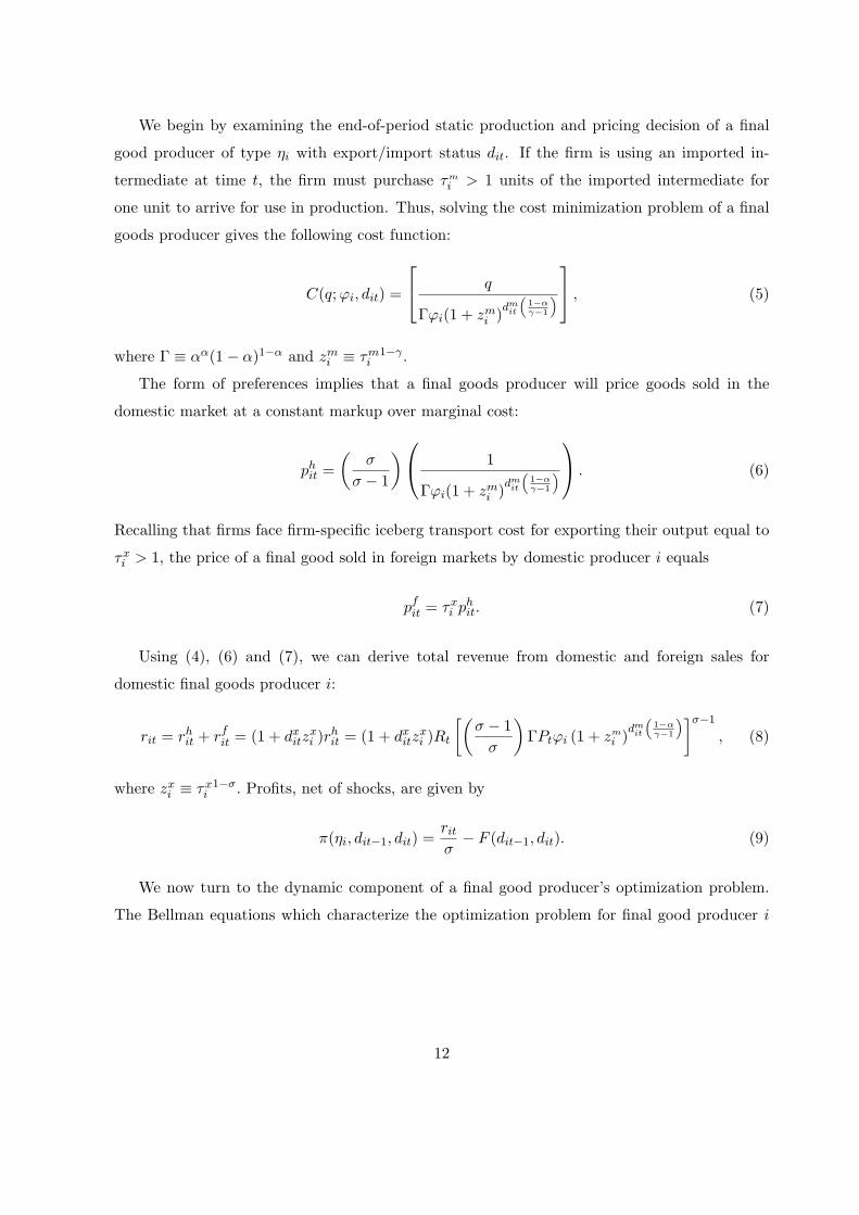
We begin by examining the end-of-period static production and pricing decision of a final

good producer of type ηi with export/import status dit. If the firm is using an imported in-

termediate at time t, the firm must purchase τmi > 1 units of the imported intermediate for

one unit to arrive for use in production. Thus, solving the cost minimization problem of a final

goods producer gives the following cost function:

C(q;φi, dit) =

q

Γφi(1 + zmi )dmit

(1−αγ−1

) , (5)

where Γ ≡ αα(1− α)1−α and zmi ≡ τmi1−γ .

The form of preferences implies that a final goods producer will price goods sold in the

domestic market at a constant markup over marginal cost:

phit =

(σ

σ − 1

) 1

Γφi(1 + zmi )dmit

(1−αγ−1

) . (6)

Recalling that firms face firm-specific iceberg transport cost for exporting their output equal to

τxi > 1, the price of a final good sold in foreign markets by domestic producer i equals

pfit = τxi phit. (7)

Using (4), (6) and (7), we can derive total revenue from domestic and foreign sales for

domestic final goods producer i:

rit = rhit + rfit = (1 + dxitzxi )r

hit = (1 + dxitz

xi )Rt

[(σ − 1

σ

)ΓPtφi (1 + zm

i )dmit

(1−αγ−1

)]σ−1

, (8)

where zxi ≡ τxi1−σ. Profits, net of shocks, are given by

π(ηi, dit−1, dit) =ritσ

− F (dit−1, dit). (9)

We now turn to the dynamic component of a final good producer’s optimization problem.

The Bellman equations which characterize the optimization problem for final good producer i

12

with (ηi, dit−1, ϵχit, ϵ

dit) are:

V (ηi, dit−1, ϵχit) = max

ϵχit(0), ϵχit(1) +

∫W (ηi, dit−1, ϵ

d)dHd(ϵd)

, (10)

W (ηi, dit−1, ϵdit) = max

d′∈D

(ϵd(d′) + π(ηi, dit−1, d

′) + β(1− ξ)

∫V (ηi, d

′, ϵχ)dHχ(ϵχ)

), (11)

where β ∈ (0, 1) is the discount factor. Now V (·, ·, ·) represents the value of a firm at the

beginning of the period and equation (10) characterizes the decision to exit or remain after

observing the exit cost shock. Equation (11) characterizes the firm’s export and import decision

after observing export/import cost shocks and recursively defines the value of a firm with state

variable (ηi, dit−1) and cost shock ϵdit.

In what follows, it is useful to define expected value functions as:

V (ηi, dit−1) =

∫V (ηi, dit−1, ϵ

χ)dHχ(ϵχ), (12)

W (ηi, dit−1) =

∫W (ηi, dit−1, ϵ

d)dHd(ϵd). (13)

We focus on stationary equilibria in which aggregate variables such as the aggregate price

index, P , aggregate revenue, R, the measure of final goods producers, and the distribution of

those producers by type and by export/import status is constant. We denote the stationary

equilibrium distribution of these variables across operating firms by µ∗(η, d). Of course, indi-

vidual firms enter, exit, and change their export/import status over time as they receive the

idiosyncratic shocks described above. We drop the time subscript and denote the state for final

good producer i as (ηi, di).

In the stationary equilibrium, free entry into final goods production implies that the expected

value of an entering firm must equal the fixed entry cost:∫V (η, (0, 0))gη(η)dη = fe. (14)

Stationarity also requires that the number of firms which exit equals the number of successful

entrants:

M

∫ (∑d∈D

Pχ(0|η, d)µ∗(η, d))gη(η)dη = Me

∫ (Pχ(1|η, (0, 0))

)gη(η)dη, (15)

where M is the mass of incumbents, Me is the mass of firms that attempt to enter, Pχ(0|η, d) is

13

the probability of exit for a firm with state (η, d) and Pχ(1|η, d) = 1−Pχ(0|η, d) is the probability

of not exiting for such a firm. Now, using the properties of extreme-value distributed random

variables (see, for example, Ben-Akiva and Lerman, 1985), we can derive the latter probability

as:

Pχ(1|η, d) = (1− ξ)

(exp(W (η, d)/ϱχ)

exp(0) + exp(W (η, d)/ϱχ)

), (16)

where W (·, ·) is defined in equation (13).

The final condition that the stationary equilibrium must satisfy is that the measure of firms

with state (η, d) is constant. To write that condition, we first derive the choice probabilities for

all possible current export/import statuses conditional on continuing to operate and the firm’s

state, (η, d). These follow the familiar logit formula (see, for example, McFadden, 1978) and are

as follows:

P d(d′|η, d) = exp([π(η, d, d′) + β(1− ξ)V (η, d′)]/ϱd)∑d∈D exp([π(η, d, d) + β(1− ξ)V (η, d)]/ϱd)

(17)

for d′ ∈ D. Hence, the equilibrium condition is written

Mµ∗(η, d) = M∑d′∈D

P d(d|η, d′)Pχ(1|η, d′)µ∗(η, d′) +MePd(d|η, (0, 0))Pχ(1|η, (0, 0))gη(η), (18)

for all states (η, d). The first term on the right-hand side is the measure of survivors from last

period with state (η, d) while the second term represents the measure of new entrants with that

state.

4 Structural Estimation

4.1 Empirical Methodology

We begin by placing distributional assumptions on the parameters which determine plant i′s

type, ηi. Let (σ − 1) ln(φi) be drawn from N(0, (σφ)2). We also assume that, conditional on

φi, that zxi and zm

i are independent of each other and are drawn at the time of entry from log

normal distributions with means µx and µm and standard deviations σx and σm, respectively.

Henceforth, we let plant i′s type be designated by ηi ≡ ((σ − 1) ln(φi), ln(zxi ), ln(z

mi ))′.

We assume that plant revenue, export intensity, and import intensity are measured with

error. Export and import intensities in the stationary equilibrium for a plant i at time t that

14

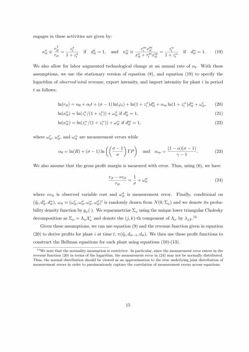
engages in these activities are given by:

κxit ≡rfitrit

=zxi

1 + zxiif dxit = 1, and κm

it ≡τmi xmit

xoit + τmi xmit=

zmi

1 + zmi

if dmit = 1. (19)

We also allow for labor augmented technological change at an annual rate of αt. With these

assumptions, we use the stationary version of equation (8), and equation (19) to specify the

logarithm of observed total revenue, export intensity, and import intensity for plant i in period

t as follows:

ln(rit) = α0 + αtt+ (σ − 1) ln(φi) + ln(1 + zxi )dxit + αm ln(1 + zm

i )dmit + ωr

it, (20)

ln(κxit) = ln(zxi /(1 + zxi )) + ωxit if d

xit = 1, (21)

ln(κmit) = ln(zm

i /(1 + zmi )) + ωm

it if dmit = 1, (22)

where ωrit, ω

xit, and ωm

it are measurement errors while

α0 = ln(R) + (σ − 1) ln

((σ − 1

σ

)ΓP

)and αm =

(1− α)(σ − 1)

γ − 1. (23)

We also assume that the gross profit margin is measured with error. Thus, using (6), we have

rit − vcitrit

=1

σ+ ωσ

it (24)

where vcit is observed variable cost and ωσit is measurement error. Finally, conditional on

(ηi, dxit, d

mit), ωit ≡ (ωr

it, ωxit, ω

mit , ω

σit)

′ is randomly drawn from N(0,Σω) and we denote its proba-

bility density function by gω(·). We reparametrize Σω using the unique lower triangular Cholesky

decomposition as Σω = ΛωΛ′ω and denote the (j, k)-th component of Λω by λj,k.

14

Given these assumptions, we can use equation (9) and the revenue function given in equation

(20) to derive profits for plant i at time t, π(ηi, dit−1, dit). We then use these profit functions to

construct the Bellman equations for each plant using equations (10)-(13).

14We note that the normality assumption is restrictive. In particular, since the measurement error enters in therevenue function (20) in terms of the logarithm, the measurement error in (24) may not be normally distributed.Thus, the normal distribution should be viewed as an approximation to the true underlying joint distribution ofmeasurement errors in order to parsimoniously capture the correlation of measurement errors across equations.

15

Finally, we use maximum likelihood to estimate the following parameter vector θ:15

θ ≡ (σ, f, fx, fm, cx, cm, ζ, α0, αt, αm, µx, µm, σφ, σx, σm, ξ, ϱχ, ϱd, vec(Λω)′, θ′0)

′, (25)

where vec(Λω) = (λ11, λ21, λ22, λ31, λ32, λ33, λ41, λ42, λ43, λ44)′ is the parameter vector deter-

mining the measurement error distribution while the set of parameters that specify the initial

distribution in 1990 is given by θ0 = (µφ0 , µ

x0 , µ

m0 , σφ

0 , σx0 , σ

m0 , αx

0 , αx1 , α

x2 , α

x3 , α

m0 , αm

1 , αm2 , αm

3 )′. In

what follows, we briefly describe the estimation methodology we use to estimate θ and provide

full details in the appendix.

Recalling that ϵχ and ϵd are type I extreme-value distributed random variables, we can write

the Bellman’s equations given by (12)-(13) for plant i as follows (see the appendix):

V (ηi, dit−1) = ϱχ ln(exp(0) + exp(W (ηi, dit−1)/ϱ

χ)), (26)

W (ηi, dit−1) = ϱd ln

(∑d′∈D

exp([π(ηi, dit−1, d

′) + β exp(αt)(1− ξ)V (ηi, d′)]/ϱd

)), (27)

where we have “detrended” firms’ problems by using the trend-adjusted discount factor β exp(αt)

in place of the discount factor β.16

Given a value for θ, we can solve the approximated model with a finite number of grid points

over firms’ types, η = ((σ−1) ln(φ), ln(zx), ln(zm))′. The continuous state space of (σ−1) ln(φ)

is approximated by nφ grid points uniformly distributed between φ and φ while the continuous

state space of ln(zx) and ln(zm) is approximated by nz grid points so that ln(zx/(1 + zx))

and ln(zm/(1 + zm)) are uniformly distributed between 0 and 1 together with two additional

end points at 0.0001 and 0.9999. Thus, the continuous state space of η is approximated by

nη = nφ × nz × nz points. The distribution function of η is accordingly approximated by a

multinomial distribution. In practice, we choose φ = −5, φ = 5, nφ = 20, and nz = 22.

Let ηk and ωk for k = 1, ..., nη be the grid points and weights associated with the multinomial

distribution, respectively. Given a θ, we can find the fixed point of the Bellman’s equations for

each ηk by iterating on (26)-(27) starting from an initial guess of W o(ηk, d) = 0 ∀d ∈ D, until

convergence. Once the fixed point is computed, we evaluate the conditional choice probabilities

in equations (16)-(17) for each ηk. We denote these probabilities as Pχθ (·|η

k, d) for the exit choice

15The discount factor β is not estimated but is set to 0.95. It is difficult to identify the discount factor indynamic discrete choice models (cf., Rust, 1987).

16In estimation, we restrict the value of β exp(αt)(1 − ξ) to be no more than 0.99 so that the value functioniteration does not diverge.

16

and as P dθ (·|ηk, d) for the export/import choice. The stationary distribution, µ∗

θ(η, d) is then

computed using the conditions for a stationary equilibrium given by equations (15) and (18).

The density of initial draws upon successful entry, geθ(η) is evaluated at ηk as

geθ(ηk) =

ωkPχθ (1|η

k, (0, 0))∑nη

j=1 ωjPχ

θ (1|ηj , (0, 0)). (28)

Finally, we need to derive the conditional density function for observed components of ωit,

conditional on (ηi, dit). Conditioning on ηi, we can compute an estimate of ωit, ωit(ηi) using

(20)-(22). We can then derive the following conditional density function:

gω,θ(ωit|ηi, dit) =

gωr(ωr

it(ηi))gωσ |ωr(ωσit(ηi)|ωr

it(ηi)) for dit = (0, 0),

gωr(ωrit(ηi))gωx|ωr(ωx

it(ηi)|ωrit(ηi))gωσ |ωr,ωx(ωσ

it(ηi)|ωrit(ηi), ω

xit(ηi)) for dit = (1, 0),

gωr(ωrit(ηi))gωm|ωr(ωm

it (ηi)|ωrit(ηi))gωσ |ωr,ωm(ωσ

it(ηi)|ωrit(ηi), ω

mit (ηi)) for dit = (0, 1),

gω(ωit(ηi)) for dit = (1, 1),

where gωr(·) is the marginal distribution of ωrit, gωj |ωr(ω

jit|ωr

it) is the conditional distribution of

ωjit given ωr

it for j ∈ x,m, σ, and gωσ |ωr,ωk(ωσit|ωr

it, ωkit) is the conditional distribution of ωσ

it

given ωrit and ωk

it for k ∈ x,m.

We now discuss the construction of the likelihood function for plant i. Let tio denote the

first year in which plant i appears in the data. Conditioning on ηi, the likelihood contribution

from the observation for plant i in period t > tio is computed as:

Lit(θ|ηi, dit−1) =

Pχθ (0|ηi, dit−1) for χit = 0,

Pχθ (1|ηi, dit−1)︸︷︷︸Staying

P dθ (dit|ηi, dit−1)︸︷︷︸

Export/Import

gω,θ(ωit|ηi, dit)︸︷︷︸Revenue/Intensity

for χit = 1.

For the initial period of operation for plant i, tio, the likelihood is given by Litio(θ|ηi, (0, 0)) =

P dθ (ditio |ηi, (0, 0))gω,θ(ωitio |ηi, ditio). With these, we can write the likelihood contribution from

plant i conditioned on (ηi, ditio) as

Li(θ|ηi, ditio) =Ti∏

t=tio+1

Lit(θ|ηi, dit−1), (29)

where Ti is the last year in which plant i appears in the data.

To compute the likelihood contribution from plant i, we integrate out η from the conditional

17

likelihood (29) using appropriate distributions of η as implied by the model. In particular, we

assume that η is drawn from geθ(η) defined in (28) for a plant that enters during the sample

period. For a plant observed in the first year of the sample period, 1990, we could assume that

η is distributed according to the stationary distribution µ∗θ(η, d) defined in (18). In the mid

1980’s, however, Chile experienced aggregate shocks, which may have caused deviations from

the steady state in 1990 and the stationarity assumption may not be appropriate for the initial

year. For this reason, we use a “flexible” but parsimonious initial conditions distribution in the

spirit of Heckman (1981) to determine the distribution of η in 1990 which we denote as µ0,θ(η, d).

Details of this procedure are given in the appendix.

The likelihood contribution from plant i is determined as:

Li(θ) =

∑nη

k=1 Li(θ|ηk, ditio)µ0,θ(ηk, ditio) for tio = 1990∑nη

k=1 Li(θ|ηk, ditio)P dθ (ditio |ηk, (0, 0))gω,θ(ωitio |ηk, ditio)geθ(ηk) for tio > 1990.

Finally, the parameter vector θ is estimated by maximizing the following log-likelihood function:

L(θ) ≡N∑i=1

Li(θ), (30)

where N is the number of plants in the data.

In summary, for each candidate parameter vector, θ, we solve the discretized versions of

(26)-(27) and then use those solutions to obtain the choice probabilities using (16)-(17), the

stationary distribution for (η, d), the conditional distributions for ω, and the distribution of η

upon entry. We then use these to evaluate the log-likelihood function given by (30). We repeat

this process to maximize L(θ) over the parameter space of θ to determine our estimate of θ.

4.2 Identification

In this section, we briefly discuss which features of the data allow our estimation procedure to

estimate particular parameters within θ. First, given the short panel data of seven periods, it

is not possible to identify plant-specific productivities and transport costs for each plant due to

the incidental parameters problem. For this reason, we follow the random effects approach by

imposing parametric distributional assumptions as described in the previous section.17 Specifi-

17Nonparametric identification of unobserved heterogeneity is difficult especially in the presence of state de-pendence as in our model. Kasahara and Shimotsu (2009) show that it is possible to nonparametrically identifythe distribution of unobserved heterogeneity when the length of panel data is sufficiently long and the covariates

18

cally, we assume that the distribution of ((σ− 1) lnφi, ln(zxi ), ln(z

mi )) is normally distributed at

the time of entry and we identify their means and standard deviations, (µx, µm, σφ, σx, σm), by

exploiting variation in productivities and export/import intensities among new entrants.

The per-period fixed cost of exporting, fx, is identified from the frequency with which ex-

porters become non-exporters. The sunk cost of exporting, cx, can be separately identified from

the per-period fixed cost, fx, by examining the extent to which past exporting status matters for

current exporting frequencies, after controlling for other plant characteristics. Once we control

for plant characteristics, whether a plant exported last year or not should not affect the proba-

bility of exporting when the sunk cost of exporting is zero. On the other hand, if a plant faces

large sunk costs of exporting, then a plant that exported last year is more likely to export this

year than a plant that did not export last year. Similarly the fixed and sunk costs associated

with importing, fm and cm, may be identified from the frequencies of importing and the extent

to which past importing status affects the probability of importing.

The fixed cost of operating, f , is identified from the frequencies of exiting across plants with

similar plant characteristics. The cost complementarity parameter, ζ, is identified by comparing

the frequencies of exporting among non-importers with the frequencies of exporting among

importers across plants after controlling for plant characteristics.

The scale parameters for exit shocks and export/import cost shocks, ϱχ and ϱd, are important

determinants of the elasticities of the different choice probabilities with respect to payoff relevant

state variables. Consequently, the scale parameter for exit shocks, ϱχ, is identified by differences

in exiting frequencies across plants with different plant characteristics while we may identify scale

parameters for shocks associated with export/import choices, ϱd, by differences in exporting

and importing frequencies across plants with different plant characteristics. The elasticity of

substitution in consumption, σ, is identified from average gross profit margins as specified in

equation (24).

Finally, we note that our estimate of θ alone does not allow us to identify the parameters of

the technology for producing final goods given in equation (2) including labor’s share, α, and the

elasticity of substitution between intermediates, γ. Instead, we compute the average material

shares in variable cost as our estimate of 1 − α and then use this estimate, our estimates of σ

and αm, and the second equation in (23) to derive an estimate of γ.

provide sufficient variation across different types.

19

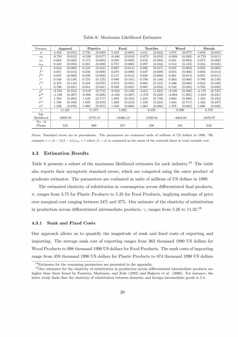
Table 6: Maximum Likelihood Estimates

Params. Apparel Plastics Food Textiles Wood Metalsσ 4.459 (0.055) 3.750 (0.039) 5.249 (0.065) 4.231 (0.042) 4.974 (0.077) 3.849 (0.033)α0 -0.791 (0.012) -0.528 (0.017) -0.466 (0.016) -0.673 (0.010) -0.869 (0.020) -0.753 (0.011)αt 0.063 (0.003) 0.172 (0.003) 0.033 (0.002) 0.016 (0.002) 0.031 (0.003) 0.073 (0.002)αm 0.249 (0.058) 0.201 (0.030) 0.757 (0.086) 0.297 (0.034) 0.314 (0.133) 0.234 (0.035)f 0.044 (0.008) 0.123 (0.016) 0.087 (0.014) 0.092 (0.017) 0.027 (0.003) 0.056 (0.005)fx 0.051 (0.012) 0.036 (0.009) 0.078 (0.009) 0.037 (0.009) 0.055 (0.006) 0.083 (0.014)fm 0.037 (0.009) 0.030 (0.009) 0.117 (0.014) 0.028 (0.009) 0.061 (0.013) 0.055 (0.011)cx 0.549 (0.138) 0.710 (0.125) 0.998 (0.101) 0.790 (0.146) 0.363 (0.068) 0.790 (0.136)cm 0.478 (0.116) 0.459 (0.076) 0.874 (0.081) 0.665 (0.121) 0.496 (0.088) 0.643 (0.108)ζ 0.796 (0.031) 0.814 (0.041) 0.930 (0.025) 0.885 (0.034) 0.742 (0.035) 0.762 (0.029)µx -3.704 (0.354) -3.519 (0.772) -0.834 (0.149) -3.651 (1.024) -2.520 (0.396) -4.178 (0.745)µm -1.539 (0.207) -0.988 (0.206) -3.168 (0.267) -1.570 (0.229) -4.004 (1.205) -1.924 (0.221)σx 1.350 (0.285) 1.128 (0.717) 1.682 (0.162) 1.233 (0.739) 2.063 (0.368) 1.334 (0.434)σm 1.196 (0.189) 1.635 (0.219) 1.209 (0.210) 1.109 (0.224) 1.644 (0.717) 1.462 (0.237)σφ 1.220 (0.076) 1.069 (0.074) 1.240 (0.068) 1.064 (0.080) 1.276 (0.082) 1.066 (0.049)γ 11.321 11.071 5.262 8.558 9.996 8.795

log-likelihood -3800.59 -3776.13 -10466.13 -5339.84 -4604.60 -4879.97No. ofPlants 534 369 857 530 561 642

Notes: Standard errors are in parentheses. The parameters are evaluated units of millions of US dollars in 1990. We

compute γ = (σ − 1)(1− α)/αm + 1 where (1− α) is computed as the mean of the material share in total variable cost.

4.3 Estimation Results

Table 6 presents a subset of the maximum likelihood estimates for each industry.18 The table

also reports their asymptotic standard errors, which are computed using the outer product of

gradients estimator. The parameters are evaluated in units of millions of US dollars in 1990.

The estimated elasticity of substitution in consumption across differentiated final products,

σ, ranges from 3.75 for Plastic Products to 5.25 for Food Products, implying markups of price

over marginal cost ranging between 24% and 37%. Our estimate of the elasticity of substitution

in production across differentiated intermediate products, γ, ranges from 5.26 to 11.32.19

4.3.1 Sunk and Fixed Costs

Our approach allows us to quantify the magnitude of sunk and fixed costs of exporting and

importing. The average sunk cost of exporting ranges from 363 thousand 1990 US dollars for

Wood Products to 998 thousand 1990 US dollars for Food Products. The sunk costs of importing

range from 459 thousand 1990 US dollars for Plastic Products to 874 thousand 1990 US dollars

18Estimates for the remaining parameters are presented in the appendix.19Our estimates for the elasticity of substitution in production across differentiated intermediate products are

higher than those found by Feenstra, Markusen, and Zeile (1992) and Halpern et al. (2006). For instance, thelatter study finds that the elasticity of substitution between domestic and foreign intermediate goods is 5.4.

20

for food products. Thus, both exporting and importing requires high start-up costs, which

may arise because starting to import requires establishing a network with foreign suppliers,

learning government regulations, or implementing new materials. It is important to note that

the exporting and importing costs actually incurred are lower than these estimates since plants

start exporting and/or importing when they get lower cost shocks. Furthermore, as we discuss

below, plants that both export and import pay considerably less of the sunk costs because of

cost complementarities.

We note that controlling for permanent unobserved heterogeneities in productivity and trans-

portation costs is important for estimation of the sunk costs. Without controlling for permanent

unobserved heterogeneities, the sunk costs will be overestimated.20 Our specification has a lim-

itation, however, in that it does not allow for serially correlated transitory shocks, which could

lead to an upward bias in our sunk cost estimates.21

The fixed costs of exporting range from 36 to 83 thousand 1990 US dollars while the fixed

costs of importing range from 28 to 117 thousand 1990 US dollars, indicating that both exporters

and importers also pay substantial per-period fixed costs to continue to export and import. The

parameter determining the degree of complementarity in exporting and importing sunk and fixed

costs, ζ, ranges from 0.74 to 0.93, indicating that a firm can save between 7 and 26 percent of

the per-period fixed costs and sunk costs associated with trade by simultaneously engaging in

both export and import activities. Hence, the estimated total fixed costs of trading for a plant

that both exports and imports range from 54 thousand 1990 US dollars for Plastic Products to

181 thousand 1990 US dollars for Food Products.

4.3.2 Importing and Exporting

The estimates of αm, µx, µm, σx, and σm indicate that the effects of exporting and importing

on total revenue differ across plants but, on average, their impact is large. In particular, for the

“average” plant in an industry with zxi = exp(µx) and zm

i = exp(µm), the revenue premium from

exporting ranges from 1.5% for Metals to 36.1% for Food Products while the revenue premium

20For instance, when we re-estimate the model for Apparel industry by fixing the standard deviations of perma-nent unobserved heterogeneities at one-half of the original maximum likelihood estimates, the sunk cost estimatefor exporting increases from 0.549 to 2.423.

21To the best of our knowledge, the only previous study that estimates the magnitude of sunk costs of exportingis Das et al. (2007) while there is no previous study that estimates importing sunk costs. Despite using differentempirical specifications and looking at different countries and industries, our estimates of exporting sunk costsare similar in magnitude, although larger, to the estimates of Das, Roberts, and Tybout, especially given ourrelatively large standard errors. Their estimates range from 344 thousand 1986 US dollars to 430 thousand 1986US dollars for leather products, basic chemicals, and knitted fabrics industries in Columbia.

21

0 0.1 0.2 0.3 0.4 0.5 0.6 0.7 0.8 0.9 1.00

0.1

0.2

0.3

0.4

0.5

0.6

Export Intensity

Fre

quen

cy

Wearing Apparel (ISIC 3220)

0 0.1 0.2 0.3 0.4 0.5 0.6 0.7 0.8 0.9 1.00

0.1

0.2

0.3

0.4

0.5

0.6

Import Intensity

Fre

quen

cy


0 0.1 0.2 0.3 0.4 0.5 0.6 0.7 0.8 0.9 1.00

0.1

0.2

0.3

0.4

0.5

0.6

Export Intensity

Fre

quen

cy

Food Products (ISIC 311)

0 0.1 0.2 0.3 0.4 0.5 0.6 0.7 0.8 0.9 1.00

0.1

0.2

0.3

0.4

0.5

0.6

Import Intensity

Fre

quen

cy


actual exporterspredicted exporterspredicted non−exporters

actual importerspredicted importerspredicted non−importers

actual exporterspredicted exporterspredicted non−exporters

actual importerspredicted importerspredicted non−importers

Figure 1: Export and Import Intensities (Actual vs. Predicted)

from importing intermediates varies from 0.6% for Wood Products to 6.4% for Plastics.22 Fur-

thermore, the estimates of σx and σm suggest substantial heterogeneity in gains from exporting

and importing. Note that since plants with larger gains from exporting and importing are more

likely to self-select into those activities, the average revenue gains from exporting and importing

among actual exporters and importers is even larger than the gain for the “average” plant.

Figure 1 compares the actual and predicted distribution of export and import intensities

for one of our four digit industries, Wearing Apparel, and one of our three digit industries,

Food Products. In the top panels, the solid line indicates the actual export intensities while

the dashed line indicates the predicted export intensities. The empirical models quantitatively

replicate the observed pattern of export intensities. The figure also plots the distribution of

latent export intensities among non-exporters if they had exported. The distribution of non-

exporters (dotted line) is skewed left relative to that of exporters (dashed line). This is because,

in the model, plants with lower transportation costs are more likely to export than plants with

22The revenue premium from exporting is derived from the coefficient on dxit in equation (20): ln(1 + zxi )

while the revenue increase from importing intermediates is derived from the coefficient on dmit in that equation:αm ln(1 + zm

i ).

22

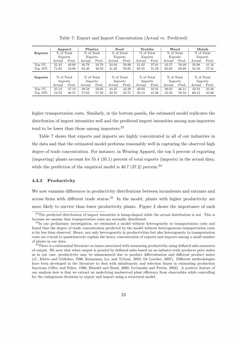
Table 7: Export and Import Concentration (Actual vs. Predicted)

Apparel Plastics Food Textiles Wood MetalsExports % of Total % of Total % of Total % of Total % of Total % of Total

Exports Exports Exports Exports Exports ExportsActual Pred. Actual Pred. Actual Pred. Actual Pred. Actual Pred. Actual Pred.

Top 5% 55.43 40.68 46.79 34.79 24.94 50.99 51.02 37.01 42.57 58.49 34.98 41.10Top 10% 71.03 54.96 64.46 48.58 41.28 59.95 68.35 51.59 62.63 69.60 54.16 57.41

Imports % of Total % of Total % of Total % of Total % of Total % of TotalImports Imports Imports Imports Imports Imports

Actual Pred. Actual Pred. Actual Pred. Actual Pred. Actual Pred. Actual Pred.Top 5% 35.13 37.19 38.58 50.05 44.45 42.29 40.93 32.31 39.03 46.11 42.53 35.20Top 10% 54.70 46.57 57.63 57.56 59.70 55.75 58.13 41.08 52.50 59.10 60.12 45.86

higher transportation costs. Similarly, in the bottom panels, the estimated model replicates the

distribution of import intensities well and the predicted import intensities among non-importers

tend to be lower than those among importers.23

Table 7 shows that exports and imports are highly concentrated in all of our industries in

the data and that the estimated model performs reasonably well in capturing the observed high

degree of trade concentration. For instance, in Wearing Apparel, the top 5 percent of exporting

(importing) plants account for 55.4 (35.1) percent of total exports (imports) in the actual data,

while the prediction of the empirical model is 40.7 (37.2) percent.24

4.3.3 Productivity

We now examine differences in productivity distributions between incumbents and entrants and

across firms with different trade status.25 In the model, plants with higher productivity are

more likely to survive than lower productivity plants. Figure 2 shows the importance of such

23The predicted distribution of import intensities is hump-shaped while the actual distribution is not. This isbecause we assume that transportation costs are normally distributed.

24In our preliminary investigation, we estimated a model without heterogeneity in transportation costs andfound that the degree of trade concentration predicted by the model without heterogeneous transportation costsis far less than observed. Hence, not only heterogeneity in productivities but also heterogeneity in transportationcosts are crucial to quantitatively explain the heavy concentration of exports and imports among a small numberof plants in our data.

25There is a substantial literature on issues associated with measuring productivity using deflated sales measuresof output. We note that when output is proxied by deflated sales based on an industry-wide producer price indexas in our case, productivity may be mismeasured due to product differentiation and different product mixes(cf., Klette and Griliches, 1996; Katayama, Lu, and Tybout, 2003; De Loecker, 2007). Different methodologieshave been developed in the literature to deal with simultaneity and selection biases in estimating productionfunctions (Olley and Pakes, 1996; Blundel and Bond, 2000; Levinsohn and Petrin, 2002). A positive feature ofour analysis here is that we extract an underlying unobserved plant efficiency from observables while controllingfor the endogenous decisions to export and import using a structural model.

23

Table 8: Mean of Predicted Productivity

Relative Mean of φ for Apparel Plastics Food Textiles Wood MetalsIncumbents 1.288 1.456 1.349 1.534 1.165 1.225Exporters 2.492 2.092 1.788 2.238 2.018 2.106Importers 2.154 1.807 2.239 2.075 2.869 1.772Ex&Importers 3.257 2.373 2.631 2.758 3.284 2.569

Notes: The reported numbers are relative to the productivity level at entry in the estimated model. In particular, the

original numbers are divided by the mean of φ at entry (i.e.,∫φgφ(φ)dφ). “Exporters” are plants that export while

“Importers” are plants that import. “Ex&Importers” represent plants that both export and import.

a selection mechanism for Wearing Apparel and Food Products. In the top panels, the actual

productivity distribution among incumbents (solid line) is skewed right relative to the actual

productivity distribution among new entrants.26 The bottom panels show that the empirical

models qualitatively capture the observed difference in the productivity distributions between

incumbents and new entrants.27 In Table 8, the predicted average productivity advantage of

incumbents relative to that of plants attempting to enter ranges from 17% in Wood Products to

53% for Textiles, indicating that selection through endogenous exiting may play an important

role in determining aggregate productivity.

Exporters and importers tend to have higher productivities than domestic plants that do

not engage in any trading activities because higher productivity plants are more likely to export

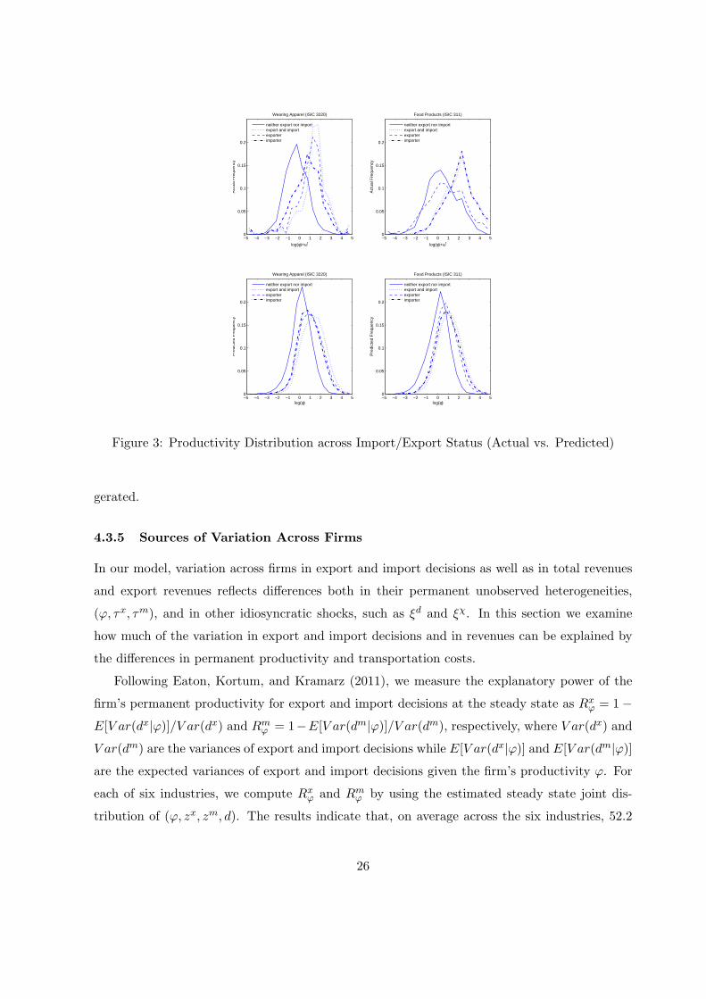
and import and because importing increases productivity. This is shown in Figure 3 for Apparel

and Food. In the top panels of the figure, the actual productivity distributions among plants

that export, plants that import and plants that do both are skewed right relative to the actual

distribution among plants that do neither. As the bottom panels show, the estimated models

replicate the basic patterns of the differences in productivity distributions across plants with

different trading status. This is also demonstrated in Table 8 for all the industries in our

sample. The average productivity advantage of exporters and importers relative to the average

incumbent is large, ranging from 54% for exporters in Plastic Products to 170% for importers

in Wood Products. The table also shows that plants which both export and import are even

more productive on average.

26To construct the actual productivity distribution, we first compute a revenue residual, lnφi + ωrit, for each

plant-time observation as our measure of “actual productivity,” and then plot a histogram of these residuals.27The numbers used to construct Figures 1-3 as well as those reported in Tables 8-12 are directly computed

using the approximated distribution function rather than simulating the data from the estimated models. Theapproximation methods are presented in a supplementary appendix which is available upon request.

24

−5 −4 −3 −2 −1 0 1 2 3 4 50

0.05

0.1

0.15

0.2

log(φ)+ωr

Act

ual F

requ

ency


−5 −4 −3 −2 −1 0 1 2 3 4 50

0.05

0.1

0.15

0.2

log(φ)

Pre

dict

ed F

requ

ency


−5 −4 −3 −2 −1 0 1 2 3 4 50

0.05

0.1

0.15

0.2

log(φ)+ωr

Act

ual F

requ

ency


−5 −4 −3 −2 −1 0 1 2 3 4 50

0.05

0.1

0.15

0.2

log(φ)

Pre

dict

ed F

requ

ency


IncumbentsEntrants

IncumbentsEntrants

IncumbentsEntrants

IncumbentsEntrants

Figure 2: Productivity Distribution of Incumbents and New Entrants (Actual vs. Predicted)

4.3.4 Dynamics

Table 9 shows predicted transition probabilities of export/import status conditional on not

exiting from the market. The table also reports the distribution of entrants as well as the

steady state distribution of plants according to export/import status. Comparing these results

to those from the actual data in Table 4, we see that the estimated models are able to replicate

the observed persistence in export/import status. The model also captures the new entrants’

distribution and the steady state distribution of export/import status reasonably well.

The empirical models generate the observed persistence in export/import status for the fol-

lowing two reasons. First, the presence of sunk costs of exporting and importing generates “true

state dependence” in export/import decisions. Second, unobserved heterogeneity may lead to

“spurious state dependence” even without sunk costs because, for instance, highly productive

plants are likely to keep exporting while less productive plants do not export. We note that

in our specification, plant-specific shocks have a permanent unobserved component and serially

uncorrelated transitory component. If the transitory component is actually serially correlated,

our estimated effects of permanent unobserved heterogeneity and/or sunk costs could be exag-

25

−5 −4 −3 −2 −1 0 1 2 3 4 50

0.05

0.1

0.15

0.2

log(φ)+ωr

Act

ual F

requ

ency


−5 −4 −3 −2 −1 0 1 2 3 4 50

0.05

0.1

0.15

0.2

log(φ)

Pre

dict

ed F

requ

ency


−5 −4 −3 −2 −1 0 1 2 3 4 50

0.05

0.1

0.15

0.2

log(φ)+ωr

Act

ual F

requ

ency


−5 −4 −3 −2 −1 0 1 2 3 4 50

0.05

0.1

0.15

0.2

log(φ)

Pre

dict

ed F

requ

ency


neither export nor importexport and importexporterimporter




Figure 3: Productivity Distribution across Import/Export Status (Actual vs. Predicted)

gerated.

4.3.5 Sources of Variation Across Firms

In our model, variation across firms in export and import decisions as well as in total revenues

and export revenues reflects differences both in their permanent unobserved heterogeneities,

(φ, τx, τm), and in other idiosyncratic shocks, such as ξd and ξχ. In this section we examine

how much of the variation in export and import decisions and in revenues can be explained by

the differences in permanent productivity and transportation costs.

Following Eaton, Kortum, and Kramarz (2011), we measure the explanatory power of the

firm’s permanent productivity for export and import decisions at the steady state as Rxφ = 1−

E[V ar(dx|φ)]/V ar(dx) and Rmφ = 1−E[V ar(dm|φ)]/V ar(dm), respectively, where V ar(dx) and

V ar(dm) are the variances of export and import decisions while E[V ar(dx|φ)] and E[V ar(dm|φ)]

are the expected variances of export and import decisions given the firm’s productivity φ. For

each of six industries, we compute Rxφ and Rm

φ by using the estimated steady state joint dis-

tribution of (φ, zx, zm, d). The results indicate that, on average across the six industries, 52.2

26

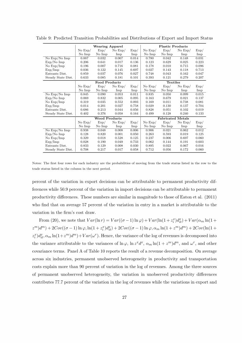
Table 9: Predicted Transition Probabilities and Distributions of Export and Import Status

Wearing Apparel Plastic ProductsNo Exp/ Exp/ No Exp/ Exp/ No Exp/ Exp/ No Exp/ Exp/No Imp No Imp Imp Imp No Imp No Imp Imp Imp


Food Products TextilesNo Exp/ Exp/ No Exp/ Exp/ No Exp/ Exp/ No Exp/ Exp/No Imp No Imp Imp Imp No Imp No Imp Imp Imp


Wood Products Fabricated MetalsNo Exp/ Exp/ No Exp/ Exp/ No Exp/ Exp/ No Exp/ Exp/No Imp No Imp Imp Imp No Imp No Imp Imp Imp


Notes: The first four rows for each industry are the probabilities of moving from the trade status listed in the row to the

trade status listed in the column in the next period.

percent of the variation in export decisions can be attributable to permanent productivity dif-

ferences while 50.9 percent of the variation in import decisions can be attributable to permanent

productivity differences. These numbers are similar in magnitude to those of Eaton et al. (2011)

who find that on average 57 percent of the variation in entry in a market is attributable to the

variation in the firm’s cost draw.

From (20), we note that V ar(ln r) = V ar((σ− 1) lnφ)+V ar(ln(1+ zxi )dxit)+V ar(αm ln(1+

zm)dm) + 2Cov((σ− 1) lnφ, ln(1 + zxi )dxit) + 2Cov((σ− 1) lnφ, αm ln(1 + zm)dm) + 2Cov(ln(1 +

zxi )dxit, αm ln(1+zm)dm)+V ar(ωr). Hence, the variance of the log of revenues is decomposed into

the variance attributable to the variances of lnφ, ln zxdx, αm ln(1 + zm)dm, and ωr, and other

covariance terms. Panel A of Table 10 reports the result of a revenue decomposition. On average

across six industries, permanent unobserved heterogeneity in productivity and transportation

costs explain more than 90 percent of variation in the log of revenues. Among the three sources

of permanent unobserved heterogeneity, the variation in unobserved productivity differences

contributes 77.7 percent of the variation in the log of revenues while the variations in export and

27

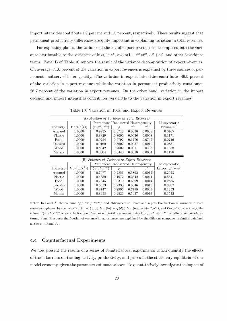
import intensities contribute 4.7 percent and 1.5 percent, respectively. These results suggest that

permanent productivity differences are quite important in explaining variation in total revenues.

For exporting plants, the variance of the log of export revenues is decomposed into the vari-

ance attributable to the variances of lnφ, ln zx, αm ln(1+ zm)dm, ωx+ωr, and other covariance

terms. Panel B of Table 10 reports the result of the variance decomposition of export revenues.

On average, 71.0 percent of the variation in export revenues is explained by three sources of per-

manent unobserved heterogeneity. The variation in export intensities contributes 49.9 percent

of the variation in export revenues while the variation in permanent productivity contributes

26.7 percent of the variation in export revenues. On the other hand, variation in the import

decision and import intensities contributes very little to the variation in export revenues.

Table 10: Variation in Total and Export Revenues

(A) Fraction of Variance in Total Revenues

Permanent Unobserved Heterogeneity IdiosyncraticIndustry V ar(ln(r)) (φ, τx, τm) φ τx τm Errors: ωr

Apparel 1.0000 0.9235 0.8713 0.0038 0.0008 0.0765Plastic 1.0000 0.8829 0.8090 0.0036 0.0008 0.1171Food 1.0000 0.9254 0.5792 0.1776 0.0745 0.0746

Textiles 1.0000 0.9169 0.8607 0.0037 0.0010 0.0831Wood 1.0000 0.8942 0.7002 0.0911 0.0133 0.1058Metals 1.0000 0.8804 0.8440 0.0018 0.0004 0.1196

(B) Fraction of Variance in Export Revenues

Permanent Unobserved Heterogeneity Idiosyncratic

Industry V ar(ln(rf )) (φ, τx, τm) φ τx τm Errors: ωx + ωr

Apparel 1.0000 0.7077 0.2851 0.3892 0.0012 0.2923Plastic 1.0000 0.4659 0.1972 0.2642 0.0041 0.5341Food 1.0000 0.7345 0.3319 0.6899 0.0014 0.2655

Textiles 1.0000 0.6313 0.2338 0.3646 0.0015 0.3687Wood 1.0000 0.8747 0.2996 0.7798 0.0003 0.1253Metals 1.0000 0.8458 0.2526 0.5057 0.0017 0.1542

Notes: In Panel A, the columns “φ,” “τx,” “τm,” and “Idiosyncratic Errors ωr” report the fraction of variance in total

revenues explained by the terms V ar((σ−1) lnφ), V ar(ln(1+zxi )dxit), V ar(αm ln(1+zm)dm), and V ar(ωr), respectively; the

column “(φ, τx, τm)” reports the fraction of variance in total revenues explained by φ, τx, and τm including their covariance

terms. Panel B reports the fraction of variance in export revenues explained by the different components similarly defined

as those in Panel A.

4.4 Counterfactual Experiments

We now present the results of a series of counterfactual experiments which quantify the effects

of trade barriers on trading activity, productivity, and prices in the stationary equilibria of our

model economy, given the parameter estimates above. To quantitatively investigate the impact of

28

trade barriers and export/import complementarities, we conduct the following six counterfactual

experiments: (1) Autarky (fx, fm → ∞); (2) No Trade in Final Goods (fx → ∞); (3) No Trade

in Intermediates (fm → ∞); (4) No Complementarity in Fixed Trading Costs (ζ = 1); (5)

The transportation cost of exporting, τx, increases by 10%; and (6) The transportation cost of

importing, τm, increases by 10%.

To determine the full impact of a counterfactual experiment, it is necessary to compute how

the equilibrium aggregate price changes as a result of the experiment because the “reduced-

form” parameter α0 in the revenue function given by (20) depends on the aggregate price, (see

(23)). This can be achieved by finding a new equilibrium aggregate price at which the free entry

condition (14) holds in the experiments. The appendix provides a detailed description of our

approach.

Table 11 presents the results of the counterfactual experiments using the estimated models.

According to these experiments, moving from autarky to trade decreases the industry price-

index by between 2.6% for Wood Products to 31.9% for Plastic Products, suggesting that there

are substantial increases in consumers’ purchasing power for these goods due to trade. This

increases consumer welfare and this positive welfare effect occurs because under trade, more

productive firms start exporting and importing, which in turn increases aggregate labor demand

and the real wage.28 The impact of trade on aggregate productivity, measured by a productivity

average using the plants’ market shares as weights, can be understood by comparing “ln(Average

φ)” at the steady state between trade and autarky. Moving from trade to autarky decreases

this measure of aggregate productivity at the steady state by between 1.7% for Food Products

and 8.4% for Plastic Products. Note that once we take into account the additional productivity

effect arising from importing intermediates, the impact of trade on total factor productivity

(TFP) is much larger at 8.6% and 21.4% for those two industries. Comparing these effects, we

28In our industry-level counterfactual experiments, the change in P is an estimate of the effect of trade re-strictions on the industry-level price index so its inverse is a measure of the change in real purchasing power ofa consumer for goods in that industry. If these were the only goods in the consumer’s consumption basket, thechange in the industry price index would capture the effect of trade liberalization on aggregate consumer welfare.This is a standard result in the literature (see Arkolakis, Costinot, and Rodriguez-Clare (2012, ACR-C hereafter),for example) and can be seen from the aggregate budget constraint, PQ = L, which implies that aggregate utilityis given by U = Q = L

P. Now, since L is constant, changes in aggregate welfare are measured by the inverse

of changes in the aggregate price index. Of course, if there are other goods in consumers’ consumption baskets,changes in industry-level price indexes would be weighted by expenditure share in calculating the effect of changesin the trading environment on consumers’ overall welfare. We also note that compared to the relatively modestaggregate welfare gains from trade discussed in ACR-C for the U.S., we would expect larger estimated welfaregains in our study because: (1) The import penetration ratio for Chile is approximately 30% which is much largerthan the U.S. ratio of 7%; and (2) The industries we study are very active in trade so we would expect fairlysizable price effects from prohibiting trade.

29

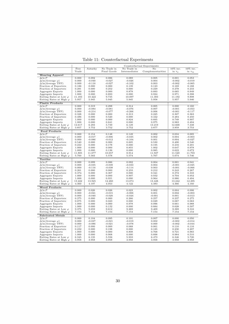
Table 11: Counterfactual Experiments

Counterfactual ExperimentsFree Autarky No Trade in No Trade in No 10% inc. 10% inc.Trade Final Goods Intermediates Complementarities in τx in τm

Wearing Apparel∆ lnP 0.000 0.092 0.086 0.089 0.005 0.001 0.053∆ ln(Average φ) 0.000 -0.040 -0.027 -0.026 0.004 -0.002 -0.019∆ ln(Average TFP) 0.000 -0.116 -0.027 -0.102 0.003 -0.002 -0.065Fraction of Exporters 0.186 0.000 0.000 0.139 0.123 0.169 0.188Fraction of Importers 0.281 0.000 0.252 0.000 0.229 0.278 0.233Aggregate Exports 1.000 0.000 0.000 0.878 0.893 0.685 0.949Aggregate Imports 1.000 0.000 0.893 0.000 0.924 0.971 0.398Exiting Rates at Low φ 11.183 10.422 9.735 10.097 11.383 11.192 9.898Exiting Rates at High φ 5.957 5.945 5.945 5.945 5.958 5.957 5.946

Plastic Products∆ lnP 0.000 0.319 0.298 0.314 0.005 0.000 0.160∆ ln(Average φ) 0.000 -0.084 -0.081 -0.076 0.007 -0.001 -0.053∆ ln(Average TFP) 0.000 -0.214 -0.077 -0.206 0.006 -0.001 -0.117Fraction of Exporters 0.328 0.000 0.000 0.313 0.225 0.307 0.363Fraction of Importers 0.486 0.000 0.520 0.000 0.442 0.484 0.450Aggregate Exports 1.000 0.000 0.000 0.824 0.895 0.749 0.907Aggregate Imports 1.000 0.000 0.841 0.000 0.975 0.983 0.494Exiting Rates at Low φ 12.617 6.293 5.739 6.129 13.219 12.668 7.338Exiting Rates at High φ 3.857 3.752 3.752 3.752 3.877 3.859 3.753

Food Products∆ lnP 0.000 0.154 0.148 0.149 0.002 0.034 0.005∆ ln(Average φ) 0.000 -0.017 -0.006 -0.035 0.002 0.004 -0.003∆ ln(Average TFP) 0.000 -0.086 -0.012 -0.104 0.001 0.004 -0.027Fraction of Exporters 0.540 0.000 0.000 0.605 0.530 0.490 0.540Fraction of Importers 0.222 0.000 0.178 0.000 0.195 0.216 0.201Aggregate Exports 1.000 0.000 0.000 0.855 1.002 0.647 0.978Aggregate Imports 1.000 0.000 0.136 0.000 0.985 0.622 0.672Exiting Rates at Low φ 11.805 11.677 10.657 8.914 11.927 11.520 11.703Exiting Rates at High φ 5.760 5.582 5.578 5.574 5.767 5.674 5.746

Textiles∆ lnP 0.000 0.099 0.086 0.092 0.004 0.001 0.041∆ ln(Average φ) 0.000 -0.035 -0.039 -0.033 0.004 -0.001 -0.025∆ ln(Average TFP) 0.000 -0.116 -0.038 -0.114 0.003 -0.001 -0.066Fraction of Exporters 0.261 0.000 0.000 0.233 0.212 0.243 0.267Fraction of Importers 0.374 0.000 0.367 0.000 0.341 0.372 0.333Aggregate Exports 1.000 0.000 0.000 0.907 0.932 0.704 0.952Aggregate Imports 1.000 0.000 0.921 0.000 0.964 0.980 0.494Exiting Rates at Low φ 13.222 13.925 12.260 13.074 13.428 13.242 12.295Exiting Rates at High φ 4.360 4.197 4.053 4.122 4.383 4.366 4.160

Wood Products∆ lnP 0.000 0.026 0.026 0.023 0.002 0.004 0.006∆ ln(Average φ) 0.000 -0.021 -0.015 -0.006 0.001 0.002 -0.003∆ ln(Average TFP) 0.000 -0.040 -0.020 -0.024 -0.001 0.001 -0.013Fraction of Exporters 0.275 0.000 0.000 0.266 0.257 0.237 0.275Fraction of Importers 0.075 0.000 0.023 0.000 0.029 0.067 0.063Aggregate Exports 1.000 0.000 0.000 0.978 0.996 0.661 0.988Aggregate Imports 1.000 0.000 0.132 0.000 0.884 0.628 0.507Exiting Rates at Low φ 9.375 9.659 9.612 9.269 9.409 9.389 9.316Exiting Rates at High φ 7.154 7.154 7.154 7.154 7.154 7.154 7.154

Fabricated Metals∆ lnP 0.000 0.104 0.095 0.101 0.007 0.000 0.050∆ ln(Average φ) 0.000 -0.027 -0.021 -0.019 0.002 -0.002 -0.014∆ ln(Average TFP) 0.000 -0.086 -0.021 -0.078 0.000 -0.002 -0.044Fraction of Exporters 0.117 0.000 0.000 0.068 0.061 0.110 0.116Fraction of Importers 0.232 0.000 0.198 0.000 0.185 0.230 0.207Aggregate Exports 1.000 0.000 0.000 0.808 0.768 0.721 0.965Aggregate Imports 1.000 0.000 0.908 0.000 0.898 0.984 0.510Exiting Rates at Low φ 6.345 6.135 5.556 5.933 6.473 6.346 5.720Exiting Rates at High φ 3.958 3.958 3.958 3.958 3.958 3.958 3.958

30

see that the majority of TFP effect of trade is induced by importing intermediates.29

The counterfactual experiments under no trade in final goods or no trade in intermediates

(but not both) highlight the interaction between exporting and importing in the presence of

heterogeneous firms. According to the estimated models, when the economy moves from full

trade to no trade in final goods, both the fraction of importers of intermediates and the level of

imported intermediates declines in all of our industries. Furthermore, when the economy moves

from full trade to no trade in intermediates, the fraction of exporters of final goods falls in all

industries except Food Products while total exports of final goods decline in all industries.30

Thus, generally policies that prohibit the import of foreign materials could have a large negative

impact on the exporting of final

consumption goods – that is, import protection can lead to export destruction.

We now briefly examine the role of complementarities between export and import fixed and

sunk costs relative to the role played by the complementarities in the revenue function. To

do so we conduct an experiment to determine what would happen to the fraction of importers

and the fraction of exporters if there was no complementarity between exporting and importing

in the fixed and sunk cost functions. We find that eliminating cost complementarities lowers

the fraction of exporters and importers as well as aggregate exports and imports for all of our

industries, providing evidence that the cost complementarities play a role in inducing plants to

both export and import simultaneously.

We conduct additional (less extreme) experiments to examine what would happen to prices

and productivity if the transportation cost parameters, τx and τm, were 10% higher than the

actual estimates. The results are presented in columns (5) and (6) of Table 11. A 10 percent

increase in transportation costs of either form have a relatively small impact on the fraction

of exporters and importers but a substantial impact on aggregate exports and imports. This

implies that the impact of an increase in transportation costs (or tariffs) on aggregate exports

and imports operates mainly through the intensive margin rather than through the extensive

margin. This finding is consistent with the findings of Das et al. (2007). We also note that a

29We remind the reader that our assumption of an exogenously fixed measure of intermediate goods blueprintsimplies that our model does not capture the full general equilibrium effects on welfare, resource allocation,and productivity of trade liberalization. In particular, if the measure of intermediate goods were endogenouslydetermined, increased trade would presumably induce resource allocations within intermediate goods producersas well as additional reallocations between intermediate and final good producers. However, since we assume thatthe measure of intermediates produced within a country is fixed and in our estimation we treat all producers asfinal good suppliers, we miss some of these resource reallocations that might affect our measures of productivityand consumer purchasing power gains.

30For Food Products, the fraction of exporters rises slightly when trade in intermediates is restricted becauseof the relatively large price effect.

31

10 percent increase in import tariffs has a substantial effect on the average TFP ranging from

1.3 percent in Wood Products to 11.7 percent in Plastic Products.

The last two rows in each panel of Table 11 report average exit rates at the steady state for low

productivity firms (φ < 1) and for high productivity firms (φ ≥ 1).31 When the economy moves

from autarky to trade, an increase in profitability from exporting and importing lowers exiting

rates while an increase in the real wage tends to increase exiting rates, especially for the least

productive firms.For all industries except for Wood Products, the latter effect dominates, and

moving from autarky to trade induces a substantial increase in exit rates for the less productive

firms and, hence, a resource reallocation from less to more efficient firms. 32

To examine the distributional effects of trade policies, Table 12 reports the effect of alterna-

tive policies on average revenues across different values of φ, zx, and zm. We classify the firm’s

state space into eight categories by classifying each of φ, zx, and zm into two categories; “H”

and “L.”33 Recall that high transport costs is associated with low levels of zj so, for example,

a firm with (φ, zx, zm) = (L,L, L) is a low productivity firm with high transport costs for both

exporting and importing. For all six industries, moving from free trade to autarky increases the

size of firms with low productivity and high transportation costs while it decreases the size of

firms with high productivity and low transportation costs. Thus, an increase in trade barriers

leads to resource allocation from efficient to inefficient firms.

Because changes in trade policies affect both extensive and intensive margins, different trade

regimes will lead to different size distributions. Figure 4 shows the distribution of revenues

across different trade policies. Trade regimes closer to free trade tend to have a size distribution

that stochastically dominates the distribution under regimes with trade barriers, especially for

Plastic Products and Food Products industries.

5 Conclusions and Extensions

We have developed and estimated a stochastic industry model of importing and exporting with

heterogeneous firms. The estimated model is consistent with many key features of the data

regarding productivity, exporting, and importing. The results of our counterfactual experiments

31Recall that the distribution of lnφ is normalized so that its expectation is equal to zero at the time of entry.32In the model of Melitz (2003), the latter effect dominates the former for a set of parametric productivity

distributions he considers. On the other hand, in our model with additional stochastic elements such as iid costshocks, the effect of moving from autarky to trade on exit rates is ambiguous in general, and it depends on theparameter values.

33We define φ to be “L” if lnφ < 0 and “H” if lnφ ≥ 0 while we let zj for j = x,m to be “L” if zj/(1+zj) < 0.2and “H” if zj/(1 + zj) ≥ 0.2.

32

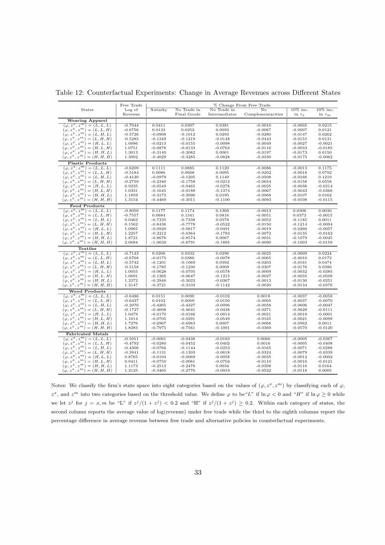
Table 12: Counterfactual Experiments: Change in Average Revenues across Different States

Free Trade % Change From Free TradeStates Log of Autarky No Trade in No Trade in No 10% inc. 10% inc.

Revenue Final Goods Intermediates Complementarities in τx in τm

Wearing Apparel(φ, zx, zm) = (L,L, L) -0.7044 0.0411 0.0307 0.0381 -0.0010 -0.0005 0.0215(φ, zx, zm) = (L,L,H) -0.6756 0.0123 0.0252 0.0093 -0.0067 -0.0007 0.0121(φ, zx, zm) = (L,H,L) -0.5726 -0.0908 -0.1012 0.0293 -0.0280 -0.0147 0.0262(φ, zx, zm) = (L,H,H) -0.5285 -0.1349 -0.1219 -0.0148 -0.0443 -0.0155 0.0131(φ, zx, zm) = (H,L,L) 1.0086 -0.0213 -0.0155 -0.0098 -0.0049 -0.0027 -0.0021(φ, zx, zm) = (H,L,H) 1.0751 -0.0878 -0.0133 -0.0762 -0.0116 -0.0033 -0.0185(φ, zx, zm) = (H,H,L) 1.3013 -0.3140 -0.3082 0.0061 -0.0197 -0.0173 0.0150(φ, zx, zm) = (H,H,H) 1.3902 -0.4029 -0.3285 -0.0828 -0.0330 -0.0175 -0.0062

Plastic Products(φ, zx, zm) = (L,L, L) -0.6209 0.1111 0.0885 0.1120 -0.0086 -0.0013 0.1175(φ, zx, zm) = (L,L,H) -0.5184 0.0086 0.0668 0.0095 -0.0202 -0.0018 0.0792(φ, zx, zm) = (L,H,L) -0.4120 -0.0979 -0.1205 0.1149 -0.0508 -0.0166 0.1219(φ, zx, zm) = (L,H,H) -0.2759 -0.2340 -0.1758 -0.0212 -0.0654 -0.0158 0.0558(φ, zx, zm) = (H,L,L) 0.9235 -0.0549 -0.0465 -0.0278 -0.0025 -0.0038 -0.0214(φ, zx, zm) = (H,L,H) 1.0331 -0.1645 -0.0188 -0.1374 -0.0067 -0.0043 -0.0366(φ, zx, zm) = (H,H,L) 1.1859 -0.3173 -0.3090 0.0195 -0.0068 -0.0107 0.0162(φ, zx, zm) = (H,H,H) 1.3154 -0.4469 -0.3011 -0.1100 -0.0093 -0.0108 -0.0115

Food Products(φ, zx, zm) = (L,L, L) -0.8050 0.1177 0.1174 0.1309 -0.0013 0.0306 0.0030(φ, zx, zm) = (L,L,H) -0.7557 0.0684 0.1341 0.0816 -0.0051 0.0373 -0.0015(φ, zx, zm) = (L,H,L) 0.0462 -0.7335 -0.7338 0.0578 -0.0052 -0.1185 0.0011(φ, zx, zm) = (L,H,H) 0.1562 -0.8436 -0.7778 -0.0522 -0.0150 -0.1214 -0.0094(φ, zx, zm) = (H,L,L) 1.0965 -0.0920 -0.0817 -0.0491 -0.0019 -0.0266 -0.0057(φ, zx, zm) = (H,L,H) 1.2257 -0.2212 -0.0364 -0.1783 -0.0072 -0.0135 -0.0162(φ, zx, zm) = (H,H,L) 1.8721 -0.8676 -0.8574 0.0067 -0.0031 -0.1079 -0.0045(φ, zx, zm) = (H,H,H) 2.0684 -1.0639 -0.8791 -0.1895 -0.0090 -0.1003 -0.0159

Textiles(φ, zx, zm) = (L,L, L) -0.7143 0.0200 0.0332 0.0296 -0.0025 -0.0009 0.0224(φ, zx, zm) = (L,L,H) -0.6768 -0.0175 0.0380 -0.0078 -0.0065 -0.0010 0.0172(φ, zx, zm) = (L,H,L) -0.5742 -0.1201 -0.1069 0.0592 -0.0203 -0.0161 0.0474(φ, zx, zm) = (L,H,H) -0.5158 -0.1785 -0.1230 0.0009 -0.0307 -0.0176 0.0386(φ, zx, zm) = (H,L,L) 1.0055 -0.0628 -0.0705 -0.0578 -0.0009 -0.0032 -0.0385(φ, zx, zm) = (H,L,H) 1.0691 -0.1265 -0.0647 -0.1215 -0.0027 -0.0035 -0.0509(φ, zx, zm) = (H,H,L) 1.2372 -0.2946 -0.3022 -0.0367 -0.0013 -0.0130 -0.0251(φ, zx, zm) = (H,H,H) 1.3147 -0.3721 -0.3103 -0.1142 -0.0030 -0.0134 -0.0376

Wood Products(φ, zx, zm) = (L,L, L) -0.6486 0.0151 0.0090 -0.0102 0.0018 -0.0037 -0.0058(φ, zx, zm) = (L,L,H) -0.6437 0.0102 0.0069 -0.0150 -0.0005 -0.0037 -0.0070(φ, zx, zm) = (L,H,L) -0.2070 -0.4265 -0.4327 -0.0096 -0.0058 -0.0606 -0.0047(φ, zx, zm) = (L,H,H) -0.1727 -0.4608 -0.4641 -0.0438 -0.0271 -0.0628 -0.0111(φ, zx, zm) = (H,L,L) 1.0479 -0.0170 -0.0166 -0.0014 -0.0021 -0.0018 -0.0001(φ, zx, zm) = (H,L,H) 1.1014 -0.0705 -0.0291 -0.0549 -0.0165 -0.0021 -0.0099(φ, zx, zm) = (H,H,L) 1.7276 -0.6967 -0.6963 0.0007 -0.0068 -0.0562 0.0011(φ, zx, zm) = (H,H,H) 1.8283 -0.7975 -0.7561 -0.1001 -0.0369 -0.0570 -0.0120

Fabricated Metals(φ, zx, zm) = (L,L, L) -0.5011 -0.0061 -0.0438 -0.0183 0.0060 -0.0005 -0.0367(φ, zx, zm) = (L,L,H) -0.4792 -0.0280 -0.0452 -0.0402 0.0016 -0.0005 -0.0408(φ, zx, zm) = (L,H,L) -0.4306 -0.0766 -0.1144 -0.0253 -0.0165 -0.0071 -0.0288(φ, zx, zm) = (L,H,H) -0.3941 -0.1131 -0.1303 -0.0618 -0.0324 -0.0079 -0.0339(φ, zx, zm) = (H,L,L) 0.8765 -0.0104 -0.0069 -0.0058 -0.0035 -0.0012 -0.0002(φ, zx, zm) = (H,L,H) 0.9411 -0.0750 -0.0061 -0.0704 -0.0110 -0.0016 -0.0121(φ, zx, zm) = (H,H,L) 1.1173 -0.2513 -0.2478 0.0034 -0.0308 -0.0116 0.0164(φ, zx, zm) = (H,H,H) 1.2125 -0.3465 -0.2776 -0.0919 -0.0522 -0.0118 0.0005

Notes: We classify the firm’s state space into eight categories based on the values of (φ, zx, zm) by classifying each of φ,

zx, and zm into two categories based on the threshold value. We define φ to be“L” if lnφ < 0 and “H” if lnφ ≥ 0 while

we let zj for j = x,m be “L” if zj/(1 + zj) < 0.2 and “H” if zj/(1 + zj) ≥ 0.2. Within each category of states, the

second column reports the average value of log(revenue) under free trade while the third to the eighth columns report the

percentage difference in average revenue between free trade and alternative policies in counterfactual experiments.

33

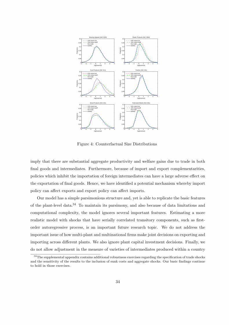
−3 −2 −1 0 1 2 3 40

0.05

0.1

0.15

0.2

0.25

0.3

log(revenue)

Fre

quen

cy


−3 −2 −1 0 1 2 3 40

0.05

0.1

0.15

0.2

0.25

0.3

log(revenue)

Fre

quen

cy

Plastic Products (ISIC 3560)

−3 −2 −1 0 1 2 3 40

0.05

0.1

0.15

0.2

0.25

0.3

log(revenue)

Fre

quen

cy


−3 −2 −1 0 1 2 3 40

0.05

0.1

0.15

0.2

0.25

0.3

log(revenue)

Fre

quen

cy

Textiles (ISIC 321)

−3 −2 −1 0 1 2 3 40

0.05

0.1

0.15

0.2

0.25

0.3

log(revenue)

Fre

quen

cy

Wood Products (ISIC 331)

−3 −2 −1 0 1 2 3 40

0.05

0.1

0.15

0.2

0.25

0.3

log(revenue)

Fre

quen

cy

Fabricated Metals (ISIC 381)

10% export tax10% import tarifffree tradeautarky






Figure 4: Counterfactual Size Distributions

imply that there are substantial aggregate productivity and welfare gains due to trade in both

final goods and intermediates. Furthermore, because of import and export complementarities,

policies which inhibit the importation of foreign intermediates can have a large adverse effect on

the exportation of final goods. Hence, we have identified a potential mechanism whereby import

policy can affect exports and export policy can affect imports.

Our model has a simple parsimonious structure and, yet is able to replicate the basic features

of the plant-level data.34 To maintain its parsimony, and also because of data limitations and

computational complexity, the model ignores several important features. Estimating a more

realistic model with shocks that have serially correlated transitory components, such as first-

order autoregressive process, is an important future research topic. We do not address the

important issue of how multi-plant and multinational firms make joint decisions on exporting and

importing across different plants. We also ignore plant capital investment decisions. Finally, we

do not allow adjustment in the measure of varieties of intermediates produced within a country

34The supplemental appendix contains additional robustness exercises regarding the specification of trade shocksand the sensitivity of the results to the inclusion of sunk costs and aggregate shocks. Our basic findings continueto hold in those exercises.

34

in response to changes in the trading environment. These features could be incorporated into

our theoretical and empirical framework and such extensions are important topics for our future

research.

References

[1] Alvarez, R. and R.A. Lopez (2005) “Exporting and Performance: Evidence from Chilean

Plants,” Canadian Journal of Economics, 38(4), 1384-400.

[2] Amiti, M. and J. Konings (2007) “Trade Liberalization, Intermediate Inputs, and Produc-

tivity: Evidence from Indonesia,” American Economic Review, 97(5), 1611-163.

[3] Arkolakis, Costas, Arnaud Costinot, and Andres Rodrıguez-Clare (2012) “New Trade

Models, Same Old Gains?” American Economic Review, 102(1), 94-130.

[4] Atkeson, A. and A. Burstein (2007) “Innovation, Firm Dynamics, and International

Trade,” NBER Working Paper No. 13326.

[5] Aw, B.Y., S. Chung, and M.J. Roberts (2000) “Productivity and Turnover in the Export

Market: Micro-level Evidence from the Republic of Korea and Taiwan(China),” World

Bank Economic Review, 14, 65-90.

[6] Ben-Akiva, M. and M. Lerman (1985) Discrete Choice Analysis: Theory and Application

to Travel Demand, MIT Press, Cambridge, MA.

[7] Bernard, A.B. and J.B. Jensen (1999) “Exceptional Exporter Performance: Cause, Effect,

and or Both?” Journal of International Economics, 47, 1-25.

[8] Bernard, A.B. and J.B. Jensen (2004) “Why Some Firms Export?” Review of Economics

and Statistics, 86(2), 561-569.

[9] Bernard, A.B., J. Eaton, J.B. Jensen, and S. Kortum (2003) “Plants and Productivity in

International Trade,” American Economic Review, 93(4), 1268-1290.

[10] Bernard, Andrew B., J. Bradford Jensen, and Peter K. Schott (2005) “Importers, Ex-

porters, and Multinationals: A Portrait of Firms in the U.S. that Trade Goods,” NBER

Working Paper No. 11404.

35

[11] Bernard, A.B., S. Redding, and P. Schott (2007) “Comparative Advantage and Heteroge-

neous Firms,” Review of Economic Studies, 74(1), 31-66.

[12] Blundell, R.W. and S.R. Bond (2000) “GMM Estimation with Persistent Panel Data: an

Application to Production Functions,” Econometric Reviews, 19(3), 321-340.

[13] Clerides, S., Lach, S., and J.R. Tybout (1998) “Is Learning by Exporting Important?

Micro-Dynamic Evidence from Colombia, Mexico, and Morocco,” Quarterly Journal of

Economics, 113, 903-947.

[14] De Loecker, J. (2007) “Product Differentiation, Multi-Product Firms and Estimating the

Impact of Trade Liberalization on Productivity,” NBER Working Paper No. 13155.

[15] Das, S. M. Roberts, and J. Tybout (2007) “Market Entry Costs, Producer Heterogeneity,

and Export Dynamics,” Econometrica, 75(3), 837-873.

[16] Devereux, M., A. Head, and B. Lapham (1996a) “Monopolistic Competition, Increas-

ing Returns, and the Effects of Government Spending,” Journal of Money, Credit, and

Banking, 28(2), 233-254.

[17] Devereux, M., A. Head, and B. Lapham (1996b) “Aggregate Fluctuations with Increasing

Returns to Specialization and Scale,” Journal of Economic Dynamics and Control, 20,

627-656.

[18] Eaton, J., and S. Kortum (2002) “Technology, Geography, and Trade,” Econometrica,

70(5), 1741-79.

[19] Eaton, J., S. Kortum, and F. Kramarz (2004) “Dissecting Trade: Firms, Industries, and

Export Destinations,” American Economic Review, Papers and Proceedings, 94(2), 150-

154.

[20] Eaton, J., S. Kortum, and F. Kramarz (2011) “An Anatomy of International Trade: Evi-

dence from French Firms,” Econometrica, 79(5), 1453-1498.

[21] Ethier, W.J. (1982) “National and International Returns to Scale in the Modern Theory

of International Trade,” American Economic Review, 72(3), 389-405.

[22] Feenstra, Robert C., J.R. Markusen, and W. Zeile (1992) “Accounting for Growth with

New Inputs: Theory and Evidence,” American Economic Review, 82(2), 415-421.

36

[23] Fernandes, A. (2007) “Trade policy, Trade Volumes and Plant-level Productivity in Colom-

bian Manufacturing Industries,” Journal of International Economics, 71(1), 52-71.

[24] Fuentes, R., M. Larrain K. Schmidt-Hebbel (2006) “Sources of Growth and Behavior of

TFP in Chile,” Cuadernos de Economia 43(127), 113-142.

[25] Grossman, G.M. and E. Helpman (1991) Innovation and Growth in the Global Economy,

Cambridge, MA: The MIT Press.

[26] Halpern, L. M. Koren, and A. Szeidl (2006) “Imports and Productivity,” mimeo, Federal

Reserve Bank of New York.

[27] Heckman, J. J. (1981) “The Incidental Parameters Problem and the Problem of Initial

Conditions in Estimating a Discrete Time-Discrete Data Stochastic Process,” in C. F.

Manski and D. McFadden (eds), Structural Analysis of Discrete Data with Econometric

Applications, MIT Press, Cambridge, MA, 114-178.

[28] Helpman, E., M.J. Melitz, and S.R. Yeaple (2004) “Export versus FDI with Heterogeneous

Firms” American Economic Review, 94, 300-316.

[29] Kasahara, Hiroyuki, and Joel Rodrigue (2005) “Does the Use of Imported Intermediates

Increase Productivity? Plant-Level Evidence,” EPRI Working Paper # 2005-7.

[30] Kasahara, H., and J. Rodrigue (2008) “Does the Use of Imported Intermediates Increase

Productivity? Plant-Level Evidence,” Journal of Development Economics, 87(1), 106-118.

[31] Kasahara, H., and K. Shimotsu (2008) “Nonparametric Identification of Finite Mixture

Models of Dynamic Discrete Choices,” Econometrica, 77(1), 135-175.

[32] Katayama, H., S. Lu, and J.R. Tybout (2003) “Why Plant-level Productivity Studies are

often Misleading, and an Alternative Approach to Inference,” NBER Working Paper No.

9617.

[33] Klette, T.J., and Z. Griliches (1996) “The Inconsistency of Common Scale Estimators

When Output Prices are Unobserved and Endogenous,” Journal of Applied Econometrics,

11, 343-361.

[34] Levinsohn, J. and A. Petrin (2003) “Estimating Production Functions Using Inputs to

Control for Unobservables,” Review of Economic Studies, 70: 317-341.

37

[35] Liu, L. (1993) “Entry-Exit, Learning and Productivity Change: Evidence from Chile,”

Journal of Development Economics, 42: 217-242.

[36] McFadden, D. (1978) “Modeling the Choice of Residential Location,” in A. Karlquist et al.

(eds.), Spatial Interaction Theory and Residential Location, Amsterdam: North-Holland.

[37] Melitz, M.J.(2003) “The Impact of Trade on Intra-Industry Reallocations and Aggregate

Industry Productivity,” Econometrica, 71: 1695-1725.

[38] Muendler, M-A.(2004) “Trade, Technology and Productivity: A Study of Brazilian Man-

ufacturers 1986-1998,” CESifo Working Paper Series No. 1148.

[39] Olley, S. and Pakes, A. (1996) “The Dynamics of Productivity in the Telecommunications

Equipment Industry,” Econometrica, 65(1): 292-332.

[40] Pavcnik, N. (2002) “Trade Liberalization, Exit, and Productivity Improvements: Evidence

From Chilean Plants,” Review of Economic Studies, 69(1): 245-276.

[41] Roberts, M. and J.R. Tybout (1997) “Decision to Export in Columbia: An Empirical

Model of Entry with Sunk Costs” American Economic Review, 87: 545-564.

[42] Rodrigue, J. (2007) “FDI and Exports: An Empirical Framework,” mimeo, Queen’s Uni-

versity.

[43] Romer, P. (1987) “Growth Based on Increasing Returns Due to Specialization,” American

Economic Review, 77(2), 56-62.

[44] Rust, J. (1987) “Optimal replacement of GMC bus engines: an empirical model of Harold

Zurcher.” Econometrica 55(5): 999-1033.

[45] Tybout, J.R. (1996) “Chile, 1979-1986: Trade Liberalization and its Aftermath,” in M.

Roberts and J. Tybout (eds.), Industrial Evolution in Developing Countries, Oxford:

Oxford University Press.

[46] Trefler, D. (2004) “The Long and Short of the Canada-U.S. Free Trade Agreement,”

American Economic Review, 94(4): 870-895.

[47] Yi, K-M. (2003)“Can Vertical Specialization Explain the Growth of World Trade?” Jour-

nal of Political Economy, 111(1): 52-102.

38

A Appendix

A.1 Estimation Procedure

A.1.1 Type I Extreme-Value Distributions

Here, we briefly discuss the properties of Type I extreme-value distributed random variables

(cf., Ben-Akiva and Lerman (1985)). Assume that ϵ(0) and ϵ(1) are independently drawn from

identical extreme-value distributions with mean zero and variance ϱ2π2

6 , where ϱ is the shape pa-

rameter.35 Let V (0) and V (1) be real numbers. We use the following two properties for our esti-

mation. The first property is: E[max(V (0)+ϵ(0), V (1)+ϵ(1)] = ϱ ln[exp(V (0)/ϱ)+exp(V (1)/ϱ)],

where the expectation is taken with respect to the distribution of ϵ(0) and ϵ(1). The second

property is: P (V (0) + ϵ(0) > V (1) + ϵ(1)) = exp(V (0)/ϱ)exp(V (0)/ϱ)+exp(V (1)/ϱ) . In the multivariate case,

when we have ϵ(d) for d = 0, 1, 2, ..., J , the first property is E[maxj=0,1,...,J V (j) + ϵ(j)] =

ϱ ln[∑J

j=0 exp(V (j)/ϱ)] while the second property is P [V (d)+ϵ(d) > V (j)+ϵ(j) for all j = d] =exp(V (d)/ϱ)∑J

j′=0 exp(V (j′)/ϱ).

A.1.2 Initial Distribution Specification

Following Heckman (1981), we specify the distribution of η in 1990 as µ0,θ(η, d) = P x0 (d

x|η)P x0 (d

m|η)gη,0(η),

where (σ − 1) lnφ, ln zx, ln zm are independently normally distributed with means µφ0 , µ

x0 , and

µm0 , and standard deviations σφ

0 , σx0 , and σm

0 so that gη,0(η) =1

σφ0 σ

x0σ

m0ϕ((σ−1) lnφ−µφ

0

σφ0

)ϕ(ln zx−µx

0σx0

)×

ϕ(ln zm−µm

0σm0

), while P x

0 (dx|η) and P x

0 (dm|η) are specified under logit formulas:

P x0 (d

x|η) =exp(αx

0 + αx1(σ − 1) lnφ+ αx

2 ln zx + αx

3 ln zm)

1 + exp(αx0 + αx

1(σ − 1) lnφ+ αx2 ln z

x + αx3 ln z

m),

Pm0 (dm|η) =

exp(αm0 + αm

1 (σ − 1) lnφ+ αm2 ln zx + αm

3 ln zm)

1 + exp(αm0 + αm

1 (σ − 1) lnφ+ αm2 ln zx + αm

3 ln zm).

A.1.3 Counterfactual Experiments Procedure

Denote the equilibrium aggregate price under the parameter θ by P (θ). Suppose that we are in-

terested in a counterfactual experiment characterized by a counterfactual parameter vector θ that

is different from the estimated parameter vector θ. Recall that we have the following relationship

between α0 and the equilibrium price P : α0 = ln[(Γ(σ − 1)/σ)σ−1R

]+(σ−1) lnP (θ), where the

aggregate price is explicitly written as a function of θ. At the counterfactual aggregate price P (θ),

the coefficient α0 takes a value of α0 = ln[(Γ(σ − 1)/σ)σ−1R

]+ (σ − 1) lnP (θ) = α0 + k(θ, θ),

35The cumulative distribution function of ϵ(d) for d = 0, 1 is exp(− exp(−(ϵ(d) − γ))), where γ is Euler’sconstant.

39

where k(θ, θ) ≡ (σ − 1) ln(P (θ)/P (θ)

)represents the equilibrium price change (up to the pa-

rameter (σ − 1)). Thus, replacing α0 with α0, we may evaluate the revenue function at the

counterfactual aggregate price P (θ) (i.e. at the counterfactual value of α0):

r(ηi, dit; k(θ, θ)) = exp(k(θ, θ) + α0 + αtt+ ln[1 + zxi ]d

xit + αm ln[1 + zmi ]dmit + (σ − 1) lnφi

). (31)

The equilibrium price change, k(θ, θ), is then determined so that the following equilibrium free

entry condition holds: fe =∫V(η′, dit = (0, 0); θ, k(θ, θ)

)gη(η

′; θ)dη′. Here V(η′, dit; θ, k(θ, θ)

)is the solution to the Bellman equations (10)-(13) when the revenue function (31) is used to

compute profits and gη(η′; θ) is the probability density function from which the initial plant

characteristic vector is drawn.36

A.2 Additional Maximum Likelihood Estimates

Table 13 presents the maximum likelihood estimates for the remaining parameters.

Table 13: Remaining Maximum Likelihood Estimates

Params Apparel Plastics Food Textiles Wood Metals

ϱd 0.131 (0.031) 0.165 (0.026) 0.272 (0.022) 0.195 (0.033) 0.099 (0.016) 0.179 (0.028)ϱχ 0.269 (0.084) 0.450 (0.149) 0.517 (0.147) 0.639 (0.163) 0.044 (0.021) 0.130 (0.032)ξ 0.059 (0.009) 0.038 (0.007) 0.056 (0.005) 0.037 (0.007) 0.072 (0.006) 0.040 (0.005)

λ11 0.314 (0.003) 0.331 (0.005) 0.394 (0.002) 0.294 (0.003) 0.416 (0.004) 0.328 (0.003)λ22 1.321 (0.059) 1.404 (0.037) 0.844 (0.007) 1.281 (0.031) 0.905 (0.020) 1.190 (0.037)λ21 -0.253 (0.108) -0.069 (0.089) 0.000 (0.022) -0.198 (0.070) -0.166 (0.032) -0.406 (0.080)λ33 0.676 (0.017) 0.571 (0.007) 0.936 (0.011) 0.638 (0.009) 0.881 (0.056) 0.699 (0.015)λ32 0.076 (0.073) 0.042 (0.047) -0.021 (0.052) -0.021 (0.053) 0.065 (0.125) -0.025 (0.059)λ31 -0.041 (0.059) 0.039 (0.025) -0.184 (0.033) -0.017 (0.029) -0.460 (0.080) 0.012 (0.032)λ44 0.170 (0.002) 0.159 (0.002) 0.198 (0.001) 0.181 (0.002) 0.186 (0.002) 0.172 (0.002)λ43 0.023 (0.011) 0.009 (0.010) 0.013 (0.008) 0.009 (0.009) 0.018 (0.019) 0.016 (0.009)λ42 -0.043 (0.010) -0.018 (0.012) -0.020 (0.005) -0.031 (0.009) -0.007 (0.009) -0.011 (0.010)λ41 0.049 (0.003) 0.060 (0.004) 0.080 (0.003) 0.046 (0.003) 0.091 (0.004) 0.078 (0.003)

µφ0 0.057 (0.081) 0.687 (0.112) 0.974 (0.079) 0.450 (0.077) 0.345 (0.083) 0.539 (0.085)

µx0 -4.080 (0.540) -4.765 (0.288) -2.737 (0.200) -3.936 (0.331) -3.238 (0.344) -3.970 (0.375)

µm0 -1.646 (0.147) -1.047 (0.161) -3.110 (0.142) -1.439 (0.117) -3.963 (0.726) -1.875 (0.149)

σφ0 1.233 (0.065) 1.267 (0.089) 1.518 (0.061) 1.284 (0.058) 1.258 (0.065) 1.361 (0.064)

σx0 1.387 (0.345) 1.390 (0.135) 2.771 (0.244) 1.342 (0.196) 1.936 (0.270) 1.094 (0.268)

σm0 1.154 (0.117) 1.340 (0.132) 1.309 (0.140) 1.240 (0.108) 1.831 (0.467) 1.281 (0.119)ax0 -0.744 (1.610) 1.500 (2.461) 1.761 (0.810) 0.197 (1.185) 2.529 (2.271) 2.367 (1.771)

ax1 1.549 (0.368) 0.836 (0.256) 0.602 (0.117) 1.218 (0.188) 1.069 (0.297) 0.802 (0.203)

ax2 1.206 (0.569) 1.045 (0.750) 1.353 (0.148) 1.101 (0.360) 1.560 (0.438) 1.438 (0.548)

ax3 -0.336 (0.399) 0.059 (0.223) 0.130 (0.237) -0.035 (0.211) 0.254 (0.506) 0.448 (0.245)

am0 -1.203 (1.259) 1.978 (2.833) -1.586 (0.552) 0.065 (0.942) -0.348 (1.300) 0.994 (1.786)

am1 0.906 (0.186) 1.331 (0.295) 1.188 (0.155) 1.008 (0.160) 0.866 (0.318) 0.949 (0.163)

am2 0.175 (0.354) 0.850 (0.825) 0.278 (0.083) 0.251 (0.271) 0.355 (0.268) 0.579 (0.502)

am3 0.123 (0.217) 0.281 (0.227) 0.395 (0.174) 0.674 (0.154) 0.847 (0.393) 0.810 (0.197)fe 4.194 4.995 13.036 4.103 5.730 3.792

Notes: Standard errors are in parentheses. The parameters are evaluated units of millions of US dollars in 1990.

36For every pair (θ, θ), there exists a unique value of k(θ, θ) that satisfies the free entry condition because the

value function V(η′, dit; θ, k(θ, θ)

)is strictly increasing in k(θ, θ).

40

Productivity and the Decision to Import and Export: Theory...

Documents

Transcript of Productivity and the Decision to Import and Export: Theory...