Productivity and Inflation - Reserve Bank of · PDF file6.2 Robustness to Additional Control...

PRODUCTIVITY AND INFLATION

Tim Bulman and John Simon

Research Discussion Paper 2003-10

September 2003

Economic Research Department Reserve Bank of Australia

We would like to thank Badi Baltagi, Anthony Richards, Malcom Edey, Alex Heath and the RBA’s Prices, Wages and Labour section, and participants at an RBA seminar for helpful comments and suggestions; the errors remaining are our own. The views expressed in this paper are those of the authors and should not be attributed to the Reserve Bank of Australia.

i

Abstract

This paper examines the effect of inflation on productivity growth in Australia. Broad historical correlations suggest a negative relationship between inflation and aggregate productivity growth. The low-frequency nature of the relationship, however, means it is difficult to establish statistical causation at the aggregate level. We look at the industry-level relationships in an effort to overcome this limitation and to understand the relationship better. On this level we find clearly significant results with industry-level inflation explaining industry productivity. We also find that the relationship varies by industry, with the strongest evidence of a negative relationship being found in the cases of concentrated industries, i.e., those dominated by large firms. Finally, we find evidence that the negative effects of inflation on productivity do not operate solely through a reduction in capital accumulation but also through a reduction in multifactor productivity growth.

JEL Classification Numbers: D23, D24, E31, L11, L16 Keywords: inflation, productivity, industrial structure

ii

Table of Contents

1. Introduction 1

2. Theoretical Preamble 3

3. Previous Research 4

4. Methodology and Data 8

4.1 Model 9

4.2 Data 10

4.3 Stationarity 13

5. Results 13

5.1 Considering the Results in More Depth 16

6. Robustness 19

6.1 Robustness to Sample Period 19

6.2 Robustness to Additional Control Variables 21

7. Discussion 23

7.1 Capital Accumulation 24

7.2 The Role of Industrial Structure 25

7.3 The Aggregate Effect 26

8. Conclusion 27

Appendix A: Industry Productivity and Price Series 28

Appendix B: Output Gap Series 32

Appendix C: Sample Estimation Results 33

iii

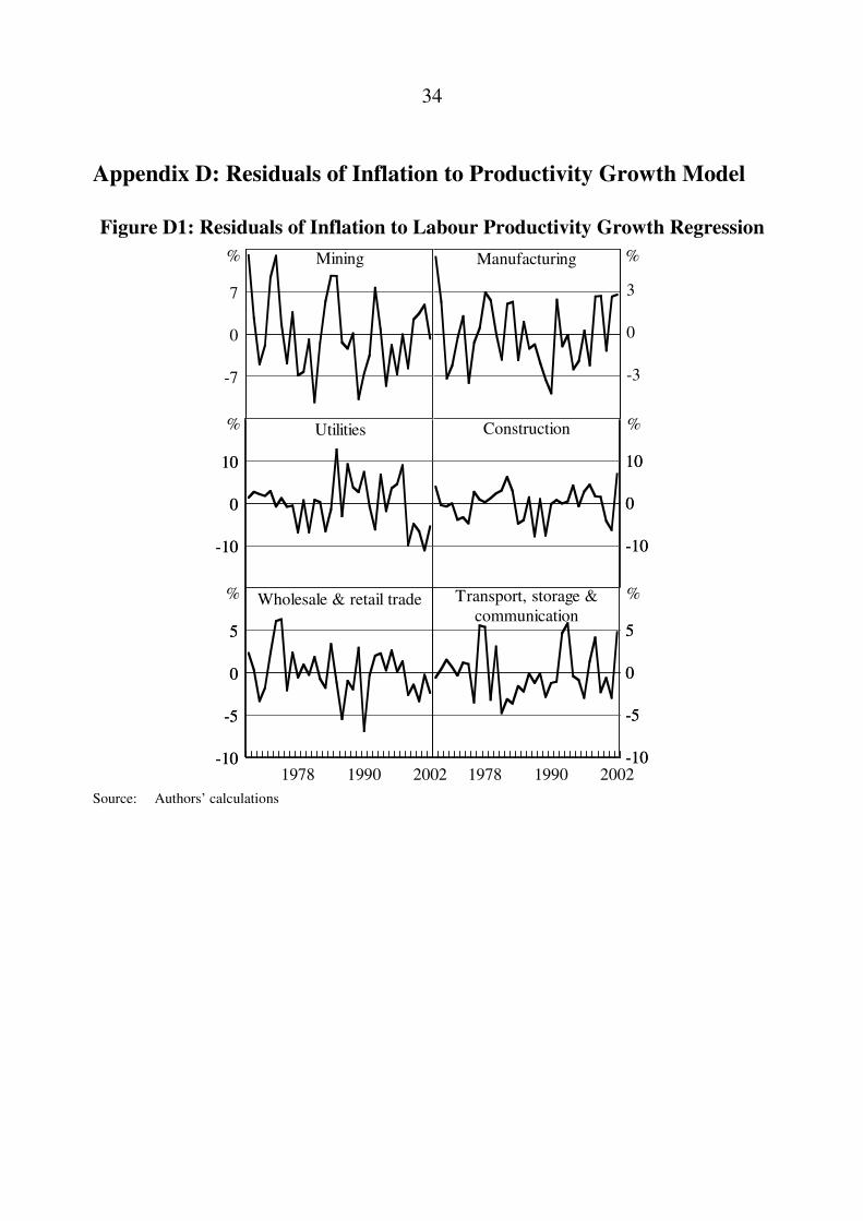
Appendix D: Residuals of Inflation to Productivity Growth Model 34

Appendix E: Reverse Causal Flow 35

References 39

PRODUCTIVITY AND INFLATION

Tim Bulman and John Simon

1. Introduction

That inflation has costs is widely accepted. What is less clear is the path by which inflation generates these costs – there are many alternative theories. The interaction of inflation with the tax system, the reduction in the value of the price mechanism, the diversion of resources from productive activities to managing inflation, or even the cost of adjusting prices on menus have all been posited as costs of high inflation.1 However, quantifying these channels empirically is much harder than describing them theoretically. Regardless, whatever the channel of effect, they must all ultimately reduce output. And inflation’s negative effect on output is most likely to be reflected in lower productivity growth.2 Consequently, in considering the costs of inflation, the relationship between inflation and productivity is key. This paper investigates this relationship without attempting to isolate the strength of any particular channel. Notwithstanding this, our results suggest something about the characteristics of the channel and we discuss these in some detail later in the paper.

At the simplest level, broad historical correlations suggest a negative relationship between productivity and inflation (Table 1). Most OECD countries had low productivity growth and high inflation in the 1970s and, to a lesser extent, the 1980s. Productivity growth then generally increased through the 1990s at the same time as inflation generally fell.

1 See Blanchard and Fisher (1989) for a discussion of how nominal rigidities affect various

economic models. 2 Productivity is that component of output unrelated to changes in the amount of capital and

labour inputs. While inflation may affect the accumulation of labour and capital it is most likely that its major effect will be to impede the efficiency of their organisation – hence lowering productivity. We address the possibility that inflation affects the accumulation of capital by looking at the difference between labour productivity and multifactor productivity: see especially Section 7.1.

2

Table 1: OECD Productivity and Inflation Experiences Average annual percentage change in consumer price index

and GDP per employed person 1970–1973 1973–1979 1979–1989 1989–1999

CPI 6.3 11.4 7.9 3.0 Australia

Productivity 1.8 1.9 1.0 2.2

CPI 4.6 9.0 6.8 2.4 Canada


CPI 7.1 10.5 7.1 2.4 Denmark


CPI 6.2 10.2 7.7 2.1 France


CPI 5.3 5.0 3.0 – Germany

Productivity 3.4 2.7 1.5 –

CPI 6.6 15.6 11.7 4.4 Italy


CPI 7.6 10.3 2.7 1.3 Japan


CPI 11.1 15.8 9.3 5.7 Korea


CPI 6.8 7.4 3.0 2.2 Netherlands

Productivity 4.2 2.1 –0.3 0.6

CPI 8.0 13.0 12.0 2.0 New Zealand

Productivity 3.6 –1.6 0.5 0.6

CPI 7.9 8.5 6.0 2.6 Norway


CPI 6.8 9.3 7.9 3.8 Sweden


CPI 6.4 4.7 3.3 2.4 Switzerland


CPI 8.1 14.4 7.6 4.0 UK


CPI 4.9 8.2 6.1 3.2 US


Sources: CPI inflation – IMF; real GDP per person employed – OECD

3

The duration of these OECD fluctuations suggests a long-term, low-frequency relationship between inflation and productivity, however, this makes it difficult to establish statistical causation. To address this problem, this paper focuses on industry-level data. Industry-level data offer a number of potential benefits over aggregate data. Because each industry is different there is much more variation in the data, which in turns brings greater statistical power. Also, we suspect that industry-level characteristics may affect the nature of the relationship. Thus, the industry-level results are interesting in their own right.

2. Theoretical Preamble

The simplest models in macroeconomics generally assume that nominal and real variables are unrelated in the long run. ‘Inflation is always and everywhere a monetary phenomenon’ (Friedman 1956, p 4); productivity is a purely real occurrence. But upon reflection, we may reasonably think that inflation – or at the least, things associated with it – must matter for firms’ ability to improve their productivity, for example. And in an effort to better model the behaviour of actual economies, much economic research has been directed at investigating the real effects of nominal fluctuations. This section discusses some possible explanations for the nexus.

In considering a link between inflation and productivity there are two possible causal directions: productivity affects inflation or inflation affects productivity. The first generally has higher productivity allowing cost reductions that flow through to product prices and thereby reduce inflation. Higher productivity growth thus represents a positive supply shock that lowers inflationary pressures.

The second effect posits that inflation affects productivity growth. From first principles, prices matter because they are a highly efficient means of transmitting the myriad of individual demand and supply decisions that occur throughout the economy.3 In an inflationary environment, the price mechanism loses its efficiency. It seems plausible then, that when prices are changing frequently, firms may find it more difficult to distinguish an increase in the relative scarcity of their

3 An insight best expressed by Hayek (1945).

4

inputs from an across-the-board increase in prices. This may cause firms to direct resources previously devoted to research and development, and organisational and managerial improvements, towards making basic decisions about optimal input allocations and the price of outputs. Similarly, the reduced certainty brought about by inflation increases the risk of entrepreneurial errors and would potentially induce lower levels of investment. This would all lower the overall productivity of the firm.

There are also arguments based on the interaction of the tax system with higher inflation. During periods of high inflation the tax system distorts incentives through its treatment of depreciation and capital gains. These distortions are also likely to have negative effects on productivity.4

3. Previous Research

Early research into the inflation-productivity nexus was stimulated by the experience of high inflation of the 1970s and the subsequent fall in productivity growth. Most of the literature has debated the statistical question of whether the data support any relationship, and if so, the causal direction. Minimal work explores the theoretical side, or how inflation may be transmitted into slower productivity growth and vice versa. By country, a range of literature examines the relationship in the G7 economies, but we are aware of no comprehensive and conclusive recent Australian study of the inflation-productivity relationship. Further, all these studies only observe the relationship at the aggregate level without gaining from potential industry-specific insights. Notwithstanding this, we glean some useful points from what’s gone before. (Table 2 summarises the literature’s findings.)

4 See, e.g., the papers cited by Jarrett and Selody (1982, p 362); also, Freeman and

Yerger (2000).

Tab

le 2

: T

he P

rodu

ctiv

ity

Gro

wth

-Inf

lati

on R

elat

ions

hip

Surv

ey o

f em

piri

cal e

vide

nce

Pap

er

Sam

ple

Pro

duct

ivit

y m

easu

re

Sign

ific

ant

rela

tion

ship

C

ausa

l dir

ecti

on

Infl

atio

n

prod

uctiv

ity

grow

th

Prod

uctiv

ity

grow

th

infl

atio

n Ja

rret

t and

Se

lody

(19

82)

Can

ada

aggr

egat

e:

1963

:Q2–

1979

:Q4

Lab

our

(hou

rs)

Yes

Y

es

Yes

Cla

rk (

1982

) U

S ag

greg

ate:

19

47:Q

1–19

81:Q

2 L

abou

r Y

es

Yes

N

o

Ram

(19

84)

US

aggr

egat

e:

1953

:Q1–

1982

:Q4

Lab

our

(hou

rs)

Yes

Y

es

No

Buc

k an

d Fi

tzro

y (1

988)

W

est G

erm

any

(40

indu

stri

es):

19

50–1

977

(ann

ual)

Mul

tifac

tor

Yes

Y

es

No

Saun

ders

and

B

isw

as (

1990

) U

K a

ggre

gate

: 19

77:Q

3–19

85:Q

2 L

abou

r (h

ours

) Y

es

Yes

N

o

Sbor

done

and

K

uttn

er (

1994

) U

S:

1947

:Q1–

1994

:Q2

Non

-far

m

busi

ness

labo

ur

Yes

W

eakl

y, y

es

No

Smyt

h (1

995a

) W

est G

erm

any

aggr

egat

e:

1951

–199

1 M

ultif

acto

r Y

es

Not

test

ed

Not

test

ed

Smyt

h (1

995b

) U

S: 1

955–

1990

P

riva

te b

usin

ess

Priv

ate

non-

farm

bus

ines

s M

anuf

actu

ring

Mul

tifac

tor

Y

es

Yes

Y

es

Not

test

ed

Not

test

ed

5

Cam

eron

, Hum

an

d Si

mps

on

(199

6)

US,

UK

, Can

ada:

19

53–1

991

Wes

t Ger

man

y:

1960

–199

1

Lab

our

(em

ploy

men

t)

May

aff

ect

grow

th, n

ot le

vel

of p

rodu

ctiv

ity

No

No

Cho

wdh

ury

and

Mal

lik (

1998

) A

ustr

alia

: 195

8–19

96 a

nd

1968

:Q1–

1997

:Q3

New

Zea

land

: 196

8–19

96

Lab

our

(em

ploy

men

t)

No

clea

r fi

ndin

gs

for

leve

ls o

r gr

owth

N

ot te

sted

N

ot te

sted

Free

man

and

Y

erge

r (2

000)

12

OE

CD

eco

nom

ies(a

) : 19

61–1

994

(ann

ual)

M

anuf

actu

ring

la

bour

(ho

urs)

O

nly

in a

min

orit

y of

cou

ntri

es

Onl

y in

a m

inor

ity

of c

ount

ries

N

o

Tsi

onas

(20

01)

Eur

opea

n ec

onom

ies(b

) : 19

60–1

997

Mul

tifac

tor

No

long

-run

re

latio

nshi

p B

elgi

um, F

inla

nd,

Fran

ce, G

erm

any,

G

reec

e, I

rela

nd, U

K

Bel

gium

, Fr

ance

, Ger

man

y,

Gre

ece,

UK

Tsi

onas

(20

03)

15 E

urop

ean

econ

omie

s:

1960

–199

7 C

ount

ry-s

peci

fic

prod

uctiv

ity

inde

x (B

alta

gi, G

riff

in

and

Ric

h 19

95)

In s

ome

coun

trie

s B

elgi

um, F

inla

nd,

Fran

ce, G

erm

any,

G

reec

e, I

rela

nd, U

K

Bel

gium

, Fr

ance

, Ger

man

y,

Gre

ece,

UK

Not

es:

(a)

Eco

nom

ies

stud

ied

wer

e B

elgi

um, C

anad

a, D

enm

ark,

Fra

nce,

Ger

man

y, I

taly

, Jap

an, N

ethe

rlan

ds, N

orw

ay, S

wed

en, U

K, a

nd U

S.

(b

) E

cono

mie

s st

udie

d w

ere

Aus

tria

, B

elgi

um,

Den

mar

k, F

inla

nd,

Fra

nce,

Ger

man

y, G

reec

e, I

rela

nd,

Ital

y, N

ethe

rlan

ds,

Nor

way

, P

ortu

gal,

Spa

in,

Sw

eden

,

and

UK

.

6 6 6

7

The early view was a little circumspect about the nature of any relationship between productivity growth and inflation. Nonetheless, both Keynesian and neo-classical theory (e.g., Lucas’s (1973) simple model of an output-inflation trade-off) suggest a negative relationship. Into this context, the earliest papers sought to reconcile the observed North American acceleration in inflation and following decline in productivity growth. Jarret and Selody (1982) proposed two rationales for this occurrence: that the tax system’s lack of neutrality during periods of inflation increases the private sector’s tax burden,5 and that inflation’s increasing variance with higher levels of inflation would cause sub-optimal resource allocations and increase the probability of ‘entrepreneurial error’, hence reducing investment. Using 1963–1979 Canadian data, Jarret and Selody found a bi-directional relationship, with the rise in inflation explaining nearly the entire slowdown in productivity growth. US data over the period 1948–1981 demonstrate a similar correlation, with causation running one-way from higher inflation to slower productivity growth (Clark 1982).6 Methodologically, these studies apply Granger-type causality tests to OLS (Clark 1982; Ram 1984) or Full Information Maximum Likelihood (Jarret and Selody 1982) estimations.

A second group of papers took up the debate in the mid 1990s. These had the advantage of being able to observe the productivity growth-inflation relationship after the 1980s’ disinflation, and also draw on the experience of a wider range of G7 economies. They are more equivocal about the existence of any relationship.

A further group of papers is sceptical of any inflation-productivity growth relationship. These papers take two tacks. One approach is to argue that the results show that the business cycle drives simultaneous variations in both productivity growth and inflation, not a long-run relationship.7 The stylised facts have productivity growth peaking ahead of the business cycle, with inflation then accelerating. In response, the monetary authorities increase interest rates, thus slowing output growth hence productivity growth through the effects of labour hoarding. Inflation’s slow-down lags that of the real economy. Thus, an appropriate model of the productivity growth-inflation relationship must absorb the

5 See, e.g., Feldstein (1982a, 1982b). 6 Ram (1984) reaches the same conclusion, using a CPI-based measure of inflation. 7 E.g., Sbordone and Kuttner (1994); Freeman and Yerger (2000).

8

business cycle through variables such as real interest rates, the output gap, or variations in GDP growth.

The other critique argues the statistical point that productivity growth and inflation have different orders of integration.8 These studies claim inflation is non-stationary while productivity growth is stationary, and therefore there cannot be a long-run relationship. Statistically speaking, this seems a not unreasonable complaint. Nonetheless, there is much debate about whether inflation is better characterised as an I(1) process or as stationary around a broken trend. For example, Hendry (2001) finds that UK inflation is best characterised as I(0) but non-stationary due to regime breaks over a very long sample. If this is the case, the observation that one cannot reject that inflation is I(1) over a particular sample does not necessarily lead to the conclusion that it could not possibly be related to productivity growth.9

In summary, we take several points from the literature. Methodologically, the literature is uniform in its approach. Almost all the papers run Granger causality tests, or a close relative, VAR models. Second, there does appear to be a relationship between productivity growth and inflation, and, where it is determinable, the causality appears to flow from inflation to productivity growth. Third, two pitfalls are to be avoided: ignoring the macroeconomic context of the inflation-productivity growth relationship; and ignoring the statistical issues of correlating series with potentially different orders of integration. A final point is that we could find no comprehensive and satisfactory Australian study of the inflation-productivity growth relationship. Our study addresses this gap.

4. Methodology and Data

The correlation apparent in the relationship between Australian aggregate inflation and productivity growth in Table 1 can be tested econometrically, using annual data. It is marginally statistically significant – as mentioned in the introduction. This may be for many reasons but two are most important: 1) we only have 36

8 E.g., Sbordone and Kuttner (1994); Cameron et al (1996); Freeman and Yerger (2000);

Tsionas (2003). 9 Hall (1999) argues emphatically that inflation should be treated as mean-reverting, even if it

may statistically appear otherwise.

9

annual observations representing one ‘cycle’ in the productivity-inflation relationship, so statistical significance is difficult to achieve; and 2) the aggregate data may mask divergent industry-level relationships. By estimating each industry separately we are not forcing all the coefficients to be the same and can reveal if there are significant differences between industries.10 The Seemingly Unrelated Regression (SUR) estimation technique applied to industry level data offers the possibility of ameliorating some of these problems. While we will have the same length of data for each individual industry, the SUR method is potentially more efficient because it uses cross-equation information.

4.1 Model

Following previous practice and the insights from the literature we look at Granger-causality regressions with an output gap to control for the business cycle. Thus the basic regression estimated (explaining causation from the IPDs to productivity growth) is:

ititititititiit YPPAAA εα ++++++= −−−− 2121 , (1)

where Ait is productivity growth, Pit is the change in the implicit price deflators (IPDs), and Yit is the output gap, all for industry i in year t. We look at both labour and multifactor productivity (MFP) to shed light on the effect of inflation on capital accumulation. The data seem most comfortable with the inclusion of two lags; two lags also has the advantage of minimising the loss of degrees of freedom.

Some of the theories discussed suggest that inflation slows the optimal accumulation of capital. If that is the major channel transmitting inflation’s effects into productivity growth, we would expect to see a relationship between inflation and labour productivity but not between inflation and multifactor productivity (which takes account of capital accumulation) – this explanation does not hold, as Section 5 reveals. We explore this angle more fully in Section 7.

10 For example, each industry will probably have a different correlation with the aggregate

business cycle.

10

4.2 Data11

Australian data are more problematic than those available for the G7 studies we are trying to replicate. Unlike the series dating from WWII available to other studies, the Australian data needed to calculate productivity measures become complete only in 1966, and even this run is subject to discontinuities.

We begin with the non-farm market-sector ANZSIC (Australia New Zealand Standard Industry Classification) industries. Finance and insurance is excluded because the necessary data only begin in 1986, which would severely limit our available observations. The remaining industries were not seriously affected by the transition from ASIC (Australian Standard Industry Classification) to ANZSIC,12 and all have output that is relatively easy to measure.13 For each of these industries we constructed measures of prices, and multifactor and labour productivity, plus a measure of the business cycle specific to that industry. Appendix A shows the price and productivity variables by industry.

Our price variables are the industry gross-value-added (GVA) implicit price deflators (IPDs). These are relatively straightforward to calculate, being an index created by dividing each industry’s nominal GVA by its real GVA. As these are measures based on value added they can be affected by changes in input prices as well as output prices. Nonetheless, the IPDs represent the specific price environment an industry faces in the course of its business.14

11 Through the course of this study we introduce other variables to test the robustness of our

model and to explore the transmission mechanism between inflation and productivity growth. We discuss these series as they appear.

12 To ensure we had enough observations, some ‘industries’ had to be re-aggregated after the ABS (Australian Bureau of Statistics) disaggregated them – for example – transport & storage from communications when it shifted from ASIC to ANZSIC.

13 These industry sectors are mining, manufacturing, electricity gas & water (‘utilities’), construction, wholesale & retail trade, and transport, storage & communications. Although several of these series are available in a less aggregated form from the early 1980s (transport & storage separates from communications, as does wholesale from retail trade later), maximising our number of observations is important and given the SUR model does not adjust for unbalanced data, we keep these series aggregated through our full sample.

14 We examine the correlation between industry and these aggregate price measures and what this might suggest in Section 5.2.

11

Labour productivity is also a relatively clean calculation – in particular, it is free of capital measurement issues. We calculate it by dividing an industry’s real GVA with the total number of hours worked in that industry. Total hours were calculated by multiplying the year-to-August average weekly number of hours worked (for both full- and part-time employees, that includes, in particular, overtime and strikes) by the year-to-August average total number of people employed in that industry.15

More complex is multifactor productivity. Here we followed a standard Solow growth accounting framework, which treats productivity growth as the residual of output growth after growth of labour and capital input are accounted for. Thus:

itititititit LKYMFP βα −−= (2)

where all terms are expressed in year t for industry i as annual percentage changes, Y is industry i’s real GVA, α and β are the factor share of income attributable to capital and labour respectively, L is labour input, and K is capital input. The income shares were calculated by dividing an unpublished ABS series of industry-level capital rental on the productive capital stock16 with industry nominal GVA. Labour’s share of income is the complement of capital’s share.17 The capital input measure comes from the ABS’s experimental ‘capital services’ index, which accounts for productive capacity of capital, making it more appealing than the standard capital stock measure. Labour input is the total hours worked series calculated for the labour productivity measure.

To absorb the business cycle component of our data, we need a measure of each industry’s output gap. We generate this by subtracting a Hodrick-Prescott filter

15 Both these series are sourced from the ABS’s Labour Force Survey. The ABS recommends

use of this source over the alternatives, at least for total employment (ABS Cat No 6248.0). 16 We are grateful to the Capital, Production and Deflators section of the ABS for providing

these data. 17 The calculated capital shares are highly plausible. For example, mining has a high capital

share of income (66 per cent on average for 1965–2002) while construction has a low capital share (1965–2002 average of 19 per cent).

12

generated trend of logged industry GVA growth from the same output measure.18 These gaps are plotted in Figure B1. For reference, they are plotted against an aggregate non-farm output gap series (generated in Gruen, Robinson and Stone (2002)). While there is discussion in the literature about whether the HP filter is the most appropriate output gap measure, it is the most feasible one in our case. It also manages to control for the regular feature that productivity is higher in booms and lower in recessions due to problems with the measurement of work intensity. Further, when we augmented our model with other business cycle measures, they were not significant.19

For completeness, we must mention some caveats about our data. These caveats are typical of any study using longer-term Australian macroeconomic data. As there is no consistent measure of nominal or real GVA from 1966 to 2002 both GVA series had to be generated. The shift from SNA68 to SNA93 in the early 1990s is the most important break; the change from ASIC to ANZSIC around the same time is far less important. To overcome this break, we use the full length of the latest dataset and splice the early series onto years prior to 1975 for real GVA and 1989 for nominal GVA.20 Likewise, some of our later series combine disaggregated series. We simply aggregate additively or by using a weighted average of the two sub-series where appropriate.

The second caveat is that any series generated from gross-value-added suffers issues related to the inclusion of taxes and subsidies. In calculating GVA, the ABS currently excludes taxes and subsidies on output but includes the taxes and subsidies in production; however, the rental estimates include taxes and subsidies on output. This is inconsistent, but not fatally so given the length of our study (Simon and Wardrop 2002).

18 We set the smoothing parameter to 100, as is standard practice for an annual series. We

reduced the end-point problem at the start of our series by applying the HP filter to industry GVA from 1965, while the data analysed starts in 1967.

19 Discussed in Section 6.2. 20 There are two years of overlap between the new and old real GVA series. So, in splicing the

series together, we used the average ratio of the two series across these two years.

13

4.3 Stationarity

A critique made of earlier studies correlating productivity growth with inflation is that the two series are of different orders of integration. Specifically, these papers argue that inflation is I(1), whereas productivity growth is stationary. Here we check our series using Augmented Dickey-Fuller (ADF) tests. Table 3 indicates that non-stationarity would not seem to be a problem for our study.

Table 3: Augmented Dickey-Fuller Test Results Reject null hypothesis of non-stationarity

IPDs Labour productivity MFP

Mining Yes** Yes** Yes**

Manufacturing Yes** Yes** Yes**

Utilities Yes** Yes** Yes**

Construction Yes** Yes** Yes**

Wholesale & retail trade No Yes** Yes**

Transport, storage & communications

No Yes** Yes**

Note: ** indicate the result’s significance at the 5 per cent levels.

We see that only for wholesale & retail trade and transport, storage & communications do we fail to reject that the IPD is I(1). A range of factors lead us to treat all series as I(0): the weight of evidence from the other industries; our economic priors (that inflation is I(0), potentially with breaks); the tendency of the ADF test to under-reject the null hypothesis; and, our caution regarding the series for the transport, storage & communications industry group (discussed in Section 5).

5. Results

Table 4 presents our core results for the effect of growth in the IPDs on productivity growth. The results in the opposite direction are not the focus of this paper but are reported and discussed in Appendix E. Here we have suppressed the results for the output gap – the coefficients are uniformly significant and of the expected (positive) sign. While our interest lies in the sign and significance of any relationship, not the numerical value of the actual coefficients, an example of the

14

output from a complete system of equations is reproduced in Appendix C.21 Table 4 also reports the R2 for each equation within the SURs. A plot of residuals from the IPDs to labour productivity regressions are presented in Figure D1, the residuals from the MFP regressions were not appreciably different.

Table 4: Productivity Growth and Inflation Model IPDs causal effect on industry productivity growth, with two lags on

price and productivity variables: 1967–2002 From IPDs to

labour productivity From IPDs to

multifactor productivity

Coefficient R2 Coefficient R2

Mining –** 0.45 –** 0.41

Manufacturing 0 0.08 0 0.25

Utilities –** 0.20 0 0.39

Construction +** 0.26 +* 0.20

Wholesale & retail trade –** 0.46 –** 0.47


0 0.21 0 0.30

Average relationship(a) –** 0.88 –* 0.95

Aggregate relationship(b) 0 0.42 0 0.37 Notes: Number of observations = 34; number of parameters = 5.

(a) We calculate this ‘average’ result for the industry-level productivity growth and prices models using a

cross-sectional estimate, described in Pesaran and Smith (1995).

(b) The ‘aggregate’ result is a straightforward Ordinary Least Squares estimate of the model with the

changes of the GDP deflator and aggregate labour and multifactor productivity substituted for the

industry price and productivity measures.

Table 4 presents the results of two tests, as do all the following tables reporting results from the various models. The first test asks whether the lagged independent coefficients sum to a sign significant at the 10 per cent confidence level. The signs report these results, with a zero indicating the coefficients have no significant sign.22 The second test is the traditional Granger causality test of the joint

21 Results from the complete estimates of the other equations are available upon request from

the authors. 22 The simple t-test is 0: 210 =+ ββH , where 1β and 2β are the coefficients on the lags of the

explanatory variable (e.g., in the equations using the IPDs to explain productivity growth, the first and second lags of the IPDs).

15

significance of the coefficients on the lags of the explanatory variable, with * and ** indicating significance at the 10 per cent and 5 per cent levels, respectively.23

The first group of results in Table 4 describes the SUR estimates of the industry-level relationship. These results are followed by the cross-sectional estimate, which is an unbiased means of observing the ‘average’ relationship across our six industries. The aggregate (i.e., whole economy) relationship is the final reported result. We discuss these aggregate models and their results further in Section 7.3.

It is clear from these results that the aggregate pattern hides some divergent industry level results. We find many significant results with the majority showing a negative relationship, although the construction industry is an exception. The results for MFP confirm this pattern in labour productivity with some marginal differences.

Results for causal flow in the ‘reverse’ causal direction differ between labour productivity and MFP. With labour productivity there is little evidence of any significant ‘causation’ from productivity to inflation and, thus, we can be confident of the results. For MFP there is a more perplexing relationship – faster MFP growth now appears to cause higher prices in the next two years. This is not the expected relationship and certainly doesn’t square with the predominantly negative relationship seen in Table 4 or the theoretical priors. We examine this in more detail in Appendix E but, for now, leave its interpretation open. Given this, one may want to treat the MFP results with more caution.24

The results for the industry group of transport, storage & communications are insignificant for the causal flow from prices to productivity growth. The parameter estimates for this case are consistently insignificant in the various regressions we run. While we do not fully understand why this is the case, the explanation may partly lie in this industry group being composed of two very different sectors – communications (controlled by a government-owned monopoly for most of our sample) and transport & storage. Table 6, which summarises the industries’

23 This F-test’s nul hypothesis is: 0: 210 == ββH . 24 However, if anything, this confirms the finding that lower inflation leads to higher

productivity – reverse causality is not the reason for our inflation to productivity story because it is of the wrong sign.

16

structures, gives some indication of the extent of these differences. The productivity-inflation relationship may behave differently in these sectors, leading us to find no significant relationship across the industry group as a whole. Disaggregated series for these sectors are only available from 1981, meaning there is little scope to get statistically meaningful results from the disaggregated series.

5.1 Considering the Results in More Depth

While we have used industry inflation in our regressions it may be that each industry is merely responding to aggregate inflation as proxied by the industry inflation series. Our industry-level price measures must all contain some element of aggregate inflation. Table 5 reports the IPDs’ contemporaneous correlation with the aggregate price measures of the GDP deflator and CPI inflation through the full sample.

Table 5: Correlation of the IPDs and Aggregate Inflation Measures IPD GDP deflator CPI inflation

Mining 0.55 0.49

Manufacturing 0.83 0.77

Utilities 0.54 0.57

Construction 0.74 0.76

Wholesale & retail trade 0.63 0.68

Transport, storage & communications 0.76 0.65 Note: ‘GDP deflator’ is annual percentage change in the non-farm GDP deflator.

As expected, most of the IPDs’ movements are common across the economy. Further testing, however, indicates that industry deflators are to be preferred to the aggregate deflator. Aggregate inflation (measured by the GDP deflator) is uniformly insignificant when added to our equations. When we substitute CPI inflation or changes in the GDP deflator for the IPDs in our model, neither performs at all well at predicting productivity growth.25 This is useful information. These results indicate that the industry-specific component of the IPDs seems to matter more for an industry’s productivity growth than aggregate inflation.

25 The GDP deflator performs less poorly, as is expected given its slightly higher correlation

with the IPDs. Reassuringly, both are good predictors of the IPDs.

17

Returning to the issue of why the sign of causation from inflation to productivity growth diverges between industries, we look more closely at how the industries differ. One of the simplest means of understanding how industries differ is asking how production in that industry is organised – in particular, whether it is dominated by small or large firms. Of course there are other ways in which the industries differ, but given limited data this seems to best help us understand our results.

Table 6 summarises the most relevant measures. We present the N-firm concentration ratio for an industry – the proportion of gross-value-added produced by the largest N firms – and information on the 1st and 9th deciles for firm income and sales. Note, these measures do not impose any priors about how these firms competitively interact in the market; rather they all observe the industry structure at the level of the firm qua autonomous economic agent.

Table 6: Industry Structure Firm size characteristics by industry

4-firm GVA concentration

ratio(a)

20-firm GVA concentration

ratio(a)

Firm income ($’000) Firm sales ($’000)

1st decile firm

9th decile firm

1st decile firm

9th decile firm

Communications 0.95 0.96 na na na na

Mining 0.32 0.56 150 25 126 130 25 753

Utilities 0.18 0.56 na na na na

Transport & storage

0.28 0.46 47 1 422 48 1 503

Wholesale & retail trade

0.14 0.21 100 4 484 89 4 194

Manufacturing 0.07 0.19 66 4 064 60 3 540

Construction 0.04 0.17 37 1 222 43 1 282 Notes: (a) A similar measure of concentration for the largest 12 and 25 firms in an industry is available for the

start of our sample. It suggests that the rankings in 1969 were not too different from those reported here.

Sources: ABS; Industry Commission and Department of Industry, Science and Tourism (1997). Concentration

ratios are an average of the ratios for 1998/99 and 1999/00 published by the ABS. The income and sales

distribution data was collected in the 1995 wave of the Business Longitudinal Survey.

18

We see a consistent picture here. Large firms appear to be more important in mining, utilities and trade than in manufacturing and construction. Both the smallest and the largest firms are smaller in manufacturing and construction than in wholesale and retail trade, utilities and mining. Likewise, the largest 4, or 20, firms are responsible for a smaller proportion of an industry’s output in these least concentrated industries. This pattern of industrial structure correlates with the signs in our results for the inflation-productivity growth relationship.26

Our results show a break in the sign of the inflation-productivity growth relationship, from the negative relationship observed in the mining, utilities and wholesale & retail trade industries, to the insignificant relationship observed in the manufacturing industry, to the positive relationship observed in construction. At the same point, there is an observable shift in the industry structure, albeit not a clear break. Those industries where large firms play a more important role reported a negative relationship. Contrast construction where the relationship was positive: small firms appear to be relatively more important in the construction industry. In between lies manufacturing, where no significant relationship was observed, and where small firms play an intermediate role in producing the industry’s output.

We hypothesise that observed sign differences may reflect compositional effects within the industries. Specifically, in the concentrated industries we would not expect much change amongst the firms in business. Thus, inflation’s observed effect on productivity growth probably reflects within-firm effects. On the other hand, we would expect much higher rates of firm bankruptcy and formation in industries where small firms play a larger role. So the differences in results may reflect compositional differences between the industries. We explore this idea further in Section 7.2.

26 Note that transport & storage is disaggregated from communications in Table 6. This is

intended to illustrate the differences in these industries, and particularly to highlight that while communications is dominated by one firm, transport & storage is one of the less concentrated industries. Its firms are similar in size (as measured by the 1st and 9th deciles) to those in construction, another low-concentration industry. This is likely to indicate why we do not observe a strongly significant inflation-productivity growth relationship when we aggregate these industries together.

19

This section presented our core results. We analyse them in Section 7 after considering their robustness in the next section; the reader less concerned with iterations of the results may proceed directly to Section 7.

6. Robustness

There are two principle ways we test our findings’ robustness: one splits the sample; the other includes additional control variables that may substitute for inflation in the productivity-inflation relationship. The test is whether a significant relationship remains despite including these alternative controls. There are a number of factors that limit the testing we can do. First, we have limited observations: 34 in the full sample, 17 when we split it, leaving 9 degrees of freedom if we include alternative controls in the sub-samples. Second, we are estimating this system over six industries, across three periods, using two measures of productivity growth, so we would expect some of our results to be incorrect when applying a 10 per cent confidence level. These considerations mean we use the following discussion to suggest where the weight of evidence lies rather than focusing on individual results.

6.1 Robustness to Sample Period

First we assess the relationship’s robustness across different periods. The Australian inflation-productivity growth experience is unlike those of the G7 countries studied elsewhere as productivity growth does not slow until the 1980s (see Table 1). Yet the relationship remains when limited to observations over different samples (Table 7).

When the sample is split only 12 degrees of freedom remain, and this is likely to have a non-trivial effect on the significance of our results. Furthermore, there is less variation in inflation in the post 1986 sample and, correspondingly, relatively more noise. Nonetheless, where the sub-sample results are significant, they are generally of the same sign as the full sample results.

20

Table 7: Productivity Growth and Inflation Model: Robustness Tests Relationship between IPDs and industry productivity growth

IPDs to labour productivity model:

ititititititiit YPPAAA εβββββα ++++++= −−−− 524132211 ,

where A is labour productivity growth

1967–2002 Pre-1986 sample Post-1985 sample

Coefficient R2 Coefficient R2 Coefficient R2

Mining –** 0.45 –** 0.68 +** 0.69

Manufacturing 0 0.08 0 0.29 0 0.32

Utilities –** 0.20 –** 0.43 0 0.09

Construction +** 0.26 +** 0.64 0 0.13


–** 0.46 –** 0.75

–** 0.59


0 0.21

0 0.53

0 0.39

IPDs to multifactor productivity model:

ititititititiit YPPAAA εβββββα ++++++= −−−− 524132211 ,

where A is MFP growth

1967–2002 Pre-1986 sample Post-1985 sample

Coefficient R2 Coefficient R2 Coefficient R2

Mining –** 0.41 –** 0.39 0 0.69

Manufacturing 0 0.25 0 0.36 0 0.44

Utilities 0 0.39 –** 0.58 0 0.61

Construction +* 0.20 +** 0.68 0 0.28


–** 0.47 0 0.72

–** 0.54


0 0.30 0 0.62

0 0.31

Notes: Like Table 4, this table contains the results from two tests. The signs indicate whether the lagged

independent coefficients sum to a sign significant at the 10 per cent confidence level. A 0 indicates the

coefficients have no determinable sign. * and ** represent the results from the conventional Granger

causality tests, on the joint significance of the lagged coefficients. * and ** indicate the relevant lagged

explanators are jointly significant at the 10 per cent and 5 per cent levels, respectively.

Number of observations: full sample = 34; pre-1986 sample = 17; post-1985 sample = 17.

Number of parameters = 5.

21

6.2 Robustness to Additional Control Variables

Other variables may be more closely related to productivity growth than inflation, and hence reduce the significance in our model. There are three groups of possible variables other than inflation that we consider. The first group focuses on the uncertainty aspect of higher inflation rates. We know higher levels of inflation are associated with more variance in the inflation rate,27 hence with greater cyclical volatility (Blanchard and Simon 2001). Perhaps a range of variables measuring output and aggregate inflation variability would also predict productivity growth. A second group of variables focuses on the business cycle aspect of inflation. The final group looks at agents’ predictions of aggregate inflation, with the premise that agents determine their behaviour more by these than the actual inflation outcomes.

Returning to first principles, the primary role of prices is as an efficient means of transmitting information about relative supply and demand conditions in diverse parts of the economy. By definition, inflation is a period of rising prices. But prices generally do not rise smoothly; instead, there is an iterated process of prices jumping levels. These changes do not necessarily happen in a coordinated or consistent way. And therein lies the problem for agents. Because the relative prices of a firm’s inputs and outputs change faster during inflations, the firm has to be able to distinguish between a change in relative scarcities and a rise in the overall price level. Thus the firm’s essential function of determining optimal input and output combinations becomes more complex.

We can test this theory and observe whether it offsets the IPDs’ role in explaining productivity growth in a variety of ways. One approach is to focus on the effects of uncertainty in general. To do this we treat uncertainty and volatility as synonymous. We can observe the relationship between productivity growth and variability in real output, the CPI, and inflation expectations as measured by the Economic Group Bond Market Inflation Expectations series and by the Melbourne Institute-Westpac inflation expectations survey. ‘Variability’ is measured in two ways: the standard deviation of the quarterly data across a window of the previous 5 years, and as the error in the predicted level of the variable from an

27 There is a succession of important papers on this point, dating from Okun (1971);

Taylor (1981) is a classic reference.

22

autoregressive model, run from 9–16 quarters prior to time t.28 We chose the 2-year lag between the autoregressive system and the actual inflation outcome to approximate the lead-time between a business decision (e.g., investment in a new technology or organisational structure) and its appearance in the firm’s productivity performance.

Over the full sample, the only consistent effect of including the standard deviation of the GDP deflator, CPI inflation and bond market inflation expectations is to make the standard errors of our Granger causality coefficients larger, but generally not so as to make the IPDs insignificant. This outcome is not unexpected given adding these variables means two more parameters are being estimated, hence 2 fewer degrees of freedom are available. The coefficients of the alternative variables are generally insignificant, with parameter estimates varying widely as different lags are included in the estimates. The best performing addition is the standard deviation of the GDP deflator,29 but it shared the other variables’ inability to perform better than the IPDs at explaining productivity growth. For example, CPI inflation’s standard deviation only significantly explained productivity growth in the utilities equation. The autoregressive CPI predictions based on past CPI inflation and bond market inflation expectations were even less effective in our models.30 In sum, the IPDs consistently outperform intuitively sensible alternatives at explaining productivity growth.31

A criticism of earlier studies is that they ignored cyclicality as a driver of the apparent prices and productivity growth relationship.32 While the model estimated in Table 7 does include an industry-specific output gap, some other variable may be more appropriate. We consider interest rates (both nominal and real), growth of

28 Both these approaches require quarterly data, thus excluding the only annually available IPDs. 29 This explained IPD growth in the productivity-to-prices equations (see Appendix E) for

mining, manufacturing and utilities at the 5 per cent confidence level, which tells us that higher IPDs are associated with greater volatility in the aggregate inflation measures – not a remarkable result.

30 This result does not imply that uncertainty does not play a role in inflation’s effect on productivity growth. Instead, this merely indicates that we have not been able to locate a better proxy for this uncertainty than our IPDs.

31 All of these results are available upon request from the authors. 32 See especially Sbordone and Kuttner (1994).

23

industry and aggregate value added, and the change in the ratio of capital to labour inputs. None of these emerge as significant.33

In summary, the model seems to pass the robustness tests as well as could be expected given the limitations created by the number of observations. Our results suggest that, at the least, something that is highly correlated with inflation causes changes in the rate of productivity growth.34 Furthermore, this is something that has remained correlated through some quite substantial monetary policy regime changes. Section 7 proceeds on the basis that inflation is, in fact, causing the changes in productivity growth. On these foundations, it suggests a means of tying down the transmission mechanism, building on insights from the various industries’ differing experiences.

7. Discussion

Section 5 found a significant causal flow from inflation to productivity growth that varied by industry. Section 6 established that this finding is reasonably robust. This section discusses our results by expanding on some of the issues up to now implicit in this paper.

A group of arguments suggest the inflation-productivity growth nexus is all about capital accumulation. These effects should be revealed in differing effects of inflation on labour and multifactor productivity growth – we explore this first. We then set out the contention that the relationship is a story of comparative industrial structure. In particular, we focus on one aspect of industrial structure, the distribution of firm sizes. This comes from synthesising two observations. The first is that the relationship’s sign appears to correlate with the importance of small relative to large firms in the industry’s production. The other is that industry inflation, reflecting the industry environment, matters more than aggregate

33 The exception is the change in the industries’ respective real GVA, which was significant and

negative, but generally did not dramatically alter the IPDs’ coefficients and standard errors. This result is limited to the multifactor productivity growth equation. Again, all of these results are available upon request from the authors.

34 A possible alternative explanator relates to variations in labour’s relative share of total output. However, this variable is not significant when added to our model, and does not materially affect the coefficients on the IPDs. Again, these results are available from the authors.

24

inflation for industry productivity growth. We proffer this as a partial explanation of our results – other, unobserved, factors also undoubtedly play a role. We conclude this section by searching for alternative means of understanding this relationship, but a lack of data frustrates this inquiry.

7.1 Capital Accumulation

Inflation’s output costs are often traced to its effect on capital accumulation. Specifically, it is argued that sub-optimal levels of capital investment arise from the distorting effects of taxation on capital income, with this fiscal distortion accentuated by its interaction with monetary policy.35 A similar argument is found in references to inflation’s confounding effect on the ‘organisation of markets’, particularly markets for financial assets and savings, leading to capital being less efficiently allocated.

The inflation-productivity growth literature evokes these arguments to explain the observed decline of labour productivity growth as price growth accelerates.36 We can test whether this contention is correct by observing the relationship between inflation and multifactor productivity growth. As multifactor productivity measures output per unit of both labour and capital input, it is ‘net’ of the effects of a slower accumulation of capital per worker.37 To simplify, if inflation only affects labour productivity growth, then slower capital accumulation is the likely explanation for the inflation-productivity nexus; but if inflation also affects multifactor productivity growth, at least part of the explanation lies elsewhere.

We do not find evidence that supports the capital story. When we ask inflation to explain both multifactor and labour productivity growth, our results are highly similar for multifactor productivity growth – recall Table 4. Higher inflation means

35 Feldstein outlines a number of inter-related routes through which inflation interacts with

capital accumulation: Inflation distorts the measurement of profits, of interest payments, and of capital gains. The resulting mismeasurement…cause[s] a substantial increase in the effective tax rate on the real income from capital employed in the nonfinancial corporate sector. (Feldstein 1982a, p 153)

36 Recall from Table 2 that the bulk of the studies only measure productivity in terms of output per unit of labour input, and do not also correlate inflation with multifactor productivity growth.

37 For exactness, recall that our labour input measures are not employment levels but total hours worked.

25

slower output growth per unit of labour input and capital input. That there is some shifting of significance between the labour and multifactor productivity growth regressions may indicate that capital possibly plays some role, but that it is far from primary.38

7.2 The Role of Industrial Structure

A range of indicators tie the productivity-inflation relationship to industry-specific factors – first and foremost, the results vary by industry and, also, it is industry price deflators that are significant in our model.39 The model’s preference for industry deflators over aggregate deflators tells us that our observation of inflation affecting productivity growth is not only repeated instances of economy-wide trends, but shows firms reacting to price changes in their immediate environment. How firms react to these changes varies by industry, as shown by the previous regressions results. While a range of factors differentiates the industries, we focus on the distribution of firm sizes in this section – in large part because this is most easily quantified.

Let us first conjecture about the process within any given firm. Higher inflation creates a less certain environment for planning, greater cash-flow pressure, an increase in real investment in inventories, delays in account payments and greater bad debts from insolvent debtors. These increased costs of monitoring agents and managing production processes would all be expected to reduce productivity levels and lead to less scope for implementing ongoing improvements to productivity. In larger firms the problems might be expected to be greater. The larger the firm, the more complex becomes the manager’s job. Most simply, faster price rises adds an extra layer of uncertainty, so thwarting their task.

The way this general reduction in efficiency translates to industry-wide findings depends on compositional effects. In industries dominated by large firms we would expect there to be minimal compositional effects and, thus, that the within firm effects would also be reflected at the industry level. This is consistent with our

38 In addition, growth of capital services is not statistically significant in our model, although it

visually seems to lead the productivity measures by 2–3 years. Finally, neither the real nor the nominal interest rate sits significantly in our model.

39 At this point, it is useful to review Tables 4, 5 and 6.

26

finding that higher inflation Granger-causes slower productivity growth in the more concentrated industries. There are few compositional effects obscuring the basic effect and we can be fairly confident that the industry relationships also reflect firm level relationships. In less concentrated industries with more small firms, compositional effects become more important.

Among smaller firms, churning – i.e., entry and exit of firms – is greater.40 Firm size and failure risk are negatively related, and so we would expect a higher incidence of insolvency in industries that are less concentrated and have smaller firms on average. We also know that the least efficient firms are the most susceptible to insolvency.41 Bringing these observations together, we conjecture that higher inflation pushes small low-efficiency firms out of business. Inefficient firms are more likely to fail and small firms have less reserves to see them through hard times. The compositional change resulting from this ‘cull of the slowest’ could then lift the average productivity level for those industries where small firms are responsible for a larger proportion of output. This might still imply a negative effect on productivity at the aggregate level to the extent that the affected industry is reduced below its efficient size.

7.3 The Aggregate Effect

The preceding work has used the industry level results to gain a richer understanding of the inflation-productivity relationship. Nonetheless, one may still be interested in the average effect. The aggregate results alluded to in the introduction and presented in Table 4 are one way of looking at this.

At the aggregate level, Granger causality tests suggest that there may be a negative relationship at the 10 per cent level of significance.42 An alternative is to look at cross-sectional and mean group estimates. We follow Pesaran and Smith (1995) in

40 On the Australian relationship, see e.g., Bickerdyke, Lattimore and Madge (2000); on the

relationship across the OECD economies excluding Australia, see e.g., Scarpetta et al (2002). 41 Both Bickerdyke et al (2000) and Scarpetta et al (2002) provide empirical evidence that

insolvency risk increases as efficiency declines. 42 While the lags of inflation are jointly significant (p-values of 0.07 and 0.05 for labour and

multifactor productivity growth, respectively), the sum of the lags is negative but is not statistically different from zero. For brevity, the entire model and results are not reported here, but are available upon request.

27

calculating consistent estimates of the average effect. The mean group estimate, which involves averaging the individual industry estimates, shows a negative but insignificant average relationship. The cross-sectional regression finds a negative and significant average relationship.43 Thus, there is general agreement across the three methods about the average effect – inflation broadly leads to reduced productivity growth.

Some issues remain open in the work above. We focus on one particular difference between industries. There are others we have not accounted for and that must also influence the prices-productivity growth relationship. More fundamentally, this paper has not specifically addressed the longer run dynamics of the inflation-productivity nexus. It cannot distinguish between a sustained acceleration in productivity growth and a shift in the level of productivity distributed over a period of time. Thus, while we expect that the ‘between-firm’ effect will dissipate in the medium- to long-run, we do not have the data to conclusively prove this.

8. Conclusion

This paper has explored the relationship between inflation and productivity growth. Using measures of productivity and inflation for single-digit Australian market-sector industries, we find a statistically significant relationship between these variables. After accounting for the business cycle, we argue that what seems to matter for productivity outcomes is economic agents’ immediate inflationary environments. In particular, industry inflation appears more important in explaining productivity than aggregate inflation. Also, the distribution of firms of different sizes in an industry seems to matter.

Taken together, the results are consistent with international evidence of a negative relationship between inflation and productivity growth. Hence they suggest that a part of the productivity slowdown of the 1970s and its acceleration in the 1990s can be attributed to the rise and fall of inflation, though undoubtedly other factors were also at work. They also suggest that it is important to consider industry level forces when analysing the aggregate trends.

43 The full details of these regressions are available on request.

28

Appendix A: Industry Productivity and Price Series

Figure A1: Mining Price and Productivity Measures 3-year moving averages, annual changes

-15

-10

-5

0

5

10

15

20

25

30

25

20

15

10

5

0

-5

-10

2001

Labour productivity growth

MFP growth

IPD

% %

1991 19961981 19861971 1976

(LHS)

(LHS)

(RHS, inverted)

Sources: ABS; authors’ calculations

29

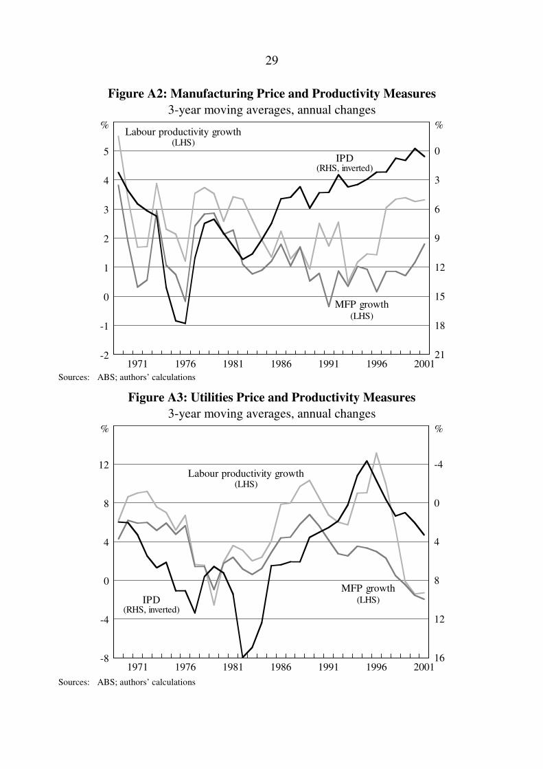
Figure A2: Manufacturing Price and Productivity Measures 3-year moving averages, annual changes

-2

-1

0

1

2

3

4

5

21

18

15

12

9

6

3

0

% %

20011991 19961981 19861971 1976


MFP growth

IPD

(LHS)

(LHS)

(RHS, inverted)


Figure A3: Utilities Price and Productivity Measures 3-year moving averages, annual changes

-8

-4

0

4

8

12

16

12

8

4

0

-4

% %

20011991 19961981 19861971 1976


MFP growthIPD

(LHS)

(LHS)(RHS, inverted)


30

Figure A4: Construction Price and Productivity Measures 3-year moving averages, annual changes

-4

-2

0

2

4

6

25

20

15

10

5

0


MFP growth

IPD(LHS)

(LHS)

(RHS, inverted)

% %

20011991 19961981 19861971 1976 Sources: ABS; authors’ calculations

Figure A5: Wholesale and Retail Trade Price and Productivity Measures 3-year moving averages, annual changes

-4

-2

0

2

4

6

8

18

15

12

9

6

3

0


MFP growth

IPD

(LHS)

(LHS)

(RHS, inverted)

% %


31

Figure A6: Transport, Storage and Communications Price and Productivity Measures

3-year moving averages, annual changes

-2

0

2

4

6

16

12

8

4

0


MFP growth

IPD

(LHS)

(LHS)

(RHS, inverted)

% %


32

Appendix B: Output Gap Series

Figure B1: Output Gap Series Percentage deviation from trend value-added growth

-4

0

4

-10

0

10

-4

0

4

-4

0

4

-8

-4

0

4

-8

-4

0

4

(LHS)Mining

Manufacturing %

%

%

%

(RHS)Non-farm GDP output

gap

Utilities


(LHS)

-20

-10

0

10

-20

-10

0

10

-4

0

4

-4

0

4

%% Construction

Transport, storage &communication

200219901978200219901978

(LHS) (LHS)

Sources: RBA; authors’ calculations

33

Appendix C: Sample Estimation Results

Table C1: Sample Estimate Results Coefficients for IPDs to labour productivity growth equation

Variable Mining Manufacturing Utilities Construction Wholesale & retail trade

Transport, storage &

communications

At-1 –0.47

(0.00)

–0.38

(0.03)

0.07

(0.66)

0.27

(0.10)

0.29

(0.07)

–0.18

(0.30)

At-2 –0.44

(0.00)

–0.07

(0.69)

–0.10

(0.55)

–0.21

(0.24)

–0.30

(0.03)

–0.39

(0.02)

Pt-1 –0.11

(0.19)

0.04

(0.71)

0.20

(0.31)

0.19

(0.06)

0.16

(0.20)

0.09

(0.42)

Pt-2 –0.21

(0.02)

0.02

(0.87)

–0.54

(0.01)

0.08

(0.43)

–0.43

(0.00)

–0.03

(0.81)

Yt 1.11

(0.00)

0.27

(0.02)

0.70

(0.36)

0.23

(0.05)

0.54

(0.01)

0.36

(0.12)

Const 11.99

(0.00)

3.30

(0.00)

7.09

(0.00)

–0.82

(0.41)

3.67

(0.00)

6.04

(0.00)

R2 0.45 0.08 0.20 0.26 0.46 0.21 Notes: Standard errors are reported in parantheses.

Dependent variable: At, where A is labour productivity growth.

Number of observations = 34; number of parameters = 5.

34

Appendix D: Residuals of Inflation to Productivity Growth Model

Figure D1: Residuals of Inflation to Labour Productivity Growth Regression

-10

0

10

-10

0

10

-10

0

10

-10

0

10

-3

0

3

-7

0

7

Mining Manufacturing %

%

%

% Utilities

-10

-5

0

5

-10

-5

0

5

-10

-5

0

5

-10

-5

0

5

%%

Construction

Transport, storage &communication

200219901978


200219901978 Source: Authors’ calculations

35

Appendix E: Reverse Causal Flow

Table 4 presented the results for the model of inflation’s effect on productivity growth. Table E1 reports the results for the reverse direction of productivity’s effects on inflation.

Table E1: Productivity Growth to Inflation Model Industry productivity growth’s causal effect on IPDs, with two lags on price and

productivity variables: 1967–2002 From labour

productivity to IPDs From multifactor

productivity to IPDs

Coefficient R2 Coefficient R2

Mining 0 0.20 0 0.19

Manufacturing + 0.42 +** 0.55

Utilities 0 0.38 +* 0.46

Construction 0 0.10 +* 0.12


+* 0.52 +** 0.54


0 0.31 +** 0.37

Notes: Number of observations = 34; number of parameters = 5.

We see that there is little relationship for labour productivity but a predominant positive effect from MFP to inflation. Intuitively this doesn’t make a lot of sense and it is also at odds with the results that show higher inflation causing lower productivity. Nonetheless, following an idea from Lowe (1995) we consider whether this may reflect the operation of a third, omitted factor: wages. Lowe argues that higher nominal wage growth is associated with faster productivity growth, and conversely that when an industry’s real product wages44 fall, that industry’s labour productivity will also fall as it employs more workers, particularly more marginal workers. Further, Lowe argues nominal wages should

44 Lowe (1995) defines real product wages as nominal wage growth deflated by the IPD.

For clarity, contrast this with real consumption wages, which are nominal wages deflated by the CPI – Lowe (1995) argues this version of wages should not effect employment, hence productivity.

36

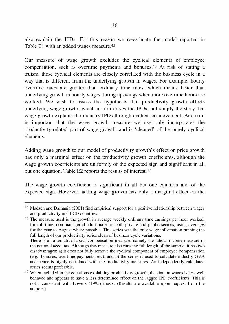
also explain the IPDs. For this reason we re-estimate the model reported in Table E1 with an added wages measure.45

Our measure of wage growth excludes the cyclical elements of employee compensation, such as overtime payments and bonuses.46 At risk of stating a truism, these cyclical elements are closely correlated with the business cycle in a way that is different from the underlying growth in wages. For example, hourly overtime rates are greater than ordinary time rates, which means faster than underlying growth in hourly wages during upswings when more overtime hours are worked. We wish to assess the hypothesis that productivity growth affects underlying wage growth, which in turn drives the IPDs, not simply the story that wage growth explains the industry IPDs through cyclical co-movement. And so it is important that the wage growth measure we use only incorporates the productivity-related part of wage growth, and is ‘cleaned’ of the purely cyclical elements.

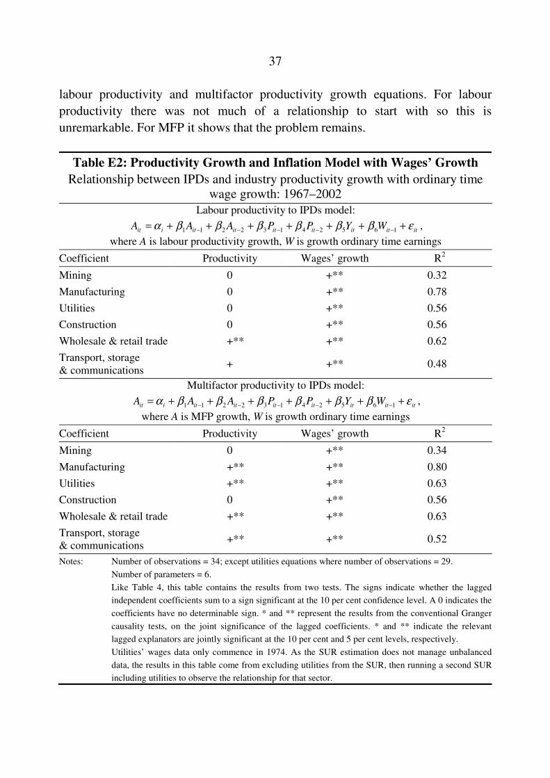
Adding wage growth to our model of productivity growth’s effect on price growth has only a marginal effect on the productivity growth coefficients, although the wage growth coefficients are uniformly of the expected sign and significant in all but one equation. Table E2 reports the results of interest.47

The wage growth coefficient is significant in all but one equation and of the expected sign. However, adding wage growth has only a marginal effect on the

45 Madsen and Damania (2001) find empirical support for a positive relationship between wages

and productivity in OECD countries. 46 The measure used is the growth in average weekly ordinary time earnings per hour worked,

for full-time, non-managerial adult males in both private and public sectors, using averages for the year-to-August where possible. This series was the only wage information running the full length of our productivity series clean of business cycle variations.

There is an alternative labour compensation measure, namely the labour income measure in the national accounts. Although this measure also runs the full length of the sample, it has two disadvantages: a) it does not fully remove the cyclical component of employee compensation (e.g., bonuses, overtime payments, etc); and b) the series is used to calculate industry GVA and hence is highly correlated with the productivity measures. An independently calculated series seems preferable.

47 When included in the equations explaining productivity growth, the sign on wages is less well behaved and appears to have a less determined effect on the lagged IPD coefficients. This is not inconsistent with Lowe’s (1995) thesis. (Results are available upon request from the authors.)

37

labour productivity and multifactor productivity growth equations. For labour productivity there was not much of a relationship to start with so this is unremarkable. For MFP it shows that the problem remains.

Table E2: Productivity Growth and Inflation Model with Wages’ Growth Relationship between IPDs and industry productivity growth with ordinary time

wage growth: 1967–2002 Labour productivity to IPDs model:

itititititititiit WYPPAAA εββββββα +++++++= −−−−− 16524132211 ,

where A is labour productivity growth, W is growth ordinary time earnings

Coefficient Productivity Wages’ growth R2

Mining 0 +** 0.32

Manufacturing 0 +** 0.78

Utilities 0 +** 0.56

Construction 0 +** 0.56

Wholesale & retail trade +** +** 0.62


+ +** 0.48

Multifactor productivity to IPDs model:

itititititititiit WYPPAAA εββββββα +++++++= −−−−− 16524132211 ,

where A is MFP growth, W is growth ordinary time earnings

Coefficient Productivity Wages’ growth R2

Mining 0 +** 0.34

Manufacturing +** +** 0.80

Utilities +** +** 0.63

Construction 0 +** 0.56

Wholesale & retail trade +** +** 0.63


+** +** 0.52

Notes: Number of observations = 34; except utilities equations where number of observations = 29.

Number of parameters = 6.

Like Table 4, this table contains the results from two tests. The signs indicate whether the lagged

independent coefficients sum to a sign significant at the 10 per cent confidence level. A 0 indicates the

coefficients have no determinable sign. * and ** represent the results from the conventional Granger

causality tests, on the joint significance of the lagged coefficients. * and ** indicate the relevant

lagged explanators are jointly significant at the 10 per cent and 5 per cent levels, respectively.

Utilities’ wages data only commence in 1974. As the SUR estimation does not manage unbalanced

data, the results in this table come from excluding utilities from the SUR, then running a second SUR

including utilities to observe the relationship for that sector.

38

These results clearly show that wages affect inflation. However, the wages’ growth variable does not account for the curious causal relationship between growth in multifactor productivity and the IPDs. We added a range of other variables and tried alternative but intuitively sensible models, but were unable to explain the results in Table E2. Given the odd relationship predominately appears in the multifactor productivity growth equations, a possible explanation may be the measurement issues with our multifactor productivity growth series. Measuring multifactor productivity growth as a residual of an output function means the series also captures the measurement error in capital – which is especially hard to measure accurately – and the aggregate hours and real and nominal GVA series. However, this explanation is unconvincing given multifactor productivity growth behaved similarly to labour productivity growth in the model observing price growth’s effect on productivity growth. So, in sum, the results for MFP growth remain anomalous, and a potential area for future research.

39

References

Baltagi B, J Griffin and P Rich (1995), ‘The measurement of firm-specific indexes of technical change’, Review of Economics and Statistics, 77(4), pp 654–663.

Bickerdyke I, R Lattimore and A Madge (2000), ‘Business failure and change: an Australian perspective’, Productivity Commission Staff Research Paper, AusInfo, Canberra.

Blanchard O and S Fisher (1989), Lectures on macroeconomics, MIT Press, Cambridge.

Blanchard O and J Simon (2001), ‘The long and large decline in U.S. output volatility’, Brookings Papers on Economic Activity, 1, pp 135–174.

Buck A and F Fitzroy (1988), ‘Inflation and productivity growth in the Federal Republic of Germany’, Journal of Post Keynesian Economics, 10(2), pp 428–444.

Cameron N, D Hum and W Simpson (1996), ‘Stylized facts and stylized illusions: inflation and productivity revisited’, Canadian Journal of Economics, 29(1), pp 152–162.

Chowdhury A and G Mallik (1998), ‘A land locked into low inflation: how far is the promised land?’, Economic Analysis & Policy, 28(2), pp 233–243.

Clark P (1982), ‘Inflation and the productivity decline’, AEA Papers and Proceedings, 72(2), pp 149–154.

Feldstein M (1982a), ‘Inflation, capital taxation, and monetary policy’, in R Hall (ed), Inflation: causes and effects, University of Chicago Press, Chicago, pp 153–167.

Feldstein M (1982b), ‘Inflation, tax rules, and investment: some econometric evidence’, Econometrica, 50(4), pp 825–862.

Freeman D and D Yerger (2000), ‘Does inflation lower productivity? Time series evidence on the impact of inflation on labour productivity in 12 OECD nations’, Atlantic Economic Journal, 28(3), pp 315–332.

40

Friedman M (1956), ‘The quantity theory of money: a restatement’, in M Friedman (ed), Studies in the quantity theory of money, Chicago UP, Chicago, pp 3–21.

Gruen D, T Robinson and A Stone (2002), ‘Output gaps in real time: are they reliable enough to use for monetary policy?’, Reserve Bank of Australia Research Discussion Paper No 2002-06.

Hall R (1999), ‘Comment on A Estrella and F Mishkin, “Rethinking the role of NAIRU in monetary policy: implications of model formulation and uncertainty”’, in J Taylor (ed), Monetary policy rules, Chicago UP, Chicago, pp 431–434.

Hayek F (1945), ‘The use of knowledge in society’, American Economic Review, 35(4), pp 519–530.

Hendry D (2001), ‘Modelling UK inflation, 1875-1991’, Journal of Applied Econometrics, 16(3), pp 255–276.

Industry Commission and Department of Industry, Science and Tourism (1997), A portrait of Australian business: results of the 1995 business longitudinal survey, Commonwealth of Australia, Canberra.

Jarrett P and J Selody (1982), ‘The productivity-inflation nexus in Canada, 1963–1979’, Review of Economics and Statistics, 64(3), pp 361–367.

Lowe P (1995), ‘Labour-productivity growth and relative wage: 1978–1994’, in P Anderson, J Dwyer and D Gruen (eds), Productivity and growth, Proceedings of a Conference, Reserve Bank of Australia, Sydney, pp 93–134.

Lucas R (1973), ‘Some international evidence on output-inflation tradeoffs’, American Economic Review, 63(3), pp 326–334.

Madsen JB and R Damania (2001), ‘Labour demand and wage-induced innovations: evidence from the OECD countries’, International Review of Applied Economics, 15, pp 323–334.

41

Okun A (1971), ‘The mirage of steady inflation’, Brookings Papers on Economic Activity, 1971(2), pp 435–498.

Pesaran MH and R Smith (1995), ‘Estimating long-run relationships from dynamic heterogeneous panels’, Journal of Econometrics, 68, pp 79–113.

Ram R (1984), ‘Causal ordering across inflation and productivity growth in the post-War United States’, Review of Economics and Statistics – Notes, 66(3), pp 472–477.

Saunders P and B Biswas (1990), ‘An empirical note on the relationship between inflation and productivity in the United Kingdom’, British Review of Economic Issues, 12(28), pp 67–77.

Sbordone A and K Kuttner (1994), ‘Does inflation reduce productivity’, Economic Perspectives, 18(6), pp 2–14.

Scarpetta S, P Hemmings, T Tressel and J Woo (2002), ‘The role of policy and institutions for productivity and firm dynamics: evidence from micro and industry data’, OECD Economics Department Working Paper 2002/15.

Simon J and S Wardrop (2002), ‘Australian use of information technology and its contribution to growth’, Reserve Bank of Australia Research Discussion Paper No 2002-02.

Smyth D (1995a), ‘Inflation and total factor productivity in Germany’, Weltwirschaftliches Archiv, 131(2), pp 403–405.

Smyth D (1995b), ‘The supply side effects of inflation in the United States: evidence from multifactor productivity’, Applied Economic Letters, 2, pp 482–483.

Taylor J (1981), ‘On the relation between the variability of inflation and the average inflation rate’, Carnegie-Rochester Conference Series on Public Policy, 15, pp 57–85.

Tsionas E (2001), ‘Euro-land: any good for the European south?’, Journal of Policy Modeling, 23(1), pp 67–81.

42

Tsionas E (2003), ‘Inflation and productivity: empirical evidence from Europe’, Review of International Economics, 11(1), pp 114–129.

Productivity and Inflation - Reserve Bank of · PDF file6.2 Robustness to Additional Control...

Documents

Transcript of Productivity and Inflation - Reserve Bank of · PDF file6.2 Robustness to Additional Control...