Production assessment of low production rate of well in a ...Journal of Petroleum Exploration and...

Vol.:(0123456789)1 3

Journal of Petroleum Exploration and Production Technology (2019) 9:543–560 https://doi.org/10.1007/s13202-018-0491-y

ORIGINAL PAPER - PRODUCTION ENGINEERING

Production assessment of low production rate of well in a supergiant gas condensate reservoir: application of an integrated strategy

Reza Azin1 · Hassan Sedaghati1 · Rouhollah Fatehi2 · Shahriar Osfouri3 · Zahra Sakhaei1

Received: 23 September 2017 / Accepted: 10 May 2018 / Published online: 1 June 2018 © The Author(s) 2018

AbstractIn this study, a novel and integrated strategy is proposed to investigate the problem of low production rate of gas well in a supergiant gas condensate reservoir. In this strategy, the nodal analysis approach is applied for production optimization and performance assessment of a real inclined well. A multi-layered gas condensate reservoir model was constructed and simulated using actual reservoir rock and fluid properties. Effects of reservoir rock and fluid model simplification on inflow performance relationship (IPR) curves were investigated. Also, five different tubing pressure drop models were evaluated using extracted pseudo spontaneous potential (PSP) data from reservoir model to select the most accurate one for comput-ing tubing performance relationship (TPR) data. Then, accuracy of nodal analysis in prediction of well operating point was investigated through comparing with reservoir simulator results. Results of nodal analysis for this well indicated that a significant discrepancy exists between calculated and actual production rate. Sensitivity analysis on uncertainty parameters, skin factor and drainage radius, shows that skin factor of the investigated well varies between 11 and 12.9 for drainage radius in the range of 3000–20000 ft. Therefore, the problem of low well production rate was attributed to high skin factor as a result of formation damage. Also, results demonstrated that reduction of skin can lead to maximum 73% enhancement in daily volumetric gas production rate of well.

Keywords Gas condensate well · Nodal analysis · Inflow performance relationship (IPR) · Tubing performance relationship (TPR) · Drainage radius · Skin factor

Introduction

The worldwide demand for fossil fuels, especially natural gas as an environmental friendly energy resource with eco-nomically feasible production, is annually increasing. Also, given the fact that economy of many countries depends on oil and gas revenues, producing a certain daily volume of hydrocarbon while preserving reservoirs to meet the needs

of future generations are essential (Najibi et al. 2009). Non-normative withdrawals of reservoirs as well as drilling numerous wells without any certain schedule cause exces-sive pressure drop of reservoirs and as a consequence low ultimate recovery (Shadizadeh and Zoveidavianpoor 2009).

The best way to avoid such problems is an integrated res-ervoir-well production optimization, which ensures oil com-panies that drilled wells and surface facilities are working at their peak performance at all times to maximize production (Shadizadeh and Zoveidavianpoor 2009). Several parameters can be considered in production optimization of hydrocarbon reservoirs, including drilling schedule, number of producer and injector wells, pattern of well placement, production rate and surface facilities (Guyaguler and Gumrah 1999). Usu-ally, these parameters are optimized using simple reservoir models as well as mathematical or programming techniques involving economic strategies. Take the work done by Lee and Aronofsky in 1958 as one of the early studies in this field. They maximized crude oil production from homoge-neous and simple reservoir models using a developed linear

* Reza Azin [email protected]

1 Department of Petroleum Engineering, Faculty of Petroleum, Gas and Petrochemical Engineering, Persian Gulf University, Bushehr, Iran

2 Department of Mechanical Engineering, Faculty of Petroleum, Gas and Petrochemical Engineering, Persian Gulf University, Bushehr, Iran

3 Department of Chemical Engineering, Faculty of Petroleum, Gas and Petrochemical Engineering, Persian Gulf University, Bushehr, Iran

http://orcid.org/0000-0001-8338-6874

http://crossmark.crossref.org/dialog/?doi=10.1007/s13202-018-0491-y&domain=pdf

544 Journal of Petroleum Exploration and Production Technology (2019) 9:543–560

1 3

programming for the optimization problem (Lee and Aro-nofsky 1958). Bohannon in 1970 optimized efficiency of a designed system having several oil reservoirs producing in one or more gathering systems named as “multi-reservoir pipeline system”. He presented a linear programming model to define the optimum 15-years development plan for this designed system (Bohannon 1970). Also, the optimal type, location and trajectory of an unconventional well for the different reservoir types and fluid systems were determined by Yeten et al. in 2002. They applied an optimization pro-cedure including genetic algorithm for their goal (Yeten et al. 2002). Furthermore, Onwunalu and Durlofsky in 2011 developed a new well pattern optimization procedure for large-scale field development by utilizing particle swarm optimization technique (Onwunalu and Durlofsky 2011). In 2016, Nozohour-leilabady and Fazelabdolabadi maximized the Net Present Value for designed scenarios with multiple injector and producer wells and cases with deviated wells in a real reservoir model. Artificial bee colony optimization technique was used in their study (Nozohour-leilabady and Fazelabdolabadi 2016). Recently, a comprehensive produc-tion optimization study for an oil field located in the Middle East was done by Izadmehr et al. In their study, different fac-tors influencing oil production such as artificial lift model, water injection flow rate, drilling new producer and injector wells and gas injection were examined in different scenarios through reservoir simulation to choose the optimized plan (Izadmehr et al. 2017).

Among the existing production optimization meth-ods, nodal analysis is the well-known and most powerful approach in production engineering for optimization process of oil and gas systems (Dale 1991). For the first time in 1954, Gilbert presented and used nodal analysis approach for the optimization of fluid production from reservoirs (Gilbert 1954). Nodal analysis considers the reservoir-wellbore sys-tem, simultaneously. A reservoir with certain specifications (porosity, permeability, thickness, etc.) delivers the fluid into the bottom hole of the well under defined operating condi-tions (flow rate and pressure). This fluid must overpass from the bottom to the top of the well and then surface facilities. This path from the bottom to the top of the well has many joints, valves, etc., that cause a pressure drop. Nodal analysis utilizes the computation of pressure drop across each section (from the reservoir to surface) to estimate production rate with regard to the existing conditions (Gilbert 1954). Pres-sure drop of fluid flow across the porous media and tubing are described by inflow (IPR) and outflow or tubing (TPR) performance relationship. Incorporating TPR curve with IPR provides an intersection which shows the well deliverabil-ity (also called well operating point or natural flow point) for a system with defined reservoir and wellhead pressure (Dale 1991). This well operating point obtained through the nodal analysis, represents optimum production condition

(production rate and pressure) for the system with certain characteristics which satisfies both inflow and outflow com-ponents. Therefore, oil and gas wells should produce in their operating point conditions to achieve maximum possible efficiency. Application of nodal analysis has contributed to ameliorate drilling and completion techniques, production and efficiency of many gas and oil systems. Works done by Shadizadeh and Zoveidavianpoor in 2009 (Shadizadeh and Zoveidavianpoor 2009), Dmour in 2013 (Dmour 2013) and Soleimani in 2017 (Soleimani 2017) are brilliant examples for the usage of this approach.

There are many gas and oil wells around the world which do not produce in their operating conditions for different rea-sons. Investigation performed on drilled wells in South Pars gas field located in Persian Gulf showed that most of them produce in low rate with unknown reason. On this subject in the current study, one of the wells in South Pars gas field is selected as a case study. According to available well data and challenges of production data analysis, an innovative and integrated procedure based on nodal analysis is designed and employed for production optimization and troubleshooting the well problem. It is worth noting that complexities and challenges of production data analysis in this reservoir are addressed by Heidari Sureshjani et al. (Heidari Sureshjani et al. 2016), Lak et al. (Lak et al. 2014), and Azin et al. (Azin et al. 2014) in six general steps, including data gath-ering/extraction/quality check, choke modeling, well rate determination, well bottom-hole pressure estimation, layer rate allocation, and reservoir property estimation. In next parts, methodology for generating IPR and TPR curves as two main tools of this research is described first, followed by assessing the impacts of reservoir rock and fluid model simplification on IPR curves. Next, all necessary tools for accomplishing nodal analysis are calculated. Then, the pro-posed methodology is validated for the well under study. Finally, sensitivity analysis is performed to figure out pos-sible sources of low production rate. Concluding remarks appear at the end.

Methodology

In this section, first the gas condensate reservoir simula-tion and procedure for generating IPR curves are explained. Then, details of TPR curve generation for nodal analysis through well simulation are presented.

Reservoir simulation

A sector of heterogeneous, two-dimensional, radial and multi-layered model of the investigated gas condensate field is constructed using real fluid and rock properties. For this purpose, commercial reservoir simulator CMG, version

545Journal of Petroleum Exploration and Production Technology (2019) 9:543–560

1 3

2012.10 is utilized. In this study, the module of IMEX and GEM are used for a modified black-oil and compositional simulation of the studied reservoir. Thermodynamic reser-voir fluid behavior is simulated using WINPROP module of CMG package. The reservoir contains lean gas with com-position shown in Table 1. Properties of plus fraction com-ponent including molecular weight and specific gravity are 214.89 g/mol and 0.835, respectively. Peng-Robinson equa-tion of state (PR-EOS) is applied for phase behavior studies of reservoir fluid. The phase envelope of main reservoir fluid is shown in Fig. 1. Details of EOS tuning using measured Pressure–Volume–Temperature (PVT) experimental data are described by Osfouri et al. (Osfouri and Azin 2016; Osfouri et al. 2015) (Table 2).

The studied reservoir is heterogeneous and multi-layered. Petrophysical specifications of each layers of studied res-ervoir including vertical (Kv) and horizontal (Kh) perme-abilities, porosity ( ∅ ) and thickness (h) are given in Table 2. In the base constructed model, a vertical well is located at the center of reservoir model and perforated along the whole reservoir thickness. Grid model was designed in radial coordinate. This designed grid model has 100 grid blocks in radial direction and their size increases logarithmically with distance from well. In other words, fine grid blocks were used in near wellbore region to accurately model the effect of condensate banking and two-phase flow on well pro-ductivity. The coarse grids were employed at distances far from well where single-phase flow regime prevails. Water phase in reservoir is in an immobile state. Relative perme-ability curves of gas and condensate phases are illustrated in Fig. 2. Drainage radius and skin factor of the reservoir are 3280 ft and 0, respectively. It should be mentioned that

an uncertainty exists in values of drainage radius and skin factor. It is prevalent to determine these uncertain param-eters accurately through history matching of the simulation model to actual reservoir. Nevertheless, due to the lack of

Table 1 Composition of reservoir fluid

Component Mole (%)

H2S 0.12CO2 1.92N2 3.51C1 82.79C2 5.35C3 2.00iC4 0.43nC4 0.72iC5 0.32nC5 0.29C6 0.39C7 0.48C8 0.45C9 0.29C10 0.22C11 0.15C12+ 0.57

Fig. 1 Phase diagram of reservoir fluid

Table 2 Petrophysical specification of reservoir layers

Layer Kh, mD Kv, mD ∅ h, ft

1 0.1166 0.0559 0.0169 1172 18.6542 0.0985 0.0764 513 16.6094 0.0709 0.0633 674 0.1658 0.0444 0.0148 695 0.1065 0.0004 0.0010 516 38.4135 0.1538 0.0671 367 35.3243 0.1208 0.0971 368 41.0909 0.1422 0.1011 459 0.0760 0.0003 0.0011 2510 4.5335 0.0728 0.0575 911 33.7305 0.2363 0.1071 1912 31.7728 0.3967 0.1107 2813 3.2442 0.0676 0.0405 7414 0.1285 0.0508 0.0148 6315 0.2069 0.0560 0.0222 13216 0.1012 0.0475 0.0197 3917 1.4744 0.1465 0.1102 1618 0.0667 0.0005 0.0339 1619 3.8710 0.0931 0.0753 4820 10.2853 0.2699 0.1236 4721 19.1637 2.3491 0.2082 4722 17.1848 2.0416 0.2313 4723 5.5656 0.1236 0.1058 2324 16.1507 0.2029 0.0559 3225 18.6719 2.0149 0.1401 6326 30.5272 0.2372 0.1406 3227 1.8467 0.0829 0.0685 13328 0.1939 0.0520 0.0178 67


1 3

proper and sufficient actual data, back-calculation method was employed to obtain data for nodal analysis. At the end, validity of the constructed reservoir model is checked. Other features of the constructed model are reported in Table 3.

One of the operational tools for evaluating performance of wells in petroleum engineering is IPR curve. IPR for a well is the relationship between flow rate of the well (Q) and flowing pressure of the well or bottom-hole pressure (Pwf) at certain average reservoir pressure (Pr). Study of behavior and changes in IPR is essential in petroleum engineering. Because, these curves are used for consideration of differ-ent operating conditions, specification of optimum produc-tion rate and also design of production and artificial lift equipment (Gilbert 1954; Golan and Whitson 1991). Some numerical/analytical models with special assumption have been developed based on Darcy’s equation for calculation of IPR curve mostly in oil or dry gas wells (Al-Attar and AL-Zuhair 2008; Brar and Aziz 1978; Chase and Alkandari 1993; Evinger and Muskat 1942; Fetkovich 1973; Mishra and Caudle 1984; Vogel 1968). Nevertheless, many inves-tigators generalized these numerical / analytical models for calculation of IPR curves in gas condensate wells consider-ing two-phase flow in near wellbore region (Al-Shawaf et al.

2014; Fevang and Whitson 1996; O’Dell 1967; Orodu et al. 2012). However, these models are insufficient to account for condensate accumulation and complex flow behavior in this region (Jokhio and Tiab 2002; Sakhaei et al. 2017). Actual conditions of near wellbore area in gas condensate reservoirs such as effect of high flow rate, high capillary number, non-Darcy effects and reservoir heterogeneity are not considered in these models (Kumar et al. 2006). These assumptions can cause significant error in predicting performance of wells. Therefore, gas condensate reservoir performance may be predicted with high accuracy and less assumptions through numerical simulation of a radial, single-well and hetero-geneous model with fine grid in near wellbore to consider all phenomena in this area. An example of IPR construc-tion through reservoir simulation is given by Sakhaei et al. (Sakhaei et al. 2017). A similar approach was used in this study to generate data points to plot IPR curves by simu-lation. This approach includes (1) constructing a reservoir model, followed by running the model at several different bottom-hole pressures (well production with constant bot-tom-hole pressure), (2) continuous recording of gas produc-tion rate as a function of average reservoir pressure in each bottom-hole pressure and (3) running the model at each step until average reservoir pressure reaches to the bottom-hole pressure. Therefore, a series of bottom-hole pressure data will be obtained as function of gas production flow rate at different average reservoir pressures.

Well simulation

The pressure drop needed to lift reservoir fluids to the surface at a certain rate controlled by wellhead choke, is another sig-nificant factor affecting well deliverability. This pressure drop is determined based on the mechanical energy equation for flow between two points. In this regard, pressure drop along the tubing is a function of mechanical configuration of the wellbore, properties of fluids and production rates (Orkisze-wski 1967). The relationship between pressure drop along the tubing and production rate is called TPR and is valid for a defined wellhead pressure (Ikoku 1992). For plotting TPR curve, it is necessary to calculate bottom-hole pressure (Pwf) at various production rates (Q) for a certain wellhead pressure (Pwh). Given the fact that multiphase flows occur in almost all gas and oil wells (Rai et al. 1989), several empirical/ana-lytical correlations have been developed to estimate pressure drop in multiphase flow depending on reservoir and well con-ditions, tubing and production rate (Ansari et al. 1990; Aziz and Govier 1972; Baxendell and Thomas 1961; Beggs and Brill 1973; Fancher Jr and; Brown 1963; Gray 1974; Hage-dorn and Brown 1965; Hasan and Kabir 1988; Mukherjee and Brill 1985; Poettman and Carpenter 1952). Selection of optimum correlation among these correlations are essential to estimate pressure drop along tubing, plot TPR curve, evaluate

Fig. 2 Gas/oil relative permeability curves

Table 3 Conditions of the base constructed reservoir model

Initial reservoir pressure, Pisa 5280Reservoir temperature, K 375Dew point pressure, Pisa 4500Maximum liquid dropout, % 2.5Wellbore radius, ft 0.29Total thickness, ft 1430Reservoir depth, ft 3000Connate water saturation 0.25Grid number in r, θ and z direction 100,1,28


1 3

well performance, determine operating point, design suitable surface facilities and production optimization.

In this study, multiphase flow simulation of the well is uti-lized to select proper correlation to calculate pressure gradi-ent along the objective gas condensate well. For this purpose, Schlumberger PIPESIM software version 2008.1 is applied. Necessary input data into PIPESIM software includes required data for simulation of phase behavior of fluid, inflow perfor-mance of the vertical well, tubing and fluid flow within the tubing. Compositional model is suggested for simulation of thermodynamic behavior of gases by PIPESIM (Schlumberger 2008). Therefore, phase behavior of fluid within the well was simulated using the composition of reservoir fluids presented in Table 1 and PR-EOS. Also, reservoir temperature and static pressure needed for simulation of inflow performance of the well were mentioned in previous section. Furthermore, the IPR curve extracted from reservoir model was imported to PIPESIM as field data to find suitable and accurate model for estimating IPR data in constructed well model. Among available models in PIPESIM, back-pressure model (Schlum-berger 2008) has best match with numerical/ empirical data. Data needed for simulation of tubing is given in Table 4. For simulating fluid flow within the tubing and selecting optimum pressure drop model, pseudo spontaneous potential (PSP) data elicited from reservoir model, as another empirical data, is brought into software. By calculating PSP data in defined well-head pressure and production rate and comparing with elicited data, optimum model for predicting pressure drop along tub-ing is selected. It is vital to note that empirical correlations of Hagedorn and Brown (HBR) (Hagedorn and Brown 1965), Mukherjee and Brill (MB) (Mukherjee and Brill 1985), Gray (Gray 1974), Ansari et al. analytical model (Ansari et al. 1990) and NOSLIP correlation (Schlumberger 2008) were selected for comparison. Similar approach was applied in previous work (Azin et al. 2016).

Results and discussion

The single-well model was constructed using real fluid and rock properties. Back-calculations were employed to plot IPR curves and elicit other data necessary for selecting the opti-mum pressure drop model in tubing and performing nodal analysis. The conceptual structure of integration procedure used in this study for production optimization of the gas condensate well is shown in Fig. 3. According to this figure, after running necessary tools for nodal analysis, accuracy and

reliability of this method were assessed. Eventually, the main reason for the problem of low production rate was determined using this approach and through sensitivity analysis.

Simplification of the reservoir rock and fluid model

Reservoir simulation is an applicable tool for predicting the reservoir performance under different scenarios in the least possible time and cost compared with studies on real fields. However, its application for some situations such as reservoirs with intricate phase behavior (gas condensate and volatile oil reservoirs) or heterogeneous and multi-layered formation is very time-consuming and practically impossible. In this study, compositional simulation of 28-layer gas condensate reservoir caused a significant jump in runtime due to the high volume of EOS and flash calculations in heterogeneous reservoir model with large number of grid blocks. In this regard, the reservoir fluid and rock model were simplified and examined in different states to choose a suitable one which gives satisfactory output.

Typically, compositional simulators are used for simulating gas condensate and volatile oil reservoirs due to the impor-tance of changes in composition of these reservoir fluids (Jamal et al. 2006). However, in many cases, simulation of compositional model for these types of reservoirs is not neces-sary. For an optimal performance, an intermediate simulator between standard black-oil and compositional, called modified black-oil, can be used. In this way, the volume of calculations decreases remarkably (El-Banbi et al. 2006). Hence, after simulating thermodynamic behavior of reservoir fluid, com-positional as well as modified black-oil model were exported from WINPROP to import to GEM and IMEX and results were compared.

Furthermore, the actual 28-layer reservoir model was simplified to a single-layer model. The average porosity and permeability of the single-layer model were calculated by implementing average properties of 28-layer model (Table 2) using Eqs. (1)–(3). The average petrophysical specifications of single-layer model are reported in Table 5.

According to the explained procedure in Sect. 2.1, IPR curves were plotted and compered in four different average

(1)�̄ =

∑�hi∑hi

(2)K̄h =

∑Khihi∑hi

(3)K̄v =

∑hi

∑ hi

Kvi

Table 4 Vertical well specification

Parameter Value

True vertical depth, ft 4430.8Tubing roughness 0.0018Tubing diameter, in 6


1 3

Fig. 3 Proposed strategy for integrated well performance analysis


1 3

reservoir pressures (Pr) through compositional and modi-fied black-oil simulation of single-layer reservoir model. These results are demonstrated in Fig. 4. It should be mentioned that only reservoir rock and fluid model were simplified and other specifications such as the number of grid blocks in the radial direction, well perforation, well-bore radius and reservoir pore volume were the same in all cases. Also, IPR curves were plotted by running reservoir model at similar bottom-hole pressures for both simula-tors. As observed from Fig. 4, the IPR curve moves down-ward by decreasing average reservoir pressure. In other words, for a specific bottom-hole pressure, well produces a lower rate at lower average reservoir pressure. Also, in defined average reservoir pressure, when the bottom-hole pressure becomes close to average reservoir pressure, flow rate decreases and becomes zero due to absence of any pressure drawdown. Maximum flow rate, i.e., absolute open flow (AOF) potential, happens when bottom-hole pressure tends to be zero. According to Fig. 4, for the tar-get gas condensate reservoir, compositional and modified black-oil simulator have good agreement with each other in estimation of flow rate in various bottom-hole pressure. The relative errors of estimated IPR curves using these two simulators are reported in Table 6. These reported errors of less than 10% show that selecting modified black-oil simulator instead of compositional gives good results with significantly lower runtime. So, the modified black-oil as an optimal simulator was utilized for running the reservoir

model in other parts of this study. Also, results illustrated in Fig. 4 and Table 6 state that for average reservoir pres-sure above dew point pressure, the error between these two simulators is insignificant. This is due to small changes in reservoir fluid composition at pressures higher than dew point pressure with low rate of retrograde condensation.

The relative error was calculated using Eq. (4):

where, N is the number of points. Qest

i And Qact

i are esti-

mated well production rate using modified black-oil and compositional simulator in the same bottom-hole pressure, respectively.

Another option for alleviating the number of reservoir layers is reconstruction of the 28-layer as 4-layer model. Table 2 shows that layers 5, 9 and 18 have very low verti-cal permeability. These low permeable layers act as a bar-rier for exchanging flow between reservoir layers. There-fore, it is expected that adjoining layers have different pressure distribution along the reservoir drainage radius. However, embedded layers between two low permeable layers have almost the same pressure distribution due to their high vertical permeability. So, these layers can be considered as one main layer. That is to say, the actual 28-layer model was restored as 4-layer. Like single-layer model, average specifications of 4-layer model were deter-mined by utilizing Eqs. (1)–(3). Characteristics of 4-layer model as well as sub-layer of each main layer are presented in Table 7. It is vital to note that simplification of 28-layer reservoir model to 4-layer decreased runtime in compo-sitional simulator slightly. Considering the fact that each

(4)RE% =100

N

N∑

i=1

(|||||

Qest

i− Qact

i

Qact

i

|||||

)

Table 5 Average petrophysical specification of single-layer reservoir model

Main layer Sub-layer Kh, mD Kv, mD ∅ h, ft

SL 1–28 9.68 0.00 0.066 1430

Fig. 4 Comparison of modified black-oil and compositional simula-tors for single-layer reservoir model

Table 6 Relative errors between modified black-oil and compositional simulators in predicting production rate for single-layer reservoir model

Pr, psi Relative errors, %

5000 24000 53000 72000 7

Table 7 Average petrophysical specification of the 4-layer reservoir model

Main layer Sub-layer Kh, mD Kv, mD ∅ h, ft

ML1 1–5 5.90 0.0024 0.0315 355ML2 6–9 31.56 0.0017 0.0735 141ML3 10–18 4.75 0.0099 0.0393 396ML4 19–28 10.06 0.1304 0.1075 538


1 3

point of IPR curves is achieved in separate runs, likewise, extracting IPR curves from compositional simulation of 4-layer model were time-consuming and difficult. Modi-fied black-oil simulator with acceptable error required less runtime for both 4- and 28-layer reservoir models.

Figure 5 shows extracted IPR curves from modified black-oil simulator for 1-, 4- and 28-layer reservoir models in the same conditions. According to Fig. 5a, a substantial differ-ence exists between estimated flow rate of single-layer and real 28-layer reservoir model in almost all bottom-hole pres-sures. However, 4-layer model is in good agreement with results of 28-layer model, as shown in Fig. 5b. For a closer examination, the relative errors of estimated production rate of single-layer and 4-layer reservoir model with respect to results of 28-layer model are provided in Table 8. As seen, single-layer model has a relatively high error in well produc-tion rate. Also, this error increases with decreasing average reservoir pressure. The reported relative errors for 4-layer reservoir model confirm the observed results of Fig. 5b. Equation (4) was used for calculation of relative error with

the difference that Qest

i is estimated production rate of 1- or

4-layer model. Qact

i is well production rate in 28-layer model.

Therefore, oversimplification of a multilayer reservoir into a single layer leads to a non-realistic IPR model which may result in an operating point different from that observed in a gas well.

To better explain the reason for these observations, aver-age pressure distribution of reservoir layers with depth of 1-, 4- and 28-layer model in average reservoir pressure of 4650 psi and bottom-hole pressure of 900 psi were plotted and compared simultaneously. These results are demonstrated in Fig. 6, which indicates that the average pressure in layers of single-layer and 28-layer models are far from each other. The lack of exchanging flow between reservoir layers because of

Fig. 5 Comparison of a single-layer and b 4-layer reservoir model with the actual 28-layer model

Table 8 Relative errors of single-layer and 4-layer reservoir model in predicting production rate

Pr, psi Relative errors, % (single-layer)

Relative errors, % (4-layer)

5000 14 1.04000 23 2.53000 33 3.02000 37 3.5

Fig. 6 Average pressure distribution of reservoir layers with depth


1 3

existence of almost non-permeable layers (5, 9 and 18), leads a discontinuity in pressure distribution of 28-layer model (Fig. 6). Therefore, the behavior of actual 28-layer model is not close to the single-layer one. In opposite, if the vertical permeability is high in a multi-layered heterogeneous reser-voir, exchange of flow occurs between layers and pressure of layers approaches equilibrium. In such situation, the behav-ior of multi-layered reservoir will be close to a single-layer and homogeneous reservoir. In this study, different pressure distributions caused a significant discrepancy between pre-dicted well production rates and IPR curves of single-layer and 28-layer model. As seen in Table 8, this difference is higher at lower reservoir pressure due to more extension of condensate accumulation region and as a result, higher dif-ferences in pressure distribution. Also, Fig. 6 shows that the 4-layer model pressure distribution is close to the 28-layer model. It is the main reason for high accuracy of this model in estimating well production rates.

Nodal analysis

As mentioned, nodal analysis is a well-known approach in production engineering that can be used to improve perfor-mance of gas and oil systems. IPR curves, as one of the main tools in this approach, were calculated through simulation of the reservoir fluid flow and presented in the previous sec-tion. Also, the gas condensate well simulation was applied to determine the optimum pressure drop model in tubing and calculate TPR curves. Five pressure drop models including Hagedorn and Brown (HBR) (Hagedorn and Brown 1965), Mukherjee and Brill (MB) (Mukherjee and Brill 1985), Gray

(Gray 1974), Ansari et al. analytical model (Ansari et al. 1990) and NOSLIP correlation (Schlumberger 2008) were selected to define the most accurate one. PIPESIM software recommends the HBR correlation (Hagedorn and Brown 1965) for gas condensate wells due to the comprehensive-ness of data used to develop this model (Schlumberger 2008). Also, the Gray’s model is developed for gas con-densate wells (Gray 1974). Furthermore, literature indicates that correlations which use average values of liquid and gas phase properties to calculate pressure drop have strong per-formance for a wide range of conditions (Kabir and Hasan 2006). Gray’s empirical correlation (Gray 1974) and Ansari et al. analytical model (Ansari et al. 1990) are examples of these correlations. Also, MB (Mukherjee and Brill 1985) and NOSLIP correlations (Schlumberger 2008) have been suggested by Azin et al. (Azin et al. 2014, 2016) for comput-ing pressure drop of gas condensate wells.

The PSP data consisting of pressure distribution with depth in the well were utilized to examine accuracy of the mentioned correlations. PSP data actually are gained using downhole production logging tool. The production logging tool incorporates different electrical probes and measure-ment tools for recording flow rate, fluid velocity, fluid type, density, temperature and pressure profile in different flow rates (Eisa et al. 2013). In designed strategy for well performance analysis (Fig. 3), this pressure profile was obtained through running the reservoir model (the modi-fied black-oil simulation of 28-layer model) with the well producing at a constant flow rate (60 and 120 MMSCFD). These measured data through reservoir simulation as well as estimated gradient pressure using five mentioned

Fig. 7 Comparison of tubing pressure drop models in a Q = 60 MMSCFD and b Q = 120 MMSCFD


1 3

pressure drop models are demonstrated in Fig. 7 for two different production rates. Pressure drop calculations were begun from the highest possible point at depth of 3000 ft. As seen in Fig. 7, the Ansari et al. (Ansari et al. 1990), Gray (Gray 1974) and NOSLIP (Schlumberger 2008) cor-relations show good match for estimation of measured data in both production rates, while HBR (Hagedorn and Brown 1965) and MB (Mukherjee and Brill 1985) cor-relations deviate from measured data. The relative errors of each model in different production rates are presented in Table 9. This table shows that Ansari et al. (Ansari et al. 1990), Gray (Gray 1974) and NOSLIP (Schlum-berger 2008) correlations anticipate the pressure drop with

a relative error of less than 3%, and the MB correlation (Mukherjee and Brill 1985) has the lowest accuracy.

Among three correlations with highest accuracy, Gary’s model (Gray 1974) was selected as the optimum pressure drop model to calculate TPR curves for the studied well. TPR curves were plotted at four specified wellhead pres-sures of 600, 1500, 2500 and 3500 psi. Nodal analysis was performed using these TPR curves and calculated IPR curves for the 28-layer reservoir model to ascertain the operating points of well at different average reservoir pres-sures and flowing wellhead pressures. Results are shown in Fig. 8 for different reservoir pressures. At a given aver-age reservoir pressure (Pr) and flowing wellhead pressure (Pwh), intersection of TPR and IPR curves represent well operating point. According to Fig. 8, the operating point of well changes by shifting both the IPR and TPR curves when the fixed pressures (Pr or Pwh) in the system with specified properties (tubing size, etc.) are changed. Reser-voir depletion and as a result decline in reservoir pressure causes the intersection of IPR and TPR curves move down-ward at a certain wellhead pressure. Take the results for plotted TPR curve at Pwh = 600 psi in Fig. 8 as an exam-ple. In some situations, there is no intersection between the IPR and TPR curves in the operating condition, like when the reservoir pressure declines to 2000 psi and wellhead pressure is 2500 psi. This represents that the well will not flow under these reservoir conditions. Therefore, different solutions for this problem should be investigated to elevate well productivity in present or future life of the well. Solu-tions include decreasing the wellhead pressure, changing the tubing size or installing artificial lift equipment. The values of production rate and bottom-hole pressure cor-responding to natural flow points of the well at different conditions are reported in Table 10.

To assess the validity of obtained operating points using nodal analysis (Table 10), these points were directly com-puted through reservoir simulation. For this purpose, the 28-layer reservoir model was run at four different constant wellhead pressures (600, 1500, 2500 and 3500 psi). When the average reservoir pressure reached 2000, 3000, 4000 and 5000 psi, the operating points were extracted from reservoir simulator. These elicited operating points are presented in Table 11 for different operating conditions.

Table 9 Accuracy of tubing pressure drop models in comparison with measured data

Pressure drop model Relative error, %

Q = 60 MMSCFD Q = 120 MMSCFD

Ansari et al. (Ansari et al. 1990) 0.67 2.08Gray (Gray 1974) 1.88 2.31HBR (Hagedorn & Brown 1965) 5.40 6.95NOSLIP 2.59 2.01MB (Mukherjee & Brill 1985) 13.90 13.03

Fig. 8 Nodal analysis for the 28-layer reservoir model

Table 10 Operating points through nodal analysis for 28-layer reservoir model

Pwh, psi Pr = 5000 psi Pr = 4000 psi Pr = 3000 psi Pr = 2000 psi

Q, MMSCFD Pwf, psi Q, MMSCFD Pwf, psi Q, MMSCFD Pwf, psi Q, MMSCFD Pwf, psi

600 410.4086 3001 295.1422 2226 206.5070 1639 120.2845 10991500 383.2343 3178 259.7290 2471 160.5800 1994 – –2500 323.3958 3572 177.8528 2989 – – – –3500 229.9897 4129 – – – – – –


1 3

Table 12 shows the relative errors of nodal analysis com-pared to reservoir simulation in determining production rates and bottom-hole pressures of operating points at various operating conditions. According to this table, nodal analysis has a negligible error in forecasting operating points com-pared to numerical reservoir simulation. Overall, accuracy of nodal analysis in prediction of the operating point reduces by decreasing average reservoir pressure. This increased error can be attributed to the extension of condensate bank, two-phase flow in the near wellbore area and differences in pro-duction history of reservoir model.

Figure 9 shows application of nodal analysis for single-layer and 4-layer reservoir models. The operating points for simplified reservoir models are reported in Table 13. As expected, the operating points by nodal analysis in 4-layer model shows better results than single-layer model compared

Table 11 Operating points through reservoir simulation



600 410.5144 3040 303.6800 2550 217.7679 1666 124.0269 11411500 385.2462 3205 269.3775 2484 170.3649 1998 – –2500 325.7036 3583 185.9858 2990 – – – –3500 231.4046 4128 – – – – – –

Table 12 Percentage of relative error of nodal analysis in predicting production rate and bottom-hole pressure for the 28-layer reservoir model


Q Pwf Q Pwf Q Pwf Q Pwf

600 0.02 1.28 2.81 1.02 5.17 1.57 3.02 3.751500 0.52 0.84 3.58 0.55 5.74 0.18 – –2500 0.70 0.32 4.37 0.05 – – – –3500 0.70 0.02 – – – – – –

Fig. 9 Nodal analysis for the single-layer and 4-layer reservoir mod-els

Table 13 Operating points through nodal analysis for single-layer and 4-layer reservoir model



Single-layer 600 433.3725 3158 325.9187 2431 239.8809 1859 144.3980 1243 1500 408.7104 3333 292.1207 2646 193.7127 2140 – – 2500 351.1414 3706 210.1653 3098 – – – – 3500 258.3900 4219 – – – – – –

4-layer 600 410.9239 3004 293.2625 2214 202.0954 1611 117.5400 1082 1500 387.2530 3203 256.9339 2456 156.3771 1976 – – 2500 325.2180 3580 175.2143 2981 – – – – 3500 229.6670 4118 – – – – – –


1 3

to reservoir simulator (Table 11). The average relative errors of nodal analysis for single-layer and 4-layer reservoir mod-els compared to reservoir simulation are 10 and 3.61%, respectively.

Problem of low gas production rate in an inclined well

In this part, nodal analysis is performed on an inclined gas well drilled in the supergiant offshore gas condensate field, which penetrates along 1112 ft of total reservoir production region (1430 ft), completed as open-hole. Vertical well pen-etration was changed to 1112 ft of total reservoir thickness in constructed reservoir model. Production rates from reservoir model were corrected for the inclined well conditions using the Peaceman’s model (Peaceman 1983). Details of this method are provided in the appendix. Also, the constructed well model was modified using actual values of true vertical depth (1112 ft) and measured depth (1778 ft) of the inclined well.

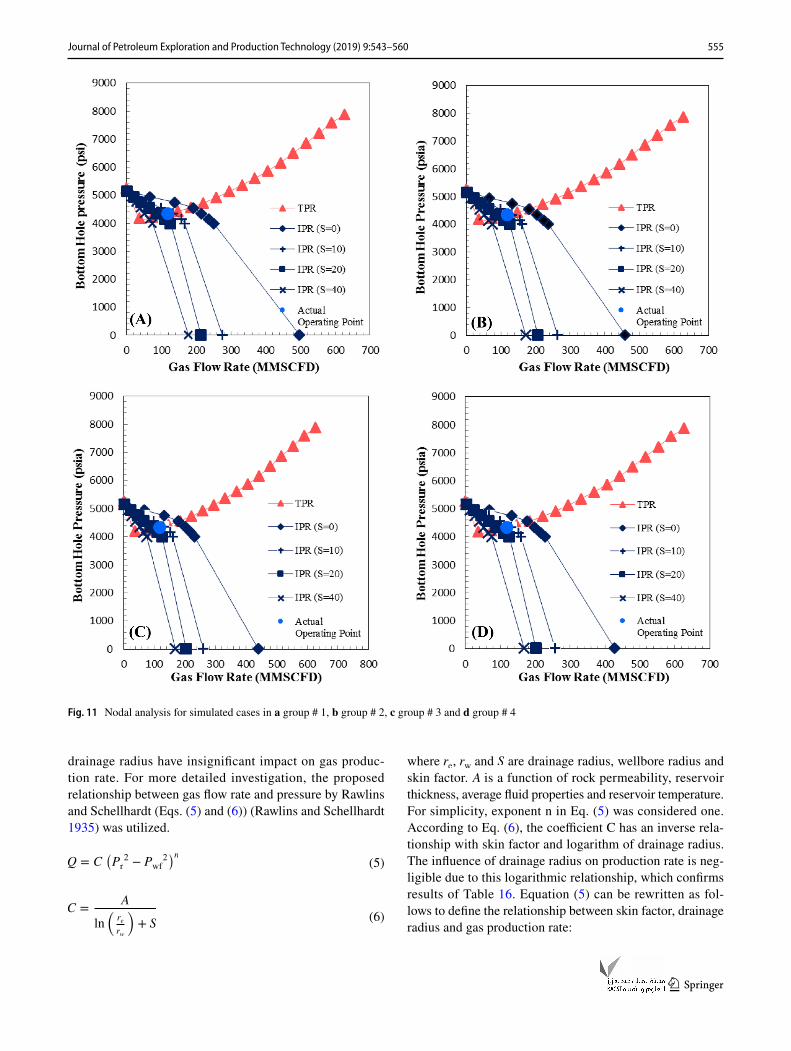
Actual operating conditions of target well are reported in Table 14. Figure 10 shows results of nodal analysis for the objective well and comparison of real and calculated operat-ing points. According to this figure, actual production rate has a remarkable difference with calculated production rate by nodal analysis. Rock properties, fluid properties, reservoir specifications, well geometry and well flowing pressure are principal factors affecting the IPR curve. TPR curve depends on wellhead pressure and physical conditions of the tubing (Beggs 1980). In this research, all these effectual factors were considered using real conditions of target well. How-ever, uncertainty exists in the values of drainage radius and skin factor of investigated reservoir. In the prior sections, the constructed reservoir model was run for drainage radius and skin factor of 3280 ft and 0, which are suspected to cause significant difference in well performance in real reservoir. Effects of these parameters on IPR curve and operating point were studied through sensitivity analysis. Variations of drainage radius and skin factor were divided into four groups (1, 2, 3 and 4) presented in Table 15. Skin factor is set to change in the range of 0–40. The drainage radius were 5000, 10,000, 15,000 and 20,000 ft for group 1, 2, 3 and 4, respectively. Totally, 16 different cases were run to perform the sensitivity analysis.

Since the IPR curve depends on reservoir and well con-ditions, distinct IPR curves were obtained for each of the

simulated cases in Table 15. Also, TPR curve appertains to wellhead pressure and physical conditions of the tubing and was unchanged in all cases. Gray’s model (Gray 1974) was suggested to model inclined wells (Azin et al. 2016), and was used in this section. Figure 11 shows results of nodal analysis for simulated cases according to Table 15. Well operating points in different simulated cases which were achieved from intersection of IPR and TPR curves, are reported in Table 16.

Results of Table 16 show that gas production rate is highly dependent on skin factor. However, variations in

Table 14 Actual operating conditions of the target well

Parameter Value

Q, MMSCFD 118Pwf, psi 4353Pwh, psi 3244Pr, psi 5280

Fig. 10 Comparison of actual and calculated operating points

Table 15 Categories for sensitivity analysis

Simulated case Skin factor Drainage radius, ft

Group # 1 1 0 5000 2 10 5000 3 20 5000 4 40 5000

Group # 2 5 0 10,000 6 10 10,000 7 20 10,000 8 40 10,000

Group # 3 9 0 15,000 10 10 15,000 11 20 15,000 12 40 15,000

Group # 4 13 0 20,000 14 10 20,000 15 20 20,000 16 40 20,000


1 3

drainage radius have insignificant impact on gas produc-tion rate. For more detailed investigation, the proposed relationship between gas flow rate and pressure by Rawlins and Schellhardt (Eqs. (5) and (6)) (Rawlins and Schellhardt 1935) was utilized.

(5)Q = C(Pr

2 − Pwf2)n

(6)C =

A

ln

(re

rw

)+ S

where re , rw and S are drainage radius, wellbore radius and skin factor. A is a function of rock permeability, reservoir thickness, average fluid properties and reservoir temperature. For simplicity, exponent n in Eq. (5) was considered one. According to Eq. (6), the coefficient C has an inverse rela-tionship with skin factor and logarithm of drainage radius. The influence of drainage radius on production rate is neg-ligible due to this logarithmic relationship, which confirms results of Table 16. Equation (5) can be rewritten as fol-lows to define the relationship between skin factor, drainage radius and gas production rate:

Fig. 11 Nodal analysis for simulated cases in a group # 1, b group # 2, c group # 3 and d group # 4


1 3

According to Eq. (7), a plot of (ln(re)+ S) vs.

(Pr

2−Pwf2

Q

)

yields a straight line with slope of A and y-intercept of B. Figure 12 shows this straight line for the reported data in Table 16. According to this figure, the relationship between

(7)ln(re)+ S = A

(Pr

2 − Pwf2

Q

)

+ B

skin factor, logarithm of drainage radius and operating point can be expressed by Eq. (8) for the objective well.

Using actual operating conditions reported for target well in Table 14, Eq. (8) simplifies to Eq. (9):

Considering different values for skin factor, correspond-ing drainage radius was calculated by Eq. (9) to determine operating point, and results are shown in Table 17 as group (A) According to these results, for skin factor less than 10, the corresponding drainage radius is very large and unrea-sonable. On the other hand, for skin factor above 15, cor-responding drainage radius will be very short. By assuming logical values for drainage radius, corresponding skin factor was computed using Eq. (9) and summarized in Table 17 as group (B) Results of this table show that for drainage radius range of 3000–20,000 ft, the skin factor is variable between 11 and 12.9, quite high for the investigated gas condensate well. So, the problem of low well production rate can be attributed to this high skin factor.

Based on Table 17 (group B), skin factor is 11.67 for drainage radius of 10,000 ft. In this case, if skin factor reduces to the values of 5 or 0, the gas production rate increases from 118 MMSCFD to 160 and 204 MMSCFD by considering the current value of bottom-hole pressure and average reservoir pressure in Eq. (8). In other words, the daily volume of gas production of this well would increase to 42–86 MMSCFD (maximum 73%). Hence, finding the rea-son for this high skin factor is essential as the first step before suggesting a suitable remedy for this problem. Accordingly, five different skin factors will be introduced and their exist-ence evaluated for the objective well. In the ideal conditions, a vertical well which is completed as open-hole, produces

(8)ln(re)+ S = 308.9946

(Pr

2 − Pwf2

Q

)

− 2.5503

(9)ln(re)+ S = 20.88

Table 16 Well operating points for different simulated cases

Simulated case Q, MMSCFD Pwf, psi

Group # 1 1 177 4604 2 122 4419 3 88.3 4340 4 55.7 4288

Group # 2 5 172 4588 6 121 4416 7 88.2 4339 8 56.1 4289

Group # 3 9 171 4582 10 120 4415 11 88.4 4340 12 56.5 4289

Group # 4 13 170 4579 14 120 4415 15 88.4 4340 16 56.7 4289

Fig. 12 (ln(re

)+ S) vs.

(Pr

2−Pwf

2

Q

) for the target well

Table 17 Estimated skin factor and drainage radius for target well

Skin factor Drainage radius, ft

Group A 0 1.18E09 5 7.93E06 10 53,446 12 7233 15 360

Group B 12.88 3000 12.36 5000 11.67 10,000 11.27 15,000 10.98 20,000


1 3

single-phase fluid from formation with no damage at a rate determined by Darcy’s law (Ahmed and McKinney 2011). There are five types of skin factor observed in real cases, including mechanical skin, completion pseudoskin, geomet-rical pseudoskin, multiphase pseudoskin, and rate-dependent skin frequently occur in hydrocarbon reservoirs (Ahmed and McKinney 2011; Ezenweichu and Laditan 2015; Jianchun et al. 2014).

Mechanical skin factor refers to permeability reduction due to formation damage through plugging the flow paths in porous formation with solid particles of drilling fluid or different process like well stimulation by acidizing (Ezen-weichu and Laditan 2015; Jianchun et al. 2014). For the objective well, no evidence is reported for formation dam-age. Completion pseudoskin addresses formation damage due to completion. Usually, the well completion as open-hole is the cheapest method and implies radial flow regime in the near wellbore area. Other completion techniques are employed to isolate produced fluid from different layers or prevent water and gas coning (Holditch 1992). Furthermore, a well may partially penetrate to the formation. Partial well penetration and well completion using other methods than open-hole cause flow regime become non-radial like spheri-cal or hemispherical flows (Ahmed and McKinney 2011). Extra pressure drop due to well completion and penetration is defined by the completion pseudoskin factor concept. As mentioned, the target well of this study was completed as open-hole and completion pseudoskin does not exist for this well.

Geometrical pseudoskin arises when the well perfor-mance is influenced by well geometry. Geometry of wells are divided into vertical, horizontal, inclined, etc (Ismail and El-Khatib 1996; Kumar and Bryant 2008). The verti-cal well which penetrates totally in production formation is known as base well. Any difference between base well productivity and wells with other geometry are referred as geometrical pseudoskin. In the constructed reservoir model, the well was considered as vertical well and production rates were corrected using Peaceman’s model (Peaceman 1983) for the inclined conditions. So, this type of skin factor cannot exist for the investigated well. Also, multiphase pseudoskin refers to skin caused by multiphase flow in the formation, especially near wellbore area, due to water and gas coning, gas production from liquid hydrocarbon or liquid production from gas condensate fluid. Multiphase flow is associated with higher drawdown pressure compared to single-phase. This extra drawdown pressure is known as multiphase pseu-doskin factor. In the gas condensate reservoir under study, the bottom-hole pressure is below the dew point. Therefore, multiphase flow occurs near wellbore and cause reduction of well deliverability. In the constructed reservoir model, fine grid blocks were used in the near wellbore region and vari-ations in gas saturation and decreasing relative permeability

of this phase were included in the model. Hence, this type of skin cannot be the reason for significant difference between calculated and actual gas production rate.

The last one is rate-dependent skin which occurs fre-quently in high-rate gas wells and indicates deviation from the Darcy’s law. The non-Darcy flow that occurs due to high velocity and turbulence of flow in about 5–10 ft around the wellbore causes the relationship between the flow rate and pressure to become non-linear (Huang and Ayoub 2008). Effect of non-Darcy flow is applied in numerical simulation of reservoirs by considering rate-dependent skin. Including this type of skin factor in the constructed reservoir model showed little or no impact on gas production rate, as shown in Fig. 13.

Among different sources of skin factor, the completion pseudoskin and rate-dependent skin are negligible accord-ing to the investigated reservoir and well conditions. Also, geometrical and multiphase pseudoskin were included in the constructed reservoir and well models. Therefore, mechani-cal skin or formation damage could be the only reason for the high skin factor in studied gas condensate well. Mini-mizing this skin factor is the key to achieve high yield of gas production, which needs more study for finding a suit-able remedy. Generally, as stated by Civan (Civan 2015), the development of technologies and strategies for cost-effective formation damage control and remediation is both a science and an art. Literature show that there are no universally proven technologies used as a remedy for all reservoirs. Nevertheless, creative approaches, supported by science and laboratory and field tests yield the best solution. Mechanical high-pressure hydraulic fracturing (Keelan and Koepf 1977; Wang et al. 2017), chemical low-pressure treatment (Bridges 2000), formation acidizing (Martin 2004) and acoustic well stimulation (Kolle and Theimer 2010) are examples of the more common treatment methods.

Fig. 13 Average reservoir pressure and gas production rate with and without rate-dependent skin


1 3

Conclusion

The objective of this study was to investigate the reasons for low production rate in a producing well of a supergiant gas condensate reservoir. An integrated strategy was pro-posed and employed for production optimization and trou-bleshooting the well problem. In this strategy, nodal analysis approach was used for investigation of well performance. IPR and TPR curves were plotted through reservoir and well simulation. Effects of simplifying reservoir rock and fluid model on IPR curves were assessed due to difficulties and the high amount of time consumed when extracting IPR curves from compositional simulation of 28-layer model. It was found that oversimplification of a multilayer reser-voir into a single layer leads to a non-realistic IPR model which may result in an operating point different from that observed in a gas well. Also, different pressure distributions caused a significant difference between the estimated well production rates from single-layer and 28-layer model. This difference increased by decreasing reservoir pressure. The 4-layer model had high accuracy compared to real reser-voir model and showed pressure distribution approximately similar to the 28-layer model. Five different tubing pressure drop models were examined using the rational elicited PSP data from reservoir model for selecting the optimal model. Among these correlations, the Gary’s model was found as the optimum pressure drop model for computing TPR curves. Nodal analysis accuracy in prediction of well operat-ing point was confirmed through its good agreement with the results gained from running base constructed reservoir and well models. Results of nodal analysis for real inclined well indicated that a striking difference exists between calculated and actual production rate. Sensitivity analysis conducted on two uncertain parameters including skin factor and drainage radius indicated that skin factor of investigated well is 11.67 for drainage radius of 10,000 ft. Therefore, the problem of low well production rate was attributed to this high skin factor as a result of formation damage skin near wellbore. Also, results indicated that maximum 73% increment in gas production of the well can be achieved by reduction of this skin factor.

Open Access This article is distributed under the terms of the Crea-tive Commons Attribution 4.0 International License (http://creat iveco mmons .org/licen ses/by/4.0/), which permits unrestricted use, distribu-tion, and reproduction in any medium, provided you give appropriate credit to the original author(s) and the source, provide a link to the Creative Commons license, and indicate if changes were made.

Appendix

Usually, in the numerical simulation of hydrocarbon res-ervoirs, the Peaceman’s model is applied to calculate well production rate (CMG 2012). According to this model, well production rate is calculated using Eq. (10) (Peaceman 1983):

where WI and Pwb are well index and well block pressure, respectively. This model is developed for vertical wells and needs be corrected for inclined wells. As seen in Fig. 14, the inclined well path can be portrayed on X, Y and Z directions of Cartesian coordinates. The well index can be computed in these three directions by utilizing length of the well image in each direction (Lx, Ly and Lz) and the proposed model by Peaceman for calculation of the equivalent radius (ro), as follows (Peaceman 1983):

(10)Q = WI(Pwb − Pwf)

(11)WIx =2�

√KyKz(Lx)

ln

�ro,x

rw

�+ S

(12)WIy =2�

√KxKz(Ly)

ln

�ro,y

rw

�+ S

(13)WIz =2�

√KxKy(Lz)

ln

�ro,z

rw

�+ S

Fig. 14 The inclined well path and its x-, y- and z-components

http://creativecommons.org/licenses/by/4.0/

http://creativecommons.org/licenses/by/4.0/


1 3

where k, S and rw are permeability, skin factor and wellbore radius, respectively. The total well index is calculated by Eq. (A-8):

Therefore, the well index is corrected using above equa-tions. By applying the modified well index according to Eq. (10), production rates for vertical well conditions are con-verted to inclined well.

References

Ahmed T, McKinney P (2011) Advanced reservoir engineering. Gulf Professional Publishing

Al-Attar HH, AL-Zuhair S A general approach for deliverability calcu-lations of gas wells. In: SPE North Africa Technical Conference & Exhibition, 2008. Society of Petroleum Engineers

Al-Shawaf A, Kelkar M, Sharifi M (2014) A new method to predict the performance of gas-condensate reservoirs. SPE Reservoir Eval Eng 17:177–189

Ansari A, Sylvester N, Shoham O, Brill J A comprehensive mechanistic model for upward two-phase flow in wellbores. In: SPE Annual Technical Conference and Exhibition, 1990. Society of Petroleum Engineers

Azin R, Chahshoori R, Osfouri S, Lak A, Sureshjani MH, Gerami S (2014) Integrated Analysis of choke performance and flow behaviour in high-rate, deviated gas-condensate wells. Gas Pro-cess J:8–18

Azin R, Osfouri S, Chahshoori R, Heidari SMH, Gerami S (2016) Evaluation of pressure drop empirical correlations in producing wells of a gas condensate. Field Pet Res 25:160–171. https ://doi.org/10.22078 /pr.2016.605

Aziz K, Govier GW (1972) Pressure drop in wells producing oil and gas J Can Pet Technol 11

(14)ro,x = 0.28

((Ky

Kz

)0.5

Δz2 +(

Kz

Ky

)0.5

Δy2)0.5

(Ky

Kz

)0.25

+(

Kz

Ky

)0.25

(15)ro,y = 0.28

((Kx

Kz

)0.5

Δz2 +(

Kz

Kx

)0.5

Δx2)0.5

(Kx

Kz

)0.25

+(

Kz

Kx

)0.25

(16)ro,z = 0.28

((Kx

Ky

)0.5

Δy2 +(

Ky

Kx

)0.5

Δx2)0.5

(Kx

Ky

)0.25

+(

Ky

Kx

)0.25

(17)WI =

√(WIx)

2 + (WIy)2 + (WIz)

2

Baxendell P, Thomas R (1961) The calculation of pressure gradients in high-rate flowing wells J Petrol Technol 13:1023–021,028

Beggs HD (1980) Production Optimization. Society of Petroleum Engineers

Beggs DH, Brill JP (1973) A study of two-phase flow in inclined pipes. J Pet Technol 25:607–617

Bohannon JM (1970) A linear programming model for optimum development of multi-reservoir pipeline systems J Petrol Technol 22:1429–421,436

Brar G, Aziz K (1978) Analysis of modified isochronal tests to predict the stabilized deliverability potential of gas wells without using stabilized flow data (includes associated papers 12933, 16320 and 16391. J Petrol Technol 30:297–304

Bridges KL (2000) Completion and workover fluids vol 19. Society of Petroleum Engineers

Chase R, Alkandari H Prediction of gas well deliverability from just a pressure buildup or drawdown test. SPE Eastern Regional Meet-ing, 1993. Society of Petroleum Engineers

Civan F (2015) Reservoir formation damage. Gulf Professional Publishing

CMG (2012) CMG software user manual,ver. 2012.10Dale BH (1991) Production Optimization Using NODAL Analysis. Oil

and Gas Consultants international publications, TulsaDmour H (2013) Optimization of well production system by NODAL

analysis technique petroleum. Sci Technol 31:1109–1122Eisa M, Kumar A, Zaouali Z, Chaabouni H, Al-Ghadhban H, Kadhim F

Integrated Workflow to evaluate and understand well performance in Multi layer Mature gas reservoirs, Bahrain Case Study. In: SPE Middle East Oil and Gas Show and Conference, 2013. Society of Petroleum Engineers

El-Banbi AH, Fattah KA, Sayyouh H (2006) New modified black-oil PVT correlations for Gas condensate and volatile oil fluids. In: SPE Annual Technical Conference and Exhibition. Society of Petroleum Engineers

Evinger H, Muskat M (1942) Calculation of theoretical productivity factor. Trans AIME 146:126–139

Ezenweichu CL, Laditan OD (2015) The causes, effects and mini-mization of formation damage in horizontal wells. Pet Coal 57:169–184

Fancher GH Jr, Brown KE (1963) Prediction of pressure gradients for multiphase flow in tubing. Soc Pet Eng J 3:59–69

Fetkovich M The isochronal testing of oil wells. Fall Meeting of the Society of Petroleum Engineers of AIME, 1973. Society of Petro-leum Engineers

Fevang Ø, Whitson C (1996) Modeling gas-condensate well deliver-ability. SPE Reservoir Eng 11:221–230

Gilbert W Flowing and gas-lift well performance. Drilling and produc-tion practice, 1954. American Petroleum Institute

Golan M, Whitson CH (1991) Well performance. Prentice HallGray H (1974) Vertical flow correlation in gas wells User manual

for API14B, subsurface controlled safety valve sizing computer program

Guyaguler B, Gumrah F (1999) Comparison of genetic algorithm with linear programming for the optimization of an underground gas-storage field. Situ 23:131–149

Hagedorn AR, Brown KE (1965) Experimental study of pressure gradients occurring during continuous two-phase flow in small-diameter vertical conduits. J Petrol Technol 17:475–484

Hasan AR, Kabir CS (1988) A study of multiphase flow behavior in vertical wells. SPE Prod Eng 3:263–272

Heidari Sureshjani MH et al (2016) Production data analysis in a gas-condensate field: methodology, challenges and uncertainties Ira-nian. J Chem Chem Eng (IJCCE) 35:113–127

Holditch SA (1992) Well completions: Part 9. Production Engineering Methods

https://doi.org/10.22078/pr.2016.605

https://doi.org/10.22078/pr.2016.605


1 3

Huang H, Ayoub JA (2008) Applicability of the Forchheimer equation for non-Darcy flow in porous media. Spe Journal 13:112–122

Ikoku CU (1992) Natural gas production engineering. Krieger Pub. Co.Ismail G, El-Khatib H (1996) Multi-lateral horizontal drilling prob-

lems & solutions experienced offshore Abu Dhabi. In: Abu Dhabi International Petroleum Exhibition and Conference. Society of Petroleum Engineers

Izadmehr M, Daryasafar A, Bakhshi P, Tavakoli R, Ghayyem MA (2017) Determining influence of different factors on production optimization by developing production scenarios. J Pet Explora-tion Prod Technol 1–16

Jamal H, SM FA, Rafiq M I (2006) Petroleum reservoir simulation: a basic approach. Gulf Publishing Company

Jianchun G, Cong L, Yong X, Jichuan R, Chaoyi S, Yu S (2014) Res-ervoir stimulation techniques to minimize skin factor of Long-wangmiao Fm gas reservoirs in the Sichuan Basin Natural. Gas Industry B 1:83–88

Jokhio SA, Tiab D (2002) Establishing Inflow Performance Relation-ship (IPR) for gas condensate wells. In: SPE Gas Technology Symposium. Society of Petroleum Engineers

Kabir CS, Hasan AR (2006) Simplified wellbore flow modeling in gas-condensate systems. SPE Prod Oper 21:89–97

Keelan D, Koepf E (1977) The role of cores and core analysis in evalu-ation of formation damage. J Petrol Technol 29:482–490

Kolle JJ, Theimer T (2010) Testing of a Fluid-Powered Turbo-Acoustic Source for Formation-Damage Remediation. In: SPE International Symposium and Exhibition on Formation Damage Control. Soci-ety of Petroleum Engineers

Kumar N, Bryant S (2008) Optimizing injection intervals in vertical and horizontal wells for CO2 sequestration. In: SPE Annual Tech-nical Conference and Exhibition. Society of Petroleum Engineers

Kumar V, Bang VSS, Pope GA, Sharma MM, Ayyalasomayajula PS, Kamath J (2006) Chemical stimulation of gas/condensate res-ervoirs. In: SPE Annual Technical Conference and Exhibition. Society of Petroleum Engineers

Lak A, Azin R, Osfouri S, Gerami S, Chahshoori R (2014) Choke modeling and flow splitting in a gas-condensate offshore platform. J Nat Gas Sci Eng 21:1163–1170

Lee A, Aronofsky J (1958) A linear programming model for scheduling crude oil production. J Petrol Technol 10:51–54

Martin A (2004) Stimulating sandstone formations with non-HF treat-ment systems. In: SPE Annual Technical Conference and Exhibi-tion. Society of Petroleum Engineers

Mishra S, Caudle B (1984) A simplified procedure for gas deliver-ability calculations using dimensionless IPR curves. In: SPE Annual Technical Conference and Exhibition. Society of Petro-leum Engineers

Mukherjee H, Brill JP (1985) Empirical equations to predict flow patterns in two-phase inclined flow. Int J Multiphase Flow 11:299–315

Najibi H, Rezaei R, Javanmardi J, Nasrifar K, Moshfeghian M (2009) Economic evaluation of natural gas transportation from Iran’s South-Pars gas field to market Applied Thermal Engineering 29

Nozohour-leilabady B, Fazelabdolabadi B (2016) On the application of artificial bee colony (ABC) algorithm for optimization of well placements in fractured reservoirs; efficiency comparison with the particle swarm optimization (PSO). Methodol Pet 2:79–89

O’Dell H (1967) Successfully cycling a low-permeability, high-yield gas condensate reservoir. J Petrol Technol 19:41–47

Onwunalu JE, Durlofsky L (2011) A new well-pattern-optimiza-tion procedure for large-scale field development. SPE Journal 16:594–607

Orkiszewski J (1967) Predicting two-phase pressure drops in vertical pipe. J Petrol Technol 19:829–838

Orodu O, Ako C, Makinde F, Owarume M (2012) Well deliverability predictions of gas flow in gas-condensate reservoirs, modelling near-critical wellbore problem of two phase flow in 1-dimension. Brazilian Journal of Petroleum and Gas 6

Osfouri S, Azin R (2016) an overview of challenges and errors in sampling and recombination of gas condensate fluids. J Oil Gas Petrochem Technol 3:1–13

Osfouri S, Azin R, Mohammadrezaei A (2015) A modified four-coef-ficient model for plus fraction characterization of a supergiant gas condensate reservoir. Gas Technol J 1:3–11

Peaceman DW (1983) Interpretation of well-block pressures in numeri-cal reservoir simulation with nonsquare grid blocks and aniso-tropic permeability. Soc Pet Eng J 23:531–543

Poettman FH, Carpenter PG (1952) The multiphase flow of gas, oil, and water through vertical flow strings with application to the design of gas-lift installations. Drilling and Production Practice. American Petroleum Institute

Rai R, Singh I, Srini-Vasan S (1989) Comparison of multiphase-flow correlations with measured field data of vertical and deviated oil wells in India (includes associated paper 20380). SPE Prod Eng 4:341–349

Rawlins EL, Schellhardt MA (1935) Back-pressure data on natural-gas wells and their application to production practices. Bureau of Mines, Bartlesville, Okla.(USA)

Sakhaei Z, Mohamadi-Baghmolaei M, Azin R, Osfouri S (2017) Study of production enhancement through wettability alteration in a super-giant gas-condensate reservoir. J Mol Liq 233:64–74

Schlumberger (2008) Pipesim software user manual, ver. 2008.1Shadizadeh S, Zoveidavianpoor M (2009) A Successful experience in

optimization of a production well in a southern iranian oil field Iranian J Chem Eng 6

Soleimani M (2017) Well performance optimization for gas lift opera-tion in a heterogeneous reservoir by fine zonation and different well type integration. J Nat Gas Sci Eng 40:277–287

Vogel J (1968) Inflow performance relationships for solution-gas drive wells. J Pet Technol 20:83–92

Wang F, Pan Z, Zhang S (2017) Modeling water leak-off behavior in hydraulically fractured gas shale under multi-mechanism domi-nated conditions. Transp Porous Media 118:177–200

Yeten B, Durlofsky LJ, Aziz K (2002) Optimization of nonconventional well type, location and trajectory. In: SPE annual technical confer-ence and exhibition. Society of Petroleum Engineers

Publisher’s Note Springer Nature remains neutral with regard tojurisdictional claims in published maps and institutional affiliations.

Production assessment of low production rate of well in a ...Journal of Petroleum Exploration and...

Documents

Transcript of Production assessment of low production rate of well in a ...Journal of Petroleum Exploration and...