1

©The McGraw-Hill Companies, Inc., 2006 McGraw-Hill/Irwin

Chapter 15

Demand Management

and Forecasting

2

Simple & Weighted Moving Average Forecasts

Exponential Smoothing

Simple Linear Regression

Multiple Regression

OBJECTIVES

3

Types of Forecasts

Qualitative (Judgmental)

Quantitative

Time Series Analysis

Causal Relationships

Simulation

4

Components of Demand

Average demand for a period of time

Trend

Seasonal element

Cyclical elements

Random variation

Autocorrelation

5

Finding Components of Demand

1 2 3 4

x

x x x

x x

x x x

x x x x x

x x x x x x x x

x x

x x x x

x x

x x

x

x x

x x

x x

x x

x x

x x

x

x

Year

Sale

s

Seasonal variation

Linear

Trend

6

Time Series Analysis

Time series forecasting models try to predict the

future based on past data

You can pick models based on:

1. Time horizon to forecast

2. Data availability

3. Accuracy required

4. Size of forecasting budget

5. Availability of qualified personnel

7

Simple Moving Average Formula

The simple moving average model assumes an average is a

good estimator of future behavior

The formula for the simple moving average is:

Ft = Forecast for the coming period

N = Number of periods to be averaged

A t-1 = Actual occurrence in the past period for up to “n” periods

n

A+...+A +A +A =F n-t3-t2-t1-t

t

8

Simple Moving Average Problem (1)

Week Demand 3 week 6 week

1 650

2 678

3 720

4 785

5 859

6 920

7 850

8 758

9 892

10 920

11 789

12 844

Question: What are the 3-week and 6-week moving average forecasts for demand?

Assume you only have 3 weeks and 6 weeks of actual demand data for the respective forecasts

n

A+...+A +A +A =F n-t3-t2-t1-t

t

9

500

550

600

650

700

750

800

850

900

950

1 2 3 4 5 6 7 8 9 10 11 12Week

Dem

an

d

Demand

3-Week

6-Week

Plotting the moving averages and comparing them shows how the

lines smooth out to reveal the overall upward trend in this example

Note how the 3-Week is smoother than the Demand, and 6-Week is even smoother

10

Simple Moving Average Problem (2) Data

Week Demand

1 820

2 775

3 680

4 655

5 620

6 600

7 575

Question: What is the 3 week moving

average forecast for this data?

Assume you only have 3 weeks and 5

weeks of actual demand data for the

respective forecasts

11

Simple Moving Average Problem (2) Solution

Week Demand 3-Week 5-Week

1 820

2 775

3 680

4 655

5 620

6 600

7 575

12

Weighted Moving Average Formula

While the moving average formula implies an equal weight being placed on

each value that is being averaged, the weighted moving average permits an

unequal weighting on prior time periods

wt = weight given to time period “t”

occurrence (weights must add to one)

The formula for the moving average is:

n-tn3-t32-t21-t1t Aw+...+Aw+A w+A w=F

1=wn

1=i

i

13

Weighted Moving Average Problem (1) Data

Weights:

t-3 .2

t-2 .3

t-1 .5

Week Demand

1 650

2 678

3 720

4

Question: Given the weekly demand and weights, what is the forecast for the

4th period or Week 4?

Note that the weights place more emphasis on the most recent data, that is time

period “t-1”

In Excel use the =SUMPRODUCT(…, …) function.

14

Weighted Moving Average Problem (1) Solution

Week Demand Forecast

1 650

2 678

3 720

4

15

Weighted Moving Average Problem (2) Data

Weights:

t-3 .1

t-2 .2

t-1 .7

Week Demand

1 820

2 775

3 680

4 655

Question: Given the weekly demand information and weights, what is the three

week weighted moving average forecast of the 5th period or week?

16

Excel Example of Weighted Moving Average

A B C D E

1 Week Demand Forecast Weights

2 1 820 0.1

3 2 775 0.2

4 3 680 0.7

5 4 655

6 5

17

Exponential Smoothing Model

Premise: The most recent observations might have the highest predictive value

Therefore, we should give more weight to the more recent time periods when forecasting

Ft = Ft-1 + a(At-1 - Ft-1)

constant smoothing Alpha

period epast t tim in the occurance ActualA

period past time 1in alueForecast vF

period t timecoming for the lueForcast vaF

:Where

1-t

1-t

t

a

18

Exponential Smoothing Model – Alternate form

11 )1( ttt FAF aa

Microsoft Excel uses the

dampening factor in the Data

Analysis Exponential Smoothing

routine

factor Dampening -1

constant smoothing Alpha

a

a

19

Exponential Smoothing Problem (1) Data

Week Demand

1 820

2 775

3 680

4 655

5 750

6 802

7 798

8 689

9 775

10

Question: Given the weekly demand

data, what are the exponential

smoothing forecasts for periods

2-10 using a=0.10 and a=0.60?

Assume F1=D1

20

Week Demand 0.1 0.6

1 820 820.00 820.00

2 775 820.00 820.00

3 680 815.50 793.00

4 655 801.95 725.20

5 750 787.26 683.08

6 802 783.53 723.23

7 798 785.38 770.49

8 689 786.64 787.00

9 775 776.88 728.20

10 776.69 756.28

Answer: The respective alphas columns denote the forecast values. Note

that you can only forecast one time period into the future.

21

Exponential Smoothing Problem (1) Plotting

500

550

600

650

700

750

800

850

1 2 3 4 5 6 7 8 9 10

Dem

and

Week

Demand

Note how that the smaller alpha results in a smoother line in this example

22

The MAD Statistic to Determine

Forecasting Error

The ideal MAD is zero which would mean there is no forecasting error

The larger the MAD, the less the accurate the resulting model

MAD 1.25 deviation standard 1

deviation standard 0.8 MAD 1

n

F-A

=MAD

n

1=t

tt

23

MAD Problem Data

Question: What is the MAD value given the forecast values in the table below?

Month Sales Forecast 1 220 n/a

2 250 255

3 210 205

4 300 320

5 325 315

24

MAD Problem Solution

Month Sales Forecast Abs Error

1 220 n/a

2 250 255 5

3 210 205 5

4 300 320 20

5 325 315 10

40

Note that by itself, the MAD only lets us know the mean error in a

set of forecasts

10=4

40=

n

F-A

=MAD

n

1=t

tt

25

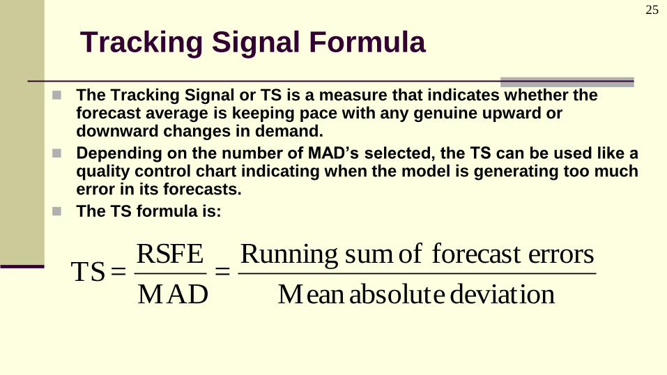
Tracking Signal Formula

The Tracking Signal or TS is a measure that indicates whether the forecast average is keeping pace with any genuine upward or downward changes in demand.

Depending on the number of MAD’s selected, the TS can be used like a quality control chart indicating when the model is generating too much error in its forecasts.

The TS formula is:

deviation absoluteMean

errorsforecast of sum Running=

MAD

RSFE=TS

26

Tracking Signal

Month Forecast Actual Deviation RSFE Abs. Dev. Sum of AD MAD TS

1 1000 950 -50 -50 50 50 50 -1

2 1000 1070 70 20 70 120 60 0.33

3 1000 1100 100 120 100 220 73.33 1.64

4 1000 960 -40 80 40 260 65 1.23

5 1000 1090 90 170 90 350 70 2.43

6 1000 1050 50 220 50 400 66.67 3.30

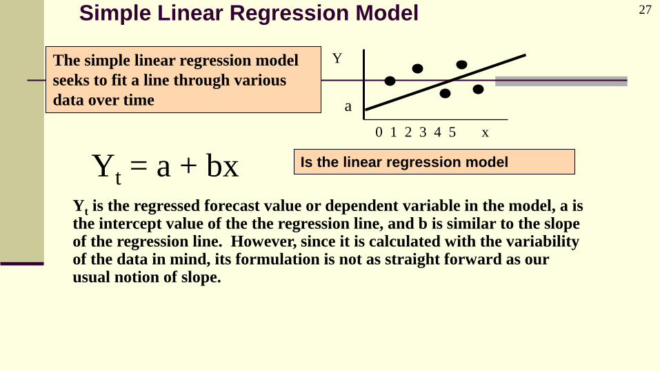
27 Simple Linear Regression Model

Yt = a + bx

0 1 2 3 4 5 x

Y The simple linear regression model

seeks to fit a line through various

data over time

Is the linear regression model

a

Yt is the regressed forecast value or dependent variable in the model, a is the intercept value of the the regression line, and b is similar to the slope of the regression line. However, since it is calculated with the variability of the data in mind, its formulation is not as straight forward as our usual notion of slope.

28

Multiple Regression:

Using time series data Forecasting based on many pieces of information that are

historically related.

Independent data (data used to forecast another set of data) is

generally lagged in time.

Examination of the “errors” reveals model structure

weaknesses.

Errors should be random and unpredictable.

29

Algebra 1 Review

Draw a line between two points

(x1,y1)

(x2,y2)

12 xxx

General line equation

bmxy where,

m is the slope

12

12

xx

yy

x

ym

12 yy

y

b is the intercept

(you need the slope and one point)

),( yx

xmyb

Intercept b

30

Simple Linear Regression

Draw a line among many points General line equation

ii xbby 10ˆ where,

b1 is the estimated slope

21)var(

),cov(

x

xy

s

s

x

yxb

b0 is the intercept

(you need the slope and one point)

xbyb 10

Intercept b

31

Simple Regression - example

The owner of Best of Beans Café believes that the

store sells more coffee in the morning hours when

the temperature is cold and fewer cups of coffee

when the temperature is warm.

Develop a regression to help forecast the sales any

day based on the morning temperature.

32

Cu

ps

of

Co

ffe

e o

ld

Temperature (F)

Example: Best of Beans Café

Date Temperature

7:00AM

Cups of Coffee Sold

(7-9AM)

1/1/2009 20 187

1/15/2009 -3 305

1/29/2009 14 276

2/12/2009 -2 296

2/26/2009 15 238

3/12/2009 34 159

3/26/2009 28 190

4/9/2009 40 150

4/23/2009 42 133

5/7/2009 50 127

33

SUMMARY OUTPUT

Regression Statistics

Multiple R 0.95105994

R Square 0.90451501

Adjusted R Square 0.89257939

Standard Error 21.9427493

Observations 10

ANOVA

df SS MS F Significance F

Regression 1 36488.23 36488.23 75.7828 2.36537E-05

Residual 8 3851.874 481.4842

Total 9 40340.1

Coefficients Standard

Error t Stat P-value Lower 95% Upper 95%

Intercept 300.670433 11.8265 25.42344 6.14E-09 273.3984671 327.9424

Temperature 7:00AM -3.5029594 0.402392 -8.70533 2.37E-05 -4.43087791 -2.57504

34

Simple Regression - example

How many cups of coffee would the owner of Best of Beans

Café estimate will be sold if the morning temperature is 32

degrees?

How many cups of coffee would the owner of Best of Beans

Café estimate will be sold if the morning temperature is -15

degrees?

35

Multiple Regression - example

You are working for General Motors in the light truck

division. Your responsibilities include forecasting the

number of units to produce in the next six months.

36 Interest Rates & Light Vechicles

0

2

4

6

8

10

12

141

98

4

19

86

19

88

19

90

19

92

19

94

19

96

19

98

20

00

20

02

20

04

20

06

Mill

ion

s o

f u

nit

s

0

2

4

6

8

10

12

14R

ea

ga

n

H.W

.Bu

s

Ira

q W

ar

Be

rlin

Clin

ton

G.W

.Bu

9/1

1/0

1T

alib

an

Ira

q W

ar

Pri

me

Ra

te

Autos and light truck assemblies(millions)

Average majority prime rate chargedby banks on short-term loans tobusiness, quoted on an investmentbasis (lagged 6 months)

37

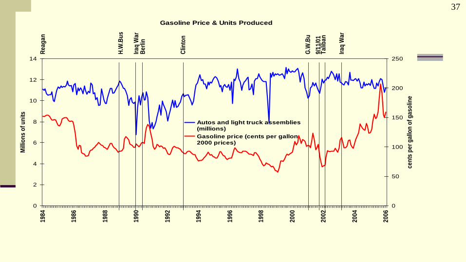
Gasoline Price & Units Produced

0

2

4

6

8

10

12

14

19

84

19

86

19

88

19

90

19

92

19

94

19

96

19

98

20

00

20

02

20

04

20

06

Mill

ion

s o

f u

nit

s

0

50

100

150

200

250

Re

ag

an

H.W

.Bu

s

Ira

q W

ar

Be

rlin

Clin

ton

G.W

.Bu

9/1

1/0

1T

alib

an

Ira

q W

ar

ce

nts

pe

r g

allo

n o

f g

as

olin

e

Autos and light truck assemblies(millions)

Gasoline price (cents per gallon 2000 prices)

38

34. War is good for business. ("Destiny")

35. Peace is good for business. ("Destiny")

Ferengi Rules of Acquisition

Download the “Forecasting Spreadsheet.xls”