Product Life Cycle, and Market Entry and Exit Decisions ...

Plea

se n

ote

that

this

is a

n au

thor

-pro

duce

d PD

F of

an

artic

le a

ccep

ted

for p

ublic

atio

n fo

llow

ing

peer

revi

ew. T

he p

ublis

her v

ersi

on is

ava

ilabl

e on

its

site

.

[This document contains the author’s accepted manuscript. For the publisher’s version, see the link in the header of this document.]

Product Life Cycle, and Market Entry and Exit Decisions Under Uncertainty

By Tailan Chi and John Liu The University of Kansas

Paper citation:

Chi, Tailan. (2001) Product Life Cycle, and Market Entry and Exit Decisions Under Uncertainty. IIE Transactions, 33 (9), 695-704.

Abstract: A key characteristic of the product life cycle (PLC) is the depletion of the product’s market potential due to technological obsolescence. Based on this concept, we develop a stochastic model for evaluating market entry and exit decisions during the PLC under uncertainty. The model explicates the conditions for the optimality of a two-threshold policy based on the estimated earnings potential of the product, and can be used by manufacturing firms to assess entry and exit decisions under such conditions. To aid the applications of the model in actual decision situations, we also provide the procedures for computing the exact and approximate values of the two thresholds.

Chi, Tailan. (2001) Product Life Cycle, and Market Entry and Exit Decisions Under Uncertainty. IIE Transactions, 33 (9), 695-704. Publisher's Official Version: http://dx.doi.org/10.1023/A:1010901813523/ Open Access Version: http://kuscholarworks.ku.edu/dspace/


Tailan Chi and John Liu*

School of Business Administration University of Wisconsin-Milwaukee

P. O. Box 742 Milwaukee, WI 53201-0742

USA

Accepted for publication in IIE Transactions, 33 (9), pp. 54-66, 2001.

* Address all correspondence to this author.



ABSTRACT

A key characteristic of the product life cycle (PLC) is the depletion of the product’s market

potential due to technological obsolescence. Based on this concept, we develop a stochastic

model for evaluating market entry and exit decisions during the PLC under uncertainty. The

model explicates the conditions for the optimality of a two-threshold policy based on the

estimated earnings potential of the product, and can be used by manufacturing firms to assess

entry and exit decisions under such conditions. To aid the applications of the model in actual

decision situations, we also provide the procedures for computing the exact and approximate

values of the two thresholds.

1. Introduction

Many technology-based products, such as consumer durables and office automation

apparatus, have been found to exhibit a pattern of evolution that resembles the life of a living

organism [1, 2, 3, 4]. The evolution process—commonly referred to as the product life cycle

(PLC)—begins with the introduction of a new product (birth) and ends with the exhaustion of the

product’s market potential (death) due to technological obsolescence [5]. In general, a product’s

birth coincides with the commercialization of a technology innovator’s R&D results, and its

death coincides with the termination of the product’s manufacture by the last remaining

technology follower/laggard in the industry. Hence, firms that operate in the same industry but

possess differing technological resources may enter and exit at different points in time during a

product’s life cycle. In addition, the innovating firm that has developed a new product sometimes

does not have the production and marketing resources to commercialize the product by itself and

may be compelled to sell or license its technology to a more established firm [6]. While the exit


decisions of the innovator and follower are similar, their entry decisions differ significantly.

Specifically, the innovator has the choice between commercializing the technology itself and

selling or licensing it to another firm, and the follower faces only the decision of whether to

acquire the technology for a price when it is available for purchase or license.

This study attempts to model the entry and exit decisions in the PLC from the perspective

of a technology follower that can gain access to, at a price, the technology requisite for the entry

into a given product market. The entry decision involves an evaluation of the potential earnings

from the product against the price for acquiring the requisite assets. The exit decision arises in

the later stages of the product’s life cycle (i.e., sometime after the entry) and involves an

evaluation of the remaining earnings potential against the salvage value of the existing assets.

The key variable in both of these decisions is, obviously, the potential earnings from the product

in the future. As has been demonstrated in numerous studies since the path-breaking work of

Bass [1], a fundamental characteristic of the PLC is that the product’s potential for future

earnings depletes as its life cycle progresses. Existing models of the PLC, whose focus tends to

be on marketing decisions such as advertising and pricing, have generally treated the depletion of

the product’s earnings potential during its life cycle as a deterministic process.1

Given one’s necessarily incomplete knowledge of the natural world, the future earnings

from a product can only be estimated imperfectly based on the current understanding of the

Given the extent

of uncertainty about a product’s future earnings, however, it is our position that analytical rigor

in modeling the entry and exit decisions during the PLC calls for a more realistic representation

of earnings depletion process through the use of a stochastic model.

1 For a review of various evolutionary functions that have been used in the literature to model a

product’s earnings or sales potential during the PLC, see Feichtinger, Hartl and Sethi [7].


factors affecting its market potential. These factors may include (but are not limited to) the state

and growth of the general economy, the availability of substitutes, and the pace of technological

change in the industry. Since these factors tend to evolve over time with a significant degree of

unpredictability, new information about them can be expected to arrive on a continuous basis

during a product’s life cycle. This possibility for continuously updating the estimation of the

product’s earnings potential can be accounted for through the use of a stochastic process (e.g.,

Brownian motion) to represent the evolvement of the estimation over time.

In this paper, we study the entry and exit decisions in the PLC by developing a stochastic

model that treats the earnings potential of the product as a Brownian motion with negative drift

to represent the earnings depletion process with random disturbances. This model is set up in

section 2. As will be discussed in section 3, the model presents a challenging boundary-value

problem represented in a system of second-order ordinary differential equations (ODEs), and a

closed-form solution of the ODE system is not attainable. The section identifies the appropriate

boundary conditions for obtaining a solution and also derives a power-series solution. Our result

suggests that the optimal control of the PLC is characterized by a two-threshold policy for the

entry and exit decisions. Specifically, the policy identifies both an entry threshold and an exit

threshold such that the expected payoff from the product is maximized by entering the product

market when its earnings potential is above the entry threshold and exit the product market when

the potential falls to the exit threshold. Section 4 explains the methods for computing the two

thresholds both under an exact solution and under an approximate solution and use numerical

results to show how the thresholds vary with the key parameters of the system. The last section

summarizes and concludes the paper.


2. Problem formulation

As explained in the introduction section, what we attempt to model in this paper is the

market entry and exit decisions of a firm whose primary competencies lie in manufacturing and

marketing. Suppose at time t = 0 the firm has an opportunity to acquire some technology that

will enable it to introduce a new product into the market. Acquisition of the technology may

involve the purchase or license of some patent rights from the current owner of the technology.

Let ),0( ∞∈x denote the current estimate of the future earnings from the product over its life

time. The cost of acquiring the technology and any investment required to effectuate production

and marketing of the product constitutes an initial entry cost C(x). It is reasonable to assume this

entry cost to have both a fixed component and a scale-dependent variable component that rises

with x. A simple function that contains both of these components is

C(x) = I + bx,

with b being a scale coefficient. The firm’s entry decision essentially involves an assessment of

whether the potential earnings from the product, x, justifies the initial entry cost, C(x).

Once an entry decision is fully implemented, the firm will have acquired an additional

bundle of assets in the form of technology, plant and equipment, and marketing expertise. If for

some reason it decides to exit the market later, those assets may still have some salvage value. It

is again reasonable to assume the salvage value of those assets to increase with x—the product’s

remaining earnings potential. Let the salvage value be an exponential function of x,

)()( 0xVxV γη −= ,


with V0 being a constant, γ ∈( , )0 1 and ]2,1[∈η . The value of V0 can be set in the vicinity of the

value of the initial investment in the introduction of the product.2 xγ As can be seen, the value of

equals 1 at x = 0 and falls toward 0 as x becomes very large. So, the lower bound of V(x) is 0 if

η = 1 and is V0 if η = 2. Obviously, a reasonable function for V(x) requires a coordinated choice

of the values for γ and η based on how specialized the assets are. If the assets can not be used for

any other purpose, they would lose all their value as x falls to 0, implying a value of η close to 1

and a relatively small γ. If the assets can be employed just as gainfully for another purpose, their

value would depreciate little as the value of x falls, implying a value of η close to 2 and a value

of γ close to 1. The sensitivity of V(x) to changes in x is given by γγ ln)( 0xVxV −=′ . It should be

noted that our problem is meaningful only if the new is worth more than the old, that is,

I bx V x+ ≥ −0 ( )η γ .

Once the firm starts to manufacture and market the product, it will inevitably receive new

information about the product’s earnings potential on a continuous basis as a result of its direct

involvement in the production and marketing activities. This type of learning can be modeled as

a continuously updated forecast of the product’s yield in the rest of its life. Let ),0[ ∞∈tX denote

the estimated remaining yield of the product as of time t > 0 after the firm’s entry is carried out.

2 One may wonder why we do not simply substitute C(x) for V0 since we consider the value of

the initial investment to be an appropriate value for V0. The reason is that there is likely a

considerable lag between the time of entry and the time of exit. Entry necessarily occurs before

exit, so the initial investment becomes a known constant after the entry decision is fully

implemented. In addition, as a result of the time lag, the value of x observed at entry time is

likely to be very different from the value of x observed at exit time.


We treat Xt as a stochastically evolving variable given the uncertainty about the evolution of the

technological and market conditions during the product’s life cycle. Specifically, we characterize

the evolution of Xt in the PLC using the following stochastic process:

tttt dWXdtXfdX )()( σρ+−= , (1)

where Wt is a Wiener process (i.e., a standard Brownian motion), σ is a constant representing the

maximum standard deviation of dXt, and ρ(Xt) is a scaling function defining the evolution of the

standard deviation in the PLC. As the extent of uncertainty about the remaining yield is likely to

diminish as Xt approaches zero, we require 1)(0 ≤≤ tXρ and 0)(lim0

→→ tX

Xt

ρ . As suggested by

Pindyck [8], a simple function that embodies these properties is

ρ λ( )X Xt t= ,

where λ is a constant that affects the sensitivity of the volatility to changes in Xt.

Since the evolution of the remaining yield is modeled as a stochastic depletion process,

the drift term in (1) has a negative sign. Within the drift term, the function f(Xt) represents the

estimated yield in each time increment, which by definition is expected to reduce the remaining

yield of the product by the same amount. We give f(Xt) the following functional form:

)(1)()(

t

tt X

XrXfξ+

= , (2)

where r(Xt) and ξ(Xt) are both increasing functions of Xt. As the total yield of the product in the

rest of its life is given by Xt, a higher yield level in each time increment, f(Xt), also means that the

remaining yield will be depleted at a faster pace. The specification of f(Xt) allows two opposing

forces to operate as the remaining yield gets depleted with the accumulation of realized earnings.

The component in the numerator, r(Xt), represents the force of technology diffusion because a

rise in this component accelerates the depletion process as a result of technological obsolescence.


The rest of the function, 1/[1+ξ(Xt)], represents the force of market diffusion because the gradual

fall in the value of Xt, which is expected to occur as sales accumulate with the product reaching

more consumers, has a positive effect on the yield of each successive period f(Xt) due to greater

consumer awareness [1]. For simplicity, we assume r(Xt) = αXt and ξ(Xt) = βXt, with α and β

being constants. Based on these assumptions, we can rewrite (2) and (1) as, respectively,

t

tt X

XXfβ

α+

=1

)( , (3)

dX XX

dt X dWtt

tt t= −

++

αβ

σ λ1

. (4)

It should be noted again that the function defined in (3) represents the instantaneous yield rate as

well as the depletion rate of the remaining yield. As time t does not enter explicitly in either the

drift term or the volatility term, the stochastic process defined in (4) is stationary.

As the evolution of the remaining yield Xt is defined as a stochastic depletion process, the

value of Xt will fall to zero at some ∞<t . Let τ denote the time at which Xt reaches zero, i.e.,

τ ≡ ≥ ≤inf{ | }t X t0 0 . The life of the product obviously comes a natural end at t = τ as its yield

potential is exhausted. But the optimal decision may entail the termination of the product before

its life ends naturally. Let θ denote the exit time at which the firm decides to discontinue the

product. Then, we have τ θ≤ if the earnings are naturally depleted and θ τ< if the product is

discontinued before its earnings are depleted. The actual life of a product, therefore, is either τ or

θ, whichever comes first (i.e.,θ τ∧ ).

Then, based on the stochastic process defined in (4) above, the expected payoff from the

product over its life cycle, conditioned on an initial state of x ∈ ∞[ , )0 , can be expressed as

)()(1

)(00

bxIeVdteX

XE Xt

t

tx +−

−+

+∧−∧ − ∧∫ τθµτθ µ τθγη

βα , (5)


where µ is an applicable discount rate. Within the expectation sign in (5), the first term gives the

discounted value of the earnings over the product’s life and the second term gives the discounted

salvage value of the assets at the time of termination; the term outside the expectation sign is the

initial entry cost at t = 0. After an entry decision is executed, the entry cost becomes a sunk cost,

and the problem that the firm faces is reduced to finding the optimal stopping time such that the

expected payoff in the product’s remaining life is maximized. This optimal stopping problem can

be stated as follows.

.)(1

max)( )(00

−+

+≡ ∧−∧ − ∧∫ τθµτθ µ

θτθγη

βαπ eVdte

XXEx Xt

t

tx (6)

Then, the firm’s optimal decision rule at the time of entry is just3

+≤

=otherwise.Enter

,)( ifenter not Do)(

bxIxxJ

π

3. Solution of the model

Based on the underlying stochastic process defined in (4), we can derive the following

second-order differential equation from the optimal stopping problem stated in (6) using Ito’s

lemma [9, 10]:

01

)()(1

)(21

2

22 =

++−

+−

xxx

dxxd

xx

dxxdx

βαµππ

βαπλσ . (7)

Finding a solution to this differential equation entails the identification of appropriate boundary

conditions. As the optimized payoff function defined in (6) is necessarily non-decreasing in x,

there must exist two threshold values of x, xz ˆˆ > , such that entry is warranted for all zx ˆ≥ and

3 Since the stochastic process defined in (4) is stationary, the value and shape of π(x) remains the

same whether x is observed at t = 0 or any other time.


exit is warranted for all xx ˆ≤ . These two thresholds provide two natural points of x that can be

used in our derivation of the needed boundary conditions. First, optimality of the entry and exit

decisions requires that the optimized payoff be equal to the value of the initial entry cost at the

entry threshold z and be equal to the salvage value at the exit threshold x . These requirements

give us the following two boundary conditions:

zbIz ˆ)ˆ( +=π , (8)

)()ˆ( ˆ0

xVx γηπ += . (9)

Two additional boundary conditions come from the optimality requirement of “smooth pasting”

that the marginal change in the optimized payoff be equal to the marginal entry cost at the entry

threshold and be equal to the marginal change in the salvage value at the exit threshold, that is,

bz =′ )ˆ(π , (10)

γγπ ln)ˆ( ˆ0

xVx −=′ . (11)

The five equations specified in (7) to (11) in theory give a unique solution of π(x) for the interval

]ˆ,ˆ[ zxx ∈ , as well as the two threshold values of x.

Although an analytical solution to the differential equation is not attainable, it is possible

to derive a series solution that will enable us to examine the asymptotic properties of the solution

and develop approximating algorithms. Because the derivation of the series solution is long and

involves mostly technical details, we will present only the result in the text and leave the detailed

mathematical operations in the appendix. As shown in the appendix, the following expression is

a series solution to the differential equation specified in (7):

∑∞

=

+′+⋅+++=0

1221221 )]0()1()ln([),;(~

n

nnnn xbwaxwwcwwwxπ , (12)


where an(1), )0(nb′ and cn are given by (A16), (A20) and (A25), respectively. The two

coefficients w1 and w2 need to be determined jointly with the two threshold values of x, z and x ,

using the same boundary conditions given in (8) to (11). To be complete, we rewrite the four

boundary conditions for the series solution ),;(~21 wwxπ as

zbIwwz ˆ),;ˆ(~21 +=π , (13)

)(),;ˆ(~ ˆ021

xVwwx γηπ += , (14)

bwwz =′ ),;ˆ(~21π , (15)

γγπ ln),;ˆ(~ ˆ021

xVwwx −=′ . (16)

As shown in the appendix, the power series given in (12) is convergent for )1,0(β

∈x , that is, it

constitutes a valid solution to the differential equation specified in (7) for )1,0(β

∈x .

In practice, one can compute the exact values of the two control thresholds by solving

numerically the ODE system specified in (7) to (11) or approximate their values using the series

solution given in (12) to (16). The ensuing section will discuss how to compute the threshold

values both under the exact solution and under the approximate solution and compare the results

obtained with these two solution methods.

4. Numerical analysis: Procedures and results

The first part of this section will explain the procedure for obtaining the exact solution

and then illustrate the solution with some numerical examples. The second part of the section

will present the algorithm for obtaining the approximate solution and examine its accuracy.


4.1 Exact solution

Although the system of ODEs specified in equations (7) to (11) are in principle solvable

numerically, the computation of a numerical solution is complicated by the fact that the interval

over which the solution must be evaluated, )ˆ,ˆ( zxx ∈ , is unknown and thus does not have fixed

endpoints. To overcome this difficulty, we need to convert the unknown interval to a known

interval with two fixed endpoints. The conversion can be performed as follows. First, create a

new independent variable ]1,0[∈u and define ),(0 xq π= ,)(1 dx

xdq π= zq ˆ2 = and xq ˆ3 = . Then,

we can express the remaining yield in the relevant interval )ˆ,ˆ( zx as

)( 232 qquqx −+= ,

and perform a change of variable to obtain

xzqqdudx ˆˆ23 −=−= ,

)()(231

0 qqqdudx

dxxd

dudq

−==π ,

)()()(232

2

2

21 qq

dxxd

dudx

dxxd

dudq

−==ππ .

Finally, using the redefined functions, we can set up the problem as a system of four first-order

differential equations and solve it for the interval ]1,0[∈u with four boundary conditions:

)( 2310 qqq

dudq

−= , (17)

223232

0

232

11 2)()()]([1

)1(λσ

µβ

α qqqquq

qqquq

qdudq

−

−++

−++−

= , (18)

02 =dudq , (19)


03 =dudq , (20)

20 )0( bqIq += , (21)

)()1( 300

qVq γη += , (22)

bq =)0(1 , (23)

γγ ln)1( 301

qVq −= . (24)

The problem defined in (17) to (24) can be easily implemented in such numerical solvers

as MathCad and Maple V. We used the fourth-order Runge-Kutta method provided in MathCad

Professional to solve the problem. The computation typically takes less than ten seconds on a PC

with a 400MHz Pentium II processor, but requires 1-3 minutes with a slower 90MHz Pentium

processor. Figure 1 shows an example of the solution to the differential equation (7).

-------------------------------- Insert Figure 1 about here --------------------------------

In Figure 1, the dotted line on the top represents the initial capital C(x) and the dashed

line on the bottom represents the salvage function V(x). The solid line in the middle represents

the optimized payoff π(x) for the interval )ˆ,ˆ( zxx ∈ , and the intersections of this line with the

other two lines indicate the values of the optimal entry and exit thresholds. It can be seen from

the figure that the optimized payoff function π(x) is strictly increasing in x for the interval ( , )x z ,

validating the optimality of a two-threshold policy. As explained earlier, this policy calls for

entry under zx ˆ≥ and exit under xx ˆ≤ .

-------------------------------- Insert Figure 2 about here --------------------------------


It is of particular interest to examine how the optimal entry and exit thresholds respond to

the extent of volatility in the potential yield. Note that in our model the parameter σ is the basic

index of volatility. Figure 2 shows graphically the sensitivity of the entry and exit thresholds to

the value of σ. As the figure indicates, a rise in volatility raises the entry threshold z and lowers

the exit threshold x , thus widening the distance between the two thresholds. The intuition behind

this result is that greater uncertainty justifies more caution in the entry and exit decisions that are

at least partially irreversible (e.g., due to sunk cost). It can also be seen that the entry threshold z

is significantly more sensitive to a change in σ than does the exit threshold x . The reason lies in

the fact that the volatility of the underlying stochastic process, as defined in (4), is determined by

the function xλσ and thus falls with the value of x. Since the value of x near the exit threshold

x is much smaller than its value near the entry threshold z , the impact of a change in σ on the

volatility of the process is much weaker near the exit threshold than near the entry threshold.

4.2. Approximate solution

In the rest of this section, we sketch an algorithm for computing the approximate solution

and assess its advantages and disadvantages as compared to the exact solution.

Given that the approximate solution is a convergent power series, the change in the value

of the solution will diminish as the approximation order (i.e., the order of the power series) is

increased. In order to achieve a proper balance between accuracy and computational demand, the

algorithm being proposed here is designed to raise the approximation order successively until the

fractional change in the results meets a prespecified convergence criterion. Let ω denote the

convergence criterion, L denote the starting order and M denote the highest order the algorithm

will go to. Then, the basic steps entailed in the algorithm can be outlined as follows.

1. Define the system.


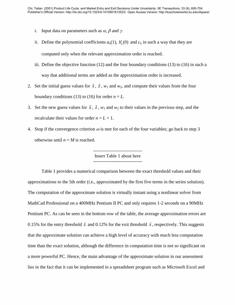
i. Input data on parameters such as α, β and γ.

ii. Define the polynomial coefficients an(1), )0(nb′ and cn in such a way that they are

computed only when the relevant approximation order is reached.

iii. Define the objective function (12) and the four boundary conditions (13) to (16) in such a

way that additional terms are added as the approximation order is increased.

2. Set the initial guess values for x , z , w1 and w2, and compute their values from the four

boundary conditions (13) to (16) for order n = L.

3. Set the new guess values for x , z , w1 and w2 to their values in the previous step, and the

recalculate their values for order n = L + 1.

4. Stop if the convergence criterion ω is met for each of the four variables; go back to step 3

otherwise until n = M is reached.

-------------------------------- Insert Table 1 about here

--------------------------------

Table 1 provides a numerical comparison between the exact threshold values and their

approximations to the 5th order (i.e., approximated by the first five terms in the series solution).

The computation of the approximate solution is virtually instant using a nonlinear solver from

MathCad Professional on a 400MHz Pentium II PC and only requires 1-2 seconds on a 90MHz

Pentium PC. As can be seen in the bottom row of the table, the average approximation errors are

0.15% for the entry threshold z and 0.12% for the exit threshold x , respectively. This suggests

that the approximate solution can achieve a high level of accuracy with much less computation

time than the exact solution, although the difference in computation time is not so significant on

a more powerful PC. Hence, the main advantage of the approximate solution in our assessment

lies in the fact that it can be implemented in a spreadsheet program such as Microsoft Excel and


does not require the use of a specialized mathematics package or any skills in solving differential

equations numerically. For those who have both experience in solving differential equations and

access to specialize mathematics packages such as MathCad Professional, the exact solution may

require a little less programming work.

5. Concluding remarks

The notion of product life cycle (PLC) was initially established and has received broad

attention in the marketing literature. Existing research so far has focused on such questions as

advertising and pricing and, in general, has been conducted under a deterministic framework.

The model developed in this paper adopts a more realistic stochastic framework to examine the

market entry and exit decisions during the PLC under uncertainty. Although the two-threshold

policy derived from our model looks remarkably simple, our work suggests that determination of

these thresholds in a given decision context poses many challenging tasks. Our model, and the

solution procedure and computation algorithm derived in this paper, can aid manufacturing firms

in making such decisions.

As pointed out in the introduction section, our model applies mainly to situations where

the entry involves only the acquisition of some manufacturing assets (such as technology and

equipment) via purchase or license, rather than the commercialization of one’s own R&D results.

Extension of the model to evaluate such technology switching decisions represents clearly an

interesting direction for future research.

Acknowledgements

We thank three anonymous referees for their constructive comments. All remaining

errors, however, are solely our own responsibility.


References

[1] Bass, F. M. (1969) A new product growth model for consumer durables. Management

Science, 15(5), 215-227.

[2] Harrell, S.G., and Taylor, E.D. (1981) Modeling the product life cycle for consumer

durables. Journal of Marketing, 45, 68-75.

[3] Tigert, D. and Farivar, B. (1981) The Bass new product growth model: A sensitivity

analysis for a high technology product. Journal of Marketing, 45, 81-90.

[4] Mesak, H.I. and Berg, W.D. (1995) Incorporating price and replacement purchases in new

product diffusion models for consumer durables. Decision Sciences, 26(4), 425-449.

[5] Klepper, S. (1996) Entry, exit, growth, and innovation over the product life cycle. The

American Economic Review, 86, 562-583.

[6] Teece, D.J. (1986) Profiting from technological innovation: Implications for integration,

collaboration, licensing and public policy. Research Policy, 15, 285-305.

[7] Feichtinger, G., Hartl, R.F. and Sethi, S. (1994) Dynamic optimal control models in

advertising: Recent developments. Management Science, 40(2), 195-226.

[8] Pindyck, R.S. (1993) Investments of uncertain cost. Journal of Financial Economics, 34,

53-76.

[9] Karlin, S. and Taylor, H.M. (1981) A Second Course in Stochastic Processes, Academic

Press, Inc., San Diego, CA.

[10] Dixit, A.K. and Pindyck, R.S. (1994) Investment under Uncertainty, Princeton University

Press, Princeton, N.J.

[11] Braun, M. (1983) Differential Equations and Their Applications, Third Edition, Springer-

Verlag, New York.


Appendix4

In this appendix, we derive a series solution to the differential equation specified in (7)

and determine the solution’s convergence region. The derivation follows standard methods that

are explained in most textbooks on the theory of ordinary differential equations (see Chapter 2 of

Braun [11], for instance).

Let K = 2/λσ2. Then, the differential equation derived in (7) can be represented as

0)1()1(

=+

+−′+

−′′xx

KxxK

xxKx

βαπµπ

βαπ . (A1)

It can be easily verified that all the coefficient functions in (A1) are rational functions and that

this ODE has regular singular points at x = 0 and x = –1/β. So long as the salvage value V(x) is

nontrivial, we only need attend to the case of x = 0. Given that (A1) has a regular singular point

at x = 0 and contains only rational functions in its coefficients, the existence theorem of an ODE

implies that this differential equation has at least one nontrivial power series solution around

x = 0 that converges in an interval x R< , with R > 0 being the convergence radius.

Rearranging the terms in the form of polynomials, (A1) becomes

( ) ( )1 1 0+ ′′ − ′ − + + =β π α π µ β π αx x Kx K x Kx . (A2)

Write the homogeneous part of (A2) as

L x x Kx K x( ) ( ) ( )π β π α π µ β π= + ′′ − ′ − + =1 1 0 . (A3)

Let the solutions of (A3) be in the form of

π ( )x a xnn s

n= +

=

∞

∑0

,

4 The appendix only presents the main steps of the derivation in order to save space. A more

detailed derivation is available from the corresponding author upon request.


with a0 0≠ . Its first-order and second-order derivatives are

′ = + + −

=

∞

∑π ( ) ( )x n s a xnn s

n

1

0, (A4)

′′ = + + − + −

=

∞

∑π ( ) ( )( )x n s n s a xnn s

n1 2

0. (A5)

Substitute (A4) and (A5) into (A3) and we get

.

)()1)(()1)((

)1()()1)(()1()(

0

1

0

000

1

00

1

0

2

∑∑

∑∑∑

∑∑∑

∞

=

++∞

=

+

∞

=

+∞

=

+∞

=

−+

∞

=

+∞

=

−+∞

=

−+

−−

+−−+++−++=

+−+−−+++=

n

snn

n

snn

n

snn

n

snn

n

snn

n

snn

n

snn

n

snn

xKaxKa

xasnKxasnsnxasnsn

xaxKxasnKxxasnsnxxL

µβµ

αβ

βµαβπ

Combining terms with the same power of x, we obtain

.}])())(1([)1)({(

}])1([)1({)1()(

111

011

0

sn

nnnn

ss

xKaaKsnKsnsnasnsn

xaKKsssassxssaL

+∞

=−+

−

∑ −−+−+−++++++

−−−+++−=

µβµαβ

µαβπ

Setting the coefficients of x to zero gives

( )s sa− =1 00 , (A6)

0])1([)1( 01 =−−−++ aKKsssass µαβ , (A7)

))(1(])1()1)(2([ 21

snsnKaaKsnKsnsna nn

n +−++−−+−−+−+−

= −− µβµαβ (A8)

for n ≥ 2. The solution of equation (A6) is either s = 0 or s = 1, with the two solutions differ by

an integer; hence, we can only use one of these two values in a solution to the differential

equation. Note that any arbitrary value of a0 satisfies (A6), whether s = 0 or s = 1. Suppose s = 1

and let an(1) denote the value of an for s = 1. Set a0(1) = 1 and we obtain

2)()1(1Ka µα +

= , (A9)


)1()1(

)1()1(

)1()1( 21 −− ++

+−−−

−= nnn ann

Kann

KKnnna µβµαβ (A10)

for n ≥ 2. To reduce clutter in the derivation that follows, let

nKKn

nKKnnnhn

µαβµαβ−−−=

−−−= )1()1( , (A11)

d = µβK, (A12)

A0 = 1, (A13)

A1 = (α + µ)K, (A14)

12 −− ⋅−⋅= nnnn AhAdA (A15)

for n ≥ 2. Then, (A9) and (A10) can be expressed as

)2()1(

+Γ=

nAa n

n , (A16)

where !)1( nn =+Γ . With a0(1) = 1 and an(1) given by (A16) for n ≥ 1, the series

π11

01( ) ( )x a xn

n

n= +

=

∞

∑ (A17)

is a general homogeneous solution of (A3).

Using s = 0, we can construct another linearly independent general solution of (A3) as

follows. First, we derive the other homogeneous solution for s = 0 following the same procedure.

Let bn(0) denote the value of an for s = 0 and set b0(s) = s. Substituting b0(0), b1(0) and bn(0) for

a0(1), a1(1) and an(1) in (A6), (A7) and (A8) gives us

b0(0) = 0,

b1(0) = µK,

b n n K n Kn n

b Kn n

bn n n( ) ( )( ) ( )( )

( )( )

( )0 2 1 11

01

01 2= −− − − − −

−+

−− −β α µ µβ


for n ≥ 2. Their first order derivatives with respect to s, ′ ==

b db sdsnn

s( ) ( )0

0, are

0)0(0 =′b , (A18)

Kb )()0(1 µαβ −+=′ , (A19)

( )

)0()1(

)0()1(

)12()0()1(

)1()1)(2(

)0()1(

)12()1()1)(2()1)(32()0(

22221

122

−−−

−

′−

+−

−−′

−−−−−−

−

−−−−−−−−−−−

−=′

nnn

nn

bnn

Kbnn

nKbnn

KnKnn

bnn

nKnKnnnnKnb

µβµβµαβ

µαβαβ

(A20)

for n ≥ 2. Using (A18), (A19) and (A20), we can write the other homogeneous solution with

s = 0 as

∑∞

=

′=0

)0()(n

nn xbxy . (A21)

Then, making use of both (A17) and (A21), we can construct another linearly independent

general solution of (A3) as

.)0()1(ln

)()(ln)(

00

1

12

∑∑∞

=

∞

=

+ ′+⋅=

+⋅=

n

nn

n

nn xbxax

xyxxx ππ (A22)

Finally, it can be verified that a particular non-homogeneous series solution of (A1) is

π ∗ +

=

∞

= ∑( )x c xnn

n

1

0

, (A23)

where c0 is a constant that needs to be selected,

01 2)(

2cKKc µαα +

+−= , (A24)

21 )1()1()1(

−− ++

+−−−

−= nnn cnn

Kcnn

KKnnnc µβµαβ (A25)


for n ≥ 2. To select a proper c0, we require the derivatives of the particular non-homogeneous

solution π ∗ ( )x to possess properties that are similar to those of the salvage value function V x( )

near x = 0. This requirement can be expressed as lim( )

x

d xdx→

∗

+≥

00

π and lim

( )x

d xdx→

∗

+<

0

2

2 0π

, and

translates to 0 0< ≤+

c αα µ

. A simple selection can be, for example, c0 =+α

α µ. Using the

particular non-homogeneous solution π ∗ ( )x and the two general homogeneous solutions π1(x)

and π2(x), we can express a general non-homogeneous solution of (A1) as

~( ; , ) ( ) ( ) ( )π π π πx w w x w x w x1 2 1 1 2 2= + +∗ , (A26)

where w1 and w2 are the integral constants to be determined by terminal conditions. Substituting

(A17), (A22) and (A23) into (A26), we can rewrite the general solution as

,)]0()1()ln([

)0()1()ln(

)]()([ln)()(),;(~

0

12212

02

0

121

0

1

121121

∑

∑∑∑∞

=

+

∞

=

∞

=

+∞

=

+

∗

′+⋅+++=

′+++=

+⋅++=

n

nnnn

n

nn

n

nn

n

nn

xbwaxwwcw

xbwxaxwwxc

xyxxwxwxwwx ππππ

(A27)

where an(1), )0(nb′ and cn are given by (A16), (A25) and (A20), respectively.

As per the theory of differential equations, the series solution ~( ; , )π x w w1 2 is applicable

only over its convergence region. In our case, the convergence region is an interval of x over

which ~( ; , )π x w w1 2 converges. In order to know whether the series solution gives a meaningful

approximation, we need to determine the convergence region. We will establish the convergence

region of the solution in two steps, using lemma 1 and lemma 2 derived below. Lemma 1 will

show that there are two possible convergence regions depending on whether the approximation


oscillates, and lemma will show that the approximation does oscillate for a sufficiently large n.

The convergence region of the solution, as will be demonstrated below, is )1,0(β

∈x .

Lemma 1. Suppose the asymptotic optimized payoff ),;(~21 wwxπ is given by (A27). Then,

≥∀<⋅>∃∈

≥∀≥⋅>∃∞∈

−

−

, 0 s.t. ,0 if )1,0(

, 0 s.t. ,0 if ),0(for converges ),;(~

1

1

21 NnAANx

NnAANxwwx

nn

nn

βπ

where An is given by (A15).

Proof. Obviously, the convergence radius R of ~( ; , )π x w w1 2 in (A27) is identical to that of π1(x)

in (A17), which can be determined from

Ra

aA n

A nA n

An

n

n n

n

n n

n

n= =

++

=+

→∞ + →∞ + →∞ +

lim lim( )( )

lim( )

1 1 1

32

2ΓΓ

. (A28)

Let 1

lim−

∞→=

n

nn A

Aψ . Dividing both sides of (A15) by An−1 yields an asymptotic equation

nhd−=

ψψ .

Solve this equation for ψ and we have

242

2,1dhh nn +±−

=ψ .

From (A11), we can see that limn nh

→∞= ∞ . If there exits an integer N ≥ 1 such that

AA

n

n−

≥1

0 for

all n ≥ N, then we have ψ ≥ 0, implying that 2)4( 21 dhh nn ++−=ψ should be used in (A28) to

determine the convergence region. If ψ ≥ 0 is the case, the limit specified in (A28) is

∞=+−

=++−

+=

+=

∞→∞→ ββψ2

2)4(211lim2lim

21 ndhh

nRnn

nn.


On the other hand, if NnAAn

n ≥∀<−

01

, then 02)4( 22 <+−−= dhh nnψ is the case, which

renders the limit of (A28) as

βββψ12

2)4(211lim2lim

22

=−−

=+−−

+=

+=

∞→∞→ ndhhnR

nnnn

.

This concludes the proof.

Lemma 2. The optimized payoff ~( ; , )π x w w1 2 converges for )1,0(β

∈x .

Proof. Based on Lemma 1, it is sufficient to show that limn n nA A

→∞ +⋅ <1 0 . By (A13) and (A14), we

have A0 0> and A1 0> . By (A15), we know

A dA h An n n n+ − += −1 1 1

for n ≥ 2. From (A11), we see that hn increases with n, leading to limn nh

→∞= ∞ . Then by induction,

there must exists an ∞<*n such that 0* >nh , 01* ≥−nA , 0* ≥nA and 01* <+nA . Furthermore, it

can be verified that AA

n

n+

<1

0 for all *nn ≥ , that is, limn

n

n

AA→∞

+

<1

0 . The proof of the Lemma 2 is

thus concluded.


Biographical Sketches

Tailan Chi is an Associate Professor at the School of Business Administration, University of Wisconsin-Milwaukee. He received his B.E. degree from the University of International Business and Economics, Beijing, China, his M.B.A. degree from University of San Francisco, and his M.A. degree in economics and Ph.D. degree in business administration from the University of Washington. His research interests are in the area of organization and decision economics. He has published in journals such as Management Science, Strategic Management Journal, Decision Sciences, and IEEE Transactions on Engineering management. He is a member of the Academy of International Business, Academy of Management, American Economic Association, INFORMS, and Strategic Management Society. John Liu is a Professor at the School of Business Administration, University of Wisconsin-Milwaukee. He received his M.S. degree in Engineering-Economic Systems from Stanford University and Ph.D. degree in Industrial Engineering from the Pennsylvania State University. His primary research interests are stochastic optimization models, and manufacturing and distribution systems. His current research focuses on technology acquisition and diffusion, and quality regulation in manufacturing and service. He has published in journals such as Operations Research, Management Science, the European Journal of Operational Research, and the Journal of Production and Operations Management. He is a member of INFORMS and IIE. Complete Addresses of Authors Tailan Chi School of Business Administration University of Wisconsin-Milwaukee P. O. Box 742 Milwaukee, WI 53201-0742 USA Tel: (414) 229-5429 Fax: (414) 229-6957 Email: [email protected] John Liu School of Business Administration University of Wisconsin-Milwaukee P. O. Box 742 Milwaukee, WI 53201-0742 USA Tel: (414) 229-3833 Fax: (414) 229-6957 Email: [email protected]


Table 1. Comparison of Approximations with Exact Solutions: Entry and Exit Thresholds

Exact Solution Approximation Approximation Error

σ Entry

ez Exit

Entry

Exit

e

ae

zzz

ˆˆˆ −

e

ae

xxx

ˆˆˆ −

0.1 3.000 1.705 3.000 1.704 0.0000 0.0006

0.2 3.092 1.682 3.090 1.679 0.0006 0.0018

0.3 3.212 1.653 3.200 1.656 0.0037 0.0018

0.4 3.372 1.633 3.372 1.630 0.0000 0.0018

0.5 3.560 1.629 3.572 1.629 0.0034 0.0000

Average 0.0015 0.0012

Values of Other Parameters: λ = 1, α = .2, β = .1, I = 1.4, b = .3, V0 = 2, η = 1.15, γ = .5, µ = .1.


Fig. 1. Sample trajectory of optimal payoff.

C(x), π(x), V(x)

x

Values of Parameters σ = .2, λ = 1, α = .2, β = .1,

I = 1.4, b = .3, V0 = 2, η = 1.15, γ = .5, µ = .1

Optimal Thresholds

68161ˆ =x 09223ˆ =z


Product Life Cycle, and Market Entry and Exit Decisions ...

Documents

Transcript of Product Life Cycle, and Market Entry and Exit Decisions ...