Product Differentiation and Brand Competition in the...

ISSN 2280-6180 (print) © Firenze University Press ISSN 2280-6172 (online) www.fupress.com/bae

Bio-based and Applied Economics 1(3): 297-312, 2012

Product Differentiation and Brand Competition in the Italian Breakfast Cereal Market: a Distance Metric Approach

Paolo Sckokai1, aleSSandro Varacca

Dipartimento di Economia Agroalimentare, Facoltà di Agraria, Università Cattolica del Sacro Cuore, Piacenza, Italy

Abstract. This article employs a nation-wide sample of supermarket scanner data to study product and brand competition in the Italian breakfast cereal market. A modi-fied Almost Ideal Demand System (AIDS), that includes Distance Metrics (DMs) as proposed by Pinkse, Slade and Brett (2002), is estimated to study demand responses, substitution patterns, own-price and cross-price elasticities. Estimation results provide evidence of some degree of brand loyalty, while consumers do not seem loyal to the product type. Elasticity estimates point out the presence of patterns of substitution within products sharing the same brand and similar nutritional characteristics.

Keywords. Distance metric, almost ideal demand system, breakfast cereals, differen-tiated products

JEL-codes. Q11, D12, L11.

1. Introduction

Although it’s not as developed as in the United States and in the rest of Europe, the market of breakfast cereals has been expanding over the last ten years also in Italy, show-ing an upward trend in market penetration, volume and value sales. In particular, in the years 2004-07 we observed a sharp increase in households’ expenditure in breakfast cere-als, even though this positive trend has flattened in late 2008-09, probably because of the ongoing economic crisis, and begun to fall late 2009-10.

The market for breakfast cereals is characterized by a relevant concentration: the con-centration ratio (CR4) is almost 80% and the first two players hold 75% of the market shares. Overall, in 2007 Kellogg’s accounted for a share of 49.9% in volume sales consider-ing the entire market, followed by Nestlé which accounted for 25%. Because of its pres-ence in the muesli business only, Cameo had a relatively low market share (4%) when considered within the overall market. The same applies also to Barilla: the Italian brand accounted for 1.4% of the entire market, since it is present only in the segments of simple and fortified cereals.

In terms of volume sales across different market segments, Kellogg’s was clearly domi-nating the market with a 45% share in muesli cereals, 46% in fortified cereals and 54% in

1 Corresponding author: [email protected].

298 P. Sckokai and A. Varacca

simple cereals. The following player was Nestlé, accounting for 38% of volume sales in for-tified cereals and 20% in simple cereals. Cameo was the second player in the muesli busi-ness after Kellogg’s, with a volume sales share of 32%, after being the segment-leader for years. Although it was the second player in the muesli business, Cameo did not play any significant role in other segments. After launching its new product line “Gran Cereale”, in 2006 Barilla had just re-engaged the competition in fortified and simple cereals after the withdrawal of “Mulino Bianco Armonie di Cereali”, thus its share was still below 2% in both businesses, but increasing over time.

Given this strong concentration and the strong reputation of the leading brands, manu-facturers wishing to set up new businesses in this market incur in high entry barriers when trying to build their (new) reputation and when trying to set up new brands; the result is that consumers can choose among a range of products supplied by a limited number of firms.

Although the Italian market is still lagging behind the European and American mar-kets in terms of per capita consumption, most operators argue that outlooks are encour-aging (even for new manufacturers) thanks to the likely evolution of demand in terms of new target consumers (mainly women and children). In fact, innovation plays a strategic role, since a relevant number of new products is systematically launched on the market every year by the two biggest players.

In this context of extreme concentration and relevant product innovation activity, we aim to study this market from two points of view: the role that brand loyalty plays on consumers’ choices as well as consumers’ behavior when faced with (new) different products. In line with the methodology proposed by Pinkse, Slade and Brett (2002) and applied by Bonanno (2013), our aim of investigating consumers’ attitude towards different breakfast cereals is carried out through a modified Almost Ideal Demand System (AIDS) that accounts for products’ qualitative attributes. Both continuous and discrete charac-teristics are employed to compute Distance Metrics, which are included in the model as interaction terms among cross-product prices.

The DM approach was developed to address the challenges of differentiated products in demand applications. It was first proposed by Pinkse, Slade and Brett (2002) which developed the DM technique to overcome the dimensionality limitation of neoclassical demand models. Recent examples of studies based on DM are Pinkse and Slade (2004), Rojas and Peterson (2008), Pofahl and Richards (2009) and Bonanno (2013).

The insight of this approach is that each product can be viewed as a unique combina-tion of characteristics and that substitution patterns among products might be the result of the proximity between these characteristics. In line with the Lancaster’s approach to demand theory (Lancaster, 1966), such characteristics can be thought as spatial attributes where different products can be positioned along, according to their own peculiarities; this means that any differentiated product can be considered as a combination of charac-teristics in a multidimensional space and substitution patterns are spatially determined. The products attributes can be both continuous and discrete.

In demand estimation, the DM method is applied by defining cross-price coefficients as functions of different distance measures between products. Besides accounting for spa-tial distance in products’ characteristics, this methodology also allows us to address one of the AIDS model weaknesses, namely the large number of cross-price coefficients to be estimated when the model accounts for a sizable number of products.

299Brand competition in breakfast cereals

2. The model

The demand for breakfast cereals in Italy is modeled following the Linear Approxi-mated–Almost Ideal Demand System developed by Deaton and Muellbauer (1980):

W b p X Plog log ( / )jrt jrtk

J

jkrt krt jrt rt rt jrt1∑α β ε= + + +=

. (1)

The subscript r denotes the regional markets we’re dealing with (r = 1,...R) while t denotes the time period (t = time = 1,...T). The system is made up of J equations, where j=1,…J is the number of products in each market r, and in each time period t; these equations are linked each other by the expenditure term Xrt and by the properties of the demand functions.

The total level of expenditure for the J products is Xrt, defined as j∑pjrt*qjrt . The

product j’s sales share (the share of expenditure allocated to product j) in market r, at time t is Wjrt, defined as p q X ( * ) /jrt jrt rt . Prt is a log-linear analogue of the Laspeyeres price index defined as

j∑log pjrt*Wjrt where W jrt are fixed budget shares, and it is employed to

normalize the total expenditure Xrt.In principle, J-1 equation and J(J-1)/2 cross price coefficients can be estimated by

imposing to the system the restrictions implied by the properties of the demand func-tions2. For large J, it might become impractical to estimate a large system of equations, and this is likely to be the case when analyzing brand-level data. The adoption of the Dis-tance Metrics approach will reduce the number of cross-price parameters bjkrt to be esti-mated through the definition of a new subset of metrics related to the cross price coef-ficients.

In this application of the Distance Metrics method (which will be referred to as DM-LA/AIDS), let Z j

c and Z jD be product j’s attributes, measured in continuous space (calo-

ries, fat content, etc…) and in discrete space (brand, flavour, etc…), respectively. Let jkcδ

and jkDδ be measures of closeness between products j and k, function of continuous and

discrete attributes, respectively.The continuous measure of closeness, namely the continuous Distance Metrics ( jk

cδ ), is defined adopting the inverse measure of the Euclidean distance in product space between j and k. The Euclidean distance indicates how distant two products are in the attribute space, given their characteristics: if two products were different, the magnitude of this indicator would get larger. Mathematically, this distance between j and k is the square root of the sum of the squared differences between continuous attributes Zl

c belonging to product j and k:

Z ZED .jkl

jlc

klc 2

∑( )= − (2)

2 The restrictions are the following: (1) Adding-up: a b 1; 0; 0j

J

jrtj

J

jkrtj

J

jrt1 1 1∑ ∑ ∑β= = == = =

; (2) Homogeneity of degree 0:

b 0k

J

jkrt1∑ ==

; (3) Symmetry: bjkrt = bkjrt; ∀ jk


The continuous DM ( jkcδ ) is then specified as the reciprocal of the Euclidean distance:

ED 11 2*jk

c

jk

δ =+ (3).

This measure varies between 0 and 1, and gets closer to 1 the more similar are the products in terms of characteristics, since the value of ED is closer to 0. This provides a continuously defined indicator of the proximity of two products within the defined attrib-ute space.3

Discrete DMs do measure the competitive effect of attributes that are not measura-ble through continuous characteristics. Mathematically, discrete DMs are represented by dummy variables whose value is 1 whenever product j and k share the same qualitative status or level for a discrete attribute D:

if z z

if z z

1 0

0 0jkD jl

DklD

jlD

klD

δ =− =

− ≠ (4)

For food products, examples of discrete attributes might be: brand, category, presence of a given characteristics (i.e. functional vs. nonfunctional,...)4

Given the closeness measures jkcδ and jk

Dδ , the cross-price parameter term of the LA/AIDS is reformulated as follows:

k=1

J

∑bjkrtlog pkrt = bjjrtlog pjrt + λ jk≠ j

J

∑δ jkc log pkrt +

d∑ϕ j

D

k≠ j

J

∑δ jkDlog pkrt . (5)

Replacing the cross price parameter (2) in the LA/AIDS equation (1) we obtain:

Wjrt =α jrt + bjjrtlog pjrt + λ jk≠ j

J


d∑ϕ j

D

k≠ j

J

∑δ jkDlog pkrt + β jrtlog (Xrt / Prt )+ ε jt , (6)

which gives bj1 = λ jδ j1c +

d∑ϕ j

Dδ j1D ,…, bjm = λ jδ jm

c +d∑ϕ j

Dδ jmD

, where ϕ jDand λ j are param-

3 The use of bilateral indexes in a multilateral context (more than two different products) can bring to some problems related to the intransitivity of such indexes (Rao et al., 2002). In principle, with N products, N(N-1)/2 bilateral indexes can be obtained. However, the index obtained comparing two products’ characteristics may be different from the indirect index obtained by comparing the same two products with a third product that is part of the analysed set. This problem was addressed by Hill (1997) and Diewert (2005) through the proposal of sev-eral multilateral formulas. Further research may refine the model introducing such formulas in the DMs calcula-tions.4 For example, taking D1 = brand, a value of jk

D1δ = 0 implies that the two products are made by different manu-facturers.


eters to be estimated. Since (Zjl – Zkl)2 = (Zkl – Zjl)2 then jkcδ = kj

cδ and symmetry can be imposed to the λj parameters across equations (i.e., for each product j). Furthermore, symmetry can also be imposed for ϕ Ds because there is no difference between jk

Dδ and 1kj

Dδ = (if D=brand and 1jkDδ = , then also 1kj

Dδ = ). Therefore this implies that bjk = bkj across the J equations.

Given symmetry, in principle J-1 equations can be estimated with only two cross price parameters. To further reduce the dimensionality of the estimation one may assume own-price and expenditure coefficients to be constant across equations, thereby reducing the estimation to a single equation. Because of the restrictiveness of this assumption, in this work we assume that these coefficients, together with the intercept, are functions of sub-sets of product characteristics and market parameters:

z jrtm

m jm0 ∑α α α= + α (7)

b b zjjrts

s jsb

0 ∑γ= +

zjrth

h jh0 ∑β β β= + β

The choice of these shifters is arbitrary and results may not be invariant to their choice. However, when using DMs, such choice can be justified based on the available data and on the objectives of the study (Rojas and Peterson, 2008; Pofahl and Richards, 2009; Bonanno, 2013). For example, in this study, the discrete shifters of the cross-price and expenditure parameters (z z ,j

bjβ ) are those that allow to identify a specific product cat-

egory, for which we wish to estimate a demand elasticity, while the shifters of the inter-cept (z j

a) are those identifying market specificities of each product (i.e. regional/seasonal demand features).

Thus, the final specification of the LA/AIDS model becomes5:

Wjrt =α0 +m∑αmz jm

α + log pjrt γ 0 +s∑γ sz js

b⎛⎝⎜

⎞⎠⎟

+ λk≠ j

J


d∑ϕ D

k≠ j

J

∑δ jkDlog pkrt + β0 +

h∑βhz jh

β⎛⎝⎜

⎞⎠⎟

log Xrt / Prt( )+ ε jrt (8)

Wjrt =α0 +m∑αmz jm

α + log pjrt γ 0 +s∑γ sz js

b⎛⎝⎜

⎞⎠⎟

+ λk≠ j

J


d∑ϕ D

k≠ j

J

∑δ jkDlog pkrt + β0 +

h∑βhz jh

β⎛⎝⎜

⎞⎠⎟

log Xrt / Prt( )+ ε jrt

3. Data

The database employed for estimating the model has been obtained from a Sympho-nyIRI census® scanner dataset including forty-eight monthly observations of breakfast

5 One problem arising from the inclusion of distance metrics into the model has to do with the imposition of the standard demand theory restrictions: with the new interaction terms in equation (8), the standard parametric restrictions of homogeneity and adding up cannot be imposed in a straightforward way. Further research may refine the model in order to solve this problem.


cereals sales for the period January 2004 – December 2007. Sales are recorded in Hyper- and Supermarkets located in seventeen Italian IRI regions covering most of the national territory. Each of the forty-eight monthly observations reports product-specific data for: volume sales; value sales; unit sales; percentage of store selling (indicating the share of stores where at least one unit of a particular product was sold); weighted distribution (indicating the share of annual sales represented by the stores where at least one unit of a particular product was sold); average number of items per store (the average number of barcodes available for that product in the stores selling the product; namely, it is a meas-ure of the depth of the product’s distribution); volume of sales under any type of price promotion; value of sales under any type of price promotion; units sold under any type of price promotion.

The products chosen for this analysis belong to firms operating nationally with a value of expenditure share in the national market of at least 0.5%. Since the database accounted for some small producers typically bound to regional markets, data were reduced by filtering for these producers, in order to obtain a nationally representa-tive market of Italy with 8,160 observation: 10 product combination identified by ven-dor (Barilla, Cameo, Kellogg’s, Nestle and Private Label) and segment (Muesli, Fortified and Simple) observed across 48 months (from January 2004 to December 2007) and 17 regions (Liguria, Lombardia, Trentino Alto Adige, Friuli Venezia Giulia, Veneto, Emilia Romagna, Toscana, Lazio, Umbria, Sardegna, Marche, Puglia, Campania, Sicilia, Valle d’Aosta+Piemonte, Abruzzo+Molise, Basilicata+Calabria)6. These 8,160 observations built up the database from which the share values Wjrt were calculated.

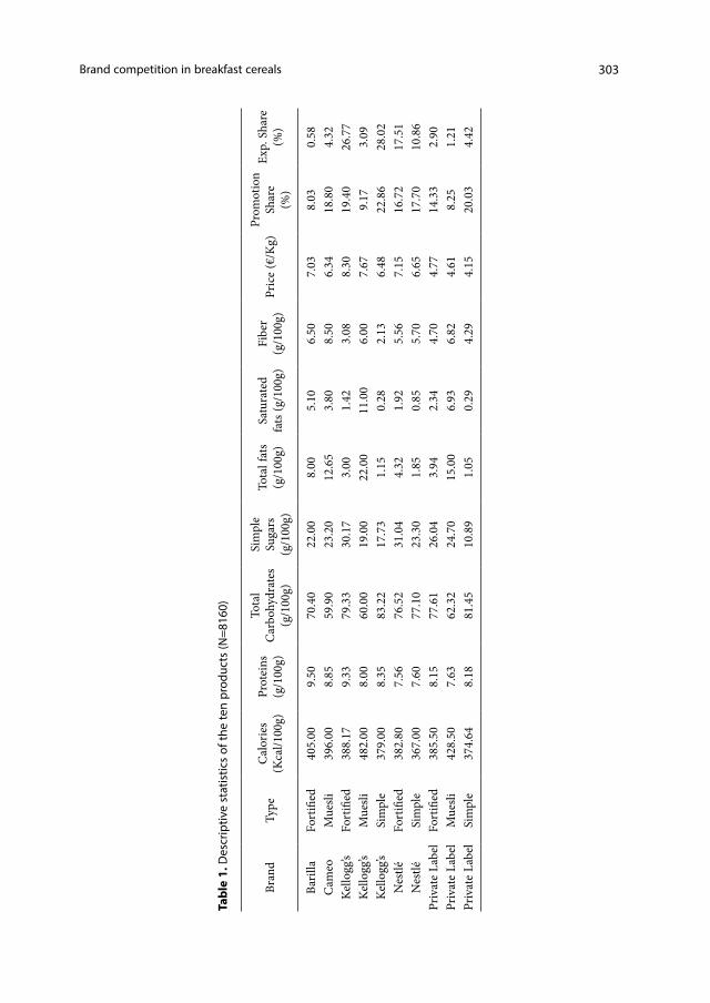
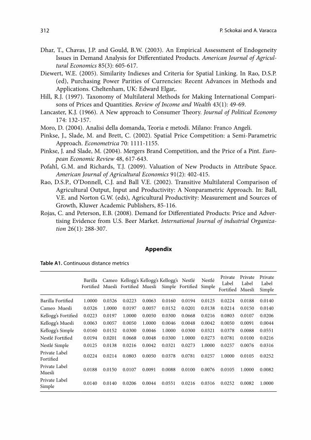
Euclidean Distances and continuous DMs were computed from hand collected information on: calories (Kcal/100g); proteins (g/100g); carbohydrates, total and sim-ple (g/100g); fats, total and saturated (g/100g); fiber (g/100g); calcium (mg/100g); sodi-um (g/100g); iron (mg/100g) (the matrix of continuous Distance Metrics is reported in Appendix 1). Such measures were included in the database together with the dummy vari-ables representing discrete DMs. Finally, prices for each of the ten products were com-puted dividing Value Sales by the corresponding Volume Sales.

Table 1 presents descriptive statistics of the data for the 10 products included in our analysis; products’ characteristics are included together with average prices, expenditure shares and the promotion share in value terms per item. Muesli products are the fat-test and most caloric ones while private labels are the cheapest products on the market. Despite their high price, Kellogg’s fortified products are the ones showing the second larg-est expenditure share after Kellogg’s simple, that are also the most merchandised ones. Overall Kellogg’s holds more than 50% of the market in breakfast cereals, followed by Nestlé and Private Labels.

4. Model specification

In estimating the LA/AIDS model we need to account for the issue of endogeneity, since the model may not account for factors affecting consumer’s behaviour (Wjt) which

6 IRI regions are defined consistently with the administrative borders of the Italian regions except for “Piemonte and Val d’Aosta”, “Basilicata and Calabria” and “Abruzzo and Molise”.


Tabl

e 1.

Des

crip

tive

stat

istic

s of

the

ten

prod

ucts

(N=8

160)

Bran

dTy

peC

alor

ies

(Kca

l/100

g)Pr

otei

ns

(g/1

00g)

Tota

l C

arbo

hydr

ates

(g

/100

g)

Sim

ple

Suga

rs

(g/1

00g)

Tota

l fat

s (g

/100

g)Sa

tura

ted

fats

(g/1

00g)

Fibe

r (g

/100

g)Pr

ice

(€/K

g)Pr

omot

ion

Shar

e(%

)

Exp.

Sha

re

(%)

Baril

laFo

rtifi

ed40

5.00

9.50

70.4

022

.00

8.00

5.10

6.50

7.03

8.03

0.58

Cam

eoM

uesli

396.

008.

8559

.90

23.2

012

.65

3.80

8.50

6.34

18.8

04.

32Ke

llogg

’sFo

rtifi

ed38

8.17

9.33

79.3

330

.17

3.00

1.42

3.08

8.30

19.4

026

.77

Kello

gg’s

Mue

sli48

2.00

8.00

60.0

019

.00

22.0

011

.00

6.00

7.67

9.17

3.09

Kello

gg’s

Sim

ple

379.

008.

3583

.22

17.7

31.

150.

282.

136.

4822

.86

28.0

2N

estlé

Fort

ified

382.

807.

5676

.52

31.0

44.

321.

925.

567.

1516

.72

17.5

1N

estlé

Sim

ple

367.

007.

6077

.10

23.3

01.

850.

855.

706.

6517

.70

10.8

6Pr

ivat

e La

bel

Fort

ified

385.

508.

1577

.61

26.0

43.

942.

344.

704.

7714

.33

2.90

Priv

ate

Labe

lM

uesli

428.

507.

6362

.32

24.7

015

.00

6.93

6.82

4.61

8.25

1.21

Priv

ate

Labe

lSi

mpl

e37

4.64

8.18

81.4

510

.89

1.05

0.29

4.29

4.15

20.0

34.

42


are related to suppliers/retailers’ price setting choices. Considering that we are actually dealing with differentiated products, retail prices may not be considered fully exogenous. In fact, in an oligopolistic market, prices are likely to be determined by strategic pricing rules of firms, incorporating both supply and demand characteristics of those products. Whenever these pricing rules involve some unobserved demand characteristics, assum-ing prices as exogenous would lead to biased and inconsistent parameter estimates. The same problem arises with the expenditure variable. Instruments are therefore employed to deal with the endogeneity of prices and expenditure. Instrumental variable estimates were obtained following Dhar, Chavas and Gould (2003): ten first-stage regressions for price were specified as:

P US MRCH PRD ITPS irt i i irt i irt i irt i irt0 1 2 3 4θ θ θ θ θ= + + + + (9)

i j k j J, ,∑= + ≠ …

while the expenditure first stage regression was specified as:

X TTR D INC INC , rt rtr

R

rt rt rt1

1 22∑η φ φ= + + +

=

(10)

where:USirt = Unit Sales; adopting this variable means accounting for package-related cost varia-tions if we assume that large package sized products are likely to sell a smaller number of units with respect to small package sized products;

MRCHirt = Merchandised units sold/Unit Sales; this variable measures the amount of product sold through any merchandising and ought to capture the cost of selling a brand.

PRDirt = Price Reduction =

100 * Price merchandised product – Price not_merchandised productPrice not_merchandised product

;

the price-reduction variable is thought to capture costs associated with this kind of mer-chandising (note that this price reduction must be communicated to consumers for this variable to be relevant);

ITPSirt = Average Number Of Items Per Store selling; for a given product in a particular geographical area, this measure is the average number of barcodes available for that prod-uct per store selling that product. This variable is able to capture the depth of the prod-uct’s presence on the shelves and is adopted as an indicator of market power.

TTRt = linear time trend, capturing any time-specific unobservable effect of consumers’ expenditure;


Drt = regional dummy variables able to capture variation in expenditure across regions;

INCrt= yearly household expenditures on all consumer goods differentiated by region, as a proxy of household income.

Fitted values for prices and expenditure obtained by estimating (9) and (10) were used to replace the corresponding actual values in model (8).With regard to model (8), we have to choose appropriate shifters for the intercept, own-price and expenditure coef-ficients. We adopt brand and type discrete shifters both for the own-price parameter ( z js

b ) and the expenditure parameter ( z jh

β ), in order to derive proper elasticity measures. In fact z jsb and z jh

β identify different products through 2 sets of dummy variables: the former identifies the brand (namely: Barilla, Cameo, Nestlé, Kellogg’s and Private Label), the lat-ter identifies the type (namely: Fortified, Muesli and Simple). The own-price parameters are also shifted by one physical product’s characteristics: average calories Kcal( ). This par-ticular products’ characteristic was adopted because of its property to describe syntheti-cally multiple nutritional features of the products we study (sugar content, fats and fiber); this should avoid the risk of multicollinearity. Thus the price and expenditure shifters in (8) are defined as:

z Brand Type Kcals

s jsb

nn jn

b

pp jp

bl∑ ∑ ∑γ γ γ γ= + + (11)

z Brand Typeh

h jhn

n jnp

p jp∑ ∑ ∑β β β= +β β β

(12)

The intercept term is shifted by two sets of discrete variables z jma , one set of monthly

dummies accounting for seasonal patterns of consumption and one set of regional dum-mies accounting for regional differences in food consumption habits. Thus:

z Region Month m

m jmg

g jgm

m jm∑ ∑ ∑α α α= +α α α

Model (8) then becomes:

Wjrt =α0 +g∑α gRegionjg

α +m∑αmMonthjm

α + log p̂ jrt (γ 0 +n∑γ nBrand jn

b +p∑γ pTypejp

b + γ l Kcal)+ λk≠ j

J

∑δ jkc log p̂krt +

d∑ϕ D

k≠ j

J

∑δ jkDlog p̂krt + (β0 +

n∑βnBrand jn

β +p∑β pTypejp

β ) log ( X̂ rt / Prt )+ ε jrt

Wjrt =α0 +g∑α gRegionjg

α +m∑αmMonthjm

α + log p̂ jrt (γ 0 +n∑γ nBrand jn

b +p∑γ pTypejp

b + γ l Kcal)+ λk≠ j

J

∑δ jkc log p̂krt +

d∑ϕ D

k≠ j

J

∑δ jkDlog p̂krt + (β0 +

n∑βnBrand jn

β +p∑β pTypejp

β ) log ( X̂ rt / Prt )+ ε jrt

In this model, d∑ϕ D

can be considered as indicators of loyalty. In fact, assuming D = Brand, ϕ Br would be a measure of the cross-price effect of j with respect to other products


sharing the same brand (if j and k share the same brand, 1jkBrδ = and log p

k j

J

jkBr

krt∑δ≠

will

account only for those products k whose 1jkBrδ = ). In fact, if ϕ Br > 0 consumers are likely

to respond to an increase in price of the products sharing the same brand by switching to an alternative item produced by the same manufacturer; thus, consumers are brand loyal. On the other hand, if ϕ Br < 0 , consumers are likely to respond to an increase in price of the products sharing the same brand by switching to an alternative manufacturer; thus, consumers are not brand loyal.

Since jkcδ represents a measure of how distant two products j and k are in the attrib-

ute space, two products with similar characteristics will show a higher value for jkcδ as

compared to couples showing different attribute sets. Thus, any term log p* jkc

krtδ will influence more the demand response if j and k are close to each other. This means that

log p ˆk j

J

jkc

krt∑δ≠

can be interpreted as a weighted average of cross-prices, where their weights

jkcδ are their distance from j. In this context the continuous closeness measure, λ, is a

measure of the impact of all products similar to j on its expenditure share: for λ > 0 con-sumers tend to respond to any increase in similar products’ prices by switching to items with similar nutritional profiles, while for λ < 0 consumers tend to respond by switching to items with different nutritional profiles.

5. Estimation and empirical results

Parameter estimates of the first-stage regressions for prices and expenditure are omit-ted for brevity7. Estimation of model (13) was carried out through least squares estimation in TSP 5.0. Results showed that most parameters associated with the monthly dummies were not statistically significant; for this reason, a second restricted model was estimated excluding such dummies. The fit of the two models was then compared through a Likeli-hood ratio test which showed that the null hypothesis of all monthly dummy parameters being equal to zero could not be rejected8. Thus, we have chosen the restricted model as final specification of our demand system.

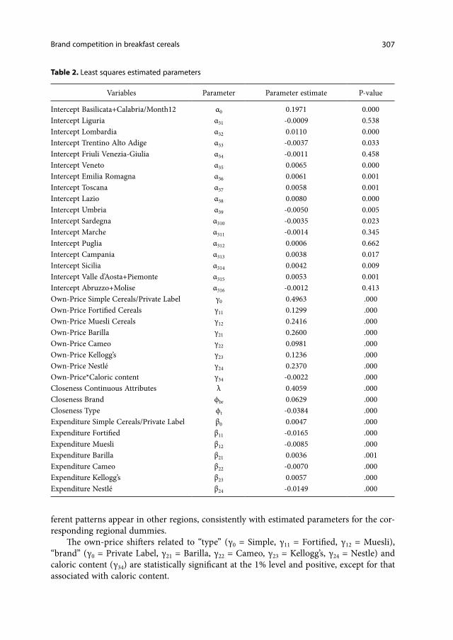
Parameter estimates of the restricted model are reported in table 2. In terms of explanatory power, the model shows a very good R-squared (0.95), which is a remarkable result for a model of this type.

5.1 Estimated coefficients

The regional shifters of the intercept highlight differences in regional food habits: α0 identifies Basilicata+Calabria (Region 17) which does not statistically differ from Liguria (α31), Friuli Venezia-Giulia (α34), Marche (α311), Puglia (α312), Abruzzo+Molise (α316). Dif-

7 Such results are available from the authors upon request.8 The chi-square of the Likelihood ratio test was 11.013 with 11 degrees of freedom, with a corresponding P-val-ue of 0.442.


ferent patterns appear in other regions, consistently with estimated parameters for the cor-responding regional dummies.

The own-price shifters related to “type” (γ0 = Simple, γ11 = Fortified, γ12 = Muesli), “brand” (γ0 = Private Label, γ21 = Barilla, γ22 = Cameo, γ23 = Kellogg’s, γ24 = Nestle) and caloric content (γ34) are statistically significant at the 1% level and positive, except for that associated with caloric content.

Table 2. Least squares estimated parameters

Variables Parameter Parameter estimate P-value

Intercept Basilicata+Calabria/Month12 α0 0.1971 0.000Intercept Liguria α31 -0.0009 0.538Intercept Lombardia α32 0.0110 0.000Intercept Trentino Alto Adige α33 -0.0037 0.033Intercept Friuli Venezia-Giulia α34 -0.0011 0.458Intercept Veneto α35 0.0065 0.000Intercept Emilia Romagna α36 0.0061 0.001Intercept Toscana α37 0.0058 0.001Intercept Lazio α38 0.0080 0.000Intercept Umbria α39 -0.0050 0.005Intercept Sardegna α310 -0.0035 0.023Intercept Marche α311 -0.0014 0.345Intercept Puglia α312 0.0006 0.662Intercept Campania α313 0.0038 0.017Intercept Sicilia α314 0.0042 0.009Intercept Valle d’Aosta+Piemonte α315 0.0053 0.001Intercept Abruzzo+Molise α316 -0.0012 0.413Own-Price Simple Cereals/Private Label γ0 0.4963 .000Own-Price Fortified Cereals γ11 0.1299 .000Own-Price Muesli Cereals γ12 0.2416 .000Own-Price Barilla γ21 0.2600 .000Own-Price Cameo γ22 0.0981 .000Own-Price Kellogg’s γ23 0.1236 .000Own-Price Nestlé γ24 0.2370 .000Own-Price*Caloric content γ34 -0.0022 .000Closeness Continuous Attributes λ 0.4059 .000Closeness Brand ϕbr 0.0629 .000Closeness Type ϕt -0.0384 .000Expenditure Simple Cereals/Private Label β0 0.0047 .000Expenditure Fortified β11 -0.0165 .000Expenditure Muesli β12 -0.0085 .000Expenditure Barilla β21 0.0036 .001Expenditure Cameo β22 -0.0070 .000Expenditure Kellogg’s β23 0.0057 .000Expenditure Nestlé β24 -0.0149 .000


Any positive sign of the own-price coefficient would reduce the negative impact of the own-price on the corresponding quantity, making the demand function more inelastic and consumers less price sensitive9. Therefore, given the significance and the positive sign of all γs in our estimation, the consumers’ price sensitiveness for brands like Barilla, Cameo, Kel-logg’s and Nestlé and for types like muesli and fortified is lower than for the reference cat-egory (Private Labels for simple cereals). Nevertheless this effect is mitigated by the caloric content of the product, which increases the price sensitivity due to its negative sign.

The positive sign of ϕ Br (.0647) suggests that any increase in price for a products k sharing the same brand with j induces a switch in consumption to products of the same manufacturer. The market is therefore characterized by a certain level of brand loyalty. On the contrary, the negative sign of ϕT (-.037504) implies that consumers are likely to switch to other types of cereals as a response to a price increase.

The last set of parameters to be discussed are expenditure shifters, both related to “brand” (β21 = Barilla, β22 = Cameo, β23 = Kellogg’s, β24 = Nestle) and to “Type” (β11 = Fortified, β12 = Muesli). In particular, negative and significant coefficients for the inter-action between expenditure and “type” discrete attributes indicate that an increase in the total purchases of breakfast cereals leads to a smaller share of Fortified and Muesli cereals. Differently, an increase in expenditure for breakfast cereals leads to a larger share for sim-ple cereals. The same intuition applies also for “brand” discrete shifter: results show that an increase in expenditure for cereals leads to larger (smaller) shares allocated to Barilla, Kellogg and Private Label (Cameo and Nestle).

5.2 Own-price and cross-price elasticities

Estimated Marshallian own-price and cross-price elasticities are obtained using the restricted model’s estimated parameters and applying the following formulas:

∑ ∑∑ ∑

∑∑ ∑

η

γ γ γ γβ β β

λδ δβ β β

=

+ + +− + + − =

+− + + ≠

β β

β β

z z z

wz z if j k

wz z

ww

if j k

1

jk

n n jnb

p p jpb

l jlb

jrt nn jn

pp jp

jkc

d

DjkD

jrt nn jn

pp jp

krt

jrt

0

o

0

(14)

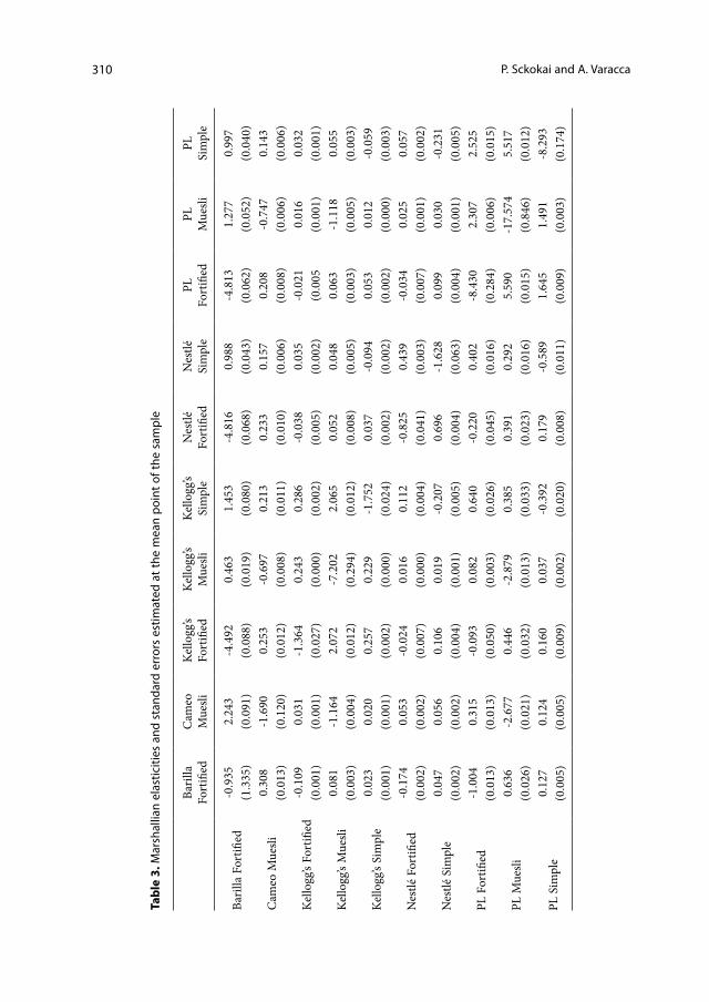
where wjrt ( wkrt ) is the average of product j’s (k’s) expenditure share. Own-price and cross-price elasticities, together with their standard errors, are reported in table 3. All elas-

9 This is consistent with the structure of the Slutsky term for estimating price responses in the AIDS model (Moro, 2004):

sX

pz W W z lnX lnP jj

rt

jrts

s jsb

jrt jrth

h jh rt rt2 0

2

0

2

∑ ∑γ γ β β( )

( ) ( )= + + − + + −β if j=k

sjk =Xrtp jrt pkrt

λ +d∑ϕ D⎛

⎝⎜⎞⎠⎟+WjrtWkrt + β0 +

h∑βhz jh

β⎛⎝⎜

⎞⎠⎟

β0 +h∑βhz jh

β⎛⎝⎜

⎞⎠⎟lnXrt − lnPrt( )⎡

⎣⎢⎢

⎤

⎦⎥⎥ if j≠K


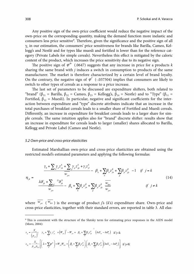
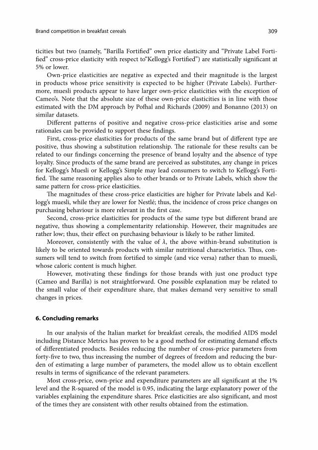
ticities but two (namely, “Barilla Fortified” own price elasticity and “Private Label Forti-fied” cross-price elasticity with respect to“Kellogg’s Fortified”) are statistically significant at 5% or lower.

Own-price elasticities are negative as expected and their magnitude is the largest in products whose price sensitivity is expected to be higher (Private Labels). Further-more, muesli products appear to have larger own-price elasticities with the exception of Cameo’s. Note that the absolute size of these own-price elasticities is in line with those estimated with the DM approach by Pofhal and Richards (2009) and Bonanno (2013) on similar datasets.

Different patterns of positive and negative cross-price elasticities arise and some rationales can be provided to support these findings.

First, cross-price elasticities for products of the same brand but of different type are positive, thus showing a substitution relationship. The rationale for these results can be related to our findings concerning the presence of brand loyalty and the absence of type loyalty. Since products of the same brand are perceived as substitutes, any change in prices for Kellogg’s Muesli or Kellogg’s Simple may lead consumers to switch to Kellogg’s Forti-fied. The same reasoning applies also to other brands or to Private Labels, which show the same pattern for cross-price elasticities.

The magnitudes of these cross-price elasticities are higher for Private labels and Kel-logg’s muesli, while they are lower for Nestlé; thus, the incidence of cross price changes on purchasing behaviour is more relevant in the first case.

Second, cross-price elasticities for products of the same type but different brand are negative, thus showing a complementarity relationship. However, their magnitudes are rather low; thus, their effect on purchasing behaviour is likely to be rather limited.

Moreover, consistently with the value of λ, the above within-brand substitution is likely to be oriented towards products with similar nutritional characteristics. Thus, con-sumers will tend to switch from fortified to simple (and vice versa) rather than to muesli, whose caloric content is much higher.

However, motivating these findings for those brands with just one product type (Cameo and Barilla) is not straightforward. One possible explanation may be related to the small value of their expenditure share, that makes demand very sensitive to small changes in prices.

6. Concluding remarks

In our analysis of the Italian market for breakfast cereals, the modified AIDS model including Distance Metrics has proven to be a good method for estimating demand effects of differentiated products. Besides reducing the number of cross-price parameters from forty-five to two, thus increasing the number of degrees of freedom and reducing the bur-den of estimating a large number of parameters, the model allow us to obtain excellent results in terms of significance of the relevant parameters.

Most cross-price, own-price and expenditure parameters are all significant at the 1% level and the R-squared of the model is 0.95, indicating the large explanatory power of the variables explaining the expenditure shares. Price elasticities are also significant, and most of the times they are consistent with other results obtained from the estimation.


Tabl

e 3.

Mar

shal

lian

elas

ticiti

es a

nd s

tand

ard

erro

rs e

stim

ated

at t

he m

ean

poin

t of t

he s

ampl

e

Baril

la

Fort

ified

Cam

eo

Mue

sliKe

llogg

’s Fo

rtifi

edKe

llogg

’s M

uesli

Kello

gg’s

Sim

ple

Nes

tlé

Fort

ified

Nes

tlé

Sim

ple

PL

Fort

ified

PL

Mue

sliPL

Si

mpl

e

Baril

la F

ortifi

ed-0

.935

2.24

3-4

.492

0.46

31.

453

-4.8

160.

988

-4.8

131.

277

0.99

7(1

.335

)(0

.091

)(0

.088

)(0

.019

)(0

.080

)(0

.068

)(0

.043

)(0

.062

)(0

.052

)(0

.040

)

Cam

eo M

uesli

0.30

8-1

.690

0.25

3-0

.697

0.21

30.

233

0.15

70.

208

-0.7

470.

143

(0.0

13)

(0.1

20)

(0.0

12)

(0.0

08)

(0.0

11)

(0.0

10)

(0.0

06)

(0.0

08)

(0.0

06)

(0.0

06)

Kello

gg’s

Fort

ified

-0.1

090.

031

-1.3

640.

243

0.28

6-0

.038

0.03

5-0

.021

0.01

60.

032

(0.0

01)

(0.0

01)

(0.0

27)

(0.0

00)

(0.0

02)

(0.0

05)

(0.0

02)

(0.0

05(0

.001

)(0

.001

)

Kello

gg’s

Mue

sli0.

081

-1.1

642.

072

-7.2

022.

065

0.05

20.

048

0.06

3-1

.118

0.05

5(0

.003

)(0

.004

)(0

.012

)(0

.294

)(0

.012

)(0

.008

)(0

.005

)(0

.003

)(0

.005

)(0

.003

)

Kello

gg’s

Sim

ple

0.02

30.

020

0.25

70.

229

-1.7

520.

037

-0.0

940.

053

0.01

2-0

.059

(0.0

01)

(0.0

01)

(0.0

02)

(0.0

00)

(0.0

24)

(0.0

02)

(0.0

02)

(0.0

02)

(0.0

00)

(0.0

03)

Nes

tlé F

ortifi

ed-0

.174

0.05

3-0

.024

0.01

60.

112

-0.8

250.

439

-0.0

340.

025

0.05

7(0

.002

)(0

.002

)(0

.007

)(0

.000

)(0

.004

)(0

.041

)(0

.003

)(0

.007

)(0

.001

)(0

.002

)

Nes

tlé S

impl

e0.

047

0.05

60.

106

0.01

9-0

.207

0.69

6-1

.628

0.09

90.

030

-0.2

31(0

.002

)(0

.002

)(0

.004

)(0

.001

)(0

.005

)(0

.004

)(0

.063

)(0

.004

)(0

.001

)(0

.005

)

PL F

ortifi

ed-1

.004

0.31

5-0

.093

0.08

20.

640

-0.2

200.

402

-8.4

302.

307

2.52

5(0

.013

)(0

.013

)(0

.050

)(0

.003

)(0

.026

)(0

.045

)(0

.016

)(0

.284

)(0

.006

)(0

.015

)

PL M

uesli

0.63

6-2

.677

0.44

6-2

.879

0.38

50.

391

0.29

25.

590

-17.

574

5.51

7(0

.026

)(0

.021

)(0

.032

)(0

.013

)(0

.033

)(0

.023

)(0

.016

)(0

.015

)(0

.846

)(0

.012

)

PL S

impl

e0.

127

0.12

40.

160

0.03

7-0

.392

0.17

9-0

.589

1.64

51.

491

-8.2

93(0

.005

)(0

.005

)(0

.009

)(0

.002

)(0

.020

)(0

.008

)(0

.011

)(0

.009

)(0

.003

)(0

.174

)


Our findings indicate that, globally, consumers tend to be brand loyal but not type loyal, so that they respond to price changes by switching to products of the same brand, but with similar nutritional profiles. Furthermore, Private Labels are confirmed to be the most price-sensitive products, while the products supplied by the biggest players on the market are the less-price sensitive ones. Although being the produce with the smaller market share, Barilla Grancereale shows the lowest own-price elasticity, which probably indicates that it is perceived as a niche product.

Despite the relatively large range of products available in the market, resulting from innovation proposed by market leaders, the strong concentration of the market makes very difficult for consumers to take any advantage from the competition among National Brands (NB). This intuition is supported by our findings, since the price sensitiveness of NB cereals products is rather low. In this context, Private labels represent an alternative and offer an increasing range of cheaper products; on the other hand, their reliance on low prices makes Private labels demand extremely price sensitive.

Besides the strong implications these findings have on the demand side, the supply side deserves to be taken into account as well. As we previously mentioned, the biggest players on the market (namely Kellogg’s and Nestlé) show an important product innova-tion rate: new products are yearly launched on the market, and some of them disappear rather quickly. Consistently with our findings concerning the absence of consumers’ loy-alty to the product type and their tendency to switch to products with similar nutritional attributes, it would be interesting to carry out a cost-benefit analysis for innovating manu-facturers. Product innovation in a broad sense will undoubtedly help to keep consumers loyal to the brand; however one should propose new lines in line with this consumer pro-file. For example, a consumer may be happier to switch from simple cereals to fortified cereals rather than to more caloric ones (muesli).

From a methodological point of view, the model can certainly be further improved. The choice of the DM shifters is rather arbitrary and may strongly affect the results; more-over, the issue of multicollinearity is very likely to arise. Further difficulties could arise when dealing with spatial attributes other than the nutritional ones; in such cases, defin-ing a unique unit of measurement and choosing the correct dimensionality could repre-sent a significant hurdle. Finally, if one adopts the DM approach, the imposition of the standard demand theory restrictions is no longer straightforward. Thus, further research may try to overcome these problems through an appropriate reformulation of the model.

Acknowledgements

An earlier version of this paper was presented at the 1st AIEAA Conference ‘Towards a Sustainable Bio-economy: Economic Issues and Policy Challenges’. 4-5 June, 2012, Tren-to, Italy.

References

Bonanno A. (2013). Functional Foods as Differentiated Products: the Italian Yogurt Mar-ket. European Review of Agricultural Economics 40(1): 45-71.

Deaton, A. and Muellbauer, J. (1980). An Almost Ideal Demand System. The American Economic Review 70(6): 312-326.


Dhar, T., Chavas, J.P. and Gould, B.W. (2003). An Empirical Assessment of Endogeneity Issues in Demand Analysis for Differentiated Products. American Journal of Agricul-tural Economics 85(3): 605-617.

Diewert, W.E. (2005). Similarity Indiexes and Criteria for Spatial Linking. In Rao, D.S.P. (ed), Purchasing Power Parities of Currencies: Recent Advances in Methods and Applications. Cheltenham, UK: Edward Elgar,.

Hill, R.J. (1997). Taxonomy of Multilateral Methods for Making International Compari-sons of Prices and Quantities. Review of Income and Wealth 43(1): 49-69.

Lancaster, K.J. (1966). A New approach to Consumer Theory. Journal of Political Economy 174: 132-157.

Moro, D. (2004). Analisi della domanda, Teoria e metodi. Milano: Franco Angeli.Pinkse, J., Slade, M. and Brett, C. (2002). Spatial Price Competition: a Semi-Parametric

Approach. Econometrica 70: 1111-1155.Pinkse, J. and Slade, M. (2004). Mergers Brand Competition, and the Price of a Pint. Euro-

pean Economic Review 48, 617-643.Pofahl, G.M. and Richards, T.J. (2009). Valuation of New Products in Attribute Space.

American Journal of Agricultural Economics 91(2): 402-415.Rao, D.S.P., O’Donnell, C.J. and Ball V.E. (2002). Transitive Multilateral Comparison of

Agricultural Output, Input and Productivity: A Nonparametric Approach. In: Ball, V.E. and Norton G.W. (eds), Agricultural Productivity: Measurement and Sources of Growth, Kluwer Academic Publishers, 85-116.

Rojas, C. and Peterson, E.B. (2008). Demand for Differentiated Products: Price and Adver-tising Evidence from U.S. Beer Market. International Journal of industrial Organiza-tion 26(1): 288-307.

Appendix

Table A1. Continuous distance metrics

Barilla Fortified

Cameo Muesli

Kellogg’s Fortified

Kellogg’s Muesli

Kellogg’s Simple

Nestlé Fortified

Nestlé Simple

Private Label

Fortified

Private Label

Muesli

Private Label

Simple

Barilla Fortified 1.0000 0.0326 0.0223 0.0063 0.0160 0.0194 0.0125 0.0224 0.0188 0.0140Cameo Muesli 0.0326 1.0000 0.0197 0.0057 0.0152 0.0201 0.0138 0.0214 0.0150 0.0140Kellogg’s Fortified 0.0223 0.0197 1.0000 0.0050 0.0300 0.0668 0.0216 0.0803 0.0107 0.0206Kellogg’s Muesli 0.0063 0.0057 0.0050 1.0000 0.0046 0.0048 0.0042 0.0050 0.0091 0.0044Kellogg’s Simple 0.0160 0.0152 0.0300 0.0046 1.0000 0.0300 0.0321 0.0378 0.0088 0.0551Nestlé Fortified 0.0194 0.0201 0.0668 0.0048 0.0300 1.0000 0.0273 0.0781 0.0100 0.0216Nestlé Simple 0.0125 0.0138 0.0216 0.0042 0.0321 0.0273 1.0000 0.0257 0.0076 0.0316Private Label Fortified 0.0224 0.0214 0.0803 0.0050 0.0378 0.0781 0.0257 1.0000 0.0105 0.0252

Private Label Muesli 0.0188 0.0150 0.0107 0.0091 0.0088 0.0100 0.0076 0.0105 1.0000 0.0082

Private Label Simple 0.0140 0.0140 0.0206 0.0044 0.0551 0.0216 0.0316 0.0252 0.0082 1.0000

Product Differentiation and Brand Competition in the...

Documents

Transcript of Product Differentiation and Brand Competition in the...