PROCESS MODELLING AND MODEL ANALYSIS © CAPE Centre, The University of Queensland Hungarian Academy...

© CAPE Centre, The University of Queensland Hungarian Academy of Sciences

PROCESS MODELLING AND MODEL ANALYSIS

Analysis of

Dynamic Process Models

C13

2



Overview of Dynamic Analysis

Controllability and observability Stability Structural control properties Model structure simplification Model reduction

3



State Controllability

A system is said to be “(state) controllable” if for any t0 and any initial state x(t0)= x0 and any final state xf, there exists a finite time t1> t0 and control u(t), such that x(t1)= xf

nrank has , ... ,,,

matrixility controllab theiff lecontrollab is

equation state with thesystem LTIA

12 BABAABBU

BuAxx

n

4



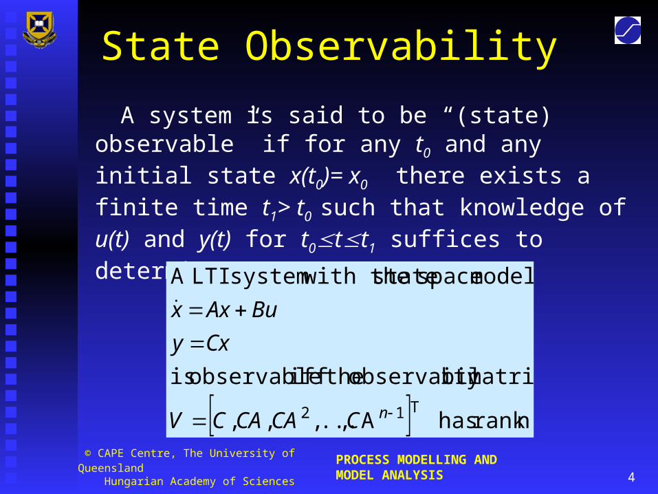
State Observability

A system is said to be “(state) observable” if for any t0 and any initial state x(t0)= x0 there exists a finite time t1> t0 such that knowledge of u(t) and y(t) for t0tt1 suffices to determine x0

nrank has A, ... ,,,

matrixity observabil theiff observable is

model space state with thesystem LTIA

T12

nCCACACV

Cxy

BuAxx

5



MATLAB functions (V4.2)

Controllability

Observability

)()(

states eduncontroll %

),(

corankAlengthunco

BActrbco

)()(

states unobserved %

),(

obrankAlengthunob

CAobsvob

6



Example

2

11

2

1

2

1

04761.09558.1

0

1

00415.50

0415.501847.7

x

xy

ux

x

x

x

Model equations

Controllability2)( ;

50.04150

7.1847-1.0),(

];0;1 [

0]; 50.0415 ;0415.50 1847.7[

corankBActrbco

B

A

2)( ;97.8712-16.4343-

0.0476- 1.9558),(

0.04761];- 1.9558[

0]; 50.0415 ;0415.50 1847.7[

obrankCAobsvob

C

A

Observability

7



Stability of systems - overview Two stability notions

- bounded input bounded output (BIBO) - asymptotic stability

Testing asymptotic stability of LTI systems MATLAB functions (e.g. eig(A)) Stability of nonlinear process systems

- Lyapunov’s principle

8



BIBO Stability

A system is said to be “bounded input, bounded output (BIBO) stable” if it responds with a bounded output signal to any bounded input signal, i.e.

BIBO stability is external stability

norm. signal a is ||.|| where

|||| ||||

then ][ if

yu

uy

S

9



Asymptotic Stability

A system is said to be “asymptotically stable” if for a “small” deviation in the initial state the resulting “perturbed” solution goes to the original solution in the limit, i.e.

asymptotic stability is internal stability

norm. vector a is ||.|| where

if 0 ||)()(||

then ||||whenever 0

000

ttxtx

xx

10



Asymptotic Stability of LTI Systems

A LTI system with state space realization matrices (A,B,C) is asymptotically stable if and only if all the eigenvalues of the state matrix A have negative real parts, i.e.

asymptotic stability is a system property

iR allfor 0 }e{ Ai,

11



MATLAB Function and Example

2

11

2

1

2

1

04761.09558.1

0

1

00415.50

0415.501847.7

x

xy

ux

x

x

x

Model equations

Analysis

i

i

Aeig

A

49.9124 3.5924-

49.9124 3.5924-

)(

0]; 50.0415 ;0415.50 1847.7[

Stable!

12



Asymptotic Stability of Nonlinear Systems

Lyapunov principle: construct a generalized energy function V for the system, such that:

If such a V exists then the system is asymptotically stable

)(every for 0 )( :

)( , 0 :

txxdt

dVitydissipativ

xVV(x)itenesspos. defin

13



Structural properties of systems

A dynamic system possesses a structural property if “almost every” system with the same structure has this property (“same structure” = identical structure graph)

Properties include:Structural controllabilityStructural observabilityStructural stability

14



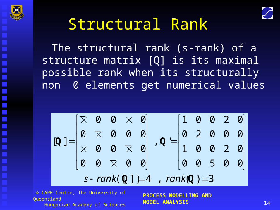
Structural Rank

The structural rank (s-rank) of a structure matrix [Q] is its maximal possible rank when its structurally non 0 elements get numerical values

3)( , 4])([

00500

02001

00020

02001

' ,

0000

000

0000

000

][

QQ

QQ

rankranks

15



Structural Controllability

A system is structurally controllable if the structural rank (s-rank) of the block structure matrix [A,B] is equal to the number of state variables n

))(( ])([

... )( , ][ ][ ][ 1

BA,UBA,

BAABBBA,UBABA,

rankranks

n

16



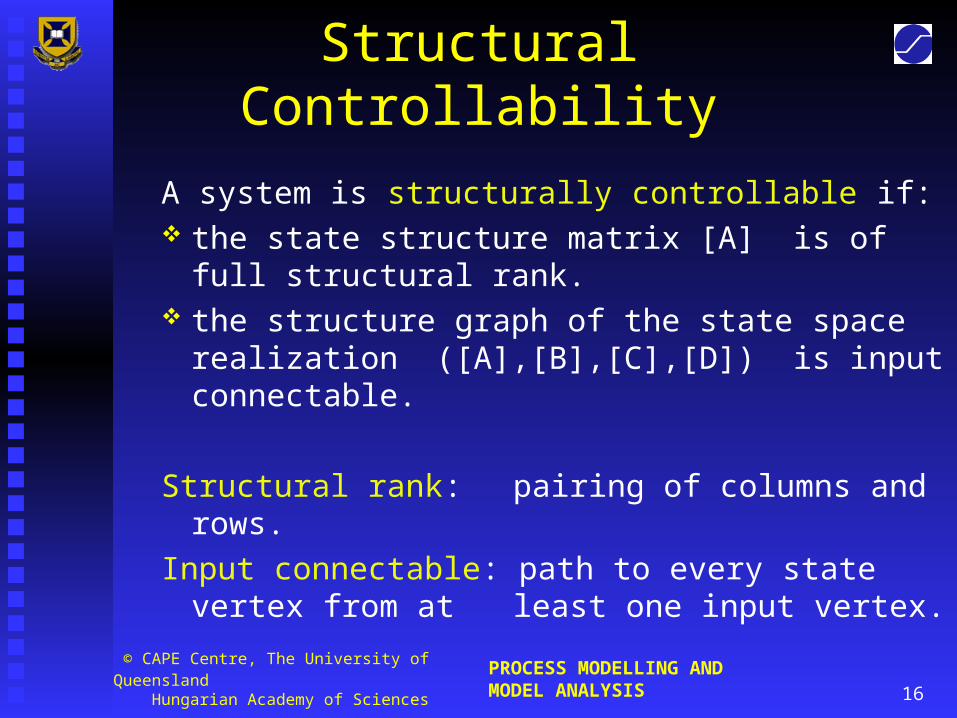
Structural Controllability

A system is structurally controllable if: the state structure matrix [A] is of full structural

rank. the structure graph of the state space realization

([A],[B],[C],[D]) is input connectable.

Structural rank: pairing of columns and rows.

Input connectable: path to every state vertex from at least one input vertex.

17



Example: Heat exchanger modelled by 3 connected lumped volumes

y1

u2

x1 x2 x3

x4 x5 x6

u1

y2

[A] is of full structural rank (because of self loops)

Structure graph

18



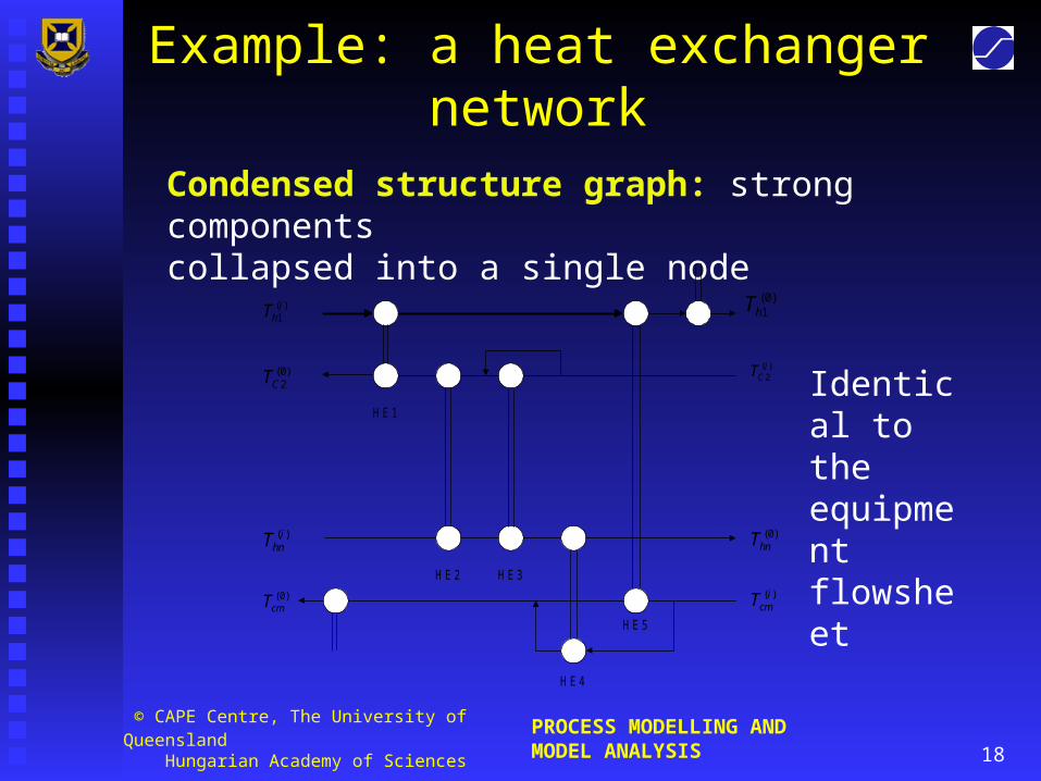
Example: a heat exchanger network

Identical to the equipment flowsheet

Condensed structure graph: strong components collapsed into a single node

)0(cmT

)(ihnT

)0(2CT

)(1i

hT)0(

1hT

)(2i

CT

)0(hnT

)(icmT

HE2

HE4

HE1

HE3

HE5

19



Structural Observability

A system is structurally observable if the structural rank (s-rank) of the block structure matrix [C,A]T is equal to the number of state variables n

))(( )],([

...)( ,

][

][ ,

1

T

CA,VAC

CA

CA

C

CA,VA

CAC

rankranks T

n

20



Structural Observability

A system is structurally observable if: the state structure matrix [A] is of full structural

rank. the structure graph of the state space realization

([A],[B],[C],[D]) is output connectable.

Structural rank: pairing of columns and rows.

Output connectable: path from every state vertex to

at least one output vertex.

21



Structural Stability

Method of circle familiesconditions depending on the sign of non-touching circle families (computationally hard)

Method of conservation matrices

If the state matrix A is a conservation matrix then the system is structurally stable.

niaa

jiaa

jiijii ,...,1 , || :diagdominant

0 , 0 :patternsign ijii

22



Model Simplification and Reduction

LTI models with state space representation

States can be classified into: slow modes (“small” negative eigenvalues)

states essentially constant fast modes (“large” negative eigenvalues)

go to steady state rapidly medium modes

xyuxdt

dxCBA ,

23



Model Structure Simplification

Elementary simplification steps variable removal:

steady state assumption on a state variableremoves the vertex and all adjacent edgesand conserves the paths.

variable lumping:for a vertex pair with similar dynamics, it lumps the two vertices together, unites adjacent edgesand conserves the paths.

24



Example: A heat exchanger 1. Variable removal

Steady-state variables: cold side temperatures

y1

u2

x1 x2 x3u1

y2

25



Example: A heat exchanger 1. Variable lumping

Lumped variables: cold side temperatures hot side temperatures

y1

u2

XH

XC

u1

y2

26



Equivalent State Space Models

Two state space models are equivalent if they give rise to the same input-output model.

Equivalence transformation of state space models of LTI systems are:

11

1

, ,

exists ,

TTTT

T

T T

CCBBAA

xx

nn

27



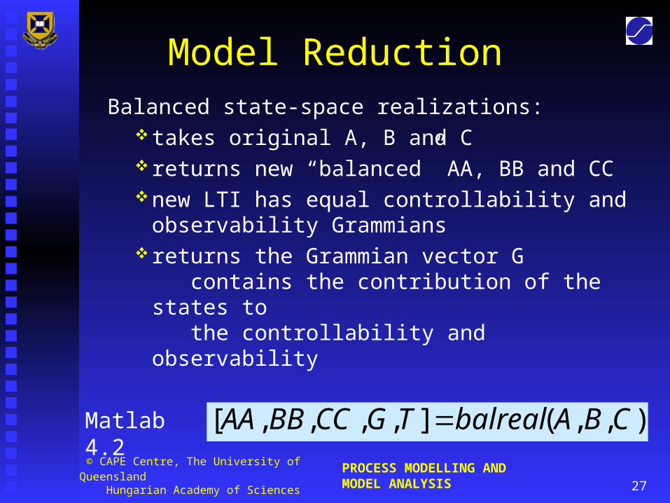
Model Reduction

Balanced state-space realizations: takes original A, B and C returns new “balanced” AA, BB and CCnew LTI has equal controllability and

observability Grammians returns the Grammian vector G

contains the contribution of the states to the controllability and observability

),,(],,,,[ CBAbalrealTGCCBBAA Matlab 4.2

28



Model Reduction

Use Grammian information for reduction• eliminate states where g(i)<g(1)/10

Model reduction of states x(ie1),…, x(ie1) done using (Matlab 4.2):

ELIM)DD,CC,BB,modred(AA,],,,[

];...;;[ 21

DRCRBRAR

iiiELIM ejee

PROCESS MODELLING AND MODEL ANALYSIS © CAPE Centre, The University of Queensland Hungarian Academy...

Documents

Transcript of PROCESS MODELLING AND MODEL ANALYSIS © CAPE Centre, The University of Queensland Hungarian Academy...