Proceedings of the Second International Workshop on ... · Proceedings of the Second International...

Proceedings of the Second International Workshop on SustainableUltrascale Computing Systems (NESUS 2015)

Krakow, Poland

Jesus Carretero, Javier Garcia BlasRoman Wyrzykowski, Emmanuel Jeannot.

(Editors)

September 10-11, 2015

NESUSNetwork for Sustainable Ultrascale Computing

IC1305

Second NESUS Workshop • September 2015 • Vol. I, No. 1

A Scheduler for Cloud Bursting ofMap-Intensive Traffic Analysis Jobs

Ricardo Morla†, Pedro Gonçalves†, Jorge Barbosa‡†INESC TEC and Faculty of Engineering, University of Porto‡LIACC and Faculty of Engineering, University of Porto

Porto, [email protected]

Abstract

Network traffic analysis is important for detecting intrusions and managing application traffic. Low cost, cluster-based traffic analysis solutions have been proposed for bulk processing of large blocks of traffic captures, scalingout the processing capability of a single network analysis node. Because of traffic intensity variations owing tothe natural burstiness of network traffic, a network analysis cluster may have to be severely over-dimensionedto support 24/7 continuous packet block capture and processing. Bursting the analysis of some of the packetblocks to the cloud may attenuate the need for over-dimensioning the local cluster. In fact, existing solutionsfor network traffic analysis in the cloud are already providing the traditional benefits of cloud-based services tonetwork traffic analysts and opening the door to cloud-based Elastic MapReduce-style traffic analysis solutions. Inthis paper we propose a scheduler of packet block network analysis jobs that chooses between sending the job to alocal cluster versus sending it to a network analysis service on the cloud. We focus on map-intensive jobs suchas string matching-based virus and malware detection. We present an architecture for an Hadoop-based networkanalysis solution including our scheduler, report on using this approach in a small cluster, and show schedulingperformance results obtained through simulation. We achieve up to more than 50% reduction on the amount ofnetwork traffic we need to burst out using our scheduler compared to simple traffic threshold scheduler and fullresource availability scheduler. Finally we discuss scaling out issues for our network analysis solution.

Keywords Packet Network Traffic Analysis, Hadoop, Cloud Bursting

I. Introduction

Many companies invest in their private IT data cen-ters to meet most of their needs. However, these pri-vate data centers might not cope with workload peaks,leading to delays and lower throughput. Using ex-tra computing power to handle the unpredictable andinfrequent peak data workloads is expensive and inef-ficient, since a portion of the resources will be inactivemost of the time. Migrating the whole application toa cloud infrastructure, though possibly cheaper thaninvesting in the private data center because servers areonly rented when needed, is still expensive and couldcompromise private and important data. A hybrid

model offers the best solution to address the needs forelasticity when peak workloads appear, while provid-ing local privacy if needed. In this model, the localIT data center of an enterprise is optimized to fulfillthe vast majority of its needs, resorting to additionalresources in the cloud when the local data center re-sources become scarce [1]. This technique is calledCloud Bursting and enables an enterprise to scale outtheir local infrastructure by bursting their applicationsto a third-party public cloud seamlessly, if the needarises [2].

Cloud Bursting could be of use to network man-agers and security experts. In fact, their need formore computational power that can perform more

1

Ricardo Morla, Pedro Gonçalves,Jorge Barbosa 11

Book paper template • September 2014 • Vol. I, No. 1

complex network intrusion detection and applicationtraffic management is hand in hand with the variabil-ity of network traffic and of traffic analysis workload.Big data style analysis software and services usingthe open source YARN and Hadoop platform1 areavailable both in the research community [3, 4] andcommercially2. Although [3] in particular provides arange of network analysis jobs from low level packetand flow statistics to intrusion detection, their perfor-mance evaluation focuses mainly on the throughputof the analysis system with different file sizes. In par-ticular, Map and Reduce run time distributions thatcould be helpful for large scale evaluation have notbeen characterized.

Three types of network traffic analysis are typical[5]: 1) real-time analysis, where continuous streamsof data are analyzed and processed as they arrive; 2)batched analysis, where data is aggregated in batchesand analyzed periodically; and 3) forensics analysisare analysis that only occur when special events aretriggered, for example, when a major intrusion hasbeen detected and requires detailed analysis of loggedtraffic. This work focuses on 24/7 continuous batchanalyses of consecutive captures of network packettraffic and on the natural variability that characterizessuch traffic. Because intrusion detection results foreach batch must be delivered as soon as possible toallow for early detection, traffic variability in a contin-uous batch processing means either over-dimensioningthe computing cluster or waiting longer to get detec-tion results. Our proposal is to use Cloud Burstingto burst some jobs and achieve lower waiting times.We present an integrated solution in section II that wehave implemented in our networking laboratory. Animportant part of this solution is the scheduler thatdecides whether to burst a job based on the size ofthe file that needs to be analyzed and on the resourceusage in the cluster. We present our Map-intensive job,job model, scheduler rationale, and cluster capacityestimation in section III. In section IV we show resultsof running our network analysis job in a small Hadoopcluster. The goal here is to provide an example ofhow the scheduler works and to obtain an empiricaldistribution for the Map run time to be used in our

1http://hadoop.apache.org2http://www.pravail.com

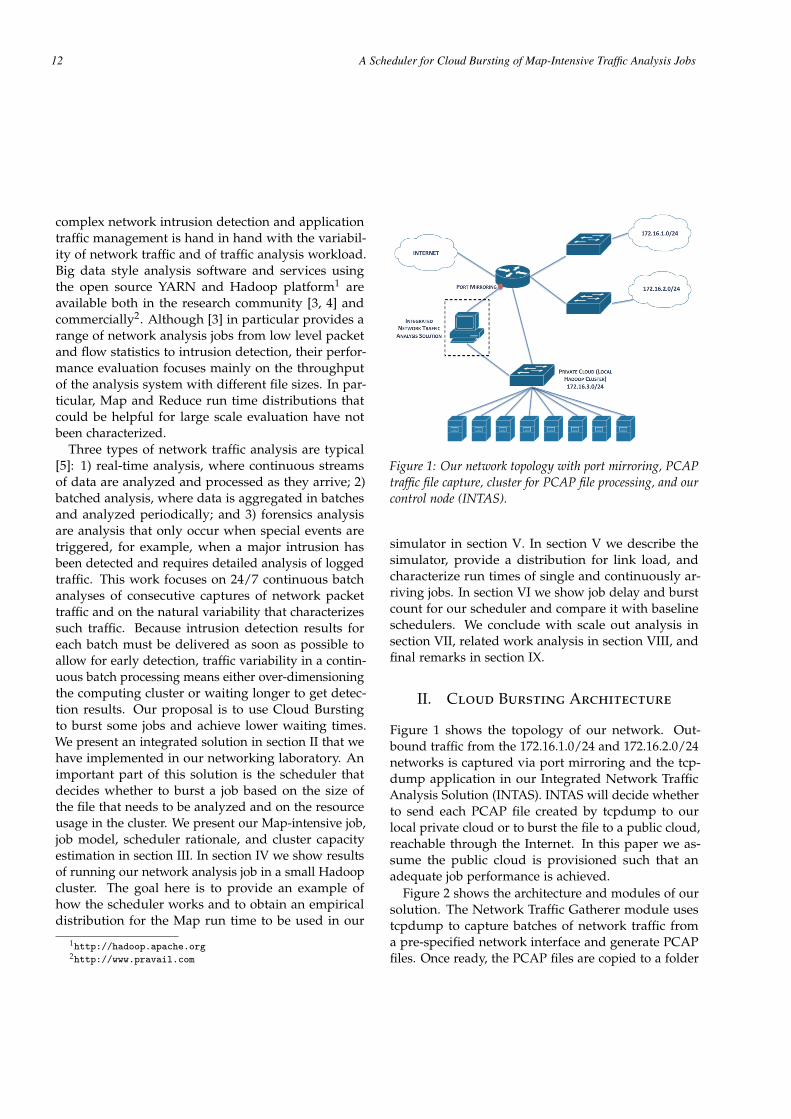
Figure 1: Our network topology with port mirroring, PCAPtraffic file capture, cluster for PCAP file processing, and ourcontrol node (INTAS).

simulator in section V. In section V we describe thesimulator, provide a distribution for link load, andcharacterize run times of single and continuously ar-riving jobs. In section VI we show job delay and burstcount for our scheduler and compare it with baselineschedulers. We conclude with scale out analysis insection VII, related work analysis in section VIII, andfinal remarks in section IX.

II. Cloud Bursting Architecture

Figure 1 shows the topology of our network. Out-bound traffic from the 172.16.1.0/24 and 172.16.2.0/24networks is captured via port mirroring and the tcp-dump application in our Integrated Network TrafficAnalysis Solution (INTAS). INTAS will decide whetherto send each PCAP file created by tcpdump to ourlocal private cloud or to burst the file to a public cloud,reachable through the Internet. In this paper we as-sume the public cloud is provisioned such that anadequate job performance is achieved.

Figure 2 shows the architecture and modules of oursolution. The Network Traffic Gatherer module usestcpdump to capture batches of network traffic froma pre-specified network interface and generate PCAPfiles. Once ready, the PCAP files are copied to a folder

2

12 A Scheduler for Cloud Bursting of Map-Intensive Traffic Analysis Jobs


Figure 2: The architecture of INTAS.

where the PCAP File Processor module determineswhether or not the PCAP file is new before deliveringit to the Scheduler/Load Balancer. Using the clus-ter resource utilization information provided by theResource Monitor, the Scheduler decides whether tolaunch the job locally or to burst it. In either case, thePCAP file is first uploaded to HDFS on the destinationcluster through the HDFS Uploader module. After theupload is complete, the Job Launcher connects to theHadoop cluster to launch the map-intensive networkanalysis job.

III. Scheduler

III.1 Map-Intensive Network AnalysisJobs

Map-intensive network analysis jobs such as traffic clas-sification and virus or malware detection using stringmatching can have the following two-phase design.The Map phase checks packet payload for the presenceof signature keys. This outputs a list of which applica-tions or viruses were identified on which packets. Thereduce phase merges these results and writes them tothe job’s output file.

The Map phase of this kind of network analysis job

is computationally expensive. Simply put, all possiblestring sequences in the packet’s transport layer payloadmust be compared to the signature keys of the differentviruses, malware, or specific applications we want tofind. For a signature key with bkey bytes and a stringcomparison factor kkey[second/byte], the total process-ing time of a packet is tpacket = kkey (bpacket − bkey),with bpacket ≥ bkey. For small keys and relatively largepackets, we can have a close approximation of tpacketby using its upper bound k bpacket, where k is the sumof all string comparison factors and which can also beexpressed as k = nkavg with n keys and kavg averagestring comparison factor. This upper bound is propor-tional to the size of the packet. We find an estimate ofk by benchmarking the target cluster as reported laterin the paper.

Under the Map-Reduce paradigm, each traffic cap-ture file is split into a number of data blocks and eachblock is processed by a Map process. Although theexact number of packets in each block can change ac-cording to the nature of the network traffic, the size inbytes of almost all data blocks is pre-configured andindependent of the nature of the traffic. Our estimatefor the Map processing time of a block with bblock bytesis tblock = k bblock. We assume the switching time be-tween processing of packets is much smaller than theactual processing.

The Reduce phase of this kind of network analysisjobs is much less computationally demanding than theMap phase. We assume the Reduce processing time tobe zero.

III.2 Job Completion Time Estimate

The number of map tasks that a network analysisjob launches depends on the size of the input traf-fic capture file and on the Map-Reduce data blocksize. A block size of 128 MB is typical, which fora slightly under 900 MB traffic capture file size b f ilewould yield 7 data blocks on which 7 Map processeswould need to run. More generically, we computem = b f ile/bblock and estimate the number of Map pro-cesses to be M = dme. We disable speculative execu-tion to improve this estimate.

The container is the unit of resource allocation inHadoop YARN. Typically, two containers run per host.

3



The mapping to containers sets the limit to the numberof Maps that a network analysis task can run simulta-neously. One Map process runs on a container. EachMap-Reduce job is managed by an ApplicationMasterthat requires an additional host throughout the com-plete lifetime of the job. Although Reduces also requirecontainers, their impact on resource usage in this kindof network analysis job is much smaller than that ofMaps and we do not consider them.

For a YARN cluster with H hosts, the number ofMaps that can run simultaneously is Ms = 2(H− 1)−1. Comparing Ms and M takes us to the concept of Mapwaves. Each wave of Ms Maps will run simultaneouslyfor approximately tblock, after which a new wave of Ms(or fewer) Maps will start. This repeats until all MMaps have run. We compute n = M/Ms and estimatethe number of waves as N = dne. Our estimate forthe job completion time is tMjob = (N − 1) ∗ tblock +k(m− bmc)bblock if the last wave has a single Map task(in which case M− NMs = 1), and tMjob = N ∗ tblockotherwise, which is the more frequent case.

In addition to TMjob, the scheduler needs have anestimate of the time it takes the system to upload thecaptured traffic file from the capture node to HDFS.We use a simple estimate Tupload = b f ile/r with r in[bytes/second]. The total job completion time estimateis Tjob = TMjob + Tupload.

At any moment in time after the job has been sched-uled, the estimate for the job completion time Tremaining

jobcan be updated as follows:

• TMjob + (b f ile − buploadedf ile )/r , if the upload not fin-

ished yet. buploadedf ile is the number of bytes that

have been uploaded so far.

• TMjob − Ndone tblock − twave , if the upload finished.Ndone is the number of completed waves and twaveis how long the current wave has been running.

This estimate is valid for a single job running in thecluster.

III.3 Scheduling Concurrent Jobs

An incoming traffic analysis job is scheduled regardlessof the size of the capture file when no job is running

on the cluster. When traffic peaks, it is possible that anew chunk of traffic is captured and ready for analysisbefore the traffic analysis job of the previous chunk isover. In this case where a job is running in the localcluster when a new job arrives, the scheduler will haveto decide whether to send the incoming job to the localcluster or to the cloud.

Our baseline scheduler verifies if there are enoughcontainers for the job in the local cluster. If thereare, the job is ran locally; otherwise the job is sent tothe public cloud. We assume the connection to thepublic cloud and the public cloud cluster itself areprovisioned such that an adequate response time isachieved. We do not explore public cloud performancein this paper.

The approach of the baseline scheduler is over sim-plifying and can send more jobs to the public cloudthan needed: 1) the time it takes to upload the capturefile to the local HDFS can be enough for the current jobto complete and the incoming job to be processed lo-cally; 2) the last wave of a job may use fewer resourcesthan the previous waves, which can be used by the in-coming job. Our proposed scheduler takes advantageof the job completion time estimate and wave modelpresented in the previous section to try to reduce thenumber of uploads to the public cloud and reducingthe impact on job completion time.

Our proposed scheduler schedules incoming candi-date job locally if:

• S0. Local cluster is empty or enough containersare available to run the incoming job.

• S1. Local cluster has single current job and currentjob finishes before or up to Th1 seconds after in-coming job upload time to local cluster HDFS. Forthis we use Tremaining

job of the current job and Tupload

of the incoming candidate job. Th1 provides sometolerance to the decision and can be chosen to bea few percent of the wave duration.

• S2. Local cluster has single current job and: 1) thenext to the last wave of current job finishes beforeor up to Th1 seconds after incoming job uploadtime to local cluster HDFS and 2) the number ofcontainers of the last wave of the candidate incom-ing job is smaller than or equal to the number of

4



containers not used by last wave of the currentjob.

III.4 Benchmarking and Estimating Capac-ity

Our scheduler requires an estimate of the block execu-tion time tblock and of the upload to HDFS rate r. Ourapproach for estimating these values is to run the net-work analysis job we are interested in benchmarkingon an sample data set prior to running the job on thetarget traffic capture files. This provides samples formeasure Map completion time and file upload time,which can be averaged or maxed and used as estimatefor tblock and r.

Estimating the capacity of a cluster for this kindof network analysis is important for: 1) definingthe traffic throughput that a given cluster can sup-port for analysis and 2) specifying how many andwhat kind of nodes there should be in the clusterfor a given traffic throughput that needs to be ana-lyzed. We estimate the maximum throughput of atraffic capture that a cluster can support as Thput =Ms ∗ bblock/tblock = (2(H − 1) − 1)/k. Using this es-timate, a cluster with 10 nodes, 128 MB block size,and tblock = 5min (k = 2.23 µs/byte) would supportapproximately 60 Mbit/s traffic captures, which yieldsa maximum 10 minute traffic capture file of 4.5 GB.

IV. String Matching Job in SmallPhysical Clusters

We ran a Map-intensive string matching job with 200signature keys on H=5 node low-end YARN clusters.To more easily launch our Hadoop 2.3.0 cluster we usea private cloud based on Openstack IceHouse3 andthe Sahara Openstack module4 that provisions data-intensive application clusters like YARN. The bare-metal operating system is Ubuntu 14.04. Each baremetal runs a single virtual machine YARN node.

Due to time and lab resource constraints we ran thetwo experiments of this section in different hardware.The scheduling experiment was run on a heteroge-neous cluster with the following bare-metals: Intel

3https://www.openstack.org/software/icehouse/4http://docs.openstack.org/developer/sahara/

Core i7-3770 3.40GHz, two Intel Core i7 950 3.07GHz,Intel E5504 2.00GHz. The map runtime experimentwas run on a homogeneous cluster in which the bare-metal CPUs are older, 2008 Intel Core 2 Quad Q9300running at 2.50GHz. CPU names are as reported by/proc/cpuinfo.

We captured two PCAP files locally on a 100 Mbit/slink for 10 minutes each. One file (A) is 1.22 GB andthe other (B) is 2.01 GB, corresponding to 17 Mbit/sand 26 Mbit/s of traffic going out of our local network.One file has 10 128 MB data blocks and the other 16.

IV.1 Scheduling

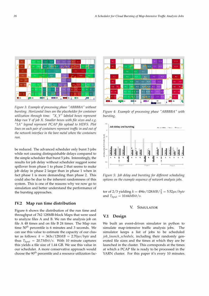
For our scheduling experiments we replayed the twoPCAP files A and B into our system every 10 min-utes according to this sequence: "ABBBBA-ABABAA-AAAAAA". File A has the cluster running slightlybelow capacity whereas file B has the cluster runningabove capacity. This means that during the first phase"ABBBBA" the cluster will be running well above ca-pacity, during the second phase "ABABAA" the clusterwill be just slightly over capacity, and during the thirdphase "AAAAAA" the cluster will be running belowcapacity.

Figures 3 and 4 show an example of processing thefirst phase "ABBBBA". To produce analysis results assoon as possible, the Maps for job 6A should startimmediately after the upload is completed, i.e. onthe right side of the small box near 6A. Notice thatwithout scheduler (figure 3, job id 54), the Maps haveto wait until the previous job completes – which isa considerable amount of time. In figure 4 with thescheduler and by bursting job 5B, job 6A can startimmediately after upload.

Figure 5 shows how the job sequence was burst or de-layed using the three different scheduling approaches:no scheduler, simple, and advanced. Because we wantto have an idea of the impact of the scheduler on eachjob individually, we can compare the run time of a jobTjob with the sum of the job’s Map run times dividedby the number Ms of Maps that can run simultane-ously. We define this metric as D = Tjob/Tideal − 1with Tideal = 1/Ms ∑i ti

block and where tiblock is the run

time of the ith Map of the job. The results confirm ourintuition that by bursting some jobs the job delay can

5



Figure 3: Example of processing phase "ABBBBA" withoutbursting. Horizontal lines are the placeholder for containerutilization through time. "X_Y" labeled boxes representMap run Y of job X. Smaller boxes with file sizes and e.g."1A" legend represent PCAP file upload to HDFS. Plotlines on each pair of containers represent traffic in and out ofthe network interface in the bare metal where the containersrun.

be reduced. The advanced scheduler only burst 3 jobswhile not causing distinguishable delays compared tothe simple scheduler that burst 5 jobs. Interestingly, theresults for job delay without scheduler suggest somespillover from phase 1 to phase 2 that seems to makejob delay in phase 2 larger than in phase 1 when infact phase 1 is more demanding than phase 2. Thiscould also be due to the inherent randomness of thissystem. This is one of the reasons why we now go tosimulation and better understand the performance ofthe bursting approaches.

IV.2 Map run time distribution

Figure 6 shows the distribution of the run time andthroughput of 762 128MB-block Maps that were usedto analyze files A and B. We ran the analysis job onfile A 48 times and on file B 24 times. The Map runtime 50th percentile is 6 minutes and 3 seconds. Wecan use this value to estimate the capacity of our clus-ter as follows: k = 363s/128MB = 2.70µs/byte andthus Thput = 20.7Mbit/s. With 10 minute capturesthis yields a file size of 1.44 GB. We use this value inour scheduler. A more conservative approach wouldchoose the 90th percentile and a resource utilization fac-

Figure 4: Example of processing phase "ABBBBA" withbursting.

Figure 5: Job delay and bursting for different schedulingoptions on the example sequence of network analysis jobs.

tor of 2/3 yielding k = 494s/128MB/ 23 = 5.52µs/byte

and Thput = 10.64Mbit/s.

V. Simulator

V.1 Design

We built an event-driven simulator in python tosimulate map-intensive traffic analysis jobs. Thesimulator keeps a list of jobs to be scheduledjob_launch_schedule, including their randomly gen-erated file sizes and the times at which they are belaunched in the cluster. This corresponds at the timesat which a PCAP file is ready to be processed in theYARN cluster. For this paper it’s every 10 minutes.

6



0

0.1

0.2

0.3

0.4

0.5

0.6

0.7

0.8

0.9

1

0 200 400 600 800 1000

y:

Pro

port

ion o

f M

ap

ssh

ort

er

than x

x: Map run time (s)

Map run time CDF

0

0.1

0.2

0.3

0.4

0.5

0.6

0.7

0.8

0.9

1

0 100 200 300 400 500

y:

Pro

port

ion o

f M

ap

sw

ith t

hro

ug

hp

ut

smalle

r th

an x

x: Map throughput (kB/s)

Map throughput CDF

Figure 6: Empirical CDFs of run time and throughput of762 Maps of our network analysis job.

This list is populated before the simulation starts andjobs are popped out and launched as the simulationprogresses. YARN can be configured to allow a max-imum of simultaneously running applications in thecluster. To account for this, a job that is popped outof the job_launch_schedule list will go to a job_waitinglist. If the number of currently running applications isbelow the maximum, the oldest job is removed fromthe job_waiting list and included in the job_runninglist. Jobs in the job_runnig list will compete for avail-able cluster containers in round-robin. Only the jobat the top of the list will get a container to run a Map.For every container a running job gets to run a Mapit will be pushed to the back of the list. Container re-lease events are scheduled according to the randomlygenerated Map run time distribution and processed bythe simulation together with job launch events. Thesimulation finishes when there are no more events toprocess or maximum simulation time is reached. Blocksize is 128MB.

0

0.1

0.2

0.3

0.4

0.5

0.6

0.7

0.8

0.9

1

0 20 40 60 80 100

y:

Pro

port

ion o

f lo

ad

ob

serv

ati

ons

smalle

r th

an x

x: Link load (%)

Link load CDF

Figure 7: 10 Gbps link load empirical CDF.

V.2 Workload Distributions

Synthetic workload generation requires two compo-nents. The first is a distribution for the Map run time,for which we use the Map run time empirical distribu-tion obtained from our 5 node clusters and shown infigure 6. The second is the PCAP file size distributionthat determines the number of data blocks and Maptasks that the job needs to process. As this is directlyrelated to the amount of traffic through a packet net-work, we build on publicly available data from theCAIDA Center for Applied Internet Data Analysis inSan Diego, CA5. We use every month, hour-long av-erage bitrate on both directions of their 10 Gbps SanDiego links to Chicago and San Jose to build a 247point empirical link load distribution. We show theCDF of this distribution in figure 7. Average link loadis 31%.

Figure 8 shows the Q-Q plots for our synthetic dataand the empirical distributions. Notice how close theQ-Q points are to the y = x line. Because we havefewer observations in the high link load region thepoints there are not as close to the y = x line as theother points.

Simulation results in the rest of the paper are ob-tained by running 104 jobs for each link capacity. Incontinuously arriving jobs including when the sched-ulers are used we run each set of 104 jobs 20 times toget final results.

5 The CAIDA UCSD http://www.caida.org/data/passive/trace_stats/

7



0

50

100

150

200

250

300

350

400

450

500

0 100 200 300 400 500

y:

Map t

hro

ughput

(kB

/s)

synth

eti

c data

x: Map throughput (kB/s) real data

Map throughput Q-Q

0

20

40

60

80

100

0 20 40 60 80 100

y:

Link

load (

%)

synth

eti

c data

x: Link load (%) real data

Link load Q-Q

Figure 8: Q-Q plots comparing 10k synthetic data pointsand the empirical distributions of Map throughput and linkload from figures 6 and 7.

V.3 Single Job

Understanding the performance of a cluster under asingle job workload helps validate the simulator andcan provide insights into the performance analysis ofour scheduler under a continuous workload. Figure9 shows the run time CDF of a single job for a fixedlink bitrate that we vary from 1 Mbps to 40 Mbps onour H=5 simulated cluster. The bitrate grows from leftCDF to right CDF. We can notice groups of CDFs thatcorrespond to waves in our job model. The first groupgoes up to 12.53 Mbit/s which yields a 7 128MB blockPCAP file requiring exactly the number of Maps (7)that can run simultaneously in a wave. We call this thewave boundary bit rate. With a slight increase to 15Mbit/s, file size of 1073 MB, and 9 Maps (8 128 blocksand 1 48 MB block), there is a significant increase in the50th percentile run time from 495 s at 12.53 Mbit/s to698 s at 15 Mbit/s, as this file size requires two waves ofMaps. As the link traffic increases to include multiplewaves this difference seems to decrease. Unless statedotherwise, link throughput values and their linestylemapping in figure 9 are used throughout the paper.

As discussed in section V.2, link throughput is notconstant and this has an impact on job runtime andresource usage CDFs. Figure 10 shows run time forlinks with capacity equal to the fixed bitrate valuesused in the previous section. Run times are generallysmaller than those in figure 9 as the random workloaddistribution is applied to the link capacity and on aver-age results in smaller bitrates and smaller PCAP filesto process. Notice that the wave phenomenon is no

0

0.1

0.2

0.3

0.4

0.5

0.6

0.7

0.8

0.9

1

0 200 400 600 800 1000 1200 1400 1600 1800

y:

Pro

port

ion o

f Jo

bs

short

er

than x

x: Job run time (s)

Job run time CDF

Figure 9: CDFs of the run time of fixed workload jobs onan Ms = 7 cluster. From left to right the link throughputvalues in Mbit/s are: (1, 2, 5, 7, 10, 12, 12.53), (15, 17,20, 22, 24.5, 25.05), (27, 30, 32, 35, 37, 37.58), (40, 42,45, 47, 50, 100). The 100 Mbit/s line is out of range. TheCDFs for each link throughput form groups according to thenumber of waves that our model indicates (1:long dash, 2:solid, 3:short dash, 4:long-short dash). Line width in eachgroup increases with link throughput.

longer obvious to observe except for the first two linkcapacity values.

V.4 Continuously Arriving Jobs

We now consider the case that we are most interestedin: PCAP files freshly captured and uploaded to beprocessed by our network analysis job every 10 min-utes. Bit rate and Map processing time distributionswill make some jobs last more than 10 minutes, in

0

0.1

0.2

0.3

0.4

0.5

0.6

0.7

0.8

0.9

1

0 200 400 600 800 1000 1200 1400 1600 1800

y:

Pro

port

ion o

f Jo

bs

short

er

than x

x: Job run time (s)

Job run time CDF

Figure 10: CDFs of the run time of random workload jobson an Ms = 7 cluster following our random workloaddistribution.

8



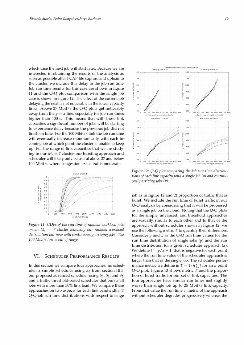
which case the next job will start later. Because we areinterested in obtaining the results of the analysis assoon as possible after PCAP file capture and upload tothe cluster, we include this delay in the job run time.Job run time results for this case are shown in figure11 and the Q-Q plot comparison with the single jobcase is shown in figure 12. The effect of the current jobdelaying the next is not noticeable in the lower capacitylinks. Above 27 Mbit/s the Q-Q plots get noticeablyaway from the y = x line, especially for job run timeshigher than 400 s. This means that with these linkcapacities a significant number of jobs will be startingto experience delay because the previous job did notfinish on time. For the 100 Mbit/s link the job run timewill eventually increase monotonically with each in-coming job at which point the cluster is unable to keepup. For the range of link capacities that we are study-ing in our Ms = 7 cluster, our bursting approach andscheduler will likely only be useful above 27 and below100 Mbit/s where congestion exists but is moderate.

0

0.1

0.2

0.3

0.4

0.5

0.6

0.7

0.8

0.9

1

0 200 400 600 800 1000 1200 1400 1600 1800

y:

Pro

port

ion o

f Jo

bs

short

er

than x

x: Job run time (s)

Job run time CDF

Figure 11: CDFs of the run time of random workload jobson an Ms = 7 cluster following our random workloaddistribution but now with continuously arriving jobs. The100 Mbit/s line is out of range.

VI. Scheduler Performance Results

In this section we compare four approaches: no sched-uler, a simple scheduler using S0 from section III.3,our proposed advanced scheduler using S0, S1, and S2,and a traffic threshold-based scheduler that bursts alljobs with more than 50% link load. We compare theseapproaches on two aspects for each link bandwidth: 1)Q-Q job run time distributions with respect to singe

Continuously arriving vs. single Job run time Q-Q

200

400

600

800

1000

1200

1400

0 200 400 600 800 1000 1200 1400 1600 1800

y:

Sin

gle

job

run t

ime (

s)

x: Continuously arriving job run time (s)

1.0 through 12.5 Mbit/s

200

400

600

800

1000

1200

1400

0 200 400 600 800 1000 1200 1400 1600 1800

y:

Sin

gle

job

run t

ime (

s)



200

400

600

800

1000

1200

1400

0 200 400 600 800 1000 1200 1400 1600 1800

y:

Sin

gle

job

run t

ime (

s)



200

400

600

800

1000

1200

1400

0 200 400 600 800 1000 1200 1400 1600 1800

y:

Sin

gle

job

run t

ime (

s)



Figure 12: Q-Q plot comparing the job run time distribu-tions of each link capacity with a single job (y) and continu-ously arriving jobs (x).

job as in figure 12 and 2) proportion of traffic that isburst. We include the run time of burst traffic in ourQ-Q analysis by considering that it will be processedas a single job on the cloud. Noting that the Q-Q plotsfor the simple, advanced, and threshold approachesare visually similar to each other and to that of theapproach without scheduler shown in figure 12, weuse the following metric T to quantify their differences.Consider y and x as the Q-Q run time values for therun time distribution of single jobs (y) and the runtime distribution for a given scheduler approach (x).We define t = y/x− 1, that is negative for each pointwhere the run time value of the scheduler approach islarger than that of the single job. The scheduler perfor-mance metric we define is T = 1/n ∑ t for an n pointQ-Q plot. Figure 13 shows metric T and the propor-tion of burst traffic for our set of link capacities. Thefour approaches have similar run times just slightlyworse than single job up to 25 Mbit/s link capacity.From that value the run time T metric of the approachwithout scheduler degrades progressively whereas the

9



-1

-0.8

-0.6

-0.4

-0.2

0

0 10 20 30 40 50 0

0.2

0.4

0.6

0.8

1

T m

etr

ic v

alu

e

Pro

port

ion o

f tr

affi

c b

urs

t

Bit rate (Mbit/s)

Scheduler run time comparison

NoneSimple

AdvancedThreshold

Figure 13: T metric and proportion of traffic burst for differ-ent scheduler approaches. T metric values are closer to thetop of the graph, traffic burst values closer to the bottom.

other three approaches are reasonably similar and notmuch worse than lower link capacities or single job.Looking at burst traffic, the simple approach burstsalmost twice as much traffic as the advanced approach.The approach with less burst traffic is the advancedscheduler up to 45 Mbit/s. At 35 Mbit/s the advancedscheduler bursts 56% less traffic than the other twoschedulers. Thus for the range of values where burst-ing could be useful, i.e. from 27 Mbit/s and below 100Mbit/s, the advanced scheduler yields both the small-est amount of burst traffic and single-job comparablerun times.

VII. Scaling Out

12 Mbit/s and the other bit rate values used in figure 9are not link capacities that can be found in typical net-work links. Four typical link capacities are 10 Mbit/s,100 Mbit/s, 1Gbit/s, and 10Gbit/s. The conservativecapacity estimation approach in section IV.2 puts ourMs = 7 cluster at approximately 11 Mbit/s, which isnot enough for the four typical link capacities. Withthat in mind, in figure 14 we show job run time for thefour typical link capacities on clusters of 3 differentsizes: our Ms = 7 initial cluster and Ms = 70 andMs = 700 clusters.

0

0.1

0.2

0.3

0.4

0.5

0.6

0.7

0.8

0.9

1

0 500 1000 1500 2000 2500 3000 3500

y:

Pro

port

ion o

f Jo

bs

short

er

than x

x: Job run time (s)

Job run time CDF

Figure 14: CDFs of the run time of random workload jobsfor typical link bitrates on clusters of different sizes. Longdash: 10 Mbit/s and 100 Mbit/s on an Ms=7 cluster. Solidline: 10 Mbit/s, 100 Mbit/s, and 1 Gbit/s on an Ms = 70cluster. Short dash: 10 Mbit/s, 100 Mbit/s, 1 Gbit/s, and 10Gbit/s on an Ms = 700 cluster.

VIII. Related Work

In the introduction we provided arguments for therelevance of our approach in the context of the analysisof network traffic. In summary, cloud bursting ofbatched Map-intensive network analysis jobs and thescheduling of such bursts has not been proposed beforein the traffic analysis literature. In this section wetake a look at different general-purpose cloud burstingapproaches and argue that they are not adequate toour batched Map-intensive network analysis jobs.

Existing open-source virtualized data center man-agement tools such as OpenStack and OpenNebulaalready support cloud bursting. Their initial focus wasto provide an abstraction layer for the low level de-tails of transitioning VMs (Virtual Machines) betweendata centers [1]. Throughout recent years, continuousimprovements have been made to the amount of pro-vided features and configurable parameters to bettersuit the users’ needs. Today, many available solutionsincluding Seagull [1] and the OPTIMIS Project [2] of-fer scheduling policies that determine if and whento burst to the cloud. However, these solutions aretypically geared towards web applications and do notadequately support applications that need to processlarge amounts of data.

As the world embraces the ever-growing paradigm

10



of Big Data, Cloud Bursting can also be used in the con-text where cloud resources are used to store additionaldata if local resources become scarce. In fact, the useof Cloud Bursting for data-intensive computing hasnot only been proved feasible but scalable as well. [6]presents a middleware that supports a custom MapRe-duce type API and enables data-intensive computingwith Cloud Bursting in a scenario where the data issplit across a local private data center and a publiccloud data center. Data is processed using computingpower from both the local and public cloud data cen-ters. Furthermore, data on one end can be processedwith computing power from the other end, albeit low-ering the overall job execution time. BStream [7] isa Cloud Bursting implementation that uses HadoopYARN with MapReduce in the local data center andthe Storm stream processing engine in the cloud toprocess MapReduce jobs instead of using YARN. Theuse of Storm allows the output of Maps to be streamedto Reduces in the cloud. Both [6] and [7] are bettersuited for forensic jobs for which a large data set mustbe analyzed and outputs from local Maps need to beprocessed on the cloud, than for batched analysis ofsmaller yet still computationally demanding data sets.In our case jobs can fit both in the local data centeror the public cloud and the challenge is to processcontinuously arriving jobs.

IX. Conclusion

We have set out to explore cloud bursting for Map-intensive network traffic analysis jobs. Using our pro-posed architecture for collecting, cloud bursting, andprocessing traffic on Hadoop clusters, we character-ized the run times of Maps on our physical clustersand used it to drive a simulation assessment of ourjob model and cloud bursting scheduler. Our sched-uler bursts out up to more than 50% less traffic thanother schedulers we compared. We plan to extendthe traffic analysis modeling to other types of networktraffic analyses and on platforms such as Spark usingGPUs and to understand heterogeneity and energyconsumption issues of scaling out the traffic analysis.

References

[1] T. Guo, U. Sharma, P. Shenoy, T. Wood, and S. Sahu.Cost-Aware Cloud Bursting for Enterprise Applications,ACM Transactions on Internet Technology, 13(3):1-24, 2014.

[2] S. K. Nair, et al. Towards Secure Cloud Bursting, Bro-kerage and Aggregation. Proceedings of the 8th IEEEEuropean Conference on Web Services, ECOWS2010, pages 189-196, 2010.

[3] Y. Lee and Y Lee. Toward scalable internet trafficmeasurement and analysis with Hadoop, ACM SIG-COMM Computer Communication Review, 43(1):5-13, 2012.

[4] RIPE. Large-scale PCAP Data Analysis UsingApache Hadoop, https://github.com/RIPE-NCC/hadoop-pcap, 2012.

[5] A. Pallavi and P. Hemlata. Network Traffic AnalysisUsing Packet Sniffer, International Journal of Engi-neering Research and Applications, 2(3):854-856,2012.

[6] T. Bicer, D. Chiu, and G. Agrawal. A Framework forData-Intensive Computing with Cloud Bursting. 2011IEEE International Conference on Cluster Comput-ing, pages 169âAS177, September 2011.

[7] S. Kailasam, P. Dhawalia, S. J. Balaji, G. Iyer, and J.Dharanipragada. Extending MapReduce across Cloudswith BStream. IEEE Transactions on Cloud Comput-ing, 2(3):362-376, July 2014.

11


Proceedings of the Second International Workshop on ... · Proceedings of the Second International...

Documents

Transcript of Proceedings of the Second International Workshop on ... · Proceedings of the Second International...