Proceedings of the 3rd Workshop on Neural Generation and ...
320
EMNLP-IJCNLP 2019 Neural Generation and Translation Proceedings of the Third Workshop November 4, 2019 Hong Kong, China
Transcript of Proceedings of the 3rd Workshop on Neural Generation and ...

EMNLP-IJCNLP 2019
Neural Generation and Translation
Proceedings of the Third Workshop
November 4, 2019Hong Kong, China

c©2019 The Association for Computational Linguistics
Apple and the Apple logo are trademarks of Apple Inc., registered inthe U.S. and other countries.
Order copies of this and other ACL proceedings from:
Association for Computational Linguistics (ACL)209 N. Eighth StreetStroudsburg, PA 18360USATel: +1-570-476-8006Fax: [email protected]
ISBN 78-1-950737-83-3
ii

Introduction
Welcome to the Third Workshop on Neural Generation and Translation. This workshop aims to cultivateresearch on the leading edge in neural machine translation and other aspects of machine translation,generation, and multilinguality that utilize neural models. In this year’s workshop we are extremelypleased to be able to host four invited talks from leading lights in the field, namely: Michael Auli, MohitBansal, Mirella Lapata and Jason Weston. In addition this year’s workshop will feature a session devotedto a new shared task on efficient machine translation. We received a total of 68 submissions, from whichwe accepted 36. There were three crosssubmissions, seven long abstracts and 26 full papers. There werealso seven system submission papers. All research papers were reviewed twice through a double blindreview process, and avoiding conflicts of interest. The workshop had an acceptance rate of 53%. Dueto the large number of invited talks, and to encourage discussion, only the two papers selected for bestpaper awards will be presented orally, and the remainder will be presented in a single poster session.We would like to thank all authors for their submissions, and the program committee members for theirvaluable efforts in reviewing the papers for the workshop. We would also like to thank Google and Applefor their generous sponsorship.
iii


Organizers:
Alexandra Birch, (Edinburgh)Andrew Finch, (Apple)Hiroaki Hayashi (CMU)Ioannis Konstas (Heriot Watt University)Thang Luong, (Google)Graham Neubig, (CMU)Yusuke Oda, (Google)Katsuhito Sudoh (NAIST)
Program Committee:
Roee Aharoni Shumpei KubosawaAntonio Valerio Miceli Barone Sneha KuduguntaJoost Bastings Lemao LiuMarine Carpuat Shujie LiuDaniel Cer Hongyin LuoBoxing Chen Benjamin MarieEunah Cho Sebastian J. MielkeLi Dong Hideya MinoNan Du Makoto MorishitaKevin Duh Preslav NakovOndrej Dušek Vivek NatarajanMarkus Freitag Laura Perez-BeltrachiniClaire Gardent Vinay RaoUlrich Germann Alexander RushIsao Goto Chinnadhurai SankarEdward Grefenstette Rico SennrichRoman Grundkiewicz Raphael ShuJiatao Gu Akihiro TamuraBarry Haddow Rui WangVu Cong Duy Hoang Xiaolin WangDaphne Ippolito Taro WatanabeSébastien Jean Sam WisemanHidetaka Kamigaito Biao Zhang
v

Invited Speakers:
Michael Auli (Facebook AI Research)Mohit Bansal (University of North Carolina)Nanyun Peng (University of Southern California)Jason Weston (Facebook AI Research)
vi

Table of Contents
Findings of the Third Workshop on Neural Generation and TranslationHiroaki Hayashi, Yusuke Oda, Alexandra Birch, Ioannis Konstas, Andrew Finch, Minh-Thang
Luong, Graham Neubig and Katsuhito Sudoh. . . . . . . . . . . . . . . . . . . . . . . . . . . . . . . . . . . . . . . . . . . . . . . . . . . .1
Hello, It’s GPT-2 - How Can I Help You? Towards the Use of Pretrained Language Models for Task-Oriented Dialogue Systems
Paweł Budzianowski and Ivan Vulic . . . . . . . . . . . . . . . . . . . . . . . . . . . . . . . . . . . . . . . . . . . . . . . . . . . . . . 15
Recycling a Pre-trained BERT Encoder for Neural Machine TranslationKenji Imamura and Eiichiro Sumita . . . . . . . . . . . . . . . . . . . . . . . . . . . . . . . . . . . . . . . . . . . . . . . . . . . . . . 23
Generating a Common Question from Multiple Documents using Multi-source Encoder-Decoder ModelsWoon Sang Cho, Yizhe Zhang, Sudha Rao, Chris Brockett and Sungjin Lee . . . . . . . . . . . . . . . . . . 32
Generating Diverse Story Continuations with Controllable SemanticsLifu Tu, Xiaoan Ding, Dong Yu and Kevin Gimpel . . . . . . . . . . . . . . . . . . . . . . . . . . . . . . . . . . . . . . . . . 44
Domain Differential Adaptation for Neural Machine TranslationZi-Yi Dou, Xinyi Wang, Junjie Hu and Graham Neubig . . . . . . . . . . . . . . . . . . . . . . . . . . . . . . . . . . . . . 59
Transformer-based Model for Single Documents Neural SummarizationElozino Egonmwan and Yllias Chali . . . . . . . . . . . . . . . . . . . . . . . . . . . . . . . . . . . . . . . . . . . . . . . . . . . . . . 70
Making Asynchronous Stochastic Gradient Descent Work for TransformersAlham Fikri Aji and Kenneth Heafield . . . . . . . . . . . . . . . . . . . . . . . . . . . . . . . . . . . . . . . . . . . . . . . . . . . . 80
Controlled Text Generation for Data Augmentation in Intelligent Artificial AgentsNikolaos Malandrakis, Minmin Shen, Anuj Goyal, Shuyang Gao, Abhishek Sethi and Angeliki
Metallinou . . . . . . . . . . . . . . . . . . . . . . . . . . . . . . . . . . . . . . . . . . . . . . . . . . . . . . . . . . . . . . . . . . . . . . . . . . . . . . . . . . 90
Zero-Resource Neural Machine Translation with Monolingual Pivot DataAnna Currey and Kenneth Heafield . . . . . . . . . . . . . . . . . . . . . . . . . . . . . . . . . . . . . . . . . . . . . . . . . . . . . . . 99
On the use of BERT for Neural Machine TranslationStephane Clinchant, Kweon Woo Jung and Vassilina Nikoulina. . . . . . . . . . . . . . . . . . . . . . . . . . . . .108
On the Importance of the Kullback-Leibler Divergence Term in Variational Autoencoders for Text Gen-eration
Victor Prokhorov, Ehsan Shareghi, Yingzhen Li, Mohammad Taher Pilehvar and Nigel Collier 118
Decomposing Textual Information For Style TransferIvan P. Yamshchikov, Viacheslav Shibaev, Aleksander Nagaev, Jürgen Jost and Alexey Tikhonov
128
Unsupervised Evaluation Metrics and Learning Criteria for Non-Parallel Textual TransferRichard Yuanzhe Pang and Kevin Gimpel . . . . . . . . . . . . . . . . . . . . . . . . . . . . . . . . . . . . . . . . . . . . . . . . 138
Enhanced Transformer Model for Data-to-Text GenerationLi GONG, Josep Crego and Jean Senellart . . . . . . . . . . . . . . . . . . . . . . . . . . . . . . . . . . . . . . . . . . . . . . . 148
Generalization in Generation: A closer look at Exposure BiasFlorian Schmidt . . . . . . . . . . . . . . . . . . . . . . . . . . . . . . . . . . . . . . . . . . . . . . . . . . . . . . . . . . . . . . . . . . . . . . . 157
vii

Machine Translation of Restaurant Reviews: New Corpus for Domain Adaptation and RobustnessAlexandre Berard, Ioan Calapodescu, Marc Dymetman, Claude Roux, Jean-Luc Meunier and Vas-
silina Nikoulina . . . . . . . . . . . . . . . . . . . . . . . . . . . . . . . . . . . . . . . . . . . . . . . . . . . . . . . . . . . . . . . . . . . . . . . . . . . . 168
Adaptively Scheduled Multitask Learning: The Case of Low-Resource Neural Machine TranslationPoorya Zaremoodi and Gholamreza Haffari . . . . . . . . . . . . . . . . . . . . . . . . . . . . . . . . . . . . . . . . . . . . . . 177
On the Importance of Word Boundaries in Character-level Neural Machine TranslationDuygu Ataman, Orhan Firat, Mattia A. Di Gangi, Marcello Federico and Alexandra Birch . . . . 187
Big Bidirectional Insertion Representations for DocumentsLala Li and William Chan . . . . . . . . . . . . . . . . . . . . . . . . . . . . . . . . . . . . . . . . . . . . . . . . . . . . . . . . . . . . . . 194
A Margin-based Loss with Synthetic Negative Samples for Continuous-output Machine TranslationGayatri Bhat, Sachin Kumar and Yulia Tsvetkov . . . . . . . . . . . . . . . . . . . . . . . . . . . . . . . . . . . . . . . . . . 199
Mixed Multi-Head Self-Attention for Neural Machine TranslationHongyi Cui, Shohei Iida, Po-Hsuan Hung, Takehito Utsuro and Masaaki Nagata . . . . . . . . . . . . . 206
Paraphrasing with Large Language ModelsSam Witteveen and Martin Andrews . . . . . . . . . . . . . . . . . . . . . . . . . . . . . . . . . . . . . . . . . . . . . . . . . . . . . 215
Interrogating the Explanatory Power of Attention in Neural Machine TranslationPooya Moradi, Nishant Kambhatla and Anoop Sarkar . . . . . . . . . . . . . . . . . . . . . . . . . . . . . . . . . . . . . 221
Auto-Sizing the Transformer Network: Improving Speed, Efficiency, and Performance for Low-ResourceMachine Translation
Kenton Murray, Jeffery Kinnison, Toan Q. Nguyen, Walter Scheirer and David Chiang . . . . . . . 231
Learning to Generate Word- and Phrase-Embeddings for Efficient Phrase-Based Neural Machine Trans-lation
Chan Young Park and Yulia Tsvetkov . . . . . . . . . . . . . . . . . . . . . . . . . . . . . . . . . . . . . . . . . . . . . . . . . . . . 241
Transformer and seq2seq model for Paraphrase GenerationElozino Egonmwan and Yllias Chali . . . . . . . . . . . . . . . . . . . . . . . . . . . . . . . . . . . . . . . . . . . . . . . . . . . . .249
Monash University’s Submissions to the WNGT 2019 Document Translation TaskSameen Maruf and Gholamreza Haffari . . . . . . . . . . . . . . . . . . . . . . . . . . . . . . . . . . . . . . . . . . . . . . . . . . 256
SYSTRAN @ WNGT 2019: DGT TaskLi GONG, Josep Crego and Jean Senellart . . . . . . . . . . . . . . . . . . . . . . . . . . . . . . . . . . . . . . . . . . . . . . . 262
University of Edinburgh’s submission to the Document-level Generation and Translation Shared TaskRatish Puduppully, Jonathan Mallinson and Mirella Lapata . . . . . . . . . . . . . . . . . . . . . . . . . . . . . . . . 268
Naver Labs Europe’s Systems for the Document-Level Generation and Translation Task at WNGT 2019Fahimeh Saleh, Alexandre Berard, Ioan Calapodescu and Laurent Besacier . . . . . . . . . . . . . . . . . . 273
From Research to Production and Back: Ludicrously Fast Neural Machine TranslationYoung Jin Kim, Marcin Junczys-Dowmunt, Hany Hassan, Alham Fikri Aji, Kenneth Heafield,
Roman Grundkiewicz and Nikolay Bogoychev . . . . . . . . . . . . . . . . . . . . . . . . . . . . . . . . . . . . . . . . . . . . . . . . 280
Selecting, Planning, and Rewriting: A Modular Approach for Data-to-Document Generation and Trans-lation
Lesly Miculicich, Marc Marone and Hany Hassan . . . . . . . . . . . . . . . . . . . . . . . . . . . . . . . . . . . . . . . . 289
viii

Efficiency through Auto-Sizing:Notre Dame NLP’s Submission to the WNGT 2019 Efficiency TaskKenton Murray, Brian DuSell and David Chiang . . . . . . . . . . . . . . . . . . . . . . . . . . . . . . . . . . . . . . . . . . 297
ix


Workshop Program
09:00-09:10 Welcome and Opening RemarksFindings of the Third Workshop on Neural Generation and Translation
09:10-10:00 Keynote 1Michael Auli, Facebook AI Research
10:00-10:30 Shared Task Overview
10:30-10:40 Shared Task Oral Presentation
10:40-11:40 Poster Session (see list below)
11:40-12:30 Keynote 2Jason Weston, Facebook AI Research
12:30-13:30 Lunch Break
13:30-14:20 Keynote 3Nanyun Peng, USC
14:20-15:10 Best Paper Session
15:10-15:40 Coffee Break
15:20-16:30 Keynote 4Mohit Bansal, University of North Carolina
16:30-17:00 Closing Remarks
xi

Poster Session
Hello, It’s GPT-2 - How Can I Help You? Towards the Use of Pretrained LanguageModels for Task-Oriented Dialogue SystemsPaweł Budzianowski and Ivan Vulic
Automated Generation of Search AdvertisementsJia Ying Jen, Divish Dayal, Corinne Choo, Ashish Awasthi, Audrey Kuah and Zi-heng Lin
Recycling a Pre-trained BERT Encoder for Neural Machine TranslationKenji Imamura and Eiichiro Sumita
Generating a Common Question from Multiple Documents using Multi-sourceEncoder-Decoder ModelsWoon Sang Cho, Yizhe Zhang, Sudha Rao, Chris Brockett and Sungjin Lee
Positional Encoding to Control Output Sequence LengthSho Takase and Naoaki Okazaki
Attending to Future Tokens for Bidirectional Sequence GenerationCarolin Lawrence, Bhushan Kotnis and Mathias Niepert
Generating Diverse Story Continuations with Controllable SemanticsLifu Tu, Xiaoan Ding, Dong Yu and Kevin Gimpel
Domain Differential Adaptation for Neural Machine TranslationZi-Yi Dou, Xinyi Wang, Junjie Hu and Graham Neubig
Transformer-based Model for Single Documents Neural SummarizationElozino Egonmwan and Yllias Chali
Making Asynchronous Stochastic Gradient Descent Work for TransformersAlham Fikri Aji and Kenneth Heafield
Controlled Text Generation for Data Augmentation in Intelligent Artificial AgentsNikolaos Malandrakis, Minmin Shen, Anuj Goyal, Shuyang Gao, Abhishek Sethiand Angeliki Metallinou
Zero-Resource Neural Machine Translation with Monolingual Pivot DataAnna Currey and Kenneth Heafield
xii

November 4, 2019 (continued)
Two Birds, One Stone: A Simple, Unified Model for Text Generation from Structuredand Unstructured DataHamidreza Shahidi, Ming Li and Jimmy Lin
On the use of BERT for Neural Machine TranslationStephane Clinchant, Kweon Woo Jung and Vassilina Nikoulina
On the Importance of the Kullback-Leibler Divergence Term in Variational Autoen-coders for Text GenerationVictor Prokhorov, Ehsan Shareghi, Yingzhen Li, Mohammad Taher Pilehvar andNigel Collier
Decomposing Textual Information For Style TransferIvan P. Yamshchikov, Viacheslav Shibaev, Aleksander Nagaev, Jürgen Jost andAlexey Tikhonov
Unsupervised Evaluation Metrics and Learning Criteria for Non-Parallel TextualTransferRichard Yuanzhe Pang and Kevin Gimpel
Enhanced Transformer Model for Data-to-Text GenerationLi GONG, Josep Crego and Jean Senellart
Generalization in Generation: A closer look at Exposure BiasFlorian Schmidt
Machine Translation of Restaurant Reviews: New Corpus for Domain Adaptationand RobustnessAlexandre Berard, Ioan Calapodescu, Marc Dymetman, Claude Roux, Jean-LucMeunier and Vassilina Nikoulina
Improved Variational Neural Machine Translation via Promoting Mutual Informa-tionXian Li, Jiatao Gu, Ning Dong and Arya D. McCarthy
Adaptively Scheduled Multitask Learning: The Case of Low-Resource Neural Ma-chine TranslationPoorya Zaremoodi and Gholamreza Haffari
Latent Relation Language ModelsHiroaki Hayashi, Zecong Hu, Chenyan Xiong and Graham Neubig
On the Importance of Word Boundaries in Character-level Neural Machine Trans-lationDuygu Ataman, Orhan Firat, Mattia A. Di Gangi, Marcello Federico and AlexandraBirch
xiii

November 4, 2019 (continued)
Big Bidirectional Insertion Representations for DocumentsLala Li and William Chan
The Daunting Task of Actual (Not Operational) Textual Style Transfer Auto-EvaluationRichard Yuanzhe Pang
A Margin-based Loss with Synthetic Negative Samples for Continuous-output Ma-chine TranslationGayatri Bhat, Sachin Kumar and Yulia Tsvetkov
Context-Aware Learning for Neural Machine TranslationSébastien Jean and Kyunghyun Cho
Mixed Multi-Head Self-Attention for Neural Machine TranslationHongyi Cui, Shohei Iida, Po-Hsuan Hung, Takehito Utsuro and Masaaki Nagata
Paraphrasing with Large Language ModelsSam Witteveen and Martin Andrews
Interrogating the Explanatory Power of Attention in Neural Machine TranslationPooya Moradi, Nishant Kambhatla and Anoop Sarkar
Insertion-Deletion TransformerLaura Ruis, Mitchell Stern, Julia Proskurnia and William Chan
Auto-Sizing the Transformer Network: Improving Speed, Efficiency, and Perfor-mance for Low-Resource Machine TranslationKenton Murray, Jeffery Kinnison, Toan Q. Nguyen, Walter Scheirer and David Chi-ang
Learning to Generate Word- and Phrase-Embeddings for Efficient Phrase-BasedNeural Machine TranslationChan Young Park and Yulia Tsvetkov
Transformer and seq2seq model for Paraphrase GenerationElozino Egonmwan and Yllias Chali
Multilingual KERMIT: It’s Not Easy Being GenerativeHarris Chan, Jamie Kiros and William Chan
xiv
November 4, 2019 (continued)
Monash University’s Submissions to the WNGT 2019 Document Translation TaskSameen Maruf and Gholamreza Haffari
SYSTRAN @ WNGT 2019: DGT TaskLi GONG, Josep Crego and Jean Senellart
University of Edinburgh’s submission to the Document-level Generation and Trans-lation Shared TaskRatish Puduppully, Jonathan Mallinson and Mirella Lapata
Naver Labs Europe’s Systems for the Document-Level Generation and TranslationTask at WNGT 2019Fahimeh Saleh, Alexandre Berard, Ioan Calapodescu and Laurent Besacier
From Research to Production and Back: Ludicrously Fast Neural Machine Transla-tionYoung Jin Kim, Marcin Junczys-Dowmunt, Hany Hassan, Alham Fikri Aji, KennethHeafield, Roman Grundkiewicz and Nikolay Bogoychev
Selecting, Planning, and Rewriting: A Modular Approach for Data-to-DocumentGeneration and TranslationLesly Miculicich, Marc Marone and Hany Hassan
Auto-Sizing the Transformer Network: Shrinking Parameters for the WNGT 2019Efficiency TaskKenton Murray, Brian DuSell and David Chiang
xv


Proceedings of the 3rd Workshop on Neural Generation and Translation (WNGT 2019), pages 1–14Hong Kong, China, November 4, 2019. c©2019 Association for Computational Linguistics
www.aclweb.org/anthology/D19-56%2d
Findings of the Third Workshop onNeural Generation and Translation
Hiroaki Hayashi♦, Yusuke Oda♣, Alexandra Birch♠, Ioannis Konstas4,Andrew Finch♥, Minh-Thang Luong♣, Graham Neubig♦, Katsuhito Sudoh?
♦Carnegie Mellon University, ♣Google Brain, ♠University of Edinburgh4Heriot-Watt University, ♥Apple, ?Nara Institute of Science and Technology
Abstract
This document describes the findings of theThird Workshop on Neural Generation andTranslation, held in concert with the annualconference of the Empirical Methods in Nat-ural Language Processing (EMNLP 2019).First, we summarize the research trends of pa-pers presented in the proceedings. Second,we describe the results of the two shared tasks1) efficient neural machine translation (NMT)where participants were tasked with creatingNMT systems that are both accurate and effi-cient, and 2) document generation and trans-lation (DGT) where participants were taskedwith developing systems that generate sum-maries from structured data, potentially withassistance from text in another language.
1 Introduction
Neural sequence to sequence models (Kalchbren-ner and Blunsom, 2013; Sutskever et al., 2014;Bahdanau et al., 2015) are now a workhorse be-hind a wide variety of different natural languageprocessing tasks such as machine translation, gen-eration, summarization and simplification. The3rd Workshop on Neural Machine Translationand Generation (WNGT 2019) provided a forumfor research in applications of neural models tomachine translation and other language genera-tion tasks (including summarization (Rush et al.,2015), NLG from structured data (Wen et al.,2015), dialog response generation (Vinyals andLe, 2015), among others). Overall, the workshopwas held with two goals.
First, it aimed to synthesize the current stateof knowledge in neural machine translation andgeneration: this year we continued to encouragesubmissions that not only advance the state of theart through algorithmic advances, but also analyzeand understand the current state of the art, point-ing to future research directions. Towards this
goal, we received a number of high-quality re-search contributions on both workshop topics, assummarized in Section 2.
Second, the workshop aimed to expand the re-search horizons in NMT: we continued to organizethe Efficient NMT task which encouraged partic-ipants to develop not only accurate but computa-tionally efficient systems. In addition, we orga-nized a new shared task on “Document-level Gen-eration and Translation”, which aims to push for-ward document-level generation technology andcontrast the methods for different types of inputs.The results of the shared task are summarized inSections 3 and 4.
2 Summary of Research Contributions
We published a call for long papers, ex-tended abstracts for preliminary work, and cross-submissions of papers submitted to other venues.The goal was to encourage discussion and interac-tion with researchers from related areas.
We received a total of 68 submissions, fromwhich we accepted 36. There were three cross-submissions, seven long abstracts and 26 full pa-pers. There were also seven system submissionpapers. All research papers were reviewed twicethrough a double blind review process, and avoid-ing conflicts of interest.
There were 22 papers with an application togeneration of some kind, and 14 for translationwhich is a switch from previous workshops wherethe focus was on machine translation. The caliberof the publications was very high and the numberhas more than doubled from last year (16 acceptedpapers from 25 submissions).
1

3 Shared Task: Document-levelGeneration and Translation
The first shared task at the workshop focused ondocument-level generation and translation. Manyrecent attempts at NLG have focused on sentence-level generation (Lebret et al., 2016; Gardent et al.,2017). However, real world language generationapplications tend to involve generation of muchlarger amount of text such as dialogues or multi-sentence summaries. The inputs to NLG sys-tems also vary from structured data such as ta-bles (Lebret et al., 2016) or graphs (Wang et al.,2018), to textual data (Nallapati et al., 2016). Be-cause of such difference in data and domain, com-parison between different methods has been non-trivial. This task aims to (1) push forward suchdocument-level generation technology by provid-ing a testbed, and (2) examine the differences be-tween generation based on different types of in-puts including both structured data and transla-tions in another language.
In particular, we provided the following 6 trackswhich focus on different input/output require-ments:
• NLG (Data → En, Data → De): Gener-ate document summaries in a target languagegiven only structured data.
• MT (De↔ En): Translate documents in thesource language to the target language.
• MT+NLG (Data+En → De, Data+De →En): Generate document summaries giventhe structured data and the summaries in an-other language.
3.1 Evaluation Measures
We employ standard evaluation metrics for data-to-text NLG and MT along two axes:
Textual Accuracy Measures: We used BLEU(Papineni et al., 2002) and ROUGE (Lin,2004) as measures for texutal accuracy com-pared to reference summaries.
Content Accuracy Measures: We evaluate thefidelity of the generated content to the inputdata using relation generation (RG), contentselection (CS), and content ordering (CO)metrics (Wiseman et al., 2017).
Train Valid Test
# documents 242 240 241Avg. # tokens (En) 323 328 329Avg. # tokens (De) 320 324 325Vocabulary size (En) 4163 - -Vocabulary size (De) 5425 - -
Table 1: Data statistics of RotoWire English-GermanDataset.
The content accuracy measures were calculatedusing information extraction models trained on re-spective target languages. We followed (Wisemanet al., 2017) and ensembled 6 information extrac-tion models (3 CNN-based, 3 LSTM-based) withdifferent random seeds for each language.
3.2 Data
Due to the lack of a document-level parallel corpuswhich provides structured data for each instance,we took an approach of translating an existingNLG dataset. Specifically, we used a subset ofthe RotoWire dataset (Wiseman et al., 2017) andobtained professional German translations, whichare sentence-aligned to the original English arti-cles. The obtained parallel dataset is called theRotoWire English-German dataset, and consists ofbox score tables, an English article, and its Ger-man translation for each instance. Table 1 showsthe statistics of the obtained dataset. We used thetest split from this dataset to calculate the evalua-tion measures for all the tracks.
We further allowed the following additional re-sources for each track:
• NLG: RotoWire, Monolingual
• MT: WMT19, Monolingual
• MT+NLG: RotoWire, WMT19, Monolingual
RotoWire refers to the RotoWire dataset (Wise-man et al., 2017) (train/valid), WMT19 refersto the set of parallel corpora allowable by theWMT 2019 English-German task, and Monolin-gual refers to monolingual data allowable by thesame WMT 2019 task, pre-trained embeddings(e.g., GloVe (Pennington et al., 2014)), pre-trainedcontextualized embeddings (e.g., BERT (Devlinet al., 2019)), pre-trained language models (e.g.,GPT-2 (Radford et al., 2019)).
2

Systems which follow these resource con-straints are marked constrained, otherwise uncon-strained. Results are indicated by the initials(C/U).
3.3 Baseline SystemsConsidering the difference in inputs for MT andNLG tracks, we prepared two baselines for respec-tive tracks.
FairSeq-19 FairSeq (Ng et al., 2019) was usedfor MT and MT+NLG tracks for both direc-tions of translations. We used the publishedWMT’19 single model and did not tune onin-domain data.
NCP+CC: A two-stage model from (Puduppullyet al., 2019) was used for NLG tracks. Weutilized the pretrained English model trainedon RotoWire dataset for English article gen-eration, while the German model was trainedon RotoWire English-German dataset.
3.4 Submitted SystemsFour teams, Team EdiNLG, Team FIT-Monash,Team Microsoft, Team Naver Labs Europe, andTeam SYSTRAN-AI participated in the sharedtask. We note the common trends across manyteams and discuss the systems of individual teamsbelow. On MT tracks, all the teams have adopteda variant of Transformer (Vaswani et al., 2017)as a sequence transduction model and trained oncorpora with different data-augmentation meth-ods. Trained systems were then fine-tuned onin-domain data including our RotoWire English-German dataset. The focus of data augmentationwas two-fold: 1) acquiring in-domain data and 2)utilizing document boundaries from existing cor-pora. Most teams applied back-translation on vari-ous sources including NewsCrawl and the originalRotoWire dataset for this purpose.
NLG tracks exhibited a similar trend for the se-quence model selection, except for Team EdiNLGwho employed LSTM.
3.4.1 Team EdiNLGTeam EdiNLG built their NLG system upon(Puduppully et al., 2019) by extending it to fur-ther allow copying from the table in addition togenerating from vocabulary and the content plan.Additionally, they included features indicating thewin/loss team records and team rank in terms ofpoints for each player. They trained the NLG
model for both languages together, using a sharedBPE vocabulary obtained from target game sum-maries and by prefixing the target text with the tar-get language indicator.
For MT and MT+NLG tracks, they mined thein-domain data by extracting basketball-relatedtexts from Newscrawl when one of the follow-ing conditions are met: 1) player names from theRotoWire English-German training set appear, 2)two NBA team names appear in the same docu-ment, or 3) “NBA” appears in titles. This resultedin 4.3 and 1.1 million monolingual sentences forEnglish and German, respectively. The obtainedsentences were then back-translated and added tothe training corpora. They submitted their systemEdiNLG in all six tracks.
3.4.2 Team FIT-MonashTeam FIT-Monash built a document-level NMTsystem (Maruf et al., 2019) and participated inMT tracks. The document-level model was initial-ized with a pre-trained sentence-level NMT modelon news domain parallel corpora. Two strategiesfor composing document-level context were pro-posed: flat and hierarchical attention. Flat atten-tion was applied on all the sentences, while hier-archical attention was computed at sentence andword-level in a hierarchical manner. Sparse atten-tion was applied at sentence-level in order to iden-tify key sentences that are important for translatingthe current sentence.
To train a document-level model, the team fo-cused on corpora that have document boundaries,including News Commentary, Rapid, and the Ro-toWire dataset. Notably, greedy decoding was em-ployed due to computational cost. The submittedsystem is an ensemble of three runs indicated asFIT-Monash.
3.4.3 Team MicrosoftTeam Microsoft (MS) developed a Transformer-based NLG system which consists of twosequence-to-sequence models. The two stepmethod was inspired by the approach from(Puduppully et al., 2019), where the first modelis a recurrent pointer network that selects encodedrecords, and the second model takes the selectedcontent representation as input and generates sum-maries. The proposed model (MS-End-to-End)learned both models at the same time with a com-bined loss function. Additionally, they have in-vestigated the use of pre-trained language models
3

for NLG track. Specifically, they fine-tuned GPT-2 (Radford et al., 2019) on concatenated pairsof (template, target) summaries, while construct-ing templates following (Wiseman et al., 2017).The two sequences are concatenated around a spe-cial token which indicates “rewrite”. At decod-ing time, they adopted nucleus sampling (Holtz-man et al., 2019) to enhance the generation quality.Different thresholds for nucleus sampling were in-vestigated, and two systems with different thresh-olds were submitted: MS-GPT-50 and MS-GPT-90, where the numbers refer to Top-p thresholds.
The generated summaries in English using thefollowing systems were then translated with theMT systems which is described below. Hence,this marks Team Microsoft’s German NLG (Data→ De) submission unconstrained, due to the us-age of parallel data beyond the RotoWire English-German dataset.
As for the MT model, a pre-trained systemfrom (Xia et al., 2019) was fine-tuned on the Ro-toWire English-German dataset, as well as back-translated sentences from the original RotoWiredataset for the English-to-German track. Back-translation of sentences obtained from Newscrawlaccording to the similarity to RotoWire data(Moore and Lewis, 2010) was attempted but didnot lead to improvement. The resulting system isshown as MS on MT track reports.
3.4.4 Team Naver Labs EuropeTeam Naver Labs Europe (NLE) took the ap-proach of transferring the model from MT toNLG. They first trained a sentence-level MTmodel by iteratively extend the training set fromthe WMT19 parallel data and RotoWire English-German dataset to back-translated Newscrawldata. The best sentence-level model was thenfine-tuned at document-level, followed by fine-tuning on the RotoWire English-German dataset(constrained NLE) and additionally on the back-translated original RotoWire dataset (uncon-strained NLE).
To fully leverage the MT model, input recordvalues prefixed with special tokens for recordtypes were sequentially fed in a specific order.Combined with the target summary, the pair ofrecord representations and the target summariesformed data for a sequence-to-sequence model.They fine-tuned their document-level MT modelon these NLG data which included the originalRotoWire and RotoWire English-German dataset.
The team tackled MT+NLG tracks by concate-nating source language documents and the se-quence of records as inputs. To encourage themodel to use record information more, they ran-domly masked certain portion of tokens in thesource language documents.
3.4.5 Team SYSTRAN-AITeam SYSTRAN-AI developed their NLG systembased on the Transformer (Vaswani et al., 2017).The model takes as input each record from the boxscore featurized into embeddings and decode thesummary. In addition, they introduced a contentselection objective where the model learns to pre-dict whether or not each record is used in the sum-mary, comprising a sequence of binary classfica-tion decision.
Furthermore, they performed data augmenta-tion by synthesizing records whose numeric val-ues were randomly changed in a way that does notchange the win / loss relation and remains within asane range. The synthesized records were used togenerate a summary to obtain new (record, sum-mary) pairs and were included added the train-ing data. To bias the model toward generatingmore records, they further fine-tuned their modelon a subset of training examples which containN(= 16) records in the summary. The submit-ted systems are SYSTRAN-AI and SYSTRAN-AI-Detok, which differ in tokenization.
3.5 Results
We show the results for each track in Table 2through 7. In the NLG and MT+NLG tasks, we re-port BLEU, ROUGE (F1) for textual accuracy, RG(P), CS(P, R), and CO (DLD) for content accuracy.While for MT tasks, we only report BLEU. Wesummarize the shared task results for each trackbelow.
In NLG (En) track, all the participants en-couragingly submitted systems outperforming astrong baseline by (Puduppully et al., 2019).We observed an apparent difference between theconstrained and unconstrained settings. TeamNLE’s approach showed that pre-training of thedocument-level generation model on news cor-pora is effective even if the source input differs(German text vs linearized records). Among con-strained systems, it is worth noting that all the sys-tems but Team EdiNLG used the Transformer, butthe result did not show noticeable improvementscompared to EdiNLG. It was also shown that the
4
generation using pre-trained language models issensitive to how the sampling is performed; theresults of MS-GPT-90 and MS-GPT-50 differ onlyin the nucleus sampling hyperparameter, whichled to significant differences in every evaluationmeasure.
The NLG (De) track imposed a greater chal-lenge compared to its English counterpart due tothe lack of training data. The scores has generallydropped compared to NLG (En) results. To alle-viate the lack of German data, most teams devel-oped systems under unconstrained setting by uti-lizing MT resources and models. Notably, TeamNLE’s has achieved similar performance to theconstrained system results on NLG (En). How-ever, Team EdiNLG achieved similar performanceunder the constrained setting by fully leveragingthe original RotoWire using the sharing of vocab-ulary.
In MT tracks, we see the same trend that thesystem under unconstrained setting (NLE) out-performed all the systems under the constrainedsetting. The improvement observed in the un-constrained setting came from fine-tuning on theback-translated original RotoWire dataset, whichoffers purely in-domain parallel documents.
While the results are not directly comparabledue to different hyperparameters used in systems,fine-tuning on in-domain parallel sentences wasshown effective (FairSeq-19 vs others). Whenincorporating document-level data, it was shownthat document-level models (NLE, FIT-Monash,MS) perform better than sentence-level models(EdiNLG, FairSeq-19), even if a sentence-levelmodel is trained on document-aware corpora.
For MT+NLG tracks, interestingly, no teamsfound the input structured data useful, thus apply-ing MT models for MT+NLG tracks. Comparedto the baseline (FairSeq-19), fine-tuning on in-domain data resulted in better performance over-all as seen in the results of Team MS and NLE.The key difference between Team MS and NLE isthe existence of document-level fine-tuning, whereTeam NLE outperformed in terms of textual accu-racy (BLEU and ROUGE) overall, in both targetlanguages.
4 Shared Task: Efficient NMT
The second shared task at the workshop focusedon efficient neural machine translation. ManyMT shared tasks, such as the ones run by the
Conference on Machine Translation (Bojar et al.,2017), aim to improve the state of the art for MTwith respect to accuracy: finding the most accu-rate MT system regardless of computational cost.However, in production settings, the efficiency ofthe implementation is also extremely important.The efficiency shared task for WNGT (inspired bythe “small NMT” task at the Workshop on AsianTranslation (Nakazawa et al., 2017)) was focusedon creating systems for NMT that are not only ac-curate, but also efficient. Efficiency can include anumber of concepts, including memory efficiencyand computational efficiency. This task concernsitself with both, and we cover the detail of the eval-uation below.
4.1 Evaluation Measures
We used metrics to measure several different as-pects connected to how good the system is. Thesewere measured for systems that were run on CPU,and also systems that were run on GPU.
Accuracy Measures: As a measure of translationaccuracy, we used BLEU (Papineni et al.,2002) and NIST (Doddington, 2002) scores.
Computational Efficiency Measures: We mea-sured the amount of time it takes to translatethe entirety of the test set on CPU or GPU.Time for loading models was measured byhaving the model translate an empty file, thensubtracting this from the total time to trans-late the test set file.
Memory Efficiency Measures: We measured:(1) the size on disk of the model, (2) thenumber of parameters in the model, and (3)the peak consumption of the host memoryand GPU memory.
These metrics were measured by having par-ticipants submit a container for the virtualizationenvironment Docker1, then measuring from out-side the container the usage of computation timeand memory. All evaluations were performed ondedicated instances on Amazon Web Services2,specifically of type m5.large for CPU evalu-ation, and p3.2xlarge (with a NVIDIA TeslaV100 GPU).
1https://www.docker.com/2https://aws.amazon.com/
5

System BLEU R-1 R-2 R-L RG CS (P/R) CO Type
EdiNLG 17.01 44.87 18.53 25.38 91.41 30.91 64.13 21.72 CMS-GPT-90 13.03 45.25 15.17 21.34 88.70 32.84 50.58 17.36 CMS-GPT-50 15.17 45.34 16.64 22.93 94.35 33.91 53.82 19.30 CMS-End-to-End 15.03 43.84 17.49 23.86 93.38 32.40 58.02 18.54 CNLE 20.52 49.38 22.36 27.29 94.08 41.13 54.20 25.64 USYSTRAN-AI 17.59 47.76 20.18 25.60 83.22 31.74 44.90 20.73 CSYSTRAN-AI-Detok 18.32 47.80 20.19 25.61 84.16 34.88 43.29 22.72 C
NCP+CC 15.80 44.83 17.07 23.46 88.59 30.47 55.38 18.31 C
Table 2: Results on the NLG: (Data→ En) track of DGT task.
System BLEU R-1 R-2 R-L RG CS (P/R) CO Type
EdiNLG 10.95 34.10 12.81 19.70 70.23 23.40 41.83 16.06 CMS-GPT-90 10.43 41.35 12.59 18.43 75.05 31.23 41.32 16.32 UMS-GPT-50 11.84 41.51 13.65 19.68 82.79 34.81 42.51 17.12 UMS-End-to-End 11.66 40.02 14.36 20.67 80.30 28.33 49.13 16.54 UNLE 16.13 44.27 17.50 23.09 79.47 29.40 54.31 20.62 U
NCP+CC 7.29 29.56 7.98 16.06 49.69 21.61 26.14 11.84 C
Table 3: Results on the NLG: (Data→ De) track of DGT task.
System BLEU Type
FIT-Monash 47.39 CEdiNLG 41.15 CMS 57.99 CNLE 62.16 UNLE 58.22 C
FairSeq-19 42.91 C
Table 4: DGT results on the MT track (De→ En).
System BLEU Type
FIT-Monash 41.46 CEdiNLG 36.85 CMS 47.90 CNLE 48.02 C
FairSeq-19 36.26 C
Table 5: DGT results on the MT track (En→ De)
4.2 DataThe data used was from the WMT 2014 English-German task (Bojar et al., 2014), using the pre-processed corpus provided by the Stanford NLPGroup3. Use of other data was prohibited.
4.3 Baseline SystemsTwo baseline systems were prepared:
Echo: Just send the input back to the output.
Base: A baseline system using attentional LSTM-based encoder-decoders with attention (Bah-danau et al., 2015).
4.4 Submitted SystemsTwo teams, Team Marian and Team Notre Damesubmitted to the shared task, and we will summa-rize each below.
4.4.1 Team MarianTeam Marian’s submission (Kim et al., 2019) wasbased on their submission to the shared task theprevious year, consisting of Transformer mod-els optimized in a number of ways (Junczys-Dowmunt et al., 2018). This year, they made
3https://nlp.stanford.edu/projects/nmt/
6

System BLEU R-1 R-2 R-L RG CS (P/R) CO Type
EdiNLG 36.85 69.66 41.47 57.25 81.01 77.32 78.49 62.21 CMS 47.90 75.95 51.75 65.61 80.98 76.88 84.57 67.84 CNLE 48.24 75.89 51.80 65.90 80.65 75.10 88.72 69.17 C
FairSeq-19 36.26 68.22 40.31 56.38 81.64 77.67 75.82 60.83 C
Table 6: Results on the MT+NLG: (Data+En→ De) track of DGT task.
System BLEU R-1 R-2 R-L RG CS (P/R) CO Type
EdiNLG 41.15 76.57 50.97 66.62 91.40 78.99 63.04 51.73 CMS 57.99 83.03 63.03 75.44 95.77 92.49 91.62 84.70 CNLE 62.24 84.38 66.11 77.17 95.63 91.71 92.69 85.05 C
FairSeq-19 42.91 77.57 52.66 68.66 93.53 83.33 84.22 70.47 C
Table 7: Results on the MT+NLG: (Data+De→ En) track of DGT task.
101 102 103
Time [s]
24
25
26
27
28
29
30
31
32
BLEU
%
Marian.cpu_base2Marian.cpu_medium1
Marian.cpu_small2
Marian.cpu_tiny11
(a) CPU Time vs. Accuracy
100 101 102Time [s]
18
20
22
24
26
28
30
32
BLEU
%
Marian.gpu_base4bitMarian.gpu_baseMarian.gpu_big
ndnlp.all-l21-01-small
ndnlp.baseline-small
ndnlp.encoder-l21-01-smallndnlp.encoder-l21-1-small
ndnlp.fc-l21-01-smallndnlp.fc-l21-1-smallndnlp.fc-l21-10-smallndnlp.fc-linf1-100-small
(b) GPU Time vs. Accuracy
102 103
Memory [MiB]
24
25
26
27
28
29
30
31
32
BLEU
%
Marian.cpu_base2Marian.cpu_medium1
Marian.cpu_small2
Marian.cpu_tiny11
(c) CPU Memory vs. Accuracy
103 104
Memory [MiB]
18
20
22
24
26
28
30
32
BLEU
%
Marian.gpu_base4bitMarian.gpu_baseMarian.gpu_big
ndnlp.all-l21-01-small
ndnlp.baseline-small
ndnlp.encoder-l21-01-smallndnlp.encoder-l21-1-small
ndnlp.fc-l21-01-smallndnlp.fc-l21-1-smallndnlp.fc-l21-10-smallndnlp.fc-linf1-100-small
(d) GPU Memory vs. Accuracy
Figure 1: Time and memory vs. accuracy measured by BLEU on the newstest2015 set, calculated on both CPU andGPU. White diamonds (�) represent the results in the previous campaign. Orange areas show regions dominatedby some Pareto frontier systems.
7

a number of improvements. Improvements weremade to teacher-student training by (1) creatingmore data for teacher-student training using back-ward, then forward translation, (2) using multipleteachers to generate better distilled data for train-ing student models. In addition, there were mod-eling improvements made by (1) replacing sim-ple averaging in the attention layer with an effi-ciently calculable “simple recurrent unit,” (2) pa-rameter tying between decoder layers, which re-duces memory usage and improves cache localityon the CPU. Finally, a number of CPU-specific op-timizations were performed, most notably includ-ing 8-bit matrix multiplication along with a flexi-ble quantization scheme.
4.4.2 Team Notre DameTeam Notre Dame’s submission (Murray et al.,2019) focused mainly on memory efficiency. Theydid so by performing “Auto-sizing” of the trans-former network, applying block-sparse regulariza-tion to remove columns and rows from the param-eter matrices.
4.5 Results
A brief summary of the results of the shared task(for newstest2015) can be found in Figure 1, whilefull results tables for all of the systems can befound in Appendix A. From this figure we canglean a number of observations.
For the CPU systems, all submissions from theMarian team clearly push the Pareto frontier interms of both time and memory. In addition, theMarian systems also demonstrated a good trade-off between time/memory and accuracy.
For the GPU systems, all systems from the Mar-ian team also outperformed other systems in termsof the speed-accuracy trade-off. However, theMarian systems had larger memory consumptionthan both Notre Dame systems, which specificallyoptimized for memory efficiency, and all previoussystems. Interestingly, each GPU system by theMarian team shares almost the same amount ofGPU memory as shown in Table 12 and Figure2(b). This may indicate that the internal frame-work of the Marian system tries to reserve enoughamount of the GPU memory first, then use the ac-quired memory as needed by the translation pro-cesses.
On the other hand, we can see that the NotreDame systems occupy only a minimal amount ofGPU memory, as the systems use much smaller
Marian.g
pu_ba
se4bit
Marian.g
pu_ba
se
Marian.g
pu_big
ndnlp
.all-l2
1-01-s
mall
ndnlp
.baseline
-small
ndnlp
.encod
er-l21
-01-sm
all
ndnlp
.encod
er-l21
-1-sm
all
ndnlp
.fc-l21-0
1-sma
ll
ndnlp
.fc-l21-1
-small
ndnlp
.fc-l21-1
0-sma
ll
ndnlp
.fc-lin
f1-100-s
mall
0
2500
5000
7500
10000
12500
15000
17500
20000
Mem
ory [M
iB]
CPUGPU
(a) empty
Marian.g
pu_ba
se4bit
Marian.g
pu_ba
se
Marian.g
pu_big
ndnlp
.all-l2
1-01-s
mall
ndnlp
.baseline
-small
ndnlp
.encod
er-l21
-01-sm
all
ndnlp
.encod
er-l21
-1-sm
all
ndnlp
.fc-l21-0
1-sma
ll
ndnlp
.fc-l21-1
-small
ndnlp
.fc-l21-1
0-sma
ll
ndnlp
.fc-lin
f1-100-s
mall
0
2500
5000
7500
10000
12500
15000
17500
20000
Mem
ory [M
iB]
CPUGPU
(b) newstest2015
Figure 2: Memory consumption for each GPU system.
8

amounts on the empty set (Figure 2(a)). Thesedifferent approaches to constant or variable sizememory consumption may be based on differentunderlying perspectives of “memory efficiency,”and it may be difficult to determine which policyis better without knowing the actual environmentin which a system will be used.
5 Conclusion
This paper summarized the results of the ThirdWorkshop on Neural Generation and Translation,where we saw a number of research advances.Particularly, this year introduced a new documentgeneration and translation task, that tested the ef-ficacy of systems for both the purposes of transla-tion and generation in a single testbed.
Acknowledgments
We thank Apple and Google for their monetarysupport of student travel awards for the workshop,and AWS for its gift of AWS credits (to GrahamNeubig) that helped support the evaluation.
ReferencesDzmitry Bahdanau, Kyunghyun Cho, and Yoshua Ben-
gio. 2015. Neural machine translation by jointlylearning to align and translate. In Proc. ICLR.
Ondrej Bojar, Rajen Chatterjee, Christian Federmann,Yvette Graham, Barry Haddow, Shujian Huang,Matthias Huck, Philipp Koehn, Qun Liu, VarvaraLogacheva, et al. 2017. Findings of the 2017 con-ference on machine translation (wmt17). In Proc.WMT, pages 169–214.
Ondrej Bojar et al. 2014. Findings of the 2014 work-shop on statistical machine translation. In Proc.WMT, pages 12–58.
Jacob Devlin, Ming-Wei Chang, Kenton Lee, andKristina Toutanova. 2019. BERT: Pre-training ofDeep Bidirectional Transformers for Language Un-derstanding. In Proceedings of the 2019 Conferenceof the North American Chapter of the Associationfor Computational Linguistics: Human LanguageTechnologies, Volume 1 (Long and Short Papers),pages 4171–4186, Minneapolis, Minnesota. Associ-ation for Computational Linguistics.
George Doddington. 2002. Automatic evaluationof machine translation quality using n-gram co-occurrence statistics. In Proc. HLT, pages 138–145.
Claire Gardent, Anastasia Shimorina, Shashi Narayan,and Laura Perez-Beltrachini. 2017. The WebNLGChallenge: Generating Text from RDF Data. InProceedings of the 10th International Conference on
Natural Language Generation, pages 124–133, San-tiago de Compostela, Spain. Association for Com-putational Linguistics.
Ari Holtzman, Jan Buys, Maxwell Forbes, and YejinChoi. 2019. The Curious Case of Neural Text De-generation. arXiv:1904.09751 [cs].
Marcin Junczys-Dowmunt, Kenneth Heafield, HieuHoang, Roman Grundkiewicz, and Anthony Aue.2018. Marian: Cost-effective high-quality neuralmachine translation in C++. In Proceedings of the2nd Workshop on Neural Machine Translation andGeneration, pages 129–135, Melbourne, Australia.Association for Computational Linguistics.
Nal Kalchbrenner and Phil Blunsom. 2013. Recurrentcontinuous translation models. In Proc. EMNLP,pages 1700–1709.
Young Jin Kim, Marcin Junczys-Dowmunt, and HanyHassan. 2019. From research to production andback: Fast and accurate neural machine translation.In Proceedings of the 3rd Workshop on Neural Gen-eration and Translation.
Remi Lebret, David Grangier, and Michael Auli. 2016.Neural Text Generation from Structured Data withApplication to the Biography Domain. In Proceed-ings of the 2016 Conference on Empirical Methodsin Natural Language Processing, pages 1203–1213,Austin, Texas. Association for Computational Lin-guistics.
Chin-Yew Lin. 2004. ROUGE: A Package for Auto-matic Evaluation of Summaries. In Text Summariza-tion Branches Out, pages 74–81, Barcelona, Spain.Association for Computational Linguistics.
Sameen Maruf, Andre F. T. Martins, and Gholam-reza Haffari. 2019. Selective Attention for Context-aware Neural Machine Translation. In Proceed-ings of the 2019 Conference of the North AmericanChapter of the Association for Computational Lin-guistics: Human Language Technologies, Volume 1(Long and Short Papers), pages 3092–3102, Min-neapolis, Minnesota. Association for ComputationalLinguistics.
Robert C. Moore and William Lewis. 2010. Intelligentselection of language model training data. In Proc.ACL, pages 220–224.
Kenton Murray, Brian DuSell, and David Chiang.2019. Auto-sizing the transformer network: Shrink-ing parameters for the wngt 2019 efficiency task. InProceedings of the 3rd Workshop on Neural Gener-ation and Translation.
Toshiaki Nakazawa, Shohei Higashiyama, ChenchenDing, Hideya Mino, Isao Goto, Hideto Kazawa,Yusuke Oda, Graham Neubig, and Sadao Kurohashi.2017. Overview of the 4th workshop on asian trans-lation. In Proc. WAT, pages 1–54, Taipei, Taiwan.Asian Federation of Natural Language Processing.
9

Ramesh Nallapati, Bowen Zhou, Cicero dos Santos,Caglar Gulcehre, and Bing Xiang. 2016. Ab-stractive Text Summarization using Sequence-to-sequence RNNs and Beyond. In Proceedings of The20th SIGNLL Conference on Computational NaturalLanguage Learning, pages 280–290, Berlin, Ger-many. Association for Computational Linguistics.
Nathan Ng, Kyra Yee, Alexei Baevski, Myle Ott,Michael Auli, and Sergey Edunov. 2019. FacebookFAIR’s WMT19 news translation task submission.In Proceedings of the Fourth Conference on Ma-chine Translation (Volume 2: Shared Task Papers,Day 1), pages 314–319, Florence, Italy. Associationfor Computational Linguistics.
Kishore Papineni, Salim Roukos, Todd Ward, and Wei-Jing Zhu. 2002. BLEU: a method for automaticevaluation of machine translation. In Proc. ACL,pages 311–318.
Jeffrey Pennington, Richard Socher, and ChristopherManning. 2014. Glove: Global Vectors for WordRepresentation. In Proceedings of the 2014 Con-ference on Empirical Methods in Natural LanguageProcessing (EMNLP), pages 1532–1543, Doha,Qatar. Association for Computational Linguistics.
Ratish Puduppully, Li Dong, and Mirella Lapata. 2019.Data-to-text generation with content selection andplanning. In Proceedings of the AAAI Conferenceon Artificial Intelligence, volume 33, pages 6908–6915.
Alec Radford, Jeffrey Wu, Rewon Child, David Luan,Dario Amodei, and Ilya Sutskever. 2019. LanguageModels are Unsupervised Multitask Learners.
Alexander M. Rush, Sumit Chopra, and Jason Weston.2015. A neural attention model for abstractive sen-tence summarization. In Proc. EMNLP, pages 379–389.
Ilya Sutskever, Oriol Vinyals, and Quoc VV Le. 2014.Sequence to sequence learning with neural net-works. In Proc. NIPS, pages 3104–3112.
Ashish Vaswani, Noam Shazeer, Niki Parmar, JakobUszkoreit, Llion Jones, Aidan N. Gomez, LukaszKaiser, and Illia Polosukhin. 2017. Attention is allyou need. In Proc. NIPS.
Oriol Vinyals and Quoc Le. 2015. A neural conversa-tional model. arXiv preprint arXiv:1506.05869.
Qingyun Wang, Xiaoman Pan, Lifu Huang, BoliangZhang, Zhiying Jiang, Heng Ji, and Kevin Knight.2018. Describing a Knowledge Base. In Proceed-ings of the 11th International Conference on NaturalLanguage Generation, pages 10–21, Tilburg Uni-versity, The Netherlands. Association for Computa-tional Linguistics.
Tsung-Hsien Wen, Milica Gasic, Nikola Mrksic, Pei-Hao Su, David Vandyke, and Steve Young. 2015.
Semantically conditioned lstm-based natural lan-guage generation for spoken dialogue systems. InProc. EMNLP, pages 1711–1721.
Sam Wiseman, Stuart Shieber, and Alexander Rush.2017. Challenges in Data-to-Document Generation.In Proceedings of the 2017 Conference on Empiri-cal Methods in Natural Language Processing, pages2253–2263.
Yingce Xia, Xu Tan, Fei Tian, Fei Gao, Di He, We-icong Chen, Yang Fan, Linyuan Gong, YichongLeng, Renqian Luo, Yiren Wang, Lijun Wu, JinhuaZhu, Tao Qin, and Tie-Yan Liu. 2019. MicrosoftResearch Asia’s Systems for WMT19. In Proceed-ings of the Fourth Conference on Machine Transla-tion (Volume 2: Shared Task Papers, Day 1), pages424–433, Florence, Italy. Association for Computa-tional Linguistics. WMT.
A Full Shared Task Results
For completeness, in this section we add tables ofthe full shared task results. These include the fullsize of the image file for the translation system(Table 8), the comparison between compute timeand evaluation scores on CPU (Table 9) and GPU(Table 10), and the comparison between memoryand evaluation scores on CPU (Table 11) and GPU(Table 12).
10

Table 8: Image file sizes of submitted systems.
Team System Size [MiB]Marian cpu base2 135.10
cpu medium1 230.22cpu small2 93.00cpu tiny11 91.61gpu base4bit 322.68gpu base 452.59gpu big 773.27
Notre Dame all-l21-01-small 2816.63baseline-small 2845.04encoder-l21-01-small 2813.67encoder-l21-1-small 2779.60fc-l21-01-small 2798.94fc-l21-1-small 2755.80fc-l21-10-small 2755.76fc-linf1-100-small 2759.10
Table 9: Time consumption and MT evaluation metrics (CPU systems).
Dataset Team SystemTime Consumption [s]
BLEU % NISTTotal Diff
Empty Marian cpu base2 4.97 — — —cpu medium1 6.03 — — —cpu small2 4.67 — — —cpu tiny11 4.71 — — —
newstest2014 Marian cpu base2 57.52 52.55 28.04 7.458cpu medium1 181.81 175.78 28.58 7.539cpu small2 28.32 23.64 26.97 7.288cpu tiny11 22.26 17.56 26.38 7.178
newstest2015 Marian cpu base2 45.01 40.04 30.74 7.607cpu medium1 139.06 133.03 31.32 7.678cpu small2 22.64 17.97 29.57 7.437cpu tiny11 18.08 13.37 28.92 7.320
11

Table 10: Time consumption and MT evaluation metrics (GPU systems).
Dataset Team SystemTime Consumption [s]
BLEU % NISTTotal Diff
Empty Marian gpu base4bit 9.77 — — —gpu base 2.69 — — —gpu big 5.22 — — —
Notre Dame all-l21-01-small 7.92 — — —baseline-small 8.13 — — —encoder-l21-01-small 7.96 — — —encoder-l21-1-small 7.89 — — —fc-l21-01-small 7.85 — — —fc-l21-1-small 7.56 — — —fc-l21-10-small 7.57 — — —fc-linf1-100-small 7.61 — — —
newstest2014 Marian gpu base4bit 12.42 2.66 27.50 7.347gpu base 4.22 1.53 28.00 7.449gpu big 7.09 1.88 28.61 7.534
Notre Dame all-l21-01-small 36.80 28.89 21.60 6.482baseline-small 36.07 27.95 25.28 7.015encoder-l21-01-small 35.82 27.86 23.20 6.725encoder-l21-1-small 35.41 27.52 22.06 6.548fc-l21-01-small 35.76 27.91 24.07 6.869fc-l21-1-small 34.46 26.90 23.97 6.859fc-l21-10-small 34.00 26.43 23.87 6.852fc-linf1-100-small 34.46 26.84 23.80 6.791
newstest2015 Marian gpu base4bit 11.97 2.20 29.99 7.504gpu base 3.98 1.29 30.79 7.595gpu big 6.80 1.58 31.15 7.664
Notre Dame all-l21-01-small 30.21 22.29 24.13 6.670baseline-small 30.47 22.35 27.85 7.224encoder-l21-01-small 29.67 21.71 25.45 6.869encoder-l21-1-small 29.93 22.04 24.47 6.734fc-l21-01-small 29.80 21.95 26.39 7.053fc-l21-1-small 28.42 20.87 26.77 7.093fc-l21-10-small 28.63 21.06 26.54 7.051fc-linf1-100-small 28.91 21.29 26.04 6.971
12
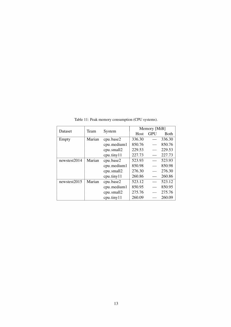
Table 11: Peak memory consumption (CPU systems).
Dataset Team SystemMemory [MiB]
Host GPU BothEmpty Marian cpu base2 336.30 — 336.30
cpu medium1 850.76 — 850.76cpu small2 229.53 — 229.53cpu tiny11 227.73 — 227.73
newstest2014 Marian cpu base2 523.93 — 523.93cpu medium1 850.98 — 850.98cpu small2 276.30 — 276.30cpu tiny11 260.86 — 260.86
newstest2015 Marian cpu base2 523.12 — 523.12cpu medium1 850.95 — 850.95cpu small2 275.76 — 275.76cpu tiny11 260.09 — 260.09
13

Table 12: Peak memory consumption (GPU systems).
Dataset Team SystemMemory [MiB]
Host GPU BothEmpty Marian gpu base4bit 788.67 14489 15277.67
gpu base 791.82 14489 15280.82gpu big 2077.75 14489 16566.75
Notre Dame all-l21-01-small 3198.89 991 4189.89baseline-small 3261.73 973 4234.73encoder-l21-01-small 3192.87 1003 4195.87encoder-l21-1-small 3164.45 1003 4167.45fc-l21-01-small 3160.32 999 4159.32fc-l21-1-small 3069.05 1049 4118.05fc-l21-10-small 3092.01 1057 4149.01fc-linf1-100-small 3116.35 1037 4153.35
newstest2014 Marian gpu base4bit 781.83 14641 15422.83gpu base 793.07 14641 15434.07gpu big 2078.78 14961 17039.78
Notre Dame all-l21-01-small 3199.95 9181 12380.95baseline-small 3285.20 9239 12524.20encoder-l21-01-small 3194.96 9169 12363.96encoder-l21-1-small 3164.86 9119 12283.86fc-l21-01-small 3160.80 9155 12315.80fc-l21-1-small 3070.67 9087 12157.67fc-l21-10-small 3068.12 9087 12155.12fc-linf1-100-small 3119.96 9087 12206.96
newstest2015 Marian gpu base4bit 783.05 14641 15424.05gpu base 789.34 14641 15430.34gpu big 2077.42 14961 17038.42
Notre Dame all-l21-01-small 3198.86 6171 9369.86baseline-small 3266.11 6359 9625.11encoder-l21-01-small 3193.13 6103 9296.13encoder-l21-1-small 3166.56 6135 9301.56fc-l21-01-small 3160.88 6159 9319.88fc-l21-1-small 3079.92 6017 9096.92fc-l21-10-small 3069.32 6015 9084.32fc-linf1-100-small 3130.95 6015 9145.95
14

Proceedings of the 3rd Workshop on Neural Generation and Translation (WNGT 2019), pages 15–22Hong Kong, China, November 4, 2019. c©2019 Association for Computational Linguistics
www.aclweb.org/anthology/D19-56%2d
Hello, It’s GPT-2 - How Can I Help You?Towards the Use of Pretrained Language Models
for Task-Oriented Dialogue Systems
Paweł Budzianowski1,2,3 and Ivan Vulic2,3
1Engineering Department, Cambridge University, UK2Language Technology Lab, Cambridge University, UK
3PolyAI Limited, London, [email protected], [email protected]
Abstract
Data scarcity is a long-standing and crucialchallenge that hinders quick development oftask-oriented dialogue systems across multipledomains: task-oriented dialogue models areexpected to learn grammar, syntax, dialoguereasoning, decision making, and language gen-eration from absurdly small amounts of task-specific data. In this paper, we demonstratethat recent progress in language modeling pre-training and transfer learning shows promiseto overcome this problem. We propose a task-oriented dialogue model that operates solelyon text input: it effectively bypasses ex-plicit policy and language generation modules.Building on top of the TransferTransfo frame-work (Wolf et al., 2019) and generative modelpre-training (Radford et al., 2019), we vali-date the approach on complex multi-domaintask-oriented dialogues from the MultiWOZdataset. Our automatic and human evaluationsshow that the proposed model is on par witha strong task-specific neural baseline. In thelong run, our approach holds promise to miti-gate the data scarcity problem, and to supportthe construction of more engaging and moreeloquent task-oriented conversational agents.
1 Introduction
Statistical conversational systems can be roughlyclustered into two main categories: 1) task-oriented modular systems and 2) open-domainchit-chat neural models. The former typically con-sist of independently trained constituent modulessuch as language understanding, dialogue manage-ment, and response generation. The main goal ofsuch systems is to provide meaningful system re-sponses which are invaluable in building conversa-tional agents of practical value for restricted do-mains and tasks. However, data collection andannotation for such systems is complex, time-intensive, expensive, and not easily transferable
(Young et al., 2013). On the other hand, open-domain conversational bots (Li et al., 2017; Serbanet al., 2017) can leverage large amounts of freelyavailable unannotated data (Ritter et al., 2010;Henderson et al., 2019a). Large corpora allowfor training end-to-end neural models, which typ-ically rely on sequence-to-sequence architectures(Sutskever et al., 2014). Although highly data-driven, such systems are prone to producing unre-liable and meaningless responses, which impedestheir deployment in the actual conversational ap-plications (Li et al., 2017).
Due to the unresolved issues with the end-to-end architectures, the focus has been extended toretrieval-based models. Here, the massive datasetscan be leveraged to aid task-specific applications(Kannan et al., 2016; Henderson et al., 2017,2019b). The retrieval systems allow for the fullcontrol over system responses, but the behaviourof the system is often highly predictable. It alsodepends on the pre-existing set of responses, andthe coverage is typically insufficient for a mul-titude of domains and tasks. However, recentprogress in training high-capacity language mod-els (e.g., GPT, GPT-2) (Radford et al., 2018, 2019)on large datasets reopens the question of whethersuch generative models can support task-orienteddialogue applications. Recently, Wolf et al. (2019)and Golovanov et al. (2019) showed that the GPTmodel, once fine-tuned, can be useful in the do-main of personal conversations. In short, theirapproach led to substantial improvements on thePersona-Chat dataset (Zhang et al., 2018), show-casing the potential of exploiting large pretrainedgenerative models in the conversational domain.1
In this paper, we demonstrate that large gener-ative models pretrained on large general-domain
1E.g., TransferTransfo (Wolf et al., 2019) yields gains inall crucial dialogue evaluation measures such as fluency, con-sistency and engagingness on the Persona-Chat dataset.
15

Figure 1: Dialogue-context-to-text task.
corpora can support task-oriented dialogue appli-cations. We first discuss how to combine a setof diverse components such as word tokenization,multi-task learning, and probabilistic sampling tosupport task-oriented applications. We then showhow to adapt the task-oriented dialogue frameworkto operate entirely on text input, effectively by-passing an explicit dialogue management moduleand a domain-specific natural language generationmodule. The proposed model operates entirelyin the sequence-to-sequence fashion, consumingonly simple text as input. The entire dialogue con-text, which includes the belief state, the databasestate and previous turns, is provided to the decoderas raw text. The proposed model follows the re-cently proposed TransferTransfo framework (Wolfet al., 2019), and relies on pretrained models fromthe GPT family (Radford et al., 2018, 2019).
Our results in the standard Dialogue-Context-to-Text task (see Figure 1) on the multi-domain Multi-WOZ dataset (Budzianowski et al., 2018b) suggestthat our GPT-based task-oriented dialogue modellearns to generate and understand domain-specifictokens, which in turn leads to a seamless adapta-tion to particular focused domains. While auto-matic evaluation indicates that our framework stillfalls slightly short of a strong task-specific neuralbaseline, it also hints at the main advantage of ourframework: it is widely portable and easily adapt-able to a large number of domains, bypassing theintricate modular design only at a small cost in per-formance. Furthermore, user-centered evaluationssuggest that there is no significant difference be-tween the two models.
2 From Unsupervised Pretraining toDialogue Modeling
Task-oriented dialogue modeling requires substan-tial amounts of domain-specific manually labeled
data. A natural question to ask is: Can we leveragetransfer learning through generative pretraining onlarge unlabelled corpora to enable task-oriented di-alogue modeling. In this work, we rely on the stan-dard language modeling (LM) pretraining, wherethe task is to predict the next word given the pre-ceding word sequence (Bengio et al., 2003). Theobjective maximizes the likelihood over the wordsequence S = {w1, ..., w|S|}:
L1(S) =
|S|∑
i=1
log P (wi|w0, w1, ..., wi−1). (1)
Transfer learning based on such LM pretrainingcombined with the Transformer decoder model(Vaswani et al., 2017) resulted in significantprogress across many downstream tasks (Rei,2017; Howard and Ruder, 2018; Radford et al.,2018, 2019).
2.1 TransferTransfo FrameworkGolovanov et al. (2019) and Wolf et al. (2019)achieved a first successful transfer of a genera-tive pretrained GPT model to an open-domain di-alogue task. The pretrained GPT model is fine-tuned in a multi-task learning fashion followingthe original work (Radford et al., 2018). The LMobjective from Eq. (1) is combined with the nextutterance classification task:
p(c, a) = softmax(hl ∗ Wh). (2)
c and a represent the context of the conversation(c) and a proposed answer (a), hl is the last hiddenstate of the transformer decoder, and Wh is learntduring the fine-tuning phase. The model signifi-cantly improves upon previous baselines over allautomatic dialogue evaluation metrics as well asin evaluation with human subjects when evaluatedon the Persona-Chat dataset (Zhang et al., 2018).
The GPT input consists of token embeddingsand positional embeddings. In order to move froma single-speaker setting to a setting with two inter-locutors, Wolf et al. (2019) introduced dialogue-state embeddings. These embeddings inform themodel whether the current token comes from anutterance of the first speaker or an utterance of thesecond speaker. The dialogue-state embeddingsare learned during the fine-tuning phase.
3 Domain Transfer for (Task-Oriented)Dialogue Modeling
We now briefly discuss several advances in model-ing of natural language that facilitate applicability
16

Figure 2: The framework for modeling task-oriented conversations based on a pretrained GPT model which usesonly unstructured simple text as input. The context, belief state, and database state are joined together withoutexplicit standalone dialogue policy and generation modules. The token-level (i.e., dialogue-state) embeddings arelearned following Wolf et al. (2019).
of pretrained generative models in task-oriented di-alogue modeling. To the best of our knowledge,this work is first to combine these existing compo-nents to enable task-oriented dialogue modeling.
3.1 Domain Adaptation and DelexicalizationDealing with out-of-vocabulary (OOV) words hasbeen a long-standing challenge in dialogue mod-eling, e.g., it is crucial for task-oriented genera-tion where the generated output is often delexical-ized (Wen et al., 2015). Delexicalization replacesslot values by their corresponding (generic) slottokens and it allows learning value-independentparameters. Recently, owing to subword-level to-kenisation (Sennrich et al., 2016), language mod-els are now able to deal with OOVs and domain-specific vocabularies more effectively (Radfordet al., 2018).
3.2 Simple Text-Only InputThere have been some empirical validations re-cently which suggest that posing NLP tasks in theform of simple text can yield improvements withunsupervised architectures (Wolf et al., 2019; Rad-ford et al., 2019). For instance, in task-orienteddialogue modeling the Sequicity model (Lei et al.,2018) sees the classification over the belief stateas a generation problem. That way, the entire dia-logue model pipeline is based on the sequence-to-sequence architecture: the output from one modelis the input to the subsequent recurrent model. Wefollow this approach by providing both the beliefstate and the knowledge base state in a simple textformat to the generator. This significantly simpli-fies the paradigm of building task-oriented mod-els: any new source of information can be simply
added to as another part of the text-only input pro-vided in “natural language”.
3.3 Transferring Language GenerationCapabilities
Transformer architecture shows ability to learnnew (i.e., domain-specific) token embeddings inthe fine-tuning phase (Radford et al., 2018; Wolfet al., 2019). This means that the GPT models canadapt through special tokens to particular tasks.By providing the input representation as text withdomain-specific tokens, we can use off-the-shelfarchitectures and adapt to the domain-specific in-put without the need of training new dialogue sub-modules. As mentioned in §2.1, the token levellayer (Figure 2) informs the transformer decoderwhat part of the input comes from the system sideor from the user side. In our framework, we createtwo task-oriented specific tokens (System andUser tokens) that are learned during fine-tuning.
3.4 Generation Quality
Finally, the long-standing problem of dull andrepetitive response generation (Li et al., 2017) hasbeen in the focus of recent work (Kulikov et al.,2018; Holtzman et al., 2019). Owing to new sam-pling strategies, generative models are now able tocreate longer and more coherent sequence outputs.This has been validated also for open-domain di-alogue modeling (Wolf et al., 2019; Golovanovet al., 2019). We experiment with standard de-coding strategies as well as with the recentlyproposed nucleus sampling procedure (Holtzmanet al., 2019). A standard greedy sampling strategy
17

chooses the most probable word as :
arg maxwi
= log P (wi|w0, w1, ..., wi−1).
On the other hand, nucleus sampling is restrictedonly to words from the p-th percentile of the dis-tribution during generation. The probabilities ofwords for which the cumulative sum exceeds thepercentile are rescaled and the sequence is sam-pled from this subset. We probe the ability of suchlarge pretrained models to generate more variedand semantically richer responses relying on nu-cleus sampling in lieu of greedy sampling withouthurting the actual performance.
4 Fine-Tuning GPT on MultiWOZ
To evaluate the ability of transferring the GPT gen-eration capability to constrained/focused dialoguetasks and domains, we rely on the multi-domainMultiWOZ dataset (Budzianowski et al., 2018b).MultiWOZ consists of 7 domains and 10, 438 di-alogues and it is substantially larger than previ-ous available datasets (Wen et al., 2017; El Asriet al., 2017). The conversations are natural asthey were gathered through human-human inter-actions. However, the dialogues are based ondomain-specific vocabulary such as booking IDsor telephone numbers that need to be delexicalizedas they are entirely database-dependent.
Natural Language as (the Only) Input. GPToperates solely on the text input. This is in oppo-sition to the standard task-oriented dialogue archi-tectures (Wen et al., 2017; Zhao et al., 2017) wherethe belief state and the database state are encodedin a numerical form. For example, the databasestate is typically defined as n-bin encodings repre-senting a number of available entities at the currentstate of the conversation (Wen et al., 2017). There-fore, we transform the belief state and the knowl-edge base representation to a simple text represen-tation. The belief state takes the following form:
Domain1 Slot1 Value1 Slot2 Value2Domain2 Slot1 ...
and the database representation is provided as:
Domain1 # of entitiesDomain2 # of entities ...
This is also similar in spirit to the Sequicity archi-tecture (Lei et al., 2018) where the second recur-rent model takes as input the belief state in the nat-ural language (i.e., simple text-only) form. In this
work, we also transform the knowledge base stateto a similar natural language format. These twopieces of information are then concatenated withthe history of the conversation forming the full di-alogue context, see Figure 2. Following Wolf et al.(2019), we add new token embeddings for two par-ties involved in the conversation to inform the at-tention layers what part of the context comes fromthe user, and what part is related to the system. Fig-ure 2 presents the final architecture.
Training Details. We use the open-source im-plementation of the GPT architecture that providesboth GPT and GPT-2 fine-tunable checkpoints.2
Following previous work (Radford et al., 2018;Wolf et al., 2019), we set the weight on the lan-guage model loss to be two times higher than theone for the response prediction. The parametersfor the batch size (24), learning rate (1e-5) and thenumber of candidates per sequence (2) were cho-sen based on the grid search. 3
5 Results and Analysis
Following prior work (Budzianowski et al., 2018b;Zhao et al., 2019; Chen et al., 2019), our evalu-ation task is the dialogue-context-to-text genera-tion task (see Figure 1). Given a dialogue history,the oracle belief state and the database state, themodel needs to output the adequate response. Byrelying on the oracle belief state, prior work hasbypassed the possible errors originating from nat-ural language understanding (Budzianowski et al.,2018b).
The main evaluation is based on the comparisonbetween the following two models: 1) the base-line is a neural response generation model with anoracle belief state obtained from the wizard anno-tations as in (Budzianowski et al., 2018a); 2) themodel proposed in §4 and shown in Figure 2 thatworks entirely with text-only format as input (see§4). We test all three available pretrained GPTmodels - the original GPT model (Radford et al.,2018). and two GPT-2 models referred to as small(GPT2) and medium (GPT2-M) (Radford et al.,2019).
2https://github.com/huggingface/transfer-learning-conv-ai
3We searched over the following values: learning rates ∈{1-e4, 1-e5, 5-e6, 1-e6}, batch sizes ∈ {8, 12, 16, 20, 24} andcandidate set sizes ∈ {1, 2, 4, 6}.
18

Baseline GPT GPT2-S GPT2-M
Inform (%) 76.7 71.53 66.43 70.96Success (%) 64.63 55.36 55.16 61.36BLEU (%) 18.05 17.80 18.02 19.05
Table 1: Evaluation on MultiWOZ with the greedysampling procedure.
Baseline GPT GPT2-S GPT2-M
Inform (%) 72.57 70.43 69.3 73.96Success (%) 57.63 51.0 54.93 61.20BLEU (%) 15.75 15.65 15.64 16.55
Table 2: Evaluation on MultiWOZ with the nucleussampling procedure.
5.1 Evaluation with Automatic Measures
We report scores with three standard automaticevaluation measures. Two of them relate to thedialogue task completion: whether the system hasprovided an appropriate entity (Inform) and thenanswered all requested attributes (Success rate).Finally, fluency is measured by the BLEU score(Papineni et al., 2002).
First, three versions of GPT were fine-tuned onMultiWOZ and evaluated with greedy sampling.The results are summarized in Table 1). Theyshow that the baseline obtains the highest score ontask-related metrics while the highest BLUE scorewas achieved by GPT2-M. Although the resultsare lower for the GPT-based methods, we note thedesign simplicity of the GPT-based task-orienteddialogue models. Further, the gap in performancemight be partially attributed to the chosen greedysampling procedure which puts too much focuson the properties of the original pretraining phase(Holtzman et al., 2019).
Therefore, we also report the results with thenucleus sampling method in Table 2. The scoresconfirm the importance of choosing the correctsampling method. The GPT2 models improvethe score on Inform and Success metrics. It isworth noting the consistent drop in BLUE scoresacross all models. This comes from the fact thatnucleus sampling allows for increased variability:this might reduce the probability of generatingdomain-specific tokens.
We have also qualitatively analyzed a sampleof successful dialogues. Only around 50% of di-alogues are successful both with the baseline andwith the GPT-based models. Moreover, there areno clearly observed distinct patterns between suc-cessful dialogues for the two model types. This
Model 1 vs Model 2
GPT 59 % 41% BaselineGPT 46 % 54 % TargetGPT2 46 % 54 % TargetGPT2 45 % 55 % BaselineBaseline 43 % 57 % TargetGPT2 51 % 49 % GPT
Table 3: Human ranking of responses between all pairsof four analyzed models and the original responses.
suggests that they might be effectively ensembledusing a ranking model to evaluate the score of eachresponse (Henderson et al., 2019b). We will inves-tigate the complementarity of the two approachesalong with ensemble methods in future work.
5.2 Human Evaluation
In another, now user-centered experiment, the goalwas to analyze the generation quality. Turkers, na-tive speakers of English, were asked to rate theirbinary preference when presented with one-turnresponses from the baseline, GPT, GPT2-M andthe original dialogues (Target). The turkers wererequired to choose what response they prefer whenpresented with two responses from two differentmodels, resulting in more than 300 scores per eachmodel pair.
The results are summarized in Table 3, whilesome example dialogues with responses are pro-vided in Figure 3. As expected, the original re-sponses are ranked higher than all neural modelswith the largest difference observed between theoracle and the baseline model. Although the gen-erated output from the GPT is strongly preferredagainst the neural baseline, interestingly the oppo-site is observed with the GPT2 model. These in-conclusive results call for further analyses in fu-ture work, and also show that there are no sub-stantial differences in the quality of generated re-sponses when comparing the strong neural base-line and the GPT-based models.
6 Conclusion
In this paper, we have made a first step towardsleveraging large pretrained generative models formodeling task-oriented dialogue in multiple do-mains. The simplicity of the fine-tuning proce-dure where all necessary information can be en-coded as simple text enables a quick adaptationto constrained domains and domain-specific vo-
19

cabularies. We hope that this framework will in-form and guide future research in hope of simulta-neously improving and simplifying the design oftask-oriented conversational systems.
ReferencesYoshua Bengio, Réjean Ducharme, Pascal Vincent, and
Christian Jauvin. 2003. A neural probabilistic lan-guage model. Journal of machine learning research,3(Feb):1137–1155.
Paweł Budzianowski, Iñigo Casanueva, Bo-HsiangTseng, and Milica Gašic. 2018a. Towards end-to-end multi-domain dialogue modelling. Tech.Rep. CUED/F-INFENG/TR.706, University of Cam-bridge, Engineering Department.
Paweł Budzianowski, Tsung-Hsien Wen, Bo-HsiangTseng, Iñigo Casanueva, Stefan Ultes, Osman Ra-madan, and Milica Gasic. 2018b. MultiWOZ-ALarge-scale multi-domain wizard-of-oz dataset fortask-oriented dialogue modelling. In Proceedings ofEMNLP, pages 5016–5026.
Wenhu Chen, Jianshu Chen, Pengda Qin, XifengYan, and William Yang Wang. 2019. Semanticallyconditioned dialog response generation via hierar-chical disentangled self-attention. arXiv preprintarXiv:1905.12866.
Layla El Asri, Hannes Schulz, Shikhar Sharma,Jeremie Zumer, Justin Harris, Emery Fine, RahulMehrotra, and Kaheer Suleman. 2017. Frames: Acorpus for adding memory to goal-oriented dialoguesystems. In Proceedings of SIGDIAL, pages 207–219.
Sergey Golovanov, Rauf Kurbanov, Sergey Nikolenko,Kyryl Truskovskyi, Alexander Tselousov, andThomas Wolf. 2019. Large-scale transfer learningfor natural language generation. In Proceedings ofthe 57th Annual Meeting of the Association for Com-putational Linguistics, pages 6053–6058, Florence,Italy. Association for Computational Linguistics.
Matthew Henderson, Rami Al-Rfou, Brian Strope, Yun-hsuan Sung, Laszlo Lukacs, Ruiqi Guo, Sanjiv Ku-mar, Balint Miklos, and Ray Kurzweil. 2017. Effi-cient natural language response suggestion for smartreply. arXiv preprint arXiv:1705.00652.
Matthew Henderson, Paweł Budzianowski, IñigoCasanueva, Sam Coope, Daniela Gerz, Girish Ku-mar, Nikola Mrkšic, Georgios Spithourakis, Pei-Hao Su, Ivan Vulic, and Tsung-Hsien Wen. 2019a.A repository of conversational datasets. In Pro-ceedings of the Workshop on NLP for Conversa-tional AI. Data available at github.com/PolyAI-LDN/conversational-datasets.
Matthew Henderson, Ivan Vulic, Daniela Gerz, IñigoCasanueva, Paweł Budzianowski, Sam Coope,Georgios Spithourakis, Tsung-Hsien Wen, Nikola
Mrksi’c, and Pei-Hao Su. 2019b. Training neural re-sponse selection for task-oriented dialogue systems.In Proceedings of ACL.
Ari Holtzman, Jan Buys, Maxwell Forbes, and YejinChoi. 2019. The curious case of neural text degener-ation. arXiv preprint arXiv:1904.09751.
Jeremy Howard and Sebastian Ruder. 2018. Universallanguage model fine-tuning for text classification. InProceedings of the 56th Annual Meeting of the As-sociation for Computational Linguistics (Volume 1:Long Papers), pages 328–339.
Anjuli Kannan, Karol Kurach, Sujith Ravi, TobiasKaufmann, Andrew Tomkins, Balint Miklos, GregCorrado, Laszlo Lukacs, Marina Ganea, PeterYoung, et al. 2016. Smart reply: Automated re-sponse suggestion for email. In Proceedings of the22nd ACM SIGKDD International Conference onKnowledge Discovery and Data Mining, pages 955–964. ACM.
Ilya Kulikov, Alexander H Miller, Kyunghyun Cho,and Jason Weston. 2018. Importance of a searchstrategy in neural dialogue modelling. arXivpreprint arXiv:1811.00907.
Wenqiang Lei, Xisen Jin, Min-Yen Kan, ZhaochunRen, Xiangnan He, and Dawei Yin. 2018. Sequicity:Simplifying task-oriented dialogue systems with sin-gle sequence-to-sequence architectures. In Proceed-ings of ACL, pages 1437–1447.
Jiwei Li, Will Monroe, Tianlin Shi, Sébastien Jean,Alan Ritter, and Dan Jurafsky. 2017. Adversariallearning for neural dialogue generation. In Proceed-ings of the 2017 Conference on Empirical Methodsin Natural Language Processing, pages 2157–2169.
Kishore Papineni, Salim Roukos, Todd Ward, and Wei-Jing Zhu. 2002. BLEU: A method for automaticevaluation of machine translation. In Proceedingsof ACL, pages 311–318.
Alec Radford, Karthik Narasimhan, Tim Salimans, andIlya Sutskever. 2018. Improving language under-standing by generative pre-training.
Alec Radford, Jeffrey Wu, Rewon Child, David Luan,Dario Amodei, and Ilya Sutskever. 2019. Languagemodels are unsupervised multitask learners. OpenAIBlog, 1(8).
Marek Rei. 2017. Semi-supervised multitask learn-ing for sequence labeling. In Proceedings of the55th Annual Meeting of the Association for Compu-tational Linguistics (Volume 1: Long Papers), pages2121–2130.
Alan Ritter, Colin Cherry, and Bill Dolan. 2010. Un-supervised modeling of twitter conversations. InHuman Language Technologies: The 2010 AnnualConference of the North American Chapter of the As-sociation for Computational Linguistics, pages 172–180.
20

Rico Sennrich, Barry Haddow, and Alexandra Birch.2016. Neural machine translation of rare words withsubword units. In Proceedings of the 54th AnnualMeeting of the Association for Computational Lin-guistics (Volume 1: Long Papers), volume 1, pages1715–1725.
Iulian Vlad Serban, Alessandro Sordoni, Ryan Lowe,Laurent Charlin, Joelle Pineau, Aaron Courville, andYoshua Bengio. 2017. A hierarchical latent variableencoder-decoder model for generating dialogues. InProceedings of AAAI, pages 3295–3301.
Ilya Sutskever, Oriol Vinyals, and Quoc V Le. 2014.Sequence to sequence learning with neural networks.In Proceedings of NeurIPS, pages 3104–3112.
Ashish Vaswani, Noam Shazeer, Niki Parmar, JakobUszkoreit, Llion Jones, Aidan N Gomez, ŁukaszKaiser, and Illia Polosukhin. 2017. Attention is allyou need. In Advances in neural information pro-cessing systems, pages 5998–6008.
Tsung-Hsien Wen, Milica Gašic, Nikola Mrkšic, Pei-Hao Su, David Vandyke, and Steve Young. 2015. Se-mantically conditioned lstm-based natural languagegeneration for spoken dialogue systems. In Proceed-ings of the 2015 Conference on Empirical Methodsin Natural Language Processing (EMNLP).
Tsung-Hsien Wen, David Vandyke, Nikola Mrkšic,Milica Gašic, Lina M Rojas-Barahona, Pei-Hao Su,Stefan Ultes, and Steve Young. 2017. A network-based end-to-end trainable task-oriented dialoguesystem. In Proceedings of EACL, pages 438–449.
Thomas Wolf, Victor Sanh, Julien Chaumond, andClement Delangue. 2019. Transfertransfo: Atransfer learning approach for neural networkbased conversational agents. arXiv preprintarXiv:1901.08149.
Steve Young, Milica Gašic, Blaise Thomson, and Ja-son D. Williams. 2013. POMDP-based statisticalspoken dialog systems: A review. Proceedings ofthe IEEE, 101(5):1160–1179.
Saizheng Zhang, Emily Dinan, Jack Urbanek, ArthurSzlam, Douwe Kiela, and Jason Weston. 2018. Per-sonalizing dialogue agents: I have a dog, do youhave pets too? In Proceedings of the 56th An-nual Meeting of the Association for ComputationalLinguistics (Volume 1: Long Papers), pages 2204–2213.
Tiancheng Zhao, Kaige Xie, and Maxine Eskenazi.2019. Rethinking action spaces for reinforcementlearning in end-to-end dialog agents with latent vari-able models. In Proceedings of the 2019 Confer-ence of the North American Chapter of the Associ-ation for Computational Linguistics: Human Lan-guage Technologies, Volume 1 (Long and Short Pa-pers), pages 1208–1218.
Tiancheng Zhao, Ran Zhao, and Maxine Eskenazi.2017. Learning discourse-level diversity for neuraldialog models using conditional variational autoen-coders. In Proceedings of ACL, pages 654–664.
21

Figure 3: The comparison of generated responses from the baseline model and GPT2-M.
22

Proceedings of the 3rd Workshop on Neural Generation and Translation (WNGT 2019), pages 23–31Hong Kong, China, November 4, 2019. c©2019 Association for Computational Linguistics
www.aclweb.org/anthology/D19-56%2d
Recycling a Pre-trained BERT Encoder for Neural Machine Translation
Kenji Imamura and Eiichiro SumitaNational Institute of Information and Communications Technology
3-5 Hikaridai, Seika-cho, Soraku-gun, Kyoto 619-0289, Japan{kenji.imamura,eiichiro.sumita}@nict.go.jp
Abstract
In this paper, a pre-trained BidirectionalEncoder Representations from Transformers(BERT) model is applied to Transformer-based neural machine translation (NMT).
In contrast to monolingual tasks, the numberof unlearned model parameters in an NMTdecoder is as huge as the number of learnedparameters in the BERT model. To trainall the models appropriately, we employ two-stage optimization, which first trains only theunlearned parameters by freezing the BERTmodel, and then fine-tunes all the sub-models.
In our experiments, stable two-stage optimiza-tion was achieved, in contrast the BLEU scoresof direct fine-tuning were extremely low. Con-sequently, the BLEU scores of the proposedmethod were better than those of the Trans-former base model and the same model with-out pre-training. Additionally, we confirmedthat NMT with the BERT encoder is more ef-fective in low-resource settings.
1 Introduction
Bidirectional Encoder Representations fromTransformers (BERT) (Devlin et al., 2019) is alanguage representation model trained in advanceon a very large monolingual dataset. We adaptthis model to our own tasks after fine-tuning(Freitag and Al-Onaizan, 2016; Servan et al.,2016) using task-specific data. Systems usingBERT have achieved high accuracy in varioustasks, such as the General Language Understand-ing Evaluation (GLUE) benchmark (Wang et al.,2019) and the reading comprehension benchmarkusing the Stanford Question Answering Dataset(SQuAD) (Rajpurkar et al., 2018). However,most tasks using BERT are monolingual becauseit was originally developed for natural languageunderstanding.
Recently, models in which the ideas of BERTare extended to multiple languages have been pro-posed (Lample and Conneau, 2019). These mod-els, which are pre-trained using multilingual data,are called cross-lingual language models (XLMs).We can construct a machine translation system us-ing two XLM models as the encoder and decoder.
In this paper, we apply a pre-trained BERT en-coder to neural machine translation (NMT) basedon the Transformer (Vaswani et al., 2017). Specif-ically, the encoder of the Transformer NMT is re-placed with the BERT encoder. Generally, sys-tems using BERT, including machine translationsystems based on an XLM, are fine-tuned usingtask-specific data. However, stable training is dif-ficult using simple fine-tuning because the num-ber of unlearned parameters is huge in our system.Therefore, we employ two-stage training, whichfirst trains only unlearned parameters and then ap-plies fine-tuning.
Our experimental results demonstrated thattwo-stage optimization stabilized training,whereas direct fine-tuning made the BLEU scoresquite low. As a result, the BLEU scores improvedin comparison with the scores of the Transformerbase model and models with the same structurebut without pre-training. Our results indicatethat we can reuse neural networks trained for onepurpose (natural language understanding, in thiscase) for another purpose (machine translation, inthis case) if we use two-stage optimization. Fromthis viewpoint, this paper presents an example ofnetwork recycling.
The remainder of this paper is organized as fol-lows. In Section 2, an overview of the BERT re-lated models is provided. In Section 3, our pro-posal, that is, NMT using the BERT model andits training method, is described. In Section 4,the proposed method is evaluated through exper-iments. In Section 5, we discuss back-translation
23

and model recycling, including related work. Fi-nally, we conclude the paper in Section 6.
2 Pre-trained Language Models
2.1 BERT
The form of the BERT model (Devlin et al., 2019)is the same as that of a Transformer encoder, inwhich the input is a word sequence and the outputconsists of representations that correspond to theinput words. The input contexts are encoded bymulti-head self-attention mechanisms.
BERT models are distributed with pre-training.The distributed models have a depth of 12 or 24layers, which is deeper than the Transformer basemodel (six layers). Users (or system develop-ers) construct various systems by adding a smallnetwork to adapt BERT to their own tasks andfine-tune the system using task-specific data. Forexample, when the BERT model is used for adocument classification task, a classifier is con-structed by adding a generation layer for classi-fication (which consists of linear and softmax sub-layers) to the BERT model. Similarly, when anamed entity recognizer is constructed, generationlayers that convert word representations to namedentity tags are added, and the entire model is fine-tuned. The numbers of additional parameters inthese models are much smaller than the number ofparameters in the BERT model.
The BERT model is pre-trained to performtwo tasks: masked language modeling and next-sentence prediction. Both tasks train the model toimprove its language prediction performance.
The masked language model is trained to restorethe original word sequence from noisy input. Inthis task, some words are replaced with special to-kens, [MASK], or other words. For instance, ifthe original sentence is “my dog is hairy”and “my dog is [MASK]” is given as the in-put word sequence, then the system predicts thatthe original word for [MASK] was hairy. Dur-ing prediction, both forward and backward con-texts in a sentence are used.
In the next-sentence prediction task, the systemlearns whether two given sentences are consecu-tive. To implement binary classification using theTransformer, a special token [CLS] is placed atthe head of an input sentence, and classification isperformed from the representation of [CLS]. Ad-ditionally, [SEP] is used as a sentence separator.
BERT has achieved high accuracy on various
tasks, such as the GLUE benchmark (Wang et al.,2019) and the reading comprehension benchmarkusing SQuAD (Rajpurkar et al., 2018). However,the above tasks are monolingual.
2.2 XLMs
XLMs, in which the ideas of BERT are extended tomultiple languages (Lample and Conneau, 2019)have been proposed. Although the form of theXLM model is also Transformer, it is trained frommultilingual corpora. It also learns bilingual cor-respondences in a Transformer model by inputtinga connected bilingual sentence.
Machine translation can be realized usingXLMs by regarding two pre-trained models as anencoder and decoder. NMT using BERT describedin this paper is fundamentally the same as XLM-based NMT. However, our aim is to connect differ-ent systems, and we regard our approach as modelrecycling (Ramachandran et al., 2016) using theBERT encoder and Transformer decoder.
Most pre-trained systems, including XLM-based machine translation, are trained only usingfine-tuning (Devlin et al., 2019; Lample and Con-neau, 2019). However, if the number of unlearnedparameters is huge compared with the number ofpre-trained parameters, then the pre-trained pa-rameter values will be destroyed due to a phe-nomenon called catastrophic forgetting (Goodfel-low et al., 2013), and consequently, training willdiverge. We must suppress this problem to stablytrain the model.
3 NMT with BERT
In this section, we describe our proposal: NMTusing the BERT encoder.
3.1 Model
The NMT system in this paper is an encoder-decoder based on the Transformer. The structureis shown in Figure 1. Because the BERT modelis also the Transformer encoder, we adopt it as theencoder for NMT without modification. The out-puts from the BERT encoder, which are represen-tations of source words, are input to the contextattention mechanism in the Transformer decoderto generate a translation. Note that we call the en-coder of the conventional NMT the Transformerencoder to distinguish it from the BERT encoder.The number of layers in the Transformer decoderis fixed to six throughout the paper.
24

Sub-words &Special Tokens
ShiftedOutput Tokens
Output Tokens
Input Sentence
[CLS] �� ... [SEP]��
BERT Tokenizer
Embeddings
Self-Attention
Feed Forward
Nx
BERT Encoder
ℎ��� ℎ� ... ℎ��ℎ�
<bos> � ...�
Embeddings
Self-Attention
Feed Forward
Context-Attention
6x
Transformer Decoder
Generator
<eos>� ...�
Figure 1: Structure of NMT using a BERT encoder.
Because the BERT encoder is pre-trained usinga specific tokenizer, we must use the BERT tok-enizer when we apply it to machine translation.The BERT tokenizer includes sub-word segmenta-tion based on WordPiece (Wu et al., 2016). Addi-tionally, the input to the encoder contains [CLS]and [SEP] tokens at the head and tail, respec-tively.
Although the Transformer decoder is used here,we assume that a recurrent neural network decoder(Sutskever et al., 2014; Bahdanau et al., 2014) canalso be applied,.
3.2 TrainingWhen we construct a system using pre-trainedBERT models, we generally add a task-specificnetwork and fine-tune the system using task-specific data. Because the additional network issmall (i.e., the number of additional parameters issmall), the models can be learned by fine-tuning.
In this paper, the additional network is the de-coder, whose number of parameters is huge. In-deed, the number of model parameters of theBERT encoder (pre-trained) and Transformer de-coder (unlearned) used in Section 4 were 110Mand 80M, respectively. We cannot train such alarge number of unlearned parameters only byfine-tuning. Thus, we employ two-stage optimiza-tion in this paper, that is decoder training and fine-tuning.
3.2.1 Decoder TrainingIn this stage, only the decoder parameters are up-dated while the encoder parameters are frozen.
Specifically, the model is trained using parallelcorpora, as in conventional NMTs. During train-ing, however, backpropagation is only applied tothe decoder and is dropped before the encoder.This means that we do not need to compute thegradients and maintain the input/output values inthe BERT encoder, and we can train the modelusing GPUs with a relatively small memory eventhough the model size is huge. Dropout is only ap-plied to the Transformer decoder, that is, it is notapplied to the BERT encoder.
Note that decoder training continues until theloss of the development set is minimized. We dis-cuss the efficient number of epochs for the decodertraining in Section 4.3 when we combine it withfine-tuning.
3.2.2 Fine-Tuning
In the fine-tuning stage, model parameters in theBERT encoder are also updated to optimize the en-tire model.
Although the model has already been traineduntil the loss of the development set is minimizedduring decoder training, both the encoder and de-coder are further optimized in an end-to-end man-ner by updating the encoder parameters. Dropoutis applied to both the BERT encoder and Trans-former decoder. In the fine-tuning stage, back-propagation is applied to all layers, and a largeamount of memory is consumed.
25

Task Set # Sentences # Tokens(En)
WMT-2014 train 4,468,840 116MEn-De newstest2013 3,000 66K
newstest2014 2,737 63Knewstest2015 2,169 68K
IWSLT-2015 train 133,317 2.7MEn-Vi tst2012 1,553 34K
tst2013 1,268 34K
Table 1: Sizes of the experimental datasets.
4 Experiments
4.1 Experimental SettingsData: In this paper, we used data for sharedtasks that were pre-processed by the Stanford NLPGroup.1 The sizes of the datasets are shown in Ta-ble 1.
The first task is the news translation taskof English-to-German (En-De) from the Work-shop on Statistical Machine Translation (WMT-2014) (Bojar et al., 2014). Four sets in totalhave been published. In this paper, we usednewstest2013 as the development set, and theother two sets (newstest2014 and 2015) wereused as test sets.
Moreover, to contrast the results with those ofa low-resource setting, we also used the English-to-Vietnamese (En-Vi) corpus used in the Inter-national Workshop on Spoken Language Transla-tion (IWSLT-2015) (Cettolo et al., 2015). We usedtst2012 as the development set and tst2013as the test set.
The target sentences of the above data were fur-ther segmented into 16K sub-words using byte-pair encoding (Sennrich et al., 2016b). For thesource sentences, we segmented 30K sub-wordsusing the BERT tokenizer if the encoder modelwas BERT. If the encoder was the conventionalTransformer, we segmented the source sentencesinto 16K sub-words using our byte-pair encoder.
BERT Model: We used a pre-trained modelpublished in the BERT GitHub repository2 calledthe BERT base model, whose features are uncasedinputs, 12 layers, 768 hidden units, and 12 heads.3
The number of parameters is about 110M. This1https://nlp.stanford.edu/projects/
nmt/2https://github.com/google-research/
bert3https://storage.googleapis.com/bert_
models/2018_10_18/uncased_L-12_H-768_A-12.zip
Type Option ValueDecoder Batch size Approx. 500 sents.training Optimizer Adam
β1 = 0.9, β2 = 0.99Learning rate 4.0 × 10⁻⁴
Warm-up 5 epochsCool-down Inverse square rootLabel smoothing 0.1Dropout 0.15Loss function Label-smoothed cross
entropyInitializer Xavier uniform
Fine-tuning Identical to decoder training except forthe learning rate and warm-up
Test Beam size 10Length penalty 1.0 (fixed)
Table 2: Hyperparameter settings.
model was trained using BookCorpus (Zhu et al.,2015) and English Wikipedia (3.3G words in to-tal).
Note that we converted the published model intoa model that is compatible with the PyTorch li-brary using a tool4 because it was trained for theTensorFlow library.
Translation System: We used fairseq5 as thebasic translator. It is an NMT system constructedon the PyTorch library and includes Transformermodels. We replaced its encoder with the BERTmodel and used the fairseq decoder without modi-fication.
The decoder used here was six-layer Trans-former. We set the numbers of hidden units andheads to be the same as those of the encoder (i.e.,768 units and 12 heads) to incorporate encoderoutputs into the decoder using the context atten-tion mechanism.
Hyperparameters: Table 2 summarizes the hy-perparameter settings. The hyperparameters forfine-tuning were almost the same as those of de-coder training, except for the learning rate (LR)and warm-up.
Evaluation: We used BLEU (Papineni et al.,2002) as the evaluation metric. The MultEvaltool (Clark et al., 2011)6 was used for statisti-cal testing, which is based on the bootstrap re-sampling method. The significance level was 5%(p < 0.05).
4https://github.com/huggingface/pytorch-pretrained-BERT
5https://github.com/pytorch/fairseq6https://github.com/jhclark/multeval
26

BLEU ↑System LR Dev. PPL ↓ 2013 2014 2015 Remark
Baselines Transformer base 4.0 × 10⁻⁴ 4.23 26.29 27.22 29.48 Stat. test baselineTransformer BERT size 4.0 × 10⁻⁴ 4.04 26.15 27.09 29.32
NMT Direct fine-tuning 8 × 10⁻⁵ 4.28 0.13 (-) 0.10 (-) 0.12 (-) # Epochs = 33with BERT 4.0 × 10⁻⁴ 4.09 0.48 (-) 0.42 (-) 0.54 (-) # Epochs = 29
Proposed:Decoder training only 4.0 × 10⁻⁴ 4.76 24.13 (-) 23.62 (-) 25.74 (-) # Epochs = 65
+ Fine-tuning 4 × 10⁻⁵ 3.93 27.14 (+) 28.27 (+) 30.68 (+) # Epochs = 218 × 10−5 3.92 27.05 (+) 28.90 (+) 30.89 (+) # Epochs = 9
1.2 × 10⁻⁴ 3.93 27.03 (+) 28.50 (+) 30.51 (+) # Epochs = 111.6 × 10⁻⁴ 3.94 26.64 28.59 (+) 30.51 (+) # Epochs = 112.0 × 10⁻⁴ 3.95 26.89 (+) 28.67 (+) 30.24 (+) # Epochs = 124.0 × 10⁻⁴ N/A because training did not converge
Table 3: Results of the system comparison.The bold values indicate the best results. The (+) and (-) symbols indicate that the results significantlyimproved or degraded (p < 0.05) with respect to the Transformer base model, respectively.
4.2 System Comparison
In this section, we compare systems using WMT-2014 data.
We compare the proposed methods withVaswani et al. (2017)’s Transformer base model(6 layers, 512 hidden units, and 8 heads) as thebaseline. For reference, we also use another Trans-former NMT called Transformer BERT size, inwhich the model structure of the encoder agreeswith that of the BERT encoder (i.e., 12 layers, 768hidden units, and 12 heads). This system is com-pared to determine whether the model capacity in-fluences translation quality.
The decoders of the proposed systems were firsttrained until the loss of the development set wasminimized (newstest2013), and then the sys-tems were fine-tuned. The learning rates duringfine-tuning were changed from 1/10 to 1 timesthose of the decoder training. The warm-up pe-riods were also changed to be proportional to thelearning rates. The results are shown in Table 3. Inthe table, Dev. PPL indicates the perplexity of thedevelopment set, and the years of the BLEU scoresdenote the results of newstest2013, 2014,and 2015, respectively.
First, we compare the baselines. TransformerBERT size yielded a better model than thatof Transformer base because its perplexity waslower. However, the BLEU scores were slightlydegraded (but not significantly). Increasing thenumber of parameters did not lead to better trans-lation quality.
Next, we compare the NMT system with BERTand the Transformer base. When the entire model
was directly fine-tuned, training converged but theBLEU scores dramatically decreased even if weused different learning rates. This implies that themodels were broken.7 Unlike monolingual tasksusing the BERT model, it was difficult to directlyapply fine-tuning for NMT using the pre-trainedBERT encoder.
By contrast, in the decoder training-only model,namely the model immediately after decoder train-ing, training was successfully finished. However,the development perplexity was higher and theBLEU scores were lower than those of the base-line. The entire model was not learned completelybecause of the data mismatch, which was that thepre-training and our training data were different.
After fine-tuning, by contrast, the perplexity de-creased and the BLEU score increased. Comparedwith those of Transformer base, the BLEU scoressignificantly improved in almost all cases. Be-cause the development perplexity decreased withrespect to Transformer BERT size, we can say thatthese improvements resulted from learning perfor-mance rather than the number of model parame-ters.
We changed the learning rates from 4×10⁻⁵ to4.0×10−4 in the fine-tuning. When the learningrate was 4.0× 10⁻⁴ (the decoder training learn-ing rate), we could not tune the model becausethere was no convergence. For the other learn-ing rates, there were no large differences in per-
7Indeed, very long translations were generated due to fre-quent repetition in the case of the low learning rate (8 ×10⁻⁵). We suppose that the decoder was not learned suffi-ciently. In the case of the high learning rate (4.0 × 10⁻⁴),long and completely wrong translations were generated. Wesuppose that the encoder was broken.
27

Decoder training Fine-tuning BLEU ↑# Epochs Dev. PPL ↓ # Epochs Dev. PPL ↓ 2013 2014 2105 Remark
0 — 33 4.28 0.13 (-) 0.10 (-) 0.12 (-) Direct fine-tuning1 33.05 34 4.23 26.67 28.77 30.16 (-)2 11.47 20 4.20 26.80 28.58 30.823 8.12 18 4.10 27.41 28.93 30.785 6.69 18 4.02 27.20 28.43 (-) 30.80
10 5.50 15 3.96 27.33 28.59 30.4220 5.08 18 3.91 27.00 28.87 30.9230 4.89 10 3.92 27.18 28.39 (-) 30.7040 4.86 12 3.91 27.01 29.04 30.7050 4.81 11 3.91 27.02 28.65 30.7765 4.76 9 3.92 27.05 28.90 30.89 Decoder training converged
Baseline for statistical testing
Table 4: Changes in the perplexity of the development set (Dev. PPL) and BLEU scores with respect to the numberof decoder training epochs.
plexity or BLEU scores. However, we confirmedthat there were some differences in convergencetime (# Epochs), and fine-tuning converged in nineepochs when the learning rate was 8×10⁻⁵. There-fore, we fixed the learning rate for fine-tuning to8×10−5 in our subsequent experiments.
4.3 Number of Epochs for Decoder TrainingThe proposed method first performs decoder train-ing until convergence, and then applies fine-tuning. However, this approach may not be opti-mal because decoder training is slow. For instance,it took 65 epochs for decoder training in the exper-iment in the previous section. In this section, weinvestigate whether decoder training can be mademore efficient by stopping it before convergence.
Table 4 shows the results after fine-tuning whendecoder training was stopped after various num-bers of epochs. Fine-tuning was conducted un-til convergence in all cases. The table shows thechanges in development perplexity and the BLEUscores, whose baselines are shown on the bottomline. Note that zero epochs of decoder training(the top line) mean that fine-tuning was directlyapplied without decoder training (the same as inTable 3).
As the number of epochs of decoder training de-creased, fine-tuning required more epochs and thefinal perplexity increased. However, the BLEUscores were almost stable. Indeed, only threescores significantly decreased with respect to thebaseline.
Because we assume that the optimal settings ofdecoder training depend on the data and hyperpa-rameters, we cannot provide explicit criteria val-ues in this paper. At the very least, our experimen-tal results show the following conclusions.
• To shorten the total training time, it is bestto perform decoder training for three epochs(3 + 18 = 21 epochs in total).
• To obtain the best model (i.e., the modelwith the minimum development perplexity),20 epochs are sufficient for decoder training(which yields a Dev. PPL of 3.91).
4.4 Experiment on a Low-resource LanguagePair
In this section, the effect of the BERT encoder ona low-resource setting is explored using IWSLT-2015 En-Vi data (133K sentences). All experi-mental settings, except for the corpus, were thesame as those in Section 4.1. The results areshown in Table 5.
In the low-resource setting, the developmentperplexity decreased in comparison with the base-line when applying the BERT encoder and per-forming decoder training only. However, theBLEU score degraded, as in the large data setting(Section 4.2).
By contrast, when fine-tuning was applied, boththe perplexity and BLEU scores largely improvedwith respect to the baseline. The BLEU score oftst2013 improved by +3.45. Considering thescore of newstest2015 in the experiment inTable 3 was +1.41 for the same settings, these re-sults show that the BERT encoder is more effectivefor improving translation quality in a low-resourcesetting.
5 Discussion and Related Work
5.1 Contrast with Back-TranslationBack-translation (Sennrich et al., 2016a) is a tech-nique to improve translation quality using mono-
28

BLEU ↑System LR Dev. PPL ↓ 2012 2013
Baseline Transformer base 4.0 × 10⁻⁴ 11.54 24.03 26.12NMT with BERT Proposed: Decoder training only 4.0 × 10⁻⁴ 11.45 21.77 (-) 23.23 (-)
+ Fine-tuning 8 × 10⁻⁵ 8.98 26.77 (+) 29.57 (+)
Table 5: Results of the IWSLT-2015 data.
lingual corpora. It translates monolingual cor-pora of the target language into the source lan-guage, generates pseudo-parallel sentences, andtrains the source-to-target translator from a mix-ture of pseudo- and manually created parallel cor-pora. Because BERT encoders are trained us-ing source monolingual corpora, they complementeach other.
However, there are differences between BERTencoders and back-translation from the viewpointof parallel corpus sizes. BERT encoders them-selves do not need parallel corpora for training.They can be applied to low-resource languagepairs for which large parallel corpora are difficultto obtain. However, huge monolingual corpora arenecessary to train BERT encoders. Therefore, theyare suitable for translation from resource-rich lan-guages (e.g., English) to low-resource languages.
By contrast, back-translation requires a certainsize of parallel corpora to translate back from thetarget to the source languages. This is becauseback-translated results are not confident if theparallel corpora are small (Edunov et al., 2018).Therefore, back-translation is suitable for translat-ing middle-resource language pairs.
Note that unsupervised machine translation canbe realized using the XLM described in Section2.2 by connecting two autoencoders as an encoder-decoder. Those autoencoders are trained to encodesource-target-source and target-source-target us-ing monolingual corpora. Therefore, this approachcan be regarded as including back-translation. Be-cause back-translation was originally developed toenhance decoders, it is reasonable to incorporate itinto pre-training.
5.2 NMT Using Source Monolingual Corpora
There are other methods that improve translationquality using source monolingual corpora.
Zhang and Zong (2016) proposed a multi-tasklearning method that learns a sentence reorder-ing model from source language corpora and atranslation model from parallel corpora. Chenget al. (2016) proposed semi-supervised NMT that
simultaneously trains a translation model andtwo autoencoders using parallel and source/targetmonolingual corpora. Both methods must use par-allel and monolingual corpora during training.
Our method explicitly distinguishes trainingstages: 1) pre-training of a BERT encoder usingmonolingual corpora, 2) training of a decoder us-ing parallel corpora, and 3) fine-tuning the entiremodel. This means that monolingual corpora areonly necessary in the pre-training stage, and wecan focus on this stage to obtain the advantages oflarge corpora.
5.3 Pre-Training versus RecyclingThe BERT model used in this paper was designedand trained for natural language understanding,and machine translation is an unintended purpose.Therefore, we use the word “recycle.”
We assume that pre-training and recycling aredistinguished by the number of unlearned param-eters. The numbers of model parameters in thispaper were 110M for the BERT encoder and 80Mfor the Transformer decoder. We could not opti-mize them using fine-tuning alone. In this case,it is appropriate to call the model recycling, andtwo-stage optimization becomes effective. We be-lieve that our study can be regarded as an exampleof model recycling.
6 Conclusions
In this paper, an NMT system that incorporates aBERT encoder was presented. We applied two-stage optimization, that is, decoder training andfine-tuning, because the number of unlearned pa-rameters was as large as the number of pre-trainedmodel parameters. Consequently, we constructeda higher quality NMT than that trained from givenparallel data. Moreover, it was particularly ef-fective in a low-resource setting. We also inves-tigated the appropriate number of epochs for de-coder training and confirmed that several to tensof epochs were sufficient.
There are some future directions for this study.First, various pre-trained models have been dis-
29

tributed, such as the BERT large model, multilin-gual BERT, and XLMs. Exploring the relation-ship between these models and translation qualityis our future work. Applying the pre-trained mod-els to various language pairs, from low- to high-resource language pairs, is also a curious direction.Regarding model recycling, we plan to combineheterogeneous models in future work.
Acknowledgments
This work was supported by the “Research andDevelopment of Enhanced Multilingual and Mul-tipurpose Speech Translation Systems” a programof the Ministry of Internal Affairs and Communi-cations, Japan.
ReferencesDzmitry Bahdanau, Kyunghyun Cho, and Yoshua
Bengio. 2014. Neural machine translation byjointly learning to align and translate. CoRR,abs/1409.0473.
Ondrej Bojar, Christian Buck, Christian Federmann,Barry Haddow, Philipp Koehn, Johannes Leveling,Christof Monz, Pavel Pecina, Matt Post, HerveSaint-Amand, Radu Soricut, Lucia Specia, and AlesTamchyna. 2014. Findings of the 2014 workshop onstatistical machine translation. In Proceedings of theNinth Workshop on Statistical Machine Translation,pages 12–58, Baltimore, Maryland, USA. Associa-tion for Computational Linguistics.
Mauro Cettolo, Kam Moejies amd Sebastian Stuker,Luisa Bentivogli, Roldano Cattoni, and MarcelloFederico. 2015. The IWSLT 2015 evaluation cam-paign. In Proceedings of the International Work-shop on Spoken Language Translation, Da Nang,Vietnam.
Yong Cheng, Wei Xu, Zhongjun He, Wei He, HuaWu, Maosong Sun, and Yang Liu. 2016. Semi-supervised learning for neural machine translation.In Proceedings of the 54th Annual Meeting of the As-sociation for Computational Linguistics (Volume 1:Long Papers), pages 1965–1974, Berlin, Germany.
Jonathan H. Clark, Chris Dyer, Alon Lavie, andNoah A. Smith. 2011. Better hypothesis testing forstatistical machine translation: Controlling for op-timizer instability. In Proceedings of the 49th An-nual Meeting of the Association for ComputationalLinguistics: Human Language Technologies, pages176–181, Portland, Oregon, USA.
Jacob Devlin, Ming-Wei Chang, Kenton Lee, andKristina Toutanova. 2019. BERT: Pre-training ofdeep bidirectional transformers for language under-standing. In Proceedings of the 2019 Conference ofthe North American Chapter of the Association for
Computational Linguistics: Human Language Tech-nologies, Volume 1 (Long and Short Papers), pages4171–4186, Minneapolis, Minnesota.
Sergey Edunov, Myle Ott, Michael Auli, and DavidGrangier. 2018. Understanding back-translation atscale. In Proceedings of the 2018 Conference onEmpirical Methods in Natural Language Process-ing, pages 489–500, Brussels, Belgium.
Markus Freitag and Yaser Al-Onaizan. 2016. Fastdomain adaptation for neural machine translation.CoRR, abs/1612.06897.
Ian J. Goodfellow, Mehdi Mirza, Da Xiao, AaronCourville, and Yoshua Bengio. 2013. An empiricalinvestigation of catastrophic forgetting in gradient-based neural networks. arXiv preprint.
Guillaume Lample and Alexis Conneau. 2019. Cross-lingual language model pretraining. CoRR,abs/1901.07291.
Kishore Papineni, Salim Roukos, Todd Ward, and Wei-Jing Zhu. 2002. Bleu: a method for automaticevaluation of machine translation. In Proceedingsof the 40th Annual Meeting of the Association forComputational Linguistics (ACL), pages 311–318,Philadelphia, Pennsylvania, USA.
Pranav Rajpurkar, Robin Jia, and Percy Liang. 2018.Know what you don’t know: Unanswerable ques-tions for squad. CoRR, abs/1806.03822.
Prajit Ramachandran, Peter J. Liu, and Quoc V. Le.2016. Unsupervised pretraining for sequence to se-quence learning. CoRR, abs/1611.02683.
Rico Sennrich, Barry Haddow, and Alexandra Birch.2016a. Improving neural machine translation mod-els with monolingual data. In Proceedings of the54th Annual Meeting of the Association for Compu-tational Linguistics (ACL-2016, Volume 1: Long Pa-pers), pages 86–96, Berlin, Germany.
Rico Sennrich, Barry Haddow, and Alexandra Birch.2016b. Neural machine translation of rare wordswith subword units. In Proceedings of the 54th An-nual Meeting of the Association for ComputationalLinguistics (Volume 1: Long Papers), pages 1715–1725, Berlin, Germany.
Christophe Servan, Josep Maria Crego, and Jean Senel-lart. 2016. Domain specialization: a post-trainingdomain adaptation for neural machine translation.CoRR, abs/1612.06141.
Ilya Sutskever, Oriol Vinyals, and Quoc V. Le. 2014.Sequence to sequence learning with neural net-works. In Proceedings of Advances in Neural Infor-mation Processing Systems 27 (NIPS 2014), pages3104–3112.
Ashish Vaswani, Noam Shazeer, Niki Parmar, JakobUszkoreit, Llion Jones, Aidan N. Gomez, LukaszKaiser, and Illia Polosukhin. 2017. Attention is allyou need. CoRR, abs/1706.03762.
30

Alex Wang, Amanpreet Singh, Julian Michael, FelixHill, Omer Levy, and Samuel R. Bowman. 2019.Glue: A multi-task benchmark and analysis platformfor natural language understanding. In InternationalConference on Learning Representations.
Yonghui Wu, Mike Schuster, Zhifeng Chen, Quoc V.Le, Mohammad Norouzi, Wolfgang Macherey,Maxim Krikun, Yuan Cao, Qin Gao, KlausMacherey, Jeff Klingner, Apurva Shah, MelvinJohnson, Xiaobing Liu, Lukasz Kaiser, StephanGouws, Yoshikiyo Kato, Taku Kudo, HidetoKazawa, Keith Stevens, George Kurian, NishantPatil, Wei Wang, Cliff Young, Jason Smith, JasonRiesa, Alex Rudnick, Oriol Vinyals, Greg Corrado,Macduff Hughes, and Jeffrey Dean. 2016. Google’sneural machine translation system: Bridging the gapbetween human and machine translation. CoRR,abs/1609.08144.
Jiajun Zhang and Chengqing Zong. 2016. Exploit-ing source-side monolingual data in neural machinetranslation. In Proceedings of the 2016 Conferenceon Empirical Methods in Natural Language Pro-cessing (EMNLP-2016), pages 1535–1545, Austin,Texas.
Yukun Zhu, Ryan Kiros, Richard S. Zemel, RuslanSalakhutdinov, Raquel Urtasun, Antonio Torralba,and Sanja Fidler. 2015. Aligning books and movies:Towards story-like visual explanations by watchingmovies and reading books. In 2015 IEEE Inter-national Conference on Computer Vision (ICCV),pages 19–27.
31

Proceedings of the 3rd Workshop on Neural Generation and Translation (WNGT 2019), pages 32–43Hong Kong, China, November 4, 2019. c©2019 Association for Computational Linguistics
www.aclweb.org/anthology/D19-56%2d
Generating a Common Question from Multiple Documents usingMulti-source Encoder-Decoder Models
Woon Sang Cho3 Yizhe Zhang† Sudha Rao† Chris Brockett† Sungjin Lee§∗3Princeton University†Microsoft Research AI§Amazon Alexa AI
3{woonsang}@princeton.edu, §{sungjinl}@amazon.com†{yizzhang,sudhra,chrisbkt}@microsoft.com
Abstract
Ambiguous user queries in search engines re-sult in the retrieval of documents that oftenspan multiple topics. One potential solution isfor the search engine to generate multiple re-fined queries, each of which relates to a subsetof the documents spanning the same topic. Apreliminary step towards this goal is to gener-ate a question that captures common conceptsof multiple documents. We propose a new taskof generating common question from multipledocuments and present simple variant of anexisting multi-source encoder-decoder frame-work, called the Multi-Source Question Gen-erator (MSQG). We first train an RNN-basedsingle encoder-decoder generator from (sin-gle document, question) pairs. At test time,given multiple documents, the Distribute stepof our MSQG model predicts target word dis-tributions for each document using the trainedmodel. The Aggregate step aggregates thesedistributions to generate a common question.This simple yet effective strategy significantlyoutperforms several existing baseline modelsapplied to the new task when evaluated usingautomated metrics and human judgments onthe MS-MARCO-QA dataset.
1 Introduction
Search engines return a list of results in responseto a user query. In the case of ambiguous queries,retrieved results often span multiple topics andmight benefit from further clarification from theuser. One approach to disambiguate such queriesis to first partition the retrieved results by topic andthen ask the user to choose from queries refined foreach partition.
For example, a query ‘how good is apple?’could retrieve documents some of which relate toapple the fruit, and some of which relate to Apple
∗ Work was done when affiliated with Microsoft Re-search AI
the company. In such a scenario, if the search en-gine generates two refinement queries ‘how goodis apple the fruit?’ and ‘how good is the companyapple?’, the user could then choose one of it as away to clarify her initial query.
In this work, we take a step towards this aimby proposing a model that generates a commonquestion that is relevant to a set of documents.At training time, we train a standard sequence-to-sequence model (Sutskever et al., 2014) witha large number of (single document, question)pairs to generate a relevant question given a sin-gle document. At test time, given multiple (N )input documents, we use our model, called theMulti-Source Question Generator (MSQG), to al-low document-specific decoders to collaborativelygenerate a common question. We first encode theN input documents separately using the trainedencoder. Then, we perform an iterative procedureto i) (Distribute step) compute predictive word dis-tributions from each document-specific decoderbased on previous context and generation ii) (Ag-gregate step) aggregate predictive word distribu-tions by voting and generate a single shared wordfor all decoders. These two steps are repeateduntil an end-of-sentence token is generated. Wetrain and test our model on the MS-MARCO-QAdataset and evaluate it by assessing whether theoriginal passages can be retrieved from the gen-erated question, as well as human judgments forfluency, relevancy, and answerability. Our modelsignificantly outperforms multiple baselines. Ourmain contributions are:
i) a new task of generating a common questionfrom multiple documents, where a commonquestion target is does not exist, unlike multi-lingual sources to common language transla-tion tasks.
ii) an extensive evaluation of an existing multi-source encoder-decoder models including
32

our simple variant model for generating acommon question.
iii) an empirical evaluation framework basedon automated metrics and human judgmentson answerability, relevancy, and fluency toextensively evaluate our proposed MSQGmodel against the baselines.
2 Related Work
The use of neural networks to generate naturallanguage questions has mostly focused on ques-tion answering (Labutov et al., 2015; Serban et al.,2016; Rothe et al., 2016; Song et al., 2017; Duanet al., 2017; Du et al., 2017; Buck et al., 2017;Song et al., 2018; Harrison and Walker, 2018; Sunet al., 2018). A number of works process multiplepassages by concatenating, adding, or attention-weight-summing among passage features into asingle feature, and use it for downstream tasks(Zoph and Knight, 2016; Garmash and Monz,2016; Libovicky and Helcl, 2017; Wang et al.,2018; Yan et al., 2018; Lebanoff et al., 2018; Ce-likyilmaz et al., 2018; Nishimura et al., 2018; Li-bovicky et al., 2018; Li et al., 2018b; Nishida et al.,2019). Our processing mechanisms are similar toGarmash and Monz (2016), Firat et al. (2016), andDong and Smith (2018). The information retrievalliterature is primarily concerned with reformulat-ing queries, by either selecting expansion termsfrom candidates as in pseudo-relevance feedback(Salton, 1971; Zhai and Lafferty, 2001; Xu andCroft, 1996; Metzler and Croft, 2007; Cao et al.,2008; Bernhard, 2010; Nogueira and Cho, 2017;Li et al., 2018a). Our task differs because thereis no supervision unlike multi-lingual translationtasks where a single target translation is availablegiven sources from multiple languages.
3 Method
3.1 Multi-Source Question GeneratorOur Multi-Source Question Generator (MSQG)model introduces a mechanism to generate a com-mon question given multiple documents. Attraining time, it employs a standard sequence-to-sequence (S2S) model using a large number of(single document, question) pairs. At test time, itgenerates a common question given multiple doc-uments, similar to Garmash and Monz (2016) andFirat et al. (2016). Specifically, our MSQG modeliterates over two interleaved steps, until an end-of-sentence (EOS) token is generated:
Distribute Step During the Distribute step, wetake an instance of the trained S2S model, and per-form inference with N different input documents.Each document is then encoded using one copy ofthe model to generate a unique target vocabularydistribution Pdec
i,t (for document i, at time t) forthe next word. Note that source information comesfrom not only encoded latent representation froma source document, but also the cross-attention be-tween source and generation.
Aggregate Step During the Aggregate step, weaggregate the N different target distributions intoone distribution by averaging them as below:
Pdect =
1
N(β1Pdec
1,t + β2Pdec2,t + · · ·+ βNPdec
N,t)
where Pdect is the final decoding distribution at
time t, and ΣNi βi = N . In our experiments,
we weight all the decoding distributions equally(βi = 1) to smooth out features that are distinct ineach document i, where i ∈ {1, . . . , N}.
Note that the average Aggregate can be per-ceived as a majority voting scheme, in that eachdocument-specific decoder will vote over the vo-cabulary and the final decision is made in a collab-orative manner. We also experimented with dif-ferent Aggregate functions: (i) MSQGmult mul-tiplies the distributions, which is analogous to aunanimous voting scheme. However, it led tosub-optimal results since one unfavorable distri-bution can discourage decoding of certain com-mon words. (ii) MSQGmax takes the maximumprobability of each word across N distributionsand normalizes them into a single distribution, butit could not generate sensible questions so we ex-cluded from our pool of baselines.
3.2 Model VariantsAvoiding repetitive generation We observedthat naively averaging the target distributions atevery decoding time continually emphasized thecommon topic, thereby decoding repetitive topicwords. To increase the diversity of generated to-kens, we mask those tokens that have already beendecoded in subsequent decoding steps. This strat-egy is reasonable for our task since questions gen-erally tend to be short and rarely have repeatedwords. This mechanism can be viewed as a hardcounterpart of the coverage models developed inTu et al. (2016) and See et al. (2017). We denotethis feature by rmrep in subscript.
33

Figure 1: Multi-Source Question Generator (MSQG)model at test time. The simple architecture signifi-cantly outperforms the baselines for generating com-mon questions, based on a number of metrics.
Shared encoder feature To initialize multipledecoders with the common meaning of the doc-uments in a partition, we broadcast the mean ofencoded latent representation to each decoder anddenote this variant by the subscript sharedh. Notethat the source document can affect the generatedtarget vocabulary distribution Pdec
i,t at Distributestep through source-generation cross-attention.
4 Results
4.1 Experimental setupOur training method uses the standard LSTM-based (Hochreiter and Schmidhuber, 1997) S2Swith bi-linear attention (Luong et al., 2015). Aninput to our encoder is a concatenation of 100-dimGloVe (Pennington et al., 2014) vector, 100-dimpredicate location vector, and 1024-dim ELMo(Peters et al., 2018) vector. Targets are embeddedinto 100-dim vectors. The S2S is bi-directionalwith a 256-dim bi-linear attention in each directionwith ReLU (Nair and Hinton, 2010). Our encoderhas two layers and we use an Adam (Kingma andBa, 2014) with a learning rate of 2× 10⁻⁵.
4.2 BaselinesS2S We compare our model with a standard S2Sbaseline where we concatenate the N documentsinto a single document to generate a question. Weprovide detailed discussions about the effect ofdocument order in supplementary material (SM).Two variants are considered (S2S and S2Srmrep).Beam size is set to 5.
MESD We also compare our model with themulti-encoder single-decoder (MESD) baselinewhere documents are encoded individually into{vi}Ni=1. The single decoder’s initial hidden stateis initialized by the mean of {vi}Ni=1, following(Dong and Smith, 2018).
4.3 Dataset
We use the Microsoft MAchine Reading COm-prehension Question-Answering Dataset (MS-MARCO-QA) (Nguyen et al., 2016), where asingle data instance consists of an anonymizedBing search query q and top-10 retrieved passages.Among the 10 passages, a passage is labelled is-selected:True if annotators used it, if any, to con-struct answers, and most instances contain one ortwo selected passages. For training S2S, we use asingle selected passage p∗ ∈ {p1, p2, . . . , p10} asinput, and the query q as target output.
4.4 Constructing Evaluation Sets
For automatic evaluation, we follow the standardevaluation method from the MS-MARCO Re-Ranking task. For each generated question q, weconstruct an evaluation set that contains 100 pas-sages in total.1
First, using the 10-passage sets from the MS-MARCO-QA development dataset as inputs, wegenerate common questions with the baselinesand our MSQG models, decoded for a maximumlength of 25 words. A sample generation is pro-vided in the SM. Secondly, we evaluate the gener-ations by using the pre-trained BERT-based MS-MARCO passage re-ranker R, which is publiclyavailable and state-of-the-art as of April 1, 2019(Nogueira and Cho, 2019). We assess whetherthe 10-passage set used to generate the questionranks higher than 90 other passages drawn froma pool of ∼8.8 million MS-MARCO passages us-ing the generated question. These 90 passages areretrieved via a different criterion: BM25 (Robert-son and Zaragoza, 2009) using Lucene2. Note thatthere are multiple 10-passage sets that generate thesame question q. For each of these 10-passagesets, we construct a 100-passage evaluation set us-ing the same 90 passages retrieved via the BM25criterion.
1A small number of evaluation sets had less than 100 pas-sages because of duplicates between the source 10-passageset and the 90 passages retrieved via BM25.
2https://lucene.apache.org/
34

Fluency Relevancy AnswerabilityMSQG S2S Human MSQG S2S Human MSQG S2S Human
Completely grammatical 81.37% 71.28% 82.48% Completely relevant 84.00% 71.00% 86.40% Completely answered 71.89% 48.45% 72.79%Comprehensible 16.58% 21.81% 16.35% Somewhat relevant 7.06% 7.56% 6.69% Somewhat answered 7.28% 5.83% 6.83%
Not comprehensible 2.05% 6.91% 1.17% Not relevant 8.94% 21.44% 6.91% Not answered 20.83% 45.72% 20.38%
Human judges preferred: Human judges preferred: Human judges preferred:Our Method Neutral Comparison Our Method Neutral Comparison Our Method Neutral Comparison
MSQG 75.77% 9.74% 14.49% S2S MSQG 79.22% 8.06% 12.72% S2S MSQG 78.50% 9.09% 12.40% S2SMSQG 42.11% 10.66% 47.24% Human MSQG 40.81% 9.67% 49.52% Human MSQG 40.66% 10.26% 49.08% Human
Table 1: Human evaluation of fluency, relevancy, and answerability. We used the top-ranked 30% of judgesprovided by a crowdsourcing service. Three judges performed each hit. Spammers were blocked at runtime.Agreement with most common was 81% overall. MSQG refers to MSQGsharedh,rmrep. The upper table showsevaluations of individual models and the lower shows pairwise comparisons: (Human ↔ MSQGsharedh,rmrep)and (MSQGsharedh,rmrep ↔ S2S). Comparison results are significant at p < 0.00001.
Retrieval StatisticsModel MRR nDCG MRR@10
Unique q% dev.
S2S 0.0520 0.2147 0.0266 70.6S2Srmrep 0.0540 0.2152 0.0284 80.4MESD 0.0509 0.2141 0.0248 68.6MEMDmult 0.0513 0.2142 0.0256 61.4MEMD 0.0560 0.2209 0.0287 66.9MSQGsharedh 0.0569 0.2220 0.0298 67.0MSQGsharedh,rmrep 0.0704 0.2337 0.0441 70.3
Table 2: Our proposed model MSQGsharedh,rmrep sig-nificantly outperforms baselines, based on the auto-mated retrieval statistics. Discussion of the proportionof unique questions is dealt in supplementary material.
4.5 Evaluation Metrics
MRR, MRR@10, nDCG An input to the re-rankerR is a concatenation of the generated ques-tion and one passage i.e. [q, p]. For each pair, itreturns a score ∈ (0, 1) where 1 denotes that theinput passage is the most suitable for q. We scoreall 100 pairs in an evaluation set. For the source10-passage set, we average the 10 scores intoone score as one combined document and obtainthe retrieval statistics MRR, MRR@10 (Voorhees,2001; Radev et al., 2002), and nDCG (Jarvelin andKekalainen, 2002) (see the SM for details).
Human Judgments We also conduct humanevaluation where we compare questions generatedby MSQGsharedh,rmrep and the S2S baseline, andthe reference question using three criteria: flu-ency, relevancy, and answerability to the original10 passages. We randomly select 200 (10-passage,reference question) sets from which we generatequestions, yielding 2,000 (passage, question) eval-uation pairs for our model, baseline, and reference,respectively (see the SM for details).
4.6 Results
Table 3 shows the mean retrieval statistics andtheir proportion of unique generated questions
from 55,065 10-passage instances. Notice thatour proposed MSQG models are more effectivein terms of retrieving the source 10-passage sets.Particularly, MSQGsharedh,rmrep outperforms thebaselines in all metrics, indicating that broadcast-ing the mean of the document vectors to initial-ize the decoders (sharedh), and increasing the cov-erage of vocabulary (rmrep) are effective mecha-nisms for generating common questions.
Overall, the retrieval statistics are relatively low.Most 100 passages in the evaluation sets have highpair-wise cosine similarities. We computed simi-larities of passage pairs for a significant portionof the dataset until convergence. A random setof 10 passages has an average pair-wise similar-ity of 0.80, whereas the top-10 re-ranked passageshave an average of 0.85 based on BERT (Devlinet al., 2018) embeddings. Given the small similar-ity margin, the retrieval task is challenging. De-spite of low statistics, we obtained statistical sig-nificance based on MRR with p < 0.00001 be-tween all model pairs (see the SM for details).
Human evaluation results are shown in Table1. In the comparison tasks, our proposed modelsignificantly outperforms the strong baseline by alarge margin. Nevertheless, judges preferred thereference over our model on all three aspects. Theindividual tasks corroborate our observations.
5 Conclusion
We present a new task of generating commonquestions based on shared concepts among doc-uments, and extensively evaluated multi-sourceencoder-decoder framework models, includingour variant model MSQG applied to this newtask. We also provide an empirical evaluationframework based on automated metrics and hu-man judgments to evaluated multi-source genera-tion framework for generating common questions.
35

ReferencesMohammad Aliannejadi, Hamed Zamani, Fabio
Crestani, and Bruce Croft. 2019. Asking clarifyingquestions in open-domain information-seeking con-versations. In SIGIR ’19.
Dzmitry Bahdanau, Kyunghyun Cho, and YoshuaBengio. 2014. Neural machine translation byjointly learning to align and translate. CoRR,abs/1409.0473.
Delphine Bernhard. 2010. Query expansion basedon pseudo relevance feedback from definition clus-ters. In Coling 2010: Posters, pages 54–62, Beijing,China. Coling 2010 Organizing Committee.
Christian Buck, Jannis Bulian, Massimiliano Cia-ramita, Wojciech Gajewski, Andrea Gesmundo, NeilHoulsby, and Wei Wang. 2017. Ask the right ques-tions: Active question reformulation with reinforce-ment learning.
Guihong Cao, Jian-Yun Nie, Jianfeng Gao, andStephen Robertson. 2008. Selecting good expansionterms for pseudo-relevance feedback. In Proceed-ings of the 31st Annual International ACM SIGIRConference on Research and Development in Infor-mation Retrieval, SIGIR ’08, pages 243–250, NewYork, NY, USA. ACM.
Asli Celikyilmaz, Antoine Bosselut, Xiaodong He, andYejin Choi. 2018. Deep communicating agents forabstractive summarization. In Proceedings of the2018 Conference of the North American Chapter ofthe Association for Computational Linguistics: Hu-man Language Technologies, Volume 1 (Long Pa-pers), pages 1662–1675, New Orleans, Louisiana.Association for Computational Linguistics.
Eric Chu and Peter J. Liu. 2018. Unsupervised neuralmulti-document abstractive summarization. CoRR,abs/1810.05739.
Jacob Devlin, Ming-Wei Chang, Kenton Lee, andKristina Toutanova. 2018. BERT: pre-training ofdeep bidirectional transformers for language under-standing. CoRR, abs/1810.04805.
Rui Dong and David Smith. 2018. Multi-input atten-tion for unsupervised OCR correction. In Proceed-ings of the 56th Annual Meeting of the Associationfor Computational Linguistics (Volume 1: Long Pa-pers), pages 2363–2372, Melbourne, Australia. As-sociation for Computational Linguistics.
Xinya Du, Junru Shao, and Claire Cardie. 2017. Learn-ing to ask: Neural question generation for readingcomprehension. In Proceedings of the 55th An-nual Meeting of the Association for ComputationalLinguistics (Volume 1: Long Papers), pages 1342–1352, Vancouver, Canada. Association for Compu-tational Linguistics.
Nan Duan, Duyu Tang, Peng Chen, and Ming Zhou.2017. Question generation for question answering.
In Proceedings of the 2017 Conference on Empiri-cal Methods in Natural Language Processing, pages866–874, Copenhagen, Denmark. Association forComputational Linguistics.
Orhan Firat, Baskaran Sankaran, Yaser Al-Onaizan,Fatos T. Yarman-Vural, and Kyunghyun Cho. 2016.Zero-resource translation with multi-lingual neuralmachine translation. CoRR, abs/1606.04164.
Jianfeng Gao, Michel Galley, and Lihong Li. 2018.Neural approaches to conversational AI. arXivpreprint arXiv:1809.08267.
Ekaterina Garmash and Christof Monz. 2016. Ensem-ble learning for multi-source neural machine transla-tion. In Proceedings of COLING 2016, the 26th In-ternational Conference on Computational Linguis-tics: Technical Papers, pages 1409–1418, Osaka,Japan. The COLING 2016 Organizing Committee.
Vrindavan Harrison and Marilyn Walker. 2018. Neuralgeneration of diverse questions using answer focus,contextual and linguistic features.
Sepp Hochreiter and Jurgen Schmidhuber. 1997. Longshort-term memory. Neural Comput., 9(8):1735–1780.
Kalervo Jarvelin and Jaana Kekalainen. 2002. Cumu-lated gain-based evaluation of ir techniques. ACMTrans. Inf. Syst., 20(4):422–446.
Diederik P. Kingma and Jimmy Ba. 2014. Adam:A method for stochastic optimization. CoRR,abs/1412.6980.
Igor Labutov, Sumit Basu, and Lucy Vanderwende.2015. Deep questions without deep understanding.In Proceedings of the 53rd Annual Meeting of theAssociation for Computational Linguistics and the7th International Joint Conference on Natural Lan-guage Processing (Volume 1: Long Papers), pages889–898, Beijing, China. Association for Computa-tional Linguistics.
Logan Lebanoff, Kaiqiang Song, and Fei Liu. 2018.Adapting the neural encoder-decoder frameworkfrom single to multi-document summarization. InProceedings of the 2018 Conference on EmpiricalMethods in Natural Language Processing, pages4131–4141, Brussels, Belgium. Association forComputational Linguistics.
Canjia Li, Yingfei Sun, Ben He, Le Wang, Kai Hui, An-drew Yates, Le Sun, and Jungang Xu. 2018a. NPRF:A neural pseudo relevance feedback framework forad-hoc information retrieval. In Proceedings of the2018 Conference on Empirical Methods in Natu-ral Language Processing, pages 4482–4491, Brus-sels, Belgium. Association for Computational Lin-guistics.
36
Ruizhi Li, Xiaofei Wang, Sri Harish Reddy Mallidi,Takaaki Hori, Shinji Watanabe, and Hynek Herman-sky. 2018b. Multi-encoder multi-resolution frame-work for end-to-end speech recognition. CoRR,abs/1811.04897.
Jindrich Libovicky and Jindrich Helcl. 2017. Attentionstrategies for multi-source sequence-to-sequencelearning. In Proceedings of the 55th Annual Meet-ing of the Association for Computational Linguis-tics (Volume 2: Short Papers), pages 196–202, Van-couver, Canada. Association for Computational Lin-guistics.
Jindrich Libovicky, Jindrich Helcl, and DavidMarecek. 2018. Input combination strategies formulti-source transformer decoder. In Proceedingsof the Third Conference on Machine Translation:Research Papers, pages 253–260, Belgium, Brus-sels. Association for Computational Linguistics.
Yi Luan, Yangfeng Ji, Hannaneh Hajishirzi, andBoyang Li. 2016. Multiplicative representations forunsupervised semantic role induction. In ACL.
Thang Luong, Hieu Pham, and Christopher D. Man-ning. 2015. Effective approaches to attention-basedneural machine translation. In Proceedings of the2015 Conference on Empirical Methods in Natu-ral Language Processing, pages 1412–1421, Lis-bon, Portugal. Association for Computational Lin-guistics.
Donald Metzler and W. Bruce Croft. 2007. Latent con-cept expansion using markov random fields. In Pro-ceedings of the 30th Annual International ACM SI-GIR Conference on Research and Development inInformation Retrieval, SIGIR ’07, pages 311–318,New York, NY, USA. ACM.
Nasrin Mostafazadeh, Chris Brockett, Bill Dolan,Michel Galley, Jianfeng Gao, Georgios Sp-ithourakis, and Lucy Vanderwende. 2017. Image-grounded conversations: Multimodal context fornatural question and response generation. In Pro-ceedings of the Eighth International Joint Confer-ence on Natural Language Processing (Volume 1:Long Papers), pages 462–472, Taipei, Taiwan. AsianFederation of Natural Language Processing.
Vinod Nair and Geoffrey E. Hinton. 2010. Rectifiedlinear units improve restricted boltzmann machines.In Proceedings of the 27th International Conferenceon International Conference on Machine Learning,ICML’10, pages 807–814, USA. Omnipress.
Tri Nguyen, Mir Rosenberg, Xia Song, Jianfeng Gao,Saurabh Tiwary, Rangan Majumder, and Li Deng.2016. MS MARCO: A human generated machinereading comprehension dataset. In Proceedingsof the Workshop on Cognitive Computation: Inte-grating neural and symbolic approaches 2016 co-located with the 30th Annual Conference on Neu-ral Information Processing Systems (NIPS 2016),Barcelona, Spain, December 9, 2016.
Kyosuke Nishida, Itsumi Saito, Kosuke Nishida, Kazu-toshi Shinoda, Atsushi Otsuka, Hisako Asano, andJunji Tomita. 2019. Multi-style generative readingcomprehension. CoRR, abs/1901.02262.
Yuta Nishimura, Katsuhito Sudoh, Graham Neubig,and Satoshi Nakamura. 2018. Multi-source neuralmachine translation with missing data. In Proceed-ings of the 2nd Workshop on Neural Machine Trans-lation and Generation, pages 92–99, Melbourne,Australia. Association for Computational Linguis-tics.
Rodrigo Nogueira and Kyunghyun Cho. 2017. Task-oriented query reformulation with reinforcementlearning. In Proceedings of the 2017 Conference onEmpirical Methods in Natural Language Process-ing, pages 574–583, Copenhagen, Denmark. Asso-ciation for Computational Linguistics.
Rodrigo Nogueira and Kyunghyun Cho. 2019. Passagere-ranking with BERT. CoRR, abs/1901.04085.
Jeffrey Pennington, Richard Socher, and Christo-pher D. Manning. 2014. GloVe: Global vectors forword representation. In Proceedings of the 2014Conference on Empirical Methods in Natural Lan-guage Processing, pages 1532–1543.
Matthew E. Peters, Mark Neumann, Mohit Iyyer, MattGardner, Christopher Clark, Kenton Lee, and LukeZettlemoyer. 2018. Deep contextualized word rep-resentations. In Proc. of NAACL.
Dragomir R. Radev, Hong Qi, Harris Wu, and WeiguoFan. 2002. Evaluating web-based question answer-ing systems. In Proceedings of the Third Interna-tional Conference on Language Resources and Eval-uation (LREC’02), Las Palmas, Canary Islands -Spain. European Language Resources Association(ELRA).
Stephen Robertson and Hugo Zaragoza. 2009. Theprobabilistic relevance framework: Bm25 and be-yond. Found. Trends Inf. Retr., 3(4):333–389.
A Rothe, Brenden Lake, and Todd Gureckis. 2016.Asking and evaluating natural language questions.In Proceedings of the 38th Annual Conference of theCognitive Science Society.
G. Salton. 1971. The SMART Retrieval System—Experiments in Automatic Document Processing.Prentice-Hall, Inc., Upper Saddle River, NJ, USA.
Abigail See, Peter J. Liu, and Christopher D. Manning.2017. Get to the point: Summarization with pointer-generator networks. In Proceedings of the 55th An-nual Meeting of the Association for ComputationalLinguistics (Volume 1: Long Papers), pages 1073–1083, Vancouver, Canada. Association for Compu-tational Linguistics.
Iulian Vlad Serban, Alberto Garcıa-Duran, CaglarGulcehre, Sungjin Ahn, Sarath Chandar, AaronCourville, and Yoshua Bengio. 2016. Generating
37
factoid questions with recurrent neural networks:The 30M factoid question-answer corpus. In Pro-ceedings of the 54th Annual Meeting of the Associa-tion for Computational Linguistics (Volume 1: LongPapers), pages 588–598, Berlin, Germany. Associa-tion for Computational Linguistics.
Linfeng Song, Zhiguo Wang, and Wael Hamza. 2017.A unified query-based generative model for questiongeneration and question answering.
Linfeng Song, Zhiguo Wang, Wael Hamza, Yue Zhang,and Daniel Gildea. 2018. Leveraging context in-formation for natural question generation. In Pro-ceedings of the 2018 Conference of the North Amer-ican Chapter of the Association for ComputationalLinguistics: Human Language Technologies, Vol-ume 2 (Short Papers), pages 569–574, New Orleans,Louisiana. Association for Computational Linguis-tics.
Xingwu Sun, Jing Liu, Yajuan Lyu, Wei He, Yan-jun Ma, and Shi Wang. 2018. Answer-focused andposition-aware neural question generation. In Pro-ceedings of the 2018 Conference on Empirical Meth-ods in Natural Language Processing, pages 3930–3939, Brussels, Belgium. Association for Computa-tional Linguistics.
Ilya Sutskever, Oriol Vinyals, and Quoc V Le. 2014.Sequence to sequence learning with neural net-works. In NIPS.
Zhaopeng Tu, Zhengdong Lu, Yang Liu, Xiaohua Liu,and Hang Li. 2016. Modeling coverage for neuralmachine translation. In Proceedings of the 54th An-nual Meeting of the Association for ComputationalLinguistics (Volume 1: Long Papers), pages 76–85, Berlin, Germany. Association for ComputationalLinguistics.
Ellen M. Voorhees. 2001. The trec question answeringtrack. Nat. Lang. Eng., 7(4):361–378.
Yizhong Wang, Kai Liu, Jing Liu, Wei He, Yajuan Lyu,Hua Wu, Sujian Li, and Haifeng Wang. 2018. Multi-passage machine reading comprehension with cross-passage answer verification. In Proceedings of the56th Annual Meeting of the Association for Compu-tational Linguistics (Volume 1: Long Papers), pages1918–1927, Melbourne, Australia. Association forComputational Linguistics.
Jinxi Xu and W. Bruce Croft. 1996. Query expansionusing local and global document analysis. In Pro-ceedings of the 19th Annual International ACM SI-GIR Conference on Research and Development inInformation Retrieval, SIGIR ’96, pages 4–11, NewYork, NY, USA. ACM.
Ming Yan, Jiangnan Xia, Chen Wu, Bin Bi, ZhongzhouZhao, Ji Zhang, Luo Si, Rui Wang, Wei Wang,and Haiqing Chen. 2018. A deep cascade modelfor multi-document reading comprehension. CoRR,abs/1811.11374.
Chengxiang Zhai and John Lafferty. 2001. Model-based feedback in the language modeling approachto information retrieval. In Proceedings of theTenth International Conference on Information andKnowledge Management, CIKM ’01, pages 403–410, New York, NY, USA. ACM.
Barret Zoph and Kevin Knight. 2016. Multi-sourceneural translation. In Proceedings of the 2016 Con-ference of the North American Chapter of the Asso-ciation for Computational Linguistics: Human Lan-guage Technologies, pages 30–34, San Diego, Cali-fornia. Association for Computational Linguistics.
38

Retrieval StatisticsModel MRR nDCG MRR@10
Unique q% dev.
S2S-M256 0.0368 0.1943 0.0147 66.3S2S-M512 0.0393 0.1980 0.0165 71.1S2S 0.0520 0.2147 0.0266 70.6S2Srmrep 0.0540 0.2152 0.0284 80.4MESD-M512 0.0367 0.1941 0.0147 72.6MESD 0.0509 0.2141 0.0248 68.6MSQG-M512 0.0450 0.2056 0.0210 72.0MSQGmult 0.0513 0.2142 0.0256 61.4MSQG 0.0560 0.2209 0.0287 66.9MSQGsharedh 0.0569 0.2220 0.0298 67.0MSQGsharedh,rmrep 0.0704 0.2337 0.0441 70.3
Table 3: Full results, comparing models constructedwith M256, M512, and Mattn
256 . M512 has the mostnumber of parameters among the three considered.
Supplementary Material
A Full Experiment Results
Table 3 shows the retrieval results on a larger setof baselines and MSQG models. Mattn
256 is anattention-based encoder-decoder with hidden size256 for both encoder and decoder. M256 andM512 are non-attention encoder-decoders withhidden sizes 256 and 512. S2S denotes Mattn
256 ,as in the main paper. It shows that models con-structed using Mattn
256 are more effective as op-posed to models usingM512 which has more pa-rameters. Furthermore, we see that the averag-ing scheme in the Reduction step, broadcasting thesame encoder mean, and increasing coverage ofvocabulary tokens are important features to gener-ating common questions using MSQG models.
B Effect of Document Order on S2S
To examine if the order of multiple input docu-ments are critical for S2S, we obtain the attentionweights at each decoding time, gathered across thedevelopment dataset. Next, we perform a simpleordinary least squares regression, where the pre-dictors are indexed word positions in a concate-nated input, and responses are assumed noisy at-tention weights over the development dataset foreach word position.
The slope coefficient fell within the 95%confidence interval that includes the null:[−2.75× 10⁻⁵, 3.03× 10⁻⁵
]and a statistically
significant intercept value of 0.0021. The resultalso validates that an average 10-passage string isapproximately 476 (≈ 1
0.0021 ) words long. Thus,we conclude that the attention weights are evenlydistributed across multiple document at test time,and the document ordering is not critical to the
Figure 2: Agglomerative Clustering of 55,065 source10-passage sets. Each set is represented by the mean of10 BERT embeddings. Both max and average linkagesyield the same inflection point at 0.0326, correspondingto 35,928 and 32,871 clusters. This method implies thatthe target proportion of unique generations should beat least 65% or 60%, which all models but MSQGmult
achieve.
performance of S2S.
C Clustering Duplicate 10-passage Sets
In the MS-MARCO-QA dataset, there are manyhighly similar 10-passage sets retrieved from se-mantically close MS-MARCO queries. Exam-ples of semantically close MS-MARCO queriesinclude [“symptoms blood sugar is low”, “lowblood sugar symptoms”, “symptoms of low bloodsugar levels” ,“signs and symptoms of low bloodsugar”, “what symptoms from low blood sugar”,... ], from which we expect duplicate generatedquestions, thus in sum, less than 55,065 differentquestions.
Therefore, to estimate the target proportion ofunique generations, we examine the number ofsemantically similar 10-passage sets through ag-glomerative clustering. Figure 2 shows cluster re-sults with varying degrees of affinity thresholds,and observe that the effective models should gen-erate at least 65% unique questions from the de-velopment dataset. This, together with the low re-trieval statistics of MSQGmult, implies that mul-tiplying the distributions is not an appropriate Re-duction step.
On the other hand, generating the most num-ber of unique questions does not imply that themodel better generates common questions. In par-ticular, S2Srmrep generates the most diverse ques-tions, however, its retrieval statistics are signifi-cantly lower than its MSQG counterparts.
39

D Statistical Significance Tests
Retrieval evaluation on ∼55K evaluation sets us-ing the re-ranker R is compute-intensive. Thus,for each model, we randomly sample and obtainretrieval statistics for 15K evaluation sets whichare enough to mimic the true evaluation set distri-bution.
Then, to assess statistical significance, we usea non-parametric two-sample test, such as Mann-Whitney (MW) or Kolmogorov-Smirnov statistic,and test whether any pair of 15K retrieval sets be-tween two models come from the same distribu-tion. In our task, both tests reached the same con-clusion. MW two-sample tests on MRR resultsshowed statistical significance at p < 0.00001 forall model pairs dealt in the main paper, in spite ofthe relatively low retrieval statistics.
E Human Evaluation Templates
UHRS comparison and individual task instruc-tions and shown in the next pages.
F Generated Questions Sample
Passage 1: cucumbers and zucchini look similarbut have nutritional differences . photo creditmartin poole / digital vision / getty images .do n’t let the similarities between cucumbersand zucchini confuse you . even though bothcylindrical vegetables are dark green with whiteflesh , they are distinctively different species . bothcucumbers and zucchini belong to the curcurbitfamily , which also counts gourds , melons , pump-kins and squash among its members . cucumbersand zucchini differ both in how people commonlyeat them and in their nutritional values . peoplealmost always eat cukes raw , while zucchini ismore often cooked .
Passage 2: cucumber and squash seedlingsboth have elongated foliage for the first set ofleaves after they emerge from the soil . the secondset of leaves on a seedling varies . cucumberleaves are in the shape of a triangle and are flatin the center and rough to the touch . squashplants vary in shape as to the particular variety, but have three to five lobes and are larger thancucumber leaves . zucchini squash has elongatedserrated leaves .
Passage 3: zucchini vs cucumber . zucchini
and cucumber are two vegetables that lookmightily similar and hard to distinguish from eachother . but in close inspection , they are actuallyvery different . so read on . zucchini . zucchini isdefined to be the kind of vegetable that is long ,green colored and has many seeds .
Passage 4: as a general rule , we prefer cu-cumbers raw and zucchini cooked . while youca n’t replace one with the other , zucchinis andcucumbers do complement one another . slice twocucumbers , two zucchinis and one sweet onion ,and soak them all in rice vinegar for at least anhour in the refrigerator .
Passage 5: cucumber and zucchini are pop-ular vegetables that are similar in appearanceand botanical classification . but they differ signif-icantly in taste , texture and culinary application. zucchini and cucumber are both members of thebotanical family cucurbitaceae , which includesmelons , squashes and gourds .
Passage 6: melon vs. squash . the cucum-ber is not particularly sweet , but it shares a genuswith the cantaloupe and is botanically classifiedas a melon . the zucchini is a variety of summersquash and is of the same species as crooknecksquash .
Passage 7: cucumber vs. zucchini . side byside , they might fool you : cucumbers andzucchinis share the same dark green skin , paleseedy flesh , and long cylindrical shape . to thetouch , however , these near - twins are not thesame : cucumbers are cold and waxy , whilezucchinis are rough and dry . the two vegetablesalso perform very differently when cooked .
Passage 8: the second set of squash leavesgrow much quicker and larger than cucumberleaves in the same time . squash leaves may beup to four times as large as a cucumber leaf whenthey are the same age .
Passage 9: in reality , zucchini is really de-fined as a vegetable so when it comes to thepreparation of it , it has different temperament .cucumber . cucumber is both classified as a fruitand a vegetable . it is long and is green in color ,too . it is part of what they call the gourd family .
40

Passage 10: zucchini ’s flowers are edible ;cucumber ’s flowers are not . zucchini is generallyconsidered as a vegetable ; cucumber is classifiedas both a fruit and a vegetable . yes , they can foolthe eye because of their similar look but as you godeeper , they are very different in so many ways .
Question generated by MSQGsharedh,rmrep:what are the difference between cucumber andzucchini
Question generated by S2S:different types of zucchini
Reference question:difference between cucumber and zucchini
41

42

43

Proceedings of the 3rd Workshop on Neural Generation and Translation (WNGT 2019), pages 44–58Hong Kong, China, November 4, 2019. c©2019 Association for Computational Linguistics
www.aclweb.org/anthology/D19-56%2d
Generating Diverse Story Continuations with Controllable Semantics
Lifu Tu1 Xiaoan Ding2 Dong Yu3 Kevin Gimpel1
1Toyota Technological Institute at Chicago, Chicago, IL, 60637, USA2University of Chicago, Chicago, IL, 60637, USA
3Tencent AI Lab, Bellevue, WA, 98004, USA
{lifu, kgimpel}@ttic.edu, [email protected], [email protected]
Abstract
We propose a simple and effective modelingframework for controlled generation of mul-tiple, diverse outputs. We focus on the set-ting of generating the next sentence of a storygiven its context. As controllable dimensions,we consider several sentence attributes, in-cluding sentiment, length, predicates, frames,and automatically-induced clusters. Our em-pirical results demonstrate: (1) our frameworkis accurate in terms of generating outputs thatmatch the target control values; (2) our modelyields increased maximum metric scores com-pared to standard n-best list generation viabeam search; (3) controlling generation withsemantic frames leads to a stronger combina-tion of diversity and quality than other controlvariables as measured by automatic metrics.We also conduct a human evaluation to assessthe utility of providing multiple suggestionsfor creative writing, demonstrating promisingresults for the potential of controllable, diversegeneration in a collaborative writing system.
1 Introduction
We consider the problem of automatic story con-tinuation generation, i.e., how to generate storycontinuations conditioned on the story context. In-spired by recent work in controllable generation(Hu et al., 2017; Ficler and Goldberg, 2017), wepropose a simple and effective modeling frame-work for controlled generation of multiple, di-verse outputs based on interpretable control vari-ables. Each control variable corresponds to anattribute of a sentence. Compared to previouswork that only seeks to control the values of sen-timent (Hu et al., 2017) and length (Kikuchi et al.,2016), we further explore neural text generationwith particular verbal predicates, semantic frames,and automatically-induced clusters.
We compare the diversity of story continuationscontrolled by different sentence attributes and find
Context:sandra needed a new phone . her old one had broken .she walked into the store and bought a new one . shewas very excited .Control Attributes and Generated Continuations:Sentiment:positive sandra was happy to have a new phone .Predicates:loved sandra loved the new one .gave sandra ’s mom gave sandra a refund .Frames:Calendric unit it was the perfect day of her life .Cardinal numbers it was a perfect one .Activity ongoing she kept it on the couch .
Table 1: Story continuations conditioned on variouscontrol attributes generated from our framework.
that using frames yields a stronger combination ofdiversity and quality than other control variablesas measured by automatic metrics. Unlike certainother attributes, frames have hundreds of possiblevalues. Some frame values can help to get a nat-ural continuation, while others are not applicablewhen considering the story context.
We quantitatively evaluate both controllabilityand diversity. Our empirical results show that:(1) our framework is accurate in terms of gener-ating outputs that match the target attribute val-ues; (2) our framework increases maximum met-rics scores compared to n-best list generationwith beam search; (3) controlling generation withframes leads to a stronger combination of diversityand quality than other control variables as mea-sured by automatic metrics.
We also explore methods to rerank continua-tions to choose attribute values automatically andobtain a small number of high-quality outputs. Weconsider two frame ranking methods: one reranksthe generated continuations using a reverse scor-ing model (Li et al., 2016) and returns the k-bestgenerations; the second first predicts the k mostlikely frames based on the context, and uses these
44

frames to generate continuations. One potentialuse case of controllable, diverse story generationis collaborative writing applications (Clark et al.,2018b). We conduct a human evaluation to assessthe utility of providing multiple suggestions fromour models in this setting, demonstrating promis-ing results for the potential of controllable genera-tion for collaborative writing.
2 Task Description and Definitions
Given a story context and a control attribute value,our goal is to generate a story continuation that:(1) conforms to the given attribute value, (2) is rel-evant to the story context, and (3) is complemen-tary to continuations with other control attributevalues, thereby providing a diverse set of continu-ations when used with multiple attribute values.
We use x = 〈x1, x2, ..., x|x|〉 to denote a storycontext and y = 〈y1, y2, ..., y|y|〉 to denote a storycontinuation. The last token y|y| is assumed to be〈eos〉. We develop a framework to model tuples(x, l, y), where l is a control attribute. The controlattribute represents a characteristic of the continu-ation, such as its length, sentiment, automatically-induced cluster, verbal predicate, or set of seman-tic frames. Table 1 shows several examples of con-trol attributes and generated continuations corre-sponding to them from our model.
3 Model
Our controllable generation framework is a vari-ation of a sequence-to-sequence (seq2seq) modelwith attention (Sutskever et al., 2014; Bahdanauet al., 2015; Luong et al., 2015). To representthe control attribute values, we define an attributeembedding function R that maps a given attributevalue l to a vector z: z = R(l). Here l canbe a single discrete number or a set of discretenumbers, depending on what attributes are beingused. The control variable z contains two parts:z = [zenc; zdec] where semicolon (;) denotes verti-cal concatenation and zenc and zdec are additionalinputs for the encoder and decoder respectively.
Encoder. For our encoder, we use a standardbidirectional recurrent neural network (RNN):
−→si = fe1([vi; zenc],−−→si−1)
←−si = fe2([vi; zenc],←−−si+1)
si = [−→si ;←−si ]
where vi is the vector representation of word xi,si ∈ Rd is the hidden state at time i, and fe1 andfe2 are the forward and backward RNN functions.
Decoder. Our decoder uses an RNN with thegeneral global attention scheme from Luong et al.(2015). An additional input zdec is fed to the de-coder at each time step to reflect the characteristicsof the control variable:
hj = fd([yj−1; zdec], hj−1)
where hj is the decoder RNN hidden vector at timestep j and fd is the decoder RNN function. Then,the conditional probability with controllable gen-eration can be decomposed as follows:
log pΘ(y | x, l) =
|y|∑
j=1
log pΘ(yj | y<j , s, l)
Here s represents the hidden states of the sourcesequence and Θ are the parameters of the seq2seqattention model.
Training. Our training objective is:
minΘ,R
∑
〈x,l,y〉∈D− log pΘ(y | x, l) (1)
where D is the training data, i.e., we assume at-tribute values l are provided during training. Inpractice, these will be predicted automatically us-ing a linguistic analyzer. With certain attributes,we do not update the attribute value embeddingsR, i.e., we fix zenc and zdec to one-hot vectors.
Inference. We can specify the value of the con-trol variable and generate specific outputs. Bychanging the variable values, we obtain multiplecontinuations for the same context. Beam searchis used for decoding.
4 Control Attributes
In this section, we describe the control attributeswe explored using our framework. Table 2 showsexamples of generated continuations for a singlestory context with several values for the control at-tributes described below. Given our simple model-ing framework, it would be natural to experimentwith combining control attributes via summationor averaging of the attribute representations, butwe leave an investigation of this to future work,focusing here on using one attribute at a time.
45

Context: i bought a pair of earbuds at target . i spent tendollars . someone told me they were cheaper at the dollarstore . they were only a dollar .Gold Continuation: i wish i had known that before .Sentimentnegative i was disappointed .neutral i decided to keep them .positive i was able to get a new pair .Length4 i was shocked .5 i was rather disappointed .6 i bought a new pair .7 i was able to buy them .8 i was glad i bought them .9 i was able to buy a new pair .10 i was able to buy a new pair .11 i was able to buy a new pair of shoes .12 i was able to buy a new pair of new ones .13 i was able to buy a new pair of rubber flavored items .14 i was able to buy a new pair and i was very happy .Verbal Predicateswish, known i wish i will always recognize them .got i got a new one .decided i never decided on the new restaurants .went i went home with a new friend .is it is a great price .get now i have to get a new one .felt i felt very disappointed .go i will go to the grocery store .took i took them to the store .left i left the store with a new tip .realized after many years , i realized that .loved i loved them .ran i ran back to the store .Frame Semanticsgold frame set* i wanted to be a professional pho-
tographer .Arriving i got the earbuds .Quantity it was a lot of fun .Becoming it ended up being a target .Cardinal numbers i paid for $ 50 dollars .Being obligated i guess i had a similar card .Kinship my parents were proud .Statement i told them i would not be a target .Causation they sent me to the seller ’s desk .Opinion i think i was a millionaire .Perception experience it was a hit .Clusters0 i ended up buying a new one .1 i bought a new pair of shoes .2 i was a good price .3 i bought a new pair of shoes for free .4 i decided to buy a new pair of headphones .Oracle BOW- i then wish that i had no time .
Table 2: Generated continuations from our frameworkwith different control attribute values. Boldface indi-cates attribute values of the human-written continua-tion. * = the frame set in the human-written continu-ation contains the following frames: Desiring, Experi-encer, Event, Being named, and Entity.
Sentiment. Stories may express sentiment re-garding their characters or circumstances. We ac-quire sentiment labels by running the pretrained
analyzer from Socher et al. (2013) on the continu-ations in the training data. The analyzer producesthree labels: “negative”, “neutral”, or “positive”.During training, zenc and zdec are fixed one-hotvectors for each value.
Length. Some prior work has generated sum-maries with a desired length (Kikuchi et al., 2016;Fan et al., 2018a). We similarly use length of thecontinuation as a control attribute. Instead of usingan embedding for each integer length value, wegroup the lengths into a small number of bins (de-tails are provided below). zenc and zdec are fixedone-hot vectors for each bin.
Verbal Predicates. Semantic role labeling(SRL) is a form of shallow semantic parsingthat annotates predicates and their argumentsin sentences. We consider predicates from asemantic role labeling as control attributes. Weuse the SRL system from AllenNLP (Gardneret al., 2018) to automatically obtain predicatesfor the continuations in our training set. Then, apredicate vector is obtained by first summing up100-dimensional GloVe embeddings (Penningtonet al., 2014) of the predicted predicates (if there ismore than one), then reducing the dimension to 64using principal component analysis.1 We wish toclarify that we do not use the argument structurefrom the SRL system. We restrict our focus tosimply the set of verbal predicates in the SRLstructure; this would presumably be simpler to usein interactive settings where users would specifyattribute values for generating continuations.
Frame Semantics. A story is composed of asequence of meaningful events (Chatman, 1980),often following particular patterns described invarious terms such as scripts (Schank and Abel-son, 1977) and frames. FrameNet (Baker et al.,1998) is an inventory of semantic frames, whichare semantic abstractions describing universal cat-egories of events, concepts, and relationships.
We consider frame semantics as another controlattribute in our framework. In order to get a framesemantic representation for a continuation, we useSEMAFOR (Das et al., 2014). SEMAFOR auto-matically produces a frame-semantic parse for asentence, which consists of spans that evoke par-ticular frames in FrameNet as well as annotations
1The reason we use PCA here is to make all attribute em-beddings have comparable embedding size, though we didnot systematically evaluate the effect of this choice.
46

of textual spans that correspond to frame-specificarguments. For our purposes, we drop the argu-ments and only use the set containing all framesthat are evoked in the sentence. A sentence maycontain multiple frames. For example, in the sen-tence “Roa’s advice made Emma a lot happier inher life!”, “a lot” evokes the Quantity frame while“Emma a lot happier” evokes the Effect frame.
The frame set variable z is computed by sum-ming embeddings for the frames in the set:
z = R(l) =∑
j∈lRj (2)
where l is the frame set and Rj is the representa-tion of frame j. The frame embeddings are learnedduring training.2 For modeling purposes, we re-strict our attention to the 100 most frequent framesin the training data. The rest of the frames arepooled together to form a single additional “catch-all” frame.
Automatically-Induced Clusters. We also ex-periment with running k-means clustering on thebag-of-words sentence representations of the con-tinuations in the training set. We treat theseautomatically-induced cluster labels as control at-tribute values. Below we describe experimentswith different cluster labels and analyze the char-acteristics of the generated outputs.
Oracle Bag-of-Words Sentence Representa-tions. We also consider the use of a bag-of-words (BOW) sentence representation as a controlattribute. Naturally, the sentence representationof the continuation is not available before gener-ating the continuation in practice. However, wecan use this attribute to verify the capability of ourmodel to reconstruct the continuation from its bag-of-words representation.
5 Experimental Setup
5.1 Datasets
We experiment with the publicly available ROCstory corpus developed by Mostafazadeh et al.(2016). It consists of approximately 100K five-sentence stories of everyday events. We sample2000 stories as a development set and 2000 as ourtest set. The remaining stories form our trainingset. Our goal is to generate the fifth sentence (the
2The dimension of the frame vector is 64 in our experi-ments.
“continuation”) given the previous four sentences.We use the 10k most frequent words in the train-ing set as our vocabulary. A special token 〈unk〉is introduced for unknown words.
5.2 Evaluation
Previous work evaluates generation tasks withautomatic metrics, such as perplexity (PPL),BLEU (Papineni et al., 2002),3 and ROUGE (Lin,2004). We adopt these in our evaluation andadd three more metrics using the pretrained storyscorer from Sagarkar et al. (2018). The scorerrates a generated continuation given its contextalong three dimensions: relevance (R), interest-ingness (I), and overall quality (O). The storyscorer does not use a gold standard continuation.
In addition, to evaluate the diversity of the gen-eration, we use Max-BLEU4 and Max-ROUGE.First, we compute BLEU and ROUGE scores overa set of outputs (y1, y2, ..., yn) with different at-tribute values given the same story context, thenwe compute the max scores:
Max-BLEU = maxi
BLEU(yi, r)
Max-ROUGE = maxi
ROUGE(yi, r)
where r is the gold standard continuation.We also use Self-BLEU (Zhu et al., 2018) to
evaluate the diversity of a set of outputs. It is cal-culated by averaging the BLEU scores computedbetween all pairs of generated continuations for agiven context, then averaging this quantity over allcontexts. The smaller the Self-BLEU score is, themore diverse are the generated outputs.
5.3 Training Details
Our seq2seq model has a 2-layer biL-STM (Hochreiter and Schmidhuber, 1997)encoder and a 1-layer LSTM decoder. The hiddendimension of all layers is 512. The word embed-ding dimension is also 512. For optimization, weuse Adam (Kingma and Ba, 2014) with learningrate 0.001. We use early stopping based onperplexity on the development set.
3In this paper, all BLEU scores are BLEU-2 scores (i.e.,using unigrams and bigrams).
4While max metric scores are not solely measuring diver-sity, they do provide a sense of the potential of the list. If allentries on the list are the same, the max metric scores wouldequal the average metric scores. The difference between themax and average metric scores therefore can be viewed asproviding a bound on the diversity.
47

Generated ContinuationsTarget Sentiment negative neutral positivenegative 68.5 19.6 12.0neutral 7.0 73.9 19.2positive 0.8 3.1 96.2
Table 3: Sentiment match percentages of generatedcontinuations and target sentiment values.
dif = 0 dif ≤ 1 dif ≤ 2 dif ≤ 33 bins 95.8 100 - -
30 bins 70.35 94.8 99.25 99.9
Table 4: Frequency (%) of the generated continuationsin the range of dif = |l− lp| where l is the continuationlength and lp is the desired length.
6 Results
We now present our experimental results. Sec-tion 6.1 includes results related to how well ourgenerated output matches the desired attribute val-ues. Section 6.2 presents results when generatingcontinuations with oracle attribute values. In Sec-tion 6.3 we use our set-level metrics to evaluatesets of outputs with various attribute values. InSection 6.4 we report results when attempting toautomatically infer attribute values to generate asmall set of high-quality outputs.
6.1 Controllability Evaluation
In this section, we evaluate the controllability ac-curacy of our framework by automatically mea-suring the match between the attribute values ofthe generated continuations and the desired val-ues. For certain control variables, like sentimentand frames, this automatic evaluation is prone toerrors in the associated analyzers. That is, the met-rics that rely on automatic analyzers could becomeartificially high if our generation models learn toproduce outputs that match the biases of the ana-lyzers. We could instead consider manual evalua-tion of control accuracy. However, we were moreinterested in devoting our manual evaluation to thequestion of whether users would find the systemoutputs useful for a particular goal.
Sentiment. We generate three continuations foreach story in the development set, one for eachsentiment label. Using the same sentiment ana-lyzer from Socher et al. (2013) as above, we ob-tain predicted sentiment labels for the continua-tions. Table 3 shows the sentiment distributionfor each label. We see that the vast majority ofthe time, the continuations match the desired val-
Predicate M% Predicate M%was 100 got 100had 100 decided 94.4went 99.9 is 100made 99.25 were 100found 100 get 99.95felt 99.55 go 100took 99.2 ended 98.25be 99.95 told 99.9gave 99.95 left 99.85said 100 bought 100
Table 5: Match percentages (M%) showing fraction ofstories for which generated continuations contain thedesired predicate. The 20 most frequent predicates areshown; additional results are in the Appendix.
ues. Matching positive sentiment is easiest for ourmodel, followed by neutral.
Length. We quantize the generation lengths intobins, each representing a size range. Below are thetwo settings we consider:
• 3 bins: We use three bins with the followinglength ranges: [1,7], [8,13], and [14,∞).
• 30 bins: We use a bin for each length. Nosentence is longer than 30.
During training, we do not update the representa-tions of the length control variable. After training,we treat the length of the continuation in the devel-opment set as the target control variable and gen-erate continuations for each length. The results areshown in Table 4 and demonstrate that our modelcan generate continuations with the desired lengthwith only small differences.
Verbal Predicates. We select the top 100 mostfrequent verbal predicates in the training data.Then for all the stories in the development set, wegenerate a continuation for each of the 100 predi-cates. We check whether the predicate appears inthe generated continuations. As the results in Ta-ble 5 show, the framework can nearly always gen-erate outputs with the desired predicates.
Frame Semantics. In order to check how fre-quently the generated output matches the desiredframes, we generate continuations for the top 100frames (one frame for each continuation) for allstories in the development set. We check whetherthe frame appears in the specific continuation us-ing SEMAFOR. The results are shown in Ta-ble 6. Most frames have very high match ac-curacies, but there are a few frames with much
48

Frame M% Frame M%Calendric unit 99.5 Locative relation 87.4Arriving 98.9 Quantity 92.5Temporal collocation 99.9 Becoming 99.6Cardinal numbers 89.1 Being obligated 97.7Kinship 94.4 Intentionally act 99.7Statement 98.0 Causation 98.6Emotion directed 98.7 Buildings 93.0Personal relationship 92.7 Food 79.2Self motion 86.4 Capability 99.9Desirability 98.1 Observable body parts 74.2
Table 6: Match percentages (M%) showing fraction ofstories for which generated continuations contain thedesired frame. Additional results are in the Appendix.
Generated ContinuationsTarget Value 0 1 2 3 4
0 79.9 2.8 3.1 0.9 13.41 5.1 63.1 26.4 1.4 4.22 2.6 2.0 90.6 0.3 4.73 20.9 20.1 24.6 31.0 3.54 0.9 0.3 0.5 0.1 98.3
Table 7: Cluster match percentages (%) for each valueof the cluster control variable.
lower accuracy, such as “Food” and “Observ-able body parts”. These are more concrete framesthat may be difficult to reasonably incorporate incertain story contexts.
Automatically-Induced Clusters. Given thecluster, the model generates a continuation. Then,we represent the continuation as a bag-of-wordssentence embedding (using the same method aswhen performing the initial clustering) and findthe cluster that has the nearest cluster embedding.Then we check whether the two clusters match.
In analyzing the clusters, we observed that clus-ter 0 corresponds to simple but reasonable con-tinuations. Cluster 2 corresponds to continuationswith positive sentiment. Cluster 4 contains contin-uations with more actions. Some of the generatedoutputs are shown in Table 2. From the results inTable 7, we still see controllability for most clus-ters; however, for target cluster 3, which is rathergeneric based on our observations, the generatedoutput seems flat.
6.2 Evaluation with Oracle Attributes
Table 8 shows automatic metric scores with oracleattribute values, i.e., using the attribute values ofthe gold standard continuations. Unsurprisingly,compared with the seq2seq baseline, the perplex-ity decreases and the ROUGE and BLEU scoresincrease with oracle attributes.We also find that
the scores from the story scorer, which does notuse the gold standard while scoring, also show im-provements over the baseline. We note that framesemantics form one of the most useful control at-tributes, aside from those that use words directly.
The oracle BOW representation of the goldstandard continuation yields the lowest perplexityand highest ROUGE and BLEU scores. It is notsurprising that using this attribute would be usefulaccording to metrics that favor matching the goldstandard. However, these results do show that oursimple modeling framework can make use of theinformation in the control variable with a high de-gree of effectiveness. In addition, while the scoresfrom the story scorer are generally higher than forother control attributes, they are roughly on parwith those when using predicates and frames.
6.3 Evaluating Sets of Continuations
We now evaluate sets of continuations using ourset-level metrics. Standard methods to gener-ate sets of outputs include beam search (BS) andtemperature-based sampling (TS), which we useas baselines. TS with temperature τ correspondsto transforming probabilities pi as follows: pi ∝p
1τi . A high temperature τ leads to high variety
in generated samples, but also more noise, whilelower temperatures lead to samples with less noisebut also less diversity.
For each attribute, we generate continuationsfor each of its values, and compare to BS and TSsystems with the same number of outputs. For ex-ample, for sentiment, we generate continuationsfor each of the 3 sentiment values and compare toBS and TS with 3 continuations.
Results are shown in Table 9. BS shows theleast diversity (as evidenced by its high self-BLEUscores). However, it generally yields high aver-age ROUGE and BLEU scores. TS does very wellin terms of diversity, and this diversity enables itto produce higher max scores than BS, but it haslower averages when using small numbers of con-tinuations (3 or 5).
Our sentiment- and cluster-controlled systemsoutperform TS in max metric scores and BS in di-versity (self-BLEU). They also have the highestaverage BLEU scores, though the differences aresmall. With 30 continuations, TS with τ = 0.5performs best across all metrics; this number ofcontinuations appears to be well-suited for tem-perature 0.5. As we move to 100 continuations, we
49

PPL (↓) ROUGE BLEU (↑) Story ScorerROUGE-1 (↑) ROUGE-L (↑) O (↑) R (↑) I (↑)
seq2seq 25.8 27.0 23.5 17.7 5.5 5.5 4.8sentiment 25.0 26.7 23.5 17.7 5.5 5.6 4.8length 23.1 27.3 24.6 20.3 5.7 5.8 5.0predicates 17.1 42.9 35.1 26.4 6.0 6.2 5.2frames 15.0 41.1 35.0 27.2 5.9 6.1 5.2clusters 24.3 28.6 25.0 18.4 5.5 6.1 5.1BOW 5.7 64.5 54.5 45.4 6.2 6.2 5.2gold standard - - - - 6.5 6.7 5.7
Table 8: Automatic metrics for baseline system and when using oracle values for control attributes. For the goldstandard continuation, we report only the story scorer results because they do not require a gold standard (unlikethe other metrics).
ROUGE BLEU (↑)ROUGE-1 (↑) ROUGE-L (↑) Self-BLEU (↓)Max (Avg) Max (Avg) Max (Avg)
BS, beam = 3 31.8 (26.7) 27.3 (22.6) 19.7 (17.0) 50.5TS, τ = 0.5 32.5 (25.5) 27.8 (21.6) 20.3 (16.3) 27.0
3 continuations: TS, τ = 0.6 30.5 (22.2) 25.9 (18.8) 19.0 (14.8) 23.8sentiment 32.8 (25.6) 28.9 (22.5) 21.1 (17.1) 30.7predicted frames 30.8 (22.5) 27.0 (19.9) 19.7 (15.7) 30.3frames + reranking 30.7 (21.9) 26.3 (18.9) 18.8 (14.7) 25.8BS, beam = 5 33.9 (26.3) 29.4 (22.3) 21.3 (16.2) 68.1
5 continuations: TS, τ = 0.5 35.0 (25.3) 30.0 (21.5) 21.7 (16.2) 40.8clusters 36.1 (24.5) 31.7 (21.4) 22.9 (16.4) 43.8BS, beam = 30 40.0 (25.4) 34.3 (20.8) 25.6 (16.0) 92.5
30 continuations: TS, τ = 0.5 43.0 (25.4) 37.5 (21.6) 28.1 (16.3) 74.0length 42.1 (24.7) 35.9 (20.0) 26.2 (14.8) 82.2BS, beam = 100 44.4 (25.0) 38.6 (20.6) 29.2 (15.9) 96.2
100 continuations: TS, τ= 0.5 47.8 (25.4) 42.3 (21.6) 32.1 (16.3) 85.6frames (individual) 47.0 (24.0) 41.2 (20.8) 29.8 (15.5) 72.1frames (sets) 48.3 (23.1) 42.7 (20.1) 31.2 (15.1) 75.5
Table 9: Metric scores to evaluate the potential of a list of continuations. We report the maximum and averagemetric scores over the continuations in each list to evaluate the quality of the lists, and self-BLEU to evaluatediversity. Best results for each metric and each number of outputs are in bold.
find that using our frame control variable leads tobetter diversity than TS, suggesting that the moveto 100 samples has introduced some amount ofrepetition. By contrast, the 100 distinct frames andframe sets yield better diversity.
6.4 Automatically Choosing Attribute Values
Using our framework, we can generate continua-tions with any attribute values. However, if we areinterested in generating a single continuation, wedo not know the ideal attribute values to use. So,we propose two methods to automatically select asmall set of values for the frame attribute.
Frames + Reranking: Following Li et al.(2016), we rerank the outputs from the 100 mostfrequent frame sets by linearly combining the for-ward score p(y | x) and the “reverse score” λp(x |y), where the latter comes from a separately-trained seq2seq model. The forward score p(y | x)is adjusted by dividing by the length of y in order
to not favor shorter outputs.
Predicted Frames: We also build a model toautomatically predict the frames in the continua-tion. Given the frames in a sentence x, we com-pute a binary frame vector fx where entry j is 1if frame j appears in x. We train a model thatpredicts the frame vector of the continuation giventhe frame vectors of the previous 4 sentences. Themodel is an LSTM followed by averaging of hid-den states. Mean squared error is minimized dur-ing training. After training, the k continuationsare selected based on the k frames with the highestpredicted score under this frame prediction model.
We use these two methods to produce 3 contin-uations for each story and report results in Table 9.They both achieve a similar balance of quality anddiversity as TS with τ = 0.6, with reranking lead-ing to greater diversity than frame prediction andthe latter showing higher ROUGE/BLEU scores.
50

7 Human Evaluation
Our previous results demonstrate that our framecontrol system has strong controllability and di-versity in generation. In this section, we conducta human evaluation to assess the utility of provid-ing multiple suggestions from our models in a cre-ative writing setting. We consider four differentsystems: BS with beam size 3; TS with 3 continu-ations using τ = 0.6, which we found to produceoutputs with more diversity than 0.5; rerankingthe 100 most frequent frame sets and using thetop 3; and using continuations from the top-3 pre-dicted frames under our frame prediction model.5
To assess which set of generations from thesefour systems are most helpful in a collaborativewriting setting, we collect annotations using Ama-zon Mechanical Turk. We randomly select 100stories. For each story, we generate three outputsas a set of suggestions for each system, so there are600 comparision pairs in total. We show workerstwo sets of outputs from different systems and askthem to select which suggestion is more helpfulfor writing the next line in the story. We also pro-vide a choice of “neither one is helpful at all”. Weask them explicitly to imagine they are writing thenext line of the given story (see the appendix formore details).
Table 10 shows the results.6 We observe thatworkers prefer the BS baseline over TS, althoughTS yields higher diversity. This could be becausethe continuations from BS are shorter, simpler, andmore fluent. In addition, we observe that work-ers prefer the outputs from the reranking systemover BS more often than not. Although the pre-dicted frame system yields more diverse outputs,workers still prefer BS, likely due to the difficultyin predicting frames. The reranking and predictedframe systems are both preferred to TS, though thegap is smaller with the predicted system. We alsosee that generating helpful suggestions is a diffi-cult task: in many cases workers thought neithersystem was helpful, especially when given the out-puts from BS/TS or TS/predicted.
One may ask why workers do not show astronger preference for the more diverse sets of
5The BS and TS baselines do not use control variables.6We remove results from 10-question sets where more
than half of the questions were answered with the “neither”option, as we were concerned that these annotators did notfully understand the task or did not spend enough time study-ing the continuations. This occurred in roughly one third ofquestion sets.
Human Preferencesystem 1 system 2 1 2 neither
BS TS 43 16 29BS reranking 18 30 15BS predicted 38 29 19TS reranking 18 38 16TS predicted 18 27 34
reranking predicted 27 24 21
Table 10: Human preferences when given three contin-uations from each pair of systems.
outputs. From our own preliminary annotations,we believe this is because diverse outputs tend tobe longer and harder to understand, and also be-cause greater diversity increases the chance of pro-ducing disfluent or nonsensical outputs. The BSoutputs, by comparison, are sensical and mostlyon-topic. Even if the suggestions are not creative,they may still help a worker to think about a newdirection for the story to take. Nonsensical or dis-fluent suggestions, however, are rarely helpful.
8 Related Work
Automatic story generation has a long history,with early work based primarily on hand-writtenrules (Klein et al., 1973; Meehan, 1977; Dehn,1981; Turner, 1993). Subsequent methods werebased on planning from artificial intelligence(Theune et al., 2003; Oinonen et al., 2006; Riedland Young, 2010) and, more recently, data-drivenmethods have been developed (McIntyre and Lap-ata, 2010; Elson, 2012; Daza et al., 2016; Roem-mele and Gordon, 2015; Clark et al., 2018a; Mar-tin et al., 2018; Fan et al., 2018b; Yao et al., 2019;Fan et al., 2019). In concurrent work, Gupta et al.(2019) also propose methods to generate more di-verse and interesting story endings, albeit withoutcontrol variables.
In stronger relevance to our work, Clark et al.(2018b) explore a creative writing setting with amachine in the loop, albeit with mixed results interms of the quality of system suggestions. Pre-dicting and controlling with frame values sug-gests a new way of interacting with collabora-tive writing systems, as long as frames can becommunicated to users in ways they can easilyunderstand. Recently, Clark et al. (2018a) pro-posed a neural text generation method that ex-plicitly represents and tracks entities. In addi-tion, event sequences (Chaturvedi et al., 2017;Liu et al., 2018) are important elements in narra-tive texts but under-explored for story generation.
51

These and related characteristics of creative writ-ing could be incorporated into our framework ascontrol attributes in future work.
The broader neural text generation communityhas also recently been interested in controllabletext generation, i.e., generating text with speci-fied characteristics reflected by control variables.In some previous work, the variables to be con-trolled are embedded into vectors which are thenfed into models to reflect the characteristics of thevariables. Kikuchi et al. (2016) and Fan et al.(2018a) developed methods for controllable sum-marization, for example permitting users to con-trol the length of the generated summary. Relatedwork has controlled style, topic, and sentiment po-larity (Hu et al., 2017; Wang et al., 2017; Shenet al., 2017; Yang et al., 2018).
Despite the widespread usage of beam searchfor neural text generation, it has long been ob-served that its outputs are lacking in diversity. Sev-eral efforts have been made to provide diverse out-puts for generation tasks, such as dialogue (Liet al., 2016) and machine translation (Devlin andMatsoukas, 2012; Gimpel et al., 2013; Li and Ju-rafsky, 2016). Diverse beam search (Vijayaku-mar et al., 2018) produces a list of outputs witha diversity-augmented objective. Ippolito et al.(2019) compare several methods for producing aset of diverse outputs from conditional languagemodels. We leave a careful comparison to suchalgorithms to future work.
9 Conclusion and Future Work
We proposed a controllable framework that gener-ates the next sentence of a story given its context.We experimented with a broad range of control at-tributes and demonstrated that our framework canaccurately generate outputs that match the targetvalues. Sets of outputs from our method showhigh diversity and high oracle metric scores. Thehuman evaluation shows that the multiple sugges-tions from our model show promise for integra-tion in a collaborative writing system. Future workcould explore other control attributes as well as acompositional framework to control multiple at-tributes jointly.
Acknowledgments
We would like to thank TTIC SL@TTIC re-searchers who participated in a preliminary anno-tation study.
ReferencesDzmitry Bahdanau, Kyunghyun Cho, and Yoshua Ben-
gio. 2015. Neural machine translation by jointlylearning to align and translate. In Proceedings ofInternational Conference on Learning Representa-tions.
Collin F. Baker, Charles J. Fillmore, and John B. Lowe.1998. The Berkeley FrameNet project. In COLING-ACL ’98: Proceedings of the Conference, pages 86–90, Montreal, Canada.
Seymour Benjamin Chatman. 1980. Story and dis-course: Narrative structure in fiction and film. Cor-nell University Press.
Snigdha Chaturvedi, Haoruo Peng, and Dan Roth.2017. Story comprehension for predicting what hap-pens next. In Proceedings of the 2017 Conferenceon Empirical Methods in Natural Language Pro-cessing, pages 1603–1614. Association for Compu-tational Linguistics.
Elizabeth Clark, Yangfeng Ji, and Noah A. Smith.2018a. Neural text generation in stories using en-tity representations as context. In Proceedings ofthe 2018 Conference of the North American Chap-ter of the Association for Computational Linguistics:Human Language Technologies, Volume 1 (Long Pa-pers), pages 2250–2260. Association for Computa-tional Linguistics.
Elizabeth Clark, Anne Spencer Ross, Chenhao Tan,Yangfeng Ji, and Noah A. Smith. 2018b. Creativewriting with a machine in the loop: Case studies onslogans and stories. In IUI, pages 329–340. ACM.
Dipanjan Das, Desai Chen, Andr F. T. Martins,Nathan Schneider, and Noah A. Smith. 2014.Frame-semantic parsing. Computational Linguis-tics, 40:1:9–56.
Angel Daza, Hiram Calvo, and Jesus Figueroa-Nazuno.2016. Automatic text generation by learning fromliterary structures. In Proceedings of the Fifth Work-shop on Computational Linguistics for Literature,pages 9–19.
Natalie Dehn. 1981. Story generation after TALE-SPIN. In IJCAI, pages 16–18.
Jacob Devlin and Spyros Matsoukas. 2012. Trait-basedhypothesis selection for machine translation. In Pro-ceedings of the 2012 Conference of the North Amer-ican Chapter of the Association for ComputationalLinguistics: Human Language Technologies, pages528–532. Association for Computational Linguis-tics.
David K. Elson. 2012. Modeling Narrative Discourse.Ph.D. thesis, Columbia University.
Angela Fan, David Grangier, and Michael Auli. 2018a.Controllable abstractive summarization. In Pro-ceedings of the 2nd Workshop on Neural Machine
52

Translation and Generation, pages 45–54. Associa-tion for Computational Linguistics.
Angela Fan, Mike Lewis, and Yann Dauphin. 2018b.Hierarchical neural story generation. In Proceed-ings of the 56th Annual Meeting of the Associationfor Computational Linguistics (Volume 1: Long Pa-pers), pages 889–898, Melbourne, Australia. Asso-ciation for Computational Linguistics.
Angela Fan, Mike Lewis, and Yann Dauphin. 2019.Strategies for structuring story generation. In Pro-ceedings of the 57th Annual Meeting of the Asso-ciation for Computational Linguistics, pages 2650–2660, Florence, Italy. Association for Computa-tional Linguistics.
Jessica Ficler and Yoav Goldberg. 2017. Controllinglinguistic style aspects in neural language genera-tion. In Proceedings of the Workshop on Stylis-tic Variation, pages 94–104, Copenhagen, Denmark.Association for Computational Linguistics.
Matt Gardner, Joel Grus, Mark Neumann, OyvindTafjord, Pradeep Dasigi, Nelson F. Liu, Matthew Pe-ters, Michael Schmitz, and Luke Zettlemoyer. 2018.Allennlp: A deep semantic natural language pro-cessing platform. In Proceedings of Workshop forNLP Open Source Software (NLP-OSS), pages 1–6.Association for Computational Linguistics.
Kevin Gimpel, Dhruv Batra, Chris Dyer, and GregoryShakhnarovich. 2013. A systematic exploration ofdiversity in machine translation. In Proceedings ofthe 2013 Conference on Empirical Methods in Natu-ral Language Processing, pages 1100–1111, Seattle,Washington, USA. Association for ComputationalLinguistics.
Prakhar Gupta, Vinayshekhar Bannihatti Kumar,Mukul Bhutani, and Alan W Black. 2019. Writer-Forcing: Generating more interesting story endings.In Proceedings of the Second Workshop on Story-telling, Florence, Italy. Association for Computa-tional Linguistics.
Sepp Hochreiter and Jurgen Schmidhuber. 1997. Longshort-term memory. Neural Computation.
Zhiting Hu, Zichao Yang, Xiaodan Liang, RuslanSalakhutdinov, and Eric P. Xing. 2017. Toward con-trolled generation of text. In Proc. of ICML.
Daphne Ippolito, Reno Kriz, Joao Sedoc, MariaKustikova, and Chris Callison-Burch. 2019. Com-parison of diverse decoding methods from condi-tional language models. In Proceedings of the 57thAnnual Meeting of the Association for Computa-tional Linguistics, pages 3752–3762, Florence, Italy.Association for Computational Linguistics.
Yuta Kikuchi, Graham Neubig, Ryohei Sasano, Hi-roya Takamura, and Manabu Okumura. 2016. Con-trolling output length in neural encoder-decoders.In Proceedings of the 2016 Conference on Empiri-cal Methods in Natural Language Processing, pages
1328–1338, Austin, Texas. Association for Compu-tational Linguistics.
Diederik Kingma and Jimmy Ba. 2014. Adam:A method for stochastic optimization. CoRR,abs/1412.6980.
Sheldon Klein, John F. Aeschlimann, David F. Bal-siger, Steven L. Converse, Claudine Court, MarkFoster, Robin Lao, John D. Oakley, and Joel Smith.1973. Automatic novel writing: A status report.Technical Report 186, University of Wisconsin-Madison.
Jiwei Li, Michel Galley, Chris Brockett, Jianfeng Gao,and Bill Dolan. 2016. A diversity-promoting ob-jective function for neural conversation models. InProceedings of the 2016 Conference of the NorthAmerican Chapter of the Association for Computa-tional Linguistics: Human Language Technologies,pages 110–119, San Diego, California. Associationfor Computational Linguistics.
Jiwei Li and Daniel Jurafsky. 2016. Mutual informa-tion and diverse decoding improve neural machinetranslation. CoRR, abs/1601.00372.
Chin-Yew Lin. 2004. Rouge: A package for automaticevaluation of summaries. In Text SummarizationBranches Out: Proceedings of the ACL-04 Work-shop, pages 74–81, Barcelona, Spain. Associationfor Computational Linguistics.
Fei Liu, Trevor Cohn, and Timothy Baldwin. 2018.Narrative modeling with memory chains and seman-tic supervision. CoRR, abs/1805.06122.
Thang Luong, Hieu Pham, and Christopher D. Man-ning. 2015. Effective approaches to attention-basedneural machine translation. In Proceedings of the2015 Conference on Empirical Methods in Natu-ral Language Processing, pages 1412–1421, Lis-bon, Portugal. Association for Computational Lin-guistics.
Lara J Martin, Prithviraj Ammanabrolu, Xinyu Wang,William Hancock, Shruti Singh, Brent Harrison, andMark O Riedl. 2018. Event representations for au-tomated story generation with deep neural nets. InThirty-Second AAAI Conference on Artificial Intelli-gence.
Neil McIntyre and Mirella Lapata. 2010. Plot induc-tion and evolutionary search for story generation. InProceedings of the 48th Annual Meeting of the Asso-ciation for Computational Linguistics, pages 1562–1572.
James R. Meehan. 1977. TALE-SPIN, an interactiveprogram that writes stories. In Proceedings of the5th International Joint Conference on Artificial In-telligence (IJCAI), pages 91–98.
Nasrin Mostafazadeh, Nathanael Chambers, XiaodongHe, Devi Parikh, Dhruv Batra, Lucy Vanderwende,
53

Pushmeet Kohli, and James Allen. 2016. A cor-pus and cloze evaluation for deeper understanding ofcommonsense stories. In Proceedings of the 2016Conference of the North American Chapter of theAssociation for Computational Linguistics: HumanLanguage Technologies, pages 839–849, San Diego,California. Association for Computational Linguis-tics.
K.M. Oinonen, Mariet Theune, Antinus Nijholt, andJ.R.R. Uijlings. 2006. Designing a story databasefor use in automatic story generation, Lecture Notesin Computer Science, pages 298–301. Springer Ver-lag.
Kishore Papineni, Salim Roukos, Todd Ward, and Wei-Jing Zhu. 2002. Bleu: a method for automatic eval-uation of machine translation. In Proceedings of the40th Annual Meeting of the Association for Com-putational Linguistics, pages 311–318, Philadelphia,Pennsylvania, USA. Association for ComputationalLinguistics.
Jeffrey Pennington, Richard Socher, and ChristopherManning. 2014. Glove: Global vectors for wordrepresentation. In Proceedings of the 2014 Con-ference on Empirical Methods in Natural LanguageProcessing (EMNLP), pages 1532–1543, Doha,Qatar. Association for Computational Linguistics.
Mark O. Riedl and Robert Michael Young. 2010. Nar-rative planning: Balancing plot and character. Jour-nal of Artificial Intelligence Research, 39:217–268.
Melissa Roemmele and Andrew S. Gordon. 2015. Cre-ative help: a story writing assistant. In Inter-national Conference on Interactive Digital Story-telling, pages 81–92. Springer.
Manasvi Sagarkar, John Wieting, Lifu Tu, and KevinGimpel. 2018. Quality signals in generated stories.In Proceedings of the Seventh Joint Conference onLexical and Computational Semantics (*SEM 2018),New Orleans, Louisiana.
Roger C. Schank and Robert P. Abelson. 1977. Scripts,Plans, Goals and Understanding: an Inquiry intoHuman Knowledge Structures. L. Erlbaum, Hills-dale, NJ.
Tianxiao Shen, Tao Lei, Regina Barzilay, and TommiJaakkola. 2017. Style transfer from non-parallel textby cross-alignment. In Advances in Neural Informa-tion Processing Systems 30, pages 6833–6844. Cur-ran Associates, Inc.
Richard Socher, Alex Perelygin, Jean Wu, JasonChuang, Christopher D. Manning, Andrew Ng, andChristopher Potts. 2013. Recursive deep modelsfor semantic compositionality over a sentiment tree-bank. In Proceedings of the 2013 Conference onEmpirical Methods in Natural Language Process-ing, pages 1631–1642. Association for Computa-tional Linguistics.
Ilya Sutskever, Oriol Vinyals, and Quoc V Le. 2014.Sequence to sequence learning with neural net-works. In Z. Ghahramani, M. Welling, C. Cortes,N. D. Lawrence, and K. Q. Weinberger, editors, Ad-vances in Neural Information Processing Systems27, pages 3104–3112. Curran Associates, Inc.
Mariet Theune, Sander Faas, Anton Nijholt, and DirkHeylen. 2003. The virtual storyteller: story creationby intelligent agents. In Proceedings of the 1st Inter-national Conference on Technologies for InteractiveDigital Storytelling and Entertainment, pages 204–215. Springer.
Scott R. Turner. 1993. Minstrel: a computer model ofcreativity and storytelling. Ph.D. thesis, Universityof California at Los Angeles.
Ashwin K. Vijayakumar, Michael Cogswell, Ram-prasaath R. Selvaraju, Qing Sun, Stefan Lee,David J. Crandall, and Dhruv Batra. 2018. Diversebeam search: Decoding diverse solutions from neu-ral sequence models. In Proc. of AAAI.
Di Wang, Nebojsa Jojic, Chris Brockett, and Eric Ny-berg. 2017. Steering output style and topic in neu-ral response generation. In Proceedings of the 2017Conference on Empirical Methods in Natural Lan-guage Processing, pages 2140–2150, Copenhagen,Denmark. Association for Computational Linguis-tics.
Zichao Yang, Zhiting Hu, Chris Dyer, Eric P Xing,and Taylor Berg-Kirkpatrick. 2018. Unsupervisedtext style transfer using language models as discrim-inators. In S. Bengio, H. Wallach, H. Larochelle,K. Grauman, N. Cesa-Bianchi, and R. Garnett, ed-itors, Advances in Neural Information ProcessingSystems 31, pages 7287–7298. Curran Associates,Inc.
Lili Yao, Nanyun Peng, Weischedel Ralph, KevinKnight, Dongyan Zhao, and Rui Yan. 2019. Plan-and-write: Towards better automatic storytelling. InThirty-Third AAAI Conference on Artificial Intelli-gence.
Yaoming Zhu, Sidi Lu, Lei Zheng, Jiaxian Guo,Weinan Zhang, Jun Wang, and Yong Yu. 2018.Texygen: A benchmarking platform for text genera-tion models. SIGIR.
A Appendix
Model. Figure 1 shows our modeling frame-work.
Additional Experimental Results. Figure 2shows the length distribution of the continuationsin the training data. Figure 3, Table 11, and Table12 show the frequency (%) of matching the targetcontrol variable for length, predicates, and frames,respectively.
54

Figure 1: Our modeling framework for controllable generation.
0 5 10 15 20 25
0
2
4
6
8
10
12
14
Figure 2: The length distribution of the continuations in the training data. The horizontal axis shows continuationlengths and the vertical axis shows the frequency (%) of the length.
Human Evaluation Setup. The form used onAmazon Mechanical Turk is shown in Figure 4.
55

Length
0 5 10 15 20
Fre
qu
en
cy(%
)
0
10
20
30
40
50
60
70
80
90
100
==
<=1
<=2
Figure 3: Frequency (%) of the generated continuations for different ranges of dif = |l − lp|. The horizontal axisis the desired length. The vertical axis is the percentage of generated outputs with the given values of dif . Here lis the story continuation length and lp is generated sentence length as the target control variable. ”==” refers tol = lp, ”<= i” refers to |l − lp| <= i.
predicate acc predicate acc predicate acc predicate acc predicate accwas 100 got 100 had 100 decided 94.4 went 99.9
is 100 made 99.25 were 100 found 100 get 99.95felt 99.55 go 100 took 99.2 ended 98.25 be 99.95told 99.9 gave 99.95 left 99.85 said 100 bought 100
came 98.7 realized 79.75 loved 99.8 have 99.1 won 100became 99.75 put 83.6 ran 100 see 99.9 saw 98.75started 99.85 buy 100 make 97.3 knew 99.6 looked 98.65
lost 99.05 enjoyed 99.95 called 98.5 learned 99.8 ate 95.35turned 93.05 do 100 wait 99.85 take 99.8 fell 99.35
wanted 90.25 find 100 thought 80.05 stopped 98.65 play 100has 98.15 eat 100 let 100 walked 99.9 did 96.55
being 99.05 done 94.05 returned 99.6 laughed 86.6 tried 99.6’s 99.25 asked 99.9 began 93.75 helped 97.65 caught 99.6
broke 99.9 getting 99.95 keep 97.15 paid 97.1 been 97finished 99.9 threw 99.4 spent 99.85 passed 99.95 help 98.85
are 99.65 drove 99.25 work 81.25 going 35.9 leave 99.85brought 98.4 feel 99.75 picked 73.65 agreed 98.35 needed 24.2worded 100 used 98.75 pay 100 kept 98.8 liked 98.65arrived 99.2 played 99.95 come 98.7 thanked 98.3 relieved 97.35
stop 99.15 playing 98.75 cried 100 died 97.75 know 89.05
Table 11: Frequency (%) of the generated continuations containing the desired predicate.
56

frame acc frame acc frame acc frame accCalendric unit 99.5 Locative relation 87.4 Arriving 98.85 Quantity 92.5Temporal collocation 99.9 Becoming 99.6 Cardinal numbers 89.05 Being obligated 97.65Kinship 94.35 Intentionally act 99.65 Statement 98 Causation 98.55Emotion directed 98.65 Buildings 93 Personal relationship 92.7 Food 79.2Self motion 86.4 Capability 99.95 Desirability 98.1 Observable body parts 74.15Experiencer focus 91.75 Time vector 99 Request 99.35 Deciding 99.6Relational quantity 95.7 Measure duration 96.7 Frequency 99.75 People 90.8Ingestion 86.25 Vehicle 86.45 Age 98.55 Increment 98.6Leadership 80.6 Desiring 90.7 Stimulus focus 93.4 Activity start 95.95Education teaching 96.5 Degree 100 Grasp 92.7 Commerce buy 98.7Scrutiny 93.5 Locale by use 65.15 Conquering 95.3 Giving 99.3Clothing 49.05 Attempt 98.95 Becoming aware 90.25 Building subparts 73.7Motion 96.55 Placing 73.15 Natural features 26.7 Getting 85.05Locating 76.55 Sufficiency 97.75 Feeling 98.7 Awareness 95.7Experiencer obj 87.4 Working on 67.65 Aggregate 70.3 Performers and roles 87.95Change position on a scale 72.45 Roadways 71.9 Containers 44.1 Coming to believe 92.4Assistance 99.4 Ordinal numbers 96.5 Relative time 92.6 Choosing 96.55Existence 88.15 Dimension 69.65 Cause harm 89.75 Perception active 87.1Text 63.6 Cause motion 81.2 Possession 76.85 Type 78.2Body movement 66 Opinion 87.7 Removing 74 Money 97.5Have as requirement 25.4 Using 93.1 Storing 71.4 People by age 57.25Contacting 73.35 Make noise 97.9 Substance 50.4 Required event 91.7Political locales 85.3 Difficulty 89.8 Activity ongoing 94 Direction 98.6Perception experience 35 Impact 95.6 Locale 87.25 Waiting 96.65Concessive 95.15 Partitive 63.65 Operate vehicle 61.55 Size 98.3
Table 12: Frequency (%) of the generated continuations containing the desired frame.
57

Figure 4: The form for human evaluation of the generation systems for their potential in a collaborative writingsetting.
58

Proceedings of the 3rd Workshop on Neural Generation and Translation (WNGT 2019), pages 59–69Hong Kong, China, November 4, 2019. c©2019 Association for Computational Linguistics
www.aclweb.org/anthology/D19-56%2d
Domain Differential Adaptation for Neural Machine Translation
Zi-Yi Dou, Xinyi Wang, Junjie Hu, Graham NeubigLanguage Technologies Institute, Carnegie Mellon University{zdou, xinyiw1, junjieh, gneubig}@cs.cmu.edu
Abstract
Neural networks are known to be data hungryand domain sensitive, but it is nearly impos-sible to obtain large quantities of labeled datafor every domain we are interested in. This ne-cessitates the use of domain adaptation strate-gies. One common strategy encourages gen-eralization by aligning the global distributionstatistics between source and target domains,but one drawback is that the statistics of differ-ent domains or tasks are inherently divergent,and smoothing over these differences can leadto sub-optimal performance. In this paper, wepropose the framework of Domain DifferentialAdaptation (DDA), where instead of smooth-ing over these differences we embrace them,directly modeling the difference between do-mains using models in a related task. We thenuse these learned domain differentials to adaptmodels for the target task accordingly. Experi-mental results on domain adaptation for neuralmachine translation demonstrate the effective-ness of this strategy, achieving consistent im-provements over other alternative adaptationstrategies in multiple experimental settings.1
1 Introduction
Most recent success of deep neural networks relyon the availability of high quality and labeledtraining data (He et al., 2017; Vaswani et al., 2017;Povey et al., 2018; Devlin et al., 2019). In par-ticular, neural machine translation (NMT) modelstend to perform poorly if they are not trained withenough parallel data from the test domain (Koehnand Knowles, 2017). However, it is not realisticto collect large amounts of parallel data in all pos-sible domains due to the high cost of data collec-tion. Moreover, certain domains by nature have farless data than others. For example, there is muchmore news produced and publicly available than
1Code is available at https://github.com/zdou0830/DDA.
LAW MEDICALNMT Models
0
5
10
15
20
25
-Log
Pro
babi
lity
LAW MEDICALLanguage Models
0
5
10
15
20
25
-Log
Pro
babi
lity
Figure 1: Mean log probabilities of NMT modelsand LMs trained on law and medical domains forthe words (”needle”, ”hepatic”, ”complete”, ”justify”,”suspend”). LM and NMT probabilities are correlatedfor each domain. (More examples in Section 5.1.)
more sensitive medical records. Therefore, it isessential to explore effective methods for utilizingout-of-domain data to train models that generalizewell to in-domain data.
There is a rich literature in domain adaptationfor neural networks (Luong and Manning, 2015;Tan et al., 2017; Chu et al., 2017; Ying et al.,2018). In particular, we focus on two lines ofwork that are conducive to unsupervised adap-tation, where there is no training data availablein the target domain. The first line of work fo-cuses on aligning representations of data from dif-ferent domains with the goal of improving datasharing across the two domains using techniquessuch as mean maximum discrepancy (Long et al.,2015) or adversarial training (Ganin et al., 2016;Sankaranarayanan and Balaji, 2017). However,these methods attempt to smooth over the differ-ences in the domains by learning domain-invariant
59

features, and in the case when these differencesare actually necessary for correctly predicting theoutput, this can lead to sub-optimal performance(Xie et al., 2017). Another line of research tries todirectly integrate in-domain models of other tasksto adapt models in the target task. For example,Gulcehre et al. (2015) use pre-trained in-domainLMs with out-of-domain NMT models by directlyusing a weighted sum of probability distributionsfrom both models, or fusing the hidden states ofboth models and fine-tuning. These LMs can po-tentially capture features of the in-domain data,but models of different tasks are inherently differ-ent and thus coming up with an optimal methodfor combining them is non-trivial.
The main intuition behind our method is thatmodels with different data requirements, namelyLMs and NMT models, exhibit similar behaviorwhen trained on the same domain, but there is littlecorrelation between models trained on data fromdifferent domains (as demonstrated empirically inFigure 1). Because of this, directly adapting anout-of-domain NMT model by integrating an in-domain LM (i.e. with methods in Gulcehre et al.(2015)) may be sub-optimal, as the in-domainand out-of-domain NMT may not be highly cor-related. However, the difference between LMsfrom two different domains will likely be similarto the difference between the NMT models. Basedon these observations, we propose a new unsuper-vised adaptation framework, Domain DifferentialAdaptation (DDA), that utilizes models of a re-lated task to capture domain differences. Specifi-cally, we use LMs trained with in-domain and out-of-domain data, which gives us hints about howto compensate for domain differences and adaptan NMT model trained on out-of-domain paral-lel data. Although we mainly examine NMT inthis paper, the general idea can be applied to othertasks as well.
We evaluate DDA in two different unsuperviseddomain adaptation settings on four language pairs.DDA demonstrates consistent improvements of upto 4 BLEU points over an unadapted NMT base-line, and up to 2 BLEU over an NMT baselineadapted using existing methods. An analysis re-veals that DDA significantly improves the NMTmodel’s ability to generate words more frequentlyseen in in-domain data, indicating that DDA is apromising approach to domain adaptation of NMTand neural models in general.
2 Background
2.1 Neural Language ModelsGiven a sequence of tokens y = (y1, y2, · · · , yN ),LMs compute a probability of the sequence p(y)by decomposing it into the probability of each to-ken yt given the history (y1, y2, · · · , yt−1). For-mally, the probability of the sequence y is calcu-lated as:
p(y) =N∏
t=1
p(yt|y1, y2, · · · , yt−1).
LMs are comonly modeled using some vari-ety of recurrent neural networks (RNN; (Hochre-iter and Schmidhuber, 1997; Cho et al., 2014)),where at each timestep t, the network first outputsa context-dependent representation sLMt , which isthen used to compute the conditional distributionp(yt|y<t) using a softmax layer. During train-ing, gradient descent is used to maximize the log-likelihood of the monolingual corpus Y :
maxθLM
∑
yi∈Ylog p(yi; θLM ).
2.2 Neural Machine Translation ModelsCurrent neural machine translation models aregenerally implemented in the encoder-decoderframework (Sutskever et al., 2014; Cho et al.,2014), where the encoder generates a context vec-tor for each source sentence x and the decoderthen outputs the translation y, one target word at atime.
Similarly to LMs, NMT models would also gen-erate hidden representation sNMT
t at each timestept, and then compute the conditional distributionp(yt|y<t,x) using a softmax layer. Both en-coder and decoder are jointly trained to maximizethe log-likelihood of the parallel training corpus(X,Y ):
maxθNMT
∑
(xi,yi)∈(X,Y )
log p(yi|xi; θNMT ).
During decoding, NMT models generate wordsone by one. Specifically, at each time step t,the NMT model calculates the probability of nextword pNMT(yt|y<t,x) for each of all previous hy-potheses {y(i)≤t−1}. After appending the new wordto the previous hypothesis, new scores would becalculated and top K ones are selected as new hy-potheses {y(i)≤t}.
60

3 Domain Differential Adaptation
In this section, we propose two approaches underthe overall umbrella of the DDA framework: Shal-low Adaptation (DDA-Shallow) and Deep Adap-tation (DDA-Deep). At a high level, both methodscapture the domain difference by two LMs, trainedon in-domain (LM-in) and out-of-domain (LM-out) monolingual data respectively. Without ac-cess to in-domain parallel data, we want to adaptthe NMT model trained on out-of-domain paralleldata (NMT-out) to approximate the NMT modeltrained on in-domain parallel data (NMT-in).
In the following sections, we assume that LM-in, LM-out as well as the NMT-out model havebeen pretrained separately before being integrated.
3.1 Shallow Adaptation
Given LM-in, LM-out, and NMT-out, our firstmethod, i.e. shallow adaptation (DDA-Shallow),combines the three models only at decoding time.As we have stated above, at each time step t,NMT-out would generate the probability of thenext word pNMT-out(yt|y<t,x) for each of all previ-ous hypotheses {y(i)<t}. Similarly, language modelsLM-in and LM-out would output probabilities ofthe next word pLM-in(yt|y<t) and pLM-out(yt|y<t),respectively.
For DDA-Shallow, the candidates proposed byNMT-out are rescored considering scores given byLM-in and LM-out. Specifically, at each decodingtimestep t, the probability of the next generatedword yt, is obtained by an interpolation of log-probabilities from LM-in, LM-out into NMT-out.
Formally, the log probability of yt is
log (p(yt)) ∝ log (pNMT-out(yt|y<t,x))+ β [log (pLM-in(yt|y<t))− log (pLM-out(yt|y<t))] ,
(1)where β is a hyper-parameter.2
Intuitively, Equation 1 encourages the model togenerate more words in the target domain as wellas reduce the probability of generating words inthe source domain.
3.2 Deep Adaptation
DDA-Shallow only functions during decodingtime so there is almost no learning involved. Inaddition, hyper-parameter β is the same for all
2Note that this quantity is simply proportional to the logprobability, so it is important to re-normalize the probabilityafter interpolation to ensure
∑k p(yt = k) = 1.
words, which limits the model’s flexibility. Oursecond more expressive deep adaptation (DDA-Deep) method enables the model to learn how tomake predictions based on the hidden states ofLM-in, LM-out, and NMT-out. We freeze the pa-rameters of the LMs and only fine-tune the fusionstrategy and NMT parameters.
Formally, at each time step t, we have three hid-den states s
(t)LM-out, s
(t)LM-in, and s
(t)NMT-out. We then
concatenate them and use a gating strategy to com-bine the three hidden states:
s(t)concat =
[s(t)LM-out; s
(t)LM-in; s
(t)NMT-out
], (2.1)
g(t)LM-out, g
(t)LM-in, g
(t)NMT-out = F
(s(t)concat
), (2.2)
s(t)DA = g
(t)LM-out � s
(t)LM-out + g
(t)LM-in � s
(t)LM-in
+ g(t)NMT-out � s
(t)NMT-out.
(2.3)
Here F is a linear transformation and � stands forelementwise multiplication. As the three gatingvalues g, we use matrices of the same dimensionas the hidden states. This design gives the modelmore flexibility in combining the states.
One potential problem of training with onlyout-of-domain parallel corpora is that our methodcannot learn a reasonable strategy to predict in-domain words, since it would never come acrossthem during training or fine-tuning. In orderto solve this problem, we copy some in-domainmonolingual data from target side to source side asin Currey et al. (2017) to form pseudo in-domainparallel corpora. The pseudo in-domain data isconcatenated with the original dataset when train-ing the models.
4 Experiments
4.1 SetupDatasets. We test both DDA-Shallow and DDA-Deep in two different data settings. In thefirst setting we use the dataset of Koehn andKnowles (2017), training on the law, medical andIT datasets of the German-English OPUS cor-pus3 (Tiedemann, 2012). The standard splits con-tain 2K development and test sentences in eachdomain, and about 715K, 1M and 337K trainingsentences respectively. In the second setting, wetrain our models on the WMT-14 datasets4 (Bojar
3http://opus.nlpl.eu4https://www.statmt.org/wmt14/translation-task.html
61

MethodDe-En Cs-En De-En
LAW MED IT WMTMED IT LAW IT LAW MED TED TED
w/o copying monolingual dataKoehn and Knowles (2017) 12.1 3.5 3.9 2.0 1.9 6.5 - -Baseline 13.60 4.34 4.57 3.29 4.30 8.56 24.25 24.00LM-Shallow 13.74 4.41 4.54 3.41 4.29 8.15 24.29 24.03DDA-Shallow 16.39* 5.49* 5.89* 4.51* 5.87* 10.29* 26.52* 25.53*w/ copying monolingual dataBaseline 17.14 6.14 5.09 4.59 5.09 10.65 25.60 24.54LM-Deep 17.74 6.01 5.16 4.87 5.01 11.88 25.98 25.12DDA-Deep 18.02† 6.51* 5.85* 5.39* 5.52† 12.48* 26.44* 25.46†
w/ back-translated dataBaseline 22.89 13.36 9.96 8.03 8.68 13.71 30.12 28.88LM-Deep 23.58 14.04 10.02 9.05 8.48 15.08 30.34 28.72DDA-Deep 23.74 13.96 10.74* 8.85 9.28* 16.40* 30.69 28.85
Table 1: Translation accuracy (BLEU; Papineni et al. (2002)) under different settings. The first three rows list thelanguage pair, the source domain, and the target domain. “LAW”, “MED” and “IT” represent law, medical and ITdomains, respectively. We use compare-mt (Neubig et al., 2019) to perform significance tests (Koehn, 2004) andstatistical significance compared with the best baseline is indicated with ∗ (p < 0.005) and † (p < 0.05).
et al., 2014) which contain data from several do-mains and test on the multilingual TED test sets ofDuh (2018).5 We consider two language pairs forthis setting, namely Czech and German to English.The Czech-English and German-English datasetsconsist of about 1M and 4.5M sentences respec-tively and the development and test sets containabout 2K sentences. Byte-pair encoding (Sennrichet al., 2016b) is employed to process training datainto subwords with a vocabulary size of 50K forboth settings.
Models. NMT-out is a 500 dimensional 2-layerattentional LSTM encoder-decoder model (Bah-danau et al., 2015) implemented on top of Open-NMT (Klein et al., 2017). LM-in and LM-outare also 2-layer LSTMs with hidden sizes of 500.Here we mainly test on RNN-based models, butthere is nothing architecture-specific in our meth-ods preventing them from being easily adaptedto other architectures such as the Transformermodel (Vaswani et al., 2017).
Baselines. We compare our methods with threebaseline models: 1) Shallow fusion and deep fu-sion (Gulcehre et al., 2015): they directly combineLM-in with NMT-out6. Shallow fusion combinesLM-in and NMT-out during decoding while deep
5http://www.cs.jhu.edu/ kevinduh/a/multitarget-tedtalks6To ensure the fairness of comparison, we use our gating
formula (Equation (2.2)) and fine-tune all parts of NMT-outfor deep fusion.
fusion learns to combine hidden states of LM-in and NMT-out. We denote shallow fusion anddeep fusion as “LM-Shallow” and “LM-Deep”.2) The copied monolingual data model (Curreyet al., 2017) which copies target in-domain mono-lingual data to the source side to form synthetic in-domain data. 3) Back-translation (Sennrich et al.,2016a) which enriches the training data by gener-ating synthetic in-domain parallel data via a target-to-source NMT model which is trained on a out-of-domain corpus.
4.2 Main Results4.2.1 Adapting Between DomainsThe first 6 result columns of Table 1 show the ex-perimental results on the OPUS dataset. We cansee the LM-Shallow model can only marginallyimprove and sometimes even harms the perfor-mance of baseline models. On the other hand, ourproposed DDA-Shallow model can outperform thebaseline significantly by over 2 BLEU points. Thisreinforces the merit of our main idea of explicitlymodeling the difference between domains, insteadof simply modeling the target domain itself.
Under the setting where additional copied in-domain data is added into the training set, bothLM-Deep and DDA-Deep perform better thanthe baseline model, with DDA-Deep consistentlyoutperforming the LM-Deep method, indicatingthe presence of an out-of-domain LM is help-ful. We also compare with back-translation, a
62

strong baseline for domain adaptation. We obtainback-translated data via a target-to-source NMTmodel and concatenate the back-translated datawith the original training data to train models.Again, DDA generally brings improvements overthe baseline and LM-Deep with back-translateddata.
4.2.2 Adapting from a General Domain to aSpecific Domain
The last two result columns of Table 1 show theexperimental results in the WMT-TED setting. Aswe can see, in this data setting our baseline perfor-mance is much stronger than the first setting. Sim-ilarly to the previous setting, DDA-Shallow cansignificantly improve the baseline model by over2 BLEU points. However, the DDA-Deep modelcannot outperform baselines by a large margin,probably because the baseline models are strongwhen adapting from a general domain to a specificdomain and thus additional adaptation strategiescan only lead to incremental improvements.
5 Analysis
5.1 Domain Differences between NMTModels and LMs
−4 −2 0 2 4 6 8 10
log pLM−LAW − log pLM−MED
−4
−2
0
2
4
6
8
10
logp N
MT−LAW−
logp N
MT−MED
Figure 2: Correlation between log pNMT-LAW −log pNMT-MED and log pLM-LAW − log pLM-MED. We de-code each model on the medical set by feeding in thegold labels and calculate the mean of total log proba-bilities. We plot 100 words that appear frequently inboth domains.
In this section, we visualize the correlation be-tween log pNMT-in − log pNMT-out and log pLM-in −log pLM-out. We treat the law domain as thetarget domain and the medical domain as the
source domain. Specifically, we train four modelsNMT-LAW, NMT-MED, LM-LAW, LM-MEDwith law and medical data and decode each modelon the medical set by feeding in the gold labels andcalculate the mean of total log probabilities, thenplot the correlation of 100 words that appear mostfrequently in both domains. Figure 2 shows thatthe difference between NMT models and LMs areroughly correlated, which supports the main moti-vation of the DDA framework.
5.2 Fusing Different Parts of the Models
In this section, we try to fuse different parts ofLMs and NMT models. Prior works have tried dif-ferent strategies such as fusing the hidden states ofLMs with NMT models (Gulcehre et al., 2015) orcombining multiple layers of a deep network (Pe-ters et al., 2018). Therefore, it would be interestingto find out which combination of hidden vectorsin our DDA-Deep method would be more helpful.Specifically, we try to fuse word embeddings, hid-den states and output probabilities.
Components LAW-MED MED-LAWWord-Embed 17.43 5.26Hidden States 18.02 5.85
Word-Embed &Hidden States 18.00 5.79
Table 2: Performance of DDA-Deep when fusing dif-ferent parts of models on the law and medical datasets.
We conduct experiments on the law and med-ical datasets in OPUS, and experimental resultsare shown in Table 2. We find that generally fus-ing hidden states is better than fusing word em-beddings, and fusing hidden states together withword embeddings does not show any improve-ments over simply fusing hidden states alone.These results indicate that combining the higher-level information captured by the encoder states ismore advantageous for domain adaptation. Also,we found that directly using DDA-Deep to fuseoutput probabilities was unstable even after try-ing several normalization techniques, possibly be-cause of the sensitivity of output probabilities.
5.3 Analysis of the Adaptation Effect
In this section, we quantitatively and qualitativelyanalyze the effect of our proposed DDA frame-work on adapting the NMT model to in-domain
63

LAW-MED LAW-IT MED-LAW MED-IT IT-LAW IT-MED0
50
100
150
200
250#
Dom
ain-
Spe
cific
Wor
ds
0 0 0 0 0 00 0 0 0 0 2
80
22
63
35
157143
103
34
82
37
189
242
Baseline DDA-Shallow Copy DDA-Deep
LAW-MED LAW-IT MED-LAW MED-IT IT-LAW IT-MED0
20
40
60
80
Ada
ptat
ion
Ext
ent
27.3
4.911.4
2.411.4
5.3
52.5
17.7 18.38.8
87.8
17.8
45.7
25.8
11.317.4
10.6 13.2
58.1
34.2
13.0
29.6
18.7 17.1
LAW-MED LAW-IT MED-LAW MED-IT IT-LAW IT-MED0
0.4
0.8
1.2
1.6
Ada
ptat
ion
Acc
urac
y
0.34
0.140.06 0.03 0.09 0.14
0.54
0.200.10 0.09
0.24 0.25
1.32
0.76
0.16
0.45
0.19
0.57
1.53
0.85
0.19
0.68
0.27
0.61
Figure 3: Number of generated domain-specific sub-words, scores of adaptation extent and adaptation accu-racy for each method. Top: count of words only exist inin-domain data produced by different models; Middle:adaptation extent of different models; Bottom: adapta-tion accuracy of different models.
data. We conduct analysis on the level of the sub-words that were used in the MT system, and studywhether our methods can generate in-domain sub-words that have never appeared or appeared lessfrequently in the out-of-domain dataset as wellas whether our methods can generate these in-domain subwords accurately.
First, we focus on domain-specific subwords,i.e. subwords that appear exclusively in the in-domain data. The counts of these subwords areshown in Figure 3. In general, both the base-line and DDA-Shallow struggle at generating sub-words that never appear in the out-of-domain par-allel data. On the other hand, copying monolin-gual data performs better in this facet, because itexposes the model to subwords that appear onlyin the in-domain data. DDA-Deep generates thelargest number of in-domain subwords among thefour models, indicating the effectiveness of ourmethod.
Second, we propose two subword-level evalu-ation metrics that study whether the models cangenerate in-domain subwords and if the generatedin-domain subwords are correct. We first define
Source warum wurde Ab- ili- fy zugelassen ?
Reference why has Ab- ili- fy been approved ?
Baselinereasons was received why a reminderwas accepted ?
DDA-Shallow why has been approved?
Copy why ,
DDA-Deep why was Ab- ili- fy authorised ?
Table 3: Translation examples under the law to medi-cal adaptation setting.
metric “Adaptation Extent” (AE) as follows:
AE =1
|V |∑
w∈V
freq in(w)freq out(w)
count(w), (3)
where V is the whole vocabulary, freq in(w) andfreq out(w) represent the frequency of subword win both in-domain and out-of-domain corpora, andcount(w) measures how many times subword wappears in the translation result.
We define “Adaptation Accuracy” (AA) in asimilar way:
AA =1
|V |∑
w∈V
freq in(w)freq out(w)
F1(w), (4)
where F1 denotes the F1-score of subword w. Inorder to avoid dividing by zero, we use add-onesmoothing when calculating freq out(w). WhileAE measures the quantity of in-domain subwordsthe models can generate, AA tells us the qualityof these subwords, namely whether the in-domainsubwords form meaningful translations.
We plot the AE and AA scores of our methodsas well as the baselines in Figure 3. The AE scoresdemonstrate that both DDA-Shallow and DDA-Deep adapt the model to a larger extent comparedto other baselines even though DDA-Shallow failsto generate domain-specific subwords. In addi-tion, the AA scores reveal that DDA-Deep outper-forms other methods in terms of adaptation accu-racy while DDA-Shallow is relatively weak in thisrespect. However, it should be noted that thereis still large gap between deep adaptation methodand the upper bound where the gold reference isused as a “translation”; the upper bound is about10 for each setting.
We also we sample some translation results andshow them in Table 3 to qualitatively demonstratethe differences between the methods. We could
64

Strategy LAW-MED MED-LAWLM-in + LM-out 18.02 6.51
two LMs-in 17.60 6.06two LMs-out 17.42 6.03
two LMs-general 17.64 6.22
Table 4: Performance of ensembling different LMs onthe law and medical datasets. LMs-general are trainedwith both in-domain and out-of-domain datasets.
see that by modifying the output probabilities,the DDA-Shallow strategy has the ability to ad-just tokens translated by the baseline model tosome extent, but it is not capable of generating thedomain-specific subwords “Ab- i li- fy”. However,the DDA-Deep strategy can encourage the modelto generate domain-specific tokens and make thetranslation more correct.
All of the above quantitative and qualitative re-sults indicate that our strategies indeed help themodel adapt from the source to target domains.
5.4 Necessity of Integrating both LMs
In this section, we further examine the necessityof integrating both in-domain and out-of-domainLMs. Although previous experimental results par-tially support the statement, we perform more de-tailed analysis to ensure the gain in BLEU pointsis because of the joint contribution of LM-in andLM-out.
Ensembling LMs. Ensembling multiple modelsis a common and broadly effective technique formachine learning, and one possible explanationfor our success is that we are simply adding moremodels into the mix. To this end, we compareDDA-Deep with three models: the first one in-tegrates NMT-out with two LMs-in trained withdifferent random seeds and the second one inte-grates NMT-out with two LMs-out; we also inte-grate two general-domain LMs which are trainedon both the in-domain and out-of-domain data andcompare the performance. The experimental re-sults are shown in Table 4.
We can see that DDA-Deep achieves the bestperformance compared with the three other mod-els, demonstrating the gain in BLEU is not simplybecause of using more models.
Continued Training. In this section, we attemptto gain more insights about the contribution of
0 1000 2000 3000 4000 5000 6000 7000 8000Number of Iterations
20
40
60
80
100
120
140
Per
plex
ity o
n D
ev S
et
no LMsLM-inLM-outLM-in + LM-out
Figure 4: Perplexity on the development set for eachmethod under the continued training setting. “noLMS”, “LM-in”, “LM-out” and “LM-in + LM-out” de-note the baseline model, LM-Deep with LM-in, LM-Deep with LM-out and DDA-Deep respectively.
LM-in and LM-out by investigating how DDA-Deep behaves under a continued training setting,where a small number of in-domain parallel sen-tences are available. We first train the NMT-out model until convergence on the out-of-domaincorpus, and then fine-tune it with DDA-Deep onthe in-domain corpus. Here we use the medi-cal and IT datasets as our out-of-domain and in-domain corpora respectively, mainly because thebaseline model performs poorly under this setting.We randomly select 10, 000 parallel sentences inthe in-domain dataset for continued training.
We freeze LM-in and LM-out as before andfine-tune the NMT-out model. The results areshown in Figure 4. We find that the perplexityof deep adaptation method on the developmentset drops more dramatically compared to baselinemodels. Figure 4 shows that integrating only LM-in or LM-out with the NMT model does not help,and sometimes even hurts the performance. Thisfinding indicates that there indeed exists somecorrelation between LMs trained on different do-mains. Using both LM-in and LM-out together isessential for the NMT model to utilize the domaindifference to adapt more effectively.
However, if we look at the BLEU points on thedevelopment set, DDA-deep with continued train-ing performs much worse than the baseline model(13.36 vs. 15.61), as shown in Table 5 (β = 0).This sheds light on some limitations of our pro-posed method, which we will discuss in the nextsection.
65

Coverage penalty β 0.00 0.05 0.10 0.15 0.20 0.25 0.30Baseline (no LMs) 15.61 16.28 17.26 17.59 17.21 16.39 15.96LM-Deep (LM-out) 13.56 14.61 15.52 15.92 15.98 15.76 15.24LM-Deep (LM-in) 12.00 13.36 14.56 15.10 15.62 15.98 15.57DDA-Deep (LM-in + LM-out) 13.36 15.18 17.52 18.46 18.62 18.03 17.17
Table 5: BLEU points of models after continued training on the IT development dataset with different values ofcoverage penalty β.
5.5 Limitations of Current DDA Methods
Although our two proposed methods under theDDA framework achieve impressive results on un-supervised domain adaptation for NMT, the trans-lation results still fall behind the gold reference bya large margin and the DDA-Deep performs muchworse than the baseline model under a continuedtraining setting as demonstrated in previous sec-tions. In this section, we specify some limitationswith our proposed methods and list a few futuredirections.
The objectives of LMs and NMT models areinherently different: LMs care more about thefluency whereas NMT models also need to con-sider translation adequacy, that is, the translationsshould faithfully reflect the source sentence (Tuet al., 2016). Therefore, directly integrating LMswith NMT models might have a negative impacton adequacy.
To verify this hypothesis, under the continuedtraining setting we adopt a decoding-time cover-age penalty (Wu et al., 2016), which is a simple yeteffective strategy to reduce the number of droppedtokens. As shown in Table 5, the coverage penaltycan improve the deep adaptation method by morethan 5 BLEU points while the baseline model canonly be improved by 2 BLEU points. The bestDDA-Deep method outperforms the baseline by1.03 BLEU points.
These results suggest some promising fu-ture directions for designing models under theDDA framework. Although current DDA meth-ods can extract domain differences from two LMs,they cannot fully reduce the negative effect of LMobjective on the NMT model. Therefore, it maybe useful to add domain related priors that en-courage the in-domain annd out-of-domain LMsto be more distinct, so that they can capture moredomain-specific information. Another possibleoption is to add extra objectives to LM pretrain-ing so that it can be fused with the NMT modelmore seamlessly.
6 Related Work
Finally, we overview related works in the generalfield of unsupervised domain adaptation, and thenlist some specific domain adaptation strategies forneural machine translation.
6.1 Unsupervised Domain AdaptationPrior unsupervised domain adaptation methodsfor neural models mainly address the problemby aligning source domain and target domain byminimizing certain distribution statistics. For in-stance, Long et al. (2015) propose deep adaptationnetworks that minimize a multiple kernel max-imum mean discrepancy (MK-MMD) betweensource and target domains. Sankaranarayananand Balaji (2017) on the other hand utilize ad-versarial training to match different domains. Re-searchers have also tried to use language modelsfor unsupervised domain adaptation. For exam-ple, Siddhant et al. (2019) propose to apply Em-beddings from Language Models (ELMo) (Peterset al., 2018) and its variants in unsupervised trans-fer learning.
6.2 Domain Adaptation for NMTDomain adaptation is an active research topic inNMT (Chu and Wang, 2018). Many previousworks focus on the setting where a small amountof in-domain data is available. For instance, con-tinued training (Luong and Manning, 2015; Fre-itag and Al-Onaizan, 2016) is one of the most pop-ular methods, whose basic idea is to first train anNMT model on out-of-domain data and then fine-tune it on the in-domain data. Also, Wang et al.(2017) propose instance weighting methods forNMT domain adaptation problem, the main goalof which is to assign higher weights to in-domaindata than out-of-domain data.
Using LMs or monolingual data to address do-main adaptation has been investigated by severalresearchers (Sennrich et al., 2016a; Currey et al.,2017; Hu et al., 2019). Moore and Lewis (2010);
66

Axelrod et al. (2011) use LMs to score the out-of-domain data and then select data that are similarto in-domain text based on the resulting scores, aparadigm adapted by Duh et al. (2013) to neuralmodels. Gulcehre et al. (2015) propose two fu-sion techniques, namely shallow fusion and deepfusion, to integrate LM and NMT model. Shal-low fusion mainly combines LM and NMT modelduring decoding while deep fusion integrates thetwo models during training. Researchers have alsoproposed to perform adaptation for NMT by re-trieving sentences or n-grams in the training datasimilar to the test set (Farajian et al., 2017; Bapnaand Firat, 2019). However, it can be difficult tofind similar parallel sentences in domain adapta-tion settings.
7 Conclusion
We propose a novel framework of domain differ-ential adaptation (DDA) that models the differ-ences between domains with the help of modelsin a related task, based on which we adapt mod-els for the target task. Two simple strategies un-der the proposed framework for neural machinetranslation are presented and are demonstrated toachieve good performance. Moreover, we intro-duce two subword-level evaluation metrics for do-main adaptation in machine translation and analy-ses reveal that our methods can adapt models to alarger extent and with a higher accuracy comparedwith several alternative adaptation strategies.
However, as shown in our analysis, there arecertain limitations for our current methods. Futuredirections include adding more prior knowledgeinto our methods as well as considering more so-phisticated combining strategies. We will also val-idate our framework on other pairs of tasks, suchas text summarization and language modeling.
Acknowledgements
We are grateful to anonymous reviewers for theirhelpful suggestions and insightful comments. Wealso thank Junxian He, Austin Matthews, PaulMichel for proofreading the paper.
This material is based upon work generouslysupported partly by the National Science Foun-dation under grant 1761548 and the Defense Ad-vanced Research Projects Agency Information In-novation Office (I2O) Low Resource Languagesfor Emergent Incidents (LORELEI) program un-der Contract No. HR0011-15-C0114. The views
and conclusions contained in this document arethose of the authors and should not be inter-preted as representing the official policies, eitherexpressed or implied, of the U.S. Government.The U.S. Government is authorized to reproduceand distribute reprints for Government purposesnotwithstanding any copyright notation here on.
ReferencesAmittai Axelrod, Xiaodong He, and Jianfeng Gao.
2011. Domain adaptation via pseudo in-domain dataselection. In Conference on Empirical Methods inNatural Language Processing (EMNLP).
Dzmitry Bahdanau, Kyunghyun Cho, and Yoshua Ben-gio. 2015. Neural machine translation by jointlylearning to align and translate. In International Con-ference on Learning Representations (ICLR).
Ankur Bapna and Orhan Firat. 2019. Non-parametricadaptation for neural machine translation. In Con-ference of the North American Chapter of the Asso-ciation for Computational Linguistics (NAACL).
Ondrej Bojar, Christian Buck, Christian Federmann,Barry Haddow, Philipp Koehn, Johannes Leveling,Christof Monz, Pavel Pecina, Matt Post, HerveSaint-Amand, et al. 2014. Findings of the 2014workshop on statistical machine translation. InWorkshop on Machine Translation (WMT).
Kyunghyun Cho, Bart van Merrienboer, Caglar Gul-cehre, Dzmitry Bahdanau, Fethi Bougares, HolgerSchwenk, and Yoshua Bengio. 2014. Learningphrase representations using rnn encoder–decoderfor statistical machine translation. In Conference onEmpirical Methods in Natural Language Processing(EMNLP).
Chenhui Chu, Raj Dabre, and Sadao Kurohashi. 2017.An empirical comparison of domain adaptationmethods for neural machine translation. In AnnualMeeting of the Association for Computational Lin-guistics (ACL).
Chenhui Chu and Rui Wang. 2018. A survey of domainadaptation for neural machine translation. In Inter-national Conference on Computational Linguistics(COLING).
Anna Currey, Antonio Valerio Miceli Barone, and Ken-neth Heafield. 2017. Copied monolingual data im-proves low-resource neural machine translation. InConference on Machine Translation (WMT).
Jacob Devlin, Ming-Wei Chang, Kenton Lee, andKristina Toutanova. 2019. Bert: Pre-training of deepbidirectional transformers for language understand-ing. In Conference of the North American Chap-ter of the Association for Computational Linguistics(NAACL).
67
Kevin Duh. 2018. The multitarget ted talks task.http://www.cs.jhu.edu/˜kevinduh/a/multitarget-tedtalks/.
Kevin Duh, Graham Neubig, Katsuhito Sudoh, and Ha-jime Tsukada. 2013. Adaptation data selection us-ing neural language models: Experiments in ma-chine translation. In Annual Meeting of the Asso-ciation for Computational Linguistics (ACL).
M Amin Farajian, Marco Turchi, Matteo Negri, andMarcello Federico. 2017. Multi-domain neural ma-chine translation through unsupervised adaptation.In Conference on Machine Translation (WMT).
Markus Freitag and Yaser Al-Onaizan. 2016. Fastdomain adaptation for neural machine translation.arXiv preprint arXiv:1612.06897.
Yaroslav Ganin, Evgeniya Ustinova, Hana Ajakan,Pascal Germain, Hugo Larochelle, Francois Lavi-olette, Mario Marchand, and Victor Lempitsky.2016. Domain-adversarial training of neural net-works. The Journal of Machine Learning Research,17(1):2096–2030.
Caglar Gulcehre, Orhan Firat, Kelvin Xu, KyunghyunCho, Loic Barrault, Huei-Chi Lin, Fethi Bougares,Holger Schwenk, and Yoshua Bengio. 2015. On us-ing monolingual corpora in neural machine transla-tion. arXiv preprint arXiv:1503.03535.
Kaiming He, Georgia Gkioxari, Piotr Dollar, and RossGirshick. 2017. Mask r-cnn. In International Con-ference on Computer Vision (ICCV).
Sepp Hochreiter and Jurgen Schmidhuber. 1997.Long short-term memory. Neural computation,9(8):1735–1780.
Junjie Hu, Mengzhou Xia, Graham Neubig, and JaimeCarbonell. 2019. Domain adaptation of neural ma-chine translation by lexicon induction. In AnnualMeeting of the Association for Computational Lin-guistics (ACL).
Guillaume Klein, Yoon Kim, Yuntian Deng, JeanSenellart, and Alexander M Rush. 2017. Opennmt:Open-source toolkit for neural machine translation.arXiv preprint arXiv:1701.02810.
Philipp Koehn. 2004. Statistical significance tests formachine translation evaluation. In Conference onEmpirical Methods in Natural Language Processing(EMNLP).
Philipp Koehn and Rebecca Knowles. 2017. Six chal-lenges for neural machine translation. In Workshopon Neural Machine Translation (WMT).
Mingsheng Long, Yue Cao, Jianmin Wang, andMichael I Jordan. 2015. Learning transferable fea-tures with deep adaptation networks. In Interna-tional Conference on Machine Learning (ICML).
Minh-Thang Luong and Christopher D Manning. 2015.Stanford neural machine translation systems for spo-ken language domains. In International Workshopon Spoken Language Translation (IWSLT).
Robert C. Moore and William Lewis. 2010. Intelligentselection of language model training data. In An-nual Meeting of the Association for ComputationalLinguistics (ACL).
Graham Neubig, Zi-Yi Dou, Junjie Hu, Paul Michel,Danish Pruthi, and Xinyi Wang. 2019. compare-mt:A tool for holistic comparison of language genera-tion systems. In Conference of the North AmericanChapter of the Association for Computational Lin-guistics (NAACL) Demo Track.
Kishore Papineni, Salim Roukos, Todd Ward, and Wei-Jing Zhu. 2002. Bleu: a method for automaticevaluation of machine translation. In Annual Meet-ing of the Association for Computational Linguistics(ACL).
Matthew Peters, Mark Neumann, Mohit Iyyer, MattGardner, Christopher Clark, Kenton Lee, and LukeZettlemoyer. 2018. Deep contextualized word rep-resentations. In Conference of the North AmericanChapter of the Association for Computational Lin-guistics (NAACL).
Daniel Povey, Gaofeng Cheng, Yiming Wang, Ke Li,Hainan Xu, Mahsa Yarmohamadi, and Sanjeev Khu-danpur. 2018. Semi-orthogonal low-rank matrixfactorization for deep neural networks. In AnnualConference of the International Speech Communi-cation Association (INTERSPEECH).
Swami Sankaranarayanan and Yogesh Balaji. 2017.Generate to adapt: Aligning domains using gener-ative adversarial networks. In Conference on Com-puter Vision and Pattern Recognition (CVPR).
Rico Sennrich, Barry Haddow, and Alexandra Birch.2016a. Improving neural machine translation mod-els with monolingual data. In Annual Meeting of theAssociation for Computational Linguistics (ACL).
Rico Sennrich, Barry Haddow, and Alexandra Birch.2016b. Neural machine translation of rare wordswith subword units. In Annual Meeting of the As-sociation for Computational Linguistics (ACL).
Aditya Siddhant, Anuj Goyal, and Angeliki Metalli-nou. 2019. Unsupervised transfer learning for spo-ken language understanding in intelligent agents. InAAAI Conference on Artificial Intelligence (AAAI).
Ilya Sutskever, Oriol Vinyals, and Quoc V. Le. 2014.Sequence to sequence learning with neural net-works. In Advances in Neural Information Process-ing Systems (NeurIPS).
Ben Tan, Yu Zhang, Sinno Jialin Pan, and Qiang Yang.2017. Distant domain transfer learning. In AAAIConference on Artificial Intelligence (AAAI).
68

Jorg Tiedemann. 2012. Parallel data, tools and inter-faces in opus. In International Conference on Lan-guage Resources and Evaluation (LREC).
Zhaopeng Tu, Zhengdong Lu, Yang Liu, Xiaohua Liu,and Hang Li. 2016. Modeling coverage for neuralmachine translation. In Annual Meeting of the Asso-ciation for Computational Linguistics (ACL).
Ashish Vaswani, Noam Shazeer, Niki Parmar, JakobUszkoreit, Llion Jones, Aidan N Gomez, ŁukaszKaiser, and Illia Polosukhin. 2017. Attention is allyou need. In Advances in Neural Information Pro-cessing Systems (NeurIPS).
Rui Wang, Masao Utiyama, Lemao Liu, Kehai Chen,and Eiichiro Sumita. 2017. Instance weighting forneural machine translation domain adaptation. InConference on Empirical Methods in Natural Lan-guage Processing (EMNLP).
Yonghui Wu, Mike Schuster, Zhifeng Chen, Quoc VLe, Mohammad Norouzi, Wolfgang Macherey,Maxim Krikun, Yuan Cao, Qin Gao, KlausMacherey, et al. 2016. Google’s neural ma-chine translation system: Bridging the gap betweenhuman and machine translation. arXiv preprintarXiv:1609.08144.
Qizhe Xie, Zihang Dai, Yulun Du, Eduard Hovy,and Graham Neubig. 2017. Controllable invariancethrough adversarial feature learning. In Advances inNeural Information Processing Systems (NeurIPS).
Wei Ying, Yu Zhang, Junzhou Huang, and Qiang Yang.2018. Transfer learning via learning to transfer.In International Conference on Machine Learning(ICML).
69

Proceedings of the 3rd Workshop on Neural Generation and Translation (WNGT 2019), pages 70–79Hong Kong, China, November 4, 2019. c©2019 Association for Computational Linguistics
www.aclweb.org/anthology/D19-56%2d
Transformer-based Model for Single Documents Neural Summarization
Elozino Egonmwan and Yllias ChaliUniversity of LethbridgeLethbridge, AB, Canada
{elozino.egonmwan, yllias.chali}@uleth.ca
Abstract
We propose a system that improves perfor-mance on single document summarizationtask using the CNN/DailyMail and News-room datasets. It follows the popular encoder-decoder paradigm, but with an extra focus onthe encoder. The intuition is that the probabil-ity of correctly decoding an information sig-nificantly lies in the pattern and correctness ofthe encoder. Hence we introduce, encode –encode – decode. A framework that encodesthe source text first with a transformer, then asequence-to-sequence (seq2seq) model. Wefind that the transformer and seq2seq modelcomplement themselves adequately, makingfor a richer encoded vector representation. Wealso find that paying more attention to the vo-cabulary of target words during abstraction im-proves performance. We experiment our hy-pothesis and framework on the task of ex-tractive and abstractive single document sum-marization and evaluate using the standardCNN/DailyMail dataset and the recently re-leased Newsroom dataset.
1 Introduction
Document summarization has been an active areaof research, especially on the CNN/DailyMaildataset. Even with recent progress (Gehrmannet al., 2018; Chen and Bansal, 2018), there isstill some work to be done in the field. Al-though extractive summarization seemto be less challenging because new words are notgenerated, identifying salient parts of the docu-ment without any guide in the form of a query, isa substantial problem to tackle.
Earlier approaches for extractive summariza-tion use manual-feature engineering implementedwith graphs (Parveen and Strube, 2015; Erkan andRadev, 2004), integer linear programming (ILP)(Boudin et al., 2015; Nayeem and Chali, 2017).
More recent approaches are data-driven and im-plement a variety of neural networks (Jadhav andRajan, 2018; Narayan et al., 2017) majorly with anencoder-decoder framework (Narayan et al., 2018;Cheng and Lapata, 2016).
Similar to the work of Nallapati et al. (2017), weconsider the extractive summarization task as a se-quence classification problem. A major challengewith this approach, is the fact that the training datais not sequentially labelled. Hence creating onefrom the abstractive ground-truth summary, is cru-cial. We improve on Nallapati et al. (2017)’s ap-proach to generate this labelled data, and evalua-tion shows that our extractive labels are more ac-curate. Another hurdle in this task, is the imbal-ance in the created data, that is, most of the doc-ument’s sentences are labelled 0 (excluded fromthe summary) than 1, because just a few sentencesactually make up a summary. Hence the neural ex-tractor tends to be biased and suffer from a lot offalse-negative labels. We also present a simple ap-proach to reduce this bias. Most importantly, ourneural extractor uses the recent bidirectional trans-former encoder (Vaswani et al., 2017) with detailsprovided in Section 3.1.
More interesting than extractive summaries,abstractive summaries correlate better withsummaries that a human would present.Abstractive summarization does notsimply reproduce salient parts of the documentverbatim, but rewrites them in a concise form,usually introducing novel words along the wayby utilizing some key abstraction techniques suchas paraphrasing (Gupta et al., 2018), compres-sion (Filippova et al., 2015) or sentence fusion(Barzilay and McKeown, 2005). However, it ismet with major challenges like grammatical cor-rectness and repetition of words especially whengenerating long-worded sentences. Nonethelessremarkable progress have been achieved with the
70

use of seq2seq models (Gehrmann et al., 2018;See et al., 2017; Chopra et al., 2016; Rush et al.,2015) and a reward instead of loss function viadeep-reinforcement learning (Chen and Bansal,2018; Paulus et al., 2017; Ranzato et al., 2015).
We see abstractive summarization in same lightas several other authors (Chen and Bansal, 2018;Hsu et al., 2018; Liu et al., 2018) – extract salientsentences and then abstract; thus sharing similaradvantages as the popular divide-and-conquer al-gorithm. More-so, it mitigates the problem of in-formation redundancy, since the mini-source, ieextracted document, contains distinct salient sen-tences. Our abstractive model is a blend of thetransformer and seq2seq model. We notice im-provements using this framework in the abstrac-tive setting. This is because, to generate coher-ent and grammatically correct sentences, we needto be able to learn long-term dependency rela-tions. The transformer complements the seq2seqmodel in this regard with its multi-head self at-tention. Also the individual attention heads in thetransformer model mimics behavior related to thesyntactic and semantic structure of the sentence(Vaswani et al., 2017, 2018). Hence, the trans-former produces a richer meaningful vector repre-sentation of the input, from which we can encodea fixed state vector for decoding.
The main contributions of this work are:
• We present a simple algorithm for building asentence-labelled corpus for extractive sum-marization training that produces more accu-rate results.
• We propose a novel framework for the taskof extractive single document summarizationthat improves the current state-of-the-art ontwo specific datasets.
• We introduce the encode - encode - decodeparadigm using two complementary models,transformer and seq2seq for generating ab-stractive summaries that improves current topperformance on two specific datasets.
2 Task Definition
Given a document D = (S1, ..., Sn) with nsentences comprising of a set of words DW ={d1, ..., dw}, the task is to produce an extractive(SE) or abstractive (SA) summary that containssalient information in D, where SE ⊆ DW andSA = {w1, ..., ws} | ∃wi 6∈ DW .
Figure 1: Extractive Model Architecture
3 Method
We describe our summarization model in twomodules – Extraction and Abstraction. The ab-straction module simply learns to paraphrase andcompress the output of the extracted documentsentences.
3.1 Extraction
As illustrated in Figure 1, our model classifieseach sentence in a document as being summary-worthy or not. However, in order to enhance thissequence classification process, we encode the in-put document with a TRANSFORMER. A logisticclassifier then learns to label each sentence in thetransformed document.
3.1.1 TRANSFORMER EncoderThe input to the Transformer is the document rep-resentation, which is a concatenation of the vec-tor representation of its sentences. Each sentencerepresentation is obtained by averaging the vectorrepresentation of its constituent words.
Si = 1/mm∑
i=1
wi (1)
Dj = S1‖S2‖. . . ‖Sn (2)
71

The transformer encoder is composed of 6stacked identical layers. Each layer contains2 sub-layers with multi-head self attention andposition-wise fully connected feed-forward net-work respectively. Full details with implementa-tion are provided in (Vaswani et al., 2017, 2018).The bidirectional Transformer often referred to asthe Transformer encoder learns a rich representa-tion of the document that captures long-range syn-tactic and semantic dependency between the sen-tences.
3.1.2 Sentence ExtractionThe final layer of our extraction model is a soft-max layer which performs the classification. Welearn the probability of including a sentence in thesummary,
yip = softmax(WS‘i + b) (3)
where W and b are trainable parameters and S‘i is
the transformed representation of the ith sentencein document Dj , by minimizing the cross-entropyloss
(4)L = −(ytlog(yp) + (1− yt)log(1− yp))
between the predicted probabilities, yp and truesentence-labels, yt during training.
3.1.3 Extractive TrainingFiltering Currently, no extractive summariza-tion dataset exists. Hence it is customary to createone from the abstractive ground-truth summaries(Chen and Bansal, 2018; Nallapati et al., 2017).We observe however, that some summaries aremore abstractive than others. Since the extractivelabels are usually gotten by doing some n-gramoverlap matching, the greater the abstractivenessof the ground-truth the more inaccurate the tunedextractive labels are. We filter out such samples 1
as illustrated in Table 1. In our work, we considera reference summary Rj as overly abstractive ifit has zero bigram overlap with the correspondingdocument Dj , excluding stop words.
#bigram(Dj , Rj) == 0 (5)
See et al. (2017) and Paulus et al. (2017) trun-cate source documents to 400 tokens and target
1Filtering is used only for the training set, to ensure thatevaluation comparisons on the test set with existing modelsare fair
summaries to 100 tokens. We totally exclude doc-uments with more than 30 sentences and trun-cate or pad as necessary to 20 sentences per doc-ument. From the over 280,000 and 1.3M train-ing pairs in the CNN/DM and Newsroom trainingdataset respectively, our filtering yields approxi-mately 150,000 and 250,000 abstractive summa-rization sub-dataset. We report evaluation scoresusing the training sets as-is versus our filteredtraining sets, to show that filtering the trainingsamples does improve results.
Document: world-renowned chef, authorand emmy winning television personality an-thony bourdain visits quebec in the nextepisode of “ anthony bourdain : parts un-known, ” airing sunday, may 5, at 9 p.m. et.follow the show on twitter and facebook.Summary: 11 things to know about quebec.o canada! our home and delicious land.’
Table 1: Example of an overly abstractive summarywith zero bigram overlap with the document from aCNN/DM training sample.
Tuning We use a very simple approach to cre-ate extractive labels for our neural extractor. Wehypothesize that each reference summary sen-tence originates from at least one document sen-tence. The goal is to identify the most-likely doc-ument sentence. Different from Nallapati et al.(2017)’s approach to greedily add sentences tothe summary that maximizes the ROUGE score,our approach is more similar to Chen and Bansal(2018)’s model that calculates the individual refer-ence sentence-level score as per its similarity witheach sentence in the corresponding document.However, our sentence-level similarity score isbased on its bigram overlap:
(6)score(Rtj) = amaxi(bigram(Di
j , Rtj))
for each tth sentence in the reference summary,Rj , per ith sentence in document Dj , in contrastto Chen and Bansal (2018)’s that uses ROUGE-Lrecall score. Additionally, for every time bothwords in the set of bigrams-overlap are stopwords,we decrement the similarity score by 1, for exam-ple, (on, the) is an invalid bigram-overlap while(the, President) is valid. We do this, to capturemore important similarities instead of trivial ones.
For statistical purposes, we evaluate our extrac-tive trainer for tuning the document’s sentences to
72

0’s and 1’s against (Nallapati et al., 2017)’s whichis our foundation.
Extractive Trainer R-1 R-2 R-LOurs 49.5 27.8 45.8
Ours + filter 51.4 31.7 50.3(Nallapati et al., 2017) 48.4 27.5 44.4
Table 2: ROUGE-F1 (%) scores of manually craftedextractive trainers for producing sentence-level extrac-tive labels for CNN/DM.
We apply our tuned dataset to the neural extrac-tive summarizer explained in Sections 3.1.1 and3.1.2 and report results in Tables 3 and 4.
Imbalanced Extractive Labels Because a sum-mary is a snippet of the document, the major-ity of the labels are rightly 0 (excluded from thesummary). Hence a high classification accuracydoes not necessarily translate to a highly salientsummary. Therefore, we consider the F1 score,which is a weighted average of the precision andrecall, and apply an early stopping criteria whenminimizing the loss, if the F1 score does not in-crease after a set number of training epochs. Addi-tionally during training, we synthetically balancethe labels, by forcing some random sentences tobe labelled as 1 and subsequently masking theirweights.
Number of sentences to extract The number ofextracted sentences is not trivial, as this signifi-cantly affects the summary length and hence eval-uation scores. Chen and Bansal (2018) introduceda stop criterion in their reinforcement learning pro-cess. We implemented a basic subjective approachbased on the dataset. Since the gold summaries aretypically 3 or 4 sentences long, we extract the top3 sentences by default, but proceed to additionallyextract a 4th sentence if the confidence score fromthe softmax function is greater than 0.55.
3.2 AbstractionThe input to our abstraction module is a subset ofthe document’s sentences which comprises of theoutput of the extraction phase from Section 3.1.2.For each document Dj , initially comprising of nsentences, we abstract its extracted sentences,
SEj = {S1
j , S2j , ..., S
mj } (7)
where m < n and SEj ⊆ Dj , by learning to
jointly paraphrase (Gupta et al., 2018) and com-press (Filippova et al., 2015). We add one more
encoding layer to the standard encoder-aligner-decoder (Bahdanau et al., 2014; Luong et al.,2015), ie, encode-encode-align-decode. The in-tuition is to seemingly improve the performanceof the decoder by providing an interpretable andrichly encoded sequence. For this, we interleavetwo efficient models – transformer (Vaswani et al.,2017) and sequence-to-sequence (Sutskever et al.,2014), specifically GRU-RNN (Chung et al., 2014;Cho et al., 2014). Details are presented in subse-quent subsections.
3.2.1 Encoder – TRANSFORMER
The transformer encoder has same implementationfrom Vaswani et al. (2017) as explained in Section3.1.1, except the inputs are sentence-level vectorrepresentations not document. Also, the sentencerepresentations in this module are not averagedconstituent word representations as in the extrac-tion module but concatenated. That is, for each ith
sentence in equation 7, its vector representation, isthe concatenation of its constituent word embed-dings
Sij = w1‖w2‖. . . ‖wn (8)
The output of equation 8 serves as the input vec-tor representation to the transformer encoder. Weuse the transformer-encoder during abstraction assort of a pre-training module of the input sentence.
3.2.2 Encoder – GRU-RNN
We use a single layer uni-directional GRU-RNN
whose input is the output of the transformer. TheGRU-RNN encoder (Chung et al., 2014; Cho et al.,2014) produces fixed-state vector representationof the transformed input sequence using the fol-lowing equations:
z = σ(stUz + xt−1W z) (9)
r = σ(stUr + xt−1W r) (10)
h = tanh(stUh + (xt−1 � r)W h) (11)
xt = (1− z)� h+ z � xt−1 (12)
where r and z are the reset and update gates re-spectively,W and U are the network’s parameters,xt is the hidden state vector at timestep t, st is theinput vector and � represents the Hadamard prod-uct.
73

Extractive Model R-1 R-2 R-LLEAD (See et al., 2017) 40.3 17.7 36.5
LEAD (Narayan et al., 2018) 39.6 17.7 36.2LEAD (ours) 40.1 17.6 36.0
(Nallapati et al., 2017) 39.6 16.2 35.3REFRESH (Narayan et al., 2018) 40.0 18.2 36.6FAST (Chen and Bansal, 2018) 41.4 18.7 37.7NEUSUM (Zhou et al., 2018) 41.6 19.0 37.0
Content Selector (Gehrmann et al., 2018) 42.0 15.9 37.3TRANS-ext 41.0 18.4 36.9
TRANS-ext + filter 42.8 21.1 38.4
Table 3: ROUGE-F1 (%) scores (with 95% confidence interval) of various extractive models on the CNN/DMtest set. The first section shows LEAD-3 model scores. The second section shows scores for baseline models. Thethird section shows our model’s scores
Extractive Model R-1 R-2 R-LLEAD* (Grusky et al., 2018) 30.49 21.27 28.42
TextRank* (Barrios et al., 2016) 22.77 9.79 18.98TRANS-ext 37.21 25.17 32.41
TRANS-ext + filter 41.52 30.62 36.96
Table 4: ROUGE-F1 (%) scores (with 95% confidence interval) of various extractive models on the Newsroomreleased test set. * marks results taken from Grusky et al. (2018)
3.3 Decoder – GRU-RNN
The fixed-state vector representation produced bythe GRU-RNN encoder is used as initial state forthe decoder. At each time step, the decoder re-ceives the previously generated word, yt−1 andhidden state st−1 at time step t−1. The outputword, yt at each time step, is a softmax probabilityof the vector in equation 11 over the set of vocab-ulary words, V .
4 Experiments
We used pre-trained 300-dimensional gloV e2
word-embeddings (Pennington et al., 2014).The transformer encoder was setup with thetransformer base hyperparameter setting fromthe tensor2tensor library (Vaswani et al., 2018)3,but the hidden size and dropout were reset to 300and 0.0 respectively. We also use 300 hiddenunits for the GRU-RNN encoder. The tensor2tensorlibrary comes with pre-processed/tokenized ver-sions of the dataset, we however perform these op-erations independently. For abstraction, our tar-get vocabulary is a set of approximately 50,000and 80,000 words for CNN/DM and Newsroom
2https://nlp.stanford.edu/projects/glove/
3https://github.com/tensorflow/tensor2tensor
corpus respectively. It contains words in ourtarget training and test sets that occur at leasttwice. Experiments showed that using this sub-set of vocabulary words as opposed to over320,000 vocabulary words contained in gloV eimproves both training time and performance ofthe model. During the abstractive training, wematch summary sentence with its correspondingextracted document sentence using equation 6 andlearn to minimize the seq2seq loss implementedin tensorflow API4 with AdamOptimizer(Kingma and Ba, 2014). We employ early stop-ping when the validation loss does not decreaseafter 5 epochs. We apply gradient clipping at 5.0(Pascanu et al., 2013). We use greedy-decodingduring training and validation and set the maxi-mum number of iterations to 5 times the target sen-tence length. Beam-search decoding is used dur-ing inference.
4.1 DatasetsWe evaluate our models on the non-anonymizedversion of the CNN-DM corpus (Hermann et al.,2015; Nallapati et al., 2016) and the recent News-room dataset (Grusky et al., 2018) released byConnected Experiences Lab5. The Newsroom
4https://www.tensorflow.org/api_docs/python/tf/contrib/seq2seq/sequence_loss
5https://summari.es
74

Abstractive Model R-1 R-2 R-LRL+Intra-Att (Paulus et al., 2017) 41.16 15.75 39.08
KIGN+Pred (Li et al., 2018) 38.95 17.12 35.68FAST (Chen and Bansal, 2018) 40.88 17.80 38.54
Bottom-Up (Gehrmann et al., 2018) 41.22 18.68 38.34TRANS-ext + abs 41.05 17.87 36.73
TRANS-ext + filter +abs 41.89 18.90 38.92
Table 5: ROUGE-F1 (%) scores (with 95% confidence interval) of various abstractive models on the CNN/DMtest set.
Abstractive Model R-1 R-2 R-LAbs-N* (Rush et al., 2015) 5.88 0.39 5.32Pointer* (See et al., 2017) 26.02 13.25 22.43
TRANS-ext + abs 33.81 15.37 28.92TRANS-ext + filter + abs 35.74 16.52 30.17
Table 6: ROUGE-F1 (%) scores (with 95% confidence interval) of various abstractive models on the Newsroomreleased test set. * marks results taken from Grusky et al. (2018)
corpus contains over 1.3M news articles togetherwith various metadata information such as the ti-tle, summary, coverage and compression ratio.CNN/DM summaries are twice as long as News-room summaries with average word lengths of 66and 26 respectively.
4.2 EvaluationFollowing previous works (See et al., 2017; Nal-lapati et al., 2017; Chen and Bansal, 2018), weevaluate both datasets on standard ROUGE-1,ROUGE-2 and ROUGE-L (Lin, 2004). It cal-culates the appropriate n-gram word-overlap be-tween the reference and system summaries.
4.3 Results AnalysisWe used the official pyrouge script6 with op-tion7. Table 3 and 5 presents extractive and ab-stractive results on the CNN/DM dataset respec-tively, while Tables 4 and 6 for the Newsroomdataset. For clarity, we present results separatelyfor each model and dataset.
Our baseline non-filtered extractive (TRANS-ext) model is highly competitive with top mod-els. Our TRANS-ext + filter produces an averageof about +1 and +9 points across reported ROUGEvariants on the CNN/DM and Newsroom datasetsrespectively, showing that our model does a bet-ter job at identifying the most salient parts of thedocument than existing state-of-the-art extractive
6https://github.com/andersjo/pyrouge/tree/master/tools/ROUGE-1.5.5
7-n 2 -w 1.2 -m -a -c 95
models. We observe the large margin in the News-room dataset results, as existing baselines are justthe LEAD-3 and TEXTRANK of (Barrios et al.,2016). The Newsroom dataset was recently re-leased and is yet to be thoroughly explored, how-ever it is a larger dataset and contains more diversesummaries as analyzed by Grusky et al. (2018).
We also experimented with the empirical out-come of using imbalanced extractive labels whichusually leads to bias towards the majority class.Interestingly, our extractive model has +20%F Score increase when trained with balanced la-bels. Switching the transformer encoder with aseq2seq encoder, resulted in a drop of about 2ROUGE points, showing that the transformer en-coder does learn features that adds meaning to thevector representation of our input sequence.
Our baseline non-filtered abstractive (TRANS-ext + abs) model is also highly competitive withtop models, with a drop of -0.81 ROUGE-2 pointsagainst Gehrmann et al. (2018)’s model which isthe current state-of-the art. Our TRANS-ext + fil-ter + abs produces an average of about +0.5 and+7 points across reported ROUGE variants on theCNN/DM and Newsroom datasets respectively,showing empirically that our model is an improve-ment of existing abstractive summarization mod-els.
On the abstractiveness of our summaries, af-ter aligning with the ground-truth as explainedin Section 3.2 about 60% of our extracted docu-ment sentences were paraphrased and compressed.
75

O: the two clubs, who occupy the top two spotsin spain’s top flight, are set to face each other atthe nou camp on sunday.G: real madrid face barcelona in the nou campR: real madrid will travel to the nou camp to facebarcelona on sunday.O: dangelo conner, from new york, filmed him-self messing around with the powerful weapon ina friend’s apartment, first waving it around, thensending volts coursing through a coke can .G: dangelo conner from new york was foolingaround with his gunR: dangelo conner, from new york ,was foolingaround with stun gun.O: jamie peacock broke his try drought with adouble for leeds in their win over salford on sun-day.G: jamie adam scored to win over salford forleedsR: jamie peacock scored two tries for leeds intheir win over salford.O: britain’s lewis hamilton made the perfect startto his world title defense by winning the openingrace of the f1 season in australia sunday to lead amercedes one-two in melbourne .G: lewis hamilton wins first race of season inaustraliaR: lewis hamilton wins opening race of 2015 f1season in australia .
Table 7: Examples of some of our generated para-phrases from the CNN/DM dataset, where O, G, Rrepresents Originating document sentence, our model’sGenerated paraphrase and Reference sentences fromthe ground-truth summary respectively.
We highlight examples of some of the generatedparaphrases in Table 7. Table 7 show that ourparaphrases are well formed, abstractive (e.g pow-erful weapon – gun, messing around – foolingaround), capable of performing syntactic manip-ulations (e.g for leeds in their win over sadford– win over salford for leeds) and compression asseen in all the examples.
5 Related Work
Summarization has remained an interesting andimportant NLP task for years due to its diverseapplications - news headline generation, weatherforecasting, emails filtering, medical cases, rec-ommendation systems, machine reading compre-
hension MRC and so forth (Khargharia et al.,2018).
Early summarization models were mostly ex-tractive and manual-feature engineered (Knightand Marcu, 2000; Jing and McKeown, 2000; Dorret al., 2003; Berg-Kirkpatrick et al., 2011). Withthe introduction of neural networks (Sutskeveret al., 2014) and availability of large training data,deep learning became a viable approach (Rushet al., 2015; Chopra et al., 2016).
Extraction has been handled on different lev-els of granularity – word (Cheng and Lapata,2016), phrases (Bui et al., 2016; Gehrmann et al.,2018), sentence (Cheng and Lapata, 2016; Nalla-pati et al., 2016, 2017) each with its challenges.Word and phrase level extraction although moreconcise usually suffers from grammatical incor-rectness, while sentence-level extraction are toolengthy and sometimes contain redundant infor-mation. Hence Berg-Kirkpatrick et al. (2011); Fil-ippova et al. (2015); Durrett et al. (2016) learn toextract and compress at sentence-level.
Identifying the likely most salient part of thetext as summary-worthy is very crucial. Someauthors have employed integer linear program-ming (Martins and Smith, 2009; Gillick and Favre,2009; Boudin et al., 2015), graph concepts (Erkanand Radev, 2004; Parveen et al., 2015; Parveenand Strube, 2015), ranking with reinforcementlearning (Narayan et al., 2018) and mostly relatedto our work – binary classification (Shen et al.,2007; Nallapati et al., 2017; Chen and Bansal,2018)
Our binary classification architecture differssignificantly from existing models because it usesa transformer as the building block instead of abidirectional GRU-RNN (Nallapati et al., 2017),or bidirectional LSTM-RNN (Chen and Bansal,2018). To the best of our knowledge, our utiliza-tion of the transformer encoder model as a build-ing block for binary classification is novel, al-though the transformer has been successfully usedfor language understanding (Devlin et al., 2018),machine translation (MT) (Vaswani et al., 2017)and paraphrase generation (Zhao et al., 2018).
For generation of abstractive summaries, beforethe ubiquitous use of neural nets, manually craftedrules and graph techniques were utilized with con-siderable success. Barzilay and McKeown (2005);Cheung and Penn (2014) fused two sentences intoone using their dependency parsed trees. Re-
76

cently, sequence-to-sequence models (Sutskeveret al., 2014) with attention (Bahdanau et al., 2014;Chopra et al., 2016), copy mechanism (Vinyalset al., 2015; Gu et al., 2016), pointer-generator(See et al., 2017), graph-based attention (Tan et al.,2017) have been explored. Since the system gener-ated summaries are usually evaluated on ROUGE,its been beneficial to directly optimize this met-ric during training via a suitable policy using rein-forcement learning (Paulus et al., 2017; Celikyil-maz et al., 2018).
Similar to Rush et al. (2015); Chen and Bansal(2018) we abstract by simplifying our extractedsentences. We jointly learn to paraphrase andcompress, but different from existing modelspurely based on RNN, we implement a blend oftwo proven efficient models – transformer encoderand GRU-RNN. Zhao et al. (2018) paraphrasedwith a transformer-decoder, we find that using theGRU-RNN decoder but with a two-level stack ofhybrid encoders (transformer and GRU-RNN) givesbetter performance. To the best of our knowledge,this architectural blend is novel.
6 Conclusion
We proposed two frameworks for extractive andabstractive summarization and demonstrated thatthey each improve results over existing state-of-the art. Our models are simple to train, andthe intuition/hypothesis behind the formulation arestraightforward and logical. The scientific correct-ness is provable, as parts of our model architecturehave been used in other NLG-related tasks such asMT with state-of-the art results.
Acknowledgments
We would like to thank the anonymous review-ers for their useful comments. The research re-ported in this paper was conducted at the Univer-sity of Lethbridge and supported by Alberta Inno-vates and Alberta Education.
ReferencesDzmitry Bahdanau, Kyunghyun Cho, and Yoshua Ben-
gio. 2014. Neural machine translation by jointlylearning to align and translate. arXiv preprintarXiv:1409.0473.
Federico Barrios, Federico Lopez, Luis Argerich, andRosa Wachenchauzer. 2016. Variations of the simi-larity function of textrank for automated summariza-tion. CoRR.
Regina Barzilay and Kathleen R McKeown. 2005.Sentence fusion for multidocument news summa-rization. Computational Linguistics, 31(3):297–328.
Taylor Berg-Kirkpatrick, Dan Gillick, and Dan Klein.2011. Jointly learning to extract and compress. InProceedings of the 49th Annual Meeting of the Asso-ciation for Computational Linguistics: Human Lan-guage Technologies-Volume 1, pages 481–490. As-sociation for Computational Linguistics.
Florian Boudin, Hugo Mougard, and Benoit Favre.2015. Concept-based summarization using integerlinear programming: From concept pruning to mul-tiple optimal solutions. In Conference on EmpiricalMethods in Natural Language Processing (EMNLP)2015.
Duy Duc An Bui, Guilherme Del Fiol, John F Hurdle,and Siddhartha Jonnalagadda. 2016. Extractive textsummarization system to aid data extraction fromfull text in systematic review development. Journalof biomedical informatics, 64:265–272.
Asli Celikyilmaz, Antoine Bosselut, Xiaodong He, andYejin Choi. 2018. Deep communicating agents forabstractive summarization. In Proceedings of the2018 Conference of the North American Chapter ofthe Association for Computational Linguistics: Hu-man Language Technologies, Volume 1 (Long Pa-pers), pages 1662–1675.
Yen-Chun Chen and Mohit Bansal. 2018. Fast abstrac-tive summarization with reinforce-selected sentencerewriting. In Proceedings of the 56th Annual Meet-ing of the Association for Computational Linguistics(Volume 1: Long Papers), pages 675–686.
Jianpeng Cheng and Mirella Lapata. 2016. Neuralsummarization by extracting sentences and words.In Proceedings of the 54th Annual Meeting of theAssociation for Computational Linguistics (Volume1: Long Papers), volume 1, pages 484–494.
Jackie Chi Kit Cheung and Gerald Penn. 2014. Unsu-pervised sentence enhancement for automatic sum-marization. In Proceedings of the 2014 Conferenceon Empirical Methods in Natural Language Pro-cessing (EMNLP), pages 775–786.
Kyunghyun Cho, Bart Van Merrienboer, Caglar Gul-cehre, Dzmitry Bahdanau, Fethi Bougares, HolgerSchwenk, and Yoshua Bengio. 2014. Learningphrase representations using rnn encoder-decoderfor statistical machine translation. arXiv preprintarXiv:1406.1078.
Sumit Chopra, Michael Auli, and Alexander M Rush.2016. Abstractive sentence summarization with at-tentive recurrent neural networks. In Proceedings ofthe 2016 Conference of the North American Chap-ter of the Association for Computational Linguistics:Human Language Technologies, pages 93–98.
77

Junyoung Chung, Caglar Gulcehre, KyungHyun Cho,and Yoshua Bengio. 2014. Empirical evaluation ofgated recurrent neural networks on sequence model-ing. arXiv preprint arXiv:1412.3555.
Jacob Devlin, Ming-Wei Chang, Kenton Lee, andKristina Toutanova. 2018. Bert: Pre-training of deepbidirectional transformers for language understand-ing. arXiv preprint arXiv:1810.04805.
Bonnie Dorr, David Zajic, and Richard Schwartz.2003. Hedge trimmer: A parse-and-trim approachto headline generation. In Proceedings of the HLT-NAACL 03 on Text summarization workshop-Volume5, pages 1–8. Association for Computational Lin-guistics.
Greg Durrett, Taylor Berg-Kirkpatrick, and Dan Klein.2016. Learning-based single-document summariza-tion with compression and anaphoricity constraints.In Proceedings of the 54th Annual Meeting of theAssociation for Computational Linguistics (Volume1: Long Papers), volume 1, pages 1998–2008.
Gunes Erkan and Dragomir R Radev. 2004. Lexrank:Graph-based lexical centrality as salience in textsummarization. Journal of artificial intelligence re-search, 22:457–479.
Katja Filippova, Enrique Alfonseca, Carlos A Col-menares, Lukasz Kaiser, and Oriol Vinyals. 2015.Sentence compression by deletion with lstms. InProceedings of the 2015 Conference on EmpiricalMethods in Natural Language Processing, pages360–368.
Sebastian Gehrmann, Yuntian Deng, and AlexanderRush. 2018. Bottom-up abstractive summarization.In Proceedings of the 2018 Conference on Empiri-cal Methods in Natural Language Processing, pages4098–4109.
Dan Gillick and Benoit Favre. 2009. A scalable globalmodel for summarization. In Proceedings of theWorkshop on Integer Linear Programming for Natu-ral Langauge Processing, pages 10–18. Associationfor Computational Linguistics.
Max Grusky, Mor Naaman, and Yoav Artzi. 2018.Newsroom: A dataset of 1.3 million summaries withdiverse extractive strategies. In Proceedings of the2018 Conference of the North American Chapter ofthe Association for Computational Linguistics: Hu-man Language Technologies, Volume 1 (Long Pa-pers), pages 708–719.
Jiatao Gu, Zhengdong Lu, Hang Li, and Victor OKLi. 2016. Incorporating copying mechanism insequence-to-sequence learning. In Proceedings ofthe 54th Annual Meeting of the Association for Com-putational Linguistics (Volume 1: Long Papers),volume 1, pages 1631–1640.
Ankush Gupta, Arvind Agarwal, Prawaan Singh, andPiyush Rai. 2018. A deep generative framework forparaphrase generation. In Thirty-Second AAAI Con-ference on Artificial Intelligence.
Karl Moritz Hermann, Tomas Kocisky, EdwardGrefenstette, Lasse Espeholt, Will Kay, Mustafa Su-leyman, and Phil Blunsom. 2015. Teaching ma-chines to read and comprehend. In Advances inneural information processing systems, pages 1693–1701.
Wan-Ting Hsu, Chieh-Kai Lin, Ming-Ying Lee, KeruiMin, Jing Tang, and Min Sun. 2018. A unifiedmodel for extractive and abstractive summarizationusing inconsistency loss. In Proceedings of the 56thAnnual Meeting of the Association for Computa-tional Linguistics (Volume 1: Long Papers), pages132–141.
Aishwarya Jadhav and Vaibhav Rajan. 2018. Extrac-tive summarization with swap-net: Sentences andwords from alternating pointer networks. In Pro-ceedings of the 56th Annual Meeting of the Associa-tion for Computational Linguistics (Volume 1: LongPapers), volume 1, pages 142–151.
Hongyan Jing and Kathleen R McKeown. 2000. Cutand paste based text summarization. In Proceed-ings of the 1st North American chapter of the As-sociation for Computational Linguistics conference,pages 178–185. Association for Computational Lin-guistics.
Debabrata Khargharia, Nabajit Newar, and NomiBaruah. 2018. Applications of text summariza-tion. International Journal of Advanced Researchin Computer Science, 9(3).
Diederik P Kingma and Jimmy Ba. 2014. Adam: Amethod for stochastic optimization. arXiv preprintarXiv:1412.6980.
Kevin Knight and Daniel Marcu. 2000. Statistics-based summarization-step one: Sentence compres-sion. AAAI/IAAI, 2000:703–710.
Chenliang Li, Weiran Xu, Si Li, and Sheng Gao. 2018.Guiding generation for abstractive text summariza-tion based on key information guide network. InProceedings of the 2018 Conference of the NorthAmerican Chapter of the Association for Computa-tional Linguistics: Human Language Technologies,Volume 2 (Short Papers), pages 55–60.
Chin-Yew Lin. 2004. Rouge: A package for auto-matic evaluation of summaries. Text SummarizationBranches Out.
Peter J Liu, Mohammad Saleh, Etienne Pot, BenGoodrich, Ryan Sepassi, Lukasz Kaiser, andNoam Shazeer. 2018. Generating wikipedia bysummarizing long sequences. arXiv preprintarXiv:1801.10198.
Thang Luong, Hieu Pham, and Christopher D Man-ning. 2015. Effective approaches to attention-basedneural machine translation. In Proceedings of the2015 Conference on Empirical Methods in NaturalLanguage Processing, pages 1412–1421.
78

Andre FT Martins and Noah A Smith. 2009. Summa-rization with a joint model for sentence extractionand compression. In Proceedings of the Workshopon Integer Linear Programming for Natural Lan-gauge Processing, pages 1–9. Association for Com-putational Linguistics.
Ramesh Nallapati, Feifei Zhai, and Bowen Zhou. 2017.Summarunner: A recurrent neural network based se-quence model for extractive summarization of docu-ments. In AAAI, pages 3075–3081.
Ramesh Nallapati, Bowen Zhou, Cicero dos Santos,Ca glar Gulcehre, and Bing Xiang. 2016. Abstrac-tive text summarization using sequence-to-sequencernns and beyond. CoNLL 2016, page 280.
Shashi Narayan, Shay B Cohen, and Mirella Lapata.2018. Ranking sentences for extractive summariza-tion with reinforcement learning. In Proceedings ofthe 2018 Conference of the North American Chap-ter of the Association for Computational Linguistics:Human Language Technologies, Volume 1 (Long Pa-pers), volume 1, pages 1747–1759.
Shashi Narayan, Nikos Papasarantopoulos, Shay BCohen, and Mirella Lapata. 2017. Neural extrac-tive summarization with side information. arXivpreprint arXiv:1704.04530.
Mir Tafseer Nayeem and Yllias Chali. 2017. Extractwith order for coherent multi-document summariza-tion. In Proceedings of TextGraphs-11: the Work-shop on Graph-based Methods for Natural Lan-guage Processing, pages 51–56.
Daraksha Parveen, Hans-Martin Ramsl, and MichaelStrube. 2015. Topical coherence for graph-based ex-tractive summarization. In Proceedings of the 2015Conference on Empirical Methods in Natural Lan-guage Processing, pages 1949–1954.
Daraksha Parveen and Michael Strube. 2015. Inte-grating importance, non-redundancy and coherencein graph-based extractive summarization. In IJCAI,pages 1298–1304.
Razvan Pascanu, Tomas Mikolov, and Yoshua Bengio.2013. On the difficulty of training recurrent neuralnetworks. In International conference on machinelearning, pages 1310–1318.
Romain Paulus, Caiming Xiong, and Richard Socher.2017. A deep reinforced model for abstractive sum-marization. arXiv preprint arXiv:1705.04304.
Jeffrey Pennington, Richard Socher, and ChristopherManning. 2014. Glove: Global vectors for wordrepresentation. In Proceedings of the 2014 confer-ence on empirical methods in natural language pro-cessing (EMNLP), pages 1532–1543.
Marc’Aurelio Ranzato, Sumit Chopra, Michael Auli,and Wojciech Zaremba. 2015. Sequence level train-ing with recurrent neural networks. arXiv preprintarXiv:1511.06732.
Alexander M Rush, Sumit Chopra, and Jason Weston.2015. A neural attention model for abstractive sen-tence summarization. In Proceedings of the 2015Conference on Empirical Methods in Natural Lan-guage Processing, pages 379–389.
Abigail See, Peter J Liu, and Christopher D Man-ning. 2017. Get to the point: Summarizationwith pointer-generator networks. arXiv preprintarXiv:1704.04368.
Dou Shen, Jian-Tao Sun, Hua Li, Qiang Yang, andZheng Chen. 2007. Document summarization us-ing conditional random fields. In IJCAI, volume 7,pages 2862–2867.
Ilya Sutskever, Oriol Vinyals, and Quoc V Le. 2014.Sequence to sequence learning with neural net-works. In Advances in neural information process-ing systems, pages 3104–3112.
Jiwei Tan, Xiaojun Wan, and Jianguo Xiao. 2017.Abstractive document summarization with a graph-based attentional neural model. In Proceedings ofthe 55th Annual Meeting of the Association for Com-putational Linguistics (Volume 1: Long Papers),pages 1171–1181.
Ashish Vaswani, Samy Bengio, Eugene Brevdo, Fran-cois Chollet, Aidan Gomez, Stephan Gouws, LlionJones, Łukasz Kaiser, Nal Kalchbrenner, Niki Par-mar, et al. 2018. Tensor2tensor for neural machinetranslation. In Proceedings of the 13th Conferenceof the Association for Machine Translation in theAmericas (Volume 1: Research Papers), volume 1,pages 193–199.
Ashish Vaswani, Noam Shazeer, Niki Parmar, JakobUszkoreit, Llion Jones, Aidan N Gomez, ŁukaszKaiser, and Illia Polosukhin. 2017. Attention is allyou need. In Advances in neural information pro-cessing systems, pages 5998–6008.
Oriol Vinyals, Meire Fortunato, and Navdeep Jaitly.2015. Pointer networks. In Proceedings of the28th International Conference on Neural Informa-tion Processing Systems-Volume 2, pages 2692–2700. MIT Press.
Sanqiang Zhao, Rui Meng, Daqing He, Andi Saptono,and Bambang Parmanto. 2018. Integrating trans-former and paraphrase rules for sentence simplifi-cation. In Proceedings of the 2018 Conference onEmpirical Methods in Natural Language Process-ing, pages 3164–3173, Brussels, Belgium. Associ-ation for Computational Linguistics.
Qingyu Zhou, Nan Yang, Furu Wei, Shaohan Huang,Ming Zhou, and Tiejun Zhao. 2018. Neural docu-ment summarization by jointly learning to score andselect sentences. In Proceedings of the 56th AnnualMeeting of the Association for Computational Lin-guistics (Volume 1: Long Papers), pages 654–663.
79

Proceedings of the 3rd Workshop on Neural Generation and Translation (WNGT 2019), pages 80–89Hong Kong, China, November 4, 2019. c©2019 Association for Computational Linguistics
www.aclweb.org/anthology/D19-56%2d
Making Asynchronous Stochastic Gradient Descent Work forTransformers
Alham Fikri Aji and Kenneth HeafieldSchool of Informatics, University of Edinburgh
10 Crichton StreetEdinburgh EH8 9AB
Scotland, European [email protected], [email protected]
Abstract
Asynchronous stochastic gradient descent(SGD) converges poorly for Transformer mod-els, so synchronous SGD has become the normfor Transformer training. This is unfortu-nate because asynchronous SGD is faster atraw training speed since it avoids waiting forsynchronization. Moreover, the Transformermodel is the basis for state-of-the-art modelsfor several tasks, including machine transla-tion, so training speed matters. To understandwhy asynchronous SGD under-performs, weblur the lines between asynchronous and syn-chronous methods. We find that summing sev-eral asynchronous updates, rather than apply-ing them immediately, restores convergencebehavior. With this method, the Transformerattains the same BLEU score 1.36 times asfast.
1 Introduction
Models based on Transformers (Vaswani et al.,2017) achieve state-of-the-art results on variousmachine translation tasks (Bojar et al., 2018). Dis-tributed training is crucial to training these mod-els in a reasonable amount of time, with thedominant paradigms being asynchronous or syn-chronous stochastic gradient descent (SGD). Priorwork (Chen et al., 2016, 2018; Ott et al., 2018)commented that asynchronous SGD yields lowquality models without elaborating further; weconfirm this experimentally in Section 2.1. Ratherthan abandon asynchronous SGD, we aim to repairconvergence.
Asynchronous SGD and synchronous SGDhave two key differences: batch size and stale-ness. Synchronous SGD increases the batch sizein proportion to the number of processors becausegradients are summed before applying one update.Asynchronous SGD updates with each gradient as
it arises, so the batch size is the same as on a sin-gle processor. Asynchronous SGD also has stalegradients because parameters may update severaltimes while a gradient is being computed.
To tease apart the impact of batch size and stalegradients, we perform a series of experiments onboth recurrent neural networks (RNNs) and Trans-formers manipulating batch size and injecting stal-eness. Out experiments show that small batchsizes slightly degrade quality while stale gradientssubstantially degrade quality.
To restore convergence, we propose a hybridmethod that computes gradients asynchronously,sums gradients as they arise, and updates less of-ten. Gradient summing has been applied to in-crease batch size or reduce communication (Deanet al., 2012; Lian et al., 2015; Ott et al., 2018; Bo-goychev et al., 2018); we find it also reduces harm-ful staleness. In a sense, updating less often in-creases staleness because gradients are computedwith respect to parameters that could have beenupdated. However, if staleness is measured by thenumber of intervening updates to the model, thenstaleness is reduced because updates happen lessoften. Empirically, our hybrid method convergescomparably to synchronous SGD, preserves finalmodel quality, and runs faster because processorsare not idle.
2 Exploring Asynchronous SGD
2.1 Baseline: The Problem
To motivate this paper and set baselines, we firstmeasure how poorly Transformers perform whentrained with baseline asynchronous SGD (Chenet al., 2016, 2018; Ott et al., 2018). We train aTransformer model under both synchronous andasynchronous SGD, contrasting the results with anRNN model. Moreover, we sweep learning ratesto verify this effect is not an artifact of choosing
80

Trans. BLEU RNN BLEULearn Rate Sync. Async. Sync. Async.0.0002 35.08 13.27 34.11 33.770.0003 35.66 30.72 33.79 33.950.00045 35.59 5.21 33.68 33.680.0006 35.42 0.00 34.30 33.760.0009 34.79 0.00 34.28 33.470.0012 33.96 0.00 34.37 33.230.0024 29.35 0.00 33.98 32.830.00375 25.25 0.00 33.80 31.89
Table 1: Performance of the Transformer and RNNmodel trained synchronously and asynchronously,across different learning rates.
hyperparameters that favor one scenario. Furtherexperimental setup appears in Section 4.1.
Results in Table 1 confirm that asynchronousSGD generally yields lower-quality systems thansynchronous SGD. For Transformers, the asyn-chronous results are catastrophic, often yielding0 BLEU. We can also see that Transformers andasynchronous SGD are more sensitive to learningrates compared to RNNs and synchronous SGD.
To understand why asynchronous SGD under-performs, we run series of ablation experimentsbased on the differences between synchronous andasynchronous SGD. We focus on two main as-pects: batch size and stale gradient updates.
2.2 Batch SizeIn asynchronous SGD, each update uses a gradi-ent from one processor. Synchronous SGD sumsgradients from all processors, which is mathemati-cally equivalent running a larger batch on one pro-cessor (though it might not fit in RAM). Therefore,the effective batch size inN -workers synchronoustraining is N times larger compared to its asyn-chronous counterparts.
Using a larger batch size reduces noise in es-timating the overall gradient (Wang et al., 2013),and has been shown to slightly improve perfor-mance (Smith et al., 2017; Popel and Bojar, 2018).To investigate whether small batch sizes are themain issue with asynchronous Transformer train-ing, we sweep batch sizes and compare with syn-chronous training.
2.3 Gradient StalenessIn asynchronous training, a computed gradient up-date is applied immediately to the model, withouthaving to wait for other processors to finish. This
approach may cause a stale gradient, where pa-rameters have updated while a processor was com-puting its gradient. Staleness can be defined as thenumber of updates that occurred between the pro-cessor pulling parameters and pushing its gradient.Under the ideal case where every processor spendsequal time to process a batch, asynchronous SGDwith N processors produces gradients with stale-nessN−1. Empirically, we can also expect an av-erage staleness of N −1 with normally distributedcomputation time (Zhang et al., 2016).
An alternative way to interpret staleness is thedistance between the parameters with which thegradient was computed and the parameters beingupdated by the gradient. Therefore, higher learn-ing rate contributes to the staleness, as the param-eters move faster.
Prior work has shown that neural models canstill be trained on stale gradients, albeit with po-tentially slower convergence or a lower quality.Furthermore, Zhang et al. (2016); Srinivasan et al.(2018) report that model performance degrades inproportion to the gradient staleness. We introduceartificial staleness to confirm the significance ofgradient staleness towards the Transformer perfor-mance.
3 Incremental Updates in Adam
Investigating the effect of batch size and stalenessfurther, we analyze why it makes a difference thatgradients computed from the same parameters areapplied one at a time (incurring staleness) insteadof summed then applied once (as in synchronousSGD). As seen in Section 4.3, our artificial stal-eness was damaging to convergence even thoughgradients were synchronously computed with re-spect to the same parameters. In standard stochas-tic gradient descent there is no difference: gradi-ents are multiplied by the learning rate then sub-stracted from the parameters in either case. TheAdam optimizer handles incremental updates andsums differently.
Adam is scale invariant. For example, supposethat two processors generate gradients 0.5 and 0.5with respect to the same parameter in the first iter-ation. Incrementally updating with 0.5 and 0.5 isthe same as updating with 1 and 1 due to scale in-variance. Updating with the summed gradient, 1,will only move parameters half as far. This is thetheory underlying the rule of thumb that learningrate should scale with batch size (Ott et al., 2018).
81

Time (t) 0 1 2 3 4 5 6
Constant gt 1 1 1 1 1 1mt 0 0.1 0.19 0.271 0.344 0.41 0.469vt 0 0.02 0.04 0.059 0.078 0.096 0.114mt 0 1 1 1 1 1 1vt 0 1 1 1 1 1 1θ 0 −0.001 −0.002 −0.003 −0.004 −0.005 −0.006
Scaled gt 0.5 1.5 0.5 1.5 0.5 1.5mt 0 0.05 0.195 0.226 0.353 0.368 0.481vt 0 0.005 0.05 0.054 0.098 0.101 0.144mt 0 0.5 1.026 0.832 1.026 0.898 1.026vt 0 0.25 1.26 0.917 1.26 1.05 1.26θ 0 −0.001 −0.002 −0.003 −0.004 −0.005 −0.005
Different sign gt −1 2 −1 2 −1 2mt 0 −0.1 0.11 −0.001 0.199 0.079 0.271vt 0 0.02 0.1 0.118 0.195 0.211 0.287mt 0 −1 0.579 −0.004 0.579 0.193 0.579vt 0 1 2.515 2 2.515 2.2 2.515θ 0 0.001 0.001 0.001 0.000 0.000 −0.000
Table 2: The Adam optimizer slows down when gradients have larger variance even if they have the same average,in this case 1. When alternating between −1 and 2, Adam takes 6 steps before the parameter has the correct sign.Updates can even slow down if gradients point in the same direction but have different scales. The learning rate isα = 0.001.
In practice, gradients reported by different pro-cessors are usually not the same: they are noisyestimates of the true gradient. In Table 2, weshow examples where noise causes Adam to slowdown. Summing gradients smooths out some ofthe noise. Next, we examine the formal basis forthis effect.
Formally, Adam estimates the full gradient withan exponentially decaying averagemt of gradientsgt.
mt ← β1mt−1 + (1− β1)gtwhere β1 is a decay hyperparameter. It also com-putes a decaying average vt of second moments
vt ← β2vt−1 + (1− β2)g2twhere β2 is a separate decay hyperparameter. Thesquaring g2t is taken element-wise. These esti-mates are biased because the decaying averageswere initialized to zero. Adam corrects for the biasto obtain unbiased estimates mt and vt.
mt ← mt/(1− βt1)vt ← vt/(1− βt2)
These estimates are used to update parameters θ
θt ← θt−1 − αmt√vt + ε
where α is the learning rate hyperparameter and εprevents element-wise division by zero.
Replacing estimators in the update rule withstatistics they estimate and ignoring the usually-minor ε
mt√vt + ε
≈ Egt√E(g2t )
which expands following the variance identity
Egt√E(g2t )
=Egt√
V ar(gt) + (Egt)2
Dividing both the numerator and denominator by|Egt|, we obtain
=sign(Egt)√
V ar(gt)/(Egt)2 + 1
The term V ar(gt)/(Egt)2 is statistical efficiency,
the square of coefficient of variation. In otherwords, Adam gives higher weight to gradients ifhistorical samples have a lower coefficient of vari-ation. The coefficient of variation of a sum of Nindependent1 samples decreases as 1/
√N . Hence
sums (despite having less frequent updates) may1Batch selection takes compute time into account, so tech-
nically noise is not independent.
82

actually cause Adam to move faster because theyhave smaller coefficient of variation. An exampleappears in Table 2: updating with 1 moves fasterthan individually applying -1 and 2.
4 Ablation Study
We conduct ablation experiments to investigate thepoor performance in asynchronous Transformertraining for the neural machine translation task.
4.1 Experiment Setup
Our experiments use systems for the WMT 2017English to German news translation task. TheTransformer is standard with six encoder andsix decoder layers. The RNN model (Baroneet al., 2017) is based on the winning WMT17submission (Sennrich et al., 2017) with 8 layers.Both models use back-translated monolingual cor-pora (Sennrich et al., 2016a) and byte-pair encod-ing (Sennrich et al., 2016b).
We follow the rest of the hyperparameter set-tings on both Transformer and RNN models assuggested in the papers (Vaswani et al., 2017; Sen-nrich et al., 2017). Both models were trainedon four GPUs with a dynamic batch size of 10GB per GPU using the Marian toolkit (Junczys-Dowmunt et al., 2018). Both models are trainedfor 8 epochs or until reaching five continuous vali-dations without loss improvement. Quality is mea-sured on newstest2016 using sacreBLEU (Post,2018), preserving newstest2017 as test for laterexperiments. The Transformer’s learning rate islinearly warmed up for 16k updates. We applyan inverse square root learning rate decay follow-ing Vaswani et al. (2017) for both models. All ofthese experiments use the Adam optimizer, whichhas shown to perform well on a variety of tasks(Kingma and Ba, 2014) and was used in the origi-nal Transformer paper (Vaswani et al., 2017).
For subsequent experiments, we will use alearning rate of 0.0003 for Transformers and0.0006 for RNNs. These were near the top in bothasynchronous and synchronous settings (Table 1).
4.2 Batch Size
We first explore the effect of batch size towardsthe model’s quality. We use dynamic batching, inwhich the toolkit fits as many sentences as it caninto a fixed amount of memory (so e.g. more sen-tences will be in a batch if all of them are short).Hence batch sizes are denominated in memory
sizes. Our GPUs each have 10 GB available forbatches which, on average, corresponds to 250sentences.
With 4 GPUs, baseline synchronous SGD hasan effective batch size of 40 GB, compared to 10GB in asynchronous. We fill in the two missingscenarios: synchronous SGD with a total effec-tive batch size of 10 GB and asynchronous SGDwith a batch size of 40 GB. Because GPU mem-ory is limited, we simulate a larger batch size inasynchronous SGD by locally accumulating gra-dients in each processor four times before sendingthe summed gradient to the parameter server (Ottet al., 2018; Bogoychev et al., 2018).
Models with a batch size of 40GB achieve betterBLEU per update, compared with its 10GB vari-ant as shown in Figure 1. However, synchronousSGD training still outperforms asynchronous SGDtraining, even with smaller batch size. From thisexperiment, we conclude that batch size is notthe primary driver of poor performance of asyn-chronously trained Transformers, though it doeshave some lingering impact on final model qual-ity. For RNNs, batch size and distributed trainingalgorithm had little impact beyond the early stagesof training, continuing the theme that Transform-ers are more sensitive to noisy gradients.
4.3 Gradient Staleness
To study the impact of gradient staleness, we in-troduce staleness into synchronous SGD. Work-ers only pull the latest parameter once every U
updates, yielding an average staleness of (U−1)2 .
Since asynchronous SGD has average staleness 3with N = 4 GPUs, we set U = 7 to achievethe same average staleness of 3. Additionally, wealso tried a lower average staleness of 2 by set-ting U = 5. We also see the effect of doublingthe learning rate so the parameter moves twice asfar, hence introduces staleness in terms of modeldistance.
In order to focus on the impact of the staleness,we set the batch size to 40 GB total RAM con-sumption, be they 4 GPUs with 10 GB each insynchronous SGD or emulated 40 GB batches oneach GPU in asynchronous SGD.
Results are shown in Figure 2. Staleness 3 sub-stantially degrades Transformer convergence andfinal quality (Figure 2a). However, the impact ofstaleness 2 is relatively minor. We also continueto see that Transformers are more sensitive than
83

0 50 100 150 200 250num updates x1000
0
10
20
30va
lidat
ion
BLEU
Convergence per-update
Trans + sync 40GBTrans + s nc 10GBTrans + sync 40GBTrans + s nc 10GB
(a) Convergence over updates in Transformer model withvarious batch sizes
0 20 40 60 80 100num updates x1000
0
10
20
30
valid
atio
n BL
EU
Convergence per-update
RNN + sync 40 GBRNN + s nc 10 GBRNN + sync 40 GBRNN + s nc 10 GB
(b) Convergence over updates in RNN model with vari-ous batch sizes
Figure 1: The effect of batch sizes on convergence of Transformer and RNN models.
0 50 100 150 200num updates x1000
0
10
20
30
valid
atio
n BL
EU
Convergence per-update (LR = 0.0003)
Trans + syncTrans + sync + avg. staleness 2Trans + sync + avg. staleness 3Trans + sync
(a) Transformer model with lr = 0.0003
0 10 20 30 40 50num updates x1000
0
10
20
30
valid
atio
n BL
EU
Convergence per-update (LR = 0.0006)
RNN + syncRNN + sync + avg. staleness 2RNN + sync + avg. staleness 3RNN + sync
(b) RNN model with lr = 0.0006
Figure 2: Artificial staleness in synchronous SGD compared to synchronous and asynchronous baselines, all withour usual learning rate for each model.
0 50 100 150 200num updates x1000
0
10
20
30
valid
atio
n BL
EU
Convergence per-update (LR = 0.0006)
Trans + syncTrans + sync + avg. staleness 2
(a) Transformer model with lr = 0.0006
0 10 20 30 40 50num updates x1000
0
10
20
30
valid
atio
n BL
EU
Convergence per-update (LR = 0.0012)
RNN + syncRNN + sync + avg. staleness 2RNN + sync + avg. staleness 3RNN + sync
(b) RNN model with lr = 0.0012
Figure 3: Artificial staleness in synchronous SGD with doubled learning rates. Transformers with learning rate0.0006 and staleness 3 (synchronous and asynchronous) did not rise above 0.
RNNs to training conditions.Results for Transformer worsen when we dou-
ble the learning rate (Figure 3). With staleness 3,the model stayed at 0 BLEU for both synchronousor asynchronous SGD, consistent with our earlierresult (Table 1).
We conclude that staleness is primary, butnot wholly, responsible for the poor performanceof asynchronous SGD in training Transformers.However, asynchronous SGD still underperformssynchronous SGD with artificial staleness of 3 and
the same batch size (40 GB). Our synchronousSGD training has consistent parameters acrossprocessors, whereas processors might have differ-ent parameters in asynchronous training. The stal-eness distribution might also play a role becausestaleness in asynchronous SGD follows a normaldistribution (Zhang et al., 2016) while our syn-thetic staleness in synchronous SGD follows a uni-form distribution.
84
5 Asynchronous Transformer Training
5.1 Accumulated Asynchronous SGDPrevious experiments have shown that increasingthe batch size and reducing staleness improves thefinal quality of asynchronous training. Increasingthe batch size can be achieved by accumulatinggradients before updating. We experiment withvariations on three ways to accumulate gradients:
Local Accumulation: Gradients can be accu-mulated locally in each processor before sendingit to the parameter server (Ott et al., 2018; Bogoy-chev et al., 2018). This approach scales the effec-tive batch size and reduces communication costsas the workers communicate less often. However,this approach does not reduce staleness as the pa-rameter server updates immediately after receiv-ing a gradient. We experiment with accumulatingfour gradients locally, resulting in 40 GB effectivebatch size.
Global Accumulation: Each processor sendsthe computed gradient to the parameter server nor-mally. However, the parameter server holds thegradient and only updates the model after it re-ceives multiple gradients (Dean et al., 2012; Lianet al., 2015). This approach scales the effectivebatch size. On top of that, it decreases staleness asthe parameter server updates less often. However,it does not reduce communication costs. We ex-periment with accumulating four gradients glob-ally, resulting in 40 GB effective batch size and0.75 average staleness.
Combined Accumulation: Local and globalaccumulation can be combined to gain the bene-fits of both: reduced communication cost and re-duced average staleness. In this approach, gradi-ents are accumulated locally in each processor be-fore being sent. The parameter server also waitsand accumulates gradients before running an opti-mizer. We accumulate two gradients both locallyand globally. This yields in 40 GB effective batchsize and 1.5 average staleness.
We tested the three gradient accumulation fla-vors on the English-to-German task with bothTransformer and RNN models. Synchronous SGDalso appears as a baseline. To compare results, wereport best BLEU, raw training speed, and timeneeded to reach several BLEU checkpoints. Re-sults are shown in Table 3.
Asynchronous SGD with global accumulationactually improves the final quality of the modelover synchronous SGD, albeit not meaningfully.
This one change, accumulating every 4 gradients(the number of GPUs), restores quality in asyn-chronous methods. It also achieves the fastest timeto reach near-convergence BLEU in both Trans-former and RNN.
While using local accumulation provides evenfaster raw speed, the model produces the worstquality among the other accumulation techniques.Asynchronous SGD with 4x local accumulation isessentially just ordinary asynchronous SGD with4x larger batch size and 4x less update frequency.In particular, gradient staleness is still the same,therefore this does not help the convergence per-update.
Combined accumulation performs somewhat inthe middle. It does not converge as fast as asyn-chronous SGD with full global accumulation butnot as poor as asynchronous SGD with full localaccumulation. Its speed is also in between, reflect-ing communication costs.
5.2 Generalization Across Learning Rates
Earlier in Table 1 we show that asynchronousTransformer learning is very sensitive towards thelearning rate. In this experiment, we use an asyn-chronous SGD with global gradient accumulationto train English-to-German on different learningrates. We compare our result with vanilla syn-chronous and vanilla asynchronous SGD.
Our finding empirically show that asynchronousTransformer training while globally accumulat-ing the gradients is significantly more robust. Asshown in Table 5, the model is now capable tolearn on higher learning rate and yield compara-ble results compared to its synchronous variant.
5.3 Generalization Across Languages
To test whether our findings on English-to-German generalize, we train two more transla-tion systems using globally accumulated gradi-ents. Specifically, we train English to Finnish (EN→ FI) and English to Russian (EN→ RU) modelsfor the WMT 2018 task (Bojar et al., 2018). Wevalidate our model on newstest2015 for EN→ FIand newstest2017 for EN→ RU. Then, we test ourmodel on newstest2017 for EN → DE and new-stest2018 for both EN → FI and EN → RU. Thesame network structures and hyperparameters areused as before.
The results shown in Table 4 empirically con-firm that accumulating the gradient to obtain a
85

TransformerCommunication accumulation batch avg. speed best hours to X BLEU
local global size staleness (wps) BLEU 33 34 35synchronous 1 4 40 GB 0 36029 35.66 5.3 7.6 15.6asynchronous 1 1 10 GB 3 39883 30.72 - - -asynchronous 4 1 40 GB 3 45177 30.98 - - -asynchronous 2 2 40 GB 1.5 43115 35.68 4.9 6.8 15.4asynchronous 1 4 40 GB 0.75 39514 35.84 4.6 6.7 11.4
RNNCommunication accumulation batch avg. speed best hours to X BLEU
local global size staleness (wps) BLEU 32 33 34synchronous 1 4 40 GB 0 23054 34.30 3.6 6.2 18.8asynchronous 1 1 10 GB 3 24683 33.76 2.7 5.1 -asynchronous 4 1 40 GB 3 27090 33.83 4.1 6.1 -asynchronous 2 2 40 GB 1.5 25578 34.20 3.2 5.9 13.7asynchronous 1 4 40 GB 0.75 24312 34.48 3.1 5.4 14.5
Table 3: Quality and convergence of asynchronous SGD with accumulated gradients on English to German dataset.Dashes indicate that model never reach the target BLEU.
Model EN→ DE EN→ FI EN→ RUnewstest 2016 2017 2017 2018 2015 2018Trans. + synchronous SGD 35.66 28.81 18.47 14.03 29.31 25.49Trans. + asynchronous SGD 30.72 24.68 11.63 8.73 21.12 17.78Trans. + asynchronous SGD + 4x global accum. 35.84 28.66 18.47 13.78 29.12 25.25RNN + synchronous SGD 34.30 27.43 16.94 12.75 26.96 23.11RNN + asynchronous SGD 33.76 26.84 14.94 10.96 26.39 22.48RNN. + asynchronous SGD + 4x global accum. 34.48 27.56 17.05 12.76 27.15 23.41
Table 4: The effect of global accumulation on translation quality for different language pairs on development andtest set, measured with BLEU score.
CommunicationSync. Async. Async
Learn Rate + 4x GA0.0003 35.66 30.72 35.840.0006 35.42 0.00 35.810.0012 33.96 0.00 33.620.0024 29.35 0.00 1.20
Table 5: Performance of the asynchronous Transformeron English to German with 4x Global accumulations(GA) across different learning rates on development setmeasured with BLEU score.
larger batch size and a lower staleness in Trans-former massively improves the result, comparedto basic asynchronous SGD (+6 BLEU on aver-age). The improvement is smaller in RNN experi-ment, but still substantial (+1 BLEU on average).We also have further confirmation that training
a Transformer model with normal asynchronousSGD is impractical.
6 Related Work
6.1 Gradient Summing
Several papers wait and sum P gradients from dif-ferent workers as a way to reduce staleness. InChen et al. (2016), gradients are accumulated fromdifferent processors, and whenever theP gradientshave been pushed, other processors cancel theirprocess and restart from the beginning. This is rel-atively wasteful since some computation is thrownout and P−1 processors still idle for synchroniza-tion. Gupta et al. (2016) suggest that restarting isnot necessary but processors still idle waiting forP to finish. Our proposed method follows Lianet al. (2015) in which an update happens everytime P gradients have arrived and processors con-
86

tinually generate gradients without synchroniza-tion.
Another direction to overcome stale gradientis to reduce its effect towards the model update.McMahan and Streeter (2014) dynamically adjustthe learning rate depending on the staleness. Duttaet al. (2018) suggests completely ignoring stalegradient pushes.
6.2 Increasing Staleness
In the opposite direction, some work has addednoise to gradients or increased staleness, typi-cally to cut computational costs. Recht et al.(2011) propose a lock-free asynchronous gradientupdate. Lossy gradient compression by bit quanti-zation (Seide et al., 2014; Alistarh et al., 2017) orthreshold based sparsification (Aji and Heafield,2017; Lin et al., 2017) also introduce noisy gradi-ent updates. On top of that, these techniques storeunsent gradients to be added into the next gradient,increasing staleness for small gradients.
Dean et al. (2012) mention that communica-tion overload can be reduced by reducing gradientpushes and parameter synchronization frequency.In McMahan et al. (2017), each processor inde-pendently updates its own local model and peri-odically synchronize the parameter by averagingacross other processors. Ott et al. (2018) accumu-lates gradients locally, before sending it to the pa-rameter server. Bogoychev et al. (2018) also lo-cally accumulates the gradient, but also updateslocal parameters in between.
7 Conclusion
We evaluated the behavior of Transformer andRNN models under asynchronous training. Wedivide our analysis based on two main differentaspects in asynchronous training: batch size andstale gradient. Our experimental results show that:
• In general, asynchronous training damagesthe final BLEU of the NMT model. However,we found that the damage with the Trans-former is significantly more severe. In ad-dition, asynchronous training also requires asmaller learning rate to perform well.
• With the same number of processors, asyn-chronous SGD has a smaller effective batchsize. We empirically show that training un-der a larger batch size setting can slightly im-proves the convergence. However, the im-
provement is very minimal. The result inasynchronous Transformer model is subpar,even with a larger batch size.
• Stale gradients play a bigger role in thetraining performance of asynchronous Trans-former. We have shown that the Transformermodel’s performed poorly by adding a syn-thetic stale gradient.
Based on these findings, we suggest applying amodification in asynchronous training by accumu-lating a few gradients (for example for the numberof processors) in the server before applying an up-date. This approach increases the batch size whilealso reducing the average staleness. We empiri-cally show that this approach combine the highquality training of synchronous SGD and hightraining speed of asynchronous SGD.
Future works should extend those experimentsto different hyper-parameter configurations. Onedirection is to investigate wether vanilla asyn-chronous Trasnformer can be trained under dif-ferent optimizers. Another direction is to exper-iment with more workers where gradients in asyn-chronous SGD are more stale.
8 Acknowledgements
Alham Fikri Aji is funded by the Indone-sia Endowment Fund for Education scholarshipscheme. This work was performed using re-sources provided by the Cambridge Service forData Driven Discovery (CSD3) operated by theUniversity of Cambridge Research ComputingService (http://www.csd3.cam.ac.uk/),provided by Dell EMC and Intel using Tier-2 fund-ing from the Engineering and Physical SciencesResearch Council (capital grant EP/P020259/1),and DiRAC funding from the Science and Tech-nology Facilities Council (www.dirac.ac.uk).
ReferencesAlham Fikri Aji and Kenneth Heafield. 2017. Sparse
communication for distributed gradient descent. InProceedings of the 2017 Conference on EmpiricalMethods in Natural Language Processing, pages440–445.
Dan Alistarh, Demjan Grubic, Jerry Li, RyotaTomioka, and Milan Vojnovic. 2017. Qsgd:Communication-efficient sgd via gradient quantiza-tion and encoding. In Advances in Neural Informa-tion Processing Systems, pages 1709–1720.
87

Antonio Valerio Miceli Barone, Jindrich Helcl, RicoSennrich, Barry Haddow, and Alexandra Birch.2017. Deep architectures for neural machine trans-lation. In Proceedings of the Second Conference onMachine Translation, pages 99–107.
Nikolay Bogoychev, Kenneth Heafield, Alham FikriAji, and Marcin Junczys-Dowmunt. 2018. Accel-erating asynchronous stochastic gradient descent forneural machine translation. In Proceedings of the2018 Conference on Empirical Methods in NaturalLanguage Processing, pages 2991–2996.
Ondej Bojar, Christian Federmann, Mark Fishel,Yvette Graham, Barry Haddow, Matthias Huck,Philipp Koehn, and Christof Monz. 2018. Find-ings of the 2018 conference on machine translation(wmt18). In Proceedings of the Third Conferenceon Machine Translation (WMT), Volume 2: SharedTask Papers, pages 272–307. Association for Com-putational Linguistics.
Jianmin Chen, Xinghao Pan, Rajat Monga, SamyBengio, and Rafal Jozefowicz. 2016. Revisit-ing distributed synchronous sgd. arXiv preprintarXiv:1604.00981.
Mia Xu Chen, Orhan Firat, Ankur Bapna, MelvinJohnson, Wolfgang Macherey, George Foster, LlionJones, Niki Parmar, Mike Schuster, Zhifeng Chen,et al. 2018. The best of both worlds: Combining re-cent advances in neural machine translation. arXivpreprint arXiv:1804.09849.
Jeffrey Dean, Greg Corrado, Rajat Monga, Kai Chen,Matthieu Devin, Mark Mao, Andrew Senior, PaulTucker, Ke Yang, Quoc V Le, et al. 2012. Largescale distributed deep networks. In Advances inneural information processing systems, pages 1223–1231.
Sanghamitra Dutta, Gauri Joshi, Soumyadip Ghosh,Parijat Dube, and Priya Nagpurkar. 2018. Slowand stale gradients can win the race: Error-runtime trade-offs in distributed sgd. arXiv preprintarXiv:1803.01113.
Suyog Gupta, Wei Zhang, and Fei Wang. 2016. Modelaccuracy and runtime tradeoff in distributed deeplearning: A systematic study. In 2016 IEEE 16thInternational Conference on Data Mining (ICDM),pages 171–180. IEEE.
Marcin Junczys-Dowmunt, Roman Grundkiewicz,Tomasz Dwojak, Hieu Hoang, Kenneth Heafield,Tom Neckermann, Frank Seide, Ulrich Germann,Alham Fikri Aji, Nikolay Bogoychev, Andre F. T.Martins, and Alexandra Birch. 2018. Marian: Fastneural machine translation in C++. In Proceedingsof ACL 2018, System Demonstrations, pages 116–121, Melbourne, Australia. Association for Compu-tational Linguistics.
Diederik P Kingma and Jimmy Ba. 2014. Adam: Amethod for stochastic optimization. arXiv preprintarXiv:1412.6980.
Xiangru Lian, Yijun Huang, Yuncheng Li, and Ji Liu.2015. Asynchronous parallel stochastic gradient fornonconvex optimization. In Advances in Neural In-formation Processing Systems, pages 2737–2745.
Yujun Lin, Song Han, Huizi Mao, Yu Wang, andWilliam J Dally. 2017. Deep gradient compression:Reducing the communication bandwidth for dis-tributed training. arXiv preprint arXiv:1712.01887.
Brendan McMahan, Eider Moore, Daniel Ramage,Seth Hampson, and Blaise Aguera y Arcas. 2017.Communication-efficient learning of deep networksfrom decentralized data. In Artificial Intelligenceand Statistics, pages 1273–1282.
Brendan McMahan and Matthew Streeter. 2014.Delay-tolerant algorithms for asynchronous dis-tributed online learning. In Advances in Neural In-formation Processing Systems, pages 2915–2923.
Myle Ott, Sergey Edunov, David Grangier, andMichael Auli. 2018. Scaling neural machine trans-lation. In Proceedings of the Third Conference onMachine Translation: Research Papers, pages 1–9.
Martin Popel and Ondrej Bojar. 2018. Training tipsfor the transformer model. The Prague Bulletin ofMathematical Linguistics, 110(1):43–70.
Matt Post. 2018. A call for clarity in reporting bleuscores. In Proceedings of the Third Conference onMachine Translation: Research Papers, pages 186–191.
Benjamin Recht, Christopher Re, Stephen Wright, andFeng Niu. 2011. Hogwild: A lock-free approachto parallelizing stochastic gradient descent. In Ad-vances in neural information processing systems,pages 693–701.
Frank Seide, Hao Fu, Jasha Droppo, Gang Li, andDong Yu. 2014. 1-bit stochastic gradient descentand its application to data-parallel distributed train-ing of speech dnns. In Fifteenth Annual Conferenceof the International Speech Communication Associ-ation.
Rico Sennrich, Alexandra Birch, Anna Currey, UlrichGermann, Barry Haddow, Kenneth Heafield, An-tonio Valerio Miceli Barone, and Philip Williams.2017. The University of Edinburgh’s neural mt sys-tems for WMT17. In Proceedings of the SecondConference on Machine Translation, pages 389–399.
Rico Sennrich, Barry Haddow, and Alexandra Birch.2016a. Improving neural machine translation mod-els with monolingual data. In Proceedings of the54th Annual Meeting of the Association for Compu-tational Linguistics (Volume 1: Long Papers), pages86–96, Berlin, Germany. Association for Computa-tional Linguistics.
88

Rico Sennrich, Barry Haddow, and Alexandra Birch.2016b. Neural machine translation of rare wordswith subword units. In Proceedings of the 54th An-nual Meeting of the Association for ComputationalLinguistics, pages 1715–1725.
Samuel L Smith, Pieter-Jan Kindermans, Chris Ying,and Quoc V Le. 2017. Don’t decay the learn-ing rate, increase the batch size. arXiv preprintarXiv:1711.00489.
Anand Srinivasan, Ajay Jain, and Parnian Barekatain.2018. An analysis of the delayed gradients problemin asynchronous SGD.
Ashish Vaswani, Noam Shazeer, Niki Parmar, JakobUszkoreit, Llion Jones, Aidan N Gomez, ŁukaszKaiser, and Illia Polosukhin. 2017. Attention is allyou need. In Advances in Neural Information Pro-cessing Systems, pages 5998–6008.
Chong Wang, Xi Chen, Alexander J Smola, and Eric PXing. 2013. Variance reduction for stochastic gra-dient optimization. In Advances in Neural Informa-tion Processing Systems, pages 181–189.
Wei Zhang, Suyog Gupta, Xiangru Lian, and Ji Liu.2016. Staleness-aware async-sgd for distributeddeep learning. In IJCAI.
89

Proceedings of the 3rd Workshop on Neural Generation and Translation (WNGT 2019), pages 90–98Hong Kong, China, November 4, 2019. c©2019 Association for Computational Linguistics
www.aclweb.org/anthology/D19-56%2d
Controlled Text Generation for Data Augmentation in IntelligentArtificial Agents
Nikolaos Malandrakis1, Minmin Shen2, Anuj Goyal2,Shuyang Gao2, Abhishek Sethi2, Angeliki Metallinou2
1 Signal Analysis and Interpretation Laboratory (SAIL), USC, Los Angeles, CA 900892 Amazon Alexa AI
[email protected],{shenm,anujgoya,shuyag,abhsethi,ametalli}@amazon.com
Abstract
Data availability is a bottleneck during earlystages of development of new capabilities forintelligent artificial agents. We investigate theuse of text generation techniques to augmentthe training data of a popular commercial ar-tificial agent across categories of functional-ity, with the goal of faster development of newfunctionality. We explore a variety of encoder-decoder generative models for synthetic train-ing data generation and propose using condi-tional variational auto-encoders. Our approachrequires only direct optimization, works wellwith limited data and significantly outperformsthe previous controlled text generation tech-niques. Further, the generated data are usedas additional training samples in an extrinsicintent classification task, leading to improvedperformance by up to 5% absolute f-score inlow-resource cases, validating the usefulnessof our approach.
1 Introduction
Voice-powered artificial agents have seenwidespread commercial use in recent years, withagents like Google’s Assistant, Apple’s Siri andAmazon’s Alexa rising in popularity. Theseagents are expected to be highly accurate inunderstanding the users’ requests and to be capableof handling a variety of continuously expandingfunctionality. New capabilities are initially definedvia a few phrase templates. Those are expanded,typically through larger scale data collection, tocreate datasets for building the machine learningalgorithms required to create a serviceable NaturalLanguage Understanding (NLU) system. This is alengthy and expensive process that is repeated fornew functionality expansion and can significantlyslow down development time.
We investigate the use of neural generativeencoder-decoder models for text data generation.
Given a small set of phrase templates for some newfunctionality, our goal is to generate new semanti-cally similar phrases and augment our training data.This data augmentation is not necessarily meant asa replacement for large-scale data collection, butrather as a way to accelerate the early stages ofnew functionality development. This task sharessimilarities with paraphrasing. Therefore, inspiredby work in paraphrasing (Prakash et al., 2016) andcontrolled text generation (Hu et al., 2018), we in-vestigate the use of variational autoencoder modelsand methods to condition neural generators.
For controlled text generation, (Hu et al., 2018)used a variational autoencoder with an additionaldiscriminator and trained the model in a wake-sleepway. (Zhou and Wang, 2018) used reinforcementvia an emoji classifier to generate emotional re-sponses. However, we found that when the num-ber of samples is relatively small compared to thenumber of categories, such an approach might becounter-productive, because the required classifiercomponents can not perform well. Inspired by re-cent advantages of connecting information theorywith variational auto-encoders and invariant fea-ture learning (Moyer et al., 2018), we instead usethis approach to our controlled text generation task,without a discriminator.
Furthermore, our task differs from typical para-phrasing in that semantic similarity between theoutput text and the NLU functionality is not theonly objective. The synthetic data should be eval-uated in terms of its lexical diversity and novelty,which are important properties of a high qualitytraining set.
Our key contributions are as follows:
• We thoroughly investigate text generationtechniques for NLU data augmentation withsequence to sequence model and variationalauto-encoders, in an atypically low-resource
90

setting.
• We validate our method in an extrinsic intentclassification task, showing that the generateddata brings considerable accuracy gains in lowresource settings.
2 Related Work
Neural networks have revolutionized the field oftext generation, in machine translation (Sutskeveret al., 2014), summarization (See et al., 2017) andimage captioning (You et al., 2016). However, con-ditional text generation has been relatively less stud-ied as compared to conditional image generationand poses some unique problems. One of the issuesis the non-differentiability of the sampled text thatlimits the applicability of a global discriminator inend-to-end training. The problem has been rela-tively addressed by using CNNs for generation (Ra-jeswar et al., 2017), policy gradient reinforcementlearning methods including SeqGAN (Yu et al.,2017), LeakGAN (Guo et al., 2018), or using latentrepresentation like Gumbel softmax ((Jang et al.,2016)). Many of these approaches suffer from hightraining variance, mode collapse or cannot be eval-uated beyond a qualitative analysis.
Many models have been proposed for text gen-eration. Seq2seq models are standard encoder-decoder models widely used in text applicationslike machine translation (Luong et al., 2015) andparaphrasing (Prakash et al., 2016). VariationalAuto-Encoder (VAE) models are another importantfamily (Kingma and Welling, 2013) and they con-sist of an encoder that maps each sample to a latentrepresentation and a decoder that generates sam-ples from the latent space. The advantage of thesemodels is the variational component and its poten-tial to add diversity to the generated data. Theyhave been shown to work well for text generation(Bowman et al., 2016). Conditional VAE (CVAE)(Kingma et al., 2014) was proposed to improve overseq2seq models for generating more diverse andrelevant text. CVAE based models (Serban et al.,2017; Zhao et al., 2017; Shen et al., 2017; Zhou andWang, 2018) incorporate stochastic latent variablesthat represents the generated text, and append theoutput of VAE as an additional input to decoder.
Paraphrasing can be performed using neural net-works with an encoder-decoder configuration, in-cluding sequence to sequence (S2S) (Luong et al.,2015) and generative models (Bowman et al., 2016)and various modifications have been proposed to
domain: Moviesintent: MovieRatingslots: movie titlecan children watch the movie movie titlecan i watch the movie movie title with my sonis movie title p. g. thirteenis movie title suitable for children
domain: Moviesintent: GetActorMoviesslots: genre, person namegive me genre movies starring person namesuggest genre movies starring person namewhat genre movies is person name inwhat are genre movies with person name
Figure 1: Example of template carrier phrases for twosignatures s.
allow for control of the output distribution of thedata generation (Yan et al., 2015; Hu et al., 2018).
Unlike the typical paraphrasing task we careabout the lexical diversity and novelty of the gener-ated output. This has been a concern in paraphrasegeneration: a generator that only produces trivialoutputs can still perform fairly well in terms oftypical paraphrasing evaluation metrics, despite theoutput being of little use. Alternative metrics havebeen proposed to encourage more diverse outputs(Shima and Mitamura, 2011). Typically evalua-tion of paraphrasing or text generation tasks is per-formed by using a similarity metric (usually somevariant of BLEU (Papineni et al., 2002)) calculatedagainst a held-out set (Prakash et al., 2016; Ra-jeswar et al., 2017; Yu et al., 2017).
3 Methodology
3.1 Problem Definition
New capabilities for virtual agents are typicallydefined by a few phrases templates, also called car-rier phrases, as seen in Fig. 1. In carrier phrasesthe entity values, like the movie title ‘Batman’, arereplaced with their entity types, like movie title.These are also called slot values and slot types,respectively, in the NLU literature. For our gen-eration task, these phrases define a category: allcarrier phrases that share the same domain, intentand slot types are equivalent, in the sense that theyprompt the same agent response. For the remainderof this paper we will refer to the combination ofdomain, intent and slot types as the signature of a
91

phrase. Given a small amount of example carrierphrases for a given signature of a new capability(typically under 5 phrases), our goal is to generateadditional semantically similar carrier phrases forthe target signature.
The core challenge lies in the very limited datawe can work with. The low number of phrases percategory is, as we will show, highly problematicwhen training some adversarial or reinforcementstructures. Additionally the high number of cate-gories makes getting an output of the desired signa-ture harder, because many similar signatures willbe very close in latent space.
Encoder Decoderz s
Discriminator
x x'
Encoder Decoderzx x'
Encoder Decoderz sx x'
s
(a)
(b)
(c)
Figure 2: The variants of VAE we used: (a) VAE, (b)Conditional VAE (CVAE) and (c) VAE with discrimi-nator
3.2 Generation modelsFollowing is a short description of the models weevaluated for data generation. For all models weassume we have training carrier phrases ci ∈ Ds
tr
across signatures s, and we pool together the datafrom all the signatures for training. The variationalauto-encoders we used can be seen in Fig 2.
Sequence to Sequence with Attention Here,we use the seq2seq with global attention proposedin (Luong et al., 2015) as our baseline generationmodel. The model is trained on all input-outputpairs of carrier phrases belonging to the same sig-nature s, e.g., c1, c2 ∈ Ds
tr. At generation, we aimto control the output by using an input carrier ofthe target signature s.
Variational Auto-Encoders (VAEs) The VAEmodel can be trained with a paraphrasing objec-tive, e.g., on pairs of carrier phrases c1, c2 ∈ Ds
tr,similarly to the seq2seq model. Alternatively, the
VAE model can be trained with a reconstruction ob-jective e.g., c1 ∈ Dtr can be both the input and theoutput. However, if we train with a reconstructionobjective, during generation, we ignore the encoderand randomly sample the VAE prior z (typicallyfrom a normal distribution). As a result, we haveno control over the output signature distribution,and we may generate any of the signatures s inour training data. This disadvantage motivates theinvestigation of two controlled VAE models.
VAE with discriminator is a modification of aVAE proposed by (Hu et al., 2018) for a similar taskof controlled text generation. In this case, adversar-ial type of training is used by training a discrimina-tor, i.e., a classifier for the category (signature s),to explicitly enforce control over the generated out-put. The network is trained in steps, with the VAEtrained first, then the discriminator is attached andthe entire network re-trained using a sleep-wakeprocess. We tried two variations of this, one train-ing a VAE, another training a CVAE, before addingthe discriminator. Note that control over the outputdepends on the discriminator performance. Whilethis model worked well for controlling between asmall number of output categories as in (Hu et al.,2018), our setup includes hundreds of signaturess, which posed challenges in achieving accuratecontrol over the output phrases (Sec. 5.2).
Conditional VAE (CVAE) Inspired by (Moyeret al., 2018) for invariant feature learning, we pro-pose to use a CVAE based controlled model struc-ture. Such structure is a modification on the VAE,where we append the desired category label, heresignature s, in 1-hot encoding, to each step ofthe decoder without an additional discriminatoras shown in (Hu et al., 2018). Note that the orig-inal conditional VAE has already been applied tocontrolled visual settings (Yan et al., 2015). It hasbeen shown that by direct optimizing the loss, thismodel automatically learns a invariant representa-tion z that is independent of the category (signatures (Moyer et al., 2018)) although no explicit con-straint is forced. We propose to use this model inour task, because it is easy to train (no wake-sleepor adversarial training), requires less data, and pro-vides us a way to control the desired VAE outputsignature, by setting the desired signature encod-ing to s. Like the standard VAE, the CVAE can betrained either with a paraphrasing or with a recon-struction objective. If training with reconstruction,
92

during generation we randomly sample from z butcan control the output signature by setting s.
All model encoders and decoders are GRUs. Forthe discriminator we tried CNN and LSTM withno significant performance differences.
4 Datasets
We experiment on two datasets collected for Alexa,a commercial artificial agent.
Movie dataset It contains carrier phrases that arecreated as part of developing new movie-relatedfunctionality. It is composed of 179 signaturesdefined with an average of eight carrier phraseseach. This data represents a typical new capabilitythat starts out with few template carriers phrases,and we use it to examine if this low resource datasetcan benefit from synthetic data generation.
Live entertainment dataset It contains live cus-tomer data from deployed entertainment relatedcapabilities (music, books, etc), selected for theirsemantic relevance to movies. These utteranceswere de-lexicalized by replacing slot values withtheir respective slot types. We used a frequencythreshold to filter out rare carrier phrases, and en-sure a minimum number of three carrier phrasesper signature.
Table 1 shows the data splits for the movie, liveentertainment and ‘all’ datasets, the latter contain-ing both movies and live entertainment data, in-cluding the number of signatures, slot types andunique non-slot words in each set. While the datasplits were stratified, signatures with fewer thanfour carriers were placed only in the train set, lead-ing to the discrepancy in signature numbers acrosspartitions.
5 Experiments
5.1 Experimental setupAt the core of our data augmentation task lies thequestion “what defines a good training data set?”.We can evaluate aspects of the generated data viasynthetic metrics, but the most reliable method isto generate data for an extrinsic task and evaluateany improvements in performance. In this paperwe employ both methods are reporting results forintrinsic and extrinsic evaluation metrics.
For the intrinsic evaluation, we train the datagenerator either only on movie data or on ‘all’ data(movies and entertainment combined), using the re-spective dev sets for hyper-parameter tuning. Dur-
ing generation, we similarly consider either themovies test set, or the ‘all’ test set, and aim togenerate ten synthetic phrases per test set phrase.VAE type generators can be trained for paraphras-ing (c1→ c2) or reconstruction (c1→ c1). Duringgeneration, sampling can be performed either fromthe prior, e.g., by ignoring the encoder and sam-pling z ∼ N (0, I) to generate an output, or fromthe posterior e.g., using c1 as input to the encoderand producing the output c2. Note that not allcombinations are applicable to all models. Thoseapplicable are shown in Table 3, where ‘para’, ‘re-con’, ‘prior’ and ‘post’ denote paraphrasing, recon-struction, prior and posterior respectively. Specialhandling was required for a VAE with reconstruc-tion training and prior sampling, where we have nocontrol over the output signature. To solve this, wecompared each output phrase to every signature inthe train set (via BLEU4 (Papineni et al., 2002))and assigned it to the highest scoring signature.Some sample output phrases can be seen in Fig. 3.
To examine the usefulness of the generated datafor an extrinsic ask, we perform intent classifica-tion, a standard task in NLU. Our classifier is a BiL-STM model. We use the same data as for the datageneration experiments (see Table 1), and groupour class labels into intents (as opposed to signa-tures), which leads to classifying 136 intents in thecombined movies and entertainment data (‘all’).Our setup follows two steps: First, the data gen-erators are trained on ‘all’ train sets, and used togenerate phrases for the dev sets (‘all’ and movies).Second, the intent classifier is trained on the ‘all’train and dev sets (baseline), vs the combination of‘all’ train, dev and generated synthetic data, whichis our proposed approach. We evaluate on the ‘all’and movies test sets, and use macro-averaged F-score across all intents as our metric.
5.2 Intrinsic evaluation
To evaluate the generated data we use an ensembleof evaluation metrics attempting to quantify threeimportant aspects of the data: (1) how accurate orrelevant the data is to the task, (2) how diverse theset of generated phrases is and (3) how novel thesesynthetic phrases are. Intuitively, a NLG systemcan be very accurate - generate valid phrases of thecorrect signature - while only generating phrasesfrom the train set or while generating the samephrase multiple times for the same signature; eitherof these scenaria would not lead to useful data. To
93

domain subset carriers signatures slots words
Moviestrain 1,382 179 21 353dev 622 109 15 292test 520 69 10 254
Live Entertainmenttrain 4269 588 120 332dev 1236 244 77 194test 1335 271 74 217
Alltrain 5,651 767 141 685dev 1,858 353 92 486test 1,855 340 84 471
Table 1: Data distribution and splits. ‘All’ contains the combined Movie and Entertainment live datasets
domain subset carriers intents
All
train 5651 136dev 1858 101train+dev 7509 136test 1855 94
Movies test 520 37
Table 2: Data distribution and splits for the extrinsictask.
evaluate accuracy we compare the generated datato a held out test set using BLEU4 (Papineni et al.,2002) and the slot carry-over rate, the probabilitythat a generated phrase contains the exact same slottypes as the target signature s. To evaluate noveltywe compare the generated data to the train set ofthe generator, using 1-BLEU4 (where higher is bet-ter) and 1-Match rate, where the match rate is thechance that a perfect match to a generated phraseexists in the train set. These scores tell us howdifferent, at the lexical level, the generated phrasesare to the phrases that already exist in the trainset. Finally, to evaluate diversity we compare thephrases in the generated data to each other, usingagain 1-BLEU4 and the unique rate, the numberof unique phrase produced over the total numberof phrases produced. These scores indicate howlexically different the generated phrases are to eachother. Figure 4 shows the set comparisons madeto generate the intrinsic evaluation metrics. Notethat these metrics mostly evaluate surface forms;we expect phrases generated for the same signatureto be semantically similar to phrases with the samesignature in the train set and to each other, how-ever we would like them to be lexically novel anddiverse.
Table 3 presents the intrinsic evaluation results,where generators are trained and tested on ‘all’ data,
for the best performing model per case, tuned onthe dev set. First, note the slot carry over (slot c.o.),which can be used as a sanity check measuring thechance of getting a phrase with the desired slottypes. Most models reach 0.8 or higher slot c.o.as expected, but some fall short, indicating failureto produce the desired signature. The failure forVAE and CVAE models with discriminators is mostnotable, and can be explained by the fact that wehave a large number of train signatures (∼800) andtoo few samples per signature (mean 8, median4), to accurately train the discriminator. We ver-ified that the discriminator overall accuracy doesnot exceed 0.35. The poor discriminator perfor-mance leads to the decoder not learning how to usesignature s. The failure of VAE with posterior sam-pling is similarly explained by the large number ofsignatures: the signatures are so tightly packed inthe latent space, that the variance of sampling z islikely to result in phrases from similar but differentsignatures.
This sanity check leaves us with five reason-ably performing models: S2S, VAE trained forreconstruction and sampled from the prior andCVAE with multiple training and sampling strate-gies. Overall, these models achieve high accuracywith respect to the slot c.o. and BLEU4 metrics,assisted by the rather limited vocabulary of the data.To examine the trade-offs between the models, inFig. 5, we show the accuracy BLEU4 as a functionof diversity unique rate, i.e., how many differentphrases we generated. Each point is a model trainedwith different hyper-parameter settings, across rele-vant hyper-parameters, network component dimen-sionalities etc. As expected, diversity is negativelycorrelated with accuracy. We make similar observa-tions for novelty metrics (plots omitted for brevity),i.e., diversity and novelty are negatively correlated
94

Model: S2SInput: i negation feel like watching a movie with person name
outp
uts
i negation like movies by person namei negation feel like watching movies by person namei negation feel like watching a movie by person namei negation like person namei negation feel like watching a moviei negation want to talk about person nameno i negation like person name movies
Model: VAE, sampling from prior distributionInput: GetMovieAwards (intent) - award title, movie title (slots)
outp
uts
did movie title win an award titleany award title won by movie titletell me any award title which movie title wonwas movie title nominated for an award title the movie movie titleany award title for movie titlewhat are the award title which movie title wongive me any award title the movie was nominated for
Model: CVAE, sampling from prior distributionInput: GetActorMovies (intent) - genre, person name (slots)
outp
uts
give me genre movies starring person nameshow me other genre movies with person name in itwhat are the genre movies that person name starred intell me genre movies starring person namewhat are genre movies with person namegenre movies starring person namesuggest genre movies starring person name
Figure 3: Sample output phrases. The S2S model and all posterior sampling models use a phrase as an input. Forprior sampling the desired signature is the model input.
NoveltyGenerated
Data
Train Set
Test Set
Diversity
Accuracy
Model
Figure 4: Intrinsic evaluation overview
to accuracy within the hyper-parameter constraintsof each model. However the trade-off is not equallysteep for all models. Across our experiments theVAE and CVAE models with reconstruction train-ing and prior sampling provided the most favorabletrade-offs with CVAE being the best option for very
high accuracy, as seen in Fig. 5.
In Table 4, we show intrinsic results on themovies test set. For brevity, we show the meanrelative change for the best performing models foreach metric, computed between using only moviedata to train the generators vs using the combined‘all’ data. In the latter case, the live entertainmentdata is added to train a more robust generator formovies. As expected, we notice a small loss in ac-curacy (-1.9 % rel. change on average for BLEU4)when using the ‘all’ data for generator training,but also a significant gain in diversity and noveltyof the movie generated data (121 % and 153 %rel. change on average respectively for 1-BLEU4).Overall, the reconstruction VAE and CVAE modelsachieve the best results and have favorable perfor-mance trade-offs when using ‘all’ data to enrichmovie data generation.
95

S2S VAE VAE+DISC CVAE CVAE+DISCtraining para recon para recon recon recon para recon
sampling post prior post prior prior post post prior
accuracyBLEU4 0.86 0.91 0.24 0.42 0.91 0.88 0.90 0.11slot c.o. 0.84 0.95 0.02 0.12 0.98 0.93 0.95 0.01
diversity1-BLEU4 0.06 0.19 0.83 0.84 0.14 0.23 0.33 0.19uniq. rate 0.58 0.68 0.98 0.76 0.44 0.56 0.68 0.97
novelty1-BLEU4 0.25 0.07 0.75 0.98 0.04 0.12 0.21 0.991-match rate 0.89 0.76 0.99 1.00 0.32 0.50 0.59 1.00
Table 3: Best performance per metric for each model when applied to ‘all’ domains.
metric % changeCVAE CVAE CVAE VAEprior posterior s2s prior
accuracyBLEU4 -0.7% -0.7% -4.3% -2.0%slot c.o. -2.7% -3.1% -9.5% -5.9%
diversity1-BLEU4 112.1% 103.6% 133.7% 134.6%uniq. rate 19.6% 19.7% 32.7% 37.1%
novelty1-BLEU4 147.1% 40.7% 222.1% 201.2%1-match rate 113.5% 36.7% 145.4% 90.1%
Table 4: Relative change when adding more training data for generator training (movies only vs ‘all’) acrossevaluation metrics on the movies test set
0.3 0.4 0.5 0.6 0.7diversity: uniq. rate
0.65
0.70
0.75
0.80
0.85
0.90
accu
racy
: ble
u4
S2SVAECVAE-priorCVAE-posteriorCVAE-S2S
Figure 5: Intrinsic accuracy BLEU4 as a function of in-trinsic diversity for the ‘all’ test set for multiple hyper-parameter combinations of each model.
5.3 Extrinsic Evaluation
In Figure 6 we present the change in the F1 scorefor intent classification when adding the gener-ated data into the classifier training (compared tothe baseline classifier with no generated data) as
a function of the intrinsic BLEU4 accuracy met-ric. The plot presents results on the movies testset. Each point is a model trained with differ-ent hyper-parameters and the line y = 0 repre-sents zero change from baseline, while modelsover this line represent improvement. Some hyper-parameter choices clearly lead to sub-optimal re-sults, but they are included to show the relationshipbetween intrinsic and extrinsic performance acrossa wider range of conditions. We notice that manygenerators produce useful synthetic data that leadto improvement in intent classification, with thebest performing ones being the CVAE models witharound 5% absolute improvement in F-score onthe movie test set (p < 0.01). This is an encour-aging results, as it verifies the usefulness of thegenerated data for improving the extrinsic low re-source task. For the ‘all’ test set experiments, theimprovement is less pronounced, with maximumgain from synthetic data being around 2%, againfor the CVAE models. This smaller improvementcould be because this test set is not as low resource(roughly twice as many train carriers phrases per
96

0.70 0.75 0.80 0.85 0.90accuracy: bleu4
0.08
0.06
0.04
0.02
0.00
0.02ex
trin
sic:
mac
rof1
diff
eren
ce CVAE-S2SCVAE-posteriorCVAE-priorS2SVAE
0.75 0.80 0.85 0.90accuracy: bleu4
0.10
0.05
0.00
0.05
extr
insi
c: m
acro
f1 d
iffer
ence
CVAE-S2SCVAE-posteriorCVAE-priorS2SVAE
(a) (b)
Figure 6: Extrinsic task performance change as a function of intrinsic accuracy BLEU4 for (a) all domains and (b)the movies domain. The y axis represents how much performance improved or deteriorated after adding syntheticdata to the train set.
intent on average, 41.55 instead of 24.25), there-fore harder to improve using synthetic data. Notethat the baseline F1 scores (no synthetic data) are0.58 for movies and 0.60 for the ‘all’ test set.
We investigate the correlation between the intrin-sic metrics and the extrinsic F score by performingOrdinary Least Squares (OLS) regression betweenthe two types of metrics, computed on the ‘all’test set. We find that intrinsic accuracy metricslike BLEU4 and slot c.o. have significant positivecorrelation with macro F (R2 of 0.31 and 0.40 re-spectively, p ≈ 0) across all experiments/models,though perhaps not as high as one might expect.We also computed via OLS the combined predic-tive power of all intrinsic metrics for predictingextrinsic F, and estimated an R2 coefficient of 0.53(p ≈ 0). The diversity and novelty metrics adda lot of predictive power to the OLS model whencombined with accuracy metrics, raising R2 from0.40 to 0.53, validating the need to take these as-pects of NLG performance into account. However,intrinsic diversity and novelty are only good predic-tors of extrinsic performance when combined withaccuracy, so they only become significant whencomparing models of similar intrinsic accuracy.
6 Conclusions
We described a framework for controlled text gener-ation for enriching training data for new NLU func-tionality. Our challenging text generation setuprequired control of the output phrases over a largenumber of low resource signatures of NLU func-
tionality. We used intrinsic metrics to evaluate thequality of the generated synthetic data in termsof accuracy, diversity and novelty. We empiri-cally investigated variational encoder-decoder typemodels and proposed to use a CVAE based model,which yielded the best results, being able to gener-ate phrases with favorable accuracy, diversity andnovelty trade-offs. We also demonstrated the use-fulness of our proposed methods by showing thatthe synthetic data can improve the accuracy of anextrinsic low resource classification task.
7 Acknowledgments
This work was performed while Nikolaos Malan-drakis was at Amazon Alexa AI, Sunnyvale.
References
Samuel R. Bowman, Luke Vilnis, Oriol Vinyals, An-drew M. Dai, Rafal Jozefowicz, and Samy Ben-gio. 2016. Generating sentences from a continu-ous space. In Proceedings of the SIGNLL Confer-ence on Computational Natural Language Learning(CONLL), pages 10–21.
Jiaxian Guo, Weinan Zhang Yong Yu Sidi Lu, Han Cai,and Jun Wang. 2018. Long text generation via ad-versarial training with leaked information. In Pro-ceedings of AAAI, pages 5141–5148.
Zhiting Hu, Zichao Yang, Xiaodan Liang, RuslanSalakhutdinov, and Eric P. Xing. 2018. Toward con-trolled generation of text. arXiv:1703.00955.
97

Eric Jang, Shixiang Gu, and Ben Poole. 2016. Cat-egorical reparameterization with gumbel-softmax.arXiv:1611.01144.
Diederik P Kingma, Shakir Mohamed, Danilo JimenezRezende, and Max Welling. 2014. Semi-supervisedlearning with deep generative models. In Advancesin Neural Information Processing Systems, pages3581–3589.
Diederik P Kingma and Max Welling. 2013. Auto-encoding variational bayes. arXiv:1312.6114.
Minh-Thang Luong, Hieu Pham, and Christo-pher D. Manning. 2015. Effective approachesto attention-based neural machine translation.arXiv:1508.04025.
Daniel Moyer, Shuyang Gao, Rob Brekelmans, AramGalstyan, and Greg Ver Steeg. 2018. Invariant repre-sentations without adversarial training. In Advancesin Neural Information Processing Systems 31, pages9101–9110.
Kishore Papineni, Salim Roukos, Todd Ward, and Wei-Jing Zhu. 2002. Bleu: A method for automatic eval-uation of machine translation. In Proceedings of the40th Annual Meeting on Association for Computa-tional Linguistics, pages 311–318.
Aaditya Prakash, Sadid A. Hasan, Kathy Lee, VivekDatla, Ashequl Qadir, Joey Liu, and Oladimeji Farri.2016. Neural paraphrase generation with stackedresidual lstm networks. arXiv:1610.03098.
Rajeswar, Subramanian S., Dutil F., Pal C., andA. Courville. 2017. Adversarial generation of nat-ural language. arXiv:1705.10929.
Abigail See, Peter J. Liu, and Christopher D. Manning.2017. Get to the point: Summarization with pointergenerator networks. In Proceedings of ACL, pages1073–1083.
Iulian Vlad Serban, Alessandro Sordoni, Ryan Lowe,Laurent Charlin, Joelle Pineau, Aaron C Courville,and Yoshua Bengio. 2017. A hierarchical latentvariable encoder-decoder model for generating dia-logues. In AAAI, pages 3295–3301.
Xiaoyu Shen, Hui Su, Yanran Li, Wenjie Li, ShuziNiu, Yang Zhao, Akiko Aizawa, and Guoping Long.2017. A conditional variational framework for dia-log generation. arXiv:1705.00316.
Hideki Shima and Teruko Mitamura. 2011. Diversity-aware evaluation for paraphrase patterns. In Pro-ceedings of the TextInfer 2011 Workshop on TextualEntailment, pages 35–39.
Ilya Sutskever, Oriol Vinyals, and Quoc V Le. 2014.Sequence to sequence learning with neural networks.Advances in neural information processing systems,pages 3104–3112.
Xinchen Yan, Jimei Yang, Kihyuk Sohn, and HonglakLee. 2015. Attribute2image: Conditional image gen-eration from visual attributes. arXiv:1512.00570.
Quanzeng You, Chen Fang Hailin Jin, Zhaowen Wang,and Jiebo Luo. 2016. Image captioning with seman-tic attention. In Proceedings of the IEEE conferenceon computer vision and pattern recognition, pages4651–4659.
Lantao Yu, Jun Wang Weinan Zhang, and Yong Yu.2017. Seqgan: Sequence generative adversarial netswith policy gradient. In Proceedings of AAAI, pages2852–2858.
Tiancheng Zhao, Ran Zhao, and Maxine Eskenazi.2017. Learning discourse-level diversity for neuraldialog models using conditional variational autoen-coders. arXiv:1703.10960.
Xianda Zhou and William Yang Wang. 2018. MojiTalk:Generating emotional responses at scale. In Pro-ceedings of ACL), pages 1128–1137.
98

Proceedings of the 3rd Workshop on Neural Generation and Translation (WNGT 2019), pages 99–107Hong Kong, China, November 4, 2019. c©2019 Association for Computational Linguistics
www.aclweb.org/anthology/D19-56%2d
Zero-Resource Neural Machine Translation with Monolingual Pivot Data
Anna CurreyUniversity of Edinburgh
Kenneth HeafieldUniversity of [email protected]
Abstract
Zero-shot neural machine translation (NMT)is a framework that uses source-pivot andtarget-pivot parallel data to train a source-target NMT system. An extension to zero-shot NMT is zero-resource NMT, which gen-erates pseudo-parallel corpora using a zero-shot system and further trains the zero-shotsystem on that data. In this paper, we ex-pand on zero-resource NMT by incorporatingmonolingual data in the pivot language intotraining; since the pivot language is usuallythe highest-resource language of the three, weexpect monolingual pivot-language data to bemost abundant. We propose methods for gen-erating pseudo-parallel corpora using pivot-language monolingual data and for leverag-ing the pseudo-parallel corpora to improve thezero-shot NMT system. We evaluate thesemethods for a high-resource language pair(German-Russian) using English as the pivot.We show that our proposed methods yieldconsistent improvements over strong zero-shotand zero-resource baselines and even catch upto pivot-based models in BLEU (while not re-quiring the two-pass inference that pivot mod-els require).
1 Introduction
Neural machine translation (NMT) has achievedimpressive results on several high-resource trans-lation tasks (Hassan et al., 2018; Wu et al.,2016). However, these systems have relied onlarge amounts of parallel training data betweenthe source and the target language; for many lan-guage pairs, such data may not be available. Eventwo high-resource languages, such as German andRussian, may not have sufficient parallel data be-tween them.
Recently, unsupervised NMT systems that learnto translate using only monolingual corpora havebeen proposed as a solution to this problem
(Artetxe et al., 2018; Lample et al., 2018). How-ever, such systems do not make full use of avail-able parallel corpora between the source and targetlanguages and a potential pivot language.
Although most language pairs may have littlein-domain parallel data available, it is often possi-ble to find parallel corpora with a third pivot lan-guage. For example, while German↔Russian par-allel data is relatively scarce, German↔Englishand Russian↔English data is abundant. Pivot-based and zero-shot NMT systems have been pro-posed as a means of taking advantage of this datato translate between e.g. German and Russian.
In pivot-based machine translation, text is firsttranslated from the source language into the pivotlanguage, and then from the pivot language intothe target language. Although such methods canresult in strong translation performance (Johnsonet al., 2017), they have a few disadvantages. Thetwo-step pivoting translation process doubles thelatency during inference and has the potential topropagate errors from the source→pivot transla-tion into the final target output. Additionally, thereis a risk that relevant information in the sourcesentence can be lost in the pivot translation (e.g.case distinctions if pivoting through English) andnot represented in the target sentence. Zero-shotmethods that take advantage of multilingual NMTsystems to perform direct source→target transla-tion have become a popular method for address-ing this problem, and zero-resource methods buildoff of zero-shot methods by fine-tuning on pseudo-parallel data to improve direct translation (seesection 2.1 for a review of zero-shot and zero-resource methods). Zero-resource methods arebeneficial because they can potentially take advan-tage of all available training data, including paral-lel and monolingual corpora.
The goal of this paper is to augment zero-resource NMT with monolingual data from the
99

pivot language. Although there have been severalexplorations into using parallel corpora througha pivot language to improve NMT (Firat et al.,2016; Lakew et al., 2017; Park et al., 2017) andusing monolingual source and target corpora inNMT (Edunov et al., 2018; Gulcehre et al., 2015;Hoang et al., 2018; Niu et al., 2018; Sennrichet al., 2016a; Zhang and Zong, 2016), this is toour knowledge the first attempt at using monolin-gual pivot-language data to augment NMT train-ing. Leveraging monolingual pivot-language datais worthwhile because the pivot language is oftenthe highest-resource language of the three (e.g. itis often English), so we expect there to be morehigh-quality monolingual pivot data than mono-lingual source or target data in many cases. Thus,we make use of parallel source↔pivot data, par-allel target↔pivot data, and monolingual pivot-language data to build a zero-resource NMT sys-tem. Although we use a basic multilingual NMTsystem as the basis, the methods proposed herecould easily be applied to any zero-shot NMT ar-chitecture.
2 Related Work
2.1 Zero-Shot and Zero-Resource NMT
Zero-shot neural machine translation, i.e. NMTbetween two languages for which no parallel datawas used at training time, is often done by lever-aging multilingual NMT systems. Firat et al.(2016) first attempted zero-shot NMT with a mul-tilingual model consisting of several encoders anddecoders, but found that without fine-tuning, themodel was not able to translate between the zero-shot language pairs. On the other hand, multilin-gual NMT with shared encoders and decoders (Haet al., 2016; Johnson et al., 2017) is more success-ful at zero-shot NMT, although its performancestill lags behind pivoting.
Several modifications to the multilingual NMTarchitecture have been proposed with the goalof improving zero-shot NMT performance; here,we review some such modifications. Lu et al.(2018) added an interlingua layer to the mul-tilingual NMT model; this layer transformslanguage-specific encoder outputs into language-independent decoder inputs. Platanios et al.(2018) updated the shared encoder/decoder mul-tilingual NMT model by adding a contextual pa-rameter generator. This generator generates theencoder and decoder parameters for a given source
and target language, taking only source and targetlanguage as input. Arivazhagan et al. (2019) aug-mented the NMT loss function with a term thatpromotes the creation of an interlingua.
In this paper, we concentrate on the task of zero-resource translation, which starts from a multilin-gual NMT system and improves the zero-shot di-rection using pseudo-parallel corpora. Firat et al.(2016) found that zero-shot NMT performancecould be strongly improved by fine-tuning on apseudo-parallel corpus created by back-translatingfrom the pivot language into each zero-shot lan-guage. Similarly, Lakew et al. (2017) improvedlow-resource zero-shot NMT by back-translatingdirectly between the two zero-shot languages andfine-tuning on the resulting corpus. Park et al.(2017) combined both of these methods and alsoincluded NMT-generated sentences on the targetside of the pseudo-parallel corpora.
2.2 NMT with Monolingual Data
This paper builds off the idea of back-translationin order to incorporate pivot-language monolin-gual data into NMT. Back-translation was intro-duced for NMT by Sennrich et al. (2016a). Thistechnique consists of first training a target→sourceNMT system and using that to translate the targetmonolingual data into the source language. Theresulting pseudo-parallel source→target corpus isused to augment the training of the final system.
Several methods for improving back-translationhave also been proposed. Zhang and Zong (2016)extended back-translation to monolingual source-language data by using the initial system to trans-late the source data to the target and re-trainingon the resulting pseudo-parallel corpus. Niuet al. (2018) augmented multilingual NMT withback-translation. They trained a single modelfor source→target and target→source translation,used that model to back-translate source and targetmonolingual data, and fine-tuned the model on theback-translated corpora.
3 Zero-Resource NMT with PivotMonolingual Data
In this paper, we concentrate on zero-resourceNMT between two languages X and Y given apivot language Z. We assume access to X↔Z andY↔Z parallel corpora, but no direct X↔Y paral-lel corpus. Our goal is to use additional monolin-gual data in the pivot language Z to improve both
100

pivot
source
pivot
target
NMTtraining
source
pivot
target
pivot
(a) An initial multilingual NMT model is trained on source↔pivot and target↔pivot parallel data (section 3.1).
pivot monolingual NMTinference
source’
target’
(b) The pivot monolingual corpus is back-translated into the source and target languages using the trained NMT model (sec-tion 3.2).
source’
target’NMT
trainingtarget’
source’
(c) The source’→target’ and target’→source’ pseudo-parallel corpora are used to train the final NMT system from scratch orfine-tune the initial model (section 3.3). In practice, we concatenate this data with a subset of the original parallel data (notshown here).
Figure 1: Illustration of the basic steps in our zero-resource NMT model using pivot-language monolingual data.
X→Y and Y→X translation simultaneously. Fig-ure 1 gives an overview of our proposed method.
3.1 Initial Multilingual Models
We start by giving an overview of the multilin-gual NMT models that are used as the basis forour experiments. Here, we do not consider single-directional bilingual NMT models, only multilin-gual NMT models. This is because we would liketo translate directly between language X and lan-guage Y at inference time without using the pivotlanguage; translating through the pivot languagewould double the amount of time it takes to trans-late and potentially lead to information loss or er-ror propagation. In this work, we also do not con-sider the case of adding monolingual data fromthe main languages of interest (X and Y), althoughsuch data would likely further improve translationquality.
Our initial multilingual NMT model is based onthe model introduced by Johnson et al. (2017), al-though here we use the transformer architecture(Vaswani et al., 2017). We train the initial modelon mixed X→Z, Z→X, Y→Z, and Z→Y paral-
lel data and use tags at the beginning and end ofeach source sentence to indicate the desired targetlanguage. We shuffle all of the data together ran-domly, regardless of source and target language.We do not employ any extensions to the zero-shotarchitecture (Arivazhagan et al., 2019; Lu et al.,2018; Platanios et al., 2018), although the meth-ods described here could easily be applied to suchextensions as well.
3.2 Back-Translation of Pivot MonolingualData
We turn now to the task of leveraging the mono-lingual corpus in the pivot language Z to improvethe multilingual NMT models. We aim to improveonly X→Y and Y→X translation, without regardto performance on the other language pairs thatare included in the multilingual system (X↔Z andY↔Z).
First, we use the initial multilingual model de-scribed in section 3.1 to back-translate the mono-lingual pivot data into both languages of interest(X and Y). Since the initial multilingual modelwas trained on both these directions (Z→X and
101
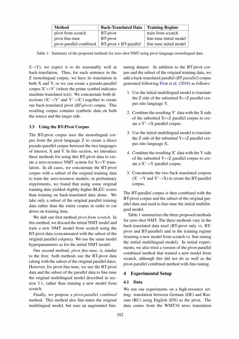
Method Back-Translated Data Training Regimepivot from scratch BT-pivot train from scratchpivot fine-tune BT-pivot fine-tune initial modelpivot-parallel combined BT-pivot + BT-parallel fine-tune initial model
Table 1: Summary of the proposed methods for zero-shot NMT using pivot-language monolingual data.
Z→Y), we expect it to do reasonably well atback-translation. Thus, for each sentence in theZ monolingual corpus, we have its translation inboth X and Y, so we can create a pseudo-parallelcorpus X’↔Y’ (where the prime symbol indicatesmachine-translated text). We concatenate both di-rections (X’→Y’ and Y’→X’) together to createour back-translated pivot (BT-pivot) corpus. Thisresulting corpus contains synthetic data on boththe source and the target side.
3.3 Using the BT-Pivot Corpus
The BT-pivot corpus uses the monolingual cor-pus from the pivot language Z to create a directpseudo-parallel corpus between the two languagesof interest, X and Y. In this section, we introducethree methods for using this BT-pivot data to cre-ate a zero-resource NMT system for X↔Y trans-lation. In all cases, we concatenate the BT-pivotcorpus with a subset of the original training datato train the zero-resource models; in preliminaryexperiments, we found that using some originaltraining data yielded slightly higher BLEU scoresthan training on back-translated data alone. Wetake only a subset of the original parallel trainingdata rather than the entire corpus in order to cutdown on training time.
We dub our first method pivot from scratch. Inthis method, we discard the initial NMT model andtrain a new NMT model from scratch using theBT-pivot data (concatenated with the subset of theoriginal parallel corpora). We use the same modelhyperparameters as for the initial NMT model.
Our second method, pivot fine-tune, is similarto the first: both methods use the BT-pivot data(along with the subset of the original parallel data).However, for pivot fine-tune, we use the BT-pivotdata and the subset of the parallel data to fine-tunethe original multilingual model described in sec-tion 3.1, rather than training a new model fromscratch.
Finally, we propose a pivot-parallel combinedmethod. This method also fine-tunes the originalmultilingual model, but uses an augmented fine-
tuning dataset. In addition to the BT-pivot cor-pus and the subset of the original training data, weadd a back-translated parallel (BT-parallel) corpusgenerated following Firat et al. (2016) as follows:
1. Use the initial multilingual model to translatethe Z side of the subsetted X↔Z parallel cor-pus into language Y.
2. Combine the resulting Y’ data with the X sideof the subsetted X↔Z parallel corpus to cre-ate a Y’→X parallel corpus.
3. Use the initial multilingual model to translatethe Z side of the subsetted Y↔Z parallel cor-pus into language X.
4. Combine the resulting X’ data with the Y sideof the subsetted Y↔Z parallel corpus to cre-ate a X’→Y parallel corpus.
5. Concatenate the two back-translated corpora(X’→Y and Y’→X) to create the BT-parallelcorpus.
The BT-parallel corpus is then combined with theBT-pivot corpus and the subset of the original par-allel data and used to fine-tune the initial multilin-gual model.
Table 1 summarizes the three proposed methodsfor zero-shot NMT. The three methods vary in theback-translated data used (BT-pivot only vs. BT-pivot and BT-parallel) and in the training regime(training a new model from scratch vs. fine-tuningthe initial multilingual model). In initial experi-ments, we also tried a version of the pivot-parallelcombined method that trained a new model fromscratch, although this did not do as well as thepivot-parallel combined method with fine-tuning.
4 Experimental Setup
4.1 DataWe run our experiments on a high-resource set-ting: translation between German (DE) and Rus-sian (RU) using English (EN) as the pivot. Thedata comes from the WMT16 news translation
102

Corpus SentencesEN↔DE 4 497 878EN↔RU 2 500 502EN monolingual 1 000 000
Table 2: Number of sentences in each training corpusfor the DE↔RU experiments.
task (Bojar et al., 2016). We use all availableparallel corpora for EN↔DE (Europarl v7, Com-mon Crawl, and News Commentary v11) andfor EN↔RU (Common Crawl, News Commen-tary v11, Yandex Corpus, and Wiki Headlines)to train the initial multilingual system, but no di-rect DE↔RU parallel data. When the paralleldata is used alongside the back-translated corporafor fine-tuning or re-training from scratch (as de-scribed in section 3.1), we randomly sample onemillion sentences from each parallel corpus.
For pivot (EN) monolingual data, we take arandom subset of one million sentences from theNews Crawl 2015 corpus. Since the goal of thispaper is to study the effectiveness of using pivot-language monolingual data, we do not use anyDE or RU monolingual data; however, we ex-pect that such data would also be beneficial. Ta-ble 2 shows the size of each training corpus af-ter preprocessing. We use the overlapping DE andRU sentences from newstest2014 as the validationset (1505 sentences), newstest2015 as the test set(1433 sentences), and newstest2016 as the held-out set (1500 sentences). The overlapping sen-tences were originally written in English and weretranslated by human translators into German andRussian (Bojar et al., 2016).
All data is tokenized and truecased using theMoses scripts (Koehn et al., 2007). We use a jointbyte pair encoding (Sennrich et al., 2016b) vocab-ulary for all three languages (DE, EN, and RU)trained on all parallel data with 50k merge opera-tions. Similarly to Johnson et al. (2017), we usetags at the beginning and end of the source sen-tence to indicate the desired target language.
4.2 Models
All models in our experiments are based on thetransformer architecture (Vaswani et al., 2017).We use the Sockeye toolkit (Hieber et al., 2017)to run all experiments. We find that the defaultSockeye hyperparameters work well, so we stickwith those throughout. We use beam search with
beam size 5 both when back-translating and dur-ing inference.
4.3 Baselines
Initial Models Without Monolingual DataWe compare our models to three baselines that aretrained without any monolingual data. We refer tothese baselines as initial models because they areused as the basis for our proposed models: we usethem to generate the BT-pivot data and we fine-tune them using the generated data to create ourproposed models.
The first baseline is a multilingual model basedon Johnson et al. (2017), but we use the trans-former architecture and add target language tagsat both the beginning and end of the source sen-tences. This multilingual model is trained onthe English↔German and English↔Russian par-allel data. We evaluate this model both withdirect (zero-shot) translation (German→Russianand Russian→German) and with pivot translationthrough English.
Secondly, we consider the zero-resource NMTmethod proposed by Lakew et al. (2017). Thismethod consists of selecting sentences from theDE↔EN parallel corpus and back-translatingthem from DE into RU, resulting in a RU’→DEpseudo-parallel corpus. The same is also donewith the RU↔EN parallel corpus to create aDE’→RU pseudo-parallel corpus. These corporaare then concatenated with the original paralleldata and used to fine-tune the multilingual model.This zero-resource method is only evaluated ondirect DE→RU and RU→DE translation (not onpivoting through EN).
We also compare our models to a zero-resourcebaseline based on the technique introduced by Fi-rat et al. (2016). This method fine-tunes the initialmultilingual model with the BT-parallel corpus de-scribed in section 3.3 (concatenated with the ori-gial data). Like the other zero-resource baseline,this baseline is only evaluated on direct translation(not on pivot translation).
Baselines with Monolingual DataIn addition to the initial models, we compareour proposed zero-resource NMT methods to twobaselines trained with monolingual EN data. Forboth of these baselines, we evaluate both directzero-shot translation and pivot translation throughEN.
103

RU→DE DE→RUBLEU test held-out test held-out
initial models
multilingual direct 15.2 14.5 3.4 2.7multilingual pivot 21.7 20.2 21.3 19.3Lakew et al., 2017 14.4 13.2 19.4 17.0Firat et al., 2016 21.0 18.3 22.6 20.7
baselines
copied corpus direct 10.2 9.5 3.7 3.1copied corpus pivot 21.1 19.9 20.9 18.9back-translation direct 14.8 14.1 3.7 2.9back-translation pivot 22.4 20.9 22.3 20.4
proposed modelspivot from scratch 22.3 21.5 23.0 20.6pivot fine-tune 22.4 21.5 23.0 20.3pivot-parallel combined 22.5 21.6 23.6 21.1
Table 3: BLEU scores for the initial multilingual models and zero-resource models without monolingual data,for the baselines with pivot monolingual data, and for our proposed zero-resource models with pivot monolingualdata. We report results on the test set (newstest2015) and the held-out set (newstest2016). For the baselines andthe initial multilingual models, we use consider both direct (zero-shot) and pivot translation.
The first is based on the copied corpus methodof Currey et al. (2017). We train an identi-cal model to the initial multilingual model, butwith additional EN→EN pseudo-parallel trainingdata from the EN monolingual corpus. Thus,this model is trained on DE↔EN, RU↔EN, andEN→EN data. We do not fine-tune this modelwith any pseudo-parallel data.
The second baseline we consider is back-translation (Sennrich et al., 2016a). Starting fromthe trained multilingual model, we back-translatethe EN monolingual data into both DE and RU,then fine-tune the multilingual model on the origi-nal training data, plus the DE’→EN and RU’→ENpseudo-parallel corpora.
5 Results
Table 3 shows translation performance (as es-timated by BLEU score) for our main experi-ments. We display results for initial multilingualmodels without any monolingual data (rows 1–4), for copied corpus and back-translation base-lines using the monolingual data (rows 5–8), andfor our proposed zero-resource models (rows 9–11). For the initial multilingual model and forthe copied corpus and back-translation baselines,we consider both direct source→target transla-tion and translation through the pivot language(source→EN→target).
5.1 Initial Models Without Monolingual Data
For the multilingual baseline, directsource→target translation does very poorly forDE→RU. Although the performance is somewhatmore reasonable for RU→DE, direct translationstill lags far behind pivot (source→EN→target)translation for this model. Our results differfrom those of Johnson et al. (2017), who showedreasonable performance in both directions forzero-shot translation. However, they tested theirzero-shot systems only on closely related lan-guages or very large-scale multilingual systems,whereas we use somewhat smaller training setsand distantly related languages. This might be anexplanation for the discrepancy in results.
Both zero-resource models (Lakew et al., 2017and Firat et al., 2016) outperform the multilingualbaseline overall for direct translation. In addi-tion, the latter closes the gap with the pivot trans-lation baseline for DE→RU and almost closes itfor RU→DE. Thus, fine-tuning on back-translatedparallel data is very helpful in improving zero-resource NMT. In the next sections, we evalu-ate methods for further improving zero-resourceNMT using EN monolingual data.
5.2 Baselines with Monolingual Data
The results for the copied corpus and back-translation baselines (using both direct and pivottranslation) are shown in rows 5–8 of Table 3.Both models are unable to translate well usingonly direct translation, but when pivot translation
104

is used, their performance improves. In partic-ular, the back-translation pivot baseline achievesslightly higher BLEU scores overall than any ofthe initial models trained without monolingualdata.
Currey et al. (2017) showed that the copied cor-pus method was useful for adding target-languagemonolingual data to NMT training. Here, we seethat the same method is not beneficial (and in factis slightly harmful compared to the baseline) foradding pivot-language monolingual data to NMT.This could be because the copied corpus is usedhere to improve translation directions that are notof interest (i.e. translation into and out of English,rather than DE↔RU translation).
5.3 Proposed Models with Monolingual Data
We display the results for our three proposed mod-els in the last three rows of Table 3. Comparedto the best pivot-based model (back-translation),the pivot from scratch and pivot fine-tune modelsperform slightly better overall in both translationdirections (DE→RU and RU→DE). Additionally,the pivot-parallel combined model improves overthe best pivot-based model by about 1 BLEUfor DE→RU and also does slightly better forRU→DE. This BLEU gain is especially interest-ing since the proposed models do not require two-step inference, unlike the back-translation pivot-based model.
Comparing to the best direct translation model(the zero-resource model based on Firat et al.,2016) leads to similar conclusions. The pivot fromscratch and pivot fine-tune methods do similarlyto this baseline for DE→RU translation and im-prove over it by 1.3–3.2 BLEU for RU→DE trans-lation. For the pivot-parallel combined model, thegains over the baseline for DE→RU are strongerthan for the other two methods, and the gains forRU→DE are similar. Thus, we have shown thatadding pivot-language monolingual data throughthese methods can strongly improve zero-resourceNMT performance.
All three of our proposed models improve overa strong direct translation baseline and performsimilarly to or better than a pivot-based translationbaseline that uses EN monolingual data withoutrequiring the two-step inference process necessaryfor pivot-based translation. The pivot from scratchand pivot fine-tune models give similar results,while the pivot-parallel combined method, which
DE→RU RU→DEBLEU iter 1 iter 2 iter 1 iter 2from scratch 23.0 23.0 22.3 22.7fine-tune 23.0 23.3 22.4 22.8combined 23.6 22.7 22.5 21.2
Table 4: BLEU scores for the proposed models on thetest set (newstest2015). We show BLEU scores for oneand two iterations (iter 1 and iter 2).
adds in the back-translated parallel corpus, yieldsthe best BLEU scores out of all models across theboard.
6 Iterating the Proposed Models
Inspired by Hoang et al. (2018) and Niu et al.(2018), we study whether iterating the pro-posed models can improve translation perfor-mance. Starting from the trained models from sec-tion 5.3, we run a second iteration as follows:
1. Back-translate the same EN data using thenew model to create a new BT-pivot corpus(as described in section 3.2).
2. For the pivot-parallel combined method,back-translate the EN side of the parallel dataas well (following Firat et al., 2016).
3. Fine-tune the model or train the model fromscratch using the new data concatenated withthe subset of the original parallel data (as de-scribed in section 3.3).
Table 4 shows the performance on the testdataset (newstest2015) when a second iteration ofback-translation and training is performed. Forthe pivot from scratch and pivot fine-tune meth-ods, we see small gains (up to 0.4 BLEU) fromrunning a second iteration. These small improve-ments help the pivot from scratch and pivot fine-tune methods catch up to the single-iteration ver-sion of the pivot-parallel combined method. Onthe other hand, running a second iteration is verycostly in terms of training time, since it requiresanother back-translation step and another train-ing step. For the pivot-parallel combined model,which was the best-performing model with one it-eration, adding a second iteration damages perfor-mance in terms of BLEU score. This seems tomatch the results of Hoang et al. (2018) that in-dicate that there are diminishing returns as moreiterations are added.
105

7 Conclusions
This paper introduced the task of zero-resourceneural machine translation using pivot-languagemonolingual data. We introduced a way of gen-erating a pseudo-parallel source↔target trainingcorpus using the monolingual pivot-language cor-pus, and we showed three ways of leveraging thiscorpus to train a final source↔target NMT sys-tem. All three methods improved over strong base-lines that used both direct source→target transla-tion and pivot translation through EN; the pivot-parallel combined method was the most success-ful.
Our proposed paradigm has several benefits.First, it shows that monolingual data from a lan-guage other than the source and target languagescan aid NMT performance, complementing litera-ture on using source- and target-language mono-lingual data in NMT. Second, this paradigm isarchitecture-agnostic, so it would be easy to ap-ply to architectures that improve upon the ba-sic zero-shot and zero-resource models (e.g. Ari-vazhagan et al., 2019; Lu et al., 2018; Platanioset al., 2018). However, the methods we have pro-posed are not without limitations. First, using thepivot-language monolingual data might not workas well when the source and target languages areclosely related; this might be a case where sourceand target monolingual data is more useful thanpivot monolingual data. These models also tune amultilingual NMT system for translation in two di-rections only (source→target and target→source),so they would not be applicable in cases where asingle massively multilingual NMT system (Aha-roni et al., 2019) is required.
In the future, we hope to additionally study theuse of source-language and target-language mono-lingual data in zero-resource NMT. We would alsolike to test our proposed zero-resource methods onother zero-shot NMT architectures and on otherlanguage pairs. We also think that data selectionmethods on the back-translated data (Niu et al.,2018) could be helpful, since zero-shot multilin-gual NMT models often generate translations inthe wrong target language (Arivazhagan et al.,2019).
ReferencesRoee Aharoni, Melvin Johnson, and Orhan Firat. 2019.
Massively multilingual neural machine translation.
arXiv preprint arXiv:1903.00089.
Naveen Arivazhagan, Ankur Bapna, Orhan Firat,Roee Aharoni, Melvin Johnson, and WolfgangMacherey. 2019. The missing ingredient in zero-shot neural machine translation. arXiv preprintarXiv:1903.07091.
Mikel Artetxe, Gorka Labaka, Eneko Agirre, andKyunghyun Cho. 2018. Unsupervised neural ma-chine translation. In 6th International Conferenceon Learning Representations.
Ondrej Bojar, Rajen Chatterjee, Christian Federmann,Yvette Graham, Barry Haddow, Matthias Huck, An-tonio Jimeno Yepes, Philipp Koehn, Varvara Lo-gacheva, Christof Monz, Matteo Negri, AurelieNeveol, Mariana Neves, Martin Popel, Matt Post,Raphael Rubino, Carolina Scarton, Lucia Spe-cia, Marco Turchi, Karin Verspoor, and MarcosZampieri. 2016. Findings of the 2016 Conferenceon Machine Translation. In Proceedings of the FirstConference on Machine Translation, pages 131–198. Association for Computational Linguistics.
Anna Currey, Antonio Valerio Miceli Barone, and Ken-neth Heafield. 2017. Copied monolingual data im-proves low-resource neural machine translation. InProceedings of the Second Conference on MachineTranslation, pages 148–156. Association for Com-putational Linguistics.
Sergey Edunov, Myle Ott, Michael Auli, and DavidGrangier. 2018. Understanding back-translation atscale. In Proceedings of the 2018 Conference onEmpirical Methods in Natural Language Process-ing, pages 489–500. Association for ComputationalLinguistics.
Orhan Firat, Baskaran Sankaran, Yaser Al-Onaizan,Fatos T Yarman Vural, and Kyunghyun Cho. 2016.Zero-resource translation with multi-lingual neuralmachine translation. In Proceedings of the 2016Conference on Empirical Methods in Natural Lan-guage Processing, pages 268–277. Association forComputational Linguistics.
Caglar Gulcehre, Orhan Firat, Kelvin Xu, KyunghyunCho, Loıc Barrault, Huei-Chi Lin, Fethi Bougares,Holger Schwenk, and Yoshua Bengio. 2015. On us-ing monolingual corpora in neural machine transla-tion. arXiv preprint arXiv:1503.03535.
Thanh-Le Ha, Jan Niehues, and Alexander Waibel.2016. Toward multilingual neural machine trans-lation with universal encoder and decoder. In Pro-ceedings of the 13th International Workshop on Spo-ken Language Translation.
Hany Hassan, Anthony Aue, Chang Chen, VishalChowdhary, Jonathan Clark, Christian Feder-mann, Xuedong Huang, Marcin Junczys-Dowmunt,William Lewis, Mu Li, Shujie Liu, Tie-Yan Liu,Renqian Luo, Arul Menezes, Tao Qin, Frank Seide,Xu Tan, Fei Tian, Lijun Wu, Shuangzhi Wu, Yingce
106

Xia, Dongdong Zhang, Zhirui Zhang, and MingZhou. 2018. Achieving human parity on automaticChinese to English news translation. arXiv preprintarXiv:1803.05567.
Felix Hieber, Tobias Domhan, Michael Denkowski,David Vilar, Artem Sokolov, Ann Clifton, and MattPost. 2017. Sockeye: A toolkit for neural machinetranslation. arXiv preprint arXiv:1712.05690.
Vu Cong Duy Hoang, Philipp Koehn, GholamrezaHaffari, and Trevor Cohn. 2018. Iterative back-translation for neural machine translation. In Pro-ceedings of the Second Workshop on Neural Ma-chine Translation and Generation, pages 18–24. As-sociation for Computational Linguistics.
Melvin Johnson, Mike Schuster, Quoc V Le, MaximKrikun, Yonghui Wu, Zhifeng Chen, Nikhil Thorat,Fernanda Viegas, Martin Wattenberg, Greg Corrado,Macduff Hughes, and Jeffrey Dean. 2017. Google’smultilingual neural machine translation system: En-abling zero-shot translation. Transactions of the As-sociation for Computational Linguistics, 5:339–351.
Philipp Koehn, Hieu Hoang, Alexandra Birch, ChrisCallison-Burch, Marcello Federico, Nicola Bertoldi,Brooke Cowan, Wade Shen, Christine Moran,Richard Zens, Chris Dyer, Ondrej Bojar, AlexandraConstantin, and Evan Herbst. 2007. Moses: Opensource toolkit for statistical machine translation. InProceedings of the 45th Annual Meeting of the ACL,pages 177–180. Association for Computational Lin-guistics.
Surafel M Lakew, Quintino F Lotito, Matteo Negri,Marco Turchi, and Marcello Federico. 2017. Im-proving zero-shot translation of low-resource lan-guages. In Proceedings of the 14th InternationalWorkshop on Spoken Language Translation.
Guillaume Lample, Ludovic Denoyer, andMarc’Aurelio Ranzato. 2018. Unsupervisedmachine translation using monolingual corporaonly. In 6th International Conference on LearningRepresentations.
Yichao Lu, Phillip Keung, Faisal Ladhak, Vikas Bhard-waj, Shaonan Zhang, and Jason Sun. 2018. A neu-ral interlingua for multilingual machine translation.In Proceedings of the Third Conference on MachineTranslation, pages 84–92. Association for Compu-tational Linguistics.
Xing Niu, Michael Denkowski, and Marine Carpuat.2018. Bi-directional neural machine translationwith synthetic parallel data. In Proceedings of theSecond Workshop on Neural Machine Translationand Generation, pages 84–91. Association for Com-putational Linguistics.
Jaehong Park, Jongyoon Song, and Sungroh Yoon.2017. Building a neural machine translation systemusing only synthetic parallel data. arXiv preprintarXiv:1704.00253.
Emmanouil Antonios Platanios, Mrinmaya Sachan,Graham Neubig, and Tom Mitchell. 2018. Contex-tual parameter generation for universal neural ma-chine translation. In Proceedings of the 2018 Con-ference on Empirical Methods in Natural LanguageProcessing, pages 425–435. Association for Com-putational Linguistics.
Rico Sennrich, Barry Haddow, and Alexandra Birch.2016a. Improving neural machine translation mod-els with monolingual data. In Proceedings of the54th Annual Meeting of the ACL, pages 86–96. As-sociation for Computational Linguistics.
Rico Sennrich, Barry Haddow, and Alexandra Birch.2016b. Neural machine translation of rare wordswith subword units. In Proceedings of the 54th An-nual Meeting of the ACL, pages 1715–1725. Associ-ation for Computational Linguistics.
Ashish Vaswani, Noam Shazeer, Niki Parmar, JakobUszkoreit, Llion Jones, Aidan N Gomez, ŁukaszKaiser, and Illia Polosukhin. 2017. Attention is allyou need. In Advances in Neural Information Pro-cessing Systems 30, pages 5998–6008.
Yonghui Wu, Mike Schuster, Zhifeng Chen, Quoc V.Le, Mohammad Norouzi, Wolfgang Macherey,Maxim Krikun, Yuan Cao, Qin Gao, KlausMacherey, Jeff Klingner, Apurva Shah, MelvinJohnson, Xiaobing Liu, ukasz Kaiser, StephanGouws, Yoshikiyo Kato, Taku Kudo, HidetoKazawa, Keith Stevens, George Kurian, NishantPatil, Wei Wang, Cliff Young, Jason Smith, JasonRiesa, Alex Rudnick, Oriol Vinyals, Greg Corrado,Macduff Hughes, and Jeffrey Dean. 2016. Google’sneural machine translation system: Bridging thegap between human and machine translation. arXivpreprint arXiv:1609.08144.
Jiajun Zhang and Chengqing Zong. 2016. Exploit-ing source-side monolingual data in neural machinetranslation. In Proceedings of the 2016 Conferenceon Empirical Methods in Natural Language Pro-cessing, pages 1535–1545. Association for Compu-tational Linguistics.
107

Proceedings of the 3rd Workshop on Neural Generation and Translation (WNGT 2019), pages 108–117Hong Kong, China, November 4, 2019. c©2019 Association for Computational Linguistics
www.aclweb.org/anthology/D19-56%2d
On the use of BERT for Neural Machine Translation
Stephane ClinchantNAVER LABS Europe, France
Kweon Woo JungNAVER Corp.,
South [email protected]
Vassilina NikoulinaNAVER LABS Europe, France
Abstract
Exploiting large pretrained models for var-ious NMT tasks have gained a lot of vis-ibility recently. In this work we studyhow BERT pretrained models could be ex-ploited for supervised Neural Machine Trans-lation. We compare various ways to in-tegrate pretrained BERT model with NMTmodel and study the impact of the mono-lingual data used for BERT training on thefinal translation quality. We use WMT-14English-German, IWSLT15 English-Germanand IWSLT14 English-Russian datasets forthese experiments. In addition to standard tasktest set evaluation, we perform evaluation onout-of-domain test sets and noise injected testsets, in order to assess how BERT pretrainedrepresentations affect model robustness.
1 Introduction
Pretrained Language Models (LM) such as ELMOand BERT (Peters et al., 2018; Devlin et al.,2018) have turned out to significantly improvethe quality of several Natural Language Process-ing (NLP) tasks by transferring the prior knowl-edge learned from data-rich monolingual corporato data-poor NLP tasks such as question answer-ing, bio-medical information extraction and stan-dard benchmarks (Wang et al., 2018; Lee et al.,2019). In addition, it was shown that these rep-resentations contain syntactic and semantic infor-mation in different layers of the network (Tenneyet al., 2019). Therefore, using such pretrainedLMs for Neural Machine Translation (NMT) isappealing, and has been recently tried by severalpeople (Lample and Conneau, 2019; Edunov et al.,2019; Song et al., 2019).
Unfortunately, the results of the above-mentioned works are not directly comparable toeach other as they used different methods, datasetsand tasks. Furthermore, pretrained LMs have
mostly shown improvements in low-resource orunsupervised NMT settings, and has been littlestudied in standard supervised scenario with rea-sonable amount of data available.
Current state of the art NMT models rely onthe Transformer model (Vaswani et al., 2017), afeed-forward network relying on attention mech-anism, which has surpassed prior state of the artarchitecture based on recurrent neural nets (Bah-danau et al., 2014; Sutskever et al., 2014). Beyondmachine translation, the transformer models havebeen reused to learn bi-directional language mod-els on large text corpora. The BERT model (De-vlin et al., 2018) consists in a transformer modelaiming at solving a masked language modellingtask, namely correctly predicting a masked wordfrom its context, and a next sentence predictiontask to decide whether two sentences are consecu-tive or not. In this work, we study how pretrainedBERT models can be exploited for transformer-based NMT, thus exploiting the fact that they relyon the same architecture.
The objective of this work is twofold. On onehand, we wish to perform systematic comparisonsof different BERT+NMT architectures for stan-dard supervised NMT. In addition, we argue thatthe benefits of using pretrained representations hasbeen overlooked in previous studies and shouldbe assessed beyond BLEU scores on in-domaindatasets. In fact, LMs trained on huge datasetshave the potentials of being more robust in generaland improve the performance for domain adapta-tion in MT.
In this study, we compare different ways to trainand reuse BERT for NMT. For instance, we showthat BERT can be trained only with a masked LMtask on the NMT source corpora and yield signif-icant improvement over the baseline. In addition,the models robustness is analyzed thanks to syn-thetic noise.
108

The paper is organized as follows. In section2, we review relevant state of the art. Section 3enumerates different models we experiment with.Finally section 4 and 5 present our results beforediscussing the main contributions of this work insection 6.
2 Related Works
The seminal work of (Bengio et al., 2003; Col-lobert and Weston, 2008) were one of the first toshow that neural nets could learn word represen-tations useful in a variety of NLP tasks, pavingthe way for the word embedding era thanks toword2vec (Mikolov et al., 2013) and its vari-ants (Pennington et al., 2014; Levy and Goldberg,2014).
With the recent advances and boost in perfor-mance of neural nets, ELMO (Peters et al., 2018)employed a Bi-LSTM network for language mod-elling and proposed to combine the different net-work layers to obtain effective word representa-tions. Shortly after the publication of ELMO,the BERT model (Devlin et al., 2018) was shownto have outstanding performance in various NLPtasks. Furthermore, the BERT model was refinedin (Baevski et al., 2019) where the transformerself-attention mechanism is replaced by two di-rectional self-attention blocks: a left-to-right andright-to-left blocks are combined to predict themasked tokens.
With respect to NMT, backtranslation (Sennrichet al., 2016a) is up to now one of the most effectiveways to exploit large monolingual data. However,backtranslation has the drawback of being onlyapplicable for target language data augmentation,while pretrained LMs can be used both for sourceand target language (independently (Edunov et al.,2019) or jointly (Lample and Conneau, 2019;Song et al., 2019)).
Lample and Conneau (2019) initializes theentire encoder and decoder with a pretrainedMaskLM or Crosslingual MaskLM language mod-els trained on multilingual corpora. Such ini-tialization proved to be beneficial for unsuper-vised machine translation, but also for English-Romanian supervised MT, bringing additional im-provements over standard backtranslation withMLM initialization.
Edunov et al. (2019) uses ELMO (Peters et al.,2018) language model to set the word embed-dings layer in NMT model. In addition, the
ELMO embedding are compared with the cloze-style BERT (Baevski et al., 2019) ones. The em-bedding network parameters are then either fixed,or fine-tuned. This work shows improvements onEnglish-German and English-Turkish translationtasks when using pretrained language model forsource word embedding initialization. However,the results are less clear when reusing embeddingon the target language side.
Futhermore, Song et al. (2019) goes onestep further and proposes Masked Sequence-to-Sequence pretraining method. Rather than mask-ing a single token, it masks a sequence of tokenin the encoder and recovers them in the decoder.This model has shown new state of the art for un-supervised machine translation.
Our work is an attempt to perform systematiccomparison on some of the aforementioned archi-tectures that incorporate pretrained LM in NMTmodel, concentrating on BERT pretrained LM rep-resentations applied on supervised machine trans-lation. However, we restrict ourselves to encoderpart only, and leave the decoder initialization forfuture work.
Regarding robustness, several recent studies(Karpukhin et al., 2019; Vaibhav et al., 2019) havetackled robustness issues with data augmentation.In this work, we study whether the robustnessproblem can be addressed at the model level ratherthan at data level. Michel et al. (2019) address ro-bustness problem with generative adversarial net-works. This method, as well as data augmentationmethods are complementary to our work and webelieve that they address different issues of robust-ness.
3 Methods
Typical NMT model adopts the encoder-decoderarchitecture where the encoder forms contextual-ized word embedding from a source sentence andthe decoder generates a target translation from leftto right.
Pretrained LM, namely BERT, can inject priorknowledge on the encoder part of NMT, providingrich contextualized word embedding learned fromlarge monolingual corpus. Moreover, pretrainedLMs can be trained once, and reused for differentlanguage pairs1.
1As opposed to backtranslation techniques which requiresfull NMT model retraining
109

In this study, we focus on reusing BERT mod-els for the NMT encoder2. We will compare thefollowing models:
• Baseline:. A transformer-big model withshared decoder input-output embedding pa-rameters.
• Embedding (Emb): The baseline modelwhere the embedding layer is replaced by theBERT parameters (thus having 6 + 6 encoderlayers). The model is then fine tuned simi-lar to the ELMO setting from (Edunov et al.,2019)
• Fine-Tuning (FT): The baseline model withthe encoder initialized by the BERT parame-ters as in Lample and Conneau (2019)
• Freeze: The baseline model with the en-coder initialized by the BERT parameters andfrozen. This means that the whole encoderhas been trained in purely monolingual set-tings, and only parameters responsible for thetranslation belong to the attention and de-coder models.
We exploit the fact that BERT uses the samearchitecture as NMT encoder which allows us toinitialize NMT encoder with BERT pretrained pa-rameters. BERT pretraining has two advantagesover NMT training:
• it solves a simpler (monolingual) task of‘source sentence encoding’, compared toNMT (bilingual task) which has to ‘encodesource sentence information’, and ‘translateinto a target language’.
• it has a possibility to exploit much largerdata, while NMT encoder is limited to sourceside of parallel corpus only.
Even though the role of NMT encoder may gobeyond source sentence encoding (nothing pre-vents the model from encoding ‘translation re-lated’ information at the encoder level), better ini-tialization of encoder with BERT pretrained LMallows for faster NMT learning. Comparing set-tings where we freeze BERT parameters againstfine-tuning BERT allows to shed some light onthe capacity of the encoder/decoder model to learn‘translation-related’ information.
2Similar approach can be applied on the target languagebut we leave it for future work.
Moreover, since the BERT models are trainedto predict missing tokens from their context, theirrepresentations may also be more robust to miss-ing tokens or noisy inputs. We perform extensiverobustness study at section 4 verifying this hypoth-esis.
Finally, language models trained on hugedatasets have the potentials of being more robustin general and improve the performance for do-main adaptation in MT. We therefore compareBERT models trained on different datasets, andperform evaluation on related test sets in order toassess the capacity of pretrained LMs on domainadaptation.
4 WMT experiments
4.1 PreprocessingWe learn BPE (Sennrich et al., 2016b) model with32K split operations on the concatenation of Wikiand News corpus. This model is used both for Pre-trained LM subwords splitting and NMT source(English) side subwords splitting. German side ofNMT has been processed with 32K BPE modellearnt on target part of parallel corpus only. Pleasenote, that this is different from standard settingsfor WMT En-De experiments, which usually usesjoint BPE learning and shared source-target em-beddings. We do not adopt standard settings sinceit contradicts our original motivation for using pre-trained LM: English LM is learnt once and reusedfor different language pairs.
4.2 TrainingBERT For pretraining BERT models, we usethree different monolingual corpora of differentsizes and different domains. Table 1 summarizesthe statistics of these three monolingual corpora.
• NMT-src: source part of our parallel corpusthat is used for NMT model training.
• Wiki: English wikipedia dump
• News: concatenation of 70M samplesfrom ”News Discussion”, ”News Crawl”and ”Common Crawl” English monolingualdatasets distributed by WMT-2019 sharedtask3. This resulted in total 210M samples.
The motivation of using NMT-src is to testwhether the resulting NMT model is more robust
3http://www.statmt.org/wmt19/translation-task.html
110

Lines TokensNMT-src 4.5M 104M
Wiki 72M 2086MNews 210M 3657M
Table 1: Monolingual (English) training data
after having being trained on the source corpora.The Wiki corpora is bigger than the NMT-src butcould be classified as out-of-domain compared tonews dataset. Finally, the news dataset is thebiggest one and consists mostly of in-domain data.
In all of our experiments, we only consider us-ing the masked LM task for BERT as the next sen-tence prediction tasks put restrictions on possibledata to use. We closely follow the masked LMtask described in (Devlin et al., 2018) with few ad-justments optimized for downstream NMT train-ing. We use frequency based sampling (Lampleand Conneau, 2019) in choosing 15% of tokens tomask, instead of uniformly sampling. Instead ofMASK token we used UNK token hoping that thustrained model will learn certain representation forunknowns that could be exploited by NMT model.Warm-up learning scheme described in (Vaswaniet al., 2017) results in faster convergence thanlinear decaying learning rate. The batch size of64000 tokens per batch is used, with maximum to-ken length of 250, half the original value, as we in-put single sentence only. We do not use [CLS] to-ken in the encoder side, as attention mechanism inNMT task can extract necessary information fromtoken-level representations. The BERT model isequivalent to the encoder side of Transformer Bigmodel. We train BERT model up to 200k iterationsuntil the accuracy for masked LM on developmentsaturates.
NMT For NMT system training, we use WMT-14 English-German dataset.
We use Transformer-Big as our baseline model.We share input embedding and output embed-ding parameters just before softmax on the de-coder side. Warm up learning scheme is usedwith warm-up steps of 4000. We use batch sizeof 32000 tokens per batch. Dropout of 0.3 is ap-plied to residual connections, and no dropout isapplied in attention layers. We decode with beamsize 4 with length penalty described in Wu et al.(2016). We conduct model selection with perplex-ity on development set. We average 5 checkpointsaround lowest perplexity.
Lines Tok/line (en/de)news14 3003 19.7/18.3news18 2997 19.5/18.3iwslt15 2385 16.4/15.4OpenSub 5000 6.3/5.5KDE 5000 8/7.7wiki 5000 17.7/15.5
Table 2: In/Out of Domain test sets. news14 andnews18 are test sets from WMT-14 and WMT-18 newstranslation shared task. iwslt: test set from IWSLT-15 MT Track4. Wiki is randomly 5K sampled fromparallel Wikipedia distributed by OPUS5, OpenSub,KDE and Wiki are randomly 5K sampled from paral-lel Wikipedia, Open Subtitles and KDE corpora dis-tributed by OPUS6
4.3 Evaluation
We believe that the impact of pretrained LM inNMT model can not be measured by BLEU per-formance on in-domain test set only. Thereforewe introduce additional evaluation that allows tomeasure the impact of LM pretraining on differentout-of-domain tests. We also propose an evalua-tion procedure to evaluate the robustness to vari-ous types of noise for our models.
Domain Besides standard WMT-14 news testset, models are evaluated on additional test setsgiven by Table 2. We include two in-domain(news) test sets, as well as additional out-of-domain test sets described in Table 2.
Noise robustness. For robustness evaluation, weintroduce different type of noise to the standardnews14 test set:
Typos: Similar to Karpukhin et al. (2019), weadd synthetic noise to the test set by randomly (1)swapping characters (chswap), (2) randomly in-serting or deleting characters (chrand), (3) upper-casing words (up). These test sets translations areevaluated against the golden news14 reference.
Unk: An unknown character is introduced at thebeginning (noted UNK.S) or at the end of the sen-tence (noted UNK.E) before a punctuation symbolif any (this unknown character could be thoughtas as an unknown emoji, a character in differentscript, a rare unicode character). This token is in-troduced both for source and target sentence, andthe evaluation is performed with the augmented-reference.
Intuitively, we expect the model to simply copyUNK token and proceed to the remaining tokens.
111

Interestingly, this simple test seems to producepoor translations, therefore puzzling the attentionand decoding process a lot. Table 3 gives an ex-ample of such translations for baseline model7.
Since the tasks are correlated, a better modelmight be better on noisy test sets as it behaves bet-ter in general. If we want to test that some modelsare indeed better, we need to disentangle this ef-fect and show that the gain in performance is notjust a random effect. A proper way would be tocompute the BLEU correlation between the orig-inal test set and the noisy versions but it wouldrequire a larger set of models for an accurate cor-relation estimation.
∆(chrF) : We propose to look at the distribu-tion of the difference of sentence charf betweenthe noisy test set and the original test set. Indeed,looking at BLEU delta may not provide enough in-formation since it is corpus-level metric. Ideally,we would like to measure a number of sentencesor a margin for which we observe an ‘importantdecrease’ in translation quality. According to Maet al. (2018); Bojar et al. (2017), sentence levelchrF achieves good correlation with human judge-ments for En-De news translations.
More formally, let s be a sentence from the stan-dard news14 test set, n a noise operation, m atranslation model and r the reference sentence8:
∆(chrF)(m,n, s) = chrF(m(n(s)), r)−chrF(m(s), r) (1)
In the analysis, we will report the distribution of∆(chrF) and its mean value as a summary. If amodel is good at dealing with noise, then the pro-duced sentence will be similar to the one producedby the noise-free input sentence. Therefore, the∆(chrF) will be closer to zero.
4.4 Results
Table 4 presents the results of our experiments.As expected, freezing the encoder with BERT pa-rameters lead to a significant decrease in transla-tion quality. However, other BERT+NMT archi-tectures mostly improve over the baseline both onin-domain and out-of-domain test sets. We con-clude, that the information encoded by BERT isuseful but not sufficient to perform the translation
7Output for (UNK.S+src) input is not an error, the modeldoes produces an English sentence!
8In the case of UNK transformation, the reference ischanged but we omit that to simplify the notation.
task. We believe, that the role of the NMT encoderis to encode both information specific to sourcesentence, but also information specific to the tar-get sentence (which is missing in BERT training).
Next, we observe that even NMTSrc.FT (NMTencoder is initialized with BERT trained on sourcepart of parallel corpus) improves over the baseline.Note that this model uses the same amount of dataas the baseline. BERT task is simpler compared tothe task of the NMT encoder, but it is still related,thus BERT pretraining allows for a better initial-ization point for NMT model.
When using more data for BERT training(Wiki.FT and News.FT), we gain even more im-provements over the baseline.
Finally, we observe comparable results forNews.Emb and News.FT (the difference in BLEUdoesn’t exceed 0.3 points, being higher forNews.FT on in-domain tests, and News.Emb forout-of-domain tests). Although News.FT config-uration keeps the size of the model same as stan-dard NMT system, News.Emb adds BERT param-eters to NMT parameters which doubles the sizeof NMT encoder. Additional encoder layers intro-duced in News.Emb does not add significant value.
4.5 Robustness analysis
Table 5 reports BLEU scores for the noisy test sets(described in section 4.3). As expected, we ob-serve an important drop in BLEU scores due tothe introduced noise. We observe that most pre-trained BERT models have better BLEU scorescompared to baseline for all type of noise (exceptNMTSrc.FT which suffers more from unknowntoken introduction in the end of the sentence com-pared to the Baseline). However, these results arenot enough to conclude, whether higher BLEUscores of BERT-augmented models are due to bet-ter robustness, or simply because these models areslightly better than the baseline in general.
This is why figure 1 reports the mean ∆(chrF)for several models. ∆(chrF) scores for UNKtests show that BERT models are not better thanexpected. However, for chswap, chrand, upper,the BERT models have a slightly lower ∆(chrF).Based on these results, we conclude that pretrain-ing the encoder with a masked LM task does notreally bring improvement in terms of robustnessto unknowns. It seems that BERT does yield im-provement for NMT as a better initialization for
112

source sentence ”In home cooking, there is much to be discovered - with a few minortweaks you can achieve good, if not sometimes better results,” said Proctor.
translation(src) ”Beim Kochen zu Hause gibt es viel zu entdecken - mit ein paar kleinennderungen kann man gute, wenn nicht sogar manchmal bessereErgebnisse erzielen”, sagte Proktor.
translation(UNK.S + src) • ”In home cooking, there is much to be discovered - with a few minortweaks you can achieve good, if not sometimes better results”, sagte Proktor.
Table 3: Example of a poor translation when adding unknown token to source sentences (translation done with abaseline transformer model)
news14 news18 iwslt15 wiki kde OpenSubBaseline 27.3 39.5 28.9 17.6 18.1 15.3NMTsrc.FT 27.7 40.1 28.7 18.3 18.4 15.3Wiki.FT 27.7 40.6 28.7 18.4 19.0 15.4News.FT 27.9 40.2 29.1 18.8 17.9 15.7News.Emb 27.7 39.9 29.3 18.9 18.2 16.0News.Freeze 23.6 35.5 26.5 15.0 15.1 13.8
Table 4: FT: initialize NMT encoder with BERT and finetune; Freeze: fix NMT encoder parameters to BERTparameters; Emb: fix encoder embeddding layer with BERT contextual word embeddings.
Figure 1: Mean ∆(chrF) for several noisy test set andmodels. For the UNK test, the BERT models are sim-ilar or worst than the basline. For the chrand, chswap,upper, the BERT models are slightly better.
NMT encoders but the full potential of maskedLM task is not fully exploited for NMT.
5 IWSLT experiments
In order to explore the potential of maskedLM encoder pretraining for NMT in lower re-source settings, we train NMT models on English-
German IWSLT 20159 and English-RussianIWSLT 201410 MT track datasets. These arepretty small datasets (compared to previous exper-iments) which contain around 200K parallel sen-tences each.
5.1 Experimental settings
In these experiments we (1) reuse pretrainedBERT models from previous experiments or (2)train IWSLT BERT model. IWSLT BERT modelis trained on the concatenation of all the data avail-able at IWSLT 2014-2018 campaigns. After filter-ing out all the duplicates it contains around 780Ksentences and 13.8M tokens.
We considered various settings for IWSLT base-line. First, for source side of the dataset, wetook 10K BPE merge operations, where BPEmodel was trained (1) either on the source side ofNMT data only, or (2) on all monolingual EnglishIWSLT data. Target side BPE uses 10K mergeoperations trained on the target side of the NMTdataset in all the IWSLST experiments. In our firstset of experiments, BPE model learnt on sourcedata only lead to similar translation performanceas BPE model learnt on all IWSLT English data.Therefore, in what follows we report results only
9https://sites.google.com/site/iwsltevaluation2015/mt-track
10https://sites.google.com/site/iwsltevaluation2014/mt-track
113

Models news14 +UNK.S +UNK.E +chswap +chrand +upBaseline 27.3 24.8 24.4 24.2 24.7 23.5NMTsrc.FT 27.7 24.9 22.9 24.4 25.2 24.5Wiki.FT 27.7 25.8 24.9 24.4 24.9 24.4News.FT 27.9 24.9 24.9 24.5 25.3 24.5News.Emb 27.7 24.7 24.8 24.6 25.3 24.2
Table 5: Robustness tests. BLEU scores for clean and ’noisified’ (with different noise type) news14 testset.
for the latter (referred as bpe10k).NMT model training on IWSLT datasets with
Transformer Big architecture on IWSLT data hasdiverged both for en-de and en-ru dataset. There-fore we use Transformer Base (tbase) architectureas a baseline model for these experiments. IWSLTBERT model is also based on tbase architecturedescribed in Vaswani et al. (2017) and for the restfollows same training procedure as described inthe section 4.
In order to explore the potential of single pre-trained model for all language pairs/datasets wetry to reuse Wiki and News pretrained BERT mod-els from previous experiments for encoder initial-ization of NMT model. However, in the previousexperiments, our pretrained BERT models used32K BPE vocabulary and Transformer Big (tbig)architecture which means that we have to reuse thesame settings for the encoder trained on IWSLTdataset. It has been shown by Ding et al. (2019),these are not optimal settings for IWSLT train-ing because it leads to too many parameters forthe amount of data available. Therefore, in or-der to reduce the amount of the parameters of themodel, we also consider the case where we re-duce the amount of the decoder layers from 6 to3 (tbig.dec3).
5.2 Results
Table 6 reports the results of different sets of theexperiments on IWSLT data. First, we observethat BERT pretrained model improves over thebaseline, in any settings (BPE vocabulary, modelarchitecture, dataset used for pretraining). Inparticular, it is interesting to mention that with-out pretraining, both tbig.bpe32k and tbig.bpe10kmodels diverge when trained on IWSLT. How-ever, BERT pretraining gives a better initializa-tion point, and allows to achieve very good per-formance both for en-de and en-ru. Thus, suchpretraining can be an interesting technique in low-resource scenarios.
en-de en-ruBaseline
tbase.bpe10k 25.9 9.6tbase.dec3.bpe10k 26.4 16.3
BERT+NMTIWSLT.FT.tbase.bpe10k 27.4 17.6IWSLT.FT.tbase.dec3.bpe10k 27.2 18.1Wiki.FT.tbig.bpe32k 26.9 17.6Wiki.FT.tbig.dec3.bpe32k 27.7 17.8News.FT.tbig.bpe32k 27.1 17.9News.FT.tbig.dec3.bpe32k 27.6 17.9
Table 6: IWSLT dataset results. IWSLT.FT: encoderis initialised with BERT model trained on IWSLTdata; tbase/tbig: transformer base/big architecture forNMT model; dec3: decoder layers reduced for 6 to3; bpe10k/bpe32k : amount of BPE merge operationsused for source language, learnt on the same dataset asBERT model (IWSLT or Wiki+News).
We do not observe big difference betweenIWSLT pretrained model and News/Wiki pre-trained model. We therefore may assume thatNews/Wiki BERT model can be considered as”general” English pretrained encoder, and be usedas a good starting point in any new model trans-lating from English (no matter target language ordomain).
6 Discussion
BERT pretraining has been very successful inNLP. With respect to MT, it was shown to pro-vide better performance in Lample and Conneau(2019); Edunov et al. (2019) and allows to in-tegrate large source monolingual data in NMTmodel as opposed to target monolingual data usu-ally used for backtranslation.
In this experimental study, we have shown that:
• The next sentence prediction task in BERTis not necessary to improve performance - amasked LM task already is beneficial.
• It is beneficial to train BERT on the source
114

corpora, therefore supporting the claim thatpretraining the encoder provide a better in-tialization for NMT encoders.
• Similar to Edunov et al. (2019), we observethat the impact of BERT pretraining is moreimportant as the size of the training data de-creases (WMT vs IWSLT).
• Information encoded by BERT is not suffi-cient to perform the translation: NMT en-coder encodes both information specific tosource sentence, and to the target sentence aswell (cf the low performance of BERT frozenencoder).
• Pretraining the encoder enables us to trainbigger models. In IWSLT, the transformerbig models were diverging, but when the en-coder is initialized with pretrained BERT thetraining became possible. For WMT14, train-ing a 12 layer encoder from scratch was prob-lematic, but News.Emb model (which con-tains 12 encoder layers) was trained and gaveone of the best performances on WMT14.
• Finetuning BERT pretrained encoder is moreconvenient : it leads to similar performancecompared to reusing BERT as embeddinglayers, with faster decoding speed.
• BERT pretrained models seem to be gener-ally better on different noise and domain testsets. However, we didn’t manage to obtainclear evidence that these models are more ro-bust.
This experimental study was limited to a par-ticular dataset, language pair and model architec-ture. However, many other combinations are pos-sible. First, similar type of study needs to be per-formed with BERT pretrained model for NMT de-coder. Also, the model can be extended to otherscenarios with BERT models such as Baevski et al.(2019). In addition, the comparison with ELMOembeddings is also interesting as in Edunov et al.(2019). Using embedding mostly influenced byneighboring words seems to echo the recent re-sults of convolutional self attention network (Yanget al., 2019). Using convolutional self attentionnetwork in BERT could bring additional benefitfor the pretrained representations. Another direc-tion could look at the impact of the number of lay-ers in BERT for NMT.
Besides, one key question in this study wasabout the role of encoder in NMT as the roles ofencoders and decoders are not clearly understoodin current neural architectures. In the transformerarchitecture, the encoder probably computes someinterlingual representations. In fact, nothing con-straints the model in reconstructing or predictinganything about the source sentences. If that is thecase, why would a monolingual encoder help forthe NMT task?
One hypothesis is that encoders have a role ofself encoding the sentences but also a translationeffect by producing interlingual representations.In this case, a monolingual encoder could be a bet-ter starting point and could be seen as a regular-izer of the whole encoders. Another hypothesis isthat the regularization of transformers models isnot really effective and simply using BERT mod-els achieve this effect.
7 Conclusion
In this paper, we have compared different ways touse BERT language models for machine transla-tion. In particular, we have argued that the ben-efit of using pretrained representations should notonly be assessed in terms of BLEU score for thein-domain data but also in terms of generalizationto new domains and in terms of robustness.
Our experiments show that fine-tuning the en-coder leads to comparable results as reusing theencoder as an additional embedding layers. How-ever, the former has an advantage of keepingthe same model size as in standard NMT set-tings, while the latter adds additional parametersto the NMT model which increases significantlythe model size and might be critical in certain sce-narios.
For MT practioners, using BERT has also sev-eral practical advantages beyond BLEU score.BERT can be trained for one source language andfurther reused for several translation pairs, thusproviding a better initialization point for the mod-els and allowing for better performance.
With respect to robustness tests, the conclusionare less clear. Even if pretrained BERT modelsobtained better performance on noisy test sets, itseems that they are not more robust than expectedand that the potential of masked LM tasks is notfully exploited for machine translation. An inter-esting future work will be to assess the robustnessof models from Song et al. (2019).
115

ReferencesAlexei Baevski, Sergey Edunov, Yinhan Liu, Luke
Zettlemoyer, and Michael Auli. 2019. Cloze-driven pretraining of self-attention networks. CoRR,abs/1903.07785.
Dzmitry Bahdanau, Kyunghyun Cho, and Yoshua Ben-gio. 2014. Neural machine translation by jointlylearning to align and translate. arXiv e-prints,abs/1409.0473.
Yoshua Bengio, Rejean Ducharme, Pascal Vincent, andChristian Janvin. 2003. A neural probabilistic lan-guage model. J. Mach. Learn. Res., 3:1137–1155.
Ondrej Bojar, Yvette Graham, and Amir Kamran.2017. Results of the wmt17 metrics shared task.In Proceedings of the Second Conference on Ma-chine Translation, Volume 2: Shared Task Papers,pages 489–513, Copenhagen, Denmark. Associationfor Computational Linguistics.
Ronan Collobert and Jason Weston. 2008. A unifiedarchitecture for natural language processing: Deepneural networks with multitask learning. In Pro-ceedings of the 25th International Conference onMachine Learning, ICML ’08, pages 160–167, NewYork, NY, USA. ACM.
Jacob Devlin, Ming-Wei Chang, Kenton Lee, andKristina Toutanova. 2018. BERT: pre-training ofdeep bidirectional transformers for language under-standing. CoRR, abs/1810.04805.
Shuoyang Ding, Adithya Renduchintala, and KevinDuh. 2019. A call for prudent choice of subwordmerge operations. CoRR, abs/1905.10453.
Sergey Edunov, Alexei Baevski, and Michael Auli.2019. Pre-trained language model representationsfor language generation. CoRR, abs/1903.09722.
Vladimir Karpukhin, Omer Levy, Jacob Eisenstein, andMarjan Ghazvininejad. 2019. Training on syntheticnoise improves robustness to natural noise in ma-chine translation. CoRR, abs/1902.01509.
Guillaume Lample and Alexis Conneau. 2019. Cross-lingual language model pretraining. CoRR,abs/1901.07291.
Jinhyuk Lee, Wonjin Yoon, Sungdong Kim,Donghyeon Kim, Sunkyu Kim, Chan Ho So,and Jaewoo Kang. 2019. Biobert: a pre-trainedbiomedical language representation model forbiomedical text mining. CoRR, abs/1901.08746.
Omer Levy and Yoav Goldberg. 2014. Neural wordembedding as implicit matrix factorization. In Pro-ceedings of the 27th International Conference onNeural Information Processing Systems - Volume 2,NIPS’14, pages 2177–2185, Cambridge, MA, USA.MIT Press.
Qingsong Ma, Ondej Bojar, and Yvette Graham. 2018.Results of the wmt18 metrics shared task: Both char-acters and embeddings achieve good performance.In Proceedings of the Third Conference on MachineTranslation, Volume 2: Shared Task Papers, pages682–701, Belgium, Brussels. Association for Com-putational Linguistics.
Paul Michel, Xian Li, Graham Neubig, andJuan Miguel Pino. 2019. On evaluation of ad-versarial perturbations for sequence-to-sequencemodels. CoRR, abs/1903.06620.
Tomas Mikolov, Ilya Sutskever, Kai Chen, Greg Cor-rado, and Jeffrey Dean. 2013. Distributed represen-tations of words and phrases and their composition-ality. In Proceedings of the 26th International Con-ference on Neural Information Processing Systems -Volume 2, NIPS’13, pages 3111–3119, USA. CurranAssociates Inc.
Jeffrey Pennington, Richard Socher, and ChristopherManning. 2014. Glove: Global vectors for wordrepresentation. In Proceedings of the 2014 Con-ference on Empirical Methods in Natural LanguageProcessing (EMNLP), pages 1532–1543, Doha,Qatar. Association for Computational Linguistics.
Matthew E. Peters, Mark Neumann, Mohit Iyyer, MattGardner, Christopher Clark, Kenton Lee, and LukeZettlemoyer. 2018. Deep contextualized word rep-resentations. CoRR, abs/1802.05365.
Rico Sennrich, Barry Haddow, and Alexandra Birch.2016a. Improving neural machine translation mod-els with monolingual data. In Proceedings of the54th Annual Meeting of the Association for Compu-tational Linguistics (Volume 1: Long Papers), pages86–96, Berlin, Germany. Association for Computa-tional Linguistics.
Rico Sennrich, Barry Haddow, and Alexandra Birch.2016b. Neural machine translation of rare wordswith subword units. In Proceedings of the 54th An-nual Meeting of the Association for ComputationalLinguistics (Volume 1: Long Papers), pages 1715–1725, Berlin, Germany. Association for Computa-tional Linguistics.
Kaitao Song, Xu Tan, Tao Qin, Jianfeng Lu, and Tie-Yan Liu. 2019. Mass: Masked sequence to sequencepre-training for language generation.
Ilya Sutskever, Oriol Vinyals, and Quoc V. Le. 2014.Sequence to sequence learning with neural net-works. In Proceedings of the 27th InternationalConference on Neural Information Processing Sys-tems - Volume 2, NIPS’14, pages 3104–3112, Cam-bridge, MA, USA. MIT Press.
Ian Tenney, Dipanjan Das, and Ellie Pavlick. 2019.Bert rediscovers the classical nlp pipeline.
Vaibhav, Sumeet Singh, Craig Stewart, and Gra-ham Neubig. 2019. Improving robustness of ma-chine translation with synthetic noise. CoRR,abs/1902.09508.
116

Ashish Vaswani, Noam Shazeer, Niki Parmar, JakobUszkoreit, Llion Jones, Aidan N Gomez, Ł ukaszKaiser, and Illia Polosukhin. 2017. Attention is allyou need. In I. Guyon, U. V. Luxburg, S. Bengio,H. Wallach, R. Fergus, S. Vishwanathan, and R. Gar-nett, editors, Advances in Neural Information Pro-cessing Systems 30, pages 5998–6008. Curran As-sociates, Inc.
Alex Wang, Amanpreet Singh, Julian Michael, Fe-lix Hill, Omer Levy, and Samuel Bowman. 2018.GLUE: A multi-task benchmark and analysis plat-form for natural language understanding. In Pro-ceedings of the 2018 EMNLP Workshop Black-boxNLP: Analyzing and Interpreting Neural Net-works for NLP, pages 353–355, Brussels, Belgium.Association for Computational Linguistics.
Yonghui Wu, Mike Schuster, Zhifeng Chen, Quoc V.Le, Mohammad Norouzi, Wolfgang Macherey,Maxim Krikun, Yuan Cao, Qin Gao, KlausMacherey, Jeff Klingner, Apurva Shah, MelvinJohnson, Xiaobing Liu, Lukasz Kaiser, StephanGouws, Yoshikiyo Kato, Taku Kudo, HidetoKazawa, Keith Stevens, George Kurian, NishantPatil, Wei Wang, Cliff Young, Jason Smith, JasonRiesa, Alex Rudnick, Oriol Vinyals, Greg Corrado,Macduff Hughes, and Jeffrey Dean. 2016. Google’sneural machine translation system: Bridging the gapbetween human and machine translation. CoRR,abs/1609.08144.
Baosong Yang, Longyue Wang, Derek F. Wong,Lidia S. Chao, and Zhaopeng Tu. 2019. Con-volutional self-attention networks. CoRR,abs/1904.03107.
117

Proceedings of the 3rd Workshop on Neural Generation and Translation (WNGT 2019), pages 118–127Hong Kong, China, November 4, 2019. c©2019 Association for Computational Linguistics
www.aclweb.org/anthology/D19-56%2d
On the Importance of the Kullback-Leibler Divergence Termin Variational Autoencoders for Text Generation
Victor Prokhorov|, Ehsan Shareghi|, Yingzhen Li�Mohammad Taher Pilehvar|}, Nigel Collier|
| Language Technology Lab, DTAL, University of Cambridge�Microsoft Research Cambridge ,}Tehran Institute for Advanced Studies
|{vp361, es776, mp792, nhc30}@cam.ac.uk�[email protected]
AbstractVariational Autoencoders (VAEs) are knownto suffer from learning uninformative latentrepresentation of the input due to issues suchas approximated posterior collapse, or en-tanglement of the latent space. We imposean explicit constraint on the Kullback-Leibler(KL) divergence term inside the VAE objec-tive function. While the explicit constraint nat-urally avoids posterior collapse, we use it tofurther understand the significance of the KLterm in controlling the information transmittedthrough the VAE channel. Within this frame-work, we explore different properties of theestimated posterior distribution, and highlightthe trade-off between the amount of informa-tion encoded in a latent code during training,and the generative capacity of the model. 1
1 Introduction
Despite the recent success of deep genera-tive models such as Variational Autoencoders(VAEs) (Kingma and Welling, 2014) and Gener-ative Adversarial Networks (GANs) (Goodfellowet al., 2014) in different areas of Machine Learn-ing, they have failed to produce similar generativequality in NLP. In this paper we focus on VAEsand their mathematical underpinning to explaintheir behaviors in the context of text generation.
The vanilla VAE applied to text (Bowman et al.,2016) consists of an encoder (inference) and de-coder (generative) networks: Given an input x,the encoder network parameterizes q�(z|x) and in-fers about latent continuous representations of x,while the decoder network parameterizes p✓(x|z)and generates x from the continuous code z. Thetwo models are jointly trained by maximizing theEvidence Lower Bound (ELBO), L(✓,�; x, z):⌦
log p✓(x|z)↵q�(z|x)
�DKL
�q�(z|x)||p(z)
�(1)
1The code is available on https://github.com/VictorProkhorov/KL_Text_VAE
where the first term is the reconstruction term, andthe second term is the Kullback-Leibler (KL) di-vergence between the posterior distribution of la-tent variable z and its prior p(z) (i.e., N (0, I)).The KL term can be interpreted as a regularizerwhich prevents the inference network from copy-ing x into z, and for the case of a Gaussian priorand posterior has a closed-form solution.
With powerful autoregressive decoders, such asLSTMs, the internal decoder’s cells are likely tosuffice for representing the sentence, leading toa sub-optimal solution where the decoder ignoresthe inferred latent code z. This allows the en-coder to become independent of x, an issue knownas posterior collapse (q�(z|x) ⇡ p(z)) where theinference network produces uninformative latentvariables. Several solutions have been proposedto address the posterior collapse issue: (i) Modi-fying the architecture of the model by weakeningdecoders (Bowman et al., 2016; Miao et al., 2015;Yang et al., 2017; Semeniuta et al., 2017), or in-troducing additional connections between the en-coder and decoder to enforce the dependence be-tween x and z (Zhao et al., 2017; Goyal et al.,2017; Dieng et al., 2018); (ii) Using more flexi-ble or multimodal priors (Tomczak and Welling,2017; Xu and Durrett, 2018); (iii) Alternating thetraining by focusing on the inference network inthe earlier stages (He et al., 2019), or augment-ing amortized optimization of VAEs with instance-based optimization of stochastic variational infer-ence (Kim et al., 2018; Marino et al., 2018).
All of the aforementioned approaches imposeone or more of the following limitations: restrain-ing the choice of decoder, modifying the trainingalgorithm, or requiring a substantial alternation ofthe objective function. As exceptions to these,�-VAE (Razavi et al., 2019) and �-VAE (Hig-gins et al., 2017) aim to avoid the posterior col-lapse by explicitly controlling the regularizer term
118

in eqn. 1. While �-VAE aims to impose a lowerbound on the divergence term, �-VAE (§2.2) con-trols the impact of regularization via an additionalhyperparameter (i.e., �DKL
�q�(z|x)||p(z)
�). A
special case of �-VAE is annealing (Bowmanet al., 2016), where � increases from 0 to 1 dur-ing training.
In this study, we propose to use an extension of�-VAE (Burgess et al., 2018) which permits usto explicitly control the magnitude of the KL termwhile avoiding the posterior collapse issue even inthe existence of a powerful decoder. We use thisframework to examine different properties of theestimated posterior and the generative behaviourof VAEs and discuss them in the context of textgeneration via various qualitative and quantitativeexperiments.
2 Kullback-Leibler Divergence in VAE
We take the encoder-decoder of VAEs as thesender-receiver in a communication network.Given an input message x, a sender generates acompressed encoding of x denoted by z, while thereceiver aims to fully decode z back into x. Thequality of this communication can be explained interms of rate (R) which measures the compressionlevel of z as compared to the original messagex, and distortion (D) which quantities the over-all performance of the communication in encod-ing a message at sender and successfully decodingit at the receiver. Additionally, the capacity of theencoder channel can be measured in terms of theamount of mutual information between x and z,denoted by I(x; z) (Cover and Thomas, 2012).
2.1 Reconstruction vs. KL
The reconstruction loss can naturally measure dis-tortion (D := �
⌦log p✓(x|z)
↵), while the KL
term quantifies the amount of compression (rate;R := DKL[q�(z|x)||p(z)]) by measuring the di-vergence between a channel that transmits zero bitof information about x, denoted by p(z), and theencoder channel of VAEs, q�(z|x). Alemi et al.(2018) introduced the H � D I(x; z) Rbounds2, where H is the empirical data entropy (aconstant). These bounds on mutual information al-low us to analyze the trade-off between the recon-struction and KL terms in eqn. (1). For instance,
2This is dependent on the choice of encoder. For otherbounds on mutual information see Poole et al. (2018); Hoff-man and Johnson (2016).
since I(x; z) is non-negative (using Jensen’s in-equality), the posterior collapse can be explainedas the situation where I(x; z) = 0, where en-coder transmits no information about x, causingR = 0, D = H . Increasing I(x; z) can be encour-aged by increasing both bounds: increasing theupper-bound (KL term) can be seen as the meanto control the maximum capacity of the encoderchannel, while reducing the distortion (reconstruc-tion loss) will tighten the bound by pushing thelower bound to its limits (H�D ! H). A similareffect on the lower-bound can be encouraged byusing stronger decoders which could potentiallydecrease the reconstruction loss. Hence, having aframework that permits the use of strong decoderswhile avoiding the posterior collapse is desirable.Similarly, channel capacity can be decreased.
2.2 Explicit KL Control via �-VAE
Given the above interpretation, we now turn to aslightly different formulation of ELBO based on�-VAE (Higgins et al., 2017). This allows con-trol of the trade-off between the reconstructionand KL terms, as well as to set explicit KL value.While �-VAE offers regularizing the ELBO via anadditional coefficient � 2 IR+, a simple exten-sion (Burgess et al., 2018) of its objective func-tion incorporates an additional hyperparameter Cto explicitly control the magnitude of the KL term,⌦log p✓(x|z)
↵q�(z|x)
� �|DKL
�q�(z|x)||p(z)
�� C| (2)
where C2IR+ and |.| denotes the absolute value.While we could apply constraint optimization toimpose the explicit constraint of KL=C, we foundthat the above objective function satisfies the con-straint (§3). Alternatively, it has been shown (Pels-maeker and Aziz, 2019) the similar effect couldbe reached by replacing the second term in eqn. 2with max
�C, DKL
�q�(z|x)||p(z)
��at the risk of
breaking the ELBO when KL<C (Kingma et al.,2016).
3 Experiments
We conduct various experiments to illustrate theproperties that are encouraged via different KLmagnitudes. In particular, we revisit the interde-pendence between rate and distortion, and shedlight on the impact of KL on the sharpness of theapproximated posteriors. Then, through a set ofqualitative and quantitative experiments for textgeneration, we demonstrate how certain genera-
119

300
340
380
−30
−15
0
βc−VAEGRU
LogDetCovDistortion
YahooYelp
315
350
385
Dis
torti
on
LogD
etC
ov−8
0−4
00
βc−VAELSTM
360
390
420
10 20 30 40 50 60 70 80 90 100Rate (C Value)
−190
−95
0
βc−VAECNN
Figure 1: Rate-Distortion and LogDetCov for C ={10, 20, ..., 100} on Yahoo and Yelp corpora.
tive behaviours could be imposed on VAEs via arange of maximum channel capacities. Finally, werun some experiments to find if any form of syn-tactic information is encoded in the latent space.For all experiments, we use the objective functionof eqn. 2 with � = 1. We do not use larger �s be-cause the constraint KL = C is always satisfied. 3
Corpora We use 5 different corpora cover-ing different domains and size through this sec-tion: Yelp and Yahoo Yang et al. (2017) bothhave (100k,10k,10k) sentences in (train, dev,test) sets and 20k words in vocabulary, Chil-dren’s Book Test (CBT; Weston et al. (2016))has (192k,10k,12k) sentences and 12k vocab,Wikipedia (WIKI; Marvin and Linzen (2018)) has(2m,270k,270k) sentences and 20k vocab, andWebText (Radford et al., 2019) has (1m,23k,24k)sentences and 22k vocab. 4
Models We examine three VAE architectures,covering a range of decoding strengths to exam-ine if the objective function in eqn. 2 is immuneto posterior collapse regardless of the choice of
3� can be seen as a Lagrange multiplier and any � valuethat allows for constraint satisfaction (R = C) is fine.
4 Corpora and preprocessing scripts will be released.
encoder-decoder architectures: �C-VAELSTM with(LSTM encoder, LSTM decoder), �C-VAEGRUwith (GRU encoder, GRU decoder) (Cho et al.,2014), and �C-VAECNN with (LSTM encoder,CNN decoder) (Dauphin et al., 2016). The di-mension of word embeddings is 256 and the di-mension of the latent variable is 64. The encoderand the decoder, for both VAELSTM and VAEGRU,have hidden size of 512 dimensions. VAECNN hasexactly the same encoder as VAELSTM, while thedecoder follows similar architecture to GLU witha bottleneck structure (with two blocks) (Dauphinet al., 2016) and has 512 channels externally and128 internally for the convolutions with the fil-ter size of 20. All models were trained for10 epochs and optimised the objective function(eqn. 2) with Adam (Kingma and Ba, 2015) withfollowing learning rates: 10�5 ⇥ 85 for VAEGRUand VAELSTM, and 10�4 for VAECNN. To couplethe encoder with the decoder we concatenate thelatent variable to word embeddings at each timestep without initialisation of hidden state.
3.1 Rate and Distortion
To analyse the dependence between the values ofexplicit rate (C) and distortion, we trained ourmodels with different values of C, ranging from10 to 100. Figure 1 reports the results for �C-VAEGRU, �C-VAELSTM, and �C-VAECNN modelson Yahoo and Yelp corpora. In all our experimentswe found that C�1 KLC+1, demonstratingthat the objective function effectively imposed thedesired constraint on KL term. Hence, setting anyC > 0 can in practice avoid the collapse issue.
The general trend is that by increasing the valueof C one can get a better reconstruction (lower dis-tortion) while the amount of gain varies depend-ing on the VAE’s architecture and corpus. 5 Addi-tionally, we measured rate and distortion on CBT,WIKI, and WebText corpora using �C-VAELSTMand observed the same trend with the increase ofC, see Table 1. This observation is consistent withthe bound on I(x; z) we discussed earlier (§2.1)such that with an increase of KL we increase anupper bound on I(x; z) which in turn allows tohave smaller values of reconstruction loss. Addi-tionally, as reported in Table 1, encouraging higherrates (via larger C) encourages more active units
5We attribute the difference in performance across ourmodels to the non-optimal selection of training hyperparam-eters, and corpus specific factors such as sentence length.
120

Bucket 1 Bucket 2 Bucket 3 All
C D R LogDetCov ||µ||22 AU BL2/RG2 BL4/RG4 BL2/RG2 BL4/RG4 BL2/RG2 BL4/RG4 BL2/RG2 BL4/RG4C
BT 3 62 3 -0.39 0.05 8 7.49/2.63 1.28/0.13 8.95/3.48 1.49/0.10 10.37/4.81 1.68/0.12 9.46/3.54 1.57/0.12
15 53 15 -0.38 0.05 29 21.68/12.92 8.99/3.07 14.82/7.01 4.25/0.81 14.68/6.73 3.31/0.36 15.87/8.86 4.60/1.43100 32 99 -43.82 1.27 64 50.00/43.23 38.74/30.16 26.78/18.49 15.99/9.23 19.24/9.90 7.65/2.24 27.65/24.33 16.09/14.24
WIK
I 3 81 3 -0.35 0.00 5 4.61/3.64 1.47/1.03 5.93/2.67 1.09/0.19 7.39/3.00 1.17/0.12 6.78/3.08 1.33/0.4215 70 15 -0.57 0.01 12 13.73/8.46 7.12/3.86 10.07/4.45 3.93/1.32 9.93/3.27 1.95/0.29 10.08/5.35 3.42/1.79100 17 100 -4.97 0.15 64 65.67/63.17 60.02/55.92 37.25/32.76 30.88/26.33 18.73/11.41 11.22/6.20 31.84/35.37 24.17/29.08
Web
Text 3 77 3 -0.21 0.01 4 9.51/5.27 2.96/1.14 9.59/4.59 1.68/0.22 12.59/6.37 3.96/1.01 11.88/5.54 3.35/0.70
15 67 15 -0.51 0.01 16 21.69/12.41 9.86/3.69 15.48/7.44 5.35/1.51 15.63/7.29 5.59/1.59 15.84/7.85 5.69/1.76100 22 100 -7.85 0.41 64 84.85/82.48 81.89/78.79 61.65/58.33 56.35/53.05 35.07/27.33 27.31/20.99 45.84/45.30 38.71/39.66
Table 1: �C-VAELSTM performance with C = {3, 15, 100} on the test sets of CBT, WIKI, and WebText. Eachbucket groups sentences of certain length. Bucket 1: length 10; Bucket 2: 10 < length 20; Bucket 3: 20< length 30, and All contains all sentences. BL2/RG2 denotes BLEU-2/ROUGE-2, BL4/RG4 denotes BLEU-2/ROUGE-2 BLEU-4/ROUGE-4, AU denotes active units, D denotes distortion, and R denotes rate.
(AU; Burda et al. (2015)) in the latent code z. 6
As an additional verification, we also group thetest sentences into buckets based on their lengthand report BLEU-2/4 and ROUGE-2/4 metrics tomeasure the quality of reconstruction step in Table1. As expected, we observe that increasing rate hasa consistently positive impact on improving BLEUand ROUGE scores.
3.2 Aggregated Posterior
To understand how the approximated posteriorsare being affected by the magnitude of the KL,we adopted an approach from Zhao et al. (2017)and looked at the divergence between the aggre-gated posterior, q�(z) =
Px⇠q(x) q�(z|x), and
prior p(z). Since during generation we generatesamples from the prior, ideally we would like theaggregated posterior to be as close as possible tothe prior.
We obtained unbiased samples of z first by sam-pling an x from data and then z ⇠ q�(z|x), andmeasured the log determinant of covariance ofthe samples (log det(Cov[q�(z)])). As reportedin Figure 1, we observed that log det(Cov[q�(z)])degrades as C grows, indicating sharper approxi-mate posteriors. We then consider the differenceof p(z) and q(z) in their means and variances, bycomputing the KL divergence from the moment-matching Gaussian fit of q(z) to p(z): This returnssmaller values for �C=5-VAEGRU (Yelp: 0, Yahoo:0), and larger values for �C=100-VAEGRU (Yelp:8, Yahoo: 5), which illustrates that the overlap be-tween q�(z) and p(z) shrinks further as C grows.
6To see if the conclusions hold with different number ofparameters, we doubled the number of parameters in �C -VAEGRU and �C -VAELSTM and observed the similar patternwith a slight change in performance.
The above observation is better pronounced inTable 1, where we also report the mean (||µ||22)of unbiased samples of z, highlighting the diver-gence from the mean of the prior distribution asrate increases. Therefore, for the case of lowerC, the latent variables observed during trainingare closer to the generated sample from the priorwhich makes the decoder more suitable for gener-ation purpose. We will examine this hypothesis inthe following section.
3.3 Text Generation
To empirically examine how channel capacitytranslates into generative capacity of the model,we experimented with the �C-VAELSTM modelsfrom Table 1. To generate a novel sentence, aftera model was trained, a latent variable z is sampledfrom the prior distribution and then transformedinto a sequence of words by the decoder p(x|z).
During decoding for generation we try three de-coding schemes: (i) Greedy: which selects themost probable word at each step, (ii) Top-k (Fanet al., 2018): which at each step samples from theK most probable words, and (iii) Nucleus Sam-pling (NS) (Holtzman et al., 2019): which at eachstep samples from a flexible subset of most proba-ble words chosen based on their cumulative mass(set by a threshold p, where p = 1 means samplingfrom the full distribution). While similar to Top-k, the benefit of NS scheme is that the vocabularysize at each time step of decoding varies, a prop-erty that encourages diversity and avoids degener-ate text patterns of greedy or beam search decod-ing (Holtzman et al., 2019). We experiment withNS (p = {0.5, 0.9}) and Top-k (k = {5, 15}).
121

Greedy Top-15 NS(p=0.9)
C=3
1: oh, i m not going to be a good man. 1: come - look on my mind, said he. 1: and what is one of those trees creatures?2: oh, it s a good thing, said the story girl. 2: how could i tell you, that it s a great deal? 2: here s a nice heart among those waters!3: oh, how can you do it, dear? 3: said i. my sister, what a fool! 3: good-bye, said reddy fox, hardly fright-
ened was out of his life.4: oh, how can you do it, dear? 4: and how was the way, you? 4: now, for a neighbor, who knows him.5: oh, how can you do it, miss? 5: said the other little breezes, but i do n t . 5: oh, prince ivan, dear me!6: and what is the matter with you? 6: and where s the news of the world? 6: cried her mother, who is hidden or power.7: and what is the matter with you? 7: ⟨unk⟩ of ⟨unk⟩, said i. ay, ⟨unk⟩! 7: but this was his plight, and the smith
knew.
C=15
1: old mother west wind and her eyes werein the same place, but she had never seenher.
1: eric found out this little while, but therein which the old man did not see it so.
1: aunt tommy took a sudden notion of re-lief and yellow-dog between him sharplyuntil he tried to go to.
2: old mother west wind and his wife hadgone and went to bed to the palace.
2: old mother west wind and his wife gaveher to take a great ⟨unk⟩, she said.
2: his lord marquis of laughter expressedthat soft hope and miss cornelia was notcomforted.
3: little joe otter and there were a ⟨unk⟩ ofthem to be seen.
3: little joe otter got back to school all the⟨unk⟩ together.
3: meanwhile the hounds were both aroundand then by a thing was not yet.
4: little joe otter s eyes are just as big as her. 4: little joyce s eyes grew well at once,there.
4: in a tone, he began to enter after dinner.
5: a few minutes did not answer the ⟨unk⟩. 5: pretty a woman, but there had vanished. 5: once a word became, just got his way.6: a little while they went on. 6: from the third day, she went. 6: for a few moments, began to find.7: a little while they went. 7: three months were as usual. 7: meantime the thrushes were ⟨unk⟩.
C=100
1: it will it, all her ⟨unk⟩, not even her withher?
1: it will her you, at last, bad and never inher eyes.
1: it s; they liked the red, but i kept her andgrowing.
2: it will get him to mrs. matilda and noth-ing to eat her long clothes.
2: other time, i went into a moment – shewent in home and.
2: it ⟨unk⟩ not to her, in school, and neverhis bitter now.
3: the thing she put to his love, when it were⟨unk⟩ and too.
3: going quite well to his mother, and re-member it the night in night!
3: was it now of the beginning, and dr.hamilton was her away and.
4: one day, to the green forest now and along time ago, sighed.
4: one and it rained for his feet, for she wastheir eyes like ever.
4: of course she flew for a long distance;and they came a longing now.
5: one and it became clear of him on thatdirection by the night ago.
5: the thing knew the tracks of ⟨unk⟩ and henever got an ⟨unk⟩ before him.
5: one door what made the pain called forher first ear for losing up.
6: every word of his horse was and the restas the others were ready for him.
6: of course he heard a sound of her as muchover the ⟨unk⟩ that night can.
6: one and he got by looking quite like herpart till the marriage know ended.
7: a time and was half the ⟨unk⟩ as beforethe first ⟨unk⟩ things were ready as.
7: every, who had an interest in that till hislegs got splendid tongue than himself.
7: without the thought that danced in theground which made these delicate child steeth so.
Table 2: Homotopy (CBT corpus) - The three blocks correspond to C = {3, 15, 100} values used for training�C-VAELSTM. The columns correspond to the three decoding schemes: greedy, top-k (with k=15), and the nucleussampling (NS; with p=0.9). Initial two latent variables z were sampled from a the prior distribution i.e. z ⇠ p(z)and the other five latent variables were obtained by interpolation. The sequences that highlighted in gray are the onethat decoded into the same sentences condition on different latent variable. Note: Even though the learned latentrepresentation should be quite different for different models (trained with different C) in order to be consistent allthe generated sequences presented in the table were decoded from the same seven latent variables.
3.3.1 Qualitative AnalysisWe follow the settings of homotopy experi-ment (Bowman et al., 2016) where first a set of la-tent variables was obtained by performing a linearinterpolation between z1 ⇠ p(z) and z2 ⇠ p(z).Then each z in the set was converted into a se-quence of words by the decoder p(x|z). Besidesthe initial motivation of Bowman et al. (2016) toexamine how neighbouring latent codes look like,our additional incentive is to analyse how sensi-tive the decoder is to small variations in the latentvariable when trained with different channel ca-pacities, C = {3, 15, 100}.
Table 2 shows the generated sentences via dif-ferent decoding schemes for each channel capac-
ity. For space reason, we only report the gener-ated sentences for greedy, Top-k = 15, and NSp = 0.9. To make the generated sequences compa-rable across different decoding schemes or C val-ues, we use the same samples of z for decoding.
Sensitivity of Decoder To examine the sensitiv-ity7 of the decoder to variations of the latent vari-able, we consider the sentences generate with thegreedy decoding scheme (the first column in Ta-ble 2). The other two schemes are not suitablefor this analysis as they include sampling proce-
7Note: we vary z in one (randomly selected) direction (in-terpolating between z1 and z2). Alternatively, the sensitivityanalysis can be done by varying z along the gradient directionof log p(x|z).
122

Greedy NS(p=0.9)
C |V| FCE %unk len. SB |V| FCE %unk len. SB
CBT3 335 86.6(0.4) 9.7 15.3 4.2 9.8k 70.4(0.0) 2.1 15.6 0.015 335 52.3(0.3) 12.7 15.2 0.3 9.8k 70.7(0.2) 2.4 15.4 0.0100 335 47.3(0.1) 21.3 17.5 0.0 9.8k 75.1(0.1) 2.2 17.6 0.0
Test 328 - 30.7 15.3 - 6.1k - 3.6 15.3 -
WIKI3 1.5k 134.6(0.8) 27.3 19.9 7.6 20k 89.8(0.1) 5.8 19.4 0.015 1.5k 69.2(0.1) 18.9 19.8 0.2 20k 89.3(0.1) 5.6 19.8 0.0100 1.5k 58.9(0.1) 34.8 20.7 0.0 20k 96.5(0.1) 4.5 20.7 0.0
Test 1.5k - 32.7 19.6 - 20k - 5.2 19.6 -
WebText3 2.3k 115.8(0.7) 18.8 17.5 2.0 21.9k 86.4(0.1) 7.1 15.6 0.015 2.3k 74.4(0.1) 15.5 15.8 0.1 21.9k 85.8(0.1) 6.9 15.9 0.0100 2.3k 62.5(0.1) 27.3 18.0 0.0 21.9k 93.7(0.1) 4.8 18.0 0.0
Test 2.2k - 30.1 16.1 - 17.1k - 6.8 16.1 -
Table 3: Forward Cross Entropy (FCE). Columns represent stats for Greedy and NS decoding schemes for �C-VAELSTM models trained with C = {3, 15, 100} on CBT, WIKI or WebText. Each entry in the table is a meanof negative log likelihood of an LM. The values in the brackets are the standard deviations. |V| is the vocabularysize; Test stands for test set; %unk is the percentage of ⟨unk⟩ symbols in a corpora; len. is the average length ofa sentence in the generated corpus; SB is the self-BLEU:4 score calculated on the 10K sentences in the generatedcorpus.
dure. This means that if we decode the same la-tent variable twice we will get two different sen-tences. We observed that with lower channel ca-pacity (C = 3) the decoder tends to generate iden-tical sentences for the interpolated latent variables(we highlight these sentences in gray), exhibit-ing decoder’s lower sensitivity to z’s variations.However, with the increase of channel capacity(C = 15, 100) the decoder becomes more sensi-tive. This observation is further supported by theincreasing pattern of active units in Table 1: Giventhat AU increases with increase of C one wouldexpect that activation pattern of a latent variablebecomes more complex as it comprises more in-formation. Therefore small change in the patternwould have a greater effect on the decoder.
Coherence of Sequences We observe that themodel trained with large values of C compromisessequences’ coherence during the sampling. This isespecially evident when we compare C = 3 withC = 100. Analysis of Top-15 and NS (p=0.9)generated samples reveals that the lack of coher-ence is not due to the greedy decoding scheme perse, and can be attributed to the model in general.To understand this behavior further, we need twoadditional results from Table 1: LogDetCov and||µ||22. One can notice that as C increases LogDet-Cov decreases and ||µ||22 increases. This indicatesthat the aggregated posterior becomes further apartfrom the prior, hence the latent codes seen during
the training diverge more from the codes sampledfrom the prior during generation. We speculatethis contributes to the coherence of the generatedsamples, as the decoder is not equipped to decodeprior samples properly at higher Cs.
3.3.2 Quantitative Analysis
Quantitative analysis of generated text withoutgold reference sequences (e.g. in Machine Trans-lation or Summarization) has been a long-standingchallenge. Recently, there have been efforts to-wards this direction, with proposal such as self-BLEU (Zhu et al.), forward cross entropy (Cıfkaet al., 2018, FCE) and Frechet InferSent Distance(Cıfka et al., 2018, FID). We opted for FCE as acomplementary metric to our qualitative analysis.To calculate FCE, first a collection of syntheticsentences are generated by sampling z ⇠ p(z)and decoding the samples into sentences. The syn-thetic sequences are then used to train a languagemodel (an LSTM with the parametrisation of ourdecoder). The FCE score is estimated by reportingthe negative log likelihood (NLL) of the trainedLM on the set of human generated sentences.
We generated synthetic corpora using trainedmodels from Table 1 with different C and decod-ing schemes and using the same exact z samplesfor all corpora. Since the generated corpora usingdifferent C values would have different coverageof words in the test set (i.e., Out-of-Vocabularyratios), we used a fixed vocabulary to minimize
123

the effect of different vocabularies in our analysis.Our dictionary contains words that are common inall of the three corpora, while the rest of the wordsthat don’t exist in this dictionary are replaced with⟨unk⟩ symbol. Similarly, we used this fixed dic-tionary to preprocess the test sets. Also, to reducebias to a particular set of sampled z’s we measurethe FCE score three times, each time we sampled anew training corpus from a �C-VAELSTM decoderand trained an LM from scratch. In Table 3 wereport the average FCE (NLL) for the generatedcorpora.
In the qualitative analysis we observed that thetext generated by the �C-VAELSTM trained withlarge values of C = 100 exhibits lower quality(i.e., in terms of coherence). This observation issupported by the FCE score of NS(p=0.9) decod-ing scheme (3), since the performance drops whenthe LM is trained on the corpus generated withC = 100. The generated corpora with C = 3and C = 15 achieve similar FCE score. How-ever, these patterns are reversed for Greedy decod-ing scheme8, where the general tendency of FCEscores suggests that for larger values of C the �C-VAELSTM seems to generate text which better ap-proximates the natural sentences in the test set. Tounderstand this further, we report additional statis-tics in Table 3: percentage of ⟨unk⟩ symbols, self-BLEU and average sentence length in the corpus.
The average sentence length, in the generatedcorpora is very similar for both decoding schemes,removing the possibility that the pathological pat-tern on FCE scores was caused by difference insentence length. However, we observe that forGreedy decoding more than 30% of the test setconsists of ⟨unk⟩. Intuitively, seeing more evi-dence of this symbol during training would im-prove our estimate for the ⟨unk⟩. As reported inthe table, the %unk increases on almost all corporaas C grows, which is then translated into gettinga better FCE score at test. Therefore, we believethat FCE at high %unk is not a reliable quantitativemetric to assess the quality of the generated syn-tactic corpora. Furthermore, for Greedy decoding,self-BLEU decreases when C increases. This sug-gests that generated sentences for higher value ofC are more diverse. Hence, the LM trained onmore diverse corpora can generalise better, whichin turn affects the FCE.
8For the other decoding schemes: Top-{5,15} andNS(p=0.5) the pattern is the same as for the Greedy. For spacereason we only report the FCE for Greedy.
In contrast, the effect the ⟨unk⟩ symbol has onthe corpora generated with the NS(p=0.9) decod-ing scheme is minimal for two reasons: First, thevocabulary size for the generated corpora, for allvalues of C is close to the original corpus (thecorpus we used to train the �C-VAELSTM). Sec-ond, the vocabularies of the corpora generatedwith three values of C is very close to each other.As a result, minimum replacement of the wordswith the ⟨unk⟩ symbol is required, making the ex-periment to be more reflective of the quality ofthe generated text. Similarly, self-BLEU for theNS(p=0.9) is the same for all values of C. Thissuggests that the diversity of sentences has mini-mal, if any, effect on the FCE.
3.4 Syntactic Test
In this section, we explore if any form of syn-tactic information is captured by the encoder andrepresented in the latent codes despite the lack ofany explicit syntactic signal during the training ofthe �C-VAELSTM. To train the models we usedthe same WIKI data set as in Marvin and Linzen(2018), but we filtered out all the sentences thatare longer than 50 space-separated tokens.9
We use the data set of Marvin and Linzen(2018) which consists of pairs of grammatical andungrammatical sentences to test various syntac-tic phenomenon. For example, a pair in subject-verb agreement category would be: (The authorlaughs, The author laugh). We encode both thegrammatical and ungrammatical sentences into thelatent codes z+ and z�, respectively. Then wecondition the decoder on the z+ and try to deter-mine whether the decoder assigns higher probabil-ity to the grammatical sentence (denoted by x+):p(x�|z+) < p(x+|z+) (denoted by p1 in Table 4).We repeat the same experiment but this time try todetermine whether the decoder, when conditionedon the ungrammatical code (z�), still prefers toassign higher probability to the grammatical sen-tence: p(x�|z�) < p(x+|z�) (denoted by p2 inTable 4). Table 4 shows the p1 and p2 for the �C-VAELSTM model trained with C = {3, 100}. Boththe p1 and p2 are similar to the accuracy and corre-spond to how many times a grammatical sentencewas assigned a higher probability.
As reported for C=3, p1 and p2 match in al-most all cases. This is to some degree expected
9We applied the filtering to decrease the training time ofour models.
124
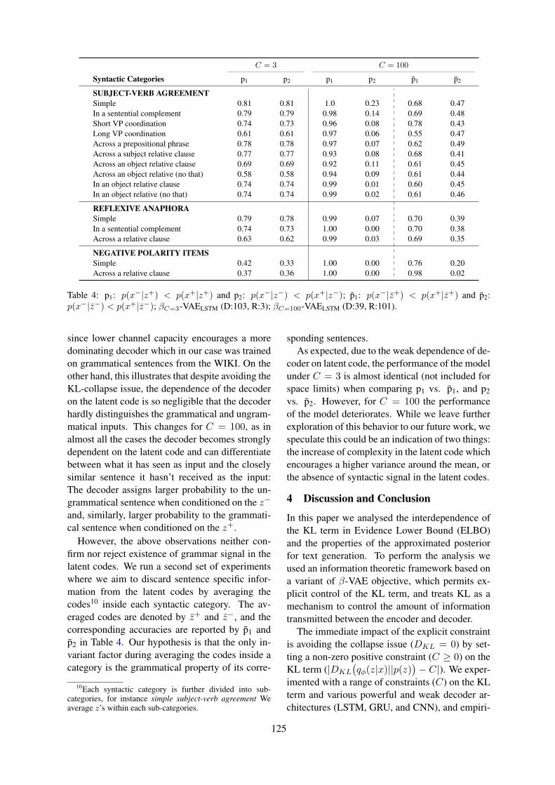
C = 3 C = 100
Syntactic Categories p1 p2 p1 p2 p1 p2
SUBJECT-VERB AGREEMENTSimple 0.81 0.81 1.0 0.23 0.68 0.47In a sentential complement 0.79 0.79 0.98 0.14 0.69 0.48Short VP coordination 0.74 0.73 0.96 0.08 0.78 0.43Long VP coordination 0.61 0.61 0.97 0.06 0.55 0.47Across a prepositional phrase 0.78 0.78 0.97 0.07 0.62 0.49Across a subject relative clause 0.77 0.77 0.93 0.08 0.68 0.41Across an object relative clause 0.69 0.69 0.92 0.11 0.61 0.45Across an object relative (no that) 0.58 0.58 0.94 0.09 0.61 0.44In an object relative clause 0.74 0.74 0.99 0.01 0.60 0.45In an object relative (no that) 0.74 0.74 0.99 0.02 0.61 0.46
REFLEXIVE ANAPHORASimple 0.79 0.78 0.99 0.07 0.70 0.39In a sentential complement 0.74 0.73 1.00 0.00 0.70 0.38Across a relative clause 0.63 0.62 0.99 0.03 0.69 0.35
NEGATIVE POLARITY ITEMSSimple 0.42 0.33 1.00 0.00 0.76 0.20Across a relative clause 0.37 0.36 1.00 0.00 0.98 0.02
Table 4: p1: p(x�|z+) < p(x+|z+) and p2: p(x�|z�) < p(x+|z�); p1: p(x�|z+) < p(x+|z+) and p2:p(x�|z�) < p(x+|z�); �C=3-VAELSTM (D:103, R:3); �C=100-VAELSTM (D:39, R:101).
since lower channel capacity encourages a moredominating decoder which in our case was trainedon grammatical sentences from the WIKI. On theother hand, this illustrates that despite avoiding theKL-collapse issue, the dependence of the decoderon the latent code is so negligible that the decoderhardly distinguishes the grammatical and ungram-matical inputs. This changes for C = 100, as inalmost all the cases the decoder becomes stronglydependent on the latent code and can differentiatebetween what it has seen as input and the closelysimilar sentence it hasn’t received as the input:The decoder assigns larger probability to the un-grammatical sentence when conditioned on the z�
and, similarly, larger probability to the grammati-cal sentence when conditioned on the z+.
However, the above observations neither con-firm nor reject existence of grammar signal in thelatent codes. We run a second set of experimentswhere we aim to discard sentence specific infor-mation from the latent codes by averaging thecodes10 inside each syntactic category. The av-eraged codes are denoted by z+ and z�, and thecorresponding accuracies are reported by p1 andp2 in Table 4. Our hypothesis is that the only in-variant factor during averaging the codes inside acategory is the grammatical property of its corre-
10Each syntactic category is further divided into sub-categories, for instance simple subject-verb agreement Weaverage z’s within each sub-categories.
sponding sentences.As expected, due to the weak dependence of de-
coder on latent code, the performance of the modelunder C = 3 is almost identical (not included forspace limits) when comparing p1 vs. p1, and p2vs. p2. However, for C = 100 the performanceof the model deteriorates. While we leave furtherexploration of this behavior to our future work, wespeculate this could be an indication of two things:the increase of complexity in the latent code whichencourages a higher variance around the mean, orthe absence of syntactic signal in the latent codes.
4 Discussion and Conclusion
In this paper we analysed the interdependence ofthe KL term in Evidence Lower Bound (ELBO)and the properties of the approximated posteriorfor text generation. To perform the analysis weused an information theoretic framework based ona variant of �-VAE objective, which permits ex-plicit control of the KL term, and treats KL as amechanism to control the amount of informationtransmitted between the encoder and decoder.
The immediate impact of the explicit constraintis avoiding the collapse issue (DKL = 0) by set-ting a non-zero positive constraint (C � 0) on theKL term (|DKL
�q�(z|x)||p(z)
�� C|). We exper-
imented with a range of constraints (C) on the KLterm and various powerful and weak decoder ar-chitectures (LSTM, GRU, and CNN), and empiri-
125

cally confirmed that in all cases the constraint wassatisfied.
We showed that the higher value of KL encour-ages not only divergence from the prior distribu-tion, but also a sharper and more concentrated ap-proximated posteriors. It encourages the decoderto be more sensitive to the variations on the latentcode, and makes the model with higher KL lesssuitable for generation as the latent variables ob-served during training are farther away from theprior samples used during generation. To anal-yse its impact on generation we conducted a setof qualitative and quantitative experiments.
In the qualitative analysis we showed that smalland large values of KL term impose different prop-erties on the generated text: the decoder trainedunder smaller KL term tends to generate repetitivebut mainly plausible sentences, while for largerKL the generated sentences were diverse but inco-herent. This behaviour was observed across threedifferent decoding schemes and complemented bya quantitative analysis where we measured the per-formance of an LSTM LM trained on differentVAE-generated synthetic corpora via different KLmagnitudes, and tested on human generated sen-tences.
Finally, in an attempt to understand the abil-ity of the latent code in VAEs to represent someform of syntactic information, we tested the abil-ity of the model to distinguish between grammati-cal and ungrammatical sentences. We verified thatat lower (and still non-zero) KL the decoder tendsto pay less attention to the latent code, but our find-ings regarding the presence of a syntactic signal inthe latent code were inconclusive. We leave it asa possible avenue to explore in our future work.Also, we plan to develop practical algorithms forthe automatic selection of the C’s value, and verifyour findings under multi-modal priors and com-plex posteriors.
Acknowledgments
The authors would like to thank the anony-mous reviewers for their helpful suggestions.This research was supported by an EPSRC Ex-perienced Researcher Fellowship (N. Collier:EP/M005089/1), an MRC grant (M.T. Pilehvar:MR/M025160/1) and E. Shareghi is supported bythe ERC Consolidator Grant LEXICAL (648909).We gratefully acknowledge the donation of a GPUfrom the NVIDIA.
ReferencesAlexander Alemi, Ben Poole, Ian Fischer, Joshua Dil-
lon, Rif A. Saurous, and Kevin Murphy. 2018. Fix-ing a broken ELBO. In ICML.
Samuel R. Bowman, Luke Vilnis, Oriol Vinyals, An-drew M. Dai, Rafal Jozefowicz, and Samy Ben-gio. 2016. Generating sentences from a continuousspace. In CoNLL.
Yuri Burda, Roger B. Grosse, and Ruslan Salakhut-dinov. 2015. Importance weighted autoencoders.CoRR, abs/1509.00519.
Christopher P. Burgess, Irina Higgins, Arka Pal, LoıcMatthey, Nick Watters, Guillaume Desjardins, andAlexander Lerchner. 2018. Understanding disentan-gling in �-vae. CoRR, abs/1804.03599.
Kyunghyun Cho, Bart van Merrienboer, CaglarGulcehre, Fethi Bougares, Holger Schwenk, andYoshua Bengio. 2014. Learning phrase representa-tions using RNN encoder-decoder for statistical ma-chine translation. CoRR, abs/1406.1078.
Ondrej Cıfka, Aliaksei Severyn, Enrique Alfonseca,and Katja Filippova. 2018. Eval all, trust a few,do wrong to none: Comparing sentence generationmodels. CoRR, abs/1804.07972.
Thomas M Cover and Joy A Thomas. 2012. Elementsof information theory. John Wiley & Sons.
Yann N. Dauphin, Angela Fan, Michael Auli,and David Grangier. 2016. Language model-ing with gated convolutional networks. CoRR,abs/1612.08083.
Adji B. Dieng, Yoon Kim, Alexander M. Rush, andDavid M. Blei. 2018. Avoiding latent variablecollapse with generative skip models. CoRR,abs/1807.04863.
Angela Fan, Mike Lewis, and Yann N. Dauphin.2018. Hierarchical neural story generation. CoRR,abs/1805.04833.
Ian J. Goodfellow, Jean Pouget-Abadie, Mehdi Mirza,Bing Xu, David Warde-Farley, Sherjil Ozair,Aaron C. Courville, and Yoshua Bengio. 2014. Gen-erative adversarial nets. In NIPS.
Anirudh Goyal, Alessandro Sordoni, Marc-AlexandreCote, Nan Rosemary Ke, and Yoshua Bengio. 2017.Z-forcing: Training stochastic recurrent networks.In NIPS.
Junxian He, Daniel Spokoyny, Graham Neubig, andTaylor Berg-Kirkpatrick. 2019. Lagging inferencenetworks and posterior collapse in variational au-toencoders. In ICLR.
Irina Higgins, Loıc Matthey, Arka Pal, ChristopherBurgess, Xavier Glorot, Matthew Botvinick, ShakirMohamed, and Alexander Lerchner. 2017. beta-vae:Learning basic visual concepts with a constrainedvariational framework. In ICLR.
126

Matthew D. Hoffman and Matthew J. Johnson. 2016.ELBO surgery: yet another way to carve up the vari-ational evidence lower bound. NIPS: Workshop onAdvances in Approximate Bayesian Inference.
Ari Holtzman, Jan Buys, Maxwell Forbes, and YejinChoi. 2019. The curious case of neural text degen-eration. CoRR, abs/1904.09751.
Yoon Kim, Sam Wiseman, Andrew C. Miller, DavidSontag, and Alexander M. Rush. 2018. Semi-amortized variational autoencoders. In ICML.
Diederik P. Kingma and Jimmy Ba. 2015. Adam: Amethod for stochastic optimization.
Diederik P. Kingma, Tim Salimans, and Max Welling.2016. Improving variational inference with inverseautoregressive flow. CoRR, abs/1606.04934.
Diederik P. Kingma and Max Welling. 2014. Auto-encoding variational bayes. In ICLR.
Joseph Marino, Yisong Yue, and Stephan Mandt. 2018.Iterative amortized inference. In ICML.
Rebecca Marvin and Tal Linzen. 2018. Targetedsyntactic evaluation of language models. CoRR,abs/1808.09031.
Yishu Miao, Lei Yu, and Phil Blunsom. 2015. Neu-ral variational inference for text processing. CoRR,abs/1511.06038.
Tom Pelsmaeker and Wilker Aziz. 2019. Effective esti-mation of deep generative language models. CoRR,abs/1904.08194.
Ben Poole, Sherjil Ozair, Aaron van den Oord, Alexan-der A Alemi, and George Tucker. 2018. On vari-ational lower bounds of mutual information. InNeurIPS Workshop on Bayesian Deep Learning.
Alec Radford, Jeff Wu, Rewon Child, David Luan,Dario Amodei, and Ilya Sutskever. 2019. Languagemodels are unsupervised multitask learners. OpenAIBlog.
Ali Razavi, Aaron van den Oord, Ben Poole, and OriolVinyals. 2019. Preventing posterior collapse withdelta-VAEs. In ICLR.
Stanislau Semeniuta, Aliaksei Severyn, and ErhardtBarth. 2017. A hybrid convolutional variational au-toencoder for text generation. In EMNLP.
Jakub M. Tomczak and Max Welling. 2017. VAE witha vampprior. CoRR, abs/1705.07120.
Jason Weston, Antoine Bordes, Sumit Chopra, andTomas Mikolov. 2016. Towards ai-complete ques-tion answering: A set of prerequisite toy tasks. InICLR.
Jiacheng Xu and Greg Durrett. 2018. Spherical latentspaces for stable variational autoencoders. CoRR,abs/1808.10805.
Zichao Yang, Zhiting Hu, Ruslan Salakhutdinov, andTaylor Berg-Kirkpatrick. 2017. Improved varia-tional autoencoders for text modeling using dilatedconvolutions. CoRR, abs/1702.08139.
Shengjia Zhao, Jiaming Song, and Stefano Ermon.2017. Infovae: Information maximizing variationalautoencoders. CoRR, abs/1706.02262.
Yaoming Zhu, Sidi Lu, Lei Zheng, Jiaxian Guo,Weinan Zhang, Jun Wang, and Yong Yu. Texygen:A benchmarking platform for text generation mod-els. In SIGIR.
127

Proceedings of the 3rd Workshop on Neural Generation and Translation (WNGT 2019), pages 128–137Hong Kong, China, November 4, 2019. c©2019 Association for Computational Linguistics
www.aclweb.org/anthology/D19-56%2d
Decomposing Textual Information For Style TransferIvan P. Yamshchikov∗Max Planck Institute
for Mathematics in the SciencesLeipzig, Germany
Viacheslav ShibaevUral Federal University
Ekaterinburg, Russia
Aleksander NagaevUral Federal University
Ekaterinburg, Russia
Jurgen JostMax Planck Institute
for Mathematics in the SciencesLeipzig, Germany
Alexey Tikhonov∗Yandex
Berlin, [email protected]
Abstract
This paper focuses on latent representationsthat could effectively decompose different as-pects of textual information. Using a frame-work of style transfer for texts, we proposeseveral empirical methods to assess infor-mation decomposition quality. We validatethese methods with several state-of-the-art tex-tual style transfer methods. Higher qualityof information decomposition corresponds tohigher performance in terms of bilingual evalu-ation understudy (BLEU) between output andhuman-written reformulations.
1 Introduction
The arrival of deep learning seems transformativefor many areas of information processing and isespecially interesting for generative models (Huet al., 2017b). However, natural language gener-ation is still a challenging task due to a numberof factors that include the absence of local infor-mation continuity and non-smooth disentangledrepresentations (Bowman et al., 2015), and discretenature of textual information (Hu et al., 2017a). Ifinformation needed for different natural languageprocessing (NLP) tasks could be encapsulated inindependent components of the obtained latent rep-resentations, one could have worked with differentaspects of text independently. This could also nat-urally simplify learning transfer for NLP modelsand potentially make them more interpretable.
Despite the fact that content and style are deeplyfused in natural language, style transfer for texts isoften addressed in the context of disentangled latentrepresentations (Hu et al., 2017a; Shen et al., 2017;Fu et al., 2018; John et al., 2018; Romanov et al.,2018; Tian et al., 2018). A majority of these worksuse an encoder-decoder architecture with one or
∗Equal contribution
multiple style discriminators to improve latent rep-resentations. An encoder takes a given sentence asan input and generates a style-independent contentrepresentation. The decoder then uses this contentrepresentation and a target style representation togenerate a new sentence in the needed style. Thisapproach seems intuitive and appealing but has cer-tain difficulties. For example, Subramanian et al.(2018) question the quality and usability of the dis-entangled representations for texts with an elegantexperiment. The authors train a state of the artarchitecture that relies on disentangled represen-tations and show that an external artificial neuralnetwork can predict the style of the input using asemantic component of an obtained latent represen-tation (that supposedly did not incorporate stylisticinformation).
In this work, we demonstrate that the decompo-sition of latent representations is, indeed, attainablewith encoder-decoder based methods but dependson the used architecture. Moreover, architectureswith higher quality of information decompositionperform better in terms of the style transfer task.
The contribution of this paper is threefold: (1)we propose several ways to quantify the quality ofthe obtained latent semantic representations; (2)we show that the quality of such representation cansignificantly differ depending on the used architec-ture; (3) finally we demonstrate that architectureswith higher quality of information decompositionperform better in terms of BLEU (Papineni et al.,2002) between output of a model and a humanwritten reformulations.
2 Related Work
It is hard to define style transfer rigorously (Xu,2017). Therefore recent contributions in the fieldare mostly motivated by several empirical resultsand rather address specific narrow aspects of style
128

that could be empirically measured. Stylistic at-tributes of text include author-specific attributes(see (Xu et al., 2012) or (Jhamtani et al., 2017)on ’shakespearization’), politeness (Sennrich et al.,2016), the ’style of the time’ (Hughes et al., 2012),gender or political slant (Prabhumoye et al., 2018),and formality of speech (Rao and Tetreault, 2018).All these attributes are defined with varying de-grees of rigor. Meanwhile, the general notion ofliterally style is only addressed in a very broadcontext. For example, Hughes et al. (2012) showsthat the style of a text can be characterized quanti-tively and not only with an expert opinion; Potashet al. (2015) demonstrate that stylized texts couldbe generated if a system is trained on a dataset ofstylistically similar texts; and literary styles of theauthors could be learned end-to-end (Tikhonov andYamshchikov, 2018a,b; Vechtomova et al., 2018).
In this particular submission we focus on a verynarrow framework of sentiment transfer. There iscertain controversy whether sentiment of a textcould be regarded as its stylistic attribute, see(Tikhonov and Yamshchikov, 2018c). However,there seems to be certain agreement in the field thatsentiment could be regarded as a viable attribute tobe changed by the style transfer system. Address-ing the problem of sentiment transfer Kabbara andCheung (2016); Li et al. (2018); Xu et al. (2018)estimate the quality of the style transfer with apre-trained binary sentiment classifier. Fu et al.(2018) and Ficler and Goldberg (2017) generalizethis ad-hoc approach and in principle enable the in-formation decomposition approach. They define astyle as a set of arbitrary quantitatively measurablecategorical or continuous parameters that could beautomatically estimated with an external classifier.In this submission we stay within this empiricalparadigm of literary style.
Generally speaking, a solution that works for oneaspect of a style could not be applied for a differentaspect of it. For example, a retrieve-edit approachby (Guu et al., 2018) works for sentiment trans-fer. A delete-retrieve model shows good results forsentiment transfer in (Li et al., 2018). However,these retrieval approaches could hardly be used forthe style of the time or formality or any other casewhen the system is expected to paraphrase a givensentence to achieve the target style. To addressthis challenge Hu et al. (2017a) propose a moregeneral approach to the controlled text generationcombining variational autoencoder (VAE) with an
extended wake-sleep mechanism in which the sleepprocedure updates both the generator and externaldiscriminator that assesses generated samples andfeedbacks learning signals to the generator. Labelsfor style were concatenated with the text represen-tation of the encoder and used with ”hard-coded”information about the sentiment of the output asthe input of the decoder. This approach is promis-ing and is used in many recent contributions. Shenet al. (2017) use an adversarial loss to decomposeinformation about the form of a sentence and applya GAN to align hidden representations of sentencesfrom two corpora. Fu et al. (2018) use an adver-sarial network to make sure that the output of theencoder does not include stylistic information. Huet al. (2017a) also use an adversarial componentto ensure there is no stylistic information withinthe representation. A dedicated component thatcontrols semantic component of the latent repre-sentation is proposed by John et al. (2018) whodemonstrate that decomposition of style and con-tent could be improved with an auxiliary multi-taskfor label prediction and adversarial objective fora bag-of-words prediction. Romanov et al. (2018)also introduce a dedicated component to controlsemantic aspects of latent representations and anadversarial-motivational training that includes aspecial motivational loss to encourage a better de-composition.
The framework of information decompositionwithin latent representations is challenged by analternative family of neural machine translation ap-proaches. These are works on style transfer with(Carlson et al., 2018) and without parallel corpora(Zhang et al., 2018) in line with (Lample et al.,2017) and (Artetxe et al., 2017). In particular,Subramanian et al. (2018) state that learning a la-tent representation, which is independent of theattributes specifying its style is rarely attainable.They experiment with the model developed in (Fuet al., 2018) where by design the discriminator,which was trained adversarially and jointly withthe model, gets worse at predicting the sentimentof the input when the coefficient of the adversarialloss increases. Authors show that a classifier thatis separately trained on the resulting encoder repre-sentations easily recovers the sentiment of a latentrepresentation produced by the encoder.
In this paper, we show that contrary to (Subra-manian et al., 2018) decomposition of the stylis-tic and semantic information is attainable with
129

autoencoder-type models and could be quanti-fied. However, the quality of such decomposi-tion severely depends on the particular architecture.We propose three different measures for informa-tion decomposition quality and using four differentarchitectures show that models with better infor-mation decomposition outperform the state-of-the-art models in terms of BLEU between output andhuman-written reformulations.
3 Style transfer
In this work we experiment with extensions of amodel, described in (Hu et al., 2017a), using Texar(Hu et al., 2018) framework. To generate plausi-ble sentences with specific semantic and stylisticfeatures every sentence is conditioned on a rep-resentation vector z which is concatenated witha particular code c that specifies desired attribute,see Figure 1. Under notation introduced in (Huet al., 2017a) the base autoencoder (AE) includesa conditional probabilistic encoder E defined withparameters θE to infer the latent representation zgiven input x
z ∼ E(x) = qE(z, c|x).
Generator G defined with parameters θG is a GRU-RNN for generating and output x defined as a se-quence of tokens x = x1, ..., xT conditioned on thelatent representation z and a stylistic component cthat are concatenated and give rise to a generativedistribution
x ∼ G(z, c) = pG(x|z, c).
These encoder and generator form an AE with thefollowing loss
Lae(θG, θE ;x, c) = −EqE(z,c|x) [log qG(x|z, c)] .(1)
This standard reconstruction loss that drives thegenerator to produce realistic sentences is com-bined with two additional losses. The first discrimi-nator provides extra learning signals which enforcethe generator to produce coherent attributes thatmatch the structured code in c. Since it is impossi-ble to propagate gradients from the discriminatorthrough the discrete sample x, we use a determin-istic continuous approximation a ”soft” generatedsentence, denoted as G = Gτ (z, c) with ”temper-ature” τ set to τ → 0 as training proceeds. Theresulting soft generated sentence is fed into the
discriminator to measure the fitness to the targetattribute, leading to the following loss
Lc(θG, θE ;x) = −EqE(z,c|x)[log qD(c|G)
].
(2)Finally, under the assumption that each struc-
tured attribute of generated sentences is controlledthrough the corresponding code in c and is inde-pendent from z one would like to control that othernot explicitly modelled attributes do not entanglewith c. This is addressed by the dedicated loss
Lz(θG;x) = −EqE(z,c|x)qD(c|x)[log qE(z|G)
].
(3)The training objective for the baseline, shown inFigure 1, is therefore a sum of the losses fromEquations (1) – (3) defined as
minθGLbaseline = Lae + λcLc + λzLz, (4)
where λc and λz are balancing parameters.
Figure 1: The generative model, where style is a struc-tured code targeting sentence attributes to control. Bluedashed arrows denote the proposed independence con-straint of latent representation and controlled attribute,see (Hu et al., 2017a) for the details.
Let us propose two further extensions of thisbaseline architecture. To improve reproducibilityof the research the code of the studied models isopen1. Both extensions aim to improve the qual-ity of information decomposition within the latentrepresentation. In the first one, shown in Figure 2,a special dedicated discriminator is added to themodel to control that the latent representation doesnot contain stylistic information. The loss of thisdiscriminator is defined as
LDz(θG;x, c) = −EqE(z|x) [log qDz(c|z)] . (5)1https://github.com/VAShibaev/textstyletransfer
130

Here a discriminator denoted as Dz is trying topredict code c using representation z. Combiningthe loss defined by Equation (4) with the adversar-ial component defined in Equation (5) the followinglearning objective is formed
minθGL = Lbaseline − λDzLDz, (6)
where Lbaseline is a sum defined in Equation (4),λDz is a balancing parameter.
Figure 2: The generative model with dedicated discrim-inator introduced to ensure that semantic part of thelatent representation does not have information on thestyle of the text.
The second extension of the baseline architec-ture does not use an adversarial component Dz thatis trying to eradicate information on c from com-ponent z. Instead, the system, shown in Figure 3feeds the ”soft” generated sentence G into encoderE and checks how close is the representation E(G)to the original representation z = E(x) in terms ofthe cosine distance. We further refer to it as shiftedautoencoder or SAE. Ideally, both E(G(E(x), c))and E(G(E(x), c)), where c denotes an inversestyle code, should be both equal to E(x)2. Theloss of the shifted autoencoder is
minθGL = Lbaseline + λcosLcos + λcos−Lcos− ,(7)
where λcos and λcos− are two balancing parame-ters, with two additional terms in the loss, namely,cosine distances between the softened output pro-cessed by the encoder and the encoded originalinput, defined as
Lcos(x, c) = cos(E(G(E(x), c)), E(x)
),
Lcos−(x, c) = cos(E(G(E(x), c)), E(x)
). (8)
2This notation is valid under the assumption that everystylistic attribute is a binary feature
Figure 3: The generative model with a dedicated lossadded to control that semantic representation of the out-put, when processed by the encoder, is close to the se-mantic representation of the input.
We also study a combination of both approachesdescribed above, shown on Figure 4.
Figure 4: A combination of an additional discriminatorused in Figure 2 with a shifted autoencoder shown inFigure 3
Tikhonov et al. (2019) carry out a series of exper-iments for these architectures. In this contribution,we work with the same data set of human-labeledpositive and negative reviews but focus solely onthe quality of information decomposition.
4 Information decomposition for texts
As we have mentioned earlier, several recent contri-butions rely on the idea that decomposing differentaspects of textual information into various compo-nents of a latent representation might be helpful fora task of style transfer. To our knowledge, this is asupposition that is rarely addressed rigorously. Themajority of the arguments in favor of informationdecomposition based architectures is of an intu-
131

itive and qualitative rather than quantitative nature.Moreover, there are specific arguments against thisidea.
In particular, Subramanian et al. (2018) showthat information decomposition does not necessar-ily occur in autoencoder-based systems using amethod developed in (Fu et al., 2018). Subrama-nian et al. (2018) demonstrate that as training pro-ceeds, the internal discriminator, which was trainedadversarially and jointly with the model, gets worseat predicting the sentiment of the input. However,an external classifier that is separately trained onthe resulting latent representations easily recoversthe sentiment. This is a strong argument in favorof the idea that actual disentanglement does nothappen. Instead of decomposing the semantic andstylistic aspects of information, the encoder merely’tricks’ internal classifier and ’hides’ stylistic in-formation in the semantic component ending up insome local optimum.
4.1 Empirical measure of informationdecomposition quality
Yelp!3 reviews dataset that was lately enhancedwith human written reformulations by (Tian et al.,2018) is one of the most frequently used baselinesfor textual style transfer at the moment. It con-sists of restaurant reviews split into two categories,namely, positive and negative. There is a humanwritten reformulation of every review in which thesentiment is changed that is commonly used as aground truth for the task performance estimation.
We applied an empirical method to estimate thequality of information decomposition to the archi-tectures described in Section 3 as well as architec-tures developed by (Tian et al., 2018). An externalclassifier was trained from scratch to predict a styleof a message using component z of a latent repre-sentation produced by an encoder. If informationdecomposition does not happen, one would expectthat accuracy of an external classifier would beclose to 1. This would mean that despite intuitiveexpectations, information about the style of a mes-sage is present in z. If decomposition were effec-tive, the accuracy of an external classifier would beclose to 0.5; in (Tikhonov et al., 2019) it is shownthat style transfer methods show varying results interms of accuracy and BLEU for different retrains,so in this paper the accuracy of an external clas-sifier and BLEU between the system’s output and
3https://www.yelp.com/dataset
human-written reformulations was measured afterfour independent retrains. On Figure 5, one can seethe results of these experiments.
Figure 5: BLEU between system’s output and human-written reformulations seems to be higher if accuracyof an external classifier is closer to one half. Systemsthat decompose information better tend to show higherBLEU.
The fact that the external classifier always pre-dicts style with the probability that is above onehalf could be partially attributed to the fact that fullinformation decomposition of sentiment and se-mantics is hardly attainable. For example, such ad-jectives as ”delicious” or ”yummy” incorporate pos-itive sentiment with the semantics of taste, whereas”polite” or ”friendly” in Yelp! reviews are combin-ing positive sentiment with the semantics of ser-vice. This internal entanglement of sentiment andsemantics is discussed in detail in (Tikhonov andYamshchikov, 2018c). It is essential to mentionthat the very fact that semantics and stylistics areentangled on the level of words does not deny a the-oretical possibility to build a latent representationwhere they are fully disentangled. Anyway, Figure5 demonstrates that the quality of the disentangle-ment is much better for SAE-type architectures.Since the shifted autoencoder controls the cosinedistance between soft output and input, the encoderhas to disentangle the semantic component, ratherthan ”hide” the sentiment information from the dis-criminator.
On Figure 6 one can see how state of the art ap-proaches compare to each other in terms of BLEUbetween output and human-written reformulations.All systems were retrained five times from scratchto report error margins of the methods since the re-sults are noisy. BLEU between output and human-written reformulations is higher for lower values of
132

external classifier accuracy. Systems that performbetter in terms of information decomposition out-perform system with lower quality of informationdecomposition. Moreover, the system that does notrely on an idea of disentangled latent representa-tions at all shows weaker results than systems withhigh information disentanglement. It is importantto note that there is a variety of methods to assessthe quality of style transfer such as PINC (Para-phrase In N-gram Changes) score (Carlson et al.,2018), POS distance (Tian et al., 2018), languagefluency (John et al., 2018), etc. The methodologyof style transfer quality assessment is addressedin detail in (Tikhonov et al., 2019), but BLEU be-tween output and input is a very natural all-purposemetric for the task of such type that is common inthe style transfer literature.
Figure 6: Overview of the BLEU between output andhuman-written reformulations of Yelp! reviews. Ar-chitecture with additional discriminator, shifted autoen-coder (SAE) with additional cosine losses, and a com-bination of these two architectures measured after fivere-runs outperform the baseline by (Hu et al., 2017a)as well as other state of the art models. Results of (Ro-manov et al., 2018) are not displayed due to the absenceof self-reported BLEU scores
Tables 1 - 2 allow to compare random examplesfor different architectures. Generally, baseline anddiscriminator perform poorly once the syntax of areview is irregular or if there are some omissionsin the text. SAE-based architectures tend to pre-serve the semantic component better. They alsoadd sentimentally charged words at random not asoften as the baseline and the discriminator-basedarchitecture.
4.2 Preservation of semantic componentAnother way to quantify the quality of latent repre-sentations is to calculate cosine distance and KL-divergence between semantic components of latentrepresentations for the inputs and correspondingoutputs. If we believe that the latent representationcaptures the semantics of the input that should bepreserved in the output, the ideal behavior of thesystem is to produce equal latent representation forboth the input and the output phrase. Indeed, onFigure 7 one can see that SAE manages to learn aspace of latent representations in which semanticcomponents of inputs and outputs are always equalto each other. Architecture with additional stylis-tic discriminator shows lower cosine distances andlower KL-divergences then the baseline yet. Thisresults are in line with the measurements discussedabove in Section 4.1.
Figure 7: Comparison of cosine distances and KL-divergences between semantic components of latentrepresentation for inputs and outputs. After 12 epochsof training SAE makes semantic component z for ev-ery output equal to the semantic component for a cor-responding input. Discriminator corresponds to lowervalues of KL-divergence and cosine distance then base-line (Hu et al., 2017a)
To get an intuition on how the resulting latentspace differs for different architectures, one canlook at the t-SNE visualizations (Maaten and Hin-ton, 2008) for the resulting latent representations ofthe data that different systems produce. In Figure 8,one can see that the baseline latent representationseasily allow recovering the sentiment.
In contrast with the baseline, the architecturewith additional discriminator obtains better disen-tanglement. Figure 9 shows that in this case onehas a harder time recovering the sentiment of thesentence based on its latent representation.
SAE does not only show a higher level of disen-tanglement but also produces equal semantic com-ponents for the input and the corresponding output.Judging by Figure 10 this makes SAE representa-tions denser in certain areas of the semantic spaceand sparser in the others.
133

input Human baselinethe carne asada burrito is awesome! the carne asada burrito is awful! the worst asada burrito is gross!the rooms are not that nice and the rooms were spacious and the rooms are excellent that nice andthe food is not that good either. food was very well cooked the food is not that good either.it was so delicious; everything tasted bad, it was so rude;i’ve never had anything like it! nothing i liked i’ve never had anything like it!so, that was my one and only i will be ordering the so, that was my one and besttime ordering the benedict there. benedict again very good meal! time ordering the perfect there.you’ll see why once you get there. you’ll see why i don’t like it you’ll see why once you get there.
once you get there.i wanted to like this place but a place like this i helped to like this placeit just became a big disappointment. is a great value it just became a big hidden.and i had my sugar bowl favorite, my sugar bowl favorite and i had my sugar bowl worst,the top hat sundae! was not in stock. the lackluster hat gross!um... we just told him that um... we just told him, amazing... we just told him thatwe didn’t want to finance. sure we’d go ahead and finance! we did definitely want to open.definitely a place to keep in mind. not a place i would recommend disappointing a place to keep in mind.firstly, their fees are generally the fees are comparable best, their fees are generallyhigher than other places. to other places. higher than other places.love the afternoon - hate the aternoon absurd the inappropriate -tea at the phoenician. tea at the phoenician tea at the insult.
Table 1: Several random input lines alongside with human written reformulation and the reformulation generatedby the baseline.
Discriminator SAE SAE + Discriminatorthe carne asada burrito is absurd! the carne asada burrito is worst! the carne asada burrito is sub-par!the rooms are delicious that nice the rooms are definitely that nice and the rooms are consistantly that nice andand the food is delicious that good either. the food is definitely that good either. the food is consistantly that good either.it was so not; i’ve never it was so disgusting; i’ve never it was so angry ; i’ve neverhad anything like it! had anything like it! had anything like it!so, that was my one and fam so, that was my one and kids so, that was my one and alwaystime solid the benedict perfectly. time ordering the benedict there. time ordering the benedict there.you’ll trash why once you get there. you’ll avoid why once you get there. you’ll see why once you get there.i wanted to like this place but i wanted to like this place but i wanted to like this place butit just delightful a big genius. it just became a big midwest. it just mildly a big stocked.and i had my sugar bowl favorite, and i had my sugar bowl broken, and i had my sugar bowl misleading,the absurd hurts ache! the garage hat holes! the top quesadilla sundae!expertly... we just delightful him um... we just loved him that um... we just entertained him thatthat we did magical want adds marvelous. we did definatly want to finance. we did perfected want to incredible.ridiculous a place to keep in mind. would a place to keep in mind. wont a place to keep in mind.firstly, their project are firstly, their draw are sheila, their round aregenerally higher than other places. generally higher than other places. generally higher than other places.horrific the trap - tea at the gut. dumb the afternoon - tea at the rabbit. wtf the afternoon - tea at the slim.
Table 2: Reformulations generated by the baseline with additional discriminator, shifted autoencoder and shiftedautoencoder with additional discriminator corresponding to the inputs in Table 1.
Aligning results shown on Figures 5 - 10 onecan clearly see several crucial things: (1) archi-tectures based on the idea of disentangled latentrepresentations show varying performance in termsof BLEU between output and human written re-formulations; (2) architectures with higher qualityof information decomposition in terms of corre-lation or KL-divergence between representationsfor input and output, show higher performance; (3)architectures that produce equal semantic compo-nents for a given input and corresponding outputshow the highest performance; (4) these results arealigned with empirical estimation of decomposi-tion quality with external classifiers; it shows that
architectures that are more successfully disentan-gling semantics of the input from its stylistics tendto perform better.
5 Conclusion
This paper addresses the questions of informationdecomposition for the task of textual style trans-fer. We propose three new architectures that uselatent representations to decompose stylistic and se-mantics information of input. Two different meth-ods to assess the quality of such decompositionare proposed. It is shown that architectures thatproduce an equal semantic component of latentrepresentations for input and corresponding output
134

Figure 8: t-SNE visualisation of the obtained latent rep-resentations for the baseline architecture proposed in(Hu et al., 2017a). Red dots represent positive reviews.Blue dots represent negative reviews. One can clearlysee that stylistic information can be recovered from therepresentation.
Figure 9: t-SNE visualisation of the obtained latent rep-resentations for the architecture with an additional dis-criminator. Red dots represent positive reviews. Bluedots represent negative reviews. One can see that it isharder to recover stylistic information from the repre-sentation.
outperform state of the art architectures in termsof BLEU between output and human written re-formulations. An empirical method to assess thequality of information decomposition is proposed.There is a correspondence between higher BLEUbetween output and human written reformulationsand better quality of information decomposition.
Figure 10: t-SNE visualisation of the obtained latentrepresentations for the shifted autoencoder. Red dotsrepresent positive reviews. Blue dots represent negativereviews. One can see that it is harder to recover stylisticinformation from the representation and the structure ofthe differs significantly from the latent representationspace obtained by the baseline.
ReferencesMikel Artetxe, Gorka Labaka, Eneko Agirre, and
Kyunghyun Cho. 2017. Unsupervised neural ma-chine translation. In arXiv preprint.
Samuel R. Bowman, Gabor Angeli, Christopher Potts,and Christopher D. Manning. 2015. A large anno-tated corpus for learning natural language inference.In Proceedings of the 2015 Conference on Empiri-cal Methods in Natural Language Processing, pages632–642.
Keith Carlson, Allen Riddell, and Daniel Rockmore.2018. Evaluating prose style transfer with the bible.Royal Society open science, 5(10):171920.
Jessica Ficler and Yoav Goldberg. 2017. Controllinglinguistic style aspects in neural language genera-tion. In Proceedings of the Workshop on StylisticVariation, volume 94-104.
Zhenxin Fu, Xiaoye Tan, Nanyun Peng, Dongyan Zhao,and Rui Yan. 2018. Style transfer in text: Explo-ration and evaluation. AAAI.
Kelvin Guu, Tatsunori B. Hashimoto, Yonatan Oren,and Percy Liang. 2018. Generating sentences byediting prototypes. Transactions of the Associationof Computational Linguistics, 6:437–450.
Zhiting Hu, Haoran Shi, Zichao Yang, BowenTan, Tiancheng Zhao, Junxian He, Wentao Wang,Xingjiang Yu, Lianhui Qin, Di Wang, Xuezhe Ma,Hector Liu, Xiaodan Liang, Wanrong Zhu, Deven-dra Singh Sachan, and Eric P. Xing. 2018. Texar:A modularized, versatile, and extensible toolkit fortext generation. In arXiv preprint.
135
Zhiting Hu, Zichao Yang, Xiaodan Liang, RuslanSalakhutdinov, and Eric P. Xing. 2017a. Towardcontrolled generation of text. In International Con-ference on Machine Learning, pages 1587–1596.
Zhiting Hu, Zichao Yang, Ruslan Salakhutdinov, andEric Xing. 2017b. On unifying deep generative mod-els. In arXiv preprint.
James M. Hughes, Nicholas J. Foti, David C. Krakauer,and Daniel N. Rockmore. 2012. Quantitative pat-terns of stylistic influence in the evolution of litera-ture. Proceedings of the National Academy of Sci-ences, 109(20):7682–7686.
Harsh Jhamtani, Varun Gangal, Eduard Hovy, and EricNyberg. 2017. Shakespearizing modern languageusing copy-enriched sequence-to-sequence models.In Proceedings of the Workshop on Stylistic Varia-tion, pages 10–19.
Vineet John, Lili Mou, Hareesh Bahuleyan, and OlgaVechtomova. 2018. Disentangled representationlearning for text style transfer. In arXiv preprint.
Jad Kabbara and Jackie Chi Kit Cheung. 2016. Stylis-tic transfer in natural language generation systemsusing recurrent neural networks. Proceedings of theWorkshop on Uphill Battles in Language Process-ing: Scaling Early Achievements to Robust Methods,pages 43–47.
Guillaume Lample, Alexis Conneau, Ludovic Denoyer,and Marc’Aurelio Ranzato. 2017. Unsupervised ma-chine translation using monolingual corpora only.In arXiv preprint.
Juncen Li, Robin Jia, He He, and Percy Liang. 2018.Delete, retrieve, generate: A simple approach to sen-timent and style transfer. In Proceedings of the 2018Conference of the North American Chapter of theAssociation for Computational Linguistics: HumanLanguage Technologies, volume 1, pages 865–1874.
Laurens van der Maaten and Geoffrey Hinton. 2008.Visualizing data using t-sne. Journal of machinelearning research, 9:2579–2605.
Kishore Papineni, Salim Roukos, Todd Ward, and Wei-Jing Zhu. 2002. Gbleu: a method for automatic eval-uation of machine translation. In Proceedings of the40th Annual Meeting of the Association for Compu-tational Linguistics (ACL), pages 311–318.
Peter Potash, Alexey Romanov, and Anna Rumshisky.2015. Ghostwriter: Using an lstm for automatic raplyric generation. In Proceedings of the 2015 Con-ference on Empirical Methods in Natural LanguageProcessing, pages 1919–1924. Association for Com-putational Linguistics.
Shrimai Prabhumoye, Yulia Tsvetkov, Alan W. Black,and Ruslan Salakhutdinov. 2018. Style transferthrough back-translation. In arXiv preprint.
Sudha Rao and Joel Tetreault. 2018. Dear sir ormadam, may i introduce the gyafc dataset: Corpus,benchmarks and metrics for formality style trans-fer. In Proceedings of the Conference of the NorthAmerican Chapter of the Association for Computa-tional Linguistics: Human Language Technologies,volume 1, pages 129–140.
Alexey Romanov, Anna Rumshisky, Anna Rogers, andDavid Donahue. 2018. Adversarial decompositionof text representation. In arXiv preprint.
Rico Sennrich, Barry Haddow, and Alexandra Birch.2016. Controlling politeness in neural machinetranslation via side constraints. In Proceedings ofthe 2016 Conference of the North American Chap-ter of the Association for Computational Linguistics:Human Language Technologies, pages 35–40.
Tianxiao Shen, Tao Lei, Regina Barzilay, and TommiJaakkola. 2017. Style transfer from non-parallel textby cross-alignment. 31st Conference on Neural In-formation Processing Systems, pages 6833–6844.
Sandeep Subramanian, Guillaume Lample, Eric M.Smith, Ludovic Denoyer, Marc Aurelio Ranzato,and Y-Lan Boureau. 2018. Multiple-attribute textstyle transfer. In arXiv preprint.
Youzhi Tian, Zhiting Hu, and Zhou Yu. 2018. Struc-tured content preservation for unsupervised textstyle transfer. In arXiv preprint.
Alexey Tikhonov, Viacheslav Shibaev, Aleksander Na-gaev, Aigul Nugmanova, and Ivan Yamshchikov.2019. Style transfer for texts: to err is human, buterror margins matter. In EMNLP.
Alexey Tikhonov and Ivan P. Yamshchikov. 2018a.Guess who? Multilingual approach for the auto-mated generation of author-stylized poetry. In IEEESpoken Language Technology Workshop (SLT),pages 787–794.
Alexey Tikhonov and Ivan P. Yamshchikov. 2018b.Sounds Wilde. Phonetically extended embeddingsfor author-stylized poetry generation. In Proceed-ings of the Fifteenth Workshop on ComputationalResearch in Phonetics, Phonology, and Morphology,pages 117–124.
Alexey Tikhonov and Ivan P. Yamshchikov. 2018c.What is wrong with style transfer for texts? In arXivpreprint.
Olga Vechtomova, Hareesh Bahuleyan, AmirpashaGhabussi, and Vineet John. 2018. Generating lyricswith variational autoencoder and multi-modal artistembeddings. In arXiv preprint.
Jingjing Xu, Xu Sun, Qi Zeng, Xuancheng Ren, Xi-aodong Zhang, Houfeng Wang, and Wenjie Li. 2018.Unpaired sentiment-to-sentiment translation: A cy-cled reinforcement learning approach. In arXivpreprint.
136

Wei Xu. 2017. From shakespeare to twitter: What arelanguage styles all about? Proceedings of the Work-shop on Stylistic Variation, pages 1–9.
Wei Xu, Alan Ritter, William B. Dolan, Ralph Grish-man, and Colin Cherry. 2012. Paraphrasing for style.Proceedings of COLING, pages 2899–2914.
Zhirui Zhang, Shuo Ren, Shujie Liu, Jianyong Wang,Peng Chen, Mu Li, Ming Zhou, and Enhong Chen.2018. Style transfer as unsupervised machine trans-lation. In arXiv preprint.
137

Proceedings of the 3rd Workshop on Neural Generation and Translation (WNGT 2019), pages 138–147Hong Kong, China, November 4, 2019. c©2019 Association for Computational Linguistics
www.aclweb.org/anthology/D19-56%2d
Unsupervised Evaluation Metrics and Learning Criteriafor Non-Parallel Textual Transfer
Richard Yuanzhe Pang1§ Kevin Gimpel21New York University, New York, NY 10011, USA
2Toyota Technological Institute at Chicago, Chicago, IL 60637, [email protected], [email protected]
Abstract
We consider the problem of automatically gen-erating textual paraphrases with modified at-tributes or properties, focusing on the settingwithout parallel data (Hu et al., 2017; Shenet al., 2017). This setting poses challengesfor evaluation. We show that the metric ofpost-transfer classification accuracy is insuffi-cient on its own, and propose additional met-rics based on semantic preservation and flu-ency as well as a way to combine them intoa single overall score. We contribute new lossfunctions and training strategies to address thedifferent metrics. Semantic preservation is ad-dressed by adding a cyclic consistency lossand a loss based on paraphrase pairs, while flu-ency is improved by integrating losses basedon style-specific language models. We experi-ment with a Yelp sentiment dataset and a newliterature dataset that we propose, using multi-ple models that extend prior work (Shen et al.,2017). We demonstrate that our metrics corre-late well with human judgments, at both thesentence-level and system-level. Automaticand manual evaluation also show large im-provements over the baseline method of Shenet al. (2017). We hope that our proposed met-rics can speed up system development for newtextual transfer tasks while also encouragingthe community to address our three comple-mentary aspects of transfer quality.
1 Introduction
We consider textual transfer, which we defineas the capability of generating textual paraphraseswith modified attributes or stylistic properties,such as politeness (Sennrich et al., 2016a), sen-timent (Hu et al., 2017; Shen et al., 2017), andformality (Rao and Tetreault, 2018). An effec-tive transfer system could benefit a range of user-
§Work completed while the author was a student at theUniversity of Chicago and a visiting student at Toyota Tech-nological Institute at Chicago.
facing text generation applications such as dia-logue (Ritter et al., 2011) and writing assistance(Heidorn, 2000). It can also improve NLP systemsvia data augmentation and domain adaptation.
However, one factor that makes textual transferdifficult is the lack of parallel corpora. Advanceshave been made in developing transfer methodsthat do not require parallel corpora (see Section 2),but issues remain with automatic evaluation met-rics. Li et al. (2018) used crowdsourcing to obtainmanually-written references and used BLEU (Pa-pineni et al., 2002) to evaluate sentiment transfer.However, this approach is costly and difficult toscale for arbitrary textual transfer tasks.
Researchers have thus turned to unsupervisedevaluation metrics that do not require references.The most widely-used unsupervised evaluationuses a pretrained style classifier and computes thefraction of times the classifier was convinced oftransferred style (Shen et al., 2017). However, re-lying solely on this metric leads to models thatcompletely distort the semantic content of the in-put sentence. Table 1 illustrates this tendency.
We address this deficiency by identifying twocompeting goals: preserving semantic content andproducing fluent output. We contribute two cor-responding metrics. Since the metrics are un-supervised, they can be used directly for tun-ing and model selection, even on test data. Thethree metric categories are complementary andhelp us avoid degenerate behavior in model selec-tion. For particular applications, practitioners canchoose the appropriate combination of our metricsto achieve the desired balance among transfer, se-mantic preservation, and fluency. It is often usefulto summarize the three metrics into one number,which we discuss in Section 3.3.
We also add learning criteria to the frame-work of Shen et al. (2017) to accord with ournew metrics. We encourage semantic preserva-
138

tion by adding a “cyclic consistency” loss (to en-sure that transfer is reversible) and a loss basedon paraphrase pairs (to show the model exam-ples of content-preserving transformations). Toencourage fluent outputs, we add losses basedon pretrained corpus-specific language models.We also experiment with multiple, complemen-tary discriminators and find that they improve thetrade-off between post-transfer accuracy and se-mantic preservation.
To demonstrate the effectiveness of our met-rics, we experiment with textual transfer modelsdiscussed above, using both their Yelp polaritydataset and a new literature dataset that we pro-pose. Across model variants, our metrics correlatewell with human judgments, at both the sentence-level and system-level.
2 Related Work
Textual Transfer Evaluation Recent work hasincluded human evaluation of the three categories(post-transfer style accuracy, semantic preserva-tion, fluency), but does not propose automaticevaluation metrics for all three (Li et al., 2018;Prabhumoye et al., 2018; Chen et al., 2018; Zhanget al., 2018). There have been recent proposalsfor supervised evaluation metrics (Li et al., 2018),but these require annotation and are therefore un-available for new textual transfer tasks. There is agreat deal of recent work in textual transfer (Yanget al., 2018b; Santos et al., 2018; Zhang et al.,2018; Logeswaran et al., 2018; Nikolov and Hahn-loser, 2018), but all either lack certain categoriesof unsupervised metric or lack human validationof them, which we contribute. Moreover, the tex-tual transfer community lacks discussion of earlystopping criteria and methods of holistic modelcomparison. We propose a one-number summaryfor transfer quality, which can be used to selectand compare models.
In contemporaneous work, Mir et al. (2019)similarly proposed three types of metrics for styletransfer tasks. There are two main differencescompared to our work: (1) They use a style-keyword masking procedure before evaluating se-mantic similarity, which works on the Yelp dataset(the only dataset Mir et al. (2019) test on) but doesnot work on our Literature dataset or similarlycomplicated tasks, because the masking proce-dure goes against preserving content-specific non-style-related words. (2) They do not provide a
way of aggregating three metrics for the purposeof model selection and overall comparison. Weaddress these two problems, and we also proposemetrics that are simple in addition to being ef-fective, which is beneficial for ease of use andwidespread adoption.
Textual Transfer Models In terms of generat-ing the transferred sentences, to address the lackof parallel data, Hu et al. (2017) used variationalautoencoders to generate content representationsdevoid of style, which can be converted to sen-tences with a specific style. Ficler and Goldberg(2017) used conditional language models to gen-erate sentences where the desired content and styleare conditioning contexts. Li et al. (2018) used afeature-based approach that deletes characteristicwords from the original sentence, retrieves simi-lar sentences in the target corpus, and generatesbased on the original sentence and the character-istic words from the retrieved sentences. Xu et al.(2018) integrated reinforcement learning into thetextual transfer problem. Another way to addressthe lack of parallel data is to use learning frame-works based on adversarial objectives (Goodfel-low et al., 2014); several have done so for tex-tual transfer (Yu et al., 2017; Li et al., 2017; Yanget al., 2018a; Shen et al., 2017; Fu et al., 2018).Recent work uses target-domain language modelsas discriminators to provide more stable feedbackin learning (Yang et al., 2018b).
To preserve semantics more explicitly, Fu et al.(2018) use a multi-decoder model to learn contentrepresentations that do not reflect styles. Shettyet al. (2017) use a cycle constraint that penalizesL1 distance between input and round-trip transferreconstruction. Our cycle consistency loss is in-spired by Shetty et al. (2017), together with theidea of back translation in unsupervised neuralmachine translation (Artetxe et al., 2017; Lampleet al., 2017), and the idea of cycle constraints inimage generation by Zhu et al. (2017).
3 Evaluation
3.1 Issues with Most Existing Methods
Prior work in automatic evaluation of textualtransfer has focused on post-transfer classifica-tion accuracy (“Acc”), computed by using a pre-trained classifier to measure classification accu-racy of transferred texts (Hu et al., 2017; Shenet al., 2017). However, there is a problem with
139

#ep Acc Sim Sentence
original input the host that walked us to the table andleft without a word .
0.5 0.87 0.65 the food is the best and the food is the .3.3 0.72 0.75 the owner that went to to the table and
made a smile .7.5 0.58 0.81 the host that walked through to the ta-
ble and are quite perfect !
Table 1: Examples showing why Acc is insufficient.The original sentence has negative sentiment, and thegoal is to transfer to positive. #ep is number of epochstrained when generating the sentence and Sim (de-scribed below) is the semantic similarity to the originalsentence. High Acc is associated with low Sim.
relying solely on this metric. Table 1 shows ex-amples of transferred sentences at several pointsin training the model of Shen et al. (2017). Acc ishighest very early in training and decreases overtime as the outputs become a stronger semanticmatch to the input, a trend we show in more detailin Section 6. Thus transfer quality is inversely pro-portional to semantic similarity to the input sen-tence, meaning that these metrics are complemen-tary and difficult to optimize simultaneously.
We also identify a third category of metric,namely fluency of the transferred sentence, andsimilarly find it to be complementary to the firsttwo. These three metrics can be used to eval-uate textual transfer systems and to do hyperpa-rameter tuning and early stopping. In our experi-ments, we found that training typically convergesto a point that gives poor Acc. Intermediate re-sults are much better under a combination of allthree unsupervised metrics. Stopping criteria arerarely discussed in prior work on textual transfer.
3.2 Unsupervised Evaluation Metrics
We now describe our proposals. We validate themetrics with human judgments in Section 6.3.
Post-transfer classification accuracy (“Acc”):This metric was mentioned above. We use a CNN(Kim, 2014) trained to classify a sentence as be-ing from X0 or X1 (two corpora corresponding todifferent styles or attributes). Then Acc is the per-centage of transferred sentences that are classifiedas belonging to the transferred class.
Semantic Similarity (“Sim”): We compute se-mantic similarity between the input and trans-ferred sentences. We embed sentences by averag-ing their word embeddings weighted by idf scores,
where idf(q) = log(|C| · |{s ∈ C : q ∈ s}|−1) (qis a word, s is a sentence, C = X0 ∪X1). We use300-dimensional GloVe word embeddings (Pen-nington et al., 2014). Then, Sim is the average ofthe cosine similarities over all original/transferredsentence pairs. Though this metric is quite simple,we show empirically that it is effective in captur-ing semantic similarity. Simplicity in evaluationmetrics is beneficial for computational efficiencyand widespread adoption. The quality of transferevaluations will be significantly boosted with evensuch a simple metric. We also experimented withMETEOR (Denkowski and Lavie, 2014). How-ever, given that we found it to be strongly corre-lated with Sim (shown in supplemental materials),we adopt Sim due to its computational efficiencyand simplicity.
Different textual transfer tasks may require dif-ferent degrees of semantic preservation. Our sum-mary metric, described in Section 3.3, can betailored by practitioners for various datasets andtasks which may require more or less weight onsemantic preservation.
Fluency (“PP”): Transferred sentences can ex-hibit high Acc and Sim while still being ungram-matical. So we add a third unsupervised metricto target fluency. We compute perplexity (“PP”)of the transferred corpus, using a language modelpretrained on the concatenation of X0 and X1.We note that perplexity is distinct from fluency.However, certain measures based on perplexityhave been shown to correlate with sentence-levelhuman fluency judgments (Gamon et al., 2005;Kann et al., 2018). Furthermore, as discussedin Section 3.3, we punish abnormally small per-plexities, as transferred texts with such perplexi-ties typically consist entirely of words and phrasesthat do not result in meaningful sentences. Oursummary metric, described in Section 3.3, can betailored by practitioners for various datasets andtasks which may require more or less weight onsemantic preservation.
3.3 Summarizing Metrics into One Score
It is often useful to summarize multiple metricsinto one number, for ease of tuning and model se-lection. To do so, we propose an adjusted geomet-ric mean (GM) of a generated sentence q:
GMt(q) =([100 ·Acc− t1]+ · [100 · Sim− t2]+
·min{[t3 − PP]+, [PP− t4]+}) 1
3 (1)
140

where t = (ti)i∈[4], and [·]+ = max(·, 0). Notethat as discussed above, we punish abnormallysmall perplexities by setting t4.
When choosing models, different practition-ers may prefer different trade-offs of Acc, Sim,and PP. As one example, we provide a set ofparameters based on our experiments: t =(63, 71, 97,−37). We sampled 300 pairs of trans-ferred sentences from a range of models from ourtwo different tasks (Yelp and literature) and askedannotators which of the two sentences is better.We denote a pair of sentences by (y+, y−) wherey+ is preferred. We train the parameters t usingthe following loss:
LGM(t) = max(0,−GMt(y+) + GMt(y
−) + 1)
In future work, a richer function f(Acc,Sim,PP)could be learned from additional annotated data,and more diverse textual transfer tasks can be in-tegrated into the parameter training.
4 Textual Transfer Models
The textual transfer systems introduced below aredesigned to target the metrics. These system vari-ants are also used for metric evaluation. Note thateach variant of the textual transfer system uses dif-ferent components described below.
Our model is based on Shen et al. (2017). Wedefine y ∈ R200 and z ∈ R500 to be latentstyle and content variables, respectively. X0 andX1 are two corpora containing sentences x(i)
0 andx(i)1 respectively, where the word embeddings are
in R100. We transfer using an encoder-decoderframework. The encoder E : X × Y → Z(where X ,Y,Z are sentence domain, style space,and content space, respectively) is defined usingan RNN with gated recurrent unit (GRU; Chunget al., 2014) cells. The decoder/generator G :Y × Z → X is defined also using a GRU RNN.We use x to denote the style-transferred versionof x. We want x
(i)t = G(y1−t, E(x
(i)t ,yt)) for
t ∈ {0, 1}.
4.1 Reconstruction and Adversarial LossesShen et al. (2017) used two families of lossesfor training: reconstruction and adversarial losses.The reconstruction loss solely helps the encoderand decoder work well at encoding and generatingnatural language, without any attempt at transfer:Lrec(θE , θG)
=∑1
t=0 Ext
[− log pG(xt | yt, E(xt,yt))
](2)
The loss seeks to ensure that when a sentence xt isencoded to its content vector and then decoded togenerate a sentence, the generated sentence shouldmatch xt. For their adversarial loss, Shen et al.(2017) used a pair of discriminators: D0 tries todistinguish between x0 and x1, and D1 betweenx1 and x0. In particular, decoderG’s hidden statesare aligned instead of output words.
Ladv t(θE , θG, θDt) = − 1k
∑ki=1 logDt(h
(i)t )
− 1k
∑ki=1 log(1−Dt(h
(i)1−t)) (3)
where k is the size of a mini-batch. Dt outputsthe probability that its input is from style t wherethe classifiers are based on the convolutional neu-ral network from Kim (2014). The CNNs use fil-ter n-gram sizes of 3, 4, and 5, with 128 filterseach. We obtain hidden states h by unfoldingG from the initial state (yt, z
(i)t ) and feeding in
x(i)t . We obtain hidden states h by unfolding G
from (y1−t, z(i)t ) and feeding in the previous out-
put probability distributions.
4.2 Cyclic Consistency Loss
We use a “cyclic consistency” loss (Zhu et al.,2017) to encourage already-transferred sentencesto be able to be recovered by transferring backagain. This loss is similar to Lrec except we nowtransfer style twice in the loss. Recall that we seekto transfer xt to xt. After successful transfer, weexpect xt to have style y1−t, and ˜xt (transferredback from xt) to have style yt. We want ˜xt to bevery close to the original untransferred xt. Theloss is defined as
Lcyc(θE , θG)=∑1
t=0 Ext
[−log pG(xt |yt, zt)
](4)
where zt = E(G(y1−t, E(xt,yt)),y1−t) or,more concisely, zt = E(xt,y1−t).
To use this loss, the first step is to transfer sen-tences xt from style t to 1− t to get xt. The sec-ond step is to transfer xt of style 1− t back to tso that we can compute the loss of the words inxt using probability distributions computed by thedecoder. Backpropagation on the embedding, en-coder, and decoder parameters will only be basedon the second step, because the first step involvesargmax operations which prevent backpropaga-tion. Still, we find that the cyclic loss greatly im-proves semantic preservation during transfer.
141

4.3 Paraphrase LossWhile Lrec provides the model with one way topreserve style (i.e., simply reproduce the input),the model does not see any examples of style-preserving paraphrases. To address this, we add aparaphrase loss very similar to losses used in neu-ral machine translation. We define the loss on asentential paraphrase pair 〈u,v〉 and assume thatu and v have the same style and content. The lossis the sum of token-level log losses for generatingeach word in v conditioned on the encoding of u:
Lpara(θE , θG)
=∑1
t=0 E〈u,v〉[−log pG(v | yt, E(u,yt))
](5)
For paraphrase pairs, we use the ParaNMT-50Mdataset (Wieting and Gimpel, 2018).1
4.4 Language Modeling LossWe attempt to improve fluency (our third metric)and assist transfer with a loss based on matching apretrained language model for the target style. Theloss is the cross entropy (CE) between the proba-bility distribution from this language model andthe distribution from the decoder:
Llang(θE , θG)=∑1
t=0Ext
[∑iCE(lt,i,gt,i)
](6)
where lt,i and gt,i are distributions over the vocab-ulary defined as follows:
lt,i = pLM 1−t( · | xt1:(i−1))
gt,i = pG( · | xt1:(i−1),y1−t, E(xt,yt))
where · stands for all words in the vocabulary builtfrom the corpora. When transferring from style tto 1 − t, lt,i is the distribution under the languagemodel pLM 1−t pretrained on sentences from style1− t and gt,i is the distribution under the decoderG. The two distributions lt,i and gt,i are overwords at position i given the i − 1 words alreadypredicted by the decoder. The two style-specificlanguage models are pretrained on the corpora cor-responding to the two styles. They are GRU RNNswith a dropout probability of 0.5, and they are keptfixed during the training of the transfer network.
4.5 Multiple DiscriminatorsNote that each of the textual transfer system vari-ants uses different losses or components described
1We first filter out sentence pairs where one sentence isthe substring of another, and then randomly select 90K pairs.
in this section. To create more variants, we add asecond pair of discriminators, D′0 and D′1, to theadversarial loss to address the possible mode col-lapse problem (Nguyen et al., 2017). In particular,we use CNNs with n-gram filter sizes of 3, 4, and5 for D0 and D1, and we use CNNs with n-gramsizes of 1, 2, and 3 for D′0 and D′1. Also, for D′0and D′1, we use the Wasserstein GAN (WGAN)framework (Arjovsky et al., 2017). The adversar-ial loss takes the following form:
Ladv ′t(θE , θG, θD′t) = 1k
∑ki=1
[D′t(h
(i)t )
−D′t(h(i)t ) + ξ(‖∇◦
h(i)t
D′t(◦h(i)t )‖2 − 1)2
](7)
where◦h(i)t = εih
(i)t + (1 − εi)h
(i)t where εi ∼
Uniform([0, 1]) is sampled for each training in-stance. The adversarial loss is based on Arjovskyet al. (2017),2 with the exception that we use thehidden states of the decoder instead of word dis-tributions as inputs to D′t, similar to Eq. (3).
We choose WGAN in the hope that its differen-tiability properties can help avoid vanishing gra-dient and mode collapse problems. We expect thegenerator to receive helpful gradients even if thediscriminators perform well. This approach leadsto much better outputs, as shown below.
4.6 SummaryWe iteratively update (1) θD0 , θD1 , θD′0 , and θD′1by gradient descent on Ladv0 , Ladv1 , Ladv ′0
, andLadv ′1
, respectively, and (2) θE , θG by gradient de-scent on Ltotal = λ1Lrec + λ2Lpara + λ3Lcyc +λ4Llang−λ5(Ladv0 +Ladv1)−λ6(Ladv ′0
+Ladv ′1).
Depending on which model is being trained (seeTable 2), the λi’s for the unused losses will bezero. More details are shown in Section 5. Theappendix shows the full algorithm.
5 Experimental Setup
5.1 DatasetsYelp sentiment. We use the same Yelp dataset asShen et al. (2017), which uses corpora of positiveand negative Yelp reviews. The goal of the transfertask is to generate rewritten sentences with similarcontent but inverted sentiment. We use the sametrain/development/test split as Shen et al. (2017).The dataset has 268K, 38K, 76K positive train-ing, development, and test sentences, respectively,and 179K/25K/51K negative sentences. Like Shen
2We use a default value of ξ = 10.
142

et al. (2017), we only use sentences with 15 orfewer words.
Literature. We consider two corpora of litera-ture. The first corpus contains works of CharlesDickens collected from Project Gutenberg. Thesecond corpus is comprised of modern literaturefrom the Toronto Books Corpus (Zhu et al., 2015).Sentences longer than 25 words are removed. Un-like the Yelp dataset, the two corpora have verydifferent vocabularies. This dataset poses chal-lenges for the textual transfer task, and it providesdiverse data for assessing quality of our evalua-tion system. Given the different and sizable vo-cabulary, we preprocess by using the named en-tity recognizer in Stanford CoreNLP (Manninget al., 2014) to replace names and locations with -PERSON- and -LOCATION- tags, respectively. Wealso use byte-pair encoding (BPE), commonlyused in generation tasks (Sennrich et al., 2016b).We only use sentences with lengths between 6 and25. The resulting dataset has 156K, 5K, 5K Dick-ens training, development, and testing sentences,respectively, and 165K/5K/5K modern literaturesentences.
5.2 Hyperparameter SettingsSection 4.6 requires setting the λ weights for eachcomponent. Depending on which model is beingtrained (see Table 2), the λi’s for the unused losseswill be zero. Otherwise, we set λ1 = 1, λ2 = 0.2,λ3 = 5, λ4 = 10−3, λ5 = 1, λ6 = 2−ep where epis the number of epochs. For optimization we useAdam (Kingma and Ba, 2014) with a learning rateof 10−4. We implement our models using Tensor-Flow (et al., 2015).3 Code is available via the firstauthor’s webpage yzpang.me.
5.3 Pretrained Evaluation ModelsFor the pretrained classifiers, the accuracies on theYelp and Literature development sets are 0.974and 0.933, respectively. For language models, theperplexities on the Yelp and Literature develop-ment sets are 27.4 and 40.8, respectively.
6 Results and Analysis
6.1 Analyzing Metric RelationshipsTable 2 shows results for the Yelp dataset and Fig-ure 1 plots learning trajectories of those models.
3Our implementation is based on code from Shen et al.(2017).
Acc Sim PP GM
M0: Shen et al. (2017) 0.818 0.719 37.3 10.0M1: M0+para 0.819 0.734 26.3 14.2M2: M0+cyc 0.813 0.770 36.4 18.8M3: M0+cyc+lang 0.807 0.796 28.4 21.5M4: M0+cyc+para 0.798 0.783 39.7 19.2M5: M0+cyc+para+lang 0.804 0.785 27.1 20.3M6: M0+cyc+2d 0.805 0.817 43.3 21.6M7: M6+para+lang 0.818 0.805 29.0 22.8
Table 2: Yelp results with various systems and auto-matic metrics at a nearly-fixed Acc, with best scores inboldface. We use M0 to denote Shen et al. (2017).
Acc Sim PP GM
M0: Shen et al. (2017) 0.694 0.728 22.3 8.81M1: M0+para 0.702 0.747 23.6 11.7M2: M0+cyc 0.692 0.781 49.9 12.8M3: M0+cyc+lang 0.698 0.754 39.2 12.0M4: M0+cyc+para 0.702 0.757 33.9 12.8M5: M0+cyc+para+lang 0.688 0.753 28.6 11.8M6: M0+cyc+2d 0.704 0.794 63.2 12.8M7: M6+para+lang 0.706 0.768 49.0 12.8
Table 3: Literature results with various systems and au-tomatic metrics at a nearly-fixed Acc, with best scoresin boldface. We use M0 to denote Shen et al. (2017).
Figure 1: Learning trajectories with models from Table2. Metrics are computed on the dev sets. Figures forLiterature (with similar trends) are in supplementary.
Table 3 shows results for the Literature dataset.Models for the Literature dataset show similar
143

Models Transfer quality Semantic preservation FluencyDataset A B A>B B>A Tie A>B B>A Tie ∆Sim A>B B>A Tie ∆PP
M0 M2 9.0 6.0 85.1 1.5 25.4 73.1 -0.05 10.4 23.9 65.7 0.9
Yelp M0 M7 9.6 14.7 75.8 2.5 54.5 42.9 -0.09 4.6 39.4 56.1 8.3M6 M7 13.7 11.6 74.7 16.0 16.7 67.4 0.01 10.3 20.0 69.7 14.3M2 M7 5.8 9.3 84.9 8.1 25.6 66.3 -0.04 14.0 26.7 59.3 7.4
Literature M2 M6 4.2 6.7 89.2 16.7 20.8 62.5 0.01 40.8 13.3 45.8 -13.3M6 M7 15.8 13.3 70.8 25.0 9.2 65.8 0.03 14.2 20.8 65.0 14.2
Table 4: Manual evaluation results (%) using models from Table 2 (i.e., with roughly fixed Acc). > means “betterthan”. ∆Sim = Sim(A) − Sim(B), and ∆PP = PP(A) − PP(B) (note that lower PP generally means betterfluency). Each row uses at least 120 sentence pairs. A cell is bold if it represents a model win of at least 10%.
trends. The figures show trajectories of statis-tics on corpora transferred/generated from the devset during learning. Each two consecutive mark-ers deviate by half an epoch of training. Lower-left markers generally precede upper-right ones.In Figure 1(a), the plots of Sim by error rate(1−Acc) exhibit positive slopes, meaning that er-ror rate is positively correlated with Sim. Curvesto the upper-left corner represent better trade-offbetween error rate and Sim. In the plots of PPby Sim in Figure 1(b), the M0 curve exhibits largepositive slope but the curves for other models donot, which indicates that M0 sacrifices PP forSim. Other models maintain consistent PP as Simincreases during training.
6.2 System-Level ValidationAnnotators were shown the untransferred sen-tence, as well as sentences produced by two mod-els (which we refer to as A and B). They wereasked to judge which better reflects the target style(A, B, or tie), which has better semantic preser-vation of the original (A, B, or tie), and which ismore fluent (A, B, or tie). Results are shown inTable 4.
Overall, the results show the same trends asour automatic metrics. For example, on Yelp,large differences in human judgments of semanticpreservation (M2>M0, M7>M0, M7>M2) alsoshow the largest differences in Sim, while M6 andM7 have very similar human judgments and verysimilar Sim scores.
6.3 Sentence-Level Validation of MetricsWe describe a human sentence-level validation ofour metrics in Table 5.
To validate Acc, human annotators were askedto judge the style of 100 transferred sentences(sampled equally from M0, M2, M6, M7). Notethat it is a binary choice question (style 0 or style 1
Metric Method of validation Yelp Lit.
Acc % of machine and human judg-ments that match
94 84
Sim Spearman’s ρ b/w Sim and humanratings of semantic preservation
0.79 0.75
PP Spearman’s ρ b/w negative PP andhuman ratings of fluency
0.81 0.67
Table 5: Human sentence-level validation of metrics;100 examples for each dataset for validating Acc; 150each for Sim and PP; see text for validation of GM.
without “tie” option) so that human annotators hadto make a choice. We then compute the percentageof machine and human judgments that match.
We validate Sim and PP by computingsentence-level Spearman’s ρ between the metricand human judgments (an integer score from 1 to4) on 150 generated sentences (sampled equallyfrom M0, M2, M6, M7). We presented pairsof original sentences and transferred sentences tohuman annotators. They were asked to rate thelevel of semantic similarity (and similarly for flu-ency) where 1 means “extremely bad”, 2 means“bad/ok/needs improvement”, 3 means “good”,and 4 means “very good.” They were also given5 examples for each rating (i.e., a total of 20 forfour levels) before annotating. From Table 5, allvalidations show strong correlations on the Yelpdataset and reasonable correlations on Literature.
We validate GM by obtaining human pairwisepreferences (without the “tie” option) of over-all transfer quality and measuring the fraction ofpairs in which the GM score agrees with the hu-man preference. Out of 300 pairs (150 from eachdataset), 258 (86%) match.
The transferred sentences used in the evaluationare sampled from the development sets producedby models M0, M2, M6, and M7, at the accuracylevels used in Table 2. In the data preparation for
144

the manual annotation, there is sufficient random-ization regarding model and textual transfer direc-tion.
6.4 Comparing Losses
Cyclic Consistency Loss. We compare the tra-jectories of the baseline model (M0) and the +cycmodel (M2). Table 2 and Figure 1 show that undersimilar Acc, M2 has much better semantic simi-larity for both Yelp and Literature. In fact, cyclicconsistency loss proves to be the strongest driverof semantic preservation across all of our modelconfigurations. The other losses do not constrainthe semantic relationship across style transfer, sowe include the cyclic loss in M3 to M7.
Paraphrase Loss. Table 2 shows that the modelwith paraphrase loss (M1) slightly improves Simover M0 on both datasets under similar Acc. ForYelp, M1 has better Acc and PP than M0 at com-parable semantic similarity. So, when used alone,the paraphrase loss helps. However, when com-bined with other losses (e.g., compare M2 to M4),its benefits are mixed. For Yelp, M4 is slightly bet-ter in preserving semantics and producing fluentoutput, but for Literature, M4 is slightly worse. Achallenge in introducing an additional paraphrasedataset is that its notions of similarity may clashwith those of content preservation in the transfertask. For Yelp, both corpora share a great deal ofsemantic content, but Literature shows systematicsemantic differences even after preprocessing.
Language Modeling Loss. When comparingbetween M2 and M3, between M4 and M5, andbetween M6 and M7, we find that the additionof the language modeling loss reduces PP, some-times at a slight cost of semantic preservation.
6.5 Results based on Supervised Evaluation
If we want to compare the models using one sin-gle number, GM is our unsupervised approach.We can also compute BLEU scores between ourgenerated outputs and human-written gold stan-dard outputs using the 1000 Yelp references fromLi et al. (2018). For BLEU scores reported forthe methods of Li et al. (2018), we use the val-ues reported by Yang et al. (2018b). We use thesame BLEU implementation as used by Yang et al.(2018b), i.e., multi-bleu.perl. We comparethree models selected during training from eachof our M6 and M7 settings. We also report post-transfer accuracies reported by prior work, as well
Model BLEU Acc∗
Fu et al. (2018)Multi-decoder 7.6 0.792Style embed. 15.4 0.095
Li et al. (2018)Template 18.0 0.867Delete/Retrieve 12.6 0.909
Yang et al. (2018b)LM 13.4 0.854LM + classifier 22.3 0.900
Untransferred 31.4 0.024
M. BLEU Acc
M0 4.9 0.818M6 22.3 0.804M6 22.5 0.843M6 16.3 0.897M7 17.0 0.814M7 16.3 0.839M7 12.9 0.901
Table 6: Results on Yelp sentiment transfer, whereBLEU is between 1000 transferred sentences and hu-man references, and Acc is restricted to the same 1000sentences. Our best models (right table) achieve higherBLEU than prior work at similar levels of Acc, but un-transferred sentences achieve the highest BLEU. Acc∗:the definition of Acc varies by row because of differentclassifiers in use. Other results from Li et al. (2018) arenot included as they are worse.
our own computed Acc scores for M0, M6, M7,and the untransferred sentences. Though the clas-sifiers differ across models, their accuracy tends tobe very high (> 0.97), making it possible to makerough comparisons of Acc across them.
BLEU scores and post-transfer accuracies areshown in Table 6. The most striking result is thatuntransferred sentences have the highest BLEUscore by a large margin, suggesting that prior workfor this task has not yet eclipsed the trivial baselineof returning the input sentence. However, at sim-ilar levels of Acc, our models have higher BLEUscores than prior work. We additionally find thatsupervised BLEU shows a trade-off with Acc: fora single model type, higher Acc generally corre-sponds to lower BLEU.
7 Conclusion
We proposed three kinds of metrics for non-parallel textual transfer, studied their relation-ships, and developed learning criteria to addressthem. We emphasize that all three metrics areneeded to make meaningful comparisons amongmodels. We expect our components to be applica-ble to a broad range of generation tasks.
Acknowledgments
We thank Karl Stratos and Zewei Chu for helpfuldiscussions, the annotators for performing manualevaluations, and the anonymous reviewers for use-ful comments. We also thank Google for a facultyresearch award to K. Gimpel that partially sup-ported this research.
145

References
Martın Abadi et al. 2015. TensorFlow: Large-scalemachine learning on heterogeneous systems. Soft-ware available from tensorflow.org.
Martin Arjovsky, Soumith Chintala, and Leon Bot-tou. 2017. Wasserstein GAN. arXiv preprintarXiv:1701.07875.
Mikel Artetxe, Gorka Labaka, Eneko Agirre, andKyunghyun Cho. 2017. Unsupervised neural ma-chine translation. arXiv preprint arXiv:1710.11041.
Liqun Chen, Shuyang Dai, Chenyang Tao, HaichaoZhang, Zhe Gan, Dinghan Shen, Yizhe Zhang,Guoyin Wang, Ruiyi Zhang, and Lawrence Carin.2018. Adversarial text generation via feature-mover’s distance. In Advances in Neural Informa-tion Processing Systems, pages 4671–4682.
Junyoung Chung, Caglar Gulcehre, KyungHyun Cho,and Yoshua Bengio. 2014. Empirical evaluation ofgated recurrent neural networks on sequence model-ing. arXiv preprint arXiv:1412.3555.
Michael Denkowski and Alon Lavie. 2014. Meteoruniversal: Language specific translation evaluationfor any target language. In Proceedings of the EACL2014 Workshop on Statistical Machine Translation.
Jessica Ficler and Yoav Goldberg. 2017. Controllinglinguistic style aspects in neural language genera-tion. In Proceedings of the Workshop on Stylis-tic Variation, pages 94–104, Copenhagen, Denmark.Association for Computational Linguistics.
Zhenxin Fu, Xiaoye Tan, Nanyun Peng, DongyanZhao, and Rui Yan. 2018. Style transfer in text: ex-ploration and evaluation. In 32nd AAAI Conferenceon Artificial Intelligence (AAAI-18).
Michael Gamon, Anthony Aue, and Martine Smets.2005. Sentence-level MT evaluation without refer-ence translations: Beyond language modeling. InProceedings of EAMT, pages 103–111.
Ian Goodfellow, Jean Pouget-Abadie, Mehdi Mirza,Bing Xu, David Warde-Farley, Sherjil Ozair, AaronCourville, and Yoshua Bengio. 2014. Generative ad-versarial nets. In Advances in Neural InformationProcessing Systems, pages 2672–2680.
George Heidorn. 2000. Intelligent writing assistance.Handbook of natural language processing, pages181–207.
Zhiting Hu, Zichao Yang, Xiaodan Liang, RuslanSalakhutdinov, and Eric P. Xing. 2017. Toward con-trolled generation of text. In Proceedings of the34th International Conference on Machine Learn-ing, volume 70 of Proceedings of Machine LearningResearch, pages 1587–1596.
Katharina Kann, Sascha Rothe, and Katja Filippova.2018. Sentence-level fluency evaluation: Refer-ences help, but can be spared! In Proceedings of the22nd Conference on Computational Natural Lan-guage Learning, CoNLL 2018, Brussels, Belgium,October 31 - November 1, 2018, pages 313–323.
Yoon Kim. 2014. Convolutional neural net-works for sentence classification. arXiv preprintarXiv:1408.5882.
Diederik P. Kingma and Jimmy Ba. 2014. Adam: Amethod for stochastic optimization. arXiv preprintarXiv:1412.6980.
Guillaume Lample, Ludovic Denoyer, andMarc’Aurelio Ranzato. 2017. Unsupervisedmachine translation using monolingual corporaonly. arXiv preprint arXiv:1711.00043.
Jiwei Li, Will Monroe, Tianlin Shi, Sebastien Jean,Alan Ritter, and Dan Jurafsky. 2017. Adversariallearning for neural dialogue generation. In Proceed-ings of the Conference on Empirical Methods in Nat-ural Language Processing, pages 2147–2159. Asso-ciation for Computational Linguistics.
Juncen Li, Robin Jia, He He, and Percy Liang. 2018.Delete, retrieve, generate: a simple approach to sen-timent and style transfer. In Proceedings of the2018 Conference of the North American Chapter ofthe Association for Computational Linguistics: Hu-man Language Technologies, Volume 1 (Long Pa-pers), pages 1865–1874. Association for Computa-tional Linguistics.
Lajanugen Logeswaran, Honglak Lee, and Samy Ben-gio. 2018. Content preserving text generation withattribute controls. In Advances in Neural Informa-tion Processing Systems, pages 5103–5113.
Christopher Manning, Mihai Surdeanu, John Bauer,Jenny Finkel, Steven Bethard, and David McClosky.2014. The Stanford CoreNLP natural language pro-cessing toolkit. In Proceedings of 52nd AnnualMeeting of the Association for Computational Lin-guistics: System Demonstrations, pages 55–60, Bal-timore, Maryland. Association for ComputationalLinguistics.
Remi Mir, Bjarke Felbo, Nick Obradovich, and IyadRahwan. 2019. Evaluating style transfer for text.In Proceedings of the 2019 Conference of the NorthAmerican Chapter of the Association for Computa-tional Linguistics: Human Language Technologies,Volume 1 (Long and Short Papers), pages 495–504,Minneapolis, Minnesota. Association for Computa-tional Linguistics.
Tu Nguyen, Trung Le, Hung Vu, and Dinh Phung.2017. Dual discriminator generative adversarialnets. In Advances in Neural Information Process-ing Systems, pages 2667–2677.
Nikola I Nikolov and Richard HR Hahnloser. 2018.Large-scale hierarchical alignment for author styletransfer. arXiv preprint arXiv:1810.08237.
146

Kishore Papineni, Salim Roukos, Todd Ward, and Wei-Jing Zhu. 2002. Bleu: a method for automatic eval-uation of machine translation. In Proceedings of the40th Annual Meeting of the Association for Compu-tational Linguistics.
Jeffrey Pennington, Richard Socher, and ChristopherManning. 2014. Glove: Global vectors for wordrepresentation. In Proceedings of the 2014 Con-ference on Empirical Methods in Natural LanguageProcessing. Association for Computational Linguis-tics.
Shrimai Prabhumoye, Yulia Tsvetkov, RuslanSalakhutdinov, and Alan W Black. 2018. Styletransfer through back-translation. In Proceedingsof the 56th Annual Meeting of the Associationfor Computational Linguistics (Volume 1: LongPapers), pages 866–876, Melbourne, Australia.Association for Computational Linguistics.
Sudha Rao and Joel Tetreault. 2018. Dear sir ormadam, may i introduce the gyafc dataset: Corpus,benchmarks and metrics for formality style transfer.arXiv preprint arXiv:1803.06535.
Alan Ritter, Colin Cherry, and William B Dolan. 2011.Data-driven response generation in social media. InProceedings of the conference on empirical methodsin natural language processing, pages 583–593. As-sociation for Computational Linguistics.
Cicero Nogueira dos Santos, Igor Melnyk, and InkitPadhi. 2018. Fighting offensive language on socialmedia with unsupervised text style transfer. arXivpreprint arXiv:1805.07685.
Rico Sennrich, Barry Haddow, and Alexandra Birch.2016a. Controlling politeness in neural machinetranslation via side constraints. In Proceedings ofthe 2016 Conference of the North American Chap-ter of the Association for Computational Linguistics:Human Language Technologies, pages 35–40. Asso-ciation for Computational Linguistics.
Rico Sennrich, Barry Haddow, and Alexandra Birch.2016b. Neural machine translation of rare wordswith subword units. In Proceedings of the 54th An-nual Meeting of the Association for ComputationalLinguistics (Volume 1: Long Papers), pages 1715–1725. Association for Computational Linguistics.
Tianxiao Shen, Tao Lei, Regina Barzilay, and TommiJaakkola. 2017. Style transfer from non-parallel textby cross-alignment. In Advances in Neural Informa-tion Processing Systems 30, pages 6833–6844. Cur-ran Associates, Inc.
Rakshith Shetty, Bernt Schiele, and Mario Fritz. 2017.Author attribute anonymity by adversarial train-ing of neural machine translation. arXiv preprintarXiv:1711.01921.
John Wieting and Kevin Gimpel. 2018. ParaNMT-50M: Pushing the limits of paraphrastic sentenceembeddings with millions of machine translations.
In Proceedings of the 56th Annual Meeting of theAssociation for Computational Linguistics. Associ-ation for Computational Linguistics.
Jingjing Xu, Xu Sun, Qi Zeng, Xiaodong Zhang, Xu-ancheng Ren, Houfeng Wang, and Wenjie Li. 2018.Unpaired sentiment-to-sentiment translation: A cy-cled reinforcement learning approach. In Proceed-ings of the 56th Annual Meeting of the Associationfor Computational Linguistics (Volume 1: Long Pa-pers), pages 979–988, Melbourne, Australia. Asso-ciation for Computational Linguistics.
Zhen Yang, Wei Chen, Feng Wang, and Bo Xu. 2018a.Improving neural machine translation with condi-tional sequence generative adversarial nets. InProceedings of the 2018 Conference of the NorthAmerican Chapter of the Association for Computa-tional Linguistics: Human Language Technologies,Volume 1 (Long Papers), pages 1346–1355, NewOrleans, Louisiana. Association for ComputationalLinguistics.
Zichao Yang, Zhiting Hu, Chris Dyer, Eric P Xing, andTaylor Berg-Kirkpatrick. 2018b. Unsupervised textstyle transfer using language models as discrimina-tors. arXiv preprint arXiv:1805.11749.
Lantao Yu, Weinan Zhang, Jun Wang, and Yong Yu.2017. Seqgan: Sequence generative adversarial netswith policy gradient. In Thirty-First AAAI Confer-ence on Artificial Intelligence.
Yi Zhang, Jingjing Xu, Pengcheng Yang, and Xu Sun.2018. Learning sentiment memories for sentimentmodification without parallel data. In Proceedingsof the 2018 Conference on Empirical Methods inNatural Language Processing, pages 1103–1108,Brussels, Belgium. Association for ComputationalLinguistics.
Jun-Yan Zhu, Taesung Park, Phillip Isola, and Alexei AEfros. 2017. Unpaired image-to-image translationusing cycle-consistent adversarial networks. arXivpreprint arXiv:1703.10593.
Yukun Zhu, Ryan Kiros, Rich Zemel, Ruslan Salakhut-dinov, Raquel Urtasun, Antonio Torralba, and SanjaFidler. 2015. Aligning books and movies: Towardsstory-like visual explanations by watching moviesand reading books. In Proceedings of the IEEE In-ternational Conference on Computer Vision, pages19–27.
147

Proceedings of the 3rd Workshop on Neural Generation and Translation (WNGT 2019), pages 148–156Hong Kong, China, November 4, 2019. c©2019 Association for Computational Linguistics
www.aclweb.org/anthology/D19-56%2d
Enhanced Transformer Model for Data-to-Text Generation
Li Gong, Josep Crego, Jean SenellartSYSTRAN / 5 rue Feydeau, 75002 Paris, France
Abstract
Neural models have recently shown signifi-cant progress on data-to-text generation tasksin which descriptive texts are generated con-ditioned on database records. In this work,we present a new Transformer-based data-to-text generation model which learns content se-lection and summary generation in an end-to-end fashion. We introduce two extensionsto the baseline transformer model: First, wemodify the latent representation of the input,which helps to significantly improve the con-tent correctness of the output summary; Sec-ond, we include an additional learning objec-tive that accounts for content selection mod-elling. In addition, we propose two data aug-mentation methods that succeed to further im-prove performance of the resulting generationmodels. Evaluation experiments show that ourfinal model outperforms current state-of-the-art systems as measured by different metrics:BLEU, content selection precision and con-tent ordering. We made publicly available thetransformer extension presented in this paper1.
1 Introduction
Data-to-text generation is an important task innatural language generation (NLG). It refers tothe task of automatically producing a descriptivetext from non-linguistic structured data (tables,database records, spreadsheets, etc.). Table 1 illus-trates an example of data-to-text NLG, with statis-tics of a NBA basketball game (top) and the corre-sponding game summary (bottom).
Traditional approaches perform the summarygeneration in two separate steps: content se-lection (“what to say”) (Duboue and McKeown,2001, 2003) and surface realization (“how to sayit”) (Stent et al., 2004; Reiter et al., 2005). Af-ter the emergence of sequence-to-sequence (S2S)
1https://github.com/gongliym/data2text-transformer
learning, a variety of data-to-text generation mod-els are proposed (Lebret et al., 2016; Mei et al.,2015; Wiseman et al., 2017) and trained in anend-to-end fashion. These models are actuallyconditional language models which generate sum-maries conditioned on the latent representation ofinput tables. Despite producing overall fluent text,Wiseman et al. (2017) show that NLG models per-form poorly on content-oriented measures.
Different from other NLG tasks (e.g., machinetranslation), data-to-text generation faces severaladditional challenges. First, data-to-text genera-tion models have to select the content before gen-erating text. In machine translation, the sourceand target sentences are semantically equivalent toeach other, whereas in data-to-text generation, themodel initially selects appropriate content fromthe input data to secondly generate fluent sen-tences that incorporate the selected content. Sec-ond, the training data in data-to-text generationtask is often very limited. Unlike machine trans-lation, where training data consist of translatedsentence pairs, data-to-text generation models aretrained from examples composed of structureddata and its corresponding descriptive summary,which are much harder to produce.
In this paper, we tackle both challenges previ-ously discussed. We introduce a new data-to-textgeneration model which jointly learns content se-lection and text generation, and we present twodata augmentation methods. More precisely, wemake the following contributions:
1. We adapt the Transformer (Vaswani et al.,2017) architecture by modifying the inputtable representation (record embedding) andintroducing an additional objective function(content selection modelling).
2. We create synthetic data following twodata augmentation techniques and investigate
148

their impacts on different evaluation metrics.
We show that our model outperforms currentstate-of-the-art systems on BLEU, content selec-tion precision and content ordering metrics.
2 Related Work
Automatic summary generation has been a topicof interest for a long time (Reiter and Dale, 1997;Tanaka-Ishii et al., 1998). It has interesting appli-cations in many different domains, such as sportgame summary generation (Barzilay and Lapata,2005; Liang et al., 2009), weather-forecast gen-eration (Reiter et al., 2005) and recipe genera-tion (Yang et al., 2016).
Traditional data-to-text generation approachesperform the summary generation in two separatesteps: content selection and surface realization.For content selection, a number of approacheswere proposed to automatically select the ele-ments of content and extract ordering constraintsfrom an aligned corpus of input data and outputsummaries (Duboue and McKeown, 2001, 2003).In (Barzilay and Lapata, 2005), the content selec-tion is treated as a collective classification problemwhich allows the system to capture contextual de-pendencies between input data items. For surfacerealization, Stent et al. (2004) proposed to trans-form the input data into an intermediary structureand then to generate natural language text from it;Reiter et al. (2005) presented a method to generatetext using consistent data-to-word rules. Angeliet al. (2010) broke up the two steps into a sequenceof local decisions where they used two classifiersto select content form database and another clas-sifier to choose a suitable template to render thecontent.
More recently, work on this topic has focusedon end-to-end generation models. Konstas andLapata (2012) described an end-to-end generationmodel which jointly models content selection andsurface realization. Mei et al. (2015) proposed aneural encoder-aligner-decoder model which firstencodes the entire input record dataset then thealigner module performs the content selection forthe decoder to generate output summary. Someother work extends the encoder-decoder modelto be able to copy words directly from the in-put (Yang et al., 2016; Gu et al., 2016; Gulcehreet al., 2016). Wiseman et al. (2017) investigatesdifferent data-to-text generation approaches andintroduces a new corpus (ROTOWIRE, see Table 1)
for the data-to-text generation task along witha series of automatic measures for the content-oriented evaluation. Based on (Wiseman et al.,2017), Puduppully et al. (2019) incorporates con-tent selection and planing mechanisms into theencoder-decoder system and improves the state-of-the-art on the ROTOWIRE dataset.
3 Data-to-Text Generation Model
In this section, we first formulate the data-to-text generation problem and introduce our data-to-text generation baseline model. Next, we detailthe extensions introduced to our baseline network,namely Record Embedding and Content SelectionModelling.
Problem StatementThe objective of data-to-text generation is to gen-erate a descriptive summary given structured data.Input of the model consists of a table of records(see Table 1, top and middle). Let s = {ri}Ii=1
be a set of records, each record ri consists of fourfeatures:
• Entity: the name of player or team (e.g.,Celtics, LeBron James)
• Type: the table header (e.g., WIN, PTS)
• Value: the value in the table (e.g., 14, Boston)
• Info: game information (e.g., H/W, V/L)which represents the team or player is Home-or Vis-team and Win- or Loss-team.
Note that there is no order relationship in s.The output t (see Table 1, bottom) is a text
document which is a descriptive summary for therecord set s. Note t = t1 . . . tJ with J as the doc-ument length. Pairs (s, t) constitute the trainingdata for data-to-text generation systems. Data-to-text generation probability is given by:
P (t|s, θ) =J∏
j=1
P (tj |s, t<j ; θ) (1)
where t<j = t1 . . . tj−1 is the generated partialdocument and θ is the model parameters.
Data-to-Text Transformer ModelIn this section, we present how we adapt the Trans-former model for the data-to-text generation tasks.First, the input embedding of Transformer encoder
149

is replaced by our record embedding to better in-corporate the record information. Second, a newlearning objective is added into our model to im-prove its content-oriented performance.
3.1 Record EmbeddingThe input of data-to-text model encoder is a se-quence of records. Each record is a tuple of fourfeatures (Entity, Type, Value, Info). Inspired byprevious work (Yang et al., 2016; Wiseman et al.,2017; Puduppully et al., 2019), we embed featuresinto vectors, and use the concatenation of featureembeddings as the embedding of record.
ri = [ri,1; ri,2; ri,3; ri,4] (2)
where ri ∈ Rdim is the ith record embedding inthe input sequence and ri,j ∈ R
dim4 is the jth fea-
ture embedding in ri.Since there is no order relationship within the
records, the positional embedding of the Trans-former encoder is removed.
3.2 Content Selection ModelingBesides record embedding, we also add a newlearning objective into the Transformer model.
As presented before, we need to select the con-tent from the input records before generating theoutput summary. Some records are generally im-portant no mater the game context, such as theteam name record and team score record, whereasthe importance of some other records depend onthe game context. For example, a player havingthe highest points in the game is more likely tobe mentioned in the game summary. Within theTransformer architecture, the self-attention mech-anism can generate the latent representation foreach record by jointly conditioning on all otherrecords in the input dataset. A binary predictionlayer is added on top of the Transformer encoderoutput (as shown in Figure 1) to predict whetheror not one record will be mentioned in the targetsummary.
The architecture of our data-to-text Transformermodel is shown in Figure 1. As presented be-fore, the encoder takes the record embedding asinput and generates the latent representation foreach record in the input sequence. The output ofencoder is then used to predict the importance ofeach record and also serves as the context of thedecoder. The decoder of our model is the same asthe original Transformer model in machine trans-lation. It predicts the next word conditioned on
the encoder output and the previous tokens in thesummary sequence.
In content selection modeling, the input recordsequences together with its label sequences areused to optimize the encoder by minimizing thecross-entropy loss. In language generation train-ing, the encoder and decoder are trained togetherto maximize the log-likelihood of the trainingdata. The two learning objectives are trained al-ternatively2.
TransformerEncoder
rJ<latexit sha1_base64="JBdZO07IximDjYGIGbzvj4OxBGM=">AAAB6nicbVBNS8NAEJ34WetX1aOXxSJ4KkkV9Fj0Ip4q2g9oQ9lsJ+3SzSbsboQS+hO8eFDEq7/Im//GbZuDtj4YeLw3w8y8IBFcG9f9dlZW19Y3Ngtbxe2d3b390sFhU8epYthgsYhVO6AaBZfYMNwIbCcKaRQIbAWjm6nfekKleSwfzThBP6IDyUPOqLHSg+rd9Uplt+LOQJaJl5My5Kj3Sl/dfszSCKVhgmrd8dzE+BlVhjOBk2I31ZhQNqID7FgqaYTaz2anTsipVfokjJUtachM/T2R0UjrcRTYzoiaoV70puJ/Xic14ZWfcZmkBiWbLwpTQUxMpn+TPlfIjBhbQpni9lbChlRRZmw6RRuCt/jyMmlWK955pXp/Ua5d53EU4BhO4Aw8uIQa3EIdGsBgAM/wCm+OcF6cd+dj3rri5DNH8AfO5w8pvo23</latexit>
r1<latexit sha1_base64="w+fMBncFYKx0kEKsDtLgWG6j6to=">AAAB6nicbVBNS8NAEJ3Ur1q/qh69LBbBU0mqoMeiF48V7Qe0oWy2k3bpZhN2N0IJ/QlePCji1V/kzX/jts1BWx8MPN6bYWZekAiujet+O4W19Y3NreJ2aWd3b/+gfHjU0nGqGDZZLGLVCahGwSU2DTcCO4lCGgUC28H4dua3n1BpHstHM0nQj+hQ8pAzaqz0oPpev1xxq+4cZJV4OalAjka//NUbxCyNUBomqNZdz02Mn1FlOBM4LfVSjQllYzrErqWSRqj9bH7qlJxZZUDCWNmShszV3xMZjbSeRIHtjKgZ6WVvJv7ndVMTXvsZl0lqULLFojAVxMRk9jcZcIXMiIkllClubyVsRBVlxqZTsiF4yy+vklat6l1Ua/eXlfpNHkcRTuAUzsGDK6jDHTSgCQyG8Ayv8OYI58V5dz4WrQUnnzmGP3A+fwAD2o2e</latexit>
r2<latexit sha1_base64="qRYq8+LBOBKrAYqfcugvOTPcEds=">AAAB6nicbVBNS8NAEJ3Ur1q/qh69LBbBU0mqoMeiF48V7Qe0oWy2k3bpZhN2N0IJ/QlePCji1V/kzX/jts1BWx8MPN6bYWZekAiujet+O4W19Y3NreJ2aWd3b/+gfHjU0nGqGDZZLGLVCahGwSU2DTcCO4lCGgUC28H4dua3n1BpHstHM0nQj+hQ8pAzaqz0oPq1frniVt05yCrxclKBHI1++as3iFkaoTRMUK27npsYP6PKcCZwWuqlGhPKxnSIXUsljVD72fzUKTmzyoCEsbIlDZmrvycyGmk9iQLbGVEz0sveTPzP66YmvPYzLpPUoGSLRWEqiInJ7G8y4AqZERNLKFPc3krYiCrKjE2nZEPwll9eJa1a1buo1u4vK/WbPI4inMApnIMHV1CHO2hAExgM4Rle4c0Rzovz7nwsWgtOPnMMf+B8/gAFXo2f</latexit>
. . .<latexit sha1_base64="D8NZwhGRc3SadH+lq9NyH2X2S6M=">AAAB7HicbVBNS8NAFHzxs9avqkcvi0XwVJIq6LHoxWMF0xbaUDbbTbt0swm7L0IJ/Q1ePCji1R/kzX/jts1BWwcWhpk37HsTplIYdN1vZ219Y3Nru7RT3t3bPzisHB23TJJpxn2WyER3Qmq4FIr7KFDyTqo5jUPJ2+H4bua3n7g2IlGPOEl5ENOhEpFgFK3k9wYJmn6l6tbcOcgq8QpShQLNfuXL5lgWc4VMUmO6nptikFONgkk+Lfcyw1PKxnTIu5YqGnMT5PNlp+TcKgMSJdo+hWSu/k7kNDZmEod2MqY4MsveTPzP62YY3QS5UGmGXLHFR1EmCSZkdjkZCM0ZyokllGlhdyVsRDVlaPsp2xK85ZNXSate8y5r9YerauO2qKMEp3AGF+DBNTTgHprgAwMBz/AKb45yXpx352MxuuYUmRP4A+fzB/K2jsY=</latexit>
Pred_layer
0/1<latexit sha1_base64="TLXKA4mwwbXo2dx+G5FnabsZdt0=">AAAB6nicbVBNS8NAEJ34WetX1aOXxSJ4qkkV9Fj04rGi/YA2lM120y7dbMLuRCihP8GLB0W8+ou8+W/ctjlo64OBx3szzMwLEikMuu63s7K6tr6xWdgqbu/s7u2XDg6bJk414w0Wy1i3A2q4FIo3UKDk7URzGgWSt4LR7dRvPXFtRKwecZxwP6IDJULBKFrpwT33eqWyW3FnIMvEy0kZctR7pa9uP2ZpxBUySY3peG6CfkY1Cib5pNhNDU8oG9EB71iqaMSNn81OnZBTq/RJGGtbCslM/T2R0ciYcRTYzoji0Cx6U/E/r5NieO1nQiUpcsXmi8JUEozJ9G/SF5ozlGNLKNPC3krYkGrK0KZTtCF4iy8vk2a14l1UqveX5dpNHkcBjuEEzsCDK6jBHdShAQwG8Ayv8OZI58V5dz7mrStOPnMEf+B8/gBWT40s</latexit>
0/1<latexit sha1_base64="TLXKA4mwwbXo2dx+G5FnabsZdt0=">AAAB6nicbVBNS8NAEJ34WetX1aOXxSJ4qkkV9Fj04rGi/YA2lM120y7dbMLuRCihP8GLB0W8+ou8+W/ctjlo64OBx3szzMwLEikMuu63s7K6tr6xWdgqbu/s7u2XDg6bJk414w0Wy1i3A2q4FIo3UKDk7URzGgWSt4LR7dRvPXFtRKwecZxwP6IDJULBKFrpwT33eqWyW3FnIMvEy0kZctR7pa9uP2ZpxBUySY3peG6CfkY1Cib5pNhNDU8oG9EB71iqaMSNn81OnZBTq/RJGGtbCslM/T2R0ciYcRTYzoji0Cx6U/E/r5NieO1nQiUpcsXmi8JUEozJ9G/SF5ozlGNLKNPC3krYkGrK0KZTtCF4iy8vk2a14l1UqveX5dpNHkcBjuEEzsCDK6jBHdShAQwG8Ayv8OZI58V5dz7mrStOPnMEf+B8/gBWT40s</latexit>
0/1<latexit sha1_base64="TLXKA4mwwbXo2dx+G5FnabsZdt0=">AAAB6nicbVBNS8NAEJ34WetX1aOXxSJ4qkkV9Fj04rGi/YA2lM120y7dbMLuRCihP8GLB0W8+ou8+W/ctjlo64OBx3szzMwLEikMuu63s7K6tr6xWdgqbu/s7u2XDg6bJk414w0Wy1i3A2q4FIo3UKDk7URzGgWSt4LR7dRvPXFtRKwecZxwP6IDJULBKFrpwT33eqWyW3FnIMvEy0kZctR7pa9uP2ZpxBUySY3peG6CfkY1Cib5pNhNDU8oG9EB71iqaMSNn81OnZBTq/RJGGtbCslM/T2R0ciYcRTYzoji0Cx6U/E/r5NieO1nQiUpcsXmi8JUEozJ9G/SF5ozlGNLKNPC3krYkGrK0KZTtCF4iy8vk2a14l1UqveX5dpNHkcBjuEEzsCDK6jBHdShAQwG8Ayv8OZI58V5dz7mrStOPnMEf+B8/gBWT40s</latexit>
TransformerDecoder
y1<latexit sha1_base64="gXLzr9lA6QyErQrPkt90wKdvXMk=">AAAB6nicbVBNS8NAEJ3Ur1q/qh69LBbBU0mqoMeiF48V7Qe0oWy2m3bpZhN2J0Io/QlePCji1V/kzX/jts1BWx8MPN6bYWZekEhh0HW/ncLa+sbmVnG7tLO7t39QPjxqmTjVjDdZLGPdCajhUijeRIGSdxLNaRRI3g7GtzO//cS1EbF6xCzhfkSHSoSCUbTSQ9b3+uWKW3XnIKvEy0kFcjT65a/eIGZpxBUySY3pem6C/oRqFEzyaamXGp5QNqZD3rVU0YgbfzI/dUrOrDIgYaxtKSRz9ffEhEbGZFFgOyOKI7PszcT/vG6K4bU/ESpJkSu2WBSmkmBMZn+TgdCcocwsoUwLeythI6opQ5tOyYbgLb+8Slq1qndRrd1fVuo3eRxFOIFTOAcPrqAOd9CAJjAYwjO8wpsjnRfn3flYtBacfOYY/sD5/AEOhI2l</latexit>
yT<latexit sha1_base64="JJSaiNpL04FogISMGU77Y0OBc24=">AAAB6nicbVBNS8NAEJ34WetX1aOXxSJ4KkkV9Fj04rFiv6ANZbOdtEs3m7C7EULpT/DiQRGv/iJv/hu3bQ7a+mDg8d4MM/OCRHBtXPfbWVvf2NzaLuwUd/f2Dw5LR8ctHaeKYZPFIladgGoUXGLTcCOwkyikUSCwHYzvZn77CZXmsWyYLEE/okPJQ86osdJj1m/0S2W34s5BVomXkzLkqPdLX71BzNIIpWGCat313MT4E6oMZwKnxV6qMaFsTIfYtVTSCLU/mZ86JedWGZAwVrakIXP198SERlpnUWA7I2pGetmbif953dSEN/6EyyQ1KNliUZgKYmIy+5sMuEJmRGYJZYrbWwkbUUWZsekUbQje8surpFWteJeV6sNVuXabx1GAUziDC/DgGmpwD3VoAoMhPMMrvDnCeXHenY9F65qTz5zAHzifP0OQjcg=</latexit>
. . .<latexit sha1_base64="D8NZwhGRc3SadH+lq9NyH2X2S6M=">AAAB7HicbVBNS8NAFHzxs9avqkcvi0XwVJIq6LHoxWMF0xbaUDbbTbt0swm7L0IJ/Q1ePCji1R/kzX/jts1BWwcWhpk37HsTplIYdN1vZ219Y3Nru7RT3t3bPzisHB23TJJpxn2WyER3Qmq4FIr7KFDyTqo5jUPJ2+H4bua3n7g2IlGPOEl5ENOhEpFgFK3k9wYJmn6l6tbcOcgq8QpShQLNfuXL5lgWc4VMUmO6nptikFONgkk+Lfcyw1PKxnTIu5YqGnMT5PNlp+TcKgMSJdo+hWSu/k7kNDZmEod2MqY4MsveTPzP62YY3QS5UGmGXLHFR1EmCSZkdjkZCM0ZyokllGlhdyVsRDVlaPsp2xK85ZNXSate8y5r9YerauO2qKMEp3AGF+DBNTTgHprgAwMBz/AKb45yXpx352MxuuYUmRP4A+fzB/K2jsY=</latexit>
Softmax
. . .<latexit sha1_base64="D8NZwhGRc3SadH+lq9NyH2X2S6M=">AAAB7HicbVBNS8NAFHzxs9avqkcvi0XwVJIq6LHoxWMF0xbaUDbbTbt0swm7L0IJ/Q1ePCji1R/kzX/jts1BWwcWhpk37HsTplIYdN1vZ219Y3Nru7RT3t3bPzisHB23TJJpxn2WyER3Qmq4FIr7KFDyTqo5jUPJ2+H4bua3n7g2IlGPOEl5ENOhEpFgFK3k9wYJmn6l6tbcOcgq8QpShQLNfuXL5lgWc4VMUmO6nptikFONgkk+Lfcyw1PKxnTIu5YqGnMT5PNlp+TcKgMSJdo+hWSu/k7kNDZmEod2MqY4MsveTPzP62YY3QS5UGmGXLHFR1EmCSZkdjkZCM0ZyokllGlhdyVsRDVlaPsp2xK85ZNXSate8y5r9YerauO2qKMEp3AGF+DBNTTgHprgAwMBz/AKb45yXpx352MxuuYUmRP4A+fzB/K2jsY=</latexit>y1
<latexit sha1_base64="gXLzr9lA6QyErQrPkt90wKdvXMk=">AAAB6nicbVBNS8NAEJ3Ur1q/qh69LBbBU0mqoMeiF48V7Qe0oWy2m3bpZhN2J0Io/QlePCji1V/kzX/jts1BWx8MPN6bYWZekEhh0HW/ncLa+sbmVnG7tLO7t39QPjxqmTjVjDdZLGPdCajhUijeRIGSdxLNaRRI3g7GtzO//cS1EbF6xCzhfkSHSoSCUbTSQ9b3+uWKW3XnIKvEy0kFcjT65a/eIGZpxBUySY3pem6C/oRqFEzyaamXGp5QNqZD3rVU0YgbfzI/dUrOrDIgYaxtKSRz9ffEhEbGZFFgOyOKI7PszcT/vG6K4bU/ESpJkSu2WBSmkmBMZn+TgdCcocwsoUwLeythI6opQ5tOyYbgLb+8Slq1qndRrd1fVuo3eRxFOIFTOAcPrqAOd9CAJjAYwjO8wpsjnRfn3flYtBacfOYY/sD5/AEOhI2l</latexit>
y2<latexit sha1_base64="UmY8miGJFsYtImgQ4UOSFc3rPPg=">AAAB6nicbVBNS8NAEJ3Ur1q/qh69LBbBU0mqoMeiF48V7Qe0oWy2m3bpZhN2J0Io/QlePCji1V/kzX/jts1BWx8MPN6bYWZekEhh0HW/ncLa+sbmVnG7tLO7t39QPjxqmTjVjDdZLGPdCajhUijeRIGSdxLNaRRI3g7GtzO//cS1EbF6xCzhfkSHSoSCUbTSQ9av9csVt+rOQVaJl5MK5Gj0y1+9QczSiCtkkhrT9dwE/QnVKJjk01IvNTyhbEyHvGupohE3/mR+6pScWWVAwljbUkjm6u+JCY2MyaLAdkYUR2bZm4n/ed0Uw2t/IlSSIldssShMJcGYzP4mA6E5Q5lZQpkW9lbCRlRThjadkg3BW355lbRqVe+iWru/rNRv8jiKcAKncA4eXEEd7qABTWAwhGd4hTdHOi/Ou/OxaC04+cwx/IHz+QMQCI2m</latexit>
<eos><latexit sha1_base64="xDzQvAFdLmBTev1IjeBitAarx+g=">AAAB9XicbVDLSgNBEJyNrxhfUY9eBoPgKexGQQ8iQS8eI5gHJGuYnfQmQ2YfzPSqYcl/ePGgiFf/xZt/4yTZgyYWNBRV3XR3ebEUGm3728otLa+sruXXCxubW9s7xd29ho4SxaHOIxmplsc0SBFCHQVKaMUKWOBJaHrD64nffAClRRTe4SgGN2D9UPiCMzTSfQfhCRHTC4j05bhbLNllewq6SJyMlEiGWrf41elFPAkgRC6Z1m3HjtFNmULBJYwLnURDzPiQ9aFtaMgC0G46vXpMj4zSo36kTIVIp+rviZQFWo8Cz3QGDAd63puI/3ntBP1zNxVhnCCEfLbITyTFiE4ioD2hgKMcGcK4EuZWygdMMY4mqIIJwZl/eZE0KmXnpFy5PS1Vr7I48uSAHJJj4pAzUiU3pEbqhBNFnskrebMerRfr3fqYteasbGaf/IH1+QPyi5LM</latexit>
<bos><latexit sha1_base64="8AaeR7MZfhElgpaTf2flakQjM2E=">AAAB9XicbVBNSwMxEM3Wr1q/qh69BIvgqexWQQ8iRS8eK9gPaNeSTbNtaDZZklm1LP0fXjwo4tX/4s1/Y9ruQVsfDDzem2FmXhALbsB1v53c0vLK6lp+vbCxubW9U9zdaxiVaMrqVAmlWwExTHDJ6sBBsFasGYkCwZrB8HriNx+YNlzJOxjFzI9IX/KQUwJWuu8AewKA9CJQ5nLcLZbcsjsFXiReRkooQ61b/Or0FE0iJoEKYkzbc2PwU6KBU8HGhU5iWEzokPRZ21JJImb8dHr1GB9ZpYdDpW1JwFP190RKImNGUWA7IwIDM+9NxP+8dgLhuZ9yGSfAJJ0tChOBQeFJBLjHNaMgRpYQqrm9FdMB0YSCDapgQ/DmX14kjUrZOylXbk9L1assjjw6QIfoGHnoDFXRDaqhOqJIo2f0it6cR+fFeXc+Zq05J5vZR3/gfP4A7fOSyQ==</latexit>
Figure 1: Model Architecture
4 Data Augmentation Methods
In data-to-text generation task, the model needs tonot only generate fluent text, but also generate textwhich is coherent with the input records. Severalcontent-oriented evaluation metrics are proposedin (Wiseman et al., 2017) to evaluate such cohe-sion, including the precision of record generationand the recall rate with respect to the records ingold summary.
In this section, we present two data augmenta-tion methods: synthetic data generation and train-ing data selection. Each of them has different im-pacts on the content-oriented evaluation results.
4.1 Synthetic Data GenerationIn order to improve the cohesion between the in-put records and output summary, we need moredata to enhance the encoder-decoder attention ofthe decoder. Here we introduce a method to gen-erate synthetic training data.
We first randomly change the values of recordsand the changed record set (s′) is then used to gen-erate automatic summary (t′) by a trained data-to-text system. The synthetic data pairs (s′, t′) arethen used to improve such system.
2An alternative approach is joint training that achievescomparable results.
150

This idea is inspired by the back-translationtechnique widely used in neural machine transla-tion, with two important differences:
First, back-translation, typically employsmonolingual human texts, which are easy found.In our case, since it is difficult to find additionalstructured (table) data for the same kind of gamematches, we use the existing data sets and intro-duce variations in the values of the table records.In order to keep the data cohesion in the table, thechange is constrained with the following rules:
• only numeric values are changed. Non-numeric values such as the position of aplayer or the city name of a team are kept thesame.
• after the change, the team scores should notviolate the win/loss relation
• the changed values should stay in the normalrange of its value type. It should not biggerthan its maximum value or smaller than itsminimum value through all games.
Our data generation technique doubles the amountof training data available for learning.
Second, another difference with the back-translation technique is the “translation direc-tion”. In machine translation, the additionalmonolingual text used is found in target lan-guage, and back-translated into the source lan-guage. Thus, ensuring that the target side of thesynthetic data follows the same distribution as realhuman texts. In our case, the target side of syn-thetic data is also automatically generated whichis known to introduce noise in the resulting net-work.
4.2 Training Data Selection
A deficiency of data-to-text NLG systems is thepoor coverage of relations produced in the gener-ated summaries. In order to increase the coverage,a simple solution consists of learning to producea larger number of relations. Here, we present astraightforward method to bias our model to out-put more relations by means of fine-tuning on thetraining examples containing a greater number ofrelations.
We use an information extraction (IE) systemto extract the number of relations of each train-ing summary. Then, we select for fine-tuning ourbaseline model the subset of training data in which
each summary contains at least N relations. Inthis work, we take advantage of the IE system3
provided by (Puduppully et al., 2019), and the dis-tribution of the number of relations in the trainingsummary is illustrated in Figure 2.
Figure 2: relation count distribution in training data.
5 Experimental Setup
5.1 Data and Preprocessing
We run the experiments with the ROTOWIRE
dataset (Wiseman et al., 2017), a dataset of NBAbasketball game summaries, paired with their cor-responding box- and line-score tables. Table 1 il-lustrates an example of the dataset. In the box-score table, each team has at most 13 players andeach player is described by 23 types of values.In the line-score table, each team has 15 differ-ent types of values. In addition, the date of eachgame is converted into the day of the week (suchas “Saturday”) as an additional record. In the pre-processing step, the input box- and line-score ta-bles are converted into a fix-length sequence ofrecords. Each sequence contains 629 records.4 Asfor the associate summaries, the average length is337 tokens, and the vocabulary size is 11.3K. TheROTOWIRE dataset contains 4853 summaries intotal, in which 3398 summaries are for training,727 for validation and 728 for test.
In content selection modelling, we need the la-bels of input records to indicate which records inthe input will be mentioned in the output sum-mary. Here we use a very simple method to gener-
3The model is publicly available at https://github.com/ratishsp/data2text-plan-py
4In the 629 records, 598 records are for players, 30records for teams and 1 record for the date.
151

NAME POS MIN PTS FGM FGA FG PCT FG3M FG3A FG3 PCT FTM FTA FT PCT OREB DREB REB AST TO STL BLK PFMatt Barnes F 26 0 0 3 0 0 3 0 0 0 0 1 4 5 4 1 0 0 0Blake Griffin F 34 24 10 17 59 0 0 0 4 5 80 4 2 6 8 4 1 0 3DeAndre Jordan C 34 9 4 8 50 0 0 0 1 4 25 5 11 16 0 1 1 2 4JJ Redick G 34 23 9 15 60 5 8 63 0 0 0 0 3 3 2 1 1 0 2Chris Paul G 36 27 6 16 38 4 6 67 11 12 92 1 2 3 9 2 2 1 3Glen Davis N/A 13 2 1 2 50 0 0 0 0 0 0 0 4 4 1 0 3 0 0Jamal Crawford N/A 29 17 5 16 31 3 8 38 4 6 67 0 2 2 2 1 2 1 2Hedo Turkoglu N/A 6 0 0 0 0 0 0 0 0 0 0 0 2 2 0 1 0 0 1Reggie Bullock N/A 14 2 1 1 100 0 0 0 0 0 0 0 0 0 1 0 0 0 0Jordan Farmar N/A 12 2 1 3 33 0 1 0 0 0 0 0 0 0 2 1 0 0 3Jared Cunningha N/A N/A N/A N/A N/A N/A N/A N/A N/A N/A N/A N/A N/A N/A N/A N/A N/A N/A N/A N/AChris Douglas-R N/A N/A N/A N/A N/A N/A N/A N/A N/A N/A N/A N/A N/A N/A N/A N/A N/A N/A N/A N/AEkpe Udoh N/A N/A N/A N/A N/A N/A N/A N/A N/A N/A N/A N/A N/A N/A N/A N/A N/A N/A N/A N/AGiannis Antetok F 38 18 8 12 67 0 1 0 2 3 67 1 8 9 6 3 2 0 3Johnny O’Bryant F 6 4 2 3 67 0 0 0 0 0 0 0 0 0 0 0 0 0 2Larry Sanders C 26 10 5 6 83 0 0 0 0 2 0 2 5 7 3 0 1 1 5O.J. Mayo G 23 3 1 6 17 0 2 0 1 3 33 0 1 1 3 2 0 0 4Brandon Knight G 27 8 3 10 30 2 6 33 0 0 0 1 4 5 5 4 0 0 3Jared Dudley N/A 30 16 7 12 58 2 4 50 0 0 0 2 6 8 3 3 2 0 2Zaza Pachulia N/A 20 5 1 3 33 0 0 0 3 4 75 2 5 7 2 2 0 0 1Jerryd Bayless N/A 28 16 7 13 54 2 3 67 0 0 0 1 3 4 2 1 0 0 4Khris Middleton N/A 24 12 5 10 50 1 5 20 1 1 100 1 3 4 2 0 1 0 2Kendall Marshal N/A 18 10 4 6 67 1 3 33 1 2 50 0 1 1 3 3 0 0 0Damien Inglis N/A N/A N/A N/A N/A N/A N/A N/A N/A N/A N/A N/A N/A N/A N/A N/A N/A N/A N/A N/AJabari Parker N/A N/A N/A N/A N/A N/A N/A N/A N/A N/A N/A N/A N/A N/A N/A N/A N/A N/A N/A N/ANate Wolters N/A N/A N/A N/A N/A N/A N/A N/A N/A N/A N/A N/A N/A N/A N/A N/A N/A N/A N/A N/A
TEAM-NAME CITY P QTR1 P QTR2 P QTR3 P QTR4 PTS FG PCT FG3 PCT FT PCT REB AST TOV WINS LOSSESClippers Los Angeles 28 22 32 24 106 46 46 74 41 29 12 19 8Bucks Milwaukee 24 28 31 19 102 53 33 53 46 29 18 14 14
The Los Angeles Clippers (19-8) defeated the Milwaukee Bucks (14-14) 106-102 on Saturday. LosAngeles has won three of their last four games. Chris Paul paced the team with a game-high 27 points andnine assists. DeAndre Jordan continued his impressive work on the boards, pulling down 16 rebounds,and Blake Griffin and J.J. Redick joined Paul in scoring over 20 points. The Clippers have a toughstretch of their schedule coming up with the Spurs, Hawks, Warriors and Raptors all on this week’sdocket. Even with the loss, Milwaukee finished their four-game Western Conference road trip 2-2, a jobwell done by the developing squad. In the three games since Jabari Parker went down with a season-ending ACL injury, coach Jason Kidd has cut the umbilical cord they had on Giannis Antetokounmpo.He played over 37 minutes for the second straight game Saturday, which is ten more minutes than hisseason average of 27 minutes per game. Larry Sanders returned to the starting lineup after sitting outThursday’s game on a league mandated one-game suspension. Ersan Ilyasova (concussion) and JohnHenson (foot) remain out, and it seems Ilyasova may be closer to returning than Henson.
Table 1: An example of box-score (top), line-score (middle) and the corresponding summary (bottom) fromROTOWIRE dataset. The definition of table header could be found at https://github.com/harvardnlp/boxscore-data
ate such labels. First, we label the entity records5.An entity record is labeled as 1 if its value is men-tioned in the associated summary, otherwise it islabeled as 0. Second, for each player or team men-tioned in the summary, the rest of its values in thetable are labeled as 1 if they occur in the same sen-tence in the summary.
5.2 Evaluation metrics
The model output is evaluated with BLEU (Pa-pineni et al., 2002) as well as several content-oriented metrics proposed by (Wiseman et al.,2017) including three following aspects:
5Record whose Value feature is an entity (see Section 3),for example: “LeBron James|NAME|LeBron James|H/W”.The labeling is according to the Value feature
• Relation Generation (RG) evaluates the num-ber of extracted relations in automatic sum-maries and their correctness (precision) w.r.tthe input record dataset;
• Content Selection (CS) evaluates the preci-sion and recall rate of extracted relations inautomatic summaries w.r.t that in the goldsummaries;
• Content Ordering (CO) evaluates the normal-ized Damerau-Levenshtein Distance (Brilland Moore, 2000) between the sequence ofextracted relations in automatic summariesand that in the gold summaries.
All these content-oriented metrics are based onan IE system which extracts record relations from
152

ModelRG CS CO
BLEU# P% P% R% DLD%
GOLD 23.32 94.77 100 100 100 100TEMPL 54.29 99.92 26.61 59.16 14.42 8.51WS-2017 23.95 75.10 28.11 35.86 15.33 14.57NCP-2019 33.88 87.51 33.52 51.21 18.57 16.19DATA-TRANS 23.31 79.81 36.90 43.06 22.75 20.60+DATA GEN 22.59 82.49 39.48 42.84 23.32 19.76+DATA SEL 26.94 79.54 35.27 47.49 22.22 19.97+BOTH 24.24 80.52 37.33 44.66 23.04 20.22
Table 2: Automatic evaluation on ROTOWIRE devel-opment set using relation generation (RG) count (#)and precision (P%), content selection (CS) precision(P%) and recall (R%), content ordering (CO) in nor-malized Damerau-Levenshtein distance (DLD%), andBLEU.
summaries. For the purpose of comparison, wedirectly use the publicly available IE system of(Puduppully et al., 2019) to evaluate our models.
5.3 Training DetailsIn all experiments, we use our model with 1 en-coder layer and 6 decoder layers, 512 hiddenunits (hence, the record feature embedding sizeis 128, see Section 3), 8 heads, GELU activa-tions (Hendrycks and Gimpel, 2016), a dropoutrate of 0.1 and learned positional embedding forthe decoder. The model is trained with the Adamoptimizer (Kingma and Ba, 2014), learning rate isfixed to 10−4 and batch size is 6. As for inference,we use beam size 4 for all experiments, and themaximum decoding length is 600.
We implement all our models in Pytorch, andtrain them on 1 GTX 1080 GPU.
6 Results
The results of our model on the developmentset are summarized in Table 2. GOLD repre-sents the evaluation result on the gold summary.The RG precision rate is 94.77%, indicating thatthe IE system for evaluation is not perfect buthas very high precision. After that, results ofthree contrast systems are reported, where TEMPL
and WS-2017 are the updated results6 of Wise-man et al. (2017) models. TEMPL is template-based generator model which generates a sum-mary consisting of 8 sentences: a general de-scription sentence about the teams playing in thegame, 6 player-specific sentences and a conclusionsentence. WS-2017 reports an encoder-decoder
6Here we all use the IE system of (Puduppully et al., 2019)which is improved from the original IE system of (Wisemanet al., 2017)
model with conditional copy mechanism. NCP-2019 is the best system configuration (NCP+CC)reported in (Puduppully et al., 2019) which is aneural content planning model enhanced with con-ditional copy mechanism. As for our model, re-sults with four configurations are reported.
DATA-TRANS represents our data-to-textTransformer model (as illustrated in Figure 1)without any data augmentation. Comparing toNCP-2019, our model performs 3.4% higheron content selection precision, 4.2% higher oncontent ordering metric and 4.4 points higheron BLEU. Our model performs better on theCO metric, we attribute this improvement to thatour model generates nearly the same number ofrelations as the gold summary which reducesthe edit distance between the two sequences ofrelations. However, our model is 7.7% lower onRG precision. And on the CS recall rate, ourmodel is 8.2% lower than NCP-2019. This isprobably due to the fact that NCP-2019 generatesmuch more records than our model (33.88 vs.23.31) which could result higher coverage on therelations in gold summary.
Comparing to TEMPL and WS-2017, ourmodel is much better on BLEU and CS precision.Our model generates nearly the same number ofrelations as WS-2017, but with 7.2% higher onrecall rate and 7.4% higher on CO metric.
By synthetic data generation (+DATA GEN), wegenerate synthetic table records as described in se-cion 4.1. These synthetic table records are thenused as input to the DATA-TRANS model to gener-ate summaries. All training table records are usedto generate synthetic data. The synthetic data isthen combined with the original training data tofine-tune the DATA-TRANS model. From Table 2,we can see that the RG and CS precisions are bothimproved by 2.7% and 2.6% respectively. There isno significant change on others metrics. The COmetric is slightly improved due to higher RG andCS precisions. The CS recall rate is slightly de-graded with the number of extracted relations.
By training data selection (+DATA SEL), we se-lect the data whose summary contains the num-ber of relations N >= 16 as the new trainingdata. The result training data size is 2242 (originalsize: 3398). It is then used to fine-tune the DATA-TRANS model. As shown in Table 2, as expected,the model after fine-tuning generates more rela-tions in the output summaries. The average num-
153

ModelRG CS CO
BLEU# P% P% R% DLD%
TEMPL 54.23 99.94 26.99 58.16 14.92 8.46WS-2017 23.72 74.80 29.49 36.18 15.42 14.19NCP-2019 34.28 87.47 34.18 51.22 18.58 16.50DATA-TRANS 24.12 79.17 36.48 42.74 22.40 20.16+DATA GEN 24.01 83.89 38.98 42.85 23.02 19.48+DATA SEL 27.47 80.70 35.33 46.25 21.87 20.03+BOTH 24.80 81.08 37.10 43.78 22.51 20.14
Table 3: Automatic evaluation on ROTOWIRE test set.
ModelRG CS CO
BLEU# P% P% R% DLD%
DATA-TRANS 23.31 79.81 36.90 43.06 22.75 20.60-CS OBJ 23.37 72.70 32.67 41.99 21.14 20.28-REC EMB 18.00 63.14 32.94 37.71 21.15 20.24
Table 4: Ablation results on ROTOWIRE dev set.
ber of relations in the output summaries increasesfrom 23.31 to 26.94. Respectively, the CS recall isincreased from 43.06% to 47.49%. However, theCS precision is slightly degraded by 1.6%.
Finally, we combine both of the data augmen-tation methods (+BOTH). Synthetic data genera-tion improves the RG and CS precisions. Train-ing data selection improves the CS recall rate bymaking the model generate more relations. Tocombine the two methods, we choose to fine-tunethe +DATA GEN model with the selected train-ing data of +DATA SEL (so this configuration isactually +DATA GEN+DATA SEL). As shown inTable 2, all content-oriented evaluation metricsare improved compared to DATA-TRANS but notas much as each single of the data augmentationmethod. This configuration is like a trade-off be-tween the two data augmentation configurations.
Results on the test set are reported in Table 3.They follow the same pattern as those found onthe development set. Our DATA-TRANS modeloutperforms all other contrast systems on BLEU,CS precision and content ordering metrics. Thesynthetic data generation method helps to improvethe RG and CS precisions. The training data se-lection method improves the CS recall by mak-ing the model generate more relations. Combiningthese two data augmentation methods, all content-oriented evaluation results are improved comparedto DATA-TRANS. However, there is no significantchange on BLEU.
7 Ablation Experiments
Next we evaluate the extensions introduced in ourdata-to-text Transformer model (DATA-TRANS)by means of ablation experiments. This is:
• The concatenation of feature embeddings asinput of the encoder presented in Section 3.1in order to generate a better representation ofthe input records.
• The secondary learning objective presentedin Sectioin 3.2 aiming at improving thecontent-oriented results.
Removing the content selection additional ob-jective function In this configuration, we keepthe same data embedding and the model architec-ture as the DATA-TRANS, but the model is trainedwithout the content selection objective. The eval-uation results are shown in Table 4 (-CS OBJ). Wecan see that the CS precision and CS recall are de-graded by 4.2% and 1% respectively. The modelextracts nearly the same number of records as thebaseline system, but with much lower precision.The content ordering metric is also degraded by1.6%. Surprisingly, there is no significant changeon BLEU.
Removing Record Encoding In this configu-ration, the record encoding is removed from theDATA-TRANS model. Instead, we directly use theValue feature (see Section 3) sequence as the in-put. To keep model size unchanged, the dimen-sion of embedding for the Value feature sequenceis four times bigger than the original feature em-bedding size (see Equation 2). In addition, we alsoadd back the positional embedding for the inputsequence. Since the record sequence has a fixedlength of 629, the positional embedding could helpto build a 1-to-1 mapping from the position inrecord sequence and the position in the real table.
The model is trained with the same data and thesame configuration as DATA-TRANS. From the re-sults in Table 4 (-REC EMB), we can see that with-out record embedding all content-oriented evalu-ation results are degraded, especially the RG pre-cision and CS recall. And again, the model stillachieves comparable BLEU score with DATA-TRANS which demonstrates the effectiveness ofTransformer model on language modeling.
An example output of -REC EMB system isshown in Table 5 (left). The generation has highprecision at the beginning, and many erroneous re-lations are generated after several sentences. OurDATA-TRANS performs much better, but we canalso observe such problem. The generation hashigh precision at the beginning and the quality de-graded after several sentences. We believe this is
154

The Los Angeles Clippers (19-8) defeated the Milwaukee
Bucks (14-14) 106-102 on Saturday. Milwaukee has won
four straight games. They were paced by J.J. Redick’s game
with 23 points, five assists and five rebounds. Chris Paul had
a nice game with 27 points and nine assists to go along with a
double-double with nine points and nine assists. The Clippers
shot 53 percent from the field and 46 percent from beyond
the arc. Milwaukee will wrap up their two-game road trip
in Houston against the Grizzlies on Tuesday. Milwaukee has
lost four straight games. They’ve lost five of their last five
games. Chris Paul (ankle) and Blake Griffin (knee) sat out
Saturday’s game. The Clippers missed their last two games
with a hamstring strain. Jordan had to leave the lead the team
with a foot injury but were able to return for the Clippers to
action on Friday.
The Los Angeles Clippers (19-8) defeated the Milwaukee
Bucks (14-14) 106-102 on Saturday. Los Angeles stopped
their two-game losing streak with the win. Jamal Crawford
paced the team with a game-high 17 points in 29 minutes off
the bench. Crawford shot 9-of-16 from the field and 3-of-8
from downtown. He had nine assists, two rebounds and two
steals in 29 minutes. Blake Griffin had 24 points, eight as-
sists, six rebounds and one steal in 34 minutes. The Clippers
will go on the road to face the Denver Nuggets on Monday.
Milwaukee has lost two straight, and are now 9-2 in their last
10 games. Jabari Parker (ankle) didn’t play Saturday as he
recorded a double-double with 18 points and nine rebounds.
Giannis Antetokounmpo (8-12 FG, 2-1 3Pt, 2-3 FT) and nine
rebounds in 38 minutes off the bench. The Clippers will stay
home and host the Brooklyn Nets on Monday.
Table 5: Example output from DATA-TRANS (right) and ablation model -REC EMB (left). The correspondingbox- and line-table are given in Table 1. Text that accurately reflects a record in the associated table data is in blue,erroneous text is in red. Text in black is not contradictory to the table records and text in orange is self-contradictorywithin the summary.
caused by the error accumulation effect in autore-gressive decoding.
Another problem we have observed, not onlyin Table 5 but also in other output summaries, isrepetition and self-contradictory. In the left ex-ample of Table 5, it contains two sentences (inorange color) which are completely contradictorywith each other. And in the right example, the sen-tence in orange color contains contradictory infor-mation within the sentence.
8 Conclusions
We presented a Transformer-based data-to-textgeneration model. Experimental results haveshown that our two modifications on the Trans-former model significantly improve the content-oriented evaluation metrics. In addition, we pro-posed two data augmentation methods, each ofthem improves different aspects of the model. Ourfinal model outperforms current state-of-the-artsystem on BLEU, content selection precision andcontent ordering metics. And we believe it hasgreat potential for the future work. In the next step,we would like to apply some experimental tech-niques of machine translation such as right-to-leftdecoding and system ensemble to the data-to-textgeneration task.
ReferencesGabor Angeli, Percy Liang, and Dan Klein. 2010. A
simple domain-independent probabilistic approachto generation. In Proceedings of the 2010 Confer-ence on Empirical Methods in Natural LanguageProcessing, pages 502–512. Association for Com-putational Linguistics.
Regina Barzilay and Mirella Lapata. 2005. Collectivecontent selection for concept-to-text generation. InProceedings of the conference on Human LanguageTechnology and Empirical Methods in Natural Lan-guage Processing, pages 331–338. Association forComputational Linguistics.
Eric Brill and Robert C Moore. 2000. An improved er-ror model for noisy channel spelling correction. InProceedings of the 38th Annual Meeting on Associa-tion for Computational Linguistics, pages 286–293.Association for Computational Linguistics.
Pablo A Duboue and Kathleen R McKeown. 2001.Empirically estimating order constraints for contentplanning in generation. In Proceedings of the 39thAnnual Meeting on Association for ComputationalLinguistics, pages 172–179. Association for Com-putational Linguistics.
Pablo A Duboue and Kathleen R McKeown. 2003. Sta-tistical acquisition of content selection rules for nat-ural language generation. In Proceedings of the2003 conference on Empirical methods in naturallanguage processing, pages 121–128. Associationfor Computational Linguistics.
Jiatao Gu, Zhengdong Lu, Hang Li, and Victor OKLi. 2016. Incorporating copying mechanism insequence-to-sequence learning. arXiv preprintarXiv:1603.06393.
155

Caglar Gulcehre, Sungjin Ahn, Ramesh Nallap-ati, Bowen Zhou, and Yoshua Bengio. 2016.Pointing the unknown words. arXiv preprintarXiv:1603.08148.
Dan Hendrycks and Kevin Gimpel. 2016. Bridgingnonlinearities and stochastic regularizers with gaus-sian error linear units.
Diederik P Kingma and Jimmy Ba. 2014. Adam: Amethod for stochastic optimization. arXiv preprintarXiv:1412.6980.
Ioannis Konstas and Mirella Lapata. 2012. Unsuper-vised concept-to-text generation with hypergraphs.In Proceedings of the 2012 Conference of the NorthAmerican Chapter of the Association for Computa-tional Linguistics: Human Language Technologies,pages 752–761. Association for Computational Lin-guistics.
Remi Lebret, David Grangier, and Michael Auli. 2016.Neural text generation from structured data with ap-plication to the biography domain. arXiv preprintarXiv:1603.07771.
Percy Liang, Michael I Jordan, and Dan Klein. 2009.Learning semantic correspondences with less super-vision. In Proceedings of the Joint Conference of the47th Annual Meeting of the ACL and the 4th Interna-tional Joint Conference on Natural Language Pro-cessing of the AFNLP: Volume 1-Volume 1, pages91–99. Association for Computational Linguistics.
Hongyuan Mei, Mohit Bansal, and Matthew R Walter.2015. What to talk about and how? selective gen-eration using lstms with coarse-to-fine alignment.arXiv preprint arXiv:1509.00838.
Kishore Papineni, Salim Roukos, Todd Ward, and Wei-Jing Zhu. 2002. Bleu: a method for automatic eval-uation of machine translation. In Proceedings ofthe 40th annual meeting on association for compu-tational linguistics, pages 311–318. Association forComputational Linguistics.
Ratish Puduppully, Li Dong, and Mirella Lapata. 2019.Data-to-text generation with content selection andplanning. In Proceedings of the AAAI Conferenceon Artificial Intelligence, volume 33, pages 6908–6915.
Ehud Reiter and Robert Dale. 1997. Building appliednatural language generation systems. Natural Lan-guage Engineering, 3(1):57–87.
Ehud Reiter, Somayajulu Sripada, Jim Hunter, Jin Yu,and Ian Davy. 2005. Choosing words in computer-generated weather forecasts. Artificial Intelligence,167(1-2):137–169.
Amanda Stent, Rashmi Prasad, and Marilyn Walker.2004. Trainable sentence planning for complex in-formation presentation in spoken dialog systems. InProceedings of the 42nd annual meeting on associa-tion for computational linguistics, page 79. Associ-ation for Computational Linguistics.
Kumiko Tanaka-Ishii, Koiti Hasida, and Itsuki Noda.1998. Reactive content selection in the generationof real-time soccer commentary. In Proceedings ofthe 17th international conference on Computationallinguistics-Volume 2, pages 1282–1288. Associationfor Computational Linguistics.
Ashish Vaswani, Noam Shazeer, Niki Parmar, JakobUszkoreit, Llion Jones, Aidan N Gomez, ŁukaszKaiser, and Illia Polosukhin. 2017. Attention is allyou need. In Advances in neural information pro-cessing systems, pages 5998–6008.
Sam Wiseman, Stuart M Shieber, and Alexander MRush. 2017. Challenges in data-to-document gen-eration. arXiv preprint arXiv:1707.08052.
Zichao Yang, Phil Blunsom, Chris Dyer, and WangLing. 2016. Reference-aware language models.arXiv preprint arXiv:1611.01628.
156

Proceedings of the 3rd Workshop on Neural Generation and Translation (WNGT 2019), pages 157–167Hong Kong, China, November 4, 2019. c©2019 Association for Computational Linguistics
www.aclweb.org/anthology/D19-56%2d
Generalization in Generation: A closer look at Exposure Bias
Florian SchmidtDepartment of Computer Science
Abstract
Exposure bias refers to the train-test discrep-ancy that seemingly arises when an autoregres-sive generative model uses only ground-truthcontexts at training time but generated ones attest time. We separate the contributions of themodel and the learning framework to clarifythe debate on consequences and review pro-posed counter-measures.In this light, we argue that generalization isthe underlying property to address and pro-pose unconditional generation as its funda-mental benchmark. Finally, we combine la-tent variable modeling with a recent formu-lation of exploration in reinforcement learn-ing to obtain a rigorous handling of true andgenerated contexts. Results on language mod-eling and variational sentence auto-encodingconfirm the model’s generalization capability.
1 Introduction
Autoregressive models span from n-gram mod-els to recurrent neural networks to transformersand have formed the backbone of state-of-the-art machine learning models over the last decadeon virtually any generative task in Natural Lan-guage Processing. Applications include machinetranslation (Bahdanau et al., 2015; Vaswani et al.,2017), summarization (Rush et al., 2015; Khan-delwal et al., 2019), dialogue (Serban et al., 2016)and sentence compression (Filippova et al., 2015).
The training methodology of such models isrooted in the language modeling task, which is topredict a single word given a context of previouswords. It has often been criticized that this set-ting is not suited for multi-step generation where– at test time – we are interested in generatingwords given a generated context that was poten-tially not seen during training. The consequencesof this train-test discrepancy are summarized asexposure bias. Measures to mitigate the prob-
lem typically rely on replacing, masking or per-tubing ground-truth contexts (Bengio et al., 2015;Bowman et al., 2016; Norouzi et al., 2016; Ran-zato et al., 2016). Unfortunately, exposure biashas never been succesfully separated from generaltest-time log-likelihood assessment and minor im-provements on the latter are used as the only signi-fier of reduced bias. Whenever explicit effects areinvestigated, no significant findings are made (Heet al., 2019).
In this work we argue that the standard trainingprocedure, despite all criticism, is an immediateconsequence of combining autoregressive model-ing and maximum-likelihood training. As such,the paramount consideration for improving test-time performance is simply regularization for bet-ter generalization. In fact, many proposed mea-sures against exposure bias can be seen as exactlythat, yet with respect to an usually implicit metricthat is not maximum-likelihood.
With this in mind, we discuss regularizationfor conditional and unconditional generation. Wenote that in conditional tasks, such as translation,it is usually sufficient to regularize the mappingtask – here translation – rather than the generativeprocess itself. For unconditional generation,where tradeoffs between accuracy and coverageare key, generalization becomes much moretangible.
The debate on the right training procedure forautoregressive models has recently been ampli-fied by the advent of latent generative models(Rezende et al., 2014; Kingma and Welling, 2013).Here, the practice of decoding with true contextsduring training conflicts with the hope of obtain-ing a latent representation that encodes significantinformation about the sequence (Bowman et al.,2016). Interestingly, the ad hoc tricks to reducethe problem are similar to those proposed to ad-
157

dress exposure bias in deterministic models.Very recently, Tan et al. (2017) have presented
a reinforcement learning formulation of explo-ration that allows following the intuition that anautoregressive model should not only be trained onground-truth contexts. We combine their frame-work with latent variable modeling and a rewardfunction that leverages modern word-embeddings.The result is a single learning regime for uncon-ditional generation in a deterministic setting (lan-guage modeling) and in a latent variable setting(variational sentence autoencoding). Empirical re-sults show that our formulation allows for bettergeneralization than existing methods proposed toaddress exposure bias. Even more, we find the re-sulting regularization to also improve generaliza-tion under log-likelihood.
We conclude that it is worthwhile explor-ing reinforcement learning to elegantly extendmaximum-likelihood learning where our desirednotion of generalization cannot be expressed with-out violating the underlying principles. As a re-sult, we hope to provide a more unified view onthe training methodologies of autoregressive mod-els and exposure bias in particular.
2 Autoregressive Modeling
Modern text generation methods are rooted inmodels trained on the language modeling task. Inessence, a language model p is trained to predict aword given its left-side context
p(wt|w1:t−1) . (1)
With a trained language model at hand, a simplerecurrent procedure allows to generate text of arbi-trary length. Starting from an initial special sym-bol w0, we iterate t = 1 . . . and alternate betweensampling wt ∼ p(wt|w1:t−1) and appending wt tothe context w1:t−1. Models of this form are calledautoregressive as they condition new predictionson old predictions.
Neural Sequence Models Although a large cor-pus provides an abundance of word-context pairsto train on, the cardinality of the context spacemakes explicit estimates of (1) infeasible. There-fore, traditional n-gram language models rely ona truncated context and smoothing techniques togeneralize well to unseen contexts.
Neural language models lift the context re-striction and instead use neural context represen-tations. This can be a hidden state as found
in recurrent neural networks (RNNs), i.e. anLSTM (Hochreiter and Schmidhuber, 1997) state,or a set of attention weights, as in a transformerarchitecture (Vaswani et al., 2017). While the con-siderations in this work apply to all autoregressivemodels, we focus on recurrent networks which en-code the context in a fixed-sized continuous rep-resentation h(w1:t−1). In contrast to transformers,RNNs can be generalized easily to variational au-toencoders with a single latent bottleneck (Bow-man et al., 2016), a particularly interesting specialcase of generative models .
2.1 Evaluation and Generalization
Conditional vs. UnconditionalConditional generation tasks, such as translationor summarization, are attractive from an appli-cation perspective. However, for the purpose ofstudying exposure bias, we argue that uncondi-tional generation is the task of choice for the fol-lowing reasons.
First, exposure bias addresses conditioning onpast words generated which becomes less essen-tial when words in a source sentence are available,in particular when attention is used.
Second, the difficulty of the underlying map-ping task, say translation, is of no concern forthe mechanics of generation. This casts sentenceautoencoding as a less demanding, yet more eco-nomic task.
Finally, generalization of conditional models isonly studied with respect to the underlying map-ping and not with respect to the conditional distri-bution itself. A test-set in translation usually doesnot contain a source sentence seen during trainingwith a different target1. Instead, it contains un-seen source-target pairs that evaluate the general-ization of the mapping. Even more, at test-timemost conditional models resort to an arg-max de-coding strategy. As a consequence, the entropyof the generative model is zero (given the source)and there is no generalization at all with respect togeneration. For these reasons, we address uncon-ditional generation and sentence auto-encoding forthe rest of this work.
The big picture Let us briefly characterize out-put we should expect from a generative modelwith respect to generalization. Figure 1 shows
1Some datasets do provide several targets for a singlesource. However, those are typically only used for BLEUcomputation, which is the standard test metric reported.
158

Figure 1: Generalization
an idealized two-dimensional dataspace of (fixed-length) sentences w ∈ V T . We sketch the sup-port of the unknown underlying generating distri-bution, the train set and the test set.2 Let us look atsome hypothetical examples w1, w2, w3, w4 gen-erated from some well trained model. Sampleslike w1 certify that the model did not overfit tothe training data as can be certified by test log-likelihood. In contrast, the remaining samplesare indistinguishable under test log-likelihood inthe sense that they identically decrease the metric(assuming equal model probability) even thoughw2, w3 have non-zero probability under the truedata distribution. Consequently, we cannot iden-tify w4 as a malformed example. Holtzman etal. (2019) show that neural generative models –despite their expressiveness – put significant prob-ability on clearly unreasonable repetitive phrases,such as I dont know. I dont know. I dont know.3
Evaluation under smoothed data distributionThe most common approach to evaluating an un-conditional probabilistic generative model is train-ing and test log-likelihood. For a latent variablemodel, the exact log-likelihood (2) is intractableand a lowerbound must be used instead. How-ever, at this point it should be noted that one canalways estimate the log-likelihood from an empir-ical distribution across output generated. That is,one generates a large set of sequences S and setsp(w) to the normalized count of w in S . However,the variance of this estimate is impractical for allbut the smallest datasets. Also, even a large test-set cannot capture the flexibility and composition-ality found in natural language.
2Here we do not discuss generalization error, the discrep-ancy between empirical test error and expected test error. Itshould also be noted that cross-validation provides anothercomplementary technique to more robust model estimation,which we omit to keep the picture simple.
3They report that this also holds for non-grammaticalrepetitive phrase, which is what we would expect for w4.
With aforementioned shortcomings of test log-likelihood in mind, it is worthwhile discussinga recently proposed evaluation technique. Fe-dus et al. (2018) propose to use n-gram statis-tics of the underlying data to asses generated out-put. For example, one can estimate an n-gram lan-guage model and report perplexity of the gener-ated data under the n-gram model. Just as BLEUand ROUGE break the sequence reward assign-ment problem into smaller sub-problems, n-gramlanguage models effectively smooth the sequencelikelihood assignment which is usually done withrespect to the empirical data distribution. Underthis metric, some sequences such as w2 which areclose to sequences in the dataset at hand might re-ceive positive probability.
This raises two questions. First, can we breaksequence-level evaluation into local statistics byusing modern word embeddings instead of n-grams (as BLEU does)? Second, can we incor-porate these measures already during training toobtain better generative models. These considera-tions will be key when defining a reward functionin Section 4.5.
3 Teacher Forcing and Exposure Bias
A concern often expressed in the context of au-toregressive models is that the recursive samplingprocedure for generation presented in Section 1 isnever used at training time; hence the model can-not learn to digest its own predictions. The result-ing potential train-test discrepancy is referred to asexposure bias and is associated with compoundingerrors that arise when mistakes made early accu-mulate (Bengio et al., 2015; Ranzato et al., 2016;Goyal et al., 2016; Leblond et al., 2018). In thiscontext, teacher-forcing refers to the fact that –seen from the test-time perspective – ground-truthcontexts are substituted for model predictions. Al-though formally teacher forcing and exposure bias
159

should be seen as cause (if any) and symptom, theyare often used exchangeably.
As is sometimes but rarely mentioned, thepresence of the ground-truth context is simplya consequence of maximum-likelihood train-ing and the chain rule applied to (1) as inp(w1:T ) =
∏p(wt|w1:t−1) (Goodfellow et al.,
2016). As such, it is out of question whethergenerated contexts should be used as long as log-likelihood is the sole criterion we care about. Inthis work we will furthermore argue the following:
Proposition 1 Exposure bias describes a lackof generalization with respect to an – usuallyimplicit and potentially task and domain depen-dent – measure other than maximum-likelihood.
The fact that we are dealing with generalization isobvious, as one can train a model – assuming suffi-cient capacity – under the criticized methodologyto match the training distribution. Approaches thataddress exposure bias do not make the above no-tion of generalization explicit, but follow the in-tuition that training on other contexts than (only)ground-truth contexts should regularize the modeland result in – subjectively – better results. Ofcourse, these forms of regularization might stillimplement some form of log-likelihood regular-ization, hence improve log-likelihood generaliza-tion. Indeed, all of the following methods do re-port test log-likelihood improvements.
Proposed methods against exposure biasScheduled sampling (Bengio et al., 2015) pro-posed for conditional generation randomly mixesin predictions form the model, which violatesthe underlying learning framework (Husz’ar,2015). RAML (Norouzi et al., 2016) proposesto effectively perturbs the ground-truth contextaccording to the exponentated payoff distributionimplied by a reward function. Alternatively,adversarial approaches (Goyal et al., 2016) andlearning-to-search (Leblond et al., 2018) havebeen proposed.
VAE Collapse In Section 4.1 we will take a lookat latent generative models. In that context, thestandard maximum-likelihood approach to autore-gressive models has been criticized from a secondperspective that is worth mentioning. Bowman etal. (2016) show empirically that autoregressive de-coders p(w|z) do not rely on the latent code z, but
collapse to a language model as in (1).While some work argues that the problem is
rooted in autoregressive decoders being “too pow-erful” (Shen et al., 2018), the proposed measuresoften address the autoregressive training regimerather than the models (Bowman et al., 2016) and,in fact, replace ground-truth contexts just as theabove methods to mitigate exposure bias.
In addition, a whole body of work has discussedthe implications of optimizing only a bound to thelog-likelihood (Alemi et al., 2017) and the impli-cations of re-weighting the information-theoreticquantities inside the bound (Higgins et al., 2017;Rainforth et al., 2018).
4 Latent Generation with ERPO
We have discussed exposure bias and how it hasbeen handled by either implicitly or explicitlyleaving the maximum-likelihood framework. Inthis section, we present our reinforcement learningframework for unconditional sequence generationmodels. The generative story is the same as in alatent variable model:
1. Sample a latent code z ∼ Rd
2. Sample a sequence from a code-conditionedpolicy pθ(w|z).
However, we will rely on reinforcement learningto train the decoder p(w|z). Note that for a con-stant code z = 0 we obtain a language model asa special case. Let us now briefly review latentsequential models.
4.1 Latent sequential models
Formally, a latent model of sequences w = w1:T
is written as a marginal over latent codes
p(w) =
∫p(w, z)dz =
∫p(w|z)p0(z)dz . (2)
The precise form of p(w|z) and whether z refersto a single factor or a sequence of factors z1:T de-pends on the model of choice.
The main motivation of enhancing p with a la-tent factor is usually the hope to obtain a meaning-ful structure in the space of latent codes. How sucha structure should be organized has been discussedin the disentanglement literature in great detail, forexample in Chen et al. (2018), Hu et al. (2017) orTschannen et al. (2018).
160

In our context, latent generative models are in-teresting for two reasons. First, explicitly in-troducing uncertainty inside the model is oftenmotivated as a regularizing technique in Bay-seian machine learning (Murphy, 2012) and hasbeen applied extensively to latent sequence mod-els (M. Ziegler and M. Rush, 2019; Schmidt andHofmann, 2018; Goyal et al., 2017; Bayer and Os-endorfer, 2014). Second, as mentioned in Sec-tion 3 (VAE collapse) conditioning on ground-truth contexts has been identified as detrimental toobtaining meaningful latent codes (Bowman et al.,2016) – hence a methodology to training decodersthat relaxes this requirement might be of value.
Training via Variational Inference Variationalinference (Zhang et al., 2018) allows to optimizea lower-bound instead of the intractable marginallikelihood and has become the standard method-ology to training latent variable models. Introduc-ing an inference model q and applying Jensen’s in-equality to (2), we obtain
log p(w) = Eq(z|w)[log
p0(z)
q(z|w)+logP (w|z)]
≥ DKL(q(z|w)||p0(z)) + Eq(z|w) [logP (w|z)] (3)
Neural inference networks (Rezende et al., 2014;Kingma and Welling, 2013) have proven as effec-tive amortized approximate inference models.
Let us now discuss how reinforcement learningcan help training our model.
4.2 Generation as Reinforcement LearningText generation can easily be formulated as a re-inforcement learning (RL) problem if words aretaken as actions (Bahdanau et al., 2016). Formally,pθ is a parameterized policy that factorizes autore-gressively pθ(w) =
∏pθ(wt|h(w1:t−1)) and h is
is a deterministic mapping from past predictionsto a continuous state, typically a recurrent neuralnetwork (RNN). The goal is then to find policy pa-rameters θ that maximize the expected reward
J(θ) = Epθ(w)[R(w,w?)] (4)
where R(w,w?) is a task-specific, not necessarilydifferentiable metric.
Policy gradient optimization The REIN-FORCE (Williams, 1992) training algorithm is acommon strategy to optimize (4) using a gradientestimate via the log-derivative
∇θJ(θ) = Epθ(w)[R(w,w?) log pθ(w)] (5)
Since samples from the policy w ∼ pθ often yieldlow or zeros reward, the estimator (5) is known forits notorious variance and much of the literature isfocused on reducing this variance via baselines orcontrol-derivative (Rennie et al., 2016).
4.3 Reinforcement Learning as Inference
Recently, a new family of policy gradient meth-ods has been proposed that draws inspiration frominference problems in probablistic models. Theunderlying idea is to pull the reward in (5) intoa new implicit distribution p that allows to drawsamples w with much lower variance as it is in-formed about reward.
We follow Tan et al. (2017) who optimizean entropy-regularized version of (4), a commonstrategy to foster exploration. They cast the rein-forcement learning problem as
J(θ, p) = Ep[R(w,w?)]+ αDKL(p(w)||pθ(w))+ βH(p) (6)
where α, β are hyper-parameters and p is the newnon-parametric, variational distribution4 acrosssequences. They show that (6) can be optimizedusing the following EM updates
E-step: pn+1∝ exp
(αpθ
n(w) +R(w,w?)
α+ β
)(7)
M-step: θn+1=argmaxθ
Epn+1 [log pθ(w)] (8)
As Tan et al. 2018 have shown, for α → 0,β = 1 and a specific reward, the framework re-covers maximum-likelihood training.5 It is explic-itly not our goal to claim text generation with end-to-end reinforcement learning but to show that itis beneficial to operate in an RL regime relativelyclose to maximum-likelihood.
4.4 Optimization with Variational Inference
In conditional generation, a policy is conditionedon a source sentence, which guides generation to-wards sequences that obtain significant reward.Often, several epochs of MLE pretraining (Rennieet al., 2016; Bahdanau et al., 2016) are necessaryto make this guidance effective.
4In (Tan et al., 2018) p is written as q, which resemblesvariational distributions in approximate Bayesian inference.However, here p is not defined over variables but datapoints.
5Refer to their work for more special cases, includingMIXER (Ranzato et al., 2016)
161
In our unconditional setting, where a source isnot available, we employ the latent code z to pro-vide guidance. We cast the policy pθ as a code-conditioned policy pθ(w|z) which is trained tomaximize a marginal version of the reward (6):
J(θ) = Ep0(z)Epθ(w|z)[R(w,w?)]] . (9)
Similar formulations of expected reward have re-cently been proposed as goal-conditioned poli-cies (Ghosh et al., 2018). However, here it is ourexplicit goal to also learn the representation of thegoal, our latent code. We follow Equation (3) andoptimize a lower-bound instead of the intractablemarginalization (9). Following (Bowman et al.,2015; Fraccaro et al., 2016) we use a deep RNNinference network for q to optimize the bound.The reparametrization-trick (Kingma and Welling,2013) allows us to compute gradients with respectto q. Algorithm 1 shows the outline of the trainingprocedure.
Algorithm 1 Latent ERPO Training
for do w? ∈ DATASET
Sample a latent code z ∼ q(z|w?)Sample a datapoint w ∼ p(w|z)Perform a gradient step ∇θ log pθ(w|z)
Note that exploration (sampling w) and the gra-dient step are both conditioned on the latent code,hence stochasticity due to sampling a single z iscoupled in both. Also, no gradient needs to bepropagated into p.
So far, we have not discussed how to efficientlysample from the implicit distribution p. In theremainder of this section we present our rewardfunction and discuss implications on the tractabil-ity of sampling.
4.5 RewardDefining a meaningful reward function is centralto the success of reinforcement learning. Theusual RL forumlations in NLP require a measureof sentence-sentence similarity as reward. Com-mon choices include BLEU (Papineni et al., 2002),ROUGE (Lin, 2004), CIDEr (Banerjee and Lavie,2005) or SPICE (Anderson et al., 2016). These areessentially n-gram metrics, partly augmented withsynonym resolution or re-weighting schemes.
Word-movers distance (WMD) (Kusner et al.,2015) provides an interesting alternative based onthe optimal-transport problem. In essence, WMD
computes the minimum accumulated distance thatthe word vectors of one sentence need to “travel”to coincide with the word vectors of the othersentence. In contrast to n-gram metrics, WMDcan leverage powerful neural word representa-tions. Unfortunately, the complexity of computingWMD is roughly O(T 3 log T ).
4.6 A Reward for Tractable Sampling
Tan et al. (2018) show that thanks to the factor-ization of pθ the globally-normalized inferencedistribution p in (7) can be written as a locally-normalized distribution at the word-level
p(wt|w1:t−1)∝
exp
(αpθ(wt|w1:t−1)+Rt(w,w?)
α+ β
)(10)
when the reward is written as incremental re-ward Rt defined via Rt(w,w?) = R(w1:t, w
?) −R(w1:t−1, w?). Sampling form (10) is still hard, ifRt hides dynamic programming routines or othercomplex time-dependencies. With this in mind,we choose a particularly simple reward
R(w,w?) =T∑
t=1
φ(wt)>φ(w?t ) (11)
where φ is a lookup into a length-normalized pre-trained but fixed word2vec (Mikolov et al., 2013)embedding. This casts our reward as an effi-cient, yet drastic approximation to WMD, whichassumes identical length and one-to-one word cor-respondences. Putting (10) and (11) together, wesample sequentially from
p(wt|w1:t−1)∝
exp
(αpθ(wt|w1:t−1)+φ(wt)>φ(w?t )
α+ β
)(12)
with the complexityO(dV ) of a standard softmax.Compared to standard VAE training, Algorithm 1only needs one additional forward pass (with iden-tical complexity) to sample w form p.
Equation (12) gives a simple interpretation ofour proposed training methodology. We locallycorrect predictions made by the model proportion-ally to the distance to the ground-truth in the em-beddings space. Hence, we consider the ground-truth and the model prediction for exploration.
162
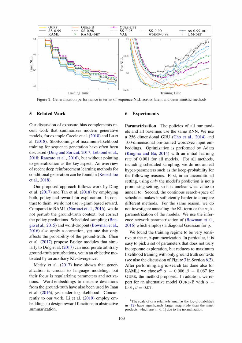
48
50
52
54
Training Time
Trai
nN
LL
52.5
53
53.5
54
Training Time
Test
NL
L
OURS OURS-B OURS-DETSS-0.99 SS-0.98 SS-0.95 SS-0.90 SS-0.99-DETRAML RAML-DET VAE WDROP-0.99 LM-DET
Figure 2: Generalization performance in terms of sequence NLL across latent and deterministic methods
5 Related Work
Our discussion of exposure bias complements re-cent work that summarizes modern generativemodels, for example Caccia et al. (2018) and Lu etal. (2018). Shortcomings of maximum-likelihoodtraining for sequence generation have often beendiscussed (Ding and Soricut, 2017; Leblond et al.,2018; Ranzato et al., 2016), but without pointingto generalization as the key aspect. An overviewof recent deep reinforcement learning methods forconditional generation can be found in (Keneshlooet al., 2018).
Our proposed approach follows work by Dinget al. (2017) and Tan et al. (2018) by employingboth, policy and reward for exploration. In con-trast to them, we do not use n-gram based reward.Compared to RAML (Norouzi et al., 2016), we donot perturb the ground-truth context, but correctthe policy predictions. Scheduled sampling (Ben-gio et al., 2015) and word-dropout (Bowman et al.,2016) also apply a correction, yet one that onlyaffects the probability of the ground-truth. Chenet al. (2017) propose Bridge modules that simi-larly to Ding et al. (2017) can incorporate arbitraryground-truth perturbations, yet in an objective mo-tivated by an auxiliary KL-divergence.
Merity et al. (2017) have shown that gener-alization is crucial to language modeling, buttheir focus is regularizing parameters and activa-tions. Word-embeddings to measure deviationsfrom the ground-truth have also been used by Inanet al. (2016), yet under log-likelihood. Concur-rently to our work, Li et al. (2019) employ em-beddings to design reward functions in abstractivesummarization.
6 Experiments
Parametrization The policies of all our mod-els and all baselines use the same RNN. We usea 256 dimensional GRU (Cho et al., 2014) and100-dimensional pre-trained word2vec input em-beddings. Optimization is preformed by Adam(Kingma and Ba, 2014) with an initial learningrate of 0.001 for all models. For all methods,including scheduled sampling, we do not annealhyper-parameters such as the keep-probability forthe following reasons. First, in an unconditionalsetting, using only the model’s prediction is not apromissing setting, so it is unclear what value toanneal to. Second, the continous search-space ofschedules makes it sufficiently harder to comparedifferent methods. For the same reason, we donot investigate annealing the KL term or the α, β-parametrization of the models. We use the infer-ence network parametrization of (Bowman et al.,2016) which employs a diagonal Gaussian for q.
We found the training regime to be very sensi-tive to the α, β-parametrization. In particular, it iseasy to pick a set of parameters that does not trulyincorporate exploration, but reduces to maximumlikelihood training with only ground truth contexts(see also the discussion of Figure 3 in Section 6.2).After performing a grid-search (as done also forRAML) we choose6 α = 0.006, β = 0.067 forOURS, the method proposed. In addition, we re-port for an alternative model OURS-B with α =0.01, β = 0.07.
6The scale of α is relatively small as the log-probabilitiesin (12) have significantly larger magnitude than the innerproducts, which are in [0, 1] due to the normalization.
163

Data For our experiments, we use a one millionsentences subset of the BooksCorpus (Kiros et al.,2015; Zhu et al., 2015) with a 90-10 train-test splitand a 40K words vocabulary. The corpus size ischosen to challenge the above policy with bothscenarios, overfitting and underfitting.
6.1 Baselines
As baselines we use a standard VAE and a VAEwith RAML decoding that uses identical rewardas our method (see Tan et al.(2018) for details onRAML as a special case). Furthermore, we usetwo regularizations of the standard VAE, sched-uled sampling SS-P and word-dropout WDROP-P
as proposed by Bowman et al. (2016), both withfixed probability p of using the ground-truth.
In addition, we report as special cases withz = 0 results for our model (OURS-DET), RAML(RAML-DET), scheduled sampling (SS-P-DET),and the VAE (LM, a language model).
6.2 Results
Figure 2 shows training and test negative sequencelog-likelihood evaluated during training and Table1 shows the best performance obtained. All figuresand tables are averaged across three runs.
Model Train NLL Test NLLOURS 48.52 52.54OURS-B 49.51 52.61OURS-DET 48.06 52.87SS-0.99 48.11 52.60SS-0.98 48.21 52.62SS-0.95 48.38 52.69SS-0.90 49.02 52.89SS-0.99-DET 48.08 52.90RAML 48.26 52.56RAML-DET 48.26 52.86WDROP-0.99 48.19 52.86LM 47.65 53.01VAE 47.86 52.66WDROP-0.9 50.86 54.65
Table 1: Training and test performance
We observe that all latent models outperformtheir deterministic counterparts (crossed curves)in terms of both, generalization and overall testperformance. This is not surprising as regulariza-tion is one of the benefits of modeling uncertaintythrough latent variables. Scheduled sampling doesimprove generalization for p ≈ 1 with diminishingreturns at p = 0.95 and in general performed bet-ter than word dropout. Our proposed models out-perform all others in terms of generalization and
test performance. Note that the performance dif-ference over RAML, the second best method, issolely due to incorporating also model-predictedcontexts during training.
Despite some slightly improved performance,all latent models except for OURS-B have a KL-term relatively close to zero. OURS-B is α-β-parametrized to incorporte slightly more modelpredictions at higher temperatur and manages toachieve a KL-term of about 1 to 1.5 bits. Thesefindings are similar to what (Bowman et al., 2016)report with annealing but still significantly behindwork that addresses this specific problem (Yanget al., 2017; Shen et al., 2018). Appendix A illus-trates how our models can obtain larger KL-terms– yet at degraded performance – by controlling ex-ploration. We conclude that improved autoregres-sive modeling inside the ERPO framework cannotalone overcome VAE-collapse.
We have discussed many approaches that devi-ate from training exclusively on ground-truth con-texts. Therefore, an interesting quantity to mon-itor across methods is the fraction of words thatcorrespond to the ground-truth. Figure 3 showsthese fractions during training for the configura-tions that gave the best results. Interestingly, in thelatent setting our method relies by far the least onground-truth contexts whereas in the deterministicsetting the difference is small.
0.9
0.95
1
Training Time
OURS OURS-B OURS-DET RAMLSS-0.98 SS-0.99 SS-0.95 LM/VAE
Figure 3: Fraction of correct words during training.Numbers include forced and correctly predicted words.
7 Conclusion
We have argued that exposure bias does not pointto a problem with the standard methodology oftraining autoregressive sequence model. Instead,it refers to a notion of generalization to unseen se-quences that does not manifest in log-likelihoodtraining and testing, yet might be desirable in or-der to capture the flexibility of natural language.
To rigorously incorporate the desired gener-alization behavior, we have proposed to follow
164

the reinforcement learning formulation of Tan etal. (2018). Combined with an embedding-basedreward function, we have shown excellent gener-alization performance compared to the unregular-ized model and better generalization than existingtechniques on language modeling and sentence au-toencoding.
Future work We have shown that the simplereward function proposed here leads to a formof regularization that fosters generalization whenevaluated inside the maximum-likelihood frame-work. In the future, we hope to conduct a humanevaluation to assess the generalization capabili-ties of models trained under maximum-likelihoodand reinforcement learning more rigorously. Onlysuch a framework-independent evaluation can re-veal the true gains of carefully designing re-ward functions compared to simply performingmaximum-likelihood training.
ReferencesAlexander A. Alemi, Ben Poole, Ian Fischer, Joshua V.
Dillon, Rif A. Saurous, and Kevin Murphy. 2017.An information-theoretic analysis of deep latent-variable models. CoRR, abs/1711.00464.
Peter Anderson, Basura Fernando, Mark Johnson,and Stephen Gould. 2016. SPICE: semanticpropositional image caption evaluation. CoRR,abs/1607.08822.
Dzmitry Bahdanau, Philemon Brakel, Kelvin Xu,Anirudh Goyal, Ryan Lowe, Joelle Pineau, Aaron C.Courville, and Yoshua Bengio. 2016. An actor-critic algorithm for sequence prediction. CoRR,abs/1607.07086.
Dzmitry Bahdanau, Kyunghyun Cho, and Yoshua Ben-gio. 2015. Neural machine translation by jointlylearning to align and translate. In ICLR.
Satanjeev Banerjee and Alon Lavie. 2005. METEOR:An automatic metric for MT evaluation with im-proved correlation with human judgments. In ACLWorkshop on Intrinsic and Extrinsic EvaluationMeasures for Machine Translation and/or Summa-rization, pages 65–72, Ann Arbor, Michigan. Asso-ciation for Computational Linguistics.
Justin Bayer and Christian Osendorfer. 2014. Learn-ing stochastic recurrent networks. arXiv preprintarXiv:1411.7610. ArXiv.
Samy Bengio, Oriol Vinyals, Navdeep Jaitly, andNoam Shazeer. 2015. Scheduled sampling for se-quence prediction with recurrent neural networks.In NIPS.
Samuel R. Bowman, Gabor Angeli, Christopher Potts,and Christopher D. Manning. 2015. A large anno-tated corpus for learning natural language inference.In EMNLP.
Samuel R. Bowman, Luke Vilnis, Oriol Vinyals, An-drew M. Dai, Rafal Jozefowicz, and Samy Ben-gio. 2016. Generating sentences from a continuousspace. In ACL.
Massimo Caccia, Lucas Caccia, William Fedus, HugoLarochelle, Joelle Pineau, and Laurent Charlin.2018. Language gans falling short. CoRR,abs/1811.02549.
Tian Qi Chen, Xuechen Li, Roger B. Grosse, andDavid Duvenaud. 2018. Isolating sources of dis-entanglement in variational autoencoders. CoRR,abs/1802.04942.
Wenhu Chen, Guanlin Li, Shujie Liu, Zhirui Zhang,Mu Li, and Ming Zhou. 2017. Neural sequence pre-diction by coaching. CoRR, abs/1706.09152.
Kyunghyun Cho, Bart van Merrienboer, Caglar Gul-cehre, Dzmitry Bahdanau, Fethi Bougares, HolgerSchwenk, and Yoshua Bengio. 2014. Learningphrase representations using RNN encoder–decoderfor statistical machine translation. In EMNLP, pages1724–1734.
Nan Ding and Radu Soricut. 2017. Cold-start rein-forcement learning with softmax policy gradients.CoRR, abs/1709.09346.
William Fedus, Ian J. Goodfellow, and Andrew M. Dai.2018. Maskgan: Better text generation via filling inthe . In ICLR.
Katja Filippova, Enrique Alfonseca, Carlos A Col-menares, Lukasz Kaiser, and Oriol Vinyals. 2015.Sentence compression by deletion with lstms. InEMNLP 2015, pages 360–368.
Marco Fraccaro, Søren Kaae Sønderby, Ulrich Paquet,and Ole Winther. 2016. Sequential neural modelswith stochastic layers. pages 2199–2207. NIPS.
Dibya Ghosh, Abhishek Gupta, and Sergey Levine.2018. Learning actionable representations withgoal-conditioned policies. CoRR, abs/1811.07819.
Ian Goodfellow, Yoshua Bengio, and Aaron Courville.2016. Deep Learning. MIT Press.
Anirudh Goyal, Alex Lamb, Ying Zhang, SaizhengZhang, Aaron C. Courville, and Yoshua Bengio.2016. Professor forcing: A new algorithm for train-ing recurrent networks. In NIPS.
Anirudh Goyal, Alessandro Sordoni, Marc-AlexandreCote, Nan Rosemary Ke, and Yoshua Bengio. 2017.Z-forcing: Training stochastic recurrent networks.In NIPS.
165

Tianxing He, Jingzhao Zhang, Zhiming Zhou, andJames R. Glass. 2019. Quantifying exposure bias forneural language generation. CoRR, abs/1905.10617.
Irina Higgins, Loıc Matthey, Arka Pal, ChristopherBurgess, Xavier Glorot, Matthew M Botvinick,Shakir Mohamed, and Alexander Lerchner. 2017.beta-vae: Learning basic visual concepts with a con-strained variational framework. In ICLR.
Sepp Hochreiter and Jurgen Schmidhuber. 1997. Longshort-term memory. Neural Comput., 9(8):1735–1780.
Ari Holtzman, Jan Buys, Maxwell Forbes, and YejinChoi. 2019. The curious case of neural text degen-eration. CoRR, abs/1904.09751.
Z. Hu, Z. Yang, Liang X., R. Salakhutdinov, and E. R.Xing. 2017. Toward controlled generation of text.In International Conference on Machine Learning(ICML).
Ferenc Husz’ar. 2015. How (not) to train your genera-tive model: Scheduled sampling, likelihood, adver-sary?
Hakan Inan, Khashayar Khosravi, and Richard Socher.2016. Tying word vectors and word classifiers:A loss framework for language modeling. ArXiv,abs/1611.01462.
Yaser Keneshloo, Tian Shi, Naren Ramakrishnan, andChandan K. Reddy. 2018. Deep reinforcementlearning for sequence to sequence models. CoRR,abs/1805.09461.
Urvashi Khandelwal, Kevin Clark, Dan Jurafsky, andLukasz Kaiser. 2019. Sample efficient text sum-marization using a single pre-trained transformer.CoRR, abs/1905.08836.
Diederik P. Kingma and Jimmy Ba. 2014. Adam: Amethod for stochastic optimization. In ICLR.
Diederik P Kingma and Max Welling. 2013. Auto-encoding variational bayes. arXiv preprintarXiv:1312.6114.
Ryan Kiros, Yukun Zhu, Ruslan Salakhutdinov,Richard S Zemel, Antonio Torralba, Raquel Urta-sun, and Sanja Fidler. 2015. Skip-thought vectors.arXiv preprint arXiv:1506.06726.
Matt J. Kusner, Yu Sun, Nicholas I. Kolkin, and Kil-ian Q. Weinberger. 2015. From word embeddingsto document distances. In ICML, ICML’15, pages957–966. JMLR.org.
Remi Leblond, Jean-Baptiste Alayrac, Anton Osokin,and Simon Lacoste-Julien. 2018. SEARNN: train-ing rnns with global-local losses. In ICLR.
Siyao Li, Deren Lei, Pengda Qin, and William Wang.2019. Deep reinforcement learning with distribu-tional semantic rewards for abstractive summariza-tion.
Chin-Yew Lin. 2004. Rouge: A package for automaticevaluation of summaries. page 10.
Sidi Lu, Yaoming Zhu, Weinan Zhang, Jun Wang,and Yong Yu. 2018. Neural text generation: Past,present and beyond. CoRR, abs/1803.07133.
Zachary M. Ziegler and Alexander M. Rush. 2019. La-tent normalizing flows for discrete sequences. arXivpreprint arXiv:1901.10548.
Stephen Merity, Nitish Shirish Keskar, and RichardSocher. 2017. Regularizing and optimizing LSTMlanguage models. CoRR, abs/1708.02182.
Tomas Mikolov, Ilya Sutskever, Kai Chen, Greg S Cor-rado, and Jeff Dean. 2013. Distributed representa-tions of words and phrases and their compositional-ity. In NIPS.
Kevin P. Murphy. 2012. Machine Learning: A Proba-bilistic Perspective. The MIT Press.
Mohammad Norouzi, Samy Bengio, Zhifeng Chen,Navdeep Jaitly, Mike Schuster, Yonghui Wu, andDale Schuurmans. 2016. Reward augmented max-imum likelihood for neural structured prediction.CoRR, abs/1609.00150.
Kishore Papineni, Salim Roukos, Todd Ward, andWei Jing Zhu. 2002. Bleu: a method for automaticevaluation of machine translation.
Tom Rainforth, Adam R. Kosiorek, Tuan Anh Le,Chris J. Maddison, Maximilian Igl, Frank Wood,and Yee Whye Teh. 2018. Tighter variationalbounds are not necessarily better. In ICML.
Marc’Aurelio Ranzato, Sumit Chopra, Michael Auli,and Wojciech Zaremba. 2016. Sequence level train-ing with recurrent neural networks. In ICLR.
Steven J. Rennie, Etienne Marcheret, Youssef Mroueh,Jerret Ross, and Vaibhava Goel. 2016. Self-criticalsequence training for image captioning. CoRR,abs/1612.00563.
Danilo Jimenez Rezende, Shakir Mohamed, and DaanWierstra. 2014. Stochastic back-propagation andvariational inference in deep latent gaussian models.In ICML.
Alexander M. Rush, Sumit Chopra, and Jason Weston.2015. A neural attention model for abstractive sen-tence summarization. In EMNLP.
Florian Schmidt and Thomas Hofmann. 2018. Deepstate space models for unconditional word genera-tion. In NeurIPS.
Iulian Vlad Serban, Alessandro Sordoni, Yoshua Ben-gio, Aaron C Courville, and Joelle Pineau. 2016.Building end-to-end dialogue systems using gener-ative hierarchical neural network models. In AAAI.
166

Xiaoyu Shen, Hui Su, Shuzi Niu, and Vera Demberg.2018. Improving variational encoder-decoders in di-alogue generation. CoRR, abs/1802.02032.
Bowen Tan, Zhiting Hu, Zichao Yang, RuslanSalakhutdinov, and Eric P. Xing. 2018. Connectingthe dots between MLE and RL for sequence genera-tion. CoRR, abs/1811.09740.
Michael Tschannen, Olivier Bachem, and Mario Lucic.2018. Recent advances in autoencoder-based repre-sentation learning. CoRR, abs/1812.05069.
Ashish Vaswani, Noam Shazeer, Niki Parmar, JakobUszkoreit, Llion Jones, Aidan N. Gomez, LukaszKaiser, and Illia Polosukhin. 2017. Attention is allyou need. In NIPS.
Ronald J. Williams. 1992. Simple statistical gradient-following algorithms for connectionist reinforce-ment learning. Mach. Learn., 8(3-4):229–256.
Zichao Yang, Zhiting Hu, Ruslan Salakhutdinov, andTaylor Berg-Kirkpatrick. 2017. Improved varia-tional autoencoders for text modeling using dilatedconvolutions. CoRR, abs/1702.08139.
Cheng Zhang, Judith Butepage, Hedvig Kjellstrom,and Stephan Mandt. 2018. Advances in variationalinference. IEEE transactions on pattern analysisand machine intelligence.
Yukun Zhu, Ryan Kiros, Richard Zemel, RuslanSalakhutdinov, Raquel Urtasun, Antonio Torralba,and Sanja Fidler. 2015. Aligning books and movies:Towards story-like visual explanations by watch-ing movies and reading books. arXiv preprintarXiv:1506.06724.
167

Proceedings of the 3rd Workshop on Neural Generation and Translation (WNGT 2019), pages 168–176Hong Kong, China, November 4, 2019. c©2019 Association for Computational Linguistics
www.aclweb.org/anthology/D19-56%2d
Machine Translation of Restaurant Reviews:New Corpus for Domain Adaptation and Robustness
Alexandre Bérard Ioan Calapodescu Marc DymetmanClaude Roux Jean-Luc Meunier Vassilina Nikoulina
Naver Labs [email protected]
AbstractWe share a French-English parallel corpus ofFoursquare restaurant reviews, and define anew task to encourage research on Neural Ma-chine Translation robustness and domain adap-tation, in a real-world scenario where better-quality MT would be greatly beneficial. Wediscuss the challenges of such user-generatedcontent, and train good baseline models thatbuild upon the latest techniques for MT robust-ness. We also perform an extensive evaluation(automatic and human) that shows significantimprovements over existing online systems. Fi-nally, we propose task-specific metrics basedon sentiment analysis or translation accuracyof domain-specific polysemous words.
1 IntroductionVery detailed information about social venues suchas restaurants is available from user-generated re-views in applications like Google Maps, TripAd-visor or Foursquare1 (4SQ). Most of these reviewsare written in the local language and are not di-rectly exploitable by foreign visitors: an analysis ofthe 4SQ database shows that, in Paris, only 49% ofthe restaurants have at least one review in English,and the situation can be much worse for other citiesand languages (e.g., only 1% of Seoul restaurantsfor a French-only speaker).
Machine Translation of such user-generatedcontent can improve the situation and make thedata available for direct display or for down-stream NLP tasks (e.g., cross-lingual informationretrieval, sentiment analysis, spam or fake reviewdetection), provided its quality is sufficient.
We asked professionals to translate 11.5k French4SQ reviews (18k sentences) to English. We be-lieve that this resource2 will be valuable to the
1https://foursquare.com/2https://europe.naverlabs.com/
research/natural-language-processing/machine-translation-of-restaurant-reviews/
community for training and evaluating MT systemsaddressing challenges posed by user-generatedcontent, which we discuss in detail in this paper.
We conduct extensive experiments and combinetechniques that address these challenges (e.g., fac-tored case, noise generation, domain adaptationwith tags) on top of a strong Transformer baseline.In addition to BLEU evaluation and human evalua-tion, we use targeted metrics that measure how wellpolysemous words are translated, or how well sen-timents expressed in the original review can still berecovered from its translation.
2 Related work
Translating restaurant reviews written by casualcustomers presents several challenges for NMT, inparticular robustness to non-standard language andadaptation to a specific style or domain (see Sec-tion 3.2 for details).
Concerning robustness to noisy user generatedcontent, Michel and Neubig (2018) stress differ-ences with traditional domain adaptation prob-lems, and propose a typology of errors, many ofwhich we also detected in the 4SQ data. They alsoreleased a dataset (MTNT), whose sources wereselected from a social media (Reddit) on the ba-sis of being especially noisy (see Appendix for acomparison with 4SQ). These sources were thentranslated by humans to produce a parallel corpusthat can be used to engineer more robust NMT sys-tems and to evaluate them. This corpus was thebasis of the WMT 2019 MT Robustness Task (Liet al., 2019), in which Berard et al. (2019) rankedfirst. We use the same set of robustness and do-main adaptation techniques, which we study morein depth and apply to our review translation task.
Sperber et al. (2017), Belinkov and Bisk (2018)and Karpukhin et al. (2019) propose to improverobustness by training models on data-augmented
168

corpora, containing noisy sources obtained by ran-dom word or character deletions, insertions, substi-tutions or swaps. Recently, Vaibhav et al. (2019)proposed to use a similar technique along withnoise generation through replacement of a cleansource by one obtained by back-translation.
We employ several well-known domain adapta-tion techniques: back-translation of large monolin-gual corpora close to the domain (Sennrich et al.,2016b; Edunov et al., 2018), fine-tuning with in-domain parallel data (Luong and Manning, 2015;Freitag and Al-Onaizan, 2016; Servan et al., 2016),domain tags for knowledge transfer between do-mains (Kobus et al., 2017; Berard et al., 2019).
Addressing the technical issues of robustnessand adaptation of an NMT system is decisive forreal-world deployment, but evaluation is also crit-ical. This aspect is stressed by Levin et al. (2017)(NMT of curated hotel descriptions), who point outthat automatic metrics like BLEU tend to neglectsemantic differences that have a small textual foot-print, but may be seriously misleading in practice,for instance by interpreting available parking as ifit meant free parking. To mitigate this, we conductadditional evaluations of our models: human eval-uation, translation accuracy of polysemous words,and indirect evaluation with sentiment analysis.
3 Task descriptionWe present a new task of restaurant review trans-lation, which combines domain adaptation and ro-bustness challenges.
3.1 Corpus descriptionWe sampled 11.5k French reviews from 4SQ,mostly in the food category,3 split them into sen-tences (18k), and grouped them into train, validand test sets (see Table 1). The French reviewscontain on average 1.5 sentences and 17.9 words.Then, we hired eight professional translators totranslate them to English. Two of them cre-ated the training set by post-editing (PE) the out-puts of baseline NMT systems.4 The other sixtranslated the valid and test sets from scratch.They were asked to translate (or post-edit) the re-views sentence-by-sentence (to avoid any align-ment problem), but they could see the full con-
3https://developer.foursquare.com/docs/resources/categories
4ConvS2S or Transformer Big trained on the “UGC” cor-pus described in Section 6, without domain adaptation or ro-bustness tricks.
Corpus Sentences Reviews Words (FR)4SQ-PE 12 080 8 004 141 9584SQ-HT 2 784 1 625 29 0754SQ-valid 1 243 765 13 9764SQ-test 1 838 1 157 21 525
Table 1: 4SQ corpora. 4SQ-PE is the training set. 4SQ-HT is not used in this work.
text. We manually filtered the test set to removetranslations that were not satisfactory. The full re-views and additional metadata (e.g., location andtype of the restaurant) are also available as part ofthis resource, to encourage research on contextualmachine translation. 4SQ-HT was translated fromscratch by the same translators who post-edited4SQ-PE. While we did not use it in this work, itcan be used as extra training or development data.We also release a human translation of the French-language test set (668 sentences) of the Aspect-Based Sentiment Analysis task at SemEval 2016(Pontiki et al., 2016).
3.2 ChallengesTranslating restaurant reviews presents two mainchallenges compared to common tasks in MT.First, the reviews are written in a casual style, closeto spoken language. Some liberty is taken w.r.t.spelling, grammar, and punctuation. Slang is alsovery frequent. MT should be robust to these vari-ations. Second, they generally are reactions, byclients of a restaurant, about its food quality, ser-vice or atmosphere, with specific words relating tothese aspects or sentiments. These require somedegree of domain adaptation. The following tableillustrates these issues, with outputs from an onlineMT system. Examples of full reviews from 4SQ-PE along with metadata are shown in Appendix.
(1)é qd g vu sa ... (source)and when I saw that ... (reference)é qd g seen his ... (online MT)
(2)c’est trooop bon !it’s toooo good!it’s good trooop!
(3)le cadre est nulthe setting is lousythe frame is null
(4)le garçon a pété un cablethe waiter went crazythe boy farted a cable
(5)pizza nickel, tres bonnes pattesgreat pizza, very good pastanickel pizza, very good legs
169

Examples 1 and 2 fall into the robustness cat-egory: 1 is an extreme form of SMS-like, quasi-phonetic, language (et quand j’ai vu ça); 2 is a lit-eral transcription of a long-vowel phonetic stress(trop → trooop). Example 3 falls into the domaincategory: in a restaurant context, cadre typicallyrefers to the setting. Examples 4 and 5 involve bothrobustness and domain adaptation: pété un cable isa non-compositional slang expression and garçonis not a boy in this domain; nickel is slang for great,très is missing an accent, and pâtes is misspelled aspattes, which is another French word.
Regarding robustness, we found many of thesame errors listed by Michel and Neubig (2018)as noise in social media text: SMS language (éqd g vu sa), typos and phonetic spelling (pattes),repeated letters (trooop, merciiii), slang (nickel,bof, mdr), missing or wrong accents (tres), emoti-cons (‘:-)’) and emojis (😉), missing punctua-tion, wrong or non-standard capitalization (lower-case proper names, capitalized words for empha-sis). Regarding domain aspects, there are polyse-mous words with typical specific meaning carte →map, menu; cadre → frame, executive, setting), id-iomatic expressions (à tomber par terre → to diefor), and venue-related named entities (La Boîte àSardines).
4 Robustness to noise
We propose solutions for dealing with non-standard case, emoticons, emojis and other issues.
4.1 Rare character placeholderWe segment our training data into subwords withBPE (Sennrich et al., 2016c), implemented in Sen-tencePiece (Kudo and Richardson, 2018). BPE candeal with rare or unseen words by splitting theminto more frequent subwords but cannot deal withunseen characters.5 While this is not a problem inmost tasks, 4SQ contains a lot of emojis, and some-times symbols in other scripts (e.g., Arabic). Uni-code now defines around 3k emojis, most of whichare likely to be out-of-vocabulary.
We replace rare characters on both sides of thetraining corpus by a placeholder (<x>); a modeltrained on this data is typically able to copy theplaceholder at the correct position. Then, at in-ference time, we replace the output tokens <x>by the rare source-side characters, in the same or-
5Unless actually doing BPE at the byte level, as suggestedby Radford et al. (2019).
Uppercase LowercaseInput UNE HONTE ! une honte !Pre-proc UN E _H ON TE _! une _honte _!MT output A _H ON E Y ! A _dis gra ce !Post-proc A HONEY! A disgrace!
Table 2: Capital letters break NMT. BPE segmentationand translation of capitalized or lowercase input.
der. This approach is similar to that of Jean et al.(2015), who used the attention mechanism to re-place output UNK symbols with the aligned word inthe source. Berard et al. (2019) used the same tech-nique to deal with emojis in the WMT robustnesstask.
4.2 Capital lettersAs shown in Table 2, capital letters are anothersource of confusion. HONTE and honte are con-sidered as two different words. The former isout-of-vocabulary and is split very aggressively byBPE. This causes the MT model to hallucinate.
Lowercasing A solution is to lowercase the in-put, both at training and at test time. However,when doing so, some information may be lost (e.g.,named entities, acronyms, emphasis) which mayresult in lower translation quality.
Factored translation Levin et al. (2017) do fac-tored machine translation (Sennrich and Haddow,2016; Garcia-Martinez et al., 2016) where a wordand its case are split in two different features. Forinstance, HONTE becomes honte + upper.
We implement this with two embedding matri-ces, one for words and one for case, and repre-sent a token as the sum of the embeddings of itsfactors. For the target side, we follow Garcia-Martinez et al. (2016) and have two softmax op-erations. We first predict the word in its lowercaseform and then predict its case.6 The embeddingsof the case and word are then summed and used asinput for the next decoder step.
Inline casing Berard et al. (2019) propose an-other approach, inline casing, which does not re-quire any change in the model. We insert the caseas a regular token into the sequence right after theword. Special tokens <U>, <L> and <T> (upper,lower and title) are used for this purpose and ap-pended to the vocabulary. Contrary to the previous
6Like the “dependency model” of Garcia-Martinez et al.(2016), we use the current state of the decoder and the embed-ding of the output word to predict its case.
170

solution, there is only one embedding matrix andone softmax.
In practice, words are assumed to be lowercaseby default and the <L> tokens are dropped to keepthe factored sequences as short as possible. “Bestfries EVER” becomes “best <T> _f ries _ever<U>”. Like Berard et al. (2019), we force Senten-cePiece to split mixed-case words like MacDon-alds into single-case subwords (Mac and Donalds).
Synthetic case noise Another solution that weexperiment with (see Section 6) is to inject noiseon the source side of the training data by changingrandom source words to upper (5% chance), title(10%) or lower case (20%).
4.3 Natural noiseOne way to make an NMT system more robust is totrain it with some of the most common errors thatcan be found in the in-domain data. Like Berardet al. (2019), we detect the errors that occur nat-urally in the in-domain data and then apply themto our training corpus, while respecting their natu-ral distribution. We call this “natural noise gen-eration” in opposition to what is done in (Sper-ber et al., 2017; Belinkov and Bisk, 2018; Vaibhavet al., 2019) or in Section 4.2, where the noise ismore synthetic.
Detecting errors We compile a general-purposeFrench lexicon as a transducer,7 implemented to betraversed with extended edit distance flags, similarto Mihov and Schulz (2004). Whenever a word isnot found in the lexicon (which means that it is apotential spelling mistake), we look for a Frenchword in the lexicon within a maximum edit dis-tance of 2, with the following set of edit operations:
(1) deletion (e.g., apelle instead of appelle)
(2) insertion (e.g., appercevoir instead ofapercevoir)
(3) constrained substitution on diacritics (e.g.,mangè instead of mangé)
(4) swap counted as one operation: (e.g.,mnager instead of manger)
(5) substitution (e.g., menger instead ofmanger)
(6) repetitions (e.g., Merciiiii with a thresholdof max 10 repetitions)
We apply the transducer to the French monolin-gual Foursquare data (close to 1M sentences) todetect and count noisy variants of known Frenchwords. This step produces a dictionary mapping
7In Tamgu: https://github.com/naver/tamgu
the correct spelling to the list of observed errorsand their respective frequencies.
In addition to automatically extracted spellingerrors, we extract a set of common abbreviationsfrom (Seddah et al., 2012) and we manually iden-tify a list of common errors in French:
(7) Wrong verb endings (e.g., il a manger in-stead of il a mangé)
(8) Wrong spacing around punctuation symbols(e.g., Les.plats ... instead of Les plats...)
(9) Upper case/mixed case words (e.g., manQuede place instead of manque de place)
(10) SMS language (e.g., bcp instead of beau-coup)
(11) Phonetic spelling (e.g., sa instead of ça)
Generating errors With this dictionary, de-scribing the real error distribution in 4SQ text, wetake our large out-of-domain training corpus, andrandomly replace source-side words with one oftheir variants (rules 1 to 6), while respecting thefrequency of this variant in the real data. We alsomanually define regular expressions to randomlyapply rules 7 to 11 (e.g., "er "→"é ").
We obtain a noisy parallel corpus (which we useinstead of the “clean” training data), where about30% of all source sentences have been modified, asshown below:
Error type Examples of sentences with injected noise
(1) (6) (9) L’Union eUropéene espere que la réunionde suiviii entre le Président [...]
(2) (3) (10) Le Comité notte avec bcp d’interet k lesprojets d’articles [...]
(4) (7) (8) Réunoin sur.la comptabiliter nationale [...]
5 Domain AdaptationTo adapt our models to the restaurant review do-main we apply the following types of techniques:back-translation of in-domain English data, fine-tuning with small amounts of in-domain paralleldata, and domain tags.
5.1 Back-translationBack-translation (BT) is a popular technique fordomain adaptation when large amounts of in-domain monolingual data are available (Sennrichet al., 2016b; Edunov et al., 2018). While ourin-domain parallel corpus is small (12k pairs),Foursquare contains millions of English-languagereviews. Thus, we train an NMT model8 in the re-verse direction (EN→FR) and translate all the 4SQ
8Like the “UGC” model with rare character handling andinline case described in Section 6.3.
171

English reviews to French.9 This gives a large syn-thetic parallel corpus.
This in-domain data is concatenated to the out-of-domain parallel data and used for training.
Edunov et al. (2018) show that doing back-translation with sampling instead of beam searchbrings large improvements due to increased diver-sity. Following this work, we test several settings:
Name Description
BT-B Back-translation with beam search.
BT-S Back-translation with sampling.
BT-S × 3 Three different FR samplings for each ENsentence. This brings the size of the back-translated 4SQ closer to the out-of-domaincorpus.
BT No oversampling, but we sample a new ver-sion of the corpus for each training epoch.
We use a temperature10 of T = 10.9 to avoid the
extremely noisy output obtained with T = 1 andstrike a balance between quality and diversity.
5.2 Fine-tuningWhen small amounts of in-domain parallel data areavailable, fine-tuning (FT) is often the preferredsolution for domain adaptation (Luong and Man-ning, 2015; Freitag and Al-Onaizan, 2016). It con-sists in training a model on out-of-domain data,and then continuing its training for a few epochson the in-domain data only.
5.3 Corpus tagsKobus et al. (2017) propose a technique for multi-domain NMT, which consists in inserting a to-ken in each source sequence specifying its domain.The system can learn the particularities of multipledomains (e.g., polysemous words that have a dif-ferent meaning depending on the domain), whichwe can control at test time by manually setting thetag. Sennrich et al. (2016a) also use tags to controlpoliteness in the model’s output.
As our corpus (see Section 6.1) is not clearly di-vided into domains, we apply the same techniqueas Kobus et al. (2017) but use corpus tags (eachsub-corpus has its own tag: TED, Paracrawl, etc.)which we add to each source sequence. Like in(Berard et al., 2019), the 4SQ post-edited and back-translated data also get their own tags (PE and BT).
9This represents ≈15M sentences. This corpus is notavailable publicly, but the Yelp dataset (https://www.yelp.com/dataset) could be used instead.
10with p(wi) = exp(zi/T )∑|V |k=1
exp(zk/T )
Corpus tag SRC: La carte est trop petite.
TED The map is too small.
Multi-UN The card is too small.
PE The menu is too small.
Figure 1: Example of ambiguous source sentence,where using corpus tags help the model pick a more ad-equate translation.
Corpus Lines Words (FR) Words (EN)WMT 29.47M 1 003M 883.5MUGC 51.39M 1 125M 1 041M
Table 3: Size of the WMT and UGC training corpora(after filtering).
Figure 1 gives an example where using the PE cor-pus tag at test time helps the model pick a moreadequate translation.
6 Experiments
6.1 Training dataAfter some initial work with the WMT 2014 data,we built a new training corpus named UGC (UserGenerated Content), closer to our domain, bycombining: Multi UN, OpenSubtitles, Wikipedia,Books, Tatoeba, TED talks, ParaCrawl11 andGourmet12 (See Table 3). Notably, UGC does notinclude Common Crawl (which contains a lot ofmisaligned sentences and caused hallucinations),but it includes OpenSubtitles (Lison and Tiede-mann, 2016) (spoken-language, possibly closer to4SQ). We observed an improvement of more than 1BLEU on news-test 2014 when switching to UGC,and almost 6 BLEU on 4SQ-valid.
6.2 Pre-processingWe use langid.py (Lui and Baldwin, 2012) to fil-ter sentence pairs from UGC. We also remove du-plicate sentence pairs, and lines longer than 175words or with a length ratio greater than 1.5 (seeTable 3). Then we apply SentencePiece and ourrare character handling strategy (Section 4.1). Weuse a joined BPE model of size 32k, trained on theconcatenation of both sides of the corpus, and setSentencePiece’s vocabulary threshold to 100. Fi-nally, unless stated otherwise, we always use theinline casing approach (see Section 4.2).
11Corpora available at http://opus.nlpl.eu/123k translations of dishes and other food terminology
http://www.gourmetpedia.eu/
172

6.3 Model and settingsFor all experiments, we use the Transformer Big(Vaswani et al., 2017) as implemented in Fairseq,with the hyperparameters of Ott et al. (2018).Training is done on 8 GPUs, with accumulated gra-dients over 10 batches (Ott et al., 2018), and a maxbatch size of 3500 tokens (per GPU). We train for20 epochs, while saving a checkpoint every 2500updates (≈ 2
5 epoch on UGC) and average the 5best checkpoints according to their perplexity on avalidation set (a held-out subset of UGC).
For fine-tuning, we use a fixed learning rate, anda total batch size of 3500 tokens (training on asingle GPU without delayed updates). To avoidoverfitting on 4SQ-PE, we do early stopping ac-cording to perplexity on 4SQ-valid.13 For eachfine-tuned model we test all 16 combinations ofdropout in {0.1, 0.2, 0.3, 0.4} and learning rate in{1, 2, 5, 10} × 10−5. We keep the model with thebest perplexity on 4SQ-valid.14
6.4 Evaluation methodologyDuring our work, we used BLEU (Papineni et al.,2002) on news-valid (concatenation of news-test2012 and 2013) to ensure that our models stayedgood on a more general domain, and on 4SQ-validto measure performance on the 4SQ domain.
For sake of brevity, we only give the final BLEUscores on news-test 2014 and 4SQ-test. Scores on4SQ-valid, and MTNT-test (for comparison withMichel and Neubig, 2018; Berard et al., 2019) aregiven in Appendix. We evaluate “detokenized”MT outputs15 against raw (non-tokenized) refer-ences using SacreBLEU (Post, 2018).16
In addition to BLEU, we do an indirect eval-uation on an Aspect-Based Sentiment Analysis(ABSA) task, a human evaluation, and a task-related evaluation based on polysemous words.
6.5 BLEU evaluationCapital letters Table 4 compares the case han-dling techniques presented in Section 4.2. Tobetter evaluate the robustness of our models tochanges of case, we built 3 synthetic test sets from4SQ-test, with the same target, but all source wordsin upper, lower or title case.
13The best perplexity was achieved after 1 to 3 epochs.14The best dropout rate was always 0.1, and the best learn-
ing rate was either 2 × 10⁻⁵ or 5 × 10−5.15Outputs of our models are provided with the 4SQ corpus.16SacreBLEU signature: BLEU+case.mixed+numrefs.1
+smooth.exp+tok.13a+version.1.2.10
Model BLEU Case insensitive BLEU4SQ Upper Lower Title
Cased 31.78 16.02 32.42 26.67LC to cased 30.91 33.09 33.09 33.09Factored case 31.62 32.31 32.96 29.86Inline case 31.55 31.08 32.63 29.61Noised case 31.99 32.64 33.73 33.63Table 4: Robustness to capital letters (see Section 4.2).4SQ’s source side has been set to upper, lower or titlecase. The first column is case sensitive BLEU. “LC tocased” always gets the same scores because it is invari-ant to source case.
Model news noised news 4SQUGC (Inline case) 40.68 35.59 31.55+ natural noise 40.43 40.35 31.69Table 5: Baseline model with or without natural noise(see Section 4.3). Noised news is the same type of noise,artificially applied to news-test.
Inline and factored case perform equally well,significantly better than the default (cased) model,especially on all-uppercase inputs. Lowercasingthe source is a good option, but gives a slightlylower score on regular 4SQ-test.17 Finally, syn-thetic case noise added to the source gives surpris-ingly good results. It could also be combined withfactored or inline case.
Natural noise Table 5 compares the baseline“inline case” model with the same model aug-mented with natural noise (Section 4.3). Per-formance is the same on 4SQ-test, but signifi-cantly better on news-test artificially augmentedwith 4SQ-like noise.
Domain adaptation Table 6 shows the resultsof the back-translation (BT) techniques. Surpris-ingly, BT with beam search (BT-B) deterioratesBLEU scores on 4SQ-test, while BT with samplinggives a consistent improvement. BLEU scores onnews-test are not significantly impacted, suggest-ing that BT can be used for domain adaptationwithout hurting quality on other domains.
Table 7 compares the domain adaptation tech-niques presented in Section 5. We observe that:1. Concatenating the small 4SQ-PE corpus to
the 50M general domain corpus does not helpmuch, unless using tags.
17The “LC to cased” and “Noised case” models are not ableto preserve capital letters for emphasis (as in Table 2), and the“Cased” model often breaks on such examples.
173

Model news 4SQUGC (Inline case) 40.68 31.55UGC ⊕ BT-B 40.56 30.17UGC ⊕ BT-S 40.64 32.64UGC ⊕ BT 40.84 32.69UGC ⊕ BT-S × 3 40.63 32.84
Table 6: Comparison of different back-translationschemes (see Section 5.1). ⊕ denotes the concatena-tion of several training corpora.
Model Tag news 4SQUGC (Inline case) – 40.68 31.55UGC ⊕ 4SQ-PE – 40.80 32.05UGC + FT – 39.78 35.02
UGC ⊕ 4SQ-PE + tags – 40.71 32.12PE 38.97 34.36
UGC ⊕ BT + tags – 40.67 33.47BT 39.02 33.00
Table 7: Domain adaptation with 4SQ-PE fine-tuning(FT) or corpus tags. The “tag” column represents thecorpus tag used at test time (if any).
2. 4SQ-PE + tags is not as good as fine-tuningwith 4SQ-PE. However, fine-tuned models getslightly worse results on news.
3. Back-translation combined with tags gives alarge boost.18 The BT tag should not be usedat test time, as it degrades results.
4. Surprisingly, using no tag at test time worksfine, even though all training sentences hadtags.19
As shown in Table 8, these techniques can becombined to achieve the best results. The nat-ural noise does not have a significant effect onBLEU scores. Back-translation combined withfine-tuning gives the best performance on 4SQ(+4.5 BLEU vs UGC). However, using tags insteadof fine-tuning strikes a better balance between gen-eral domain and in-domain performance.
6.6 Targeted evaluationIn this section we propose two metrics that tar-get specific aspects of translation adequacy: trans-lation accuracy of domain-specific polysemouswords and Aspect-Based Sentiment Analysis per-formance on MT outputs.
18Caswell et al. (2019); Berard et al. (2019) observed thesame thing.
19We tried keeping a small percentage of UGC with no tag,or with an ANY tag, but this made no difference.
Model news 4SQWMT 39.37 26.26UGC (Inline case) 40.68 31.55Google Translate (Feb 2019) 36.31 29.63DeepL (Feb 2019) ? 32.82UGC ⊕ BT + FT 39.55 35.95UGC ⊕ BT ⊕ PE + tags 40.99 35.72Nat noise ⊕ BT + FT 39.91 36.35Nat noise ⊕ BT ⊕ PE + tags 40.72 35.60
Table 8: Combination of several robustness or domainadaptation techniques. At test time, we don’t use any tagon news, and use the PE tag on 4SQ (when applicable).BT: back-translation. PE: 4SQ-PE. FT: fine-tuning with4SQ-PE. ⊕: concatenation.
French word MeaningsCadre setting, frame, executiveCuisine food, kitchenCarte menu, card, map
Table 9: French polysemous words found in 4SQ, andtranslation candidates in English. The most frequentmeanings in 4SQ are underlined.
Translation of polysemous words We proposeto count polysemous words specific to our domain,similarly to (Lala and Specia, 2018), to measurethe degree of domain adaptation. TER between thetranslation hypotheses and the post-edited refer-ences in 4SQ-PE reveals the most common substi-tutions (e.g., “card” is often replaced with “menu”,suggesting that “card” is a common mistranslationof the polysemous word “carte”). We filter this listmanually to only keep words that are polysemousand that have a high frequency in the test set. Ta-ble 9 gives the 3 most frequent ones.20
Table 10 shows the accuracy of our models whentranslating these words. We see that the domain-adapted model is better at translating domain-specific polysemous words.
Indirect evaluation with sentiment analysisWe also measure adequacy by how well the trans-lation preserves the polarity of the sentence re-garding various aspects. To evaluate this, we per-form an indirect evaluation on the SemEval 2016Aspect-Based Sentiment Analysis (ABSA) task(Pontiki et al., 2016). We use our internal ABSAsystems trained on English or French SemEval
20Rarer ones are: adresse (place, address), café (coffee,café), entrée (starter, entrance), formule (menu, formula),long (slow, long), moyen (average, medium), correct (decent,right), brasserie (brasserie, brewery) and coin (local, corner).
174
Model cadre cuisine carte TotalTotal (source) 23 32 29 100%WMT 13 17 14 52%UGC (Inline case) 22 27 18 80%UGC ⊕ PE + tags 23 31 29 99%Table 10: Number of correct translations for difficultpolysemous words in 4SQ-test by different models. Thefirst row is the number of source sentences that containthis word. Other domain-adapted models (e.g., “UGC+ FT” or “UGC ⊕ BT”) also get ≈ 99% accuracy.
ABSA Model Aspect PolarityABSA French 64.7 83.2ABSA English 59.5 72.1
ABSA English on MT outputsWMT 54.5 66.1UGC (Inline case) 58.1 70.7UGC ⊕ BT ⊕ PE + tags 60.2 72.0Nat noise ⊕ BT ⊕ PE + tags 60.8 73.3
Table 11: Indirect evaluation with Aspect-Based Senti-ment Analysis (accuracy in %). ABSA French: ABSAmodel trained on French data and applied to the Se-mEval 2016 French test set; ABSA English: trained onEnglish data and applied to human translations of thetest set; ABSA English on MT outputs: applied to MToutputs instead of human translations.
2016 data. The evaluation is done on the SemEval2016 French test set: either the original version(ABSA French), or its translation (ABSA English).As shown in Table 11, translations obtained withdomain-adapted models lead to significantly betterscores on the ABSA task than the generic models.
6.7 Human EvaluationWe conduct a human evaluation to confirm the ob-servations with BLEU and to overcome some ofthe limitations of this metric.
We select 4 MT models for evaluation (see Ta-ble 12) and show their 4 outputs at once, sentence-by-sentence, to human judges, who are asked torank them given the French source sentence in con-text (with the full review). For each pair of models,we count the number of wins, ties and losses, andapply the Wilcoxon signed-rank test.
We took the first 300 test sentences to create 6tasks of 50 sentences each. Then we asked bilin-gual colleagues to rank the output of 4 models bytheir translation quality. They were asked to doone or more of these tasks. The judge did notknow about the list of models, nor the model thatproduced any given translation. We got 12 an-
Pairs Win Tie LossTags ≈ Tags + noise 82 453 63Tags ≫ Baseline 187 337 74Tags ≫ GT 226 302 70Tags + noise ≫ Baseline 178 232 97Tags + noise ≫ GT 218 315 65Baseline ≫ GT 173 302 123
Table 12: In-house human evaluation (“≫” means bet-ter with p ≤ 0.05). The 4 models Baseline, GT, Tagsand Tags + noise correspond respectively to rows 2(UGC with inline case), 3 (Google Translate), 6 (Com-bination of BT, PE and tags) and 8 (Same as 6 withnatural noise) in Table 8.
swers. The inter-judge Kappa coefficient rangedfrom 0.29 to 0.63, with an average of 0.47, whichis a good value given the difficulty of the task. Ta-ble 12 gives the results of the evaluation, whichconfirm our observations with BLEU.
We also did a larger-scale monolingual eval-uation using Amazon Mechanical Turk (see Ap-pendix), which lead to similar conclusions.
7 ConclusionWe presented a new parallel corpus of user re-views of restaurants, which we think will be valu-able to the community. We proposed combinationsof multiple techniques for robustness and domainadaptation, which address particular challenges ofthis new task. We also performed an extensiveevaluation to measure the improvements broughtby these techniques.
According to BLEU, the best single techniquefor domain adaptation is fine-tuning. Corpus tagsalso achieve good results, without degrading per-formance on a general domain. Back-translationhelps, but only with sampling or tags. The robust-ness techniques (natural noise, factored case, rarecharacter placeholder) do not improve BLEU.
While our models are promising, they still showserious errors when applied to user-generated con-tent: missing negations, hallucinations, unrecog-nized named entities, insensitivity to context.21
This suggests that this task is far from solved.We hope that this corpus, our natural noise dic-
tionary, model outputs and human rankings willhelp better understand and address these prob-lems. We also plan to investigate these problemson lower resource languages, where we expect thetask to be even harder.
21See additional examples in Appendix.
175

ReferencesYonatan Belinkov and Yonatan Bisk. 2018. Syn-
thetic and Natural Noise Both Break Neural MachineTranslation. In ICLR.
Alexandre Berard, Calapodescu Ioan, and ClaudeRoux. 2019. NAVER LABS Europe’s Systems forthe WMT19 Machine Translation Robustness Task.In WMT.
Isaac Caswell, Ciprian Chelba, and David Grangier.2019. Tagged Back-Translation. In WMT.
Sergey Edunov, Myle Ott, Michael Auli, and DavidGrangier. 2018. Understanding Back-Translation atScale. In EMNLP.
Markus Freitag and Yaser Al-Onaizan. 2016. Fast Do-main Adaptation for Neural Machine Translation.arXiv.
Mercedes Garcia-Martinez, Loic Barrault, and FethiBougares. 2016. Factored Neural Machine Transla-tion. arXiv.
Sébastien Jean, Kyunghyun Cho, Roland Memisevic,and Yoshua Bengio. 2015. On Using Very LargeTarget Vocabulary for Neural Machine Translation.NAACL-HLT.
Vladimir Karpukhin, Omer Levy, Jacob Eisenstein, andMarjan Ghazvininejad. 2019. Training on SyntheticNoise Improves Robustness to Natural Noise in Ma-chine Translation. arXiv.
Catherine Kobus, Josep Crego, and Jean Senellart.2017. Domain Control for Neural Machine Trans-lation. In RANLP.
Taku Kudo and John Richardson. 2018. SentencePiece:A simple and language independent subword tok-enizer and detokenizer for Neural Text Processing.In EMNLP.
Chiraag Lala and Lucia Specia. 2018. Multimodal lex-ical translation. In LREC.
Pavel Levin, Nishikant Dhanuka, Talaat Khalil, FedorKovalev, and Maxim Khalilov. 2017. Toward a full-scale neural machine translation in production: theBooking.com use case. In MT Summit XVI.
Xian Li, Paul Michel, Antonios Anastasopoulos,Yonatan Belinkov, Nadir K. Durrani, Orhan Firat,Philipp Koehn, Graham Neubig, Juan M. Pino, andHassan Sajjad. 2019. Findings of the First SharedTask on Machine Translation Robustness. In WMT.
Pierre Lison and Jörg Tiedemann. 2016. OpenSub-titles2016: Extracting Large Parallel Corpora fromMovie and TV Subtitles. In LREC.
Marco Lui and Timothy Baldwin. 2012. langid.py: AnOff-the-shelf Language Identification Tool. In Pro-ceedings of the ACL 2012 System Demonstrations,ACL.
Minh-Thang Luong and Christopher D. Manning.2015. Stanford Neural Machine Translation Systemsfor Spoken Language Domain. In IWSLT.
Paul Michel and Graham Neubig. 2018. MTNT: ATestbed for Machine Translation of Noisy Text. In
EMNLP.Stoyan Mihov and Klaus U. Schulz. 2004. Fast Approx-
imate Search in Large Dictionaries. ComputationalLinguistics.
Myle Ott, Sergey Edunov, David Grangier, and MichaelAuli. 2018. Scaling Neural Machine Translation. InWMT.
Kishore Papineni, Salim Roukos, Todd Ward, andWj Zhu. 2002. BLEU: a Method for Automatic Eval-uation of Machine Translation. In ACL.
Maria Pontiki, Dimitris Galanis, Haris Papageor-giou, Ion Androutsopoulos, Suresh Manandhar, Mo-hammed AL-Smadi, Mahmoud Al-Ayyoub, YanyanZhao, Bing Qin, Orphée De Clercq, VeroniqueHoste, Marianna Apidianaki, Xavier Tannier, Na-talia Loukachevitch, Evgeniy Kotelnikov, Núria Bel,Salud Maria Jiménez-Zafra, and Gülşen Eryiğit.2016. SemEval-2016 Task 5: Aspect Based Senti-ment Analysis. In Proceedings of the 10th Interna-tional Workshop on Semantic Evaluation (SemEval).
Matt Post. 2018. A Call for Clarity in Reporting BLEUScores. In WMT.
Alec Radford, Jeffrey Wu, Rewon Child, David Luan,Dario Amodei, and Ilya Sutskever. 2019. LanguageModels are Unsupervised Multitask Learners.
Djamé Seddah, Benoît Sagot, Marie Candito, VirginieMouilleron, and Vanessa Combet. 2012. Build-ing a treebank of noisy user-generated content: TheFrench Social Media Bank. In The 11th Interna-tional Workshop on Treebanks and Linguistic The-ories (TLT).
Rico Sennrich and Barry Haddow. 2016. Linguistic In-put Features Improve Neural Machine Translation.In WMT.
Rico Sennrich, Barry Haddow, and Alexandra Birch.2016a. Controlling Politeness in Neural MachineTranslation via Side Constraints. In NAACL-HLT.
Rico Sennrich, Barry Haddow, and Alexandra Birch.2016b. Improving Neural Machine TranslationModels with Monolingual Data. In ACL.
Rico Sennrich, Barry Haddow, and Alexandra Birch.2016c. Neural Machine Translation of Rare Wordswith Subword Units. In ACL.
Christophe Servan, Josep Crego, and Jean Senel-lart. 2016. Domain specialization: a post-trainingdomain adaptation for neural machine translation.arXiv.
Matthias Sperber, Jan Niehues, and Alex Waibel.2017. Toward Robust Neural Machine Translationfor Noisy Input Sequences. In IWSLT.
Vaibhav, Sumeet Singh, Craig Stewart, and GrahamNeubig. 2019. Improving Robustness of MachineTranslation with Synthetic Noise. In NAACL.
Ashish Vaswani, Noam Shazeer, Niki Parmar, JakobUszkoreit, Llion Jones, Aidan N. Gomez, ŁukaszKaiser, and Illia Polosukhin. 2017. Attention Is AllYou Need. In NIPS.
176

Proceedings of the 3rd Workshop on Neural Generation and Translation (WNGT 2019), pages 177–186Hong Kong, China, November 4, 2019. c©2019 Association for Computational Linguistics
www.aclweb.org/anthology/D19-56%2d
Adaptively Scheduled Multitask Learning:The Case of Low-Resource Neural Machine Translation
Poorya Zaremoodi1,2 Gholamreza Haffari11Monash University, Melbourne, Australia
2CSIRO Data61, Sydney, [email protected]
Abstract
Neural Machine Translation (NMT), a data-hungry technology, suffers from the lack ofbilingual data in low-resource scenarios. Mul-titask learning (MTL) can alleviate this is-sue by injecting inductive biases into NMT,using auxiliary syntactic and semantic tasks.However, an effective training schedule is re-quired to balance the importance of tasks toget the best use of the training signal. Therole of training schedule becomes even morecrucial in biased-MTL where the goal is toimprove one (or a subset) of tasks the most,e.g. translation quality. Current approachesfor biased-MTL are based on brittle hand-engineered heuristics that require trial and er-ror, and should be (re-)designed for each learn-ing scenario. To the best of our knowledge,ours is the first work on adaptively and dy-namically changing the training schedule inbiased-MTL. We propose a rigorous approachfor automatically reweighing the training dataof the main and auxiliary tasks throughoutthe training process based on their contribu-tions to the generalisability of the main NMTtask. Our experiments on translating from En-glish to Vietnamese/Turkish/Spanish show im-provements of up to +1.2 BLEU points, com-pared to strong baselines. Additionally, ouranalyses shed light on the dynamic of needsthroughout the training of NMT: from syntaxto semantic.
1 Introduction
While Neural Machine Translation (NMT) isknown for its ability to learn end-to-end with-out any need for many brittle design choicesand hand-engineered features, it is notorious forits demand for large amounts of bilingual datato achieve reasonable translation quality (Koehnand Knowles, 2017). Recent work has investi-gated multitask learning (MTL) for injecting in-ductive biases from auxiliary syntactic and/or se-
0
0.05
0.1
0.15
0.2
0.25
200
6001000
1400
1800
2200
2600
3000
3400
3800
4200
4600
5000
5400
5800
6200
6600
7000
7400
7800
8200
8600
9000
9400
9800
Aver
age
Wei
ght
Training iteration
Adaptive vs Fixed schedules
Adaptive-SemanticAdaptive-SyntacticAdaptive-NERFixed-schedule
Figure 1: The dynamic in the relative importance ofnamed entity recognition, syntactic parsing, and se-mantic parsing as the auxiliary tasks for the main ma-chine translation task (based on our experiments in §3).The plot shows our proposed adaptive scheduling vsfixed scheduling (Kiperwasser and Ballesteros, 2018)(scaled down for better illustration).
mantic tasks into NMT to improve its generali-sation (Zaremoodi and Haffari, 2018; Zaremoodiet al., 2018; Kiperwasser and Ballesteros, 2018).
The majority of the MTL literature has focusedon investigating how to share common knowledgeamong the tasks through tying their parametersand joint training using standard algorithms. How-ever, a big challenge of MTL is how to get the bestsignal from the tasks by changing their importancein the training process aka training schedule; seeFigure 1.
Crucially, a proper training schedule wouldencourage positive transfer and prevent negativetransfer, as the inductive biases of the auxiliarytasks may interfere with those of the main taskleading to degradation of generalisation capabili-ties. Most of the works on training schedule fo-cus on general MTL where the goal is to im-prove the performance of all tasks. They arebased on addressing the imbalance in task dif-ficulties and co-evolve easy and difficult tasksuniformly (performance-wise). These methods
177
achieve competitive performance with existingsingle-task models of each task, and not necessar-ily much better performance (Chen et al., 2018;Guo et al., 2018b). On the other hand, biased-MTLfocuses on the main task to achieve higher im-provements on it. (Zaremoodi and Haffari, 2018)has proposed a fixed training schedule to balanceout the importance of the main NMT task vs auxil-iary task to improve NMT the most. (Kiperwasserand Ballesteros, 2018) has shown the effective-ness of a changing training schedule through theMTL process. However, their approach is basedon hand-engineered heuristics, and should be (re-)designed and fine-tuned for every change in tasksor even training data.
In this paper, for the first time to the best ofour knowledge, we propose a method to adap-tively and dynamically set the importance weightsof tasks for biased-MTL. By using influence func-tions from robust statistics (Cook and Weisberg,1980; Koh and Liang, 2017), we adaptively exam-ine the influence of training instances inside mini-batches of the tasks on the generalisation capabil-ities on the main task. The generalisation is mea-sured as the performance of the main task on avalidation set, separated from the training set, ineach parameter update step dynamically. In thispaper, we consider translation as the main taskalong with syntactic and semantic auxiliary tasks,and re-weight instances in such a way to max-imise the performance of the translation task. Asour method is general and does not rely on hand-engineered heuristics, it can be used for effectivelearning of multitask architectures beyond NMT.
We evaluate our method on translating from En-glish to Vietnamese/Turkish/Spanish, with auxil-iary tasks including syntactic parsing, semanticparsing, and named entity recognition. Comparedto strong training schedule baselines, our methodachieves considerable improvements in terms ofBLEU score. Additionally, our analyses on theweights assigned by the proposed training sched-ule show that although the dynamic of weights aredifferent for different language pairs, the underly-ing pattern is gradually altering tasks importancefrom syntactic to semantic-related tasks.
In summary, our main contributions to MTL andlow-resource NMT are as follows:
• We propose an effective training schedule forbiased-MTL that adaptively and dynamicallyset the importance of tasks throughout the
training to improve the main task the most.
• We extensively evaluate on three languagepairs, and experimental results show thatour model outperforms the hand-engineeredheuristics.
• We present an analysis to better understandand shed light on the dynamic of needs of anNMT model during training: from syntax tosemantic.
2 Learning to Reweigh Mini-Batches
Suppose we are given a set of a main task alongwith K − 1 auxiliary tasks, each of which with itsown training set {(x(k)
i ,y(k)i )}Nk
i=1. In multitaskformulation, parameters are learned by maximis-ing the log-likelihood objective:
argmaxΘmtl
K∑
k=1
Nk∑
i=1
w(k)i logPΘmtl
(y(k)i |x
(k)i ).
Without loss of generality, let us assume weuse minibatch-based stochastic gradient descent(SGD) to train the parameters of the multitask ar-chitecture. In standard multitask learning w(k)
i isset to 1, assuming all of the tasks and their train-ing instances have the same importance. Con-ceptually, these weights provide a mechanism tocontrol the influence of the data instances fromauxiliary tasks in order to maximise the bene-fit in the generalisation capabilities of the maintask. Recently, (Zaremoodi and Haffari, 2018;Kiperwasser and Ballesteros, 2018) have proposedhand-engineered heuristics to set the importanceweights and change them dynamically throughoutthe training process, e.g., iterations of the stochas-tic gradient descent (SGD). However, there is noguarantee that these fixed schedules give rise tolearning the best inductive biases from the auxil-iary tasks for the main task.
Our main idea is to determine the importanceweights w(k)
i for each training instance based onits contribution to the generalisation capabilitiesof the MTL architecture for machine translation,measured on a validation set Dval separated fromthe training set. As shown in Figure 2, at eachparameter update iteration for the MTL architec-ture, the MTL training mini-batch is the concate-nation of single mini-batches from all MTL tasks.We then assign an Adaptive Importance Weight
178

Translation Syntactic Parsing
Semantic Parsing
Adaptive Importance Weights
Multi-Task NMT
Figure 2: High-level idea for training an MTL architec-ture using adaptive importance weights (AIWs). Here,translation is the main task along with syntactic and se-mantic parsing as auxiliary linguistic tasks.
(AIW) to each training instance in the MTL mini-batch, regardless from the task which they comefrom. In the experiments of §3, we will see thatour proposed method automatically finds interest-ing patterns in how to best make use of the datafrom the auxiliary and main tasks, e.g. it starts byassigning higher weights (on average) to syntacticparsing which is then shifted to semantic parsing.
More specifically, we learn the AIWs based onthe following optimisation problem:
argminwww−∑
(x,y)∈Dval
logPΘmtl(www)(x|y) (1)
Θmtl(www) := Θ(t)mtl + (2)
η
K∑
k=1
|b(k)|∑
i=1
w(k)i ∇ logP
Θ(t)mtl
(y(k)i |x
(k)i )
where w(k)i is the raw weight of the ith training
instance in the mini-batch b(k) of the kth task,Θmtl is the resulting parameter in case SGD up-date rule is applied on the current parameters Θ(t)
mtl
using instances weighted by www. Following (Renet al., 2018), we zero out negative raw weights,and then normalise them with respect to the otherinstances in the MTL training mini-batch to obtain
the AIWs: w(k)i =
w(k)i∑
k′∑
i′ w(k′)i′
where w(k)i =
ReLU(w(k)i ).
In the preliminary experiments, we observedthat using w(k)
i as AIW does not perform well. We
Algorithm 1 Adaptively Scheduled MultitaskLearning
1: while t=0 ... T-1 do2: b(1), .., b(K) ← SampleMB(D(1), ..,D(K))
3: b(val) ← SampleMB(D(val))
. Step 1: Update model with initialised
weights
4: `(k)i ← − logPΘt
mtl(y
(k)i |x
(k)i ) . Forward
5: w(k)i,0 ← 0 . Initialise weights
6: Ltrn ←∑K
k=1
∑|b(k)|i=1 w
(k)i,0 `
(k)i
7: gtrn ← Backward(Ltrn,Θtmtl)
8: Θtmtl = Θt
mtl + ηgtrn
. Step 2: Calculate loss of the updated model
on validation MB
9: Lval = −∑|bval|
i=1 logPΘtmtl
(yi|xi). Step 3: Calculate raw weights.
10: gval ← Backward(Lval, w(k)0 )
11: w(k) = gval
. Step 4: Normalise weights to get AIWs
12: w(k)i = ReLU(w
(k)i )
13: w(k)i =
w(k)i∑
k′∑
i′ w(k′)i′
+ 1
. Step 5: Update MTL with AIWs
14: Ltrn ←∑K
k=1
∑|b(k)|i=1 w
(k)i `
(k)i
15: gtrn ← Backward(Ltrn,Θtmtl)
16: Θt+1mtl = Θt
mtl + ηgtrn
17: end while
speculate that a small validation set does not pro-vide a good estimation of the generalisation, henceinfluence of the training instances. This is exacer-bated as we approximate the validation set by onlyone of its mini-batches for the computational effi-ciency. Therefore, we hypothesise that the com-puted weights should not be regarded as the finalverdict for the usefulness of the training instances.Instead, we regarded them as rewards for enhanc-ing the training signals of instances that lead to alower loss on the validation set. Hence, we use1+w
(k)i as our AIWs in the experiments. The full
algorithm is in Algorithm 1.
Implementation Details. As exactly solving theoptimisation problem in Eq. (1) is challenging,we resort to an approximation and consider theraw weights as the gradient of the validation loss
179

(3) b
ackw
ard
over
bac
kwar
d
Multi- Task NMT
Multi- Task NMT
Multi- Task NMT(1
) For
war
d
(2) b
ackw
ard
Figure 3: Computation graph of the proposed method for adaptively determining weights.
wrt the training instances’ weights around zero.This is a notion called influence in robust statistics(Cook and Weisberg, 1980; Koh and Liang, 2017).
More concretely, let us define the loss functionL(Θmtl) := −∑|bval|
i=1 logPΘmtl(yi|xi), where
bval is a minibatch from the validation set. Thetraining instances’ raw weights, i.e. influences, arethen calculated using the chain rule:
www = ∇w0L(Θmtl(w0))∣∣∣w0=000
= ∇ΘmtlL(Θmtl)
∣∣∣Θmtl=Θ
(t)mtl
· ∇w0Θmtl(w0)∣∣∣w0=000
The last term∇w0Θmtl involves backpropagation
through Θmtl wrt w0, which according to Eq. (2),involves an inner backpropagation wrt Θmtl. Thecomputation graph is depicted in Figure 3.
3 Experiments
3.1 Bilingual CorporaWe use three language-pairs, translating from En-glish to Vietnamese (Vi), Turkish (Tr) and Span-ish (Es). We have chosen them to analyse theeffect of adaptive mini-batch weighting on lan-guages with different underlying linguistic struc-tures. The structure of Vietnamese and Span-ish is generally subject-verb-object (SVO) whileTurkish follows subject-object-verb (SOV) struc-ture. Although Spanish is not a low-resource lan-guage we have chosen it because of available ac-curate POS taggers and Named-Entity recognisersrequired for some of the analyses. For each pair,we use BPE (Sennrich et al., 2016) with 40K typeson the union of the source and target vocabularies.We use the Moses toolkit (Koehn et al., 2007) to
filter out pairs where the number of tokens is morethan 250 and pairs with a source/target length ratiohigher than 1.5. For fair comparison, we add theVal data used in the AIW-based approach to thetraining set of the competing baselines.
• English-Vietnamese: we use the prepro-cessed version of IWSLT 2015 corpus (Cet-tolo et al., 2015) provided by (Luong andManning, 2015). It consists of about 133Ktraining pairs from the subtitles of TED andTEDx talks and their translations. We use”tst2013” as the test set and ”tst2012” isdivided and used as validation and meta-validation sets (with the ratio 2 to 1).
• English-Turkish: we use WMT parallel cor-pus (Bojar et al., 2016) with about 200Ktraining pairs gathered from news articles.”newstest2016”, ”newstest2017” and ”new-stest2018” parts are used as validation, meta-validation and test set.
• English-Spanish: we have used the first 150Ktraining pairs of Europarl corpus (Koehn,2005). ”newstest2011”, ”newstest2012” and”newstest2013” parts are used as validation,meta-validation and test set, respectively.
3.2 Auxiliary tasksFollowing (Zaremoodi and Haffari, 2018), wehave chosen following auxiliary tasks to injectthe syntactic and semantic knowledge to improveNMT:
• Named-Entity Recognition (NER): we useCONLL shared task1 data. This dataset is
1https://www.clips.uantwerpen.be/conll2003/ner
180

En→Vi En→Tr En→EsBLEU BLEU BLEU METEOR
Dev Test Dev Test Dev Test Dev TestMT only 22.83 24.15 8.55 8.5 14.49 13.44 31.3 31.1MTL with Fixed Schedule
+ Uniform 23.10 24.81 9.14 8.94 12.81 12.12 29.6 29.5+ Biased (Constant)†‡ 23.42 25.22 10.06 9.53 15.14 14.11 31.8 31.3+ Exponential‡ 23.45 25.65 9.62 9.12 12.25 11.62 28.0 28.1+ Sigmoid‡ 23.35 25.36 9.55 9.01 11.55 11.34 26.6 26.9
MTL with Adaptive Schedule+ Biased + AIW 23.95 25.75 10.67 10.25 11.23 10.66 27.5 27.4+ Uniform + AIW 24.38 26.68 11.03 10.81 16.05 14.95 33.0 32.5
Table 1: Results for three language pairs. ”+ AIW” indicates Adaptive Importance Weighting is used in training.†: Proposed in (Zaremoodi and Haffari, 2018), ‡: Proposed in (Kiperwasser and Ballesteros, 2018).
consists of a collection of newswire articlesfrom the Reuters Corpus.
• Syntactic Parsing: we use Penn TreeBankparsing with the standard split (Marcheggianiand Titov, 2017). This task is casted toSEQ2SEQ transduction by linearising con-stituency trees (Vinyals et al., 2015)
• Semantic Parsing: we use Abstract MeaningRepresentation (AMR) corpus Release 2.02
linearised by the method proposed in (Kon-stas et al., 2017). This corpus is gatheredfrom from newswire, weblogs, web discus-sion forums and broadcast conversations.
3.3 MTL architecture and training schedule
Since partial-sharing has been shown to be moreeffective than full sharing (Liu et al., 2017; Guoet al., 2018a; Zaremoodi and Haffari, 2018), weuse the MTL architecture proposed in (Zaremoodiand Haffari, 2018). We use three stacked LSTMlayers in encoders and decoders. For En→Viand En→Tr, one/two layer(s) are shared amongencoders/decoders while for En→Es, two/onelayer(s) are shared among encoders/decoders. TheLSTM dimensions, batch size and dropout are setto 512, 32 and 0.3, respectively. We use Adamoptimiser (Kingma and Ba, 2014) with the learn-ing rate of 0.001. We train models for 25 epochsand save the best model based on the perplexityon the validation (Val) set. We have implementedthe methods using PyTorch on top of OpenNMT(Klein et al., 2017).
2https://catalog.ldc.upenn.edu/LDC2017T10
Fixed hand-engineered schedule baselines.We use different MTL scheduling strategieswhere at each update iteration:
• Uniform: Selects a random mini-batch fromall of the tasks;
• Biased (Zaremoodi and Haffari, 2018): Se-lects a random mini-batch from the transla-tion task (bias towards the main task) and an-other one for a randomly selected task.
We also use schedules proposed in (Kiper-wasser and Ballesteros, 2018). They consider aslope parameter3 α and the fraction of trainingepochs done so far t = sents/||corpus||. Theschedules determine the probability of selectingeach of the tasks as the source of the next train-ing pair. In each of these schedules the probabilityof selecting the main task is:
• Constant: Pm(t) = α; When α is set to 0.5,it is similar to the Biased schedule we haveseen before.
• Exponential: Pm(t) = 1 − e−αt; In thisschedule the probability of selecting the maintask increases exponentially throughout thetraining.
• Sigmoid: Pm(t) =1
1 + e−αt; Similar to the
previous schedule, the probability of select-ing the main task increases, following a sig-moid function.
In each of these schedules, the rest of the proba-bility is uniformly divided among the remaining
3Following their experiments, we set α to 0.5.
181

tasks. By using them, a mini-batch can have train-ing pairs from different tasks which makes it in-efficient for partially shared MTL models. Hence,we modified these schedules to select the sourceof the next training mini-batch.
Combination of Adaptive and Fixed schedulesAs mentioned in Section 2, we assign an AIWto each training instance inside mini-batches ofall tasks, i.e. applying AIWs on top of Uniformschedule. Additionally, we also apply it on topof Biased schedule to analyse the effect of thecombination of AIWs (for instances) and a hand-engineered heuristic (for mini-batch selection).
3.4 Results and Analysis
Table 1 reports the results for baselines and theproposed method4. As seen, our method hasmade better use of the auxiliary tasks and achievedthe highest performance (see Section 3.4 for ananalysis of the generated translations). It showsthat while some of the heuristic-based schedulesare beneficial, our proposed Adaptive ImportanceWeighting approach outperforms them. There rea-sons are likely that the hand-engineered strategiesdo not consider the state of the model, and they donot distinguish among the auxiliary tasks.
It is interesting to see that the Biased scheduleis beneficial for standard MTL, while it is harm-ful when combined with the AIWs. The stan-dard MTL is not able to select training signals on-demand, and using a biased heuristic strategy im-proves it. However, our weighting method can se-lectively filter out training signals; hence, it is bet-ter to provide all of the training signals and leavethe selection to the AIWs.
Analysis on how/when auxiliary tasks havebeen used? This analysis aims to shed light onhow AIWs control the contribution of each taskthrough the training. As seen, our method has thebest result when it is combined with the UniformMTL schedule. In this schedule, at each update it-eration, we have one mini-batch from each of thetasks, and AIWs are determined for all of the train-ing pairs in these mini-batches. For this analysis,we divided the training into 200 update iterationchunks. In each chunk, we compute the averageweights assigned to the training pairs of each task.
4METEOR score (Denkowski and Lavie, 2014) is re-ported only for Spanish as it is the only target languages inour experiments which is supported by it.
Figure 1 shows the results of this analysis forthe MTL model trained with En→Vi as the maintask. and Figure 4 shows the results of this analy-sis for En→Es and En→Tr. Also, it can be seenthat at the beginning of the training the Adap-tive Importance Weighting mechanism graduallyincreases the training signals which come from theauxiliary tasks. However, after reaching a certainpoint in the training, it will gradually reduce theauxiliary training signals to concentrate more onthe adaptation to the main task. It can be seen thatthe weighting mechanism distinguishes the impor-tance of auxiliary tasks. More interestingly, it canbe seen that for the English→Turkish, the contri-bution of NER task is more than the syntactic pars-ing while for the other languages we have seen thereverse. It shows that our method can adaptivelydetermine the contribution of the tasks by consid-ering the demand of the main translation task.
As seen, it gives more weight to the syntac-tic tasks at the beginning of the training while itgradually reduces their contribution and increasesthe involvement of the semantics-related task. Wespeculate the reason is that at the beginning ofthe training, the model requires more lower-levellinguistic knowledge (e.g. syntactic parsing andNER) while over time, the needs of model grad-ually change to higher-level linguistic knowledge(e.g. semantic parsing).
Analysis of The Effect of Auxiliary Tasks onThe Generated Translations In this analysis,we want to take a deeper look at the generatedtranslations and see how the proposed method im-proved the quality of the translations. More specif-ically, we want to compare the number of words inthe gold translations which are missed in the gen-erated translations produced by the following sys-tems: (i) MT only; (ii) MTL-Biased; (iii) MTL-Uniform + AIW. To find out what kind of knowl-edge is missed in the process of generating thetranslations, we categorised words by their Part-of-Speech tags and named-entities types. We havedone this analysis on En→Es language pair asthere are accurate annotators for the Spanish lan-guage. We use Stanford POS tagger (Toutanovaet al., 2003) and named-entity recogniser (Finkelet al., 2005) to annotate Spanish gold translations.Then, we categorised the missed words in thegenerated translations concerning these tags, andcount the number of missed words in each cat-egory. Figure 5 depicts the result. As seen in
182

0
0.1
0.2
0.3
0.4
0.5
0.6
0.7
0.8
0.9
1
200
600
1000
1400
1800
2200
2600
3000
3400
3800
4200
4600
5000
5400
5800
6200
6600
7000
7400
7800
8200
8600
9000
9400
9800
Auxiliary tasks Translation
(a) Translation task (En→Es) vs. auxiliary tasks.
0
0.01
0.02
0.03
0.04
0.05
0.06
0.07
0.08
200
600
1000
1400
1800
2200
2600
3000
3400
3800
4200
4600
5000
5400
5800
6200
6600
7000
7400
7800
8200
8600
9000
9400
9800
Semantic Parsing Syntactic Parsing Named-Entity Recognition
(b) Auxiliary tasks vs. each other.
0
0.1
0.2
0.3
0.4
0.5
0.6
0.7
0.8
0.9
1
200
600
1000
1400
1800
2200
2600
3000
3400
3800
4200
4600
5000
5400
5800
6200
6600
7000
7400
7800
8200
8600
9000
9400
9800
Auxiliary tasks Translation
(c) Translation task (En→Tr) vs. auxiliary tasks.
0
0.01
0.02
0.03
0.04
0.05
0.06
0.07
0.08
0.09
200
600
1000
1400
1800
2200
2600
3000
3400
3800
4200
4600
5000
5400
5800
6200
6600
7000
7400
7800
8200
8600
9000
9400
9800
Semantic Parsing Syntactic Parsing Named-Entity Recognition
(d) Auxiliary tasks vs. each other.
Figure 4: Weights assigned to the training pairs of different tasks (averaged over 200 update iteration chunks).Y-axis shows the average weight and X-axis shows the number of update iteration. In the top figures, the maintranslation task is English→Spanish while in the bottom ones it is English→Turkish.
Figure 5a, the knowledge learned from auxiliarytasks helps the MTL model to miss less numberof named-entities during translation. Moreover,AIWs help the MTL model further by making bet-ter use of the knowledge conveyed in the auxiliarytasks. We can see the same pattern for the POSof missed words. As seen, for most POS cate-gories, the standard MTL has missed less numberof words in comparison with the MT only base-line. Furthermore, our method helps the MTLmodel to miss even less amount of words in everyof the POS categories (specifically in Noun andPreposition categories). We speculate the reasonis that the AIWs makes it possible to control thecontribution of each of the auxiliary tasks sepa-rately and taking into account the demand of themodel at each stage of the training procedure.
4 Related Work
Multitask learning (Caruana, 1997) has been usedfor various NLP problems, e.g. machine trans-lation (Dong et al., 2015), dependency parsing(Peng et al., 2017), key-phrase boundary classi-fication (Augenstein and Søgaard, 2017), video
captioning (Pasunuru and Bansal, 2017), Chineseword segmentation, and text classification prob-lem (Liu et al., 2017). For the case of low-resourceNMT, (Niehues and Cho, 2017) has explored theuse of part-of-speech and named-entity recogni-tion in improving NMT. (Kiperwasser and Balles-teros, 2018) has investigated part-of-speech tag-ging and dependency parsing tasks, and (Zare-moodi et al., 2018; Zaremoodi and Haffari, 2018)have tried syntactic parsing, semantic parsing, andnamed-entity recognition tasks.
The current research on MTL is focused on en-couraging positive transfer and preventing the neg-ative transfer phenomena in two lines of research:(1) Architecture design: works in this area tryto learn effective parameter sharing among tasks(Ruder et al., 2017; Zaremoodi et al., 2018); (2)Training schedule: works in this area, includingours, focus on setting the importance of tasks.
Training schedule is the beating heart of MTL,and has a critical role in the performance of theresulted model. Since there are more than onetask involved in MTL, the performance is mea-sured differently in different MTL flavours: (1)
183

200
300
400
500
600
700
800
900
1000
1100
1200
OTROS ORG PERS LUG
MT MTL-Biased MTL-Uniform + AIW
(a) Named-Entities
0
2000
4000
6000
8000
10000
12000
14000
Adjective
s
Conjunctions
Determiners
Punctuati
onNouns
Pronouns
Adverbs
Prepositions
VerbsDates
Numerals
MT MTL-Biased MTL-Uniform + AIW
(b) Part-of-Speech tags
Figure 5: The number of words in the gold English→Spanish translation which are missed in the generated trans-lations (lower is better). Missed words are categorised by their tags (Part-of-Speech and named-entity types).
general-MTL aims to improve performance of alltasks; (2) biased-MTL aims to improve one (ora subset) of tasks the most. Training schedulesdesigned for the global-MTL are focused on co-evolving easy and difficult tasks uniformly. Thesemethods are designed to achieve competitive per-formance with existing single-task models of eachtask (Chen et al., 2018; Guo et al., 2018b). On theother hand, training schedules for biased-MTL fo-cus on achieving higher improvements on the maintask, and our method belongs to this category.
Training schedules can be fixed/dynamicthroughout the training and be hand-engineered/adaptive. (Zaremoodi and Haffari,2018) has made use of a fixed hand-engineeredschedule for improving low-resource NMT withauxiliary linguistic tasks. Recently, (Guo et al.,2019) has proposed an adaptive way to computethe importance weights of tasks. Instead ofmanual tuning of importance weights via a largegrid search, they model the performance of eachset of weights as a sample from a GaussianProcess (GP), and search for optimal values. Infact, their method is not completely adaptive as astrong prior needs to be set for the main task. Thismethod can be seen as a guided yet computation-ally exhaustive trial-and-error where in each trial,MTL models need to be re-trained (from scratch)with the sampled weights. Moreover, the weightof tasks are fixed throughout the training. At least,for the case of low-resource NMT, it has beenshown that dynamically changing the weightsthroughout the training is essential to make betteruse of auxiliary tasks (Kiperwasser and Balles-teros, 2018). (Kiperwasser and Ballesteros, 2018)has proposed hand-engineered training schedules
for MTL in NMT, where they dynamically changethe importance of the main task vs the auxiliarytasks throughout the training process. Whiletheir method relies on hand-engineered scheduleswhich should be tuned by trial-and-error, ourproposed method adaptively and dynamically setsthe importance of the tasks and learn the MTLmodel in the course of a single training run.
5 Conclusions
This paper presents a rigorous approach for adap-tively and dynamically changing the trainingschedule in biased-MTL to make the best use ofauxiliary tasks. To balance the importance ofthe auxiliary tasks vs. the main task, we re-weight training data of tasks to adjust their con-tributions to the generalisation capabilities of theresulted model on the main task. In this paper,we consider low-resource translation as the maintask along with syntactic and semantic auxiliarytasks. Our experimental results on English to Viet-namese/Turkish/Spanish show up to +1.2 BLEUscore improvement compared to strong baselines.Additionally, the analyses show that the proposedmethod automatically finds a schedule which putsmore importance to the auxiliary syntactic tasks atthe beginning while gradually it alters the impor-tance toward the auxiliary semantic task. As thismethod does not rely on hand-engineered heuris-tics, as a future work, we want to apply it for ef-fective learning of multitask architectures beyondNMT.
Acknowledgement
This work is supported by CSIRO Data61 througha PhD Fellowship to P. Z., and by an Amazon Re-
184

search Award to G. H. This work is partly spon-sored by DARPA through the contract no FA8750-19-2-0501. The views and conclusions containedherein are those of the authors and should notbe interpreted as necessarily representing the of-ficial policies or endorsements, either expressedor implied, of DARPA or the US government.This work was supported by the Multi-modalAustralian ScienceS Imaging and VisualisationEnvironment (MASSIVE) (www.massive.org.au)through computational infrastructure. We wouldlike to thank anonymous reviewers for their in-sightful comments.
ReferencesIsabelle Augenstein and Anders Søgaard. 2017. Multi-
task learning of keyphrase boundary classification.In Proceedings of the Annual Meeting of the Asso-ciation for Computational Linguistics, pages 341–346.
Ondrej Bojar, Rajen Chatterjee, Christian Federmann,Yvette Graham, Barry Haddow, Matthias Huck, An-tonio Jimeno Yepes, Philipp Koehn, Varvara Lo-gacheva, Christof Monz, et al. 2016. Findings ofthe 2016 conference on machine translation. InACL 2016 First Conference On Machine Transla-tion (WMT16), pages 131–198. The Association forComputational Linguistics.
Rich Caruana. 1997. Multitask learning. Machinelearning, 28(1):41–75.
Mauro Cettolo, Jan Niehues, Sebastian Stuker, LuisaBentivogli, Roldano Cattoni, and Marcello Federico.2015. The iwslt 2015 evaluation campaign. InIWSLT 2015, International Workshop on SpokenLanguage Translation.
Zhao Chen, Vijay Badrinarayanan, Chen-Yu Lee, andAndrew Rabinovich. 2018. Gradnorm: Gradientnormalization for adaptive loss balancing in deepmultitask networks. In International Conference onMachine Learning, pages 793–802.
R Dennis Cook and Sanford Weisberg. 1980. Char-acterizations of an empirical influence function fordetecting influential cases in regression. Technomet-rics, 22(4):495–508.
Michael Denkowski and Alon Lavie. 2014. Meteoruniversal: Language specific translation evaluationfor any target language. In Proceedings of the EACL2014 Workshop on Statistical Machine Translation.
Daxiang Dong, Hua Wu, Wei He, Dianhai Yu, andHaifeng Wang. 2015. Multi-task learning for mul-tiple language translation. In Proceedings of the53rd Annual Meeting of the Association for Compu-tational Linguistics and the 7th International Joint
Conference on Natural Language Processing (Vol-ume 1: Long Papers), pages 1723–1732.
Jenny Rose Finkel, Trond Grenager, and ChristopherManning. 2005. Incorporating non-local informa-tion into information extraction systems by gibbssampling. In Proceedings of the 43rd annual meet-ing on association for computational linguistics,pages 363–370.
Han Guo, Ramakanth Pasunuru, and Mohit Bansal.2018a. Soft layer-specific multi-task summarizationwith entailment and question generation. In Pro-ceedings of the 56th Annual Meeting of the Associa-tion for Computational Linguistics, pages 687–697.
Han Guo, Ramakanth Pasunuru, and Mohit Bansal.2019. Autosem: Automatic task selection and mix-ing in multi-task learning. CoRR, abs/1904.04153.
Michelle Guo, Albert Haque, De-An Huang, SerenaYeung, and Li Fei-Fei. 2018b. Dynamic task priori-tization for multitask learning. In Proceedings of theEuropean Conference on Computer Vision (ECCV),pages 270–287.
Diederik Kingma and Jimmy Ba. 2014. Adam: Amethod for stochastic optimization. arXiv preprintarXiv:1412.6980.
Eliyahu Kiperwasser and Miguel Ballesteros. 2018.Scheduled multi-task learning: From syntax totranslation. Transactions of the Association forComputational Linguistics, 6:225–240.
Guillaume Klein, Yoon Kim, Yuntian Deng, JeanSenellart, and Alexander Rush. 2017. Opennmt:Open-source toolkit for neural machine translation.In Proceedings of ACL 2017, System Demonstra-tions, pages 67–72.
Philipp Koehn. 2005. Europarl: A parallel corpus forstatistical machine translation. In MT summit, vol-ume 5, pages 79–86.
Philipp Koehn, Hieu Hoang, Alexandra Birch, ChrisCallison-Burch, Marcello Federico, Nicola Bertoldi,Brooke Cowan, Wade Shen, Christine Moran,Richard Zens, Chris Dyer, Ondrej Bojar, AlexandraConstantin, and Evan Herbst. 2007. Moses: Opensource toolkit for statistical machine translation. InProceedings of the 45th Annual Meeting of the Asso-ciation for Computational Linguistics on InteractivePoster and Demonstration Sessions, pages 177–180.
Philipp Koehn and Rebecca Knowles. 2017. Six chal-lenges for neural machine translation. In Pro-ceedings of the First Workshop on Neural MachineTranslation, pages 28–39.
Pang Wei Koh and Percy Liang. 2017. Understand-ing black-box predictions via influence functions.In Proceedings of the 34th International Conferenceon Machine Learning-Volume 70, pages 1885–1894.JMLR. org.
185

Ioannis Konstas, Srinivasan Iyer, Mark Yatskar, YejinChoi, and Luke Zettlemoyer. 2017. Neural amr:Sequence-to-sequence models for parsing and gen-eration. In Proceedings of the Annual Meeting of theAssociation for Computational Linguistics, pages146–157.
Pengfei Liu, Xipeng Qiu, and Xuanjing Huang. 2017.Adversarial multi-task learning for text classifica-tion. In Proceedings of the 55th Annual Meetingof the Association for Computational Linguistics,pages 1–10.
Minh-Thang Luong and Christopher D. Manning.2015. Stanford neural machine translation systemsfor spoken language domain. In International Work-shop on Spoken Language Translation, Da Nang,Vietnam.
Diego Marcheggiani and Ivan Titov. 2017. En-coding sentences with graph convolutional net-works for semantic role labeling. arXiv preprintarXiv:1703.04826.
Jan Niehues and Eunah Cho. 2017. Exploiting linguis-tic resources for neural machine translation usingmulti-task learning. In Proceedings of the SecondConference on Machine Translation, pages 80–89.
Ramakanth Pasunuru and Mohit Bansal. 2017. Multi-task video captioning with video and entailmentgeneration. In Proceedings of ACL.
Hao Peng, Sam Thomson, and Noah A. Smith. 2017.Deep multitask learning for semantic dependencyparsing. In Proceedings of the 55th Annual Meet-ing of the Association for Computational Linguistics(Volume 1: Long Papers), pages 2037–2048.
Mengye Ren, Wenyuan Zeng, Bin Yang, and RaquelUrtasun. 2018. Learning to reweight examples forrobust deep learning. In International Conferenceon Machine Learning, pages 4331–4340.
Sebastian Ruder, Joachim Bingel, Isabelle Augenstein,and Anders Søgaard. 2017. Sluice networks: Learn-ing what to share between loosely related tasks.arXiv preprint arXiv:1705.08142.
Rico Sennrich, Barry Haddow, and Alexandra Birch.2016. Neural Machine Translation of Rare Wordswith Subword Units. In Proceedings of the AnnualMeeting of the Association for Computational Lin-guistics, pages 1715–1725.
Kristina Toutanova, Dan Klein, Christopher D Man-ning, and Yoram Singer. 2003. Feature-rich part-of-speech tagging with a cyclic dependency network.In Proceedings of the 2003 conference of the NorthAmerican chapter of the association for computa-tional linguistics on human language technology-volume 1, pages 173–180.
Oriol Vinyals, Ł ukasz Kaiser, Terry Koo, Slav Petrov,Ilya Sutskever, and Geoffrey Hinton. 2015. Gram-mar as a foreign language. In Advances in NeuralInformation Processing Systems, pages 2773–2781.
Poorya Zaremoodi, Wray L. Buntine, and Gholam-reza Haffari. 2018. Adaptive knowledge sharing inmulti-task learning: Improving low-resource neuralmachine translation. In Proceedings of the 56th An-nual Meeting of the Association for ComputationalLinguistics,, pages 656–661.
Poorya Zaremoodi and Gholamreza Haffari. 2018.Neural machine translation for bilingually scarcescenarios: a deep multi-task learning approach. InProceedings of the 2018 Conference of the NorthAmerican Chapter of the Association for Computa-tional Linguistics: Human Language Technologies,pages 1356–1365.
186

Proceedings of the 3rd Workshop on Neural Generation and Translation (WNGT 2019), pages 187–193Hong Kong, China, November 4, 2019. c©2019 Association for Computational Linguistics
www.aclweb.org/anthology/D19-56%2d
On the Importance of Word Boundariesin Character-level Neural Machine Translation
Duygu Ataman*University of Trento
Fondazione Bruno [email protected]
Orhan FıratGoogle AI
Mattia A. Di GangiUniversity of Trento
Fondazione Bruno [email protected]
Marcello FedericoAmazon AI
Alexandra BirchUniversity of [email protected]
Abstract
Neural Machine Translation (NMT) modelsgenerally perform translation using a fixed-size lexical vocabulary, which is an importantbottleneck on their generalization capabilityand overall translation quality. The standardapproach to overcome this limitation is to seg-ment words into subword units, typically usingsome external tools with arbitrary heuristics,resulting in vocabulary units not optimizedfor the translation task. Recent studieshave shown that the same approach can beextended to perform NMT directly at the levelof characters, which can deliver translationaccuracy on-par with subword-based models,on the other hand, this requires relativelydeeper networks. In this paper, we proposea more computationally-efficient solutionfor character-level NMT which implementsa hierarchical decoding architecture wheretranslations are subsequently generated at thelevel of words and characters. We evaluatedifferent methods for open-vocabulary NMTin the machine translation task from Englishinto five languages with distinct morpholog-ical typology, and show that the hierarchicaldecoding model can reach higher translationaccuracy than the subword-level NMT modelusing significantly fewer parameters, whiledemonstrating better capacity in learninglonger-distance contextual and grammaticaldependencies than the standard character-levelNMT model.
*Work done while the first author was a visiting post-graduate research student at the University of Edinburgh andprior to joining Amazon.
1 IntroductionNeural Machine Translation (NMT) models are typicallytrained using a fixed-size lexical vocabulary. In addition tocontrolling the computational load, this limitation also servesto maintain better distributed representations for the most fre-quent set of words included in the vocabulary. On the otherhand, rare words in the long tail of the lexical distribution areoften discarded during translation since they are not foundin the vocabulary. The prominent approach to overcome thislimitation is to segment words into subword units (Sennrichet al., 2016) and perform translation based on a vocabularycomposed of these units. However, subword segmentationmethods generally rely on statistical heuristics that lack anylinguistic notion. Moreover, they are typically deployed as apre-processing step before training the NMT model, hence,the predicted set of subword units are essentially not op-timized for the translation task. Recently, (Cherry et al.,2018) extended the approach of NMT based on subword unitsto implement the translation model directly at the level ofcharacters, which could reach comparable performance tothe subword-based model, although this would require muchlarger networks which may be more difficult to train. Themajor reason to this requirement may lie behind the fact thattreating the characters as individual tokens at the same leveland processing the input sequences in linear time increasesthe difficulty of the learning task, where translation wouldthen be modeled as a mapping between the characters in twolanguages. The increased sequence lengths due to process-ing sentences as sequences of characters also augments thecomputational cost, and a possible limitation, since sequencemodels typically have limited capacity in remembering long-distance context.
In many languages, words are the core atomic units ofsemantic and syntactic structure, and their explicit model-ing should be beneficial in learning distributed representa-tions for translation. There have been early studies in NMTwhich proposed to perform translation at the level of char-acters while also regarding the word boundaries in the trans-lation model through a hierarchical decoding procedure, al-though these approaches were generally deployed throughhybrid systems, either as a back-off solution to translate un-known words (Luong and Manning, 2016), or as pre-trainedcomponents (Ling et al., 2015). In this paper, we explorethe benefit of achieving character-level NMT by processingsentences at multi-level dynamic time steps defined by theword boundaries, integrating a notion of explicit hierarchyinto the decoder. In our model, all word representations arelearned compositionally from character embeddings using bi-
187

directional recurrent neural networks (bi-RNNs) (Schusterand Paliwal, 1997), and decoding is performed by generat-ing each word character by character based on the predictedword representation through a hierarchical beam search algo-rithm which takes advantage of the hierarchical architecturewhile generating translations.
We present the results of an extensive evaluation com-paring conventional approaches for open-vocabulary NMTin the machine translation task from English into fivemorphologically-rich languages, where each language be-longs to a different language family and has a distinct mor-phological typology. Our findings show that using the hierar-chical decoding approach, the NMT models are able to obtainhigher translation accuracy than the subword-based NMTmodels in many languages while using significantly fewerparameters, where the character-based models implementedwith the same computational complexity may still struggle toreach comparable performance. Our analysis also shows thatexplicit modeling of word boundaries in character-level NMTis advantageous for capturing longer-term contextual depen-dencies and generalizing to morphological variations in thetarget language.
2 Neural Machine TranslationIn this paper, we use recurrent NMT architectures based onthe model developed by Bahdanau et al. (Bahdanau et al.,2014). The model essentially estimates the conditional prob-ability of translating a source sequence x “ px1, x2, . . . xmqinto a target sequence y “ py1, y2, . . . ynq, using the decom-position
ppy|xq “nź
j“1
ppyj |yăj , xm, .., x1q (1)
where yăj is the target sentence history defined by the se-quence ty1...yj´1u.
The inputs of the network are one-hot vectors representingthe tokens in the source sentence, which are binary vectorswith a single bit set to 1 to identify a specific token in thevocabulary. Each one-hot vector is then mapped to a densecontinuous representation, i.e. an embedding, of the sourcetokens via a look-up table. The representation of the sourcesequence is computed using a multi-layer bi-RNN, also re-ferred as the encoder, which maps x into m dense vectorscorresponding to the hidden states of the last bi-RNN layerupdated in response to the input token embeddings.
The generation of the translation of the source sentenceis called decoding, and it is conventionally implemented inan auto-regressive mode, where each token in the target sen-tence is generated based on an sequential classification pro-cedure defined over the target token vocabulary. In this de-coding architecture, a unidirectional recurrent neural network(RNN) predicts the most likely output token yi in the targetsequence using an approximate search algorithm based on theprevious target token yi´1, represented with the embeddingof the previous token in the target sequence, the previous de-coder hidden state, representing the sequence history, and thecurrent attention context in the source sequence, representedby the context vector ct. The latter is a linear combinationof the encoder hidden states, whose weights are dynamicallycomputed by a dot product based similarity metric called theattention model (Luong et al., 2015).
The probability of generating each target word yi is esti-mated via a softmax function
ppyi “ zj |x; θq “ ezTj oi
řKk“1 e
zTkoi
(2)
where zj is the jth one-hot vector of the target vocabu-lary of size K, and oi is the decoder output vector for the ith
target word yi. The model is trained by maximizing the log-likelihood of a parallel training set via stochastic gradient-descent (Bottou, 2010), where the gradients are computedwith the back propagation through time (Werbos, 1990) al-gorithm.
Due to the softmax function in Equation 2, the size of thetarget vocabulary plays an important role in defining the com-putational complexity of the model. In the standard architec-ture, the embedding matrices account for the vast majorityof the network parameters, thus, the amount of embeddingsthat could be learned and stored efficiently needs to be lim-ited. Moreover, for many words corresponding to the long tailof the lexical distribution, the model fails in learning accu-rate embeddings, as they are rarely observed in varying con-text, leading the model vocabulary to typically include themost frequent set of words in the target language. This cre-ates an important bottleneck over the vocabulary coverage ofthe model, which is especially crucial when translating intolow-resource and morphologically-rich languages, which of-ten have a high level of sparsity in the lexical distribution.
The standard approach to overcome this limitation hasnow become applying a statistical segmentation algorithm onthe training corpus which splits words into smaller and morefrequent subword units, and building the model vocabularycomposed of these units. The translation problem is thenmodeled as a mapping between sequences of subword unitsin the source and target languages (Sennrich et al., 2016; ?;Ataman et al., 2017). The most popular statistical segmen-tation method is Byte-Pair Encoding (BPE) (Sennrich et al.,2016), which finds the optimal description of a corpus vo-cabulary by iteratively merging the most frequent charactersequences. One problem related to the subword-based NMTapproach is that segmentation methods are typically imple-mented as pre-processing steps to NMT, thus, they are notoptimized simultaneously with the translation task in an end-to-end fashion. This can lead to morphological errors at dif-ferent levels, and cause loss of semantic or syntactic infor-mation (Ataman et al., 2017), due to the ambiguity in sub-word embeddings. In fact, recent studies have shown thatthe same approach can be extended to implement the NMTmodel directly at the level of characters, which could allevi-ate potential morphological errors due to subword segmenta-tion. Although character-level NMT models have shown thepotential to obtain comparable performance with subword-based NMT models, this would require increasing the compu-tational cost of the model, defined by the network parameters(Kreutzer and Sokolov, 2018; Cherry et al., 2018). As givenin Figure 1a implementing the NMT decoder directly at thelevel of characters leads to repetitive passes over the attentionmechanism and the RNNs modeling the target language foreach character in the sentence. Since the distributed repre-sentations of characters are shared among different word andsentence-level context, the translation task requires a networkwith high capacity to learn this vastly dynamic context.
3 Hierarchical DecodingIn this paper, we explore the benefit of integrating a notion ofhierarchy into the decoding architecture which could increasethe computational efficiency in character-level NMT, follow-ing the work of (Luong and Manning, 2016). In this architec-ture, the input embedding layer of the decoder is augmentedwith a character-level bi-RNN, which estimates a composi-tion function over the embeddings of the characters in eachword in order to compute the distributed representations oftarget words.
Given a bi-RNN with a forward (f ) and backward (b)layer, the word representation w of a token of t characters
188
(a)
(b)
Figure 1: (a) Hierarchical NMT decoder: input words are encoded as character sequences and the translation ispredicted at the level of words. The output words are generated as character sequences. (b) Character-level NMTdecoder: the next token in the sentence is predicted by computing the attention weights and the target contextrepetitively for each character in the sentence.
is computed from the hidden states htf and h0
b , i.e. the finaloutputs of the forward and backward RNNs, as follows:
w “Wfhtf `Wbh
0b ` b (3)
where Wf and Wb are weight matrices associated to eachRNN and b is a bias vector. The embeddings of charac-ters and the parameters of the word composition layer arejointly learned while training the NMT model. Since all tar-get word representations are computed compositionally, thehierarchical decoding approach eliminates the necessity ofstoring word embeddings, significantly reducing the numberof parameters.
Each word in the target sentence is predicted by an RNNoperating at the level of words, using the compositional targetword representations, target sentence history and the contextvector computed by the attention mechanism only in the be-ginning of a new word generation. Instead of classifying thepredicted target word in the vocabulary, its distributed rep-resentation is fed to a character-level RNN to generate thesurface form of the word one character at a time by modelingthe probability of observing the kth character of the jth wordwith length l, ppyj,k|yăj , yj,ăkq, given the previous words inthe sequence and the previous characters in the word.
The translation probability is then decomposed as:
ppy|xq “nź
j“1
lź
k“1
ppyj,k|yj,ăk, yăj , xămq (4)
Similar to (Luong and Manning, 2016), the informationnecessary to generate the surface form is encoded into theattentional vector ht:
ht “ tanhpW rct;htsq (5)
where ht is the hidden state of the word-level RNN represent-ing the current target context. The attentional vector is usedto initialize the character RNN, and after the generation ofthe first character in the word, character decoding continuesin an auto-regressive mode, where the embedding of the eachcharacter is fed to the RNN to predict the next character in theword. The decoder consecutively iterates over the words andcharacters in the target sentence, where each RNN is updatedat dynamic time steps based on the word boundaries.
4 Hierarchical Beam Search
function HierarhicalBeamSearch(Hyp,Best,t)NewHyp Ð ()for all (seq,score,state) in Hyp do:
(chars,logpr, ˆstate) Ð CharRNNFwd(tail(seq), state)for all (c,lp) in (characters,logpr) do:hyp=[append(seq,c),score+lp, ˆstate]if (IsSolution(hyp) andhyp.score ą Best.score)then Best=hypelse Push(NewHyp,hyp)
NewHyp Ð Prune(NewHyp,Best)NewHyp Ð TopB(NewHyp)NewHyp.state Ð WordRNNFwd(NewHyp)if (NewHyp)
return BeamSearch(NewHyp,Best,t+1)else return Best
Algorithm 1: Hierarchical beam search algo-rithm.
189
Model BLEU Avg. Num.AR CS DE IT TR Params
Subwords 14.27 16.60 24.29 26.23 8.52 22MCharacters 12.72 16.94 22.23 24.33 10.63 7.3M
Hierarchical 15.55 16.79 23.91 26.64 9.74 7.3M
Table 1: Results of the evaluation of models in translating languages with different morphological typology usingthe IWSLT data sets. The average number of parameters are calculated only for the decoders of the NMT modelsat a resolution of millions (M). The best scores for each translation direction are in bold font. All improvementsover the baselines are statistically significant (p-value ă 0.01).
Figure 2: Lexical sparsity and average sentence lengths in different languages.
In order to achieve efficient decoding with the hierarchicalNMT decoder, we implement a hierarchical beam search al-gorithm. Similar to the standard algorithm, the beam searchstarts by predicting the B most likely characters and storingthem in a character beam along with their probabilities. Thebeams are reset each time the generation of a word is com-plete and the B most likely words are used to update thehidden states of the word-level RNN, which are fed to thecharacter RNN to continue the beam search. When the beamsearch is complete, the most likely character sequence is gen-erated as the best hypothesis.
5 ExperimentsWe evaluate decoding architectures using different levels ofgranularity in the vocabulary units and the attention mech-anism, including the standard decoding architecture imple-mented either with subword (Sennrich et al., 2016) or fullycharacter-level (Cherry et al., 2018) units, which constitutethe baseline approaches, and the hierarchical decoding archi-tecture, by implementing all in Pytorch (Paszke et al., 2017)within the OpenNMT-py framework (Klein et al., 2017). Inorder to evaluate how each generative method performs inlanguages with different morphological typology, we modelthe machine translation task from English into five languagesfrom different language families and exhibiting distinct mor-phological typology: Arabic (templatic), Czech (mostly fu-sional, partially agglutinative), German (fusional), Italian(fusional) and Turkish (agglutinative). We use the TED Talkscorpora (Cettolo, 2012) for training the NMT models, whichrange from 110K to 240K sentences, and the official devel-opment and test sets from IWSLT1 (Cettolo et al., 2017). Thelow-resource settings for the training data allows us to exam-ine the quality of the internal representations learned by eachdecoder under high data sparseness. In order to evaluate how
1The International Workshop on Spoken Language Trans-lation.
the performance of each method scales with increasing datasize, we evaluate the models also by training with a multi-domain training data using the public data sets from WMT2
(Bojar et al., 2016) in the English-to-German direction, fol-lowed by an analysis on each model’s capability in generaliz-ing to morphological variations in the target language, usingthe Morpheval (Burlot et al., 2018) evaluation sets.
All models are implemented using gated recurrent units(GRU) (Cho et al., 2014) with the same number of parame-ters. The hierarchical decoding model implements a 3-layerGRU architecture, which is compared with a character-leveldecoder which also uses a 3-layer stacked GRU architecture.The subword-level decoder has a 2-layer stacked GRU ar-chitecture, to account also for the larger number of embed-ding parameters. The models using the standard architec-ture have the attention mechanism after the first GRU layer,and have residual connections after the second layer (Baroneet al., 2017). The hierarchical decoder implements the at-tention mechanism after the second layer and has a residualconnection between the first and second layers.
The source sides of the data used for training character-level NMT models are segmented using BPE with 16,000merge rules on the IWSLT data, and 32,000 on WMT. Forsubword-based models we learn shared merging rules forBPE for 16,000 (in IWSLT) and 32,000 (in WMT) units.The models use an embedding and hidden unit size of 512under low-resource (IWSLT) and 1024 under high-resource(WMT) settings, and are trained using the Adam (Kinga andBa, 2015) optimizer with a learning rate of 0.0003 and decayof 0.5, batch size of 100 and a dropout of 0.2. Decoding inall models is performed with a beam size of 5. The accuracyof each output is measured in terms of the BLEU metric (Pa-pineni et al., 2002) and the significance of the improvementsare measured using bootstrap hypothesis testing (Clark et al.,2011).
2The Conference on Machine Translation, with sharedtask organized for news translation.
190

Variation Chars Subwords Hier.Paradigm contrast features
Positive vs. comparative adjective 71.4 68.4 70.1Present vs. future tense 85.7 92.0 90.6
Negation 97.8 97.0 94.8Singular vs. plural noun 88.2 88.8 88.6
Present vs. past tense 92.0 93.3 95.4Compound generation 60.2 65.4 57.8
Indicative vs. conditional mode 86.4 88.2 92.3Average 83.1 84.7 84.2
Agreement featuresPronoun vs. Nouns (gender) 96.5 97.4 98.8Pronoun vs. Nouns (number) 95.4 96.0 93.4
Pronoun (plural) 88.6 94.3 92.2Pronoun (relative-gender) 74.2 76.4 78.9Pronoun (relative-number) 84.2 90.2 87.0
Positive vs. superlative adjective 76.2 68.2 80.4Simple vs. coordinated verbs (number) 96.4 93.4 97.2Simple vs. coordinated verbs (person) 92.3 92.8 93.5Simple vs. coordinated verbs (tense) 82.4 86.0 90.2
Average 87.4 88.3 90.17
Table 2: Results of the evaluation of models in capturing morphological variations in the output using the Morphe-val English-German test set. The accuracy is measured with the percentage of correctly captured morphologicalcontrasts. The best scores for each translation direction are in bold font.
6 Results
The results of the experiments given in Table 1 show thatthe hierarchical decoder can reach performance comparableto or better than the NMT model based on subword units inall languages while using almost three times less number ofparameters. The improvements are especially evident in Ara-bic and Turkish, languages with the most complex morphol-ogy, where the accuracy with the hierarchical decoder is 1.28and 1.22 BLEU points higher, respectively, and comparablein Czech, Italian and German, which represent the fusionallanguages. In Czech, the hierarchical model outperforms thesubword-based model by 0.19 BLEU and in Italian by 0.41BLEU points. The subword-based NMT model achieves thebest performance in German, a language that is rich in com-pounding, where explicit subword segmentation might allowlearning better representations for translation units.
The fully character-level NMT model, on the other hand,obtains higher translation accuracy than the hierarchicalmodel in Turkish, with an improvement of 0.91 BLEU, andin Czech with 0.15 BLEU points. As can be seen in the statis-tical characteristics of the training sets illustrated by plottingthe token-to-type ratios in each language (Figure 2), these twodirections constitute the most sparse settings, where Turkishhas the highest amount of sparsity in the benchmark, followedby Czech, and the improvements seem to be proportional tothe amount of sparsity in the language. This suggests thatin case of high lexical sparsity, learning to translate based onrepresentations of characters might aid in reducing contextualsparsity, allowing to learn better distributed representations.As the training data size increases, one would expect the like-lihood of observing rare words to decrease, especially in lan-guages with low morphological complexity, along with thesignificance of representing rare and unseen words (Cherry
Model newstest15Subwords 22.71Characters 20.34
Hierarchical 22.19
Table 3: Experiment results in the English-to-Germandirection with WMT data sets. Translation accuracy ismeasured with BLEU. Best scores are in bold font.
et al., 2018). Our results support this hypothesis, where de-creasing lexical sparsity, either in the form of the training datasize, or the morphological complexity of the target language,eliminates the advantage of character-level translation. InArabic and Italian, where the training data is almost twice aslarge as the other languages, using the hierarchical model pro-vides improvements of 2.83 and 2.31 BLEU points over thecharacter-level NMT model. In German, the fully character-level NMT model still achieves the lowest accuracy, with 2.06BLEU points below the subword-based model. This might bedue to the increased level of contextual ambiguity leading todifficulty in learning reliable character embeddings when themodel is trained over larger corpora. Another factor whichmight affect the lower performance of character-level modelsis the average sentence lengths, which are much longer com-pared to the sentence lengths resulting from with subwordsegmentation (Figure 2).
In the experiments conducted in the English-to-Germantranslation direction, the results of which are given in Table3, accuracy obtained with the hierarchical and subword-basedNMT decoders significantly increase with the extension of
191

Input when a friend of mine told me that I needed tosee this great video about a guy protesting bicycle fines
in New York City, I admit I wasn’t very interested.Output bir arkadasım New York’ta bisiklet protestosunu
Subword-based protesto etmek icin bu filmi izlemeyeDecoder ihtiyacım oldugunu soylemisti.Output bana bir arkadasım bana New York’ta bir adam ile ilgili
Character-based bir adam hakkında gormem gereken bir adam hakkındaDecoder gormem gerektigini soyledi.Output bir arkadasım New York’ta bisiklet yapmaya
Hierarchical ihtiyacım oldugunu soyledigi zaman,Decoder kabul ettim.
Reference bir arkadasım New York sehrindeki bisiklet cezalarını protestoeden bir adamın bu harika videosunu izlemem gerektiginisoylediginde, kabul etmeliyim ki cok da ilgilenmemistim.
Table 4: Example translations with different approaches in Turkish
the training data, where the subword-based model obtains thebest accuracy, followed by the hierarchical model, and thecharacter-level NMT model obtains significantly lower accu-racy compared to both approaches. Studies have shown thatcharacter-level NMT models could potentially reach the sameperformance with the subword-based NMT models (Cherryet al., 2018), although this might require increasing the ca-pacity of the network. On the other hand, the consistency inthe accuracy obtained using the hierarchical decoding modelfrom low to mid resource settings suggests that explicit mod-eling of word boundaries aids in achieving a more efficientsolution to character-level translation.
Since solely relying on BLEU scores may not be sufficientin understanding the generative properties of different NMTmodels, we perform an additional evaluation in order to as-sess the capacity of models in learning syntactic or morpho-logical dependencies using the Morpheval test suites, whichconsist of sentence pairs that differ by one morphologicalcontrast, and each output accuracy is measured in terms ofthe percentage of translations that could convey the morpho-logical contrast in the target language. Table 2 lists the per-formance of different NMT models implementing decodingat the level of subwords, characters, or hierarchical word-character units in capturing variances in each individual mor-phological paradigm and preserving the agreement betweeninflected words and their dependent lexical items. The resultsof our analysis support the benefit of using BPE in German asa subword segmentation algorithm, which obtains the highestaccuracy in most of the morphological paradigm generationtasks, although the character-level model shows to be promis-ing in capturing some morphological features better than theformer, such as negation or comparative adjectives. In cap-turing syntactic agreement features, the hierarchical decodingmodel performs much better than the subword and character-level models, which is likely due to processing the sentencecontext at the word level, inducing a better notion of syntacticordering during generation.
In order to better illustrate the differences in the outputs ofeach NMT model, we also present some sample translationsin Table 4, obtained by translating English into Turkish usingthe NMT models trained on the TED Talks corpus. The in-put sentences are selected such that they are sufficiently longso that one can see the ability of each model in capturinglong-distance dependencies in context. The input sentence isfrom a typical conversation, which requires remembering along context with many references. We highlight the wordsin each output that is generated for the first time. Most of themodels fail to generate a complete translation, starting to for-get the sentence history after the generation of a few words,
indicated by the start of generation of repetitions of the pre-viously generated words. The character-level decoder seemsto have the shortest memory span, followed by the subword-based decoder, which completely omits the second half of thesentence. Despite omitting the translations of the last fourwords in the input and some lexical errors, the hierarchicaldecoder is the only model which can generate a meaningfuland grammatically-correct sentence, suggesting that model-ing translation based on a context defined at the lexical levelmight help to learn better grammatical and contextual depen-dencies, and remembering longer history.
Although current methodology in NMT allows more effi-cient processing by implementing feed-forward architectures(Vaswani et al., 2017), our approach can conceptually be ap-plied within these frameworks. In this paper, we limit theevaluation to recurrent architectures for comparison to previ-ous work, including (Luong and Manning, 2016), (Sennrichet al., 2016) and (Cherry et al., 2018), and leave implementa-tion of hierarchical decoding with feed-forward architecturesto future work.
7 ConclusionIn this paper, we explored the idea of performing the decod-ing procedure in NMT in a multi-dimensional search spacedefined by word and character level units via a hierarchicaldecoding structure and beam search algorithm. Our modelobtained comparable to better performance than conven-tional open-vocabulary NMT solutions, including subwordand character-level NMT methods, in many languages whileusing a significantly smaller number of parameters, showingpromising application under high-resource settings.Our soft-ware is available for public usage 3.
8 AcknowledgmentsThis project received funding from the European UnionsHorizon 2020 research and innovation programme un-der grant agreements 825299 (GoURMET) and 688139(SUMMA).
3https://github.com/d-ataman/Char-NMT
192
ReferencesDuygu Ataman, Matteo Negri, Marco Turchi, and Marcello
Federico. 2017. Linguistically motivated vocabulary re-duction for neural machine translation from Turkish to En-glish. The Prague Bulletin of Mathematical Linguistics,108(1):331–342.
Dzmitry Bahdanau, Kyunghyun Cho, and Yoshua Bengio.2014. Neural machine translation by jointly learningto align and translate. Computing Research Repository,arXiv:1409.0473.
Antonio Valerio Miceli Barone, Jindrich Helcl, Rico Sen-nrich, Barry Haddow, and Alexandra Birch. 2017. Deeparchitectures for neural machine translation. In Proceed-ings of the 2nd Conference on Machine Translation, pages99–107.
Ondrej Bojar, Rajen Chatterjee, Christian Federmann, YvetteGraham, Barry Haddow, Matthias Huck, Antonio JimenoYepes, Philipp Koehn, Varvara Logacheva, Christof Monz,et al. 2016. Findings of the 2016 Conference on MachineTranslation. In Proceedings of the 1st Conference on Ma-chine Translation, volume 2, pages 131–198.
Leon Bottou. 2010. Large-Scale Machine Learning withStochastic Gradient Descent. In Proceedings of 19thInternational Conference on Computational Statistics(COMPSTAT), pages 177–186. Springer.
Franck Burlot, Yves Scherrer, Vinit Ravishankar, Ondrej Bo-jar, Stig-Arne Gronroos, Maarit Koponen, Tommi Niemi-nen, and Francois Yvon. 2018. The WMT’18 Morphevaltest suites for English-Czech, English-German, English-Finnish and Turkish-English. In Proceedings of the 3rdConference on Machine Translation, volume 2, pages550–564.
Mauro Cettolo. 2012. WIT3: Web inventory of transcribedand translated talks. In Conference of European Associa-tion for Machine Translation, pages 261–268.
Mauro Cettolo, Marcello Federico, Luisa Bentivogli, JanNiehues, Sebastian Stuker, Katsuitho Sudoh, KoichiroYoshino, and Christian Federmann. 2017. Overview ofthe iwslt 2017 evaluation campaign. In Proceedings of the14th International Workshop on Spoken Language Trans-lation, pages 2–14.
Colin Cherry, George Foster, Ankur Bapna, Orhan Firat, andWolfgang Macherey. 2018. Revisiting character-basedneural machine translation with capacity and compres-sion. In Proceedings of the 2018 Conference on EmpiricalMethods in Natural Language Processing, pages 4295–4305.
Kyunghyun Cho, Bart van Merrienboer, Dzmitry Bahdanau,and Yoshua Bengio. 2014. On the properties of neural ma-chine translation: Encoder–decoder approaches. In Pro-ceedings of 8th Workshop on Syntax, Semantics and Struc-ture in Statistical Translation (SSST), pages 103–111.
Jonathan H Clark, Chris Dyer, Alon Lavie, and Noah ASmith. 2011. Better hypothesis testing for statistical ma-chine translation: Controlling for optimizer instability. InProceedings of the 49th Annual Meeting of the Associationfor Computational Linguistics, volume 2, pages 176–181.
D Kinga and J Ba. 2015. Adam: A method for stochastic op-timization. In International Conference on Learning Rep-resentations (ICLR), volume 5.
Guillaume Klein, Yoon Kim, Yuntian Deng, Jean Senel-lart, and Alexander Rush. 2017. OpenNMT: Open-sourcetoolkit for neural machine translation. Proceedings ofACL 2017, System Demonstrations, pages 67–72.
Julia Kreutzer and Artem Sokolov. 2018. Learning to seg-ment inputs for nmt favors character-level processing. InProceedings of the 15th International Workshop on Spo-ken Language Translation, pages 166–172.
Wang Ling, Isabel Trancoso, Chris Dyer, and Alan W. Black.2015. Character-based neural machine translation. Com-puting Research Repository, arxiv:1511.04586.
Minh-Thang Luong and Christopher D. Manning. 2016.Achieving open vocabulary neural machine translationwith hybrid word-character models. In Proceedings of the54th Annual Meeting of the Association for ComputationalLinguistics, volume 1, pages 1054–1063.
Minh-Thang Luong, Hieu Pham, and Christopher D. Man-ning. 2015. Effective approaches to attention-based neuralmachine translation. In Proceedings of the 2015 Confer-ence on Empirical Methods in Natural Language Process-ing, pages 1412–1421.
Kishore Papineni, Salim Roukos, Todd Ward, and Wei-JingZhu. 2002. BLEU: a Method for Automatic Evaluation ofMachine Translation. In Proceedings of the 40th AnnualMeeting of the Association for Computational Linguistics,pages 311–318.
Adam Paszke, Sam Gross, Soumith Chintala, GregoryChanan, Edward Yang, Zachary DeVito, Zeming Lin, Al-ban Desmaison, Luca Antiga, and Adam Lerer. 2017. Au-tomatic differentiation in Pytorch.
Mike Schuster and Kuldip K Paliwal. 1997. Bidirectionalrecurrent neural networks. IEEE Transactions on SignalProcessing, 45(11):2673–2681.
Rico Sennrich, Barry Haddow, and Alexandra Birch. 2016.Neural machine translation of rare words with subwordunits. In Proceedings of the 54th Annual Meeting ofthe Association for Computational Linguistics, volume 1,pages 1715–1725.
Ashish Vaswani, Noam Shazeer, Niki Parmar, Jakob Uszkor-eit, Llion Jones, Aidan N Gomez, Łukasz Kaiser, and IlliaPolosukhin. 2017. Attention is all you need. In Advancesin Neural Information Processing Systems, pages 5998–6008.
Paul J Werbos. 1990. Backpropagation Through Time: Whatit does and how to do it. In Proceedings of the Institute ofElectrical and Electronics Engineers (IEEE), volume 78,pages 1550–1560.
193

Proceedings of the 3rd Workshop on Neural Generation and Translation (WNGT 2019), pages 194–198Hong Kong, China, November 4, 2019. c©2019 Association for Computational Linguistics
www.aclweb.org/anthology/D19-56%2d
Big Bidirectional Insertion Representations for Documents
Lala LiGoogle Research, Brain Team
William ChanGoogle Research, Brain [email protected]
Abstract
The Insertion Transformer is well suited forlong form text generation due to its parallelgeneration capabilities, requiring O(log2 n)generation steps to generate n tokens. How-ever, modeling long sequences is difficult,as there is more ambiguity captured in theattention mechanism. This work proposesthe Big Bidirectional Insertion Representa-tions for Documents (Big BIRD), an insertion-based model for document-level translationtasks. We scale up the insertion-based mod-els to long form documents. Our key contri-bution is introducing sentence alignment viasentence-positional embeddings between thesource and target document. We show an im-provement of +4.3 BLEU on the WMT’19English→German document-level translationtask compared with the Insertion Transformerbaseline.
1 Introduction
Recently, insertion-based models (Stern et al.,2019; Welleck et al., 2019; Gu et al., 2019; Chanet al., 2019) have been introduced for text gen-eration. Unlike traditional autoregressive left-to-right models (Cho et al., 2014; Sutskever et al.,2014; Vaswani et al., 2017), insertion-based mod-els are not restricted to generating text sequencesin a serial left-to-right manner, but these modelsare endowed with the capabilities of parallel gen-eration. More specifically, Stern et al. (2019);Chan et al. (2019) showed that we can teach neuralnets to generate text to follow a balanced binarytree order. An autoregressive left-to-right modelwould require O(n) generation steps to gener-ate n tokens, whereas the Insertion Transformer(Stern et al., 2019) and KERMIT (Chan et al.,2019) following a balanced binary tree policy re-quires only O(log2 n) generation steps to generaten tokens. This is especially important for long-
form text generation, for example, Document-Level Machine Translation.
Document-Level Machine Translation is be-coming an increasingly important task. Recent re-search suggests we are nearing human-level parityfor sentence-level translation in certain domains(Hassan et al., 2018), however, we lag signifi-cantly behind in document-level translation (Lubliet al., 2018). Various papers have proposed in-corporating context for document-level translation(Junczys-Dowmunt, 2019), which has been shownto improve translation quality. There are two pri-mary methods to include context in a document-level machine translation model compared to asentence-level translation model.
1. Source Contextualization. We can includesource context, wherein when we generatethe target sentence, we can condition on thecorresponding source sentence and its neigh-bours, or even the whole source document.This allows the target sentence to be contex-tualized to the source document.
2. Target Contextualization. We can includetarget context, wherein when we generate thetarget sentence, we can condition on all thetarget tokens generated thus far in the wholedocument. This allows the target sentence tobe contextualized to other target sentences.
Target contextualization is especially difficult inan autoregressive left-to-right model (i.e., Trans-former (Vaswani et al., 2017)), the model mustgenerate the whole document in linear fashion,which would be prohibitively expensive costingO(n) iterations to generate n tokens. Additionally,the model is unable to model bidirectional context,since the text is always generated in a left-to-rightmanner. Some prior work have focused on utiliz-ing block coordinate descent like algorithms dur-ing inference (Maruf and Haffari, 2018), however
194

this adds complexity and additional runtime costduring inference.
Insertion-based models, for example, the Inser-tion Transformer (Stern et al., 2019) is one po-tential solution. The Insertion Transformer cangenerate text following a balanced binary tree or-der. It requires O(log2 n) iterations to generate ntokens, offering significant inference time advan-tages over a serial generation model. The sourcedocument is naturally fully conditioned on, whichprovides full source contextualization. Addition-ally, the generation order offers bidirectional con-textualization, permitting target contextualizationthat is not solely on a left-to-right basis.
In this paper, we present Big BidirectionalInsertion Representations for Documents (BigBIRD). We address the limitations of scaling upthe Insertion Transformer to document-level ma-chine translation. We present a model that canmodel long-form documents with thousands of to-kens in a fully contextualized manner.
2 Big BIRD
In this section, we present Big BidirectionalRepresentations for Documents (Big BIRD). BigBIRD is an extension of the Insertion Transformer(Stern et al., 2019), scaling up from sentences todocuments. The key contributions are 1) extend-ing the context window size to cover a document,and 2) informing the model of sentence positionalinformation, which are aligned between sourceand target sentences.
Insertion Transformer. In the Insertion Trans-former (Stern et al., 2019), sequences are gener-ated via insertion operations. In the context of Ma-chine Translation, there is a source canvas x and atarget canvas y, where the target canvas is updatedat each iteration via inserting one token at eachplausible location. At time t during training, a hy-pothesis target canvas yt must be a subsequenceof the final output. For example, if the final out-put is [A,B,C,D,E], then yt = [B,D] wouldbe a valid intermediate canvas, in which case themodel would be taught to predict [A,C,E]. Themodel is taught to insert multiple tokens at incom-plete slots, or predict end-of-slot for completedslots. The intermediate canvases are uniformlysampled from the ground truth target sequence.During inference, the target canvas starts empty,and tokens will be inserted iteratively until themodel predicts to insert empty tokens everywhere,
or the sequence has exceeded the specified maxi-mum length.
Larger Context and Sentence-Positional Em-beddings. Longer sequences lead to more un-certainties for the Insertion Transformer. For ex-ample, if a token in yt appears in multiple sen-tences in the final output, there is ambiguity to themodel which sentence it belongs to (and thereforewhere to attend to on both the source and targetcanvases). While there is location information en-dowed in the Transformer model, we hypothesizethat token level positional information is insuffi-cient (especially since we have limited trainingdata). We believe that endowing the model withsentence-level positional information (i.e., whichsentence each token belongs to) may help signifi-cantly disambiguate in such situations and help themodel build a more robust attention mechanism.
Based on this motivation and assuming that thedatasets have not only parallel documents, but alsosentence alignment between source and target doc-uments (which is true for WMT’19 document-level translation), we use sentence-positional em-beddings on both the source and target sequencesas shown in Figure 1. The intention is to endowthe model with this prior knowledge on sentencealignment between the source and target, and thusmore easily attend to the appropriate sentencesbased on sentence locality. More specifically, onthe source side, we do not use any sentence sepa-rator tokens; on the target side, we start each sen-tence with a sentence separator. During inferencewe initialize the output hypothesis with empty〈s〉 sentence separator tokens, where the numberof 〈s〉 equals to the number of source sentences,which is equal to the number of target sentencesto be generated. These 〈s〉 tokens serve as sen-tence anchor points, and have sentence-positionalinformation. Figure 1 visualizes the model.
In this work we increased the context windowsize to cover multiple sentences or a short docu-ment. Note that there is only a limit on the max-imum number of tokens in the entire sequence;there is no limit on the length of a single sentence,or the total number of sentences in the sequence.
3 Experiments
We experiment with the WMT’19English→German document-level translationtask (Barrault et al., 2019). The training datasetconsists of parallel document-level data (Eu-
195

Figure 1: Big Bidirectional Insertion Representations for Documents
roparl, Rapid, News-Commentary) and parallelsentence-level data (WikiTitles, Common Crawl,Paracrawl). The test set is newstest2019. Thedocument-level portion contains 68.4k paralleldocuments, or a total of 7.7M parallel sentences;while the sentence-level portion has 19.9Mparallel sentences. We generated a vocabulary of32k subwords from the training data using theSentencePiece tokenizer (Kudo and Richardson,2018).
The Big BIRD model is as described in Section2, and the baseline Insertion Transformer modelhas exactly the same configurations except with-out sentence-positional embeddings. To be ex-plicit, our baseline Insertion Transformer modelis also given the prior knowledge of number ofsource sentences in the document. The target can-vas is initialized target with 〈s〉 sentence separatortokens, where the number of 〈s〉 tokens is equalto the number of sentences in the document. Allour models follow the same architecture as theTransformer Base model in (Vaswani et al., 2017),and a context window of 1536 tokens during train-ing (determined based on the longest document inthe test set). All models were trained with theSM3 optimizer (Anil et al., 2019) with momen-tum 0.9, learning rate 0.1, and a quadratic learningrate warm-up schedule with 10k warm-up steps.The learning rate were chosen after some prelim-inary comparison runs between Adam and SM3.We opted to use the SM3 optimizer over Adamdue to its more memory efficient properties, thusallowing us to use larger minibatches. Trainingwas around 800k steps at batch size 512.
During training, each batch consists of 256 sub-
Model BLEU
Insertion Transformer 25.3
Big BIRD 29.6
Table 1: WMT19 English→German Document-LevelTranslation.
documents and 256 sentences. Sub-documents arecontinuous sentences dynamically sampled from adocument. The lengths of sub-documents are uni-formly sampled in (0, 1536] tokens. The numberof sampled sub-documents from each document is1/10 of the number of sentences in the full doc-ument. Sentences directly come from sentence-level data. This 1:1 mixing of sub-documents andsentences results in training examples of vastlydifferent lengths and therefore many masked po-sitions, and we plan to improve it in the future bypacking multiple sentences into one example.
We report sacreBLEU (Post, 2018) scores of thetwo models in Table 1. Our Big BIRD model out-performs the Insertion Transformer model by +4.3BLEU.
When we inspected the outputs more closely forthe two models, we uncovered an interesting phe-nomenon. The Insertion Transformer, even thoughits target canvas is also initialized with the cor-rect number of sentence 〈s〉 separators, strugglesto align source and target sentences. For example,it can map two sources sentences into one sen-tence in the target, or vice versa. This is not al-ways bad, as long as it captures the semantics ac-curately. However, there are cases when misalign-ment causes loss of coherency. Table 2 shows suchan example where Big BIRD captures alignment
196

Source:(...) Chelsea faces Videoton in the UEFA Europa Leaguge at 3 p.m. on Thursday in London.
Target:(...) Chelsea trifft in der UEFA Europa League am Donnerstag um 15 Uhr in London auf Videoton.
Insertion Transformer:(...) Chelsea Gesichter am Donnerstag um 15.00 Uhr in London. Chelsea Gesichter Videoton in derUEFA Europa Leaguge.Translation: (Google Translate)Chelsea faces on Thursday at 15.00 in London. Chelsea faces Videoton in UEFA Europa Leaguge.
Big BIRD:(...) Chelsea sieht am Donnerstag um 15.00 Uhr in London Videoton in der UEFA Europa Leaguge.Translation: (Google Translate)Chelsea sees Videoton in UEFA Europa League on Thursday at 15.00 in London.
Table 2: An example where the Insertion Transformer gets confused with sentence alignment: it maps one sentencefrom the source into two sentences in the translation and loses semantic accuracy. When given sentence alignmentexplicitly, i.e. Big BIRD, it translates the sentence coherently.
better than the Insertion Transformer, and there-fore its translation is more accurate and coherent.
4 Conclusion
In this paper, we presented Big BIRD, an adap-tation of the Insertion Transformer to document-level translation. In addition to a large contextwindow, Big BIRD also uses sentence-positionalembeddings to directly capture sentence alignmentbetween source and target documents. We showboth quantitatively and qualitatively the promiseof Big BIRD, with a +4.3 BLEU improvementover the baseline model and examples where BigBIRD achieves better translation quality via sen-tence alignment. We believe Big BIRD is apromising direction for document level under-standing and generation.
ReferencesRohan Anil, Vineet Gupta, Tomer Koren, and Yoram
Singer. 2019. Memory-Efficient Adaptive Opti-mization for Large-Scale Learning. In arXiv.
Loc Barrault, Ondej Bojar, Marta R. Costa-juss, Chris-tian Federmann, Mark Fishel, Yvette Graham, BarryHaddow, Matthias Huck, Philipp Koehn, ShervinMalmasi, Christof Monz, Mathias Mller, SantanuPal, Matt Post, and Marcos Zampieri. 2019. Find-ings of the 2019 Conference on Machine Transla-tion. In ACL.
William Chan, Nikita Kitaev, Kelvin Guu, MitchellStern, and Jakob Uszkoreit. 2019. KERMIT: Gen-
erative Insertion-Based Modeling for Sequences. InarXiv.
Kyunghyun Cho, Bart van Merrienboer, Caglar Gul-cehre, Dzmitry Bahdanau, Fethi Bougares, Hol-ger Schwenk, and Yoshua Bengio. 2014. Learn-ing Phrase Representations using RNN Encoder-Decoder for Statistical Machine Translation. InEMNLP.
Jiatao Gu, Qi Liu, and Kyunghyun Cho. 2019.Insertion-based Decoding with Automatically In-ferred Generation Order. In arXiv.
Hany Hassan, Anthony Aue andChang Chen, VishalChowdhary, Jonathan Clark, Christian Feder-mann, Xuedong Huang, Marcin Junczys-Dowmunt,William Lewis, Mu Li, Shujie Liu, Tie-Yan Liu,Renqian Luo, Arul Menezes, Tao Qin, Frank Seide,Xu Tan, Fei Tian, Lijun Wu, Shuangzhi Wu, YingceXia, Dongdong Zhang, Zhirui Zhang, and MingZhou. 2018. Achieving Human Parity on AutomaticChinese to English News Translation. In arXiv.
Marcin Junczys-Dowmunt. 2019. Microsoft Transla-tor at WMT 2019: Towards Large-Scale Document-Level Neural Machine Translation. In WMT.
Taku Kudo and John Richardson. 2018. Sentencepiece:A simple and language independent subword tok-enizer and detokenizer for neural text processing. InProceedings of the 2018 Conference on EmpiricalMethods in Natural Language Processing: SystemDemonstrations, pages 66–71.
Samuel Lubli, Rico Sennrich, and Martin Volk. 2018.Has Machine Translation Achieved Human Parity?A Case for Document-level Evaluation. In EMNLP.
197

Sameen Maruf and Gholamreza Haffari. 2018. Doc-ument Context Neural Machine Translation withMemory Networks. In ACL.
Matt Post. 2018. A Call for Clarity in Reporting BLEUScores. In WMT.
Mitchell Stern, William Chan, Jamie Kiros, and JakobUszkoreit. 2019. Insertion Transformer: FlexibleSequence Generation via Insertion Operations. InICML.
Ilya Sutskever, Oriol Vinyals, and Quoc Le. 2014.Sequence to Sequence Learning with Neural Net-works. In NIPS.
Ashish Vaswani, Noam Shazeer, Niki Parmar, JakobUszkoreit, Llion Jones, Aidan N. Gomez, LukaszKaiser, and Illia Polosukhin. 2017. Attention Is AllYou Need. In NIPS.
Sean Welleck, Kiante Brantley, Hal Daume, andKyunghyun Cho. 2019. Non-Monotonic SequentialText Generation. In ICML.
198

Proceedings of the 3rd Workshop on Neural Generation and Translation (WNGT 2019), pages 199–205Hong Kong, China, November 4, 2019. c©2019 Association for Computational Linguistics
www.aclweb.org/anthology/D19-56%2d
A Margin-based Loss with Synthetic Negative Samples forContinuous-output Machine Translation
Gayatri Bhat Sachin Kumar Yulia TsvetkovLanguage Technologies Institute
Carnegie Mellon University{gbhat,sachink,ytsvetko}@cs.cmu.edu
Abstract
Neural models that eliminate the softmaxbottleneck by generating word embeddings(rather than multinomial distributions over avocabulary) attain faster training with fewerlearnable parameters. These models are cur-rently trained by maximizing densities of pre-trained target embeddings under von Mises-Fisher distributions parameterized by corre-sponding model-predicted embeddings. Thiswork explores the utility of margin-based lossfunctions in optimizing such models. Wepresent syn-margin loss, a novel margin-based loss that uses a synthetic negative sam-ple constructed from only the predicted andtarget embeddings at every step. The lossis efficient to compute, and we use a geo-metric analysis to argue that it is more con-sistent and interpretable than other margin-based losses. Empirically, we find that syn-margin provides small but significant improve-ments over both vMF and standard margin-based losses in continuous-output neural ma-chine translation.
1 Introduction
A new approach to conditional language mod-eling (Kumar and Tsvetkov, 2019) generatescontinuous-valued embeddings in place of discretetokens (such as words or subwords). These em-beddings are trained to lie in a pretrained wordembedding space by maximizing, at each step oftraining, the von Mises-Fisher (vMF) probabilitydensity of the target pretrained embedding giventhe model-predicted embedding (§2). This elimi-nates the softmax bottleneck to ensure time- andmemory-efficient training.
We investigate alternative loss functions for thisnew class of models, specifically margin-basedformulations. These have been used to train em-beddings for a range of tasks (Bojanowski et al.,
2017; Bredin, 2017; Wu et al., 2018), and stan-dard margin-based losses yield slight but incon-sistent improvements over vMF on continuous-output neural machine translation (NMT). We pro-pose syn-margin, a novel margin-based loss forwhich negative samples are synthesized using onlythe predicted and target embeddings, without sam-pling from or searching through the large pre-trained embedding space (§3). These samplesare constructed by extracting the portion of thepredicted embedding that is not along the tar-get embedding; intuitively, suppressing this com-ponent will increase the predicted embedding’ssimilarity to the target. We use a geometricanalysis to argue that this principled construc-tion renders syn-margin loss more consistent andinterpretable than standard margin-based lossesthat select negative samples randomly or heuris-tically (Collobert et al., 2011; Hadsell et al., 2006;Schroff et al., 2015; Mikolov et al., 2013a). Em-pirically, we find that syn-margin attains small butstatistically significant improvements over vMF(§4) on continuous-output neural machine trans-lation (NMT).
The key contributions of this work are: (1) theformulation of syn-margin loss, which is applica-ble across natural language processing and com-puter vision tasks for which the targets lie in pre-trained embedding spaces (2) a geometric analysisof the functionality of syn-margin loss, which pro-vides insights into the mechanism of margin-basedlosses in general and (3) the empirical result of im-proved performance on continuous-output NMT.
2 Continuous-output models
Conditional language models generate text condi-tioned on some input, e.g., produce translations ofinput sentences (Sutskever et al., 2014; Bahdanauet al., 2015; Luong et al., 2015). State-of-the-art
199

neural models generate the text as a sequence ofdiscrete tokens such as words.1
A traditional model, at every step of genera-tion, produces a context vector c that encodes boththe conditioning input and the output from previ-ous generation steps. It then transforms c into adiscrete distribution over the target vocabulary Vusing a softmax-activated linear transformation ofsize |c| × |V |. These models are typically trainedusing cross-entropy loss, and inference uses eithergreedy or beam decoding.
Instead of the multinomial distribution overV , continuous-output conditional language mod-els generate a d-dimensional word embedding u(Kumar and Tsvetkov, 2019). For this purpose,the |c| × |V | transformation is replaced by a lin-ear layer of size |c| × d. This design enables themodel to have far fewer parameters than the origi-nal (d� V ).
The model is trained and decoded in conjunc-tion with a table of pretrained embeddings forwords in V . Proposing that the predicted embed-ding u parametrizes a von Mises-Fisher distribu-tion over all d-dimensional vectors, Kumar andTsvetkov (2019) train the model by maximizingthe probability density at the target word’s pre-trained embedding u under this distribution cen-tered at u:
p(u; u) = Cm(‖u‖)euTu
where
Cm(‖u‖) = ‖u‖d/2−1
(2π)d/2Id/2−1(‖u‖)with Iv being the modified Bessel function of thefirst kind of order v.
Thus, every predicted embedding is driven to-wards its target embedding u, which can be iden-tified since target words are available during train-ing. This is much faster than training in thediscrete-output case, since vMF densities are im-plicitly normalized. During inference, choosingthe most likely word reduces to finding the pre-dicted embedding’s nearest neighbour (by cosinesimilarity) in the L2-normalized pretrained em-bedding space.2
1The discrete units may be words, sub-word units (Sen-nrich et al., 2016), characters (Ling et al., 2015; Kim et al.,2016) or tokens of any other granularity. We focus on thegeneration of words, since pretrained embeddings spaces atthis granularity are interpretable and semantically coherentacross languages.
2In line with the inference mechanism, all references we
ûu
û-uû-uû-u
û
u
û-ucosθ
θ
û-ucosθ
ûu
û-uû-uû-u
û
u
û-ucosθ
θ
û-ucosθ
Figure 1: Synthesizing negative samples. Considerpredicted and target embeddings u (blue) and u (solidblack), respectively. To synthesize a negative exam-ple for the margin-based loss by projection (top), weproject u onto u (dotted blue), use this to find compo-nent of u that is orthogonal to u (dotted orange) andnormalize it to obtain uorth (solid orange). To synthe-size by difference (bottom), we normalize u − u toobtain udiff (long orange).
3 Margin-based loss formulations
To explore the space of additional loss functionsfor continuous-output models, we study margin-based losses commonly used to compare embed-dings in both natural language and image process-ing (Collobert et al., 2011; Schroff et al., 2015)tasks:
L = max{0, λ+ u′T u− uT u} (1)
This requires u to be closer to u than to somenegative sample u′ by a margin of λ. (Since theembeddings are normalized, inner product corre-sponds to cosine similarity.) Here λ is a hyperpa-rameter that, along with u′, decides whether u is‘close enough’ to u.
The negative sample u′ is usually chosen by (1)stochastic processes such as negative sampling:randomly choosing an embedding from the pre-trained embedding table, and averaging loss overk random draws or (2) heuristic selections such asthe most informative negative sample introducedby Lazaridou et al. (2015): the embedding in thetable that is closest to u− u.
3.1 The role of negative samplesWhat is the role of the negative sample in thismargin-based loss? We investigate with a geomet-
make to ‘similarity’ or ‘closeness’ will be in the cosine, notEuclidean sense. In a slight change of notation, we willhenceforth use u to refer to the unit vector along a predictedembedding rather than the predicted embedding itself.
200

ric analysis.At the outset, consider predicted and target em-
beddings u and u, both of unit length. The pre-dicted embedding’s components parallel and or-thogonal to u are (uTu)u and u−(uTu)u (dottedblue and dotted orange lines respectively in Fig-ure 1, which illustrates this decomposition). Letthe unit vector along this orthogonal componentbe uorth (solid orange line). It follows that (1)uorth ⊥ u and (2) u is a linear combination ofthese orthogonal vectors, say, λ1u+ λ2uorth.
Now, choose any embedding x of unit lengthfrom the d-dimensional space (not necessarily thepretrained embedding of any word) to use asthe negative sample in a margin-based loss. Letits projections along u and uorth be λ3u andλ4uorth Since these are orthogonal, x decomposesas λ3u+ λ4uorth + y where y is some vector or-thogonal to both u and uorth (y = 0 when d = 2).
Using the decomposed forms of u and uorth
in the margin-based loss, the second argument ofequation 1 becomes
λ+λ4uorthT u−(1−λ3)u
T u+yT (λ1u+λ2uorth)
Applying orthogonality to set the final term tozero gives
L = max{0, λ+ λ4uorthT u− (1− λ3)u
T u}Thus, regardless of the actual negative sample
chosen, the loss reduces to a form wherein somescalar multiples of u and uorth are the positive andnegative samples respectively. The loss essentiallypenalizes the component of u that is orthogonal tou.
3.2 Synthesized negative samples
Drawing on this insight, we propose to use the syn-thesized vector uorth as the negative sample in amargin-based loss. This sets λ4 and λ3 at 1 and 0respectively, providing a steady training signal. Incontrast, these coefficients fluctuate during train-ing if heuristic or stochastic methods are used toselect negative samples. We also propose a secondclosely related negative sample udiff , synthesizedby subtraction rather than projection: the unit vec-tor along the difference u − u (see Figure 1 fora visualization). Synthesizing uorth and udiff isefficient since it does not require any samplingfrom or searching through the pretrained embed-ding space. We refer to the loss formulations us-ing uorth and udiff as syn-margin by projection(SMP) and difference (SMD) respectively.
Although uorth and udiff are functions of u,they are plugged into L as constant vectors de-tached from the computational graph; this pre-vents them from being optimized to minimize L.We highlight that using these synthesized nega-tive samples cannot lead to a degenerate state inwhich all the word embeddings collapse to a singlepoint. This is because the target embeddings are,unlike in some previous work that uses margin-based losses, pretrained and fixed.
4 Experimental Setup
We follow Kumar and Tsvetkov (2019) to conductexperiments on neural machine translation.Datasets We evaluate our models on IWSLT’16(Cettolo et al., 2015) French→English andGerman→English datasets. We pretrain target em-beddings on a large English-language corpus (4B+tokens) using FastText on default settings (Bo-janowski et al., 2017) and L2-normalize the em-beddings. Vocabulary sizes are limited to 50000.We follow Kumar and Tsvetkov (2019) in usingthe standard development (tst2013 and tst2014)and test (tst2015 and tst2016) sets associated withthe parallel corpora and in processing the data;train, development and test splits contain roughly200K, 2300 and 2200 parallel sentences each.Setup We use a neural machine translationsystem with attention (Bahdanau et al., 2015),set up to match that described in Kumar andTsvetkov (2019). The encoder and decoder are 1-layer bidirectional and 2-layer LSTMs with 1024-dimensional hidden and output states. Word em-beddings are 512-dimensional on the encoder sideand 300-dimensional on the decoder side. De-coder input and target embeddings are tied tothe same parameter matrix, these embeddings aretransformed to the correct dimensions with a lin-ear layer when used as inputs to the decoder. Gen-erated embeddings are normalized before comput-ing margin-based losses (vMF loss accounts sepa-rately for embedding norm). We train for up to 20epochs with Adam (Kingma and Ba, 2015), an ini-tial learning rate of 0.0005 and no dropout. Dur-ing inference, vMF density is used to choose anoutput word given an embedding predicted by thevMF system, and the predicted embedding’s near-est neighbour is chosen as the output for margin-trained systems. Hyperparameters are selected us-ing performance on the development set and wereport means and standard deviations of BLEU
201

Output Type Loss Function IWSLTFr→En
IWSLTDe→En
Discrete Cross-entropy: untied embeddings 31.3 ± 0.4 25.1 ± 0.2Cross-entropy: tied embeddings 31.3 ± 0.9 24.8 ± 0.2
Continuous
von Mises-Fisher 31.8 ± 0.3 25.0 ± 0.2Most informative negative sample 32.0 ± 0.2 25.1‡ ± 0.1Negative sampling 32.2∗ ± 0.4 24.8 ± 0.2Syn-margin by difference (SMD) 32.0∗ ± 0.3 25.4∗†‡ ± 0.3Syn-margin by projection (SMP) 32.3∗† ± 0.2 25.3∗‡ ± 0.5
Table 1: Experimental results. Means and standard deviations of BLEU scores across 4 runs of each experiment,for the (1) discrete-output baseline, (2) continuous-output models trained using vMF, most informative negativeexample (Lazaridou et al., 2015) and negative sampling, and (3) proposed syn-margin losses constructed usingvector projection and vector difference, on IWSLT’16 Fr→En and De→En datasets. Asterisks, daggers and doubledaggers indicate significant gains over vMF, most informative negative sample and negative sampling respectively(p = 0.05).
scores (Papineni et al., 2002) over 4 runs of eachexperiment.Baselines and benchmarks We compare syn-margin losses constructed using projection (SMP)and difference (SMD) techniques against: (1)vMF loss (specifically, the negative log-likelihoodformulation in the original paper), (2) margin-based loss averaged over 5 negative samplesdrawn uniformly at random from the pretrainedword embeddings and (3) margin-based loss usingthe most informative negative sample (Lazaridouet al., 2015). We also report results on a softmax-based system with identical architecture except inthe last layer, initializing the softmax parameterswith pretrained embeddings, with and without tiedembeddings.
5 Results and Analysis
Syn-margin methods show small (+0.4 and +0.5BLEU) and statistically significant gains overvMF on both datasets, although there is no con-sistent winner among the two syn-margin vari-ants (Table 1). The improvement over most infor-mative negative sample and negative sampling isless prominent, and significant only in some cases.Syn-margin’s computational efficiency matchesthat of vMF (Figure 2).
Comparing translations produced by vMF andsyn-margin models in the Fr→En task, we findSMP translations to be more grammatical. Theybetter preserve grammatical information such asgender (SMP correctly predicts the fragment ‘herpersonality’ while vMF generates ‘his personal-ity’) and tense (SMP generates ‘does it predict’
Figure 2: Speed comparisons. We compare the num-ber of training instances that can processed per secondfor each loss formulation. Syn-margin is found to befaster than other margin-based methods, and compara-ble in speed to vMF.
while vMF produces ‘does it predicted’), and arebetter-formed without cascading errors.
Next, to develop a qualitative understanding ofthe synthesized negative samples, we identify pre-dicted embeddings’ and SMP negative samples’nearest neighbours (NN) among the pretrained tar-get embeddings. Either both embeddings share acommon NN, or in a weak pattern, the SMP’s NNcaptures u’s semantic or grammatical divergencefrom u. For instance, where the target is ‘means’and the prediction’s NN is ‘meant’, the negativesample’s NN ‘held’ penalizes past-tense informa-tion in the predicted embedding. Similarly, tar-get ‘Hollywood’ and prediction ‘movies’ are as-sociated with negative sample ‘concerts’. Thisconfirms our intuition about the functionality of
202

vMF Laz Random SMD SMPCorrect prediction: similarity to nearest neighbour 0.96 0.87 0.88 0.91 0.88Wrong prediction: similarity to nearest neighbour 0.91 0.80 0.83 0.88 0.86Wrong prediction: similarity to target embedding 0.39 0.28 0.21 0.41 0.42
Accuracy (%) 23.55 23.18 23.39 23.89 24Accuracy @2 (%) 28.91 28.04 28.28 29.59 29.89Accuracy @5 (%) 32.23 31.45 31.16 32.96 33.22
Accuracy @10 (%) 34.77 33.85 33.42 35.49 35.6
Table 2: Error margins and accuracies. The average similarity of predicted embeddings to their nearest neigh-bours is lower in SMP/SMD-trained models than in vMF-trained models. Among predicted embeddings whosenearest neighbours are not the targets, similarity to the targets increases when we switch from vMF to syn-marginloss. This is potentially linked to the increase in accuracies @2, 5 and 10 that results from the switch to syn-marginloss.
margin-based losses in general and syn-margin inparticular.
We briefly analyze the properties of embeddingspredicted by vMF and SMP Fr→En systems.Among incorrect predictions (cases in which thepretrained embedding closest to u is not u), theaverage cosine similarity between predicted em-beddings and their nearest pretrained embeddingsfalls from vMF to SMP (0.91 to 0.86), while thatbetween the predicted and target embeddings rises(0.39 to 0.42). This is accompanied by increasesin accuracy @2, @5 and @10 (Table 2).
6 Related Work
Pretrained embeddings trained in an unsupervisedmanner (Mikolov et al., 2013a) are used as in-put and intermediate representations of data fornatural language processing tasks such as part-of-speech tagging and named entity recognition (Maand Hovy, 2016), sentiment analysis (Tang et al.,2016) and dependency parsing (He et al., 2018).
We build on (Kumar and Tsvetkov, 2019), oneof the first instances of using pretrained embed-dings as model outputs for complex sequence-generation tasks. Closely related work on em-bedding prediction includes zero-shot learning forword translation (Nakashole, 2018; Conneau et al.,2018) and image labeling (Lazaridou et al., 2015),as well as rare word prediction (Pinter et al., 2018)and classification (Card et al., 2019).
Margin-based losses are commonly used to trainneural networks that predict dense vectors for clas-sification tasks, and have long been used in com-puter vision. Standard formulations include con-trastive (Hadsell et al., 2006) and triplet (Schroffet al., 2015) losses; triplet loss is identical to themax-margin framework we use. Other closely re-
lated approaches are the imposition of an angu-lar margin constraint and the minimization of dis-tance to the farthest intra-class example coupledwith maximization of distance to the nearest inter-class example (Liu et al., 2016; Deng et al., 2017).In contrast to syn-margin, many of these lossespertain to trainable target embedding spaces.
The triplet loss has also been used in variousNLP applications (Collobert et al., 2011). Tech-niques used to pick negative samples include per-turbing training data (Smith and Eisner, 2005),sampling according to word frequency (Mikolovet al., 2013b), sampling until a non-zero loss is ob-tained (Weston et al., 2011) and searching for thenegative sample that gives the largest (Rao et al.,2016) or most informative (Lazaridou et al., 2015)loss. These techniques also correspond to train-able target embedding spaces, and are all equallyor less efficient than syn-margin.
7 Conclusion
We explore the use of margin-based loss functionsto train continuous-output neural models, provid-ing a geometric analysis of their functionality inthis framework. Through this analysis, we developa principled method to synthesize negative sam-ples for margin-based losses, efficiently and on thefly. We argue that these negative samples are moreconsistent and interpretable than those picked us-ing stochastic or heuristic techniques. Experi-ments on neural machine translation show that theproposed syn-margin loss improves over vMF andis either comparable or preferable to other margin-based losses. The analysis and loss function wepropose are more generally applicable to neuralmodels whose outputs lie in pretrained embeddingspaces.
203

Acknowledgments
We gratefully acknowledge Anjalie Field, AditiChaudhury, Elizabeth Salesky, Shruti Rijhwaniand our anonymous reviewers for the helpful feed-back and discussions. This material is based uponwork supported by NSF grant IIS1812327 and anAmazon MLRA award.
ReferencesDzmitry Bahdanau, Kyunghyun Cho, and Yoshua Ben-
gio. 2015. Neural machine translation by jointlylearning to align and translate. In Proc. ICLR.
Piotr Bojanowski, Edouard Grave, Armand Joulin, andTomas Mikolov. 2017. Enriching word vectors withsubword information. TACL.
Herve Bredin. 2017. Tristounet: Triplet loss forspeaker turn embedding. In Proc. ICASSP.
Dallas Card, Michael Zhang, and Noah A. Smith. 2019.Deep weighted averaging classifiers. In Proc. FAT*.
Mauro Cettolo, Jan Niehues, Sebastian Stuker, LuisaBentivogli, Roldano Cattoni, and Marcello Federico.2015. The IWSLT 2015 evaluation campaign. InProc. IWSLT.
Ronan Collobert, Jason Weston, Leon Bottou, MichaelKarlen, Koray Kavukcuoglu, and Pavel Kuksa.2011. Natural language processing (almost) fromscratch. JMLR.
Alexis Conneau, Guillaume Lample, Marc’AurelioRanzato, Ludovic Denoyer, and Herve Jegou. 2018.Word translation without parallel data. In Proc.ICLR.
Jiankang Deng, Yuxiang Zhou, and Stefanos Zafeiriou.2017. Marginal loss for deep face recogni-tion. In Proc. CVPR, Faces in-the-wild Work-shop/Challenge.
Raia Hadsell, Sumit Chopra, and Yann LeCun. 2006.Dimensionality reduction by learning an invariantmapping. In Proc. CVPR.
Junxian He, Graham Neubig, and Taylor Berg-Kirkpatrick. 2018. Unsupervised learning of syn-tactic structure with invertible neural projections. InProc. EMNLP.
Yoon Kim, Yacine Jernite, David Sontag, and Alexan-der M Rush. 2016. Character-aware neural languagemodels. In Proc. AAAI.
Diederik P Kingma and Jimmy Ba. 2015. Adam: Amethod for stochastic optimization. In Proc. ICLR.
Sachin Kumar and Yulia Tsvetkov. 2019. Von Mises-Fisher loss for training sequence to sequence modelswith continuous outputs. In Proc. ICLR.
Angeliki Lazaridou, Georgiana Dinu, and Marco Ba-roni. 2015. Hubness and pollution: Delving intocross-space mapping for zero-shot learning. InProc. ACL.
Wang Ling, Tiago Luıs, Luıs Marujo, Ramon Fernan-dez Astudillo, Silvio Amir, Chris Dyer, Alan WBlack, and Isabel Trancoso. 2015. Finding functionin form: Compositional character models for openvocabulary word representation. In Proc. EMNLP.
Weiyang Liu, Yandong Wen, Zhiding Yu, and MengYang. 2016. Large-margin softmax loss for convo-lutional neural networks. In Proc. ICML.
Minh-Thang Luong, Hieu Pham, and Christopher D.Manning. 2015. Effective approaches to attention-based neural machine translation. In Proc. EMNLP.
Xuezhe Ma and Eduard Hovy. 2016. End-to-end se-quence labeling via bi-directional LSTM-CNNS-CRF. In Proc. ACL.
Tomas Mikolov, Kai Chen, Greg Corrado, and JeffreyDean. 2013a. Efficient estimation of word represen-tations in vector space. In ICLR Workshop.
Tomas Mikolov, Ilya Sutskever, Kai Chen, Greg S Cor-rado, and Jeff Dean. 2013b. Distributed representa-tions of words and phrases and their compositional-ity. In Proc. NeurIPS.
Ndapa Nakashole. 2018. Norma: Neighborhood sen-sitive maps for multilingual word embeddings. InProc. EMNLP.
Kishore Papineni, Salim Roukos, Todd Ward, and Wei-Jing Zhu. 2002. BLEU: A method for automaticevaluation of machine translation. In Proc. ACL.
Yuval Pinter, Robert Guthrie, and Jacob Eisenstein.2018. Mimicking word embeddings using subwordRNNs. In Proc. ACL.
Jinfeng Rao, Hua He, and Jimmy Lin. 2016. Noise-contrastive estimation for answer selection withdeep neural networks. In Proc. CIKM.
Florian Schroff, Dmitry Kalenichenko, and JamesPhilbin. 2015. Facenet: A unified embedding forface recognition and clustering. In Proc. CVPR.
Rico Sennrich, Barry Haddow, and Alexandra Birch.2016. Neural machine translation of rare words withsubword units. In Proc. ACL.
Noah A Smith and Jason Eisner. 2005. Contrastive es-timation: Training log-linear models on unlabeleddata. In Proc. ACL.
Ilya Sutskever, Oriol Vinyals, and Quoc V Le. 2014.Sequence to sequence learning with neural net-works. In Proc. NIPS.
Duyu Tang, Furu Wei, Bing Qin, Nan Yang, Ting Liu,and Ming Zhou. 2016. Sentiment embeddings withapplications to sentiment analysis. IEEE Transac-tions on Knowledge and Data Engineering.
204

Jason Weston, Samy Bengio, and Nicolas Usunier.2011. Wsabie: Scaling up to large vocabulary im-age annotation. In Proc. IJCAI.
Ledell Yu Wu, Adam Fisch, Sumit Chopra, KeithAdams, Antoine Bordes, and Jason Weston. 2018.Starspace: Embed all the things! In Proc. AAAI.
205

Proceedings of the 3rd Workshop on Neural Generation and Translation (WNGT 2019), pages 206–214Hong Kong, China, November 4, 2019. c©2019 Association for Computational Linguistics
www.aclweb.org/anthology/D19-56%2d
Mixed Multi-Head Self-Attention for Neural Machine Translation
Hongyi Cui1, Shohei Iida1, Po-Hsuan Hung1, Takehito Utsuro1, Masaaki Nagata2
1Graduate School of Systems and Information Engineering, University of Tsukuba, Japan2NTT Communication Science Laboratories, NTT Corporation, Japan
Abstract
Recently, the Transformer becomes a state-of-the-art architecture in the filed of neuralmachine translation (NMT). A key point ofits high-performance is the multi-head self-attention which is supposed to allow the modelto independently attend to information fromdifferent representation subspaces. However,there is no explicit mechanism to ensure thatdifferent attention heads indeed capture dif-ferent features, and in practice, redundancyhas occurred in multiple heads. In this pa-per, we argue that using the same global at-tention in multiple heads limits multi-headself-attention’s capacity for learning distinctfeatures. In order to improve the expres-siveness of multi-head self-attention, we pro-pose a novel Mixed Multi-Head Self-Attention(MMA) which models not only global and lo-cal attention but also forward and backward at-tention in different attention heads. This en-ables the model to learn distinct representa-tions explicitly among multiple heads. In ourexperiments on both WAT17 English-Japaneseas well as IWSLT14 German-English trans-lation task, we show that, without increas-ing the number of parameters, our modelsyield consistent and significant improvements(0.9 BLEU scores on average) over the strongTransformer baseline. 1
1 Introduction
Neural machine translation (NMT) has madepromising progress in recent years with differ-ent architectures, ranging from recurrent neu-ral networks (Sutskever et al., 2014; Cho et al.,2014; Bahdanau et al., 2015; Luong et al., 2015),convolutional networks (Gehring et al., 2017) andmost recently, self-attention networks (Trans-former) (Vaswani et al., 2017).
1Our code is available at:https://github.com/yokusama/transformer-mma
Among the different architectures, the Trans-former (Vaswani et al., 2017) has recently at-tracted most attention in neural machine transla-tion, due to its high parallelization in computa-tion and improvements in quality. A key pointof its high-performance is the multi-head self-attention which allows the model to jointly attendto information from different representation sub-spaces at different positions. There is a huge gap(around 1 BLEU score) between the performanceof the Transformer with only one head and eightheads (Vaswani et al., 2017; Chen et al., 2018).
However, all encoder self-attention heads fullytake global information into account, there isno explicit mechanism to ensure that differ-ent attention heads indeed capture different fea-tures (Li et al., 2018). Concerning the results pre-sented by some latest researches, the majorityof the encoder self-attention heads, can even bepruned away without substantially hurting model’sperformance (Voita et al., 2019; Michel et al.,2019). Moreover, the ability of multi-head self-attention, in which lacking capacity to capture lo-cal information (Luong et al., 2015; Yang et al.,2018; Wu et al., 2019) and sequential informa-tion (Shaw et al., 2018; Dehghani et al., 2019),has recently come into question (Tang et al.,2018).
Motivated by above findings, we attribute theredundancy arising in encoder self-attention headsto the using of same global self-attention amongall attention heads. Additionally, it is because ofthe redundancy, multi-head self-attention is un-able to leverage its full capacity for learning dis-tinct features in different heads. In response, inthis paper, we propose a novel Mixed Multi-HeadSelf-Attention (MMA) which can capture distinctfeatures in different heads explicitly by differentattention function. Concretely, MMA is com-posed of four attention functions: Global Atten-
206

Figure 1: The architecture of Transformer with Mixed Multi-Head Self-Attention
tion which models dependency of arbitrary wordsdirectly. Local Attention, where attention scopeis restricted for exploring local information. For-ward and Backward Attention which attends towords from the future and from the past respec-tively, serving as a function to model sequence or-der. MMA enables the model to learn distinct rep-resentations explicitly in different heads and im-proves the expressive capacity of multi-head self-attention. Besides, our method is achieved simplyby adding hard masks before calculating attentionweights, the rest is the same as the original Trans-former. Hence our method does not introduce ad-ditional parameters and does not affect the trainingefficiency.
The primary contributions of this work can besummarized as follows:
• We propose a novel Mixed Multi-Head Self-Attention (MMA) that extracts different as-pects of features in different attention heads.
• Experimental results on two language pairsdemonstrate that the proposed model consis-tently outperforms the vanilla Transformer inBLEU scores. Qualitative analysis shows ourMMA can make better use of word order in-formation and the improvement in translatingrelatively long sentence is especially signifi-cant.
2 Transformer Architecture
In this section, we briefly describe the Transformerarchitecture (Vaswani et al., 2017) which includes
an encoder and a decoder. The Transformer aimsto model a source sentence x to a target sentencey by minimizing the negative log likelihood of thetarget words.
The encoder consists of N identical layers, eachlayers has two sublayers with residual connec-tion (He et al., 2016). The first is a multi-headself-attention layer and the second is a positionwise fully connected feed-forward network layer:
H l = LN(H l−1 + MA(Ql−1,K l−1, V l−1)) (1)
H l = LN(H l + FFN(H l)) (2)
where Ql−1, K l−1, V l−1 come from the outputof the previous encoder layer H l−1. LN(·) andFFN(·) represent layer normalization (Ba et al.,2016) and feed-forward networks.
The multi-head attention MA(·) linearly projectthe queries, keys and values h times for differentrepresentation of Q, K, V , and computes scaleddot-product attention (Luong et al., 2015) ATT(·)for each representation. Then these are concate-nated and once again projected, the final atten-tional context is calculated as follows:
headh = ATT(QWQh ,KWK
h , V W Vh ) (3)
MA = Concat(headh)WO (4)
where WQh , WK
h and W Vh are parameter matri-
ces to transform hidden state into different repre-sentation subspaces and WO is output projection.
207

ATT(·) is computed by:
ei =QiK
⊤√
d(5)
ATT(Q,K, V ) = Softmax(ei)V (6)
where ei is the i-th energy and d is the dimensionof hidden state.
The decoder is also composed of N identicallayers and it contains a third sublayer, which per-forms attention over the output of the encoder be-tween the self-attention sublayer and feed-forwardnetwork sublayer.
3 Proposed Architecture
Our proposed approach is mainly motivated bythe fact that redundancy has occurred in multi-heads (Voita et al., 2019; Michel et al., 2019),which limits the capacity of multi-head self-attention. As each self-attention layer has a sameglobal receptive field, this can not guarantee thatevery head has learned useful features in differentsubspaces through the same attention function.
To tackle the problem mentioned above, besidesglobal information, we also model local and se-quential information for multi-head self-attentionby applying local attention, forward attention andbackward attention respectively. We refer to itas Mixed Multi-head Self-Attention (MMA), asshown in Figure 1. This is achieved by adding hardmask to each attention head. In this way, Eq.(3) isredefined as:
ATT(Q,K, V ) = Softmax(ei + Mi)V (7)
Since attention weights are calculated by the soft-max function, for i-th word, if a mask Mi,j =−∞ is added to the j-th position, it means thatSoftmax(ei,j + Mi,j) = 0 and there is no at-tention of Qi to Kj . On the contrary, if a maskMi,j = 0, it means no change in attention func-tion and Qi attends to and captures relevant infor-mation from Kj .
3.1 Global and Local Attention
Global attention and local attention differ in termsof whether the attention is placed on all posi-tions or only a few positions. Global atten-tion is the original attention function in Trans-former (Vaswani et al., 2017), and it has a global
receptive field which is used to connect with arbi-trary words directly. Under our framework, we de-fine the hard mask for global attention as follows:
MGi,j = 0 (8)
But global attention may be less powerful andcan potentially render it impractical for longer se-quences (Luong et al., 2015). On the other hand,self-attention can be enhanced by local attentionwhich focuses more on restricted scope ratherthan the entire context (Wu et al., 2019; Xu et al.,2019). Based on the above findings, we also de-fine a local attention which simply employs a hardmask to restrict the attention scope by:
MLi,j =
{0, i − w ≤ j ≤ i + w
−∞, otherwise(9)
where w is the attention scope which means, fora given i-th word, it can only attends to the set ofwords within the window size [i − w, i + w].
We aim to combine the strengths both of globalattention and local attention. Towards this goal,we apply global attention and local attention totwo distinct attention heads.
3.2 Forward and Backward AttentionAs for RNN-based NMT, bidirectional recurrentencoder (Schuster and Paliwal, 1997) is the mostcommonly used encoder (Bahdanau et al., 2015).It consists of forward and backward recurrent en-coding that receive information from both past andfuture words. However, the Transformer foregoesrecurrence and completely relies on predefined po-sition embedding to represent position informa-tion. Therefore, it has considerable difficultiesin considering relative word order (Shaw et al.,2018).
In order to enhance the ability of position-awareness in self-attention, we present an straight-forward way of modeling sequentiality in the self-attention by a forward attention which only attendsto words from the future, and a backward atten-tion which inversely only attends to words fromthe past. The masks in forward and backward at-tention can be formally defined as:
MFi,j =
{0, i ≤ j
−∞, otherwise(10)
MBi,j =
{0, i ≥ j
−∞, otherwise(11)
208

En-Ja Ja-EnModel #Params BLEU ∆ #Params BLEU ∆
Transformer 71M 33.58 – 71M 23.24 –Transformer MMA + 0 34.39†† + 0.81 + 0 24.16†† + 0.92
Table 1: Evaluation results on WAT17 English⇔Japanese translation task. #Params denotes the number of pa-rameters and ∆ denotes relative improvement over the Transformer baseline. † † (p < 0.01) indicates statisticalsignificance different from the Transformer baseline.
Model De-EnVariational Attention (Deng et al., 2018) 33.30Pervasive Attention (Elbayad et al., 2018) 34.18Multi-Hop Attention (Iida et al., 2019) 35.13Dynamic Convolution (Wu et al., 2019) 35.20RNMT Fine-tuned (Sennrich and Zhang, 2019) 35.27Transformer (Vaswani et al., 2017) 34.46Transformer MMA 35.41††
Table 2: Evaluation results on IWSLT14 De-En. ∆ denotes relative improvement over the Transformer baseline.† † (p < 0.01) indicates statistical significance different from the Transformer baseline.
With the help of forward and backward attention,we assume that the Transformer can can make bet-ter use of word order information.
3.3 Mixed Multi-Head Self-Attention
With different heads applied different attentionfunction and different receptive field, the modelis able to learn different aspects of features. Tofully utilize the different features, we concatenateall mixed attention heads as in Eq.(4):
MA = Concat(headG, headL, headF , headB)WO
where headG, headL, headF , headB representhead with global attention, local attention, forwardattention and backward attention respectively.
Our method only adds hard masks before soft-max function, the rest is the same as the originalmodel. Hence our method brings increase the pa-rameters of the Transformer and does not affectthe training efficiency.
4 Experiments
4.1 Datasets
To test the proposed approach, we perform experi-ments on WAT17 English-Japanese and IWSLT14German-English translation task with differentamounts of training data.WAT17 English-Japanese: We use the data fromWAT17 English-Japanese translation task whichcreated from ASPEC (Nakazawa et al., 2017).
Training, validation and test sets comprise 2M,1.8K, 1.8K sentence pairs respectively. We adoptthe official 16K vocabularies preprocessed by sen-tencepiece.2
IWSLT14 German-English: We use the TEDdata from the IWSLT14 German-English sharedtranslation task (Cettolo et al., 2014) which con-tains 160K training sentences and 7K validationsentences randomly sampled from the trainingdata. We test on the concatenation of tst2010,tst2011, tst2012, tst2013 and dev2010. For thisbenchmark, data is lowercased and tokenized withbyte pair encoding (BPE) (Sennrich et al., 2016).
4.2 Setup
Our implementation is built upon open-sourcetoolkit fairseq3 (Ott et al., 2019). For WAT17dataset and IWSLT14 dataset, we use the con-figurations of the Transformer base and smallmodel respectively. Both of them consist of a6-layer encoder and 6-layer decoder, the size ofhidden state and word embedding are set to 512.The dimensionality of inner feed-forward layeris 2048 for base and 1024 for small model.The dropout probability is 0.1 and 0.3 for baseand small model. Models are optimized withAdam (Kingma and Ba, 2014). We use the samewarmup and decay strategy for learning rate asVaswani et al. (2017) with 4000 warmup steps.
2https://github.com/google/sentencepiece3https://github.com/pytorch/fairseq
209

Model De-En ∆ Ja-En ∆
Transformer 34.46 – 23.24 –- Position Embedding 16.55 – 12.83 –
Transformer MMA 35.41 + 0.95 24.16 + 0.92- Position Embedding 34.66 + 18.11 23.80 +10.97
Table 3: Results on IWSLT14 De-En and WAT17 Ja-En for effectiveness of learning word order. ”- PositionEmbedding” indicates removing positional embedding from Transformer encoder or Transformer MMA encoder.∆ denotes relative improvement over the counterpart of the Transformer baseline.
During training, we employ label smoothing ofvalue 0.1 (Szegedy et al., 2016). All models aretrained on a single NVIDIA RTX2080Ti with abatch size of around 4096 tokens. The base modelare trained for 20 epochs, the small model aretrained for 45 epochs.
The number of heads are 8 for base model and4 for small model. We replace multi-head self-attention in the encoder layers by our mixed multi-head self-attention. For a fair comparison, we ap-ply each attention function twice in base model.By doing this, our Transformer MMA have thesame number of parameters as the original Trans-former.
For evaluation, we use a beam size of 5 forbeam search, translation quality is reported viaBLEU (Papineni et al., 2002) and statistical signif-icance test is conducted by paired bootstrap resam-pling method (Koehn, 2004).
4.3 ResultsIn Table 1 and Table 2, we present the experi-ment results measured by BLEU on WAT17 andIWSLT14.
On WAT17 English⇒Japanese (En-Ja) andJapanese⇒English (Ja-En) translation task, with-out increasing the number of parameters, ourTransformer MMA outperforms the correspond-ing baseline 0.81 BLEU score on En-Ja and 0.92BLEU score on En-Ja.
On IWSLT14 German⇒English (De-En) trans-lation task, our model achieves 35.41 in termsof BLEU score, with 0.95 improvement over thestrong Transformer baseline. In order to comparewith existing models, we list out some latest andrelated work and our model also achieves consid-erable improvements over these results.
Overall, our evaluation results show the intro-duction of MMA consistently improves the trans-lation quality over the vanilla Transformer, and theproposed approach is stable across different lan-guages pairs.
5 Analysis
5.1 Effectiveness of MMA
Neural machine translation must consider thecorrelated ordering of words, where order hasa lot of influence on the meaning of a sen-tence (Khayrallah and Koehn, 2018). In vanillaTransformer, the position embedding is a de-terministic function of position and it allowsthe model to be aware of the order of the se-quence (Yang et al., 2019). As shown in Ta-ble 3, Transformer without position embeddingfails on translation task, resulting in a decreaseof 17.91 BLEU score. With the help of proposedMMA, the performance is only reduced by 0.75BLEU score without position embedding, and18.11 points higher than the Transformer baseline.The same result holds true for a distant languagepair Japanese-English where word oder is com-pletely different. When removing position em-bedding, the Transformer baseline drops to 12.83BLEU score. However, our model still achieves23.80 in terms of BLEU score, with 10.97 pointsimprovement over the Transformer counterpart.
From the cognitive perspective, due to the char-acter of local attention which only focuses on re-stricted scope, the local attention head’s depen-dence on word order information is reduced. In theforward and backward head, directional informa-tion is explicitly learned by our forward and back-ward attention. The above experimental resultsconfirm our hypothesis that, other than global in-formation, Transformer MMA takes local and se-quential information into account when perform-ing self-attention function, revealing its effective-ness on utilizing word order information.
5.2 Effect on Sentence Length
Following Bahdanau et al. (2015), we groupsource sentences of similar lengths to evaluate theperformance of the proposed Transformer MMAand vanilla Transformer. We divide our test set
210
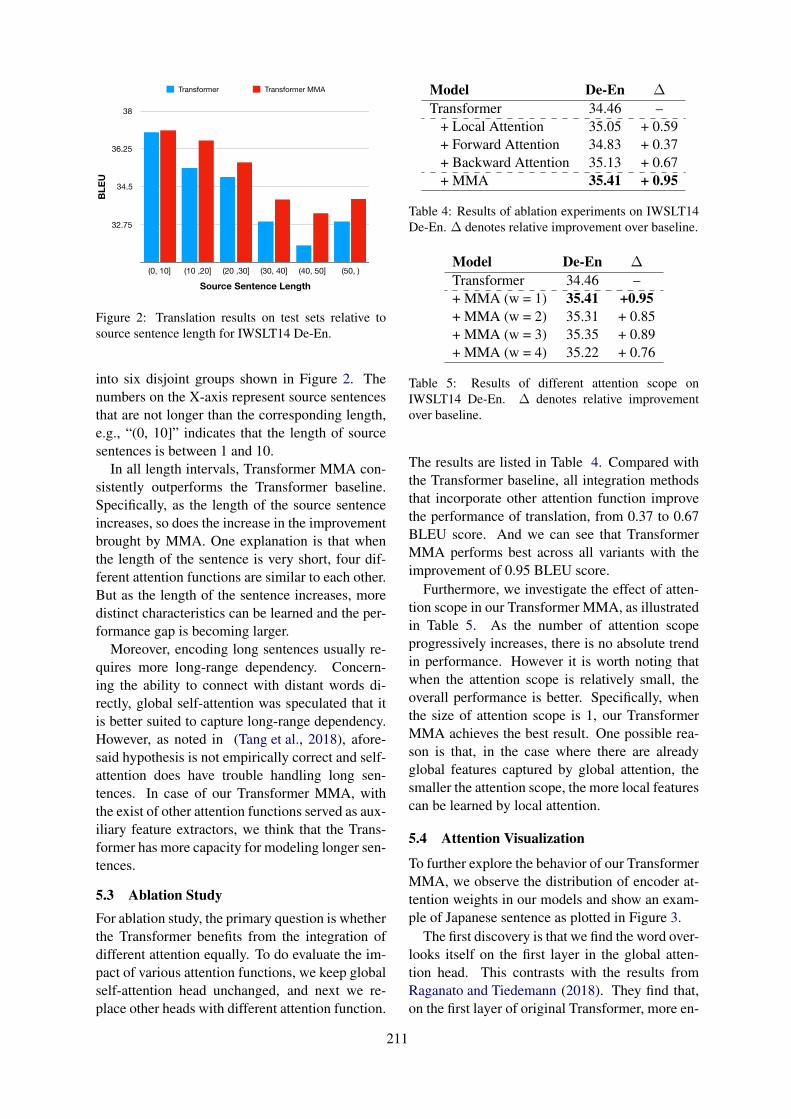
Figure 2: Translation results on test sets relative tosource sentence length for IWSLT14 De-En.
into six disjoint groups shown in Figure 2. Thenumbers on the X-axis represent source sentencesthat are not longer than the corresponding length,e.g., “(0, 10]” indicates that the length of sourcesentences is between 1 and 10.
In all length intervals, Transformer MMA con-sistently outperforms the Transformer baseline.Specifically, as the length of the source sentenceincreases, so does the increase in the improvementbrought by MMA. One explanation is that whenthe length of the sentence is very short, four dif-ferent attention functions are similar to each other.But as the length of the sentence increases, moredistinct characteristics can be learned and the per-formance gap is becoming larger.
Moreover, encoding long sentences usually re-quires more long-range dependency. Concern-ing the ability to connect with distant words di-rectly, global self-attention was speculated that itis better suited to capture long-range dependency.However, as noted in (Tang et al., 2018), afore-said hypothesis is not empirically correct and self-attention does have trouble handling long sen-tences. In case of our Transformer MMA, withthe exist of other attention functions served as aux-iliary feature extractors, we think that the Trans-former has more capacity for modeling longer sen-tences.
5.3 Ablation StudyFor ablation study, the primary question is whetherthe Transformer benefits from the integration ofdifferent attention equally. To do evaluate the im-pact of various attention functions, we keep globalself-attention head unchanged, and next we re-place other heads with different attention function.
Model De-En ∆
Transformer 34.46 –+ Local Attention 35.05 + 0.59+ Forward Attention 34.83 + 0.37+ Backward Attention 35.13 + 0.67+ MMA 35.41 + 0.95
Table 4: Results of ablation experiments on IWSLT14De-En. ∆ denotes relative improvement over baseline.
Model De-En ∆
Transformer 34.46 –+ MMA (w = 1) 35.41 +0.95+ MMA (w = 2) 35.31 + 0.85+ MMA (w = 3) 35.35 + 0.89+ MMA (w = 4) 35.22 + 0.76
Table 5: Results of different attention scope onIWSLT14 De-En. ∆ denotes relative improvementover baseline.
The results are listed in Table 4. Compared withthe Transformer baseline, all integration methodsthat incorporate other attention function improvethe performance of translation, from 0.37 to 0.67BLEU score. And we can see that TransformerMMA performs best across all variants with theimprovement of 0.95 BLEU score.
Furthermore, we investigate the effect of atten-tion scope in our Transformer MMA, as illustratedin Table 5. As the number of attention scopeprogressively increases, there is no absolute trendin performance. However it is worth noting thatwhen the attention scope is relatively small, theoverall performance is better. Specifically, whenthe size of attention scope is 1, our TransformerMMA achieves the best result. One possible rea-son is that, in the case where there are alreadyglobal features captured by global attention, thesmaller the attention scope, the more local featurescan be learned by local attention.
5.4 Attention Visualization
To further explore the behavior of our TransformerMMA, we observe the distribution of encoder at-tention weights in our models and show an exam-ple of Japanese sentence as plotted in Figure 3.
The first discovery is that we find the word over-looks itself on the first layer in the global atten-tion head. This contrasts with the results fromRaganato and Tiedemann (2018). They find that,on the first layer of original Transformer, more en-
211

Figure 3: Visualization of the attention weights of Japanese sentence “これらは腰椎装具装用または運動制限により全症例軽快した。” (meaning “These persons were improved in all cases by wearing lumbar bracesor limiting exercises”). The deeper blue color refers to larger attention weights.
coder self-attention heads focus on the word it-self. This change is in line with our assumptionthat, due to the existence of other attention heads,global attention head can focus more on capturingglobal information.
The second discovery is that, on the upper lay-ers, forward and backward attention heads movethe attention more on distant words. This suggestsforward and backward attention is able to serveas a complement to capturing long-range depen-dency.
6 Related Work
In the field of neural machine translation, thetwo most used attention mechanisms are addi-tive attention (Bahdanau et al., 2015) and dot at-tention (Luong et al., 2015). Based on the latter,Vaswani et al. (2017) proposed a multi-head self-attention, that is not only highly parallelizable butalso with better performance.
However, self-attention, which employs nei-ther recurrence nor convolution, has greatdifficulty in incorporating position informa-tion (Vaswani et al., 2017). To tackle this prob-lem, Shaw et al. (2018) presented an extensionthat can be used to incorporate relative positioninformation for sequence. And Shen et al. (2018)tried to encode the temporal order and introduceda directional self-attention which only composesof directional order. On the other hand, although
with a global receptive field, the ability of self-attention recently came into question (Tang et al.,2018). And modeling localness, either restrictingcontext sizes (Yang et al., 2018; Wu et al., 2019;Child et al., 2019) or balancing the contribution oflocal and global information (Xu et al., 2019), hasbeen shown to be able to improve the expressive-ness of self-attention. In contrast to these studies,we aim to improve the self-attention in a system-atic and multifaceted perspective, rather than justpaying attention to one specific characteristic.
Compared to a conventional NMT model withonly a single head, multi-head is assumed to have astronger ability to extract different features in dif-ferent subspaces. However, there are no explicitmechanism that make them distinct (Voita et al.,2019; Michel et al., 2019). Li et al. (2018) hadshown that using a disagreement regularization toencourage different attention heads to have dif-ferent behaviors can improve the performance ofmulti-head attention. Iida et al. (2019) proposed amulti-hop attention where the second-hop servesas a head gate function to normalize the atten-tional context of each head. Not only limited in thefield of neural machine translation, Strubell et al.(2018) combined multi-head self-attention withmulti-task learning, this led to a promising resultfor semantic role labeling. Similar to the abovestudies, we also attempt to model diversity formulti-head attention. In this work, we apply dif-
212

ferent attention function to capture different as-pects of features in multiple heads directly, whichis more intuitive and explicit.
7 Conclusion
In this work, we improve the self-attention net-works by modeling multi-head attention to learndifferent aspects of feature through different at-tention function. Experimental results on WAT17English-Japanese and IWSLT14 German-Englishtranslation tasks demonstrate that our proposedmodel outperforms the Transformer baseline aswell as some latest and related models. Our analy-sis further shows our Transformer MMA can makebetter use of word order information and the im-provement in translating longer sentences is espe-cially significant. Moreover, we perform ablationstudy to compare different architectures. To ex-plore the behavior of our proposed model, we vi-sualize the attention distribution and confirm thediversity among multiple heads in MMA.
In the future, we plan to apply our method onother sequence to sequence learning tasks, such astext summarization.
ReferencesJimmy Ba, Jamie Ryan Kiros, and Geoffrey E. Hinton.
2016. Layer normalization. ArXiv.
Dzmitry Bahdanau, Kyunghyun Cho, and Yoshua Ben-gio. 2015. Neural machine translation by jointlylearning to align and translate. In ICLR.
Mauro Cettolo, Jan Niehues, Sebastian Stuker, LuisaBentivogli, and Marcello Federico. 2014. Report onthe 11th IWSLT evaluation campaign, IWSLT 2014.In IWSLT.
Mia Xu Chen, Orhan Firat, Ankur Bapna, MelvinJohnson, Wolfgang Macherey, George Foster, LlionJones, Mike Schuster, Noam Shazeer, Niki Parmar,Ashish Vaswani, Jakob Uszkoreit, Lukasz Kaiser,Zhifeng Chen, Yonghui Wu, and Macduff Hughes.2018. The best of both worlds: Combining recentadvances in neural machine translation. In ACL,pages 76–86.
Rewon Child, Scott Gray, Alec Radford, and IlyaSutskever. 2019. Generating long sequences withsparse transformers. ArXiv.
Kyunghyun Cho, Bart van Merrienboer, Caglar Gul-cehre, Dzmitry Bahdanau, Fethi Bougares, HolgerSchwenk, and Yoshua Bengio. 2014. Learningphrase representations using rnn encoder–decoderfor statistical machine translation. In EMNLP, pages1724–1734.
Mostafa Dehghani, Stephan Gouws, Oriol Vinyals,Jakob Uszkoreit, and Lukasz Kaiser. 2019. Univer-sal transformers.
Yuntian Deng, Yoon Kim, Justin Chiu, Demi Guo, andAlexander Rush. 2018. Latent alignment and varia-tional attention. In NIPS.
Maha Elbayad, Laurent Besacier, and Jakob Verbeek.2018. Pervasive attention: 2D convolutional neuralnetworks for sequence-to-sequence prediction. InCoNLL, pages 97–107.
Jonas Gehring, Michael Auli, David Grangier, DenisYarats, and Yann N Dauphin. 2017. ConvolutionalSequence to Sequence Learning. In ICML.
Kaiming He, Xiangyu Zhang, Shaoqing Ren, and JianSun. 2016. Deep residual learning for image recog-nition. CVPR.
Shohei Iida, Ryuichiro Kimura, Hongyi Cui, Po-HsuanHung, Takehito Utsuro, and Masaaki Nagata. 2019.Attention over heads: A multi-hop attention for neu-ral machine translation. In ACL: Student ResearchWorkshop, pages 217–222.
Huda Khayrallah and Philipp Koehn. 2018. On theimpact of various types of noise on neural machinetranslation. In ACL: Workshop on Neural MachineTranslation and Generation, pages 74–83.
Diederik P. Kingma and Jimmy Ba. 2014. Adam: Amethod for stochastic optimization. In ICLR.
Philipp Koehn. 2004. Statistical significance tests formachine translation evaluation. In EMNLP, pages388–395.
Jian Li, Zhaopeng Tu, Baosong Yang, Michael R.Lyu, and Tong Zhang. 2018. Multi-head attentionwith disagreement regularization. In EMNLP, pages2897–2903.
Thang Luong, Hieu Pham, and Christopher D. Man-ning. 2015. Effective approaches to attention-basedneural machine translation. In EMNLP, pages1412–1421.
Paul Michel, Omer Levy, and Graham Neubig. 2019.Are sixteen heads really better than one? ArXiv.
Toshiaki Nakazawa, Shohei Higashiyama, ChenchenDing, Hideya Mino, Isao Goto, Hideto Kazawa,Yusuke Oda, Graham Neubig, and Sadao Kurohashi.2017. Overview of the 4th workshop on Asian trans-lation. In WAT.
Myle Ott, Sergey Edunov, Alexei Baevski, AngelaFan, Sam Gross, Nathan Ng, David Grangier, andMichael Auli. 2019. fairseq: A fast, extensibletoolkit for sequence modeling. In NAACL, pages48–53.
Kishore Papineni, Salim Roukos, Todd Ward, and Wei-Jing Zhu. 2002. Bleu: a method for automatic eval-uation of machine translation. In ACL, pages 311–318.
213
Alessandro Raganato and Jorg Tiedemann. 2018. Ananalysis of encoder representations in transformer-based machine translation. In EMNLP WorkshopBlackboxNLP: Analyzing and Interpreting NeuralNetworks for NLP, pages 287–297.
Mike Schuster and Kuldip K Paliwal. 1997. Bidirec-tional recurrent neural networks. IEEE Transactionson Signal Processing.
Rico Sennrich, Barry Haddow, and Alexandra Birch.2016. Neural machine translation of rare words withsubword units. In ACL, pages 1715–1725.
Rico Sennrich and Biao Zhang. 2019. Revisiting low-resource neural machine translation: A case study.In ACL, pages 211–221.
Peter Shaw, Jakob Uszkoreit, and Ashish Vaswani.2018. Self-attention with relative position represen-tations. In NAACL, pages 464–468.
Tao Shen, Tianyi Zhou, Guodong Long, Jing Jiang,Shirui Pan, and Chengqi Zhang. 2018. Disan: Di-rectional self-attention network for rnn/cnn-free lan-guage understanding. In AAAI.
Emma Strubell, Patrick Verga, Daniel Andor,David Weiss, and Andrew McCallum. 2018.Linguistically-informed self-attention for semanticrole labeling. In EMNLP, pages 5027–5038.
Ilya Sutskever, Oriol Vinyals, and Quoc V. Le. 2014.Sequence to sequence learning with neural net-works. In NIPS.
Christian Szegedy, Vincent Vanhoucke, Sergey Ioffe,Jonathon Shlens, and Zbigniew Wojna. 2016. Re-thinking the inception architecture for computer vi-sion. In CVPR.
Gongbo Tang, Mathias Muller, Annette Rios, and RicoSennrich. 2018. Why self-attention? a targeted eval-uation of neural machine translation architectures.In EMNLP, pages 4263–4272.
Ashish Vaswani, Noam Shazeer, Niki Parmar, JakobUszkoreit, Llion Jones, Aidan N Gomez, Ł ukaszKaiser, and Illia Polosukhin. 2017. Attention is allyou need. In NIPS.
Elena Voita, David Talbot, Fedor Moiseev, Rico Sen-nrich, and Ivan Titov. 2019. Analyzing multi-headself-attention: Specialized heads do the heavy lift-ing, the rest can be pruned. In ACL, pages 5797–5808.
Felix Wu, Angela Fan, Alexei Baevski, Yann Dauphin,and Michael Auli. 2019. Pay less attention withlightweight and dynamic convolutions. In ICLR.
Mingzhou Xu, Derek F. Wong, Baosong Yang, YueZhang, and Lidia S. Chao. 2019. Leveraging localand global patterns for self-attention networks. InACL, pages 3069–3075.
Baosong Yang, Zhaopeng Tu, Derek F. Wong, Fan-dong Meng, Lidia S. Chao, and Tong Zhang. 2018.Modeling localness for self-attention networks. InEMNLP, pages 4449–4458.
Baosong Yang, Longyue Wang, Derek F. Wong,Lidia S. Chao, and Zhaopeng Tu. 2019. Assessingthe ability of self-attention networks to learn wordorder. In ACL, pages 3635–3644.
214

Proceedings of the 3rd Workshop on Neural Generation and Translation (WNGT 2019), pages 215–220Hong Kong, China, November 4, 2019. c©2019 Association for Computational Linguistics
www.aclweb.org/anthology/D19-56%2d
Paraphrasing with Large Language Models
Sam WitteveenRed Dragon AI
Martin AndrewsRed Dragon AI
Abstract
Recently, large language models such as GPT-2 have shown themselves to be extremelyadept at text generation and have also beenable to achieve high-quality results in manydownstream NLP tasks such as text classifica-tion, sentiment analysis and question answer-ing with the aid of fine-tuning. We presenta useful technique for using a large languagemodel to perform the task of paraphrasing ona variety of texts and subjects. Our approachis demonstrated to be capable of generatingparaphrases not only at a sentence level butalso for longer spans of text such as paragraphswithout needing to break the text into smallerchunks.
1 Introduction
Paraphrase generation is an NLP task that has mul-tiple uses in content creation, question answering,translation, and data augmentation. It is a taskthat has been attempted for many decades usingstatistical and rules-based approaches (McKeown,1979; Meteer and Shaked, 1988).
We propose a system that generates paraphrasedexamples in an autoregressive fashion using a neu-ral network, without the need for techniques suchas top-k word selection or beam search.
We demonstrate that by using large languagemodels we are able to produce not only para-phrases that are longer and of a higher quality thanprevious work, but can also paraphrase text be-yond the individual sentence-level (i.e. full para-graphs at a time).
The large language models we use implementthe encoder-decoder structure of the transformerarchitecture (Vaswani et al., 2017) which has beenshown to learn different representations of lan-guage at each level of its encoding (Devlin et al.,2019). The power of language models like GPT-2(Radford et al., 2019) and BERT allows them to
develop useful representations of language whichcan be used far beyond just generation of the nextword (Rothe et al., 2019). In our experiments,we have observed that the models have representa-tions of syntax and grammar, allowing them to befine-tuned for the task of paraphrase generation.
2 Related Work
Paraphrase generation has attracted a number ofdifferent NLP approaches. These have includedrule-based approaches (McKeown, 1979; Meteerand Shaked, 1988) and data-driven methods (Mad-nani and Dorr, 2010), with recently the most com-mon approach being that the task is treated as alanguage translation task (Bannard and Callison-Burch, 2005; Barzilay and McKeown, 2001; Panget al., 2003) - often performed using a bilin-gual corpus pivoting back and forth (Madnani andDorr, 2010; Prakash et al., 2016; Mallinson et al.,2017). Other methods proposed include morerecently the use of Deep Reinforcement Learn-ing (Li et al., 2018) , supervised learning usingsequence-to-sequence models (Gupta et al., 2018;Prakash et al., 2016) and unsupervised approaches(Bowman et al., 2016; Roy and Grangier, 2019).
3 Methodology
In this section, we define the task, present our im-plementation, describe our evaluation protocol andthe paraphrase datasets used.
Paraphrase generation can be described as gen-erating a phrase which is semantically as close aspossible to the original while being rewritten innew words and phrases.
3.1 Large Language Model training
Training language models has become a popularway of creating models suited for Transfer Learn-ing in the field of NLP. (Howard and Ruder, 2018;
215
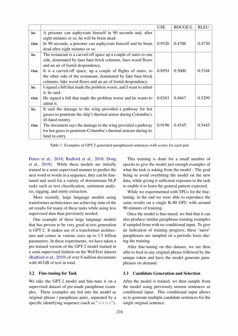
USE ROUGE-L BLEUIn: A prisoner can asphyxiate himself in 90 seconds and, after
eight minutes or so, he will be brain dead.Out: In 90 seconds, a prisoner can asphyxiate himself and be brain
dead after eight minutes or so.0.9326 0.4706 0.4730
In: The restaurant is a carved-off space up a couple of stairs to oneside, dominated by faux bare-brick columns, faux-wood floorsand an air of foetid despondency.
Out: It is a carved-off space, up a couple of flights of stairs, tothe other side of the restaurant, dominated by fake bare-brickcolumns, fake wood floors and an air of foetid despondency.
0.8954 0.5000 0.5348
In: I signed a bill that made the problem worse, and I want to admitit, he said.
Out: He signed a bill that made the problem worse and he wants toadmit it.
0.8363 0.4667 0.5299
In: It said the damage to the wing provided a pathway for hotgasses to penetrate the ship’s thermal armor during Columbia’sill-fated reentry.
Out: The document says the damage to the wing provided a pathwayfor hot gases to penetrate Columbia’s thermal armour during itsfatal re-entry.
0.9190 0.4545 0.5445
Table 1: Examples of GPT-2 generated paraphrased sentences with scores for each pair
Peters et al., 2018; Radford et al., 2018; Donget al., 2019). While these models are initiallytrained in a semi-supervised manner to predict thenext word or words in a sequence, they can be fine-tuned and used for a variety of downstream NLPtasks such as text classification, sentiment analy-sis, tagging, and entity extraction.
More recently, large language models usingtransformer architectures are achieving state of theart results for many of these tasks while using lesssupervised data than previously needed.
One example of these large language modelsthat has proven to be very good at text generationis GPT-2. It makes use of a transformer architec-ture and comes in various sizes up to 1.5 billionparameters. In these experiments, we have taken apre-trained version of the GPT-2 model trained ina semi-supervised fashion on the WebText dataset(Radford et al., 2019) of over 8 million documentswith 40 GB of text in total.
3.2 Fine-tuning for Task
We take the GPT-2 model and fine-tune it on asupervised dataset of pre-made paraphrase exam-ples. These examples are fed into the model asoriginal phrase / paraphrase pairs, separated by aspecific identifying sequence (such as ”>>>>”).
This training is done for a small number ofepochs to give the model just enough examples ofwhat the task is asking from the model : The goalbeing to avoid overfitting the model on the newdata, while giving it sufficient exposure to the taskto enable it to learn the general pattern expected.
While we experimented with TPUs for the fine-tuning, in the end we were able to reproduce thesame results on a single K-80 GPU with around90 minutes of training.
Once the model is fine-tuned, we find that it canalso produce similar paraphrase training examplesif sampled from with no conditional input. To givean indication of training progress, these ’naive’paraphrases are sampled on a periodic basis dur-ing the training.
After fine-tuning on this dataset, we are thenable to feed in any original phrase followed by theunique token and have the model generate para-phrases on demand.
3.3 Candidate Generation and Selection
After the model is trained, we then sample fromthe model using previously unseen sentences asconditional input. This conditional input allowsus to generate multiple candidate sentences for thesingle original sentence.
While the quality of the paraphrases is some-what variable, by generating multiple outputs andthen scoring them, we can select just the best qual-ity paraphrases based on a number of criteria thatserve to filter our output down to a set of satisfac-tory results.
First, we obtain a similarity score between thegenerated paraphrase and the original sentence byusing the Universal Sentence Encoder (USE) (Ceret al., 2018) to make a 512 dimensional sentenceembedding for each output sentence and then com-pare them to the embedding of the original sen-tence via the cosine similarity measure.
As a second step, we measure the ROUGE-L (Lin, 2004) score of the candidate paraphrasesagainst the original sentence and eliminate candi-dates with a ROUGE-L score of above 0.7 . Thisprevents candidates that are too close to the orig-inal sentence being chosen. After testing bothcutoff scores for ROUGE-L and BLEU (Papineniet al., 2002), ROUGE-L has shown to be more use-ful at finding candidates that are more unique incomparison to the original sentence.
By choosing samples with sufficiently lowROUGE-L scores but as high a similarity as pos-sible, we end up with an output that is semanti-cally similar to the original phrase but has a uniqueword order when compared to the original phrase.
3.4 DatasetsWe fine-tuned multiple versions of the model onseveral different datasets : 2 datasets of sentencesand their matching paraphrases; and 1 dataset ofparagraphs with matching paraphrases :
1. The MSR Paraphrase Identification dataset(Dolan et al., 2004) which consists of justover 4,000 examples of original sentenceswith a matching paraphrased sentence in itstrain set.
2. An original dataset of 10,000 sentences fromonline news articles along with matchingparaphrases that were human-generated.
3. A further original dataset of paragraphs withcorresponding paraphrased paragraphs fromvarious entertainment, news, and food ar-ticles found online, where the paraphraseswere human-generated.
We fine-tuned 3 versions of the GPT-2 model,one corresponding to each dataset, and then madepredictions using the same system outlined above.
By calculating USE, ROUGE-L and BLEUscores for each dataset we are able to quantify thequality of human-generated paraphrases and thenuse that as a comparison for the models generatedsentences (see Table 2).
Dataset USE R-L BLEUMSR train 0.8462 0.4315 0.4593MSR test 0.8415 0.4202 0.4966News dataset 0.8948 0.4686 0.5648Paragraphs dataset 0.9208 0.4966 0.5762
Table 2: Average USE, ROUGE-L, BLEU Scores ofthe datasets
4 Experiments
We implemented the system described above us-ing GPT-2 and trained it on the different datasetsfor various lengths of training.
To evaluate the output of the model, we ran-domly selected sentences from sources such asWikipedia, news sites and entertainment sites withno matching paraphrase to use as the conditionalinput to the model.
5 Results and Scoring
When comparing our generated sentences with theaverage scores of the original datasets, we can seethat that they compare favorably.
As discussed earlier, we assessed the semanticsimilarity of the sentence meanings using Univer-sal Sentence Encoder (Cer et al., 2018) and com-pared them to the average USE score from thedatasets that were trained on. This showed thatthe system can generate paraphrases which are se-mantically on par with the human-generated onesin each of the datasets.
We also compared the ROUGE-L (Lin, 2004)scores of the generated samples with the aver-age values for the datasets which were human-generated. This again shows that our phrases arecoherent and on par with human-generated para-phrases.
When we further compared the results of unfil-tered examples generated by the model (Table 3)we observe that when the USE score is below 0.85we see clear deterioration in the semantic similar-ity quality of the paraphrased versions.
We also observe that if the USE score is tooclose to 1.0 then the ROUGE-L score also risesand the generated examples are too similar in word
216

While the quality of the paraphrases is some-what variable, by generating multiple outputs andthen scoring them, we can select just the best qual-ity paraphrases based on a number of criteria thatserve to filter our output down to a set of satisfac-tory results.
First, we obtain a similarity score between thegenerated paraphrase and the original sentence byusing the Universal Sentence Encoder (USE) (Ceret al., 2018) to make a 512 dimensional sentenceembedding for each output sentence and then com-pare them to the embedding of the original sen-tence via the cosine similarity measure.
As a second step, we measure the ROUGE-L (Lin, 2004) score of the candidate paraphrasesagainst the original sentence and eliminate candi-dates with a ROUGE-L score of above 0.7 . Thisprevents candidates that are too close to the orig-inal sentence being chosen. After testing bothcutoff scores for ROUGE-L and BLEU (Papineniet al., 2002), ROUGE-L has shown to be more use-ful at finding candidates that are more unique incomparison to the original sentence.
By choosing samples with sufficiently lowROUGE-L scores but as high a similarity as pos-sible, we end up with an output that is semanti-cally similar to the original phrase but has a uniqueword order when compared to the original phrase.
3.4 DatasetsWe fine-tuned multiple versions of the model onseveral different datasets : 2 datasets of sentencesand their matching paraphrases; and 1 dataset ofparagraphs with matching paraphrases :
1. The MSR Paraphrase Identification dataset(Dolan et al., 2004) which consists of justover 4,000 examples of original sentenceswith a matching paraphrased sentence in itstrain set.
2. An original dataset of 10,000 sentences fromonline news articles along with matchingparaphrases that were human-generated.
3. A further original dataset of paragraphs withcorresponding paraphrased paragraphs fromvarious entertainment, news, and food ar-ticles found online, where the paraphraseswere human-generated.
We fine-tuned 3 versions of the GPT-2 model,one corresponding to each dataset, and then madepredictions using the same system outlined above.
By calculating USE, ROUGE-L and BLEUscores for each dataset we are able to quantify thequality of human-generated paraphrases and thenuse that as a comparison for the models generatedsentences (see Table 2).
Dataset USE R-L BLEUMSR train 0.8462 0.4315 0.4593MSR test 0.8415 0.4202 0.4966News dataset 0.8948 0.4686 0.5648Paragraphs dataset 0.9208 0.4966 0.5762
Table 2: Average USE, ROUGE-L, BLEU Scores ofthe datasets
4 Experiments
We implemented the system described above us-ing GPT-2 and trained it on the different datasetsfor various lengths of training.
To evaluate the output of the model, we ran-domly selected sentences from sources such asWikipedia, news sites and entertainment sites withno matching paraphrase to use as the conditionalinput to the model.
5 Results and Scoring
When comparing our generated sentences with theaverage scores of the original datasets, we can seethat that they compare favorably.
As discussed earlier, we assessed the semanticsimilarity of the sentence meanings using Univer-sal Sentence Encoder (Cer et al., 2018) and com-pared them to the average USE score from thedatasets that were trained on. This showed thatthe system can generate paraphrases which are se-mantically on par with the human-generated onesin each of the datasets.
We also compared the ROUGE-L (Lin, 2004)scores of the generated samples with the aver-age values for the datasets which were human-generated. This again shows that our phrases arecoherent and on par with human-generated para-phrases.
When we further compared the results of unfil-tered examples generated by the model (Table 3)we observe that when the USE score is below 0.85we see clear deterioration in the semantic similar-ity quality of the paraphrased versions.
We also observe that if the USE score is tooclose to 1.0 then the ROUGE-L score also risesand the generated examples are too similar in word
USE R-LIn: A prisoner can asphyxiate himself in 90 seconds and, after eight minutes or
so, he will be brain dead.Out 1: After 8 minutes, a brain fart will subdue the sufferer. 0.524 0.0Out 2: After 8 minutes, he will be brain-dead and his heart will stop. 0.565 0.138Out 3: A brain aneurysm can asphyxiate itself in 90 seconds and, after eight min-
utes, it will be dead.0.721 0.412
Out 4: After eight minutes, a brain anesthetist can asphyxiate a prisoner in 90 sec-onds and for several minutes after that.
0.758 0.167
Out 5: A brain-dead prisoner canasphyxiate himself in 90 seconds and then outloud after eight minutes.
0.809 0.312
Out 6: At asphyxiation, the prisoner canasphyxiate himself in 90 seconds and, after8 minutes, he will be brain dead.
0.884 0.514
Out 7: After eight minutes, a prisoner can asphyxiate himself in 90 seconds and,after that, he will be brain dead.
0.884 0.514
Out 8*: In 90 seconds, a prisoner can asphyxiate himself and be brain deadafter eight minutes or so
0.932 0.473
Out 9: A prisoner can asphyxiate himself in 90 seconds and, after eight minutes,he will be brain dead.
0.972 0.824
Table 3: Showing Candidates Selection and Scoring - *Selected Sentence
and phrase selection to the original sentence to beuseful paraphrases.
This technique can be performed not only atsentence-level but also to generate paragraph-levelparaphrases. Comparing USE and ROUGE-Lscores of the generated paragraphs we see they areagain on par with the human generated examplesfrom our paragraph dataset (samples are given inthe Supplemental Materials).
Due to the pre-training of the Language Model,the model is able to generalize to and generateparaphrases for types of content it has never seenduring the fine-tuning phase.
6 Discussion
The technique outlined in this paper shows the ap-plicability of large language models to the para-phrasing task. It also highlights that there is stillmuch to be learnt about further applications oflarge language models, and also the approachesused to fine-tune and use them for applications.
Most of the results from models such as GPT-2 have focused on the quality of text genera-tion rather than quantitative methods for measur-ing and improving the quality of text created, tomake it more consistent and usable. We pro-pose the scoring and filtering of candidates usingtechniques such as we have shown with USE andROUGE-L, may be a useful technique not just for
paraphrasing but other text generation tasks.The ability of our technique to work with long
spans of text also gives it an advantage over priorwork which used rule-based and other statisticalapproaches which performed best on shorter spansof text.
Our experiments show that pre-training of GPT-2 on such a large amount of data in the WebTextdataset allows it to ’understand’ the syntax and toa degree the grammar of English allowing it tobe able to quickly learn the task of paraphrasingthrough fine-tuning training on a small set of para-phrasing examples.
7 Future Work
Extrapolating from the paraphrasing results intomore generalizable ideas, we hope to investigatethe extent by which the representations learned inthe different layers of the transformer network cor-respond to different parts of the linguistic hierar-chy. One possible approach to doing this would beto trace a set of ’markers’ through the transformernetworks existing attention mechanism, in parallelto the text which gives rise to that structure.
In addition, the ability of the networks to learntasks within the span of a single context frame in-dicates the possibility of an inherent bias towardsmeta-( or one-shot) learning. These will be thesubject of further work.
217

USE R-LIn: A prisoner can asphyxiate himself in 90 seconds and, after eight minutes or
so, he will be brain dead.Out 1: After 8 minutes, a brain fart will subdue the sufferer. 0.524 0.0Out 2: After 8 minutes, he will be brain-dead and his heart will stop. 0.565 0.138Out 3: A brain aneurysm can asphyxiate itself in 90 seconds and, after eight min-
utes, it will be dead.0.721 0.412
Out 4: After eight minutes, a brain anesthetist can asphyxiate a prisoner in 90 sec-onds and for several minutes after that.
0.758 0.167
Out 5: A brain-dead prisoner canasphyxiate himself in 90 seconds and then outloud after eight minutes.
0.809 0.312
Out 6: At asphyxiation, the prisoner canasphyxiate himself in 90 seconds and, after8 minutes, he will be brain dead.
0.884 0.514
Out 7: After eight minutes, a prisoner can asphyxiate himself in 90 seconds and,after that, he will be brain dead.
0.884 0.514
Out 8*: In 90 seconds, a prisoner can asphyxiate himself and be brain deadafter eight minutes or so
0.932 0.473
Out 9: A prisoner can asphyxiate himself in 90 seconds and, after eight minutes,he will be brain dead.
0.972 0.824
Table 3: Showing Candidates Selection and Scoring - *Selected Sentence
and phrase selection to the original sentence to beuseful paraphrases.
This technique can be performed not only atsentence-level but also to generate paragraph-levelparaphrases. Comparing USE and ROUGE-Lscores of the generated paragraphs we see they areagain on par with the human generated examplesfrom our paragraph dataset (samples are given inthe Supplemental Materials).
Due to the pre-training of the Language Model,the model is able to generalize to and generateparaphrases for types of content it has never seenduring the fine-tuning phase.
6 Discussion
The technique outlined in this paper shows the ap-plicability of large language models to the para-phrasing task. It also highlights that there is stillmuch to be learnt about further applications oflarge language models, and also the approachesused to fine-tune and use them for applications.
Most of the results from models such as GPT-2 have focused on the quality of text genera-tion rather than quantitative methods for measur-ing and improving the quality of text created, tomake it more consistent and usable. We pro-pose the scoring and filtering of candidates usingtechniques such as we have shown with USE andROUGE-L, may be a useful technique not just for
paraphrasing but other text generation tasks.The ability of our technique to work with long
spans of text also gives it an advantage over priorwork which used rule-based and other statisticalapproaches which performed best on shorter spansof text.
Our experiments show that pre-training of GPT-2 on such a large amount of data in the WebTextdataset allows it to ’understand’ the syntax and toa degree the grammar of English allowing it tobe able to quickly learn the task of paraphrasingthrough fine-tuning training on a small set of para-phrasing examples.
7 Future Work
Extrapolating from the paraphrasing results intomore generalizable ideas, we hope to investigatethe extent by which the representations learned inthe different layers of the transformer network cor-respond to different parts of the linguistic hierar-chy. One possible approach to doing this would beto trace a set of ’markers’ through the transformernetworks existing attention mechanism, in parallelto the text which gives rise to that structure.
In addition, the ability of the networks to learntasks within the span of a single context frame in-dicates the possibility of an inherent bias towardsmeta-( or one-shot) learning. These will be thesubject of further work.
218

Acknowledgments
We would like to thank Google for access to theTFRC TPU program which was used in trainingand fine-tuning models for this paper.
ReferencesColin J. Bannard and Chris Callison-Burch. 2005.
Paraphrasing with bilingual parallel corpora. InProceedings of the 43rd Annual Meeting of the As-sociation for Computational Linguistics (ACL05),pages 597–604, Ann Arbor, Michigan. Associationfor Computational Linguistics.
Regina Barzilay and Kathleen McKeown. 2001. Ex-tracting paraphrases from a parallel corpus. In Pro-ceedings of the 39th Annual Meeting on Associationfor Computational Linguistics, ACL ’01, pages 50–57, Stroudsburg, PA, USA. Association for Compu-tational Linguistics.
Samuel R. Bowman, Luke Vilnis, Oriol Vinyals, An-drew M. Dai, Rafal Jozefowicz, and Samy Ben-gio. 2016. Generating sentences from a continuousspace. In Proceedings of The 20th SIGNLL Con-ference on Computational Natural Language Learn-ing, pages 10–21, Berlin, Germany. Association forComputational Linguistics.
Daniel Cer, Yinfei Yang, Sheng yi Kong, Nan Hua,Nicole Limtiaco, Rhomni St. John, Noah Con-stant, Mario Guajardo-Cespedes, Steve Yuan, ChrisTar, Yun-Hsuan Sung, Brian Strope, and RayKurzweil. 2018. Universal sentence encoder. ArXiv,abs/1803.11175.
Jacob Devlin, Ming-Wei Chang, Kenton Lee, andKristina Toutanova. 2019. Bert: Pre-training ofdeep bidirectional transformers for language under-standing. In Proceedings of the 2019 Conferenceof the North American Chapter of the Associationfor Computational Linguistics: Human LanguageTechnologies, Volume 1 (Long and Short Papers),pages 4171–4186, Minneapolis, Minnesota. Associ-ation for Computational Linguistics.
William B. Dolan, Chris Quirk, and Chris Brockett.2004. Unsupervised construction of large para-phrase corpora: Exploiting massively parallel newssources. In COLING.
Li Dong, Nan Yang, Wenhui Wang, Furu Wei, Xi-aodong Liu, Yu Wang, Jianfeng Gao, Ming Zhou,and Hsiao-Wuen Hon. 2019. Unified languagemodel pre-training for natural language understand-ing and generation. CoRR, abs/1905.03197.
Ankush Gupta, Arvind Agarwal, Prawaan Singh, andPiyush Rai. 2018. A deep generative framework forparaphrase generation. In Thirty-Second AAAI Con-ference on Artificial Intelligence.
Jeremy Howard and Sebastian Ruder. 2018. Universallanguage model fine-tuning for text classification.In Proceedings of the 56th Annual Meeting of theAssociation for Computational Linguistics (Volume1: Long Papers), pages 328–339, Melbourne, Aus-tralia. Association for Computational Linguistics.
Zichao Li, Xin Jiang, Lifeng Shang, and Hang Li.2018. Paraphrase generation with deep reinforce-ment learning. In Proceedings of the 2018 Con-ference on Empirical Methods in Natural LanguageProcessing, pages 3865–3878.
Chin-Yew Lin. 2004. Rouge: A package for auto-matic evaluation of summaries. In ACL 2004, pages74–81, Barcelona, Spain. Association for Computa-tional Linguistics.
Nitin Madnani and Bonnie J. Dorr. 2010. Generat-ing phrasal and sentential paraphrases: A surveyof data-driven methods. Computational Linguistics,36:341–387.
Jonathan Mallinson, Rico Sennrich, and Mirella Lap-ata. 2017. Paraphrasing revisited with neural ma-chine translation. In Proceedings of the 15th Con-ference of the European Chapter of the Associationfor Computational Linguistics: Volume 1, Long Pa-pers, pages 881–893.
Kathleen McKeown. 1979. Paraphrasing using givenand new information in a question-answer system.In 17th Annual Meeting of the Association for Com-putational Linguistics, pages 67–72.
Marie Meteer and Varda Shaked. 1988. Strategies foreffective paraphrasing. In Coling Budapest 1988Volume 2: International Conference on Computa-tional Linguistics.
Bo Pang, Kevin Knight, and Daniel Marcu. 2003.Syntax-based alignment of multiple translations:Extracting paraphrases and generating new sen-tences. In Proceedings of the 2003 Human Lan-guage Technology Conference of the North Ameri-can Chapter of the Association for ComputationalLinguistics, pages 181–188.
Kishore Papineni, Salim Roukos, Todd Ward, and Wei-Jing Zhu. 2002. Bleu: a method for automatic eval-uation of machine translation. In Proceedings of the40th Annual Meeting of the Association for Com-putational Linguistics, pages 311–318, Philadelphia,Pennsylvania, USA. Association for ComputationalLinguistics.
Matthew E. Peters, Mark Neumann, Mohit Iyyer,Matt Gardner, Christopher Clark, Kenton Lee, andLuke Zettlemoyer. 2018. Deep contextualized wordrepresentations. pages 2227–2237, New Orleans,Louisiana. Association for Computational Linguis-tics.
Aaditya Prakash, Sadid A. Hasan, Kathy Lee, Vivek V.Datla, Ashequl Qadir, Joey Liu, and Oladimeji Farri.2016. Neural paraphrase generation with stackedresidual LSTM networks. CoRR, abs/1610.03098.
219

Alec Radford, Karthik Narasimhan, Tim Salimans, andIlya Sutskever. 2018. Improving language under-standing by generative pre-training.
Alec Radford, Jeff Wu, Rewon Child, David Luan,Dario Amodei, and Ilya Sutskever. 2019. Languagemodels are unsupervised multitask learners.
Sascha Rothe, Shashi Narayan, and Aliaksei Severyn.2019. Leveraging pre-trained checkpoints for se-quence generation tasks. CoRR, abs/1907.12461.
Aurko Roy and David Grangier. 2019. Unsuper-vised paraphrasing without translation. ArXiv,abs/1905.12752.
Ashish Vaswani, Noam Shazeer, Niki Parmar, JakobUszkoreit, Llion Jones, Aidan N Gomez, ŁukaszKaiser, and Illia Polosukhin. 2017. Attention is allyou need. In Advances in neural information pro-cessing systems, pages 5998–6008.
220

Proceedings of the 3rd Workshop on Neural Generation and Translation (WNGT 2019), pages 221–230Hong Kong, China, November 4, 2019. c©2019 Association for Computational Linguistics
www.aclweb.org/anthology/D19-56%2d
Interrogating the Explanatory Power of Attention in Neural MachineTranslation
Pooya Moradi, Nishant Kambhatla, and Anoop SarkarSimon Fraser University8888 University DriveBurnaby, BC, Canada
{pooya moradi, nkambhat, anoop}@sfu.ca
Abstract
Attention models have become a crucial com-ponent in neural machine translation (NMT).They are often implicitly or explicitly used tojustify the model’s decision in generating aspecific token but it has not yet been rigor-ously established to what extent attention isa reliable source of information in NMT. Toevaluate the explanatory power of attention forNMT, we examine the possibility of yieldingthe same prediction but with counterfactual at-tention models that modify crucial aspects ofthe trained attention model. Using these coun-terfactual attention mechanisms we assess theextent to which they still preserve the genera-tion of function and content words in the trans-lation process. Compared to a state of the artattention model, our counterfactual attentionmodels produce 68% of function words and21% of content words in our German-Englishdataset. Our experiments demonstrate that at-tention models by themselves cannot reliablyexplain the decisions made by a NMT model.1
1 Introduction
One shortcoming of neural machine translation(NMT), and neural models in general, is that it isoften difficult for humans to comprehend the rea-sons why the model is making predictions (Fenget al., 2018; Ghorbani et al., 2019). The maincause of such a difficulty is that in neural mod-els, information is implicitly represented by real-valued vectors, and conceptual interpretation ofthese vectors remains a challenge. Why do wewant neural models to be interpretable? In orderto debug a neural model during the error analy-sis process in research experiments, it is neces-sary to know how much each part of the model is
1The source code to reproduce the experiments isavailable at: https://github.com/sfu-natlang/attention_explanation
contributing to the error in the prediction. Beingable to interpret the deficiencies of a model is alsocrucial to further improve upon it. This requiresan explainable understanding of the internals ofthe model, including how certain concepts are be-ing modeled or represented. Therefore developingmethods to interpret and understand neural modelsis an important research goal.
Visualizing and interpreting neural models hasbeen extensively studied in computer vision (Si-monyan et al., 2013; Bach et al., 2015; Zeiler andFergus, 2014; Montavon et al., 2017), and morerecently in natural language processing (NLP)(Karpathy et al., 2015; Li et al., 2016a; Strobeltet al., 2017, 2018). Recently, the integration of at-tention mechanism (Bahdanau et al., 2014) withan NMT sequence to sequence model (Sutskeveret al., 2014) has led to significant improvementsin translation quality especially for longer sen-tence lengths. The attention mechanism providesa weighted average over the information from thesource encodings to be used at each translationstep. These weights are often regarded as a mea-sure of importance, and are implicitly or explicitlyused as an explanation for the model’s decision.However it has not yet been established to whatextent such explanations are reliable.
The example in Figure 1 shows a model trans-lating the German sentence “und wir wollen diesesmaterial fur alle verfugbar machen.” (and wewant to make this material accessible to every-one.). At the time that the model is translating“verfugbar” to “accessible”, it is mostly attendingto “verfugbar” (left heatmap). It is tempting toconclude that “verfugbar” having the most atten-tion is why the model is generating the token “ac-cessible”. However, we manipulate the attentionweights such that the “verfugbar” receives no at-tention and “alle” is given the most attention (rightheatmap). We observe that in the second case, the
221

und wir wollen dieses material für verfügbar machen .
and we want to make
this material to beModel
current state
of translation
accessible
attentionoutput
alle und wir wollen dieses material für verfügbar machen .
and we want to make
this material to beModel
current state
of translation
accessible
attentionoutput
alle
Figure 1: Two distinct attention weights yielding the same prediction. The model is translating the source word“verfugbar” to “accessible”. In the left attention heatmap, the focus of the attention is on the word “verfugbar”.However, in the right heatmap, “verfugbar” is not attended to at all and “alle” has received the most attention.
model makes the same decision again and outputs“accessible”. This example shows that using at-tention weights to reason about the model’s pre-dictions can be misleading, as these two heatmapsconvey different explanations.
There are relatively few previous studies on in-vestigating the power of attention mechanism inrationalizing a model’s predictions in NLP (Jainand Wallace, 2019; Serrano and Smith, 2019) andthey all target text classification tasks where atten-tion is over the input document. Their findings donot generalize easily to NMT due to the differencein how the decoder works in the translation taskwhich produces a sequence rather than a class la-bel. NMT is a sequence-to-sequence (Seq2Seq)task, which is different from text classification.Also, the size of the output space is quite limitedin text classification, whereas in NMT, it is equalto the vocabulary size of the target language thatcan be very large. Furthermore, different neuralarchitectures (e.g., presence of an encoder and de-coder in NMT), require different analysis and in-terpretations. To the best of our knowledge there isno existing work on addressing the question of in-terpretability of attention models for the machinetranslation task.
To investigate if the explanation implied by at-tention weights faithfully justifies why a modelproduced its output, we study to what extent itis possible to yield the same prediction by us-ing counterfactual attention weights that suggesta contradictory explanation. The intuition behindthis approach is that multiple contradictory jus-tifications should not exist for a decision. Tobe specific, in the setting of an encoder-decodermodel (Sec 2), we propose several counterfactualattention weighting methods that suggest differ-ent explanations compared to the original attentionweights (Sec 3) and analyze their performance in
preserving the generation of function2 and contentwords (Sec 4). Function words (e.g., a, the, is)have little lexical meaning in contrast to contentwords and thus we are curious whether explana-tory power of the attention mechanism differs forgeneration of these two groups of words.
2 Encoder-Decoder Model withAttention Mechanism
Given a training sentence pair (x, y) where x =[x1, x2, ..., xm] is a sentence in the source lan-guage and y = [y1, y2, ..., yn] is its correspond-ing translation in the target language, the encoder,which is a recurrent neural network (RNN), runsover the source sentence to calculate the contextu-alized representation of the source words. Here,we use a bidirectional encoder, and concatenatethe forward and backward hidden states to buildthe final representation.
−→ht =
−−→fenc(xt,
−−→ht−1)
←−ht =
←−−fenc(xt,
←−−ht+1)
ht = [−→ht ,←−ht ]
(1)
Then the decoder starts to generate output to-kens using the following probability distribution:
p(yt|y<t, x) = softmax(gdec(st, ct))
with gdec being a transformation function thatproduces a vocabulary-sized vector, and st is thehidden unit of the decoder’s RNN updated as:
st = fdec(yt−1, st−1, ct−1)
2The reference for function words (we added new func-tion words including the EOS token to this) can be found at:semanticsimilarity.files.wordpress.com/2013/08/jim-oshea-fwlist-277.pdf
222
where fdec is a RNN. Here ct is the context vec-tor calculated by attention mechanisms:
ct =
m∑
i=1
αtihi
where αt is the normalized attention weightsover the source context:
αti =ea(st,hi)
∑j ea(st,hj)
Here, a is a scoring function that determinesthe contribution of each source context vector tothe final context vector. Implementation of a de-pends on the choice of the attention method. Inthis work, we use general attention (Luong et al.,2015) as the scoring function:
a(st, hi) = s⊤t Wahi
3 Approach
Given a trained NMT model M , a test sentencex with y being its translation generated by M atthe decoding step t in which αt is the attentionvector, attending to the source word at positionmt = argmaxi αt[i] or k-best attended-to wordsin the source are often implicitly or explicitly re-garded as a justification for the model’s predictionat the time step t.
A vital criteria for such a justification is that oneshould not be able to find a contradictory expla-nation for the model’s decision. More precisely,if at the time of inference, it is possible to ma-nipulate the original attention weights to consti-tute an alternative attention vector α′
t, such thatargmaxi α
′t[i] 6= mt and the decision of the model
is preserved, then these weights cannot be usedfor justification as they are contradictory. Thus,we are interested in assessing for what percentageof the words in the translation, counterfactual at-tention weights exist. These percentages can shedlight on the reliability of the attention weights asa potential explanation. Note that at the inferencetime we manipulate attention vector for each out-put token separately and in isolation to make surethe output tokens at time steps t + 1 and after willnot be affected by the change at time step t. Thismeans that our output translations are unaffectedby our counterfactual attention models which arepurely for the examination of how attention mightexplain the model’s decision.
The main task here is to find a counterfactualattention vector if it exists at all. An exhaustivesearch approach in which every possible attentionvector is examined is computationally intractableand unlikely to provide much insight. Instead weexperiment with a few specific counterfactual at-tention weighting methods that we think providethe most insight. It is important to note that in thiscase, the calculated percentage of the preservedwords will be a lower-bound estimation for thetrue percentage. As a result, the explanation of-fered by attention weights are more unreliable thanwhat we’ll find. We experiment with the followingattention methods to create counterfactual atten-tion weights:
• RandomPermute (Jain and Wallace, 2019):We set α′
t = random permute(αt) suchthat argmaxi α
′t[i] 6= mt.
• Uniform: In this method, α′t = 1
m~1. Here,
m is the length of the source sentence.
• ZeroOutMax: A simple approach to createa counterfactual attention vector is to removethe maximum attention weight. So we seta(st, hmt) = −∞.
We also experiment with four additional atten-tion methods where our motivation is not findingcounterfactual attention weights, but to improveour understanding of how attention weights influ-ence the model’s prediction:
• ZeroOut: In what conditions does the de-coder overlook the information provided byattention mechanism? To answer this ques-tion, we set all attention weights to zero atinference time (attention is still used whiletraining the model).
• LastEncoderState: Here, we only usethe final hidden state of the encoder as thecontext vector to be used in the decoder. Notethat this is different from seq2seq without at-tention in which final hidden state of the en-coder is used to initialize the decoder. Whenthe focus is on the final hidden state of theencoder in the original attention weights, thismethod does not produce a counterfactual at-tention vector, which is why we don’t intendto use this method to create a contradictoryexplanation, but rather to gain more insightinto the sensitivity of the model to attentionweights.
223

• OnlyMax: In this and the following method,the source hidden state with the maximumattention still receives the highest attention,and so these two methods do not outputcounterfactual attention vectors. Howeverwe are curious to what extent other attentionweights are required to preserve the model’soutput. Note that the weights produced bythese methods can be counted as contra-dictory when multiple attention weights areused for justifying predictions. Because al-though the most attended source context isnot changed, the relative ranking of the restof the source context in terms of attentionweights is changed. However, these kindsof justifications are mostly discussed in textclassification. In this specific method we onlykeep the most attended source hidden state:α′
t[mt]=1.
• KeepMaxUniformOthers: Here, we setα′
t[mt] = αt[mt], but for all other positionsα′
t[i] = (1−α′t[mt])/m. This is to investigate
if using other source hidden states uniformlyhas any added benefit.
4 Experiments
4.1 DataIn this work we use the German-English datasetfrom IWSLT20143. We concatenate dev2010,dev2012, tst2010, tst2011 and tst2012 to be usedas the test data. Data is tokenized using Moses(Koehn et al., 2007).
4.2 Model DetailsOpenNMT (Klein et al., 2017) is used for ourSeq2Seq implementation. We use Long Short-Term Memory (LSTM) as RNN units. EachLSTM unit has 2 layers, and the dimension sizefor LSTM units and word embeddings is set to500. The model is trained using Adam trainer withlearning rate 0.001 for 50000 steps using earlystopping. Vocabulary size for both the source andtarget language is set to 50000. Sentences longerthat 50 tokens are pruned.
5 Results
Table 1 shows the percentage of function and con-tent words generated by the trained model. As ex-pected, the majority of the generated tokens are
3https://sites.google.com/site/iwsltevaluation2014/
function words. We discuss our findings in moredetail in the subsequent subsections.
Number of tokens (+EOS) 139465Percentage of function words 68%Percentage of content words 32%
Table 1: Percentage of function and content words inthe generated translation.
Method % for FWs % for CWs1 RandomPermute 33% 6%2 Uniform 53% 11%3 ZeroOutMax 52% 15%4 Aggregate(1+2+3) 68% 21%5 ZeroOut 9% 0%6 LastEncoderState 20% 2%7 OnlyMax 71% 83%8 KeepMaxUniformOthers 86% 86%
Table 2: Percentage of the preserved function and contentwords in the proposed attention methods: Trying out all themethods to find a counterfactual attention vector maximizesthe chance of success. We use methods in row 5-8 only toshed light on the sensitivity of the model’s output to pertur-bation in attention weight. They are not necessarily countedas counterfactual attention methods. Higher preservation ratestands for better performance.
5.1 Effectiveness of the proposedcounterfactual attention methods
Table 2 shows the percentage of function andcontent words for which counterfactual attentionweights were found using the proposed attentionmethods. The Uniform method (row 2) is themost effective method to create counterfactual at-tention weights for function words. However, forcontent words, the ZeroOutMax method (row 3)is the most successful method.
From Table 2, we also derive thatRandomPermute is not as effective as theUniform and ZeroOutMax methods. Ourjustification is that in the RandomPermutemethod, it is highly probable that the contextvector is biased toward a random source hiddenstate. Such bias can lead to misleading noise inthe context vector. However, there isn’t such abias in the Uniform or ZeroOutMax methods.
To maximize the chance of finding a counter-factual attention, for each output token, we try outall the proposed methods to check if we can find acounterfactual attention (row 4). As evident fromTable 2, this approach greatly increases the chanceof finding a counterfactual attention. Note that aspreviously stated, these percentages are a lower-bound for the true percentage.
224

5.2 Function words are more easilygenerated compared to content words
An important observation in Table 2 is that theproposed methods are considerably more effectivein preserving function words compared to con-tent words. The production of function wordsrely more on the target context, in contrast to con-tent words which rely more on the source context.Accordingly, perturbation in the original attentionweights likely has significantly more impact ondiminishing content words compared to functionwords.
This ties well with the main idea behind con-text gates in which the influence of source con-text and target context is controlled dynamically(Tu et al., 2017). Since the generation of func-tion words relies more on the target context, onemay wonder to what extent attention is needed forpreserving function words? To answer this ques-tion, we completely zero out the attention usingZeroOut. Row 5 shows that only 9% of functionwords were preserved in this method.
Moreover it can be seen that the model couldnot preserve any content word when this methodis employed. Interestingly, we found that the pre-served function words in this method were all oc-currences of “,”. Apparently the decoder’s lan-guage model is so strong in predicting “,” withoutattention. This finding suggests that a basic repre-sentation of the source context is still necessary topreserve function words.
5.3 Highlighting top preserved tokens
An important question that may arise is whethereach attention method tends to preserve a spe-cific group of words. To address this question, welisted the top preserved function words and con-tent words for all the proposed methods. We ob-served that they mostly preserve the same groupof words but with different percentages. As a re-sult, we only list the top preserved tokens for theaggregate method.
Table 3 contains the top 20 content words sortedby the number of times they were preserved. Itis interesting to note that for many of these fre-quent tokens, more than half of their total occur-rences are preserved without focusing on their cor-responding translation in the source sentence (e.g.,“going”, “know”, “thing”, etc).
In Table 4, we sort such tokens based on theircoverage, which is the percentage of their total
Token # preserved Coveragegoing 310 70%people 237 46%know 219 62%world 215 67%like 189 47%
think 176 50%way 162 68%get 160 53%
thing 147 79%things 142 56%time 139 54%see 137 51%
years 136 64%make 126 49%little 113 55%just 109 29%
really 93 37%bit 92 88%
said 89 59%got 86 59%
Table 3: Top 20 content words preserved by the aggre-gate method sorted by the number of times they werepreserved.
Token Coverage Totalbit 88% 105
course 87% 91thank 83% 89thing 79% 186fact 78% 74half 78% 27own 75% 75ones 73% 30states 73% 30
difference 71% 21going 70% 444turns 69% 26way 68% 237able 67% 85
world 67% 323doing 66% 103planet 65% 37years 64% 212know 62% 353united 62% 21
Table 4: Top 20 content words preserved by the aggre-gate method sorted by percentage of their total occur-rences that are preserved (coverage).
225

occurrences that are not affected when a counter-facual attention is applied4. We repeat the sameprocess for function words (Table 5 and Table 6).
As evident from Table 5, we have successfullyyielded the same token in 94% of the occurrencesof the EOS token but with a contradictory expla-nation. This can be explained by the previous find-ings suggesting special hidden units keep trackof translation length (Shi et al., 2016). As a re-sult, EOS token is generated upon receiving signalfrom these units rather than using attention. Thisindicates that attention weights are highly unreli-able for explaining the generation of EOS tokens.This is worth noting because early generation ofthe EOS token is often a major reason of the under-translation problem in NMT (Kuang et al., 2018).Thus, attention weights should not be used to de-bug early generation of EOS, and that some otherunderlying influence in the network (Ding et al.,2017) might be responsible for the model’s deci-sion in this case.
5.4 Last encoder hidden state is a poorrepresentation of the source context inthe attentional model
The last encoder state in a non-attentional modelis passed to the decoder as the representationof the source context (Cho et al., 2014) al-though the accuracy of this representation hasbeen shown to degrade as sentence length in-creases (Bahdanau et al., 2014). We experimentwith the LastEncoderState method to inves-tigate how well the last encoder state can be rep-resentative of the source context in the attentionalsetting, and if exclusively attending to it can beused as a counterfactual attention.
Row 6 in Table 2 shows that there is a signifi-cant gap between the LastEncoderState andthe counterfactual methods proposed in Table 2.A possible explanation for this result is that inthe presence of attention mechanism, the modelis trained to distribute the source-side informationamong the encoder states to be easier to select therelevant parts of the information with respect tothe decoding state. Consequently, the last encoderstate does no longer capture the whole informa-tion.
4We consider only the tokens that have appeared morethan 20 times. The reason is that there are many preservedwords that have appeared only once (coverage=1) and it isnot clear if the coverage remains the same when frequencyincreases.
Token # preserved Coverage, 7329 85%
EOS 6364 94%the 5210 82%. 3947 60%
of 3003 87%to 2923 86%
and 2639 67%a 2187 65%
that 1936 69%i 1737 76%
's 1732 95%you 1501 72%it 1497 72%is 1496 88%in 1364 64%we 1246 64%
they 624 69%" 620 81%have 613 70%be 582 91%
't 580 96%'re 542 86%
this 541 42%so 531 57%are 526 77%was 514 66%do 433 77%
about 417 65%what 415 61%can 400 54%
Table 5: Top 30 function words preserved by the aggre-gate method sorted by the number of times they werepreserved.
If we look at Table 7, we can see that the mostcovered functions words, are the words that usu-ally appear at the end of the sentence (e.g., “EOS”,“.”, “?”, “!”). This is because most of the con-text captured by the last encoder state is centeredaround the last part of the sentence in which thesetokens appear.
5.5 Attention of non-maximum sourcehidden states
Row 7 shows that a majority of output tokenscan be preserved even when the model attendsto a single source hidden state. Row 8 showsthat when other source hidden states are uniformlycombined, although the ratio of unaffected contentwords has increased by 3%, ratio of unaffected
226

Token Coverage Total't 96% 602's 95% 1819
EOS 94% 6748be 91% 641is 88% 1707of 87% 3450to 86% 3383
're 86% 631, 85% 8582
'm 84% 311been 82% 233lot 82% 148the 82% 6386
" 81% 770are 77% 679do 77% 565i 76% 2290
who 73% 300it 72% 2089
you 72% 2099have 70% 876up 70% 235
they 69% 904that 69% 2812well 67% 153and 67% 3922was 66% 774were 65% 240same 65% 154
a 65% 3369
Table 6: Top 30 function words preserved by the aggre-gate method sorted by coverage.
function words has increased by 15%. This againunderlines the importance of the basic representa-tion of the source context for generation of func-tion words.
5.6 Summary
Our findings can be summarized as follows:
• It is possible to generate 68% of functionwords and 21% of content words with a coun-terfactual attention indicating unreliability ofusing attention weights as explanation.
• The generation of function words relies moreon the target context, whereas the generationof content words relies more on the sourcecontext. This results in a higher likelihood of
Token Coverage TotalEOS 99% 6748
. 98% 6526? 88% 589
't 86% 602! 68% 22
" 60% 770's 24% 1819
; 24% 63are 18% 679is 18% 1707
Table 7: Top 10 unaffected function words in theLastEncoderState method.
generation of preserved function words com-pared to that of preserved content words.
• Generation of EOS tokens cannot be reliablyexplained by using attention weights. In-stead, this depends on the length of the tar-get translation which is implicitly pursued byspecial hidden units. As a result, EOS tokenis emitted upon receiving a signal from theseunits rather than information from attention.
• The last encoder state is a poor representationof the source sentence and cannot be effec-tively used as the source context vector.
• It is possible to generate 86% of tokens byonly using the source hidden state with themaximum attention and using other sourcehidden states uniformly suggesting that itmay not be necessary to assign highly tunedweights to each source hidden state.
6 Related Work
Relevance-based interpretation is a common tech-nique in analyzing predictions in neural models.In this method, inputs of a predictor are assigneda scalar value quantifying the importance of thatparticular input on the final decision. Saliencymethods use the gradient of the inputs to defineimportance (Li et al., 2016a; Ghaeini et al., 2018;Ding et al., 2019). Layer-wise relevance propa-gation that assigns relevance to neurons based ontheir contribution to activation of higher-layer neu-rons is also investigated in NLP (Arras et al., 2016;Ding et al., 2017; Arras et al., 2017). Anothermethod to measure relevance is by removing theinput, and tracking the difference in in network’s
227

output (Li et al., 2016b). While these methods fo-cus on explaining a model’s decision, Shi et al.(2016); Kadar et al. (2017); Calvillo and Crocker(2018) investigate how a particular concept is rep-resented in the network.
Analyzing and interpreting the attention mech-anism in NLP (Koehn and Knowles, 2017; Ghaderand Monz, 2017; Tang and Nivre, 2018; Clarket al., 2019; Vig and Belinkov, 2019) is anotherdirection that has drawn major interest. Althoughattention weights have been implicitly or explic-itly used to explain a model’s decisions, the re-liability of this approach is not proven. Severalattempts have been made to investigate the reli-ability of this approach for explaining a models’decision in NLP (Serrano and Smith, 2019; Baanet al., 2019; Jain et al., 2019; Jain and Wallace,2019), and also in information retrieval (Jain andMadhyastha, 2019).
Our work was inspired by Jain and Wallace(2019). However, in this work we have focused onsimilar issues in neural machine translation whichis has different challenges compared to text clas-sification in terms of objective and architecture.Moreover, our paper studies the effect of differentcounterfactual attention methods.
7 Conclusion
Using attention weights to justify a model’s pre-diction is tempting and seems intuitive at the firstglance. It is, however, not clear whether attentioncan be employed for such purposes. There mightexist alternative attention weights resulting in thesame decision by the model but promoting differ-ent contradictory explanation.
We propose several attention methods to createcounterfactual attention weights from the originalweights, and we measure to what extent these newcontradictory weights can yield the same outputas the original one. We find that in many cases,an output token can be generated even though acounterfactual attention is fed to the decoder. Thisimplies that using attention weights to rationalizea model’s decision is not a reliable approach.
8 Future Work
In the future, we intend to study the extent towhich attention weights correlate with importancemeasured by gradient-based methods. While wehave separated function and content words in thiswork, we would like to extend our findings to other
categories such as parts of speech (POS) or out-of-vocabulary (OOV) words. Another logical investi-gation for future would be to address interpretabil-ity of copy mechanism in NMT (Gu et al., 2016).Proving the correlation between attention and themodel predictions in more sophisticated attentionmodels such as Transformer (Vaswani et al., 2017)is also worth exploring.
Acknowledgments
We would like to thank the anonymous reviewersfor their helpful comments. The research was alsopartially supported by the Natural Sciences andEngineering Research Council of Canada grantsNSERC RGPIN-2018-06437 and RGPAS-2018-522574 and a Department of National Defence(DND) and NSERC grant DGDND-2018-00025to the second author.
ReferencesLeila Arras, Franziska Horn, Gregoire Montavon,
Klaus-Robert Muller, and Wojciech Samek. 2016.Explaining predictions of non-linear classifiers inNLP. In Proceedings of the 1st Workshopon Representation Learning for NLP, pages 1–7,Berlin, Germany. Association for ComputationalLinguistics.
Leila Arras, Gregoire Montavon, Klaus-Robert Muller,and Wojciech Samek. 2017. Explaining recurrentneural network predictions in sentiment analysis. InProceedings of the 8th Workshop on ComputationalApproaches to Subjectivity, Sentiment and SocialMedia Analysis, pages 159–168, Copenhagen, Den-mark. Association for Computational Linguistics.
Joris Baan, Maartje ter Hoeve, Marlies van der Wees,Anne Schuth, and Maarten de Rijke. 2019. Dotransformer attention heads provide transparencyin abstractive summarization? arXiv preprintarXiv:1907.00570.
Sebastian Bach, Alexander Binder, Gregoire Mon-tavon, Frederick Klauschen, Klaus-Robert Muller,and Wojciech Samek. 2015. On pixel-wise explana-tions for non-linear classifier decisions by layer-wiserelevance propagation. PLOS ONE, 10(7):1–46.
Dzmitry Bahdanau, Kyunghyun Cho, and Yoshua Ben-gio. 2014. Neural machine translation by jointlylearning to align and translate. arXiv preprintarXiv:1409.0473.
Jesus Calvillo and Matthew Crocker. 2018. Lan-guage production dynamics with recurrent neuralnetworks. In Proceedings of the Eight Workshopon Cognitive Aspects of Computational LanguageLearning and Processing, pages 17–26, Melbourne.Association for Computational Linguistics.
228
Kyunghyun Cho, Bart van Merrienboer, Caglar Gul-cehre, Dzmitry Bahdanau, Fethi Bougares, HolgerSchwenk, and Yoshua Bengio. 2014. Learningphrase representations using RNN encoder–decoderfor statistical machine translation. In Proceedingsof the 2014 Conference on Empirical Methodsin Natural Language Processing (EMNLP), pages1724–1734, Doha, Qatar. Association for Computa-tional Linguistics.
Kevin Clark, Urvashi Khandelwal, Omer Levy, andChristopher D. Manning. 2019. What doesBERT look at? an analysis of BERT’s atten-tion. In Proceedings of the 2019 ACL WorkshopBlackboxNLP: Analyzing and Interpreting NeuralNetworks for NLP, pages 276–286, Florence, Italy.Association for Computational Linguistics.
Shuoyang Ding, Hainan Xu, and Philipp Koehn. 2019.Saliency-driven word alignment interpretation forneural machine translation. In Proceedings of theFourth Conference on Machine Translation, pages1–12, Florence, Italy. Association for Computa-tional Linguistics.
Yanzhuo Ding, Yang Liu, Huanbo Luan, andMaosong Sun. 2017. Visualizing and understand-ing neural machine translation. In Proceedingsof the 55th Annual Meeting of the Associationfor Computational Linguistics (Volume 1: LongPapers), pages 1150–1159, Vancouver, Canada. As-sociation for Computational Linguistics.
Shi Feng, Eric Wallace, Alvin Grissom II, Mohit Iyyer,Pedro Rodriguez, and Jordan Boyd-Graber. 2018.Pathologies of neural models make interpretationsdifficult. In Proceedings of the 2018 Conference onEmpirical Methods in Natural Language Processing,pages 3719–3728, Brussels, Belgium. Associationfor Computational Linguistics.
Hamidreza Ghader and Christof Monz. 2017. Whatdoes attention in neural machine translation payattention to? In Proceedings of the EighthInternational Joint Conference on Natural LanguageProcessing (Volume 1: Long Papers), pages 30–39,Taipei, Taiwan. Asian Federation of Natural Lan-guage Processing.
Reza Ghaeini, Xiaoli Fern, and Prasad Tadepalli. 2018.Interpreting recurrent and attention-based neuralmodels: a case study on natural language infer-ence. In Proceedings of the 2018 Conference onEmpirical Methods in Natural Language Processing,pages 4952–4957, Brussels, Belgium. Associationfor Computational Linguistics.
Amirata Ghorbani, Abubakar Abid, and James Zou.2019. Interpretation of neural networks is fragile. InProceedings of the AAAI Conference on ArtificialIntelligence, volume 33, pages 3681–3688.
Jiatao Gu, Zhengdong Lu, Hang Li, and Victor O.K.Li. 2016. Incorporating copying mechanism insequence-to-sequence learning. In Proceedings
of the 54th Annual Meeting of the Associationfor Computational Linguistics (Volume 1: LongPapers), pages 1631–1640, Berlin, Germany. Asso-ciation for Computational Linguistics.
Rishabh Jain and Pranava Madhyastha. 2019. Modelexplanations under calibration. arXiv preprintarXiv:1906.07622.
Sarthak Jain, Ramin Mohammadi, and Byron C. Wal-lace. 2019. An analysis of attention over clinicalnotes for predictive tasks. In Proceedings of the 2ndClinical Natural Language Processing Workshop,pages 15–21, Minneapolis, Minnesota, USA. Asso-ciation for Computational Linguistics.
Sarthak Jain and Byron C. Wallace. 2019. Atten-tion is not explanation. In Proceedings of the 2019Conference of the North American Chapter of theAssociation for Computational Linguistics: HumanLanguage Technologies, Volume 1 (Long and ShortPapers), pages 3543–3556, Minneapolis, Minnesota.Association for Computational Linguistics.
Akos Kadar, Grzegorz Chrupała, and Afra Alishahi.2017. Representation of linguistic form and func-tion in recurrent neural networks. ComputationalLinguistics, 43(4):761–780.
Andrej Karpathy, Justin Johnson, and Li Fei-Fei. 2015.Visualizing and understanding recurrent networks.arXiv preprint arXiv:1506.02078.
Guillaume Klein, Yoon Kim, Yuntian Deng, JeanSenellart, and Alexander Rush. 2017. Open-NMT: Open-source toolkit for neural machine trans-lation. In Proceedings of ACL 2017, SystemDemonstrations, pages 67–72, Vancouver, Canada.Association for Computational Linguistics.
Philipp Koehn, Hieu Hoang, Alexandra Birch, ChrisCallison-Burch, Marcello Federico, Nicola Bertoldi,Brooke Cowan, Wade Shen, Christine Moran,Richard Zens, Chris Dyer, Ondrej Bojar, Alexan-dra Constantin, and Evan Herbst. 2007. Moses:Open source toolkit for statistical machine transla-tion. In Proceedings of the 45th Annual Meetingof the Association for Computational LinguisticsCompanion Volume Proceedings of the Demo andPoster Sessions, pages 177–180, Prague, Czech Re-public. Association for Computational Linguistics.
Philipp Koehn and Rebecca Knowles. 2017. Sixchallenges for neural machine translation. InProceedings of the First Workshop on NeuralMachine Translation, pages 28–39, Vancouver. As-sociation for Computational Linguistics.
Shaohui Kuang, Junhui Li, Antonio Branco, Wei-hua Luo, and Deyi Xiong. 2018. Attention fo-cusing for neural machine translation by bridgingsource and target embeddings. In Proceedingsof the 56th Annual Meeting of the Associationfor Computational Linguistics (Volume 1: LongPapers), pages 1767–1776, Melbourne, Australia.Association for Computational Linguistics.
229

Jiwei Li, Xinlei Chen, Eduard Hovy, and Dan Jurafsky.2016a. Visualizing and understanding neural mod-els in NLP. In Proceedings of the 2016 Conferenceof the North American Chapter of the Associationfor Computational Linguistics: Human LanguageTechnologies, pages 681–691, San Diego, Califor-nia. Association for Computational Linguistics.
Jiwei Li, Will Monroe, and Dan Jurafsky. 2016b. Un-derstanding neural networks through representationerasure. arXiv preprint arXiv:1612.08220.
Thang Luong, Hieu Pham, and Christopher D. Man-ning. 2015. Effective approaches to attention-basedneural machine translation. In Proceedings of the2015 Conference on Empirical Methods in NaturalLanguage Processing, pages 1412–1421, Lisbon,Portugal. Association for Computational Linguis-tics.
Gregoire Montavon, Sebastian Lapuschkin, Alexan-der Binder, Wojciech Samek, and Klaus-RobertMuller. 2017. Explaining nonlinear classificationdecisions with deep taylor decomposition. PatternRecognition, 65:211–222.
Sofia Serrano and Noah A. Smith. 2019. Is attentioninterpretable? In Proceedings of the 57th AnnualMeeting of the Association for ComputationalLinguistics, pages 2931–2951, Florence, Italy. As-sociation for Computational Linguistics.
Xing Shi, Kevin Knight, and Deniz Yuret. 2016.Why neural translations are the right length. InProceedings of the 2016 Conference on EmpiricalMethods in Natural Language Processing, pages2278–2282, Austin, Texas. Association for Compu-tational Linguistics.
Karen Simonyan, Andrea Vedaldi, and Andrew Zisser-man. 2013. Deep inside convolutional networks: Vi-sualising image classification models and saliencymaps. arXiv preprint arXiv:1312.6034.
Hendrik Strobelt, Sebastian Gehrmann, MichaelBehrisch, Adam Perer, Hanspeter Pfister, andAlexander M Rush. 2018. S eq 2s eq-v is: A visualdebugging tool for sequence-to-sequence models.IEEE transactions on visualization and computergraphics, 25(1):353–363.
Hendrik Strobelt, Sebastian Gehrmann, Hanspeter Pfis-ter, and Alexander M Rush. 2017. Lstmvis: Atool for visual analysis of hidden state dynamicsin recurrent neural networks. IEEE transactionson visualization and computer graphics, 24(1):667–676.
Ilya Sutskever, Oriol Vinyals, and Quoc V Le.2014. Sequence to sequence learning with neu-ral networks. In Advances in neural informationprocessing systems, pages 3104–3112.
Rico Tang, Gongbo andSennrich and Joakim Nivre.2018. An analysis of attention mechanisms: The
case of word sense disambiguation in neural ma-chine translation. In Proceedings of the ThirdConference on Machine Translation: ResearchPapers, pages 26–35, Belgium, Brussels. Associa-tion for Computational Linguistics.
Zhaopeng Tu, Yang Liu, Zhengdong Lu, Xiaohua Liu,and Hang Li. 2017. Context gates for neural ma-chine translation. Transactions of the Associationfor Computational Linguistics, 5:87–99.
Ashish Vaswani, Noam Shazeer, Niki Parmar, JakobUszkoreit, Llion Jones, Aidan N Gomez, ŁukaszKaiser, and Illia Polosukhin. 2017. Attention isall you need. In Advances in neural informationprocessing systems, pages 5998–6008.
Jesse Vig and Yonatan Belinkov. 2019. Analyzingthe structure of attention in a transformer languagemodel. In Proceedings of the 2019 ACL WorkshopBlackboxNLP: Analyzing and Interpreting NeuralNetworks for NLP, pages 63–76, Florence, Italy. As-sociation for Computational Linguistics.
Matthew D Zeiler and Rob Fergus. 2014. Visualiz-ing and understanding convolutional networks. InEuropean conference on computer vision, pages818–833. Springer.
230

Proceedings of the 3rd Workshop on Neural Generation and Translation (WNGT 2019), pages 231–240Hong Kong, China, November 4, 2019. c©2019 Association for Computational Linguistics
www.aclweb.org/anthology/D19-56%2d
Auto-Sizing the Transformer Network:Improving Speed, Efficiency, and Performance
for Low-Resource Machine Translation
Kenton Murray Jeffery Kinnison Toan Q. Nguyen Walter Scheirer David ChiangDepartment of Computer Science and Engineering
University of Notre Dame{kmurray4, jkinniso, tnguye28, walter.scheirer, dchiang}@nd.edu
Abstract
Neural sequence-to-sequence models, particu-larly the Transformer, are the state of the art inmachine translation. Yet these neural networksare very sensitive to architecture and hyper-parameter settings. Optimizing these settingsby grid or random search is computationallyexpensive because it requires many trainingruns. In this paper, we incorporate architecturesearch into a single training run through auto-sizing, which uses regularization to delete neu-rons in a network over the course of training.On very low-resource language pairs, we showthat auto-sizing can improve BLEU scores byup to 3.9 points while removing one-third ofthe parameters from the model.
1 Introduction
Encoder-decoder based neural network models arethe state-of-the-art in machine translation. How-ever, these models are very dependent on selectingoptimal hyperparameters and architectures. Thisproblem is exacerbated in very low-resource datasettings where the potential to overfit is high. Un-fortunately, these searches are computationally ex-pensive. For instance, Britz et al. (2017) used over250,000 GPU hours to compare various recurrentneural network based encoders and decoders formachine translation. Strubell et al. (2019) demon-strated the neural architecture search for a largeNLP model emits over four times the carbon diox-ide relative to a car over its entire lifetime.
Unfortunately, optimal settings are highly de-pendent on both the model and the task, whichmeans that this process must be repeated often.As a case in point, the Transformer architecturehas become the best performing encoder-decodermodel for machine translation (Vaswani et al.,2017), displacing RNN-based models (Bahdanauet al., 2015) along with much conventional wis-dom about how to train such models. Vaswani
et al. ran experiments varying numerous hyper-parameters of the Transformer, but only on high-resource datasets among linguistically similar lan-guages. Popel and Bojar (2018) explored ways totrain Transformer networks, but only on a high-resource dataset in one language pair. Less workhas been devoted to finding best practices forsmaller datasets and linguistically divergent lan-guage pairs.
In this paper, we apply auto-sizing (Murray andChiang, 2015), which is a type of architecturesearch conducted during training, to the Trans-former. We show that it is effective on very low-resource datasets and can reduce model size sig-nificantly, while being substantially faster thanother architecture search methods. We make threemain contributions.
1. We demonstrate the effectiveness of auto-sizingon the Transformer network by significantly re-ducing model size, even though the number of pa-rameters in the Transformer is orders of magnitudelarger than previous natural language processingapplications of auto-sizing.2. We demonstrate the effectiveness of auto-sizingon translation quality in very low-resource set-tings. On four out of five language pairs, we ob-tain improvements in BLEU over a recommendedlow-resource baseline architecture. Furthermore,we are able to do so an order of magnitude fasterthan random search.3. We release GPU-enabled implementations ofproximal operators used for auto-sizing. Previousauthors (Boyd et al., 2010; Duchi et al., 2008) havegiven efficient algorithms, but they don’t neces-sarily parallelize well on GPUs. Our variationsare optimized for GPUs and are implemented asa general toolkit and are released as open-sourcesoftware.1
1https://github.com/KentonMurray/ProxGradPytorch
231

2 Hyperparameter Search
While the parameters of a neural network are op-timized by gradient-based training methods, hy-perparameters are values that are typically fixedbefore training begins, such as layer sizes andlearning rates, and can strongly influence the out-come of training. Hyperparameter optimizationis a search over the possible choices of hyper-parameters for a neural network, with the objec-tive of minimizing some cost function (e.g., error,time to convergence, etc.). Hyperparameters maybe selected using a variety of methods, most of-ten manual tuning, grid search (Duan and Keerthi,2005), or random search (Bergstra and Bengio,2012). Other methods, such as Bayesian optimiza-tion (Bergstra et al., 2011; Snoek et al., 2012), ge-netic algorithms (Benardos and Vosniakos, 2007;Friedrichs and Igel, 2005; Vose et al., 2019), andhypergradient updates (Maclaurin et al., 2015), at-tempt to direct the selection process based on theobjective function. All of these methods requiretraining a large number of networks with differenthyperparameter settings.
In this work, we focus on a type of hyperpa-rameter optimization called auto-sizing introducedby Murray and Chiang (2015) which only requirestraining one network once. Auto-sizing focuses ondriving groups of weights in a parameter tensor tozero through regularization. Murray and Chiang(2015) focused on the narrow case of two hiddenlayers in a feed-forward neural network with a rec-tified linear unit activation. In this work, we lookat the broader case of all of the non-embedding pa-rameter matrices in the encoder and decoder of theTransformer network.
3 GPU Optimized Proximal GradientDescent
Murray and Chiang (2015) train a neural networkwhile using a regularizer to prune units from thenetwork, minimizing:
L = −∑
f , e in data
log P(e | f ; W) + λR(‖W‖),
where W are the parameters of the model and R is aregularizer. For simplicity, assume that the param-eters form a single matrix W of weights. Murray
Algorithm 1 Parallel `∞ proximal stepRequire: Vector v with n elementsEnsure: Decrease the largest absolute value in v
until the total decrease is ηλ1: vi ← |vi|2: sort v in decreasing order3: δi ← vi − vi+1, δn ← vn
4: ci ←i∑
i′=1
i′δi′ . prefix sum
5: bi = 1i (clip[ci−1,ci](ηλ) − ci−1)
6: pi =
n∑
i′=i
bi′ . suffix sum
7: v← v − p8: restore order and signs of v
v1v2
v3
δ1 = b1
δ2
b2
δ3
(a) (b)
Figure 1: Illustration of Algorithm 1. The shaded area,here with value ηλ = 2, represents how much the `∞proximal step will remove from a sorted vector.
and Chiang (2015) try two regularizers:
R(W) =∑
i
∑
j
W2i j
12
(`2,1)
R(W) =∑
i
maxj|Wi j| (`∞,1)
The optimization is done using proximal gradi-ent descent (Parikh and Boyd, 2014), which al-ternates between stochastic gradient descent stepsand proximal steps:
W ← W − η∇ log P(e | f ; w)
W ← arg minW′
(12η‖W −W′‖2 + R(W′)
)
To perform the proximal step for the `∞,1 norm,they rely on a quickselect-like algorithm that runsin O(n) time (Duchi et al., 2008). However, this al-gorithm does not parallelize well. Instead, we useAlgorithm 1, which is similar to that of Quattoniet al. (2009), on each row of W.
232

The algorithm starts by taking the absolutevalue of each entry and sorting the entries in de-creasing order. Figure 1a shows a histogram ofsorted absolute values of an example v. Intuitively,the goal of the algorithm is to cut a piece off thetop with area ηλ (in the figure, shaded gray).
We can also imagine the same shape as a stackof horizontal layers (Figure 1b), each i wide and δi
high, with area iδi; then ci is the cumulative areaof the top i layers. This view makes it easier tocompute where the cutoff should be. Let k be theindex such that ηλ lies between ck−1 and ck. Thenbi = δi for i < k; bk = 1
k (ηλ − ck−1); and bi = 0 fori > k. In other words, bi is how much height of theith layer should be cut off.
Finally, returning to Figure 1b, pi is the amountby which vi should be decreased (the height of thegray bars). (The vector p also happens to be theprojection of v onto the `1 ball of radius ηλ.)
Although this algorithm is less efficient than thequickselect-like algorithm when run in serial, thesort in line 2 and the cumulative sums in lines 4and 6 (Ladner and Fischer, 1980) can be paral-lelized to run in O(log n) passes each.
4 Transformer
The Transformer network, introduced by Vaswaniet al. (2017), is a sequence-to-sequence model inwhich both the encoder and the decoder consistof stacked self-attention layers. Each layer of thedecoder can attend to the previous layer of the de-coder and the output of the encoder. The multi-head attention uses two affine transformations, fol-lowed by a softmax. Additionally, each layer has aposition-wise feed-forward neural network (FFN)with a hidden layer of rectified linear units:
FFN(x) = W2(max(0,W1x + b1)) + b2.
The hidden layer size (number of columns of W1)is typically four times the size of the model dimen-sion. Both the multi-head attention and the feed-forward neural network have residual connectionsthat allow information to bypass those layers.
4.1 Auto-sizing Transformer
Though the Transformer has demonstrated re-markable success on a variety of datasets, itis highly over-parameterized. For example,the English-German WMT ’14 Transformer-basemodel proposed in Vaswani et al. (2017) has more
Figure 2: Architecture of the Transformer (Vaswaniet al., 2017). We apply the auto-sizing method to thefeed-forward (blue rectangles) and multi-head attention(orange rectangles) in all n layers of the encoder anddecoder. Note that there are residual connections thatcan allow information and gradients to bypass any layerwe are auto-sizing.
than 60M parameters. Whereas early NMT mod-els such as Sutskever et al. (2014) have mostof their parameters in the embedding layers, theadded complexity of the Transformer, plus paralleldevelopments reducing vocabulary size (Sennrichet al., 2016) and sharing embeddings (Press andWolf, 2017) has shifted the balance. Nearly 31%of the English-German Transformer’s parametersare in the attention layers and 41% in the position-wise feed-forward layers.
Accordingly, we apply the auto-sizing methodto the Transformer network, and in particular tothe two largest components, the feed-forward lay-ers and the multi-head attentions (blue and orangerectangles in Figure 2). A difference from thework of Murray and Chiang (2015) is that thereare residual connections that allow information tobypass the layers we are auto-sizing. If the regu-larizer drives all the neurons in a layer to zero, in-formation can still pass through. Thus, auto-sizingcan effectively prune out an entire layer.
4.2 Random Search
As an alternative to grid-based searches, randomhyperparameter search has been demonstrated tobe a strong baseline for neural network architec-ture searches as it can search between grid pointsto increase the size of the search space (Bergstra
233

Dataset Size
Ara–Eng 234kFra–Eng 235kHau–Eng 45kTir–Eng 15k
Table 1: Number of parallel sentences in training bi-texts. The French-English and Arabic-English data isfrom the 2017 IWSLT campaign (Mauro et al., 2012).The much smaller Hausa-English and Tigrinya-Englishdata is from the LORELEI project.
and Bengio, 2012). In fact, Li and Talwalkar(2019) recently demonstrated that many architec-ture search methods do not beat a random baseline.In practice, randomly searching hyperparameterdomains allows for an intuitive mixture of con-tinuous and categorical hyperparameters with noconstraints on differentiability (Maclaurin et al.,2015) or need to cast hyperparameter values into asingle high-dimensional space to predict new val-ues (Bergstra et al., 2011).
5 Experiments
All of our models are trained using the fairseq im-plementation of the Transformer (Gehring et al.,2017).2 Our GPU-optimized, proximal gradientalgorithms are implemented in PyTorch and arepublicly available.3 For the random hyperparame-ter search experiments, we use SHADHO,4 whichdefines the hyperparameter tree, generates fromit, and manages distributed resources (Kinnisonet al., 2018). Our SHADHO driver file and modi-fications to fairseq are also publicly available.5
5.1 Settings
We looked at four different low-resource languagepairs, running experiments in five directions:Arabic-English, English-Arabic, French-English,Hausa-English, and Tigrinya-English. The Ara-bic and French data comes from the IWSLT2017 Evaluation Campaign (Mauro et al., 2012).The Hausa and Tigrinya data were provided bythe LORELEI project with custom train/dev/testsplits. For all languages, we tokenized and true-cased the data using scripts from Moses (Koehnet al., 2007). For the Arabic systems, we translit-
2https://github.com/pytorch/fairseq3https://github.com/KentonMurray/ProxGradPytorch4https://github.com/jeffkinnison/shadho5https://bitbucket.org/KentonMurray/fairseq autosizing
erated the data using the Buckwalter translitera-tion scheme. All of our systems were run us-ing subword units (BPE) with 16,000 merge op-erations on concatenated source and target train-ing data (Sennrich and Haddow, 2016). We clipnorms at 0.1, use label smoothed cross-entropywith value 0.1, and an early stopping criterionwhen the learning rate is smaller than 10−5. All ofour experiments were done using the Adam opti-mizer (Kingma and Ba, 2015), a learning rate of10−4, and dropout of 0.1. At test time, we de-coded using a beam of 5 with length normalization(Boulanger-Lewandowski et al., 2013) and evalu-ate using case-sensitive, detokenized BLEU (Pap-ineni et al., 2002).
5.1.1 BaselineThe originally proposed Transformer model is toolarge for our data size – the model will overfit thetraining data. Instead, we use the recommendedsettings in fairseq for IWSLT German-English asa baseline since two out of our four language pairsare also from IWSLT. This architecture has 6 lay-ers in both the encoder and decoder, each with 4attention heads. Our model dimension is dmodel =
512, and our FFN dimension is 1024.
5.1.2 Auto-sizing parametersAuto-sizing is implemented as two different typesof group regularizers, `2,1 and `∞,1. We applythe regularizers to the feed-forward network andmulti-head attention in each layer of the encoderand decoder. We experiment across a range of reg-ularization coefficient values, λ, that control howlarge the regularization proximal gradient step willbe. We note that different regularization coeffi-cient values are suited for different types or reg-ularizers. Additionally, all of our experiments usethe same batch size, which is also related to λ.
5.1.3 Random search parametersAs originally proposed, the Transformer networkhas 6 encoder layers, all identical, and 6 de-coder layers, also identical. For our randomsearch experiments, we sample the number of at-tention heads from {4, 8, 16} and the model dimen-sion (dmodel) from {128, 256, 512, 1024, 2048}. Di-verging from most implementations of the Trans-former, we do not require the same number of en-coder and decoder layers, but instead sample eachfrom {2, 4, 6, 8}. Within a layer, we also samplethe size of the feed-forward network (FFN), vary-
234

ing our samples over {512, 1024, 2048}. This toodiffers from most Transformer implementations,which have identical layer hyperparameters.
5.2 Auto-sizing vs. Random SearchTable 2 compares the performance of randomsearch with auto-sizing across, BLEU scores,model size, and training times. The baseline sys-tem, the recommended IWSLT setting in fairseq,has almost 40 million parameters. Auto-sizingthe feed-forward network sub-components in eachlayer of this baseline model with `2,1 = 10.0 or`∞,1 = 100.0 removes almost one-third of the to-tal parameters from the model. For Hausa-Englishand Tigrinya-English, this also results in substan-tial BLEU score gains, while only slightly hurt-ing performance for French-English. The BLEUscores for random search beats the baseline for alllanguage pairs, but auto-sizing still performs beston Tigrinya-English – even with 72 different, ran-dom hyperparameter configurations.
Auto-sizing trains in a similar amount of time tothe baseline system, whereas the cumulative train-ing time for all of the models in random searchis substantially slower. Furthermore, for Tigrinya-English and French-English, random search foundmodels that were almost 10 and 5 times larger re-spectively than the auto-sized models.
5.3 Training timesOne of the biggest downsides of searching overarchitectures using a random search process is thatit is very time and resource expensive. Contrary tothat, auto-sizing relies on only training one model.
Auto-sizing relies on a proximal gradient stepafter a standard gradient descent step. However,the addition of these steps for our two group reg-ularizers does not significantly impact trainingtimes. Table 3 shows the total training time forboth `2,1 = 0.1 and `∞,1 = 0.5. Even with theextra proximal step, auto-sizing using `2,1 actuallyconverges faster on two of the five language pairs.Note that these times are for smaller regularizationcoefficients. Larger coefficients will cause morevalues to go to zero, which will make the modelconverge faster.
5.4 Auto-sizing Sub-ComponentsAs seen above, on very low-resource data, auto-sizing is able to quickly learn smaller, yet better,models than the recommended low-resource trans-former architecture. Here, we look at the impact
of applying auto-sizing to various sub-componentsof the Transformer network. In section 3, fol-lowing the work of Murray and Chiang (2015),auto-sizing is described as intelligently applyinga group regularizer to our objective function. Therelative weight, or regularization coefficient, is ahyperparameter defined as λ. In this section, wealso look at the impact of varying the strength ofthis regularization coefficient.
Tables 4 and 5 demonstrate the impact ofvarying the regularization coefficient strength hason BLEU scores and model size across variousmodel sub-components. Recall that each layer ofthe Transformer network has multi-head attentionsub-components and a feed-forward network sub-component. We denote experiments only apply-ing auto-sizing to feed-forward network as “FFN”.We also experiment with auto-sizing the multi-head attention in conjunction with the FFN, whichwe denote “All”. A regularization coefficient of0.0 refers to the baseline model without any auto-sizing. Columns which contain percentages re-fer to the number of rows in a PyTorch parameterthat auto-sizing was applied to, that were entirelydriven to zero. In effect, neurons deleted from themodel. Note that individual values in a row maybe zero, but if even a single value remains, infor-mation can continue to flow through this and it isnot counted as deleted. Furthermore, percentagesrefer only to the parameters that auto-sizing wasapplied to, not the entire model. As such, withthe prevalence of residual connections, a value of100% does not mean the entire model was deleted,but merely specific parameter matrices. More spe-cific experimental conditions are described below.
5.4.1 FFN matrices and multi-head attentionRows corresponding to “All” in tables 4 and 5 lookat the impact of varying the strength of both the`∞,1 and `2,1 regularizers across all learned pa-rameters in the encoder and decoders (multi-headand feed-forward network parameters). Using `∞,1regularization (table 5), auto-sizing beats the base-line BLEU scores on three language pairs: Hau–Eng, Tir–Eng, Fra–Eng. However, BLEU scoreimprovements only occur on smaller regulariza-tion coefficients that do not delete model portions.
Looking at `2,1 regularization across all learnedparameters of both the encoder and decoder(“Enc+Dec All” in table 4), auto-sizing beats thebaseline on four of the five language pairs (all ex-cept Eng–Ara). Again, BLEU gains are on smaller
235
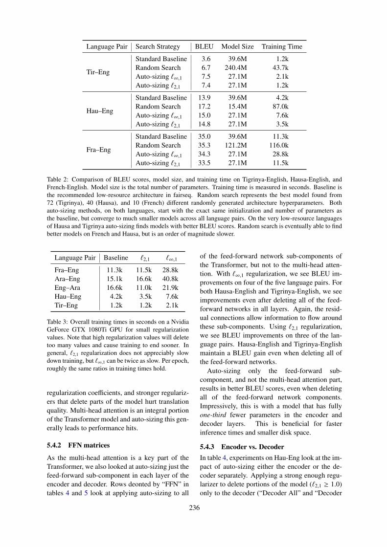
Language Pair Search Strategy BLEU Model Size Training Time
Tir–Eng
Standard Baseline 3.6 39.6M 1.2kRandom Search 6.7 240.4M 43.7kAuto-sizing `∞,1 7.5 27.1M 2.1kAuto-sizing `2,1 7.4 27.1M 1.2k
Hau–Eng
Standard Baseline 13.9 39.6M 4.2kRandom Search 17.2 15.4M 87.0kAuto-sizing `∞,1 15.0 27.1M 7.6kAuto-sizing `2,1 14.8 27.1M 3.5k
Fra–Eng
Standard Baseline 35.0 39.6M 11.3kRandom Search 35.3 121.2M 116.0kAuto-sizing `∞,1 34.3 27.1M 28.8kAuto-sizing `2,1 33.5 27.1M 11.5k
Table 2: Comparison of BLEU scores, model size, and training time on Tigrinya-English, Hausa-English, andFrench-English. Model size is the total number of parameters. Training time is measured in seconds. Baseline isthe recommended low-resource architecture in fairseq. Random search represents the best model found from72 (Tigrinya), 40 (Hausa), and 10 (French) different randomly generated architecture hyperparameters. Bothauto-sizing methods, on both languages, start with the exact same initialization and number of parameters asthe baseline, but converge to much smaller models across all language pairs. On the very low-resource languagesof Hausa and Tigrinya auto-sizing finds models with better BLEU scores. Random search is eventually able to findbetter models on French and Hausa, but is an order of magnitude slower.
Language Pair Baseline `2,1 `∞,1
Fra–Eng 11.3k 11.5k 28.8kAra–Eng 15.1k 16.6k 40.8kEng–Ara 16.6k 11.0k 21.9kHau–Eng 4.2k 3.5k 7.6kTir–Eng 1.2k 1.2k 2.1k
Table 3: Overall training times in seconds on a NvidiaGeForce GTX 1080Ti GPU for small regularizationvalues. Note that high regularization values will deletetoo many values and cause training to end sooner. Ingeneral, `2,1 regularization does not appreciably slowdown training, but `∞,1 can be twice as slow. Per epoch,roughly the same ratios in training times hold.
regularization coefficients, and stronger regulariz-ers that delete parts of the model hurt translationquality. Multi-head attention is an integral portionof the Transformer model and auto-sizing this gen-erally leads to performance hits.
5.4.2 FFN matrices
As the multi-head attention is a key part of theTransformer, we also looked at auto-sizing just thefeed-forward sub-component in each layer of theencoder and decoder. Rows deonted by “FFN” intables 4 and 5 look at applying auto-sizing to all
of the feed-forward network sub-components ofthe Transformer, but not to the multi-head atten-tion. With `∞,1 regularization, we see BLEU im-provements on four of the five language pairs. Forboth Hausa-English and Tigrinya-English, we seeimprovements even after deleting all of the feed-forward networks in all layers. Again, the resid-ual connections allow information to flow aroundthese sub-components. Using `2,1 regularization,we see BLEU improvements on three of the lan-guage pairs. Hausa-English and Tigrinya-Englishmaintain a BLEU gain even when deleting all ofthe feed-forward networks.
Auto-sizing only the feed-forward sub-component, and not the multi-head attention part,results in better BLEU scores, even when deletingall of the feed-forward network components.Impressively, this is with a model that has fullyone-third fewer parameters in the encoder anddecoder layers. This is beneficial for fasterinference times and smaller disk space.
5.4.3 Encoder vs. DecoderIn table 4, experiments on Hau-Eng look at the im-pact of auto-sizing either the encoder or the de-coder separately. Applying a strong enough regu-larizer to delete portions of the model (`2,1 ≥ 1.0)only to the decoder (“Decoder All” and “Decoder
236

`2,1 coefficientModel Portion 0.0 0.1 0.25 0.5 1.0 10.0
Hau–Eng
Encoder All 13.9 16.0 17.1 17.4 15.3 89% 16.4 100%Encoder FFN 15.4 15.1 16.3 15.9 100% 16.7 100%Decoder All 12.6 16.1 16.2 13.0 3% 0.0 63%Decoder FFN 11.8 14.7 14.4 11.7 79% 13.1 100%Enc+Dec All 15.8 17.4 17.8 12.5 61% 0.0 100%Enc+Dec FFN 14.7 15.3 14.2 12.8 86% 14.8 100%
Tir–EngEncoder All 3.6 3.3 4.7 5.3 7.2 8.4 100%Enc+Dec All 3.8 4.0 6.5 7.0 0.0 100%Enc+Dec FFN 4.0 4.2 3.3 5.1 7.4 100%
Fra–EngEncoder All 35.0 35.7 34.5 34.1 33.6 97% 32.8 100%Enc+Dec All 35.2 33.1 29.8 23% 24.2 73% 0.3 100%Enc+Dec FFN 35.6 35.0 34.2 15% 34.2 98% 33.5 100%
Ara–EngEnc+Dec All 27.9 28.0 24.7 1% 20.9 20% 14.3 72% 0.3 100%Enc+Dec FFN 26.9 26.7 1% 25.5 23% 25.9 97% 25.7 100%
Eng–AraEnc+Dec All 9.4 8.7 7.5 5.8 23% 3.7 73% 0.0 100%Enc+Dec FFN 8.6 8.3 3% 8.3 22% 7.9 93% 8.0 100%
Table 4: BLEU scores and percentage of parameter rows deleted by auto-sizing on various sub-components of themodel, across varying strengths of `2,1 regularization. 0.0 refers to the baseline without any regularizer. Blankspaces mean less than 1% of parameters were deleted. In the two very low-resource language pairs (Hausa-Englishand Tigrinya-English), deleting large portions of the encoder can actually help performance. However, deletingthe decoder hurts performance.
`∞,10.0 0.1 0.25 0.5 1.0 10.0 100.0
Hau–EngEnc+Dec All 13.9 15.5 14.7 16.0 16.7 14.9 4% 1.5 100%Enc+Dec FFN 13.4 14.3 14.1 12.9 15.3 0% 15.0 100%
Tir–EngEnc+Dec All 3.6 4.6 3.4 3.4 3.7 7.4 0% 2.4 100%Enc+Dec FFN 3.6 3.8 3.9 3.6 4.7 0% 7.5 100%
Fra–EngEnc+Dec All 35.0 35.2 35.4 34.9 35.3 26.3 13% 1.7 100%Enc+Dec FFN 34.8 35.5 35.4 35.0 34.1 0% 34.3 100%
Ara–EngEnc+Dec All 27.9 27.3 27.5 27.6 26.9 18.5 22% 0.6 100%Enc+Dec FFN 27.8 27.2 28.3 27.6 25.4 0% 25.4 100%
Eng–AraEnc+Dec All 9.4 9.1 8.3 8.4 8.7 5.2 25% 0.6 100%Enc+Dec FFN 8.8 9.2 9.0 8.9 8.2 0% 8.3 100%
Table 5: BLEU scores and percentage of model deleted using auto-sizing with various l∞,1 regularization strengths.On the very low-resource language pairs of Hausa-English and Tigrinya-English, auto-sizing the feed-forwardnetworks of the encoder and decoder can improve BLEU scores.
237

FFN”) results in a BLEU score drop. However, ap-plying auto-sizing to only the encoder (“EncoderAll” and “Encoder FFN”) yields a BLEU gainwhile creating a smaller model. Intuitively, thismakes sense as the decoder is closer to the out-put of the network and requires more modeling ex-pressivity.
In addition to Hau–Eng, table 4 also con-tains experiments looking at auto-sizing all sub-components of all encoder layers of Tir–Eng andFra–Eng. For all three language pairs, a small reg-ularization coefficient for the `2,1 regularizer ap-plied to the encoder increases BLEU scores. How-ever, no rows are driven to zero and the model sizeremains the same. Consistent with Hau–Eng, us-ing a larger regularization coefficient drives all ofthe encoder’s weights to all zeros. For the smallerHau–Eng and Tir–Eng datasets, this actually re-sults in BLEU gains over the baseline system. Sur-prisingly, even on the Fra–Eng dataset, which hasmore than 15x as much data as Tir–Eng, the per-formance hit of deleting the entire encoder wasonly 2 BLEU points.
Recall from Figure 2 that there are residualconnections that allow information and gradientsto flow around both the multi-head attention andfeed-forward portions of the model. Here, we havethe case that all layers of the encoder have beencompletely deleted. However, the decoder still at-tends over the source word and positional embed-dings due to the residual connections. We hypoth-esize that for these smaller datasets that there aretoo many parameters in the baseline model andover-fitting is an issue.
5.5 Random Search plus Auto-sizing
Above, we have demonstrated that auto-sizing isable to learn smaller models, faster than randomsearch, often with higher BLEU scores. To com-pare whether the two architecture search algo-rithms (random and auto-sizing) can be used inconjunction, we also looked at applying both `2,1and `∞,1 regularization techniques to the FFN net-works in all encoder and decoder layers duringrandom search. In addition, this looks at how ro-bust the auto-sizing method is to different initialconditions.
For a given set of hyperparameters generatedby the random search process, we initialize threeidentical models and train a baseline as well as onewith each regularizer (`2,1 = 1.0 and `∞,1 = 10.0).
none `2,1 `∞,1
Hau–Eng 17.2 16.6 17.8Tir–Eng 6.7 7.9 7.6Fra–Eng 35.4 34.7 34.1Ara–Eng 27.6 25.6 25.9Eng–Ara 9.0 7.6 8.4
Table 6: Test BLEU scores for the models with the bestdev perplexity found using random search over num-ber of layers and size of layers. Regularization valuesof `2,1 = 1.0 and `∞,1 = 10.0 were chosen based on ta-bles 4 and 5 as they encouraged neurons to be deleted.For the very low-resource language pairs, auto-sizinghelped in conjunction with random search.
We trained 216 Tir–Eng models (3 · 72 hyper-parameter config.), 120 Hau–Eng, 45 Ara–Eng,45 Eng–Ara, and 30 Fra–Eng models. Using themodel with the best dev perplexity found duringtraining, table 6 shows the test BLEU scores foreach of the five language pairs. For the very low-resource language pairs of Hau–Eng and Tir–Eng,auto-sizing is able to find the best BLEU scores.
6 Conclusion
In this paper, we have demonstrated the effective-ness of auto-sizing on the Transformer network.On very low-resource datasets, auto-sizing wasable to improve BLEU scores by up to 3.9 pointswhile simultaneously deleting one-third of the pa-rameters in the encoder and decoder layers. Thiswas accomplished while being significantly fasterthan other search methods.
Additionally, we demonstrated how to applyproximal gradient methods efficiently using aGPU. Previous work on optimizing proximal gra-dient algorithms serious impacts speed perfor-mance when the computations are moved off of aCPU and parallelized. Leveraging sorting and pre-fix summation, we reformulated these methods tobe GPU efficient.
Overall, this paper has demonstrated the effi-cacy of auto-sizing on a natural language process-ing application with orders of magnitude more pa-rameters than previous work. With a focus onspeedy architecture search and an emphasis on op-timized GPU algorithms, auto-sizing is able to im-prove machine translation on very low-resourcelanguage pairs without being resource or time-consuming.
238

Acknowledgements
This research was supported in part by Univer-sity of Southern California, subcontract 67108176under DARPA contract HR0011-15-C-0115. Wewould like to thank Justin DeBenedetto for help-ful comments.
ReferencesDzmitry Bahdanau, Kyunghyun Cho, and Yoshua Ben-
gio. 2015. Neural machine translation by jointlylearning to align and translate. In Proc. ICLR.
P. G. Benardos and G.-C. Vosniakos. 2007. Optimiz-ing feedforward artificial neural network architec-ture. Engineering Applications of Artificial Intelli-gence, 20:365–382.
James Bergstra and Yoshua Bengio. 2012. Randomsearch for hyper-parameter optimization. Journal ofMachine Learning Research, 13:281–305.
James S. Bergstra, Remi Bardenet, Yoshua Bengio, andBalazs Kegl. 2011. Algorithms for hyper-parameteroptimization. In Advances in Neural InformationProcessing Systems, pages 2546–2554.
Nicolas Boulanger-Lewandowski, Yoshua Bengio, andPascal Vincent. 2013. Audio chord recognition withrecurrent neural networks. In Proc. InternationalSociety for Music Information Retrieval, pages 335–340.
Stephen Boyd, Neal Parikh, Eric Chu, Borja Peleato,and Jonathan Eckstein. 2010. Distributed optimiza-tion and statistical learning via the alternating direc-tion method of multipliers. Foundations and Trendsin Machine learning, 3(1):1–122.
Denny Britz, Anna Goldie, Minh-Thang Luong, andQuoc Le. 2017. Massive exploration of neural ma-chine translation architectures. In Proc. EMNLP,pages 1442–1451.
Kai-Bo Duan and S. Sathiya Keerthi. 2005. Whichis the best multiclass SVM method? An empiricalstudy. In International Workshop on Multiple Clas-sifier Systems, pages 278–285.
John Duchi, Shai Shalev-Shwartz, Yoram Singer, andTushar Chandra. 2008. Efficient projections ontothe `1-ball for learning in high dimensions. In Proc.ICML, pages 272–279.
Frauke Friedrichs and Christian Igel. 2005. Evolution-ary tuning of multiple SVM parameters. Neurocom-puting, 64:107–117.
Jonas Gehring, Michael Auli, David Grangier, DenisYarats, and Yann N. Dauphin. 2017. ConvolutionalSequence to Sequence Learning. In Proc. ICML.
Diederik P. Kingma and Jimmy Lei Ba. 2015. Adam:A method for stochastic optimization. In Proc.ICLR.
Jeffery Kinnison, Nathaniel Kremer-Herman, DouglasThain, and Walter Scheirer. 2018. Shadho: Mas-sively scalable hardware-aware distributed hyperpa-rameter optimization. In Proc. IEEE Winter Confer-ence on Applications of Computer Vision (WACV),pages 738–747.
Philipp Koehn, Hieu Hoang, Alexandra Birch, ChrisCallison-Burch, Marcello Federico, Nicola Bertoldi,Brooke Cowan, Wade Shen, Christine Moran,Richard Zens, et al. 2007. Moses: Open sourcetoolkit for statistical machine translation. In Proc.ACL: Demos, pages 177–180.
Richard E. Ladner and Michael J. Fischer. 1980. Par-allel prefix computation. J. ACM, 27(4):831–838.
Liam Li and Ameet Talwalkar. 2019. Random searchand reproducibility for neural architecture search.
Dougal Maclaurin, David Duvenaud, and Ryan Adams.2015. Gradient-based hyperparameter optimizationthrough reversible learning. In Proc. ICML, pages2113–2122.
Cettolo Mauro, Girardi Christian, and Federico Mar-cello. 2012. Wit3: Web inventory of transcribed andtranslated talks. In Proc. EAMT, pages 261–268.
Kenton Murray and David Chiang. 2015. Auto-sizingneural networks: With applications to n-gram lan-guage models. In Proc. EMNLP.
Kishore Papineni, Salim Roukos, Todd Ward, and Wei-Jing Zhu. 2002. BLEU: a method for automaticevaluation of machine translation. In Proc. ACL,pages 311–318.
Neal Parikh and Stephen Boyd. 2014. Proximal al-gorithms. Foundations and Trends in Optimization,1(3):123–231.
Martin Popel and Ondrej Bojar. 2018. Training tipsfor the Transformer model. The Prague Bulletin ofMathematical Linguistics, 110(1):43–70.
Ofir Press and Lior Wolf. 2017. Using the outputembedding to improve language models. In Proc.EACL: Volume 2, Short Papers, pages 157–163.
Ariadna Quattoni, Xavier Carreras, Michael Collins,and Trevor Darrell. 2009. An efficient projection forl1,∞ regularization. In Proc. ICML, pages 857–864.
Rico Sennrich and Barry Haddow. 2016. Linguisticinput features improve neural machine translation.In Proc. First Conference on Machine Translation:Volume 1, Research Papers, volume 1, pages 83–91.
Rico Sennrich, Barry Haddow, and Alexandra Birch.2016. Neural machine translation of rare words withsubword units. In Proc. ACL, pages 1715–1725.
239

Jasper Snoek, Hugo Larochelle, and Ryan P. Adams.2012. Practical Bayesian optimization of machinelearning algorithms. In Advances in Neural Infor-mation Processing Systems, pages 2951–2959.
Emma Strubell, Ananya Ganesh, and Andrew McCal-lum. 2019. Energy and policy considerations fordeep learning in NLP. In Proc. ACL.
Ilya Sutskever, Oriol Vinyals, and Quoc V Le. 2014.Sequence to sequence learning with neural net-works. In Advances in Neural Information Process-ing Systems, pages 3104–3112.
Ashish Vaswani, Noam Shazeer, Niki Parmar, JakobUszkoreit, Llion Jones, Aidan N. Gomez, ŁukaszKaiser, and Illia Polosukhin. 2017. Attention is allyou need. In Advances in Neural Information Pro-cessing Systems, pages 5998–6008.
Aaron Vose, Jacob Balma, Alex Heye, AlessandroRigazzi, Charles Siegel, Diana Moise, BenjaminRobbins, and Rangan Sukumar. 2019. Recombina-tion of artificial neural networks. arXiv:1901.03900.
240
Proceedings of the 3rd Workshop on Neural Generation and Translation (WNGT 2019), pages 241–248Hong Kong, China, November 4, 2019. c©2019 Association for Computational Linguistics
www.aclweb.org/anthology/D19-56%2d
Learning to Generate Word- and Phrase-Embeddingsfor Efficient Phrase-Based Neural Machine Translation
Chan Young Park Yulia TsvetkovLanguage Technologies Institute
Carnegie Mellon University{chanyoun,ytsvetko}@cs.cmu.edu
Abstract
Neural machine translation (NMT) often failsin one-to-many translation, e.g., in the trans-lation of multi-word expressions, compounds,and collocations. To improve the translationof phrases, phrase-based NMT systems havebeen proposed; these typically combine word-based NMT with external phrase dictionariesor with phrase tables from phrase-based sta-tistical MT systems. These solutions intro-duce a significant overhead of additional re-sources and computational costs. In this pa-per, we introduce a phrase-based NMT modelbuilt upon continuous-output NMT, in whichthe decoder generates embeddings of wordsor phrases. The model uses a fertility mod-ule, which guides the decoder to generate em-beddings of sequences of varying lengths. Weshow that our model learns to translate phrasesbetter, performing on par with state of the artphrase-based NMT. Since our model does notresort to softmax computation over a huge vo-cabulary of phrases, its training time is about112x faster than the baseline.
1 Introduction
Despite the successes of neural machine transla-tion (Wu et al., 2016; Vaswani et al., 2017; Ahmedet al., 2018), state of the art NMT systems arestill challenged by translation of typologically di-vergent language pairs, especially when languagesare morphologically rich (Burlot and Yvon, 2017).One of the reasons lies in increased sparsity ofword types, which leads to the demand for (of-ten unavailable) significantly larger training cor-pora (Koehn and Knowles, 2017). Another rea-son is an implicit assumption of sequence to se-quence (seq2seq) models that input sequences aretranslated into a target language word-by-word orsubword-by-subword (Sennrich et al., 2016).
This is not the case for typologically diver-gent language pairs, for example when translat-
ing into English from agglutinative languages withhigh rates of morphemes per word (e.g., Turk-ish and Quechua) or languages with productivecompounding processes like German or Finnish(Matthews et al., 2016). Another ubiquitoussource of one-to-many correspondences is a trans-lation of idiomatic phrases and multi-word expres-sions (Rikters and Bojar, 2017).
While outperformed by NMT overall, transla-tion models in traditional statistical phrase-basedapproaches (Koehn, 2009, SMT) provide an in-ventory of phrase translations, which can be usedto address the above challenges. To combine thebenefits of NMT and phrase-based SMT, phrase-based NMT systems have been proposed (Huanget al., 2017; Lample et al., 2018) which combineword-based NMT with external phrase memories(Tang et al., 2016; Dahlmann et al., 2017). How-ever, prior approaches to phrase-based NMT in-troduced a significant overhead of additional re-sources and computation.
We introduce a phrase-based continuous-outputNMT (PCoNMT) model built upon continuous-output NMT (Kumar and Tsvetkov, 2019), inwhich the decoder generates embeddings of wordsor phrases (§2). The model extracts phrases inthe target language from one-to-many word align-ments and pre-computes word and phrase embed-dings which constitute the output space of ourmodel (§2.2). A fertility module guides the de-coder, providing the probability of generating aword or a phrase at each time step (§2.3). Experi-mental results show that the proposed model out-performs the conventional attention-based NMTsystems (Bahdanau et al., 2014) by up to 4.8BLEU, and the baseline continuous-output mod-els by up to 1.6 BLEU, and beat the state-of-the-art phrase-based NMT system in translation fromGerman and Turkish into English.
Since our model does not resort to softmax
241

Figure 1: Phrase-based neural machine translation architectures generate word- and phrase embeddings at eachstep of decoding. The PCoNMT models are guided by on the fertility prediction and the attention.
computation over a huge vocabulary, it also main-tains the computational efficiency of continuous-output NMT, even with additional ngram embed-ding tables, and is faster than the state-of-the-artbaseline by 112x (§3), making our models energy-efficient (Strubell et al., 2019).
The key contributions of our work are twofold:(1) we develop a phrase-based NMT model thatoutperforms existing baselines and better trans-lates phrases, while (2) maintaining the computa-tional efficiency of NMT end-to-end approaches.1
2 Phrase-based Continuous-output NMT
2.1 Embedding output layerKumar and Tsvetkov (2019) introducedcontinuous-output machine translation (CoNMT)which replaces the softmax layer in the con-ventional seq2seq models with a continuousembeddings layer. The model predicts the embed-ding of the target word instead of its probability.It is trained to maximize the von Mises-Fisher(vMF) probability density of the pretrained target-language embeddings given the embeddingspredicted by the model at every step; at inferencetime, predicted embedding is compared to theembeddings in the pre-trained embedding table,and the closest embedding is selected as an outputword. While maintaining the translation quality oftraditional seq2seq approaches, CoNMT approachalleviates the computational bottleneck of thesoftmax layer: it is substantially more efficient totrain and the models are more compact, withoutlimiting the output vocabulary size.
1Our code and data are available at https://github.com/chan0park/PCoNMT
Extending the CoNMT approach, we pro-pose phrase-based continuous-output NMT(PCoNMT). As depicted in Figure 1, we augmentthe original model with (1) additional embeddingtables for phrases, and (2) a fertility module thatguides the choice of embedding table to look-upin (described in §2.3). Having additional largeembedding tables, which significantly increasethe vocabulary size, could be a considerableoverhead to a word-based model with the softmaxlayer. However, since we generate embeddingsin the final layer and do not resort to the softmaxcomputation, our models maintain the compu-tational efficiency of continuous-output models(§3) during the training time. At inference time,the only overhead incurred by our model isgetting another set of vMF scores for the phraseembedding table for each output step. This isalmost negligible compared to the computation ofthe entire network.
In addition to efficiency benefits, since thePCoNMT approach enables us to pre-computeembeddings of less frequent phrases and phrasesthat do not have a literal translation, e.g., multi-word expressions, it facilitates better translationsspecifically where the translation is notoriouslychallenging for NMT.
2.2 Output embedding tables
To construct embedding tables for target-languagephrases, we first extract the list of output phrasesfrom parallel corpora. Following Tang et al.(2016), in this work, we focus on one-to-manyword alignments in the training corpus. Con-sider as an example translation of German com-
242

s1
e1
s2 …
Decoder
o1
y1
Attn
sword
y1
gen∑
α1
< s >
Word Table
Phrase Tables1
x1 x3x2
h3h2h1 …… Encoder
xn
hn
λe,3λe,2λe,1 λe,n
Encoder Fertilities
…
Fertility Prediction
λd,word
λd,phrasesphrase
Figure 2: The detailed architecture of our model which consist of three components (encoder, fertility module,and decoder), described in §2. Given an input sentence {x1, x2 . . . xn}, our model generates the output sentence{y1, y2 . . . ym}, where yi corresponds to words or phrases, e.g. quality of life. At each step, the decoder generatesan embedding ei, then the fertility module guides it to generate a word or a phrase, via the word- or phrase-embedding table, respectively.
pounds to English, e.g., Lebensqualitat in Germanis translated as quality of life. We extract all suchone-to-many word alignments from the parallelcorpora using Fastalign (Dyer et al., 2013). Thereare several standard approaches to extract mean-ingful phrases from a monolingual corpus, suchas using scores like pointwise mutual information(PMI) (Mikolov et al., 2013). However, for ourmodel, we utilize word-alignment results to con-struct a phrase list since we are particularly inter-ested in multi-word translation cases. Note thatwith this approach, phrases in target-side embed-ding tables can be different depending on whichlanguage pair and which corpus are being used.
After extracting all noisy one-to-many align-ments from the parallel corpus, we filter our phraselist in order to keep only the useful phrases and toremove potential erroneous phrases coming fromalignment errors. We filter according to the fol-lowing heuristics: (1) a phrase should appear atleast twice in the parallel corpus; (2) it should notcontain any punctuation; (3) PMI of the phraseshould be positive; (4) a bigram phrase should notrepeat the same word; and (5) the phrase shouldnot contain only stopwords.
We train embeddings for the resulting list ofwords and phrases as follows. First, we preprocessthe target language’s large monolingual corpus toconcatenate words to match the longest phrase inthe extracted phrase list. For example, the sen-
tence ‘I went to a graduate school’ will be con-verted into ‘I went to a graduate school’ if wehave went to and graduate school in our phraselist. This concatenated corpus is then used to trainfastText (Peters et al., 2018) embeddings for bothphrases and words simultaneously. We use fast-Text because it encodes subword-level informa-tion which may provide a signal about each wordin a phrase. From this training, we obtain both theword- and phrase-tables, which are of the same di-mension.
2.3 Fertility module
We introduce a fertility module, similar to the fer-tility concept in SMT (Brown et al., 1993). Thefertility indicates how many target words eachsource word should produce in the output. TheSMT models keep the fertility probabilities overfertility count, typically from zero to four, and useit to produce probability over words. We integratethis fertility concept into our PCoNMT model.
Our fertility module predicts the fertility proba-bility φe = [φe0, ..., φeN ], where φei indicates thescalar probability of the source word at positione being translated into i words. This is predictedbased on the word embedding and encoder’s out-put of the word: φe = FFNN(xe;he). FFNNis the feed-forward neural network, and (xe;he)denotes the concatenation of xe and he, whichare embedding and encoder’s hidden state of eth
243

source word, respectively. The dimension of fer-tility vector φ, N , can be arbitrarily large, but inthis paper we explore two different variants; thefirst one is Fertility4 where each dimension cor-responds to zero to three words to produce re-spectively (N ∈ {0, 1, 2, 3}), and the second oneis Fertility2 which simplifies the fertility predic-tion into binary classification by setting N=1 as acut-off point, i.e., whether the model should gen-erate a word (N ≤ 1) or a phrase (N > 1).Therefore, φe becomes a four-dimensional vec-tor of [φe0, φe1, φe2, φe3] for Fertility4, and two-dimensional vector of [
∑1n=0 φen,
∑∞n=2 φen] for
Fertility2.At decoding time, we combine this fertility
probability of each source word and the attentionto guide the decoder to generate a phrase or aword. To get the probability of producing a wordλd,word for timestep d, we use attention given toeach source word as a weight to its fertility proba-bility and sum over the entire source sentence:
λd,word =
{∑e ad,e (φe0 + φe1) (dim = 4)∑e ad,e [φe]0 (dim = 2)
λd,phrase = 1− λd,word,
where ad,e is a scalar value of attention assignedfor source word e at timestep d and [φe]0 is the0th element of φe, which basically is the same as(φe0 + φe1) in Fertility4. We use this λd,word andλd,phrase to weight the scores in word table and inphrase table, respectively:
sword = λd,word · Score(ed, Tword)sphrase = λd,phrase · Score(ed, Tphrase)
yd = argmax(sword; sphrase),
where sword is a vector of scores for word in theword embedding table Tword, and Score is a scorefunction to measure how similar the predicted em-bedding ed and the embeddings in T . For theScore function, we use vMF as proposed in Ku-mar and Tsvetkov (2019). Finally, we get an out-put, yd for the timestep d by doing argmax overweighted scores from both word and phrase tables.
2.4 Model TrainingThe training of PCoNMT model is achieved bytwo separate steps. First, we only train the seq2seqmodules as CoNMT does. We use vMF loss to op-timize the embedding prediction. Once we find theoptimal parameters for the CoNMT components,
IWSLT IWSLTMWT
Attn 23.83 -NPMT 27.27 -CoNMT 27.07 24.98
PCoNMT 28.69 28.89+Fertility4 28.04 24.93+Fertility2 28.29 25.12
Table 1: Evaluation results (BLEU) on IWSLT 2014De–En task.
WMT WMTMWT
NPMT 3.58 -CoNMT 7.44 7.67
PCoNMT 8.87 7.70+Fertility4 8.12 8.53+Fertility2 8.39 8.61
Table 2: Evaluation results (BLEU) on WMT 2017 Tr–En task.
we freeze those parameters, and separately trainparameters of the fertility module.2 During thepreprocessing, we extract the actual fertility valuefor each source word using the word-alignmentmodel and the filtered phrase list, then set it as agold label for the fertility prediction training.
3 Experiments
In this section, we evaluate our model in termsof translation quality and training efficiency. Weused IWSLT 2014 dataset for De–En machinetranslation task, following the same preprocess-ing and splits as in Ranzato et al. (2016). Forthe Tr–En task, we used WMT 17 train and testdataset (Bojar et al., 2018). The training cor-pora size for IWSLT 2014 and WMT 17 is about153K and 200K sentences, respectively. All re-sults are reported with case-sensitive BLEU-4 (Pa-pineni et al., 2002). In addition to the two of-ficial datasets, we subset the given test sets tosentences that actually contain multi-word transla-tion (MWT) cases by running the word-alignmentmodel. The size of extracted MWT subsets forIWSLT 2014 and WMT 17 are 335 (5%) and 116
2Although we have omitted the results due to space, wealso have tried jointly training the fertility prediction andtranslation in a multi-task learning setting. However, thejoint-learning has consistently hurt the translation quality.
244

speed ↓(samples/sec)
convergence ↑(epochs)
total time ↑(hours)
NPMT 15.4 40 110CoNMT 256.0 6 1.00PCoNMT 261.0 6 0.98
Table 3: Training efficiency results on IWSLT 2014De–En dataset.
(4%), respectively. Also note that following Ku-mar and Tsvetkov (2019), in this paper, we onlyused greedy decoding.
We compared our proposed model with threebaselines: (1) Attn: Standard attention-basedNMT model as in Wiseman and Rush (2016);(2) CoNMT: RNN-based Continuous-outputNMT systems (Kumar and Tsvetkov, 2019);(3) NPMT: The state of the art phrase-based NMTmodel proposed by Huang et al. (2017). ForNPMT, we ran its released code with the same pre-processed data we are using without changing anyhyperparameters they set.3 For both De–En andTr–En CoNMT models, we used the best hyperpa-rameter settings reported by Kumar and Tsvetkov(2019) for De–En. For our model, PCoNMT, weonly changed the batch size from the original set-ting in CoNMT and chose other additional param-eters based on the performance on the validationset.
Although we use recurrent architectures inthis paper to make our findings comparable toprior work that uses the same setting, we be-lieve using multi-layer self-attention mechanism(Vaswani et al., 2017) as a base of our modelhas further potential to improve the performance.Even with Transformers, the conventional token-by-token generation scheme will be still prone tomistakes in multi-word generations. Therefore,explicitly handling the phrase generation as wepropose is likely to be helpful, which we leave itas future work.
Translation quality De–En and Tr–En transla-tion results are summarized in Tables 1 and 2.PCoNMT significantly outperforms both the con-ventional attention-based model (by >4 BLEU)and its base CoNMT model (by 1.6 BLEU), andalso performs better than NPMT (by 1.4 BLEU).The fertility module is shown to be relatively
3The number we got from the experiment is different fromthe one reported in the original paper, which possibly is root-ing from slightly different preprocessing steps.
ClassDe–En Tr–En
Tot. P R F-1 Tot. P R F-1
N ≤ 1 97% 0.97 0.96 0.97 97% 0.97 0.95 0.96N > 1 3% 0.33 0.28 0.31 3% 0.17 0.1 0.13
Table 4: The Precision, Recall, and F1 evaluation re-sults on the fertility prediction of Fertility2. ”Tot.” isthe percentage for the number of occurrences of eachlabel in the gold label.
ClassDe–En Tr–En
Total P R F-1 Total P R F-1
N = 0 10% 0.59 0.09 0.15 14% 0.56 0.30 0.39N = 1 86% 0.88 0.95 0.91 83% 0.86 0.91 0.89N = 2 4% 0.27 0.35 0.31 3% 0.12 0.19 0.14N = 3 0% 0.16 0.14 0.15 0% 0 0 0
Table 5: The Precision, Recall, and F1 evaluation re-sults on the fertility prediction of Fertility4. ”Tot.” isthe percentage for the number of occurrences of eachlabel in the gold label.
more helpful in Tr–En task, while showing lessimpact in De–En task. We also observed thatFertility2 consistently generates better transla-tions than Fertility4. On the more difficult MWTsubset containing multi-word phrases, PCoNMTobtains large absolute gains in BLEU, confirmingtheir effectiveness in phrase translations. Exam-ples of translations are shown in Table 7.
Computational efficiency We report the train-ing efficiency of models in three metrics: speed,number of training epochs till convergence, andtotal training time. All results were measured onthe same machine with the same batch size. Themachine was a single-node local machine withNVIDIA GTX 1080 Ti. During the training, noother process was executed except for the trainingfor the fair comparison.
Table 3 shows that CoNMT and PCoNMT canprocess 28 times faster than NPMT, and convergesix times faster, i.e., reducing the entire trainingtime by 112x. Somewhat surprisingly, PCoNMTfurther accelerates the CoNMT as it can reducethe timestep needed for a sample by generatingphrases. This result proves that additional phraseembeddings of PCoNMT has little impact on com-putational efficiency while training.
Fertility Prediction Evaluation The fertilityprediction can have a significant impact on thetranslation as it guides the decoder to decide whento generate phrases and when to generate words.We evaluate the prediction results on the test set
245

with the gold label obtained from the word align-ment model in Table 5 and Table 4.
In both datasets, we observe that the data ishighly skewed toward word-level classes as mosttranslations are word-to-word generation. This re-sults in Fertility4 not to predict N = 3 classesat all in the Tr–En dataset. The comparison be-tween Table 5 and Table 4 shows that the Fertility2has slighly higher F-1 score than Fertility4 in bothdatasets. It implies that aggregating the classesinto two made the prediction task easier for themodel, which thus led to the improved translationquality shown in the previous results.
Analysis on Generated Phrases Table 6presents further analysis of the generated phrases.We first see in which category of phrases ourmodel performs well compared to the baseline,CoNMT, to know from where the improvement ofour model is coming. As for the phrase categories,we consider three categories, compound nouns(CNs, e.g., thought experiment), verb phrases(VPs, e.g., grow apart), and collocations (COs,e.g., at risk). We randomly sampled a hundredgenerated phrases from the De–En test set, andmanually annotate the category of phrases andwhether it is the correct translation. We also lookat the output of CoNMT baseline for the same testsamples, and also annotate if the sampled phrasesare well translated in the CoNMT output.
The results in Table 6 show that the most fre-quently generated phrases are collocations (56%)followed by verb phrases (28%) and compoundnouns (16%). Among the entire sampled phrases,64 percent of phrases were correct in PCoNMToutput while CoNMT had 50 percent of them cor-rect. Specifically, our model significantly outper-formed the baseline in compound word generationcases while performs worse in verb phrases gen-eration. By looking into the instances of wrongverb phrase generation, we found that a significantamount of those errors are related to the tense ofthe verb.
4 Related Work
Multi-word Expressions for NMT There havebeen several studies that incorporate multi-wordphrases into supervised NMT (Tang et al., 2016;Wang et al., 2017; Dahlmann et al., 2017). Mostapproaches rely on pre-defined phrase dictionar-ies obtained from methods such as phrase-basedStastitical MT (Koehn et al., 2003) or word-
Category Total PCoNMT CoNMT
CNs 16% 0.63 0.25VPs 28% 0.5 0.57COs 56% 0.71 0.54
Sum 100% 0.64 0.50
Table 6: Percentages of categories of randomly sam-pled 100 phrases generated by PCoNMT on IWSLT2014 De–En test set and the accuracy of PCoNMT andCoNMT phrase translations, respectively.
alignment. Tang et al. (2016) use a method thatcombines phrase probability and word probabil-ity obtained from a softmax layer enabling thedecoder to decide to switch between phrase gen-eration and word generation based on context.Dahlmann et al. (2017) use a separate SMT modelto generate phrases along with an NMT model.Wang et al. (2017) proposed a similar approachto have an SMT model run in parallel, where anadditional module decide whether to use a phrasegenerator from the SMT model or the neural de-coder.
Recent works have also explored using an ad-ditional RNN to compute phrase generation prob-abilities. Huang et al. (2017) proposed Neu-ral Phrase MT (NPMT) that is built upon Sleep-WAke Network (SWAN), a segmentation-basedsequence modeling technique, which automati-cally discovers phrases given the data and appendsthe special symbol $ to the source and target data.The model gets these segmented word/phrase se-quences as input and keeps two levels of RNNsto encode and decode phrases. NPMT establishedstate of the art results for phrase-based NMT, butat a price of significant computational overhead.
The main differences between previous studiesand our work are: (1) we do not rely on SMTmodel and adapt in an end-to-end manner only re-quiring some preprocessing using word-alignmentmodels; and (2) we use phrase embedding ta-bles to represent phrases instead of keeping exter-nal phrase memory and its generation probability.By using the phrase embeddings along with thecontinuous-output layer, we significantly reducethe computational complexity and propose an ap-proach to overcome the phrase generation bottle-neck.
Fertility in MT Fertility (Brown et al., 1993)has been a core component in phrase-based SMT
246

German src und Sie sollten auch an Dinge wie Lebensqualitat denkenEnglish ref and you also want to think about things like quality of lifeBaseline CoNMT and you should think of things like lifePCoNMT and you should think of things like quality of life .German src wer ein Gehirn hat , ist gefahrdet .English ref everyone with a brain is at risk .Baseline CoNMT who has a brain is risk .PCoNMT who has a brain is at risk .German src ich stecke voller Widerspruche .English ref I am full of contradictions .Baseline CoNMT I ’m put .PCoNMT I ’m full of contradictions
Table 7: Translation output examples from CoNMT and PCoNMT systems.
models (Koehn et al., 2003). Fertility gives thelikelihood of each source word of being translatedinto n words. Fertility helps in deciding whichphrases should be stored in the phrase tables. Tuet al. (2016) revisited fertility to model coveragein NMT to address the issue of under-translation.They used a fertility vector to express how manywords should be generated per source word and acoverage vector to keep track of words translatedso far. We use a very similar concept in this workbut the fertility module is introduced with a pur-pose to guide the decoder to switch over generat-ing phrases and words.
5 Conclusion
We proposed PCoNMT, a phrase-based NMT sys-tem built upon continuous-output NMT models.We also introduced a fertility module that guidesthe decoder by providing the probabilities of gen-erating a phrase and a word by leveraging theattention mechanism. Our experimental resultsshowed that our model outperforms the state ofthe art phrase NMT systems, and also speeds upthe computation by 112x.
Acknowledgments
We gratefully acknowledge Sachin Kumar and ouranonymous reviewers for the helpful feedback.This material is based upon work supported byNSF grant IIS1812327 and an Amazon MLRAaward.
ReferencesKarim Ahmed, Nitish Shirish Keskar, and Richard
Socher. 2018. Weighted transformer network formachine translation. In Proc. ICLR.
Dzmitry Bahdanau, Kyunghyun Cho, and Yoshua Ben-
gio. 2014. Neural machine translation by jointlylearning to align and translate. In Proc. of ICLR.
Ondrej Bojar, Christian Federmann, Mark Fishel,Yvette Graham, Barry Haddow, Philipp Koehn, andChristof Monz. 2018. Findings of the 2018 confer-ence on machine translation (wmt18). In Proceed-ings of the Third Conference on Machine Transla-tion: Shared Task Papers, pages 272–303.
Peter F Brown, Vincent J Della Pietra, Stephen A DellaPietra, and Robert L Mercer. 1993. The mathemat-ics of statistical machine translation: Parameter esti-mation. Computational linguistics, 19(2):263–311.
Franck Burlot and Francois Yvon. 2017. Evaluatingthe morphological competence of machine transla-tion systems. In Proc. of WMT, pages 43–55.
Leonard Dahlmann, Evgeny Matusov, PavelPetrushkov, and Shahram Khadivi. 2017. Neu-ral machine translation leveraging phrase-basedmodels in a hybrid search. In Proc. of EMNLP.
Chris Dyer, Victor Chahuneau, and Noah A. Smith.2013. A simple, fast, and effective reparameteriza-tion of IBM Model 2. In Proc. of NAACL.
Po-Sen Huang, Chong Wang, Sitao Huang, DengyongZhou, and Li Deng. 2017. Towards neural phrase-based machine translation. In Proc. of ICLR.
Philipp Koehn. 2009. Statistical machine translation.Cambridge University Press.
Philipp Koehn and Rebecca Knowles. 2017. Six chal-lenges for neural machine translation. In Proc. ofWNGT.
Philipp Koehn, Franz Josef Och, and Daniel Marcu.2003. Statistical phrase-based translation. In Pro-ceedings of the 2003 Conference of the North Amer-ican Chapter of the Association for ComputationalLinguistics on Human Language Technology - Vol-ume 1, NAACL ’03, pages 48–54, Stroudsburg, PA,USA. Association for Computational Linguistics.
Sachin Kumar and Yulia Tsvetkov. 2019. Von mises-fisher loss for training sequence to sequence modelswith continuous outputs. In Proc. of ICLR.
247

Guillaume Lample, Myle Ott, Alexis Conneau, and Lu-dovic Denoyer. 2018. Phrase-based & neural unsu-pervised machine translation. In Proc. of EMNLP,pages 5039–5049.
Austin Matthews, Eva Schlinger, Alon Lavie, and ChrisDyer. 2016. Synthesizing compound words for ma-chine translation. In Proc. of ACL, pages 1085–1094.
Tomas Mikolov, Ilya Sutskever, Kai Chen, Greg S Cor-rado, and Jeff Dean. 2013. Distributed representa-tions of words and phrases and their compositional-ity. In Advances in neural information processingsystems, pages 3111–3119.
Kishore Papineni, Salim Roukos, Todd Ward, and Wei-Jing Zhu. 2002. BLEU: a method for automaticevaluation of machine translation. In Proc. of ACL,pages 311–318.
Matthew Peters, Mark Neumann, Mohit Iyyer, MattGardner, Christopher Clark, Kenton Lee, and LukeZettlemoyer. 2018. Deep contextualized word rep-resentations. In Proceedings of the 2018 Confer-ence of the North American Chapter of the Associ-ation for Computational Linguistics: Human Lan-guage Technologies, Volume 1 (Long Papers), pages2227–2237.
Marc’Aurelio Ranzato, Sumit Chopra, Michael Auli,and Wojciech Zaremba. 2016. Sequence level train-ing with recurrent neural networks.
Matss Rikters and Ondej Bojar. 2017. Paying attentionto multi-word expressions in neural machine trans-lation. In Proc. of Machine Translation Summit.
Rico Sennrich, Barry Haddow, and Alexandra Birch.2016. Neural machine translation of rare words withsubword units. In Proc. of ACL.
Emma Strubell, Ananya Ganesh, and Andrew McCal-lum. 2019. Energy and policy considerations fordeep learning in nlp. In Proc. of ACL.
Yaohua Tang, Fandong Meng, Zhengdong Lu, Hang Li,and Philip LH Yu. 2016. Neural machine transla-tion with external phrase memory. arXiv preprintarXiv:1606.01792.
Zhaopeng Tu, Zhengdong Lu, Yang Liu, Xiaohua Liu,and Hang Li. 2016. Modeling coverage for neuralmachine translation. In Proceedings of the 54th An-nual Meeting of the Association for ComputationalLinguistics (Volume 1: Long Papers), volume 1,pages 76–85.
Ashish Vaswani, Noam Shazeer, Niki Parmar, JakobUszkoreit, Llion Jones, Aidan N Gomez, ŁukaszKaiser, and Illia Polosukhin. 2017. Attention is allyou need. In Advances in neural information pro-cessing systems, pages 5998–6008.
Xing Wang, Zhaopeng Tu, Deyi Xiong, and MinZhang. 2017. Translating phrases in neural machinetranslation. In Proc. of EMNLP, pages 1421–1431.
Sam Wiseman and Alexander M Rush. 2016.Sequence-to-sequence learning as beam-search opti-mization. In Proceedings of the 2016 Conference onEmpirical Methods in Natural Language Process-ing, pages 1296–1306.
Yonghui Wu, Mike Schuster, Zhifeng Chen, Quoc VLe, Mohammad Norouzi, Wolfgang Macherey,Maxim Krikun, Yuan Cao, Qin Gao, KlausMacherey, et al. 2016. Google’s neural ma-chine translation system: Bridging the gap betweenhuman and machine translation. arXiv preprintarXiv:1609.08144.
248
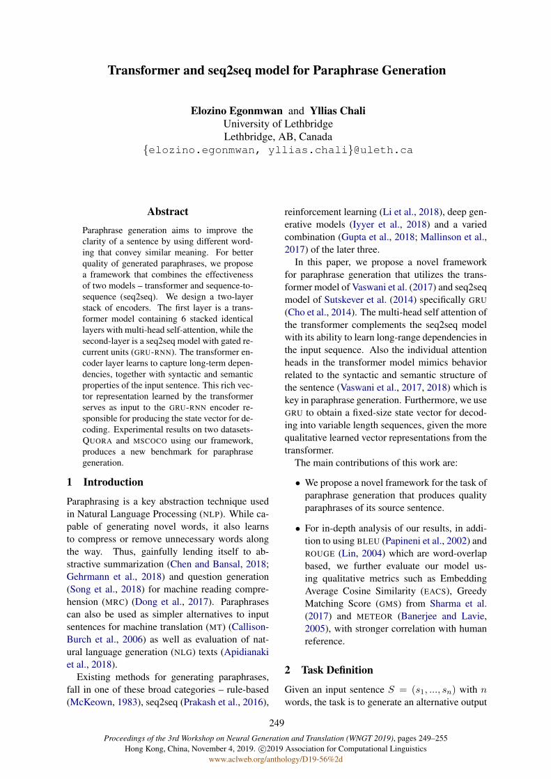
Proceedings of the 3rd Workshop on Neural Generation and Translation (WNGT 2019), pages 249–255Hong Kong, China, November 4, 2019. c©2019 Association for Computational Linguistics
www.aclweb.org/anthology/D19-56%2d
Transformer and seq2seq model for Paraphrase Generation
Elozino Egonmwan and Yllias ChaliUniversity of LethbridgeLethbridge, AB, Canada
{elozino.egonmwan, yllias.chali}@uleth.ca
Abstract
Paraphrase generation aims to improve theclarity of a sentence by using different word-ing that convey similar meaning. For betterquality of generated paraphrases, we proposea framework that combines the effectivenessof two models – transformer and sequence-to-sequence (seq2seq). We design a two-layerstack of encoders. The first layer is a trans-former model containing 6 stacked identicallayers with multi-head self-attention, while thesecond-layer is a seq2seq model with gated re-current units (GRU-RNN). The transformer en-coder layer learns to capture long-term depen-dencies, together with syntactic and semanticproperties of the input sentence. This rich vec-tor representation learned by the transformerserves as input to the GRU-RNN encoder re-sponsible for producing the state vector for de-coding. Experimental results on two datasets-QUORA and MSCOCO using our framework,produces a new benchmark for paraphrasegeneration.
1 Introduction
Paraphrasing is a key abstraction technique usedin Natural Language Processing (NLP). While ca-pable of generating novel words, it also learnsto compress or remove unnecessary words alongthe way. Thus, gainfully lending itself to ab-stractive summarization (Chen and Bansal, 2018;Gehrmann et al., 2018) and question generation(Song et al., 2018) for machine reading compre-hension (MRC) (Dong et al., 2017). Paraphrasescan also be used as simpler alternatives to inputsentences for machine translation (MT) (Callison-Burch et al., 2006) as well as evaluation of nat-ural language generation (NLG) texts (Apidianakiet al., 2018).
Existing methods for generating paraphrases,fall in one of these broad categories – rule-based(McKeown, 1983), seq2seq (Prakash et al., 2016),
reinforcement learning (Li et al., 2018), deep gen-erative models (Iyyer et al., 2018) and a variedcombination (Gupta et al., 2018; Mallinson et al.,2017) of the later three.
In this paper, we propose a novel frameworkfor paraphrase generation that utilizes the trans-former model of Vaswani et al. (2017) and seq2seqmodel of Sutskever et al. (2014) specifically GRU
(Cho et al., 2014). The multi-head self attention ofthe transformer complements the seq2seq modelwith its ability to learn long-range dependencies inthe input sequence. Also the individual attentionheads in the transformer model mimics behaviorrelated to the syntactic and semantic structure ofthe sentence (Vaswani et al., 2017, 2018) which iskey in paraphrase generation. Furthermore, we useGRU to obtain a fixed-size state vector for decod-ing into variable length sequences, given the morequalitative learned vector representations from thetransformer.
The main contributions of this work are:
• We propose a novel framework for the task ofparaphrase generation that produces qualityparaphrases of its source sentence.
• For in-depth analysis of our results, in addi-tion to using BLEU (Papineni et al., 2002) andROUGE (Lin, 2004) which are word-overlapbased, we further evaluate our model us-ing qualitative metrics such as EmbeddingAverage Cosine Similarity (EACS), GreedyMatching Score (GMS) from Sharma et al.(2017) and METEOR (Banerjee and Lavie,2005), with stronger correlation with humanreference.
2 Task Definition
Given an input sentence S = (s1, ..., sn) with nwords, the task is to generate an alternative output
249

S: What are the dumbest questions ever askedon Quora?G: what is the stupidest question on quora?R: What is the most stupid question asked onQuora?S: How can I lose fat without doing any aero-bic physical activityG: how can i lose weight without exercise?R: How can I lose weight in a month withoutdoing exercise?S: How did Donald Trump won the 2016 USApresidential election?G: how did donald trump win the 2016 presi-dentialR: How did Donald Trump become presi-dent?
Table 1: Examples of our generated paraphrases onthe QUORA sampled test set, where S, G, R repre-sents Source, Generated and Reference sentences re-spectively.
sentence Y = (y1, ..., ym) | ∃ym 6∈ S with mwords that conveys similar semantics as S, wherepreferably, m < n but not necessarily.
3 Method
In this section, we present our framework for para-phrase generation. It follows the popular encode-decode paradigm, but with two stacked layers ofencoders. The first encoding layer is a trans-former encoder, while the second encoding layeris a GRU-RNN encoder. The paraphrase of a givensentence is generated by a GRU-RNN decoder.
3.1 Stacked Encoders
3.1.1 Encoder – TRANSFORMER
We use the transformer-encoder as sort of a pre-training module of our input sentence. The goalis to learn richer representation of the input vectorthat better handles long-term dependencies as wellas captures syntactic and semantic properties be-fore obtaining a fixed-state representation for de-coding into the desired output sentence. The trans-former contains 6 stacked identical layers mainlydriven by self-attention implemented by Vaswaniet al. (2017, 2018).
3.1.2 Encoder – GRU-RNN
Our architecture uses a single layer uni-directionalGRU-RNN whose input is the output of the trans-
S: Three dimensional rendering of a kitchen areawith various appliances.G: a series of photographs of a kitchenR: A series of photographs of a tiny modelkitchenS: a young boy in a soccer uniform kicking a ballG: a young boy kicking a soccer ballR: A young boy kicking a soccer ball on a greenfield.S: The dog is wearing a Santa Claus hat.G: a dog poses with santa hatR: A dog poses while wearing a santa hat.S: the people are sampling wine at a wine tasting.G: a group of people wine tasting.R: Group of people tasting wine next to somebarrels.
Table 2: Examples of our generated paraphrases onthe MSCOCO sampled test set, where S, G, R repre-sents Source, Generated and Reference sentences re-spectively.
former. The GRU-RNN encoder (Chung et al.,2014; Cho et al., 2014) produces fixed-state vectorrepresentation of the transformed input sequenceusing the following equations:
z = σ(xtUz + st−1W z) (1)
r = σ(xtUr + st−1W r) (2)
h = tanh(xtUh + (st−1 � r)W h) (3)
st = (1− z)� h+ z � st−1 (4)
where r and z are the reset and update gates re-spectively,W and U are the network’s parameters,st is the hidden state vector at timestep t, xt is theinput vector and � represents the Hadamard prod-uct.
3.2 Decoder – GRU-RNN
The fixed-state vector representation produced bythe GRU-RNN encoder is used as initial state forthe decoder. At each time step, the decoder re-ceives the previously generated word, yt−1 andhidden state st−1 at time step t−1. The outputword, yt at each time step, is a softmax probabilityof the vector in equation 3 over the set of vocabu-lary words, V .
250

50KMODEL BLEU METEOR R-L EACS GMS
VAE-SVG-EQ (Gupta et al., 2018) 17.4 22.2 - - -RbM-SL (Li et al., 2018) 35.81 28.12 - - -
TRANS (ours) 35.56 33.89 27.53 79.72 62.91SEQ (ours) 34.88 32.10 29.91 78.66 61.45
TRANSEQ (ours) 37.06 33.73 30.89 80.81 63.63TRANSEQ + beam (size=6) (ours) 37.12 33.68 30.72 81.03 63.50
100KMODEL BLEU METEOR R-L EACS GMS
VAE-SVG-EQ (Gupta et al., 2018) 22.90 25.50 - - -RbM-SL (Li et al., 2018) 43.54 32.84 - - -
TRANS (ours) 37.46 36.04 29.73 80.61 64.81SEQ (ours) 36.98 34.71 32.06 79.65 63.49
TRANSEQ (ours) 38.75 35.84 33.23 81.50 65.52TRANSEQ + beam (size=6) (ours) 38.77 35.86 33.07 81.64 65.42
150KMODEL BLEU METEOR R-L EACS GMS
VAE-SVG-EQ (Gupta et al., 2018) 38.30 33.60 - - -TRANS (ours) 39.00 38.68 32.05 81.90 65.27
SEQ (ours) 38.50 36.89 34.35 80.95 64.13TRANSEQ (ours) 40.36 38.49 35.84 82.84 65.99
TRANSEQ + beam (size=6) (ours) 39.82 38.48 35.40 82.48 65.54
Table 3: Performance of our model against various models on the QUORA dataset with 50k,100k,150k trainingexamples. R-L refers to the ROUGE-L F1 score with 95% confidence interval
4 Experiments
We describe baselines, our implementation set-tings, datasets and evaluation of our proposedmodel.
4.1 Baselines
We compare our model with very recent models(Gupta et al., 2018; Li et al., 2018; Prakash et al.,2016) including the current state-of-the-art (Guptaet al., 2018) in the field. To further highlight thegain of stacking 2 encoders we use each compo-nent – Transformer (TRANS) and seq2seq (SEQ)as baselines.
• VAE-SVG-EQ (Gupta et al., 2018): This isthe current state-of-the-art in the field, witha variational autoencoder as its main compo-nent.
• RbM-SL (Li et al., 2018): Different fromthe encoder-decoder framework, this isa generator-evaluator framework, with theevaluator trained by reinforcement learning.
• Residual LSTM (Prakash et al., 2016): Thisimplements stacked residual long short termmemory networks (LSTM).
• TRANS: Encoder-decoder framework as de-scribed in Section 3 but with a single trans-former encoder layer.
• SEQ: Encoder-decoder framework as de-scribed in Section 3 but with a single GRU-RNN encoder layer.
4.2 Implementation
We used pre-trained 300-dimensional gloV e1
word-embeddings (Pennington et al., 2014) as thedistributed representation of our input sentences.We set the maximum sentence length to 15 and 10respectively for our input and target sentences fol-lowing the statistics of our dataset.
For the transformer encoder, we used thetransformer base hyperparameter setting from
1https://nlp.stanford.edu/projects/glove/
251

MODEL BLEU METEOR R-L EACS GMSResidual LSTM (Prakash et al., 2016) 37.0 27.0 - - -
VAE-SVG-EQ (Gupta et al., 2018) 41.7 31.0 - - -TRANS (ours) 41.8 38.5 33.4 79.6 70.3
SEQ (ours) 40.7 36.9 35.8 78.9 70.0TRANSEQ (ours) 43.4 38.3 37.4 80.5 71.1
TRANSEQ + beam (size=10) (ours) 44.5 40.0 38.4 81.9 71.3
Table 4: Performance of our model against various models on the MSCOCO dataset. R-L refers to the ROUGE-LF1 score with 95% confidence interval
the tensor2tensor library (Vaswani et al., 2018)2,but set the hidden size to 300. We set dropout to0.0 and 0.7 for MSCOCO and QUORA datasets re-spectively. We used a large dropout for QUORA
because the model tends to over-fit to the trainingset. Both the GRU-RNN encoder and decoder con-tain 300 hidden units.
We pre-process our datasets, and do not use thepre-processed/tokenized versions of the datasetsfrom tensor2tensor library. Our target vocabularyis a set of approximately 15,000 words. It con-tains words in our target training and test sets thatoccur at least twice. Using this subset of vocabu-lary words as opposed to over 320,000 vocabularywords contained in gloV e improves both trainingtime and performance of the model.
We train and evaluate our model after eachepoch with a fixed learning rate of 0.0005, andstop training when the validation loss does notdecrease after 5 epochs. The model learnsto minimize the seq2seq loss implemented intensorflow API3 with AdamOptimizer.We use greedy-decoding during training and vali-dation and set the maximum number of iterationsto 5 times the target sentence length. For test-ing/inference we use beam-search decoding.
4.3 Datasets
We evaluate our model on two standard datasetsfor paraphrase generation – QUORA4 andMSCOCO (Lin et al., 2014) as described in Guptaet al. (2018) and used similar settings. TheQUORA dataset contains over 120k exampleswith a 80k and 40k split on the training andtest sets respectively. As seen in Tables 1 and
2https://github.com/tensorflow/tensor2tensor
3https://www.tensorflow.org/api_docs/python/tf/contrib/seq2seq/sequence_loss
4https://data.quora.com/First-Quora-Dataset-Release-Question-Pairs
2, while the QUORA dataset contains questionpairs, MSCOCO contains free form texts whichare human annotations of images. Subjectiveobservation of the MSCOCO dataset reveals thatmost of its paraphrase pairs contain more novelwords as well as syntactic manipulations thanthe QUORA pairs making it a more interestingparaphrase generation corpora. We split theQUORA dataset to 50k, 100k and 150k trainingsamples and 4k testing samples in order to alignwith baseline models for comparative purposes.
4.4 EvaluationFor quantitative analysis of our model, we usepopular automatic metrics such as BLEU, ROUGE,METEOR. Since BLEU and ROUGE both mea-sure n − gram word-overlap with difference inbrevity penalty, we report just the ROUGE-L value.We also use 2 additional recent metrics – GMS
and EACS by (Sharma et al., 2017)5 that measurethe similarity between the reference and generatedparaphrases based on the cosine similarity of theirembeddings on word and sentence levels respec-tively.
4.5 Result AnalysisTables 3 and 4 report scores of our model on bothdatasets. Our model pushes the benchmark on allevaluation metrics compared against current pub-lished top models evaluated on the same datasets.Since several words could connote similar mean-ing, it is more logical to evaluate with metrics thatmatch with embedding vectors capable of measur-ing this similarity. Hence we also report GMS andEACS scores as a basis of comparison for futurework in this direction.
Besides quantitative values, Tables 1 and 2show that our paraphrases are well formed, ab-stractive (e.g dumbest – stupidest, dog is wearing
5https://github.com/Maluuba/nlg-eval
252

– dog poses), capable of performing syntactic ma-nipulations (e.g in a soccer uniform kicking a ball– kicking a soccer ball) and compression. Some ofour paraphrased sentences even have more brevitythan the reference, and still remain very meaning-ful.
5 Related Work
Our baseline models – VAE-SVG-EQ (Gupta et al.,2018) and RbM-SL (Li et al., 2018) are bothdeep learning models. While the former uses avariational-autoencoder and is capable of generat-ing multiple paraphrases of a given sentence, thelater uses deep reinforcement learning. In tune,with part of our approach, ie, seq2seq, there existsample models with interesting variants – residualLSTM (Prakash et al., 2016), bi-directional GRU
with attention and special decoding tweaks (Caoet al., 2017), attention from the perspective of se-mantic parsing (Su and Yan, 2017).
MT has been greatly used to generate para-phrases (Quirk et al., 2004; Zhao et al., 2008) dueto the availability of large corpora. While muchearlier works have explored the use of manuallydrafted rules (Hassan et al., 2007; Kozlowski et al.,2003).
Similar to our model architecture, Chen et al.(2018) combined transformers and RNN-based en-coders for MT. Zhao et al. (2018) recently used thetransformer model for paraphrasing on differentdatasets. We experimented using solely a trans-former but got better results with TRANSEQ. Tothe best of our knowledge, our work is the firstto cross-breed the transformer and seq2seq for thetask of paraphrase generation.
6 Conclusions
We proposed a novel framework, TRANSEQ thatcombines the efficiency of a transformer andseq2seq model and improves the current state-of-the-art on the QUORA and MSCOCO paraphras-ing datasets. Besides quantitative results, we pre-sented examples that highlight the syntactic andsemantic quality of our generated paraphrases.
In the future, it will be interesting to apply thisframework for the task of abstractive text summa-rization and other NLG-related problems.
Acknowledgments
We would like to thank the anonymous review-ers for their useful comments. The research re-
ported in this paper was conducted at the Univer-sity of Lethbridge and supported by Alberta Inno-vates and Alberta Education.
ReferencesMarianna Apidianaki, Guillaume Wisniewski, Anne
Cocos, and Chris Callison-Burch. 2018. Automatedparaphrase lattice creation for hyter machine trans-lation evaluation. In Proceedings of the 2018 Con-ference of the North American Chapter of the Asso-ciation for Computational Linguistics: Human Lan-guage Technologies, Volume 2 (Short Papers), pages480–485.
Satanjeev Banerjee and Alon Lavie. 2005. Meteor: Anautomatic metric for mt evaluation with improvedcorrelation with human judgments. In Proceedingsof the acl workshop on intrinsic and extrinsic evalu-ation measures for machine translation and/or sum-marization, pages 65–72.
Chris Callison-Burch, Philipp Koehn, and Miles Os-borne. 2006. Improved statistical machine transla-tion using paraphrases. In Proceedings of the mainconference on Human Language Technology Con-ference of the North American Chapter of the Asso-ciation of Computational Linguistics, pages 17–24.Association for Computational Linguistics.
Ziqiang Cao, Chuwei Luo, Wenjie Li, and Sujian Li.2017. Joint copying and restricted generation forparaphrase. In Thirty-First AAAI Conference on Ar-tificial Intelligence.
Mia Xu Chen, Orhan Firat, Ankur Bapna, MelvinJohnson, Wolfgang Macherey, George Foster, LlionJones, Mike Schuster, Noam Shazeer, Niki Parmar,et al. 2018. The best of both worlds: Combiningrecent advances in neural machine translation. InProceedings of the 56th Annual Meeting of the As-sociation for Computational Linguistics (Volume 1:Long Papers), pages 76–86.
Yen-Chun Chen and Mohit Bansal. 2018. Fast abstrac-tive summarization with reinforce-selected sentencerewriting. In Proceedings of the 56th Annual Meet-ing of the Association for Computational Linguistics(Volume 1: Long Papers), volume 1, pages 675–686.
Kyunghyun Cho, Bart Van Merrienboer, Caglar Gul-cehre, Dzmitry Bahdanau, Fethi Bougares, HolgerSchwenk, and Yoshua Bengio. 2014. Learningphrase representations using rnn encoder-decoderfor statistical machine translation. arXiv preprintarXiv:1406.1078.
Junyoung Chung, Caglar Gulcehre, KyungHyun Cho,and Yoshua Bengio. 2014. Empirical evaluation ofgated recurrent neural networks on sequence model-ing. arXiv preprint arXiv:1412.3555.
Li Dong, Jonathan Mallinson, Siva Reddy, and MirellaLapata. 2017. Learning to paraphrase for question
253

answering. In Proceedings of the 2017 Conferenceon Empirical Methods in Natural Language Pro-cessing, pages 875–886.
Sebastian Gehrmann, Yuntian Deng, and AlexanderRush. 2018. Bottom-up abstractive summarization.In Proceedings of the 2018 Conference on Empiri-cal Methods in Natural Language Processing, pages4098–4109.
Ankush Gupta, Arvind Agarwal, Prawaan Singh, andPiyush Rai. 2018. A deep generative framework forparaphrase generation. In Thirty-Second AAAI Con-ference on Artificial Intelligence.
Samer Hassan, Andras Csomai, Carmen Banea, RaviSinha, and Rada Mihalcea. 2007. Unt: Subfinder:Combining knowledge sources for automatic lex-ical substitution. In Proceedings of the FourthInternational Workshop on Semantic Evaluations(SemEval-2007), pages 410–413.
Mohit Iyyer, John Wieting, Kevin Gimpel, and LukeZettlemoyer. 2018. Adversarial example generationwith syntactically controlled paraphrase networks.In Proceedings of the 2018 Conference of the NorthAmerican Chapter of the Association for Computa-tional Linguistics: Human Language Technologies,Volume 1 (Long Papers), pages 1875–1885.
Raymond Kozlowski, Kathleen F McCoy, and K Vijay-Shanker. 2003. Generation of single-sentence para-phrases from predicate/argument structure usinglexico-grammatical resources. In Proceedings of thesecond international workshop on Paraphrasing-Volume 16, pages 1–8. Association for Computa-tional Linguistics.
Zichao Li, Xin Jiang, Lifeng Shang, and Hang Li.2018. Paraphrase generation with deep reinforce-ment learning. In Proceedings of the 2018 Con-ference on Empirical Methods in Natural LanguageProcessing, pages 3865–3878.
Chin-Yew Lin. 2004. Rouge: A package for auto-matic evaluation of summaries. Text SummarizationBranches Out.
Tsung-Yi Lin, Michael Maire, Serge Belongie, JamesHays, Pietro Perona, Deva Ramanan, Piotr Dollar,and C Lawrence Zitnick. 2014. Microsoft coco:Common objects in context. In European confer-ence on computer vision, pages 740–755. Springer.
Jonathan Mallinson, Rico Sennrich, and Mirella Lap-ata. 2017. Paraphrasing revisited with neural ma-chine translation. In Proceedings of the 15th Con-ference of the European Chapter of the Associationfor Computational Linguistics: Volume 1, Long Pa-pers, pages 881–893.
Kathleen R McKeown. 1983. Paraphrasing questionsusing given and new information. ComputationalLinguistics, 9(1):1–10.
Kishore Papineni, Salim Roukos, Todd Ward, and Wei-Jing Zhu. 2002. Bleu: a method for automatic eval-uation of machine translation. In Proceedings ofthe 40th annual meeting on association for compu-tational linguistics, pages 311–318. Association forComputational Linguistics.
Jeffrey Pennington, Richard Socher, and ChristopherManning. 2014. Glove: Global vectors for wordrepresentation. In Proceedings of the 2014 confer-ence on empirical methods in natural language pro-cessing (EMNLP), pages 1532–1543.
Aaditya Prakash, Sadid A Hasan, Kathy Lee, VivekDatla, Ashequl Qadir, Joey Liu, and OladimejiFarri. 2016. Neural paraphrase generation withstacked residual lstm networks. arXiv preprintarXiv:1610.03098.
Chris Quirk, Chris Brockett, and William Dolan.2004. Monolingual machine translation for para-phrase generation. In Proceedings of the 2004 con-ference on empirical methods in natural languageprocessing, pages 142–149.
Shikhar Sharma, Layla El Asri, Hannes Schulz, andJeremie Zumer. 2017. Relevance of unsuper-vised metrics in task-oriented dialogue for evalu-ating natural language generation. arXiv preprintarXiv:1706.09799.
Linfeng Song, Zhiguo Wang, Wael Hamza, Yue Zhang,and Daniel Gildea. 2018. Leveraging context infor-mation for natural question generation. In Proceed-ings of the 2018 Conference of the North AmericanChapter of the Association for Computational Lin-guistics: Human Language Technologies, Volume 2(Short Papers), pages 569–574.
Yu Su and Xifeng Yan. 2017. Cross-domain seman-tic parsing via paraphrasing. In Proceedings of the2017 Conference on Empirical Methods in NaturalLanguage Processing, pages 1235–1246.
Ilya Sutskever, Oriol Vinyals, and Quoc V Le. 2014.Sequence to sequence learning with neural net-works. In Advances in neural information process-ing systems, pages 3104–3112.
Ashish Vaswani, Samy Bengio, Eugene Brevdo, Fran-cois Chollet, Aidan Gomez, Stephan Gouws, LlionJones, Łukasz Kaiser, Nal Kalchbrenner, Niki Par-mar, et al. 2018. Tensor2tensor for neural machinetranslation. In Proceedings of the 13th Conferenceof the Association for Machine Translation in theAmericas (Volume 1: Research Papers), volume 1,pages 193–199.
Ashish Vaswani, Noam Shazeer, Niki Parmar, JakobUszkoreit, Llion Jones, Aidan N Gomez, ŁukaszKaiser, and Illia Polosukhin. 2017. Attention is allyou need. In Advances in neural information pro-cessing systems, pages 5998–6008.
254

Sanqiang Zhao, Rui Meng, Daqing He, Andi Saptono,and Bambang Parmanto. 2018. Integrating trans-former and paraphrase rules for sentence simplifi-cation. In Proceedings of the 2018 Conference onEmpirical Methods in Natural Language Process-ing, pages 3164–3173, Brussels, Belgium. Associ-ation for Computational Linguistics.
Shiqi Zhao, Cheng Niu, Ming Zhou, Ting Liu, andSheng Li. 2008. Combining multiple resources toimprove smt-based paraphrasing model. In Pro-ceedings of ACL-08: HLT, pages 1021–1029.
255

Proceedings of the 3rd Workshop on Neural Generation and Translation (WNGT 2019), pages 256–261Hong Kong, China, November 4, 2019. c©2019 Association for Computational Linguistics
www.aclweb.org/anthology/D19-56%2d
Monash University’s Submissions to the WNGT 2019 DocumentTranslation Task
Sameen Maruf and Gholamreza HaffariFaculty of Information Technology, Monash University, Australia
{firstname.lastname}@monash.edu
Abstract
We describe the work of Monash Universityfor the shared task of Rotowire documenttranslation organised by the 3rd Workshop onNeural Generation and Translation (WNGT2019). We submitted systems for both di-rections of the English-German language pair.Our main focus is on employing an estab-lished document-level neural machine transla-tion model for this task. We achieve a BLEUscore of 39.83 (41.46 BLEU per WNGT eval-uation) for En-De and 45.06 (47.39 BLEU perWNGT evaluation) for De-En translation di-rections on the Rotowire test set. All exper-iments conducted in the process are also de-scribed.
1 Introduction
This paper describes the work of Monash Uni-versity for the shared task of Rotowire documenttranslation organised by the 3rd Workshop onNeural Generation and Translation (WNGT 2019).Despite the boom of work on document-level ma-chine translation in the past two years, we havewitnessed a lack of the application of the proposedapproaches to MT shared tasks. Thus, our mainfocus in this work is on employing an establisheddocument-level neural machine translation modelfor this task.
We first explore a strong sentence-level base-line, trained on large-scale parallel data madeavailable by WMT 2019 for their news transla-tion task.1 We use this system as the initialisationof the document-level models, first proposed byMaruf et al. (2019), making use of the completedocument (both past and future sentences) as theconditioning context when translating a sentence.Given the task of translating Rotowire basketballarticles, we leverage the document-delimited data
1http://www.statmt.org/wmt19/translation-task.html
provided by the organisers of WMT 2019 to trainthe document-level models. Due to resource con-straints, we do not use any monolingual data norany sort of pre-trained embeddings for training thebaseline or our document-level models. We en-semble 3 independent runs of all models usingtwo strategies of ensemble decoding. We haveconducted experiments for both directions of theEnglish-German language pair. Our submissionsachieve a BLEU score of 39.83 (41.46 BLEU perWNGT evaluation) for En→De and 45.06 (47.39BLEU per WNGT evaluation) for De→En trans-lation directions on the Rotowire test set (Hayashiet al., 2019).
2 Sentence-level Model
As in the original paper, our document-level mod-els are based on the state-of-the-art Transformerarchitecture (Vaswani et al., 2017). In the remain-der of this section, we will describe how we pre-pare the data to train our sentence-level model andthe training setup.
2.1 Data PreparationTo train our sentence-level model, we want to usethe maximum allowable high-quality data from theEnglish-German news task in WMT 2019. Thiswould produce a fair baseline for comparing withour document-level models. Upon considering thetask of translating basketball-related articles, wehave decided to utilise parallel data from Europarlv9, Common Crawl, News Commentary v14 andthe Rapid corpus.2
Before proceeding to the pre-processing, we re-move repetitive sentences3 from Rapid corpus oc-curring at the start and end of the documents.
2Given the limited time and resources at our disposal, wedid not use the ParaCrawl corpus.
3“European Commission - Announcement”, “RelatedLinks”, “Audiovisual material”, etc.
256
Corpus #Sentence-PairsEuroparl v9 1.79MCommon Crawl 2.37MNews Commentary v14 0.33MRapid 1.46MRotowire 3247
Table 1: Sentence-parallel training corpora statistics.
From all corpora, we also remove sentences withlength greater than 75 tokens after tokenisation.4,5
Table 1 summarises the number of sentences ofeach corpus in the pre-processed sentence-paralleldataset. We further apply truecasing using Moses(Koehn et al., 2007) followed by joint byte-pairencoding (BPE) with 50K merge operations (Sen-nrich et al., 2016).
2.2 Model and TrainingWe use the DyNet toolkit (Neubig et al., 2017)for all of our experiments; the implementationof the sentence-level system is in DyNet, namelyTransformer-DyNet.6 Our experiments are run ona single V100 GPU, so we use a rather small mini-batch size of 900 tokens. Furthermore, we havefiltered sentences with length greater than 85 to-kens to fit the computation graph in GPU memory.The hyper-parameter settings are the same as inthe Transformer-base model except the number oflayers which is set to 4. We also employ all fourtypes of dropouts as in the original Transformerwith a rate of 0.1. We use the default Adam opti-miser (Kingma and Ba, 2014) with an initial learn-ing rate of 0.0001 and employ early stopping.
3 Document-level Models
The motivation behind our participation in theshared task is to test the document-level MT mod-els (Maruf et al., 2019) on real world tasks. Herewe will briefly describe the models, data pre-processing and training/decoding setup.
3.1 Model DescriptionThere are two ways to incorporate context intothe sentence-level model: (i) integrate monolin-gual context into the encoder, or (ii) integratethe bilingual context into the decoder. For both,
4The threshold was carefully chosen based upon the max-imum length of sentences in the Rotowire training set so thatwe do not remove any of the sentences from the shared taskcorpus.
5Tokenisation script was provided by WNGT organisers.6https://github.com/duyvuleo/
Transformer-DyNet
the document-level context representation is com-bined with the deep representation of either thesource or target word (output from the last layerof the Transformer) using a gating mechanism (Tuet al., 2018).
The document-level context representation isitself computed in two ways: (i) a single-levelflat attention over all sentences in the document-context, or (ii) a hierarchical attention which hasthe ability to identify the key sentences in thedocument-context and then attend to the key wordswithin those sentences. For the former, we usea soft attention over the sentences, while for thelatter we use a sparse attention over the sentencesand a soft or sparse attention over the words in thesentences. For more details of how the document-level context representations are computed, we re-fer the reader to the original paper (Maruf et al.,2019).
3.2 Data Preparation
Since our document-level model requires doc-ument boundaries, we are unable to use thesentence-parallel corpus as is. Out of all theWMT19 corpora, News Commentary and Rapidcorpus are document delimited.7 The Rotowiredataset also has document boundaries provided.Thus, we decided to combine these three corporato construct the document-parallel training cor-pus.8 Furthermore, we remove documents fromthis document-parallel corpus which have sen-tence lengths greater than 75 (after tokenisation).We also remove short documents with number ofsentences less than 5, and long documents withnumber of sentences greater than 145. The filtereddocument-parallel corpus comprises 49K docu-ments making up approximately 1.36M sentence-pairs. The corpus is then truecased using thetruecaser model trained on the sentence-level cor-pus followed by BPE. Since we filtered out sen-tences with lengths greater than 85 while train-ing the baseline, we also filter those from thedocument-level corpus. However, removing indi-vidual sentences from documents could introducenoise in the training process, hence we remove en-tire such documents. Finally, we use 48K doc-
7Europarl v9 also had document boundaries but these re-sulted in very long documents and thus we decided againstusing it for the document-level training.
8The training corpus used for training the document-levelmodels is a subset of the training corpus used for training thebaseline sentence-level model.
257

Figure 1: Ensemble decoding.
uments comprising 1.21M sentences for trainingour document-level models.
3.3 TrainingWe use a stage-wise method to train the variants ofthe document-context NMT model. We pre-trainthe sentence-level model described in the previ-ous section and then use it to compute the mono-lingual and the bilingual context representations.These are then used to compute the document-level context representation in our models. Thepre-trained sentence-level model is also used toinitialise our document-level model and is furtherfine-tuned alongwith training the document-levelmodel in the second stage. Here we also employall four types of dropouts9 but with a higher rateof 0.2 to avoid overfitting. Since the documentson average have lengths much shorter than 900 to-kens, we update the model parameters after pro-cessing 5 documents instead of a single document.
3.4 DecodingFor the models using the source monolingual con-text, we do an initial pass over the source doc-uments to compute the initial context representa-tions, which are then used by the document-levelmodel to perform a greedy decoding to obtain thetarget translations. For the models using the bilin-gual context, we need an initial bilingual contextwhich is computed by generating initial transla-tions from the sentence-level NMT model. Thisis followed by a second pass of decoding, wherethe translation for each sentence is updated us-ing the document-context NMT model while fix-ing the translations of the other sentences. Thisis what we refer to as two-pass iterative decoding
9input dropout - dropout applied to the sum of token em-beddings and position encodings, residual dropout - dropoutapplied to the output of each sublayer before adding to thesublayer input, relu dropout - dropout applied to the innerlayer output after ReLU activation in each feed-forward sub-layer, and attentiondropout - dropout applied to attentionweight in each attention sublayer
Figure 2: Ensemble-Avg decoding.
(Maruf and Haffari, 2018). It should also be men-tioned that since decoding is a computationally ex-pensive process, we perform greedy decoding inboth passes.
4 Experimental Evaluation
4.1 SetupWe have 3 independent runs of the sentence-levelTransformer architecture. For each of these runs,we train the variants of the document-level mod-els: (i) the flat attention over sentences in the con-text, and (ii) the hierarchical attention with sparseattention over sentences and soft/sparse attentionover words in the sentences, using the two typesof context. Results are reported on the Rotowiretest set for the single best model obtained throughearly stopping on the Rotowire development set.
We also decode the test set with an ensembleof the systems for the 3 independent runs. This isdone in two ways:
• Ensemble. This is the traditional way ofensembling where the different models arecombined by averaging the target probabil-ity distributions when computing the softmax(Figure 1).
• Ensemble-Avg. Apart from combining theprobability distributions at the softmax level,we also average the context representationsfrom each run, i.e., we use the same initialcontext representations for the different runsof a document-level model (Figure 2).
For evaluation, BLEU (Papineni et al., 2002)is reported on the detruecased translations (withoriginal tokenisation) and is calculated using theMultEval toolkit (Clark et al., 2011).
4.2 English→GermanIt can be seen from Table 2 that for all runs, thedocument-level models outperform the sentence-level baseline trained with 4 times the data. The
258

Integration into Encoder Integration into DecoderSystem Transformer Attention H-Attention H-Attention Attention H-Attention H-Attention
soft sparse-soft sparse-sparse soft sparse-soft sparse-sparseRun 1 34.70 37.93 38.28 37.07 38.23 38.13 38.43Run 2 34.45 38.40 38.72 38.27 37.42 38.20 39.02Run 3 33.15 37.43 38.64 38.25 38.64 38.65 37.97Ensemble 36.10 39.36 39.83 39.28 39.33 39.51 39.71Ensemble-Avg 36.10 39.25 39.79 39.22 39.42 39.54 39.71
Table 2: BLEU scores for the Transformer vs. variants of our document-level NMT model for English→German.bold: Best performance.
Integration into Encoder Integration into DecoderSystem Transformer Attention H-Attention H-Attention Attention H-Attention H-Attention
soft sparse-soft sparse-sparse soft sparse-soft sparse-sparseRun 1 37.75 42.58 43.47 42.58 44.42 44.30 42.96Run 2 37.86 43.27 42.37 43.81 43.47 43.42 44.05Run 3 37.35 43.75 44.08 44.11 43.53 44.16 43.81Ensemble 39.33 44.23 44.52 44.56 44.94 45.06 44.66Ensemble-Avg 39.33 43.66 43.85 43.96 44.83 44.99 44.62
Table 3: BLEU scores for the Transformer vs. variants of our document-level NMT model for German→English.bold: Best performance.
hierarchical attention model with soft attentionover words is the best when using monolingualcontext (atleast +3.58 BLEU for all runs), whilethe hierarchical attention model with sparse atten-tion over the words is the best in majority caseswhen using the bilingual context (atleast +3.73BLEU for all runs). Among the two types ofcontext, the bilingual context yields better BLEUscores in majority cases.
For traditional ensemble decoding, we get upto+3.73 BLEU improvement for our best hierarchi-cal attention model over the sentence-level model.For ensemble-avg decoding, we see improvementsalmost equivalent to ensemble decoding. When itcomes to speed, there is negligible difference be-tween the two approaches.
4.3 German→English
From Table 3, we see that the document-levelmodels again outperform the sentence-level Trans-former baseline for all runs by a wider marginthan for English→German. For the monolin-gual context, the hierarchical attention model withsparse attention over words is the best in majoritycases (atleast +5.95 BLEU), while for the bilin-gual context, there does not seem to be a clear win-ner (atleast +6.19 BLEU). Again, using the bilin-
gual context yields better performance than usingmonolingual context in terms of BLEU.
For ensemble decoding, we get upto +5.73BLEU improvement for our best hierarchical at-tention model when using the bilingual contextover the sentence-level baseline. However, forthe ensemble-avg decoding, we see the perfor-mance decrease in comparison to simple ensem-ble counterparts when using the monolingual con-text. The context representations that we aver-aged for the ensemble-avg decoding were comingfrom independent models (not checkpoints fromthe same model) and we believe this to be the rea-son we observe either deteriorating performanceor no improvements for the ensemble-avg decod-ing in comparison to the ensemble decoding.
4.4 Analysis
Figure 3 illustrates the attention matrices10 for anexample German sentence as inferred by the flatand hierarchical attention models. The sentence-level attention component of the hierarchical at-tention model (Figure 3b) appears to be more dis-tributed than its counterpart in the flat attentionmodel (Figure 3a). For the word ‘Sie’ in the Ger-
10For this analysis, the attention weights are an averageover heads of per-head attention weights.
259

(a) Flat Attention over Sentences (b) Attention over sentences for the Hierarchical Attention
(c) Scaled Attention over words for the Hierarchical Attention
Figure 3: Attention maps for the Flat Attention and Hierarchical Attention (sparse-sparse) models for a sourcesentence and source-side context (all in German). The current German sentence (position 22) has been masked.
man sentence, Figure 3c shows the scaled word-level attention map (scaled with the sentence-levelattention weights) for the top three sentences, asobserved in Figure 3b. Sie is an ambiguous pro-noun in German and can be translated to she, they(sie) and even you in the polite form (Sie). It iseven more ambiguous when used at the start of thesentence since the capitalisation removes this dis-tinction. It can be seen from Figure 3c that thewords given the highest attention weights whileencoding this word are mostly other mentions ofthe same pronoun (Sie, sie). It should also be men-tioned that in the 12-th sentence, both occurrencesof the pronoun ‘sie’ also translate to ‘they’ as inthe current sentence.
4.5 Submissions
We have submitted our best ensemble models,one for each translation direction, as reported inTables 2 and 3, for the official evaluation. Asmentioned before, we computed BLEU scores viaMultEval toolkit on tokenised and cased Rotowiretest set. Table 4 shows the scores as provided bythe WNGT organisers. Surprisingly, the scores
Lang. Pair Our Scores WNGT ScoresEn→De 39.83 41.46De→En 45.06 47.39
Table 4: BLEU scores for submitted systems.
have increased further. We have been interestedin exploring the effectiveness of NMT under con-strained resource conditions, i.e., without back-translation on large monolingual data and pre-trained contextualised embeddings. We believethese enhancements could further improve uponthe reported results.
Acknowledgments
The authors are grateful to the anonymous re-viewers for their helpful comments and to PhilipArthur for discussion. This work was supportedby the Multi-modal Australian ScienceS Imag-ing and Visualisation Environment (MASSIVE)(www.massive.org.au). G. H. is supportedby a Google Faculty Research Award.
260
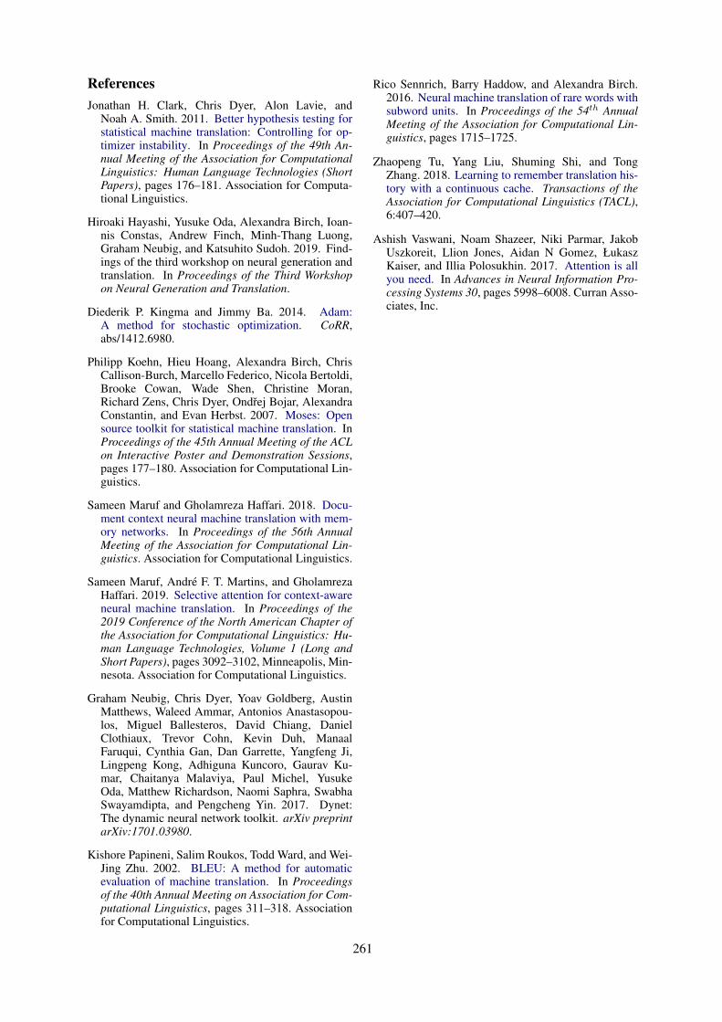
ReferencesJonathan H. Clark, Chris Dyer, Alon Lavie, and
Noah A. Smith. 2011. Better hypothesis testing forstatistical machine translation: Controlling for op-timizer instability. In Proceedings of the 49th An-nual Meeting of the Association for ComputationalLinguistics: Human Language Technologies (ShortPapers), pages 176–181. Association for Computa-tional Linguistics.
Hiroaki Hayashi, Yusuke Oda, Alexandra Birch, Ioan-nis Constas, Andrew Finch, Minh-Thang Luong,Graham Neubig, and Katsuhito Sudoh. 2019. Find-ings of the third workshop on neural generation andtranslation. In Proceedings of the Third Workshopon Neural Generation and Translation.
Diederik P. Kingma and Jimmy Ba. 2014. Adam:A method for stochastic optimization. CoRR,abs/1412.6980.
Philipp Koehn, Hieu Hoang, Alexandra Birch, ChrisCallison-Burch, Marcello Federico, Nicola Bertoldi,Brooke Cowan, Wade Shen, Christine Moran,Richard Zens, Chris Dyer, Ondrej Bojar, AlexandraConstantin, and Evan Herbst. 2007. Moses: Opensource toolkit for statistical machine translation. InProceedings of the 45th Annual Meeting of the ACLon Interactive Poster and Demonstration Sessions,pages 177–180. Association for Computational Lin-guistics.
Sameen Maruf and Gholamreza Haffari. 2018. Docu-ment context neural machine translation with mem-ory networks. In Proceedings of the 56th AnnualMeeting of the Association for Computational Lin-guistics. Association for Computational Linguistics.
Sameen Maruf, Andre F. T. Martins, and GholamrezaHaffari. 2019. Selective attention for context-awareneural machine translation. In Proceedings of the2019 Conference of the North American Chapter ofthe Association for Computational Linguistics: Hu-man Language Technologies, Volume 1 (Long andShort Papers), pages 3092–3102, Minneapolis, Min-nesota. Association for Computational Linguistics.
Graham Neubig, Chris Dyer, Yoav Goldberg, AustinMatthews, Waleed Ammar, Antonios Anastasopou-los, Miguel Ballesteros, David Chiang, DanielClothiaux, Trevor Cohn, Kevin Duh, ManaalFaruqui, Cynthia Gan, Dan Garrette, Yangfeng Ji,Lingpeng Kong, Adhiguna Kuncoro, Gaurav Ku-mar, Chaitanya Malaviya, Paul Michel, YusukeOda, Matthew Richardson, Naomi Saphra, SwabhaSwayamdipta, and Pengcheng Yin. 2017. Dynet:The dynamic neural network toolkit. arXiv preprintarXiv:1701.03980.
Kishore Papineni, Salim Roukos, Todd Ward, and Wei-Jing Zhu. 2002. BLEU: A method for automaticevaluation of machine translation. In Proceedingsof the 40th Annual Meeting on Association for Com-putational Linguistics, pages 311–318. Associationfor Computational Linguistics.
Rico Sennrich, Barry Haddow, and Alexandra Birch.2016. Neural machine translation of rare words withsubword units. In Proceedings of the 54th AnnualMeeting of the Association for Computational Lin-guistics, pages 1715–1725.
Zhaopeng Tu, Yang Liu, Shuming Shi, and TongZhang. 2018. Learning to remember translation his-tory with a continuous cache. Transactions of theAssociation for Computational Linguistics (TACL),6:407–420.
Ashish Vaswani, Noam Shazeer, Niki Parmar, JakobUszkoreit, Llion Jones, Aidan N Gomez, ŁukaszKaiser, and Illia Polosukhin. 2017. Attention is allyou need. In Advances in Neural Information Pro-cessing Systems 30, pages 5998–6008. Curran Asso-ciates, Inc.
261

Proceedings of the 3rd Workshop on Neural Generation and Translation (WNGT 2019), pages 262–267Hong Kong, China, November 4, 2019. c©2019 Association for Computational Linguistics
www.aclweb.org/anthology/D19-56%2d
SYSTRAN @ WNGT 2019: DGT Task
Li Gong, Josep Crego, Jean SenellartSYSTRAN / 5 rue Feydeau, 75002 Paris, France
AbstractThis paper describes SYSTRAN participationto the Document-level Generation and Trans-lation (DGT) Shared Task of the 3rd Workshopon Neural Generation and Translation (WNGT2019). We participate for the first time usinga Transformer network enhanced with modi-fied input embeddings and optimising an addi-tional objective function that considers contentselection. The network takes in structured dataof basketball games and outputs a summary ofthe game in natural language.
1 Introduction
Data-to-text generation is an important task innatural language generation (NLG). It refers tothe task of automatically producing a descriptivetext from non-linguistic structured data (tables,database records, spreadsheets, etc.). Table 1 illus-trates an example of data-to-text NLG, with statis-tics of a NBA basketball game (top) and the corre-sponding game summary (bottom).
Different from other NLG tasks (e.g., machinetranslation), data-to-text generation faces severaladditional challenges: First, data-to-text genera-tion models have to select the content before gen-erating text. In machine translation, the sourceand target sentences are semantically equivalent toeach other, whereas in data-to-text generation, themodel initially selects appropriate content fromthe input data to secondly generate fluent sen-tences that incorporate the selected content; Sec-ond, the training data in data-to-text generationtask is often very limited. Unlike machine trans-lation, where training data consist of translatedsentence pairs, data-to-text generation models aretrained from examples composed of structureddata and its corresponding descriptive summary,which are much harder to produce.
In this paper, we tackle both challenges previ-ously discussed. We introduce a new data-to-text
generation model which jointly learns content se-lection and text generation. In addition, we presenttwo data augmentation methods that further boostperformance of the NLG system.
2 Data Resources
We use the official data set made available for theWNGT 2019 DGT task (Hayashi et al., 2019). Itconsists of the the ROTOWIRE dataset (Wisemanet al., 2017), a dataset of NBA basketball gamesummaries, paired with their corresponding box-and line-score tables. Table 1 illustrates an ex-ample of the dataset. In the box-score table, eachteam has at most 13 players and each player is de-scribed by 23 types of values. In the line-score ta-ble, each team has 15 different types of values. Asfor the associate summaries, the average length is337 tokens, and the vocabulary size is 11.3K. TheROTOWIRE dataset contains 4, 853 summaries intotal, in which 3, 398 summaries are for training,727 for validation and 728 for test. In addition,the next monolingual resources were consideredusable in all tracks:
• Any monolingual data allowable by theWMT 2019 English-German news task,
• Pre-trained word/subword/character embed-dings (e.g., GloVe, fastText),
• Pre-trained contextualized embeddings (e.g.,ELMo, BERT),
• Pre-trained language models (e.g., GPT-2).
3 Data-to-Text Transformer Model
In this section, we present how we adapt the Trans-former model for the data-to-text generation tasks.First, the input embedding of Transformer encoderis replaced by our record embedding to better in-corporate the record information. Second, a new
262

TEAM-NAME WIN LOSS PTS AST ...Cavaliers 51 28 90 25 ...Celtics 37 42 99 30 ...
NAME POS PTS FGM FGA CITY ...LeBron James F 14 5 14 Cleveland ...Kevin Love F 19 6 12 Cleveland ...Kyrie Irving N/A N/A N/A N/A Cleveland ...Brandon Bass F 12 6 8 Boston ...Avery Bradley G 15 7 12 Boston ...Marcus Smart G 19 7 10 Boston ...... ... ... ... ... ... ...
POS: position, PTS: points, FGM: Player field goalsmade; FGA: Player field goals attempted; AST: assists;CITY: player team city.
The Boston Celtics (37-42) defeated the Cleveland Cavaliers (51-28) 99-90on Friday in Cleveland. With the Cavaliers solidified as the No.2 seed forthe Eastern Conference playoffs , they did not try particularly hard to win thisgame, starting with sitting Kyrie Irving (hip) to make sure he stays healthy.Regardless, the Celtics took advantage, picking up a huge victory as they fightto stay in the playoffs. Marcus Smart led the way scoring for Boston, posting19 points on 7-of-10 shooting in 34 minutes. Avery Bradley was close behind,scoring 15 points (7-12 FG) in 31 minutes. The Celtics starting frontcourt ofTyler Zeller and Brandon Bass combined to score 25 points and grab 11rebounds. Boston’s final starter, Evan Turner, struggled shooting the ball andonly scored four points, but still managed to dish out 13 assists and grab sixrebounds. Isaiah Thomas, as he has done so well since joining the Celtics,provided solid production off the bench, scoring 17 points (4-12 FG, 2-6 3Pt)in 23 minutes. ...
Table 1: Example of data-records (left) and document summary (right) from the ROTOWIRE dataset. Entities andvalues corresponding to data-records are boldfaced.
learning objective is added into our model to im-prove its content-oriented performance.
3.1 Record EmbeddingThe input of data-to-text model encoder is a se-quence of records. Each record is a tuple of fourfeatures (Entity, Type, Value, Info). Inspired byprevious work (Yang et al., 2016; Wiseman et al.,2017; Puduppully et al., 2019), we embed featuresinto vectors, and use the concatenation of featureembeddings as the embedding of record.
ri = [ri,1; ri,2; ri,3; ri,4] (1)
where ri ∈ Rdim is the ith record embedding inthe input sequence and ri,j ∈ R
dim4 is the jth fea-
ture embedding in ri.Since there is no order relationship within the
records, the positional embedding of the Trans-former encoder is removed.
3.2 Content Selection ModelingBesides record embedding, we also add a newlearning objective into the Transformer model.
As presented before, we need to select the con-tent from the input records before generating theoutput summary. Some records are generally im-portant no mater the game context, such as theteam name record and team score record, whereasthe importance of some other records depend onthe game context. For example, a player havingthe highest points in the game is more likely tobe mentioned in the game summary. Within theTransformer architecture, the self-attention mech-anism can generate the latent representation foreach record by jointly conditioning on all otherrecords in the input dataset. A binary prediction
layer is added on top of the Transformer encoderoutput (as shown in Figure 1) to predict whetheror not one record will be mentioned in the targetsummary.
The architecture of our data-to-text Transformermodel is shown in Figure 1. As presented be-fore, the encoder takes the record embedding asinput and generates the latent representation foreach record in the input sequence. The output ofencoder is then used to predict the importance ofeach record and also serves as the context of thedecoder. The decoder of our model is the same asthe original Transformer model in machine trans-lation. It predicts the next word conditioned onthe encoder output and the previous tokens in thesummary sequence.
In content selection modeling, the input recordsequences together with its label sequences areused to optimize the encoder by minimizing thecross-entorpy loss. In language generation train-ing, the encoder and decoder are trained togetherto maximize the log-likelihood of the trainingdata. The two learning objectives are trained al-ternatively.
4 Data Augmentation Methods
In data-to-text generation task, the model needs tonot only generate fluent text, but also generate textwhich is coherent with the input records. Severalcontent-oriented evaluation metrics are proposedin (Wiseman et al., 2017) to evaluate such cohe-sion, including the precision of record generationand the recall rate with respect to the records ingold summary.
In this section, we present two data augmenta-tion methods: synthetic data generation and train-
263

TransformerEncoder
rJ<latexit sha1_base64="JBdZO07IximDjYGIGbzvj4OxBGM=">AAAB6nicbVBNS8NAEJ34WetX1aOXxSJ4KkkV9Fj0Ip4q2g9oQ9lsJ+3SzSbsboQS+hO8eFDEq7/Im//GbZuDtj4YeLw3w8y8IBFcG9f9dlZW19Y3Ngtbxe2d3b390sFhU8epYthgsYhVO6AaBZfYMNwIbCcKaRQIbAWjm6nfekKleSwfzThBP6IDyUPOqLHSg+rd9Uplt+LOQJaJl5My5Kj3Sl/dfszSCKVhgmrd8dzE+BlVhjOBk2I31ZhQNqID7FgqaYTaz2anTsipVfokjJUtachM/T2R0UjrcRTYzoiaoV70puJ/Xic14ZWfcZmkBiWbLwpTQUxMpn+TPlfIjBhbQpni9lbChlRRZmw6RRuCt/jyMmlWK955pXp/Ua5d53EU4BhO4Aw8uIQa3EIdGsBgAM/wCm+OcF6cd+dj3rri5DNH8AfO5w8pvo23</latexit>
r1<latexit sha1_base64="w+fMBncFYKx0kEKsDtLgWG6j6to=">AAAB6nicbVBNS8NAEJ3Ur1q/qh69LBbBU0mqoMeiF48V7Qe0oWy2k3bpZhN2N0IJ/QlePCji1V/kzX/jts1BWx8MPN6bYWZekAiujet+O4W19Y3NreJ2aWd3b/+gfHjU0nGqGDZZLGLVCahGwSU2DTcCO4lCGgUC28H4dua3n1BpHstHM0nQj+hQ8pAzaqz0oPpev1xxq+4cZJV4OalAjka//NUbxCyNUBomqNZdz02Mn1FlOBM4LfVSjQllYzrErqWSRqj9bH7qlJxZZUDCWNmShszV3xMZjbSeRIHtjKgZ6WVvJv7ndVMTXvsZl0lqULLFojAVxMRk9jcZcIXMiIkllClubyVsRBVlxqZTsiF4yy+vklat6l1Ua/eXlfpNHkcRTuAUzsGDK6jDHTSgCQyG8Ayv8OYI58V5dz4WrQUnnzmGP3A+fwAD2o2e</latexit>
r2<latexit sha1_base64="qRYq8+LBOBKrAYqfcugvOTPcEds=">AAAB6nicbVBNS8NAEJ3Ur1q/qh69LBbBU0mqoMeiF48V7Qe0oWy2k3bpZhN2N0IJ/QlePCji1V/kzX/jts1BWx8MPN6bYWZekAiujet+O4W19Y3NreJ2aWd3b/+gfHjU0nGqGDZZLGLVCahGwSU2DTcCO4lCGgUC28H4dua3n1BpHstHM0nQj+hQ8pAzaqz0oPq1frniVt05yCrxclKBHI1++as3iFkaoTRMUK27npsYP6PKcCZwWuqlGhPKxnSIXUsljVD72fzUKTmzyoCEsbIlDZmrvycyGmk9iQLbGVEz0sveTPzP66YmvPYzLpPUoGSLRWEqiInJ7G8y4AqZERNLKFPc3krYiCrKjE2nZEPwll9eJa1a1buo1u4vK/WbPI4inMApnIMHV1CHO2hAExgM4Rle4c0Rzovz7nwsWgtOPnMMf+B8/gAFXo2f</latexit>
. . .<latexit sha1_base64="D8NZwhGRc3SadH+lq9NyH2X2S6M=">AAAB7HicbVBNS8NAFHzxs9avqkcvi0XwVJIq6LHoxWMF0xbaUDbbTbt0swm7L0IJ/Q1ePCji1R/kzX/jts1BWwcWhpk37HsTplIYdN1vZ219Y3Nru7RT3t3bPzisHB23TJJpxn2WyER3Qmq4FIr7KFDyTqo5jUPJ2+H4bua3n7g2IlGPOEl5ENOhEpFgFK3k9wYJmn6l6tbcOcgq8QpShQLNfuXL5lgWc4VMUmO6nptikFONgkk+Lfcyw1PKxnTIu5YqGnMT5PNlp+TcKgMSJdo+hWSu/k7kNDZmEod2MqY4MsveTPzP62YY3QS5UGmGXLHFR1EmCSZkdjkZCM0ZyokllGlhdyVsRDVlaPsp2xK85ZNXSate8y5r9YerauO2qKMEp3AGF+DBNTTgHprgAwMBz/AKb45yXpx352MxuuYUmRP4A+fzB/K2jsY=</latexit>
Pred_layer
0/1<latexit sha1_base64="TLXKA4mwwbXo2dx+G5FnabsZdt0=">AAAB6nicbVBNS8NAEJ34WetX1aOXxSJ4qkkV9Fj04rGi/YA2lM120y7dbMLuRCihP8GLB0W8+ou8+W/ctjlo64OBx3szzMwLEikMuu63s7K6tr6xWdgqbu/s7u2XDg6bJk414w0Wy1i3A2q4FIo3UKDk7URzGgWSt4LR7dRvPXFtRKwecZxwP6IDJULBKFrpwT33eqWyW3FnIMvEy0kZctR7pa9uP2ZpxBUySY3peG6CfkY1Cib5pNhNDU8oG9EB71iqaMSNn81OnZBTq/RJGGtbCslM/T2R0ciYcRTYzoji0Cx6U/E/r5NieO1nQiUpcsXmi8JUEozJ9G/SF5ozlGNLKNPC3krYkGrK0KZTtCF4iy8vk2a14l1UqveX5dpNHkcBjuEEzsCDK6jBHdShAQwG8Ayv8OZI58V5dz7mrStOPnMEf+B8/gBWT40s</latexit>
0/1<latexit sha1_base64="TLXKA4mwwbXo2dx+G5FnabsZdt0=">AAAB6nicbVBNS8NAEJ34WetX1aOXxSJ4qkkV9Fj04rGi/YA2lM120y7dbMLuRCihP8GLB0W8+ou8+W/ctjlo64OBx3szzMwLEikMuu63s7K6tr6xWdgqbu/s7u2XDg6bJk414w0Wy1i3A2q4FIo3UKDk7URzGgWSt4LR7dRvPXFtRKwecZxwP6IDJULBKFrpwT33eqWyW3FnIMvEy0kZctR7pa9uP2ZpxBUySY3peG6CfkY1Cib5pNhNDU8oG9EB71iqaMSNn81OnZBTq/RJGGtbCslM/T2R0ciYcRTYzoji0Cx6U/E/r5NieO1nQiUpcsXmi8JUEozJ9G/SF5ozlGNLKNPC3krYkGrK0KZTtCF4iy8vk2a14l1UqveX5dpNHkcBjuEEzsCDK6jBHdShAQwG8Ayv8OZI58V5dz7mrStOPnMEf+B8/gBWT40s</latexit>
0/1<latexit sha1_base64="TLXKA4mwwbXo2dx+G5FnabsZdt0=">AAAB6nicbVBNS8NAEJ34WetX1aOXxSJ4qkkV9Fj04rGi/YA2lM120y7dbMLuRCihP8GLB0W8+ou8+W/ctjlo64OBx3szzMwLEikMuu63s7K6tr6xWdgqbu/s7u2XDg6bJk414w0Wy1i3A2q4FIo3UKDk7URzGgWSt4LR7dRvPXFtRKwecZxwP6IDJULBKFrpwT33eqWyW3FnIMvEy0kZctR7pa9uP2ZpxBUySY3peG6CfkY1Cib5pNhNDU8oG9EB71iqaMSNn81OnZBTq/RJGGtbCslM/T2R0ciYcRTYzoji0Cx6U/E/r5NieO1nQiUpcsXmi8JUEozJ9G/SF5ozlGNLKNPC3krYkGrK0KZTtCF4iy8vk2a14l1UqveX5dpNHkcBjuEEzsCDK6jBHdShAQwG8Ayv8OZI58V5dz7mrStOPnMEf+B8/gBWT40s</latexit>
TransformerDecoder
y1<latexit sha1_base64="gXLzr9lA6QyErQrPkt90wKdvXMk=">AAAB6nicbVBNS8NAEJ3Ur1q/qh69LBbBU0mqoMeiF48V7Qe0oWy2m3bpZhN2J0Io/QlePCji1V/kzX/jts1BWx8MPN6bYWZekEhh0HW/ncLa+sbmVnG7tLO7t39QPjxqmTjVjDdZLGPdCajhUijeRIGSdxLNaRRI3g7GtzO//cS1EbF6xCzhfkSHSoSCUbTSQ9b3+uWKW3XnIKvEy0kFcjT65a/eIGZpxBUySY3pem6C/oRqFEzyaamXGp5QNqZD3rVU0YgbfzI/dUrOrDIgYaxtKSRz9ffEhEbGZFFgOyOKI7PszcT/vG6K4bU/ESpJkSu2WBSmkmBMZn+TgdCcocwsoUwLeythI6opQ5tOyYbgLb+8Slq1qndRrd1fVuo3eRxFOIFTOAcPrqAOd9CAJjAYwjO8wpsjnRfn3flYtBacfOYY/sD5/AEOhI2l</latexit>
yT<latexit sha1_base64="JJSaiNpL04FogISMGU77Y0OBc24=">AAAB6nicbVBNS8NAEJ34WetX1aOXxSJ4KkkV9Fj04rFiv6ANZbOdtEs3m7C7EULpT/DiQRGv/iJv/hu3bQ7a+mDg8d4MM/OCRHBtXPfbWVvf2NzaLuwUd/f2Dw5LR8ctHaeKYZPFIladgGoUXGLTcCOwkyikUSCwHYzvZn77CZXmsWyYLEE/okPJQ86osdJj1m/0S2W34s5BVomXkzLkqPdLX71BzNIIpWGCat313MT4E6oMZwKnxV6qMaFsTIfYtVTSCLU/mZ86JedWGZAwVrakIXP198SERlpnUWA7I2pGetmbif953dSEN/6EyyQ1KNliUZgKYmIy+5sMuEJmRGYJZYrbWwkbUUWZsekUbQje8surpFWteJeV6sNVuXabx1GAUziDC/DgGmpwD3VoAoMhPMMrvDnCeXHenY9F65qTz5zAHzifP0OQjcg=</latexit>
. . .<latexit sha1_base64="D8NZwhGRc3SadH+lq9NyH2X2S6M=">AAAB7HicbVBNS8NAFHzxs9avqkcvi0XwVJIq6LHoxWMF0xbaUDbbTbt0swm7L0IJ/Q1ePCji1R/kzX/jts1BWwcWhpk37HsTplIYdN1vZ219Y3Nru7RT3t3bPzisHB23TJJpxn2WyER3Qmq4FIr7KFDyTqo5jUPJ2+H4bua3n7g2IlGPOEl5ENOhEpFgFK3k9wYJmn6l6tbcOcgq8QpShQLNfuXL5lgWc4VMUmO6nptikFONgkk+Lfcyw1PKxnTIu5YqGnMT5PNlp+TcKgMSJdo+hWSu/k7kNDZmEod2MqY4MsveTPzP62YY3QS5UGmGXLHFR1EmCSZkdjkZCM0ZyokllGlhdyVsRDVlaPsp2xK85ZNXSate8y5r9YerauO2qKMEp3AGF+DBNTTgHprgAwMBz/AKb45yXpx352MxuuYUmRP4A+fzB/K2jsY=</latexit>
Softmax
. . .<latexit sha1_base64="D8NZwhGRc3SadH+lq9NyH2X2S6M=">AAAB7HicbVBNS8NAFHzxs9avqkcvi0XwVJIq6LHoxWMF0xbaUDbbTbt0swm7L0IJ/Q1ePCji1R/kzX/jts1BWwcWhpk37HsTplIYdN1vZ219Y3Nru7RT3t3bPzisHB23TJJpxn2WyER3Qmq4FIr7KFDyTqo5jUPJ2+H4bua3n7g2IlGPOEl5ENOhEpFgFK3k9wYJmn6l6tbcOcgq8QpShQLNfuXL5lgWc4VMUmO6nptikFONgkk+Lfcyw1PKxnTIu5YqGnMT5PNlp+TcKgMSJdo+hWSu/k7kNDZmEod2MqY4MsveTPzP62YY3QS5UGmGXLHFR1EmCSZkdjkZCM0ZyokllGlhdyVsRDVlaPsp2xK85ZNXSate8y5r9YerauO2qKMEp3AGF+DBNTTgHprgAwMBz/AKb45yXpx352MxuuYUmRP4A+fzB/K2jsY=</latexit>y1
<latexit sha1_base64="gXLzr9lA6QyErQrPkt90wKdvXMk=">AAAB6nicbVBNS8NAEJ3Ur1q/qh69LBbBU0mqoMeiF48V7Qe0oWy2m3bpZhN2J0Io/QlePCji1V/kzX/jts1BWx8MPN6bYWZekEhh0HW/ncLa+sbmVnG7tLO7t39QPjxqmTjVjDdZLGPdCajhUijeRIGSdxLNaRRI3g7GtzO//cS1EbF6xCzhfkSHSoSCUbTSQ9b3+uWKW3XnIKvEy0kFcjT65a/eIGZpxBUySY3pem6C/oRqFEzyaamXGp5QNqZD3rVU0YgbfzI/dUrOrDIgYaxtKSRz9ffEhEbGZFFgOyOKI7PszcT/vG6K4bU/ESpJkSu2WBSmkmBMZn+TgdCcocwsoUwLeythI6opQ5tOyYbgLb+8Slq1qndRrd1fVuo3eRxFOIFTOAcPrqAOd9CAJjAYwjO8wpsjnRfn3flYtBacfOYY/sD5/AEOhI2l</latexit>
y2<latexit sha1_base64="UmY8miGJFsYtImgQ4UOSFc3rPPg=">AAAB6nicbVBNS8NAEJ3Ur1q/qh69LBbBU0mqoMeiF48V7Qe0oWy2m3bpZhN2J0Io/QlePCji1V/kzX/jts1BWx8MPN6bYWZekEhh0HW/ncLa+sbmVnG7tLO7t39QPjxqmTjVjDdZLGPdCajhUijeRIGSdxLNaRRI3g7GtzO//cS1EbF6xCzhfkSHSoSCUbTSQ9av9csVt+rOQVaJl5MK5Gj0y1+9QczSiCtkkhrT9dwE/QnVKJjk01IvNTyhbEyHvGupohE3/mR+6pScWWVAwljbUkjm6u+JCY2MyaLAdkYUR2bZm4n/ed0Uw2t/IlSSIldssShMJcGYzP4mA6E5Q5lZQpkW9lbCRlRThjadkg3BW355lbRqVe+iWru/rNRv8jiKcAKncA4eXEEd7qABTWAwhGd4hTdHOi/Ou/OxaC04+cwx/IHz+QMQCI2m</latexit>
<eos><latexit sha1_base64="xDzQvAFdLmBTev1IjeBitAarx+g=">AAAB9XicbVDLSgNBEJyNrxhfUY9eBoPgKexGQQ8iQS8eI5gHJGuYnfQmQ2YfzPSqYcl/ePGgiFf/xZt/4yTZgyYWNBRV3XR3ebEUGm3728otLa+sruXXCxubW9s7xd29ho4SxaHOIxmplsc0SBFCHQVKaMUKWOBJaHrD64nffAClRRTe4SgGN2D9UPiCMzTSfQfhCRHTC4j05bhbLNllewq6SJyMlEiGWrf41elFPAkgRC6Z1m3HjtFNmULBJYwLnURDzPiQ9aFtaMgC0G46vXpMj4zSo36kTIVIp+rviZQFWo8Cz3QGDAd63puI/3ntBP1zNxVhnCCEfLbITyTFiE4ioD2hgKMcGcK4EuZWygdMMY4mqIIJwZl/eZE0KmXnpFy5PS1Vr7I48uSAHJJj4pAzUiU3pEbqhBNFnskrebMerRfr3fqYteasbGaf/IH1+QPyi5LM</latexit>
<bos><latexit sha1_base64="8AaeR7MZfhElgpaTf2flakQjM2E=">AAAB9XicbVBNSwMxEM3Wr1q/qh69BIvgqexWQQ8iRS8eK9gPaNeSTbNtaDZZklm1LP0fXjwo4tX/4s1/Y9ruQVsfDDzem2FmXhALbsB1v53c0vLK6lp+vbCxubW9U9zdaxiVaMrqVAmlWwExTHDJ6sBBsFasGYkCwZrB8HriNx+YNlzJOxjFzI9IX/KQUwJWuu8AewKA9CJQ5nLcLZbcsjsFXiReRkooQ61b/Or0FE0iJoEKYkzbc2PwU6KBU8HGhU5iWEzokPRZ21JJImb8dHr1GB9ZpYdDpW1JwFP190RKImNGUWA7IwIDM+9NxP+8dgLhuZ9yGSfAJJ0tChOBQeFJBLjHNaMgRpYQqrm9FdMB0YSCDapgQ/DmX14kjUrZOylXbk9L1assjjw6QIfoGHnoDFXRDaqhOqJIo2f0it6cR+fFeXc+Zq05J5vZR3/gfP4A7fOSyQ==</latexit>
Figure 1: Model Architecture
ing data selection. Each of them has different im-pacts on the content-oriented evaluation results.
4.1 Synthetic Data Generation
In order to improve the cohesion between the in-put records and output summary, we need moredata to enhance the encoder-decoder attention ofthe decoder. Here we introduce a method to gen-erate synthetic training data.
We first randomly change the values of recordsand the changed record set (s′) is then used to gen-erate automatic summary (t′) by a trained data-to-text system. The synthetic data pairs (s′, t′) arethen used to improve such system.
In order to keep the data cohesion in the table,the change is constrained with the following rules:
• only numeric values are changed. Non-numeric values such as the position of aplayer or the city name of a team are kept thesame.
• after the change, the team scores should notviolate the win/loss relation
• the changed values should stay in the normalrange of its value type. It should not biggerthan its maximum value or smaller than itsminimum value through all games.
Our data generation technique doubles the amountof training data available for learning.
4.2 Training Data Selection
A deficiency of data-to-text NLG systems is thepoor coverage of relations produced in the gener-ated summaries. In order to increase the coverage,a simple solution consists of learning to producea larger number of relations. Here, we present a
Figure 2: relation count distribution in training data.
straightforward method to bias our model to out-put more relations by means of fine-tuning on thetraining examples containing a greater number ofrelations.
We use an information extraction (IE) systemto extract the number of relations of each train-ing summary. Then, we select for fine-tuning ourbaseline model the subset of training data in whicheach summary contains at least N relations. Inthis work, we take advantage of the IE system1
provided by (Puduppully et al., 2019), and the dis-tribution of the number of relations in the trainingsummary is illustrated in Figure 2.
5 Experimental Setup
5.1 Data and Preprocessing
We run the experiments with the ROTOWIRE
dataset (Wiseman et al., 2017), a dataset of NBAbasketball game summaries, paired with their cor-responding box- and line-score tables. Table 1 il-lustrates an example of the dataset. In the box-score table, each team has at most 13 players andeach player is described by 23 types of values.In the line-score table, each team has 15 differ-ent types of values. In addition, the date of eachgame is converted into the day of the week (suchas “Saturday”) as an additional record. In the pre-processing step, the input box- and line-score ta-bles are converted into a fix-length sequence ofrecords. Each sequence contains 629 records.2 Asfor the associate summaries, the average length is337 tokens, and the vocabulary size is 11.3K. The
1The model is publicly available at https://github.com/ratishsp/data2text-plan-py
2In the 629 records, 598 records are for players, 30records for teams and 1 record for the date.
264

ROTOWIRE dataset contains 4853 summaries intotal, in which 3398 summaries are for training,727 for validation and 728 for test.
In content selection modelling, we need the la-bels of input records to indicate which records inthe input will be mentioned in the output sum-mary. Here we use a very simple method to gener-ate such labels. First, we label the entity records3.An entity record is labeled as 1 if its value is men-tioned in the associated summary, otherwise it islabeled as 0. Second, for each player or team men-tioned in the summary, the rest of its values in thetable are labeled as 1 if they occur in the same sen-tence in the summary.
5.2 Evaluation metrics
The model output is evaluated with BLEU (Pa-pineni et al., 2002) as well as several content-oriented metrics proposed by (Wiseman et al.,2017) including three following aspects:
• Relation Generation (RG) evaluates the num-ber of extracted relations in automatic sum-maries and their correctness (precision) w.r.tthe input record dataset;
• Content Selection (CS) evaluates the preci-sion and recall rate of extracted relations inautomatic summaries w.r.t that in the goldsummaries;
• Content Ordering (CO) evaluates the normal-ized Damerau-Levenshtein Distance (Brilland Moore, 2000) between the sequence ofextracted relations in automatic summariesand that in the gold summaries.
All these content-oriented metrics are based onan IE system which extracts record relations fromsummaries. For the purpose of comparison, wedirectly use the publicly available IE system of(Puduppully et al., 2019) to evaluate our models.
5.3 Training Details
In all experiments, we use our model with 1 en-coder layer and 6 decoder layers, 512 hiddenunits (hence, the record feature embedding sizeis 128, see Section 3), 8 heads, GELU activa-tions (Hendrycks and Gimpel, 2016), a dropoutrate of 0.1 and learned positional embedding for
3Record whose Value feature is an entity (see Section ??),for example: “LeBron James|NAME|LeBron James|H/W”.The labeling is according to the Value feature
ModelRG CS CO
BLEU# P% P% R% DLD%
GOLD 23.32 94.77 100 100 100 100TEMPL 54.29 99.92 26.61 59.16 14.42 8.51WS-2017 23.95 75.10 28.11 35.86 15.33 14.57NCP-2019 33.88 87.51 33.52 51.21 18.57 16.19DATA-TRANS 23.31 79.81 36.90 43.06 22.75 20.60+DATA GEN 22.59 82.49 39.48 42.84 23.32 19.76+DATA SEL 26.94 79.54 35.27 47.49 22.22 19.97+BOTH 24.24 80.52 37.33 44.66 23.04 20.22
Table 2: Automatic evaluation on ROTOWIRE devel-opment set using relation generation (RG) count (#)and precision (P%), content selection (CS) precision(P%) and recall (R%), content ordering (CO) in nor-malized Damerau-Levenshtein distance (DLD%), andBLEU.
the decoder. The model is trained with the Adamoptimizer (Kingma and Ba, 2014), learning rate isfixed to 10−4 and batch size is 6. As for inference,we use beam size 4 for all experiments, and themaximum decoding length is 600.
We implement all our models in Pytorch, andtrain them on 1 GTX 1080 GPU.
6 Results
The results of our model on the developmentset are summarized in Table 2. GOLD repre-sents the evaluation result on the gold summary.The RG precision rate is 94.77%, indicating thatthe IE system for evaluation is not perfect buthas very high precision. After that, results ofthree contrast systems are reported, where TEMPL
and WS-2017 are the updated results4 of Wise-man et al. (2017) models. TEMPL is template-based generator model which generates a sum-mary consisting of 8 sentences: a general de-scription sentence about the teams playing in thegame, 6 player-specific sentences and a conclusionsentence. WS-2017 reports an encoder-decodermodel with conditional copy mechanism. NCP-2019 is the best system configuration (NCP+CC)reported in (Puduppully et al., 2019) which is aneural content planning model enhanced with con-ditional copy mechanism. As for our model, re-sults with four configurations are reported.
DATA-TRANS represents our data-to-textTransformer model (as illustrated in Figure 1)without any data augmentation. Comparing toNCP-2019, our model performs 3.4% higheron content selection precision, 4.2% higher on
4Here we all use the IE system of (Puduppully et al., 2019)which is improved from the original IE system of (Wisemanet al., 2017)
265

content ordering metric and 4.4 points higheron BLEU. Our model performs better on theCO metric, we attribute this improvement to thatour model generates nearly the same number ofrelations as the gold summary which reducesthe edit distance between the two sequences ofrelations. However, our model is 7.7% lower onRG precision. And on the CS recall rate, ourmodel is 8.2% lower than NCP-2019. This isprobably due to the fact that NCP-2019 generatesmuch more records than our model (33.88 vs.23.31) which could result higher coverage on therelations in gold summary.
Comparing to TEMPL and WS-2017, ourmodel is much better on BLEU and CS precision.Our model generates nearly the same number ofrelations as WS-2017, but with 7.2% higher onrecall rate and 7.4% higher on CO metric.
By synthetic data generation (+DATA GEN), wegenerate synthetic table records as described in se-cion 4.1. These synthetic table records are thenused as input to the DATA-TRANS model to gener-ate summaries. All training table records are usedto generate synthetic data. The synthetic data isthen combined with the original training data tofine-tune the DATA-TRANS model. From Table 2,we can see that the RG and CS precisions are bothimproved by 2.7% and 2.6% respectively. There isno significant change on others metrics. The COmetric is slightly improved due to higher RG andCS precisions. The CS recall rate is slightly de-graded with the number of extracted relations.
By training data selection (+DATA SEL), we se-lect the data whose summary contains the num-ber of relations N >= 16 as the new trainingdata. The result training data size is 2242 (originalsize: 3398). It is then used to fine-tune the DATA-TRANS model. As shown in Table 2, as expected,the model after fine-tuning generates more rela-tions in the output summaries. The average num-ber of relations in the output summaries increasesfrom 23.31 to 26.94. Respectively, the CS recall isincreased from 43.06% to 47.49%. However, theCS precision is slightly degraded by 1.6%.
Finally, we combine both of the data augmen-tation methods (+BOTH). Synthetic data genera-tion improves the RG and CS precisions. Train-ing data selection improves the CS recall rate bymaking the model generate more relations. Tocombine the two methods, we choose to fine-tunethe +DATA GEN model with the selected train-
ModelRG CS CO
BLEU# P% P% R% DLD%
TEMPL 54.23 99.94 26.99 58.16 14.92 8.46WS-2017 23.72 74.80 29.49 36.18 15.42 14.19NCP-2019 34.28 87.47 34.18 51.22 18.58 16.50DATA-TRANS 24.12 79.17 36.48 42.74 22.40 20.16+DATA GEN 24.01 83.89 38.98 42.85 23.02 19.48+DATA SEL 27.47 80.70 35.33 46.25 21.87 20.03+BOTH 24.80 81.08 37.10 43.78 22.51 20.14
Table 3: Automatic evaluation on ROTOWIRE test set.
ing data of +DATA SEL (so this configuration isactually +DATA GEN+DATA SEL). As shown inTable 2, all content-oriented evaluation metricsare improved compared to DATA-TRANS but notas much as each single of the data augmentationmethod. This configuration is like a trade-off be-tween the two data augmentation configurations.
Results on the test set are reported in Table 3.They follow the same pattern as those found onthe development set. Our DATA-TRANS modeloutperforms all other contrast systems on BLEU,CS precision and content ordering metrics. Thesynthetic data generation method helps to improvethe RG and CS precisions. The training data se-lection method improves the CS recall by mak-ing the model generate more relations. Combiningthese two data augmentation methods, all content-oriented evaluation results are improved comparedto DATA-TRANS. However, there is no significantchange on BLEU.
7 Conclusions
We present an enhanced Transformer-based data-to-text generation model for the WNGT2019 En-glish NLG task. Experimental results have shownthat our enhanced transformer model outperformscurrent state-of-the-art system on BLEU, contentselection precision and content ordering metics.In addition, we proposed two data augmentationmethods, each of them improves different content-oriented evaluation metrics.
ReferencesEric Brill and Robert C Moore. 2000. An improved er-
ror model for noisy channel spelling correction. InProceedings of the 38th Annual Meeting on Associa-tion for Computational Linguistics, pages 286–293.Association for Computational Linguistics.
Hiroaki Hayashi, Yusuke Oda, Alexandra Birch, Ioan-nis Constas, Andrew Finch, Minh-Thang Luong,Graham Neubig, and Katsuhito Sudoh. 2019. Find-ings of the third workshop on neural generation and
266

translation. In Proceedings of the Third Workshopon Neural Generation and Translation.
Dan Hendrycks and Kevin Gimpel. 2016. Bridgingnonlinearities and stochastic regularizers with gaus-sian error linear units.
Diederik P Kingma and Jimmy Ba. 2014. Adam: Amethod for stochastic optimization. arXiv preprintarXiv:1412.6980.
Kishore Papineni, Salim Roukos, Todd Ward, and Wei-Jing Zhu. 2002. Bleu: a method for automatic eval-uation of machine translation. In Proceedings ofthe 40th annual meeting on association for compu-tational linguistics, pages 311–318. Association forComputational Linguistics.
Ratish Puduppully, Li Dong, and Mirella Lapata. 2019.Data-to-text generation with content selection andplanning. In Proceedings of the AAAI Conferenceon Artificial Intelligence, volume 33, pages 6908–6915.
Sam Wiseman, Stuart M Shieber, and Alexander MRush. 2017. Challenges in data-to-document gen-eration. arXiv preprint arXiv:1707.08052.
Zichao Yang, Phil Blunsom, Chris Dyer, and WangLing. 2016. Reference-aware language models.arXiv preprint arXiv:1611.01628.
267

Proceedings of the 3rd Workshop on Neural Generation and Translation (WNGT 2019), pages 268–272Hong Kong, China, November 4, 2019. c©2019 Association for Computational Linguistics
www.aclweb.org/anthology/D19-56%2d
University of Edinburgh’s Submission to the Document-level Generationand Translation Shared Task
Ratish Puduppully ∗ and Jonathan Mallinson ∗ and Mirella LapataInstitute for Language, Cognition and Computation
School of Informatics, University of Edinburgh10 Crichton Street, Edinburgh EH8 9AB
[email protected] [email protected] [email protected]
Abstract
The University of Edinburgh participatedin all six tracks: NLG, MT, and MT+NLGwith both English and German as tar-geted languages. For the NLG track,we submitted a multilingual system basedon the Content Selection and Planningmodel of Puduppully et al. (2019). Forthe MT track, we submitted Transformer-based Neural Machine Translation mod-els, where out-of-domain parallel data wasaugmented with in-domain data extractedfrom monolingual corpora. Our MT+NLGsystems disregard the structured input dataand instead rely exclusively on the sourcesummaries.
1 Track 1/2: Natural LanguageGeneration
The Natural Language Generation (NLG) track re-volved around systems that take structured data inthe form of tabular data from a basketball gameas input, and generate a summary of this game inthe target language. We entered one multilingualsystem which outputs summaries in both Englishand German. A multilingual model allows us toovercome the limited amount of German trainingdata.
We adopted the content selection and planningapproach of Puduppully et al. (2019), made ex-tensions to the model and parameterized the de-coder with a language tag, indicating the targetlanguage. The training was done using the fullROTOWIRE English dataset and the ROTOWIRE
English-German dataset. We first explain the ap-proach of Puduppully et al. (2019), describe the
∗Ratish worked on Tracks 1/2 and Jonathan on Tracks3/4/5/6.
extensions to their model and show how languagetags can be added to the decoder to indicate thetarget language.
1.1 The Content Selection and PlanningApproach of Puduppully et al. (2019)
Puduppully et al. (2019) model p(y|r) as thejoint probability of text y and content plan z,given input r. They further decompose p(y, z|r)into p(z|r), a content selection and planningphase, and p(y|r, z), a text generation phase:
p(y|r) =∑
z
p(y, z|r) =∑
z
p(z|r)p(y|r, z)
Given input records, probability p(z|r) is modeledusing Pointer Networks (Vinyals et al., 2015). Theprobability of output text y conditioned on previ-ously generated content plan z and input table r ismodeled as follows:
p(y|r, z) =|y|∏
t=1
p(yt|y<t, z, r)
where y<t = y1 . . . yt−1. They use an encoder-decoder architecture with an attention mechanismto compute p(y|r, z). The architecture is shown inFigure 1.
The content plan z is encoded into {ek}|z|k=1
using a bidirectional LSTM. Because the con-tent plan is a sequence of input records, theydirectly feed the corresponding content selectedrecord vectors {rcsj }
|r|j=1 as input to the LSTM
units, which share the record encoder with the firststage. For details of the content selection stage,please refer Puduppully et al. (2019).
The text decoder is also based on a recurrentneural network with LSTM units. The decoder isinitialized with the hidden states of the final stepin the encoder. At decoding step t, the input ofthe LSTM unit is the embedding of the previously
268

𝑟1 𝑟2 𝑟3 𝑟4 … 𝑟|𝑟| 𝐸𝑂𝑆
𝒉3 𝒅4𝒉4𝒉1 𝒉2
𝒓𝒔 𝒓𝟑𝒄𝒔 𝒓|𝒓|
𝒄𝒔 𝒓𝟏𝒄𝒔
𝒓𝟑𝒄𝒔 𝒓|𝒓|
𝒄𝒔 𝒓𝟏𝒄𝒔
𝒆1 𝒆2 𝒆3
𝒅2 𝒅4𝒅1𝒅4 𝒅3
𝑦3 𝑦2 𝑦1 𝑆𝑂𝑆
𝑦3 𝑦2 𝑦1
Plan
Attention
𝒓𝟏𝒄𝒔 𝒓𝟐
𝒄𝒔 𝒓𝟑𝒄𝒔 𝒓𝟒
𝒄𝒔 … 𝒓|𝒓|𝒄𝒔
𝒓𝒆
𝒅𝟒𝒂𝒕𝒕
𝑝𝑔𝑒𝑛(𝑦4|𝑟, 𝑧, 𝑦<4)
𝑝𝑐𝑜𝑝𝑦(𝑦4|𝑟, 𝑧, 𝑦<4)Text
Generation
Content Plan
Encoding
Content
Selection &
Planning
Encoder Decoder Vector Content Selection Gate
𝑝(𝑧|𝑟)
𝑝(𝑦|𝑟, 𝑧)
Figure 1: Generation model with content selection and planning. The text is generated conditioned onthe input content plan. At any time step, output token is generated from vocabulary or copied from thecontent plan.
predicted word yt−1. Let dt be the hidden state ofthe t-th LSTM unit. The probability of predictingyt from the output vocabulary is computed via:
βt,k ∝ exp(dᵀtWbek) (1)
qt =∑
k
βt,kek
dattt = tanh(Wd[dt;qt])
pgen(yt|y<t, z, r)=softmaxyt(Wydattt + by) (2)
where∑
k βt,k = 1, Wb ∈ Rn×n,Wd ∈Rn×2n,Wy ∈ Rn×|Vy |,by ∈ R|Vy | are parame-ters, and |Vy| is the output vocabulary size.
They further augment the decoder with a copymechanism, allowing the ability to copy words di-rectly from the value portions of records in thecontent plan (i.e., {zk}|z|k=1). They experimentedwith joint (Gu et al., 2016) and conditional copymethods (Gulcehre et al., 2016). Specifically, theyintroduce a variable ut ∈ {0, 1} for each time stepto indicate whether the predicted token yt is copied(ut = 1) or not (ut = 0). The probability of gen-erating yt is computed by:
p(yt|y<t, z, r) =∑
ut∈{0,1}p(yt, ut|y<t, z, r)
where ut is marginalized out.
1.2 Copying from Table and PlanWe extended the copy mechanism further such thatut can take three values: yt is generated from the
vocabulary (ut = 0), yt is copied from the contentplan (ut = 1) and yt is copied from the table (ut =2).
Conditional Copy The variable ut is first com-puted as a switch gate, and then is used to obtainthe output probability:
p(ut|y<t, z, r) = softmax(wu · dattt + bu)
αt,j ∝ exp(dtᵀWcr
csj ) (3)
p(yt, ut|y<t, z, r) =
p(ut|y<t, z, r)∑
yt←zk βt,k ut = 1
p(ut|y<t, z, r)∑
k βt,k∑
yt←rj,j∈γk
αt,j ut = 2
p(ut|y<t, z, r)pgen(yt|y<t, z, r) ut = 0
where∑
j∈γk αt,j = 1. yt ← zk indicatesthat yt can be copied from zk, yt ← rj indi-cates that yt can be copied from rj . γk indi-cates records in table corresponding to the kthrecord in plan, for example: if k is ‘PTS’ valueof player Jeff Teague, then γk corresponds to allthe records for the entity Jeff Teague in the ta-ble including ‘PTS’, ‘REB’, ‘NAME1’, ‘NAME2’etc. βt,k and pgen(yt|y<t, z, r) are computed as inEquations (1)–(2), and wu ∈ R3×n, bu ∈ R3 areparameters.
269

𝑟1 𝑟2 𝑟3 𝑟4 … 𝑟|𝑟| 𝐸𝑂𝑆
𝒉3 𝒅4𝒉4𝒉1 𝒉2
𝒓𝒔 𝒓𝟑𝒄𝒔 𝒓|𝒓|
𝒄𝒔 𝒓𝟏𝒄𝒔
𝒓𝟑𝒄𝒔 𝒓|𝒓|
𝒄𝒔 𝒓𝟏𝒄𝒔
𝒆1 𝒆2 𝒆3
𝒅2 𝒅4𝒅1𝒅4 𝒅3
𝑦3 𝑦2 𝑦1 𝑆𝑂𝑆
𝑦3 𝑦2 𝑦1
Plan
Attention
Data
Attention
𝒓𝟏𝒄𝒔 𝒓𝟐
𝒄𝒔 𝒓𝟑𝒄𝒔 𝒓𝟒
𝒄𝒔 … 𝒓|𝒓|𝒄𝒔
𝒓𝒆
𝒅𝟒𝒂𝒕𝒕
𝑝𝑔𝑒𝑛(𝑦4|𝑟, 𝑧, 𝑦<4)
𝑝𝑐𝑜𝑝𝑦(𝑦4|𝑟, 𝑧, 𝑦<4)Text
Generation
Content Plan
Encoding
Content
Selection &
Planning
Encoder Decoder Vector Content Selection Gate
𝑝(𝑧|𝑟)
𝑝(𝑦|𝑟, 𝑧)
Figure 2: Generation model with content selection and planning and attention over table and contentplan. The text is generated conditioned on the content plan and the table. At any time step, output tokenis generated from vocabulary, copied from the content plan or copied from input table.
1.3 Attending to the Table and Content PlanThe output text is generated by attending to boththe content plan and the input table (See Figure 2.)
δt,j ∝ exp(dᵀtWcr
CSj ) (4)
st =∑
j
δt,jrCSj
dattt = tanh(Wd[dt;qt; st])
pgen(yt|y<t, z, r)=softmaxyt(Wydattt + by) (5)
where∑
j δt,j = 1, Wc ∈ Rn×n,Wd ∈Rn×3n,Wy ∈ Rn×|Vy |,by ∈ R|Vy | are parame-ters, and |Vy| is the output vocabulary size.
1.4 Feature for Team Points and Ranking ofPlayer Points
Upon inspection of the ROTOWIRE game sum-maries in the development set, we observed thatthe summaries often describe the statistics of thewinning team followed by the statistics of the los-ing team. The highest ranked players of eitherteam are also often described in sequence in thesummaries. Currently, we rely on the word em-beddings of the team and player points to helpthe model disambiguate the winning from the los-ing team and to learn the relative performances ofthe players. We hypothesize that explicitly provid-ing information about the relative performance ofplayers and teams should make the learning easier.
We thus experimented with a feature for thewinning/losing team and the ranking of player
points within a team. Specifically, we added a bi-nary feature for team records: win for each recordin the winning team, loss for each record in thelosing team. We further rank players in a teamon the basis of their points and we add a featureindicating their rank in the team. For instance,Kyle Lowry scored the highest number of pointsin the home team and we add feature hometeam-0to each of his records. Player Jahlil Okafor wasthe second highest scorer in the visiting team andwe add the feature visteam-1 to each of his recordsand so on.
1.5 Training a Single Multilingual Model
We trained a single model for English and Germandata-to-text with a common BPE (Sennrich et al.,2015b) vocabulary of 2000 symbols for the outputsummaries. Player names and values of recordsin summaries were not BPEd. The target text wasprefixed with token indicating the language of out-put ‘EN’ or ‘DE’. During inference, we forced themodel to generate output in the desired language.
1.6 Dataset
We made use of the full ROTOWIRE Englishdataset of Wiseman et al. (2017) and the Germandataset provided as part of the shared task. Thestatistics of the dataset are given in Table 1.
270

Train Dev TestEnglish 3398 727 728German 242 240 241
Table 1: Count of examples in Training, Devel-opment and Test sections of English and Germandataset.
ModelRG CS CO
BLEUP% P% R% DLD%
EN 91.41 30.91 64.13 21.72 17.01DE 70.23 23.40 41.83 16.08 10.95
Table 2: Automatic evaluation for track 1/2 onthe ROTOWIRE test set using record generation(RG) precision, content selection (CS) precisionand recall, content ordering (CO) in normalizedDamerau-Levenshtein distance, and BLEU.
1.7 Results
Table 2 shows our results for English and Germandatasets on the Test set as provided by the sharedtask organizers.
2 Track 3/4 : Machine Translation
The Machine Translation (MT) track revolves ar-round systems that translate source summaries tothe target language. Our submission takes advan-tage of existing state-of-the-art techniques in ma-chine translation, including (1) transformer net-works (Vaswani et al., 2017). (2) subword units(Sennrich et al., 2015b) and (3) the inclusionof in-domain monolingual data used via back-translation (Sennrich et al., 2015a).
For our submission, we focus on finding in-domain basketball summary data from withingeneral-purpose monolingual datasets. We de-velop several heuristics allowing us to extract mil-lions of in-domain monolingual sentences, whichare then back-translated and included within thetraining data. This additional monolingual dataimproves bleu scores between 5 and 7 points.
2.1 Data
The translation models were trained on both theROTOWIRE English-German and all WMT19 par-allel training data. A summary of the training datacan be found in table 3. For ease of comparisonto the NLG task, tokenization was done using thetokenizer provided by the shared task organizers.BPE was employed with a joint BPE subword vo-cabulary of 50k.
Dataset SizeEuroparl v9 18.39Common Crawl corpus 24.00News Commentary v14 3.38Document-split Rapid corpus 14.01Wikititles 13.05ParaCrawl 162.64ROTOWIRE EN-DE 0.033Total 235.47
Table 3: Size (number of parallel training sen-tences) in 100,000 of the EN-DE training data.
2.1.1 In-Domain Parallel DataTable 3 highlights the extremely limited amount ofin-domain parallel training data used; ROTOWIRE
English-German makes up only 0.001% the paral-lel training data. To ensure our translation systemproduces in-domain translation, we supplementedthe parallel data with in-domain monolingual data.We used back-translation to translate clean mono-lingual data from the target language to the sourcelanguage.
Finding in-domain data for basketball is nottrivial, as there are no explicit basketball WMT19monolingual training sets. Therefore, we ex-tracted in-domain basketball data from the avail-able general-purpose monolingual datasets.
We considered all documents within the NewsCrawl 2007-2018 dataset and included all sen-tences which appeared within a document whereany of the following conditions were met: (1)Contains a player’s name, as taken from the RO-TOWIRE English-German training data; (2) Con-tains two team names; (3) the title contains theword NBA. For German, 1.1 million monolingualtarget sentences were collected, and for English,4.32 million monolingual target sentences. Thesesentences were then back-translated via sampling(Edunov et al., 2018) and used to augment the par-allel training data.
2.2 Model Description
For our submissions, we used the Transformermodel as implemented within OpenNMT-py(Klein et al., 2017). Transformers are state-of-the-art NMT approaches which rely on multi-headedattention applied to both the source and target sen-tences. All experiments are performed with 6encoder-decoder layers, with an embedding layerof size 512, a feed-forward layer size of 2048, and
271

EN-DE DE-ENMonolingual 34.44 40.72Parallel 28.65 33.48
Table 4: Track 3-6: ROTOWIRE dev set results,showing BLEU without monolingual data Paralleland with monolingual data Monolingual.
ModelRG CS CO
BLEUP% P% R% DLD%
EN-DE 81.01 77.32 78.49 62.21 36.85DE-EN 91.40 78.99 63.04 51.73 41.15
Table 5: Automatic evaluation for track 3-6 onthe ROTOWIRE test set using record generation(RG) precision, content selection (CS) precisionand recall, content ordering (CO) in normalizedDamerau-Levenshtein distance, and BLEU.
8 attentional heads. We set the batch size to 4096tokens and maximum sentence length to 100 BPEsubwords. Dropout and label smoothing were alsoboth set to 0.1. All other settings were set theirdefault values as specified in OpenNMT-py. De-coding was performed with a beam size of ~15,length penalty averaging, and the decoder wasconstrained to block repeating 4-grams. Modelselection was done using the BLEU score on thedevelopment set.
2.3 Results
Results on the development set in Table 4 showthat the inclusion of monolingual data leads toa significant increase in bleu (between 5 and 7points). Table 5 shows test set results for both En-glish and German target languages. The resultswere provided by the shared task organizers.
3 Track 5/6: MT + NLG
The MT + NLG track combines the previoustracks, models take in as input both the structureddata and the summary in the source language andproduce a summary in the target language as out-put. We chose to disregard the structured data andinstead exclusively use the source summary, trans-lating it to the target language. As such this sub-mission to this track is a replication of our MTsubmission with results shown in Table 5.
ReferencesSergey Edunov, Myle Ott, Michael Auli, and David
Grangier. 2018. Understanding back-translation atscale. arXiv preprint arXiv:1808.09381.
Jiatao Gu, Zhengdong Lu, Hang Li, and Victor O.K.Li. 2016. Incorporating copying mechanism insequence-to-sequence learning. In Proceedings ofthe 54th Annual Meeting of the Association for Com-putational Linguistics (Volume 1: Long Papers),pages 1631–1640.
Caglar Gulcehre, Sungjin Ahn, Ramesh Nallapati,Bowen Zhou, and Yoshua Bengio. 2016. Pointingthe unknown words. In Proceedings of the 54th An-nual Meeting of the Association for ComputationalLinguistics (Volume 1: Long Papers), pages 140–149.
Guillaume Klein, Yoon Kim, Yuntian Deng, JeanSenellart, and Alexander M. Rush. 2017. Open-NMT: Open-source toolkit for neural machine trans-lation. In Proc. ACL.
Ratish Puduppully, Li Dong, and Mirella Lapata. 2019.Data-to-text generation with content selection andplanning. In Proceedings of the AAAI Conferenceon Artificial Intelligence, volume 33, pages 6908–6915.
Rico Sennrich, Barry Haddow, and Alexandra Birch.2015a. Improving neural machine translationmodels with monolingual data. arXiv preprintarXiv:1511.06709.
Rico Sennrich, Barry Haddow, and Alexandra Birch.2015b. Neural machine translation of rarewords with subword units. arXiv preprintarXiv:1508.07909.
Ashish Vaswani, Noam Shazeer, Niki Parmar, JakobUszkoreit, Llion Jones, Aidan N Gomez, ŁukaszKaiser, and Illia Polosukhin. 2017. Attention is allyou need. In Advances in neural information pro-cessing systems, pages 5998–6008.
Oriol Vinyals, Meire Fortunato, and Navdeep Jaitly.2015. Pointer networks. In C. Cortes, N. D.Lawrence, D. D. Lee, M. Sugiyama, and R. Garnett,editors, Advances in Neural Information ProcessingSystems 28, pages 2692–2700. Curran Associates,Inc.
Sam Wiseman, Stuart Shieber, and Alexander Rush.2017. Challenges in data-to-document generation.In Proceedings of the 2017 Conference on Empiri-cal Methods in Natural Language Processing, pages2253–2263.
272

Proceedings of the 3rd Workshop on Neural Generation and Translation (WNGT 2019), pages 273–279Hong Kong, China, November 4, 2019. c©2019 Association for Computational Linguistics
www.aclweb.org/anthology/D19-56%2d
Naver Labs Europe’s Systems for theDocument-Level Generation and Translation Task at WNGT 2019
Fahimeh Saleh∗
Monash [email protected]
Alexandre BérardNaver Labs Europe
Ioan Calapodescu
Laurent BesacierUniversité Grenoble-Alpes
Abstract
Recently, neural models led to significant im-provements in both machine translation (MT)and natural language generation tasks (NLG).However, generation of long descriptive sum-maries conditioned on structured data remainsan open challenge. Likewise, MT that goesbeyond sentence-level context is still an openissue (e.g., document-level MT or MT withmetadata). To address these challenges, wepropose to leverage data from both tasks anddo transfer learning between MT, NLG, andMT with source-side metadata (MT+NLG).First, we train document-based MT systemswith large amounts of parallel data. Then, weadapt these models to pure NLG and MT+NLGtasks by fine-tuning with smaller amounts ofdomain-specific data. This end-to-end NLGapproach, without data selection and planning,outperforms the previous state of the art on theRotowire NLG task. We participated to the“Document Generation and Translation” taskat WNGT 2019, and ranked first in all tracks.
1 Introduction
Neural Machine Translation (NMT) and NeuralLanguage Generation (NLG) are the top lines ofthe recent advances in Natural Language Process-ing. Although state-of-the-art NMT systems havereported impressive performance on several lan-guages, there are still many challenges in this fieldespecially when context is considered. Currently,the majority of NMT models translate sentencesindependently, without access to a larger context(e.g., other sentences from the same document orstructured information). Additionally, despite im-provements in text generation, generating long de-scriptive summaries conditioned on structured datais still an open challenge (e.g., table records). Ex-
∗This work was done while the author was visiting atNaver Labs Europe.
isting models lack accuracy, coherence, or ade-quacy to source material (Wiseman et al., 2017).
The two aspects which are mostly addressedin data-to-text generation techniques are identi-fying the most important information from inputdata, and verbalizing data as a coherent docu-ment: “What to talk about and how?” (Mei et al.,2016). These two challenges have been addressedseparately as different modules in pipeline sys-tems (McKeown, 1985; Reiter and Dale, 2000) orin an end-to-end manner with PCFGs or SMT-like approaches (Mooney and Wong, 2007; Angeliet al., 2010; Konstas and Lapata, 2013), or morerecently, with neural generation models (Wisemanet al., 2017; Lebret et al., 2016; Mei et al., 2016).In spite of generating fluent text, end-to-end neu-ral generation models perform weakly in terms ofbest content selection (Wiseman et al., 2017). Re-cently, Puduppully et al. (2019) trained an end-to-end data-to-document generation model on theRotowire dataset (English summaries of basketballgames with structured data).1 They aimed to over-come the shortcomings of end-to-end neural NLGmodels by explicitly modeling content selectionand planning in their architecture.
We suggest in this paper to leverage the datafrom both MT and NLG tasks with transfer learn-ing. As both tasks have the same target (e.g.,English-language stories), they can share the samedecoder. The same encoder can also be used forNLG and MT if the NLG metadata is encoded asa text sequence. We first train domain-adapteddocument-level NMT models on large amounts ofparallel data. Then we fine-tune these models onsmall amounts of NLG data, transitioning fromMT to NLG. We show that separate data selec-tion and ordering steps are not necessary if NLGmodel is trained at document level and is given
1https://github.com/harvardnlp/boxscore-data
273

Corpus Lang(s) Split Docs Sents
DGT EN-DEtrain 242 3247valid 240 3321test 241 3248
Rotowire ENtrain 3398 45.5kvalid 727 9.9ktest 728 10.0k
WMT19-sent EN-DE train – 28.5MWMT19-doc 68.4k 3.63M
News-crawl EN train 14.6M 420MDE 25.1M 534M
Table 1: Statistics of the allowed resources. The En-glish sides of DGT-train, valid and test are respectivelysubsets of Rotowire-train, valid and test. More mono-lingual data is available, but we only used Rotowire andNews-crawl.
enough information. We propose a compact way toencode the data available in the original database,and enrich it with some extra facts that can be eas-ily inferred with a minimal knowledge of the task.We also show that NLG models trained with thisdata capture document-level structure and can se-lect and order information by themselves.
2 Document-Level Generation andTranslation Task
The goal of the Document-Level Generation andTranslation (DGT) task is to generate summariesof basketball games, in two languages (Englishand German), by using either structured data aboutthe game, a game summary in the other language,or a combination of both. The task features 3tracks, times 2 target languages (English or Ger-man): NLG (Data to Text), MT (Text to Text) andMT+NLG (Text + Data to Text). The data andevaluation are document-level, encouraging par-ticipants to generate full documents, rather thansentence-based outputs. Table 1 describes the al-lowed parallel and monolingual corpora.
3 Our MT and NLG Approaches
All our models (MT, NLG, MT+NLG) are basedon Transformer Big (Vaswani et al., 2017). Detailsfor each track are given in the following sections.
3.1 Machine Translation TrackFor the MT track, we followed these steps:
1. Train sent-level MT models on all the WMT19parallel data (doc and sent) plus DGT-train.
2. Back-translate (BT) the German and EnglishNews-crawl by sampling (Edunov et al., 2018).
3. Re-train sentence-level MT models on a con-catenation of the WMT19 parallel data, DGT-train and BT. The later was split into 20 parts,one part for each training epoch. This is almostequivalent to oversampling the non-BT data by20 and doing a single epoch of training.
4. Fine-tune the best sentence-level checkpoint(according to valid perplexity) on document-level data. Like Junczys-Dowmunt (2019), wetruncated the WMT documents into sequencesof maximum 1100 BPE tokens. We also aggre-gated random sentences from WMT-sent intodocuments, and upsampled the DGT-train data.Contrary to Junczys-Dowmunt (2019), we donot use any sentence separator or documentboundary tags.
5. Fine-tune the best doc-level checkpoint onDGT-train plus back-translated Rotowire-trainand Rotowire-valid.
We describe the pre-processing and hyperpa-rameters in Section 4. In steps (1) and (3), we trainfor at most 20 epochs, with early stopping basedon newstest2014 perplexity. In step (4), we trainfor at most 5 additional epochs, with early stoppingaccording to DGT-valid perplexity (doc-level). Inthe last step, we train for 100 epochs, with BLEUevaluation on DGT-valid every 10 epochs. We alsocompute the BLEU score of the best checkpointaccording to DGT-valid perplexity, and keep thecheckpoint with highest BLEU.
The models in step (5) overfit very quickly,reaching their best valid perplexity after only 1 or 2epochs. For DE-EN, we found that the best DGT-valid BLEU was achieved anywhere between 10and 100 epochs (sometimes with a high valid per-plexity). For EN-DE, perplexity and BLEU cor-related better, and the best checkpoint accordingto both scores was generally the same. The sameobservations apply when fine-tuning on NLG orMT+NLG data in the next sections.
Like Berard et al. (2019), all our MT modelsuse corpus tags: each source sentence starts with aspecial token which identifies the corpus it comesfrom (e.g., Paracrawl, Rotowire, News-crawl). Attest time, we use the DGT tag.
One thing to note, is that document-level decod-ing is much slower than its sentence-level counter-part.2 The goal of this document-level fine-tuning
2On a single V100, sent-level DGT-valid takes 1 minute totranslate, while doc-level DGT-valid takes 6 minutes.
274

was not to increase translation quality, but to allowus to use the same model for MT and NLG, whichis easier to do at the document level.
3.2 Natural Language Generation TrackOriginal metadata consists of one JSON documentper game, containing information about teams andtheir players. We first generate compact represen-tations of this metadata as text sequences. Then,we fine-tune our doc-level MT models (from step4) on the NLG task by using this representationon the source side and full stories on the targetside. We train on a concatenation of DGT-train,Rotowire-train and Rotowire-valid. We filter thelater to remove games that are also in DGT-valid.Our metadata has the following structure:1. Date of the game as text.2. Home team information (winner/loser tag, team name and
city, points in the game, season wins and losses and team-level scores) and information about its next game (date,home/visitor tag, other team’s name), inferred from theother JSON documents in Rotowire-train.
3. Visiting team information and details on its next game.4. N best players of the home team (player name, followed
by all his non-zero scores in a fixed order and his start-ing position). Players are sorted by points first, then byrebounds and assists.
5. N best players of the visiting team.
To help the models identify useful information,we use a combination of special tokens and posi-tional information. For instance, the home teamis always first, but a <WINNER> tag precedes thewinning team and its players. We ignore all-zerostatistics, but always use the same position for eachtype of score (e.g., points, then rebounds, then as-sists) and special tokens to help identify them (e.g.,<PTS> 16 and <REB> 8). We try to limit the num-ber of tags to keep the sequences short (e.g., madeand attempted free throws and percentage: <FT> 35 60). An example of metadata representation isshown in Table 2.
3.3 MT+NLG TrackFor the MT+NLG track, we concatenate the MTsource with the NLG data. We use the same meta-data encoding method as in the NLG track and wefine-tune our doc-level MT models (from step 4).We also randomly mask tokens in the MT source(by replacing them with a <MASK> token), with20% or 50% chance (with one different samplingper epoch). The goal is to force the model to usethe metadata because of missing information in thesource. At test time, we do not mask any token.
4 Experiments4.1 Data Pre-processingWe filter the WMT19-sent parallel corpus withlangid.py (Lui and Baldwin, 2012) and removesentences of more than 175 tokens or with alength ratio greater than 1.5. Then, we applythe official DGT tokenizer (based on NLTK’sword_tokenize) to the non-tokenized text (ev-erything but DGT and Rotowire).
We apply BPE segmentation (Sennrich et al.,2016) with a joined SentencePiece-like model(Kudo and Richardson, 2018), with 32k mergeoperations, obtained on WMT + DGT-train (En-glish + German). The vocabulary threshold is setto 100 and inline casing is applied (Berard et al.,2019). We employ the same joined BPE modeland Fairseq dictionary for all models. The meta-data is translated into the source language of theMT model used for initialization,3 and segmentedinto BPE (except for the special tokens) to allowtransfer between MT and NLG. Then, we add acorpus tag to each source sequence, which spec-ifies its origin (Rotowire, News-crawl, etc.)
Like Junczys-Dowmunt (2019), we splitWMT19 documents that are too long into shorterdocuments (maximum 1100 BPE tokens). We alsotransform the sent-level WMT19 data into doc-level data by shuffling the corpus and groupingconsecutive sentences into documents of randomlength. Finally, we upsample the doc-level data(WMT19 and DGT) by 8 times its original size(in terms of sent count). We do so by samplingrandom spans of consecutive sentences untilreaching the desired size.
The DGT and Rotowire data is already tok-enized and does not need filtering nor truncating.We segment it into BPE units and add corpus tags.
4.2 SettingsAll the models are Transformer Big (Vaswani et al.,2017), implemented in Fairseq (Ott et al., 2018).We use the same hyper-parameters as Ott et al.(2018), with Adam and an inverse square rootschedule with warmup (maximum LR 0.0005). Weapply dropout and label smoothing with a rate of0.1. The source and target embeddings are sharedand tied with the last layer. We train with half-precision floats on 8 V100 GPUs, with at most3500 tokens per batch and delayed updates of 10
3Only week days, months and player positions need to betranslated.
275

Metadata <DATE> Freitag Februar 2017 <WINNER> Oklahoma City Thunder <PTS> 114 <WINS> 29 <LOSSES> 22 <REB> 47 <AST> 21 <TO> 20 <FG> 3880 48 <FG3> 13 26 50 <FT> 25 33 76 <NEXT> Sonntag Februar 2017 <HOME> Portland Trail Blazers <LOSER> Memphis Grizzlies <PTS>102 <WINS> 30 <LOSSES> 22 <REB> 29 <AST> 21 <TO> 12 <FG> 40 83 48 <FG3> 3 19 16 <FT> 19 22 86 <NEXT> Samstag Februar 2017<VIS> Minnesota Timberwolves <WINNER> <PLAYER> Russell Westbrook <PTS> 38 <REB> 13 <AST> 12 <STL> 3 <PF> 2 <FG> 8 20 40 <FG3>5 7 71 <FT> 17 17 100 <POS> Guard <PLAYER> Steven Adams <PTS> 16 <REB> 12 <AST> 2 <STL> 1 <BLK> 2 <PF> 4 <FG> 7 13 54 <FT>2 6 33 <POS> Center <PLAYER> Joffrey Lauvergne <PTS> 16 <REB> 8 <AST> 2 <PF> 3 <FG> 6 7 86 <FG3> 3 4 75 <FT> 1 2 50 <POS>Bank <LOSER> <PLAYER> Marc Gasol <PTS> 31 <REB> 4 <AST> 8 <STL> 2 <BLK> 1 <PF> 4 <FG> 14 24 58 <FG3> 0 4 0 <FT> 3 3 100 <POS>Center <PLAYER> Mike Conley <PTS> 18 <REB> 1 <AST> 2 <STL> 3 <FG> 7 16 44 <FG3> 1 5 20 <FT> 3 5 60 <POS> Guard <PLAYER> ZachRandolph <PTS> 16 <REB> 10 <AST> 3 <STL> 1 <PF> 4 <FG> 6 14 43 <FG3> 0 1 0 <FT> 4 4 100 <POS> Bank
Reference story The Oklahoma City Thunder defeated the visiting Memphis Grizzlies 114 - 102 , at Chesapeake Energy Arena on Friday evening . The Grizzlies led by four after threequarters , but then Russell Westbrook went absolutely ballistic in the fourth quarter , scoring 19 points in the quarter , including 15 points straight and unanswered , totake his team from down 102 - 99 to the final score of 114 - 102 . This snaps the Grizzlies three-game win streak , while Westbrook added to his ridiculous triple-doublecount , as he notched his 25th of the season . The Thunder ( 29 - 22 ) only scored 21 points in the first quarter , before outscoring the Grizz by 12 in the second , totake an eight-point lead into half time . They were then outscored by 12 in the third , and entered the fourth down by four . The Thunder outscored the Grizz by 14in the fourth , behind Russell Westbrook and his takeover .Westbrook finished with 38 points , 13 rebounds , 12 assists and three steals to lead his squad to a big win .Westbrook also matched a career-best as he went 17-of-17 from the foul line . Three other players scored in double digits for the Thunder , including Steven Adams andJoffrey Lauvergne , who pitched in 16 points each . The Thunder go on to visit Portland on Sunday . Meanwhile , the Grizzlies ( 30 - 22 ) saw their win streak cometo an end as they went scoreless in the last 2:50 as they were stifled by an overwhelming push of energy and intensity from the Thunder and their home crowd . MarcGasol finished with a team-high 31 points , to go along with eight assists , four rebounds , two steals and one block , in 42 minutes . Zach Randolph came up big in 29minutes off the bench , with 16 points and 10 rebounds , while Mike Conley chipped in 18 points , three steals and two assists . Chandler Parsons added 12 points on3-of-6 shooting , in 25 minutes . The Grizzlies will have to put this one in the past , as they go right back in action on Saturday , when they visit Minnesota to take onthe Timberwolves .
Generated story The Oklahoma City Thunder defeated the Memphis Grizzlies , 114 - 102 , at Chesapeake Energy Arena on Friday . Despite there being just five ties and six leadchanges in this game , it was close throughout . In fact , neither team led by more than 12 points , as the nine-point final margin was one of the largest leads of the game. Oklahoma City actually won this game , despite being out shot from the field , from three-point range and from the free-throw line . Rebounding was the decisivestatistic , with the Thunder winning that battle , 47 - 29 . They also dominated the assist-to-turnover ratio , recording 10 more assists and committing three less turnovers. The Grizzlies ( 30 - 22 ) have now lost three of their last four games , as they continue to fall down the standings . Marc Gasol did all he could for Memphis , as heled the team with 31 points , four rebounds , eight assists and two steals . Mike Conley finished second on the team , totaling 18 points , two assists and three steals. Mike Conley finished second on the team , amassing 18 points and three steals . Zach Randolph was huge off the bench , providing 16 points , 10 rebounds andthree assists . The Grizzlies will be off until Saturday , when they play the Minnesota Timberwolves on the road for their next game . The Thunder ( 29 - 22 ) haverode Russell Westbrook ’s triple-double train all year and they got another one here . Westbrook collected 38 points , 13 rebounds , 12 assists and three steals . StevenAdams recorded a double-double , amassing 16 points and 12 rebounds . Joffrey Lauvergne was a nice spark off the bench , providing 16 points and eight rebounds .The Thunder will look to keep rolling on Sunday against the Portland Trail Blazers .
Table 2: Metadata: our metadata encoding. Reference story: story #48 from DGT-valid. Generated story:output of the English NLG model (3-player). Green: text based on facts from the metadata. Blue: correct factswhich are not explicitly in the metadata. Red: hallucinations or incorrect facts. Orange: repetitions.
Track Target Constrained Valid TestNLG
ENno 23.5 20.5
MT yes 60.2 58.2MT no 64.2 62.2MT+NLG yes 64.4 62.2NLG
DEno 16.9 16.1
MT yes 49.8 48.0MT+NLG yes 49.4 48.2
Table 3: Doc-level BLEU scores on the DGT valid andtest sets of our submitted models in all tracks.
batches. When fine-tuning on DGT-train or Ro-towire + DGT-train (Step 5 of the MT track, orNLG/MT+NLG fine-tuning), we use a fixed learn-ing rate schedule (Adam with 0.00005 LR) and amuch smaller batch size (1500 tokens on a sin-gle GPU without delayed updates). We train for100 epochs, compute DGT-valid perplexity at eachepoch, and DGT-valid BLEU every 10 epochs.
4.3 BLEU evaluationSubmitted models. For each track, we selectedthe best models according to their BLEU score onDGT-valid. The scores are shown in Table 3, anda description of the submitted models is given inTable 4. We compute BLEU using SacreBLEUwith its tokenization set to none,4 as the modeloutputs and references are already tokenized withNLTK. Hayashi et al. (2019) give the full results of
4SacreBLEU signature: BLEU+case.mixed+numrefs.1+smooth.exp+tok.none+version.1.3.1
the task: the scores of the other participants, andvalues of other metrics (e.g., ROUGE). Our NLGmodels are “unconstrained” because the WMT19parallel data, which we used for pre-training, wasnot allowed in this track. Similarly, we do two sub-missions for DE-EN MT: one constrained, wherewe fine-tuned the doc-level MT model on DGT-train only, and one unconstrained, where we alsoused back-translated Rotowire-train and valid. Allthe MT and MT+NLG models are ensembles of5 fine-tuning runs. Cascading the English NLGmodel with the ensemble of EN-DE MT modelsgives a BLEU score of 14.9 on DGT-test, slightlylower than the end-to-end German NLG model(16.1). We see that in the same data conditions(unconstrained mode), the MT+NLG models arenot better than the pure MT models. Furthermore,we evaluated the MT+NLG models with MT-onlysource, and found only a slight decrease of ≈ 0.3BLEU, which confirms our suspicion that the NLGinformation is mostly ignored.
NMT analysis. Table 5 shows the BLEU scoresof our MT models at different stages of training(sent-level, doc-level, fine-tuned), and comparesthem against one of the top contestants of theWMT19 news translation task (Ng et al., 2019).
English NLG analysis. Table 6 shows a 5.7BLEU improvement on Rotowire-test by our En-glish NLG model compared to the previous state
276

Track N best players DetailsNLG (EN) 4 Rotowire BT + DGT-train + tagsNLG (DE) 6 Rotowire BT + DGT-train + tags
MT (DE-EN) N/A
Unconstrained: Rotowire BT +DGT-train + tags + ensembleConstrained: DGT-train only +ensemble
MT (EN-DE) N/A DGT-train only + ensemble
MT+NLG (EN) 3 Rotowire BT + DGT-train + 20%text masking + tags + ensemble
MT+NLG (DE) 3 Rotowire BT + DGT-train +tags + ensemble
Table 4: Description of our submissions.
Model Target Valid Test News 2019FAIR 2019
EN48.5 47.7 41.0
Sent-level 55.6 54.2 40.9Doc-level 56.5 55.0 38.5Fine-tuned 61.7 59.6 21.7FAIR 2019
DE37.5 37.0 40.8
Sent-level 47.3 46.7 42.9Doc-level 48.2 47.5 41.6Fine-tuned 48.0 46.7 41.3
Table 5: BLEU scores of the MT models at differentstages of training, and comparison with the state of theart. Scores on DGT-valid and DGT-test are doc-level,while News 2019 is sent-level (and so is decoding).On the latter, we used the DGT corpus tag for DE-EN,and the Paracrawl tag for EN-DE (we chose the tagswith best BLEU on newstest2014). Scores by the “fine-tuned” models are averaged over 5 runs.
of the art. Figure 1 shows the DGT-valid BLEUscores of our English NLG models when varyingthe number of players selected in the metadata. Wesee that there is a sweet spot at 4, but surprisingly,increasing the number of players up to 8 does notdegrade BLEU significantly. We hypothesize thatbecause the players are sorted from best to worst,the models learn to ignore the last players.
From Table 7, we see that sorting players helps,but only slightly. Using only team-level informa-tion, and no information about players gives worsebut still decent BLEU scores.
Week day, player position or team-level ag-gregated scores can be removed without hurtingBLEU. However, information about next games
Model Rotowire testWiseman et al. (2017) 14.5
Puduppully et al. (2019) 16.5Ours (4-player) 22.2
Table 6: English NLG comparison against state-of-the-art on Rotowire-test. BLEU of submitted NLG (EN)model, averaged over 3 runs. Because Rotowire tok-enization is slightly different, we apply a set of fixes tothe model outputs (e.g., 1-of-3 → 1 - of - 3).
0 1 2 3 4 5 6 7 8Maximum players per team
20
21
22
23
DG
T-va
lid B
LEU
Figure 1: DGT-valid BLEU (by the best checkpoint) de-pending on the maximum number of selected playersfor the English NLG track.
Model Valid TestBaseline (3 players, sorted) 22.7 20.4No player 20.1 18.8All players, sorted 22.7 20.9All players, shuffled 22.0 20.0(1) No next game 22.0 19.9(2) No week day 22.2 20.5(3) No player position 22.6 20.5(4) No team-level sums 22.5 20.5(5) Remove most tags 22.6 20.8(1) to (5) 21.3 19.7
Table 7: English NLG ablation study, starting from a3 best player baseline (the submitted NLG model has 4players). BLEU averages over 3 runs. Standard devia-tion ranges between 0.1 and 0.4.
seems useful. Interestingly, relying on positiononly and removing most tags (e.g., <PTS>, <FT>)seems to be fine. In this case, we also print all-zerostats, for the position of each statistic to be consis-tent across players and games.
Train-test overlap on Rotowire. We found asignificant overlap between Rotowire train andtest: 222 out of 728 Rotowire-test games are also inRotowire-train (68/241 for DGT-test). The corre-sponding stories are always different but bear manysimilarities (some sentences are completely identi-cal). Rotowire-train gets 24.2 BLEU when evalu-ated against Rotowire-test (subset of 222 stories).This gives us an estimate of human-level perfor-mance on this task. Our submitted NLG modelgets 21.8 on the same subset. This overlap maycause an artificial increase in BLEU, that wouldunfairly favor overfitted models. Indeed, when fil-tering Rotowire-train to remove games that werealso in DGT test, we found a slight decrease inBLEU (19.8 instead of 20.4).
277

Stadium name (+)
REF: The Golden State Warriors ( 56 - 6 ) defeated the Orlando Magic ( 27 - 35 ) 119 - 113at Oracle Arena on Monday .NLG: The Golden State Warriors ( 56 - 6 ) defeated the Orlando Magic ( 27 - 35 ) 119 - 113on Monday at Oracle Arena .
Team alias (+)REF: The Heat held the Sixers to 38 percent shooting and blocked 14 shots in the win .NLG: The Sixers shot just 38 percent from the field and 32 percent from the three-point line ,while the Heat shot 44 percent from the floor and a meager 28 percent from deep .
Double-doubles ortriple-doubles (+)
REF: Kevin Love ’s 29-point , 13-rebound double-double led the way for the Cavs , who ’drested Kyrie Irving on Tuesday .NLG: Love led the way for Cleveland with a 29-point , 13-rebound double-double that alsoincluded three assists and two steals .
Player injuries (-) NLG: The Timberwolves ( 28 - 44 ) checked in to Saturday ’s contest with an injury-riddledfrontcourt , as Ricky Rubio ( knee ) and Karl-Anthony Towns ( ankle ) were sidelined .
Ranking (-) NLG: The Heat ( 10 - 22 ) fell to 10 - 22 and remain in last place in the Eastern Conference ’sSoutheast Division .
Season-levelplayer stats (-)
NLG: It was a season-high in points for Thomas , who ’s now averaging 17 points per gameon the season
Table 8: Correctly predicted information that is not explicitly in the metadata (+), or hallucinations (-).
4.4 Qualitative evaluation
As shown in Table 2, the NLG model (3-player) has several good properties besides coher-ent document-level generation and the ability to“copy” metadata. It has learned generic informa-tion about the teams and players. As such, it cangenerate relevant information which is absent frommetadata (see Table 8). For example, the modelcorrectly predicts the name of the stadium wherethe game was played. This implies that it knowswhich team is hosting (this information is encodedimplicitly by the position of the team in the data),and what is the stadium of this team’s city (not inthe metadata). Other facts that are absent from themetadata, and predicted correctly nonetheless, areteam aliases (e.g., the Sixers) and player nicknames(e.g., the Greek Freak). The model can also gen-erate other surface forms for the team names (e.g.,the other Cavalier).
The NLG model can infer some informationfrom the structured data, like double-digit scores,“double-doubles” (e.g., when a player has morethan 10 points and 10 assists) and “triple-doubles”.On the other hand, some numerical facts are in-accurate (e.g., score differences or comparisons).Some facts which are not present in the structureddata, like player injuries, season-level player statis-tics, current ranking of a team, or timing infor-mation are hallucinated. We believe that most ofthese hallucinations could be avoided by addingthe missing facts to the structured data. Morerarely, model duplicates a piece of information.
Another of its flaws is a poor generalization tonew names (team, city or player). This can quickly
be observed by replacing a team name by a fictionalone in the metadata. In this case, the model almostalways reverts to an existing team. This may bedue to overfitting, as earlier checkpoints seem tohandle unknown team names better, even thoughthey give lower BLEU. This generalization prop-erty could be assessed by doing a new train/testsplit, that does not share the same teams.
5 ConclusionWe participated in the 3 tracks of the DGT task:MT, NLG and MT+NLG. Our systems rely heav-ily on transfer learning, from document-level MT(high-resource task) to document-level NLG (low-resource task). Our submitted systems ranked firstin all tracks.
For the MT task, the usual domain adaptationtechniques performed well. The MT+NLG mod-els did not show any significant improvement overpure MT. The MT models are already very goodand probably do not need the extra context (whichis generally encoded in the source-language sum-mary already). Finally, our NLG models, boot-strapped from the MT models, do fluent and co-herent text generation and are even able to in-fer some facts that are not explicitly encoded inthe structured data. Some of their current limi-tations (mostly hallucinations) could be solved byadding extra information (e.g., injured players, cur-rent team rank, number of consecutive wins, etc.)
Our aggressive fine-tuning allowed us to spe-cialize MT models into NLG models, but it willbe interesting to study whether a single model cansolve both tasks at once (i.e., with multi-task learn-ing), possibly in both languages.
278

ReferencesGabor Angeli, Percy Liang, and Dan Klein. 2010. A
Simple Domain-Independent Probabilistic Approachto Generation. In EMNLP.
Alexandre Berard, Calapodescu Ioan, and ClaudeRoux. 2019. NAVER LABS Europe’s Systems forthe WMT19 Machine Translation Robustness Task.In WMT - Shared Task Paper.
Sergey Edunov, Myle Ott, Michael Auli, and DavidGrangier. 2018. Understanding Back-Translation atScale. In EMNLP.
Hiroaki Hayashi, Yusuke Oda, Alexandra Birch, Ioan-nis Constas, Andrew Finch, Minh-Thang Luong,Graham Neubig, and Katsuhito Sudoh. 2019. Find-ings of the Third Workshop on Neural Genera-tion and Translation. In Proceedings of the ThirdWorkshop on Neural Generation and Translation(WNGT).
Marcin Junczys-Dowmunt. 2019. Microsoft Transla-tor at WMT 2019: Towards Large-Scale Document-Level Neural Machine Translation. In WMT - SharedTask Papers.
Ioannis Konstas and Mirella Lapata. 2013. A GlobalModel for Concept-to-Text Generation.
Taku Kudo and John Richardson. 2018. SentencePiece:A simple and language independent subword tok-enizer and detokenizer for Neural Text Processing.In EMNLP.
Rémi Lebret, David Grangier, and Michael Auli. 2016.Neural Text Generation from Structured Data withApplication to the Biography Domain. In EMNLP.
Marco Lui and Timothy Baldwin. 2012. Langid.Py: AnOff-the-shelf Language Identification Tool. In Pro-ceedings of the ACL 2012 System Demonstrations,ACL.
Kathleen R. McKeown. 1985. Text Generation: UsingDiscourse Strategies and Focus Constraints to Gen-erate Natural Language Text. Cambridge UniversityPress.
Hongyuan Mei, Mohit Bansal, and Matthew R Walter.2016. What to talk about and how? Selective Gener-ation using LSTMs with Coarse-to-Fine Alignment.In NAACL-HLT.
Raymond J Mooney and Yuk Wah Wong. 2007. Gen-eration by Inverting a Semantic Parser that Uses Sta-tistical Machine Translation. In NAACL-HLT.
Nathan Ng, Kyra Yee, Alexei Baevski, Myle Ott,Michael Auli, and Sergey Edunov. 2019. FacebookFAIR’s WMT19 News Translation Task Submission.In WMT - Shared Task Papers.
Myle Ott, Sergey Edunov, David Grangier, and MichaelAuli. 2018. Scaling Neural Machine Translation. InWMT.
Ratish Puduppully, Li Dong, and Mirella Lapata. 2019.Data-to-Text Generation with Content Selection andPlanning. In Proceedings of the AAAI Conference onArtificial Intelligence.
Ehud Reiter and Robert Dale. 2000. Building NaturalLanguage Generation Systems. Cambridge Univer-sity Press.
Rico Sennrich, Barry Haddow, and Alexandra Birch.2016. Neural Machine Translation of Rare Wordswith Subword Units. In ACL.
Ashish Vaswani, Noam Shazeer, Niki Parmar, JakobUszkoreit, Llion Jones, Aidan N. Gomez, ŁukaszKaiser, and Illia Polosukhin. 2017. Attention Is AllYou Need. In NIPS.
Sam Wiseman, Stuart Shieber, and Alexander Rush.2017. Challenges in Data-to-Document Generation.In EMNLP.
279

Proceedings of the 3rd Workshop on Neural Generation and Translation (WNGT 2019), pages 280–288Hong Kong, China, November 4, 2019. c©2019 Association for Computational Linguistics
www.aclweb.org/anthology/D19-56%2d
From Research to Production and Back:Ludicrously Fast Neural Machine Translation
Young Jin Kim†∗ Marcin Junczys-Dowmunt†∗Hany Hassan† Alham Fikri Aji‡ Kenneth Heafield†‡
Roman Grundkiewicz†‡ Nikolay Bogoychev‡
†Microsoft, 1 Microsoft Way, Redmond, WA 98121, USA{youki,marcinjd,hanyh}@microsoft.com
‡University of Edinburgh, Edinburgh, Scotland, EU{a.fikri,kheafiel,rgrundkie,n.bogoych}@ed.ac.uk
AbstractThis paper describes the submissions of the“Marian” team to the WNGT 2019 efficiencyshared task. Taking our dominating submis-sions to the previous edition of the sharedtask as a starting point, we develop improvedteacher-student training via multi-agent dual-learning and noisy backward-forward trans-lation for Transformer-based student models.For efficient CPU-based decoding, we pro-pose pre-packed 8-bit matrix products, im-proved batched decoding, cache-friendly stu-dent architectures with parameter sharingand light-weight RNN-based decoder architec-tures. GPU-based decoding benefits from thesame architecture changes, from pervasive 16-bit inference and concurrent streams. Thesemodifications together with profiler-based C++code optimization allow us to push the Paretofrontier established during the 2018 edition to-wards 24x (CPU) and 14x (GPU) faster mod-els at comparable or higher BLEU values. Ourfastest CPU model is more than 4x faster thanlast year’s fastest submission at more than 3points higher BLEU. Our fastest GPU modelat 1.5 seconds translation time is slightly fasterthan last year’s fastest RNN-based submis-sions, but outperforms them by more than 4BLEU and 10 BLEU points respectively.
1 Introduction
This paper describes the submissions of the “Mar-ian” team to the Workshop on Neural Generationand Translation (WNGT 2019) efficiency sharedtask (Hayashi et al., 2019). The goal of the task isto build NMT systems on CPUs and GPUs placedon the Pareto Frontier of efficiency and accuracy.
Marian (Junczys-Dowmunt et al., 2018a) is anefficient neural machine translation (NMT) toolkitwritten in pure C++ based on dynamic computa-tional graphs.1 Marian is a research tool which can∗First authors with equal contribution.1https://github.com/marian-nmt/marian
be used to define state-of-the-art systems that atthe same time can produce truly deployment-readymodels across different devices. This is accom-plished within a single execution engine that doesnot require specialized, inference-only decoders.Our submissions to last year’s edition of the sameshared task defined the Pareto frontiers for trans-lation quality versus CPU-based and GPU-baseddecoding speed (Junczys-Dowmunt et al., 2018b).
The title of this paper refers to beneficial co-development of our shared task submissions andour in-productions systems at Microsoft. The im-provements from our submission to last year’s edi-tion of the shared task (Junczys-Dowmunt et al.,2018b) enabled fast CPU-based decoding withlight-weight Transformer models and were a firststep towards deploying them in Microsoft’s onlinetranslation services. Subsequent improvementsresulted in a successful launch of Marian as theMicrosoft Translator training and inference tool(Microsoft-Translator). Our submissions to thisyear’s edition start out with the currently deployedstudent model architectures as they are used for Mi-crosoft online-translation systems and explore bet-ter teacher-student training and faster CPU-boundinference for the needs of the shared task. Theseinnovations are finding their way back into our pro-duction systems at the time of writing.
We improve all aspects of our submissions fromlast year. Better teachers trained via multi-agentdual learning provide higher quality training datafor student models. Better teacher-student trainingvia noisy backward-forward translation minimizesthe gap between teacher and student and allows tostrongly reduce student size via parameter sharingand fewer decoder layers. At the same time, we areable to shift the need for smaller architectures todecoding with low-precision inference (8-bit on theCPU, 16-bit on the GPU). Similar to last year, wedo not let the BLEU score drop below 26 points.
280

2 Better teacher-student training
Extending our submission from last year (Junczys-Dowmunt et al., 2018b), we train four forward (en-de) and four inverse (de-en) teacher models accord-ing to the Transformer-big configuration (modelsize 1024, filter size 4096, 6 blocks, file size 813MiB) from Vaswani et al. (2017). We think of ateacher as the set of all models that have been usedto create the artificial training data.
Unless stated differently, our student is a singlemodel that follows the Transformer-base configu-ration (model size 512, filter size 2048, 6 blocks)with modifications. See Section 3 for details. Forall models, we use the same vocabulary of 32,000subwords, computed with SentencePiece (Kudoand Richardson, 2018). The training data is pro-vided by the shared task organizers and restrictedto about 4 Million sentences from the WMT newstranslation task for English-German. Use of otherdata is not permitted.
We again implement the interpolated sequence-level knowledge distillation method proposed byKim and Rush (2016): The teacher ensemble isused to forward-translate the training data andcollect 8-best lists for each sentence. Choosingthe best translation for each sentence based onsentence-level BLEU compared to the original tar-get, we create a synthetic target data. The studentis trained on the original source and this syntheticforward translated target.
Table 1 contains BLEU scores of the teacherensemble (T) and a student model distilled fromthis teacher (Student← T). The gap is 2.4 BLEU.
2.1 Knowledge distillation with noisybackward-forward translation
In our experience, student training benefits fromforward-translated data that was not seen duringteacher training. Since we do not have accessto additional monolingual source data, we gener-ate noisy back-translated sentences (Edunov et al.,2018), one set per inverse teacher model. Noisysentences are generated by sampling from the out-put softmax distribution via added Gumbel noise.We then use the forward (en-de) teacher ensembleto translate the sampled English sentences into Ger-man and choose the best output from the 8-best listmeasured against the original target. This increasesthe training corpus 5-fold. Training on this newdata reduces the gap to the teacher to 1.3 BLEU; asingle teacher model is only 0.4 BLEU better.
System BLEU
Teacher (T) 28.9Single teacher model 28.0
Student without teacher 25.9Student← T 26.5Student← T with 4×NBFT 27.6
Teacher with MADL (T-MADL) 29.8Single teacher model 29.2
Student← T-MADL 26.9Student← T-MADL with 4×NBFT 28.3
Table 1: Effects of noisy backward-forward translation(NBFT) and Multi-Agent Dual Learning on teacher-student training (newstest2014)
It seems unusual to feed our student with de-graded training data, but the goal is to closelymimic the teacher. Since the forward translationsare correct outputs of the teacher over noised inputs,the space of probed translations that would not beavailable to the student otherwise is increased. Therole of choosing the best translation from the 8-bestlist should be investigated in the future.
2.2 Multi-Agent Dual Learning
Apart from closing the gap between teacher andstudent, we can try to improve the teacher and hopethe student follows. We adapt Multi-Agent DualLearning (MADL) by Wang et al. (2019) for thispurpose. MADL requires additional monolingualdata which we cannot supply. Instead, using theteacher-ensembles for each direction, we generatesynthetic German and English corpora from thetraining data (without noise). We again select thebest translations from the generated 8-best lists andjoin (original English - original German), (originalEnglish - synthetic German) and (synthetic English- original German) data sets into new training datafor four new teacher models.
Individual teacher models improve by about1.2 BLEU and an ensemble of four new teach-ers by 0.9 BLEU (Table 1). We repeat the inter-polated knowledge-distillation procedure with thenew teacher. The student model (T← T-MADL)improves only slightly when trained without thenoisy input data (+0.4 BLEU), but by a large mar-gin with noisy forward-backward translation. Thegap between the new teacher and its student re-mains at 1.5 BLEU, but a student outperforms asingle teacher without MADL (28.3 vs 28.0).
281

0
200
400
600
800
1,000
227
345
434 453533
650
845922
982
113 100140 154
204147
279351 351
Wor
dspe
rsec
ond
BaseAAN
WNM
T18 SRUSSRU
SSRU-Tied
MKL
32-bi
t
FBGEMM8-b
it
SIMD
&
Profilin
g Batch
prunin
g
26.0
27.0
28.0
29.028.5
28.3 28.4 28.528.3 28.3 28.2 28.2 28.2
BL
EU
BLEU batch 32 batch 1
(a) Performance on a single CPU core and thread for newstest2014 on AWS m5.large, dedicated instance
0
10,000
20,000
30,000
9,124
13,990 14,308 14,607 14,675
17,987
22,484
26,789
178 198 207 221 220 212 249 217
Wor
dspe
rsec
ond
BaseAAN
WNM
T18 SRUSSRU
SSRU-Tied
Pervasi
ve
FP16Profi
ling
Concu
rrent
strea
ms Batch
prunin
g
26.0
27.0
28.0
29.0
Not
finis
hed
atsu
bmis
sion28.5 28.4 28.4
28.628.3 28.3 28.3 28.3
BL
EU
BLEU batch 512 batch 1
(b) Performance on a NVidia Volta 100 GPU for newstest2014 on AWS p3.x2large
Figure 1: BLEU scores versus words per second with different student architectures and optimizations on CPU andGPU. Results left of the dotted black line are for different architectures with Marian v1.7 as it was released beforethe shared task. Results right of the dotted black line are recently implemented runtime optimizations applied to“SSRU-Tied”. These optimizations will be available with Marian v1.9.
3 Faster student architectures
As mentioned before, our student architecture is avariant of the Transformer-base configuration fromVaswani et al. (2017) with a model size of 512, fil-ter size of 2048 and six blocks of layers in encoderand decoder. Our encoder is always a Transformerencoder with self-attention, our decoder differs inchoice of auto-regression mechanisms and parame-ter tying. In this section, we do not change dimen-sions or number of blocks. Other dimensions andmodel depths are discussed in Section 6.
Figure 1 provides an overview about the evolu-tion of student architectures explored for the previ-ous shared task, as Microsoft in-production models
and as candidate submissions for the current editionof the shared task. All student variants have beentrained with the best teacher-student procedurefrom the previous section; the example model usedthere was SSRU-Tied (bold in Figure. 1) which isalso the Microsoft Translator in-production model.
We discuss the influence of self-regression mech-anisms in Section 3.1 and parameter tying inSection 3.2. Architecture-indepedent but device-specific optimizations for the CPU are detailed inSection 4 and for the GPU in Section 5. Moregeneral optimizations are outlined in Section 4.2.Performance has been measured with Marian v1.7,measurements are self-reported by Marian.
282

3.1 SSRU instead of self-attention or AANIn previous work (Junczys-Dowmunt et al., 2018b)and later experiments, we found that replacing theself-attention mechanims in Transformer decoderswith an Average Attention Network (Zhang et al.,2018) or modern RNN variants does not affect stu-dent quality while resulting in faster decoding onGPU and CPU. This is mainly caused by reducingthe decoder complexity from O(n2) to O(n) overthe number of output tokens n. In Figure 1 wesee how switching from a vanilla Transformer-basevariant to a student with AAN improves speed onboth devices, but more so on the GPU.
While we had good results for AANs in Junczys-Dowmunt et al. (2018b), we feel somewhat uneasyabout the flat element-wise average used to accu-mulate over inputs. RNNs share the linear com-putational complexity of the AAN over input sizeduring decoding2, but can learn a more complexaccumulation function. A particularly interestingRNN variant is the SRU (Simple Recurrent Unit)proposed earlier than AANs by Lei et al. (2017)3.This RNN variant has no matrix multiplication inits recurrent step and is (at decode-time) surpris-ingly similar to the AAN if we think of the forget-gate as an adaptive exponential average:
f t = σ(Wtxt + bf )
rt = σ(Wrxt + br)
ct = f t � ct−1 + (1− f t)�Wxt
ht = rt � tanh(ct) + (1− rt)� xt
where the cell-state ct−1 is elementwise-interpolated via forget-gate f t with its transformedinput xt to form the new cell-state ct. The originalformulation adds an output reset-gate rt to act asa learnable skip connection for the input xt andtanh(ct).
In the Transformer, every block g(·) is fol-lowed by an additive skip connection and a layer-normalization operation (Ba et al., 2016):
ht = α� LN(g(xt) + xt) + β
where α and β are trainable scale and bias vectors.2AANs parallelize better during training since the aver-
age can be computed non-recurrently, however for the smallstudent models the increase in training time is negligible.
3We are describing the SRU based on V1 of the preprinton Arxiv from September 2017. Subsequent updates and pub-lications seem to have changed the implementation, resultingin more complex variants, e.g. Lei et al. (2018). We imple-mented the SRU at time of publication of V1 and missed theupdates, but our variant seems to work just fine.
Given that this construction fulfills a similar roleto the reset-gate in the original SRU formulation,we drop the reset-gate rt and replace the tanh non-linearity with a ReLU operation4 to arrive at ourSimpler Simple Recurrent Unit (SSRU):
f t = σ(Wtxt + bf )
ct = f t � ct−1 + (1− f t)�Wxt
ht = α� LN(ReLU(ct) + xt) + β
which replaces the self-attention block in the trans-former decoder. This variant saves another matrixmultiplication and does not seem to suffer fromany performance degradation for student models5
compared to self-attention, AANs, traditional RNNvariants, or the original SRU. In Figure 1a we cansee how switching from Base to AAN to SRUand finally to SSRU does not affect BLEU much(within 0.2 per cent) and is actually highest for theSSRU. Speed on CPU increases significantly, bothfor batch size 32 and 1. On the GPU (Figure 1b)there are small improvements.
3.2 Tied decoder layersWork on the Universal Transformer (Dehghaniet al., 2019) has shown the effectiveness of depth-wise recurrence in Transformer models — i.e. thesame parameters are being reused for every corre-sponding layer across Transformer blocks withoutquality loss. This is remarkable by itself, but thereis also a potential for efficient CPU-bound com-putations. Although the repeated application ofthe same parameter set across different layers doesnot reduce the total number of floating point op-erations6 that need to be performed compared tousing different parameters per layer, it reduces theparameter size of the decoder layers six-fold andimproves CPU cache-locality.
We tie all layers in the decoder (not the encoder)and probably manage to keep the entire set of de-coder parameters in L2-cache during translation.Moving from SSRU to SSRU-Tied in Figure 1a,we see a 1.39x speed up and a small drop of 0.2BLEU. The GPU is largely unaffected since cache-locality is less of an issue here.
4The transformer uses ReLU non-linearities everywhere.5It seems however that student-sized models trained from
scratch behave worse when using either SRU or SSRU com-pared to all the alternatives. There is however no differ-ence between the SRU and SSRU which seems to confirmthat the reset-gate rt can be dropped when the additive skip-connection is already present.
6It does when projections of the encoder into decoder spacefor purpose of applying cross-attention can be cached.
283

Optimization Batch 1 Batch 32
mixed 32/16-bit 1.38 (1.00) 0.82 (1.00)8-bit FBGEMM 1.89 (1.36) 1.30 (1.58)SIMD & Profiling 2.39 (1.72) 1.42 (1.73)Batch pruning 2.39 (1.72) 1.51 (1.84)
Table 2: Relative speed-up for new CPU-bound op-timizations compared to float32 MKL baseline andWNMT2018 mixed precision inference (in parenthe-ses) for same SSRU-Tied student model.
4 Optimizing for the CPU
All CPU-bound results in Figure 1a have been com-puted with a setup from our WNMT2018 submis-sion (Junczys-Dowmunt et al., 2018b). On batch-level, a shortlist selects the 75 most common targetwords and up to 75 most probable translations perinput-batch word. This set of words is used to cre-ate an output vocabulary matrix over a couple ofhundred words instead of 32,000 which reduces thecomputational load with no loss in quality (com-pare with GPU-bound BLEU scores in Figure 1b).
For systems left of the dotted black line, matrixmultiplication is executed with mixed 32-bit (In-tel’s MKL library) and 16-bit (own implementationbased on Devlin (2017)) kernels. All systems rightof the dotted line, are the same model as “SSRU-Tied” without re-training, but executed with dif-ferent runtime optimizations. In this section wediscuss new runtime optimizations which will beavailable in Marian v1.9.
4.1 8-bit matrix multiplication with packing
The AWS m5.large target platform for CPU-bounddecoding is equipped with an Intel Xeon Platinum8175 CPU. This CPU supports 8-bit integer instruc-tions with AVX-512 (Advanced Vector eXtensions-512) which can be used to accelerate deep neuralnetwork models (Wu et al., 2016; Rodriguez et al.,2018; Bhandare et al., 2019). With the open sourceFBGEMM library, we integrated 8-bit quantizationand matrix multiplication routines with AVX-512SIMD instructions into our code.
To fully benefit from the faster computation ofmatrix products in 8-bit, we chose to pre-quantizeand pre-pack all parameter matrices offline, exceptfor the embeddings matrix, then save them to amodel file. Activations computed during inferenceare quantized on-the-fly. Matrix products with theshort-listed output layer or with non-parameter ma-trices are executed in 32-bit with MKL.
Quantization. Among the quantization methodsoffered by FBGEMM, we see the best results whenquantizing each column of the weight matrix sepa-rately with different scales and offsets per columnwhich have to be provided to the FBGEMM API.
As reported by Lin et al. (2016); Bhandare et al.(2019) and confirmed by our own observations, thedistribution of floating point values per column ina weight matrix seems to follow a normal distri-bution. We compute the average xj and standarddeviation σj per column j and quantize with sat-uration into the range (xj − 7σj , xj + 7σj). Wedetermined the factor 7 empirically, testing BLEUfor values from 1 to 10. This prevents outliers inthe weight matrix from distorting the resolution ofthe quantized values. We seem to lose no morethan 0.3 BLEU due to quantization for some mod-els, and only 0.1 BLEU for SSRU-Tied in a baseconfiguration. By comparison, when quantizing tominimum-maximum values in columns, we lose upto 4.0 BLEU for certain models. See the FBGEMMblog (FBGEMM) for more details on quantization.
Packing. We mentioned in Section 3.2 how therepeated application of the same parameters acrosslayers helps L2-cache locality. Packing allows usto also benefit from the CPU’s L1-cache and vec-tor registers by changing the layout of the inputmatrices for a GEMM operation. The FBGEMMAPI explicitly exposes the packing operation aswell as matrix multiplication on pre-quantized andpre-packed matrices.
In Table 2 we see a respectable speed-up againsta pure MKL float32 version and our mixed 32/16-bit inference (in parentheses). The speed-up ismore impressive in the case of batch-size 1 whichis our deployment scenario, but the large batchwhich we use for the shared task benefits as well.
4.2 Other optimizations
Speed improvements in one part of the code oftenexpose bottlenecks in other places, as these nowtake up a larger fraction of the time during profiling.We found that element-wise kernels did not vector-ize properly and fixed that; we replaced expensiveC++ shared-pointers with light-weight non-lockingsmart-pointers for all small objects and changedthe access pattern to model configuration options;we improved our beam-search algorithm to removefinished batch-entries dynamically. The combinedspeed-up (Table 2) from these optimizations furtherimproves on top of the “fancier” methods.
284

5 Optimizing for the GPU
We use the same models for our GPU-bound ex-periments as for CPU decoding. Different thanfor our experiments on the CPU, we see in Fig-ure 1b that the most influential architecture changeis the replacement of decoder self-attention withcomplexity O(n2) with any other auto-regressivelayer with complexity O(n). There are small speedimprovements as we move to layers with smalleramounts of FLOPS, but the parallelization insidethe GPU nearly hides these changes. As mentionedbefore, layer-tying barely affects the speed whilethere was significant improvement on the CPU. Wegain a lot more from the model-independent run-time optimizations described next.
Pervasive FP16 inference. On NVidia Volta 100GPUs with at least CUDA 9.2 it is straightforwardto activate FP16 matrix multiplication with verysmall modifications to the code. All other oper-ations are executed in 32-bit floating point whileinputs to the matrix product are rounded on-the-fly.Outputs are accumulated in 32-bit floats. We usedthis for our GPU submissions last year.
This year we extended Marian to perform per-vasive FP16 inference, i.e. parameters are directlystored in 16-bit floats and all operations stay in 16-bit. The matrix product does not need to convert to16-bit before or to 32-bit after execution. Improve-ments in speed stem from operations other thanthe matrix product and from faster memory accessand copying. In Figure 1b, we see a respectablespeed improvement for large batches and no lossin BLEU. Interestingly, there is no speed-up forbatch-size 1.
Profiling. GPU decoding also benefits stronglyfrom the profiler-based optimizations mentioned inSection 4.2. In a situation where the translation of afull WMT test sets can be performed in one or twosecond, the time spent during the construction ordestruction of millions of book-keeper objects likehypotheses or beams starts to matter a lot. The gainhere is larger than for the pervasive FP16 inference.Unfortunately we did not finish the GPU version ofthe batch-pruning algorithm in time for the shared-task or this description.7 With the large batches wecould expect additional improvements.
7The beam search algorithm in the FP16 branch had di-verged from the CPU branch and there was no good way toquickly apply the new beam search version to GPU decoding.This will be done in Marian v1.9.
Concurrent streams. We found that the power-ful Volta 100 GPU was not fully saturated evenwhen decoding with large batch sizes. Hence, wesend multiple batches at once to the same GPUusing two CPU threads. The CUDA scheduler as-signs different default streams to each CPU threadand we get similar benefits from streams as if thesewere assigned explicitly. Going beyond two threadsdoes not seem to help. In the case of decoding withbatch size 1 it’s actually detrimental. We hypothe-size that our GPU decoding is not as efficient as itcould be and unnecessarily exchanges informationbetween GPU and CPU. This happens in shorterand more frequent intervals for batch-size 1.
6 Submissions and discussion
6.1 Submissions
We submit four CPU students and three GPU sys-tems, summarized in Table 3. We report model con-figurations, architectures, dimensions, depth, num-ber of parameters, file sizes in MiB for CPU andGPU, translation speed in words per second andBLEU for newstest2014, omitting newstest2015.Time has been measured by the shared-task organiz-ers on AWS m5.large (CPU) and p3.x2large (GPU)instances.
Until this moment, we kept model dimensionsand decoder depth constant while optimizing aconfiguration that corresponds to the Microsoft in-production models (bold row in Table 3). For thefinal shared task submissions, we vary model di-mensions and — similar to Senellart et al. (2018)— decoder depth in order to explore the trade-offsbetween quality and speed on the Pareto frontier.
We train a shallower base-configuration “(1)Base” with two tied decoder layers and small loss inBLEU compared to the 6-layer version. The speed-up is significant on both device types. To coverhigher-quality models, we add a “(2) Large” config-uration with improved BLEU but slower translationspeed. As in the previous year, we do not submitmodels below 26 BLEU, but due to the improvedteacher-student training, we can cut down modelsize drastically before that threshold is reached.We are seeing respectable BLEU scores for our“(3) Small” and “(4) Tiny” configurations at im-pressive word-per-second rates, 2,668 and 3,597respectively. Compared to last year’s fastest CPU-bound submission (Senellart et al., 2018), theseare more than three and four times faster at over 3points higher BLEU.
285

100 1,000 10,000
26.0
27.0
28.0
358 (2)
982 (0)1,197 (1)
2,668 (3)
3,597 (4)
4141
230
473
669
8.7×24.0×
5.2×
5.6×
5.4×
Words per second (log scale)
BL
EU
2019 CPU (v1.9)2018 CPU (v1.4)
10,000 100,000
27,371 (2)
48,426 (1)48,426 (1)
1,973
7,073
11,045
13.8×
6.8×
4.4×
Words per second (log scale)
2019 GPU (v1.9)2018 GPU (v1.4)
Figure 2: Relative speed improvements for fastest Marian models of comparable or better quality than submis-sions to WNMT2018 on newstest2014. Numbers in parentheses next to words-per-second values correspond tonumbered submissions in Table 3. We also include our unsubmitted in-production model (0).
File size [MiB] Words per secondConfiguration Auto-reg. Emb. FFN Depth Params. CPU GPU CPU GPU BLEU
Teacher×8 Self-Att. 1024 4096 6 1673.3 M – – 29.8
Base Self-Att. 512 2048 6 60.6 M – – 28.5Base SSRU 512 2048 6 57.4 M – – 28.5(0) Base SSRU 512 2048 6 tied 39.0 M – 982 26,789 28.2
(1) Base†‡ SSRU 512 2048 2 tied 39.0 M 85 75 1,197 48,246 28.0(2) Large†‡ SSRU 1024 3072 6 tied 108.4 M 199 207 358 27,371 28.6(3) Small† SSRU 256 2048 3 tied 17.6 M 41 34 2,668 – 27.0(4) Tiny† SSRU 256 1536 1 15.7 M 39 31 3,597 – 26.4(5) Base 4-bit‡ SSRU 512 2048 2 tied 39.0 M – 19 – 23,532 27.5
Table 3: Configuration of student models and submissions. Models marked with † were submitted to the CPUtrack, with ‡ to the GPU track. Speed and BLEU for submissions as reported by the shared-task organizers.
The file sizes reported in Table 3 refer to pre-packed 8-bit models with 32-bit embeddings forthe CPU, and to models stored in FP16 for the GPU.As a separate experiment, we also applied 4-bit log-arithmic quantization to further reduce the modelsize (Aji and Heafield, 2019) for a GPU model: “(5)Base 4-bit”. This model is quantized in the formof s · 2k where s is an optimized scale factor. Wedo not quantize biases. After initial quantization,we finetune the model to recover from the loss ofquality. However, compression is only done on themodel level. Therefore in this experiment, we onlyaim to improve the efficiency in terms of modelsize. We compressed the model size 8x smallercompared to 32-bit floating-point model, with a 0.5drop to 27.5 BLEU. By quantizing the base model,we gained smaller model size (19 MiB) and betterBLEU compared to the Tiny model (31 MiB).
6.2 Results and discussion
Unfortunately, in this edition of the efficiencyshared task, we competed mostly against ourselves;one other team participated in the GPU track (seeFigure 3), no other in the CPU track. Hence, weconcentrate on improvements against our own his-toric results. Based on Figure 2, we can claim thatthe Marian 2019 team has left the Marian 2018team in the dust. We connected each of our pastsubmissions with one of our current submissionsvia a speed-up arrow if the current submission isthe fastest model to have at least equal BLEU. Theconnected models are not necessarily similar interms of size or architecture. By combining im-proved knowledge distillation methods with moreefficient models and more optimized code, we wereable to push the Pareto frontier towards 4.4 to 24.0times faster translation systems at improved BLEU.
286

0 10 20 30 40 50 60 70 80 90 100 110 120 130 140
21.0
22.0
23.0
24.0
25.0
26.0
27.0
28.0
29.0
2019: Marian CPU
2019: Marian GPU
2019: others GPU
2018: others GPU
2018: others CPU
2018: Marian GPU
2018: Marian CPU
Million translated source tokens per USD
BL
EU
2019 CPU systems2019 GPU systems2018 CPU systems2018 GPU systems
Figure 3: Pareto frontier for cost-effectiveness vs BLEU for all submissions (ours and other participants) from2018 and 2019 on newstest2014 as reported by the organizers. We omit the weak baselines.
In Junczys-Dowmunt et al. (2018b), we com-pared the cost-effectiveness of GPU and CPU de-coding in terms of millions of words translated perUSD based on AWS instance costs. We updatedthe costs to reflect current prices, 0.096 USD and3.06 USD per hour for CPU and GPU instancesrespectively, and visualized the results for all partic-ipants from both shared tasks — WNMT2018 andWNGT2019 — in Figure 3. Compared to last yearwhere CPU and GPU decoding were similarly cost-effective at similar BLEU, we are starting to see atrend that highly-efficient CPU decoding is about toout-compete GPU-bound decoding in terms of cost-effectiveness according to the AWS price model.
If run on the GPU, the smaller models from ourfastest CPU-track submissions would not improvespeed-wise over our fastest GPU-track submis-sions; they would just achieve lower BLEU scoresat similar speed. Our mid-sized student model al-ready translates a WMT test set in ca. 1.5 seconds,the smaller models cannot improve over that for
these short test sets. Furthermore, these are cost-effectiveness scores reported within settings of theshared task which favors (maybe unrealistically)bulk and batched translation. At Microsoft Transla-tor, our preferred scenario is translation with batch-size 1 for low latency.
Going back to Figure 1 and comparing speedfor batch-size 1 alone, we are seeing that a singleCPU core with our highly optimized CPU mod-els is faster than a Volta 100 GPU with the samemodels. This may of course be an artifact of under-optimized GPU performance in Marian, but onthe other hand, we do not see any other partici-pant in the shared task with more efficient GPUdecoding algorithms. There is also the unexploredquestion of multi-core CPU decoding, where thecurrent shared-task setup — again somewhat unre-alistically — allows only single-thread CPU-boundsubmissions. Improvements here might go a longway in term of better cost-effectiveness on the CPUcompared to the GPU.
287
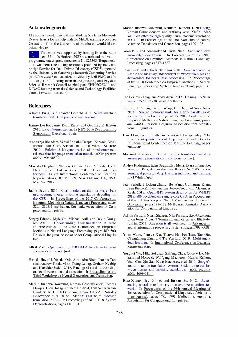
AcknowledgmentsThe authors would like to thank Shufang Xie from MicrosoftResearch Asia for his help with the MADL training procedure.Co-authors from the University of Edinburgh would like toacknowledge:
This work was supported by funding from the Euro-pean Union’s Horizon 2020 research and innovation
programme under grant agreements No 825303 (Bergamot).It was performed using resources provided by the Cam-
bridge Service for Data Driven Discovery (CSD3) operatedby the University of Cambridge Research Computing Service(http://www.csd3.cam.ac.uk/), provided by Dell EMC and In-tel using Tier-2 funding from the Engineering and PhysicalSciences Research Council (capital grant EP/P020259/1), andDiRAC funding from the Science and Technology FacilitiesCouncil (www.dirac.ac.uk).
ReferencesAlham Fikri Aji and Kenneth Heafield. 2019. Neural machine
translation with 4-bit precision and beyond.
Jimmy Lei Ba, Jamie Ryan Kiros, and Geoffrey E. Hinton.2016. Layer Normalization. In NIPS 2016 Deep LearningSymposium, Barcelona, Spain.
Aishwarya Bhandare, Vamsi Sripathi, Deepthi Karkada, VivekMenon, Sun Choi, Kushal Datta, and Vikram Saletore.2019. Efficient 8-bit quantization of transformer neu-ral machine language translation model. arXiv preprintarXiv:1906.00532.
Mostafa Dehghani, Stephan Gouws, Oriol Vinyals, JakobUszkoreit, and Lukasz Kaiser. 2019. Universal trans-formers. In 7th International Conference on LearningRepresentations, ICLR 2019, New Orleans, LA, USA,May 6-9, 2019.
Jacob Devlin. 2017. Sharp models on dull hardware: Fastand accurate neural machine translation decoding onthe CPU. In Proceedings of the 2017 Conference onEmpirical Methods in Natural Language Processing, pages2820–2825, Copenhagen, Denmark. Association for Com-putational Linguistics.
Sergey Edunov, Myle Ott, Michael Auli, and David Grang-ier. 2018. Understanding back-translation at scale.In Proceedings of the 2018 Conference on EmpiricalMethods in Natural Language Processing, pages 489–500,Brussels, Belgium. Association for Computational Linguis-tics.
FBGEMM. Open-sourcing FBGEMM for state-of-the-artserver-side inference [online].
Hiroaki Hayashi, Yusuke Oda, Alexandra Birch, Ioannis Con-stas, Andrew Finch, Minh-Thang Luong, Graham Neubig,and Katsuhito Sudoh. 2019. Findings of the third workshopon neural generation and translation. In Proceedings of theThird Workshop on Neural Generation and Translation.
Marcin Junczys-Dowmunt, Roman Grundkiewicz, TomaszDwojak, Hieu Hoang, Kenneth Heafield, Tom Neckermann,Frank Seide, Ulrich Germann, Alham Fikri Aji, NikolayBogoychev, et al. 2018a. Marian: Fast neural machinetranslation in C++. In Proceedings of ACL 2018, SystemDemonstrations, pages 116–121.
Marcin Junczys-Dowmunt, Kenneth Heafield, Hieu Hoang,Roman Grundkiewicz, and Anthony Aue. 2018b. Mar-ian: Cost-effective high-quality neural machine translationin C++. In Proceedings of the 2nd Workshop on NeuralMachine Translation and Generation, pages 129–135.
Yoon Kim and Alexander M Rush. 2016. Sequence-levelknowledge distillation. In Proceedings of the 2016Conference on Empirical Methods in Natural LanguageProcessing, pages 1317–1327.
Taku Kudo and John Richardson. 2018. Sentencepiece: Asimple and language independent subword tokenizer anddetokenizer for neural text processing. In Proceedingsof the 2018 Conference on Empirical Methods in NaturalLanguage Processing: System Demonstrations, pages 66–71.
Tao Lei, Yu Zhang, and Yoav Artzi. 2017. Training RNNs asfast as CNNs. CoRR, abs/1709.02755.
Tao Lei, Yu Zhang, Sida I. Wang, Hui Dai, and Yoav Artzi.2018. Simple recurrent units for highly parallelizablerecurrence. In Proceedings of the 2018 Conference onEmpirical Methods in Natural Language Processing, pages4470–4481, Brussels, Belgium. Association for Computa-tional Linguistics.
Darryl Lin, Sachin Talathi, and Sreekanth Annapureddy. 2016.Fixed point quantization of deep convolutional networks.In International Conference on Machine Learning, pages2849–2858.
Microsoft-Translator. Neural machine translation enablinghuman parity innovations in the cloud [online].
Andres Rodriguez, Eden Segal, Etay Meiri, Evarist Fomenko,Young Jin Kim, Haihao Shen, and Barukh Ziv. 2018. Lowernumerical precision deep learning inference and training.Intel White Paper.
Jean Senellart, Dakun Zhang, Bo Wang, Guillaume Klein,Jean-Pierre Ramatchandirin, Josep Crego, and AlexanderRush. 2018. OpenNMT system description for WNMT2018: 800 words/sec on a single-core CPU. In Proceedingsof the 2nd Workshop on Neural Machine Translation andGeneration, pages 122–128, Melbourne, Australia. Associ-ation for Computational Linguistics.
Ashish Vaswani, Noam Shazeer, Niki Parmar, Jakob Uszkoreit,Llion Jones, Aidan N Gomez, Łukasz Kaiser, and Illia Polo-sukhin. 2017. Attention is all you need. In Advances inneural information processing systems, pages 5998–6008.
Yiren Wang, Yingce Xia, Tianyu He, Fei Tian, Tao Qin,ChengXiang Zhai, and Tie-Yan Liu. 2019. Multi-agentdual learning. In International Conference on LearningRepresentations.
Yonghui Wu, Mike Schuster, Zhifeng Chen, Quoc V Le, Mo-hammad Norouzi, Wolfgang Macherey, Maxim Krikun,Yuan Cao, Qin Gao, Klaus Macherey, et al. 2016. Google’sneural machine translation system: Bridging the gap be-tween human and machine translation. arXiv preprintarXiv:1609.08144.
Biao Zhang, Deyi Xiong, and Jinsong Su. 2018. Accel-erating neural transformer via an average attention net-work. In Proceedings of the 56th Annual Meeting ofthe Association for Computational Linguistics (Volume 1:Long Papers), pages 1789–1798, Melbourne, Australia.Association for Computational Linguistics.
288

Proceedings of the 3rd Workshop on Neural Generation and Translation (WNGT 2019), pages 289–296Hong Kong, China, November 4, 2019. c©2019 Association for Computational Linguistics
www.aclweb.org/anthology/D19-56%2d
Selecting, Planning, and Rewriting: A Modular Approach forData-to-Document Generation and Translation
Lesly Miculicich∗† Marc Marone ∗‡Hany Hassan‡
† Idiap Research Institute, Ecole Polytechnique Federale de Lausanne (EPFL), [email protected]
‡Microsoft, 1 Microsoft Way, Redmond, WA 98121, USA{v-mamaro,hanyh}microsoft.com
AbstractIn this paper, we report our system submis-sions to all 6 tracks of the WNGT 2019shared task on Document-Level Generationand Translation. The objective is to generate atextual document from either structured data:generation task, or a document in a differentlanguage: translation task. For the translationtask, we focused on adapting a large scale sys-tem trained on WMT data by fine tuning it onthe RotoWire data. For the generation task, weparticipated with two systems based on a se-lection and planning model followed by (a) asimple language model generation, and (b) aGPT-2 pre-trained language model approach.The selection and planning module chooses asubset of table records in order, and the lan-guage models produce text given such a sub-set.
1 Introduction
Data-to-text generation focuses on generating nat-ural text from structured inputs such as tablerecords. Traditional data-to-text systems used apipelined approach for data selection followed byplanning and text generation. Recently, End-to-End neural generation systems have been pro-posed such as (Wiseman et al., 2017). While suchsystems generate more fluent output, they are notfaithful to the facts in the structured data.
One of the difficulties of the generation task isthat the models have to learn two different aspects:“what to say” (i.e. selecting relevant information)and “how to say it” (i.e. generating the actual textbased on these facts). We believe that availabledata-sets are too small for allowing current neu-ral network models, based on encoder-decoder ar-chitectures, to capture the complexity of the prob-lem. Recently, (Puduppully et al., 2019) proposedan end-to-end system that explicitly models a con-tent selection and planning module separated from
∗Equal contribution. Work done while interning at Mi-crosoft
the text generation, showing improvements withrespect to previous end-to-end systems (Wisemanet al., 2017). We adopt this approach and divideour model into two parts noted as: content selec-tion and planning, and text generation. This di-vision helps the system to produce more coher-ent document structure. One drawback of thisapproach is the limitation of the language modelgeneration coverage. We tackle this limitationby adopting pre-trained language models such asOpenAI’s GPT-2 (Radford et al., 2019). Followingthe shared task guidelines (Hayashi et al., 2019),we evaluate our models using an information ex-traction (IE) system.
2 Translation Tasks
We submitted translation results for both di-rections: English-to-German and German-to-English. Our models are based on the trans-former architecture trained with multi-agent duallearning (MADL) (Xia et al., 2019). This systemuses the transformer big configuration (modelsize1024, filter size 4096, 6 blocks for each encoderand decoder) from (Vaswani et al., 2017), usingdropout of 0.2. It is trained with 3 primary trans-lations models and 3 dual translation models (fordetails refer to (Xia et al., 2019)). The base mod-els were trained with 20M filtered sentence-pairsfrom WMT 2019 shared translation task (Bojaret al., 2019), plus 120M English, and 120M Ger-man monolingual sentences from Newscrawl (Bo-jar et al., 2019). The vocabulary is shared andcomposed of word segments obtained by applyingthe BPE algorithm with 35K merge operations.
We fine-tuned the base models with 3Ksentence-pairs of the Rotowire English-Germanparallel data. We use batches of 4096 tokens andoptimize with different learning rates. The best re-sult was obtained with learning rate of 10−5 forboth directions. Additionally, for the German-to-English translation task, we back-translate the
289

monolingual Rotowire English corpus. For thispurpose, the documents were split into sentences1
to obtain 45K English sentences in total, then weuse the MADL model which was fine-tuned withparallel Rotowire data to obtain their respectiveGerman translations. Finally, we fine-tune theMADL system again using the concatenation oforiginal parallel sentences and the back-translatedcorpus. Since we do not have an in-domain mono-lingual German corpus, we ensemble 3 replicasof the fine-tuned MADL models trained with 10,20, and 30% dropout for the English-German task.Additionally, we back-translate 1M monolingualsentences from Newscrawl which were selectedbased on their similarity to Rotowire data follow-ing (Moore and Lewis, 2010). However, this didnot lead to any further improvements in the sys-tems.
All translation systems used text summariesonly. We did not use the additional data tables inthe submitted results for the MT + NLG track. Inour experiments, we find that adding the structureddata did not lead to improvements over the base-line systems.
2.1 Results
Table 1 shows the results of our systems for bothdirections measured with sacre-BLEU. Fine tun-ing with Rotowire parallel data brings an improve-ment of 7.9 BLEU points for English-to-Germanand 9.3 for German-to-English in the test set.Further improvement of 1.9 BLEU points is ob-tained with back-translation of monolingual Ro-towire data for the latter direction. The dropoutensemble adds a very small gain of 0.2 BLEU. Wefound that selected data from Newscrawl does notadd any significant improvement.
We also evaluate our German-to-English systemwith the content oriented metrics provided by theorganizers of the shared-task. Table 2 shows thevalues for development and test sets. We showthe results measured with the ground-truth trans-lation for comparison. The content generation(RG) of the best system reaches two percentagepoints higher than the ground-truth. The transla-tion model produces fewer referring expressions,and morphological variations than the ground-truth to refer to entities, which makes it easierfor the information extraction tools to recognizethem. The Content selection (CS) reaches high
1https://github.com/neulab/DGT
EN→ DE DE→ ENMADL 39.99 48.71+ RW parallel 47.90 57.99+ RW monolingual ? – 59.94+ Ensemble ? 48.09 –
Table 1: Machine translation results measured withsacre-BLEU and task-specific tokenization1. ? denotesa late entry, not in the official evaluation.
precision (92%) and recall (93%), and the contentorder (CO) score is 89. Further manual analysisindicates that the main issues are the translation oftextual numbers, and the morphological variationof entities.
3 Generation Task
One of the difficulties of the data-to-documentgeneration task, as formulated by (Wiseman et al.,2017), is that the models have to learn to select arelatively small portion of table records and theirorder for generating text. We argue that the sizeof available data-sets for training (i.e. Rotowirewith 3.4K samples) is too small for allowing thenetwork to capture the complexity of the task. Inconsequence, following (Puduppully et al., 2019;Moryossef et al., 2019), we divide the work intwo parts : (a) content selection and planning, and(b) text generation. The idea is to introduce a di-rect signal to the system i.e. adding a loss functionthat guides an orderly selection of records, allevi-ating the work of the text generator.
Our system is based on (Puduppully et al.,2019) with two main differences. First, we usea transformer network for encoding each record inrelation to other records, instead of a more com-plex gated approach as previous work. Second, weshare the vocabularies of record values and sum-mary text, thus the final estimated distribution forprediction over the whole vocabulary is summedinstead of concatenated. Figure 1 shows the archi-tecture of the model. In the following, we describeeach component in detail:
3.1 Content selection and Planning
Given a set of records r = r1, r2, ..., rM , the ob-jective is to select a subset of them in the correctorder r ∈ r. We use an encoder-decoder architec-ture to model this problem. Similar to (Wisemanet al., 2017), we create embeddings of each fea-ture record (e.g. value, key, etc.) and concatenate
290
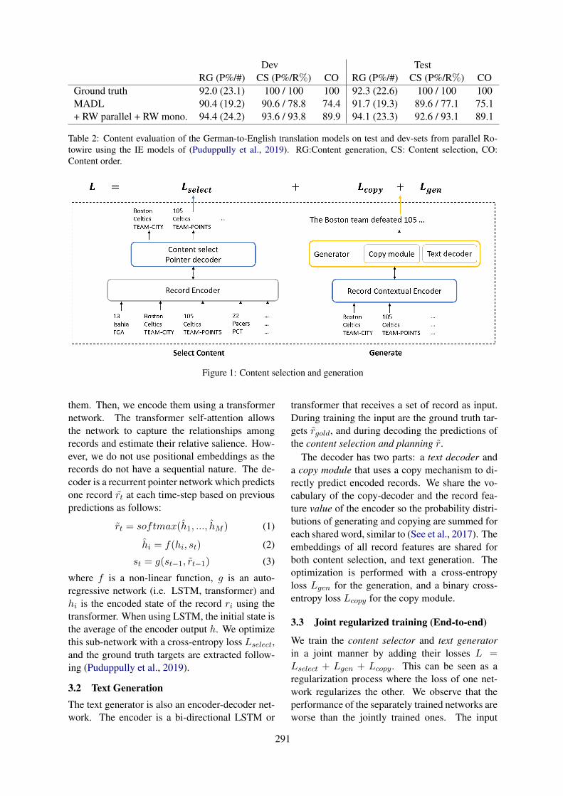
Dev TestRG (P%/#) CS (P%/R%) CO RG (P%/#) CS (P%/R%) CO
Ground truth 92.0 (23.1) 100 / 100 100 92.3 (22.6) 100 / 100 100MADL 90.4 (19.2) 90.6 / 78.8 74.4 91.7 (19.3) 89.6 / 77.1 75.1+ RW parallel + RW mono. 94.4 (24.2) 93.6 / 93.8 89.9 94.1 (23.3) 92.6 / 93.1 89.1
Table 2: Content evaluation of the German-to-English translation models on test and dev-sets from parallel Ro-towire using the IE models of (Puduppully et al., 2019). RG:Content generation, CS: Content selection, CO:Content order.
Figure 1: Content selection and generation
them. Then, we encode them using a transformernetwork. The transformer self-attention allowsthe network to capture the relationships amongrecords and estimate their relative salience. How-ever, we do not use positional embeddings as therecords do not have a sequential nature. The de-coder is a recurrent pointer network which predictsone record rt at each time-step based on previouspredictions as follows:
rt = softmax(h1, ..., hM ) (1)
hi = f(hi, st) (2)
st = g(st−1, rt−1) (3)
where f is a non-linear function, g is an auto-regressive network (i.e. LSTM, transformer) andhi is the encoded state of the record ri using thetransformer. When using LSTM, the initial state isthe average of the encoder output h. We optimizethis sub-network with a cross-entropy loss Lselect,and the ground truth targets are extracted follow-ing (Puduppully et al., 2019).
3.2 Text GenerationThe text generator is also an encoder-decoder net-work. The encoder is a bi-directional LSTM or
transformer that receives a set of record as input.During training the input are the ground truth tar-gets rgold, and during decoding the predictions ofthe content selection and planning r.
The decoder has two parts: a text decoder anda copy module that uses a copy mechanism to di-rectly predict encoded records. We share the vo-cabulary of the copy-decoder and the record fea-ture value of the encoder so the probability distri-butions of generating and copying are summed foreach shared word, similar to (See et al., 2017). Theembeddings of all record features are shared forboth content selection, and text generation. Theoptimization is performed with a cross-entropyloss Lgen for the generation, and a binary cross-entropy loss Lcopy for the copy module.
3.3 Joint regularized training (End-to-end)
We train the content selector and text generatorin a joint manner by adding their losses L =Lselect + Lgen + Lcopy. This can be seen as aregularization process where the loss of one net-work regularizes the other. We observe that theperformance of the separately trained networks areworse than the jointly trained ones. The input
291

P R F1 DLSingle Baseline 41 68 51 0.76Single CSP 43 67 52 0.75Joint Baseline + TG 45 62 52 0.75Joint CSP + TG 46 71 56 0.70
Table 3: Evaluation of Content Selection and Plan-ning (CSP) module, with and without joint trainingwith the Text Generator (TG). Baseline: (Puduppullyet al., 2019). P: precision, R: recall, DL: Damerau-Levenshtein distance.
Figure 2: Augmenting data by swapping the target val-ues of each document at different percentage rates. Ineach case, we doubled the training set.
for the text generator is ground truth during train-ing. At decoding time, we perform 2 consecutivebeam search of 5 beams, the first one for the con-tent selection, and the second for generating text.We tuned the architecture using the developmentset. We evaluated different configurations of trans-formers and LSTMs, from 1 to 2 layers, with di-mensions of 252 and 512, and dropout from 0.1to 0.3. The best results are obtained using LSTMsdecoders with 512 size dimension for all hiddenlayers and embeddings, each encoder and decoderhas 2 layers, and we use dropout of 0.3. We alsoused data augmentations by swapping values in ofthe target at a range of 10, 20, and 30 percent ofthe values in each sample. Finally, we train thenetwork with batches of 5 document samples, andupdated the parameters each 20 batches. We useAdam optimizer at an initial learning rate of 10−3.
3.4 ResultsWe test the content selection and planning mod-ule by comparing the output subset of records withthe ground-truth records (i.e. the records extractedfrom the summary text with the IE tools). Weuse F1 and Damerau-Levenshtein (DL), the laterto evaluate the correct order of records. The work-shop metrics are not used here because the inde-pendently trained models do not output text. Re-
sults in Table 3 show that our model outperformsthe baseline (Puduppully et al., 2019), and the jointtraining helps to further improve over the singlemodels. Figure 2 shows the F1 scores while aug-menting data by varying the percentage of swapsin the target training set. Adding samples with 5%of random swaps in each sample document helpsboth single and jointly trained models. Finally, Ta-ble 4 shows the evaluation results of the final jointsystem with the workshop metrics.
During a qualitative evaluation, we noticed thatthe content selection and planning module learnsto output the most common sequence of recordsin the training data. In general, the sequence ofrecords depends on the style of the commentator(e.g. describing first match results and then im-portant player’s scores). Our system mismatchesless common styles, which affects the scoring oftesting and development that contain different dis-tribution of record sequences.
4 Generation with Pretrained LM
We experiment with using pretrained languagemodels to enhance coverage and fluency of the textgeneration, since the amount of training data avail-able for the generation the task is relatively small.In particular, we use a pretrained PyTorch imple-mentation2 of the GPT-2 (Radford et al., 2019)language model. The original GPT-2 descriptionshowed that this large scale language model ad-ditionally learned to complete other tasks such assummarization and translation. For example, thelanguage model can be used for summarization,by providing an input document concatenated withthe string TL;DR: and the output is the gener-ated summary. Inspired by these results, we pro-pose our summary rewrite model. Our model is atwo phases approach: the first is the content selec-tion model proposed in 3.1, the second is a GPT2-based generation module. Based on the output ofthe content selection module, our model providesa rough summary as input to GPT-2 model whichgenerates the desired summary.
The baseline results in (Wiseman et al.,2017) show that simple templates are very ef-fective at conveying information from the datatables. We use similar templates to gener-ate a rough summary that is used as input inour rewrite model. The model takes input
2https://github.com/huggingface/pytorch-transformers
292

Data to EN Data to DEBLEU RG CS (P/R) CO BLEU RG CS (P/R) CO
End-to-end 15.03 93.38 32.34 / 58.04 18.52 11.66 80.30 27.89 / 48.96 16.43GPT-50 15.17 94.35 33.84 / 53.82 19.26 11.84 82.79 34.23 / 42.32 16.93GPT-90 13.03 88.70 32.81 / 50.64 17.34 10.43 75.05 30.97 / 41.48 16.27
Table 4: Generation results of our submitted systems as reported by the shared task organizers (Hayashi et al.,2019). RG: Relation Generation precision, CS: Content Selection (precision/recall), CO: Content Ordering.
of the form template summary <R> goldsummary, which is used to fine-tune the pre-trained GPT-2 model. The templates consist ofsimple sentences involving a single record fromthe dataset, such as the number of points scoredby a player. At training time we generate tem-plates from the ground truth records following(Puduppully et al., 2019). At test time, we usethe content selection module to select appropriaterecords. This effectively replaces the original gen-erator network with the GPT-2 model, using textas an intermediate encoding. See Appendix sec-tions A.1 and A.2 for a full example.
4.1 DecodingRecently, (Holtzman et al., 2019) suggested thattop-k token sampling (as used in the original GPT-2 results) is not ideal for generating realistic textfrom likelihood trained language models. Theyinstead propose Nucleus Sampling or top-p sam-pling, which samples tokens from the top p portionof the output distribution. We experiment withseveral values of p and find that this provides aneffective way to control generation quality. Oursubmitted models (GPT-50 and GPT-90) samplefrom the top 50% and 90% of the output distribu-tion when decoding.
4.2 ResultsWe find that the template rewriting approach iscompetitive with the end-to-end trained models interms of content metrics (Table 4), and subjec-tively appears to create natural sounding genera-tions.
For lower values of p in top-p sampling, we findthat the model remains more true to the templates,tending to create short summaries that do not de-viate much from the input facts. For larger valuesof p, where decoding is allowed to sample frommore of the distribution, the output tends be longerbut may deviate from the facts. We also note thatwhen regenerating summaries for high values ofp (with a different random seed), there are signif-
icant changes to the text but not to the facts re-flected in the summary. See Appendix sectionsA.4 and A.5 for examples of generations at var-ious p values. For both settings we observe oc-casional mistakes such as repetitions, suggestingthat our values for p should have been tuned morecarefully.
For the German generation track, we apply ourmodel described in 2 to the English generations,since we did not have a GPT-2 scale languagemodel for German.
5 Discussion and Conclusion
For the translation task we experimented with asimple fine tuning approach for a large scale sys-tem trained on general domain data. It proved veryeffective to fine tune a pre-trained system usingRotoWire data. Our analysis indicates that the re-maining problems are more related to number for-matting which is a more generic issue for NMTsystems and not a domain specific problem.
The generation task proved to be more chal-lenging. Mainly generating faithful, accurate andfluent summaries can be a quite challenging taskgiven the discrepancies between the provided dataand the desired summaries. Our analysis indicatesthat there is a mismatch between the gold selec-tion plan and the system output. The system out-puts the most common sequence of facts whereasthe gold presents more variety of fact sequencesdue to different writing styles. This issue shouldbe further studied in future.
Utilizing large scale pre-trained LMs (such asGPT-2) is a very promising direction, since it de-couples the dependency of selection and genera-tion resources. Our current approach of feedingthe template-based input to GPT2 is quite simpleand efficient. We would like to investigate moreprincipled methods of doing this in the future.
293

6 Acknowledgment
We would like to thank Tao Qin and his team atMSRA for providing the MADL translation base-line systems.
ReferencesOndrej Bojar, Rajen Chatterjee, Christian Feder-
mann, Mark Fishel, Yvette Graham, Barry Had-dow, Matthias Huck, Antonio Jimeno Yepes, PhilippKoehn, Andre Martins, Christof Monz, Matteo Ne-gri, Aurelie Neveol, Mariana Neves, Matt Post,Marco Turchi, and Karin Verspoor. 2019. Proceed-ings of the fourth conference on machine translation(volume 2: Shared task papers, day 1). Florence,Italy. Association for Computational Linguistics.
Hiroaki Hayashi, Yusuke Oda, Alexandra Birch, Ioan-nis Constas, Andrew Finch, Minh-Thang Luong,Graham Neubig, and Katsuhito Sudoh. 2019. Find-ings of the third workshop on neural generation andtranslation. In Proceedings of the Third Workshopon Neural Generation and Translation.
Ari Holtzman, Jan Buys, Maxwell Forbes, and YejinChoi. 2019. The curious case of neural text degen-eration. arXiv preprint arXiv:1904.09751.
Robert C. Moore and William Lewis. 2010. Intelligentselection of language model training data. In Pro-ceedings of the ACL 2010 Conference Short Papers,pages 220–224, Uppsala, Sweden. Association forComputational Linguistics.
Amit Moryossef, Yoav Goldberg, and Ido Dagan. 2019.Step-by-step: Separating planning from realizationin neural data-to-text generation. In Proceedings ofthe 2019 Conference of the North American Chap-ter of the Association for Computational Linguistics:Human Language Technologies, Volume 1 (Longand Short Papers), pages 2267–2277, Minneapolis,Minnesota. Association for Computational Linguis-tics.
Ratish Puduppully, Li Dong, and Mirella Lapata. 2019.Data-to-text generation with content selection andplanning. In Proceedings of the AAAI Conferenceon Artificial Intelligence, volume 33, pages 6908–6915.
Alec Radford, Jeff Wu, Rewon Child, David Luan,Dario Amodei, and Ilya Sutskever. 2019. Languagemodels are unsupervised multitask learners.
Abigail See, Peter J. Liu, and Christopher D. Manning.2017. Get to the point: Summarization with pointer-generator networks. In Proceedings of the 55th An-nual Meeting of the Association for ComputationalLinguistics (Volume 1: Long Papers), pages 1073–1083, Vancouver, Canada. Association for Compu-tational Linguistics.
Ashish Vaswani, Noam Shazeer, Niki Parmar, JakobUszkoreit, Llion Jones, Aidan N Gomez, ŁukaszKaiser, and Illia Polosukhin. 2017. Attention is allyou need. In Advances in neural information pro-cessing systems, pages 5998–6008.
Sam Wiseman, Stuart Shieber, and Alexander Rush.2017. Challenges in data-to-document generation.In Proceedings of the 2017 Conference on Empiri-cal Methods in Natural Language Processing, pages2253–2263, Copenhagen, Denmark. Association forComputational Linguistics.
Yingce Xia, Xu Tan, Fei Tian, Fei Gao, Di He, WeicongChen, Yang Fan, Linyuan Gong, Yichong Leng,Renqian Luo, Yiren Wang, Lijun Wu, Jinhua Zhu,Tao Qin, and Tie-Yan Liu. 2019. Microsoft researchasia’s systems for WMT19. In Proceedings of theFourth Conference on Machine Translation (Volume2: Shared Task Papers, Day 1), Florence, Italy. As-sociation for Computational Linguistics.
294

A Rewrite Model
Below are example generations from our models,with some highlighted comparisons. “...” indi-cates text omitted for brevity.
Each configuration correctly introduces theteams. However, note that the stadium differs.The End-to-end model claims that the game tookplace at the United Center. The GPT modelsclaim that the game took place at the Air CanadaCent(er|re), the correct stadium for the home team(the Toronto Raptors). In fact, the GPT model useswhat may be a more correct spelling (centre).
All models report player statistics (some ex-ample sentences are bolded) and game statistics.There are some occasional mistakes. . Some arelogical (the Raptors won), and others seems to berelated to decoding.
A.1 Gold Template Input
The Raptors are from Toronto. The
Raptors were HOME. The Raptors scored
122 points. The 76ers are from
Philadelphia. The 76ers were AWAY.
The 76ers scored 95 points. ... Robert
Covington scored 20 points. Robert
Covington had 5 rebounds. Robert
Covington had 2 assists. Robert
Covington had 2 steals. Robert
Covington made 7 shots. Robert
Covington had 11 attempts. Jahlil
Okafor scored 15 points. ...
A.2 Gold Summary
The host Toronto Raptors defeated
the Philadelphia 76ers, 122 - 95, at
Air Canada Center on Monday. ... The
Raptors were lights - out shooting, as
they went 55 percent from the field and
68 percent from three - point range.
They also held the Sixers to just 42
percent from the field and dominated
the defensive rebounding, 34 - 26.
Fastbreak points was a huge difference
as well, with Toronto winning that
battle, 21 - 6. ... Robert Covington
had one of his best games of the season
though, tallying 20 points, five
rebounds, two assists and two steals
on 7 - of - 11 shooting. Jahlil Okafor
got the start for Embiid and finished
with 15 points and five rebounds. ...
A.3 End-to-End Summary
The Toronto Raptors defeated the
visiting Philadelphia 76ers 122 - 95
, at United Center on Saturday evening.
The Raptors (11 - 6) came in to Friday’s
contest having lost four of their last
six games, and have now lost five of
their last seven games. They were led
by Terrence Ross, who scored a game -
high 22 points on 8 - of - 11 shooting
from the field and 3 - of - 5 from three
- point range. Kyle Lowry followed
up with 24 points, eight assists and
four rebounds, in 32 minutes. Jonas
Valanciunas recorded a double - double
with 12 points and 11 rebounds, in 22
minutes off the bench. The Raptors
shot 55 percent from the field and
68 percent from long range , while the
76ers shot 55 percent from the field
and 68 percent from behind the arc .
Robert Covington was the high - point
man for the 76ers, with 20 points ,
including 6 - of - 9 from three - point
range. ... The Sixers will look to
bounce back when they visit the New York
Knicks on Monday.
A.4 Top-0.5 Sampling (GPT-50)
The Toronto Raptors defeated the
Philadelphia 76ers, 122 - 95, at
Air Canada Centre on Saturday. The
Raptors (11 - 6) were able to prevail
despite being outshot, out rebounded
and out - rebounded by the Sixers (7
- 15) in the contest. ... The Raptors
were led by Terrence Ross, who posted
a game - high 22 points on 8 - of - 11
shooting, including 3 - of - 5 from long
range. Kyle Lowry followed up with 24
points, eight assists and four rebounds,
in 32 minutes. Jonas Valanciunas
chipped in 12 points and 11 rebounds, in
22 minutes off the bench. The Raptors
shot a respectable 55 percent from the
field and 68 percent from long range,
but were out - rebounded by the Sixers
by a 52 - 40 margin. Philadelphia
had five players in double figures,
led by Robert Covington, who scored
20 points on 6 - of - 9 shooting from
295

behind the arc. The Sixers will look
to bounce back, as they travel to Boston
to take on the Celtics on Monday. ...
The Raptors will look to extend their
winning streak to four on Monday against
the Orlando Magic.
A.5 Top-0.9 Sampling (GPT-90)We show summaries from two different seeds forthe least restrictive sampling setting, p = 0.9.Some details change but most of the content
supported by the data remains the same. Aggre-gated across the entire set, the information metricsremain nearly identical. This less restricted modelmore frequently outputs hallucinations and sur-rounding details not supported by the tabular data.
Sample One:The Toronto Raptors defeated the
Philadelphia 76ers, 122 - 95, at Air
Canada Centre on Saturday. ... Lowry
added 24 points, eight assists
and four rebounds in 32 minutes.
Jonas Valanciunas scored 12 points
and grabbed 11 rebounds in 22 minutes
as a starter. ...
Sample Two:The Toronto Raptors defeated the
Philadelphia 76ers, 122 - 95, in
overtime at Air Canada Centre on
Tuesday . ... After a rather lopsided
first quarter, the Raptors came
out flat for the first 40 - plus
minutes of this game. Philadelphia
ended up hanging around for the
final four minutes of regulation , as
Toronto took the lead for good with
16 seconds remaining in regulation.
... In overtime, the Raptors took a
13 - point lead into the locker room
thanks to a clutch 30 - foot field goal
from Terrence Ross with eight seconds
remaining in regulation. ... Kyle
Lowry added 24 points, eight assists
and four rebounds in 32 minutes , while
Jonas Valanciunas added a 12 - point,
11 - rebound double - double in just
22 minutes. ...
296

Proceedings of the 3rd Workshop on Neural Generation and Translation (WNGT 2019), pages 297–301Hong Kong, China, November 4, 2019. c©2019 Association for Computational Linguistics
www.aclweb.org/anthology/D19-56%2d
Efficiency through Auto-Sizing:Notre Dame NLP’s Submission to the WNGT 2019 Efficiency Task
Kenton Murray Brian DuSell David ChiangDepartment of Computer Science and Engineering
University of Notre Dame{kmurray4,bdusell1,dchiang}@nd.edu
Abstract
This paper describes the Notre Dame Natu-ral Language Processing Group’s (NDNLP)submission to the WNGT 2019 shared task(Hayashi et al., 2019). We investigated the im-pact of auto-sizing (Murray and Chiang, 2015;Murray et al., 2019) to the Transformer net-work (Vaswani et al., 2017) with the goal ofsubstantially reducing the number of param-eters in the model. Our method was able toeliminate more than 25% of the model’s pa-rameters while suffering a decrease of only 1.1BLEU.
1 Introduction
The Transformer network (Vaswani et al., 2017)is a neural sequence-to-sequence model that hasachieved state-of-the-art results in machine trans-lation. However, Transformer models tend to bevery large, typically consisting of hundreds of mil-lions of parameters. As the number of parame-ters directly corresponds to secondary storage re-quirements and memory consumption during in-ference, using Transformer networks may be pro-hibitively expensive in scenarios with constrainedresources. For the 2019 Workshop on Neural Gen-eration of Text (WNGT) Efficiency shared task(Hayashi et al., 2019), the Notre Dame NaturalLanguage Processing (NDNLP) group looked ata method of inducing sparsity in parameters calledauto-sizing in order to reduce the number of pa-rameters in the Transformer at the cost of a rela-tively minimal drop in performance.
Auto-sizing, first introduced by Murray andChiang (2015), uses group regularizers to encour-age parameter sparsity. When applied over neu-rons, it can delete neurons in a network and shrinkthe total number of parameters. A nice advantageof auto-sizing is that it is independent of model ar-chitecture; although we apply it to the Transformer
network in this task, it can easily be applied to anyother neural architecture.
NDNLP’s submission to the 2019 WNGT Effi-ciency shared task uses a standard, recommendedbaseline Transformer network. Following Mur-ray et al. (2019), we investigate the applicationof auto-sizing to various portions of the network.Differing from their work, the shared task useda significantly larger training dataset from WMT2014 (Bojar et al., 2014), as well as the goal ofreducing model size even if it impacted transla-tion performance. Our best system was able toprune over 25% of the parameters, yet had a BLEUdrop of only 1.1 points. This translates to over 25million parameters pruned and saves almost 100megabytes of disk space to store the model.
2 Auto-sizing
Auto-sizing is a method that encourages sparsitythrough use of a group regularizer. Whereas themost common applications of regularization willact over parameters individually, a group regu-larizer works over groupings of parameters. Forinstance, applying a sparsity inducing regularizerto a two-dimensional parameter tensor will en-courage individual values to be driven to 0.0. Asparsity-inducing group regularizer will act overdefined sub-structures, such as entire rows orcolumns, driving the entire groups to zero. De-pending on model specifications, one row or col-umn of a tensor in a neural network can corre-spond to one neuron in the model.
Following the discussion of Murray and Chiang(2015) and Murray et al. (2019), auto-sizing worksby training a neural network while using a regular-izer to prune units from the network, minimizing:
L = −∑
f , e in data
log P(e | f ; W) + λR(‖W‖).
W are the parameters of the model and R is a reg-
297

Figure 1: Architecture of the Transformer (Vaswaniet al., 2017). We apply the auto-sizing method to thefeed-forward (blue rectangles) and multi-head attention(orange rectangles) in all N layers of the encoder anddecoder. Note that there are residual connections thatcan allow information and gradients to bypass any layerwe are auto-sizing. Following the robustness recom-mendations, we instead layer norm before.
ularizer. Here, as with the previous work, we ex-periment with two regularizers:
R(W) =∑
i
∑
j
W2i j
12
(`2,1)
R(W) =∑
i
maxj|Wi j| (`∞,1)
The optimization is done using proximal gradi-ent descent (Parikh and Boyd, 2014), which al-ternates between stochastic gradient descent stepsand proximal steps:
W ← W − η∇ log P(e | f ; w)
W ← arg minW′
(12η‖W −W′‖2 + R(W′)
)
3 Auto-sizing the Transformer
The Transformer network (Vaswani et al., 2017) isa sequence-to-sequence model in which both the
encoder and the decoder consist of stacked self-attention layers. The multi-head attention usestwo affine transformations, followed by a softmaxlayer. Each layer has a position-wise feed-forwardneural network (FFN) with a hidden layer of rec-tified linear units. Both the multi-head attentionand the feed-forward neural network have residualconnections that allow information to bypass thoselayers. In addition, there are also word and posi-tion embeddings. Figure 1, taken from the originalpaper, shows the architecture. NDNLP’s submis-sion focuses on the N stacked encoder and decoderlayers.
The Transformer has demonstrated remarkablesuccess on a variety of datasets, but it is highlyover-parameterized. For example, the baselineTransformer model has more than 98 million pa-rameters, but the English portion of the trainingdata in this shared task has only 116 million to-kens and 816 thousand types. Early NMT mod-els such as Sutskever et al. (2014) have most oftheir parameters in the embedding layers, but thetransformer has a larger percentage of the model inthe actual encoder and decoder layers. Though thegroup regularizers of auto-sizing can be applied toany parameter matrix, here we focus on the pa-rameter matrices within the encoder and decoderlayers.
We note that there has been some work recentlyon shrinking networks through pruning. However,these differ from auto-sizing as they frequently re-quire an arbitrary threshold and are not includedduring the training process. For instance, Seeet al. (2016) prunes networks based off a varietyof thresholds and then retrains a model. Voitaet al. (2019) also look at pruning, but of attentionheads specifically. They do this through a relax-ation of an `0 regularizer in order to make it dif-ferentiable. This allows them to not need to usea proximal step. This method too starts with pre-trained model and then continues training. Michelet al. (2019) also look at pruning attention headsin the transformer. However, they too use thresh-olding, but only apply it at test time. Auto-sizingdoes not require a thresholding value, nor does itrequire a pre-trained model.
Of particular interest are the large, position-wise feed-forward networks in each encoder anddecoder layer:
FFN(x) = W2(max(0,W1x + b1)) + b2.
298

W1
W2
ReLU
Figure 2: Auto-sizing FFN network. For a row in theparameter matrix W1 that has been driven completelyto 0.0 (shown in white), the corresponding column inW2 (shown in blue) no longer has any impact on themodel. Both the column and the row can be deleted,thereby shrinking the model.
W1 and W2 are two large affine transformationsthat take inputs from D dimensions to 4D, thenproject them back to D again. These layers makeuse of rectified linear unit activations, which werethe focus of auto-sizing in the work of Murray andChiang (2015). No theory or intuition is given asto why this value of 4D should be used.
Following (Murray et al., 2019), we apply theauto-sizing method to the Transformer network,focusing on the two largest components, the feed-forward layers and the multi-head attentions (blueand orange rectangles in Figure 1). Rememberthat since there are residual connections allow-ing information to bypass the layers we are auto-sizing, information can still flow through the net-work even if the regularizer drives all the neuronsin a layer to zero – effectively pruning out an entirelayer.
4 Experiments
All of our models are trained using the fairseq im-plementation of the Transformer (Gehring et al.,2017).1 For the regularizers used in auto-sizing,we make use of an open-source, proximal gradienttoolkit implemented in PyTorch2 (Murray et al.,2019). For each mini-batch update, the stochasticgradient descent step is handled with a standardPyTorch forward-backward call. Then the proxi-mal step is applied to parameter matrices.
4.1 Settings
We used the originally proposed transformer ar-chitecture – with six encoder and six decoder lay-ers. Our model dimension was 512 and we used8 attention heads. The feed-forward network sub-components were of size 2048. All of our sys-tems were run using subword units (BPE) with32,000 merge operations on concatenated sourceand target training data (Sennrich and Haddow,2016). We clip norms at 0.1, use label smoothedcross-entropy with value 0.1, and an early stop-ping criterion when the learning rate is smallerthan 10−5. We used the Adam optimizer (Kingmaand Ba, 2015), a learning rate of 10−4, and dropoutof 0.1. Following recommendations in the fairseqand tensor2tensor (Vaswani et al., 2018) codebases, we apply layer normalization before a sub-component as opposed to after. At test time, wedecoded using a beam of 5 with length normal-ization (Boulanger-Lewandowski et al., 2013) andevaluate using case-sensitive, tokenized BLEU(Papineni et al., 2002).
For the auto-sizing experiments, we looked atboth `2,1 and `∞,1 regularizers. We experimentedover a range of regularizer coefficient strengths, λ,that control how large the proximal gradient stepwill be. Similar to Murray and Chiang (2015), butdiffering from Alvarez and Salzmann (2016), weuse one value of λ for all parameter matrices inthe network. We note that different regularizationcoefficient values are suited for different types orregularizers. Additionally, all of our experimentsuse the same batch size, which is also related to λ.
4.2 Auto-sizing sub-components
We applied auto-sizing to the sub-components ofthe encoder and decoder layers, without touchingthe word or positional embeddings. Recall from
1https://github.com/pytorch/fairseq2https://github.com/KentonMurray/ProxGradPytorch
299

System Disk Size Number of Parameters newstest2014 newstest2015Baseline 375M 98.2M 25.3 27.9
All `2,1 = 0.1 345M 90.2M 21.6 24.1Encoder `2,1 = 0.1 341M 89.4M 23.2 25.5Encoder `2,1 = 1.0 327M 85.7M 22.1 24.5
FFN `2,1 = 0.1 326M 85.2M 24.1 26.4FFN `2,1 = 1.0 279M 73.1M 24.0 26.8
FFN `2,1 = 10.0 279M 73.1M 23.9 26.5FFN `∞,1 = 100.0 327M 73.1M 23.8 26.0
Table 1: Comparison of BLEU scores and model sizes on newstest2014 and newstest2015. Applying auto-sizingto the feed-forward neural network sub-components of the transformer resulted in the most amount of pruningwhile still maintaining good BLEU scores.
Figure 1, that each layer has multi-head attentionand feed-forward network sub-components. Inturn, each multi-head attention sub-component iscomprised of two parameter matrices. Similarly,each feed-forward network has two parameter ma-trices, W1 and W2. We looked at three main exper-imental configurations:
• All: Auto-sizing is applied to every multi-head attention and feed-forward network sub-component in every layer of the encoder anddecoder.
• Encoder: As with All, auto-sizing is appliedto both multi-head attention and feed-forwardnetwork sub-components, but only in the en-coder layers. The decoder remains the same.
• FFN: Auto-sizing applied only to the feed-forward network sub-components W1 andW2, but not to the multi-head portions. Thistoo is applied to both the encoder and de-coder.
4.3 ResultsOur results are presented in Table 1. The base-line system has 98.2 million parameters and aBLEU score of 29.7. It takes up 375 megabytes ondisk. Our systems that applied auto-sizing only tothe feed-forward network sub-components of thetransformer network maintained the best BLEUscores while also pruning out the most parame-ters of the model. Overall, our best system used`2,1 = 1.0 regularization for auto-sizing and left73.1 million parameters remaining. On disk, themodel takes 279 megabytes to store – roughly100 megabytes less than the baseline. The perfor-mance drop compared to the baseline is 1.1 BLEUpoints, but the model is over 25% smaller.
Applying auto-sizing to the multi-head atten-tion and feed-forward network sub-components ofonly the encoder also pruned a substantial amountof parameters. Though this too resulted in asmaller model on disk, the BLEU scores wereworse than auto-sizing just the feed-forward sub-components. Auto-sizing the multi-head atten-tion and feed-forward network sub-components ofboth the encoder and decoder actually resulted ina larger model than the encoder only, but with alower BLEU score. Overall, our results suggestthat the attention portion of the transformer net-work is more important for model performancethan the feed-forward networks in each layer.
5 Conclusion
In this paper, we have investigated the impact ofusing auto-sizing on the transformer network ofthe 2019 WNGT efficiency task. We were ableto delete more than 25% of the parameters in themodel while only suffering a modest BLEU drop.In particular, focusing on the parameter matricesof the feed-forward networks in every layer of theencoder and decoder yielded the smallest modelsthat still performed well.
A nice aspect of our proposed method is thatthe proximal gradient step of auto-sizing can beapplied to a wide variety of parameter matri-ces. Whereas for the transformer, the largest im-pact was on feed-forward networks within a layer,should a new architecture emerge in the future,auto-sizing can be easily adapted to the trainableparameters.
Overall, NDNLP’s submission has shown thatauto-sizing is a flexible framework for pruning pa-rameters in a large NMT system. With an ag-gressive regularization scheme, large portions of
300

the model can be deleted with only a modest im-pact on BLEU scores. This in turn yields a muchsmaller model on disk and at run-time.
Acknowledgements
This research was supported in part by Universityof Southern California, subcontract 67108176 un-der DARPA contract HR0011-15-C-0115.
ReferencesJose M Alvarez and Mathieu Salzmann. 2016. Learn-
ing the number of neurons in deep networks. In Ad-vances in Neural Information Processing Systems,pages 2270–2278.
Ondrej Bojar, Christian Buck, Christian Federmann,Barry Haddow, Philipp Koehn, Johannes Leveling,Christof Monz, Pavel Pecina, Matt Post, HerveSaint-Amand, et al. 2014. Findings of the 2014workshop on statistical machine translation. In Pro-ceedings of the ninth workshop on statistical ma-chine translation, pages 12–58.
Nicolas Boulanger-Lewandowski, Yoshua Bengio, andPascal Vincent. 2013. Audio chord recognition withrecurrent neural networks. In Proc. InternationalSociety for Music Information Retrieval, pages 335–340.
Jonas Gehring, Michael Auli, David Grangier, DenisYarats, and Yann N. Dauphin. 2017. ConvolutionalSequence to Sequence Learning. In Proc. ICML.
Hiroaki Hayashi, Yusuke Oda, Alexandra Birch, Ioan-nis Constas, Andrew Finch, Minh-Thang Luong,Graham Neubig, and Katsuhito Sudoh. 2019. Find-ings of the third workshop on neural generation andtranslation. In Proceedings of the Third Workshopon Neural Generation and Translation.
Diederik P. Kingma and Jimmy Lei Ba. 2015. Adam:A method for stochastic optimization. In Proc.ICLR.
Paul Michel, Omer Levy, and Graham Neubig. 2019.Are sixteen heads really better than one? Advancesin Neural Information Processing Systems.
Kenton Murray and David Chiang. 2015. Auto-sizingneural networks: With applications to n-gram lan-guage models. In Proc. EMNLP.
Kenton Murray, Jeffery Kinnison, Toan Q. Nguyen,Walter Scheirer, and David Chiang. 2019. Auto-sizing the transformer network: Improving speed,efficiency, and performance for low-resource ma-chine translation. In Proceedings of the Third Work-shop on Neural Generation and Translation.
Kishore Papineni, Salim Roukos, Todd Ward, and Wei-Jing Zhu. 2002. BLEU: a method for automaticevaluation of machine translation. In Proc. ACL,pages 311–318.
Neal Parikh and Stephen Boyd. 2014. Proximal al-gorithms. Foundations and Trends in Optimization,1(3):123–231.
Abigail See, Minh-Thang Luong, and Christopher DManning. 2016. Compression of neural machinetranslation models via pruning. In Proceedingsof The 20th SIGNLL Conference on ComputationalNatural Language Learning, pages 291–301.
Rico Sennrich and Barry Haddow. 2016. Linguisticinput features improve neural machine translation.In Proc. First Conference on Machine Translation:Volume 1, Research Papers, volume 1, pages 83–91.
Ilya Sutskever, Oriol Vinyals, and Quoc V Le. 2014.Sequence to sequence learning with neural net-works. In Advances in Neural Information Process-ing Systems, pages 3104–3112.
Ashish Vaswani, Samy Bengio, Eugene Brevdo, Fran-cois Chollet, Aidan N. Gomez, Stephan Gouws,Llion Jones, Łukasz Kaiser, Nal Kalchbrenner, NikiParmar, Ryan Sepassi, Noam Shazeer, and JakobUszkoreit. 2018. Tensor2tensor for neural machinetranslation. CoRR, abs/1803.07416.
Ashish Vaswani, Noam Shazeer, Niki Parmar, JakobUszkoreit, Llion Jones, Aidan N. Gomez, ŁukaszKaiser, and Illia Polosukhin. 2017. Attention is allyou need. In Advances in Neural Information Pro-cessing Systems, pages 5998–6008.
Elena Voita, David Talbot, Fedor Moiseev, Rico Sen-nrich, and Ivan Titov. 2019. Analyzing multi-headself-attention: Specialized heads do the heavy lift-ing, the rest can be pruned. In Proceedings of the57th Annual Meeting of the Association for Com-putational Linguistics, pages 5797–5808, Florence,Italy. Association for Computational Linguistics.
301


Author Index
Aji, Alham Fikri, 80Andrews, Martin, 215Ataman, Duygu, 187
Berard, Alexandre, 168, 273Besacier, Laurent, 273Bhat, Gayatri, 199Birch, Alexandra, 1, 187Bogoychev, Nikolay, 280Brockett, Chris, 32Budzianowski, Paweł, 15
Calapodescu, Ioan, 168, 273Chali, Yllias, 70, 249Chan, William, 194Chiang, David, 231, 297Cho, Woon Sang, 32Clinchant, Stephane, 108Collier, Nigel, 118Crego, Josep, 148, 262Cui, Hongyi, 206Currey, Anna, 99
Di Gangi, Mattia A., 187Ding, Xiaoan, 44Dou, Zi-Yi, 59DuSell, Brian, 297Dymetman, Marc, 168
Egonmwan, Elozino, 70, 249
Federico, Marcello, 187Fikri Aji, Alham, 280Finch, Andrew, 1Firat, Orhan, 187
Gao, Shuyang, 90Gimpel, Kevin, 44, 138GONG, Li, 148, 262Goyal, Anuj, 90Grundkiewicz, Roman, 280
Haffari, Gholamreza, 177, 256Hassan, Hany, 280, 289Hayashi, Hiroaki, 1Heafield, Kenneth, 80, 99, 280
Hu, Junjie, 59Hung, Po-Hsuan, 206
Iida, Shohei, 206Imamura, Kenji, 23
Jost, Jürgen, 128Junczys-Dowmunt, Marcin, 280Jung, Kweon Woo, 108
Kambhatla, Nishant, 221Kim, Young Jin, 280Kinnison, Jeffery, 231Konstas, Ioannis, 1Kumar, Sachin, 199
Lapata, Mirella, 268Lee, Sungjin, 32Li, Lala, 194Li, Yingzhen, 118Luong, Minh-Thang, 1
Malandrakis, Nikolaos, 90Mallinson, Jonathan, 268Marone, Marc, 289Maruf, Sameen, 256Metallinou, Angeliki, 90Meunier, Jean-Luc, 168Miculicich, Lesly, 289Moradi, Pooya, 221Murray, Kenton, 231, 297
Nagaev, Aleksander, 128Nagata, Masaaki, 206Neubig, Graham, 1, 59Nguyen, Toan Q., 231Nikoulina, Vassilina, 108, 168
Oda, Yusuke, 1
Pang, Richard Yuanzhe, 138Park, Chan Young, 241Pilehvar, Mohammad Taher, 118Prokhorov, Victor, 118Puduppully, Ratish, 268
303

Rao, Sudha, 32Roux, Claude, 168
Saleh, Fahimeh, 273Sarkar, Anoop, 221Scheirer, Walter, 231Schmidt, Florian, 157Senellart, Jean, 148, 262Sethi, Abhishek, 90Shareghi, Ehsan, 118Shen, Minmin, 90Shibaev, Viacheslav, 128Sudoh, Katsuhito, 1Sumita, Eiichiro, 23
Tikhonov, Alexey, 128Tsvetkov, Yulia, 199, 241Tu, Lifu, 44
Utsuro, Takehito, 206
Vulic, Ivan, 15
Wang, Xinyi, 59Witteveen, Sam, 215
Yamshchikov, Ivan P., 128Yu, Dong, 44
Zaremoodi, Poorya, 177Zhang, Yizhe, 32