Proceedings of the 20th Czech-Japan Seminar on Data Analysis...

Pardubice, Czech Republic

September 17–20, 2017

Proceedings of the 20th Czech-JapanSeminar on Data Analysis and Decision

Making under Uncertainty

Edited byVilem Novak

Masahiro InuiguchiMartin Stepnicka

Organizing institution:

Institute for Research and Applications of Fuzzy Modeling

Co-organizing institutions:

• Faculty of Mathematics and Physics of the Charles University• Institute of Information Theory and Automation (UTIA) of the Czech Academy

of Sciences

Title: Proceedings of the 20th Czech-Japan Seminar on Data Analysisand Decision Making under UncertaintyCZECH-JAPAN SEMINAR 2017, Pardubice, Czech Republic, September 17–20,2017

Editors: Vilem Novak, Masahiro Inuiguchi, Martin StepnickaPublisher: University of Ostrava

c© Vilem Novak, Masahiro Inuiguchi, Martin Stepnicka, 2017c© University of Ostrava, Institute for Research and Applications of Fuzzy Modeling

ISBN: 978-80-7464-932-5

Committees

Programme ChairsVilem Novak (University of Ostrava)Masahiro Inuiguchi (Osaka University)

Programme Committee:Ondrej Cepek (Charles University in Prague)Martin Gavalec (University of Hradec Kralove)Takeshi Itoh (Tohoku University)Radim Jirousek (University of Economics, FM Jindrichuv Hradec)Irina Perfilieva (University of Ostrava)Jaroslav Ramık (Silesian University in Opava)Shogo Shiode (Kobe Gakuin University)Shao Chin Sung (Aoyama Gakuin University)Jirina Vejnarova (Czech Academy of Sciences, Prague)Milan Vlach (Charles University in Prague)

Financial ChairMartin Stepnicka (University of Ostrava)

Organizing ChairPetra Stevuliakova (University of Ostrava)

Organizing Committee:Martin Dyba (University of Ostrava)Petr Hurtık (University of Ostrava)Vojtech Molek (University of Ostrava)

Foreword

Dear Colleagues,with the great pleasure and at the same time with the great surprise I am writing

this foreword. Why surprise? Because this is already 20th Czech-Japan Seminar on DataAnalysis and Decision Making under Uncertainty! Nobody in the beginning expected thatwe would have succeeded in establishing such a nice and long tradition.

The idea to establish Czech-Japan seminars came from two people — Jaroslav Ramıkwho in that time was worker of IRAFM (Institute for Research and Applications of FuzzyModeling) and Milan Vlach who was professor in JAIST (Japan Advanced Institute forScience and Technology). Other people who were instrumental in establishing this traditionare Masahiro Inuiguchi, Tetsuzo Tanino and Hiroaki Ishii and Junzo Watada of the OsakaUniversity.

The first Czech-Japan seminar took place in March 1999 in JAIST in Hokuriku andthe second one in September of the same year in Celadna — a holiday resort in Beskydy inthe Czech Republic. Since then, the seminar took place each year alternately in Japan andin the Czech Republic. During the years, the seminars were organized in various placesboth Japan as well as in the Czech Republic: in Japan, e.g., in Kyoto, Fukuoka, Nagasaki,Sendai, Osaka; in Czechia, e.g., in Jindrichuv Hradec, Valtice, Liblice, Litomysl, MarianskeLazne and few other places.

This year, the seminar takes place in the nice town of East Bohemia — Pardubice.The town has a population of more than ninety thousand and is located at the confluenceof two rivers, the Labe and Chrudimka, 96 kilometres east of Prague. The town has along history: the first mention of Pardubice comes from 1295 and the city was founded in1340. Until 1918, the town was part of the Austrian monarchy. The history of Pardubiceis related to its growth as an important industrial town. In 1845, the first train arrived toPardubice, in 1911, Jan Kaspar made history by flying the first long-haul flight towardsPrague. The present factories include the Synthesia chemical factory — manufacturer ofthe ingloriously known plastic explosive Semtex and oil refinery Paramo.

The Czech-Japan seminars were quite successful both in producing new scientific resultsand in putting together an international group of researchers. I wish that the jubilee 20th-meeting will be no exception and hope that all of us meet again next year somewhere inJapan in the 21st-meeting.

Ostrava, September 2017 Vilem NovakUniversity of Ostrava, IRAFM

Table of Contents

Composition in exponential families: Case of multivariate normal distributionBINA V. . . . . . . . . . . . . . . . . . . . . . . . . . . . . . . . . . . . . . 9

Causality and Intervention in Business Process ManagementBINA V., JIROUSEK R. . . . . . . . . . . . . . . . . . . . . . . . . . . . . 15

Fuzzy Neural Networks on Embedded platformsCERMAK P., MARTINU J. . . . . . . . . . . . . . . . . . . . . . . . . . . 25

Hidden Auto-Conflict in the Theory of Belief FunctionsDANIEL M., KRATOCHVIL V. . . . . . . . . . . . . . . . . . . . . . . . 34

The two-sided (max/min, plus) problem is NP-completeGAVALEC M., PONCE D., ZIMMERMANN K. . . . . . . . . . . . . . . 46

F-transform based numerical solution of partial differential equationsHOLCAPEK M., VALASEK R. . . . . . . . . . . . . . . . . . . . . . . . . 54

Maximizing Minimum Range Methods for Interval Weight Estimation from aGiven Pairwise Comparison MatrixINUIGUCHI M., INNAN S. . . . . . . . . . . . . . . . . . . . . . . . . . . 65

Annual planning in badminton using a fuzzy approachKRIZKOVA S., GAVALEC M. . . . . . . . . . . . . . . . . . . . . . . . . 75

Fuzzy quantifiers on fuzzy four-fold tablesKUPKA J., RUSNOK P. . . . . . . . . . . . . . . . . . . . . . . . . . . . . 82

Transductive Learning Using Feature Spaces Provided by Semidefinite Program-mingsKUSUNOKI Y., IWASA K., TATSUMI K. . . . . . . . . . . . . . . . . . . 88

Inconsistency of Fuzzy Grey Analytic Hierarchy Process Pairwise ComparisonMatrixMLS K. . . . . . . . . . . . . . . . . . . . . . . . . . . . . . . . . . . . . . 94

Proposal of Probabilistic risk Evaluation for System Development Project Basedon Requirements AnalysisMOCHIDA S. . . . . . . . . . . . . . . . . . . . . . . . . . . . . . . . . . . 99

Scheduling Problem on Operation RoomsMOHRI S., ISHII H. . . . . . . . . . . . . . . . . . . . . . . . . . . . . . . 109

Linguistic Characterization of Natural Data by Applying Intermediate Quantifierson Fuzzy Association RulesMURINOVA P., BURDA M. . . . . . . . . . . . . . . . . . . . . . . . . . 115

Experimental Comparison of Three On-Line Fuzzy Classification SystemsNAKASHIMA T. . . . . . . . . . . . . . . . . . . . . . . . . . . . . . . . . 127

Triangular Norms in Max-t fuzzy algebrasNEMCOVA Z. . . . . . . . . . . . . . . . . . . . . . . . . . . . . . . . . . 134

Bivariate Fuzzy Transform Based on Tensor Product of Two Polynomial Spacesin Analysis of Correlation FunctionsNGUYEN L., HOLCAPEK M. . . . . . . . . . . . . . . . . . . . . . . . . 144

Computational Complexity of Coalitional Stable Assignments in Group ActivitySelection GamesNIWA N., SUZUKI S., TSUBOTA T., SUNG S.-CH. . . . . . . . . . . . . 154

Question Selection Methods for Adaptive Testing with Bayesian NetworksPLAJNER M., MAGAUINA A., VOMLEL J. . . . . . . . . . . . . . . . . 164

Strict and Strong Consistency in Pairwise Comparisons Matrix With Fuzzy Ele-mentsRAMIK J. . . . . . . . . . . . . . . . . . . . . . . . . . . . . . . . . . . . . 176

A machine learning method for incomplete and imbalanced medical datSALMAN I., VOMLEL J. . . . . . . . . . . . . . . . . . . . . . . . . . . . 188

Standard Path Reduction based Algorithm for Optimal Paths in Multi-ObjectiveNetworksTAKAHASHI N., YAMAMOTO H., AKIBA T., SUNG S.-CH. . . . . . . 196

Separable Hedonic Games and Contractually StabilitiesTANAKA M., SUNG S.-CH. . . . . . . . . . . . . . . . . . . . . . . . . . 204

Identification of Causal Effect in semi-Markovian Model On Example of EconomicModelVACHOVA L. . . . . . . . . . . . . . . . . . . . . . . . . . . . . . . . . . . 212

A Note on Stepwise Solution Concepts for Two and Three Player BargainingVLACH M. . . . . . . . . . . . . . . . . . . . . . . . . . . . . . . . . . . . 218

Interval estimation for a fuzzy linear regression modelYOON J. H., KIM H. K., JUNG H.-Y., LEE W.-J., CHOI S. H. . . . . . 227

Author index 235

Composition in exponential families:

Case of multivariate normal distribution

Vladislav BINA

Faculty of Management, University of Economics in PragueJarosovska 1117/II, 37701, Jindrichuv Hradec

Czech [email protected]

Abstract

The paper presents an application of operator of composition into the field of multi-variate continuous distributions, namely employs the properties of an important classof exponential families. Thanks to the fact that the exponential families are closedwith respect to the operations of marginalization, conditioning and multiplication itis possible to define the operator of composition in general. After outlining of generalframework author presents an application of composition in case of two bivariate nor-mal distributions.

Keywords: Operator of composition, Continuous random variable, Exponential fam-ily, Multivariate normal distribution.

1 Introduction

The presented paper presents a contribution to the field of theory of compositional models, namelythe issue of composition of multidimensional densities of continuous random variables. As wealready presented in paper [4], the approach is a general alternative to the copula approach basedon Sklar’s famous theorem (see [12]) elaborated later into the form of a vine approach, e.g., [1].For a basic discussion of the properties, advantages and disadvantages of the compositional modelapproach and copula based approaches, see [5] and [2].

The paper recalls a general definition of an operator of composition in continuous case (alreadyintroduced in [2]) and the results presented in [4] for case of general exponential families. Thebasic aim is to provide a first step for building of multidimensional compositional models fromlow-dimensional normal distributions.

2 Preliminaries and basic notions

Throughout the presented paper we consider a finite index set N = 1, . . . , n together with aset of random variables Xii∈N with values, or vectors of values, denoted by the correspondinglowercase letters. The domain of variables will be denoted by the corresponding bold uppercaseletter Xi. In general, variables with a finite or countable set of possible states are called discrete;other variables are called continuous. In this paper, we will focus on the later case.

The probability density functions of continuous random variables will be denoted by lowercaseletters of the Latin alphabet (f, g, h, . . . ), e.g., the abbreviated notation f(xK) denotes a multidi-mensional density of variables having indices from set K ⊆ N . For a probability density functionf(xK) and any set of variable indices L ⊂ K, a marginal probability density f(xL) of f(xK) canbe computed for each xL as follows

f(xL) =

∫

XK\L

f(xK)dxK\L

where obviously the integration runs over the domains of all variables in K \L. We will also employan equivalent way to denote the marginal f(xL), namely f↓L which was introduced by GlennShafer (see, e.g., [11]).

CZECH-JAPAN SEMINAR 2017 9

Having probability density f(xK) and two disjoint subsets L,M ⊆ K we define the conditionalprobability density of XL given a value xM = xM for every xL∪M as

f(xL |xM = xM)f(xM = xM) = f(xL, xM = xM).

Let us note that for f(xM = xM) = 0 the definition is ambiguous, but we do not need to excludesuch cases.

Other important properties of composition in continuous case are summarized in [4].

3 Composition in exponential families

As we mentioned above, in the conference paper [2] we presented properties of composition incertain copula class, namely the formulation of the composition for copula densities from the classof strict Archimedean copulas of general dimension. But the resulting expressions are significantlysimplified in case of two dimensional copulas, see [3].

The possibility to define the operation of composition for densities of distributions from ex-ponential families was studied in [4]. The exponential family is an interesting set of probabilitydistributions that can be expressed in a certain form, e.g., see [7].

Now, let us recall the most important notions and properties introduced in the context ofcompositional model in [4]. Density f(xL) belongs to the exponential family if it can be expressedin the form

f(xL; θL) = h(xL)eηL(θL)·T (xL)−A(ηL)

where θL is a (real) vector of parameters and h(xL), T (xL), ηL(θL) and A(ηL) are vector functions.The function ηL(θL) is a natural parameter (or exponential parameter), T (xL) is a sufficient

statistic, A(ηL) is a log-partition function and h(xL) is a non-negative base measure. Obviously,the product of ηL(θL) and T (xL) vector functions is a scalar product. Examples of the mostimportant members of the exponential family, such as Gaussian, binomial, multinomial, Gammaand Beta distributions can be found, e.g., in [8].

It can be shown that exponential family is closed with regard to several important operations,particularly product, marginalization and conditioning, see, e.g., Lemmata 6 and 8 in [7].

If both operands belong to the exponential family, the result of operation of composition isdefined and can be expressed in the above form and thus also belongs to the exponential family.

Theorem 1. For two densities f(xL) and g(xM ) belonging to an exponential family, i.e. such thatf(xL) = hL(xL)eηL·TL(xL)−AL(ηL) and g(xM ) = hM (xM )eηM ·TM (xM )−AM (ηM ) the composition alsobelongs to the exponential family.

Proof. For disjoint L and M we get the product of both densities, which obviously also belongs tothe exponential family.

If the other possibility realizes, i.e. if L ∩M 6= ∅ then we can express

g(xM ) = hM (xM )eηL∩M ·TL∩M (xL∩M )+ηM\L·TM\L(xM\L)−AM (ηL∩M ,ηM\L).

According to [7] the conditional distribution

g(xM\L |xL∩M = xL∩M) = hL∩MeηM\L·TM\L(xM\L)−AL∩M(ηM\L)

where hL∩M and AL∩M are dependent on the values of conditioning variables. It is now apparentthat the product of f(xL) and g(xM\L |xL∩M ) again belongs to the exponential family since it canbe written in the corresponding form, i.e.

(f . g)(xL∪M ) = hLhL∩MeηL·TL(xL)+ηM\L·TM\L(xM\L)−AL(ηL)−AL∩M(ηM\L).

10 CZECH-JAPAN SEMINAR 2017

4 Multivariate normal distribution

The non-degenerate multivariate normal distribution has a symmetric and positive definite covari-ance matrix Σ. In such case, the multivariate normal distribution f(xL) with vector of means µLand covariance matrix ΣL has a density given by formula

f(xL;µL,ΣL) =1√

(2π)`|ΣL|exp

(−1

2(xL − µL)TΣ−1L (xL − µL)

)

where ` is a dimension (length) of xL vector, symbol T stands for a vector transpose, |ΣL| isdeterminant of covariance matrix and Σ−1L is an inverse of covariance matrix.

Thus, multivariate density f(xL;µL,ΣL) has variables and functions according to definition ofexponential family given in the following way

xL = (x1, . . . , x`)T,

ηL =

(Σ−1L µL− 1

2Σ−1L

),

TL(xL) =

(xLxLx

TL

),

AL(ηL) =1

2µTLΣ−1L µL +

1

2log |ΣL|,

hL(xL) = (2π)− `

2 .

4.1 Conditional multivariate density

Let us have a multivariate density g(xM ;µM ,ΣM ) and let us divide index set M into two disjointparts such that A = L∩M and B = M \L. Thus, the m-dimensional vector xM can be partitionedinto two parts of dimensions mA and mB (mA +mB = m) in such a way that

xM =

(xAxB

)

and similarly

µM =

(µAµB

).

The covariance matrix is partitioned into the corresponding blocks in the following way

ΣM =

(ΣAA ΣAB

ΣBA ΣBB

)

having sizes (m2A mAmB

mAmB m2B

).

Thus, having the multivariate density g(xM ) ∼ N (µM ,ΣM ) the conditional multivariate den-sity g(xM\L |xL∩M = a) = g(xB |xA = a) is again a multivariate density distribution (see, e.g., [6])

and g(xB |xA = a) ∼ N (µB ,ΣB) where

µB = µB + ΣBAΣ−1AA(a− µA)

andΣB = ΣBB −ΣBAΣ−1AAΣAB .

We can somewhat surprisingly see, that the known value a influences the mean of conditionaldensity but not its covariance matrix. Let us note that the formula for ΣB is known as the Schurcomplement of ΣAA in ΣM and Σ−1AA is a generalized inverse (see again [6]).


4.2 Product of multivariate densities

Similarly, the product of two multivariate normal densities is again multivariate normal distribution(must be then renormalized, see [9]). For two multivariate densities f(xL) ∼ N (µL,ΣL) andg(xM ) ∼ N (µM ,ΣM ) we get

f(xL)g(xM ) ∼ N (µ,Σ)

whereµ = Σ

(Σ−1L µL + Σ−1M µM

)

andΣ =

(Σ−1L + Σ−1M

)−1.

The normalizing constant is (see [10]) equal to

(2π)−`+m

2 |ΣL + ΣM |12 exp

(−1

2(µL − µM )

T(ΣL + ΣM )

−1(µL − µM )

).

5 Example of composition

Now, let us set two multivariate densities. First density f(xL;µL,ΣL) has variables, parametersand functions given in the following way

xL = (x1, x2)T,

µL = (1, 0)T,

ΣL =

(2 11 2

),

ηL =

(Σ−1L µL− 1

2Σ−1L

)=

23 − 1

3− 1

316

16 − 1

3

,

TL(xL) =

(xLxLx

TL

)=

x1 x2x21 x1x2x1x2 x22

,

AL(ηL) =1

2µTLΣ−1L µL +

1

2log |ΣL| =

1

3+

1

2log 3,

hL(xL) = (2π)− `

2 = (2π)−1.

This corresponds to the two-dimensional density

f(xL) = f(x1, x2) =1

2π√

3exp

(1

3

(2x1 − x2 − x21 + x1x2 − x22 − 1

)).

Second density g(xM ;µM ,ΣM ) has variables, parameters and functions given by

xM = (x2, x3)T,

µM = (0, 2)T,

ΣM =

(1 1

212 2

),

ηM =

(Σ−1M µM− 1

2Σ−1M

)=

− 4

787

− 47

17

17 − 2

7

,

TM (xM ) =

(xM

xMxTM

)=

x2 x3x22 x2x3x2x3 x23

,

AM (ηM ) =1

2µTMΣ−1M µM +

1

2log |ΣM | =

8

7+

1

2log

7

4,

hM (xM ) = (2π)−m

2 = (2π)−1.


This corresponds to the two-dimensional density

g(xM ) = g(x2, x3) =1

π√

7exp

(2

7

(−2x2 + 4x3 − 2x22 + x2x3 − x23 − 4

)).

Now, we need to compute conditional density g(x3 |x2 = b). And since we have A given byvariable x2 and B by variable x3, according to Subsection 4.1 parameters and functions given by

µ3 = µB + ΣBAΣ−1AA(a− µA) = 2 +b

2,

Σ3 = ΣBB −ΣBAΣ−1AAΣAB =7

4,

η3 =

(Σ−13 µ3

− 12Σ−13

)=

(8+2b7− 2

7

),

T3(x3) =

(x3x23

),

A3(η3) =1

2µT3 Σ−13 µ3 +

1

2log |Σ3| =

(b+ 4)2

28+

1

2log

7

4,

hM (xM ) = (2π)− 1

2 .

This corresponds to the conditional density

g(x3 |x2 = b) =1√π 7

2

exp

(8 + 2b

7x3 −

2

7x23 −

(b+ 4)2

28

).

Finally, the composition is computed as a product of bivariate density f(xL) and conditionaldensity g(x3 |x2 = b) for all possible values of x2 inserted.

x = (x1, x2, x3)T,

µ = Σ(Σ−1L µL + Σ−13 µ3

),

Σ =(Σ−1L + Σ−13

)−1.

The result corresponds to the three-dimensional density

h(x1,x2, x3) =

=1

2π√

42πexp

(1

3

(2x1 − x2 − x21 + x1x2 − x22 − 1

)+

8 + 2x27

x3 −2

7x23 −

(x2 + 4)2

28

).

6 Conclusion

Throughout the paper author focuses on the continuous random variables and important subclassof distributions, so called exponential families. A general definition of operator of composition andits properties are in a way restricted within the framework of exponential families. But thanks tothe fact that exponential families are closed with respect to the operations necessary for definitionof composition it is feasible to define the operator of composition.

After discussion of general properties author presents an example of particular operations lead-ing to the composition of pair of bivariate normal densities. This can be easily generalized andit is feasible to perform the operations automatically within suitable computational environment(capable of matrix manipulations).

AcknowledgementThe research was supported by the National Science Foundation of the Czech Republic (GA CR)under grant no. 15-00215S.


References

[1] K. Aas, C. Czado, A. Frigessi, and H. Bakken, Pair-Copula Constructions of Multiple Depen-dence. Insurance: Mathematics and Economics, 44(2):182–198, 2009.

[2] V. Bına, An Operator of Composition for the Multivariate Copula Construction. In AIPConference Proceedings, 1636, MaxEnt’13, pages 5–10, Canberra, Australia, 2014.

[3] V. Bına, Operator of Composition for Continuous Copulas. In: Proceedings of the 16th Czech-Japan Seminar on Data Analysis and Decision Making under Uncertainty, pages 62–69,Marianske Lazne, 2013.

[4] V. Bına, Composition operator for densities of continuous variables. International Journal ofApproximate Reasoning, Available online 25 January 2017, DOI: 10.1016/j.ijar.2017.01.008.

[5] V. Bına and R. Jirousek, A Short Note on Multivariate Dependence Modeling. Kybernetika,9(3):420–432, 2013.

[6] M. L. Eaton, Multivariate Statistics: a Vector Space Approach, John Wiley and Sons, 1983.

[7] E. L. Lehmann, Testing statistical hypotheses, 2nd Edition. Springer Texts in Statistics,Springer, 1986.

[8] F. Nielsen and V. Garcia, Statistical exponential families: A digest with flash cards, 2009.CoRR abs/0911.4863. URL http://arxiv.org/abs/0911.4863

[9] K. B. Petersen and M. S. Pedersen, The Matrix Cookbook, Technical University of Denmark,2012.

[10] C. E. Rasmussen and C. K. I. Williams, Gaussian Processes for Machine Learning, the MITPress, 2006.

[11] G. Shafer, Probabilistic Expert Systems. CBMS-NSF Regional Conference Series in AppliedMathematics. Society for Industrial and Applied Mathematics, Philadelphia, USA, 1996.

[12] A. Sklar, Fonctions de repartition a n dimensions et leurs marges. Publ. Inst. Statist. Univ.Paris, 8:229–231, 1959.


Causality and Intervention

in Business Process Management

Vladislav BINA1 and Radim JIROUSEK1,2

1 Faculty of Management, University of Economics, PragueJarosovska 1117/II, 69121 Jindrichuv Hradec

Czech RepublicE-mail: [email protected]

2 Inst. of Information Theory and Automation AV CRPod Vodarenskou vezı 4, Praha 8


Abstract

Business processes, as well as various other fields of management and decision-making,involves causal relations. The paper presents an algebraic approach to the modelingof causality in systems of stochastic variables. The methodology is based on an op-erator of a composition that provides the possibility of composing a multidimensionaldistribution from low-dimensional building blocks taking advantage of the dependencestructure of the problem variables. The authors formally define and demonstrate ona hypothetical example a surprisingly elegant unifying approach to conditioning by asingle variable and to the evaluation of the effect of an intervention. Both operationsare realized by the composition with a degenerated distribution and differ only in thesequence in which the operator of the composition is performed.

Keywords: Compositional models, operator of composition, causality, conditioning,intervention.

1 Introduction

The purpose of this paper is to foster a new method for causality modeling that can be incorporatedinto standard business process models. Without a doubt, causality and its proper treatment playsan important role in this modeling and may be used to solve a great variety of problems. Forexample, Feugas, Mosser, and Duchien [3] use it to predict the effect of business process evolutionon the quality of service. They show the possibility of coping with one phenomenon that also willbe discussed in this paper. Namely, with the fact that the characteristics of the quality of service,such as the response time, are influenced by hidden factors.

As Kirkwood argues in his book [9] human beings are quick problem solvers, because quickproblem solvers were the ones who survived. For this, it is necessary to distinguish correctlybetween causes and effects. However, in many complex situations, it is not a simple task, asbusiness processes are complex systems as a rule, especially when one considers systems withcausal loops. To simplify the problem, we consider only the causal relations in this paper thatcan be well described by Markovian probabilistic models. In fact, we restrict our attention only tosituations that are well described by Pearl’s causal diagrams [15].

The exact approaches to causality modeling are often applied to the spheres of social sciences,e.g., applications in strategic management by Michael Ryall [16], in psychology by York Hagmayeret al. [4], in educational research and other social sciences [14]. For other examples the reader canalso refer to an introduction to causal inference by Morgan and Winship [13] where the applicationsare aimed at the fields of sociology, political science, and economics.

Though graphical modeling for business process representation has been considered classicalfrom its very beginning (flowcharts in the 20th, PERT in 50th, influence diagrams in 80th, . . . ), the


nnn

C

A

E

Compulsory lectures

regular Attendance

successful Exams?

?

(a)

nnn

C

A

E

T Traditionppppppppppppppppp??

p p p p p p p p p p p p p p p p p pI

(b)

Figure 1: Causal models for the hypothetical example.

application of Pearl’s causal diagrams (i.e., employment of directed graphs) to represent causal-ity using arrows pointing from causes to effects, though quite intuitive and generally accepted,may bring some technical complications. Moreover, their advantage is diminishing when the dia-grams containing hundreds of nodes are considered. In these situations, one may acknowledge an“algebraic” approach based on compositional models, in which computations of conditioning andinterventions are computed in a similar way using the operator of a composition.

The goal of this paper is not to introduce a mathematical theory of compositional models. Forthis, the reader is referred to [6]. We want to convince the reader that incorporating of causalcompositional models into business process models may help them to solve otherwise unsolvableproblems. To make the following explanation as simple as possible, we present the results justusing a trivial hypothetical example.

1.1 Motivation - Hypothetical Example

Analyzing data from universities, we found out that regular lecture attendance significantly in-creases the chances of passing exams on the first attempt. In connection with this, we were notsurprised that students from universities where attendance at lectures was compulsory were slightlymore successful in passing exams than students from universities where attendance was optional.These results led us to construct a simple and “natural” causal model with a causal diagram fromFigure 1(a).

After publishing these research results, we succeeded in convincing the public to such an extentthat eventually all universities excepted the rules that their lectures henceforth would be compul-sory. We were quite satisfied that our research had made a real impact and expected that it wouldmanifest itself in the form of better results at university exams. Unfortunately, the opposite provedto be true; on average, fewer students passed the exam on the first attempt. How could this bepossible?

All this could happen because of a wrong causal graph. It was true that the new rules increasedthe percentage of regular attendance to lectures. It was also true that regular attendants were moresuccessful at exams; yet, the impact of the law was negative because the causal model did not reflectanother important cause - the fact that regulations and therefore also the behavior of students isdifferent between traditional universities and new ones. Taking this fact into account, we canconstruct a new causal diagram (see Figure 1(b)), which describes the situation much better, andwhich can explain the decrease in success rates at the exams. Unfortunately, when we collected thedata we did not recorded the type of university (traditional vs. new one), and therefore we have totreat the respective variable as a “hidden” one, which is why the respective arrows are dotted inFigure 1(b). As it will be shown later, if we had used the second causal model (even if we had toconsider the type of university to be hidden - a non-measurable variable) to estimate the impactof an intervention realized by the new regulations, we would have really predicted a slight declinein the number of successful students.

In connection with this failure, one question arises. Was it possible to realize that the causalmodel from Figure 1(a) did not correspond to the situation described? The answer is positive andwill be discussed in more details in Secion 4.


1.2 Causal Models

The purpose why we foster the employment of causal models in business process modeling is evidentfrom the previous hypothetical example (for another example see, e.g., Vachova and Bına [18]).Prior to any serious intervention, the managerial board should take into consideration all possibleways of predicting a potential impact of the intended action.

In [15] (see page 29), Pearl says causal models may help to answer the following three types ofqueries:

• predictions/conditioning - are the students more successful if the lectures are compulsory?

• interventions - will the students be more successful if we introduce a regulation making thelectures compulsory?

• counterfactuals - would the students be more successful had the lectures been compulsory,given that they are not too successful and the lectures are optional?

In this paper, we will be interested only in the first two tasks: prediction (conditioning) andintervention. Let us stress the difference between them. While prediction gives evidence only aboutthe students from universities where attendance at lectures is compulsory, intervention speaks aboutthe success of all students when we make sure that lectures are compulsory at all universities. Inwhat follows, we will show how to answer these questions with the help of compositional causalmodels. It will appear that, in contrast to causal diagrams, where the required results are computedin two totally dissimilar ways, we can use the same apparatus for causal compositional models.Syntactically, both these answers can be got as a composition of a model with a degenerated one-dimensional distribution. The only difference is just in a pair of parentheses. Unfortunately (butquite naturally), this pair of parentheses may bring some computational difficulties.

2 Compositional Models

In this paper we consider finite valued variables A,E,C, T,X, Y, Z,W, ... that are denoted by up-per case Latin characters. Boldface characters, such as a,b, c denote values, or combination ofvalues of these variables. Sets of these variables are denoted by lower case characters (x, y, ...),and their probability distributions are denoted using characters of a Greek alphabet, such asκ, λ, π. So, κ(X1, X2, . . . , Xn) denotes an n-dimensional probability distribution, and κ(a) isa value of this distribution for state a, which is a combination (vector) of values of variablesX1, X2, . . . , Xn. An (n− 1)-dimensional marginal distribution of κ is denoted by κ−Xi , or, denot-ing x = X1, . . . , Xi−1, Xi+1, . . . , Xn, we use also the symbol κ↓x. The latter symbol κ↓y can beused for any y ⊆ X1, . . . , Xn.

2.1 Operator of Composition

The term compositional model is derived from the fact that these multidimensional models (dis-tributions) are composed (assembled) from a system of low-dimensional distributions using anoperator of composition that was introduced first in [5]. For its rigorous mathematical definitionand a detailed survey of its properties see [6]; here we will do just with the following brief summary.

Consider two (non-empty) sets of variables x and y (notice that they may be, but need not tobe, disjoint, one may be a subset of the other). Let κ and λ be distributions defined for x and y,respectively, such that the marginal distribution λ↓x∩y dominates κ↓x∩y, i.e.,

∀a λ↓x∩y(a) = 0 =⇒ κ↓x∩y(a) = 0.

In this case we can define composition of κ and λ by the formula (notice that we define 0·00 = 0)

κ . λ =κ · λλ↓x∩y

.

Note that for disjoint x and y the marginal κ↓x∩y = λ↓x∩y = 1, and κ . λ = λ . κ simplifies to aproduct of (independent) distributions. If λ↓x∩y does not dominate κ↓x∩y then the composition is


not defined. However, to avoid technical problems, let us assume in this paper that whenever weuse the operator of composition we assume it is defined.

It is known that the composition of distributions κ(x) and λ(y) is always a distribution ofvariables x ∪ y. In [6], many properties of the operator of the composition are proven. In thispaper, we need mainly the following three that are formulated for κ(x) and λ(y).

(κ . λ)↓x = κ; (1)

z ⊇ x ∩ y =⇒ (κ . λ)↓z = κ↓x∩z . λ↓y∩z, (2)

x ⊇ y =⇒ κ . λ = κ; (3)

z ⊆ x =⇒ κ↓z . κ = κ. (4)

2.2 Causal Compositional Models

Consider variables X1, X2, . . . , Xn. For each variable Xi let C(Xi) denote the set of the variablesthat are causes of Xi. Naturally, we assume that Xi 6∈ C(Xi). In accordance with Pearl [15], wesay that the causal model is Markovian if there exists an ordering of variables (without loss ofgenerality we will assume that it is the ordering X1, X2, . . . , Xn) such that C(X1) = ∅, and for alli = 2, 3, . . . , n, C(Xi) ⊆ X1, . . . , Xi−1. It means that considering only Markovian models, weexclude feedback relations.

Denote xi = C(Xi) ∪ Xi. If we have probability distributions µi(xi) we can construct acompositional causal model (CCM) as

κ(X1, . . . , Xn) = µ1(x1) . µ2(x2) . . . . . µn(xn). (5)

Therefore the proper causal models for the example from Section 1.1 (Fig. 1(b)) is just

τ(T ) . ω(C, T ) . α(A,C) . ε(A,E, T ).

To understand properly expression (5) (and therefore also the above-presented causal modelfor the example) we have to highlight some properties following from formulas (1)–(2). First ofall, we have to realize that the composition is not commutative. The reader can get a simplecounterexample when considering a composition of two distributions κ(x), λ(y) for which κ↓x∩y 6=λ↓x∩y. Though the absence of commutativity is often considered a drawback, for causal models itcan be an advantage, because causal relation is also asymmetric. As we will see later, the operationof composition is neither associative. Therefore, to make expression (5) unambiguous, we have tomake an agreement that if not specified by parentheses otherwise, in all formulas the operator isperformed from left to right, i.e.,

µ1(x1) . µ2(x2) . . . . . µn(xn)

= (. . . ((µ1(x1) . µ2(x2)) . µ3(x3)) . . . . . µn−1(xn−1)) . µn(xn).

There are several theorems in [6] saying under what conditions one can change the orderingof distributions in a compositional model without influencing the resulting joint distribution. Itis important to stress that for causal models, most of such transformations are forbidden. Forcausal models, we can consider only the orderings guaranteeing their Markovianity, i.e., for whichC(Xi) ⊆ X1, . . . , Xi−1. And it is the result of Kratochvıl that says that all these orderings definethe same joint probability distribution κ(X1, . . . , Xn) (see [10]).

In what follows, we will need the following three properties (for the respective proofs see [6]).For distributions µ1(x1), µ2(x2), µ3(x3)

x1 ⊇ x2 ∩ x3 =⇒ µ1 . µ2 . µ3 = µ1 . µ3 . µ2; (6)

x1 ⊇ x2 ∩ x3 =⇒ µ1 . µ2 . µ3 = µ1 . (µ2 . µ3); (7)

x2 ⊇ x1 ∩ x3 =⇒ µ1 . µ2 . µ3 = µ1 . (µ2 . µ3). (8)

The reader certainly realized that all the above introduced properties, including property (6),describe Markovianity preserving modifications. It means that, for example, if µ1 . µ2 . µ3 isMarkovian CCM then x1 ⊇ x2 ∩ x3 guarantees that µ1 . µ3 . µ2 is also Markovian (it follows fromthe fact that under this assumption x3 ∩ (x1 ∪ x2) = x3 ∩ x1).


2.3 Perfectization Procedure

Consider an arbitrary compositional model κ(x1 ∪ . . . ∪ xn) = π1(x1) . . . . . πn(xn). Property 1guarantees that π1 = κ↓x1 but generally πj 6= κ↓xj for j > 1. This may be in some situationsdisadvantageous. For example, if we want to know probability of variable X ∈ x1 then we can getit directly from π1 without necessity to consider multidimensional model κ. However, if X 6∈ x1 theonly way how to ascertain the probability of X one has to consider κ↓x1∪...∪xj = π1 . . . . . πj suchthat X ∈ x1∪ . . .∪xj . This disadvantage can easily be circumvented when restricting our attentionto perfect sequences, for which, as it was proved in [6], all πj are marginals of the multidimensionalmodel κ.

We say that a compositional model κ = π1 . . . . . πn is perfect if

π1 . π2 = π2 . π1,π1 . π2 . π3 = π3 . (π1 . π2),

...π1 . π2 . . . . . πn = πn . (π1 . . . . . πn−1).

Perhaps, it is not visible for the first sight, but it is not difficult to prove a stronger propertythan that mentioned above. In [6], it is proved that a compositional model κ = π1 . . . . . πn isperfect if and only if all distributions πj are marginals of the multidimensional model κ. Therefore,considering that low-dimensional distributions πk are carriers of local information, the constructedmultidimensional model – if it is perfect – represents global information faithfully reflecting all ofthe local input.

It is important to realize that restricting our attention only to perfect models is not at the lossof generality. This is because any compositional model π1 . . . . . πn can be transformed into aperfect model κ1 . . . . . κn using the following procedure:

κ1 = π1,

κ2 = κ↓K2∩K1

1 . π2,

κ3 = (κ1 . κ2)↓K3∩(K1∪K2) . π3,

...

κn = (κ1 . . . . . κn−1)↓Kn∩(K1∪...Kn−1) . πn.

In this case, namely, κ1 . . . . . κn is perfect and π1 . . . . . πn = κ1 . . . . . κn. Moreover, since πj andκj are defined for the same set of variables, it is evident that if π1 . . . . . πn is Markovian that alsoκ1 . . . . . κn is Markovian.

Perhaps, we should mention that from the theoretical point of view the process of perfectizationdescribed above is simple. Unfortunately, it need not be valid from the point of view of compu-tational complexity. The process requires marginalization that may be, in some situations, rathercomputationally expensive (for details on marginalization in compositional models see [1, 12]).

3 Conditioning and Intervention

Let us recall the difference between conditioning and intervention. Going back to our example,while conditioning by C = 1 gives evidence only about the universities, where attendance at lecturesis compulsory, the intervention do(C = 1) speaks about all universities under the assumption thatwe make sure (e.g., by a legislative act) that attendance at lectures is compulsory at all universities.

To simplify the following formulas, denote in the rest of this subsection y = x1 ∪ . . . ∪ xn andz = y \ X for some X ∈ x1 ∪ . . . ∪ xn. It means that considering a causal compositional modelκ(y) = µ1(x1) . µ2(x2) . . . . . µn(xn) the conditioning by X = a leads to a distribution of variablesz: κ(z|X = a).

As shown in [2, 7], we can realize both the conditioning and intervention as a composition of thecausal compositional model µ1 . . . . . µn with a degenerated one-dimensional distribution δa(X),which is a distribution of variable X achieving probability 1 for value X = a, i.e.,

δa(X) =

1 if X = a,0 otherwise.


Using this denotation we use the following simple formulas proven in [7]:

κ(z|X = a) = (δa(X) . (µ1 . µ2 . . . . . µm))−X

,

andκ(z|do(X = a)) = (δa(X) . µ1 . µ2 . . . . . µm)

−X.

The goal of this paper is to illustrate the applicability of causal compositional models to businessprocess modeling, and thus we do not go more deeply into theory of compositional models (for thisthe reader is referred to [6, 7, 8], nevertheless let us stress the importance of the pair of bracketsin which the formulas above differ from each other. This difference arises from the fact that theoperator of composition is not associative.

The reader familiar with Pearl’s causal diagrams [15] has certainly noticed an advantage of theintroduced compositional models. While here we can compute both conditioning and interventionfrom one causal compositional model, in causal diagrams we have to consider two different graphs.Conditioning is computed from the “full” causal diagram, from which, for the computation ofintervention, we have to delete all the arrows heading to the intervention variable.

3.1 Anticipating Operator

In the next section we will illustrate on our example from Section 1.1 the possibility to computeresults of intervention and conditioning even in the case of model with a hidden variable. For thistask, it will appear advantageous to compensate the lack of associativity by introducing anotheroperator, so called anticipating operator , defining a special type of composition. For a set ofvariables z and distributions κ(x) and µ(y) it is defined by the formula:

κ ©.zµ = (µ↓(z\x)∩y · κ) . µ.

Its advantage is expressed by Theorem 9.4 in [6] saying that for π(z), κ(x) and µ(y)

π(z) . κ(x) . µ(y) = π(z) . (κ(x) ©.zµ(y)). (9)

3.2 Elimination of Hidden Variables

Let us now derive formulas to be used for computation of conditioning and intervention in thesimple causal compositional model describing our example from Section 1.1. Assuming it is in aperfect form we can express it with the help of its marginals:

κ(A,C,E, T ) = κ(T ) . κ(C, T ) . κ(A,C) . κ(A,E, T ).

Computation of the conditional κ(E|C = a) is simple.

κ(E|C = a) =(δa(C) . (κ(T ) . κ(C, T ) . κ(A,C) . κ(A,E, T ))

)↓E

=((δa(C) . κ(A,C,E, T )

)−T)↓E

(2)=

(δa(C) . (κ(A,C,E, T ))−T

)↓E=(δa(C) . κ(A,C,E)

)↓E.

Notice that during these computations we used the property (2) from Section 2.1. This is why thesymbol (2) appears above the respective equality sign. This type of explanation will also be usedin the subsequent computations.

To compute κ(E|do(C = a)) we will need to apply most of the properties introduced above,as well as the anticipating operator defined in the preceding section. Since we cannot expect thereader is accustomed to the computations with the operator of composition we will perform justone elementary modification at each of the following steps. This is why the following computationslook even more cumbersome than they really are.


κ(E|do(C = a)) =(δa(C) . κ(T ) . κ(C, T ) . κ(A,C) . κ(A,E, T )

)↓E

(3)=

(δa(C) . κ(T ) . κ(A,C) . κ(A,E, T )

)↓E

(6)=

(δa(C) . κ(A,C) . κ(T ) . κ(A,E, T )

)↓E

(9)=

(δa(C) . κ(A,C) .

(κ(T ) ©.C,Aκ(A,E, T )

))↓E

(2)=

(δa(C) . κ(A,C) .

(κ(T ) ©.C,Aκ(A,E, T )

)−T)↓E

To express(κ(T ) ©.C,Aκ(A,E, T )

)−Twe will take advantage of the idea of extension used for

this purpose by Pearl in [15]. The reader can realize that it is the way how to take into accountthe mutual dependence of variables A,C,E (notice that it plays the same role of what is realizedby inheritance of parents in Shachter’s edge reversal rule [17]).

(κ(T ) ©.C,Aκ(A,E, T )

)−T=(κ(T ) ©.Aκ(A,E, T )

)−T

=

((κ(C, T ) ©.Aκ(A,E, T )

)−C)−T=(κ(A) · κ(C, T ) . κ(A,E, T )

)↓A,E

=(κ(A) · κ(C) . κ(C, T ) . κ(A,E, T )

)↓A,E

(3)=

(κ(A) · κ(C) . κ(C, T ) . κ(A,C) . κ(A,E, T )

)↓A,E

(7)=

(κ(A) · κ(C) . (κ(C, T ) . κ(A,C)) . κ(A,E, T )

)↓A,E

=(κ(A) · κ(C) . κ(A,C, T ) . κ(A,E, T )

)↓A,E

(8)=

(κ(A) · κ(C) . (κ(A,C, T ) . κ(A,E, T ))

)↓A,E

=(κ(A) · κ(C) . κ(A,C,E, T )

)↓A,E (2)=(κ(A) · κ(C) . κ(A,C,E)

)↓A,E

=(κ(C) ©.Aκ(A,C,E)

)−C,

which eventually leads to

κ(E|do(C = a)) =

(δa(C) . κ(A,C) .

(κ(C) ©.Aκ(A,C,E)

)−C)↓E.

3.3 Hypothetical Example - Numerical Computations

Let us illustrate the above-derived formulas on data corresponding to the example from Section 1.1.For the sake of simplicity, we consider all the variables to be binary. The data concerning 200students from 16 universities are presented together with corresponding percentages as estimatesof corresponding probabilities (see Table 1).

From Table 1 we can immediately see that the total probability of a success at the first attemptis κ(E = 1) = 0.68.

Let us first consider the inapt model without the hidden variable T (recall that it assumes theconditional independence of C and E given A). To construct it, we need three distributions, namelya distribution for variable C, a distribution for variables A,C and the last one for variables A,E.Then we compute these distributions from Table 1, and denote them κc(C), κac(A,C), κae(A,E),respectively. Constructing the compositional model corresponding to the graph from Figure 1(a)

κ(A,C,E) = κc(C) . κac(A,C) . κae(A,E) = κac(A,C) . κae(A,E)

we cannot expect to get a perfect model (the reader can see that it is really not perfect from thelast row in Table 1), and therefore keep in mind that the estimated distributions κc, κac and κaeare not marginals of κ.


Table 1: Estimates of probabilities

C 0 0 0 0 1 1 1 1A 0 0 1 1 0 0 1 1E 0 1 0 1 0 1 0 1

frequencies 18 42 22 38 12 12 12 44

percentages 0.09 0.21 0.11 0.19 0.06 0.06 0.06 0.22

κace = κac . κae 0.11 0.19 0.9 0.21 0.04 0.08 0.08 0.20

Now, it is an easy task to compute

κ(E|do(C = 1)) = κ(E|C = 1) = ((δ1(C) . κac(A,C)) . κae(A,E))↓E

,

from which we immediately get

κ(E = 0|do(C = 1)) = κ(E = 0|C = 1) = 0.31,

κ(E = 1|do(C = 1)) = κ(E = 1|C = 1) = 0.69.

Therefore, as it was said in Introduction, this model expects a slight increase of success after theintervention making attendance at lectures compulsory at all universities.

Consider, now, a more complex model including the hidden variable T , i.e.,

λ(A,C,E, T ) = λt(T ) . λct(C, T ) . λac(A,C) . λaet(A,E, T ).

As said above, since the type of a university is for us a hidden variable, for this model we canestimate only one distribution from the data, namely λac = κac.

Fortunately, as it was shown in the preceding section, in this very model we can eliminate thehidden variable getting

λ(E|C = 1) =(δ1(C) . λace(A,C,E)

)↓E,

and

λ(E|do(C = 1)) =

(δ1(C) . λa,c(A,C) .

(λc(C) ©.Aλa,c,e(A,C,E)

)−C)↓E,

from which we get

λ(E = 0|C = 1) = 0.30,

λ(E = 1|C = 1) = 0.70,

λ(E = 0|do(C = 1)) = 0.33,

λ(E = 1|do(C = 1)) = 0.67.

4 Model verification

When discussing the hypothetical example, in Fig. 1 we introduced two possible causal models thatwere denoted κ and λ in Section 3.3. Each of them yielded different results for the interventiondo(C = 1). In this section we are going to show that based on the data from Section 3.3 we shouldnot have taken the simpler model from Fig. 1(a) (i.e., model κ) into consideration.

When setting up a model, one should always consider, and verify, all (or at least most of)the conditional independence relations that can be read from the model. For this, several toolswere described in the literature. When the model is in a form of a Bayesian network, one canuse either a d-separation rule or the rule based on separation in a moralized ancestral graph [11].For the compositional models, persegrams were designed [10], from which one can read all theindependence relations that must hold in the considered model.


Table 2: Conditional frequencies of C and E for A = 0 (left) and A = 1 (right)

E=0 E=1 E=0 E=1

C=0 18 42 C=0 22 38

C=1 12 12 C=1 12 44

We do not describe here the mentioned procedures. Just let us recall how the conditionalindependence relation is defined. Consider a distribution π(x), and variables X,Y ∈ x, and asubset (possibly empty) of variables y ⊆ x \ X,Y . We say that for distribution π variables Xand Y are conditionally independent given set of variables y (in symbol X ⊥⊥π Y |x) if

π↓y∪X,Y · π↓y = π↓y∪X · π↓y∪Y .

Either of the above-mentioned tools yields the following systems of conditional independencerelations:

• for model κ described in Fig. 1(a) it is just one relation: C ⊥⊥κ E|A;

• for model λ described in Fig. 1(b) there are two relations: A ⊥⊥λ T |C, and E ⊥⊥λ C|A, T.In the latter model, both the independence relations contain the unobserved variable T , so we

do not have a possibility to verify (or, better said, to exclude) this model.But, having data from Table 1 we can test whether the conditional independence C ⊥⊥ E|A

holds true, which is necessary for model κ. The test of this relation can be performed using well-known Cochran-Mantel-Haenszel test or in a simplified manner using the sum of partial chi-squaresfor two conditional probabilities in Table 2. Now we get value of chi-square for A = 0 equal toχ20 = 2.987 and for A = 1 equal to χ2

1 = 3.246 both with one degree of freedom. Therefore weyield summary test statistics χ2 = 6.233 which is with two degrees of freedom above the fivepercent critical value, now equal to 5.99. And thus we should had rejected the null hypothesis ofconditional independence of C and E given A, and should not had considered this causal model.

5 Conclusions

On a slightly paradoxical example we tried to convince the reader that considering causal influencein business process models may be not only useful but sometimes inevitable, and that having sucha causal model one should do their best to verify the model (or more precisely, to test whether themodel is not excluded by the data). The necessity of having a simple example led us to illustratethe proposed approach on artificially generated data. However, we tried to generate realisticallylooking (non-degenerated) data and this is why the numerical results may seem not so convincing.Naturally, when more mutually dependent effects are taken into consideration, or when consideringa more complex model with a greater number of variables, the results obtained from descriptiveand causal models can be substantially different.

Another purpose of this paper was to show that causal models need not be only causal dia-grams. The employment of causal compositional models can be used to describe causal relationsamong considered variables. The composition of model distributions with a special (degenerated)distribution surprisingly provides a possibility to evaluate both conditional probabilities and theeffects of causal interventions using a unifying apparatus of compositional models.

AcknowledgementThe research was partially supported by GA CR under the project number 15-00215S. The secondauthor wants to express his sincere thanks to Judea Pearl for the motivation to start employingcausal models in applications.

References

[1] V. Bına, R. Jirousek. Marginalization in Multidimensional Compositional Models. Kyber-netika, 42, 4, 405–422, 2006.


[2] V. Bına, R. Jirousek. On computations with causal compositional models. Kybernetika, 51, 3,525–539, 2015.

[3] A. Feugas, S. Mosser, L. Duchien. A Causal Model to predict the Effect of Business Pro-cess Evolution on Quality of Service. In Proceedings of the 9th International ACM SigsoftConference on the Quality of Software Architectures, pages 143–152. ACM, New York, 2013.

[4] Y. Hagmayer, S. A. Sloman, D. A. Lagnado, M. R. Waldmann. Causal reasoning throughintervention. In Causal learning: Psychology, philosophy, and computations, Alison Gopnikand Laura Schulz (eds.) Oxford University Press, Oxford, New York, 2007.

[5] R. Jirousek. Composition of Probability Measures on Finite Spaces. In 13th Conf. on Uncer-tainty in Artificial Intelligence, pages 274–281. Morgan Kaufman, San Francisco, 1997.

[6] R. Jirousek. Foundations of compositional model theory. Int. J. General Systems, 40, 6, 623–678, 2011.

[7] R. Jirousek. On Causal Compositional models: simple examples. In Proc. of the 15th Interna-tional Conference on Information Processing and Management of Uncertainty in Knowledge-Based Systems, A. Laurent et al. (eds.), Part I, pages 517–526, Springer International Pub-lishing, CCIS 442, Switzerland, 2014.

[8] R. Jirousek, V. Kratochvıl. Foundations of compositional models: structural properties. Int.J. General Systems 44, 1, 2–25, 2015.

[9] C. W. Kirgwood. System Dynamics Methods: A Quick Introduction. Arizona State University,2013. [http://www.public.asu.edu/~kirkwood/sysdyn/SDIntro/SDIntro.htm]

[10] V. Kratochvıl. Probabilistic Compositional Models: solution of an equivalence problem. Int.J. Approximate Reasoning, 54, 5, 590–601, 2013.

[11] S. L. Lauritzen. Graphical Models. Oxford University Press, 1996.

[12] F. M. Malvestuto. Marginalization in Models Generated by Compositional Expressions. Ky-bernetika 51, 4, 541–570, 2015.

[13] S. Morgan, C. Winship. Counterfactuals and Causal Inference: Methods and Principles forSocial Research, Cambridge University Press, New York, 2007.

[14] R. J. Murnane, J. B. Willett. Methods Matter: Improving Causal Inference in Educationaland Social Science Research. Oxford University Press, Oxford, 2011.

[15] J. Pearl. Causality: Models, Reasoning, and Inference. Cambridge University Press, New York,2009.

[16] M. Ryall. Causal Ambiguity, Complexity, and Capability-Based Advantage, Management Sci-ence, 55, (3), 389–403, 2009.

[17] R. D. Shachter. Evaluating Influence Diagrams. Operations Res., 34, 871–882, 1986.

[18] L. Vachova, V. Bına. A Note on Computation of Causal Effect in Economic Models. In Pro-ceedings of the 31st Mathematical models in Economy, pages 974–979, College of Polytechnics,Jihlava, 2013.


Fuzzy Neural Networks on Embedded platforms

Petr CERMAK1 and Jiri MARTINU2

1 Silesian University in OpavaBezruc sq. 13, Opava, 74601


2 [email protected]

Abstract

Fuzzy modeling is the method that describes a behavior of real systems using the fuzzylogic and the fuzzy reasoning. However, in cases when the need for real-time controlof the process in embedded systems behavior arises, a standard HW platforms suchas personal computers or the ARM platforms are not suitable regarding their limitedperformance. Additionally, there are many cases in which the conventional approachesfail due to nonlinear system behavior. The afore mentioned is the reason of involvingstate-of-the-art technologies such as the FPGAs and the Fuzzy Neural Networks intothe chain of modeling. The Takagi-Sugeno fuzzy non-linear regression model is alsoone of the suitable Artificial Intelligence means for fuzzy modeling.

Keywords: Fuzzy, Neural network, Takagi-Sugeno, FUZNET-FPGA, HDL, FPGA,SMMDPU, SoC.

1 Introduction

The T-S fuzzy non-linear regression models (Takagi-Sugeno models) appear as one of the suitabletools used in complex systems modeling technique, as in [1, 2, 3]. Identification of fuzzy modelscan be divided into two steps: a structure identification and a parameter estimation. The struc-ture identification depends on the relevant input variables, number of rules, and partitioning ofthe input space. Parameter estimation phase, the model parameters are determined. Parameterestimation process can be relatively easily automated by different optimizing techniques with thehelp of a neural network learning process. In my experience, a structural identification takes highinfluence to a quality of modeling. Procedures of the structural and parametric identification wasimplemented into the FUZNET Fuzzy neural network development system [3]. Implementationsallow fuzzy reasoning, parametric and structural identification on different platforms, pure applica-tion software implementation on a particular OS, mixed software implementation on a bare metalwith the Scheme programming language. Whenever we need faster response, we must select imple-mentation/synthesis on a Field Programmable Gate Arrays (FPGA). All those implementationswill be further discussed.

2 Brief background of TS fuzzy neuro modeling

This chapter briefly introduces the TS fuzzy neuro modeling. T-S fuzzy nonlinear regression modelis described by a system of the following rules:

IF (x1 is A1,1) AND . . . (xn is An,1)THEN (y2 = f (x1,x2, x3, ..., xn))IF (x1 is A1,r) AND . . . (xn is An,r)THEN (yr = f (x1,x2, x3, ..., xn))

. (1)


Figure 1: Structure of Fuzzy Neural Network and Space Diversification with corresponding Errorvalues [2, 3]

In Fig. 1, we can see FNN of TSK system with 4 rules [3]. The antecedent parts of the rulesare in the layer (C) and consequent part is in the layer (E). The Layer (B) computes values ofmembership functions according to Layer (A) inputs:

µ (x, s1, s2, c) =

x < c es1(x−c)2

x ≥ c es2(x−c)2. (2)

The Layer (D) realizes normalized antecedent output of all rules:

αr =wrn∑

s=1

ws

. (3)

The final value is computed using the sum and multiply operators between the normalizedantecedent outputs and the outputs of regression functions in the Layer (E):

y∗ =

n∑

r=1

αrfr (X1, X2) . (4)

Second part of Fig. 1 shows diversification of the Input space. There are 9 Rules, each with acalculated error in subspace.

The k index specifies all trainings values belonging to r-th Rule subspace:

Er =

K∑

k=1

αk,r |yk − y∗k| =K∑

k=1

αk,rEk (5)

The value of the Rule Subspace Error allows to determine which Rules and Term must beexpanded or merged. The Rules with a lower Error can be merged and complexity decreases.Rules with the higher Error can be expanded, complexity increases and the error of the wholemodel decreases. The maximal number of rules is set by the Init. Both shapes of the Membershipfunctions and the linear regression coefficients are adjusted during an on-line learning process.Please refer to the [1]for further description.


3 FUZNET

The proposed FUZNET program tool was developed based on fuzzy neural network technologyincluding the new identifying procedures [1, 2, 3]. This fuzzy neural network environment appearsto be suitable for fuzzy non-linear regression model identification as well as for the FUZNETprogram including its application in real system modeling.

This system is extension of the neural network (NN) development system based on the BackPropagation algorithm. The Figure 2 shows the basic FUZNET structure.

Figure 2: The FUZNET structure [1, 2, 3]

3.1 FNN description

For the FUZNET Kenel and its Fuzzy-Neural network the number of inputs with the languagevalues, determination of layers (an its neurons), initial values, weights and the membership func-tions types must be specified. The algorithms, data structures and interfaces for the FNN learningprocess and its following computations create the FUZNET Kernel. Included are also procedures(scripts) for communication with debugging GUI tools and an interface for the Dynamic LinkLibraries (DLL) for exporting the interface function to the Matlab m-files. The scripts allowsmonitoring of the FNN structure and step-by-step debugging.

3.2 Additional algorithms for optimization of FNN

For optimization of the FNN, the genetic optimization algorithm was selected [2]. We can separateprocess of GA optimization on two subtasks. The first - a structural model identification, deter-mines how many linguistic values will be used for each fuzzy variables belonging to certain input.The configuration of inputs and fuzzy variables with membership functions also determines maxnumber of rules in FNN. The second one - a parametric identification, indicates that the shapesof membership functions are determined. In the case of TSK system, it also provides setting ofthe regression coefficients in the consequent parts. Those coefficients are in fact the weights of thelinear perceptrons in the FNN. The GA determines also the parameters of of the FNN learningprocess, namely the learning coefficients. The GA use some advanced genetic operators, namely[2]:

• Crossover operator

• Mutation operator

• Sexual reproduction

• Life time of gene

• Shaded zone

A dynamic structure adaptation is performed by the on-line learning functionality [1].


Figure 3: The FUZNET implementation on different HW platforms [3], modified

According the Figure 3 scheme, the following implementation options were considered:

• FuzNet on the PC or the ARM platform with the Scheme interpreter installed (e.g. Dr.Racket, Armpit Scheme [4])

• FPGA with the FuzNet dedicated IP Core

The first option proved the functionality but its processing was relatively slow mainly on theARM-based platform (STM32F407). The Scheme implementation structure programing includesthe following main steps:

1. Creating of all objects (neurons, layers, etc.)

2. Creating all FNN connections between layers

3. Providing initializations of needed parameters

4. Storing of the state after initialization to the data-tree

The regression coefficients, shapes of the membership functions and other configuration parametersare stored in the tree-data structure. This allows to store and reload a whole configuration ofthe FNN at any time. There is also a possibility of using additional algorithms for the FNNoptimization by means of Genetic Algorithms (GA).

The FUZNET IP core on the FPGA was chosen for further implementation in need of fastprocessing. This option is further discussed in the following chapter.

4 FUZNET on the Field Programmable Gate Arrays

In the real engineering, we need to model complex systems working in Real Time in time criticalapplications. The Time Response and Transport Delay must be in the order of milliseconds andthere exist also some space restrictions. In such situations, we must use the FPGA or ASICs (inproduction). Computation on processor based systems (Intel, ARM, etc.) could be distributedon each of the cores. But overhead of OS and the bottleneck - access to RAM - it is a seriousproblem. We need an amount of a distributed RAM [5] as storage for the Fuzzy Neural Networkscoefficients and for the set of quite simple operations like comparison, multiplexing signals andDSP [6] (Digital Signal Processor block). Because operations, distributed memory and BRAMare hardware blocks, we need to define connections between them. We can use some languagesfor electronic design automation. The major software systems for a HDL design supports twolanguages, namely VHDL and Verilog. The following code is our example of the HDL harwaredescription for the Linear regression computation fr:

LIBRARY i e e e ;USE i e e e . s t d l o g i c 1 1 6 4 . a l l ;USE i e e e . numer ic std . a l l ;USE work . ar r pkg . a l l ;

e n t i t y LinReg i s Port (


Figure 4: Synthesized functions LinReg and MaxVct

c l k : in boolean ;r s t : in boolean ;Sys Inp : in t v l a r r a y ;Lin Reg : in t c o e f a r r a y ;LR value : out s igned (31 downto 0) ) ;end LinReg ;

a r c h i t e c t u r e Behav iora l o f LinReg i sfunc t i on prod ar r ( Inputs : t v l a r r a y ; Coefs : t c o e f a r r a y )re turn s igned (31 downto 0) i s

v a r i a b l e LR v : s igned (31 downto 0) :=( o the r s => ’ 0 ’ ) ;

beginf o r Rct in 0 to Inputs ’ r i g h t loop

LR v := LR v + t o i n t e g e r ( Inputs ( Rct ) ∗Coefs ( Rct ) ) ;

end loop ;re turn LR v + Coefs ( Coefs ’ r i g h t ) ;

end prod ar r ;

beginLR value <= prod ar r ( Sys Inp , Lin Reg ) ;

end Behaviora l ;

This example describes a new LinReg entity block with the entity LinReg is Port connector portand with the description of the architecture Behavioral of LinReg is behavior. Behavior definedbetween begin and end seems like programming construct for loop. But in comparison to classicalprogram code execution, each operation in loop is separated/synthesized to a different piece ofhardware. This allows parallel computation during the one clock cycle. The output diagram afterimplementation/synthesis on the FPGA logic hardware is shown on Fig. 4.

The Sys Inp Inputs are the 32-bit signed values used for computation. The Lin Reg coefficientsare the linear regression coefficients and together with the Sys Inp inputs they compute the value offunction in the consequent layer (E). The VctMax in the second example shows how to determinea maximal value from the Sys Inp input vector. This example can realize the VctMin - minimum,product

∏layer (C) functions with minor modification. It is obvious that we used some basic

blocks like:


• RTL ADD - adder included in DSP,

• RTL MULT - multiplier included in DSP,

• RTL GT - comparison great than,

• RTL MUX - multiplexer,

• input connectors,

• output connector,

• paths as “wires”.

Because the Fuzzy Neural Network in Fig. 1 is in its nature a distributed computational network,we can describe computational functions of all layers and neurons by a simple operation in HDL.We do not mention the learning process yet. In need of an on-line Fuzzy Neural Network adaptationthe situation appears to be more complicated. We have two ways to realize the on-line adaptationprocess:

• to implement/synthesize the whole proces in HDL,

• to program softcore processor/s and use them for the on-line adaptation.

The HD (Hardware Description) and synthesis of the whole adaptation process could be very hardtask and also utilization of resources on the FPGA could be terrible, however it could be thespeediest way for computation. In the case we would like to change the adaptation process, wemust to redesign the whole HD.

The second case uses the softcore processors with the low level gate utilization. Low levelgate utilization decreases the time delay of the gates paths and increases the value of a maximumprocessor frequency. The Adaptation algorithm is realized using firmware or software. Softwareprocessor is shortly described in the next chapter.

4.1 Softcore SMMDPU

SYSTEM MEDIA Multiple Data Processor Unit SMMDPU [7] is low number gate stack basedmultiprocessor with a compile and debug support on the FPGA fabric. Processor has still a fixedarithmetic. The SMMDPU Proto covers HD for max. 24 data processors configurable to use adata width from the 16 to the 128 bits. In the case of synthesis for the FUZNET, the data widthis set to the 64 bits. It is essential to convert numbers from textual to binary form in blockIntCnv B D H for compiling and debuging. The binary, hexadecimal and decimal formats areallowed. It is possible to define the custom instruction names, new functions and variable namesstored in block Vocabulary. The keyword searching HD in the Block Vocabulary we can synthesizeas sequential or fully parallel. Parallelized version of the Vocabulary HD consumes a quite hugeamount of hardware logic. In the case of the maximum optimization, the IntCnv B D H andVocabulary blocks can operate only in a few processor clock cycles. Compile and debug support isrealized as state machine in the CompileDebug block.

4.2 FUZNET-FPGA structure

Let the programmable logic realizing forward computation and the Softcore processors realizingon-line adaptation to join to the new proposed tool - FUZNET-FPGA . The Fig. 6 shows theproposed block diagram of the FUZNET-FPGA with TS configured as follows: 2 Inputs, 1 Output,3 Membership functions per Input. The maximum number of rules is set to 9. Computation procesconsists of steps given by single or multiple clocks on Programmable Logic.


Figure 5: Parts of the Interactive SMMDPU Processor [7]

Figure 6: Block schema of the FUZNET-FPGA for certain TS configuration.

Computation, forward propagation process :

1. Acquire Inputs in Layer (A)

2. Compute Output of Membership functions, layer (B) in parallel way and propagate to Layer(C)

3. Compute Agregation operation∏

in Layer (C), Results send to inputs of Rules

4. Normalize wr in Layer (D), propagate αr parameters to Rules

5. Compute Regression Functions of the Rules in parallel way using LinReg Fig. 4. Layer(E),multiply with αr in Layer (F)


6. Result as sum of in y∗, Layer (G).

Sharing of the Regression Coefficients and Shape Parameters of the Membership functions makes

it possible using double ported memory BRAMs. On Figure we can see as BRAM blocks.

Process of the On-Line adaptation :

1. Measure adequacy, Measure Error

2. Adequacy is ok? If Yes goto 1

3. Accessing to BRAMs. Backpropagate error

4. Adaptation shapes of Membership functions,(s1, s2, c) and adaptation of Regression Coeffi-cients for LinReg Fig. 4., store into BRAMs

5. Goto 1.

5 Conclusion

Major contribution of this paper is description of the FUZNET implementation on the Field Pro-grammable Gate Arrays. Decomposition of the T-S fuzzy Neural Network is provided. EachComputational Blocks are described in Hardware Description Language. Such kind of decom-position and optimized hardware synthesis allows forward computation (T-S model) in massiveparallel way within less than millisecond. The on-line adaptation needs to use the Softcore DataMultiprocessor SMMDPU and it is slightly slower. Access to the Hardware blocks is realized usingdual port BRAM memory. In the frame of the current state of the project the synthesized designstest and performance tests on different FPGA chips of the Xilinx Series 7 Kintex platform areperformed [8].

Usage of the FUZNET-FPGA is supposed in the areas of the real time complex systems mod-eling, prediction of the time series and control with adaptation. Possible usage areas are thefollowing:

• Automotive industry

• Industry 4.0

• Control of VTOL and UAVs

AcknowledgementThe authors would like to thank for support Project SGS/3/2016 ”Embedded Image processingmethods for medical and UAV use” and company SYSTEM MEDIA for granted licence of theSMMDPU IP Core.

References

[1] P. Cermak. Online Learning of Neural Takagi-Sugeno Fuzzy Model. In 24rd InternationalConference of the North American Fuzzy Information Processing Society, pages 478-483, AnnArbor, Michigan, U.S.A., 2005.

[2] P. Cermak, P. Chmiel. Parameters optimization of fuzzy-neural dynamic models, In 23rdInternational Conference of the North American Fuzzy Information Processing Society, pages762-767, Banff, Alberta, Canada, 2004.

[3] P. Cermak, M. Pokorny. The fuzzy-neuro development system FUZNET, In 18th InternationalConference on Methods Models in Automation Robotics (MMAR), pages 75-80, Miedzyzdroje,Poland, 2013.


[4] H. Montas. A Scheme Interpreter for ARM Microcontrollers, Fischell Department of Bioengi-neering of the A.J. Clark School of Engineering at the University of Maryland at College Park,Maryland, U.S.A., http://armpit.sourceforge.net/, 2012.

[5] Xilinx. 7 Series FPGAs Memory Resources, User Guide, UG473 (v1.12) September 27, 2016.https://www.xilinx.com/support/documentation/user guides/ug473 7Series Memory Re-sources.pdf.

[6] Xilinx. 7 Series DSP48E1 Slice, User Guide, UG479 (v1.9) September 27, 2016.https://www.xilinx.com/support/documentation/user guides/ug479 7Series DSP48E1.pdf.

[7] SYSTEM MEDIA. SMMDPU IP Core, User Guide, Opava, Czech Republic, 2016.

[8] Xilinx. 7 Series FPGAs Data Sheet: Overview, DS180 (v2.4) March 28, 2017.https://www.xilinx.com/support/ documentation/data sheets/ds180 7Series Overview.pdf.


Hidden Auto-Conflict in the Theory

of Belief Functions

Milan DANIEL1 and Vaclav KRATOCHVIL2

1 Jan Becher - Karlovarska Becherovka, a.s., Pernod Ricard groupLuxembourg Plaza, Premyslovska 43, Prague 3, CZ - 130 00


2 Institute of Information Theory and Automation, Czech Academy of SciencesPod vodarenskou vezı 4, Prague 8, CZ - 182 08


Abstract

Hidden conflicts of belief functions in some cases where the sum of all multiples ofconflicting belief masses being equal to zero were observed. Relationships of hiddenconflicts and auto-conflicts of belief functions are pointed out. We are focused on hid-den auto-conflicts here — on hidden conflicts appearing when three or more numericallysame belief functions are combined. Hidden auto-conflict is a kind of internal conflict.Degrees of hidden auto-conflicts and full non-conflictness are defined and analysed. Fi-nally, computational issues of hidden auto-conflicts and non-conflictness are presented.

Keywords: Belief functions; Dempster-Shafer theory; Uncertainty; Conflicting be-lief masses; Internal conflict; Conflict between belief functions; Auto-Conflict; Hiddenconflict; Hidden auto-conflict; Full non-conflictness.

1 Introduction

When combining belief functions (BFs) by the conjunctive rules of combination, some conflictsoften appear (they are assigned either to ∅ by non-normalised conjunctive rule ∩© or distributedamong other belief masses by normalisation in Dempster’s rule of combination ⊕). Combinationof conflicting BFs and interpretation of their conflicts are often questionable in real applications.Thus a series of papers related to conflicts of BFs was published, e.g. [1, 2, 3, 4, 5, 6, 7, 8, 9, 10].A new interpretation of conflicts of belief functions was introduced in [11]: important distinctionof internal conflicts of individual BFs (due to their inconsistency) from conflicts between BFs (dueto conflict/contradiction of evidences represented by the BFs) was introduced there. Note thatzero sum of all multiples of conflicting belief masses (denoted by m ∩©(∅)) is usually considered asnon-conflictness of the belief functions in all these approaches.

When analyzing the conflict between belief functions based on their non-conflicting parts1

defined by Daniel in [4] a positive value of conflict was observed even in a situation when sum ofall multiples of conflicting belief masses equals to zero. This arose a series of new questions: howto interpret the sum of conflicting masses, is the conflict based on non-conflicting parts of belieffunctions correct? These questions are studied in [13]. The answers are positive in favour of theconflict based on non-conflicting parts. This led to a definition of a hidden conflict of BFs there.

Different levels / degrees of hidden conflicts are defined and investigated there. In correspon-dence to the degrees of hidden conflict, there are studied different degrees of non-conflictness, in-cluding full non-conflictness and conditions, under which belief functions are fully non-conflicting.In accordance with the original Daniel’s approach from [11], there are observed and investigated notonly hidden conflicts between two belief functions, but also internal hidden conflicts of individualBFs. The research covers also computational aspects of hidden conflict.

1Conflicting and non-conflicting parts of belief functions originally come from [12].


By investigating a hidden conflict, we have noticed a hidden auto-conflict. Auto-conflict is aterm describing hidden conflict defined by Martin’s et al. in [14, 15, 8]. It is a sum of multiplesof conflicting belief masses when two or more numerically same BFs are conjunctively combined.An idea of auto-conflict of any positive order was defined and briefly presented in 2006 [14] andfurther studied in [15] two years later. Our current contribution is focused to investigation ofhidden auto-conflict and its relation to original Martin’s et al. results.

2 Preliminaries

We assume classic definitions of basic notions from theory of belief functions [16] on finite exhaustiveframes of discernment Ωn = ω1, ω2, ..., ωn.

A basic belief assignment (bba) is a mapping m : P(Ω) −→ [0, 1] such that∑

A⊆Ωm(A) =1; the values of the bba are called basic belief masses (bbm). m(∅) = 0 is usually assumed.P(Ω) = X |X⊆Ω is power-set of Ω. A belief function (BF) is a mapping Bel : P(Ω) −→ [0, 1],Bel(A) =

∑∅6=X⊆A m(X). A plausibility function Pl(A) =

∑∅6=A∩X m(X). Because there is a

unique correspondence among m and corresponding Bel and Pl thus we often speak about m asof belief function.

A focal element is a subset of the frame of discernment X ⊆ Ω, such that m(X) > 0. In the caseof 0 < |X | < n it is a proper focal element. If all the focal elements are singletons (i.e. one-elementsubsets of Ω), then we speak about a Bayesian belief function (BBF); in fact, it is a probabilitydistribution on Ω. If there are only focal elements such that |X | = 1 or |X | = n we speak aboutquasi-Bayesian BF (qBBF). In the case of m(Ω) = 1 we speak about vacuous BF (VBF) andotherwise about a non-vacuous BF; in the case of the only focal element ∅ 6= X ⊂ Ω, i.e., ifm(X) = 1, we speak about a categorical BF. If all focal elements have a non-empty intersection,we speak about a consistent BF; and if all of them are nested, about a consonant BF.

Dempster’s (normalized conjunctive) rule of combination ⊕ is given as

(m1 ⊕m2)(A) =∑

X∩Y=A

Km1(X)m2(Y )

for A 6= ∅, where K = 11−κ , κ=

∑X∩Y=∅ m1(X)m2(Y ), and (m1 ⊕m2)(∅) = 0, see [16]. Putting

K = 1 and (m1 ∩©m2)(∅) = κ we obtain the non-normalized conjunctive rule of combination ∩© ,see e. g. [17].

Smets’s pignistic probability is given by BetP (ωi) =∑

ωi∈X⊆Ω1

|X|m(X)

1−m(∅) , see e.g. [17]. Nor-

malized plausibility of singletons2 of Bel is a probability distribution Pl P such that Pl P (ωi) =Pl(ωi)∑ω∈Ω Pl(ω) [18, 19].

A conflict of BFs Bel′, Bel′′ based on their non-conflicting parts is defined by the expressionConf(Bel′, Bel′′) = (m′

0 ∩©m′′0)(∅), where non-conflicting part Bel0 (of a BF Bel) is unique conso-

nant BF such that Pl P0 = Pl P (normalized plausibility of singletons corresponding to Bel0 isthe same as that corresponding to Bel). For an algorithm to compute Bel0 see [4].

The auto-conflict of order s of a belief function Bel given by bba m if defined by

as(m) = ( ∩©si=1m)(∅),

where s ≥ 1 and ∩© is the non-normalized conjunctive combination; and simply a2(m) = (m ∩©m)(∅),[15, 14].

The basic properties of auto-conflict are the following[15, 14]:

as(m) ≤ as+1(m),

and

a(m) = a2(m) > 0 implies lims→∞as(m) = 1.

2A plausibility of singletons is called a contour function by Shafer in [16], thus P l P (Bel) is a normalization ofa contour function in fact.


3 Hidden Conflicts of Belief Functions

3.1 An Introductory Example

Let us suppose two simple consistent belief functions Bel′ and Bel′′ on a three-element frame ofdiscernment Ω3 = ω1, ω2, ω3 given by the bbas m′(ω1, ω2) = 0.6, m′(ω1, ω3) = 0.4, andm′′(ω2, ω3) = 1.0. Then (m′ ∩©m′′)(∅) = 0 what seems — and it is usually considered — tobe a non-conflictness of m′ and m′′, but there is positive conflict based on non-conflicting partsConf(Bel′, Bel′′) = (m′

0 ∩©m′′0)(∅) = 0.4 > 0. (This holds true despite of Theorem 4 from [4] which

should be revised in a future).We can easily verify this situation: the only focal element of m′′ has a non-empty intersection

with both focal elements of m′, thus (m′ ∩©m′′)(∅) = ∑X∩Y=∅ m

′(X)m′′(Y ) = (empty sum) = 0;Bel′′ is already consonant itself, thus Bel′′0 = Bel′′, m′′

0 = m′′, Pl′(ω1) = 1, Pl′(ω2) =0.6, Pl′(ω3) = 0.4, thus m′

0(ω1) = 0.4, m′0(ω1, ω2) = 0.2, m′

0(ω1, ω2, ω3) = 0.4, henceConf(Bel′, Bel′′) = (m′

0 ∩©m′′0)(∅) = m′

0(ω1)m′′0(ω2, ω3) = 0.4 · 1 = 0.4.

b

b bbb∩©

b

b bbb=

b

b bbb

Figure 1: Introductory Example: focal elements of m′,m′′, and of m′ ∩©m′′.

3.2 Observation of Hidden Conflict

The following questions arise: Does (m′ ∩©m′′)(∅) = 0 really represent non-conflictness of respectiveBFs? Is the definition of conflict based on non-conflicting parts correct? Are m′ and m′′ conflictingor non-conflicting? What does (m′ ∩©m′′)(∅) = 0 mean?

We can formalize our assumptions from [13] as follows:

Assumption As1 Conjunctive combination of two mutually non-conflicting BFs Bel′ and Bel′′

is mutually non-conflicting with any of the individual BFs Bel′ and Bel′′.

By induction, Assumption As1 can be extended as follows:

Assumption As1∗ Conjunctive combination of two mutually non-conflicting BFs Bel′ and Bel′′

is mutually non-conflicting with any number of combinations with individual BF Bel′ and also

with any number of combinations with the other individual BF Bel′′, thus with ∩©k1Bel′ and with

∩©l1Bel′, for any k, l ≥ 1.

Supposing symmetry of conflictness / non-conflictness we obtain As1∗∗ as it follows:

Assumption As1∗∗ Conjunctive combination of two mutually non-conflicting BFs Bel′ and Bel′′

is mutually non-conflicting with any number of combinations of any of both the individual BFs

Bel′ and/or Bel′′, thus with ∩©k1Bel′ ∩© ∩©l

1Bel′, for any k, l ≥ 0, k + l ≥ 1.

Thus Assumption As1∗ is just a reformulation of As1 and supposing symmetry of conflictness/ non-conflictness also Assumption As1∗∗ is just a reformulation of As1.

Based on Assumption As1, we can easily show that the BF from Introductory Example are notnon-conflicting: Let us suppose thatBel′ andBel′′ are non-conflicting now. Thus their combinationBel′ ∩©Bel′′ should be also non-conflicting with both of them. Does this hold for BFs from ourexample? This holds true when we combine m′ ∩©m′′ with m′′ one more time. It follows from theidempotency of categoricalm′′: m′ ∩©m′′ ∩©m′′ = m′ ∩©m′′ and therefore (m′ ∩©m′′ ∩©m′′)(∅) = 0 again.On the other hand, we obtain positive (m′ ∩©m′′ ∩©m′)(∅) = (m′ ∩©m′ ∩©m′′)(∅) = 0.48. See Table 1and Figure 2. When m′′ and m′ are combined once, then we observe m ∩©(∅) = 0. When combiningm′′ with m′ twice then m ∩©(∅) = 0.48. We observe some kind of a hidden conflict. And we havean argument for correctness of positive value of Conf(Bel′, Bel′′).

Analogous result was obtained using a decisional interpretation of the BFs [13]. Hence (m′∩©m′′)(∅)really does not mean non-conflictness of the BFs. It means a simple or partial compatibility ofrespective focal elements only.


Table 1: Hidden conflict in the Introductory Example

X : ω1 ω2 ω3 ω1,ω2 ω1,ω3 ω2,ω3 Ω3 ∅m′(X) : 0.0 0.0 0.0 0.60 0.40 0.00 0.00 —m′′(X) : 0.0 0.0 0.0 0.00 0.00 1.00 0.00 —

(m′∩©m′′)(X) : 0.00 0.60 0.40 0.00 0.00 0.00 0.00 0.00

(m′∩©m′′∩©m′′)(X) : 0.00 0.60 0.40 0.00 0.00 0.00 0.00 0.00(m′∩©m′′∩©m′)(X) : 0.00 0.36 0.16 0.00 0.00 0.00 0.00 0.48

(m′∩©m′′∩©m′∩©m′′)(X) : 0.00 0.36 0.16 0.00 0.00 0.00 0.00 0.48

b

b bbb∩©

b

b bbb

b

b bbb∩© =

b

b bbb

b

b bbb∩© = ∅ b

b band

Figure 2: Arising of a hidden conflict between BFs in the Introductory Example: focal elementsof m′,m′,m′′ — m′ ∩©m′,m′′ and of (m′ ∩©m′) ∩©m′′.

3.3 A Simple Definition of Hidden Conflict and its Relationship to Auto-Conflict

Definition 1 Let us suppose two BFs Bel′, Bel′′ defined by bbas m′,m′′, such that (m′ ∩©m′′)(∅) = 0.If there further holds (m′ ∩©m′′ ∩©m′)(∅) > 0 or (m′ ∩©m′′ ∩©m′′)(∅) > 0 we say that there is a hiddenconflict of the BFs.

Observation 1 A condition (m′ ∩©m′′ ∩©m′)(∅) > 0 or (m′ ∩©m′′ ∩©m′′)(∅) > 0 from Definition 1 isequivalent to the following condition (m′ ∩©m′′ ∩©m′ ∩©m′′)(∅) > 0.

We have to note that a hidden conflict is quite a new phenomenon first time defined in [13],it is qualitatively different from the other referred approaches, even different form ideas of allDaniel’s works on conflict of belief functions from previous years. Till now, it was supposed thatm ∩©(∅) includes both all conflicts between BFs and also all internal conflicts of individual BFs.Thus conflict between BFs was supposed to be less or equal to m ∩©(∅). Here, we deal with asituation of a positive conflict between BFs while m ∩©(∅) = 0. The presented approach is newand different from all previous ones, but it is definitely not against all of the previous approaches,especially not against the conflict between BFs based on their non-conflicting parts, which hasenabled observation of hidden conflict and which is supported by the existence of a hidden conflict.

We have already observed that m ∩©(∅) = 0 does not mean full non-conflictness of BFs andthat the condition (m′ ∩©m′′ ∩©m′ ∩©m′′)(∅) > 0 together with (m′ ∩©m′′)(∅) = 0 defines a hiddenconflict. What about the condition (m′ ∩©m′′ ∩©m′ ∩©m′′)(∅) = 0? Is this condition sufficient for fullnon-conflictness of BFs Bel′ and Bel′′? May some conflict be still hidden there?

There are repeated combinations ofm′ and m′′ which resembles Martin’s auto-conflict. There isa(m′) = (m′⊕m′)(∅) = 0 and also a(m′′) = (m′′⊕m′′)(∅) = 0, thus there is no auto-conflict of theindividual input BFs. But a(m′ ⊕m′′) = ((m′ ⊕m′′)⊕ (m′ ⊕m′′)(∅) = (m′ ∩©m′′ ∩©m′ ∩©m′′)(∅) > 0.The simple definition of the hidden conflict is: (m′ ∩©m′′)(∅) = 0 and a(m′ ⊕ m′′) > 0. Thusthe question from the previous example may be reformulated: Is the condition a(m′ ⊕ m′′) = 0sufficient for full non-conflictness of BFs Bel′ and Bel′′?

We have shown that validity of the condition (m′ ∩©m′′ ∩©m′ ∩©m′′)(∅) = 0 is sufficient for fullnon-conflictness of BFs Bel′ and Bel′′ only on Ω3 - on the frame of discernment of the IntroductoryExample. It is not sufficient in general. To solve the question in general, we have to consider alarger frame of discernment.

3.4 Little Angel Example

For Ω5 one can find the following Little Angel Example (see Table 2 and Figure 3). Similarlyto Introductory Example, we have two consistent BFs Beli and Belii with disjoint sets of max-


Table 2: Hidden Conflict in the Little Angel Example

X : A=ω1,ω2,ω5 B=ω1,ω2,ω3,ω4 C=ω1,ω3,ω4,ω5 X=ω2,ω3,ω4,ω5 ∅mi(X) : 0.1 0.30 0.60 0.00 —mii(X) : 0.0 0.00 0.00 1.00 —

X : A∩X B∩X C∩X A∩B∩X A∩C∩X B∩C∩X ∅(mi∩©mii)(X) : 0.1 0.3 0.6 0.0 0.0 0.0 0.000

(mi∩©mii∩©mii)(X) : 0.10 0.30 0.60 0.00 0.00 0.00 0.00(mi∩©mi∩©mii)(X) : 0.01 0.09 0.36 0.06 0.12 0.36 0.00

(mi∩©mi∩©mii∩©mii)(X) : 0.01 0.09 0.36 0.06 0.12 0.36 0.00

(mi∩©mii∩©mii∩©mii)(X) : 0.010 0.090 0.360 0.060 0.120 0.360 0.000(mi∩©mi∩©mi∩©mii)(X) : 0.001 0.027 0.216 0.036 0.126 0.486 0.108

m∗(X) : 0.001 0.027 0.216 0.036 0.126 0.486 0.108

where m∗ = mi∩©mi∩©mi∩©mii∩©mii∩©mii.

plausibility elements and where zero condition (mi∩©mii)(∅) = 0 holds true. Moreover here holdsalso (mi∩©mii∩©mi ∩©mii)(∅) = 0 (see Table 2) while Conf(Beli, Belii) = 0.1 is positive again.Positiveness of the Conf value can be easily seen from the fact that sets of max-plausibilityelements are disjoint for Pli and Plii. Numerically, we have again Belii0 = Belii, and Pl P i =(10/39, 4/39, 9/39, 9/39, 7/39). We obtainmi

0(ω1) = 0.1,mi0(ω1, ω3, ω4) = 0.2,mi

0(ω1, ω3, ω4, ω5) =0.3,mi

0(Ω5) = 0.4, and Conf(Beli, Belii) = mi0(ω1)mii(X) = 0.1.

Analogous arguments hold true for the positive Conf and hidden conflict again (of the 2nddegree this time): (i) BetP i = (0.2583, 0.1083, 0.225, 0.225, 0.1833) which is not numerically thesame as Pl P i, but both prefer ω1, whereas BetP ii = Pl P ii = (0.00, 0.25, 0.25, 0.25, 0.25).(ii) Despite to the assumption As1* there is ((mi∩©mii)∩©(mi∩©mi))(∅) = 0.108 > 0, see Table 2.

In language of auto-conflicts there is a2(mi∩©mii) = 0 and a3(m

i∩©mii) > 0.

For an existence of a hidden conflict, it is the structure of focal elements that is important —not their belief masses. Belief masses are important for the size of a conflict. In general, we cantake mi(A) = a, mi(B) = b, mi(C) = c, for A,B,C defined in Table 2 and for any a, b, c > 0,such that a+ b + c = 1 and we obtain m(∅) = 6abc as a hidden conflict of the 2nd degree (in ournumeric case there is 6abc = 6 · 0.1 · 0.3 · 0.6 = 0.108). For a graphical representation of the LittleAngel Example, see Figure 3.

Degrees of hidden conflict, its maximal value, and the issue of full non-conflictness will bebriefly introduced in the following subsection.

3.5 Degrees of Hidden Conflict and Full Non-conflictness

When analyzing examples from the previous section, we have observed different levels where con-flicts were hidden. We can formalize degrees of hidden conflict:

Definition 2 Assume two BFs Beli, Belii defined by bbas mi,mii, such that for some k > 0( ∩©k

j=1(mi ∩©mii))(∅) = 0. If there further holds ( ∩©k+1

j=1 (mi ∩©mii))(∅) > 0 we say that there is a

hidden conflict of the k-th degree of BFs Beli and Belii.

Analogously to a particular degree of hidden conflict, there are degrees of non-conflictnessas well. Particular degree of non-conflictness is not important. However, there is an importantquestion whether there is some hidden conflict or not, i.e. whether or not the BFs in question arefully non-conflicting.

Definition 3 We say that BFs Beli and Belii are fully non-conflicting if there is no hidden conflict

of any degree. I.e. if ( ∩©kj=1(m

i ∩©mii))(∅) = 0 for any k > 0.

Thus there is a question of how many times we have to combine (mi ∩©mii), i.e., for which kvalue of ( ∩©k

j=1(mi ∩©mii))(∅) shows whether there is some hidden conflict of the BFs Beli and

Belii or not.


b

b

bb

b ∩© ∩©

b

b

bb

b∩©

b

b

bb

b

b

b

bb

b

b

b

bb

b ∩©

b

b

bb

b∩©

b

b

bb

b

=

=

b

b

bb

b=

b

b

bb

b∩©

b

b

bb

b= and∅

Figure 3: Arrising of a hidden conflict between BFs in the Little Angel Example. Focal elementsof mi, mi ∩©mi, mi ∩©mi ∩©mi and of (mi ∩©mi ∩©mi) ∩©mii. Red-colored focal elements are thoseresponsible for creation of the empty-set in the last step.

Theorem 1 (maximal degree of hidden conflict) For any non-vacuous BFs Beli and Belii

on any frame Ωn it holds that

( ∩©n−1j=1 (m

i ∩©mii))(∅) = 0 iff ( ∩©kj=1(m

i ∩©mii))(∅) = 0 (1)

for any k > n− 2.

Considering the notion of auto-conflict we obtain the following theorem:

Theorem 2 For any two BFs Beli and Belii defined by bbas mi and mii the following holds:(i) There is a hidden conflict of the k-th degree of BFs Beli and Belii if and only ifak(m

i ∩©mii) = 0 & ak+1(mi ∩©mii) > 0.

(ii) Beli and Belii are fully non-conflicting if and only if auto-conflict of any order of theirconjunctive combination is zero, i.e., if and only if ak(m

i ∩©mii) = 0 for any k > 0.(iii) If Beli and Belii are non-vacuous BFs on any finite frame of discernment Ωn it holds that

an−1(mi ∩©mii) = 0 iff ak(m

i ∩©mii) = 0 for any k > n− 2.

4 Hidden Auto-Conflict of a Belief Function

4.1 Examples and Definition of Hidden Auto-Conflict

Let us return to properties of auto-conflict. In general, the following holds true:

as(m) ≤ as+1(m) & a2(m) > 0 ⇒ lims→∞as(m) = 1

by [14]. It is stated in [15] that lims→∞as(m) = 1 holds true (without any assumption). Thisis not correct generally, (any consistent BF is a counter-example) but under non-explicitly statedassumption of BFs considered in [15]. I.e. a special subclass of quasi-Bayesian BFs, BFs withall singletons plus Ωn as their focal elements. I.e. qBBFs with exactly n + 1 focal elements.


Such BFs have always a2(m) > 0. On the other hand for all the consistent BFs it hods thata(m) = a2(m) = 0 = ak(m), for any k > 0. Even limk→∞ak(m) = 0.

For any other BFs it holds that a(m) ≥ 0 and as(m) ≤ as+1(m). Moreover it holds thatak−1(m) < ak(m) implies ak(m) < ak+1(m). This follows the number and cardinalities offocal elements of ak(m); ak(m) has all focal elements of ak−1(m), plus possibly some additionalfocal elements (defined by intersection of focal elements of ak−1(m)). Furthermore, if ak−1(m) andak(m) have the same focal elements, this holds true also for any as(m) where s > k. Specially,whenever ∅ is a focal element of ak(m) it is also a focal element of any as(m) where s > k andas(m) < as+1(m).

If a(m) = as(m) = 0 for a non-consistent BF Bel and some s > 1, then there exists somek > s, such that ak(m) > 0. We can call such an auto-conflict as hidden auto-conflict. Therewas not hidden auto-conflict in our Introductory example of hidden conflict, but there is a hiddenauto-conflict in the Little Angel Example:

Hidden auto-conflict in the Little Angel Example: Let us compute conjunctive combinationof the input BFs Beli and Belii: m = mi ⊕mii. We obtain m(ω2, ω5) = 0.1, m(ω2, ω3, ω4) =0.3, m(ω3, ω4, ω5) = 0.6, m(∅) = 0 (See line (mi ⊕mii)(X) in Table 2.)

There is no auto-conflict: a(m) = 0 (See line (mi∩©mi∩©mii∩©mii)(X) in Table 2.) There is a(positive) auto-conflict of degree 3: a3(m) = 0.108 (See line (m∗(X) in Table 2.) Thus the positiveauto-conflict of the order 3 a3(m) = 0.108 is hidden by zero auto-conflict a(m).

For focal elements and arising of the hidden auto-conflict of m = mi ⊕mii see Figure 4.

∅

b

b

bb

b ∩©

b

b

bb

b ∩©

b

b

bb

b =

b

b

bb

b ∩©

b

b

bb

b = and

b

b

bb

b

Figure 4: Arising of a hidden auto-conflict of BF Beli ∩©Belii, focal elements of Beli ∩©Belii,∩©2

1(Beli ∩©Belii), and ∩©31(Beli ∩©Belii).

Definition 4 We say that BF Bel defined by bba m has a hidden auto-conflict, if its auto-conflicta(m) = a2(m) = 0 and if as(m) > 0 for some s > 0.

We say that BF Bel defined by bba m have hidden auto-conflict of degree s if as+1(m) = 0 andas+2(m) > 0.

Example 1 We can find an example of hidden auto-conflict even on Ω3 frame of discernment.Let us suppose BF given by bba miii from Table 1; we obtain a(miii) = 0 and a3(m

iii) = 0.18 there.Hence again, the positive auto-conflict of the order 3 a3(m

iii) = 0.18 is hidden by zero auto-conflicta(miii). For focal elements and arising of the hidden auto-conflict of m = mi ⊕mii see Figure 6.

Example 2 (A general example) We can take conjunctive sum of any two BFs with hiddenconflict of 2nd degree, thus Bel = Beli ∩©Belii : there is (mi∩©mi∩©mii∩©mii)(∅) = 0 = a(mi∩©mii)and a3(m

i∩©mii) = (mi∩©mi∩©mi∩©mii∩©mii∩©mii)(∅) > 0. Thus the positive a3(m) is hidden bya(m) = 0.

4.2 Maximal Degree of Hidden Auto-Conflict

The following theorem provides a solution to the question whether BF Bel on Ωn has any auto-conflict or whether it is completely non-conflicting.


Table 3: Example of a hidden auto-conflict on Ω3

X : ω1 ω2 ω3 ω1,ω2 ω1,ω3 ω2,ω3 Ω3 ∅miii(X) : 0.0 0.0 0.0 0.50 0.30 0.20 0.00 —

(miii∩©miii)(X) : 0.30 0.20 0.12 0.25 0.09 0.04 0.00 0.00(miii∩©miii∩©miii)(X) : 0.36 0.21 0.09 0.125 0.027 0.008 0.00 0.18

b

b bbb∩©

b

b bbb=

b

b bbb

b

b bbb

b

b bbb

Figure 5: Focal elements of miii and miii ∩©miii; no auto-conflict of non-consistent BF Beliii:a2(m

iii) = 0.

Theorem 3 For any belief function Bel on Ωn the following holds:

an(Bel) = 0 iff ak(Bel) = 0 for all k ≥ n. (2)

Thus, maximal degree of hidden auto-conflict is equal to n− 2.

Idea of proof. Number of focal elements (f.e.) is decreased until it is fixed. Thus there is at mostn− 1 decreases (creations of less f.e.); n-times Bel, (n− 1)-times ∩©.

For a given BF Bel it may be sufficient to compute auto-conflict of even lesser degree:

Theorem 4 For a given belief function Bel on Ωn the following holds:

as+1(Bel) = 0 iff ak(Bel) = 0 for all k ≥ s+ 1, (3)

where s is maximal cardinality of a proper focal element of Bel (focal element different from Ωn).Thus Bel may have hidden auto-conflict up to degree s− 1.

Idea of proof. Analogously to the proof of Theorem 3, there is at most s decreases for s < n.

According to this theorem we can see that a special class of qBBFs with just n+1 focal elementhas maximal cardinality of a proper focal element 1 and maximal degree of hidden auto-conflict0. Thus there is no hidden auto-conflict on the special class of BFs on which auto-conflicts werestudied by Martin et al. [15]. Similarly, according to Theorem 3, we can see that there is no hiddenauto-conflict of any BF on Ω2.

For a general BF on Ωn, there are proper focal elements up to cardinality s = n − 1. Thuss+ 1 = n and we can consider Theorem 3 to be a special case of Theorem 4.

We have an upper bound for a degree of hidden conflict. And we can ask the following questions:May be this upper bound reached? How the BFs with maximal degree of auto-conflict looks like?

Example 3 (A general example) Similarly to hidden conflicts in general, structure of focalelements is important for existence and particular degree of hidden auto-conflicts (not values ofbelief masses - values are important for resulting value of hidden auto-conflicts). Thus we canpresent a BF Bel(n) on Ωn, having all subsets of Ωn of cardinality n− 1 as its focal elements. Forsimplicity we may assume m(n)(X) = 1/n for all |X | = n − 1. We obtain an−1(Bel(n)) = 0 andan(Bel(n)) > 0. There is a hidden conflict of n− 2 degree.

Example 4 [Specific examples] (i) Simple example of maximal degree of hidden auto-conflict onΩ3 (thus maximal degree is 1 there) was already presented in Example 1. There is a(miii) = 0 anda3(m

iii) = 0.18.(ii) Having Bel(3) from Example 3 with m(3)(X) = 1/3, we obtain a(m(3)) = 0 and a3(m

(3)) =

2/9 = 0.222. ( ( ∩©31m

(3))(ωi) = 2/9 and ( ∩©31m

(3))(X) = 1/27 for |X | = 2 ).


b

b bbb

b

b bbb

b

b bbb=

b

b bbb

b

b bbb=

b

b bbb∩© ∩© ∩© and∅ b

b bbb

Figure 6: Arising of a hidden auto-conflict of BF Beliii on Ω3; focal elements of miii, miii ∩©miii

and miii ∩©miii ∩©miii.

(iii) Let us suppose Bel(16) on Ω16 now: m(16)(X) = 1/16 = 0.0625 for all |X | = 15 andm(16)(X) = 0 otherwise. We obtain a15(Bel(16)) = 0 and a16(Bel(16)) = 1.134227 · 10−6. Thusthere is very small hidden auto-conflict of 14th degree. Value of the auto-conflict rapidly growsup with order: a18(Bel(16)) = 4.428801 · 10−5, a24(Bel(16)) = 5.460487 · 10−3, a36(Bel(16)) =0.1480689.(iv) Supposing mxvi with bbms mxvi(X): 0.005, 0.010, 0.015, 0.020, 0.030, 0.040, 0.050, 0.0600.065, 0.075, 0.085, 0.095, 0.105, 0.110, 0.115, 0.120 for |X | = 15 and mxvi(X) = 0 otherwisewe obtain: a15(Belxvi) = 0 and a16(Belxvi) = 7.089108 · 10−9. Thus even less value of auto-conflict of 14th degree than in (iii). Value of the auto-conflict rapidly grows up with degree again:a18(Belxvi) = 2.789497 · 10−7, a24(Belxvi) = 4.029782 · 10−5, a36(Belxvi) = 0.001939817.

Theorem 5 Belief functions on Ωn with maximal degree n− 2 of hidden auto-conflict are just BFfrom one of the following categories:(i) Bel(n) with structure as in Example 3(ii) Bel(n) with structure as in Example 3 extended with focal element Ωn

There are no other BFs on Ωn with hidden auto-conflict of degree n− 2.

Idea of proof. Both the classes are obvious. Decreasing number of focal elements removes thehidden auto-conflict; decreasing cardinality of any of the focal elements decreases degree of hiddenconflict/auto-conflict.

Remark We can compare very similar equations (1) and (2) in Theorems 1 and 3 differing justin one order of auto-conflict. Is this difference correct? YES, it is. From Theorem 5 we can seethat for obtaining maximal degree of a hidden auto-conflict, we need combination of n pieces ofBF Bel(n), thus we need multiples of n focal elements of cardinality (n− 1). The same we need inthe situation from Theorem 1: for maximal degree of hidden conflict all focal elements X of both

the BFs have to satisfy |X | ≥ n− 1; but in this case (mi ⊕mii) is an argument of ∩©n−1j=1 , thus, (at

least) one of the focal elements s.t. X = |n− 1| is a focal element of let us say Beli and thereforeit is enough to combine only from n − 1 pieces of BF Belii to obtain the intersection of all n fo-cal elements s.t. X = |n−1|. Thus there is really less order of auto-conflict sufficient in Theorem 1.

4.3 Characterisation and Overview of Properties of Auto-Conflict andof Hidden Auto-Conflict

Simply, any consistent belief function has no auto-conflict of any order and therefore no hiddenauto-conflict as well. (Any intersection of any number of focal elements of a consistent BF is

non-empty, thus ( ∩©k1m)(∅) = 0 for any k > 0).

For non-consistent belief function Bel on Ωn there are possible auto-conflicts of some degrees.From the examples shown earlier in this section, we have seen that auto-conflict a(Bel) may beequal to zero, thus that there is a hidden auto-conflict. From Theorem 3 we know that degree ofhidden auto-conflict is at most n− 2, i.e., that any non-consistent BF has (positive) auto-conflictof order n.

Auto-conflict is utilized by Martin et al. as an alternative measure of internal conflict for belieffunctions. But, values of auto-conflicts of higher orders have no reasonable interpretation and away how to compare them with values of auto-conflict (of 2nd order). Hidden auto-conflict may beconsidered as an extension of this measure of internal conflict. Unfortunately, analogously to valuesof higher order auto-conflicts, we have no procedure to compare the values of hidden auto-conflictsof different degrees.


Theorem 6 For auto-conflicts of a belief function Bel on Ωn, the following holds:(i) Auto-conflict of a consistent BF of any order is zero (there is no auto-conflict in fact).

Also lims→∞as(Bel) = 0 for any consistent BF Bel.(ii) Auto-conflict of order 1 is e equal to m(∅), hence it is zero for any normalised BF Bel.(iii) Auto-conflicts of orders from 2 to k + 1 are zero for any non-consistent BF, where k ≤ n− 2is a degree of hidden auto-conflict; specially,

for k = 0 a2(Bel) > 0 and also as(Bel) > 0 for all s > 2,for k = 1 a2(Bel) = 0 and as(Bel) > 0 for all s > 2,for k = 2 a2(Bel) = a3(Bel) = 0 and as(Bel) > 0 for all s > 3, etc...

(iv) Positive auto-conflict is increasing: if as(Bel) > 0 then as(Bel) < as+1(Bel), thusa1(Bel) = a2(Bel) = ... = ak+1(Bel) = 0 < ak+2(Bel) < ak+3(Bel) < ..., for 0 ≤ k ≤ n− 2.And lims→∞as(Bel) = 1 for any non-consistent BF.

Figure 7: Average auto-conflicts of qBBFs .from [15], |Θ| = |Ω| = 2 – 10. (|X | = 1 for all .proper focal elements).

Figure 8: Auto-conflicts of general non-consistentBFs and of non-consistent BFs with proper focalelements X up to |X | = k (darker) on |Ω12| = 12

Hidden auto-conflicts of qBBFs from [15] are just around the curves from [1, 0] to [∞, 1] seeFigure 7; for proper focal elements holds |X | = 1 there. Whereas hidden auto-conflicts of generalnon-consistent BFs are in the entire grey area on Figure 8, BF with proper focal elements X upto |X | = k in darker grey area above the curve from [k, 0] to [∞, 1], and zero auto-conflicts ofconsistent BFs are on straight line [0, 1] to [∞, 0].

Yes, auto-conflict is an intrinsic property of belief functions as it is stated in [15] but, a(Bel) ≥ 0in general. Hence it may be equal to zero while there may be no or some hidden auto-conflict.

We have seen, that a(Bel) > 0 is an intrinsic property of a class of quasi-Bayesian BFs withjust n+1 focal elements, which was studied in [15]. More generally, it is also an intrinsic propertyof a class of non-consistent BFs with two or more disjunctive focal element e.g. X ∩ Y = ∅; therealways holds that a(Bel) > 0.

5 Computational Issues

Based on Definition 4 and Theorem 3, the complexity of computation of the degree of hiddenauto-conflict of BF Bel is — on a general Ωn — O(n) of ∩© operations. In the case of checkingexistence of a hidden auto-conflict of a BF we obtain the complexity O(log2(n)) of ∩© operations

utilizing a simplification of computation based on ∩©2kj=1m = ∩©k

j=1m ∩© ∩©kj=1m. Note that the

complexity of ∩© operation depends on the number and structure of focal elements.During our analysis of hidden conflicts a series of example computations was performed on

frames of discernment of cardinality from 5 up to 16. A number of focal elements rapidly growsup to |P(Ω)| = 2|Ω|−1 when conjunctive combination ∩© is repeated; see e.g. 65534 focal elementsof the presented BFs Bel(16) and Belxvi on Ω16 in Example 4. Because the degree of the hiddenauto-conflict and existence of the hidden auto-conflict depends on the number and the structureof focal elements not on their bbms, we have usually used same bbms for all focal elements of aBF in our computations on frames of cardinality greater than 10.

All our experiments were performed in R Language and Environment [20] using R Studio [21].We are currently developing an R package for dealing with belief functions on various frames of


discernment. It is based on a relational database approach — nicely implemented in R in packagecalled data.table [22].

6 Several Important Remarks

We have to underline that neither hidden conflict of belief functions nor hidden auto-conflict ofa belief function are a new measure of conflict. These notions are intended for understandingconflictness / non-conflictness, they enable to point out the conflict also in situations where con-flicts had not been expected, in situations where m ∩©(∅) = 0; hence to point out and to help tounderstand the conflicts which are hidden by m ∩©(∅) = 0.

The values either of hidden conflict or hidden auto-conflict have not yes any enough reasonableinterpretation. We are only interesting whether they are zero (thus no hidden conflict is there) orwhether they are positive (thus hidden conflicts appear there).

Both degrees of hidden conflict and degrees of hidden auto-conflict do not present any size ora strength of the conflict. They present the level / degree how the conflict is hidden. Thus theyare rather degrees of hiddenness of the conflicts / auto-conflicts. The higher degree, the higherhiddenness, thus less conflict and less strength of the same value. We continue with notation from[13] here. It seems that conflict / auto-conflict hidden in degree k is better formulation than k-thdegree of hidden (auto-)conflict or (auto-)conflict of degree k.

Repeating application of conjunctive combination ⊕ of a BF with itself is used here to simulatesituation where different independent believers have numerically the same bbm. Thus this hasnothing to do with idempotent belief combination (where no conflict between two BFs is possible).

There is brand new idea of hidden conflicts in [13] and in this contribution. The assumptionof non-conflictness when m ∩©(∅) = 0 was relaxed, due to observation of conflict even in the caseswhere m ∩©(∅) = 0 . Both these studies want to point out the existence of hidden (auto-)conflictsin situations where no conflict was expected till now. Thus the definitions of hidden conflict andhidden auto-conflict are not anything against the previous Daniel’s research and results on conflictof belief functions e.g. [11, 2, 4]. Of course, same parts of the previous approaches should beupdated to be fully consistent with the new presented results on hidden (auto-)conflicts.

7 Conclusion

Following recently observed and analysed hidden conflicts of belief functions [13], a relationship ofhidden conflicts of BFs and auto-conflict of a BF has been pointed out and analysed in this study.Further hidden auto-conflict of a belief function has been defined and analysed here. New resultshas been compared with Martin’s et al. results on auto-conflict.

These qualitatively new phenomena of conflicts of BFs moves us to better understanding ofnature of conflicts of belief functions in general and bring a challenge to elaborate and updateexisting approaches to conflicts of BFs.

Acknowledgement

This work was supported by the Czech Science Foundation (project 16-12010S).

References

[1] Thomas Burger. Geometric views on conflicting mass functions: From distances to angles.International Journal of Approximate Reasoning, 70:36–50, 2016.

[2] Milan Daniel. Properties of plausibility conflict of belief functions. In International Conferenceon Artificial Intelligence and Soft Computing, pages 235–246. Springer, 2013.


[3] Milan Daniel and Jianbing Ma. Conflicts of belief functions: continuity and frame resizement.In International Conference on Scalable Uncertainty Management, pages 106–119. Springer,2014.

[4] Milan Daniel. Conflict between belief functions: a new measure based on their non-conflictingparts. In International Conference on Belief Functions, pages 321–330. Springer, 2014.

[5] Sebastien Destercke and Thomas Burger. Toward an axiomatic definition of conflict betweenbelief functions. IEEE transactions on cybernetics, 43(2):585–596, 2013.

[6] Eric Lefevre and Zied Elouedi. How to preserve the conflict as an alarm in the combinationof belief functions? Decision Support Systems, 56:326–333, 2013.

[7] Weiru Liu. Analyzing the degree of conflict among belief functions. Artificial Intelligence,170(11):909–924, 2006.

[8] Arnaud Martin. About conflict in the theory of belief functions. In Belief Functions: Theoryand Applications, pages 161–168. Springer, 2012.

[9] Johan Schubert. The internal conflict of a belief function. In Belief Functions: Theory andApplications, pages 169–177. Springer, 2012.

[10] Philippe Smets. Analyzing the combination of conflicting belief functions. Information fusion,8(4):387–412, 2007.

[11] Milan Daniel. Conflicts within and between belief functions. In International Conference onInformation Processing and Management of Uncertainty in Knowledge-Based Systems, pages696–705. Springer, 2010.

[12] Milan Daniel. Non-conflicting and conflicting parts of belief functions. In ISIPTA, volume 11,pages 149–158. Citeseer, 2011.

[13] Milan Daniel and Vaclav Kratochvıl. Hidden conflict of belief functions. In In preparation,2017.

[14] Christophe Osswald and Arnaud Martin. Understanding the large family of dempster-shafertheory’s fusion operators — a decision-based measure. In International Conference on Infor-mation Fusion, 2006.

[15] Arnaud Martin, Anne-Laure Jousselme, and Christophe Osswald. Conflict measure for thediscounting operation on belief functions. In International Conference on Information Fusion,pages 1003–1010, 2008.

[16] Glenn Shafer. A mathematical theory of evidence, volume 1. Princeton University PressPrinceton, 1976.

[17] Philippe Smets. Decision making in the tbm: the necessity of the pignistic transformation.International Journal of Approximate Reasoning, 38(2):133–147, 2005.

[18] Barry R Cobb and Prakash P Shenoy. On the plausibility transformation method for trans-lating belief function models to probability models. International journal of approximatereasoning, 41(3):314–330, 2006.

[19] Milan Daniel. Probabilistic transformations of belief functions. In European Conference onSymbolic and Quantitative Approaches to Reasoning and Uncertainty, pages 539–551. Springer,2005.

[20] R Core Team. R: A Language and Environment for Statistical Computing. R Foundation forStatistical Computing, Vienna, Austria, 2016.

[21] RStudio Team. RStudio: Integrated Development Environment for R. RStudio, Inc., Boston,MA, 2015.

[22] Matt Dowle and Arun Srinivasan. data.table: Extension of ‘data.frame‘, 2016. R packageversion 1.10.0.


The two-sided (max/min, plus) problem is

NP-complete

Martin GAVALEC1 and Daniela PONCE1 and Karel ZIMMERMANN1,2

1 University of Hradec KraloveFIM UHK, Rokitanskeho 62, 50003 Hradec Kralove

Czech [email protected], [email protected]

2 Charles University PragueMFF UK, Malostranske nam. 25, 11800 Praha 1


Abstract

The two-sided (max/min,+) linear system of equations

maxj∈J

(aij + xj) = mink∈J

(bik + yk), i ∈ I

with real coefficients is considered. Recognizing the solvability of the system is shownto be an NP-complete problem. An application of the problem to the synchronizationof cyclically repeated groups of activities with deterministic processing times is brieflydiscussed.

Keywords: (max, plus) algebra; (min, plus) algebra; (max, plus) linear system; (min,plus) linear system; two-sided (max/min, plus) linear system; NP-completeness.

1 Introduction

The systems we are going to study have (max,+) linear functions on one side and (min,+) linearfunctions on the other side. Such systems of equation can be applied to synchronizing the releaseand completion times of activities with given processing times.]

Example 1.1 The following example gives a motivation for the research presented in thispaper. We use the notation I = 1, . . . ,m and J = 1, . . . , n, for natural numbers m,n.

We assume that passengers should be transported from places Pj , j ∈ J to destinations Dk, k ∈K via transit points Ti, i ∈ I. The passengers are supposed to change for other transport means atthe transit points. The distances between Ti and Pj are equal to aij > 0 and the distances betweenTi and Dk are equal to cik > 0. The components of x = (x1, . . . , xn)T denote the departure timesat Pj , j ∈ J and the components of y = (y1, . . . , yn)T denote the arrival times to destinationsDk, k ∈ K. We assume that the passengers can continue their journey from Ti to Dk onlyafter all passengers who need to continue via Ti have arrived there. If the passengers from Pj donot continue through Ti, we set aij = −∞. The departure times from Ti to Dk are, under ourassumptions, equal to yk − cik. The earliest feasible departure times from a fixed transit point Tito a fixed Dk must satisfy the inequality

maxj∈J

(xj + aij) ≤ yk − cik.

The departure times of the passengers from Ti coordinated with their latest arrival times to Timust satisfy the relations

maxj∈J

(xj + aij) ≤ mink∈K

yk − cik.


We may investigate the question whether there exist x, y satisfying the system of equations

maxj∈J

(xj + aij) = mink∈K

(yk − cik), i ∈ I.

If x, y satisfy the system of equations, no unnecessary delays between arrivals and departures inthe transit points will occur.

In the rest of this paper we assume J = K. No loss of generality will be caused by thisassumption because the missing entries can be filled in by coefficients −∞ on the left and ∞ onthe right hand side. For computing with infinite values in (max,+)-linear and (min,+)-linearfunctions, see, e.g., [1, 3, 6].

2 Problem formulation and solvability

The following notation is used: R is the set of real numbers, I = 1, . . . ,m, J = 1, . . . , n, A, Bare matrices with elements aij , bij ∈ R, i ∈ I, j ∈ J (the superscript T denotes transposition)

(A ox)i = maxj∈J

(aij + xj), (B o′ y)i = minj∈J

(bij + yj), for i ∈ I,

A ox =((A ox)1, . . . , (A ox)m

)T, B o′ y =

((B o′ y)1, . . . , (B o′ y)m

)T.

We will study the system of equations with vector variables x, y

A ox = B o′ y (1)

which was applied in the motivating example. The set of all solutions (x, y) of (1) will be denotedM(A,B).

Assume A,B ∈ Rm×n. For any x, y ∈ Rn, (x, y) belongs to M(A,B) if and only if

maxj∈J

(aij + xj) = mink∈J

(bik + yk), i ∈ I. (2)

System (2) is equivalent to the conjunction of the following conditions.

(∀i ∈ I)(∀j ∈ J)(∀k ∈ J) aij + xj ≤ bik + yk, (3)

(∀i ∈ I)(∃j ∈ J)(∃k ∈ J) aij + xj = bik + yk, (4)

or, after an easy modification, to

(∀i ∈ I)(∀j ∈ J)(∀k ∈ J) xj − yk ≤ bik − aij , (5)

(∀i ∈ I)(∃j ∈ J)(∃k ∈ J) xj − yk = bik − aij , (6)

For i ∈ I, j, k ∈ J , put q(i)jk = bik − aij and define the square matrix Q = (qjk) ∈ Rn×n by

putting qjk = mini∈I

q(i)jk . Also write

Wi =

(j, k) ∈ J × J | q(i)jk = qjk

. (7)

Theorem 2.1 For any x, y ∈ Rn, (x, y) ∈M(A,B) if and only if

(∀j ∈ J)(∀k ∈ J) xj − yk ≤ qjk, (8)

(∀i ∈ I)(∃(j, k) ∈Wi) xj − yk = qjk. (9)

ProofThe assertions follow directly from (3), (4) and (7).


3 NP-completeness

The solvability of the system of equations (1) will be be investigated in the rest of this paper. Thisproblem will be referred to as the ‘two-sided (max/min, plus) problem’ (TSMMP) .

The main result says that the recognition version of the problem is NP-complete. In particular,it will be shown in Section 4 that the so-called consistent choice (CC) problem polynomiallytransforms to TSMMP. As CC is NP-complete, so is TSMMP.

3.1 Consistent choice

For a set M denote by P2(M) the set of all two-element subsets of M . Let m,n be natural numbersand letM = (Mi; i ∈ N) be a system of non-empty disjoint sets, each Mi having cardinality ≤ m.We will call the number m the width of M.

Furthermore, put M =⋃

(Mi; i ∈ N). Let P ⊆ P2(M) be such that

(∀i, j ∈ N)(∀x ∈Mi, y ∈Mj)[xy ∈ P ⇒ i 6= j

]. (10)

A subset C ⊆M is called a consistent choice in (M, P ) if

(∀i ∈ N) |Mi ∩ C| = 1, (11)

(∀x, y ∈ C)[x 6= y ⇒ xy ∈ P

]. (12)

By the consistent m-choice (CCm) problem we understand the problem of recognizing whetherthere exists a consistent choice in (M, P ) for every system M, of widthm, consisting of non-empty disjoint sets and every P ⊆ P2(

⋃M), satisfying (10). CCm has been studied in [5] underthe description of the problem of compatible representatives, among other similar problems.

3.2 Polynomial-time transformations

We say that a recognition problem A1 polynomially transforms to another recognition problem A2

if, given any string x, we can construct a string y within polynomial time (depending on |x|) suchthat x is a yes instance of A1 if and only if y is a yes instance of A2. If A1 is NP-complete andpolynomially transforms to A2, then A2 is NP-complete as well [2, 4]. The following result, withslightly modified notation, was published in [5].

Theorem 3.1 Let m ≥ 2 be a natural number. Then

(i) the satisfiability problem SATm polynomially transforms to CCm,

(ii) CCm is NP-complete for m > 2.

4 NP-completeness of TSMMP

The main result of this paper is proved in this section.

Theorem 4.1

(i) CC3 polynomially transforms to TSMMP,

(ii) TSMMP is NP-complete.

Proof (i) Suppose (M, P ) is an instance of CC3. That is,M is a system of non-empty disjointsets (Mh;h ∈ H), each Mh having cardinality ≤ 3.

Without any loss of generality, we may assume that every Mh is a three-element set of naturalnumbers. Thus, we have M =

⋃h∈H

Mh = 1, 2, . . . , 3p, where H = 1, 2, . . . , p and Mh =

3h− 2, 3h− 1, 3h for every h ∈ H, Furthermore, P is a set of two-element subsets of M suchthat

(∀h, h′ ∈ H)(∀s ∈Mh, s′ ∈Mh′)

[s, s′ ∈ P ⇒ h 6= h′

]. (13)


We say that (M, P ) is a yes instance of CC3 if there is a consistent choice in (M, P ), i.e., C ⊆Mwith

(∀h ∈ H) |Mh ∩ C| = 1, (14)

(∀s, s′ ∈ C)[s 6= s′ ⇒ s, s′ ∈ P

]. (15)

In the opposite case, (M, P ) is called a no instance of CC3.Our aim is to construct an instance of TSMMP, (A,B), which is solvable if and only if (M, P )

is a yes instance of CC3. The construction of (A,B) has to be done in polynomial time dependingon |(M, P )|.

The rows of A,B will be indexed by i ∈ I = 1, 2, . . . ,m, and the columns by j ∈ J =1, 2, . . . , n, where p = |H|, m = 1 + 4p and n = 3p.

Using the notation from Section 2, we write q(i)jk = bik − aij for every i ∈ I, j, k ∈ J , and define

the square matrices Q(i) =(

(q(i)jk

)∈ Rn×n. Furthermore, we define Q =

(qjk)∈ Rn×n by putting

qjk = mini∈I

q(i)jk . We also define, for every i ∈ I,

Wi =

(j, k) ∈ J × J | q(i)jk = qjk

. (16)

By Theorem 2.1, (A,B) is solvable if and only if there are x, y ∈ R(n) such that

(∀j ∈ J)(∀k ∈ J) xj − yk ≤ qjk, (17)

(∀i ∈ I)(∃(j, k) ∈Wi) xj − yk = qjk. (18)

System (A,B), the auxiliary matrices Q(i), i ∈ I, and the goal matrix Q are constructed in thereversed order, starting from the given instance (M, P ). The construction is done and verified inseven steps. Steps S1–S4 describe the conditions to be satisfied by Q, Q(i) and Wi, while S5 showshow to choose the entries in A and B in order that the described conditions will be satisfied. S6and S7 show that (A,B) constructed in S5 is solvable (it is a yes instance of TSMMP) if and onlyif the given (M, P ) is a yes instance of CC3.

Step 1. The goal matrix Q ∈ Rn×n encoding (M, P ) will be computed as follows: if Q isexpressed in 3× 3 blocks Sgh, g, h ∈ H, then

(a) the diagonal blocks have the form

Shh =

0 −1 −1−1 0 −1−1 −1 0

, (19)

(b) the entries of every non-diagonal block Sgh, g 6= h have values 0 or −1, according to thefollowing rule: if j ∈Mg, k ∈Mh then

qjk =

0 if j, k ∈ P−1 otherwise.

(20)

The zero entries in the diagonal block Shh encode the elements of the input set Mh, while thezero entries of the non-diagonal block matrix Sgh encode the consistency relation P between theelements of Mg and Mh. The entries −1 in a non-diagonal block Sgh encode the inconsistent pairs(j, k) /∈ P with j ∈Mg, k ∈Mh.

Step 2. The matrices Q(i) ∈ R(n, n), for i ∈ M will be constructed in S5 by choosing the ithrows in A and B in such a way that the following conditions will be satisfied (using 3 × 3 blocks

S(i)gh , similarly as in S1).

(a) If i = 1, then all entries in Q(1) are 0. Put ia = 1.

(b) If i = ia + h ∈ ia + 1, ia + 2, . . . , ia + p and h ∈ H, then the entries in the diagonal block

S(ia+h)hh are 0, while the entries in the remaining blocks S

(ia+h)g′h′ with (g′, h′) 6= (h, h) have positive

values. Put ib = ia + p.


(c) If i = ib + j ∈ ib + 1, ib + 2, . . . , ib + 3p and 3h− 2 ≤ j ≤ 3h with h ∈ H, then the entriesin the jth row of Q(ib+j) have the values 0 or −1, as determined by (19) and (20). Moreover, all

three diagonal entries in the diagonal block matrix S(ib+j)hh are equal to 0, in accordance with (19).

All remaining entries in Q(ib+j) are non-negative.

Step 3. Compute QM = min1≤i≤1+4pQ(i), the minimum of the matrices defined in S2, and

verify that it is equal to Q defined in S1.First, qMjk ≤ 0 for every j, k ∈ J , in view of S2(a). Therefore, the non-negative values in S2(b)

and S2(c) do not influence the entries in QM .Second, qMjk is equal to 0 or−1, in accordance with (19) and (20). This is guaranteed individually

in the jth row of Q(ib+j), for every j ∈ J , in view of S3(c). Hence, QM = Q.

Step 4. Compute Wi for every i ∈ I.(a) If i = 1, then all entries in Q(1) are 0. Therefore, W1 = (j, k) ∈ J × J | qjk = 0. In

particular, (j, j) ∈W1 for every j ∈ J .

(b) If i = ia + h ∈ ia + 1, ia + 2, . . . , ia + p and h ∈ H, then the only entries in Q(ia+h) with

value qjk are the diagonal entries in the diagonal block S(ia+h)hh which are equal to 0. The other

entries have the minimal value either −1, or positive. Hence every Wia+h consists of the threediagonal positions in Shh.

(c) If i = ib + j ∈ ib + 1, ib + 2, . . . , ib + 3p and 3h − 2 ≤ j ≤ 3h with h ∈ H, then Wib+j

contains the jth row in Q(ib+j), and, moreover, the diagonal positions in the diagonal block matrix

S(ib+j)hh (one of these positions is also contained in the jth row). Depending on P , there may exist

further positions contained in Wib+j , but this has no influence on the result.

Step 5. Compute the ith rows, Ai and Bi, for every i ∈ I, so that the properties described inS2 would be satisfied.

(a) If i = 1, then all entries in Q(1) are 0. This condition is fulfilled when aij = bik = 2. Clearly,any constant value can be used instead of 2.

(b) If i = ia + h ∈ ia + 1, ia + 2, . . . , ia + p and h ∈ H, then the entries in the diagonal block

S(ia+h)hh are 0, while the entries in the remaining blocks S

(ia+h)g′h′ with (g′, h′) 6= (h, h) have positive

values.The conditions are satisfied when we put aij = bik = 2 for the positions (j, k) in the block Shh

(that is, for j, k ∈ 3h− 2, 3h− 1, 3h), and put aij = 0, bik = 4 for the other (j, k).

(c) If i = ib + j ∈ ib + 1, ib + 2, . . . , ib + 3p and 3h− 2 ≤ j ≤ 3h with h ∈ H, then the entriesin the jth row of Q(ib+j) have the values 0, −1, as determined by (19) and (20). Moreover, all

three diagonal entries in the diagonal block matrix S(ib+j)hh are equal to 0, in accordance with (19).

All remaining entries in Q(ib+j) are non-negative.For fixed j ∈ J , the above conditions are satisfied if we put aij = 3, put bik = 3 (bik = 2)

provided that the q(i)jk = 0 (q

(i)jk = −1), and put aij′ = 2 (respectively aij′ = 1) provided that the

row j′ 6= j intersects Shh (respectively does not intersect Shh).

Step 6. Assume that (A,B) is a solvable instance of TSMMP. Then, by Theorem 2.1, thereare x, y ∈ R(n) such that for every i ∈ I there is a pair (j, k) ∈ Wi such that xj − yk = qjk. Forevery h ∈ H, Wia+h consists of three diagonal positions in Shh, according to Step 4(b). Thus, inparticular we have (jh, jh) ∈Wia+h where jh ∈Mh = 3h− 2, 3h− 1, 3h.

We verify that C = jh|h ∈ H is a consistent choice in (M, P ). Assume g, h ∈ H, g 6= h.Then we have xjg − yjg = q(jg, jg) = 0, i.e., xjg = yjg , and similarly, xjh = yjh .

By an easy computation we get q(jg, jh)+q(jh, jg) = (xjg−yjh)+(xjh−yjg ) = (xjg−xjh)+(xjh−xjg ) = 0. In view of Step 1, all entries in Q are non-positive. Therefore, q(jg, jh) + q(jh, jg) = 0implies q(jg, jh) = q(jh, jg) = 0. That is, jg, jh ∈ P , by (20). We have proved that (M, P ) is ayes instance of CC3.

Step 7. Conversely, assume that given (M, P ) is a yes instance of CC3. That is, there is aP -consistent choice C = jh|h ∈ H with jh ∈ Mh = 3h − 2, 3h − 1, 3h. We define vectorsx, y ∈ R(n) as follows. Put xj = 2 if j = jg for some g ∈ H, and put yk = 2 if k = jh for someh ∈ H. Furthermore, put xj = 0, yk = 4 for the remaining j, k ∈ J .

It is easy to verify that conditions (17), (18) are satisfied. Hence, (A,B) is solvable and (x, y)is its solution.


The computation in steps S1–S7 has been done in O(p2) = O(|(M, P )|2) time. That is, wehave proved that CC3 polynomially transforms to TSMMP.

(ii) The NP-completeness of TSMMP follows from (i) and from Theorem 3.1 (ii).

5 Example

The polynomial transformation of a given (M, P ) to (A,B) is illustrated in this section. We startwith a simple situation with a consistent choice from two sets.

Assume H = 1, 2, M1 = 1, 2, 3, M2 = 4, 5, 6 and

P =1, 6 , 2, 4 , 2, 5

.

Step 1.We have p = 2, m = |I| = 1 + 4p = 9, n = |J | = 3p = 6. A,B ∈ R9×6 will be constructed in

such a way that the goal matrix has the form

Q =

0 −1 −1 −1 −1 0−1 0 −1 0 0 −1−1 −1 0 −1 −1 −1−1 0 −1 0 −1 −1−1 0 −1 −1 0 −1

0 −1 −1 −1 −1 0

. (21)

In block notation, we have

Q =

[S11 S12

S21 S22

]. (22)

The zero diagonals in the block matrices S11 (respectively S22) are the sets W1 (respectivelyW2) encoding M1 (respectively M2) from the given CC3 instance (M, P ). In view of (18), at leastone zero element must be chosen from every one of the above mentioned diagonals. The consistencyof the chosen elements is ensured by the block matrices S12 and S21, in which the zeros encode theconsistency relation P , while the −1s correspond to inconsistent pairs. In fact, each matrix is thetranspose of each other, as a consequence of the symmetry of Q.

Step 2.

For i ∈ I, the matrices Q(i) with entries q(i)jk = bik − aij are computed in such a way that Q =

mini∈I

Q(i). The matrix minimum is computed independently for each pair of indices (j, k). In the

pictures, the first additional column in Q(i) contains the values aij , while the first row containsthe values bik.

All entries in Q(1) are equal to 0. In the figure below, Q(2), respectively Q(3), were computedfrom the second rows A2 = (2, 2, 2, 0, 0, 0), B2 = (2, 2, 2, 4, 4, 4) and from the third rows A3 =(0, 0, 0, 2, 2, 2), B2 = (4, 4, 4, 2, 2, 2), respectively, in accordance with S2(b) in the proof of Theorem4.1.

a2j |b2k 2 2 2 4 4 42 0 0 0 2 2 22 0 0 0 2 2 22 0 0 0 2 2 20 2 2 2 4 4 40 2 2 2 4 4 40 2 2 2 4 4 4

,

a3j |b3k 4 4 4 2 2 20 4 4 4 2 2 20 4 4 4 2 2 20 4 4 4 2 2 22 2 2 2 0 0 02 2 2 2 0 0 02 2 2 2 0 0 0

. (23)

Similarly, we compute Q(4), Q(5), Q(6), Q(7), Q(8), and Q(9) from the corresponding rows in Aand B. These matrices induce the zeros and −1s prescribed in the corresponding row of the goalmatrix Q, and also the three diagonal zeros in the corresponding block matrices S11, S22.


a4j |b4k 3 2 2 2 2 33 0 −1 −1 −1 −1 02 1 0 0 0 0 12 1 0 0 0 0 11 2 1 1 1 1 21 2 1 1 1 1 21 2 1 1 1 1 2

,

a5j |b5k 2 3 2 3 3 22 0 1 0 1 1 03 −1 0 −1 0 0 −12 0 1 0 1 1 01 1 2 1 2 2 11 1 2 1 2 2 11 1 2 1 2 2 1

,

a6j |b6k 2 2 3 2 2 22 0 0 1 0 0 02 0 0 1 0 0 03 −1 −1 0 −1 −1 −11 1 1 2 1 1 11 1 1 2 1 1 11 1 1 2 1 1 1

,

a7j |b7k 2 3 2 3 2 21 1 2 1 2 1 11 1 2 1 2 1 11 1 2 1 2 1 13 −1 0 −1 0 −1 −12 0 1 0 1 0 02 0 1 0 1 0 0

,

a8j |b8k 2 3 2 2 3 21 1 2 1 1 2 11 1 2 1 1 2 11 1 2 1 1 2 12 0 1 0 0 1 03 −1 0 −1 −1 0 −12 0 1 0 0 1 0

,

a9j |b9k 3 2 2 2 2 31 2 1 1 1 1 21 2 1 1 1 1 21 2 1 1 1 1 22 1 0 0 0 0 12 1 0 0 0 0 13 0 −1 −1 −1 −1 0

.

As the result of these computations, we get

A =

2 2 2 2 2 22 2 2 0 0 00 0 0 2 2 23 2 2 1 1 12 3 2 1 1 12 2 3 1 1 11 1 1 3 2 21 1 1 2 3 21 1 1 2 2 3

, B =

2 2 2 2 2 22 2 2 4 4 44 4 4 2 2 23 2 2 2 2 32 3 2 3 3 22 2 3 2 2 22 3 2 3 2 22 3 2 2 3 23 2 2 2 2 3

.

For every consistent choice C consisting of j1 ∈ M1, j2 ∈ M2 with j1, j2 ∈ P , there is asolution x, y ∈ R(n), which can be found by the rules shown in S7 of the proof of Theorem 4.1.

For example, if C = 1, 6, then we get x = (2, 0, 0, 0, 0, 2)T and y = (2, 4, 4, 4, 4, 2)T . Otherpossible solutions are computed with C = 2, 4 (when we get x = (0, 2, 0, 2, 0, 0)T and y =(4, 2, 4, 2, 4, 4)T ), or with C = 2, 5 (x = (0, 2, 0, 0, 2, 0)T and y = (4, 2, 4, 4, 2, 4)T ).

Conclusions

The solvability and computational complexity of the two-sided (max/min, plus) problem (TSMMP)were investigated. Necessary and sufficient conditions for the solvability of a given instance havebeen described.

Moreover, it has been proved that the recognition version of TSMMP is NP-complete. Inparticular, it has been proved that the consistent choice problem of width 3 (CC3) polynomiallytransforms to TSMMP. As CC3 is known to be NP-complete, so is TSMMP.

AcknowledgementThe support of the Grant Agency of Excellence UHK FIM is gratefully acknowledged.


References

[1] Butkovic, P. Max-linear Systems: Theory and Algorithms, Springer-Verlag, Berlin, 2010.

[2] Cook, S.A. The Complexity of Theorem Proving Procedures. In Proc. 3rd ACM Symp. on theTheory of Computing, pages 151–158, ACM, New York, 1971.

[3] Cuninghame-Green, R.A. Minimax Algebra. Lecture Notes in Economics and MathematicalSystems, Springer-Verlag, Berlin, 1979.

[4] Garey, M.R., Johnson, D.S. Computers and Intractability: A Guide to the Theory of NP-completeness. W. H. Freeman & Comp., San Francisco, 1979.

[5] Knuth, D.E., Raghunathan, A., The problem of compatible representatives, SIAM J. onDiscrete Mathematics Archive, 5(3):422–427, 1992.

[6] Krivulin, N.K. Methods of Idempotent Algebra in Modelling and Analysis of Complex Systems.St. Petersburg University Press, St. Petersburg, 2009 (in Russian).


F-transform based numerical solution of partial

differential equations

Michal HOLCAPEK1 and Radek VALASEK1

1 University of Ostrava, Institute for Research and Applications of Fuzzy Modeling,NSC IT4Innovations,

30. dubna 22, 701 03 Ostrava 1, Czech [email protected], [email protected]

Abstract

In this paper, we propose a numerical method based on the F-transform for solving acertain type of partial differential equations (PDEs) with homogeneous Dirichlet bound-ary conditions and initial conditions. We show how the PDEs, after the application ofthe Crank-Nicolson scheme for time discretization, can be approximated by a systemof linear equations with the direct F-transform components as their variables. Thenumerical solution of PDEs is obtained by solving the system of linear equations andthe application of the inverse F-transform. The proposed method is then adjusted tothe three-dimensional boundary value problem.

Keywords: Partial differential equations, multivariate F-transform, Black-Scholesequation, Financial modeling.

1 Introduction

The fuzzy transform (F-transform, for short) was introduce by Perfilieva in [9] (see also [10]) asa soft computing method that is used for the approximation of functions. A generalization totwo-dimensional case was proposed in [11] (see also [12]). The F-transform has two phases: directand inverse. The direct F-transform transforms a bounded continuous (integrable) real functionto a finite vector of real numbers that are called the components of F-transform. The inverseF-transform sends the latter vector back to a continuous function as the result that approximatesthe original one.

The F-transform technique has been already applied, among others, in solving (partial) differ-ential equations. In [9], a numerical method based on the F-transform has been proposed for anordinary Cauchy problem. The proposed technique which generalized the Euler method showed itspotential for solving differential equations in comparison with numerous classical techniques. In[11] (see also [12]), the F-transform technique was used to solve special types of partial differentialequations (PDEs). In [2], a novel algorithm based on the F-transform has been proposed to obtainan approximate solution for a class of second-order ordinary differential equations with classicalinitial conditions. In [7], new numerical methods based on the higher degree F-transform for solv-ing the Cauchy problem have been presented. The results of the proposed methods outperformedthe second order Runge-Kutta method.

The aim of this paper is to propose a numerical solution of a type of PDEs that satisfies thehomogeneous Dirichlet boundary conditions and an initial condition with the help of n-variateF-transform. This type of PDEs is very important in financial mathematics, particularly, in optionpricing (see [1, 3, 8]).

The structure of this paper is as follows: Section 2 introduces the concept of multidimensionaluniform fuzzy partition. Section 3 contains the definition of the direct and inverse multivariateF-transform. A numerical solution of a type of PDEs is proposed in Section 4. Section 5 illustratesthe proposed method on an example of 3D boundary valued problem. Section 6 is a conclusion.


2 Multidimensional uniform fuzzy partition

Let Z and Rn denote the set of integers and the set of real vectors, respectively. A uniform fuzzypartition can be defined using a generating function K which may be modified by a parameterh specifying the required bandwidth. Each basic function of the uniform fuzzy partition is thenobtained by a shift of the modified generating function K, where the uniformity for all shifts issupposed (see, [4]). In the multidimensional case, we need to extend the generating function ofone variable to a function of n variables. We propose the following straightforward extension ofDefinition 2.1 in [4].

Definition 1 A function K : Rn → [0, 1] is said to be a n-variate generating function if K is aneven Lebesgue integrable function (fuzzy relation) for which

K(x)

> 0, if x ∈ (−1, 1)n;

= 0, otherwise.(1)

and the function of one variable

K(c1, . . . , ci−1, x, ci+1, . . . , cn)

is non-increasing in [0, 1] for any choice of i = 1, . . . , n and constants c1, . . . , ci−1, ci+1, . . . , cn ∈(−1, 1). A n-variate generating function K is said to be normal if K(0, . . . , 0) = 1.

We say that K is a generating function if K is a univariate generating function. In this paper,we restrict ourselves to fuzzy partitions of Rn that are constructed by the product of n generatingfunctions (cf., [6]).1 The following lemma has been proved in [5].

Lemma 1 Let K1, . . . ,Kn be generating functions. Then,

K(x1, . . . , xn) = K1(x1) · · ·Kn(xn)

defines an n-variate generating function.

In the next example, we introduce the most popular uniform generating functions in the theoryand applications of the F-transform.

Example 1 Functions KT ,KC : R→ [0, 1] defined by

KT (x) = max(1− |x|, 0), (2)

KC(x) =

12 (1 + cos(πx)), −1 ≤ x ≤ 1;

0, otherwise,(3)

for any x ∈ R, are called the triangle and raised cosine generating functions.

Using an n-variate generating function, we can construct a uniform fuzzy partition of Rn asfollows (cf., Definition 3.1 in [4]).

Definition 2 Let K be an n-variate generating function, and let h ∈ Rn+ and c ∈ Rn be vectors of

positive real numbers and real numbers, respectively. A system of fuzzy relations A = Ak | k ∈ Zndefined by

Ak(x1, . . . ,xn) = K

(x1 − c1h1

− k1, · · · ,xn − cnhn

− kn)

is said to be an n-dimensional uniform fuzzy partition of Rn determined by the triplet (K,h, c) ifa la Ruspini condition is satisfied, i.e.,

∑

k∈Zn

Ak(x1, . . . , xn) = 1 (4)

for any (x1, . . . , xn) ∈ Rn. The parameters h and c are called the bandwidth, shift and centralnode, respectively. The functions Ak, k ∈ Zn, are called basic functions.

1An example of bivariate generating function, which cannot be constructed by the product of two univariategenerating functions can be found in [5].


Figure 1: Triangle 2D fuzzy partition of the square [−6, 6] × [−6, 6] determined by the triplet(KTT , (2, 1), (−6,−6)).

Note that we restrict ourselves here to uniform fuzzy partitions where only two functions in eachdirection can be overlapped. The reason is a simpler expression of boundary and initial conditionsby the F-transform components as will be seen in the next section. An application of generalizedfuzzy partitions (for the formal definition, we refer to []) is the subject of our future research.

We use ck = (ck1, . . . , ckn) = (c1 + k1h1, . . . , cn + knhn) to denote the k-th node of an n-dimensional uniform fuzzy partition determined by (K,h, c). The basic function Ak can be thenexpressed as

Ak(x1, . . . , xn) = K

(x1 − ck1

h1, . . . ,

xn − cknhn

). (5)

For n-variate generating functions which are the products of univariate ones is useful the fol-lowing lemma (see ).

Lemma 2 Let K =∏n

s=1Ks be a multivariate generating function. Then, (K,h, c) determinesan n-dimensional fuzzy partition if and only if each triplet (Ks, hs, cs), s = 1, . . . , n, determines a1-dimensional uniform fuzzy partition.

For the purpose of this paper, we restrict ourselves to the uniform fuzzy partitions of an n-orthotope Φ =

∏ns=1[as, bs]. Generally, if Φ is an n-orthotope and A = Ak | k ∈ Zn is a uniform

fuzzy partition of Rn determined by the triplet (K,h, c), then A|Φ ⊂ A is said to be a uniformfuzzy partition of Φ determined by (K,h, c) provided that for any Ak ∈ A|Φ there exists x ∈ Φsuch that Ak(x) > 0, and

∑Ak∈A|Φ A(x) = 1 for any x ∈ Φ. Intuitively, the family A|Φ consists

of all basic functions from A that have a non-empty intersection with Φ.For the sake of simplicity, we consider the following definition of a uniform fuzzy partition of an

n-orthotope Φ. For an n-variate generating partition K and natural numbers Ms > 2, s = 1, . . . , n,each uniform fuzzy partition of Φ is determined by a triplet (K,h, c) such that

h = (h1, . . . , hn) =

(b1 − a1

M1, . . . ,

bn − anMn

)and c = (a1, . . . , an). (6)

Denote by K =∏n

s=10, . . . ,Ms the set of indexes. Then, for any k = (k1, . . . , kn) ∈ K, the k-thbasic function of the uniform fuzzy partition of Φ has the following form:

Ak = K

(x1 − a1

h1− k1, . . . ,

xn − anhn

− kn). (7)

An example of 2-dimensional uniform fuzzy partition of the square [−6, 6]× [−6, 6] determined by(KTT , (2, 1), (−6,−6)) is depicted in Fig. 1.


3 Multivariate F-transform

Let A|Φ = Ak | k ∈ K be a fixed n-dimensional fuzzy partition of an n-orthotope Φ determinedby a triplet (K,h, c) such that condition (6) is satisfied, where K =

∏ns=10, . . . ,Ms. The direct

n-variate F-transform of a given function f with the domain Φ with respect to a uniform fuzzypartition A|Φ is defined as the weighted average of this function, where the weights are determinedfrom the basic functions of the uniform fuzzy partition. In this paper, we consider the followingdefinition (cf. [10, 11]).

Definition 3 Let A|Φ = Ak | k ∈ K be a uniform fuzzy partition of an n-orthotope Φ, and letf be a bounded and continuous function on Ω. We say that the family F = Fk | k ∈ K of realnumbers given by

Fk =

∫Φf(x1, . . . , xn)Ak(x1, . . . , xn) dx1 . . . dxn∫

ΦAk(x1, . . . , xn) dx1 . . . dxn

, k ∈ K,

is the direct (integral) n-variate F-transform of f with respect to A|Φ. The real value Fk of thefamily F is called the k-th component of the direct n-variate F-transform with respect to A|Φ.

One can see that the original continuous function f is now expressed by a family of multivariateF-transform components, where each component carries a local information about the originalfunction f . Denote by < the lexicographical ordering of the index set K and arrange the elementsof K into the sequence k1 < · · · < kP , where P = |K|. Then, the family F can be interpreted asa P -dimensional vector of components of multidimensional F-transform. In the next part, we usethe previously introduced linear ordering of the F-transform components.

The following definition provides the way how the original function can be approximated fromthe F-transform components. This phase is called the inverse (n-dimensional) F-transform withrespect to a uniform fuzzy partition.

Definition 4 A|Φ = Ak | k ∈ K be a uniform fuzzy partition of an n-orthotope Φ, and let f be abounded and continuous function on Φ. Let F = Fk | k ∈ K be the direct n-variate F-transformof f with respect to A|Φ. The inverse n-variate F-transform of f with respect to A|Φ is

F[f ](x1, . . . , xn) =∑

k∈KFkAk(x1, . . . , xn), (8)

for any (x1, . . . , xn) ∈ Φ.

Obviously, using the lexicographical ordering of K, expression (8) can be written as follows(P = |K|):

F[f ](x1, . . . , xn) =

P∑

r=1

FkrAkr

(x1, . . . , xn). (9)

4 Numerical solution of PDEs by multivariate F-transform

4.1 Formulation of problem

Let Ω =∏n

s=1(ai, bi). In this paper, we are interested in the following type of partial differentialequations (PDEs):

∂f

∂t=

n∑

i,j=1i≤j

αij∂f

∂xi∂xj+

n∑

i=1

αi∂f

∂xi+ αf + g, (10)

where f, g : Ω × (0, T ) → R are bounded and continuous functions Ω × (0, T ) (f satisfies therespective differentiability conditions) and αij , αi, α : Ω → R, and the following homogeneousDirichlet boundary condition and the initial condition are assumed:

f(x1, . . . , xn, t) = 0, (x1, . . . , xn, t) ∈ ∂Ω× (0, T ),

f(x1, . . . , xn, 0) = ϕ(x1, . . . , xn), (x1, . . . , xn) ∈ Ω.


We use t to denote the time variable, which appears very often as a variable in real boundaryvalue problems, for example, in physics or financial mathematics. Therefore, we choose its domain(0, T ). Nevertheless, our results remains true if one replaces the time variable t by an arbitraryvariable y with a domain (a, b). In the next subsection, we provide a numerical solution of (10)with the help of multivariate F-transform.

4.2 Numerical solution based on the F-transform technique

The first step in our proposal is based on the discretization of the time domain by means of theCrank-Nicolson method that is often used for the numerical solution of PDEs. For the sake ofsimplicity, we put x = (x1, . . . , xn) and write

f(x, t) = f(x1, . . . , xn, t),

αij(x) = αij(x1, . . . , x2)

and similarly for the functions g, αi and α. Let L > 2 be a natural number and ht = TL . Denote

t` = ` · ht for ` = 0, . . . , L. Then, for any x ∈ Ω, we have

f(x, t`+1)− f(x, t`)

ht=

1

2

( n∑

i,j=1i≤j

αij(x)∂f

∂si∂sj(x, t`+1) +

n∑

i=1

αi(x)∂f

∂si(x, t`+1) + α(x)f(x, t`+1)

+ g(x, t`+1) +

n∑

i,j=1i≤j

αij(x)∂f

∂si∂sj(x, t`) +

n∑

i=1

αi(x)∂f

∂si(x, t`) + α(x)f(x, t`) + g(x, t`)

).

Similarly to the method of finite differences (FMD), the second step in our proposal is adiscretization of the domain Ω to get a family of nodes over which (including time) the previousequation can be transformed into a system of linear equations. In contrast to FMD, we use theF-transform components that represent the original function f and its partial derivatives and alsothe function g at the given nodes. Since the F-transform does not preserve the product of twofunction, we do not consider the F-transform components for the functions αij , αi and α, insteadwe use their function values at the given nodes. The procedure is detailed described in the nextpart.

Let A|Φ = Ak,` | k ∈ K, ` = 0, . . . , L be an (n + 1)-dimensional fuzzy partition of Φ =Ω × [0, T ], where Ω is the topological closure of Ω and K =

∏ns=10, . . . ,Ms, determined by a

triplet (K,h, c) such that h = (h1, . . . , hn, ht) and c = (a1, . . . , an, 0) with

hi =bs − asMs

, s = 1, . . . , n, and ht =T

L.

Denote csks= as + kshs for ks = 0, . . . ,Ms and s = 1, . . . , n. Note that cs0 = as and csMs

= bs.Finally, put K− =

∏ni=11, . . . ,Mi−1. Then, for any k ∈ K− and ` = 0, . . . , L−1, we can rewrite

the previous equation with the help of the F-transform components as follows:

Fk,`+1 − Fk,`

ht=

1

2

( n∑

i,j=1i≤j

αij(ck)Fxixj

k,`+1 +

n∑

i=1

αi(ck)F xi

k,`+1 + α(ck)Fk,`+1 +Gk,`+1

+

n∑

i,j=1i≤j

αij(ck)Fxixj

k,` +

n∑

i=1

αi(ck)F xi

k,` + α(ck)Fk,` +Gk,`

),

where Fxixj

k,` , F xi

k,`, Fk,` and Gk,` are the F-transform components of the functions ∂f∂xi∂xj

, ∂f∂xi

, f

and g at the node (ck, t`), where ck = (c1k1, . . . , cnkn

).Denote by ei the unit vector with the value 1 at the i-th position and the zero vector by 0

(i = 1, . . . , n). Further, let us express the values of multivariate F-transform components of partial


derivatives by the symmetric finite differences, i.e., for any i, j = 1, . . . , n, i 6= j, we have

Fxixj

k,` =Fk+ei+ej ,` − Fk+ei+(−ej),` − Fk+(−ei)+ej ,` + Fk+(−ei)+(−ej),`

4hihj,

F xixi

k,` =Fk+ei,` − 2Fk,` + Fk+(−ei),`

h2i

,

F xi

k,` =Fk+ei,` − Fk−ei,`

2hi,

where u+ v denotes the common addition of vectors u and v and −u the opposite vector to u. Forsimplicity, we write u− v instead of u+ (−v) for vectors u and v. Now, using the substitution ofthe previous expressions of the multivariate F-transform components of (partial) derivatives intothe previous equation, and by a simple manipulation, we obtain the following equation:

n∑

i,j=1i<j

Cei+ej (ck)Fk+ei+ej ,`+1 +

n∑

i,j=1i<j

Cei−ej (ck)Fk+ei−ej ,`+1 +

n∑

i,j=1i<j

C−ei+ej (ck)Fk−ei+ej ,`+1+

n∑

i,j=1i<j

C−ei−ej (ck)Fk−ei−ej ,`+1 +

n∑

i=1

Cei(ck)Fk+ei,`+1 + C0(ck)Fk,`+1 +

n∑

i=1

C−ei(ck)Fk−ei,`+1

=

n∑

i,j=1i<j

−Cei+ej (ck)Fk+ei+ej ,` +

n∑

i,j=1i<j

C?ei−ej (ck)Fk+ei−ej ,` +

n∑

i,j=1i<j

C?−ei+ej (ck)Fk−ei+ej ,`

+

n∑

i,j=1i<j

C?−ei−ej (ck)Fk−ei−ej ,` +

n∑

i=1

C?ei(ck)Fk+ei,` + C?

0 (ck)Fk,` +

n∑

i=1

C?−ei(ck)Fk−ei,` +Dk,`

where, for any i, j = 1, . . . , n with i < j, we have:

Cei+ej (ck) = C−ei−ej (ck) = −αij(ck)

8hihjht` ,

C−ei+ej (ck) = Cei−ej (ck) = −Cei+ej ,

Cei(ck) = −(αii(ck)

h2i

+αi(ck)

2hi

)ht`2,

C−ei(ck) = C0,ei +αi(ck)

2hiht` ,

C0(ck) = 1−(α(ck)−

n∑

i=1

2αii(ck)

h2i

)hti2,

(11)

C?ei+ej (ck) = C?

−ei−ej)(ck) = −Cei+ej (ck),

C?−ei+ej (ck) = C?

ei−ej)(ck) = −C−ei+ej (ck),

C?ei(ck) = −Cei(ck),

C?−ei(ck) = −C−ei(ck),

C?0 (ck) = 2− C0(ck)

(12)

Dk,` = (Gk,`+1 +Gk,`)ht2. (13)

To express the previous equation in a more compact way, denote by E = ei | i = 1, . . . , n∪0the set of all unit vectors ei and the zero vector 0, and define, for any k ∈ K− and j ∈ Zn,

Cj(ck) =

C0(xk), if j = 0;

Cu+v(ck), if |u|, |v| ∈ E, |v| 6= |u|, j = u+ v;

0, otherwise,

(14)


where |u| = (|u1|, . . . , |un|), and analogously C?j (k). For example, if n = 2, then C(1,−1)(ck) =

C(1,0)+(0,−1)(ck) or C(2,3)(ck) = 0. Using the ordered sequence k1 < · · · < kN of all indexes ofK−, where N = |K−| and < is the lexicographical ordering, we can express the previous equationin a more compact form as follows:

N∑

j=1

Ckj−ki(cki

)Fkj ,`+1 =

N∑

j=1

C?kj−ki

(cki)Fkj ,` +Dki,`. (15)

Let us consider two N ×N matrices K and K? defined by

Kij = Ckj−ki(cki

), K?ij = C?

kj−ki(cki

),

and two vectors

F−` = (Fk1,`, . . . , FkN ,`)T , D` = (Dk1,`, . . . , FkN ,`)

T .

Then, equation (15) can be written in the matrix form as follows:

KF−`+1 = K?F−` + D`. (16)

Note that the both matrices K and K∗ are sparse. Recall that

F−0 = (ϕ(ck1), . . . , ϕ(ckN

))T

according to the initial condition, i.e. for t = t0. Moreover, using the (n+ 1)-variate F-transformof the function g, one can simply compute the vector

D` =ht2

(Gk1,`+1 +Gk1,`, . . . , GkN ,`+1 +GkN ,`))T , ` = 0, . . . , L− 1.

Since F−0 and D0 are known, we can compute the vector F−1 of the multivariate F-transformcomponents for t = t1 as a solution of equation (16). Repeating this procedure, one can find thecomponents of the (n+ 1)-variate F-transform for all the indexes from K−×0, . . . , L. Using thehomogeneous boundary condition, one can complete the family F = Fk,` | k ∈ K, ` = 0, . . . , Lof the multivariate F-transform components of f by adding

Fk,` = 0 for k ∈ K \K− and l = 0, . . . , L.

Let k1 < · · · < kP , where P = |K|, be the linear ordering of the indexes of K introduced inSection 3. The approximate solution of the PDEs in (10) with a homogeneous Dirichlet boundarycondition and an initial condition is obtained by the inverse (n+ 1)-variate F-transform, i.e.,

F[f ](x1, . . . , xn, t) =

P∑

j=1

L∑

`=0

Fkj ,`Akj ,`(x1, . . . , xn, t). (17)

for any (x1, . . . , xn, t) ∈ Φ = Ω × [0, T ], where Ω denotes the topological closure of Ω. One couldsee that F[f ] satisfies the homogeneous boundary and initial conditions.

5 3D boundary value problem

In this section, we present the real procedure used in the numerical solution of 3D PDEs with thehelp of fuzzy transform technique. A numerical solution of 2D PDEs can be found in [].

Let Ω = (a1, b1)× (a2, b2), and let f, g : Ω× (0, T )→ R be bounded and continuous functions(f satisfies the respective differentiability conditions), and let αij , αi, α : Ω→ R, i, j = 1, 2 (i ≤ j),be real functions. The task is to solve numerically the partial differential equation

∂f

∂t=

2∑

i,j=1i≤j

αij(x1, x2)∂f

∂xi∂xj+

2∑

i=1

αi(x1, x2)∂f

∂xi+ α(x1, x2)f + g, (18)


under the homogeneous Dirichlet boundary condition and the initial condition:

f(x1, x2, t) = 0, (x1, x2, t) ∈ ∂Ω× (0, T ),

f(x1, x2, 0) = ϕ(x1, x2), (x1, x2) ∈ Ω.

Put Φ =∏2

s=1[as, bs]× [0, T ]. Let L,M1,M2 be natural numbers greater than 2 and A|Φ = Ak,` |k ∈ ∏2

s=10, . . . ,Ms, ` = 0, . . . , L be a 3-dimensional fuzzy partition of Φ determined by atriplet (K, (h1, h2, ht), (a1, a2, 0)), where

hs =bs − asMs

, s = 1, 2, and ht =T

L.

Put csks= as + kshs for any ks = 0, . . . ,Ms and s = 1, 2. For a 3-dimensional boundary values

problem, we set

K− =

2∏

s=1

1, . . . ,Ms − 1,

i.e., for a fixed time t` we must compute (M1 − 2) · (M2 − 2) F-transform components Fk,`. From(11), one can simply derive the coefficients of the matrix K, particularly, we have

C(1,1)(ck) = C(−1,−1)(ck) = −α1,2(ck)

8h1h2ht,

C(−1,1)(ck) = C(1,−1)(ck) =α1,2(ck)

8h1h2ht,

C(1,0)(ck) = −(α1,1(ck)

h21

+α1(ck)

2h1

)ht2,

C(0,1)(ck) = −(α2,2(ck)

h22

+α2(ck)

2h2

)ht2,

C(0,0)(ck) = 1−(α(ck −

2α1,1(ck)

h21

− 2α2,2(ck)

h22

)ht2,

C(−1,0)(ck) = −(α1,1(ck)

h21

− α1(ck)

2h1

)ht2,

C(0,−1)(ck) = −(α2,2(ck)

h22

− α2(ck)

2h2

)ht2.

According to (12), the (principally non-zero) coefficients of the matrix K∗ are

C?(1,1)(ck) = C?

(−1,−1)(ck) = −C(1,1)(ck),

C?(−1,1)(ck) = C?

(1,−1)(ck) = −C(−1,1)(ck),

C?(0,1)(ck) = −C(0,1)(ck),

C?(0,−1)(ck) = −C(0,−1)(ck),

C?(0,0)(ck) = 2− C(0,0)(ck).

Finally, we can compute Dk,` = (Gk,`+1 +Gk,`)ht

2 from (13), where Gk,` denote the coefficient ofthe multivariate F-transform of g for k ∈ K−, which is k-component of the vector D`. IntroducingF−0 from the initial condition, we can iteratively solve the equation in (16) to get the multivariateF-transform components for all the indexes from K− × 0, . . . , L. Completing the family F =Fk,` | k ∈ K, ` = 0, . . . , L using the homogeneous boundary condition and applying the inverse3-variate F-transform we find the numerical solution of the PDEs in (18).

In the end of this section, we provide an illustrative example.

Example 2 Solve the following partial differential equation:

∂f

∂t=∂2f

∂x2+∂2f

∂y2+

∂2f

∂x∂y+∂f

∂x+∂f

∂y+

160

(20x+ 1) · (8y + 1)· f + g (19)


Figure 2: Solution of the PDEs from Example 2 for t = 1.

where

g(x, y, t) = t

(sin(πx)

(sin2(3πy)

(x2

(− 160t

(20x+ 1)(8y + 1)+ 19π2t+ 2

)

− 2xt− 2t

)− 3πx(x+ 2)t sin(6πy)

)− 18π2x2t sin(πx) cos2(3πy)

− πxt cos(πx) sin(3πy)

((x+ 4) sin(3πy) + 6πx cos(3πy)

))

and the boundary and initial conditions is as follows:

f(x, y, t) = 0, (x, y, t) ∈ ∂((0, 2)× (0, 1))× (0, 1),

f(x, y, 0) = 0, (x, y) ∈ (0, 2)× (0, 1).

The analytical solution of the PDEs is as follows:

f(x, y, t) = t2x2 sin(πx) sin2(3πy), (x, y, t) ∈ [0, 2]× [0, 1]× [0, 1]. (20)

In Fig. 2, we depict a part of the previous solution at the time t = 1. For simplicity, we usethe triangle 3D fuzzy partition of the 3-orthotope [0, 2] × [0, 1] × [0, 1] determined by the triplet(KTTT , (h, h, 1/64), (0, 0, 0)) for different settings of the bandwidth h. The time discretization isadjusted to L = 64 = 26 and we put ht = 1/64. The axis x and y are discretized by Mm = Mx,m =My,m = 2m for m = 6, . . . , 10, and we put h4,m = 4/Mm and h8,m = 8/Mm. The multivariateF-transforms are computed with respects to different uniform fuzzy partitions with the vector ofbandwidths (hr,m, hr,m, 1/64) for r = 4, 8 and m = 6, . . . , 10. A comparison of the numericalsolution of PDEs with the help of the F-transform for different uniform fuzzy partitions is depictedin Tables 1 and 2. Particularly, we compare the analytical and numerical solution of PDEs at thetime t = 1 (the last step of iteration) with respect to the following error:

Errnorm =||fas − fns||||fns||

(21)

and with respect to times that are used for the computations. For a comparison, we include thefinite difference method (FDM). For simplicity, we use FT-4 and FT-8 to denote the F-transformsthat are derived from bandwidths h4,m and h8,m (m = 6, . . . , 10), respectively. Note that FT-4(FT-8) deals with 16 (64) times less sparse matrices K and K∗; therefore, the computation time issignificantly shorter for higher levels of discretization. One can see from tables that the F-transform


based method can obtain nearly the same results as the FDM with less effort (smaller sparse matri-ces) and consequently we obtain shorter computational times. Note that the computational timesdepicted in Table 2 include also the computational times used for the derivation of the F-transformcomponents of G. Since the applied algorithm can be improved by, e.g., parallelization, the resultingcomputational times can be significantly decreased.

Discretization FDM FT-4 FT-8

32 0.0212464 0.00052 0.02265 0.07871128 0.00130 0.00599 0.02259256 0.00033 0.00156 0.00598512 0.00008 0.00042 0.001551024 0.00002 0.00014 0.000422048 0.00007 0.00014

Table 1: Comparison of errors of the numerical solution of PDEs from Example 2 at the time t = 1with respect to different levels of discretization.

Discretization FDM FT-4 FT-8

32 0.04564 0.25 0.24 0.19128 2.14 0.91 0.75256 26.5 3.6 3512 403 15.3 121024 6241 76.1 50.22048 570 218

Table 2: Comparison of computational times for the finite difference method (FDM) and theF-transform based method (FT-4 and FT-8).

6 Conclusion

In this paper, we proposed a method for a numerical solution of a type of partial differentialequations with homogeneous Dirichlet boundary conditions and initial conditions, which is basedon the multivariate F-transform. We derived a system of linear equations whose solution providesthe components of the direct F-transform. The approximate solution of PDEs was introduced bythe inverse F-transform. The proposed method of numerical solution of PDEs by means of theF-transform was demonstrated on an artificial example 3D-boundary valued problems.

Acknowledgment

This work was supported by the project LQ1602 IT4Innovations excellence in science. The addi-tional support was provided by the Czech Science Foundation through the project of No.16-09541S.

References

[1] F. Black and M. Scholes. The pricing of options and corporate liabilities. Journal of PoliticalEconomy, 81:637–659, 1973.

[2] W. Chen and Y. Schen. Approximate solution for a class of second-order ordinary differentialequations by the fuzzy transform. Intelligent and Fuzzy Systems, 27:73–82, 2014.


[3] Espen Gaarder Haug. The Complete Guide to Option Pricing Formulas. McGraw-Hill Edu-cation, 2007.

[4] Michal Holcapek, Vilem Novak, Irina Perfilieva, and Vladik Kreinovich. Necessary and suf-ficient conditions for generalized uniform fuzzy partitions. Fuzzy Sets and Systems (2014),http://dx.doi.org/10.1016/j.fss.2014.10.017, 2014.

[5] Michal Holcapek and Tomas Tichy. Discrete multivariate f-transform of higher degree. In2015 IEEE International Conference on Fuzzy Systems (FUZZ-IEEE 2015) (IEEE, 2015),pages 1–8.

[6] Petra Hodakova. Fuzzy (F-) transform of functions of two variables and its applications inimage processing. PhD thesis, University of Ostrava, 2014.

[7] A. Khastan, I. Perfilieva, and Z. Alijani. A new fuzzy approximation method to cauchyproblems by fuzzy transform. Fuzzy sets syst., 288:75–89, 2016.

[8] R. Merton. Theory of rational option pricing. Bell Journal of Economics and ManagementScience, 4:141–183, 1973.

[9] Irina Perfilieva. Fuzzy transform: Application to the reef growth problem. In R.V. Demiccoand G.J. Klir, editors, Fuzzy Logic in Geology, chapter 9, pages 275–300. Academic Press,Amsterdam, 2003.

[10] Irina Perfilieva. Fuzzy transforms and their applications to image compression. Bloch, Isabelle(ed.) et al., Fuzzy logic and applications. 6th international workshop, WILF 2005, Crema,Italy, September 15–17, 2005. Revised selected papers. Berlin: Springer. Lecture Notes inComputer Science 3849. Lecture Notes in Artificial Intelligence, 19–31 (2006), 2006.

[11] Martin Stepnicka and Radek Valasek. Fuzzy transforms and their application to wave equation.J. Electr. Eng., 55(12):7–10, 2004.

[12] Martin Stepnicka and Radek Valasek. Numerical solution of partial differential equations withhelp of fuzzy transform. In Proc. of the 2005 IEEE International Conference on Fuzzy Systems(FUZZ-IEEE 2005), pages 1153–1162, 2005.


Maximizing Minimum Range Methods for

Interval Weight Estimation from a Given Pairwise

Comparison Matrix

Masahiro INUIGUCHI1 and Shigeaki INNAN1

1 Graduate School of Engineering Science, Osaka University1-3 Machikaneyama-cho, Toyonaka, Osaka 560-8531

[email protected], [email protected]

Abstract

In order to express the vagueness of human judgement, methods for interval weight es-timation from a crisp pairwise comparison matrix were proposed in Interval AHP. Theinterval weights estimated by the original method do not reflect well the vagueness ofhuman judgement existing in the given pairwise comparison matrix. Then β-relaxationof minimum widths and γ-relaxation of minimum weighted widths are proposed forbetter interval weight estimation methods. However, their qualities depend on the se-lection of parameters β and γ. To overcome this shortcoming, a parameter-free intervalweight estimation method has been proposed. In this paper, we further investigateparameter-free interval weight estimation methods and examine their usefulness bynumerical experiments. We show that the parameter-free methods have similar per-formances to β- and γ-relaxation methods with appropriate parameters although theiraccuracy scores are a little worse.

Keywords: AHP, Interaval Weight Estimation, Linear Programming.

1 Introduction

AHP (Analytic Hierarchy Process) [1] is a useful tool for multiple criteria decision making. Under apredetermined hierarchical structure of criteria and alternatives, the decision maker gives pairwisecomparison matrices showing the relative importance between alternatives and between criteria.From a pairwise comparison matrix between alternatives in view of each criterion, the scores ofalternatives in the criterion are obtained by the maximum eigenvalue method or by the geometricmean method [2]. Similarly, from a pairwise comparison matrix between criteria, the weights ofcriteria are obtained also by the maximum eigenvalue method or by the geometric mean method.Using the weighted sum of scores, the holistic scores of alternatives are obtained. Because humanjudgement is often imperfect, the obtained pairwise comparison matrices are often inconsistent.In the conventional AHP, the consistency index is defined to evaluate the consistency and if theconsistency index is in a certain range, the estimated scores and weights are accepted and used forthe decision analysis.

On the other hand, from the viewpoint that the inconsistency of pairwise comparison is causedby the human vague evaluation on scores and weights, Interval AHP [3] has been proposed. InInterval AHP, weights are estimated as intervals reflecting the vagueness of human evaluation.Such interval weights are estimated by minimizing the sum of widths of interval weights under thereasonability of the given pairwise comparison matrix and the normality of interval weights. Theestimation problem is reduced to a linear programming problem. However, recently, it is shownthat the interval weights estimated by the conventional Interval AHP is not adequate [4, 5].

Several approaches [4, 5] to interval weight estimation have been proposed. β-relaxationmethod [5] considers all suboptimal interval weights by relaxing the optimality of the conven-tional interval weight estimation problem. The logarithmic conversion method [4] is proposed forovercoming the tendency of the conventional method that the width of a larger interval weight


becomes smaller than that of smaller interval weight. Although the logarithmic conversion methodevaluates the widths of interval weights fairly but the normality condition cannot be introducedwithout losing the linearity of the reduced estimation problem. Then weights are introduced to theobjective function for improving the unbalanced influence of the widths among interval weights [6],This approach replaces the sum of widths of interval weights with the weighted sum of widths ofinterval weights in the objective function of the estimation problem. The concept of β-relaxationmethod can be applied to this modified problem. It is called γ-relaxation method.

The results of numerical experiments show that β- and γ-relaxation method work well whenparameter β and γ are chosen appropriately. Especially, β-relaxation method with appropriate βperforms best. Tuning parameters β and γ may require some effort. Parameter-free methods forinterval weight estimation with good performances are much-needed.

Under the circumstances, a parameter-free approach to interval weight estimation has beenproposed by the authors [6]. In the parameter-free method, to estimate the interval weight ofthe ith item (criterion or alternative), we first minimize the sum of widths of interval weights ofitems except the ith one. Then, we maximize (resp. minimize) the upper (resp. lower) bound ofinterval weight of the ith item with keeping the sum of widths of interval weights of items exceptthe ith one at the minimum. The maximum (resp. minimum) value defines the upper (resp. lower)bound of the estimated ith interval weight. In this way, all possible fluctuations to the ith itemare considered in the estimated ith interval weight. It is shown that this parameter-free estimationmethod works as well as β-relaxation method with appropriate β by numerical experiments withreal-valued pairwise comparison matrices.

In this paper, we apply the idea of the previous parameter-free method to minimization ofweighted sum of widths of interval weights. Moreover, we examine the performances of theseparameter-free methods by numerical experiments. Although real-valued pairwise comparisonmatrices are used for numerical experiments in the previous paper [6], in real world applications,we do not often come across real-valued pairwise comparison matrices because human evaluationcannot be so accurate. In the conventional AHP, considering this fact, components of pairwisecomparison matrices are selected from integers 1 to 9 or their reciprocals. Therefore, in this paper,we use discretized pairwise comparison matrices whose components take values from integers 1 to 9or their reciprocals. Two numerical experiments are executed in this paper. One evaluates to whatextent estimated interval weights are similar to true interval weights by a coincidence index. Theother evaluates to what extent the dominance relations obtained from estimated interval weightsare similar to that obtained from true interval weights. The previous interval weight estimationmethod in Interval AHP, β- and γ-relaxed methods and the proposed two parameter-free methodsare compared in the first experiment. On the other hand, those methods as well as the eigen valuemethod in the conventional AHP are compared in the second experiment.

This paper is organized as follows. In Section 2, the conventional Interval AHP as well as β-and γ-relaxation methods are briefly reviewed. In Section 3, two parameter-free interval weightestimation methods are proposed. In Section 4, numerical experiments and their results are de-scribed. The property and advantage of the proposed methods are demonstrated. In Section 5,some concluding remarks are given.

2 Previous Approaches in Interval AHP

2.1 The conventional method

We briefly review Interval AHP proposed in [3]. For the sake of simplicity, we define N =1, 2, . . . , n and N\j = N\j = 1, 2, . . . , j − 1, j + 1, . . . , n for j ∈ N .

In AHP, a weight vector w = (w1, w2, . . . , wn)T for criteria or for alternatives is estimated froma pairwise comparison matrix A.

A =

1 · · · a1n

... aij...

an1 · · · 1

, (1)

where we assume the reciprocity, i.e., aij = 1/aij , i, j ∈ N . Because the (i, j)th component aij of Ashows the relative importance of the ith item over the jth item. Theoretically, we have aij = wi/wj ,


i, j ∈ N for weights wi and wj of ith and jth items. However, because of the vagueness of humanjudgement, we assume only aij ≈ wi/wj , i, j ∈ N , where ≈ stands for “approximately equals to”.Then wi, i ∈ N are estimated so as to minimize the sum of differences between aij and wi/wj ,i, j ∈ N (i < j) in the conventional AHP (see [7]).

In Interval AHP, we assume an interval weight vector W = (W1,W2, . . . ,Wn)T reflecting thevagueness of human evaluation instead of a weight vector w, where Wi = [wL

i , wRi ], i ∈ N and

wLi ≤ wR

i , i ∈ N . Accordingly, we assume that aij is obtained as wi/wj with randomly chosenwi ∈ Wi and wj ∈ Wj . Therefore, W should satisfy aij ∈ [wL

i /wRj , w

Ri /w

Lj ], i, j ∈ N, i < j. Let

W(A) be the set of all interval weight vectors W satisfying this condition. Moreover, correspondingto the normality condition of w in the conventional AHP, we require the interval weight vectorW to satisfy the normality condition, i.e.,

∑j∈N\i w

Rj + wL

i ≥ 1, i ∈ N and∑j∈N\i w

Lj + wR

i ≤1, i ∈ N . This condition ensures that for any wi ∈ Wi, there exist wj ∈ Wj , j ∈ N\i such that∑j∈N\i wj +wi = 1. Let WN be the set of all interval weight vectors W satisfying the normality

condition.In Interval AHP [3], interval weights Wi, i ∈ N are estimated by solving the following linear

programming problem:

minimizeW

d(W ) |W ∈ W(A) ∩WN, ε ≤ wLi ≤ wR

i , i ∈ N, (2)

where ε is a small positive number and d :WN → [0,+∞) is defined by

d(W ) =∑

i∈N(wR

i − wLi ). (3)

d(W ) shows the sum of widths of interval weights Wi, i ∈ N and it has been considered that thesmaller d(W ) the better estimation.

Let WDM and d be the set of optimal solutions and the optimal value to problem (2), respec-tively.

Once an interval weight vector W is obtained, we define a dominance relation between alter-natives under the assumption that utility values ui(op) of alternatives op in view of each criterionare given. We use dominance relation [8] defined by

op % oq ⇔ ∀w ∈W , eTw = 1;∑

i∈Nwi(ui(op)− ui(oq)) ≥ 0, (4)

where e = (1, 1, . . . , 1) ∈ Rn. op % oq implies that op certainly dominates oq. This dominancerelation is only a preorder (reflexive and transitive) because of interval weights. From %, we obtaina strong dominance relation by op oq ⇔ op % oq and oq 6% op. (4) is rewritten as

op % oq ⇔ min

∑

i∈Nwi(ui(op)− ui(oq))

∣∣∣∣w ∈W , eTw = 1

≥ 0. (5)

2.2 β- and γ-Relaxation Methods

It is shown that the conventional method for interval weight estimation does not reflect the vague-ness of evaluation [5]. Some alternative approaches have been proposed and examined their use-fulness by numerical experiments [5]. The results of numerical experiments [5] show that β- andγ-relaxation methods work well. Especially, β-relaxation method performs best among the alter-native approaches. Then we describe β- and γ-relaxation methods in this subsection.

It is demonstrated that interval weights estimated by the conventional estimation method tendto be narrow [5, 6]. The minimization of the sum of the widths of interval weights can makethe estimated interval weights too narrow. Therefore, we enlarge the widths of estimated intervalweights by relaxing its minimality. Namely, we consider all interval weight vectors W such thatd(W ) ≤ β · d, where β > 1 shows the degree of relaxation. Consequently, the interval weight vector


W is estimated by solving the following two linear programming problems for each j ∈ N :

maximizeW

wRj | W ∈ W(A) ∩WN, d(W ) ≤ β · d,

ε ≤ wLi ≤ wR

i , i ∈ N, (6)

minimizeW

wLj | W ∈ W(A) ∩WN, d(W ) ≤ β · d,

ε ≤ wLi ≤ wR

i , i ∈ N. (7)

Then the estimated interval weights Wj = [wLj , w

Rj ], j ∈ N are obtained by the optimal values of

those linear programming problems. The interval weight vectors W satisfy the normality conditionas show in [9].

Estimated interval weights by the conventional method has the tendency that the width ofa larger interval weight becomes smaller than that of smaller interval weight. To overcome thisproperty, weights are introduced to the objective function of the conventional interval weight

estimation problem. The weights λi, i ∈ N are determined by λi =(

n

√∏j∈N aij

)−1

, i ∈ N ,

which are related to the estimated weights in the geometric mean method in the conventionalAHP. The sum of the widths of interval weights d(W ) of (3) is replaced with the weighted sum ofthe widths of interval weights,

dλ(W ) =∑

i∈Nλi(w

Ri − wL

i ). (8)

Let dλ be the optimal value of problem (2) with replacement of d(W ) with dλ(W ). Then theinterval weights Wj = [wL

j , wRj ], j ∈ N are estimated by (6) and (7) with replacements of d(W )

and d with dλ(W ) and dλ. This estimation method is called γ-relaxation method.The results of numerical experiments reported in [5] show the advantage of β-relaxation of

minimum widths with a suitable parameter β over several other estimation methods. However,β-relaxation of minimum widths needs a selection of suitable parameter β. Tuning of β may requiresome effort and the best β depends on the problem setting.

3 The Proposed Method

Considering the parameter dependency of β- and γ-relaxation methods, we propose a parameter-free estimation methods for the interval weights. The interval weights estimated by the conventionalmethod tend to be narrow. Then β- and γ-relaxation methods are proposed to relax the minimalityof the sum and weighted sum of widths of interval weights, respectively. In the proposed parameter-free methods, we plan to make the widths of interval weights wider. The wider interval weightsare, the more easily they satisfy constraints of problem (2). Therefore, maximizing the widths ofinterval weights with no constraints other than those of problem (2) does not work well. Then theidea of the proposed methods is to consider all possible variation of the kth interval weights underthe sum or weighted sum of widths of other interval weights is kept at the minimum when the kth

interval weight is estimated. In this way, considering the poorness of data, we give all possiblefluctuation to it when we estimate the kth interval weight.

Let us define the sum and weighted sum of widths of interval weights except the kth one by

dk(W ) =∑

i∈N\k(wR

i − wLi ), k ∈ N, (9)

dλk(W ) =∑

i∈N\kλi(w

Ri − wL

i ), k ∈ N. (10)

Then the proposed method using the sum of interval weights is described as follows.

〈1〉 Solve the following linear programming problem for each k ∈ N :

minimizeW

dk(W ) |W ∈ W(A) ∩WN, ε ≤ wLi ≤ wR

i , i ∈ N. (11)

Let dk be the optimal value to problem (11).


Table 1: Four settings of true interval priority weightsitem A B C DX1 [0.27, 0.33] [0.23, 0.37] [0.23, 0.37] [0.25, 0.35]X2 [0.21, 0.29] [0.19, 0.31] [0.20, 0.30] [0.20, 0.30]X3 [0.15, 0.25] [0.15, 0.25] [0.17, 0.23] [0.15, 0.25]X4 [0.09, 0.21] [0.11, 0.19] [0.10, 0.20] [0.10, 0.20]X5 [0.03, 0.17] [0.07, 0.13] [0.03, 0.17] [0.05, 0.15]

〈2〉 Solve the following two linear programming problems for each k ∈ N :

maximizeW

wRk | W ∈ W(A) ∩WN, dk(W ) = dk, ε ≤ wL

i ≤ wRi , i ∈ N, (12)

minimizeW

wLk | W ∈ W(A) ∩WN, dk(W ) = dk, ε ≤ wL

i ≤ wRi , i ∈ N. (13)

Let wLi (k) and wR

i (k), i ∈ N be values of wLi and wR

i , i ∈ N , respectively, at the obtainedoptimal solution.

〈3〉 The interval weights Wj = [wLj , w

Rj ], j ∈ N are estimated by the following equations:

wRj = max

k∈NwRj (k), (14)

wLj = min

k∈NwLj (k). (15)

Because we have ([wL1 (k), wR

1 (k)], [wL2 (k), wR

2 (k)], . . . , [wLn(k), wR

n (k)]) ∈ WN, k ∈ N , weobtain ([wL

1 , wR1 ], [wL

2 , wR2 ], . . . , [wL

n, wRn ]) ∈ WN (see [8, 9]).

We note the following facts:

1. Problems (11), (14) and (15) has bounded solution owing to the normality condition.

2. we do not always have wLk = wL

k (k), wRk = wR

k (k), k ∈ N because the constraints of problems(12) and (13) depend on k ∈ N . This is why we take step 〈3〉.

When we use the weighted sum of interval weights instead of the sum of interval weights,dk(W ) and dk are replaced with dλ

k(W ) and dλ

k, respectively in the procedure composed of 〈1〉 to

〈3〉, where dλk

is the optimal value to problem (11) with replacement of dk(W ) with dλk(W ).

The good performances of the proposed method with sum of interval weights have been observedin numerical experiments with real-valued pairwise comparison matrices [6]. However, consideringthe human ability, it is hard for the decision maker to give precise relative importance degrees forcomponents of pairwise comparison matrices. As indicated in the conventional AHP, each compo-nent of a pairwise comparison matrix would be given a number from 1, 2,..., 9 or their reciprocals.In this paper, we conduct the numerical experiments with pairwise comparison matrices whosecomponents are numbers from 1, 2,..., 9 and their reciprocals. Namely, each component of a pair-wise comparison matrix is assumed to be given by the closest number to the relative importanceamong 1, 2,..., 9 and their reciprocals. Moreover, to confirm the necessity of interval weight esti-mation, we compare the performance of the proposed method in preference estimation with a crispweight estimation method of the conventional AHP.

4 Numerical Experiments

4.1 Generation of pairwise comparison matrices

In this section, we examine the performances of the proposed parameter-free interval estimationmethods. by numerical experiments. In the experiments, we set n = 5 (number of criteria) andassume the decision maker has true interval weights Ti = [tLi , t

Ri ], i ∈ N of criteria, unconsciously.

Moreover, the decision maker is assumed to perceive randomly selected priority weights vi ∈ Tiand vj ∈ Tj when s/he makes a pairwise comparison. Therefore, we generate vi and vj by random


Table 2: Coincidence degrees of the estimated interval weightsSetting A

Estimation method X1 X2 X3 X4 X5 averageConventional method 0.104 0.240 0.423 0.400 0.457 0.325β-relaxation method 0.354 0.499 0.490 0.639 0.707 0.538γ-relaxation method 0.307 0.444 0.515 0.587 0.571 0.485

The proposed method (1) 0.372 0.426 0.538 0.579 0.623 0.508The proposed method (2) 0.264 0.324 0.435 0.489 0.544 0.411

Setting BEstimation method X1 X2 X3 X4 X5 average

Conventional method 0.134 0.242 0.418 0.358 0.506 0.331β-relaxation method 0.594 0.609 0.534 0.553 0.469 0.552γ-relaxation method 0.618 0.578 0.561 0.551 0.590 0.580


Setting CEstimation method X1 X2 X3 X4 X5 average



Setting DEstimation method X1 X2 X3 X4 X5 average



numbers obeying uniform distribution on Ti and Tj , respectively. Namely, components a0ij and

a0ji of a pairwise comparison matrix A0 = (a0

ij) are evaluated by vi/vj and vj/vi, respectively,

for i, j ∈ N such that i < j. We assume a0ii = 1, i ∈ N . By this way, we get a real-valued

pairwise comparison matrix A0. However, because of the limit of human recognition ability, a0ij is

discretized to aij by

aij =

min(round(a0ij), 9), if a0

ij ≥ 1,1

min(round(a0ji), 9)

, if a0ij < 1, (16)

where round is the round-off function. By this way, we obtain a discretized pairwise comparisonmatrix A = (aij). Using A, we estimate the interval priority weights Wi = [wL

i , wRi ], i ∈ N by

several estimation methods. Then we evaluate the similarity between Ti and Wi, i ∈ N . To makethe comparisons unbiased, we evaluate their similarities for 1,000 pairwise comparison matricesgenerated in the same way. In the following numerical experiments, we prepare four settings oftrue interval weights Ti, i ∈ N . They are given in Table 1. Each setting of true interval priorityweights has its character. In setting A, the width of the true interval priority weight increases asits center value decreases. In setting B, the width of the true interval priority weight increases asits center value increases. In setting C, the width of the true interval priority weight increase asits center value leaves from 0.2. In setting D, the width of the true interval priority weight staysthe same although its center value varies. In all settings, Ti satisfies

∑i∈N (tRi + tLi )/2 = 1 and the

normality condition, T = (T1, T2, . . . , Tn)T ∈ WN.

4.2 Coincidence degrees

In order to measure the accuracy of estimated interval priority weights, we evaluate the degreesof coincidence between true interval priority weights Ti, i ∈ N and the estimated interval priority


Table 3: Estimation performance of dominance relation between alternativesSetting A

C.I.average ≤ 0.1 ≤ 0.150.0520 931 992

Estimation method risk mismatch reverseConventional method 2.853 3.082 0.004β-relaxation method 0.416 2.974 0γ-relaxation method 0.696 2.597 0

The proposed method (1) 0.470 2.701 0The proposed method (2) 0.297 3.755 0AHP (crisp estimation) 5.023 5.023 0.023

AHP with minimal difference 2.425 2.839 0

Setting Baverage ≤ 0.1 ≤ 0.150.0278 1,000 1,000

risk mismatch reverse3.192 3.494 0.0090.613 2.669 00.78 2.149 0.0030.893 3.472 0.0040.563 4.086 05.009 5.009 0.0092.206 2.603 0

Setting C

C.I.average ≤ 0.1 ≤ 0.150.0525 937 991

Estimation method risk mismatch reverseConventional method 2.243 2.919 0.054β-relaxation method 0.212 3.677 0.003γ-relaxation method 0.291 2.926 0.006

The proposed method (1) 0.389 3.684 0.008The proposed method (2) 0.219 4.631 0.005AHP (crisp estimation) 4.099 4.099 0.099

AHP with minimal difference 1.698 2.537 0.005

Setting Daverage ≤ 0.1 ≤ 0.150.0354 999 1,000

risk mismatch reverse2.314 2.813 0.0340.230 3.209 0.0010.343 2.563 0.0020.429 3.504 0.0060.256 4.41 0.0044.041 4.041 0.0411.585 2.325 0.001

weights Wi, i ∈ N . We calculate the following index:

Pi =s(Ti ∩Wi)

s(Ti) + s(Wi)− s(Ti ∩Wi), (17)

where we define s([xL, xR]) = xR − xL and s(∅) = 0. Index Pi shows a coincidence degree of thetrue interval priority weight with the estimated interval priority weight. Index Pi takes values in[0, 1]. The larger values of Pi, the better estimation.

In this experiments, we compare two proposed methods with the conventional estimationmethod, β-relaxation method and γ-relaxation method. The parameters β and γ are selectedas β = 1.2 and γ = 1.1 which are performed well in the preliminary experiments. The averagesof Pi in 1,000 pairwise comparison matrices and their average are shown in Table 2. In Table 2,the proposed method (1) stands for the proposed method using dk while the proposed method (2)stands for the proposed method using dλ

k. In the estimation problem, for each i ∈ N , only five

data about wi is given in the form of ratios wi/wj between two variables. It is hard to estimatethe interval weights because of a poor setting. Therefore, Pi values are not very high as shown inTable 2. Nevertheless, the estimated interval weights of some estimation methods take Pi valuesmore than 0.5. In all settings, Pi values in the conventional estimation method are rather low anddistributed widely. Thus, it is hard to say that the estimated interval weights are coincide with thetrue interval weights. On the other hand, β-relaxation method performs very well. Between theproposed methods, the method using dk (the proposed method (1)) works better. Its performanceis comparable to γ-relaxation method. γ-relaxation method also works well although its perfor-mance is less than β-relaxation method. The proposed method using dλ

k(the proposed method

(2)) performs less than β-, γ-relaxation and the proposed method using dk. Nevertheless, its per-formance is much better than the conventional estimation method. Considering the needlessnessof parameter tuning, the proposed methods would be useful.

4.3 Estimation accuracy of dominance relation

In this experiment, we evaluate the estimation accuracy of dominance relation between alternatives.We compare the five interval estimation methods considered in the previous experiment and theeigen vector methods in the conventional AHP without and with a minimal difference threshold.


Table 4: Marginal utility function values of five alternativescriteria

alternative X1 X2 X3 X4 X5

o1 0.25 0.30 0.10 0.15 0.20o2 0.20 0.25 0.30 0.10 0.15o3 0.15 0.20 0.25 0.30 0.10o4 0.10 0.15 0.20 0.25 0.30o5 0.30 0.10 0.15 0.20 0.25

The method with a minimal difference threshold implies the confirmation of dominance relationbetween alternatives only when the total utility difference is not less than the given threshold. Theintroduction of the minimal difference threshold comes from the fact that the estimated dominancerelation becomes a weak order in the conventional AHP unlike the true dominance relation. Thethreshold given in this example is 0.01. In the conventional AHP, the estimated dominance relationis accepted when the following consistency index (C.I.) is not larger than 0.1 or 0.15:

C.I. =µmax − 1

n− 1, (18)

where µmax is the maximal eigen value of the pairwise comparison matrix A. For reference, in eachsetting, the average value of C.I. and the number of pairwise comparison matrices whose C.I. isnot greater than 0.1 and 0.15 are shown in the C.I. row of Table 3. Those values show that theevaluation by the conventional AHP is accepted with high probability. Therefore, the comparisonwith the conventional AHP is significant and important in knowing the necessity of the intervalweight estimations.

In order to evaluate the dominance relation, we need marginal utility function values ui(op) ofthe ith criterion. In this numerical experiment, those values are given as in Table 4. For each of1,000 pairwise comparison matrices generated under each setting, we estimate the interval weightsWi, i ∈ N and then the dominance relation between alternatives using (5). We compare thedominance relation estimated from Wi, i ∈ N with the relation estimated from Ti, i ∈ N . In eachpairwise comparison matrix, we count pairs of alternatives satisfying each of the following cases:

risk: A strong dominance is estimated from Wi, i ∈ N when no dominance is confirmed in Ti,i ∈ N , or the reverse strong dominance is estimated from Wi, i ∈ N when a strong dominance isconfirmed in Ti, i ∈ N .mismatch: Different results are obtained between evaluations by Ti, i ∈ N and by Wi, i ∈ N .reverse: The reverse strong dominance is estimated from Wi, i ∈ N when a strong dominance isconfirmed in Ti, i ∈ N .

If the reverse strong dominance is estimated from Wi, i ∈ N when a strong dominance is confirmedin Ti, i ∈ N , the dominance evaluation by Wi, i ∈ N is devastating. The dominance evaluationby Wi, i ∈ N includes a fallacy if ‘reverse’ count is positive. If a strong dominance is estimatedfrom Wi, i ∈ N when no dominance is confirmed in Ti, i ∈ N , the dominance evaluation by Wi,i ∈ N is audacious. The dominance evaluation by Wi, i ∈ N includes a risk or possibly a fallacyif ‘risk’ count is positive. If different results are obtained between evaluations by Ti, i ∈ N and byWi, i ∈ N , the dominance evaluation by Wi, i ∈ N is errant. The dominance evaluation by Wi,i ∈ N includes a doubt if ‘mismatch’ count is positive.

Using 1,000 data about risk, mismatch and reverse, we obtain frequency distributions of risk,mismatch and reverse over the number of alternative pairs ranged from 0 to 10. We note that wehave 10 possible alternative pairs because we have five alternatives. From the distributions, wecan calculate the expected risk, mismatch and reverse. The expected risk, mismatch and reverseof each estimation method in each setting are shown in the lower part of Table 3. The smallerthose expected values, the better the estimation.

From Table 3, we find that the performances of the conventional interval weight estimationmethod and the conventional AHP are not very good. The true dominance relation obtained fromTi, i ∈ N is only a preorder. Indeed, no dominance is confirmed in five alternative pairs in settingsA and B and in four alternative pairs in settings C and D. The fact that the estimated dominancerelation becomes a weak order in the conventional AHP downgrades its evaluation. As in Table 3,


‘risk’ and ‘mismatch’ counts take at least five in settings A and B and at least four in settingsC and D. To compensate this disadvantage, we introduced minimal difference threshold to theconventional AHP. The minimal difference threshold improves the performance well. Nevertheless,‘risk’ count is still higher than those in the other four methods. The conventional AHP withthe minimal difference threshold almost outperforms the conventional interval weight estimationmethod.

β- and γ-relaxation methods as well as the proposed methods (1) and (2) share a similarproperty that ‘risk’ counts are smaller than the others. Therefore, these methods can evaluate thedominances keeping ‘risk’ count small without a great deterioration of ‘mismatch’ count. Namely,for avoid a risk, applications of those interval weight estimation methods are suitable. Amongthose four interval weight estimation methods, β-relaxation method could be the best. However,a parameter tuning is necessary. Actually, we selected parameters β and γ so as to maximize thecoincidence degrees Pi, i ∈ N using the true interval weights. In real world applications, we do notknow true interval weights so that a good selection of parameters β and γ would be difficult. Inthis sense, the proposed methods (1) and (2) are useful because they do not require any parametertuning and the performances are not much worse than β-relaxation method.

5 Concluding Remarks

In this paper, we proposed two parameter-free interval weight estimation methods and examinedtheir performances by numerical experiments. We discretized randomly generated pairwise com-parison matrices considering the limit of human ability as in the conventional AHP. In a numericalexperiment about coincidence degrees to true interval weights, we compared the proposed twomethods with three previous methods: the conventional interval weight estimation method, β- andγ-relaxation methods. It is shown that the proposed methods are a little worse than but compara-ble to β- and γ-relaxation methods which perform very well. Moreover, in a numerical experimentabout estimation accuracy of dominance relation, we compared the proposed two methods withformerly described three methods and the conventional AHP as well as the conventional AHPwith a minimal difference threshold. It is shown that β- and γ-relaxation methods as well as theproposed two methods give risk-averse evaluations. The performances of the proposed methodsare a little worse than β- and γ-relaxation methods with appropriate parameters. In the sense thatthe proposed methods do not require any parameter tuning, the proposed methods are useful.

The further confirmation of the usefulness of the proposed methods by numerical experimentswith various settings as well as a further improvement of the proposed methods with considerationof their properties are necessary. Good estimation methods for interval weights from an intervalpairwise comparison matrix should be investigated. Moreover, the proposed methods should beapplied to both weight evaluations on alternatives and criteria in the hierarchy of the decisionproblem, and their performances should be evaluated. These would be a part of future researchtopics.

Acknowledgment

This work was supposed by JSPS KAKENHI Grant Number 26350423.

References

[1] T. L. Saaty, The Analytic Hierarchy Process, McGraw-Hill, New York, 1980.

[2] T. L. Saaty and C. G. Vargas, Comparison of eigenvalue, logarithmic least squares and leastsquares methods in estimating ratios, Mathematical Modelling, Vol.5, pp.309–324, 1984.

[3] K. Sugihara and H. Tanaka: Interval evaluations in the analytic hierarchy process by possi-bilistic analysis, Computational Intelligence, Vol.17, pp.567–579, 2001.

[4] M. Inuiguchi and S. Innan, Logarithmic conversion approach to the estimation of interval prior-ity weights from a pairwise comparison matrix, Integrated Uncertainty in Knowledge Modellingand Decision Making: 4th International Symposium, IUKM 2015, Proceedings, pp.89–101, 2015.


[5] S. Innan and M. Inuiguchi, Modified interval weight estimation methods for interval AHP andtheir comparisons, Proceedings of ISIS 2015, The 16th International Symposium on AdvancedIntelligent Systems, pp.1410–1417, 2015.

[6] S. Innan and M. Inuiguchi, Improvement of interval weight estimation in Interval AHP, Proceed-ings of SCIS-ISIS 2016, Joint 8th International Conference on Soft Computing and IntelligentSystems and 17th International Symposium on Advanced Intelligent Systems, pp.552–557, 2016.

[7] Y. Kato, Exposition of AHP: Fundamentals and applications (in Japanese), Minerva Shobo,Kyoto, 2013.

[8] T. Entani and M. Inuiguchi, Pairwise comparison based interval analysis for group decisionaiding with multiple criteria, Fuzzy Sets and Systems, Vol.274, pp.79–96, 2015.

[9] H. Tanaka, K. Sugihara and Y. Maeda, Non-additive measures by interval probability functions,Information Sciences, Vol.164, pp.209–227, 2004.


Annual planning in badminton using a fuzzy

approach

Sarka KRIZKOVA1 and Martin GAVALEC2

University of Hradec Kralove, Faculty of Informatics and Management, Czech Republic1 [email protected], 2 [email protected]

Abstract

This article enhances the importance of annual planning in sport, focusing specificallyon badminton. This article describes the basic concept of annual planning, while re-viewing the main strategies of annual planning. It also describes the basic concept ofthe periodisation which is used for annual planning. A great annual plan is based ongood multi-criteria decision making thus in the article, it is briefly proposed usagingfuzzy theory for annual planning.

Keywords: periodisation, annual planning, badminton, decision making, fuzzy theory.

1 Introduction

Annual planning is the tool used by athletes to reach their goals. Especially while society is goal-oriented with sport being no exception. Nowadays the main aim in sports is to be better no matterhow the athletes will achieve that. The athletes are pushed by their club, country or sponsors toachieve the best results. In order to achieve such great results, coaches help their athletes executefavorite sport training and reach required goals through planning and adjusting their trainings[1]. Thus the coach has to plan and schedule the entire program appropriately, so that the skills,bio-movement capabilities and mental characteristic improvements can be followed consequentlyand logically [2]. Badminton is one of the most complex sports in the world and at the same timeis a great competition for players and coaches at various levels. Therefore, it is necessary to havean annual periodisation in order to create psychological and physiological adaptations required forathletes [2]. Despite badmintons long history in the world, there has not been yet any ideas usingfuzzy theory for annual planning.

2 Literature review

The book published by [3] provides the first serious summary of scientific and empiric concept ofperiodisation in the training process. The recent work of [4] describes training programmes designedas an organisational/ management problem. On one hand periodisation can be defined as planneddistribution or variation in training methods and means on a cyclic or periodic basis [5]. The basicgoals are to exploit complementary training effects at optimal times, manage fatigue, and preventstagnation or overtraining [6]. Corresponding decisions should be made with respect to severalaspects, including biological response to training stimuli, the athletes development status andspecific demands of badminton [4]. Stated differently, periodisation is a problem in the game theoryand the periodisation is a form of coopetition [7]. In terms relating to game theory, periodisation isthe use of planned unpredictability to manipulate or outmanoeuvre another player [8]. Paper by [9]describes that in the coaching the right amount of unpredictability should not be left to chance.The risk/reward trade off is also useful analogy. In fact, the available tactics are so numerous thatthe issue really becomes of avoiding haphazard strategies.

3 Annual planning in badminton

Planning a workout is methodical and a scientific procedure. Planning helps coaches to eliminaterandomness as well as aimless approaches used in training. Appropriate planning considers an


athletes potential, rate of development, the facilities and equipment. An annual training programis necessary to maximise performance. In principle, this means that athletes must train continuallyfor 11 months, then reduce the amount of work during the last month. This work should vary fromregular training to facilitate physiological, psychological, and CNS rest and regeneration beforebeginning another year of training. Suitable planning is based on the athletes performance (incompetitions or during tests), progress in training factors and competition schedule.

Annual planning is the tool used by athletes for a decade. Annual planning is in fact the roofof training procedure during the period which is divided into smaller cycles listed in the followingsubsections. Planning workout is methodical and scientific procedure. Planning helps coachesto eliminate the random as well as the aimless approach used in training. Appropriate planningconsider an athletes potential, rate of development, the facilities and equipment. An annual trainingprogram is necessary to maximize performance. In principle, this means that athletes must traincontinually for 11 months, then reduce the amount of work during the last month. This work shouldvary from regular training to facilitate physiological, psychological, and CNS rest and regenerationbefore beginning another year of training. Suitable planning is based on the athletes performance(in competitions or during tests), progress in training factors and competition schedule. Annualplanning is the tool used by athletes for a decade. The annual planning is in the fact the roof oftraining procedure during the period which is divided into smaller cycles listed in the followingsubsections [10].

Planning is based on the concept of the periodisation. Such scheduling increases the trainingorganisation and provides possibility of orderly and scientific conducting the periodisation [2].Before athletes or coaches start planning cycles they need to set a goal. Goals can be set in thelong term plan as well as in the short term plan. The goal is set according the player vision ormission. The goal has to be measurable and clearly defined, because it helps to evaluate the plan.

In training methodology, one of the most challenging and complex problems is peaking athleticshape on the planned date. Often, athletes peak before the main competition due to being pushedto reach a high level without adequately alternating work with short regeneration phases. It isalso common for athletes to peak after the top competition, the result of deficient preparation oran inadequate load or demand. A typical example of poor planning occurs in gymnastics whenroutines are finalised just before an important competition.

3.1 Sections of the annual plan

• Weekly cycles

Usually the plan is organised into weekly sections.

• Competitions

This section allows targeted competitions to be identified at the start of the season. Usuallythe tournaments are divided to three main categories. ”A” tournaments are targeted tour-naments, where athletes is aiming to play at their optimal level and if they do so they couldwin their event. On the ”B” tournament the player would hope to compete well, but wouldnot be expected to be contesting the later stages of that event. On the ”C” tournamentathletes tested their strategies and the result is not important at all.

• Training camps

This section allows for the strategically placing training camps thus the player develop theirability in the different training environment.

• Testing/review

This section helps identify the timing of the tests, formal review and evaluation.

• Activity volume

The total amount of the time spent each week in the training and competition. It relates tothe total quantity of work performed in the training session/phase. In sports like runningand cycling volume can be represented as time or duration, or distance covered, whereas inthe weight room volume or volume load can be reps x sets x weight lifted for each resistanceexercise. For sprints, throws, and lower body jumps can be number of repetitions. Volume can


be increased through increasing the volume (method above) during the session or increasingthe density (frequency) of training, or both.

• Activity intensity

Intensity is a measure of how hard the activity - training and competition is. Intensityrelates to power output, opposing force, or velocity of progression. It requires an increase inneuromuscular activation and can be expressed as meters per second (speed), kg (force), orWatts (power). The complexity of the badminton training and competition makes this verydifficult to measure in the reality. Thus Borg defines the RPE scale as is shown in table1,which helps coach and players evaluate each sessions and plan each session with respect totheir planned goal [11]. Two RPE scales are commonly used:

– The original Borg scale or category scale (6 to 20 scale)

– The revised category-ratio scale (0 to 10 scale)

The original scale was developed in healthy individuals to correlate with exercise heart rates(e.g., RPE 15 would approximate a HR of 150 bpm), and to enable subjects to better under-stand terminology [11]. The category ratio scale was later developed and has since also beenmodified to more specifically record symptomatic breathlessness (Modified Borg DyspnoeaScale) shown in the table 1. RPE scales are particularly valuable when HR measures of ex-ercise intensity are inaccurate or dampened, such as in patients on beta blocker medication.This is due to the scales ability to capture the perceived exertion from central cardiovascu-lar,respiratory and central nervous system functions.

• Activity load

Activity load is the effective activity volume x activity intensity. In theory than, an adultinternationally player should have a training load maximum of 300 i.e. 30 hours per weekx 10 on the intensity scale. Of course the real number is much lower, as maximal intensitycould not be reached for all the 30 hours.

Table 1: Borg Rating of Perceived Exertion Scale

Activity intensity Description of the difficulty of the training units0 Nothing at all

0.5 Very, very light1 Very light2 Fairly light3 Moderate4 Somewhat hard5 Medium6 Hard7 Very hard8 Very hard9 Very, very hard10 Maximal

3.2 Periodisation in the annual planning

A key factor for annual planning is the periodisation. This concept divides planning into easymanage segments called phases of training. In badminton there are two main phases - preparatoryand competitive. After these two phases is the transition phase. In some literature the transitionphase is included as well between preparatory and competitive phase. Preparatory phase has twosubsections - general preparation and specific preparation. Competitive phase has two subsections- precompetitive and competitive.


3.3 Cycle of the annual planning

• Long term training cycle

A period of training which ends with the peak performance. The aim is usually to win orachieve a particular level of performance on that tournament. Long term cycles can be fromthree months till four years length depend on the level of the athlete.

• Medium term training cycle

As was mentioned in section periodisation we have several phases. Each of long term cycleis split into medium cycle of transition, preparation and competition.

• Short term training cycle

Short term cycles (between 1 and 12 weeks) are sub-divisions of the medium term cycles.The transition cycle is often short in the duration so is not usually broken down into shortterm blocks. The preparation cycle is usually split into short term cycles called generalpreparation and specific preparation. General preparation tends to involve an emphasis on:

– Basic fitness (strength, flexibility, endurance and speed)

– Technical development (in a tactical context)

Specific preparation involves a shift towards:

– Sports-specific fitness (elastic strength, speed-endurance, agility etc.)

– Tactics (employing new/refined technical skills)

The competition cycle is usually split into short term cycles called competition developmentand priority competition. Activities in the competition cycle are characterized by:

– Maintenance of fitness levels

– High intensity, short duration work

– Tactical emphasis

Where a short term cycle consists of a number of weeks, it may necessary to split thatdown into shorter blocks (e.g. 3 to 6 weeks). This can be useful to refresh the training,giving a different emphasis and hence potentially supporting greater training adaptation.The example of annual plan is shown in Figure 1 [12] .

4 Decision making while annual planning

While coach prepares annual plan there is a lot of key factors but as well there is a lot otherfactors which needs to be included, but often they are forgotten. These factors can make differentas being top national player and be an international player. Usually the coaches create the planin the excel according the goal setting for the season. The top international players aiming formedals at the Olympics usually have four-years plan with several micro-cycle. The internationalplayers with goal to reach exact position in the ranking usually plan for one year according thetournament calendar.

Is it shown in Figure 2 [12] the example of annual plan with two main peak. During the seasonin the badminton there are two separate competitive seasons such as national championship andEuropean championship. Because there are two distinct competitive phases such a plan is calleda bicycle (bi in Latin means two). Figure 2 illustrates a bicycle that incorporates the followingtraining phases:

• Preparatory phase I which should be the longer preparatory phase

• Competitive phase I

• Short transition (12 weeks) linked with a preparatory phase II. The unloading transitionphase is for recovery


Figure 1: Example of the long cycle term

• Competitive phase II

• Transition phase

Thus this kind of planning not reflect all factors influence performance and it is very subjectivedespite of the coaches or athletes experiences and knowledges. In this article is proposed to usedfuzzy theory to built up more objective annual plan, because the annual plan is about decisionmaking with the aim to fulfill goals.

4.1 Fuzzy approach in decision making

Fuzzy sets theory has been broadly used for modelling decision making processes based on impreciseand vague information such as judgment of decision makers. Qualitative aspects are representedby means of linguistic variables, which are expresses qualitatively by linguistic terms and quanti-tatively by fuzzy set in the universe of discourse and respective membership function [13]. Thuscreating the annual plan using fuzzy approach, coaches need to define important criteria for plan-ning and evaluate them with respect to importance for the players. In the second step sub-criteriaand sub sub-criteria are defined.Then the coaches need to structure hierarchical model and priori-


Figure 2: Example of the year plan

tise the order of criteria. Some of the key factors involved in decision making are fitness, fatigue,intensity, volume, specificity, variation, strength, endurance, periodisation and programming.

5 Conclusion

Badminton coaches are under real pressure to make a great annual plan for their athlets. Theyusually do not make it for one player only but for the whole club including different level of theplayers with different ambitions. The coaches must attempt to prepare an effective and comprehen-sive annual periodisation for promoting the qualitative and quantitative levels among the athletes.Thus the players develop all required factors at the championship level including physical, mental,technical and tactical readiness. These key factors are usually hardly measurable thus using fuzzytheory while designing annual plan give coaches additional support. One of the limitations of thispaper is small number of articles describe decision making in the badminton.

AcknowledgementThe support of the Specific Research Grant #2107 of UHK FIM is gratefully acknowledged.

References

[1] Jay Hoffman. Physiological aspects of sport training and performance. Champaign, IL: HumanKinetics, 2 edition, 1961.

[2] Tudor O. Bompa. Periodization Training for Sports. Human Kinetics, 1 edition, 1999.

[3] Lev P Matveyev. Fundamentals of Sports Training. FiS Publisger, 1 edition, 1964.

[4] Mel C. Siff. Supertraining. Supertraining Institute, 6 edition, 2000.

[5] F. W. Dick. Planning the programme: Sport training principle. A and C Black, London, 3edition, 1997.

[6] J. Graham. Periodization research and an example application. Strength and ConditioningJournal, 24( 6):62–70, 2002.


[7] A. M.Brandenburg and B. J.Nalebuff. The right game: Use game theory to shape strategy.Harvard Business Review, 73(4):57–71, July/August 1995.

[8] M. D. Davis. Game theory. Dover, NY, 1 edition, 1997.

[9] Avinash K. Dixit and Barry J. Nalebuff. Thinking Strategically. W. W. Norton, NY, 1 edition,1991.

[10] E. Alijani. Textbook of Science of training. Chakameh Publisher, 1 edition, 2005.

[11] G. Borg. Borg’s perceived exertion and pain scales. Human Kinetics, 1 edition, 1998.

[12] Mike Woodward. Badminton coach education level 2, 2013.

[13] L. A. Zadeh. Outline of a new approach to the analysis of complex systems and decisionprocesses. IEEE Trans. Syst. Man Cybernet, 3:28–44, 1973.


Fuzzy quantifiers on fuzzy four-fold tables

Jirı KUPKA1 and Pavel RUSNOK2

Institute for Research and Applications of Fuzzy ModelingCentre of Excellence IT4Innovations - Division of University of Ostrava

30. dubna 22, 701 03 Ostrava, Czech [email protected] [email protected]

Abstract

We propose a generalization of four-fold table known from classical statistics to thecase when fuzzy sets represent attributes in data. We define fuzzy quantifiers on thegeneralized four-fold table and investigate various classes of such quantifiers. We presenttheorems that allow constructing new fuzzy quantifiers with the help of fuzzy logicconnectives. Fuzzy confirmation measure, which is used in fuzzy association analysis,is shown as an example of the implicative class of fuzzy quantifiers.

Keywords: Association analysis, Fuzzy quantifiers, Confidence, Four-fold table.

1 Introduction

Association rules and Apriori algorithm, for searching such rules, were introduced in [1, 2]. As-sociation analysis was investigated already in a more general framework of Observational Calculiin [3]. For more recent work and detailed description of the relationship between ObservationalCalculi and Association rules see [4].

More theoretically founded research of association rules that preceded the research in 90’swas already performed in late 60’s, see [3]. Many fuzzifications of association rule method’s wereproposed, but many of them were ad-hoc and even repetitive. Fuzzy association analysis is stilllacking more detailed theoretical analysis as it was done in the case of classical associations in [3, 4].For a good survey of various approaches to fuzzy associations see [5] and reference therein.

The (fuzzy) associational analysis is not used purely for finding patterns in the data but is alsoapplied in the wider context of machine learning. The classical association analysis was appliedto the task of classification (see [6, Chapter 6.8] and references therein). On the other hand, alsoprediction and regression of variables were successfully performed with the help of fuzzy associationanalysis (see [7, 8, 9, 10]).

We mentioned the lack of theoretical investigation in the context of fuzzy association analysis.We think that it is needed to show which approaches are more meaningful from a theoreticalpoint of view than just empirical evidence, that is changing from a study to study. However,there are already some investigations for example of suitable operators in support measure offuzzy association rules in [11]. But the authors investigate only a few types of measures, andmore general investigations are needed. We contribute to a wider type of association analysisby generalizing classical four-fold tables to so-called fuzzy four-fold tables. We define a fuzzyquantifier and investigate various classes of them. We follow the approach of Ivanek, in [12, 13],who showed some ways of constructing quantifiers in Observational Calculi via fuzzy connectives.We generalize his results to fuzzy four-fold table and also show the relationship to known fuzzyassociation analysis.

The article is structured in the following way. In Section 2, we recall some basic definitionsand also we define various classes of fuzzy quantifiers. In Section 3, we present the constructiontheorems for fuzzy quantifiers. We conclude with Section 4.

2 Definitions

In general we consider an (m+ 1)-dimensional table D of the following form:


Table 1: Tables representing an initial dataset D and data consisting of fuzzy attributes ϕ, ψ, etc.that are derived from the dataset D.

X1 X2 . . . Xm Yo1 e11 e21 . . . em1 f1o2 e12 e22 . . . em2 f2...

...... . . .

......

oN e1N e2N . . . emN fN

→

ϕ ψ . . .o1 ϕ(o1) ψ(o1) . . .o2 ϕ(o2) ψ(o2) . . ....

...... . . .

oN ϕ(on) ψ(oN ) . . .

Table 2: Example of fuzzy four-fold table E(ϕ,ψ,⊗,¬), where ⊗ is the minimum t-norm and ¬ isinvolutive negation ¬a = 1− a.

ϕ ψo1 0.3 1o2 0.6 0.3

ψ ¬ψϕ 0.6 0.6¬ϕ 1 0.4

Rows oi are called objects and columns Xi and Y are attributes or variables in this paper. Ourtask is to get some knowledge from the data set and then to predict value of the dependent variableY from a new m-dimensional vector.

Attributes ϕ,ψ are called fuzzy attributes if they are constructed with the help of a system offuzzy sets (e.g. representing evaluative linguistic expressions). For each fuzzy attribute ϕ one canget ϕ(oi) ∈ [0, 1] for any oi ∈ D.

Recall, that a t-norm (triangular norm) is a map ⊗ : [0, 1]2 7→ [0, 1], which is commutative,associative, non-decreasing in both arguments and its neutral element is 1, i.e. a ⊗ 1 = a for alla ∈ [0, 1]. A t-conorm ⊕ satisfies all the axioms of t-norm except that the neutral element is 0, i.e.0⊕ a = a for all a ∈ [0, 1]. Finally, a negation is a non-increasing operation ¬ : [0, 1] 7→ [0, 1] suchthat ¬0 = 1 and ¬1 = 0.

For any two fuzzy attributes ϕ,ψ, a generalized fuzzy four-fold table E(ϕ,ψ,⊗,¬) can beconstructed, i.e.

E :=ψ ¬ψ

ϕ a b¬ϕ c d

, (1)

wherea =

∑oi∈D ϕ(oi)⊗ ψ(oi),

b =∑

oi∈D ϕ(oi)⊗ ¬ψ(oi),c =

∑oi∈D ¬ϕ(oi)⊗ ψ(oi),

d =∑

oi∈D ¬ϕ(oi)⊗ ¬ψ(oi).

Example 1 Let us consider an example of trivial data in Table 2 consisting of two objects with twofuzzy attributes defined on the objects. The fuzzy four-fold table E(ϕ,ψ,⊗,¬) with the minimumt-norm and the involutive negation is calculated next to it.

2.1 Fuzzy quantifiers

A fuzzy quantifier q is a map defined on the set of the fuzzy four-fold tables, i.e. q : (R+0 )4 → [0, 1],

(a, b, c, d) 7→ e. To simplify the notation, we occasionally write fuzzy quantifiers as maps of fewervariables, when they do not depend on all variables. There are many classes of classic (non-fuzzy)quantifiers, for a survey of them we refer to [14].

A fuzzy quantifier q is implicational if and only if it satisfies a monotonicity condition: a′ ≥a, b′ ≤ b implies

q(a′, b′) ≥ q(a, b). (2)

A fuzzy quantifier q is double implicational if and only if a′ ≥ a, b′ ≤ b and c′ ≤ c implies

q(a′, b′, c′) ≥ q(a, b, c).

A fuzzy quantifier q is equivalence if and only if a′ ≥ a, b′ ≤ b, c′ ≤ c and d′ ≥ d implies

q(a′, b′, c′, d′) ≥ q(a, b, c, d).


A fuzzy quantifier q is ratio-implicational if and only if a′b ≥ ab′ implies

q(a′, b′) ≥ q(a, b).It follows easily from definitions that every equivalence quantifier is double implicational and

every double implicational quantifier is implicational as well. Moreover, every ratio-implicationalquantifier is also an implicational one.

2.2 Examples

Here we present examples of every class of fuzzy quantifier introduced in previous section.A quantifier

q(a, b) =a

a+ b

is implicational and known from association rule mining as the confidence measure.A quantifier

q(a, b, c) =a

a+ b+ c

is double implicational and is known after the name Jaccard measure.A quantifier

q(a, b, c, d) =a+ d

a+ b+ c+ d

is equivalence.And finally, a quantifier

q(a, b) =a

a+ θ · b θ > 0

is ratio-implicational.

3 Construction theorems

Results mentioned in this section are highly motivated by results obtained by J. Ivanek in [12, 13].Ivanek proved seven construction theorems for quantifiers defined on classical four-fold tables. Wegeneralize his results for fuzzy quantifiers on fuzzy four-fold tables.

3.1 From implicational quantifiers equivalency ones

It is possible to define a double implicational quantifier from implicational one as the followinglemma shows.

Lemma 1 Let q be an implicational quantifier and let ⊗ : [0, 1]2 → [0, 1] be a map nondecreasingin each argument. Then the quantifier q constructed by

q(a, b, c) := ⊗(q(a, b), q(a, c))

is double implicational. If ⊗ is a t-norm then q satisfies the inequality

q(a, b, c) ≤ min(q(a, b), q(a, c))

for all generalized four-fold tables (1).

Furthermore, we can get from double implicational quantifier, by the following construction,the equivalence quantifier.

Lemma 2 Let q be a double implicational quantifier and ⊕ : [0, 1]2 → [0, 1] be a map nondecreasingin each argument. Then the quantifier q constructed by

q(a, b, c, d) := ⊕(q(a, b, c), q(d, b, c))

is an equivalence. Moreover, if ⊕ is a t-conorm, q satisfies the inequality

q(a, b, c, d) ≥ max(q(a, b, c), q(d, b, c))

for all generalized four-fold tables (1).


We have shown how to construct the double implicational quantifiers from implicational quanti-fiers first and then from there the equivalency quantifiers. The recipes for constructing implicationalquantifiers themselves are shown in the following section.

3.2 From fuzzy implications to fuzzy implicational quantifiers

Below, we consider boundary conditions for implicational quantifiers - q(∞,∞) = q(0, 0) = 1and q(0,∞) = 0. To shorten our notation, fuzzy implicational quantifiers can be seen as mapsq : (R+

0 )2 → [0, 1], (a, b) 7→ e, satisfying boundary and the monotonicity condition (2).

Remark 1 In the original definition ([12]), any implicational quantifier is a map defined on pairsof natural numbers (i.e. on (N ∪ 0)2) preserving the monotonicity condition. Our boundarycondition (and also dealing with fuzzy attributes) requires extension of this notion to R2 whereR denotes the extended real half-line [0,∞]. Boundary conditions are simple natural restrictionscoming from the notion of a confidence of an association rule used in data mining.

A fuzzy implication is a binary operation I : [0, 1]2 → [0, 1] for which I(0, 0) = I(1, 1) = 1,I(1, 0) = 0 and x′ ≤ x, y′ ≥ y implies I(x′, y′) ≥ I(x, y).

Lemma 3 Let I be fuzzy implication and ϕ1, ϕ0 : R→ [0, 1] be functions such that, for i = 1, 2,

1. ϕi is nonincreasing,

2. ϕi(0) = 1, and

3. ϕi(∞) = 0.

Then qI : R2 → [0, 1] defined by qI(a, b) := I(ϕ1(a), ϕ0(b)) is a fuzzy implicational quantifier.

Note that the fuzzy implicational quantifiers fulfill boundary conditions automatically due tothe construction in Lemma 3. However, we need to impose the boundary conditions on q for theconstruction in the following Lemma 4 to work.

3.3 From fuzzy implicational quantifiers to fuzzy implications

It is possible to go the other way around and construct fuzzy implications from fuzzy implicationalquantifiers.

Lemma 4 Let q be a fuzzy implicational quantifier and ψ1, ψ0 : [0, 1]→ R be functions such that,for i = 1, 2,

1. ψi is nonincreasing,

2. ψi(1) = 0, and

3. ψi(0) =∞.

Then Iq : [0, 1]2 → [0, 1] defined by Iq(a, b) := q(ψ1(a), ψ0(b)) is a fuzzy implication.

Remark 2 In Lemmas above one can take simply any rotation ϕ : R2 → [0, 1]2 (or its inverse)for which

ϕ(0, 0) = (1, 1), ϕ(∞, 0) = (0, 1), ϕ(0,∞) = (1, 0), ϕ(∞,∞) = (0, 0),

and which reverses monotonicity of each argument. Special cases of such rotations are maps inLemmas 3 and 4 above.


3.4 Fuzzy ratio-implicational quantifiers

Ratio-implicational quantifiers have certain properties summarized in the following lemma.

Lemma 5 Let q(a, b) be a ratio-implicational fuzzy quantifier. Then:

(i) q(a, b) is implicational,

(ii) if a′b = ab′ then q(a′, b′) = q(a, b),

(iii) there are numbers m∗, M∗ ∈ [0, 1] such that

m∗ = q(0, b) for all b > 0,

M∗ = q(a, 0) for all a > 0,

m∗ ≤ q(a, b) ≤M∗ for all a, b > 0.

(iv) there is a non-decreasing function f∗ defined on non-negative real numbers and ∞ such that

q(a, b) = f∗(ab ).

Lemma 5 allows us to prove the following two theorems, which link together the ratio-implicatio-nal quantifiers, fuzzy implications and ratios b

a+b and aa+b .

Theorem 1 Let I be a fuzzy implication then qI(a, b) = I(

ba+b ,

aa+b

)is a ratio-implicational

quantifier with m∗ = 0 and M∗ = 1.

Theorem 2 states very strong statement, that every ratio-implicational quantifier, which fulfillsthe conditions q(0, b) = 0 for all b > 0 and q(a, 0) = 0 for all a > 0, can be expressed as fuzzyimplication.

Theorem 2 Let q be a ratio-implicational quantifier with m∗ = 0 and M∗ = 1. Then there existsa fuzzy implication Iq such that

q(a, b) = Iq

(b

a+ b,

a

a+ b

).

4 Conclusion

We have presented a few possible ways of constructing fuzzy quantifiers on fuzzy four-fold tables.Some of the constructions can be used in post-processing of fuzzy association rules, which are minedfrom data, while its confidence (implicational fuzzy quantifier) is calculated for them. With thehelp of constructions presented in this paper, we may mine double implications and equivalencesin the sense of Section 2.1.

Our general definition of fuzzy four-fold table allows us to investigate other approaches to fuzzyassociation rules and compare them. In our future work, we will concentrate on this.

Acknowledgment

This work was supported by the NPU II project LQ1602 IT4Innovations excellence in science.

References

[1] Rakesh Agrawal, Tomasz Imielinski, and Arun Swami. Mining association rules between setsof items in large databases. Proceedings of the 1993 ACM SIGMOD International Conferenceon Management of Data, pages 207–216, 1993.

[2] Rakesh Agrawal and Ramakrishnan Srikant. Fast algorithms for mining association rules inlarge databases. In Proceedings of the 20th International Conference on Very Large DataBases, VLDB ’94, pages 487–499, San Francisco, CA, USA, 1994. Morgan Kaufmann Pub-lishers Inc.


[3] Petr Hajek and Tomas Havranek. Mechanizing Hypothesis Formation (Mathematical Founda-tions for a General Theory). Springer-Verlag, 1978.

[4] Jan Rauch. Observational calculi and association rules, volume 469. Springer, 2012.

[5] Martin Ralbovsky. Fuzzy GUHA. PhD thesis, University of Economics, Prague, 2009.

[6] Jiawei Han. Data Mining: Concepts and Techniques. Morgan Kaufmann Publishers Inc., SanFrancisco, CA, USA, 2005.

[7] Martin Stepnicka, Antonın Dvorak, Viktor Pavliska, and Lenka Vavrıckova. A linguisticapproach to time series modeling with the help of f-transform. Fuzzy Sets and Systems,180(1):164–184, 2011.

[8] Martin Stepnicka, Michal Burda, and Lenka Stepnickova. Fuzzy rule base ensemble generatedfrom data by linguistic associations mining. Fuzzy Sets and Systems, 285:140–161, 2016.

[9] Jirı Kupka and Pavel Rusnok. On regression methods based on linguistic descriptions. InIEEE International Conference on Fuzzy Systems (FUZZ-IEEE), pages 1–7. IEEE, 2015.

[10] Pavel Rusnok. Linguistic descriptions as a modeling tool for multivariate time series. InProceedings of the 2015 Conference of the International Fuzzy Systems Association and theEuropean Society for Fuzzy Logic and Technology, 2015.

[11] Didier Dubois, Eyke Hullermeier, and Henri Prade. A systematic approach to the assessmentof fuzzy association rules. Data Mining and Knowledge Discovery, 13(2):167–192, 2006.

[12] Jirı Ivanek. Construction of implicational quantifiers from fuzzy implications. Fuzzy sets andsystems, 151(2):381–391, 2005.

[13] Jirı Ivanek. Combining implicational quantifiers for equivalence ones by fuzzy connectives.International journal of intelligent systems, 21(3):325–334, 2006.

[14] Jan Rauch. Classes of association rules: an overview. In Data Mining: Foundations andPractice, pages 315–337. Springer, 2008.


Transductive Learning Using Feature Spaces

Provided by Semidefinite Programmings

Yoshifumi KUSUNOKI, Keigo IWASA and Keiji TATSUMI

Graduate School of Engineering, Osaka University2-1, Yamadaoka, Suita, Osaka 565-0871

[email protected]

Abstract

In this paper, we study transductive learning, which is a non-inductive version of semi-supervised learning. Under assumption that data in the same cluster have the samelabel, we exploit the cluster structure to estimate the labels of unlabeled data. To thatend, we focus feature vectors obtained by semidefinite-programming-based clusteringmethods. Such feature vectors emphasize the cluster structure in the data. That is,data in the same cluster are mapped to similar feature vectors. Hence, we expect thata classifier for feature vectors of labeled data can correctly classify unlabeled data. Theabove idea is realized by simultaneously optimization of semidefinite programmings forclustering and the max-margin problem of the support vector machine.

Keywords: Transductive learning, Support vector machine, Semidefinite program-ming.

1 Introduction

In this paper, we propose a new method to solve transductive learning, which is a machine learn-ing problem like supervised learning. Supervised learning is to construct a classifier from a dataset consisting of labeled objects, i.e., input and output (class label) pairs. On the other hand,transductive learning is another problem to assign labels to unlabeled objects using (a few) labeledobjects and (many) labeled objects. We can use the information of the input vectors of unlabeledobjects in the transductive learning unlike in the supervised learning. Additionally, in the trans-ductive learning, we need not to obtain classifiers for unseen objects. When there are a lot of databut assigning labels takes much cost, the transductive learning is effective.

Since we know unlabeled object in transductive learning, we can exploit distribution and/orcluster structures of data for the label prediction. In this study, under the assumption that objectsin the same cluster are grouped into the same class, we consider a transductive learning methodbased on clustering techniques. In semidefinite-programming-based clustering methods, such asmax-cut [4], we solve an optimization problem where objects which may belong to the same clusterare mapped to similar feature vectors by dealing with the Gram matrix of feature vectors as avariable to be optimized. We combine that idea with SVM (Support Vector Machine) [1], whichis one of major methods of supervised learning. In other words, we simultaneously optimizethe margin maximization problem of SVM for classification of labeled objects and the clusteringproblem to find suitable feature vectors. As a result, we expect that unlabeled objects are correctlyclassified.

The rest of this paper is organized as follows. In Section 2, we describe settings of transductivelearning. Additionally, we introduce S3VM [2] which is an SVM-based method for transductivelearning. In Section 3, we provide the detail of the proposed method. First, we reformulate theoptimization of SVM to a semidefinite programming. Remarking that we can deal with the Grammatrix of objects as a variable, we add objective functions and constraints for the Gram matrix tothe semidefinite programming. The labels of the unlabeled objects are determined by its optimalsolution. In Section 4, to examine the effectiveness of the proposed method, we show results ofnumerical experiments. We argue that the proposed method reduces classification error for theunlabeled objects comparing with S3VM and SVM only for the labeled objects.


2 Transductive Learning

2.1 Settings

In this section, we explain problem settings in transductive (semi-supervised) learning. Let X ⊆ Rn

be the set of input vectors which are n-dimensional real valued, and let C = 1, . . . , c be the set oflabels. A data set S is given by m pairs of input vectors and labels: S = ((x1, y1), . . . , (xm, ym)),where (xi, yi) ∈ X × C ∪ 0 for i = 1, . . . ,m. Here yi = 0 means that the i-th label is unknown.The aim of transductive learning is to determine the labels of the unlabeled objects using thewhole data set S. Remark that, contrary to supervised learning, we can exploit input vectors xi ofunlabeled objects. On the other hand, inductive semi-supervised learning is a problem to obtaina classifier d which assigns a label to each input vectors in X .

2.2 Semi-supervised Support Vector Machine

Now, we introduce S3VM (semi-supervised support vector machine) studied in [2]. S3VM is aextension of SVM (support vector machine), which is a method for supervised learning. S3VM canbe applied to the inductive semi-supervised learning.

S3VM models a classifier by c discriminant functions fp : X → R, p = 1, . . . , c. They arereal-valued linear functions: fp(x) = (wp)>x+ bp. The label of x ∈ X is determined by a classifierd : X → C, which is based on the linear discriminant functions:

d(x) = argmaxp∈C

fp(x).

The parameters ((w1, b1), . . . , (wc, bc)) are obtained by the one-against-all approach. That is,for each label p ∈ C we consider a 2-class problem associated with S, and obtain the p-th pa-rameter (wp, bp) by binary S3VM. The data set of the p-th 2-class problem, denoted by Sp =((x1, yp1), . . . , (xm, ypm)), is defined as follows.

ypi =

1 if yi = p,

−1 if yi ∈ C \ p,0 if yi = 0.

In the rest of this section, we consider S3VM for 2-class problems. Let C = −1, 1 be the setof labels. We deal with one linear discriminant function f(x) = w>x+ b. In S3VM, the followingoptimization problem is solved to obtain the parameter (w, b) and the labels y = (y1, . . . , ym) ofobjects.

minimizew,b,y

1

2‖w‖2 +

µ2l

2

∑

i:yi 6=0

L(yi, f(xi)) +µ2u

2

∑

i:yi=0

L(yi, f(xi))

subject to yi = yi, i : yi 6= 0,∑

i:yi=0

yi = 2r − 1,

(1)

where, L is the `2 hinge loss function defined as follows.

L(y, y′) = (max(0, 1− yy′))2. (2)

The first term in the objective function of (1) is a regularization term. The second and thirdterms in the objective function is losses of classification for the labeled and unlabeled objects,respectively. µl and µu are weights for the losses.

The first constraint of (1) fixes the labels of labeled objects. The second constraint balancesthe numbers of objects in class −1 and class 1, r is the constant adjusting the balance. In this

study, we set r =⌈mu|i | yi=1|

ml

⌉, where ml and mu are the numbers of labeled and unlabeled

objects, respectively.To solve the problem (1), we adopt S3VMlight [2]. S3VMlight is an algorithm based on a label

exchange local search. First, the problem (1) without the third term in the objective function


and the second constraint is solved, and the parameter (w, b) of f is obtained. b is modified tosatisfy the second constraint of balancing classes. Label variables yi of unlabeled objects i are fixedaccording to the discriminant function f .

yi =

1 if f(xi) ≥ 0

−1 if f(xi) < 0(3)

Next, with fixing the variables yi, i = 1, . . . ,m, the problem (1) is solved, and obtain thediscriminant function f . With fixing f , we consider a pair (i, j) satisfying the following condition.

yi = yj = 0, yi 6= yj , L(yi, f(xi)) + L(yj , f(xj)) > L(−yi, f(xi)) + L(−yj , f(xj)). (4)

This condition means that the loss L is decreased if the objects i and j are exchanged. Hence, weupdate their labels as yi = −yi and yj = −yj .

As shown above, to solve the problem (1), S3VMlight iteratively and alternately solves (1) withfixed y and updates y with the fixed discriminant function f . Furthermore, by gradually increasingthe weight µu, an effect like simulated annealing is provided, and prevents solutions from trappinglocal optimal points.

3 Feature Space Obtained by Semidefinite Programming

In this study, we propose a method for transductive learning using feature vectors reflecting clusterstructure. First, we reformulate the optimization problem of SVM to a semidefinite programming.

We consider SVM for supervised learning, i.e., there are no unlabeled objects. An optimizationproblem of SVM with the one-against-all approach is formulated by the following convex quadraticprogramming.

minimizew,b

c∑

p=1

‖wp‖2

subject to ypi ((wp)>xi + bp) ≥ 1, i = 1, . . . ,m, p = 1, . . . , c.

(5)

Let X = [x1 · · · xm] be the matrix of the input vectors, and W = [w1 · · · wc] be that ofnormal vectors. Define X = [X W ]. The Gram matrix of X is

X>X =

[X>X X>WW>X W>W

]. (6)

Furthermore, let U = X>W , S = X>X, T = W>W . The problem (5) is reformulate the followingsemidefinite programming.

minimizeT,U,b

tr(T )

subject to ypi (uip + bp) ≥ 1, i = 1, . . . ,m, p = 1, . . . , c,

S = X>X,[

S UU> T

] O,

(7)

where tr means the trace of a matrix, and A 0 means A is a semidefinite matrix. uip is the ip-thelement of the matrix U .

The Gram matrix S is fixed to X>X in (7), however, we can deal with S as a variable. Considera nonlinear mapping ϕ for the input vectors x1, . . . , xm, and their feature vectors ϕ(x1), . . . , ϕ(xm).Suppose that S is the Gram matrix of the feature vectors. The problem (7) is considered as SVMwith the nonlinear mapping ϕ. Since providing the feature vectors ϕ(x1), . . . , ϕ(xm) is equivalentto providing their Gram matrix S, we can deal with the nonlinear mapping as a variable in theoptimization problem. By considering appropriate objective functions and constraints for S, wecan simultaneously obtain optimal feature vectors and discriminant functions in the correspondingfeature space.


3.1 Proposed Method

To realize the above idea, we consider suitable feature vectors for transductive learning. In thisstudy, we assume that objects belonging to the same cluster in the input space have the samelabel. Under that assumption, if we can concentrate objects which can be grouped as clustersin the input space, we can attain correct classification of unlabeled objects by classifying labeledobjects.

We consider objective functions and constrains, added to (7), to obtain suitable feature vectors.Let G be the Gram matrix of the input vectors or a kernel matrix induced by some kernel function,and let S be a matrix variable representing the Gram matrix of feature vectors. First, we proposemaximization of the inner product of matrices 〈G,S〉 =

∑mi=1

∑mj=1 gijsij , where gij and sij are

the ij-th element of G and S, respectively. To maximizing 〈G,S〉, the inner product sij in thefeature space becomes large if gij in the input space is large, in other words, i and j are put closelyin feature space if they are close in the input space. Furthermore, we expected that the closenessin the input space is emphasized in the feature space since we maximize linear function 〈G,S〉.

However, only by maximizing of 〈G,S〉, we may obtain a totally different distribution of featurevectors from that of input vectors. To avoid such unsuitable cases, we fix the inner products ofsome pairs (i, j) to sij = gij . This constraint moderates deviation of feature vectors from inputvectors.

Let E ∈ 0, 1m×m be a matrix representing unfixed pairs. That is, letting eij be the ij-thelement of E, for ij such that sij is free, we set eij = 1, and for ij such that sij = gij , we seteij = 0. The diagonal elements eii of E is 0, and E is symmetric, namely sij = sji.

Provided E and a kernel matrix G, we consider the following optimization problem.

minimizeS,T,U,b

−∑

(i,j):eij=1

gijsij + λ tr(T )

subject to ypi (uip + bp) ≥ 1, i : yi 6= 0, p = 1, . . . , c,

sij = gij , (i, j) : eij = 0,[

S UU> T

] O,

(8)

where λ > 0 is a parameter balancing maximizing 〈G,S〉 and the objective function of SVM, andthe first constraint is to correctly classify the labeled objects. Let U, b be an optimal solution of(8). The unlabeled objects are classified by the following decision rule.

di = argmaxp=1,...,c

uip + bp. (9)

By increasing λ, the margins of linear discriminant functions for the feature vectors of labeledobjects become larger. On the other hand, the effect of maximizing 〈G,S〉 becomes stronger.

Consider the problem (8) without the first constraint, and consider a sub-matrixG′ = (gij)i,j=k1,...,kl

of G and a sub-matrix E′ = (eij)i,j=k1,...,klof E. Suppose that all elements of G′ are non-negative

and all non-diagonal elements of E′ is 1. Then, all feature vectors corresponding to k1, . . . , klbecome parallel. Roughly speaking, the objective function of maximizing 〈G,S〉 has an effect toconcentrate feature vectors. In contrast, the first constraint of (8) separates objects in differentclasses.

When all elements of E is 0, the optimization problem (8) coincides with SVM for supervisedlearning.


The dual problem of (8) is expressed as follows.

minimizeR,V

∑

(i,j):eij=0

gijrij + 2∑

i:yi 6=0

c∑

p=1

ypi vip

subject to ypi vip ≤ 0, i : yi 6= 0, p = 1, . . . , c,∑

i:yi 6=0

vip = 0, p = 1, . . . , c,

vip = 0, i : yi = 0, p = 1, . . . , c,

rij = gij , (i, j) : eij = 1,[

R VV > λI

] O,

(10)

where rij and vip express elements of R and V , respectively.We solve semidefinite programmings by the primal-dual interior point method. Let k be the

size of the semidefinite matrix and let l be the number of constraints in the standard form of asemidefinite programming. Each iteration of the interior point method needs computational costO(k3 + l3) [3]. Hence, when the number of the elements ij such that eij = 1 is small, solving(10) as the standard form reduces the computational cost. On the other hand, the number of theelements ij such that eij = 1 is large, we solve (8) as the standard form.

3.2 Procedure

We describe a concrete procedure of the proposed method. First, the standard SVM is applied toonly labeled objects, and obtain uip = (wp)>φ(xi) + bp, i = 1, . . . ,m, p = 1, . . . , c, where φ is afeature mapping corresponding to some kernel function. Let G be the kernel matrix induced by φ.For each object i, we define di = argmaxp=1,...,cuip + bp. Consider unlabeled objects which arecorrectly classified by the SVM, namely, objects i such that yi = 0 and uidi + bdi −maxp 6=diuip +bp ≥ 2. The labels of the correctly classified objects are fixed, namely, yi = di. We use them aslabeled objects.

Next, we determine the matrix E expressing unfixed inner products. For each pair (i, j) ofunlabeled objects, we set eij = 0. That is, we fix sij = gij for all pairs of unlabeled objects. Forthe other pairs (i, j), we determine eij = 0 or 1 using a given threshold gth. If gij ≥ gth then weset eij = 1, otherwise eij = 0. That is, the inner products of pairs with small values (or largedistances) are fixed. By solving (8), we obtain uip, bp, i = 1, . . . ,m, p = 1, . . . , c, and by (9).

4 Numerical Experiments

To evaluate generalization capability of the proposed method, we conduct numerical experimentscomparing with S3VM. We also compare our method with SVM for labeled data sets, i.e., onlylabeled objects are used to obtain classifiers. We use benchmark data sets: “iris”, “wine”, “derma-tology”, “balance” obtained from UCI Machine Learning Repository [5]. We adopt RBF (RadialBasis Function) kernel for the kernel matrix G, which is defined by for x, y ∈ X ,

κ(x, y) = exp

(−‖x− y‖

2

γ2

), (11)

where γ, called a kernel parameter, controls the scale of the input space. We select γ = 1, 2, 5, 10, 20,50.

For a data set, ω% of objects are randomly selected and they are used for labeled ones, andthe rest of objects are used for unlabeled ones. A method is applied to the data set. Using theobtained classifier, we calculate classification error for the unlabeled objects (namely, ratio of thenumber of misclassified objects to that of total unlabeled objects). This evaluation is conducted10 times for each data set and each method with each parameter. We select ω = 5, 10, 20.

In proposed method, we choose the threshold as gth = 0, 0.5, 0.9, 0.99. We set λ = 1 in (8). Forthe parameters of S3VM, we set µl =∞ and µu = 103.


Table 1: Comparison of classification errors of SDPSVM, S3VM, SVMLabel rate 5% 10% 20%

Method SDPSVM S3VM SVM SDPSVM S3VM SVM SDPSVM S3VM SVMIris 11.8 ± 3.4 11.8 ± 9.8 13.2 ± 6.6 6.9 ± 3.1 6.7 ± 3.8 7.9 ± 4.9 4.0 ± 1.6 4.7 ± 2.9 3.9 ± 1.8

(2,0) 2 2 (2,0.5) 2 2 (10,0.99) 2 20Wine 4.2 ± 1.2 6.9 ± 4.2 8.0 ± 4.2 3.3 ± 1.1 3.5 ± 1.2 5.4 ± 1.7 2.4 ± 0.6 2.4 ± 1.2 3.5 ± 1.3

(5,0) 2 5 (20,0.5) 2 5 (50,0.9) 2 20Derm 4.3 ± 1.6 6.0 ± 2.3 7.5 ± 2.2 3.3 ± 0.9 4.1 ± 1.6 5.0 ± 1.5 2.7 ± 0.4 2.8 ± 0.7 3.2 ± 0.9

(10,0) 10 10 (5,0) 5 10 (10,0) 5 5Balance 13.8 ± 2.5 14.3 ± 4.0 13.6 ± 2.1 9.1 ± 2.3 10.3 ± 1.8 9.5 ± 2.1 5.8 ± 1.9 7.1 ± 3.5 5.8 ± 2.0

(20,0.99) 50 10 (10,0.99) 5 10 (10,0.99) 10 10

We show results of the numerical experiments in Table 1. Each row shows the means andthe standard deviations of classification errors of the three methods for the benchmark data setappeared in the leftmost column. From left to right, we show the results in the case of ω = 5, 10, 20.For each value of ω, the corresponding results of the proposed method, S3VMand SVM are orderedfrom left to right. Since the errors of the three methods are changed by their parameters, we showthe best (smallest) results in the table. The set of numbers appeared below each error is theselected parameters for the corresponding setting. From the results of numerical experiments, inmost cases, we can see that the proposed method is better than S3VM and SVM.

5 Concluding Remarks

In this study, we proposed a method for transductive learning, which simultaneously optimizesfeature vectors and linear discriminant functions by a semidefinite programming. For future work,we extend the proposed method so that it can be applied to inductive semi-supervised learning.

References

[1] S. Abe: Support Vector Machines for Pattern Classification, Springer, New York, 2010.

[2] O. Chapelle, V. Sindhwani, S. S. Keerthi: Optimization Techniques for Semi-Supervised Sup-port Vector Machines. Journal of Machine Learning Research, Vol. 9, pp. 203–233, 2008.

[3] K. Fujisawa, M. Kojima, K. Nakata: Exploiting Sparsity in Primal-dual Interior-point Meth-ods for Semidefinite Programming. Mathematical Programming, Vol. 79, pp. 235-253, 1997.

[4] M. X. Goemans and D. P. Williamson: Improved Approximation Algorithms for MaximumCut and Satisfiability Problems Using Semidefinite Programming. Journal of the Associationfor Computing Machinery, Vol. 42, No. 6, pp. 1115–1145, 1995.

[5] M. Lichman: UCI Machine Learning Repository [http://archive.ics.uci.edu/ml]. Irvine,CA: University of California, School of Information and Computer Science, 2013.


Inconsistency of Fuzzy Grey Analytic Hierarchy

Process Pairwise Comparison Matrix

Karel MLS

University of Hradec KraloveRokitanskeho 62, 500 03 Hradec Kralove


Abstract

Pairwise comparisons of objects represent a popular method for capturing the decisionmaker's subjective preferences. For many reasons, these comparisons organised in thepairwise comparison matrix are generally inconsistent. In this paper, several approachesto quantification of the inconsistency of pairwise matrices are discussed. Namely, theoriginal Saaty's Consistency Index and Consistency Ratio based on the maximal eigen-vector, and Geometric Consistency Index based on the row geometric mean procedureare mentioned. Moreover, Fuzzy Consistency Index based on fuzzy maximal eigenvectorof fuzzy comparison matrix constructed with triangular fuzzy numbers is introduced.Referring to the previous research on decision making in high uncertainty situationswith small or incomplete discrete data, grey comparison matrix and Grey ConsistencyIndex are proposed.

Keywords: Fuzzy Grey AHP, Consistency, Pairwise Comparison Matrix.

1 Introduction

The discussion on the importance of absolute consistency of pairwise comparison matrix A has along tradition. It was mostly focused on how sensitive the preferences weight vector w to particularinconsistencies in A is. While the most authors consider inconsistencies in human estimates of localpreferences as mistakes or imperfections, which are to be eliminated [1, 2], there are also voicesadvocating a positive role of inconsistency in decision making models. According to some authors,intransitive decisions may not be necessarily irrational, and in fact, may even better representthe preferences of decision makers [3, 4]. In general, pairwise comparisons allow inconsistent orintransitive preferences to arise. The well-known and widely used Analytic Hierarchy Process(AHP) [5], based on pairwise comparisons for eliciting preferences, is an example of the methods,that has been deeply criticised for allowing some inconsistencies or even intransitivities to happen.

In this paper, representative examples of existing methods benefiting from pairwise comparisons(Fuzzy and Fuzzy Grey AHP) are firstly mentioned. These were developed in pursuit to improvethe traditional AHP approach in processing decision makers' uncertainty, or the situations whenthere is a lack of data, respectively. Then, the appropriate inconsistency indices are described.Finally the inconsistency measure for the Fuzzy Grey AHP is proposed.

2 Fuzzy Grey Analytic Hierarchy Process

The fundamental scale for pairwise comparisons has been carefully designed to enable the widerange of (nonlinear) evaluations with numerical and verbal intensities and meanings (from 1 - equalimportance to 9 - extreme importance) [6]. Nevertheless, it only enables to express the cognitiveuncertainty of the decision maker.


The pairwise comparison matrix A for the crisp case can be set as:

A =

1 a12 a13 . . . a1na21 1 a23 . . . a2n...

......

. . ....

an1 an2 an3 . . . 1

(1)

The matrix A is reciprocal with positive elements aij , and aij = 1aji

for all i, j = 1, 2, ..., n.

In this case - in so called classical AHP, the formula Aw = λmaxw has been proposed by Saatyto compute the weights of compared items. There λmax is the maximal eigenvalue of the matrixA and w is the corresponding eigenvector.

In practice, human thinking and reasoning is usually fuzzy and contextually sensitive, consid-ering the possibility of partial membership of the element in a set which is more acceptable thanthe crisp option. Concepts like Young-Old, Hot-Cold or Rich-Poor are typical representatives ofa fuzzy set. The formal fuzzification of the AHP (FAHP) has been introduced by Laarhoven andPedrycz [7] soon after the original Saaty's method definition in 1981. The usual approach is basedon the transformation of real elements in the comparison matrix into the fuzzy numbers or intofuzzy linguistic variables. Then, after specific fuzzy operations, alternatives' rating is obtained.

Using triangular fuzzy numbers a = (aL; aM ; aU ) as elements of the fuzzy comparison matrix

A, where aL, aM , and aU stand for the lower, the middle and the upper values of the fuzzy number,results in the following record [8]:

A =

(1; 1; 1) (aL12; aM12 ; aU12) . . . (aL1n; aM1n; aU1n)

(aL21; aM21 ; aU21) (1; 1; 1) . . . (aL2n; aM2n; aU2n;

......

. . ....

(aLn1; aMn1; aUn1) (aLn2; aMn2; aUn2) . . . (1; 1; 1)

, (2)

where aij = (aLij ; aMij ; aUij) = ( 1

aUji

; 1aMji

; 1aLji

) for all i, j = 1, 2, ..., n.

In this case, fuzzified Saaty's formula is AW = λmaxW . For λmax = (λLmax;λMmax;λUmax) and

W = (WL;WM ;WU ).To obtain the lower, the middle, and the upper normalised maximal eigenvectors WL,WM ,

and WU , the appropriate formulas were defined:

WL : ALWL = λLmaxWL,WL = (wL

1 , ..., wLn ),

n∑

i=1

wLi = 1, (3)

WM : AMWM = λMmaxWM ,WM = (wM

1 , ..., wMn ),

n∑

i=1

wMi = 1, (4)

WU : AUWU = λUmaxWU ,WU = (wU

1 , ..., wUn ),

n∑

i=1

wUi = 1. (5)

More detailed analysis of the proper computation of the fuzzy eigenvalue as well as the fuzzyeigenvector is discussed in [9].

Specific field of FAHP analysis is dedicated to the consistency of the fuzzy model.To cover situations with partial information as well, interval or more general grey system ex-

tension of the standard AHP method is needed. Fuzzy Grey AHP (FGAHP) was introduced in[10]. Grey System Theory (GST) has been designed for solving high uncertainty problems withsmall and incomplete discrete data sets [11]. GST includes fuzziness, but while fuzzy mathematicsneeds some previous information (usually based on cognitive experiences), GST handles with ob-jective data. Actually, it does not require any previous information other than explicit data frommeasurements or observations.

Grey numbers are characterised by their degree of greyness g =|g−g|

|dmax−dmin| , where dmin, dmax

are minimum and maximum values of the domain D of the grey number ⊗g, g, g ∈ D are the lowerand upper limits of the grey number.


There is g = 0 iff g = g for white number and g = 1 iff g = dmin and g = dmax for blacknumber.

Adding some new information, the degree of greyness of a grey number could be reduced.Whereas getting all such information to get a white number is not possible in real situations,whitenisation function to convert a grey number into a white number is introduced [12].

Grey comparison matrix ⊗A is composed of the grey numbers representing expert's imperfectknowledge about pairs of elements ⊗aij of the hierarchy:

⊗A =

1 ⊗a12 ⊗a13 . . . ⊗a1n⊗a21 1 ⊗a23 . . . ⊗a2n

......

.... . .

...⊗an1 ⊗an2 ⊗an3 . . . 1

(6)

where ⊗aij = 1⊗aji

and aij , aij are the lower and the upper limits of ⊗aij , respectively. Con-

currently, with respect to Saaty's fundamental scale, dmin = 19 and dmax = 9.

The local grey priority vector ⊗w was in [10] formulated according to the Row Geometric MeanMethod (RGMM) as

⊗w = (⊗w1,⊗w2, ...,⊗wn)T ,⊗wi ∈[( n∏

m=1

aim

) 1n

,( n∏

m=1

aim

) 1n]. (7)

3 Inconsistency Measures

The inconsistency of a crisp pairwise comparison matrix A is measured by the Consistency IndexCIn as

CIn =λmax − nn− 1

(8)

where λmax is the principle eigenvalue of A and CIn ≥ 0.If A is an n×n positive reciprocal matrix, then A is consistent iff CIn = 0. To compensate the

dependency of the inconsistency measure CI on the order n of the matrix A, Saaty proposed theConsistency Ratio (CR). This is obtained by taking the ratio between CIn to its expected valueover a large number of positive reciprocal matrices of order n Random Index RI, which entries arechosen randomly [5].

For the prioritisation procedure based on geometric mean - RGMM - the Geometric ConsistencyIndex (GCI) was proposed and studied in [13], with an interpretation analogous to that consideredfor Saaty's CR.

GCI =2

(n− 1)(n− 2)

∑

i<j

log2 eij (9)

where eij = aijwj

wiis the error obtained where the ratio ωi

ωjis approximated by aij .

There are several more inconsistency measures or indices of pairwise comparisons, introducedby different authors so far. The summary of these measures and the analysis of their propertieswith respect of the axiomatic system were introduced in [14]. It has been shown, that CI andGCI are the only two measures fulfilling all the proposed axioms.

Consistency Index CI and Consistency Ratio CR were also fuzzified. The formula (8) canbe fuzzified by replacing the maximal eigenvalue λmax with the fuzzy maximal eigenvalue λmax.Then, considering triangular fuzzy numbers, Fuzzy Consistency Index CI can be defined with theformula

CI =λmax − nn− 1

=(λLmax − n

n− 1;λMmax − nn− 1

;λUmax − nn− 1

)(10)

Center-of-area (COA) defuzzification method was applied on the CR to get the crisp num-ber. Similarly to CR, fuzzy pairwise comparison matrix is said to be acceptably inconsistent ifCOA

CR< 0.1 [9].


4 Inconsistency in Fuzzy Grey AHP

In this section, a method for obtaining the inconsistency measure in fuzzy grey pairwise matricesis introduced. Firstly, suppose the grey pairwise matrix ⊗A from (6). Then, the grey analogy ofthe crisp original Saaty's formula is

⊗A⊗ w = ⊗λmax ⊗ w, (11)

where ⊗λmax is the grey maximal eigenvalue with the lower limit λmax and the upper limitλmax

λmax = min

maxλ; |A− λI| = 0, A = aijni,j=1

; aij ∈ [aij , aij ], i, j = 1, ..., n

, (12)

λmax = max

maxλ; |A− λI| = 0, A = aijni,j=1

; aij ∈ [aij , aij ], i, j = 1, ..., n

. (13)

Then, considering discrete grey numbers, the Grey Consistency Index ⊗CI is defined with theformula

⊗CI =⊗λmax − nn− 1

. (14)

The lower and the upper limits of the ⊗CI are computed as


,


.

(15)

Grey Consistency Ratio ⊗CR is defined as

⊗CR =⊗CIRI

, (16)

with the lower and the upper limits

CR =CI

RI=

λmax − nRI(n− 1)

,

CR =CI

RI=

λmax − nRI(n− 1)

.

(17)

Finally, applying some whitenisation function F to the ⊗CR leads to the white (crisp) number∇ ⊗ CR. Analogously to the classical AHP method, the grey pairwise comparison matrix ⊗A issaid to be acceptably consistent if ∇⊗ CR < 0.1.

5 Conclusions and Future Research

In this paper, the method for computing the inconsistency degree of a fuzzy grey pairwise compar-ison matrix is introduced. The proposed formula is taking into account the reciprocity of pairwisecomparisons, the key property of all pairwise comparison matrices in AHP. Grey Consistency In-dex ⊗CI and Grey Consistency Ratio ⊗CR computed from the grey consistency matrix ⊗A areestimated from the corresponding lower and upper limits.

Future research will be focused on two main domains: first, the sensitivity of ⊗CR to thedegree of greyness of the input grey pairwise comparison matrix ⊗A will be analysed in moredetail, and second, application of grey numbers and grey consistency indices in group decision,conflict resolution and negotiational situations will be proposed.

AcknowledgementThe support of the Grant Agency of Excellence, University of Hradec Kralove, is greatly acknowl-edged.


References

[1] Tien-Chin Wang and Yueh-Hsiang Chen. Applying fuzzy linguistic preference relations to theimprovement of consistency of fuzzy ahp. Information Sciences, 178(19):3755–3765, 2008.

[2] Alessio Ishizaka and Markus Lusti. An expert module to improve the consistency of ahpmatrices. International Transactions in Operational Research, 11(1):97–105, 2004.

[3] Pedro Linares. Are inconsistent decisions better? an experiment with pairwise comparisons.European Journal of Operational Research, 193(2):492–498, 2009.

[4] Thomas L Saaty. Relative measurement and its generalization in decision making why pair-wise comparisons are central in mathematics for the measurement of intangible factors theanalytic hierarchy/network process. Revista de la Real Academia de Ciencias Exactas, Fisicasy Naturales. Serie A. Matematicas, 102(2):251–318, 2008.

[5] Roseanna W Saaty. The analytic hierarchy processwhat it is and how it is used. Mathematicalmodelling, 9(3-5):161–176, 1987.

[6] Patrick T Harker and Luis G Vargas. The theory of ratio scale estimation: Saaty’s analytichierarchy process. Management science, 33(11):1383–1403, 1987.

[7] PJM Van Laarhoven and Witold Pedrycz. A fuzzy extension of saaty’s priority theory. Fuzzysets and Systems, 11(1-3):229–241, 1983.

[8] Jaroslav Ramık and Petr Korviny. Inconsistency of pair-wise comparison matrix with fuzzyelements based on geometric mean. Fuzzy Sets and Systems, 161(11):1604–1613, 2010.

[9] Jana Krejcı. Fuzzy eigenvector method for obtaining normalized fuzzy weights from fuzzypairwise comparison matrices. Fuzzy Sets and Systems, 315:26–43, 2017.

[10] Karel Mls and Martin Gavalec. Fuzzy grey AHP. In Talasova, J and Stoklasa, J and Talasek, T,editor, MATHEMATICAL METHODS IN ECONOMICS (MME 2014), pages 673–678, 2014.32nd International Conference on Mathematical Methods in Economics (MME), Olomouc,CZECH REPUBLIC, SEP 10-12, 2014.

[11] Sifeng Liu and Yi Lin. Grey information: theory and practical applications. Springer Science& Business Media, 2006.

[12] Yingjie Yang and Robert John. Grey sets and greyness. Information Sciences, 185(1):249–264,2012.

[13] Juan Aguaron and Jose Marıa Moreno-Jimenez. The geometric consistency index: Approxi-mated thresholds. European journal of operational research, 147(1):137–145, 2003.

[14] Matteo Brunelli and Michele Fedrizzi. Axiomatic properties of inconsistency indices for pair-wise comparisons. Journal of the Operational Research Society, 66(1):1–15, 2015.


Proposal of Probabilistic risk Evaluation for

System Development Project Based on

Requirements Analysis

Shinji MOCHIDA

University of Marketing and Distribution Sciences/Faculty of Commerce3-1 Gakuen Nishimachi Nishiku Kobe

[email protected]

Abstract

The term ”business system” refers to the methods which use to manage their informa-tion or business resource. Business system is build in order to earn benefit efficiently,orreduce cost in activities. All companies employ business systems during the develop-ment of new software, mechanical equipment or other business. In system developmentprojects budget and duration are limited. Thus more efficient project managementis needed in order to maintain schedules and reduce cost. But in most business sys-tem development project, costs and completion dates are difficult to predict. Thereare many risks for schedule delay and over cost. Narrowing down requirements toapplicable specifications is effective means to shorten schedules and reduce costs.Alsoevaluating risk properly avoids schedule delay and over cost. This paper aims to eval-uate risk of business system development project using requirement analysis with costshare rates[1] and probabilistic risk evaluation. Cost share rate is defined as the per-centage of total cost assigned to each requirement. Cost share rate could indicatesessentiality of requirements. It is effective to focus on efficient requirements in order tobuild system efficiently.Additionally this paper propose old Japanese craftsmen shipsin order to avoid loss in system development projects. There are plus risks and minusrisks against productivity of system development project. Also about benefit, even ifthe risk managements are planned ,unavoidable troubles remain. Then target profit ofproject must be over the benefit that is planned,this is old Japanese craftsman’s idea.

Keywords: Cost Share Rate, Project Management, Requirements Analysis, β distri-bution, Bayesian analysis, Expected monetary value,Risk management.

1 Introduction

Meeting budget, finishing on schedule, and maintaining high quality are all important in projectmanagement. More efficient project management is needed in order to maintain schedules andreduce cost. In system development project, most large risk is in process that is translating re-quirements from clients into system specification by developers(see Figure 1). Risks are causedfrom misunderstanding requirements by system developer. Or requirements do not have enoughitems are needed by clients. Usually clients can not describe all items in requirements, becauseclients do not understand real purpose at first place or beginning of project. Thus finding essentialand critical requirements is needed in order to reduce risk. Discussing and focusing on essential andcritical requirements are needed in order to satisfy clients’ demand. Thus this paper propose themethod to find essential and critical requirements with cost share rate. Cost share rate is definedas the percentage of total cost assigned to each requirement. Cost share rate could indicates essen-tiality of requirements. If essential and critical requirements are specified, it is possible to narrowdown requirements to applicable specifications.And possibility for success of system developmentproject increase. Also this paper aims to evaluate risk of business system development project usingwith probabilistic risk evaluation. Because there are plus and minus risks in system development


projects, probabilistic risk evaluation is supposed to have possibility for evaluating risks properly.Although also even if the risk managements are planned ,unavoidable troubles remain. If plannedvalue of system is just set according to requirements from clients, it does not meet value that clientsexpect because of unpredictable risks.Then to satisfy clients’ demand, project value must be overthe value that is expected by clients(see Figure 1). This is traditional Japanese craftsman’s idea.On the other hand nowadays agile project management is needed in order to avoid uncertainty inprojects. Also from agile management, evaluating requirements and risks properly are needed too.At the conclusion, this paper shows the potential to evaluate risk of business system developmentusing cost share rate and probabilistic risk evaluation. Additionally ,because there are plus andminus risk in system development project ,this paper shows possibility to predict risk and benefitproperly using Bayesian analysis. Bayesian analysis could visualize invisible plus risk to gain profit.

Figure 1: Risks in business system development project with customer and developer

2 Expected Value and Unexpected Risk

2.1 Japanese Craftsmen Ships and Benefit

Even if risk management is planned or scheduled in detail, unavoidable risk or trouble remain.Japanese traditional craftsman manage this issues well. They know relation ship with value, riskand idea (see Equation 1). Traditional Japanese craftsmen ship is consisted of two points. Thefirst point is behavior pattern, and the second point is technical skill. The craftsmens behaviorpattern is consisted of four points as follows:(1) Dont want to do dull works.(2) They know where benefit comes from.(3) Customer is the first.(4) Quality is satisfaction of the customer.In the first item, dull work is work that doesnt need ideal or new technical skill. Dull work haslots of risks that does not satisfy clients. The situation that the second point means is as shown inFigure 2. Craftsman says I will show you what you have never seen. These behavior pattern givescraftsmen them identity and pride. From interview with the master of carpenter in Japan, mastertells that staffs need to image of final construction and total costs. In old Japanese team, all staffsare allowed to work beyond their order. Thus in traditional Japanese work way staffs arent givenperfect orders or detailed instruction. They know idea that clients do not expect give them profit.Also they know revolutionary idea cancels out unexpected or invisible risks.

Profit = V alue− (Cost+ PredictableRisk + UnpredictableRisk) + Idea(V alue) (1)


Function Level

Cost / Hours(contractor)

Basic

Advance

Not conscious

Benefit

Advanced RequirementsFrom CustomerBasic

RequirementsFrom Customer

From real purpose

and creative idea

Approve high price level

Agree price level

function benefit

Figure 2: Japanese craftsmenship and benefit

2.2 Risk Management in Traditional Japanese Way

Japanese craftsmen know creative and original products give them benefit and identity. They needextra time to create idea. Thus, increasing productivity and saving time will be possible to makeextra time in order to create original idea. At the results, developing productivity makes time tocreate idea, and provides benefit and identity to craftsmen. In traditional Japanese craftsmen ship,there two important points that lead project to success, one is idea that cover defects, anotheris increasing productivity,this is Kaizen. Finding a good transition way and exceed difficulties isessential point in traditional Japanese work way. Transition way is series of tasks of work. Findingefficient way is essential point to finish project under budgets and on schedule. In typical workway in US expected troubles are listed at first by risk management, and measures are settled foreach trouble under risk management. On the other hand, in Japan team develops sub plans withtheir experience in order to exceed troubles when they meet troubles. Previously settled measuresunder risk management need much cost. But sub plan according to the situation at that timeneed less cost that previously settled measures need. Also it could be called Japanese concurrentengineering, because staffs think as they as can in their position parallel. Figure 3 shows thedifference of Japanese way and US way to execute projects. In US way staffs are required to makeactual products under the plan exactly. In Japanese way staffs aim to develop ideal productswith Kaizen activity. Kaizen activity aims to realize ideal goal. Thus there is no limit or goal forspiral curves of Kaizen activity. Finding good transition way is needed in order to avoid scheduledelay and over cost. In Japanese way staffs could choice transition way flexibly and effectivelyaccording to actual working situations or their skills. On the other hand, in US way tasks willbe executed according to a plan that is planned previously under risk management. Good pint ofUS way is sourcing the cheapest manpower or parts from all over the world. But good point ofJapanese way is finding better transition way flexibly and effectively according to actual workingsituations, and prioritization of tasks would be left to staffs. Thus in Japanese way, they couldexceed troubles with small cost using their experiences. Finding good transition way is based on


Japanese Kaizen activity. Japanese Kaizen is based on Japanese old craftsmen ships. Japanese oldcraftsmen ships aim to develop products better than customer imagine. Japanese Kaizen does notonly aim to reduce costs but also aim to develop ideal products. Japanese Kaizen aims to improveproducts that customer have not ever seen. Essential sprit of Japanese way is over specificationfrom customer. Traditional Japanese craftsmen know that even if they avoid risk ,risks remain.Thus they know creative idea is needed to cover defects. Also experience is needed to exceed risks.

Japanese way

ManualStandardDesigned All Plan

Team has responsibility.

Responsibilityis assigned individually.

US way

IdeaTry and errors

Trouble

Proceed by using Idea &ExperienceFind back up plan

Measures by Risk Managements

High COST

TRANSITION WAY

CONNECTION POINT

Low COST

Trouble

Figure 3: Good way for Troubleshooting

3 Project management and Risk management

3.1 Predicting All Risks

Business System development projects are challenging in that are many requirements demandedfrom customers even while these requirements are proposed with the same priority. Thus it isimportant to narrow down and prioritize requirements according to their essentiality and criticalityto finish on schedule. Although system developers estimate according to the complexity of projects[2], but customers expect the cost to be based on the number of requirements they propose. Thus,this paper proposes cost share rate for business system development projects based on requirementsanalysis in order to estimate accurately. Cost share rate is defined as the percentage of total costassigned to each requirement. Cost share rate could distinguish essential requirements. Andrequirements that has large cost share rate must have large risk, also should be under strictcontrol. Because big change or modification for essential requirement give large impact to costsor schedule[3]. There are plus and minus risk in system development project ,Additionally, therepredictable risks and unpredictable or invisible risks. To recognize plus risk and unpredictablerisks are point in order to predict all risks in system development project.

3.2 Project Process and Risk

The processes that have high risk is planning and design process in project(see Table 1). In Table 1survey, Preparation and design processes have high risk for schedule delay. On the other hand pro-gramming, test, document process have less risk except creating DB process. Because creating DBprocess must follow DB design process, creating DB process is delayed. Also in beginning of eachtask there are high risk. We collected the productivity data from the screen design work in a past


system development project, and apply to the Weibull distribution(see Equation 2)[4]. Thus theparameters are acquired by fitting productivity data into Weibull distribution. Productivity dataconsist of productivity according to time. Thus parameters(see Table ??) and curve (see Figure 4)are acquired. Productivity at a certain time is obtained by f(t) as shown in Figure 4. Figure 4shows that area of g(t):actual work days(colored blue area) is just match area of f(t):planned workdays(area enclosed with square). It shows there is high risk at beginning of each task. Additionallyin Figure 4 area S(area enclosed with square and Weibull curve) indicates probability distributiondensity of schedule delay, and gravity center of distribution density. In this possibility of scheduledelay is 0.18(x=0.18). On the other hand in beginning project prior probability of schedule delayis considered 0.1, this is from past experience(see Table 4).Table 4 shows there are 10% for refine-ment(contingency). It is considered as prior probability for schedule delay.Thus these parametersas follows apply to Equation 3.P(A)=0.1P(B|A)=0.18P (B) = 5

16

∴ P (B|A) = 0.18×0.1516

= 0.0.6

At the result it became the result of 0.6. it is less than that is in begging because of actualdelay days. It is clear posterior probability is falling down, posterior probability is falling downtoo. Reducing uncertainty ai beginning of each task is needed to reduce risk for schedule delay ofprojects.

Table 1: Sample data from past project

ItemPre Design Programing Test Doc Sum

*1 Dialog Function DB Dialog Function DB *2

Start date:x 0 0.52 0.6 0.59 0.7 0.74 0.59 0.947 0.931

Schejule day 11 29 27 27 9 58 39 3 13 216

Actual day 35 34 36 27 9 55 62 2 7 267

Delay day 24 5 9 0 0 -3 23 -1 -6 51

*1 Survey and Preparation *2 Document

f(t) = K

(1− exp(−(

t+ a

η)m)

)+ d (2)

K : final productivity, a : preparation days, η : study resistance, m : efficiency, d : work repetition

P (A|B) =P (B|A)P (A)

P (B)(3)

4 Prediction of Cost Share Rate

Taking correct requirements is essential to estimate properly.And over cost or schedule delay iscaused by missing evaluation of requirements. Otherwise over cost or schedule delay is causedby many remediation of requirements. Remediation for essential requirement and uncertain re-quirement has large risk.thus It is vital to distinguish the requirement which gives large impactsto specification or budget of project.This research propose the method to distinguish influentialrequirements that has large risks.This paper shows a method to distinguish an influential re-quirements with with linguistic analysis and cost share rate. At first overlapping keywords areextracted form each requirements with linguistic analysis.Overlapping keywords are words thatappear in one requirement and groups of keywords that appear in each category in system devel-opment project(see Figure 2). Cost share rate is defined as the percentage of total cost assigned to


0

0.2

0.4

0.6

0.8

1

1.2

‐7 ‐6 ‐5 ‐4 ‐3 ‐2 ‐1 0 1 2 3 4 5 6 7 8 9 10 11 12 13 14 15 16

Planned work days and Actual work days

g(ｔ) ｆ(ｔ)

t(days)

Area of g(t):ActualWork days

Area of f(t):PlannedWork days

Planned

Work

Start date

Productivity

S Gravity

Center

x=0.18

Area S indicates

probability

distribution

density of

schedule delay

Figure 4: Planned work days and Actual work days

each requirement. This paper analyzes the requirements that were requested in past small systemdevelopment projects by linguistic analysis. This small project is building a knowledge collectingsystem. In this project requirements were revised four times. Thus this paper analyzes requirementversion one and version four. Cost share rate indicates importance of each requirement.Cost sharerate is defined as the percentage of total cost assigned to each requirement( see Figure 5, Figure 6).

0

5

10

15

20

25

30

Req01 Req02 Req03 Req04 Req05 Req06

Cost share rate(%)

Design Development Test Document Print Interface

Figure 5: Cost share rate from requirement ver-sion one

0

5

10

15

20

25

30

Req01 Req02 Req03 Req04 Req05 Req06 Req07

Cost share rate(%)

Design Development Test Document Print Interface

Figure 6: Cost share rate from requirement ver-sion four

5 Probability Prediction of schedule delay

This paper consider one of risk of system development project is schedule delay. Thus this researchsuppose probability of schedule delay follows β distribution(see Equation 4),Then parameters (seeTable 3) are gained by curve fitting sample data into β distribution. Sample data in Table 1 are


Table 2: Overlap keywords from requirement version one and Relation with typical category

Req01 Req02 Req03 Req04 Req05 Req06

Req01 0 3 3 2 2 2

Req02 3 0 4 3 3 2

Req03 3 4 0 7 3 3

Req04 2 3 7 0 2 2

Req05 2 3 3 2 0 3

Req06 2 2 3 2 3 0

Design 1 3 4 3 2 0

Development 3 2 5 4 3 4

Print 0 0 0 0 0 0

Check 0 0 0 0 0 0

Interface 0 0 0 0 0 0

Document 0 0 0 0 0 0

The number of over 4 relationship with requirement of each category are colored

surveyed in past system development project; Rdf system for tool tracking in machine factory.In this analyzing process x is probability parameter that indicates start day for each task, andy is ratio for schedule delay against actual days. Table 1 shows that survey/preparation,designand programming process have risk of schedule delay. Although test and writing document processhave no risk of schedule delay. Figure 7 shows β distribution curve in this case from parameters(seeTable 3).

f(x) = c× xα −1(1− x)β −1 (4)

Table 3: Acquire Parameter for β distribution

C α β

0.839835 1.020625 3.047617

6 Risk Prediction for business system development project

Figure 7 shows that probability of schedule delay is 0.225. Thus this research assign probability ofrisk(0.225) to essential requirements that distinguished by requirements analysis.Actually Table 5shows that requirement3 and requirement4 are about design and development, requirement6 isabout development.These requirements are essential, and assigned probability of risk as 0.225.Requirement1 is about Main Design,and assigned probability of risk as 0.1, because in past threeproject contingency is set as10% (see Table 4). Contingency is set for refinement(deleting,adding orrefactoring).Table 4 shows occupying cost rate for each work process from surveying of past systemdevelopment project, that are medical record system,knowledge management system.Thus risk iscalculated probability of risk × cost(see equation 5), distribution of cost is calculated by cost sharerate. In estimated cost of requirement version one, estimated total cost is 109(see Table 5).And atcompletion actual total cost is 109.1(see Table 6). At the result these results are just match.

Risk(Expected Monetary Cost) = Probability × Cost (5)


Table 4: Cost Occupying Rate Data from Past Project

Project Design Development Testing Document Refinement Total

P1 3 4 1 1 1 10

P2 1 6 1 1 1 10

P3 1 6 1 1 1 10

Average 1.7 5.3 1 1 1 10

Table 5: Estimated budget from requirement version one with risk analysis

Requirement Attribute Cost Share Schdule Conditional Monitary Risk EstimatedVersion one Rate Ver delay Probability (Contengency) Cost Ver

one(%) Probability one

Requirement1 M 22.5 0 0.1 2.25 24.75

Requirement2 25 0 0 0 25

Requirement3 D/De 5 0.225 0 1.125 6.125

Requirement4 D/De 7.5 0.225 0 1.6875 9.1875

Requirement5 22.5 0 0 0 22.5

Requirement6 De 17.5 0.225 0 3.9375 21.4375

Toatal 100 9 109

M:Main, D:design, De:Development

Table 6: Total cost at completion

Requirement Attribute Cost Share Increased Total CostVersion four Rate Ver cost At

four(%) Rate(%) Completion

Requirement1 M 25 20 27

Requirement2 25 10 27.5

Requirement3 D/De 5 0 5

Requirement4 D/De 7.5 5 7.875

Requirement5 12.5 0 22.5

Requirement6 De 12.5 10 19.25

Requirement7 12.5 0

Toatal 100 109.125

M:Main, D:design, De:Development


0

0.2

0.4

0.6

0.8

1

0 0.2 0.4 0.6 0.8 1

y

x

Gravity Centerx=0.225

Figure 7: Beta distribution from past project

7 Conclusion

Meeting budget, finishing on schedule are all important in project management. However it is verydifficult to meet budget and finish on fine in system development project. There are gaps betweenestimates by system developers and the estimates that customers are expecting, because there isa difference between system developers and customers in grouping the costs to estimate. Estimatemiss by developer causes finally over cost and schedule delay. Also lack in requirement from clientscause over cost and schedule delay. As this paper shows, usually estimate is measured by amountof source code of system or complexity of system. It is not estimated based on essentiality or riskof requirements. Misunderstanding of requirement causes misses in estimate or schedule.Then, thispaper proposes a method to find essential requirements in order to estimate accurately.Additionally,distinguishing requirements that have high risk is vital in order to finish projects fine. Usually onrisk management risks are evaluated according to staffs’ experience, not based on requirementsanalysis. Thus this paper show better results by using cost share rate from requirement analysis.Cost share rate could indicates essentiality of requirements. If essential or critical requirementscould be distinguished with cost share rate, We could deal with essential requirements properly,and we could avoid risks. Additionally, this paper shows there high risk in beginning of projectaccording to β distribution(see Figure 7). Also there are high risks in beginning of each tasks(seeFigure 4), because there is low productivity in beginning of each tasks. However, this result wasobtained by small case. Thus further research and study is needed to refine and improve thismethod to obtain cost share rate and risk more accurately.

8 Discussion

Customers and developers estimate costs differently, resulting in differing expectations for projectcost. If estimates could be proposed according to the cost of customers requirements, there wouldbe improved understanding between system developers and customers. Because in business systemdevelopment projects there are many ways to implement requirements, there are large variabilityin translating user’s requirement into system specification. Estimate differs greatly according tostaff’s skill. And it is one reason why estimate does not meet final cost or budget. Thus properestimate by requirement analysis is needed in order to finish business system development projectfine. Final estimate is build by adding contingency to base estimate. Also correct probability forrisk is needed to build proper estimate. Requirements have invisible risks. There are plus risk


and minus risk. Minus risk gets prospect of profit worse, but plus risk gets prospect of profitwell. But plus risk is not visible, plus risk is only in mind of staffs individually.This is one reasonwhy experimental figure:10% of contingency budget is just match at completion actual extra cost.Actually estimated cost:109 match total cost:109(see Table 5,Table 6).Therefore there is potentialto predict risk accurately using conditional probability or Bayesian analysis [6][7][8] in order tovisualize plus risk.

AcknowledgementThis work was supported by JSPS KAKENHI Grant Number 17K00354.The author would like to thank INTERLINK Inc. and TECHNO SOLUTION Inc. for data andadvices.

References

[1] Shinji Mochida,James Righter, Joshua D. Summers: A Study of Project Cost ManagementBased on Requirements Analysis, International Journal of BMFSA Vol. 21, No. 1 ,jp, 2016.21-27

[2] Parviz F. Rad, Kou Itou, japanese translation: PROJECT ESTIMATING AND COST MAN-AGEMENT ,Seisansei Syutupan,jp, 2004

[3] Beshoy Morkos,James Mathieson,Joshua D. Summers: Comparative analysis of requirementschange pre-diction models: manual, linguistic, and neural net-work, Research in EngineeringDesign Vol. 25 ,Springer,US, 2014.139-156

[4] Shinji Mochida: A Study on Method of Measuring Performance for Project Management,20th ISPE International Conference on Concurrent Engineering ,IOS Press Ebooks,US, 2013.264-273

[5] Project Management Institute: A Guide to the Project Management Body of KnowledgeFourth Ed. (JAPANESE TRANSLATION,Project Management Institute,US, 2008

[6] Christian Robert : The Bayesian Choice: From Decision-Theoretic Foundations to Computa-tional Implementation ,Springer Texts in Statistics,US, 2007

[7] Paul G Hoel,Akira Asai,Masayasu Murakami japanese translation : ELEMENTARY STATIS-TICS ,Springer Texts in Statistics,jp, 2011

[8] David Blackwell,Kazuyoshi Mikuni japanese translation : BASIC STATISTICS ,Ko-gakusha,jp, 1972


Scheduling Problem on Operation Rooms

Shintaro MOHRI1 and Hiroaki ISHII2

1 Faculty of Economics, KOBE GAKUIN University518 Arise, Ikawadani-cho, Nishi-ku, Kobe 651-2180

[email protected]

2 School of Science and Technology, KWANSEI GAKUIN University2-1 Gakuen, Sanda, Hyogo 669-1337

[email protected]

Abstract

Efficiency improvement in medical services is a important problem in recent years,and many researches are being considered. In this paper, the scheduling problem atmedical service is considered that there is a due date to be operated each operation,and there is a constraint that a medical team has been determined. The due date ofoperation depends on the illness or patient’s condition. For describing these conditions afuzzy scheduling problem that describe as the degree of satisfying due date constraintsis formulated. And a two-step procedure to solve this problem is introduced. Firststep, the integer programming problem is formulated to decide the assignment the jobsto each day. Next Parallel machine scheduling problem is considered as bin packingproblem to decide the schedule for each day.

Keywords: operation room, scheduling, bin packing problem, Integer programming

1 Introduction

The importance of medical services is increasing due to decreasing birthrate and aging populationin many countries including Japan in recent years. Also the efficient management of medicalservices has become necessary by increasing in social security costs and sophistication of medicalcare. Surgeries in the hospital are a large part of the profit and medical services. operative datescheduling was summarized by Cardon et al[1]. They classify problems by patient characteristics,performance measures, decision delineation and research methodology. Vijayakumar et al. [4]proposed the dual bin-packing approach to operation cases. They applied an integer programmingand heuristic algorithm to their problem. Also the approximation algorithm for a fuzzy schedulingproblem in the operation room with due date is considered by the authors[3]. In this paper, thescheduling of the operation for efficient management of the operating room and the medical team isconsidered and the solution procedure based on integer programming and parallel machine problemis developed.

2 Problem description

There are various constraints in accordance with the symptoms for each surgery. In particular,there are the cases that due date in surgery is very strict, and the lateness is not permitted. Theother hand, the due date is not so strict in mild case. This constraint is expressed as fuzzy variable.Also the medical team that treats the operation has been determined. There is the constraint thatone medical team can operate only one operation at a time. This constraint is satisfied by thealgorithm that determine the schedule for each day.


2.1 Notation

In this section, the notation for the scheduling problem is defined. There is the surgery JRl withmedical team Rl to operate. The operating room is M1, M2 i.e. m = 2. Due date is definedfor each operation, and the urgency for exceeding due date is different depend on each operation.The solution of the problem is the schedule that the date of these operations are determined anddetermine the actual schedule of each operation on each day. The notation is defined as follows.

• Let JRli (i = 1, 2, · · · , imax) be the Job. This operation is operated by medical team RlD

• Let Rl ∈ R be the medical team. The medical team Rl cannot operate two operationssimultaneously. The total operating time of the medical team is limited for each day.

• Let di (i = 1, 2, · · · , imax) be the due date of the operation JRli . It is desirable that JRl

i isoperated by this due date.

• Let Tj (j = 1, 2, · · · , kmax) be the time slot, and |Tj | be the length of time slot. It is the daysin the schedule term.

The purpose of this problem is to determine the schedule of operations JRli under satisfy

constraints. The solution procedure of this problem is following two steps. The First step isconsidering the integer programming problem and assign dates of each operation. The next stepis considering the parallel machine scheduling problem for each day.

2.1.1 Satisfaction degree for due date

Satisfaction degree of due date is given as a function of real number taking a value between 0 to 1with the operation day as a parameter. Since each date is a discrete value, it is enough to decidethe value for each day. Satisfaction degree with due date depends on a disease or a condition ofa patient. Usually the satisfaction degree is 1 until the due date and it is non-incrementing valueafter the due date. The following examples are conceivable.

When the operative date of Ji is allowed to be delayed from di to di + L days. For operationday Td, the satisfaction degree µJi(Td) is defined as

µJi(Td) =

1 (Td ≤ di)(di+L)−Td

L = 1 + di−Td

L (di < Td ≤ di + L)0 (Td > di + 5)

(1)

𝑑𝑖 + 𝐿

𝑀1

𝑑𝑖 𝑇𝑑

𝜇𝑗𝑖(𝑇𝑑)

𝑂

Figure 1: Definition of Satisfaction degree for due date


Example

When the operative date of J5 is allowed to be delayed from d5 = 3 to 3 + 4(L = 4) days. Foroperation day Td = 0, 1, 2, · · ·, the satisfaction degree µJ5(Td) is defined as

µ(1), µ(2), µ(3), µ(4), µ(5), µ(6), µ(7), µ(8), · · · = 1, 1, 1, 0.75, 0.5, 0.25, 0, 0, · · · (2)

In the case of severe surgery in which delay in treatment is life-threatening, satisfaction degreewhen delayed from the due date may be 0. That is

µJi(Td) =

1 (Td ≤ di)0 (Td > di)

(3)

It can be defined individually depend on each case for operation.

2.2 Integer programming problem

In this section, the problem of assigning each operation to each schedule is considered by formulat-ing an integer programming problem that maximizes the minimum value of the satisfaction degreethat due date lateness of surgery operative date. To solve the problem the parameter for resourceconstraints to the formulation of integer programming problems is introduced .

Ril =

1 If Rl is required for processing job Ji0 otherwise

(4)

In this problem, the element which Ril = 1 is unique.

Example

There is the job JR35 which require the medical team R3 for processing. The parameters of R5l are

defined as:R51, R52, R53, R54, R55, R55, · · · = 0, 0, 1, 0, 0, 0, · · · (5)

Let LTjbe the limit of total working time for day Tj , LRl

be the limit of total working timefor medical team Rl. Let Lµ be the minimum acceptable level of satisfaction degree.

Let the decision variable xijk be allocated the work Ji assigned to the schedule k, and maximizethe minimum value of satisfaction that can accept the objective function.

The integer programming problem is formulated by using this parameter.

Maximizing Lµ (6)

xijk =

1 Job Ji is proceesed on Mk at time interval Tj0 otherwise

for all i, j, k, (7)

∑

Allj,k

xijk = 1 for all i, (8)

∑

Alli,k

pi · xijk ≤ 2LTjfor all j, (9)

∑

Alli,k

Ril · pi · xijk ≤ LRlfor all j, (10)

∑

Alli,k

Ril · pi · xijk ≤ LTjfor all j, (11)

∑

Alli,k

µijxijk > Lµ for all j, (12)

The equation (7) is the intger constraint. The equation (8) is ensuring that all jobs are certainlyprocessed just once. The inequality (9) and (10) are ensuring that total jobs can be processed for


each day. The inequality (11) is ensuring that total jobs can be processed for each day for eachmedical team. This ensure the feasibility of the schedule at the next step. The inequality (12) isthe satisfaction degree constraint.

2.3 Bin packing problem

The jobs are assigned to each date by the previous formulation. Next step, the procedure is requiredthat construct the actual schedule as Uniform Parallel Machine Scheduling Problem with resourceconstraints. From the result of the previous integer programming problem, it is guaranteed that theprocessing time for a each medical team on a day is shorter than the term on the day. Therefore,in order to solve the conflict of allocation of medical team, the jobs of the medical team is united asone work. This problem is P2||Cmax, which is a partition problem which divides the jobs into two.Here, since the partition problem is NP-Hard, approximate solution method is proposed. P2||Cmax

problem is transformed to a modified bin-packing problem. In the classical bin-packing problemis given a list of items with various sizes and bins with fixed capacity. The problem is to packall items into a minimum number of bins without over the capacity. In this study, the problem isconsidered as that the capacity of bins is variable and all capacities are same. The problem is anumber of bins is fixed, and minimizing capacity of bins. Our problem in the previous section isfollowing. Jobs are supposed as items. Processing time is as the Processing jobs in an operatingroom m on the day l is equivalent to that packing items into each bin. Capacity is equal to the sumof the processing time to the work of the day if number of bins are fixed. The bin packing problemis NP-complete, exact algorithm does not exist. However the approximate solution procedure ofthe above problems is given by Ishii [2].

MFD

FFD(First Fit Decreasing) is an approximate algorithm for the classical bin packing problem. Allitems put into the bins in order as follows. The largest item which is not in any bins is put into thebin which is the smallest rest capacity. The algorithm MFD which solve our modified bin-packingproblem is based on FFD. To apply FFD repeatedly with setting properly the upper bounds andlower bounds of the capacity. Seeking the smallest capacity by the Bisection method that FFDcan put all items into the fixed number of bottles.

2.4 Heuristic Algorithm for improvement the solution

Assignment of the operations for each day by integer programming is supposed that the operationsby a medical team is unity and preemption is allowed. However the schedule that obtained byreducing parallel machine problem have differ from this assumption.

2.4.1 Improvement for each day

If there is the day with an overtime, one operation room has an overtime and the other operationroom have a margin, because the solution of ¶2|pmtn|Cmax satisfy the constraints of business hour.If let to be overtime, the margin is greater than to. Let M1 be the machine which have overtimeand M2 be the machine which have a margin. If there is the jobs group on M1 which can bedivided two parts such as it can improve the total processing time of the day by assigning them toboth machines, assign one part to first on M1 and assign the other part to last on M2 respectively.The feasibility of the processing is satisfied.

2.4.2 Improvement through the days interval

If there is no date which can be improved the completion time by adjusting the jobs in the day,the solution can be improved by exchanging with the jobs assigned to another date.

3 Constraint of job release time

Here the constraint for the release time of operation is considered. For example, depending on thecase of a patient, there the case that preparations or examination requires a certain amount of


time and it is impossible to start surgery immediately. The satisfaction degree µr of a release dateis defined as maximizing the minimum value of this satisfaction degree.

The satisfaction degree of the start time is also defined similarly to the satisfaction degree ofthe due date. Satisfaction degree is given as a function of real number taking a value from 0 to 1with the operation day of surgery as an argument. Since each schedule is a discrete value, you candecide the value for each schedule. Normally, the degree of satisfaction before release day becomes0, and for after day, the satisfaction degree is set to 1. If the schedule can be adjusted to someextent, the satisfaction degree can be set to the non-decreasing value of [0, 1].

Let Ji has the release date dri and allowed to the advancement of a schedule for span Ai i.e.The operative date of Ji is allowed to the advancement of a schedule between dri to Ai days. Foroperation day Td, the satisfaction degree µrJi(Td) is defined as

µrJi(Td) =

0 (Td ≤ dri −A)

1 +Td−driA (dri −A < Td ≤ dri )

1 (dri )

(13)

Example

When the operative date of J5 is allowed to be start from 3(dri − A = 3) to 7(dri = 7) days, i.e.dri = 7 and A = 3 For operation day Td = 0, 1, 2, · · ·, the satisfaction degree µrJ5(Td) is defined as

µr(1), µr(2), µr(3), µr(4), µr(5), µr(6), µr(7), µr(8), · · · = 0, 0, 0, 0.25, 0.5, 0.75, 1, 1, · · · (14)

By introducing this value, the preceding integer programming problem is as follows.

Maximizing µmax (15)

xijk =

1 Job Ji is processed on Mk at time interval Tj0 otherwise

(16)

∑

Alli,j,k

xijk = 1 for all i, (17)

∑

Allj|Tj>dixijk = 0 for all j, (18)

∑

Tj |Tj>di

pixijk ≤ LG for all j, (19)

∑

Tj ,Mk

pixijk ≤ T for all j, (20)

µij · xijk ≥ µmax for all i, (21)

µsi j · xijk ≥ µmax for all i, (22)

The inequality (22) is the satisfaction degree for release date constraint.

4 Conclusion

In this paper, the scheduling problem for operating rooms with due date constraint and medicalteam constraint is considered. The problem is formulated as a fuzzy scheduling problem, anddevelop the approximate algorithms based on a integer programming and bin-packing problem.In real situation, there are many types operation cases and many types of resource constraints.Especially to formulate the variety of resource constraint such as doctor, nurse, equipment, etc. isour further works .


References

[1] B. Cardon, E. demeulemeester, J. Belien. Operating room planning and scheduling: A litera-ture review. European Journal of Operational Research, 201:921–932, 2010.

[2] H. Ishii. Approximate algorithms for scheduling problem Communications of the OperationsResearch Society of Japan, 31:26–35, 1986, in Japanese.

[3] S. Mohei, H Ishii, Fuzzy Scheduling Problem for Surgical Operating Rooms In Proc. of theICBI2014, Honolulu, Hawai, U.S.A., 2014.

[4] B. Vijayakumar et al. A dual bin-packing approach to scheduling surgical cases at a publicly-funded hospital. European Journal of Operational Research, 224, 583–591, 2013.


Linguistic Characterization of Natural Data byApplying Intermediate Quantifiers on Fuzzy

Association Rules

Petra Murinova and Michal Burda

University of OstravaInstitute for Research and Applications of Fuzzy Modeling

NSC IT4 Innovations30. dubna 22, 701 03 Ostrava 1, Czech Republic

[email protected], [email protected]

Abstract

The objective of this paper is to apply fuzzy natural logic together with the FuzzyGUHA method for analysis and linguistic characterization of scientific data. FuzzyGUHA is a tool for extracting linguistic association rules from data. Obtained asso-ciations are IF-THEN rules composed of evaluative linguistic expressions, which allowthe quantities to be characterized with vague linguistic terms such as “very small”,“big”, “medium” etc. Originally, fuzzy GUHA provides several numerical indices ofrule quality, which may not be easily understandable for domain experts that are notfamiliar with GUHA association rules. Therefore, we show in this paper that the theoryof intermediate quantifiers (a constituent of fuzzy natural logic) can be applied to theresults in an automatic manner in order to obtain natural linguistic summarization.We also present an idea of how the theory of generalized Aristotles’s syllogisms can beused for a detailed data analysis.Keywords: Fuzzy natural logic, Linguistic associations mining, Intermediate quanti-fiers, Generalized syllogisms, Fuzzy GUHA.

1 Introduction

The main goal of this paper is to put together theoretical results on intermediate quantifiers whichwere proposed in several papers (see e.g. [12, 14, 19, 17]) with the Fuzzy GUHA method [9], and tointroduce a linguistic characterization of natural data using generalized intermediate quantifiers.The theory of intermediate quantifiers was introduced by Novak in [19] and now is a constituentof the theory of Fuzzy Natural Logic (FNL), which is a mathematical counterpart of the conceptof Natural Logic introduced by Lakoff [11]. This theory is based on Lukasiewicz fuzzy type theory( L-FTT) [17], which is one of the existing higher-order fuzzy logics.

Fuzzy GUHA is a special method for automated search of association rules from numericaldata. Generally, obtained associations are in the form A ∼ B, which means that the occurrenceof A is associated with the occurrence of B, where A and B are formulae created from objects’attributes. As proposed by Hajek et al. [9], the original GUHA method allowed only booleanattributes to be involved. Some parts of their approach was independently re-invented by Agrawal[1] many years later and is also known as the mining of association rules or market basket analysis.A detailed book on the GUHA method is [10], where one can find distinct statistically approvedassociations between attributes of given objects. Fuzzy GUHA is an extension of a classical GUHAmethod for fuzzy data. In this paper, we work with associations in the form of IF-THEN rulescomposed of evaluative linguistic expressions, which allow the quantities to be characterized withvague linguistic terms such as “very small”, “big”, “medium” etc.

To measure the interestingness of a rule, many numerical characteristics or indices have beenproposed (see [29, 7] for a nice overview). As a supplement to them, we try to utilize the theoryof intermediate quantifiers to characterize the intensity of association, which allows us to uselinguistic characterizations such as “almost all”, “most”, “some”, or “few”. As a result, we mayautomatically obtain the following sentences from numerical bio-statistical data:


• Almost all people, who suffer atopic tetter, live in an area affected by heavy industry andsmoke, suffer from asthma.

• Most people who smoke and suffer from respiratory diseases also suffer from ischemic diseaseof leg.

In the practice, it is often the case that some data are not available e.g. due the error inmeasures, missing results, or if the respondent is not willing to answer or has no opinion on thegiven subject. We can completely remove the cases with missing values to obtain clean data, but itcan result in an excessive loss of information. Alternatively, we can handle missing values by usingfuzzy partial logics, which were proposed by Behounek and Novak in [5]. They provide formalapparatus for several types of missing information such as “unknown” or “undefined” (i.e. notmeaningful) value. Basically, the semantics of these logics formed by algebras of truth values isextended by a special value “∗”.

The approach of this paper puts together results of several papers ([24, 26, 25, 27]). The maingoal of this paper is to put together GUHA method, the theory of evaluative linguistic expressionsand the theory of intermediate quantifiers and to bring new results from natural data using obtainedinformation in sentences of natural language.

The rest of the paper is structured as follows: In the next section, we briefly overview the specialmethods of fuzzy natural logic (FNL) and we recall Fuzzy GUHA method. The main section ofthis paper is Section 3 where we show how the theory of intermediate quantifiers, which is one ofthree theories of fuzzy natural logic, can be applied together with Fuzzy GUHA method for ananalysis of natural data. At the end of this paper, we propose an idea for future work, which willbe based on the application of the theory of syllogistic reasoning.

2 Preliminaries

In this section, we give a very brief review of special methods of fuzzy natural logic and we recallFuzzy GUHA method, which finds distinct associations between attributes of given objects.

By a fuzzy set, we denote a function A : U → [0, 1] where U is a universe and [0,1] is a supportset of some standard algebra of truth values. The set of all fuzzy sets over U is denoted by F (U).If A is a fuzzy set in U , we will write A ⊂∼ U .

2.1 Fuzzy natural logic

Fuzzy natural logic is developed using formal tools of the fuzzy type theory (FTT) that was indetail elaborated in [17]. The main objective of FNL is to develop a mathematical model of specialhuman reasoning schemes that employ natural language. So, FNL also includes a model of thesemantics of natural language. FNL is a formal mathematical theory that consists of three theories:

• The theory of evaluative linguistic expressions [18];

• The theory of fuzzy IF-THEN rules and approximate reasoning [21];

• The formal theory of intermediate quantifiers, generalized syllogisms and generalized squareof opposition [12, 13].

The FNL has a very high potential for applications. In [20], we can find an application of fuzzynatural logic and fuzzy transform for analysis, forecasting and linguistic characterization of timeseries. In [30], linguistic associations are used to drive an ensemble of forecasters, and in [4] toadjust flood predictions. Some of the methods are available as a software package “lfl” (LinguisticFuzzy Logic) [3] for the open-source R statistical environment [28].

2.2 Basic symbols

The language consists of variables xα, . . ., special constants cα, . . . (α ∈ Types), the symbol λ,and brackets. The connectives (which are special constants) are fuzzy equality/equivalence ≡,conjunction ∧∧∧, implication ⇒⇒⇒, negation ¬¬¬, strong conjunction &&&, strong disjunction ∇∇∇, disjunction∨∨∨, and delta ∆∆∆. We recall that by T ` Ao we mean Ao is provable in T .


The truth values form an MV∆-algebra. Standard Lukasiewicz MV∆-algebra

L = 〈[0, 1],∨,∧,⊗,→, 0, 1,∆〉 (1)

is a special case of MV∆-algebra, where

∧ = minimum, ∨ = maximum,

a⊗ b = 0 ∨ (a+ b− 1), a→ b = 1 ∧ (1− a+ b),

¬a = a→ 0 = 1− a, ∆(a) =

1 if a = 1,

0 otherwise.

The Lukasiewicz disjunction which interprets ∇∇∇ is defined as a⊕ b = 1 ∧ (a+ b).A frame M is a model of T (M |= T ) if all axioms are true in the degree 1 in M . If Ao is true

in the degree 1 in all models of T then we write T |= Ao.Interpretation of formulas in a frame M is defined w.r.t. an assignment p of elements from M

to variables. Namely, p is a function from the set of all variables of the language J to elementsfrom M in keeping with the corresponding types.

We will also need the following crisp predicate of sharp ordering of formulas from Formo:

<(oo)o≡ λxo λyo ·∆∆∆(xo⇒⇒⇒ yo)∧∧∧¬¬¬∆∆∆(xo ≡ yo).

2.2.1 The theory of evaluative linguistic expressions

In the sequel, we suppose a special formal theory TEv in a language JEv of L-FTT where TEv

provides formalization of a meaning of evaluative linguistic expressions. Evaluative linguistic ex-pressions are expressions of natural language, such as small, medium, big, very short, more or lessdeep, quite roughly strong. This theory is a special theory of higher order fuzzy logic, which wasintroduced in [18], and it is based on on the standard Lukasiewicz MV-algebra which was definedin (1).

The meaning of an evaluative linguistic expression is constructed by means of a special formulathat represents intension. The latter is interpreted in a model by a function from the set ofpossible worlds (in our theory, we prefer to speak about contexts) in a set of fuzzy sets. Intensiondetermines, in each context, the corresponding extension that is a fuzzy set in a certain universeconstructed as a horizon, which can be shifted along the universe.

By context in TEv, we understand a formula wαo, whose interpretation is a function w : L →Mα. Hence, the context determines in Mα a triple of elements,

〈vL, vS , vR〉, vL, vS , vR ∈Mα,

and vL = Mp(w⊥), vS = Mp(w†), vR = Mp(w>).For the theory of intermediate quantifiers, we consider only abstract expressions such as “very

small” that contain no specification of “what is indeed small. For example, “very small animal”suggests considering various sizes of animals, depending on the context. Expressions of the form“〈noun〉 is A ” where A is an evaluative expression, are called evaluative (linguistic) predications.Consequently, these expressions have only one (abstract) context; as a result, their intension actu-ally coincides with their extension. Therefore, we will omit the context in the formulas introducedbelow.

The meaning of evaluative expressions is obtained as an interpretation of special formulas in amodel of TEv. The core idea are three horizons, which are defined as follows:

LH oo := λzo · ⊥ ∼ zo,MH oo := λzo · † ∼ zo,RH oo := λzo · > ∼ zo.

The LH is a left horizon interpreted by a function assigning to each zo a truth degree of the fuzzyequality with ⊥; a similar construct applies to the right RH and middle MH horizons.

A 〈linguistic hedge〉 represents a class of adverbial modification that includes a class of inten-sifying adverbs such as “very”, “roughly”, “approximately”, or “significantly”. Two basic kinds oflinguistic hedges can be distinguished in two groups as follows:


• narrowing hedges, e.g. “extremely”, “significantly”, “very”;

• widening hedges, e.g. “more or less”, “roughly”, “very roughly”.

We recall that, for example, “very small” is more precise than “small” which is more precise than“roughly small”.

We introduce the following special linguistic hedges: Ex,Si,Ve,ML,Ro,QR, VR (extremely,significantly, very, more or less, roughly, quite roughly, very roughly, respectively), which areordered as follows:

Ex Si Ve ννν ML Ro QR VR (2)

By , we denote a relation of the partial ordering of the hedges. It can be found in [18, page 23].The ννν is an empty hedge. Note that hedges Ex,Si,Ve have a narrowing effect, and ML,Ro,QR,VRhave a widening effect with respect to the empty hedge. A special role in our theory is played byformulas Sm ∆∆∆, Me ∆∆∆, Bi∆∆∆, where the connective ∆∆∆ has been used as a specific hedge that canbe taken as the linguistic hedge “utmost” (or, alternatively, a “limit”). This construct makes itpossible to also include classical quantifiers in our theory without the need to introduce them asspecial cases that are different from the rest of the theory.

2.3 Definition of intermediate quantifiers

Intermediate quantifiers are linguistic expressions, such as most, many, almost all, a few, a largepart of, etc. which belong among generalized quantifiers whose theory has been studied alreadyfor many years (cf., for example,[32]). This theory was further generalized to the fuzzy approach(cf.[8]). The formal theory of intermediate quantifiers using the fuzzy type theory (a higher-orderfuzzy logic) was introduced in [19].

The basic idea consists in the assumption that intermediate quantifiers are just classical quan-tifiers ∀ or ∃ but the universe of quantification is modified. This is achieved using the theory ofevaluative linguistic expressions introduced in the previous subsection.This idea is characterizedby the following definition:

Definition 1. Let A,B, z ∈ Formoα be formulas and x ∈ Formα be variables where α ∈ S . Anintermediate quantifier of a type 〈1, 1〉 interpreting the sentence “〈Quantifier〉 B’s are A” is oneof the following formulas:

(Q∀Ev x)(B,A) := (∃z)((∆∆∆(z ⊆ B)&&&(∀x)(z x ⇒⇒⇒ Ax)) ∧∧∧ Ev((µB)z)), (3)

(Q∃Ev x)(B,A) := (∃z)((∆∆∆(z ⊆ B)&&&(∃x)(zx ∧∧∧ Ax)) ∧∧∧ Ev((µB)z)) (4)

where x represents elements, z,A,B are interpreted as fuzzy sets. The (µB)z represents a measureof the fuzzy sets z w.r.t. B and Ev is an evaluative expressions.

By putting of the specific evaluative linguistic expression we obtain the definition of the concreteintermediate quantifier. By Ex Bi we mean that the fuzzy set z is “extremely big” w.r.t. B, theformula Bi Ve denotes the fact that the fuzzy set z is “very big” w.r.t. B and, finally, by ¬¬¬(Sm ννν)we understand that z is “not small” w.r.t. B.

Definition 2. The following special intermediate quantifiers can be introduced – see Table 1.

Theorem 1 (Valid implications; [19]). Let A, . . . , G be the basic intermediate quantifiers definedabove. Then the following sets of implications are provable in T IQ:

(a) T IQ ` A⇒⇒⇒ P, T IQ ` P⇒⇒⇒ T, T IQ ` T⇒⇒⇒ K.

(b) T IQ ` E⇒⇒⇒ B, T IQ ` B⇒⇒⇒ D, T IQ ` D⇒⇒⇒ G.

In a finite model, the measure (µB)z can be given by

(µB)z =

1 if z = B,|z||B|

(5)

where |z| =∑u∈Mα

z(u) and |B| =∑u∈Mα

B(u). In this text, we restrict ourselves only on thequantifiers “Almost all”, “Most”, and “Many”.


Table 1: A definition of special intermediate quantifiers

A: All B are A := (Q∀Bi∆∆∆x)(B,A) ≡ (∀x)(Bx⇒⇒⇒ Ax),

E: No B are A := (Q∀Bi∆∆∆x)(B,¬¬¬A) ≡ (∀x)(Bx⇒⇒⇒¬¬¬Ax),

P: Almost all B are A := (Q∀Bi Exx)(B,A) ≡ (∃z)((∆∆∆(z ⊆ B)&&&(∀x)(zx⇒⇒⇒ Ax))∧∧∧ (Bi Ex)((µB)z)),

B: Few B are A := (Q∀Bi Exx)(B,¬¬¬A) ≡ (∃z)((∆∆∆(z ⊆ B)&&&(∀x)(zx⇒⇒⇒¬¬¬Ax))∧∧∧ (Bi Ex)((µB)z)),

T: Most B are A := (Q∀Bi Vex)(B,A) ≡ (∃z)((∆∆∆(z ⊆ B)&&&(∀x)(zx⇒⇒⇒ Ax))∧∧∧ (Bi Ve)((µB)z)),

D: Most B are not A := (Q∀Bi Vex)(B,¬¬¬A) ≡ (∃z)((∆∆∆(z ⊆ B)&&&(∀x)(zx⇒⇒⇒¬¬¬Ax))∧∧∧ (Bi Ve)((µB)z)),

K: Many B are A := (Q∀¬¬¬(Sm ννν)x)(B,A) ≡ (∃z)((∆∆∆(z ⊆ B)&&&(∀x)(zx⇒⇒⇒ Ax))∧∧∧¬¬¬(Sm ννν)((µB)z)),

G: Many B are not A := (Q∀¬¬¬(Sm ννν)x)(B,¬¬¬A) ≡ (∃z)((∆∆∆(z ⊆ B)&&&(∀x)(zx⇒⇒⇒¬¬¬Ax))∧∧∧¬¬¬(Sm ννν)((µB)z)),

I: Some B are A := (Q∃Bi∆∆∆x)(B,A) ≡ (∃x)(Bx∧∧∧Ax),

O: Some B are not A := (Q∃Bi∆∆∆x)(B,¬¬¬A) ≡ (∃x)(Bx∧∧∧¬¬¬Ax).

2.4 Fuzzy GUHA

The classical GUHA method [9] deals with data in the form of Table 2, where o1, . . . , on denoteobjects, X1, . . . , Xm denote independent boolean attributes, Z denotes the dependent (explained)boolean attribute, and finally, symbols aij (or ai) ∈ 0, 1 denote whether an object oi carries anattribute Xj (or Z) or not.

Table 2: Standard GUHA Table.X1 . . . Xm Z

o1 a11 . . . a1m a1

......

. . ....

...on an1 . . . anm an

The objective of the GUHA method is to search for associations of the form

A(X1, . . . , Xp) ' B(Z),

where A, B are predicates containing only the connective AND and X1, . . . , Xp, for p ≤ m, are allvariables occurring in A. The A, B are called the antecedent and consequent, respectively.

The relationship between the antecedent and consequent is described by the so called quantifier'. There are many quantifiers that characterize validity of the association in data [10]. Forinstance, the so-called implicational quantifier is defined as true if

a

a+ b> γ and

a

n> r,

where γ ∈ [0, 1] is a user-specified degree of confidence and r ∈ [0, 1] is a degree of support. Here adenotes the number of positive occurrences of A as well as B in the data; and b is the number ofpositive occurrences of A and of negated B, i.e. of ‘not B’.

The aim of this paper is to replace the classical GUHA implicational quantifier with some ofthe generalized intermediate quantifiers. Namely, we restrict ourselves on the quantifier “Almostall” (P), “Most” (T), and “Many” (K) – see Definition 2. The algorithm for finding the truthvalue of the quantifier uses the truth degrees of both the antecedent and consequent evaluated oneach object oi and searches such z from Definition 2 by using a specific optimization technique,whose description is going to be published elsewhere. Contrary to the classical GUHA or fuzzyGUHA quantifiers, the intermediate quantifiers result in a non-crisp truth value from the interval[0, 1].


3 Algorithm using fuzzy natural logic

Let there be a model M |= T IQ which was constructed in [19] with the frame defined as follows:

M = 〈(Mα,=α)α∈Types ,L∆〉.

Recall that Mo = [0, 1] is the support of the Lukasiewicz MV∆-algebra. The fuzzy equality =o

is the Lukasiewicz biresiduation ↔. Furthermore, Mε = u1, . . . , un is a finite set with a fixednumbering of its elements and =ε is a fuzzy equality defined by

[ui =ε uj ] = (1−min

(1,|i− j|s

))

for some fixed natural number s ≤ r. This a separated fuzzy equality w.r.t. the Lukasiewiczconjunction ⊗. It can be verified that all the logical axioms of L-FTT and of the theory ofevaluative linguistic expressions are true in the degree 1 in M .

Let A,B, z ∈ Formoα and the interpretation of µ be defined by (5). Then the general definitionof the intermediate quantifier

(Q∀Evx)(B,A) := (∃z)((∆∆∆(z ⊆ B)&&&(∀x)(zx ⇒⇒⇒ Ax)) ∧∧∧ (Ev)((µB)z)), (6)

can be rewritten in the finite model as follows:

∨

z⊆B

( ∧

u∈Mα

(z(u)→ A(u)

)∧ f

( |z||B|

)), (7)

where→ is Lukasiewicz implication and f : [0, 1]→ [0, 1] is a non-decreasing function representingEv . Recall that z,A,B ⊂∼ Mα in (7) are fuzzy sets which interpret formulas z,A,B ∈ Formoα

from (6). Later we will work with the semantical definition of intermediate quantifiers (7) and soby z,A,B ⊂∼ Mα we will mean fuzzy sets. Note that ∆∆∆(z ⊆ B) means that in the concrete model

M |= T IQ, z(u) ≤ B(u) holds for all u ∈Mα, ∧ stands for minimum, ∨ for maximum, and → for Lukasiewicz implication. Therefore, we can rewrite the definition further as follows:

supz⊆B

minprop(z), size(z)

, (8)

where

prop(z) := minu∈Mα

z(u)→ A(u)

== min

u∈Mα

1, 1− z(u) +A(u)

, size(z) := f

( |z||B|

). (9)

Lemma 1. Let A,B ⊂∼Mα be fuzzy sets.

Let p ∈ [prop(B), 1] and let

zp(u) := minB(u), 1− p+A(u)

,

for all u ∈ Mα. Then:

(a) zp ⊆ B,

(b) prop(zp) = p,

(c) size(zp) = maxsize(z′) | ∀z′ ⊆ B : prop(z′) ≥ p.

Proof. (a) Evidently, zp(u) ≤ B(u), for all u ∈Mα.(b) For all u ∈Mα, we obtain that

1− zp(u) +A(u) =

= 1−minB(u), 1− p+A(u)

+A(u) ≥ p. (10)


Hence prop(zp) ≥ p. Now we are going to prove that prop(zp) = p. Assume to the contrary thatprop(zp) > p. Then for all u ∈Mα we obtain that

min1, 1−minB(u), 1− p+A(u)+A(u) > p.

For p = 1 we obtain immediately a contradiction. For p < 1, we can derive:

1−minB(u), 1− p+A(u)

+A(u) > p,

and then

1− p+A(u) > minB(u), 1− p+A(u)

,

1− p+A(u) > B(u),

1−B(u) +A(u) > p,

prop(B) > p,

which is again a contradiction.(c) Assume to the contrary that there exists such z′ ⊂∼Mα, such that z′ ⊆ B, prop(z′) ≥ p and

size(z′) > size(zp). Then for some u ∈Mα, z′(u) > zp(u), i.e.

z′(u) > minB(u), 1− p+A(u)

.

Hence, either z′(u) > B(u), which breaks the assumption that z′ ⊆ B, or z′(u) > 1 − p + A(u),which is in contradiction with prop(z′) ≥ p.

Lemma 2. Let π : p 7→ prop(zp) and σ : p 7→ size(zp) be functions with domain p ∈ [prop(B), 1].Then

supz⊆B

minprop(z), size(z)

(same as (8)) equals tosup

p∈[prop(B),1]

minπ(p), σ(p)

.

Proof. Let Z := z ⊂∼ Mα | z ⊆ B and let us define for each p ∈ [prop(B), 1], Zp := z ⊂∼Mα | z ⊆ B ∧ prop(z) = p. Evidently, Zp ⊆ Z, Zp ∩ Zp′ = ∅ for any p 6= p′, and

⋂

p∈[prop(B),1]

Zp = Z.

Now, let t(z) := minprop(z), size(z). It is clear that

supz⊆B

t(z)

= supp∈[prop(B),1]

supz∈Zp

t(z)

.

Note that zp ∈ Zp, hence,maxz∈Zpsize(z) = size(zp) = σ(p)

(see Lemma 1), and prop(z) = π(p) = p, for each z ∈ Zp. Then

supz∈Zp

t(z)

= supz∈Zp

minprop(z), size(z)

=

= minprop(zp), size(zp) = minπ(p), σ(p).


Algorithm 1 The Algorithm for Evaluation of an Intermediate Quantifier

1: function evaluateQuantifier(Aoε, Boε, f, δ)2: d←∑

u∈MεB(u)

3: lo← minu∈Mε

1, 1−B(u) +A(u)

4: hi← 15: repeat6: α← lo+hi

27: c←∑

u∈Mεmin

B(u), 1− α+A(u)

8: β ← f(cd

)

9: if α ≤ β then10: lo← α11: end if12: if α ≥ β then13: hi← α14: end if15: until hi− lo ≤ δ16: return α17: end function

4 Experiment on Real Data

We illustrate the use of our proposal on a famous Edgar Anderson’s Iris dataset [6, 2]. It isa multivariate data set that quantifies the morphologic variation of iris flowers of three relatedspecies. It contains four numeric columns with sepal and petal length and width, and a categoricalcolumn of iris species (setosa, versicolor, virginica).

The process of analysis was conducted as follows. First of all, numeric columns were transformedinto membership degrees of fuzzy sets. From each numeric column, 5 fuzzy sets were extractedthat model the following linguistic expressions: small, very small, medium, big, and very big. (E.g.the original numerical column “Sepal.Length” was used as a basis for the following fuzzy sets:“Sm.Sepal.Length”, “VeSm.Sepal.Length”, “Me.Sepal.Length”, “Bi.Sepal.Length”, and “VeBi.Se-pal.Length”.)

On the transformed data set, a fuzzy GUHA from the “lfl” package [3] of the R statisticalenvironment [28] was executed. We have searched for all rules with at most four predicates in theantecedent. A detailed analysis of the iris data set is not the purpose of this paper – therefore, weprovide only a few examples of the obtained rules that also illustrate the latter use of intemediatequantifiers. Among other, e.g. the following rule was obtained from the data set:

Sm.Sepal.Length & Sm.Petal.Length⇒ Sm.Petal.Width,

γ = 0.995, r = 0.132,

which may be interpreted as:

“If an object has both sepal and petal of small length then it has petal of small widthwith support 0.132 and confidence 0.995.”

In order to provide a linguistic characterization of the intensity of the rule, we have then evaluatedmembership degrees of the three intermediate quantifiers “Almost all”, “Most”, and “Many”. Theabove-mentioned rule thus can be interpreted as:

“Almost all irises with both sepal and petal of small length have its petal width small.”

For other rules see Table 3.As can be seen, the most strict quantifier (among the three that were evaluated) is “Almost all”.

It corresponds roughly to the confidence around 0.98, although generally, there is not a functionaldependency between confidence and quantifier’s truth degree. (The investigation of how the truthdegree of the quantifiers relates to the confidence or other interest measures is given for futurework.) A slightly weaker is the quantifier “Most”, which was still 1 although the truth degree of


Table 3: Example of obtained rules together with the degrees of support and confidence andmembership degrees of quantifiers “almost all”, “most”, and “many”

supp. conf. all almost all most many existsSm.Sepal.Len & Sm.Petal.Len ⇒ Sm.Petal.Width 0.132 0.995 0.954 1.000 1.000 1.000 1.000Sm.Sepal.Len & Sm.Petal.Len ⇒ Me.Sepal.Width 0.119 0.902 0.000 0.682 0.902 1.000 1.000

Me.Sepal.Width ⇒ Sm.Petal.Width 0.218 0.350 0.000 0.174 0.255 1.000 1.000Sm.Sepal.Len ⇒ Me.Sepal.Width 0.120 0.831 0.000 0.632 0.790 1.000 1.000

Sm.Sepal.Len ⇒ Sm.Petal.Len 0.132 0.915 0.491 0.802 0.934 1.000 1.000Sm.Petal.Len ⇒ Me.Sepal.Width 0.222 0.687 0.000 0.324 0.469 1.000 1.000

Sm.Petal.Width ⇒ Me.Sepal.Width 0.218 0.686 0.000 0.329 0.469 1.000 1.000VeSm.Sepal.Len ⇒ Sm.Petal.Width 0.064 1.000 0.999 1.000 1.000 1.000 1.000VeSm.Sepal.Len ⇒ Me.Sepal.Width 0.054 0.852 0.021 0.532 0.776 1.000 1.000Me.Sepal.Width ⇒ VeSm.Sepal.Len 0.054 0.087 0.000 0.142 0.200 0.886 1.000

“Almost all” decreased to 0.941. The weakest is the “many” quantifier that has a truth degree0.962 even for a rule where the other two quantifiers decreased below 0.23.

As can be seen, the provided example shows that the fuzzy GUHA association rules may beinterpreted using intermediate quantifiers that provide a linguistic description of the intensity ofthe found relationship. If missing information is present in the data, we can follow the principleof the theory of possibility and evaluate the quantifiers by considering the most pessimistic andoptimistic case, which may result in an interval of possible membership degrees.

5 Application of generalized syllogisms

In the previous section, we showed that the theory of intermediate quantifiers can be applied forthe interpretation of natural data using intermediate quantifiers. A very interesting question is: isit possible to infer other new results from linguistic expressions which were derived before? Themain idea is to use the theory of syllogistic reasoning, which was in detail studied our previouspapers (see [14, 15, 16]).

A syllogism (or logical appeal) is a special kind of logical argument in which the conclusion isinferred from two premises: the major premise (first) and minor premise (second). The syllogismswill be written as triples of formulas 〈P1, P2, C〉. The generalized intermediate syllogism (or simply,the intermediate syllogism) is obtained from any traditional syllogism (valid or not) when replacingone or more of its formulas by formulas containing intermediate quantifiers.

We say that a syllogism 〈P1, P2, C〉 is valid in a theory T if T ` P1 &&&P2⇒⇒⇒ C, or equivalently,if T ` P1⇒⇒⇒ (P2⇒⇒⇒ C). Note that this means that in every model M |= T the inequality

M (P1)⊗M (P2) ≤M (C) (11)

holds true. Hence, the truth degree of both premises is equal to Lukasiewicz conjunction and it isless than or equal to the truth degree of the conclusion.

Generally, we may even consider the syllogisms as follows :

Q1 A is BQ2 C is DQC E is F

Most good jokes are oldMost good jokes are funnySome funny jokes are old

(12)

where A,B,C,D,E, F ∈ Formoα are formulas. A typical example of a syllogism with the inter-mediate quantifier “Most” in both premises is included in (12). Changing the formulas results inconcrete examples of syllogisms including those of Figures 1–4, which were introduced and whosevalidity was syntactically proved in [14].

Below we introduce typical examples as follows:

Figure-II: AEOAll birds have wings.No humans have wings.Some humans are not birds.

or


Figure-I: ATK

All people who suffer from respiratorydiseases suffer from asthma.Most people who live in area affected byheavy industrysuffer from respiratory diseases.Many people who live in area affected byheavy industrysuffer from suffer from asthma.

Typical examples of, so called, non-trivial syllogisms which consist of the intermediate quantifiersin the both premises are follows:

Figure-III: TTI

Most people who suffer from respiratorydiseases suffer from asthma.Most people who suffer from respiratorydiseasessuffer from ischemic disease of leg.Some people who suffer from asthma suf-fer from ischemic disease of leg.

5.1 Inferred generalized syllogisms

A practical application of syllogistic reasoning may be also in reducing of the size of the set ofrules obtained from data. If some rule can be derived from the others then it is very likely not somuch important or interesting because it does not carry any new knowledge. On the other side, ifwe obtain from data a rule that is more intense that the one that can be derived from the otherrules, it may be an indicator that such rule may carry some surprising and thus potentially usefulknowledge.

From (4) by the theory of syllogistic reasoning we can infer the following generalized syllogismswhich give us the new information about studied natural data.

Figure-III: PPI

Almost all irises with both sepal and petalof small length have its petal width small.Almost all irises with both sepal andpetal of small length have its sepal widthmedium.Some irises with medium sepal widthhave small petal width.

By the property of the monotonicity of all the quantifiers which was introduced in Theorem 1 wevan infer other valid syllogisms, for example, PTI-III, TPI-III and TTI-III.

Similarly, we obtain the following syllogism of Figure-III:

Figure-III: PPI

Almost all irises with small sepal lengthhave medium sepal width.Almost all irises with small sepal lengthhave small petal length.Some irises with small petal length havemedium sepal width.

Analogously as in previous syllogism by monotonicity property we infer other syllogisms.

Figure-I: APP

All irises with small petal width havemedium sepal width.Almost all irises with very small sepallength have small petal width.Almost all irises with very small sepallength have medium sepal width.

By changing of the both premises we obtain the generalized syllogism of Figure-IV as follows:


Figure-IV: KAI

Many irises with very small sepal lengthhave small petal width.All irises with small petal width havemedium sepal width.Some irises with medium sepal widthhave very small sepal length.

By Theorem 1 we can infer the generalized syllogisms TAI-IV and PAI-IV.

6 Conclusion

In this paper, we have applied a standard data-mining method, namely the Fuzzy GUHA method,together with the theory of intermediate quantifiers, which is one of three main theories of fuzzynatural logic. We have found the linguistic associations in the form of IF-THEN rules composed ofevaluative linguistic expressions. The theory of intermediate quantifiers was successfully appliedto the resulting rules in order to provide a linguistic description of the intensity of the relationshipcaptured by the rules. We have shown a practical example on a real data set. The main idea forthe future is to apply the theory of generalized Aristotle’s syllogisms and the theory of generalizedAristotle’s square of opposition, which give to infer a new possible information from the result thatwas found before. Alternatively, we may use the syllogisms to prune the generated rules from rulesthat are potentially not so useful as those that cannot be derived from the others. Moreover, wewould like to extend our approach to data with missing values by applying fuzzy partial logics [5].

Acknowledgement

The paper has been supported by the project “LQ1602 IT4Innovations excellence in science”.

References

[1] Agrawal, R., Srikant, R.: Fast algorithms for mining association rules. In: Proc. 20th Int.Conf. on Very Large Databases, pp. 487–499. AAAI Press, Chile (1994)

[2] Anderson, E.: The species problem in iris. Annals of the Missouri Botanical Garden 23(3),457–509 (1936). URL http://www.jstor.org/stable/2394164

[3] Burda, M.: Linguistic fuzzy logic in R. In: Proc. IEEE International Conference On FuzzySystems (FUZZ-IEEE), pp. 1–7. IEEE, Istanbul (2015)

[4] Burda, M., Rusnok, P., Stepnicka, M.: Mining linguistic associations for emergent floodprediction adjustment. Advances in Fuzzy Systems 2013 (2013)

[5] Behounek, L., Novak, V.: Towards fuzzy partial logic. In Proceedings of the IEEE 45thInternational Symposium on Multiple-Valued Logics (ISMVL 2015) pp. 139–144 (2015)

[6] Fisher, R.A.: The use of multiple measurements in taxonomic problems. Annalsof Eugenics 7(2), 179–188 (1936). DOI 10.1111/j.1469-1809.1936.tb02137.x. URLhttp://dx.doi.org/10.1111/j.1469-1809.1936.tb02137.x

[7] Geng, L., Hamilton, H.J.: Interestingness measures for data mining: A survey. ACM Com-puting Surveys 38(3), 9 (2006)

[8] Glockner, I.: Fuzzy Quantifiers: A Computational Theory. Springer, Berlin (2006)

[9] Hajek, P.: The question of a general concept of the GUHA method. Kybernetika 4, 505–515(1968)

[10] Hajek, P., Havranek, T.: Mechanizing hypothesis formation: Mathematical foundations for ageneral theory. Springer-Verlag, Berlin/Heidelberg/New York (1978)

[11] Lakoff, G.: Linguistics and natural logic. Synthese 22, 151–271 (1970)


[12] Murinova, P., Novak, V.: A formal theory of generalized intermediate syllogisms. Fuzzy Setsand Systems 186, 47–80 (2013)

[13] Murinova, P., Novak, V.: Analysis of generalized square of opposition with intermediatequantifiers. Fuzzy Sets and Systems 242, 89–113 (2014)

[14] Murinova, P., Novak, V.: The structure of generalized intermediate syllogisms. Fuzzy Setsand Systems 247, 18–37 (2014)

[15] Murinova, P., Novak, V.: Generalized conjunctive syllogisms with more premisses in fuzzynaturral logic. Proocedings of FLINS (2016)

[16] Murinova, P., Novak, V.: Syllogisms and 5-square of opposition with intermediate quantifiers.Logica Universalis (2016)

[17] Novak, V.: On fuzzy type theory. Fuzzy Sets and Systems 149, 235–273 (2005)

[18] Novak, V.: A comprehensive theory of trichotomous evaluative linguistic expressions. FuzzySets and Systems 159(22), 2939–2969 (2008)

[19] Novak, V.: A formal theory of intermediate quantifiers. Fuzzy Sets and Systems 159(10),1229–1246 (2008)

[20] Novak, V.: Linguistic characterization of time series. Fuzzy Sets and Systems 285, 52–72(2015)

[21] Novak, V., Lehmke, S.: Logical structure of fuzzy IF-THEN rules. Fuzzy Sets and Systems157, 2003–2029 (2006)

[22] Novak, V., Murinova, P.: On general properties of intermediate quantifiers. In IPMU 2014,Part II, Communications in Computer and Informationa Science, Springer, Berlin pp. 355–364(2014)

[23] Novak, V., Perfilieva, I., Dvorak, A., Chen, G., Wei, Q., Yan, P.: Mining pure linguisticassociations from numerical data. Int. Journal of Approximate Reasoning 48, 4–22 (2008)

[24] Novak, V., Perfilieva, I., Pavliska, V.: The use of higher order f-transform in time seriesanalysis. World Congress IFSA 2011 and AFSS 2011 pp. 2211–2216 (2011)

[25] Novak, V., Stepnicka, M., Kupka, J.: Linguistic descriptions: their structure and applications.in: H. Larsen, M. Martin-Bautista, M. Vila, T.Andreasen, H. Christiansen (Eds.), FlexibleQuery Answering Systems, Springer, Berlin, Heidelberg 39, 209–220 (2013)

[26] Novak, V., Stepnicka, M., Perfilieva, I., Vavrıckova, L., Dvorak, A.: Analysis of seasonal timeseries using fuzzy approach. Int. J. Gen. Sys. 39, 305–328 (2010)

[27] Perfilieva, I.: Fuzzy transform: theory and applications. Fuzzy sets and systems 157, 993–1023(2006)

[28] R Core Team: R: A Language and Environment for Statistical Computing. R Foundation forStatistical Computing, Vienna, Austria (2016). URL https://www.R-project.org/

[29] Tan, P.N., Kumar, V., Srivastava, J.: Selecting the right objective measure for associationanalysis. Information Systems 29(4), 293–313 (2004)

[30] Stepnicka, M., Burda, M., Stepnickova, L.: Fuzzy rule base ensemble generated from data bylinguistic associations mining. Fuzzy Sets and Systems 285, 140 – 161 (2016). Special Issueon Linguistic Description of Time Series

[31] Westerstahl, D.: Aristotelian syllogisms and generalized quantifiers. Studia Logica: An Inter-national Journal for Symbolic Logic 48, 577–585 (1989)

[32] Westerstahl, D.: Quantifiers in formal and natural languages. In: D. Gabbay, F. Guenthner(eds.) Handbook of Philosophical Logic vol. IV, pp. 1–131. D. Reidel, Dordrecht (1989)


Experimental Comparison of Three On-Line

Fuzzy Classification Systems

Tomoharu NAKASHIMA

Osaka Prefecture UniversityGakuen-cho 1-1, Naka-ku, Sakai, Osaka 599-8531

[email protected]

Abstract

This paper compares the performance of the on-line version of fuzzy classifiers in adynamic environment. The classification problems that are considered in this paperassume that the true classification boundaries changes over time. In order to tacklethis difficult situation, on-line learning frameworks are employed in the fuzzy classifier.Three on-line learning methods as well as a famous delta learning method are investi-gated for their classification performance.

Keywords: Machine learning, Fuzzy if-then rules, Classification, On-line learning.

1 Introduction

Information explosion in recent years has brought the need for those information systems that candeal with a massive volume of data within a reasonable computa-tional time. Not only the dataare growing, but also the property of the data chang-es over time. Even the source of the datamight change itself over time, making the previous data rather obsolete.

On-line learning is one of the promising methods for the circumstances de-scribed above. On-line learning methods modify the models such as classifiers and regression functions based on a fewtraining patterns. They can be applied for learning problems with an intractably large numberof training patterns. If the number of training patterns is too large to handle at once, only asmall subset of the training patterns is used to train a learning model and incrementally update itusing another small subset of the training patterns. On-line learning techniques are also useful indynamic problem where the true input-output relation or the true classification boundaries changesover time. In this case, available training pat-terns at each time can be used to update the learningmodel.

There are several machine learning approaches for on-line learning including confidence-weightedlearning [1] and passive-aggressive learning [2]. These ap-proaches are proposed for linear classi-fiers. The weights of a linear classifier are adaptively updated once a training pattern are newlyavailable. The weight update for both passive-aggressive and confidence-weighted learning is con-ducted so that the amount of weight change is minimized while the loss function of the new trainingpatterns is zero or probabilistically small.

Fuzzy rule-based systems have been shown their good performance in classifi-cation tasks [3].In the case of classification, a fuzzy classifier is constructed from a given set of training patterns.The fuzzy classifier consists of a set of fuzzy if-then rules. In this paper, fuzzy if-then rules withantecedent fuzzy sets and a con-sequent real value are considered for the fuzzy classifier. Theantecedent fuzzy sets are assumed to be given a priori by using human knowledge. The consequentreal values are obtained by using some learning technique from given training patterns.

Although the fuzzy systems have been shown to be effective for classification, the classificationproblems have been assumed to be static. That is, true classifica-tion boundaries did not changebut only remained still. In this paper, two on-line learning algorithms are introduced to fuzzy rule-based classification systems in order to handle dynamic classification where the true classificationboundaries changes over time. As on-line learning algorithms, the paper focuses passive-aggressivelearning and confidence-weighted learning.


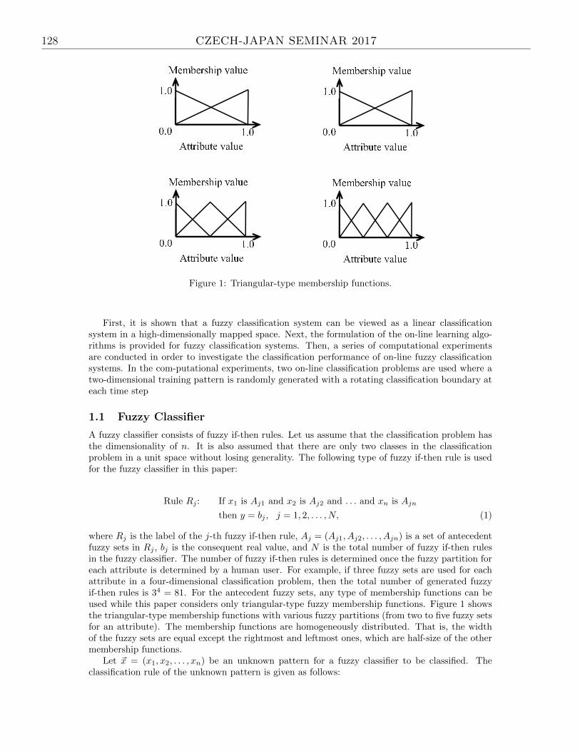
Figure 1: Triangular-type membership functions.

First, it is shown that a fuzzy classification system can be viewed as a linear classificationsystem in a high-dimensionally mapped space. Next, the formulation of the on-line learning algo-rithms is provided for fuzzy classification systems. Then, a series of computational experimentsare conducted in order to investigate the classification performance of on-line fuzzy classificationsystems. In the com-putational experiments, two on-line classification problems are used where atwo-dimensional training pattern is randomly generated with a rotating classification boundary ateach time step

1.1 Fuzzy Classifier

A fuzzy classifier consists of fuzzy if-then rules. Let us assume that the classification problem hasthe dimensionality of n. It is also assumed that there are only two classes in the classificationproblem in a unit space without losing generality. The following type of fuzzy if-then rule is usedfor the fuzzy classifier in this paper:

Rule Rj : If x1 is Aj1 and x2 is Aj2 and . . . and xn is Ajn

then y = bj , j = 1, 2, . . . , N, (1)

where Rj is the label of the j-th fuzzy if-then rule, Aj = (Aj1, Aj2, . . . , Ajn) is a set of antecedentfuzzy sets in Rj , bj is the consequent real value, and N is the total number of fuzzy if-then rulesin the fuzzy classifier. The number of fuzzy if-then rules is determined once the fuzzy partition foreach attribute is determined by a human user. For example, if three fuzzy sets are used for eachattribute in a four-dimensional classification problem, then the total number of generated fuzzyif-then rules is 34 = 81. For the antecedent fuzzy sets, any type of membership functions can beused while this paper considers only triangular-type fuzzy membership functions. Figure 1 showsthe triangular-type membership functions with various fuzzy partitions (from two to five fuzzy setsfor an attribute). The membership functions are homogeneously distributed. That is, the widthof the fuzzy sets are equal except the rightmost and leftmost ones, which are half-size of the othermembership functions.

Let ~x = (x1, x2, . . . , xn) be an unknown pattern for a fuzzy classifier to be classified. Theclassification rule of the unknown pattern is given as follows:


~x =

Class 1, if

N∑

j=1

bj · µj(~x) > 0,

Class 2, otherwise,

(2)

where µj(~x) is the compatibility of the j-th fuzzy if-then rule with the unknown pattern, which iscalculated using multiplication of membership values as follows:

µj(~x) = µj1(x1) · µj2(x2) · . . . · µjn(xn), (3)

where µji(xi), i = 1, 2, . . . , n is the membership value for the i-th attribute xi.

2 On-Line Learning Techniques

On-line learning techniques in this paper incrementally update the parameters of classifier models.The parameter update occurs every time a new training pattern becomes available. It is assumedthat only a single pattern becomes available at a time. Let us define ~xt as the training patternthat is available at Time t. The class of the training pattern ~xt is defined as ct (ct ∈ 1, 2).It is assumed that only one training pattern becomes available at each time step. This sectionintroduce a linear classifier as the conventional method as well as two on-line learning methodsthat are applicable to the linear classifier.

2.0.1 Linear Classifier

The class of an n-dimensional pattern ~x = (x1, x2, . . . , xn) is determined by the following rule:

~x =

Class 1, if

n∑

i=1

wi · xi + w0 > 0,

Class 2, otherwise,

(4)

where ~w = (w1, w2, . . . , wn) is a weight vector. The weight vector is determined so that theclassification error of the linear classifier is minimized in terms of a given set of training patterns.Typically, a least mean squared method is used. However, this is not exactly applicable in thispaper as there is no training pattern available for training the linear classifier model. It is alsopossible that the classification boundary changes over time. There are implicit requirements in theleast mean square method that all training patterns are available for training and the classificationboundary stays still and never changes.

The assumption in this paper is that not all training patterns are available before trainingclassifier models but gradually made available over time. Thus the classi-fier model requires toperform on-line learning where the model adapts itself every time a new training pattern becomesavailable.

2.1 Passive-Aggressive Learning

The training of the linear classifier described in Subsection 2.0.1 is generally formulated as anoptimization problem where the weight vector ~w = (w0, w1, . . . , wn) is determined in a way theerror between the target class of training patterns and the classification results by the linearclassifier is minimized. This formulation is possible if all the training patterns are available ata time. However, this paper considers a different situation where not all training patterns areavailable but only a limited number of training patterns is available at each time step. Crammer[3] proposed an on-line learning called passive-aggressive learning in order to tackle this specialsituation of training linear classifiers. The passive-aggressive learning uses the following hingefunction for calculating the error between the target class and the classification result:

lhinge(~x, c, ~w) = max0, 1− c× ~w · ~x, (5)

where ~x and c are a training pattern and its target class, respectively. This hinge loss functiongives the degree of errors in terms of the current weight vector ~w. In most of the cases, there exist


multiple weight vectors that makes the value of the loss function. The weight vector is modified sothat the amount of the update is minimized. Thus the optimization problem at time t is formulatedas follows:

~wt+1 = arg min~w

1

2||~w − ~wt||2 (6)

subject to lhinge(~xt, ct, ~w) = 0 (7)

where ~wt+1 is the updated weighted vector which will be used at the next time step, and ~wt, ~xt,and c are the current weight vector, the available training pattern and the target class at time t,respectively.

2.2 Confidence-Weighted Learning

The passive-aggressive learning in Subsection 2.1 has shown its powerful on-line performance inclassification and is already used in real-world systems. There is, however, a disadvantage in thismethod that the learning technique is too sensitive to noisy data. In order to overcome this problem,confidence-weighted learning technique was proposed by Dredze and Crammer [1]. This learningtechnique assumes that the weights in the linear function are not real values, but follows Gaussianprobability distributions. In this way, each weight has two parameters: the mean value and thewidth of a Gaussian function. The mean value shows the probable value of the correspondingweight, and the width shows the confidence in the mean value. When the confidence in the meanis low, the width of the Gaussian function is large while the width is small when the confidence ishigh. In the update of the Gaussian functions, the mean value will not largely modified when thewidth is small as the confidence in the mean value is high. On the other hand, when the width ofthe Gaussian function is large, the mean value will be moved largely because it is not sure if thecurrent mean value is appropriate or not.

Now that the weight vector ~w follows the Gaussian function, it is written as

~w ∼ N(~µ,∑

), (8)

where ~µ and∑

are the mean vectors and the co-variance matrix, respectively. When a trainingpattern ~xt becomes available with its target class ct for training the linear function at time t,the update of the weight values are performed so that the amount of the modification shouldbe minimized subject to the restriction that the probability of correct classification for the newtraining is higher than η. This is written as an optimization problem that is formulated as follows:

(~µt+1,

t+1∑) = arg min

~µ,∑DKL(N(µ,

∑)||N(~µt,

t∑)), (9)

subject to Prob~w N(~µ,

∑t)ct · (~w · ~xt) ≥ 0 ≥ η, (10)

where DKL is the Kalback-Leibler divergence between the two Gaussian distributions.

2.3 Adaptive Regularization of Weight Vectors

Adaptive regularization of weight vectors (AROW) [4] is an improved version of the confidenceweighted learning. This method has the following features:

• It decreases the variance for each vector only gradually.

• It correctly classifies the currently available training pattern as in the confidence weightedlearning and passive-aggressive learning.

• It minimizes the variation in the confidence distributions by the update.

Mathematical formulation of the adaptive regularization of weight vectors are written as follows:

(~µt+1,

t+1∑) = arg min

~µ,∑DKL(N(µ,

∑)||N(~µt,

t∑)) + λ1l(ct, ~µ · ~xt) + λ2~x

Tt

∑

t

~xt, (11)


l(ct, ~µ · ~xt) = (max 0, 1− ct(~µ · ~xt)2. (12)

As it can be seen from (11), each term in the formulation corresponds to the three featuresthat were mentioned above.

2.4 Applying the On-Line Learning Techniques to Fuzzy Classifiers

The on-line learning techniques in Subsections 2.1 and 2.2 can be applied to fuzzy classifiers.Equations (2) and (4) are the classification rule for an input pattern by a fuzzy classifier and alinear classifier, respectively. They can be seen as the same if the membership values of fuzzy if-then rules is treated as an input vector in a mapped space. That is, the fuzzy classifier performing a

linear classification in the mapped space by the fuzzy if-then rules. In the mapped space, ~µ(·) is the

input vector and ~b = (b1, b2, . . . , bN ) can be viewed as the weight vector in the linear classification.In this perspective, the fuzzy classifier can be updated in an on-line manner using either thepassive-aggressive learning or the confidence-weighted learning.

If the passive-aggressive learning is applied to the fuzzy classifier, the vector of the consequentreal values ~b is updated by solving the following optimization problem:

~bt+1 = arg min~b

1

2||~b−~bt||2 (13)

subject to lhinge(~µ(~xt), ct,~b) = 0 (14)

wherelhinge(~µ(~xt), ct,~b) = max

0, 1− ct ×~b · µ(~xt)

(15)

.In the case of the confidence-weighted learning, the consequent real values of fuzzy if-then rules

are assumed to follow Gaussian functions with the mean vector ~µb and the co-variance matrix∑b.

Then the parameters are modified by solving the following optimization problem:

(µt+1b ,

t+1∑

b

) = arg min~µb,∑

b

DKL(N(~µb,∑

b

)||N(~µtb,

t∑

b

)) (16)

subject to Prob~b N(~µtb,∑t

b)

ct · (~b · µ(~xt)) ≥ 0

≥ η. (17)

3 Noisy and Dynamic Classification Problems

3.1 Generating noisy training patterns

Without the loss of generality, let us consider a two-class classification problem in this paper.The classification problem in the computational experiments in this paper is a noisy and dynamicproblem. The noise is added in the generation process of training patterns. First, a two-dimensionalvector is randomly generated in the unit space [0, 1]2. Secondly, the class of the generated vectoris decided from the current classification boundary. Then, noise is added to the generated vector.The modified vector is only employed as a training pattern of the classifiers if the modifid vectorlies inside the unit two-dimensional space.

3.2 Dynamic Classification Boundary

The classification problems in the computational experiments of this paper is dynamic in the sensethat the true classification boundary is not static but keep changing over time. The classificationboundary rotates around some point. This kind of information is not used as a prior knowledgewhen a classifier is constructed. The only available information is the training pattern generatedby the procedure described in Subsection 3.1. Only a single training pattern is generated at atime step. We consider a linear and a non-linear classification boundary in the computationalexperiments in this paper as follows:


[Linear classification boundary]y = x. (18)

[Non-linear classification boundary]

y =1

2sin(2π · x · 0.4) · cos(2π · x · 0.6) +

1

2. (19)

Note that the above equations are at time step 0 and will rotate around a prespecified point bythe degree of one. The boundaries at time step 0 are shown in Fig. 2.

(a) Linear boundary (b) Non-linear boundary

Figure 2: Classification boundaries at time step 0. (a) the linear case and (b) the non-linear case.

4 Experiments

4.1 Experimental Settings

We consider two problems in the computational experiments of this paper. One is a static on-line problem where from a set of training patterns, randomly selected one is used to train theclassification models at one time. The other is its dynamic version where the classification boundarychanges over time.

4.2 Experimental Results

The computational experiments involve various on-line learning for fuzzy systems such as theconfidence-weighted learning, passive-aggressive learning, delta learning, and the adaptive regular-ization of weight vectors. In this section we only show the results for the classification problemwith the linear classification boundary in Fig. 2(a). First we show the experimental results for thestatic problem in Fig. 3.

From Fig. 3, it is shown that the AROW method quickly adapts the fuzzy classifier and keepshigh classification rates throughout the experiments. Next, we show the experimental results forthe dynamic problem in Fig. 4.

From Fig. 4, it is shown that the classification accuracy by the AROW is not stable at allbut goes ups and downs as the classification boundaries changes over time. This shows the poorclassification performance of AROW for dynamic problems.

5 Conclusions

This paper investigates the performance of AROW method for the on-line learning of fuzzy classi-fiers. Noticing that the fuzzy classifier performs a linear classification in a mapped space, we canre-formulate the on-line learning of the fuzzy classifiers as the optimization of consequent real vec-tors in the fuzzy if-then rules. AROW method is the target of the investigation. The experimentalresults show that AROW performs almost equally as the other on-line methods for static problem.


Figure 3: Experimental results for the static problem.

Figure 4: Experimental results for the dynamic problem.

However, for a dynamic problem it is not the case as AROW is too slow to adapt the weight vectorto the changing environment.

References

[1] Dredze, M. and Crammer, K.: Confidence-Weighted Linear Classification. Proc. of the 25thinternational conference on Machine learning, 264–271 (2008)

[2] Crammer, K., Dekel, O., Keshet, J., S-Shwartz, S., and Singer Y.: Online Passive-AggressiveAlgorithms. Journal of Machine Learning Research 7, 551–585 (2006)

[3] Ishibuchi, H., Nakashima, T., and Nii, M.: Classification and Modeling with Linguistic Infor-mation Granules: Advanced Approaches to Linguistic Data Mining, Springer (2004)

[4] Crammer, K., Kulesza, A., and Dredze, M.: Adaptive Regularization of Weight Vectors. Ma-chine Learning 7 (2), 155–187 (2013)


Triangular Norms in Max-t fuzzy algebras

Zuzana NEMCOVA

University of Hradec KraloveRokitanskeho 62, Hradec Kralove


Abstract

Many issues in the subject areas of optimization, geometry, control theory, machinescheduling, discrete event processes, manufacturing systems, telecommunication net-works, and traffic control can be solved by using various types of extremal algebras,according to the character of the study. Extremal algebras can help to understand thedevelopment of the system dynamics. The attractiveness of these tools is grounded inthe fact that the classes of the above mentioned nonlinear problems can be studied byapplying a linear-algebraic approach. The paper gives an overview and basic character-istics of a triangular norms (briefly t-norms) used in the so called max-t fuzzy algebrasto study steady states of discrete event systems. Among four main t-norms belong Lukasiewicz, Godel, Product and Drastic norm. Also an overview of basic literaturecovering this domain is given in the text.

Keywords: T-norm, Extremal algebra, Max-t fuzzy algebra.

1 Extremal Algebras

Extremal algebras are used mainly for describing and studying systems working in discrete time.During the operation of such a system, a stable state can arise. The system is described by atransition matrix and the eigenvectors of such a matrix represent the stable states of the system.

With the use of extremal algebras, we are able to get various answers about system character-istics. Some examples of these questions follow.

• What is the maximum speed at which the system could run?

• What is the latest time to start so that the production meets the delivery dates?

• If all machines start working at time zero, at what time will each machine finish work on theproject?

• Can the system repeatedly reach some sequence of states?

• How great a delay and to which events can be tolerated without prejudice to the calculatedfinishing time of the project?

• How to choose a sequence of nodes when travelling through some network, so that we visitas many nodes as possible before the given supplies are exhausted?

The term extremal algebra was used for the first time by [24]. This concept occurs under differentnames in the literature, for example, tropical algebra, max-algebra, or fuzzy algebra. It is a specialalgebraic structure equipped with two operations ⊕ and ⊗. The operation ⊕ is not addition as inusual algebra, but is one of the operations of extremum: maximum or minimum. The operationof ⊗ is a chosen group or semigroup operation so that these two operations can be commutativeand associative. The distributive law holds, and there exist neutral elements with respect to bothoperations [26]. For example, if one chooses ⊕ = max and ⊗ = min, one speaks of a max-minalgebra; if one chooses ⊕ = max and ⊗ = +, one speaks of max-plus algebra.

The operations ⊕, ⊗ are then extended in a natural way to Cartesian products of vectors andmatrices. The detailed mathematical investigation at a general level can be found in [3].


2 Max-t Fuzzy Algebras

The discrete time systems studied with the use of max-t fuzzy algebras can be sometimes intuitivelycalled fuzzy systems. But this can be confusing in some ways because the whole study of the systemin this way is not about studying “classical” fuzzy systems, which means constructing the functionof membership, fuzzification, inference and defuzzification. The main focus lies in the descriptionof the development of the system’s states in time. Both the states described by vectors and thetransition matrix have fuzzy numbers as entries. And this may be the reason why these systemsare sometimes called fuzzy. Naturally, the terminology is continually developing. For the transitionfrom one state to another, various operations for the conjunction of the sets are used. And theseoperations are also much used for studying “classical” fuzzy systems.

Fuzzy logic appeared as a necessary extension of Zadeh’s theory of fuzzy sets [25]. The devel-opment of fuzzy logic over the last two decades has been driven by the applications in artificialintelligence and decision making processes.

The standard membership degrees of fuzzy sets (values from the unit interval), can be under-stood in a natural way as the truth degrees of an infinite valued logic, with [0, 1] as its truth degreeset.

According to [10], fuzzy algebra claims that each object, say x, of the universe, denoted by X,belongs to a fuzzy set A with respect to a characteristic real number µA(x) called the degree ofmembership. In other words, it is the truth degree of the formula x ∈ A.

With this understanding, the intersection of the fuzzy sets A and B, i.e., A ∩ B, is µA∩B(x),and this corresponds to the truth degree of the statement x ∈ A AND x ∈ B. The word AND hasthe meaning of a conjunction connective. It can be claimed that the theory of crisp sets becomespresented in the language of classical logic. Already the first paper of Zadeh [25] offers differentproposals for understanding the above mentioned operation of conjunction, AND, as taking theminimum (or as taking a usual, algebraic product). Similarly, for the operation of union A ∪ B,Zadeh suggests taking the maximum of the membership degrees in A,B (or their algebraic sum).These relationships have been widely used in theoretical considerations about the foundations offuzzy set theory. In particular, in the last decade, there has been initiated an enormous developmentin the field of fuzzy logic in the narrow sense. [7]

Max-t fuzzy algebra is defined over the interval [0, 1], and, as the name suggests, has two binaryoperations: the operation of maximum (denoted by ⊕) and one of the t-operations, (denoted by ⊗)are used. These operations are extended to vectors and matrices in a formal way. According to thechosen t-operation, we can then talk, for example, about max- Lukasiewicz, max-min, max-prod ormax-drast fuzzy algebra.

3 Triangular Norms

Triangular norms (briefly t-norms) were first introduced by Karl Menger in 1942 in his paper [18].The main idea was to construct metric spaces where probability distributions (instead of numbers)describe the distance between two elements of the space. [12]

Schweizer and Sklar in [23] integrated t-norms into the context of probabilistic metric spaces.These t-norms are the operations used to interpret the conjunction in fuzzy logics and the in-tersection of fuzzy sets [13]. These functions have applications in many areas, such as decisionmaking processes, statistics, game theory, information and data fusion, probability theory, andrisk management. The t-norms, together with t-conorms, play a key role in fuzzy set theory. In-teresting results with practical impact using t-norms in the calculations can be found for examplein [4, 5, 15].

The t-norm is an operation of conjunction, denoted by 4, satisfying [11]:

14x = x

x4y = y4xx4(y4z) = (x4y)4z

If w ≤ x and y ≤ z then w4y ≤ x4z.

In other words, the operation is associative, commutative, nondecreasing, and has 1 as a neutralelement.


Remark 3.1. In fact, any operation that agrees with the truth table for two-valued conjunction isa candidate for a t-norm and that is why the definition of fuzzy logic operations may vary fromapplication to application. [11]

Although there exist many families of t-norms (for example, the Aczel–Alsina, the Jane Doe1,Hamacher, Dombi, Yager, Einstein product, for an overview see [6, 12]), four main t-norms will bedescribed in the following text: Lukasiewicz, Godel, Product and Drastic.

How to choose a suitable t-norm is a good question. The answer is not obvious. Each t-normoffers a good approach and sees things from a different perspective. In general, the t-norms can notbe linearly ordered. According to [10], some t-norms can be characterized as optimistic, with othersas pessimistic. Others assign a case a high degree of membership when one or more parametershave extreme values.

To fulfill domain-context demands, various applications require various t-norms, and sometimesit is necessary to create a new one. In [20], the following three basic methods of forming a newt-norm are described in detail:

• construction of a new t-norm on the basis of some given t-norms with the use of a monotonictransformation,

• the use of the addition and multiplication of real numbers together with a function of onevariable, called additive and multiplicative generators,

• forming a new t-norm from a family of given t-norms based on the concept of the “ordinalsum.”

3.1 Lukasiewicz Norm

The main motivation for the development of logic was to create a logical system that is free of someof the paradoxes in two-valued Boolean logic. The revolutionary step was made by Jan Lukasiewiczwith his introduction of three-valued logic, and later on also multi-valued logic [16, 17].

Both Lukasiewicz implication and negation were designed by Jan Lukasiewicz in 1930. Acomplete description of the derivation of Lukasiewicz conjunction can be also found in [7].

As mentioned above, the Lukasiewicz logic has the two following primitive connectives, impli-cation and negation [7]:

x→L y = min(1, 1− x+ y) (1)

¬x = 1− x (2)

From these primitive properties, further connectives are defined as syntactic abbreviations:

ϕ&ψ = ¬(ϕ→L ¬ψ), ϕ Y ψ = ¬ϕ→L ψ (3)

With the above defined properties, one gets a conjunction and a strong disjunction with truthdegree functions that are usually called Lukasiewicz arithmetical conjunction and Lukasiewiczarithmetical disjunction:

x& y = maxx+ y − 1, 0, x Y y = minu+ v, 1. (4)

Then, in the case of conjunction,

x⊗L y = maxx+ y − 1, 0. (5)

Lukasiewicz implication has applications in many fields. Together with the negation of Lukasiewiczimplication, it was used by Mills in [19] to design sensors for small robots. Lukasiewicz implicationis also used in [14] as a measure of the entropy of the fuzziness of messages, to develop fuzzy infor-mation theory. The use of the fuzzy conjunction in digital hardware implementation is formulatedin [22].

The fuzzy extension of description logics using Lukasiewicz logic (the formalism for the repre-sentation of structured knowledge) is described in [1]. Description logic is frequently used in thedesign of ontologies, which have been successfully used as part of expert and multiagent systems,as a knowledge base in robotics, as well as the core element in the Semantic Web (which aims atconverting the current Web into a “Web of data” by defining the meaning of information).


Lukasiewicz arithmetical conjunction can also be used in many types of situations in real life.The fact that the number 1 is subtracted and the maximum with zero is taken (in case thatx + y < 1) leads to the observation that the count of the operation is the remainder, some partthat is over the unit. Following this idea, the conjunction can be used to compute the amount ofmoney that should be paid off for a phone bill, where x can be the price for the total SMSs, and ycan represent the price for the calls in total. The number 1 here is replaced by the amount of thelump sum. There are other similar situations, for example, data backup on a server, the maximalcapacity of a pond, overspending of project funds, or savings of partners with a common bill.

3.2 Godel Norm

This is the simplest norm, in the literature known also as the “minimum norm” or the “strongestnorm”; the conjunction is defined as the minimum of the entries: of the truth degrees of theconstituents [6].

x⊗G y = min(x, y) (6)

In contrast to Lukasiewicz logic (which might be considered as a logic of absolute or metric com-parison), Godel logic is a logic with a relative comparison.

3.3 Product Norm

The definition of the product norm follows, a complete description of this norm can be found in[9].

x⊗p y = x · y (7)

In [21] there can be found the application and comparison of the Godel and Product norms in aclassification problem—the ordering of some finite set of evaluations according to certain criteria.The product norm corresponds here to the stochastic or probability independence of elementaryevents (propositional letters), while the Godel norm represents another kind of extreme situation:the logical dependence of propositional letters.

3.4 Drastic Norm

The drastic triangular norm (in the literature there can be also found the term “weakest norm” or“drastic product”) is the basic example of a non-divisible t-norm on any partially ordered set, see[2]. The drastic triangular norm (the operation of ⊗d) is defined as follows:

x⊗d y =

min(x, y) if max(x, y) = 1

0 if max(x, y) < 1(8)

The drastic norm is “drastic” in the sense that when there is some possibility of using, for example,two weighted paths, say path x and path y, they can be used if and only if one of them is equalto 1. Otherwise such a concatenated path can not be used. Moreover, if the walk consists of morethan two paths, then at most one path can be weighted by a value less than 1. The interpretationof the drastic norm then reflects a situation when extreme demands are imposed on the reliabilityof a system: the walk is reliable if there is no more than one unsure segment.

The matrix powers in max-drast algebra behave differently than those in max-min algebra.However, the properties of the matrix periods in both cases show some similarity.

The differences between the four basic t-norms can be seen in Figure 2. Although the figuredepicts the intersection of the fuzzy sets in the classical conception, the plots show the differencebetween the operations clearly. The contour plots for the basic t-norms can be seen in Figure 1(the contour plot shows us the sets where the function in question has constant values). From thefigure it can also be seen that the Godel, Product and Lukasiewicz norms are continuous whereasthe drastic norm is not. According to [20], the continuity of the operations on fuzzy sets is a highlydesirable feature in many applications.

The norms can be also compared, for details see [12], since they are just functions. Thecomparison is done pointwise. If for two t-norms, say 41 and 42, it holds that

x 41 y ≤ x 42 y


for all x, y ∈ [0, 1], then 41 is weaker than 42 (or, equivalently, it can be said, 42 is stronger than41), and thus one can write 41 ≤ 42. This yields the following order of the four basic t-norms:

Drastic < Lukasiewicz < Product < Godel.

It can also be observed from the definitions of the operations for the t-norms that by using theproduct or Lukasiewicz norm, new elements (values) are generated, whereas for the Godel anddrastic norm this is not true. The drastic norm is also characterized by the fact that small changesin the inputs produce big changes in the output. This results from the character of the operations.

The characteristic of idempotency can be formulated as follows: the value x is idempotent ifx4x = x. Note that the values 0 and 1 are idempotent elements for any t-norm. The t-norm isArchimedean (i.e., for any two elements a and b from the set there exists n ∈ N such that n ·a > b)if and only if its only idempotent elements are the trivial ones 0 and 1. [2]

Figure 1: Contour plot of the t-norms: (a) Godel, (b) Product, (c) Lukasiewicz, (d) Drastic. [12]


Figure 2: T-norms used in the realization of the intersection of fuzzy sets A and B: (a) Godel, (b)Product, (c) Lukasiewicz, (d) Drastic. [20]

4 Triangular Conorms

A brief characterization of the triangular conorms (t -conorms for short) will be given next. At-conorm is an operation of disjunction, the dual operation to that of a t-norm, on the unit interval,


denoted by ∇, and satisfying [11]

0∇x = x

x∇y = y∇xx∇(y∇z) = (x∇y)∇z

If w ≤ x and y ≤ z then w∇y ≤ x∇z.

A t-conorm can be generated from a t-norm by

x∇y = 1− (x+ 1)4(y + 1) (9)

Among the basic t-conorms there are [12]

Maximum: x⊕G y = max(x, y)

Probabilistic sum: x⊕p y = x+ y − x · y Lukasiewicz sum: x⊕L y = min(x+ y, 1)

Drastic sum: x⊕d y =

1 if min(x, y) > 0

max(x, y) if min(x, y) = 0

It can be easily seen from the definition of a conorm that the difference between norms andconorms lies in their boundary conditions. The name, t-conorm, comes from the fact that in theunit interval, the value x acts in a similar way as its complement 1− x. [12]

Similarly to triangular norms, the conorms can be visualized, see Figure 4 for 3D and Figure 3for contour plots.

Remark 4.1. Since both the operations for t-norms and t-conorms were introduced as operationswith two arguments, they can be, of course, extended to n-ary operations in the usual way byinduction.

Figure 3: Contour plot of the t-conorms: (a) Maximum, (b) Product, (c) Lukasiewicz, (d) Drastic.[12]


Figure 4: T-conorms used in the realization of the intersection of fuzzy sets A and B: ((a) Maxi-mum, (b) Product, (c) Lukasiewicz, (d) Drastic. [20]

AcknowledgementThe financial support of the Excellence Project at FIM UHK is gratefully acknowledged.

References

[1] Bobillo, F. and Straccia, U. (2011). Reasoning with the finitely many-valued Lukasiewiczfuzzy description logic. Information Sciences, 181(4):758–778.


[2] Casasnovas, J. and Mayor, G. (2008). Discrete t-norms and operations on extended multisets.Fuzzy Sets and Systems, 159(10):1165–1177.

[3] Cuninghame-Green, R. A. (1979). Minimax Algebra. Lecture Notes in Economics and Math-ematical Systems vol. 166. Springer-Verlag, Berlin.

[4] Chaira, T. (2015). Fuzzy mathematical morphology using triangular operators and its appli-cation to images. Journal of Intelligent and Fuzzy Systems, 28(5):2269–2277.

[5] Chen, X.-G. and Du, H. (2015). Interval-valued triangular fuzzy soft set and its method ofdynamic decision making. Xi Tong Gong Cheng Yu Dian Zi Ji Shu/Systems Engineering andElectronics, 37(5):1111–1115.

[6] Gottwald, S. (2001). A Treatise on Many-Valued Logics, volume 3. Research Studies PressBaldock.

[7] Gottwald, S. (2005). Mathematical fuzzy logic as a tool for the treatment of vague information.Information Sciences, 172(1):41–71.

[8] Goverde, R. (2010). A delay propagation algorithm for large-scale railway traffic networks.Transportation Research Part C: Emerging Technologies, 18(3):269–287.

[9] Hajek, P., Godo, L., and Esteva, F. (1996). A complete many-valued logic with product-conjunction. Archive for Mathematical Logic, 35(3):191–208.

[10] Iliadis, L., Spartalis, S., and Tachos, S. (2008). Application of fuzzy t-norms towards a newartificial neural networks evaluation framework: A case from wood industry. InformationSciences, 178(20):3828–3839. Special Issue on Industrial Applications of Neural Networks10th Engineering Applications of Neural Networks 2007.

[11] Jantzen, J. (2007). Foundations of Fuzzy Control. John Wiley & Sons.

[12] Klement, E. P., Mesiar, R., and Pap, E. (2000). Triangular Norms. Springer.

[13] Klement, E. P., Mesiar, R., and Pap, E. (2004). Triangular norms. Position paper I: Basicanalytical and algebraic properties. Fuzzy Sets and Systems, 143(1):5–26.

[14] Kosko, B. (1986). Fuzzy entropy and conditioning. Information sciences, 40(2):165–174.

[15] Liang, C., Zhao, S., and Zhang, J. (2014). Aggregation operators on triangular intuitionisticfuzzy numbers and its application to multi-criteria decision making problems. Foundations ofComputing and Decision Sciences, 39(3):189–208.

[16] Lukasiewicz, J. (1930). Philosophische bemerkungen zu mehrwertigen systemen des aus-sagenkalk. C. R. Soc. Sci. Lett. Varsovie, 23:51–77.

[17] Lukasiewicz, J. (1970). Studies in Logic and the Foundations of Mathematics. North-Holland.

[18] Menger, K. (1942). Statistical metrics. Proceedings of the National Academy of Sciences,28(12):535–537.

[19] Mills, J. W. (1993). Lukasiewicz’ insect: The role of continuous-valued logic in a mobilerobot’s sensors, control, and locomotion. In Proceedings of The Twenty-Third InternationalSymposium on Multiple-Valued Logic, 1993, pages 258–263. IEEE.

[20] Pedrycz, W. and Gomide, F. (2007). Fuzzy Systems Engineering: Toward Human-centricComputing. John Wiley & Sons.

[21] Perovic, A., Ognjanovic, Z., Raskovic, M., and Radojevic, D. (2011). Finitely additive prob-ability measures on classical propositional formulas definable by Godel’s t-norm and productt-norm. Fuzzy Sets and Systems, 169(1):65–90.

[22] Rudas, I. J., Batyrshin, I. Z., Zavala, A. H., Nieto, O. C., Horvath, L., and Vargas, L. V.(2008). Generators of fuzzy operations for hardware implementation of fuzzy systems. InMICAI 2008: Advances in Artificial Intelligence, pages 710–719. Springer.


[23] Schweizer, B., Sklar, A., et al. (1960). Statistical metric spaces. Pacific J. Math,10(19601):313–335.

[24] Vorobjov, N. N. (1967). Extremal Algebra of positive Matrices. Datenverarbeitung und Ky-bernetik, 3:37–71.

[25] Zadeh, L. (1965). Fuzzy sets. Information and Control, 8:338–353.

[26] Zimmermann, K. (2003). Disjunctive optimization, max-separable problems and extremalalgebras. Theoretical Computer Science, 293(1):45–54.


Bivariate Fuzzy Transform Based on Tensor

Product of Two Polynomial Spaces in Analysis of

Correlation Functions

Linh NGUYEN and Michal HOLCAPEK

University of OstravaInstitute for Research and Applications of Fuzzy Modelling, NSC IT4Innovations

30. dubna 22, 701 03 Ostrava 1, Czech RepublicLinh.Nguyen, [email protected]

Abstract

This paper introduces a new type of fuzzy transformation of higher degree applied tobivariate complex-valued functions, which is based on the tensor product of two poly-nomial spaces. We demonstrate that the new type of fuzzy transform is efficient in thestudy of random processes, namely, in the analysis of correlation functions of randomprocesses after the application of higher degree fuzzy transform.

Keywords: Fuzzy transform, tensor product space, functional approximation, corre-lation function.

1 Introduction

The theory of fuzzy transform (F-transform) has been introduce by Perfilieva in the seminal paper[1] devoted to a new type of approximation of real-valued functions with a motivation in fuzzymodeling (Sugeno–Takagi models). The F-transform consists of two phases, namely, the directand inverse F-transform. A generalization of the F-transform towards higher degrees (denotedas an Fm-transform for m ∈ N) has been proposed in [2], where the original F-transform is ofdegree zero. The generalization uses the linear spaces of polynomials of degrees at most equal tom as its approximation spaces that are, in fact, the subspaces of weighted Hilbert spaces whoseweighted functions together form a fuzzy partition of the real line or usually a closed subinterval.The direct Fm-transform transforms a given (real-valued or complex-valued) function into a vectorof polynomials that are the orthogonal projections of the given function into the approximationspaces. The inverse Fm-transform provides an approximation of the original function made fromits direct Fm-transform components. Among the most important advantages of Fm-transformbelongs: the low computational cost, the very good compression ability, or the high efficiency inthe noise reduction. Therefore, it is not surprising that the Fm-transform has been successfullyapplied in many fields of computer science as well as applied mathematics [3, 4, 5, 6, 7, 8, 9, 10].

The theory of fuzzy transform, particularly the Fm-transform, has been generalized to bivariate(multivariate) case in [11, 12, 13, 14]. The theoretical results on the bivariate Fm-transform gaverise efficient methods that have been successfully applied to image processing like the edge detectionor the image reconstruction [11, 15].

Recently, we investigated the Fm-transform to analyze stationary random processes. The pre-liminary results can be found in [16]. Due to our analysis of the correlation function of a randomprocess obtained by the inverse Fm-transform (an approximate random process), we realized thatthere is an interesting relationship between the correlation functions of the original random processand the approximate random process, which can be nicely described by a new type of bivariatehigher degree fuzzy transform, where the standard approximation space of bivariate polynomialsis replaced by the tensor product of two spaces of univariate polynomials. The aim of this paperis to introduced the “new” type of bivariate fuzzy transform including a computation method forthe derivation of its components (bivariate polynomials) and demonstrate its usefulness in theinvestigation of the correlation function of random processes.


The paper is structured as follows. The next section contains a necessary background for theintroduction of the bivariate Fm-transform based on the tensor product of two polynomial spaces.The third section provides the definition and basic properties. The fourth section is devoted to theanalysis of the correlation function of a random process after the application of Fm-transform.

2 Preliminaries

2.1 Fuzzy partition

Fuzzy transform technique is based on a fuzzy partition of the real line (n-dimensional space) ora closed interval (n-dimensional cuboid). In this paper, we consider a generalized uniform fuzzypartition of the real line R and the plane R2. The both uniform fuzzy partitions are determinedfrom generating functions defined as follows.

Definition 1. A real-valued function K : R → [0, 1] is said to be a generating function if it iscontinuous, even, non-increasing on [0, 1) and vanishing outside of (−1, 1).

The following example provides two generating functions which are frequently used in applica-tions of the F-transform.

Example 1. The functions Ktr,Krc : R→ [0, 1] defined by

Ktr(t) = max(1− |t|, 0) (1)

Krc(t) =

12 (1 + cos(πt)), −1 ≤ t ≤ 1;

0, otherwise,(2)

for any t ∈ R, are called the triangle and raised cosine generating functions, respectively.

In [17], a generalized uniform fuzzy partition of the real line is introduced as follows. We useR+ and Z to denote the set of positive real numbers and integers, respectively.

Definition 2. Let K be a generating function, let x0 ∈ R, and let h, k ∈ R+. A family A = Ak |k ∈ Z of fuzzy sets on R determined by

Ak(x) = K

(x− x0 − kr

h

)(3)

is said to be a generalized uniform fuzzy partition of R determined by the quadruple (K,h, r, x0)if the following condition is fulfilled

∑

k∈ZAk(x) = 1, x ∈ R. (4)

The fuzzy set Ak is called the k-th basic function of the generalized uniform fuzzy partition A. Theparameters h, r and x0 are called the bandwidth, shift and central node.

Note that condition (4) is called the Ruspiny condition or the partition of unity. For the sake ofsimplicity, we omit the term “generalized” in the expression “generalized uniform fuzzy partition”.

For a bivariate fuzzy transform, we extend the previous definition to a uniform fuzzy partitionof the plane, where the bivariate generating function is defined as the product of two univariategenerating functions. A more general definition of bivariate (multivariate) uniform fuzzy partitioncan be found in [18].

Definition 3. Let K1,K2 be generating functions. A function K : R2 → [0, 1] defined by

K(x, y) = K1(x) ·K2(y), (x, y) ∈ R2,

is called the bivariate generating function determined by K1 and K2.


A uniform fuzzy partition of the plane is defined in the similar way as the uniform fuzzypartition of the real line. For the sake of simplicity, we omit a reference to uniform generatingfunctions that determine a bivariate generating function if we do not need to specify them or noconfusion can appear.

Definition 4. Let K be a bivariate generating function, let (x0, y0) ∈ R2, and let (h1, h2), (r1, r2) ∈R2

+. A family A = Ak1,k2 | k1, k2 ∈ Z of fuzzy relations on R2 determined by

Ak1,k2(x, y) = K(x− x0 − k1r1

h1,y − y0 − k2r2

h2

),

is said to be a uniform fuzzy partition of R2 determined by the quadruple (K, (h1, h2),(r1, r2), (x0, y0)) if the following condition is fulfilled:

∑

k1,k2∈ZAk1,k2(x, y) = 1, for any (x, y) ∈ R2.

The fuzzy relation Ak1,k2 is called the (k1, k2)-th basic function of the uniform fuzzy partitionA. The pairs (h1, h2), (r1, r2) and (x0, y0) are called the bandwidth, shift and central node,respectively.

Obviously, the adjustment of a central node x0 has no influence on the theoretical results con-cerning the fuzzy transform. Therefore, we restrict our investigation to the uniform fuzzy partitions,where x0 = 0, and we deal with the uniform fuzzy partitions determined by triplets (K,h, r). Thesame restriction is also assumed for the uniform fuzzy partitions of the plane that are determinedsimply by triplets (K, (h1, h2), (r1, r2)). Additionally, we use Ak[h](x) and Ak1,k2 [h1, h2](x, y) todenote the basic functions of uniform fuzzy partitions of R and R2, respectively, in all the situa-tions when the bandwidth is important and should be emphasized. A simple consequence of thedefinition of uniform fuzzy partition of the plane is the following statement.

Lemma 1. Let A = Ak1,k2 | k1, k2 ∈ Z be a uniform fuzzy partition of R2 determined by thetuple (K, (h1, h2), (r1, r2)), where K is a bivariate generating function determined by the generatingfunctions K1 and K2. If AX = AX,k1 | k1 ∈ Z and AY = AY,k2 | k2 ∈ Z denote the families offuzzy sets determined by triplets (K1, h1, r1) and (K2, h2, r2) as in (3), respectively, then AX andAY are uniform fuzzy partitions of R and

Ak1,k2(x, y) = AX,k1(x) ·AY,k2(y), x, y ∈ R,

holds for any k1, k2 ∈ Z.

Proof. It is sufficient to show that AX and AY are uniform fuzzy partitions of R; the rest ofthe proof immediately follows from the definition of the basic function Ak1,k2 . Let x, y ∈ R bearbitrary. Since A is a uniform fuzzy partition, we find that

1 =∑

k1,k2∈ZAk1,k2(x, y) =

∑

k1∈ZAX,k1(x) ·

∑

k2∈ZAY,k2(y),

which implies∑k1∈ZAX,k1(x) = 1 and

∑k2∈ZAY,k2(y) = 1.

2.2 Univariate fuzzy transform

Let L2loc(R) be a set of all complex-valued functions that are square integrable on any closed

subinterval of the real line. Below, we recall the definition of the direct and inverse Fm-transformwith the components (polynomials) derived from the monomial basis [14, 19, 20]. We use N todenote the set of natural numbers with zero.

Definition 5. Let f ∈ Lloc(R), m ∈ N, and let A be a uniform fuzzy partition of the real linedetermined by the triplet (K,h, r). The direct fuzzy transform of degree m (direct Fm-transform)of f with respect to A is a family

FmA [f ] = Fmk [f ] | k ∈ Z ,


of polynomials of the shape

Fmk [f ](x) = Cz,0 + Ck,1

(x− xkh

)+ · · ·+ Ck,m

(x− xkh

)m(5)

with the coefficients determined by

(Ck,0, Ck,1, . . . , Ck,m)T = (Zm)−1 · Ym,k,

where Zm = (Zij) is a (m+ 1)× (m+ 1) invertible matrix defined by

Zij =

∫ 1

−1xi+j−2K(x) dx, i, j = 1, . . . ,m+ 1, (6)

and Ym,k = (Yk,1, . . . , Yk,m+1)T is a vector defined by

Yk,` =

∫ 1

−1f(hx+ xk) · x`−1K(x) dx, ` = 1, . . . ,m+ 1. (7)

The polynomial Fmk [f ] is called the k-th component of the direct Fm-transform with respect to A.

The inverse Fm-transform is a linear like combination of the components of the direct Fm-transform and the values of basic functions.

Definition 6. Let f ∈ L2loc(R), let A = Ak | k ∈ Z be a uniform fuzzy partition of the real line,

and let FmA [f ] = Fmk [f ] | k ∈ Z denote the direct Fm-transform of the function f with respectto A. The inverse fuzzy transform of degree m (inverse Fm-transform) of f with respect to A isdefined by

fmA (x) =∑

k∈ZFmk [f ](x) ·Ak(x), x ∈ R. (8)

The inverse Fm-transform fmA approximates the original function f . The quality of the ap-proximation depends on the parameter’s setting of the fuzzy partition A. For details, we refer to[2, 19, 20].

3 Bivariate fuzzy transform based on tensor product of twopolynomial spaces

3.1 Definitions

Let Pm and Pn (m,n ∈ N) denote the linear spaces of all complex-valued polynomials P (x) andP (y) of degree at most equal to m and n, respectively. For any m,n ∈ N, we use Pm ⊗ Pn denotethe tensor product of Pm and Pn. It is easy to see that Pm ⊗ Pn is a linear space of dimensionN = (m+ 1)(n+ 1). For any ` = 1, . . . , N , consider P`(x, y) = xq`yr` , where q`, r` ∈ N such that`− 1 = (n+ 1) · q` + r` and r` ≤ n. Obviously, ql is the quotient and r` is the remainder when wedivide `−1 by n+ 1 in long division. Then, P1, . . . , PN = xiyj | i = 0, 1, . . . ,m, j = 0, 1, . . . , nforms a basis of the tensor product Pm ⊗ Pn.

Let L2loc(R2) be a set of all complex-valued functions f defined on R2 that satisfy

∫

I

|f(x, y)|2dxdy <∞,

for any compact set I ⊂ Rn. Let A = Ak1,k2 | k1, k2 ∈ Z be a uniform fuzzy partition of R2

determined by a triplet (K, (h1, h2), (r1, r2)). For any k1, k2 ∈ Z, put xk1 = k1r1 and yk2 = k2r2.Let L2(Ak1,k2) be the set of complex-valued functions f defined on the rectangle Uk1,k2 = [xk1 −h1, xk1 + h1]× [yk2 − h2, yk2 + h2] such that

∫

Uk1,k2

|f(x, y)|2dxdy <∞.


Define on L2(Ak1,k2) an operator 〈·, ·〉Ak1,k2 : L2(Ak1,k2) × L2(Ak1,k2) → C, where C denotes theset of all complex numbers, as follows:

〈f, g〉Ak1,k2 =

∫

Uk1,k2

f(x, y)g(x, y)Ak1,k2(x, y)dxdy (9)

where g(x, y) denotes the complex conjugate of g(x, y). The operator forms an inner product inL2(Ak1,k2). Furthermore, L2(Ak1,k2) equipped by the inner product 〈·, ·〉Ak1,k2 is a Hilbert space,

where we identify functions that differs in a set of zero measure. We refer to the space L2(Ak1,k2)as the weighted Hilbert space with respect to the basic function Ak1,k2 . For (h1, h2) = (1, 1) and(k1, k2) = (0, 0), i.e., A0,0[1, 1] = K, we use L2(K) and 〈·, ·〉K to denote the space L2(A0,0[1, 1]) andits inner product, respectively. Let f, g ∈ L2(Ak1,k2), and let L be a linear subspace of L2(Ak1,k2).We say that f is orthogonal to g in L2(Ak1,k2) and denote it by f⊥Ak1,k2 g, if 〈f, g〉Ak1,k2 = 0.

Similarly we say that f is orthogonal to L in L2(Ak1,k2) and denote it by f⊥Ak1,k2L, if f⊥Ak1,k2 gfor any g ∈ L.

Since any function from L2loc(R2) restricted to Uk1,k2 belongs to L2(Ak1,k2), the inner product

〈f |Uk1,k2 , g|Uk1,k2 〉Ak1,k2 is well defined for any f, g ∈ L2loc(R2), where f |Uk1,k2 and g|Uk1,k2 denote

the respective restrictions to Uk1,k2 . In the sequel, the arguments of 〈·, ·〉Ak1,k2 or ‖ · ‖Ak1,k2 (the

norm of the Hilbert space L2(Ak1,k2)) are always the functions that are restricted to Uk1,k2 . Forexample, if P and Q are two polynomials and we use 〈P,Q〉Ak1,k2 , then P and Q are polynomialsrestricted to Uk1,k2 . Notice that the computation of the inner product with respect to a basicfunction does not require the restriction of functions on a rectangle, the restriction is importantonly from the formal point of view and ensures that we deal within our framework of the weightedHilbert spaces.

For any k1, k2 ∈ Z, let us denote by Pm,k1 ⊗ Pn,k2 the set of bivariate polynomials from thetensor product Pm⊗Pn that are restricted to Uk1,k2 . It is easy to see that Pm,k1 ⊗Pn,k2 is a closedlinear subspace of L2(Ak1,k2). Similarly to the definition of Fm-transform, the bivariate fuzzytransform based on the tensor product of polynomial spaces has two phases. Their definitions areas follows.

Definition 7. Let A = Ak1,k2 | k1, k2 ∈ Z be a uniform fuzzy partition of R2, and let f be afunction from L2

loc(R2). The direct fuzzy transform based on Pm⊗Pn (the direct Fm⊗n-transform)of f with respect to A is a family

Fm⊗nA [f ] =Fm⊗nk1,k2

[f ] ∈ Pm,k1 ⊗ Pn,k2 | k1, k2 ∈ Z, (10)

where (f − Fm⊗nk1,k2[f ])⊥Ak1,k2 (Pm,k1 ⊗ Pn,k2) in L2(Ak1,k2). The bivariate polynomial Fm⊗nk1,k2

[f ] is

called the (k1, k2)-th component of the direct Fm⊗n-transform of f with respect to A.

Definition 8. Let A = Ak1,k2 | k1, k2 ∈ Z be a uniform fuzzy partition of R2, let f ∈ L2loc(R2),

and let Fm⊗nA [f ] =Fm⊗nk2,k2

[f ] | k1, k2 ∈ Z

denote the direct Fm⊗n-transform of f with respect to

A. The function

fm⊗nA (x, y) =∑

k1,k2∈ZFm⊗nk1,k2

[f ](x, y) ·Ak1,k2(x, y), (x, y) ∈ R2, (11)

is called the inverse fuzzy transform based on tensor product Pm⊗Pn (the inverse Fm⊗n-transform)of f with respect to A.

3.2 Computation of the direct Fm⊗n-transform components

In this subsection, we introduce the computation of the direct Fm⊗n-transform components forwhich the (k1, k2)-th component is computed with respect to the basis

P`

(x− tk1h1

,y − tk2h2

)| ` = 1, . . . , N

of the approximation space Pm,k1 ⊗Pn,k2 , where P` = P`(x, y) = xq`yr` (` = 1, . . . , N) denotes the`-th element of the basis of Pm ⊗ Pn restricted to the square [−1, 1]× [−1, 1].


Let us define the following square matrix of the size N ×N (N = (m+ 1)(n+ 1)):

Zm⊗n =

〈P1, P1〉K 〈P1, P2〉K . . . 〈P1, PN 〉K〈P2, P1〉K 〈P2, P2〉K . . . 〈P2, PN 〉K

· · · · · · . . . · · ·〈PN , P1〉K 〈PN , P2〉K . . . 〈PN , PN 〉K

, (12)

where 〈·, ·〉K is the inner product in L2(K). Recall that

〈P`, Pk〉K =

∫ 1

−1

∫ 1

−1xq`+qkyr`+rk dxdy (13)

For any `, k = 1, . . . , N . Recall that Zm denotes the (m + 1) × (m + 1) matrix whose elementsare the inner products of polynomials from the monomial basis 1, . . . , xm of the space Pm (seeDefinition 5). Similarly, define the (n+1)× (n+1) matrix Zn that consists of the inner product ofpolynomials from the monomial basis 1, . . . , yn of the space Pn. The following lemma is essentialin the computation of the direct Fm⊗n-transform components.

Lemma 2. Let Zm⊗n be the matrix defined in (12). Then, Zm⊗n = Zm⊗Zn, where ⊗ means thetensor (Kronecker) product of matrices. Moreover, Zm⊗n is a real and invertible matrix.

Proof. The first part of the statement is a simple consequence of Fubini’s theorem. By Lemma2.8 in [20] (see also Lemma 8 in [19]), the matrices Zm and Zn are real and invertible. It is wellknown that (Zm⊗n)−1 = (Zm)−1 ⊗ (Zn)−1. Hence, Zm⊗n is real and invertible.

Using the properties of the inner product and the previous lemma, one can prove the followingstatement that provides a simple approach based on matrix calculus to the computation of thedirect Fm⊗n-transform components.

Theorem 3. Let f ∈ L2loc(R), and let A be a uniform fuzzy partition of R2 determined by the

tuple (K, (h1, h2), (r1, r2)). Let m,n ∈ Z and N = (m+ 1)(n+ 1). Then, the (k1, k2)-th componentof the direct Fm⊗n-transform of f with respect to A has the following form

Fm⊗nk1,k2[f ](x, y) =

N∑

`=1

Ck1,k2,` · P`(x− tk1h1

,y − tk2h2

)(14)

determined by(Ck1,k2,1, Ck1,k2,2, . . . , Ck1,k2,N )T = (Zm⊗n)−1 · Yk1,k2m⊗n (15)

where Zm⊗n is the matrix defined in (12), and

Yk1,k2m⊗n = (Yk1,k2,1, Yk1,k2,2, . . . , Yk1,k2,N )T

is defined by

Yk1,k2,k =

∫ 1

−1

∫ 1

−1f(uh1 + tk1 , vh2 + tk2) · Pk(u, v) · K(u, v)dudv, (16)

for k = 1, . . . , N .

From (15), one can see that also the Fm⊗n-transform is a linear map. Moreover, if a bivariatefunction can be express as a product of two univariate functions, each component of the directFm⊗n-transform of the original function is the product of a component of the direct Fm-transformand a component of the direct Fn-transform applied to the univariate functions as the followingstatement shows.

Theorem 4. Let f be a bivariate complex-valued function such that f(x, y) = X (x) · Y (y)where X ,Y ∈ L2

loc(R). Let A be a uniform fuzzy partition of R2 determined by the tuple(K, (h1, h2), (r1, r2)) with K(x, y) = K1(x) · K2(y). Then, for any k1, k2 ∈ Z, (x, y) ∈ [tk1 −h1, tk1 + h1]× [tk2 − h2, tk2 + h2], it holds that

Fm⊗nk1,k2[f ](x, y) = Fmk1 [X ](x) · Fnk2 [Y ](y),

where Fmk1 [X ] and Fnk2 [Y ] are the k1-th and k2-th components of the direct Fm- and Fn-transformsof the function X and Y with respect to the uniform fuzzy partitions of the real line determinedby the triplets (K1, h1, r1) and (K2, h2, r2), respectively.


Sketch of proof. It is a consequence of Lemma 2, Fubini’s theorem and matrix calculus.

The following corollary is a straightforward consequence of Theorem 4. It provides a simple wayfor the computation of the inverse Fm⊗n-transform of bivariate functions that can be separatedinto a product of two univariate functions.

Corollary 5. Let the assumptions of Theorem 4 be satisfied. Then,

fm⊗nA (x, y) = X mA1

(x) · Y nA2

(y),

where X mA1

and Y nA2

are the inverse Fm- and Fn-transforms of the function X and Y with respectto the uniform fuzzy partitions AX and AY of the real line respectively determined by the triplets(K1, h1, r1) and (K2, h2, r2), respectively.

Example 2. Let us consider two bivariate functions

1. f(x, y) = (x+ y) sin 3y − 3 cosx,

2. g(x, y) = 5 cos 2x · sin(3y + π

3

).

In Figure 1, we display the inverse F2⊗1-transform of f with respect to the bivariate uniform fuzzypartition determined by the triplet (K,h, r), where K(x, y) = Ktr(x)·Ktr(y) and h = r = (0.4, 0.4).The result is restrict on the rectangle [0, 4]2. Additionally, by using the same fuzzy partition wecompute the inverse F0⊗2-transform of function g. However, instead of using Theorem 3 and, then,Definition 8 for the computation, we apply Corollary 5 because g is a variable separable function.As a result, we only need to compute the inverse F0-transform and inverse F2-transform of thefunctions X (x) = 5 cos 2x and Y (y) = sin

(3y + π

3

), respectively, with respect to the triangular

uniform fuzzy partition determined by the triplet (Ktr, 0.4, 0.4). The result is then obtain by theapplication of Corollary 5, which is depicted in Figure 2.

Figure 1: Inverse F2⊗1-transform of f

4 Fm⊗n-transform in the analysis of correlation functions

Let ξ(t), t ∈ R, be a complex-valued random process, and assume that Γ(t, s) is its correlationfunction, i.e.,

Γ(t, s) = E(ξ(t) · ξ(s)

), (t, s) ∈ R2.

We know that the theory of correlation functions is one of the fundamental tools in the investigationof the behavior of random processes (see, e.g., [21]). Recently, we provided in [16] an analysis ofrandom processes using the fuzzy transform of higher degree. This analysis is a continuation ofthe research introduced in [22, 23]. In what follows, we show that the Fm⊗n-transform reveals


Figure 2: Inverse F0⊗2-transform of g

the relationship between the correlation function of a random processes ξ(t) and the correlationfunction of the inverse Fm-transform of ξ(t).

Let AX be a uniform fuzzy partition of the real line determined by the triplet (K,h, r). Itfollows from [16] that the k1-th component of the direct Fm-transform of ξ(t) with respect to AXis determined as follows:

Fmk1 [ξ](t) =

m∑

i,p=0

(t− tk1h

)i· Ti+1p+1 ·

∫ 1

−1ξ(hτ − tk1) · τpK(τ)dτ

where (Tij)i,j=1,m+1 = (Zm)−1. Let Fm⊗mk1,k2[Γ] be the (k1, k2)-th component of the direct Fm⊗m-

transform of Γ with respect to the uniform fuzzy partition of R2 determined by the tuple (K, (h, h),(r, r)) with K(x, y) = K(x) · K(y). As a result, for any k1, k2 ∈ Z, t ∈ [tk1 − h, tk1 + h] andt′ ∈ [tk2 − h, tk2 + h], we find that

Cor(Fmk1 [ξ](t), Fmk2 [ξ](t′)

)= E

(Fmk1 [ξ](t) · Fmk2 [ξ](t′)

)

=

m∑

i,j,p,ι=0

(t− tk1h

)i·(t′ − tk2h

)j·

Ti+1p+1 · Tj+1ι+1 ·E(∫ 1

−1ξ(hτ + tk1) · τpK(τ)dτ ·

∫ 1

−1ξ(hs+ tk2) · sιK(s)ds

)

=

m∑

i,j,p,ι=0

(t− tk1h

)i·(t′ − tk2h

)j·

V(m+1)i+j+1(m+1)p+i+1 ·∫ 1

−1

∫ 1

−1Γ (hτ + tk1 , hs+ tk2) · τpsιK(τ)K(s)dτds

=

(m+1)2∑

`,κ=1

(t− tk1h

)q`·(t′ − tk2h

)r`· V`κ ·

∫ 1

−1

∫ 1

−1Γ (hτ + tk1 , hs+ tk2) · τ qκsrκK(τ)K(s)dτds

=Fm⊗mk1,k2[Γ](t, t′),

where (V`κ)`,κ=1,(m+1)2

= (Zm⊗m)−1 = (Zm)−1 ⊗ (Zm)−1, and q` and r` are the quotient and

remainder, respectively, of the division of `− 1 by m+ 1. Finally, from this result, i.e.,

Cor(Fmk1 [ξ](t), Fmk2 [ξ](t′)

)= Fm⊗mk1,k2

[Γ](t, t′),

it is easy to prove that

Cor(ξmA (t), ξmA (t′)

)= Γm⊗mA (t, t′), t, t′ ∈ R.


By the previous analysis, one can see that the Fm⊗n-transform can be used in the investigationof the correlation function of the inverse Fm-transform of a random process ξ(t), namely, insteadof the derivation of correlation function from the random process Fm[ξ](t) one can directly applythe Fm⊗n-transform on the correlation function of ξ(t). Furthermore, the properties of the Fm⊗n-transform can help to study the interesting properties of correlation functions of random processesthat are obtained by the higher degree fuzzy transform. This investigation is a subject of ourfuture research.

5 Conclusions

In this paper, we introduced a new type of fuzzy transformation of bivariate complex-valuedfunctions which is called the Fm⊗n-transform. This novel transformation is defined within theframework of the bivariate higher degree fuzzy transform, where the (bivariate) polynomial space(approximation space) is replaced by the tensor product of two (univariate) polynomial spaces.We proposed an approach based on matrix calculus to the computation of Fm⊗n-transform com-ponents and show that the Fm⊗n-transform becomes very simple for bivariate functions that canbe separated into a product of two univariate functions. Finally, we demonstrated the advantageof the application of the Fm⊗n-transform in the investigation of correlation functions of randomprocesses.

AcknowledgementThis work was supported by the project LQ1602 IT4Innovations excellence in science. The addi-tional support was provided by the Czech Science Foundation through the project of No.16-09541S.

References

[1] I. Perfilieva. Fuzzy transforms: theory and applications. Fuzzy Sets and Systems, 157:993–1023, 2006.

[2] I. Perfilieva, M. Dankova, and B. Bede. Towards a higher degree F-transform. Fuzzy Sets andSystems, 180:3–19, 2011.

[3] V. Novak, M. Stepnicka, A. Dvorak, I. Perfilieva, V. Pavliska, and L. Vavrıckova. Analysis ofseasonal time series using fuzzy approach. Int. Journal of General Systems, 39:305–328, 2010.

[4] M. Stepnicka, A. Dvorak, and V. Pavliska. A linguistic approach to time series modeling withthe help of F–transform. Fuzzy Sets and Systems, 180:164–184, 2011.

[5] V. Novak, I. Perfilieva, and V. Krejnovich. F-transform in the analysis of periodic signals. InM. Inuiguchi, Y. Kusunoki, and M. Seki, editors, Proc. 15th Czech-Japan Seminar on DataAnalysis and Decision Making under Uncertainty, pages 150–158. Osaka University, Osaka,Japan, 2012.

[6] V. Novak, V. Pavliska, M. Stepnicka, and L. Stepnickova. Time series trend extraction andits linguistic evaluation using F-transform and fuzzy natural logic. In Studies in Fuzzinessand Soft Computing, pages 429–442. Springer Verlag, 2014.

[7] V. Novak, I. Perfilieva, M. Holcapek, and V. Kreinovich. Filtering out high frequencies intime series using F-transform. Information Sciences, 274:192–209, 2014.

[8] V. Novak and I. Perfilieva. Forecasting Direction of Trend of a Group of Analogous Time SeriesUsing F-Transform and Fuzzy Natural Logic. The International Journal of ComputationalIntelligence Systems, 8:15–28, 2015.

[9] Khastan Alireza, Irina Perfilieva, and Zahra Alijani. A new fuzzy approximation method tocauchy problems by fuzzy transform. Fuzzy Sets and Systems, 288:75–95, 2016.

[10] Irina Perfilieva, Petra Stevuliakova, and Radek Valasek. F-transform-based shooting methodfor nonlinear boundary value problems. Soft Computing, page 34933502, 2017.


[11] P. Hodakova. Fuzzy (F–)transform of functions of two variables and its applications in imageprocessing, (PhD thesis). University of Ostrava, 2015.

[12] M. Holcapek. Discrete multivariate F-transform of higher degree. In Proc. IEEE InternationalConference on Fuzzy Systems 2015. Istanbul, Turkey, August 2-5 2015.

[13] M. Kokainis and S. Asmuss. Higher degree F-transforms based on B-splines of two variables.In 16th International Conference on Information Processing and Management of Uncertaintyin Knowledge-Based Systems, IPMU 2016, pages 648–659. Eindhoven, The Netherlands, June,20.–24. 2016.

[14] Linh Nguyen, Michal Holcapek, and Vilem Novak. Multivariate fuzzy transform of complex-valued functions determined by monomial basis. Soft Computing, pages 3641–3658, 2017.

[15] I. Perfilieva, P. Hodakova, and P. Hurtık. Differentiation by the F-transform and applicationto edge detection. Fuzzy Sets and Systems, 288:96–114, 2016.

[16] Linh Nguyen and Michal Holcapek. Higher degree fuzzy transform: Application to stationaryprocesses and noise reduction. In Proceeding of EUSFLAT 2017, Warsaw, Poland. 2017.

[17] Michal Holcapek, Irina Perfilieva, Vilem Novak, and Vladik Kreinovich. Necessary and suffi-cient conditions for generalized uniform fuzzy partitions. Fuzzy sets syst., 277:97–121, 2015.

[18] Michal Holcapek and Tomas Tichy. Discrete multivariate F-transform of higher degree. InProc. of IEEE International Conference on Fuzzy Systems (FUZZ-IEEE). IEEE, 2015.

[19] M. Holcapek, Linh Nguyen, and T. Tichy. Polynomial alias higher degree fuzzy transform ofcomplex-valued functions. Fuzzy Sets and Systems, page submitted, 2016.

[20] M. Holcapek and Linh Nguyen. Trend-cycle estimation using fuzzy transform of higher degree.Iranian Journal of fuzzy systems, page In press, 2017.

[21] A.M. Yaglom. An Introduction to The Theory of Stationary Random Functions. RevisedEnglish ed. Translated and edited by Richard A. Silverman. Englewood Cliffs, NJ: Prentice-Hall, Inc. XIII, 1962.

[22] M. Holcapek, V. Novak, and I. Perfilieva. Analysis of stationary processes using fuzzy trans-form. In Proc. European Society for Fuzzy Logic and Technology, pages 714–721. Istanbul,Turkey, 2013.

[23] M. Holcapek, V. Novak, and I. Perfilieva. Noise reduction in time series using F-transform.In Proc. IEEE International Conference on Fuzzy Systems 2013. Hyderabad, India, 2013.


Computational Complexity of Coalitional Stable

Assignments in Group Activity Selection Games

Natsuki NIWA1, Souta SUZUKI2, Takashi TSUBOTA3 and Shao-Chin SUNG4

1,3,4 Aoyama Gakuin University,5-10-1 Fuchinobe, Chuo, Sagamihara, Kanagawa, 252-5258, Japan

2 Mitsui Knowledge Industry Co., Ltd.,2-5-1 Atago, Minato-ku, Tokyo, 105-6215, Japan

[email protected], [email protected], [email protected], [email protected]

Abstract

Group Activity Selection (GAS) is a model of coalition formation games introducedby Darmann et al. [2], where an outcome of such a game is an assignment which as-sociates each player to one of given activities. It is assumed that each player caresnot only which activity she or he is assigned, but also the number of participants areassigned to the same activity. An outcome is coalitional stable if there exists no single-player or group of players who has incentive to change the outcome. In this paper,we are concerned with the computational complexity of problems related to coalitionalstable assignments in GAS. We investigate the computational complexity of the exis-tence related to coalitional stable assignments. Moreover, we show that contractuallycoalitional stable assignments can be constructed in polynomial time of the number ofplayers and activities.

Keywords: Group Activity Selection, Coalitional Stabilities, Computational Com-plexity.

1 Introduction

GAS occurs in situations where an organizer wants to arrange players for one or some groupactivities. Each player will participates in at most one activity, and cares not only the groupactivity he or she participates in, but also a number of participants in the group activity. Moreover,it is assume that each player has a preference over the all possible alternatives of (activity, groupsize), or a possibility of “doing nothing”.

An outcomes is an assignment of players to activities. An assignment naturally partitions aset of players into one or some groups, where each group is a set of players whom assigned tosame non-void activity, or a singleton group of player whom assigned to void activity. The goalis to find an outcome which satisfies a stability concept. Darmann et al. [2] figured that GAS isa generalized model of anonymous hedonic games, which is the coalition formation games whereeach player is concerned with the size of the coalition which he or she belongs to. By the analogiesfrom such games, they introduced some stability concepts for special cases of GAS.

In this paper, we are concerned with the computational complexity of problems related tocoalitional stable, which includes core stable, strictly core (SC) stable, contractually core (CC)stable, and contractual strictly core (CSC) stable, assignments in GAS. Darmann [1] claimed thatchecking whether a core stable assignment exists is NP-complete. First, we propose the proof ofchecking whether a core stable or a SC stable assignment exists is NP-complete. Secondly, weshow that CC stable or CSC stable assignments always exists and propose the polynomial timealgorithms to construct such stable assignments.

2 Preliminaries

Let N = 1, 2, . . . , n be a set of players and let A = M∪ V be a set of activities, where M =a1, a2, . . . , am and V = v1, v2, . . . , vn. Each vi ∈ V is void activity, that means “doing nothing”.


An alternative (a, k) is a pair of an activity a ∈ A and the number k ∈ [1, n] of participants in a,where [p, q] = r ∈ Z | p ≤ r ∧ r ≤ q for any integers p and q. We denote by X = A × [1, n]the collection of all possible alternatives. Each player i ∈ N is endowed with a preference i(i.e., a complete transitive binary) over X. By i and ∼i, we denote the corresponding strictpreference and indifference with respect to i. An instance (N ,A,) of GAS is a tuple of a set Nof players, a set A of activities, and a profile = (1,2, . . . ,n) of players’ preferences, suchthat (vi, 1) i (v, k) for each player i ∈ N and for each alternative (v, k) ∈ V × [1, n].

An outcome for an instance (N ,A,) is an assignment µ : N → A. To describe a group sizeof each activity at µ, we define Gµ(a) = i ∈ N | µ(i) = a.

Here, we introduce some subdomain of preferences. We say that a preference profile is a-gaspif each player i ∈ N has x ∈ X | x ∼i (vi, 1) = (vi, 1) and x ∼i y for each x, y ∈ x′ ∈ X |x′ i (vi, 1). We say that a preference profile is strict if each player i ∈ N has either x i yor y i x for any x, y ∈ X with x 6= y. For each player i ∈ N , we say that the preference iis increasing with respect to a ∈ M if (a, k) i (a, k − 1) for each k ∈ [2, n]. We say that thepreference profile is increasing, if for each player i ∈ N , his or her preference i is increasingwith respect to each activity a ∈M.

The description size of a profile is O(n3m2). We set ranking over X for all players i ∈ N ,

ranki(a, k) =∣∣(a′, k′) ∈ X | (a, k) i (a′, k′)

∣∣

From profile , rankings of all players can be obtained in O(n3m2) time. Each query “(a, k) i(b, `)” to player i’s preference can be answered in constant time, because (a, k) i (b, `) if and onlyif ranki(a, k) ≥ ranki(b, `). We assume that rankings are computed as a preprocess.

2.1 On Coalitional Stabilities

An assignment µ is individually rational (IR) if (vi, 1) i (µ(i), |Gµ(µ(i))|) for each player i ∈ N .By the analogies from hedonic games, Darmann et al. has defined some stability concepts forspecial cases of GAS [2] [1]. We define some coalitional stabilities for GAS by the analogies fromhedonic games [6].

An assignment µ is core stable if there exists no core deviation, which is a pair (T , a) of a playerset T ∈ T ′ ⊆ N | T ′ 6= ∅ and an activity a ∈ A with Gµ(a) ⊆ T such that

• (a, |T |) i (µ(i), |Gµ(µ(i))|) for each i ∈ T .

An assignment µ is strictly core (SC) stable if there exists no SC deviation, which is a pair (T , a)of a player set T ∈ T ′ ⊆ N | T ′ 6= ∅ and an activity a ∈ A with Gµ(a) ⊆ T such that

• (a, |T |) i (µ(i), |Gµ(µ(i))|) for each i ∈ T , and

• (a, |T |) i (µ(i), |Gµ(µ(i))|) for some i ∈ T .

An assignment µ is contractually core (CC) stable if there exists no CC deviation, which is apair (T , a) of a player set T ∈ T ′ ⊆ N | T ′ 6= ∅ and an activity a ∈ A with Gµ(a) ⊆ T such that

• (a, |T |) i (µ(i), |Gµ(µ(i))|) for each i ∈ T , and

• (µ(j), |Gµ(µ(j)) \ T |) j (µ(j), |Gµ(µ(j))|) for each j ∈ N \ T .

An assignment µ is contractual strictly core (CSC) stable if there exists no CSC deviation, whichis a pair (T , a) of a player set T ∈ T ′ ⊆ N | T ′ 6= ∅ and an activity a ∈ A with Gµ(a) ⊆ Tsuch that

• (a, |T |) i (µ(i), |Gµ(µ(i))|) for each i ∈ T ,

• (a, |T |) i (µ(i), |Gµ(µ(i))|) for some i ∈ T , and

• (µ(j), |Gµ(µ(j)) \ T |) j (µ(j), |Gµ(µ(j))|) for each j ∈ N \ T .


3 Core Stability

Darmann [1] claimed that it is NP-complete to decide whether GAS admits a core stable assignmenteven when preference profile is strict and increasing and the hardness-proof proceeds by a reductionfrom Exact Cover By 3-Sets (X3C) [3]. However, the approach of reduction was not stated.We now define a problem that is NP-complete is the strong sense.

Exact Cover By 3-Sets (X3C)

Instance : A pair (R, S), where R = 1, 2, . . . , 3q and S ⊆ S ⊆ R | |S| = 3.Question : Is there S′ ⊆ S, where

⋃S∈S′ S = R and |S′| = q?

In the following, we define the existence of a core stable assignment as a decision problem.

Existence of a core stable assignment (GC)

Instance : Instance (N ,A,) of GAS.

Question : Is there an core stable assignment in (N ,A,)?

First, we guess how he construct an instance of GC from an instance of X3C by his previousresearch [2] which is also described reduction from X3C to GC. Let (R, S) an instance of X3C,an instance of GC as follows. Let N = R and A = M∪ V, where M = aS | S ∈ S and V =v1, v2, . . . , v3q. For each player i ∈ N , let preference i such that x ∈ A×[1, 3q] | x i (vi, 1) =(aS , k) ∈M× [1, 3q] | i ∈ S ∧ k ≥ 3 and let = (1,2, . . . ,3q).

Theorem 1. There is an instance of X3C, where a “yes” answer to X3C and “no” answer to GC.

Proof. We show that there is no core stable assignment. We set instance (R, S) of X3C asfollows, R = 1, 2, . . . , 6 and S = S1,S2, . . . ,S5, where S1 = 1, 2, 3,S2 = 4, 5, 6,S3 =1, 3, 4,S4 = 1, 2, 5,S5 = 2, 3, 6. It is obvious that the answer to X3C is “yes”. We setinstance (N ,A,) of GC from (R, S). For each player i ∈ N , preference i satisfies as follows.

(aS3 , 3) 1 (aS4 , 3) 1 (aS1 , 3) 1 (v1, 1)

(aS4 , 3) 2 (aS5 , 3) 2 (aS1 , 3) 2 (v2, 1)

(aS5 , 3) 3 (aS3 , 3) 3 (aS1 , 3) 3 (v3, 1)

(aS3 , 3) 4 (aS2 , 3) 4 (v4, 1)

(aS4 , 3) 5 (aS2 , 3) 5 (v5, 1)

(aS5 , 3) 6 (aS2 , 3) 6 (v6, 1)

There is a core deviation for all assignments. Hence, there is no core stable assignment.

It is obvious that this reduction is not enough. Hence, we propose addition of gadget andrestriction of preferences. We start explaining how we construct an instance of GAS from aninstance of X3C. Given an instance (R, S) of X3C, an instance (N ,A,) of GC is as follows.Let N = R ∪ 3q + 1, 3q + 2, and A = M∪ V, where M = aS | S ∈ S ∪ b, c, d and V =v1, v2, . . . , v3q+2. The player preferences are as follow. Let Yi = x ∈ X | x i (vi, 1) for eachplayer i ∈ R. For each player i ∈ R, let Yi = Y 1

i ∪ Y 2i ∪ Y 3

i ,

• where x i y, for each s ∈ 1, 2, for each x ∈ Y si , and for each y ∈ Y s+1i and

• where x ∼i y, for each s ∈ [1, 3], and for each x, y ∈ Y si .

For each player i ∈ R, Let Y 1i = (b, 3q + 1), Y 2

i = (aS , k) ∈ A′ × 3 | i ∈ S and Y 3i =

d×4, 7, . . . , 3q+1. Let Y3q+1 = (c, 2), (b, 3q+1) such that (c, 2) 3q+1 (b, 3q+1). Let Y3q+2 =(d×4, 7, . . . , 3q+1)∪(c, 2) such that (d, k) 3q+2 (c, 2) for each (d, k) ∈ d×4, 7, . . . , 3q+1. Let = (1,2, . . . ,3q+2).

Observation 2. From an instance of X3C, an instance of GC is constructed in polynomial timeof |R| and |S|

It is obvious to be able to construct A and N in polynomial time. In addition, preference i ofeach player i ∈ N can be constructed in polynomial time by setting ranki(a, k) for each (a, k) ∈X and constructing a binary relation based on that rank.


Lemma 1. A “yes” answer to X3C implies a “yes” answer to GC.

Proof. If An answer to X3C is “yes”, there exists S′. We prove that an assignment µ′, where foreach S ∈ S′, and for each i ∈ S, µ′(i) = aS and µ′(3q + 1) = c, µ′(3q + 2) = c, is core stable.

We show that there is not a core deviation for each activity. For each player i ∈ R and foreach (aS , k), (a′S , k

′) ∈ aS | S ∈ S × [1, 3q + 2], (aS , k) i (vi, 1) ∧ (a′S , k′) i (vi, 1) implies

(aS , k) ∼ (a′S , k′). Hence, there is not a core deviation for each activity aS ∈ a′S | S ∈ S. Only

each player i ∈ R strictly prefer (µ′(i), |Gµ′(µ′(i))|) to alternatives (b, 3q + 1). However, |R| = 3q,there is not a core deviation for the activity b. Each player i ∈ N satisfies (µ′(i), |Gµ′(µ′(i))|) i xfor each alternative x ∈ c × [1, 3q + 2], so there is not a core deviation for the activity c.Only the player 3q + 2 strictly prefer (µ′(3q + 2), |Gµ′(µ′(3q + 2))|) to alternatives (d, k) suchthat k ∈ 4, 7, . . . , 3q + 1. there is not a core deviation for the activity d. Hence, µ′ is corestable.

Lemma 2. A “yes” answer to GC implies a “yes” answer to X3C.

Proof. We show that any IR assignment µ is not core stable. We set Sµ = S ∈ S | ∃i ∈ N [µ(i) =aS ]. For each player i ∈ R and for each S ∈ S, if i ∈ S, it satisfies (aS , 3) i (vi, 1), so Gµ(aS) = Sfor each S ∈ Sµ. From assumption, there is no S′, so |Sµ| 6= q. In addition, |Sµ| < q from eachplayer i ∈ N should be assigned at most one activity. Let P = N \⋃S∈Sµ S, P satisfies P 6= ∅.For any IR assignment µ,

• µ(3q + 1) = v3q+1, µ(3q + 2) = v3q+2 implies there is core deviation (3q + 1, 3q + 2, c).

• µ(3q + 1) = c, µ(3q + 2) = c implies there is core deviation (P ∪ 3q + 2, d).

• µ(i) = d for each i ∈ P ∪ 3q + 2 implies there is core deviation (R∪ 3q + 1, b).

• µ(i) = b for each i ∈ R ∪ 3q + 1 implies there is core deviation (3q + 1, 3q + 2, c).

Therefore, there is not core stable assignment.

Theorem 3. It is NP-complete to decide whether GAS admits a CS assignment.

Proof. We can verify of µ is indeed core stable in polynomial time of n and m. Hence, this theoremfollows from lemma 1 and lemma 2.

Dramann [1] stated that it is NP-complete to decide whether GAS admits a core stable assign-ment even when preference profile is strict and increasing. So we focus preference profile is strictand increasing.

Given an instance (R, S) of X3C, we construct an instance (N ,A,) of GC which preferenceprofile is strict and increasing as follows. The set of players N and the set of activities N is sameas general case. The preference profile is as follow. Let Yi = x ∈ X | x i (vi, 1) for each playeri ∈ N . For each player i ∈ R, let Yi = Y 1

i ∪ Y 2i ∪ Y 3

i ,

• where x i y, for each s ∈ [1, 2], for each x ∈ Y si , and for each x ∈ Y s+1i .

For each player i ∈ R, let Y 1i = (b, 3q + 1), (b, 3q + 2), Y 2

i = (αS , k) ∈ A′ × [1, 3q + 2] | i ∈S ∧k ≥ 3 and Y 3

i = (d, `) | ` ≥ 2. In addition, for each S ∈ S, there is a player i ∈ S such that,

• i ∈ S ′ implies (αS′ , 3) i (αS , 3) for each S ′ ∈ S \ S.

We set Y3q+1 = c, b× [2, 3q+ 2] such that (c, 2) 3q+1 (b, 3q+ 2) and Y3q+2 = c, d× [2, 3q+ 2]such that (d, 2) 3q+2 (c, 3q + 2). Let = (1,2, . . . ,3q+2).

It is known that X3C remains NP-complete even if each i ∈ R occurs in at most three membersof S [3]. We use this assumption in the proof of lemma 3, to prove there always exists instanceabove. Let MS = aS | S ∈ S. Let a bipartite graph G(N ,A,), where V (G(N ,A,)) =MS ∪ Rand E(G(N ,A,)) = αS , i ∈ MS ∪ R | S ∈ S ∧ i ∈ S. We show there exists the completematching of G(N ,A,) from MS to R from Hall’s theorem.

Lemma 3. For any X3C instance, there is an instance of GC which preference profile is strictand increasing.


Proof. From |S| = 3 for each S ∈ S, each aS ∈ MS connects three vertex of R. In addition,from each i ∈ R occurs in at most three members of S, each vertex i ∈ R connects three vertexofMS . We assume there is not a complete matching. From Hall’s theorem, there is U ⊆MS suchthat |Γ(U)| < |U|. There is a vertex aS ∈ U which connects at most two vertex of R or there is avertex i ∈ R which connects greater than or equal to four vertex of MS . Therefore, from Hall’stheorem, there exists a complete matching of G(N ,A,) from MS to R.

From the bipartite graph G(N ,A,) contains a complete matching, maximum matching is acomplete matching from MS to R. Find a maximum matching MS to R by Hopcroft-Karpalgorithm [4], whose running time is O(|E|

√|V |).

Observation 4. From instance of X3C, an instance of GC which preference profile is strict andincreasing is constructed in polynomial time of |R| and |S|.

From (R, S), an instance (N ,A,) is constructed in polynomial time of n and m. It is obviousto be able to construct A and N in polynomial time. In addition, preference i of each playeri ∈ N can be constructed in polynomial time by setting rank ranki(a, k) for each (a, k) ∈ Xbased on complete matching of G from MS to R.

Theorem 5. It is NP-complete to decide whether GAS admits a core stable assignment even whenpreference profile is strict and increasing.

Proof. We can verify of µ is indeed core stable in polynomial time of n and m. Therefore we provethat an answer to X3C is “yes” if and only if an answer to GC is “yes”.

First, we show a “yes” answer to X3C implies a “yes” answer to GC. If an answer to X3Cis “yes”, there exists S′. We show that an assignment µ′, where µ′(i) = aS for each S ∈ S′

and for each i ∈ S, and µ′(3q + 1) = c, µ′(3q + 2) = c, is core stable. For each alternative(aS , k) ∈MS × [1, 3q + 2], let P(aS , k) = i ∈ N | (aS , k) i (vi, 1). For each activity aS ∈MS ,k < 3 implies P (aS , k) = ∅ and k ≥ 3 implies P (aS , k) = S. From assumption, there is aplayer i ∈ S such that (µ′(i), |Gµ′(µ′(i))|) i (αS , 3). Hence, there is no core deviation (S, aS) foreach activity aS ∈ MS . There is no core deviation related to the activity b, c and d as the proofof theorem 2. Hence, the assignment µ′ is core stable.

Secondly, we show a “yes” answer to GC implies a “yes” answer to X3C. This proof is the sameas the proof of theorem 2. For any IR assignment, there exists core deviation.

4 Strictly Core Stability

In the following, define Existence of a SC stable assignment as a decision problem.

Existence of a SC stable assignment (GSC)

Instance : Instance (N ,A,) of GAS.

Question : Is there an assignment which is core stable in (N ,A,)?

We start by first explaining how we construct an instance of GSC from an instance of X3C. Givenan instance (R, S)of X3C, we construct an instance (N ,A,)of GSC as follows. Let N = R, andA = M∪ V, where M = aS | S ∈ S and V = v1, v2, . . . , v3q. For each player i ∈ N , letpreference i such that, x ∈ A × [1, 3q] | x i (vi, 1) = (aS , k) ∈ M× [1, 3q] | i ∈ S ∧ k ≥ 3and x ∼i y for each alternative x, y ∈ x ∈ A× [1, 3q] | x i (vi, 1) and let = (1,2, . . . ,3q).

Observation 6. The above preference profile is a-GAS.

Observation 7. From instance of X3C, an instance of GSC is constructed in polynomial timeof |R| and |S|.Observation 8. We can verify an assignment is SC stable in polynomial time of |R| and |S|.

We can also verify an assignment µ is indeed SC stable in polynomial time of n and m byscanning the whole profile for each a ∈ A and for each k ∈ [1, n].

Theorem 9. It is NP-complete to decide whether GAS admits SC assignment even when preferenceprofile is a-GAS.


Proof. We can verify of µ is indeed SC in polynomial time n and m, so we prove that an answerto X3C is “yes” if and only if an answer to GSC is “yes”.

First, we show that a “yes” answer to X3C implies a “yes” answer to GSC. If an answer toX3C is “yes”, there exists S′. Let an assignment µ′, where µ′(i) = aS , for each S ∈ S′ and foreach i ∈ S. From assumption, it is obvious that the assignment µ′ is SC stable.

Secondly, we show that a “yes” answer to GSC implies a “yes” answer to X3C. We shows thatany IR assignment µ is not core stable. We set Sµ = S ∈ S | ∃i ∈ N [µ(i) = aS ]. For each playeri ∈ R and for each S ∈ S, if i ∈ S, it satisfies (aS , 3) i (vi, 1), so Gµ(aS) = S for each S ∈ Sµ.By assumption, there is no S′. Hence |Sµ| 6= q. In addition, from each player i ∈ N should beassigned at most one activity, Sµ satisfies |Sµ| < q. Thus, let P is N \⋃S∈Sµ S, it satisfies P 6= ∅.Each player i ∈ P satisfies (aS , 3) i (µ(i), |Gµ(µ(i))|) for S ∈ S ′ ∈ S | i ∈ S ′. Therefore, thereexists SC deviation (S, aS) for each S ∈ S ′ ∈ S | ∃i ∈ P[i ∈ S ′]

Darmann [1] pointed out that An assignment µ is core stable if and only if µ is SC stable whenpreference profile is strict. Hence, it is also NP-complete to decide whether GAS admits a SCstable assignment even when preference profile is increasing and strict.

5 Contractually Core Stability

In the following, we show that we can verify whether an assignment is CC stable in O(n3m) time,by scanning the whole profile. First, we define the extension knapsack algorithm.

Extension knapsack problem

Instance : Collection of Item Set ISS = IS1, IS2, . . . , ISp, and Capacity W

• Each item j ∈ ISi has a weight wj and a profit cj , for each ISi ∈ ISSTask : Find S ⊆ ⋃IS∈ISS IS such that |S∩ISi| ≤ 1 for each ISi ∈ ISS,

∑j∈S wj ≤

W and∑j∈S cj is maximum.

Let ` = |⋃IS∈ISS IS|. We finds optimum solution in O(`W ) by dynamic programming algo-rithm [5].

Input : ISS = IS1, IS2, . . . , ISpOutput : S ⊆ ⋃IS∈ISS IS

Step 1. Set x(0, 0) := 0 and x(0, k) := 0 for k = 1, . . . ,W

Step 2. For i := 1 to |ISS| do :

Step 2.1. For k := 1 to W do :

Step 2.1.1 x(i, k) := x(i− 1, k), interim := 0

Step 2.1.2 Repeat the following steps for each item j ∈ ISiIf wj ≤ k ∧ x(j − 1, k − wj) + cj > x(i, k) then,

s(i, k, interim) := 0, s(i, k, j) := 1, interim := j and x(i, k) :=x(i− 1, k − wj) + cj

Step 3. Let k := W , Set S := ∅,Step 3.1. For i := |ISS| down to 1 do :

For each item j ∈ ISi, if s(i, k, j) = 1 then S := S ∪ j, k := k − wj .

Lemma 4. The running time of the proposed algorithm is O(`W ) time.

Proof. Now we consider the running time of Step 2. Step 2 repeats O(|ISS|) times. Step 2.1repeatsO(W ) times and Step 2.1.2 repeatsO(|ISi|) times. Hence, the running time of the proposedalgorithm is O(`W ) time.

Theorem 10. The proposed algorithm finds an optimum solution in O(`W ) time.


Proof. The variable x(j, k) denotes the minimum total weight of a subset S ⊆ IS1∪, . . . ∪ ISiwith

∑j∈S wj ≤ W and

∑j∈S cj = k. The algorithm correctly computes these values using the

recursion formulas

x(i, k) =

x(i− 1, k − wi) + ci if wj ≤ k ∧ x(i− 1, k − wi) + cj > x(i, k)x(i− 1, k) otherwise

for i = 1, . . . , |ISS| and k = 0, . . . ,W . For each j ∈ ISi, the variables s(i, k, j) indicate which ofthese two cases applies. So the algorithm enumerates all subsets S ⊆ ⋃IS∈ISS IS except thosethat are infeasible or those that are dominated by others: S is said to be dominated by S′ if∑i∈S ci =

∑i∈S′ ci and

∑i∈S wi ≤

∑i∈S′ wi. In Step 3. the best feasible subset is chosen.

For each a ∈ A and for each k ∈ [1, n], let Tµ(a, k) = i ∈ N | (a, k) i (µ(i), |Gµ(µ(i))|). Foreach a ∈ A and for each k ∈ [1, |Gµ(a)| − 1], let

• contµ(k, a) = i ∈ Gµ(a) | (a, |Gµ(a)|) i (a, |Gµ(a)| − k).

We show that we can verify whether an assignment is CC stable in O(n3m).

Input : An instance (N ,A,) of GAS and an assignment µ.

Output : A CC deviation on µ if it exists. “no” otherwise.

Step 1. Set Tµ(a, k) for each a ∈ A and for each k ∈ [1, n].

Step 2. Set contµ(k, a) for each a ∈ A and for each k ∈ [1, |Gµ(a)| − 1].

Step 3. Repeat the following steps for each a ∈ A and for each value k ∈ [1, n].

Step 3.1. if |Tµ(a, k)| ≥ k ∧Gµ(a) ⊆ Tµ(a, k)∧ |Gµ(α)| < k, then go to Step 3.2.

Step 3.2. Repeat the following steps for each b ∈ a′ ∈ A\a | ∃i ∈ Tµ(a, k)[µ(i) =a′] and for each s ∈ [1, |Tµ(a, k) ∩Gµ(b)|].Step 3.2.1 If there exists P = i ∈ Gµ(b) | (a, k) i (µ(i), |Gµ(µ(i))|) such

that |P| = s ∧ contµ(s, b) ⊆ P then dev(b) := dev(b) ∪ P.Step 3.3. Find T ⊆ Tµ(a, k) such that |T | = k − |Gµ(a)| by extension knapsack

algorithm.

Step 3.3.1 If there exists, return (T ∪Gµ(a), a).

Step 3.4. For each b ∈ A \ a, dev(b) := ∅.Step 4. return “no”.

We apply extension knapsack problem in Step 3.3. In more details, we can set dev(b) as a set ofitem IS for each activity b ∈ a′ ∈ A\ a | ∃i ∈ Tµ(a, k)[µ(i) = b], and set each item’s value andweight as the size of each element of dev(b). we set k − |Gµ(a)| as the capacity W .

Lemma 5. The running time of the proposed O(n3m) time.

Proof. Step 1 is O(n2m) time and Step 2 is O(nm) time. Now we consider the running time ofStep 3. Step 3 repeats nm times and From lemma 4, the running time of Step 3.3 is time O(n2).Therefore, the total running time is O(n3m) time.

For CC deviation (T , a), let ta′ = |Gµ(a′) ∩ T | for each a′ ∈ A \ a. The correctness of thealgorithm is described by showing that contµ(ta′ , a

′) ⊆ T for each a′ ∈ b ∈ A\a | ∃i ∈ T [µ(i) =b] if and only if core deviation (T , a) is CC deviation.

Theorem 11. The proposed algorithm find a CC deviation in O(n3m).

Proof. First, we show that contµ(ta′ , a) ⊆ T for each a′ ∈ b ∈ A \ a | ∃i ∈ T [µ(i) = b]implies core deviation (T , a) is CC deviation. We assume that, for each a′ ∈ b ∈ A \ a | ∃i ∈T [µ(i) = b], contµ(ta′ , a

′) ⊆ T and a pair (T , a) is not CC deviation. From the assumption, ifcontµ(ta′ , a

′) ⊆ T for each a′ ∈ b ∈ A \ a | ∃i ∈ T [µ(i) = b], then any player i ∈ N \ T doesnot satisfy (µ(i), |Gµ(µ(i)) \ T |) i (µ(i), |Gµ(µ(i))|). Hence, the pair (T , a) is CC deviation. Thiscontradicts that (T , a) is not CC deviation.


Next, we show that, if core deviation (T , a) is CC deviation, contµ(ta′ , a) ⊆ T for each a′ ∈b ∈ A \ a | ∃i ∈ T [µ(i) = b]. We assume that, for some a′ ∈ b ∈ A \ a | ∃i ∈ T [µ(i) =b], contµ(ta′ , a

′) 6⊆ T and core deviation (T , a) is CC deviation. From the assumption, eachplayer i ∈ N \ T satisfies (µ(i), |Gµ(µ(i)) \ T |) i (µ(i), |Gµ(µ(i))|). From the assumption, thereexists a′ ∈ b ∈ A \ a | ∃i ∈ T [µ(i) = b] such that contµ(ta′ , a

′) 6⊆ T , so, there is playeri ∈ Gµ(a) \ T such that (µ(i), |Gµ(µ(i))|) i (µ(i), |Gµ(µ(i)) \ T |). This contradicts that (T , a) isCC deviation.

A CC stable assignment can be obtained by the following algorithm.

Input : An instance (N ,A,) of GAS.

Output : An assignment µ.

Step 1. Set µ(i) = vi for each i ∈ N .

Step 2. Repeat the following steps until there exists no CC deviation from µ.

Step 2.1. Find an arbitrary CC deviation (T , a)

Step 2.2. Set µ(i) = a for each i ∈ T .

Step 3. Return µ

Lemma 6. The running time of the proposed algorithm is O(n5m2) time.

Proof. Step 2 repeats at most n(nm− 1) times. Step 2.1. is O(n3m) time. Therefore, the runningtime of the proposed algorithm is O(n5m2) time.

Theorem 12. The proposed algorithm construct a CC stable assignment in O(n5m2) time.

Proof. By implementing of a CC deviation (T , a), no one worse off and there exists some playerin T such that strictly better off. Hence, above algorithm will be terminated in a finite numberof steps (at most n(nm− 1) implementations). When the algorithm does terminate, it returns anassignments which no CC deviation exists, which an assignments is CC stable.

6 Contractual Strictly Core Stability

In the following, we show that a CSC stable assignments of each instance can be constructed inO(n6m2) time. First, we show that we can also verify whether an assignment is CSC stable inO(n4m) as the algorithm of CC stable. For each a ∈ A and for each k ∈ [1, n], let WT µ(a, k) =i ∈ N | (a, k) i (µ(i), |Gµ(µ(i))|).

Input : An instance (N ,A,) of GAS and an assignment µ.

Output : A CSC deviation on µ if it exists. “no” otherwise.

Step 1. Set WT µ(a, k) for each a ∈ A and for eachk ∈ [1, n].

Step 2. Set contµ(k, a) for each a ∈ A and for each k ∈ [1, |Gµ(a)| − 1].

Step 3. Repeat the following steps for each a ∈ A and for each value k ∈ [1, n].

Step 3.1. If |WT µ(a, k)| ≥ k ∧ Gµ(a) ⊆ WT µ(a, k) ∧ |Gµ(α)| < k, then go toStep 3.2.

Step 3.2. Repeat the following steps for each b ∈ a′ ∈ A\a | ∃i ∈ WT µ(a, k)[µ(i) =a′] and for each s ∈ [1, |WT µ(a, k) ∩Gµ(b)|].Step 3.2.1 If there exists P = i ∈ Gµ(b) | (a, k) i (µ(i), sizeµ(i)) such

that |P| = s ∧ contµ(s, b) ⊆ P then dev(b) := dev(b) ∪ P.Step 3.3. Find T ⊆ WT µ(a, k) such that |T | = k−|Gµ(a)| by extension knapsack

algorithm.

Step 3.3.1 If there exists and it satisfies (a, k) i (µ(i), |Gµ(µ(i))|) for someplayer i ∈ T ∪Gµ(a), return (T ∪Gµ(a), a).

Step 3.4. For each b ∈ A \ a, dev(b) := ∅.Step 4. return “no”.


Step 3.3 is applied by the extension of knapsack algorithm. However, there is a difference fromthe algorithm of CC stable. For CSC deviation (S, a), there exists a player i ∈ S such that(a, |S|) i (µ(i), |Gµ(mu(i))|). Hence, we put one item before applying the extension of knapsackand apply the extension of knapsack algorithm at most n − 1 times more than the algorithm ofCCS.

Lemma 7. The running time of the proposed algorithm is O(n4m) time.

Proof. Step 1 of the algorithm is O(n2m) time. Step 2 of the algorithm is O(nm) time. Now weconsider the running time of Step 3. Step 3 repeats O(nm) times. In a straightforward way, Step3.1 can be implemented with running time O(1). Step 3.2 can be implemented with running timeO(n2) and Step 3.3 can be implemented with running time O(n3). Therefore, the total runningtime is O(n4m) time.

Theorem 13. CSC deviation can be found in O(n4m).

Proof. For CSC deviation (T , a), let ta′ = |Gµ(a′)∩T | for each a′ ∈ A\a. The correctness of thealgorithm is described by showing that contµ(ta′ , a

′) ⊆ T for each a′ ∈ b ∈ A\a | ∃i ∈ T [µ(i) =b] if and only if (T , a) is CSC deviation. This proof is the same way as proof of theorem 11.

A CSC stable assignment can be obtained by the following algorithm.

Input : An instance (N ,A,) of GAS.

Output : An assignment µ.

Step 1. Set µ(i) = vi for each i ∈ N .

Step 2. Repeat the following steps until there exists no CSC deviation from µ.

Step 2.1. Find an arbitrary CSC deviation (T , a)

Step 2.2. Set µ(i) = a for each i ∈ T .

Step 3. Return µ

Lemma 8. The running time of the proposed algorithm is O(n6m2) time.

Proof. Step 2 repeats at most n(mn − 1) times. The Step 2.1. is O(n4m) time. Therefore, therunning time of the proposed algorithm is O(n5m2) time.

Theorem 14. The proposed algorithm construct a CSC stable assignment in O(n5m2) time.

Proof. By implementing of a CSC deviation (T , a), no one worse off and there exists some playerin T such that strictly better off. Hence, above algorithm will be terminated in a finite numberof steps (at most n(nm− 1) implementations). When the algorithm does terminate, it returns anassignments which no CSC deviation exists, which an assignments is CSC stable.

For the strict preference, we show that the CSC stable assignments can be efficiently constructed.We show that a CSC stable assignments of each instance can be constructed in O(n2m) time.

Input : An strict GAS instance (N ,A,)

Output : An assignment µ

Step 1. Set µ(i) := vi, for all i ∈ N and P := N ,B = A.

Step 2. Repeat the following steps until P = ∅Step 2.1. Select a player i ∈ NStep 2.2. Find (a, k) ∈ M × [1, |P|] such that (a, k) i (b, s) for each (b, s) ∈

(B × [1, |P|]) \ (a, k)Step 2.3. If (a, k) i (vi, 1), set b := a and S ⊆ P such that |S| = k ∧ i ∈ S.

Otherwise set b := vi and S := iStep 2.4. For each j ∈ S, µ(j) := b. Set P := P \ S and B := B \ b

Step 3. Return µ.


For instances of GAS, the ranking calculation time O(n3m2) can not be included in the calculationtime of the proposed algorithm. From this reason, we will discuss it supposing that it is an oraclepreference profile. We define the oracle for query about a player’s preference. Before we proceedthe definition of the oracle, we define query about a player’s preference as a decision problem.

Query about player’s preference

Instance : GAS instance (N ,A,), player i ∈ N , Alternative x, y ∈ X.

Question : Player i weakly prefer x than y?

An oracle problem query about player’s preference is an abstract device which, for any instance,returns “yes” or “no”. It is assumed that the oracle may return the answer in just one step.

Lemma 9. The running time of the proposed algorithm is O(n2m) time.

Proof. Step 2 repeats O(n) times. Step 2.2 can be implemented with running time O(nm). There-fore, the total running time is O(n2m) time.

Theorem 15. A CSC stable assignments of each instance with strict preference can be constructedin O(n2m) time.

Proof. Let activities which players are assigned to at each repetition of Step 2 be (b1, b2, . . . , bq),and let Pi = j ∈ N | µ(j) = bi. It satisfies that collect all Pi is a partition of N . For eachrepetition k ∈ [1, q], it always holds that

• There exists player i ∈ Pr such that (br, |Pr|) i (br, |Pr|+ s) for each r ∈ [1, k − 1] and for

each s ∈ [1, |N \⋃ki=1 Pi|].

• There exists player i ∈ Pk such that (bk, |Pk|) i (br, |Pr| − s) for each r ∈ [k + 1, q] and for

each s ∈ [1, |N \⋃ki=1 Pi|]

• There exists player j ∈ Pk such that (bk, |Pk|) j (bk, |Pk| − s) for each s ∈ [1, |N \⋃ki=1 Pi|]

Hence output µ is CSC stable assignment.

Contractually strict core stability implies contractually core stability. Hence, CC stable assign-ments of each instance can be constructed in O(n2m) time when preference profile is strict.

References

[1] A. Darmann, ’Group Activity Selection from Ordinal Preferences’ Algorithmic Decision The-ory Volume 9346, pp 35-51, (2015).

[2] A. Darmann, E. Elkind, J. Lang, S. Kurz, J. Schauer, G. Woeginger, ’Group Activity SelectionProblem’ Internet and Network Economics Volume 7695, pp 156-169, (2012).

[3] M.R. Garey, D.S. Johnson, ’Computers and Intractability; A Guide to the Theory of NP-Completeness’ W. H. Freeman & Co., (1990)

[4] J.E. Hopcroft, R.M. Karp, ’An n5/2 algorithm for maximum matching in bipartite graphs.’SIAM J. Comput 2, pp 225-231, (1973)

[5] S. Martello, P. Toth, ’Knapsack Problems: Algorithms and Computer Implementations’ JohnWiley & Sons, Inc (1990).

[6] S.C. Sung, D. Dimitrov, ’On Myopic Stability Concepts for Hedonic Games’ Theory andDecision Volume 62, pp 31-45, (2007).


Question Selection Methods for Adaptive Testing

with Bayesian Networks

Martin PLAJNER1 and Amal MAGAUINA1 and Jirı VOMLEL2

1 Faculty of Nuclear Sciences and Physical Engineering,Czech Technical University, Prague

Trojanova 13, Prague, 120 00, Czech [email protected]

2 Institute of Information Theory and Automation,Czech Academy of Sciences,

Pod vodarenskou vezı 4, Prague 8, 182 08, Czech Republic

Abstract

The performance of Computerized Adaptive Testing systems, which are used for testingof human knowledge, relies heavily on methods selecting correct questions for testedstudents. In this article we propose three different methods selecting questions withBayesian networks as students’ models. We present the motivation to use these methodsand their mathematical description. Two empirical datasets, paper tests of specifictopics in mathematics and Czech language for foreigners, were collected for the purposeof methods’ testing. All three methods were tested using simulated testing procedureand results are compared for individual methods. The comparison is done also withthe sequential selection of questions to provide a relation to the classical way of testing.The proposed methods are behaving much better than the sequential selection whichverifies the need to use a better selection method. Individually, our methods behavedifferently, i.e., select different questions but the success rate of model’s predictions isvery similar for all of them. This motivates further research in this topic to find anordering between methods and to find the best method which would provide the bestpossible selections in computerized adaptive tests.

Keywords: Computerized Adaptive Testing, Question Selection, Bayesian Networks.

1 Introduction

In our research we focus on Computerized Adaptive Testing (CAT). In CAT there is not a singlestatic version of a test distributed to many students but an individual test is dynamically createdduring the course of testing for each individual participant. The next question is selected withregard to student’s previous answers. This leads to several benefits as a better student assessment,a better motivation, etc. [4, 8]

We employ Bayesian networks for our research in this domain. The most recent papers we havepublished consider the beneficial effect of monotonicity conditions while learning model parameters.In this paper we aim at the testing process itself while the network is already learned. We takea closer look at the question selection procedure. There are many options how to select the nextquestion from a bank of possible questions. This selection process is crucial for a successful adaptivetesting procedure because the order in which questions are selected affects the rate in which themodel improve its estimations. There is so far no definite answer which objective function producesthe best possible results. In this article we discuss several question selection functions and comparethem on two real models.

The paper is organized as follows. First, we describe the concept of Computerized AdaptiveTesting, our models, and the notation we use. A short overview of two empirical data sets ispresented. Both sets contain results of a paper (written) test collected for the purpose of our


research. The first dataset is formed by results of high school tests of mathematical skills in thedomain of functions; the second dataset has been collected from test results of foreign students ofCzech language. In Section 4, we propose three different types of methods and to compare we alsouse linear selection process (questions are asked in the same order as they are ordered in the set ofpossible questions). All methods are tested on two available data sets. Results of experiments arepresented in Section 5 of this paper where methods are compared and contrasted. The concludingsection summarizes our results and points out possibilities for further improvements in this area.

2 Computerized Adaptive Testing

CAT is a concept of testing which is getting a large scientific attention for about two decades [9,10, 12]. With CAT we build computer administered and computer controlled tests. The computersystem is selecting questions for a student taking the test and evaluating his/her performance.

The process can be divided into two phases: model creation and testing. In the first phase thestudent model is created while in the second phase the model is used to actually test examinees.There are many different model types usable for adaptive testing as can be found, for example,in [1, 2, 3]. In this work we are working with Bayesian Networks. Regardless of the model thetesting part follows the same scheme. With a prepared and calibrated model, CAT repeats followingsteps:

• The next question to be asked is selected.

• This question is asked and an answer is obtained.

• This answer is inserted into the model.

• The model (which provides estimates of the student’s skills) is updated.

• Answers to all questions are estimated given the current estimates of student’s skills. (opti-onal)

This procedure is repeated until a termination criterion is reached. Criteria can be of varioustypes, for example, a time restriction, a number of questions, or a confidence interval of theestimated variables (i.e., reliability of the test).

In this article we consider the first step of the testing procedure which is the question selectionprocedure.

3 Bayesian Network Models

We use Bayesian Networks (BNs) to model students. Details about BNs can be found in, forexample, [6, 5]. We restrict ourselves to the following BN structure. Networks have two levels,variables in the parent’s level are addressed as skill variables S ∈ S where S is the set of all skills.The children level contains question variables X ∈ X where X is the set of all questions.

• We will use symbol X to denote the multivariable (X1, . . . , Xn) taking states x = (x1, . . . , xn).The total number of question variables is n, the set of all indexes of question variables isN = 1, . . . , n. Question variables are binary and they are observable.

• We will use symbol S to denote the multivariable (S1, . . . , Sm) taking states s = (s1, . . . , sm).The set of all indexes of skill variables is M = 1, . . . ,m. In this article we use only binaryskill variables. The set of all possible state configurations of S is V al(S). Skill variables areall unobservable.

3.1 Data and specific models

To test our theoretical methods we have collected empirical data. We obtained two different datasets which are described here.

First, we designed a paper test of mathematical knowledge of grammar school students. Thetest focuses on simple functions (mostly polynomial, trigonometric, and exponential/logarithmic).


Students were asked to solve various mathematical problems (reffered as questions) including graphdrawing and reading, calculating points on the graph, root finding, describing function shapes andother function properties. Questions are open (the mathematical problem’s solution has to beincluded) and results are stored as binary correct/wrong values. In total 281 participants took thetest. For the purpose of this paper this data set is modeled by two different Bayesian networkmodels. One of them is shown in Figure 1. It consists of 53 questions and 8 skill nodes. These skillnodes represent different student skills connected to questions. This models is further referred toas Mathematical knowledge test Model (MM).

Figure 1: CAT MM structure

The second dataset was collected with a test of Czech language for non-native speaker students.This test contained multiple choice questions with four possible answers. One answer was correct.The test was assessed in a binary way where each question was either correct or incorrect. Thistest contains 30 questions and 143 students participated in the testing process. The model whichwas created by a domain expert is shown in Figure 2. Apart from 30 question nodes it has 11 skillnodes. Each skill, again, represents a specific ability a student should have to answer a connectedquestion correctly. The skills include abilities related to morphology, vocabulary, conjugation, etc.This model is referred to as Czech language test Model (CM)1.

Figure 2: CAT CM structure

4 Question Selection Methods

The task of the question selection is repeated in every step of testing of an individual student. Itsprocess is described in detail below.

1More detailed information can be found (in Czech) in the master thesis of Amal Magauina available athttps://dspace.cvut.cz/


We define the question evidence e as:

e = Xi1 = xi1 , . . . , Xin = xin |i1, . . . , in ∈N.

where i1, . . . , in = I are indexes of already answered questions. Remaining questions are unob-served (unanswered) X = Xi|i ∈N \ I.

The goal is to select a question from X to be asked next. The selection is dependent on acriterion function which may take different forms. Below, we describe three possible questionselection methods. In this paper we also use, as a comparison method, a sequential selection.While using the sequential selection, the question we select is simply chosen in the same orderas they are ordered in the question input list. This type of question selection is often used innon-adaptive tests where questions are always asked in the same sequence.

Three methods, we present further, are:

• Maximization of the Expected Entropy Reduction (also called Information Gain)

• Maximization of the Expected Skills Variance

• Maximization of the Expected Question Variance

The motivation for selecting these three possibilities is discussed for each criterion separately.

4.1 Maximization of the Expected Entropy Reduction

The purpose of an adaptive test is to provide the best possible information about a tested student.Each student is modeled by his skills. The criterion described in this section uses the Shannonentropy calculated over all skill values which we define in this section. It is a measure of thecertainty of skills estimation. Because of that we want to select a question which provides thelargest expected information gain if asked, i.e., a question which reduces uncertainty the most.This method is further referred to as Skills’ Entropy.

We compute the cumulative Shannon entropy over all skill variables of S given the evidence e:

H(e) =∑

j∈M

1∑

s=0

−P (Sj = s|e) · logP (Sj = s|e) . (1)

Assume we decide to ask a question X ∈ X . After inserting the observed outcome the entropyover all skills changes. We can compute the value of new entropy for evidence extended by X = xas:

H(e, X = x) =∑

j∈M

1∑

s=0

−P (Sj = s|e, X = x) · logP (Sj = s|e, X = x) . (2)

This entropy H(e, X = x) is the sum of individual entropies over all skill nodes. Another optionwould be to compute the entropy of the joint probability distribution of all skill nodes. This wouldtake into account correlations between these nodes. In our task we want to estimate marginalprobabilities of all skill nodes. In the case of high correlations between two (or more) skills thelatter criterion would assign them a lower significance in the model. This is the behavior wewanted to avoid. The first criterion assigns the same significance to all skill nodes which is a bettersolution. Moreover, the computational time required for the proposed method is lower.

Now, we can compute the expected entropy after answering question X:

EH(X, e) =

1∑

x=0

P (X = x|e) ·H(e, X = x) . (3)

Finally, we choose a question X∗ that maximizes the information gain IG(X, e)

X∗ = arg maxX∈X

IG(X, e) , where (4)

IG(X, e) = H(e)− EH(X, e) . (5)


4.2 Maximization of the Expected Skills Variance

With this criterion we want to select a question which leads to the largest variance of state pro-babilities of skill variables. The rationale behind this selection is very similar to the one discussedin the previous method. The goal is to provide the most accurate estimation of student’s skillsand also to provide the best separation of students based on their skills. We measure the variancebetween skill’s state probabilities (student having the skill). The variance is measured for twopossible answers to one question, i.e., correct and incorrect. The criterion searches for a questionwhich provides the largest variance in these two possibilities. This method is further referred toas Skills’ Variance.

We consider unaswered question X ∈ X to be asked. First, we establish following notation:

pj0 = P (Sj = 1|X = 0, e) ,

pj1 = P (Sj = 1|X = 1, e) ,

where Sj ∈ S. The symbol pj0 stands for the probability of a student having the examined skill

Sj even though the answer to the question X was incorrect. pj1 is the case where the answer was

correct and the student has the skill Sj . Naturally, the value of pj1 should be larger than pj0. Wecompute the average value pj :

pj = P (X = 0|e) · pj0 + P (X = 1|e) · pj1 .

Then, the expected variance of states’ probabilities of the skill Sj after answering the question Xcan be obtained using the following formula:

varj(Sj |e, X) = (pj − pj0)2 · P (X = 0|e) + (pj − pj1)2 · P (X = 1|e) . (6)

This value has to be computed for each skill in the model. Afterwards, we compute the average ofthese values for the question X:

var(S|e, X) =1

m

∑

j∈Mvarj(Sj |e, X) . (7)

We select a question which has the highest average value computed from (7):

X∗ = arg maxX∈X

var(S|e, X) . (8)

Maximization of (6) can be viewed as a generalization of the criterion of student separation des-cribed in our previous article [7]. The difference is that in this case we consider the probability ofSj = 1 after answering X instead of the most probable state of Sj .

4.3 Maximization of the Expected Question Variance

Previous two criteria aimed at skills directly. This third one aims at questions instead. From allunanswered questions we want to find a question with the highest expected variance of correctanswer probabilities for all possible state combinations. This criterion is motivated as follows: ifthe question’s correct answer probability varies a lot with changing skill states it means that thisquestion is significantly affected when student skills shifts. It follows from the Bayes rule thatthis question also has a significant influence on the skills. This method is further referred to asQuestions’ Variance.

The expected variance of the question’s X correct answer probability is computed given thefollowing formula:

var(X|e) =∑

s∈V al(S)

(P (X = 1|e)− P (X = 1|s, e))2 · P (s|e) . (9)

A question with the highest value of expected variance given by (9) is selected to be asked next.The use of this function for computations during testing is impractical because of its computational


complexity as it would take long time to select the next question. We propose an approximationof Formula (9). We compute the variance for a single skill node and then take into account theircombined average instead of the full computation over all states’ combinations.

We establish following notation:

rj0 = P (X = 1|Sj = 0) ,

rj1 = P (X = 1|Sj = 1) ,

where Sj ∈ S, X ∈ X . rj0 stands for the probability, that the student answers correctly to the

question even though he/she has no skill in question. rj1 is the same situation while the student

has all examined skills. Intuitively, the value rj1 has to be larger than rj0.With the average value

rj = P (Sj = 0|e) · rj0 + P (Sj = 1|e) · rj1we can compute the expected variance of correct answer probability for the question X using thenext formula:

varj(X|e) = (rj − rj0)2 · P (Sj = 0|e) + (rj − rj1)2 · P (Sj = 1|e) ,

var(X|e) =1

m

∑

j∈Mvarj(X|e) .

(10)

A question X∗ we select is maximizing this variance.

X∗ = arg maxX∈X

var(S|e, X) . (11)

The value (rj − ris) can be viewed as differential of P (X = 1|Sj = s) of skill variables Sj thathave only two states s ∈ 0, 1. Therefore, if P is the probability density function of the continuousskill variable Sj , we can view it as a finite equivalent of the probability P (X = 1|Sj = s) derivative

with respect to s. It means that var(X|e) is similar to Fisher’s information which is a commonlyused criterion for IRT (Item Response Theory) [11] – another possible type of model for CAT.More detailed explanation of this criterion in the case of continuous skill variables can be foundin [7].

5 Experiments

5.1 Experimental Setup

To evaluate models we have done experiments on both data sets with models MM and CM describedabove. We have used 10 fold cross-validation method for both data sets. Models were first learnedusing standard EM algorithm from learning data. Next, we performed a simulation of CAT testfor every model and for every student using testing data.

During simulated testing we first estimated the skills of a student based on his/her answers. Atthe start of each step we compute marginal probability distributions for all skills S. This happensbefore selecting a new question and updating the model with the new answer. We use evidencee obtained in previous steps which is at the start of testing empty. Then, based on estimatedskills we predict answers to all questions, where we select the most probable state of each questionX ∈ X :

x∗ = arg maxx

P (X = x|S) . (12)

By comparing this value to the real answer x′ of the question X we obtain a success rate of theresponse estimates for all questions X ∈ X of a test result t (particular student’s result) in onestep

SRt =

∑X∈X I(x∗ = x′)

|X | , where (13)

I(expr) =

1 if expr is true0 otherwise.

(14)


The total success rate of one model in one step for all test data is defined as

SR =

∑Dt=1 SRt

D, (15)

where D is the dataset size.

5.2 Experimental Results

Average results of simulated tests for both data sets, i.e., both models described above, are dis-played in graphs 3 and 4 for each model separately. Graphs show success rates SR in the first 30steps. Step 0 is the state before asking any questions. At this point the prediction is based only ondata itself. There is no evidence and the selection criterion adds no benefit. Therefore the SR isthe same over all cases for a single model. For comparison we include also the sequential selectionas described in Section 4.

0.70

0.75

0.80

0.85

step

succ

ess

rate

0 5 10 15 20 25 30

Questions' VarianceSkills' EntropySkills' VarianceSequential

Figure 3: MM success rates for first 30 questions of simulated testing

As we can see in these graphs the worst performing method is the sequential selection. It isapparent that the rate in which this method improves its estimates is lower than the rate of theremaining methods. This is caused by the fact that it is selecting questions which are not mostinformative in the current test situation for the tested student.

The Skills’ Variance method of the selection has the lowest performance (or same) from threeproposed methods in both models. As explained below it is the only method which has statisticallysignificantly worse results in one instance. Particular reasons for this behavior has to be exploredfurther as there might be many possible causes.

Questions selected by individual methods are not the same even though the success rate ofquestion estimates is very similar. The selected questions are displayed in the Tables 3 and 4.Numbers displayed correspond to the total number of selections of the particular question in theMM and the CM in the first five steps of simulated testing. Questions which were not selectedat all are not included in the tables. By inspecting these tables we can easily see that there aredifferences in individual methods. Some questions were not selected at all by one method whilethe other two methods selected them in some cases only. For example, in the MM the questionX42 was not selected by Skills’ Entropy while Questions’ Variance selected it in 112 cases in thefirst five steps. Nevertheless, we can see a trend of good questions which are selected very oftenand soon in the process of testing by all methods. For example, in the MM the question X43 was


0.70

0.75

0.80

0.85

step

succ

ess

rate

0 5 10 15 20 25 30

Questions' VarianceSkills' EntropySkills' VarianceSequntial

Figure 4: CM success rates for first 30 questions of simulated testing

selected for all students by Skills’ Entropy and only for 7/10 of the dataset by the two remainingmethods.

5.3 Wilcoxon tests

To confirm our conclusions described above we used the Wilcoxon signed-rank test. Tables 1 and2 contain p-values obtained from Wilcoxon tests to compare the success rates of two criteria. Analternative hypothesis is that the overall success rate of the i-th criterion (row index) is greaterthan the overall success rate of the j-th criterion (column index).

Table 1: MM Wilcoxon tests p-values

sequentialSkills’

EntropySkills’

VarianceQuestions’Variance

sequential - 1 1 1Skills’ Entropy 1.17 · 10−5 - 1.62 · 10−1 9.39 · 10−1

Skills’ Variance 2.20 · 10−4 8.40 · 10−1 - 9.99 · 10−1

Questions’ Variance 2.04 · 10−8 6.15 · 10−2 9.22 · 10−3 -

Table 2: CM Wilcoxon tests p-values

sequentialSkills’

EntropySkills’

VarianceQuestions’Variance

sequential - 1 1 1Skills’ Entropy 1.10 · 10−4 - 5.14 · 10−1 8.76 · 10−1

Skills’ Variance 8.77 · 10−5 4.92 · 10−1 - 8.58 · 10−1

Questions’ Variance 7.72 · 10−6 1.27 · 10−1 1.46 · 10−1 -

As we can see in both cases, p-values of the sequential selection compared to all other criteria aremuch smaller than the borderline of α = 0.05. This confirms the fact that the sequential selectionprovides the worst results. The table of the MM also shows that the success rate of Questions’Variance method is greater than the SR of Skills’ Variance method (p-value = 9.22 · 10−3). This


shows there is statistically important improvement in success rates of the former over the lattermethod. All other pairs of different selection criteria show statistically insignificant differencewithin the selected confidence interval. Therefore, for the remaining pairs we can not establish anystatistically sound order.

6 Conclusions and Future Work

This article considered different ways of selecting questions during the procedure of ComputerizedAdaptive Testing. We presented three different types of methods to select questions during CATwhich were afterwards tested. For testing we used two data sets collected for this purpose.

The first important empirical observation is that the question selection method has a significantimpact on the quality of predictions during the CAT procedure. In the comparisons all threeproposed methods clearly outperformed the sequential selection. The motivation to study thesemethods is thus valid.

The next observation is that three proposed methods behave differently. In this case thedifference in the quality of prediction is not large, it is statistically insignificant, but the methodsare distinguishable since they select different questions. The first step in the future research isto provide generalizations of these methods to support multi-state skill variables. It seems thatespecially for Skills’ Variance it may be very beneficial to test a model with skill nodes havingmore than two states. It is necessary to show if we can improve these methods and establish anyordering between them which would be valid generally over different models.AcknowledgementThis work was supported by the Czech Science Foundation (project No. 16-12010S) and by theGrant Agency of the Czech Technical University in Prague, grant No. SGS17/198/OHK4/3T/14.


Tab

le3:

Th

efr

equ

ency

ofqu

esti

ons

X1-

X61

sele

ctio

ns

du

rin

gsi

mu

late

dte

stin

gu

sin

gcr

iter

ion

(a)

Skil

ls’

Entr

opy,

(b)

Skil

ls’

Vari

an

ce,

(c)

Qu

esti

on

s’V

ari

an

cefo

rth

eM

Mm

od

el.

Qu

esti

ons

wh

ich

wer

en

ever

sele

cted

are

not

incl

ud

ed.

X3

X5

X7

X10

X11

X12

X13

X19

X25

X26

X27

X29

X30

X32

X33

X38

X39

X41

X42

X43

X44

X50

X51

X61

1-

--

--

--

--

--

--

--

--

--

281

--

--

2-

--

--

--

118

--

--

-149

--

-14

--

--

--

3-

62

10

5-

--

70

-8

--

--

--

-38

--

--

68

20

4-

9-

11

-1

8-

-23

725

18

-28

--

113

--

-16

220

5-

24

-13

13

14

-9

31

914

49

-19

--

33

--

538

10

27

X3

X5

X7

X10

X11

X12

X13

X19

X25

X26

X27

X29

X30

X32

X33

X38

X39

X41

X42

X43

X44

X50

X51

X61

1-

--

--

--

--

--

--

56

--

--

-197

28

--

-2

--

--

--

-49

--

--

-105

--

-108

-10

9-

--

310

53

--

--

-48

--

--

-14

38

--

35

915

--

45

14

44

65

7-

1-

16

-13

--

--

11

3-

80

35

13

949

18

11

59

82

1-

-8

32

-24

114

9-

13

11

-32

20

27

40

20

28

X3

X5

X7

X10

X11

X12

X13

X19

X25

X26

X27

X29

X30

X32

X33

X38

X39

X41

X42

X43

X44

X50

X51

X61

1-

--

--

--

--

--

--

84

--

--

-197

--

--

2-

--

--

--

113

--

--

-15

--

-106

--

47

--

-3

-16

3-

--

-22

--

--

-21

4-

-61

66

25

--

49

14

46

59

72

-1

--

--

--

25

17

16

-18

36

12

-47

39

14

512

14

-10

-1

-12

717

12

15

25

10

16

518

10

--

70

10

26


Tab

le4:

Th

efr

equ

ency

ofqu

esti

ons

X2-

X49

sele

ctio

ns

du

rin

gsi

mu

late

dte

stin

gu

sin

gcr

iter

ion

(a)

Skil

ls’

Entr

opy,

(b)

Skil

ls’

Vari

an

ce,

(c)

Xu

esti

on

s’V

ari

an

cefo

rth

eC

Mm

od

el.

Xu

esti

ons

whic

hw

ere

nev

erse

lect

edare

not

incl

ud

ed.

X2

X3

X4

X6

X7

X13

X16

X18

X21

X22

X26

X28

X35

X36

X37

X39

X43

X45

X47

X48

X49

1-

--

--

--

--

--

-143

--

--

--

--

2-

14-

--

-86

--

43

--

--

--

--

--

-3

194

-13

-4

25-

-15

--

--

--

3-

-60

-4

1215

814

812

9-

-12

6-

--

16

5-

-11

24

526

221

132

1310

-5

710

--

4-

20

12

-7

-

X2

X3

X4

X6

X7

X13

X16

X18

X21

X22

X26

X28

X35

X36

X37

X39

X43

X45

X47

X48

X49

1-

--

--

--

--

--

-143

--

--

--

--

2-

14-

--

-77

--

52

--

--

--

--

--

-3

144

-18

--

29-

-6

--

--

--

3-

-69

-4

415

719

-8

21-

-8

6-

--

-4

6-

117

27

515

333

31-

59

-2

14

92

--

--

22

111

4

X2

X3

X4

X6

X7

X13

X16

X18

X21

X22

X26

X28

X35

X36

X37

X39

X43

X45

X47

X48

X49

1-

--

--

--

--

--

-143

--

--

--

--

223

18-

--

-29

--

58

--

--

--

--

-15

-3

1625

-15

--

13-

--

6-

--

--

3-

-65

-4

2029

-18

3-

13-

-33

6-

-1

-4

12

-13

-5

1029

211

6-

243

-9

5-

-6

-20

81

-3

6


References

[1] R. G. Almond and R. J. Mislevy. Graphical Models and Computerized Adaptive Testing.Applied Psychological Measurement, 23(3):223–237, 1999.

[2] R. G. Cowell, A. P. Dawid, S. L. Lauritzen, and D. J. Spiegelhalter. Probabilistic Networksand Expert Systems. Springer, 1999.

[3] M. J. Culbertson. Graphical Models for Student Knowledge: Networks, Parameters, and ItemSelection. PhD thesis, University of Illinois at Urbana, 2014.

[4] K. C. Moe and M. F. Johnson. Participants’ Reactions To Computerized Testing. Journal ofEducational Computing Research, 4(1):79–86, jan 1988.

[5] T. D. Nielsen and F. V. Jensen. Bayesian Networks and Decision Graphs (Information Scienceand Statistics). Springer, 2007.

[6] J. Pearl. Probabilistic reasoning in intelligent systems: networks of plausible inference. MorganKaufmann Publishers Inc., dec 1988.

[7] M. Plajner and J. Vomlel. Student Skill Models in Adaptive Testing. In Proceedings of theEighth International Conference on Probabilistic Graphical Models, pages 403–414. JMLR.org,2016.

[8] S. Tonidandel, M. A. Quinones, and A. A. Adams. Computer-adaptive testing: the impactof test characteristics on perceived performance and test takers’ reactions. The Journal ofapplied psychology, 87(2):320–32, apr 2002.

[9] W. J. van der Linden and C. A. W. Glas. Computerized Adaptive Testing: Theory andPractice, volume 13. Kluwer Academic Publishers, 2000.

[10] W. J. van der Linden and C. A. W. Glas, editors. Elements of Adaptive Testing. SpringerNew York, NY, 2010.

[11] W. J. van der Linden and R. K. Hambleton. Handbook of Modern Item Response Theory.Springer New York, 2013.

[12] H. Wainer and N. J. Dorans. Computerized Adaptive Testing: A Primer. Routledge, 2015.


Strict and Strong Consistency in Pairwise

Comparisons Matrix With Fuzzy Elements

Jaroslav RAMIK

Faculty of Business Administration in KarvinaSilesian University in Opava


Abstract

This paper forms both theoretical and practical innovation basis for decision makingprocess in micro and macro economics. The decision making problem considered hereis to rank n alternatives from the best to the worst, using the information given bythe decision maker(s) in the form of an n × n pairwise comparisons matrix. Here,we deal with pairwise comparisons matrices with fuzzy elements. Fuzzy elements ofthe pairwise comparisons matrix are applied whenever the decision maker is uncertainabout the value of his/her evaluation of the relative importance of elements in ques-tion. We investigate pairwise comparisons matrices with elements from abelian linearlyordered group (alo-group) over a real interval which is a generalization of traditionalmultiplicative or additive approaches. The concept of reciprocity and consistency ofpairwise comparisons matrices with fuzzy elements is well known. Here, we extendthese concepts, namely to the strong as well as strict consistency of pairwise com-parisons matrices with fuzzy elements (PCF matrices). We derive the necessary andsufficient conditions for strong/strict consistency and investigate their properties as wellas some consequences to the problem of ranking the alternatives. Illustrating examplesare presented and discussed.

Keywords: Multi-Criteria Optimization, Pairwise Comparisons Matrix, Fuzzy Ele-ments, Strong Consistency, Strict Consistency, Alo-Group.

1 Introduction

A decision making problem (DM problem) which forms an application background in this papercan be formulated as follows:Let X = x1, x2, ..., xn be a finite set of alternatives (n > 1). The DM aim is to rank thealternatives from the best to the worst (or, vice versa), using the information given by the decisionmaker in the form of an n× n pairwise comparison matrix.

Fuzzy sets being the elements of the pairwise comparison matrix can be applied whenever thedecision maker (DM) is not sure about the preference degree of his/her evaluation of the pairs inquestion. Fuzzy elements may be taken also as aggregations of crisp pairwise comparisons of agroup of decision makers in the group DM problem, see e.g. [21]. Decision makers acknowledgefuzzy pairwise preference data as imprecise knowledge about regular preference information. Thepreference matrix with fuzzy elements is then seen as a tool constraining an ill-known preciseconsistent comparison matrix. Inconsistencies, i.e. incompatibilities in comparison data are thusexplicitly explained by the imprecise (or, inexact, vague etc.) nature of human-originated informa-tion. The former works that investigated the problem of finding a rank of the given alternativesbased on some pairwise comparison matrices are e.g. [6] - [10] and [20]. In [20] some simple lin-ear programming models for deriving the priority weights from various interval fuzzy preferencerelations are proposed. Leung and Cao [6] proposed a new definition of the pairwise comparisonreciprocal matrix by setting deviation tolerances based on an idea of allowing inconsistent infor-mation. Mahmoudzadeh and Bafandeh [7] further discussed Leung and Cao’s work and proposeda new method of fuzzy consistency test by direct fuzzification of QR (Quick Response) algorithm


which is one of the numerical methods for calculating eigenvalues of an arbitrary matrix. Therecent results on pairwise comparison method are presented in [12]. Ramik and Korviny in [15]investigated inconsistency of pairwise comparison matrix with fuzzy elements based on geometricmean. They proposed a new inconsistency index which, however, does not measure satisfactorilyinconsistency as well as uncertainty. In [16] and [17], the author presented a general approach forpairwise comparison matrices with fuzzy number elements based on alo-groups which unifies theprevious approaches.

The recent paper is in some sense a continuation of [16]. In comparison to [16], we extend ourapproach from fuzzy number entries (where the core is a singleton) to fuzzy intervals (where thecore is an interval). These elements are the matrix entries of pairwise comparison matrices (PCFmatrices). We newly redefine the concepts of reciprocity and consistency and, moreover, introducethe strong reciprocity and strong consistency of PCF matrices. Then we derive necessary and suf-ficient conditions for strong reciprocity and strong consistency, which can be easily checked. Thenwe investigate some consequences of the new concepts of strong reciprocity and strong consistencyto the problem of ranking the alternatives. Moreover, we also solve the problem of measuring theinconsistency of PCF matrices by defining corresponding indexes. We present several numericalexamples in order to illustrate the proposed concepts and derived properties.

2 Preliminaries

Here, it will be useful to understand fuzzy sets as special nested families of subsets of a set, see[14].

A fuzzy subset of a nonempty set X (or a fuzzy set on X) is a family Aαα∈[0,1] of subsets of Xsuch that A0 = X,Aβ ⊂ Aα whenever 0 ≤ α ≤ β ≤ 1, and Aβ = ∩0≤α<βAα whenever 0 < β ≤ 1.The membership function of A is the function µA from X into the unit interval [0, 1] defined byµA(x) = supα | x ∈ Aα. Given α ∈]0, 1], the set [A]α = x ∈ X | µA(x) ≥ α is called the α-cutof fuzzy set A.

Remark 1. Usually, an opposite approach is adopted: A fuzzy set A is defined by the membershipfunction µA from X into the unit interval [0, 1] and then the family Aαα∈[0,1] of subsets of Xis defined by the concept of α-cut [A]α of fuzzy set A. Our approach, however, seems to be morelogical, as the concept of fuzzy set is based on the concept of set, and not on the concept of function.It is more appropriate and elegant.

Remark 2. Let A be a subset of a set X and let Aαα∈[0,1] be the family of subsets of X definedby A0 = X and Aα = A for each positive α ∈ [0, 1]. It can easily be seen that this family is a fuzzyset on X and that its membership function is equal to the characteristic function of A; we call itthe crisp fuzzy set on X.

If X is a nonempty subset of the n-dimensional Euclidean space Rn, then a fuzzy set A in Xis called closed, bounded, compact or convex if the α-cut [A]α is a closed, bounded, compact orconvex subset of X for every α ∈]0, 1], respectively.

We say that a fuzzy subset A of R∗ = R ∪ −∞ ∪ +∞ is a fuzzy interval whenever A isnormal and its membership function µA satisfies the following condition: there exist a, b, c, d ∈ R∗,−∞ ≤ a ≤ b ≤ c ≤ d ≤ +∞, such that

µA(t) = 0 if t < a or t > d,µA is strictly increasing and continuous on the interval [a, b],

µA(t) = 1 if b ≤ t ≤ c,µA is strictly decreasing and continuous on the interval [c, d].

(1)

A fuzzy interval A is bounded if [a, d] is a compact interval. Moreover, for α = 0 we define thezero-cut of A as [A]0 = [a, d]. A bounded fuzzy interval A is the triangular fuzzy number if b = c.

An abelian group is a set, G, together with an operation (read: operation odot) that combinesany two elements a, b ∈ G to form another element in G denoted by a b, see [1]. The symbol isa general placeholder for a concretely given operation. (G,) satisfies the following requirementsknown as the abelian group axioms, particularly: commutativity, associativity, there exists anidentity element e ∈ G and for each element a ∈ G there exists an element a(−1) ∈ G called theinverse element to a.


The inverse operation ÷ to is defined for all a, b ∈ G as follows

a÷ b = a b(−1). (2)

An ordered triple (G,,≤) is said to be abelian linearly ordered group, alo-group for short, if(G,) is a group, ≤ is a linear order on G, and for all a, b, c ∈ G

a ≤ b implies a c ≤ b c. (3)

If G = (G,,≤) is an alo-group, then G is naturally equipped with the order topology inducedby ≤ and G × G is equipped with the related product topology. We say that G is a continuousalo-group if is continuous on G×G.

By definition, an alo-group G is a lattice ordered group. Hence, there exists maxa, b, for eachpair (a, b) ∈ G × G . Nevertheless, a nontrivial alo-group G = (G,,≤) has neither the greatestelement nor the least element.

Because of the associative property, the operation can be extended by induction to n-aryoperation.G = (G,,≤) is divisible if for each positive integer n and each a ∈ G there exists the (n)-th

root of a denoted by a(1/n), i.e.(a(1/n)

)(n)= a.

Let G = (G,,≤) be an alo-group. Then the function ‖.‖ : G→ G defined for each a ∈ G by

‖a‖ = maxa, a(−1) (4)

is called a G-norm.The operation d : G×G→ G defined by d(a, b) = ‖a÷ b‖ for all a, b ∈ G is called a G-distance.

Next, we present the well known examples of alo-groups, see also [2], [3], or, [17].

Example 1. Additive alo-group R = (]−∞,+∞[,+,≤), see [17], is a continuous alo-group with:e = 0, a(−1) = −a, a(n) = n.a.

Example 2. Multiplicative alo-group R+ = (]0,+∞[, •,≤), see [17], is a continuous alo-groupwith:e = 1, a(−1) = a−1 = 1/a, a(n) = an. Here, by • we denote the usual operation of multiplication.

Example 3. Fuzzy additive alo-group Ra=(]−∞,+∞[,+f ,≤), see [17], is a continuous alo-groupwith:

a+f b = a+ b− 0.5, e = 0.5, a(−1) = 1− a, a(n) = n.a− n− 1

2.

Example 4. Fuzzy multiplicative alo-group ]0,1[m=(]0, 1[, •f ,≤), see [2], is a continuous alo-groupwith:

a •f b =ab

ab+ (1− a)(1− b) , e = 0.5, a(−1) = 1− a.

3 PCF matrices

In this paper we shall investigate n×n pairwise comparison matrices with elements being boundedfuzzy intervals of the alo-group G over an interval G of the real line R. We call them shortly PCFmatrices. Moreover, we assume that all diagonal elements of these PCF matrices are crisp (in thesense of Remark 2), particularly they are equal to the identity element of G.

The general approach based on alo-group is useful as it unifies various approaches known fromthe literature. This fact has been demonstrated on the previous 4 examples, where the well knowncases of alo-groups are shown. Particularly, all concepts and properties which will be presentedbellow can be easily applied to any of those alo-groups. In practice, the type of alo-group willdepend on the particular DM problem. In some DM problems, it is more appropriate to apply e.g.additive alo-group (see Example 1), in other cases, the multiplicative alo-group (Example 2), orfuzzy alo-groups (Examples 3 and 4) are more natural from an interpretation point of view.

Notice that elements of PCF matrices may be crisp and/or fuzzy numbers, and/or fuzzy in-tervals, and/or fuzzy intervals with bell-shaped membership functions, triangular fuzzy numbers,trapezoidal fuzzy numbers etc. Such fuzzy elements may be either evaluated by individual decisionmakers, or, they may be made up of crisp pairwise evaluations of decision makers in a group DMproblem, see e.g. [19].


3.1 Reciprocity and strong reciprocity of PCF matrices

Now, we shall define reciprocity properties for PCF matrices. Reciprocity of a PC matrix is anatural property defining the evaluation of couples of alternatives in the reverse order. First,we define reciprocity for PCF matrices, then we define the concept of the strong reciprocity andinvestigate some relationships between the two properties. We derive necessary and sufficientconditions for a PCF matrix to satisfy strong reciprocity condition. Our approach will cover theclassical definitions of reciprocity presented e.g. in [13], and [17].

Definition 1. Let C = cij be an n× n PCF matrix, α ∈ [0, 1]. C is said to be α--reciprocal,if the following condition holds:For every i, j ∈ 1, 2, ..., n there exist cij ∈ [cij ]α and cji ∈ [cji]α such that

cij cji = e, (5)

or, equivalently,

cji = c(−1)ij . (6)

C = cij is said to be -reciprocal, if C is α--reciprocal for all α ∈ [0, 1].

Remark 3. If C = cij is a PCF matrix with crisp elements, then cij = cij , cij ∈ G for all i andj, and condition (5) coincides with the classical definition of reciprocity for crisp PCF matrices: A

crisp PCF matrix C = cij is -reciprocal if for all i and j: cji = c(−1)ij .

Particularly, C = cij is additive-reciprocal if cji = −cij for all i and j; C = cij ismultiplicative-reciprocal if cji = 1

cijfor all i and j.

Remark 4. Clearly, if C = cij is an α--reciprocal PCF matrix, α, β ∈ [0, 1], β ≤ α, thenC = cij is β--reciprocal.

Notation. Let C = cij be a PCF matrix. As each element of C is a fuzzy interval, we havethat each α-cut of C is a closed interval, we denote

[cLij(α), cRij(α)] = [cij ]α.

Here, cLij(α) is the left end point of this interval, cRij(α) is the right end point of the interval.In the following proposition two necessary and sufficient conditions for reciprocity of PCF

matrices are derived. From now on, the proofs of all propositions and theorems are left to the kindreader.

Proposition 1. Let C = cij be a PCF matrix, 0 ≤ α ≤ 1. The following three conditions areequivalent.

(i) C is α--reciprocal.

(ii) For all i, j ∈ 1, 2, ..., n it holds

[cLij(α), cRij(α)] ∩ [(cRji(α))(−1), (cLji(α))(−1)] 6= Ø. (7)

(iii) For all i, j ∈ 1, 2, ..., n it holds

cLij(α) ≤ cLji(α))(−1), (8)

cRij(α) ≥ cRji(α))(−1). (9)

Now, consider the following optimization problem:

(P1)α −→ max; (10)

subject to

cLij(α) ≤ cLji(α))(−1), (11)

cRij(α) ≥ cRji(α))(−1). (12)


0 ≤ α ≤ 1. (13)

Remark 5. Generally, problem (P1) is a nonlinear one-dimensional optimization problem. Inparticular cases, e.g. if the membership functions of the elements of the PCF matrix are piece-wiselinear, then the optimal solution can be easily calculated. The optimal solution α∗ of (P1) givesthe maximum level α such that a PCF matrix C = cij is α- -reciprocal. Moreover, C = cijis an -reciprocal PCF matrix, if and only if α∗ = 1 is the optimal solution of (P1).

For a PCF matrix with non-crisp elements the reciprocity condition investigated in this sectionis a rather weak condition which has nearly no impact on the shapes of membership functionsof its elements. That is why we shall ask stronger requirements to define the concept of strongreciprocity.

Definition 2. Let C = cij be an n × n PCF matrix, α ∈ [0, 1]. C is said to be strong α--reciprocal, if the following condition holds:For every i, j ∈ 1, 2, ..., n and for every cij ∈ [cij ]α there exists cji ∈ [cji]α such that

cij cji = e. (14)

C = cij is said to be strong -reciprocal, if C is strong α--reciprocal for all α ∈ [0, 1].

Remark 6. Evidently, by Definition 2 and Definition 3, every strong α--reciprocal PCF matrixis α--reciprocal, but not vice-versa, see Example 5.

Proposition 2. Let C = cij be an n × n PCF matrix, α ∈ [0, 1]. Then the following threeconditions are equivalent.

(i)C is strong α- -reciprocal.

(ii) For all i, j ∈ 1, 2, ..., n,

cLij(α) cRji(α) = e and cRij(α) cLji(α) = e. (15)

(iii) For all i, j ∈ 1, 2, ..., n,

[cLji(α), cRji(α)] = [(cRij(α))(−1), (cLij(α))(−1)]. (16)

Remark 7. When evaluating fuzzy elements of a PCF matrix C = cij, only one of the mem-bership functions of elements cij and cji, i 6= j, should be constructed, the other should naturallysatisfy condition (15), or (16). Then the PCF matrix becomes strong -reciprocal.

Remark 8. Notice that Remark 4 is not true for strong reciprocity, namely, if C = cij is astrong α--reciprocal PCF matrix, α, β ∈ [0, 1], β < α, then C = cij need not be strong β--reciprocal. It is, however, β--reciprocal.

Example 5. Consider the additive alo-group R = (R,,≤) with = +, see Example 1. LetPCF matrices C = cij, and D = dij be given as follows:

C =

0 (1; 2; 4) (4; 5; 7)(−4;−2;−1) 0 (3; 4; 4)(−7;−6;−4) (−4;−4;−3) 0

,

D =

0 (1; 2; 5) (4; 5; 8)(−5;−2;−1) 0 (3; 4; 5)(−9;−5;−4) (−5;−4;−3) 0

.

Here, C and D are 3× 3 PCF matrices, particularly, PCF matrices with triangular fuzzy numberelements and the usual piece-wise linear membership functions.Solving (P1) with C, we obtain the optimal solution α∗ = 3

4 , hence, by Proposition 1, C is α-+-reciprocal for every α ≤ 0.75. This is, by condition (iii) in Proposition 2, not strong α-+-reciprocal


for α ≤ 0.75.Solving (P1) with D, we obtain the optimal solution α∗∗ = 1, hence, by Proposition 1, D is α-+-reciprocal for every α ∈ [0, 1], i.e. D is +-reciprocal. However, for each α ∈]0, 1[ condition (iii)in Proposition 2 is not satisfied for the fuzzy element (4; 5; 8) and (−9;−5;−4) in the matrix D,hence, D is not strong α-+-reciprocal. If we change element (−9;−5;−4) for (−8;−5;−4), weobtain a new matrix which is strong +-reciprocal.

3.2 Consistency of PCF matrices

Rationality and compatibility of a decision making process can be achieved by the consistencyproperty of PCF matrices.

Let G = (G,,≤) be as earlier a divisible and continuous alo-group, C = cij be a crisp PCFmatrix, where cij ∈ G ⊂ R for all i, j ∈ 1, 2, ..., n. The following definition is known, see e.g. [3].

Definition 3. A crisp PCF matrix C = cij is -consistent if for all i, j, k ∈ 1, 2, ..., n

cik = cij cjk. (17)

The following equivalent condition for consistency of PCF matrices is popular e.g. in AHP, see[7], or [3].

Proposition 3. A crisp PC matrix C = cij is -consistent if and only if there exists a vectorw = (w1, w2, ..., wn), wi ∈ G such that

wi ÷ wj = cij for all i, j ∈ 1, 2, ..., n. (18)

Now, we extend Definition 4 to non-crisp PCF matrices as follows, see also [17].

Definition 4. Let α ∈ [0, 1]. A PCF matrix C = cij is said to be α--consistent, if the followingcondition holds:For every i, j, k ∈ 1, 2, ..., n, there exists cik ∈ [cik]α, cij ∈ [cij ]α and cjk ∈ [cjk]α such that

cik = cij cjk. (19)

The matrix C is said to be -consistent, if C is α--consistent for all α ∈ [0, 1]. If for someα ∈ [0, 1] the matrix C is not α--consistent, then C is called α--inconsistent.

Remark 9. If C is crisp, then Definition 5 is equivalent to Definition 4.

Remark 10. Let α, β ∈ [0, 1], α ≥ β. Evidently, if C = cij is α--consistent, then it is β--consistent.

Remark 11. Let α ∈ [0, 1]. By Definition 2 and Definition 5, if C = cij is α--consistent, thenit is α--reciprocal. Consequently, if C = cij is -consistent, then it is -reciprocal.

In order to extend Proposition 3 to the non-crisp case we define the notion of consistent vectorwith respect to a PCF matrix.

Definition 5. Let α ∈ [0, 1], C = cij be a PCF matrix. A vector w = (w1, w2, ..., wn), wi ∈ Gfor all i ∈ 1, 2, ..., n, is an α--consistent vector with respect to C if for every i, j ∈ 1, 2, ..., nthere exists cij ∈ [cij ]α such that

wi ÷ wj = cij . (20)

The next proposition gives three necessary and sufficient conditions for a PCF matrix to be α--

consistent.

Proposition 4. Let α ∈ [0, 1], C = cij be a PCF matrix. The following four conditions areequivalent.

(i) C = cij is α--consistent.

(ii) There exists a vector w = (w1, w2, ..., wn) with wi ∈ G, i ∈ 1, 2, ..., n, such that for alli, k ∈ 1, 2, ..., n it holds

cLik(α) ≤ wi ÷ wk ≤ cRik(α). (21)


(iii) For all i, j, k ∈ 1, 2, ..., n, it holds

[cLik(α), cRik(α)] ∩ [cLij(α) cLjk(α), cRij(α) cRjk(α)] 6= Ø. (22)

(iv) For all i, j, k ∈ 1, 2, ..., n, it holds

cLik(α) ≤ cRij(α) cRjk(α), (23)

cRik(α) ≥ cLij(α) cLjk(α). (24)

Remark 12. Property (iv) in Proposition 4 is useful for checking α--consistency of PCF matrices.For a given PCF matrix C = cij it can be easily calculated whether inequalities (23) and (24)are satisfied or not.

3.3 Strong consistency of PCF matrices

In this section the consistency property of PCF matrices investigated in the previous section,particularly in Definition 5, will be strengthen. Similarly to α--strong reciprocity defined inDefinition 3, we define strong α--consistent PCF matrices and derive their properties.

Definition 5. Let α ∈ [0, 1]. A PCF matrix C = cij is said to be strong α--consistent, if thefollowing condition holds:For every i, j, k ∈ 1, 2, ..., n, and for every cij ∈ [cij ]α, there exist cik ∈ [cik]α and cjk ∈ [cjk]αsuch that

cik = cij cjk. (25)

The matrix C is said to be strong -consistent, if C is strong α--consistent for all α ∈ [0, 1].


Remark 14. Evidently, by Definitions 5 and 7, each strong α--consistent PCF matrix is α--consistent.

Remark 15. Notice that Remark 10 is not true for strong consistency. Here, the situation issimilar to Remark 8 for strong reciprocity. Particularly, if C = cij is a strong α--consistentPCF matrix, α, β ∈ [0, 1], β < α, then C = cij need not be strong β--consistent. However, itmust be β--consistent.

In the following proposition, we prove a parallel property to the property of Remark 11, namely,that a strong α--consistent PCF matrix is strong α--reciprocal.

Proposition 5. Let C = cij be a PCF matrix, α ∈ [0, 1]. If C = cij is strong α--consistent,then C = cij is strong α--reciprocal. Moreover, if C = cij is strong -consistent, thenC = cij is strong -reciprocal.

In the following proposition we derive two necessary and sufficient conditions for strong α--consistency of a PCF matrix. This property may be useful for checking strong consistency of PCFmatrices.

Proposition 6. Let α ∈ [0, 1], C = cij be a PCF matrix. The following three conditions areequivalent.

(i) C = cij is strong α--consistent.

(ii) For all i, j, k ∈ 1, 2, ..., n, it holds

[cLik(α), cRik(α)] ∩ [cRij(α) cLjk(α), cLij(α) cRjk(α)] 6= ø. (26)

(iii) For all i, j, k ∈ 1, 2, ..., n, it holds

cLik(α) ≤ cLij(α) cRjk(α), (27)

cRik(α) ≥ cRij(α) cLjk(α). (28)

Remark 16. Property (iii) in Proposition 6 is useful for checking strong α--consistency of PCFmatrices. For a given PCF matrix C = cij it can be easily calculated whether inequalities (27)and (28) are satisfied or not.


3.4 Strict consistency of PCF matrices

In this section the consistency property of PCF matrices investigated in the previous section,particularly in Definition 7, will be even more strengthen. Similarly to α--strong consistencydefined in Definition 3, we define strict α--consistent PCF matrices and derive their properties.

Definition 6. Let α ∈ [0, 1]. A PCF matrix C = cij is said to be strict α--consistent, if thefollowing condition holds:For every i, j, k ∈ 1, 2, ..., n, for every cik ∈ [cik]αand for every cij ∈ [cij ]α, there exist cjk ∈ [cjk]αsuch that

cik = cij cjk. (29)

The matrix C is said to be strict -consistent, if C is strict α--consistent for all α ∈ [0, 1].


Remark 18. Evidently, by Definitions 5, 7 and 8, each strict α--consistent PCF matrix is α--consistent.

Remark 19. Similarly to Remark 11, we obtain that a strict α--consistent PCF matrix is strongα--reciprocal.

In the following proposition we derive two necessary and sufficient conditions for strong α--consistency of a PCF matrix. This property may be useful for checking strong consistency of PCFmatrices.

Proposition 7. Let α ∈ [0, 1], C = cij be a PCF matrix. The following two conditions areequivalent.

(i) C = cij is strict α--consistent.

(ii) For all i, j, k ∈ 1, 2, ..., n, it holds

cLik(α) ≥ cRij(α) cLjk(α), (30)

cRik(α) ≤ cLij(α) cRjk(α). (31)

Example 6. Consider the additive alo-group R = (R,,≤) with = +, see Example 1. LetPCF matrices B = bij be given as follows:

B =

0 (1; 3; 4) (4; 6; 8)(−4;−2;−1) 0 (2; 4; 5)(−8;−6;−4) (−5;−4;−2) 0

,

or, equivalently, using Definition 1 by α-cuts for α ∈ [0; 1], we obtain

B =

[0; 0] [1 + 2α; 4− α] [4 + 2α; 8− 2α][−4 + 2α;−1− α] [0; 0] [2 + 2α; 5− α][−8 + 2α;−4− 2α] [−5 + α;−2− 2α] [0; 0]

.

Here, B is a 3× 3 PCF matrix, particularly a PCF matrix with triangular fuzzy number elements,see (1), and the corresponding piece-wise linear membership functions.Checking (31) and (32), we obtain that B is not strict α--consistent PCF matrix for any α,0 ≤ α ≤ 1.Checking inequalities (27) and (28), we obtain that B is strong α--consistent PCF matrix forall α, 0 ≤ α ≤ 2

3 . Therefore, for all α, 0 ≤ α ≤ 23 , B is strong α--consistent but not strict

α--consistent PCF matrix.Checking inequalities (23) and (24), we obtain that α--consistent PCF matrix for all α, 0 ≤ α ≤ 5

6 .It is also clear that B is α--inconsistent PCF matrix for all α, 5

6 < α ≤ 1.


4 Priority vectors, inconsistency of PCF matrices

Definition of the priority vector for ranking the alternatives will be based on Proposition 4, (ii),particularly on the optimal solution of the following optimization problem:

(P2)

α −→ max; (32)

subject to

cLij(α) ≤ wi ÷ wj ≤ cRij(α) for all i, j ∈ 1, 2, ..., n, (33)

n⊙

k=1

wk = e, (34)

0 ≤ α ≤ 1, wk ∈ G, for all k ∈ 1, 2, ..., n. (35)

If optimization problem (P2) has a feasible solution, i.e. system of constraints (34) - (36) hasa solution, then (P2) has also an optimal solution. Let α∗ and w∗ = (w∗1 , ..., w

∗n) be an optimal

solution of problem (P2). Then α∗ is called the -consistency grade of C, denoted by g(C), i.e.

g(C) = α∗. (36)

Here, by Definition 7, w∗ = (w∗1 , ..., w∗n) is an α∗--consistent vector with respect to C called the

-priority vector of C.If optimization problem (P2) has no feasible solution, then we define

g(C) = 0. (37)

In that case, the priority vector is not defined at this moment, it will be defined later.Generally, problem (P2) is a nonlinear optimization problem that can be efficiently solved e.g.

by the dichotomy method, which is a sequence of optimization problems, see e.g. [11]. For instance,given α ∈ [0, 1], = +, problem (P2) can be solved as an LP problem (with variables w1, ..., wn).

The proof of the following proposition can be found in [17].

Proposition 8. Let C = cij be a PCF matrix, where all entries cij are triangular fuzzy numbers.If w∗ = (w∗1 , ..., w

∗n) is an optimal solution of (P2), i.e. -priority vector of C, then w∗ is unique.

Remark 20. The optimal solution α∗ and w∗ = (w∗1 , ..., w∗n) of problem (P2) should be unique as

decision makers usually ask for unique decision, or, a unique ranking of the alternatives in X. Asufficient condition for uniqueness of the priority vector w∗ = (w∗1 , ..., w

∗n) is that all elements cij

of the PCF matrix C are bounded fuzzy intervals (i.e. fuzzy numbers) and, particularly, that thecore of each cij ,

Core(cij) = t ∈ G|µcij (t) = 1,is a singleton, see Proposition 8. However, this is not the case of PCF matrices where the entriesare fuzzy intervals (i.e. trapezoidal fuzzy numbers). Then the uniqueness is not secured andmultiple solutions of (P2) can occur. In practical decision making problems such cases usuallyrequire reconsidering evaluations of some elements of the PCF matrix.

If, at least for one triple of elements i, j, k ∈ 1, 2, ..., n and some α ∈ [0, 1], the condition (19)is not satisfied for any c

′ij ∈ [cij ]α, c

′ik ∈ [cik]α and any c

′kj ∈ [ckj ]α, then the PCF matrix C is

α--inconsistent. If for all α ∈ [0, 1] the PCF matrix C is α--inconsistent, then we say that Cis -inconsistent. It is an important task to measure an intensity of -inconsistency of the givenPCF matrix. In some cases the PCF matrix can be ”close” to some -consistent matrix, in theother cases -inconsistency can be strong, meaning that the PCF matrix can be ”far” from any-consistent matrix.

The inconsistency of C will be measured by the minimum of the distance of the ”ratio” matrixW = wi ÷ wj to the ”left” matrix CL = cLij(0) and/or ”right” matrix CR = cRij(0), asfollows.


Let w = (w1, ..., wn), wi ∈ G, i, j ∈ 1, ..., n, i < j. Denote

dij(L,w) = e if cLij(0) ≤ wi ÷ wj ≤ cRij(0),= ‖cLij(0)÷ (wi ÷ wj)‖ otherwise,

(38)

dij(R,w) = e if cLij(0) ≤ wi ÷ wj ≤ cRij(0),= ‖cRij(0)÷ (wi ÷ wj)‖ otherwise,

(39)

Iij(C,w) = mindij(L,w), dij(R,w), (40)

where ‖...‖ is the G-norm from Section 2. We define

I(C,w) = maxIij(C,w)|1 ≤ i < j ≤ n. (41)

Consider the following optimization problem.

(P3)I(C,w) −→ min; (42)

subject to

n⊙

k=1

wk = e, (43)

wk ∈ G, for all k ∈ 1, 2, ..., n. (44)

The -inconsistency index of C, I(C), is defined as

I(C) = infI(C,w)|wk satisfies (44), (45). (45)

Remark 21. If w∗ = (w∗1 , ..., w∗n) is the optimal solution of (P3), then

I(C) = I(C,w∗).

Generally, the uniqueness of optimal solution of (P3) is not saved. Depending on the particularoperation , problem (P3) may have multiple optimal solutions which is an unfavorable fact fromthe point of view of the DM. In this case, the DM should reconsider some (fuzzy) evaluations ofpairwise comparison matrix.

Now, we define a priority vector also in case of g(C) = 0, i.e. if no feasible solution of (P2)exists. In contrast to the case of g(C) > 0, this priority vector cannot become an α--consistencyvector of C for some α > 0. If g(C) = 0, then the optimal solution w∗ = (w∗1 , ..., w

∗n) of (P3) will

be called the -priority vector of C.

Remark 22. If C = cij is a PCF matrix, then exactly one of the following two cases occurs:

• Problem (P2) has a feasible solution. Then consistency grade g(C) = α, for some α, 0 ≤α ≤ 1, and I(C) = e.

• Problem (P2) has no feasible solution. Then consistency grade g(C) = 0, C is-inconsistent,and I(C) > e.

Remark 23. In particular, assume that C is -consistent, then g(C) = 1 and by the propertiesof the distance function, (41) and (42), we obtain I(C) = e. However, if C is -inconsistent, theng(C) = 0 and I(C) > e.

Example 7. Let E = eij be a PCF matrix on the fuzzy multiplicative alo-group ]0,1[m=(]0, 1[, •f ,≤), with:

a •f b =ab

ab+ (1− a)(1− b) , e = 0.5, a(−1) = 1− a, (46)


‖a‖ = maxa, 1− a.Fuzzy multiplicative alo-group ]0,1[m is divisible and continuous. For more details and properties,see Example 4, [4], and [17]. Let

E =

0.5 (0.45; 0.6; 0.7) (0.4; 0.5; 0.65)(0.3; 0.4; 0.55) 0.5 (0.3; 0.4; 0.55)(0.35; 0.5; 0.6) (0.45; 0.6; 0.7) 0.5

,

or, equivalently by α-cuts, α ∈ [0; 1], we obtain

E =

[0.5; 0.5] [0.45 + 0.15α; 0.7− 0.1α] [0.4 + 0.1α; 0.65− 0.15α][0.3 + 0.1α; 0.5− 0.1α] [0.5; 0.5] [0.3 + 0.1α; 0.55− 0.15α]

[0.35 + 0.15α; 0.6− 0.1α] [0.45 + 0.15α; 0.7− 0.1α] [0.5; 0.5]

.

Here, E is a 3×3 PCF matrix, the elements of E are triangular fuzzy numbers with the piece/wiselinear membership functions. By property (ii) in Proposition 2, E is strong α--reciprocal for allα ∈ [0, 1], i.e. E is strong -reciprocal. Solving problem (P2), the •f -priority vector w∗ of E isw∗ = (0.533, 0.500, 0.467) and, the consistency grade g•f (E) = 0.556. Hence, E is α--consistentfor all α ≤ 0.556. Moreover, inconsistency index I•f (E) = 0.5.

5 Conclusion

This paper deals with pairwise comparison matrices with fuzzy elements. Fuzzy elements of thepairwise comparison matrix are usually applied whenever the decision maker is not sure aboutthe value of his/her evaluation of the relative importance of elements in question. In comparisonwith PC matrices investigated in the literature, here we investigate PC matrices with elementsfrom abelian linearly ordered group (alo-group) over a real interval (called PCF matrices). Wegeneralized the concept of reciprocity and consistency of pairwise comparison matrices with tri-angular fuzzy numbers to bounded fuzzy intervals of alo-groups (trapezoidal fuzzy numbers). Wealso defined the concept of priority vector which is an extension of the well known concept incrisp case and which is used for ranking the alternatives. Such an approach allows for extendingthe additive, multiplicative and also fuzzy approaches known from the literature. The concept ofreciprocity and consistency of pairwise comparison matrices with triangular fuzzy numbers (PCFmatrices) was already studied in the former author’s works as well as in the other literature onthis subject, see e.g. [8], [11], [17], [18], [20] and [12]. Here, we defined stronger concepts, namelythe strong reciprocity and strong consistency of PCF matrices and investigated their propertiesas well as some consequences to the problem of ranking the alternatives. Particularly, we derivednecessary and sufficient conditions for PCF matrices to be strong reciprocal and strong consis-tent. Strong reciprocity and/or strong consistency may be useful when constructing membershipfunctions of fuzzy elements of PCF matrices. Moreover, we also solved the problem of measuringthe inconsistency of PCF matrices by defining corresponding indexes. The first index, called theconsistency grade, g(C), is the maximal α of the α-cut, such that the corresponding PCF matrixis α-consistent. Moreover, the inconsistency index I(C) of the PCF matrix C was defined for mea-suring the fuzziness of this matrix by the distance of the PCF matrix to the closest crisp consistentmatrix. Consequently, a PCF matrix is either consistent, then 0 ≤ g ≤ 1, and the inconsistencyindex I is equal to the identity element e of G, or, the PCF matrix is inconsistent, then g = 0, andI is greater than the identity element e. Several numerical examples were presented to illustratethe concepts and properties.

AcknowledgementThis paper was supported by the Ministry of Education, Youth and Sports Czech Republic withinthe Institutional Support for Long-term Development of a Research Organization in 2017.

References

[1] Bourbaki, N. Algebra II. Springer Verlag, Heidelberg-New York-Berlin, 1990.


[2] Cavallo, B., D’Apuzzo, L. (2009). A general unified framework for pairwise comparison ma-trices in multicriteria methods. International Journal of Intelligent Systems, 24: 4, 377–398,2009.

[3] Cavallo, B., D’Apuzzo, L. Characterizations of Consistent Pairwise Comparison Matrices overAbelian Linearly Ordered Groups. International Journal of Intelligent Systems, 25:1035–1059,2010.

[4] Cavallo, B., D’Apuzzo, L. Deriving weights from a pairwise comparison matrix over an alo-group. Soft Computing, 16:353–366, 2012.

[5] Ishizaka, A., Nguyen, N.H. Calibrated fuzzy AHP for current bank account selection. ExpertSystems with Applications, 40:3775–3783, 2013.

[6] Leung, L.C., Cao, D. On consistency and ranking of alternatives in fuzzy AHP. EuropeanJournal of Operational Research, 124:102–113, 2000.

[7] Mahmoudzadeh, M., Bafandeh, A.R. A new method for consistency test in fuzzy AHP. Journalof Intelligent and Fuzzy Systems, 25: 2 457–461, 2013.

[8] Mikhailov, L. (2003). Deriving priorities from fuzzy pairwise comparison judgments. FuzzySets and Systems, 134:365–385, 2003.

[9] Mikhailov, L. A fuzzy approach to deriving priorities from interval pairwise comparison judge-ments. European Journal of Operational Research, 159:687–704, 2004.

[10] Mikhailov, L., Tsvetinov, P. Evaluation of services using a fuzzy analytic hierarchy process.Applied Soft Computing, 5:23–33, 2004.

[11] Ohnishi, S., Dubois, D. et al. A fuzzy constraint based approach to the AHP. In: Uncertaintyand Intelligent Inf. Syst., World Sci., Singapore, 2008, 217–228, 2008.

[12] Kou, G., Ergu, D., Lin, C. S.; Chen, Y. Pairwise comparison matrix in multiple criteriadecision making. Technological and Economic Development of Economy,22:5, 738-765, 2016.

[13] Ohnishi, S., Yamanoi, T., Imai, H. A weights representation for fuzzy constraint-based AHP. IPMU 2008 http://www.gimac.uma.es/ipmu08/proceedings/papers/036-OhnishiYamanoiImai.pdf

[14] Ramik, J., Vlach, M. Generalized concavity in optimization and decision making. KluwerAcademic Publishers, Boston-Dordrecht-London 2001.

[15] Ramik, J., Korviny, P. Inconsistency of pairwise comparison matrix with fuzzy elements basedon geometric mean. Fuzzy Sets and Systems, 161:1604–1613, 2010.

[16] Ramik, J. Isomorphisms between fuzzy pairwise comparison matrices. Fuzzy Optim. Decis.Making, 14:199–209, 2014.

[17] Ramik, J. Pairwise comparison matrix with fuzzy elements on alo-group. Information Sciences,297:236–253.

[18] Salo, A.A. (1996). On fuzzy ratio comparison in hierarchical decision models. Fuzzy Sets andSystems 84 21–32, 2015.

[19] Bilgic, T., Turksen, I.B. Measurement of membership functions: theoretical and empiricalwork. In: Dubois, D., Prade, H., Eds. Fundamentals of fuzzy sets, Kluwer Academic Publ.,New York, 2000, 195–227.

[20] Xu, Z.S., Chen, J. Some models for deriving the priority weights from interval fuzzy preferencerelations. European Journal of Operational Research, 184:266–280, 2008.

[21] Zhang, H. Group decision making based on multiplicative consistent reciprocal preferencerelations. Fuzzy Sets and Systems, 282:31–46, 2016.


A machine learning method for incomplete and

imbalanced medical data

Issam SALMAN1 and Jirı VOMLEL2

1Department of Software EngineeringFaculty of Nuclear Sciences and Physical Engineering

Czech Technical University in PragueTrojanova 13, 12000, Prague, Czech Republic

[email protected] of Information Theory and Automation

Academy of Science of the Czech RepublicPod vodarenskou vezı 4, 18208, Prague, Czech Republic

[email protected]

Abstract

Our research reported in this paper is twofold. In the first part of the paper we usestandard statistical methods to analyze medical records of patients suffering myocardialinfarction from the third world Syria and a developed country - the Czech Republic.One of our goals is to find whether there are statistically significant differences betweenthe two countries. In the second part of the paper we present an idea how to deal withincomplete and imbalanced data for tree-augmented naive Bayesian (TAN). All resultspresented in this paper are based on a real data about 603 patients from a hospital inthe Czech Republic and about 184 patients from two hospitals in Syria.

Keywords: Machine Learning, Data analysis, Bayesian networks, Missing data, Im-balanced data, Acute Myocardial Infarction.

1 Introduction

Acute myocardial infarction (AMI) is commonly known as a heart attack. A heart attack occurswhen an artery leading to the heart becomes completely blocked and the heart doesn’t get enoughblood or oxygen. Without oxygen, cells in that area of the heart die. AMI is responsible for morethan a half of deaths in most countries worldwide. Its treatment has a significant socioeconomicimpact.

One of the main objectives of our research is to design, analyze, and verify a predictive model ofhospital mortality based on clinical data about patients. A model that predicts well the mortalitycan be used, for example, for the evaluation of the medical care in different hospitals. The evalua-tion based on mere mortality would not be fair to hospitals that treat often complicated cases. Itseems better to measure the quality of the health care using the difference between predicted andobserved mortality.

A related work was published by [1]. The authors analyze the mortality data in U.S. hospitalsusing the logistic regression model. Other work was published by [2]. The authors compare differentmachine learning methods using a real medical data from a hospital.

2 Data

Our dataset contains data about 787 patients characterized by 24 variables. 603 patients of themare from the Czech Republic [2] and 184 are from Syria. The attributes are listed in the Table 1.Most of the attributes are real valued, four attributes are nominal. Only a subset of attributes wasmeasured for the Syrian patients.


Most records contain missing values, i.e., for most patients only some attribute values areavailable. The thirty days mortality is recorded for all patients. In the Czech Republic the resultsof blood tests are reported in millimoles per liter of blood. In Syria some of the measurements arereported in milligrams per liter and some in millimoles per liter. We standartize all measurementsto the millimoles per liter scale.

We will note U = X1, X2, . . . , Xm for a discrete domain, where Xi, i ∈ 1, 2, . . . ,m isa discrete attribute and take on values from a finite set, denoted by V al(Xi). We use capitalletters such as X, Y , Z for attribute names, and lower-case letters such as x,y,z to denote specificvalues taken by those variables. Sets of variables are denoted by boldface capital letters such asX,Y,Z and assignments of values to the variables in these sets are denoted by boldface lowercaseletters x,y,z. A classified discrete domain is a discrete domain where one of the attributes isdistinguished as class. We will use UC = A1, A2, . . . , An, C for a classified discrete domain. Adataset D = u1, . . . ,uN of instances of UC , where each ui, i ∈ 1, . . . , N is a tuple of the form(a1

i , . . . , ani , ci) where a1

i ∈ V al(A1), . . . , ani ∈ V al(An) and ci ∈ V al(C). Also we note that theclass is always known, and a missing value in the dataset is denoted by NA.

Table 1: Attributes

Attribute Code type value range in data CountryAge AGE real [23, 94] SYR, CZHeight HT real [145, 205] CZWeight WT real [35, 150] CZBody Mass Index BMI real [16.65, 48.98] CZGender SEX nominal male, female SYR, CZNationality NAT nominal Czech, Syrian SYR, CZSTEMI Location STEMI nominal inferior, anterior, lateral SYR, CZHospital Hospital nominal CZ, SYR1, SYR2 SYR, CZKalium K real [2.25, 7.07] CZUrea UR real [1.6, 61] SYR, CZKreatinin KREA real [17, 525] SYR, CZUric acid KM real [97, 935] SYR, CZAlbumin ALB real [16, 60] SYR, CZHDL Cholesterol HDLC real [0.38, 2.92] SYR, CZCholesterol CH real [1.8, 9.9] SYR, CZTriacylglycerol TAG real [0.31, 11.9] SYR, CZLDL Cholesterol LDLC real [0.261, 7.79] SYR, CZGlucose GLU real [2.77, 25.7] SYR, CZC-reactive protein CRP real [0.3, 359] SYR, CZCystatin C CYSC real [0.2, 5.22] SYR, CZN-terminal prohormone ofbrain natriuretic peptide

NTBNP real [22.2, 35000] CZ

Troponin TRPT real [0, 25] CZGlomerular filtration rate(based on MDRD)

GFMD real [0.13, 7.31] CZ

Glomerular filtration rate(based on Cystatin C)

GFCD real [0.09, 7.17] CZ

3 Preliminary Statistical Analysis

For a preliminary statistical analysis [3] we selected a subset of attributes that are highly corre-lated with the class [5] and present in both groups, namely, we considered these variables: age,nationality, gender, STEMI location, and the class mortality.

The STEMI location encoded by 1 denotes a STEMI.inf, 2 denotes a STEMI.ant, and 3 denotesa STEMI.lat. The nationality is encoded by a binary variable, where 0 means Czech and 1 meansSyrian. The Gender is encoded by a binary variable where 0 denotes a man, while 1 stands for


a female. The mortality is also encoded as a binary variable, where 0 means that the patientsurvived 30 days, while 1 means that he/she did not.

Already from Figure 1, where the histogram of the age values is presented, we can see thatfrom patients that didn’t survive a high percentage are young patients from Syria.

Figure 1: Histogram of the age values

Table 2: The Chi-Square Test of conditional independence

gender STEMI loc. mortality nationalityage value .174 -.010 .048 -.381

sign. .0001 .775 .181 .0001gender value .022 .068 .92

sign. .53 .057 .01STEMI loc. value -.026 -.036

sign. 0.46 .312mortality value .089

sign. 0.013

The standard chi-square test of conditional independence between two variables reveals (seeTable 2) that there is a significant dependence (at the level 0.05) between the mortality andnationality, the gender and nationality, also there are a significant dependencies between the genderand age, the mortality and gender – the patients from Syria have the lowest probability to survive,also they are younger and there is higher percentage of woman.

Finally, we learned the logistic regression model, that describes the relationship between theconsidered independent variables and the mortality as the dependent variable. We have got:

logit P (C = 1|A = a) = β0 + β1a1 + . . .+ β4a4

= −0.034 + 0.001 · a1 + 0.027 · a2 − 0.007 · a3 + 0.065 · a4

where a1: age, a2: gender, a3: STEMI loc, and a4: nationality. Variables age and nationalityappeared to be statistically significant for mortality prediction.

From the preliminary statistical analysis we can conclude that:


• In Syria the mortality from AIM is significantly higher than in the Czech Republic – 87.3%Syrian patients survive, while 94.7% patients from the Czech Republic survive.

• The age of patients in Syria is lower in average (the average difference is 13 years) and thereis a higher prevalence of women among the patients with AIM in Syria than in the CzechRepublic.

• The STEMI location is related to the mortality.

4 Machine Learning Methods

The preliminary statistical analysis studied mostly the pairwise relations only. Since the explana-tory variables may combine their influence and the influence of a variable may be mediated by an-other variable it is worth of studying the relations of variables alltogether. Our data are incompleteand imbalanced. We will present an idea for dealing with that type of data using tree-augmentednaive Bayesian (TAN).

4.1 Bayesian networks

A Bayesian network [6] is an annotated directed acyclic graph that encodes a mass probabilitydistribution over a set of random variables U. Formally, a Bayesian network for U is a pairB = 〈G,Θ〉. The first component, G, is a directed acyclic graph whose vertices correspond to therandom variables U = X1, X2, . . . , Xm, and whose edges represent direct dependencies betweenthe variables. The graph G encodes independence assumptions: each variable Xi is independent ofits non-descendants given its parents in G. The second component of the pair, namely Θ, representsthe set of parameters that quantifies the network. It contains the parameter θxi|Πxi

= f(xi|Πxi)for each possible value xi of Xi and Πxi of ΠXi , where ΠXi denotes the set of parents of Xi in G.Accordingly, a Bayesian network B defines a unique joint probability distribution over U given by:

f(X1 = x1, . . . , Xm = xm) =

m∏

i=1

f(Xi = xi|ΠXi = Πxi) =

m∏

i=1

θxi|Πxi

for each ΠXi which is a parent of Xi.

4.2 Learning with Trees

A directed acyclic graph on X1, X2, . . . , Xn is a tree if ΠXi contains exactly one parent for all Xi, exceptfor one variable that has no parents (this variable is referred to as the root). A tree network can bedescribed by identifying the parent of each variable [7]. A function π : 1, . . . , n → 0, . . . , n is said todefine a tree over X1, X2, . . . , Xn if there is exactly one i such that π(i) = 0 (namely the root of the tree),and there is no sequence i1, . . . , ik such that π(ij) = ij+1 for i ≤ j < k and π(ik) = i1 (i.e., no cycles).Such a function defines a tree network where ΠXi = Xπ(i) if π(i) > 0 and ΠXi = ∅ if π(i) = 0.

4.3 Learning Maximum Likelihood TAN

Let A1, A2, . . . , An be a set of attribute variables and C be the class variable. We say that B (Bayesiannetwork) is a TAN model if ΠC = ∅ and there is a function that defines a tree over A1, A2, . . . , An . Theoptimization problem consists on finding a tree defining function π over A1, A2, . . . , An such that the loglikelihood is maximized [8] LL(BT |D) =

∑u∈D log f(u). To learn the maximum likelihood TAN we should

use the following equation to compute the parameters [8], θai,Πai=

Nai,Πai(ai,Πai

)

NΠai(Πai

)where Nai,Πai

(ai,Πai)

stands for the number of times that attribute i has value ai and its parents have values Πai in the dataset.Similarly, NΠai

(Πai) is the number of times that the parents of attribute Ai have values Πai in the dataset.

5 Learning TAN from incomplete data

Missing data are a very common problem which is important to consider in a many data mining appli-cations, and machine learning or pattern recognition applications. Some variables may not be observable(i.e. hidden) even for training instances. Now more and more datasets are available, and most of themare incomplete. Therefore, we want to find a way to build a new model from an incomplete dataset.Normally, to learn the maximum likelihood TAN structure [8], we need a complete data, such that all


instances ui, i ∈ 1, . . . , N from UC are complete and don’t have any missing value. In case the dataare incomplete and there is an instance which has a missing value, we will not use the whole instance inTAN structure learning i.e. not use the other known values from that instance in TAN structure learning.Note that the class is always known, and a missing value in the dataset is denoted by NA. Our goalis to learn a tree-augmented naive Bayesian (TAN) from incomplete data. Some previous work by [13]propose maximizing conditional likelihood for BN parameter learning. They apply their method to MCAR(Missing Completely At Random) incomplete data by using available case analysis in order to find the bestTAN classifier. In other work by [9] also deals with TAN classifiers and expectation-maximization (EM)principle for partially unlabeled data. In their work, only the variable corresponding to the class can havemissing. Also, other work by [10] deals with TAN based on the EM principle, where they have proposedan adaptation of the learning process of Tree Augmented Naive Bayes classifier from incomplete data. Intheir work, any variable can have missing values in the dataset. The TAN algorithm can be adapted tolearn from incomplete datasets, such that most available data will be used in TAN structure learning. Theprocedure is shown in Algorithm 1, where the Conditional Mutual Information ”CMI” is defined as:

I(X,Y |Z) =∑

x,y,zf(x,y,z) log

f(z)f(x,y,z)

f(x,z)f(y,z)

where the sum is only over x,y,z such that f(x,z) > 0 and f(y,z) > 0.

Algorithm 1 TAN For Incomplete Data

1: procedure CMI(Ai, Aj , C) . // Conditional Mutual Information2: D = u1, . . . ,uN,um = (ai, aj , c),m ∈ 1, . . . , N, such that um = (a1, . . . , an, c) ∈ D3: Foreach um ∈ D4: If(ai == NA|aj == NA)5: Delete um from D6: endfor7: Compute Ip = I(Ai, Aj |C) from D8: return Ip9: Endprocedure

10: Read D = u1, . . . ,uN,um = (a1, . . . , an, c),m ∈ 1, . . . , N11: var:12: n the number of attribute variables A;13: Ip[n][n] the WeightMatrix;14: UG the UndirectedGraph;15: UT the UndirectedTree;16: T the DirectedTree;17: TAN the DirectedGraph;18: Foreach Ai, i ∈ 1, . . . , n− 119: Foreach Aj , j ∈ 2, . . . , n20: Ipij = CMI(Ai, Aj , C)21: Ip[i][j] = Ipij

22: Ip[j][i] = Ipij

23: EndForeach24: EndForeach25: G = ConstructUndirectedGraph(Ip[i][j])26: UT = MaximumWeightedSpanningTree(G);27: T = MakeDirected(UT );28: TAN = AddClass(T );

In Algorithm 1, on line 25 we build a complete undirected graph in which the vertices are the attributesA1, . . . , An. Annotate the weight of an edge connecting Ai to Aj , i 6= j by Ipij = I(Ai, Aj |C) One line 26we build a subgraph from G, without any cycles and with the maximum possible total edge weight. Online 27 we transform the resulting undirected tree to a directed one by choosing a root variable and settingthe direction of all edges to be outward from it. On line 28 we add the class C to the graph as a node andadd edges from C to all other nodes in the graph

The idea behind Algorithm 1 is that we believe if we use more data then the estimates of conditionalmutual information are more reliable.


6 Imbalanced Data

In case of imbalanced data the classifiers are more sensitive to detecting the majority class and less sensitiveto the minority class. Thus, if we don’t take care of the issue, the classification output will be biased,in many cases resulting in always predicting the majority class. Many methods have been proposed inthe past few years to deal with imbalanced data. In our research the mortality rate of patients withmyocardial infarction refers to the percentage of patients who have not survived more than 30 days, wherethe results are 89% of patients survive and 11% of patients do not survive, therefore the data are quiteimbalanced. One of the most common and simplest strategies to handle imbalanced data is to under-samplethe majority class [11, 12]. While different techniques have been proposed in the past, they did not bringany improvement with respect to simply selecting samples at random. So, for this analysis we propose thefollowing steps:

• Let M be the number of samples for the majority class, and N be the number of samples for theminority class, and M be L times greater than N.

• Divide the instances which have majority class into L distinct clusters.

• Train L predictors, where each predictor is trained on only one of the distinct clusters, but on all ofthe data from the rare class. To be clear, the data from the minority class are used in the trainingof all L predictors.

• Use model averaging for the L learned predictors as your final predictor. i.e (in our case we will com-pute a conditional mutual information between each pair of attributes (Ai, Aj), i, j ∈ 1, 2, . . . , n, i 6= jgiven the class L times for each pair, in each time will use only one of the distinct clusters and alldata from the minority class, then we will use the average of conditional mutual information for eachpair to compute a weight matrix).

After integrating this step into the Algorithm 1, we will have a TAN algorithm which deals with anincomplete and imbalance data 2:

Algorithm 2 TAN for incomplete and imbalance data1: var2: M The number of samples for the majority class3: N The number of samples for the minority class4: DT All instances of the majority class, DT ⊂ D5: DF All instances of the minority class, DF ⊂ D6: integer division L = M/N7: Divide DT to L parts, DTk

, k ∈ 1, . . . , L8: Foreach DTk

9: Dk = DTk∪DF

10: EndForeach11: Compute WeightMatrix Ipk

[n][n] foreach Dk

12: Ip[n][n] = the average of Ipk[n][n], k ∈ 1, . . . , L . // Ip is the WeightMatrix which wwill be

used in Algorithm 113: Continue from line 26 in Algorithm 1 using Ip

7 Results

For each data record classified by a classifier there are four possible classification results. Either the classifiergot a positive example labeled as positive (in our data the positive example is the patient survived) or itmade a mistake and marked it as negative. Conversely, a negative example may have been mislabeled asa positive one, or correctly marked as negative. Our results are summarized in Figure 2 using the ROCcurves. We use the 10 fold cross validation as the model evaluation method. The ROC curve shows howthe classifier can sacrifice the true positive rate (TP rate: number of positive examples, labeled as such overtotal positives) for the false positive rate(FP rate: number of negative examples, labeled as positive overtotal negatives) (1-specificity) by plotting the TP rate to the FP rate. In other words, it shows how manycorrect positive classifications can be gained as you allow for more and more false positives by changingthe threshold.

In Figure 2 we compare our results with normal TAN ( [8]) and SMOTE algorithm ( [4]) for TAN.Algorithm 2 has achieved the highest area under the ROC curve (AUC) with 0.82. The results of Algo-rithm 1 (ROC = 0.77) is better than the normal TAN algorithm (ROC = 0.62). But SMOTE algorithmwith TAN (ROC = 0.802) is better than Algorithm 1.


0.0 0.2 0.4 0.6 0.8 1.0

0.0

0.2

0.4

0.6

0.8

1.0

FP.rate

TP

.rat

e

Normal TAN (0.62)TAN_SMOTE (0.802)Algorithm (1) (0.77)Algorithm (2) (0.82)

Figure 2: ROCs (TAN , TAN SMOTI , Algorithm(1) , Algorithm(2))

8 Conclusions

First, we used medical data on patients with AIM for preliminary statistical analysis. We found a sig-nificant difference between Syrian patients and Czech patients. Second, Bayesian networks are a tool ofchoice for reasoning in uncertainty, with incomplete data. However, often, Bayesian network structurallearning only deals with complete data. We have proposed here an adaptation of the learning process ofthe Tree Augmented Naive Bayes classifier from incomplete and imbalanced datasets. This methods havebeen successfully tested on our dataset. We have seen that our Algorithm 2 performed better than normalTAN and TAN-SOMTE.

AcknowledgementThis work was supported by the Czech Science Foundation through projects 16-12010S, and the studentgrant CTU SGS16/253/OHK3/3T/14.

References

[1] H. M. Krumholz, S.-L. T. Normand, D. H. Galusha, J. A. Mattera, A. S. Rich, Y. Wang and Y. Wang,Risk-Adjustment Models for AMI and HF 30-Day Mortality, Methodology, Harvard Medical School,


Department of Health Care Policy, (2007).

[2] J. Vomlel and H. Kruzık and P. Tuma and J. Precek, and M. Hutyra, Machine Learning Methods forMortality Prediction in Patients with ST Elevation Myocardial Infarction, In the Proceedings of TheNineth Workshop on Uncertainty Processing WUPES’12, Czech Republic, 204–213, (2012).

[3] L. Wasserman. All of Statistics, Springer-Verlag New York, (2004).

[4] N. V. Chawla, K. W. Bowyer, L. O. Hall, and W. P. Kegelmeyer, Synthetic Minority Over-samplingTechnique, Journal of Artificial Intelligence Research, Volume 11, Issue 16, 321–357, (2002).

[5] M. Hall and E. Frank, G. Holmes, B. Pfahringer, P. Reutemann, and H. Witten, The WEKA DataMining Software: an Update, In ’ACM SIGKDD Exploration ACM SIGKDD Explorations’, Volume11, Issue 1. (2009), 10–18.

[6] F. V. Jensen, An Introduction to Bayesian Networks, Springer, (1996).

[7] J. Pearl, Probabilistic reasoning in intelligent systems: networks of plausible inference, Morgan Kauf-mann Publishers Inc. San Francisco, CA, USA, (1988).

[8] N. Friedman, D. Geiger, and M. Goldszmidt, Bayesian network classifiers, Machine Learning Journal,Volume 29, Issue 2. (1997). 131–163.

[9] I. Cohen and F. Cozman and N. Sebe and M. C. Cirelo and T. S. Huang, Semi-supervised learningof classifiers: theory, algorithms and their application to human-computer interaction, IEEE Trans-actions on Pattern Analysis and Machine Intelligence, Volume 26, Issue 12, 1553–1568, (2004).

[10] O. C. H. Francois and P. Leray, Learning the Tree Augmented Naive Bayes Classifier from incompletedatasets,

Third European Workshop on Probabilistic Graphical Models, 91–98, (2006).

[11] R. Laza, R. Pavon, M. Reboiro-Jato and F. Fdez-Riverola R. Laza and et al, Evaluating the effect ofunbalanced data in biomedical document classification, Journal of Integrative Bioinformatics, Volume16, Issue 3, pp. 177, (2011).

[12] M. M. Rahman and D. N. Davis, Addressing the Class Imbalance Problem in Medical Datasets,International Journal of Machine Learning and Computing, volume 3, Issue 2, 224-228,(2013)

[13] R. Greiner and W. Zhou, Structural extension to logistic regression, Eighteenth Annual NationalConference on Artificial Intelligence (AAI02), 167–173, (2002).


Standard Path Reduction based Algorithm for

Optimal Paths in Multi-Objective Networks

Natsumi TAKAHASHI1, Hisashi YAMAMOTO2, Tomoaki AKIBA3 andShao-Chin SUNG4

1,4 Aoyama Gakuin University5-10-1 Fuchinobe, Chuo-ku, Sagamihara Kanagawa, 252-5258, Japan

[email protected], [email protected] Tokyo Metropolitan University

6-6 Asahigaoka, Hino Tokyo 191-0065, [email protected]

3 Chiba Institute of Technology2-17-1 Tsudanuma Narashino Chiba 275-0016, Japan

[email protected]

Abstract

Many networks have been applied extensively in the real world, for example, schedulingof a production and distribution management system and search system for optimalroutes in the Internet Services. These networks are formulated as a multi-objective net-work which has multi-criteria. In this study, we obtain optimal paths (Pareto solutions)for such a multi-objective network. Extended Dijkstra’s algorithm is effective in obtain-ing Pareto solutions of multi-objective network. However, this algorithm takes largememory area to obtain optimal paths when criteria of network are increase. Therefore,our previous study proposed the algorithm that standard path reduced search spacefrom that of extended Dijkstra’s algorithm. This study considers several standard pathsand evaluates the efficiency of standard path reduction. We conduct experiments tocompare computing times of the proposed algorithms which differ in the number ofstandard paths.

Keywords: Multi-objective Network, Dijkstra’s Algorithm, Optimal Path Problem,Pareto Solutions.

1 Introduction

Many network systems have been applied extensively in the real world, for example, schedulingof a production and distribution management system and search systems for optimal routes onInternet services. Many papers have deal with networks with two specific nodes. When networkhas two specific nodes (start node and terminal node), many paths between two specific nodes areformed by combinations of edges. Each edge has criteria, for example, distances, costs, and thetime required. We obtain the particular path which minimizes the values of criteria. Such a pathis called optimal path in this study.

Dijkstra [5] and the Bellman-Ford algorithms [4, 6] are well known to be effective in obtainingthe optimal path for one-objective networks. In this paper, we consider multi-objective networks,where each edge has two and more criteria. For multi-objective networks, several studies haveconsidered one criterion as an objective function and the other criteria as the constraints [3, 7].However, a few studies have been conducted on multi-objective networks for obtaining Paretosolutions. Akiba et al. [1, 2] proposed an extended Dijkstra’s algorithm that obtained all Paretosolutions in two and three objective networks by applying the algorithm for an optimal path witha constraint condition. In multi-objective networks, the search for paths uses a large memoryarea and takes much computing time in the extended Dijkstra’s algorithm. For three-objectivenetwork, Akiba et al. [2] made their algorithm more efficient than the extended Dijkstra’s algorithm.


However, their algorithms could not obtain all Pareto solutions. Thus, an efficient and exactalgorithm that can obtain all Pareto solutions is required.

Our previous study considered two or more objective network. We extended the idea of Taka-hashi et al. [8] to network with more than three objective functions. That study proposed thereduction idea of search space by using standard paths. In our study, “Standard path reduction”means reducing search space by standard path. More standard paths tend to reduce more searchspace. But, it needs computing time to obtain standard paths. Therefore, this study evaluatesefficiency of standard path reduction. We conduct numerical experiments and compare computingtimes of the proposed algorithms which differ in the number of standard paths.

2 Definition of Problem

2.1 Network Systems

This section defines some notations to state our problem. Let G = (V,E) be a given network. Vdenotes a set of nodes. Node s ∈ V is the start node, and t ∈ V is the terminal node in a network.E denotes a set of directed edges E = e1, e2, . . . , en, where n is the number of edges, and ej isthe j-th edge for j = 1, 2, . . . , n. Connection of node s to node t needs some edges. The set of suchedges is called a path from node s to node t. M denotes the number of objective functions. Eachedge ej ∈ E has a non-negative cost vector cj = (c1j , c2j , . . . , cMj), where its i-th component cijis the cost associated with the i-th objective. Also, we suppose costs c1j , c2j , . . . , cMj in cj occurif edge ej is included in a path. For example, for each simple path P , the cost of P is defined asfollows.

∑

ej∈EP

cj =

∑

ej∈EP

c1j ,∑

ej∈EP

c2j , . . . ,∑

ej∈EP

cMj

,

where EP is the set of edges appearing in P .

2.2 Optimal Path Search Problem of Multi-Objective Network

For j = 1, 2, . . . , n, let xj ∈ 0, 1 be a binary variable, where xj = 1 if the path includes edge ej , andxj = 0 if not. Each edge in a path can not be gone through at the same time. So, the followingequations hold. For v ∈ V ,

∑

ej∈E:start(ej)=v

xj −∑

ej∈E:end(ej)=v

xj =

1 if v = s,−1 if v = t,0 otherwise.

(1)

where start(ej) and end(ej) mean the start and end node of an edge ej , respectively.By using above variables, we define n-dimensional vector x = (x1, x2, . . . , xn). Any paths from

node s to node t can be expressed by vector x , whose components satisfy equation (1). Then,X denotes a set of paths from node s to node t. Next, we define the following function. Fori = 1, 2, . . . ,M ,

gi(x) =∑

ej∈Ecijxj . (2)

gi(x) is i-th total cost to construct path x. Next, we describe the definition of Pareto solutionsconsidered in this study.

Definition of Pareto solutions

We consider two paths x,x′ ∈ X. x dominates x′, when gi(x) ≤ gi(x′) for i = 1, 2, . . . ,M andat least one strict inequality holds. Then x is called as Pareto solution, if any other paths do notdominate x .

Therefore, multi-objective optimal path problem in this study can be expressed as follows.


Definition of optimal path problem

For i = 1, 2, . . . ,M

gi(x) =∑

ej∈Ecijxj → min

s.t.x ∈ X.(3)

3 Extended Dijkstra’s Algorithm

As mentioned in section 1, the extended Dijkstra’s algorithms for a constrained optimal path prob-lem were proposed by Aneja et al. [3]. Akiba et al. [1, 2] extended Dijkstra’s algorithm for Paretosolutions in two and three objective network. Our algorithm is based on this algorithm. Thissection describes the extended Dijkstra’s algorithm. To explain procedure of extended Dijkstra’salgorithm, we define following notations. For v ∈ V ,

xv : n-dimensional vector, that means a path from start node s to node v.Wv: set of adjacent nodes to node v.

And for v ∈ V and i = 1, 2, . . . ,M ,

ìv: total cost associated with the i-th objective when a target goes through the path from node sto node v, that is ìv ≡ gi(xv).

Next, we define “label” (v, `1v, `2v, . . . , `Mv) as the combination of node v and M total costs(`1v, `2v, . . . , `Mv). Let Lv be a set of labels for node v. Suppose that there are two labels,(v, `1v, `2v, . . . , `Mv) and (v, `′1v, `

′2v, . . . , `

′Mv). For i = 1, 2, . . . ,M , if ìv ≥ `′iv are satisfied

and at least one strict inequality holds, then the label (v, `′1v, `′2v, . . . , `

′Mv) dominates the label

(v, `1v, `2v, . . . , `Mv).Figure 1 illustrates how to calculate labels of nodes. In this example, M = 3. There are two

paths from start node s to node 1. One path goes through edge e1. This path generates the label(1, 15, 10, 30) for node 1. The other path uses edges e2 and e5. The label by this path is calculatedas (1, 10 + 5, 20 + 15, 10 + 10) = (1, 15, 35, 20). Compared with these two labels, no labels aredominated. Therefore (1, 15, 10, 30), (1, 15, 35, 20) is assigned to the set L1. For node 2, wecan obtain two labels, (2, 10, 20, 10) and (2, 25, 20, 45). Compared with these two labels, (2, 25,20, 45) is dominated by (2, 10, 20, 10). Then L2 = (2, 10, 20, 10). These labels of node 1 andnode 2 generate the labels of terminal node t. In the similar way, Lt = (t, 25, 30, 35), (t, 20, 40,20). This is the procedure for calculating labels by extended Dijkstra’s algorithm. Details of theextended Dijkstra’s algorithm are described as follows.

Extended Dijkstra’s algorithm

STEP 1 : (Initialize) Set Lv ← (s, 0, 0, . . . , 0),Wv ← φ, v ← s.STEP 2 : Obtain the set Wv of adjacent nodes to node v.STEP 3 : (Obtain the path to adjacent nodes)

STEP 3-1 : Select node ω(∈Wv).

STEP 3-2 : Select (v, `1v, `2v, . . . , `Mv) ∈ Lv.STEP 3-3 : Calculate (ω, `1v + c1j , `2v + c2j , . . . , `Mv + cMj) for edge ej when start(ej) is

v and end(ej) is ω, and (ω, `∗1ω, `∗2ω, . . . , `

∗Mω)← (ω, `1v + c1j , `2v + c2j , . . . , `Mv + cMj).

STEP 3-4 : Compare (ω, `∗1ω, `∗2ω, . . . , `

∗Mω) with all components of Lω.

If label (ω, `∗1ω, `∗2ω, . . . , `

∗Mω) is Pareto solution, (ω, `∗1ω, `

∗2ω, . . . , `

∗Mω) is memorized to

a set of Lω.


Figure 1: Image of label Calculation

STEP 3-5 : Go to STEP 3-6 if all (v, `1v, `2v, . . . , `Mv) are selected in STEP 3-2. Go toSTEP 3-2 otherwise.

STEP 3-6 : Go to STEP 4 if all nodes in Wv (that is, adjacent nodes to v) are selected inSTEP 3-1. Go to STEP 3-1 otherwise.

STEP 4 : (Obtain the path from known path to adjacent nodes and calculate the labels)

STEP 4-1 : Select node ω ∈Wv.

STEP 4-2 : Select label (σ, `1σ, `2σ, . . . , `Mσ) ∈ Lσ for node σ which is one of all nodesconnecting with node ω.

STEP 4-3 : Calculate (ω, `1σ+c1j , `2σ+c2j , . . . , `Mσ+cMj) for edge ej when start(ej) is σand end(ej) is ω, and set (ω, `∗1ω, `

∗2ω, . . . , `

∗Mω)← (ω, `1σ+c1j , `2σ+c2j , . . . , `Mσ+cMj).

STEP 4-4 : Compare (ω, `∗1ω, `∗2ω, . . . , `

∗Mω) with all elements of Lω.

If label (ω, `∗1ω, `∗2ω, . . . , `

∗Mω) is Pareto solution, (ω, `∗1ω, `

∗2ω, . . . , `

∗Mω) is memorized to

a set of Lω.

STEP 4-5 : If all (σ, `1σ, `2σ, . . . , `Mσ) are selected in STEP 4-2, go to STEP 4-6. Else goto STEP 4-2.

STEP 4-6 : If all nodes in Wv are selected in STEP 4-1, go to STEP 5. Else go to STEP4-1.

STEP 5 : (Select next node or output Pareto solutions)

STEP 5-1 : If v = t and all nodes v(∈ V ) are selected in STEP 2, go to STEP 5-2. Else,go to STEP 2 after selecting v′(∈Wv) and setting v ← v′.

STEP 5-2 : Output all Pareto solutions Lv and the algorithm finishes.

Next, we show the procedure to obtain Pareto solutions, which is used at STEP 3-4 and STEP 4-4in the above algorithm.

Searching procedure for Pareto solutions

STEP 1 : Receive Lω and (ω, `∗1ω, `∗2ω, . . . , `

∗Mω).

STEP 2 : Select (ω, `′1ω, `′2ω, . . . , `

′Mω) ∈ Lω.

STEP 3 : If all of inequalities `∗1ω ≥ `′1ω, `∗2ω ≥ `′2ω, . . . , `

∗Mω ≥ `′Mω are satisfied, go to STEP 5.

Else, Lω ← Lω ∪ (ω, `∗1, `∗2, . . . , `∗Mω) and go to STEP 4.STEP 4 : If all of inequalities `∗1ω ≤ `′1ω, `

∗2ω ≤ `′2ω, . . . , `

∗Mω ≤ `′Mω are satisfied, Lω ← Lω \

(ω, `′1ω, `′2ω, . . . , `

′Mω).

STEP 5 : If all (ω, `′1ω, `′2ω, . . . , `

′Mω) are selected in STEP 2, return Lω. Else go to STEP 2.

4 Proposed Algorithm

As mentioned in section 1, extended Dijkstra’s algorithm needs large memory area and muchcomputing time to obtain Pareto solutions. Akiba et al. [2] improved extended Dijkstra’s algorithmin order to reduce search space. However, this improved algorithm by Akiba et al. could not obtain


all Pareto solution. In this paper, based on the idea of standard path reduction by Takahashi etal. [8], we extend their idea to more than three-objective networks. In addition, our algorithm canobtain all Pareto solutions.

This section explains the property which is used to reduce search space. If some path x fromstart node to terminal node is obtained, then path x has the following property.

Property 1. The Space does not include Pareto solution, which satisfies all inequalities gi ≥ gi(x).

Property 1 is derived from the definition of Pareto solutions. Our study uses this property andobtains some path to reduce search space.The path is defined as standard path in our study. Weconsider standard path in the following section.

4.1 Standard Path Reduction

To obtain standard path, we consider the following one-objective optimal problem with a constraintcondition. For i = 1, 2, . . . ,M ,

M∑

i=1

wigi(x)→ min

s.t.x ∈ X,M∑

i=1

wi = 1, wi > 0.

(4)

For the path which satisfies this problem, following property is discussed.

Property 2. Let px be a path that minimizes expression (4) for x ∈ X, i = 1, 2, . . . ,M . That is,

px ≡ arg minx∈X∑Mi=1 wigi(x). Then px is Pareto solution.

To reduce larger search space, we propose the algorithm which uses several standard paths. Wevary coefficients wi of expression (4) and generate several standard paths. For k = 0, 1, 2, . . . ,K,let h(k) be the weight variable, where h(k) = 1 if k = 0, and h(k) > 1 if k 6= 0. We define standardpaths pxk,u generated by expression (4) as follows.

Property 3. For k, u, let pxk,u be the standard path pxk,u ≡ arg minx∈X∑Mi=1 wigi(x),

where

pxk,u : wu =h(k)

h(k) +M − 1, wi =

1

h(k) +M − 1(i = 1, 2, . . . ,M, i 6= u). (5)

Figure 2 illustrates the search space of standard paths reduction in three-dimensional spacewith g1, g2 and g3 as axes. For i = 1, 2, 3, gi corresponds to gi(x). The standard paths pxk,u areintersections of solutions and the planes which differ in the coefficient of Property 3. In addition,these standard paths are Pareto Solutions. For each of standard paths pxk,u, there is no Paretosolution in the space which satisfies all inequalities gi ≥ gi(pxk,u)(i = 1, 2, 3). Then this space isexcluded from search space, and path search becomes efficient.

For each k(= 1, 2, . . . ,K), M standard paths are derived from expression (5). When k = 0(that is, h(k) = 1), the only one standard path px is obtained because wu = wi. We proposethe algorithm that KM + 1 standard paths, pxk,u, reduce search space. Each standard path isobtained by Dijkstra’s algorithm before conducting the extended Dijkstra’s algorithm. Then thesestandard paths reduce search space of the extended Dijkstra’s algorithm.

To obtain above standard paths, our proposed algorithm adds the following steps which reducesearch space for Pareto solutions.

Proposed Algorithm(Add the STEP 0 to the extended Dijkstra’s algorithm)


Figure 2: Image of reduced space by standard paths

STEP 0 :(Obtain the optimal path for px and pxk,u)

STEP 0-1 : Obtain px by using the Dijkstra’s algorithm.

STEP 0-2 : Obtain vector (g1(px), g2(px), . . . , gM (px)) by the path px from STEP 0-1.

STEP 0-3 : k ← 1.

STEP 0-4 : u← 1.

STEP 0-5 : Obtain pxk,u by using the Dijkstra’s algorithm.

STEP 0-6 : Obtain vector (g1(pxk,u), g2(pxk,u), . . . , gM (pxk,u)) by the path pxk,u fromSTEP 0-5.

STEP 0-7 : If u = M , go to STEP 0-8. Else, u← u+ 1 and go to STEP 0-5.

STEP 0-8 : If k = K, go to STEP 1. Else, k ← k + 1 and go to STEP 0-4.

(Substitute following STEPs for STEP 3-3 and STEP 4-3 of extended Dijkstra’s algorithm)

STEP 3-3 : Calculate (ω, `1v+c1j , `2v+c2j , . . . , `Mv+cMj) for edge ej when start(ej)is v and end(ej) is ω, and set (ω, `∗1ω, `

∗2ω, . . . , `

∗Mω)← (ω, `1v+c1j , `2v+c2j , . . . , `Mv+

cMj).If one of following M + 1 conditions is satisfied, go to STEP 3-5;(a) `∗1ω ≥ g1(px), `∗2ω ≥ g2(px), . . . , `∗Mω ≥ gM (px),(b)For one of u, `∗1ω ≥ g1(pxk,u), `∗2ω ≥ g2(pxk,u), . . . , `∗Mω ≥ gM (pxk,u).Else go to STEP 3-4.

STEP 4-3 : Calculate (ω, `1σ+c1j , `2σ+c2j , . . . , `Mσ+cMj) for edge ej when start(ej)is σ and end(ej) is ω, and set (ω, `∗1ω, `

∗2ω, . . . , `

∗Mω)← (ω, `1σ+c1j , `2σ+c2j , . . . , `Mσ+

cMj). If one of following M + 1 conditions is satisfied, go to STEP 4-5;(a) `∗1ω ≥ g1(px), `∗2ω ≥ g2(px), . . . , `∗Mω ≥ gM (px),(b) For one of u, `∗1ω ≥ g1(pxu,k), `∗2ω ≥ g2(pxk,u), . . . , `∗Mω ≥ gM (pxk,u).Else go to STEP 4-4.

5 Numerical Experiments for Evaluation

Our proposed algorithm can reduce search space than the extended Dijkstra’s algorithm. In caseof more standard paths, reduced space more expands. But, standard path reduction needs theadditional procedures to obtain the standard paths which minimize

∑Mi=1 wigi(x). So, we evaluate

some algorithms which are different in the number of standard paths.Numerical experiments were conducted by PC with Intel Core i7 CPU (2.4GHz), Memory 16.0

GB and MS-Windows 8.1 Update 64 bit. Used program was written in C programming languageand compiled by Visual Studio 2010. We conducted numerical experiments in case of M = 3 and


Figure 3: Comparison of computing time for M = 3

Figure 4: Comparison of computing time for M = 4

M = 4. For j = 1, 2, . . . , n, components of cost vector (c1j , c2j , c3j(, c4j)) were generated by uniformrandom values from 1 to 100, from 1 to 1000, and from 1 to 10000. For each k(= 0, 1, 2, . . . ,K),h(k) = k · 10 + 1 (h(k) is the parameter of expression(5)). Each experiment was conducted fivetimes for different networks in cost vectors. The averages of these experiments are illustrated infollowing figures.

Following two figures show five cases which differ in the number of standard paths. K determinesthe number of h(k). Figure 3 shows comparisons of computing times in M = 3. In this case, thenumber of nodes were from 100 to 1000. “Proportion” means the ratio of each algorithm’s timeto extended Dijkstra’s algorithm’s time. Figure 4 is the results of computing time in case thatnetworks have from 100 to 500 nodes and M = 4. Compared with extended Dijkstra’s algorithm,computing times of proposed algorithms are much reduced. Numerical experiments suggest usingmore standard paths is more efficient in cases that the number of nodes and objective functionsare large. But the difference between K = 4 and K = 5 is small.

6 Conclusion

In this study, we considered the optimal path search problem of multi-objective network. Ourstudy focused on the effective standard path reduction. Using these paths, we proposed the efficientalgorithm for obtaining Pareto solutions. As the evaluation in M = 3 and M = 4, our proposed


algorithm was compared in terms of computing time. Our numerical experiments suggested thatthe number of standard path influenced effects of standard path reduction. Using more standardpaths was more efficient in cases that the number of nodes and objective functions were large.However the difference between K = 4 and K = 5 tended to be small.

In this analysis, effective number of standard path is different depending on the number ofnodes and the number of objective functions. In addition, suppose that weight variables h(k) takedifferent values, efficiency of standard path is probably influenced. As the future works, we need toconsider effective relation among the number of standard paths, the number of nodes, and weightvariables.

References

[1] T. Akiba, H. Yamamoto, T. Egashira and S. Iwakami. Fast Algorithm for the Pareto Solutionsof a Two-objective Network. Journal of the Society of Plant Engineers Japan 24(2) 49-59, 2012.

[2] T. Akiba T, H. Yamamoto, D.Q. Rui and H. Nagatsuka. A Fast Calculation Method for thePartial Group of All Pareto Solutions at a Three-objective Network. International Journal ofQuality Technology and Quantitative Management 9(3) 305-316, 2012.

[3] Y.P. Aneja, V. Aggarwal and K. P. K. Nair. Shortest chain subject to side constrains, Networks13 295-302, 1983.

[4] R. Bellman. On a Routing Problem. Quarterly of Applied Mathematics 16(1), 87-90, 1958.

[5] E.W. Dijkstra. A note on two problems in connection with graphs. Numerische Mathematik1, 269-271, 1959.

[6] L. R. Ford and D. R. Fulkerson. Flows in Networks. Princeton University Press, 1962.

[7] Y. Kambayashi, H. Yamachi, Y. Tsujimura and H. Yamamoto. Integrating UncomfortableIntersection-Turns to Subjectively Optimal Route Selection Using Genetic Algorithm. Proc.5th IEEE Int. Conf. on Computational Cybernetics, 203-208, 2007.

[8] N. Takahashi, H. Yamamoto, T. Akiba and X. Xiao. Algorithm for Obtaining Optimal Pathin Three-objective Network with a Reduction of Search Space. Innovation and Supply ChainManagement 9(3) 103-109, 2015.


Separable Hedonic Games and

Contractually Stabilities

Masaya TANAKA1 and Shao-Chin SUNG2

Aoyama Gakuin University,5-10-1 Fuchinobe, Chuo, Sagamihara, Kanagawa,

252-5258, [email protected], [email protected]

Abstract

We are concerned with the problem of constructing stable partitions for hedonic gameswith respect from contractually stability concepts, including contractually individual(CI), contractually core (CC), contractually strict core (CSC). In general, every instanceof hedonic games has at least one stable partition when one of the contractually stabilityconcepts is under consideration. For additive instances, it is known that a CI stablepartition can be constructed in quadratic time in term of the number of players. In thispaper, we consider a wider domain, namely separable instances. A instance of hedonicgames is separable when any player classifies any other players as friends, enemies orothers and the classification characterize her or his preference. However, it is not clearwhether such a stable partition can be constructed efficiently with the characteristicof separable instance. We propose two quadratic time algorithms which respectivelyconstruct a CI stable partition and a CC stable partition for every separable instance.Moreover, we show that CSC stable partition can be obtained by one of the proposedalgorithms when a subdomain of separable instance is under consideration.

Keywords: Hedonic Game, Separability, Contractually Stabilities.

1 Introduction

In situations of coalition formation, each player may only care about coalitions that she or he maybelong. Such hedonic aspect of coalition formation games is pointed out by Dreze and Greenberg [6].As a formal model of coalition formation with hedonic aspect, hedonic coalition formation gamesor simply hedonic games was introduced by Banerjee et al.[3]. Main study related to hedonic gamesincludes (i) stability test of outcomes, (ii) existence of stable outcomes, (iii) construction of stableoutcomes (e.g., see [4, 5, 8]).

In this paper, we are concerned with the problem of constructing contractually individual (CI)stable, contractually core (CC) stable or contractually strict core (CSC) stable partition for hedonicgames. For the existence of such partitions, Ballester [2] pointed out that CI stable partitionsexist, Sung and Dimitrov [8] pointed out that CSC stable partitions exist for all instances ofhedonic games. In general, the size of each instance is exponential of the number of players, andin a straightforward way, a CI stable, CC stable or CSC stable partition can be constructed inpolynomial time with respect to the size of instances.

Aziz et al. [1] claimed that a CI stable partition of each additive instance can be constructedin polynomial time in terms of the number of players; however their algorithm fails to produce CIstable partition for some additive instance. Recently, their claim is proved in a sophisticated wayby Iwasaki and Sung [7], and Tanaka and Sung [9] proposed a more efficient algorithm to constructa CI stable partition with a simpler proof of correctness.


2 Preliminaries

2.1 Hedonic Games

Let N = 1, 2, ..., n be the set of n players. A coalition is a nonempty subset of N . For eachplayer i ∈ N , we denote by Ni = X ⊆ N | i ∈ X the collection of all coalitions containing i.Each player i ∈ N is endowed with a preference i (i.e., a complete transitive binary relation)over Ni. An instance 〈N,〉 of hedonic games is a pair of the set N = 1, 2, ..., n of players anda profile = (1,2, ...,n) of player’s preferences. In general, each player’s preference can bedescribed by a ranking of O(2n) coalitions, and hence, the size of a preference profile is O(n2n).

An outcome Π of 〈N,〉 is a partition of N , i.e., a collection of coalitions such that eachplayer i ∈ N appears in exactly one of its coalitions. For each partition Π of N , we denote by Π(i)the coalition in Π containing player i ∈ N , i.e., Π(i) = Π ∩Ni.

2.2 Separable Preferences

Let us introduce the domain of separable preferences. For each player i ∈ N , let

• Gi = j ∈ N \ i | i, j i i,

• Ui = j ∈ N \ i | i, j ∼i i, and

• Bi = j ∈ N \ i | i i i, j.

Observe that (Gi, Ui, Bi) is a partition of N \ i. Then, a preference profile = (1,2, ...,n)is called separable if, for every i, j ∈ N such that i 6= j and for each X ∈ N i ∩N j ,

• j ∈ Gi if and only if X i X \ j,

• j ∈ Ui if and only if X ∼i X \ j, and

• j ∈ Bi if and only if X \ j i X.

We notice that, for each i ∈ N , Gi, Ui and Bi characterize i’separable preference.Let i be a separable preference, and let X and Y be coalition in Ni. A sufficient condition

of X i Y is (Y \X) ∩Gi = ∅ and (X \ Y ) ∩ Bi = ∅. A sufficient condition of X i Y is X 6= Yand Y \X ⊆ Bi and X \ Y ⊆ Gi.

A separable instance of hedonic games is the one with an separable preference profile. The sizeof an separable instance is O(n2n).

For some subdomain of preferences, each player’s preference can be described in a more compactway. One of such subdomains is the domain of additive preferences. A preference profile isadditive if, for each i ∈ N , there exists a function vi : Ni → R s.t. for all X,Y ∈ Ni,

• X i Y if and only if∑

j∈X vi(j) ≥∑

j∈Y vi(j).

An additive instance of hedonic games is the one with an additive preference profile. As in allprevious results, we assume that each additive instance of hedonic games is described by n2 realvalues vi(j)i,j∈N , and hence, the size of an additive instance is O(n2).

2.3 Contractually Stabilities

Let us introduce contractually stabilities. Contractually stabilities are based on deviations whichneeds all player’s agreement.

A partition Π is contractually individual (CI) stable with respect to 〈N,〉 if, for each i ∈ Nand each X ∈ Π ∪ ∅, at least one of the following conditions holds.

• Π(i) i X ∪ i.

• Π(i) j Π(i) \ i for some j ∈ Π(i) \ i.

• X j X ∪ i for some j ∈ X.


The first condition means player i has no incentive to leave Π(i) and to join X.The second conditionmeans some player j ∈ Π(i) disagrees player i to leave Π(i). The last condition means someplayer j ∈ X disagrees player i to join X.

A partition Π is contractually core (CC) stable with respect to 〈N,〉 if, for any coalitionX ⊆ N , at least one of the following conditions holds.

• Π(i) i X for some i ∈ X.

• Π(i) i Π(i) \X for some i ∈ N \X.

The first condition means player i has no incentive to leave Π(i) and to form X. The secondcondition means some player i disagrees the players of X to leave Π(i).

A partition Π is contractually strict core (CSC) stable with respect to 〈N,〉 if, for any coalitionX ⊆ N , at least one of the following conditions holds.

• Π(i) i X for some i ∈ X.

• Π(i) i X for each i ∈ X.

• Π(i) i Π(i) \X for some i ∈ N \X.

The first condition means player i disagrees to leave Π(i) and to form X. The second conditionmeans any player i in X has no incentive to leave Π(i) and to form X. The third condition meanssome player i disagrees the players of X to leave Π(i).

3 Existence of Contractually Stable Partitions

For any instance of hedonic games, contractually stable partition always exists.

Proposition 1. A contractually stable partition always exists.

For the existence of contractually strict core (CSC) stable partitions, Sung and Dimitrov [8]pointed out that the answer is ”yes” for all instances of hedonic games. Contractually strictcore stability implies contractually core (CC) stability and contractually individual (CI) stability.Hence, there always exists a CC stable partition and a CI stable partition.

A CSC stable partition can be constructed by the following algorithm.

Input: An instance 〈N,〉 of hedonic games.

Output: A partition of N .

Step 1. Set Π be an arbitrary partition of N .

Step 2. Repeats the following until there exists no CSC deviation from Π.

Step 2-1. Find a CSC deviation X.

Step 2-2. Set Π := Y \X | Y ∈ Π ∧ Y 6⊆ X ∪ X.Step 3. Return Π.

Observe that, by implementing of a CSC deviation X, no one worse off and there exists some playerin X such that strictly better off. Hence, above algorithm will be terminated in a finite numberof steps (at most n2n−1 − n implementations). When the algorithm does terminate, it returns apartition from which no CSC deviation exists, which means such a partition is CSC stable.

4 Efficient Construction of CI Stable Partitions

It is known that a contractually individual (CI) stable partition can be constructed for any additiveinstances in polynomial time [9].

Proposition 2. A CI stable partition of an additive instance can be constructed in O(n2) time.


The following algorithm which can construct a CI stable partition for any additive instancesin O(n2) time.

Let 〈N,〉 be an additive instance of hedonic games. Consider the following directed graphG〈N,〉 = (V,E) induced by 〈N,〉.

• V = N and E = (i, j) ∈ V × V | vi(j) > 0.

Let Γ be a collection of pairwise disjoint coalitions. By U(Γ) =⋃

X∈ΓX we denote the unionof all coalitions in Γ, and by R(Γ) = N \U(Γ) we denote the complement of U(Γ). For each i ∈ N ,let

• AΓ(i) = X ∈ Γ | vj(i) ≥ 0 for each j ∈ X ∪ ∅.

Input: An additive instance 〈N,〉 of hedonic games.

Output: A collection Γ of pairwise disjoint coalitions.

Step 1. Find the set S of players each of which is accessible (in G〈N,〉) from someplayer j ∈ N whose strong connected component is not singleton.

Step 2. Set Γ := S if S is nonempty, and otherwise set Γ := ∅.Step 3. Repeat the following until R(Γ) = ∅.

Step 3-1. Select a player i ∈ R(Γ) satisfying vi(j) ≤ 0 for each j ∈ R(Γ).

Step 3-2. Find the best coalition X ∈ AΓ(i) for player i, i.e., X i Y for eachY ∈ AΓ(i).

Step 3-3. Update Γ by removing X from Γ (if X ∈ Γ), and by inserting X ∪ iinto Γ, i.e., Γ := (Γ \ X) ∪ X ∪ i.

Step 4. Return Γ.

Now, we consider construction for a separable instance. Before we discuss how to construct,we define the problem of constructing a CI stable partition.

Construction of a CI stable partition

Instance: Separable hedonic game 〈N,〉, Gi, Ui, Bi for each i ∈ N .

Find: Construct a CI partition with respect to 〈N,〉.

By making little changes, the algorithm can be applied for any separable instances. Let 〈N,〉be a separable instance. Firstly, we again define the directed graph G〈N,〉 = (V,E) inducedby 〈N,〉.

• V = N and E = (i, j) ∈ V × V | j ∈ Gi.

Secondly, for each i ∈ N , let

• AΓ(i) = X ∈ Γ | i ∈ Gj ∪ Uj for each j ∈ X ∪ ∅.

Lastly, we make a little change of Step 3-1. We select a player i ∈ R(Γ) in Step 3-1 such that, foreach j ∈ R(Γ) \ i, j /∈ Gi. The changes about the algorithm is related to player’s preference.

Before we consider the running time of the algorithm with above changes when the input is aseparable instance. Now, we make a assumption for a preference. It is that we can directly queryabout the preference for any player. Why can we assume that? By the size of a preference, wemay not describe all of the preference for any player. Hence, we define the oracle for query about aplayer’s preference to reflect the assumption. Before the definition of oracle, we define query abouta player’s preference as a decision problem.

Query about player’s preference

Instance: Hedonic game 〈N,〉, player i ∈ N , coalition X,Y ∈ Ni.

Question: Does player i weakly prefer X than Y ?

An oracle for the problem, query about player’s preference, is an abstract device which, for anyinstance, returns ’yes’ or ’no’. It is assumed that the oracle may return the answer in just one step.


Observation 1. For any separable instance 〈N,〉, G〈N,〉 is computed in O(n2) time.

We don’t make a change of Step 1. Hence, the running time of Step 1 is the same as beforemaking the changes.

Proposition 3. The set S defined in Step 1 can computed in O(n2) time.

Lemma 1. The total running time of the algorithm with the changes is O(n2).

Proof. As shown in Proposition 3, Step 1 can be implemented with running time O(n2). Obviously,Step 2 and Step 4 can be done with O(n) time.

Now we consider the running time of Step 3. First of all, Step 3 repeats |N \ S| < n times. Bymaintaining in-degrees and out-degrees of all vertices in G〈R(Γ),〉 in such a way that all in-degreesand out-degrees are updated in O(n) time whenever a player is excluded from R(Γ), Step 3-1can be implemented with running time O(n). By the definition of the oracle, Step 3-2 can beimplemented with running time O(n). In a straightforward way, Step 3-3 can be implementedwith running time O(n) as well. Therefore, the total running time is O(n2).

Theorem 1. A CI stable partition of a separable instance can be constructed in O(n2) time.

Proof. Let Π be the outcome of the algorithm with the changes. By the definition of the set S, foreach i ∈ S, there exists j ∈ S such that i 6= j and i ∈ Gj . Therefore, by the definition of separablepreference, for each i ∈ S, there exists j ∈ Π(i) \ i such that Π(i) j Π(i) \ i.

Let i ∈ N \S, and let X be the best coalition in AΓ(i) for player i found in Step 3-2. From theconstruction, Π(i) ∼i X and Π(i) is the best coalition in AΠ(i) ∪ Π(i). Hence, either player ihas no incentive to leave Π(i) or player i is not allowed to join any coalition Y in Π \ Π(i)(i.e., Y 6∈ AΠ(i)) satisfying Y ∪ i i Π(i). Therefore, Π is a CIS partition.

We can construct for any separable instance defined in Section 2.2. Let us introduce the domainof weakly separable preferences. A preference profile = (1,2, ...,n) is weakly separable if, forevery i, j ∈ N such that i 6= j and for each X ∈ N i \ N j ,

• i, j i i if and only if X ∪ j i X and

• i i i, j if and only if X i X ∪ j.

The output of the proposed algorithm is not always CI stable if the input is a weakly separableinstance. The proposed algorithm is correct whenever it is applied for our separable instances.

5 Efficient Construction of CC Stable Partitions

The algorithm of Section 3 can construct a contractually core (CC) stable partition for any instanceof hedonic games. However, the algorithm is not efficient. In the following, we propose the efficientalgorithm to construct a CC stable partition for any separable instances. Now, we define theproblem of constructing a CC stable partition.

Construction of a CC stable partition

Instance: Separable hedonic game 〈N,〉, Gi, Ui, Bi for each i ∈ N .

Find: Construct a CC partition with respect to 〈N,〉.

In the following, we show that a CC stable partition of each separable instance can be con-structed in O(n2) time. The running time is linear with respect to the size n2 of an additiveinstance. Hence, the construction algorithm is efficiently.

Let 〈N,〉 be a separable instance of hedonic games. Let Γ be a collection of pairwise disjointcoalitions. Let k be a natural number which means how many times Step 2 repeated. Let leader(k)be a player which be selected k times repeats in Step 2. By R(Γ) = N \⋃X∈ΓX, we denote theset of players which be not included any coalition of Π.

Input: An instance of Construction of a CC stable partition.

Output: A collection Γ of pairwise disjoint coalitions.


Step 1. Set Γ := ∅, k := 1.

Step 2. Repeats the following until R(Γ) = ∅.Step 2-1. Select a player i ∈ R(Γ) and set leader(k) := i.

Step 2-2. Let X := i ∪ (Gi ∩R(Γ)).

Step 2-3. Let Γ := Γ ∪ X, k := k + 1.

Step 3. Return Γ.

Let Π be the outcome of the proposed algorithm. The following observations follows from theabove algorithm.

Observation 2. The outcome Π is a partition of N .

Observation 3. From the construction, for each k ∈ [1, |Π|] and any coalition X ⊆ Π(leader(k))\leader(k), X ⊆ Gleader(k).

Let A and B be a collection of coalitions which is defined by the following.

• A = X ∈ 2N \ (Π ∪ ∅) | ∃k ∈ [1, |Π|][Π(leader(k)) ∩X 6= ∅ and leader(k) /∈ X

].

• B = 2N \ (Π ∪ ∅ ∪ A).

Clearly, (A,B) is a partition of 2N \ (Π ∪ ∅).

Observation 4. For each coalition X ∈ B, there exists leader(k) ∈ X such that k ∈ [1, |Π|].

Lemma 2. The running time of the proposed algorithm is O(n2) time.

Proof. In a straightforward way, Step 1 and Step 3 of the algorithm is O(1) time.Now we consider the running time of Step 2. Step 2 repeats |N | times. In a straightforward way,

Step 2-1 can be implemented with running time O(1). Step 2-2 and Step 2-3 can be implementedwith running time O(n). Therefore, the total running time is O(n2) time.

Theorem 2. A CC stable partition of a separable instance can be constructed in O(n2) time.

Proof. We show that each coalition is not CC deviation from Π for 〈N,〉. (Π,A,B) is a partitionof all coalitions (2N \ ∅). Unfortunately, each coalition in Π is not deviation. Now, we considercoalitions in A or B.

Firstly, we consider the coalitions in A. By the definition of A, for each coalition X ∈ A, thereexists player leader(k) ∈ N \ X such that k ∈ [1, |Π|] and Π(leader(k)) ∩ X 6= ∅. Therefore, byObservation 3 and the definition of separable preference, Π(leader(k)) leader(k) Π(leader(k))\X,thus leader(k) disagrees deviation X. Hence, X is not a CC deviation.

Lastly, we consider the coalitions in B. By Observation 4, for each coalition X ∈ B, thereexists leader(k) ∈ X such that k ∈ [1, |Π|] and leader(`) /∈ X for each ` ∈ [1, k). From theconstruction, for each ` ∈ (k, |Π|], Gleader(k) ∩ Π(leader(`)) = ∅. Therefore, by the definition ofseparable preference, Π(leader(k)) leader(k) X, thus leader(k) has no incentive to form coali-tion X. Hence, X is not a CC deviation. Therefore, we can now conclude that Π is a CC stablepartition.

The problem of construction of a CC stable partition has Gi, Ui and Bi for each i ∈ N as theinstance. But, we don’t need Ui and Bi for each i ∈ N on the algorithm. Hence, we can constructa CC stable partition for any separable instances if the instance of the problem is 〈N,〉 and Gi foreach i ∈ N . Also, the oracle for query about player’s preference is not necessary on the algorithm.

The output of the proposed algorithm is not always CC stable if the input is a weakly separableinstance. The proposed algorithm are correct whenever this is applied for separable instances.


6 Efficient Construction of CSC Stable Partitions

Before we precede to our result on contractually strict core (CSC) stanility, let us introduce the do-main of strictly separable preferences. A preference profile = (1,2, ...,n) is strictly separableif is separable and Ui = ∅ for each i ∈ N .

Now, we define the problem of constructing a CSC stable partition.

Construction of a CSC stable partition

Instance: Strictly separable hedonic game 〈N,〉, Gi, Ui, Bi for each i ∈ N .

Find: Construct a CSC partition with respect to 〈N,〉.

The outcome of the proposed algorithm in section 5 is a CSC stable partition when the input ofthe algorithm is a hedonic game instance satisfying strictly separable. Let Π be the outcome of thealgorithm when the input is a strictly separable instance. Let A and B be collection of coalitionssame as in section 5.

Theorem 3. A CSC stable partition of a strictly separable instance can be constructed in O(n2)time.

Proof. We show that each coalition is not CSC deviation from Π for 〈N,〉. (Π,A,B) is a partitionof all coalitions (2N \ ∅). Unfortunately, each coalition in Π is not deviation. Now, we considercoalitions in A or B.

Firstly, we consider the coalitions in A. Any coalition in A is not deviation from the samereason of CC stability.

Hence, we consider the coalitions in B. By Observation 4, for each coalition X ∈ B, thereexists leader(k) ∈ X such that k ∈ [1, |Π|] and leader(`) /∈ X for each ` ∈ [1, k). From theconstruction, for each ` ∈ (k, |Π|], Π(leader(`)) ⊆ Bleader(k). Therefore, by the definition ofseparable preference, Π(leader(k)) leader(k) X, thus leader(k) disagrees to form coalition X.Hence, X is not a CSC deviation. Therefore, we can now conclude that Π is a CSC stablepartition.

The problem of construction of a CSC stable partition has Gi, Ui and Bi for each i ∈ N as theinstance. But, we don’t need Ui and Bi for each i ∈ N on the algorithm. Hence, we can constructa CSC stable partition for any strictly separable instances if the instance of the problem is 〈N,〉and Gi for each i ∈ N .

The output of the proposed algorithm is not always CSC stable if the input is a separableinstance. The proposed algorithm are correct whenever this is applied for strictly separable in-stances.

References

[1] Aziz, H. Brandt, F. Seedig, H.G. (2013). Computing Desirable Partitions in Additively Sepa-rable Hedonic Games. Artificial Intelligence 195, 316-334.

[2] Ballester, C. (2004). NP-Completeness in Hedonic Games. Games and Economic Behavior 49,1-30.

[3] Banerjee, S. Konishi, H. Sonmez, T. (2001). Core in a Simple Coalition Formation Game.Social Choice and Welfare 18, 135-153.

[4] Bogomolnaia, A. Jackson, M.O. (2002). The Stability of Hedonic Coalition Structures. Gamesand Economic Behavior 38, 201-230.

[5] Dimitrov, D. Borm, P. Hendrickx, R. Sung S.-C. (2006). Simple Priorities and Core Stabilityin Hedonic Games. Social Choice and Welfare 26, 421-433.

[6] Dreze, J. Greenberg, J. (1980). Hedonic Coalitions: Optimality and Stability. Econometrica48, 987-1003.


[7] Iwasaki, H. Sung S.-C. (2015). Computing Stable Partition in Additively Separable HedonicGames. In Proceedings of the 18th Czech-Japan Seminar on Data Analysis and DecisionMaking under Uncertainty, 65-70.

[8] Sung, S.-C. Dimitrov, D. (2007). On Myopic Stability Concepts for Hedonic Games. Theoryand Decision 62, 31-45.

[9] Tanaka, H. Sung S.-C. (2016). Linear Time Construction of CIS Partitions. In Proceedingsof the 19th Czech-Japan Seminar on Data Analysis and Decision Making under Uncertainty,91-96.


Identification of Causal Effect in semi-Markovian

Model On Example of Economic Model

Lucie VACHOVA

University of Economics, Prague/Faculty of Management, Department of Exact MethodsJarosovska 1117, Jindrichuv Hradec, 37701


Abstract

Existence of causal links among variables belongs to topics connected (not only) tothe field of economics. Based on theoretical background the relations among variablescan be identified. In the acyclic causal diagram with nodes representing variables andarrows representing potential existence of causal relationships, the causal effect is theimpact of changes in related variables in response to an intervention. In case of atomicintervention, the value of exactly one variable is set to the fixed value. In a model withexistence of unobserved variables, the question of causal effect identifiability appears.Provided that desired causal effect is not possible to be computed in a model, thealterations of model can be employed. In the paper some possible alterations of semi-Markovian model to make the causal effect identifiable (as suggested in [5]) are used.The semi-Markovian model is a model that contains unobserved variables and eachunobserved variable is a root node with exactly two observed children. The applicabilityof given alterations is examined on example of simple economic model.

Keywords: Causal Effect, semi-Markovian Model, Identifiability.

1 Introduction and Basic Notions

The paper considers the simple economic application of causality modelling. In causal modelthe arrows represent causal relationship between corresponding variables. In some cases the causaleffect (as the impact of changes in related variables in response to an intervention) can be identified.

First, in Section 2 some basic notions related to causal modelling are introduced. In the paperwe will use the methodology based on Judea Pearl’s approach to causality. In case that modelcontains unobserved variables and each of them is a root node with exactly two observed children,we call this model as semi-Markovian. In Section 2.1 Theorems for identifying causal effect ofatomic intervention in semi-Markovian models are presented (as introduced by Tien and Pearl,see [4]). In case of atomic intervention, the value of exactly one variable is set to the fixed value.Additionaly some alterations of model are introduced to be done for situation that the causal effectis not possible to be identified. In Section 3 example is presented to show the effect of some suchalteration on causal effect identifiability.

2 Causal Modeling

First let us introduce some basic notions regarding causal modeling. Identification of causal effectis in center of interest as can be seen for example in work of Galles and Pearl [1], Pearl [2], Spirteset al. [3], etc. Usually graphs are employed to represent the causal relations. A directed acyclicgraph (DAG) is a graph with all edges directed and containing no directed cycles.

A causal structure of a set of variables V is a directed acyclic graph (DAG) in which each nodecorresponds to a distinct element of V , and each link represents a direct functional relationshipamong the corresponding variables. A causal model is a pair M = 〈S,ΘS〉 (S is a causal structure,ΘS is a set of parameters that are compatible with S). The parameters ΘS assign a functionxi = fi(pai, ui) to each Xi ∈ V and a probability measure P (ui) to each Ui, where pai are


U

X Y X Y

Figure 1: Confounding variable U in causal model

particular values of variables from PAi, i.e., of the parents of Xi in S and where each Ui is arandom disturbance (unmeasured variable) distributed according to P (ui), independently of allother U (ui represents an instantiation of Ui) [2] .

An intervention (denoted x) is setting the fixed value on the specific set of variables in thediagram. Given two disjoint sets of variables X and Y , a causal effect of X on Y is a function fromX to the space of probability distributions on Y (denoted by P (y | x)). For each realization x ofX, P (y | x) gives the probability of Y = y induced by deleting from the causal model all equationscorresponding to variables in the set X and substituting X = x in the remaining equations.

The causal effect of X on Y is identifiable from a graph G if the quantity P (y | x) can becomputed uniquely from any positive probability of the observed variables (see, e.g., [2]). In casethat unmeasured variables are absent, all causal effects are identifiable. The joint probabilityfunction P (v) = P (v1, . . . , vn) is the product

P (v) =∏

i P (vi|pai)

Considering all the variables as observable, the post-intervention distribution is expressed asfollows (truncated factorization formula [2]):

P (v|x) =

∏i|Vi /∈X P (vi|pai) for all v consistent with X = x,

0 for all v inconsistent with X = x

If some confounders are not observable, we have to deal with question of the causal effectidentifiability. Whether the causal effect is identifiable or not depends on structure of diagram -namely, on position of variable under intervention, confounders and variables effected by interven-tion. Let us consider V = V1, . . . , Vn as a set of observable variables and U = U1, . . . , Um as a setof unobservable variables. Then the joint probability function changes to

P (v) =∑

u

∏i|Vi∈V P (vi|pavi)

∏i|Ui∈U P (ui|paui)

where Pavi and Paui denotes sets of parents of Vi and Ui respectively [2]. And the post-interventiondistribution is then expressed as

P (v|x) =

∑u

∏i|Vi /∈X P (vi|pavi)

∏i P (ui|paui) if v consistent with x,

0 if v inconsistent with x

2.1 Atomic Intervention in semi-Markovian Model

An atomic intervention is such an interventin when a single variable is forced to take on some fixedvalue (X = x). Given V = V1, . . . , Vn is the set of observed variables, we denote P (v|x) the causaleffect of atomic intervention on X on all other observed variables (i.e., the causal effect of X onV \X). In this section we will limit our interest to semi-Markovian models. We will understandsemi-Markovian model as a model with unobserved variables, in which each unobserved variable isa root node with two observed children. In semi-Markovian model, the bidirected edge is often usedto depict the confounding effect of unobserved variable. A bidirected path is a path that containsonly bidirected edges (see, e.g., [4]). In Figure 1 the difference between using node and bidirectededge to indicate presence of confounding variable U in graph is shown.


nobidirected edgeconnected to X

no bidirected edgeconnected to any

child of X

Theorem 1

no bidirected pathconnecting X to

any of Chx

Theorem 2

not possible tocompute P (v|x)

Theorem 3

alterations of model

no

yes

no

yes

no

yes

Figure 2: Identifiablity of Causal Effect P (v|x)

For a semi-Markovian model, the joint probability distribution P (v) is expressed as

P (v) =∑

u

∏i P (vi|pai, ui)

∏i P (ui)

where Pai and U i are sets of measurable and unmeasurable parents of Vi respectively [4]. Thepost-intervention distribution is then written as

P (v|x) =

∑u

∏i|Vi /∈X P (vi|pai, ui)

∏i P (ui) if v consistent with x,

0 if v inconsistent with x

In Figure 2 steps to be taken to decide on identifiability of P (v|x) in semi-Markovian modelare summarized. In the following Theorems three situations in which the causal effect P (v|x) isidentifiable are described, together with the formulas for its computing, as introduced by Tian andPearl [4]. They differ according to structure of model, namely the position of bidirected edges. Formore details and proofs see [4].

Theorem 1 (Tian-Pearl [4]) If there is no bidirected edge connected to X, then P (v|x) is iden-tifiable and is given by

P (v|x) = P (v|x, pax)P (pax)

Theorem 2 (Tian-Pearl [4]) If there is no bidirected edge connected to any child of X, thenP (v|x) is identifiable and is given by

P (v|x) = (∏

i|Vi∈ChxP (vi|pai))

∑x

P (v)∏i|Vi∈Chx

P (vi|pai)

where Chx depicts the set of childred of X.


N

T

P

S

N

T

P

S

C

Figure 3: Alterations of causal model

Let us assign two variables to the same group if and only if these two variables are connectedby a bidirected path. In this way the set of variables V can be partitioned into k disjoint groupsS1, . . . , Sk. Depict Nj the set of U variables that are parents of variables in Sj . The sets N1, . . . , Nk

make a partition of U . Define

Qj =∑

nj

∏i|Vi∈Sj

P (vi|pai, ui)P (nj), j = 1, . . . , k.

Then P (v) can be expressed as

P (v) =∑

u

∏i P (vi|pai, ui)

∏i P (ui) =

k∏

j=1

Qj

Then Sj is a c-component of V in G, and Qj is a c-factor corresponding to c-component Sj .

Product∏k

j=1Qj is so called Q-decomposition of P (v) [4].

Theorem 3 (Tian-Pearl [4]) P (v|x) is identifiable if and only if there is no bidirected path con-necting X to any of ist children. When P (v|x) is identifiable, it is given by

P (v|x) = P (v)QX

∑xQ

X

where QX is the c-factor corresponding to the c-component SX that contains X.

3 Modeling of Intervention

In case that the bidirected path connecting X to some child of X exists, the causal effect P (v|x) isnot computable using any above mentioned Theorems (1-3). In such a case the only possible wayto identify the causal effect is to employ some alterations to model. Several types of alterations canbe identified based on their position in the graph or according to form of alteration. As mentionedabove, relations between variables are based on theoretical assumptions. So first it is necessary toverify that the model is structured in a correct way.

In the following text let us assume that in the model the relations were proven and the bidirectededges are correctly labeled. Thus we can focus strictly on position of alteration in model. In [5]some possible alterations of semi-Markovian model are suggested. Using simple economic modellet us present their application.


N

T

P

S

C

N

T

P

S

C

L

Figure 4: Alterations of causal model

Left part of Figure 3 presents causal relations among variables, namely selling price S, numberof customers N , unit sales T and profit P . Moreover there is one unobservable variable representedby bidirected edge, that (in a graph) is a parent node of nodes S and N (we can understand thisvariable for example as crisis). For the purpose of computation let us depict this variable as U1.We will consider selling price as a variable under intervention.

Given that bidirected path exists between S and its child (namely N), the causal effect P (v|s)is not identifiable (see Theorem 3). Figure 2 then suggests to look for alteration of model. The goalis to introduce such an alteration that would allow to express P (v|s) without using unobservablevariable U1. In order to compute causal effect one possible way is that the bidirected path connect-ing S to its child is to be broken directly by introducing new observable variable. Example of suchsituation is shown on right part of Figure 3 by introducing the node C (representing competitorprice). By this step the bidirected path between S and N is interrupted and the causal effect ispossible to be identified using the Theorem 2 as follows

P (v|s) = P (n|s, c) · P (p|s, t)∑s′P (s′,c,n,t,p)

P (n|s′,c)·P (p|s′,t)

The desired causal effect is then identified as

P (v|s) = P (n|s, c) · P (p|s, t) · P (t|n) · P (c)

and is expressed without necessity to include unobservable variable U1.In case we consider another unobservable variable to be included in model (such as on the left

part of Figure 4 by adding bidirected edge between nodes C and N) we cause the indentifiabilityof causal effect P (v|s) unenforceable, since again there is the bidirected path between nodes S andN . For the purpose of this example, let us call this variable reputation (U2). In such a case wehave to look for another suitable alteration to the model. By entering the new observable variable(such as customer loyalty L) we can again compute the causal effect P (v|s) using Theorem 2. Thesituation is complicated by the fact that new variable is not allowed to become the child of S. Onthe right side of Figure 4, the new model is presented. And the causal effect is then computedwithout including U2 as

P (v|s) = P (n|s, c, l) · P (p|s, t)∑s′P (s′,c,n,t,p,l)

P (n|s′,c,l)·P (p|s′,t)


4 Conclusion and Future Research

In this paper we focused on identifiability of causal effect in semi-Markovian model and its usein a simple economic model. Our interest was limited only to atomic intervention and its effectto all other observable variables in the model (P (v|x)). Based on work of Tien and Pearl [4] andusing some possible alterations of causal model suggested in [5] we presented simple example howto make the causal effect identifiable. There are several types of alterations that can be employed.The question then arrises about suitability of using different alterations and about the way how todecide on them.

AcknowledgementThe research was supported by GA CR under grant no. 15-00215S.

References

[1] D. Galles. and J. Pearl. Testing identifiability of causal effects. Uncertainty in Artificial Intel-ligence, 11:185–195, 1995.

[2] J. Pearl, J. Causality: Models, Reasoning, and Inference. Cambridge University Press, NewYork, 2009.

[3] P. Spirtes, C. Glymour, R. Scheines. Causation, Prediction, and Search. Springer-Verlag, NewYork, 1997.

[4] J. Tian, J. Pearl. On the Identification of Causal Effects. UCLA Cognitive Systems Laboratory,Technical Report (R-290-L), 2003.

[5] L. Vachova. On the Causal Effect Identification in semi-Markovian Models. In CJS 2016:Proceedings of 19th Czech-Japan Seminar on Data Analysis and Decision Making under Un-certainty, Osaka, Japonsko, 2016.


A Note on Stepwise Solution Concepts for Two

and Three Player Bargaining

Milan VLACH

Charles UniversityDepartment of Theoretical Computer Science and Mathematical Logic

Malostranske namestı 25, 118 00 Praha 1, Czech [email protected]

Academy of Sciences of the Czech RepublicInstitute of Information Theory and Automation

Pod vodarenskou vezı 4, 182 08 Praha 8, Czech [email protected]

Abstract

We are concerned with stepwise solution concepts for two and three player cooperativebargaining problems whose Pareto sets are surfaces of a class of comprehensive closedconvex sets bounded from above in two and three dimensional real linear spaces. Afternecessary preliminaries, we discuss the discrete Raiffa solution concept and its variantsin two dimensions, and ordinal Shapley-Shubik solution concept in three dimensions.Then we propose an alternative stepwise solution concept in three dimensions thatcombines ideas from the Raiffa and Shapley-Shubik approaches.

Keywords: Cooperative bargaining, Stepwise solutions, Raiffa’s solution, Ordinal so-lution.

1 Introduction

We continue our previous study [2, 16] of pure bargaining games. By a pure bargaining game wemean the question of solving conflicts of interests among a finite number of players in situationswhere the only possible outcomes are payoffs on which all the players will reach a unanimousagreement, or payoffs that each player will get in the event of a disagreement.

In terms of coalitional games this means that no coalitions except the grand coalition and thesingleton coalitions are relevant. It follows that there is no difference between pure bargaininggames involving two players only and two player coalitional games because no intermediate coali-tions between the grand coalition and singleton coalitions exist in this case. If three or more playerswith conflicting interests are involved, then some intermediate coalitions of players may form andmay act against the other players or coalitions. Therefore, the theory of pure bargaining gameswith more than two players is concerned with a special (rather narrow) class of coalitional games.

Since Nash’s work [3, 4] in the early 1950’s, there have been two different approaches to an-alyzing and solving bargaining games: a strategic (noncooperative) approach and an axiomatic(cooperative) approach. In the strategic approach the problem is formalized as a non-cooperativegame in extensive form the solution of which is some of the Nash equilibriums, usually a sub-game perfect equilibrium. Thus the strategic approach involves modeling the process of bargainingamong players explicitly. In the axiomatic approach, one is abstracting away the details of thebargaining process. Players have the possibility of concluding mutually beneficial binding agree-ments, and the solution is defined by a list of reasonable conditions (axioms) that the solution isrequired to satisfy.

We are concerned with the axiomatic approach. The reader interested in the strategic approachor in the relationships between axiomatic and strategic approaches will find sufficient information,for example, in the book by Osborn and Rubinstein [5] and in a survey on the so-called NashProgram by Serrano [11].


Through the paper we use the following notation. For x = (x1, . . . , xn) and y = (y1, . . . , yn)from Rn, we write x < y and x ≤ y if, respectively, xi < yi and xi ≤ yi for each i from 1, 2, . . . , n.The relations > and ≥ between the elements of Rn are defined analogously. The sets x ∈ Rn :x ≥ 0 and x ∈ Rn : x > 0 are denoted by Rn

+ and Rn++, respectively. If A is a subset of Rn

and x is a point in Rn, then we denote the sets a+ x : a ∈ A and a− x : a ∈ A by A+ x andA− x, respectively. Similarly, if λ is a real number, we define λA as the set λa : a ∈ A. We saythat a point a ∈ A is Pareto optimal in A if x = a whenever x belongs to S and satisfies x ≥ a.

Denoting by S the set of n-vectors x = (x1, x2, . . . , xn) whose components represent the playerspayoffs that can be reached by unanimous agreements, we can represent a pure bargaining gameby an ordered pair (S, d) where d = (d1, d2, . . . , dn) is an element from Rn whose componentsrepresent the players payoffs in the case of disagreement. For obvious reason, we say that the setSd = x ∈ S : x ≥ d is the individually rational part of (S, d).

As a rule, we are not interested only in one particular bargaining game (S, d) but in some fixedcollection of such games. If B is such a fixed collection, then we say that B is a bargaining problemand define the notion of a solution concept for B as a function f from B to Rn such that, for eachgame (S, d) from B, the value f(S, d) of f at (S, d) belongs to S ∪ d.

As mentioned previously, when there are only two players then there is no difference betweenbargaining games and coalitional games, while when more than two players are involved the bar-gaining games are very special cases of coalitional games. In the latter case, the differences in thegeometry of two-dimensional spaces and of spaces of three or more dimensions may significantlyinfluence the properties of problems and solution concepts.

First (Section 2) we consider the two player bargaining problems. Then (Section 3) we discussthe problems involving three players. In both cases we are interested in the stepwise solutionconcepts proposed by [1]. In particular, we will analyze a recently proposed solution concept[2, 16] which combines ideas of the discrete Raiffa solution concept [6, 7, 8] with the Shapley-Shubik ordinal solution concept [12, 9, 10].

2 Two players

The first mathematical models of pure bargaining games proposed and analyzed in the early 1950’sby Nash [3, 4] and Raiffa [6, 7] are concerned with games of two players. For convenience andhistorical reason, we first recall Nash’s axiomatic model.

2.1 The Nash concept

A particular solution concept for a bargaining problem can be defined in a number of differentways. For example, the Nash solution concept (let us denote it by N) for two player problem Bwhere B is the set of games (S, d) in which S is a convex compact subset of R2 containing d, andat least one point x such that x > d, can be specified

• either explicitly by assigning to each bargaining game (S, d) ∈ B the maximizer of the product(x1 − d1)(x2 − d2) over the individually rational part of (S, d) (see, Figure 1);

• or implicitly by requiring N to satisfy the following four conditions:

1. Pareto optimality: (N(S, d) + R2+) ∩ S = N(S, d) for each (S, d) ∈ B.

2. Symmetry: N1(S, d) = N2(S, d) for each (S, d) ∈ B such that (x2, x1) ∈ S whenever(x1, x2) ∈ S.

3. Scale invariance: For each (S, d), if A is a positive affine transformation of R2 toitself, then N(A(S), A(d)) = A(N(S, d)).

4. Independence of irrelevant alternatives: For every pair (S, d), (T, d) of in-stances such that S ⊆ T , if N(T, d) is in S, then N(T, d) = N(S, d).

Note that neither of these two definitions specifies some explicit bargaining procedure.


(x, √x)

S

d

Figure 1: Nash’s Solution

2.2 The Raiffa concept

Independently and almost at the same time as Nash, Raiffa [6, 7] proposed several solution conceptsthat differ from that of Nash. Two of them (one discrete, one continuous) arise as results ofprocedures in which the set S is kept unchanged while the disagreement point gradually changes.In the discrete case, which we are interested in, each new disagreement point is defined as theaverage of the players’ most preferred points of S with respect to the old disagreement point.

To simplify description of the discrete Raiffa’s solution concept, we reduce the domain of gamesconsidered by Nash. We assume that B consists of games (S, d) where d belongs to S, and where:

1. S is a nonempty, closed, and convex subset of R2.

2. S is bounded from above in the sense that there exist a = (a1, a2) in R2++ and a real number α

such that a1x1 + a2x2 ≤ α for all x = (x1, x2) from S.

3. S is comprehensive in the sense that if x and z are points in S such that x ≤ z, then therectangle defined by x and z is also included in S.

4. Every point of “upper” (north-east) boundary of S is Pareto optimal in S.

The first two conditions guarantee that:

• The maximal payoff of each player is bounded.

• A weighted average of payoff vectors from S is also in S, which means that the payoffs can bebased on the linear von Neumann-Morgenstern utilities, and the players can conduct lotteries.

The third condition can be interpreted as free disposability of utility in the sense the players canthrow away, or donate, some of their gains from bargaining.

To define the discrete Raiffa solution concept for B formally, we first introduce for each (S, d)from B two mappings y 7→ u(S, y) and y 7→ m(S, y) from S to R2 as follows:

u(S, y) = (u1(S, y), u2(S, y)) and m(S, y) = (m1(S, y),m2(S, y))

where

u1(S, y) = maxx1 : (x1, y2) ∈ S,u2(S, y) = maxx2 : (y1, x2) ∈ S;

m1(S, y) =1

2(y1 + u1(S, y)) = y1 +

1

2(u1(S, y)− y1),

m2(S, y) =1

2(y2 + u2(S, y)) = y2 +

1

2(u2(S, y)− y2).

It follows from the properties of S that these mappings are well defined1. Moreover, for each yin S, we have m(S, y) ∈ S by convexity of S, and u(S, y) ≥ y by definition of u. The point u(S, y),

1Sets x1 : (x1, y2) ∈ S and x2 : (y1, x2) ∈ S are nonempty for each y ∈ S, S is bounded from above, and Sis closed.


which may (but not necessarily) belong to S, is usually called the ideal or utopia or bliss point for(S, y).

The discrete Raiffa solution concept for B, let us denote it by R, is defined by setting, for eachgame (S, d) from B, the value R(S, d) as the limit of the sequence xk(S, d) of points generatedas follows (see Figure 2):

x0(S, d) = d, (1)

xk+1(S, d) = m(S, xk(S, d)) for k ≥ 0. (2)

x0 = d

x1

x2

x3 solution

S

Figure 2: Discrete Raiffa Solution

It is easy to see that R is a well defined solution concept for B. Indeed, the limit of xk(S, d)exists and belongs to S for every (S, d) ∈ B because: (i) S is closed, (ii) S is bounded from above,(iii) xk(S, d) belongs to S for each k, and (iv) xk+1(S, d) ≥ xk(S, d).

2.2.1 Properties

The discrete Raiffa solution concept has a number of desirable properties. Here we present someof them.

Property 1. For each (S, d) ∈ B, R(S, d) is Pareto optimal in S.

Property 2. For each (S, d) ∈ B, R(S, d) belongs to the individually rational part of (S, d).

Property 3. For each (S, d) ∈ B, if d is not Pareto optimal in S, then R(S, d) 6= d.

Property 4. For each (S, d) ∈ B, if all players are symmetric in (S, d), then they are also sym-metric in R(S, d).

Property 5. For each (S, d) ∈ B, if A is a positive affine transformation of R2 to itself, thenR(A(S), A(d)) = A(R(S, d)).

Property 6. For each (S, d) and (T, d) from B, if Sd = Td, then R(S, d) = R(T, d).

Let us verify that Property 1 is satisfied. The verification of the remaining properties is straight-forward.

First we show that u(S, ·) is continuous on S for each (S, d) ∈ B. We know that the functionsu1(S, ·) and u2(S, ·) are finite real valued functions on S. It follows from the convexity of S,that u1(S, ·) and u2(S, ·) are concave on S. Consequently, u1(S, ·) and u2(S, ·) are continuous inthe interior of S. Now consider a boundary point x of S. According to the assumptions aboutgames from B, the point x is Pareto optimal in S. Therefore u1(S, x) = x1 and u2(S, x) = x2 .Let xk be a sequence of point in S converging to x. It follows that lim infk→∞ u1(S, xk) ≥ x1because u1(S, xk) ≥ xk1 for each k. Let y1 denote the lim supk→∞ u1(S, xk), and assume thaty1 > x1. Then the point (y1, x2) is the limit point of (u1(S, xk), xk2). It follows that (y1, x2)is in S because S is closed. However this contradicts the Pareto optimality of x. Thereforelimk→∞ u1(S, xk) = x1 = u1(S, xk). Similarly we obtain that limk→∞ u2(S, xk) = x2 = u2(S, xk).


Now we know that u(S, ·) is a continuous not only in the interior of S but also on the boundaryof S.

Next we observe that if x from S is such that u(S, x) = x, then x is Pareto optimal in S.Indeed: assume that x ∈ S is not Pareto optimal in S. Then there exists a point y ∈ S differentfrom x such that y1 > x1 or y2 > x2. Since S is comprehensive, at least one of the points (y1, x2)and (x1, y2) belongs to S. Therefore u1(S, x) > x1 or u2(S, x) > x2.

To conclude the proof, it is sufficient to show that u(S,R(S, d)) = R(S, d). Since R(S, d) is thelimit of the sequence xk(S, d) defined by (1) and (2), we have

R(S, d) = limk→∞

xk+1(S, d) = limk→∞

m(S, xk(S, d)) = limk→∞

(xk(S, d) +1

2(u(S, xk(S, d))− xk(S, d))

= limk→∞

xk(S, d) +1

2limk→∞

u(S, xk(S, d))− 1

2limk→∞

xk(S, d)

=1

2limk→∞

xk(S, d) +1

2limk→∞

u(S, xk(S, d)) =1

2R(S, d) +

1

2limk→∞

u(S, xk(S, d)).

By the continuity of u(S, ·), we have

limk→∞

u(S, xk(S, d)) = u(S, limk→∞

xk(S, d)) = u(S,R(S, d)).

It follows that

R(S, d) =1

2R(S, d) +

1

2u(S,R(S, d)) and R(S, d) = u(S,R(S, d)),

as required for completing the proof.

2.2.2 Remarks

Remark 1. Recently, Diskin et al. [1] have introduced a solution concept which is composed oftwo functions. One function specifies an interim agreement and the other specifies the terminalagreement. When specified for two player problems2 this concept can be defined as follows:

A stepwise solution concept of a bargaining problem B is a pair (f, g) of functions from Binto R2 such that, for each game (S, d) from B,

• both f(S, d) and g(S, d) belong to S,

• and f(S, d) = f(S, g(S, d)).

Clearly, the discrete Raiffa solution concept can be viewed as a special stepwise solution concept(f, g) where the function f and g are defined by

f(S, d) = d+1

2(u(S, d)− d),

and g(S, d) is the limit of the sequence dk(S, d) of points constructed inductively by

d0(S, d) = d and dk+1(S, d) = f(S, dk(S, d)).

Remark 2. Diskin et al. [1] extend Raiffa’s approach by introducing a family (fp, gp)0<p<1

of similar but different stepwise solution concepts where each member of the family is specified bya value of a real parameter p from the interval (0, 1) as follows: the function fp is defined by

fp(S, d) = d+p

2(u(S, d)− d),

and g(S, d) is the limit of the sequence dk(S, d) of points constructed inductively by

d0(S, d) = d and dk+1(S, d) = fp(S, dk(S, d)).

2Diskin et al. are concerned with problems in Rn for n ≥ 2.


Remark 3. Nash’s and Raiffa’s solution concepts (and many others) are invariant with respectto positive affine transformations (Property 5). Taking into account the fact that a large part ofmodern economic theory is based on ordinal preferences it is natural to ask whether these conceptsare invariant with respect to every strictly increasing transformation of individual utilities. It iseasy to construct examples to show that neither Nash’s nor Raiffa’s concept has this property.

However the situation is much worse in this respect. In the case of two player bargainingproblems B considered in this section, all solution concepts satisfying this stronger requirement(let us call them ordinal) are quite uninteresting. To realize this, consider (S, d) from B whered = 0 and where

S = (x1, x2) : x1 ≥ 0, x2 ≥ 0, x1 + x2 ≤ 1.Let T be the transformation defined by

T (x1, x2) =

(2x1

1 + x1,

x22− x2

). (3)

It can easily be verified that T preserves utility orderings of both players on the square

Q = (x1, x2) : 0 ≤ x1 ≤ 1, 0 ≤ x2 ≤ 1,

and it maps the set S onto itself, see Figure 3. It follows that each solution concept f for B which

S T(S)

T

T(x1,x2) = (2x1/1+x1, x2 /2-x2)

Figure 3: Fixed points of T

is invariant with respect to ordinal transformations must assign to game (S, 0) a point in S whichis also a fixed point (on S) of transformation (3). However, the only fixed points of T on S are thepoints

(0, 0), (0, 1), (1, 0), (1, 1).

The point (1, 1) is uninteresting because it does not belong to S. The remaining points are alsonot appealing as results of bargaining: (0, 0) is the point of disagreement, and points (0, 1) (1, 0),are maximally asymmetric (dictatorial).

Fortunately, the main argument of this proof of nonexistence of ordinal solution concepts cannotbe extended to problems with three or more players. We will see in the next section that aninteresting ordinal solution concept exists for problems with more than two players.

3 Three players

Analogously to the previous section we assume that bargaining problem B consists of games (S, d)with d ∈ S and such that:

1. S is a nonempty, closed, and convex subset of R3.

2. S is bounded from above in the sense that there exist a = (a1, a2, a3) in R3++ and a real

number α such that a1x1 + a2x2 + a3x3 ≤ α for all x = (x1, x2, x3) from S.

3. S is comprehensive in the sense that if x and z are points in S such that x ≤ z, then thehyper-rectangle defined by x and z is also included in S.

4. Every point of “upper” boundary of S is Pareto optimal in S.


3.1 The Raiffa concept

The extension of the discrete Raiffa solution concept and of the family of concepts introduced byDiskin et al. to problems with three (or more) players is straightforward. First we define mappingsu and m by

u1(S, y) = maxx1 : (x1, y2, y3) ∈ S,u2(S, y) = maxx2 : (y1, x2, y3) ∈ S;u3(S, y) = maxx3 : (y1, y2, x3) ∈ S;

m1(S, y) =1

3(y1 + u1(S, y)) = y1 +

1

3(u1(S, y)− y1),

m2(S, y) =1

3(y2 + u2(S, y)) = y2 +

1

3(u2(S, y)− y2),

m3(S, y) =1

3(y3 + u3(S, y)) = y3 +

1

3(u2(S, y)− y3),

and then we use an analogue of (1) and (2); that is, we define R(S, d) as the limit of the sequencexk(S, d) of points from R3 generated as follows

x0(S, d) = d,

xk+1(S, d) = m(S, xk(S, d)) for k ≥ 0.

3.2 The Shapley-Shubik concept

As mentioned previously, in the case of two player bargaining problems considered by Nash andRaiffa, all ordinal solution concepts are quite unappealing. This impossibility result, however, doesnot hold for problems with more than two players.

An ordinal solution for the three player problem has been constructed by Shapley and Shubik[13], see also [14]. Recently Safra and Samet [9], [10] have generalized the ordinal Shapley-Shubikconcept for problems with more than three players and demonstrated that there is even a continuumof ordinal concepts that lead to efficient and symmetric outcomes.

The construction of such an ordinal solution concept for the three player problem is based onthe fact that if Q is a Pareto surface in R3 and (a1, a2, a3) is a point in R3 \ Q, then there is aunique point (b1, b2, b3) such that the points

(a1, b2, b3), (b1, a2, b3), (b1, b2, a3)

belong to Q, see Figure 4.

3

2

1

a

b

Q = (x,y,z): φ(x,y,z) = 0

(b1, b2, a3)

(b1, a2, b3)

(a1, b2, b3)

φ(a1,b2,b3) = 0

φ(b1,b2,a3) = 0φ(b1,a2,b3) = 0

φ(a1,a2,a3) < 0φ(b1,b2,b3) > 0

Q

Figure 4: Shapley’s construction

Using this fact, the outcome of the Shapley-Shubik concept for each instance (S, d) can bedefined as the limit of the sequence xk of points obtained by setting x0 = d and generating


points xk to be the unique points xk = (xk1 , xk2 , x

k3) determined by the property that the points

(xk−11 , xk2 , xk3), (xk1 , x

k−12 , xk3), (xk1 , x

k2 , x

k−13 )

belong to Pareto surface of S. It can be seen that the outcomes of this procedure are individuallyrational, symmetric, and Pareto optimal, and that the concept can be formalized as stepwise one.

3.3 Alternatives

We propose to combine the Shapley-Shubik concept with the discrete Raiffa concept. The newinterim point in the Raiffa solution procedure is obtained by averaging from three particular pointson Pareto surface that are determined by the old interim point. We can see that in the Shapley-Shubik procedure each interim point determines three special points on the Pareto surface of Swhich are different from the points used in the Raiffa procedure, see Figure 5. Therefore it is ofinterest to apply averaging on the triple of points from the Shapley-Shubik procedure. In this way

Figure 5: Alternative construction

we obtain the solution outcome to a game (S, d) from B as the limit of the sequence yk of pointsfrom S defined as follows.

Again we set y0 = d. Let (x1, x2, x3) be the point obtained from y0 by one step of the Shapley-Shubik procedure. We construct the next interim point y1 by the same averaging that is used inthe Raiffa procedure, but now using the points3

(y01 , x2, x3), (x1, y02 , x3), (x1, x2, y

03)

instead of using the points

(m1(S, y0), y02 , y03), (y01 ,m2(S, y0), y03), (y01 , y

02 ,m3(S, y0)).

Then we continue in the same way, that is, we construct yk+1 from yk as follows. First we use thefact that there is a unique point (x1, x2, x3) such that the points (yk1 , x2, x3), (x1, y

k2 , x3), (x1, x2, y

33)

belong to S and set

yk+1 =1

3((yk1 , x2, x3) + (x1, y

k2 , x3) + (x1, x2, y

k3 )).

Again the convexity of S guarantees that, for each k, the point yk belongs to S and yk+1 ≥ yk.Because the set S is closed and bounded from above, we know that the sequence yk convergesto a point in S. In fact, all properties analogous to those for two players are satisfied.

It is clear that the same results can be obtained for analogous combination of the Shapley-Shubik procedure with every member of the family (fp, gp) proposed in [1].

AcknowledgementThis paper was written with the support of the Czech Science Foundation project No. P402/12/G097DYME - Dynamic Models in Economics, and the Charles University project Progress Q48 - Com-puter Science.

3For a bargaining set in B, they form a unique von Neumann-Morgenstern stable set, [17].


References

[1] Diskin, A., Koppel, M., Samet, D.: Generalized Raiffa solutions. Games and Economic Be-havior 73, 452–458 (2011)

[2] Mihola, J., Valencık, R., Vlach, M.: Game theoretic models of distribution systems. Proceed-ings of the 14th Czech-Japan Seminar on Data Analysis and Decision under Uncertainty, pp.89–93, Charles University, Hejnice, (September 2011)

[3] Nash, J.: The Bargaining Problem. Econometrica 18, 155–162 (1950)

[4] Nash, J.: Two Person Cooperative Games. Econometrica 21, 128–140 (1953)

[5] Osborn, M.J., Rubinstein, A.: Bargaining and Markets. Academic Press, San Diego, California(1990)

[6] Raiffa. H.: Arbitration schemes for generalized two-person games. Report No. M720-1, R30,Engineering Research Institute, University of Michigan, Ann Arbor (June, 1950)

[7] Raiffa. H.: Arbitration Schemes for Generalized Two Person Games. Contributions to theTheory of Games II (H.W. Kuhn and A.W. Tucker eds.), 361–387, Princeton University Press,Princeton, New Jersey (1953)

[8] Luce, R.D., Raiffa, H.: Games and Decisions: Introduction and Critical Survey. Wiley, NewYork, (1957)

[9] Safra, Z., Samet, D.: An ordinal solution to bargaining problems with many players. Gamesand Economic Behavior 46, 129–142 (2004)

[10] Samet, D., Safra, Z.: A family of ordinal solutions to bargaining problems with many players.Games and Economic Behavior 50, 89–106 (2005)

[11] Serrano, R.: Fifty years of the Nash program. Investigaciones Economicas 29, 219–258 (2005)

[12] Shapley, L.S: Utility comparison and the theory of games. In: La Decision, edited by Guild-band, G.Th., Editions du CNRS, Paris, 251–263 (1969). Reprinted in: The Shapley value(A.E. Roth ed.), Cambridge University Press, 307–319 (1988)

[13] Shapley, L.S., Shubik, M.: Game Theory in Economics – Chapter 4: Preferences and Utility.R-904/4-NSF, Published by The Rand Corporation (December, 1974)

[14] Shubik, M.: Game Theory in the Social Sciences. Cambridge, Mass. The MIT Press (1982,1984)

[15] Thomson, W.: Cooperative models of bargaining. In: Aumann, R.J., Hart, S.(Eds.), Hand-book of Game Theory, Chapter 35. North Holland, New York, pp. 1237–1248 (1994)

[16] Vlach, M.: Variant forms of the Raiffa solution to the bargaining problem. In Proc. of the33rd Int’l Conf. on Mahematical Methods in Economics, pages 876–881, Cheb, Czech Republic,2015.

[17] Von Neumann, J., Morgenstern, O.: Theory of Games and Economic Behavior. PrincetonUniversity Press, Princeton (1944)


Interval estimation for a fuzzy linear regression

model

Jin Hee YOON1, Hae Kyung KIM2, Hye-Young JUNG3, Woo-Joo LEE4 andSeung Hoe CHOI5

1 School of Mathematics and Statistics, Sejong University209 Neungdong-ro Gwangjin-gu, Seoul 05006

South [email protected]

2,4 Department of Mathematics, Yonsei University50 Yonsei-ro, Seodaemun-gu, Seoul 03722

South [email protected];[email protected]

3 Department of Statistics, Seoul National University1 Gwanak-ro, Gwanak-gu, Seoul 08826


5 School of Liberal Arts and Science, Korea Aerospace University, Koyang76 Hanggongdaehang-ro, Deogyang-gu, Koyang, Gyeonggi-do 10540


Abstract

In this paper, a statistical inferences for linear regression models with vague data arestudied. The least squares estimation for fuzzy parameters of regression models basedon fuzzy-valued data is considered, and analogues of normal equations and fuzzy leastsquares estimators are derived. An examples is introduced to illustrate the results.

Keywords: Interval estimation, Fuzzy least squares estimation, Fuzzy regressionmodel, Fuzzy data.

1 Introduction

In a real world, sometimes we face ambiguous or vague data in many situations, such as ‘about 10’,‘rather greater than 10’, ‘more or less between 5 and 10’, etc. Moreover, linguistically expressedoutcomes such as ‘light’, ‘moderate’, and ‘heavy’ to describe the degree or intensity of a certainevent occur frequently in everyday life. The boundaries of these data or information are not welldefined and often vague. In these cases, due to the vagueness of data, the traditional least squaresmethod cannot be applied. Even if approximate estimates are computed based on vague databy some numerical methods, the resulting estimators do not enjoy any tractable finite optimalityproperty, e.g., the best linear unbiased estimator, etc.

Linear models for regression analysis with vague observations have been used quite extensivelyin the past few years. One of the more widely used models is the one suggested by Tanaka et. al[16] . The model gives a crisp relationship between the dependent and independent variables basedon the given data from a statistical viewpoint.

The constraints of vagueness to least squares approaches led to a new class of statistical regres-sion problems, proposed by many authors such as [4, 5, 6, 9, 13, 14, 19, 22]. The fuzzy regressionmodel, first proposed by Tanaka [16, 17], obtains parameters by solving linear programming prob-lems. The basic notion of fuzzy variable and fuzzy sample that unites the randomness and fuzzinessproposed in [10, 11, 12, 18]. A type of linear estimation theory with random fuzzy data was de-veloped in [15] using a suitable notion of expectation and variance for fuzzy random variables. In


particular, Diamond [5] developed several models for least squares approaches for special types ofparametric fuzzy data, so-called triangular fuzzy numbers, giving some criteria for when fuzzy datasets can be fitted to the models, and deriving analogues of the normal equations. The problems ofstatistical inference with vague data, i.e., estimation, testing hypotheses and analysis of variancewith fuzzy data, are also considered by various authors [1, 2, 3, 7, 20, 21].

In this paper, we extend a linear regression model to include specific cases where observationsare vague or even linguistic and consider some statistical inference of the model.

2 Preliminaries

Consider a classical univariate linear model. In matrix notation, the model can be given by

Y = Xβ + ε, (1)

where Y = (Y1, · · · , Yn)t is an (n × 1) vector of observable response variables, X is an (n × q)matrix of known constants xij , β = (β0, β1, · · · , βp−1)t denotes the (p × 1) vector of unknownparameters, and ε = (ε1, · · · , εn)t is an (n × 1) vector of unobservable random variables (errors)assumed to follow a distribution with d.f. F such that E[εn] = 0 and V ar [εn] = σ2In, σ2 <∞. Itis usual to take xi1 ≡ 1, i = 1, · · · , n.

The usual method of estimation in this case is the least squares method, and the least squaresestimator (LSE) is given by βn = (Xt

nXn)−1XtnY , where the design matrix Xn is supposed to

have full rank. The LSE has the usual optimal properties under the Gaussian model, in whichthe error terms are assumed to be Gaussian. These are unbiased and asymptotically efficient. Infact, they have the minimum variance among unbiased estimators. The Gauss-Markov theorempresents a more general result in that it applies to the linear regression models with general errordistributions. All that is assumed is that the error distribution has a mean of zero and a finitevariance σ2.

Throughout this work, the experimental data involved are assumed to be imprecise. Moreover,in order to obtain a generalization of the least squares method in relation to the situation ofimprecise data, which reduces to the classical method when the model elements are crisp, weconsider the following fuzzy linear regression model:

Yi = B0 ⊕B1xi1 ⊕ · · · ⊕Bp−1xi,p−1 ⊕ Φi, i = 1, · · · , n (2)

where Yi is random fuzzy variable and xij (j = 1, · · · , p) are crisp variables, and Bj are unknownregression fuzzy parameters estimated on the basis of fuzzy and crisp observations Yi and xij ,respectively. Φi are assumed to be random fuzzy variables allowing negative spreads. In (2), thesymbol ⊕ is the addition of fuzzy sets which is defined later.

Note that in model (2), two different kinds of uncertainty, vagueness and randomness, areconsidered simultaneously. In fact, randomness resulting from measurement errors and fuzzinessresulting from system fuzziness are two different kinds of uncertainty that coexist in a regressionanalysis. In practice, precision of data is almost never attainable, and the most that one canexpect is that observations are valid subject to random error. From this point of view, model (2)is different from the fuzzy regression models that are discussed in [5, 8] and other reports. Thusmodel (2) can be considered an extension of the standard linear regression model to the case wherethe observations of the explanatory and response variables are fuzzy numbers, since crisp valuescan be treated as degenerated fuzzy numbers.

Models dealing with imprecision or vagueness of data will be certain fuzzy sets of the spaceof real numbers. When taking the new model into account, we introduce some definitions in [5]regarding the fuzzy sets and the fuzzy numbers, as well as some basic results of fuzzy theory.

There are several metrics which can be defined on the more general class Fc(Rd). The distancebetween two fuzzy numbers is commonly based on the distance between their α-cuts. A usefultype of metric can be defined via support functions. The support function of any compact convexset A ⊂ Rd is defined as function sA : Sd−1 → R1 given by, for all t ∈ Sd−1

sA(t) = supa∈A

< t, a >


where Sd−1 is the (d− 1)-dimensional unit sphere in Rd and < ·, · > denotes the scalar product onRd. Note that for convex and compact A ⊂ Rd the support function sA is uniquely determined.A metric on Fc(Rd) is defined by the L2-metric on the space of Lebesque integrable functions

δ2(A,B) =

[d ·∫ 1

0

∫

Sn−1

|sA(α, r)− sB(α, r)|2µ(dr)dα

]1/2

for all A,B ∈ Fc(Rd). [14] proposed a metric between fuzzy numbers X and Y as the distancebetween the images of X and Y . For X,Y ∈ Fc(R1), define

d2M (X,Y ) =

∫ 1

0

(X−α − Y −α )2dα+

∫ 1

0

(X+α − Y +

α )2dα,

where X−α , X+α are the lower and upper endpoints of Xα. Diamond [5] defined another metric in

the set of all triangular fuzzy numbers as follows. Let T (R1) denote the set of all triangular fuzzynumbers in R1. For X,Y ∈ T (R1), define

d2(X,Y ) = D22(suppX, suppY ) + [m(X)−m(Y )]2,

where suppX denotes the compact interval of support of X, and m(X) its mode. If X = (x, ξl, ξr)M,Y = (y, ηl, ηr)M, then

d2D(X,Y ) = [y − ηl − (x− ξl)]2 + [y + ηr − (x+ ξr)]2 + (y − x)2. (3)

3 Estimations for a fuzzy regression model

The subject of statistical analysis under (2) is concerned primarily with the problem of making in-ferences about the fuzzy parameters B0, B1, · · · , Bp−1. We consider new multiple linear regressionmodel :

Yi = B0 ⊕B1xi1 ⊕ · · ·+Bp−1xi,p−1 ⊕ Φi, i = 1, · · · , n, (4)

when xij are the ith fixed input values of the jth variables (j = 1, · · · , p − 1) which gives riseto observations Yi, which are triangular fuzzy numbers with vector representations Yi = (yi −ηli, yi, yi + ηri ) where yi are the modes and ηli, η

ri are the left and right spreads of Yi, respectively.

B0, B1, · · · , Bp−1 are the unknown regression parameters which are triangular fuzzy numbers withvector representations Bi = (bi − δli, bi, bi + δri ) with the mode bi and the left and right spreads δliand δri , respectively. We assume that Φi are the crisp random vectors for expressing randomnesswhich are expressed by Φi = (εmi − εli, εmi , εmi + εri ) with crisp random variables εli, ε

mi , εri .

Note that the fuzzy regression coefficient Bj may be interpreted as the increment in fuzzy Ycorresponding to a unit increase in xij when all other variables are held constant. The componentform of model (4) is given by the following crisp models:

ηli = δl0 + δl1xi1 + · · ·+ δlp−1xi,p−1 + εli,

yi = b0 + b1xi1 + · · ·+ bp−1xi,p−1 + εmi ,

ηri = δr0 + δr1xi1 + · · ·+ δrp−1xi,p−1 + εri ,(5)

where ηli ≥ 0, ηri ≥ 0, and the error terms εli, εri in Φi are constrained to be ηli ≥ 0, ηri ≥ 0, a.s.

In the least squares approach, we seek estimators for B = (B0, · · · , Bp−1)t that minimizes

the sum of squares of residuals of the n observed Y ’s from their predicted value Y . Any vectorBn = (B0, · · · , Bp−1)t which minimizes

Q(B0, · · · , Bp−1) =

n∑

i=1

d2D

Yi,

p−1∑

j=0

Bjxij

is called a fuzzy least squares estimator of B based on fuzzy data (xij , Yi), j = 0, 1, · · · , p− 1;i = 1, · · · , n, where xi0 = 1 and dD is a metric defined in (3). Moreover, we have Q(B0, · · · , Bp−1)


in as

n∑

i=1

yi −

p−1∑

j=0

bjxij

2

+

(yi − ηli)−

p−1∑

j=0

(bj − δlj)xij

2

+

(yi + ηri )−

p−1∑

j=0

(bj + δrj )xij

2 ,

where xi0 = 1 for i = 1, · · · , n. The function Q is to be minimized with respect to B1, · · · Bp−1.The fuzzy least squares estimators of B1, · · · Bp−1 must satisfy

∂Q

∂bj= 0,

∂Q

∂δlj= 0,

∂Q

∂δlj= 0, for j = 0, 1, · · · , p− 1.

In particular, for p = 2, i.e., the simple fuzzy linear model, the normal equations becomes

3∑yi +

∑(ηri − ηli) = 3nb0 + 3b1

∑xi − nδl0 + nδr0 − δl1

∑xi + δr1

∑xi,

3∑xiyi +

∑(ηri − ηli)xi= 3b0

∑xi + 3b1

∑x2i − δl0

∑xi + δr0

∑xi − δl1

∑x2i + δr1

∑x2i ,∑

yi −∑ ηli = nb0 + b1∑xi − nδl0 − δl1

∑xi,∑

yi +∑ηri = nb0 + b1

∑xi + nδr0 + δr1

∑xi,∑

xiyi −∑xiη

li = b0

∑xi + b1

∑x2i − δl0

∑xi − δl1

∑x2i ,∑

xiyi +∑xiη

ri = b0

∑xi + b1

∑x2i + δr0

∑xi + δr1

∑x2i .

It is more convenient to deal with the objective function of quadratic forms if they are expressedin vector notation. Let y = (y1, · · · , yn)t, ηl = (ηl1, · · · , ηln)t and ηr = (ηr1, · · · , ηrn)t. Moreover,b = (b0, b1, · · · , bp−1)t, δl = (δl0, δ

l1, · · · , δlp−1)t and δr = (δr0, δ

r1, · · · , δrp−1)t. Then the vector terms

of Q(B) = Q(b, δl, δr) are given by

3(y −Xb)t(y −Xb)− 2(y −Xb)t(ηl −Xδl) + (ηl −Xδl)t(ηl −Xδl)+ 2(y −Xb)t(ηr −Xδr) + (ηr −Xδr)t(ηr −Xδr).

To find the values of b, δl and δr in Rp that minimize the function Q, we set to zero the partialderivatives with respect to b, δl and δr. For this, first we obtain

∂Q

∂b= −6(Xty −XtXb)− 2(Xtηl −XtXδl) + 2(Xtηr −XtXδr),

∂Q

∂δl= 2(Xty −XtXb)− 2(Xtηl −XtXδl),

∂Q

∂δr= −2(Xty −XtXb)− 2(Xtηr −XtXδr)

and let bn,ˆδln and δrn denote the solution of the equations for b, δl and δr when the derivatives

are set equal to zero. We get the fuzzy least squares normal equations as

XtXbn = Xty,

XtXˆδln = Xtηl,

XtXδrn = Xtηr.

(6)

If rank(X) = p, then the solution of (6) is given by the linear estimators

bn = (XtX)−1Xty,

δl

n = (XtX)−1Xtδr,

δr

n = (XtX)−1Xtδr.

(7)

Note that if Yi and Bj are crisp, i.e., ηri = ηli = 0 for all i and δrj = δlj = 0 for all j, then thenormal equations (6) and its solution (7) are reduced to the ordinary results

XtXbn = Xty


andbn = (XtX)−1Xty

respectively.

Note. From the standard linear theory, the resulting least squares estimators in (7) enjoymany tractable finite sample optimality properties, e.g., the minimum variance linear unbiased

estimators, etc. However, we need to restrict the coverage of the estimatorsˆδln and δrn to some

interval or region of δl

n ≥ 0 and δr

n ≥ 0 so that bn − δl

n ≤ bn and bn + δr

n ≥ bn.

4 Interval estimation

In model (4), we now assume that the crisp random variables εmi , εli, εri in error term Φi follow

some distribution such that E[εmi ] = E[εli] = E[εri ] = 0 and V ar[εmi ] = σ2m, V ar[εli] = σ2

l andV ar[εri ] = σ2

r . Under these assumptions, (7) is the standard least squares estimator of (6) and the

well-known Gauss-Markov Theorem states that for every fixed p-vector c ∈ Rp, ctbn, ctˆδln and ctδrn

are the best linear unbiased estimator (BLUE) of ctbn, ctδln and ctδrn, respectively, in the sensethat they have the minimum variance in the entire class of linear unbiased estimators of ctbn, ctδln

and ctδrn, respectively. Moreover, under mild regularity conditions it follow that bn,ˆδln and δrn are

weakly consistent of b, δl and δr, respectively, in fact they are strongly consistent too. Althoughthese constitute important optimal properties of the FLSE, it is of little practical application unlesswe have some idea of the corresponding distributions. If we consider the additional assumption

that the random errors in (4) are normally distributed, it follows that the FLSE bn,ˆδln and δrn

coincides with the MLE and that

bn ∼ Np (b, σ2m(XtX)−1),

ˆδln ∼ Np−1(δl, σ2

l (XtX)−1),

δrn ∼ Np−1(δr, σ2r(XtX)−1).

(8)

Also, the confidence intervals and hypothesis tests for the fuzzy regression parameters, and predic-tion intervals for a new observation, based on known values of the fuzzy regression variables, canbe applied using standard theory.

The least squares method gives no estimators for the error variances σ2l , σ2

m and σ2r , but the

estimators based on the residuals of least squares are

σ2l =

1

n− pn∑

i=1

(ηli − ηli)2, σ2m =

1

n− pn∑

i=1

(yi − yi)2, σ2r =

1

n− pn∑

i=1

(ηri − ηri )2 (9)

which are unbiased estimators of σ2l , σ2

m and σ2r , respectively.

As in the crisp case, it is helpful to be able to extend a point estimate for a fuzzy parameter to aninterval estimate so that its accuracy can be assessed. Now, we will consider three types confidenceintervals: confidence interval on individual fuzzy regression parameters, confidence intervals on thefuzzy mean response, prediction intervals on future fuzzy observations.

First, we will derive the confidence intervals on individual fuzzy regression coefficients Bi. Fromthe marginal distributions of (8), we have for j = 0, 1, · · · , p− 1

bi − δli ∼ N(bi − δli, (σ2m + σ2

l )cii), bi ∼ N(bi, σ2mcii), bi + δri ∼ N(bi + δri , (σ

2m + σ2

r)cii),

where cii is the (i+ 1)th diagonal element of the (XtX)−1 matrix. Moreover, σ2m, σ2

l and σ2r are

estimates of σ2m, σ2

l and σ2r in (9), respectively, based on a χ2 variable with common (n−p) degrees

of freedom, i.e., (n−p)σ2m/σ

2m ∼ χ2(n−p), (n−p)σ2

l /σ2l ∼ χ2(n−p) and (n−p)σ2

r/σ2r ∼ χ2(n−p).

Note that bi and σ2m, δli and σ2

l , and δri and σ2r are independent, respectively.

Now we assume that σ2m = σ2

l = σ2r(= σ2), and if

T(l)i =

(bi − δli)− (bi − δli)√σ2m + σ2

l

√cii

, T(m)i =

bi − biσm√cii, T

(r)i =

(bi + δri )− (bi + δri )√σ2m + σ2

r

√cii


for i = 0, 1, · · · , p−1, then the distributions of T(l)i , T

(m)i and T

(r)i are Student’s t with 2(n−p), n−p

and 2(n− p) degrees of freedoms, respectively. In the case of T(m)i , for a fixed i ∈ 0, 1, · · · , p− 1,

let t α2(3)

(n− p) be defined, as usual, by

P[T

(m)i < t α

2(3)(n− p)

]= 1− α

2(3).

Therefore, using Bonferroni’s inequality, a 100(1 − α)% simultaneous confidence intervals forthe mode bi, the left and right spreads δli and δri of the regression coefficient Bi = (bi−δli, bi, bi+δri ),i = 0, 1, · · · , p− 1, is

(bi − δli)− t α2(3)

(2(n− p))√σ2m + σ2

l

√cii ≤ δli ≤ (bi − δli) + t α

2(3)(2(n− p))

√σ2m + σ2

l

√cii,

bi − t α2(3)

(n− p)σm√cii ≤ bi ≤ bi + t α

2(3)(n− p)σm

√cii,

(bi + δri )− t α2(3)

(2(n− p))√σ2m + σ2

r

√cii ≤ δri ≤ (bi + δri ) + t α

2(3)(2(n− p))

√σ2m + σ2

r

√cii.

(10)

5 Conclusions

In this paper, we have presented some results concerning statistical inference in the presence ofvague data. We provided a confidence interval for a linear regression model based on the fuzzy leastsquares estimator which elucidates some of the statistical procedures for regression parameters,especially the three types of confidence regions for the fuzzy regression parameters, the fuzzy meanresponse and the fuzzy future responses. Analysis of such models is likely to be more complicatedthan that of the classical linear models. It will also be important to consider the problem of testinghypotheses concerning regression analysis in the presence of vague data which is going to be dealtwith in our next research.

References

[1] B. F. Arnold, Statistical tests optimally meeting certain fuzzy requirements on the powerfunction and on the sample size, Fuzzy Sets and Systems,75: 365-372, 1995.

[2] M. R.Casals, M. A. Gil, and P. Gil, A note on the operativeness of Neyman-Pearson testswith fuzzy information, Fuzzy Sets and Systems, 30:215-220, 1989.

[3] M. R. Casals, and P. Gil, Bayesian sequential test for fuzzy parametric hypotheses from fuzzyinformation, Inform. Sci. 80:283-298, 1994.

[4] Celmins, A. Least squares model fitting to fuzzy vector data, Fuzzy Sets and Systems, 22:245-269, 1987.

[5] Diamond, P. Fuzzy Least Squares, Inform. Sci. 46:141-157, 1988.

[6] Diamond, P. and Korner, R. Extended fuzzy linear models and least squares estimates, Com-puters Math. Applic., 33:15-32, 1997.

[7] P. Grzegorzewski, Testing statistical hypotheses with vague data, Fuzzy Sets and Systems,112:501-510, 2000.

[8] C. Kao and C. Chyu, A fuzzy linear regression model with better explanatory power, FuzzySets and Systems, 126:401-409, 2002.

[9] H. K. Kim, J. H. Yoon, and Y. Li, Asymptotic properties of least squares estimation withfuzzy observations, Inform. Sci., 178:439-451, 2008.

[10] R. Kruse, The strong law of large numbers for fuzzy random variables, Inform. Sci., 28:233-241, 1982.

[11] H. Kwakernaak, Fuzzy random variables, Part I: definitions and theorems, Inform. Sci., 15:1-19, 1978.


[12] H. Kwakernaak, Fuzzy random variables, Part II: algorithms and examples for the discretecase, Inform. Sci., 17:253-278, 1978.

[13] W-J. Lee, H-Y. Jung, J. H. Yoon and S. H. Choi, The statistical inferences of fuzzy regressionbased on bootstrap Techniques, Soft computing, 19:883-890, 2015.

[14] M. Ming, M. Friedman. and A. Kandel, General fuzzy least squares, Fuzzy Sets and Systems,88:107-118, 1997.

[15] W. Nather, Linear statistical inference for random fuzzy data, Statistics, 29:221-240, 1997.

[16] H. Tanaka, S. Uejima, and K. Asai, Linear regression analysis with fuzzy model, IEEETrans.Syst., Man Cybernet., 12:903-907, 1982.

[17] H. Tanaka, Fuzzy data analysis by possibilistic linear models, Fuzzy Sets and Systems, 24:363-375, 1987.

[18] M. L. Puri, and D. A. Ralescu, Fuzzy Random Variables, Jour. Math. Anal. Appl., 114:409-422, 1986.

[19] A. Wunsche and W. Nather, Least-squares fuzzy regression with fuzzy random variables, FuzzySets and Systems 130:43-50, 2002.

[20] H. C. Wu, Statistical hypotheses testing for fuzzy data, Inform. Sci., 175:30-56, 2005.

[21] H. C. Wu, Analysis of variance for fuzzy data, Inter. Jour. of Syst. Sci., 38(3):235-246, 2007.

[22] J. H. Yoon, S. H. Choi and P. Grzegorzewski, On Asymptotic Properties of the Multiple FuzzyLeast Squares Estimator, Soft Methods for Data Science, 525-532, 2016.


Author index 235

Author index

Akiba T., 196

Bına V., 9, 15Burda M., 115

Cermak P., 25Choi S. H., 227

Daniel M., 34

Gavalec M., 46, 75

Holcapek M., 54, 144

Innan S., 65Inuiguchi M., 65Ishii H., 109Iwasa K., 88

Jirousek R., 15Jung H.-Y., 227

Kim H. K., 227Kratochvıl V., 34Krızkova S., 75Kupka J., 82Kusunoki Y., 88

Lee W.-J., 227

Magauina A., 164Martinu J., 25Mls K., 94Mochida S., 99Mohri S., 109Murinova P., 115

Nakashima T., 127Nemcova Z., 134Nguyen L., 144Niwa N., 154

Plajner M., 164Ponce D., 46

Ramık J., 176Rusnok P., 82

Salman I., 188Sung S.-CH., 154, 196, 204Suzuki S., 154

Takahashi N., 196Tanaka M., 204Tatsumi K., 88Tsubota T., 154

Vachova L., 212Valasek R., 54Vlach M., 218Vomlel J., 164, 188

Yamamoto H., 196Yoon J. H., 227

Zimmermann K., 46

Title: Proceedings of the 20th Czech-Japan Seminar on Data Analysisand Decision Making under UncertaintyCZECH-JAPAN SEMINAR 2017, Pardubice, Czech Republic, September 17–20,2017

Editors: Vilem Novak, Masahiro Inuiguchi, Martin StepnickaPublisher: University of Ostrava, Dvorakova 7, 70103 OstravaEdition: First, 2017Cover design: Tomas Fabık

Typesetting: by authors using LATEXcompletion by Martin Dyba

Proceedings of the 20th Czech-Japan Seminar on Data Analysis...

Documents

Transcript of Proceedings of the 20th Czech-Japan Seminar on Data Analysis...