Applying Forgotten Lessons in Field Reliability Data Analysis to Performance-based Support Contracts

Ettore Settannia*a, Linda B. Newnesa, Nils E. Thenenta, Glenn C. Parryb, Daniel Bumblauskasc, Peter Sandbornd & Yee Mey Gohe

a University of Bathb University of the West of Englandc University of Northern Iowad University of Marylande Loughborough University

Abstract Assumptions used in field reliability data analysis may be seldom made explicit or questioned in practice, yet these assumptions affect how engineering managers develop metrics for use in long-term support contracts. To address this issue, this article describes a procedure to avoid the pitfalls in employing the results of field data analysis for repairable items. The procedure is then implemented with the aid of a simplified example based on a real case study in defense avionics, and is streamlined so that the computations can be replicated in other applications.

Keywords: Statistical analysis; Repairable items; Reliability data; Performance-based logistics; Avionics; Case study.

i

Introduction

The research presented in this article outlines and implements a strategy to improve the

understanding of reliability baseline data in industry by avoiding common pitfalls in the analysis

of field reliability data for repairable items. The topic is of particular relevance to those seeking

to reduce ambiguity when using real-world data to identify supportability factors of repairable

items subject to in-service support solutions through Performance-Based Logistics (PBL) or

availability type contracts.

Sols, Nowicki and Verma (2007) point out that a major aspect in the success of performance-

oriented equipment support solutions is the ability to reach and maintain agreement on the key

equipment support requirements. In practice, such requirements are determined by knowledge

about current support activities gained through the analysis of field reliability data. Thus, how

field reliability data analysis is performed impacts whether or not a business will embark on a

long-term equipment support contract and the financial conditions they impose. Example case

studies are available on fleets of aircraft engines (Bowman and Schmee, 2001) and industrial

machinery (Huang et al., 2013; Lugtigheid et al., 2007).

Most “textbook” examples and popular modeling choices that practitioners may have at hand

assume situations that are ideal from a mathematical perspective, but hardly resemble the

underlying field data. In practice, models may be chosen for their computational tractability

rather than for their appropriateness to the situation described by the data being analyzed; terms

such as “failure rate” may be used in situations so heterogeneous that they are almost devoid of

meaning. A set-of-numbers may be called a “data set” despite lacking information about the

specific context in which the numbers were generated (Ascher, 1983a; Ascher, 1999). Hence, to

evaluate whether a model is adequate for the purpose at hand, one should first question what the

1

field data represents (Evans, 1995) and be aware that impeccable mathematics is not a guarantee

that the statistics are meaningful in decision making (Evans, 1999).

This article highlights assumptions that are often made in reliability data analysis yet seldom

made explicit and questioned in practice. A strategy for a meaningful reliability data analysis is

outlined to assist engineering managers in critically evaluating which analytical option is

adequate for a specific case. The strategy is illustrated through a simplified example underpinned

by real-life failure reports for defense avionics.

Assumptions and “Forgotten” Lessons in Field Data Analysis

Although with a focus on wind turbines’ gearbox, a recent systemic review of the literature

shows that such research themes as “Condition monitoring, prognostics and fault diagnostics”

and “Reliability analysis and prediction” are underpinned, respectively, by test-rig/experimental

and field data (Igba et al. 2015). However, the same reference does not mention whether and to

what extent obtaining the data in the field rather than test-rig conditions affects the methods and

techniques used. This section aims to address this often-overlooked aspect.

Product reliability is typically modeled in terms of uncertain lifetime distributions that are

either a given or estimated from historical or actuarial data through statistical analysis. Widely-

used maintenance performance metrics such as the Mean Time Between Failures (MTBF) are

often computed from a given product lifetime distribution and then used to draw cost-

effectiveness considerations. Examples include procurement (Blanchard, 1992; Waghmode and

Sahasrabudhe, 2011), development of business cases for a product design (Sandborn, 2013;

Tuttle and Shwartz, 1979), and lifecycle engineering (Dhillon, 2010).

A popular modeling choice is to assume a priori that a product’s lifetime is exponentially

distributed. Examples include common microelectronics reliability prediction models (Held and

2

Fritz, 2009), as well as most non-electronics hardware cost-effectiveness models (Blanchard,

1992). Such a choice is implicitly made when expressing reliability of both new and fielded

items using a constant MTBF that is the reciprocal of a “failure rate” which is presumably

measured in laboratory conditions. Although convenient when it comes to mathematical

formulations, the exponential law and the associated assumption of a constant failure rate have

been criticized for fostering erroneous decisions, hindering the use of engineering fundamentals

and quality control practices to gain understanding about possible “humps” in the failure rate

curve (Wong and Lindstrom, 1988). However, even when alternatives to the exponentially-

distributed lifetime model are chosen for a joint reliability engineering and financial evaluation,

evidence from field reliability data is seldom employed (e.g., Gosavi, et al., 2011; Sinisuka and

Nugraha, 2013; Waghmode and Sahasrabudhe, 2011). This is also the case for PBL and

availability type contracts (e.g., Rahman, 2014; Wu and Ryan, 2014).

Alternatively, statistical analysis of empirical reliability data can support the formulation and

testing of a hypothesis regarding the model chosen. Different methods can be used for this

purpose, which are described in detail elsewhere (Meeker and Escobar, 1998; Phillips, 2003). In

practice, trying to fit a probability distribution to the reliability data provided might become

more of a “reflex reaction” for reliability engineers, and the algorithms employed for the data

fitting exercise are largely treated as a black box (Newton, 1991). This is not just a problem for

the academic. With specific reference to aviation maintenance, Busch (2013, p. 28) notes that

technicians with decades of expertise may have a tendency to analyze such data as those from

health-monitoring through “…pattern matching against the historical library in their noggins.”

Hence, just like a priori assumptions about lifetime distributions, decisions based purely on fit to

data can be very misleading (Phillips, 2003).

3

These limitations can be overcome if a sound strategy for the statistical analysis of reliability

data is in place, starting from preliminary data exploration (Meeker and Escobar, 1998). Via data

exploration one identifies aspects that may appear trivial, but can undermine the meaningfulness

of the statistical analysis in spite of impeccable underlying mathematics. Such aspects include,

but are not limited to:

• Which type of item does the data refer to? (e.g., repairable or non-repairable)

• In which context did the data arise? (e.g., test rig or field)

• What is the physical meaning of the data? (e.g., removals or physical failures)

• Is there structure in the data? (e.g. trend or identically and independently distributed—

i.i.d.)

• Do the observations begin and end at the same time? (e.g., single sample data or censoring)

A useful distinction is to be made between single sample data and recurrence data. Single

sample data are data collected from a complete sample of non-repairable items observed until

times to failure are observed for all of them (Phillips, 2003). The analytical derivation of a

product lifetime distribution is implicitly underpinned by single sample data from test-rig

conditions (Sandborn, 2013). Recurrence data is a term used by Meeker and Escobar (1998) to

denote a sequence of failure times for one or more copies of an item which upon failure is

restored to operation by repair. Typically, recurrence data are the empirical basis for modeling a

repairable item’s failure trends and patterns as a stochastic process of point events in time (Cox,

1983).

A common pitfall is to approach recurrence data obtained for repairable fielded items in the

same way one would approach single sample data. Authors such as Newton (1991) and Ascher

(1999) have demonstrated how insidious such a practice is, as it leads to terminological and

4

conceptual ambiguities, pessimistic estimates, and contradictory conclusions from the same data

set. The literature, however, does not offer many examples on how to avoid common mistakes in

empirical data analysis. Most works fit a pre-selected model to empirical data without much

preliminary data exploration to ground such a choice. For example, both Weckman et al. (2006)

and Bowman and Schmee (2001) present cases in aircraft engine support, but differ in their

model choice. They respectively fit a model meant for repairable items and one meant for and

non-repairable items to failure occurrence data. Held and Fritz (2009) claim that avionics field

reliability data were used to compare two failure rate prediction models but disclose no details

about the data used and how the analysis was carried out. Works like Lugtigheid et al. (2007) and

Jolly and Singh (2014) combine models for repairable and non-repairable items within the same

case study. However, they present the empirical data aggregately and limit the explanation of

their analysis to how the models were fitted using a particular software package. Gosavi et al.

(2011) mention that data from an automotive manufacturer were used but only the chosen

failure-time distributions and their parameters are given. In some cases, the parameters for the

chosen models are retrieved from databases (Sinisuka and Nugraha, 2013) or subjective

judgment (Waghmode and Sahasrabudhe, 2011), which may call for a Bayesian approach

(Hauptmanns, 2011).

Commercial software tools (such as JMP®, Weibull++ ®, etc.) offer a range of capabilities for

performing reliability analyses. In comparing different software packages, Sikos and Klemeš

(2010) implicitly endorse the common assumptions and offer no indication as to the importance

of preliminary data exploration when a software’s analytical capabilities are applied to empirical

case studies. Hence, the presence of specific features in a software package does not guarantee

that practitioners are adequately guided with regard to how, why and when to use them.

5

Materials and Methods

Methodology concerns “the attempts to investigate and obtain knowledge about the world in

which we find ourselves” (Flood and Carlson 1988). One aspect that is rarely acknowledged in

the analysis of field data is that the process of determining whether a piece of equipment is to be

categorized as defective is both technical and social in nature (Aubin 2004). Hence, the meaning

of an object (e.g., a piece of equipment) or an observation, which is often taken for granted, is in

fact dependent on the context and the observer (Evans, 1995).

With this caveat in mind, this research is descriptive and inductive, since the interest is in

deriving the qualities of a phenomenon from available observations, while providing insight into

the specific context. As most studies using real-world data, it applies predefined computational

techniques to the data. However, it cannot be regarded as purely “theory confirming” since it

aims to evaluate critically such data and techniques.

The research strategy followed in this article to inform the selection of specific methods for

data collection and analysis is based on the strategy for the analysis of reliability data as defined

by Meeker and Escobar (1998). A possible strategy for the analysis of reliability data, with an

emphasis on preliminary data exploration, is outlined in Exhibit 1. The strategy is applied for

illustrative purposes to the data in Exhibit 2. The data is based on a real-life case study in defense

avionics, with proprietary information masked or omitted, and only a small subset of the original

data considered to ensure the procedures and results presented in this study are replicable.

Exhibit 1 HERE

Exhibit 2 HERE

The amount of data in Exhibit 2 is sufficient to apply most techniques for the statistical

analyses of reliability data. However, only by providing adequate context regarding the

6

underlying situation from which the data arose does one avoid misconceptions between

approaches meant for repairable items and those meant for non-repairable items (Ascher, 1999).

For fielded repairable items the data set is a sequence of times to a recurrent event, namely a

functional failure. The term “functional failure” emphasizes that an item can perform

unsatisfactorily in fulfilling its intended purpose without there being manifestations of undesired

physical conditions - that is, “material” failures (Yellman, 1999). Upon functional failure,

unscheduled removals of replaceable items are recorded. Further inspection may either identify

what went wrong or lead to a “No Fault Found” (NFF) if it was not possible to replicate a

suspected malfunctioning. The distinction is particularly important for PBL support solutions, as

the NFF returned items also impact performance (Smith, 2004).

By contrast, for a collection of items that are discarded upon their first failure, the data set

would consist of each item’s time to “material” failure, a unique event. For such reason this time

is often referred to as survival time, borrowing the terminology used in the biometry field

(Kleinbaum and Klein, 2012).

Exhibit 2 provides recurrence data for five copies (A, B, …, E) of a fielded repairable item.

Underpinning Exhibit 2 are chronological logs of functional failure events that have resulted in

the removal of an item from a “socket” (on an aircraft), and its transfer to the support service

provider for inspection. Each event outcome is either the detection of a “material” failure in one

of the inspected item’s component modules (a, b,…,f ) or an NFF.

To specifically address repairable items, a distinction between “recurrence” and

“interrecurrence” times is introduced. Recurrence times are the items’ ages, or service times at

failure. This is different from the term “time to failure” which implicitly refers to the time it

takes for a non-repairable item to fail catastrophically in test-rig conditions. In Exhibit 2,

7

recurrence time values are recorded under the “time since new” heading and computed for each

event as the difference between the event log date and the item shipping date. The sequence of

“time since new” values is not ranked by magnitude, as it would be if all the items were

considered at risk of becoming an event starting from the same point in time. Such a situation is

common in field data analysis and is known as staggered entry (Meeker and Escobar, 1998) or

left-truncation of survival times (Kleinbaum and Klein, 2012).

Interrecurrence times (sometimes referred to as “time between failures”) are times between

successive occurrences of a functional failure event for the same item. When the first failure

occurs for a certain item the “interrecurrence time” and the “recurrence time” (or “time since

new”) take the same value. Zero-valued interrecurrence times in Exhibit 2 denote that, upon the

same functional failure occurrence, a material failure has been detected for more than one

module within the same item. In some cases, an NFF occurs along with the detection of a

modules’ material failure. This means that the malfunction the item was originally inspected for

could not be replicated, while a different problem was detected instead.

It is common that observations for one or more items cease before all possible failure events

are observed. The term right-censoring (or Type I censoring) is used when some failure times are

known to be greater than a certain value, but are not known exactly (Meeker and Escobar, 1998).

Censored times providing such partial information as the times to “non-failure,” if ignored will

lead to overly pessimistic reliability estimates (Newton, 1991). For all the items in Exhibit 2,

observations cease at a fixed date defined by the last entry in the original data set. The values

recorded under the “censored time” heading are the differences between the date the observations

cease and the last event-per-item’s dates.

8

To allow further analysis, it is necessary to modify the original data set in Exhibit 2 in such a

way to obtain Exhibit 3.

Exhibit 3 HERE

In Exhibit 3, one finds only records having non-zero interrecurrence times, with additional

information on the modules that materially failed and/or an NFF was recorded as a dichotomous

time-dependent explanatory variable. By contrast, if two or more events are logged on the same

date for different items, they remain distinct lines in the new data set. As Walls and Bendell

(1986) point out, simultaneous failures may be simply due to rounding induced by the crudity of

the timescale, although genuine multiple occurrences may indicate incipient or cascade-type

failures within the data set. Additional lines in the new data set accommodate non-zero censored

time. The date assigned to each such line is the date the observations end.

Exhibit 3 also shows additional elements compared to Exhibit 2. The individual items’

recurrence times are superimposed onto a common timescale having the earliest entry date as the

origin, thus obtaining unique magnitude-ranked recurrence times. At each recurrence time the

cumulative age for the items in the risk set is also computed. For example, by the time the first

failure occurs in item C at age 1344 days, item A will have completed 1861 days, B 1403 days,

etc., yielding an aggregate age of 6787 days. An indication of the number of items under

observation at each recurrence time, called “risk set size,” is also given. A repairable item is not

removed from the set until its last observed event, while different items may enter the set at

different times in the case of staggered entries. In the example, the set is the same until

observations end. However, one should be aware that the timescale used may affect how the size

of the risk set changes over time (Kleinbaum and Klein, 2012).

9

Implementation of Procedure to a Numerical Case

Empirical recurrence data such as those in Exhibit 3 provide a sample pattern of a random

process of point events in time. Such a pattern can be visualized as shown in Exhibit 4.

Exhibit 4 HERE

A common way of treating such data analytically is by focusing on the intervals between

successive point events and, assuming they are independently and identically distributed, fit a

parametric distribution to them, be it exponential, Weibull, lognormal, etc. (Meeker and Escobar,

1998; Lewis, 1996). Regardless of which distribution is used, this is not appropriate for two main

reasons (Ascher, 1999):

The possible effects of the chronological order of the events are ignored a priori.

The same interpretation is mistakenly given to such concepts as “hazard rate,” which ex-

presses a property of the times to failure of a sample of non-repairable items, and “rate of

occurrence of failures,” which expresses a property of a sequence of times to successive

failures of one or more copies of a repairable item.

To take these potential pitfalls into account the analysis is structured as presented below.

Testing data for trends

It has been shown that, if a set-of-numbers representing times between successive failures is

considered in a different order, its “eyeball” interpretation will change, whereas the result of

fitting any distribution to such numbers will not (Ascher, 1983a). Hence, it is good practice to

preliminarily check on whether the sequence of the events the data set refers to has repercussions

on analysis before attempting any distribution-fitting exercise.

10

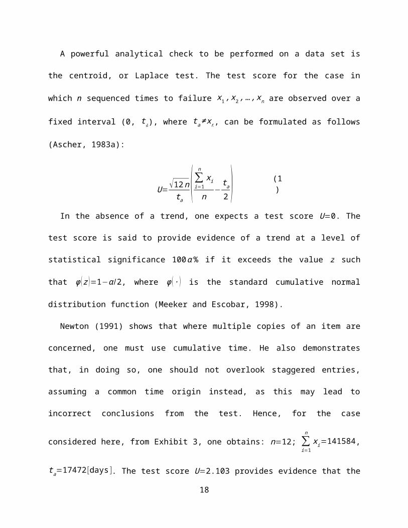
A powerful analytical check to be performed on a data set is the centroid, or Laplace test. The

test score for the case in which n sequenced times to failure x1, x2 , …, xn are observed over a

fixed interval (0, t a), where t a≠ xn, can be formulated as follows (Ascher, 1983a):

U=√12 nta

(∑i=1

n

x i

n−

ta

2 ) (1)

In the absence of a trend, one expects a test score U=0. The test score is said to provide

evidence of a trend at a level of statistical significance 100α % if it exceeds the value z such that

ϕ ( z )=1−α /2, where ϕ ( ∙ ) is the standard cumulative normal distribution function (Meeker

and Escobar, 1998).

Newton (1991) shows that where multiple copies of an item are concerned, one must use

cumulative time. He also demonstrates that, in doing so, one should not overlook staggered

entries, assuming a common time origin instead, as this may lead to incorrect conclusions from

the test. Hence, for the case considered here, from Exhibit 3, one obtains: n=12; ∑i=1

n

x i=141584,

t a=17472[days ]. The test score U=2.103 provides evidence that the interrecurrence times are

tending to become smaller (colloquially, the item is “sad,” - see Ascher, 1983a) at a 5% level of

statistical significance. To graphically check for trends, one may plot the cumulative number of

recurrences versus time (if the plot approximates to a straight line, there is no such trend) and

also check whether there is correlation between lagged failure-time observations via a

correlogram (Walls and Bendell, 1986). For the case considered here, Exhibit 5 shows an

increasing slope over time (the data-fitting model shown alongside the point observations will be

discussed later).

Exhibit 5 HERE

11

The correlogram in Exhibit 6 shows the autocorrelation coefficients computed following

Makridakis et al. (1998) up to an eight period lag. Theoretically, for a series of random numbers,

all the coefficients should be zero, but in practice it is sufficient that, for a sample of n

observations, 95% of all sample coefficients lie within the range of ± 1.96/√n.

Exhibit 6 HERE

In Exhibit 6, all values lie within such range (the critical values ± 0.47 are obtained for n=17,

considering the times to non-failure). This result suggests “white noise” data, making it less

straightforward to reject the hypothesis that there is no trend.

Fitting models to data

The test for trend suggests a “sad” repairable item which, in principle, calls for fitting a

nonstationary model to the data (Ascher, 1983a). Several data-fitting models can be suitable for a

repairable item. Such models are parametric or non-parametric in nature, depending on whether

or not they embed underlying assumptions on particular characteristics of the population studied

(Meeker and Escobar, 1998). Below, appropriate formulations from amongst the best-known

modeling options are identified considering the nature of the empirical data employed here. For

ease of exposition, a distinction between recurrence time models, interrecurrence time models,

and regression models is introduced. The application of such models to the data is illustrated to

help guide practice.

Recurrence time models

The main aspect of recurrence time models is that a sequence of time to failures for a

population of repairable items is described by a property called the Rate of Occurrence of Failure

—ROCOF (Ascher, 1999), expressed in failures per unit time per item.

12

A model implying a minimum set of assumptions regarding the process which generates the

items histories is the population’s Mean Cumulative recurrence Function - MCF. It is the

expected number of failures experienced across a population of items by a certain age. A

procedure to obtain a nonparametric MCF estimator from empirical data with confidence bounds

is described in Meeker and Escobar (1998). The procedure’s focus is on the unique recurrence

times for a population of items. At each recurrence time, ranked by magnitude, one determines

the mean of the distribution of reported failures across all the items still observed at that time

(the “risk set”), and the MCF estimator as the cumulative sum of those means up to that time.

Graphically, the non-parametric MCF is a step-function with jumps at each recurrence time.

Exhibit 7 shows the MCF and confidence bounds for the data considered here. Due to the

presence of staggered entries, the unique recurrence times are determined on a common

timescale (Exhibit 3).

Exhibit 7 HERE

A ROCOF can only be obtained for each pair of successive recurrence times dividing the

difference between the value of the MCF estimator at each time by the time interval length.

A parametric alternative is to model recurrence data as a Poisson process (Cox, 1983). In the

presence of a trend, it is recommended that a Non Homogeneous Poisson Process (NHPP) is

employed (Walls and Bendell, 1986). More sophisticated theoretical models exist (Lindqvist,

2008). However, when it comes to fitting a Poisson process to empirical recurrence data the

formulation known as power law NHPP (Crow, 1990) is a convenient option. Power law NHPP

is characterized by a non-stationary ROCOF of the form, v (t ,θ )=λβ t β−1, where t is an item age

(the rate is not constant over time), and θ=[ β λ ] is the vector of unknown parameters that can

be estimated by maximum likelihood via the following equations:

13

β̂=n /∑i=1

n

ln( t a

x i) (2a)

λ̂=n/ t aβ̂ (2b)

where n are distinct recurrence times x1 , x2 , …, xn observed for an item over (0, t a).

These equations are the most commonly used in the literature (e.g., Ascher, 1983a; Meeker

and Escobar, 1998), but assume a single item. Crow (1990) provides two variations for use: first,

when data are obtained from multiple copies of an item observed over the same time period and

second, when observation start and end times are different for each copy. In principle, the latter

cases would be more appropriate for the example considered here, but since the equations are not

in a closed-form they would need to be solved numerically. For the sake of simplicity, here we

refer to an “equivalent single item” and use the aggregated values in Exhibit 3 to obtain the

estimates β̂=2.32 , and λ̂=1.73 ×10−9 by applying (2a-b).

An estimate of β̂ greater than one is consistent with the “sad” item result obtained from the

trend test, whereas β̂=1 would have been consistent with a homogeneous Poisson process - HPP,

implying that the interrecurrence times are independently exponentially distributed (Ascher,

1983a; Cox, 1983). The curve in Exhibit 5 is the Cumulative Intensity Function - CIF - of an

NHPP with the estimated ROCOF, E ( N (t ))= λ̂ t β̂=1.73 ×10−9t 2.32. The curve expresses the mean

(or expected, as denoted by the operator E) number of support interventions, N (t ), that an

“equivalent single item” will have demanded by a certain time t. This provides a useful

indication of how the “pressure” on the support system’s resources may evolve over time.

A goodness-of-fit test for the estimated NHPP is to compare the difference between expected

number of failures and the actual data with a Chi-distribution (Crow, 1990). To do so, usually

three time intervals are identified with at least five total failures in each interval. However, from

14

Exhibit 3, one obtains T 1=(t 1, t 1 )=(0 ,2394 );T 2=(t 2 , t 2 )=(2394 ,3255 ); and

T 3=(t 3 ,t 3 )= (3255 ,3698 ), with N (T j )=4 for j=1,2,3. The difference between expected failures,

e j= λ̂ t jβ̂− λ̂ t j

β̂, and actual data is not significant since χ2=∑j=1

3 [ N (T j )−e j ]2e j

=0.89 is below the

critical value of a Chi-distribution with 1 degree of freedom at the 10% significance level.

Interrecurrence time models

Parametric lifetime distributions are typically meant to model non-repairable items that fail

once. A property of the time to failure of such items is the hazard rate: the instantaneous

potential, per unit time, for an event (“material” failure) to occur at a given instant given survival

up to that instant (Kleinbaum and Klein, 2012). Specific parametric failure-time models like the

Weibull distribution are commonly chosen in practice for electronic devices due to their

flexibility (Sandborn, 2013). One may even notice that the ROCOF of a power law NHPP is

numerically analogous to the hazard rate of a Weibull distribution. As Ascher (1999)

demonstrates, this may cause misconceptions since the two are not equivalent in terms of

interpretation, even when they are equal.

Newton (1991) shows that trying to model a repairable item by fitting a lifetime distribution

does not makes sense unless interrecurrence times are being analyzed, since this amounts to

analyzing the non-repairable components which reside in a repairable item. Also, the parametric

distribution-fitting approach requires the reordering of interrecurrence times by magnitude.

Hence, one should proceed only once the necessary checks described earlier have provided no

strong evidence against the hypothesis that interrecurrence times are i.i.d. Assuming it is

legitimate to do so for the empirical data considered here, Exhibit 8 shows the reordered

interrecurrence times and the computation of the necessary statistics (Newton, 1991).

15

Exhibit 8 HERE

The procedure starts with a nonparameteric estimate of the Cumulative Hazard Function -

CHF - the Kaplan-Meier estimator (Kleinbaum and Klein, 2012). A fundamental difference from

Exhibit 3 is that the risk set in Exhibit 8 is formed by a number of fictitious non-repairable items

equivalent to the number of recurrences. Using the values of t i and the estimate of the cumulative

density function (CDF) of the interrecurrence times shown in Exhibit 8, one obtains the

coordinates for the Weibull plot shown in Exhibit 9.

Exhibit 9 HERE

An estimate of the distribution’s parameters can then be obtained by fitting a line to the plot

shown, whereby the reciprocal of the slope is the distribution shape parameter ❑̂= 10.96

=1.04

and the intercept the natural logarithm of the scale parameter θ̂=e7.03 =1129.80.

Another approach is to compute maximum-likelihood estimate (MLE) for the distribution

parameters. This approach provides, in principle, versatility and statistical efficiency also in the

presence of censored data (Meeker and Escobar, 1998). A robust algorithm to obtain such

estimates is available through the “fitdistr” function in the MASS package (Venables and Ripley,

2007) for the open-source statistical software R (R Development Core Team, 2012). Due to the

presence of censored data, the extension of the original function provided in the fitdistrplus

package (Delignette-Muller and Dutang, 2012) has been used. The estimates ❑̂mle=1.18 and

θ̂mle=1470.17 are obtained via a minor reorganization of the information in Exhibit 8 that is

required by the algorithm.

Exhibit 10 shows the empirical and two estimated density functions. In the presence of

censored times, the application of commonly-used goodness-of-fit tests is problematic; although

16

procedures exist (D'Agostino and Stephens, 1986), they only apply to the case in which censored

observations are all greater than the largest observed value. This situation may reasonably occur

for single sample data obtained in test-rig conditions. In the absence of adequate alternatives, it is

suggested analysts proceed through visual inspection (Delignette-Muller and Dutang, 2012).

Exhibit 10 HERE

Using the maximum likelihood estimated parameters, the hazard rate function for the

Weibull distribution, and the corresponding CHF are, respectively,

h (t )=β̂mle

θ̂mle (t

θ̂mle )β̂mle−1

=0.000803( t1470.17 )

0.181

, and H ( t )=( tθ̂mle)

β̂mle

=( t1470.17 )

1.18

. Unlike the

ROCOF for the models based on recurrence times, the hazard rate expresses a conditional

probability of failure per unit time for a non-repairable component. Hence, an NHPP model

described by a distribution’s CHF would not be comparable with one obtained by direct

estimation of the stochastic process’ CIF.

Regression models

In the previous sub-sections, the focus was either on a sequence of times to failures, or on a

lifetime distribution. In both cases, a common underlying assumption is that data are from

indistinguishable copies of an item, which assumedly operate under identical conditions. Also,

some functional form of the ROCOF and the hazard rate has to be chosen upfront.

In the case of field data, one may be interested in taking into account the heterogeneities

encountered in a population of repairable items, if some information on such differences is

available - the items may not be indistinguishable or operated under identical conditions, and

choosing an underlying distribution of time to failures can hardly be possible (Ascher, 1983b).

Such limitations are overcome by semi-parametric regression models for survival analysis based

17

on the Cox Proportional Hazard (CPH) model widely used in biometrics (Kleinbaum and Klein,

2012). A distinguishing feature is the hazard rate formulation which varies between groups or

other measurements on the cases that serve as explanatory factors (also known as covariates, or

regression variables) (Meeker and Escobar, 1998).

Exhibit 3 shows that the explanatory variables chosen due to practical considerations for the

numerical example considered here are “inherently” time-dependent, thus requiring an

“extended” CPH (Kleinbaum and Klein, 2012). When using such a model for recurrent events

the data layout is particularly important since, for each recurrence, the “start” and “stop” times

must be specified. A suitable layout can be obtained from Exhibit 3 with minimum

modifications. Given the data layout is suitable, the model is fit to empirical data using the

“coxph” function included in the survival package for the statistical software R (Venables

and Ripley, 2007, Ch. 13). Statistically significant associations were found for such explanatory

variables as the detection of a material failure in modules a and c, or an NFF. The estimated

coefficients were, respectively, δ a=−.962; δ c=.899; and δNFF=1.758.

The interpretation of such coefficients is based on a relative measure called “hazard ratio” for

the effect of each variable, adjusted for the other variables in the model (Kleinbaum and Klein,

2012). For example, for the explanatory variable NFF the ratio is e1.758=5.801. Since the variable

is time-dependent, the interpretation of its estimate is, at any given time, the hazard for an item

which has not yet experienced an NFF (but may experience it later) is approximately

1/5.801≅ 0.17 times the hazard for an item which has already experienced an NFF by that time.

Discussion

The statistical analysis of real-world data is the basis for delicate choices such as whether or

not to embark on long-term support contracts for repairable items, and what financial conditions

18

are set. Field data, however, often describes situations that are less ideal than those described by

“textbook” approaches and popular modeling choices. A lack of guidance on how to choose

between competing modeling options often leads practitioners to apply models that are meant for

non-repairable items, such as lifetime distributions, to recurrence data gathered for fielded

repairable items. Thus, aspects such as the investigation of trends in the data and the possibility

of using models meant for items experiencing recurrent events are overlooked altogether (e.g.,

Bowman and Schmee, 2001). In some cases, elements pertaining to models meant for repairable

and non-repairable items coexist ambiguously (e.g., Huang et al., 2013).

One characteristic of field data for repairable items is time censoring. If neglected, it may

lead to pessimistic reliability estimates, incorrect conclusions from testing for trends, and

inappropriate “goodness-of-fit.” These aspects can be easily handled by choosing an appropriate

data layout as described in this work.

An adequate data layout eases the preliminary exploration of data. Preliminary data

exploration is an aspect of great practical relevance as it allows identification of structures in the

data that may (or may not) lead to rejection of the commonly (uncritically) made hypothesis of

independently and identically distributed (i.i.d.) failure times. In the absence of a clear strategy

for the statistical analysis of reliability data, a constant failure rate, and hence exponentially

distributed times to failure, is often chosen upfront. Justifications for such a choice include that

the i.i.d. assumption is not likely to be rejected for small data sets (Walls and Bendell, 1986), or

for large enough populations observed for a sufficiently long period (Meeker and Escobar, 1998),

or, that it seems difficult to treat data which are not i.i.d. analytically (Ascher, 1983a).

In the illustrative example presented here, particular attention has been paid to staggered

entries and right-censored data, to avoid misleading results while testing for trends or applying

19

inadequate formulations of the data-fitting models considered. In practice, this aspect is

overlooked due to difficulties arising when data are obtained from multiple copies of an item, for

which observations do not start and stop at the same time. For example, Weckman et al. (2006)

estimate power law NHPP’s parameters for a fleet of aircraft engines using Crow’s equations that

apply when the empirical data used refer to copies of an item with the same start and end time.

Whether this assumption is reflected by the underlying data is not discussed.

Another issue is that seldom is adequate context provided to a set-of-numbers before

undertaking a data-fitting exercise. Most practitioners fail to appreciate differences between

models that are meant for non-repairable items, such as parametric lifetime distributions, and

those meant for repairable items which, by contrast, focus on a sequence of times to failures

(Ascher, 1999). As a consequence, some works may implicitly treat the ROCOF of a stochastic

point process as if it were a lifetime distribution’s hazard function (e.g. Lugtigheid et al., 2007;

Waghmode and Sahasrabudhe, 2011). However, it is usually advised not to do so since the two

are not the same even if they are numerically equivalent (Ascher, 1999; Crow, 1990).

Due to their practical relevance, lifetime distribution models were not ignored in the research

presented here, with the caveat that numerical equivalence between such concepts as ROCOF

and hazard rate must not lead to confusion. Estimating a ROCOF can assist those seeking to

estimate the replacement rate for a line-replaceable item and determine if the rate increases with

age (which is relevant to support burn-in, recall, and retirement policies).

Practical Implications for Engineering Managers

This work provides insight to practicing engineering managers in terms of obtaining “actionable

knowledge” by making intelligent use of existing reliability data. For example, based on the

authors’s experience on a case study in the defense avionics industry, to successfully execute

20

PBL or availability type contracts, engineering managers across partner organizations are

constantly searching for insight to facilitate the provision of equipment availability over time.

They look at the data, attempt to detect trends and “see things” happening for a population of

items deployed in the field. The analytics chosen for this purpose have practical repercussions on

how organizations work with their suppliers and customers to face day-to-day issues that affect

availability and end customer satisfaction, as well as long-term issues. The strategy for field

reliability data described in this work helps engineering managers to navigate different options,

from data exploration to the implementation of data analytics, and to place the focus on

computational devices that are appropriate to the real-life situation engineering managers face.

This is becoming particularly useful in maintenance planning and prioritization for engineering

managers.

The same case study also reveals that engineering managers are often presented with

information they are expected to understand, but they may not necessarily be specialists or

subject matter experts in the field. The procedure presented here is self-contained and fully

replicable to facilitate communication across engineering management teams with managers

having different levels of familiarity with reliability engineering and statistical data analysis.

This helps overcome constrains imposed by upfront modeling choices and the use of specific

software packages. While useful for illustrative purposes, a simplified example may be limiting

to convince a firm to adjust its strategy. An application and extension of the approach illustrated

in this study to a full scale industrial case in defense avionics availability can be found elsewhere

(Settanni et al., 2015).

One of the co-authors also has direct experience as a practicing engineering manager in

the electric energy sector. In this sector, engineering asset and operations managers analyze

21

maintenance data from fleets of similar assets to make operating decisions about resource

allocation decisions across a network of equipment – see e.g., Bumblauskas (2015). This

research can be useful to asset and operations managers as it presents data analytics that are

mostly overlooked in the literature such as MCF and power law NHPP, with few exceptions

including Bumblauskas et al. (2012). By indicating the overall number of support interventions

that an item is expected to demand, on average, after a certain time period in field, these models

can help prevent putting excessive pressure on the capacity of a support system, or in this case

the electric power grid.

Analytics such as NHPP and MCF can be particularly important in a PBL, where the

service providers’ ability to commit on performance such as repair lead times is greatly affected

by how well the overall support system’s capacity is managed. MCF plots can also be used to

compare batches of items that differ for design, support policy, etc. They may also reveal

whether attempts to improve reliability by consecutive product design iterations results in a

reduction of the total number of interventions that, on average, a fielded product requires over

time.

Closing Remarks

This article contributes to improving the understanding of reliability baselines used in

industry for fielded repairable items by offering a strategy to avoid common pitfalls in data

analysis. The strategy, from preliminary data exploration to data-fitting, has been illustrated for a

case study in defense avionics underpinned by real-life data. The case has been simplified so that

the procedures and results presented in this research can be replicated.

The importance of exploring data and providing adequate context to a set-of-numbers have

been highlighted to prevent misconceptions due to common assumptions and popular modeling

22

choices. This aspect is of practical relevance in situations involving the execution of performance

and availability-based contracts, where fair organizational accountability is achieved through a

shared and unambiguous understanding of reliability baselines.

The limitations of this research are mainly due to a current lack of examples in the literature

on how to proceed when one cannot apply the most common ways to perform reliability data

analysis. This lack complicates the identification and implementation of alternative model

formulations. By bringing forth some of the available, yet seemingly forgotten, “lessons” in field

reliability data analysis, this research aspires not to be comprehensive, but to provide impulse to

the intellectual process of analysis in future work so that current gaps can be bridged.

References

Ascher, H. (1983a). Discussion of "point processes and renewal theory: a brief survey". In J. K.

Skwirzynski (Ed.), Electronic Systems Effectiveness and Life Cycle Costing (pp.113–117).

Berlin Heidelberg: Springer-Verlag.

Ascher, H. (1983b). Regression analysis of repairable systems reliability data. In J. K.

Skwirzynski (Ed.), Electronic Systems Effectiveness and Life Cycle Costing (pp. 119–133).

Berlin Heidelberg: Springer-Verlag.

Ascher, H. E. (1999). A set-of-numbers is NOT a data-set. IEEE Transactions on Reliability,

48(2), 135–140.

Aubin, B. R. (2004). Aircraft Maintenance: The Art and Science of Keeping Aircraft Safe.

Warrendale, PA: SAE.

Blanchard, B. S. (1992). Logistics engineering and management (4.ed.). Englewood Cliffs, N.Y:

Prentice-Hall.

23

Bowman, R. A., and Schmee, J. (2001). Pricing and managing a maintenance contract for a fleet

of aircraft engines. Simulation, 76(2), 69–77.

Busch, M. (2013). Thinking slow: Why many career A&Ps are not great trouble shooters. Sport

Aviation, 62(10), 26–29.

Bumblauskas, D. (2015). A Markov decision process model case for optimal maintenance of

serially dependent power system components. Journal of Quality in Maintenance

Engineering, 21(3), 271-293

Bumblauskas, D., Meeker, W., and Gemmill, D. (2012). Maintenance and recurrent event

analysis of circuit breaker data. International Journal of Quality & Reliability Management,

29(5), 560-575.

Cox, D. R. (1983). Point processes and renewal theory: a brief survey. In J. K. Skwirzynski

(Ed.), Electronic Systems Effectiveness and Life Cycle Costing (pp.107–112). Berlin

Heidelberg: Springer-Verlag.

Crow, L. H. (1990). Evaluating the reliability of repairable systems. In Proceedings of the

Annual Reliability and Maintainability Symposium (pp.275–279). New York: IEEE.

D'Agostino, R. B., and Stephens, M. A. (1986). Goodness-of-fit techniques. New York: Dekker.

Delignette-Muller, M. L. and Dutang, C. (2012). Fitting parametric univariate distributions to

non censored or censored data using the R fitdistrplus package. Retrieved from

http://www.icesi.edu.co/CRAN/web/packages/fitdistrplus/vignettes/intro2fitdistrplus.pdf

Dhillon, B. S. (2010). Life cycle costing for engineers. Boca Raton, FL: Taylor & Francis.

Evans, R. A. (1995). Models Models Everywhere - And Not A One To Want. IEEE Transactions

on Reliability, 44(4), 537.

24

Evans, R. A. (1999). Stupid statistics. IEEE Transactions on Reliability, 48(2), 105.

Flood, R. L., and Carson, E. R. (1988). Dealing with complexity: An introduction to the theory

and application of systems science. New York: Plenum Press.

Gosavi, A., Murray, S. L., Tirumalasetty, M. V., and Shewade, S. (2011). A Budget-Sensitive

Approach to Scheduling Maintenance in a Total Productive Maintenance (TPM) Program.

Engineering Management Journal, 23(3), 46–56.

Hauptmanns, U. (2011). Reliability data acquisition and evaluation in process plants. Journal of

Loss Prevention in the Process Industries, 24(3), 266–273.

Held, M., and Fritz, K. (2009). Comparison and evaluation of newest failure rate prediction

models: FIDES and RIAC 217Plus. Microelectronics Reliability, 49(9–11), 967–971.

Huang, X., Kreye, M. E., Parry, G., Goh, Y. M., and Newnes, L. B. (2013). The cost of service.

In P. Sandborn (Ed.), Cost Analysis of Electronic Systems (pp. 349–362). Singapore: World

Scientific Publishing.

Igba, J., Alemzadeh, K., Durugbo, C., and Henningsen, K. (2015). Performance assessment of

wind turbine gearboxes using in-service data: Current approaches and future trends.

Renewable and Sustainable Energy Reviews, 50, 144–159.

Kleinbaum, D. G., and Klein, M. (2012). Survival Analysis: A self-learning text. New York:

Springer.

Jolly, S.S. and Singh, B. J. (2014). An approach to enhance availability of repairable systems: a

case study of SPMs. International Journal of Quality & Reliability Management, 31(9),

1031–1051.

Lewis, E. E. (1996). Introduction to reliability engineering (2nd ed.). Wiley: New York.

25

Lindqvist, H. B. (2008). Maintenance of Repairable Systems. In K. A. H. Kobbacy, and D. N. P.

Murthy (Eds.), Complex System Maintenance Handbook (pp. 235-261). London: Springer.

Lugtigheid, D., Jardine, A. K. S., and Jiang, X. (2007). Optimizing the performance of a

repairable system under a maintenance and repair contract. Quality and Reliability

Engineering International, 23(8), 943–960.

Makridakis, S. G., Wheelwright, S. C., and Hyndman, R. J. (1998). Forecasting: Methods and

applications (3rd ed.). New York: Wiley.

Meeker, W. Q., and Escobar, L. A. (1998). Statistical methods for reliability data. New York:

Wiley.

Newton, D. W. (1991). Some pitfalls in reliability data analysis. Reliability Engineering &

System Safety, 34(1), 7–21.

Phillips, M. J. (2003). Statistical methods for reliability data analysis. In H. Pham (Ed.),

Handbook of reliability engineering (pp. 475–492). London : Springer.

R Development Core Team. (2012). R: A Language and Environment for Statistical Computing.

Vienna, Austria. Retrieved from http://www.R-project.org/

Rahman, A. (2014). Maintenance contract model for complex asset/equipment. International

Journal of Reliability, Quality and Safety Engineering, 21(1), 1–11.

Sandborn, P. (Ed.). (2013). Cost Analysis of Electronic Systems. Singapore: World Scientific.

Settanni, E., Newnes, L. B., Thenent, N. E., Bumblauskas, D., Parry, G., Goh, Y.M. (2015). A

case study in estimating avionics availability from field reliability data. Quality and

Reliability Engineering International. In press. DOI: 10.1002/qre.1854

26

Sikos, L., and Klemeš, J. (2010). Evaluation and assessment of reliability and availability

software for securing an uninterrupted energy supply. Clean Technologies and Environmental

Policy, 12(2), 137–146.

Sinisuka, N. I., and Nugraha, H. (2013). Life cycle cost analysis on the operation of power

generation. Journal of Quality in Maintenance Engineering, 19(1), 5–24.

Smith, T. C. (2004). Reliability growth planning under performance based logistics. In

Proceedings of the Annual Reliability and Maintainability Symposium (pp. 418–423). New

York: IEEE.

Sols, A., Nowicki, D., and Verma, D. (2007). Defining the fundamental framework of an

effective Performance-Based Logistics (PBL) contract. Engineering Management Journal,

19(2), 40–50.

Tuttle, D. E., and Shwartz, M. N. (1979). Lower avionic temperature lower life cycle cost. In

Proceedings of the Annual Reliability and Maintainability Symposium (pp. 332–337). New

York: IEEE.

Venables, W. N., and Ripley, B. D. (2007). Modern applied statistics with S (4. ed.). New York:

Springer.

Waghmode, L., and Sahasrabudhe, A. (2011). Modelling maintenance and repair costs using

stochastic point processes for life cycle costing of repairable systems. International Journal of

Computer Integrated Manufacturing, 25(4-5), 353–367.

Walls, L. A., and Bendell, A. (1986). The structure and exploration of reliability field data: What

to look for and how to analyse it. Reliability Engineering, 15(2), 115–143.

Weckman, G. R., Marvel, J. H., and Shell, R. L. (2006). Decision support approach to fleet

maintenance requirements in the aviation industry. Journal of Aircraft, 43(5), 1352–1360.

27

Wong, K. L., and Lindstrom, D. L. (1988). Off the bathtub onto the roller-coaster curve. In

Proceedings of the Annual Reliability and Maintainability Symposium (pp. 356–363). New

York: IEEE.

Wu, X., and Ryan, S. M. (2014). Joint Optimization of Asset and Inventory Management in a

Product–Service System. Engineering Economist, 59(2), 91–116.

Yellman, T. W. (1999). Failures and related topics. IEEE Transactions on Reliability, 48(1), 6–8.

28