Proceedings first edited 5

Proceedings of National Seminar on Statistical Approaches in Data Science 6-7 February 2019

ISBN: 978-81-935819-2-6

2

PROCEEDINGS OF NATIONAL SEMINAR

ON

STATISTICAL APPROACHESSTATISTICAL APPROACHESSTATISTICAL APPROACHESSTATISTICAL APPROACHES

ININININ

DATA SCIENCEDATA SCIENCEDATA SCIENCEDATA SCIENCE

6666----7 FEB 20197 FEB 20197 FEB 20197 FEB 2019

Publication Division

St.Thomas College (Autonomous), Thrissur

Kerala-680001, India

2019


ISBN: 978-81-935819-2-6

3

EDITORIAL BOARDEDITORIAL BOARDEDITORIAL BOARDEDITORIAL BOARD

Chief Editor

Dr.V.M.Chacko

Managing Editor

Prof. Jeena Joseph

Editors

Dr. T.A.Sajesh

Dr. Rani Sebastian

Dr. Nicy Sebastian

Prof. R. S. Rasin

Mrs. Dhanya Sunny

Mrs. Haritha P U

Miss. Reshma T S

Prof. Rejin Varghese

Language: English, Year: 2019, ISBN 978-81-935819-2-6

Publisher: Publication Division, St. Thomas College (Autonomous), Thrissur

The proceedings of National Seminar on Statistical Approaches in Data Science are a

peer reviewed book containing original unpublished research papers. All rights are

reserved. No part of this publication may be reproduced, stored in or introduced into

a retrieval system or transmitted, in any form, or by any means, electronic,

mechanical, photocopying, recording or otherwise without prior written permission of

the publisher.

Contact- Email: [email protected], Ph.No.91 9961 335938, 91 9656 335938


ISBN: 978-81-935819-2-6

4

ADVISORY COMMITTEE

His Grace Mar Andrews Thazhath, Archbishop, Thrissur Archdiocese, Patron

His Excellency Mar Tony Neelamkavil, Aux.Bishop, Thrissur Archdiocese, Manager

Dr. M. Manoharan, Professor (University of Calicut)

Dr. Davis Antony M (Christ College, Irinjalakkuda)

Dr. S M Sunoj (Cochin University of Science &Technology)

Dr. P. O Jenson (Sahridaya College, Kodakara)

ORGANIZING COMMITTEE

Dr. Ignatius Antony, Principal (Chairman)

Dr.V.M.Chacko, Assistant Professor & Head (Convener)

Prof. Jeena Joseph, Assistant Professor (Coordinator)

Dr. T.A.Sajesh, Assistant Professor & Coordinator (Data Science)

Dr. Rani Sebastian, Assistant Professor

Dr. Nicy Sebastian, Assistant Professor

Prof. R. S. Rasin, Assistant Professor

Prof. Dhanya Sunny Guest Lecturer

Prof. Haritha P U, Guest Lecturer

Prof. Reshma T S., Guest Lecturer

Prof. Rejin Varghese, Assistant Professor (Data Science)

Miss. Sajna O K, Research Scholar

Mrs. Deepthi K S, Research Scholar

Miss. Beenu Thomas, Research Scholar

Miss. Rajitha C, Research Scholar


ISBN: 978-81-935819-2-6

5

WELCOME

St. Thomas' College Thrissur is one of the leading academic institutions in the higher education sector of Kerala since 1919. It has a long and proud tradition of excellence in training, teaching and research in many academic disciplines of Science, Arts, Commerce and Humanities.

Post graduate Department of Statistics and Research Centre, St.Thomas’ College, Thrissur provides robust computational support to meet the needs of students and researchers. Collection, analysis and interpretation of numerical data have significant role in every research programme. The rapid development in information technology and expansion of the means of communication have made the data collection an easy task upto a certain extent.

However, the processing and organizing of data pose multifarious problems to researchers and experimenters. Here comes the role of Statistics, as a science to provide powerful tools for the analysis and interpretation at every step of research. Data science

is an emerging discipline that draws upon knowledge in statistical methodology and

computer science to create impactful predictions and insights for a wide range of

traditional scholarly fields. Statistical ideas are having a profound impact in science, industry and public policy. The Statistics Department at St.Thomas has pioneered many of the tools and ideas behind the research and applications often classified as “data science,” where statistics and computer science join together. The Department sees an even brighter future for data science as it harnesses a wider set of ideas to build a new more subtle and powerful science of data. As well as being interested in prediction and statistical computation, our Department puts equal weight on designing experiments, modeling and trying to understand and quantify causal mechanisms, not simply averages and associations, with large data sets. These views are reflected in our curriculum targeted to data science specialists, our faculty’s research and the work of our research students.

The Department of Statistics decided to conduct a National Seminar on

Statistical Approaches in Data Science, during 6 - 7 February 2019. The seminar is intended to impart an understanding of the statistical ideas and methods involved in carrying out research for researchers and teachers from various disciplines of learning.

We are pleased to publish the proceedings of the seminar which containing the

abstracts, full papers and programme schedule. We hope that all of you will enjoy the seminar at large.

Wish you all the best………….

Dr. Ignatius Antony Dr. V. M. Chacko Prof. Jeena Joseph

Principal HOD& Convener Coordinator


ISBN: 978-81-935819-2-6

6

About St.Thomas College (Autonomous), Thrissur

St. Thomas’ College Thrissur is one of the leading academic institutions in the higher education sector of Kerala since 1919. It has a long and proud tradition of excellence in training, teaching and research in many academic disciplines of Science, Arts, Commerce and Humanities. It attracts the brightest minds from all over Kerala and from different parts of the country and Asia. Its alumni have made outstanding contributions to academics, governance and industry. The University Grants Commission

has granted Autonomous Status in 2014 to the college and recognized as College with

Potential for Excellence in 2016. The college has 14 PG courses and 20 UG courses. All the 9 aided PG departments are Research centers having more than 100 research scholars and 40 research guides.

About the PG and Research Department of Statistics

The Degree Course in B.A. Statistics was started in the year 1955 under the Dept. of Mathematics and Statistics affiliated to the University of Madras. In the year 1958 the B.A. Course was converted to three year B.Sc. course in Statistics under the University of Kerala. The Department of Statistics was established in the year 1984 and the M.Sc. course in Statistics commenced in the same year with Operations Research, Numerical Mathematics and Computer Programming as optional subjects. Department was elevated as Research centre of the Calicut university in the year 2013.Prof.Sebastian J Kulathinal (1984 – 1994), Prof. V.D. Johny (1994 – 2000), Prof A P Jose(2000 – 2003), Dr. T.B. Ramkumar(2003 – 2014) served as the Heads of Department. Prof. A. P. Jose was the Vice principal (2001 – 2003) of the college. Eminant teachers Prof . Krishnakumar (NAAC coordinator 2013), Prof. M.K.Jose, Prof. A. S. Raffy, Prof. P. K. Sasidharan and T. D. Xavier served the department for several years. Dr. P. O. Jenson, the Principal (Rtd) was the member of the department and will be retiring on 2018 April 30. Currently 6 permanent and 3 guest faculty members are working in the department. The department has four research guides and four research scholars. The department offers Certificate

course in Statistical Computing using SPSS for UG students and Certificate course in

Statistical Computing using R for PG students. Moreover department provides UGC coaching, JAM coaching etc. The department started B.Voc Data Science course jointly with Department of Computer Science with the UGC assistance in 2018.


ISBN: 978-81-935819-2-6

7

Programme Schedule

06 February 2019

Time Session Name

9.00-9.30 am Registration

09.30-10.30 am Inauguration

Welcome Dr. V. M. Chacko, Head of the Department

Presidential Address Dr. Ignatius Antony, Principal

Inauguration His Grace Mar Tony Neelamkavil Aux. Bishop of Thrissur Archdiocese

Benedictory Speech

Rev. Fr. Varghese Kuthur Executive Manager

Felicitation Rev. Dr. Martin Kolombrath, Vice Principal

Dr. Thomas Paul Kattookkaran

Vice Principal

Dr. K. L. Joy, Vice Principal

Vote of Thanks Prof. Jeena Joseph, Coordinator

10.30-10.45 am Tea Break

10.45-11.45 am

Technical Session I

Chair: Dr.P.O.Jenson, Principal, Sahridaya College, Kodakara [Principal (Rtd), Department of Statistics, St.Thomas College, Thrissur]

Invited Talk 1

Dr. A. Krishnamoorthy, Emeritus Fellow (UGC), Centre for Research in Mathematics, CMS College, Kottayam 686000 [Former Professor, Dept. of Mathematics Cochin University of Science and Technology]

Topic

Queueing theory: perspectives from a social

angle

11.45-12.45 pm

Technical Session II

Chair: Dr. T. D. Xavier, Asso. Professor(Rtd) Department of Statistics, St.Thomas College, Thrissur

Invited Talk 2

Dr. P. G. Sankaran, Professor, Dept. of Statistics, [Former Pro-Vice Chancellor, Cochin University of Science and Technology]

Topic

Modeling and analysis of current status lifetime

data

12.45-1.30 pm Lunch Break

1.30-3.30 pm

Technical Session III

Chair: Prof. A. P. Jose, HOD Department of Statistics, St.Thomas College, Thrissur (Rtd)

Invited Talk 3

Rakesh Poduval, Senior Statistician, Hedonic Products, Zurich, Switzerland


ISBN: 978-81-935819-2-6

8

Topic Introduction to python for data science

Invited Talk 4

Dr. V. Bhuvaneswari, Asst. Professor, Bharathiar University, Coimbatore

Topic Data Science – A Road Map

3.30-3.45 pm Tea Break

3.45-4.30 pm

Contributory Session I

Dr. Mariamma Antony, Assistant Professor &

Head, Department of Statistics, Little Flower

College, Guruvayoor

Title: On Some Tailed Distributions And

Related Time Series Models

Dr. DIVYA P R, Assistant Professor & Head,

Dept. of Statistics, Vimala College

(Autonomous), Thrissur

Title: Construction and Selection of Single

Sampling Variables Plan Through Decision

Region

07 February 2019

9.30-11.00 am

Technical Session IV

Chair: Prof. A.S.Raffy, St. Aloysius College, Elthuruth, Thrissur [Associate Professor (Rtd), Department of Statistics, St.Thomas College, Thrissur]

Invited Talk 5

M. Syluvai Anthony, Assistant Professor, Dept. of Statistics, Loyola College, Chennai

11.00-11.15 am Tea Break

11.15-12.45 pm

Invited Talk 6

Ranjith Kalyana Sundaram, Data Scientist, Maersk Group Analytics, Chennai, Tamil Nadu, India

Lunch Break 12.45-1.30 pm

1.30-3.00 pm

Contributory Session V

Dr. Bindu Punathumparambath, Assistant

Professor, Dept. of Statistics, Govt. Arts & Science College, Calicut, Kerala, India Title: Stress-Strength Reliability of Asymmetric

Double Lomax Distribution

Martin Joseph, Department of Statistics,

Loyola College, Chennai

Title: Advocating Box-Cox transformations to

model count response data:

A case study

Reshma T. S., Dept. of Statistics, St.Thomas

College (Autonomous), Thrissur

Title: Bayesian analysis of generalized maxwell

- boltzmann distribution under different loss

functions and prior distributions.


ISBN: 978-81-935819-2-6

9

Rimsha H, Catholicate College, Pathanamthitta

Title: Some Results Related to Location Scale

family of Esscher Transformed Laplace

Distribution

Beenu Thomas, Dept. of Statistics, St.Thomas


Title: Mixed Distribution of Exponential and

Gamma

Deepthi K S, Dept. of Statistics, St.Thomas


Title: Estimation of Stress-Strength model

using Three Parameter Generalized Lindley

Distribution

Rajitha C, Dept. of Statistics, St.Thomas


Title: A Queueing Network model for the

performance analysis of Eye Care Clinic

Dr.V.M.Chacko, Assistant Professor & Head,

Dept. of Statistics, St.Thomas College

(Autonomous), Thrissur

Title: On Joint Risk Importance Measure

Tea Break 3.00-3.15 am

3.15 -3.15pm Tea Break

3.15-4.00 pm Valedictory Session

Welcome Dr.T.A.Sajesh Coordinator

Presidential Address Dr. V. M. Chacko Head of the Department

Inauguration

Dr. Ignatius Antony Principal

Felicitation

Rev. Dr. Martin Kolambrath Vice-Principal

Dr. Thomas Paul Kattookkaran Vice-Principal

Dr.K.L.Joy, Vice-Principal

Vote of Thanks Dr. Rani Sebastian, Assistant Professor

4.00-4.30 pm Cultural Programmes


ISBN: 978-81-935819-2-6

10

AUTHERS

INVITED TALKS:

• Dr. A. Krishnamoorthy, Emeritus Professor, Dept. of

Mathematics, Cochin University of Science and

Technology, Cochin

• Dr. P. G. Sankaran, Professor, Former Pro-Vice Chancellor

Cochin University of Science and Technology, Cochin

• Dr.V.Bhuvaneswari, Department of Computer

Applciations, Bharathiar University, Coimbatore

• Rakesh Poduval, Senior Statistician, Hedonic Products,

Zurich, Switzerland

• M. Syluvai Anthony, Assistant Professor, Dept. of

Statistics, Loyola College, Chennai

• Ranjith Kalyana Sundaram, Data Scientist at Maersk

Group Analytics, Chennai, Tamil Nadu, India CONTRIBUTORY PAPERS:

• Dr.V.M.Chacko, Assistant Professor & Head, Dept. of Statistics, St.Thomas College (Autonomous), Thrissur

• Prof. Jeena Joseph, Assistant Professor, Dept. of Statistics, St.Thomas College (Autonomous), Thrissur

• Dr. Bindu Punathumparambath, Assistant Professor, Dept. of Statistics,

Govt. Arts & Science College, Calicut, Kerala, India

• Dr.Mariamma Antony, Assistant Professor & Head, Department of Statistics, Little Flower College, Guruvayoor

• Dr.Divya P R, Assistant Professor & Head, Dept. of Statistics, Vimala College (Autonomous), Thrissur

• Martin Joseph, Department of Statistics, Loyola College, Chennai

• Reshma T. S., Dept. of Statistics, St.Thomas College (Autonomous), Thrissur

• Rimsha H, Catholicate College, Pathanamthitta

• Beenu Thomas, Dept. of Statistics, St.Thomas College (Autonomous), Thrissur

• Deepthi K S, Dept. of Statistics, St.Thomas College (Autonomous), Thrissur

• Rajitha C, Dept. of Statistics, St.Thomas College (Autonomous), Thrissur


ISBN: 978-81-935819-2-6

11

Queueing Theory: Perspectives From A Social Angle

A Krishnamoorthy

Emeritus Fellow (UGC), Centre for Research in Mathematics

CMS College, Kottayam 686000

Abstract

Queueing theory was developed initially for tackling problems arising in

telecommunication. However, subsequently it pervaded several branches

of Engineering, Technology, Medical field and so on. The purpose of this

presentation is to give a social flavour to queueing theory-- individual,

social and system optimization.

------------------------------------------------------------------------------------------------------------

Modeling And Analysis Of Current Status Lifetime Data

P.G.Sankaran

Cochin University of Science and Technology

Cochin 682022

[email protected]

Abstract

Researchers working with survival data are handling issues associated

with incomplete data, particular those associated with various forms of

censoring. An extreme form of interval censoring, known as current status

observation, refers to situations where the only available information on a

survival random variable is whether or not lifetime exceeds a random

independent monitoring time . In this talk, a brief review of the extensive

literature on the analysis of current status data is presented. Recent

extensions of these ideas to more complex forms of survival data

including, competing risks, multivariate survival data, and general

counting processes are also discussed. Non parametric inference

procedures for estimation of survival function are given. In addition,

modern theory of efficient estimation in semi-parametric models hasis

discussed. Finally, the models are applied to real life situations.


ISBN: 978-81-935819-2-6

12

Data Science – A Road Map

V.Bhuvaneswari

Department of Computer Applciations ,Bharathiar University

[email protected]

Abstract

Data Science has emerged as an important field in the current data era

to analyze explosive amount of data generated by machines, business

and human. Big Data Analytics is used as a platform to analyze Data

insights from huge volume of data. This paper provides a detailed

overview on data evolution, data characteristics, Life cycle for

analyzing data and techniques. An overview of various open source and

commercial tools is presented. The paper provides a Road map of Data

Science.

Keywords: Data Analytics, Big Data

I. Introduction

Data Evolution

Data has become the buzz word in the current technological era with new evolving areas related to data management like Data Science, Data Analytics and Big Data. Tremendous increase in data growth happened as social networks like Facebook, Twitter, Whatsup, Orkut, made data sharing easier connecting millions of users through digital tags. The evolution of data transformed, data measurement from Gigabytes to Terabytes, Petabytes, Exabytes, and Yottabytes. The exponential growth of rate of data is expected to be larger than the Physical Universe in the era of Internet of Things creating new universe the “Digital Universe”.

All the entities in the digital universe are revolving around “data” creating data deluge. The prediction of increase in size of data in digital universe from 2015 to 2020 is estimated to grow by a factor of 300 exabytes to 40,000 exabytes [1] with a prediction that the growths of data will double every year after 2020. Every entities in digital space like “business, individuals, machines” produce and consume data in multiple forms creating a digital ecosystem coining data with a new term “Big Data”.

Data Science has evolved as new a discipline which integrates multiple disciplines like Mathematics, Statistics, Visualization, Databases, Machine Learning, Artificial Intelligence, Visualization and other domains under a common umbrella to analyze huge volume of data. Data Analytics has evolved as important tool to explore and examine insights from the huge data accumulated across domains. Big Data platforms such as Hadoop, SPARK are used for processing storing large volumes of data in conventional computing architectures. This paper provides a detailed road map of data science and analytic tools.


ISBN: 978-81-935819-2-6

13

Data Characteristics

The volume of data measured in units greater than terabyte is called as Big Data. The data which do not fit in the commodity hardware for processing is also called as Big Data. The characteristics that transform simple data to Big Data with three defining dimensions are called data volume, velocity and variety. They are collectively termed as 3V’s proposed by D.Laney in the year 2001[2]. The three V‟s are described below: Volume: In accordance with the survey organized by IBM in 2012, if the data size exceeds beyond one terabyte, then it could be treated as big data [3]. Snapshots of huge volume of data generated are as follows: Hundreds of petabytes of data roughly equivalent to 100 million gigabytes are processed by Google per month. Amazon maintains a big bank of 152 million customer accounts [4]. Nearly 750 million pictures are uploaded to Facebook on a monthly basis. Velocity: It refers to rapid and timely collection of data which in turn enhance the commercial value of big data. Few instances are APPLE receives about 47,000 APP downloads every minute. Every 60 seconds, consumers spend $272070 on web shopping. Variety: It refers to data representation formats, since the data gets generated from multitude of sources. The different data formats are structured, semi-structured and unstructured. According to Cuckier(2010), only 5% of structured data exists in the form of spreadsheets or relational databases. The rest 95% of data which encompasses documents, audio, video, images, graphs and social media text messages are in unstructured form [5].

The other dimensions of data include Veracity, Value, Virality where veracity in data represents the inconsistencies that prevail in data. The Value of data characteristics is analyzing the data which is trustful to drive the business process. Virality of data characteristics represents the rate of data spread. The various types of data that coexist with big data is shown in Fig.1 with description given in Table1.


ISBN: 978-81-935819-2-6

14

Table 1 Data: Big Data

S.No Types of Data

Description Instances

1 Smart Data

Actionable, customized and segmented big data, that can be visualized according to the need of the business[6] .

Brand Sentiment Analysis

2 Fast Data

Instant decisions, real time analysis, crucial for modern enterprises.

Disease outbreaks can be analyzed at the moment so that action can be taken to curb the spread.

3 Identity Data

Future of Big data, used for predictive modeling and machine learning.

Credit card numbers associated with name and address

4 People Data

Customized to analyze the behavior of the customer. Coexist with on-site analytics.

Every activity of the humans on the internet are tracked.

II. Data Analytics

Data is proliferating at an exponential rate, there should be some techniques available to mine and refine it into distilled product information. Data analytics referred as “Actionable Intelligence” is used to convert data into useful and actionable items. The primary objective of data analytics is to control future outcomes. Data Analytics is important as data is viewed as asset and business organization invest huge budget for storage and maintenance of data and except Return of Investment(ROI) from data. Data Analytics when used as tool in business, data can be turned into a competitive advantage delivering back ROI by providing deep insights of their own business. Analytics also helps to understand the trends in their business process and also helps to drive business for future. Usecase : Data Analytics Traffic

To control traffic on the road requires analysis of number of vehicles on the road, with a count on maximum, minimum and the average vehicle flow rate. The data analytics when used as a tool help the traffic police to regulate daily traffic, help public to take optimized roots, plan for traffic controlling for events for maintenance of roads, drainage, etc., The trends and patterns in traffic data can also be predicted to understand future traffic in terms of increase of vehicles, congestion in roads which helps for planning construction of roads, bridges and lanes. Data Analytics also exists as solution for complex problems for natural disasters like prediction of frequency and the magnitude of the occurrence of earthquake in a specific area.


ISBN: 978-81-935819-2-6

15

2.1 Data Analytics - Process

Data analytics is classified into various types to analyze data in a methodological way the basic hierarchy of Analytics is given in Fig.2

Fig 2. Data Analytics Steps

There are four different types of data analytics as shown in Fig 3. , but choosing the right analytics at the right time make the big data to deliver richer insights , since the data emerges out from multitude of sources[7]. A View of commonly used techniques in data analytics are given in Table 2. Descriptive Analytics: The most basic form of analytics which learn from the past behaviors to observe their impact on future outcomes. This type of analytics is applied when the company really wants to measure the overall performance of the company in its entirety. Diagnostic Analytics: An advance form of analytics which is mainly used to discover or to identify the root cause of the problem about why something happened. Analytic Dashboards are used to display the results.


ISBN: 978-81-935819-2-6

16

Fig 3: Data Analytics - Types

Predictive Analytics: It helps to forecast the future outcomes by connecting data to effective action. Predictive analytics can be used for the entire sales process, analyzing lead source, number of communications, types of communications, social media etc.,

Prescriptive Analytics: The most vital analysis used by the organizations to reveal the type of action that should be taken in the future. It usually results in the rules and the recommendations for the next steps. For example, in the health care industry, the patient population can be supervised by using prescriptive analytics to measure the number of patients who are clinically obese, then add filters for factors like diabetes and LDL cholesterol levels to determine the type of treatment.

Table 2 Techniques for Data Analytics

Data Analytics Techniques and Methods

Exploratory Data Analytics (EDA)

Statistical Measures, Probability Distributions Correlation, Regression Reporting Visualization

Descriptive Analytics Cluster and Factor Analysis Multiregression, Bayesian Clustering KNN, Self Organizing Maps Principal Component Analysis Affinity Analysis

Predictive Analytics Algorithms with Re-Enforcement Learning

Decision Tree Ensemble, Bosting, Support Vector Machine Neural Networks Bayesian Classifier Time Series Analysis

Prescriptive Analytics Requires Deep Machine Learning Algorithms

Linear and Non Linear Programming Monte Carlo Simulation Sensitivity Analysis


ISBN: 978-81-935819-2-6

17

III. Tools for Data Analytics

The various open source and commercial tools available to interpret data are presented below.

3.1 Open Source Analytical Tools

R - It is the most popular and also robust analytical tool widely used now-a-days. 1800 new packages were introduced in R between April 2015 and April 2016. The total number of R packages is now over 8000[8]. R also integrates with Big data platform which in turn helps us to perform the big data analytics in a versatile manner.

Python – The other powerful analytical tool, favorite for data scientists. It includes many analytical and statistical libraries like numpy, scipy etc which makes it as an effective analytical tool.

Tableau Public – It is one of the simple tool used to democratizes visualization. Although there are great alternatives to data visualization, Tableau Public’s million row limit acts as a great playground for personal use. With Tableau’s visuals, one can quickly investigate a hypothesis, explore the data, and check your intuitions.

Open Refine - A data cleaning software , formerly known as Google Refine helps to get everything ready for analysis. It operates on a row of data which have cells under columns, which is very similar to relational database tables. Open Refine could be used for geocoding addresses to geographic coordinates.

KNIME - One of the best data analytics tools that allow you to manipulate, analyze, and modeling data in an intuitive way via visual programming. KNIME is used to integrate various components for data mining and machine learning via its modular data pipelining concept.

Google Fusion Tables - A much cooler, larger, and nerdier version of Google Spreadsheets. An incredible tool for data analysis, mapping, and large dataset visualization.

NodeXL - It is a visualization and analysis software of relationships and networks. NodeXL provides exact calculations. It is a free and open-source network analysis and visualization software. NodeXL is one of the best statistical tools for data analysis which includes advanced network metrics, access to social media network data importers, and automation[9].

Apache Spark – Spark is another open source processing engine that is built with a focus on analytics, especially on unstructured data or enormous volumes of data. Spark has become tremendously popular in the last couple of years. This is because of various reasons – easy integration with the Hadoop ecosystem being one of them. Spark has its own machine learning library which makes it ideal for analytics as well.


ISBN: 978-81-935819-2-6

18

PIG and HIVE – Pig and Hive are integral tools in the Hadoop ecosystem that reduce the complexity of writing MapReduce queries. Both these languages are like SQL (Hive more so than Pig). Most companies that work with Big Data and leverage the Hadoop platform use Pig and/or Hive.

3.2 Commercial Analytics Tools

SAS – SAS continues to be widely used in the industry. It is a robust, versatile and easy to learn tool. SAS has added tons of new modules. Some of the specialized modules that have been added in the recent past are – SAS analytics for IOT, SAS Anti-money Laundering, and SAS Analytics Pro for Midsize Business.

QlikView – Qlikview and Tableau are essentially vying for the top spot amongst the data visualization giants. Qlikview is supposed to be slightly faster than Tableau and gives experienced users a bit more flexibility. Tableau has a more intuitive GUI and is easier to learn.

Excel – Excel is of course the most widely used analytics tool in the world. Whether you are an expert in R or Tableau, you will still use Excel for the grunt work. Excel becomes vital when the analytics team interfaces with the business steam.

References

1 J. Gantz , D. Reinsel. The Digital Universe In 2020: Big Data, Bigger Digital Shadows, And Biggest Growth In The Far East, proceedings of IDC iView,IDC Anal. Future, 2012.

2 Doug Laney, “3d data management : controlling data volume, velocity and variety”, Appl. Delivery Strategies Meta Group, 2001.

3 IBM Data Growth and Standards : http://www.ibm.com/developerworks/xml/library/x-dtagrowth/index.html?ca=drs , 2012.

4 K.Cukier, “Data,data everywhere”, Economist,2010, pp. 3-16. 5 Amir Gandomi, Murtaza HaiderTed, “Beyond the hype : big data concepts,

methods and analytics,” International Journal of Information Management, pp. 137-144, 2015.

6 https://www.wired.com/insights/2013/04/big-data-fast-data-smart-data/ 7 http://www.revelwood.com/uploads/whitepapers/PA/WP_Real-World-

Predictive-Analytics_IBM_SPSS.pdf. 8 http://analyticstraining.com/2011/10-most-popular-analytic-tools-in-

business/ 9 http://www.digitalvidya.com/blog/data-analytics-tools/


ISBN: 978-81-935819-2-6

19

On Joint Risk Importance Measure V M Chacko

Department of Statistics

St.Thomas College (Autonomous), Thrissur

[email protected]

Abstract

Importance measures for the multistate systems mainly concern

reliability importance of an individual component. This paper

introduces risk importance measure for components in the multistate

system with n components. Joint risk importance measures for two

and three components are defined. A relationship between Schur-

convexity property and joint risk importance is proved. Examples are

given.

Keywords- Importance measures, risk, multistate system,

reliability, Schur-convexity

I. Introduction

Reliability and risk plays a very important role in design, manufacturing and production process. Most of the real life systems are made up of components having two or more levels of performance. A power generation system can produce electric power 100MW, 75MW, 50 MW according to its capacity at the time of performance. An oil transpiration system can supply oil using all its parallel pipes with specified capacity. An amplifier in a radio system is found to be more important component. The identification of most important component in Nuclear power generation system is vital in terms of risk rather than reliability. Importance measures (IMs) quantify the criticality of a particular component within a system design. They have been widely used as tools for identifying system weakness, and to prioritize reliability improvement activities. They can also provide valuable information for the safety and operation of a system. In a binary system, reliability optimization mainly deals with maximizing the system reliability under constraints such as cost, weight, and/or size, or on minimizing the cost under reliability constraints. But optimization using risk is still unsolved. However, the extend to which a group of component and its state affect the system is a major concern to the system designer and system controller. From reliability perspective, at the design stage system designers are highly interested in knowing the impact of each potential system component on the system design.

When considering multistate system(MSS) with multistate components, research efforts have been focused on generalizing frequently used binary important measures to accommodate the multistate behavior. These approaches characterize, for a given component, the most important component state with regard to its impact on system reliability/risk. For multistate system with multistate components, the problem related to


ISBN: 978-81-935819-2-6

20

multistate system reliability improvement and risk reduction is still evolving. To solve this problem, methods dependent on the information obtained from multistate IMs can be developed for efficient resource allocation. The knowledge about the IM can be used as a guide to provide redundancy so that system reliability is increased. Thus, measures that can differentiate such an impact are highly desirable. IMs are used to measure the effect of the reliability of individual components on the system reliability. From the design point of view, it is crucial to identify the weakness of the system and how failure of each individual component affects proper functioning of the system; so that efforts can be spent properly to improve the system reliability or reduce risk. In general, there are two ways to improve the reliability or reduce risk of a binary system, 1) increase the reliability of individual components, and/or 2) add redundant components to the system. The Risk Reduction Worth is defined as the decrease in risk when a component is assumed to be optimized or be made perfectly reliable. The Risk Reduction Worth can either be defined as a ratio or as an interval. The FV-importance is introduced by Fussell and Vesely which is based on the cut set and path set. Risk Achievement Worth (RAW) has been introduced for risk analysis terminology. Risk Achievement Worth mainly used as a risk importance measure in probabilistic safety assessments of nuclear power stations. Also Risk Reduction Worth (RRW) is using risk analysis terminology. RRW of component � at time � is denoted by �� (�) and defined as the ratio of the actual system unreliability to the system unreliability with component � replaced by a perfect component i.e. �� (�) ≡ 1. Now consider the joint importance. Joint reliability importance(JRI) of two or more components is a quantitative measure of the interactions of two or more components or states of two or more components. It is investigated to provide information on the type and degree of interactions between two or more components by identifying the sign and size of it. The value of JRI represents the degree of interactions between two or more components with respect to system reliability. JRI indicates how components interact in system reliability [2]. Joint structural importance (JSI) is used when the component reliabilities are not available. A wide range of IMs have been introduced [2], [13]; for binary systems since Birnbaum’s work [7]. For example, the Structural importance(SI) is used to measure the topological importance of components in the systems. The Birnbaum reliability importance measures the effect of an improvement in component reliability on system reliability; and the joint importance was introduced to measure how two components in a system interact in contribution to the system [2], [13]. The various importance measures can be categorized into either reliability importance or structural importance. A binary system is formed from 2-value logic, e.g., functioning/not-functioning. Although such a system has many practical applications, a model based on dichotomizing the system states is often oversimplified and insufficient for describing many commonly encountered situations in real life. As a result, multistate systems are frequently required. In multistate systems, the components and/or the system performance have more than 2 states. There are numerous examples of multistate systems, with more than 2 ordered or unordered states at the system level, the subsystem level, or the component level [16]. Research on the importance measure for multistate systems has been conducted by several authors [8], [10], [12], [20], who mainly focus on how to extend the reliability importance of individual components from the binary system case to the multistate system case. Ref. [19], extended the joint importance concepts in the multistate system setting with the introduction of JRI and JSI


ISBN: 978-81-935819-2-6

21

for two components. Little research has been done on investigating the joint importance of components (or states) for multistate systems in terms of risk. However, the joint importance provides additional information, which the traditional marginal reliability importance cannot provide, to system designers [14]. Investigating the joint importance in multistate systems is therefore important and helpful in practice. In this paper, the joint risk importance measures two and three components, for multistate systems are studied. The joint risk importance measures how components (or states) in the system interact in contribution to the system performance considering component risk. The paper is structured as follows. Section II introduces the method of finding Joint risk importance measure (JRkI) for two or more components. Section III introduces a relationship between the joint risk importance and Schur-convexity property for the multistate systems. Discussion on this work is given in section IV. An example of an offshore electrical power generation system is given in section V to identify the situation where the requirement of joint risk importance arises. Conclusions are given in section VI.

II. Joint Risk Importance Measures

Assume the n-component multistate system under study is monotone, i.e., the improvement of any component does not degrade the system’s state, and the components are mutually state independent. The following definitions are also used in this paper. If for, )X,...,X(X n1= , the system structure function is (.)φ ,

),...,max()()...,min()( 11 nn XXXorXXX == φφ

then the system is a multistate series (or parallel) system with state 0,1,…,M, where (.)φ

is a non-decreasing and iX is state of component i , 0 ≤

iX ≤ M [9].

For binary state systems, the pivotal decomposition of structure function is �� = � ��1 , + �1 − � ��0 , 1 − �� = 1 −� ��1 , − �1 − � ��0 , 1 − �� = 1 − � ℎ�1 , − �1 − � ℎ�0 , = 1 − �1 − � ℎ�1 , − � ℎ�0 , �� = 1 − �1 − � ℎ�1 , − � ℎ�0 , where � = 1 − �� = ��1 , − ℎ�0 , Clearly

�� = ��1 , − ��0 , = �� = �1 −��0 , − �1 −��1 , �� = ��0 , − ��1 ,


ISBN: 978-81-935819-2-6

22

�� = �1 − �! ℎ�1 , 1! , + �!ℎ�1 , 0! , − �1 − �! ℎ�0 , 1! , − �!ℎ�0 , 0! ,

�"��!�� = −�1 , 1! , +��1 , 0! , +��0 , 1! , − ℎ�0 , 0! ,

�"��!�� = −#ℎ�1 , 1! , − ℎ�1 , 0! , $ + [��0 , 1! , − ℎ�0 , 0! , ] �"��!�� = ��! ��0 , − ��! ��1 , = ��! ℎ�0 , − ��! ℎ�1 ,

�'��(��)�� = ��( [− *�1 − �+ℎ�1+, 1! , 1 , + �+ℎ�0+, 1! , 1 , − �1 −�+ℎ�1+, 0! , 1 , − �+ℎ�0+, 0! , 1 , , + �1 − �+ℎ�1+, 1! , 0 , +�+ℎ�0+, 1! , 0 , − �1 − �+ℎ�1+, 0! , 0 , − �+ℎ�0+, 0! , 0 , ] �-��+��!�� = [*��1+, 1! , 1 , − ��0+, 1! , 1 , + ℎ�1+, 0! , 1 , + ��0+, 0! , 1 , , − ℎ�1+ , 1! , 0 , + ��0+ , 1! , 0 , +��1+, 0! , 0 , − ��0+, 0! , 0 , The marginal reliability importance and risk importance of a component is same

ii

iGq

F

p

RI

∂

∂=

∂

∂=)(

and joint risk importance of two components isji

jiGqq

FI

∂∂

∂=

2

),(where F=1-

R, ))(()( XEGR φ= and, iq ,

jq are unreliability/risks of the components i and j of the

system G with structure function φ respectively, i.e.,

),( jiJRkI =ji qq

F

∂∂

∂2

= )).,0,0(),1,0(),0,1(),1,1(( phphphph jijijiji +++−

In order to generalize this equation for more than two components, i.e., to measure the risk importance of the system with respect to the interactive effect of more than two components, at first we shall calculate change in the joint risk importance of two components with respect to the change of risk of third component. If there is any change in the joint risk importance due to change in state of third component we can say that there is an interactive effect for three component for the system risk reduction. That is, in the binary setup, the change in the joint risk importance is found to be as follows

)1|,()0|,(),,( =−== kjiJRIkjiJRIkjiJRI

where ++−== ),,1,0(),,0,0()|,( pqhpqhqkjiJRI kjikji ),,,1,1(),,0,1( pqhpqh kjikji −


ISBN: 978-81-935819-2-6

23

III. Schur-Convexity And Joint Importance

The characterization help to identify the sign of joint risk importance measures. In this section we shall prove some characterization results for the joint risk importance using Schur-convexity property. [11] discussed Schur-convexity for multistate systems.

A vector )a,...,aa(a n, 21= is said to be majorize the vector )b,...,bb(b n, 21= , i.e. ba ≥ if

∑ ∑= =

≥n

ji

n

ji]i[]i[ ba for j =1,2,....., 1−n , and ∑ ∑

= =

≥j

i

j

i]i[]i[ ba

1 1

for j =2,…, n , when ]i[a and

]i[b are

components of a and b arranged in decreasing arrangement. A real valued function f is said to be Schur-convex (Schur-concave) if

)b(f)()a(f ≤≥ whenever ba ≥ .

A characterization of f to be Schur-convex (Schur-concave) is that, for ji ≠

( ) .)(a

)a(f

a

)a(faa

ji

ji 0≤≥

∂−

∂

∂−

This characterization is known as Schur-Ostrowaki's condition. If na,...,a1 denote n

vectors each with m components, then f defined on ( )nmR is said to be a Schur-convex

(Schur-concave) if, for ji ≠ and for two components k and m ,

( ) .)(a

)a,...,a(f

a

)a,...,a(faa

mj

n

ki

n

mjki 011

≤≥

∂−

∂

∂−

For proving Schur-convexity property of performance measure of multistate system,

let 1=)X(jφ if j)X( ≥φ and zero otherwise, we consider

∂

∂−

∂

∂−

lkim

lkimq

F

q

Fqq )(

where

],)([1)(11 jXPXERF j ≥−=−=−= φφ ].[ mXPq iim <=

Let 1'=iX if mX i ≥ and zero otherwise.

+==== ]0',0',1)([. lijlkim XXXPqqR φ +===− ]1',0',1)([)1( lijlkim XXXPqq φ

+===− ]0',1',1)([)1( lijlkim XXXPqq φ ].1',1',1)([)1)(1( ===−− lijlkim XXXPqq φ

−===−=∂

∂]0',0',1)([ lijlk

im

XXXPqq

Fφ +===− ]1',0',1)([)1( lijlk XXXPq φ

+===+ ]0',1',1)([ lijlk XXXPq φ ].1',1',1)([)1( ===− lijlk XXXPq φ


ISBN: 978-81-935819-2-6

24

+===−=∂

∂]0',0',1)([ lijim

lk

XXXPqq

Fφ ]1',0',1)([ === lijim XXXPq φ

]0',1',1)([)1( ===−− lijlm XXXPq φ ].1',1',1)([)1( ===−+ lijim XXXPq φ

Suppose that

).,...,,...,,...,(),...,,...,,...,( 11 nlinli XxyXXyxX φφ =

That is, the system is symmetric [21]. We can prove that

[ ]]1)0,0([]1)0,1([2]1)1,1([)( =+=−=−=

∂

∂−

∂

∂lijlijlijlkim

lkim

PPPqqq

F

q

Fφφφ

and

][)()( 2JRkIqq

q

F

q

Fqq lkim

lkim

jkim −−=

∂

∂−

∂

∂−

where JRkI represents the joint risk importance of binary-imaged multistate system, i.e.,

R is Schur-convex (Schur-concave)implies LHS>(<)0 ⇒ 0)(><JRkI . Thus the sign of

the joint importance for two components can be verified using the Schur-convexity property of multistate system.

IV. Discussion

As is the case of reliability, risk plays an important role in system design. Risk reduction individually and jointly require in Nuclear power systems. The basic notion of the joint risk importance measures for two and three of components is studied. The concept of proposed joint risk importance measures can be extended and explained in many engineering applications for risk reduction and risk achievement. Schur-convexity serves as a characterizing criteria for the joint importance measures to be positive or negative. The form and degree of interaction in reducing risk can be obtained using risk importance measures.

V. Example

Eaxmple 1: Ref. [15] considered an offshore electrical power generation system. The purpose of this system is to supply two nearby oilrings with electrical power. Both

oilrings have their own main generation, represented by equivalent generators 1A and

3A

each having capacity of 50MW. In addition the oilring has a standby generator 2A that

is switched into the network in case of outage of 1A or

3A , or may be used in extreme load

situations in either of the oilrings. The 2A also has capacity 50MW. The control unit, U ,

continuously supervises the supply from each of the generators with automatic control of

the switches. If for instance the supply from 3A to oilring 2 is not sufficient, whereas the


ISBN: 978-81-935819-2-6

25

supply from 1A to oilring 1 is sufficient, U can activate

2A to supply oilring 2 with

electrical power through the subsea cables L .

TABLE 1

MINIMAL PATH VECTORS OF 2φ

Levels U 1A L

2A 3A

1 4 4 2 2 0

1,2 2 0 0 0 2

2 4 4 2 4 0

2 4 4 4 2 0

3 4 4 2 2 2

3,4 2 0 0 0 4

4 4 4 2 4 2

4 4 4 4 2 2

4 4 4 4 4 0

The components have states {0, 2, 4} and the system have states {0, 1, 2, 3, 4}, where 0, 1, 2, 3 and 4 represents the states of system at capacities 0MW, 12.5MW, 25MW, 37.5MW, and 50MW respectively. The minimal path vectors to the levels of the

structure function ),/L)A(I)U(IAAmin()U(I)A,A,L,A,U( 44440 1233212 ==+>=φ are given (Table 1).

Example 2: Consider a series system of three components with risk q1, q2 and q3.

The F=1- (1-q1 )(1-q2 )(1-q3). �.��/ = �1 − �"�1 − �-. �1.��"��/ = −�1 − �-.

VI. Conclusions

The joint risk importance measures play an important role in reliability/risk studies. For identifying the most important group of components, we have suggested a new joint risk importance measures for 2 or 3 components to the multistate system. We can use the JSI measures when reliabilities are not available. At the reliability design phase, the joint risk importance can improve system designer’s understanding of the relationship between components and system and also among the components, which is quite desirable. This paper introduced joint risk importance measures for multistate system on the basis of the performance. Also a characterization result for the joint importance is derived using Schur-convexity property. From the optimization point of view, we need importance of each components, joint risk importance of two components or three or more components. In this respect, the main advantage of our joint risk importance measure is the information provided by them. It gives useful information for safe and efficient operation of the system, where existing importance measures gives information about individual component reliability importance and joint reliability importance of components.

REFERENCES [1] A. M. Abouammoh, and Al-kadi, “On measures of importance for components in multistate coherent system”, Microel.Reliab., VoL 31, No. 1, pp 109-122, 1991. [2] M. J. Armstrong, “Joint reliability importance of components”, IEEE Trans.


ISBN: 978-81-935819-2-6

26

Reliab.,Vol. 44, No. 3, pp.408-412, Sep. 1995. [3] T. Aven, “On performance measures for multistate monotone systems”, Reliab.

Eng. Syst. Saf., Vol. 41(3), pp 259–266, 1993. [4] R. E. Barlow, and F. Proschan, “Statistical theory of reliability and Life testing”, NewYork: Holt, Rinheart & Winston, 1975. [5] R. E. Barlow, and A. Wu, “Coherent system with multistate components”, Math.

Oper. Res., Vol. 3, pp. 275-281, Nov. 1978. [6] H. W. Block and T. Savits, “A decomposition for multistate monotone ystem”, Jr.

Appl. Prob., Vol. 19, pp. 391–402, Jun.1982. [7] Z. W. Birnbaum, “On the importance of different components in a multicomponent system”, in Multivariate analysis II, P. R. Krishnaiah, Ed. NewYork: Academic Press, 1969, pp. 591-592 [8] V. C. Bueno, “On the importance of components for multistate monotone systems”, Stat. Prob. Lett.,Vol. 7, pp. 51-59, Jul. 1989. [9] V. M. Chacko, “Joint Importance measures for multistate reliability system”, Opsearch (Available online) Vol.48, No.3, 257-278, 2011 [10] E. El-Neweihi, F. Proschan, and J. Sethuraman, “Multistate coherent systems”, Jr. Appl. Prob.,Vol. 15, pp. 675–688, Dec. 1978 [11] G. Gopal, “Schur property of the performance function for the multistate coherent system”, Proc. 3 In. Conf. mathematical meth. Reliab., Trondheim, Norway, Jun. 2002, pp.255-258. [12] W. S. Griffith, “Multistate reliability models”, Jr. Appl. Prob., Vol. 17, pp.735–744, 1989. [13] J. S. Hong, and C. H. Lie, “Joint reliability importance of two edges in an undirected network”, IEEE Trans. Reliab.,Vol. 47, No. 1, pp. 97-101, Mar. 1993 [14] J. S. Hong, H. Y. Koo, and C. H. Lie, “Joint reliability importance of k-out-n systems”, Europ. Jr. Oper. Res., Vol.42, pp. 539–547, Aug. 2002. [15] G. Levitin, and A. Lisnianski, “Importance and sensitivity analysis of multistate systems using the universal generating function”, Reliab. Eng. Syst. Saf, Vol. 65, pp. 271-282, 1999. [16] B. Natvig, S. Sormo, A. T. Holen, and G. Hogasen, “Multistate reliability theory -a case study”, Adv. Appl. Prob,Vol. 18, pp. 921-932, 1986. [17] F. C. Meng, “Component relevancy and characterization results in multistate systems”, IEEE Trans. Reliab.,Vol. 42, pp.478-483, Sep.1993. [18] F. C. Meng, “Comparing the importance of system components by some structural characteristics”, IEEE Trans. Reliab., Vol. 45, pp. 59-65, Mar. 1996. [19] S. Wu, “Joint importance of multstate systems”, Comp. Indust. Eng., Vol. 49, pp. 63–75, Jul. 2005 [20] S. Wu, and L-Y. Chan, “Performance utility analysis of multistate systems”,

IEEE Trans. Reliab., Vol. 52, pp. 14-21, Mar. 2003. [21] J. Xue and K. Yang, “Symmetric relations in multistate systems”,IEEE Trans.

Reliab., Vol. 44, pp.689-693, Dec.1995.


ISBN: 978-81-935819-2-6

27

Advocating Box-Cox transformations to model count response data:

A case study

Martin Joseph1, Martin L.William

2

Department of Statistics, Loyola College, Chennai 1E-mail :[email protected]

Abstract

In modelling a count response variable, a commonly followed approach is

to assume that it is Poisson and take the square-root transformation to

build a linear regression model for the transformed variable or build a

‘Generalized Linear Model’ with log link function. However, in some

situations, the count variable may not be distributed according to Poisson

law and, in such cases the above approaches are not justified. In this

paper, we advocate the Box-Cox approach which identifies the

appropriate transformation to be applied on the response variable to build

a regression model. This is performed with a case study on bike-sharing

system in the United States for modelling the count data on ‘number of

bikes taken on rent by customers’.We show that Box-Cox approach leads

to more accurate prediction.

REFERENCES

[1] G.E.P. Box and D.R. Cox (1964). Analysis of Transformations, Journal of the Royal Statistical Society (B), 26(2), 211-252 [2] Michael H. Kutner, Christopher J. Nachtsheim, John Neter, William Li. Applied Linear Statistical Models, Fifth Edition, McGraw-Hill Irwin Publications


ISBN: 978-81-935819-2-6

28

On a Bathtub Shaped Failure Rate Model

V M Chacko and Beenu Thomas

Department of Statistics, St.Thomas College, Thrissur

Kerala-680001, India

[email protected]

Abstract

Many of the real life systems exhibit bathtub shapes for their failure

rate functions. This paper considered a generalization of existing

model and discusses the failure rate behavior but this proposed

distribution allows only bathtub (upside down bathtub) shapes for its

hazard rate function. The model is illustrated with example.

Keywords: Bathtub failure rate, Reliability

I. Introduction

There are many distributions for modeling lifetime data. Many of them exhibit bathtub shape for their failure rate functions. Most real life system exhibit bathtub shapes for their failure rate functions.

In this paper we consider generalization of a one parameter bathtub shaped failure rate model discussed in Chacko et.al (2017) but exhibiting bathtub shaped failure rate and discuss the failure rate behavior of the distribution. The inference procedure also becomes simpler than GL, GG and EW distributions. The generalization of the one parameter bathtub shaped failure rate distribution and their properties are discussed in section II and model using additional scale parameter is discussed in section III respectively. Data analysis is given in section IV. Conclusions are given at the final section.

II. Generalization of Bathtub shaped failure rate model

Consider a life time random variable X having distribution function F(x) and failure rate function h(x), ℎ�� = 1 + 23� + �3�"1 + 3� + �3�" , � > 0, 2 > 0, 3 > 0, where α is the shape parameter and λ is the scale parameter

51 + 23� + �3�"1 + 3� + �3�" 6� = �2 − 13 7ln�1 + 3� + �3�"2 − 2;<�2= */>"?@√- ,√3 C + �

Corresponding distribution function is

�� = 1 − �D�@>�EFGH �IJ�GKLMK�LM1 1 DNOPQNJ��GK1HR/T'√' > π6√3, � > 0,−∞ < 2 < ∞ , 3 > 0. The probability density function (PDF) is given by


ISBN: 978-81-935819-2-6

29

X�� = />Y?@>�?@1/>?@>�?@1 �D�@>�EFGH �IJ�GKLMK�LM1 1 DNOPQNJ��GK1HR/T'√' > πZ√', � > 0, −∞ < 2 < ∞, 3 > 0.

Since distribution function can be computed from failure rate function, we consider failure rate function, for λ=1 at first, ℎ�� = 1 + 2� + �"1 + � + �" , � > 0, 2 > 0.

( ) ( )∫ ∫ ∫∫ +++

−=

+

++

−=

++

++dxdx

xx

xadx

xx

xadx

xx

xax1

111

1

1

1

1222

2

( )( ) ( )∫ ∫ ∫+

++−

++

+−= dxdx

xxdx

xx

xa 1

12

1

12

121

22

( )

( ) ∫∫ ∫ ++

−−

= dxduu

dww

a1

1

1

32

21

2

12

(By substituting[ = //>@>@1 , \ = />"@√- )

= �YD/" ]^_�1 + � + �" − �2 − 1 /√-2;<�2= �/>"@√- + �

Here, we consider a simplified form of distribution function,

�� = 1 − �D�@>�YD/�I`a�GKRKR1 1 DNOPQNJ��GK1R/T'√' > πZ√', � > 0, 2 > 0 (1)

It is an alternative model for GL, GG, EW distributions. Clearly F (0) = 0, F(∞ = 1, F is non-decreasing and right continuous. More over F is absolutely continuous. The probability density function (PDF) is given by X�� = />Y@>@1/>@>@1 �D�@>�YD/�I`a�GKRKR1 1 DNOPQNJ��GK1R/T'√' > πZ√', � > 0, 2 > 0. (2)

It is a positively skewed distribution. Probability density function is unimodel. Peakedness increases

with the increase of value of α


ISBN: 978-81-935819-2-6

30

Figure 1. Failure rate function for a=2,2.5,2.8 and b=1

Figure 2. Failure rate function for a=0.5,0.75,0.9 and b=1

Figure 1 shows Upside down bathtub shape in its failure rate function. From Figure 2, the shape of the hazard rate function appears monotonically decreasing or to initially decrease and then increase, a bathtub shape. The proposed distribution allows only bathtub shapes or constant failure rate for its hazard rate function.

0 2 4 6 8 10

1.0

1.2

1.4

1.6

1.8

2.0

x

h(x

)

a=2 b=1a=2.5 b=1

a=2.8 b=1

a=2 b=1a=2.5 b=1

a=2.8 b=1

a=2 b=1a=2.5 b=1

a=2.8 b=1

0 2 4 6 8 10

0.5

0.6

0.7

0.8

0.9

1.0

x

h(x

)

a=0.5 b=1

a=0.75 b=1

a=0.9 b=1

a=0.5 b=1

a=0.75 b=1

a=0.9 b=1

a=0.5 b=1

a=0.75 b=1

a=0.9 b=1


ISBN: 978-81-935819-2-6

31

Proposition 1: The proposed distribution is a generalization of Exponential distribution. When a=1, it becomes exponential distribution X�� = �D@, � > 0. When a = 1, it becomes constant failure rate model.

2.1 Moments

All the raw and central moments, moment generating functions etc exist, since the function f(x) is having countable number of discontinuities, and integrable but the resulting function require more mathematical treatment. It can be done by softwares like Matlab, R etc. 2.2 Quantile and Median

In this section, we determine the explicit formulas of the quantile and the median of this

distribution. The quantile px of the distribution is given from

pxF p =)( , 10 << p .

We obtain the 100 thp percentile,

( ) ( ))1log(

3

63

21tan

2

1log1

1

2

p

x

xxax −−=

−

+

−++

−+

− π

Setting 5.0=p in Eq. (3.1), we get the median of the distribution as follows.

( ) ( ))5.01log(

3

63

21tan

2

1log1

1

2

−−=

−

+

−++

−+

− πx

xxax

px is the solution of above monotone increasing function. Software can be used to obtain

the quantiles/percentiles.

2.3 Distribution of Maximum and Minimum

To analyse series and parallel system reliability, we need to get the distribution of Minimum and Maximum. Let X1, X2,…, Xn be a simple random sample from the proposed distribution with CDF and PDF as in (1) and (2), respectively. Let X(1), X(2),…, X(n) denote the order statistics obtained from this sample. In this section we provide the expressions for the PDFs of order statistics for the distribution. The PDF of X(r) is given by, Xb:d�� = /e�b,dDb>/ [��; g]bD/[1 − ��; g]dDbX��; g


ISBN: 978-81-935819-2-6

32

where ��; g, X��; g are the CDF and PDF given by (1) and (2), respectively. Xb:d�� = /e�b,dDb>/ [1 − Ex]bD/[Ex]dDb />Y@>@1/>@>@1 [Ex]�3 where Ex = �D

jkl@>�YD/mI`a�GKRKR1 1 DNOPQNJnoGK1R√'pq√' > rZ√'stu

v .

Then the PDF of the smallest and largest order statistics �/ and �d is respectively

given by: X/�� = 1w�1, = [Ex]dD/ 1 + 2� + �"1 + � + �" [Ex] Xd�� = 1w�=, 1 [1 − Ex]dD/ 1 + 2� + �"1 + � + �" [Ex]

The CDF of X(r) is given by, �b:d�� = ∑ *d!,�!��[1 − ��]dD!d!yb

∑

=

−−

=

n

rj

jnj

nr ExExj

nxF ][]1[)(: (4)

Then the CDF of the smallest and largest order statistics �/and �dis respectively given

by:

�/�� = 1 − z�−n�+�2−1olog�1+�+�22 −arctan��1+2�/√3√3 − π6√3pq�= �d�� = z1 − �−n�+�2−1olog�1+�+�22 −arctan��1+2�/√3√3 − π6√3pq�d

Reliability of a series system having n components with n independent and identically

distributed (iid) distribution is ( )xF1 and reliability of a parallel system having n

components with iid distribution is )(xFn.

III. Statistical Inference

Method of maximum likelihood estimation and asymptotic confidence intervels are obtained in this section. 3.1. Maximum likelihood estimation

In this section, we derive the maximum likelihood estimates of the unknown parameters α and λ of the proposed distribution based on a complete sample. Let us assume that we have a simple random sample X1, X2, …, Xn from this proposed distribution. The likelihood function of this sample is

∏=

=n

i

i axfL1

),;( λ


ISBN: 978-81-935819-2-6

33

The log-likelihood function becomes

∑=

+

+

−++

−+−∑

=++−++=

n

i

ix

ix

ix

a

ix

n

i ix

ix

ix

ixaL

1]}

363

)3

21arctan(

2

)2)(1log([

)1({

1)]2)(1log()2)(1[log(log π

λλλ

λλλλλ

The first partial derivatives of the log-likelihood function with respect to the two-parameters are

∑∑==

+

+

−++

−

++

=∂

∂ n

i

i

iin

ii

i

x

xx

xax

a

L

1

2

1 363

)3

21arctan(

2

))(1log(1

1

1log π

λ

λλ

λλ

λ

and

∑=

∑= ++

+−−

++

+−

++

+=

∂

∂ n

i

n

iixix

ixixa

ixix

ixix

ixixa

ixiaxL

1 1 2)(1

22(

22

)1({[]

2)(1

)22(

2)(1

)22([

log

λλ

λλ

λλλ

λ

λλ

λ

λ

]}6

)3

21arctan(

)2)3

21(1(3

2[

32

)1())]2)(1log(

πλ

λ

λ

λλλ +

+−

++

−−++− ix

ixixa

ixix

Setting the left side of the above two equations to zero, we get the likelihood equations as a system of two nonlinear equations in 2 and3. Solving this system in 2 and 3 gives the maximum likelihood estimates of 2 and 3. It can be obtain estimates using R software by numerical methods. When scale parameter is 1, the likelihood equations becomes,

( ) ( )

( ) ( )

∏

+

+−

−−+−

++

++=

++

=

== ∏ ni

xx

n

i in

ix

aix

e

ixix

ixiax

ii

xfxxxaL 1

2

1log

121

363

3

211tan

1

21

21

2

,,,,

π

K

( ) ( )[ ] ( )( )

∑=

+

+−

−++

−+−∑=

++−++=

n

i

ix

ixixaix

n

iixixixiaxL

1 363

3

211tan

2

21log

11

21log

21loglog

π


ISBN: 978-81-935819-2-6

34

( ) ( ) ( )( )

∑=

++−+∑

=∑=

−∑=

++−++=n

i

ixixa

n

i

n

iix

n

iixixixiaxL

1 2

21log1

1 11

21log21loglog

( )∑=

+

+

−−n

i

ix

a1 363

3

21arctan

1π

( )( )

∑ ∑= =

=

+

+

−++

−++

⇒=∂

∂ n

i

n

i

i

ii

ii

i

x

xx

xax

x

a

L

1 1

2

20

363

3

21arctan

2

1log

10

log π

( )∑ ∑

= =

=

+

+

−++

−

++

⇒=∂

∂ n

i

n

i

i

ii

i

i

x

xx

xax

a

L

1 1

2

0363

3

21arctan

2

1log

1

10

log π

( )∑ ∑

= =

=

+

+

−++

=

++

⇒n

i

n

i

i

ii

i

i

x

xx

xax

1 1

2

0363

3

21arctan

2

1log

1

1 π

Numerical methods require to solve the equations. 3.2 Asymptotic Confidence Bounds

In this section, we derive the asymptotic confidence intervals of these parameters when

2 > 0 and 3 > 0 as the MLEs of the unknown parameters 2 > 0 and 3 > 0 cannot be obtained in closed forms, by using variance covariance matrix �D/, where �D/ is the inverse of the observed information matrix which defined as follows

�D/ = jl−�"��2" − �"��2�3− �"��3�2 −�"��3" tv

D/

=n �2;�2� <^��2�, 3� <^��3�, 2� �2;�3� q

The second partial derivatives as follows


ISBN: 978-81-935819-2-6

35

∑= ++

−=∂

∂ n

i ii

i

xxa

x

a

L

122

1

2

2

))(1(

)(log

λλ

λ

( )( )

( )( )∑ ∑

= =

−

++

+−++−

++

+−++=

∂

∂ n

i

n

iii

iiiii

ii

iiiii

xx

xxxxx

xxa

xaxxxxaL

1 122

2222

22

2222

2

2

)(1

)2(2)(1

)(1

)2(2)(1log

λλ

λλλ

λλ

λλλ

λ

( )( )

( )∑

=

++−

++

+

−

++

+−++−n

i

ii

ii

ii

ii

iiiii

xxxx

xx

xx

xxxxxa

14

2

2

22

222

2222)(1log2

)(1

)2(

)(1

)2(2))(1(

2

)1(

λ

λλλλλ

λλ

λλλ

λλλλ

[ ]∑=

−+

+−−

++

+++

+

++

−−

+n

i

a

ix

ix

ix

ixix

ix

ixa

136

3

)1(2

4

3

211tan2

2

3

211

1

3

22

61

3

211

22

3

211

2

1

3

2

3

)1(

λ

π

λ

λλ

λ

λ

λλ

λλ

( )( )

∑=

++−++

+−∑

=++

+−++=

∂∂

∂

n

iixix

ixix

ixixn

iixixa

ixixiaxixixixa

a

L

1)

2)(1log(

2)(1

22

22

1

1 22)(1

)2

2(2

)(1log2

λλλλ

λλ

λλλ

λλλλ

λ

( )( )∑ ∑

= =

++−

++

+

−++

+−++=

∂∂

∂ n

i

n

i

ii

ii

ii

ii

iiiiii

xxxx

xx

xxa

xxaxxxxa

a

L

1 12

2

2

2

22

222

4

))(1log(2)(1

22

)(1

)2()(1log

λ

λλλλ

λλ

λλ

λλλλ

λ

∑=

−

+

+−

++

+n

i

i

i

i x

x

x

122

1

2

363

3

21tan3

3

211

2

λ

π

λ

λ

λ

λ

We can derive the �1 − �100%confidence intervals of the parameters 2and3 by using variance matrix as in the following forms


ISBN: 978-81-935819-2-6

36

2� ± ��1T�2;�2�, 3� ± ��1��2;�3�

where ��1 is the upper*�",�� percentile of the standard normal distribution.

Numerical procedures requires for estimating parameter.

IV. Data Analysis

We considered the data sets are obtained strengths of 1.5 cm glass fibres data [6] to estimate the parameter values.

Data Set : 1

The data are the strengths of 1.5 cm glass fibres, measured at the National Physical

Laboratory, England. Unfortunately, the units of measurement are not given in the paper.

The data set 1 is in Table 1.

Table 1: Streangth of glass fibers

0.55, 0.93, 1.25, 1.36, 1.49, 1.52, 1.58, 1.61, 1.64, 1.68, 1.73, 1.81, 2, 0.74, 1.04, 1.27,

1.39, 1.49, 1.53, 1.59, 1.61, 1.66, 1.68, 1.76, 1.82, 2.01, 0.77, 1.11, 1.28, 1.42, 1.5, 1.54,

1.6, 1.62, 1.66, 1.69, 1.76, 1.84, 2.24, 0.81, 1.13, 1.29, 1.48, 1.5, 1.55, 1.61, 1.62, 1.66,

1.7, 1.77, 1.84, 0.84, 1.24, 1.3, 1.48, 1.51, 1.55, 1.61, 1.63, 1.67, 1.7, 1.78 and 1.89.

Hence by Non Linear method we get the estimate a = -2.7503138 and 0.2124807.ˆ =b

Figure 5. Failure rate function a=-2.7503138 and b=0.2124807

0 5 10 15 20 25 30

-0.5

0.0

0.5

1.0

x

h(x

)


ISBN: 978-81-935819-2-6

37

We obtained bathtub shaped curve for the given dataset as in figure 5.

V. Discussion

There are many distributions in reliability which exhibit Bathtub shaped failure rate model, but most of them are complicated in finding estimators or may not be suitable for given data. More over the search for distribution only with Bathtub/Upside down Bathtub shaped failure rate model resulted in the proposed distribution. Identifying the failure rate model is crucial to the maintenance and replacement policies. The optimal burn in time can be computed for the Bathtub shaped failure rate models. The model suggested here provides Bathtub shaped failure rate distributions. Any way the problem of computing Moments, characteristic functions etc still remains.

References [1]V.M.Chacko, T. Beenu and Deepthi K S, A ‘One Parameter’ Bathtub Shaped Failure Rate Distribution, Reliability: Theory and Applications, No.3, Vol 12(46), 38-43, 2017 [2] Nadarajah, S., Bakouch, H.S., and R. Tahmasbi. 2011. A generalized Lindley

distribution.Technical Report, School of Mathematics, University of Manchester, UK. [3] Nadarajah, S., and A.K. Gupta. 2007. The exponentiated gamma distribution with application to drought data. Calcutta Statistical Association Bulletin 59:233–234. [4] Pal, M. M. Ali, J.Woo- Exponentiated Weibull Distribution, Statistica, anno LXVI, n.2,2006. [5] Aarset M V, How to identify a bathtub hazard rate. IEEE Transactions on Reliability 36, 106-108. 1987. [6] Smith, R. L. and Naylor, J. C. (1987). A comparison of maximum likelihood and Bayesian estimators for the three-parameter Weibull distribution. Applied Statistics,,Vol. 36, pp. 358–369.


ISBN: 978-81-935819-2-6

38

Construction and Selection of Single Sampling Variables Plan Through

Decision Region

P.R Divya


Vimala College( Autonomous), Thrissur Abstract

This paper proposes a new procedure for designing Variables Single

Sampling Plan through Quality Decision Region (QDR) and Probabilistic

Quality Region (PQR). Usually Sampling Plans are designed with levels

like AQL, LQL and MAPD. A new method for designing Variable Single

Sampling plan based on range of quality instead of point-wise description

of quality is studied. This method can be adopted in the elementary

production process where the stipulated quality level is advisable to fix at

any later stages. The advantages of this new variables plan over

conventional sampling plans are well discussed. Tables are constructed

for the selection of parameters of this plan indexed through acceptable

quality level and limiting quality level, for standard deviation is known or

unknown. Further it is shown that the proposed procedure yields

reduction in sample size.

Key Words: Acceptable quality level, Limiting Quality level,

Operating Characteristic Curve, Probabilistic Quality Region,

Quality Decision Region, Variables Single Sampling Plan.

I. Introduction

Acceptance sampling is a statistical tool used for making decisions on a lot of products, which should be released for the use of consumer. Variables sampling plan constitute one of the major areas on the theory and practice of acceptance sampling. Variables sampling plans involves a statistic, mean with an acceptance limit which compared with attributes plans. Whenever the quality characteristic of interest is a measurable, variables sampling plan can be applied. The main advantage of the variables sampling plan is the same operating characteristic (OC) curve can be attained with smaller sample size than required by attributes sampling plan. Generally variable sampling plan would require less sample size. Also, when destructive testing is employed, the variables sampling is particularly useful with reduced cost of inspection than any other attribute sampling plan. Another advantage is that measurement data usually provide more information about the manufacturing process than attribute measurements. Generally, measured quality characteristics are more useful than simple classification of the item as conforming or nonconforming. It is emphasized that when acceptable quality levels of a process are very small, the sample size required through attributes sampling plan is very large. Under such conditions, there will be significant advantage towards switching to variables inspection.

Already various authors have studied selection of plan parameters using different acceptable quality levels (AQL) under MIL-STD 414 scheme. Owen (1967) has developed variables sampling plans based on the normal distribution when standard deviation of the process is unknown. Hamaker (1979) has given a procedure for finding


ISBN: 978-81-935819-2-6

39

the parameters with unknown sigma variable sampling plans. Bravo and Wetherill (1980) have developed a method for designing double sampling variable plans with OC curves matching with equivalent single sampling plans. Schilling (1982) has studied exclusively acceptance sampling which deals with conventional variable sampling plans. Muthuraj (1988) has given expression for finding inflection point on the OC curve for Single Sampling Variable Plans, for both standard deviation known and unknown. Baillie (1992) has developed tables for variable double sampling plans when the process standard deviation is unknown. Suresh (1993) has constructed tables for designing Single Sampling Variable Plan indexed through AQL and LQL with their relative slopes as a measure for sharpness of inspection. Further Suresh (1993) has also constructed tables for designing Single Sampling Variables Plan indexed through (p1, K1) and (p2, K2) along with the relative efficiency of variables plan over attributes plan considering filter and incentive effects. Balamurali et.al (2005) have proposed a procedure for designing variables repetitive group sampling plan through minimum average sample number. Balamurali and Jun (2007) have also studied the multiple dependent state sampling plans by variables for lot acceptance based on measurement data.

This paper proposes a new procedure for selection of variable single sampling plan. Also introduces a new concept for designing variable single sampling plan through Quality Decision Region (QDR) and Probabilistic Quality Region (PQR). Certain numerical illustrations are also provided for shop- floor application to industry.

II. Variable single sampling plan with known standard deviation

When the standard deviation σ is known, single sampling variable plan is specified with

sample size σn and acceptability constant σk . A sample of size σn is drawn at random

from the lot inspected and sentenced by the decision rule

Accept the lot if Ukx ≤+−

σσ …........................... (2.1)

Reject the lot if Ukx >+−

σσ

Where −

x the average quality characteristic derived from the sample and U, upper specification limit.

For a variable single sampling plan ( )σσ kn , with known standard deviation ( )σ and

upper specification limit (U), the proportion non-conforming is given as )()(1 νν −=−= FFp ………………………. (2.2)

where ( )

σ

µν

−=

U

and =µ mean of the characteristic under study, then

,2

1)(

2

2

dzeyF

zy

−

∞−

∫

=

π Z � N(0,1) …………………… (2.2)

The OC function of the plan is Pa(p)= F(w) ………………………………(2.3)

where ( )σσ ν knw −= ………………………………………………. (2.4)

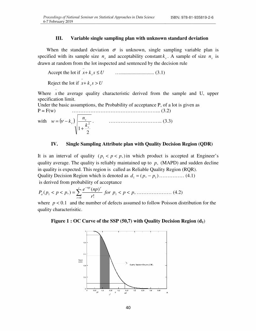
Proceedings of National Seminar on 6-7 February 2019

III. Variable single sampling

When the standard deviation

specified with its sample size

drawn at random from the lot inspected and sentenced by the decision rule

Accept the lot if skx s+−

Reject the lot if skx s >+−

Where −

x the average quality characteristic derived from the sample and U, upper specification limit. Under the basic assumptions, the Probability of acceptance P, of a lot is given asP = F(w) …………………………………………….. (3.

with ( )

21

2

s

s

sk

nkw

+

−= ν . ………………………….. (3.3)

IV. Single Sampling Attribute plan with Quality Decision Region (QDR)

It is an interval of quality

quality average. The quality is reliably maintained up to

in quality is expected. This region is called as Reliable Quality Region (RQR).

Quality Decision Region which is denoted as

is derived from probability of acceptance

0

*1!

()(

r

npepppP

c

r

np

a =<< ∑=

−

where 1.0<p and the number of defects assumed to follow Poisson distribution for the

quality characterisitic.

Figure 1 : OC Curve of the SSP (50,7) with Quality Decision Region (d

Proceedings of National Seminar on Statistical Approaches in Data Science ISBN: 978-81

40

Variable single sampling plan with unknown standard deviation

When the standard deviation σ is unknown, single sampling variable plan is

specified with its sample size sn and acceptability constant sk . A sample of size

drawn at random from the lot inspected and sentenced by the decision rule

U≤ …........................... (3.1)

U>

the average quality characteristic derived from the sample and U, upper

Under the basic assumptions, the Probability of acceptance P, of a lot is given asP = F(w) …………………………………………….. (3.2)

. ………………………….. (3.3)

Single Sampling Attribute plan with Quality Decision Region (QDR)

It is an interval of quality )( *1 ppp << in which product is accepted at Engineer’s

quality average. The quality is reliably maintained up to *p (MAPD) and sudden decline


which is denoted as )( 1*1 ppd −= …………… (4.1)


*1

)pppfor

npr

<< ………………… (4.2)

and the number of defects assumed to follow Poisson distribution for the

Figure 1 : OC Curve of the SSP (50,7) with Quality Decision Region (d

81-935819-2-6

plan with unknown standard deviation

is unknown, single sampling variable plan is

. A sample of size sn is

the average quality characteristic derived from the sample and U, upper

Under the basic assumptions, the Probability of acceptance P, of a lot is given as

Single Sampling Attribute plan with Quality Decision Region (QDR)

in which product is accepted at Engineer’s

(MAPD) and sudden decline


…………… (4.1)

and the number of defects assumed to follow Poisson distribution for the

Figure 1 : OC Curve of the SSP (50,7) with Quality Decision Region (d1)


ISBN: 978-81-935819-2-6

41

From Figure 1 1d represent the Quality Decision Region (QDR). A general result is that

2*1 ppp << for any Single Sampling Attribute plan. When *p approaching 1p , then

*np also approaching 1np .Then 1d is small. Therefore straighter OC can be performed.

When *p approaching 2p then *np approaching 2np . That is when *p approaching 2p ,

at lower quality level acceptance is more. After MAPD, at lower quality level if

acceptance is more, then the product is not at all useful. Therefore When *np approaching

2np , OC will be relatively less discriminating about the quality. Thus Quality Decision

Region (QDR), 1d is a good measure for defining the quality of a product.

4. 1. Variables single sampling plan with Quality Decision Region (QDR) - case of

known standard deviation:



in quality is expected.

Quality Decision Range is denoted as ( )1*1 ppnd −= σσ ………………………… (4.1.1)


),()( *1 wFpppPa =<< with ( )σσ ν knw −= ……………..for *1 ppp <<

Where p is the fraction nonconforming in a lot.

Values of the parameters ( )σσ kn , and QDR )( 1σd when sigma is known, are tabulated in

Table1.This is done for several combinations of (AQL, LQL). Suppose for example that AQL=0.0010, LQL=0.0050 and MAPD=0.00194. Then from

Table 1, using equation (4.1.1) the Quality Decision Region .0310.0)( 1 =σdQDR Thus

the Parameters of known sigma variables single sampling plan can be determined as

.0310.0)(,8000.2,33 1 === σσσ dQDRkn

4. 2. Variables single sampling plan with Quality Decision Region (QDR) - case of

unknown standard deviation:



in quality is expected.

Quality Decision Range is denoted as ( )1*1 ppnd ss −= ………………….. (4.2.1)


),()( *1 wFpppPa =<< with ( )

21

2s

s

sk

nkw

+

−= ν ……………..for *1 ppp <<


Values of the parameters ( )ss kn , and QDR )( 1sd when sigma is unknown, are tabulated in

Table1.This is done for several combinations of (AQL, LQL). Suppose for example that AQL=0.0010, LQL=0.0050 and MAPD=0.00194. Then using

Table 1, with equation (4.2.1) the Quality Decision Region .1504.0)( 1 =sdQDR Thus the

Parameters of unknown sigma variables single sampling plan can be determined as


ISBN: 978-81-935819-2-6

42

.1504.0)(,8000.2,160 1 === sss dQDRkn

V. Single Sampling Attribute Plan with Probabilistic Quality Region (PQR)

It is an interval of quality )( 21 ppp << in which product is accepted with a minimum

probability 0.10 and maximum probability 0.95. Probabilistic Quality Region denoted by

)( 122 ppd −= is derived from probability of acceptance

21

0

21!

)()( pppfor

r

npepppP

c

r

rnp

a <<=<< ∑=

−

………………….. (3.1)

Where 1.0<p and the number of defects assumed to follow Poisson distribution.

Figure 2 represents the OC curve indicating the Probabilistic Quality Region (PQR).

From Figure 2 2d represent the Probabilistic Quality Region (PQR).

Figure 2: OC Curve of the SSP (75,5) with Probabilistic Quality Region (d2)

5.1. Variable single sampling plan with Probabilistic Quality Region (PQR) - case of

known standard deviation:

It is an interval of quality (p1< p< p2) in which product is accepted with a minimum probability 0.10 and maximum probability 0.95.

Probabilistic Quality Region denoted by ( )122 ppnd −= σσ ………………………..

(5.1.1) is derived from probability of acceptance

),()( 21 wFpppPa =<< with ( )σσ ν knw −= for 21 ppp <<


ISBN: 978-81-935819-2-6

43

Where p is the fraction nonconforming in a lot. Values of the parameters ( )σσ kn , and

PQR )( 2σd when sigma is known, are tabulated in Table1.This is done for several

combinations of (AQL, LQL). Suppose for example that AQL=0.0010, LQL=0.0050 and MAPD=0.00194. Then from Table 1, using equation (5.1.1) the Probabilistic Quality

Region, .1320.0)( 2 =σdPQR Thus the Parameters of known sigma variables single

sampling plan can be determined as .1320.0)(,8000.2,33 2 === σσσ dPQRkn

5.2. Variable single sampling plan with Probabilistic Quality Region (PQR) - case of

unknown standard deviation:

It is an interval of quality (p1< p< p2) in which product is accepted with minimum probability 0.10 and maximum probability 0.95.

Probabilistic Quality Region denoted as ( )122 ppnd ss −= …………………. (5.2.1)


),()( 21 wFpppPa =<< with ( )

21

2s

s

sk

nkw

+

−= ν for 21 ppp <<


Values of the parameters ( )ss kn , and PQR )( 2sd when sigma is unknown, are tabulated in

Table1.This is done for several combinations of (AQL, LQL). Suppose for example that AQL=0.0010, LQL=0.0050 and MAPD=0.00194. Then from Table 1, using equation

(5.2.1) the Probabilistic Quality Region .640.0)( 2 =sdPQR Thus the Parameters of

unknown sigma variables single sampling plan can be determined as

.640.0)(,8000.2,160 2 === sss dPQRkn

VI. Comparison of sampling plans

It is observed that, variables single sampling plan yield a reduction in sample size than the attribute single sampling plan at the specified AQL and LQL. It indicates that the variables single sampling plan can achieve the same operating characteristics with smaller sample size as compared with attribute single sampling plan. It is also observed from Table -2, that the smaller sample size are required for variables single sampling plan as compared with attribute single sampling plan. Therefore variables single sampling plan is economically superior to attribute single sampling plan.

It can also be seen that the variables single sampling plan with smaller value of

PQR, that is for smaller values of 2d or )( 2σd seems to be closer to the ideal OC curve in

that the probability of acceptance at AQL or smaller is increased. From Table 3, it can be seen that when Probabilistic Quality Region (PQR) is decreasing, Maximum Allowable Average Outgoing Quality (MAAOQ) and Average Outgoing Quality Limit (AOQL) is increasing. Therefore PQR method possesses wide potential applicability in industry insuring a higher standard of quality attainment. If the Probabilistic Quality Region is small, straighter OC can be performed. Therefore, it can be seen that the sampling plan


ISBN: 978-81-935819-2-6

44

with a smaller value of PQR )( 2d seems to be closer to the ideal OC curve. Compared

with attribute single sampling plan, the variables single sampling plan seems to be closer to the ideal OC curve.

Suppose for example that AQL=0.6640, LQL=1.4760. Using Table 2, the parameters of the Attribute single sampling plan can be determined as

.412.1056)(,13,5601 2 === dPQRcn

The parameters of known sigma variables single sampling plan can be determined

as .140.77)(,3078.2,95 2 === σσσ dPQRkn

The parameters of unknown sigma variables single sampling plan can be

determined as .200.284)(,3095.2,350 2 === sss dPQRkn Certain parametric values for

variable single sampling plan are carried out in Table 5.

VII. Efficiency comparison using Probabilistic Quality Region

The relative efficiencies are given by the ratio of Probabilistic Quality Region (PQR) of

the sampling plans viz.,σ2

2

d

d,

sd

d

2

2 , σ2

2

d

d s , s

R

d

d

2

2 , have been computed and given in Table

4. From the computed values one can notice that the ratios are decreasing as AQL and LQL increases.

VIII. Conclusion

The purpose of this paper is to design a variable sampling plan through Quality Decision Region (QDR) and Probabilistic Quality Region (PQR) for accepting lots of products whose quality characteristic follows a normal distribution. The proposed variables single sampling plan through Probabilistic Quality Region (PQR) provides better protection than conventional attribute single sampling plans with smaller sample size. This plan is based on a simple statistic and it is easier to apply than double and multiple sampling plans. It is observed that the sampling plan with smaller value of PQR

( )2d seems to be closer to the ideal shape of OC curve. So compared to attribute single

sampling plan through PQR, the variable single sampling plan through PQR seems to be closer to the ideal shape of OC curve. It is seen that the variable single sampling plan through Probabilistic Quality region (PQR) is economically superior to attribute single sampling plans. The Scope of this paper is purely based on a new methodology of designing sampling plan based on range of quality instead of point- wise description of quality. So this method can be adopted in the elementary production process where the stipulated quality level is advisable to fix at a later stage. The Quality Decision Region (QDR) and Probabilistic Quality Region (PQR) idea has been experimented on designing of Single Sampling Variables Plan which results with minimization of sample size. Quality Region concept possesses wider potential applicability in industry ensuring

higher standard of quality attainment. The Quality Decision Region '' 1d is a good

measure for defining quality, since the Quality Decision Region '' 1d , depends upon the

inflection point. MAPD is a key measure for assessing the degree of sharpness of inspection with inflection point which empowers the OC curve to discriminate between


ISBN: 978-81-935819-2-6

45

good and bad lots. Further successful matching based on MAPD has also been accomplished using the abscissa of the inflection point and tangent at that abscissa. Also translation of the original OC curve from an acceptance to a surveillance criterion can be

accomplished through a shift in *p . This mode of relaxing *p has been found to be of

convenience to the technician or engineer who are unfamiliar with basic statistical theory.

REFERENCES

1. Baillie, D.H., 1992. Double sampling plans for inspection by variables when the

process standard deviation is unknown. International Journal of Quality and Reliabilility Management 9, 59-70.

2. Balamurali, S., Park,H., Jun,C.H., Kim,K.-J.,Lee,J.,2005. Designing of variables repetitive group sampling plan involving minimum average sample number. Communications in Statistics- Simulation and computation 34(3), 799-809.

3. Balamurali, S., Jun,C.H., 2007. Multiple dependent state sampling plans for lot acceptance based on measurement data. European Journal of Operational Research 180, 1221-1230.

4. Bravo,P.C., Wetherill, G.B.,1980. The matching of sampling plans and the design of double sampling plans. Journal of the Royal Statistical Society A 143, 49-67.

5. Hamaker, H.C., 1979. Acceptance sampling for percent defective by variables and by attributes. Journal of Quality Technology, Vol.11, No.3, 2(2), 139-148.

6. Muthuraj .D., 1988. “Contributions to the study of Sampling Inspection Plans with special reference to point of control and inflection point of the OC curve”, Ph.D Thesis, Bharathiar University, Coimbatore, India.

7. Owen, D.B., 1967. Variables sampling plans based on the normal distribution. Technometrics 9, 417-423.

8. Schilling, E.G., 1982. Acceptance Sampling in Quality Control. Marcel Dekker, New York.

9. Suresh, K.K., 1993. “A study on Acceptance Sampling using Acceptable Quality Levels”, Ph.D Thesis, Bharathiar University, Coimbatore, Tamilnadu, India.


ISBN: 978-81-935819-2-6

46

Table 1: Variables Single Sampling Plans with Quality Decision Region (QDR) and Probabilistic

Quality Region (PQR) indexed by AQL and LQL

AQL

LQL

MAPD

Known sigma

unknown sigma

σn σk

QDR

)( 1σd

PQR

)( 2σd sn sk

QDR

)( 1sd

PQR

)( 2sd

0.0010 0.0020 0.00141 191 2.9700 0.0783 0.1910 1032 2.970 0.4231 1.032

0.0010 0.0025 0.00155 107 2.9300 0.0589 0.1605 567 2.930 0.3119 0.851

0.0010 0.0030 0.00164 74 2.9000 0.0474 0.1480 381 2.900 0.2438 0.762

0.0010 0.0040 0.00184 45 2.8400 0.0378 0.1350 226 2.840 0.1898 0.678

0.0010 0.0050 0.00194 33 2.8000 0.0310 0.1320 160 2.800 0.1504 0.640

0.0010 0.0060 0.00198 26 2.7700 0.0255 0.1300 124 2.770 0.1215 0.620

0.0010 0.0070 0.00211 22 2.7300 0.0244 0.1320 102 2.730 0.1132 0.612

0.0010 0.0080 0.00211 19 2.7100 0.0211 0.1330 87 2.710 0.0966 0.609

0.0010 0.0090 0.00220 17 2.6800 0.0204 0.1360 76 2.680 0.0912 0.608

0.0010 0.0100 0.00218 15 2.6600 0.0177 0.1350 67 2.660 0.0791 0.603

0.0010 0.0120 0.00226 13 2.6200 0.0164 0.1430 55 2.620 0.0693 0.605

0.0010 0.0150 0.00235 11 2.5700 0.0149 0.1540 44 2.570 0.0594 0.616

0.0025 0.0050 0.00350 161 2.6800 0.1610 0.4025 736 2.680 0.7360 1.840

0.0025 0.0060 0.00382 99 2.6400 0.1307 0.3465 443 2.640 0.5848 1.551

0.0025 0.0075 0.00411 62 2.6000 0.0998 0.3100 267 2.600 0.4299 1.335

0.0025 0.0100 0.00454 38 2.5400 0.0775 0.2850 157 2.540 0.3203 1.178

0.0025 0.0120 0.00480 29 2.5000 0.0667 0.2755 117 2.500 0.2691 1.112

0.0025 0.0150 0.00513 22 2.4500 0.0579 0.2750 85 2.450 0.2236 1.063

0.0025 0.0200 0.00556 16 2.3800 0.0490 0.2800 59 2.380 0.1805 1.033

0.0025 0.0250 0.00551 12 2.3300 0.0361 0.2700 45 2.330 0.1355 1.013

0.0025 0.0300 0.00547 10 2.2900 0.0297 0.2750 37 2.290 0.1099 1.018

0.0025 0.0350 0.00568 9 2.2500 0.0286 0.2925 31 2.250 0.0986 1.008

0.0050 0.0100 0.00698 138 2.4400 0.2732 0.6900 547 2.440 1.0831 2.735

0.0050 0.0120 0.00757 85 2.4000 0.2185 0.5950 327 2.400 0.8404 2.289

0.0050 0.0150 0.00830 53 2.3500 0.1749 0.5300 196 2.350 0.6468 1.960

0.0050 0.0200 0.00929 32 2.2800 0.1373 0.4800 114 2.280 0.4891 1.710

0.0050 0.0250 0.00986 23 2.2300 0.1118 0.4600 79 2.230 0.3839 1.580

0.0050 0.0300 0.01020 18 2.1900 0.0936 0.4500 61 2.190 0.3172 1.525

0.0050 0.0350 0.01062 15 2.1500 0.0843 0.4500 49 2.150 0.2754 1.470

0.0050 0.0400 0.01113 13 2.1100 0.0797 0.4550 41 2.110 0.2513 1.435

0.0100 0.0200 0.01430 116 2.1700 0.4988 1.1600 388 2.170 1.6684 3.880

0.0100 0.0250 0.01563 64 2.1200 0.3603 0.9600 208 2.120 1.1710 3.120

0.0100 0.0300 0.01665 44 2.0800 0.2926 0.8800 137 2.080 0.9111 2.740

0.0100 0.0350 0.01770 33 2.0400 0.2541 0.8250 100 2.040 0.7700 2.500

0.0100 0.0400 0.01876 26 2.0000 0.2278 0.7800 78 2.000 0.6833 2.340

0.0100 0.0450 0.01951 22 1.9700 0.2092 0.7700 64 1.970 0.6086 2.240

0.0100 0.0500 0.02029 19 1.9400 0.1955 0.7600 54 1.940 0.5557 2.160

0.0100 0.0600 0.02143 15 1.8900 0.1715 0.7500 41 1.890 0.4686 2.050

0.0200 0.0400 0.02870 94 1.8800 0.8178 1.8800 259 1.880 2.2533 5.180

0.0200 0.0450 0.03018 67 1.8500 0.6821 1.6750 182 1.850 1.8528 4.550

0.0200 0.0500 0.03174 52 1.8200 0.6105 1.5600 137 1.820 1.6084 4.110

0.0200 0.0600 0.03422 35 1.7700 0.4977 1.4000 89 1.770 1.2656 3.560

0.0200 0.0700 0.03599 26 1.7300 0.4157 1.3000 64 1.730 1.0234 3.200

0.0200 0.0800 0.03799 21 1.6900 0.3778 1.2600 50 1.690 0.8995 3.000

0.0200 0.0900 0.03979 17 1.6500 0.3364 1.1900 40 1.650 0.7916 2.800

0.0200 0.1000 0.04130 15 1.6200 0.3195 1.2000 34 1.620 0.7242 2.720


ISBN: 978-81-935819-2-6

47

Table 2: Variable Plans by −σ method, −s method, and −R method matched with Attribute plans

AQL%

LQL%

Attributes plan

−σ method

−s method −R method

n c PQR

)( 2d σn σk

PQR

)( 2σd sn sk

PQR

)( 2sd Rn Rk

PQR

)( 2Rd

0.1680 0.3650 5601 14 1103.397 138 2.7920 27.186 677 2.7930 133.369 880 1.2004 173.360

0.3320 0.7400 2601 13 1061.208 112 2.5586 45.696 478 2.5599 195.024 616 1.1000 251.328

0.6640 1.4760 1301 13 1056.412 95 2.3078 77.140 350 2.3095 284.200 446 0.9922 362.152

1.3270 2.9380 651 13 1048.761 79 2.0338 127.269 245 2.0358 394.695 306 0.8744 492.966

1.9870 4.3820 435 13 1041.825 71 1.8606 170.045 194 1.8630 464.630 239 0.7999 572.405

2.6540 5.3290 326 13 872.050 64 1.7292 171.200 161 1.7319 430.675 197 0.7434 526.975

3.3190 7.2580 261 13 1028.079 60 1.6229 236.340 139 1.6258 547.521 168 0.6977 661.752

3.9240 8.3150 201 12 882.591 52 1.5306 228.332 113 1.5541 496.183 135 0.6581 592.785

4.5650 10.2110 173 12 976.758 49 1.4531 276.654 101 1.4567 570.246 120 0.6248 677.520

5.2380 11.6620 151 12 970.024 46 1.3805 295.504 91 1.3843 584.584 107 0.5935 687.368

5.8660 13.0070 135 12 964.035 44 1.3188 314.204 84 1.3228 599.844 97 0.5670 692.677

6.5540 14.4680 121 12 957.594 42 1.2568 332.388 77 1.2609 609.378 88 0.5403 696.432

Table 3: Variable Single Sampling Plan indexed by AOQL and LQL

AOQL% AQL%

Attributes plan Matched Variables Plan

n c MAAOQ PQR

)( 2d σn σk MAAOQ PQR

)( 2σd sn sk MAAOQ PQR

)( 2sd

0.1000 0.050 1342 2 0.0009 67.10 20 2.8799 0.0009 1.00 105 2.8868 0.0009 5.250

0.1000 0.025 841 1 0.0007 79.90 12 2.8763 0.0007 1.14 61 2.8883 0.0007 5.795

0.1000 0.075 2544 4 0.0008 165.36 11 2.8261 0.0008 0.72 61 2.8381 0.0008 3.965

0.5000 0.075 169 1 0.0030 14.37 9 2.3247 0.0036 0.77 32 2.3440 0.0033 2.720

0.5000 0.100 169 1 0.0030 13.52 9 2.3249 0.0036 0.72 33 2.3435 0.0033 2.640

0.5000 0.250 275 2 0.0040 13.75 15 2.3287 0.0047 0.75 56 2.3394 0.0045 2.800

1.0000 0.250 85 1 0.0070 5.10 8 2.0570 0.0075 0.48 25 2.0791 0.0069 1.500

Table 4: The Relative Efficiencies of Probabilistic Quality Region (PQR)

AQL% LQL%

Attributes

Plan

−σ

method

−smethod

−Rmethod

Relative Efficiency

)( 2d )( 2σd )( 2sd )( 2Rd

σ2

2

d

d

sd

d

2

2

σ2

2

d

d s

s

R

d

d

2

2

0.1680 0.365 1103.397 27.186 133.369 173.360 40.5870 8.2733 4.9058 1.2999

0.3320 0.740 1061.208 45.696 195.024 251.328 23.2232 5.4414 4.2679 1.2887

0.6640 1.476 1056.412 77.140 284.200 362.152 13.6947 3.7171 3.6842 1.2743

1.3270 2.938 1048.761 127.269 394.695 492.966 8.2405 2.6571 3.1013 1.2490

1.9870 4.382 1041.825 170.045 464.630 572.405 6.1268 2.2423 2.7324 1.2320

2.6540 5.329 872.050 171.200 430.675 526.975 5.0938 2.0248 2.5156 1.2236

3.3190 7.258 1028.079 236.340 547.521 661.752 4.3500 1.8777 2.3167 1.2086

3.9240 8.315 882.591 228.332 496.183 592.785 3.8654 1.7788 2.1731 1.1947

4.5650 10.211 976.758 276.654 570.246 677.520 3.5306 1.7129 2.0612 1.1881

5.2380 11.662 970.024 295.504 584.584 687.368 3.2826 1.6593 1.9783 1.1758

5.8660 13.007 964.035 314.204 599.844 692.677 3.0682 1.6071 1.9091 1.1548

6.5540 14.468 957.594 332.388 609.378 696.432 2.8810 1.5714 1.8333 1.1429


ISBN: 978-81-935819-2-6

48

Table 5: Certain Parametric Values for Variable Single Sampling Plan

AOQL% AQL%

known sigma

σn σk MAAOQ

MAPD

MAAOQR =1

MAPD

AOQLR =2

0.10 0.08 11 2.8261 0.0008 0.8257 1.0643

0.25 0.05 10 2.5746 0.0017 0.8172 1.1827

0.50 0.10 9 2.3249 0.0036 0.8084 1.1224

0.75 0.25 8 2.1727 0.0053 0.8100 1.1516

1.00 0.50 13 2.0606 0.0094 0.7321 0.7814

1.50 0.50 11 1.8873 0.0110 0.7343 0.7917

2.00 1.00 11 1.7586 0.0191 0.7201 0.7539

2.50 1.50 10 1.6528 0.0238 0.7193 0.7542

3.00 2.00 13 1.5775 0.0298 0.6822 0.6860

3.50 2.50 16 1.5159 0.0348 0.6570 0.6611

4.00 3.00 15 1.4484 0.0396 0.6557 0.6628

4.50 3.50 15 1.3873 0.0445 0.6494 0.6561

5.00 4.00 17 1.3117 0.0487 0.6323 0.6530

5.50 4.50 16 1.2892 0.0536 0.6345 0.6506

6.00 5.00 19 1.2456 0.0574 0.6185 0.6363

6.50 5.50 18 1.2060 0.0623 0.6183 0.6448

7.00 6.00 18 1.1665 0.0666 0.6145 0.6458

7.50 6.50 17 1.1199 0.0718 0.6136 0.6408

8.00 7.00 19 1.0913 0.0753 0.6042 0.6417

8.50 7.50 19 1.0584 0.0793 0.6011 0.6442

9.00 8.00 18 1.0197 0.0842 0.6004 0.6422

9.50 8.50 18 0.9808 0.0892 0.5967 0.6354

10.00 9.00 20 0.9661 0.0912 0.5899 0.6469

unknown sigma

sn sk MAAOQ

MAPD

MAAOQR =1

MAPD

AOQLR =2

61 2.8381 0.0008 0.8127 1.0093

43 2.5900 0.0016 0.8204 1.2645

33 2.3435 0.0033 0.8134 1.2190

29 2.1922 0.0052 0.8026 1.1534

41 2.0736 0.0091 0.7332 0.8099

21 1.9116 0.0108 0.7912 1.1039

28 1.7752 0.0183 0.7234 0.7909

25 1.6705 0.0232 0.7163 0.7731

30 1.5912 0.0291 0.6819 0.7041

35 1.5271 0.0340 0.6572 0.6759

25 1.4485 0.0388 0.6743 0.6980

23 1.3912 0.0436 0.6718 0.7022

34 1.3548 0.0479 0.6334 0.6620

31 1.3000 0.0527 0.6320 0.6591

35 1.2639 0.0565 0.6187 0.6567

32 1.2157 0.0614 0.6178 0.6546

31 1.1764 0.0621 0.6144 0.6561

29 1.1302 0.0707 0.6121 0.6495

31 1.1004 0.0743 0.6041 0.6508

30 1.0675 0.0782 0.6017 0.6539

28 1.0291 0.0830 0.6004 0.6514

27 0.9903 0.0880 0.5973 0.6450

30 0.9746 0.0901 0.5899 0.6550


ISBN: 978-81-935819-2-6

49

On Some Tailed Distributions And Related Time Series Models

Mariamma Antony

Department of Statistics, Little Flower College

Guruvayoor, Kerala

Email: [email protected] Abstract

We encounter tailed distributions in life testing experiments

where an item fails instantaneously. In clinical trials,

sometimes a medicine has no response initially and later there

may be response, the length of response is described by certain

probability distribution. In this paper, we study tailed

generalized geometric Linnik distribution. Relation between

stable laws and tailed geometric Linnik distribution is

established. Time series models with tailed generalized

geometric Linnik marginals are developed. The stationarity of

the processes is established. The model is extended to pth

order. Tailed generalized geometric asymmetric Linnik

distribution is introduced and studied.

Keywords: Laplace distribution, Linnik distribution, Stable Laws, Stationarity, Tailed distributions, Time Reversibility.

I. Introduction

Tailed distributions have found applications in various fields and were studied by many authors (see, Littlejohn (1994), Muraleedharan (1999), Muraleedharan and Kale (2002) ).We encounter tailed distributions in life testing experiments where an item fails instantaneously. In clinical trials, some times a medicine has no response initially with a certain probability and on a later stage there may be response, the length of the response is described by certain probability distribution. DEFINITION 1.1

Let the random variable X has distribution function F(x) and characteristic function

( ).X tφ A tailed random variable U with tail probability θ associated with X is defined by

the characteristic function

( ) (1 ) ( )U Xt tφ θ θ φ= + −

. (1.1

Linnik (1963) proved that the function

( )1

, 0 2, 01

tt

αφ α λ

λ= < ≤ >

+ (1.2)

is the characteristic function of a probability distribution. The distribution corresponding to the characteristic function (1.2) is called Linnik (orα - Laplace) distribution. A random

variable X with characteristic function φ in (1.2) is denoted by ( ), .X dL α λ Note that the

( ),L α λ distributions are symmetric and for 2α = , it becomes the classical symmetric

Laplace distribution. Pillai (1985) introduced a generalization of the Linnik distribution with characteristic function (1.2), namely semi α -Laplace distribution. A random variable X on R has semi α -Laplace distribution if its characteristic function )t(φ is of the form

)t(t1

1)t(

δ+=φ

α (1.3)


ISBN: 978-81-935819-2-6

50

where )t(δ satisfies the functional equation

( )1( ) , 0 1, 0 2.t p t pαδ δ α= < < < ≤ (1.4)

DEFINITION 1.2

A random variable X on R is said to have geometric Linnik distribution and write

),(GLdX λα if its characteristic function )t(φ is

1( ) , , 0 2, 0.

1 ln(1 )t t R

tα

φ α λλ

= ∈ < ≤ >+ +

(1.5)

DEFINITION 1.3

A random variable X on R has the generalized Linnik distribution and write

( , , )X d GeL pα λ if it has the characteristic function

1( )

(1 ) pt

tα

φλ

=+

, 0, 0, 0 2.p λ α> > < ≤ (1.6)

DEFINITION 1.4

A random variable X on R is said to have type I generalized geometric Linnik

distribution and write 1( , , )X d GeGL pα λ if it has the characteristic function

1( ) ,

1 ln(1 )t

p tα

φλ

=+ +

0 2, 0, 0.pα λ< ≤ > > (1.7)

In Section 2, we introduce tailed distributions associated with type I generalized geometric Linnik distribution and study its properties. Tailed Type II generalized geometric Linnik distribution is also discussed in this Section. Tailed type I generalized geometric asymmetric Linnik distribution is studied in Section 3. In Section 4, a first order autoregressive model with tailed Type I generalized geometric Linnik distribution as marginal is developed.

II. Tailed Generalized Geometric Linnik Distributions

Now we introduce tailed Type I generalized geometric Linnik distribution and obtain a representation of the same.

In (1.1), when

λ+τ+

=φα

t1ln1

1)t(X , then

( )( )

1 ln 1( ) .

1 ln 1U

t

t

t

α

α

τθ λφ

τ λ

+ +=

+ + (2.1)

The random variable U with characteristic function (2.1) is called tailed Type I generalized

geometric Linnik and denoted by ( )1 , , ,TGeGL α λ τ θ

THEOREM 2.1

Let X and Y be independent random variables such that X has tailed generalized

geometric exponential distribution with Laplace transform 1

(1 )1 ln(1 )

θ θτ δ

+ −+ +

and Y

is stable with characteristic function α

λ− te , 0 2, , , 0,α λ δ τ< ≤ > 0 1.θ< < Then

YXZ1

α= has ( )1 , , ,TGeGL α λ τ θ distribution.


ISBN: 978-81-935819-2-6

51

PROOF

=φ

αYitXZ

1

eE)t(

( )1

0

( )Y tx dF xαφ∞

= ∫

0

( )t x

e dF xα

λ∞

−= ∫

( )1

(1 )1 ln 1 t

αθ θ

τ λ= + −

+ +

( )( )

1 ln 1.

1 ln 1

t

t

α

α

τθ λ

τ λ

+ +=

+ +

This completes the proof. Now we consider the type II generalized geometric Linnik distribution and study

the tailed distribution generated by it. DEFINITION 2.1

A random variable X is said to have tailed type II generalized geometric Linnik

distribution and write ( )2 , , ,X d TGeGL α λ τ θ distribution if it has thecharacteristic

function

( )

( )

1 ln 1 (1 )

( ) ,0 2,0 1, , 0.

1 ln 1

X

t

t

t

τα

τα

θ λ θφ α θ λ τ

λ

+ + + − = < ≤ < < >

+ +

The tailed type II generalized geometric Linnik distribution being the tailed form of type II generalized geometric Linnik is infinitely divisible.

As in the case of 1TGeGL distribution, we now obtain a representation of

2TGeGL random variables in terms of tailed geometric gamma and stable random

variables. DEFINITION 2.2

A random variable X is said to have tailed geometric gamma distribution if it has Laplace transform

( )1

1( ) (1 ) , , 0,0 1.

1 ln 1τ

φ δ θ θ δ τ θδ

= + − > < <+ +

THEOREM 2.2

Let X and Y be independent random variables such that X has Laplace transform

( )[ ]τδ++θ−+θ

1ln1

1)1( and Y is stable with characteristic function , 0 2.

te

αλ

α−

< ≤

Then YXU1

α= has distribution ( )2 , , , .TGeGL α λ τ θ

Proof follows analogous to the proof of Theorem 2.1.


ISBN: 978-81-935819-2-6

52

III. Tailed Generalized Geometric Asymmetric Linnik Distribution Here we discuss the tailed distributions generated by generalized geometric

asymmetric Linnik distributions. DEFINITION 3.1

A random variable X is said to have tailed type I generalized geometric asymmetric

Linnik distribution and write ( )1 , , , ,U d TGeGAL α λ µ τ θ if it has characteristic function

( )( )

1 ln 1( ) .

1 ln 1U

t i t

tt i t

α

α

τθ λ µφ

τ λ µ

+ + −=

+ + −

The type II generalized geometric asymmetric Linnik distribution can be defined

using (1.1) with )t(Xφ replaced by

( )1

.

1 ln 1 t i tτ

αλ µ + + −

That is, a random variable U having tailed type II generalized geometric asymmetric

Linnik distribution denoted by ( )2 , , , ,TGeGAL α λ µ τ θ has characteristic function

( )1

(1 ) .

1 ln 1 t i tτ

αθ θ

λ µ

+ − + + −

IV. Time Series Models With Tailed Generalized Geometric Linnik

Distribution As Marginals

Now we develop a first order autoregressive model with 1TGeGL distribution as marginal.

Consider the model

1

. .

. . 1

nn

n n

w p pX

X w p p

ε

ε−

=

+ − (4.1)

n1nn XI ε+= −

where{ }nε and { }nI are two sequences of independent and identically distributed random

variables with nI , 1nX − and nε mutually independent such that

( ) ( )0 1 1 .n nP I p P I= = = − =

We have the model (4.1) in terms of characteristic functions is

1

( )( )

(1 ) ( )n

n

n

X

X

tt

p p tε

φφ

φ−

=+ −

.

In the stationary case,

( )

( ) .(1 ) ( )n

X

X

tt

p p tε

φφ

φ=

+ −

If X has characteristic function (2.1), then

( )( )

1 ln 1( )

1 ln 1n

t

tc t

α

ε α

τθ λφ

τ λ

+ +=

+ +, where (1 ) .c p p θ= + −


ISBN: 978-81-935819-2-6

53

That is,

( )1

( ) 1 .1 ln 1

nt

c c c tε α

τθ τθφ

τ λ

= + −

+ +

Hence, if the model (4.1) is stationary with ( )1 , , ,TGeGL α λ τ θ marginal distribution, then

the distribution of the innovation sequence { }nε is ( )1 , , , .c

TGeGL c τθα λ τ

If ( )0 1 , , ,d

X TGeGL α λ τ θ= and { }nε are independent and identically distributed as

( )1 , , ,c

TGeGL c τθα λ τ , then the characteristic function of 1X is

1 0 1( ) (1 ) ( ) ( )X Xt p p t tεφ φ φ = + −

λ+τ+

λ+τθ+

λ+τ+

λ+τθ+

−+=α

α

α

α

t1lnc1

t1ln1

t1ln1

t1ln1

)p1(p

( )( )

1 ln 1.

1 ln 1

t

t

α

α

τθ λ

τ λ

+ +=

+ +

That is, 1 0.X dX

If 1 0 ,nX d X− we can prove that 0nX d X and hence the process { }nX is stationary.

Based on this, we now define stationary first order autoregressive tailed Type I generalized geometric Linnik process as follows:

Let ( )0 1 , , ,X d TGeGL α λ τ θ

and for 1, 2,...n =

1

. .

. . 1

nn

n n

w p pX

X w p p

ε

ε−

=

+ −

where{ }nε is a sequence of independent and identically distributed ( )1 , , ,c


random variables where (1 ) .c p p θ= + −

It can be shown that the process { }nX is not time reversible. For this, consider the

characteristic function

( )1 2 1

1, 1 2( , ) n n

n n

it X it XX X t t E eφ +

+

+=

2 1 1 2( ) ( ) (1 ) ( )n n nX Xt p t p t tεφ φ φ = + − +

λ+τ+

λ+τθ+

=α

α

t1lnc1

t1ln1 ( )( )

( )( )

1 1 2

2 1 2

1 ln 1 1 ln 1(1 ) .

1 ln 1 1 ln 1

t t t

p p

t t t

α α

α α

τθ λ τθ λ

τ λ τ λ

+ + + + +

+ − + + + + +

This expression is not symmetric in 1t and 2.t

REMARK 4. 1

If { }nε is a sequence of independent and identically distributed

( )1 , , ,c

TGeGL c τθα λ τ , where θ−+= )p1(pc then (4.1) is asymptotically stationary with

( )1 , , ,TGeGL α λ τ θ marginal distribution.


ISBN: 978-81-935819-2-6

54

Consider the kth order autoregressive process

1 1

2 2

. .

. .

. . .

. .

n

n n

n n n

n k n k

w p p

X w p p

X X w p p

X w p p

ε

ε

ε

ε

−

−

−

+= +

+

M

(4.3)

If the process { }nX is stationary, then in terms of characteristic function, (4.3) is

( )( ) ,

(1 ) ( )n

X

X

tt

p p tε

φφ

φ=

+ −where

1

1 , 0 1.k

i i

i

p p p

=

− = < <∑

Thus a necessary and sufficient condition for the model (4.3) defines a stationary AR(k)

process with ( )1 , , ,TGeGL α λ τ θ marginal distribution is that { }nε is distributed as

( )1 , , , .c


As in the case of 1TGeGL random variables, we now consider the first order

autoregressive model (4.1). We can prove that if { }nε are independent and identically

distributed ( )1 , , , ,c

TGeGAL c τθα λ µ τ random variables and

( )0 1 , , , ,X d TGeGAL α λ µ τ θ , then the model (4.1) is stationary with

( )1 , , , ,TGeGAL α λ µ τ θ marginals. Also if the model (4.1) is stationary with

( )1 , , , ,TGeGAL α λ µ τ θ marginals then it can be easily seen that the distribution of { }nε is

( )1 , , , ,c

TGeGAL c τθα λ µ τ where (1 ) .c p p θ= + − Based on this we can develop first

order autoregressive models with tailed Type I generalized geometric asymmetric Linnik marginal distribution. The model can be easily extended to higher order autoregressive model as in (4. 3).

References

1. Linnik, Yu.V. (1963) Linear forms and statistical criteria, I, II. Selected

Translations in Math. Statist. Prob. 3, 1-90. 2. Littlejohn, R.P. (1994) A reversibility relationship for two Markovian time series

models with stationary exponential tailed distribution. J. Appl. Prob.31, 575-581. 3. Muralidharan, K. (1999) Tests for the mixing proportions in the mixture of a

degenerate and exponential distribution. J. Ind. Statist. Assoc. 37, 105-119. 4. Muralidharan, K. and Kale, B.K. (2002) Modified gamma distribution with

singularity at zero. Commun.Statist. -Simul. Comput. 31, 143-158. 5. Pillai, R.N. (1985). Semi α-Laplace distributions. Commun. Statist.-Theor. Meth.

14, 991-1000.


ISBN: 978-81-935819-2-6

55

Estimation of Stress-Strength model using Three Parameter Generalized Lindley

Distribution

K. S Deepthi & V M Chacko

Department of Statistics, St. Thomas' College (Autonomous),

Thrissur, Kerala - 680 001 (India)

[email protected], [email protected]

Abstract

This paper deals with the reliability of a multicomponent stress-strength

model assuming that the components follow three parameter generalized

Lindley model. In a Multicomponent system with k components, strength of

each component experiencing a random stress: the problem of estimation

reliability is considered. The reliability of such a system is obtained when

strength and stress variables are given by three parameter Lindley

distribution. The system is regarded as alive only if with at least r out of

)( krk < components, the strength of system exceeds the stress. The

maximum likelihood estimation of reliability of the multicomponent system

is obtained.

Key Words: Reliability, Stress-Strength Model

I. Introduction

The estimation of reliability is a very common problem in statistical literature. The most widely approach applied for reliability estimation is well-known stress-strength model. Consider two independent random variables X andY . Suppose Y represents the 'stress' and

X represents the 'strength'. The reliability parameter )( XYPR <= is referred to as a

stress-strength model, which is used in engineering statistics, quality control and other fields. In a reliability, the stress-strength model describes the life of a component that has a random strength variable X and is subjected to random variable stressY . The system fails if and only if the stress is greater than strength at any time.

The estimation of a stress-strength model when X and Y are random variables having a specified distribution has been discussed by many authors including Raqab and Kundu (2005) discussed comparison of different estimates of stress-strength model for a scaled Burr type X distribution, Kundu and Gupta (2005) studied the stress-strength reliability based on generalized exponential distribution, Kundu and Gupta (2006) discussed estimation of stress-strength reliability in Weibull distribution, Raqab et al. (2008), Kundu and Raqab (2009)discussed estimation of stress-strength reliability with three parameter weibull distribution, Al-Mutairi et al. (2013) discussed estimation of stress-strength reliability in lindley distribution, Sharma et. al (2015) discussed stress-strength reliability model with application to headand neck cancer data based on inverse lindley distribution.

Let the random samples kXXXY ,,,, 21 L be independent, )( yG be the continuous

distribution function of Y and )(xF be the common continuous distribution function of

kXXX ,,, 21 L .The reliability in a multicomponent stress-strength model developed by

Bhattacharyya and Johnson (1974) is given by

[, PR ks = at least s of the ),,,( 21 kXXX L exceed ]Y


ISBN: 978-81-935819-2-6

56

∑ ∫=

∞

∞−

−−

=

k

si

ikiydGyFyF

i

k)()]([)](1[

where kXXX ,,, 21 L are identically independently distributed (iid) with common

distribution function )(xF and subjected to the common random stress Y . Recently,

Srinivasa Rao (2012) developed the multicomponent stress-strength reliability based on generalized exponential distribution, Srinivasa Rao et. al (2015) discussed the multicomponent stress-strength reliability with the Burr-XII distribution, the multicomponent stress-strength model using Lindley distributionis considered Marwa Khalil (2017).

Lindley (1958) introduced Lindley distribution in the context of fiducial and Baysian statistics and the probability density function (pdf) of one parameter Lindley distribution is given by

,)1(1

);(2

xexxf

θ

θ

θθ −+

+= .0,0 >> θx (1)

The probability density function of the Lindley distribution given in (1) is a mixture of

Exponential ( )θ and Gamma ( )θ,2 . The Equation (1) can be expressed as

)()1()();( 21 xfpxpfxf −+=θ (2)

where )(1 xf and )(2 xf are the density function of Exponential ( )θ and Gamma ( )θ,2

distribution and p is the mixing proportion. Properties, extension and applicationsof the

Lindley distributions have been studied in the context of reliability analysis byGhitanyet. al (2008). Shanker and Mishra (2013) obtained a two parameter Lindley distribution is given by

,)(1

),;(2

yeyyg

θααθ

θθα −+

+= .1,0,0 −>>> αθθy (3)

The power Lindley (PL) distribution proposed by Ghitanyet. al (2013) an extensionof the Lindley distribution. Ekhosuehi and Opone (2018) introduced a three parameter generalized Lindley distribution. Then the probability density function (pdf) of TPLDis given by

( ) ,1

),,;( 12

αλααββλ

αλλβα x

exxxf−−+

+= 0,,,0 >> λβαx (4)

Here β and λ are scale parameters and α is shape parameter. The

correspondingcumulative distribution function (cdf) is given by

,1

11),,;(

αλα

βλ

λβλλβα x

ex

xF−

+

++−= 0,,,0 >> λβαx (5)

and the survival function is given by

,1

1),,;(

αλα

βλ

λβλλβα x

ex

xS−

+

++= 0,,,0 >> λβαx (6)

The hazard rate function of TPL distribution is given by


ISBN: 978-81-935819-2-6

57

( ),

1),,;(

12

α

αα

λβλ

βαλλβα

x

xxxh

++

+=

−

0,,,0 >> λβαx (7)

The graph of the hazard rate function of the TPGLD for different value of the parameters is given in Figure 2.

(a) 15.1,25.0,85.0 === λβα (b) 2.1,25.0,8.0 === λβα


ISBN: 978-81-935819-2-6

58

(c) 1,15.0,5.0 === λβα (d) 5.2,45.0,5.1 === λβα

Figure 2 – Different parameter values of Hazard rate function of the TPGLD Clearly from Figure 2, the TPGLD exhibits monotone increasing, decreasing and bathtub

shaped failure rate behavior. It increases monotonically when 1>α and, decreasing and

bathtub when .1<α

The main objective of this paper is to check the appropriateness of the multicomponent stress-strength reliability of three parameter generalized Lindley distribution. Next we have to examine extent the reliability of parallel case and series case of the multicomponent stress-strength model.

This paper deals with the reliability of a multicomponent stress-strength model assuming that the components follow three parameter Lindley model. Section 2 discussed the multicomponent system reliability in three parameter generalized Lindley distribution. The

maximum likelihood estimator of reliability, krR , , is determined in section 3. Real data is

used as a practical application of the proposed model in section 4. Conclusions are given in section 5.

II. System Reliability

Let X and Y be two random variables that follows independent identically

distributedthree parameter Lindley distribution with common shape parameter ( )11,, λβα

and ( )22 , λβ respectively. Suppose 2

,,, 21 nXXX K and 1

,,, 21 nYYY K are two independent

samples from X and Y , respectively. The stress-strength reliability is

( ) ( ) ( )∫∞

=<=0

::,2:1:21

dxxfxFXYPRnknr XYnknrkr

(8)

where, ( )xFnrY1:

and ( )xfnkX

2: are the thr cumulative distribution function and th

k

probability density function of 1:nrY and

2:nkX respectively.

Then the thk probability density function of

2:nkX is given by


ISBN: 978-81-935819-2-6

59

( ) ( )[ ] )()(1 2

2:

12xfxFxF

k

nkxf

knk

X nk

−− −

= (9)

and the thr cumulative density function of 1:nrY is given by

[ ]∑=

−−⋅

=

1

1

1:)(1)()(

1n

rj

jnj

Y xFxFj

nxF

nr (10)

From (9) and (10) in (8),we obtain

( )

dxex

ex

ex

ex

exxj

n

k

nkR

kn

x

k

x

jn

x

jn

rj

xx

kr

−

−

−

−

−

−

=

∞−−−

⋅

+

++

⋅

+

++−

⋅

+

++×

⋅

+

++−⋅⋅+

+= ∑ ∫

2

11

1

2

1

21

11

111

1

11

111

22

222

022

2221

1

12

11

2

1,

1

1

1

11

1

1

1

11

1

ααα

αα

λα

λα

λα

λα

λαα

βλ

λβλ

βλ

λβλ

βλ

λβλ

βλ

λβλβ

βλ

αλ

( )

( )( )

( )( )

+

+−−−−−−+Γ+

+

−−−−−−+Γ×

+

+⋅

−

−−×

−

−

−

−

+=

+−−−−−−+−−−−−−+

−−−−−−−

=

−

=

−

=

−

=

−−

= =

−

=

−−−+∑∑∑∑ ∑ ∑∑

1

2112

65432121

2112

654321211

1

11

1

22

2

6

5

54

3

0 0

1

0

1

0 0 0 32

2

1

1112

11

2

1,

6543212165432121

43226511

1 1

1

2

2 3

3

4 5

5

6

53

1

11

1

11

1

llllllnnllllllnn

lllnllln

n

rj

jn

l

kn

l

k

l

lk

l

j

l

lj

l

llkj

kr

nn

llllllnn

nn

llllllnn

l

lj

l

j

l

lk

l

k

l

kn

l

jn

j

n

k

nkR

λλαλλα

β

βλ

λ

βλ

λ

βλ

αλ

(11)

where ( )⋅Γ is the gamma function. We now present some special cases of krR , with a

different arrangement of the components.

2.1. Reliability of the Parallel System

For parallel case, the reliability of the system is given by

( ) ( )( )21

,,,max,,,max 21211 nn XXXYYYPR KK <=

Then the stress-strength reliability of parallel system is

( )

( )( )

( )( )

+

+−−−−+Γ+

+

−−−−+Γ

+×

+

−

−−

+=

+−−−−+−−−−+

−−−

−

=

−−

= =

−−−

=

−−−+∑ ∑ ∑∑

1

2112

654321

2112

6543211

1

11

1

1

0

1

0 0 22

2

6

51

5

1

2

2

0

1

11

2

12,

654321654321

432

2

3

32

4

1

5

65151

6

5321

21

1

1

1

11

1

llllnnllllnn

lln

n

l

ln

l

n

l

llnln

l

llnn

nn

nn

llllnn

nn

llllnn

l

ln

l

n

l

nnR

λλαλλα

β

βλ

λ

βλ

λ

βλ

αλ

2.2. Reliability of the Series System

The reliability of system for the series case is

( ) ( )( )21

,,,min,,,max 21212 nn XXXYYYPR KK <=

Then the stress-strength reliability of series system is


ISBN: 978-81-935819-2-6

60

( )

( )( )

( )( )

+

+−−−+Γ+

+

−−−+Γ

+×

+

−

−−

+=

+−−−+−−−+

−−

−

= =

−

=

−−

−∑∑∑

1

2112

65221

2112

652211

1

11

1

1

0 0 0 22

2

6

51

5

1

2

2

11

2

121,

6522165221

22

2

1

5

51

6

651

51

1

1

1

1

11

1

lllnnlllnn

ln

n

l

n

l

ln

l

lln

ln

n

nn

lllnn

nn

lllnn

l

ln

l

n

l

nnR

λλαλλα

β

βλ

λ

βλ

λ

βλ

αλ

Now present another special cases of krR , with a different arrangement of the components.

1. For 1=r and 1=k , the minimum strength component is subjected to the minimum stress component.

( )

( )( )

( )( )

+

+−−−−+Γ+

+

−−−−+Γ

+

+×

−

−

−

−

+=

+−−−−−+−−−−+

−−−−

=

−

=

−

= =

−

=

−∑∑∑∑∑

1

2112

652121

2112

6521211

11

1

22

2

1

1

0

1

0 0 0 6

5

52

2

1

11

11

2

1211,1

6521121652121

226511

1 1

1

2

2 5

5

6

5

1

11

111

1

lllllnnllllnn

lnllln

n

j

n

l

n

l

j

l

lj

l

lj

nn

llllnn

nn

llllnn

l

lj

l

j

l

n

l

n

j

nnnR

λλαλλα

β

βλ

λ

βλ

λ

βλ

αλ

2. For 1nr = and kk = , the thk strength component is subjected to the maximum

stress component.

( )

( )( )

( )( )

+

+−−−−−+Γ+

+

−−−−−+Γ×

+

+

−

×

−−

−

−−

+=

+−−−−−+−−−−−+

−−−−−−

−

=

−

=

−−

= =

−

=

−−−+∑∑ ∑ ∑∑

1

2112

6543221

2112

65432211

1

11

1

22

2

6

51

5

1

0

1

0

1

0 0 0 4

3

32

212

11

2

1,

65432216543221

4322651

2

2 3

3

4

1

5

51

6

531

1

1

11

111

1

lllllnnlllllnn

lllnlln

kn

l

k

l

lk

l

n

l

ln

l

llkn

kn

nn

lllllnn

nn

lllllnn

l

ln

l

n

l

lk

l

k

l

kn

k

nkR

λλαλλα

β

βλ

λ

βλ

λ

βλ

αλ

III. Maximum Likelihood Estimator of krR ,

Suppose 2

,,, 21 nXXX K be the random sample of the strength of the 2n systems that are

distributed as three parameter generalized Lindley r.v's with parameter 1λ and 1β . Let

1,,, 21 nYYY K be the random sample of the stress of the 1n systems that are distributed as

three parameter generalized Lindley r.v's with parameter 2λ and 2β and common shape

parameter α .

Then the log-likelihood function of the observed sample is

( ) ( ) ( )

( ) ( ) ( )

( ) ∑∑

∑∑∑

∑

==

===

=

−−+

+++−+−−+

+++−++=

11

122

2

1

2

1

1

222121

1

1

1

1

111212212121

log1

log1loglog2log1

log1loglog2log),,,,(log

n

j

j

n

j

j

n

j

j

n

i

i

n

i

i

n

i

i

yy

ynnxx

xnnnnL

α

αα

α

λα

ββλλλα

ββλλααλλββ

(12)

The maximum likelihood estimators of 2121 ,,, λλββ and α denoted by 2121ˆ,ˆ,ˆ,ˆ λλββ and


ISBN: 978-81-935819-2-6

61

α respectively can be obtained as the solution of the following nonlinear equations

∑= +

++

−=∂

∂ 2

1 111

12

1

1

1

log n

i ix

nLαββλ

λ

β (13)

∑= +

++

−=∂

∂ 1

211

11

2

1

1

log n

ij jy

nLαββλ

λ

β (14)

∑=

−+

−=∂

∂ 2

111

12

1

2

1 1

2log n

i

ixnnL α

βλ

β

λλ (15)

∑=

−+

−=∂

∂ 1

122

21

2

1

2 1

2log n

j

jynnL α

βλ

β

λλ (16)

and

( ) ( ) ( )

( ) ( ) ( )

( ) ∑∑

∑∑∑

∑

==

===

=

−−+

+++−+−−+

+++−++=

11

122

2

1

2

1

1

222121

1

1

1

1

111212212121

log1

log1loglog2log1

log1loglog2log),,,,(log

n

j

j

n

j

j

n

j

j

n

i

i

n

i

i

n

i

i

yy

ynnxx

xnnnnL

α

αα

α

λα

ββλλλα

ββλλααλλββ

∑∑

∑∑∑∑

==

====

−+

++−+

++

+=

∂

∂

22

1222

1

2

1

1 21

1

11 1

21

loglog

logloglog

loglog

n

j

jj

n

j

j

n

j j

jjn

i

ii

n

i

i

n

i i

ii

yyy

y

yyxxx

x

xxnnL

α

α

α

α

α

λ

βλ

βαα (17)

By using the invariance property of the maximum likelihood estimator of krR , denotedby

ML

krR ,ˆ can obtained by replacing 2121 ,,, λλββ and α by their maximum likelihood

estimators. Therefore the maximum likelihood of krR , is obtained by

( )

( )

( )( )

( )

+

+−−−−−−+Γ+

+

−−−−−−+Γ×

+

+⋅

−

−−×

−

−

−

−

+=

+−−−−−−+−−−−−−+

−−−−−−−

=

−

=

−

=

−

=

−−

= =

−

=

−−−+∑∑∑∑ ∑ ∑∑

1

2112

65432121

2112

654321211

1

11

1

22

2

6

5

54

3

0 0

1

0

1

0 0 0 32

2

1

1112

11

2

1,

6543212165432121

43226511

1 1

1

2

2 3

3

4 5

5

6

53

ˆˆˆ

1

ˆˆˆ

ˆ

ˆˆ1

ˆ

1

1

11

ˆˆ1

ˆˆˆ

llllllnnllllllnn

lllnllln

n

rj

jn

l

kn

l

k

l

lk

l

j

l

lj

l

llkjML

kr

nn

llllllnn

nn

llllllnn

l

lj

l

j

l

lk

l

k

l

kn

l

jn

j

n

k

nkR

λλαλλα

β

βλ

λ

βλ

λ

βλ

λα

(18)

The asymptotic variance of ML

krR ,ˆ is given by

( ) ( )∑∑= =

−

∂

∂

∂

∂=

5

1

5

1

1,,

,ˆ

i j j

kr

i

krML

kr IRR

RAV θθθ

(19)

where ( )αλλββθ ,,,, 2121= and ( )θ1−I is the Fisher Information Matrix. Therefore, an


ISBN: 978-81-935819-2-6

62

asymptotic ( )%1100 η− confidence interval for Rr;k can obtain as ( )ML

kr

ML

kr RAVZR ,

2

,ˆˆ

η±

where 2

ηZ is the upper 2

ηquantile of standard normal distribution.

IV. Conclusion

The method of reliability estimation of stress strength model is discussed. We obtained an expression of reliability. The non-linear estimation require use of softaware like R, Matlab etc. The distributions of stress and strength are assumed to be bathtub shaped, which is quire desirable since the strength of human life increases at first stage (infant morality period), remains constant for a long period (useful life) and thereafter decreases (wear out period). So modeling stress strength reliability problems using bathtub shaped failure rate model become more realistic.

References

1. Al-Mutairi, D. K., Ghitany, M. E. &Kundu, D. (2013), ‘Inferences on stress-strength reliability from lindley distributions’, Communications in StatisticsTheory and Methods 42(8), 1443–1463.

2. Bhattacharyya, G. K. & Johnson, R. A. (1974), ‘Estimation of reliability in multicomponentstress-strength model’, Journal of the American Statistical Association, 69, 966–970.

3. Ghitany, M. E., Atieh, B. &Nadarajah, S. (2008), ‘Lindley distribution and it’sapplication’, Journal of Mathematics and Computers in Simulation 76, 493–506.

4. Ghitany, M.E., Al-Mutairi, D., Balakrishnan, N. &I.Al-Enezi (2013),‘Power Lindleydistribution and associated inference’, Computational Statistics and Data Analysis,64, pp. 20-33.

5. Kundu, D. & Gupta, R.D. (2005),‘Estimation of P[Y < X] for generalized exponential distribution’, Metrika, 61, 291–308.

6. Kundu, D. & Gupta, R.D. (2006),‘Estimation of R = P[Y < X] for Weibull distributions’, IEEE Transactions on Reliability,55, 270–280.

7. Kundu, D., Raqab, M.Z. (2009),‘Estimation of R = P(Y < X) for three-parameter Weibull Distribution’,Statistics and Probability Letters, 79, 1839–1846.

8. Lindley, D. V. (1958), ‘Fiducial distributions and bayes’ theorem’, Journal of theRoyal Statistical Society. Series B (Methodological), 102–107.

9. Marwa Khalil (2017), ‘Estimation a Stress-Strength Model for Using the Lindley Distribution’ , Rev.Colomb.Estad, 40(1), 105 -121.

10. Nosakhare Ekhosuehi & Festus Opone (2018),‘A Three Parameter Generalized Lindley Distribution: Properties and Application’, Statistica 78(3).

11. Raqab, M.Z., Kundu, D. (2005). ‘Comparison of different estimators of P[Y < X] for ascaled Burr type X distribution’. Communications in Statistics-Simulation and Computation, 34, 465–483.

12. Sharma, V. K., Singh, S. K., Singh, U. & Agiwal, V. (2014), ‘The inverseLindley distribution: A stress-strength reliability model’, arXiv preprint arXiv:1405.6268.

13. Sharma, V. K., Singh, S. K., Singh, U. & Agiwal, V. (2015), ‘The inverse lindley distribution: a stress-strength reliability model with application to headand neck cancer data’, Journal of Industrial and Production Engineering, 32(3), 162–173.

14. Shanker and Mishra (2013),‘A two parameter Lindley distribution’,STATISTICS IN TRANSITION-new series, Spring, 14(1), 45–56.

15. Srinivasa Rao, G., Muhammad Aslam & Kundu, D. (2015),‘Burr-XII Distribution ParametricEstimation and Estimation of Reliability of Multicomponent Stress-


ISBN: 978-81-935819-2-6

63

Strength’, Communications in Statistics-Simulation and Computation, 44(23),4953-4961.

16. Srinivasa Rao, G.(2012),‘Estimation of Reliability in Multicomponent Stress-strength Based on Generalized Exponential Distribution’, Rev.Colomb.Estad.

[online],35(1),67-76.


ISBN: 978-81-935819-2-6

64

A Queueing Network model

for the performance analysis of Eye Care Clinic.

Rajitha C and Chacko V M

Department of statistics

St. Thomas College (Autonomous), Thrissur-1

Abstract In this paper we study an open queueing network with Poisson arrival and

exponential service times at stations of an eye care clinic. The steady state

characteristics of the network is obtained and each station solved

independently by using M/M/1/∞ model. Also studied the same with blocking.

Blocking occurred when at least one service center has limited queueing

space or capacity before it.

Keywords: Queueing networks, Blocking, Steady state.

I. Introduction Collection of interactive queueing systems is known as network of queues. Queueing networks mainly classified as open queueing networks, closed queueing networks and mixed queueing networks. Open queueing networks described as customers can arrive from outside the system at any node and depart from the system from any node.At least one service center has limited waiting space or capacity before it, those are classified in to restricted queueing networks.

When waiting space between the stations are finite then there occur .Hunt [3] used a modified series model to find solution for a two station series queue with finite queueing space between stations. Takahashi et al.[8] , Perros and Atlok[6] suggested approximate analysis for open queueing networks with blocking. Analysis of blocking in open restricted queueing system by decomposition method done Koizumi et al.[5] Recently analysis of restricted queueing networks-a blocking approach with special reference to health care system studied by Sreekala and Manoharan [7].

In this paper first we study an open queueing network of eye care clinic with infinite capacity in each station. Steady state equations and performance parameters are obtained. When waiting space between stations are finite there occurs blocking. The steady state analysis with blocking is done in next section. Analysis of each station using decomposition approach is also presented in the paper.

We consider an eye care system as an open queueing network system. In this model six stations are defined. First node �/ is for admission, customers arrive according to homogeneous Poisson process. Second station is for vision checking and this node follows

M/M/1/∞/FCFS schedule. The third node is for scanning.S3 also follows M/M/1/K/FCFS. Patients after treatment also joins the queue for further scanning. Fourth node is checking by doctor follows M/M/1/K/FCFS. After checking by doctor some patients leave from the system with probability ∝/ and remaining admitted for treatment with probability 1-∝/.Last node is for treatment

II. Methodological Framework We consider an open queueing network of eye care clinic with five single servers of finite and infinite capacity. Stations denoted by � (i=1,2,…,5). Customers arrive according to homogeneous Poisson process with rate ʎ and service rate follows exponential distribution with rate µ i (i=1,2, …, 5).There is only finite capacity for nodes 3,4 and 5 and others are of infinite capacity. Diagrammatic representation of which is:


ISBN: 978-81-935819-2-6

65

infinite infinite finite finite

1 finite 1-∝/

Figure 1. Eye care queueing network with blocking Waiting space between stations four, five and six are of finite capacity and other stations infinite. Therefore blocking happens only between �- →��,�� →��and �� →�-. We are

model the flows�" →�-, �- →��,�� →��.Arrival to each node is according to Poisson process. The types of congestion listed in table 1. Table 1: Types of congestions

Flow Cause of congestion Facing station Congestion type �/ →�" Not applicable Not applicable No congestion �" →�- �- is full �" Classic Congestion �- →�� - is full �- Blocking �� →�� is full �� Blocking �� →�- �� is full �� Blocking

III. Steady –state Analysis

In this section we first consider the system without blocking. Here we assumed each station has infinite capacity. The steady state analysis is done by referring Gross and Harris[2] and Bose[1]. 3.1 Steady State Analysis without blocking

The routing probability matrix generally defined as

� �

��;�� ;�/ ;�" ;�- ;�� ;��;/� ;// ;/" ;/- ;/� ;/�;"� ;"/ ;"" ;"- ;"� ;"�;-� ;-/ ;-" ;-- ;-� ;-�;�� ;�/ ;�" ;�- ;�� ;��;�� ;�/ ;�" ;�- ;�� ;��

��

whererij is the routing probability from station i to station j (i,j= 1,2,..,5). The routing probability matrix of our model based on figure 1 is

� �

��0 1 0 0 0 00 0 1 0 0 00 0 0 1 0 00 0 0 0 1 0∝/ 0 0 0 0 1 �∝/0 0 0 1 0 0 �

��

Admission

S1

Vision Checking

S2

Scan

S3

Doctor

S4

Treatment S5

ʎ ∝/∝

1 1 1


ISBN: 978-81-935819-2-6

66

We can find ʎ ∶ � � 1,2, … 5 (Total arrival rates) by solving the traffic equations: ʎ1 = ʎ ʎ2 =r12 ʎ1

ʎ3 = r23 ʎ4+ r53 ʎ5

ʎ4=r34 ʎ3

ʎ5= r45 ʎ4 By substitution we get,

ʎ1= ʎ2= ʎ

ʎ3= ʎ/D�/D∝G∝G

ʎ4=∝Gʎ/D�/D∝G∝G (1)

ʎ5= ʎ We assume there is an infinite buffer between stations. So we can solve each station independently applying M/ M/ 1/∞ queueing model. 3.2 Average queue length and Average queue delay

Average queue length of station i is obtained from the formula � � = � "1 − � ,�2 where� = ʎ� �<1 (i=1,2,…,5)

By using Little’s formula we can obtain the average steady state waiting time, � � = � "ʎ �1 − � , � = 1,2, …5�3 3.3 Steady state analysis with blocking

When potential blockingexists between stations (no buffer), congestion at any particular station could potentially affect congestion levels at all upstream stations. To find interactions between stations we modify Jacksons approach with the help of effective service time Takahashi et al. (1980). The effective service time comprised with treatment time and service time. Treatment time equal to service time for networks without blocking. Here we assume effective service times follows exponential distribution, the mean

effective service time at station i denoted by/ ¡�. Effective waiting time is defined as the

convex combination of waiting times. Defined as 1¢£ = ; � o1¢ p +¤; !! o1¢ +�!p, where; � is the routing probability of patients leaving from state i without facing any wait, ; ! is the routing probability from station i to j. In our model stations �-,��, 2=6�� face

blocking. The effective service time corresponding to �-,��, 2=6��are / ¡' = ;-� * / ', + ;-� * / ' +��, (4) 1¢£� = ;�� o 1¢�p + ;�� o 1¢� +��p, �5 1¢£� = ;�� o 1¢�p + ;�- o 1¢� +�-�p �6 By substituting routing probabilities 1¢£- = 1¢- + �� , 1¢£� = g/ o 1¢�p + 1 − g/ o 1¢� +��p 2=6


ISBN: 978-81-935819-2-6

67

1¢£� = 1¢� +�-�

Using equations (2) and (3) obtain steady state queue lengths and waiting times in terms of effective service times.

IV. Analysis of Stations

By using single node decomposition approximation by Takahashi et al.[8] the steady state of every station can solve independently from last station to first station. The steady state of each finite station (M/M/1/∞�\�\�) is analyzed using this approximation. 4.1 Analysis of station five (S5)

In our model, station five represents who needs recheck and treatment in the clinic. The downstream node S4 is also finite. So S5 face blocking if S4 is full. Corresponding to S5the queue length and queue delay obtained by solving (2) and (3) in terms of effective service times (6). The queue length corresponding to S5 is �� = ��ʎ�� ʎ�⁄ = ��r�� ʎ� ʎ�⁄ where�� is the blocked persons at S4 waiting to enter S5.

4.2 Analysis of station four (S4)

Station four represents patients who entered for doctors checking. The downstream node S3 is also finite. So S4 face blocking if S3 is full. Corresponding to S4the queue length and queue delay obtained by solving (2) and (3) in terms of effective service times (5). The queue length corresponding to S4is �-�� = ��ʎ-� ʎ�⁄ = ��r-� ʎ- ʎ�⁄ where�-�� is the blocked persons at S3 waiting to enter S4.

4.3 Analysis of station three (S3)

Station three represents patients who entered for scanning before doctors checking. The downstream node S2 is infinite. So the effective service time / ¡' = / '. The queue length corresponding to S3 is �"-� = �-�

V. Conclusion We studied open queueing network with infinite and finite waiting space between stations of eye care clinic. When waiting space is finite blocking occurs between stations. Which is studied by decomposition approach. This approach can apply to many open restricted queueing models of different areas.

References [1]. S.K Bose, An introduction to queueing Systems, Kluwer academic/ Plenum publishers, New York, 2002 [2]. G. Gross and C. Harris, Fundamentals of queueing theory, John Wiley and sons, 1998 [3]. G. C. Hunt, Sequential arrays of waiting lines, Operations Research 4 (1956), 674-683 [4]. J.R. Jackson, Network of waiting lines, Operations Research 5 (1957), 518-521. [5]. N. Koizumi, E. Kuno and T. E. Smith, Modelling patients flows using a queueing network with blocking, Health care Manag. Sci. 8 (2005). 49-60 [6]. H. G. Perros and T. Attiok, Approximate analysis of open networks of queues with blocking: Tandem Configurations, IEEE Trans. Soft. Eng. 12 (1986), 450-461 [7]. M. S. Sreekala and M. Manoharan, Analysis of restricted queueing networks- A blocking approach, Journal of Statistical Science and Application, Vol.2 (2016), 220-230 [8]. Y. Takahashi, H. Miyahara and T. Hasegawa, An approximation method for open restricted queueing networks, Operations Research 28 (1980). 594-602.


ISBN: 978-81-935819-2-6

68

Some Results Related to Location Scale family of Esscher Transformed Laplace

Distribution

Dais George1 and Rimsha H

2*

1Catholicate College, Pathanamthitta, Kerala, India

[email protected] 2 Research Scholar, Bharathiar University

[email protected]

Abstract

Esscher transformed Laplace distribution is an asymmetric and heavy-

tailed distribution introduced by Sebastian George and Dais George

(2012). It is a tilted version of the classical Laplace distribution. In this

paper, we consider some properties and representations of the location

scale family of Esscher transformed Laplace distribution. The estimation

procedure of the distribution is also considered. Some applications of this

distribution are also discussed.

Keywords: Convolution, Entropy, Hazard Rate Function, Three parameter

Esscher transformed Laplace distribution.

-----------------------------------------------------------------------------------------

Bayesian Analysis Of Generalized Maxwell - Boltzmann Distribution Under Different

Loss Functions And Prior Distributions.

Reshma T. S. and Nicy Sebastian

Department of Statistics, St. Thomas College (Autonomous), Thrisssur

Kerala, India-680001

[email protected], [email protected]

Abstract

Present paper discussed Bayesian estimation of Maxwell-Boltzmann

distribution by considering different combinations of loss functions and

prior distributions. Here we assumed that the rate parameter of Maxwell-

Boltzmann distribution follows extension of Jeffrey’s prior and gamma

prior. Square error, precautionary, Stein’s and Al-Bayyati’s loss function

are the loss functions considered in this paper. Under the mutual

combinations of considered loss functions and prior distributions, we have

derived different estimators of rate parameter. These estimators are

compared in terms of mean square error by using the programming

language R. We also introduced the corresponding methods by using

generalized Maxwell-Boltzmann distribution, which can be obtained by

extending the pathway property of Mathai (2005).

Keywords:

Extension of Jeffrey’s prior, Gamma prior, squared error loss function,

precautionary loss function, Al-Bayyati’s loss function, Stein’s loss

function.


ISBN: 978-81-935819-2-6

69

Mixed Distribution of Exponential and Gamma Distributions

Beenu Thomas

[email protected]


St.Thomas College (Autonomous), Thrissur, Kerala, India

Abstract

Lifetime distributions for many components usually have a bathtub-

shaped failure rate in practice. However, there are very few practical

models having bathtub shaped failure rate function. Models with bathtub-

shaped failure rate function are useful in reliability analysis, and

particularly in reliability related decision making and cost analysis. This

paper introduces a new distribution, which is a mixture of Exponential

and Gamma distribution, which may have bathtub shaped failure rate

function. Some of its statistical properties are obtained. Parameter

estimation methods are given for this new distribution. Application is

illustrated using real data.

Key Words: Reliability, Bathtub shaped failure rate, Mixture, Gamma

distribution, Exponential distribution.

Proceedings first edited 5

Documents

Transcript of Proceedings first edited 5