Problem 4algebra.sci.csueastbay.edu/.../homework/495_HW2_F18.docx · Web view2018-09-10 · ......

STAT 495 FALL, 2018STAT 4910

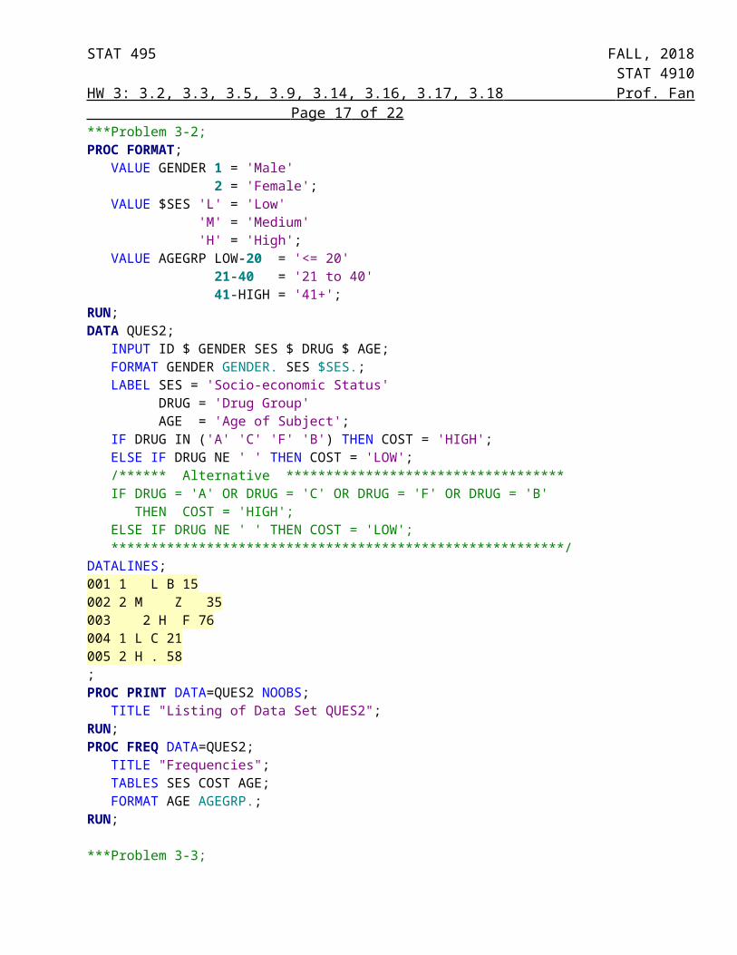
HW 3: 3.2, 3.3, 3.5, 3.9, 3.14, 3.16, 3.17, 3.18 Prof. Fan of 17 3.2 The data set containing ID, GENDER, SES, DRUG, and AGE is read in using column input. Three formats are created into groups: GENDER (1=Male, 2=Female), SES (L=Low, M=Medium, H=High), and AGE (LOW-20 = <=20, 21-40 = 21 to 40, 41-HIGH = 40+) by using PROC FORMAT statement.

Using PROC PRINT to obtain a listing of the data set, the output is shown below: (by using PROC PRINT statement to check if there is missing value and here we can see there are missing values for DRUG and COST for Observation 005)

Using PROC FREQ to obtain the frequencies tables for SES (Socio-economic status), COST, AND AGE (Age of Subject) are shown below: (using NOOBS option to suppress the observation column in the PROC PRINT statement)

Each of tables consists frequency count, percentage, cumulative frequency, and cumulative percentage based on the groups that were defined in PROC FORMAT, and these are calculated based on the listing of data set for QUES2 in SAS. The frequency counts are listed in the second column. For SES (socio-economic status), both 003 and 005 are grouped in High category, 002 is grouped in Medium category, and 001 and 004 is grouped in Low category. Therefore, the frequency for each category (High, Medium, and Low) is 2, 1, and 2 respectively. The frequencies for COST and AGE are calculated in the same way.

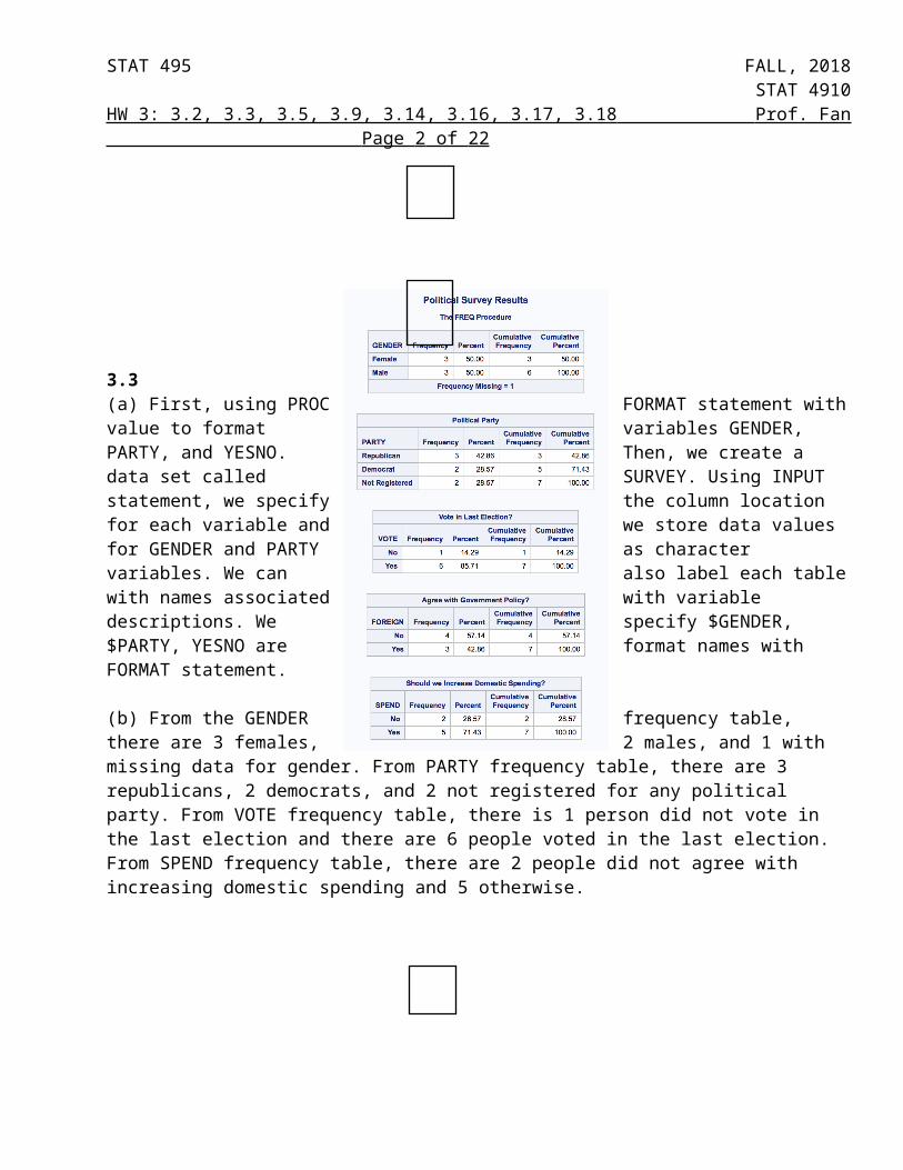
3.3 (a) First, using PROC FORMAT statement with value to format variables GENDER, PARTY, and YESNO. Then, we create a data set called SURVEY. Using INPUT statement, we specify the column location for each variable and we store data values for GENDER and PARTY as character variables. We


HW 3: 3.2, 3.3, 3.5, 3.9, 3.14, 3.16, 3.17, 3.18 Prof. Fan of 17 can also label each table with names associated with variable descriptions. We specify $GENDER, $PARTY, YESNO are format names with FORMAT statement.

(b) From the GENDER frequency table, there are 3 females, 2 males, and 1 with missing data for gender. From PARTY frequency table, there are 3 republicans, 2 democrats, and 2 not registered for any political party. From VOTE frequency table, there is 1 person did not vote in the last election and there are 6 people voted in the last election. From SPEND frequency table, there are 2 people did not agree with increasing domestic spending and 5 otherwise.

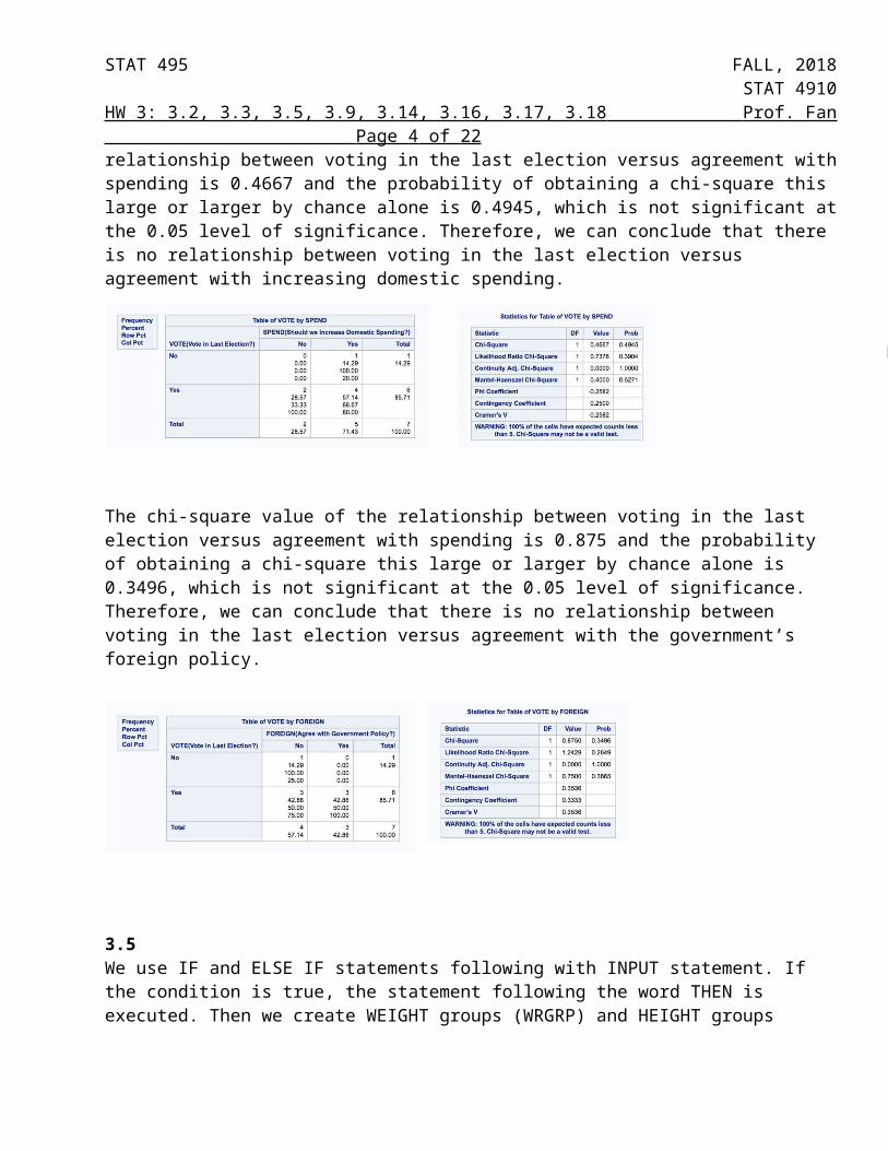
(c) When we already have frequency tables for GENDER, PARTY, VOTE, FOREIGN, and SPEND above, we can construct two-way contingency tables (on the left) and use them to compute chi-square statistics and test if there is a relationship between voting in the last election versus agreement with spending and foreign policy. The TABLE specification, VOTE*(SPEND FOREIGN) is a request for two two-way table: VOTE*SPEND and VOTE*FOREIGN. Once we have observed and expected frequencies for each cell, the chi-square statistic can be computed. By adding an / CHISQ option in TABLES statement, now SAS will compute chi-square and the probability of obtaining a value as large or larger by chance alone.

The number of DF in a chi-square statistic is equal to ((R−1)×(C−1)) .Both our 2×2 chi-sqaure has 1 df.


HW 3: 3.2, 3.3, 3.5, 3.9, 3.14, 3.16, 3.17, 3.18 Prof. Fan of 17 By FREQUENCY and the output (on the left) we obtain below, 0 voter disagreed with increasing domestic spending was not voted in the last election. 1 voter agreed with increasing domestic spending was voted in the last election and so on. The chi-square value of the relationship between voting in the last election versus agreement with spending is 0.4667 and the probability of obtaining a chi-square this large or larger by chance alone is 0.4945, which is not significant at the 0.05 level of significance. Therefore, we can conclude that there is no relationship between voting in the last election versus agreement with increasing domestic spending.

The chi-square value of the relationship between voting in the last election versus agreement with spending is 0.875 and the probability of obtaining a chi-square this large or larger by chance alone is 0.3496, which is not significant at the 0.05 level of significance. Therefore, we can conclude that there is no relationship between voting in the last election versus agreement with the government’s foreign policy.

3.5 We use IF and ELSE IF statements following with INPUT statement. If the condition is true, the statement following the word THEN is executed. Then we create WEIGHT groups (WRGRP) and HEIGHT groups (HTGRP) accordingly. For example, considering WEIGHT variable, If the condition of weight between 0 to 100 (we write 0<=WEIGHT<100 )is satisfied, then the variable WEIGHT will be set to 1. If the condition of weight between 101 to 150 (we write 101<=WEIGHT<150) is satisfied and it is followed by ELSE IF statement, then the variable WEIGHT will be set to 2, and so forth. Same way for creating HEIGHT groups. Then we can obtain frequency table for WRGRP and HTGRP by using PROC FREQ statement.

From the output below, we obtain frequency count of 1 for weight around 0-100 and height between 0-70 and frequency count of 0 for weight around 0-100 and not height greater than 70 for first row. Same way for the rest.


HW 3: 3.2, 3.3, 3.5, 3.9, 3.14, 3.16, 3.17, 3.18 Prof. Fan of 17

3.9H0: There is marginal homogeneity. The use of vitamins has no association to having disease X.HA: There is no marginal homogeneity.

McNemar's Test of Use of Vitamins vs. Existence of Disease

The FREQ Procedure

Table of CONTROL by CASE

CONTROL CASE

Frequency‚ Percent ‚ Row Pct ‚ Col Pct ‚No ‚Yes ‚ Total ƒƒƒƒƒƒƒƒƒˆƒƒƒƒƒƒƒƒˆƒƒƒƒƒƒƒƒˆ No ‚ 200 ‚ 50 ‚ 250 ‚ 45.45 ‚ 11.36 ‚ 56.82 ‚ 80.00 ‚ 20.00 ‚ ‚ 68.97 ‚ 33.33 ‚ ƒƒƒƒƒƒƒƒƒˆƒƒƒƒƒƒƒƒˆƒƒƒƒƒƒƒƒˆ Yes ‚ 90 ‚ 100 ‚ 190 ‚ 20.45 ‚ 22.73 ‚ 43.18 ‚ 47.37 ‚ 52.63 ‚ ‚ 31.03 ‚ 66.67 ‚ ƒƒƒƒƒƒƒƒƒˆƒƒƒƒƒƒƒƒˆƒƒƒƒƒƒƒƒˆ Total 290 150 440 65.91 34.09 100.00

Statistics for Table of CONTROL by CASE

McNemar's Test ƒƒƒƒƒƒƒƒƒƒƒƒƒƒƒƒƒƒƒƒƒƒƒƒƒƒƒƒƒƒ Statistic (S) 11.4286 DF 1 Asymptotic Pr > S 0.0007 Exact Pr >= S 9.131E-04


HW 3: 3.2, 3.3, 3.5, 3.9, 3.14, 3.16, 3.17, 3.18 Prof. Fan of 17 Conclusion: Reject H0. The McNemar c2 = 11.4286 is high, with a p-value = 0.0007. The CASES were less likely to use vitamins. In other words, one is more likely to have disease X if vitamins were not used.

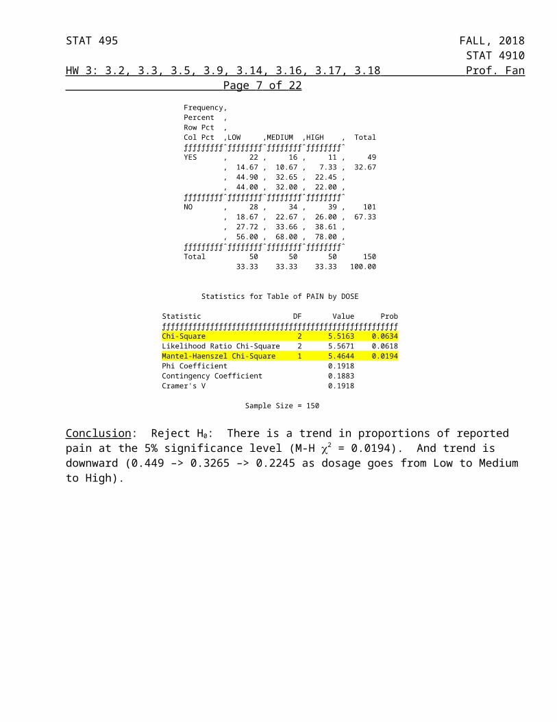
3.14From the output, we see that the regular Chi-square test gives a Chi-square value of 5.5163 with a p value of .0634 and the Mantel-Haenszel(M-H) chi-square test for trend is 5.4644 with a p value of .019.

H0: there is no (linear) trend.HA: there is a (linear) trend.

Chi-Square test for trend of pain vs. dosage

The FREQ Procedure

Table of PAIN by DOSE

PAIN DOSE

Frequency‚ Percent ‚ Row Pct ‚ Col Pct ‚LOW ‚MEDIUM ‚HIGH ‚ Total ƒƒƒƒƒƒƒƒƒˆƒƒƒƒƒƒƒƒˆƒƒƒƒƒƒƒƒˆƒƒƒƒƒƒƒƒˆ YES ‚ 22 ‚ 16 ‚ 11 ‚ 49 ‚ 14.67 ‚ 10.67 ‚ 7.33 ‚ 32.67 ‚ 44.90 ‚ 32.65 ‚ 22.45 ‚ ‚ 44.00 ‚ 32.00 ‚ 22.00 ‚ ƒƒƒƒƒƒƒƒƒˆƒƒƒƒƒƒƒƒˆƒƒƒƒƒƒƒƒˆƒƒƒƒƒƒƒƒˆ NO ‚ 28 ‚ 34 ‚ 39 ‚ 101 ‚ 18.67 ‚ 22.67 ‚ 26.00 ‚ 67.33 ‚ 27.72 ‚ 33.66 ‚ 38.61 ‚ ‚ 56.00 ‚ 68.00 ‚ 78.00 ‚ ƒƒƒƒƒƒƒƒƒˆƒƒƒƒƒƒƒƒˆƒƒƒƒƒƒƒƒˆƒƒƒƒƒƒƒƒˆ Total 50 50 50 150 33.33 33.33 33.33 100.00

Statistics for Table of PAIN by DOSE

Statistic DF Value Prob ƒƒƒƒƒƒƒƒƒƒƒƒƒƒƒƒƒƒƒƒƒƒƒƒƒƒƒƒƒƒƒƒƒƒƒƒƒƒƒƒƒƒƒƒƒƒƒƒƒƒƒƒƒƒ Chi-Square 2 5.5163 0.0634 Likelihood Ratio Chi-Square 2 5.5671 0.0618 Mantel-Haenszel Chi-Square 1 5.4644 0.0194 Phi Coefficient 0.1918 Contingency Coefficient 0.1883 Cramer's V 0.1918

Sample Size = 150

Conclusion: Reject H0: There is a trend in proportions of reported pain at the 5% significance level (M-H 2 = 0.0194). And trend is downward (0.449 –> 0.3265 –> 0.2245 as dosage goes from Low to Medium to High).


HW 3: 3.2, 3.3, 3.5, 3.9, 3.14, 3.16, 3.17, 3.18 Prof. Fan of 17 3.16 Relative Risk of MI The FREQ Procedure

Table of group by response

group response

Frequency‚ Percent ‚ Row Pct ‚ Col Pct ‚yes ‚no ‚ Total ƒƒƒƒƒƒƒƒƒˆƒƒƒƒƒƒƒƒˆƒƒƒƒƒƒƒƒˆ placebo ‚ 240 ‚ 1760 ‚ 2000 ‚ 8.00 ‚ 58.67 ‚ 66.67 ‚ 12.00 ‚ 88.00 ‚ ‚ 75.00 ‚ 65.67 ‚ ƒƒƒƒƒƒƒƒƒˆƒƒƒƒƒƒƒƒˆƒƒƒƒƒƒƒƒˆ aspirin ‚ 80 ‚ 920 ‚ 1000 ‚ 2.67 ‚ 30.67 ‚ 33.33 ‚ 8.00 ‚ 92.00 ‚ ‚ 25.00 ‚ 34.33 ‚ ƒƒƒƒƒƒƒƒƒˆƒƒƒƒƒƒƒƒˆƒƒƒƒƒƒƒƒˆ Total 320 2680 3000 10.67 89.33 100.00

Relative Risk of MI

The FREQ Procedure

Statistics for Table of group by response

Estimates of the Relative Risk (Row1/Row2)

Type of Study Value 95% Confidence Limits ƒƒƒƒƒƒƒƒƒƒƒƒƒƒƒƒƒƒƒƒƒƒƒƒƒƒƒƒƒƒƒƒƒƒƒƒƒƒƒƒƒƒƒƒƒƒƒƒƒƒƒƒƒƒƒƒƒƒƒƒƒƒƒƒƒ Case-Control (Odds Ratio) 1.5682 1.2028 2.0446 Cohort (Col1 Risk) 1.5000 1.1783 1.9095 Cohort (Col2 Risk) 0.9565 0.9335 0.9802

Sample Size = 3000

Estimated Relative Risk (RR) of having a heart attack for those on Placebo to those on Aspirin is 1.5. In other words, the estimated risk of a heart attack for Placebo group is 1.5 times than those in the Aspirin group. In addition, since the C.I. of the RR, (1.17, 1.91), is strictly greater than 1. We can conclude that taking aspirin regularly can reduce the risk of heart attack.

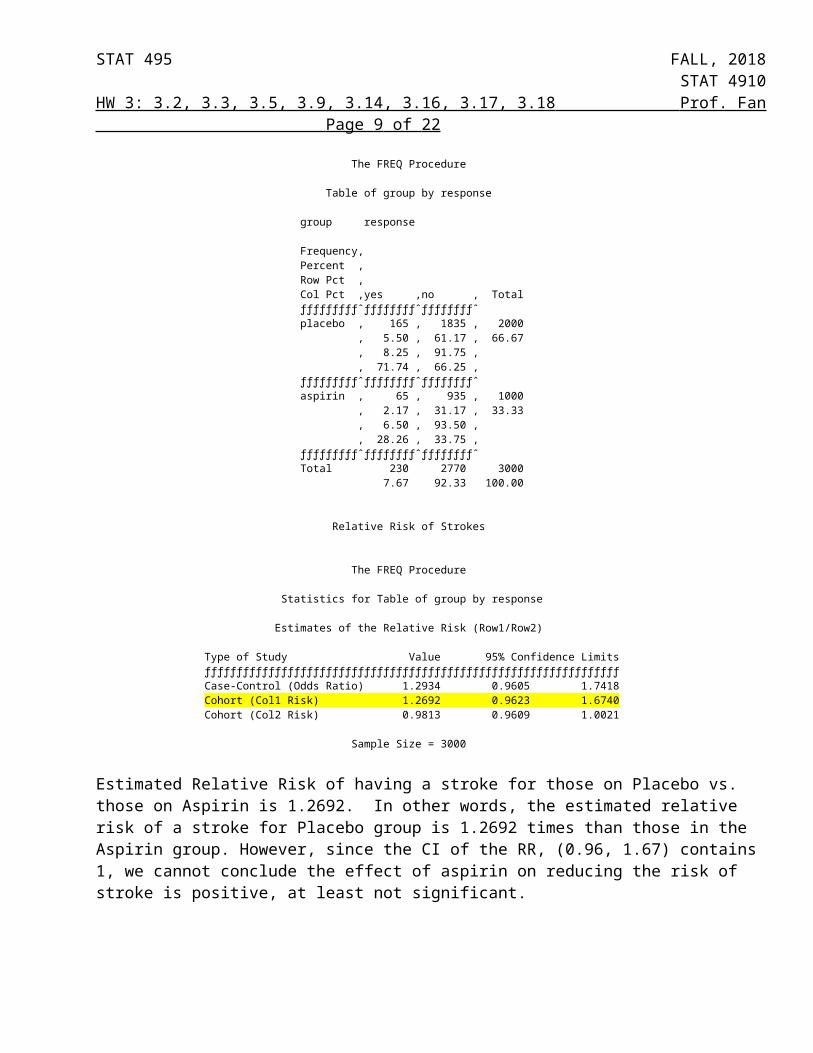
Relative Risk of Strokes 5 The FREQ Procedure

Table of group by response

group response

Frequency‚ Percent ‚ Row Pct ‚ Col Pct ‚yes ‚no ‚ Total ƒƒƒƒƒƒƒƒƒˆƒƒƒƒƒƒƒƒˆƒƒƒƒƒƒƒƒˆ placebo ‚ 165 ‚ 1835 ‚ 2000 ‚ 5.50 ‚ 61.17 ‚ 66.67


HW 3: 3.2, 3.3, 3.5, 3.9, 3.14, 3.16, 3.17, 3.18 Prof. Fan of 17 ‚ 8.25 ‚ 91.75 ‚ ‚ 71.74 ‚ 66.25 ‚ ƒƒƒƒƒƒƒƒƒˆƒƒƒƒƒƒƒƒˆƒƒƒƒƒƒƒƒˆ aspirin ‚ 65 ‚ 935 ‚ 1000 ‚ 2.17 ‚ 31.17 ‚ 33.33 ‚ 6.50 ‚ 93.50 ‚ ‚ 28.26 ‚ 33.75 ‚ ƒƒƒƒƒƒƒƒƒˆƒƒƒƒƒƒƒƒˆƒƒƒƒƒƒƒƒˆ Total 230 2770 3000 7.67 92.33 100.00

Relative Risk of Strokes

The FREQ Procedure

Statistics for Table of group by response



Sample Size = 3000

Estimated Relative Risk of having a stroke for those on Placebo vs. those on Aspirin is 1.2692. In other words, the estimated relative risk of a stroke for Placebo group is 1.2692 times than those in the Aspirin group. However, since the CI of the RR, (0.96, 1.67) contains 1, we cannot conclude the effect of aspirin on reducing the risk of stroke is positive, at least not significant.

3.17

The SAS System

The FREQ Procedure

Table 1 of TEMP by COLDS Controlling for SMOKES=smoker

TEMP COLDS

Frequency‚ Percent ‚ Row Pct ‚ Col Pct ‚yes ‚no ‚ Total ƒƒƒƒƒƒƒƒƒˆƒƒƒƒƒƒƒƒˆƒƒƒƒƒƒƒƒˆ poor ‚ 20 ‚ 100 ‚ 120 ‚ 7.02 ‚ 35.09 ‚ 42.11 ‚ 16.67 ‚ 83.33 ‚ ‚ 57.14 ‚ 40.00 ‚ ƒƒƒƒƒƒƒƒƒˆƒƒƒƒƒƒƒƒˆƒƒƒƒƒƒƒƒˆ good ‚ 15 ‚ 150 ‚ 165 ‚ 5.26 ‚ 52.63 ‚ 57.89 ‚ 9.09 ‚ 90.91 ‚ ‚ 42.86 ‚ 60.00 ‚ ƒƒƒƒƒƒƒƒƒˆƒƒƒƒƒƒƒƒˆƒƒƒƒƒƒƒƒˆ Total 35 250 285 12.28 87.72 100.00


HW 3: 3.2, 3.3, 3.5, 3.9, 3.14, 3.16, 3.17, 3.18 Prof. Fan of 17

Statistics for Table 1 of TEMP by COLDS Controlling for SMOKES=smoker

Statistic DF Value Prob ƒƒƒƒƒƒƒƒƒƒƒƒƒƒƒƒƒƒƒƒƒƒƒƒƒƒƒƒƒƒƒƒƒƒƒƒƒƒƒƒƒƒƒƒƒƒƒƒƒƒƒƒƒƒ Chi-Square 1 3.7013 0.0544 Estimates of the Relative Risk (Row1/Row2)


Sample Size = 285

The SAS System

The FREQ Procedure

Table 2 of TEMP by COLDS Controlling for SMOKES=nonsmoke

TEMP COLDS

Frequency‚ Percent ‚ Row Pct ‚ Col Pct ‚yes ‚no ‚ Total ƒƒƒƒƒƒƒƒƒˆƒƒƒƒƒƒƒƒˆƒƒƒƒƒƒƒƒˆ poor ‚ 30 ‚ 100 ‚ 130 ‚ 8.45 ‚ 28.17 ‚ 36.62 ‚ 23.08 ‚ 76.92 ‚ ‚ 54.55 ‚ 33.33 ‚ ƒƒƒƒƒƒƒƒƒˆƒƒƒƒƒƒƒƒˆƒƒƒƒƒƒƒƒˆ good ‚ 25 ‚ 200 ‚ 225 ‚ 7.04 ‚ 56.34 ‚ 63.38 ‚ 11.11 ‚ 88.89 ‚ ‚ 45.45 ‚ 66.67 ‚ ƒƒƒƒƒƒƒƒƒˆƒƒƒƒƒƒƒƒˆƒƒƒƒƒƒƒƒˆ Total 55 300 355 15.49 84.51 100.00

Statistics for Table 2 of TEMP by COLDS Controlling for SMOKES=nonsmoke

Statistic DF Value Prob ƒƒƒƒƒƒƒƒƒƒƒƒƒƒƒƒƒƒƒƒƒƒƒƒƒƒƒƒƒƒƒƒƒƒƒƒƒƒƒƒƒƒƒƒƒƒƒƒƒƒƒƒƒƒ Chi-Square 1 9.0106 0.0027



Sample Size = 355

The FREQ Procedure


HW 3: 3.2, 3.3, 3.5, 3.9, 3.14, 3.16, 3.17, 3.18 Prof. Fan of 17

Summary Statistics for TEMP by COLDS Controlling for SMOKES

Cochran-Mantel-Haenszel Statistics (Based on Table Scores)

Statistic Alternative Hypothesis DF Value Prob ƒƒƒƒƒƒƒƒƒƒƒƒƒƒƒƒƒƒƒƒƒƒƒƒƒƒƒƒƒƒƒƒƒƒƒƒƒƒƒƒƒƒƒƒƒƒƒƒƒƒƒƒƒƒƒƒƒƒƒƒƒƒƒ 1 Nonzero Correlation 1 12.4770 0.0004 2 Row Mean Scores Differ 1 12.4770 0.0004 3 General Association 1 12.4770 0.0004

Estimates of the Common Relative Risk (Row1/Row2)

Type of Study Method Value 95% Confidence Limits ƒƒƒƒƒƒƒƒƒƒƒƒƒƒƒƒƒƒƒƒƒƒƒƒƒƒƒƒƒƒƒƒƒƒƒƒƒƒƒƒƒƒƒƒƒƒƒƒƒƒƒƒƒƒƒƒƒƒƒƒƒƒƒƒƒƒƒƒƒƒƒƒƒ Case-Control Mantel-Haenszel 2.2289 1.4185 3.5024 (Odds Ratio) Logit 2.2318 1.4205 3.5064

Cohort Mantel-Haenszel 1.9775 1.3474 2.9021 (Col1 Risk) Logit 1.9822 1.3508 2.9087


The results of combining the two groups can be analyzed with the Mantel-Haenszel statistics, which gives the estimated relative risk of getting colds for poor to good temperature control 1.98 (95% CI 1.35, 2.90).

Given the condition of smoking or non-smoking (smoking status is controlled):H0: Colds and Temperature are conditionally independent.HA: Colds and Temperature are not conditionally independent.

The General Association CMH 2 = 12.477 (p-value =0.0004), therefore we can reject H0 there is strong evidence against the independence of temperature control and getting colds.

The results for Smokers show 2 = 3.7013 with a p-value = 0.0544, with an estimated risk of colds for those of poor temperature is 1.833 times the risk for those of good temperature (95% CI 0.9795, 3.4313). For non-smokers, 2 = 9.0106 with a p-value = 0.0027, with an estimated risk of colds for those of poor temperature is 2.0769 times the risk for those of good temperature (95% CI 1.2789, 3.3728).

3.18 The FREQ Procedure

Table 1 of GROUP by RESULT Controlling for STUDY=One

GROUP RESULT

Frequency‚ Percent ‚ Row Pct ‚ Col Pct ‚Survived‚Died ‚ Total ƒƒƒƒƒƒƒƒƒˆƒƒƒƒƒƒƒƒˆƒƒƒƒƒƒƒƒˆ MgSO4 ‚ 20 ‚ 100 ‚ 120 ‚ 6.67 ‚ 33.33 ‚ 40.00 ‚ 16.67 ‚ 83.33 ‚


HW 3: 3.2, 3.3, 3.5, 3.9, 3.14, 3.16, 3.17, 3.18 Prof. Fan of 17 ‚ 44.44 ‚ 39.22 ‚ ƒƒƒƒƒƒƒƒƒˆƒƒƒƒƒƒƒƒˆƒƒƒƒƒƒƒƒˆ Placebo ‚ 25 ‚ 155 ‚ 180 ‚ 8.33 ‚ 51.67 ‚ 60.00 ‚ 13.89 ‚ 86.11 ‚ ‚ 55.56 ‚ 60.78 ‚ ƒƒƒƒƒƒƒƒƒˆƒƒƒƒƒƒƒƒˆƒƒƒƒƒƒƒƒˆ Total 45 255 300 15.00 85.00 100.00

Statistics for Table 1 of GROUP by RESULT Controlling for STUDY=One




Sample Size = 300

The FREQ Procedure

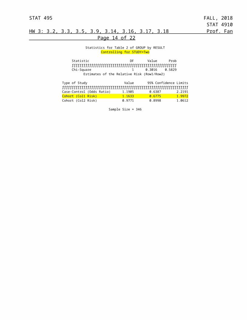
Table 2 of GROUP by RESULT Controlling for STUDY=Two

GROUP RESULT

Frequency‚ Percent ‚ Row Pct ‚ Col Pct ‚Survived‚Died ‚ Total ƒƒƒƒƒƒƒƒƒˆƒƒƒƒƒƒƒƒˆƒƒƒƒƒƒƒƒˆ MgSO4 ‚ 25 ‚ 150 ‚ 175 ‚ 7.23 ‚ 43.35 ‚ 50.58 ‚ 14.29 ‚ 85.71 ‚ ‚ 54.35 ‚ 50.00 ‚ ƒƒƒƒƒƒƒƒƒˆƒƒƒƒƒƒƒƒˆƒƒƒƒƒƒƒƒˆ Placebo ‚ 21 ‚ 150 ‚ 171 ‚ 6.07 ‚ 43.35 ‚ 49.42 ‚ 12.28 ‚ 87.72 ‚ ‚ 45.65 ‚ 50.00 ‚ ƒƒƒƒƒƒƒƒƒˆƒƒƒƒƒƒƒƒˆƒƒƒƒƒƒƒƒˆ Total 46 300 346 13.29 86.71 100.00

Statistics for Table 2 of GROUP by RESULT Controlling for STUDY=Two

Statistic DF Value Prob ƒƒƒƒƒƒƒƒƒƒƒƒƒƒƒƒƒƒƒƒƒƒƒƒƒƒƒƒƒƒƒƒƒƒƒƒƒƒƒƒƒƒƒƒƒƒƒƒƒƒƒƒƒƒ Chi-Square 1 0.3016 0.5829 Estimates of the Relative Risk (Row1/Row2)

Type of Study Value 95% Confidence Limits ƒƒƒƒƒƒƒƒƒƒƒƒƒƒƒƒƒƒƒƒƒƒƒƒƒƒƒƒƒƒƒƒƒƒƒƒƒƒƒƒƒƒƒƒƒƒƒƒƒƒƒƒƒƒƒƒƒƒƒƒƒƒƒƒƒ Case-Control (Odds Ratio) 1.1905 0.6387 2.2191 Cohort (Col1 Risk) 1.1633 0.6775 1.9972


HW 3: 3.2, 3.3, 3.5, 3.9, 3.14, 3.16, 3.17, 3.18 Prof. Fan of 17 Cohort (Col2 Risk) 0.9771 0.8998 1.0612

Sample Size = 346


HW 3: 3.2, 3.3, 3.5, 3.9, 3.14, 3.16, 3.17, 3.18 Prof. Fan of 17 The SAS System The FREQ Procedure

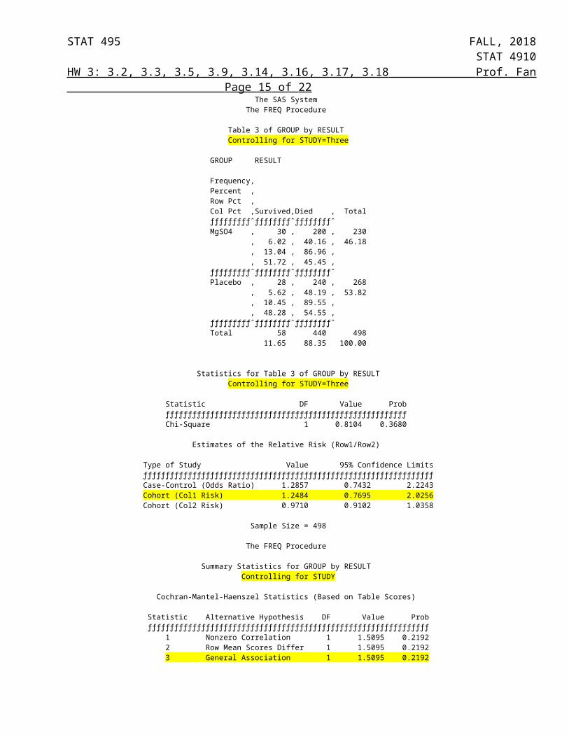
Table 3 of GROUP by RESULT Controlling for STUDY=Three

GROUP RESULT

Frequency‚ Percent ‚ Row Pct ‚ Col Pct ‚Survived‚Died ‚ Total ƒƒƒƒƒƒƒƒƒˆƒƒƒƒƒƒƒƒˆƒƒƒƒƒƒƒƒˆ MgSO4 ‚ 30 ‚ 200 ‚ 230 ‚ 6.02 ‚ 40.16 ‚ 46.18 ‚ 13.04 ‚ 86.96 ‚ ‚ 51.72 ‚ 45.45 ‚ ƒƒƒƒƒƒƒƒƒˆƒƒƒƒƒƒƒƒˆƒƒƒƒƒƒƒƒˆ Placebo ‚ 28 ‚ 240 ‚ 268 ‚ 5.62 ‚ 48.19 ‚ 53.82 ‚ 10.45 ‚ 89.55 ‚ ‚ 48.28 ‚ 54.55 ‚ ƒƒƒƒƒƒƒƒƒˆƒƒƒƒƒƒƒƒˆƒƒƒƒƒƒƒƒˆ Total 58 440 498 11.65 88.35 100.00

Statistics for Table 3 of GROUP by RESULT Controlling for STUDY=Three




Sample Size = 498

The FREQ Procedure

Summary Statistics for GROUP by RESULT Controlling for STUDY

Cochran-Mantel-Haenszel Statistics (Based on Table Scores)

Statistic Alternative Hypothesis DF Value Prob ƒƒƒƒƒƒƒƒƒƒƒƒƒƒƒƒƒƒƒƒƒƒƒƒƒƒƒƒƒƒƒƒƒƒƒƒƒƒƒƒƒƒƒƒƒƒƒƒƒƒƒƒƒƒƒƒƒƒƒƒƒƒƒ 1 Nonzero Correlation 1 1.5095 0.2192 2 Row Mean Scores Differ 1 1.5095 0.2192 3 General Association 1 1.5095 0.2192

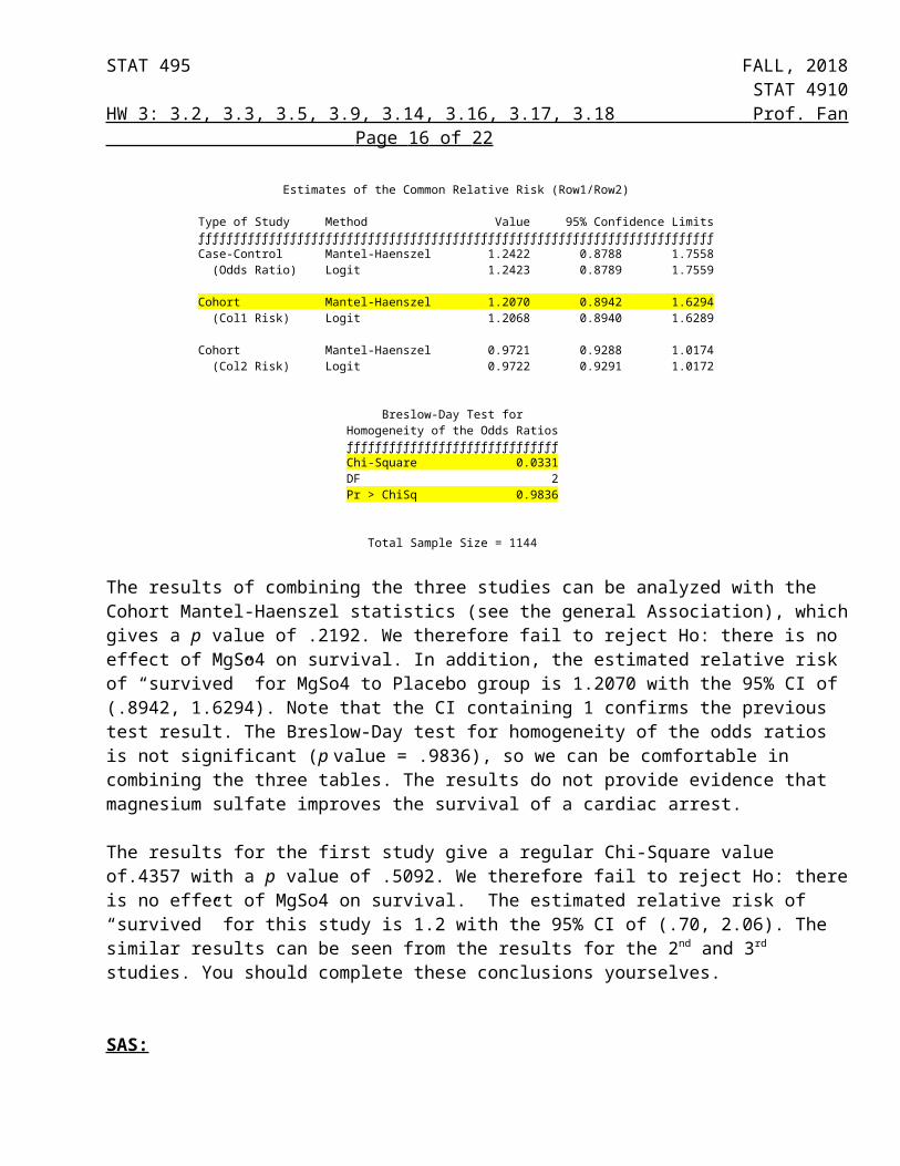
Estimates of the Common Relative Risk (Row1/Row2)

Type of Study Method Value 95% Confidence Limits ƒƒƒƒƒƒƒƒƒƒƒƒƒƒƒƒƒƒƒƒƒƒƒƒƒƒƒƒƒƒƒƒƒƒƒƒƒƒƒƒƒƒƒƒƒƒƒƒƒƒƒƒƒƒƒƒƒƒƒƒƒƒƒƒƒƒƒƒƒƒƒƒƒ Case-Control Mantel-Haenszel 1.2422 0.8788 1.7558 (Odds Ratio) Logit 1.2423 0.8789 1.7559



HW 3: 3.2, 3.3, 3.5, 3.9, 3.14, 3.16, 3.17, 3.18 Prof. Fan of 17


Breslow-Day Test for Homogeneity of the Odds Ratios ƒƒƒƒƒƒƒƒƒƒƒƒƒƒƒƒƒƒƒƒƒƒƒƒƒƒƒƒƒƒ Chi-Square 0.0331 DF 2 Pr > ChiSq 0.9836

Total Sample Size = 1144

The results of combining the three studies can be analyzed with the Cohort Mantel-Haenszel statistics (see the general Association), which gives a p value of .2192. We therefore fail to reject Ho: there is no effect of MgSo4 on survival. In addition, the estimated relative risk of “survived” for MgSo4 to Placebo group is 1.2070 with the 95% CI of (.8942, 1.6294). Note that the CI containing 1 confirms the previous test result. The Breslow-Day test for homogeneity of the odds ratios is not significant (p value = .9836), so we can be comfortable in combining the three tables. The results do not provide evidence that magnesium sulfate improves the survival of a cardiac arrest.

The results for the first study give a regular Chi-Square value of.4357 with a p value of .5092. We therefore fail to reject Ho: there is no effect of MgSo4 on survival. The estimated relative risk of “survived” for this study is 1.2 with the 95% CI of (.70, 2.06). The similar results can be seen from the results for the 2nd and 3rd studies. You should complete these conclusions yourselves.

SAS:***Problem 3-2;PROC FORMAT; VALUE GENDER 1 = 'Male' 2 = 'Female'; VALUE $SES 'L' = 'Low' 'M' = 'Medium' 'H' = 'High'; VALUE AGEGRP LOW-20 = '<= 20' 21-40 = '21 to 40' 41-HIGH = '41+';RUN;DATA QUES2; INPUT ID $ GENDER SES $ DRUG $ AGE; FORMAT GENDER GENDER. SES $SES.; LABEL SES = 'Socio-economic Status' DRUG = 'Drug Group' AGE = 'Age of Subject'; IF DRUG IN ('A' 'C' 'F' 'B') THEN COST = 'HIGH'; ELSE IF DRUG NE ' ' THEN COST = 'LOW'; /****** Alternative *********************************** IF DRUG = 'A' OR DRUG = 'C' OR DRUG = 'F' OR DRUG = 'B' THEN COST = 'HIGH';


HW 3: 3.2, 3.3, 3.5, 3.9, 3.14, 3.16, 3.17, 3.18 Prof. Fan of 17 ELSE IF DRUG NE ' ' THEN COST = 'LOW'; *********************************************************/DATALINES;001 1 L B 15002 2 M Z 35003 2 H F 76004 1 L C 21005 2 H . 58;PROC PRINT DATA=QUES2 NOOBS; TITLE "Listing of Data Set QUES2";RUN;PROC FREQ DATA=QUES2; TITLE "Frequencies"; TABLES SES COST AGE; FORMAT AGE AGEGRP.;RUN;

***Problem 3-3;PROC FORMAT; VALUE $GENDER 'M' = 'Male' 'F' = 'Female'; VALUE $PARTY '1' = 'Republican' '2' = 'Democrat' '3' = 'Not Registered'; VALUE YESNO 0 = 'No' 1 = 'Yes';RUN;DATA SURVEY; INPUT ID 1-3 GENDER $ 4 PARTY $ 5 VOTE 6 FOREIGN 7 SPEND 8; LABEL PARTY = 'Political Party' VOTE = 'Vote in Last Election?' FOREIGN = 'Agree with Government Policy?' SPEND = 'Should we Increase Domestic Spending?'; FORMAT GENDER $GENDER. PARTY $PARTY. VOTE FOREIGN SPEND YESNO.;DATALINES;007M1110013F2101137F1001117 1111428M3110017F3101037M2101;


HW 3: 3.2, 3.3, 3.5, 3.9, 3.14, 3.16, 3.17, 3.18 Prof. Fan of 17 PROC FREQ DATA=SURVEY; TITLE "Political Survey Results"; TABLES GENDER PARTY VOTE FOREIGN SPEND; TABLES VOTE*(SPEND FOREIGN) / CHISQ;RUN;

***Problem 3-5;***Method 1 ***;DATA DEMOG; INPUT WEIGHT HEIGHT GENDER $; *Create weight groups; IF 0 LE WEIGHT LT 101 THEN WTGRP = 1; ELSE IF 101 LE WEIGHT LT 151 THEN WTGRP = 2; ELSE IF 151 LE WEIGHT LE 200 THEN WTGRP = 3; ELSE IF WEIGHT GT 200 THEN WTGRP = 4; *Create height groups; IF 0 LE HEIGHT LE 70 THEN HTGRP = 1; ELSE IF HEIGHT GT 70 THEN HTGRP = 2;DATALINES;155 68 M98 60 F202 72 M280 75 M130 63 F. 57 F166 . M;PROC FREQ DATA=DEMOG; TABLES WTGRP*HTGRP;RUN;** Prob 3.9 Paired Data*;proc format;

value $response 'Y'='Yes''N'='No';

data VITAMINS;input CASE $ CONTROL $ count@@;format CASE $response. CONTROL $response.;datalines;Y Y 100Y N 50N Y 90N N 200;

run;

/* McNemar's Test with exact p-value and Kappa coefficient */proc freq data=VITAMINS;

title "McNemar's Test of Use of Vitamins vs. Existence of Disease";exact mcnem;


HW 3: 3.2, 3.3, 3.5, 3.9, 3.14, 3.16, 3.17, 3.18 Prof. Fan of 17

weight count;table CONTROL*CASE/agree;

run;** Prob 3.14*;proc format;

value PAIN 1 = 'YES' 2 = 'NO';value DOSE 1 = 'LOW' 2 = 'MEDIUM' 3 = 'HIGH';

run;data dose;

do DOSE = 1 to 3;do i = 1 to 50;

ret = (ranuni(135) > (0.6 + 0.08* DOSE));PAIN = 2 - ret;output;

end;end;format PAIN PAIN. DOSE DOSE.;drop i;drop ret;

run;proc print data=dose noobs;run;proc freq order=data data=dose;

title "Chi-Square test for trend of pain vs. dosage";table PAIN*DOSE/chisq;

run;** Prob 3.16 Rel Risk of MI*;data MI;

input group $ response $ count;datalines;placebo yes 240placebo no 1760aspirin yes 80aspirin no 920;

run;proc freq data = MI order=data;

title "Relative Risk of MI";weight count;tables group*response/ measures;

run;

** Prob 3.16 Rel Risk of Strokes*;data STROKES;

input group $ response $ count;datalines;placebo yes 165placebo no 1835aspirin yes 65


HW 3: 3.2, 3.3, 3.5, 3.9, 3.14, 3.16, 3.17, 3.18 Prof. Fan of 17

aspirin no 935;

run;proc freq data = STROKES order=data;

title "Relative Risk of Strokes";weight count;tables group*response/ measures;

run;** Prob 3.17*;data colds;input SMOKES $ TEMP $ COLDS $ count@@;datalines;

smoker poor yes 20 smoker poor no 100smoker good yes 15 smoker good no 150nonsmoke poor yes 30 nonsmoke poor no 100nonsmoke good yes 25 nonsmoke good no 200

;run;proc freq order=data data=colds;

weight count;table SMOKES*TEMP*COLDS/all;

run;** Prob 3.18*;data cardiac;input STUDY $ GROUP $ RESULT $ count@@;datalines;

One MgSO4 Survived 20 One MgSO4 Died 100One Placebo Survived 25 One Placebo Died 155Two MgSO4 Survived 25 Two MgSO4 Died 150Two Placebo Survived 21 Two Placebo Died 150Three MgSO4 Survived 30 Three MgSO4 Died 200Three Placebo Survived 28 Three Placebo Died 240

;run;proc freq order=data data=cardiac;

weight count;table STUDY*GROUP*RESULT/all;

run;

Problem 4algebra.sci.csueastbay.edu/.../homework/495_HW2_F18.docx · Web view2018-09-10 · ......

Documents

Transcript of Problem 4algebra.sci.csueastbay.edu/.../homework/495_HW2_F18.docx · Web view2018-09-10 · ......