Probing the Standard Model Frontier with B

Physics at CDFAlessandro Cerri

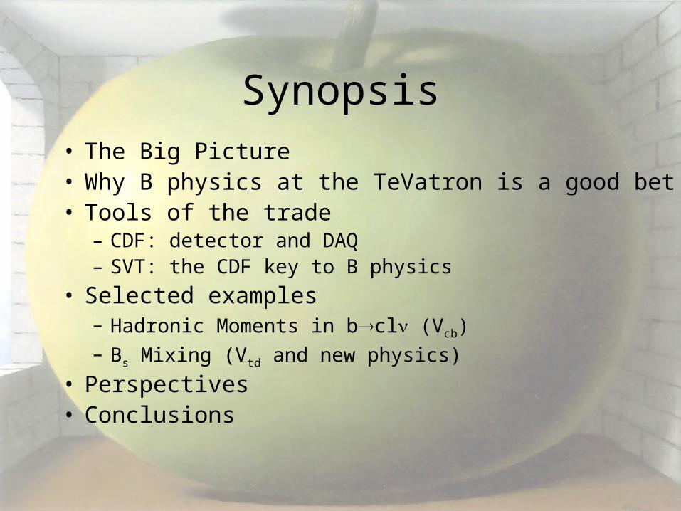
Synopsis• The Big Picture• Why B physics at the TeVatron is a good bet• Tools of the trade

– CDF: detector and DAQ– SVT: the CDF key to B physics

• Selected examples– Hadronic Moments in bcl (Vcb)– Bs Mixing (Vtd and new physics)

• Perspectives• Conclusions

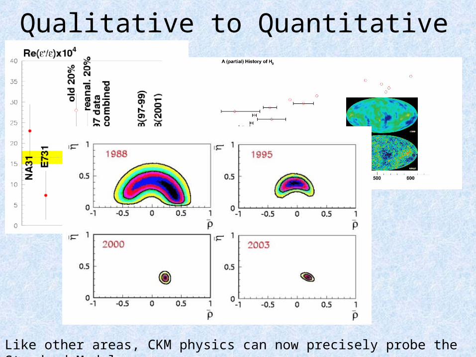
Qualitative to Quantitative

Like other areas, CKM physics can now precisely probe the Standard Model

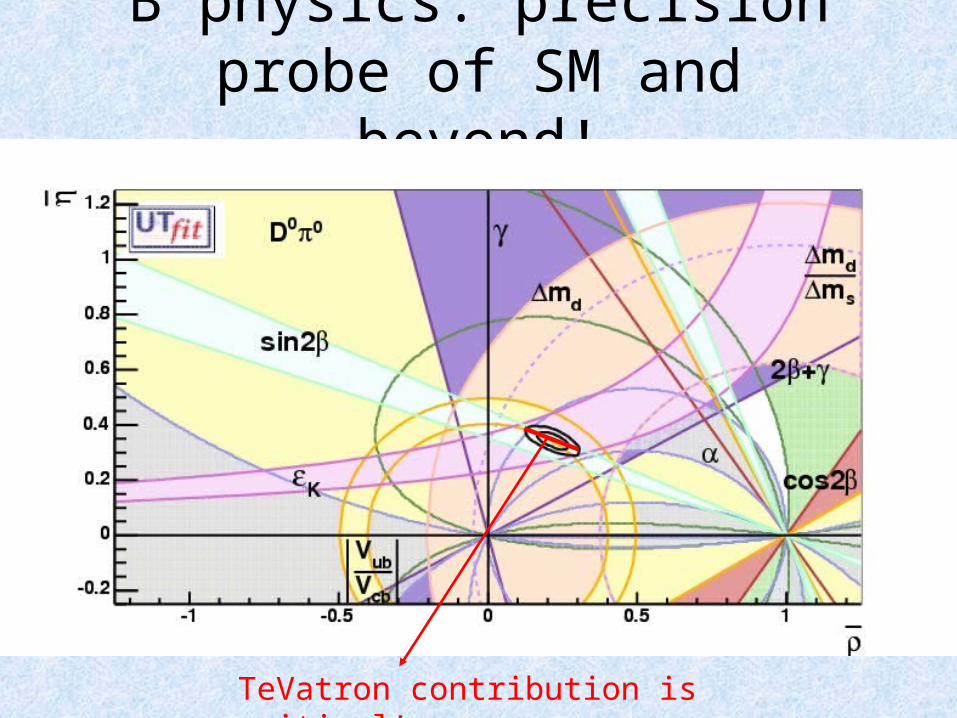
B physics: precision probe of SM and beyond!

TeVatron contribution is critical!

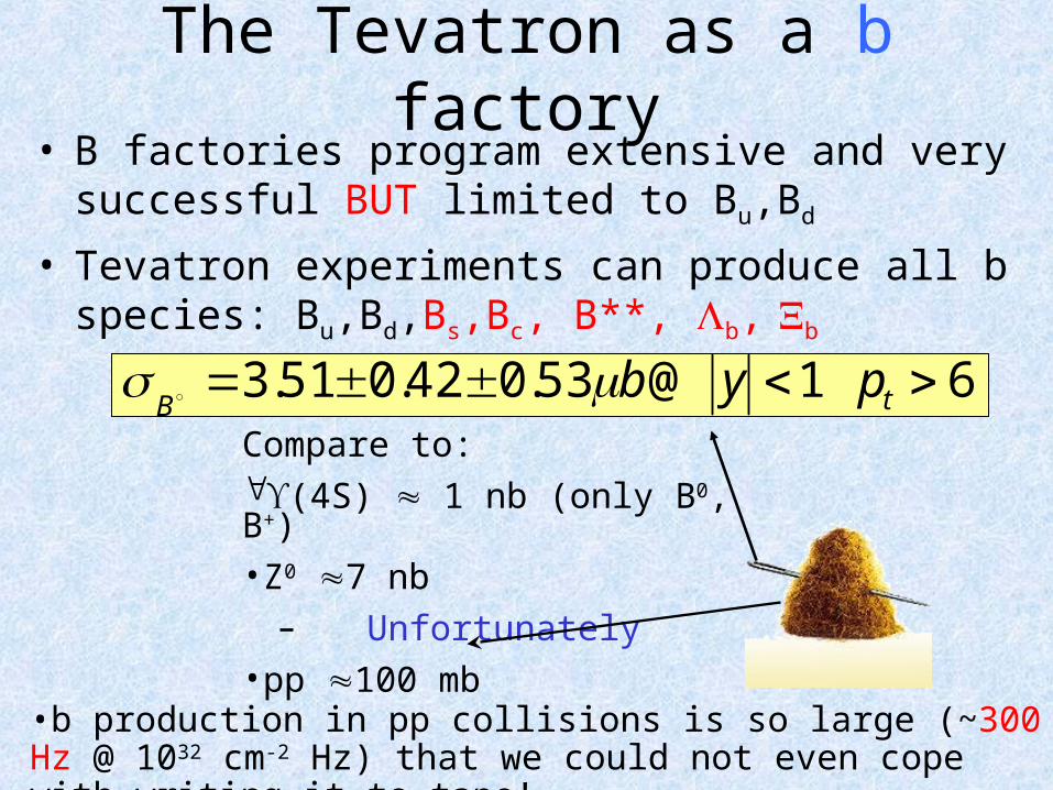
The Tevatron as a b factory• B factories program extensive and very

successful BUT limited to Bu,Bd

• Tevatron experiments can produce all b species: Bu,Bd,Bs,Bc, B**, b, b

61@53.042.051.3 tBpyb

Compare to:(4S) 1 nb (only B0, B+)•Z0 7 nb

Unfortunately•pp 100 mb

•b production in pp collisions is so large (~300 Hz @ 1032 cm-2 Hz) that we could not even cope with writing it to tape!

Path to New PhysicsCKM measurements could hint to new physics through

discrepancies with SM predictions. How do we get there?• Design/improve the “tools of the trade”

– Experimental (detector & techniques)– Theoretical (phenomenological devices)

• Measure uncharted properties at the boundaries of our knowledge– Masses– Lifetimes– Branching ratios

• Press further ahead and investigate beyond the boundaries:– Mixing– CP asymmetries

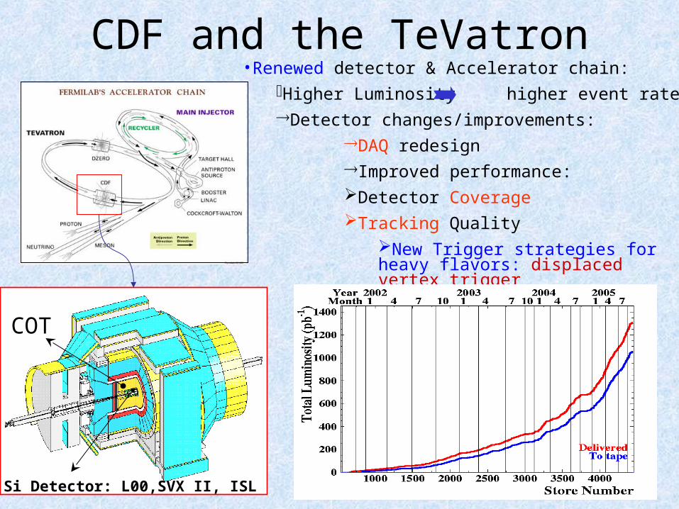
CDF and the TeVatron•Renewed detector & Accelerator chain:

Higher Luminosity higher event rateDetector changes/improvements:

DAQ redesignImproved performance:Detector CoverageTracking Quality

New Trigger strategies for heavy flavors: displaced vertex trigger

COT

Si Detector: L00,SVX II, ISL

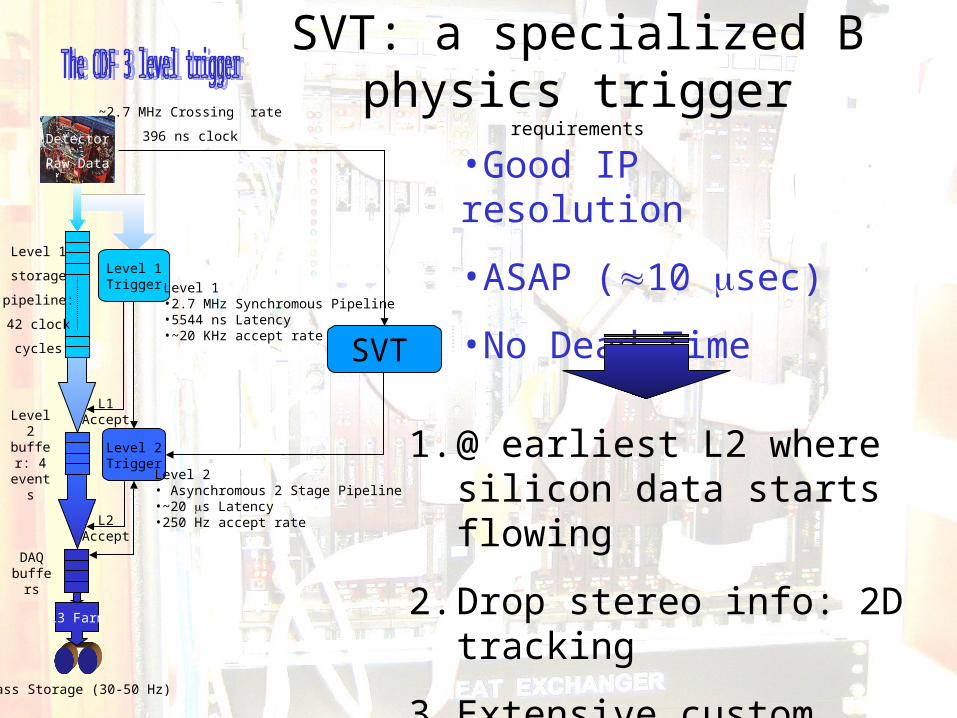
SVT: a specialized B physics trigger

requirementsDetector

Raw Data

Level 1

storage

pipeline:

42 clock

cycles

Level 1Trigger

L1Accept

Level 2Trigger

Level 2 buffer:

4 events

L2Accept

DAQ buffers

L3 Farm

Level 1•2.7 MHz Synchromous Pipeline•5544 ns Latency•~20 KHz accept rate

Level 2• Asynchromous 2 Stage Pipeline•~20 s Latency•250 Hz accept rate

Mass Storage (30-50 Hz)

~2.7 MHz Crossing rate

396 ns clock

•Good IP resolution

•ASAP (10 sec)

•No Dead Time

1. @ earliest L2 where silicon data starts flowing

2. Drop stereo info: 2D tracking

3. Extensive custom design

SVT

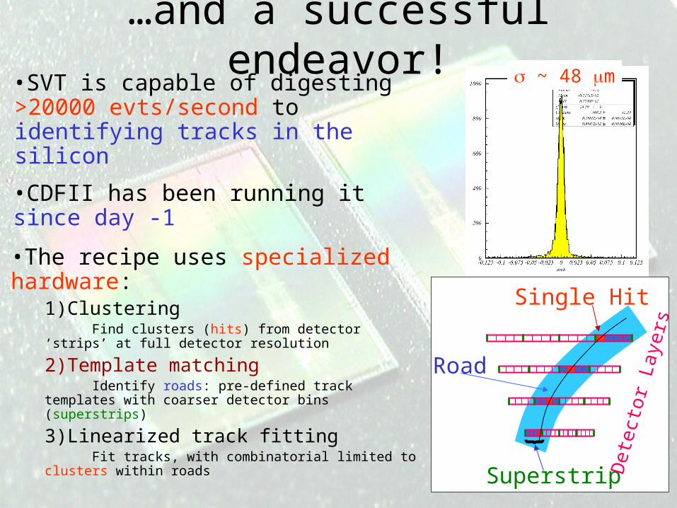
…and a successful endeavor!

•SVT is capable of digesting >20000 evts/second to identifying tracks in the silicon

~ 48 m

Single Hit

Superstrip

Road

Dete

ctor

Laye

rs

•CDFII has been running it since day -1

•The recipe uses specialized hardware:

1)Clustering Find clusters (hits) from detector ‘strips’ at full detector resolution

2)Template matching Identify roads: pre-defined track templates with coarser detector bins (superstrips)

3)Linearized track fitting Fit tracks, with combinatorial limited to clusters within roads

Benchmarks

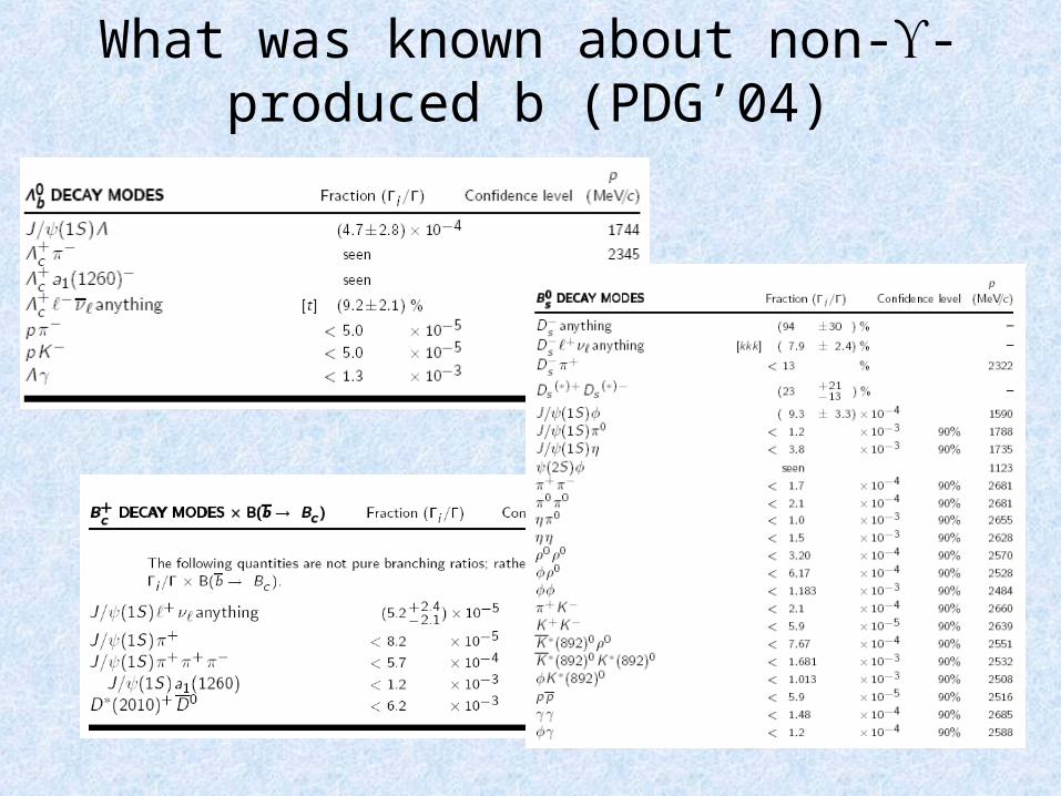
What was known about non--produced b (PDG’04)

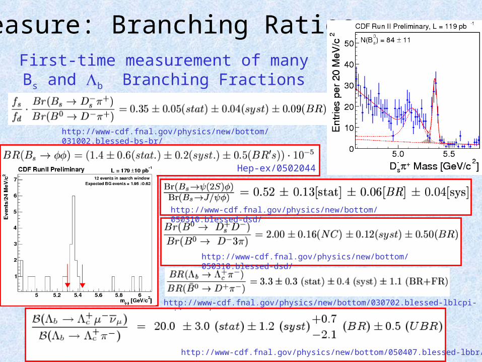
Measure: Branching Ratios

http://www-cdf.fnal.gov/physics/new/bottom/031002.blessed-bs-br/

http://www-cdf.fnal.gov/physics/new/bottom/030702.blessed-lblcpi-ratio_new/

http://www-cdf.fnal.gov/physics/new/bottom/050310.blessed-dsd/

http://www-cdf.fnal.gov/physics/new/bottom/050407.blessed-lbbr/

http://www-cdf.fnal.gov/physics/new/bottom/050310.blessed-dsd/

First-time measurement of many Bs and b Branching Fractions

Hep-ex/0502044

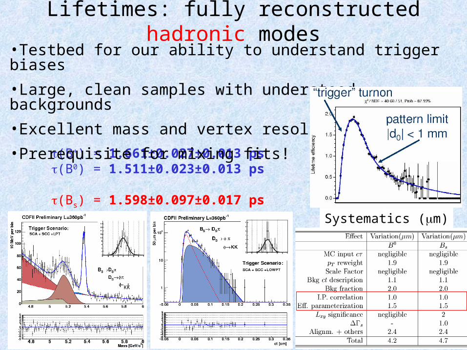
Lifetimes: fully reconstructed hadronic modes

(B+) = 1.661±0.027±0.013 ps (B0) = 1.511±0.023±0.013 ps

(Bs) = 1.598±0.097±0.017 ps

•Testbed for our ability to understand trigger biases

•Large, clean samples with understood backgrounds

•Excellent mass and vertex resolution

•Prerequisite for mixing fits!

http://www-cdf.fnal.gov/physics/new/bottom/050303.blessed-bhadlife/

KK

Systematics (m)

Improving SM Tools

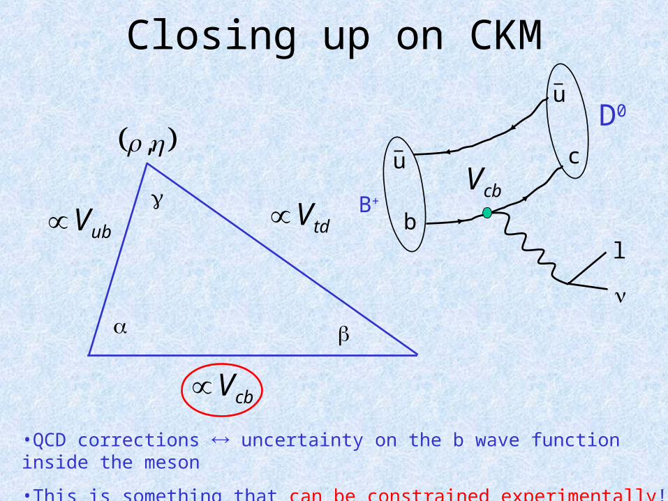
Closing up on CKM

,

tdVubV

cbV

u

u

B+

D0

•QCD corrections uncertainty on the b wave function inside the meson

•This is something that can be constrained experimentally!

c

bcbV

l

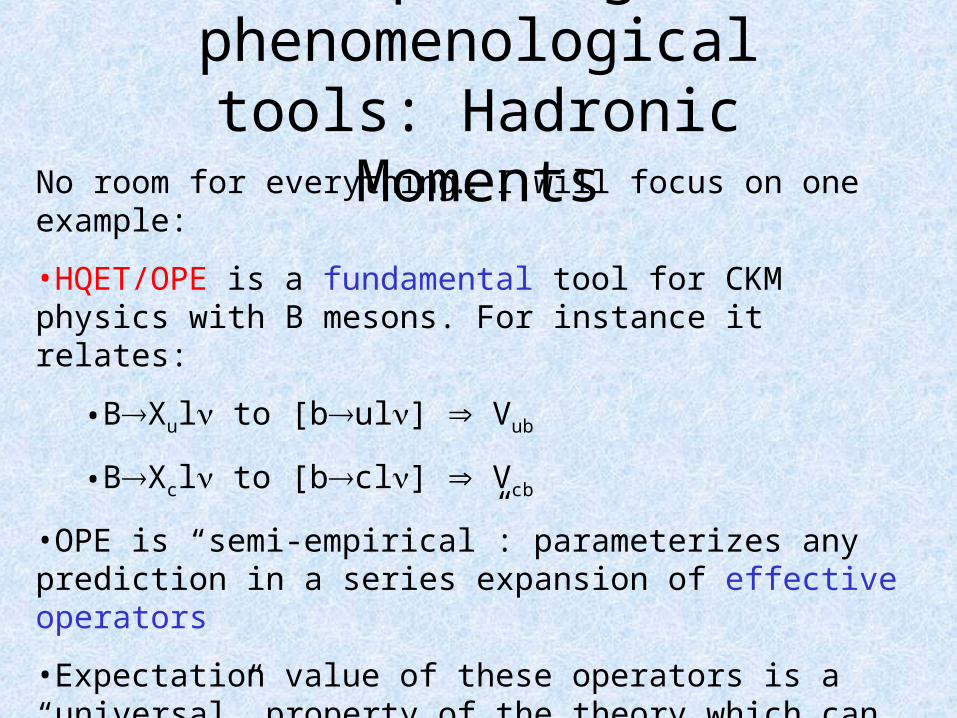
Improving phenomenological tools:

Hadronic MomentsNo room for everything… I will focus on one example:

•HQET/OPE is a fundamental tool for CKM physics with B mesons. For instance it relates:

•BXul to [bul] Vub

•BXcl to [bcl] Vcb

•OPE is “semi-empirical”: parameterizes any prediction in a series expansion of effective operators

•Expectation value of these operators is a “universal” property of the theory which can be assessed with concurrent measurements

•Example: Vcb (±1%exp±2.5%theo) Hadronic Moments

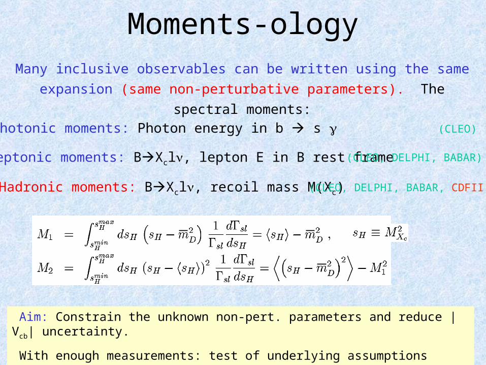
Moments-ology

• Hadronic moments: BXcl, recoil mass M(Xc)

• Leptonic moments: BXcl, lepton E in B rest frame

• Photonic moments: Photon energy in b s

(CLEO, DELPHI, BABAR)

(CLEO)

(CLEO, DELPHI, BABAR, CDFII)

Many inclusive observables can be written using the same

expansion (same non-perturbative parameters). The spectral

moments:

Aim: Constrain the unknown non-pert. parameters and reduce |Vcb| uncertainty.

With enough measurements: test of underlying assumptions (duality…).

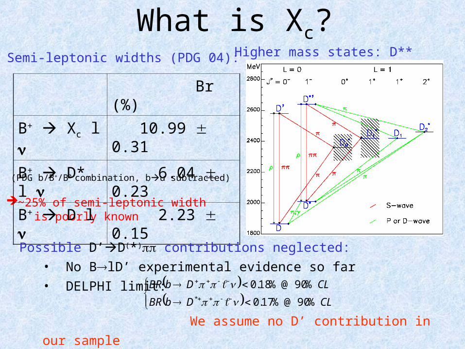
What is Xc?

~25% of semi-leptonic width is poorly known

Higher mass states: D**Semi-leptonic widths (PDG 04):

Br (%)

B+ Xc l 10.99 0.31

B+ D* l

6.04 0.23

B+ D l 2.23 0.15(PDG b/B+/B0 combination, bu subtracted)

Possible D’D(*) contributions neglected:• No BlD’ experimental evidence so far • DELPHI limit:

We assume no D’ contribution in our sample

CLDbBR

CLDbBR

%90@%17.0

%90@%18.0*

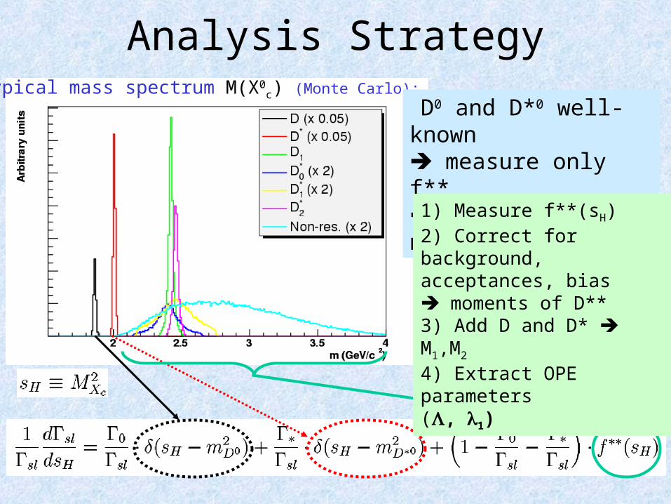
Analysis StrategyTypical mass spectrum M(X0

c) (Monte Carlo): D0 and D*0 well-known measure only f** only shape needed1) Measure f**(sH)2) Correct for background,acceptances, bias moments of D**3) Add D and D* M1,M2

4) Extract OPE parameters (, 1)

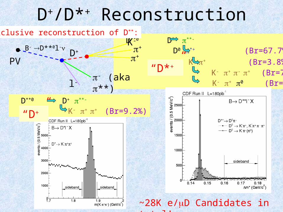
D+/D*+ Reconstruction D**0 D*+ **-

D0 *+ (Br=67.7%)

K- + (Br=3.8%) K- + - + (Br=7.5%) K- + 0 (Br=13.0%)

Exclusive reconstruction of D**:

“D*+”

B- D**0l-

PV

l-- (aka **)

+

+

K-

D+

D**0 D+ **- K- + + (Br=9.2%)“D+”

~28K e/D Candidates in total!

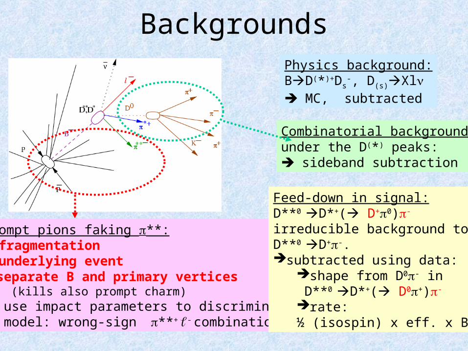
Backgrounds

Combinatorial backgroundunder the D(*) peaks: sideband subtraction

Physics background:BD(*)+Ds

-, D(s)Xl MC, subtracted

Prompt pions faking **:• fragmentation• underlying eventseparate B and primary vertices (kills also prompt charm) use impact parameters to discriminate model: wrong-sign **+ - combinations

Feed-down in signal:D**0 D*+( D+0)-

irreducible background toD**0 D+-.subtracted using data:

shape from D0- in D**0 D*+( D0+)-

rate: ½ (isospin) x eff. x BR

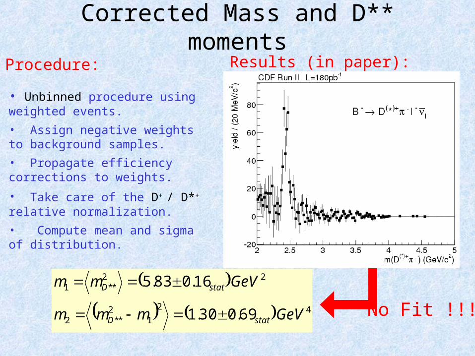
Corrected Mass and D** moments

Procedure:

• Unbinned procedure using weighted events.

• Assign negative weights to background samples.

• Propagate efficiency corrections to weights.

• Take care of the D+ / D*+ relative normalization.

• Compute mean and sigma of distribution.

42

12

**2

22**1

69.030.1

16.083.5

GeVmmm

GeVmm

statD

statD

Results (in paper):

No Fit !!!

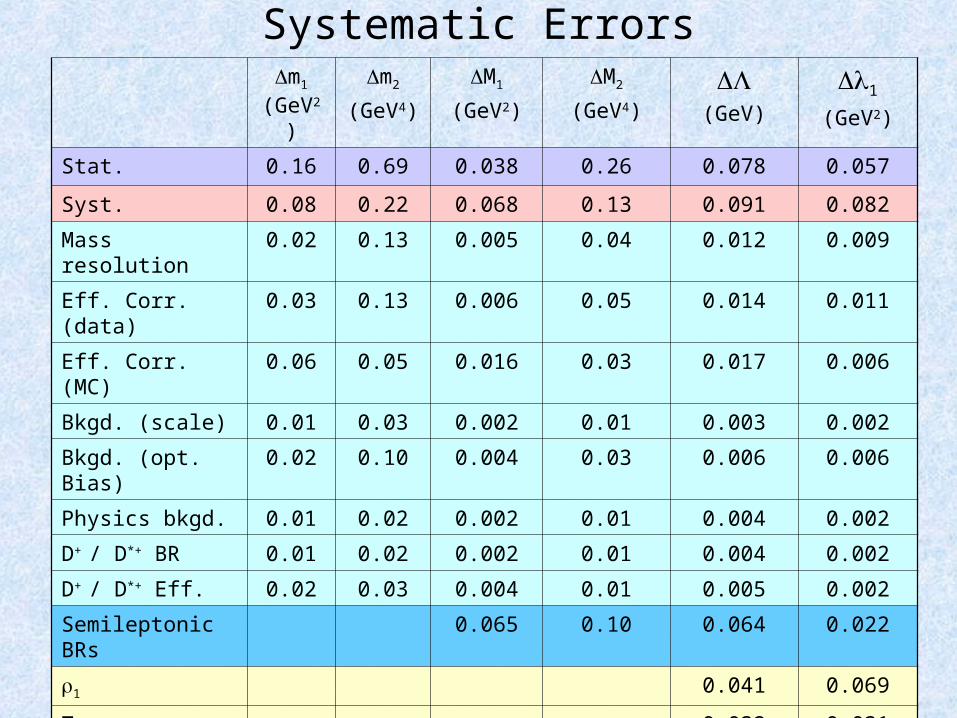
Systematic Errorsm1

(GeV2)m2

(GeV4)

M1

(GeV2)

M2

(GeV4)

(GeV)

1

(GeV2)

Stat. 0.16 0.69 0.038 0.26 0.078 0.057

Syst. 0.08 0.22 0.068 0.13 0.091 0.082

Mass resolution 0.02 0.13 0.005 0.04 0.012 0.009

Eff. Corr. (data) 0.03 0.13 0.006 0.05 0.014 0.011

Eff. Corr. (MC) 0.06 0.05 0.016 0.03 0.017 0.006

Bkgd. (scale) 0.01 0.03 0.002 0.01 0.003 0.002

Bkgd. (opt. Bias) 0.02 0.10 0.004 0.03 0.006 0.006

Physics bkgd. 0.01 0.02 0.002 0.01 0.004 0.002

D+ / D*+ BR 0.01 0.02 0.002 0.01 0.004 0.002

D+ / D*+ Eff. 0.02 0.03 0.004 0.01 0.005 0.002

Semileptonic BRs

0.065 0.10 0.064 0.022

1 0.041 0.069

Ti 0.032 0.031

s 0.018 0.007

mb, mc 0.001 0.008

Choice of pl* cut 0.019 0.009

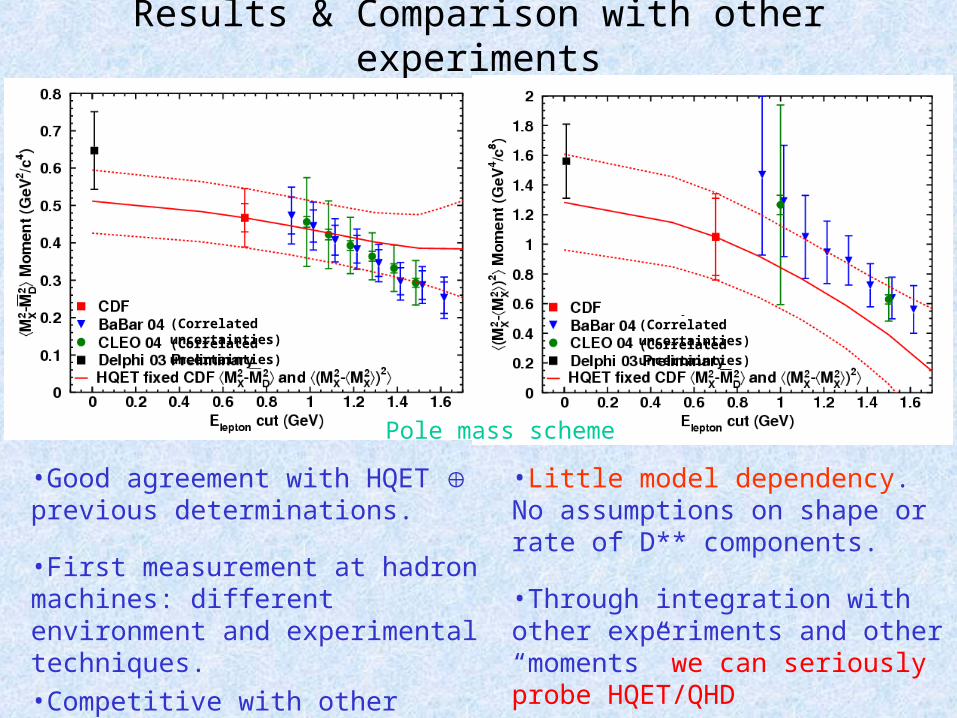
Results & Comparison with other experiments

•Good agreement with HQET previous determinations.

•First measurement at hadron machines: different environment and experimental techniques.•Competitive with other experiments.

•Little model dependency. No assumptions on shape or rate of D** components.

•Through integration with other experiments and other “moments” we can seriously probe HQET/QHD

Pole mass scheme

(Correlated uncertainties)(Correlated uncertainties)

(Correlated uncertainties)(Correlated uncertainties)

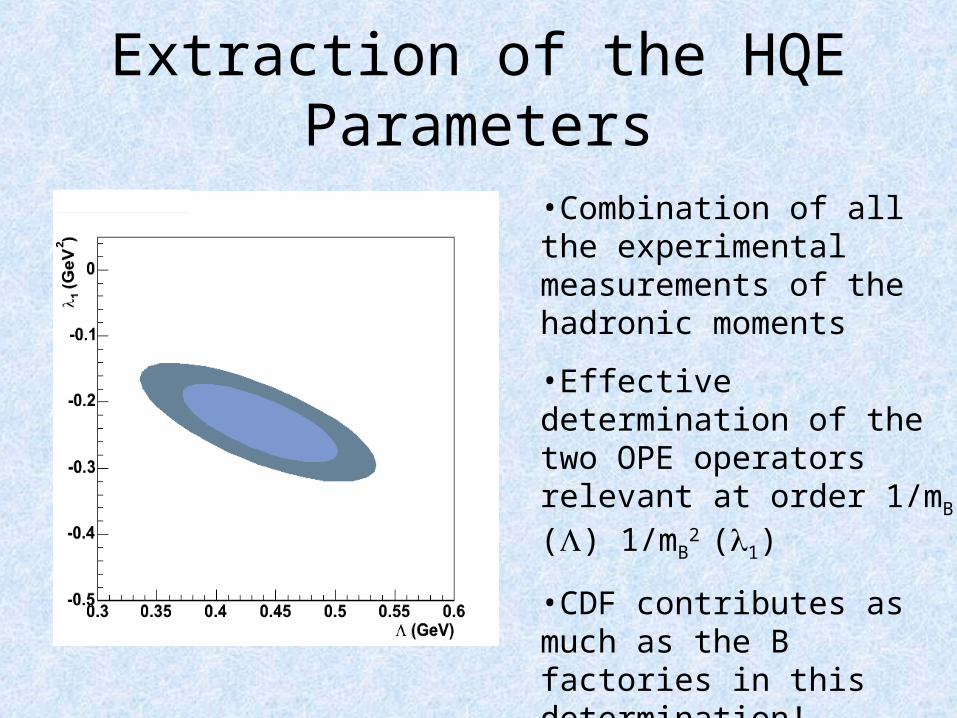
Extraction of the HQE Parameters

•Combination of all the experimental measurements of the hadronic moments

•Effective determination of the two OPE operators relevant at order 1/mB

() 1/mB

2 (1)

•CDF contributes as much as the B factories in this determination!

Bs Mixing

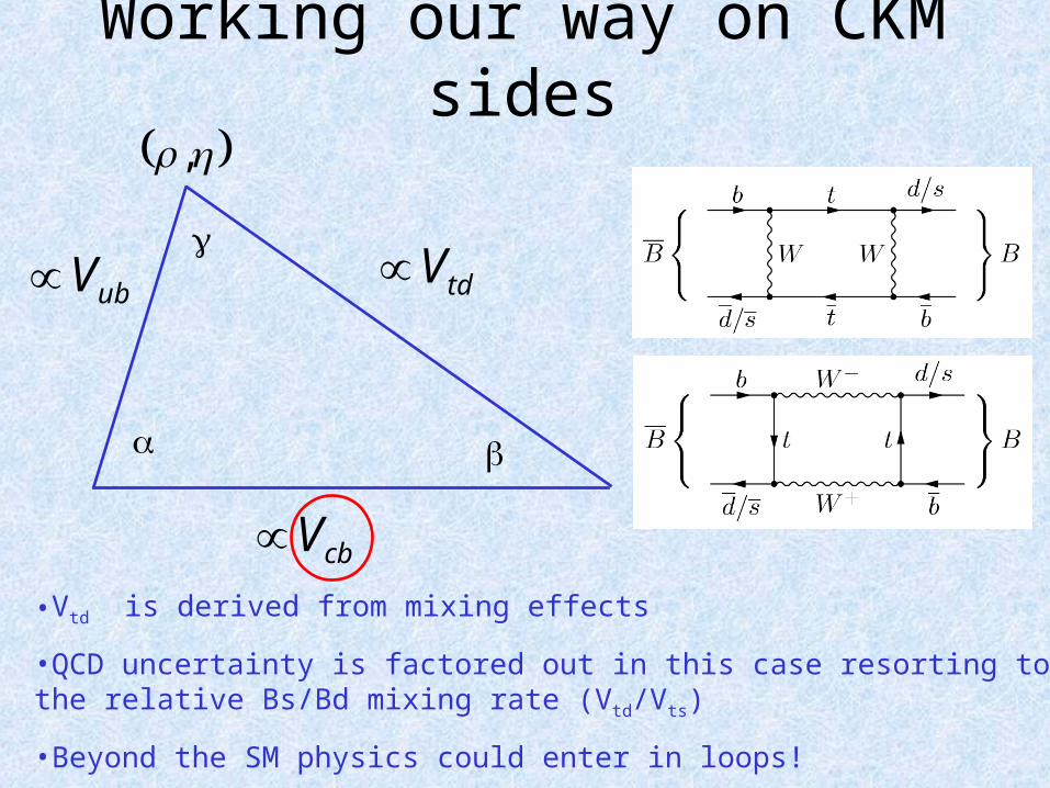
Working our way on CKM sides

,

tdVubV

cbV•Vtd is derived from mixing effects

•QCD uncertainty is factored out in this case resorting to the relative Bs/Bd mixing rate (Vtd/Vts)

•Beyond the SM physics could enter in loops!

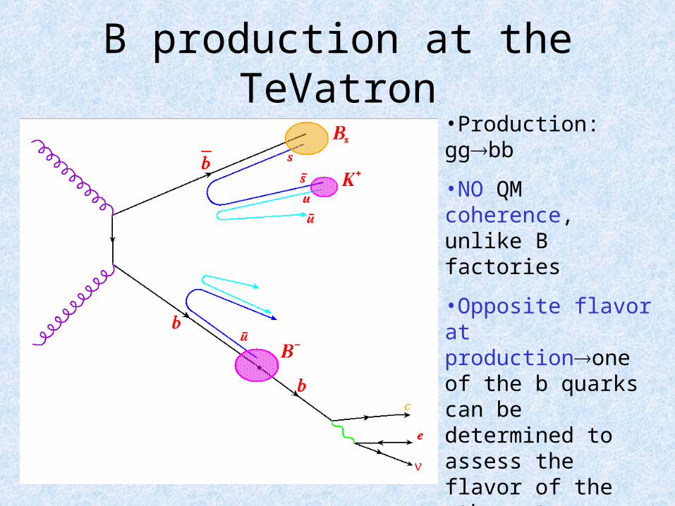
B production at the TeVatron

•Production: ggbb

•NO QM coherence, unlike B factories

•Opposite flavor at productionone of the b quarks can be determined to assess the flavor of the other at production

•Fragmentation products have some memory of b flavor as well

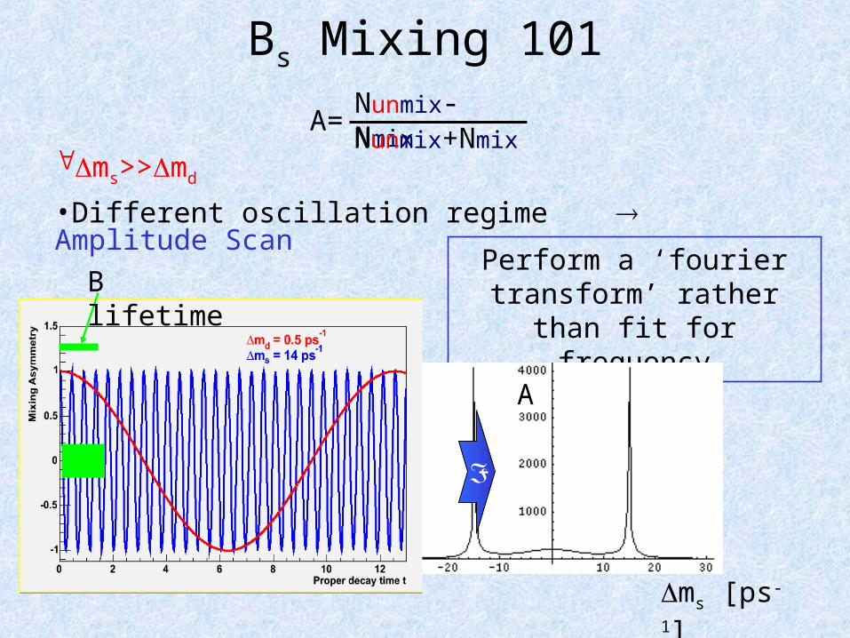
Bs Mixing 101

ms>>md

•Different oscillation regime Amplitude Scan

Perform a ‘fourier transform’ rather than

fit for frequency

ms [ps-

1]

B lifetime

A

Nunmix-NmixNunmix+Nmix

A=

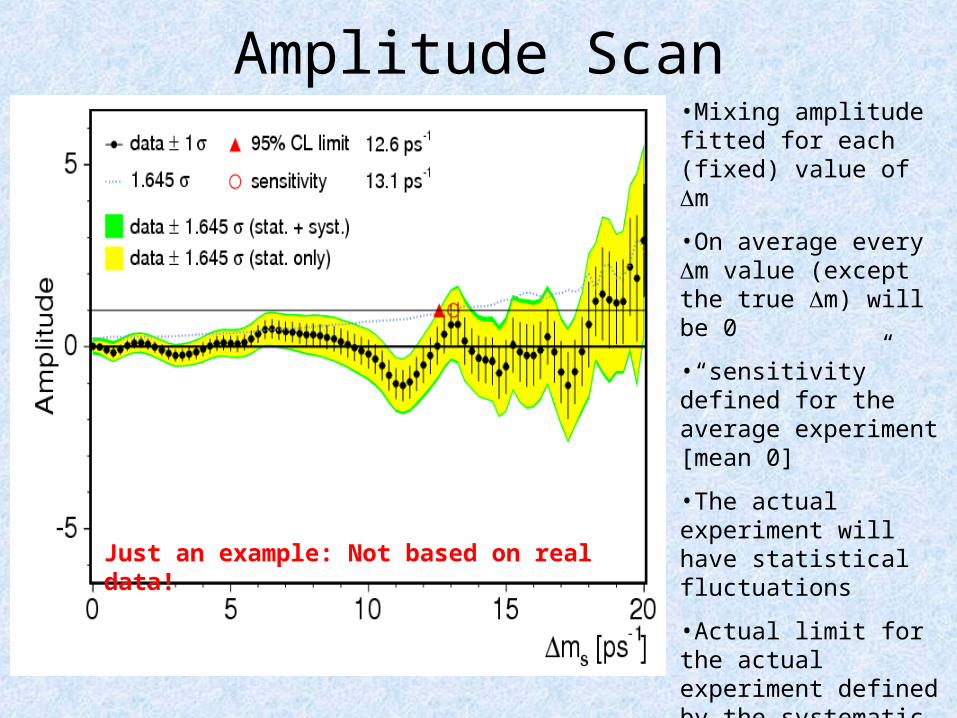
Amplitude Scan

Just an example: Not based on real data!

•Mixing amplitude fitted for each (fixed) value of m

•On average every m value (except the true m) will be 0

•“sensitivity” defined for the average experiment [mean 0]

•The actual experiment will have statistical fluctuations

•Actual limit for the actual experiment defined by the systematic band centered at the measured asymmetry

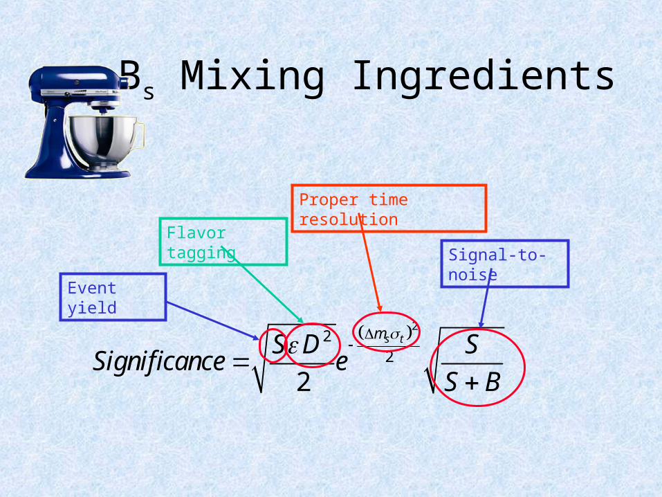
Bs Mixing Ingredients

222

2

s tmS D SSignificance e

S B

Event yield

Flavor taggingSignal-to-noise

Proper time resolution

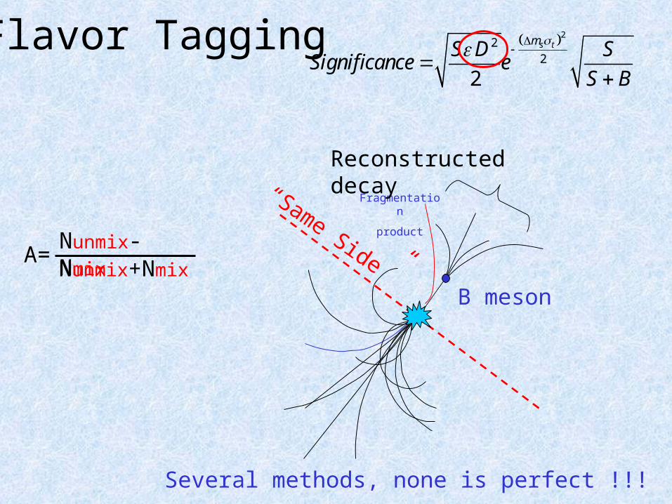
Flavor Tagging

Several methods, none is perfect !!!

Fragmentation

product

B meson

Reconstructed decay“Same Side”

222

2

s tmS D SSignificance e

S B

Nunmix-NmixNunmix+Nmix

A=

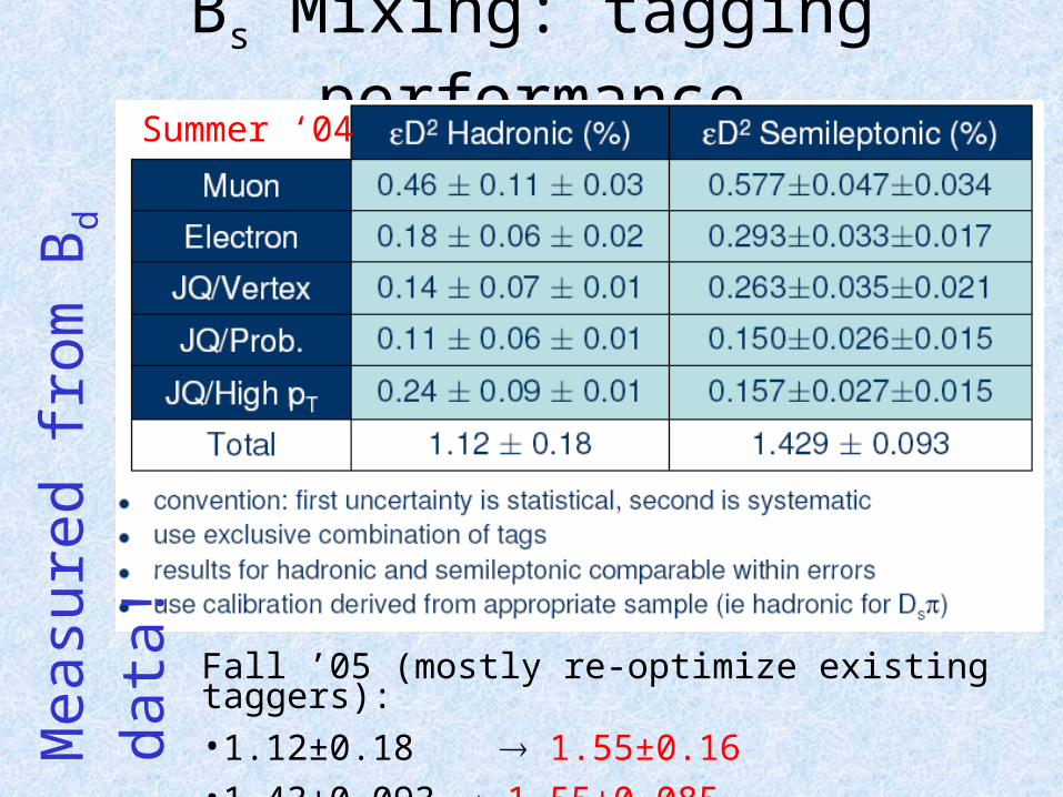
Bs Mixing: tagging performanceSummer ‘04

Fall ’05 (mostly re-optimize existing taggers): •1.12±0.18 1.55±0.16•1.43±0.093 1.55±0.085

Measu

red f

rom

Bd

data

!

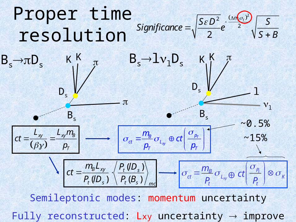
Proper time resolution

222

2

s tmS D SSignificance e

S B

BsllDs K K

ll

Ds

Bs

T

xy

pBct

xy xy B

TL

T T

L L mct

m

p ppct

~0.5%

KBsDsK

Ds

Bs

Semileptonic modes: momentum uncertainty

Fully reconstructed: Lxy uncertainty improve reconstruction

mcst

st

st

xyB

BP

lDP

lDP

Lmct

)(

)(

)(

~15%

Kt

PL

t

Bct

Pct

Pm t

xy

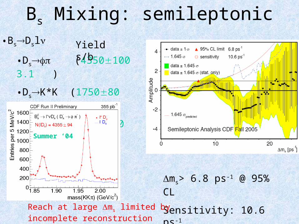
Bs Mixing: semileptonic

ms> 6.8 ps-1 @ 95% CL

Sensitivity: 10.6 ps-1

•BsDsl

•Ds (4350100 3.1 )

•DsK*K (175080 0.42 )

•Ds (157090 0.32)

Reach at large ms limited by incomplete reconstruction (ct)!

Summer ‘04

Yield s/b

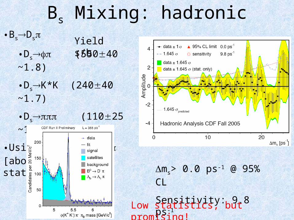
Bs Mixing: hadronic

ms> 0.0 ps-1 @ 95% CL

Sensitivity: 9.8 ps-1

•BsDs

•Ds (55040 ~1.8)

•DsK*K (24040 ~1.7)

•Ds (11025 ~1.0)

•Using also BsDs [about 1/3 more statistics]

Low statistics, but promising!

Yield s/b

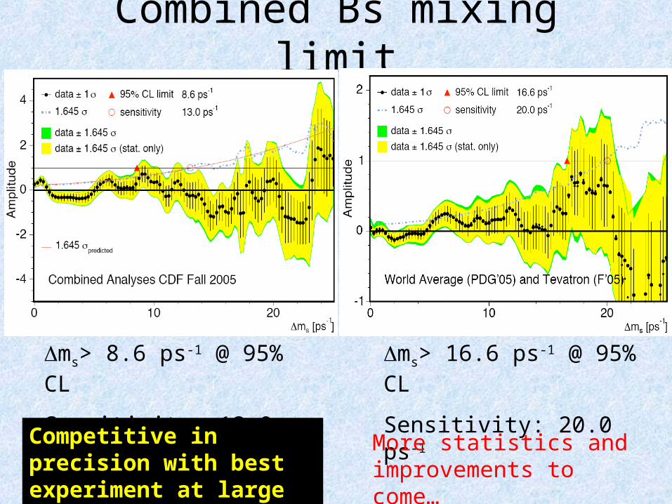
Combined Bs mixing limit

ms> 8.6 ps-1 @ 95% CL

Sensitivity: 13.0 ps-1

ms> 16.6 ps-1 @ 95% CL

Sensitivity: 20.0 ps-1Competitive in precision with best experiment at large ms

More statistics and improvements to come…

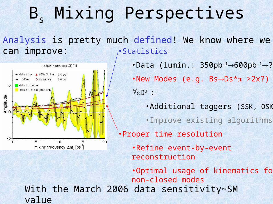
Bs Mixing Perspectives

Analysis is pretty much defined! We know where we can improve: •Statistics

•Data (lumin.: 350pb-1600pb-1??)

•New Modes (e.g. BsDs* >2x?)

D2 :

•Additional taggers (SSK, OSK…)

•Improve existing algorithms

•Proper time resolution

•Refine event-by-event reconstruction

•Optimal usage of kinematics for non-closed modes

With the March 2006 data sensitivity~SM value

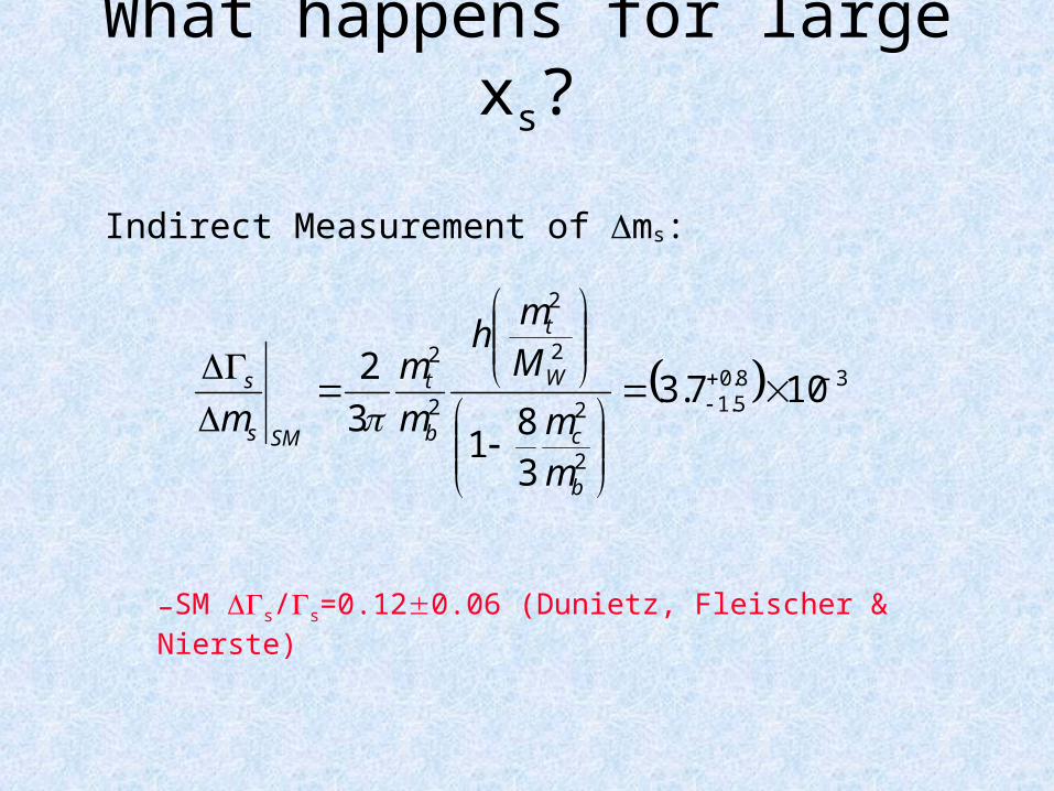
What happens for large xs?

Indirect Measurement of ms:

–SM s/s=0.120.06 (Dunietz, Fleischer & Nierste)

38.05.1

2

2

2

2

2

2

107.3

38

13

2

b

c

W

t

b

t

SMs

s

m

m

M

mh

m

m

m

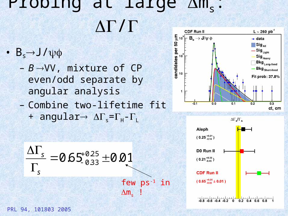
Probing at large ms: /

• BsJ/– B VV, mixture of CP

even/odd separate by angular analysis

– Combine two-lifetime fit + angular s=H-L

PRL 94, 101803 2005

01.065.0 25.033.0

s

s

few ps-1 in ms !

Beyond the SMAnalyses like this have laid down the path and the tools and techniques for the exploration of the SM boundaries:

•Non SM effects:

•bd ?

•bs

•Rare decays (bs)

•Bs, etc.

•BK

•Bs

•xs

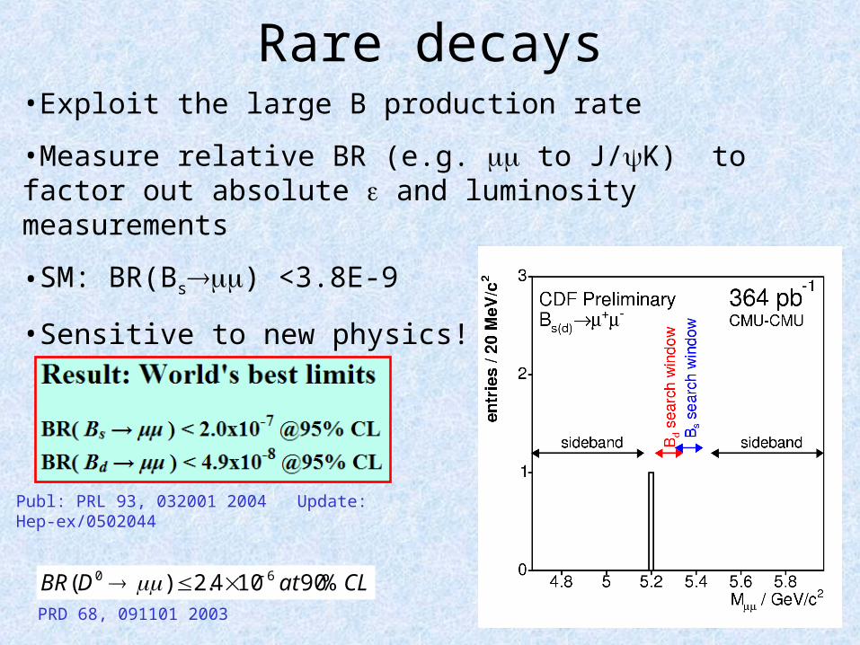
Rare decays•Exploit the large B production rate

•Measure relative BR (e.g. to J/K) to factor out absolute and luminosity measurements

•SM: BR(Bs) <3.8E-9

•Sensitive to new physics!

Publ: PRL 93, 032001 2004 Update: Hep-ex/0502044

PRD 68, 091101 2003

CLatDBR %90104.2)( 60

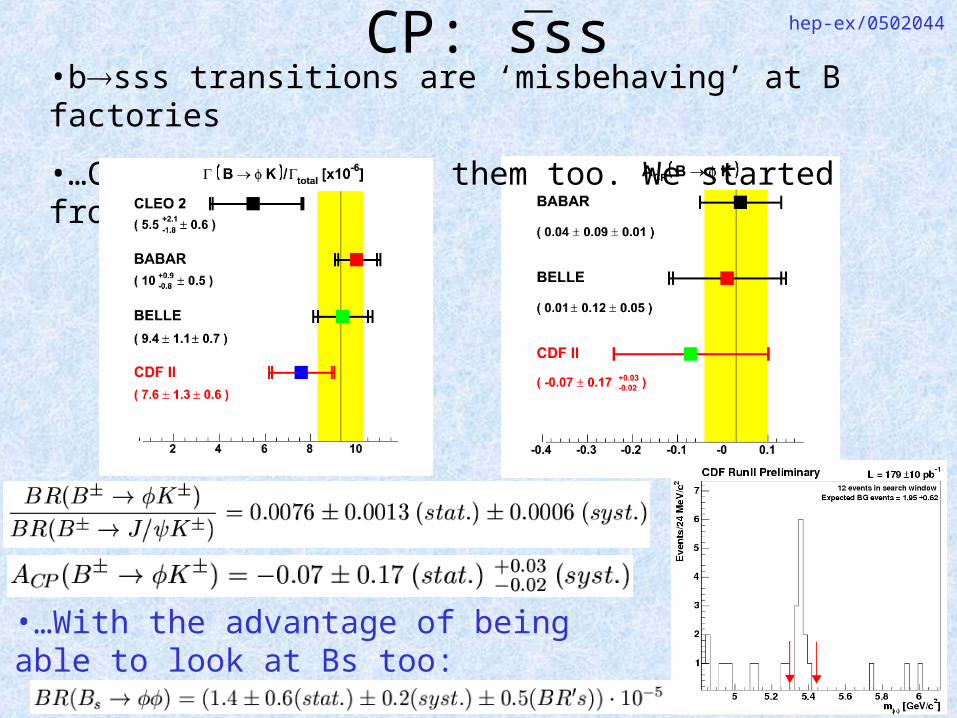
CP: sss•bsss transitions are ‘misbehaving’ at B factories

•…CDF II can look at them too. We started from K:

hep-ex/0502044

•…With the advantage of being able to look at Bs too:

Perspectives

Exciting times ahead:• Most analyses sensitive to BSM

physics are statistically limited• Significant improvements can be

made including new modes and techniques

• Bs results will be an important complementary addition to the CKM mapping!

Conclusions•We are living an exciting transition era of more and more quantitative results in the CKM sector

•BSM physics could be around the corner, but hard to discern models without direct evidences

•With LHC we will soon jump in the completely uncharted territory!

•Living this constant exploration of new discoveries puts us at the forefront of human knowledge, but this is not news!

“Modern science did not spring perfect and complete, as Athena from the head of Zeus, from the mind of Galileo and Descartes”

Purgatory

A guiding theme

•Exploring the boundaries of knowledge is a recurrent theme in history

•Geographical explorations exemplify the paradigm:

Question (Why? Where? What? When? Who?)

Development of tools (ships, telescope, microscope…)

Explore the boundaries of knowledge

(ships, telescope, microscope)

Jump in! (the unknown)

(America, planets, atoms…)

G. Galilei

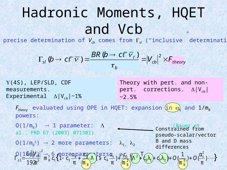
Hadronic Moments, HQET and Vcb

Ftheory evaluated using OPE in HQET: expansion in s and 1/mB powers:

O(1/mB) 1 parameter: (Bauer et al., PRD 67 (2003) 071301)

O(1/mB2) 2 more parameters: 1, 2

O(1/mB3) 6 more parameters: 1, 2, T1-4

(4S), LEP/SLD, CDF measurements. Experimental |Vcb|~1%

Theory with pert. and non-pert. corrections. |Vcb|~2.5%

Most precise determination of Vcb comes from sl (“inclusive” determination):

}{ )π

α()

m

1()λcλc(Λ

m

c)

π

αc(1Λ

m

c

π

αc1cm

192π

GΓ

2s

3B

27162

2B

54

B

321

5B

2

3

2F

sl OOV

sscb

theorycbb

sl FVcbBR

cb

2)()(

Constrained from pseudo-scalar/vector B and D mass differences

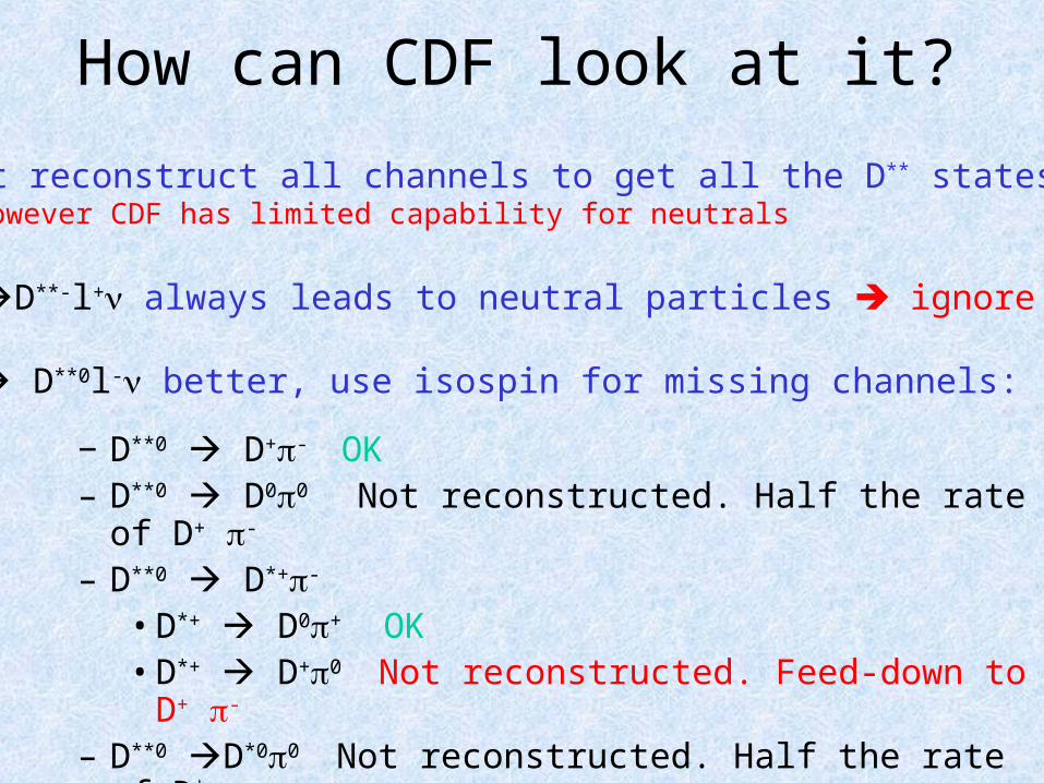
How can CDF look at it?

− D**0 D+- OK– D**0 D00 Not reconstructed. Half the rate of D+ -

– D**0 D*+-

• D*+ D0+ OK• D*+ D+0 Not reconstructed. Feed-down to D+ -

– D**0 D*00 Not reconstructed. Half the rate of D*+ -

Must reconstruct all channels to get all the D** states. However CDF has limited capability for neutrals

• B0D**-l+ always leads to neutral particles ignore it

• B- D**0l- better, use isospin for missing channels:

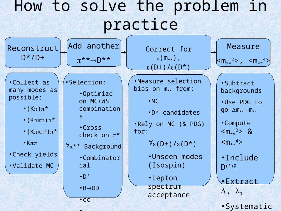
How to solve the problem in practice

Reconstruct D*/D+

Add another

**D**Correct for (m**),

(D+)/(D*)

Measure

<m**2>,

<m**4>

•Selection:

•Optimize on MC+WS combinations

•Cross check on *

** Background

•Combinatorial

•D’

•BDD

•cc

•…

•Collect as many modes as possible:

•(K)*

•(K)*

•(K0)*

•K

•Check yields

•Validate MC

•Measure selection bias on m** from:

•MC

•D* candidates

•Rely on MC (& PDG) for:

(D+)/(D*)

•Unseen modes (Isospin)

•Lepton spectrum acceptance

•Subtract backgrounds

•Use PDG to go m**m**

•Compute <m**

2> & <m**

4>

•Include D(*)0

•Extract , 1

•Systematics

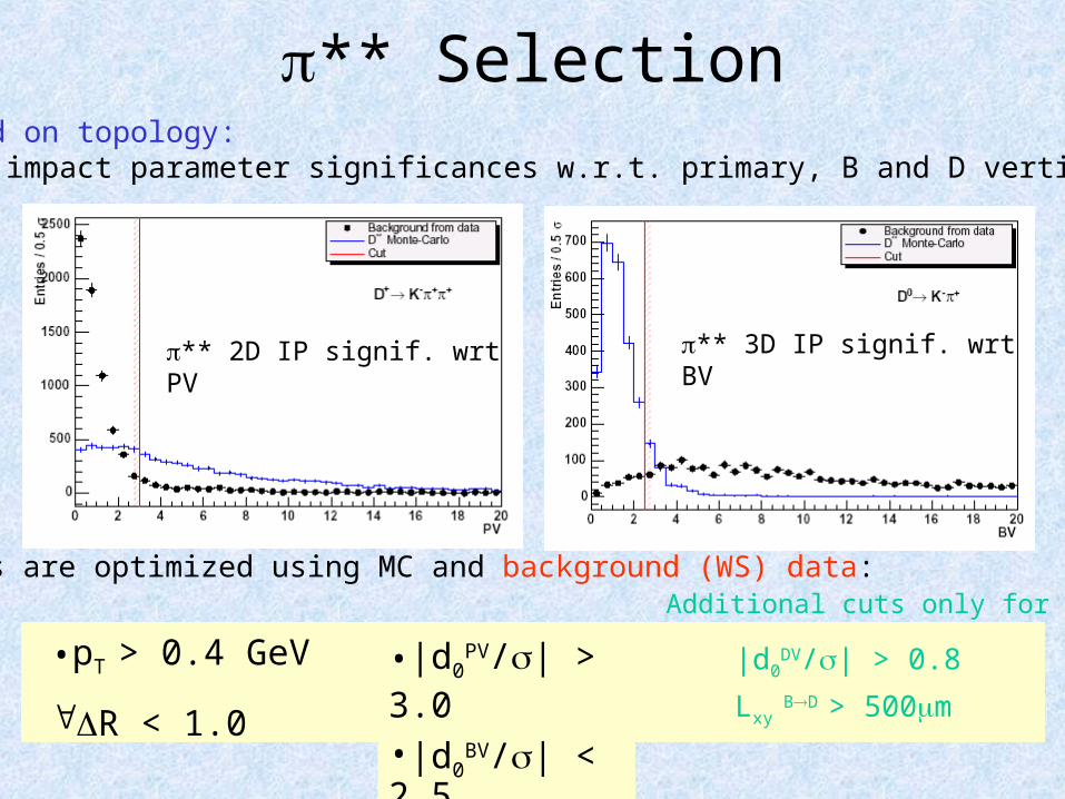
** SelectionBased on topology:

• impact parameter significances w.r.t. primary, B and D vertices

** 3D IP signif. wrt BV** 2D IP signif. wrt PV

•pT > 0.4 GeV

R < 1.0

•|d0PV/| >

3.0•|d0

BV/| < 2.5

|d0DV/| > 0.8

Lxy BD > 500m

Cuts are optimized using MC and background (WS) data:Additional cuts only for D+:

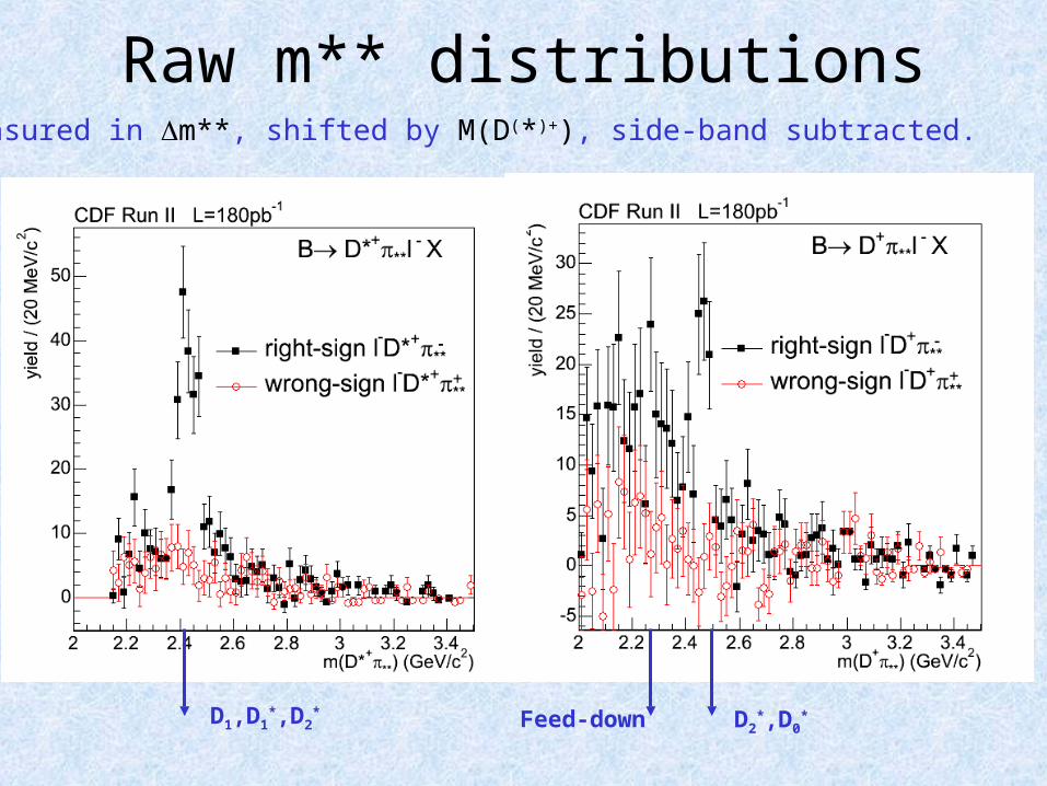
Raw m** distributionsMeasured in m**, shifted by M(D(*)+), side-band subtracted.

D2*,D0

*Feed-downD1,D1*,D2

*

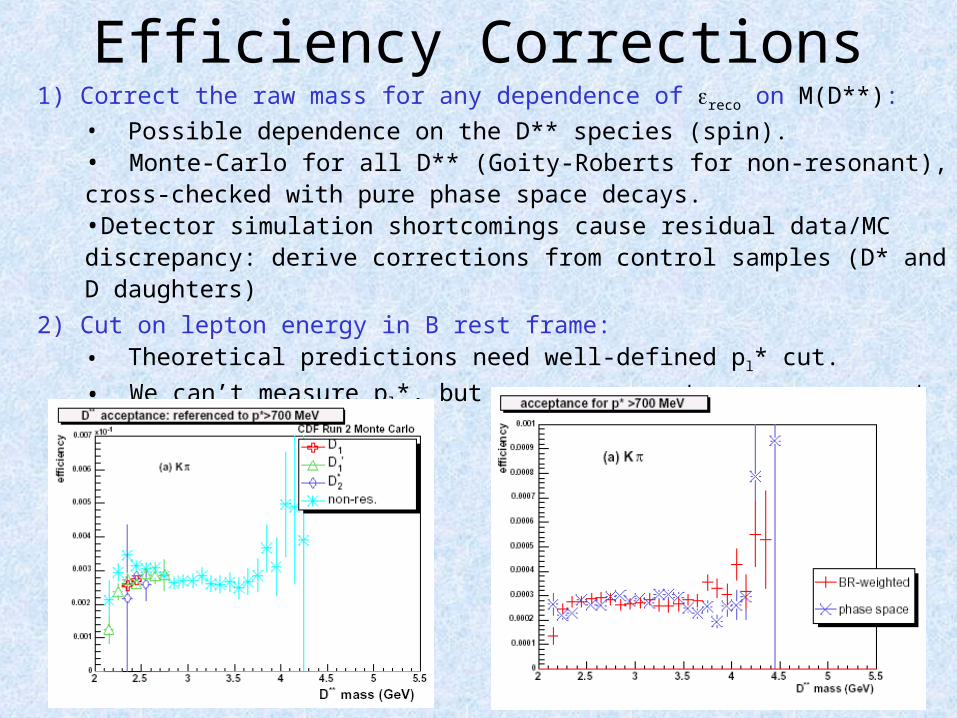
Efficiency Corrections1) Correct the raw mass for any dependence of reco on M(D**):

• Possible dependence on the D** species (spin).• Monte-Carlo for all D** (Goity-Roberts for non-resonant), cross-checked with pure phase space decays.•Detector simulation shortcomings cause residual data/MC discrepancy: derive corrections from control samples (D* and D daughters)

2) Cut on lepton energy in B rest frame:• Theoretical predictions need well-defined pl* cut.

• We can’t measure pl*, but we can correct our measurement to a

given cut: pl* > 700 MeV/c.

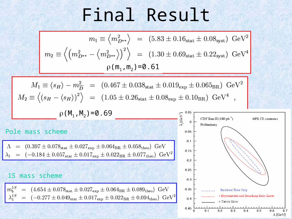
Final Result

Pole mass scheme

1S mass scheme

(m1,m2)=0.61

(M1,M2)=0.69

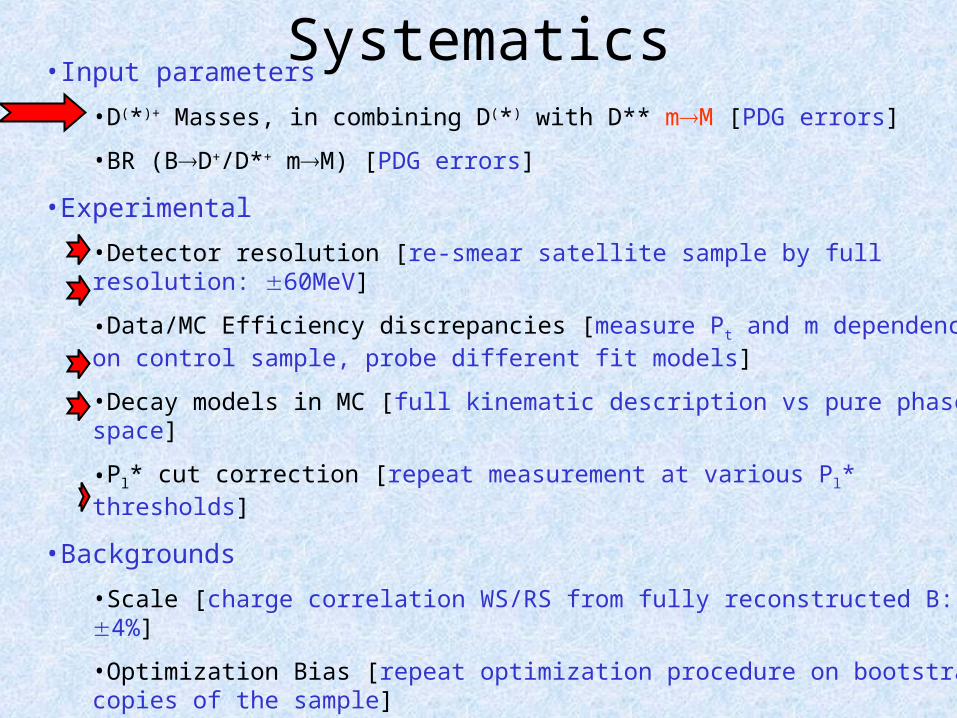
Systematics•Input parameters

•D(*)+ Masses, in combining D(*) with D** mM [PDG errors]

•BR (BD+/D*+ mM) [PDG errors]

•Experimental

•Detector resolution [re-smear satellite sample by full resolution: 60MeV]

•Data/MC Efficiency discrepancies [measure Pt and m dependency on control sample, probe different fit models]

•Decay models in MC [full kinematic description vs pure phase space]

•Pl* cut correction [repeat measurement at various Pl* thresholds]

•Backgrounds

•Scale [charge correlation WS/RS from fully reconstructed B: 4%]

•Optimization Bias [repeat optimization procedure on bootstrap copies of the sample]

•Physics background [vary 100%]

•BXc [estimate / yield and kinematic differences using MC]

•Fake leptons [no evidence in WS D+l+, charge-correlated negligible]

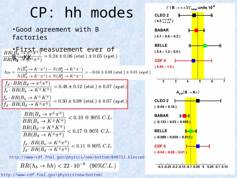
CP: hh modes

http://www-cdf.fnal.gov/physics/new/bottom/040722.blessed-bhh/

•Good agreement with B factories

•First measurement ever of BsKK

http://www-cdf.fnal.gov/physics/new/bottom/040624.blessed_Lb_hh_limit/