Probability Theory Oral Exam study notes Notes …nica/oral/prob_notes.pdf · Abstract. These are...

Probability Theory Oral Exam study notes

Notes transcribed by Mihai Nica

Abstract. These are some study notes that I made while studying for myoral exams on the topic of Probability Theory. I took these notes from a fewdierent sources, and they are not in any particular order. They tend to movearound a lot. They also skip some of the basics of measure theory which arecovered in the real analysis notes. Please be extremely caution with thesenotes: they are rough notes and were originally only for me to help me study.They are not complete and likely have errors. I have made them availableto help other students on their oral exams (Note: I specialized in probabilitytheory, so these go a bit further into a few topics that most people would dofor their oral exam). See also the sections on Conditional Expectation and theLaw of the Iterated Logarithm from my Limit Theorem II notes.

Contents

Independence and Weak Law of Large Numbers 51.1. Independence 51.2. Weak Law of Large Numbers 9

Borel Cantelli Lemmas 122.3. Borel Cantelli Lemmas 122.4. Bounded Convergence Theorem 15

Central Limit Theorems 173.5. The De Moivre-Laplace Theorem 173.6. Weak Convergence 173.7. Characteristic Functions 243.8. The moment problem 313.9. The Central Limit Theorem 333.10. Other Facts about CLT results 353.11. Law of the Iterated Log 36

Moment Methods 394.12. Basics of the Moment Method 394.13. Poisson RVs 424.14. Central Limit Theorem 42

Martingales 515.15. Martingales 515.16. Stopping Times 53

Uniform Integrability 586.17. An 'absolute continuity' property 586.18. Denition of a UI family 586.19. Two simple sucient conditions for the UI property 596.20. UI property of conditional expectations 596.21. Convergence in Probability 606.22. Elementary Proof of Bounded Convergence Theorem 606.23. Necessary and Sucient Conditions for L1 convergence 60

UI Martingales 627.24. UI Martingales 627.25. Levy's 'Upward' Theorem 627.26. Martingale Proof of Kolmogorov 0-1 Law 637.27. Levy's 'Downward' Theorem 637.28. Martingale Proof of the Strong Law 64

3

CONTENTS 4

7.29. Doob's Subartingale Inequality 64

Kolmogorov's Three Series Theorem using L2 Martingales 66

A few dierent proofs of the LLN 739.30. Truncation Lemma 739.31. Truncation + K3 Theorem + Kronecker Lemma 749.32. Truncation + Sparsication 769.33. Levy's Downward Theorem and the 0-1 Law 799.34. Ergodic Theorem 809.35. Non-convergence for innite mean 81

Ergodic Theorems 8210.36. Denitions and Examples 8210.37. Birkho's Ergodic Theorem 8610.38. Recurrence 8810.39. A Subadditive Ergodic Theorem 8810.40. Applications 90

Large Deviations 9110.41. LDP for Finite Dimesnional Spaces 9210.42. Cramer's Theorem 103

Bibliography 109

Independence and Weak Law of Large Numbers

These are notes from Chapter 2 of [2].

1.1. Independence

Definition. A,B indep if P(A ∩ B) = P(A)P(B), X,Y are indep if P(X ∈C, Y ∈ D) = P(X ∈ C)P(Y ∈ D) for every C,D ∈ R. Two σ−algebras areindependent if A ∈ F and B ∈ G has A,B independent.

Exercise. (2.1.1) Show that if X,Y are indep then σ(X) and σ(Y ) are. ii)Show that if X is F-measurable and Y is G−measurable then and F , G are inde-pendent, then X and Y are independent

Proof. This is immediate from the denitions.

Exercise. (2.1.2) i) Show A,B are independent then Acand B are independenttoo. ii) Show A,B are independent i 1A and 1B are independent.

Proof. i) P(B) = P(A∩B)+P(Ac∩B) = P(A)P(B)+P(Ac∩B) , rearrange.ii) Simple using1A ∈ C = A if 1 ∈ C and = Ac otherwise.

Remark. By the above quick exercises, all of independence is dened by in-dependence of σ-algbras, so we will view that as the ventral object.

Definition. F1,F2 . . . are independent if for any nite subset and for any setsAi ∈ Fi from an index set i ∈ I ⊂ N we have P (∩Ai) =

∏P(Ai). X1, X2, . . .

are independent if σ(X1), σ(X2) . . . are independent.A1, A2, . . . are independent if1A1

, 1A2, . . . are independent.

Exercise. (2.1.3.) Same as previous exercise with more than two sets.

Example. (2.1.1) The usually example of three events which are pairwise in-dependent but not independent on the space of three fair coinips.

1.1.1. Sucient Conditions for Independence. We will work our way toTheorem 2.1.3 which is the main result for this subsection.

Definition. We call a collection of sets A1,A2 . . .An independent if any col-lection from an index set i ∈ I ⊂ 1, . . . , n Ai ∈ Ai is independent. (Just like thedenition for the σ- algebras only we dont require A to be a sigma algebra)

Lemma. (2.1.1) If we suppose that each Ai contains Ω then the criteria forindependence works with I = 1, . . . , n

Proof. When you put Ak = Ω it doesn't change the intersection and it doesntchange the product since P(Ak) = 1.

5

1.1. INDEPENDENCE 6

Definition. A π−system is a collection A which is closed under intersections,i.e. A,B ∈ A =⇒ A ∩B ∈ A.

A λ−system is a collection L that satises:i) Ω ∈ Lii) A,B ∈ L and A ⊂ B =⇒ B −A ∈ Liii) An ∈ L and An ↑ A =⇒ A ∈ L

Remark. (Mihai - From Wiki) An equivalent def'n of a λ−system is:i) Ω ∈ Lii) A ∈ L =⇒ Ac ∈ Liii)A1, A2, . . . ∈ L disjoint =⇒ ∪∞n=1An ∈ LIn this form, the denition of a λ−system is more comparable to the denition

of a σ algebra, and we can see that it is strictly easier to be a λ−system than aσ−algebra (only needed to be closed under disjoint unions rather than arbitrarycountable unions). The rst denition presented by Durret however is more usefulsince it is easier to check in practice!

Theorem. (2.1.2) (Dynkin's π − λ) Theorem. If P is a π−system and L is aλ−system that contain P, then σ(P) ⊂ L.

Proof. In the appendix apparently? Will come back to this when I do measuretheory.

Theorem. (2.1.3) Suppose A1,A2 are independent of each other and each Aiis a π−system. Then σ(A1), . . . , σ(An) are independent.

Proof. (You can basically reduce to the case n = 2 ) Fix any A2, . . . , An inA2, . . . ,An respectively and let F = A2∩. . .∩An Let L = A : P(A ∩ F ) = P(A)P(F ).Then we verify that L is a λ−system by using basic properties of P. For A ⊂ Bboth in F we have:

P ((B −A) ∩ F ) = P (B ∩ F )−P(A ∩ F )

= P(B)P(F )−P(A)P(F )

= P(B −A)P(F )

(increasing limits is easy by continuity of probability)By the π − λ theorem, σ(A1) ⊂ L, since this works for any F , we have then

that σ(A1),A2,A3, . . . ,An are independent.Iterating the argument n− 1 more times gives the desired result.

Remark. (Durret) The reason the π − λ theorem is helpful here is because itis hard to check that for A,B ∈ L that A ∩B ∈ L or that A ∪B ∈ L. However, itis easy to check that if A,B ∈ L with A ⊂ B then B −A ∈ L. The π − λ theoremcoverts these π and λ systems (which are easier to work with) to σ algebras (whichare harder to work with, but more useful)

Theorem. (2.1.4) In order for X1, X2, . . . , Xn to be independent, it is su-cient that for all x1, x2, . . . , xn ∈ (−∞,∞] that:

P (X1 ≤ x1, . . . , Xn ≤ xn) =

n∏i=1

P (Xi ≤ xi)

Proof. Let Ai be sets of the form Xi ≤ xi. It is easy to check that this isa π−system, so the result is a direct application of the previous theore m.

1.1. INDEPENDENCE 7

Exercise. (2.1.4.) Suppose (X1, . . . , Xn) has density f(x1, . . . , xn) and f canbe written as a product g1(x1) · . . . · gn(xn) . Show that the X ′is are independent.

Proof. Let gi(xi) = cigi(xi) where ci is chosen so that´gi = 1. Can verify

that∏ci = 1 from f =

∏g and

´f = 1. Then integrate along the margin to see

that each gi is in fact a pdf for Xi. Can then apply Thm 2.1.4 after replacing g'sby g's

Exercise. (2.1.5) Same as 2.1.4 but on a discrete space with a probabilitymass function instead of a probability density function.

Proof. Work the same but with sums instead of integrals.We will now prove that functions of independent random variables are still

independent (to be made more precise in a bit)

Theorem. (2.1.5) Suppose Fi,j 1 ≤ i ≤ n and 1 ≤ j ≤ m(i) are independentσ−algebras and let Gi = σ(∪jFi,j). Then G1, . . . ,Gn are independent.

Proof. (Its another π−λ proof based on the Thm 2.1.3) Let Ai be the collec-tion of the sets of the form ∩jAi,j with Ai.j taken from Fi,j . Can verify that Ai isa π−system that contains ∪jFi,j (its closed under intersections by its denition).Since the Fi,j 's are all independent, it is clear the π−systems A′is are independent.By thm 2.1.3, we know that σ(Ai) = Gi are all independent too.

Theorem. (2.1.6) IF for 1 ≤ i ≤ n and 1 ≤ j ≤ m(i) the random variablesXi,j are independent and fi : Rm(i) → R are measurable functions, then the randomvariables Yi :=fi(Xi,1, . . . , Xi,m(i)) are all independent.

Proof. Let Fi,j = σ (Xi,j) and Gi = σ (∪jFi,j). By the previous theorem(2.1.5.), the G′is are independent. Since fi

(Xi,1, . . . , Xi,m(i)

):= Yi ∈ Gi, these

random variables are independent too.

Remark. (Durret) This theorem is the rigourous justication for the type ofreasing like If X1, . . . , Xn are iid, then X1 is indep of (X2, . . . , Xn)

1.1.2. Independence, Distribution, and Expectation.

Example. (Mihai - From Wiki) The Lebesgue measure on R is the uniquemeasure with µ ((a, b)) = b− a

Proof. We will show that it is the unique measure on [0, 1] , you get unique-ness on all of R by stiching together all the intervals [n, n + 1]. Say ν is an-other measure with ν ((a, b)) = b − a. First verify that µ(A) = b − a for all setsA ∈ A,A := (a, b), (a, b], [a, b), [a, b] : 0 ≤ a, b ≤ 1 and that A is a π−system.Then notice the collection L = A : µ(A) = ν(A) is a λ−system by the basicproperties of a measure. Since A ⊂ L by the hypothesis of the problem, by theπ − λ theorem σ(A) ⊂ L. But σ(A) = B is all of the Borel sets! Hence µ and νagree on all Borel sets.

Theorem. (2.1.7.) Suppose X1, . . . , Xn are independent and Xi has distribu-tion µi. Then (X1, . . . , Xn) has distribution µ1 × . . .× µn.

Proof. Verify that the measure of (X1, . . . , Xn) and the measure µ1× . . .×µnagree on rectangle sets of the form A1 × . . . × An using independence. Sincethese sets are a π system that generate the entire Borel sigma algebra, the two

1.1. INDEPENDENCE 8

measures agree everywhere. (More specically, the rectangle sets are a π−systemwith σ(Rectangles) =Borel sets. The collection of sets where µ(X1,...,Xn) = µ1 ×. . .× µn is easily veried to be a λ-system. So Rectangles ⊂ Sets where they agree=⇒ Borel sets ⊂Sets where they agree by the π − λ theorem.

Theorem. (2.1.8.) Suppose X,Y are independent and have distributions µand ν. If h : R2 → R has h ≥ 0 or E [h(X,Y )] <∞ then:

Eh(X,Y ) =

ˆ ˆh(x, y)µ(dx)ν(dy)

Suppose now h(x, y) = f(x)g(y). If f ≥ 0 and g ≥ 0 or if E |f(X)| < ∞ andE |g(Y )| <∞ then:

E [f(X)g(Y )] = E [f(X)]E [g(Y )]

Proof. This is essentiall the Tonelli theorem and the Fubini theorem. Reviewthis when you go over integration.

Theorem. (2.1.9) If X1, . . . , Xn are independent and have Xi ≥ 0 for all i orE |Xi| <∞ for all i. Then:

E

(n∏i=1

Xi

)=

n∏i=1

E (Xi)

Proof. By induction using the last theorem and the result that X1 is inde-pendent from (X2, . . . , Xn) in this case.

Remark. (Durret) Dont forget that uncorrelated ;independent.

1.1.3. Sums of Independent Random Variables.

Theorem. (2.1.10) If X and Y are independent, with F (x) = P(X ≤ x) andG(y) = P(Y ≤ y) then:

P(X + Y ≤ z) =

ˆF (z − y)dG(y)

Where integrating dG is shorthand for, integrate with respect to the measureν whose distribution function is G

Proof. Let h(x, y) = 1x+y≤z. Let µ and ν be the probability measures withdistribution functions F and G. For xed y we have:ˆ

h(x, y)µ(dx) =

ˆ1x+y≤z(x, y)µ(dx)

=

ˆ1−∞,z−y](x)µ(dx)

= µ(∞, z − y)

= F (z − y)

Hence:

P(X + Y ≤ z) =

ˆ ˆ1x+y≤zµ(dx)ν(dy)

=

ˆF (z − y)ν(dy)

1.2. WEAK LAW OF LARGE NUMBERS 9

Theorem. (2.1.11) If X,Y have densities, then X + Y has density:

h(x) =

ˆf(x− y)dG(y)

=

ˆf(x− y)g(y)dy

Proof. Write:

ˆF (z − y)ν(dy) =

ˆ z

−∞

ˆf(x− y)dG(y)dx

There are some examples of the gamma distributions (basically gamma(α, λ)is the sum of α independent expoenntial variables with parameter λ)

1.1.4. Constructing Independent Random Variables. Kolmogorov Ex-tension Theorem is here, I'll come back to this later

Theorem. (Kolmogorov Extension Theorem) If you are given a family of mea-sures µn on Rn that are consistnet:

µn+1 ((a1, b1]× . . .× (an, bn]× R) = µn ((a1, b1]× . . .× (an, bn])

then there exists a unique probability measure P on (RN on sequences so thatP agrees with µn on cylinder sets of size n.

1.2. Weak Law of Large Numbers

1.2.1. L2 Weak Laws.

Theorem. (2.2.1) If X1, . . . are uncorrelated and E(X2i ) <∞ then:

Var(∑

Xi

)=∑

Var(Xi)

Proof. Just expand it out, dross terms die since the r.v.s are uncorrelated.(Helps to assume WOLOG that E(Xi) = 0)

Lemma. (2.2.2) If p > 0 then E |Zn|p → 0 then Zn → 0 in probability

Proof. By Cheb ineq. This was one of the things on our types of convergencediagram.

Theorem. (2.2.3.) If X1, . . . are uncorrelated and E(Xi) = µ and Var(Xi) <C <∞. If Sn =

∑Xi then Sn/n→ µ in L2 and in probability.

Proof. E[(Sn/n− µ)

2]

= 1n2Var(Sn) = 1

n2

∑Var(Xn) ≤ Cn

n2 → 0

Example. (2.2.1)Basically this example is a simlar result set up in such a way to remark that

the convergence is uniform in some sense. Specically they have a family of coupled

bernoulli variables Xpn, and they are saying that E

[(Spn/n− µ)

2]→ 0 uniformly

for the whole family. Indeed, the estimate we used in them 2.2.3. just needs anupper bound on the variance.


1.2.2. Triangular Arrays.

Definition. A triangular array is an array of random variables Xn,k. Therow sum Sn is dened to be Sn =

∑kXn,k

Theorem. (2.2.4.) Let µn = E(Sn), σ2n := Var(Sn). If σ2

n/b2n → 0 then:

Sn − µnbn

→ 0

In L2 and in probability.

Proof. Have (similar to before) E(

((Sn − µn) /bn)2)

= b−2n Var (Sn)→ 0

Example. These examples are actually really nice and I like them a lot! How-ever, I'm going to skip them for now.

1.2.3. Truncation. To truncate a random variable X at level M means toconsider:

X = X1|X|<M

To extend some of our results to random variables without a nitie secondmoment, we will truncate them.

Theorem. (2.2.6) For each n let Xn,k, 1 ≤ k ≤ n be a triangular array

of independent random variables. Let bn > 0 and bn → ∞, and let Xn,k =Xn,k1|Xn,k|≤bn. Suppose that:

n∑k=1

P (|Xn,k| > bn) → 0 as n→∞ and

b−2n

n∑k=1

E(X2n,k

)→ 0 as n→∞

Then let Sn =∑kXn,k and put an =

∑nk=1 E

(Xn,k

). Then:

Sn − anbn

→ 0 in probabiliy

Proof. Writing Sn for the sum of the truncated variables, we have:

P

(∣∣∣∣Sn − anbn

∣∣∣∣ > ε

)≤ P

(Sn 6= Sn

)+ P

(∣∣∣∣∣ Sn − anbn

∣∣∣∣∣ > ε

)The rst term is controlled by

∑P (|Xn,k| > b), namely:

P(Sn 6= Sn

)≤ P

(∪nk=1

Xn,k 6= Xn,k

)≤

n∑k=1

P (|Xn,k| > bn)→ 0

The second term is controlled by Cheb inequality and our bound on the Xn's.Have L2 convergence by:

E

(Sn − anbn

)2

= b−2n Var

(Sn

)= b−2

n

n∑k=1

Var(Xn,k

)≤ b−2

n

n∑k=1

E(X2n,k

)→ 0

So this also converges in probability to zero (by cheb ineq)


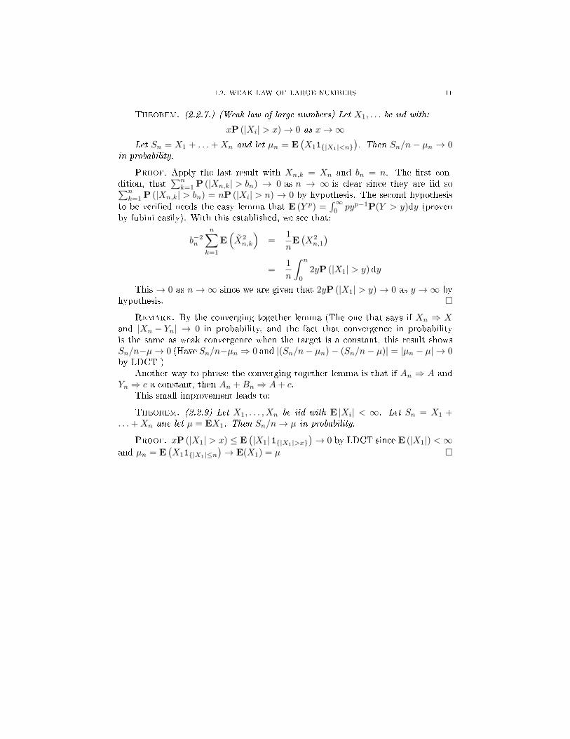
Theorem. (2.2.7.) (Weak law of large numbers) Let X1, . . . be iid with:

xP (|Xi| > x)→ 0 as x→∞Let Sn = X1 + . . . + Xn and let µn = E

(X11|X1|<n

). Then Sn/n− µn → 0

in probability.

Proof. Apply the last result with Xn,k = Xn and bn = n. The rst con-dition, that

∑nk=1 P (|Xn,k| > bn) → 0 as n → ∞ is clear since they are iid so∑n

k=1 P (|Xn,k| > bn) = nP (|Xi| > n) → 0 by hypothesis. The second hypothesis

to be veried needs the easy lemma that E (Y p) =´∞

0pyp−1P(Y > y)dy (proven

by fubini easily). With this established, we see that:

b−2n

n∑k=1

E(X2n,k

)=

1

nE(X2n,1

)=

1

n

ˆ n

0

2yP (|X1| > y) dy

This → 0 as n→∞ since we are given that 2yP (|X1| > y)→ 0 as y →∞ byhypothesis.

Remark. By the converging together lemma (The one that says if Xn ⇒ Xand |Xn − Yn| → 0 in probability, and the fact that convergence in probabilityis the same as weak convergence when the target is a constant, this result showsSn/n−µ→ 0 (Have Sn/n−µn ⇒ 0 and |(Sn/n− µn)− (Sn/n− µ)| = |µn − µ| → 0by LDCT )

Another way to phrase the converging together lemma is that if An ⇒ A andYn ⇒ c a constant, then An +Bn ⇒ A+ c.

This small improvement leads to:

Theorem. (2.2.9) Let X1, . . . , Xn be iid with E |Xi| < ∞. Let Sn = X1 +. . .+Xn ane let µ = EX1. Then Sn/n→ µ in probability.

Proof. xP (|X1| > x) ≤ E(|X1| 1|X1|>x

)→ 0 by LDCT since E (|X1|) <∞

and µn = E(X11|X1|≤n

)→ E(X1) = µ

Borel Cantelli Lemmas

2.3. Borel Cantelli Lemmas

2.3.1. Preliminaries. For sets An dene:

lim supAn = ω : lim sup 1An(ω) = 1 = limn→∞

⋃k≥n

Ak =⋂n

⋃k≥n

Ak = An i.o.

lim inf An = ω : lim inf 1An(ω) = 1 = limn→∞

⋂k≥n

Ak =⋃n

⋂k≥n

Ak = An a.b.f.o.

Here i.o. stands for infently often and a.b.f.o. stands for all but netly-many often. (Sometimes people write this one as a.a. for almost always.

Lemma. (lim supAn)c

= lim inf (Acn)

Proof. Just check it from the denitions, or can convince yourself logic: if Andoes not happen infeitly often, then it stops happening at some ntie point, so Acnhappens all but netly many often.

Theorem. P (lim supAn) ≥ lim supP(An) and P (lim inf An) ≤ lim inf P(An)

Proof. By continuity of measure P(lim supAn) = limn→∞P(⋃

k≥nAk

)and

each P(⋃

k≥nAk

)≥ supk≥nP(Ak) by set inclusion and the result follows.

The other direction can be proven in the same way OR you can take comple-ments to see it from the rst result using.

2.3.2. First Borel Cantelli Lemma and Applications.

Lemma. If An are events with∑∞n=1 P(An) <∞ then:

P (An i.o.) = 0

Proof. Standard proof:P (An i.o) = limn→∞P (∪k≥nAk) ≤ limn→∞∑k≥nP(Ak)→

0.Fancy proof: LetN =

∑n 1An so that An i.o. = N =∞. By Fubini/Tonelli

however, E(N) = E (∑n 1An) =

∑nE (1An) =

∑nP(An) <∞ =⇒ P (N =∞) =

0.

Theorem. XnP→ X if and only if for every subsequence Xnm there is a further

subsequence Xnmk

a.s.→ X

Proof. (⇒) Take the sub-subsequeunce so that P(∣∣∣Xnmk

−X∣∣∣ > 1

k

)< 2−k,

then by Borel Cantelli Xnk → X a.s.(⇐) Suppose by contradiction that there is a δ > 0 and ε0 > 0 so that

P (|Xn −X| > δ) > ε0 for infently many n. But then that subsequence can haveno a.s. convergent subsubsequence contradiction

12

2.3. BOREL CANTELLI LEMMAS 13

Theorem. If f is continuous and Xn → X in probability then f(Xn)→ f(X)for continuous f . If f is bounded , then E(f(Xn))→ E(f(X)) too.

Proof. Check the subsequence/subsubsequence requirment for the the f(Xn)→f(X) bit.

The next part is the in probability bounded convergence theorem. One cansee it nicely with the subsequebce/subsubsequence property as follows: Given any

subsequence Xnk nd a sub-subssequence Xnkm

a.s.→ X and then by a.s. boundedconvergence theorem we will have Ef(Xnmk

) → Ef(X). But then Ef(Xn) →Ef(X). (Otherwise there is an ε0 so that they are o by ε0 inetly often, but thiscreates a subseqeunce with no convergent subsubsequence)

This can also be proven directly (it is proven somewhere else)

Theorem. If Xn are non-negative r.v's and∑∞n=1 E(Xn) < ∞ then Xn → 0

a.s.

Proof. Find a sequence an of positive real numbers so that an → ∞ and∑∞n=1 anE(Xn) <∞ still. Now consider:

∞∑n=1

P

(Xn >

1

an

)≤∞∑n=1

anE (Xn) <∞

Which means that P(Xn >

1ani.o.)

= 0 by Borel Cantelli. Since 1an→ 0, this

means that Xn → 0 a.s.(How does one get the an's? Very roughly: By scaling by a constant lets

suppose∑

E(Xn) = 1. Find numbers n1, n2, . . . so that nk is the rst numberwith

∑nki=1 E(Xi) > 1 − 1

2k. Clearly nk → ∞. Now you can choose ai = k for

all nk < i < ak+1 safely by comparison with the sequence∑k 1

2kwhich we know

converges)

Theorem. 4-moment Strong Law of Large NumbersIf X1, X2, . . . are iid with E(X4

1 ) <∞ then Sn/n→ E(X1) a.s.

Proof. (Its like a weak law proof using Cheb inequality, but the fact thatE(X4

1 ) < ∞ makes the inequality so strong as to be summable. Then the Borelcantelli lemma is used to improve convergence in probability to a.s. convergence)

WOLOG assume that Xn are mean 0. (Just subtract it) Let's begin by com-puting (using combinatorics basically):

2.3. BOREL CANTELLI LEMMAS 14

E

[(Snn

)4]

= n−4E

( n∑i=1

Xi

)4

= n−4E

[n∑i=1

X4i

]+ n−4

(4

2

)E

n∑i=1

n∑j=1

j<i

X2iX

2j

+n−4

(4

1

)E

n∑i=1

n∑j=1

j<i

X3iXj

+ n−4

(4

2

)(2

1

)E

n∑i=1

n∑j=1

j<i

n∑k=1

k<i,j

X2iXjXk

+n−4 (4!)E

n∑i=1

n∑j=1

j<i

n∑k=1

k<i,j

n∑k=1

l<i,j,k

XiXjXkXl

Everything but the rst two terms vanishes by virtue of independence and the

fact that E(Xi) = 0. By the iid-ness we can write:

E

[(Snn

)4]

= n−4nE[X4

1

]+ n−4

(4

2

)(n

2

)E[X2

1

]2= c1n

−3 + c2n−2

for some constants c1 and c2.Finally, since n−2 and n−3 are both summable, we can nd a sequence εn → 0

so that ε−4n n−2 and ε−4

n n−3 are STILL summable (example: εn = n−1/10) we cannow use a Cheb inequality:

∞∑n=1

P

(Snn> εn

)≤

∞∑n=1

ε−4n E

[(Snn

)4]

≤ c1

∞∑n=1

ε−4n n−3 + c2

∞∑n=1

ε−4n n−2

< ∞So by Borel Cantelli, P

(Snn > εni.o.

)= 0 and we conclued that Snn → 0 a.s.

Remark. You could also leave εn = ε xed, and then this shows that for everyε > 0, Snn < ε eventually almost surely. Then taking the intersection of a countable

number of these events we'd see that Snn → 0.

Once you have that E[(Snn

)4]= c1n

−3 + c2n−2 you could also just apply the

last theorem to see that(Snn

)4 → 0 almost surely, but this is a bit more fancy.

Remark. The converse the Borel Cantelli lemma's is false. As one see's inthe fancy proof,

∑P(An) is actually equal to E(N) where N is the number of

events that occur. Of course, E(N) could be ∞ and yet N <∞ a.s. (To explictlyconstruct this, take any random variable with E(N) = ∞ but N < ∞ a.s. andthen on the probability space (Ω,F ,P) = ([0, 1],B,m) put An = (0,P(N > n)]so that P(An) = P(N > n) and

∑P(An) =

∑P(N > n) = E(N) = ∞ and yet

lim supAn = ∩nAn = ∅

2.4. BOUNDED CONVERGENCE THEOREM 15

2.3.3. Second Borel Cantelli Lemma.

Theorem. If An are independent and∑

P(An) =∞ then P(Ani.o.) = 1

Proof. (Depends on the inequality 1 − p ≤ e−p and the idea to look at thecomplement)

We will actually show that P (lim inf Acn) = 0. Have:

P

(N⋂

n=M

Acn

)=

N∏n=M

(1−P (An))

≤N∏

n=M

e−P(An)

= exp

(−

N∑n=M

P(An)

)→ 0 as N →∞

Since⋂Nn=M Acn ↓

⋂∞n=M Acn asN →∞ we have thenP (

⋂∞n=M Acn) = limN→∞P (

⋂∞n=M Acn) =

0 and consequently, since this holds for all M , we will have P (lim inf Acn) =limM→∞P (

⋂∞n=M Acn) = 0

Theorem. If X1, X2, . . . are ii.d with E |Xi| = ∞ then P (|Xn| ≥ n i.o.) =1. Moreover, we can improve this and show that P

(lim sup Xn

n =∞)

= 1 and

P(

lim sup |Sn|n =∞)

= 1

Proof. We have the bound:

∞ = E |X1| =ˆ ∞

0

P (|X1| > x) dx ≤∞∑n=0

P (|X1| > n) =

∞∑n=0

P (|Xn| > n)

So by the second Borel Cantelli, P (|Xn| ≥ n i.o.) = 1.We can improve this a bit to see that for any C > 0 that P (|Xn| ≥ Cn i.o.) = 1

since E(|X1|C

)is still ∞. Since this holds for every C, choosing C = 1, 2, 3, . . . and

taking the intersection of the counatble set of probability 1 events|Xn|n > k i.o.

,

we see that P(lim sup Xn

n =∞)

= 1.

Now to see that P(lim sup Sn

n =∞)

= 1 we will show for each C > 0 that

P(|Sn|n > C i.o.

)= 1. This is indeed the case because we know thatP

(Xnn > 2C i.o.

)=

1 and whenever Xnn > 2C we have either |Sn−1|

n−1 > C or |Sn|n > C, which shows thatXnn > 2C i.o.

⊂|Sn|n > C i.o.

(Pf of this fact: If |Sn−1|

n−1 > C then done! Otherwise |Sn−1|n−1 ≤ C and we have

then Snn = n−1

nSnn−1 + Xn

n ≥n−1n (−C) + 2C > C.)

2.4. Bounded Convergence Theorem

Theorem. In probability bounded convergence theorem

If YnP→ Y and |Yn| < K a.s., then Yn

L1

→ Y

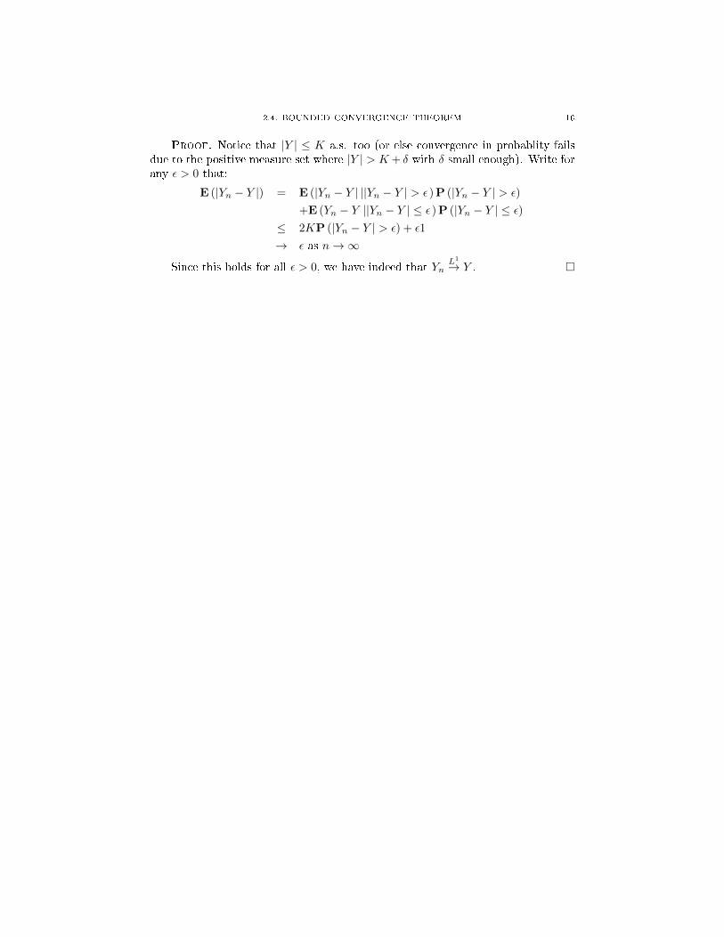
2.4. BOUNDED CONVERGENCE THEOREM 16

Proof. Notice that |Y | ≤ K a.s. too (or else convergence in probablity failsdue to the positive measure set where |Y | > K + δ with δ small enough). Write forany ε > 0 that:

E (|Yn − Y |) = E (|Yn − Y | ||Yn − Y | > ε )P (|Yn − Y | > ε)

+E (Yn − Y ||Yn − Y | ≤ ε )P (|Yn − Y | ≤ ε)≤ 2KP (|Yn − Y | > ε) + ε1

→ ε as n→∞

Since this holds for all ε > 0, we have indeed that YnL1

→ Y .

Central Limit Theorems

These are notes from Chapter 3 of [2].

3.5. The De Moivre-Laplace Theorem

Let X1, X2. . . . be iid with P (X1 = 1) = P (X1 = −1) = 12 and let Sn =∑

k≤nXk. By simple combinatorics,

P (S2n = 2k) =

(2n

n+ k

)2−2n

Using Stirling's Formula now, n! ∼ nne−n√

2πn as n → ∞ where an ∼ bnmeans that an/bn → 1 as n→∞ so then:(

2n

n+ k

)= . . . . . . ∼

(1− k2

n2

)−n(1 +

k

n

)−k (1− k

n

)kWe now use the basic lemma:

Lemma. (3.1.1.) If cj → 0, aj →∞ and ajcj → λ then (1 + cj)aj → eλ.

Exercise. (3.1.1.) (Generalization of the above) If max1≤j≤n |cj,n| → 0 and∑nj=1 cj,n → λ and supn

∑nj=1 |cj,n| <∞ then

∏nj=1 (1 + cj,n)→ eλ

(Both proofs can be seen by taking logs and using the fact from the Taylorexpansion for log that log(1 + x)/x→ 1) This leads to:

Theorem. (3.1.2.) If 2k/√

2n→ x then P (S2n = 2k) ∼ (πn)−1/2e−x2/2

And a bit more gives (mostly just a change of variables from here):

Theorem. (3.1.3) The De-Moivre Laplace Theorem: If a < b then as m→∞we have:

P(a ≤ Sm/

√m ≤ b

)→

bˆ

a

(2π)−1/2e−x2/2dx

3.6. Weak Convergence

Definition. For distribution functions Fn, We write Fn ⇒ F and say Fnconverges weakly to F to mean that Fn(x) = P (Xn ≤ x)→ F (x) = P (X ≤ x)for all continuity points x of the function F (x). We sometimes conate the randomvariable and its distribtuion function and write Xn ⇒ X or even Fn ⇒ X or othercombinations.

17

3.6. WEAK CONVERGENCE 18

3.6.1. Examples.

Example. (3.2.1.) Let X1, . . . be iid coin ips, by our abover work in the DeMoivre-Leplace theorem, we have that Fn ⇒ F

Example. (3.2.2.) (The Glivenko-Cantelli Theorem) Let X1, . . . , Xn be iidwith distribution function F and let

Fn(x) =1

n

n∑m=1

1Xm≤x

Be its empirical distribution function. The G-C theorem is that:

supx|Fn(x)− F (x)| → 0 a.s.

In words: the empircal distribtuion function converges uniformly almost surely

Proof. (Pf idea: the fact that Fn(x) → F (x) is just the strong law for theindicator 1Xn<x, the only trick is to make the convergence uniform)

Fix x and let Yn = 1Xn≤x. Since Yn are iid with E(Yn) = P (Xn ≤ x) = F (x),

the strong law implies that Fn(x) = n−1∑nm=1 Ym → F (x) a.s.

At this point it is notable to remark that if F was continuous, then it is possibleto show that pointwise convergence to increasing continuous functions is always uni-form convergence, and quoting that we would be done (the proof of this follows bywhat we are about to do). However, F has possibly countably many discontinuities,so we will have to work around that.

Similarly, let F (x−) := limh→0−,h<0 F (x − h) and let Zn = 1Xn<x so thatE(Zn) = F (x−) and we will ahve Fn(x−)→ F (x−) again by the strong law.

Now, for any ε > 0, and η > 0 choose any ε−net of [0, 1] (i.e. nitely manypoints of distance no more than ε from each other), say 0 = y0 < . . . < yk = 1. Letxk = inf y : F (y) ≥ yk (This is called the right inverse or something). Noticethat in this way we have F (xk)−F (xk−) ≤ yk − yk−1 = ε . Choose Nε(ω) so largenow so that |Fn(xk)− F (xk)| < η and |Fn(xk−)− F (xk−)| < η (this is ok sincethere are nitely many points xk and we have almost sure convergence at each ofthem).

For any point x ∈ (xj−1, xj) we use the monotonicity of F , along with ourinequalities with ε and η now to get:

Fn(x) ≤ Fn(xj−) ≤ F (xj−) + η ≤ F (xj−1) + η + ε ≤ F (x) + η + ε

Fn(x) ≥ Fn(xj−1) ≥ F (xj−1)− η ≥ F (xk)− η − ε ≥ F (x)− η − ε

So we have an inequality sandwhich, |Fn(x)− F (x)| ≤ ε + η which holds forevery x. Since ε and η are arbitary, we get the convergence.

Example. (3.2.3.) Let X have distribution F . Then X + 1n has distribution

Fn(x) = F (x− 1n )/ As n→∞ we have:

Fn(x)→ F (x−) = limy↑x

F (y)

So in this case the convergence really is only at the continuity points.

Example. (3.2.4.) (Waiting for rare events, convergence of a geometric to aexponential distribution) Let Xp be the number of trials needed to get a success


in a sequence of independent trials with success probability p. Then P (Xp ≥ n) =

(1− p)n−1for n = 1, 2, . . . and it follows that:

P (pXp > x)→ e−x for all x ≥ 0

In other words pXp ⇒ E where E is an exponential random variable.

Example. (3.2.5.) Birthday Problem. Fix an N and letX1, . . . be independentand uniformly distributed on 1, 2, . . . , N and let TN = min n : Xn = Xm for some m < n.Notice that:

P (TN > n) =

n∏m=2

(1− m− 1

N

)By exercise 3.1.1., (the one that concludes

∏nj=1 (1 + cj,n)→ eλ when

∑nj=1 cj,n →

λ and the cj,n's are small) have then:

P(TN/N

1/2 > x)→ exp

(−x2/2

)for all x ≥ 0

Theorem. (Schee's Theorem) If fn are probability density functions withfn → f∞ pointwise as n→∞ then µn to µ∞ in the total variation distance

‖µn − µ∞‖TV := supB|µn(B)− µ∞(B)| → 0

Proof. Have: ∣∣∣∣ˆB

fn −ˆB

f∞

∣∣∣∣ ≤ ˆΩ

|fn − f∞|

= 2

ˆΩ

(fn − f∞)+

→ 0

(we have employed the usual trick for the TV distance here btw) By the dom-inated convergence thereom.

Example. (3.2.6.) (Central Order Statistics) Put 2n + 1 points uniformly atrandom and independently in (0, 1). Let Vn+1 be the n+ 1st largest point.

Lemma. Vn+1 has density function:

fVn+1(x) = (2n+ 1)

(2n

n

)xn(1− x)n

Proof. There are 2n + 1 ways to pick which of the 2n + 1 points will be thespecial central order point. Then there are

(2nn

)ways to divide up the remaining

2n points into two groups of n, one group to be placed on the left and another tobe placed on the right, and nally xn(1 − x)n is the probability that these pointsfall where they need to.

Changing variables x = 12 + y

2√

2n, Yn = 2

(Vn+1 − 1

2

)√2n gives...

fYn(y)→ (2π)−1/2 exp(−y2/2

)as n→∞

By Schee's theorem then, we have weak convergence to the standard normal.(This isnt entirely surprising since f looks a bit like a binomial random vari-

able...this is actually used in this calculation)

Exercise. (Convergence of the maxima of random variables)Come back to this when you review maximum distributions.


3.6.2. Theory. The next result is useful for proving things about weak con-vergence

Theorem. (3.2.2.) [Skohorod Representation Theorem] If Fn ⇒ F∞then thereare random variables Yn with the distribution Fn so that Yn → Y∞a.s.

Proof. Let (Ω,F ,P) = ((0, 1),R,m) be the usual Lebesgue measure on (0, 1).Dene Yn(x) = sup y : Fn(y) < x =: F→n (x), (this is called the right inverse). Byan earlier theorem (or easy exercise), we know Yn has the distribution Fn. We willnow show that Yn(x)→ Y∞(x) for all but a countable number of x.

Durret has a proof of this....but I prefer the proof from Resnick where hedevelops the idea of the left inverse a bit more fully. Review this when you doextreme values!

Remark. This theorem only works if the random variables have seprable sup-port. Since we are working with R valued random variables, this works. If theywere functions or something, it might not work.

Exercise. (3.2.4.) (Fatou's lemma) Let g ≥ 0 be continuous. If Xn ⇒ X∞then:

lim inf E(g(Xn)) ≥ E (g(X∞))

Proof. Just use Skohorod to make versions of the Xn's which converge a.s.and apply the ordinary Fatou lemma to that.

Exercise. (3.2.5.) (Integration to the limit) Suppose g, h are continuous withg(x) > 0 and |h(x)| /g(x)→ 0 as |x| → ∞. If Fn ⇒ F and

´g(x)dFn(x) ≤ C <∞

then: ˆh(x)dFn(x)→

ˆh(x)dF (x)

Proof. Create random variables on Ω = (0, 1) as in the Skohord representationtheorem so that Fn, F are the distribution functions for Xn, X and Xn → X a.s.We desire to show that E(h(Xn)) → E(h(X)). Now for any ε > 0 we nd M solarge so |x| > M =⇒ |h(x)| ≤ εg(x) and then we will have for any x > M that:

E (h(Xn)) = E (h(Xn); |Xn| ≤ x) + E (h(Xn); |Xn| > x)

→ E (h(X); |X| ≤ x) + E (h(Xn); |Xn| > x) (bounded convergence thm)

≤ E (h(X); |X| ≤ x) + εE (g(Xn); |Xn| > x)

≤ E (h(X); |X| ≤ x) + εC

The rst term converges to E(h(X)) by the LDCT. The other side of theinequality can be handled by Fatou, or I think we could do the above work a littlemore carefully to get it.

Theorem. (3.2.3.) Xn ⇒ X∞ if and only if E (g(Xn))→ E (g(X)) for everybounded continuous function g.

Proof. ( =⇒ ) Follows by the Skorod repreresentation theorem and thebounded convergence theorem.


(⇐=) Let gx,ε be a smoothed out version of the step down Heaviside stepfunction at x. For example:

gx,ε =

1 y ≤ x0 y ≥ x+ ε

linear x ≤ y ≤ x+ ε

This is a continuous linear function, so we have E (gx,ε(Xn))→ E(gx,ε(X)) foreach choice of x, ε. This basically gives the result, to do it properly, look at:\

lim supn→∞

P (Xn ≤ x) ≤ lim supn→∞

E (gx,ε(Xn)) = E (gx,ε(X)) ≤ P (X ≤ x+ ε)

lim infn→∞

P (Xn ≤ x) ≥ lim infn→∞

P (gx−ε,ε (Xn) ≤ x) = E (gx−ε,x(X)) ≥ P (X ≤ x− ε)

Combining these inequalites we see that we have the desired convergence forcontinuity points of X.

Theorem. (3.2.4.) (Continuous mapping theorem) If g is measurable andDg = x : g is discontinuous at x. If Xn ⇒ X and P (X ∈ Dg) = 0 then g(Xn)⇒g(X) and if g is bounded then E (g(Xn))→ E (g(X))

Proof. Firstly, lets notice that if g is bounded, the using Skohorod we will havea version of the variables so that Xn → X a.s. and then g(Xn)→ g(X) everywhereexcept on the set Dg. Since this is a null set we get E (g(Xn))→ E (g(X))

Now, we verify that g(Xn) ⇒ g(X) by the boudned-continuous characteriza-tion, for if f is any bounded continuous function then f g is bounded and hasDfg so E (f g(Xn))→ E (f g(X)) by the above argument.

Theorem. (3.2.5.) (Portmanteau Theorem) The following are equivalent:(i) Xn ⇒ X(ii) E (f(Xn))→ E (f(X)) for all bounded continuous f(iii) lim infnP (Xn ∈ G) ≥ P (X ∈ G) for all G open(iv) lim supnP (Xn ∈ F ) ≤ P (X ∈ F ) for all F closed(v) P (Xn ∈ A)→ P (X ∈ A) for all A with P (X ∈ ∂A) = 0

Proof. [(i) =⇒ (ii))] Is the theorem we just did.[(ii) =⇒ (iii)] Use Skohord to get an a.s. convergent version and then use

Fatou[(iii) ⇐⇒ (iv)] Take complements.[(iii)+(iv) =⇒ (v)] Look at the interior A and closure A. Since ∂A = A−A

is a null set, we know that A, A, A are all the same up to null sets. We then getP (Xn ∈ A) → P (X ∈ A) by getting a liminf/limsup sandwhich doing the liminfP (Xn ∈ A) = P (Xn ∈ A) and the limsup on P

(Xn ∈ A

)= P (Xn ∈ A) and

using the inequalities from (iii) and (iv).

Remark. In Billinglsey he does the proof without using Skohorhod by looking

at the sets like Aε = ∪x∈ABε(x) and the function f ε =(1− 1

εd(x,A))+

which is 1on A, 0 outside of Aε and is uniformly continuous. This has the advantage that itwill work in spaces where the Skohorod theorem will not work (for example I thinkthe Skohorod theorem will fail for function-valued-random variables)

One advantage of doing this is that, since the f ε that appears above is uniformlycontinuosu, we may restrict our attention to uniformly continuous functions f ,which is sometimes a little easier to check.


Theorem. (3.2.6.) (Helly's Selection Theorem) For every sequence Fn ofdistribution function,s there is a subseqeunce Fnk and a right continuous non-decreasing function F so that limk→∞ Fnk(y) → F (y) at all continuity points yof F .

Remark. F is not necessarily a distribution function as it might not havelimx→−∞ F (x) = 0 and limx→∞ F (x) = 1. This happens when mass leaks out to+∞ or −∞ i.e. Fn(x) ≡ δn.

Proof. Let qk enumerate the rationals. Since Fn(q1) ∈ [0, 1], by Bolzanno

Weirestrass there is a subsequence n(1)k so that F

n(1)k

(q1) converges. Call the limit

G(q1). Since Fn(2)k

(q2) ∈ [0, 1] again by B-W we nd a sub-sub-sequence n(2)k so that

Fn(2)k

(q2) converges. Repeating this, we get a big collection of nested subsequnces

so that Fn(k)k

(qk) → G(qk) for each k. Taking the diagonal nk = n(k)k we get that

Fnk(q)→ G(q) for all rationals q.Now let F (x) = inf G(q) : q ∈ Q : q > x. This is right continuous since:

limxn↓x

F (xn) = inf G(q) : q ∈ Q, q > xn for some n

= inf G(q) : q ∈ Q, q > x = F (x)

To see that Fn(x)→ F (x) at continuity points, just approximate F (x) by F (r1)and F (r2) where r1, r2 are rationals with r1 < x < r2 and use the convergence ofG.

F is non-decreasing since Fn(x1) ≤ Fn(x2) for all x1 ≤ x2 so any limit along asubsequence will have this property too.

Remark. In functional analysis the selection theorem is that for X a seperatblen.v.s, the unit ball in the dual spaceB∗ = f ∈ X∗ : ‖f‖ ≤ 1 is weak* compact(Recall the weak* topology on X ∗is the one characterized by fn → f ⇐⇒ fn(x)→f(x) for all x) The proof of this is just the subsequences/diagonal sequences trickof the rst part of the proof.

If we apply this version of Helley's theorem to the space X = C ([0, 1]) whichhas X ∗ =nite signed measures then we get that every sequence of measures µnhas a subseqeunce µnk so that Eµnk (f)→ Eν(f) for every bounded continuous f .This is exactly the notion of weak convergence, µnk ⇒ ν, we have! ν need not bea probability measure here, it is only a nite signed meausre. However, by usingFatou, we know that µ([0, 1]) ≤ lim infn→∞ µn ([0, 1]) = 1 so mass can be lost, butmass cannot be gained.

We will now look at conditions under which we can be sure that no mass islost....i.e. the limit is in fact a proper probability measure.

Definition. We say that a family of proability measures µαα∈I is tight iffor all ε > 0 there is a compact set K so that:

µα(Kc) < ε∀α ∈ I

Theorem. (3.2.7.) Let µn be a sequence of probability measures on R. Everysub sequential limit µnk ⇒ ν is a probability measure if and only if µn is tight.

Proof. (⇐=) Suppose µn is tight and Fnkl ⇒ F . For any ε > 0 nd Mε sothat µn ([−Mε,Mε]

c) < ε for all n. Find continuity points r and s for F so that


r < −Mε and s > Mε. Since Fn(r)→ F (r) and Fn(s)→ F (s) we have:

µ ([r, s]c) = 1− F (s) + F (r) ≤ . . . ≤ ε

This shows that lim supx→∞ 1 − F (x) + F (−x) ≤ ε, and since ε arbitary thislimsup is 0. Now, since lim supx→∞ F (x) ≤ 1 and lim infx→−∞ F (x) ≥ 0 we havethat 0 = lim supx→∞ 1−F (x)+F (−x) ≥ lim infx→∞ 1−F (x)+F (−x) ≥ 1−1+0 =0, so we have equality everywhere from which we conclude that lim supx→∞ F (x) =1 and lim infx→−∞ F (x) = 0 and so indeed F is a probability measure.

(Basically the estimate above shows that no mass can leak away)( =⇒ ) We prove the contrapositive. If Fn is not tight, then there exists an

ε0 > 0 so that for every set [−n, n] there is a nk so that Fnk [−n, n]c ≥ ε0. By

Helley, this has a convergent sub-subsequence and the limit is easily veried to notbe a probability measure.

Theorem. (3.2.8.) If there is a ϕ ≥ 0 so that ϕ(x)→∞ as |x| → ∞ and:

supn

ˆϕ (x) dFn(x) = C <∞

Then Fn is tight.

Proof. Do a generalized Chebushev-type estimate:

Fn [−M,M ]c

= P (|Xn| ≥M) ≤ 1

inf |x| > M : ϕ(x)E (ϕ(Xn)) ≤ C/ inf

|x|≥Mϕ(x)→ 0

Theorem. (3.2.9.) If each subsequence of Xn has a further subsequence thatconverges a.s. to X, then Xn ⇒ X

Proof. The rst condition is actually equivalent to XnP→ X, which implies

Xn ⇒ X.

Definition. (The Levy/Prohov Metric) Dene a metric on measures, by d (µ, ν)is the smallest ε > 0 so that:

Pµ (A) ≤ Pν(Aε) + ε Pν(A) ≤ Pµ(Aε) + ε∀A ∈ B

Exercise. (3.2.6.) This is indeed a metric and µn ⇒ µ if and only if d(µn, µ) =0

Proof. (⇐=) is clear by using closed sets and checking the limsup of closedsets characterization of weak convergence.

( =⇒ ) You need to use the separability of R here.

Exercise. (3.2.12.) If Xn ⇒ c then XnP→ c.

Proof. For any ε > 0 we have P (|Xn − c| > ε) = E(1[c−ε,c+ε]c(Xn)

)→

E(1[c−ε,c+ε]c(c)

)= 0

Remark. The converse is also true since converging in probability implies weakconvergence (most easily seen by the bounded convergence theorem)

Exercise. (3.2.13) (Converging Together Lemma) If Xn ⇒ X and Yn ⇒ cthen Xn + Yn ⇒ X + c.

3.7. CHARACTERISTIC FUNCTIONS 24

Remark. Does not hold if Yn ⇒ Y in general. For example, on Ω = (0, 1)let Xn(ω) = n-th digit of the binary expansion of ω. Notice that Xn is always acoinip, so Xn ⇒ A where A is a coinip is clear. (This is a good example whereXn ⇒ X but there is no convergence in proability or a.s. convergence or anything)If Yn(ω) = 1−Xn(ω) then this is still a coin ip. But Xn+Yn = 1 now is a constantand does not converge to a sum of coinips or anything like that.

Proof. Since Yn ⇒ c we know that YnP→ Y . Now ,for any closed set F let

Fε = x : d (x, F ) ≤ ε. Then:

P (Xn + Yn ∈ F ) ≤ P (|Yn − c| > ε) + P (Xn + c ∈ Fε)

So taking limsup now:

lim supP (Xn + Yn ∈ F ) ≤ lim supP (|Yn − c| > ε) + lim supP (Xn + c ∈ Fε)→ 0 + P (X + c ∈ Fε)

Finally, since F is closed, we have that P (X ∈ F ) = P(X ∈ ∩nF1/n

)=

limn→∞P(X ∈ F1/n

)so taking ε → 0 in the above inequality gives us weak con-

vergence via Portmeanteau theorem.

Corollary. If Xn ⇒ X, Yn ≥ 0 and Yn ⇒ c then XnYn ⇒ cX. (Thisactually holds withouth Yn ≥ 0 or c > 0 by splitting up the probaility space)

Proof. Notice that log(Xn) ⇒ log(X) and log(Yn) ⇒ log(x) . Then by theconverging together lemma log(Xn) + log(Yn) ⇒ log(X) + log(c). Then take expto get XnYn ⇒ cX. (might need to truncate or something to make this morerigourous.)

Exercise. (3.2.15) If Xn =(X1n, . . . , X

nn

)is uniformly distributed over the

surface of a sphere of radius√n then X1

n ⇒a standard normal

Proof. Let Y1, . . . be iid standard normals and let Xin = Yi

(n/∑nm=1 Y

2m

)1/2then check indeed that

(X1n, . . . , X

nn

)are uniformly distrbuted over the surfact of

a sphere of radius√n, so this is a legit way to construct the distribution Xi

n. Then

X1n = Y1

(n/∑nm=1 Y

2m

)1/2 ⇒ Y1 (n/n)1/2

by the strong law of large numbers andthe convering together lemma.

3.7. Characteristic Functions

3.7.1. Denition, Inversion Formula. If X is a random variable we deneits characteristic function by:

ϕ(t) = E(eitX

)= E (cos tX) + iE (sin tX)

Proposition. (3.3.1) All characteristic functions have:i) ϕ(0) = 1

ii) ϕ(−t) = ϕ(t)iii) |ϕ(t)| =

∣∣E (eitX)∣∣ ≤ E(∣∣eitX ∣∣) = 1

iv) |ϕ(t+ h)− ϕ(t)| ≤ E(∣∣eihX − 1

∣∣) since this does not depend on t, thisshows that ϕ is uniformly continuos.

v) ϕaX+b(t) = eitbϕX (at)vi) For X1, X2 independent, ϕX1+X2

(t) = ϕX1(t)ϕX2

(t)


Proof. The only one I will comment on is iv). This holds since |z| =(x2 + y2

)1/2is convex, so:

|ϕ(t+ h)− ϕ(t)| ≤∣∣∣E(e(i(t+h)X − eitX

)∣∣∣≤ E

(∣∣∣e(i(t+h)X − eitX∣∣∣)

= E(∣∣eihX − 1

∣∣)→ 0 as h→ 0 by BCT

Since this→ 0 and does not depend on t, we see that ϕ is uniformly continuous.

Example. I collect the examples in a table:Name PDF Char. Fun Remark

Coin Flip P(X = ± 1

2

)= 1

2

ϕ(t) =(eit − e−it

)/2

= cos t

Poisson P(X = k) = e−λ λk

k! ϕ(λ) = exp(λ(eit − 1)

)Normal ρ(X = x) =

1√2π

exp(−x

2

2

) ϕ(t) = exp(− t

2

2

)Prove this by deriving ϕ′ = −tϕ. Or complete the

square

Uniform ρ(X = x) = 1b−a1[a,b](x) ϕ(t) = exp(itb)−exp(ita)

it(b−a)

If b = −a this is:

ϕ(t) =sin(at)

at

This one is useful to think about for the inversionformula

´∞−∞

e−ita−e−itbit(b−a) ϕ(t)dt ≈ µX(a, b) 1

b−a i.e.ˆϕ1AϕXdt ≈ µX(A)

1

L(A)

Triangular ρ(X = x) = (1− |x|) + ϕ(t) = 21−cos tt2 Use the fact that the triangular is the sum of two

independent Uniforms

Dierence Y = X − X (independentcopy)

ϕY (t) = |ϕX(t)|2

SuperpositionDierence

Y = CX where C is a ±1coinip

ϕY (t) = Re(ϕX(t)) Use the fact that ϕ is linear with respect tosuperposition,

∑λiFi has char fun

∑λiϕi. In this

case its with 12FX + 1

2F−XExppoential ρ(X = x) = e−x ϕ(t) = 1

1−itBilateral Exp ρ(X = x) = 1

2e−|x|

ϕ(t) = Re

(1

1− it

)=

1

1 + t2

Use the superposition dierence trick

Polya's ρ(X = x) =(1− cosx)/πx2

ϕ(t) = (1− |t|)+Pf comes from the inversion formula and the

triangle distribution. Used in Polya's theorem toshow that convex, decreasing functions ϕ withϕ(0) = 1 are characteristic function of something

Cauchy ρ(X = x) = 1/π(1 + x2) ϕ(t) = exp (− |t|) Pf comes from inverting the bilateral exp.


Theorem. (3.3.4.) The inversion formula. Let ϕ(t) =éitxµ(dx) where µ is

a probability measure. If a < b then:

limT→∞

(2π)−1

T

−T

e−ita − e−itb

itϕ(t)dt = µ(a, b) +

1

2µ (a, b)

Proof. Write

IT =

T

−T

e−ita − e−itb

itϕ(t)dt

=

T

−T

ê−ita − e−itb

iteitxµ(dx)dt

Notice that e−ita−e−itbit =

´ bae−itydy so this is bounded above in norm by b−a.

Hence we can apply Fubini to get:

IT =

T

−T

ê−ita − e−itb

iteitxµ(dx)dt

=

ˆ T

−T

e−ita − e−itb

iteitxdtµ(dx)

=

ˆ T

−T

ˆ b

a

e−ityeitxdydtµ(dx)

=

ˆ T

−T

x−bˆ

x−a

eitydydtµ(dx)

= . . .

=

ˆ (ˆ T

−T

sin(t(x− a)

tdt

)+

(ˆ T

−T

sin(t(x− a)

tdt

)µ(dx)

Where we use the fact that cos is odd here so it cancels itself out. (This relieson T nite)

Now if we letR(θ, T ) =´ T−T

sin(θt)t dt then we can show thatR(θ, T ) = 2sgnθ

´ Tθ0

sin(x)x dx→

π for θ 6= 0 and = 0 for θ = 0. We have then:

IT =

ˆR(x− a, T )µ(dx) +

ˆR(x− b, T )µ(dx)

→ˆ

2π a < x < b

π x = a or x = b

0 x < a or x > b

µ(dx)

So by bounded convergence theorem, we get the result.


Exercise. (3.3.2.) Similarly:

µ (a) = limT→∞

1

2T

T

−T

e−itaϕ(t)dt

The inversion formula basically tells us that distributions are characterized bytheir char functions. Two easy consequences are then that:

Exercise. (3.3.3.) ϕ is real if and only if X and −X have the same distribu-tion.

Proof. X and −X have the same distribution i Xd= CX for C a ±1 coinip

i ϕX = ϕCX i ϕX = Re (ϕX). (We had everything except the ⇐= before theinversion formula, and the inversion formula gives us this.)

Exercise. (3.3.4.) The sum of two normal distributions is again normal.

Proof. The c.f. for a sum of two normals is the c.f. for a normal, so it mustbe a normal distribution.

Theorem. (3.3.5.) If´|ϕ(t)| dt < ∞ then µ has bounded continuous density

function :

f(y) =1

2π

ê−ityϕ(t)dt

Proof. As we observed before, the kernal e−ita−e−itb

it , has∣∣∣ e−ita−e−itbit

∣∣∣ ≤ b− aso we see that µ has no point masses since:

µ(a, b) +1

2µ (a, b) =

1

2π

∞

−∞

e−ita − e−itb

itϕ(t)dt

≤ b− a2π

∞

−∞

|ϕ(t)| dt

→ 0 as b− a→ 0

Can now caluclate the density function by looking at µ (x, x+ h) with theinversion formula, using Fubini and taking h→ 0:

µ(x, x+ h) + 0 =1

2π

ˆ ˆ x+h

x

e−ityϕ(t)dydt

=

ˆ x+h

x

(1

2π

ê−ityϕ(t)dt

)dy

The dominated convergence theorem tells us that f is continuous:

f(y + h)− f(y) =1

2π

ê−ity

(1− e−ith

)ϕ(t)dt

→ 0 by LDCT

Exercise. (3.3.5.) Given an example of a measure µ which has a density, butfor which

´|ϕ(t)|dt =∞


Proof. The uniform distribution has this since ϕ(t) ≈ 1t . This makes sense

since the distribution fucntion is not continuous.

Exercise. (3.3.6.) If X1, X2, . . . are iid uniform in (−1, 1) then∑i≤nXi has

density:

f(x) =1

π

∞

0

(sin t

t

)ncos(tx)dx

This is a piecewise n-th order polynomial.

Remark. Theorem 3.3.5, the Riemann-Lebesgue Lemma, and the followingresult all tell us that point masses in the distribution correspond to the behaivourat ∞ for the c.f.

Theorem. (Riemann-Lebesgue lemma)If µ has a density function f , then ϕµ(t)→ 0 as t→∞.

Proof. If f is dierentiable and compactly supported then we have:

|ϕµ(t)| =

∣∣∣∣ˆ f(x)e−itxdx

∣∣∣∣=

∣∣∣∣ˆ 1

itf ′(x)e−itxdx

∣∣∣∣≤ 1

|t|

ˆ|f ′(x)| dx

→ 0

Any arbitrary density function can be approximated by such f (indeed, theseare dense in L1 by the construction of the Lebesgue integral....just smoothly ap-proximate open intervals) (Alternativly, show it for simple functions, which are alsodense in L1)

Exercise. (3.3.7.) If X,X are iid copies of a R.V. with c.f. ϕ then:

limT→∞

1

2T

T

−T

|ϕ(t)|2 dt = P(X − X = 0) =∑x

µ (x)2

Proof. The result follows by the inversion formula and since ϕX−X = |ϕX |2

Corollary. If ϕ(t)→ 0 as t→∞ then µ has no atoms.

Proof. If ϕ(t)→ 0 then the average 12T

´ T−T |ϕ(t)|2 dt→ 0 as T →∞ too, so

by the previous formula µ has no atoms.

Remark. Don't forget there are distributions like the Cantor function whichhave no atoms and there is no density.


3.7.2. Weak Convergence - IMPORTANT!.

Theorem. (3.3.6.) (Continuity Theorem) Let µn be probability measure withc.f. ϕn.

i) If µn ⇒ µ∞ then ϕn(t)→ ϕ∞(t) for all t.ii) If ϕn → ϕ pointwise andϕ(t) is continuous at 0, then the associated sequence

of distribution functions µn is tight and converges weakly to the measure µ with charfunction ϕ.

Proof. i) is clear since eitX is bounded and continuousii) We will rst show that is suces to check that µn is tight. Suppose µn is

tight. We claim that µn ⇒ µ∞ by the every subsequence has a sub-subsequencecriteria. Indeed, given any subsequence µnk we use Helley to nd a subsubsequenceµnklwith µnkl ⇒ µ0 for some µ0. Now since the sequence is tight, we know that

µ0 is a legitimate probability distribution. By i) since µnkl ⇒ µ0 we know that

ϕnkl (t)→ ϕ0(t). However, by hypothesis, ϕn → ϕ so it must be that ϕ = ϕ0!To see that the sequence is tight, you use the continuity at 0. The idea

is to use that 1u

´ u−u (1− ϕ(t)) dt → 0 by this continuity. If you write it out,

1u

´ u−u (1− ϕ(t)) dt should control something like µ(|x| > 2

u ), so this is exactlywhat is needed for tightness.

Remark. Here is a good example to keep in mind for the continuity theorem:Take Xn ∼ N(0, n) so that ϕn(t) = exp

(−nt2/2

)→ 0 for t 6= 0 and = 1 at t = 0.

Xn can't converge weakly to anything since µn ((−∞, x])→ 0 for any x.

Exercise. (3.3.9) If Xn ⇒ X and is normal with mean µn and variance σ2n

and X is normal with mean µ and variance σ2 then µn → µ and σ2n → σn

Proof. Look at the c.f's

Exercise. (3.3.10) IfXn and Yn are independent andXn ⇒ X∞ and Yn ⇒ Y∞then Xn + Yn ⇒ X∞ + Y∞\

Proof. Look at the cfs.

Exercise. (3.3.12.) Interpret the identity sin t/t =∏∞m=1 cos(t/2m) prob-

abilistically. (You can get this formula from sin t = 2 sin(t/2) cos(t/2) appliedrepeatedly and using 2k sin(t/2k)→ t as k →∞)

Proof. sin t/t is the cf for a [−1, 1] random variable. cos(t/2m) is the c.f. fora coinip Xm = ± 1

2m . So this is saying that the sum of intently many coinipslike this is a uniform random variable.

This is equivalent to the fact the the n-th binary digit of a uniformly chosen xfrom [0, 1] is a coinip. Add 1 =

∑∞m=1 2−m to both random variables, and then

divide by 2.

Exercise. (3.3.13.) Let X1, . . . be iid coinips taking values 0 and 1 and letX =

∑j≥1(2Xj)/3

j . [This converges almost surely by the Kolmogorov 3 series

theorem]. This has the Cantor distribution. Compute the ch.f. ϕ of X and noticethat ϕ has the same value at t = 3kπ.

Proof. Each X has c.f. 12

(1 + eit

)so 2X/3j has 1

2

(1 + eit

2

3j

)so we have

that ϕ =∏∞k=1

12

(1 + eit

2

3j

)If you put in t = 3kπ you get a e2πi in the rst k

terms and the value of the function does not change.


Remark. This fact shows that ϕ(t) 9 0 as t → ∞, which means that it isimpossible for this random variable to have a density (by the Riemann Lebesgue

lemma). You can see there are no atoms because for ω ∈ 0, 1N a possible sequenceof the Xi's, X(ω) is the number whose ternary expansion is ω, so for a given x, theset X(ω) = x consists of at most one sequence: namely the ternary expansionof x (you have to replace 2's with 1's ..... you get the idea). Consequently, we canexplicitly see that for any x, P(X = x) = 0 and X has no atoms.

3.7.3. Moments and Derivatives. Part of the proof of the ϕn → ϕ andϕ continuous at 0 implies Xn ⇒ X theorem was the estimate that µ

|x| > 2

u

≤

u−1´ u−u (1− ϕ(t)) dt (This was used to show that if ϕ is continuous at 0 then ϕn

is tight) This suggests that the local behaivour at 0 is related to the decay of themeasure at ∞. We see more of this here:

Exercise. (3.3.14) If´|x|n µ(dx) <∞ then the c.f. ϕ has continuous deriva-

tives of order n given by ϕ(n)(t) =´

(ix)neitxµ(dx)

Proof. Lets do n = 1 rst. Consider that:

ϕ (t+ h)− ϕ(t)

h=

1

h

ˆeitx(eihx − 1)µ(dx)

Now use the estimate that 1h

(eihx − 1

)≤ |x| (to see this write 1

h

(eihx − 1

)=

i´ x

0eihzdz and then bound the integral) so we can apply a dominated convergence

theorem to get the result. The case n > 1 is not much dierent.

Exercise. (3.3.15.) By dierntiating the characteristic function for a normal

random variable, we see that for X ∼ N(0, 1) with c.f. e−t2/2 we have:

E(X2n

)= (2n− 1) · (2n− 3) · . . . · 3 · 1 ≡ (2n− 1)!!

The next big result is that:

Theorem. (3.3.8.) If E(|X|2) <∞ then:

ϕ(t) = 1 + itE(X)− t2E(X2)/2 + ε(t)

With:

|ε(t)| ≤ Emin

(|tX|3

3!,

2 |tX|2

2!

)Remark. Just using what we just did, you would need the condition that

E(|X|3

)< ∞ to get that ϕ was thrice dierentiable and then you would have

the result by Taylor's theorem. However, by doing some slightly more carefulcalculations, we can actually show that:∣∣∣∣∣eix −

n∑m=0

(ix)m

m!

∣∣∣∣∣ ≤ min

(|x|n+1

(n+ 1)!,

2 |x|n

n!

)(Again this is done by integration type estimates) and then using Jensen's inequaltiywe'll have: ∣∣∣∣∣E (eitX)−

n∑m=0

E(itX)

m

m!

∣∣∣∣∣ ≤ Emin

(|tX|3!

n+1

, 2|tX|n

2!

)So even if we only have two moments, we know the error is bounded by

t2E(|X|2) and is hence o(t2)

3.8. THE MOMENT PROBLEM 31

Theorem. (3.3.10) (Polya's criterion) Let ϕ(t) be real nonnegative and haveϕ(0) = 1 and ϕ(t) = ϕ(−t) and say ϕ is decreasing and convex on (0,∞) with:

limt↓0

ϕ(t) = 1, limt↑∞

ϕ(t) = 0

Then there is a probability measure ν on (0,∞) so that:

ϕ(t) =

∞

0

(1−

∣∣∣∣ ts∣∣∣∣)+

ν(ds)

Since this is a superposition of the characteristic function for the Polya r.v.,ρ(XPOLY A = x) ∼ (1 − cosx)/x2,ϕPOLY A(t) ∼ (1− |t|)+

, this shows that ϕ is achar function.

Proof. I'm going to skip the rather technical proof. Part of it is that you canapprixmate ϕ by piecewise linear functions, and for those its easier.

Example. (3.3.10.) exp (− |t|α) is a char function for all 0 < α < 2

Proof. The idea is to write exp (− |t|α) as a limit of characteristic functions,namely:

exp (− |t|α) = limn→∞

(ψ(t ·

√2n−1/α

)nwhere ψ(t) = 1 − (1 − cos t)α/2. This convergence is seen since 1 − cos(t) ∼

−t2/2.ψ is a char function because we can write is a linear combination of powers(cos t)

n(recall cos t is the char fun for a coinip), by:

1− (1− cos t)α/2 =

∞∑n=1

(α/2

n

)(−1)n+1(cos t)n

Exercise. (3.3.23.) This family of RV's is of interest because they are stablein the sense that a scaled sum of many iid copies has the same distribution:

X1 + . . .+Xn

n1/α∼ X

The case α = 2 is the normal distribution and the case α = 1 is the Cauchydistribution.

3.8. The moment problem

Suppose´xkdFn(x) has a limit µk for each k. We know then that the Fn are

tight (a single function that goes to ∞ at ∞ for which supn´φ(x)dFn(x) < ∞

shows its tight by a Cheb estimate). Then we know by Helley that every subse-quence has a subsubsequence that converges weakly to a legit probability distribu-tion. We also know that every limit point will have moments µk (can check in thiscase that Fnk ⇒ F and

´xkdFn(x)→ µk shows

´xkdF (x)→ µk too...to this will

use the fact that sup´xk+1dFn(x) < ∞ I think), so every limit distribution has

the moments µk.Question: Is there a unique limit???? It would suce to check that there is

only one distribution with the moments µk. Unfortunatly this is not always true.

3.8. THE MOMENT PROBLEM 32

Example. (An example of a collection of dierent probability distribution whohave the same moments)

Consider the lognormal density:

f0(x) = (2π)−1/2

x−1 exp(− log x2/2

)x ≥ 0

(This is what you get if you look at the density of exp (Z) for Z ∼ N(0, 1) astandard normal)

For −1 ≤ a ≤ 1 let:

fa(x) = f0(x) (1 + a sin (2π log x))

To see that this has the same moments as f0, check that:∞

0

xrf0(x) sin(2π log x)dx = 0

Indeed after a change of variable, we see that the integral is like´

exp(−s2/2

)sin(2πs)ds

which is 0 since its odd.One can check that the moments of the lognormal density are µk = E (exp (kZ)) =

exp(k2/2

)(its the usual completing the square trick, or you can do it with deriva-

tives) Notice that these get very large very fast! Also notice that the density decays

like exp(− (log x)

2)which is rather slow.

We will now show that if the moments don't grow too fast (or equivalently ifthe density decays fast) then there IS a unique distribution.

Theorem. (3.3.11) If lim supk→∞ µ1/2k2k /2k = r < ∞ then there is at most

one distribution function with moments µk.

Proof. Let F be any d.f. with moments µk. By Cauchy-Scwarz, the absolute

value |X| has moments, νk =´|x|k dF (x) withν2k = µ2k and ν2k+1 ≤

√µ2kµ2k+2

and so:

lim supk→∞

ν1/k

k= r <∞

We next use the modied Taylor series for char functions to conclude that theerror in the taylor expansion of ϕ(t) at 0 is:∣∣∣∣ϕ(θ + t)− ϕ(θ)− tϕ′(θ)− . . .− tn−1

(n− 1)!ϕ(n−1)(θ)

∣∣∣∣ ≤ |t|n νnn!

Since νk ≤ (r + ε)kkk, and using the bound ek ≥ kk/k! we see that the aboveestimate implies that ϕconverges uniformly to its Taylor series about any point θin a nhd of xed radius |t| ≤ 1/er.

If G is any other distribution with moment s µk , we know that G and F havethe same Taylor series! But then G and F agree in a n'h'd of 0 by the abovecharacterization. By induction, we can repeatedly make the radius of the n'h'dbigger and bigger to see the char functions of F and G agree everywhree. But inthis case F must be equal to G by the inversion formula.

Remark. This condition is slightly stronger than Carleman's Condition

that:∞∑k=1

1

µ1/2k2k

<∞

3.9. THE CENTRAL LIMIT THEOREM 33

3.9. The Central Limit Theorem

Proposition. We have the following estimate:∣∣∣∣E (eitX)− (1 + itE(X)− t2

2E(X2)

)∣∣∣∣ ≤ E

(min

(|tX|3

3!, 2|tX|2

2!

))

≤ t2E

(min

(|t| |X|3

3!, |X|2

))

Proof. Do integration by parts on the function f(x) = eix. We aim to show∣∣eix − (1 + ix− x2)∣∣ ≤ min

(|x|33! ,

2|x|22!

). The fact that

∣∣eix − (1 + ix− x2)∣∣ ≤ |x|33!

is just by the usual Taylor series. The other fact follows by a trick. Do a taylorseries expansion to rst order, then add/subtract x2/2. The write x2/2 =

´ x0ydy=

eix = 1 + ix−xˆ

0

yei(x−y)dy

=

(1 + ix− x2

2

)+x2

2−

xˆ

0

yei(x−y)dy

=

(1 + ix− x2

2

)+

xˆ

0

ydy −xˆ

0

yei(x−y)dy

=

(1 + ix− x2

2

)−

xˆ

0

y(ei(x−y) − 1

)dy

But∣∣ei(x−y) − 1

∣∣ ≤ 2 so the error term is bounded by´ x

0y2dy = 2|x|2

2 and weare done.

Now put in x = X and then take E and use Jensen's inequality,∣∣∣∣E (eitX)− (1 + itE(X)− t2

2E(X2)

)∣∣∣∣ ≤ E(∣∣eitX − (1 + iX −X2

)∣∣)≤ E

(min

(|tX|3

3!,

2 |tX|2

2!

))

= t2E

(min

(|t| |X|3

3!, |X|2

))

Theorem. (iid CLT) If Xn are iid with E(X) = 0 and E(X2) = 1 thenSn√n⇒ N(0, 1).

Proof. Have by the last estimate that:

φ(t) = 1− t2

2+ ε(t)

3.9. THE CENTRAL LIMIT THEOREM 34

where the error ε(t) is ε(t) ≤ t2E(

min(|t||X|3

3! , |X|2))

. Hence the char function

for Sn/√n is:

φSn/√n = φ

(t√n

)n=

(1− t2

2n+ ε

(t√n

))nNow notice that n

(− t2

2n + ε(

t√n

))→ − t

2

2 since nε(

t√n

)≤ n t

2

nE(

min(|t|√n3!|X|3 , |X|2

))→

0 as n→∞ by the LDCT. We now use the fact that if cn → c then(1 + cnn )n → ec

so have:

φSn/√n → exp

(− t

2

2

)By the continuity theorem, have then Sn√

n⇒ N(0, 1)

Lemma. If zn → z0 then(1 + zn

n

)n → e−z.

Proof. Suppose WOLOG that∣∣ znn

∣∣ < 12 for all n in consideration. Since

log (1 + z) is a holomorphic function and invertable (with ez as its invers) in then'h'd|z| < 1

2 it suces to show that:

log((

1 +znn

)n)→ z

But log(1 + z) has a absolutly convergent taylor series expansion around z = 0in this n'h'd. Write this as log(1 + z) = z + zg(z) where g(z) is given by someabsolutly convergent power sereis in this n'h'd and g(0) = 0.We have:

log((

1 +znn

)n)= n log

(1 +

znn

)= n

(znn

+znng(znn

))= zn + zng

(znn

)→ z + zg(0) = z

Theorem. (CLT for Triangular Arrays - Lindeberg-Feller Theorem)A sum of small independent errors is normally distributed.Let Xn,m 1 ≤ m ≤ n be a triangular array of independent (but not nessisarily

iid) random variables. Suppose E(Xn,m) = 0. Suppose that:

n∑m=1

E(X2n,m

)→ σ2 > 0

and that:

∀ε > 0, limn→∞

n∑m=1

E(|Xn,m|2 ; |Xn,m| > ε

)= 0

Then:

Sn → N(0, σ2)

3.10. OTHER FACTS ABOUT CLT RESULTS 35

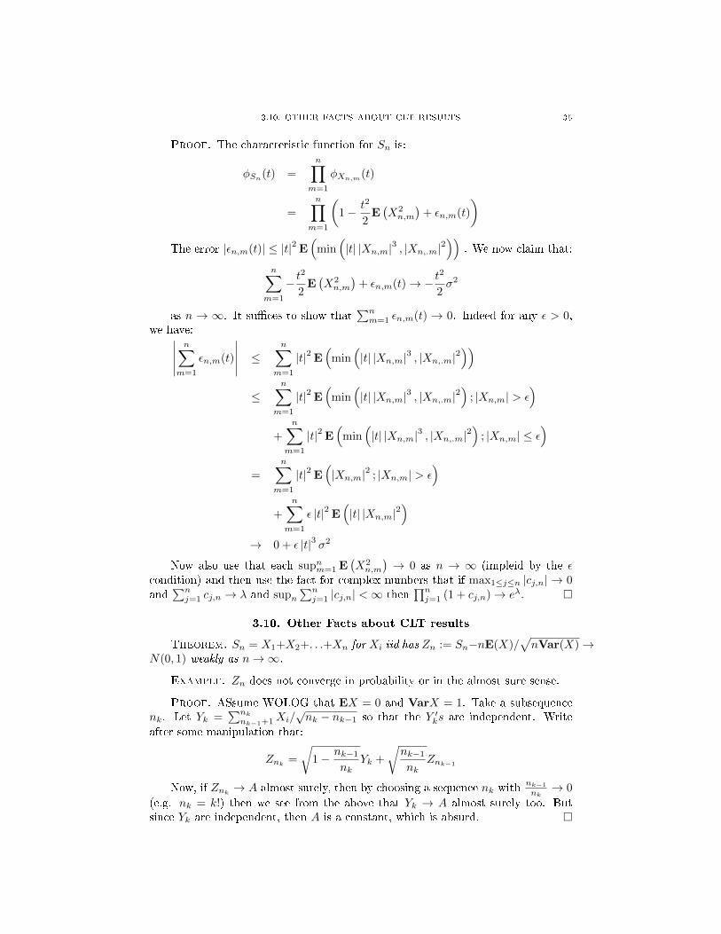
Proof. The characteristic function for Sn is:

φSn(t) =

n∏m=1

φXn,m(t)

=

n∏m=1

(1− t2

2E(X2n,m

)+ εn,m(t)

)The error |εn,m(t)| ≤ |t|2 E

(min

(|t| |Xn,m|3 , |Xn,.m|2

)). We now claim that:

n∑m=1

− t2

2E(X2n,m

)+ εn,m(t)→ − t

2

2σ2

as n → ∞. It suces to show that∑nm=1 εn,m(t) → 0. Indeed for any ε > 0,

we have:∣∣∣∣∣n∑

m=1

εn,m(t)

∣∣∣∣∣ ≤n∑

m=1

|t|2 E(

min(|t| |Xn,m|3 , |Xn,.m|2

))≤

n∑m=1

|t|2 E(

min(|t| |Xn,m|3 , |Xn,.m|2

); |Xn,m| > ε

)+

n∑m=1

|t|2 E(

min(|t| |Xn,m|3 , |Xn,.m|2

); |Xn,m| ≤ ε

)=

n∑m=1

|t|2 E(|Xn,m|2 ; |Xn,m| > ε

)+

n∑m=1

ε |t|2 E(|t| |Xn,m|2

)→ 0 + ε |t|3 σ2

Now also use that each supnm=1 E(X2n,m

)→ 0 as n → ∞ (impleid by the ε

condition) and then use the fact for complex numbers that if max1≤j≤n |cj,n| → 0and

∑nj=1 cj,n → λ and supn

∑nj=1 |cj,n| <∞ then

∏nj=1 (1 + cj,n)→ eλ.

3.10. Other Facts about CLT results

Theorem. Sn = X1+X2+. . .+Xn for Xi iid has Zn := Sn−nE(X)/√nVar(X)→

N(0, 1) weakly as n→∞.

Example. Zn does not converge in probability or in the almost sure sense.

Proof. ASsume WOLOG that EX = 0 and VarX = 1. Take a subsequencenk. Let Yk =

∑nknk−1+1Xi/

√nk − nk−1 so that the Y ′ks are independent. Write

after some manipulation that:

Znk =

√1− nk−1

nkYk +

√nk−1

nkZnk−1

Now, if Znk → A almost surely, then by choosing a sequence nk withnk−1

nk→ 0

(e.g. nk = k!) then we see from the above that Yk → A almost surely too. Butsince Yk are independent, then A is a constant, which is absurd.

3.11. LAW OF THE ITERATED LOG 36

Example. If X1, . . . are independent and Xn → Z as n→∞ almost surely orin probability, then Z ≡ cons′t almost surely.

Proof. Suppose by contradiction that Z is not almost surely a constant. Thennd x < y so that P (Z ≤ x) 6= 0 and P (Z ≥ y) 6= 0. (e.g look at infx : P(Z ≤x) 6= 0 and supy : P(Z ≥ y) 6= 0, if these are equal then X is a.s constant. Ifthey are not equal, then can nd the desired x, y). Assume WOLOG that x, y arecontinuity points of Z (indeed, any subinterval of (x, y) will work and there canonly be countably many discontinuities)

Now, since a.s convergecne and convergence in probability are stronger thanweak convergence, we have that P(Xn ≤ x) → P(Z ≤ x) 6= 0 and P(Xn ≥ y) →P(Z ≥ y) 6= 0. In particular then the sequences P(Xn ≤ x) is not summable. Bythe second Borel Cantelli lemma, Xn ≤ x happens innitely often a.s. Similarly,Xn ≥ y happens innitely often a.s. On this measure 1 set, Xn has no chance toconverge a.s. or in probability, as it is both ≤ x and ≥ y innitely often and theseare separated by some positive gap.

Example. Once we have proven the CLT, we can show that actually lim sup Sn√n

=∞

Proof. First, check that

lim sup Sn√n> M

is a tail event. By the Kolmogorv

0-1 law, to show that this is probability 1 it suces to show that the probability is

postive. Then notice that by the central limit theorem the limn→∞P(Sn√n> M

)→

P (χ > M) > 0 so it cannot be that

lim sup Sn√n> M

is a probabilty 0 event.

Since this holds for every M we get the result.

Theorem. (2.5.7. from Durret) If X1, . . . are iid with E(X1) = 0 and E(X21 ) =

σ2 <∞ then:Sn√

n log n12 +ε→ 0 a.s.

Remark. Compare this with the law of the iterated log:

lim supn→∞

Sn√n log log n

= σ√

2

Proof. It suces, via the Kronecker lemma, to check that∑ Xn√

n logn1/2+ε

converges. By the K1 series theorem, it suces to check that the variances aresummable. Indeed:

Var

(Xn√

n log n1/2+ε

)≤ σ2

n log1+2ε

which is indede summable (e.g. Cauchy condensation test)!

3.11. Law of the Iterated Log

The Law of the iterated log tells us that when each Xn are iid coinips ±1 withprobability 1/2 or if the Xn are iid N(0, 1) Gaussian random variables, then:

lim supn→∞

Sn√n log(log n)

=√

2 a.s

The proof is divided into two parts:


3.11.1.

∀ε > 0, P

(lim supn→∞

Sn√n log(log n)

>√

2 + ε

)= 0

. The√

2 comes from the 2 appearing in the Cherno bound P (maxk≤n Sk ≥ λ) ≤exp

(−λ2

2n

).

Proposition. Cherno Bound:

P

(maxk≤n

Sk ≥ λ)≤ exp

(−λ

2

2n

)Proof. Since Sn is martingale, we have Doob's inequality for submartingales:

P

(maxk≤n

Sk ≥ λ)≤ E (|Sn|)

λ

Of course, any convex function of martingale is a submartingale we can applythe inequality like we would for any Cheb inequality e.g.

P

(maxk≤n

Sk ≥ λ)≤ E [exp (θSn)]

exp (θλ)

If the Sn are Gaussian, then applying the directly leads to the Cherno boundafter optimizing over θ. If the Xn are ±1 then one must rst get subgaussian tailsfor E [exp (θSn)], which is known as the Hoeding inequality. Again, once we havethis optimizing over θ gives the result.

Idea of this half: With the Cherno bound in hand, we can estimate:

P

(maxk≤n

Sk >√

2 + ε√c log(log c)

)≤ exp

−(√


)2

2n

≤ exp

(− (1 + ε)

c

nlog(log(c)

)So now if let An be the event that

Sk >

√(2 + ε)k log (log k)

for some θn−1 ≤

k ≤ θn, then P(An) ≤ PP(

maxk≤n Sk >√


)with c = θn−1 and

n = θn so by the above estimate its:

P(An) ≤ exp

(− (1 + ε)

θn−1

θnlog(log(θn−1)

)≤ n−(1+ε) 1

θ

Which is summable if we choose θ correctly!!! Hence by Borel Cantelli, this eventonly happens nitely often almost surely.

Extra short summary of the idea:Doob's inequality controls the whole sequence maxk≤n Sk just by looking at

Sn. By Cherno bound, Sn has subgaussian tails. By looking in the range θn−1 ≤k ≤ θn we can use this to ensure that the probability of exceeding

√n log(log n))

is summable.


3.11.2.

∀ε > 0, P

(lim supn→∞

Sn√n log(log n)

>√

2− ε

)= 1

.

Proof. The ideas is based on the fact that the sequenec Sn/√n log(log n)

behaives a little bit like a sequence of independent random variables. (Comparethis to the reason that Sn/

√n cannot converge almost surely)

In this one we use the fact that Snk−Snk−1is an independent family of random

variables. We can then use Borel Cantelli for independent r.v.s and the Mill's rationto show tthat Snk − Snk−1

>√

2− ε√n log(log n)) innetly often.

Then by the rst half of the law of the iterated log, Snk is not too big...so theselarge dierences force the whole Sn/

√n log log n >

√2− ε intently often.

Moment Methods

These are based on some ideas from the notes by Terrence Tao [4].

4.12. Basics of the Moment Method

4.12.1. Introduction. Suppose you wanted to prove that Xn ⇒ X for somerandom variables Xn. One method, called the moment method is to rst provethat E

(Xkn

)→ E

(Xk)for every k and then to do some analytical work to show

that this is sucient in this case for Xn ⇒ X.The reason this is good, is because E

(Xkn

)might be easy to work with. For

many situations, Xkn has some combinatorial way of being looked at that might

make a limit easy to see. For example, if Xn is a sum, =∑ni=1 Yi then X

kn gives a

binomial-y type formula and so on. The same thing works for random matrices theempirical spectral distribution (i.e. Xn = a randomly chosen eigenvalue of a randommatrix M) then E

(Xkn

)' E

[Tr(Mkn

)]which again has a nice writing out as sums

of the form∑Mi1i2Mi2i3 . . . and again you can try to look at it combinatorially.

Some analytical justication is always needed, because E(Xkn

)→ E

(Xk)does

not always imply Xn ⇒ X. Every case must be handled individually.For this reason, every proof here is divided into two section: one where com-

binatorics is used to justify E(Xkn

)→ E

(Xk)and one where analytical methods

are used to argue why this is enough to show Xn ⇒ X (The latter half sometimesincludes tricks like reducing to bounded random variables via truncation)

4.12.2. Criteria for which moments converging implies weak con-

vergence. There are some broadly applicable criteria under which E(Xkn

)→

E(Xk)

=⇒ Xn ⇒ X which are covered here that will be useful throughout.

Theorem. Suppose that E(Xkn

)→ µk and there is a unique distribution X

for which µk = E(Xk). Then Xn ⇒ X

Proof. [sketch] First, we see that the Xn must be tight (this uses the factthat lim supE (Xn) <∞ since its converging to µ1...a Cheb inequality then showsits tight). By Helley's theorem, every subsequence Xnk has a further subsequenceXnk`

that converges weakly and the tightness guarantees us that the limit is alegitimate probability distribution. The resulting distribution must have momentsµk. SinceX is the unique distribution with moments µk, it must be thatXnkl

⇒ X.Since every sequence has a sub-sub-sequence converging toX, we concludeXn ⇒ X(this is the sub-sequence/sub-sub-sequence characterization of convergence in ametric space)

Unfortunately, given a random variable X whose moments are µk, it is notalways true that X is the unique distribution with moments µk.

39

4.12. BASICS OF THE MOMENT METHOD 40

Example. (An example of a collection of dierent probability distribution whohave the same moments)

Consider the lognormal density:

f0(x) = (2π)−1/2

x−1 exp(− log x2/2

)x ≥ 0

(This is what you get if you look at the density of exp (Z) for Z ∼ N(0, 1) astandard normal)

For −1 ≤ a ≤ 1 let:

fa(x) = f0(x) (1 + a sin (2π log x))

To see that this has the same moments as f0, check that:∞

0

xrf0(x) sin(2π log x)dx = 0

Indeed after a change of variable, we see that the integral is like´

exp(−s2/2

)sin(2πs)ds

which is 0 since its odd.

Remark. One can check that the moments of the lognormal density are µk =E (exp (kZ)) = exp

(k2/2

)(its the usual completing the square trick, or you can do

it with derivatives) Notice that these get very large very fast! Also notice that the

density decays like exp(− (log x)

2)as x→∞ which is rather slow. The following

criteria show that as long as µk is not growing to fast or if the desnity goes to zerofast enough as x→∞, then there IS at most one distribution X with moments µk.Here is a super baby version of the type of result that is useful:

Theorem. If Xn and X are all bounded in some range [−M,M ] then E(Xkn)→

E(Xk) for all k i Xn ⇒ X

Proof. (⇐=) is clear because the function f(x) = xk is bounded when werestrict to the range [−M,M ]

( =⇒ ) We will verify that for any bounded continuous function f(x) thatE (f(Xn)) → E (f(X)). By the Stone Wierestrass theorem, we can approximateany bounded continuous f uniformly by polynomials. I.e. ∀ε > 0 nd a polynomialp so that ‖p− f‖ ≤ ε where ‖·‖is the sup norm on the interval [−M,M ] . We havethat E (p(Xn)) → E(p(X)) since p is a nite linear combination of powers xk andwe know that E(Xk

n)→ E(Xk) for each k. Hence:

|E (f(Xn))−E (f(X))| ≤ |E (f(Xn)− p(Xn))|+ |E (p(Xn))−E(p(X))|+ |E (f(X)− p(X))|≤ ε+ |E (p(Xn))−E(p(X))|+ ε

→ 2ε+ 0

Remark. The same idea works to show that if X,Y are two random vari-ables on [−M,M ] whose moments agree, then E(f(X)) = E(f(Y )) for all bounded

continuous f or in other words Xd= Y .

The more advanced proofs use Fourier Analysis. The connection is that themoments of X correspond to the derivatives of the characteristic function and theupshot is that if two distributions have the same characteristic function, then theyare the same random variable.

4.12. BASICS OF THE MOMENT METHOD 41

The rst theorem says that if the moments don't grow too fast then there is atmost one distribution function.

Theorem. (3.3.11 for Durret) If lim supk→∞ µ1/2k2k /2k = r <∞ then there is

at most one distribution function with moments µk.

Proof. Let F be any d.f. with moments µk. By Cauchy-Scwarz, the absolute

value |X| has moments, νk =´|x|k dF (x) withν2k = µ2k and ν2k+1 ≤

√µ2kµ2k+2

and so:

lim supk→∞

ν1/k

k= r <∞

We next use the modied Taylor series for char functions to conclude that theerror in the taylor expansion of ϕ(t) at 0 is:∣∣∣∣ϕ(θ + t)− ϕ(θ)− tϕ′(θ)− . . .− tn−1

(n− 1)!ϕ(n−1)(θ)

∣∣∣∣ ≤ |t|n νnn!

Since νk ≤ (r + ε)kkk, and using the bound ek ≥ kk/k! we see that the aboveestimate implies that ϕconverges uniformly to its Taylor series about any point θin a nhd of xed radius |t| ≤ 1/er.

If G is any other distribution with moment s µk , we know that G and F havethe same Taylor series! But then G and F agree in a n'h'd of 0 by the abovecharacterization. By induction, we can repeatedly make the radius of the n'h'dbigger and bigger to see the char functions of F and G agree everywhree. But inthis case F must be equal to G by the inversion formula.

The next theorem says that if the probability density goes to zero as x →∞ fast enough, then again then again we have moments converging implies weakconvergence.

Theorem. (2.2.9. from Tao) (Carleman continuity theorem) Let Xnbe a se-quence of uniformly subguassian real random variables (i.e. ∃ constats C, c so thatP (|Xn| > λ) ≤ C exp

(−cλ2

)for all Xn and for all λ.) and let X be another

subgaussain random variable. Then:

E(Xkn)→ E

(Xk)

for all k ⇐⇒ Xn ⇒ X

Remark. The subgaussian hypothesis is key for both directions here.

Proof. (⇐=) Fix a k. Take a smooth function ϕ that is 1 inside [−1, 1] andvanishes outside of [−2, 2] notice that ϕ (·/N) is then 1 inside [−N,N ] and vanishesoutside of [−2N, 2N ]. Hence, for any N , the function x → xkϕ (x/N) is bounded.Hence by weak convergence, we know that E

(Xknϕ (Xn/N)

)→ E

(Xkϕ (X/N)

)for any choice of N . On the other hand, from the uniformly subguassian hy-pothesis, E

(Xkn (1− ϕ(Xn/N)

)and E

(Xkn (1− ϕ(Xn/N)

)can be made arbitarily

small by taking N large enough, as E(Xkn (1− ϕ(Xn/N)

)≤ E

(Xkn1|Xn|>N

)≤´∞

Nλk−1C exp

(−cλ2

)→ 0 uniformly in N . For any ε > 0 choose N so large so

that this is < ε and we will have then that:∣∣E (Xkn

)−E (Xn)

∣∣ ≤ ∣∣E (Xknϕ (Xn/N)

)−E (Xnϕ (Xn/N))

∣∣+∣∣E (Xk

n (1− ϕ(Xn/N))∣∣+

∣∣E (Xkn (1− ϕ(Xn/N)

)∣∣≤

∣∣E (Xknϕ (Xn/N)

)−E (Xnϕ (Xn/N))

∣∣+ 2ε

→ 2ε

4.14. CENTRAL LIMIT THEOREM 42

( =⇒ )From the uniformly subguassian case, we know that E(Xkn

)≤ (Ck)

k/2

so by Taylor's theorem with reminder we know that:

FXn(t) =

k∑j=0

(it)j

j!E(Xjn

)+O

((Ck)

k/2 |t|k+1)

where the error term is uniform in t and in n. The same thing holds for FX sowe have:

lim supn→∞

|Fxn(t)− FX(t)| = O(

(Ck)k/2 |t|k+1

)= O

((|t|√k

)k)

so now for any xed t, taking k →∞ shows that FXn(t)→ FX(t) . By the Levycontinuity theorem (the one that says pointwise convergence of the characteristicfunctions to a target function that is continuous at 0 implies weak convergence)

Here is the Levy Continuity theorem that was used above for the case that youneed a refresher:

Theorem. (Levy Continuity Theorem) Say Xn is a sequence of RVs and FXnconverges pointwise to something, call it F . The following are equivalent:

i) F is continuous at 0ii) Xn is tightiii) F is the characteristic function of some R.V.iv) Xn converges in distribution to some R.V. X.

4.13. Poisson RVs

Put the characterization of poisson rvs and the trick for looking at sums ofindicator rv's from Remco's random graph notes here.

Example. One nice way to do this: use the formula that if Y =∑Ii1 is a

sum of indicators then E [(Y )r] =∑i1...ir∈Z P (Ii1 = . . . = Iir = 1) where the sum

is over distinct indices.

Remark. This follows from the general properties of occupations(Occ1

A

)k

=

OcckAk . Any sum of disjoint sum of indicator functions can be thought of as a

Bernouilli point process with∑Ii = Occ1

A.

4.14. Central Limit Theorem

The standard way to prove the CLT is by Fourier analysis/charaterstic func-tions. Here we are going to explore how the moment method can be used to provethe CLT using combinatorial methods and other tricks, like truncation/concentrationbounds, only. The proof is maybe not as easy as these Fourier methods, but its agood example of the power of these other methods.


4.14.1. Convergence of Moments for Bounded Random Variables.

Proposition. For a N(0,1) Gaussian random variable Z we have:

E(Zk)

= 0 if k is odd

E(Zk)

= (k − 1)!! if k is even

Where (k − 1)!! = (k − 1)(k − 3) · . . . · 3 · 1.

Proof. The odd moments are 0 since the distribution is symmetric. The evenmoments can be found by calculating and then dierentiating the moment generat-ing function of a Gaussian, or one can use integration by parts on

´x2k exp

(−x2/2

)to get a recurrence relatrion E

(Z2k

)= (2k−1)E

(Z2k−2

)for the even moments.

Remark. We will now strive to show that for iid X1, . . . , Xn, the moments ofZn converge to those of a Gaussian. Lets look at the rst few moments . Have bylinearity of expectation:

E(Zkn)

= n−k/2∑

1≤i1...ik≤n

E (Xi1 . . . Xik)

We can analyze this easily for small values of k:o) for k = 0 this expression is trivially 1i) for k = 1 the expression is trivially 0 since E(X) = 0ii) When k = 2 we can split into diagonal and o-diagonal components:

n−1∑

1≤i≤n

E(X2i ) + 2n−1

∑1≤i<j≤n

E (XiXj)

By independence, the o diagonal terms die. Each E(X2i ) = 1 so we have that

E(Z2n

)= 1, which is what we wanted.

iii) For k = 3 we can similarly split it up:

n−3/2∑

1≤i≤n

E(X3i )+n−3/2

∑1≤i<j≤n

E(3X2

iXj

)+E

(3XiX

2j

)+n−3/2

∑1≤i<j<k≤n

E (6XiXjXk)

Again by independence, the last three terms vanish. The rst term DOES notvanish, however, we know by the boundedness hypothesis that E

(X3i

)< M3 so we

have that∑

1≤i≤nE(X3i ) ≤ nM3 so the whole thing is bounded by n−3/2nM3 → 0

iv) For k = 4 the expansion is getting pretty complicated. Exapanding like wehave been above, we see that any terms with a X1

i will vanish by independence(just as the last few terms above have been). The terms with no singletons all haveat least a X2

i . Since the sum of the exponts is 4, the only possibilities are 4 = 4 + 0and 4 = 2 + 2. I.e The terms are in this case:

n−2∑

1≤i≤n

E(X4i

)+ n−2

∑1≤i<j≤n

E

((4

2

)X2iX

2j

)The rst term is ≤ n−2nM4 → 0. The second term DOES not die. Each

summand is equal to E((

42

)X2iX

2j

)=(

42

)E(X2i

)E(X2j

)=(

42

)by the independence

and unit variance assumption. Hence this is:

→ 0 + n−2

(n

2

)(4

2

)Now notice that n−2

(n2

)(42

)= 3 which is exactly the term we wanted.


We will now tackle the general case. With analogy to the case iv) above wewill see that the only term that can survives as n → ∞ is the term where all ofthe powers are 2 (this explains why odd moments must vanish...they cant have thisterm!) To explain this nicely, it is easiest to use some notation from graphs. Thisgives us the terminology we need to refer to the dierent objects and see what'srelevant.

Theorem. Suppose X1, . . . , Xn are independent and they are uniformly boundedby some constant M . Suppose also that for every i, E(Xi) = 0 and Var(Xi) =E(X2

i ) = 1. Then the random variable Zn = X1+...+Xn√n

has:

E(Zkn)→ 0 if k is odd

E(Z2wn

)→ (2w − 1)!!

Proof. Let Kn be the complete graph on n vertices (including a self loopfor each vertex) and let Pk be the paths of length k on this graph. Notice thatthere is a bijection between elements of Pk and monomials in the expansion of

(X1 + . . .+Xn)kby π = (π1, . . . , πk) ↔ Xπ1Xπ2 . . . Xπk . For this reason, we can

write out:

E(Zkn)

= n−k/2∑π∈Pk

E (Xπ1Xπ2 . . . Xπk)

To talk about the terms appear here, we introduce some notation. For 1 ≤j ≤ n let #j(π) be the number of time the vertex j appears on the path π. Denesupp(π), the support of π to be the set of vertices that π passes through. Let theweight of π, denotedwt(π) be the number of distinct vertices the path πvisits sothat wt(π) = |supp(π)|.

The following two claims show that in the above expression for E(Zkn), only

paths whose weight is exactly k/2 have a non-zero contribution to E(Zkn)as n→∞.

Claim 1: If w < k/2 then:

n−k/2∑

π∈Pk:wt(π)=w

E (Xπ1Xπ2 . . . Xπk)→ 0 as n→∞

Rmk: This is because there are not enough paths with wt(π) = w.Pf: Each termE (Xπ1

Xπ2. . . Xπk) hasE (Xπ1

Xπ2. . . Xπk) ≤Mk by the bounded

assumption. Hence it suces to show that n−k/2 |π ∈ Pk : wt(π) = w| → 0. In-deed, to construct such a path π, there are

(nw

)ways to pick which vertices will be

in the support of π and then there are at most w choices for each step of the path.This bounde gives:

n−k/2 |π ∈ Pk : wt(π) = w| ≤ n−k/2(n

w

)wk

≤ n−k/2nwCk

→ 0 since w < k/2 by hypothesis

Claim 2: If w > k/2 then:

n−k/2∑

π∈Pk:wt(π)=w

E (Xπ1Xπ2

. . . Xπk) = 0

Rmk: This is because each such path has a member who appears exactly once,and so by independence, E(Xsinglton) = 0 kills the whole monomial.


Pf: By the pigeonhole principle, if w > k/2 then for any path π ∈ π ∈ Pk :wt(π) = w there must be at least one index j0 ∈ supp(π) so that #j0(π) =1. (Otherwise all the vertices in supp(π) have #j(π) ≥ 2 and then

∑#j(π) =

lenght(π) = k will be violated since∑

#j(π) ≥ 2 |supp(π)| = 2w > k will beviolated). But then, for such π:

E (Xπ1Xπ2

. . . Xπk) = E

∏j∈supp(π)

X#j(π)j

=

∏j∈supp(π)

E(X

#j(π)j

)by independence

= E(X

#j0 (π)j0

) ∏j∈supp(π),j 6=j0

E(X

#j(π)j

)= E

(X1j0

) ∏j∈supp(π),j 6=j0

E(X

#j(π)j

)= 0 since E (X) = 0

Since all the terms vanish, there sum does too.These two claims together already show that E

(Zkn)→ 0 for k odd since for

odd k every path π has either wt(π) > k/2 or wt(π) < k/2. All that remains in theproof is the following claim:

Claim 3: When k is even and w = k/2 we have:

n−k/2∑

π∈Pk:wt(π)=w

E (Xπ1Xπ2

. . . Xπk)→ (2w − 1)!!

Pf: For any path π ∈ Pk with wt(π) = w = k/2 either #j(π) = 2 for allj ∈ supp(π) or there is at least one vertex j0 with #j0(π) = 1. (If there are novertices with #j0(π) = 1, all the vertices in supp(π) have #j(π) ≥ 2 and then∑

#j(π) = lenght(π) = k lets us see that k =∑

#j(π) ≥ 2 |supp(π)| = 2w =k means that the middle equality is actually an equality, which only happens if#j(π) = 2 for all j)

In the case that there is a vertex with #j0(π) = 1 , the same argument as fromthe previous claim shows that E (Xπ1Xπ2 . . . Xπk) is 0 (essentially: the E

(X1j0

)factors out of the term and this is zero)

In the case that #j(π) = 2 for all j ∈ supp(π) we procede as follows. (Theseare the only terms that contribute!) We have:

E (Xπ1Xπ2 . . . Xπk) = E

∏j∈supp(π)

X#j(π)j

=

∏j∈supp(π)

E(X

#j(π)j

)=

∏j∈supp(π)

E(X2j

)=

∏j∈supp(π)

1 = 1


Hence, by the above arguments, we have:

n−k/2∑

π∈Pk:wt(π)=w

E (Xπ1Xπ2

. . . Xπk) = n−k/2∑

π∈Pk:wt(π)=w;#j(π)=2∀j∈supp(π)

E (Xπ1Xπ2 . . . Xπk)

= n−k/2∑

π∈Pk:wt(π)=w;#j(π)=2∀j∈supp(π)

1

= n−k/2 |π ∈ Pk : wt(π) = w; #j(π) = 2∀j ∈ supp(π)|

It remains only to enumerate this set. To create such a path, we rst choose windices from the n possible to be on the list. There are

(nw

)ways to do this. Then,

from the list of the chose w indices, we must arange them into a path of length kso that each appears twice. There are

(k

2, 2, . . . , 2︸︷︷︸w

)ways to do this, where we use

the notation that for n =∑mi=1 ai, we write

(n

a1,...,am

):= n!

a1!a2!...am! . This is the

number of ways you can divide a group of n people into m rooms, where the roomlabeled i must have ai people in it. (For us we are dividing the k terms π1, . . . , πkinto into w groups of 2). Hence:

n−k/2 |π ∈ Pk : wt(π) = w; #j(π) = 2∀j ∈ supp(π)| = n−k/2(n

w

)(k

2, 2, . . . , 2︸︷︷︸w

)

= n−wn(n− 1) · . . . · (n− w + 1)

w!

(2w)!

2wusing 2w = k

=1(2w)!

w!2w+O(n−1)

→ (2w − 1)!!

As desired!

Remark. [The Lindeberg swapping trick] The proof above shows that only theterms coming from path π with wt(π) = w and with #j(π) = 2 for all j ∈ supp(π)contribute. We counted these explicitly to get the result.

The Lindeberg swapping trick is a dierent trick to show the convergence weneed. We will show that E(Zkn) → E(Zk) for Z a N(0, 1) R.V. without explicitlycalcualting E(Zk) of E

(Zkn). To do this let Y1, . . . , Yn be iid N(0,1) Gaussians, and

since the sum of Gaussians is Gaussian, we know that: Wn := Y1+...+Yn√n

is a N(0,1)

Gaussian too. Hence E(Zk) = E(W kn ). By the arguments in Claim's 1,2 and 3 from

the proof, the only terms that don't vanish are the terms from path π with wt(π) =w and with #j(π) = 2 for all j ∈ supp(π) and, since E(X2) = 1, we get that

E(Zkn)

= n−k/2 |π ∈ Pk : wt(π) = w; #j(π) = 2∀j ∈ supp(π)| + o(1). However,

the same logic applies toE(W kn

). HenceE

(W kn

)= n−k/2 |π ∈ Pk : wt(π) = w; #j(π) = 2∀j ∈ supp(π)|+

o(1) too. So, without having to explicitly enumerate this, we have∣∣E (Zkn)−E

(W kn

)∣∣→0. Since E

(W kn

)= E(Zk) this is the desired result.

4.14.2. Analytic step. We start by using the moment results above to provea central limit theorem for bounded random variables. We will then use truncationto reduce the unbounded case to the bounded case.

Theorem. (CLT for bounded random variables)


Suppose X1, . . . , Xn are uniformly bounded by some constantM and let E(X) =0 and Var(X) = 1 then:

X + . . .+Xn√n

⇒ N(0, 1)

Proof. SinceX's are bounded, by the Cherno bound, the sums Zn = X1+...+Xn√n

are uniformly subguassian. By the Carleman continuity theorem, to show weakconvergence it suces to check that E

(Zkn)→ E

(Gk)which is the content of the

previous section.Alternativly, since we know the moments of N(0, 1), we can check directly with

Stirling approximation that µ1/2k2k ≈

√k and so supµ

1/2k2k /k <∞ would allow us to

use the other criteria.

We use truncation to improve this to a central limit theorem for arbitary ran-dom variables.

Theorem. (Bounded CLT =⇒ CLT) Suppose that for any sequence of iidbounded random variables, X1, X2, . . . with E(X) = µ and Var(X) = σ2 we have aCLT:

(X1 + . . .+Xn)− nµ√nσ2

⇒ N(0, 1)

Then we have a central limit theorem for any sequence of iid random variables.I.e. we can drop the condition of being bounded.

Proof. As usual dene X = Xn,>N +Xn,≤N with Sn,≤N =∑nk=1Xk,≤N and

Sn,>N =∑nk=1Xk,>N . Similarly dene µ≤N , µ>N , σ≤N and σ>N to be the means

and variances of the truncated r.v.s. By the bounded CLT, we know that for anyxed N that:

Zn,≤N :=Sn,≤N − nµ≤N√

nσ≤N⇒ N(0, 1) as n→∞ with N xed

We now claim that there will be a sequence Nn →∞ so that Zn,≤Nn ⇒ N(0, 1)as n→∞ to. This is a diagonalization argument. (This is just a fact about metricspaces, if xn,N → x0 for all N then there is a subsequence Nn so that xn,Nn → x0.To do this, start by letting N1 = 1 and K0 = 1. Take K1 so large now so thatd(xn,N1+1, x0) < 1/1 for all n > K1. Let N1 = N2 = . . . = NK1 = 1 and letNK1+1 = N1+1 = 2. Now repeat this, takeK2 so large so that d(xn,N2+1, x0) < 1/2for all n > K2 (and WOLOG K2 ≥ N1 + 1) and let NK1+1 = . . . = NK2

= 2 andlet NK2+1 = NK1+1 + 1 = 3. Continuing in this way, we have a sequence Kn →∞as n → ∞ of switching points with Ni = k for Kk < i ≤ Kk+1 and so for suchi we have that d(xi,Ni , x0) < 1/Kk which shows xn,Nn → x0. Recall that weakconvergence is metrizable by the Levy metric too)

Now, by the dominated convergence theorem, we have that σ≤Nn → σ sinceNn →∞. Have then:

Sn,≤Nn − nµ≤Nn√nσ

=Sn,≤N − nµ≤Nn√

nσNn

σNnσ⇒ N(0, 1)

(You can check that cn → c and Xn ⇒ X then cnXn ⇒ cX by the Sko-horod Represetnation theorem, or by taking logs and using the converging togetherlemma)


Meanwhile, from the dominated convergence theorem again, we see that σ>Nn →0 as n → ∞. Hence we claim that the other piece

Sn,>Nn−nµ>Nn√nσ

→ 0 by a Cheb

estimate:

P

(∣∣∣∣Sn,>Nn − nµ>Nn√nσ

∣∣∣∣ > λ

)≤ 1

(λ√nσ)

2Var (Sn,>Nn)

=1

λ2

1

nnσ2>Nn

σ2

=1

λ2

σ2>Nn

σ2→ 0

So nally then, we use the converging together lemma (this says that Xn ⇒ Xand Yn ⇒ Y has Xn + Yn ⇒ X + Y as long as one of them X or Y is a constant),we have that:

Sn − nµ√nσ

=Sn,≤Nn − nµ≤Nn√

nσ+Sn,>Nn − nµ>Nn√

nσ

⇒ N(0, 1) + 0

Exercise. (2.2.15.) (Lindeberg CLT) Assuming the bounded central limittheorem, prove the following:

Let X1, X2, . . .be independent (but not nessisarily iid) with E(Xi) = 0 andVar(Xi) = 1. Suppose we have the Lindeberg condition:

limN→∞

lim supn→∞

1

n

n∑j=1

E |Xj,>N |2 = 0

Show that X1+...+Xn√n

⇒ N(0, 1)

Proof. As before, truncate and nd a sequenceNn →∞ so that thatSn,≤Nn−nµ≤Nn√

n→

N(0, 1) and from here we have only left to prove thatSn,>Nn−nµ>Nn√

n→ 0. By our

Cheb inequality, we have:

P

(∣∣∣∣Sn,>Nn − nµ>Nn√n

∣∣∣∣ > λ

)≤ 1

(λ√n)

2Var (Sn,>Nn)

≤ 1

λ2n

n∑j=1

E |Xj,>Nn |2

≤ 1

λ2

lim supk→∞

1

k

k∑j=1

E |Xk,>Nn |2

By the Lindeberg hypothesis, this → 0 as n → ∞ since Nn → ∞ as n → ∞.

By the converging together lemma again, we can sum the two pieces to see that wehave a CLT.

4.14.3. More Lindeberg swapping trick.

Theorem. (2.2.11. from Tao) (Berry-Esseen theorem, weak form) Let X withE(X) = 0, Var(X) = 1 and nite third moment, let ϕ be a smooth function with


uniformly bounded derivatives up to third order. Let Zn = (X1 + . . . + Xn)/√n

where X1, . . . , Xn are iid copies of X. Then we have:

|E (ϕ(Zn))−E (ϕ(G))| ≤ 1

3!

(E(|G|3

)+ E

(|X|3

)) 1

n1/2supx∈R|ϕ′′′(x)|

Where G is a standard N(0,1) Gaussian.

Proof. We use the Lindeberg swapping trick. Let Y1, . . . , Yn be iid N(0,1)

Gaussians and letWn = (Y1+. . .+Yn)/√n so thatWn

d= G. The main improvement

to Lindeberg swappign trick here is that we swap the variables, one at a time. Thatis, dene for 0 ≤ i ≤ n:

Zn,i :=X1 + . . .+Xi + Yi+1 + . . .+ Yn√

n

This partially swapped random variable is some kind of mix between Zn andWn with Zn,n = Zn and Zn,0 = Wn. We have a telescoping sum now:

ϕ (Zn)− ϕ(Wn) = −n−1∑i=0

(ϕ(Zn,i)− ϕ(Zn,i+1))

So to estimate our error it suces to estimate the error in ϕ(Zn,i)−ϕ(Zn,i+1).This is do-able since these two terms are very similar. If we dene Sn,i by:

Sn,i =X1 + . . .+Xi + Yi+2 + . . .+ Yn√

n

(Notice the term with index i+ 1 is ommited) then we have that:

Zn,i = Sn,i +Yi+1√n

Zn,i+1 = Sn,i +Xi+1√n

Hence we can Taylor expand both terms about Sn,i :

ϕ(Zn,i) = ϕ (Sn,i) + ϕ′(Sn,i)Yi+1√n

+1

2ϕ′′ (Sn,i)

Y 2i+1

n+ E1

|E1| ≤1

3!

|Yi+1|3


And similarly:

ϕ(Zn,i+1) = ϕ (Sn,i) + ϕ′(Sn,i)Xi+1√n

+1

2ϕ′′ (Sn,i)

X2i+1

n+ E2

|E2| ≤1

3!

|Xi+1|3


Now, since Xi and Yi have the same rst and second moments, and both areindependent of Sn,i, we may write:

E (ϕ(Zn,i)− ϕ (Zn,i+1)) = E (ϕ (Sn,i)− ϕ (Sn,i)) + E (ϕ′(Sn,i))E

(Xi+1 − Yi+1√

n

)+

(1

2ϕ′′(Sn,i)

)E

(X2i+1 − Y 2

i+1

n

)+ E (E1 − E2)


The rst three terms on the RHS vanish! The last error term is bounded by:

|E (E1 − E2)| ≤ E (|E1|) + E (|E2|)

=1

3!

E(|Yi+1|3

)n3/2

supx∈R|ϕ′′′(x)|+ 1

3!

E(|Xi+1|3

)n3/2

supx∈R|ϕ′′′(x)|

=1

3!

(E(|G|3

)+ E

(|X|3

)) 1


So nally, then, summing we have:

|ϕ (Zn)− ϕ(Wn)| =

∣∣∣∣∣n−1∑i=0

(ϕ(Zn,i)− ϕ(Zn,i+1))

∣∣∣∣∣≤ n

[1

3!

(E(|G|3

)+ E

(|X|3

)) 1


]=

1

3!

(E(|G|3

)+ E

(|X|3

)) 1


as desired.

Remark. By the method of the proof, we can see that if they agree up to threemoments, the error term will be like ϕ(4) and so on.

Martingales

There are notes based on the second half of the book by David Williams [5]and also some parts of the book by Jeery Rosenthal [3].

5.15. Martingales

Definition. A ltration on a probability triple (Ω,F ,P) is an increasingfamily of σ algebras Fn

F0 ⊂ F1 ⊂ F2 ⊂ . . . ⊂ FWe dene

F∞ := σ

(⋃n

Fn

)Remark. Filtration are a way to keep track of information. Fn is the amount

of information one has at time n, and we are gaining information as time goes on.To be precise, the information in Fn is the value Z(ω) for every Fn measurablefunction Z. Very commonly, we are in the setup that there is a stochastic processW and Fn is given by:

Fn = σ (W0,W1, . . . ,Wn)

So that the information we have in Fn is the value of W0(ω),W1(ω) . . .Wn(ω)

Definition. A process X = (Xn : n ≥ 0) is called adapted (to the ltrationFn if for each n, Xn is Fn−measurable.

Remark. An adapted process X is one where Xn(ω) is known at time n. Inthe set up where Fn = σ (W0, . . . ,Wn) this means that Xn = fn (W0,W1, . . . ,Wn)for some Bn+1 measurable function fn : Rn → R

Definition. A process X is called a martingale (relative to Fn, P) if:i) X is adapted.ii) E [|Xn|] <∞∀niii) E [Xn |Fn−1 ] = Xn−1 a.s. for n ≥ 1A supermartingale is one where we have:

E [Xn |Fn−1 ] ≤ Xn−1 a.s. for n ≥ 1

And a submartingale is one where:

E [Xn |Fn−1 ] ≥ Xn−1 a.s. for n ≥ 1

Remark. A supermartingale decreases on average, and a submartingale in-crease on average. These correspond to superharmonic/subharmonic functions.We can prove many theorems about martingales by rst proving the correspondingstatement about supermartingales, and then use the fact that for martingales X,

51

5.15. MARTINGALES 52

both X and −X are supermartingales. By replacing Xn by Xn−X0 we can supposeWOLOG that X0 ≡ 0

Proposition. For m < n, a supermartingale X has:

E [Xn |Fm ] = E [E [Xn |Fn+1 ] |Fm ]

≤ E [Xn−1 |Fm ]

≤ . . .

≤ E [Xm |Fm ] = Xm

Example. Let X1, . . . be a sequence of independent RVs with E [|Xk|] < ∞and E (Xk) = 0 ∀k. Dene S0 := 0 and Sn :=

∑ni=1Xi and Fn := σ (X1, . . . , Xn).

For n ≥ 1 we have:

E [Sn |Fn−1 ] = E [Sn−1 |Fn−1 ] + E [Xn |Fn−1 ]

= Sn−1 + E [Xn]

= Sn−1

The Three Series Theorem tells you when such a seqeunce converges! There isa nice proof using martingales that we will get too,.

Example. Let X1, . . . be a sequence of independent non-negative randomvariables with E(Xk) = 1. Dene M0 := 1 and Mn :=

∏ni=1Xi with again

Fn = σ (X1, X2, . . . , Xn). Then for n ≥ 1 we have a.s.:

E [Mn |Fn−1 ] = E [Mn−1Xn |Fn−1 ]

= Mn−1E [Xn |Fn−1 ]

= Mn−1E [Xn] = Mn−1

So M is a martingale.

Remark. Because M here is a non-negative martingale, it will be a conse-quence of the martingale convergence theorem that M∞ = limn→∞Mn exists.

Example. Take any ltration Fn and let ξ ∈ L1(Ω,F ,P). Dene Mn :=E [ξ |Fn ]. By the tower property:

E [Mn |Fn−1 ] = E [E [ξ |Fn ] |Fn−1 ]

= E [ξ |Fn−1 ]

= Mn−1

Hence M is a martingale.

Remark. In this case, the Levy Upward theorem will tell us that Mn →M∞ := E [ξ |F∞ ] a.s.

Remark. One sometimes calls a Martingale a Fair game by imagining that weare gambling on the process Xn so that Xn − Xn−1 is our net winnings per unitstake in the game n. (i.e. if this is 0 we break even, if this is +10 we gain $10, ifthis is -1000 we owe $1000 to the casino). The martingale condition says that ourexpected return is 0 (i.e. its a fair game). A supermartingale is a typically casinogame where we are always losing money on average.

5.16. STOPPING TIMES 53

Definition. We call a process C = (C1, C2, C3, . . .) previsible if Cn is Fn−1measurablefor n ≥ 1. In other words, the value of Cn can be determined with only informationfrom Fn−1.

Remark. We can think of a previsible process as a gambling strategy for anadapted process Xn by dening a new process:

Yn =∑

1≤k≤n

Ck (Xk −Xk−1) =: (C •X)n

We think of Yn as our net wealth at time n, where we make a stake of Cn onthe n-th betting event Xn −Xn−1. Cnmust be previsible for this too make sense,because when we decide how much to bet, we can base this descision only on Fn−1,which is all the information known at that time.

Note that (C •X)0 = 0 (This looks a lot like a stochastic integral!) C •X issometimes called the martingale transform of X by C. Notice that if Cn = 1for every n, then C •X = X

Theorem. (You can't beat the system theorem)i) Let C be a bounded non-negative previsible process. i.e. ∃K so that 0 ≤

Cn(ω) ≤ K for all n and a.e. ω. Let X be a super-martingale [respectivly martin-gale]. Then C •X is a supermartingale [martingale].

ii) If C is bounded (but possible not non-negative) |Cn(ω)| ≤ K for all n anda.e. ω. and X is a martingale, then C •X is martingale.

iii) In i) and ii), the boundedness condition on C may be replaced by the re-quirement that Cn ∈ L2 provided we also insist that Xn ∈ L2.

Remark. i) says that if you are playing a casino-favourable game, and you haveto bet between 0 and K at each round, what remains is still a casino-favourablegame

ii) says if you are playing a fair game, and now you even allowed to bet EITHERway (i.e. can bet negative stake) then the game is still fair.

iii) relaxs the boundedness a bit.

Proof. i) Let Y = C • X. Since Cn is bounded and non-negative, we havethat:

E [Yn − Yn−1 |Fn−1 ] = CnE [Xn −Xn−1 |Fn−1 ]

≤ 0 [respecivly = 0]

(The boundedness is needed for the taking out what is known proposition weused)

ii) Write Y = C •X = C+ •X − C− •X where C+ = |C| 1C≥0 and C− =

|C| 1C<0. Apply the last theorem to both pieces sepeatly.

iii) If Cn and Xn are both L2 then E [|Yn|] = E |(C •X)n| < ∞ by CauchySchwarz. Now we can look at Y m = C •X1|C•X|<m for which part ii applies, sowe have that Y m is a martingale for each m. Then write E [Yn − Yn−1 |Fn−1 ] =E[limm→∞ Y mn − Y mn−1 |Fn−1

]= 0 by LDCT.

5.16. Stopping Times

Definition. A map T : 0, 1, . . . ,∞ is called a stopping time if:

T ≤ n ∈ Fn ∀n ≤ ∞


The idea is that the time T is when you would choose to quit gambling atthe casino. Of course, your descision to quit after time n can depend only on theinformation up to and including time n.

Definition. Let X be a supermartingale and let T be a stopping time. Sup-pose you always bet 1 unit and quit playing at (immediatly after) time T . Thenyour 'stake process' is C(T )given by:

C(T )n :=

1 if n ≤ T (ω)

0 otherwise

Your 'winnings process' is the process XT given by:

XTn (ω) :=

(C(T ) •X

)(ω) = XT (ω)∧n(ω)−X0(ω)

C(T )n is previsible since T is a stopping time. Morevover, it is postive and

bounded above by 1.

Proposition. If X is a supermartingale [respectivly martingale] and T is astopping time, then the stopped process XT = (XT∧n : n ∈ Z+) is a supermartingale[respectivly martingale]. So in particular, E (XT∧n) ≤ E(X0)∀n. [respectivly =]

Remark. Don't get confused and think that E(XT ) = E(X0), this requiressome conditions on T , which we have none here. (Example: hitting time for arandom walk on Z) Another way to think about this is to think of τ = T ∧ n as abounded stopping time. This is the point of view taken by Rosenthal.

Proof. The process XT =(C(T ) •X

)is a supermartingale [resp. martingale]

by the previous theorem.

Theorem. (10.10) Doob's Optional-Stopping TheoremLet T be a stopping time and let X be a supermartingale [respectively a mar-

tingale]. Then under any of the folloing conditions:i) T is bounded (i.e. ∃N so that T < N a.s.ii) X is bounded (i..e ∃K so that |Xn| ≤ K ∀n a.s.) and T is a.s. niteiii) E(T ) <∞ and ∃K so that |Xn −Xn+1| ≤ K ∀n a.s.iv) If E(T ) <∞ and ∃K so that E (|Xn+1 −Xn| Fn) 1T>n ≤ C.We conclude that:

E (XT ) ≤ E(X0) [respectivly = ]

Proof. Everything is based on the fact that E(XT∧n) ≤ E(X0) which hasalready been proven. i) Follows by setting n = N ii) Follows since T ∧ n → T a.s.as n→∞ and so XT∧n → XT a.s. as n→∞. Since X is bounded, by the boundedconvergence theorem, E(XT ) ≤ E(X0) too. iii) Consider:

|XT∧n −X0| ≤ K(T ∧ n) ≤ KTUsing KT as a dominant majorant, by the dominated convergence theorem the

result follows as in ii)iv) Similar to iii) I guess?

Theorem. If X is a non-negative supermartingale, and T is a stopping timewhich is a.s. nite, then:

E(XT ) ≤ E(X0)


Proof. Have XT∧n → XT a.s. in this case, and now by Fatou's lemma:

E(XT ) = E(lim supXT∧n)

≤ lim supE(XT∧n)

= E(X0)

Theorem. (From Rosenthal) Let T be a stopping time which is almost surelynite. Then:

E(XT ) = E(X0) ⇐⇒ limE(XT∧n) = E(limXT∧n)

Proof. limE(XT∧n) = limE(X0) = E(X0) while limXT∧n = XT since T isa.s. nite, so the equality above is clear.

Theorem. (From Rosenthal) Let X be a maringale and T a stopping timewhich is almost surely nit. Suppse E |XT | < ∞ and limn→∞E

[Xn1T>n

]= 0.

Then E(XT ) = E(X0)

Proof. Have:

E(X0) = E (XT∧n) = E [Xn1T>n] + E [XT 1T<n]

= E [Xn1T>n] + E [XT ]−E [XT 1T>n]

XT 1T>n → 0a.s since T <∞ a.s. and it is bounded by the dominant majorantXT , so this Egoes to zero by the LDCT. The other E goes to zero by hypothesis.

Lemma. Suppose that T is a stooping time and that for some N ∈ N, and someε > 0 we have that:

P (T ≤ n+N |Fn ) > ε a.s.∀n ∈ NThen:

E(T ) <∞

Example. Suppose a monkey types on a typewriter and let T be the stoppingtime that he types ABRACADABRA (11 letters). Then chooisng N = 11 andε = 26−11 we get the above (he always has an ε chance of typing the phrase in thenext 11 letter)

Proof. (Thinking of the monkey typing, the idea is to pretend that a lett-ter is a string of 26 letters, which each of the 2611 letter appearing with equalprobability. The expected time that ABRACADABRA is ever typed is less thanthe amount of time until the ABRACADABRA letter appears. This is boundedeasily. The lemma is the genralization of this with 26 replaced by N and 26−11

replaced by ε)Notice P(T > N) < 1 − ε. Now by induction, we show that P(T > kN) ≤

(1− ε)k:

P(T > kN) ≤ P(T > kN |T > (k − 1)N )P (T > (k − 1)N)

≤ (1− ε)(1− ε)k−1 by setting n = (k − 1)N and ind. hyp.

= (1− ε)k

Now let S = dT eN /N so that where dxeN := kN where k is the unique integerso that (k − 1)N ≤ x ≤ kN (its like the ceiling function using N as the rounding


threshold instead of 1, it is easily veried that d·eN = N⌈ ·N

⌉.) We have easily that

T ≤ NS The previous result tells us that P(S > k) ≤ (1− ε)k, so nally

E(T ) ≤ NE [S]

= N∑

kP(S > k)

≤ N∑

(1− ε)k < N

ε<∞

Example. (Setting up the right martingale!) In the monkey/typerwriter prob-lem, use martingales to explicitly compute E(T ).

Proof. We know by the lemma that E(T ) < ∞. Let us open a casino thatwill allow gamblers to arrive and gamble with us on what letters the monkey typesout. We will oer only fair bets to all our gamblers so that our resulting fortuneis a martingale. We will close the casino and stop gambling only at time T . Nowsuppose that we have a sequence of greedy gamblers who each have the followingbetting strategy:

• Start with $1• Bet $1 that an 'A' comes up.

If lose: fortune at $0 and forced to quit the game If win: fortune at $26 and continue to gamble!

• Bet $26 that a 'B' comes up If lose: fortune at $0 and forced to quit the game If win: fortune at $262 and continue to gamble!

• Bet $262 that an 'R' comes up

•...

The gambler goes through all the letters in ABRACADABRA in this way. Noticethese are fair bets always: he goes up 25 times his stake if he wins, and loses hisstake when he loses: −1 25

26 + 25 126 = 0.

Suppose a gambler with this betting strategy starts his betting sequence foreach letter in the monkey's typing sequence. Let Xn be the casino's fortune at timen. This is a martingale, and has E(|Xn+1 −Xn| ≤ K) from some K (K = 26 · 2611

should do), so since E(T ) <∞ we can use our theorem to know that 0 = E(X0) =E(XT ).

On the other hand, what is the casino's fortune at time T? At time T , themonkey has just nished typing out ABRACADABRA for the very rst time.This is very good for 3 gamblers: the gambler who started playing when the rstunderlined A way typed, the gambler who started when the second underlined Awas typed, and the gambler who started when the third underlined A was typed.These three gamblers are up 2611−1, 264−1 and 261−1 dollars respectively (theirfortune minus their inital money), so the total the casino has to pay out to theseguys is 2611 + 264 + 26− 3.

Every other gambler has lost his initial $1. (They kept betting till they lost!)There are (T − 3) such gamblers. So the casino has made a prot of T − 3 fromthese guys.

In sum, we have the casino's fortune is XT = −(2611 +264 +26−3)+(T −3) =T −

(2611 + 264 + 26

). E(XT ) = 0 gives then E(T ) = 2611 + 264 + 26


Remark: To simplify the algebra slightly (the ±3 thing) just pretend that everygambler pays a $1 fee to play at the casino, and that fee includes their rst bet!Then all the gamblers payed the fee, (+$T ) and the payout the casino has to giveis ($2611 + 264 + 26)

Here is a small improvement on the optional stopping time theorem:

Theorem. If T is a stopping time with E(T ) <∞ and E(|Xn+1 −Xn| 1T>n |Fn

)≤

c1τ>n then:E(XT ) = E(X0)

Proof. Write:

Xn∧t = X0 +

T∧n−1∑k=0

Xk+1 −Xk

So therefore, |Xn∧t| ≤M with:

M : = |X0|+T∧n−1∑k=0

|Xk+1 −Xk|

= |X0|+∞∑k=0

|Xk+1 −Xk| 1T>k

Now we claim M has E(M) <∞ since:

E(M) = E [X0] +

∞∑k=0

E[|Xk+1 −Xk| 1T>k

]= E [X0] +

∞∑k=0

E[E[|Xk+1 −Xk| 1T>k |Fn

]]≤ E [X0] +

∞∑k=0

cP(τ > n) by the hypothsis

≤ ∞So by LDCT it works

Uniform Integrability

There are notes based on the second half of the book by David Williams [5].

6.17. An 'absolute continuity' property

Lemma. Suppose X ∈ L1. Then given any ε > 0 there exists δ > 0 so thatP(F ) < δ =⇒ E (|X| ;F ) < ε

Proof. Can do this directly by looking at Xn = X1X<n or can do this bycontradiction as follows:

Suppose by contradiction that there exists ε0 > 0 and sequence Fn withP(Fn) < 2−n and E (|X| ;Fn) ≥ ε0. Let F = lim supFn. By Borel cantelli,P(F ) = 0, while on the other hand, by Fatou's lemma we have that:

lim infn

E (|X| ;F cn) = lim infn

E(|X| 1F cn

)≥ E

(lim inf |X| 1F cn

)= E (|X| 1F c)= E (|X| ;F c)

where here we have used that lim inf 1An = 1lim inf An and lim inf Acn = (lim supAn)c.

Subtracting the above inequality from E(|X|) gives:ε0 ≤ lim sup

nE (|X| ;Fn) ≤ E (|X| ;F )

which is a contradiction

Corollary. If X ∈ L1 and ε > 0 then there exists K > 0 such that E (|X| ; |X| > K) <ε

Proof. Take δ as in the lemma and then by using the Markov inequality:

P (|X| > K) ≤ 1

KE(|X|)→ 0

We know that evenually P (|X| > K) < δ for K large enough.

6.18. Denition of a UI family

Definition. (12.1) A class C of random variables is called uniformly inte-grable (UI) if given ε > 0 there exists K ∈ [0,∞) such that:

E (|X| ; |X| > K) < ε ∀X ∈ C

Remark. In this language the rst lemma says that a single integrable randomvariable is always uniformly integrable. Of course by taking maximums over a niteset, it is clear then that any nite family of random variables is UI too.

Proposition. Every uniformly integrable family is bounded in L1.

58

6.20. UI PROPERTY OF CONDITIONAL EXPECTATIONS 59

Proof. Choose ε = 1 to get a K1 so that for every X ∈ C we have:E(|X|) = E (|X| ; |X| > K1) + E (|X| ; |X| < K1)

≤ 1 +K1

is a uniform bound.

Example. Here is an example of a famly that is bounded in L1 but is NOTuniformly integrable.

On (Ω,F ,P) = ([0, 1],B,m) choose Xn = n1(0,n−1) so that E(Xn) = 1 for alln but for any K > 0 if we choose n so large so that n > K then we will havethat E (Xn;Xn > K) = E(Xn) = 1. Notice in this case that Xn → 0 a.e. butE(Xn) 9 0

6.19. Two simple sucient conditions for the UI property

Theorem. If C is a class of random variables which is bounded in Lp for somep > 1 , then C is UI.

Proof. Suppose that E (|X|p) < A for all X ∈ C. We use the inequality thatx > K =⇒ x ≤ K1−pxp Then consider:

E (|X| ; |X| > K) ≤ K1−pE (|X|p ; |X| > K)

≤ K1−pA

→ 0 as K →∞

Theorem. If C is a class of random variables dominated by some integrablenon-negative random variable Y (i.e. |X| ≤ Y a.e. for all X ∈ C) then C is UI.

Proof. Have:

E (|X| ; |X| > K) ≤ E (Y ;Y > K)

→ 0 as K →∞which follows by our result for a single R.V. we proved already.

6.20. UI property of conditional expectations

Theorem. If X ∈ L1 then the class:

E(X |G ) : G a sub-σ-algebra of Fis uniformly integrable.

Proof. Let ε > 0 be given. Choose δ > 0 such thtat for F ∈ F , P(F ) <δ =⇒ E (|X| ;F ) < ε and then choose K so large so that K−1E (|X|) < δ.

Now let G be any sub-σ-algebra of F and let Y be any version of E (X |G ) . ByJensen's ineq:

|Y | ≤ E (|X| |G ) a.s.

Hence E (|Y |) ≤ E (|X|) and:KP (|Y | > K) ≤ E (|Y |) ≤ E (|X|) ≤ δK

So we have that P (|Y | > K) < δ. Since |Y | > K is G−meusurable, we havethen that:

E (|Y | ; |Y | ≥ K) ≤ E (|X| ; |Y | ≥ K) < ε

6.23. NECESSARY AND SUFFICIENT CONDITIONS FOR L1 CONVERGENCE 60

6.21. Convergence in Probability

Definition. We say that Xn → X in probability if for every ε > 0:

P (|Xn −X| > ε)→ 0 as n→∞

Lemma. If Xn → X a.s. then Xn → X in probability,

Proof. Suppose by contradiction that there exists ε0 so thatP (|Xnk −X| > ε0) 90. But then letA = lim sup |Xn −X| > ε0 andP(A) ≥ lim supP (|Xn −X| > ε0) >0 since the limiti is not zero, and we know for sure that Xn 9 X on the set A ofpositive measure.

6.22. Elementary Proof of Bounded Convergence Theorem

Theorem. If Xn → X in probabliyt and |Xn| ≤ K for some constant K thenE (|Xn −X|)→ 0.

Proof. First verifty that P (|X| ≤ K) = 1 since for every ε > 0 we have thatP (|X| > K + ε) ≤ P (|Xn −X| > ε) + P (|Xn| > K) → 0 as n → ∞. (Then takeintersection over a countable collection of ε′s)

Now consider that:

E (|Xn −X|) = E (|Xn −X| ; |Xn −X| < ε) + E (|Xn −X| ; |Xn −X| ≥ ε)≤ ε+ 2KP (|Xn −X| > ε)

→ ε

6.23. Necessary and Sucient Conditions for L1 convergence

Theorem. Let (Xn) be a sequence in L1 and let X ∈ L1. Then Xn → X inL1 (i.e. E (|Xn −X|)→ 0 if and only if the following two conditions are satised:

i) Xn → X in probabilityii) the sequence Xn is UI

Proof. (⇐) Dene φK : R→ R by

φK(x) =

−K x < −Kx −K < x < K

K K < x

This is sort of de-extreming function since it never takes values more than Kin abs value.

Given any ε > 0, use the uniform integrability of Xn to nd a K so that for alln we have:

E (|Xn − φK(Xn)|) ≤ E (|Xn| ; |Xn| < K) <ε

3Since the singleton X is UI on its own we can also assume the above works for

X as well.

E (|X − φK(X)|) ≤ E (|X| ; |X| < K) <ε

3

6.23. NECESSARY AND SUFFICIENT CONDITIONS FOR L1 CONVERGENCE 61

Now we notice that since |φK(x)− φK(y)| ≤ |x− y| then we know that Xn → X inprobability means that φK(Xn)→ φK(X) in probability (its actually true for anycontinuous function....) so by the bounded convergence theorem we know that:

E (|φK(Xn)− φK(X)|) < ε/3

for n large enough. By triangle inequality then combinging these three esti-mates we get that E (|Xn −X|) < ε as desired.

(⇒) The two facts are seen seperatly. Conv. in probability is just by Markovinequality:

P (|Xn −X| > ε) ≤ 1

εE (|Xn −X|)→ 0

UI goes as follows:Given ε > 0 choose N so large so that n ≥ N =⇒ E (|Xn −X|) < ε/2. Now

use the UI of a nite family to choose δ so that P (F ) < δ gives:

E (|Xn| ;F ) < ε for 1 ≤ n ≤ NE (|X| ;F ) < ε/2

Now since Xn is bounded in L1 (E (|Xn|) ≤ E (|Xn −X|) + E (|X|) → 0 +E (|X|)), we can choose K such that:

K−1 supr

E (|Xr|) < δ

And then by Markov we have P (|Xn| > K) ≤ K−1 supr E (|Xr|) < δ holds forany n.

Now for n ≥ N we exploit the fact that E (|Xn −X|) < ε/2 to get:

E (|Xn| ; |Xn| > K) ≤ E (|X| ; |Xn| > K) + E (|X −Xn|)< ε/2 + ε/2

And for n ≤ N we exploit the fact that any nite family is UI:

E (|Xn| ; |Xn| > K) < ε

(Since P (|Xn| > K) < δ )

Remark. You can also say that Xn → X in L1 ⇐⇒ Xn → X in probabilityand E (|Xn|) → E (|X|) the proof of the harder direction is similar to the aboveusing this time a bump function φK which is equal to x on [0,K] and 0 on [K+1,∞)and linearly interpolates on [K,K + 1]

UI Martingales

There are notes based on the second half of the book by David Williams [5]

7.24. UI Martingales

Definition. AUI Martingale is a martingaleM so that Mn is a collectionof UI random variables.

Theorem. Let M be a UI martingale. Then:

M∞ := limMn exists a.s. and in L1

Moreover, for every n, we have:

Mn = E (M∞ |Fn ) a.s.

Proof. If M is a UI martingale, then it is bounded in L1, (every UI collectionis bounded in L1) and hence it converges a.s. to some M∞ by the martingaleconvergence theorem. Moreover, by our characterization of L1 convergence (asconvergence in probability + UI) since Mn → M∞a.s. and Mn is UI, we knowmoreover that Mn →M∞ in L1 as well. (Basically if you are a UI martingale, youare fantastically friendly!)

Finally to see thatMn = E (M∞ |Fn ) a.s. it suces to show that E (M∞;F ) =E (Mn;F ) for each F ∈ Fn. To see this consider that for any r ≥ n we haveE (Mn;F ) = E (Mr;F ) by the martingale property and so we can write:

|E (Mn;F )−E (M∞;F )| = |E (Mr;F )−E (M∞;F )|≤ E (|Mr −M∞| ;F )

≤ E (|Mr −M∞|)→ 0 as r →∞

Remark. The UI property of the martingale is what gives the L1 convergence,which is what is used to verify that Mn = E (M∞ |Fn ). If the martingale wasconvergent, but not UI, we wouldn't have this!

7.25. Levy's 'Upward' Theorem

Theorem. Levy's 'Upward' TheoremLet ξ ∈ L1 and dene Mn = E (ξ |Fn ) a.s. Then M is a UI martingale and:

Mn → η := E (ξ |F∞ )

almost surely and in L1

To put it more simply:

E (ξ |Fn )→ E (ξ |F∞ ) a.s. and in L1

62

7.27. LEVY'S 'DOWNWARD' THEOREM 63

Proof. We know M is a martingale because of the tower property, M is UIby the UI property of conditional expectations (basically followed by Jensen since|E (X |G )| ≤ E(|X|). By the previous theorem, we know that M∞ = limn→∞Mn

exists and the convergence is in a.s. and in L1.It remains only to show that M∞ = η a.s. where η dened as above. WOLOG

assume that ξ > 0. We claim that E (η;F ) = E (M∞;F ) for every F ∈ F∞. Indeed,if we let A be the collection of such sets, we see that each Fn ⊂ A by the towerproperty. F∞ = ∪Fn ⊂ A too,

Now since M∞, η are F∞ (indeed M∞ = limMn), and E (η;F ) = E (M∞;F )then the two are both versions of E (η |F∞ ) = η.

(If X,Y are F measurable and E(X;A) = E(Y ;A) then set A = X > Y tosee that E (X − Y ;X > Y ) = 0 =⇒ P (X > Y ) = 0 similarly for the other wayaround.....its really just a sanity check that the denition of conditional expectationmakes sense)

7.26. Martingale Proof of Kolmogorov 0-1 Law

Theorem. Let X1, X2, . . . be a sequence of independent RVs dene:

Tn = σ (Xn+1, . . .) , T :=⋂n

Tn

Then if F ∈ T then P(F ) = 0 or 1

Proof. Dene Fn = σ (X1, X2, . . . , Xn). Let F ∈ T and let η = IF . Sinceη ∈ F∞, Levy's Upward Theorem shows that:

η = E (η |F∞ ) = limE (η |Fn ) a.s. and in L1

However, since for each n η is Tn measurable, and is hence independent of Fn(Tn are the variable with index greater than n while Fn are variables with indexless than n) Hence:

E (η |Fn ) = E(η) = P(F )

So we have:

η = P(F ) a.s.

But this can only happen if P(F ) = 0 or 1, as these are the only values that1F takes.

Remark. You can do this proof in one line. For any F ∈ T

1F = E (1F |F∞ )

= limn→∞

E (1F |Fn )

= limn→∞

E (1F )

= P(F )

7.27. Levy's 'Downward' Theorem

Theorem. Suppose (Ω,F ,P) is a probability triple and that G−n : n ∈ N isa collection of sub-σ−algebras of F such that:

G−∞ :=⋂k

G−k ⊂ . . . ⊂ G−(n+1) ⊂ G−n ⊂ . . . ⊂ G−1

7.29. DOOB'S SUBARTINGALE INEQUALITY 64

(In other words, they are backwards of a normal ltration, which gets ner andner, these get coarser and coarser.....except they are labeled with negative numbers)

Let γ ∈ L1 and dene:

M−n := E (γ |G−n )

Then:

M−∞ := limM−n exists a.s and in L1

and:

M−∞ = E (γ |G−∞ ) a.s.

Proof. The upcrossing lemma applied to the martingale:

(Mk,Gk : −N ≤ k ≤ −1)

can be used exactly as in the proof of the martingale convergence theorem toshow that limM−n exists a.s.

The uniform-integrability result about UI martingales then shows that limM−nexists in L1 and a.s.

The fact that M−∞ = E (γ |G−∞ ) holds uses the same trick as earlier, forF ∈ G−∞ ⊂ G−r we have that E (M−r;F ) = E (γ;F ) for everyr and taking r →∞gives the result.

7.28. Martingale Proof of the Strong Law

Theorem. Let X1, X2, . . . be iid with E (|X|) <∞. Let Sn =∑k≤nXk. Then

n−1Sn → E(X) a.s.

Proof. Dene G−n := σ (Sn, Sn+1, . . .) and G−∞ =⋂n G−n. By a symmetry

argument, we see that E (X1 |G−n ) = n−1Sn. So by Levy's downward theorem,n−1Sn = E (X1 |G−n ) → E (X1 |G−∞ ) = L a.s. and in L1. We now argue that Lmust be a constant because the event

n−1Sn = c

is a tail event (can see that it

does not depend on the rst N variables and this works for any N) and by the 0-1law it must therefore be constant. Since the convergence n−1Sn → L is in L1 wecan check that:

L = E(L) = limE(n−1Sn

)= E(X)

7.29. Doob's Subartingale Inequality

Theorem. LEt Z be a non-negative submartingale. Then for c > 0:

P

(supk≤n

Zk ≥ c)≤ 1

cE

(Zn; sup

k≤nZk ≥ c

)≤ 1

cE (Zn)

Proof. Let F =

supk≤n Zk ≥ cthen F is a disjoint union:

F = F0 ∪ . . . ∪ Fn

Where Fk is the event that Zk exceeds the value c for the rst time. Fk =Zk ≥ c ∩ Zi < c 1 ≤ i ≤ k − 1. On each of these events, we can perform a

7.29. DOOB'S SUBARTINGALE INEQUALITY 65

Cheb type inequality comparing to Zk and at the last step we can compare to Znusing the martingale propety:

P (Fk) = E (1Fk)

≤ E

(Zkc1Fk

)=

1

cE (Zk;Fk)

≤ 1

cE (Zn;Fk) by the submartingale property

Summing over k then gives the result.

Lemma. IfM is a martingale, and φ is a convex function, and E (|c(Mn)|) <∞for all n, then c(M) is a submartingale.

Proof. This is immediate by the conditional form of Jensen's inequality:

E (c(Mn) |Fm ) ≥ c (E (Mn |Fm )) = c(Mm)

Theorem. (Kolmogorov's Inequality)Let X1, . . . be a sequence of mean zero RVs in L2. Dene σ2

k = Var(Xk) andSn =

∑k≤nXk and Vn = Var(Sn) =

∑nk=1 σ

2k. Then for c > 0:

c2P

(supk≤n|Sk| ≥ c

)≤ Vn

Proof. Sn is a martingale, and so S2 is a submartingale. Applying Doob'ssubmartingale theorem to this is exactly the result we want.

Kolmogorov's Three Series Theorem using L2

Martingales

There are notes based on the second half of the book by David Williams [5] .Here is a mind map of the theorems in this section:

66

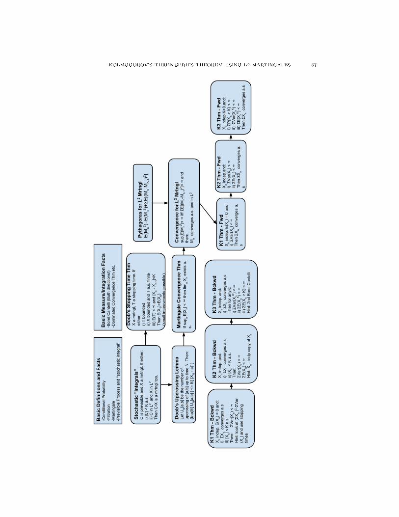
KOLMOGOROV'S THREE SERIES THEOREM USING L2 MARTINGALES 67

Bas

ic D

efin

ition

s an

d Fa

cts

-Con

ditio

nal P

roba

blity

-Filt

ratio

n-M

artin

gale

-Pre

visi

ble

Pro

cess

and

"sto

chas

tic in

tegr

al"

Doo

b's

Stop

ping

Tim

e Th

mX

a m

rtngl

, T a

sto

ppin

g tim

e. If

ei

ther

:i)

T bo

unde

dii)

X b

ound

ed a

nd T

a.s

. fin

iteiii

) E(T

) < ∞

and

|Xn -

Xn-

1|<K

Then

E(X

T)=E

(X0)

(sm

all i

mpr

ovm

ents

pos

sibl

e)

Stoc

hast

ic "

Inte

gral

s"

C is

pre

visi

ble

and

X a

mrtn

gl. I

f eith

er:

i) |C

| < K

a,s

,ii)

C in

L2

and

X in

L2

Then

C•X

is a

mrtn

gl to

o.

Doo

b's

Upc

ross

ing

Lem

ma

Let U

N[a

,b] b

e th

e nu

mbe

r of

upcr

ossi

ng o

f [a,

b] u

p to

tim

e N

. The

n:(b

-a)E

[ UN[a

,b] ]

<=

E[ (

XN -

a)- ]

Mar

tinga

le C

onve

rgen

ce T

hmIf

sup n E

|Xn|

< ∞

then

lim

n Xn e

xist

s a.

s.

Pyth

agor

as fo

r L2 M

rtng

lE

(Mn2 )

=E(M

02 )+Σ

E[(M

n-M

n-1)

2 ]

Con

verg

ence

for L

2 Mrt

ngl

sup nE

(Mn2 )

< ∞

iff Σ

E[(M

n-M

n-1)

2 ]< ∞

and

th

en:

Mn

conv

erge

s a.

s. a

nd in

L2

K1

Thm

- Fw

dX

n ind

ep. E

(Xn)

= 0

and

:i)

ΣV

ar(X

n) <

∞Th

en Σ

Xn

conv

erge

s a.

s

K2

Thm

- Fw

dX

n ind

ep.a

nd:

i) Σ

Var

(Xn)

< ∞

ii) Σ

E(X

n) <

∞Th

en Σ

Xn

conv

erge

s a.

s

K3

Thm

- Fw

dX

n ind

ep K

>0.a

nd:

i) ΣP

(Xn >

K) <

∞

ii) Σ

Var

(XnK

) < ∞

iii) Σ

E(X

nK) <

∞

Then

ΣX

n co

nver

ges

a.s

K1

Thm

- B

ckw

dX

n ind

ep. E

(Xn)

= 0

and

:i)

ΣX

n co

nver

ges

a.s

ii) |X

n| <

K a

.s.

Then

:

ΣVar

(Xn)

< ∞

Hin

t: lo

ok a

t (ΣX

n )2 -

ΣVar

(Xn)

and

use

sto

ppin

g tim

es

K2

Thm

- B

ckw

dX

n ind

ep. a

nd:

i) Σ

Xn

conv

erge

s a.

sii)

|Xn|

< K

a.s

. Th

en:

ΣV

ar(X

n) <

∞ΣE

(Xn)

< ∞

Hin

t: X

n - in

dp c

opy

of X

n

K3

Thm

- B

ckw

dX

n ind

ep. a

nd:

i) Σ

Xn

conv

erge

s a.

sTh

en fo

r any

K:

i)

ΣVar

(XnK

) < ∞

ii) Σ

E(X

nK) <

∞iii

) ΣE

(Xn >

K) <

∞

Hin

t: 2n

d B

orel

Can

telli

Bas

ic M

easu

re/In

tegr

atio

n Fa

cts

-Bor

el C

ante

lli (B

oth

dire

ctio

ns!)

-Dom

inat

ed C

onve

rgen

ce T

hm e

tc.


Definition. We say that a martingaleM is in L2 if E(M2n) <∞ for all n ∈ N.

Theorem. (Pythagoras for L2 Martingales) Say Mn is an L2 martingale then:

E(M2n) = E

(M2

0

)+

n∑k=1

E[(Mk −Mk−1)

2]

Proof. Since E (Mk −Mk−1 |Fk−1 ) = 0, we have that E [(Mk −Mk−1)X] =0 for any Fk−1 measurable X. Putting X = Mj−Mj−1 shows that the termsMk−Mk−1 andMj−Mj−1 are orthogonal. Then writeMn = M0 =

∑nk=1 (Mk −Mk−1)

gives the result.

Theorem. (Convergence of L2Martingales) SayMn is an L2 martingale. Have:

supE(M2n) <∞ ⇐⇒

∑E[(Mk −Mk−1)2

]<∞

and in the case that this holds, we have:

Mn →M∞ almost surely and in L2

Proof. By Pythagoras:

supn

E(M2n) = E(M2

0 ) + supn

n∑k=1

E[(Mk −Mk−1)

2]

Hence supnE(M2n <∞ if and only if

∑E[(Mk −Mk−1)2

]<∞.

Since E(|Mn|) ≤ E(|Mn|2

)1/2

<∞, by the Martingale Convergence Theorem,

Mn converges to some M∞almost surely. To get L2 convergence, use Pythagoras

to bound E[(M∞ −Mn)

2]by∑k≥nE

[(Mk −Mk−1)

2].

Theorem. (Kolmogorov 1 Series Theorem - Fwd Direction) Suppose Xn areindependent.

If:

∞∑n=1

Var(Xn) < ∞

E(Xn) = 0∀n

Then:∞∑n=1

Xn converges a.s.

Proof. Let Mn =∑nk=1Xk, this is a martingale. ∞ >

∑Var(Xk) =∑

E(X2k

)=∑

E[(Mn −Mn−1)

2]so by the convergence theorem for L2 mar-

tingales, Xn converges a.s.

Theorem. (Kolmogorov 2 Series Theorem - Fwd Direction) Suppose Xn areindependent.


If:

∞∑n=1

Var(Xn) < ∞

∞∑n=1

E(Xn) < ∞

Then:∞∑n=1

Xn converges a.s.

Proof. Let Yk = Xk − E(Xk) then∑

Var (Yk) =∑

Var(Xk) < ∞ by hy-pothesis, and so

∑Yk converges almost surely by the 1 series theorem. Have then:

n∑k=1

Xk =

n∑k=1

Yk +

n∑k=1

E(Xk)

a.s−−→∞∑k=1

Yk +

∞∑k=1

E(Xk)

Theorem. (Kolmogorov 3 Series Theorem - Fwd Direction) Suppose Xn areindependent and K > 0.

Dene:

XKn := Xn1|Xn|≤K

If:

∞∑n=1

P(Xn > K) < ∞

∞∑n=1

E(XKn ) < ∞

∞∑n=1

Var(XKn

)< ∞

Then:∞∑n=1

Xn converges a.s.

Proof. Since∑∞n=1 P

(XKn 6= Xn

)=∑∞n=1 P(Xn > K) < ∞, by the Borel

Cantelli lemma, we know that P(XKn 6= Xn i.o.

)= 0 . Hence XK

n = Xn for all butnitely many n almost surely.

Since∑∞n=1 E

(XKn

)< ∞ and

∑∞n=1 Var(XK

n ) < ∞, we have∑∞n=1X

Kn con-

verges almost surely by the Two Series Theorem.

Hence∑∞n=1Xn =

∑Nn=1Xn +

∑∞n=N+1X

Kn converges almost surely too.

Theorem. (Kolmogorov 1 Series Theorem - Bckwd Direction) Suppose Xn areindependent and K > 0.


If:

E(Xn) = 0 ∀n|Xn| < K a.s. ∀n∑∞

n=1Xnconverges a.s.

Then:∞∑n=1

Var(Xn) <∞

Proof. The trick is to look at:

Yn :=

(n∑k=1

Xk

)2

−n∑k=1

Var(Xk)

Yn is easily veried to be a martingale by expanding the (·)2 and usingE(Xn

∑n−1k=1 Xk) =

0 and E(X2n) = Var(Xn).

[[Side note: Since Yn is a martingale, we have that for any n that E(Yn) = 0,or in other words:

n∑k=1

Var(Xk) = E

( n∑k=1

Xk

)2

Which is very close to giving us what we want. (We now see why an extracondition such as |Xn| < K is needed: almost sure convergence of

∑Xn is not

enough to give L2 convergence) ]]To nish the proof, we use stopping times in a smart way. For convenience,

dene the martingale Sn :=∑nk=1Xk. For each c > 0 dene the stopping time:

Tc = inf n : |Sn| > c

Notice that:

|ST c | ≤ |ST c−1|+ |XT c | ≤ c+K

This actually works for Sn too as long as n < Tc.by the hypothesis that |Xn| <∞ for all n. Hence, using Tc as a stopping time

on the martingale Y gives us E(YT∧n) = E(Y0) = 0 for all n, or in other words:

E

[Tc∧n∑k=1

Var(Xk)

]= E

(Tc∧n∑k=1

Xk

)2

≤ (c+K)2 by the previous argument

Now, we claim there exists some c so that P(Tc =∞) > 0. Otherwise, Tn <∞almost surely for every n ∈ N, and taking the intersection over all N we concludefrom the denition of Tc that lim sup |Sn| = ∞, which contradicts the hypothseisthat

∑∞k=1Xk converges almost surely.


For such c, we have that:

(c+K)2 ≥ E

[Tc∧n∑k=1

Var(Xk)

]

=

(n∑k=1

Var(Xk)

)P (Tc > n) +

(Tc∑k=1

Var(Xk)

)P (Tc ≤ n)

≥

(n∑k=1

Var(Xk)

)P (Tc > n)

→

( ∞∑k=1

Var(Xk)

)P (Tc =∞)

So∑∞k=1 Var(Xk) ≤P (Tc =∞)

−1(c+K)2 <∞ as desired.

Theorem. (Kolmogorov 2 Series Theorem - Bckwd Direction) Suppose Xn areindependent and K > 0.

If:

|Xn| < K a.s. ∀n∑∞n=1Xnconverges a.s.

Then:∞∑n=1

Var(Xn) < ∞

∞∑n=1

E(Xn) < ∞

Proof. The trick is to create two independent copies of the sequence Xn, callthem Xn and Xn, and to look at the dierence:

Zn := Xn − Xn

(To be precise, dene the X ′ns on some probability space Ω, the Xn's on some

probability space ω and the Z ′ns are dened on Ω × Ω) This will be a sequenceof independent random variables with E(Zn) = 0, |Zn| < 2K. Since

∑Xn con-

verges almost surely, we have also that∑Xn converges almost surely. Hence∑

Zn converges almost surely too! Finally notice that < ∞ by hypothesis. Now,by the One Series Thm (Bck Direction) we have that

∑Var(Zn) < ∞. Hence∑

Var(Xn) = 12

∑Var(Zn) <∞ too.

Finally, we use the One Series Thm (Fwd direction) to see that∑

(Xn −E(Xn))converges almost surely, and we conclude that

∑E(Xn) =

∑Xn−

∑(Xn −E(Xn))

converges too since its the dierence of two a.s. convergent things.

Theorem. (Kolmogorov 3 Series Theorem - Bckwd Direction) Let Xn be asequence of random variables.

If: ∑Xn <∞

Then for any K > 0 we dene:

XKn := Xn1|Xn|≤K


and we have:

∞∑n=1

P(Xn > K) < ∞

∞∑n=1

E(XKn ) < ∞

∞∑n=1

Var(XKn

)< ∞

Proof. Since∑Xn converges almost surely, then Xn → 0 almost surely (in-

deed Xn → 0 ⊃ ∑Xn converges). Hence |Xn| > K for all but nitely many

K i.e. P(|Xn| > K i.o) = 0. Since the Xn are independent, by the second BorelCantelli Lemma, we have that

∑∞n=1 P(Xn > K) <∞.

Since Xn = XKn for all but nitely many n, we have that

∑XKn converges

almost surely.∑∞n=1 E(XK

n ) < ∞,∑∞n=1 Var

(XKn

)< ∞ follow then by the Kol-

moogrov Two Series Theorem Bckward Direction.

A few dierent proofs of the LLN

Here is a collection of some dierent proofs of the LLN...this is a repeat of someof the earlier sections.

There are dierent ways to prove the strong law of large numbers. Here arethe techniques I know:

• Truncation + K3 Theorem + Kronecker Lemma• Truncation + Sparsication• Levy's downward theorem + 0-1 Law• Ergodic Theorem

9.30. Truncation Lemma

This lemma is the starting point for two of the dierent proofs.

Lemma. (Kolmogorov's Truncation Lemma)Suppose that X1, X2, . . . are IID with E(|X|) < ∞. Dene Yn = Xn1|Xn|<n

then:i) E(Yn)→ E(X)ii) P (Yn = Xn eventually ) = 1iii)

∑∞n=1 n

−2E(Y 2n ) ≤ 4E (|X|) <∞

Proof. i) is just by the dominated convergence theorem usingX as a dominantmajorant. ii) is just by Borel Cantelli since P (Yn 6= Xn) = P (|Xn| ≥ n) andeveryon'e favourite formula for expectation:

∑P (|X| ≥ n) =

∑P (b|X|c ≥ n) =

E (b|X|c) ≤ E(|X|).iii) follows is based on the telescoping sum estimate:

∑n≥m

1

n2≤∑n≥m

2

n(n+ 1)=∑n≥m

2

n− 2

n+ 1≤ 2

m

73

9.31. TRUNCATION + K3 THEOREM + KRONECKER LEMMA 74

and using Fubini to switch the sum and the integral. Consider that:

∞∑n=1

n−2E(Y 2n

)=

∞∑n=1

E(n−2X21|X|<n

)= E

(X2

( ∞∑n=1

n−21|X|<n

))

= E

X2

∞∑n=d|X|e

n−2

≤ E

(X2 2

d|X|e

)≤ 2E (|X|) <∞

9.31. Truncation + K3 Theorem + Kronecker Lemma

Lemma. (Kolmogorov 3 Series Thm) Say X1, . . . are iid and K > 0. DeneXKn = Xn1|Xn|<K then:

∞∑n=1

P (Xn > K) < ∞∞∑n=1

E(XKn

)< ∞

∞∑n=1

Var(XKn

)< ∞

⇐⇒∞∑n=1

Xn converges a.s

\

Remark. The proof of =⇒ is fairly straightforward using the idea of L2

martingales and the martingale convergence theorem. Even with martingale tools,the proof of ⇐= requires a few tricks.

Remark. For the strong law however, we only need the forward direction, andactually we only need the 1 series theorem (which is the case where K = ∞ andE(Xk) = 0 always). To get this from scratch is actually surprisingly quick usingmartingales, the steps are:

• Upcrossing lemma and Martingale convergence theorem• Pythagoras formula for L2 martingales

Lemma. Cesaro Lemma:If an are positive weights with

∑ak → ∞ and xn is a sequence with xn → L

then the weighted average:n∑k=1

akxk

n∑k=1

ak

→ L too

9.31. TRUNCATION + K3 THEOREM + KRONECKER LEMMA 75

Proof. The fact that∑ak → ∞ shows that for any xed N the rst N

terms of the sequence xk are irrelevant;∑Nk=1 akxk is some nite amount and the

numerator∑nk=1 ak →∞ drowns them out. Hence only the tail of the xk's matter

and since xk is converging to L, every term is eventually with ε of L and so theweighted average will also be with ε of L from this point on.

Lemma. Kronecker's LemmaIf bn is an increasing sequence of real numbers with bn ↑ ∞ and xn is a sequence

of real numbers then: ∑ xnbn

<∞ =⇒∑xnbn

→ 0

Proof. Let un =∑ni=1

xibi

be the partial sums of our convergent sequence withu∞ = limn un. Use the dierences bn+1 − bn as the weights for the Cesaro lemmato get: ∑

xn =∑

bk (uk − uk−1)

= bnun −n∑k=1

(bk − bk−1)uk−1

So then: ∑xnbn

= un −∑nk=1(bk − bk−1)uk−1∑nk=1(bk − bk−1)

→ u∞ − u∞ = 0

Here is a bonus little result that we basically used as part of the theorem:

Theorem. (Strong Law under Variance Constraint)Let Wn be a sequence of independent random variables so that E(Wn) = and∑n−2Var(Wn) <∞. Then n−1

∑k≤nWk → 0 a.s.

Proof. By the Kronecker lemma, it is sucient to show that∑n−1Wn con-

verges a.s. But the convergence of this series is exactly the result of the Kolmogorov1 Series theorem, so we are done!

Theorem. (Stong Law) If X1, . . . are iid with E (|X|) <∞ then n−1∑nk=1Xk →

E(X) a.s.

Proof. Dene Yn = Xn1|Xn|<n as in the truncation lemma. Since Xn = Yneventually almost surely, it suces to show that n−1

∑nk=1 Yk → E(X) a.s. Indeed,

if we let Wk = Yk − E(Yk) then Wk are independent mean zero random variableswith

∑n−2Var(Wn) =

∑n−2Var(Yn) ≤

∑n−2E(Y 2

n ) < ∞ by the Kolmogorovtruncation lemma.

Now notice that by the Kolmogorov 1 Series Theorem, since the sum of vari-ances is nite, we know that

∑k≤n n

−1Wn converges a.s. But then by the Kronecker

lemma, we know that n−1∑k≤nWn → 0 almost surely.

Finally:

n−1∑k≤n

Yn = n−1∑k≤n

Wn + n−1∑k≤n

E(Yk)→ 0 + E(X)

since E(Yk)→ E(X) (to be precise, we invoked the Cesaro lemma here)

9.32. TRUNCATION + SPARSIFICATION 76

One advantage of doing it with the K3 theorem is that you can get slightlystronger results and estimates about how fast the convergence goes.

Theorem. (2.5.7. from Durret) If X1, . . . are iid with E(X1) = 0 and E(X21 ) =

σ2 <∞ then:Sn√

n log n12 +ε→ 0 a.s.

Remark. Compare this with the law of the iterated log:

lim supn→∞

Sn√n log log n

= σ√

2

Proof. It suces, via the Kronecker lemma, to check that∑ Xn√

n logn1/2+ε

converges. By the K1 series theorem, it suces to check that the variances aresummable. Indeed:

Var

(Xn√

n log n1/2+ε

)≤ σ2

n log1+2ε

which is indeed summable (e.g. Cauchy condensation test)!

9.32. Truncation + Sparsication

I'm going to do some examples of problems where if you want to show that:

Xn

cn→ 1

a.s. for some non-negative increasing sequences Xn, cn ≥ 0 it is enough to provethe result for a subsequence nk that has cnk+1

/cnk → 1

Remark. The advantage to looking along a subsequence is that along a sub-sequence we can use things like the Borel Cantelli lemma's more easily. A lot oftimes we use this to prove large number type laws of the form Xn/E(Xn) → 1a.s. and this technique can be used to prove the SLLN.

Theorem. Let Xn be an increasing sequence of non-negative random variablesand let cn be an increasing sequence of non-negative constants. Suppose that nk isa sub-sequence with:

cnkcnk+1

→ 1 as k →∞

Then:Xnk

cnk→ 1 a.s =⇒ Xn

cn→ 1 a.s.

Proof. For any n nd the unique k so that nk ≤ n < nk+1. Then, sinceXn and cn are increasing and non-negative, we have that Xnk < Xn < Xnk+1

andcnk+1

> cn > cnkso then:(cnkcnk+1

)Xnk

cnk=

Xnk

cnk+1

<Xn

cn<Xnk+1

cnk=

(cnk+1

cnk

)Xnk+1

cnk+1

Now sincecnkcnk+1

→ 1 as k → ∞, for any ε > 0 we can nd K so large so that

cnk+1/cnk < 1 + ε and cnk/cnk+1

> 1− ε for all k ≥ K and then have:

(1− ε)Xnk

cnk<Xn

cn< (1 + ε)

Xnk+1

cnk+1


Now taking limsup and liminf of both sides, using the fact thatXnkcnk→ 1 a.s.

we get that:

(1− ε) < lim infXn

cn< lim sup

Xn

cn< (1 + ε) a.s

But since this holds for all ε > 0 it must be that the limit exists and equals 1a.s.

Remark. The main thing is the inequality that is used. The hypothesis canbe relaxed in diernt ways, for example, suppose that for ever ε > 0 there exists

a subsequence nk so that lim supcnkcnk+1

< 1 + ε andXnkcnk→ 1 a.s. Then the result

will still hold.

Theorem. (2.3.8. From Durret Prob Theory and Examples)If A1, A2, . . . are pairwise independent and

∑∞n=1 P (An) =∞ then as n→∞ :

n∑m=1

1Am

n∑m=1

P (Am)

= 1 a.s.

Proof. We use a Cheb inequality to control how far Sn :=∑nm=1 1Am can be

from its mean, and then we can use Borel Cantelli to get a.s. convergence alongcertain subsequences. Then the sparsication will nish it up for us.

By Cheb, we have:

P (|Sn −E(Sn)| > δE(Sn)) ≤ 1

δ2E(Sn)2Var(Sn)

≤ E(Sn)

δ2E(Sn)2

=1

δ2E(Sn)

Where we have using independence thatVar(Sn) =∑

Var(1Am) ≤∑

E(12Am

) =∑P(Am) = E(Sn). Now by hypothesis, E(Sn) =

∑P(Am) → ∞ so letting

nk = infn : E(Sn) ≥ k2

gives us a subsequence along which:

P

(∣∣∣∣ SnkE(Snk)

− 1

∣∣∣∣ ≥ δ) ≤ 1

δ2k2

So by Borel Cantelli, we know thatSnk

E(Snk ) → 1. (Pf 1) choose δ = δk → 0

so that its still summabl and apply BC lemma once, get∣∣∣ Snk

E(Snk ) − 1∣∣∣ ≥ δk i.o

is null Pf 2) For each δ we know that∣∣∣ Snk

E(Snk ) − 1∣∣∣ ≥ δ i.o is null and so taking

intersections wiht δ = 1n shows us the a.s. convergence)

Finally we notice that since E(Sn+1) − E(Sn) ≤ 1, we have that cnk+1/cnk ≤[

(k + 1)2 + 1]/k2 → 1, so the sparication trick works out here.

Example. If Xn are increasing r.v.'s with E(Xn)nα → a and Var(Xn) ≤ Bnβ

with β < 2α, show that Xnnα → a almost surely.


Proof. It suces to show that Xn−E(Xn)nα → 0. Have:

P (|Xn −E(Xn)| > δnα) ≤ 1

δ2n2αVar (Xn) ≤ B

δ2nβ−2α

If we now look along a subsequnece nm = mc with c chosen so large so thatmc(β−2α) is summable (i.e. c > (2α − β)−1 will do by the p-test) then a standard

Borel Cantelli shows us thatXnm−E(Xnm )

nαm→ 0. Now we notice that

nαm+1

nαm=

(m+1)αc

mαc → 1 so our sparsifaction kicks in and fnishes the job for us.

Example. If Xn are independent Poisson RV with E(Xn) = λn and if∑λn =

∞ then Sn =∑k≤nXk has Sn

E(Sn) → 1 a.s.

Proof. Similar to the above at rst.....I'm having a bit of a hiccup showingthat nm+1

nm→ 1 though in the case that the λns are very large though.

Example. (Record Values) If X1, X2 . . . is a sequence of iid random variableswith no atoms, let Ak =

Xk > supj<kXj

be the record at k event. (Think

of the Xi's as the shot put value for an olympian, and Ak is the event that hisk-th shot is a new presonal record for him). By choosing the values rst, thenputting them in some order, its not too hard to see that they are independent andP(An) = 1

n . Then the above theorem applies and since∑

1n ∼ log n we get that

for Rn, the number of records up to time n that:

Rnlog n

→ 1

Theorem. (Etememadi's SLLN) If Xn are identically distributed and pairwiseindependent and E(|X|) <∞then n−1

∑k≤nXk → E(X) a.s.

Proof. By handling the positive and negative parts separately, we assumeWOLOG that X ≥ 0. By ii) from the truncation lemma it suces to show thatn−1

∑k≤n Yk → E(X) a.s. where Yk = Xk1Xk<k. Actually, since E(Yk)→ E(X)

it suces to check that n−1(∑

k≤n Yk −E(∑

k≤n Yk

))→ 0 which is what we will

verify.For any α > 1, let nm = bαmc and we will restrict out attention to this

subsequence. Consider:

E

∣∣∣∣∣∣∑k≤nm

Yk −E

∑k≤nm

Yk

∣∣∣∣∣∣ > δnm

≤ 1

δ2n2m

Var

∑k≤nm

Yk

=

1

δ2n2m

∑k≤nm

Var (Yk)

Now we sum over m and use Fubini to swich the order of the sum:

∞∑m=1

E

∣∣∣∣∣∣∑k≤nm

Yk −E

∑k≤nm

Yk

∣∣∣∣∣∣ > δn2m

≤ 1

δ2

∞∑m=1

1

n2m

∑k≤nm

Var (Yk)

=1

δ2

∞∑k=1

Var(Yk)∑

m:nm>k

1

n2m

9.33. LEVY'S DOWNWARD THEOREM AND THE 0-1 LAW 79

Now we just have to estimate∑m:nm>k

1n2m∼ 1

k2 and then we will be able

to apply the truncation lemma to see the convergence we want. Indeed this is ageometric series so we have

∑nm>k

1n2m

=∑m:αm>k α

−2m ≤ (1− α−2)k−2

Hence by the truncation lemma this is summable, and we conclude by a stan-dard application of Borel cantelli that:∑

k≤nm Yk −E(∑

k≤nm Yk

)nm

→ 0

By E(Yn) ↑ E(X) this shows that n−1m

∑k≤nm Yk → E(X) which is exactly the

convergence we want along the subsequence nm. We will now use our sparsicationtools to strenthen the result to convergence n−1

∑k≤n Yk. For convenience at this

point, dene Wn =∑k≤n Yk and we desire to show that n−1

m Wnm → E(X) for

every α > 1 =⇒ n−1Wn.Indeed, for any n > 0 nd the nm so that nm < n < nm+1 and consider that:

Wnm

nm

nmnm+1

=Wnm

nm+1≤ Wn

n≤Wnm+1

nm=Wnm+1

nm+1

nm+1

nm

Now take lim sup and lim inf everywhere, use n−1m Wnm → E(X) and nm/nm+1 →

α we get:1

αE (X) ≤ lim inf

Wn

n≤ lim sup

Wn

n≤ αE(X)

But since this holds for any α we get lim Wn

n = E(X) as desired.

9.33. Levy's Downward Theorem and the 0-1 Law

This one requires the most tech: You need Levy's Downward theorem:

Theorem. Suppose (Ω,F ,P) is a probability triple and that G−n : n ∈ N isa collection of sub-σ−algebras of F such that:

G−∞ :=⋂k

G−k ⊂ . . . ⊂ G−(n+1) ⊂ G−n ⊂ . . . ⊂ G−1

(In other words, they are backwards of a normal ltration, which gets ner andner, these get coarser and coarser.....except they are labeled with negative numbers)

Let γ ∈ L1 and dene:

M−n := E (γ |G−n )

Then:

M−∞ := limM−n exists a.s and in L1

and:

M−∞ = E (γ |G−∞ ) a.s.

Remark. To prove this one from scratch, you would do:

• Upcrossing lemma• Martingale convergence theorem• Facts about uniform integrability

UI =⇒ L1 bounded L1 conv ⇐⇒ UI and conv in prob E(X |Fn ) is UI

9.34. ERGODIC THEOREM 80

We also need the Kolmogorov 0− 1 law for this proof. (fortunatly this has an easyproof using the Levy upward theorem).

Theorem. (Kolmogorov 0-1 Law) If X1, X2, . . . are independent and A ∈ T =∩∞n=1σ (Xn, Xn+1, . . .) then P(A) = 0 or 1,

Proof. We will show that A is independent of itself. Firstly:a) If A ∈ σ (X1, . . . , Xk) and B ∈ σ (Xk+1, . . .) then A and B are independent.(This follows by some of those proofs using π systems)b) If A ∈ σ (X1, . . .) and B ∈ T then A,B are indep.By a), B ∈ T ⊂ σ (Xk+1, . . .) is independent of σ (X1, . . . , Xk) for each k.

Hence, it will be independent of σ(X1, . . .) = ∪nσ(X1, . . .)Since T ⊂ σ (X1, . . .) part b) shows us that A is independent of itself. (Put

A = B in the last theorem) and the result follows.

Remark. Here's another slightly slicker proof using monotone class theoremrather than π − λ:

a) If B ∈ T then B is independent to σ (X1, . . . , Xn)b) Let A be the set of events that are independent of B. Check that its a

montone class! (Follows by continuity of measure)c) SinceA contains each σ (X1, . . . , Xn), it contains the algebra ∪nσ (X1, . . . , Xn)

(Remark: its not a sigma algebra! these are all the events that depend on netlymany things)

d) By the monotone class theorem, we have thatA actually contains σ (∪nσ (X1, . . . , Xn)) =σ (X1, . . .). Hence B ∈ A is independent of itself!

Once we have all this tech though, the following sneaky trick proves the stronglaw right away:

Theorem. Let X1, X2, . . . be iid with E (|X|) <∞. Let Sn =∑k≤nXk. Then

n−1Sn → E(X) a.s.

Proof. Dene G−n := σ (Sn, Sn+1, . . .) and G−∞ =⋂n G−n. By a symmetry

argument, we see that E (X1 |G−n ) = n−1Sn. So by Levy's downward theorem,n−1Sn = E (X1 |G−n ) → E (X1 |G−∞ ) = L a.s. and in L1. We now argue that Lmust be a constant because the event

n−1Sn = c

is a tail event (can see that it

does not depend on the rst N variables and this works for any N) and by the 0-1law it must therefore be constant. Since the convergence n−1Sn → L is in L1 wecan check that:

L = E(L) = limE(n−1Sn

)= E(X)

9.34. Ergodic Theorem

Problem. The strong law of large numbers says that for an iid sequenceX1, X2, . . . with E |X1| <∞ that:

limN→∞

1

N

N∑n=1

Xn = E(X1) a.s.

Show how this is a consequence of the pointwise ergodic theorem.

9.35. NON-CONVERGENCE FOR INFINITE MEAN 81

Proof. Let µ be the law of the random variable X. Introduce the space Ω =RN = (x1, x2, . . .) : xi ∈ R of sequences and put the product meausre µ× µ× . . .on this space. (To be more technical: one should use the Caratheodory extensiontheorem starting with the algebra of cylinder sets and the premeasure given bynite products of µ. This also makes it clear that sigma algebra on this space isthe sigma algebra generated by these cylinder sets. Since this is a standard rsttheorem in a probability course, I will omit the details of this.)

Dene f : Ω→ R to be the rst random coordinate:

f (x1, x2, x3, . . .) = x1

Notice that the law of f is µ, so since E |X1| < ∞ is given, we know thatf ∈ L1 (µ× µ× . . .). Let T : Ω→ Ω be the shift operator:

T (x1, x2, x3, . . .) = (x2, x3, . . .)

Since we are working with the product measure, all the coordinates have thesame distribution and T is a measure preserving transformation on (Ω,F ,P).

We now notice that T is ergodic. This will follow by the Kolmogorov-Zero-Onelaw for iid sequences. Suppose A is is T -invariant. Then it is also Tn-invariant, andconsequently any such event A does not depend on the rst n coordinates of thepoint ω ∈ Ω. Since this holds for every n, we conclude that A is a tail event. (Inthe tail sigma algebra σ (∩∞n=1σ (∪∞k=nFk)) where Fk is the sigma algebra of eventsthat depend only on the rst k coordinates.) The Kolmogorov-Zero-One law statesthat such events have either P(A) = 0 or 1 and hence T is ergodic. (Again, I omitthe proof of the Kolmogorov-Zero-One law)

Finally, notice that:

1

N

N∑n=1

f (Tnx) =1

N

N∑n=1

(Tnx)1

=1

N

N∑n=1

xn

so by the pointwise ergodic theorem, applied to the ergodic transformation Tand the L1 fucntion f on this space we know that:

1

N

N∑n=1

xnµ×... a.s.−−−−−−→ E(f) = E(X)

This is exactly the statement of the strong law of large numbers!(One remark: I am using the statement of the ergodic theorem for a single

transformation T and am taking averages 1N

∑Nn=1 f (Tnx). In class we proved it

for Zd-systems. The proof for the Zd systems can be adapted for this simpler caseI am using.)

9.35. Non-convergence for innite mean

Remark. If E(|X|) = ∞ then we should have lim sup |Sn| /n using the trickthat |Xn| > n i.o and |Xn| > C =⇒ |Sn−1| / (n− 1) > C/2 or |Sn| /n > C.

Ergodic Theorems

These are notes from Chapter 7 of [2].Xn is siad to be a stationary sequence if for each k ≥ 1 it has the same

distribution as the shifted sequnece Xn+k. The basic fact about these sequences,called the ergodic theorem is that if E (|f(X0)|) <∞ then:

limn→∞

1

n

n−1∑m=0

f (Xm) exits a.s.

If Xn is ergodic (a generalization of the notion of irreducibility for Markovchains) then the limit is E (f(X0))

10.36. Denitions and Examples

Definition. X0, X1, . . . is said to be a stationary sequence if for every kthe shifted sequence Xn+k : n ≥ 0 has the same distribution i.e. for each m thevectors (X0, . . . , Xm) and (Xk, . . . , Xk+m) have the same distribution.

We begin by giving four examples that will be our constant companions:

Example. (7.1.1.) X0, X1, . . . are iid

Example. (7.1.2.) Let Xn be a Markov chain with transition probabilityp(x,A) and stationary distribution π, i.ie. π(A) =

´p(x,A)π(dx). If X0 has

distribution π then X0, X1, . . . is a stationary sequence.A special case to keep in mind for this one is the deterministic Markov chain on

the state space S = A,B with A moving to B with probability 1. The stationarydistribution is π(A) = π(B) = 1

2 I.e. (X0, X1, . . .) = (A,B,A,B, . . .) or (B,A,B,A, . . .)

each with probability 12 .

Example. (7.1.3.) (Rotation of a circle) Let Ω = [0, 1), F =Borel subsets,P =Lebesgue measure. Let θ ∈ (0, 1) and for n ≥ 0 let Xn(ω) = (ω + nθ)mod 1where x mod 1 := x− bxc is the decimal part of x.

This is a special case of the deterministic shift Markov chain this time withinnitely many states. (i.e. p(x, y) = 1 if y = (x+ θ) mod 1 and 0 for all othersets)

Theorem. (7.1.1.) If X0, X1, . . . is a stationary sequence and g : R0,1,... → Ris measurable then Yk = g (Xk, Xk+1, . . .) is a stationary sequence

Proof. For x ∈ R0,1,... dene gk(x) = g(xk, xk+1, . . .) and for B ∈ B0,1,...let:

A = x : (g0(x), g1(x), . . .) ∈ B

82

10.36. DEFINITIONS AND EXAMPLES 83

To check stationarity now, we observe that:

P ((Y0, Y1, . . .) ∈ B) = P ((X0, X1, . . .) ∈ A)

= P ((Xk, Xk+1, . . .) ∈ A)

= P ((Yk, Yk+1, . . .) ∈ B)

which proves the desired result.

Example. (7.1.4.) (Bernoulli Shifts) Let Ω = [0, 1) and F =Borel subsets,P =Lebesgue measure. Let Yn(ω) = 2Yn−1(ω) mod 1. This is a special case of7.1.1, the iid sequence case, the connection being that between an innite sequenceof iid coin ips and a real number in [0, 1) identied by the diadic decomposition.

If we let X0, . . . be iid with P(Xi = 0) = P(Xi = 1) = 12 and we let g(x) =∑∞

i=0 xi2−(i+1) then the identication Yn = g (Xn, Xn+1, . . .) (check that Yn =

2Yn−1 mod 1here) shows us that Yn is indeed stationary.This is also a special case of the determenistic Markov chain with p(x, y) = 1

for y = 2x mod 1 and 0 for all other sets.Examples 7.1.3 and 7.1.4 are special cases of the following situation:

Definition. Let (Ω,F ,P) be a probability space. A map ϕ : Ω→ Ω is calledmeasure preserving if P

(ϕ−1A

)= P(A) for all A ∈ F .

Example. (7.1.5.) Let ϕn be ϕ composed with itself n times. If X is a randomvariable then Xn(ω) = X (ϕnω) denes a stationary sequence. To check this letB ∈ Rn+1 and A = ω : (X0(ω), . . . Xn(ω)) ∈ B then:

P ((Xk, . . . , Xk+1) ∈ B) = P(ϕkω ∈ A

)= P(ω ∈ A) = P ((X0, . . . , Xn) ∈ B)

Remark. The last exampe is more than an important example. In fact, it isthe ONLY example! For if Y0, Y1, . . . is a stationary sequence taking valuies in a nicespace, then the Kolmogorov Extension Thoerem allows us to construct a measureon the sequence space

(S0,1,...,S0,1,...)

)so that the sequence Xn(ω) = ωn has

the same distribution as that of Yn, n ≥ 0. If we let ϕ be the shift operator here,ϕ (ω1, ω2, . . .) = (ω1, ω2, . . .) and let X(ω) = ω0 then ϕ is measure preserving (thisfollows sinc e Y is stationary) and Xn(ω) = X(ϕnω).

Theorem. (7.1.2.) Any stationary sequence Xn, n ≥ 0 can be embedded ina two-sided stationary sequence Yn;n ∈ Z

Proof. Dene: P (Y−m ∈ A0, . . . Yn ∈ Am+n) := P (X0 ∈ A0, . . . , Xm+n ∈ Am+n).Since Xn is a stationary sequence, this is a consist denition and the Kolmogorovextension theorem gives us the measure we want, Yn(ω) = ωn is a shift.

In view of the above observation, it suces to give our denitons and proveour results in the setting of Example 7.1.5.. Thus our set up is:

(Ω,F ,P) ≡ a probability space

ϕ ≡ a measure preserving map

Xn(ω) = X (ϕnω) where X is a r.v.

Definition. Let ϕ be a measure preserving map. We say that a set A ∈ F isinvariant for ϕ if ϕ−1A = A a.s. (i.e. the symmetric dierence of the two sets isa null set: some people call this almost invariant). We will say that a set B isinvariant in the strict sense if ϕ−1B = B exactly.


Exercise. (7.1.1) The class of invariant events I is a σ−algebra and a randomvariable X is I measurable if and only ifX is an invariant , i.e. X ϕ = X a.s.

Proof. Closed under countable unions and intersections is clear since ϕ−1

plays nice with these operations. If X ϕ = X a.s. then we have that for any Borelset B that X−1(B) = (X ϕ)

−1(B) = ϕ−1

(X−1(B)

)which shows that every set

X−1(B) is an invariant set, i.e. σ(X) ⊂ I and X is I measurable.

Exercise. (7.1.2.)i) For any set A dene B = ∪∞n=0ϕ

−n(A). Then ϕ−1(B) ⊂ Bii) If ϕ−1(B) ⊂ B and C = ∩∞n=0ϕ

−n(B) then ϕ−1(C) = Ciii) A set A is almost invariant ⇐⇒ there is a set C which is invariant in the

strict sense and P (A4C) = 0

Proof. i) Have ϕ−1(B) = ϕ−1 (∪∞n=0ϕ−n(A)) = ∪∞n=1ϕ

−n(A) ⊂ B.ii) Since ϕ−1(B) ⊂ B, we conclude actually that ϕ−n(B) ⊂ ϕ−(n−1) (B) and

so the sequnceB,ϕ−1(B), ϕ−2(B) . . .

is actually a decreasing sequence. Hence

C = limn→∞ ϕ−n(B) and we see that ϕ−1(C) = limn→∞ ϕ−n(B) too, so the twoare equal.

iii) ( =⇒ ) If A is invariant, then dene B and C as above. If A is almostinvariant, then each ϕ−1(A) is a.s. equal to A and so the countable intersection Bis a.s. equal to A too, and then the countable intersection C is a.s. equal to A too,so P(A4C) = 0. (By a.s. equal here I mean · a.s. equal ? ⇐⇒ P (·4?) = 0 )

(⇐=) Conversly if P (A4C) = 0 is invariant, then ϕ−1(A) = ϕ−1(C−A4C) =ϕ−1(C)−ϕ−1(A4C) = C−ϕ−1(A4C) which is eqaual to A a.s. sinceP(A4C) = 0and P

(ϕ−1(A4C)

)= P(A4C) = 0 too

Definition. A measure preserving transformation on (Ω,F ,P) is said to beergodic if I is trivial, i.e. for all A ∈ I, P(A) ∈ 0, 1. Equivalently, by theprevious exercise, the only invariant random variables are a.s. constants.

If ϕ is not ergodic, then the space can be split into two sets, A and Ac eachof positive measure so that ϕ(A) = A and ϕ(Ac) = Ac. In other words, ϕ is notirreducible.

Lets go back and see what this means for the examples we have:

Example. (7.1.6) (iid sequences) We begin by observing that if Ω = R0,1,2...andϕ is the shift operator, then an invaraint set A has A = ϕ−1(A) ∈ σ(X1, X2, . . .)iterating gives us that:

A ∈ ∩∞n=1σ(Xn, Xn+1, . . .) = T the tails σ-algebra

So I ⊂ T , by the Kolmogorov 0-1 law, T is indeed trivial so we know that thesequence is ergodic.

Example. (7.1.7) (Markov Chains) We will show that the resulting stationarysequence and map is ergodic if and only if the Markov chain is irreducible.

Supppose we have a Markov chain on a countable state space S with stationarydistribution π(x) > 0. All the states are then recurrent and we can write S = ∪iRiwhere Ri are the disjoint irreducible closed sets. If X0 ∈ Ri then with probabilityone, Xn ∈ Ri for all n ≥ 1 so ω : X0(ω) ∈ Ri ∈ I. This shows that if the Markovchain is not irreducible, then the sequence is not ergodic.


To prove the converse, note that if A ∈ I, then 1A θn = 1A where θn is theshift by n operator. If we let Fn = σ (X0, . . . Xn) then the shift invariance of 1Aand the Markov property imply that:

Eπ (1A |Fn ) = Eπ (1A θn |Fn ) = h(Xn)

where h(x) = Ex(1A). By Levy's 0-1 law, the LHS converges to 1A as n→∞..... I'm going to skip the rest of this for now...

Example. (7.1.8) Rotation of the circle is not Ergodic if θ = m/n wherem < nare positive integers, for the set A = ∪n−1

k=0(B + k/n) will be invariant for any setB ⊂ [0, 1/n]

Coversly, if θ is irrational then ϕ IS ergodic. This relies on the unique writ-ing, for L2 functions, that f(x) =

∑k cke

2πikx in the L2 sense, and with ck =´fe−2πikxdx. Now f(ϕ(x)) =

∑k cke

2πik(x+θ) =∑cke

2πikθe2πikxso this equals

f(x) if and only if e2ikθ = 1 for some k or else ck = 0. If θ is irrational, then weget that ck = 0 for all k 6= 0 and so f is a constant.

Exercise. (7.1.3.) (A direct proof of ergodicitiy for irrational shifts)Show that xn = nθ mod 1 is dense in [0, 1), then show that for a Borel set

with |A| > 0 then for every δ > 0 there is an interval J s.t. |A ∩ J | > (1− δ) |J |

Example. (7.1.9) Bernoulli Shifts is ergodic. To prove this, we recall therepresentation that: Yn =

∑∞m=0 2−(m+1)Xn+m where X0, X1,. . . are iid coin ips.

We then use the following fact:

Theorem. (7.1.3) Let g : R0,1,... → R be measurable. If X0, X1, . . . is anergodic stationary sequence, then Yk = g (Xk, . . .) is ergodic too.

Proof. The same set translation idea as before works, e.g. let:

A = x : (g0(x), g1(x), . . .) ∈ B

And then observe:

P ((Y0, Y1, . . .) ∈ B) = P ((X0, X1, . . .) ∈ A)

= P ((Xk, Xk+1, . . .) ∈ A)

= P ((Yk, Yk+1, . . .) ∈ B)

So if any IY ′s = IX′s and both are trivial together.

Exercise. (7.1.4.) Prove directly using a Fourier series type argument thatthe Bernoulli shift is ergodic.

Exercise. (7.1.5.) Continued Fractions. For any x ∈ (0, 1), we have thedecomposition:

x =1

a0 + 1a1+...

This is called the continued fraction representation, we write x = [a0; a1; . . .]for short. The way to compute these is by an = bϕnxc with ϕx = 1

x −⌊

1x

⌋= 1

xmod 1.

Check that ϕ preserves the µ given by µ(A) = 1log 2

´A

dx1+x for A ⊂ (0, 1).

10.37. BIRKHOFF'S ERGODIC THEOREM 86

Proof. Assume µ is given by integration against a density ρ. The requirementthat µ

(ϕ−1(a, b)

)= µ(a, b) gives (from ϕ−1(a, b) =

⋃∞n=1( 1

b+n ,1

a+n ) ):

ˆ b

a

ρ(x)dx =

∞∑n=1

ˆ 1a+n

1b+n

ρ(x)dx

Taking the b derivative now gives us:

ρ(x) =

∞∑n=1

ρ

(1

x+ n

)1

(x+ n)2

From which we can verify that ρ(x) = 11+x is a solution.

10.37. Birkho's Ergodic Theorem

Throughout this section, we will suppose that ϕ is a measure preserving trans-formation on (Ω,F ,P) . The main theorem in this section is:

Theorem. (7.2.1.) (Birkho's Ergodic Theorem) For any X ∈ L1:

1

n

n−1∑m=0

X (ϕmω)→ E (X |I ) a.s. and in L1

Remark. When the sequence is ergodic, I is trivial, so E(X |I) = E(X) . Theproof is not intuitive but none of the steps are dicult.

Lemma. (7.2.2.) (Maximal ergodic lemma) Let Xj(ω) = X(ϕjω

). and Sk(ω) =∑

0≤j≤k−1Xj(ω) and Mk(ω) = max (0, S1(ω), . . . , Sk(ω)) then E (X;Mk > 0) ≥ 0

Proof. The idea is to compare X to something likeMk(ω)−Mk(ϕω) (we willuse X(ω) = Sj+1(ω) − Sj(ϕω) to get the ball rolling) and then notice that thisintegrates to 0, (since ϕ is measure preserving) and is hence positive on the setMk > 0 (since Mk = 0 and Mk(ϕω) ≥ 0 on Mk > 0c...so really we are noticing itis non-positive on the complement and it integrates to zero.)

Specically, for j ≤ k we have Mk(ϕω) ≥ Sj(ϕω) so adding X(ω) gives:

X(ω) +Mk(ϕω) ≥ X(ω) + Sj(ϕω) = Sj+1(ω)

So rearranging gives:

X(ω) ≥ Sj+1(ω)−Mk(ϕω) for j ≤ k

The result also holds for j = 0 since S0+1(ω) = X(ω) andMk ≥ 0, so we takingthe maximum over all these k + 1 inequalities gives us:

X(ω) ≥ max (S1(ω), . . . , Sk(ω))−Mk(ϕω)

= Mk(ω)−Mk(ϕω)

Now integrating gives:

E (X;Mk > 0) ≥ˆMk>0

Mk(ω)−Mk(ϕω)dP

≥ˆMk(ω)−Mk(ϕω)dP

= 0

10.37. BIRKHOFF'S ERGODIC THEOREM 87

Where the second ≥ comes from the fact that Mk(ω)−Mk(ϕω) is non-positiveon the complement Mk > 0c and the last = 0 comes from the fact that ϕ ismeasure preserving.

Theorem. (7.2.1.) (Birkho's Ergodic Theorem) For any X ∈ L1:

1

n

n−1∑m=0

X (ϕmω)→ E (X |I ) a.s. and in L1

Proof. (Idea) We will assume WOLOG that E(X |I ) = 0 (we can applythe theorem to Y = X − E(X |I ) and exploit that E (X |I ) is I is ϕ invari-ant, so it comes out of the sum). Let Sk(ω) =

∑0≤j≤k−1Xj(ω). The idea is

to look at X = lim sup 1nSn. Since this is invariant, it is I measurable and con-

sequently the set X > ε ∈ I which we use to our advantage. We want toshow P(X > ε) = 0 for all ε > 0. If we let X∗ = (X(ω)− ε) 1X>ε, then

E(X∗∣∣X > ε

)= E

(X∣∣X > ε

)− εP

(X > ε

)= E

(E (X |I )

∣∣X > ε)−

εP(X > ε

)= 0 − εP

(X > ε

), so it suces to show that E

(X∗∣∣X > ε

)≥ 0

which we will do with the maximal ergodic lemma....I am going to skip the details for now...

Theorem. (7.2.3.) Wiener's Maximal InequalityLet Xj(ω) = X(ϕjω) and Sk(ω) =

∑0≤j≤k−1Xj(ω). Let Ak(ω) = Sk(ω)/k

and Dk = max (A1, . . . , Ak). For α > 0 we have:

P (Dk > α) ≤ α−1E (|X|)

Proof. Let B = Dk > α apply the maximal ergodic lemma to X ′ = X − αwith X ′j(ω) = X ′(ϕjω), S′k(ω) =

∑0≤j≤k−1X

′j(ω) and M ′k = max (0, S′1 . . . , S

′k)

we conclude that E (X ′;M ′ > 0) ≥ 0. Since M ′k > 0 = Dk > α it follows that:ˆDk>α

(X − α)dP ≥ 0

=⇒ˆDk>α

XdP ≥ˆDk>α

αdP = αP(Dk > α)

And we nally make the comparison E |X| ≥´Dk>αXdP to get the result.

(not sure why this holds....)

Let's apply the ergodic theorem to our examples

Example. (7.2.1.) iid sequences. Since I is trivial, the ergodic theorem says:

1

n

n−1∑m=0

Xm → E(X0) a.s. and in L1

The a.s. convergence is the strong law of large numbers

Remark. The L1 part of the strong law can be proven by the charaterizationXn → X in L1 ⇐⇒ Xn → X in P and Xn is UI ⇐⇒ Xn → X in P andE(|Xn|) → E(|X|) the last bit is easy to check for the sequence of averages, lookat the positive and negative parts seperatly.

10.39. A SUBADDITIVE ERGODIC THEOREM 88

Example. (7.2.2.) For irreducible Markov chains, this says that:

1

n

n−1∑m=0

f(Xm)→∑x

f(x)π(x) a.s. and in L1

Example. (7.2.3.) (Rotation of the circle) When θ is irrational, the sequenceis ergodic, and so I is trivial, we have:

1

n

n−1∑m=0

1ϕmω∈A → |A|

Example. (7.2.4.) (Benfords Law) Let θ = log10 2 and takeAk = [log10 k, log10(k + 1)]taking x = 0 as the starting point for the shifts, we have:

1

n

n−1∑m=0

1Ak (ϕm(0))→ log10

(k + 1

k

)Notice that the rst digit of 2m is k if and only if mθ = m log10 2 mod 1 ∈ Ak

(take logs to see this), so the above result tells us something about the distributionof the rst digit of 2m, namely that the long time averages of P(rst digit is k)tends to log10

(k+1k

)This is called Benfords law!

Example. (7.2.5.) (Bernoulli Shift) If Ω = [0, 1), ϕ(ω) = 2ω mod 1. Leti1, . . . , ik ∈ 0, 1 and let r = i12−1+. . .+ik2−k and letX(ω) = 1 if r ≤ ω ≤ r+2−k

in other words X = 1 if the rst k binary digits match i1, . . . , ik. The ergodictheorem implies that:

1

n

n−1∑m=0

X (ϕmω)→ 2−k a.s.

i.e. in almost every ω ∈ [0, 1] the pattern i1, . . . , ik occurs with the expectedfrequencey. This is the denition of a normal number....this result says almost allnumbers all normal.

10.38. Recurrence

I'm going to skip this section for now

10.39. A Subadditive Ergodic Theorem

Theorem. (7.4.1.) (Subadditive Ergodic Theorem) Suppose Xm,n, 0 ≤ m < nis a collection of random variables that satisfy:

i) X0,m +Xm,n ≥ X0,n

ii) Xnk,(n+1)k, n ≥ 1 is a stationary sequence for each kiii) The distribution of Xm,m+k, k ≥ 1 does not depend on miv) E

(X+

0,1

)<∞ and for each n, E (X0,n) ≥ γ0n where γ0 > −∞

Then:a) limn→∞

E(X0,n)n = infm

E(X0,m)m =: γ

b) X = limn→∞X0,n

n exists a.s. and in L1so E(X) = γc) If all the stationary sequences in ii) are ergodic, then X = γ a.s.

Here are some examples for motivation. The validitiy of ii) and iii) is clear ineach case, so we just verify i) and iv).

10.39. A SUBADDITIVE ERGODIC THEOREM 89

Example. (7.4.1.) (Stationary Sequences.) This example shows that Birkho'sErgodic theorem is contained as a special case of this ergodic theorem.

Suppose ξ1, ξ2, . . . is a stationary sequence with E |ξk| < ∞ and let Xm,n =ξm+1 + . . .+ ξn. Then X0,n = X0,m +Xm,n and iv) holds with γ0 = E(ξ).

The conclusion of the subadditive ergodic theorem is exactly that limn→∞1n

∑k≤n ξk

exists a.s. and in L1, which is the statement of Birkho's Ergodic theorem. Fromhere though I think you have to check by hand what the limit is.

Remark. This is a good example of the feature that usual happens when applythe subadditive ergodic lemma:

Xn,m ≈ something up to size m− something up to size nor≈ something happening between m and n

Which makes the condition X0,m + Xm,n look a lot like X0,n, and they canbe easily compered. Another example, which we wont see for a bit is to let Xm,n

be the passage time from (m,m) to (n, n) in a last passage percolation setting.X0,m +Xm,n is the passage time for paths from (0, 0) to (n, n) passing through thepoint (m,m) so it less than the passage time X0,n which is the time from (0, 0, ) to(n, n) without this restriction.

Example. (7.4.3.) (Longest Common Subsequences) Given two ergodic sta-tionary subsequencesX1, . . . and Y1, . . . let Lm,n = max K : Xik = Yjk s.t.m < i1 < i2 < . . . < iK ≤ nand m < j1 < j2 < . . . < jK ≤ n. It is clear that:

L0,m + Lm,n ≥ L0,n

So the subadditive theorem applies to Xm,n = −Lm,n. iv) holds since 0 ≤Lm,n ≤ n a.s. The conclusion of the theorem gives us that:

L0,n

n→ γ = sup

m≥1E

(L0,m

m

)Remark. By mapping to the plane, you can make this look like some sort of

highly dependent percolation ala the precognitive/psychic dude I saw a talk aboutonce

Theorem. (7.4.1.) (Subadditive Ergodic Theorem) Suppose Xm,n, 0 ≤ m < nis a collection of random variables that satisfy:

i) X0,m +Xm,n ≥ X0,n

ii) Xnk,(n+1)k, n ≥ 1 is a stationary sequence for each kiii) The distribution of Xm,m+k, k ≥ 1 does not depend on miv) E

(X+

0,1

)<∞ and for each n, E (X0,n) ≥ γ0n where γ0 > −∞

Then:a) limn→∞

E(X0,n)n = infm

E(X0,m)m =: γ

b) X = limn→∞X0,n

n exists a.s. and in L1so E(X) = γc) If all the stationary sequences in ii) are ergodic, then X = γ a.s.

Proof. There are four steps, the rst second and fourth are standarderidized,but there are many dierent proofs of the third step.

Step 1: Check that E |X0,n| ≤ Cn and use this to show that limn→∞E(X0,n)

n =

infmE(X0,m)

m =: γ using subadditivity of the sequence of expected values.

10.40. APPLICATIONS 90

Step 2: Use Birkho's Ergodic thoerem to get a limit for the averages 1k (X0,m +Xn,m+n +X2n,2n+m + . . .)→

E (X0,m |Im ) =: Am for each choice of m. We then use these Am's to controlX := lim supn→∞X0,n/n ≤ Am/m from which we can conclude that E(X) ≤ γ

Step 3: Let X := lim infn→∞X0,n

n and show that E (X) ≥ γ.Once we have the sandwhich X ≤ X and the γ ≤ E(X) ≤ E(X) ≤ γ , we can

conclude that X = X almost everywhere, which is exactly the converge a.e. wewant.

Step 4: Do some work to prove that the covnergence happens in L1 too.I might go over the details later

10.40. Applications

Example. (7.5.1.) (Products of random matrices) Suppose A1, . . . is a sta-tionary sequence of k × k matrices with positive entries and let:

αm,n(i, j) = (Am+1 · · ·An) (i, j)

be the i, j-th entry of the product. It is clear that:

α0,m(1, 1)αm,n(1, 1) ≤ α0,n(1, 1)

so if we let Xm,n = − logαm,n(1, 1) then X is subadditive.

Example. (7.5.2.) (Increasing sequences in random permutations) Let π bea permutation of 1, 2, . . . n and let `(π) be the length of the longest increasingsequence in π. Hammersely attacked this problem by putting a rate one Poissonproces in the plane and for s < t let Ys,t denote the length of the longest increasingpath lying in the square Rs,t from (s, s) to (t, t). It is clear then that Y0,m+Ym,n ≤Y0,n. Applying the subadditive ergodic theorem to −Y0,n (i.e. a superadditiveergodic theorem) shows that:

Y0,n

n→ γ ≡ sup

m≥1E

(Y0,m

m

)a.s.

Since Ynk,(n+1)k, n ≥ 0 is iid and hence ergodic, the limit is actually a constant!To get from this result to the result about random permutations, let τ(n) be

the smallest value of t for which there are n points in R0,t. By a law of largenumbers we will have that τ(n)/

√n→ 1 a.s., which allows us to convert from our

Poissonized grid to the permutations.

Large Deviations

These are notes from the rst few chapters of the famous book by Amir Demboand Ofer Zeitouni [1]

A large deviation principle (LDP) characterizes the limign behavious as ε→ 0of a family of probability measures µε on (X ,B) where X is a topological space andB is the Borel sigma albebra of the topology (smallest sigma algebra containing theopen sets). We will suppose we are working in a metric space actually so that wecan use sequences instead of nets.

Definition. A function f : X → R is called lower semicontinuous if the levelsets Ψf (α) := x : f(x) ≤ α are closed subsets of X .

Proposition. f is lower semicontinous if and only if for all sequence xn →x0we have:

lim infn

f(xn) ≥ f(x0)

Proof. (⇒) Suppose by contradiction that xn → x0 but lim infn f(xn) <f(x0). Then ∃ε0 > 0 so that lim infn f(xn) < f(x0) − ε0. For any ε > 0 theset x : f(x) > f(x0)− ε is an open set (by the def'n of lower semicontinuous)containing x0. Hence since xn → x0, xn ∈x : f(x) > f(x0)− ε0 eventually. Butthen lim infn f(xn) ≥ f(x0)− ε0, a contradiction.

(⇐) Fix an α and suppose x : f(x) ≤ α is non-empty. Given any convergentsequence yn ∈ x : f(x) ≤ α , yn → y we wish to show that y ∈ x : f(x) ≤ αtoo. Suppose by contradiction y /∈ x : f(x) ≤ α. Then there exists ε0 > 0 so thatf(y) > α + ε0. Now, yn → y and the given property gives that lim infn f(yn) ≥f(y) > α+ ε0. But this is impossible as f(yn) ≤ α for every n is given.

Definition. A rate function I is a lower semicontinous mapping from I : X →[0,∞]. A good rate function is a rate function so that the level sets x : f(x) ≤ αare compact. The eective domain of I is the set DI := x : I(x) <∞. Whenthere is no confusion, we call DI the domain of I.

Remark. If a rate function I is good, the sets x : f(x) ≤ α are compact.This means that infx x : f(x) ≤ α is achieved at some point x0.

Definition. A collection of probability measure µε are said to satisfy the largedeviation principle with rate function I if for all A ∈ B we have:

− infx∈A

I(x) ≤ lim infε→0

ε logµε(A)

≤ lim supε→0

ε logµε(A) ≤ − infx∈A

I(x)

Definition. A set A that satises infx∈A I(x) = infx∈A I(x) is called anI-continuity set.

91

10.41. LDP FOR FINITE DIMESNIONAL SPACES 92

Remark. What's the deal with the Aand A in the above denition? Are theyreally needed?

Suppose we replacedAbyA. Then take some non-atomic measures i.e µε(x) =0 ∀x ∈ X . Then plugging inA = x, the LDP would give−I(x0) ≤ lim inf ε log(0) =−∞ so I(x0) = ∞ .... since this holds for any x0 we conclude I is a silly ratefunction!

The form of the LDP codies a particularly convenient way of stating asymp-totic results that, on the one hand, are accurate enough to be useful and, on theother hand, are loose enough to be correct.

Remark. Since µε (X ) = 1, pluggin in A = X the whole space tells us thatinfx∈X I(x) = 0. When I is a good rate function, this means that there exists atleast one point x for which I(x) = 0

Remark. The following two conditions together are equivalent to the LDP(just unravel some denitions)

1. For every α <∞ and every measurable set A with A ⊂ x : I(x) > α:=

lim supε→0

ε logµε(A) ≤ −α

2. For any x ∈ DI the eective domain of I and any measurable function Awith x ∈ A:

lim infε→0

ε logµε(A) ≥ −I(x)

10.41. LDP for Finite Dimesnional Spaces

Lets look at the simplest possible framework where we can have some largedeviation results.


Definition. Table of denitions used in this section:

Σ = a1, . . . , aN : Underlying Alphabet with |Σ| = N elements

M1(Σ) : Probability measures on the alphabet Σ

M1(Σ) = µ : P (Σ)→ [0, 1] : µ is a probability measure

M1(Σ) =

v ∈ R|N | : 0 ≤ vi ≤ 1∀i and

∑i

vi = 1

Σµ;µ ∈M1(Σ) : Elements of Σthat µ takes with non-zero probability

Σµ = ai : µ(ai) > 0 ⊂ Σ

Lyn;y = (y1, . . . , yn) ∈ Σn : Empirical measure of a sequence y, called the type of y

Lyn(ai) =

1

n

n∑j=1

1ai(yj)

Lyn(ai) = Fraction of occurances of ai in y

LYn : Empircal measure of a random sequence Y

with Y = (Y1, Y2, . . . , Yn) , Yiiid∼ µ

Ln : All possible types sequences of length n

Ln = ν : ν = Lyn for some y

Tn(ν); ν ∈ Ln : The type class of ν

Tn(ν) = y ∈ Σn : Lyn = ν

10.41.1. Basic Results and Sanov's Theorem.

Lemma. (Approximation lemma for sequence types)a) |Ln| ≤ (n+ 1)|Σ|

b)dV (ν,Ln) := infµ∈Ln dV (ν, µ) ≤ |Σ|2nHere dV (µ, ν) is the total variation distance between two probability measures

dV (µ, ν) := supA⊂Σ [ν(A)− µ(A)]

Proof. To prove a): For any µ ∈ Ln, we know that µ = Lyn for some y.

Hence, each µ(ai) ∈

0n ,

1n ,

2n , . . . ,

nn

, so there are at most n + 1 choices for each

component of µ. This means that there are at most (n + 1)|Σ|choices for such ameasure µ since there are |Σ|-components for the measure µ.

To prove b): Since L contains all the probability vectors whose elements comefrom the set

0n ,

1n , . . . ,

nn

, for any measure ν ∈ M1 (Σ) we can always nd a

measure µ ∈ Ln so that |µ(ai)− ν(ai)| ≤ 12n for each ai. The result follows by the

fact that:

dV (µ, ν) =1

2

|Σ|∑i=1

|ν(ai)− µ(ai)|

(See the notes on Markov chains for details on this one...its actually prettysimple if you draw some pictures!)

Remark. The result in a) can be improved by using the fact that the compo-nents µ(ai) of µ cannot all be chosen independently (since they must sum to 1).


For example, the last component is determined once the rst |Σ| − 1 components

are xed, so we could improve the ineuality to |Ln| ≤ (n+ 1)|Σ|−1

.

Remark. From this lemma we know that the size of Ln grows polynomialin n and that sets in Ln approximate all the measures in M1(Σ) uniformly andarbitartily well as n→∞. Both of these properties will fail to hold when |Σ| =∞.

Definition. The entropy of a probability vector ν ∈M1(Σ) is:

H(ν) = −|Σ|∑i=1

ν(ai) log (ν(ai))

=

|Σ|∑i=1

ν(ai) log

(1

ν(ai)

)Definition. The relative entropy of a probability vector ν with respect to

another probability vector µ is:

H(ν|µ) =

|Σ|∑i=1

ν(ai) log

(ν(ai)

µ(ai)

)

For the purposes of handling 0's in this formula, we will take the conventionthat 0 log(0) = 0 and 0 log

(00

)= 0.

Remark. By application of Jensen's inequality to the convex function x log(x), it is possible to verify that H(ν|µ) ≥ 0 with equality only when µ = ν. Also, noticethat H(ν|µ) is nite whenever Σν ⊂ Σµ. Moreover, if we think of H(·|µ) : M1(Σ)→R, we see that H(·|µ) is a continuous function on the compact set ν : Σν ⊂ Σµ ⊂M1(Σ) because x log(x) is continuous for 0 ≤ x ≤ 1. Also H(·|µ) =∞ for ν outside

this set because we will have a log(ν(ai)0 ) when ν(ai) 6= 0 but µ(ai) = 0. These are

some properties we expect of a good rate function!

We will now do some estimates relating the size of dierent sets (e.g. thenumber of sequences in a type class) to quantities involving these entropies.

Lemma. Choose a measure µ ∈ M1(Σ) and consider a sequence Y1, . . . , YN ofi.i.d. µ random variables. (We wil use Pµwhen denoting probabilities involvingthese to remind us that the Y 's are µdistributed). Let ν ∈ Ln. If y ∈ Tn(ν) is inthe type class of ν, then:

Pµ ((Y1, Y2, . . . , Yn) = y) = exp (−n [H(ν) +H(ν|µ)])

Proof. If Σν * Σµ, then there is an element ak withν(ak) ≥ 1n that has

µ(ak) = 0. In this case, there is at least one instance of ak on the sequence y butthere are NONE on the sequence (Y1, . . . , Yn) (almost surely). So the probabilityof the event we are interested in on the LHS is 0. The RHS is also 0 becuaseH(ν|µ) =∞ when Σν * Σµ, so we have the desired equality.


Otherwise, we may assume that Σν ⊂ Σµ and that H(ν|µ) <∞. Notice that:

Pµ ((Y1, . . . , Yn) = y) =

n∏k=1

Pµ (Yk = yk) by independence

= (Pµ(Y = a1))#k:yk=a1 · (Pµ(Y = a2))

#k:yk=a2 . . . regroup terms

=

|Σ|∏i=1

µ(ai)nν(ai) since Y ∼ µand y ∈Tn(ν)

Hence:

log (Pµ (Y1, . . . , Yn) = y) = n

|Σ|∑i=1

ν(ai) log (µ(ai))

= n

|Σ|∑i=1

ν(ai) log (ν(ai))− ν(ai) log

(ν(ai)

µ(ai)

)= n (−H(ν)−H(ν|µ))

= −n (H(ν) +H(ν|µ))

Taking exp of both sides gives the desired result.

Corollary. Pµ ((Y1, . . . , Yn) = y) = exp (−nH(µ))

Proof. Follows by the lemma since H(µ|µ) = 0.

Lemma. For every ν ∈ Ln:

(n+ 1)−|Σ| exp (nH(ν)) ≤ |Tn(ν)| ≤ exp (nH(ν))

Proof. The upper bound is what you get when you take our last corollaryand bound the probability by 1:

1 ≥ Pν ((Y1, . . . , Yn) ∈ Tn(ν))

=∑

y∈Tn(ν)

Pν ((Y1, . . . , Yn) = y)

= |Tn(ν)| exp (−nH(ν))

To prove the lower bound, we rst aim to prove that for any measure µ ∈ Lnthat the empirical measure LY

n of the sequence (Y1, . . . , Yn) has:

Pν(LYn = ν

)≥ Pν

(LYn = µ

)(Note: Pν(LYn = µ) is a bit like Pν((Y1, . . . , Yn) = y) but not quite because

the former does NOT care about the order of the Y1, . . . , Yn, while in the latter theorder does matter. Hence there will be some factors counting the number of waysto rearrange the Y 's that will arise here. These factors are the additional dicultywe must overcome here) When Σµ * Σν the probability on the RHS is 0 and the


result holds. Otherwise, consider:

Pν(LYn = ν

)Pν (LY

n = µ)=

∑y∈Tn(ν) Pν ((Y1, . . . , Yn) = y)∑y∈Tn(µ) Pν ((Y1, . . . , Yn) = y)

=|Tn(ν)|

∏|Σ|i=1 ν(ai)

nν(ai)

|Tn(µ)|∏|Σ|i=1 ν(ai)nµ(ai)

by the previous lemma

=

|Σ|∏i=1

(nµ(ai))!

(nν(ai))!ν(ai)

n(ν(ai)−µ(ai)) by a counting argument

The last expression is a product of terms of the form m!`!

(`n

)`−mwith ` = nν(ai)

and m = nµ(ai). Considering the cases m ≥ ` and m < ` separately, it is easily

veried that m!`! ≥ `

(m−`) always holds. Hence m!`!

(`n

)`−m ≥ nm−` so we have:

Pν(LYn = ν

)Pν (LY

n = µ)≥|Σ|∏i=1

nn(µ(ai)−ν(ai)) = nn(∑µ(ai)−

∑ν(ai)) = nn(1−1) = 1

Which proves the desired mini-result that Pν(LYn = ν

)≥ Pν

(LYn = µ

). Fi-

nally, to get the lower bound on the inequality of the lemma, we have:

1 =∑µ∈Ln

Pν(LYn = µ

)≤ |Ln|Pν

(LYn = ν

)= |Ln| |Tn(ν)| exp (−nH(ν))

So rearranging and using the bound |Ln| ≤ (n + 1)|Σ|gives the desired lowerbound for |Tn(ν)|.

Lemma. For any ν ∈ Ln we have:

(n+ 1)−|Σ| exp (−nH(ν|µ)) ≤ Pµ(LYn = ν

)≤ exp (−nH(ν|µ))

Proof. We have:

Pµ(LYn = ν

)=

∑y∈Tn(ν)

P ((Y1, . . . , Yn) = y)

= |Tn(ν)| exp (−n (H(ν) +H(ν|µ))

So the bounds (n + 1)−|Σ| exp (nH(ν)) ≤ |Tn(ν)| ≤ exp (nH(ν)) give exactlyour desired result.

Theorem. (Sanov's Theorem for Finite Alphabets) For every Γ ⊂ M1(Σ) wehave:

− infν∈Γ

H(ν|µ) ≤ lim infn→∞

1

nlogPµ

(LYn ∈ Σ

)≤ lim sup

n→∞

1

nlogPµ

(LYn ∈ Σ

)≤ − inf

ν∈ΓH(ν|µ)


Proof. By the lemmas, we have the upper bound:

Pµ(LYn ∈ Γ

)=

∑ν∈Γ∩Ln

Pµ(LYn = ν

)≤

∑ν∈Γ∩Ln

exp (−nH(ν|µ))

≤∑

ν∈Γ∩Ln

exp

(−n inf

ν∈Γ∩LnH(ν|µ)

)≤ |Γ ∩ Ln| exp

(−n inf


)≤ |Ln| exp

(−n inf


)≤ (n+ 1)|Σ| exp

(−n inf


)The accompanying lower bound is:

Pµ(LYn ∈ Γ

)=

∑ν∈Γ∩Ln

Pµ(LYn = ν

)≥

∑ν∈Γ∩Ln

(n+ 1)−|Σ| exp (−nH(ν|µ))

≥ (n+ 1)−|Σ| exp

(−n inf


)+

∑ν∈Γ∩Ln

0

Now, since limn→∞1n log (n+ 1)

|Σ|= 0, this term has no contribution to the

nal logarthimic limit. So we have, by taking log and then limsup of these twoinequalities (recall: a lim sup(−xn) = − lim inf(xn)):

lim supn→∞

1

nlogPµ

(LYn ∈ Γ

)≤ − lim inf

n→∞

inf


lim supn→∞

1

nlogPµ

(LYn ∈ Γ

)≥ − lim inf

n→∞

inf


+ 0

Since these are equal, it must be that lim supn→∞1n logPµ

(LYn ∈ Γ

)= − lim infn→∞ infν∈Γ∩Ln H(ν|µ).

Similarly, by taking lim inf of our two inequalities we get we get:

lim infn→∞

1

nlogPµ

(LYn ∈ Γ

)= − lim sup

n→∞

inf


It remains only to argue that− lim supn→∞ infν∈Γ∩Ln H(ν|µ) ≥ − infν∈Γ H(ν|µ)

and − lim infn→∞ infν∈Γ∩Ln H(ν|µ) ≤ − infν∈ΓH(ν|µ). The latter is trivial be-cause Γ ∩ Ln ⊂ Γ for every n, so infν∈Γ∩Ln H(ν|µ) ≥ infν∈ΓH(ν|µ) always holds.The former holds because of the fact we saw earlier that Ln approximates anyset Γ uniformly well, in the sense of dV . To be precise, take any ν ∈ Γ withΣν ⊂ Σµ and let δ so small so that ν′ : dV (ν, ν′) < δ ⊂ Γ. Take N so largenow so that |Σ| /2n < δ for n > N and then we will be able to nd νn ∈ Ln sothat νn ∈ ν′ : dV (ν, ν′) < δ ⊂ Γ. Doing this for every n > N , we can obtain asequence νn → ν as n → ∞ in the dV sense. For this sequence, we have (keeping


in mind that H(·|µ) is continuous here:

− lim supn→∞

inf

ν′∈Γ∩LnH(ν′|µ)

≥ − lim

n→∞H(νn|µ) = −H(ν|µ)

The inequality also holds trivially for pointsν ∈ Γ with Σν * Σµ because in thiscase the RHS is −∞. Since this holds for every point ν ∈ Γ, taking inf over theLHS gives us the desired result.

Exercise. Prove that for every open set Γ that

− limn→∞

inf


= limn→∞

1

nlog(Pµ(LYn ∈ Γ

))= − inf

ν∈ΓH(ν|µ)

If Γ is an open set, then Γ = Γ . Hence, looking at the statement of thetheorem, we notice that the LHS and RHS are equal, so we must have equalityeverywhere (its an equality sandwhich!). Hence limn→∞

1n log

(Pµ(LYn ∈ Γ

))=

− infν∈ΓH(ν|µ). (Rmk: For a general large deviation principle, one side of theinequality is Γ and the other side is Γ so the fact that the limit exists in this caseis something special that doesnt happen in general).

Exercise. Prove that if Γ is a subset of ν ∈M1(Σ) : Σν ⊂ Σµand Γ ⊂ Γ,then the same conclusion as the previous exercise holds. Moreover, show that thereis a unique ν? ∈ Γ that achieves the minimum of H(ν|µ) in this case.

Suppose Γ ⊂ ν ∈M1(Σ) : Σν ⊂ Σµ and Γ ⊂ Γ. Since H(·|µ) is continuouson the set ν ∈M1(Σ) : Σν ⊂ Σµ, we have that infν∈ΓH(ν|µ) ≥ infν∈Γ H(ν|µ) =infν∈Γ H(ν|µ) by continuity. This again completes the sandwhich in this case, so weknow limn→∞

1n log

(Pµ(LYn ∈ Γ

))= − infν∈ΓH(ν|µ). Moreover in this case, since

Γ is compact here, there must be a minimizing element ν? ∈ Γ that minimizesH(ν?|µ) = infν∈Γ H(ν|µ) = infν∈Γ H(ν|µ).

Exercise. Assume that Σµ = Σ and that Γ is a convex subset of M1(Σ) ofnon-empty interior. Prove that all of the conclusion of the previous exercise apply.Moreover, prove that the point ν? is unique.

First we claim that in this case that Γ ⊂ Γ so we can apply the last exercise.If this is not the case then there is a ν ∈ Γ with ν /∈ Γ. Take any ν0 ∈ Γnowand consider the line νt = tν + (1 − t)νo. It is sucient to show that νt ∈ Γfort > 0 for then we will have shown that ν is a limit point of νt and have ourcontradiction. To see that νt ∈ Γ, nd a ε0 so that for all ε < ε0 we have ν

ε0 ∈ Γfor

every νε0 in B(ν0, ε). For every such νε0, the line segment νεt = tν + (1 − t)νεois contained in Γ by convexity. Finally, we notice that the collection of pointsνεt : 0 < t ≤ 1, 0 < ε ≤ ε0 contains a small n'h'd of radius ε0t around the point νt.(Draw a picture to see the geometry here). Hence each νt ∈ Γas desired.

To see that the limit point ν?is unique, it suces to prove that H(·|µ) is strictlyconvex for if H(·|µ) is strictly convex, then taking a convex combination of dierentpoints ν?1and ν

?2 that minimize H(·|µ) would yield an even more extreme minimum:

H(tν?1 + (1− t)ν?2 |µ) < tH(ν?1 |µ) + (1− t)H(ν?2 |µ), which contradicts that ν1, ν2 areminimizing.

Lemma. H(·|µ) is strictly convex.

Proof. We will actually prove a slightly stronger statement, that H(tν1 +(1 − t)ν2|tµ1 + (1 − t)µ2) ≤ tH(ν1|µ1) + (1 − t)H(ν2|µ2) with equality only whenν1µ2 = ν2µ1. Setting µ1 = µ2 = µ will prove the strict convexity of H(·|µ). The


result is a consequence of the following inequality. Let x1, . . . , xn and y1, . . . , ynbe non-negative numbers. Then the following inequality holds with equality onlyif xi/yi is constant: ∑

xi log

(xiyi

)≥(∑

xi

)log

(∑yi∑yi

)This holds by using the fact that f(z) = z log(z) is strictly convex, so by

Jensen's inequality:∑yif

(xiyi

)∑yi

≥ f

∑ yi

(xiyi

)∑yi

= f

(∑xi∑yi

)To prove the inequality forH(·|·) now, consider the above inequality with n = 2,

and x1 = tν1(ai), x2 = (1− t)ν2(ai), y1 = tµ1(ai), and y2 = (1− t)µ2(ai). Have:

tν1(ai) log

(tν1(ai)

tµ1(ai)

)+(1−t)ν2(ai) log

((1− t)ν2(ai)

(1− t)µ2(ai)

)≥ (tν1(ai) + tν2(ai)) log

(tν1(ai) + (1− t)ν2(ai)

tµ1(ai) + (1− t)µ2(ai)

)Summing over ai now will give exactly H(tν1 + (1 − t)ν2|tµ1 + (1 − t)µ2) ≤

tH(ν1|µ1) + (1− t)H(ν2|µ2) as desired.

10.41.2. ++.

10.41.3. Cramer's Theorem for Finite Alphabets in R.

Definition. Fix a function f : Σ→ R and, in the language of the last section,

where Yiiid∼ µ let Xi = f(Yi). Without los of generality assume further that Σ = Σµ

and that f(a1) < . . . < f(a|Σ|). Let Sn = 1n

∑nj=1Xj be the average of the rst

n random variables. Cramar's theorem deals with the LDP associated with thereal-valued random variables Sn.

Remark. In the case here, the random variableXi's take values in the compactinterval K =

[f(a1), . . . , f(a|Σ|)

]. Consequently, so does the normalized average

Sn. Moerover, by our denitions:

Sn =

|Σ|∑i=1

f(ai)LYn (ai)

=⟨f , LY

n

⟩where f :=

(f(a1), . , f(a|Σ|)

)Hence given any A ⊂ R, we can associate a set ΓA ⊂ M1(R) by ΓA =

ν : 〈f , ν〉 ∈ A. By the above and this denition, we have:

Sn ∈ A ⇐⇒ LYn ∈ ΓA

This naturally gives rise the LDP for the sum Sn:

Theorem. (Cramer's Theorem for nite subsets of R) For any set A ⊂ R wehave:

− infν∈ΓA

H(ν|µ) = − infx∈A

I(x) ≤ lim infn→∞

1

nlog(Pµ(Sn ∈ A)

)≤ lim sup

n→∞

1

nlog(Pµ

(Sn ∈ A

))≤ − inf

x∈AI(x) = − inf

ν∈ΓAH(ν|µ)


With I(x) = infν:〈f ,ν〉=xH(ν|µ). One can verify that I(x) is continuous atx ∈ K and it satises there:

I(x) = supλ∈Rλx− Λ(λ)

where

Λ(λ) = log

|Σ|∑i=1

µ(ai)eλf(ai)

Proof. When the set A is open, so is the set ΓA, and the bounds directly

follow. To get the fact about Λ, consider as follows. By Jensen's inequality, for anymeasure ν, we have:

Λ(λ) = log

(Σ∑i=1

µ(ai)eλf(ai)

)

= log

(Σ∑i=1

ν(ai)

(µ(ai)e

λf(ai)

ν(ai)

))

≥|Σ|∑i=1

ν(ai) log

(µ(ai)e

λf(ai)

ν(ai)

)

=

Σ∑i=1

ν(ai)

(log

(µ(ai)

ν(ai)

)+ λf(ai)

)= λ 〈f , ν〉 −H(ν|µ)

Since log is strictly concave, equality holds when all the terms are equal. Wewill denote the special measure ν that achieves this by νλwhich has νλ(ai) =µ(ai) exp (λf(ai)− Λ(λ)). Rearranging the above inequality to put H(ν|µ) andthen taking inf gives:

I(x) = infν:〈f ,ν〉=x

H (ν|µ) ≥ λx− Λ(λ) ∀x

with equality at x = 〈f , νλ〉. I.e. I(〈f , νλ〉) = λ 〈f , νλ〉 − Λ (λ) for every λ.Now, the function Λ(λ) is dierentiable with Λ′(λ) = 〈f , νλ〉. Fix an x0 now

in Λ′(λ) : λ ∈ R, say x0 = Λ′(λ0) = 〈f , νλ0〉. Consider the optimization problem

supλ∈R λx0 − Λ(λ). By taking derivatives, it is clear the maximum occurs atλ = λ0 and the optimal value here is λ0 〈f , νλ0

〉 − Λ(λ0). This is equal to I(x0) byour earlier remark! This argument establishes that I(x) = supλ∈R λx− Λ(λ) forevery x ∈ Λ′(λ) : λ ∈ R.

We will now show that Λ′(λ) : λ ∈ R ⊂ K =(f(a1), f(a|Σ|

). First we notice

that Λ′(·) is strictly increasing (since Λ(·) is strictly convex by the inequality Λ(λ) ≥λ 〈f , νλ〉−H(νλ|µ) = λΛ′(λ)+H (νλ|µ)). Notice moreover from Λ′(λ) = 〈f , νλ〉 thatf(a1) ≤ Λ′(λ) ≤ f(a|Σ|). Moreover, since νλ(ai) ∝ exp (λf(ai)) by taking λ→ −∞or to ∞ we can achieve Λ′(λ) = 〈f , νλ〉 → f(a1) and → f(a|Σ|). By continuitytherefore, Λ′ can achieve every value in the open interval K = (f(a1), f(a|Σ|)).


To include the endpoints, set x = f(a1) and let ν?(a1) = 1 so that 〈f , ν?〉 =f(a1) = x. Have H(ν?|µ) = − log(µ(a1)). Have then the string of inequalities:

− logµ(a1) = H (ν?|µ) ≥ I(x) ≥ supλλx− Λ(λ)

≥ limλ→−∞

(λx− Λ(λ)) = − logµ(a1)

So we get an equality sandwich and conclude that for x = f(a1) that I(x) =supλ λx− Λ(λ). The same argument works to show that the point x = f(a|Σ|)works too.

Putting together all these arguments we indeed recover the desired result for xanywhere in the whole interval x ∈ K =

[f(a1), f(a|Σ|)

].

10.41.4. Gibbs Conditioning Principle. We know that Sn → 〈f , µ〉 asn → ∞, and Cramer's theorem quanites the rate for us. Let us the following

question now, given some set A ∈ R what does the eventSn ∈ A

look like?

When A does not contain the mean 〈f , µ〉 this is a rare event whose probability isvery small, so when conditioning on it we will get some interesting behavior. Tobe precise, we will look at the conditional law of the constituent random variablesY1, . . . , Yn that make up Sn when we condition on Sn ∈ A:

µ?n(ai) = Pµ

(Y1 = ai|Sn ∈ A

), i = 1, . . . , |Σ|

By symmetry between switching indices i↔ j, we expect that Yi and Yj will beidentically distrbuted (although not independent) when we condition like this. Forthis reason, we restrict our attention to Y1 as above. Notice that for any functionφ : Σ→ R that:

〈φ, µ?n〉 = E[φ(Y1)|Sn ∈ A

]= E

[φ(Yj)|Sn ∈ A

]for any j = 1, . . . , |Σ|

= E

n∑j=1

1

nφ(Yj)|Sn ∈ A

= E

[⟨φ,LY

n

⟩|⟨f , LY

n

⟩∈ A

]by writing Sn =

⟨f , LY

n

⟩If we let Γ = ν : 〈f , ν〉 ∈ A, then this can be written simply as:

µ?n = E[LYn |LY

n ∈ Γ]

We will address the question of what are the possible limits as n → ∞ of thisconditional law µ?n. This is called the Gibbs Conditioning Principle.

Theorem. (Gibb's Conditioning Principle) Suppose that we have a set Γ forwhich IΓ := infν∈Γ H(ν|µ) = infν∈ΓH(ν|µ). Dene the set of measures thatminimize the relative entropy:

M :=ν ∈ Γ : H(ν|µ) = IΓ

Then:a) All the limit points of µ?n belong to co (M)-the closure of the convex hull

ofM.b) When Γ is a convex set of non-empty interior, the setM consists of a single

point to which µ?n converges as n→∞.


Remark. a) The condition that IΓ exists or the condition that Γ is a convexset might seem strange. However, by earlier exercises we know these conditionswhere IΓ exists. Also by an earlier exercise, the condition that Γ is convex alsoshows there is a unique minimizing element of H(ν|µ), i.e. M = ν?.\

b) The result is kind of intutive in the following sense. We know by Sanov'stheorem that P

Proof. Firstly, we notice that part a) =⇒ part b), because when Γ is a convexset of non-empty interior. We know from an earlier exercise that M consists of asingle point in this case. By compactness, every subsequence of µ?n must have asub-subsequence converge to something, and the only candidate is the single pointinM by part a). Hence µ?n converges to the single point inM too. To prove parta), we break up the main ideas into two claims:

Claim 1: For any U ⊂M1(Σ), we have that dV (µ?n, co (U)) ≤ Pµ(LYn ∈ U c|LY

n ∈ Γ)

Pf: For any U , we have:

E[LYn |LY

n ∈ Γ]−E

[LYn |LY

n ∈ U ∩ Γ]

= E[LYn |LY

n ∈ Γ ∩ U]P[LYn ∈ U |LY

n ∈ Γ]

+

+E[LYn |LY

n ∈ Γ ∩ U c]P[LYn ∈ U c|LY

n ∈ Γ]

−E[LYn |LY

n ∈ U ∩ Γ]

= E[LYn |LY

n ∈ Γ ∩ U](P(LY

n ∈ U ∩ Γ)

P(LYn ∈ Γ)

− 1

)+E

[LYn |LY


n ∈ Γ]

= E[LYn |LY

n ∈ Γ ∩ U](−P(LY

n ∈ U c ∩ Γ)

P(LYn ∈ Γ)

)+E

[LYn |LY


n ∈ Γ]

= P[LYn ∈ U c|LY

n ∈ Γ] (

E[LYn |LY

n ∈ Γ ∩ U c]−E

[LYn |LY

n ∈ Γ ∩ U])

Hence, since the dV (α, β) = 12

∑|Σ|i=1 |α(ai)− β(ai)| depends only on the dier-

ence between the mearsures, we can factor out to P[LYn ∈ U c|LY

n ∈ Γ]from any

formulas we have. Now use the measure E[LYn |LY

n ∈ Γ ∩ U]∈ co(U) (NOTE: this

is where the convex hull comes in...if you take the average of some measures in aset U , you might escape the set U but you will still be in co(U) since averaging islike a convex conbination) and µ?n = E

[LYn |LY

n ∈ Γ]we have:

dV (µ?n, co (U)) ≤ dV(E[LYn |LY

n ∈ Γ],E[LYn |LY

n ∈ Γ ∩ U])

≤ P[LYn ∈ U c|LY

n ∈ Γ]dV(E[LYn |LY

n ∈ Γ ∩ U c],E[LYn |LY

n ∈ Γ ∩ U])

≤ P[LYn ∈ U c|LY

n ∈ Γ]· 1

Which proves the result.Claim 2: LetMδ = ν : dV (ν,M) < δ. Then for every δ > 0:

limn→∞

Pµ(LYn ∈Mδ|LY

n ∈ Γ)

= 1

10.42. CRAMER'S THEOREM 103

Pf: By Sanov's theorem in this case we know that infν∈ΓH(ν|µ) = IΓ =− limn→∞

1n log

(Pµ(LYn ∈ Γ

)). We also have:

lim supn→∞

1

nlog(Pµ(LYn ∈ (Mδ

)c ∩ Γ)≤ − inf

ν∈(Mδ)c∩ΓH(ν|µ)

≤ − infν∈(Mδ)c∩Γ

H(ν|µ)

SinceMδis an open set, we know that(Mδ

)c∩ Γ is a compact set, so this inf is

achieved at some point ν ∈(Mδ

)c ∩ Γ. Since ν /∈ M, we know that H(ν|µ) > IΓ.

So nally then, we put all this together to conclude that Pµ(LYn ∈

(Mδ

)c |LYn ∈ Γ

)goes to zero exponentially fast:

lim supn→∞

1

nlogPµ

(LYn ∈

(Mδ

)c |LYn ∈ Γ

)= lim sup

n→∞

1

nlog(Pµ(LYn ∈ (Mδ

)c ∩ Γ)− 1

nlog(Pµ(LYn ∈ Γ

))≤ −H(ν|µ) + IΓ

< 0

Which proves limn→∞Pµ(LYn ∈

(Mδ

)c |LYn ∈ Γ

)= 0. Taking complements

gives the desired result.Finally, applying the two claims together, we know that for any δ > 0 that

dV(µ?n, co

(Mδ

))≤ Pµ

(LYn ∈

(Mδ

)c |LYn ∈ Γ

)→ 0 as n → ∞. Hence each limit

point of µ?n must be inMδ. Since δ is arbitary, it must be that all the limit pointsare in co (M), as desired.

10.42. Cramer's Theorem

Theorem. Suppose Xi are iid taking values in R with law µ. Assume furtherthat Xi has exponential moments of all orders. Dene:

Λ(λ) = log (E (exp(λX)))

(This is well dened for all λ ∈ R since X has nite exponential moments) Let

Sn =1

n

n∑i=1

Xi

Then Sn satises and LDP with rate function

Λ?(x) = supλ∈R

λx− Λ(λ)

that is to say for all measurable sets Γ ⊂ R:

− infx∈Γ

I(x) ≤ lim infn→∞

1

nlog (P (Sn ∈ Γ))

≤ lim supn→∞

1

nlog (P (Sn ∈ Γ)) ≤ − inf

x∈ΓI(x)

The proof is divided into lemma.

Lemma. (The Λ−Lemma: Properties of Λ and Λ∗)a) Λ(λ) is convexb) Λ?(x) is convexc) Λ?(x) has compact level sets and is lower semicontinuous (i.e. Λ?(x) is a

good rate function)


d) Λ?(x) can be rewritten:

Λ?(x) =

supλ≥0 λx− Λ(λ) x ≥ E(X)

supλ≤0 λx− Λ(λ) x ≤ E(X)

e) Λ?(x) is increasing for x ≥ E(X) and is decreasing for x ≤ E(X) and it hasΛ? (E(X)) = 0

f) Λ is dierentiable and Λ′(η) = E [X1 exp (ηX)] /E [exp (ηX)] and Λ′(η) =y =⇒ Λ?(y) = ηy − Λ(η)

Proof. Proof here!

Lemma. (The upper bound) For closed sets F we have that:

lim supn→∞

1

nlog (P (Sn ∈ F )) ≤ − inf

x∈FI(x)

Proof. The main idea of the proof is to use the exponential Chebyshev in-equality, for a random variable Y and for any r ≥ 0 have:

P (Z > x) = P (exp (rZ) > exp (rx))

= E[1exp(rZ)>exp(rx)

]≤ E

[exp (rZ)

exp (rx)1exp(rZ)>exp(rx)

]≤ E

[exp (rZ)

exp (rx)

]= exp (−rx)E [exp (rZ)]

We will rst prove the result of the lemma for open sets of the form F = [a,∞),a > E(X) and F = (−∞, b], b < E(X). We will then use this to prove it for generalclosed sets F . (once the claim is established for these semi-innite intervals, anyclosed set F that misses E(X) can be covered by a union of these intervals and wewill use this to get the result)

When F is a semi-innite interval:If F = [a,∞) with a > E(X), the we x λ ≥ 0 arbitary and apply the exponetial

Chebyshev inequality to Sn with r = nλ to get:

P (Sn ∈ [a,∞)) = P (Sn > a)

≤ exp (−anλ)E [exp (nλSn)]

= exp (−anλ)E [exp (λX)]nby independence

= exp (−anλ) Λ(λ)n

Divinding by n and taking a log now gives:

1

nlog (P (Sn ∈ [a,∞))) ≤ − (aλ− Λ(λ))

Since this holds for any λ ≥ 0, we can take the inmum over all possible λ ≥on the RHS and the inequality will still be true. After passing through the − sign,


this becomes a sup and we get:

1

nlog (P (Sn ∈ [a,∞))) ≤ − sup

λ≥0(aλ− Λ(λ))

= −Λ?(a) by the Λ−lemma

= − infx∈[a,∞)

Λ?(x)

We know that infx∈[a,∞) Λ?(x) = Λ?(a) since Λ? is increasing to the right ofE(X).

The result also holds for sets F of the form F = (−∞, b] by the same argument,inserting some factors of −1 in the appropriate places (Alternativly, apply the result

for sets [a,∞) to the random variables X = −X)When F is an arbitary closed set:Finally for arbitary closed sets F there are two cases to consider. If E(X) ∈

F , then infx∈F Λ?(x) = 0 by the Λ−lemma since Λ?(E(X)) = 0. Otherwise, ifE(X) /∈ F , since F is closed, we can nd an interval (a, b) so that E(X) ∈ (a, b)and (a, b) ⊂ F c. HAve then that F ⊂ (−∞, b] ∪ [a,∞) and then we can use ourprevious estimates:

lim supn→∞

1

nlog (P (Sn ∈ F )) ≤ lim sup

n→∞

1

nlog (P (Sn ∈ (−∞, b] ∪ [a,∞)))

≤ lim supn→∞

1

nlog (P (Sn ∈ (−∞, b]) + P (Sn ∈ [a,∞))

≤ max

(lim supn→∞

1

nlogP (Sn ∈ (−∞, b]) , lim sup

n→∞

1

nlogP (Sn ∈ [a,∞))

)≤ max

(− infx∈(−∞,b]

Λ?(x),− infx∈[a,∞)

Λ?(x)

)= − inf

x∈(−∞,b]∪[a,∞)Λ?(x)

≤ − infx∈F

Λ?(x)

Here we have employed the fact that lim sup 1n log (An +Bn) = max

(lim sup 1

n logAn, lim sup 1n logBn

)(a simple ε argument gives this)

Lemma. (Tilting inequality) For any random variable X, we have that:

lim inf1

nlogP (Sn ∈ (−δ, δ)) ≥ inf

λΛ(λ) = −Λ?(0)

Proof. The second inequality follows from the denition of Λ?: Λ?(0) =supλ∈R−Λ(λ) = − infλ∈R Λ(λ).

The proof is divided into two cases depending on the particulars of where therandom variable X has its mass

Case I: P (X < 0) > 0 and P (X > 0) > 0In this case we claim that there is an η ∈ R such that:

Λ(η) = infλ∈R

Λ(λ) and Λ′(η) = 0

This is because Λ(λ) = logE (exp (λX)) → ∞ as λ → +∞ This happensbecause X has postive probability to be > 0 and these values will give contributionto E(exp (λX)) that tends to +∞. Also, by the same token, since X has postiveprobability to be negative, Λ(λ) = logE (exp (λX)) → ∞ as λ → −∞. Hence Λ


must achieve its inmum somewhere. This is unique since Λis convex. Since Λ isdierentiable, its derivative must be zero at this point.

Now dene a new probability meausre µ by declaring the Radon-Nikodymderivative of µ w.r.t. µ to be:

dµ(x)

dµ(x)= exp (ηx− Λ(η))

(Note that exp (−Λ(λ)) is exactly the normalizing constant we need to make µa probabbility measure since

´exp(ηx)dµ(x) = E(exp(ηX)) = Λ(η).)

Notice that under this new lawEµ(X) =´x exp (ηx− Λ(η)) dx = Eµ (X exp (ηx)) exp (−Λ(η)) =

Λ′(η) = 0 by the choice of η.Now consider a kind of reverse Cheb estimate, using the inequality that exp (η

∑xi) <

exp (nδη) when |∑xi| < nδ: (here we use the notation µn to be the law of Sn, the

normalized sum of X ∼ µ and µn likewise to be the normaized sum of X ∼ µ)

µn (−δ, δ) =

ˆ

|∑xi|<nδ

dµ(x1) . . . dµ(xn)

≥ exp (−nηδ)ˆ

|∑xi|<nδ

exp(η∑

xi

)dµ(x1) . . . dµ(xn)

= exp (−nηδ) exp (nΛ(η))

ˆ

|∑xi|<nδ

dµ(x1) . . . dµ(xn)

= exp (n (Λ(η)− ηδ)) µn ((−δ, δ))By the weak law of large numbers for µn, we know that µn(−δ, δ) → 1. So

taking 1n log, and taking limits, we get:

limn→∞

1

nlogµn (−δ, δ) ≥ Λ(η)− δη + 0

Now nally, to get rid of the −δη here, take any ε > 0 small, then use the aboveinequality to get:

limn→∞

1

nlogµn (−δ, δ) ≥ lim

n→∞

1

nlogµn (−ε/η, ε/η)

≥ Λ(η)− ε= inf

λ∈RΛ(λ)− ε

Since this works for any ε we get the desired inequality.Case II: Assume that P (X < 0) = 0In this case Λ(·) is monotone increasing and infλ∈R Λ(λ) = µ (0) (achieved

as λ→ −∞) so then the inequality follows by µn (−δ, δ) ≥ P (Xi = 0 for each i) =µ(0)n and the inequality follows. The case when P (X > 0) = 0 is similar.

Remark. There is a similar proof of Case II by replacing X with Xθ := X+θZwhere Z ∼ N(0, 1). The random variable Xθ falls back into case I. By taking θsuciently small, we can control the probability.

Corollary. For any random variable X, we have that:

lim inf1

nlogP (Sn ∈ (x0 − δ, x0 + δ)) ≥ −Λ?(x0)


Proof. Put X = X − x0. Then Λ(λ) = logE(

exp(λX))

= Λ(λ) − λx0

and Λ?(x) = supλ λx − Λ(λ) = supλ λ(x + x0) − Λ(λ) = Λ?(x + x0). So using

the inequality from the lemma gives ≥ −Λ?(0) = −Λ?(x0). Notice that in thiscase the tilting parameter η has Λ(η) = −Λ?(x0) and Λ′(η) = x0. One could havealternativly proven the cororly by nding η so that Λ satised these values.

Lemma. (The lower bound - extending local lower bound to arbitary open sets).For open sets G:

− infx∈G

Λ?(x) ≤ lim infn→∞

1

nlog (P (Sn ∈ G))

Proof. We extend the previous lemma, which was such a lower bound forintervals (−δ, δ) to arbitary open sets. This is an argument that works in generaland will be reused many times.

For any ε > 0, nd an x? ∈ G so that infx∈G Λ?(x) > Λ?(x?) − ε. Since G isan open set, nd a δ > 0 so that the ball of radius δ centered at x∗ is completelycontained in G, that is (x∗ − δ, x∗ + δ) ⊂ G. ]

By applying the previous lemma to the random variable X = X−x? (this kindof shift has the eect at the Λ level ΛX(λ) = ΛX(λ)+λx∗ and Λ?X(λ) = Λ∗

X(λ−x∗))

We get that:

lim inf1

nP (Sn ∈ (x? − δ, x? + δ)) ≥ −Λ?(x?)

Consider then:

lim inf1

nP (Sn ∈ G) ≥ lim inf

1

nP (Sn ∈ (x? − δ, x? + δ))

≥ −Λ?(x?)

> − infx∈G

Λ?(x)− ε

Since this holds for all ε > 0, we get the desired result.

Theorem. Cramer's Theorem in Rd. Same statement.

Lemma. (Upper Bound for Cramer's Theorem in Rd) For compact sets K ⊂ Rdwe have the following WEAK LDP upper bound:

lim supn→∞

1

nlog (P (Sn ∈ K)) ≤ − inf

x∈KI(x)

and moreover, Sn is exponetially tight: for all α ∈ R, there exists a compactset Kα so that:

lim supn→∞

1

nlog (P (Sn ∈ Kc

α)) ≤ −α

Together, these two statements implie the LDP upper bound.

Proof. To see that Sn is exponenitally tight, we use the Cramer's theorem in1D applied to the random variable 〈X, ei〉. By creating a big enough rectangle boxso that all of these variables are controled, we can make sure that outside this boxthe exponential rate of decay is as large as we want.

More specically, we have from the 1d cramer upper bound that:

P (|〈Sn, ei〉| > L) ≤ exp (−n (Λ?i (L) ∧ Λ?i (−L)))


and since each Λ?i → ∞ as L → ±∞, we can nd an L large enough so that

all of these are ≥ α + 1. The box Kα = [−L,L]dwill now work for exponential

tightness.To prove the weak LDP upper bound, consider as follows. Fix any ε > 0 and

consider as follows.For every x ∈ K nd λx so that Λ?(x) ≤ 〈λx, x〉 − Λ(λx) + ε. Then, since

inner products are continuous, nd a δx > 0 so that |〈λx, x〉 − 〈λx, y〉| < ε for ally ∈ Bδ(x). Have then that for all y ∈ Bδx(x) that Λ?(x) ≤ 〈λx, y〉 − Λ (λy) + 2ε.Finally then, by the exponential Cheb inequality with parameter λx we have that:

P (Sn ∈ Bδx(x)) ≤ P

(〈λx, Sn〉 ≥ inf

y∈Bδx (x)〈λx, y〉

)≤ exp

(−n inf


)E (exp (n 〈λx, Sn〉))

= exp

(−n inf


)exp (nΛ(λx))

= exp

(−n(

infy∈Bδx (x)

(〈λx, y〉 − Λ(λx))

))≤ exp (−n (Λ?(x)− 2ε))

Now this argument produces a δx for each x ∈ K. Since K is a compact set, weand Bδx(x)x∈K is an open cover of K, we can nd a nite set of points x1, . . . , xN

so thatBδxi (xi)

Ni=1

cover K. Finally then have that:

P (Sn ∈ K) ≤N∑i=1

P(Sn ∈ Bδxi (xi)

)≤ N exp

(−n(

Nmini=1

Λ?(xi)− 2ε

))≤ N exp

(−n(

infx∈K

Λ?(xi)− 2ε

))Taking 1

n and log gives:

1

nlog (P (Sn ∈ K)) ≤ 1

nlogN − inf

x∈KΛ?(xi) + 2ε

For n large enough, the rst term is less than ε and we get teh LDP upperbound with an error of 3ε. However, since this argument works for any ε > 0, weget the LDP upper bound precisly.

Bibliography

[1] A. Dembo and O. Zeitouni. Large Deviations Techniques and Applications. Stochastic Mod-elling and Applied Probability. Springer, 2009.

[2] R. Durrett. Probability: Theory and Examples. Cambridge Series in Statistical and Probabilis-tic Mathematics. Cambridge University Press, 2010.

[3] J.S. Rosenthal. A First Look at Rigorous Probability Theory. World Scientic, 2000.[4] T. Tao. Topics in Random Matrix Theory. Graduate studies in mathematics. American Math-

ematical Soc.[5] D. Williams. Probability with Martingales. Cambridge mathematical textbooks. Cambridge

University Press, 1991.

109

Probability Theory Oral Exam study notes Notes …nica/oral/prob_notes.pdf · Abstract. These are...

Documents

Transcript of Probability Theory Oral Exam study notes Notes …nica/oral/prob_notes.pdf · Abstract. These are...