Probability and Statistics - Montefiore

Probability and Statistics

Kristel Van Steen, PhD2

Montefiore Institute - Systems and Modeling

GIGA - Bioinformatics

ULg

[email protected]

CHAPTER 4: IT IS ALL ABOUT DATA 4a - 1

CHAPTER 4: IT IS ALL ABOUT DATA

1 An introduction to statistics

1.1 Different flavors of statistics

1.2 Trying to understand the true state of affairs

Parameters and statistics

Populations and samples

1.3 True state of affairs + Chance = Sample data

Random and independent samples

1.4 Sampling distributions

Formal definition of a statistics

Sample moments

Sampling from a finite population

Strategies for variance estimation - The Delta method


1.5 The Standard Error of the Mean: A Measure of Sampling Error

1.6 Making formal inferences about populations: a preview to

hypothesis testing

2 Exploring data

2.1 Looking at data

2.2 Outlier detection and influential observations

2.3 Exploratory Data Analysis (EDA)

2.4 Box plots and violin plots

2.5 QQ plots


1 An introduction to statistics

1.1 Different flavors of statistics

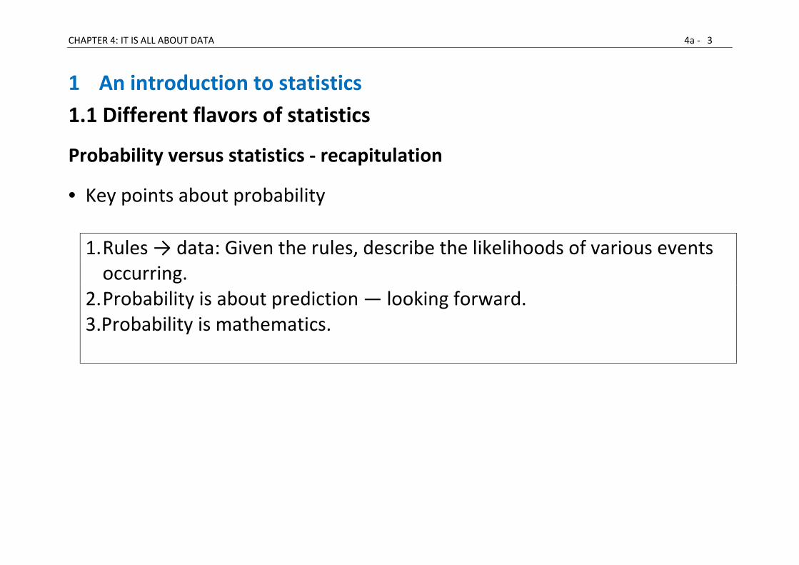
Probability versus statistics - recapitulation

• Key points about probability

1. Rules → data: Given the rules, describe the likelihoods of various events

occurring.

2. Probability is about prediction — looking forward.

3.Probability is mathematics.


• Key points about statistics

1. Rules ← data: Given only the data, try to guess what the rules were. That

is, some probability model controlled what data came out, and the best

we can do is guess — or approximate — what that model was. We might

guess wrong; we might refine our guess as we get more data.

2. Statistics is about looking backward.

3. Statistics is an art. It uses mathematical methods, but it is more than

maths.

4. Once we make our best statistical guess about what the probability

model is (what the rules are), based on looking backward, we can then

use that probability model to predict the future �

The purpose of statistics is to make inference about unknown quantities

from samples of data


(DeCaro, S. A. (2003). A student's guide to the conceptual side of inferential statistics from

http://psychology.sdecnet.com/stathelp.htm.)

Descriptive statistics

• With descriptive statistics we condense a set of known numbers into a few

simple values (either numerically or graphically) to simplify an

understanding of those data that are available to us.

o This is analogous to writing up a summary of a lengthy book. The book

summary is a tool for conveying the gist of a story to others.

o The mean and standard deviation of a set of numbers is a tool for

conveying the gist of the individual numbers (without having to specify

each and every one).


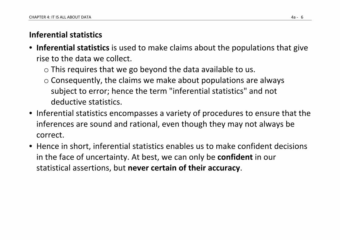
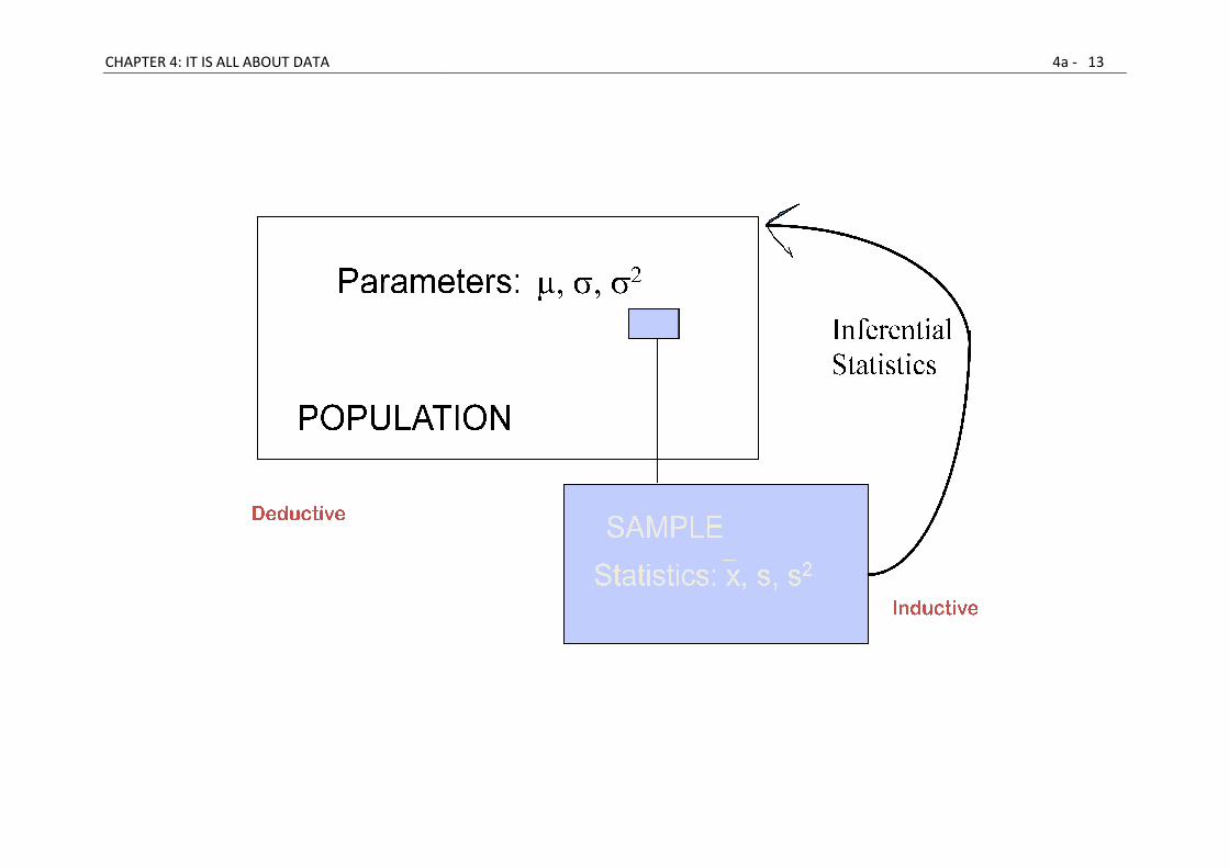
Inferential statistics

• Inferential statistics is used to make claims about the populations that give

rise to the data we collect.

o This requires that we go beyond the data available to us.

o Consequently, the claims we make about populations are always

subject to error; hence the term "inferential statistics" and not

deductive statistics.

• Inferential statistics encompasses a variety of procedures to ensure that the

inferences are sound and rational, even though they may not always be

correct.

• Hence in short, inferential statistics enables us to make confident decisions

in the face of uncertainty. At best, we can only be confident in our

statistical assertions, but never certain of their accuracy.


Relation between descriptive and inferential statistics


Relation between inductive statistics and deductive statistics

• Whereas inductive statistics deal with a limited amount of data,

deductive statistics involve the logical deduction of the sample properties

from knowledge of the population properties (quite similar to

interpolation)


GENERALISATION BASED ON STUDY DATA


1.2 Trying to Understand the True State of Affairs

Parameters and statistics

• The world just happens to be a certain way, regardless of how we view it.

• The phrase "true state of affairs" refers to the real nature of any

phenomenon of interest.

• In statistics, the true state of affairs refers to some quantitative property of

a population. Numeric properties of populations (such as their means,

standard deviations, and sizes) are called parameters. Recall from earlier

chapters that the parameters of a population (say, its mean and standard

deviation) are based on each and every element in that population…

• Samples (or subsets) of populations also have numeric properties, but we

call them statistics.

• Thus, for the scientist using inferential statistics, population parameters

represent the true state of affairs.


• We seldom know the true state of affairs. The process of inferential

statistics consists of making use of the data we do have (observed data) to

make inferences about population parameters.

• Unfortunately, the true state of affairs is also dependent on all of the data

we don't have (unobserved data). Nevertheless, an important aspect of

sample data is that they are actual elements from an underlying population.

In this way, sample data are 'representatives' of the population that gave

rise to them. This implies that sample data can be used to estimate

population parameters.

• Therefore, inferential statistics (both estimating and testing components)

involve inductive reasoning: “from specific towards more general”


Samples and populations

• Since sample data are only representatives, they are not expected to be

perfect estimators. Consider that we necessarily lose information about a

book when we only read a book review. Similarly, we lack information

about a population when we only have access to a subset of that

population.

• It would be useful to have some measure of how reliable (or

representative) our sample data really are. What is the probability of

making an error?

• Obviously, in order to get a better handle on how representative our data

are, we must first consider the sampling process itself: we must first study

how to generate samples from populations, before we can learn to

generalize from samples to populations

• It is in this context that the importance of random and independent

sampling begins to emerge.


4: IT IS ALL ABOUT DATA

4a - 13


1.3 True state of affairs + Chance = Sample data

• Some elements (say, 'heights') in a population are more frequent than

others. These more frequent elements are thus over-represented in the

population compared to less common elements (e.g., the heights of very

short and very tall individuals).

• The laws of chance tell us that it is always possible to randomly select any

element in a population, no matter how rare (or under-represented) that

element may be in the population. If the element exists, then it can be

sampled, plain and simple.

• However, the laws of probability tell us that rare elements are not expected

to be sampled often, given that there are more numerous elements in that

same population. It is the more numerous (or more frequent) elements

that tend to be sampled each time a random and independent sample is

obtained from the population.


Random and independent samples

• A sample is random if all elements in the population are equally eligible to

be sampled, meaning that chance, and chance alone, determines which

elements are included in the sample.

• A sample is independent if the chances of being sampled are not affected

by which elements have already been sampled.

• When the sampling process is truly random and independent, samples are

expected to reflect the most representative elements of the underlying

population.


• Example to illustrate these two ideas

o Imagine that you are interested in the average age of all university

students in the United States.

o For convenience sake, you decide to randomly select one student from

each class offered at your university this term.

o With respect to the original population of interest (all university

students in the U.S.), your sample is not random, because only students

at your university are eligible to be sampled.

o Your sample is also not independent, because once you select a student

from a class, no other student in that class has a chance of being

sampled.

o In this case, any claims you make based on your sample cannot be

applied to the population you are really interested in. At best, you are

only investigating the population of students at one particular

university.


Random digits

• Random numbers can be generated in several standard software packages

or can be retrieved from already existing tables, such as the one below

• How would you use these numbers if you had to select randomly 5 items

from a set of 20?


Important consequence of random and independent sampling

• Chance factors virtually guarantee that sampled data will vary in their

degree of representativeness from sample to sample.

• A rare sample may occur and occurs when, just by chance, a relatively

large number of the extreme (high or low) elements in the population end

up in the sample: the percentage of extreme values in the sample is higher

than the actual percentage in the population

• The logic is to assume that any particular sample mean is typical of the

underlying population. This assumption is reasonable only when the

sampling process is random and independent; otherwise, rare samples

might artificially occur too often.


Sampling error

• Sampling error refers to discrepancies between the statistics of random

samples and the true population values; but this "error" is simply due to

which elements in the population end up in the sample.

• In other words, sampling error refers to natural chance factors, not to

errors of measurement or errors due to poorly designed and poorly

executed experiments!!!

• We have control over the execution of an experiment, but nature imparts a

certain degree of unavoidable error.


• Illustration of sampling error: tossing a fair coin six times and obtaining

{HHHHHH}. We expect a fair coin to land heads 50% of the time, so what

went wrong?

o It turns out there are N = 64 possibilities, but only 20 contain exactly

three heads and three tails. In contrast, there is only one outcome

containing exactly six heads, which makes it a rare (but not impossible)

event.

o Nonetheless, three heads (in any order) is the most frequent element in

this population; it is also the mean.

o It was because of random sampling that we failed to observe one of

these more representative samples, such as {HTHHTT}, not because the

mean of the population isn't really 3…


o The laws of chance combined with the true state of affairs create a

natural force that is always operating on the sampling process.

Consequently, the means of different samples taken from the same

population are expected to vary around the 'true' mean just by chance


The Central-Limit Theorem revisited

• A simple example of the central limit theorem is given by the problem of

rolling a large number of identical dice, each of which is weighted unfairly in

some unknown way. The distribution of the sum (or average) of the rolled

numbers will be well approximated by a normal distribution, the

parameters of which can be determined empirically. • In more general probability theory, “a central limit theorem” is any of a set

of weak-convergence theories: o They all express the fact that a sum of many independent and

identically distributed (i.i.d.) random variables, or alternatively, random

variables with specific types of dependence, will tend to be distributed

according to one of a small set of "attractor" distributions. o When the variance of the i.i.d. variables is finite, the "attractor"

distribution is the normal distribution.


Explanation to the figure

• The sample means are generated using a random number generator, which

draws numbers between 1 and 100 from a uniform probability distribution.

• It illustrates that increasing sample sizes result in the 500 measured sample

means being more closely distribut

case). • The input into the normalized Gaussian function is the mean of sample

means (~50) and the mean sample standard deviation divided by the square

root of the sample size (~28.87/

(since it refers to the spread of sample means).

4: IT IS ALL ABOUT DATA

The sample means are generated using a random number generator, which

draws numbers between 1 and 100 from a uniform probability distribution.

It illustrates that increasing sample sizes result in the 500 measured sample

means being more closely distributed about the population mean (50 in this

The input into the normalized Gaussian function is the mean of sample


root of the sample size (~28.87/ ), i.e. the standard deviation

(since it refers to the spread of sample means).

4a - 24

The sample means are generated using a random number generator, which

draws numbers between 1 and 100 from a uniform probability distribution. It illustrates that increasing sample sizes result in the 500 measured sample

ed about the population mean (50 in this

The input into the normalized Gaussian function is the mean of sample


the standard deviation of the mean


1.4 Sampling Distributions

• A population is the collection of all possible elements that fit into some

category of interest, such as "all adults living in the United States."

• Once we've defined a population, we need to specify with respect to

what?

o For instance, all adults living in the United States with respect to their

height.

o Now the population of interest has shifted from a collection of people

to a collection of numbers (heights, in this case).

o When the elements in the population have been measured or scored in

some way, it is possible to talk about distributions.

• We can generate a distribution of anything, as long as we have values /

scores to work with (cfr tossing a coin and scoring the sample wrt nr of

heads).


• When the distribution of interest consists of all the unique samples of size n

that can be drawn from a population, the resulting distribution of sample

means is called the sampling distribution of the mean.

• There are also sampling distributions of medians, standard deviations, and

any other statistic you can think of.

• In other words, populations, which are distributions of individual elements,

give rise to sampling distributions, which describe how collections of

elements are distributed in the population.

• Note that we have now made a distinction between two distributions:

o the distribution of individual elements (the population) and

o the distribution of all unique samples of a particular size from that

population (the sampling distribution). [A sample is unique if no other

sample in the distribution contains exactly the same elements.]


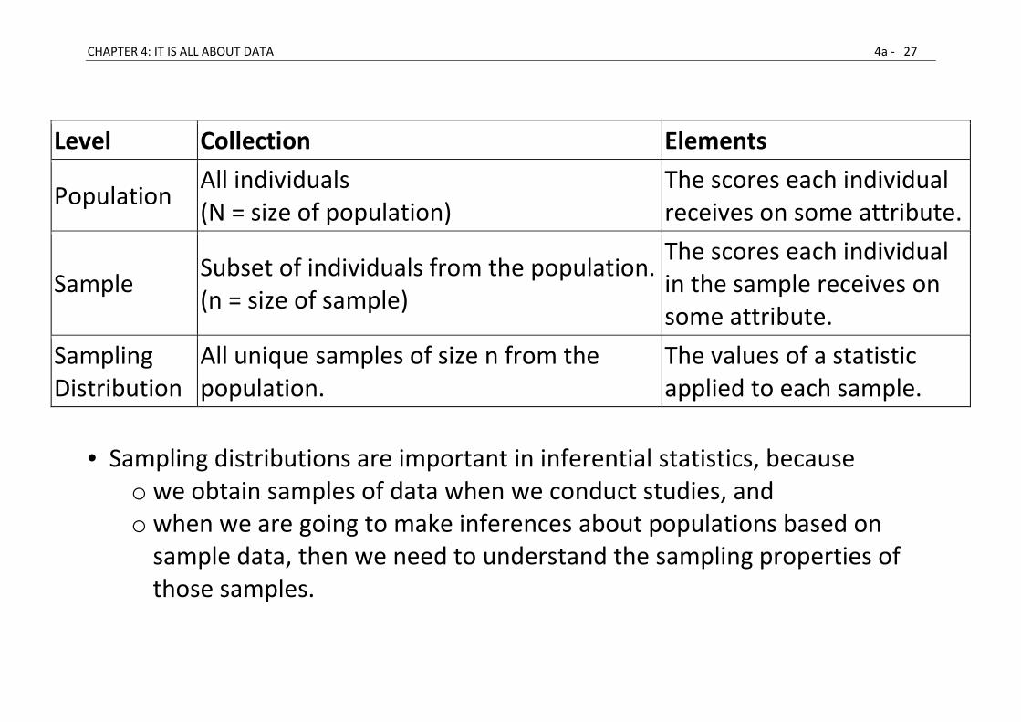
Level Collection Elements

Population All individuals

(N = size of population)

The scores each individual

receives on some attribute.

Sample Subset of individuals from the population.

(n = size of sample)

The scores each individual

in the sample receives on

some attribute.

Sampling

Distribution

All unique samples of size n from the

population.

The values of a statistic

applied to each sample.

• Sampling distributions are important in inferential statistics, because

o we obtain samples of data when we conduct studies, and

o when we are going to make inferences about populations based on

sample data, then we need to understand the sampling properties of

those samples.


• In inferential statistics we make use of two important properties of

sampling distributions (cfr Central Limit Theorem), expressed in lay terms

as:

o The mean of all unique samples of size n (i.e., the average of all the

means) is identical to the mean of the population from which those

samples are drawn. Thus, any claims about the mean of the sampling

distribution apply to the population mean.

o The shape of the sampling distribution increasingly approximates a

normal curve as sample size (n) is increased, even if the original

population is not normally distributed.

• If the original population is itself normally distributed, then the sampling

distribution will be normally distributed even when the sample size is only

one.

o Can you explain this?


Another example: sampling distribution of the sampling proportion


Theoretical sampling distributions

• Unless the details of a population are known in advance, it is not possible to

perfectly describe any of its sampling distributions.

o We would have to first measure all the elements in the population, in

which case we could simply calculate the desired parameter, and then

there would be no point in collecting samples.

• For this reason, a variety of idealized, theoretical sampling distributions

have been described mathematically, including the student t distribution or

the F distribution (see later, Chapter 5-6), which can be used as statistical

models for the real sampling distributions.

• The theoretical sampling distributions can then be used to obtain the

likelihood (or probability) of sampling a particular mean if the mean of the

sampling distribution (and hence the mean of the original population) is

some particular value. The population parameter will first have to be

hypothesized, as the true state of affairs is generally unknown. This is called

the null hypothesis (cfr preview on hypothesis testing + Chapter 6)


Formal definition of a statistic

• Given an independent data set , let

be an estimate of the parameter (describing the population from which

the sample was drawn).

• Repetitions of the same experiment will give different sets of values for

. Hence, itself is a random variable with a certain probability

distribution. This distribution will depend on the functional form of h and of

the underlying random variable X.

• Therefore, we need to write where

are random variables, representing a sample from random variable X (and X

is in this context referred to as the population).

• Assumptions: All are independent AND


Mathematical expression for some popular statistics

• Sample mean:

• Sample variance:

• k-th sample moment:

See practicals to derive expectations and variances of these

new random variables ….


Strategies for variance estimation

• Even with a simple random sampling design, the variance estimation of

some statistics requires non-standard estimating techniques.

o For example, the variance of the median is conspicuously absent

in the standard texts. o The sampling error of a ratio estimator is complicated because both

the numerator and denominator are random variables. • Hence estimating techniques are needed that are sufficiently flexible to

accommodate both the complexities of the sampling design and the

various forms of statistics.


Method 1: replicated sampling

• The essence of this strategy is to facilitate the variance calculation by

selecting a set of replicated subsamples instead of a single sample.

• It requires each subsample to be drawn independently and to use an

identical sample selection design.

• Then an estimate is made in each subsample by the identical process,

and the sampling variance of the overall estimate (based on all subsamples)

can be estimated from the variability of these independent subsample

estimates.


Method 2: Jackknife or bootstrap

• Jackknife and bootstrap approaches are popular when estimating variances

and confidence intervals, but is beyond the scope of this introductory

course

• The jackknife procedure is to estimate the parameter of interest n times,

each time deleting one sample data point. The average of the resulting

estimators, called "pseudovalues”, is the jackknife estimate for the

parameter. For large n, the jackknife estimate is approximately normally

distributed about the true parameter.

• The bootstrap method involves drawing samples repeatedly from the

empirical distribution. So in practice, n samples are drawn with

replacement, from the original n data points. Each time, the parameter of

interest is estimated from the bootstrap sample, and the average over all

bootstrap samples is taken to be the bootstrap estimate of the parameter

of interest.


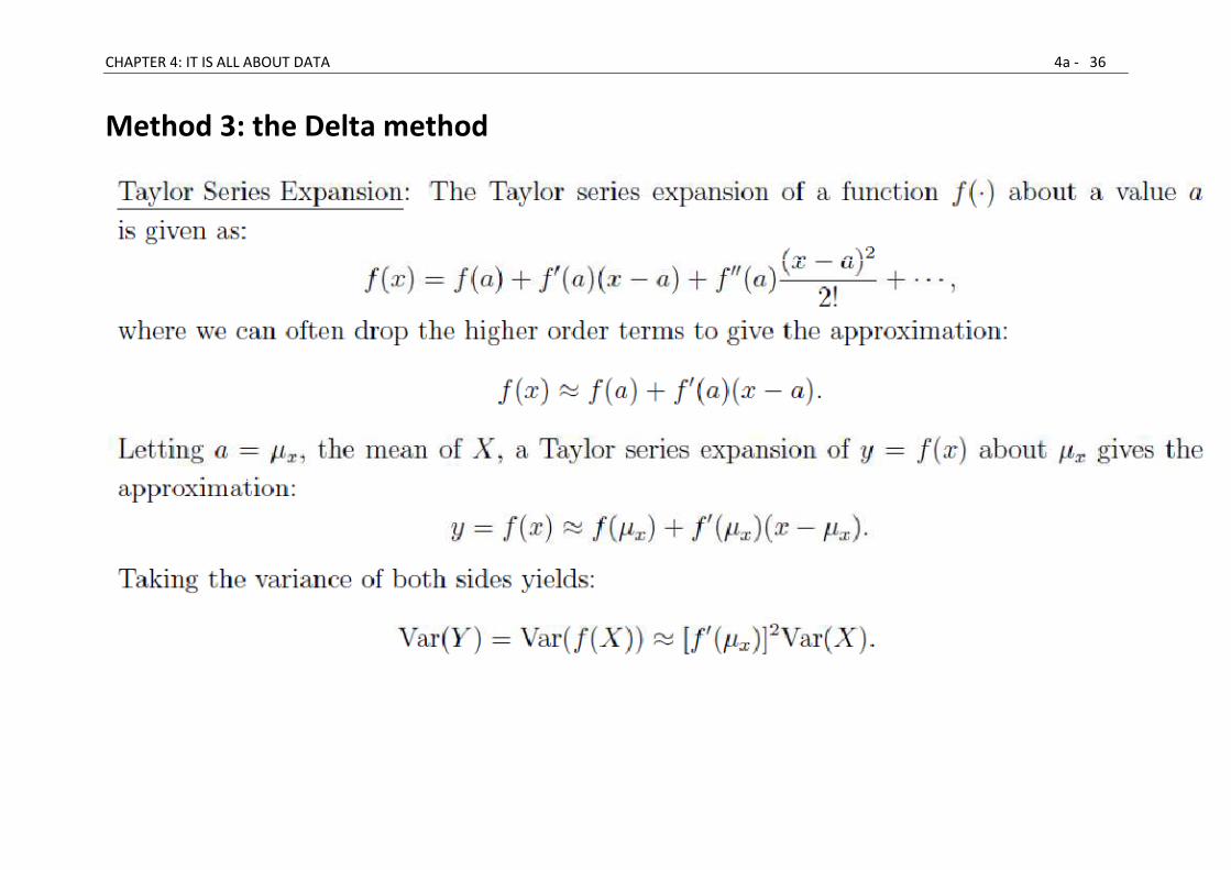
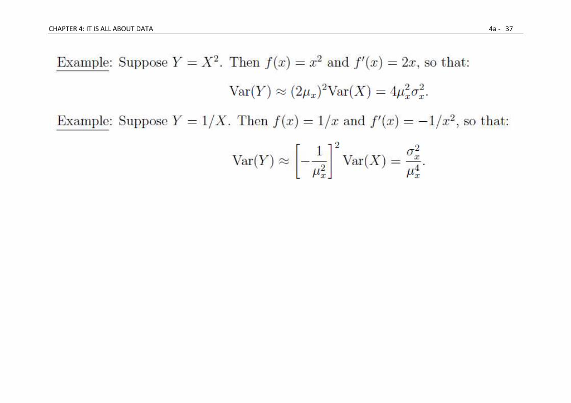
Method 3: the Delta method


Hence the approximate variance of the ratio estimator is

The corresponding estimated variance of the ratio estimator is

Finite population corrections: see section 1.5 of this Chapter


1.5 The Standard Error of the Mean: A Measure of Sampling Error

• Sampling distributions have a standard deviation, which describes the

variability of the sample statistics from their mean (which, remember,

equals the population parameter).

• Sample size determines both the size and the variability of a sampling

distribution

o The number of unique samples that can be drawn from a population

depends on the size of those samples.

o As sample size increases, the variability among all possible sample

means decreases: If all the elements in the original population are

sampled (i.e., if n = N), then there is only one possible sample that can

be obtained (the sample is the population) and the variability of a single

number is zero.


• The standard deviation of a sampling distribution of means is given a

special name: standard error of the mean (often abbreviated as SEM).

• SEM is a measure of sampling error because it describes the variability

among all possible means that could be sampled in an experiment.

• If there is a lot of variability in the sampling distribution (as is the case

when the distribution consists of small samples), then sample means can

vary greatly. On the other hand, if there is little variability in the sampling

distribution (as is the case when the distribution consists of large

samples), then sample means will tend to be very similar, and very close

to the true population mean.

• So the degree of variability in the sampling distribution bears directly on

the degree to which observed results (sample means) are expected to

vary just by chance.


• How can we know whether our sample is representative of the

underlying population?

o Avoid small samples, as there are more extreme (i.e., rare) sample

means in the sampling distribution, and we are more likely to get one of

them in an experiment.

o We have control over sampling error because sample size determines

the standard error (variability) in a sampling distribution.

o In Chapter 6, we will see that sample size is closely connected to the

concept of power: if a specific power is targeted to identify an effect in

a testing strategy, then one can compute the necessary sample size to

achieve the pre-specified power of the test.

o On a practical note: Realize that large samples are not always attainable

and that clever more complicated sample strategies than simple

random sampling need to be followed.


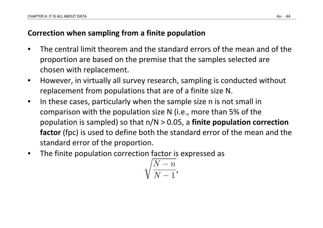
Correction when sampling from a finite population

• The central limit theorem and the standard errors of the mean and of the

proportion are based on the premise that the samples selected are

chosen with replacement.

• However, in virtually all survey research, sampling is conducted without

replacement from populations that are of a finite size N.

• In these cases, particularly when the sample size n is not small in

comparison with the population size N (i.e., more than 5% of the

population is sampled) so that n/N > 0.05, a finite population correction

factor (fpc) is used to define both the standard error of the mean and the

standard error of the proportion. • The finite population correction factor is expressed as

,


• Therefore, when dealing with means, the standard error of the mean for

finite populations is

• When referring to populations, the standard error of the proportion for

finite populations is

• Note that the correction is always smaller than 1, hence reducing the

original uncorrected value.

• As a consequence, more precise estimates are obtained after correction …


1.6 Making Formal Inferences about Populations: Preview to

Hypothesis Testing

• When there are many elements in the sampling distribution, it is always

possible to obtain a rare sample (i.e., one whose mean is very different

from the true population mean).

• The probability of such an outcome occurring just by chance is determined

by the particular sampling distribution specified in the null hypothesis

• When the probability p of the observed sample mean occurring by chance

is really low (typically less than one in 20, e.g., p < .05), the researcher has

an important decision to make regarding the hypothesized true state of

affairs.


• One of two inferences can be made:

1 The hypothesized value of the population mean is correct and a rare

outcome has occurred just by chance (as in the coin-tossing example).

2 The true population mean is probably some other value that is more

consistent with the observed data. Reject the null hypothesis in favor

of some alternative hypothesis.

• The rational decision is to assume #2, because the observed data (which

represent direct, albeit partial, evidence of the true state of affairs), are

just too unlikely if the hypothesized population is true.

• Thus, rather than accept the possibility that a rare event has taken place,

the statistician chooses the more likely possibility that the hypothesized

sampling distribution is wrong.


• However, rare samples do occur, which is why statistical inference is

always subject to error.

o Inferential statistics only helps out to rule out values; it does not tell

us what the population parameters really are. We are inferring the

values based on what they are likely not to be

o Only in the natural sciences does evidence contrary to a hypothesis

lead to rejection of that hypothesis without error.

Probability and Statistics - Montefiore

Documents

Transcript of Probability and Statistics - Montefiore