Probability, random variables. Continuous random variable ...
Upload
hamza-iqbalCategory
view
750download
18
Probability and Random Processes
for Electrical Engineers
John A. Gubner
University of Wisconsin{Madison

Discrete Random Variables
Bernoulli(p)
}(X = 1) = p; }(X = 0) = 1� p.E[X] = p; var(X) = p(1� p); GX(z) = (1� p) + pz.
binomial(n;p)
}(X = k) =
�n
k
�pk(1� p)n�k; k = 0; : : : ; n.
E[X] = np; var(X) = np(1� p); GX(z) = [(1� p) + pz]n.
geometric0(p)
}(X = k) = (1� p)pk; k = 0; 1; 2; : : : :
E[X] =p
1� p; var(X) =
p
(1� p)2; GX (z) =
1� p
1� pz.
geometric1(p)
}(X = k) = (1� p)pk�1; k = 1; 2; 3; : : ::
E[X] =1
1� p; var(X) =
p
(1� p)2; GX (z) =
(1� p)z
1� pz.
negative binomial or Pascal(m;p)
}(X = k) =
�k � 1
m � 1
�(1� p)mpk�m; k = m;m + 1; : : : :
E[X] =m
1� p; var(X) =
mp
(1� p)2; GX (z) =
�(1� p)z
1� pz
�m.
Note that Pascal(1; p) is the same as geometric1(p).
Poisson(�)
}(X = k) =�ke��
k!; k = 0; 1; : : : :
E[X] = �; var(X) = �; GX(z) = e�(z�1).

Fourier Transforms
Fourier Transform
H(f) =
Z 1
�1
h(t)e�j2�ft dt
Inversion Formula
h(t) =
Z 1
�1
H(f)ej2�ft df
h(t) H(f)
I[�T;T ](t) 2Tsin(2� Tf)
2� Tf
2Wsin(2�Wt)
2�WtI[�W;W ](f)
(1� jtj=T )I[�T;T ](t) T
�sin(� Tf)
� Tf
�2
W
�sin(�Wt)
�Wt
�2(1� jf j=W )I[�W;W ](f)
e��tu(t)1
� + j2�f
e��jtj2�
�2 + (2�f)2
�
�2 + t2� e�2��jfj
e�(t=�)2=2p2� � e��
2(2�f)2=2


Preface
Intended Audience
This book contains enough material to serve as a text for a two-coursesequence in probability and random processes for electrical engineers. It is alsouseful as a reference by practicing engineers.
For students with no background in probability and random processes, a�rst course can be o�ered either at the undergraduate level to talented juniorsand seniors, or at the graduate level. The prerequisite is the usual undergrad-uate electrical engineering course on signals and systems, e.g., Haykin and VanVeen [18] or Oppenheim and Willsky [30] (see the Bibliography at the end ofthe book).
A second course can be o�ered at the graduate level. The additional prereq-uisite is some familiarity with linear algebra; e.g., matrix-vector multiplication,determinants, and matrix inverses. Because of the special attention paid tocomplex-valued Gaussian random vectors and related random variables, thetext will be of particular interest to students in wireless communications. Ad-ditionally, the last chapter, which focuses on self-similar processes, long-rangedependence, and aggregation, will be very useful for students in communicationnetworks who are interested modeling Internet tra�c.
Material for a First Course
In a �rst course, Chapters 1{5 would make up the core of any o�ering. Thesechapters cover the basics of probability and discrete and continuous randomvariables. Following Chapter 5, additional topics such as wide-sense stationaryprocesses (Sections 6.1{6.5), the Poisson process (Section 8.1), discrete-timeMarkov chains (Section 9.1), and con�dence intervals (Sections 12.1{12.4) canalso be included. These topics can be covered independently of each other, inany order, except that Problem 15 in Chapter 12 refers to the Poisson process.
Material for a Second Course
In a second course, Chapters 7{8 and 10{11 would make up the core, withadditional material from Chapters 6, 9, 12, and 13 depending on student prepa-ration and course objectives. For review purposes, it may be helpful at the be-ginning of the course to assign the more advanced problems from Chapters 1{5that are marked with a ?.
Features
Those parts of the book mentioned above as being suitable for a �rst courseare written at a level appropriate for undergraduates. More advanced problemsand sections in these parts of the book are indicated by a ?. Those parts of thebook not indicated as suitable for a �rst course are written at a level suitable
iii

iv Preface
for graduate students. Throughout the text, there are numerical superscriptsthat refer to notes at the end of each chapter. These notes are usually rathertechnical and address subtleties of the theory.
The last section of each chapter is devoted to problems. The problems areseparated by section so that all problems relating to a particular section areclearly indicated. This enables the student to refer to the appropriate partof the text for background relating to particular problems, and it enables theinstructor to make up assignments more quickly.
Tables of discrete random variables and of Fourier transform pairs are foundinside the front cover. A table of continuous random variables is found insidethe back cover.
When cdfs or other functions are encountered that do not have a closed form,Matlab commands are given for computing them. For a list, see \Matlab" inthe index.
The index was compiled as the book was being written. Hence, there aremany pointers to speci�c information. For example, see \noncentral chi-squaredrandom variable."
With the importance of wireless communications, it is vital for students tobe comfortable with complex random variables, especially complex Gaussianrandom variables. Hence, Section 7.5 is devoted to this topic, with specialattention to the circularly symmetric complex Gaussian. Also important in thisregard are the central and noncentral chi-squared random variables and theirsquare roots, the Rayleigh and Rice random variables. These random variables,as well as related ones such as the beta, F , Nakagami, and student's t, appearin numerous problems in Chapters 3{5 and 7.
Chapter 10 gives an extensive treatment of convergence in mean of orderp. Special attention is given to mean-square convergence and the Hilbert spaceof square-integrable random variables. This allows us to prove the projectiontheorem, which is important for establishing the existence of certain estimators,and conditional expectation in particular. The Hilbert space setting allows usto de�ne the Wiener integral, which is used in Chapter 13 on advanced topicsto construct fractional Brownian motion.
We give an extensive treatment of con�dence intervals in Chapter 12, notonly for normal data, but also for more arbitrary data via the central limittheorem. The latter is important for any situation in which the data is notnormal; e.g., sampling for quality control, election polls, etc. Much of thismaterial can be covered in a �rst course. However, the last subsection onderivations is more advanced, and uses results from Chapter 7 on Gaussianrandom vectors.
With the increasing use of self-similar and long-range dependent processesfor modeling Internet tra�c, we provide in Chapter 13 an introduction to thesedevelopments. In particular, fractional Brownian motion is a standard exampleof a continuous-time self-similar process with stationary increments. Fractionalautoregressive integrated moving average (FARIMA) processes are developedas examples of important discrete-time processes in this context.
July 19, 2002

Table of Contents
1 Introduction to Probability 1
1.1 Review of Set Notation : : : : : : : : : : : : : : : : : : : : : : : 21.2 Probability Models : : : : : : : : : : : : : : : : : : : : : : : : : : 51.3 Axioms and Properties of Probability : : : : : : : : : : : : : : : 12
Consequences of the Axioms : : : : : : : : : : : : : : : : : : : 121.4 Independence : : : : : : : : : : : : : : : : : : : : : : : : : : : : : 16
Independence for More Than Two Events : : : : : : : : : : : : 161.5 Conditional Probability : : : : : : : : : : : : : : : : : : : : : : : 19
The Law of Total Probability and Bayes' Rule : : : : : : : : : 191.6 Notes : : : : : : : : : : : : : : : : : : : : : : : : : : : : : : : : : 221.7 Problems : : : : : : : : : : : : : : : : : : : : : : : : : : : : : : : 24
2 Discrete Random Variables 33
2.1 Probabilities Involving Random Variables : : : : : : : : : : : : : 33Discrete Random Variables : : : : : : : : : : : : : : : : : : : : 36Integer-Valued Random Variables : : : : : : : : : : : : : : : : 36Pairs of Random Variables : : : : : : : : : : : : : : : : : : : : 38Multiple Independent Random Variables : : : : : : : : : : : : 39Probability Mass Functions : : : : : : : : : : : : : : : : : : : : 42
2.2 Expectation : : : : : : : : : : : : : : : : : : : : : : : : : : : : : : 44Expectation of Functions of Random Variables, or the Law of
the Unconscious Statistician (LOTUS) : : : : : : : : : : : 47?Derivation of LOTUS : : : : : : : : : : : : : : : : : : : : : : 47Linearity of Expectation : : : : : : : : : : : : : : : : : : : : : 48Moments : : : : : : : : : : : : : : : : : : : : : : : : : : : : : : 49Probability Generating Functions : : : : : : : : : : : : : : : : 50Expectations of Products of Functions of Independent Ran-
dom Variables : : : : : : : : : : : : : : : : : : : : : : : : 52Binomial Random Variables and Combinations : : : : : : : : : 54Poisson Approximation of Binomial Probabilities : : : : : : : 57
2.3 The Weak Law of Large Numbers : : : : : : : : : : : : : : : : : : 57Uncorrelated Random Variables : : : : : : : : : : : : : : : : : 58Markov's Inequality : : : : : : : : : : : : : : : : : : : : : : : : 60Chebyshev's Inequality : : : : : : : : : : : : : : : : : : : : : : 60Conditions for the Weak Law : : : : : : : : : : : : : : : : : : 61
2.4 Conditional Probability : : : : : : : : : : : : : : : : : : : : : : : 62The Law of Total Probability : : : : : : : : : : : : : : : : : : 63The Substitution Law : : : : : : : : : : : : : : : : : : : : : : : 66
2.5 Conditional Expectation : : : : : : : : : : : : : : : : : : : : : : : 69Substitution Law for Conditional Expectation : : : : : : : : : 70Law of Total Probability for Expectation : : : : : : : : : : : : 70
v
vi Table of Contents
2.6 Notes : : : : : : : : : : : : : : : : : : : : : : : : : : : : : : : : : 722.7 Problems : : : : : : : : : : : : : : : : : : : : : : : : : : : : : : : 74
3 Continuous Random Variables 85
3.1 De�nition and Notation : : : : : : : : : : : : : : : : : : : : : : : 85The Paradox of Continuous Random Variables : : : : : : : : : 90
3.2 Expectation of a Single Random Variable : : : : : : : : : : : : : 90Moment Generating Functions : : : : : : : : : : : : : : : : : : 94Characteristic Functions : : : : : : : : : : : : : : : : : : : : : 96
3.3 Expectation of Multiple Random Variables : : : : : : : : : : : : 98Linearity of Expectation : : : : : : : : : : : : : : : : : : : : : 99Expectations of Products of Functions of Independent Ran-
dom Variables : : : : : : : : : : : : : : : : : : : : : : : : 993.4 ?Probability Bounds : : : : : : : : : : : : : : : : : : : : : : : : : 1003.5 Notes : : : : : : : : : : : : : : : : : : : : : : : : : : : : : : : : : 1033.6 Problems : : : : : : : : : : : : : : : : : : : : : : : : : : : : : : : 104
4 Analyzing Systems with Random Inputs 117
4.1 Continuous Random Variables : : : : : : : : : : : : : : : : : : : : 118?The Normal CDF and the Error Function : : : : : : : : : : : 123
4.2 Reliability : : : : : : : : : : : : : : : : : : : : : : : : : : : : : : : 1234.3 Cdfs for Discrete Random Variables : : : : : : : : : : : : : : : : 1264.4 Mixed Random Variables : : : : : : : : : : : : : : : : : : : : : : 1274.5 Functions of Random Variables and Their Cdfs : : : : : : : : : : 1304.6 Properties of Cdfs : : : : : : : : : : : : : : : : : : : : : : : : : : 1344.7 The Central Limit Theorem : : : : : : : : : : : : : : : : : : : : : 137
Derivation of the Central Limit Theorem : : : : : : : : : : : : 1394.8 Problems : : : : : : : : : : : : : : : : : : : : : : : : : : : : : : : 142
5 Multiple Random Variables 155
5.1 Joint and Marginal Probabilities : : : : : : : : : : : : : : : : : : 155Product Sets and Marginal Probabilities : : : : : : : : : : : : 155Joint and Marginal Cumulative Distributions : : : : : : : : : : 157
5.2 Jointly Continuous Random Variables : : : : : : : : : : : : : : : 158Marginal Densities : : : : : : : : : : : : : : : : : : : : : : : : 159Specifying Joint Densities : : : : : : : : : : : : : : : : : : : : 162Independence : : : : : : : : : : : : : : : : : : : : : : : : : : : 163Expectation : : : : : : : : : : : : : : : : : : : : : : : : : : : : 163?Continuous Random Variables That Are not Jointly Contin-
uous : : : : : : : : : : : : : : : : : : : : : : : : : : : : : : 1645.3 Conditional Probability and Expectation : : : : : : : : : : : : : : 1645.4 The Bivariate Normal : : : : : : : : : : : : : : : : : : : : : : : : 1685.5 ?Multivariate Random Variables : : : : : : : : : : : : : : : : : : 172
The Law of Total Probability : : : : : : : : : : : : : : : : : : 1755.6 Notes : : : : : : : : : : : : : : : : : : : : : : : : : : : : : : : : : 177
July 19, 2002

Table of Contents vii
5.7 Problems : : : : : : : : : : : : : : : : : : : : : : : : : : : : : : : 178
6 Introduction to Random Processes 185
6.1 Mean, Correlation, and Covariance : : : : : : : : : : : : : : : : : 1886.2 Wide-Sense Stationary Processes : : : : : : : : : : : : : : : : : : 189
Strict-Sense Stationarity : : : : : : : : : : : : : : : : : : : : : 189Wide-Sense Stationarity : : : : : : : : : : : : : : : : : : : : : 191Properties of Correlation Functions and Power Spectral Den-
sities : : : : : : : : : : : : : : : : : : : : : : : : : : : : : : 1936.3 WSS Processes through Linear Time-Invariant Systems : : : : : 1956.4 The Matched Filter : : : : : : : : : : : : : : : : : : : : : : : : : : 1996.5 The Wiener Filter : : : : : : : : : : : : : : : : : : : : : : : : : : 201
?Causal Wiener Filters : : : : : : : : : : : : : : : : : : : : : : 2036.6 ?Expected Time-Average Power and the Wiener{
Khinchin Theorem : : : : : : : : : : : : : : : : : : : : : : : : : : 206Mean-Square Law of Large Numbers for WSS Processes : : : 208
6.7 ?Power Spectral Densities for non-WSS Processes : : : : : : : : : 210Derivation of (6.22) : : : : : : : : : : : : : : : : : : : : : : : : 211
6.8 Notes : : : : : : : : : : : : : : : : : : : : : : : : : : : : : : : : : 2126.9 Problems : : : : : : : : : : : : : : : : : : : : : : : : : : : : : : : 214
7 Random Vectors 223
7.1 Mean Vector, Covariance Matrix, and Characteristic Function : : 2237.2 The Multivariate Gaussian : : : : : : : : : : : : : : : : : : : : : : 226
The Characteristic Function of a Gaussian Random Vector : : 227For Gaussian RandomVectors, Uncorrelated Implies Indepen-
dent : : : : : : : : : : : : : : : : : : : : : : : : : : : : : : 228The Density Function of a Gaussian Random Vector : : : : : 229
7.3 Estimation of Random Vectors : : : : : : : : : : : : : : : : : : : 230Linear Minimum Mean Squared Error Estimation : : : : : : : 230MinimumMean Squared Error Estimation : : : : : : : : : : : 233
7.4 Transformations of Random Vectors : : : : : : : : : : : : : : : : 2347.5 Complex Random Variables and Vectors : : : : : : : : : : : : : : 236
Complex Gaussian Random Vectors : : : : : : : : : : : : : : : 2387.6 Notes : : : : : : : : : : : : : : : : : : : : : : : : : : : : : : : : : 2397.7 Problems : : : : : : : : : : : : : : : : : : : : : : : : : : : : : : : 240
8 Advanced Concepts in Random Processes 249
8.1 The Poisson Process : : : : : : : : : : : : : : : : : : : : : : : : : 249?Derivation of the Poisson Probabilities : : : : : : : : : : : : : 253Marked Poisson Processes : : : : : : : : : : : : : : : : : : : : 255Shot Noise : : : : : : : : : : : : : : : : : : : : : : : : : : : : : 256
8.2 Renewal Processes : : : : : : : : : : : : : : : : : : : : : : : : : : 2568.3 The Wiener Process : : : : : : : : : : : : : : : : : : : : : : : : : 257
Integrated White-Noise Interpretation of the Wiener Process : 258
July 19, 2002
viii Table of Contents
The Problem with White Noise : : : : : : : : : : : : : : : : : 260The Wiener Integral : : : : : : : : : : : : : : : : : : : : : : : : 260Random Walk Approximation of the Wiener Process : : : : : 261
8.4 Speci�cation of Random Processes : : : : : : : : : : : : : : : : : 263Finitely Many Random Variables : : : : : : : : : : : : : : : : 263In�nite Sequences (Discrete Time) : : : : : : : : : : : : : : : : 266Continuous-Time Random Processes : : : : : : : : : : : : : : 269
8.5 Notes : : : : : : : : : : : : : : : : : : : : : : : : : : : : : : : : : 2708.6 Problems : : : : : : : : : : : : : : : : : : : : : : : : : : : : : : : 270
9 Introduction to Markov Chains 279
9.1 Discrete-Time Markov Chains : : : : : : : : : : : : : : : : : : : : 279State Space and Transition Probabilities : : : : : : : : : : : : 281Examples : : : : : : : : : : : : : : : : : : : : : : : : : : : : : : 282Stationary Distributions : : : : : : : : : : : : : : : : : : : : : 284Derivation of the Chapman{Kolmogorov Equation : : : : : : : 287Stationarity of the n-step Transition Probabilities : : : : : : : 288
9.2 Continuous-Time Markov Chains : : : : : : : : : : : : : : : : : : 289Kolmogorov's Di�erential Equations : : : : : : : : : : : : : : : 291Stationary Distributions : : : : : : : : : : : : : : : : : : : : : 294
9.3 Problems : : : : : : : : : : : : : : : : : : : : : : : : : : : : : : : 294
10 Mean Convergence and Applications 299
10.1 Convergence in Mean of Order p : : : : : : : : : : : : : : : : : : 29910.2 Normed Vector Spaces of Random Variables : : : : : : : : : : : : 30310.3 The Wiener Integral (Again) : : : : : : : : : : : : : : : : : : : : 30710.4 Projections, Orthonality Principle, Projection Theorem : : : : : 30810.5 Conditional Expectation : : : : : : : : : : : : : : : : : : : : : : : 311
Notation : : : : : : : : : : : : : : : : : : : : : : : : : : : : : : 31310.6 The Spectral Representation : : : : : : : : : : : : : : : : : : : : : 31310.7 Notes : : : : : : : : : : : : : : : : : : : : : : : : : : : : : : : : : 31610.8 Problems : : : : : : : : : : : : : : : : : : : : : : : : : : : : : : : 316
11 Other Modes of Convergence 323
11.1 Convergence in Probability : : : : : : : : : : : : : : : : : : : : : 32411.2 Convergence in Distribution : : : : : : : : : : : : : : : : : : : : : 32511.3 Almost Sure Convergence : : : : : : : : : : : : : : : : : : : : : : 330
The Skorohod Representation Theorem : : : : : : : : : : : : : 33511.4 Notes : : : : : : : : : : : : : : : : : : : : : : : : : : : : : : : : : 33711.5 Problems : : : : : : : : : : : : : : : : : : : : : : : : : : : : : : : 337
12 Parameter Estimation and Con�dence Intervals 345
12.1 The Sample Mean : : : : : : : : : : : : : : : : : : : : : : : : : : 34512.2 Con�dence Intervals When the Variance Is Known : : : : : : : : 34712.3 The Sample Variance : : : : : : : : : : : : : : : : : : : : : : : : : 34912.4 Con�dence Intervals When the Variance Is Unknown : : : : : : : 350
July 19, 2002

Table of Contents ix
Applications : : : : : : : : : : : : : : : : : : : : : : : : : : : : 351Sampling with and without Replacement : : : : : : : : : : : : 352
12.5 Con�dence Intervals for Normal Data : : : : : : : : : : : : : : : 353Estimating the Mean : : : : : : : : : : : : : : : : : : : : : : : 353Limiting t Distribution : : : : : : : : : : : : : : : : : : : : : : 355Estimating the Variance | Known Mean : : : : : : : : : : : : 355Estimating the Variance | Unknown Mean : : : : : : : : : : 357?Derivations : : : : : : : : : : : : : : : : : : : : : : : : : : : : 358
12.6 Notes : : : : : : : : : : : : : : : : : : : : : : : : : : : : : : : : : 36012.7 Problems : : : : : : : : : : : : : : : : : : : : : : : : : : : : : : : 362
13 Advanced Topics 365
13.1 Self Similarity in Continuous Time : : : : : : : : : : : : : : : : : 365Implications of Self Similarity : : : : : : : : : : : : : : : : : : 366Stationary Increments : : : : : : : : : : : : : : : : : : : : : : : 367Fractional Brownian Motion : : : : : : : : : : : : : : : : : : : 368
13.2 Self Similarity in Discrete Time : : : : : : : : : : : : : : : : : : : 369Convergence Rates for the Mean-Square Law of Large Num-
bers : : : : : : : : : : : : : : : : : : : : : : : : : : : : : : 370Aggregation : : : : : : : : : : : : : : : : : : : : : : : : : : : : 371The Power Spectral Density : : : : : : : : : : : : : : : : : : : 373Notation : : : : : : : : : : : : : : : : : : : : : : : : : : : : : : 374
13.3 Asymptotic Second-Order Self Similarity : : : : : : : : : : : : : : 37513.4 Long-Range Dependence : : : : : : : : : : : : : : : : : : : : : : : 38013.5 ARMA Processes : : : : : : : : : : : : : : : : : : : : : : : : : : : 38313.6 ARIMA Processes : : : : : : : : : : : : : : : : : : : : : : : : : : 38413.7 Problems : : : : : : : : : : : : : : : : : : : : : : : : : : : : : : : 387
Bibliography 393
Index 397
July 19, 2002

x Table of Contents
July 19, 2002

CHAPTER 1
Introduction to Probability
If we toss a fair coin many times, then we expect that the fraction of headsshould be close to 1=2, and we say that 1=2 is the \probability of heads." Infact, we might try to de�ne the probability of heads to be the limiting valueof the fraction of heads as the total number of tosses tends to in�nity. Thedi�culty with this approach is that there is no simple way to guarantee thatthe desired limit exists.
An alternative approach was developed by A. N. Kolmogorov in 1933.Kolmogorov's idea was to start with an axiomatic de�nition of probability andthen deduce results logically as consequences of the axioms. One of the successesof Kolmogorov's approach is that under suitable assumptions, it can be provedthat the fraction of heads in a sequence of tosses of a fair coin converges to1=2 as the number of tosses increases. You will meet a simple version of thisresult in the weak law of large numbers in Chapter 2. Generally speaking,a law of large numbers is a theorem that gives conditions under which thenumerical average of a large number of measurements converges in some senseto a probability or other parameter speci�ed by the underlying mathematicalmodel. Other laws of large numbers are discussed in Chapters 10 and 11.
Another celebrated limit result of probability theory is the central limittheorem, which you will meet in Chapter 4. The central limit theorem saysthat when you add up a large number of random perturbations, the overalle�ect has a Gaussian or normal distribution. For example, the central limittheorem explains why thermal noise in ampli�ers has a Gaussian distribution.The central limit theorem also accounts for the fact that the speed of a particlein an ideal gas has the Maxwell distribution.
In addition to the more famous results mentioned above, in this book youwill learn the \tools of the trade" of probability and random processes. Theseinclude probability mass functions and densities, expectation, transform meth-ods, random processes, �ltering of processes by linear time-invariant systems,and more.
Since probability theory relies heavily on the use of set notation and settheory, a brief review of these topics is given in Section 1.1. In Section 1.2, weconsider a number of simple physical experiments, and we construct mathemat-ical probability models for them. These models are used to solve several sampleproblems. Motivated by our speci�c probability models, in Section 1.3, we in-troduce the general axioms of probability and several of their consequences.The concepts of statistical independence and conditional probability are intro-duced in Sections 1.4 and 1.5, respectively. Section 1.6 contains the notes thatare referenced in the text by numerical superscripts. These notes are usuallyrather technical and can be skipped by the beginning student. However, the
1

2 Chap. 1 Introduction to Probability
notes provide a more in-depth discussion of certain topics that may be of in-terest to more advanced readers. The chapter concludes with problems for thereader to solve. Problems and sections marked by a ? are intended for moreadvanced readers.
1.1. Review of Set NotationLet be a set of points. If ! is a point in , we write ! 2 . Let A and B
be two collections of points in . If every point in A also belongs to B, we saythat A is a subset of B, and we denote this by writing A � B. If A � B andB � A, then we write A = B; i.e., two sets are equal if they contain exactlythe same points.
Set relationships can be represented graphically in Venn diagrams. Inthese pictures, the whole space is represented by a rectangular region, andsubsets of are represented by disks or oval-shaped regions. For example, inFigure 1.1(a), the disk A is completely contained in the oval-shaped region B,thus depicting the relation A � B.
If A � , and ! 2 does not belong to A, we write ! =2 A. The set of allsuch ! is called the complement of A in ; i.e.,
Ac := f! 2 : ! =2 Ag:This is illustrated in Figure 1.1(b), in which the shaded region is the complementof the disk A.
The empty set or null set of is denoted by 6 ; it contains no points of. Note that for any A � , 6 � A. Also, c = 6 .
( a )
A B A
Ac
( b )
Figure 1.1. (a) Venn diagram of A � B. (b) The complement of the disk A, denoted byAc, is the shaded part of the diagram.
The union of two subsets A and B is
A [B := f! 2 : ! 2 A or ! 2 Bg:Here \or" is inclusive; i.e., if ! 2 A [B, we permit ! to belong to either A orB or both. This is illustrated in Figure 1.2(a), in which the shaded region isthe union of the disk A and the oval-shaped region B.
The intersection of two subsets A and B is
A \B := f! 2 : ! 2 A and ! 2 Bg;
July 18, 2002

1.1 Review of Set Notation 3
hence, ! 2 A \B if and only if ! belongs to both A and B. This is illustratedin Figure 1.2(b), in which the shaded area is the intersection of the disk A andthe oval-shaped region B. The reader should also note the following specialcase. If A � B (recall Figure 1.1(a)), then A\B = A. In particular, we alwayshave A \ = A.
B
( a )
A A B
( b )
Figure 1.2. (a) The shaded region is A [B. (b) The shaded region is A \B.
The set di�erence operation is de�ned by
B nA := B \Ac;
i.e., B nA is the set of ! 2 B that do not belong to A. In Figure 1.3(a), B nAis the shaded part of the oval-shaped region B.
Two subsets A and B are disjoint or mutually exclusive if A \B = 6 ;i.e., there is no point in that belongs to both A and B. This condition isdepicted in Figure 1.3(b).
BA
( a ) ( b )
B
A
Figure 1.3. (a) The shaded region is B n A. (b) Venn diagram of disjoint sets A and B.
Using the preceding de�nitions, it is easy to see that the following propertieshold for subsets A;B, and C of .
The commutative laws are
A [B = B [A and A \B = B \A:The associative laws are
A \ (B \C) = (A \B) \ C and A [ (B [ C) = (A [B) [C:
July 18, 2002

4 Chap. 1 Introduction to Probability
The distributive laws are
A \ (B [C) = (A \B) [ (A \C)and
A [ (B \C) = (A [B) \ (A [C):DeMorgan's laws are
(A \B)c = Ac [Bc and (A [B)c = Ac \Bc:
We next consider in�nite collections of subsets of . Suppose An � ,n = 1; 2; : : : : Then
1[n=1
An := f! 2 : ! 2 An for some n � 1g:
In other words, ! 2 S1n=1An if and only if for at least one integer n � 1,
! 2 An. This de�nition admits the possibility that ! 2 An for more than onevalue of n. Next, we de�ne
1\n=1
An := f! 2 : ! 2 An for all n � 1g:
In other words, ! 2 T1n=1An if and only if ! 2 An for every positive integer n.
Example 1.1. Let denote the real numbers, = (�1;1). Then thefollowing in�nite intersections and unions can be simpli�ed. Consider the in-tersection 1\
n=1
(�1; 1=n) = f! : ! < 1=n; for all n � 1g:
Now, if ! < 1=n for all n � 1, then ! cannot be positive; i.e., we must have! � 0. Conversely, if ! � 0, then for all n � 1, ! � 0 < 1=n. It follows that
1\n=1
(�1; 1=n) = (�1; 0]:
Consider the in�nite union,
1[n=1
(�1;�1=n] = f! : ! � �1=n; for some n � 1g:
Now, if ! � �1=n for some n � 1, then we must have ! < 0. Conversely, if! < 0, then for large enough n, ! � �1=n. Thus,
1[n=1
(�1;�1=n] = (�1; 0):
July 18, 2002
1.2 Probability Models 5
In a similar way, one can show that
1\n=1
[0; 1=n) = f0g;
as well as
1[n=1
(�1; n] = (�1;1) and1\n=1
(�1;�n] = 6 :
The following generalized distributive laws also hold,
B \� 1[n=1
An
�=
1[n=1
(B \An);
and
B [� 1\n=1
An
�=
1\n=1
(B [An):
We also have the generalized DeMorgan's laws,� 1\n=1
An
�c=
1[n=1
Acn;
and � 1[n=1
An
�c=
1\n=1
Acn:
Finally, we will need the following de�nition. We say that subsets An; n =1; 2; : : : ; are pairwise disjoint if An \Am = 6 for all n 6= m.
1.2. Probability ModelsConsider the experiment of tossing a fair die and measuring, i.e., noting,
the face turned up. Our intuition tells us that the \probability" of the ith faceturning up is 1=6, and that the \probability" of a face with an even number ofdots turning up is 1=2.
Here is a mathematical model for this experiment and measurement. Let be any set containing six points. We call the sample space. Each pointin corresponds to, or models, a possible outcome of the experiment. Forsimplicity, let
:= f1; 2; 3; 4;5; 6g:Now put
Fi := fig; i = 1; 2; 3; 4;5; 6;
July 18, 2002

6 Chap. 1 Introduction to Probability
andE := f2; 4; 6g:
We call the sets Fi and E events. The event Fi corresponds to, or models, thedie's turning up showing the ith face. Similarly, the event E models the die'sshowing a face with an even number of dots. Next, for every subset A of , wedenote the number of points in A by jAj. We call jAj the cardinality of A. Wede�ne the probability of any event A by
}(A) := jAj=jj:It then follows that }(Fi) = 1=6 and }(E) = 3=6 = 1=2, which agrees with ourintuition.
We now make four observations about our model:
(i) }(6 ) = j6 j=jj = 0=jj = 0.(ii) }(A) � 0 for every event A.(iii) If A and B are mutually exclusive events, i.e., A \B = 6 , then }(A [
B) = }(A) +}(B); for example, F3 \ E = 6 , and it is easy to checkthat }(F3 [E) = }(f2; 3; 4; 6g) = }(F3) +}(E).
(iv) When the die is tossed, something happens; this is modeled mathemat-ically by the easily veri�ed fact that }() = 1.
As we shall see, these four properties hold for all the models discussed in thissection.
We next modify our model to accommodate an unfair die as follows. Observethat for a fair die,�
}(A) =jAjjj =
X!2A
1
jj =X!2A
p(!);
where p(!) := 1=jj. For an unfair die, we rede�ne } by taking
}(A) :=X!2A
p(!);
where now p(!) is not constant, but is chosen to re ect the likelihood of occur-rence of the various faces. This new de�nition of } still satis�es (i) and (iii);however, to guarantee that (ii) and (iv) still hold, we must require that p benonnegative and sum to one, or, in symbols, p(!) � 0 and
P!2 p(!) = 1.
Example 1.2. Consider a die for which face i is twice as likely as face i�1.Find the probability of the die's showing a face with an even number of dots.
Solution. To solve the problem, we use the above modi�ed probabilitymodel withy p(!) = 2!�1=63. We then need to realize that we are being askedto compute }(E), where E = f2; 4; 6g. Hence,
}(E) = [21 + 23 + 25]=63 = 42=63 = 2=3:
�If A = 6 , the summation is always taken to be zero.yThe derivation of this formula appears in Problem 8.
July 18, 2002

1.2 Probability Models 7
This problem is typical of the kinds of \word problems" to which probabilitytheory is applied to analyze well-de�ned physical experiments. The applicationof probability theory requires the modeler to take the following steps:
1. Select a suitable sample space .2. De�ne }(A) for all events A.3. Translate the given \word problem" into a problem requiring the calcu-
lation of }(E) for some speci�c event E.
The following example gives a family of constructions that can be used tomodel experiments having a �nite number of possible outcomes.
Example 1.3. Let M be a positive integer, and put := f1; 2; : : :;Mg.Next, let p(1); : : : ; p(M ) be nonnegative real numbers such that
PM!=1 p(!) = 1.
For any subset A � , put
}(A) :=X!2A
p(!):
In particular, to model equally likely outcomes, or equivalently, outcomes thatoccur \at random," we take p(!) = 1=M . In this case, }(A) reduces to jAj=jj.
Example 1.4. A single card is drawn at random from a well-shu�ed deckof playing cards. Find the probability of drawing an ace. Also �nd the proba-bility of drawing a face card.
Solution. The �rst step in the solution is to specify the sample space and the probability }. Since there are 52 possible outcomes, we take :=f1; : : : ; 52g. Each integer corresponds to one of the cards in the deck. To specify}, we must de�ne }(E) for all events E � . Since all cards are equally likelyto be drawn, we put }(E) := jEj=jj.
To �nd the desired probabilities, let 1; 2; 3; 4 correspond to the four aces, andlet 41; : : : ; 52 correspond to the 12 face cards. We identify the drawing of an acewith the event A := f1; 2; 3; 4g, and we identify the drawing of a face card withthe event F := f41; : : : ; 52g. It then follows that }(A) = jAj=52 = 4=52 = 1=13and }(F ) = jF j=52 = 12=52 = 3=13.
While the sample spaces in Example 1.3 can model any experiment witha �nite number of outcomes, it is often convenient to use alternative samplespaces.
Example 1.5. Suppose that we have two well-shu�ed decks of cards, andwe draw one card at random from each deck. What is the probability of drawingthe ace of spades followed by the jack of hearts? What is the probability ofdrawing an ace and a jack (in either order)?
July 18, 2002

8 Chap. 1 Introduction to Probability
Solution. The �rst step in the solution is to specify the sample space and the probability }. Since there are 52 possibilities for each draw, there are522 = 2,704 possible outcomes when drawing two cards. Let D := f1; : : : ; 52g,and put
:= f(i; j) : i; j 2 Dg:Then jj = jDj2 = 522 = 2,704 as required. Since all pairs are equally likely,we put }(E) := jEj=jj for arbitrary events E � .
As in the preceding example, we denote the aces by 1; 2; 3; 4. We let 1 denotethe ace of spades. We also denote the jacks by 41; 42; 43; 44, and the jack ofhearts by 42. The drawing of the ace of spades followed by the jack of heartsis identi�ed with the event
A := f(1; 42)g;
and so }(A) = 1=2,704 � 0:000370. The drawing of an ace and a jack isidenti�ed with B := Baj [Bja, where
Baj :=�(i; j) : i 2 f1; 2; 3; 4g and j 2 f41; 42; 43;44g
corresponds to the drawing of an ace followed by a jack, and
Bja :=�(i; j) : i 2 f41; 42; 43; 44g and j 2 f1; 2; 3; 4g
corresponds to the drawing of a jack followed by an ace. Since Baj and Bja aredisjoint,}(B) = }(Baj)+}(Bja) = (jBajj+jBjaj)=jj. Since jBajj = jBjaj = 16,}(B) = 2 � 16=2,704 = 2=169 � 0:0118.
Example 1.6. Two cards are drawn at random from a single well-shu�eddeck of playing cards. What is the probability of drawing the ace of spadesfollowed by the jack of hearts? What is the probability of drawing an ace anda jack (in either order)?
Solution. The �rst step in the solution is to specify the sample space andthe probability}. There are 52 possibilities for the �rst draw and 51 possibilitiesfor the second. Hence, the sample space should contain 52�51 = 2,652 elements.Using the notation of the preceding example, we take
:= f(i; j) : i; j 2 D with i 6= jg;
Note that jj = 522 � 52 = 2,652 as required. Again, all such pairs are equallylikely, and so we take }(E) := jEj=jj for arbitrary events E � . The eventsA and B are de�ned as before, and the calculation is the same except thatjj = 2,652 instead of 2,704. Hence, }(A) = 1=2,652 � 0:000377, and }(B) =2 � 16=2,652 = 8=663 � 0:012.
July 18, 2002

1.2 Probability Models 9
Example 1.7 (The Birthday Problem). In a group of n people, what isthe probability that two or more people have the same birthday?
Solution. The �rst step in the solution is to specify the sample space and the probability }. Let D := f1; : : : ; 365g denote the days of the year, andlet
:= f(d1; : : : ; dn) : di 2 Dgdenote the set of all possible sequences of n birthdays. Then jj = jDjn. Sinceall sequences are equally likely, we take }(E) := jEj=jj for arbitrary eventsE � .
Let Q denote the set of sequences (d1; : : : ; dn) that have at least one pair ofrepeated entries. For example, if n = 9, one of the sequences in Q would be
(364; 17; 201;17;51;171;51;33;51):
Notice that 17 appears twice and 51 appears 3 times. The set Q is very compli-cated. On the other hand, consider Qc, which is the set of sequences (d1; : : : ; dn)that have no repeated entries. A typical element of Qc can be constructed asfollows. There are jDj possible choices for d1. For d2 there are jDj � 1 possiblechoices because repetitions are not allowed for elements of Qc. For d3 there arejDj � 2 possible choices. Continuing in this way, we see that
jQcj = jDj � (jDj � 1) � (jDj � [n� 1]) =jDj!
(jDj � n)!:
It follows that }(Qc) = jQcj=jj, and }(Q) = 1 �}(Qc). A plot of }(Q) as afunction of n is shown in Figure 1.4. As the dashed line indicates, for n � 23,the probability of two more more people having the same birthday is greaterthan 1=2.
Example 1.8. A certain memory location in an old personal computeris faulty and returns 8-bit bytes at random. What is the probability that areturned byte has seven 0s and one 1? Six 0s and two 1s?
Solution. Let := f(b1; : : : ; b8) : bi = 0 or 1g. Since all bytes are equallylikely, put }(E) := jEj=jj for arbitrary E � . Let
A1 :=
�(b1; : : : ; b8) :
8Pi=1
bi = 1
�and
A2 :=
�(b1; : : : ; b8) :
8Pi=1
bi = 2
�:
Then }(A1) = jA1j=jj = 8=256 = 1=32, and }(A2) = jA2j=jj = 28=256 =7=64.
July 18, 2002

10 Chap. 1 Introduction to Probability
0 5 10 15 20 25 30 35 40 45 50 550
0.1
0.2
0.3
0.4
0.5
0.6
0.7
0.8
0.9
1
Figure 1.4. A plot of }(Q) as a function of n. For n � 23, the probability of two or morepeople having the same birthday is greater than 1=2.
In some experiments, the number of possible outcomes is countably in�nite.For example, consider the tossing of a coin until the �rst heads appears. Here isa model for such situations. Let denote the set of all positive integers, :=f1; 2; : : :g. For ! 2 , let p(!) be nonnegative, and suppose that
P1!=1 p(!) =
1. For any subset A � , put
}(A) :=X!2A
p(!):
This construction can be used to model the coin tossing experiment by identi-fying ! = i with the outcome that the �rst heads appears on the ith toss. Ifthe probability of tails on a single toss is � (0 � � < 1), it can be shown thatwe should take p(!) = �!�1(1 � �) (cf. Example 2.8. To �nd the probabil-ity that the �rst head occurs before the fourth toss, we compute }(A), whereA = f1; 2; 3g. Then
}(A) = p(1) + p(2) + p(3) = (1 + �+ �2)(1 � �):
If � = 1=2, }(A) = (1 + 1=2 + 1=4)=2 = 7=8.
For some experiments, the number of possible outcomes is more than count-ably in�nite. Examples include the lifetime of a lightbulb or a transistor, anoise voltage in a radio receiver, and the arrival time of a city bus. In thesecases, } is usually de�ned as an integral,
}(A) :=
ZA
f(!) d!; A � ;
July 18, 2002

1.2 Probability Models 11
for some nonnegative function f . Note that f must also satisfyRf(!) d! = 1.
Example 1.9. Consider the following model for the lifetime of a lightbulb.For the sample space we take the nonnegative half line, := [0;1), and weput
}(A) :=
ZA
f(!) d!;
where, for example, f(!) := e�!. Then the probability that the lightbulb'slifetime is between 5 and 7 time units is
}([5; 7]) =
Z 7
5
e�! d! = e�5 � e�7:
Example 1.10. A certain bus is scheduled to pick up riders at 9:15. How-ever, it is known that the bus arrives randomly in the 20-minute interval between9:05 and 9:25, and departs immediately after boarding waiting passengers. Findthe probability that the bus arrives at or after its scheduled pick-up time.
Solution. Let := [5; 25], and put
}(A) :=
ZA
f(!) d!:
Now, the term \randomly" in the problem statement is usually taken to meanthat f(!) � constant. In order that }() = 1, we must choose the constant tobe 1=length() = 1=20. We represent the bus arriving at or after 9:15 with theevent L := [15; 25]. Then
}(L) =
Z[15;25]
1
20d! =
Z 25
15
1
20d! =
25� 15
20=
1
2:
Example 1.11. A dart is thrown at random toward a circular dartboard ofradius 10 cm. Assume the thrower never misses the board. Find the probabilitythat the dart lands within 2 cm of the center.
Solution. Let := f(x; y) : x2 + y2 � 100g, and for any A � , put
}(A) :=area(A)
area()=
area(A)
100�:
We then identify the event A := f(x; y) : x2 + y2 � 4g with the dart's landingwithin 2 cm of the center. Hence,
}(A) =4�
100�= 0:04:
July 18, 2002

12 Chap. 1 Introduction to Probability
1.3. Axioms and Properties of ProbabilityThe probability models of the preceding section suggest the following ax-
iomatic de�nition of probability. Given a nonempty set , called the samplespace, and a function} de�ned on the subsets of , we say} is a probabilitymeasure if the following four axioms are satis�ed:1
(i) The empty set 6 is called the impossible event. The probability ofthe impossible event is zero; i.e., }(6 ) = 0.
(ii) Probabilities are nonnegative; i.e., for any event A, }(A) � 0.(iii) If A1; A2; : : : are events that are mutually exclusive or pairwise disjoint,
i.e., An \Am = 6 for n 6= m, thenz
}
� 1[n=1
An
�=
1Xn=1
}(An):
This property is summarized by saying that the probability of the unionof disjoint events is the sum of the probabilities of the individual events,or more brie y, \the probabilities of disjoint events add."
(iv) The entire sample space is called the sure event or the certainevent. Its probability is always one; i.e., }() = 1.
We now give an interpretation of how and } model randomness. Weview the sample space as being the set of all possible \states of nature."First, Mother Nature chooses a state !0 2 . We do not know which statehas been chosen. We then conduct an experiment, and based on some physicalmeasurement, we are able to determine that !0 2 A for some event A � . Insome cases, A = f!0g, that is, our measurement reveals exactly which state !0was chosen by Mother Nature. (This is the case for the events Fi de�ned atthe beginning of Section 1.2). In other cases, the set A contains !0 as well asother points of the sample space. (This is the case for the event E de�ned atthe beginning of Section 1.2). In either case, we do not know before makingthe measurement what measurement value we will get, and so we do not knowwhat event A Mother Nature's !0 will belong to. Hence, in many applications,e.g., gambling, weather prediction, computer message tra�c, etc., it is useful tocompute }(A) for various events to determine which ones are most probable.
In many situations, an event A under consideration depends on some systemparameter, say �, that we can select. For example, suppose A� occurs if wecorrectly receive a transmitted radio message; here � could represent a voltagethreshold. Hence, we can choose � to maximize }(A�).
Consequences of the Axioms
Axioms (i){(iv) that de�ne a probability measure have several importantimplications as discussed below.
zSee the paragraph Finite Disjoint Unions below and Problem 9 for further discussionregarding this axiom.
July 18, 2002

1.3 Axioms and Properties of Probability 13
Finite Disjoint Unions. Let N be a positive integer. By taking An = 6 for n > N in axiom (iii), we obtain the special case (still for pairwise disjointevents)
}
� N[n=1
An
�=
NXn=1
}(An):
Remark. It is not possible to go backwards and use this special case toderive axiom (iii).
Example 1.12. If A is an event consisting of a �nite number of samplepoints, say A = f!1; : : : ; !Ng, then2 }(A) =
PNn=1
}(f!ng). Similarly, if Aconsists of a countably many sample points, say A = f!1; !2; : : :g, then directlyfrom axiom (iii), }(A) =
P1n=1
}(f!ng).
Probability of a Complement. Given an event A, we can always write =A [ Ac, which is a �nite disjoint union. Hence, }() = }(A) +}(Ac). Since}() = 1, we �nd that
}(Ac) = 1�}(A):Monotonicity. If A and B are events, then
A � B implies }(A) � }(B):
To see this, �rst note that A � B implies
B = A [ (B \Ac):
This relation is depicted in Figure 1.5, in which the disk A is a subset of the
BA
Figure 1.5. In this diagram, the disk A is a subset of the oval-shaped region B; the shadedregion is B \ Ac, and B = A [ (B \ Ac).
oval-shaped region B; the shaded region is B \Ac. The �gure shows that B isthe disjoint union of the disk A together with the shaded region B \Ac. SinceB = A [ (B \Ac) is a disjoint union, and since probabilities are nonnegative,
}(B) = }(A) +}(B \Ac)
� }(A):
July 18, 2002

14 Chap. 1 Introduction to Probability
Note that the special case B = results in }(A) � 1 for every event A. Inother words, probabilities are always less than or equal to one.
Inclusion-Exclusion. Given any two events A and B, we always have
}(A [B) = }(A) +}(B) �}(A \B): (1.1)
To derive (1.1), �rst note that (see Figure 1.6)
B
( a )
A BA
( b )
Figure 1.6. (a) Decomposition A = (A \Bc)[ (A \B). (b) Decomposition B = (A \B)[(Ac \B).
A = (A \Bc) [ (A \B)
and
B = (A \B) [ (Ac \B):Hence,
A [B =�(A \Bc) [ (A \B)� [ �(A \B) [ (Ac \B)�:
The two copies of A \B can be reduced to one using the identity F [ F = Ffor any set F . Thus,
A [B = (A \Bc) [ (A \B) [ (Ac \B):
A Venn diagram depicting this last decomposition is shown in Figure 1.7. Tak-ing probabilities of the preceding equations, which involve disjoint unions, we
BA
Figure 1.7. Decomposition A [B = (A \Bc) [ (A \B)[ (Ac \B).
July 18, 2002

1.3 Axioms and Properties of Probability 15
�nd that
}(A) = }(A \Bc) +}(A \B);}(B) = }(A \B) +}(Ac \B);
}(A [B) = }(A \Bc) +}(A \B) +}(Ac \B):
Using the �rst two equations, solve for }(A\Bc) and }(Ac \B), respectively,and then substitute into the �rst and third terms on the right-hand side of thelast equation. This results in
}(A [B) =�}(A) �}(A \B)� +}(A \B)+�}(B) �}(A \B)�
= }(A) +}(B) �}(A \B):
Limit Properties. Using axioms (i){(iv), the following formulas can be de-rived (see Problems 10{12). For any sequence of events An,
}
� 1[n=1
An
�= lim
N!1}
� N[n=1
An
�; (1.2)
and
}
� 1\n=1
An
�= lim
N!1}
� N\n=1
An
�: (1.3)
In particular, notice that if An � An+1 for all n, then the �nite union in (1.2)reduces to AN . Thus, (1.2) becomes
}
� 1[n=1
An
�= lim
N!1}(AN ); if An � An+1: (1.4)
Similarly, if An+1 � An for all n, then the �nite intersection in (1.3) reduces toAN . Thus, (1.3) becomes
}
� 1\n=1
An
�= lim
N!1}(AN ); if An+1 � An: (1.5)
Formulas (1.1) and (1.2) together imply that for any sequence of events An,
}
� 1[n=1
An
��
1Xn=1
}(An):
This formula is known as the union bound in engineering and as countablesubadditivity in mathematics. It is derived in Problems 13 and 14 at the endof the chapter.
July 18, 2002

16 Chap. 1 Introduction to Probability
1.4. IndependenceConsider two tosses of an unfair coin whose \probability" of heads is 1=4.
Assuming that the �rst toss has no in uence on the second, our intuition tells usthat the \probability" of heads on both tosses is (1=4)(1=4) = 1=16. This moti-vates the following de�nition. Two events A and B are said to be statisticallyindependent, or just independent, if
}(A \B) = }(A)}(B): (1.6)
The notation A??B is sometimes used to mean A and B are independent.We now make some important observations about independence. First, it is asimple exercise to show that if A and B are independent events, then so are Aand Bc, Ac and B, and Ac and Bc. For example, using the identity
A = (A \B) [ (A \Bc);
we have
}(A) = }(A \B) +}(A \Bc)
= }(A)}(B) +}(A \Bc);
and so
}(A \Bc) = }(A) �}(A)}(B)= }(A)[1�}(B)]= }(A)}(Bc):
By interchanging the roles of A and Ac and/or B and Bc, it follows that if anyone of the four pairs is independent, then so are the other three.
Now suppose that A and B are any two events. If }(B) = 0, then weclaim that A and B are independent. To see this, �rst note that the right-hand side of (1.6) is zero; as for the left-hand side, since A \B � B, we have0 � }(A \ B) � }(B) = 0, i.e., the left-hand side is also zero. Hence, (1.6)always holds if }(B) = 0.
We now show that if}(B) = 1, then A and B are independent. This followsfrom the two preceding paragraphs. If }(B) = 1, then }(Bc) = 0, and we seethat A and Bc are independent; but then A and B must also be independent.
Independence for More Than Two Events
Suppose that for j = 1; 2; : : :; Aj is an event. When we say that the Aj areindependent, we certainly want that for any i 6= j,
}(Ai \Aj) = }(Ai)}(Aj):
And for any distinct i; j; k, we want
}(Ai \Aj \Ak) = }(Ai)}(Aj)}(Ak):
July 18, 2002

1.4 Independence 17
We want analogous equations to hold for any four events, �ve events, and soon. In general, we want that for every �nite subset J containing two or morepositive integers,
}
� \j2J
Aj
�=Yj2J
}(Aj):
In other words, we want the probability of every intersection involving �nitelymany of the Aj to be equal to the product of the probabilities of the individualevents. If the above equation holds for all �nite subsets of two or more positiveintegers, then we say that the Aj are mutually independent, or just inde-pendent. If the above equation holds for all subsets J containing exactly twopositive integers but not necessarily for all �nite subsets of 3 or more positiveintegers, we say that the Aj are pairwise independent.
Example 1.13. Given three events, say A, B, and C, they are mutuallyindependent if and only if the following equations all hold,
}(A \B \C) = }(A)}(B)}(C)
}(A \B) = }(A)}(B)
}(A \C) = }(A)}(C)
}(B \C) = }(B)}(C):
It is possible to construct events A, B, and C such that the last three equationshold (pairwise independence), but the �rst one does not.3 It is also possiblefor the �rst equation to hold while the last three fail.4
Example 1.14. A coin is tossed three times and the number of heads isnoted. Find the probability that the number of heads is two, assuming thetosses are mutually independent and that on each toss the probability of headsis � for some �xed 0 � � � 1.
Solution. To solve the problem, let Hi denote the event that the ith tossis heads (so }(Hi) = �), and let S2 denote the event that the number of headsin three tosses is 2. Then
S2 = (H1 \H2 \Hc3) [ (H1 \Hc
2 \H3) [ (Hc1 \H2 \H3):
This is a disjoint union, and so }(S2) is equal to
}(H1 \H2 \Hc3) +}(H1 \Hc
2 \H3) +}(Hc1 \H2 \H3): (1.7)
Next, since H1, H2, and H3 are mutually independent, so are (H1 \H2) andH3. Hence, (H1 \H2) and H
c3 are also independent. Thus,
}(H1 \H2 \Hc3) = }(H1 \H2)}(H
c3)
= }(H1)}(H2)}(Hc3)
= �2(1� �):
July 18, 2002
18 Chap. 1 Introduction to Probability
Treating the last two terms in (1.7) similarly, we have }(S2) = 3�2(1 � �). Ifthe coin is fair, i.e., � = 1=2, then }(S2) = 3=8.
In working the preceding example, we did not explicitly specify the samplespace or the probability measure }. This is common practice. However, theinterested reader can �nd one possible choice for and } in the Notes.5
Example 1.15. If A1; A2; : : : are mutually independent, show that
}
� 1\n=1
An
�=
1Yn=1
}(An):
Solution. Write
}
� 1\n=1
An
�= lim
N!1}
� N\n=1
An
�; by (1.3);
= limN!1
NYn=1
}(An); by independence;
=1Yn=1
}(An);
where the last step is just the de�nition of the in�nite product.
Example 1.16. Consider an in�nite sequence of independent coin tosses.Assume that the probability of heads is 0 < p < 1. What is the probability ofseeing all heads? What is the probability of ever seeing heads?
Solution. We use the result of the preceding example as follows. Let be a sample space equipped with a probability measure } and events An; n =1; 2; : : : ; with }(An) = p, where the An are mutually independent.6 The eventAn corresponds to, or models, the outcome that the nth toss results in a heads.The outcome of seeing all heads corresponds to the event
T1n=1An, and its
probability is
}
� 1\n=1
An
�= lim
N!1
NYn=1
}(An) = limN!1
pN = 0:
The outcome of ever seeing heads corresponds to the event A :=S1n=1An.
Since}(A) = 1�}(Ac), it su�ces to compute the probability of Ac =T1n=1A
cn.
Arguing exactly as above, we have
}
� 1\n=1
Acn
�= lim
N!1
NYn=1
}(Acn) = lim
N!1(1� p)N = 0:
Thus, }(A) = 1� 0 = 1.
July 18, 2002

1.5 Conditional Probability 19
1.5. Conditional ProbabilityConditional probability gives us a mathematically precise way of handling
questions of the form, \Given that an event B has occurred, what is the condi-
tional probability that A has also occurred?" If }(B) > 0, we put
}(AjB) :=}(A \B)}(B)
: (1.8)
We call}(AjB) the conditional probability of A given B. In order to justifyusing the word \probability" in reference to }(�jB), note that it is an easyexercise to show that if we put Q(A) = }(AjB) for �xed B with }(B) > 0,then Q satis�es axioms (i){(iv) in Section 1.3 that de�ne a probability measure.Note, however, that although Q is a probability measure, it has the specialproperty that if A � Bc, then Q(A) = 0. In other words, if B implies A hasnot occurred, and if B occurs, then }(AjB) = 0.
The de�nition of conditional probability satis�es the following intuitiveproperty, \If A and B are independent, then }(AjB) does not depend on B."In fact, if A and B are independent,
}(AjB) =}(A \B)}(B)
=}(A)}(B)}(B)
= }(A):
Observe that }(AjB) as de�ned in (1.8) is the unique solution of
}(A \B) = }(AjB)}(B) (1.9)
when }(B) > 0. If }(B) = 0, then no matter what real number we assign to}(AjB), both sides of (1.9) are zero; clearly the right-hand side is zero, and, forthe left-hand side, note that since A\B � B, we have 0 � }(A\B) �}(B) = 0.Hence, in probability theory, when }(B) = 0, the value of }(AjB) is permittedto be arbitrary, and it is understood that (1.9) always holds.
The Law of Total Probability and Bayes' Rule
From the identityA = (A \B) [ (A \Bc);
it follows that
}(A) = }(A \B) +}(A \Bc)
= }(AjB)}(B) +}(AjBc)}(Bc): (1.10)
This formula is the simplest version of the law of total probability. In manyapplications, the quantities on the right of (1.10) are known, and it is requiredto �nd }(BjA). This can be accomplished by writing
}(BjA) :=}(B \A)}(A)
=}(A \B)}(A)
=}(AjB)}(B)
}(A):
July 18, 2002

20 Chap. 1 Introduction to Probability
Substituting (1.10) into the denominator yields
}(BjA) =}(AjB)}(B)
}(AjB)}(B) +}(AjBc)}(Bc):
This formula is the simplest version of Bayes' rule.
Example 1.17. Polychlorinated biphenyls (PCBs) are toxic chemicals.Given that you are exposed to PCBs, suppose that your conditional proba-bility of developing cancer is 1/3. Given that you are not exposed to PCBs,suppose that your conditional probability of developing cancer is 1/4. Supposethat the probability of being exposed to PCBs is 3/4. Find the probability thatyou were exposed to PCBs given that you do not develop cancer.
Solution. To solve this problem, we use the notation
E = fexposed to PCBsg and C = fdevelop cancerg:With this notation, it is easy to interpret the problem as telling us that
}(CjE) = 1=3; }(CjEc) = 1=4; and }(E) = 3=4; (1.11)
and asking us to �nd }(EjCc). Before solving the problem, note that theabove data implies three additional equations as follows. First, recall that}(Ec) = 1 � }(E). Similarly, since conditional probability is a probabilityas a function of its �rst argument, we can write }(CcjE) = 1 �}(CjE) and}(CcjEc) = 1�}(CjEc). Hence,
}(CcjE) = 2=3; }(CcjEc) = 3=4; and }(Ec) = 1=4: (1.12)
To �nd the desired conditional probability, we write
}(EjCc) =}(E \ Cc)}(Cc)
=}(CcjE)}(E)
}(Cc)
=(2=3)(3=4)}(Cc)
=1=2}(Cc)
:
To �nd the denominator, we use the law of total probability to write
}(Cc) = }(CcjE)}(E) +}(CcjEc)}(Ec)
= (2=3)(3=4) + (3=4)(1=4) = 11=16:
Hence,
}(EjCc) =1=2
11=16=
8
11:
July 18, 2002

1.5 Conditional Probability 21
In working the preceding example, we did not explicitly specify the samplespace or the probability measure }. As mentioned earlier, this is commonpractice. However, one possible choice for and } is given in the Notes.7
We now generalize the law of total probability. Let Bn be a sequence ofpairwise disjoint events such that
Pn}(Bn) = 1. Then for any event A,
}(A) =Xn
}(AjBn)}(Bn):
To derive this result, put B :=SnBn, and observe that
}(B) =Xn
}(Bn) = 1:
It follows that }(Bc) = 0. Next, for any event A, A \Bc � Bc, and so
0 � }(A \Bc) � }(Bc) = 0:
Hence, }(A \Bc) = 0. Writing
A = (A \Bc) [ (A \B);
it follows that
}(A) = }(A \Bc) +}(A \B)= }(A \B)= }
�A \
�[n
Bn
��= }
�[n
[A \Bn]
�=
Xn
}(A \Bn): (1.13)
To compute the posterior probabilities}(BkjA), write
}(BkjA) =}(A \Bk)}(A)
=}(AjBk)}(Bk)
}(A):
Applying the law of total probability to }(A) in the denominator yields thegeneral form of Bayes' rule,
}(BkjA) =}(AjBk)}(Bk)Xn
}(AjBn)}(Bn):
July 18, 2002

22 Chap. 1 Introduction to Probability
1.6. NotesNotes x1.3: Axioms and Properties of Probability
Note 1. When the sample space is �nite or countably in�nite, }(A) isusually de�ned for all subsets of by taking
}(A) :=X!2A
p(!)
for some nonnegative function p that sums to one; i.e., p(!) � 0 andP
!2 p(!)= 1. (It is easy to check that if } is de�ned in this way, then it satis�es theaxioms of a probability measure.) However, for larger sample spaces, such aswhen is an interval of the real line, e.g., Example 1.10, it is not possible tode�ne }(A) for all subsets and still have } satisfy all four axioms. (A proofof this fact can be found in advanced texts, e.g., [4, p. 45].) The way aroundthis di�culty is to de�ne }(A) only for some subsets of , but not all subsetsof . It is indeed fortunate that this can be done in such a way that }(A) isde�ned for all subsets of interest that occur in practice. A set A for which }(A)is de�ned is called an event, and the collection of all events is denoted by A.The triple (;A;}) is called a probability space.
Given that }(A) is de�ned only for A 2 A, in order for the probabil-ity axioms to make sense, A must have certain properties. First, axiom (i)requires that 6 2 A. Second, axiom (iv) requires that 2 A. Third, ax-iom (iii) requires that if A1; A2; : : : are mutually exclusive events, then theirunion,
S1n=1An, is also an event. Additionally, we need in Section 1.4 that if
A1; A2; : : : are arbitrary events, then so is their intersection,T1n=1An. We show
below that these four requirements are satis�ed if we assume only that A hasthe following three properties,
(i) The empty set 6 belongs to A, i.e., 6 2 A.(ii) If A 2 A, then so does its complement, Ac, i.e., A 2 A implies Ac 2 A.(iii) If A1; A2; : : : belong to A, then so does their union,
S1n=1An.
A collection of subsets with these properties is called a �-�eld or a �-algebra.Of the four requirements above, the �rst and third obviously hold for any �-�eldA. The second requirement holds because (i) and (ii) imply that 6 c = mustbe in A. The fourth requirement is a consequence of (iii) and DeMorgan's law.
Note 2. In light of the preceding note, we see that to guarantee that}(f!ng) is de�ned in Example 1.12, it is necessary to assume that the sin-gleton sets f!ng are events, i.e., f!ng 2 A.Notes x1.4: Independence
Note 3. Here is an example of three events that are pairwise independent,but not mutually independent. Let
:= f1; 2; 3; 4; 5;6;7g;
July 18, 2002

1.6 Notes 23
and put }(f!g) := 1=8 for ! 6= 7, and }(f7g) := 1=4. Take A := f1; 2; 7g,B := f3; 4; 7g, and C := f5; 6; 7g. Then }(A) = }(B) = }(C) = 1=2. and}(A \ B) = }(A \ C) = }(B \ C) = }(f7g) = 1=4. Hence, A and B, A andC, and B and C are pairwise independent. However, since }(A \ B \ C) =}(f7g) = 1=4, and since }(A)}(B)}(C) = 1=8, A, B, and C are not mutuallyindependent.
Note 4. Here is an example of three events for which }(A \ B \ C) =}(A)}(B)}(C) but no pair is independent. Let := f1; 2; 3; 4g. Put}(f1g) =}(f2g) = }(f3g) = p and }(f4g) = q, where 3p + q = 1 and 0 � p; q � 1.Put A := f1; 4g, B := f2; 4g, and C := f3; 4g. Then the intersection of anypair is f4g, as is the intersection of all three sets. Also, }(f4g) = q. Since}(A) = }(B) = }(C) = p+q, we require (p+q)3 = q and (p+q)2 6= q. Solving3p+ q = 1 and (p + q)3 = q for q reduces to solving 8q3 + 12q2 � 21q + 1 = 0.Now, q = 1 is obviously a root, but this results in p = 0, which implies mutualindependence. However, since q = 1 is a root, it is easy to verify that
8q3 + 12q2 � 21q+ 1 = (q � 1)(8q2 + 20q� 1):
By the quadratic formula, the desired root is q =��5+3
p3�=4. It then follows
that p =�3 � p
3�=4 and that p + q =
��1 + p3�=2. Now just observe that
(p+ q)2 6= q.
Note 5. Here is a choice for and } for Example 1.14. Let
:= f(i; j; k) : i; j; k = 0 or 1g;with 1 corresponding to heads and 0 to tails. Now put
H1 := f(i; j; k) : i = 1g;H2 := f(i; j; k) : j = 1g;H3 := f(i; j; k) : k = 1g;
and observe that
H1 = f (1; 0; 0) ; (1; 0; 1) ; (1; 1; 0) ; (1; 1; 1) g;H2 = f (0; 1; 0) ; (0; 1; 1) ; (1; 1; 0) ; (1; 1; 1) g;H3 = f (0; 0; 1) ; (0; 1; 1) ; (1; 0; 1) ; (1; 1; 1) g:
Next, let }(f(i; j; k)g) := �i+j+k(1� �)3�(i+j+k). Since
Hc3 = f (0; 0; 0) ; (1; 0; 0) ; (0; 1; 0) ; (1; 1; 0) g;
H1 \ H2 \Hc3 = f(1; 1; 0)g. Similarly, H1 \Hc
2 \ H3 = f(1; 0; 1)g, and Hc1 \
H2 \H3 = f(0; 1; 1)g. Hence,S2 = f (1; 1; 0) ; (1; 0; 1) ; (0; 1; 1) g
= f(1; 1; 0)g[ f(1; 0; 1)g[ f(0; 1; 1)g;and thus, }(S2) = 3�2(1� �).
July 18, 2002

24 Chap. 1 Introduction to Probability
Note 6. To show the existence of a sample space and probability measurewith such independent events is beyond the scope of this book. Such construc-tions can be found in more advanced texts such as [4, Section 36].
Notes x1.5: Conditional Probability
Note 7. Here is a choice for and } for Example 1.17. Let
:= f(e; c) : e; c = 0 or 1g;where e = 1 corresponds to exposure to PCBs, and c = 1 corresponds todeveloping cancer. We then take
E := f(e; c) : e = 1g = f (1; 0) ; (1; 1) g;and
C := f(e; c) : c = 1g = f (0; 1) ; (1; 1) g:It follows that
Ec = f (0; 1) ; (0; 0) g and Cc = f (1; 0) ; (0; 0) g:Hence, E \C = f(1; 1)g, E \Cc = f(1; 0)g, Ec \C = f(0; 1)g, and Ec \ Cc =f(0; 0)g.
In order to specify a suitable probability measure on , we work backwards.First, if a measure } on exists such that (1.11) and (1.12) hold, then
}(f(1; 1)g) = }(E \C) =}(CjE)}(E) = 1=4;
}(f(0; 1)g) = }(Ec \ C) =}(CjEc)}(Ec) = 1=16;
}(f(1; 0)g) = }(E \Cc) =}(CcjE)}(E) = 1=2;
}(f(0; 0)g) = }(Ec \ Cc) = }(CcjEc)}(Ec) = 3=16:
This suggests that we de�ne } by
}(A) :=X!2A
p(!);
where p(!) = p(e; c) is given by p(1; 1) := 1=4, p(0; 1) := 1=16, p(1; 0) := 1=2,and p(0; 0) := 3=16. Starting from this de�nition of }, it is not hard to checkthat (1.11) and (1.12) hold.
1.7. ProblemsProblems x1.1: Review of Set Notation
1. For real numbers �1 < a < b <1, we use the following notation.
(a; b] := fx : a < x � bg(a; b) := fx : a < x < bg[a; b) := fx : a � x < bg[a; b] := fx : a � x � bg:
July 18, 2002

1.7 Problems 25
We also use
(�1; b] := fx : x � bg(�1; b) := fx : x < bg(a;1) := fx : x > ag[a;1) := fx : x � ag:
For example, with this notation, (0; 1]c = (�1; 0] [ (1;1) and (0; 2] [[1; 3) = (0; 3). Now analyze
(a) [2; 3]c,
(b) (1; 3) [ (2; 4),(c) (1; 3) \ [2; 4),(d) (3; 6] n (5; 7).
2. Sketch the following subsets of the x-y plane.
(a) Bz := f(x; y) : x+ y � zg for z = 0;�1;+1.(b) Cz := f(x; y) : x > 0; y > 0; and xy � zg for z = 1.
(c) Hz := f(x; y) : x � zg for z = 3.
(d) Jz := f(x; y) : y � zg for z = 3.
(e) Hz \ Jz for z = 3.
(f) Hz [ Jz for z = 3.
(g) Mz := f(x; y) : max(x; y) � zg for z = 3, where max(x; y) isthe larger of x and y. For example, max(7; 9) = 9. Of course,max(9; 7) = 9 too.
(h) Nz := f(x; y) : min(x; y) � zg for z = 3, where min(x; y) is thesmaller of x and y. For example, min(7; 9) = 7 = min(9; 7).
(i) M2 \N3.
(j) M4 \N3.
3. Let denote the set of real numbers, = (�1;1).
(a) Use the distributive law to simplify
[1; 4]\�[0; 2][ [3; 5]
�:
(b) Use DeMorgan's law to simplify�[0; 1][ [2; 3]
�c.
(c) Simplify1\n=1
(�1=n; 1=n).
July 18, 2002

26 Chap. 1 Introduction to Probability
(d) Simplify1\n=1
[0; 3 + 1=(2n)).
(e) Simplify1[n=1
[5; 7� (3n)�1].
(f) Simplify1[n=1
[0; n].
Problems x1.2: Probability Models
4. A letter of the alphabet (a{z) is generated at random. Specify a samplespace and a probability measure }. Compute the probability that avowel (a, e, i, o, u) is generated.
5. A collection of plastic letters, a{z, is mixed in a jar. Two letters drawn atrandom, one after the other. What is the probability of drawing a vowel(a, e, i, o, u) and a consonant in either order? Two vowels in any order?Specify your sample space and probability }.
6. A new baby wakes up exactly once every night. The time at which thebaby wakes up occurs at random between 9 pm and 7 am. If the parentsgo to sleep at 11 pm, what is the probability that the parents are notawakened by the baby before they would normally get up at 7 am? Specifyyour sample space and probability }.
7. For any real or complex number z 6= 1 and any positive integer N , derivethe geometric series formula
N�1Xk=0
zk =1� zN
1� z; z 6= 1:
Hint: Let SN := 1 + z + � � �+ zN�1, and show that SN � zSN = 1� zN .Then solve for SN .
Remark. If jzj < 1, jzjN ! 0 as N !1. Hence,
1Xk=0
zk =1
1� z; for jzj < 1:
8. Let := f1; : : : ; 6g. If p(!) = 2 p(! � 1) for ! = 2; : : : ; 6, and ifP6!=1 p(!) = 1, show that p(!) = 2!�1=63. Hint: Use Problem 7.
July 18, 2002

1.7 Problems 27
Problems x1.3: Axioms and Properties of Probability
9. Suppose that instead of axiom (iii) of Section 1.3, we assume only thatfor any two disjoint events A and B, }(A [B) = }(A) +}(B). Use thisassumption and inductionx on N to show that for any �nite sequence ofpairwise disjoint events A1; : : : ; AN ,
}
� N[n=1
An
�=
NXn=1
}(An):
Using this result for �nite N , it is not possible to derive axiom (iii), whichis the assumption needed to derive the limit results of Section 1.3.
?10. The purpose of this problem is to show that any countable union can bewritten as a union of pairwise disjoint sets. Given any sequence of setsFn, de�ne a new sequence by A1 := F1, and
An := Fn \ F cn�1 \ � � � \ F c
1 ; n � 2:
Note that the An are pairwise disjoint. For �nite N � 1, show that
N[n=1
Fn =N[n=1
An:
Also show that 1[n=1
Fn =1[n=1
An:
?11. Use the preceding problem to show that for any sequence of events Fn,
}
� 1[n=1
Fn
�= lim
N!1}
� N[n=1
Fn
�:
?12. Use the preceding problem to show that for any sequence of events Gn,
}
� 1\n=1
Gn
�= lim
N!1}
� N\n=1
Gn
�:
13. The Finite Union Bound. Show that for any �nite sequence of eventsF1; : : : ; FN ,
}
� N[n=1
Fn
��
NXn=1
}(Fn):
Hint: Use the inclusion-exclusion formula (1.1) and induction on N . Seethe last footnote for information on induction.
xIn this case, using induction on N means that you �rst verify the desired result for N = 2.Second, you assume the result is true for some arbitrary N � 2 and then prove the desiredresult is true for N + 1.
July 18, 2002

28 Chap. 1 Introduction to Probability
?14. The In�nite Union Bound. Show that for any in�nite sequence of eventsFn,
}
� 1[n=1
Fn
��
1Xn=1
}(Fn):
Hint: Combine Problems 11 and 13.
?15. Borel{Cantelli Lemma. Show that if Bn is a sequence of events for which
1Xn=1
}(Bn) < 1; (1.14)
then
}
� 1\n=1
1[k=n
Bk
�= 0:
Hint: Let G :=T1n=1Gn, where Gn :=
S1k=nBk. Now use Problem 12,
the union bound of the preceding problem, and the fact that (1.14) implies
limN!1
1Xn=N
}(Bn) = 0:
Problems x1.4: Independence
16. A certain binary communication system has a bit-error rate of 0:1; i.e.,in transmitting a single bit, the probability of receiving the bit in error is0:1. To transmit messages, a three-bit repetition code is used. In otherwords, to send the message 1, 111 is transmitted, and to send the message0, 000 is transmitted. At the receiver, if two or more 1s are received, thedecoder decides that message 1 was sent; otherwise, i.e., if two or morezeros are received, it decides that message 0 was sent. Assuming bit errorsoccur independently, �nd the probability that the decoder puts out thewrong message. Answer: 0:028.
17. You and your neighbor attempt to use your cordless phones at the sametime. Your phones independently select one of ten channels at random toconnect to the base unit. What is the probability that both phones pickthe same channel?
18. A new car is equipped with dual airbags. Suppose that they fail inde-pendently with probability p. What is the probability that at least oneairbag functions properly?
19. A discrete-time FIR �lter is to be found satisfying certain constraints,such as energy, phase, sign changes of the coe�cients, etc. FIR �lters canbe thought of as vectors in some �nite-dimensional space. The energyconstraint implies that all suitable vectors lie in some hypercube; i.e., a
July 18, 2002

1.7 Problems 29
square in IR2, a cube in IR3, etc. It is easy to generate random vectorsuniformly in a hypercube. This suggests the following Monte{Carlo pro-cedure for �nding a �lter that satis�es all the desired properties. Supposewe generate vectors independently in the hypercube until we �nd one thathas all the desired properties. What is the probability of ever �nding sucha �lter?
20. A dart is thrown at random toward a circular dartboard of radius 10 cm.Assume the thrower never misses the board. Let An denote the event thatthe dart lands within 2 cm of the center on the nth throw. Suppose thatthe An are mutually independent and that}(An) = p for some 0 < p < 1.Find the probability that the dart never lands within 2 cm of the center.
21. Each time you play the lottery, your probability of winning is p. You playthe lottery n times, and plays are independent. How large should n beto make the probability of winning at least once more than 1=2? Answer:
For p = 1=106, n � 693147.
22. Consider the sample space = [0; 1] equipped with the probability mea-sure
}(A) :=
ZA
1 d!; A � :
For A = [0; 1=2], B = [0; 1=4][ [1=2; 3=4], and C = [0; 1=8][ [1=4; 3=8][[1=2; 5=8][ [3=4;7=8], determine whether or not A, B, and C are mutuallyindependent.
Problems x1.5: Conditional Probability
23. The university buys workstations from two di�erent suppliers, Moon Mi-crosystems (MM) and Hyped{Technology (HT). On delivery, 10% of MM'sworkstations are defective, while 20% of HT's workstations are defective.The university buys 140 MM workstations and 60 HT workstations.
(a) What is the probability that a workstation is from MM? From HT?
(b) What is the probability of a defective workstation? Answer: 0:13.
(c) Given that a workstation is defective, what is the probability that itcame from Moon Microsystems? Answer: 7=13.
24. The probability that a cell in a wireless system is overloaded is 1=3. Giventhat it is overloaded, the probability of a blocked call is 0:3. Given thatit is not overloaded, the probability of a blocked call is 0:1. Find theconditional probability that the system is overloaded given that your callis blocked. Answer: 0:6.
25. A certain binary communication system operates as follows. Given thata 0 is transmitted, the conditional probability that a 1 is received is ".Given that a 1 is transmitted, the conditional probability that a 0 is
July 18, 2002

30 Chap. 1 Introduction to Probability
received is �. Assume that the probability of transmitting a 0 is the sameas the probability of transmitting a 1. Given that a 1 is received, �nd theconditional probability that a 1 was transmitted. Hint: Use the notation
Ti := fi is transmittedg; i = 0; 1;
and
Rj := fj is receivedg; j = 0; 1:
26. Professor Random has taught probability for many years. She has foundthat 80% of students who do the homework pass the exam, while 10%of students who don't do the homework pass the exam. If 60% of thestudents do the homework, what percent of students pass the exam? Ofstudents who pass the exam, what percent did the homework? Answer:
12=13.
27. The Bingy 007 jet aircraft's autopilot has conditional probability 1=3 offailure given that it employs a faulty Hexium 4 microprocessor chip. Theautopilot has conditional probability 1=10 of failure given that it employsnonfaulty chip. According to the chip manufacturer, unrel, the probabil-ity of a customer's receiving a faulty Hexium 4 chip is 1=4. Given thatan autopilot failure has occurred, �nd the conditional probability that afaulty chip was used. Use the following notation:
AF = fautopilot failsgCF = fchip is faultyg:
Answer: 10=19.
?28. You have �ve computer chips, two of which are known to be defective.
(a) You test one of the chips; what is the probability that it is defective?
(b) Your friend tests two chips at random and reports that one is defec-tive and one is not. Given this information, you test one of the threeremaining chips at random; what is the conditional probability thatthe chip you test is defective?
(c) Consider the following modi�cation of the preceding scenario. Yourfriend takes away two chips at random for testing; before your friendtells you the results, you test one of the three remaining chips atrandom; given this (lack of) information, what is the conditionalprobability that the chip you test is defective? Since you have notyet learned the results of your friend's tests, intuition suggests thatyour conditional probability should be the same as your answer topart (a). Is your intuition correct?
July 18, 2002

1.7 Problems 31
29. Given events A, B, and C, show that
}(A \B \C) = }(AjB \C)}(BjC)}(C):
Also show that}(A \CjB) = }(AjB)}(CjB)
if and only if}(AjB \C) = }(AjB):
In this case, A and C are conditionally independent given B.
July 18, 2002

32 Chap. 1 Introduction to Probability
July 18, 2002

CHAPTER 2
Discrete Random Variables
In most scienti�c and technological applications, measurements and obser-vations are expressed as numerical quantities, e.g., thermal noise voltages, num-ber of web site hits, round-trip times for Internet packets, engine temperatures,wind speeds, loads on an electric power grid, etc. Traditionally, numerical mea-surements or observations that have uncertain variability each time they arerepeated are called random variables. However, in order to exploit the ax-ioms and properties of probability that we studied in Chapter 1, we need tode�ne random variables in terms of an underlying sample space . Fortunately,once some basic operations on random variables are derived, we can think ofrandom variables in the traditional manner.
The purpose of this chapter is to show how to use random variables to modelevents and to express probabilities and averages. Section 2.1 introduces the no-tions of random variable and of independence of random variables. Several ex-amples illustrate how to express events and probabilities using multiple randomvariables. For discrete random variables, some of the more common probabilitymass functions are introduced as they arise naturally in the examples. (A sum-mary of the more common ones can be found on the inside of the front cover.)Expectation for discrete random variables is de�ned in Section 2.2, and thenmoments and probability generating functions are introduced. Probability gen-erating functions are an important tool for computing both probabilities andexpectations. In particular, the binomial random variable arises in a naturalway using generating functions, avoiding the usual combinatorial development.The weak law of large numbers is derived in Section 2.3 using Chebyshev's in-equality. Conditional probability and conditional expectation are developed inSections 2.4 and 2.5, respectively. Several examples illustrate how probabili-ties and expectations of interest can be easily computed using the law of totalprobability.
2.1. Probabilities Involving Random VariablesA real-valued function X(!) de�ned for points ! in a sample space is
called a random variable.
Example 2.1. Let us construct a model for counting the number of headsin a sequence of three coin tosses. For the underlying sample space, we take
:= fTTT, TTH, THT, HTT, THH, HTH, HHT, HHHg;
which contains the eight possible sequences of tosses. However, since we areonly interested in the number of heads in each sequence, we de�ne the random
33

34 Chap. 2 Discrete Random Variables
variable (function) X by
X(!) :=
8>><>>:0; ! = TTT;1; ! 2 fTTH, THT, HTTg;2; ! 2 fTHH, HTH, HHTg;3; ! = HHH:
This is illustrated in Figure 2.1.
HTT
HTHHHTHHH
TTT TTH THT
THH
IR
0123
Figure 2.1. Illustration of a random variable X that counts the number of heads in asequence of three coin tosses.
With the setup of the previous example, let us assume for speci�city thatthe sequences are equally likely. Now let us �nd the probability that the numberof heads X is less than 2. In other words, we want to �nd }(X < 2). But whatdoes this mean? Let us agree that }(X < 2) is shorthand for
}(f! 2 : X(!) < 2g):
Then the �rst step is to identify the event f! 2 : X(!) < 2g. In Figure 2.1,the only lines pointing to numbers less than 2 are the lines pointing to 0 and 1.Tracing these lines backwards from IR into , we see that
f! 2 : X(!) < 2g = fTTT, TTH, THT, HTTg:Since the sequences are equally likely,
}(fTTT, TTH, THT, HTTg) =jfTTT, TTH, THT, HTTgj
jj=
4
8=
1
2:
The shorthand introduced above is standard in probability theory. Moregenerally, if B � IR, we use the shorthand
fX 2 Bg := f! 2 : X(!) 2 Bg
July 18, 2002

2.1 Probabilities Involving Random Variables 35
and1
}(X 2 B) := }(fX 2 Bg) = }(f! 2 : X(!) 2 Bg):If B is an interval such as B = (a; b],
fX 2 (a; b]g := fa < X � bg := f! 2 : a < X(!) � bgand
}(a < X � b) = }(f! 2 : a < X(!) � bg):Analogous notation applies to intervals such as [a; b], [a; b), (a; b), (�1; b),(�1; b], (a;1), and [a;1).
Example 2.2. Show that
}(a < X � b) = }(X � b)�}(X � a):
Solution. It is convenient to �rst rewrite the desired equation as
}(X � b) = }(X � a) +}(a < X � b):
Now observe that
f! 2 : X(!) � bg = f! 2 : X(!) � ag [ f! 2 : a < X(!) � bg:Since we cannot have an ! with X(!) � a and X(!) > a at the same time, theevents in the union are disjoint. Taking probabilities of both sides yields thedesired result.
If B is a singleton set, say B = fx0g, we write fX = x0g instead of�X 2
fx0g.
Example 2.3. Show that
}(X = 0 or X = 1) = }(X = 0) +}(X = 1):
Solution. First note that the word \or" means \union." Hence, we aretrying to �nd the probability of fX = 0g[fX = 1g. If we expand our shorthand,this union becomes
f! 2 : X(!) = 0g [ f! 2 : X(!) = 1g:Since we cannot have an ! with X(!) = 0 and X(!) = 1 at the same time,these events are disjoint. Hence, their probabilities add, and we obtain
}(fX = 0g [ fX = 1g) = }(X = 0) +}(X = 1):
July 18, 2002

36 Chap. 2 Discrete Random Variables
The following notation is also useful in computing probabilities. For anysubset B, we de�ne the indicator function of B by
IB(x) :=
�1; x 2 B;0; x =2 B:
Readers familiar with the unit-step function,
u(x) :=
�1; x � 0;0; x < 0;
will note that u(x) = I[0;1)(x). However, the indicator notation is often morecompact. For example, if a < b, it is easier to write I[a;b)(x) than u(x � a) �u(x� b). How would you write I(a;b](x) in terms of the unit step?
Discrete Random Variables
We say X is a discrete random variable if there exist distinct real num-bers xi such that X
i
}(X = xi) = 1:
For discrete random variables,
}(X 2 B) =Xi
IB(xi)}(X = xi):
To derive this equation, we apply the law of total probability as given in (1.13)with A = fX 2 Bg and Bi = fX = xig. Since the xi are distinct, the Bi aredisjoint, and (1.13) says that
}(X 2 B) =Xi
}(fX 2 Bg \ fX = xig):
Now observe that
fX 2 Bg \ fX = xig =
� fX = xig; xi 2 B;6 ; xi =2 B:
Hence,}(fX 2 Bg \ fX = xig) = IB(xi)}(X = xi):
Integer-Valued Random Variables
An integer-valued random variable is a discrete random variable whosedistinct values are xi = i. For integer-valued random variables,
}(X 2 B) =Xi
IB(i)}(X = i):
July 18, 2002

2.1 Probabilities Involving Random Variables 37
Here are some simple probability calculations involving integer-valued randomvariables.
}(X � 7) =Xi
I(�1;7](i)}(X = i) =7X
i=�1}(X = i):
Similarly,
}(X � 7) =Xi
I[7;1)(i)}(X = i) =1Xi=7
}(X = i):
However,
}(X > 7) =Xi
I(7;1)(i)}(X = i) =1Xi=8
}(X = i);
which is equal to }(X � 8). Similarly
}(X < 7) =Xi
I(�1;7)(i)}(X = i) =6X
i=�1}(X = i);
which is equal to }(X � 6).When an experiment results in a �nite number of \equally likely" or \totally
random" outcomes, we model it with a uniform random variable. We say thatX is uniformly distributed on 1; : : : ; n if
}(X = k) =1
n; k = 1; : : : ; n:
For example, to model the toss of a fair die we would use }(X = k) = 1=6for k = 1; : : : ; 6. To model the selection of one card for a well-shu�ed deck ofplaying cards we would use }(X = k) = 1=52 for k = 1; : : : ; 52. More generally,we can let k vary over any subset of n integers. A common alternative to1; : : : ; n is 0; : : : ; n � 1. For k not in the range of experimental outcomes, weput }(X = k) = 0.
Example 2.4. Ten neighbors each have a cordless phone. The number ofpeople using their cordless phones at the same time is totally random. Find theprobability that more than half of the phones are in use at the same time.
Solution. We model the number of phones in use at the same time asa uniformly distributed random variable X taking values 0; : : : ; 10. Zero isincluded because we allow for the possibility that no phones are in use. Wemust compute
}(X > 5) =10Xi=6
}(X = i) =10Xi=6
1
11=
5
11:
If the preceding example had asked for the probability that at least half thephones are in use, then the answer would have been }(X � 5) = 6=11.
July 18, 2002

38 Chap. 2 Discrete Random Variables
Pairs of Random Variables
If X and Y are random variables, we use the shorthand
fX 2 B; Y 2 Cg := f! 2 : X(!) 2 B and Y (!) 2 Cg;which is equal to
f! 2 : X(!) 2 Bg \ f! 2 : Y (!) 2 Cg:Putting all of our shorthand together, we can write
fX 2 B; Y 2 Cg = fX 2 Bg \ fY 2 Cg:We also have
}(X 2 B; Y 2 C) := }(fX 2 B; Y 2 Cg)= }(fX 2 Bg \ fY 2 Cg):
In particular, if the events fX 2 Bg and fY 2 Cg are independent for all sets Band C, we say that X and Y are independent random variables. In light ofthis de�nition and the above shorthand, we see that X and Y are independentrandom variables if and only if
}(X 2 B; Y 2 C) = }(X 2 B)}(Y 2 C) (2.1)
for all sets2 B and C.
Example 2.5. On a certain aircraft, the main control circuit on an autopi-lot fails with probability p. A redundant backup circuit fails independently withprobability q. The airplane can y if at least one of the circuits is functioning.Find the probability that the airplane cannot y.
Solution. We introduce two random variables, X and Y . We set X = 1 ifthe main circuit fails, and X = 0 otherwise. We set Y = 1 if the backup circuitfails, and Y = 0 otherwise. Then }(X = 1) = p and }(Y = 1) = q. We assumeX and Y are independent random variables. Then the event that the airplanecannot y is modeled by
fX = 1g \ fY = 1g:Using the independence of X and Y , }(X = 1; Y = 1) =}(X = 1)}(Y = 1) =pq.
The random variables X and Y of the preceding example are said to beBernoulli. To indicate the relevant parameters, we write X � Bernoulli(p)and Y � Bernoulli(q). Bernoulli random variables are good for modeling theresult of an experiment having two possible outcomes (numerically representedby 0 and 1), e.g., a coin toss, testing whether a certain block on a computerdisk is bad, whether a new radar system detects a stealth aircraft, whether acertain internet packet is dropped due to congestion at a router, etc.
July 18, 2002

2.1 Probabilities Involving Random Variables 39
Multiple Independent Random Variables
We say that X1; X2; : : : are independent random variables, if for every �nitesubset J containing two or more positive integers,
}
� \j2J
fXj 2 Bjg�
=Yj2J
}(Xj 2 Bj);
for all sets Bj . If for every B, }(Xj 2 B) does not depend on j for all j, thenwe say the Xj are identically distributed. If the Xj are both independentand identically distributed, we say they are i.i.d.
Example 2.6. Ten neighbors each have a cordless phone. The number ofpeople using their cordless phones at the same time is totally random. For oneweek (�ve days), each morning at 9:00 am we count the number of people usingtheir cordless phone. Assume that the numbers of phones in use on di�erentdays are independent. Find the probability that on each day fewer than threephones are in use at 9:00 am. Also �nd the probability that on at least one day,more than two phones are in use at 9:00 am.
Solution. For i = 1; : : : ; 5, let Xi denote the number of phones in use at9:00 am on the ith day. We assume that the Xi are independent, uniformlydistributed random variables taking values 0; : : : ; 10. For the �rst part of theproblem, we must compute
}
� 5\i=1
fXi < 3g�:
Using independence,
}
� 5\i=1
fXi < 3g�
=5Yi=1
}(Xi < 3):
Now observe that since theXi are nonnegative, integer-valued random variables,
}(Xi < 3) = }(Xi � 2)
= }(Xi = 0 or Xi = 1 or Xi = 2)
= }(Xi = 0) +}(Xi = 1) +}(Xi = 2)
= 3=11:
Hence,
}
� 5\i=1
fXi < 3g�
= (3=11)5 � 0:00151:
For the second part of the problem, we must compute
}
� 5[i=1
fXi > 2g�
= 1�}� 5\i=1
fXi � 2g�
July 18, 2002

40 Chap. 2 Discrete Random Variables
= 1�5Yi=1
}(Xi � 2)
= 1� (3=11)5 � 0:99849:
Calculations similar to those in the preceding example can be used to �ndprobabilities involving the maximum or minimum of several independent ran-dom variables.
Example 2.7. Let X1; : : : ; Xn be independent random variables. Evaluate
}(max(X1; : : : ; Xn) � z) and }(min(X1; : : : ; Xn) � z):
Solution. Observe that max(X1; : : : ; Xn) � z if and only if all of the Xk
are less than or equal to z; i.e.,
fmax(X1; : : : ; Xn) � zg =n\k=1
fXk � zg:
It then follows that
}(max(X1; : : : ; Xn) � z) = }
� n\k=1
fXk � zg�
=nY
k=1
}(Xk � z);
where the second equation follows by independence.For the min problem, observe that min(X1; : : : ; Xn) � z if and only if at
least one of the Xi is less than or equal to z; i.e.,
fmin(X1; : : : ; Xn) � zg =n[k=1
fXk � zg:
Hence,
}(min(X1; : : : ; Xn) � z) = }
� n[k=1
fXk � zg�
= 1�}� n\k=1
fXk > zg�
= 1�nYk=1
}(Xk > z):
July 18, 2002

2.1 Probabilities Involving Random Variables 41
Example 2.8. A drug company has developed a new vaccine, and wouldlike to analyze how e�ective it is. Suppose the vaccine is tested in severalvolunteers until one is found in whom the vaccine fails. Let T = k if the �rst
time the vaccine fails is on the kth volunteer. Find }(T = k).
Solution. For i = 1; 2; : : : ; let Xi = 1 if the vaccine works in the ithvolunteer, and let Xi = 0 if it fails in the ith volunteer. Then the �rst failureoccurs on the kth volunteer if and only if the vaccine works for the �rst k � 1volunteers and then fails for the kth volunteer. In terms of events,
fT = kg = fX1 = 1g \ � � � \ fXk�1 = 1g \ fXk = 0g:
Assuming the Xi are independent, and taking probabilities of both sides yields
}(T = k) = }(fX1 = 1g \ � � � \ fXk�1 = 1g \ fXk = 0g)= }(X1 = 1) � � � }(Xk�1 = 1) �}(Xk = 0):
If we further assume that the Xi are identically distributed with p :=}(Xi = 1)for all i, then
}(T = k) = pk�1(1� p):
The preceding random variable T is an example of a geometric randomvariable. Since we consider two types of geometric random variables, bothdepending on 0 � p < 1, it is convenient to write X � geometric1(p) if
}(X = k) = (1� p)pk�1; k = 1; 2; : : : ;
and X � geometric0(p) if
}(X = k) = (1� p)pk; k = 0; 1; : : : :
As the above exmaple shows, the geometric1(p) random variable represents the�rst time something happens. We will see in Chapter 9 that the geometric0(p)random variable represents the steady-state number of customers in a queuewith an in�nite bu�er.
Note that by the geometric series formula (Problem 7 in Chapter 1), for anyreal or complex number z with jzj < 1,
1Xk=0
zk =1
1� z:
Taking z = p shows that the probabilities sum to one in both cases. Note thatif we put q = 1� p, then 0 < q � 1, and we can write }(X = k) = q(1� q)k�1
in the geometric1(p) case and }(X = k) = q(1� q)k in the geometric0(p) case.
July 18, 2002

42 Chap. 2 Discrete Random Variables
Example 2.9. If X � geometric0(p), evaluate }(X > 2).
Solution. We could write
}(X > 2) =1Xk=3
}(X = k):
However, since }(X = k) = 0 for negative k, a �nite series is obtained bywriting
}(X > 2) = 1�}(X � 2)
= 1�2X
k=0
}(X = k)
= 1� (1 � p)[1 + p+ p2]:
Probability Mass Functions
The probability mass function (pmf) of a discrete random variable Xtaking distinct values xi is de�ned by
pX (xi) := }(X = xi):
With this notation
}(X 2 B) =Xi
IB(xi)}(X = xi) =Xi
IB(xi)pX(xi):
Example 2.10. If X � geometric0(p), write down its pmf.
Solution. Write
pX(k) := }(X = k) = (1� p)pk; k = 0; 1; 2; : : : :
A graph of pX(k) is shown in Figure 2.2.
The Poisson random variable is used to model many di�erent physical phe-nomena ranging from the photoelectric e�ect and radioactive decay to computermessage tra�c arriving at a queue for transmission. A random variable X issaid to have a Poisson probability mass function with parameter � > 0, denotedby X � Poisson(�), if
pX(k) =�ke��
k!; k = 0; 1; 2; : : ::
A graph of pX(k) is shown in Figure 2.3. To see that these probabilities sumto one, recall that for any real or complex number z, the power series for ez is
ez =1Xk=0
zk
k!:
July 18, 2002

2.1 Probabilities Involving Random Variables 43
0 1 2 3 4 5 6 7 8 90
0.05
0.1
0.15
0.2
0.25
0.3
0.35
k
p X
k ( )
Figure 2.2. The geometric0(p) pmf pX(k) = (1� p)pk with p = 0:7.
The joint probability mass function of X and Y is de�ned by
pXY (xi; yj) := }(X = xi; Y = yj) = }(fX = xig \ fY = yjg): (2.2)
Two applications of the law of total probability as in (1.13) can be used to showthat3
}(X 2 B; Y 2 C) =Xi
Xj
IB(xi)IC(yj)pXY (xi; yj): (2.3)
If B = fxkg and C = IR, the left-hand side of (2.3) is�
}(X = xk; Y 2 IR) = }(fX = xkg \) = }(X = xk):
The right-hand side of (2.3) reduces toP
j pXY (xk; yj). Hence,
pX (xk) =Xj
pXY (xk; yj):
Thus, the pmf ofX can be recovered from the joint pmf ofX and Y by summingover all values of Y . Similarly,
pY (y`) =Xi
pXY (xi; y`):
�Because we have de�ned random variables to be real-valued functions of !, it is easy tosee, after expanding our shorthand notation, that
fY 2 IRg := f! 2 : Y (!) 2 IRg = :
July 18, 2002

44 Chap. 2 Discrete Random Variables
0 2 4 6 8 10 12 140
0.02
0.04
0.06
0.08
0.1
0.12
0.14
0.16
0.18
k
p X
k ( )
Figure 2.3. The Poisson(�) pmf pX(k) = �ke��=k! with � = 5.
In this context, we call pX and pY marginal probability mass functions.From (2.2) it is clear that if X and Y are independent, then pXY (xi; yj) =
pX(xi)pY (yj). The converse is also true, since if pXY (xi; yj) = pX (xi)pY (yj),then the double sum in (2.3) factors, and we have
}(X 2 B; Y 2 C) =
�Xi
IB(xi)pX (xi)
��Xj
IC(yj)pY (yj)
�= }(X 2 B)}(Y 2 C):
Hence, for a pair of discrete random variables X and Y , they are independentif and only if their joint pmf factors into the product of their marginal pmfs.
2.2. ExpectationThe notion of expectation is motivated by the conventional de�nition of
numerical average. Recall that the numerical average of n numbers, x1; : : : ; xn,is
1
n
nXi=1
xi:
We use the average to summarize or characterize the entire collection of numbersx1; : : : ; xn with a single \typical" value.
If X is a discrete random variable taking n distinct, equally likely, realvalues, x1; : : : ; xn, then we de�ne its expectation by
E[X] :=1
n
nXi=1
xi:
July 18, 2002

2.2 Expectation 45
Since }(X = xi) = 1=n for each i = 1; : : : ; n, we can also write
E[X] =nXi=1
xi}(X = xi):
Observe that this last formula makes sense even if the values xi do not occurwith the same probability. We therefore de�ne the expectation, mean, oraverage of a discrete random variable X by
E[X] :=Xi
xi}(X = xi);
or, using the pmf notation pX(xi) =}(X = xi),
E[X] =Xi
xi pX(xi):
In complicated problems, it is sometimes easier to compute means than prob-abilities. Hence, the single number E[X] often serves as a conveniently com-putable way to summarize or partially characterize an entire collection of pairsf(xi; pX(xi))g.
Example 2.11. Find the mean of a Bernoulli(p) random variable X.
Solution. Since X takes only the values x0 = 0 and x1 = 1, we can write
E[X] =1Xi=0
i}(X = i) = 0 � (1� p) + 1 � p = p:
Note that while X takes only the values 0 and 1, its \typical" value p is neverseen (unless p = 0 or p = 1).
Example 2.12 (Every Probability is an Expectation). There is a close con-nection between expectation and probability. If X is any random variable andB is any set, then IB(X) is a discrete random variable taking the values zeroand one. Thus, IB(X) is a Bernoulli random variable, and
E[IB(X)] = }�IB(X) = 1
�= }(X 2 B):
Example 2.13. When light of intensity � is incident on a photodetector,the number of photoelectrons generated is Poisson with parameter �. Find themean number of photoelectrons generated.
Solution. Let X denote the number of photoelectrons generated. Weneed to calculate E[X]. Since a Poisson random variable takes only nonnegativeinteger values with positive probability,
E[X] =1Xn=0
n}(X = n):
July 18, 2002

46 Chap. 2 Discrete Random Variables
Since the term with n = 0 is zero, it can be dropped. Hence,
E[X] =1Xn=1
n�ne��
n!
=1Xn=1
�ne��
(n� 1)!
= �e��1Xn=1
�n�1
(n� 1)!:
Now change the index of summation from n to k = n� 1. This results in
E[X] = �e��1Xk=0
�k
k!= �e��e� = �:
Example 2.14 (In�nite Expectation). Here is random variable for whichE[X] =1. Suppose that }(X = k) = C�1=k2, k = 1; 2; : : : ; wherey
C :=1Xk=1
1
k2:
Then
E[X] =1Xk=1
k}(X = k) =1Xk=1
kC�1
k2= C�1
1Xk=1
1
k= 1
as shown in Problem 34.
Some care is necessary when computing expectations of signed random vari-ables that take more than �nitely many values. It is the convention in proba-bility theory that E[X] should be evaluated as
E[X] =Xi:xi�0
xi}(X = xi) +Xi:xi<0
xi}(X = xi);
assuming that at least one of these sums is �nite. If the �rst sum is +1 andthe second one is �1, then no value is assigned to E[X], and we say that E[X]is unde�ned.
yNote that C is �nite by Problem 34. This is important since if C = 1, then C�1 = 0and the probabilities would sum to zero instead of one.
July 18, 2002

2.2 Expectation 47
Example 2.15 (Unde�ned Expectation). With C as in the previous ex-ample, suppose that for k = 1; 2; : : :; }(X = k) = }(X = �k) = 1
2C�1=k2.
Then
E[X] =1Xk=1
k}(X = k) +�1X
k=�1k}(X = k)
=1
2C
1Xk=1
1
k+
1
2C
�1Xk=�1
1
k
=12C
+�12C
= unde�ned:
Expectation of Functions of Random Variables, or the Law of the Un-conscious Statistician (LOTUS)
Given a random variable X, we will often have occasion to de�ne a newrandom variable by Z := g(X), where g(x) is a real-valued function of thereal variable x. More precisely, recall that a random variable X is actually afunction taking points of the sample space, ! 2 , into real numbers X(!).Hence, the notation Z = g(X) is actually shorthand for Z(!) := g(X(!)). Wenow show that if X has pmf pX , then we can compute E[Z] = E[g(X)] withoutactually �nding the pmf of Z. The precise formula is
E[g(X)] =Xi
g(xi) pX (xi): (2.4)
Equation (2.4) is sometimes called the law of the unconscious statistician(LOTUS). As a simple example of its use, we can write, for any constant a,
E[aX] =Xi
axi pX (xi) = aXi
xi pX(xi) = aE[X]:
In other words, constant factors can be pulled out of the expectation.
?Derivation of LOTUS
To derive (2.4), we proceed as follows. LetX take distinct values xi. Then Ztakes values g(xi). However, the values g(xi) may not be distinct. For example,if g(x) = x2, and X takes the four distinct values �1 and �2, then Z takes onlythe two distinct values 1 and 4. In any case, let zk denote the distinct valuesof Z, and put
Bk := fx : g(x) = zkg:Then Z = zk if and only if g(X) = zk, and this happens if and only if X 2 Bk.Thus, the pmf of Z is
pZ(zk) := }(Z = zk) = }(X 2 Bk);
July 18, 2002

48 Chap. 2 Discrete Random Variables
where}(X 2 Bk) =
Xi
IBk (xi) pX (xi):
We now compute
E[Z] =Xk
zk pZ(zk)
=Xk
zk
�Xi
IBk (xi) pX (xi)
�=
Xi
�Xk
zkIBk (xi)
�pX(xi):
From the de�nition of the Bk in terms of the distinct zk, the Bk are disjoint.Hence, for �xed i in the outer sum, in the inner sum, only one of the Bk
can contain xi. In other words, all terms but one in the inner sum are zero.Furthermore, for that one value of k with IBk(xi) = 1, we have xi 2 Bk, andzk = g(xi); i.e., for this value of k,
zkIBk (xi) = g(xi)IBk (xi) = g(xi):
Hence, the inner sum reduces to g(xi), and
E[Z] = E[g(X)] =Xi
g(xi) pX (xi):
Linearity of Expectation
The derivation of the law of the unconscious statistician can be generalizedto show that if g(x; y) is a real-valued function of two variables x and y, then
E[g(X;Y )] =Xi
Xj
g(xi; yj) pXY (xi; yj):
In particular, taking g(x; y) = x+ y, it is a simple exercise to show that E[X +Y ] = E[X] + E[Y ]. Using this fact, we can write
E[aX + bY ] = E[aX] + E[bY ] = aE[X] + bE[Y ]:
In other words, expectation is linear.
Example 2.16. A binary communication link has bit-error probability p.What is the expected number of bit errors in a transmission of n bits?
Solution. For i = 1; : : : ; n, let Xi = 1 if the ith bit is received incorrectly,and let Xi = 0 otherwise. Then Xi � Bernoulli(p), and Y := X1 + � � �+ Xn
is the total number of errors in the transmission of n bits. We know fromExample 2.11 that E[Xi] = p. Hence,
E[Y ] = E
� nXi=1
Xi
�=
nXi=1
E[Xi] =nXi=1
p = np:
July 18, 2002

2.2 Expectation 49
Moments
The nth moment, n � 1, of a real-valued random variable X is de�nedto be E[Xn]. In particular, the �rst moment of X is its mean E[X]. Lettingm = E[X], we de�ne the variance of X by
var(X) := E[(X �m)2]
= E[X2 � 2mX +m2]
= E[X2]� 2mE[X] +m2; by linearity;
= E[X2]�m2
= E[X2]� (E[X])2:
The variance is a measure of the spread of a random variable about its meanvalue. The larger the variance, the more likely we are to see values of X thatare far from the mean m. The standard deviation of X is de�ned to bethe positive square root of the variance. The nth central moment of X isE[(X �m)n]. Hence, the second central moment is the variance.
Example 2.17. Find the second moment and the variance of X if X �Bernoulli(p).
Solution. Since X takes only the values 0 and 1, it has the unusualproperty that X2 = X. Hence, E[X2] = E[X] = p. It now follows that
var(X) = E[X2]� (E[X])2 = p� p2 = p(1� p):
Example 2.18. Find the second moment and the variance of X if X �Poisson(�).
Solution. Observe that E[X(X � 1)]+ E[X] = E[X2]. Since we know thatE[X] = � from Example 2.13, it su�ces to compute
E[X(X � 1)] =1Xn=0
n(n� 1)�ne��
n!
=1Xn=2
�ne��
(n� 2)!
= �2e��1Xn=2
�n�2
(n� 2)!:
Making the change of summation k = n� 2, we have
E[X(X � 1)] = �2e��1Xk=0
�k
k!
= �2:
July 18, 2002
50 Chap. 2 Discrete Random Variables
It follows that E[X2] = �2 + �, and
var(X) = E[X2]� (E[X])2 = (�2 + �) � �2 = �:
Thus, the Poisson(�) random variable is unusual in that its mean and varianceare the same.
Probability Generating Functions
Let X be a discrete random variable taking only nonnegative integer values.The probability generating function (pgf) of X is4
GX(z) := E[zX ] =1Xn=0
zn}(X = n):
Since for jzj � 1, ���� 1Xn=0
zn}(X = n)
���� �1Xn=0
jzn}(X = n)j
=1Xn=0
jzjn}(X = n)
�1Xn=0
}(X = n) = 1;
GX has a power series expansion with radius of convergence at least one. Thereason that GX is called the probability generating function is that the proba-bilities }(X = k) can be obtained from GX as follows. Writing
GX(z) = }(X = 0) + z}(X = 1) + z2}(X = 2) + � � � ;we immediately see that GX(0) = }(X = 0). We also see that
G0X(z) = }(X = 1) + 2z}(X = 2) + 3z2}(X = 3) + � � � :
Hence, G0X(0) =}(X = 1). Continuing in this way shows that
G(k)X (z)jz=0 = k!}(X = k);
or equivalently,
G(k)X (z)jz=0
k!= }(X = k): (2.5)
The probability generating function can also be used to �nd moments. Since
G0X(z) =
1Xn=1
nzn�1}(X = n);
July 18, 2002

2.2 Expectation 51
setting z = 1 yields
G0X(z)jz=1 =
1Xn=1
n}(X = n) = E[X]:
Similarly, since
G00X(z) =
1Xn=2
n(n� 1)zn�2}(X = n);
setting z = 1 yields
G00X(z)jz=1 =
1Xn=2
n(n� 1)}(X = n) = E[X(X � 1)] = E[X2]� E[X]:
In general, since
G(k)X (z) =
1Xn=k
n(n� 1) � � � (n� [k� 1])zn�k}(X = n);
setting z = 1 yields
G(k)X (z)jz=1 = E
�X(X � 1)(X � 2) � � � (X � [k � 1])
�:
The right-hand side is called the kth factorial moment of X.
Example 2.19. Find the probability generating function ofX � Poisson(�),and use the result to �nd E[X] and var(X).
Solution. Write
GX(z) = E[zX ]
=1Xn=0
zn}(X = n)
=1Xn=0
zn�ne��
n!
= e��1Xn=0
(z�)n
n!
= e��ez�
= exp[�(z � 1)]:
Now observe that G0X (z) = exp[�(z � 1)]�, and so E[X] = G0
X(1) = �. SinceG00X(z) = exp[�(z � 1)]�2, E[X2]� E[X] = �2, and so E[X2] = �2 + �. For the
variance, write
var(X) = E[X2]� (E[X])2 = (�2 + �)� �2 = �:
July 18, 2002

52 Chap. 2 Discrete Random Variables
Expectations of Products of Functions of Independent Random Vari-ables
If X and Y are independent, then
E[h(X) k(Y )] = E[h(X)]E[k(Y )]
for all functions h(x) and k(y). In other words, if X and Y are independent,then for any functions h(x) and k(y), the expectation of the product h(X)k(Y )is equal to the product of the individual expectations. To derive this result, weuse the fact that
pXY (xi; yj) := }(X = xi; Y = yj)
= }(X = xi)}(Y = yj); by independence;
= pX(xi) pY (yj):
Now write
E[h(X) k(Y )] =Xi
Xj
h(xi) k(yj) pXY (xi; yj)
=Xi
Xj
h(xi) k(yj) pX(xi) pY (yj)
=Xi
h(xi) pX (xi)
�Xj
k(yj) pY (yj)
�= E[h(X)]E[k(Y )]:
Example 2.20. A certain communication network consists of n links. Sup-pose that each link goes down with probability p independently of the otherlinks. For k = 0; : : : ; n, �nd the probability that exactly k out of the n linksare down.
Solution. Let Xi = 1 if the ith link is down and Xi = 0 otherwise. Thenthe Xi are independent Bernoulli(p). Put Y := X1 + � � �+Xn. Then Y countsthe number of links that are down. We �rst �nd the probability generatingfunction of Y . Write
GY (z) = E[zY ]
= E[zX1+���+Xn ]
= E[zX1 � � �zXn ]
= E[zX1 ] � � �E[zXn ]; by independence:
Now, the probability generating function of a Bernoulli(p) random variable iseasily seen to be
E[zXi ] = z0(1� p) + z1p = (1� p) + pz:
July 18, 2002

2.2 Expectation 53
Thus,GY (z) = [(1� p) + pz]n:
To apply (2.5), we need the derivatives of GY (z). The �rst derivative is
G0Y (z) = n[(1� p) + pz]n�1p;
and in general, the kth derivative is
G(k)Y (z) = n(n� 1) � � � (n� [k� 1]) [(1� p) + pz]n�kpk:
It now follows that
}(Y = k) =G(k)Y (0)
k!
=n(n� 1) � � � (n � [k � 1])
k!(1� p)n�kpk
=n!
k!(n� k)!pk(1� p)n�k:
Since the formula for GY (z) is a polynomial of degree n, G(k)Y (z) = 0 for all
k > n. Thus, }(Y = k) = 0 for k > n.
The preceding random variable Y is an example of a binomial(n; p) randomvariable. (An alternative derivation using techniques from Section 2.4 is givenin the Notes.5) The binomial random variable counts how many times an eventhas occurred. Its probability mass function is usually written using the notation
pY (k) =
�n
k
�pk(1 � p)n�k; k = 0; : : : ; n;
where the symbol�nk
�is read \n choose k," and is de�ned by�
n
k
�:=
n!
k!(n� k)!:
In Matlab,�nk
�= nchoosek(n; k).
For any discrete random variable Y taking only nonnegative integer values,we always have
GY (1) =
� 1Xk=0
zk pY (k)
�����z=1
=1Xk=0
pY (k) = 1:
For the binomial random variable Y this says
nXk=0
�n
k
�pk(1 � p)n�k = 1;
July 18, 2002

54 Chap. 2 Discrete Random Variables
when p is any number satisfying 0 � p � 1. More generally, suppose a and b areany nonnegative numbers with a+ b > 0. Put p = a=(a+ b). Then 0 � p � 1,and 1� p = b=(a+ b). It follows that
nXk=0
�n
k
��a
a+ b
�k�b
a+ b
�n�k= 1:
Multiplying both sides by (a + b)k(a + b)n�k = (a + b)n yields the binomialtheorem,
nXk=0
�n
k
�akbn�k = (a+ b)n:
Remark. The above derivation is for nonnegative a and b. The bino-mial theorem actually holds for complex a and b. This is easy to derive usinginduction on n along with the easily veri�ed identity�
n
k � 1
�+
�n
k
�=
�n+ 1
k
�:
On account of the binomial theorem, the quantity�nk
�is sometimes called
the binomial coe�cient. We also point out that the binomial coe�cients canbe read o� from the nth row of Pascal's triangle in Figure 2.4. Noting thatthe top row is row 0, it is immediate, for example, that
(a+ b)5 = a5 + 5a4b+ 10a3b2 + 10a2b3 + 5ab4 + b5:
To generate the triangle, observe that except for the entries that are ones, eachentry is equal to the sum of the two numbers above it to the left and right.
1
1 1
1 2 1
1 3 3 1
1 4 6 4 1
1 5 10 10 5 1
...
Figure 2.4. Pascal's triangle.
Binomial Random Variables and Combinations
We showed in Example 2.20 that if X1; : : : ; Xn are i.i.d. Bernoulli(p), thenY := X1 + � � �+Xn is binomial(n; p). We can use this result to show that the
July 18, 2002

2.2 Expectation 55
binomial coe�cient�nk
�is equal to the number of n-bit words with exactly k
ones and n � k zeros. On the one hand, }(Y = k) =�nk
�pk(1 � p)n�k. On the
other hand, observe that Y = k if and only if
X1 = i1; : : : ; Xn = in
for some n-tuple (i1; : : : ; in) of ones and zeros with exactly k ones and n � kzeros. Denoting this set of n-tuples by Bn;k, we can write
}(Y = k) = }
� [(i1;:::;in)2Bn;k
fX1 = i1; : : : ; Xn = ing�
=X
(i1;:::;in)2Bn;k
}(X1 = i1; : : : ; Xn = in)
=X
(i1;:::;in)2Bn;k
nY�=1
}(X� = i�):
Now, each factor is p if i� = 1 and 1� p if i� = 0. Since each n-tuple belongsto Bn;k, we must have k factors being p and n � k factors being 1� p. Thus,
}(Y = k) =X
(i1;:::;in)2Bn;k
pk(1� p)n�k:
Since all terms in the above sum are the same,
}(Y = k) = jBn;kj pk(1� p)n�k:
It follows that jBn;kj =�nk
�.
Consider n objects O1; : : : ; On. How many ways can we select exactly k ofthe n objects if the order of selection is not important? Each such selection is
O1 O2/ /
OnOn−1
Figure 2.5. There are n objects arranged over trap doors. If k doors are opened (and n� kshut), this device allows the corresponding combination of k of the n objects to fall into thebowl below.
July 18, 2002

56 Chap. 2 Discrete Random Variables
called a combination. One way to answer this question is to think of arrangingthe n objects over trap doors as shown in Figure 2.5. If k doors are opened(and n�k shut), this device allows the corresponding combination of k of the nobjects to fall into the bowl below. The number of ways to select the open andshut doors is exactly the number of n-bit words with k ones and n � k zeros.As argued above, this number is
�nk
�.
Example 2.21. A 12-person jury is to be selected from a group of 20potential jurors. How many di�erent juries are possible?
Solution. There are �20
12
�=
20!
12! 8!= 125970
di�erent juries.
Example 2.22. A 12-person jury is to be selected from a group of 20potential jurors of which 11 are men and 9 are women. How many 12-personjuries are there with 5 men and 7 women?
Solution. There are�115
�ways to choose the 5 men, and there are
�97
�ways
to choose the 7 women. Hence, there are�11
5
��9
7
�=
11!
5! 6!� 9!
7! 2!= 16632
possible juries with 5 men and 7 women.
Example 2.23. An urn contains 11 green balls and 9 red balls. If 12 ballsare chosen at random, what is the probability of choosing exactly 5 green ballsand 7 red balls?
Solution. Since there are�2012
�ways to choose any 12 balls, we envision
a sample space with jj = �2012�. We are interested in a subset of , call itBg;r(5; 7), corresponding to those selections of 12 balls such that 5 are greenand 7 are red. Thus,
jBg;r(5; 7)j =�11
5
��9
7
�:
Since all selections of 12 balls are equally likely, the probability we seek is
jBg;r(5; 7)jjj =
�11
5
��9
7
��20
12
� =16632
125970� 0:132:
July 18, 2002

2.3 The Weak Law of Large Numbers 57
Poisson Approximation of Binomial Probabilities
If we let � := np, then the probability generating function of a binomial(n; p)random variable can be written as
[(1� p) + pz]n = [1 + p(z � 1)]n
=
�1 +
�(z � 1)
n
�n:
From calculus, recall the formula
limn!1
�1 +
x
n
�n= ex:
So, for large n, �1 +
�(z � 1)
n
�n� exp[�(z � 1)];
which is the probability generating function of a Poisson(�) random variable(Example 2.19). In making this approximation, n should be large compared to�(z � 1). Since � := np, as n becomes large, so does �(z � 1). To keep the sizeof � small enough to be useful, we should keep p small. Under this assumption,the binomial(n; p) probability generating function is close to the Poisson(np)probability generating function. This suggests the approximationz�
n
k
�pk(1� p)n�k � (np)ke�np
k!; n large, p small:
2.3. The Weak Law of Large NumbersLet X1; X2; : : : be a sequence of random variables with a common mean
E[Xi] = m for all i. In practice, since we do not know m, we use the numericalaverage, or sample mean,
Mn :=1
n
nXi=1
Xi;
in place of the true, but unknown value, m. Can this procedure of using Mn asan estimate of m be justi�ed in some sense?
Example 2.24. You are given a coin which may or may not be fair, andyou want to determine the probability of heads, p. If you toss the coin n timesand use the fraction of times that heads appears as an estimate of p, how doesthis �t into the above framework?
Solution. Let Xi = 1 if the ith toss results in heads, and let Xi = 0otherwise. Then }(Xi = 1) = p and m := E[Xi] = p as well. Note thatX1 + � � �+Xn is the number of heads, and Mn is the fraction of heads. Are wejusti�ed in using Mn as an estimate of p?
zThis approximation is justi�ed rigorously in Problems 15 and 16(a) in Chapter 11. It isalso derived directly without probability generating functions in Problem 17 in Chapter 11.
July 18, 2002

58 Chap. 2 Discrete Random Variables
One way to answer these questions is with a weak law of large numbers(WLLN). A weak law of large numbers gives conditions under which
limn!1
}(jMn �mj � ") = 0
for every " > 0. This is a complicated formula. However, it can be interpretedas follows. Suppose that based on physical considerations, m is between 30 and70. Let us agree that if Mn is within " = 1=2 of m, we are \close enough" tothe unknown value m. For example, if Mn = 45:7, and if we know that Mn iswithin 1=2 of m, then m is between 45:2 and 46:2. Knowing this would be animprovement over the starting point 30 � m � 70. So, if jMn �mj < ", we are\close enough," while if jMn �mj � " we are not \close enough." A weak lawsays that by making n large (averaging lots of measurements), the probabilityof not being close enough can be made as small as we like; equivalently, theprobability of being close enough can be made as close to one as we like. Forexample, if }(jMn �mj � ") � 0:1, then
}(jMn �mj < ") = 1�}(jMn �mj � ") � 0:9;
and we would be 90% sure that Mn is \close enough" to the true, but unknown,value of m.
Before giving conditions under which the weak law holds, we need to intro-duce the notion of uncorrelated random variables. Also, in order to prove theweak law, we need to �rst derive Markov's inequality and Chebyshev's inequal-ity.
Uncorrelated Random Variables
Before giving conditions under which the weak law holds, we need to in-troduce the notion of uncorrelated random variables. A pair of randomvariables, say X and Y , is said to be uncorrelated if
E[XY ] = E[X]E[Y ]:
If X and Y are independent, then they are uncorrelated. Intuitively, the prop-erty of being uncorrelated is weaker than the property of independence. Recallthat for independent random variables,
E[h(X) k(Y )] = E[h(X)]E[k(Y )]
for all functions h(x) and k(y), while for uncorrelated random variables, weonly require that that this hold for h(x) = x and k(y) = y. For an example ofuncorrelated random variables that are not independent, see Problem 41.
Example 2.25. If mX := E[X] and mY := E[Y ], show that X and Y areuncorrelated if and only if
E[(X �mX )(Y �mY )] = 0:
July 18, 2002

2.3 The Weak Law of Large Numbers 59
Solution. The result is obvious if we expand
E[(X �mX )(Y �mY )] = E[XY �mXY �XmY +mXmY ]
= E[XY ]�mXE[Y ]� E[X]mY +mXmY
= E[XY ]�mXmY �mXmY +mXmY
= E[XY ]�mXmY :
Example 2.26. Let X1; X2; : : : be a sequence of uncorrelated random vari-ables; more precisely, for i 6= j, Xi and Xj are uncorrelated. Show that
var
� nXi=1
Xi
�=
nXi=1
var(Xi):
In other words, for uncorrelated random variables, the variance of the sum isthe sum of the variances.
Solution. Let mi := E[Xi] and mj := E[Xj]. Then uncorrelated meansthat
E[(Xi �mi)(Xj �mj)] = 0 for all i 6= j:
Put
X :=nXi=1
Xi:
Then
E[X] = E
� nXi=1
Xi
�=
nXi=1
E[Xi] =nXi=1
mi;
and
X � E[X] =nXi=1
Xi �nXi=1
mi =nXi=1
(Xi �mi):
Now write
var(X) = E[(X � E[X])2]
= E
�� nXi=1
(Xi �mi)
�� nXj=1
(Xj �mj)
��
=nXi=1
� nXj=1
E[(Xi �mi)(Xj �mj)]
�:
For �xed i, consider the sum over j. There is only one term in this sum forwhich j 6= i, and that is the term j = i. All the other terms are zero because
July 18, 2002

60 Chap. 2 Discrete Random Variables
Xi and Xj are uncorrelated. Hence,
var(X) =nXi=1
�E[(Xi �mi)(Xi �mi)]
�
=nXi=1
E[(Xi �mi)2]
=nXi=1
var(Xi):
Markov's Inequality
If X is a nonnegative random variable, we show that for any a > 0,
}(X � a) � E[X]
a:
This relation is known asMarkov's inequality. Since we always have }(X �a) � 1, Markov's inequality is useful only when the right-hand side is less thanone.
Consider the random variable aI[a;1)(X). This random variable takes thevalue zero if X < a, and it takes the value a if X � a. Hence,
E[aI[a;1)(X)] = 0 �}(X < a) + a �}(X � a) = a}(X � a):
Now observe thataI[a;1)(X) � X:
To see this, note that the left-hand side is either zero or a. If it is zero, there isno problem because X is a nonnegative random variable. If the left-hand sideis a, then we must have I[a;1)(X) = 1; but this means that X � a. Next takeexpectations of both sides to obtain
a}(X � a) � E[X]:
Dividing both sides by a yields Markov's inequality.
Chebyshev's Inequality
For any random variable Y and any a > 0, we show that
}(jY j � a) � E[Y 2]
a2:
This result, known as Chebyshev's inequality, is an easy consequence ofMarkov's inequality. As in the case of Markov's inequality, it is useful onlywhen the right-hand side is less than one.
July 18, 2002

2.3 The Weak Law of Large Numbers 61
To prove Chebyshev's inequality, just note that
fjY j � ag = fjY j2 � a2g:
Since the above two events are equal, they have the same probability. Hence,
}(jY j � a) = }(jY j2 � a2) � E[jY j2]a2
;
where the last step follows by Markov's inequality.The following special cases of Chebyshev's inequality are sometimes of in-
terest. If m := E[X] is �nite, then taking Y = jX �mj yields
}(jX �mj � a) � var(X)
a2:
If �2 := var(X) is also �nite, taking a = k� yields
}(jX �mj � k�) � 1
k2:
Conditions for the Weak Law
We now give su�cient conditions for a version of the weak law of largenumbers (WLLN). Suppose that the Xi all have the same mean m and thesame variance �2. Assume also that the Xi are uncorrelated random variables.Then for every " > 0,
limn!1
}(jMn �mj � ") = 0:
This is an immediate consequence of the following two facts. First, by Cheby-shev's inequality,
}(jMn �mj � ") � var(Mn)
"2:
Second,
var(Mn) = var
�1
n
nXn=1
Xi
�=� 1n
�2 nXi=1
var(Xi) =n�2
n2=
�2
n: (2.6)
Thus,
}(jMn �mj � ") � �2
n"2; (2.7)
which goes to zero as n ! 1. Note that the bound �2=n"2 can be used toselect a suitable value of n.
Example 2.27. Given " and �2, determine how large n should be so thatthe probability that Mn is within " of m is at least 0:9.
July 18, 2002
62 Chap. 2 Discrete Random Variables
Solution. We want to have
}(jMn �mj < ") � 0:9:
Rewrite this as
1�}(jMn �mj � ") � 0:9;
or}(jMn �mj � ") � 0:1:
By (2.7), it su�ces to take�2
n"2� 0:1;
or n � 10�2="2.
2.4. Conditional ProbabilityFor conditional probabilities involving random variables, we use the notation
}(X 2 BjY 2 C) := }(fX 2 BgjfY 2 Cg)=
}(fX 2 Bg \ fY 2 Cg)}(fY 2 Cg)
=}(X 2 B; Y 2 C)
}(Y 2 C):
For discrete random variables, we de�ne the conditional probabilitymass functions,
pXjY (xijyj) := }(X = xijY = yj)
=}(X = xi; Y = yj)
}(Y = yj)
=pXY (xi; yj)
pY (yj);
and
pY jX (yj jxi) := }(Y = yj jX = xi)
=}(X = xi; Y = yj)
}(X = xi)
=pXY (xi; yj)
pX (xi):
We call pXjY the conditional probability mass function of X given Y . Similarly,pY jX is called the conditional pmf of Y given X.
July 18, 2002

2.4 Conditional Probability 63
Conditional pmfs are important because we can use them to compute con-ditional probabilities just as we use marginal pmfs to compute ordinary prob-abilities. For example,
}(Y 2 CjX = xk) =Xj
IC (yj)pY jX (yj jxk):
This formula is derived by taking B = fxkg in (2.3), and then dividing theresult by }(X = xk) = pX (xk).
Example 2.28. To transmit message i using an optical communicationsystem, light of intensity �i is directed at a photodetector. When light ofintensity �i strikes the photodetector, the number of photoelectrons generatedis a Poisson(�i) random variable. Find the conditional probability that thenumber of photoelectrons observed at the photodetector is less than 2 giventhat message i was sent.
Solution. Let X denote the message to be sent, and let Y denote the num-ber of photoelectrons generated by the photodetector. The problem statementis telling us that
}(Y = njX = i) =�ni e
��i
n!; n = 0; 1; 2; : : ::
The conditional probability to be calculated is
}(Y < 2jX = i) = }(Y = 0 or Y = 1jX = i)
= }(Y = 0jX = i) +}(Y = 1jX = i)
= e��i + �ie��i :
Example 2.29. For the random variables X and Y used in the solution ofthe previous example, write down their joint pmf if X � geometric0(p).
Solution. The joint pmf is
pXY (i; n) = pX(i) pY jX (nji) = (1� p)pi�ni e
��i
n!;
for i; n � 0, and pXY (i; n) = 0 otherwise.
The Law of Total Probability
Let A � be any event, and let X be any discrete random variable takingdistinct values xi. Then the events
Bi := fX = xig = f! 2 : X(!) = xig:
July 18, 2002

64 Chap. 2 Discrete Random Variables
are pairwise disjoint, andP
i}(Bi) =
Pi}(X = xi) = 1. The law of total
probability as in (1.13) yields
}(A) =Xi
}(A \Bi) =Xi
}(AjX = xi)}(X = xi): (2.8)
Hence, we call (2.8) the law of total probability as well.Now suppose that Y is an arbitrary random variable. Taking A = fY 2 Cg,
where C � IR, yields
}(Y 2 C) =Xi
}(Y 2 CjX = xi)}(X = xi):
If Y is a discrete random variable taking distinct values yj, then setting C =fyjg yields
}(Y = yj) =Xi
}(Y = yj jX = xi)}(X = xi)
=Xi
pY jX (yj jxi)pX(xi):
Example 2.30. Radioactive samples give o� alpha-particles at a rate basedon the size of the sample. For a sample of size k, suppose that the number of par-ticles observed is a Poisson random variable Y with parameter k. If the samplesize is a geometric1(p) random variable X, �nd }(Y = 0) and}(X = 1jY = 0).
Solution. The �rst step is to realize that the problem statement is tellingus that as a function of n, }(Y = njX = k) is the Poisson pmf with parameterk. In other words,
}(Y = njX = k) =kne�k
n!; n = 0; 1; : : : :
In particular, note that }(Y = 0jX = k) = e�k. Now use the law of totalprobability to write
}(Y = 0) =1Xk=1
}(Y = 0jX = k) �}(X = k)
=1Xk=1
e�k � (1� p)pk�1
=1� p
p
1Xk=1
(p=e)k
=1� p
p
p=e
1� p=e=
1� p
e� p:
July 18, 2002

2.4 Conditional Probability 65
Next,
}(X = 1jY = 0) =}(X = 1; Y = 0)
}(Y = 0)
=}(Y = 0jX = 1)}(X = 1)
}(Y = 0)
= e�1 � (1� p) � e� p
1� p
= 1� p=e:
Example 2.31. A certain electric eye employs a photodetector whose ef-�ciency occasionally drops in half. When operating properly, the detector out-puts photoelectrons according to a Poisson(�) pmf. When the detector mal-functions, it outputs photoelectrons according to a Poisson(�=2) pmf. Let p < 1denote the probability that the detector is operating properly. Find the pmfof the observed number of photoelectrons. Also �nd the conditional probabil-ity that the circuit is malfunctioning given that n output photoelectrons areobserved.
Solution. Let Y denote the detector output, and let X = 1 indicate thatthe detector is operating properly. Let X = 0 indicate that it is malfunctioning.Then the problem statement is telling us that }(X = 1) = p and
}(Y = njX = 1) =�ne��
n!and }(Y = njX = 0) =
(�=2)ne��=2
n!:
Now, using the law of total probability,
}(Y = n) = }(Y = njX = 1)}(X = 1) +}(Y = njX = 0)}(X = 0)
=�ne��
n!p+
(�=2)ne��=2
n!(1� p):
This is the pmf of the observed number of photoelectrons.The above formulas can be used to �nd }(X = 0jY = n). Write
}(X = 0jY = n) =}(X = 0; Y = n)
}(Y = n)
=}(Y = njX = 0)}(X = 0)
}(Y = n)
=
(�=2)ne��=2
n!(1 � p)
�ne��
n!p +
(�=2)ne��=2
n!(1� p)
=1
2ne��=2p(1� p)
+ 1
;
July 18, 2002

66 Chap. 2 Discrete Random Variables
which is clearly a number between zero and one as a probability should be.Notice that as we observe a greater output Y = n, the conditional probabilitythat the detector is malfunctioning decreases.
The Substitution Law
It is often the case that Z is a function ofX and some other discrete randomvariable Y , say Z = X + Y , and we are interested in }(Z = z). In this case,the law of total probability becomes
}(Z = z) =Xi
}(Z = zjX = xi)}(X = xi):
=Xi
}(X + Y = zjX = xi)}(X = xi):
We now claim that
}(X + Y = zjX = xi) = }(xi + Y = zjX = xi):
This property is known as the substitution law of conditional probability. Toderive it, we need the observation
fX + Y = zg \ fX = xig = fxi + Y = zg \ fX = xig:From this we see that
}(X + Y = zjX = xi) =}(fX + Y = zg \ fX = xig)
}(fX = xig)=
}(fxi + Y = zg \ fX = xig)}(fX = xig)
= }(xi + Y = zjX = xi):
Writing}(xi + Y = zjX = xi) = }(Y = z � xijX = xi);
we can make further simpli�cations if X and Y are independent. In this case,
}(Y = z � xijX = xi) =}(Y = z � xi; X = xi)
}(X = xi)
=}(Y = z � xi)}(X = xi)
}(X = xi)
= }(Y = z � xi):
Thus, when X and Y are independent, we can write
}(Y = z � xijX = xi) = }(Y = z � xi);
and we say that we \drop the conditioning."
July 18, 2002

2.4 Conditional Probability 67
Example 2.32 (Signal in Additive Noise). A random, integer-valued sig-nal X is transmitted over a channel subject to independent, additive, integer-valued noise Y . The received signal is Z = X +Y . To estimate X based on thereceived value Z, the system designer wants to use the conditional pmf pXjZ.Our problem is to �nd this conditional pmf.
Solution. Let X and Y be independent, discrete, integer-valued randomvariables with pmfs pX and pY , respectively. Put Z := X + Y . We begin bywriting out the formula for the desired pmf
pXjZ(ijj) = }(X = ijZ = j)
=}(X = i; Z = j)
}(Z = j)
=}(Z = jjX = i)}(X = i)
}(Z = j)
=}(Z = jjX = i)pX (i)
}(Z = j): (2.9)
To continue the analysis, we use the substitution law followed by independenceto write
}(Z = jjX = i) = }(X + Y = jjX = i)
= }(i + Y = jjX = i)
= }(Y = j � ijX = i)
= }(Y = j � i)
= pY (j � i): (2.10)
This result can also be combined with the law of total probability to computethe denominator in (2.9). Just write
pZ(j) =Xi
}(Z = jjX = i)}(X = i) =Xi
pY (j � i)pX (i): (2.11)
In other words, if X and Y are independent, discrete, integer-valued randomvariables, the pmf of Z = X + Y is the discrete convolution of pX and pY .
It now follows that
pXjZ(ijj) =pY (j � i)pX (i)X
k
pY (j � k)pX(k);
where in the denominator we have changed the dummy index of summation tok to avoid confusion with the i in the numerator.
The Poisson(�) random variable is a good model for the number of photo-electrons generated in a photodetector when the incident light intensity is �.
July 18, 2002

68 Chap. 2 Discrete Random Variables
Now suppose that an additional light source of intensity � is also directed at thephotodetector. Then we expect that the number of photoelectrons generatedshould be related to the total light intensity �+�. The next example illustratesthe corresponding probabilistic model.
Example 2.33. If X and Y are independent Poisson random variableswith respective parameters � and �, use the results of the preceding exampleto show that Z := X + Y is Poisson(� + �). Also show that as a function of i,pXjZ(ijj) is a binomial(j; �=(�+ �)) pmf.
Solution. To �nd pZ(j), we apply (2.11) as follows. Since pX(i) = 0 fori < 0 and since pY (j � i) = 0 for j < i, (2.11) becomes
pZ(j) =
jXi=0
�ie��
i!� �
j�ie��
(j � i)!
=e�(�+�)
j!
jXi=0
j!
i!(j � i)!�i�j�i
=e�(�+�)
j!
jXi=0
�j
i
��i�j�i
=e�(�+�)
j!(� + �)j ; j = 0; 1; : : : ;
where the last step follows by the binomial theorem.Our second task is to compute
pXjZ(ijj) =}(Z = jjX = i)}(X = i)
}(Z = j)
=}(Z = jjX = i)pX (i)
pZ(j):
Since we have already found pZ(j), all we need is}(Z = jjX = i), which, using(2.10), is simply pY (j � i). Thus,
pXjZ(ijj) =�j�ie��
(j � i)!� �
ie��
i!
��e�(�+�)
j!(�+ �)j
�=
�i�j�i
(� + �)j
�j
i
�=
�j
i
���
(�+ �)
�i��
(�+ �)
�j�i;
for i = 0; : : : ; j.
July 18, 2002

2.5 Conditional Expectation 69
2.5. Conditional ExpectationJust as we developed expectation for discrete random variables in Sec-
tion 2.2, including the law of the unconscious statistician, we can develop con-ditional expectation in the same way. This leads to the formula
E[g(Y )jX = xi] =Xj
g(yj) pY jX(yj jxi): (2.12)
Example 2.34. The random number Y of alpha-particles given o� by aradioactive sample is Poisson(k) given that the sample size X = k. FindE[Y jX = k].
Solution. We must compute
E[Y jX = k] =Xn
n}(Y = njX = k);
where (cf. Example 2.30)
}(Y = njX = k) =kne�k
n!; n = 0; 1; : : : :
Hence,
E[Y jX = k] =1Xn=0
nkne�k
n!:
Now observe that the right-hand side is exactly ordinary expectation of a Pois-son random variable with parameter k (cf. the calculation in Example 2.13).Therefore, E[Y jX = k] = k.
Example 2.35. Suppose that given Y = n, X � binomial(n; p). FindE[XjY = n].
Solution. We must compute
E[XjY = n] =nX
k=0
k}(X = kjY = n);
where
}(X = kjY = n) =
�n
k
�pk(1� p)n�k:
Hence,
E[XjY = n] =nX
k=0
k
�n
k
�pk(1� p)n�k:
Now observe that the right-hand side is exactly the ordinary expectation of abinomial(n; p) random variable. It is shown in Problem 20 that the mean ofsuch a random variable is np. Therefore, E[XjY = n] = np.
July 18, 2002

70 Chap. 2 Discrete Random Variables
Substitution Law for Conditional Expectation
For functions of two variables, we have the following conditional law of theunconscious statistician,
E[g(X;Y )jX = xi] =Xk
Xj
g(xk; yj) pXY jX(xk; yjjxi):
However,
pXY jX(xk; yjjxi) = }(X = xk; Y = yj jX = xi)
=}(X = xk; Y = yj ; X = xi)
}(X = xi):
Now, when k 6= i, the intersection
fX = xkg \ fY = yjg \ fX = xigis empty, and has zero probability. Hence, the numerator above is zero fork 6= i. When k = i, the above intersections reduce to fX = xig \ fY = yjg,and so
pXY jX(xk; yjjxi) = pY jX(yj jxi); for k = i:
It now follows that
E[g(X;Y )jX = xi] =Xj
g(xi; yj) pY jX(yj jxi)
= E[g(xi; Y )jX = xi]: (2.13)
which is the substitution law for conditional expectation. Note that if g in(2.13) is a function of Y only, then (2.13) reduces to (2.12). Also, if g is ofproduct form, say g(x; y) = h(x)k(y), then
E[h(X)k(Y )jX = xi] = h(xi)E[k(Y )jX = xi]:
Law of Total Probability for Expectation
In Section 2.4 we discussed the law of total probability, which shows how tocompute probabilities in terms of conditional probabilities. We now derive theanalogous formula for expectation. WriteX
i
E[g(X;Y )jX = xi] pX(xi) =Xi
�Xj
g(xi; yj) pY jX (yj jxi)�pX(xi)
=Xi
Xj
g(xi; yj) pXY (xi; yj)
= E[g(X;Y )]:
In particular, if g is a function of Y only, then
E[g(Y )] =Xi
E[g(Y )jX = xi] pX(xi):
July 18, 2002

2.5 Conditional Expectation 71
Example 2.36. Light of intensity � is directed at a photomultiplier thatgenerates X � Poisson(�) primaries. The photomultiplier then generates Ysecondaries, where givenX = n, Y is conditionally geometric1
�(n+2)�1
�. Find
the expected number of secondaries and the correlation between the primariesand the secondaries.
Solution. The law of total probability for expectations says that
E[Y ] =1Xn=0
E[Y jX = n] pX(n);
where the range of summation follows because X is Poisson(�). The nextstep is to compute the conditional expectation. The conditional pmf of Yis geometric1(p), where p = (n + 2)�1, and the mean of such a pmf is, byProblem 19, 1=(1� p). Hence,
E[Y ] =1Xn=0
�1 +
1
n+ 1
�pX(n) = E
�1 +
1
X + 1
�:
An easy calculation (Problem 14) shows that for X � Poisson(�),
E
�1
X + 1
�= [1� e��]=�;
and so E[Y ] = 1 + [1� e��]=�.The correlation between X and Y is
E[XY ] =1Xn=0
E[XY jX = n] pX(n)
=1Xn=0
nE[Y jX = n] pX(n)
=1Xn=0
n
�1 +
1
n+ 1
�pX (n)
= E
�X
�1 +
1
X + 1
��:
Now observe that
X
�1 +
1
X + 1
�= X + 1� 1
X + 1:
It follows thatE[XY ] = � + 1� [1� e��]=�:
July 18, 2002

72 Chap. 2 Discrete Random Variables
2.6. NotesNotes x2.1: Probabilities Involving Random Variables
Note 1. According to Note 1 in Chapter 1,}(A) is only de�ned for certainsubsets A 2 A. Hence, in order that the probability
}(f! 2 : X(!) 2 Bg)be de�ned, it is necessary that
f! 2 : X(!) 2 Bg 2 A: (2.14)
To guarantee that this is true, it is convenient to consider }(X 2 B) only forsets B in some �-�eld B of subsets of IR. The technical de�nition of a randomvariable is then as follows. A function X from into IR is a random variableif and only if (2.14) holds for every B 2 B. Usually B is usually taken to be theBorel �-�eld; i.e., B is the smallest �-�eld containing all the open subsets ofIR. If B 2 B, then B is called a Borel set. It can be shown [4, pp. 182{183]that a real-valued function X satis�es (2.14) for all Borel sets B if and only if
f! 2 : X(!) � xg 2 A; for all x 2 IR:
Note 2. In light of Note 1 above, we do not require that (2.1) hold for allsets B and C, but only for all Borel sets B and C.
Note 3. We show that
}(X 2 B; Y 2 C) =Xi
Xj
IB(xi)IC(yj)pXY (xi; yj):
Consider the disjoint events fY = yjg. SinceP
j}(Y = yj) = 1, we can use
the law of total probability as in (1.13) with A = fX = xi; Y 2 Cg to write}(X = xi; Y 2 C) =
Xj
}(X = xi; Y 2 C; Y = yj):
Now observe that
fY 2 Cg \ fY = yjg =
� fY = yjg; yj 2 C;6 ; yj =2 C:
Hence,
}(X = xi; Y 2 C) =Xj
IC(yj)}(X = xi; Y = yj) =Xj
IC(yj)pXY (xi; yj):
The next step is to use (1.13) again, but this time with the disjoint eventsfX = xig and A = fX 2 B; Y 2 Cg. Then,
}(X 2 B; Y 2 C) =Xi
}(X 2 B; Y 2 C;X = xi):
July 18, 2002
2.6 Notes 73
Now observe that
fX 2 Bg \ fX = xig =
� fX = xig; xi 2 B;6 ; xi =2 B:
Hence,
}(X 2 B; Y 2 C) =Xi
IB(xi)}(X = xi; Y 2 C)
=Xi
IB(xi)Xj
IC (yj)pXY (xi; yj):
Notes x2.2: Expectation
Note 4. When z is complex,
E[zX ] := E[Re(zX )] + jE[Im(zX )]:
By writing
zn = rnejn� = rn[cos(n�) + j sin(n�)];
it is easy to check that
E[zX ] =1Xn=0
zn}(X = n):
Notes x2.4: Conditional Probability
Note 5. Here is an alternative derivation of the fact that the sum of in-dependent Bernoulli random variables is a binomial random variable. LetX1; X2; : : : be independent Bernoulli(p) random variables. Put
Yn :=nXi=1
Xi:
We need to show that Yn � binomial(n; p). The case n = 1 is trivial. Supposethe result is true for some n � 1. We show that it must be true for n + 1. Usethe law of total probability to write
}(Yn+1 = k) =nXi=0
}(Yn+1 = kjYn = i)}(Yn = i): (2.15)
To compute the conditional probability, we �rst observe that Yn+1 = Yn+Xn+1.Also, since the Xi are independent, and since Yn depends only on X1; : : : ; Xn,
July 18, 2002

74 Chap. 2 Discrete Random Variables
we see that Yn and Xn+1 are independent. Keeping this in mind, we apply thesubstitution law and write
}(Yn+1 = kjYn = i) = }(Yn +Xn+1 = kjYn = i)
= }(i +Xn+1 = kjYn = i)
= }(Xn+1 = k � ijYn = i)
= }(Xn+1 = k � i):
Since Xn+1 takes only the values zero and one, this last probability is zerounless i = k or i = k � 1. Returning to (2.15), we can writex
}(Yn+1 = k) =kX
i=k�1
}(Xn+1 = k � i)}(Yn = i):
Assuming that Yn � binomial(n; p), this becomes
}(Yn+1 = k) = p
�n
k � 1
�pk�1(1� p)n�(k�1) + (1� p)
�n
k
�pk(1� p)n�k:
Using the easily veri�ed identity,�n
k � 1
�+
�n
k
�=
�n+ 1
k
�;
we see that Yn+1 � binomial(n+ 1; p).
2.7. ProblemsProblems x2.1: Probabilities Involving Random Variables
1. Let Y be an integer-valued random variable. Show that
}(Y = n) = }(Y > n � 1)�}(Y > n):
2. Let X � Poisson(�). Evaluate }(X > 1); your answer should be interms of �. Then compute the numerical value of }(X > 1) when � = 1.Answer: 0:264.
3. A certain photo-sensor fails to activate if it receives fewer than four pho-tons in a certain time interval. If the number of photons is modeledby a Poisson(2) random variable X, �nd the probability that the sensoractivates. Answer: 0:143.
4. Let X � geometric1(p).
xWhen k = 0 or k = n + 1, this sum actually has only one term, since }(Yn = �1) =}(Yn = n+ 1) = 0.
July 18, 2002

2.7 Problems 75
(a) Show that }(X > n) = pn.
(b) Compute}(fX > n+kgjfX > ng). Hint: If A � B, then A\B = A.
Remark. Your answer to (b) should not depend on n. For this reason,the geometric random variable is said to have the memoryless prop-erty. For example, let X model the number of the toss on which the �rstheads occurs in a sequence of coin tosses. Then given a heads has notoccurred up to and including time n, the conditional probability that aheads does not occur in the next k tosses does not depend on n. In otherwords, given that no heads occurs on tosses 1; : : : ; n has no e�ect on theconditional probability of heads occurring in the future. Future tosses donot remember the past.
?5. Fromyour solution of Problem 4(b), you can see that ifX � geometric1(p),then }(fX > n + kgjfX > ng) = }(X > k). Now prove the converse;i.e., show that if Y is a positive integer-valued random variable such that}(fY > n + kgjfY > ng) = }(Y > k), then Y � geometric1(p), wherep = }(Y > 1). Hint: First show that }(Y > n) = }(Y > 1)n; then applyProblem 1.
6. At the Chicago IRS o�ce, there are m independent auditors. The kthauditor processes Xk tax returns per day, where Xk is Poisson distributedwith parameter � > 0. The o�ce's performance is unsatisfactory if anyauditor processes fewer than 2 tax returns per day. Find the probabilitythat the o�ce performance is unsatisfactory.
7. An astronomer has recently discovered n similar galaxies. For i = 1; : : : ; n,let Xi denote the number of black holes in the ith galaxy, and assume theXi are independent Poisson(�) random variables.
(a) Find the probability that at least one of the galaxies contains two ormore black holes.
(b) Find the probability that all n galaxies have at least one black hole.
(c) Find the probability that all n galaxies have exactly one black hole.
Your answers should be in terms of n and �.
8. There are 29 stocks on the Get Rich Quick Stock Exchange. The priceof each stock (in whole dollars) is geometric0(p) (same p for all stocks).Prices of di�erent stocks are independent. If p = 0:7, �nd the probabilitythat at least one stock costs more than 10 dollars. Answer: 0:44.
9. Let X1; : : : ; Xn be independent, geometric1(p) random variables. Evalu-ate }(min(X1; : : : ; Xn) > `) and }(max(X1; : : : ; Xn) � `).
10. A class consists of 15 students. Each student has probability p = 0:1of getting an \A" in the course. Find the probability that exactly one
July 18, 2002

76 Chap. 2 Discrete Random Variables
student receives an \A." Assume the students' grades are independent.Answer: 0:343.
11. In a certain lottery game, the player chooses three digits. The playerwins if at least two out of three digits match the random drawing forthat day in both position and value. Find the probability that the playerwins. Assume that the digits of the random drawing are independent andequally likely. Answer: 0:028.
12. Blocks on a computer disk are good with probability p and faulty withprobability 1 � p. Blocks are good or bad independently of each other.Let Y denote the location (starting from 1) of the �rst bad block. Findthe pmf of Y .
13. Let X and Y be jointly discrete, integer-valued random variables withjoint pmf
pXY (i; j) =
8>>>><>>>>:3j�1e�3
j!; i = 1; j � 0;
46j�1e�6
j!; i = 2; j � 0;
0; otherwise:
Find the marginal pmfs pX(i) and pY (j), and determine whether or notX and Y are independent.
Problems x2.2: Expectation
14. If X is Poisson(�), compute E[1=(X + 1)].
15. A random variable X has mean 2 and variance 7. Find E[X2].
16. Let X be a random variable with mean m and variance �2. Find theconstant c that best approximates the random variable X in the sensethat c minimizes the mean squared error E[(X � c)2].
17. Find var(X) if X has probability generating function
GX (z) = 16 +
16z +
23z
2:
18. Find var(X) if X has probability generating function
GX(z) =
�2 + z
3
�5
:
19. Evaluate GX(z) for the cases X � geometric0(p) and X � geometric1(p).Use your results to �nd the mean and variance of X in each case.
20. The probability generating function of Y � binomial(n; p) was found inExample 2.20. Use it to �nd the mean and variance of Y .
July 18, 2002

2.7 Problems 77
21. Compute E[(X + Y )3] if X and Y are independent Bernoulli(p) randomvariables.
22. Let X1; : : : ; Xn be independent Poisson(�) random variables. Find theprobability generating function of Y := X1 + � � �+Xn.
23. For i = 1; : : : ; n, let Xi � Poisson(�i). Put
Y :=nXi=1
Xi:
Find }(Y = 2) if the Xi are independent.
24. A certain digital communication link has bit-error probability p. In atransmission of n bits, �nd the probability that k bits are received incor-rectly, assuming bit errors occur independently.
25. A new school has M classrooms. For i = 1; : : : ;M , let ni denote thenumber of seats in the ith classroom. Suppose that the number of studentsin the ith classroom is binomial(ni; p) and independent. Let Y denote thetotal number of students in the school. Find }(Y = k).
26. Let X1; : : : ; Xn be i.i.d. with }(Xi = 1) = 1 � p and }(Xi = 2) = p. IfY := X1 + � � �+Xn, �nd }(Y = k) for all k.
27. Ten-bit codewords are transmitted over a noisy channel. Bits are ippedindependently with probability p. If no more than two bits of a codewordare ipped, the codeword can be correctly decoded. Find the probabilitythat a codeword cannot be correctly decoded.
28. From a well-shu�ed deck of 52 playing cards you are dealt 14 cards. Whatis the probability that 2 cards are spades, 3 are hearts, 4 are diamonds,and 5 are clubs? Answer: 0.0116.
29. From a well-shu�ed deck of 52 playing cards you are dealt 5 cards. Whatis the probability that all 5 cards are of the same suit? Answer: 0.00198.
?30. A generalization of the binomial coe�cient is the multinomial coe�-cient. Let m1; : : : ;mr be nonnegative integers that sum to n. Then�
n
m1; : : : ;mr
�:=
n!
m1! � � �mr !:
If words of length n are composed of r-ary symbols, then the multinomialcoe�cient is the number of words with exactly m1 symbols of type 1, m2
symbols of type 2, : : : , and mr symbols of type r. The multinomialtheorem says that � JX
j=1
aj
�kJ
July 18, 2002

78 Chap. 2 Discrete Random Variables
is equal to
kJXkJ�1=0
� � �k2X
k1=0
�kJ
k1; k2 � k1; : : : ; kJ � kJ�1
�ak11 ak2�k12 � � �akJ�kJ�1J :
Derive the multinomial theorem by induction on J .
Remark. The multinomial theorem can also be expressed in the form� JXj=1
aj
�n=
Xm1+���+mJ=n
�n
m1;m2; : : : ;mJ
�am1
1 am2
2 � � �amJ
J :
31. Make a table comparing both sides of the Poisson approximation of bino-mial probabilities,�
n
k
�pk(1� p)n�k � (np)ke�np
k!; n large, p small;
for k = 0; 1; 2; 3; 4;5 if n = 100 and p = 1=100. Hint: If Matlab isavailable, the binomial probability can be written
nchoosek(n; k) � p^k � (1� p)^(n� k)
and the Poisson probability can be written
(n � p)^k � exp(�n � p)=factorial(k):
32. Betting on Fair Games. Let X � Bernoulli(p) random variable. For exam-ple, we could let X = 1 model the result of a coin toss being heads. Orwe could let X = 1 model your winning the lottery. In general, a bettorwagers a stake of s dollars that X = 1 with a bookmaker who agrees topay d dollars to the bettor if X = 1 occurs; if X = 0, the stake s is keptby the bookmaker. Thus, the net income of the bettor is
Y := dX � s(1 �X);
since if X = 1, the bettor receives Y = d dollars, and if X = 0, the bettorreceives Y = �s dollars; i.e., loses s dollars. Of course the net incometo the bookmaker is �Y . If the wager is fair to both the bettor and thebookmaker, then we should have E[Y ] = 0. In other words, on average,the net income to either party is zero. Show that a fair wager requiresthat d=s = (1� p)=p.
33. Odds. Let X � Bernoulli(p) random variable. We say that the (fair) oddsagainst X = 1 are n2 to n1 (written n2 : n1) if n2 and n1 are positiveintegers satisfying n2=n1 = (1� p)=p. Typically, n2 and n1 are chosen to
July 18, 2002

2.7 Problems 79
have no common factors. Conversely, we say that the odds for X = 1 aren1 to n2 if n1=n2 = p=(1 � p). Consider a state lottery game in whichplayers wager one dollar that they can correctly guess a randomly selectedthree-digit number in the range 000{999. The state o�ers a payo� of $500for a correct guess.
(a) What is the probability of correctly guessing the number?
(b) What are the (fair) odds against guessing correctly?
(c) The odds against actually o�ered by the state are determined by theratio of the payo� divided by the stake, in this case, 500 : 1. Is thegame fair to the bettor? If not, what should the payo� be to makeit fair? (See the preceding problem for the notion of \fair.")
?34. These results are needed for Examples 2.14 and 2.15. Show that
1Xk=1
1
k= 1
and that 1Xk=1
1
k2< 2:
(The exact value of the second sum is �2=6 [38, p. 198].) Hints: For the�rst formula, use the inequalityZ k+1
k
1
tdt �
Z k+1
k
1
kdt =
1
k:
For the second formula, use the inequalityZ k+1
k
1
t2dt �
Z k+1
k
1
(k + 1)2dt =
1
(k + 1)2:
35. Let X be a discrete random variable taking �nitely many distinct valuesx1; : : : ; xn. Let pi := }(X = xi) be the corresponding probability massfunction. Consider the function
g(x) := � log}(X = x):
Observe that g(xi) = � logpi. The entropy of X is de�ned by
H(X) := E[g(X)] =nXi=1
g(xi)}(X = xi) =nXi=1
pi log1
pi:
If all outcomes are equally likely, i.e., pi = 1=n, �nd H(X). If X is aconstant random variable, i.e., pj = 1 for some j and pi = 0 for i 6= j,�nd H(X).
July 18, 2002

80 Chap. 2 Discrete Random Variables
?36. Jensen's inequality. Recall that a real-valued function g de�ned on aninterval I is convex if for all x; y 2 I and all 0 � � � 1,
g��x+ (1� �)y
� � �g(x) + (1 � �)g(y):
Let g be a convex function, and letX be a discrete random variable taking�nitely many values, say n values, all in I. Derive Jensen's inequality,
E[g(X)] � g(E[X]):
Hint: Use induction on n.
?37. Derive Lyapunov's inequality,
E[jZj�]1=� � E[jZj�]1=�; 1 � � < � <1:
Hint: Apply Jensen's inequality to the convex function g(x) = x�=� andthe random variable X = jZj�.
?38. A discrete random variable is said to be nonnegative, denoted by X � 0,if }(X � 0) = 1; i.e., ifX
i
I[0;1)(xi)}(X = xi) = 1:
(a) Show that for a nonnegative random variable, if xk < 0 for some k,then }(X = xk) = 0.
(b) Show that for a nonnegative random variable, E[X] � 0.
(c) IfX and Y are discrete random variables, we writeX � Y ifX�Y �0. Show that if X � Y , then E[X] � E[Y ]; i.e., expectation ismonotone.
Problems x2.3: The Weak Law of Large Numbers
39. Show that E[Mn] = m. Also show that for any constant c, var(cX) =c2 var(X).
40. LetX1; X2; : : : ; Xn be i.i.d. geometric1(p) random variables, and put Y :=X1 + � � � + Xn. Find E[Y ], var(Y ), and E[Y 2]. Also �nd the momentgenerating function of Y .
Remark. We say that Y is a negative binomial or Pascal randomvariable with parameters n and p.
41. Show by counterexample that being uncorrelated does not imply indepen-dence. Hint: Let }(X = �1) = }(X = �2) = 1=4, and put Y := jXj.Show that E[XY ] = E[X]E[Y ], but }(X = 1; Y = 1) 6= }(X = 1)}(Y =1).
July 18, 2002

2.7 Problems 81
42. Let X � geometric0(1=4). Compute both sides of Markov's inequality,
}(X � 2) � E[X]
2:
43. Let X � geometric0(1=4). Compute both sides of Chebyshev's inequality,
}(X � 2) � E[X2]
4:
44. Student heights range from 120 cm to 220 cm. To estimate the aver-age height, determine how many students' heights should be measuredto make the sample mean within 0:25 cm of the true mean height withprobability at least 0:9. Assume measurements are uncorrelated and havevariance �2 = 1. What if you only want to be within 1 cm of the truemean height with probability at least 0:9?
45. Show that for an arbitrary sequence of random variables, it is not alwaystrue that for every " > 0,
limn!1
}(jMn �mj � ") = 0:
Hint: Let Z be a nonconstant random variable and put Xi := Z fori = 1; 2; : : : : To be speci�c, try Z � Bernoulli(1=2) and " = 1=4.
46. Let X and Y be two random variables with means mX and mY andvariances �2X and �2Y . The correlation coe�cient of X and Y is
� :=E[(X �mX )(Y �mY )]
�X�Y:
Note that � = 0 if and only if X and Y are uncorrelated. Suppose Xcannot be observed, but we are able to measure Y . We wish to estimateX by using the quantity aY , where a is a suitable constant. AssumingmX = mY = 0, �nd the constant a that minimizes the mean squarederror E[(X � aY )2]. Your answer should depend on �X , �Y and �.
Problems x2.4: Conditional Probability
47. Let X and Y be integer-valued random variables. Suppose that condi-tioned on X = i, Y � binomial(n; pi), where 0 < pi < 1. Evaluate}(Y < 2jX = i).
48. Let X and Y be integer-valued random variables. Suppose that condi-tioned on Y = j, X � Poisson(�j). Evaluate }(X > 2jY = j).
49. Let X and Y be independent random variables. Show that pXjY (xijyj) =pX(xi) and pY jX (yj jxi) = pY (yj).
July 18, 2002
82 Chap. 2 Discrete Random Variables
50. LetX and Y be independent withX � geometric0(p) and Y � geometric0(q).Put T := X � Y , and �nd }(T = n) for all n.
51. When a binary optical communication system transmits a 1, the receiveroutput is a Poisson(�) random variable. When a 2 is transmitted, thereceiver output is a Poisson(�) random variable. Given that the receiveroutput is equal to 2, �nd the conditional probability that a 1 was sent.Assume messages are equally likely.
52. In a binary communication system, when a 0 is sent, the receiver outputsa random variable Y that is geometric0(p). When a 1 is sent, the receiveroutput Y � geometric0(q), where q 6= p. Given that the receiver outputY = k, �nd the conditional probability that the message sent was a 1.Assume messages are equally likely.
53. Apple crates are supposed to contain only red apples, but occasionally afew green apples are found. Assume that the number of red apples and thenumber of green apples are independent Poisson random variables withparameters � and , respectively. Given that a crate contains a total of kapples, �nd the conditional probability that none of the apples is green.
54. LetX � Poisson(�), and suppose that givenX = n, Y � Bernoulli(1=(n+1)). Find }(X = njY = 1).
55. Let X � Poisson(�), and suppose that given X = n, Y � binomial(n; p).Find }(X = njY = k) for n � k.
56. Let X and Y be independent binomial(n; p) random variables. Find theconditional probability that X > k given that max(X;Y ) > k if n = 100,p = 0:01, and k = 1. Answer: 0.284.
57. Let X � geometric0(p) and Y � geometric0(q), and assume X and Y areindependent.
(a) Find }(XY = 4).
(b) Put Z := X+Y and �nd pZ(j) for all j using the discrete convolutionformula (2.11). Treat the cases p 6= q and p = q separately.
58. Let X and Y be independent random variables, each taking the values0; 1; 2; 3 with equal probability. Put Z := X + Y and sketch pZ(j) for allj. Hint: Use the discrete convolution formula (2.11), and use graphicalconvolution techniques.
Problems x2.5: Conditional Expectation
59. Let X and Y be as in Problem 13. Compute E[Y jX = i], E[Y ], andE[XjY = j].
60. LetX and Y be as in Example 2.30. Find E[Y ], E[XY ], E[Y 2], and var(Y ).
July 18, 2002
2.7 Problems 83
61. Let X and Y be as in Example 2.31. Find E[Y jX = 1], E[Y jX = 0], E[Y ],E[Y 2], and var(Y ).
62. LetX � Bernoulli(2=3), and suppose that givenX = i, Y � Poisson�3(i+
1)�. Find E[(X + 1)Y 2].
63. LetX � Poisson(�), and suppose that givenX = n, Y � Bernoulli(1=(n+1)). Find E[XY ].
64. Let X � geometric1(p), and suppose that given X = n, Y � Pascal(n; q).Find E[XY ].
65. Let X and Y be integer-valued random variables. Suppose that givenY = k, X is conditionally Poisson with parameter k. If Y has mean mand variance r, �nd E[X2].
66. Let X and Y be independent random variables, with X � binomial(n; p),and let Y � binomial(m; p). Put V := X + Y . Find the pmf of V . Find}(V = 10jX = 4) (assume n � 4 and m � 6).
67. Let X and Y be as in Problem 13. Find the probability generating func-tion of Y , and then �nd }(Y = 2).
68. Let X and Y be as in Example 2.30. Find GY (z).
July 18, 2002

84 Chap. 2 Discrete Random Variables
July 18, 2002

CHAPTER 3
Continuous Random Variables
In Chapter 2, the only speci�c random variables we considered were discretesuch as the Bernoulli, binomial, Poisson, and geometric. In this chapter we con-sider a class of random variables that are allowed to take on a continuum ofvalues. These random variables are called continuous random variables and areintroduced in Section 3.1. Their expectation is de�ned in Section 3.2 and usedto develop the concepts of moment generating function (Laplace transform)and characteristic function (Fourier transform). In Section 3.3 expectation ofmultiple random variables is considered. Applications of characteristic func-tions to sums of independent random variables are illustrated. In Section 3.4Markov's inequality, Chebyshev's inequality, and the Cherno� bound illustratesimple techniques for bounding probabilities in terms of expectations.
3.1. De�nition and NotationRecall that a real-valued function X(!) de�ned on a sample space is
called a random variable. We say that X is a continuous random variableif }(X 2 B) has the form
}(X 2 B) =
ZB
f(t) dt :=
Z 1
�1IB(t)f(t) dt (3.1)
for some integrable function f . Since }(X 2 IR) = 1, f must integrate to one;i.e.,
R1�1 f(t) dt = 1. Further, since }(X 2 B) � 0 for all B, it can be shown
that f must be nonnegative.1 A nonnegative function that integrates to one iscalled a probability density function (pdf).
Here are some examples of continuous random variables. A summary of themore common ones can be found on the inside of the back cover.
The simplest continuous random variable is the uniform. It is used to modelexperiments in which the outcome is constrained to lie in a known interval,say [a; b], and all outcomes are equally likely. We used this model in the busExample 1.10 in Chapter 1. We write f � uniform[a; b] if a < b and
f(x) =
8<:1
b� a; a � x � b;
0; otherwise:
To verify that f integrates to one, �rst note that since f(x) = 0 for x < a andx > b, we can write Z 1
�1f(x) dx =
Z b
a
f(x) dx:
85

86 Chap. 3 Continuous Random Variables
Next, for a � x � b, f(x) = 1=(b� a), and soZ b
a
f(x) dx =
Z b
a
1
b� adx = 1:
This calculation illustrates a very important technique that is often incorrectlycarried out by beginning students: First modify the limits of integration, thensubstitute the appropriate formula for f(x). For example, it is quite commonto see the incorrect calculation,Z 1
�1f(x) dx =
Z 1
�1
1
b� adx = 1:
Example 3.1. If X is a continuous random variable with density f �uniform[�1; 3], �nd }(X � 0), }(X � 1), and }(X > 1jX > 0).
Solution. To begin, write
}(X � 0) = }(X 2 (�1; 0]) =
Z 0
�1f(x) dx:
Since f(x) = 0 for x < �1, we can modify the limits of integration and obtain
}(X � 0) =
Z 0
�1f(x) dx =
Z 0
�1
1
4dx = 1=4:
Similarly,}(X � 1) =R 1�1
1=4 dx = 1=2. To calculate
}(X > 1jX > 0) =}(fX > 1g \ fX > 0g)
}(X > 0);
observe that the denominator is simply}(X > 0) = 1�}(X � 0) = 1� 1=4 =3=4. As for the numerator,
}(fX > 1g \ fX > 0g) = }(X > 1) = 1�}(X � 1) = 1=2:
Thus, }(X > 1jX > 0) = (1=2)=(3=4) = 2=3.
Another simple continuous random variable is the exponential with pa-rameter � > 0. We write f � exp(�) if
f(x) =
(�e��x; x � 0;
0; x < 0:
It is easy to check that f integrates to one. The exponential random variableis often used to model lifetimes, such as how long a lightbulb burns or howlong it takes for a computer to transmit a message from one node to another.
July 18, 2002

3.1 De�nition and Notation 87
The exponential random variable also arises as a function of other randomvariables. For example, in Problem 35 you will show that if U � uniform(0; 1),then X = ln(1=U ) is exp(1). We also point out that if U and V are independentGaussian random variables,� then U2 + V 2 is exponential2 and
pU2 + V 2 is
Rayleigh (de�ned in Problem 30).Related to the exponential is the Laplace, sometimes called the double-
sided exponential. For � > 0, we write f � Laplace(�) if
f(x) = �2 e
��jxj:
You will show in Problem 45 that the di�erence of two independent exponentialrandom variables is a Laplace random variable.
Example 3.2. If X is a continuous random variable with density f �Laplace(�), �nd
}(�3 � X � �2 or 0 � X � 3):
Solution. The desired probability can be written as
}(f�3 � X � �2g [ f0 � X � 3g):Since these are disjoint events, the probability of the union is the sum of theindividual probabilities. We therefore need to compute
}(�3 � X � �2) =
Z �2
�3
�2 e
��jxj dx = �2
Z �2
�3
e�x dx;
which is equal to (e�2� � e�3�)=2, and
}(0 � X � 3) =
Z 3
0
�2 e
��jxj dx = �2
Z 3
0e��x dx;
which is equal to (1� e�3�)=2. The desired probability is then
1� 2e�3� + e�2�
2:
The Cauchy random variable with parameter � > 0 is also easy to workwith. We write f � Cauchy(�) if
f(x) =�=�
�2 + x2:
Since (1=�)(d=dx) tan�1(x=�) = f(x), and since tan�1(1) = �=2, it is easyto check that f integrates to one. The Cauchy random variable arises as thequotient of independent Gaussian random variables (Problem 18 in Chapter 5).
�Gaussian random variables are de�ned later in this section.
July 18, 2002

88 Chap. 3 Continuous Random Variables
Example 3.3. In the �-lottery you choose a number � with 1 � � � 10.Then a random variable X is chosen according to the Cauchy density withparameter �. If jXj � 1, then you win the lottery. Which value of � should youchoose to maximize your probability of winning?
Solution. Your probability of winning is
}(jXj � 1) = }(X � 1 or X � �1)
=
Z 1
1
f(x) dx +
Z 1
�1f(x) dx;
where f(x) = (�=�)=(�2 +x2) is the Cauchy density. Since the Cauchy densityis an even function,
}(jXj � 1) = 2
Z 1
1
�=�
�2 + x2dx:
Now make the change of variable y = x=�, dy = dx=�, to get
}(jXj � 1) = 2
Z 1
1=�
1=�
1 + y2dy:
Since the integrand is nonnegative, the integral is maximized by minimizing1=� or by maximizing �. Hence, choosing � = 10 maximizes your probabilityof winning.
The most important density is the Gaussian or normal. As a consequenceof the central limit theorem, whose discussion is taken up in Chapter 4, Gaus-sian random variables are good models for sums of many independent randomvariables. Hence, Gaussian random variables often arise as noise models incommunication and control systems. For �2 > 0, we write f � N (m;�2) if
f(x) =1p2� �
exp
��1
2
�x�m
�
�2�;
where � is the positive square root of �2. If m = 0 and �2 = 1, we say thatf is a standard normal density. A graph of the standard normal density isshown in Figure 3.1.
To verify that an arbitrary normal density integrates to one, we proceedas follows. (For an alternative derivation, see Problem 14.) First, making thechange of variable t = (x�m)=� shows thatZ 1
�1f(x) dx =
1p2�
Z 1
�1e�t
2=2 dt:
So, without loss of generality, we may assume f is a standard normal densitywith m = 0 and � = 1. We then need to show that I :=
R1�1 e�x
2=2 dx =p2�.
July 18, 2002

3.1 De�nition and Notation 89
−4 −3 −2 −1 0 1 2 3 4
0
0.05
0.1
0.15
0.2
0.25
0.3
0.35
0.4
Figure 3.1. Standard normal density.
The trick is to show instead that I2 = 2�. First write
I2 =
�Z 1
�1e�x
2=2 dx
��Z 1
�1e�y
2=2 dy
�:
Now write the product of integrals as the iterated integral
I2 =
Z 1
�1
Z 1
�1e�(x2+y2)=2 dx dy:
Next, we interpret this as a double integral over the whole plane and change topolar coordinates. This yields
I2 =
Z 2�
0
Z 1
0
e�r2=2r dr d�
=
Z 2�
0
��e�r2=2
����10
�d�
= 2�:
Example 3.4. If f denotes the standard normal density, show thatZ 0
�1f(x) dx =
Z 1
0
f(x) dx = 1=2:
Solution. Since f(x) = e�x2=2=
p2� is an even function of x, the two
integrals are equal. Since the sum of the two integrals isR1�1 f(x) dx = 1, each
individual integral must be 1=2.
July 18, 2002

90 Chap. 3 Continuous Random Variables
The Paradox of Continuous Random Variables
Let X � uniform(0; 1), and �x any point x0 2 (0; 1). What is }(X = x0)?Consider the interval [x0 � 1=n; x0 + 1=n]. Write
}(X 2 [x0 � 1=n; x0+ 1=n]) =
Z x0+1=n
x0�1=n
1 dx = 2=n ! 0
as n ! 1. Since the interval [x0 � 1=n; x0 + 1=n] converges to the singletonset fx0g, we concludey that }(X = x0) = 0 for every x0 2 (0; 1). We arethus confronted with the fact that continuous random variables take no �xedvalue with positive probability! The way to understand this apparent paradoxis to realize that continuous random variables are an idealized model of what wenormally think of as continuous-valuedmeasurements. For example, a voltmeteronly shows a certain number of digits after the decimal point, say 5:127 voltsbecause physical devices have limited precision. Hence, the measurement X =5:127 should be understood as saying that
5:1265 � X < 5:1275;
since all numbers in this range round to 5:127. Now there is no paradox because}(5:1265 � X < 5:1275) has positive probability.
You may still ask, \Why not just use a discrete random variable taking thedistinct values k=1000, where k is any integer?" After all, this would modelthe voltmeter in question. The answer is that if you get a better voltmeter,you need to rede�ne the random variable, while with the idealized, continuous-random-variable model, even if the voltmeter changes, the random variable doesnot.
Remark. If B is any set with �nitely many points, or even countably manypoints, then }(X 2 B) = 0 when X is a continuous random variable. To seethis, suppose B = fx1; x2; : : :g where the xi are distinct real numbers. Then
}(X 2 B) = }
� 1[i=1
fxig�
=1Xi=1
}(X = xi) = 0;
since, as argued above, each term is zero.
3.2. Expectation of a Single Random VariableLet X be a continuous random variable with density f , and let g be a
real-valued function taking �nitely many distinct values yj 2 IR. We claim that
E[g(X)] =
Z 1
�1g(x)f(x) dx: (3.2)
yThis argument is made rigorously for arbitrary continuous randomvariables in Section 4.6.
July 18, 2002

3.2 Expectation of a Single Random Variable 91
First note that the assumptions on g imply Y := g(X) is a discrete randomvariable whose expectation is de�ned as
E[Y ] =Xj
yj}(Y = yj):
Let Bj := fx : g(x) = yjg. Observe that X 2 Bj if and only if g(X) = yj , orequivalently, if and only if Y = yj . Hence,
E[Y ] =Xj
yj}(X 2 Bj):
Since X is a continuous random variable,
}(X 2 Bj) =
Z 1
�1IBj (x)f(x) dx:
Substituting this into the preceding equation, and writing g(X) instead of Y ,we have
E[g(X)] =Xj
yj
Z 1
�1IBj (x)f(x) dx =
Z 1
�1
�Xj
yjIBj (x)
�f(x) dx:
It su�ces to show that the sum in brackets is exactly g(x). Fix any x 2 IR.Then g(x) = yk for some k. In other words, x 2 Bk. Now the Bj are disjointbecause the yj are distinct. Hence, for x 2 Bk, the sum in brackets reduces toyk, which is exactly g(x).
We would like to apply (3.2) for more arbitrary functions g. However, ifg(X) is not a discrete random variable, its expectation has not yet been de�ned!This raises the question of how to de�ne the expectation of an arbitrary randomvariable. The approach is to approximate X by a sequence of discrete randomvariables (for which expectation was de�ned in Chapter 2) and then de�ne E[X]to be the limit of the expectations of the approximations. To be more preciseabout this, consider the sequence of functions qn sketched in Figure 3.2. Sinceeach qn takes only �nitely many distinct values, qn(X) is a discrete randomvariable for which E[qn(X)] is de�ned. Since qn(X) ! X, we then de�ne3
E[X] := limn!1 E[qn(X)].Now suppose X is a continuous random variable. Since qn(X) is a discrete
random variable, (3.2) applies, and we can write
E[X] := limn!1E[qn(X)] = lim
n!1
Z 1
�1qn(x)f(x) dx:
Now bring the limit inside the integral,4 and then use the fact that qn(x)! x.This yields
E[X] =
Z 1
�1limn!1 qn(x)f(x) dx =
Z 1
�1xf(x) dx:
July 18, 2002

92 Chap. 3 Continuous Random Variables
___12n
n
n
q ( )x
nx
Figure 3.2. Finite-step quantizer qn(x) for approximating arbitrary random variables bydiscrete random variables. The number of steps is n2n. In the �gure, n = 2 and so there are8 steps.
The same technique can be used to show that (3.2) holds even if g takesmore than �nitely many values. Write
E[g(X)] := limn!1E[qn(g(X))]
= limn!1
Z 1
�1qn(g(x))f(x) dx
=
Z 1
�1limn!1 qn(g(x))f(x) dx
=
Z 1
�1g(x)f(x) dx:
Example 3.5. IfX � uniform[a; b] random variable, �nd E[X] and E[cos(X)].
Solution. To �nd E[X], write
E[X] =
Z 1
�1xf(x) dx =
Z b
a
x1
b� adx =
x2
2(b� a)
����ba
;
which simpli�es to
b2 � a2
2(b� a)=
(b + a)(b� a)
2(b� a)=
a+ b
2;
which is simply the numerical average of a and b. To �nd E[cos(X)], write
E[cos(X)] =
Z 1
�1cos(x)f(x) dx =
Z b
a
cos(x)1
b� adx:
July 18, 2002

3.2 Expectation of a Single Random Variable 93
Since the antiderivative of cos is sin, we have
E[cos(X)] =sin(b) � sin(a)
b� a:
In particular, if b = a+ 2�k for some positive integer k, then E[cos(X)] = 0.
Example 3.6. LetX be a continuous randomvariable with standard Gaus-sian density f � N (0; 1). Compute E[Xn] for all n � 1.
Solution. Write
E[Xn] =
Z 1
�1xnf(x) dx;
where f(x) = exp(�x2=2)=p2�. Since f is an even function of x, the aboveintegrand is odd for n odd. Hence, all the odd moments are zero. For n � 2,apply integration by parts to
E[Xn] =1p2�
Z 1
�1xn�1 � xe�x2=2 dx
to obtain E[Xn] = (n � 1)E[Xn�2], where E[X0] := E[1] = 1. When n = 2 thisyields E[X2] = 1, and when n = 4 this yields E[X4] = 3. The general result foreven n is
E[Xn] = 1 � 3 � � � (n � 3)(n� 1):
Example 3.7. Determine E[X] if X has a Cauchy density with parameter� = 1.
Solution. This is a trick question. Recall that as noted following Exam-ple 2.14, for signed discrete random variables,
E[X] =Xi:xi�0
xi}(X = xi) +Xi:xi<0
xi}(X = xi);
if at least one of the sums is �nite. The analogous formula for continuousrandom variables is
E[X] =
Z 1
0
xf(x) dx+
Z 0
�1xf(x) dx;
assuming at least one of the integrals is �nite. Otherwise we say that E[X] isunde�ned. Write
E[X] =
Z 1
�1xf(x) dx
July 18, 2002

94 Chap. 3 Continuous Random Variables
=
Z 1
0
xf(x) dx+
Z 0
�1xf(x) dx
=1
2�ln(1 + x2)
����10
+1
2�ln(1 + x2)
����0�1
= (1� 0) + (0�1)
= 1�1= unde�ned:
Moment Generating Functions
The probability generating function was de�ned in Chapter 2 for discreterandom variables taking nonnegative integer values. For more general randomvariables, we introduce the moment generating function (mgf)
MX (s) := E[esX]:
This generalizes the concept of probability generating function because if X isdiscrete taking only nonnegative integer values, then
MX (s) = E[esX ] = E[(es)X ] = GX(es):
To see why MX is called the moment generating function, write
M 0X (s) =
d
dsE[esX ]
= E
�d
dsesX�
= E[XesX ]:
Taking s = 0, we have
M 0X (s)js=0 = E[X]:
By di�erentiating k times and then setting s = 0 yields
M(k)X (s)js=0 = E[Xk]: (3.3)
This derivation makes sense only if MX (s) is �nite in a neighborhood of s = 0[4, p. 278].
In the preceding equations, it is convenient to allow s to be complex. Thismeans that we need to de�ne the expectation of complex-valued functions of x.If g(x) = u(x) + jv(x), where u and v are real-valued functions of x, then
E[g(X)] := E[u(X)] + jE[v(X)]:
July 18, 2002

3.2 Expectation of a Single Random Variable 95
If X has density f , then
E[g(X)] := E[u(X)] + jE[v(X)]
=
Z 1
�1u(x)f(x) dx+ j
Z 1
�1v(x)f(x) dx
=
Z 1
�1[u(x) + jv(x)]f(x) dx
=
Z 1
�1g(x)f(x) dx:
It now follows that if X is a continuous random variable with density f , then
MX (s) = E[esX ] =
Z 1
�1esxf(x) dx;
which is just the Laplace transform of f .
Example 3.8. If X is an exponential random variable with parameter � >0, then for Re s < �,
MX (s) =
Z 1
0
esx�e��x dx
= �
Z 1
0
ex(s��) dx
=�
�� s:
If MX(s) is �nite for all real s in a neighborhood of the origin, say for�r < s < r for some 0 < r � 1, then X has �nite moments of all orders, andthe following calculation using the power series e� =
P1n=0 �
n=n! is valid forcomplex s with jsj < r [4, p. 278]:
E[esX ] = E
� 1Xn=0
(sX)n
n!
�
=1Xn=0
sn
n!E[Xn]; jsj < r: (3.4)
Example 3.9. For the exponential random variable of the previous exam-ple, we can obtain the power series as follows. Recalling the geometric seriesformula (Problem 7 in Chapter 1), write, this time for jsj < �,
�
�� s=
1
1� s=�=
1Xn=0
(s=�)n:
July 18, 2002

96 Chap. 3 Continuous Random Variables
Comparing this expression with (3.4) and equating the coe�cients of the powersof s, we see by inspection that E[Xn] = n!=�n. In particular, we have E[X] =1=� and E[X2] = 2=�2. Since var(X) = E[X2]�(E[X])2, it follows that var(X) =1=�2.
Example 3.10. We �nd the moment generating function of X � N (0; 1).To begin, write
MX (s) =1p2�
Z 1
�1esxe�x
2=2 dx:
We �rst show that MX(s) is �nite for all real s. Combine the exponents in theabove integral and complete the square. This yields
MX (s) = es2=2
Z 1
�1
e�(x�s)2=2p2�
dx:
The above integrand is a normal density with mean s and unit variance. Sincedensities integrate to one, MX(s) = es
2=2 for all real s. Note that since themean of a real-valued random variable must be real, our argument requiredthat s be real.5
We next show thatMX (s) = es2=2 holds for all complex s. Since the moment
generating function is �nite for all real s, we can use the power series expansion(3.4) to �ndMX . The moments ofX were determined in Example 3.6. Recallingthat the odd moments are zero,
MX(s) =1X
m=0
s2m
(2m)!E[X2m]
=1X
m=0
s2m
(2m)!1 � 3 � � � (2m� 3)(2m� 1)
=1X
m=0
s2m
2 � 4 � � �2m:
Combining this result with the power series
es2=2 =
1Xm=0
(s2=2)m
m!=
1Xm=0
s2m
2 � 4 � � �2m
shows that MX (s) = es2=2 for all complex s.
Characteristic Functions
In Example 3.8, the moment generating function was guaranteed �nite onlyfor Re s < �. It is possible to have random variables for whichMX (s) is de�ned
July 18, 2002

3.2 Expectation of a Single Random Variable 97
only for Re s = 0; i.e.,MX(s) is only de�ned for imaginary s. For example, ifXis a Cauchy random variable, then it is easy to see that MX (s) =1 for all reals 6= 0. In order to develop transform methods that always work for any randomvariable X, we introduce the the characteristic function of X, de�ned by
'X (�) := E[ej�X]: (3.5)
Note that 'X(�) = MX(j�). Also, since jej�Xj = 1, j'X(�)j � E[jej�Xj] = 1.Hence, the characteristic function always exists and is bounded in magnitudeby one.
If X is a continuous random variable with density f , then
'X (�) =
Z 1
�1ej�xf(x) dx;
which is just the Fourier transform of f . Using the Fourier inversion for-mula,
f(x) =1
2�
Z 1
�1e�j�x'X (�) d�:
Example 3.11. If X is an N (0; 1) random variable, then by Example 3.10,
MX (s) = es2=2. Thus, 'X(�) = MX (j�) = e(j�)
2=2 = e��2=2. In terms of
Fourier transforms,
1p2�
Z 1
�1ej�xe�x
2=2 dx = e��2=2:
In signal processing terms, the Fourier transform of a Gaussian pulse is aGaussian pulse.
Example 3.12. Let X be a gamma random variable with parameter p > 0(de�ned in Problem 11). It is shown in Problem 39 that MX (s) = 1=(1 � s)p
for complex s with jsj < 1. It follows that 'X(�) = 1=(1� j�)p for j�j < 1. Itcan be shown6 that 'X (�) = 1=(1� j�)p for all �.
Example 3.13. As noted above, the characteristic function of an N (0; 1)
random variable is e��2=2. What is the characteristic function of an N (m;�2)
random variable?
Solution. Let f0 denote the N (0; 1) density. If X � N (m;�2), thenfX (x) = f0((x�m)=�)=�. Now write
'X(�) = E[ej�X]
=
Z 1
�1ej�xfX (x) dx
=
Z 1
�1ej�x � 1
�f0
�x�m
�
�dx:
July 18, 2002
98 Chap. 3 Continuous Random Variables
Now apply the change of variable y = (x�m)=�, dy = dx=� and obtain
'X (�) =
Z 1
�1ej�(�y+m)f0(y) dy
= ej�mZ 1
�1ej(��)yf0(y) dy
= ej�me�(��)2=2
= ej�m��2�2=2:
If X is a discrete integer-valued random variable, then
'X (�) = E[ej�X] =Xn
ej�n}(X = n)
is a 2�-periodic Fourier series. Given 'X , the coe�cients can be recoveredby the formula for Fourier series coe�cients,
}(X = n) =1
2�
Z �
��e�j�n'X(�) d�:
When the moment generating function is not �nite in a neighborhood of theorigin, the moments ofX cannot be obtained from (3.3). However, the momentscan sometimes be obtained from the characteristic function. For example, if wedi�erentiate (3.5) with respect to �, we obtain
'0X (�) =d
d�E[ej�X] = E[jXej�X ]:
Taking � = 0 yields '0X (0) = jE[X]. The general result is
'(k)X (�)j�=0 = jkE[Xk]; assuming E[jXjk] <1:
The assumption that E[jXjk] <1 justi�es di�erentiating inside the expectation[4, pp. 344{345].
3.3. Expectation of Multiple Random VariablesIn Chapter 2 we showed that for discrete random variables, expectation is
linear and monotone. We also showed that the expectation of a product ofindependent discrete random variables is the product of the individual expec-tations. We now derive these properties for arbitrary random variables. Recallthat for an arbitrary random variable X, E[X] := limn!1 E[qn(X)], whereqn(x) is sketched in Figure 3.2, qn(x)! x, and for each n, qn(X) is a discreterandom variable taking �nitely many values.
July 18, 2002

3.3 Expectation of Multiple Random Variables 99
Linearity of Expectation
To establish linearity, write
aE[X] + bE[Y ] := a limn!1E[qn(X)] + b lim
n!1E[qn(Y )]
= limn!1E[aqn(X) + bqn(Y )]
= E[ limn!1aqn(X) + bqn(Y )]
= E[aX + bY ]:
From our new de�nition of expectation, it is clear that if X � 0, then so isE[X]. Combining this with linearity shows that monotonicity holds for generalrandom variables; i.e., X � Y implies E[X] � E[Y ].
Expectations of Products of Functions of Independent Random Vari-ables
Suppose X and Y are independent random variables. For any functionsh(x) and k(y) write
E[h(X)]E[k(Y )] := limn!1E[qn(h(X))] lim
n!1 E[qn(k(Y ))]
= limn!1E[qn(h(X))]E[qn(k(Y ))]
= limn!1E[qn(h(X))qn(k(Y ))]
= E[ limn!1 qn(h(X))qn(k(Y ))]
= E[h(X)k(Y )]:
Example 3.14. Let Z := X+Y , where X and Y are independent randomvariables. Show that the characteristic function of Z is the product of thecharacteristic functions of X and Y .
Solution. The characteristic function of Z is
'Z(�) := E[ej�Z] = E[ej�(X+Y )] = E[ej�Xej�Y ]:
Now use independence to write
'Z(�) = E[ej�X ]E[ej�Y ] = 'X (�)'Y (�):
In the preceding example, suppose that X and Y are continuous randomvariables with densities fX and fY . Then we can inverse Fourier transform thelast equation and show that fZ is the convolution of fX and fY . In symbols,
fZ(z) =
Z 1
�1fX (z � � ) fY (� ) d�:
July 18, 2002

100 Chap. 3 Continuous Random Variables
Example 3.15. In the preceding example, suppose that X and Y areCauchy with parameters � and �, respectively. Find the density of Z.
Solution. The characteristic of functions of X and Y are, by Problem 44,'X (�) = e��j�j and 'Y (�) = e��j�j. Hence,
'Z(�) = 'X (�)'Y (�) = e��j�je��j�j = e�(�+�)j�j;
which is the characteristic function of a Cauchy random variable with parameter�+ �. In terms of convolution,
(�+ �)=�
(� + �)2 + z2=
Z 1
�1
�=�
�2 + (z � � )2� �=�
�2 + �2d�:
3.4. ?Probability BoundsIn many applications, it is di�cult to compute the probability of an event
exactly. However, bounds on the probability can often be obtained in termsof various expectations. For example, the Markov and Chebyshev inequalitieswere derived in Chapter 2. Below we use Markov's inequality to derive a muchstronger result known as the Cherno� bound.z
Example 3.16 (Using Markov's Inequality). Let X be a Poisson randomvariable with parameter � = 1=2. Use Markov's inequality to bound }(X > 2).Compare your bound with the exact result.
Solution. First note that since X takes only integer values, }(X > 2) =}(X � 3). Hence, by Markov's inequality and the fact that E[X] = � = 1=2from Example 2.13,
}(X � 3) � E[X]
3=
1=2
3= 0:167:
The exact answer can be obtained by noting that }(X � 3) = 1�}(X < 3) =1�}(X = 0)�}(X = 1)�}(X = 2). For a Poisson(�) random variable with� = 1=2,}(X � 3) = 0:0144. So Markov's inequality gives quite a loose bound.
Example 3.17 (Using Chebyshev's Inequality). Let X be a Poisson ran-dom variable with parameter � = 1=2. Use Chebyshev's inequality to bound}(X > 2). Compare your bound with the result of using Markov's inequalityin Example 3.16.
zThis bound, often attributed to Cherno� (1952) [7], was used earlier by Cram�er (1938)[11].
July 18, 2002

3.4 ?Probability Bounds 101
Solution. Since X is nonnegative, we don't have to worry about theabsolute value signs. Using Chebyshev's inequality and the fact that E[X2] =�2 + � = 0:75 from Example 2.18,
}(X � 3) � E[X2]
32=
3=4
9� 0:0833:
From Example 3.16, the exact probability is 0:0144 and the Markov bound is0:167.
We now derive the Cherno� bound. Let X be a random variable whosemoment generating function MX (s) is �nite for s � 0. For s > 0,
fX � ag = fsX � sag = fesX � esag:
Using this identity along with Markov's inequality, we have
}(X � a) = }(esX � esa) � E[esX ]
esa= e�saMX (s):
Now observe that the inequality holds for all s > 0, and the left-hand side doesnot depend on s. Hence, we can minimize the right-hand side to get as tight abound as possible. The Cherno� bound is given by
}(X � a) � infs>0
�e�saMX (s)
�;
where the in�mum is over all s > 0 for which MX (s) is �nite.
Example 3.18. Let X be a Poisson random variable with parameter � =1=2. Bound }(X > 2) using the Cherno� bound. Compare your result withthe exact probability and with the bound obtained via Chebyshev's inequal-ity in Example 3.17 and with the bound obtained via Markov's inequality inExample 3.16.
Solution. First recall thatMX (s) = GX(es), where GX(z) = exp[�(z�1)]was derived in Example 2.19. Hence,
e�saMX (s) = e�sa exp[�(es � 1)] = exp[�(es � 1)� as]:
The desired Cherno� bound when a = 3 is
}(X � 3) � infs>0
exp[�(es � 1)� 3s]:
To evaluate the in�mum, we must minimize the exponential. Since exp is anincreasing function, it su�ces to minimize its argument. Taking the derivativeof the argument and setting it equal to zero requires us to solve �es � 3 = 0.
July 18, 2002

102 Chap. 3 Continuous Random Variables
The solution is s = ln(3=�). Substituting this value of s into exp[�(es�1)�3s]and simplifying the exponent yields
}(X � 3) � exp[3� �� 3 ln(3=�)]:
Since � = 1=2,
}(X � 3) � exp[2:5� 3 ln6] = 0:0564:
Recall that from Example 3.16, the exact probability is 0:0144 and Markov'sinequality yielded the bound 0:167. FromExample 3.17, Chebyshev's inequalityyielded the bound 0:0833.
Example 3.19. LetX be a continuous random variable having exponentialdensity with parameter � = 1. Compute }(X � 7) and the correspondingMarkov, Chebyshev, and Cherno� bounds.
Solution. The exact probability is }(X � 7) =R17 e�x dx = e�7 =
0:00091. For the Markov and Chebyshev inequalities, recall that from Exam-ple 3.9, E[X] = 1=� and E[X2] = 2=�2. For the Cherno� bound, we needMX (s) = �=(� � s) for s < �, which was derived in Example 3.8. Armed withthese formulas, we �nd that Markov's inequality yields }(X � 7) � E[X]=7 =1=7 = 0:143 and Chebyshev's inequality yields }(X � 7) � E[X2]=72 = 2=49 =0:041. For the Cherno� bound, write
}(X � 7) � infse�7s=(1� s);
where the minimization is over 0 < s < 1. The derivative of e�7s=(1 � s) withrespect to s is
e�7s(7s� 6)
(1� s)2:
Setting this equal to zero requires that s = 6=7. Hence, the Cherno� bound is
}(X � 7) � e�7s
(1� s)
����s=6=7
= 7e�6 = 0:017:
For su�ciently large a, the Cherno� bound on }(X � a) is always smallerthan the bound obtained by Chebyshev's inequality, and this is smaller thanthe one obtained by Markov's inequality. However, for small a, this may notbe the case. See Problem 56 for an example.
July 18, 2002

3.5 Notes 103
3.5. NotesNotes x3.1: De�nition and Notation
Note 1. Strictly speaking, it can only be shown that f in (3.1) is nonneg-ative almost everywhere; that isZ
ft2IR:f(t)<0g1 dt = 0:
For example, f could be negative at a �nite or countably in�nite set of points.
Note 2. If U and V are N (0; 1), then by Problem 41, U2 and V 2 are eachchi-squared with one degree of freedom (de�ned in Problem 12). By the RemarkfollowingProblem 46(c), U2+V 2 is chi-squared with 2 degrees of freedom, whichis the same as exp(1=2).
Notes x3.2: Expectation of a Single Random Variable
Note 3. Since qn in Figure 3.2 is de�ned only for x � 0, the de�nition ofexpectation in the text applies only arbitrary nonnegative random variables.However, for signed random variables,
X =jXj+X
2� jXj �X
2;
and we de�ne
E[X] := E
� jXj+X
2
�� E
� jXj �X
2
�;
assuming the di�erence is not of the form 1�1. Otherwise, we say E[X] isunde�ned.
We also point out that for x � 0, qn(x) ! x. To see this, �x any x � 0,and let n > x. Then x will lie under one of the steps in Figure 3.2. If x liesunder the kth step, then
k � 1
2n� x <
k
2n;
For x in this range, the value of qn(x) is (k�1)=2n. Hence, 0 � x�qn(x) < 1=2n.
Another important fact to note is that for each x � 0, qn(x) � qn+1(x).Hence, qn(X) � qn+1(X), and so E[qn(X)] � E[qn+1(X)] as well. In otherwords, the sequence of real numbers E[qn(X)] is nondecreasing. This impliesthat limn!1 E[qn(X)] exists either as a �nite real number or the extended realnumber 1 [38, p. 55].
Note 4. In light of the preceding note, we are using Lebesgue's monotoneconvergence theorem [4, p. 208], which applies to nonnegative functions.
July 18, 2002

104 Chap. 3 Continuous Random Variables
Note 5. If s were complex, we could interpretR1�1 e�(x�s)2=2 dx as a con-
tour integral in the complex plane. By appealing to the Cauchy{GoursatTheorem [9, pp. 115{121], one could then show that this integral is equal toR1�1 e�t
2=2 dt =p2�. Alternatively, one can use a permanence of form ar-
gument [9, pp. 286{287]. In this approach, one shows thatMX(s) is analytic insome region, in this case the whole complex plane. One then obtains a formulaforMX (s) on a contour in this region, in this case, the contour is the entire realaxis. The permanence of form theorem then states that the formula is valid inthe entire region.
Note 6. The permanence of form argument mentioned above in Note 5 isthe easiest approach. Since MX (s) is analytic for complex s with Re s < 1, andsince MX(s) = 1=(1� s)p for real s with s < 1, MX (s) = 1=(1� s)p holds forall complex s with Re s < 1. In particular, the formula holds for s = j�, sincein this case, Re s = 0 < 1.
3.6. ProblemsProblems x3.1: De�nition and Notation
1. A certain burglar alarm goes o� if its input voltage exceeds �ve volts atthree consecutive sampling times. If the voltage samples are independentand uniformly distributed on [0; 7], �nd the probability that the alarmsounds.
2. Let X have density
f(x) =
(2=x3; x > 1;
0; otherwise;
The median of X is the number t satisfying }(X > t) = 1=2. Find themedian of X.
3. Let X have an exp(�) density.
(a) Show that }(X > t) = e��t.
(b) Compute }(X > t+�tjX > t). Hint: If A � B, then A \B = A.
Remark. Observe that X has a memoryless property similar tothat of the geometric1(p) random variable. See the remark followingProblem 4 in Chapter 2.
4. A company produces independent voltage regulators whose outputs areexp(�) random variables. In a batch of 10 voltage regulators, �nd theprobability that exactly 3 of them produce outputs greater than v volts.
5. Let X1; : : : ; Xn be i.i.d. exp(�) random variables.
(a) Find the probability that min(X1; : : : ; Xn) > 2.
July 18, 2002
3.6 Problems 105
(b) Find the probability that max(X1; : : : ; Xn) > 2.
Hint: Example 2.7 may be helpful.
6. A certain computer is equipped with a hard drive whose lifetime (mea-sured in months) is X � exp(�). The lifetime of the monitor (also mea-sured in months) is Y � exp(�). Assume the lifetimes are independent.
(a) Find the probability that the monitor fails during the �rst 2 months.
(b) Find the probability that both the hard drive and the monitor failduring the �rst year.
(c) Find the probability that either the hard drive or the monitor failsduring the �rst year.
7. A random variable X has the Weibull density with parameters p > 0and � > 0, denoted by X � Weibull(p; �), if its density is given byf(x) := �pxp�1e��x
p
for x > 0, and f(x) := 0 for x � 0.
(a) Show that this density integrates to one.
(b) If X �Weibull(p; �), evaluate }(X > t) for t > 0.
(c) Let X1; : : : ; Xn be i.i.d. Weibull(p; �) random variables. Find theprobability that none of them exceeds 3. Find the probability thatat least one of them exceeds 3.
Remark. The Weibull density arises in the study of reliability in Chap-ter 4. Note that Weibull(1; �) is the same as exp(�).
?8. The standard normal density f � N (0; 1) is given by f(x) := e�x2=2=
p2�.
The following steps provide a mathematical proof that the normal densityis indeed \bell-shaped" as shown in Figure 3.1.
(a) Use the derivative of f to show that f is decreasing for x > 0 andincreasing for x < 0. (It then follows that f has a global maximumat x = 0.)
(b) Show that f is concave for jxj < 1 and convex for jxj > 1. Hint:
Show that the second derivative of f is negative for jxj < 1 andpositive for jxj > 1.
(c) Since ez =P1
n=0 zn=n!, for positive z, ez � z. Hence, e+x
2=2 � x2=2.
Use this fact to show that e�x2=2 ! 0 as jxj ! 1.
?9. Use the results of the preceding problem to obtain the correspondingthree results for the general normal density f � N (m;�2). Hint: Let
'(t) := e�t2=2=
p2� denote the N (0; 1) density, and observe that f(x) =
'((x�m)=�)=�.
July 18, 2002

106 Chap. 3 Continuous Random Variables
?10. As in the preceding problem, let f � N (m;�2). Keeping in mind thatf(x) depends on � > 0, show that lim�!1 f(x) = 0. Show also that forx 6= m, lim�!0 f(x) = 0, whereas for x = m, lim�!0 f(x) = 1. Withm = 0, sketch f(x) for � = 0:5; 1; and 2.
11. The gamma density with parameter p > 0 is given by
gp(x) :=
8<:xp�1 e�x
�(p); x > 0;
0; x � 0;
where �(p) is the gamma function,
�(p) :=
Z 1
0
xp�1 e�x dx; p > 0:
In other words, the gamma function is de�ned exactly so that the gammadensity integrates to one. Note that the gammadensity is a generalizationof the exponential since g1 is the exp(1) density.
Remark. In Matlab, �(p) = gamma(p).
(a) Use integration by parts to show that
�(p) = (p � 1) � �(p� 1); p > 1:
Since �(1) can be directly evaluated and is equal to one, it followsthat
�(n) = (n � 1)!; n = 1; 2; : : ::
Thus � is sometimes called the factorial function.
(b) Show that �(1=2) =p� as follows. In the de�ning integral, use
the change of variable y =p2x. Write the result in terms of the
standard normal density, which integrates to one, in order to obtainthe answer by inspection.
(c) Show that
�
�2n+ 1
2
�=
(2n� 1) � � �5 � 3 � 12n
p�; n � 1:
Remark. The integral de�nition of �(p) makes sense only for p > 0.However, the recursion �(p) = (p � 1)�(p � 1) suggests a simple way tode�ne � for negative, noninteger arguments. For 0 < " < 1, the right-hand side of �(") = (" � 1)�(" � 1) is unde�ned. However, we rearrangethis equation and make the de�nition,
�(" � 1) := � �(")
1� ":
July 18, 2002

3.6 Problems 107
Similarly writing �(" � 1) = (" � 2)�(" � 2), and so on, leads to
�("� n) =(�1)n�(")
(n� ") � � � (2 � ")(1 � "):
12. Important generalizations of the gamma density gp of the preceding prob-lem arise if we include a scale parameter. For � > 0, put
gp;�(x) := � gp(�x) = �(�x)p�1e��x
�(p); x > 0:
We write X � gamma(p; �) if X has density gp;�, which is called thegamma density with parameters p and �.
(a) Let f be any probability density. For � > 0, show that
f�(x) := � f(�x)
is also a probability density.
(b) For p = m a positive integer, gm;� is called the Erlang density withparameters m and �. We write X � Erlang(m;�) if X has density
gm;�(x) = �(�x)m�1 e��x
(m� 1)!; x > 0:
Remark. As you will see in Problem 46(c), the sum of m i.i.d.exp(�) random variables is Erlang(m;�).
(c) If X � Erlang(m;�), show that
}(X > t) =m�1Xk=0
(�t)k
k!e��t:
In other words, if Y � Poisson(�t), then }(X > t) = }(Y < m).
(d) For p = k=2 and � = 1=2, gk=2;1=2 is called the chi-squared densitywith k degrees of freedom. It is not required that k be an integer.Of course, the chi-squared density with an even number of degreesof freedom, say k = 2m, is the same as the Erlang(m; 1=2) density.Using Problem 11(b), it is also clear that for k = 1,
g1=2;1=2(x) =e�x=2p2�x
; x > 0:
For an odd number of degrees of freedom, say k = 2m + 1, wherem � 1, show that
g 2m+1
2; 12
(x) =xm�1=2e�x=2
(2m � 1) � � �5 � 3 � 1p2�
July 18, 2002

108 Chap. 3 Continuous Random Variables
for x > 0. Hint: Use Problem 11(c).
Remark. As you will see in Problem 41, the chi-squared randomvariable arises as the square of a normal random variable. In com-munication systems employing noncoherent receivers, the incomingsignal is squared before further processing. Since the thermal noise inthese receivers is Gaussian, chi-squared random variables naturallyapppear.
?13. The beta density with parameters r > 0 and s > 0 is de�ned by
br;s(x) :=
8<:�(r + s)
�(r) �(s)xr�1(1� x)s�1; 0 < x < 1;
0; otherwise;
where � is the gamma function de�ned in Problem 11. We note that ifX � gamma(p; �) and Y � gamma(q; �) are independent random vari-ables, then X=(X + Y ) has the beta density with parameters p and q(Problem 23 in Chapter 5).
(a) Find simpli�ed formulas and sketch the beta density for the followingsets of parameter values: (a) r = 1, s = 1. (b) r = 2, s = 2.(c) r = 1=2, s = 1.
(b) Use the followingapproach to show that the density integrates to one.Write �(r) �(s) as a product of integrals using di�erent variables ofintegration, say x and y, respectively. Rewrite this as an iteratedintegral, with the inner variable of integration being x. In the innerintegral, make the change of variable u = x=(x+y). Change the orderof integration, and then make the change of variable v = y=(1 � u)in the inner integral. Recognize the resulting inner integral, whichdoes not depend on u, as �(r + s). Thus,
�(r) �(s) = �(r + s)
Z 1
0
ur�1(1� u)s�1 du; (3.6)
showing that indeed, the density integrates to one.
Remark. The above integral, which is a function of r and s, is usuallycalled the beta function, and is denoted by B(r; s). Thus,
B(r; s) =�(r) �(s)
�(r + s); (3.7)
and
br;s(x) =xr�1(1� x)s�1
B(r; s); 0 < x < 1:
July 18, 2002

3.6 Problems 109
?14. Use equation (3.6) in the preceding problem to show that �(1=2) =p�.
Hint: Make the change of variable u = sin2 �. Then take r = s = 1=2.
Remark. In Problem 11, you used the fact that the normal densityintegrates to one to show that �(1=2) =
p�. Since your derivation there
is reversible, it follows that the normal density integrates to one if andonly if �(1=2) =
p�. In this problem, you used the fact that the beta
density integrates to one to show that �(1=2) =p�. Thus, you have an
alternative derivation of the fact that the normal density integrates toone.
?15. Show that Z �=2
0
sinn � d� =
p� ��n+ 1
2
�2��n+ 2
2
� :
Hint: Use equation (3.6) in Problem 13 with r = (n + 1)=2 and s = 1=2,and make the substitution u = sin2 �.
?16. The beta function B(r; s) is de�ned as the integral in (3.6) in Problem 13.Show that
B(r; s) =
Z 1
0
(1� e��)r�1e��s d�:
?17. The student's t density with � degrees of freedom is given by
f�(x) :=
�1 + x2
�
��(�+1)=2
p�B(12 ;
�2 )
; �1 < x <1;
where B is the beta function. Show that f� integrates to one. Hint: Thechange of variable e� = 1 + x2=� may be useful. Also, the result of thepreceding problem may be useful.
Remarks. (i) Note that f1 � Cauchy(1).
(ii) It is shown in Problem 24 in Chapter 5 that if X and Y are indepen-dent with X � N (0; 1) and Y chi-squared with k degrees of freedom, thenX=pY=k has the student's t density with k degrees of freedom, a result
of crucial importance in the study of con�dence intervals in Chapter 12.
?18. Show that the student's t density f�(x) de�ned in Problem 17 convergesto the standard normal density as � !1. Hints: Recall that
lim�!1
�1 +
x
�
��= ex:
Combine (3.7) in Problem 13 with Problem 11 for the cases � = 2n and� = 2n+ 1 separately. Then appeal to Wallis's formula [3, p. 206],
�
2=
2
1
2
3
4
3
4
5
6
5
6
7� � � :
July 18, 2002

110 Chap. 3 Continuous Random Variables
?19. For p and q positive, let B(p; q) denote the beta function de�ned by theintegral in (3.6) in Problem 13. Show that
fZ(z) :=1
B(p; q)� zp�1
(1 + z)p+q; z > 0;
is a valid density (i.e., integrates to one) on (0;1). Hint: Make the changeof variable t = 1=(1 + z).
Problems x3.2: Expectation of a Single Random Variable
20. Let X have density f(x) = 2=x3 for x � 1 and f(x) = 0 otherwise.Compute E[X].
21. Let X have the exp(�) density, fX (x) = �e��x, for x � 0. Use integrationby parts to show that E[X] = 1=�.
22. High-Mileage Cars has just begun producing its new Lambda Series, whichaverages � miles per gallon. Al's Excellent Autos has a limited supply ofn cars on its lot. Actual mileage of the ith car is given by an exponentialrandom variable Xi with E[Xi] = �. Assume actual mileages of di�erentcars are independent. Find the probability that at least one car on Al'slot gets less than �=2 miles per gallon.
23. The di�erential entropy of a continuous random variable X with den-sity f is
h(X) := E[� logf(X)] =
Z 1
�1f(x) log
1
f(x)dx:
If X � uniform[0; 2], �nd h(X). Repeat for X � uniform[0; 12 ] and forX � N (m;�2).
24. Let X be a continuous random variable with density f , and suppose thatE[X] = 0. If Z is another random variable with density fZ(z) := f(z�m),�nd E[Z].
?25. For the random variable X in Problem 20, �nd E[X2].
?26. Let X have the student's t density with � degrees of freedom, as de�nedin Problem 17. Show that E[jXjk] is �nite if and only if k < �.
27. Let X have moment generating function MX (s) = e�2s2=2. Use for-
mula (3.3) to �nd E[X4].
28. Let Z � N (0; 1), and put Y = Z + n for some constant n. Show thatE[Y 4] = n4 + 6n2 + 3.
July 18, 2002

3.6 Problems 111
29. Let X � gamma(p; 1) as in Problem 12. Show that
E[Xn] =�(n + p)
�(p)= p(p+ 1)(p+ 2) � � � (p+ [n� 1]):
30. Let X have the standard Rayleigh density, f(x) := xe�x2=2 for x � 0
and f(x) := 0 for x < 0.
(a) Show that E[X] =p�=2.
(b) For n � 2, show that E[Xn] = 2n=2�(1 + n=2).
(c) An Internet router has n input links. The ows in the links are in-dependent standard Rayleigh random variables. The router's bu�ermemory over ows if more than two links have ows greater than �.Find the probability of bu�er memory over ow.
31. Let X � Weibull(p; �) as in Problem 7. Show that E[Xn] = �(1 +n=p)=�n=p.
32. A certain nonlinear circuit has random input X � exp(1), and outputY = X1=4. Find the second moment of the output.
?33. Let X have the student's t density with � degrees of freedom, as de�nedin Problem 17. For n a positive integer less than �=2, show that
E[X2n] = �n��2n+12
�����2n2
���12
����2
� :
?34. Recall that the moment generating function of an N (0; 1) random variable
es2=2. Use this fact to �nd the moment generating function of an N (m;�2)
random variable.
35. If X � uniform(0; 1), show that Y = ln(1=X) � exp(1) by �nding itsmoment generating function for s < 1.
36. Find a closed-form expression for MX (s) if X � Laplace(�). Use yourresult to �nd var(X).
?37. Let X be the random variable of Problem 20. For what real values of s isMX (s) �nite? Hint: It is not necessary to evaluate MX(s) to answer thequestion.
38. Let Mp(s) denote the moment generating function of the gamma densitygp de�ned in Problem 11. Show that
Mp(s) =1
1� sMp�1(s); p > 1:
Remark. Since g1(x) is the exp(1) density, and M1(s) = 1=(1 � s) bydirect calculation, it now follows that the moment generating function ofan Erlang(m; 1) random variable is 1=(1� s)m.
July 18, 2002

112 Chap. 3 Continuous Random Variables
?39. To do this problem, use the methods of Example 3.10. Let X have thegamma density gp given in Problem 11.
(a) For real s < 1, show that MX (s) = 1=(1� s)p.
(b) The moments of X are given in Problem 29. Hence, from (3.4), wehave for complex s,
MX(s) =1Xn=0
sn
n!� �(n+ p)
�(p); jsj < 1:
For complex s with jsj < 1, derive the Taylor series for 1=(1�s)p andshow that it is equal to the above series. Thus, MX (s) = 1=(1� s)p
for all complex s with jsj < 1.
40. As shown in the preceding problem, the basic gamma density with pa-rameter p, gp(x), has moment generating function 1=(1� s)p. The moregeneral gamma density de�ned by gp;�(x) := �gp(�x) is given in Prob-lem 12.
(a) Find the moment generating function and then the characteristicfunction of gp;�(x).
(b) Use the answer to (a) to �nd the moment generating function andthe characteristic function of the Erlang density with parameters mand �, gm;�(x).
(c) Use the answer to (a) to �nd the moment generating function andthe characteristic function of the chi-squared density with k degreesof freedom, gk=2;1=2(x).
41. Let X � N (0; 1), and put Y = X2. For real values of s < 1=2, show that
MY (s) =
�1
1� 2s
�1=2
:
By Problem 40(c), it follows that Y is chi-squared with one degree offreedom.
42. Let X � N (m; 1), and put Y = X2. For real values of s < 1=2, show that
MY (s) =esm
2=(1�2s)
p1� 2s
:
Remark. For m 6= 0, Y is said to be noncentral chi-squared withone degree of freedom and noncentrality parameter m2. For m = 0,this reduces to the result of the previous problem.
43. Let X have characteristic function 'X (�). If Y := aX + b for constants aand b, express the characteristic function of Y in terms of a; b, and 'X .
July 18, 2002
3.6 Problems 113
44. Apply the Fourier inversion formula to 'X (�) = e��j�j to verify that thisis the characteristic function of a Cauchy(�) random variable.
Problems x3.3: Expectation of Multiple Random Variables
45. Let X and Y be independent random variables with moment generat-ing functions MX (s) and MY (s). If Z := X � Y , show that MZ(s) =MX (s)MY (�s). Show that if both X and Y are exp(�), then Z �Laplace(�).
46. Let X1; : : : ; Xn be independent, and put Yn := X1 + � � �+Xn.
(a) If Xi � N (mi; �2i ), show that Yn � N (m;�2), and identify m and
�2. Hint: Example 3.13 may be helpful.
(b) If Xi � Cauchy(�i), show that Yn � Cauchy(�), and identify �.Hint: Problem 44 may be helpful.
(c) If Xi is a gamma random variable with parameters pi and � (same� for all i), show that Yn is gamma with parameters p and �, andidentify p. Hint: The results of Problem 40 may be helpful.
Remark. Note the following special cases of this result. If all thepi = 1, then the Xi are exponential with parameter �, and Yn isErlang with parameters n and �. If p = 1=2 and � = 1=2, then Xi ischi-squared with one degree of freedom, and Yn is chi-squared withn degrees of freedom.
47. Let X1; : : : ; Xr be i.i.d. gamma random variables with parameters p and�. Let Y = X1 + � � �+Xr . Find E[Y n].
48. Packet transmission times on a certain network link are i.i.d. with anexponential density of parameter �. Suppose n packets are transmitted.Find the density of the time to transmit n packets.
49. The random number generator on a computer produces i.i.d. uniform(0; 1)random variables X1; : : : ; Xn. Find the probability density of
Y = ln
� nYi=1
1
Xi
�:
50. Let X1; : : : ; Xn be i.i.d. Cauchy(�). Find the density of Y := �1X1+ � � �+�nXn, where the �i are given positive constants.
51. Three independent pressure sensors produce output voltages U , V , andW , each exp(�) random variables. The three voltages are summed andfed into an alarm that sounds if the sum is greater than x volts. Find theprobability that the alarm sounds.
July 18, 2002

114 Chap. 3 Continuous Random Variables
52. A certain electric power substation has n power lines. The line loads areindependent Cauchy(�) random variables. The substation automaticallyshuts down if the total load is greater than `. Find the probability ofautomatic shutdown.
53. The new outpost on Mars extracts water from the surrounding soil. Thereare 13 extractors. Each extractor produces water with a random e�ciencythat is uniformly distributed on [0; 1]. The outpost operates normally iffewer than 3 extractors produce water with e�ciency less than 0:25. If thee�ciencies are independent, �nd the probability that the outpost operatesnormally.
?54. In this problem we generalize the noncentral chi-squared density ofProblem 42. To distinguish these new densities from the original chi-squared densities de�ned in Problem 12, we refer to the original ones ascentral chi-squared densities. The noncentral chi-squared density with kdegrees of freedom and noncentrality parameter �2 is de�ned byx
ck;�2(x) :=1Xn=0
(�2=2)ne��2=2
n!c2n+k(x); x > 0;
where c2n+k denotes the central chi-squared density with 2n+ k degreesof freedom.
(a) Show thatR10 ck;�2(x) dx = 1.
(b) If X is a noncentral chi-squared random variable with k degrees offreedom and noncentrality parameter �2, show that X has momentgenerating function
Mk;�2(s) =exp[s�2=(1� 2s)]
(1� 2s)k=2:
Hint: Problem 40 may be helpful.
Remark. When k = 1, this agrees with Problem 42.
(c) Let X1; : : : ; Xn be independent random variables with Xi � cki;�2i .Show that Y := X1 + � � �+ Xn has the ck;�2 density, and identitifyk and �2.
Remark. By part (b), if each ki = 1, we could assume that eachXi is the square of an N (�i; 1) random variable.
(d) Show that
e�(x+�2)=2
p2�x
� e�px + e��
px
2= c1;�2(x):
(Note that if � = 0, the left-hand side reduces to the central chi-squared density with one degree of freedom.) Hint: Use the powerseries e� =
P1n=0 �
n=n! for the two exponentials involvingpx.
xA closed-form expression is derived in Problem 17 of Chapter 4.
July 18, 2002

3.6 Problems 115
Problems x3.4: Probability Bounds
55. Let X be the random variable of Problem 20. For a � 1, compare}(X �a) and the bound obtained via Markov's inequality.
?56. Let X be an exponential random variable with parameter � = 1. UseMarkov's inequality, Chebyshev's inequality, and the Cherno� bound toobtain bounds on }(X � a) as a function of a .
(a) For what values of a does Markov's inequality give the best bound?
(b) For what values of a does Chebyshev's inequality give the best bound?
(c) For what values of a does the Cherno� bound work best?
July 18, 2002

116 Chap. 3 Continuous Random Variables
July 18, 2002
CHAPTER 4
Analyzing Systems with Random Inputs
In this chapter we consider systems with random inputs, and we try tocompute probabilities involving the system outputs. The key tool we use tosolve these problems is the cumulative distribution function (cdf). If X isa real-valued random variable, its cdf is de�ned by
FX (x) := }(X � x):
Cumulative distribution functions of continuous random variables are intro-duced in Section 4.1. The emphasis is on the fact that if Y = g(X), whereX is a continuous random variable and g is a fairly simple function, then thedensity of Y can be found by �rst determining the cdf of Y via simple algebraicmanipulations and then di�erentiating.
The material in Section 4.2 is a brief diversion into reliability theory. Thetopic is placed here because it makes simple use of the cdf. With the exceptionof the formula
E[T ] =
Z 1
0
}(T > t) dt
for nonnegative random variables, which is derived at the beginning of Sec-tion 4.2, the remaining material on reliability is not used in the rest of the book.
In trying to compute probabilities involving Y = g(X), the method of Sec-tion 4.1 only works for very simple functions g. To handle more complicatedfunctions, we need more background on cdfs.� Section 4.3 provides a brief in-troduction to cdfs of discrete random variables. This section is not of greatinterest in itself, but serves as preparation for Section 4.4 on mixed randomvariables. Mixed random variables frequently appear in the form Y = g(X)when X is continuous, but g has \ at spots." More precisely, there is an inter-val where g(x) is constant. For example, most ampli�ers have a linear region,say �v � x � v, where g(x) = �x. But if x > v, g(x) = �v, and if x < �v,g(x) = ��v. In this case, if a continuous random variable is applied to sucha device, the output will be a mixed random variable, which can be thoughtof has a random variable whose \generalized density" contains Dirac impulses.The problem of �nding the cdf and generalized density of Y = g(X) is studiedin Section 4.5.
At this point, having seen several generalized densities and their correspond-ing cdfs, Section 4.6 summarizes and derives the general properties that char-acterize arbitrary cdfs.
Section 4.7 introduces the central limit theorem. Although we have seenmany examples for which we can explicitly write down probabilities involving a
�The material in Sections 4.3{4.5 is not used in the rest of the book, though it does provideexamples of cdfs with jump discontinuities.
117
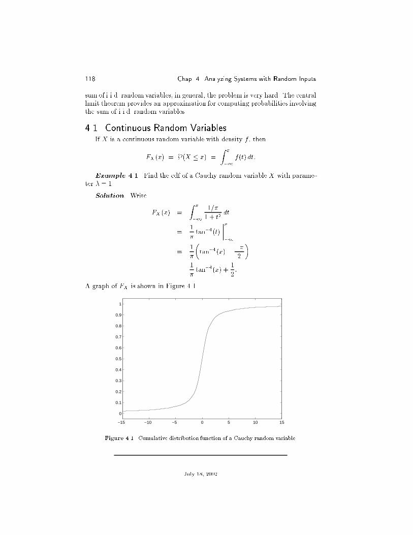
118 Chap. 4 Analyzing Systems with Random Inputs
sum of i.i.d. random variables, in general, the problem is very hard. The centrallimit theorem provides an approximation for computing probabilities involvingthe sum of i.i.d. random variables.
4.1. Continuous Random VariablesIf X is a continuous random variable with density f , then
FX (x) = }(X � x) =
Z x
�1f(t) dt:
Example 4.1. Find the cdf of a Cauchy random variable X with parame-ter � = 1.
Solution. Write
FX (x) =
Z x
�1
1=�
1 + t2dt
=1
�tan�1(t)
����x�1
=1
�
�tan�1(x)� ��
2
�=
1
�tan�1(x) +
1
2:
A graph of FX is shown in Figure 4.1.
−15 −10 −5 0 5 10 15
0
0.1
0.2
0.3
0.4
0.5
0.6
0.7
0.8
0.9
1
Figure 4.1. Cumulative distribution function of a Cauchy random variable.
July 18, 2002

4.1 Continuous Random Variables 119
Example 4.2. Find the cdf of a uniform[a; b] random variable X.
Solution. Since f(t) = 0 for t < a and t > b, we see that FX(x) =R x�1 f(t) dt is equal to 0 for x < a, and is equal to
R1�1 f(t) dt = 1 for x > b.
For a � x � b, we have
FX(x) =
Z x
�1f(t) dt =
Z x
a
1
b� adt =
x� a
b� a:
Hence, for a � x � b, FX (x) is an a�ney function of x. A graph of FX whenX � uniform[0; 1] is shown if Figure 4.2.
−0.4 −0.2 0 0.2 0.4 0.6 0.8 1 1.2 1.4
0
0.1
0.2
0.3
0.4
0.5
0.6
0.7
0.8
0.9
1
Figure 4.2. Cumulative distribution function of a uniform random variable.
We now consider the cdf of a Gaussian random variable. If X � N (m;�2),then
FX (x) =
Z x
�1
1p2� �
exp
��1
2
�t�m
�
�2�dt:
Unfortunately, there is no closed-form expression for this integral. However,it can be computed numerically, and there are many subroutines available fordoing it. For example, in Matlab, the above integral can be computed withnormcdf(x,m,sigma). If you do not have access to such a routine, you mayhave software available for computing some related functions that can be usedto calculate the normal cdf. To see how, we need the following analysis. Making
yA function is a�ne if it is equal to a linear function plus a constant.
July 18, 2002

120 Chap. 4 Analyzing Systems with Random Inputs
the change of variable � = (t�m)=� yields
FX(x) =1p2�
Z (x�m)=�
�1e��
2=2 d�:
In other words, if we put
�(y) :=1p2�
Z y
�1e��
2=2 d�; (4.1)
then
FX(x) = �
�x�m
�
�:
Note that � is the cdf of a standard normal random variable (a graph is shownin Figure 4.3). Thus, the cdf of an N (m;�2) random variable can always beexpressed in terms of the cdf of a standard N (0; 1) random variable. If yourcomputer has a routine that can compute �, then you can compute an arbitrarynormal cdf.
−3 −2 −1 0 1 2 3
0
0.1
0.2
0.3
0.4
0.5
0.6
0.7
0.8
0.9
1
Figure 4.3. Cumulative distribution function of a standard normal random variable.
For continuous random variables, the density can be recovered from the cdfby di�erentiation. Since
FX(x) =
Z x
�1f(t) dt;
di�erentiation yieldsF 0(x) = f(x):
July 18, 2002

4.1 Continuous Random Variables 121
The observation that the density of a continuous random variable can be re-covered from its cdf is of tremendous importance, as the following examplesillustrate.
Example 4.3. Consider an electrical circuit whose random input voltageX is �rst ampli�ed by a gain � > 0 and then added to a constant o�set voltage�. Then the output voltage is Y = �X +�. If the input voltage is a continuousrandom variable X, �nd the density of the output voltage Y .
Solution. Although the question asks for the density of Y , it is moreadvantageous to �nd the cdf �rst and then di�erentiate to obtain the density.Write
FY (y) = }(Y � y)
= }(�X + � � y)
= }(X � (y � �)=�); since � > 0;
= FX((y � �)=�):
If X has density fX , then
fY (y) =d
dyFX
�y � �
�
�=
1
�F 0X
�y � �
�
�=
1
�fX
�y � �
�
�:
Example 4.4. Amplitude modulation in certain communication systemscan be accomplished using various nonlinear devices such as a semiconductordiode. Suppose we model the nonlinear device by the function Y = X2. Ifthe input X is a continuous random variable, �nd the density of the outputY = X2.
Solution. Although the question asks for the density of Y , it is moreadvantageous to �nd the cdf �rst and then di�erentiate to obtain the density. Tobegin, note that since Y = X2 is nonnegative, for y < 0, FY (y) = }(Y � y) = 0.For nonnegative y, write
FY (y) = }(Y � y)
= }(X2 � y)
= }(�py � X � py )
=
Z py
�pyfX (t) dt:
The density is
fY (y) =d
dy
Z py
�pyfX(t) dt
=1
2py
�fX(
py ) + fX (�py )
�; y > 0:
July 18, 2002

122 Chap. 4 Analyzing Systems with Random Inputs
Since }(Y � y) = 0 for y < 0, fY (y) = 0 for y < 0.
When the diode input voltage X of the preceding example is N (0; 1), itturns out that Y is chi-squared with one degree of freedom (Problem 7). IfX is N (m; 1) with m 6= 0, then Y is noncentral chi-squared with one degreeof freedom (Problem 8). These results are frequently used in the analysis ofdigital communication systems.
The two preceding examples illustrate the problem of �nding the densityof Y = g(X) when X is a continuous random variable. The next exampleillustrates the problem of �nding the density of Z = g(X;Y ) when X is discreteand Y is continuous.
Example 4.5 (Signal in Additive Noise). LetX and Y be independent ran-dom variables, with X being discrete with pmf pX and Y being continuous withdensity fY . Put Z := X + Y and �nd the density of Z.
Solution. Although the question asks for the density of Z, it is moreadvantageous to �nd the cdf �rst and then di�erentiate to obtain the density.This time we use the law of total probability, substitution, and independence.Write
FZ(z) = }(Z � z)
=Xi
}(Z � zjX = xi)}(X = xi)
=Xi
}(X + Y � zjX = xi)}(X = xi)
=Xi
}(xi + Y � zjX = xi)}(X = xi)
=Xi
}(Y � z � xijX = xi)}(X = xi)
=Xi
}(Y � z � xi)}(X = xi)
=Xi
FY (z � xi) pX (xi):
Di�erentiating this expression yields
fZ(z) =Xi
fY (z � xi) pX(xi):
We should also note that FZjX(zjxi) := }(Z � zjX = xi) is called theconditional cdf of Z given X.
July 18, 2002

4.2 Reliability 123
?The Normal CDF and the Error Function
If your computer does not have a routine that computes the normal cdf, itmay have a routine to compute a related function called the error function,which is de�ned by
erf(z) :=2p�
Z z
0
e��2
d�:
Note that erf(z) is negative for z < 0. In fact, erf is an odd function. To express� in terms of erf, write
�(y) =1p2�
�Z 0
�1e��
2=2 d� +
Z y
0
e��2=2 d�
�=
1
2+
1p2�
Z y
0
e��2=2 d�; by Example 3.4;
=1
2+
1
2� 2p
�
Z y=p2
0
e��2
d�;
where the last step follows by making the change of variable � = �=p2. We
now see that�(y) = 1
2
�1 + erf
�y=p2��:
From the derivation, it is easy to see that this holds for all y, both positive andnegative. The Matlab command for erf(z) is erf(z).
In many applications, instead of �(y), we need
Q(y) := 1��(y):
Using the complementary error function,
erfc(z) := 1� erf(z) =2p�
Z 1
z
e��2
d�;
it is easy to see thatQ(y) = 1
2 erfc�y=p2�:
The Matlab command for erfc(z) is erfc(z).
4.2. ReliabilityLet T be the lifetime of a device or system. The reliability function of
the device or system is de�ned by
R(t) := }(T > t) = 1� FT (t):
The reliability at time t is the probability that the lifetime is greater than t.The mean time to failure (MTTF) is simply the expected lifetime, E[T ].
Since lifetimes are nonnegative random variables, we claim that
E[T ] =
Z 1
0
}(T > t) dt: (4.2)
July 18, 2002

124 Chap. 4 Analyzing Systems with Random Inputs
It then follows that
E[T ] =
Z 1
0
R(t) dt;
i.e., the MTTF is the integral of the reliability. To derive (4.2), writeZ 1
0
}(T > t) dt =
Z 1
0
E[I(t;1)(T )] dt
= E
� Z 1
0
I(t;1)(T ) dt
�= E
� Z 1
0
I(�1;T )(t) dt
�:
To evaluate the integral, observe that since T is nonnegative, the intersectionof [0;1) and (�1; T ) is [0; T ). Hence,Z 1
0
}(T > t) dt = E
� Z T
0
dt
�= E[T ]:
The failure rate of a device or system with lifetime T is
r(t) := lim�t#0
}(T � t +�tjT > t)
�t:
This can be rewritten as
}(T � t +�tjT > t) � r(t)�t:
In other words, given that the device or system has operated for more thant units of time, the conditional probability of failure before time t + �t isapproximately r(t)�t. Intuitively, the form of a failure rate function shouldbe as shown in Figure 4.4. For small values of t, r(t) is relatively large when
t
r t( )
Figure 4.4. Typical form of a failure rate function.
pre-existing defects are likely to appear. Then for intermediate values of t, r(t)is at indicating a constant failure rate. For large t, as the device gets older,r(t) increases indicating that failure is more likely.
July 18, 2002

4.2 Reliability 125
To say more about the failure rate, write
}(T � t+�tjT > t) =}(fT � t+�tg \ fT > tg)
}(T > t)
=}(t < T � t+�t)
}(T > t)
=FT (t +�t)� FT (t)
R(t):
Since FT (t) = 1�R(t), we can rewrite this as
}(T � t+�tjT > t) = �R(t +�t)� R(t)
R(t):
Dividing both sides by �t and letting �t # 0 yields the di�erential equation
r(t) = �R0(t)
R(t):
Now suppose T is a continuous random variable with density fT . Then
R(t) = }(T > t) =
Z 1
t
fT (�) d�;
andR0(t) = �fT (t):
We can now write
r(t) = �R0(t)
R(t)=
fT (t)Z 1
t
fT (�) d�
:
In this case, the failure rate r(t) is completely determined by the density fT (t).The converse is also true; i.e., given the failure rate r(t), we can recover thedensity fT (t). To see this, rewrite the above di�erential equation as
�r(t) =R0(t)R(t)
=d
dtlnR(t):
Integrating the left and right-hand formulas from zero to t yields
�Z t
0
r(� ) d� = lnR(t) � lnR(0):
Then
e�R t0r(�) d�
=R(t)
R(0)= R(t);
where we have used the fact that for a nonnegative, continuous random variable,R(0) = }(T > 0) = }(T � 0) = 1. Since R0(t) = �fT (t),
fT (t) = r(t)e�Rt
0r(�) d�
:
For example, if the failure rate is constant, r(t) = �, then fT (t) = �e��t, andwe see that T has an exponential density with parameter �.
July 18, 2002

126 Chap. 4 Analyzing Systems with Random Inputs
4.3. Cdfs for Discrete Random VariablesIn this section, we show that for discrete random variables, the pmf can be
recovered from the cdf. If X is a discrete random variable, then
FX (x) = }(X � x) =Xi
I(�1;x](xi) pX(xi) =Xi:xi�x
pX(xi):
Example 4.6. Let X be a discrete random variable with pX (0) = 0:1,pX(1) = 0:4, pX (2:5) = 0:2, and pX (3) = 0:3. Find the cdf FX (x) for all x.
Solution. Put x0 = 0, x1 = 1, x2 = 2:5, and x3 = 3. Let us �rst evaluateFX(0:5). Observe that
FX(0:5) =X
i:xi�0:5
pX (xi) = pX (0);
since only x0 = 0 is less than or equal to 0:5. Similarly, for any 0 � x < 1,FX(x) = pX(0) = 0:1.
Next observe that
FX (2:1) =X
i:xi�2:1
pX(xi) = pX (0) + pX(1);
since only x0 = 0 and x1 = 1 are less than or equal to 2.1. Similarly, for any1 � x < 2:5, FX(x) = 0:1 + 0:4 = 0:5.
The same kind of argument shows that for 2:5 � x < 3, FX(x) = 0:1+0:4+0:2 = 0:7.
Since all the xi are less than or equal to 3, for x � 3, FX(x) = 0:1 + 0:4 +0:2 + 0:3 = 1:0.
Finally, since none of the xi is less than zero, for x < 0, FX(x) = 0. Thegraph of FX is given in Figure 4.5.
We now show that the arguments used in the preceding example hold forthe cdf of any discrete random variable X taking distinct values xi. Fix twoadjacent points, say xj�1 < xj as shown in Figure 4.6. For xj�1 � x < xj,observe that
FX(x) =Xi:xi�x
pX(xi) =X
i:xi�xj�1pX (xi) = FX (xj�1):
In other words, the cdf is constant on the interval [xj�1; xj), with the constantequal to the value of the cdf at the left-hand endpoint, FX(xj�1). Next, since
FX(xj) =X
i:xi�xjpX (xi) =
� Xi:xi�xj�1
pX (xi)
�+ pX (xj);
July 18, 2002

4.4 Mixed Random Variables 127
−1 −0.5 0 0.5 1 1.5 2 2.5 3 3.5 4
0
0.1
0.2
0.3
0.4
0.5
0.6
0.7
0.8
0.9
1
Figure 4.5. Cumulative distribution function of a discrete random variable.
. . . . . .. . .
. . . . . .. . . x xjx 1−jx2x1
pj
p1−j
p2
p1
Figure 4.6. Analysis for the cdf of a discrete random variable.
we have
FX(xj) = FX(xj�1) + pX(xj);
or
FX(xj) � FX (xj�1) = pX(xj):
As noted above, for xj�1 � x < xj, FX(x) = FX (xj�1). Hence, FX(xj�) :=limx"xj FX(x) = FX (xj�1). It then follows that
FX(xj)� FX(xj�) = FX(xj) � FX (xj�1) = pX (xj):
In other words, the size of the jump in the cdf at xj is pX (xj), and the cdf isconstant between jumps.
4.4. Mixed Random VariablesWe say that X is a mixed random variable if }(X 2 B) has the form
}(X 2 B) =
ZB
~f(t) dt+Xi
IB(xi)~pi (4.3)
July 18, 2002

128 Chap. 4 Analyzing Systems with Random Inputs
for some nonnegative function ~f , some nonnegative sequence ~pi, and distinctpoints xi such that
R1�1
~f (t) dt +P
i ~pi = 1. Note that the mixed randomvariables include the continuous and discrete real-valued random variables asspecial cases.
Example 4.7. Let X be a mixed random variable with
}(X 2 B) :=1
4
ZB
e�jtj dt+1
3IB(0) +
1
6IB(7): (4.4)
Compute }(X < 0), }(X � 0), }(X > 2), and }(X � 2).
Solution. We need to compute }(X 2 B) for B = (�1; 0), (�1; 0],(2;1), and [2;1), respectively. Since the set B = (�1; 0) does not contain 0or 7, the two indicator functions in the de�nition of }(X 2 B) are zero in thiscase. Hence,
}(X < 0) =1
4
Z 0
�1e�jtj dt =
1
4
Z 0
�1et dt =
1
4:
Next, the set B = (�1; 0] contains 0 but not 7. Thus,
}(X � 0) =1
4
Z 0
�1e�jtj dt+
1
3=
1
4+1
3=
7
12:
For the last two probabilities, we need to consider (2;1) and [2;1). Bothintervals contain 7 but not 0. Hence, the probabilities are the same, and bothequal
1
4
Z 1
2
e�t dt+1
6=
e�2
4+1
6:
Example 4.8. With X as in the last example, compute }(X = 0) and}(X = 7). Also, use your results to verify that }(X = 0)+}(X < 0) =}(X �0).
Solution. To compute }(X = 0) = }(X 2 f0g), take B = f0g in (4.4).Then
}(X = 0) =1
4
Zf0g
e�jtj dt+1
3If0g(0) +
1
6If0g(7):
The integral of an ordinary function over a set consisting of a single point iszero, and since 7 =2 f0g, the last term is zero also. Hence, }(X = 0) = 1=3.Similarly, }(X = 7) = 1=6. From the previous example, }(X < 0) = 1=4.Hence, }(X = 0)+}(X < 0) = 1=3+ 1=4 = 7=12, which is indeed the value of}(X � 0) computed earlier.
July 18, 2002

4.4 Mixed Random Variables 129
In order to perform calculations with mixed random variables more easily, itis sometimes convenient to generalize the notion of density to permit impulses.Recall that the unit impulse or Dirac delta function, denoted by �, isde�ned by the two properties
�(t) = 0 for t 6= 0 and,
Z 1
�1�(t) dt = 1:
Putting
f(t) := ~f(t) +Xi
~pi�(t� xi); (4.5)
it is easy to verify thatZB
f(t) dt = }(X 2 B) and
Z 1
�1g(t)f(t) dt = E[g(X)]:
We call f in (4.5) a generalized probability density function. If ~f (t) = 0for all t, we say that f is purely impulsive, and if ~pi = 0 for all i, we say f isnonimpulsive.
Example 4.9. The preceding examples can be worked using delta func-tions. In these examples, the generalized density is
f(t) =1
4e�jtj +
1
3�(t) +
1
6�(t � 7);
and}(X 2 B) =
ZB
f(t) dt:
Since the impulses are located at 0 and at 7, they will contribute to the integralif and only if 0 and/or 7 lie in the set B. For example, in computing
}(0 < X � 7) =
Z 7
0+
f(t) dt;
the impulse at the origin makes no contribution, but the impulse at 7 does.Thus,
}(0 < X � 7) =
Z 7
0+
�1
4e�jtj +
1
3�(t) +
1
6�(t� 7)
�dt
=1
4
Z 7
0
e�t dt+1
6
=1� e�7
4+1
6=
5
12� e�7
4:
Similarly, in computing }(X = 0) = }(X 2 f0g), only the impulse at zeromakes a contribution. Thus,
}(X = 0) =
Zf0g
f(t) dt =
Zf0g
1
3�(t) dt =
1
3:
July 18, 2002
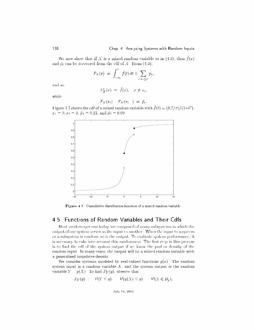
130 Chap. 4 Analyzing Systems with Random Inputs
We now show that if X is a mixed random variable as in (4.3), then ~f (x)and ~pi can be recovered from the cdf of X. From (4.3),
FX(x) =
Z x
�1~f (t) dt+
Xi:xi�x
~pi;
and soF 0X (x) = ~f(x); x 6= xi;
whileFX (xi) � FX(xi�) = ~pi:
Figure 4.7 shows the cdf of a mixed randomvariable with ~f (t) = (0:7=�)=(1+t2),x1 = 0; x2 = 3, ~p1 = 0:21, and ~p2 = 0:09.
−15 −10 −5 0 5 10 15
0
0.1
0.2
0.3
0.4
0.5
0.6
0.7
0.8
0.9
1
Figure 4.7. Cumulative distribution function of a mixed random variable.
4.5. Functions of Random Variables and Their CdfsMost modern systems today are composed of many subsystems in which the
output of one system serves as the input to another. When the input to a systemor a subsystem is random, so is the output. To evaluate system performance, itis necessary to take into account this randomness. The �rst step in this processis to �nd the cdf of the system output if we know the pmf or density of therandom input. In many cases, the output will be a mixed random variable witha generalized impulsive density.
We consider systems modeled by real-valued functions g(x). The randomsystem input is a random variable X, and the system output is the randomvariable Y = g(X). To �nd FY (y), observe that
FY (y) := }(Y � y) = }(g(X) � y) = }(X 2 By);
July 18, 2002

4.5 Functions of Random Variables and Their Cdfs 131
whereBy := fx 2 IR : g(x) � yg:
If X has density fX , then
FY (y) = }(X 2 By) =
ZBy
fX(x) dx:
The di�culty is to identify the set By. However, if we �rst sketch the functiong(x), the problem becomes manageable.
Example 4.10. Suppose g is given by
g(x) :=
8>>>><>>>>:1; �2 � x < �1;x2; �1 � x < 0;x; 0 � x < 2;2; 2 � x < 3;0; otherwise:
Find the inverse image B = fx 2 IR : g(x) � yg for y � 2, 2 > y � 1, 1 > y � 0,and y < 0.
Solution. To begin, we sketch g in Figure 4.8. Fix any y � 2. Since g isupper bounded by 2, g(x) � 2 � y for all x 2 IR. Thus, for y � 2, B = IR.
−2 −1 0 1 2 3
0
0.5
1
1.5
2
Figure 4.8. The function g from Example 4.10.
Next, �x any y with 2 > y � 1. On the graph of g, draw a horizontalline at level y. In Figure 4.9, the line is drawn at level y = 1:5. Next, at theintersection of the horizontal line and the curve g, drop a vertical line to thex-axis. In the �gure, this vertical line hits the x-axis at the point marked �.
July 18, 2002

132 Chap. 4 Analyzing Systems with Random Inputs
−2 −1 0 1 2 3
0
0.5
1
1.5
2
Figure 4.9. DeterminingB for 1 � y < 2.
Clearly, for all x to the left of this point, and for all x � 3, g(x) � y. To �ndthe x-coordinate of �, we solve g(x) = y for x. For the y-value in question, theformula for g(x) is g(x) = x. Hence, the x-coordinate of � is simply y. Thus,g(x) � y , x � y or x � 3, and so,
B = (�1; y] [ [3;1); 1 � y < 2:
Now �x any y with 1 > y � 0, and draw a horizontal line at level y asbefore. In Figure 4.10 we have used y = 1=2. This time the horizontal lineintersects the curve g in two places, and there are two points marked � on thex-axis. Call the x-coordinate of the left one x1 and that of the right one x2. Wemust solve g(x1) = y, where x1 is negative and g(x1) = x21. We must also solveg(x2) = y, where g(x2) = x2. We conclude that g(x) � y , x < �2 or �py �x � y or x � 3. Thus,
B = (�1;�2) [ [�py; y] [ [3;1); 0 � y < 1:
Note that when y = 0, the interval [0; 0] is just the singleton set f0g.Finally, since g(x) � 0 for all x 2 IR, for y < 0, B = 6 .
Example 4.11. Let g be as in Example 4.10, and suppose that X �uniform[�4; 4]. Find and sketch the cumulative distribution of Y = g(X).Also �nd and sketch the density.
Solution. Proceeding as in the two examples above, write FY (y) = }(Y �y) = }(X 2 B) for the appropriate inverse image B = fx 2 IR : g(x) � yg.
July 18, 2002

4.5 Functions of Random Variables and Their Cdfs 133
−2 −1 0 1 2 3
0
0.5
1
1.5
2
Figure 4.10. DeterminingB for 0 � y < 1.
From Example 4.10,
B =
8>><>>:6 ; y < 0;(�1;�2) [ [�py; y] [ [3;1); 0 � y < 1;(�1; y] [ [3;1); 1 � y < 2;IR; y � 2:
For y < 0, FY (y) = 0. For 0 � y < 1,
FY (y) = }(X < �2) +}(�py � X � y) +}(X � 3)
=�2� (�4)
8+y � (�py )
8+
4� 3
8
=y +
py + 3
8:
For 1 � y < 2,
FY (y) = }(X � y) +}(X � 3)
=y � (�4)
8+
4� 3
8
=y + 5
8:
For y > 2, FY (y) = }(X 2 IR) = 1. Putting all this together,
FY (y) =
8>><>>:0; y < 0;(y +
py + 3)=8; 0 � y < 1;
(y + 5)=8; 1 � y < 2;1; y � 2:
July 18, 2002

134 Chap. 4 Analyzing Systems with Random Inputs
0 0.5 1 1.5 2
0
0.1
0.2
0.3
0.4
0.5
0.6
0.7
0.8
0.9
1
Figure 4.11. Cumulative distribution function FY (y) from Example 4.11.
In sketching FY (y), we note from the formula that it is 0 for y < 0 and 1 fory � 2. Also from the formula, note that there is a jump discontinuity of 3=8 aty = 0 and a jump of 1=8 at y = 1 and at y = 2. See Figure 4.11.
From the observations used in graphing FY , we can easily obtain the gen-eralized density,
hY (y) =3
8�(y) +
1
8�(y � 1) +
1
8�(y � 2) + ~fY (y);
where
~fY (y) =
8<:[1 + 1=(2
py )]=8; 0 < y < 1;
1=8; 1 < y < 2;0; otherwise;
is obtained by di�erentiating FY (y) at non-jump points y. A sketch of hY isshown in Figure 4.12.
4.6. Properties of CdfsGiven an arbitrary real-valued random variable X, its cumulative distribu-
tion function is de�ned by
F (x) := }(X � x); �1 < x <1:
We show below that F satis�es the following eight properties:
(i) 0 � F (x) � 1.(ii) For a < b, }(a < X � b) = F (b)� F (a).
July 18, 2002

4.6 Properties of Cdfs 135
0 0.5 1 1.5 2
0
0.1
0.2
0.3
0.4
0.5
0.6
0.7
0.8
0.9
1
Figure 4.12. Density hY (y) from Example 4.11.
(iii) F is nondecreasing, i.e., a � b implies F (a) � F (b).(iv) lim
x"1F (x) = 1.
(v) limx#�1
F (x) = 0.
(vi) F (x0+) := limx#x0
F (x) = }(X � x0) = F (x0). In other words, F is
right-continuous.(vii) F (x0�) := lim
x"x0F (x) = }(X < x0).
(viii) }(X = x0) = F (x0)� F (x0�).We also point out that
}(X > x0) = 1�}(X � x0) = 1� F (x0);
and}(X � x0) = 1�}(X < x0) = 1� F (x0�):
If F (x) is continuous at x = x0, i.e., F (x0�) = F (x0), then this last equationbecomes
}(X � x0) = 1� F (x0):
Another consequence of the continuity of F (x) at x = x0 is that}(X = x0) = 0.Note that if a random variable has a nonimpulsive density, then its cumulativedistribution is continuous everywhere.
We now derive the eight properties of cumulative distribution functions.
(i) The properties of} imply that F (x) = }(X � x) satis�es 0 � F (x) � 1.
July 18, 2002

136 Chap. 4 Analyzing Systems with Random Inputs
(ii) First consider the disjoint union (�1; b] = (�1; a] [ (a; b]. It thenfollows that
fX � bg = fX � ag [ fa < X � bgis a disjoint union of events in . Now write
F (b) = }(X � b)
= }(fX � ag [ fa < X � bg)= }(X � a) +}(a < X � b)
= F (a) +}(a < X � b):
Now subtract F (a) from both sides.(iii) This follows from (ii) since }(a < X � b) � 0.(iv) We prove the simpler result limN!1 F (N ) = 1. Starting with
IR = (�1;1) =1[n=1
(�1; n];
we can write
1 = }(X 2 IR)
= }
� 1[n=1
fX � ng�
= limN!1
}(X � N ); by limit property (1.4);
= limN!1
F (N ):
(v) We prove the simpler result, limN!1 F (�N ) = 0. Starting with
6 =1\n=1
(�1;�n];
we can write
0 = }(X 2 6 )
= }
� 1\n=1
fX � �ng�
= limN!1
}(X � �N ); by limit property (1.5);
= limN!1
F (�N ):
(vi) We prove the simpler result, }(X � x0) = limN!1
F (x0 +1N ). Starting
with
(�1; x0] =1\n=1
(�1; x0 +1n ];
July 18, 2002

4.7 The Central Limit Theorem 137
we can write
}(X � x0) = }
� 1\n=1
fX � x0 +1ng�
= limN!1
}(X � x0 +1N ); by (1.5);
= limN!1
F (x0 +1N):
(vii) We prove the simpler result, }(X < x0) = limN!1
F (x0� 1N). Starting
with
(�1; x0) =1[n=1
(�1; x0 � 1n ];
we can write
}(X < x0) = }
� 1[n=1
fX � x0 � 1ng�
= limN!1
}(X � x0 � 1N); by (1.4);
= limN!1
F (x0 � 1N ):
(viii) First consider the disjoint union (�1; x0] = (�1; x0)[fx0g. It thenfollows that
fX � x0g = fX < x0g [ fX = x0gis a disjoint union of events in . Using Property (vii), it follows that
F (x0) = F (x0�) +}(X = x0):
4.7. The Central Limit TheoremLet X1; X2; : : : be i.i.d. with common mean m and common variance �2.
There are many cases for which we know the probability mass function ordensity of
nXi=1
Xi:
For example, if the Xi are Bernoulli, binomial, Poisson, gamma, or Gaussian,we know the cdf of the sum (see Example 2.20 or Problem 22 in Chapter 2and Problem 46 in Chapter 3). Note that the exponential and chi-squared arespecial cases of the gamma (see Problem 12 in Chapter 3). In general, however,�nding the cdf of a sum of i.i.d. random variables is not possible. Fortunately,we have the following approximation.
Central Limit Theorem (CLT). Let X1; X2; : : : be independent, identically
distributed random variables with �nite mean m and �nite variance �2. If
Yn :=Mn �m
�=pn
and Mn :=1
n
nXi=1
Xi;
July 18, 2002

138 Chap. 4 Analyzing Systems with Random Inputs
then
limn!1FYn(y) = �(y):
To get some idea of how large n should be, would like to compare FYn(y)and �(y) in cases where FYn is known. To do this, we need the following result.
Example 4.12. Show that if Gn is the cdf ofPn
i=1Xi, then
FYn(y) = Gn(y�pn+ nm): (4.6)
Solution. Write
FYn(y) = }
�Mn �m
�=pn
� y
�= }(Mn �m � y�=
pn )
= }(Mn � y�=pn+m)
= sP
� nXi=1
Xi � y�pn + nm
�= Gn(y�
pn+ nm):
When the Xi are exp(1), Gn is the Erlang(30; 1) cdf given in Problem 12(c)in Chapter 3. In Figure 4.13 we plot FY30(y) (dashed line) and the N (0; 1) cdf�(y) (solid line).
A typical calculation using the central limit theorem is as follows. To ap-proximate
}
� nXi=1
Xi > t
�;
write
}
� nXi=1
Xi > t
�= }
�1
n
nXi=1
Xi >t
n
�= }(Mn > t=n)
= }(Mn �m > t=n�m)
= }
�Mn �m
�=pn
>t=n�m
�=pn
�= }
�Yn >
t=n�m
�=pn
�= 1� FYn
�t=n�m
�=pn
�� 1��
�t=n�m
�=pn
�:
July 18, 2002

4.7 The Central Limit Theorem 139
−3 −2 −1 0 1 2 3
0
0.1
0.2
0.3
0.4
0.5
0.6
0.7
0.8
0.9
1
Figure 4.13. Illustration of the central limit theorem when the Xi are exponential withparameter 1. The dashed line is FY30 , and the solid line is the standard normal cumulativedistribution, �.
Example 4.13. A certain digital communication link has bit-error proba-bility p. Use the central limit theorem to approximate the probability that intransmitting a word of n bits, more than k bits are received incorrectly.
Solution. Let Xi = 1 if bit i is received in error, and Xi = 0 otherwise.We assume the Xi are independent Bernoulli(p) random variables. The numberof errors in n bits is
Pni=1Xi. We must compute
}
� nXi=1
Xi > k
�:
Using the approximation above in which t = k, m = p, and �2 = p(1 � p), wehave
}
� nXi=1
Xi > k
�� 1��
�k=n� ppp(1� p)=n
�:
Derivation of the Central Limit Theorem
It is instructive to consider �rst the following special case, which illustratesthe key steps of the general derivation. Suppose that the Xi are i.i.d. Laplacewith parameter � =
p2. Then m = 0, �2 = 1, and
Yn =Mn �m
�=pn
=pnMn =
pn
n
nXi=1
Xi =1pn
nXi=1
Xi:
July 18, 2002

140 Chap. 4 Analyzing Systems with Random Inputs
The characteristic function of Yn is
'Yn(�) = E[ej�Yn] = E
�ej(�=
pn )
nPi=1
Xi�
=nYi=1
E�ej(�=
pn )Xi
�:
Of course, E�ej(�=
pn )Xi
�= 'Xi
��=pn�, where, for the Laplace
�p2�random
variable Xi,
'Xi (�) =2
2 + �2=
1
1+ �2=2:
Thus,
E[ej(�=pn )Xi ] = 'Xi
� �pn
�=
1
1 + �2=2n
;
and
'Yn(�) =
�1
1 + �2=2n
�n=
1�1 + �2=2
n
�n :We now use the fact that for any number �,�
1 +�
n
�n! e� :
It follows that
'Yn(�) =1�
1 + �2=2n
�n ! 1
e�2=2= e��
2=2;
which is the characteristic function of an N (0; 1) random variable.We now turn to the derivation in the general case. Write
Yn =Mn �m
�=pn
=
pn
�
��1
n
nXi=1
Xi
��m
�
=
pn
�
�1
n
nXi=1
(Xi �m)
�
=1pn
nXi=1
�Xi �m
�
�:
Now let Zi := (Xi �m)=�. Then
Yn =1pn
nXi=1
Zi;
July 18, 2002

4.7 The Central Limit Theorem 141
where the Zi are zero mean and unit variance. Since the Xi are i.i.d., so arethe Zi. Let 'Z(�) := E[ej�Zi] denote their common characteristic function. Wecan write the characteristic function of Yn as
'Yn(�) := E[ej�Yn]
= E
�exp
�j�pn
nXi=1
Zi
��
= E
� nYi=1
exp
�j�pnZi
��
=nYi=1
E
�exp
�j�pnZi
��
=nYi=1
'Z
� �pn
�= 'Z
� �pn
�n:
Now recall that for any complex �,
e� = 1 + � +1
2�2 +R(�):
Thus,
'Z
� �pn
�= E[ej(�=
pn )Zi ]
= E
�1 + j
�pnZi +
1
2
�j�pnZi
�2+R
�j�pnZi
��:
Since Zi is zero mean and unit variance,
'Z
� �pn
�= 1� 1
2� �
2
n+ E
�R�j�pnZi
��:
It can be shown that the last term on the right is asymptotically negligible [4,pp. 357{358], and so
'Z
� �pn
�� 1� �2=2
n:
We now have
'Yn (�) = 'Z
� �pn
�n��1� �2=2
n
�n! e��
2=2;
which is the N (0; 1) characteristic function. Since the characteristic functionof Yn converges to the N (0; 1) characteristic function, it follows that FYn(y)!�(y) [4, p. 349, Theorem 26.3].
July 18, 2002

142 Chap. 4 Analyzing Systems with Random Inputs
Example 4.14. In the derivation of the central limit theorem, we foundthat 'Yn(�) ! e��
2=2 as n ! 1. We can use this result to give a simplederivation of Stirling's formula,
n! �p2� nn+1=2e�n:
Solution. Since n! = n(n � 1)!, it su�ces to show that
(n� 1)! �p2�nn�1=2e�n:
To this end, let X1; : : : ; Xn be i.i.d. exp(1). Then by Problem 46(c) in Chap-ter 3,
Pni=1Xi has the n-Erlang density,
gn(x) =xn�1e�x
(n � 1)!; x � 0:
Also, the mean and variance of Xi are both one. Di�erentiating (4.6) (withm = � = 1) yields
fYn (y) = gn(ypn+ n)
pn:
Note that fYn(0) = nn�1=2e�n=(n � 1)!. On the other hand, by inverting thecharacteristic function of Yn, we can also write
fYn(0) =1
2�
Z 1
�1'Yn(�) d�
� 1
2�
Z 1
�1e��
2=2 d�; by the CLT;
= 1=p2�:
It follows that (n� 1)! � p2� nn�1=2e�n.
Remark. A more precise version of Stirling's formula is [14, pp. 50{53]p2� nn+1=2e�n+1=(12n+1) < n! <
p2� nn+1=2e�n+1=(12n):
4.8. ProblemsProblems x4.1: Continuous Random Variables
1. Find the cumulative distribution function FX(x) of an exponential ran-dom variable X with parameter �. Sketch the graph of FX when � = 1.
2. The Rayleigh density with parameter � is de�ned by
f(x) :=
8<:x
�2e�(x=�)2=2; x � 0;
0; x < 0:
Find the cumulative distribution function.
July 18, 2002

4.8 Problems 143
?3. The Maxwell density with parameter � is de�ned by
f(x) :=
8><>:r
2
�
x2
�3e�(x=�)2=2; x � 0;
0; x < 0:
Show that the cdf F (x) can be expressed in terms of the standard normalcdf �(x) de�ned in (4.1).
4. If Z has density fZ(z) and Y = eZ , �nd fY (y).
5. If X � uniform(0; 1), �nd the density of Y = ln(1=X).
6. Let X �Weibull(p; �). Find the density of Y = �Xp.
7. The input to a squaring circuit is a Gaussian random variable X withmean zero and variance one. Show that the output Y = X2 has thechi-squared density with one degree of freedom,
fY (y) =e�y=2p2�y
; y > 0:
8. If the input to the squaring circuit of Problem 7 includes a �xed bias, saym, then the output is given by Y = (X +m)2, where again X � N (0; 1).Show that Y has the noncentral chi-squared density with one degree offreedom and noncentrality parameter m2,
fY (y) =e�(y+m2)=2
p2�y
� empy + e�m
py
2; y > 0:
Note that if m = 0, we recover the result of Problem 7.
9. Let X1; : : : ; Xn be independent with common cumulative distributionfunction F (x). Let us de�ne Xmax := max(X1; : : : ; Xn) and Xmin :=min(X1; : : : ; Xn). Express the cumulative distributions of Xmax and Xmin
in terms of F (x). Hint: Example 2.7 may be helpful.
10. If X and Y are independent exp(�) random variables, �nd E[max(X;Y )].
11. Digital Communication System. The received voltage in a digital commu-nication system is Z = X + Y , where X � Bernoulli(p) is a randommessage, and Y � N (0; 1) is a Gaussian noise voltage. Assuming X andY are independent, �nd the conditional cdf FZjX(zji) for i = 0; 1, the cdfFZ(z), and the density fZ(z).
12. Fading Channel. Let X and Y be as in the preceding problem, but nowsuppose Z = X=A + Y , where A, X, and Y are independent, and Atakes the values 1 and 2 with equal probability. Find the conditional cdfFZjA;X(zja; i) for a = 1; 2 and i = 0; 1.
July 18, 2002

144 Chap. 4 Analyzing Systems with Random Inputs
13. Generalized Rayleigh Densities. Let Yn be chi-squared with n degrees offreedom as de�ned in Problem 12 of Chapter 3. Put Zn :=
pYn.
(a) Express the cdf of Zn in terms of the cdf of Yn.
(b) Find the density of Z1.
(c) Show that Z2 has a Rayleigh density, as de�ned in Problem 2, with� = 1.
(d) Show that Z3 has a Maxwell density, as de�ned in Problem 3, with� = 1.
(e) Show that Z2m has a Nakagami-m density
f(z) :=
8<:2
2m�(m)
z2m�1
�2me�(z=�)2=2; z � 0;
0; z < 0;
with � = 1.
Remark. For the general chi-squared random variable Yn, it is notnecessary that n be an integer. However, if n is a positive integer, andif X1; : : : ; Xn are i.i.d. N (0; 1), then the X2
i are chi-squared with onedegree of freedom by Problem 7, and Yn := X2
1 + � � �+X2n is chi-squared
with n degrees of freedom by Problem 46(c) in Chapter 3. Hence, theabove densities usually arise from taking the square root of the sum ofsquares of standard normal random variables. For example, (X1; X2) canbe regarded as a random point in the plane whose horizontal and verticalcoordinates are independent N (0; 1). The distance of this point fromthe origin is
pX2
1 +X22 = Z2, which is a Rayleigh random variable. As
another example, consider an ideal gas. The velocity of a given particle isobtained by adding up the results of many collisions with other particles.By the central limit theorem (Section 4.7), each component of the givenparticle's velocity vector, say (X1; X2; X3) should be i.i.d. N (0; 1). Thespeed of the particle is
pX2
1 +X22 +X2
3 = Z3, which has the Maxwelldensity. When the Nakagami-m density is used as a model for fading inwireless communication channels, m is often not an integer.
14. Generalized Gamma Densities.
(a) Let X � gamma(p; 1), and put Y := X1=q. Show that
fY (y) =qypq�1e�y
q
�(p); y > 0:
(b) If in part (a) we replace p with p=q, we �nd that
fY (y) =qyp�1e�y
q
�(p=q); y > 0:
July 18, 2002

4.8 Problems 145
If we introduce a scale parameter � > 0, we have the generalizedgamma density [46]. More precisely, we say that Y � g-gamma(p; �; q)if Y has density
fY (y) =�q(�y)p�1e�(�y)q
�(p=q); y > 0:
Clearly, g-gamma(p; �;1) = gamma(p; �), which includes the Erlangand the chi-squared as special cases. Show that
(i) g-gamma(p;�1=p; p) = Weibull(p; �).
(ii) g-gamma(2;1=(p2�); 2) is the Rayleigh density de�ned in Prob-
lem 2.
(iii) g-gamma(3;1=(p2�); 2) is the Maxwell density de�ned in Prob-
lem 3.
(c) If Y � g-gamma(p; �; q), show that
E[Y n] =��(n+ p)=q)
��(p=q)�n
;
and conclude that
MY (s) =1Xn=0
sn
n!� ��(n+ p)=q)
��(p=q)�n
:
?15. In the analysis of communication systems, one is often interested in}(X >x) = 1�FX(x) for some voltage threshold x. We call F c
X(x) := 1�FX(x)the complementary cumulative distribution function (ccdf) of X.Of particular interest is the ccdf of the standard normal, which is oftendenoted by
Q(x) := 1��(x) =1p2�
Z 1
x
e�t2=2 dt:
Using the hints below, show that for x > 0,
e�x2=2
p2�
�1
x� 1
x3
�< Q(x) <
e�x2=2
xp2�
:
Hints: To derive the upper bound, apply integration by parts toZ 1
x
1
t� te�t2=2 dt;
and then drop the new integral term (which is positive),Z 1
x
1
t2e�t
2=2 dt:
If you do not drop the above term, you can derive the lower bound by ap-plying integration by parts one more time (after dividing and multiplyingby t again) and then dropping the �nal integral.
July 18, 2002

146 Chap. 4 Analyzing Systems with Random Inputs
?16. Let Ck(x) denote the chi-squared cdf with k degrees of freedom. Show thatthe noncentral chi-squared cdf with k degrees of freedom and noncentralityparameter �2 is given by (recall Problem 54 in Chapter 3)
Ck;�2(x) =1Xn=0
(�2=2)ne��2=2
n!C2n+k(x):
Remark. Note that inMatlab, Ck(x) = chi2cdf(x; k), and Ck;�2(x) =ncx2cdf(x; k; lambda^2).
?17. Generalized Rice or Noncentral Rayleigh Densities. Let Yn be noncentralchi-squared with n degrees of freedom and noncentrality parameter m2
as de�ned in Problem 54 in Chapter 3. (In general, n need not be aninteger, but if it is, and if X1; : : : ; Xn are independent normal randomvariables with Xi � N (mi; 1), then by Problem 8, X2
i is noncentral chi-squared with one degree of freedom and noncentrality parameter m2
i , andby Problem 54 in Chapter 3, X2
1 + � � �+X2n is noncentral chi-squared with
n degrees of freedom and noncentrality parameter m2 = m21 + � � �+m2
n.)
(a) Show that Zn :=pYn has the generalized Rice density,
fZn (z) =zn=2
mn=2�1e�(m2+z2)=2In=2�1(mz); z > 0;
where I� is the modi�ed Bessel function of the �rst kind, order �,
I�(x) :=1X`=0
(x=2)2`+�
`! �(`+ � + 1):
Remark. In Matlab, I�(x) = besseli(nu; x).
(b) Show that Z2 has the original Rice density,
fZ2 (z) = ze�(m2+z2)=2I0(mz); z > 0:
(c) Show that
fYn(y) =1
2
�pym
�n=2�1
e�(m2+y)=2In=2�1(mpy ); y > 0;
giving a closed-form expression for the noncentral chi-squared den-sity. Recall that you already have a closed-form expression for themoment generating function and characteristic function of a noncen-tral chi-squared random variable (see Problem 54(b) in Chapter 3).
Remark. Note that in Matlab, the cdf of Yn is given by FYn(y) =ncx2cdf(y; n; m^2).
July 18, 2002

4.8 Problems 147
(d) Denote the complementary cumulative distribution of Zn by
F cZn(z) := }(Zn > z) =
Z 1
z
fZn(t) dt:
Show that
F cZn(z) =
� zm
�n=2�1e�(m2+z2)=2In=2�1(mz) + F c
Zn�2(z):
Hint: Use integration by parts; you will need the easily-veri�ed factthat
d
dx
�x�I�(x)
�= x�I��1(x):
(e) The complementary cdf of Z2, F cZ2(z), is known as the Marcum Q
function,
Q(m; z) :=
Z 1
z
te�(m2+t2)=2I0(mt) dt:
Show that if n � 4 is an even integer, then
F cZn(z) = Q(m; z) + e�(m2+z2)=2
n=2�1Xk=1
� zm
�kIk(mz):
(f) Show that Q(m; z) = eQ(m; z), whereeQ(m; z) := e�(m2+z2)=2
1Xk=0
(m=z)kIk(mz):
Hint: [19, p. 450] Show that Q(0; z) = eQ(0; z) = e�z2=2. It then
su�ces to prove that
@
@mQ(m; z) =
@
@meQ(m; z):
To this end, use the derivative formula in the hint of part (d) to showthat
@
@meQ(m; z) = ze�(m2+z2)=2I1(mz):
Now take the same partial derivative ofQ(m; z) as de�ned in part (e),and then use integration by parts on the term involving I1.
?18. Properties of Modi�ed Bessel Functions.
(a) Use the power-series de�nition of I�(x) in the preceding problem toshow that
I0�(x) = 12 [I��1(x) + I�+1(x)]
July 18, 2002

148 Chap. 4 Analyzing Systems with Random Inputs
and thatI��1(x) � I�+1(x) = 2(�=x) I�(x):
Note that the second identity implies the recursion,
I�+1(x) = I��1(x) � 2(�=x) I�(x):
Hence, once I0(x) and I1(x) are known, In(x) can be computed forn = 2; 3; : : : :
(b) Parts (b) and (c) of this problem are devoted to showing that forintegers n � 0,
In(x) =1
2�
Z �
��ex cos � cos(n�) d�:
To this end, denote the above integral by ~In(x). Use integration byparts and a trigonometric identity to show that
~In(x) =x
2n[ ~In�1(x)� ~In+1(x)]:
Hence, in Part (c) it will be enough to show that ~I0(x) = I0(x) and~I1(x) = I1(x).
(c) From the integral de�nition of ~In(x), it is clear that ~I00(x) = ~I1(x). It
is also easy to see from the power series for I0(x) that I00(x) = I1(x).
Hence, it is enough to show that ~I0(x) = I0(x). Since the integrandde�ning ~I0(x) is even,
~I0(x) =2
�
Z �
0
ex cos � d�:
Show that
~I0(x) =1
�
Z �=2
��=2e�x sin t dt:
Then use the power series e� =P1
k=0 �k=k! in the above integrand
and integrate term by term. Then use the results of Problems 15and 11 of Chapter 3 to show that ~I0(x) = I0(x).
(d) Use the integral formula for In(x) to show that
I0n(x) = 12 [In�1(x) + In+1(x)]:
Problems x4.2: Reliability
19. The lifetime T of a Model n Internet router has an Erlang(n; 1) density,fT (t) = tn�1e�t=(n� 1)!.
(a) What is the router's mean time to failure?
July 18, 2002

4.8 Problems 149
(b) Show that the reliability of the router after t time units of operationis
R(t) =n�1Xk=0
tk
k!e�t:
(c) Find the failure rate (known as the Erlang failure rate).
20. A certain device has the Weibull failure rate
r(t) = �ptp�1; t > 0:
(a) Sketch the failure rate for � = 1 and the cases p = 1=2, p = 1,p = 3=2, p = 2, and p = 3.
(b) Find the reliability R(t).
(c) Find the mean time to failure.
(d) Find the density fT (t).
21. A certain device has the Pareto failure rate
r(t) =
(p=t; t � t0;
0; t < t0:
(a) Find the reliability R(t) for t � 0.
(b) Sketch R(t) if t0 = 1 and p = 2.
(c) Find the mean time to failure if p > 1.
(d) Find the Pareto density fT (t).
22. A certain device has failure rate r(t) = t2 � 2t+ 2 for t � 0.
(a) Sketch r(t) for t � 0.
(b) Find the corresponding density fT (t) in closed form (no integrals).
23. Suppose that the lifetime T of a device is uniformly distributed on theinterval [1; 2].
(a) Find and sketch the reliability R(t) for t � 0.
(b) Find the failure rate r(t) for 0 � t < 2.
(c) Find the mean time to failure.
24. Consider a system composed of two devices with respective lifetimes T1and T2. Let T denote the lifetime of the composite system. Suppose thatthe system operates properly if and only if both devices are functioning.In other words, T > t if and only if T1 > t and T2 > t. Express thereliability of the overall system R(t) in terms of R1(t) and R2(t), whereR1(t) and R2(t) are the reliabilities of the individual devices. Assume T1and T2 are independent.
July 18, 2002
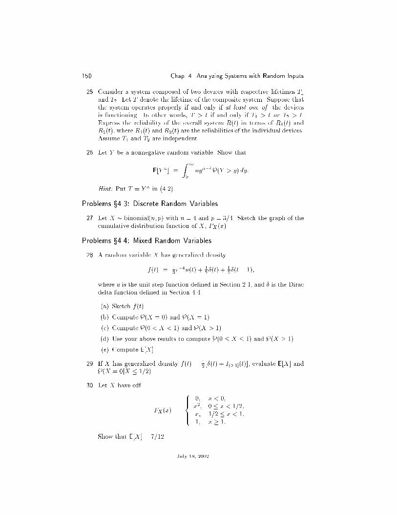
150 Chap. 4 Analyzing Systems with Random Inputs
25. Consider a system composed of two devices with respective lifetimes T1and T2. Let T denote the lifetime of the composite system. Suppose thatthe system operates properly if and only if at least one of the devicesis functioning. In other words, T > t if and only if T1 > t or T2 > t.Express the reliability of the overall system R(t) in terms of R1(t) andR2(t), where R1(t) and R2(t) are the reliabilities of the individual devices.Assume T1 and T2 are independent.
26. Let Y be a nonnegative random variable. Show that
E[Y n] =
Z 1
0
nyn�1}(Y > y) dy:
Hint: Put T = Y n in (4.2).
Problems x4.3: Discrete Random Variables
27. Let X � binomial(n; p) with n = 4 and p = 3=4. Sketch the graph of thecumulative distribution function of X, FX(x).
Problems x4.4: Mixed Random Variables
28. A random variable X has generalized density
f(t) = 13e
�tu(t) + 12�(t) +
16�(t � 1);
where u is the unit step function de�ned in Section 2.1, and � is the Diracdelta function de�ned in Section 4.4.
(a) Sketch f(t).
(b) Compute }(X = 0) and }(X = 1).
(c) Compute }(0 < X < 1) and }(X > 1).
(d) Use your above results to compute }(0 � X � 1) and }(X � 1).
(e) Compute E[X].
29. If X has generalized density f(t) = 12 [�(t) + I(0;1](t)], evaluate E[X] and
}(X = 0jX � 1=2).
30. Let X have cdf
FX(x) =
8>><>>:0; x < 0;x2; 0 � x < 1=2;x; 1=2 � x < 1;1; x � 1:
Show that E[X] = 7=12.
July 18, 2002

4.8 Problems 151
31. Sketch the graph of the cumulative distribution function of the randomvariable in Example 4.9. Also sketch corresponding impulsive densityfunction.
?32. A certain computer monitor contains a loose connection. The connectionis loose with probability 1=2. When the connection is loose, the monitordisplays a blank screen (brightness=0). When the connection is not loose,the brightness is uniformly distributed on (0; 1]. Let X denote the ob-served brightness. Find formulas and plot the cdf and generalized densityof X.
Problems x4.5: Functions of Random Variables and Their Cdfs
33. Let � � uniform[��; �], and put X := cos� and Y := sin�.
(a) Show that FX(x) = 1� 1�cos�1 x for �1 � x � 1.
(b) Show that FY (y) =12 +
1� sin
�1 y for �1 � y � 1.
(c) Use the identity sin(�=2 � �) = cos � to show that FX (x) =12 +
1� sin
�1 x. Thus, X and Y have the same cdf and are called arc-sine random variables. The corresponding density is fX (x) =(1=�)=
p1� x2 for �1 < x < 1.
34. Find the cdf and density of Y = X(X + 2) if X is uniformly distributedon [�3; 1].
35. Let g be as in Example 4.10 and 4.11. Find the cdf and density of Y =g(X) if
(a) X � uniform[�1; 1];(b) X � uniform[�1; 2];(c) X � uniform[�2; 3];(d) X � exp(�).
36. Let
g(x) :=
8<:0; jxj < 1;
jxj � 1; 1 � jxj � 2;1; jxj > 2:
Find the cdf and density of Y = g(X) if
(a) X � uniform[�1; 1];(b) X � uniform[�2; 2];(c) X � uniform[�3; 3];(d) X � Laplace(�).
July 18, 2002

152 Chap. 4 Analyzing Systems with Random Inputs
37. Let
g(x) :=
8>><>>:�x � 2; x < �1;�x2; �1 � x < 0;x3; 0 � x < 1;1; x � 1:
Find the cdf and density of Y = g(X) if
(a) X � uniform[�3; 2];(b) X � uniform[�3; 1];(c) X � uniform[�1; 1].
38. Consider the function g given by
g(x) =
8<:x2 � 1; x < 0;x� 1; 0 � x < 2;1; x � 2:
If X is uniform[�3;3], �nd the cdf and density of Y = g(X).
39. Let X be a uniformly distributed random variable on the interval [�3; 1].Let Y = g(X), where
g(x) =
8>><>>:0; x < �2;
x+ 2; �2 � x < �1;x2; �1 � x < 0;px; x � 0:
Find the cdf and density of Y .
40. Let X � uniform[�6; 0], and suppose that Y = g(X), where
g(x) =
8><>:jxj � 1; 1 � x < 2;
1�pjxj � 2; jxj � 2;
0; otherwise:
Find the cdf and density of Y .
41. Let X � uniform[�2; 1], and suppose that Y = g(X), where
g(x) =
8>>><>>>:x+ 2; �2 � x < �1;2x2
1 + x2; �1 � x < 0;
0; otherwise:
Find the cdf and density of Y .
?42. For x � 0, let g(x) denote the fractional part of x. For example, g(5:649) =0:649, and g(0:123) = 0:123. Find the cdf and density of Y = g(X) if
July 18, 2002
4.8 Problems 153
(a) X � exp(1);
(b) X � uniform[0; 1);
(c) X � uniform[v; v+ 1), where v = m+ � for some integer m � 0 andsome 0 < � < 1.
Problems x4.6: Properties of Cdfs
?43. From your solution of Problem 3(b) in Chapter 3, you can see that ifX � exp(�), then }(X > t + �tjX > t) = }(X > �t). Now provethe converse; i.e., show that if Y is a nonnegative random variable suchthat }(Y > t + �tjY > t) = }(Y > �t), then Y � exp(�), where� = � ln[1 � FY (1)], assuming that }(Y > t) > 0 for all t � 0. Hints:
Put h(t) := ln}(Y > t), which is a right-continuous function of t (Why?).Show that h(t +�t) = h(t) + h(�t) for all t;�t � 0.
Problems x4.7: The Central Limit Theorem
44. Packet transmission times on a certain Internet link are i.i.d. with meanm and variance �2. Suppose n packets are transmitted. Then the totalexpected transmission time for n packets is nm. Use the central limittheorem to approximate the probability that the total transmission timefor the n packets exceeds twice the expected transmission time.
45. To combat noise in a digital communication channel with bit-error proba-bility p, the use of an error-correcting code is proposed. Suppose that thecode allows correct decoding of a received binary codeword if the fractionof bits in error is less than or equal to t. Use the central limit theoremto approximate the probability that a received word cannot be reliablydecoded.
46. Let Xi = �1 with equal probability. Then the Xi are zero mean and haveunit variance. Put
Yn =nXi=1
Xipn:
Derive the central limit theorem for this case; i.e., show that 'Yn(�) !e��
2=2. Hint: Use the Taylor series approximation cos(�) � 1� �2=2.
July 18, 2002

154 Chap. 4 Analyzing Systems with Random Inputs
July 18, 2002

CHAPTER 5
Multiple Random Variables
The main focus of this chapter is the study of multiple continuous randomvariables that are not independent. In particular, conditional probability andconditional expectation along with corresponding laws of total probability andsubstitution are studied. These tools are used to compute probabilities involvingthe output of systems with multiple random inputs.
In Section 5.1 we introduce the concept of joint cumulative distributionfunction for a pair of random variables. Marginal cdfs are also de�ned. InSection 5.2 we introduce pairs of jointly continuous random variables, jointdensities, and marginal densities. Conditional densities, independence and ex-pectation are also discussed in the context of jointly continuous random vari-ables. In Section 5.3 conditional probability and expectation are de�ned forjointly continuous random variables. In Section 5.4 the bivariate normal den-sity is introduced, and some of its properties are illustrated via examples. InSection 5.5 most of the bivariate concepts are extended to the case of n randomvariables.
5.1. Joint and Marginal ProbabilitiesSuppose we have a pair of random variables, say X and Y , for which we
are able to compute }((X;Y ) 2 A) for arbitrary1 sets A � IR2. For example,suppose X and Y are the horizontal and vertical coordinates of a dart strikinga target. We might be interested in the probability that the dart lands withintwo units of the center. Then we would take A to be the disk of radius twocentered at the origin, i.e., A = f(x; y) : x2 + y2 � 4g. Now, even though wecan write down a formula for }((X;Y ) 2 A), we may be interested in �ndingpotentially simpler expressions for things like }(X 2 B; Y 2 C), }(X 2 B),and }(Y 2 C), etc. To this end, the notion of a product set is helpful.
Product Sets and Marginal Probabilities
The Cartesian product of two univariate sets B and C is de�ned by
B � C := f(x; y) : x 2 B and y 2 Cg:In other words,
(x; y) 2 B �C , x 2 B and y 2 C:
For example, if B = [1; 3] and C = [0:5; 3:5], then B � C is the rectangle
[1; 3]� [0:5; 3:5] = f(x; y) : 1 � x � 3 and 0:5 � y � 3:5g;which is illustrated in Figure 5.1(a). In general, if B and C are intervals, thenB � C is a rectangle or square. If one of the sets is an interval and the other
155

156 Chap. 5 Multiple Random Variables
01234
0 1 2 3 4
( a )
01234
0 1 2 3 4
( b )
Figure 5.1. The Cartesian products (a) [1;3]� [0:5;3:5] and (b)�[1;2][ [3;4]
�� [1; 4].
is a singleton, then the product set degenerates to a line segment in the plane.A more complicated example is shown in Figure 5.1(b), which illustrates theproduct
�[1; 2][ [3; 4]
�� [1; 4]. Figure 5.1(b) also illustrates the general resultthat � distributes over [; i.e., (B1 [B2)� C = (B1 � C) [ (B2 �C).
Using the notion of product set,
fX 2 B; Y 2 Cg = f! 2 : X(!) 2 B and Y (!) 2 Cg= f! 2 : (X(!); Y (!)) 2 B � Cg;
for which we use the shorthand
f(X;Y ) 2 B � Cg:
We can therefore write
}(X 2 B; Y 2 C) = }((X;Y ) 2 B � C):
The preceding expression allows us to obtain the marginal probability}(X 2 B) as follows. First, for any event F , we have F � , and therefore,F = F \ . Second, Y is assumed to be a real-valued random variable, i.e.,Y (!) 2 IR for all !. Thus, fY 2 IRg = . Now write
}(X 2 B) = }(fX 2 Bg \)
= }(fX 2 Bg \ fY 2 IRg)= }(X 2 B; Y 2 IR)
= }((X;Y ) 2 B � IR):
Similarly,}(Y 2 C) = }((X;Y ) 2 IR�C):
If X and Y are independent random variables, then
}((X;Y ) 2 B �C) = }(X 2 B; Y 2 C)
= }(X 2 B)}(Y 2 C):
July 18, 2002

5.1 Joint and Marginal Probabilities 157
Joint and Marginal Cumulative Distributions
The joint cumulative distribution function of X and Y is de�ned by
FXY (x; y) := }(X � x; Y � y)
= }((X;Y ) 2 (�1; x]� (�1; y]):
In Chapter 4, we saw that }(X 2 B) could be computed if we knew thecumulative distribution function FX (x) for all x. Similarly, it turns out thatwe can compute }((X;Y ) 2 A) if we know FXY (x; y) for all x; y. For example,it is shown in Problems 1 and 2 that
}((X;Y ) 2 (a; b]� (c; d]) = }(a < X � b; c < Y � d)
is given byFXY (b; d)� FXY (a; d)� FXY (b; c) + FXY (a; c):
In other words, the probability that (X;Y ) lies in a rectangle can be computedin terms of the cdf values at the corners.
If X and Y are independent random variables, we have the simpli�cations
FXY (x; y) = }(X � x; Y � y)
= }(X � x)}(Y � y)
= FX (x)FY (y);
and}(a < X � b; c < Y � d) =}(a < X � b)}(c < Y � d);
which is equal to [FX(b)� FX (a)][FY (d)� FY (c)].We return now to the general case (X and Y not necessarily independent).
It is possible to obtain the marginal cumulative distributions FX and FYdirectly from FXY by setting the unwanted variable to 1. More precisely, itcan be shown that2
FX(x) = limy!1FXY (x; y) =: FXY (x;1); (5.1)
andFY (y) = lim
x!1FXY (x; y) =: FXY (1; y):
Example 5.1. If
FXY (x; y) =
8<: y + e�x(y+1)
y + 1� e�x; x; y > 0;
0; otherwise;
�nd both of the marginal cumulative distribution functions, FX(x) and FY (y).
July 18, 2002

158 Chap. 5 Multiple Random Variables
Solution. For x; y > 0,
FXY (x; y) =y
y + 1+
1
y + 1� e�x(y+1) � e�x:
Hence, for x > 0,
limy!1FXY (x; y) = 1 + 0 � 0� e�x = 1� e�x:
For x � 0, FXY (x; y) = 0 for all y. So, for x � 0, limy!1FXY (x; y) = 0. The
complete formula for the marginal cdf of X is
FX(x) =
�1� e�x; x > 0;
0; x � 0:(5.2)
Next, for y > 0,
limx!1FXY (x; y) =
y
y + 1+
1
y + 1� 0� 0 =
y
y + 1:
We then see that the marginal cdf of Y is
FY (y) =
�y=(y + 1); y > 0;
0; y � 0:(5.3)
Note that since FXY (x; y) 6= FX (x)FY (y) for all x; y, X and Y are not inde-pendent,
Example 5.2. Express }(X � x or Y � y) using cdfs.
Solution. The desired probability is that of the union, }(A [ B), whereA := fX � xg and B := fY � yg. Applying the inclusion-exclusion formula(1.1) yields
}(A [B) = }(A) +}(B) �}(A \B)= }(X � x) +}(Y � y) �}(X � x; Y � y)
= FX(x) + FY (y) � FXY (x; y):
5.2. Jointly Continuous Random VariablesIn analogy with the univariate case, we say that two random variables X
and Y are jointly continuous with joint density fXY (x; y) if
}((X;Y ) 2 A) =
Z ZA
fXY (x; y) dx dy
July 18, 2002

5.2 Jointly Continuous Random Variables 159
=
Z 1
�1
Z 1
�1IA(x; y)fXY (x; y) dx dy
=
Z 1
�1
�Z 1
�1IA(x; y)fXY (x; y) dy
�dx
=
Z 1
�1
�Z 1
�1IA(x; y)fXY (x; y) dx
�dy
for some nonnegative function fXY that integrates to one; i.e.,Z 1
�1
Z 1
�1fXY (x; y) dx dy = 1:
Example 5.3. Show that
fXY (x; y) = 12� e
�(2x2�2xy+y2)=2
is a valid joint probability density.
Solution. Since fXY (x; y) is nonnegative, all we have to do is show thatit integrates to one. By completing the square in the exponent, we obtain
fXY (x; y) =e�(y�x)2=2p2�
� e�x2=2p2�
:
This factorization allows us to write the double integralZ 1
�1
Z 1
�1fXY (x; y) dx dy =
Z 1
�1
Z 1
�1
e�(2x2�2xy+y2)=2
2�dx dy
as the iterated integralZ 1
�1
e�x2=2
p2�
�Z 1
�1
e�(y�x)2=2p2�
dy
�dx:
The inner integral, as a function of y, is a normal density with mean x andvariance one. Hence, the inner integral is one. But this leaves only the outerintegral, whose integrand is an N (0; 1) density, which also integrates to one.
Marginal Densities
If A is a product set, say A = B � C, then IA(x; y) = IB(x) IC(y), and so
}(X 2 B; Y 2 C) = }((X;Y ) 2 B �C)
=
ZB
�ZC
fXY (x; y) dy
�dx (5.4)
=
ZC
�ZB
fXY (x; y) dx
�dy:
July 18, 2002

160 Chap. 5 Multiple Random Variables
At this point we would like to substitute B = (�1; x] and C = (�1; y] in orderto obtain expressions for FXY (x; y). However, the preceding integrals alreadyuse x and y for the variables of integration. To avoid confusion, we must �rstreplace the variables of integration. We change x to t and y to � . We then �ndthat
FXY (x; y) =
Z x
�1
�Z y
�1fXY (t; � ) d�
�dt;
or, equivalently,
FXY (x; y) =
Z y
�1
�Z x
�1fXY (t; � ) dt
�d�:
It then follows that
@2
@y@xFXY (x; y) = fXY (x; y) and
@2
@x@yFXY (x; y) = fXY (x; y):
Example 5.4. Let
FXY (x; y) =
8<: y + e�x(y+1)
y + 1� e�x; x; y > 0;
0; otherwise;
as in Example 5.1. Find the joint density fXY .
Solution. For x; y > 0,
@
@xFXY (x; y) = e�x � e�x(y+1);
and@2
@y@xFXY (x; y) = xe�x(y+1):
Thus,
fXY (x; y) =
�xe�x(y+1); x; y > 0;
0; otherwise:
We now show that if X and Y are jointly continuous, then X and Y areindividually continuous with marginal densities obtained as follows. TakingC = IR in (5.4), we obtain
}(X 2 B) = }((X;Y ) 2 B � IR) =
ZB
�Z 1
�1fXY (x; y) dy
�dx;
which implies the marginal density of X is
fX (x) =
Z 1
�1fXY (x; y) dy: (5.5)
July 18, 2002

5.2 Jointly Continuous Random Variables 161
Similarly,
}(Y 2 C) = }((X;Y ) 2 IR� C) =
ZC
�Z 1
�1fXY (x; y) dx
�dy;
and
fY (y) =
Z 1
�1fXY (x; y) dx:
Thus, to obtain the marginal densities, integrate out the unwanted variable.
Example 5.5. Using the joint density fXY obtained in Example 5.4, �ndthe marginal densities fX and fY by integrating out the unneeded variable. Tocheck your answer, also compute the marginal densities by di�erentiating themarginal cdfs obtained in Example 5.1.
Solution. We �rst compute fX (x). To begin, observe that for x � 0,fXY (x; y) = 0. Hence, for x � 0, the integral in (5.5) is zero. Now supposex > 0. Since fXY (x; y) = 0 whenever y � 0, the lower limit of integration in(5.5) can be changed to zero. For x > 0, it remains to computeZ 1
0
fXY (x; y) dy = xe�xZ 1
0
e�xy dy
= e�x:
Hence,
fX (x) =
�e�x; x > 0;0; x � 0;
and we see that X is exponentially distributed with parameter � = 1. Notethat the same answer can be obtained by di�erentiating the formula for FX(x)in (5.2).
We now turn to the calculation of fY (y). Arguing as above, we have fY (y) =0 for y � 0, and fY (y) =
R10 fXY (x; y) dx for y > 0. Write this integral asZ 1
0
fXY (x; y) dx =1
y + 1
Z 1
0
x � (y + 1)e�(y+1)x dx: (5.6)
If we put � = y + 1, then the integral on the right has the formZ 1
0
x � �e��x dx;
which is the mean of an exponential random variable with parameter �. Thisintegral is equal to 1=� = 1=(y+ 1), and so the right-hand side of (5.6) is equalto 1=(y + 1)2. We conclude that
fY (y) =
�1=(y + 1)2; y > 0;
0; y � 0:
Note that the same answer can be obtained by di�erentiating the formula forFY (y) in (5.3).
July 18, 2002

162 Chap. 5 Multiple Random Variables
Specifying Joint Densities
Suppose X and Y are jointly continuous with joint density fXY . De�ne
fY jX (yjx) :=fXY (x; y)
fX (x): (5.7)
For reasons that will become clear later, we call fY jX the conditional densityof Y given X. For the moment, simply note that as a function of y, fY jX (yjx)is nonnegative and integrates to one, since
Z 1
�1fY jX (yjx) dy =
Z 1
�1fXY (x; y) dy
fX(x)=
fX (x)
fX (x)= 1:
Now rewrite (5.7) as
fXY (x; y) = fY jX (yjx) fX (x):This suggests an easy way to specify a joint density. First, pick any one-dimensional density, say fX (x). Then fX(x) is nonnegative and integrates toone. Next, for each x, let fY jX (yjx) be any density in the variable y. Fordi�erent values of x, fY jX (yjx) could be very di�erent densities as a functionof y; the only important thing is that for each x, fY jX (yjx) as a function ofy should be nonnegative and integrate to one with respect to y. Now if wede�ne fXY (x; y) := fY jX(yjx) fX (x), we will have a nonnegative function of(x; y) whose double integral is one. In practice, and in the problems at the endof the chapter, this is how we usually specify joint densities.
Example 5.6. Let X � N (0; 1), and suppose that the conditional densityof Y given X = x is N (x; 1). Find the joint density fXY (x; y).
Solution. First note that
fX (x) =e�x
2=2
p2�
and fY jX(yjx) =e�(y�x)2=2p2�
:
Then write
fXY (x; y) = fY jX(yjx) fX (x) =e�(y�x)2=2p2�
� e�x2=2p2�
;
which simpli�es to
fXY (x; y) =exp[�(2x2 � 2xy + y2)=2]
2�:
By interchanging the roles of X and Y , we have
fXjY (xjy) :=fXY (x; y)
fY (y);
and we can de�ne fXY (x; y) = fXjY (xjy) fY (y) if we specify a density fY (y)and a function fXjY (xjy) that is a density in x for each �xed y.
July 18, 2002

5.2 Jointly Continuous Random Variables 163
Independence
We now consider the joint density of jointly continuous independent ran-dom variables. As noted in Section 5.1, if X and Y are independent, thenFXY (x; y) = FX(x)FY (y) for all x and y. If X and Y are also jointly continu-ous, then by taking second-order mixed partial derivatives, we �nd
@2
@y@xFX(x)FY (y) = fX (x) fY (y):
In other words, if X and Y are jointly continuous and independent, then thejoint density is the product of the marginal densities. Using (5.4), it is easy tosee that the converse is also true. If fXY (x; y) = fX (x) fY (y), (5.4) implies
}(X 2 B; Y 2 C) =
ZB
�ZC
fXY (x; y) dy
�dx
=
ZB
�ZC
fX (x) fY (y) dy
�dx
=
ZB
fX (x)
�ZC
fY (y) dy
�dx
=
�ZB
fX (x) dx
�}(Y 2 C)
= }(X 2 B)}(Y 2 C):
Expectation
If X and Y are jointly continuous with joint density fXY , then the methodsof Section 3.2 can easily be used to show that
E[g(X;Y )] =
Z 1
�1
Z 1
�1g(x; y)fXY (x; y) dx dy:
For arbitrary random variablesX and Y , their bivariate characteristic func-tion is de�ned by
'XY (�1; �2) := E[ej(�1X+�2Y )]:
If X and Y have joint density fXY , then
'XY (�1; �2) =
Z 1
�1
Z 1
�1fXY (x; y)e
j(�1x+�2y) dx dy;
which is simply the bivariate Fourier transform of fXY . By the inversionformula,
fXY (x; y) =1
(2�)2
Z 1
�1
Z 1
�1'XY (�1; �2)e
�j(�1x+�2y)d�1 d�2:
Now suppose that X and Y are independent. Then
'XY (�1; �2) = E[ej(�1X+�2Y )] = E[ej�1X ]E[ej�2Y ] = 'X (�1)'Y (�2):
July 18, 2002

164 Chap. 5 Multiple Random Variables
In other words, ifX and Y are independent, then their joint characteristic func-tion factors. The converse is also true; i.e., if the joint characteristic functionfactors, then X and Y are independent. The general proof is complicated, butif X and Y are jointly continuous, it is easy using the Fourier inversion formula.
?Continuous Random Variables That Are not Jointly Continuous
Let � � uniform[��; �], and put X := cos� and Y := sin�. As shownin Problem 33 in Chapter 4, X and Y are both arcsine random variables, eachhaving density (1=�)=
p1� x2 for �1 < x < 1.
Next, since X2+Y 2 = 1, the pair (X;Y ) takes values only on the unit circle
C := f(x; y) : x2 + y2 = 1g:Thus, }
�(X;Y ) 2 C
�= 1. On the other hand, if X and Y have a joint density
fXY , then
}�(X;Y ) 2 C
�=
Z ZC
fXY (x; y) dx dy = 0
because a double integral over a set of zero area must be zero. So, if X and Yhad a joint density, this would imply that 1 = 0. Since this is not true, therecan be no joint density.
5.3. Conditional Probability and ExpectationIf X is a continuous random variable, then its cdf FX(x) := }(X � x) =R x
�1 fX (t) dt is a continuous function of x. It follows from the properties ofcdfs in Section 4.6 that }(X = x) = 0 for all x. Hence, we cannot de�ne}(Y 2 CjX = x) by}(X = x; Y 2 C)=}(X = x) since this requires division byzero. Similar problems arise with conditional expectation. How should we de�neconditional probability and expectation in this case? Recall from Section 2.5that if X and Y are both discrete random variables, then the following law oftotal probability holds,
E[g(X;Y )] =Xi
E[g(X;Y )jX = xi] pX(xi):
If X and Y are jointly continuous, however we de�ne E[g(X;Y )jX = x], wecertainly want the analogous formula
E[g(X;Y )] =
Z 1
�1E[g(X;Y )jX = x]fX(x) dx (5.8)
to hold. To discover how E[g(X;Y )jX = x] should be de�ned, write
E[g(X;Y )] =
Z 1
�1
Z 1
�1g(x; y)fXY (x; y) dx dy
=
Z 1
�1
�Z 1
�1g(x; y)fXY (x; y) dy
�dx
July 18, 2002

5.3 Conditional Probability and Expectation 165
=
Z 1
�1
�Z 1
�1g(x; y)
fXY (x; y)
fX (x)dy
�fX (x) dx
=
Z 1
�1
�Z 1
�1g(x; y)fY jX (yjx) dy
�fX (x) dx:
It follows that if
E[g(X;Y )jX = x] :=
Z 1
�1g(x; y) fY jX(yjx) dy; (5.9)
then (5.8) holds.Now observe that if g in (5.9) is a function of y alone, then
E[g(Y )jX = x] =
Z 1
�1g(y) fY jX (yjx) dy: (5.10)
Returning now to the case g(x; y), we see that (5.10) implies that for any ~x,
E[g(~x; Y )jX = x] =
Z 1
�1g(~x; y) fY jX(yjx) dy:
Taking ~x = x, we obtain
E[g(x; Y )jX = x] =
Z 1
�1g(x; y) fY jX(yjx) dy:
Comparing this with (5.9) shows that
E[g(X;Y )jX = x] = E[g(x; Y )jX = x]:
In other words, the substitution law holds. Another important point to note isthat if X and Y are independent, then
fY jX (yjx) =fXY (x; y)
fX(x)=
fX (x) fY (y)
fX (x)= fY (y):
In this case, (5.10) becomes E[g(Y )jX = x] = E[g(Y )]. In other words, we can\drop the conditioning."
Example 5.7. Let X � exp(1), and suppose that given X = x, Y isconditionally normal with fY jX(�jx) � N (0; x2). Evaluate E[Y 2] and E[Y 2X3].
Solution. We use the law of total probability for expectation. We beginwith
E[Y 2] =
Z 1
�1E[Y 2jX = x]fX (x) dx:
July 18, 2002

166 Chap. 5 Multiple Random Variables
Since fY jX (yjx) = e�(y=x)2=2=(p2� x), we see that
E[Y 2jX = x] =
Z 1
�1y2
e�(y=x)2=2
p2� x
dy
is the second moment of a zero-mean Gaussian density with variance x2. Hence,E[Y 2jX = x] = x2, and
E[Y 2] =
Z 1
�1x2fX (x) dx = E[X2]:
Since X � exp(1), E[X2] = 2 by Example 3.9.To compute E[Y 2X3], we proceed similarly. Write
E[Y 2X3] =
Z 1
�1E[Y 2X3jX = x]fX(x) dx
=
Z 1
�1E[Y 2x3jX = x]fX(x) dx
=
Z 1
�1x3E[Y 2jX = x]fX(x) dx
=
Z 1
�1x3x2fX (x) dx
= E[X5]
= 5!; by Example 3.9:
For conditional probability, if we put
}(Y 2 CjX = x) :=
ZC
fY jX(yjx) dy;
then it is easy to show that the law of total probability
}(Y 2 C) =
Z 1
�1}(Y 2 CjX = x) fX (x) dx
holds. It can also be shown3 that the substitution law holds for conditionalprobabilities involving X and Y conditioned on X. Also, if X and Y areindependent, then }(Y 2 CjX = x) = }(Y 2 C); i.e., we can \drop theconditioning."
Example 5.8 (Signal in Additive Noise). A random, continuous-valued sig-nalX is transmitted over a channel subject to additive, continuous-valued noiseY . The received signal is Z = X + Y . Find the cdf and density of Z if X andY are jointly continuous random variables with joint density fXY .
July 18, 2002

5.3 Conditional Probability and Expectation 167
Solution. Since we are not assuming that X and Y are independent, thecharacteristic-function method of Example 3.14 does not work here. Instead,we use the laws of total probability and substitution. Write
FZ(z) = }(Z � z)
=
Z 1
�1}(Z � zjY = y) fY (y) dy
=
Z 1
�1}(X + Y � zjY = y) fY (y) dy
=
Z 1
�1}(X + y � zjY = y) fY (y) dy
=
Z 1
�1}(X � z � yjY = y) fY (y) dy
=
Z 1
�1FXjY (z � yjy) fY (y) dy:
By di�erentiating with respect to z,
fZ(z) =
Z 1
�1fXjY (z � yjy) fY (y) dy:
In particular, note that if X and Y are independent, we can drop the condi-tioning and recover the convolution result stated following Example 3.14,
fZ(z) =
Z 1
�1fX (z � y) fY (y) dy:
Example 5.9 (Signal in Multiplicative Noise). A random, continuous-val-ued signalX is transmitted over a channel subject to multiplicative, continuous-valued noise Y . The received signal is Z = XY . Find the cdf and density of Zif X and Y are jointly continuous random variables with joint density fXY .
Solution. We proceed as in the previous example. Write
FZ(z) = }(Z � z)
=
Z 1
�1}(Z � zjY = y) fY (y) dy
=
Z 1
�1}(XY � zjY = y) fY (y) dy
=
Z 1
�1}(Xy � zjY = y) fY (y) dy:
At this point we have a problem when we attempt to divide through by y. If yis negative, we have to reverse the inequality sign. Otherwise, we do not have
July 18, 2002

168 Chap. 5 Multiple Random Variables
to reverse the inequality. The solution to this di�culty is to break up the rangeof integration. Write
FZ(z) =
Z 0
�1}(Xy � zjY = y) fY (y) dy
+
Z 1
0
}(Xy � zjY = y) fY (y) dy:
Now we can divide by y separately in each integral. Thus,
FZ(z) =
Z 0
�1}(X � z=yjY = y) fY (y) dy
+
Z 1
0
}(X � z=yjY = y) fY (y) dy
=
Z 0
�1
�1� FXjY
�zy
��y�� fY (y) dy+
Z 1
0
FXjY�zy
��y� fY (y) dy:Di�erentiating with respect to z yields
fZ(z) = �Z 0
�1fXjY
�zy
��y� 1yfY (y) dy +
Z 1
0
fXjY�zy
��y� 1yfY (y) dy:
Now observe that in the �rst integral, the range of integration implies that yis always negative. For such y, �y = jyj. In the second integral, y is alwayspositive, and so y = jyj. Thus,
fZ(z) =
Z 0
�1fXjY
�zy
��y� 1jyj fY (y) dy +
Z 1
0
fXjY�zy
��y� 1jyj fY (y) dy
=
Z 1
�1fXjY
�zy
��y� 1jyj fY (y) dy:
5.4. The Bivariate NormalThe bivariate Gaussian or bivariate normal density is a generalization
of the univariate N (m;�2) density. Recall that the standard N (0; 1) densityis given by '(x) := exp(�x2=2)=p2�. The general N (m;�2) density can bewritten in terms of ' as
1p2� �
exp
��1
2
�x�m
�
�2�=
1
��'�x�m
�
�:
In order to de�ne the general bivariate Gaussian density, it is convenient tode�ne a standard bivariate density �rst. So, for j�j < 1, put
'�(u; v) :=exp�
�12(1��2) [u
2 � 2�uv + v2]�
2�p1� �2
: (5.11)
July 18, 2002

5.4 The Bivariate Normal 169
−3−2
−10
12
3 −3
−2
−1
0
1
2
30
0.05
0.1
0.15
v−axis
u−axis
Figure 5.2. The Gaussian surface '�(u; v) of (5.11) with � = 0.
For �xed �, this function of the two variables u and v de�nes a surface. Thesurface corresponding to � = 0 is shown in Figure 5.2. From the �gure and fromthe formula (5.11), we see that '0 is circularly symmetric; i.e., for all (u; v) on a
circle of radius r, in other words, for u2+v2 = r2, '0(u; v) = e�r2=2=2� does not
depend on the particular values of u and v, but only on the radius of the circleon which they lie. We also point out that for � = 0, the formula (5.11) factorsinto the product of two univariate N (0; 1) densities, i.e., '0(u; v) = '(u)'(v).For � 6= 0, '� does not factor. In other words, if U and V have joint density '�,then U and V are independent if and only if � = 0. A plot of '� for � = �0:85is shown in Figure 5.3. It turns out that now '� is constant on ellipses insteadof circles. The axes of the ellipses are not parallel to the coordinate axes.Notice how the density is concentrated along the line v = �u. As �!�1, thisconcentration becomes more extreme. As � ! +1, the density concentratesaround the line v = u. We now show that the density '� integrates to one. Todo this, �rst observe that for all j�j < 1,
u2 � 2�uv + v2 = u2(1� �2) + (v � �u)2:
It follows that
'�(u; v) =e�u
2=2
p2�
�exp�
�12(1��2) [v � �u]2
�p2�p1� �2
= '(u) � 1p1� �2
'
�v � �up1� �2
�: (5.12)
Observe that the right-hand factor as a function of v has the form of a univariate
July 18, 2002

170 Chap. 5 Multiple Random Variables
−3−2
−10
12
3−3
−2
−1
0
1
2
3
0
0.05
0.1
0.15
0.2
0.25
0.3
v−axis
u−axis
Figure 5.3. The Gaussian surface '�(u; v) of (5.11) with � = �0:85.
normal density with mean �u and variance 1��2. With '� factored as in (5.12),we can write
R1�1R1�1'�(u; v) du dv as the iterated integralZ 1
�1'(u)
� Z 1
�1
1p1� �2
'
�v � �up1� �2
�dv
�du:
As noted above, the inner integrand, as a function of v, is simply anN (�u; 1��2)density, and therefore integrates to one. Hence, the above iterated integralbecomes
R1�1 '(u) du = 1.
We can now easily de�ne the general bivariate Gaussian density with pa-rameters mX , mY , �2X , �
2Y , and � by
fXY (x; y) :=1
�X�Y'�
�x�mX
�X;y �mY
�Y
�:
More explicitly, this density is
exp�
�12(1��2) [(
x�mX
�X)2 � 2�(x�mX
�X)(y�mY
�Y) + (y�mY
�Y)2]�
2��X�Yp1� �2
: (5.13)
It can be shown that the marginals are fX � N (mX ; �2X) and fY � N (mY ; �
2Y )
(see Problems 25 and 28). The parameter � is called the correlation coe�-cient. From (5.13), we observe that X and Y are independent if and only if� = 0. A plot of fXY with mX = mY = 0, �X = 1:5, �Y = 0:6, and � = 0is shown in Figure 5.4. Notice how the density is concentrated around the line
July 18, 2002

5.4 The Bivariate Normal 171
−3−2
−10
12
3 −3
−2
−1
0
1
2
30
0.02
0.04
0.06
0.08
0.1
0.12
0.14
0.16
y−axis
x−axis
Figure 5.4. The bivariate normal density fXY (x; y) of (5.13) withmX = mY = 0, �X = 1:5,�Y = 0:6, and � = 0.
y = 0. Also, fXY is constant on ellipses of the form�x
�X
�2
+
�y
�Y
�2
= r2:
To show thatR1�1R1�1fXY (x; y) dx dy = 1 as well, use formula (5.12) for
'� and proceed as above, integrating with respect to y �rst and then x. Forthe inner integral, make the change of variable v = (y � mY )=�Y , and in theremaining outer integral make the change of variable u = (x�mX )=�X .
Example 5.10. Let random variables U and V have the standard bivariatenormal density '� in (5.11). Show that E[UV ] = �.
Solution. Using the factored form of '� in (5.12), write
E[UV ] =
Z 1
�1
Z 1
�1uv '�(u; v) du dv
=
Z 1
�1u'(u)
� Z 1
�1
vp1� �2
'
�v � �up1� �2
�dv
�du:
The quantity in brackets has the form E[V ], where V is a univariate normalrandom variable with mean �u and variance 1� �2. Thus,
E[UV ] =
Z 1
�1u'(u)[�u] du
= �
Z 1
�1u2'(u) du
= �;
July 18, 2002

172 Chap. 5 Multiple Random Variables
since ' is the N (0; 1) density.
Example 5.11. Let U and V have the standard bivariate normal densityfUV (u; v) = '�(u; v) given in (5.11). Find the conditional densities fV jU andfUjV .
Solution. It is shown in Problem 25 that fU and fV are both N (0; 1).Hence,
fV jU (vju) =fUV (u; v)
fU (u)=
'�(u; v)
'(u);
where ' is the N (0; 1) density. If we now substitute the factored form of '�(u; v)given in (5.12), we obtain
fV jU(vju) =1p
1� �2'
�v � �up1� �2
�;
i.e., fV jU(� ju) � N (�u; 1� �2). To compute fUjV we need the following alter-native factorization of '�,
'�(u; v) =1p
1� �2'
�u� �vp1� �2
�� '(v):
It then follows that
fUjV (ujv) =1p
1� �2'
�u� �vp1� �2
�;
i.e., fUjV (� jv) � N (�v; 1 � �2).
Example 5.12. If U and V have standard joint normal density '�(u; v),�nd E[V jU = u].
Solution. Recall that from Example 5.11, fV jU (�ju) � N (�u; 1 � �2).Hence,
E[V jU = u] =
Z 1
�1v fV jU (vju) dv = �u:
5.5. ?Multivariate Random VariablesLet X := [X1; : : : ; Xn]0 (the prime denotes transpose) be a length-n column
vector of random variables. We callX a random vector. We say that the vari-ables X1; : : : ; Xn are jointly continuouswith joint density fX = fX1���Xn iffor A � IRn,
}(X 2 A) =
ZA
fX (x) dx =
ZIRn
IA(x) fX (x) dx;
July 18, 2002

5.5 ?Multivariate Random Variables 173
which is shorthand forZ 1
�1� � �Z 1
�1IA(x1; : : : ; xn) fX1���Xn (x1; : : : ; xn) dx1 � � �dxn:
Usually, we need to compute probabilities of the form
}(X1 2 B1; : : : ; Xn 2 Bn) := }
� n\k=1
fXk 2 Bkg�;
where B1; : : : ; Bn are one-dimensional sets. The key to this calculation is toobserve that
n\k=1
fXk 2 Bkg =n[X1; : : : ; Xn]
0 2 B1 � � � � � Bn
o:
(Recall that a vector [x1; : : : ; xn]0 lies in the Cartesian product set B1�� � ��Bn
if and only if xi 2 Bi for i = 1; : : : ; n.) It now follows that
}(X1 2 B1; : : : ; Xn 2 Bn) =
ZB1
� � �ZBn
fX1 ���Xn(x1; : : : ; xn) dx1 � � �dxn:
For example, to compute the joint cumulative distribution function, take Bk =(�1; xk] to get
FX (x) := FX1���Xn (x1; : : : ; xn)
:= }(X1 � x1; : : : ; Xn � xn)
=
Z x1
�1� � �Z xn
�1fX1 ���Xn (t1; : : : ; tn) dt1 � � �dtn;
where we have changed the dummy variables of integration to t to avoid con-fusion with the upper limits of integration. Note also that
@nFX@xn � � �@x1
����x1;:::;xn
= fX1���Xn (x1; : : : ; xn):
We can use these equations to characterize the joint cdf and density of inde-pendent random variables. First, suppose X1; : : : ; Xn are independent. Then
FX(x) = }(X1 � x1; : : : ; Xn � xn)
= }(X1 � x1) � � �}(Xn � xn):
By taking partial derivatives, we learn that
fX1���Xn(x1; : : : ; xn) = fX1(x1) � � �fXn (xn):
Thus, if the Xi are independent, then the joint density factors. On the otherhand, if the joint density factors, then }(X1 2 B1; : : : ; Xn 2 Bn) has the formZ
B1
� � �ZBn
fX1(x1) � � �fXn (xn) dx1 � � �dxn;
July 18, 2002

174 Chap. 5 Multiple Random Variables
which factors into the product�ZB1
fX1(x1) dx1
�� � ��Z
Bn
fXn (xn) dxn
�:
Thus, if the joint density factors,
}(X1 2 B1; : : : ; Xn 2 Bn) = }(X1 2 B1) � � �}(Xn 2 Bn);
and we see that the Xi are independent.Sometimes we need to compute probabilities involving only some of the Xi.
In this case, we can obtain the joint density of the ones we need by integratingout the ones we do not need. For example,
fXi(xi) =
ZIRn�1
fX (x1; : : : ; xn) dx1 � � �dxi�1dxi+1 � � �dxn;
and
fX1X2(x1; x2) =
Z 1
�1� � �Z 1
�1fX1 ���Xn (x1; : : : ; xn) dx3 � � �dxn:
We can use these results to compute conditional densities such as
fX3 ���XnjX1X2(x3; : : : ; xnjx1; x2) =
fX1 ���Xn (x1; : : : ; xn)
fX1X2(x1; x2)
:
Example 5.13. Let
fXY Z(x; y; z) =3z2
7p2�
e�zy exph�1
2
�x�yz
�2i;
for y � 0 and 1 � z � 2, and fXY Z(x; y; z) = 0 otherwise. Find fY Z(y; z) andfXjY Z(xjy; z). Then �nd fZ(z), fY jZ(yjz), and fXY jZ(x; yjz).
Solution. Observe that the joint density can be written as
fXY Z(x; y; z) =exph�1
2
�x�yz
�2ip2� z
� ze�zy � 37z2:
The �rst factor as a function of x is an N (y; z2) density. Hence,
fY Z(y; z) =
Z 1
�1fXY Z(x; y; z) dx = ze�zy � 37z2;
and
fXjY Z(xjy; z) =fXY Z(x; y; z)
fY Z(y; z)=
exph�1
2
�x�yz
�2ip2� z
:
July 18, 2002

5.5 ?Multivariate Random Variables 175
Thus, fXjY Z(�jy; z) � N (y; z2). Next, in the above formula for fY Z(y; z), ob-serve that ze�zy as a function of y is an exponential density with parameter z.Thus,
fZ(z) =
Z 1
0
fY Z(y; z) dy = 37z2; 1 � z � 2:
It follows that fY jZ(yjz) = fY Z(y; z)=fZ(z) = ze�zy ; i.e., fY jZ(�jz) � exp(z).Finally,
fXY jZ(x; yjz) =fXY Z(x; y; z)
fZ(z)=
exph�1
2
�x�yz
�2ip2� z
� ze�zy:
The preceding example shows that
fXY Z(x; y; z) = fXjY Z(xjy; z) fY jZ(yjz) fZ (z):
More generally,
fX1���Xn (x1; : : : ; xn) = fX1(x1) fX2jX1
(x2jx1) fX3 jX1X2(x3jx1; x2) � � �
� � �fXnjX1���Xn�1(xnjx1; : : : ; xn�1):
Contemplating this equation for a moment reveals that
fX1���Xn (x1; : : : ; xn) = fX1���Xn�1 (x1; : : : ; xn�1) fXnjX1���Xn�1(xnjx1; : : : ; xn�1);
which is an important recursion that is discussed later.If g(x) = g(x1; : : : ; xn) is a real-valued function of the vector x = [x1; : : : ; xn]0,
then we can compute
E[g(X)] =
ZIRn
g(x) fX (x) dx;
which is shorthand forZ 1
�1� � �Z 1
�1g(x1; : : : ; xn) fX1���Xn (x1; : : : ; xn) dx1 � � �dxn:
The Law of Total Probability
We also have the law of total probability and the substitution law for multi-ple random variables. Let U = [U1; : : : ; Um]
0 and V = [V1; : : : ; Vn]0 be any two
vectors of random variables. The law of total probability tells us that
E[g(U; V )] =
Z 1
�1� � �Z 1
�1| {z }m times
E[g(U; V )jU = u] fU (u) du;
July 18, 2002

176 Chap. 5 Multiple Random Variables
where, by the substitution law, E[g(U; V )jU = u] = E[g(u; V )jU = u], and
E[g(u; V )jU = u] =
Z 1
�1� � �Z 1
�1| {z }n times
g(u; v) fV jU(vju) dv;
and
fV jU(vju) =fUV (u1; : : : ; um; v1; : : : ; vn)
fU (u1; : : : ; um):
When g has a product form, say g(u; v) = h(u)k(v), it is easy to see that
E[h(u)k(V )jU = u] = h(u)E[k(V )jU = u]:
Example 5.14. Let X, Y , and Z be as in Example 5.13. Find E[X] andE[XZ].
Solution. Rather than use the marginal density of X to compute E[X],we use the law of total probability. Write
E[X] =
Z 1
�1
Z 1
�1E[XjY = y; Z = z] fY Z(y; z) dy dz:
Next, from Example 5.13, fXjY Z(�jy; z) � N (y; z2), and so E[XjY = y; Z =z] = y. Thus,
E[X] =
Z 1
�1
�Z 1
�1y fY Z(y; z) dy
�dz
=
Z 1
�1
�Z 1
�1y fY jZ(yjz) dy
�fZ(z) dz
=
Z 1
�1E[Y jZ = z] fZ(z) dz:
From Example 5.13, fY jZ(�jz) � exp(z) and fZ(z) = 3z2=7; hence, E[Y jZ =z] = 1=z, and we have
E[X] =
Z 2
1
37z dz = 9
14 :
Now, to �nd E[XZ], write
E[XZ] =
Z 1
�1
Z 1
�1E[XzjY = y; Z = z] fY Z(y; z) dy dz:
We then note that E[XzjY = y; Z = z] = E[XjY = y; Z = z] z = yz. Thus,
E[XZ] =
Z 1
�1
Z 1
�1yz fY Z(y; z) dy dz = E[Y Z]:
In Problem 34 the reader is asked to show that E[Y Z] = 1. Thus, E[XZ] = 1as well.
July 18, 2002

5.6 Notes 177
Example 5.15. Let N be a positive, integer-valued random variable, andlet X1; X2; : : : be i.i.d. Further assume that N is independent of this sequence.Consider the random sum,
NXi=1
Xi:
Note that the number of terms in the sum is a random variable. Find the meanvalue of the random sum.
Solution. Use the law of total probability to write
E
� NXi=1
Xi
�=
1Xn=1
E
� nXi=1
Xi
����N = n
�}(N = n):
By independence of N and the Xi sequence,
E
� nXi=1
Xi
����N = n
�= E
� nXi=1
Xi
�=
nXi=1
E[Xi]:
Since the Xi are i.i.d., they all have the same mean. In particular, for all i,E[Xi] = E[X1]. Thus,
E
� nXi=1
Xi
����N = n
�= nE[X1]:
Now we can write
E
� NXi=1
Xi
�=
1Xn=1
nE[X1]}(N = n)
= E[N ]E[X1]:
5.6. NotesNotes x5.1: Joint and Marginal Probabilities
Note 1. Comments analogous to Note 1 in Chapter 2 apply here. Specif-ically, the set A must be restricted to a suitable �-�eld B of subsets of IR2.Typically, B is taken to be the collection of Borel sets of IR2; i.e., B is thesmallest �-�eld containing all the open sets of IR2.
Note 2. We now derive the limit formula for FX (x) in (5.1); the formulafor FY (y) can be derived similarly. To begin, write
FX(x) := }(X � x) = }((X;Y ) 2 (�1; x]� IR):
July 18, 2002

178 Chap. 5 Multiple Random Variables
Next, observe that IR =S1n=1(�1; n], and write
(�1; x]� IR = (�1; x]�1[n=1
(�1; n]
=1[n=1
(�1; x]� (�1; n]:
Since the union is increasing, we can use the limit property (1.4) to show that
FX(x) = }
�(X;Y ) 2
1[n=1
(�1; x]� (�1; n]
�= lim
N!1}((X;Y ) 2 (�1; x]� (�1; N ])
= limN!1
FXY (x;N ):
Notes x5.3: Conditional Probability and Expectation
Note 3. To show that the law of substitution holds for conditional proba-bility, write
}(g(X;Y ) 2 C) = E[IC(g(X;Y ))] =
Z 1
�1E[IC(g(X;Y ))jX = x]fX(x) dx
and reduce the problem to one involving conditional expectation, for which thelaw of substitution has already been established.
5.7. ProblemsProblems x5.1: Joint and Marginal Distributions
1. For a < b and c < d, sketch the following sets.
(a) R := (a; b]� (c; d].
(b) A := (�1; a]� (�1; d].
(c) B := (�1; b]� (�1; c].
(d) C := (a; b]� (�1; c].
(e) D := (�1; a]� (c; d].
(f) A \B.2. Show that }(a < X � b; c < Y � d) is given by
FXY (b; d)� FXY (a; d)� FXY (b; c) + FXY (a; c):
Hint: Using the notation of the preceding problem, observe that
(�1; b]� (�1; d] = R [ (A [B);and solve for }((X;Y ) 2 R).
July 18, 2002
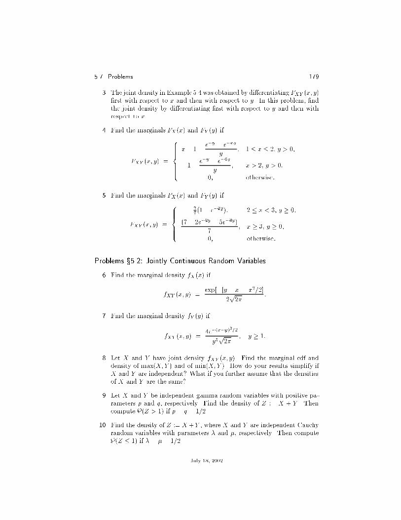
5.7 Problems 179
3. The joint density in Example 5.4 was obtained by di�erentiating FXY (x; y)�rst with respect to x and then with respect to y. In this problem, �ndthe joint density by di�erentiating �rst with respect to y and then withrespect to x.
4. Find the marginals FX (x) and FY (y) if
FXY (x; y) =
8>>>><>>>>:x� 1� e�y � e�xy
y; 1 � x � 2; y > 0;
1� e�y � e�2y
y; x > 2; y > 0;
0; otherwise:
5. Find the marginals FX (x) and FY (y) if
FXY (x; y) =
8>>><>>>:27(1� e�2y); 2 � x < 3; y � 0;
(7� 2e�2y � 5e�3y)
7; x � 3; y � 0;
0; otherwise:
Problems x5.2: Jointly Continuous Random Variables
6. Find the marginal density fX (x) if
fXY (x; y) =exp[�jy � xj � x2=2]
2p2�
:
7. Find the marginal density fY (y) if
fXY (x; y) =4e�(x�y)2=2
y5p2�
; y � 1:
8. Let X and Y have joint density fXY (x; y). Find the marginal cdf anddensity of max(X;Y ) and of min(X;Y ). How do your results simplify ifX and Y are independent? What if you further assume that the densitiesof X and Y are the same?
9. Let X and Y be independent gamma random variables with positive pa-rameters p and q, respectively. Find the density of Z := X + Y . Thencompute }(Z > 1) if p = q = 1=2.
10. Find the density of Z := X +Y , where X and Y are independent Cauchyrandom variables with parameters � and �, respectively. Then compute}(Z � 1) if � = � = 1=2.
July 18, 2002
180 Chap. 5 Multiple Random Variables
?11. If X � N (0; 1), then the complementary cumulative distribution function(ccdf) of X is
Q(x0) := }(X > x0) =
Z 1
x0
e�x2=2
p2�
dx:
(a) Show that
Q(x0) =1
�
Z �=2
0
exp
� �x202 cos2 �
�d�; x0 � 0:
Hint: For any random variables X and Y , we can always write
}(X > x0) = }(X > x0; Y 2 IR) =}((X;Y ) 2 D);
where D is the half plane D := f(x; y) : x > x0g. Now specialize tothe case where X and Y are independent and both N (0; 1). Thenthe probability on the right is a double integral that can be evaluatedusing polar coordinates.
Remark. The procedure outlined in the hint is a generalization ofthat used in Section 3.1 to show that the standard normal densityintegrates to one. To see this, note that if x0 = �1, then D = IR2.
(b) Use the result of (a) to derive Craig's formula [10, p. 572, eq. (9)],
Q(x0) =1
�
Z �=2
0
exp
� �x202 sin2 t
�dt; x0 � 0:
Remark. Simon [41] has derived a similar result for the Marcum Qfunction (de�ned in Problem 17 in Chapter 4) and its higher-ordergeneralizations. See also [43, pp. 1865{1867].
Problems x5.3: Conditional Probability and Expectation
12. Let fXY (x; y) be as derived in Example 5.4, and note that fX (x) andfY (y) were found in Example 5.5. Find fY jX (yjx) and fXjY (xjy) forx; y > 0.
13. Let fXY (x; y) be as derived in Example 5.4, and note that fX (x) andfY (y) were found in Example 5.5. Compute E[Y jX = x] for x > 0 andE[XjY = y] for y > 0.
14. Let X and Y be jointly continuous. Show that if
}(Y 2 CjX = x) :=
ZC
fY jX(yjx) dy;
then
}(Y 2 C) =
Z 1
�1}(Y 2 CjX = x)fX (x) dx:
July 18, 2002

5.7 Problems 181
15. Find }(X � Y ) if X and Y are independent with X � exp(�) andY � exp(�).
16. Let X and Y be independent random variables with Y being exponentialwith parameter 1 and X being uniform on [1; 2]. Find }(Y= ln(1+X2) >1).
17. Let X and Y be jointly continuous random variables with joint densityfXY . Find fZ(z) if
(a) Z = eXY .
(b) Z = jX + Y j.18. Let X and Y be independent continuous random variables with respective
densities fX and fY . Put Z = Y=X.
(a) Find the density of Z. Hint: Review Example 5.9.
(b) If X and Y are both N (0; �2), show that Z has a Cauchy(1) densitythat does not depend on �2.
(c) If X and Y are both Laplace(�), �nd a closed-form expression forfZ(z) that does not depend on �.
(d) Find a closed-form expression for the density of Z if Y is uniform on[�1; 1] and X � N (0; 1).
(e) If X and Y are both Rayleigh random variables with parameter �,�nd a closed-form expression for the density of Z. Your answershould not depend on �.
19. Let X and Y be independent with densities fX (x) and fY (y). If X is apositive random variable, and if Z = Y= ln(X), �nd the density of Z.
20. Let Y � exp(�), and suppose that given Y = y, X � gamma(p; y).Assuming r > n, evaluate E[XnY r ].
21. Use the law of total probability to to solve the following problems.
(a) Evaluate E[cos(X + Y )] if given X = x, Y is conditionally uniformon [x� �; x+ �].
(b) Evaluate }(Y > y) if X � uniform[1; 2], and given X = x, Y isexponential with parameter x.
(c) Evaluate E[XeY ] if X � uniform[3; 7], and given X = x, Y �N (0; x2).
(d) LetX � uniform[1; 2], and suppose that givenX = x, Y � N (0; 1=x).Evaluate E[cos(XY )].
22. Find E[XnY m] if Y � exp(�), and given Y = y, X � Rayleigh(y).
?23. Let X � gamma(p; �) and Y � gamma(q; �) be independent.
July 18, 2002

182 Chap. 5 Multiple Random Variables
(a) If Z := X=Y , show that the density of Z is
fZ (z) =1
B(p; q)� zp�1
(1 + z)p+q; z > 0:
Observe that fZ(z) depends on p and q, but not on �. It was shownin Problem 19 in Chapter 3 that fZ(z) integrates to one. Hint: Youwill need the fact that B(p; q) = �(p)�(q)=�(p+q), which was shownin Problem 13 in Chapter 3.
(b) Show that V := X=(X + Y ) has a beta density with parameters pand q. Hint: Observe that V = Z=(1 + Z), where Z = X=Y asabove.
Remark. If W := (X=p)=(Y=q), then fW (w) = (p=q) fZ(w(p=q)). Iffurther p = k1=2 and q = k2=2, then W is said to be an F randomvariable with k1 and k2 degrees of freedom. If further � = 1=2, then theX and Y are chi-squared with k1 and k2 degrees of freedom, respectively.
?24. Let X and Y be independent with X � N (0; 1) and Y being chi-squaredwith k degrees of freedom. Show that the density of Z := X=
pY=k has
a student's t density with k degrees of freedom. Hint: For this prob-lem, it may be helpful to review the results of Problems 11{13 and 17 inChapter 3.
Problems x5.4: The Bivariate Normal
25. Let U and V have the joint Gaussian density in (5.11). Show that forall � with �1 < � < 1, U and V both have standard univariate N (0; 1)marginal densities that do not involve �.
26. Let X and Y be jointly Gaussian with density fXY (x; y) given by (5.13).Find fX (x), fY (y), fXjY (xjy), and fY jX(yjx).
27. Let X and Y be jointly Gaussian with density fXY (x; y) given by (5.13).Find E[Y jX = x] and E[XjY = y].
28. If X and Y are jointly normal with parameters, mX , mY , �2X , �2Y , and �.
Compute E[X], E[X2], and E[XY ].
?29. Let '� be the standard bivariate normal density de�ned in (5.11). Put
fUV (u; v) :=1
2['�1(u; v) + '�2 (u; v)];
where �1 < �1 6= �2 < 1.
(a) Show that the marginals fU and fV are both N (0; 1). (You may usethe results of Problem 25.)
July 18, 2002

5.7 Problems 183
(b) Show that � := E[UV ] = (�1 + �2)=2. (You may use the result ofExample 5.10.)
(c) Show that U and V cannot be jointly normal. Hints: (i) To obtaina contradiction, suppose that fUV is a jointly normal density withparameters given by parts (a) and (b). (ii) Consider fUV (u; u). (iii)Use the following fact: If �1; : : : ; �n are distinct real numbers, and if
nXk=1
�ke�kt = 0; for all t � 0;
then �1 = � � � = �n = 0.
?30. Let U and V be jointly normal with joint density '�(u; v) de�ned in(5.11). Put
Q�(u0; v0) := }(U > u0; V > v0):
Show that for u0; v0 � 0,
Q�(u0; v0) =
Z �=2�tan�1(u0=v0)
0
h�(u20; �) d�
+
Z tan�1(u0=v0)
0
h�(v20 ; �) d�;
where
h�(z; �) :=
p1� �2
2�(1� � sin 2�)exp
��z(1 � � sin 2�)
2(1� �2) sin2 �
�:
This formula forQ�(u0; v0) is Simon's bivariate generalization [43, pp. 1864{1865] of Craig's univariate formula given in Problem 11. Hint: Write}(U > u0; V > v0) as a double integral and convert to polar coordinates.It may be helpful to review your solution of Problem 11 �rst.
?31. Use Simon's formula (Problem 30) to show that
Q(x0)2 =
1
�
Z �=4
0
exp
� �x202 sin2 t
�dt:
In other words, to compute Q(x0)2, we integrate Craig's integrand (Prob-lem 11) only half as far [42, p. 210] !
Problems x5.5: ?Multivariate Random Variables
?32. If
fXY Z(x; y; z) =2 exp[�jx� yj � (y � z)2=2]
z5p2�
; z � 1;
and fXY Z(x; y; z) = 0 otherwise, �nd fY Z(y; z), fXjY Z(xjy; z), fZ(z), andfY jZ(yjz).
July 18, 2002

184 Chap. 5 Multiple Random Variables
?33. Let
fXY Z(x; y; z) =e�(x�y)2=2e�(y�z)2=2e�z
2=2
(2�)3=2:
Find fXY (x; y). Then �nd the means and variances of X and Y . Also�nd the correlation, E[XY ].
?34. Let X, Y , and Z be as in Example 5.13. Evaluate E[XY ] and E[Y Z].
?35. Let X, Y , and Z be as in Problem 32. Evaluate E[XY Z].
?36. Let X, Y , and Z be jointly continuous. Assume that X � uniform[1; 2];that given X = x, Y � exp(1=x); and that given X = x and Y = y, Z isN (x; 1). Find E[XY Z].
?37. Let N denote the number of primaries in a photomultiplier, and let Xi bethe number of secondaries due to the ith primary. Then the total numberof secondaries is
Y =NXi=1
Xi:
Express the characteristic function of Y in terms of the probability gener-ating function of N , GN (z), and the characteristic function of the Xi, as-suming that the Xi are i.i.d. with common characteristic function 'X (�).Assume that N is independent of the Xi sequence. Find the density of Yif N � geometric1(p) and Xi � exp(�).
July 18, 2002

CHAPTER 6
Introduction to Random Processes
A random process or stochastic process is any family of random vari-ables. For example, consider the experiment consisting of three coin tosses. Asuitable sample space would be
:= fTTT, TTH, THT, HTT, THH, HTH, HHT, HHHg:
On this sample space, we can de�ne several random variables. For n = 1; 2; 3;put
Xn(!) :=
�0; if the nth component of ! is T;1; if the nth component of ! is H:
Then, for example, X1(THH) = 0, X2(THH) = 1, and X3(THH) = 1. For�xed !, we can plot the sequence X1(!), X2(!), X3(!), called the samplepath corresponding to !. This is done for ! = THH and for ! = HTH inFigure 6.1. These two graphs illustrate the important fact that every time thesample point ! changes, the sample path also changes.
1 2−1
−2
3n
1
2
X ( )n THH X ( )n
1 2−1
−2
3n
1
2
HTH
Figure 6.1. Sample paths Xn(!) for ! = THH at the left and for ! = HTH at the right.
In general, a random process Xn may be de�ned over any range of integersn, which we usually think of as discrete time. In this case, we can usuallyplot only a portion of a sample path as in Figure 6.2. Notice that there is norequirement that Xn be integer valued. For example, in Figure 6.2,X0(!) = 0:5and X1(!) = 2:5.
It is also useful to allow continuous-time random processes Xt where t canbe any real number, not just an integer. Thus, for each t, Xt(!) is a randomvariable, or function of !. However, as in the discrete-time case, we can �x !and allow the time parameter t to vary. In this case, for �xed !, if we plot thesample path Xt(!) as a function of t, we get a curve instead of a sequence asshown in Figure 6.3.
185

186 Chap. 6 Introduction to Random Processes
X ( )
−1
−2
−3
1 2 3
n
n
1
2
3
−1−2−3 4 5 6−4−5−6
Figure 6.2. A portion of a sample path Xn(!) of a discrete-time random process. Becausethere are more dots than in the previous �gure, the dashed line has been added to moreclearly show the ordering of the dots.
0 0.1 0.2 0.3 0.4 0.5 0.6 0.7 0.8 0.9 1−0.8
−0.6
−0.4
−0.2
0
0.2
0.4
0.6
Figure 6.3. Sample path Xt(!) of a continuous-time random process with continuous butvery wiggly sample paths.
July 18, 2002

187
0 0.1 0.2 0.3 0.4 0.5 0.6 0.7 0.8 0.9 1−2
−1
0
1
2
3
4
5
Figure 6.4. Sample path Xt(!) of a continuous-time random process with very wigglysample paths and jump discontinuities.
tT1 T2 T3 T4 T5
1
2
3
4
5
Nt
Figure 6.5. Sample path Xt(!) of a continuous-time random process with sample pathsthat are piecewise constant with jumps at random times.
July 18, 2002

188 Chap. 6 Introduction to Random Processes
Figure 6.3 shows a very wiggly but continuous waveform. However, wigglywaveforms with jump discontinuities are also possible as shown in Figure 6.4.
Figures 6.3 and 6.4 are what we usually think of when we think of a randomprocess as a model for noise waveforms. However, random waveforms do nothave to be wiggly. They can be very regular as in Figure 6.5.
The main point of the foregoing pictures and discussion is to emphasizethat there are two ways to think about a random process. The �rst way is tothink of Xn or Xt as a family of random variables, which by de�nition, is justa family of functions of !. The second way is to think of Xn or Xt as a randomwaveform in discrete or continuous time, respectively.
Section 6.1 introduces the mean function, the correlation function, and thecovariance function of a random process. Section 6.2 introduces the conceptof a stationary process and of a wide-sense stationary process. The correlationfunction and the power spectral density of wide-sense stationary processes areintroduced and their properties are derived. Section 6.3 is the heart of the chap-ter, and covers the analysis of wide-sense stationary processes through linear,time-invariant systems. These results are then applied in Sections 6.4 and 6.5 toderive the matched �lter and the Wiener �lter. Section 6.6 contains a discussionof the expected time-average power in a wide-sense stationary random process.The Wiener{Khinchin Theorem is derived and used to provide an alternativeexpression for the power spectral density. As an easy corollary of our derivationof the Wiener{Khinchin Theorem, we obtain the mean-square ergodic theoremfor wide-sense stationary processes. Section 6.7 brie y extends the notion ofpower spectral density to processes that are not wide-sense stationary.
6.1. Mean, Correlation, and CovarianceIf Xt is a random process, its mean function is
mX (t) := E[Xt]:
Its correlation function is
RX(t1; t2) := E[Xt1Xt2 ]:
Example 6.1. In modeling a communication system, the carrier signal atthe receiver is modeled by Xt = cos(2�ft + �), where � � uniform[��; �].The reason for the random phase is that the receiver does not know the exacttime when the transmitter was turned on. Find the mean function and thecorrelation function of Xt.
Solution. For the mean, write
E[Xt] = E[cos(2�ft + �)]
=
Z 1
�1cos(2�ft + �) f�(�) d�
=
Z �
��cos(2�ft + �)
d�
2�:
July 18, 2002

6.2 Wide-Sense Stationary Processes 189
Be careful to observe that this last integral is with respect to �, not t. Hence,this integral evaluates to zero.
For the correlation, write
RX(t1; t2) = E[Xt1Xt2 ]
= E�cos(2�ft1 + �) cos(2�ft2 + �)
�=
1
2E�cos(2�f [t1 + t2] + 2�) + cos(2�f [t1 � t2])
�:
The �rst cosine has expected value zero just as the mean did. The secondcosine is nonrandom, and equal to its expected value. Thus, RX(t1; t2) =cos(2�f [t1 � t2])=2.
Correlation functions have special properties. First,
RX(t1; t2) = E[Xt1Xt2 ] = E[Xt2Xt1 ] = RX(t2; t1):
In other words, the correlation function is a symmetric function of t1 and t2.Next, observe that RX(t; t) = E[X2
t ] � 0, and for any t1 and t2,��RX(t1; t2)�� � q
E[X2t1 ]E[X
2t2] : (6.1)
This is an easy consequence of the Cauchy{Schwarz inequality (see Prob-lem 1), which says that for any random variables U and V ,
E[UV ]2 � E[U2]E[V 2]:
Taking U = Xt1 and V = Xt2 yields the desired result.The covariance function is
CX(t1; t2) := E��Xt1 � E[Xt1]
��Xt2 � E[Xt2]
��;
An easy calculation shows that
CX(t1; t2) = RX(t1; t2)�mX (t1)mX (t2):
Note that the covariance function is also symmetric; i.e.,CX(t1; t2) = CX(t2; t1).Since we usually assume that our processes are zero mean; i.e., mX (t) � 0,
we focus on the correlation function and its properties.
6.2. Wide-Sense Stationary ProcessesStrict-Sense Stationarity
A random process is strictly stationary if for any �nite collection of timest1; : : : ; tn, all joint probabilities involving Xt1 ; : : : ; Xtn are the same as thoseinvolving Xt1+�t; : : : ; Xtn+�t for any positive or negative time shift �t. Fordiscrete-time processes, this is equivalent to requiring that joint probabilitiesinvolving X1; : : : ; Xn are the same as those involving X1+m; : : : ; Xn+m for anyinteger m.
July 18, 2002

190 Chap. 6 Introduction to Random Processes
Example 6.2. Consider a discrete-time process of integer-valued randomvariables Xn such that
}(X1 = i1; : : : ; Xn = in) = q(i1) r(i2ji1) r(i3ji2) � � �r(injin�1);
where q(i) is any pmf, and for each i, r(jji) is a pmf in the variable j; i.e., r isany conditional pmf. Show that if q has the property�X
k
q(k)r(jjk) = q(j); (6.2)
then Xn is strictly stationary for positive time shifts m.
Solution. Observe that
}(X1 = j1; : : : ; Xm = jm; X1+m = i1; : : : ; Xn+m = in)
is equal to
q(j1)r(j2jj1)r(j3jj2) � � �r(i1jjm)r(i2ji1) � � � r(injin�1):
Summing both expressions over j1 and using (6.2) shows that
}(X2 = j2; : : : ; Xm = jm; X1+m = i1; : : : ; Xn+m = in)
is equal toq(j2)r(j3jj2) � � �r(i1jjm)r(i2ji1) � � �r(injin�1):
Continuing in this way, summing over j2; : : : ; jm, shows that
}(X1+m = i1; : : : ; Xn+m = in) = q(i1)r(i2ji1) � � � r(injin�1);
which was the de�nition of }(X1 = i1; : : : ; Xn = in).
Strict stationarity is a very strong property with many implications. Eventaking n = 1 in the de�nition tells us that for any t1 and t1 + �t, Xt1 andXt1+�t have the same pmf or density. It then follows that for any function g(x),E[g(Xt1)] = E[g(Xt1+�t)]. Taking �t = �t1 shows that E[g(Xt1)] = E[g(X0)],which does not depend on t1. Stationarity also implies that for any functiong(x1; x2), we have
E[g(Xt1 ; Xt2)] = E[g(Xt1+�t; Xt2+�t)]
for every time shift �t. Since �t is arbitrary, let �t = �t2. Then
E[g(Xt1 ; Xt2)] = E[g(Xt1�t2 ; X0)]:
�In Chapter 9, we will see that Xn is a time-homogeneous Markov chain. The conditionon q is that it be the equilibrium distribution of the chain.
July 18, 2002

6.2 Wide-Sense Stationary Processes 191
It follows that E[g(Xt1 ; Xt2)] depends on t1 and t2 only through the time dif-ference t1 � t2.
Asking that all the joint probabilities involving anyXt1 ; : : : ; Xtn be the sameas those involving Xt1+�t; : : : ; Xtn+�t for every time shift �t is a very strongrequirement. In practice, e.g., analyzing receiver noise in a communicationsystem, it is often enough to require only that E[Xt] not depend on t and thatthe correlation RX(t1; t2) = E[Xt1Xt2 ] depend on t1 and t2 only through thetime di�erence, t1 � t2. This is a much weaker requirement than stationarityfor several reasons. First, we are only concerned with one or two variables at atime rather than arbitrary �nite collections. Second, we are not concerned withprobabilities, only expectations. Third, we are only concerned with E[Xt] andE[Xt1Xt2 ] rather than E[g(Xt)] and E[g(Xt1 ; Xt2)] for arbitrary functions g.
Wide-Sense Stationarity
We say that a process is wide-sense stationary (WSS) if the followingtwo properties both hold:
(i) The mean function mX (t) = E[Xt] does not depend on t.(ii) The correlation function RX(t1; t2) = E[Xt1Xt2 ] depends on t1 and t2
only through the time di�erence t1 � t2.
The process of Example 6.1 was WSS since we showed that E[Xt] = 0 andRX(t1; t2) = cos(2�f [t1 � t2])=2.
Once we know a process is WSS, we write RX(t1� t2) instead of RX (t1; t2).We can also write
RX(� ) = E[Xt+�Xt]; for any choice of t:
In particular, note that
RX(0) = E[X2t ] � 0; for all t:
At time t, the instantaneous power in a WSS process is X2t .y The expected
instantaneous power is then
PX := E[X2t ] = RX(0);
which does not depend on t, since the process is WSS.It is now convenient to introduce the Fourier transform of RX(� ),
SX (f) :=
Z 1
�1RX(� )e
�j2�f� d�:
We call SX (f) the power spectral density of the process. Observe that bythe Fourier inversion formula,
RX(� ) =
Z 1
�1SX (f)e
j2�f� df:
yIf Xt is the voltage across a one-ohm resistor or the current passing through a one-ohmresistor, then X2
t is the instantaneous power dissipated.
July 18, 2002

192 Chap. 6 Introduction to Random Processes
In particular, taking � = 0, shows thatZ 1
�1SX (f) df = RX(0) = PX :
To explain the terminology, \power spectral density," recall that probability
densities are nonnegative functions that are integrated to obtain probabilities.Similarly, power spectral densities are nonnegative functionsz that are inte-grated to obtain powers. The adjective \spectral" refers to the fact that SX (f)is a function of frequency.
Example 6.3. Let Xt be a WSS random process with power spectral den-sity SX (f) = e�f
2=2. Find the power in the process.
Solution. The power is
PX =
Z 1
�1SX (f) df
=
Z 1
�1e�f
2=2 df
=p2�
Z 1
�1
e�f2=2
p2�
df
=p2�:
Example 6.4. LetXt be aWSS process with correlation functionRX(� ) =5 sin(� )=� . Find the power in the process.
Solution. The power is
PX = RX(0) = lim�!0
RX(� ) = lim�!0
5sin(� )
�= 5:
Example 6.5. Let Xt be a WSS random process with ideal lowpass powerspectral density SX (f) = I[�W;W ](f) shown in Figure 6.6. Find its correlationfunction RX(� ).
Solution. We must �nd the inverse Fourier transform of SX (f). Write
RX(� ) =
Z 1
�1SX (f)e
j2�f� df
=
Z W
�Wej2�f� df
zThe nonnegativity of power spectral densities is derived in Example 6.9.
July 18, 2002

6.2 Wide-Sense Stationary Processes 193
W0W−f
1
SX )f(
Figure 6.6. Power spectral density of bandlimited noise in Example 6.5.
=ej2�f�
j2��
����f=Wf=�W
=ej2�W� � e�j2�W�
j2��
= 2Wej2�W� � e�j2�W�
2j(2�W� )
= 2Wsin(2�W� )
2�W�:
If the bandwidth W of SX (f) in the preceding example is allowed to go toin�nity, then all frequencies will be present in equal amounts. A WSS processwhose power spectral density is constant for all f is call white noise. Thevalue of the constant is usually denoted by N0=2. Since the inverse transformof a constant function is a delta function, the correlation function of white noisewith SX (f) = N0=2 is RX(� ) =
N0
2 �(� ).
Remark. Just as the delta function is not an ordinary function, whitenoise is not an ordinary random process. For example, since �(0) is not de�ned,and since E[X2
t ] = RX(0) =N0
2 �(0), we cannot speak of the second moment ofXt when Xt is white noise. On the other hand, since SX (f) = N0=2 for whitenoise, and since Z 1
�1
N0
2df = 1;
we often say that white noise has in�nite average power.
Properties of Correlation Functions and Power Spectral Densities
The correlation function RX(� ) is completely characterized by the followingthree properties.1
(i) RX(�� ) = RX(� ); i.e., RX is an even function of � .(ii) jRX(� )j � RX(0). In other words, the maximum value of jRX(� )j
occurs at � = 0. In particular, taking � = 0 rea�rms that RX(0) � 0.(iii) The power spectral density, SX (f), is a real, even, nonnegative function
of f .
July 18, 2002

194 Chap. 6 Introduction to Random Processes
Property (i) is a restatement of the fact any correlation function, as afunction of two variables, is symmetric; for a WSS process this means thatRX(t1 � t2) = RX(t2 � t1). Taking t1 = � and t2 = 0 yields the result.
Property (ii) is a restatement of (6.1) for a WSS process. However, we canalso derive it directly by again using the Cauchy{Schwarz inequality. Write��RX(� )
�� =��E[Xt+�Xt]
���
qE[X2
t+� ]E[X2t ]
=pRX(0)RX(0)
= RX(0):
Property (iii): To see that SX (f) is real and even, write
SX (f) =
Z 1
�1RX (� )e
�j2�f� dt
=
Z 1
�1RX (� ) cos(2�f� ) d� � j
Z 1
�1RX(� ) sin(2�f� ) d�:
Since correlation functions are real and even, and since the sine is odd, thesecond integrand is odd, and therefore integrates to zero. Hence, we can alwayswrite
SX (f) =
Z 1
�1RX(� ) cos(2�f� ) d�:
Thus, SX (f) is real. Furthermore, since the cosine is even, SX (f) is an evenfunction of f as well.
The fact that SX (f) is nonnegative is derived later in Example 6.9.
Remark. Property (iii) actually implies Properties (i) and (ii). (Prob-lem 9.) Hence, a real-valued function of � is a correlation function if and onlyif its Fourier transform is real, even, and nonnegative. However, if one is tryingto show that a function of � is not a correlation function, it is easier to check ifeither (i) or (ii) fails. Of course, if (i) and (ii) both hold, it is then necessaryto go ahead and �nd the power spectral density and see if it is nonnegative.
Example 6.6. Determine whether or not R(� ) := �e�j�j is a valid corre-lation function.
Solution. Property (i) requires that R(� ) be even. However, R(� ) is noteven (in fact, it is odd). Hence, it cannot be a correlation function.
Example 6.7. Determine whether or not R(� ) := 1=(1 + �2) is a validcorrelation function.
Solution. We must check the three properties that characterize correlationfunctions. It is obvious that R is even and that
��R(� )�� � R(0) = 1. The Fourier
July 18, 2002

6.3 WSS Processes through Linear Time-Invariant Systems 195
transform of R(� ) is S(f) = � exp(�2�jf j), as can be veri�ed by applying theinversion formula to S(f).x Since S(f) is nonnegative, we see that R(� ) satis�esall three properties, and is therefore a valid correlation function.
Example 6.8 (Power in a Frequency Band). Let Xt have power spectraldensity SX (f). Find the power in the frequency band W1 � f � W2.
Solution. Since power spectral densities are even, we include the corre-sponding negative frequencies too. Thus, we computeZ �W1
�W2
SX (f) df +
Z W2
W1
SX (f) df = 2
Z W2
W1
SX (f) df:
6.3. WSS Processes through Linear Time-Invariant Sys-tems
In this section, we consider passing a WSS random process through a lineartime-invariant (LTI) system. Our goal is to �nd the correlation and powerspectral density of the output. Before doing so, it is convenient to introducethe following concepts.
Let Xt and Yt be random processes. Their cross-correlation function is
RXY (t1; t2) := E[Xt1Yt2 ]:
To distinguish between the terms cross-correlation function and correlationfunction, the latter is sometimes referred to as the auto-correlation func-tion. The cross-covariance function is
CXY (t1; t2) := E[fXt1�mX (t1)gfYt2�mY (t2)g] = RXY (t1; t2)�mX (t1)mY (t2):
A pair of processes Xt and Yt is called jointly wide-sense stationary(J-WSS) if all three of the following properties hold:
(i) Xt is WSS.(ii) Yt is WSS.(iii) the cross-correlation RXY (t1; t2) = E[Xt1Yt2 ] depends on t1 and t2 only
through the di�erence t1� t2. If this is the case, we write RXY (t1� t2)instead of RXY (t1; t2).
Remark. In checking to see if a pair of processes is J-WSS, it is usuallyeasier to check property (iii) before (ii).
The most common situation in which we have a pair of J-WSS processesoccurs when Xt is the input to an LTI system, and Yt is the output. Recall
xThere is a short table of transform pairs in the Problems section and inside the frontcover.
July 18, 2002

196 Chap. 6 Introduction to Random Processes
that an LTI system is expressed by the convolution
Yt =
Z 1
�1h(t� � )X� d�;
where h is the impulse response of the system. An equivalent formula is obtainedby making the change of variable � = t� � , d� = �d� . This allows us to write
Yt =
Z 1
�1h(�)Xt�� d�;
which we use in most of the calculations below. We now show that if the inputXt is WSS, then the output Yt is WSS and Xt and Yt are J-WSS.
To begin, we show that E[Yt] does not depend on t. To do this, write
E[Yt] = E
�Z 1
�1h(�)Xt�� d�
�=
Z 1
�1E[h(�)Xt��] d�:
To justify bringing the expectation inside the integral, write the integral as aRiemann sum and use the linearity of expectation. More explicitly,
E
�Z 1
�1h(�)Xt�� d�
�� E
�Xi
h(�i)Xt��i ��i
�=
Xi
E[h(�i)Xt��i ��i]
=Xi
E[h(�i)Xt��i ]��i
�Z 1
�1E[h(�)Xt��] d�:
In computing the expectation inside the integral, observe that Xt�� is random,but h(�) is not. Hence, h(�) is a constant and can be pulled out of the expec-tation; i.e., E[h(�)Xt��] = h(�)E[Xt��]. Next, since Xt is WSS, E[Xt��] doesnot depend on t� �, and is therefore equal to some constant, say m. Hence,
E[Yt] =
Z 1
�1h(�)md� = m
Z 1
�1h(�) d�;
which does not depend on t.Logically, the next step would be to show that E[Yt1Yt2 ] depends on t1 and
t2 only through the di�erence t1 � t2. However, it is more e�cient if we �rstobtain a formula for the cross-correlation, E[Xt1Yt2 ], and show that it dependsonly on t1 � t2. Write
E[Xt1Yt2 ] = E
�Xt1
Z 1
�1h(�)Xt2�� d�
�
July 18, 2002

6.3 WSS Processes through Linear Time-Invariant Systems 197
=
Z 1
�1h(�)E[Xt1Xt2��] d�
=
Z 1
�1h(�)RX (t1 � [t2 � �]) d�
=
Z 1
�1h(�)RX ([t1 � t2] + �) d�;
which depends only on t1 � t2 as required. We can now write
RXY (� ) =
Z 1
�1h(�)RX (� + �) d�: (6.3)
If we make the change of variable � = ��, d� = �d�, then
RXY (� ) =
Z 1
�1h(��)RX (� � �) d�; (6.4)
and we see that RXY is the convolution of h(��) with RX(�). This suggeststhat we de�ne the cross power spectral density by
SXY (f) :=
Z 1
�1RXY (� )e
�j2�f� d�:
Since we are considering real-valued random variables here, we must assumeh(�) is real valued. Letting H(f) denote the Fourier transform of h(�), itfollows that the Fourier transform of h(��) is H(f)�, where the superscript �denotes the complex conjugate. Thus, the Fourier transform of (6.4) is
SXY (f) = H(f)�SX (f): (6.5)
We now calculate the auto-correlation of Yt and show that it depends onlyon t1 � t2. Write
E[Yt1Yt2 ] = E
��Z 1
�1h(�)Xt1�� d�
�Yt2
�=
Z 1
�1h(�)E[Xt1��Yt2 ] d�
=
Z 1
�1h(�)RXY ([t1 � �] � t2) d�
=
Z 1
�1h(�)RXY ([t1 � t2]� �) d�:
Thus,
RY (� ) =
Z 1
�1h(�)RXY (� � �) d�:
July 18, 2002

198 Chap. 6 Introduction to Random Processes
W1 W2W1− 0W2−
W1 W2W1− 0W2−
H f( )
f
S )f(X
1
f
Figure 6.7. Setup of Example 6.9 to show that a power spectral densitymust be nonnegative.
In other words, RY is the convolution of h and RXY . Taking Fourier transforms,we obtain SY (f) = H(f)SXY (f) = H(f)H(f)�SX (f), and
SY (f) =��H(f)
��2SX (f): (6.6)
In other words, the power spectral density of the output of an LTI system isthe product of the magnitude squared of the transfer function and the powerspectral density of the input.
Example 6.9. We can use the above formula to show that power spectraldensities are nonnegative. Suppose Xt is a WSS process with SX (f) < 0 onsome interval [W1;W2], where 0 < W1 � W2. Since SX is even, it is alsonegative on [�W2;�W1] as shown in Figure 6.7. Let H(f) := I[�W2;�W1](f) +I[W1;W2](f) as shown in Figure 6.7. Note that since H(f) takes only the values
zero and one,��H(f)
��2 = H(f). Let h(t) denote the inverse Fourier transform
of H. Since H is real and even, h is also real and even. Then Yt :=R1�1 h(t �
� )X� d� is a real WSS random process, and
SY (f) =��H(f)
��2SX (f) = H(f)SX (f) � 0;
with SY (f) < 0 for W1 < jf j < W2. Hence,R1�1 SY (f) df < 0. It then follows
that
0 � E[Y 2t ] = RY (0) =
Z 1
�1SY (f) df < 0;
which is a contradiction. Thus, SX (f) � 0.
Example 6.10. A certain communication receiver employs a bandpass �l-ter to reduce white noise generated in the ampli�er. Suppose that the white
July 18, 2002
6.4 The Matched Filter 199
noise Xt has power spectral density N0=2 and that the �lter transfer functionH(f) is given in Figure 6.7. Find the expected output power from the �lter.
Solution. The expected output power is obtained by integrating the powerspectral density of the �lter output. Denoting the �lter output by Yt,
PY =
Z 1
�1SY (f) df =
Z 1
�1
��H(f)��2SX (f) df:
Since��H(f)
��2SX (f) = N0=2 for W1 � jf j � W2, and is zero otherwise, PY =2(N0=2)(W2�W1) = N0(W2�W1). In other words, the expected output poweris N0 times the bandwidth of the �lter.
6.4. The Matched FilterConsider an air-tra�c control system which sends out a known radar pulse.
If there are no objects in range of the radar, the system returns only a noisewaveformXt, which we model as a zero-mean, WSS random process with powerspectral density SX (f). If there is an object in range, the system returns there ected radar pulse, say v(t), plus the noise Xt. We wish to design a systemthat decides whether received waveform is noise only, Xt, or signal plus noise,v(t) + Xt. As an aid to achieving this goal, we propose to take the receivedwaveform and pass it through an LTI system with impulse response h(t). If thereceived signal is in fact v(t) +Xt, then the output of the linear system isZ 1
�1h(t� � )[v(� ) +X� ] d� = vo(t) + Yt;
where
vo(t) :=
Z 1
�1h(t� � )v(� ) d�
is the output signal, and
Yt :=
Z 1
�1h(t� � )X� d�
is the output noise process. We will now try to �nd the impulse response h thatmaximizes the output signal-to-noise ratio (SNR),
SNR :=vo(t0)
2
E[Y 2t0];
where vo(t0)2 is the instantaneous output signal power at time t0, and E[Y 2t0]
is the expected instantaneous output noise power at time t0. Note that sinceE[Y 2
t0] = RY (0) = PY , we can also write
SNR =vo(t0)2
PY:
July 18, 2002

200 Chap. 6 Introduction to Random Processes
Our approach will be to obtain an upper bound on the numerator of theform vo(t0)
2 � PY �B, where B does not depend on the impulse response h. Itwill then follow that
SNR =vo(t0)2
PY� PY �B
PY= B:
We then show how to choose the impulse response so that in fact vo(t0)2 =
PY � B. For this choice of impulse response, we then have SNR = B, themaximum possible value.
We begin by analyzing the denominator in the SNR. Observe that
PY =
Z 1
�1SY (f) df =
Z 1
�1jH(f)j2SX (f) df:
To analyze the numerator, write
vo(t0) =
Z 1
�1Vo(f)e
j2�ft0 df =
Z 1
�1H(f)V (f)ej2�ft0 df;
where Vo(f) is the Fourier transform of vo(t), and V (f) is the Fourier transformof v(t). Next, write
vo(t0) =
Z 1
�1H(f)
pSX (f) � V (f)e
j2�ft0pSX (f)
df
=
Z 1
�1H(f)
pSX (f) �
�V (f)�e�j2�ft0p
SX (f)
��df;
where the asterisk denotes complex conjugation. Applying the Cauchy{Schwarzinequality (see Problem 1 and the Remark following it), we obtain the upperbound,
jvo(t)j2 �Z 1
�1jH(f)j2SX (f) df| {z }
= PY
�Z 1
�1
jV (f)j2SX (f)
df| {z }=: B
:
Thus,
SNR =jvo(t0)j2PY
� PY �BPY
= B:
Now, the Cauchy{Schwarz inequality holds with equality if and only ifH(f)pSX (f)
is a multiple of V (f)�e�j2�ft0=pSX (f). Thus, the upper bound on the SNR
will be achieved if we take H(f) to solve
H(f)pSX (f) = �
V (f)�e�j2�ft0pSX (f)
for any complex multiplier �; i.e., we should take
H(f) = �V (f)�e�j2�ft0
SX (f):
July 18, 2002
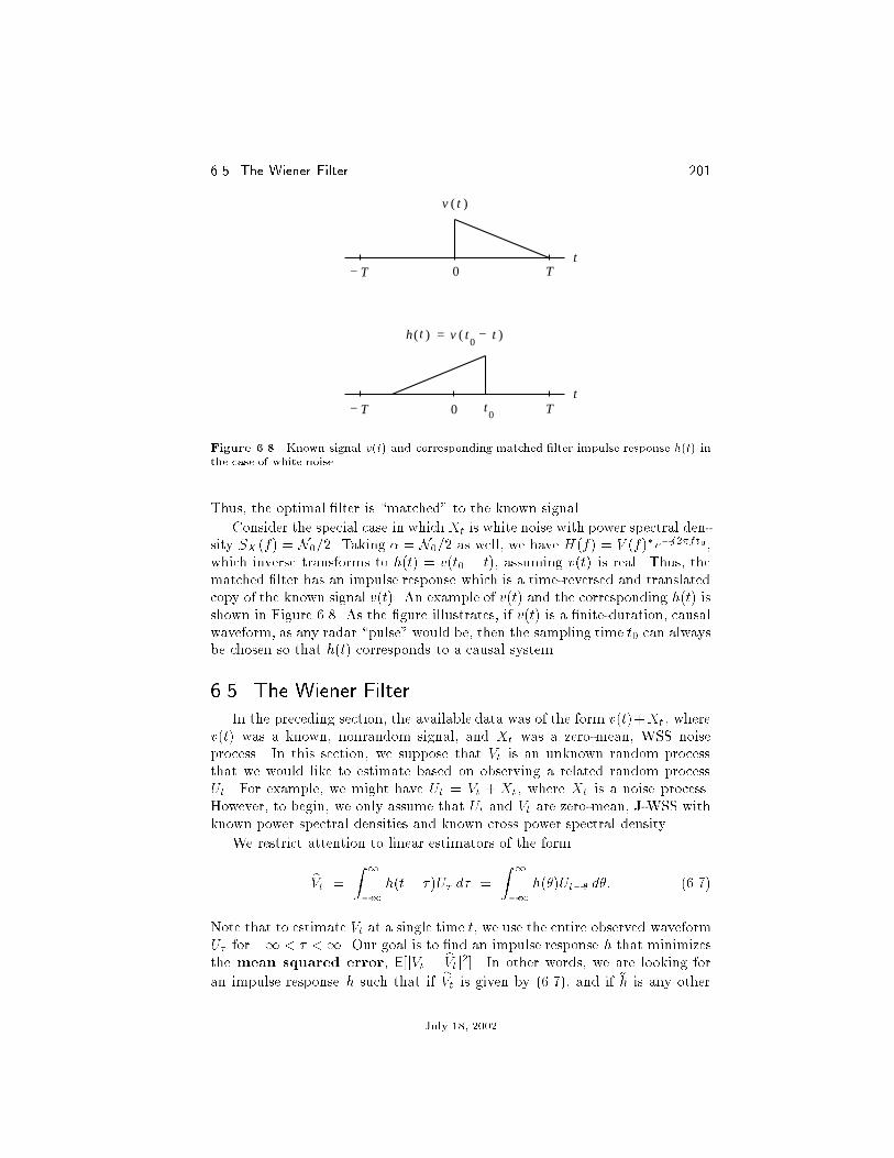
6.5 The Wiener Filter 201
0 T− Tt
v t( )
t0 T− T t
0
v t( )t −h t( ) =0
Figure 6.8. Known signal v(t) and corresponding matched �lter impulse response h(t) inthe case of white noise.
Thus, the optimal �lter is \matched" to the known signal.
Consider the special case in whichXt is white noise with power spectral den-sity SX (f) = N0=2. Taking � = N0=2 as well, we have H(f) = V (f)�e�j2�ft0,which inverse transforms to h(t) = v(t0 � t), assuming v(t) is real. Thus, thematched �lter has an impulse response which is a time-reversed and translatedcopy of the known signal v(t). An example of v(t) and the corresponding h(t) isshown in Figure 6.8. As the �gure illustrates, if v(t) is a �nite-duration, causalwaveform, as any radar \pulse" would be, then the sampling time t0 can alwaysbe chosen so that h(t) corresponds to a causal system.
6.5. The Wiener FilterIn the preceding section, the available data was of the form v(t)+Xt , where
v(t) was a known, nonrandom signal, and Xt was a zero-mean, WSS noiseprocess. In this section, we suppose that Vt is an unknown random processthat we would like to estimate based on observing a related random processUt. For example, we might have Ut = Vt + Xt, where Xt is a noise process.However, to begin, we only assume that Ut and Vt are zero-mean, J-WSS withknown power spectral densities and known cross power spectral density.
We restrict attention to linear estimators of the form
bVt =
Z 1
�1h(t� � )U� d� =
Z 1
�1h(�)Ut�� d�: (6.7)
Note that to estimate Vt at a single time t, we use the entire observed waveformU� for �1 < � <1. Our goal is to �nd an impulse response h that minimizesthe mean squared error, E[jVt � bVtj2]. In other words, we are looking for
an impulse response h such that if bVt is given by (6.7), and if ~h is any other
July 18, 2002

202 Chap. 6 Introduction to Random Processes
impulse response, and we put
eVt =
Z 1
�1~h(t � � )U� d� =
Z 1
�1~h(�)Ut�� d�; (6.8)
thenE[jVt � bVtj2] � E[jVt � eVtj2]:
To �nd the optimal �lter h, we apply the orthogonality principle, which saysthat if
E
�(Vt � bVt) Z 1
�1~h(�)Ut�� d�
�= 0 (6.9)
for every �lter ~h, then h is the optimal �lter.Before proceeding any further, we need the following observation. Suppose
(6.9) holds for every choice of ~h. Then in particular, it holds if we replace ~h byh� ~h. Making this substitution in (6.9) yields
E
�(Vt � bVt) Z 1
�1[h(�) � ~h(�)]Ut�� d�
�= 0:
Since the integral in this expression is simply bVt � eVt, we have thatE[(Vt � bVt)(bVt � eVt)] = 0: (6.10)
To establish the orthogonality principle, assume (6.9) holds for every choiceof ~h. Then (6.10) holds as well. Now write
E[jVt � eVtj2] = E[j(Vt � bVt) + (bVt � eVt)j2]= E[jVt � bVtj2 + 2(Vt � bVt)(bVt � eVt) + jbVt � eVtj2]= E[jVt � bVtj2] + 2E[(Vt � bVt)(bVt � eVt)] + E[jVt � eVtj2]= E[jVt � bVtj2] + E[jVt � eVtj2]� E[jVt � bVtj2];
and thus, h is the �lter that minimizes the mean squared error.The next task is to characterize the �lter h such that (6.9) holds for every
choice of ~h. Recalling (6.9), we have
0 = E
�(Vt � bVt) Z 1
�1~h(�)Ut�� d�
�= E
� Z 1
�1~h(�)(Vt � bVt)Ut�� d��
=
Z 1
�1E[~h(�)(Vt � bVt)Ut��] d�
=
Z 1
�1~h(�)E[(Vt � bVt)Ut��] d�
=
Z 1
�1~h(�)[RV U (�) � RbVU (�)] d�:July 18, 2002

6.5 The Wiener Filter 203
Since ~h is arbitrary, take ~h(�) = RVU (�) � RbVU (�) to getZ 1
�1
��RVU (�) � RbVU (�)��2 d� = 0: (6.11)
Thus, (6.9) holds for all ~h if and only if RV U = RbVU .The next task is to analyze RbVU . Recall that bVt in (6.7) is the response
of an LTI system to input Ut. Applying (6.3) with X replaced by U and Y
replaced by bV , we have, also using the fact that RU is even,
RbVU (� ) = RUbV (�� ) =
Z 1
�1h(�)RU (� � �) d�:
Taking Fourier transforms of
RVU (� ) = RbVU (� ) =
Z 1
�1h(�)RU (� � �) d� (6.12)
yieldsSV U (f) = H(f)SU (f):
Thus,
H(f) =SV U (f)
SU (f)
is the optimal �lter. This choice of H(f) is called the Wiener �lter.
?Causal Wiener Filters
Typically, the Wiener �lter as found above is not causal; i.e., we do not haveh(t) = 0 for t < 0. To �nd such an h, we need to reformulate the problem byreplacing (6.7) with
bVt =
Z t
�1h(t � � )U� d� =
Z 1
0h(�)Ut�� d�;
and replacing (6.8) with
eVt =
Z t
�1~h(t � � )U� d� =
Z 1
0
~h(�)Ut�� d�:
Everything proceeds as before from (6.9) through (6.11) except that lower limitsof integration are changed from�1 to 0. Thus, instead of concludingRVU (� ) =RbVU (� ) for all � , we only have RVU (� ) = RbVU (� ) for � � 0. Instead of (6.12),we have
RV U (� ) =
Z 1
0h(�)RU (� � �) d�; � � 0: (6.13)
This is known as the Wiener{Hopf equation. Because the equation onlyholds for � � 0, we run into a problem if we try to take Fourier transforms. To
July 18, 2002

204 Chap. 6 Introduction to Random Processes
K f( ) H f( )0
WtUt tV
^
f( )H
Figure 6.9. Decomposition of the causal Wiener �lter using the whitening �lter K(f).
compute SV U (f), we need to integrate RV U(� )e�j2�f� from � = �1 to � =1.But we can only use the Wiener{Hopf equation for � � 0.
In general, the Wiener{Hopf equation is very di�cult to solve. However, ifU is white noise, say RU(�) = �(�), then (6.13) reduces to
RVU (� ) = h(� ); � � 0:
Since h is causal, h(� ) = 0 for � < 0.The preceding observation suggests the construction ofH(f) using awhiten-
ing �lter as shown in Figure 6.9. If Ut is not white noise, suppose we can �nd acausal �lter K(f) such that when Ut is passed through this system, the outputis white noise Wt, by which we mean SW (f) = 1. Letting k denote the impulseresponse corresponding to K, we can write Wt mathematically as
Wt =
Z 1
0k(�)Ut�� d�: (6.14)
Then1 = SW (f) = jK(f)j2SU (f): (6.15)
Consider the problem of causally estimating Vt based on Wt instead of Ut. Thesolution is again given by the Wiener{Hopf equation,
RVW (� ) =
Z 1
0
h0(�)RW (� � �) d�; � � 0:
Since K was chosen so that SW (f) = 1, RW (�) = �(�). Therefore, the Wiener{Hopf equation tells us that h0(� ) = RVW (� ) for � � 0. Using (6.14), it is easyto see that
RVW (� ) =
Z 1
0k(�)RV U (� + �) d�; (6.16)
and then{
SVW (f) = K(f)�SV U(f): (6.17)
We now summarize the procedure.
{If k(�) is complexvalued, so isWt in (6.14). In this case, as in Problem 26, it is understoodthat RVW (�) = E[Vt+�W �
t ].
July 18, 2002

6.5 The Wiener Filter 205
1. According to (6.15), we must �rst write SU (f) in the form
SU (f) =1
K(f)� 1
K(f)�;
where K(f) is a causal �lter (this is known as spectral factorization).k
2. The optimum �lter is H(f) = H0(f)K(f), where
H0(f) =
Z 1
0
RVW (� )e�j2�f� d�;
and RVW (� ) is given by (6.16) or by the inverse transform of (6.17).
Example 6.11. Let Ut = Vt +Xt, where Vt and Xt are zero-mean, WSSprocesses with E[VtX� ] = 0 for all t and � . Assume that the signal Vt has powerspectral density SV (f) = 2�=[�2 + (2�f)2] and that the noise Xt is white withpower spectral density SX (f) = 1. Find the causal Wiener �lter.
Solution. From your solution of Problem 32, SU (f) = SV (f) + SX (f).Thus,
SU (f) =2�
�2 + (2�f)2+ 1 =
A2 + (2�f)2
�2 + (2�f)2;
where A2 := �2 + 2�. This factors into
SU (f) =A + j2�f
� + j2�f� A � j2�f
� � j2�f:
Then
K(f) =� + j2�f
A+ j2�f
is the required causal (by Problem 35) whitening �lter. Next, from your solutionof Problem 32, SV U (f) = SV (f). So, by (6.17),
SVW (f) =�� j2�f
A� j2�f� 2�
�2 + (2�f)2
=2�
(A � j2�f)(� + j2�f)
=B
A� j2�f+
B
�+ j2�f;
where B := 2�=(� +A). It follows that
RVW (� ) = BeA�u(�� ) + Be���u(� );
kIf SU (f) satis�es the Paley{Wiener condition,Z 1
�1
j lnSU (f)j1 + f2
df < 1;
then SU (f) can always be factored in this way.
July 18, 2002

206 Chap. 6 Introduction to Random Processes
where u is the unit-step function. Since h0(� ) = RVW (� ) for � � 0, h0(� ) =Be���u(� ) and H0(f) = B=(� + j2�f). Next,
H(f) = H0(f)K(f) =B
�+ j2�f� � + j2�f
A+ j2�f=
B
A+ j2�f;
and h(� ) = Be�A�u(� ).
6.6. ?Expected Time-Average Power and the Wiener{Khinchin Theorem
In this section we develop the notion of the expected time-average power ina WSS process. We then derive the Wiener{Khinchin Theorem, which impliesthat the expected time-average power is the same as the expected instantaneouspower. As an easy corollary of the derivation of the Wiener{Khinchin Theorem,we derive the mean-square ergodic theorem for WSS processes. This resultshows that E[Xt] can often be computed by averaging a single sample path overtime.
Recall that the average power in a deterministic waveform x(t) is given by
limT!1
1
2T
Z T
�Tx(t)2 dt:
The analogous formula for a random process is
limT!1
1
2T
Z T
�TX2t dt:
The problem with the above quantity is that it is a random variable becausethe integrand, X2
t , is random. We would like to characterize the process by anonrandom quantity. This suggests that we de�ne the expected time-averagepower in a random process by
ePX := E
�limT!1
1
2T
Z T
�TX2t dt
�:
We now carry out some analysis of ePX . To begin, we want to apply Parseval'sequation to the integral. To do this, we use the following notation. Let
XTt :=
(Xt; jtj � T;
0; jtj > T;
so thatR T�T X
2t dt =
R1�1��XT
t
��2 dt. Now, the Fourier transform of XTt is
eXTf :=
Z 1
�1XTt e
�j2�ft dt =
Z T
�TXt e
�j2�ft dt; (6.18)
July 18, 2002

6.6 ?Expected Time-Average Power and the Wiener{ Khinchin Theorem207
and by Parseval's equation,Z 1
�1
��XTt
��2 dt =
Z 1
�1
�� eXTf
��2 df:Returning now to ePX , we have
ePX = E
�limT!1
1
2T
Z T
�TX2t dt
�= E
�limT!1
1
2T
Z 1
�1
��XTt
��2 dt�= E
�limT!1
1
2T
Z 1
�1
�� eXTf
��2 df�
=
Z 1
�1
�limT!1
E��� eXT
f
��2�2T
�df:
The Wiener{Khinchin Theorem says that the above integrand is exactlythe power spectral density SX (f). From our earlier work, we know that PX :=
E[X2t ] = RX(0) =
R1�1 SX (f) df . Thus, ePX = PX ; i.e., the expected time-
average power is equal to the expected instantaneous power at any point intime. Note also that the above integrand is obviously nonnegative, and so if wecan show that it is equal to SX (f), then this will provide another proof thatSX (f) must be nonnegative.
To derive the Wiener{Khinchin Theorem, we begin with the numerator,
E��� eXT
f
��2� = E�� eXT
f
�� eXTf
���;
where the asterisk denotes complex conjugation. To evaluate the right-handside, use (6.18) to obtain
E
��Z T
�TXte
�j2�ft dt��Z T
�TX�e
�j2�f� d��� �
:
We can now write
E��� eXT
f
��2� =
Z T
�T
Z T
�TE[XtX�]e
�j2�f(t��) dt d�
=
Z T
�T
Z T
�TRX(t� �)e�j2�f(t��) dt d� (6.19)
=
Z T
�T
Z T
�T
� Z 1
�1SX (�)e
j2��(t��) d��e�j2�f(t��) dt d�
=
Z 1
�1SX (�)
�Z T
�Tej2��(f��)
�Z T
�Tej2�t(��f) dt
�d�
�d�:
July 18, 2002

208 Chap. 6 Introduction to Random Processes
Notice that the inner two integrals decouple so that
E��� eXT
f
��2� =
Z 1
�1SX (�)
�Z T
�Tej2��(f��) d�
��Z T
�Tej2�t(��f) dt
�d�
=
Z 1
�1SX (�) �
�2T
sin�2�T (f � �)
�2�T (f � �)
�2d�:
We can then write
E��� eXT
f
��2�2T
=
Z 1
�1SX (�) � 2T
�sin�2�T (f � �)
�2�T (f � �)
�2d�: (6.20)
This is a convolution integral. Furthermore, the quantity multiplying SX (�)converges to the delta function �(f � �) as T !1.2 Thus,
limT!1
E��� eXT
f
��2�2T
=
Z 1
�1SX (�) �(f � �) d� = SX (f);
which is exactly the Wiener{Khinchin Theorem.
Remark. The preceding derivation shows that SX (f) is equal to the limitof (6.19) divided by 2T . Thus,
S(f) = limT!1
1
2T
Z T
�T
Z T
�TRX(t� �)e�j2�f(t��) dt d�:
As noted in Problem 37, the properties of the correlation function directly implythat this double integral is nonnegative. This is the direct way to prove thatpower spectral densities are nonnegative.
Mean-Square Law of Large Numbers for WSS Processes
In the process of deriving the weak law of large numbers in Chapter 2, weshowed that for an uncorrelated sequence Xn with common mean m = E[Xn]and common variance �2 = var(Xn), the sample mean (or time average)
Mn :=1
n
nXi=1
Xi
converges to m in the sense that E[jMn � mj2] = var(Mn) ! 0 as n ! 1 by(2.6). In this case, we say that Mn converges in mean square to m, and we callthis a mean-square law of large numbers.
We now show that for a WSS process Yt with mean m = E[Yt], the samplemean (or time average)
MT :=1
2T
Z T
�TYt dt ! m
July 18, 2002
6.6 ?Expected Time-Average Power and the Wiener{ Khinchin Theorem209
in the sense that E[jMT �mj2]! 0 as T !1 if and only if
limT!1
1
2T
Z 2T
�2T
CY (� )�1� j� j
2T
�d� = 0;
where CY is the covariance (not correlation) function of Yt. We can view thisresult as a mean-square law of large numbers for WSS processes. Laws of largenumbers for sequences or processes that are not uncorrelated are often calledergodic theorems. Hence, the above result is also called the mean-squareergodic theorem for WSS processes. The point in all theorems of this typeis that the expectation E[Yt] can be computed by averaging a single sample pathover time.
We now derive this result. To begin, put Xt := Yt � m so that Xt is zeromean and has correlation function RX(� ) = CY (� ). Also,
MT �m =1
2T
Z T
�TXt dt =
eXTf
��f=0
2T;
where eXTf was de�ned in (6.18). Using (6.20) with f = 0 we can write
E[jMT �mj2] =E��� eXT
0
��2�4T 2
=1
2T� E��� eXT
0
��2�2T
=1
2T
Z 1
�1SX (�) � 2T
�sin(2�T�)
2�T�
�2d�: (6.21)
Applying Parseval's equation yields
E[jMT �mj2] =1
2T
Z 2T
�2T
RX(� )�1� j� j
2T
�d�
=1
2T
Z 2T
�2T
CY (� )�1� j� j
2T
�d�:
To give a su�cient condition for when this goes to zero, recall that by theargument following (6.20), as T ! 1 the integral in (6.21) is approximatelySX (0) if SX (f) is continuous at f = 0.3 Thus, if SX (f) is continuous at f = 0,
E[jMT �mj2] � SX (0)
2T! 0
as T !1.
Remark. If RX(� ) = CY (� ) is absolutely integrable, then SX (f) is uni-formly continuous. To see this write
jSX(f) � SX (f0)j =
����Z 1
�1RX(� )e
�j2�f� d� �Z 1
�1RX(� )e
�j2�f0� d�����
July 18, 2002

210 Chap. 6 Introduction to Random Processes
�Z 1
�1jRX(� )j je�j2�f� � e�j2�f0� j d�
=
Z 1
�1jRX(� )j je�j2�f0� [e�j2�(f�f0)� � 1]j d�
=
Z 1
�1jRX(� )j je�j2�(f�f0)� � 1j d�:
Now observe that je�j2�(f�f0)� � 1j ! 0 as f ! f0. Since RX is absolutelyintegrable, Lebesgue's dominated convergence theorem [4, p. 209] implies thatthe integral goes to zero as well.
6.7. ?Power Spectral Densities for non-WSS ProcessesIf Xt is not WSS, then the instantaneous power E[X2
t ] will depend on t. In
this case, it is more appropriate to look at the expected time-average power ePXde�ned in the previous section. At the end of this section, we show that
limT!1
E��� eXT
f
��2�2T
=
Z 1
�1RX (� )e
�j2�f� d�; (6.22)
where��
RX(� ) := limT!1
1
2T
Z T
�TRX(� + �; �) d�:
Hence, for a non-WSS process, we de�ne its power spectral density to be theFourier transform of RX(� ),
SX (f) :=
Z 1
�1RX(� )e
�j2�f� d�:
An important application the foregoing is to cyclostationary processes. Aprocess Yt is (wide-sense) cyclostationary if its mean function is periodic in t,and if its correlation function has the property that for �xed � , RX(� + �; �)is periodic in �. For a cyclostationary process with period T0, it is not hard toshow that
RX (� ) =1
T0
Z T0=2
�T0=2RX(� + �; �) d�: (6.23)
Example 6.12. Let Xt be WSS, and put Yt := Xt cos(2�f0t). Show thatYt is cyclostationary and that
SY (f) =1
4[SX(f � f0) + SX (f + f0)]:
Solution. The mean of Yt is
E[Yt] = E[Xt cos(2�f0t)] = E[Xt] cos(2�f0t):
��Note that if Xt is WSS, then RX(�) = RX(�).
July 18, 2002

6.7 ?Power Spectral Densities for non-WSS Processes 211
Because Xt is WSS, E[Xt] does not depend on t, and it is then clear that E[Yt]has period 1=f0. Next consider
RY (t+ �; �) = E[Yt+�Y�]
= E[Xt+� cos(2�f0ft+ �g)X� cos(2�f0�)]
= RX(t) cos(2�f0ft+ �g) cos(2�f0�);
which is periodic in � with period 1=f0. To compute SY (f), �rst use a trigono-metric identity to write
RY (t+ �; �) =RX(t)
2[cos(2�f0t) + cos(2�f0ft+ 2�g)]:
Applying (6.23) to RY with T0 = 1=f0 yields
RY (t) =RX(t)
2cos(2�f0t):
Taking Fourier transforms yields the claimed formula for SY (f).
Derivation of (6.22)
We begin as in the derivation of the Wiener{Khinchin Theorem, except thatinstead of (6.19) we have
E��� eXT
f
��2� =
Z T
�T
Z T
�TRX (t; �)e
�j2�f(t��) dt d�
=
Z T
�T
Z 1
�1I[�T;T ](t)RX(t; �)e
�j2�f(t��) dt d�:
Now make the change of variable � = t� � in the inner integral. This results in
E��� eXT
f
��2� =
Z T
�T
Z 1
�1I[�T;T ](� + �)RX (� + �; �)e�j2�f� d� d�:
Change the order of integration to get
E��� eXT
f
��2� =
Z 1
�1e�j2�f�
Z T
�TI[�T;T ](� + �)RX(� + �; �) d� d�:
To simplify the inner integral, observe that I[�T;T ](� + �) = I[�T��;T�� ](�).Now T � � is to the left of �T if 2T < � , and �T � � is to the right of T if�2T > � . Thus,
E��� eXT
f
��2�2T
=
Z 1
�1e�j2�f� gT (� ) d�;
July 18, 2002

212 Chap. 6 Introduction to Random Processes
where
gT (� ) :=
8>>>>>><>>>>>>:
12T
Z T��
�TRX(� + �; �) d�; 0 � � � 2T;
12T
Z T
�T��RX (� + �; �) d�; �2T � � < 0;
0; j� j > 2T:
If T much greater than j� j, then T � � � T and �T � � � �T in the abovelimits of integration. Hence, if RX is a reasonably-behaved correlation function,
limT!1
gT (� ) = limT!1
1
2T
Z T
�TRX(� + �; �) d� = RX(� );
and we �nd that
limT!1
E��� eXT
f
��2�2T
=
Z 1
�1e�j2�f� lim
T!1gT (� ) d� =
Z 1
�1e�j2�f� RX (� ) d�:
Remark. If Xt is actually WSS, then RX(� + �; �) = RX(� ), and
gT (� ) = RX(� )�1� j� j
2T
�I[�2T;2T ](� ):
In this case, for each �xed � , gT (� ) ! RX(� ). We thus have an alternativederivation of the Wiener{Khinchin Theorem.
6.8. NotesNotes x6.2: Wide-Sense Stationary Processes
Note 1. We mean that if RX is the correlation function of a WSS process,then RX it must satisfy Properties (i){(iii). Furthermore, it can be proved [50,pp. 94{96] that if R is a real-valued function satisfying Properties (i){(iii), thenthere is a WSS process having R as its correlation function.
Notes x6.6: ?Expected Time-Average Power and the Wiener{Khinchin Theorem
Note 2. To give a rigorous derivation of the fact that
limT!1
Z 1
�1SX (�) � 2T
�sin�2�T (f � �)
�2�T (f � �)
�2d� = SX (f);
it is convenient to assume SX (f) is continuous at f . Letting
�T (f) := 2T
�sin(2�Tf)
2�Tf
�2;
July 18, 2002

6.8 Notes 213
we must show that����Z 1
�1SX (�) �T (f � �) d� � SX (f)
���� ! 0:
To proceed, we need the following properties of �T . First,Z 1
�1�T (f) df = 1:
This can be seen by using the Fourier transform table to evaluate the inversetransform of �T (f) at t = 0. Second, for �xed �f > 0, as T !1,Z
ff :jfj>�fg�T (f) df ! 0:
This can be seen by using the fact that �T (f) is even and writingZ 1
�f
�T (f) df � 2T
(2�T )2
Z 1
�f
1
f2df =
1
2T�2�f;
which goes to zero as T !1. Third, for jf j � �f > 0,
j�T (f)j � 1
2T (��f)2:
Now, using the �rst property of �T , write
SX (f) = SX (f)
Z 1
�1�T (f � �) d� =
Z 1
�1SX (f) �T (f � �) d�:
Then
SX (f) �Z 1
�1SX (�) �T (f � �) d� =
Z 1
�1[SX(f) � SX (�)] �T (f � �) d�:
For the next step, let " > 0 be given, and use the continuity of SX at f to getthe existence of a �f > 0 such that for jf � �j < �f , jSX(f) � SX (�)j < ".Now break up the range of integration into � such that jf � �j < �f and �such that jf � �j � �f . For the �rst range, we need the calculation����Z f+�f
f��f
[SX (f) � SX (�)] �T (f � �) d�
�����
Z f+�f
f��f
jSX (f) � SX (�)j �T (f � �) d�
� "
Z f+�f
f��f
�T (f � �) d�
� "
Z 1
�1�T (f � �) d� = ":
July 18, 2002

214 Chap. 6 Introduction to Random Processes
For the second range of integration, consider the integral����Z 1
f+�f
[SX(f) � SX (�)] �T (f � �) d�
�����
Z 1
f+�fjSX(f) � SX (�)j �T (f � �) d�
�Z 1
f+�f
(jSX (f)j+ jSX(�)j) �T (f � �) d�
= jSX (f)jZ 1
f+�f
�T (f � �) d�
+
Z 1
f+�f
jSX(�)j �T (f � �) d�:
Observe that Z 1
f+�f
�T (f � �) d� =
Z ��f
�1�T (�) d�;
which goes to zero by the second property of �T . Using the third property, wehave Z 1
f+�f
jSX (�)j �T (f � �) d� =
Z ��f
�1jSX (f � �)j �T (�) d�
� 1
2T (��f)2
Z ��f
�1jSX (f � �)j d�;
which also goes to zero as T !1.
Note 3. In applying the derivation in Note 2 to the special case f = 0 in(6.21) we do not need SX (f) to be continuous for all f , we only need continuityat f = 0.
6.9. ProblemsRecall that if
H(f) =
Z 1
�1h(t)e�j2�ft dt;
then the inverse Fourier transform is
h(t) =
Z 1
�1H(f)ej2�ft df:
With these formulas in mind, the following table of Fourier transform pairs maybe useful.
July 18, 2002

6.9 Problems 215
h(t) H(f)
I[�T;T ](t) 2Tsin(2� Tf)
2� Tf
2Wsin(2�Wt)
2�WtI[�W;W ](f)
(1� jtj=T )I[�T;T ](t) T
�sin(� Tf)
� Tf
�2W
�sin(�Wt)
�Wt
�2(1� jf j=W )I[�W;W ](f)
e��tu(t)1
� + j2�f
e��jtj2�
�2 + (2�f)2
�
�2 + t2� e�2��jfj
e�(t=�)2=2p2� � e��
2(2�f)2=2
Problems x6.1: Mean, Correlation, and Covariance
1. The Cauchy{Schwarz inequality says that for any random variables U andV ,
E[UV ]2 � E[U2]E[V 2]: (6.24)
Derive this formula as follows. For any constant �, we can always write
0 � E[jU � �V j2] (6.25)
= E[U2]� 2�E[UV ] + �2E[V 2]:
Now set � = E[UV ]=E[V 2] and rearrange the inequality. Note that sinceequality holds in (6.25) if and only if U = �V , equality holds in (6.24) ifand only if U is a multiple of V .
Remark. The same technique can be used to show that for complex-valued waveforms,����Z 1
�1g(�)h(�)� d�
����2 �Z 1
�1jg(�)j2 d� �
Z 1
�1jh(�)j2 d�;
where the asterisk denotes complex conjugation, and for any complexnumber z, jzj2 = z � z�.
2. Show that RX(t1; t2) = E[Xt1Xt2 ] is a positive semide�nite functionin the sense that for any real or complex constants c1; : : : ; cn and any
July 18, 2002

216 Chap. 6 Introduction to Random Processes
times t1; : : : ; tn,nXi=1
nXk=1
ciRX(ti; tk)c�k � 0:
Hint: Observe that
E
����� nXi=1
ciXti
����2� � 0:
3. Let Xt for t > 0 be a random process with zero mean and correlationfunction RX(t1; t2) = min(t1; t2). If Xt is Gaussian for each t, write downthe density of Xt.
Problems x6.2: Wide-Sense Stationary Processes
4. Find the correlation function corresponding to each of the following powerspectral densities. (a) �(f). (b) �(f�f0)+�(f+f0). (c) e�f2=2. (d) e�jfj.
5. Let Xt be a WSS random process with power spectral density SX (f) =I[�W;W ](f). Find E[X2
t ].
6. Explain why each of the following frequency functions cannot be a powerspectral density. (a) e�fu(f), where u is the unit step function. (b) e�f
2
cos(f).(c) (1� f2)=(1 + f4). (d) 1=(1 + jf2).
7. For each of the following functions, determine whether or not it is a validcorrelation function.(a) sin(� ). (b) cos(� ). (c) e��
2=2. (d) e�j�j. (e) �2e�j�j. (f) I[�T;T ](� ).
8. Let R0(� ) be a correlation function, and put R(� ) := R0(� ) cos(2�f0� )for some f0 > 0. Determine whether or not R(� ) is a valid correlationfunction.
?9. Let S(f) be a real-valued, even, nonnegative function, and put
R(� ) :=
Z 1
�1S(f)ej2�f� d�:
Show that R satis�es properties (i) and (ii) that characterize a correlationfunction.
?10. Let R0(� ) be a real-valued, even function, but not necessarily a correlationfunction. Let R(� ) denote the convolution of R0 with itself, i.e.,
R(� ) :=
Z 1
�1R0(�)R0(� � �) d�:
(a) Show that R(� ) is a valid correlation function. Hint: You will needthe remark made in Problem 1.
July 18, 2002

6.9 Problems 217
(b) Now suppose that R0(� ) = I[�T;T ](� ). In this case, what is R(� ),and what is its Fourier transform?
11. A discrete-time random process is WSS if E[Xn] does not depend on nand if the correlation E[Xn+kXk] does not depend on k. In this case wewrite RX(n) = E[Xn+kXk]. For discrete-time WSS processes, the powerspectral density is de�ned by
SX (f) :=1X
n=�1RX(n)e
�j2�fn;
which is a periodic function of f with period one. By the formula forFourier series coe�cients
RX(n) =
Z 1=2
�1=2
SX (f)ej2�fn df:
(a) Show that RX is an even function of n.
(b) Show that SX is a real and even function of f .
Problems x6.3: WSS Processes through LTI Systems
12. White noise with power spectral density SX (f) = N0=2 is applied to alowpass �lter with transfer function
H(f) =
�1� f2; jf j � 1;
0; jf j > 1:
Find the output power of the �lter.
13. White noise with power spectral density N0=2 is applied to a lowpass�lter with transfer function H(f) = sin(�f)=(�f). Find the output noisepower from the �lter.
14. AWSS input signalXt with correlation functionRX(� ) = e��2=2 is passed
through an LTI system with transfer function H(f) = e�(2�f)2=2. De-note the system output by Yt. Find (a) the cross power spectral density,SXY (f); (b) the cross-correlation, RXY (� ); (c) E[Xt1Yt2 ]; (d) the outputpower spectral density, SY (f); (e) the output auto-correlation, RY (� );(f) the output power PY .
15. White noise with power spectral density SX (f) = N0=2 is applied to alowpass RC �lter with impulse response h(t) = 1
RCe�t=(RC)u(t). Find
(a) the cross power spectral density, SXY (f); (b) the cross-correlation,RXY (� ); (c) E[Xt1Yt2 ]; (d) the output power spectral density, SY (f);(e) the output auto-correlation, RY (� ); (f) the output power PY .
July 18, 2002

218 Chap. 6 Introduction to Random Processes
16. White noise with power spectral density N0=2 is passed through a linear,time-invariant system with impulse response h(t) = 1=(1 + t2). If Ytdenotes the �lter output, �nd E[Yt+1=2Yt].
17. AWSS process Xt with correlation function RX(� ) = 1=(1+�2) is passedthrough an LTI system with impulse response h(t) = 3 sin(�t)=(�t). LetYt denote the system output. Find the output power PY .
18. White noise with power spectral density SX (f) = N0=2 is passed thougha �lter with impulse response h(t) = I[�T=2;T=2](t). Find and sketch thecorrelation function of the �lter output.
19. Let Xt be a WSS random process, and put Yt :=R tt�3X� d� . Determine
whether or not Yt is WSS.
20. Consider the system
Yt = e�tZ t
�1e�X� d�:
Assume that Xt is zero mean white noise with power spectral densitySX (f) = N0=2. Show that Xt and Yt are J-WSS, and �nd RXY (� ),SXY (f), SY (f), and RY (� ).
21. A zero-mean, WSS process Xt with correlation function (1�j� j)I[�1;1](� )is to be processed by a �lter with transfer function H(f) designed so thatthe system output Yt has correlation function
RY (� ) =sin(�� )
��:
Find a formula for, and sketch the required �lter H(f).
22. Let Xt be a WSS random process. Put Yt :=R1�1 h(t � � )X� d� , and
Zt :=R1�1 g(t � �)X� d�. Determine whether or not Yt and Zt are J-
WSS.
23. Let Xt be a zero-mean WSS random process with power spectral densitySX (f) = 2=[1 + (2�f)2]. Put Yt := Xt �Xt�1.
(a) Show that Xt and Yt are J-WSS.
(b) Find the power spectral density SY (f).
(c) Find the power in Yt.
24. Let fXtg be a zero-mean wide-sense stationary random process withpower spectral density SX (f). Consider the process
Yt :=1X
n=�1hnXt�n;
with hn real valued.
July 18, 2002

6.9 Problems 219
(a) Show that fXtg and fYtg are jointly wide-sense stationary.
(b) Show that SY (f) has the form SY (f) = P (f)SX (f) where P is areal-valued, nonnegative, periodic function of f with period 1. Givea formula for P (f).
25. System Identi�cation. When white noise fWtg with power spectral densitySW (f) = 3 is applied to a certain linear time-invariant system, the output
has power spectral density e�f2
. Now let fXtg be a zero-mean, wide-sense stationary random process with power spectral density SX (f) =
ef2
I[�1;1](f). If fYtg is the response of the system to fXtg, �nd RY (� )for all � .
?26. Extension to Complex Random Processes. If Xt is a complex-valued ran-dom process, then its auto-correlation function is de�ned by RX(t1; t2) :=E[Xt1X
�t2 ]. Similarly, if Yt is another complex-valued random process,
their cross-correlation is de�ned by RXY (t1; t2) := E[Xt1Y�t2]. The con-
cepts of WSS, J-WSS, the power spectral density, and the cross powerspectral density are de�ned as in the real case. Now suppose that Xt
is a complex WSS process and that Yt =R1�1 h(t � � )X� d� , where the
impulse response h is now possibly complex valued.
(a) Show that RX(�� ) = RX (� )�.
(b) Show that SX (f) must be real valued. Hint: What does part (a) sayabout the real and imaginary parts of RX(� )?
(c) Show that
E[Xt1Y�t2] =
Z 1
�1h(��)�RX ([t1 � t2]� �) d�:
(d) Even though the above result is a little di�erent from (6.4), showthat (6.5) and (6.6) still hold for complex random processes.
27. Let Xn be a discrete-time WSS process as de�ned in Problem 11. Put
Yn =1X
k=�1hkXn�k:
(a) Suggest a de�nition of jointly WSS discrete-time processes and showthat Xn and Yn are J-WSS.
(b) Suggest a de�nition for the cross power spectral density of two discrete-time J-WSS processes and show that (6.5) holds if
H(f) :=1X
n=�1hne
�j2�fn:
Also show that (6.6) holds.
July 18, 2002

220 Chap. 6 Introduction to Random Processes
(c) Write out the discrete-time analog of Example 6.9. What conditiondo you need to impose on W2?
Problems x6.4: The Matched Filter
28. Determine the matched �lter if the known radar pulse is v(t) = sin(t)I[0;�](t),and Xt is white noise with power spectral density SX (f) = N0=2. Forwhat values of t0 is the optimal system causal?
29. Determine the matched �lter if v(t) = e�(t=p2)2=2, and SX (f) = e�(2�f)2=2.
30. Derive the matched �lter for a discrete-time received signal v(n) + Xn.Hint: Problems 11 and 27 may be helpful.
Problems x6.5: The Wiener Filter
31. Suppose Vt and Xt are J-WSS. Let Ut := Vt +Xt. Show that Ut and Vtare J-WSS.
32. Suppose Ut = Vt + Xt, where Vt and Xt are each zero mean and WSS.Also assume that E[VtX� ] = 0 for all t and � . Express the Wiener �lterH(f) in terms of SV (f) and SX (f).
33. Using the setup of the previous problem, �nd the Wiener �lter H(f) andthe corresponding impulse response h(t) if SV (f) = 2�=[�2+(2�f)2] andSX (f) = 1.
Remark. You may want to compare your answer with the causal Wiener�lter found in Example 6.11.
34. Using the setup of Problem 32, suppose that the signal has correlation
functionRV (� ) =� sin��
��
�2and that the noise has power spectral density
SX (f) = 1�I[�1;1](f). Find the Wiener �lterH(f) and the correspondingimpulse response h(t).
35. Find the impulse response of the whitening �lter K(f) of Example 6.11.Is it causal?
36. Derive the Wiener �lter for discrete-time J-WSS signals Un and Vn withzero means. Hints: (i) First derive the analogous orthogonality principle.(ii) Problems 11 and 27 may be helpful.
Problems x6.6: ?Expected Time-Average Power and the Wiener{Khinchin Theorem
37. Recall that by Problem 2, correlation functions are positive semide�nite.Use this fact to prove that the double integral in (6.19) is nonnegative,assuming thatRX is continuous. Hint: Since RX is continuous, the doubleintegral in (6.19) is a limit of Riemann sums of the formX
i
Xk
RX(ti � tk)e�j2�f(ti�tk)�ti�tk:
July 18, 2002

6.9 Problems 221
38. Let Yt be a WSS process. In each of the cases below, determine whether
or not 12T
R T�T Yt dt! E[Yt] in mean square.
(a) The covariance CY (� ) = e�j�j.
(b) The covariance CY (� ) = sin(�� )=(�� ).
39. Let Yt = cos(2�t + �), where � � uniform[��; �]. As in Example 6.1,E[Yt] = 0. Determine whether or not
limT!1
1
2T
Z T
�TYt dt ! 0:
40. Let Xt be a zero-mean, WSS process. For �xed � , you might expect
1
2T
Z T
�TXt+�Xt dt
to converge in mean square to E[Xt+�Xt] = RX(� ). Give conditions onthe process Xt under which this will be true. Hint: De�ne Yt := Xt+�Xt.
Remark. When � = 0 this says that 12T
R T�T X
2t dt converges in mean
square to RX(0) = PX = ePX .41. Let Xt be a zero-mean, WSS process. For a �xed set B � IR, you might
expectyy
1
2T
Z T
�TIB(Xt) dt
to converge in mean square to E[IB(Xt)] = }(Xt 2 B). Give conditions onthe process Xt under which this will be true. Hint: De�ne Yt := IB(Xt).
yyThis is the fraction of time during [�T; T ] that Xt 2 B. For example, we might haveB = [vmin; vmax] being the acceptable operating range of the voltage of some device. Thenwe would be interested in the fraction of time during [�T; T ] that the device is operatingnormally.
July 18, 2002

222 Chap. 6 Introduction to Random Processes
July 18, 2002

CHAPTER 7
Random Vectors
This chapter covers concepts that require some familiarity with linear alge-bra, e.g., matrix-vector multiplication, determinants, and matrix inverses. Sec-tion 7.1 de�nes the mean vector, covariance matrix, and characteristic functionof random vectors. Section 7.2 introduces the multivariate Gaussian randomvector and illustrates several of its properties. Section 7.3 discusses both lin-ear and nonlinear minimummean squared error estimation of random variablesand random vectors. Estimators are obtained using appropriate orthogonalityprinciples. Section 7.4 covers the Jacobian formula for �nding the density ofY = G(X) when the density of X is given. Section 7.5 introduces complex-valued random variables and random vectors. Emphasis is on circularly sym-metric Gaussian random vectors due to their importance in the design of digitalcommunication systems.
7.1. Mean Vector, Covariance Matrix, and CharacteristicFunction
If X = [X1; : : : ; Xn]0 is a random vector, we put mi := E[Xi], and we de�ne
Rij to be the covariance between Xi and Xj , i.e.,
Rij := cov(Xi; Xj) := E[(Xi �mi)(Xj �mj)]:
Note that Rii = cov(Xi; Xi) = var(Xi). We call the vector m := [m1; : : : ;mn]0
themean vector ofX, and we call the n�n matrixR := [Rij] the covariancematrix of X. Note that since Rij = Rji, the matrix R is symmetric. In otherwords, R0 = R. Also note that for i 6= j, Rij = 0 if and only if Xi and Xj
are uncorrelated. Thus, R is a diagonal matrix if and only if Xi and Xj areuncorrelated for all i 6= j.
If we de�ne the expectation of a random vector X = [X1; : : : ; Xn]0 to be thevector of expectations, i.e.,
E[X] :=
264 E[X1]...
E[Xn]
375 ;then E[X] = m.
We de�ne the expectation of a matrix of random variables to be the matrixof expectations. This leads to the following characterization of the covariancematrix R. To begin, observe that if we multiply an n � 1 matrix (a columnvector) by a 1 � n matrix (a row vector), we get an n � n matrix. Hence,
223

224 Chap. 7 Random Vectors
(X �m)(X �m)0 is equal to264 (X1 �m1)(X1 �m1) � � � (X1 �m1)(Xn �mn)...
...(Xn �mn)(X1 �m1) � � � (Xn �mn)(Xn �mn)
375 :The expectation of the ijth entry is cov(Xi; Xj) = Rij. Thus,
R = E[(X �m)(X �m)0] =: cov(X):
Note the distinction between the covariance of a pair of random variables, whichis a scalar, and the covariance of a column vector, which is a matrix.
Example 7.1. Write out the covariance matrix of the three-dimensionalrandom vector U := [X;Y; Z]0 if U has zero mean.
Solution. The covariance matrix of U is
cov(U ) = E[UU 0] =
24 E[X2] E[XY ] E[XZ]E[Y X] E[Y 2] E[Y Z]E[ZX] E[ZY ] E[Z2]
35 :Example 7.2. Let X = [X1; : : : ; Xn]
0 be a random vector with covariancematrix R, and let c = [c1; : : : ; cn]
0 be a given constant vector. De�ne the scalar
Z := c0(X �m) =nXi=1
ci(Xi �mi);
Show thatvar(Z) = c0Rc:
Solution. First note that since E[X] = m, Z has zero mean. Hence,var(Z) = E[Z2]. Write
E[Z2] = E
�� nXi=1
ci(Xi �mi)
�� nXj=1
cj(Xj �mj)
��
=nXi=1
nXj=1
cicjE[(Xi �mi)(Xj �mj)]
=nXi=1
nXj=1
cicjRij
=nXi=1
ci
� nXj=1
Rijcj
�:
The inner sum is the ith component of the column vector Rc. Hence, E[Z2] =c0(Rc) = c0Rc.
July 18, 2002

7.1 Mean Vector, Covariance Matrix, and Characteristic Function 225
The preceding example shows that a covariance matrix must satisfy
c0Rc = E[Z2] � 0
for all vectors c = [c1; : : : ; cn]0. A symmetric matrix R with the propertyc0Rc � 0 for all vectors c is said to be positive semide�nite. If c0Rc > 0 forall nonzero c, then R is called positive de�nite.
Recall that the norm of a column vector x is de�ned by kxk := (x0x)1=2. Itis shown in Problem 5 that
E[kX � E[X]k2] = tr(R) =nXi=1
var(Xi);
where the trace of an n� n matrix R is de�ned by
tr(R) :=nXi=1
Rii:
The joint characteristic function of X = [X1; : : : ; Xn]0 is de�ned by
'X (�) := E[ej�0X ] = E[ej(�1X1+���+�nXn)];
where � = [�1; : : : ; �n]0.Note that when X has a joint density, 'X (�) = E[ej�
0X ] is just the n-dimensional Fourier transform,
'X (�) =
ZIRn
ej�0xfX (x) dx; (7.1)
and the joint density can be recovered using the multivariate inverse Fouriertransform:
fX(x) =1
(2�)n
ZIRn
e�j�0x'X (�) d�:
Whether X has a joint density or not, the joint characteristic function canbe used to obtain its various moments.
Example 7.3. The components of the mean vector and covariance matrixcan be obtained from the characteristic function as follows. Write
@
@�kE[ej�
0X ] = E[ej�0XjXk];
and@2
@�`@�kE[ej�
0X ] = E[ej�0X(jX`)(jXk)]:
Then@
@�kE[ej�
0X ]����=0
= jE[Xk];
July 18, 2002

226 Chap. 7 Random Vectors
and@2
@�`@�kE[ej�
0X ]����=0
= �E[X`Xk]:
Higher-order moments can be obtained in a similar fashion.
If the components of X = [X1; : : : ; Xn]0 are independent, then
'X(�) = E[ej�0X ]
= E[ej(�1X1+���+�nXn)]
= E
� nYk=1
ej�kXk
�
=nY
k=1
E[ej�kXk ]
=nY
k=1
'Xk(�k):
In other words, the joint characteristic function is the product of the marginalcharacteristic functions.
7.2. The Multivariate GaussianA random vector X = [X1; : : : ; Xn]0 is said to be Gaussian or normal if
every linear combination of the components of X, e.g.,
nXi=1
ciXi; (7.2)
is a scalar Gaussian random variable.
Example 7.4. If X is a Gaussian random vector, then the numerical av-erage of its components,
1
n
nXi=1
Xi;
is a scalar Gaussian random variable.
An easy consequence of our de�nition of Gaussian random vector is thatany subvector is also Gaussian. To see this, suppose X = [X1; : : : ; Xn]
0 is aGaussian random vector. Then every linear combination of the components ofthe subvector [X1; X3; X5]
0 is of the form (7.2) if we take ci = 0 for i not equalto 1; 3; 5.
July 18, 2002

7.2 The Multivariate Gaussian 227
Sometimes it is more convenient to express linear combinations as the prod-uct of a row vector times the column vector X. For example, if we putc = [c1; : : : ; cn]
0, thennXi=1
ciXi = c0X:
Now suppose that Y = AX for some p�nmatrixA. Letting c = [c1; : : : ; cp]0,every linear combination of the p components of Y has the form
pXi=1
ciYi = c0Y = c0(AX) = (A0c)0X;
which is a linear combination of the components of X, and therefore normal.We can even add a constant vector. If Y = AX + b, where A is again p� n,
and b is p� 1, then
c0Y = c0(AX + b) = (A0c)0X + c0b:
Adding the constant c0b to the normal random variable (A0c)0X results in an-other normal random variable (with a di�erent mean).
In summary, if X is a Gaussian random vector, then so is AX + b for any
p� n matrix A and any p-vector b.
The Characteristic Function of a Gaussian Random Vector
We now �nd the joint characteristic function of the Gaussian random vectorX, 'X (�) = E[ej�
0X ]. Since we are assuming that X is a normal vector, thequantity Y := � 0X is a scalar Gaussian random variable. Hence,
'X (�) = E[ej�0X ] = E[ejY ] = E[ej�Y ]
���=1
= 'Y (�)���=1
:
In other words, all we have to do is �nd the characteristic function of Y andevaluate it at � = 1. Since Y is normal, we know its characteristic function is(recall Example 3.13)
'Y (�) := E[ej�Y ] = ej����2�2=2;
where � := E[Y ], and �2 := var(Y ). Assuming X has mean vector m, � =E[� 0X] = �0m. Suppose X has covariance matrix R. Next, write var(Y ) =E[(Y � �)2]. Since
Y � � = �0(X �m);
Example 7.2 tells us that var(Y ) = �0R�. It now follows that
'X(�) = ej�0m��0R�=2:
If X is a Gaussian random vector with mean vector m and covariance matrixR, we write X � N (m;R).
July 18, 2002

228 Chap. 7 Random Vectors
For Gaussian Random Vectors, Uncorrelated Implies Independent
If the components of a random vector are uncorrelated, then the covariancematrix is diagonal. In general, this is not enough to prove that the componentsof the random vector are independent. However, if X is a Gaussian randomvector, then the components are independent. To see this, suppose that X isGaussian with uncorrelated components. Then R is diagonal, say
R =
2664�21 0
. . .
0 �2n
3775 ;where �2i = Rii = var(Xi). The diagonal form of R implies that
�0R� =nXi=1
�2i �2i ;
and so
'X(�) = ej�0m��0R�=2 =
nYi=1
ej�imi��2i �2i =2:
In other words,
'X(�) =nYi=1
'Xi(�i);
where 'Xi (�i) is the characteristic function of the N (mi; �2i ) density. Multi-
variate inverse Fourier transformation then yields
fX (x) =nYi=1
fXi (xi);
where fXi � N (mi; �2i ). This establishes the independence of the Xi.
Example 7.5. Let X1; : : : ; Xn be i.i.d. N (m;�2) random variables. LetX := 1
n
Pni=1Xi denote the average of the Xi. Furthermore, for j = 1; : : : ; n,
put Yj := Xj �X . Show that X and Y := [Y1; : : : ; Yn]0 are jointly normal andindependent.
Solution. Let X := [X1; : : : ; Xn]0, and put a := [ 1n � � � 1n ]. Then X = aX.
Next, observe that 264 Y1...Yn
375 =
264 X1
...Xn
375�264 X
...X
375 :July 18, 2002

7.2 The Multivariate Gaussian 229
Let M denote the n � n matrix with each row equal to a; i.e., Mij = 1=n forall i; j. Then Y = X �MX = (I �M )X, and Y is a jointly normal randomvector. Next consider the vector
Z :=
�XY
�=
�a
I �M
�X:
Since Z is a linear transformation of the Gaussian random vector X, Z is alsoa Gaussian random vector. Furthermore, its covariance matrix has the block-diagonal form (see Problem 11)�
var(X ) 00 E[Y Y 0]
�:
This implies, by Problem 12, that X and Y are independent.
The Density Function of a Gaussian Random Vector
We now derive the general multivariate Gaussian density function under theassumption that R is positive de�nite. Using the multivariate Fourier inversionformula,
fX(x) =1
(2�)n
ZIRn
e�jx0�'X(�) d�
=1
(2�)n
ZIRn
e�jx0�ej�
0m��0R�=2 d�
=1
(2�)n
ZIRn
e�j(x�m)0�e��0R�=2 d�:
Now make the multivariate change of variable � = R1=2�, d� = detR1=2 d�.The existence of R1=2 and the fact that det(R1=2) =
pdetR > 0 are shown in
the Notes.1 We have
fX (x) =1
(2�)n
ZIRn
e�j(x�m)0R�1=2�e��0�=2 d�
detR1=2
=1
(2�)n
ZIRn
e�jfR�1=2(x�m)g0�e��
0�=2 d�pdetR
:
Put t = R�1=2(x�m). Then
fX (x) =1
(2�)n
ZIRn
e�jt0�e��
0�=2 d�pdetR
=1pdetR
nYi=1
�1
2�
Z 1
�1e�jti�ie��
2i =2 d�i
�:
July 18, 2002

230 Chap. 7 Random Vectors
Observe that e��2i =2 is the characteristic function of a scalar N (0; 1) random
variable. Hence,
fX (x) =1pdetR
nYi=1
1p2�
e�t2i=2
=1
(2�)n=2pdetR
exp
��1
2
nXi=1
t2i
�=
1
(2�)n=2pdetR
exp[�t0t=2]
=exp[�1
2 (x�m)0R�1(x�m)]
(2�)n=2pdetR
: (7.3)
With the norm notation, t0t = ktk2 = kR�1=2(x�m)k2, and so
fX (x) =exp[�kR�1=2(x�m)k2=2]
(2�)n=2pdetR
as well.
7.3. Estimation of Random VectorsConsider a pair of random vectors X and Y , where X is not observed, but
Y is observed. We wish to estimate X based on our knowledge of Y . By anestimator of X based on Y , we mean a function g(y) such that X := g(Y )is our estimate or \guess" of the value of X. What is the best function g touse? What do we mean by best? In this section, we de�ne g to be best if itminimizes the mean squared error (MSE) E[kX � g(Y )k2] for all functionsg in some class of functions. The optimal function g is called the minimummean squared error (MMSE) estimator. In the next subsection, we restrictattention to the class of linear estimators (actually a�ne). Later we allow gto be arbitrary.
Linear Minimum Mean Squared Error Estimation
We now restrict attention to estimators g of the form g(y) = Ay + b, whereA is a matrix and b is a column vector. Such a function of y is said to be a�ne.If b = 0, then g is linear. It is common to say g is linear even if b 6= 0 sincethis only is a slight abuse of terminology, and the meaning is understood. Weshall follow this convention. To �nd the best linear estimator is simply to �ndthe matrix A and the column vector b that minimize the MSE, which for linearestimators has the form
E� X � (AY + b)
2�:Letting mX = E[X] and mY = E[Y ], the MSE is equal to
E� �(X �mX )� A(Y �mY )
+�mX �AmY � b
2�:July 18, 2002

7.3 Estimation of Random Vectors 231
p
p
l
Figure 7.1. Geometric interpretation of the orthogonality principle.
Since the left-hand quantity in braces is zero mean, and since the right-handquantity in braces is a constant (nonrandom), the MSE simpli�es to
E� (X �mX )� A(Y �mY )
2� + kmX � AmY � bk2:No matter what matrix A is used, the optimal choice of b is
b = mX �AmY ;
and the estimate is g(Y ) = AY + b = A(Y �mY ) +mX . The estimate is trulylinear in Y if and only if AmY = mX .
We now turn to the problem of minimizing
E� (X �mX ) �A(Y �mY )
2�:The matrix A is optimal if and only if for all matrices B,
E� (X �mX )� A(Y �mY )
2� � E� (X �mX ) �B(Y �mY )
2�: (7.4)
The following condition is equivalent, and easier to use. This equivalence isknown as the orthogonality principle. It says that (7.4) holds for all B ifand only if
E��B(Y �mY )
0�(X �mX ) �A(Y �mY )
�= 0; for all B: (7.5)
Below we prove that (7.5) implies (7.4). The converse is also true, but we shallnot use it in this book.
We �rst explain the terminology and show geometrically why it is true.Recall that given a straight line l and a point p not on the line, the shortestpath between p and the line is obtained by dropping a perpendicular segmentfrom the point to the line as shown in Figure 7.1. The point p on the line wherethe segment touches is closer to p than any other point on the line. Notice alsothat the vertical segment, p � p, is orthogonal to the line l. In our situation,the role of p is played by the random variable X �mX , the role of p is playedby the random variable A(Y � mY ), and the role of the line is played by theset of all random variables of the form B(Y �mY ) as B runs over all matrices.Since the inner product between two random vectors U and V can be de�nedas E[V 0U ], (7.5) says that
(X �mX )� A(Y �mY )
July 18, 2002

232 Chap. 7 Random Vectors
is orthogonal to all B(Y �mY ).To use (7.5), �rst note that since it is a scalar equation, the left-hand side
is equal to its trace. Bringing the trace inside the expectation and using thefact that tr(��) = tr(��), we see that the left-hand side of (7.5) is equal to
E�tr��(X �mX )� A(Y �mY )
(Y �mY )
0B0��:Taking the trace back out of the expectation shows that (7.5) is equivalent to
tr([RXY � ARY ]B0) = 0; for all B; (7.6)
where RY = cov(Y ) is the covariance matrix of Y , and
RXY = E[(X �mX )(Y �mY )0] =: cov(X;Y ):
(This is our third usage of cov. We have already seen the covariance of a pair ofrandom variables and of a random vector. This is the third type of covariance,that of a pair of random vectors. When X and Y are both of dimension one,this reduces to the �rst usage of cov.) By Problem 5, it follows that (7.6) holdsif and only if A solves the equation
ARY = RXY :
If RY is invertible, the unique solution of this equation is
A = RXYR�1Y :
In this case, the complete estimate of X is
RXYR�1Y (Y �mY ) +mX :
Even if RY is not invertible, ARY = RXY always has a solution, as shown inProblem 16.
Example 7.6 (Signal in Additive Noise). Let X denote a random signal ofzero mean and known covariance matrix RX . Suppose that in order to estimateX, all we have available is the noisy measurement
Y = X +W;
where W is a noise vector with zero mean and known covariance matrix RW .Further assume that the covariance between the signal and noise, RXW , is zero.Find the linear MMSE estimate of X based on Y .
Solution. Since E[Y ] = E[X +W ] = 0, mY = mX = 0. Next,
RXY = E[(X �mX )(Y �mY )0]
= E[X(X +W )0]= RX :
July 18, 2002

7.3 Estimation of Random Vectors 233
Similarly,
RY = E[(Y �mY )(Y �mY )0]
= E[(X +W )(X +W )0]= RX + RW :
It follows thatX = RX(RX +RW )�1Y:
We now show that (7.5) implies (7.4). To simplify the notation, we assumezero means.
E[kX � BY k2] = E[k(X �AY ) + (AY � BY )k2]= E[k(X �AY ) + (A� B)Y )k2]= E[kX �AY k2] + E[k(A�B)Y k2];
where the cross terms 2E[f(A� B)Y g0(X � AY )] vanish by (7.5). If we dropthe right-hand term in the above display, we obtain
E[kX � BY k2] � E[kX � AY k2]:
Minimum Mean Squared Error Estimation
We begin with an observed vector Y and a scalar X to be estimated. (Thegeneralization to vector-valuedX is left to the problems.) We seek a real-valuedfunction g(y) with the property that�
E[jX � g(Y )j2] � E[jX � h(Y )j2]; for all h: (7.7)
Here we are not requiring g and/or h to be linear. We again have an or-thogonality principle (see Problem 17) that says that the above condition isequivalent to
E[fX � g(Y )gh(Y )] = 0; for all h: (7.8)
We claim that g(y) = E[XjY = y] is the optimal function g if X and Y arejointly continuous. In this case, we can use the law of total probability to write
E[fX � g(Y )gh(Y )] =Z
E�fX � g(Y )gh(Y )��Y = y
�fY (y) dy
Applying the substitution law to the conditional expectation yields
E�fX � g(Y )gh(Y )��Y = y
�= E
�fX � g(y)gh(y)��Y = y�
= E[XjY = y]h(y) � g(y)h(y)
= g(y)h(y) � g(y)h(y)
= 0:�In order that the expectations in (7.7) be �nite, we assume E[X2] < 1, and we restrict
g and h to be such that E[g(Y )2] <1 and E[h(Y )2] <1.
July 18, 2002

234 Chap. 7 Random Vectors
It is shown in Problem 18 that the solution g of (7.8) is unique. We can usethis fact to �nd conditional expectations if X and Y are jointly normal. Forsimplicity, assume zero means. We claim that g(y) = RXYR
�1Y y solves (7.8).
We �rst observe that�X �RXYR
�1Y Y
Y
�=
�I �RXYR
�1Y
0 I
� �XY
�is a linear transformation of [X;Y 0]0 and so the left-hand side is a Gaussianrandom vector whose top and bottom entries are easily seen to be uncorrelated:
E[(X � RXYR�1Y Y )Y 0] = RXY � RXYR
�1Y RY
= 0:
Being jointly Gaussian and uncorrelated, they are independent. Hence, for anyfunction h(y),
E[(X � RXYR�1Y Y )h(Y )] = E[X � RXYR
�1Y Y ]E[h(Y )]
= 0E[h(Y )]:
We have now learned two things about jointly normal random variables. First,we have learned how to �nd conditional expectations. Second, in looking forthe best estimator function g, and not requiring g to be linear, we found thatthe best g is linear if X and Y are jointly normal.
7.4. Transformations of Random VectorsIf G(x) is a vector-valued function of x 2 IRn, and X is an IRn-valued
random vector, we can de�ne a new random vector by Y = G(X). If X hasjoint density fX , and G is a suitable invertible mapping, then we can �nd arelatively explicit formula for the joint density of Y . Suppose that the entriesof the vector equation y = G(x) are given by264 y1
...yn
375 =
264 g1(x1; : : : ; xn)...
gn(x1; : : : ; xn)
375 :If G is invertible, we can apply G�1 to both sides of y = G(x) to obtainG�1(y) = x. Using the notation H(y) := G�1(y), we can write the entries ofthe vector equation x = H(y) as264 x1
...xn
375 =
264 h1(y1; : : : ; yn)...
hn(y1; : : : ; yn)
375 :July 18, 2002

7.4 Transformations of Random Vectors 235
Assuming that H is continuous and has continuous partial derivatives, let
H 0(y) :=
266666664
@h1@y1
� � � @h1@yn
......
@hi@y1
� � � @hi@yn
......
@hn@y1
� � � @hn@yn
377777775:
To compute}(Y 2 C) = }(G(X) 2 C), it is convenient to put B = fx : G(x) 2Cg so that
}(Y 2 C) = }(G(X) 2 C)
= }(X 2 B)
=
ZIRn
IB(x) fX(x) dx:
Now apply the multivariate change of variable x = H(y). Keeping in mind thatdx = j detH0(y) j dy,
}(Y 2 C) =
ZIRn
IB(H(y)) fX (H(y)) j detH 0(y) j dy:
Observe that IB(H(y)) = 1 if and only if H(y) 2 B, which happens if andonly if G(H(y)) 2 C. However, since H = G�1, G(H(y)) = y, and we see thatIB(H(y)) = IC (y). Thus,
}(Y 2 C) =
ZC
fX (H(y)) j detH0(y) j dy:
It follows that Y has density
fY (y) = fX (H(y)) j detH0(y) j:Since detH 0(y) is called the Jacobian of H, the preceding equations are some-times called Jacobian formulas.
Example 7.7. Let X and Y be independent univariate N (0; 1) randomvariables. Let R =
pX2 + Y 2 and � = tan�1(Y=X). Find the joint density of
R and �.
Solution. The transformation G is given by
r =px2 + y2;
� = tan�1(y=x):
The �rst thing we must do is �nd the inverse transformation H. To begin,observe that x tan � = y. Also, r2 = x2 + y2. Write
x2 tan2 � = y2 = r2 � x2:
July 18, 2002

236 Chap. 7 Random Vectors
Then x2(1 + tan2 �) = r2. Since 1 + tan2 � = sec2 �,
x2 = r2 cos2 �:
It then follows that y2 = r2�x2 = r2(1� cos2 �) = r2 sin2 �. Hence, the inversetransformation H is given by
x = r cos �;
y = r sin �:
The matrix H0(r; �) is given by
H0(r; �) =
"@x@r
@x@�
@y@r
@y@�
#=
�cos � �r sin �sin � r cos �
�;
and detH0(r; �) = r cos2 � + r sin2 � = r. Then
fR;�(r; �) = fXY (x; y)���x=r cos �y=r sin �
� j detH0(r; �) j
= fXY (r cos �; r sin �) r:
Now, since X and Y are independent N (0; 1), fXY (x; y) = fX(x) fY (y) =
e�(x2+y2)=2=(2�), and
fR;�(r; �) = re�r2=2 � 1
2�; r � 0;�� < � � �:
Thus, R and � are independent, with R having a Rayleigh density and � havinga uniform(��; �] density.
7.5. Complex Random Variables and VectorsA complex random variable is a pair of real random variables, say X
and Y , written in the form Z = X + jY , where j denotes the square root of�1. The advantage of the complex notation is that it becomes easy to writedown certain functions of (X;Y ). For example, it is easier to talk about
Z2 = (X + jY )(X + jY ) = (X2 � Y 2) + j(2XY )
than the vector-valued mapping
g(X;Y ) =
�X2 � Y 2
2XY
�:
Recall that the absolute value of a complex number z = x+ jy is
jzj :=px2 + y2:
July 18, 2002

7.5 Complex Random Variables and Vectors 237
The complex conjugate of z is
z� := x� jy;
and sozz� = (x+ jy)(x � jy) = x2 + y2 = jzj2:
The expected value of Z is simply
E[Z] := E[X] + jE[Y ]:
The covariance of Z is
cov(Z) := E[(Z � E[Z])(Z � E[Z])�] = E���Z � E[Z]
��2�:Note that cov(Z) = var(X) + var(Y ), while
E[(Z � E[Z])2] = [var(X) � var(Y )] + j[2 cov(X;Y )];
which is zero if and only ifX and Y are uncorrelated and have the same variance.If X and Y are jointly continuous real random variables, then we say that
Z = X + jY is a continuous complex random variable with density
fZ(z) = fZ(x+ jy) := fXY (x; y):
Sometimes the formula for fXY (x; y) is more easily expressed in terms of thecomplex variable z. For example, if X and Y are independent N (0; 1=2), then
fXY (x; y) =e�x
2
p2�p1=2
� e�y2
p2�p1=2
=e�jzj
2
�
Note that E[Z] = 0 and cov(Z) = 1. Also, the density is circularly symmetricsince jzj2 = x2 + y2 depends only on the distance from the origin of the point(x; y) 2 IR2.
A complex random vector of dimension n, say
Z = [Z1; : : : ; Zn]0;
is a vector whose ith component is a complex random variable Zi = Xi + jYi,where Xi and Yj are real random variables. If we put
X := [X1; : : : ; Xn]0 and Y := [Y1; : : : ; Yn]
0;
then Z = X + jY , and the mean vector of Z is E[Z] = E[X] + jE[Y ]. Thecovariance matrix of Z is
C := E[(Z � E[Z])(Z � E[Z])H ];
July 18, 2002

238 Chap. 7 Random Vectors
where the superscript H denotes the complex conjugate transpose. In otherwords, the i k entry of C is
Cik = E[(Zi � E[Zi])(Zk � E[Zk])�] =: cov(Zi; Zk):
It is also easy to show that
C = (RX + RY ) + j(RYX �RXY ): (7.9)
For joint distribution purposes, we identify the n-dimensional complex vec-tor Z with the 2n-dimensional real random vector
[X1; : : : ; Xn; Y1; : : : ; Yn]0: (7.10)
If this 2n-dimensional real random vector has a joint density fXY , then wewrite
fZ(z) := fXY (x1; : : : ; xn; y1; : : : ; yn):
Sometimes the formula for the right-hand side can be written simply in termsof the complex vector z.
Complex Gaussian Random Vectors
An n-dimensional complex random vector Z = X+jY is said to be Gaussianif the 2n-dimensional real random vector in (7.10) is jointly Gaussian; i.e., itscharacteristic function 'XY (�; �) = E[ej(�
0X+�0Y )] has the form
exp
�j(�0mX + �0mY ) � 1
2
��0 �0
� � RX RXY
RYX RY
� ���
��: (7.11)
Now observe that �� 0 �0
� � RX RXY
RYX RY
� ���
�(7.12)
is equal to� 0RX� + �0RY � + 2�0RYX�:
On the other hand, if we put w := �+ j�, and use (7.9), then (see Problem 26)
wHCw = �0(RX +RY )� + �0(RX + RY )� + 2�0(RYX �RXY )�:
Clearly, ifRX = RY and RXY = �RYX ; (7.13)
then (7.12) is equal to wHCw=2. Conversely, if (7.12) is equal to wHCw=2 forall w = �+j�, then (7.13) holds (Problem 33). We say that a complex Gaussianrandom vector Z = X + jY is circularly symmetric if (7.13) holds. If Z iscircularly symmetric and zero mean, then its characteristic function is
E[ej(�0X+�0Y )] = e�w
HCw=4; w = � + j�:
July 18, 2002

7.6 Notes 239
The density corresponding to (7.11) is (assuming zero means)
fXY (x; y) =
exp
��1
2
�x0 y0
� � RX RXY
RYX RY
��1 �xy
��(2�)n
pdetK
; (7.14)
where
K :=
�RX RXY
RYX RY
�:
It is shown in Problem 34 that under the assumption of circular symmetry(7.13),
fXY (x; y) =e�z
0C�1z
�n detC; z = x+ jy; (7.15)
and that C is invertible if and only if K is invertible.
7.6. NotesNotes x7.2: The Multivariate Gaussian Density
Note 1. Recall that an n � n matrix R is symmetric if it is equal to itstranspose; i.e., R = R0. It is positive de�nite if c0Rc > 0 for all c 6= 0. We showthat the determinant of a positive-de�nite matrix is positive. A trivial modi�-cation of the derivation shows that the determinant of a positive semide�nitematrix is nonnegative. At the end of the note, we also de�ne the square rootof a positive-de�nite matrix.
We start with the well-known fact that a symmetric matrix can be diago-nalized [22]; i.e., there is an n�n matrix P such that P 0P = PP 0 = I and suchthat P 0RP is a diagonal matrix, say
P 0RP = � =
2664�1 0
. . .
0 �n
3775 :Next, from P 0RP = �, we can easily obtain R = P�P 0. Since the deter-minant of a product of matrices is the product of their determinants, detR =detP det� detP 0. Since the determinants are numbers, they can be multipliedin any order. Thus,
detR = det � detP 0 detP= det � det(P 0P )= det � det I
= det �
= �1 � � ��n:
July 18, 2002

240 Chap. 7 Random Vectors
Rewrite P 0RP = � as RP = P�. Then it is easy to see that the columnsof P are eigenvectors of R; i.e., if P has columns p1; : : : ; pn, then Rpi = �ipi.Next, since P 0P = I, each pi satis�es p
0ipi = 1. Since R is positive de�nite,
0 < p0iRpi = p0i(�ipi) = �ip0ipi = �i:
Thus, each eigenvalue �i > 0, and it follows that detR = �1 � � ��n > 0.
Because positive-de�nite matrices are diagonalizable with positive eigenval-ues, it is easy to de�ne their square root by
pR := P
p�P 0;
where
p� :=
2664p�1 0
. . .
0p�n
3775 :Thus, det
pR =
p�1 � � �
p�n =
pdetR. Furthermore, from the de�nition
ofpR, it is clear that it is positive de�nite and satis�es
pRpR = R. We
also point out that since R = P�P 0, R�1 = P��1P 0, where ��1 is diago-nal with diagonal entries 1=�i; hence,
pR�1 = (
pR )�1. Finally, note thatp
RR�1pR = (P
p�P 0)(P��1P 0)(P
p�P 0) = I.
7.7. ProblemsProblems x7.1: Mean Vector, Covariance Matrix, and CharacteristicFunction
1. The input U to a certain ampli�er is N (0; 1), and the output is X =ZU + Y , where the ampli�er's random gain Z has density
fZ(z) = 37z
2; 1 � z � 2;
and given Z = z, the ampli�er's random bias Y is conditionally exponen-tial with parameter z. Assuming that the input U is independent of theampli�er parameters Z and Y , �nd the mean vector and the covariancematrix of [X;Y; Z]0.
2. Find the mean vector and covariance matrix of [X;Y; Z]0 if
fXY Z(x; y; z) =2 exp[�jx� yj � (y � z)2=2]
z5p2�
; z � 1;
and fXY Z(x; y; z) = 0 otherwise.
3. Let X, Y , and Z be jointly continuous. Assume that X � uniform[1; 2];that given X = x, Y � exp(1=x); and that given X = x and Y = y, Z isN (x; 1). Find the mean vector and covariance matrix of [X;Y; Z]0.
July 18, 2002

7.7 Problems 241
4. Find the mean vector and covariance matrix of [X;Y; Z]0 if
fXY Z(x; y; z) =e�(x�y)2=2e�(y�z)2=2e�z
2=2
(2�)3=2:
Also �nd the joint characteristic function of [X;Y; Z]0.
5. Traces and Norms.
(a) If M is a random n� n matrix, show that tr(E[M ]) = E[tr(M )].
(b) Let A and B be matrices of dimensionsm�n and n�m, respectively.Derive the formula tr(AB) = tr(BA). Hint: Recall that if C = AB,then
Cij :=nX
k=1
AikBkj:
(c) Show that if X is an n-dimensional random vector with covariancematrix R, then
E[kX � E[X]k2] = tr(R) =nXi=1
var(Xi):
(d) For m� n matrices U and V , show that
tr(UV 0) =mXi=1
nXk=1
UikVik:
Show that if U is �xed and tr(UV 0) = 0 for all matrices V , thenU = 0.
Remark. What is going on here is that tr(UV 0) de�nes an inner prod-uct on the space of m � n matrices.
Problems x7.2: The Multivariate Gaussian
6. If X is a zero-mean, multivariate Gaussian random variable, show that
E[(�0XX0�)k] = (2k � 1)(2k � 3) � � �5 � 3 � 1 � (�0E[XX0]�)k:
Hint: Example 3.6.
7. Wick's Theorem. Let X � N (0; R) be n-dimensional. Let (i1; : : : ; i2k) bea vector of indices chosen from f1; : : : ; ng. Repetitions are allowed; e.g.,(1; 3; 3; 4). Derive Wick's Theorem,
E[Xi1 � � �Xi2k ] =X
j1;:::;j2k
Rj1j2 � � �Rj2k�1j2k ;
July 18, 2002

242 Chap. 7 Random Vectors
where the sum is over all j1; : : : ; j2k that are permutations of i1; : : : ; i2kand such that the product Rj1j2 � � �Rj2k�1j2k is distinct. Hint: The ideais to view both sides of the equation derived in the previous problem as amultivariate polynomial in the n variables �1; : : : ; �n. After collecting allterms on each side that involve �i1 � � ��i2k, the corresponding coe�cientsmust be equal. In the expression
E[(� 0X)2k] = E
�� nXj1=1
�j1Xj1
�� � �� nXj2k=1
�j2kXj2k
��
=nX
j1=1
� � �nX
j2k=1
�j1 � � ��j2kE[Xj1 � � �Xj2k ];
we are only interested in those terms for which j1; : : : ; j2k is a permutationof i1; : : : ; i2k. There are (2k)! such terms, each equal to
�i1 � � ��i2kE[Xi1 � � �Xi2k ]:
Similarly, from
(�0R�)k =
� nXi=1
nXj=1
�iRij�j
�kwe are only interested in terms of the form
�j1�j2 � � ��j2k�1�j2kRj1j2 � � �Rj2k�1j2k ;
where j1; : : : ; j2k is a permutation of i1; : : : ; i2k. Now many of these per-mutations involve the same value of the product Rj1j2 � � �Rj2k�1j2k . First,because R is symmetric, each factor Rij also occurs as Rji. This happensin 2k di�erent ways. Second, the order in which the Rij are multipliedtogether occurs in k! di�erent ways.
8. Let X be a multivariate normal random vector with covariance matrix R.Use Wick's theorem of the previous problem to evaluate E[X1X2X3X4],E[X1X
23X4], and E[X2
1X22 ].
9. Evaluate (7.3) if m = 0 and
R =
��21 �1�2�
�1�2� �22
�:
Show that your result has the same form as the bivariate normal densityin (5.13).
10. Let X = [X1; : : : ; Xn]0 � N (m;R), and suppose that Y = AX + b, where
A is a p� n matrix, and b 2 IRp. Find the mean and variance of Y .
July 18, 2002

7.7 Problems 243
11. LetX1; : : : ; Xn be i.i.d.N (m;�2) random variables, and letX := 1n
Pni=1Xi
denote the average of the Xi. For j = 1; : : : ; n, put Yj := Xj �X. Showthat E[Yj] = 0 and that E[XYj] = 0 for j = 1; : : : ; n.
12. Let X = [X1; : : : ; Xn]0 � N (m;R), and suppose R is block diagonal, say
R =
�S 00 T
�;
where S and T are square submatrices with S being s � s and T beingt � t with s + t = n. Put U := [X1; : : : ; Xs]0 and V := [Xs+1; : : : ; Xn]0.Show that U and V are independent. Hint: Show that
'X (�) = 'U (�1; : : : ; �s)'V (�s+1; : : : ; �n);
where 'U is an s-variate normal characteristic function, and 'V is a t-variate normal characteristic function. Use the notation � := [�1; : : : ; �s]0
and � := [�s+1; : : : ; �n]0.
13. The digital signal processing chip in a wireless communication receivergenerates the n-dimensionalGaussian vectorX with mean zero and positive-de�nite covariance matrix R. It then computes the vector Y = R�1=2X.(Since R�1=2 is invertible, there is no loss of information in applying sucha transformation.) Finally, the decision statistic V = kY k2 := Pn
k=1 Y2k
is computed.
(a) Find the multivariate density of Y .
(b) Find the density of Y 2k for k = 1; : : : ; n.
(c) Find the density of V .
Problems x7.3: Estimation of Random Vectors
14. Let X denote a random signal of known mean mX and known covariancematrix RX . Suppose that in order to estimate X, all we have available isthe noisy measurement
Y = GX +W;
where G is a known gain matrix, and W is a noise vector with zero meanand known covariance matrix RW . Further assume that the covariancebetween the signal and noise, RXW , is zero. Find the linear MMSEestimate of X based on Y .
15. Let X and Y be random vectors with known means and covariance ma-trices. Do not assume zero means. Find the best purely linear estimateof X based on Y ; i.e., �nd the matrix A that minimizes E[kX � AY k2].Similarly, �nd the best constant estimate of X; i.e., �nd the vector b thatminimizes E[kX � bk2].
July 18, 2002

244 Chap. 7 Random Vectors
16. In this problem, you will show that ARY = RXY has a solution even ifRY is singular. Recall that since RY is symmetric, it can be diagonalized[22]; i.e., there is an n� n matrix P such that P 0P = PP 0 = I and suchthat P 0RYP = � is a diagonal matrix, say � = diag(�1; : : : ; �n). De�nea new random variable ~Y := P 0Y . Consider the problem of �nding thebest linear estimate of X based on ~Y . This leads to �nding a matrix ~Athat solves
~AR~Y = RX ~Y : (7.16)
(a) Show that if ~A solves (7.16), then A := ~AP 0 solves ARY = RXY .
(b) Show that (7.16) has a solution. Hint: Use the fact that if var( ~Yk) =0, then cov(Xi; ~Yk) = 0 as well. (This fact is an easy consequenceof the Cauchy{Schwarz inequality, which is derived in Problem 1 ofChapter 6.)
17. Show that (7.8) implies (7.7).
18. Show that if g1(y) and g2(y) both solve (7.8), then g1 = g2 in the sensethat
E[jg2(Y )� g1(Y )j] = 0:
Hint: Observe that
jg2(y) � g1(y)j = [g2(y) � g1(y)]IB+ (y) � [g2(y) � g1(y)]IB� (y);
where
B+ := fy : g2(y) > g1(y)g and B� := fy : g2(y) < g1(y)g:
Now write down the four versions of (7.8) obtained with g = g2 or g = g1and h(y) = IB+ (y) or h(y) = IB� (y).
19. Write down the analogs of (7.7) and (7.8) when X is vector valued. FindE[XjY = y] if [X0; Y 0]0 is a Gaussian random vector such that X hasmean mX and covariance RX , Y has mean mY and covariance RY , andRXY = cov(X;Y ).
20. LetX and Y be jointly normal random vectors as in the previous problem,and let the matrix A solve ARY = RXY . Show that given Y = y, X isconditionally N (mX + A(y �mY ); RX � ARYX). Hints: First note that(X�mX )�A(Y �mY ) and Y are uncorrelated and therefore independentby Problem 12. Next, observe that E[ej�
0X jY = y] is equal to
E�ej�
0[(X�mX )�A(Y�mY )]ej�0[mX+A(Y�mY )]
��Y = y�:
July 18, 2002

7.7 Problems 245
Problems x7.4: Transformations of Random Vectors
21. Let X and Y have joint density fXY (x; y). Let U := X + Y and V :=X � Y . Find fUV (u; v).
22. Let X and Y be independent uniform(0; 1] random variables. Let U :=p�2 lnX cos(2�Y ), and V :=p�2 lnY sin(2�Y ). Show that U and V
are independent N (0; 1) random variables.
23. Let X and Y have joint density fXY (x; y). Let U := X + Y and V :=X=(X+Y ). Find fUV (u; v). Apply your result to the case where X and Yare independent gamma random variables X � gp;� and Y � gq;�. Whattype of density is fU? What type of density is fV ? Hint: Results fromProblem 21(d) in Chapter 5 may be helpful.
Problems x7.5: Complex Random Variables and Vectors
24. Show that for a complex random variable Z = X+jY , cov(Z) = var(X)+var(Y ).
25. Consider the complex random vector Z = X+ jY with covariance matrixC.
(a) Show that C = (RX + RY ) + j(RYX � RXY ).
(b) If the circular symmetry conditions RX = RY and RXY = �RYX
hold, show that the diagonal elements of RXY are zero; i.e., thecomponents Xi and Yi are uncorrelated.
(c) If the circular symmetry conditions hold, and if C is a real matrix,show that X and Y are uncorrelated.
26. Let Z be a complex random vector with covariance matrix C = R+ jQfor real matrices R and Q.
(a) Show that R = R0 and that Q0 = �Q.(b) If Q0 = �Q, show that �0Q� = 0.
(c) If w = � + j�, show that
wHCw = �0R� + �0R� + 2�0Q�:
27. Let Z = X + jY be a complex random vector, and let A = �+ j� be acomplex matrix. Show that the transformation Z 7! AZ is equivalent to�
XY
�7!�� ��� �
� �XY
�:
Hence, multiplying an n-dimensional complex random vector by an n�ncomplex matrix is a linear transformation of the 2n-dimensional vector[X 0; Y 0]0. Now show that such a transformation preserves circular sym-metry; i.e., if Z is circularly symmetric, then so is AZ.
July 18, 2002

246 Chap. 7 Random Vectors
28. Consider the complex random vector � partitioned as
� =
�ZW
�=
�X + jYU + jV
�;
where X, Y , U , and V are appropriately sized real random vectors. Sinceevery complex random vector is identi�ed with a real random vector oftwice the length, it is convenient to put eZ := [X0; Y 0]0 and fW := [U 0; V 0]0.Since the real and imaginary parts of � are R := [X0; U 0]0 and I :=[Y 0; V 0]0, we put
e� :=
�RI
�=
2664XUYV
3775 :Assume that � is Gaussian and circularly symmetric.
(a) Show that CZW = 0 if and only if ReZ eW = 0.
(b) Show that the complex matrix A = � + j� solves ACW = CZW ifand only if eA :=
�� ��� �
�solves eAReW = ReZ eW .
(c) If A solves ACW = CZW , show that given W = w, Z is condition-ally Gaussian and circularly symmetric N (mZ + A(w �mW ); CZ �ACWZ). Hint: Problem 20.
29. Let Z = X + jY have density fZ(z) = e�jzj2
=� as discussed in the text.
(a) Find cov(Z).
(b) Show that 2jZj2 has a chi-squared density with 2 degrees of freedom.
30. Let X � N (mr ; 1) and Y � N (mi; 1) be independent, and de�ne thecomplex random variable Z := X + jY . Use the result of Problem 17 inChapter 4 to show that jZj has the Rice density.
31. The base station of a wireless communication system generates an n-dimensional, complex, circularly symmetric, Gaussian random vector Zwith mean zero and covariance matrix C. Let W = C�1=2Z.
(a) Find the density of W .
(b) Let Wk = Uk+jVk . Find the joint density of the pair of real randomvariables (Uk; Vk).
(c) If
kWk2 :=nXk=1
jWkj2 =nX
k=1
U2k + V 2
k ;
July 18, 2002

7.7 Problems 247
show that 2kWk2 has a chi-squared density with 2n degrees of free-dom.
Remark. (i) The chi-squared density with 2n degrees of freedomis the same as the n-Erlang density, whose cdf has a closed-formexpression given in Problem 12(c) in Chapter 3. (ii) By Problem 13in Chapter 4,
p2kWk has a Nakagami-n density with parameter
� = 1.
32. Let M be a real symmetric matrix such that u0Mu = 0 for all real vectorsu.
(a) Show that v0Mu = 0 for all real vectors u and v. Hint: Consider thequantity (u+ v)0M (u+ v).
(b) Show that M = 0. Hint: Note that M = 0 if and only if Mu = 0 forall u, and Mu = 0 if and only if kMuk = 0.
33. Show that if (7.12) is equal to wHCw for all w = �+j�, then (7.13) holds.Hint: Use the result of the preceding problem.
34. Assume that circular symmetry (7.13) holds. In this problem you willshow that (7.14) reduces to (7.15).
(a) Show that detK = (detC)2=22n. Hint:
det(2K) = det
�2RX �2RYX
2RYX 2RX
�= det
�2RX + j2RYX �2RYX
2RYX � j2RX 2RX
�= det
�C �2RYX
�jC 2RX
�= det
�C �2RYX
0 CH
�= (detC)2:
Remark. Thus, K is invertible if and only if C is invertible.
(b) Matrix Inverse Formula. For any matrices A, B, C, and D, let V =A+ BCD. If A and C are invertible, show that
V �1 = A�1 � A�1B(C�1 +DA�1B)�1DA�1
by verifying that the formula for V �1 satis�es V V �1 = I.
(c) Show that
K�1 =
���1 R�1
X RYX��1
���1RYXR�1X ��1
�;
where � := RX+RYXR�1X RYX , by verifying that KK�1 = I. Hint:
Note that ��1 satis�es
��1 = R�1X �R�1
X RYX��1RYXR
�1X :
July 18, 2002
248 Chap. 7 Random Vectors
(d) Show that C�1 = (��1�jR�1X RYX�
�1)=2 by verifying that CC�1 =I.
(e) Show that (7.14) reduces to (7.15). Hint: Before using the formulain part (d), �rst use the fact that (ImC�1)0 = � ImC�1; this factcan be seen using the equation for ��1 given in part (c).
July 18, 2002

CHAPTER 8
Advanced Concepts in Random Processes
The two most important continuous-time random processes are the Poissonprocess and the Wiener process, which are introduced in Sections 8.1 and 8.3,respectively. The construction of arbitrary random processes in discrete andcontinuous time using Kolmogorov's Theorem is discussed in Section 8.4.
In addition to the Poisson process, marked Poisson processes and shot noiseare introduced in Section 8.1. The extension of the Poisson process to renewalprocesses is presented brie y in Section 8.2. In Section 8.3, the Wiener processis de�ned and then interpreted as integrated white noise. The Wiener integralis introduced. The approximation of the Wiener process via a random walk isalso outlined. For random walks without �nite second moments, it is shown bya simulation example that the limiting process is no longer a Wiener process.
8.1. The Poisson ProcessA counting process fNt; t � 0g is a random process that counts how many
times something happens from time zero up to and including time t. A samplepath of such a process is shown in Figure 8.1. Such processes always have a
tT1 T2 T3 T4 T5
1
2
3
4
5
Nt
Figure 8.1. Sample path Nt of a counting process.
staircase form with jumps of height one. The randomness is in the times Tiat which whatever we are counting happens. Note that counting processes areright continuous.
Here are some examples of things that we might count:
� Nt = the number of radioactive particles emitted from a sample of ra-dioactive material up to and including time t.
249

250 Chap. 8 Advanced Concepts in Random Processes
� Nt = the number of photoelectrons emitted from a photodetector up toand including time t.
� Nt = the number of hits of a web site up to and including time t.
� Nt = the number of customers passing through a checkout line at a grocerystore up to and including time t.
� Nt = the number of vehicles passing through a toll booth on a highwayup to and including time t.
Suppose that 0 � t1 < t2 < 1 are given times, and we want to knowhow many things have happened between t1 and t2. Now Nt2 is the numberof occurrences up to and including time t2. If we subtract Nt1 , the number ofoccurrences up to and including time t1, then the di�erence Nt2 �Nt1 is simplythe number of occurrences that happen after t1 up to and including t2. We calldi�erences of the form Nt2 � Nt1 increments of the process.
A counting process fNt; t � 0g is called a Poisson process if the followingthree conditions hold:
� N0 � 0; i.e., N0 is a constant random variable whose value is always zero.
� For any 0 � s < t < 1, the increment Nt � Ns is a Poisson randomvariable with parameter �(t� s). The constant � is called the rate or theintensity of the process.
� If the time intervals
(t1; t2]; (t2; t3]; : : : ; (tn; tn+1]
are disjoint, then the increments
Nt2 �Nt1 ; Nt3 � Nt2 ; : : : ; Ntn+1 � Ntn
are independent; i.e., the process has independent increments. Inother words, the numbers of occurrences in disjoint time intervals areindependent.
Example 8.1. Photoelectrons are emitted from a photodetector at a rateof � per minute. Find the probability that during each of 2 consecutive minutes,more than 5 photoelectrons are emitted.
Solution. Let Ni denote the number of photoelectrons emitted from timezero up through the ith minute. The probability that during the �rst minuteand during the second minute more than 5 photoelectrons are emitted is
}(fN1 �N0 � 6g \ fN2 � N1 � 6g):By the independent increments property, this is equal to
}(N1 �N0 � 6)}(N2 �N1 � 6):
July 18, 2002

8.1 The Poisson Process 251
Each of these factors is equal to
1�5X
k=0
�ke��
k!;
where we have used the fact that the length of the time increments is one.Hence,
}(fN1 � N0 � 6g \ fN2 �N1 � 6g) =
�1�
5Xk=0
�ke��
k!
�2
:
We now compute the correlation and covariance functions of a Poisson pro-cess. Since N0 � 0, Nt = Nt�N0 is a Poisson random variable with parameter�(t � 0) = �t. Hence,
E[Nt] = �t and var(Nt) = �t:
This further implies that E[N2t ] = �t + (�t)2. For 0 � s < t, we can compute
the correlation
E[NtNs] = E[(Nt �Ns)Ns] + E[N2s ]
= E[(Nt �Ns)(Ns �N0)] + (�s)2 + �s:
Since (0; s] and (s; t] are disjoint, the above increments are independent, and so
E[(Nt �Ns)(Ns �N0)] = E[Nt �Ns] � E[Ns �N0] = �(t � s) � �s:It follows that
E[NtNs] = (�t)(�s) + �s:
We can also compute the covariance,
cov(Nt; Ns) = E[(Nt � �t)(Ns � �s)]
= E[NtNs]� (�t)(�s)
= �s:
More generally, given any two times t1 and t2,
cov(Nt1 ; Nt2) = �min(t1; t2):
So far, we have focused on the number of occurrences between two �xedtimes. Now we focus on the jump times, which are de�ned by (see Figure 8.1)
Tn := minft > 0 : Nt � ng:In other words, Tn is the time of the nth jump in Figure 8.1. In particular,if Tn > t, then the nth jump happens after time t; hence, at time t we must
July 18, 2002

252 Chap. 8 Advanced Concepts in Random Processes
have Nt < n. Conversely, if at time t, Nt < n, then the nth occurrence has nothappened yet; it must happen after time t, i.e., Tn > t. We can now write
}(Tn > t) = }(Nt < n) =n�1Xk=0
(�t)k
k!e��t:
From Problem 12 in Chapter 3, we see that Tn has an Erlang density with pa-rameters n and �. In particular, T1 has an exponential density with parameter�. Depending on the context, the jump times are sometimes called arrivaltimes or occurrence times.
In the previous paragraph, we de�ned the occurrence times in terms ofcounting process fNt; t � 0g. Observe that we can express Nt in terms of theoccurrence times since
Nt =1Xk=1
I(0;t](Tk):
We now de�ne the interarrival times,
X1 = T1;Xn = Tn � Tn�1; n = 2; 3; : : : :
The occurrence times can be recovered from the interarrival times by writing
Tn = X1 + � � �+Xn:
We noted above that Tn is Erlang with parameters n and �. Recalling Prob-lem 46 in Chapter 3, which shows that a sum of i.i.d. exp(�) random variablesis Erlang with parameters n and �, we wonder if the Xi are i.i.d. exponentialwith parameter �. This is indeed the case, as shown in [4, p. 301].
Example 8.2. Micrometeors strike the space shuttle according to a Pois-son process. The expected time between strikes is 30 minutes. Find the prob-ability that during at least one hour out of 5 consecutive hours, 3 or moremicrometeors strike the shuttle.
Solution. The problem statement is telling us that the expected inter-arrival time is 30 minutes. Since the interarrival times are exp(�) randomvariables, their mean is 1=�. Thus, 1=� = 30 minutes, or 0:5 hours, and so� = 2 strikes per hour. The number of strikes during the ith hour is Ni�Ni�1.The probability that during at least one hour out of 5 consecutive hours, 3 ormore micrometeors strike the shuttle is
}
� 5[i=1
fNi �Ni�1 � 3g�
= 1�}� 5\i=1
fNi � Ni�1 < 3g�
= 1�5Yi=1
}(Ni � Ni�1 � 2);
July 18, 2002

8.1 The Poisson Process 253
where the last step follows by the independent increments property of the Pois-son process. Since Ni �Ni�1 � Poisson(�[i � (i � 1)]), or simply Poisson(�),
}(Ni � Ni�1 � 2) = e��(1 + � + �2=2) = 5e�2;
we have
}
� 5[i=1
fNi �Ni�1 � 3g�
= 1� (5e�2)5 � 0:86:
?Derivation of the Poisson Probabilities
In the de�nition of the Poisson process, we required that Nt � Ns be aPoisson random variable with parameter �(t � s). In particular, this impliesthat
}(Nt+�t � Nt = 1)
�t=
��t e���t
�t! �;
as �t! 0. The Poisson assumption also implies that
1�}(Nt+�t �Nt = 0)
�t=
}(Nt+�t � Nt � 1)
�t
=1
�t
1Xk=1
(��t)k
k!
= �
�1 +
1Xk=2
(��t)k�1
k!
�! �;
as �t! 0.As we now show, the converse is also true as long as we continue to assume
that N0 � 0 and that the process has independent increments. So, instead ofassuming that Nt � Ns is a Poisson random variable with parameter �(t � s),we assume that
� During a su�ciently short time interval, �t > 0, }(Nt+�t � Nt = 1) ���t. By this we mean that
lim�t#0
}(Nt+�t � Nt = 1)
�t= �:
This property can be interpreted as saying that the probability of hav-ing exactly one occurrence during a short time interval of length �t isapproximately ��t.
� For su�ciently small �t > 0, }(Nt+�t � Nt = 0) � 1 � ��t. Moreprecisely,
lim�t#0
1�}(Nt+�t �Nt = 0)
�t= �:
July 18, 2002

254 Chap. 8 Advanced Concepts in Random Processes
By combining this property with the preceding one, we see that during ashort time interval of length �t, we have either exactly one occurrence orno occurrences. In other words, during a short time interval, at most oneoccurrence is observed.
For n = 0; 1; : : : ; let
pn(t) := }(Nt � Ns = n); t � s: (8.1)
Note that p0(s) = }(Ns � Ns = 0) =}(0 = 0) = }() = 1. Now,
pn(t +�t) = }(Nt+�t �Ns = n)
= }
n[
k=0
�fNt � Ns = n� kg \ fNt+�t �Nt = kg
�!
=nX
k=0
}(Nt+�t � Nt = k; Nt �Ns = n � k)
=nX
k=0
}(Nt+�t � Nt = k)pn�k(t);
using independent increments and (8.1). Break the preceding sum into threeterms as follows.
pn(t+�t) = }(Nt+�t � Nt = 0)pn(t)
+}(Nt+�t �Nt = 1)pn�1(t)
+nX
k=2
}(Nt+�t � Nt = k)pn�k(t):
This enables us to write
pn(t+�t) � pn(t) = �[1�}(Nt+�t � Nt = 0)]pn(t)
+}(Nt+�t �Nt = 1)pn�1(t)
+nX
k=2
}(Nt+�t � Nt = k)pn�k(t): (8.2)
For n = 0, only the �rst term on the right in (8.2) is present, and we can write
p0(t+�t) � p0(t) = �[1�}(Nt+�t � Nt = 0)]p0(t): (8.3)
It then follows that
lim�t#0
p0(t+�t) � p0(t)
�t= ��p0(t):
In other words, we are left with the �rst-order di�erential equation,
p00(t) = ��p0(t); p0(s) = 1;
July 18, 2002

8.1 The Poisson Process 255
whose solution is simply
p0(t) = e��(t�s); t � s:
To handle the case n � 2, note that since
nXk=2
}(Nt+�t �Nt = k)pn�k(t)
�nX
k=2
}(Nt+�t �Nt = k)
= }(Nt+�t �Nt � 2)
= 1� [}(Nt+�t �Nt = 0) +}(Nt+�t �Nt = 1) ];
it follows that
lim�t#0
Pnk=2
}(Nt+�t �Nt = k)pn�k(t)�t
= �� � = 0:
Returning to (8.2), we see that for n = 1 and for n � 2,
lim�t#0
pn(t+�t) � pn(t)
�t= ��pn(t) + �pn�1(t):
This results in the di�erential-di�erence equation,
p0n(t) = ��pn(t) + �pn�1(t); p0(t) = e��(t�s): (8.4)
It is easily veri�ed that for n = 1; 2; : : : ;
pn(t) =[�(t� s)]ne��(t�s)
n!;
which are the claimed Poisson probabilities, solve (8.4).
Marked Poisson Processes
It is frequently the case that in counting arrivals, each arrival is associatedwith a mark. For example, suppose packets arrive at a router according to aPoisson process of rate �, and that the size of the ith packet is Bi bytes. Thesize Bi is the mark. Thus, the ith packet, whose size is Bi, arrives at time Ti,where Ti is the ith occurrence time of the Poisson process. The total numberof bytes processed up to time t is
Mt :=NtXi=1
Bi:
We usually assume that the mark sequence is independent of the Poisson pro-cess. In this case, the mean of Mt can be computed as in Example 5.15. Thecharacteristic function of Mt can be computed as in Problem 37 in Chapter 5.
July 18, 2002

256 Chap. 8 Advanced Concepts in Random Processes
Shot Noise
Light striking a photodetector generates photoelectrons according to a Pois-son process. The rate of the process is proportional to the intensity of the lightand the e�ciency of the detector. The detector output is then passed throughan ampli�er of impulse response h(t). We model the input to the ampli�er asa train of impulses
Xt :=Xi
�(t� Ti);
where the Ti are the occurrence times of the Poisson process. The ampli�eroutput is
Yt =
Z 1
�1h(t� � )X� d�
=1Xi=1
Z 1
�1h(t � � )�(� � Ti) d�
=1Xi=1
h(t � Ti):
For any realizable system, h(t) is a causal function; i.e., h(t) = 0 for t < 0.Then
Yt =Xi:Ti�t
h(t � Ti) =
NtXi=1
h(t� Ti): (8.5)
A process of the form of Yt is called a shot-noise process or a �ltered Poissonprocess. Note that if the impulse response h(t) is continuous, then so is Yt. Ifh(t) contains jump discontinuities, then so does Yt. If h(t) is nonnegative, thenso is Yt.
8.2. Renewal ProcessesRecall that a Poisson process of rate � can be constructed by writing
Nt :=1Xk=1
I[0;t](Tk);
where the arrival timesTk := X1 + � � �+Xk;
and the Xk are i.i.d. exp(�) interarrival times. If we drop the requirement thatthe interarrival times be exponential and let them have arbitrary density f ,then Nt is called a renewal process.
If we let F denote the cdf corresponding to the interarrival density f , it iseasy to see that the mean of the process is
E[Nt] =1Xk=1
Fk(t); (8.6)
July 18, 2002
8.3 The Wiener Process 257
where Fk is the cdf of Tk. The corresponding density, denoted by fk, is thek-fold convolution of f with itself. Hence, in general this formula is di�cultto work with. However, there is another way to characterize E[Nt]. In theproblems you are asked to derive renewal equation
E[Nt] = F (t) +
Z t
0E[Nt�x]f(x) dx:
The mean function m(t) := E[Nt] of a renewal process is called the renewalfunction. Note that m(0) = E[N0] = 0, and that the renewal equation can bewritten in terms of the renewal function as
m(t) = F (t) +
Z t
0m(t � x)f(x) dx:
8.3. The Wiener ProcessThe Wiener process or Brownian motion is a random process that
models integrated white noise. Such a model is needed because, as indicatedbelow, white noise itself does not exist as an ordinary random process! Infact, the careful reader will note that in Chapter 6, we never worked directlywith white noise, but rather with the output of an LTI system whose inputwas white noise. The Wiener process provides a mathematically well-de�nedobject that can be used in modeling the output of an LTI system in responseto (approximately) white noise.
We say that fWt; t � 0g is a Wiener process if the following four conditionshold:
� W0 � 0; i.e.,W0 is a constant random variable whose value is always zero.
� For any 0 � s � t < 1, the increment Wt �Ws is a Gaussian randomvariable with zero mean and variance �2(t� s).
� If the time intervals
(t1; t2]; (t2; t3]; : : : ; (tn; tn+1]
are disjoint, then the increments
Wt2 �Wt1 ;Wt3 �Wt2 ; : : : ;Wtn+1 �Wtn
are independent; i.e., the process has independent increments.
� For each sample point ! 2 ,Wt(!) as a function of t is continuous. Morebrie y, we just say that Wt has continuous sample paths.
Remarks. (i) If the parameter �2 = 1, then the process is called a stan-dard Wiener process. A sample path of a standard Wiener process is shownin Figure 8.2.
July 18, 2002

258 Chap. 8 Advanced Concepts in Random Processes
0 0.1 0.2 0.3 0.4 0.5 0.6 0.7 0.8 0.9 1−0.8
−0.6
−0.4
−0.2
0
0.2
0.4
0.6
Figure 8.2. Sample path Wt of a standard Wiener process.
(ii) Since the �rst and third properties of the Wiener process are the sameas those of the Poisson process, it is easy to show that
cov(Wt1 ;Wt2) = �2min(t1; t2):
(iii) The fourth condition, that as a function of t, Wt should be continuous,is always assumed in practice, and can always be arranged by construction [4,Section 37]. Actually, the precise statement of the fourth property is
}(f! 2 : Wt(!) is a continuous function of tg) = 1;
i.e., the realizations ofWt are continuous with probability one. (iv) As indicatedin Figure 8.2, the Wiener process is very \wiggly." In fact, it wiggles so muchthat it is nowhere di�erentiable with probability one [4, p. 505, Theorem 37.3].
Integrated White-Noise Interpretation of the Wiener Process
We now justify the interpretation of the Wiener process as integrated whitenoise. Let Xt be a zero-mean wide-sense stationary white noise process withcorrelation function RX(� ) = �2�(� ) and power spectral density SX (f) = �2.For t � 0, put
Wt =
Z t
0
X� d�:
Then Wt is clearly zero mean. For 0 � s < t <1, consider the increment
Wt �Ws =
Z t
0X� d� �
Z s
0X� d� =
Z t
s
X� d�:
July 18, 2002

8.3 The Wiener Process 259
This increment also has zero mean. To compute its variance, write
var(Wt �Ws) = E[(Wt �Ws)2]
= E
�Z t
s
X� d�
Z t
s
X� d�
�=
Z t
s
�Z t
s
E[X�X�] d�
�d�
=
Z t
s
�Z t
s
�2�(� � �) d�
�d�
=
Z t
s
�2 d�
= �2(t� s): (8.7)
A randomprocess Xt is said to be Gaussian (cf. Section 7.2), if for every functionc(� ), Z 1
�1c(� )X� d�
is a Gaussian random variable. For example, if our white noise Xt is Gaussian,and if we take c(� ) = I(0;t](� ), thenZ 1
�1c(� )X� d� =
Z 1
�1I(0;t](� )X� d� =
Z t
0
X� d� = Wt
is a Gaussian random variable. Similarly,
Wt �Ws =
Z t
s
X� d� =
Z 1
�1I(s;t](� )X� d�
is a Gaussian random variable with zero mean and variance �2(t � s). Moregenerally, for time intervals
(t1; t2]; (t2; t3]; : : : ; (tn; tn+1];
consider the random vector
[Wt2 �Wt1 ;Wt3 �Wt2 ; : : : ;Wtn+1 �Wtn ]0:
Recall from Section 7.2 that this vector is normal, if every linear combinationof its components is a Gaussian random variable. To see that this is indeed thecase, write
nXi=1
ci(Wti+1 �Wti) =nXi=1
ci
Z ti+1
ti
X� d�
=nXi=1
ci
Z 1
�1I(ti;ti+1](� )X� d�
=
Z 1
�1
� nXi=1
ciI(ti;ti+1](� )
�X� d�:
July 18, 2002

260 Chap. 8 Advanced Concepts in Random Processes
This is a Gaussian random variable if we assume Xt is a Gaussian randomprocess. Finally, if the time intervals are disjoint, we claim that the incrementsare uncorrelated (and therefore independent under the Gaussian assumption).Without loss of generality, suppose 0 � s < t � � < � <1. Write
E[(Wt �Ws)(W� �W�)] = E
� Z t
s
X� d�
Z �
�
X� d�
�=
Z �
�
�Z t
s
�2�(�� �) d�
�d�:
In the inside integral, we never have � = � because s < � � t � � < � � � .Hence, the inner integral evaluates to zero, and the increments Wt �Ws andW� �W� are uncorrelated as claimed.
The Problem with White Noise
If white noise really existed and
Wt =
Z t
0X� d�;
then the derivative of Wt would be _Wt = Xt. Now consider the followingcalculations. First, write
d
dtE[W 2
t ] = E
�d
dtW 2
t
�= E[2Wt
_Wt]
= E
�2Wt lim
�t#0Wt+�t �Wt
�t
�= 2 lim
�t#0E[Wt(Wt+�t �Wt)]
�t:
It is a simple calculation using the independent increments property to showthat E[Wt(Wt+�t �Wt)] = 0. Hence
d
dtE[W 2
t ] = 0:
On the other hand, from (8.7), E[W 2t ] = �2t, and so
d
dtE[W 2
t ] =d
dt�2t = �2 > 0:
The Wiener Integral
The Wiener process is a well-de�ned mathematical object. We argued abovethat Wt behaves like
R t0 X� d� , where Xt is white Gaussian noise. If such noise
July 18, 2002

8.3 The Wiener Process 261
is applied to an LTI system starting at time zero, and if the system has impulseresponse h, then the output isZ 1
0
h(t� � )X� d�:
We now suppress t and write g(� ) instead of h(t � � ). Then we need a well-de�ned mathematical object to play the role ofZ 1
0
g(� )X� d�:
The required object is the Wiener integral,Z 1
0
g(� ) dW� ;
which is de�ned as follows. For piecewise constant functions g of the form
g(� ) =nXi=1
giI(ti;ti+1](� );
where 0 � t1 < t2 < � � � < tn+1 <1, we de�neZ 1
0g(� ) dW� :=
nXi=1
gi(Wti+1 �Wti):
Note that the right-hand side is a weighted sum of independent, zero-mean,Gaussian random variables. The sum is therefore Gaussian with zero mean andvariance
nXi=1
g2i var(Wti+1 �Wti) =nXi=1
g2i � �2(ti+1 � ti) = �2Z 1
0g(� )2 d�:
Because of the zero mean, the variance and second moment are the same. Hence,we also have
E
��Z 1
0g(� ) dW�
�2�= �2
Z 1
0g(� )2 d�: (8.8)
For functions g that are not piecewise constant, but do satisfyR10 g(� )2 d� <1,
the Wiener integral can be de�ned by a limiting process, which is discussed inmore detail in Chapter 10. Basic properties of the Wiener integral are exploredin the problems.
Random Walk Approximation of the Wiener Process
We now show how to approximate the Wiener process with a piecewise-constant, continuous-time process that is obtained from a discrete-time randomwalk.
July 18, 2002

262 Chap. 8 Advanced Concepts in Random Processes
0 10 20 30 40 50 60 70 80−6
−4
−2
0
2
4
6
Figure 8.3. Sample path Sk ; k = 0; : : : ; 74.
Let X1; X2; : : : be i.i.d.�1-valued random variables with}(Xi = �1) = 1=2.Then each Xi has zero mean and variance one. Let
Sn :=nXi=1
Xi:
Then Sn has zero mean and variance n. The process� fSn; n � 0g is called asymmetric random walk. A sample path of Sn is shown in Figure 8.3.
We next consider the scaled random walk Sn=pn. Note that Sn=
pn has
zero mean and variance one. By the central limit theorem, which is discussedin detail in Chapter 4, the cdf of Sn=
pn converges to the standard normal cdf.
To approximate the continuous-time Wiener process, we use the piecewise-constant, continuous-time process
W(n)t :=
1pnSbntc;
where b�c denotes the greatest integer that is less than or equal to � . Forexample, if n = 100 and t = 3:1476, then
W(100)3:1476 =
1p100
Sb100�3:1476c =1
10Sb314:76c =
1
10S314:
Figure 8.4 shows a sample path of W(75)t plotted as a function of t. As
the continuous variable t ranges over [0; 1], the values of b75tc range over the�It is understood that S0 � 0.
July 18, 2002

8.4 Speci�cation of Random Processes 263
0 0.1 0.2 0.3 0.4 0.5 0.6 0.7 0.8 0.9 1−0.6
−0.4
−0.2
0
0.2
0.4
0.6
0.8
Figure 8.4. Sample path W(75)t .
integers 0; 1; : : :; 75. Thus, the constant levels seen in Figure 8.4 are
1p75Sb75tc =
1p75Sk; k = 0; : : : ; 75:
In other words, the levels in Figure 8.4 are 1=p75 times those in Figure 8.3.
Figures 8.5 and 8.6 show sample paths ofW(150)t andW
(10;000)t , respectively.
As n increases, the sample paths look more and more like those of the Wienerprocess shown in Figure 8.2.
Since the central limit theorem applies to any i.i.d. sequence with �nitevariance, the preceding convergence to the Wiener process holds if we replacethe �1-valued Xi by any i.i.d. sequence with �nite variance.y However, if theXi only have �nite mean but in�nite variance, other limit processes can beobtained. For example, suppose the Xi are i.i.d. having a student's t densitywith � = 3=2 degrees of freedom. Then the Xi have zero mean and in�nitevariance. As can be seen in Figure 8.7, the limiting process has jumps, whichis inconsistent with the Wiener process, which has continuous sample paths.
8.4. Speci�cation of Random ProcessesFinitely Many Random Variables
In this text we have often seen statements of the form, \Let X, Y , and Zbe random variables with}((X;Y; Z) 2 B) = �(B)," where B � IR3, and �(B)
yIf the mean of theXi ism and the variance is �2, then we must replaceSn by (Sn�nm)=�.
July 18, 2002

264 Chap. 8 Advanced Concepts in Random Processes
0 0.1 0.2 0.3 0.4 0.5 0.6 0.7 0.8 0.9 1−0.8
−0.6
−0.4
−0.2
0
0.2
0.4
0.6
Figure 8.5. Sample path W(150)t .
0 0.1 0.2 0.3 0.4 0.5 0.6 0.7 0.8 0.9 1−0.6
−0.4
−0.2
0
0.2
0.4
0.6
0.8
Figure 8.6. Sample path W(10;000)t .
July 18, 2002

8.4 Speci�cation of Random Processes 265
0 0.1 0.2 0.3 0.4 0.5 0.6 0.7 0.8 0.9 1−2
−1
0
1
2
3
4
5
Figure 8.7. Sample path Sbntc=n2=3 for n = 10;000 when the Xi have a student's t density
with 3=2 degrees of freedom.
is given by some formula. For example, if X, Y , and Z are discrete, we wouldhave
�(B) =Xi
Xj
Xk
IB(xi; yj ; zk)pi;j;k; (8.9)
where the xi, yj , and zk are the values taken by the random variables, and thepi;j;k are nonnegative numbers that sum to one. If X, Y , and Z are jointlycontinuous, we would have
�(B) =
Z 1
�1
Z 1
�1
Z 1
�1IB(x; y; z)f(x; y; z) dx dy dz; (8.10)
where f is nonnegative and integrates to one. In fact, if X is discrete and Yand Z are jointly continuous, we would have
�(B) =Xi
Z 1
�1
Z 1
�1IB(xi; y; z)f(xi; y; z) dy dz; (8.11)
where f is nonnegative andXi
Z 1
�1
Z 1
�1f(xi; y; z) dy dz = 1:
The big question is, given a formula for computing �(B), how do we know thata sample space , a probability measure }, and functions X(!), Y (!), andZ(!) exist such that we indeed have
}�(X;Y; Z) 2 B
�= �(B); B � IR3:
July 18, 2002

266 Chap. 8 Advanced Concepts in Random Processes
As we show in the next paragraph, the answer turns out to be rather simple.If � is de�ned by expressions such as (8.9){(8.11), it can be shown that � is
a probability measurez on IR3; the case of (8.9) is easy; the other two requiresome background in measure theory, e.g., [4]. More generally, if we are givenany probability measure � on IR3, we take = IR3 and put }(A) := �(A) forA � = IR3. For ! = (!1; !2; !3), we de�ne
X(!) := !1; Y (!) := !2; and Z(!) := !3:
It then follows that for B � IR3,
f! 2 : (X(!); Y (!); Z(!)) 2 Bgreduces to
f! 2 : (!1; !2; !3) 2 Bg = B:
Hence, }(f(X;Y; Z) 2 Bg) =}(B) = �(B).For �xed n � 1, the foregoing ideas generalize in the obvious way to show
the existence of a sample space , probability measure}, and random variablesX1; : : : ; Xn with
}�(X1; X2; : : : ; Xn) 2 B
�= �(B); B � IRn;
where � is any given probability measure de�ned on IRn.
In�nite Sequences (Discrete Time)
Consider an in�nite sequence of random variables such as X1; X2; : : : :While(X1; : : : ; Xn) takes values in IR
n, the in�nite sequence (X1; X2; : : : ) takes valuesin IR1. If such an in�nite sequence of random variables exists on some samplespace equipped with some probability measure }, then1
}�(X1; X2; : : : ) 2 B
�; B � IR1;
is a probability measure on IR1. We denote this probability measure by �(B).Similarly,} induces on IRn the measure
�n(Bn) = }�(X1; : : : ; Xn) 2 Bn
�; Bn � IRn;
Of course, } induces on IRn+1 the measure
�n+1(Bn+1) = }�(X1; : : : ; Xn; Xn+1) 2 Bn+1
�; Bn+1 � IRn+1:
Now, if we take Bn+1 = Bn � IR for any Bn � IRn, then
�n+1(Bn � IR) = }�(X1; : : : ; Xn; Xn+1) 2 Bn � IR
�= }
�(X1; : : : ; Xn) 2 Bn; Xn+1 2 IR
�= }
�f(X1; : : : ; Xn) 2 Bng \ fXn+1 2 IRg�= }
�f(X1; : : : ; Xn) 2 Bng \�
= }�(X1; : : : ; Xn) 2 Bn
�= �n(Bn):
zSee Section 1.3 to review the de�nition of probability measure.
July 18, 2002

8.4 Speci�cation of Random Processes 267
Thus, we have the consistency condition
�n+1(Bn � IR) = �n(Bn); Bn � IRn; n = 1; 2; : : : : (8.12)
Next, observe that since (X1; : : : ; Xn) 2 Bn if and only if
(X1; X2; : : : ; Xn; Xn+1; : : : ) 2 Bn � IR� � � � ;it follows that �n(Bn) is equal to
}�(X1; X2; : : : ; Xn; Xn+1; : : : ) 2 Bn � IR� � � ��;
which is simply ��Bn � IR� � � ��. Thus,
�(Bn � IR� � � � ) = �n(Bn); Bn 2 IRn; n = 1; 2; : : : : (8.13)
The big question here is, if we are given a sequence of probability measures �non IRn for n = 1; 2; : : : ; does there exist a probability measure � on IR1 suchthat (8.13) holds? The answer to this question was given by Kolmogorov, andis known as Kolmogorov's Consistency Theorem or as Kolmogorov'sExtension Theorem. It says that if the consistency condition (8.12) holds,x
then a probability measure � exists on IR1 such that (8.13) holds [8, p. 188].
We now specialize the foregoing discussion to the case of integer-valuedrandom variables X1; X2; : : : : For each n = 1; 2; : : : ; let pn(i1; : : : ; in) denotea proposed joint probability mass function of X1; : : : ; Xn. In other words, wewant a random process for which
}�(X1; : : : ; Xn) 2 Bn
�=
1Xi1=�1
� � �1X
in=�1IBn(i1; : : : ; in)pn(i1; : : : ; in):
More precisely, with �n(Bn) given by the above right-hand side, does thereexist a measure � on IR1 such that (8.13) holds? By Kolmogorov's theorem,we just need to show that (8.12) holds.
We now show that (8.12) is equivalent to
1Xj=�1
pn+1(i1; : : : ; in; j) = pn(i1; : : : ; in): (8.14)
xKnowing the measure �n, we can always write the corresponding cdf as
Fn(x1; : : : ; xn) = �n�(�1; x1]� � � � � (�1; xn]
�:
Conversely, if we know the Fn, there is a unique measure �n on IRn such that the aboveformula holds [4, Section 12]. Hence, the consistency condition has the equivalent formulationin terms of cdfs [8, p. 189],
limxn+1!1
Fn+1(x1; : : : ; xn; xn+1) = Fn(x1; : : : ; xn):
July 18, 2002
268 Chap. 8 Advanced Concepts in Random Processes
The left-hand side of (8.12) takes the form
1Xi1=�1
� � �1X
in=�1
1Xj=�1
IBn�IR(i1; : : : ; in; j)pn+1(i1; : : : ; in; j): (8.15)
Observe that IBn�IR = IBnIIR = IBn . Hence, the above sum becomes
1Xi1=�1
� � �1X
in=�1
1Xj=�1
IBn (i1; : : : ; in)pn+1(i1; : : : ; in; j);
which, using (8.14), simpli�es to
1Xi1=�1
� � �1X
in=�1IBn (i1; : : : ; in)pn(i1; : : : ; in); (8.16)
which is our de�nition of �n(Bn). Conversely, if in (8.12), or equivalently in(8.15) and (8.16), we take Bn to be the singleton set
Bn = f(j1; : : : ; jn)g;
then we obtain (8.14).The next question is how to construct a sequence of probability mass func-
tions satisfying (8.14). Observe that (8.14) can be rewritten as
1Xj=�1
pn+1(i1; : : : ; in; j)
pn(i1; : : : ; in)= 1:
In other words, if pn(i1; : : : ; in) is a valid joint pmf, and if we de�ne
pn+1(i1; : : : ; in; j) := pn+1j1;:::;n(jji1; : : : ; in) � pn(i1; : : : ; in);
where pn+1jn;:::;1(jji1; : : : ; in) is a valid pmf in the variable j (i.e., is nonnegativeand the sum over j is one), then (8.14) will automatically hold!
Example 8.3. Let q(i) be any pmf. Take p1(i) := q(i), and take pn+1j1;:::;n(jji1; : : : ; in) :=q(j). Then, for example,
p2(i; j) = p2j1(jji) p1(i) = q(j) q(i);
andp3(i; j; k) = p3j1;2(kji; j) p2(i; j) = q(i) q(j) q(k):
More generally,pn(i1; : : : ; in) = q(i1) � � �q(in):
Thus, the Xn are i.i.d. with common pmf q.
July 18, 2002
8.4 Speci�cation of Random Processes 269
Example 8.4. Again let q(i) be any pmf. Suppose that for each i, r(jji)is a pmf in the variable j; i.e., r is any conditional pmf. Put p1(i) := q(i), andput{
pn+1j1;:::;n(jji1; : : : ; in) := r(jjin):Then
p2(i; j) = p2j1(jji) p1(i) = r(jji) q(i);and
p3(i; j; k) = p3j1;2(kji; j) p1;2(i; j) = q(i) r(jji) r(kjj):More generally,
pn(i1; : : : ; in) = q(i1) r(i2ji1) r(i3ji2) � � �r(injin�1):
Continuous-Time Random Processes
The consistency condition for a continuous-time random process is a littlemore complicated. The reason is that in discrete time, between any two con-secutive integers, there are no other integers, while in continuous time, for anyt1 < t2, there are in�nitely many times between t1 and t2.
Now suppose that for any t1 < � � � < tn+1, we are given a probabilitymeasure �t1;:::;tn+1 on IR
n+1. Fix any Bn � IRn. For k = 1; : : : ; n+1, we de�ne
Bn;k � IRn+1 by
Bn;k := f(x1; : : : ; xn+1) : (x1; : : : ; xk�1; xk+1; : : : ; xn+1) 2 Bn and xk 2 IRg:
Note the special casesk
Bn;1 = IR� Bn and Bn;n+1 = Bn � IR:
The continuous-time consistency condition is that [40, p. 244] for k = 1; : : : ; n+1,
�t1;:::;tn+1(Bn;k) = �t1;:::;tk�1;tk+1;:::;tn+1(Bn): (8.17)
If this condition holds, then there is a sample space , a probability measure}, and random variables Xt such that
}�(Xt1 ; : : : ; Xtn) 2 Bn
�= �t1;:::;tn(Bn); Bn � IRn;
for any n � 1 and any times t1 < � � � < tn.
{In Chapter 9, we will see that Xn is a Markov chain with stationary transition probabil-ities.
kIn the previous subsection, we only needed the case k = n+1. If we had wanted to allowtwo-sided discrete-time processes Xn for n any positive or negative integer, then both k = 1and k = n+ 1 would have been needed (Problem 28).
July 18, 2002
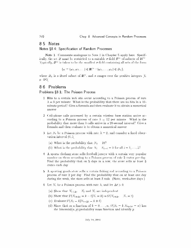
270 Chap. 8 Advanced Concepts in Random Processes
8.5. NotesNotes x8.4: Speci�cation of Random Processes
Note 1. Comments analogous to Note 1 in Chapter 5 apply here. Specif-ically, the set B must be restricted to a suitable �-�eld B1 of subsets of IR1.Typically, B1 is taken to be the smallest �-�eld containing all sets of the form
f! = (!1; !2; : : : ) 2 IR1 : (!1; : : : ; !n) 2 Bng;where Bn is a Borel subset of IRn, and n ranges over the positive integers [4,p. 485].
8.6. ProblemsProblems x8.1: The Poisson Process
1. Hits to a certain web site occur according to a Poisson process of rate� = 3 per minute. What is the probability that there are no hits in a 10-minute period? Give a formula and then evaluate it to obtain a numericalanswer.
2. Cell-phone calls processed by a certain wireless base station arrive ac-cording to a Poisson process of rate � = 12 per minute. What is theprobability that more than 3 calls arrive in a 20-second interval? Give aformula and then evaluate it to obtain a numerical answer.
3. Let Nt be a Poisson process with rate � = 2, and consider a �xed obser-vation interval (0; 5].
(a) What is the probability that N5 = 10?
(b) What is the probability that Ni � Ni�1 = 2 for all i = 1; : : : ; 5?
4. A sports clothing store sells football jerseys with a certain very popularnumber on them according to a Poisson process of rate 3 crates per day.Find the probability that on 5 days in a row, the store sells at least 3crates each day.
5. A sporting goods store sells a certain �shing rod according to a Poissonprocess of rate 2 per day. Find the probability that on at least one dayduring the week, the store sells at least 3 rods. (Note: week=�ve days.)
6. Let Nt be a Poisson process with rate �, and let �t > 0.
(a) Show that Nt+�t � Nt and Nt are independent.
(b) Show that }(Nt+�t = k + `jNt = k) =}(Nt+�t � Nt = `).
(c) Evaluate }(Nt = kjNt+�t = k + `).
(d) Show that as a function of k = 0; : : : ; n, }(Nt = kjNt+�t = n) hasthe binomial(n; p) probability mass function and identify p.
July 18, 2002

8.6 Problems 271
7. Customers arrive at a store according to a Poisson process of rate �. Whatis the expected time until the nth customer arrives? What is the expectedtime between customers?
8. During the winter, snowstorms occur according to a Poisson process ofintensity � = 2 per week.
(a) What is the average time between snowstorms?
(b) What is the probability that no storms occur during a given two-weekperiod?
(c) If winter lasts 12 weeks, what is the expected number of snowstorms?
(d) Find the probability that during at least one of the 12 weeks ofwinter, there are at least 5 snowstorms.
9. Space shuttles are launched according to a Poisson process. The averagetime between launches is two months.
(a) Find the probability that there are no launches during a four-monthperiod.
(b) Find the probability that during at least one month out of four con-secutive months, there are at least two launches.
10. Diners arrive at popular restaurant according to a Poisson process Nt ofrate �. A confused maitre d' seats the ith diner with probability p, andturns the diner away with probability 1� p. Let Yi = 1 if the ith diner isseated, and Yi = 0 otherwise. The number diners seated up to time t is
Mt :=NtXi=1
Yi:
Show that Mt is a Poisson random variable and �nd its parameter. As-sume the Yi are independent of each other and of the Poisson process.
Remark. Mt is an example of a thinned Poisson process.
11. Lightning strikes occur according to a Poisson process of rate � perminute. The energy of the ith strike is Vi. Assume the energy is indepen-dent of the occurrence times. What is the expected energy of a storm thatlasts for t minutes? What is the average time between lightning strikes?
?12. Find the mean and characteristic function of the shot-noise random vari-able Yt in equation (8.5).
Problems x8.2: Renewal Processes
13. In the case of a Poisson process, show that the right-hand side of (8.6)reduces to �t. Hint: Formula (4.2) in Section 4.2 may be helpful.
July 18, 2002
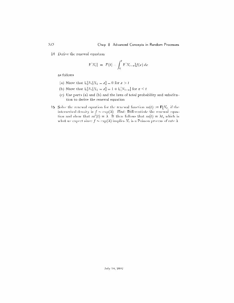
272 Chap. 8 Advanced Concepts in Random Processes
14. Derive the renewal equation
E[Nt] = F (t) +
Z t
0
E[Nt�x]f(x) dx
as follows.
(a) Show that E[NtjX1 = x] = 0 for x > t.
(b) Show that E[NtjX1 = x] = 1 + E[Nt�x] for x � t.
(c) Use parts (a) and (b) and the laws of total probability and substitu-tion to derive the renewal equation.
15. Solve the renewal equation for the renewal function m(t) := E[Nt] if theinterarrival density is f � exp(�). Hint: Di�erentiate the renewal equa-tion and show that m0(t) = �. It then follows that m(t) = �t, which iswhat we expect since f � exp(�) implies Nt is a Poisson process of rate �.
July 18, 2002

8.6 Problems 273
Problems x8.3: The Wiener Process
16. For 0 � s < t <1, use the de�nition of the Wiener process to show thatE[WtWs] = �2s.
17. Let the random vector X = [Wt1 ; : : : ;Wtn ]0, 0 < t1 < � � � < tn < 1,
consist of samples of a Wiener process. Find the covariance matrix of X.
18. For piecewise constant g and h, show thatZ 1
0
g(� ) dW� +
Z 1
0
h(� ) dW� =
Z 1
0
�g(� ) + h(� )
�dW� :
Hint: The problem is easy if g and h are constant over the same intervals.
19. Use (8.8) to derive the formula
E
��Z 1
0
g(� ) dW�
��Z 1
0
h(� ) dW�
��= �2
Z 1
0
g(� )h(� ) d�:
Hint: Consider the expectation
E
��Z 1
0
g(� ) dW� �Z 1
0
h(� ) dW�
�2 �;
which can be evaluated in two di�erent ways. The �rst way is to expandthe square and take expectations term by term, applying (8.8) wherepossible. The second way is to observe that sinceZ 1
0
g(� ) dW� �Z 1
0
h(� ) dW� =
Z 1
0
[g(� )� h(� )] dW� ;
the above second moment can be computed directly using (8.8).
20. Let
Yt =
Z t
0g(� ) dW� ; t � 0:
(a) Use (8.8) to show that
E[Y 2t ] = �2
Z t
0
jg(� )j2 d�:
Hint: Observe thatZ t
0
g(� ) dW� =
Z 1
0
g(� )I(0;t](� ) dW� :
(b) Show that Yt has correlation function
RY (t1; t2) = �2Z min(t1;t2)
0
jg(� )j2 d�; t1; t2 � 0:
July 18, 2002

274 Chap. 8 Advanced Concepts in Random Processes
21. Consider the process
Yt = e��tV +
Z t
0
e��(t��) dW� ; t � 0;
where Wt is a Wiener process independent of V , and V has zero meanand variance q2. Show that Yt has correlation function
RY (t1; t2) = e��(t1+t2)�q2 � �2
2�
�+�2
2�e��jt1�t2j:
Remark. If V is normal, then the process Yt is Gaussian and is knownas an Ornstein{Uhlenbeck process.
22. Let Wt be a Wiener process, and put
Yt :=e��tp2�
We2�t :
Show that
RY (t1; t2) =�2
2�e��jt1�t2j:
In light of the remark above, this is another way to de�ne an Ornstein{Uhlenbeck process.
23. So far we have de�ned the Wiener process Wt only for t � 0. Whende�ning Wt for all t, we continue to assume that W0 � 0; that for s < t,the increment Wt � Ws is a Gaussian random variable with zero meanand variance �2(t� s); that Wt has independent increments; and that Wt
has continuous sample paths. The only di�erence is that s or both s andt can be negative, and that increments can be located anywhere in time,not just over intervals of positive time. In the following take �2 = 1.
(a) For t > 0, show that E[W 2t ] = t.
(b) For s < 0, show that E[W 2s ] = �s.
(c) Show that
E[WtWs] =jtj+ jsj � jt� sj
2:
Problems x8.4: Speci�cation of Random Processes
24. Suppose X and Y are random variables with
}�(X;Y ) 2 A
�=Xi
Z 1
�1IA(xi; y)fXY (xi; y) dy;
where the xi are distinct real numbers, and fXY is a nonnegative functionsatisfying X
i
Z 1
�1fXY (xi; y) dy = 1:
July 18, 2002

8.6 Problems 275
(a) Show that
}(X = xk) =
Z 1
�1fXY (xk; y) dy:
(b) Show that for C � IR,
}(Y 2 C) =
ZC
�Xi
fXY (xi; y)
�dy:
In other words, Y has marginal density
fY (y) =Xi
fXY (xi; y):
(c) Show that
}(Y 2 CjX = xi) =
ZC
�fXY (xi; y)
pX (xi)
�dy:
In other words,
fY jX(yjxi) =fXY (xi; y)
pX (xi):
(d) For B � IR, show that if we de�ne
}(X 2 BjY = y) :=Xi
IB(xi)pXjY (xijy);
where
pXjY (xijy) :=fXY (xi; y)
fY (y);
then Z 1
�1}(X 2 BjY = y)fY (y) dy = }(X 2 B):
In other words, we have the law of total probability.
25. Let F be the standard normal cdf. Then F is a one-to-one mapping from(�1;1) onto (0; 1). Therefore, F has an inverse, F�1: (0; 1)! (�1;1).If U � uniform(0; 1), show that X := F�1(U ) has F for its cdf.
26. Consider the cdf
F (x) :=
8>>>><>>>>:0; x < 0;x2; 0 � x < 1=2;1=4; 1=2 � x < 1;x=2; 1 � x < 2;1; x � 2:
July 18, 2002

276 Chap. 8 Advanced Concepts in Random Processes
(a) Sketch F (x).
(b) For 0 < u < 1, sketch
G(u) := inffx 2 IR : F (x) � ug:Hint: First identify the set
Bu := fx 2 IR : F (x) � ug:Then �nd its in�mum.
27. As illustrated in the previous problem, an arbitrary cdf F is usually notinvertible, either because the equation F (x) = u has more than one so-lution, e.g., F (x) = 1=4, or because it has no solution, e.g., F (x) = 3=8.However, for any cdf F , we can always introduce the function
G(u) := inffx 2 IR : F (x) � ug; 0 < u < 1;
which, you will now show, can play the role of F�1 in Problem 25.
(a) Show that if 0 < u < 1 and x 2 IR, then G(u) � x if and only ifu � F (x).
(b) Let U � uniform(0; 1), and put X := G(U ). Show that X has cdfF .
28. In the text we considered discrete-time processes Xn for n = 1; 2; : : : : Theconsistency condition (8.12) arose from the requirement that
}�(X1; : : : ; Xn; Xn+1) 2 B � IR
�= }
�(X1; : : : ; Xn) 2 B
�;
where B � IRn. For processes Xn with n = 0;�1;�2; : : : ; we require notonly
}�(Xm; : : : ; Xn; Xn+1) 2 B � IR
�= }
�(Xm; : : : ; Xn) 2 B
�;
but also
}�(Xm�1; Xm; : : : ; Xn) 2 IR� B
�= }
�(Xm; : : : ; Xn) 2 B
�;
where now B � IRn�m+1. Let �m;n(B) be a proposed formula for theabove right-hand side. Then the two consistency conditions are
�m;n+1(B � IR) = �m;n(B) and �m�1;n(IR�B) = �m;n(B):
For integer-valued random processes, show that these are equivalent to
1Xj=�1
pm;n+1(im; : : : ; in; j) = pm;n(im; : : : ; in)
and 1Xj=�1
pm�1;n(j; im; : : : ; in) = pm;n(im; : : : ; in);
where pm;n is the proposed joint probability mass function ofXm; : : : ; Xn.
July 18, 2002

8.6 Problems 277
29. Let q be any pmf, and let r(jji) be any conditional pmf. In addition,assume that
Pk q(k)r(jjk) = q(j). Put
pm;n(im; : : : ; in) := q(im) r(im+1jim) r(im+2jim+1) � � �r(injin�1):
Show that both consistency conditions for pmfs in the preceding problemare satis�ed.
Remark. This process is strictly stationary as de�ned in Section 6.2since the upon writing out the formula for pm+k;n+k(im; : : : ; in), we seethat it does not depend on k.
30. Let �n be a probability measure on IRn, and suppose that it is given interms of a joint density fn, i.e.,
�n(Bn) =
Z 1
�1� � �Z 1
�1IBn (x1; : : : ; xn)fn(x1; : : : ; xn) dxn � � �dx1:
Show that the consistency condition (8.12) holds if and only ifZ 1
�1fn+1(x1; : : : ; xn; xn+1) dxn+1 = fn(x1; : : : ; xn):
31. Generalize the preceding problem for the continuous-time consistency con-dition (8.17).
32. Let Wt be a Wiener process. Let ft1;:::;tn denote the joint density ofWt1 ; : : : ;Wtn. Find ft1;:::;tn and show that it satis�es the density versionof (8.17) that you derived in the preceding problem. Hint: The jointdensity should be Gaussian.
July 18, 2002

278 Chap. 8 Advanced Concepts in Random Processes
July 18, 2002

CHAPTER 9
Introduction to Markov Chains
A Markov chain is a random process with the property that given the valuesof the process from time zero up through the current time, the conditionalprobability of the value of the process at any future time depends only on itsvalue at the current time. This is equivalent to saying that the future andthe past are conditionally independent given the present (cf. Problem 29 inChapter 1).
Markov chains often have intuitively pleasing interpretations. Some ex-amples discussed in this chapter are random walks (without barriers and withbarriers, which may be re ecting, absorbing, or neither), queuing systems (with�nite or in�nite bu�ers), birth{death processes (with or without spontaneousgeneration), life (with states being \healthy," \sick," and \death"), and thegambler's ruin problem.
Discrete-time Markov chains are introduced in Section 9.1 via the randomwalk and its variations. The emphasis is on the Chapman{Kolmogorov equationand the �nding of stationary distributions.
Continuous-timeMarkov chains are introduced in Section 9.2 via the Poissonprocess. The emphasis is on Kolmogorov's forward and backward di�erentialequations, and their use to �nd stationary distributions.
9.1. Discrete-Time Markov ChainsA sequence of discrete random variables, X0; X1; : : : is called a Markov
chain if for n � 1,
}(Xn+1 = xn+1jXn = xn; Xn�1 = xn�1; : : : ; X0 = x0)
is equal to}(Xn+1 = xn+1jXn = xn):
In other words, given the sequence of values x0; : : : ; xn, the conditional proba-bility of what Xn+1 will be depends only on the value of xn.
Example 9.1 (Random Walk). Let X0 be an integer-valued random vari-able that is independent of the i.i.d. sequence Z1; Z2; : : : ; where }(Zn = 1) = a,}(Zn = �1) = b, and }(Zn = 0) = 1� (a+ b). Show that if
Xn := Xn�1 + Zn; n = 1; 2; : : : ;
then Xn is a Markov chain.
Solution. It helps to write out
X1 = X0 + Z1
279

280 Chap. 9 Introduction to Markov Chains
X2 = X1 + Z2 = X0 + Z1 + Z2
...
Xn = Xn�1 + Zn = X0 + Z1 + � � �+ Zn:
The point here is that (X0; : : : ; Xn) is a function of (X0; Z1; : : : ; Zn), and hence,Zn+1 and (X0; : : : ; Xn) are independent. Now observe that
}(Xn+1 = xn+1jXn = xn; : : : ; X0 = x0)
is equal to}(Xn + Zn+1 = xn+1jXn = xn; : : : ; X0 = x0):
Using the substitution law, this becomes
}(Zn+1 = xn+1 � xnjXn = xn; : : : ; X0 = x0):
On account of the independence of Zn+1 and (X0; : : : ; Xn), the above condi-tional probability is equal to
}(Zn+1 = xn+1 � xn):
Since this depends on xn but not on xn�1; : : : ; x0, it follows by the next examplethat }(Zn+1 = xn+1 � xn) = }(Xn+1 = xn+1jXn = xn).
The Markov chain of the preceding example is called a random walk onthe integers. The random walk is said to be symmetric if a = b = 1=2. Arealization of a symmetric random walk is shown in Figure 9.1. Notice thateach point di�ers from the preceding one by �1.
To restrict the random walk to the nonnegative integers, we can take Xn =max(0; Xn�1 + Zn) (Problem 1).
Example 9.2. Show that if
}(Xn+1 = xn+1jXn = xn; : : : ; X0 = x0)
is a function of xn but not xn�1; : : : ; x0, then the above conditional probabilityis equal to
}(Xn+1 = xn+1jXn = xn):
Solution. We use the identity }(A \ B) = }(AjB)}(B), where A =fXn+1 = xn+1g and B = fXn = xn; : : : ; X0 = x0g. Hence, if
}(Xn+1 = xn+1jXn = xn; : : : ; X0 = x0) = h(xn);
then the joint probability mass function
}(Xn+1 = xn+1; Xn = xn; Xn�1 = xn�1; : : : ; X0 = x0)
July 18, 2002

9.1 Discrete-Time Markov Chains 281
0 10 20 30 40 50 60 70 80−6
−4
−2
0
2
4
6
Figure 9.1. Realization of a symmetric random walk Xn.
is equal toh(xn)}(Xn = xn; Xn�1 = xn�1; : : : ; X0 = x0):
Summing both of these formulas over all values of xn�1; : : : ; x0 shows that
}(Xn+1 = xn+1; Xn = xn) = h(xn)}(Xn = xn):
Hence, h(xn) = }(Xn+1 = xn+1jXn = xn) as claimed.
State Space and Transition Probabilities
The set of possible values that the random variables Xn can take is calledthe state space of the chain. In the rest of this chapter, we take the statespace to be the set of integers or some speci�ed subset of the integers. Theconditional probabilities
}(Xn+1 = jjXn = i)
are called transition probabilities. In this chapter, we assume that thetransition probabilities do not depend on time n. Such a Markov chain issaid to have stationary transition probabilities or to be time homogeneous.For a time-homogeneous Markov chain, we use the notation
pij := }(Xn+1 = jjXn = i)
for the transition probabilities. The pij are also called the one-step transi-tion probabilities because they are the probabilities of going from state i tostate j in one time step. One of the most common ways to specify the transi-tion probabilities is with a state transition diagram as in Figure 9.2. This
July 18, 2002

282 Chap. 9 Introduction to Markov Chains
0 11−a
a
b
1− b
Figure 9.2. A state transition diagram. The diagram says that the state space is the �niteset f0;1g, and that p01 = a, p10 = b, p00 = 1� a, and p11 = 1� b.
particular diagram says that the state space is the �nite set f0; 1g, and thatp01 = a, p10 = b, p00 = 1 � a, and p11 = 1 � b. Note that the sum of all theprobabilities leaving a state must be one. This is because for each state i,X
j
pij =Xj
}(Xn+1 = jjXn = i) = 1:
The transition probabilities pij can be arranged in a matrix P , called the tran-sition matrix, whose i j entry is pij . For the chain in Figure 9.2,
P =
�1� a ab 1� b
�:
The top row of P contains the probabilities p0j, which is obtained by notingthe probabilities written next to all the arrows leaving state 0. Similarly, theprobabilities written next to all the arrows leaving state 1 are found in thebottom row of P .
Examples
The general random walk on the integers has the state transition diagramshown in Figure 9.3. Note that the Markov chain constructed in Example 9.1 is
. . . i . . .
bi
aiai −1
bi +1
1−( )ai bi+
Figure 9.3. State transition diagram for a random walk on the integers.
a special case in which ai = a and bi = b for all i. The state transition diagramis telling us that
pij =
8>><>>:bi; j = i� 1;
1� (ai + bi); j = i;ai; j = i+ 1;0; otherwise:
(9.1)
July 18, 2002

9.1 Discrete-Time Markov Chains 283
. . .01− 1 i . . .
bi
ai0a 1a
1b
0a
1− ( )1a 1b+
b2
ai −1
bi +1
1−( )ai bi+
Figure 9.4. State transition diagram for a random walk with barrier at the origin (alsocalled a birth{death process).
Hence, the transition matrix P is in�nite, tridiagonal, and its ith row is� � � � 0 bi 1� (ai + bi) ai 0 � � � � :Frequently, it is convenient to introduce a barrier at zero, leading to the
state transition diagram in Figure 9.4. In this case, we speak of the randomwalk with barrier. If a0 = 1, the barrier is said to be re ecting. If a0 = 0, thebarrier is said to be absorbing. Once a chain hits an absorbing state, the chainstays in that state from that time onward. If ai = a and bi = b for all i, theMarkov chain is viewed as a model for a queue with an in�nite bu�er. A randomwalk with barrier at the origin is also known as a birth{death process. Withthis terminology, the state i is taken to be a population, say of bacteria. In thiscase, if a0 > 0, there is spontaneous generation. If bi = 0 for all i, we havea pure birth process. For i � 1, the formula for pij is given by (9.1) above,while for i = 0,
p0j =
8<:1� a0; j = 0;a0; j = 1;
0; otherwise:
(9.2)
The transition matrix P is the tridiagonal, semi-in�nite matrix
P =
26666641� a0 a0 0 0 0 � � �b1 1� (a1 + b1) a1 0 0 � � �0 b2 1� (a2 + b2) a2 0 � � �0 0 b3 1� (a3 + b3) a3...
......
. . .
3777775 :
Sometimes it is useful to consider a random walk with barriers at the originand at N , as shown in Figure 9.5. The formula for pij is given by (9.1) abovefor 1 � i � N � 1, by (9.2) above for i = 0, and, for i = N , by
pNj =
8<:bN ; j = N � 1;
1� bN ; j = N;0; otherwise:
(9.3)
This chain is viewed as a model for a queue with a �nite bu�er, especially ifai = a and bi = b for all i. When a0 = 0 and bN = 0, the barriers at 0 and N
July 18, 2002

284 Chap. 9 Introduction to Markov Chains
01− 1
0a 1a
1b
0a
1− ( )1a 1b+
b2
. . . N
bN
N−1 1− bN
aN−12aN−
bN−1
1− ( )aN−1 bN−1+
Figure 9.5. State transition diagram for a queue with a �nite bu�er.
are absorbing, and the chain is a model for the gambler's ruin problem. Inthis problem, a gambler starts at time zero with 1 � i � N � 1 dollars, andplays until he either runs out of money, that is, absorption into state zero, orhe acquires a fortune of N dollars and stops playing (absorption into state N ).If N = 2 and b2 = 0, the chain can be interpreted as the story of life if we viewstate i = 0 as being the \healthy" state, i = 1 as being the \sick" state, andi = 2 as being the \death" state. In this model, if you are healthy (in state 0),you remain healthy with probability 1� a0 and become sick (move to state 1)with probability a0. If you are sick (in state 1), you become healthy (moveto state 0) with probability b1, remain sick (stay in state 1) with probability1 � (a1 + b1), or die (move to state 2) with probability b1. Since state 2 isabsorbing (b2 = 0), once you enter this state, you never leave.
Stationary Distributions
The n-step transition probabilities are de�ned by
p(n)ij := }(Xn = jjX0 = i):
This is the probability of going from state i (at time zero) to state j in n steps.For a chain with stationary transition probabilities, it will be shown later thatthe n-step transition probabilities are also stationary; i.e., for m = 1; 2; : : : ;
}(Xn+m = jjXm = i) = }(Xn = jjX0 = i) = p(n)ij :
We also note that
p(0)ij = }(X0 = jjX0 = i) = �ij ;
where �ij denotes the Kronecker delta, which is one if i = j and is zerootherwise.
A Markov chain with stationary transition probabilities also satis�es theChapman{Kolmogorov equation,
p(n+m)ij =
Xk
p(n)ik p
(m)kj : (9.4)
This equation, which is derived later, says that to go from state i to state j inn+m steps, �rst you go to some intermediate state k in n steps, and then you
July 18, 2002

9.1 Discrete-Time Markov Chains 285
go from state k to state j in m steps. Taking m = 1, we have the special case
p(n+1)ij =
Xk
p(n)ik pkj:
If n = 1 as well,
p(2)ij =
Xk
pik pkj:
This equation says that the matrix with entries p(2)ij is equal to the product
PP . More generally, the matrix with entries p(n)ij , called the n-step transition
matrix , is equal to Pn. The Chapman{Kolmogorov equation thus says that
Pn+m = PnPm:
For many Markov chains, it can be shown [17, Section 6.4] that
limn!1
}(Xn = jjX0 = i)
exists and does not depend on i. In other words, if the chain runs for a longtime, it reaches a \steady state" in which the probability of being in state jdoes not depend on the initial state of the chain. If the above limit exists anddoes not depend on i, we put
�j := limn!1
}(Xn = jjX0 = i):
We call f�jg the stationary distribution or the equilibrium distributionof the chain. Note that if we sum both sides over j, we getX
j
�j =Xj
limn!1
}(Xn = jjX0 = i)
= limn!1
Xj
}(Xn = jjX0 = i)
= limn!1 1 = 1: (9.5)
To �nd the �j, we can use the Chapman{Kolmogorov equation. If p(n)ij ! �j,
then taking limits in
p(n+1)ij =
Xk
p(n)ik pkj
shows that�j =
Xk
�k pkj:
If we think of � as a row vector with entries �j, and if we think of P as thematrix with entries pij, then the above equation says that
� = �P:
July 18, 2002

286 Chap. 9 Introduction to Markov Chains
. . .01−a
a
b
1
a
b
1− ( )a+b
a
b
a
b
i . . .
1− ( )a+b
Figure 9.6. State transition diagram for a queuing system with an in�nite bu�er.
On account of (9.5), � cannot be the zero vector. Hence, � is a left eigenvectorof P with eigenvalue 1. To say this another way, I � P is singular; i.e., thereare many solutions of �(I � P ) = 0. The solution we want must satisfy notonly � = �P , but also the normalization condition,X
j
�j = 1;
derived in (9.5).
Example 9.3. The state transition diagram for a queuing system with anin�nite bu�er is shown in Figure 9.6. Find the stationary distribution of thechain.
Solution. We begin by writing out
�j =Xk
�k pkj (9.6)
for j = 0; 1; 2; : : : : For each j, the coe�cients pkj are obtained by inspection ofthe state transition diagram. For j = 0, we must consider
�0 =Xk
�k pk0:
We need the values of pk0. From the diagram, the only way to get to state0 is from state 0 itself (with probability p00 = 1 � a) or from state 1 (withprobability p10 = b). The other pk0 = 0. Hence,
�0 = �0 (1� a) + �1 b:
We can rearrange this to get
�1 =a
b�0:
Now put j = 1 in (9.6). The state transition diagram tells us that the only wayto enter state 1 is from states 0, 1, and 2, with probabilities a, 1� (a+ b), andb, respectively. Hence,
�1 = �0 a+ �1 [1� (a + b)] + �2 b:
July 18, 2002

9.1 Discrete-Time Markov Chains 287
Substituting �1 = (a=b)�0 yields �2 = (a=b)2�0. In general, if we substitute�j = (a=b)j�0 and �j�1 = (a=b)j�1�0 into
�j = �j�1 a+ �j [1� (a+ b)] + �j+1 b;
then we obtain �j+1 = (a=b)j+1�0. We conclude that
�j =�ab
�j�0; j = 0; 1; 2; : : ::
To solve for �0, we use the fact that
1Xj=0
�j = 1;
or
�0
1Xj=0
�ab
�j= 1:
The geometric series formula shows that
�0 = 1� a=b;
and
�j =�ab
�j(1� a=b):
In other words, the stationary distribution is a geometric0(a=b) probabilitymassfunction.
Derivation of the Chapman{Kolmogorov Equation
We begin by showing that
p(n+1)ij =
Xl
p(n)il plj :
To derive this, we need the following law of total conditional probability.We claim that
}(X = xjZ = z) =Xy
}(X = xjY = y; Z = z)}(Y = yjZ = z):
The right-hand side of this equation is simplyXy
}(X = x; Y = y; Z = z)}(Y = y; Z = z)
�}(Y = y; Z = z)
}(Z = z):
Canceling common factors and then summing over y yields
}(X = x; Z = z)}(Z = z)
= }(X = xjZ = z):
July 18, 2002

288 Chap. 9 Introduction to Markov Chains
We can now write
p(n+1)ij = }(Xn+1 = jjX0 = i)
=Xln
� � �Xl1
}(Xn+1 = jjXn = ln; : : : ; X1 = l1; X0 = i)
�}(Xn = ln; : : : ; X1 = l1jX0 = i)
=Xln
� � �Xl1
}(Xn+1 = jjXn = ln)}(Xn = ln; : : : ; X1 = l1jX0 = i)
=Xln
}(Xn+1 = jjXn = ln)}(Xn = lnjX0 = i)
=Xl
p(n)il plj :
This establishes that for m = 1,
p(n+m)ij =
Xk
p(n)ik p
(m)kj :
We now assume it is true for m and show it is true for m + 1. Write
p(n+[m+1])ij = p
([n+m]+1)ij
=Xl
p(n+m)il plj
=Xl
�Xk
p(n)ik p
(m)kl
�plj
=Xk
p(n)ik
�Xl
p(m)kl plj
�=
Xk
p(n)ik p
(m+1)kj :
Stationarity of the n-step Transition Probabilities
We would now like to use the Chapman{Kolmogorov equation to show thatthe n-step transition probabilities are stationary; i.e.,
}(Xn+m = jjXm = i) = }(Xn = jjX0 = i) = p(n)ij :
To do this, we need the fact that for any 0 � � < n,
}(Xn+1 = jjXn = i;X� = l) = }(Xn+1 = jjXn = i): (9.7)
To establish this fact, we use the law of total conditional probability to writethe left-hand side asXln�1
� � �Xl0
}(Xn+1 = jjXn = i;Xn�1 = ln�1; : : : ; X� = l; : : : ; X0 = l0)
�}(Xn�1 = ln�1; : : : ; X�+1 = l�+1; X��1 = l��1; : : : ; X0 = l0jXn = i;X� = l);
July 18, 2002

9.2 Continuous-Time Markov Chains 289
where the sum is (n � 1)-fold, the sum over l� being omitted. By the Markovproperty, this simpli�es toXln�1
� � �Xl0
}(Xn+1 = jjXn = i)
�}(Xn�1 = ln�1; : : : ; X�+1 = l�+1; X��1 = l��1; : : : ; X0 = l0jXn = i;X� = l);
which further simpli�es to }(Xn+1 = jjXn = i).We can now show that the n-step transition probabilities are stationary. For
a time-homogeneous Markov chain, the case n = 1 holds by de�nition. Assumeit holds for m, and use the law of total conditional probability to write
}(Xn+m+1 = jjXm = i) =Xk
}(Xn+m+1 = jjXn+m = k;Xm = i)
�}(Xn+m = kjXm = i)
=Xk
}(Xn+m+1 = jjXn+m = k)
�}(Xn+m = kjXm = i)
=Xk
p(n)ik pkj
= p(n+1)ij ;
by the Chapman{Kolmogorov equation.
9.2. Continuous-Time Markov ChainsA family of integer-valued random variables, fXt; t � 0g, is called aMarkov
chain if for all n � 1, and for all 0 � s0 < � � � < sn�1 < s < t,
}(Xt = jjXs = i;Xsn�1 = in�1; : : : ; Xs0 = i0) = }(Xt = jjXs = i):
In other words, given the sequence of values i0; : : : ; in�1; i, the conditional prob-ability of what Xt will be depends only on the condition Xs = i. The quantity}(Xt = jjXs = i) is called the transition probability.
Example 9.4. Show that the Poisson process of rate � is a Markov chain.
Solution. To begin, observe that
}(Nt = jjNs = i; Nsn�1 = in�1; : : : ; Ns0 = i0);
is equal to
}(Nt � i = j � ijNs = i; Nsn�1 = in�1; : : : ; Ns0 = i0):
July 18, 2002

290 Chap. 9 Introduction to Markov Chains
By the substitution law, this is equal to
}(Nt �Ns = j � ijNs = i; Nsn�1 = in�1; : : : ; Ns0 = i0): (9.8)
Since
(Ns; Nsn�1 ; : : : ; Ns0) (9.9)
is a function of
(Ns � Nsn�1 ; : : : ; Ns1 � Ns0 ; Ns0 � N0);
and since this is independent ofNt�Ns by the independent increments propertyof the Poisson process, it follows that (9.9) and Nt � Ns are also independent.Thus, (9.8) is equal to }(Nt � Ns = j � i), which depends on i but not onin�1; : : : ; i0. It then follows that
}(Nt = jjNs = i; Nsn�1 = in�1; : : : ; Ns0 = i0) = }(Nt = jjNs = i);
and we see that the Poisson process is a Markov chain.
As shown in the above example,
}(Nt = jjNs = i) = }(Nt � Ns = j � i) =[�(t� s)]j�ie��(t�s)
(j � i)!
depends on t and s only through t � s. In general, if a Markov chain has theproperty that the transition probability }(Xt = jjXs = i) depends on t and sonly through t� s, we say that the chain is time-homogeneous or that it hasstationary transition probabilities. In this case, if we put
pij(t) := }(Xt = jjX0 = i);
then }(Xt = jjXs = i) = pij(t � s). Note that pij(0) = �ij, the Kroneckerdelta.
In the remainder of the chapter, we assume that Xt is a time-homogeneousMarkov chain with transition probability function pij(t). For such a chain, wecan derive the continuous-time Chapman{Kolmogorov equation,
pij(t+ s) =Xk
pik(t)pkj(s):
To derive this, we �rst use the law of total conditional probability to write
pij(t+ s) = }(Xt+s = jjX0 = i)
=Xk
}(Xt+s = jjXt = k;X0 = i)}(Xt = kjX0 = i):
July 18, 2002

9.2 Continuous-Time Markov Chains 291
Now use the Markov property and time homogeneity to obtain
pij(t+ s) =Xk
}(Xt+s = jjXt = k)}(Xt = kjX0 = i)
=Xk
pkj(s)pik(t):
The reader may wonder why the derivation of the continuous-time Chapman{Kolmogorov equation is so much simpler than the derivation of the discrete-timeversion. The reason is that in discrete time, the Markov property and time ho-mogeneity are de�ned in a one-step manner. Hence, induction arguments are�rst needed to derive the discrete-time analogs of the continuous-time de�ni-
tions!
Kolmogorov's Di�erential Equations
In the remainder of the chapter, we assume that for small �t > 0,
pij(�t) � gij�t; i 6= j; and pii(�t) � 1 + gii�t:
These approximations tell us the conditional probability of being in state j attime �t in the very near future given that we are in state i at time zero. Theseassumptions are more precisely written as
lim�t#0
pij(�t)
�t= gij and lim
�t#0pii(�t)� 1
�t= gii: (9.10)
Note that gij � 0, while gii � 0.Using the Chapman{Kolmogorov equation, write
pij(t+�t) =Xk
pik(t)pkj(�t)
= pij(t)pjj(�t) +Xk 6=j
pik(t)pkj(�t):
Now subtract pij(t) from both sides to get
pij(t +�t)� pij(t) = pij(t)[pjj(�t) � 1] +Xk 6=j
pik(t)pkj(�t): (9.11)
Dividing by �t and applying the limit assumptions (9.10), we obtain
p0ij(t) = pij(t)gjj +Xk 6=j
pik(t)gkj:
This is Kolmogorov's forward di�erential equation, which can be writtenmore compactly as
p0ij(t) =Xk
pik(t)gkj: (9.12)
July 18, 2002

292 Chap. 9 Introduction to Markov Chains
To derive the backward equation, observe that since pij(t+�t) = pij(�t+t),we can write
pij(t +�t) =Xk
pik(�t)pkj(t)
= pii(�t)pij(t) +Xk 6=i
pik(�t)pkj(t):
Now subtract pij(t) from both sides to get
pij(t+�t) � pij(t) = [pii(�t) � 1]pij(t) +Xk 6=i
pik(�t)pkj(t):
Dividing by �t and applying the limit assumptions (9.10), we obtain
p0ij(t) = giipij(t) +Xk 6=i
gikpkj(t):
This is Kolmogorov's backward di�erential equation, which can be writ-ten more compactly as
p0ij(t) =Xk
gikpkj(t): (9.13)
The derivations of both the forward and backward di�erential equationsrequire taking a limit in �t inside the sum over k. For example, in deriving thebackward equation, we tacitly assumed that
lim�t#0
Xk 6=i
pik(�t)
�tpkj(t) =
Xk 6=i
lim�t#0
pik(�t)
�tpkj(t): (9.14)
If the state space of the chain is �nite, the above sum is �nite and there is noproblem. Otherwise, additional technical assumptions are required to justifythis step. We now show that a su�cient assumption for deriving the backwardequation is that X
j 6=igij = �gii < 1:
A chain that satis�es this condition is said to be conservative. For any �niteN , observe that X
k 6=i
pik(�t)
�tpkj(t) �
Xjkj�Nk 6=i
pik(�t)
�tpkj(t):
Since the right-hand side is a �nite sum,
lim�t#0
Xk 6=i
pik(�t)
�tpkj(t) �
Xjkj�Nk 6=i
gikpkj(t):
July 18, 2002

9.2 Continuous-Time Markov Chains 293
Letting N !1 shows that
lim�t#0
Xk 6=i
pik(�t)
�tpkj(t) �
Xk 6=i
gikpkj(t): (9.15)
To get an upper bound on the limit, take N � i and writeXk 6=i
pik(�t)
�tpkj(t) =
Xjkj�Nk 6=i
pik(�t)
�tpkj(t) +
Xjkj>N
pik(�t)
�tpkj(t):
Since pkj(t) � 1,Xk 6=i
pik(�t)
�tpkj(t) �
Xjkj�Nk 6=i
pik(�t)
�tpkj(t) +
Xjkj>N
pik(�t)
�t
=Xjkj�Nk 6=i
pik(�t)
�tpkj(t) +
1
�t
�1�
Xjkj�N
pik(�t)
�
=Xjkj�Nk 6=i
pik(�t)
�tpkj(t) +
1� pii(�t)
�t�Xjkj�Nk 6=i
pik(�t)
�t:
Since these sums are �nite,
lim�t#0
Xk 6=i
pik(�t)
�tpkj(t) �
Xjkj�Nk 6=i
gikpkj(t)� gii �Xjkj�Nk 6=i
gik:
Letting N !1 shows that
lim�t#0
Xk 6=i
pik(�t)
�tpkj(t) �
Xk 6=i
gikpkj(t)� gii �Xk 6=i
gik:
If the chain is conservative, this simpli�es to
lim�t#0
Xk 6=i
pik(�t)
�tpkj(t) �
Xk 6=i
gikpkj(t):
Combining this with (9.15) yields (9.14), thus justifying the backward equation.Readers familiar with linear system theory may �nd it insightful to write the
forward and backward equations in matrix form. Let P (t) denote the matrixwhose i j entry is pij(t), and let G denote the matrix whose i j entry is gij (Gis called the generator matrix, or rate matrix). Then the forward equation(9.12) becomes
P 0(t) = P (t)G;
July 18, 2002

294 Chap. 9 Introduction to Markov Chains
and the backward equation (9.13) becomes
P 0(t) = GP (t);
The initial condition in both cases is P (0) = I. Under suitable assumptions,the solution of both equations is given by the matrix exponential,
P (t) = eGt :=1Xn=0
(Gt)n
n!:
When the state space is �nite, G is a �nite-dimensional matrix, and the theoryis straightforward. Otherwise, more careful analysis is required.
Stationary Distributions
Let us suppose that pij(t)! �j as t!1, independently of the initial statei. Then for large t, pij(t) is approximately constant, and we therefore hope thatits derivative is converging to zero. Assuming this to be true, the limiting formof the forward equation (9.12) is
0 =Xk
�kgkj:
Combining this with the normalization conditionP
k �k = 1 allows us to solvefor �k much as in the discrete case.
9.3. ProblemsProblems x9.1: Introduction to Discrete-Time Markov Chains
1. LetX0; Z1; Z2; : : : be a sequence of independent discrete random variables.Put
Xn = g(Xn�1; Zn); n = 1; 2; : : : :
Show that Xn is a Markov chain. For example, if Xn = max(0; Xn�1 +Zn), where X0 and the Zn are as in Example 9.1, then Xn is a randomwalk restricted to the nonnegative integers.
2. Let Xn be a time-homogeneous Markov chain with transition probabilitiespij. Put �i :=}(X0 = i). Express
}(X0 = i;X1 = j;X2 = k;X3 = l)
in terms of �i and entries from the transition probability matrix.
3. Find the stationary distribution of the Markov chain in Figure 9.2.
4. Draw the state transition diagram and �nd the stationary distribution ofthe Markov chain whose transition matrix is
P =
24 1=2 1=2 01=4 0 3=41=2 1=2 0
35 :Answer: �0 = 5=12, �1 = 1=3, �2 = 1=4.
July 18, 2002

9.3 Problems 295
5. Draw the state transition diagram and �nd the stationary distribution ofthe Markov chain whose transition matrix is
P =
24 0 1=2 1=21=4 3=4 01=4 3=4 0
35 :Answer: �0 = 1=5, �1 = 7=10, �2 = 1=10.
6. Draw the state transition diagram and �nd the stationary distribution ofthe Markov chain whose transition matrix is
P =
26641=2 1=2 0 09=10 0 1=10 00 1=10 0 9=100 0 1=2 1=2
3775 :Answer: �0 = 9=28, �1 = 5=28, �2 = 5=28, �3 = 9=28.
7. Find the stationary distribution of the queuing system with �nite bu�erof size N , whose state transition diagram is shown in Figure 9.7.
0 1
a a
b
1− a
1− ( )a b+
b
. . . N
b
N−1 1− b
aa
b
1− ( )a b+
Figure 9.7. State transition diagram for a queue with a �nite bu�er.
8. Show that if �i :=}(X0 = i), then
}(Xn = j) =Xi
�ip(n)ij :
If f�jg is the stationary distribution, and if �i = �i, show that }(Xn =j) = �j.
Problems x9.2: Continuous-Time Markov Chains
9. The general continuous-time random walk is de�ned by
gij =
8>><>>:�i; j = i� 1;
�(�i + �i); j = i;�i; j = i+ 1;0; otherwise:
Write out the forward and backward equations. Is the chain conservative?
July 18, 2002

296 Chap. 9 Introduction to Markov Chains
10. The continuous-time queue with in�nite bu�er can be obtained by mod-ifying the general random walk in the preceding problem to include abarrier at the origin. Put
g0j =
8<:��0; j = 0;�0; j = 1;0; otherwise:
Find the stationary distribution assuming
1Xj=1
��0 � � ��j�1
�1 � � ��j�
< 1:
If �i = � and �i = � for all i, simplify the above condition to one involvingonly the relative values of � and �.
11. Modify Problem 10 to include a barrier at some �nite N . Find the sta-tionary distribution.
12. For the chain in Problem 10, let
�j = j� + � and �j = j�;
where �, �, and � are positive. Put mi(t) := E[XtjX0 = i]. Derive adi�erential equation for mi(t) and solve it. Treat the cases � = � and� 6= � separately. Hint: Use the forward equation (9.12).
13. For the chain in Problem 10, let �i = 0 and �i = �. Write down and solvethe forward equation (9.12). Hint: Equation (8.4).
14. Let T denote the �rst time a chain leaves state i,
T := minft � 0 : Xt 6= ig:Show that given X0 = i, T is conditionally exp(�gii). In other words,the time the chain spends in state i, known as the sojourn time, hasan exponential density with parameter �gii. Hints: By Problem 43 inChapter 4, it su�ces to prove that
}(T > t+�tjT > t;X0 = i) = }(T > �tjX0 = i):
To derive this equation, use the fact that if Xt is right-continuous,
T > t if and only if Xs = i for 0 � s � t:
Use the Markov property in the form
}(Xs = i; t � s � t+�tjXs = i; 0 � s � t)
= }(Xs = i; t � s � t+�tjXt = i);
July 18, 2002

9.3 Problems 297
and use time homogeneity in the form
}(Xs = i; t � s � t +�tjXt = i) = }(Xs = i; 0 � s � �tjX0 = i):
To identify the parameter of the exponential density, you may use theapproximation}(Xs = i; 0 � s � �tjX0 = i) � pii(�t).
15. The notion a Markov chain can be generalized to include random variablesthat are not necessarily discrete. We say that Xt is a continuous-timeMarkov process if
}(Xt 2 BjXs = x;Xsn�1 = xn�1; : : : ; Xs0 = x0) = }(Xt 2 BjXs = x):
Such a process is time homogeneous if }(Xt 2 BjXs = x) depends on tand s only through t�s. Show that the Wiener process is a Markov processthat is time homogeneous. Hint: It is enough to look at conditional cdfs;i.e., show that
}(Xt � yjXs = x;Xsn�1 = xn�1; : : : ; Xs0 = x0) = }(Xt � yjXs = x):
16. Let Xt be a time-homogeneous Markov process as de�ned in the previousproblem. Put
Pt(x;B) := }(Xt 2 BjX0 = x);
and assume that there is a corresponding conditional density, denoted byft(x; y), such that
Pt(x;B) =
ZB
ft(x; y) dy:
Derive the Chapman{Kolmogorov equation for conditional densities,
ft+s(x; y) =
Z 1
�1fs(x; z)ft(z; y) dz:
Hint: It su�ces to show that
Pt+s(x;B) =
Z 1
�1fs(x; z)Pt(z; B) dz:
To derive this, you may assume that a law of total conditional probabilityholds for random variables with appropriate conditional densities.
July 18, 2002

298 Chap. 9 Introduction to Markov Chains
July 18, 2002
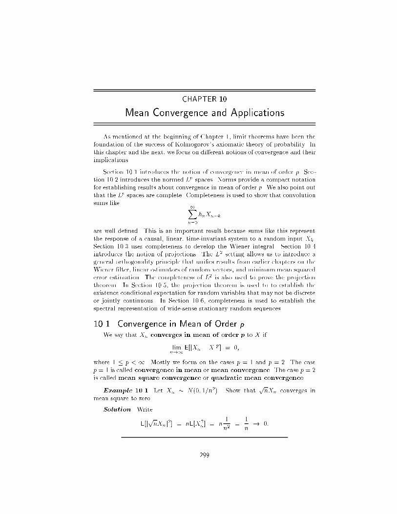
CHAPTER 10
Mean Convergence and Applications
As mentioned at the beginning of Chapter 1, limit theorems have been thefoundation of the success of Kolmogorov's axiomatic theory of probability. Inthis chapter and the next, we focus on di�erent notions of convergence and theirimplications.
Section 10.1 introduces the notion of convergence in mean of order p. Sec-tion 10.2 introduces the normed Lp spaces. Norms provide a compact notationfor establishing results about convergence in mean of order p. We also point outthat the Lp spaces are complete. Completeness is used to show that convolutionsums like 1X
k=0
hkXn�k
are well de�ned. This is an important result because sums like this representthe response of a causal, linear, time-invariant system to a random input Xk.Section 10.3 uses completeness to develop the Wiener integral. Section 10.4introduces the notion of projections. The L2 setting allows us to introduce ageneral orthogonality principle that uni�es results from earlier chapters on theWiener �lter, linear estimators of random vectors, and minimummean squarederror estimation. The completeness of L2 is also used to prove the projectiontheorem. In Section 10.5, the projection theorem is used to to establish theexistence conditional expectation for random variables that may not be discreteor jointly continuous. In Section 10.6, completeness is used to establish thespectral representation of wide-sense stationary random sequences.
10.1. Convergence in Mean of Order pWe say that Xn converges in mean of order p to X if
limn!1E[jXn �Xjp] = 0;
where 1 � p < 1. Mostly we focus on the cases p = 1 and p = 2. The casep = 1 is called convergence in mean ormean convergence. The case p = 2is called mean square convergence or quadratic mean convergence.
Example 10.1. Let Xn � N (0; 1=n2). Show thatpnXn converges in
mean square to zero.
Solution. Write
E[jpnXnj2] = nE[X2n] = n
1
n2=
1
n! 0:
299

300 Chap. 10 Mean Convergence and Applications
In the following example, Xn converges in mean square to zero, but not inmean of order 4.
Example 10.2. Let Xn have density
fn(x) = gn(x)(1� 1=n3) + hn(x)=n3;
where gn � N (0; 1=n2) and hn � N (n; 1). Show that Xn converges to zero inmean square, but not in mean of order 4.
Solution. For convergence in mean square, write
E[jXnj2] =1
n2(1� 1=n3) + (1 + n2)=n3 ! 0:
However, using Problem 28 in Chapter 3, we have
E[jXnj4] =3
n4(1� 1=n3) + (n4 + 6n2 + 3)=n3 ! 1:
The preceding example raises the question of whether Xn might convergein mean of order 4 to something other than zero. However, by Problem 8 atthe end of the chapter, if Xn converged in mean of order 4 to some X, then itwould also converge in mean square to X. Hence, the only possible limit forXn in mean of order 4 is zero, and as we saw, Xn does not converge in meanof order 4 to zero.
Example 10.3. LetX1; X2; : : : be uncorrelated randomvariables with com-mon mean m and common variance �2. Show that the sample mean
Mn :=1
n
nXi=1
Xi
converges in mean square to m. We call this the mean-square law of largenumbers for uncorrelated random variables.
Solution. Since
Mn �m =1
n
nXi=1
(Xi �m);
we can write
E[jMn �mj2] =1
n2E
�� nXi=1
(Xi �m)
�� nXj=1
(Xj �m)
��
=1
n2
nXi=1
nXj=1
E[(Xi �m)(Xj �m)]: (10.1)
July 18, 2002

10.1 Convergence in Mean of Order p 301
Since Xi and Xj are uncorrelated, the preceding expectations are zero wheni 6= j. Hence,
E[jMn �mj2] =1
n2
nXi=1
E[(Xi �m)2] =n�2
n2=
�2
n;
which goes to zero as n!1.
Example 10.4. Here is a generalization of the preceding example. LetX1; X2; : : : be wide-sense stationary; i.e., the Xi have commonmeanm = E[Xi],and the covariance E[(Xi �m)(Xj �m)] depends only on the di�erence i � j.Put
R(i) := E[(Xj+i �m)(Xj �m)]:
Show that
Mn :=1
n
nXi=1
Xi
converges in mean square to m if and only if
limn!1
1
n
n�1Xk=0
R(k) = 0: (10.2)
We call this result the mean-square law of large numbers for wide-sensestationary sequences or the mean-square ergodic theorem for wide-sensestationary sequences Note that a su�cient condition for (10.2) to hold isthat limk!1R(k) = 0 (Problem 3).
Solution. We show that (10.2) implies Mn converges in mean square tom. The converse is left to the reader in Problem 4. From (10.1), we see that
n2E[jMn�mj2] =nXi=1
nXj=1
R(i � j)
=Xi=j
R(0) + 2Xj<i
R(i � j)
= nR(0) + 2nXi=2
i�1Xj=1
R(i � j)
= nR(0) + 2nXi=2
i�1Xk=1
R(k):
On account of (10.2), given " > 0, there is an N such that for all i � N ,���� 1
i � 1
i�1Xk=1
R(k)
���� < ":
July 18, 2002

302 Chap. 10 Mean Convergence and Applications
For n � N , the above double sum can be written as
nXi=2
i�1Xk=1
R(k) =N�1Xi=2
i�1Xk=1
R(k) +nX
i=N
(i� 1)
�1
i� 1
i�1Xk=1
R(k)
�:
The magnitude of the right-most double sum is upper bounded by���� nXi=N
(i � 1)
�1
i � 1
i�1Xk=1
R(k)
����� < "
nXi=N
(i � 1)
< "
nXi=1
(i� 1)
="n(n � 1)
2
<"n2
2:
It now follows that limn!1 E[jMn � mj2] can be no larger than ". Since " isarbitrary, the limit must be zero.
Example 10.5. Let Wt be a Wiener process with E[W 2t ] = �2t. Show that
Wt=t converges in mean square to zero as t!1.
Solution. Write
E
�����Wt
t
����2� =�2t
t2=
�2
t! 0:
Example 10.6. Let X be a nonnegative random variable with �nite mean;i.e., E[X] <1. Put
Xn := min(X;n) =
(X; X � n;
n; X > n:
The idea here is that Xn is a bounded random variable that can be used toapproximate X. Show that Xn converges in mean to X.
Solution. Since X � Xn, E[jXn � Xj] = E[X � Xn]. Since X � Xn isnonnegative, we can write
E[X �Xn] =
Z 1
0
}(X �Xn > t) dt;
where we have appealed to (4.2) in Section 4.2. Next, for t � 0, a little thoughtshows that
fX �Xn > tg = fX > t+ ng:
July 18, 2002

10.2 Normed Vector Spaces of Random Variables 303
Hence,
E[X �Xn] =
Z 1
0
}(X > t+ n) dt =
Z 1
n
}(X > �) d�;
which goes to zero as n!1 on account of the fact that
1 > E[X] =
Z 1
0
}(X > �) d�:
10.2. Normed Vector Spaces of Random VariablesWe denote by Lp the set of all random variables X with the property that
E[jXjp] < 1. We claim that Lp is a vector space. To prove this, we needto show that if E[jXjp] < 1 and E[jY jp] < 1, then E[jaX + bY jp] < 1 forall scalars a and b. To begin, recall that the triangle inequality applied tonumbers x and y says that
jx+ yj � jxj+ jyj:If jyj � jxj, then
jx+ yj � 2jxj;and so
jx+ yjp � 2pjxjp:A looser bound that has the advantage of being symmetric is
jx+ yjp � 2p(jxjp + jyjp):It is easy to see that this bound also holds if jyj > jxj. We can now write
E[jaX + bY jp] � E[2p(jaXjp + jbY jp)]= 2p(jajpE[jXjp] + jbjpE[jY jp]):
Hence, if E[jXjp] and E[jY jp] are both �nite, then so is E[jaX + bY jp].For X 2 Lp, we put
kXkp := E[jXjp]1=p:We claim that k � kp is a norm on Lp, by which we mean the following threeproperties hold:
(i) kXkp � 0, and kXkp = 0 if and only if X is the zero random variable.
(ii) For scalars a, kaXkp = jaj kXkp.(iii) For X;Y 2 Lp,
kX + Y kp � kXkp + kY kp:As in the numerical case, this is also known as the triangle inequality.
July 18, 2002

304 Chap. 10 Mean Convergence and Applications
The �rst two properties are obvious, while the third one is known asMinkowski'sinequality, which is derived in Problem 9.
Observe now that Xn converges in mean of order p to X if and only if
limn!1 kXn �Xkp = 0:
Hence, the three norm properties above can be used to derive results aboutconvergence in mean of order p, as will be seen in the problems.
Recall that a sequence of real numbers xn is Cauchy if for every " > 0, forall su�ciently large n and m, jxn � xmj < ". A basic fact that can be provedabout the set of real numbers is that it is complete; i.e., given any Cauchysequence of real numbers xn, there is a real number x such that xn converges tox [38, p. 53, Theorem 3.11]. Similarly, a sequence of random variables Xn 2 Lp
is said to be Cauchy if for every " > 0, for all su�ciently large n and m,
kXn �Xmkp < ":
It can be shown that the Lp spaces are complete; i.e., ifXn is a Cauchy sequenceof Lp random variables, then there exists an Lp random variable X such thatXn converges in mean of order p to X. This is known as the Riesz{FischerTheorem [37, p. 244]. A normed vector space that is complete is called aBanach space.
Of special interest is the case p = 2 because the norm k �k2 can be expressedin terms of the inner product�
hX;Y i := E[XY ]; X; Y 2 L2:
It is easily seen that
hX;Xi1=2 = kXk2:Because the norm k � k2 can be obtained using the inner product, L2 is calledan inner-product space. Since the Lp spaces are complete, L2 in particularis a complete inner-product space. A complete inner-product space is called aHilbert space.
The space L2 has several important properties. First, for �xed Y , it is easyto see that hX;Y i is linear in X. Second, the simple relationship between thenorm and the inner product imply the parallelogram law (Problem 25),
kX + Y k22 + kX � Y k22 = 2(kXk22 + kY k22):
Third, there is the Cauchy{Schwarz inequality (Problem 1 in Chapter 6),��hX;Y i�� � kXk2kY k2:�For complex-valued random variables (de�ned in Section 7.5), we put hX;Y i := E[XY �].
July 18, 2002
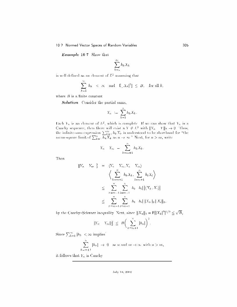
10.2 Normed Vector Spaces of Random Variables 305
Example 10.7. Show that
1Xk=1
hkXk
is well de�ned as an element of L2 assuming that
1Xk=1
jhkj < 1 and E[jXkj2] � B; for all k;
where B is a �nite constant.
Solution. Consider the partial sums,
Yn :=nX
k=1
hkXk:
Each Yn is an element of L2, which is complete. If we can show that Yn is aCauchy sequence, then there will exist a Y 2 L2 with kYn � Y k2 ! 0. Thus,the in�nite-sum expression
P1k=1 hkXk is understood to be shorthand for \the
mean-square limit ofPn
k=1 hkXk as n!1." Next, for n > m, write
Yn � Ym =nX
k=m+1
hkXk:
Then
kYn � Ymk22 = hYn � Ym; Yn � Ymi
=
� nXk=m+1
hkXk;
nXl=m+1
hlXl
�
�nX
k=m+1
nXl=m+1
jhkj jhlj��hXk; Xli
���
nXk=m+1
nXl=m+1
jhkj jhlj kXkk2 kXlk2;
by the Cauchy{Schwarz inequality. Next, since kXkk2 = E[jXkj2]1=2 �pB,
kYn � Ymk22 � B
� nXk=m+1
jhkj�2
:
SinceP1
k=1 jhkj <1 implies1
nXk=m+1
jhkj ! 0 as n and m!1 with n > m;
it follows that Yn is Cauchy.
July 18, 2002

306 Chap. 10 Mean Convergence and Applications
Under the conditions of the previous example, since kYn�Y k2 ! 0, we canwrite, for any Z 2 L2,��hYn; Zi � hY; Zi�� =
��hYn � Y; Zi��� kYn � Y k2 kZk2 ! 0:
In other words,
limn!1hYn; Zi = hY; Zi:
Taking Z = 1 and writing the inner products as expectations yields
limn!1E[Yn] = E[Y ];
or, using the de�nitions of Yn and Y ,
limn!1E
� nXk=1
hkXk
�= E
� 1Xk=1
hkXk
�:
Since the sum on the left is �nite, we can bring the expectation inside and write
limn!1
nXk=1
hkE[Xk] = E
� 1Xk=1
hkXk
�:
In other words,1Xk=1
hkE[Xk] = E
� 1Xk=1
hkXk
�:
The foregoing example and discussion have the following application. Con-sider a discrete-time, causal, stable, linear, time-invariant system with impulseresponse hk. Now suppose that the random sequence Xk is applied to the inputof this system. If E[jXkj2] is bounded as in the example, theny the output ofthe system at time n is
1Xk=0
hkXn�k;
which is a well-de�ned element of L2. Furthermore,
E
� 1Xk=0
hkXn�k
�=
1Xk=0
hkE[Xn�k]:
yThe assumption in the example,P
kjhkj <1, is equivalent to the assumption that the
system is stable.
July 18, 2002

10.3 The Wiener Integral (Again) 307
10.3. The Wiener Integral (Again)In Section 8.3, we de�ned the Wiener integralZ 1
0
g(� ) dW� :=Xi
gi(Wti+1 �Wti);
for piecewise constant g, say g(� ) = gi for ti < t � ti+1 for a �nite number ofintervals, and g(� ) = 0 otherwise. In this case, since the integral is the sum ofscaled, independent, zero mean, Gaussian increments of variance �2(ti+1 � ti),
E
��Z 1
0
g(� ) dW�
�2 �= �2
Xi
g2i (ti+1 � ti) =
Z 1
0
g(� )2 d�:
We now de�ne the Wiener integral for arbitrary g satisfyingZ 1
0
g(� )2 d� < 1: (10.3)
To do this, we use the fact [13, p. 86, Prop. 3.4.2] that for g satisfying (10.3),there always exists a sequence of piecewise constant functions gn converging tog in the mean-square sense
limn!1
Z 1
0
jgn(� )� g(� )j2 d� = 0: (10.4)
The set of g satisfying (10.3) is an inner product space with inner producth g; hi = R10 g(� )h(� ) d� and corresponding norm kgk = h g; gi1=2. Thus, (10.4)says that kgn�gk ! 0. In particular, this implies gn is Cauchy; i.e., kgn�gmk !0 as n;m!1 (cf. Problem 11). Consider the random variables
Yn :=
Z 1
0
gn(� ) dW� :
Since each gn is piecewise constant, Yn is well de�ned and is Gaussian with zeromean and variance Z 1
0
gn(� )2 d�:
Now observe that
kYn � Ymk22 = E[jYn � Ymj2]
= E
�����Z 1
0
gn(� ) dW� �Z 1
0
gm(� ) dW�
����2�= E
�����Z 1
0
�gn(� )� gm(� )
�dW�
����2�=
Z 1
0jgn(� ) � gm(� )j2 d�;
July 18, 2002

308 Chap. 10 Mean Convergence and Applications
since gn � gm is piecewise constant. Thus,
kYn � Ymk22 = kgn � gmk2:Since gn is Cauchy, we see that Yn is too. Since L2 is complete, there exists arandom variable Y 2 L2 with kYn � Y k2 ! 0. We denote this random variableby Z 1
0
g(� ) dW� ;
and call it the Wiener integral of g.
10.4. Projections, Orthonality Principle, Projection The-orem
Let C be a subset of Lp. Given X 2 Lp, suppose we want to approximateX by some bX 2 C. We call bX a projection of X onto C if bX 2 C and if
kX � bXkp � kX � Y kp; for all Y 2 C:
Note that if X 2 C, the we can take bX = X.
Example 10.8. Let C be the unit ball,
C := fY 2 Lp : kY kp � 1g:For X =2 C, i.e., kXkp > 1, show that
bX =X
kXkp :
Solution. First note that the proposed formula for bX satis�es k bXkp = 1
so that bX 2 C as required. Now observe that
kX � bXkp =
X � X
kXkp
p
=
����1� 1
kXkp
���� kXkp= kXkp � 1:
Next, for any Y 2 C,
kX � Y kp � ��kXkp � kY kp��; by Problem 15;
= kXkp � kY kp� kXkp � 1
= kX � bXkp:Thus, no Y 2 C is closer to X than bX .
July 18, 2002

10.4 Projections, Orthonality Principle, Projection Theorem 309
Much more can be said about projections when p = 2 and when the set weare projecting onto is a subspace rather than an arbitrary subset.
We now present two fundamental results about projections onto subspacesof L2. The �rst result is the orthogonality principle. Let M be a subspaceof L2. If X 2 L2, then bX 2M satis�es
kX � bXk2 � kX � Y k2; for all Y 2M; (10.5)
if and only ifhX � bX;Y i = 0; for all Y 2M: (10.6)
Furthermore, if such an bX 2 M exists, it is unique. Observe that there is noclaim that an bX 2 M exists that satis�es either (10.5) or (10.6). In practice,
we try to �nd an bX 2 M satisfying (10.6), since such an bX then automaticallysatis�es (10.5). This was the approach used to derive the Wiener �lter inSection 6.5, where we implicitly took (for �xed t)
M =�bVt : bVt is given by (6.7) and E[bV 2
t ] <1:In Section 7.3, when we discussed linear estimation of random vectors, we im-plicitly took
M = fAY + b : A is a matrix and b is a column vector g:
When we discussed minimummean squared error estimation, also in Section 7.3,we implicitly took
M =�g(Y ) : g is any function such that E[g(Y )2] <1:
Thus, several estimation problems discussed in earlier chapters are seen to bespecial cases of �nding the projection onto a suitable subspace of L2. Each ofthese special cases had its version of the orthogonality principle, and so it shouldbe no trouble for the reader to show that (10.6) implies (10.5). The converse isalso true, as we now show. Suppose (10.5) holds, but for some Y 2 M ,
hX � bX;Y i = c 6= 0:
Because we can divide this equation by kY k2, there is no loss of generality in
assuming kY k2 = 1. Now, since M is a subspace containing both bX and Y ,bX + cY also belongs to M . We show that this new vector is strictly closer toX than bX , contradicting (10.5). Write
kX � ( bX + cY )k22 = k(X � bX)� cY k22= kX � bXk22 � jcj2 � jcj2 + jcj2= kX � bXk22 � jcj2> kX � bXk22:July 18, 2002

310 Chap. 10 Mean Convergence and Applications
The second fundamental result to be presented is the Projection Theo-rem. Recall that the orthogonality principle does not guarantee the existenceof an bX 2M satisfying (10.5). If we are not smart enough to solve (10.6), whatcan we do? This is where the projection theorem comes in. To state and provethis result, we need the concept of a closed set. We say that M is closed ifwhenever Xn 2 M and kXn � Xk2 ! 0 for some X 2 L2, the limit X mustactually be in M . In other words, a set is closed if it contains all the limits ofall converging sequences from the set.
Example 10.9. Show that the set of Wiener integrals
M :=
�Z 1
0
g(� ) dW� :
Z 1
0
g(� )2 d� <1�
is closed.
Solution. A sequence Xn from M has the form
Xn =
Z 1
0
gn(� ) dW�
for square-integrable g. Suppose Xn converges in mean square to some X. Wemust show that there exists a square-integrable function g for which
X =
Z 1
0
g(� ) dW� :
Since Xn converges, it is Cauchy. Now observe that
kXn �Xmk22 = E[jXn �Xmj2]
= E
�����Z 1
0gn(� ) dW� �
Z 1
0gm(� ) dW�
����2 �= E
�����Z 1
0
�gn(� )� gm(� )
�dW�
����2 �=
Z 1
0
jgn(� ) � gm(� )j2 d�
= kgn � gmk2:Thus, gn is Cauchy. Since the set of square-integrable time functions is complete(the Riesz{Fischer Theorem again [37, p. 244]), there is a square-integrable gwith kgn � gk ! 0. For this g, write Xn �
Z 1
0
g(� ) dW�
22
= E
�����Z 1
0
gn(� ) dW� �Z 1
0
g(� ) dW�
����2 �= E
�����Z 1
0
�gn(� ) � g(� )
�dW�
����2 �=
Z 1
0jgn(� )� g(� )j2 d�
= kgn � gk2 ! 0:
July 18, 2002

10.5 Conditional Expectation 311
Since mean-square limits are unique (Problem 14), X =R10
g(� ) dW� .
Projection Theorem. IfM is a closed subspace of L2, and X 2 L2, then there
exists a unique bX 2M such that (10.5) holds.To prove this result, �rst put h := infY 2M kX � Y k2. From the de�nition
of the in�mum, there is a sequence Yn 2 M with kX � Ynk2 ! h. We willshow that Yn is a Cauchy sequence. Since L2 is a Hilbert space, Yn convergesto some limit in L2. Since M is closed, the limit, say bX , must be in M .
To show Yn is Cauchy, we proceed as follows. By the parallelogram law,
2(kX � Ynk22 + kX � Ymk22) = k2X � (Yn + Ym)k22 + kYm � Ynk22
= 4
X � Yn + Ym2
22
+ kYm � Ynk22:
Note that the vector (Yn + Ym)=2 2M since M is a subspace. Hence,
2(kX � Ynk22 + kX � Ymk22) � 4h2 + kYm � Ynk22:
Since kX � Ynk2 ! h, given " > 0, there exists an N such that for all n � N ,kX � Ynk2 < h+ ". Hence, for m;n � N ,
kYm � Ynk22 < 2((h+ ")2 + (h + ")2) � 4h2
= 4"(2h+ ");
and we see that Yn is Cauchy.Since L2 is a Hilbert space, and since M is closed, Yn ! bX for some bX 2M .
We now have to show that kX � bXk2 � kX � Y k2 for all Y 2 M . Write
kX � bXk2 = kX � Yn + Yn � bXk2� kX � Ynk2 + kYn � bXk2:
Since kX � Ynk2 ! h and since kYn � bXk2 ! 0,
kX � bXk2 � h:
Since h � kX � Y k2 for all Y 2M , kX � bXk2 � kX � Y k2 for all Y 2M .
The uniqueness of bX is left to Problem 22.
10.5. Conditional ExpectationIn earlier chapters, we de�ned conditional expectation separately for discrete
and jointly continuous random variables. We are now in a position to introducea uni�ed de�nition. The new de�nition is closely related to the orthogonalityprinciple and the projection theorem. It also reduces to the earlier de�nitionsin the discrete and jointly continuous cases.
July 18, 2002

312 Chap. 10 Mean Convergence and Applications
We say that bg(Y ) is the conditional expectation of X given Y if
E[Xg(Y )] = E[bg(Y )g(Y )]; for all bounded functions g: (10.7)
When X and Y are discrete or jointly continuous it is easy to check that bg(y) =E[XjY = y] solves this equation.z However, the importance of this de�nitionis that we can prove the existence and uniqueness of such a function bg even ifX and Y are not discrete or jointly continuous, as long as X 2 L1. Recall thatuniqueness was proved in Problem 18 in Chapter 7.
We �rst consider the case X 2 L2. Put
M := fg(Y ) : E[g(Y )2] <1g: (10.8)
It is a consequence of the Riesz{Fischer Theorem [37, p. 244] that M is closed.By the projection theorem combined with the orthogonality principle, thereexists a bg(Y ) 2M such that
hX � bg(Y ); g(Y )i = 0; for all g(Y ) 2M:
Since the above inner product is de�ned as an expectation, it is equivalent to
E[Xg(Y )] = E[bg(Y )g(Y )]; for all g(Y ) 2M:
Since boundedness of g implies g(Y ) 2M , (10.7) holds.When X 2 L2, we have shown that bg(Y ) is the projection of X onto M .
For X 2 L1, we proceed as follows. First consider the case of nonnegativeX with E[X] < 1. We can approximate X by the bounded function Xn ofExample 10.6. Being bounded, Xn 2 L2, and the corresponding bgn(Y ) existsand satis�es
E[Xng(Y )] = E[bg(Y )g(Y )]; for all g(Y ) 2M: (10.9)
SinceXn � Xn+1, bgn(Y ) � bgn+1(Y ) by Problem 29. Hence, bg(Y ) := limn!1 bgn(Y )exists. To verify that bg(Y ) satis�es (10.7), write2
E[Xg(Y )] = E�limn!1Xng(Y )
�= lim
n!1E[Xng(Y )]
= limn!1E[bgn(Y )g(Y )]; by (10:9);
= E�limn!1 bgn(Y )g(Y )�
= E[bg(Y )g(Y )]:For signed X with E[jXj] <1, consider the nonnegative random variables
X+ :=
�X; X � 0;0; X < 0;
and X� :=
� �X; X < 0;0; X � 0:
zSee, for example, the derivation following (7.8) in Section 7.3.
July 18, 2002

10.6 The Spectral Representation 313
Since X+ +X� = jXj, it is clear that X+ and X� are L1 random variables.Since they are nonnegative, their conditional expectations exist. Denote themby bg+(Y ) and bg�(Y ). Since X+ � X� = X, it is easy to verify that bg(Y ) :=bg+(Y ) � bg�(Y ) satis�es (10.7).Notation
We have shown that to every X 2 L1, there corresponds a unique functionbg(y) such that (10.7) holds. The standard notation for this function of y isE[XjY = y], which, as noted above, is given by the usual formulas when X andY are discrete or jointly continuous. It is conventional in probability theory towrite E[XjY ] instead of bg(Y ). We emphasize that E[XjY = y] is a deterministicfunction of y, while E[XjY ] is a function of Y and is therefore a random variable.We also point out that with the conventional notation, (10.7) becomes
E[Xg(Y )] = E�E[XjY ]g(Y )�; for all bounded functions g: (10.10)
10.6. The Spectral RepresentationLet Xn be a discrete-time, zero-mean, wide-sense stationary process with
correlation functionR(n) := E[Xn+mXm]
and corresponding power spectral density
S(f) =1X
n=�1R(n)ej2�fn (10.11)
so thatx
R(n) =
Z 1=2
�1=2
S(f)ej2�fn df: (10.12)
Consider the space of complex-valued frequency functions,
S :=
�G :
Z 1=2
�1=2
jG(f)j2S(f) df <1�
equipped with the inner product
hG;Hi :=
Z 1=2
�1=2
G(f)H(f)�S(f) df
xFor some correlation functions, the sum in (10.11) may not converge. However, by Her-glotz's Theorem, we can always replace (10.12) by
R(n) =
Z 1=2
�1=2
ej2�fn dS0(f);
where S0(f) is the spectral (cumulative) distribution function, and the rest of the sectiongoes through with the necessary changes. Note that when the power spectral density exists,S(f) = S00(f).
July 18, 2002

314 Chap. 10 Mean Convergence and Applications
and corresponding norm kGk := hG;Gi1=2. Then S is a Hilbert space. Further-more, every G 2 S can be approximated by a trigonometric polynomial of theform
G0(f) =NX
n=�Ngne
j2�fn:
The approximation is in norm; i.e., given any " > 0, there is a trigonometricpolynomial G0 such that kG�G0k < " [5, p. 139].
To each frequency function G 2 S, we now associate an L2 random variableas follows. For trigonometric polynomials like G0, put
T (G0) :=NX
n=�NgnXn:
Note that T is well de�ned (Problem 35). A critical property of these trigono-metric polynomials is that (Problem 36)
E[T (G0)T (H0)�] =
Z 1=2
�1=2G0(f)H0(f)
�S(f) df = hG0;H0i;
where H0 is de�ned similarly to G0. In particular, T is norm preserving onthe trigonometric polynomials; i.e.,
kT (G0)k22 = kG0k2:To de�ne T for arbitrary G 2 S, let Gn be a sequence of trigonometric poly-nomials converging to G in norm; i.e., kGn � Gk ! 0. Then Gn is Cauchy(cf. Problem 11). Furthermore, the linearity of and norm-preservation proper-ties of T on the trigonometric polynomials tells us that
kGn �Gmk = kT (Gn �Gm)k = kT (Gn) � T (Gm)k2;and we see that T (Gn) is Cauchy in L2. Since L2 is complete, there is alimit random variable, denoted by T (G) and such that kT (Gn) � T (G)k2 ! 0.Note that T (G) is well de�ned, norm preserving, linear, and continuous on S(Problem 37).
There is another way approximate elements of S. Every G 2 S can alsobe approximated by a piecewise constant function of the following form. For�1=2 � f0 < � � � < fn � 1=2, let
G0(f) =nXi=1
giI(fi�1;fi ](f):
Given any " > 0, there is a piecewise constant function G0 such that kG�G0k <". This is exactly what we did for the Wiener process, but with a di�erent norm.For piecewise constant G0,
T (G0) =nXi=1
giT (I(fi�1 ;fi]):
July 18, 2002

10.6 The Spectral Representation 315
SinceI(fi�1 ;fi ] = I[�1=2;fi] � I[�1=2;fi�1 ];
if we putZf := T (I[�1=2;f ]); �1=2 � f � 1=2;
then Zf is well de�ned by Problem 38, and
T (G0) =nXi=1
gi(Zfi � Zfi�1 ):
The family of random variables fZf ;�1=2 � f � 1=2g has many similarities tothe Wiener process (see Problem 39). We writeZ 1=2
�1=2
G0(f) dZf :=nXi=1
gi(Zfi � Zfi�1 ):
For arbitrary G 2 S, we approximate G with a sequence of piecewise constantfunctions. Then Gn will be Cauchy. Since Z 1=2
�1=2
Gn(f) dZf �Z 1=2
�1=2
Gm(f) dZf
2
= kT (Gn)�T (Gm)k2 = kGn�Gmk;
there is a limit random variable in L2, denoted byZ 1=2
�1=2G(f) dZf ;
and Z 1=2
�1=2
Gn(f) dZf �Z 1=2
�1=2
G(f) dZf
2
! 0:
On the other hand, since Gn is piecewise constant,Z 1=2
�1=2
Gn(f) dZf = T (Gn);
and since kGn � Gk ! 0, and since T is continuous, kT (Gn) � T (G)k2 ! 0.Thus,
T (G) =
Z 1=2
�1=2
G(f) dZf :
In particular, taking G(f) = ej2�fn shows thatZ 1=2
�1=2
ej2�fn dZf = T (G) = Xn;
where the last step follows from the original de�nition of T . The formula
Xn =
Z 1=2
�1=2
ej2�fn dZf
is called the spectral representation of Xn.
July 18, 2002

316 Chap. 10 Mean Convergence and Applications
10.7. NotesNotes x10.1: Convergence in Mean of Order p
Note 1. The assumption
1Xk=1
jhkj < 1
should be understood more precisely as saying that the partial sum
An :=nX
k=1
jhkj
is bounded above by some �nite constant. Since An is also nondecreasing, themonotonic sequence property of real numbers [38, p. 55, Theorem 3.14]says that An converges to a real number, say A. Now, by the same argumentused to solve Problem 11, since An converges, it is Cauchy. Hence, given any" > 0, for large enough n and m, jAn �Amj < ". If n > m, we have
An �Am =nX
k=m+1
jhkj < ":
Notes x10.5: Conditional Expectation
Note 2. The interchange of limit and expectation is justi�ed by Lebesgue'smonotone convergence theorem [4, p. 208].
10.8. ProblemsProblems x10.1: Convergence in Mean of Order p
1. Let U � uniform[0; 1], and put
Xn :=pnI[0;1=n](U ); n = 1; 2; : : : :
For what values of p � 1 does Xn converge in mean of order p to zero?
2. Let Nt be a Poisson process of rate �. Show that Nt=t converges in meansquare to � as t!1.
3. Show that limk!1R(k) = 0 implies
limn!1
1
n
n�1Xk=0
R(k) = 0;
and thus Mn converges in mean square to m by Example 10.4.
July 18, 2002

10.8 Problems 317
4. Show that if Mn converges in mean square m, then
limn!1
1
n
n�1Xk=0
R(k) = 0;
where R(k) is de�ned in Example 10.4. Hint: Observe that
n�1Xk=0
R(k) = E
�(X1 �m)
nXk=1
(Xk �m)
�= E[(X1 �m) � n(Mn �m)]:
5. Let Z be a nonnegative random variable with E[Z] <1. Given any " > 0,show that there is a � > 0 such that for any event A,
}(A) < � implies E[ZIA] < ":
Hint: Recalling Example 10.6, put Zn := min(Z; n) and write
E[ZIA] = E[(Z � Zn)IA] + E[ZnIA]:
6. Derive H�older's inequality,
E[jXY j] � E[jXjp]1=pE[jY jq]1=q;
if 1 < p; q < 1 with 1p+ 1
q= 1. Hint: Let � and � denote the factors
on the right-hand side; i.e., � := E[jXjp]1=p and � := E[jY jq]1=q. Then itsu�ces to show that
E[jXY j]��
� 1:
To this end, observe that by the convexity of the exponential function,for any real numbers u and v, we can always write
exph1pu+
1q vi� 1
peu + 1
q ev:
Now take u = ln(jXj=�)p and v = ln(jY j=�)q.7. Derive Lyapunov's inequality,
E[jZj�]1=� � E[jZj�]1=�; 1 � � < � <1:
Hint: Apply H�older's inequality to X = jZj� and Y = 1 with p = �=�.
8. Show that ifXn converges in mean of order � > 1 toX, then Xn convergesin mean of order � to X for all 1 � � < �.
July 18, 2002

318 Chap. 10 Mean Convergence and Applications
9. Derive Minkowski's inequality,
E[jX + Y jp]1=p � E[jXjp]1=p + E[jY jp]1=p;
where 1 � p <1. Hint: Observe that
E[jX + Y jp] = E[jX + Y j jX + Y jp�1]
� E[jXj jX + Y jp�1] + E[jY j jX + Y jp�1];
and apply H�older's inequality.
Problems x10.2: Normed Vector Spaces of Random Variables
10. Show that if Xn converges in mean of order p to X, and if Yn convergesin mean of order p to Y , then Xn + Yn converges in mean of order p toX + Y .
11. Let Xn converge in mean of order p to X 2 Lp. Show that Xn is Cauchy.
12. Let Xn be a Cauchy sequence in Lp. Show that Xn is bounded in thesense that there is a �nite constant K such that kXnkp � K for all n.
Remark. Since by the previous problem, a convergent sequence isCauchy, it follows that a convergent sequence is bounded.
13. Let Xn converge in mean of order p to X 2 Lp, and let Yn converge inmean of order p to Y 2 Lp. Show that XnYn converges in mean of orderp to XY .
14. Show that limits in mean of order p are unique; i.e., if Xn converges inmean of order p to both X and Y , show that E[jX � Y jp] = 0.
15. Show that ��kXkp � kY kp�� � kX � Y kp � kXkp + kY kp:
16. If Xn converges in mean of order p to X, show that
limn!1E[jXnjp] = E[jXjp]:
17. Show that 1Xk=1
hkXk
is well de�ned as an element of L1 assuming that
1Xk=1
jhkj < 1 and E[jXkj] � B; for all k;
July 18, 2002

10.8 Problems 319
where B is a �nite constant.
Remark. By the Cauchy{Schwarz inequality, a su�cient condition forE[jXkj] � B is that E[X2
k ] � B2.
Problems x10.3: The Wiener Integral (Again)
18. Recall that the Wiener integral of g was de�ned to be the mean-squarelimit of
Yn :=
Z 1
0
gn(� ) dW� ;
where each gn is piecewise constant, and kgn � gk ! 0. Show that
E
�Z 1
0
g(� ) dW�
�= 0;
and
E
��Z 1
0
g(� ) dW�
�2 �= �2
Z 1
0
g(� )2 d�:
Hint: Let Y denote the mean-square limit of Yn. Show that E[Yn]! E[Y ]and that E[Y 2
n ]! E[Y 2].
19. Use the following approach to show that the limit de�nition of the Wienerintegral is unique. Let Yn and Y be as in the text. If egn is another sequenceof piecewise constant functions with kegn � gk2 ! 0, put
eYn :=
Z 1
0
egn(� ) dW� :
By the argument that Yn has a limit Y , eYn has a limit, say eY . Show thatkY � eY k2 = 0.
20. Show that the Wiener integral is linear even for functions that are notpiecewise constant.
Problems x10.4: Projections, Orthogonality Principle, Projection Theorem
21. Let C = fY 2 Lp : kY kp � rg. For kXkp > r, �nd a projection of X ontoC.
22. Show that if bX 2M satis�es (10.6), it is unique.
23. Let N � M be subspaces of L2. Assume that the projection of X 2 L2
ontoM exists and denote it by bXM . Similarly, assume that the projectionof X onto N exists and denote it by bXN . Show that bXN is the projectionof bXM onto N .
July 18, 2002

320 Chap. 10 Mean Convergence and Applications
24. The preceding problem shows that when N �M are subspaces, the pro-jection of X onto N can be computed in two stages: First project X ontoM and then project the result onto N . Show that this is not true ingeneral if N and M are not both subspaces. Hint: Draw a disk of radiusone. Then draw a straight line through the origin. Identify M with thedisk and identify N with the line segment obtained by intersecting theline with the disk. If the point X is outside the disk and not on the line,then projecting �rst onto the ball and then onto the segment does notgive the projection.
Remark. Interestingly, projecting �rst onto the line (not the line seg-ment) and then onto the disk does give the correct answer.
25. Derive the parallelogram law,
kX + Y k22 + kX � Y k22 = 2(kXk22 + kY k22):
26. Show that the result of Example 10.7 holds if the assumptionP1
k=1 jhkj <1 is replaced by the two assumptions
P1k=1 jhkj2 <1 and E[XkXl] = 0
for k 6= l.
27. If kXn �Xk2 ! 0 and kYn � Y k2 ! 0, show that
limn!1hXn; Yni = hX;Y i:
28. If Y has density fY , show that M in (10.8) is closed. Hints: (i) Observethat
E[g(Y )2] =
Z 1
�1g(y)2fY (y) dy:
(ii) Use the fact that the set of functions
G :=
�g :
Z 1
�1g(y)2fY (y) dy <1
�is complete if G is equipped with the norm
kgk2Y :=
Z 1
�1g(y)2fY (y) dy:
(iii) Follow the method of Example 10.9.
Problems x10.5: Conditional Expectation
29. Fix X 2 L1, and suppose X � 0. Show that E[XjY ] � 0 in the sense that}(E[XjY ] < 0) = 0. Hints: To begin, note that
fE[XjY ] < 0g =1[n=1
fE[XjY ] < �1=ng:
July 18, 2002

10.8 Problems 321
By limit property (1.4),
}(E[XjY ] < 0) = limn!1
}(E[XjY ] < �1=n):
To obtain a proof by contradiction, suppose that }(E[XjY ] < 0) > 0.Then for su�ciently large n, }(E[XjY ] < �1=n) > 0 too. Take g(Y ) =IB(E[XjY ]) where B = (�1;�1=n) and consider the de�ning relationship
E[Xg(Y )] = E�E[XjY ]g(Y )�:
30. For X 2 L1, let X+ and X� be as in the text, and denote their corre-sponding conditional expectations by E[X+jY ] and E[X�jY ], respectively.Show that
E[Xg(Y )] = E��E[X+jY ]� E[X�jY ]�g(Y )�:
31. For X 2 L1, derive the smoothing property of conditional expectation,
E[XjY1] = E�E[XjY2; Y1]
��Y1�:Remark. If X 2 L2, this is an instance of Problem 23.
32. If X 2 L1 and h is a bounded function, show that
E[h(Y )XjY ] = h(Y )E[XjY ]:
33. If X 2 L2 and h(Y ) 2 L2, use the orthogonality principle to show that
E[h(Y )XjY ] = h(Y )E[XjY ]:
34. If X 2 L1 and if h(Y )X 2 L1, show that
E[h(Y )XjY ] = h(Y )E[XjY ]:Hint: Use a limit argument as in the text to approximate h(Y ) by abounded function of Y . Then apply either of the preceding two problems.
Problems x10.6: The Spectral Representation
35. Show that the mapping T de�ned by
G0(f) =NX
n=�Ngne
j2�fn 7!NX
n=�NgnXn
is well de�ned; i.e., if G0(f) has another representation, say
G0(f) =NX
n=�Negnej2�fn;
July 18, 2002

322 Chap. 10 Mean Convergence and Applications
show thatNX
n=�NegnXn =
NXn=�N
gnXn:
Hint: With dn := gn�egn, it su�ces to show that ifPN
n=�N dnej2�fn = 0,
then Y :=PN
n=�N dnXn = 0, and for this it is enough to show thatE[jY j2] = 0. Formula (10.12) may be helpful.
36. Show that ifH0(f) is de�ned similarly to G0(f) in the preceding problem,then
E[T (G0)T (H0)�] =
Z 1=2
�1=2
G0(f)H0(f)�S(f) df:
37. Show that ifGn and eGn are trigonometric polynomials with kGn�Gk ! 0
and k eGn �Gk ! 0, then
limn!1T (Gn) = lim
n!1T ( eGn):
Also show that T is norm preserving, linear, and continuous on S. Hint:
Put T (G) := limn!1 T (Gn) and Y := limn!1 T ( eGn). Show that kT (G)�Y k2 = 0. Use the fact that T is norm preserving on trigonometric poly-nomials.
38. Show that Zf := T (I[�1=2;f ]) is well de�ned. Hint: It su�ces to showthat I[�1=2;f ] 2 S.
39. Since Z 1=2
�1=2
G(f) dZf = T (G);
use results about T (G) to prove the following.
(a) Show that
E
�Z 1=2
�1=2G(f) dZf
�= 0:
(b) Show that
E
��Z 1=2
�1=2
G(f) dZf
��Z 1=2
�1=2
H(�) dZ�
�� �=
Z 1=2
�1=2
G(f)H(f)�S(f) df:
(c) Show that Zf has orthogonal (uncorrelated) increments.
July 18, 2002

CHAPTER 11
Other Modes of Convergence
This chapter introduces the three types of convergence,
� convergence in probability,
� convergence in distribution,
� almost sure convergence,
which are related to each other (and to convergence in mean of order p) asshown in Figure 11.1.
in probability in distribution
almost sure
mean of order p
Figure 11.1. Implications of various types of convergence.
Section 11.1 introduces the notion of convergence in probability. Conver-gence in probability will be important in Chapter 12 on parameter estimationand con�dence intervals, where it justi�es various statistical procedures thatare used to estimate unknown parameters.
Section 11.2 introduces the notion of convergence in distribution. Conver-gence in distribution is often used to approximate probabilities that are hardto calculate exactly. Suppose that Xn is a random variable whose cumulativedistribution function FXn(x) is very hard to compute. But suppose that forlarge n, FXn(x) � FX(x), where FX(x) is a cdf that is very easy to compute.When FXn (x) ! FX(x), we say that Xn converges in distribution to X. Inthis case, we can approximate FXn (x) by FX(x) if n is large enough. Whenthe central limit theorem applies, FX is the normal cdf with mean zero andvariance one.
Section 11.3 introduces the notion of almost-sure convergence. This kindof convergence is more technically demanding to analyze, but it allows us todiscuss important results such as the strong law of large numbers, for which wegive the usual fourth-moment proof. Almost-sure convergence also allows usthe derive the Skorohod representation, which is a powerful tool for studyingconvergence in distribution.
323

324 Chap. 11 Other Modes of Convergence
11.1. Convergence in ProbabilityWe say that Xn converges in probability to X if
limn!1
}(jXn �Xj � ") = 0 for all " > 0:
The �rst thing to note about convergence in probability is that it is impliedby convergence in mean of order p. Using Markov's inequality, we have
}(jXn �Xj � ") = }(jXn �Xjp � "p) � E[jXn �Xjp]"p
:
Hence, ifXn converges in mean of order p toX, thenXn converges in probabilityto X as well.
Example 11.1 (Weak Law of Large Numbers). Since the samplemeanMn
de�ned in Example 10.3 converges in mean square to m, it follows that Mn con-verges in probability to m. This is known as the weak law of large numbers.
The second thing to note about convergence in probability is that it ispossible to have Xn converging in probability to X, whileXn does not convergeto X in mean of order p for any p � 1. For example, let U � uniform[0; 1], andconsider the sequence
Xn := nI[0;1=n](U ); n = 1; 2; : : ::
Observe that for " > 0,
fjXnj � "g =
( fU � 1=ng; n � ";
6 ; n < ":
It follows that for all n,
}(jXnj � ") � }(U � 1=n) = 1=n ! 0:
Thus, Xn converges in probability to zero. However,
E[jXnjp] = np}(U � 1=n) = np�1;
which does not go to zero as n!1.The third thing to note about convergence in probability is that if g(x; y)
is continuous, and if Xn converges in probability to X, and Yn converges inprobability to Y , then g(Xn; Yn) converges in probability to g(X;Y ). Thisresult is derived in Problem 6. In particular, note that since the functionsg(x; y) = x + y and g(x; y) = xy are continuous, Xn + Yn and XnYn convergein probability to X + Y and XY , respectively, whenever Xn and Yn convergein probability to X and Y , respectively.
July 18, 2002

11.2 Convergence in Distribution 325
Example 11.2. Since Problem 6 is somewhat involved, it is helpful to�rst see the derivation for the special case in which Xn and Yn both convergein probability to constant random variables, say u and v, respectively.
Solution. Let " > 0 be given. We show that
}(jg(Xn; Yn)� g(u; v)j � ") ! 0:
By the continuity of g at the point (u; v), there is a � > 0 such that whenever(u0; v0) is within � of (u; v); i.e., wheneverp
ju0 � uj2 + jv0 � vj2 < 2�;
then
jg(u0; v0)� g(u; v)j < ":
Since pju0 � uj2 + jv0 � vj2 � ju0 � uj+ jv0 � vj;
we see that
jXn � uj < � and jYn � vj < � ) jg(Xn; Yn)� g(u; v)j < ":
Conversely,
jg(Xn; Yn)� g(u; v)j � " ) jXn � uj � � or jYn � vj � �:
It follows that
}(jg(Xn; Yn)� g(u; v)j � ") �}(jXn � uj � �) +}(jYn � vj � �):
These last two terms go to zero by hypothesis.
Example 11.3. Let Xn converge in probability to x, and let cn be a con-verging sequence of real numbers with limit c. Show that cnXn converges inprobability to cx.
Solution. De�ne the sequence of constant random variables Yn := cn.It is a simple exercise to show that Yn converges in probability to c. Thus,XnYn = cnXn converges in probability to cx.
11.2. Convergence in DistributionWe say that Xn converges in distribution to X, or converges weakly
to X if
limn!1FXn (x) = FX(x); for all x 2 C(FX);
July 18, 2002

326 Chap. 11 Other Modes of Convergence
where C(FX) is the set of points x at which FX is continuous. If FX has ajump at a point x0, then we do not say anything about the existence of
limn!1FXn(x0):
The �rst thing to note about convergence in distribution is that it is impliedby convergence in probability. To derive this result, �x any x at which FX iscontinuous. For any " > 0, write
FXn(x) = }(Xn � x;X � x+ ") +}(Xn � x;X > x+ ")
� FX(x+ ") +}(Xn �X < �")� FX(x+ ") +}(jXn �Xj � "):
It follows thatlimn!1FXn(x) � FX(x+ "):
Similarly,
FX (x� ") = }(X � x� ";Xn � x) +}(X � x� ";Xn > x)
� FXn(x) +}(X �Xn < �")� FXn(x) +}(jXn �Xj � ");
and we obtainFX(x� ") � lim
n!1FXn(x):
Since the liminf is always less than or equal to the limsup, we have
FX(x� ") � limn!1
FXn(x) � limn!1FXn(x) � FX (x+ "):
Since FX is continuous at x, letting " go to zero shows that the liminf and thelimsup are equal to each other and to FX (x). Hence limn!1 FXn(x) exists andequals FX(x).
The need to restrict attention to continuity points can also be seen in thefollowing example.
Example 11.4. Let Xn � exp(n); i.e.,
FXn(x) =
�1� e�nx; x � 0;
0; x < 0:
For x > 0, FXn(x) ! 1 as n ! 1. However, since FXn(0) = 0, we see thatFXn(x)! I(0;1)(x), which, being left continuous at zero, is not the cumulativedistribution function of any random variable. Fortunately, the constant randomvariable X � 0 has I[0;1)(x) for its cdf. Since the only point of discontinuity iszero, FXn (x) does indeed converge to FX(x) at all continuity points of FX .
July 18, 2002

11.2 Convergence in Distribution 327
The second thing to note about convergence in distribution is that if Xn
converges in distribution to X, and if X is a constant random variable, sayX � c, then Xn converges in probability to c. To derive this result, �rstobserve that
fjXn � cj < "g = f�" < Xn � c < "g= fc� " < Xng \ fXn < c+ "g:
It is then easy to see that
}(jXn � cj � ") � }(Xn � c� ") +}(Xn � c + ")
� FXn (c� ") +}(Xn > c + "=2)
= FXn (c� ") + 1� FXn (c+ "=2):
Since X � c, FX(x) = I[c;1)(x). Therefore, FXn(c�")! 0 and FXn (c+"=2)!1.
The third thing to note about convergence in distribution is that it is equiv-alent to the condition
limn!1E[g(Xn)] = E[g(X)] for every bounded continuous function g: (11.1)
A proof that convergence in distribution implies (11.1) can be found in [17,p. 316]. A proof that (11.1) implies convergence in distribution is sketched inProblem 19.
Example 11.5. Show that if Xn converges in distribution to X, then thecharacteristic function of Xn converges to the characteristic function of X.
Solution. Fix any �, and take g(x) = ej�x. Then
'Xn (�) = E[ej�Xn] = E[g(Xn)]! E[g(X)] = E[ej�X] = 'X (�):
Remark. It is also true that if 'Xn (�) converges to 'X (�) for all �, thenXn converges in distribution to X [4, p. 349, Theorem 26.3].
Example 11.6. Let Xn � N (mn; �2n), where mn ! m and �2n ! �2. If
X � N (m;�2), show that Xn converges in distribution to X.
Solution. It su�ces to show that the characteristic function of Xn con-verges to the characteristic function of X. Write
'Xn (�) = ejmn���2n�2=2 ! ejm���2�2=2 = 'X (�):
July 18, 2002

328 Chap. 11 Other Modes of Convergence
A very important instance of convergence in distribution is the centrallimit theorem. This result says that if X1; X2; : : : are independent, identicallydistributed random variables with �nite mean m and �nite variance �2, and if
Mn :=1
n
nXi=1
Xi and Yn :=Mn �m
�=pn
;
then
limn!1FYn(y) = �(y) :=
1p2�
Z y
�1e�t
2=2 dt:
In other words, for all y, FYn(y) converges to the standard normal cdf �(y)(which is continuous at all points y). To better see the di�erence between theweak law of large numbers and the central limit theorem, we specialize to thecase m = 0 and �2 = 1. In this case,
Yn =1pn
nXi=1
Xi:
In other words, the sample meanMn divides the sumX1+� � �+Xn by n while Yndivides the sum only by
pn. The di�erence is that Mn converges in probability
(and in distribution) to the constant zero, while Yn converges in distributionto an N (0; 1) random variable. Notice also that the weak law requires onlyuncorrelated random variables, while the central limit theorem requires i.i.d.random variables. The central limit theorem was derived in Section 4.7, whereexamples and problems can also be found. The central limit theorem is alsoused to determine con�dence intervals in Chapter 12.
Example 11.7. Let Nt be a Poisson process of rate �. Show that
Yn :=Nn
n � �p�=n
converges in distribution to an N (0; 1) random variable.
Solution. Since N0 � 0,
Nn
n=
1
n
nXk=1
(Nk �Nk�1):
By the independent increments property of the Poisson process, the terms of thesum are i.i.d. Poisson(�) random variables, with mean � and variance �. Hence,Yn has the structure to apply the central limit theorem, and so FYn(y) ! �(y)for all y.
The next example is a version of Slutsky's Theorem. We need it in ouranalysis of con�dence intervals in Chapter 12.
July 18, 2002

11.2 Convergence in Distribution 329
Example 11.8. Let Yn be a sequence of random variables with correspond-ing cdfs Fn. Suppose that Fn converges to a continuous cdf F . Suppose alsothat Un converges in probability to 1. Show that
limn!1
}(Yn � yUn) = F (y):
Solution. The result is very intuitive. For large n, Un � 1 and Fn(y) �F (y) suggest that
}(Yn � yUn) � }(Yn � y) = Fn(y) � F (y):
The precise details are more involved. Fix any y > 0 and 0 < � < 1. Then}(Yn � yUn) is equal to
}(Yn � yUn; jUn � 1j < �) +}(Yn � yUn; jUn � 1j � �):
The second term is upper bounded by }(jUn � 1j � �), which goes to zero.Rewrite the �rst term as
}(Yn � yUn; 1� � < Un < 1 + �);
which is equivalent to
}(Yn � yUn; y(1� �) < yUn < y(1 + �)): (11.2)
Now this is upper bounded by
}(Yn � y(1 + �)) = Fn(y(1 + �)):
Thus,limn!1
}(Yn � yUn) � F (y(1 + �)):
Next, (11.2) is lower bounded by
}(Y � y(1 � �); jUn � 1j < �);
which is equal to
}(Yn � y(1 � �)) �}(Yn � y(1 � �); jUn � 1j � �):
Now the second term satis�es
}(Yn � y(1 � �); jUn � 1j � �) � }(jUn � 1j � �) ! 0:
In light of these observations,
limn!1
}(Yn � yUn) � F (y(1� �)):
Since � was arbitrary, and since F is continuous,
limn!1
}(Yn � yUn) = F (y):
The case y < 0 is similar.
July 18, 2002

330 Chap. 11 Other Modes of Convergence
11.3. Almost Sure ConvergenceLet Xn be any sequence of random variables, and letX be any other random
variable. Put
G :=�! 2 : lim
n!1Xn(!) = X(!):
In other words, G is the set of sample points ! 2 for which the sequenceof real numbers Xn(!) converges to the real number X(!). We think of G asthe set of \good" !'s for which Xn(!) ! X(!). Similarly, we think of thecomplement of G, Gc, as the set of \bad" !'s for which Xn(!) 6! X(!).
We say that Xn converges almost surely to X if1
}�f! 2 : lim
n!1Xn(!) 6= X(!)g� = 0: (11.3)
In other words, Xn converges almost surely to X if the \bad" set Gc has proba-bility zero. We write Xn ! X a.s. to indicate that Xn converges almost surelyto X.
If it should happen that the bad set Gc = 6 , then Xn(!)! X(!) for every! 2 . This is called sure convergence, and is a special case of almost sureconvergence.
Because almost sure convergence is so closely linked to the convergence ofordinary sequences of real numbers, many results are easy to derive.
Example 11.9. Show that if Xn ! X a.s. and Yn ! Y a.s., then Xn +Yn ! X + Y a.s.
Solution. Let GX := fXn ! Xg and GY := fYn ! Y g. In other words,GX and GY are the \good" sets for the sequences Xn and Yn respectively.Now consider any ! 2 GX \ GY . For such !, the sequence of real numbersXn(!) converges to the real number X(!), and the sequence of real numbersYn(!) converges to the real number Y (!). Hence, from convergence theory forsequences of real numbers,
Xn(!) + Yn(!) ! X(!) + Y (!): (11.4)
At this point, we have shown that
GX \GY � G; (11.5)
where G denotes the set of all ! for which (11.4) holds. To prove thatXn+Yn !X+Y a.s., we must show that}(Gc) = 0. On account of (11.5), Gc � Gc
X[GcY .
Hence,}(Gc) � }(Gc
X ) +}(GcY );
and the two terms on the right are zero because Xn and Yn both convergealmost surely.
July 18, 2002

11.3 Almost Sure Convergence 331
In order to discuss almost sure convergence in more detail, it is helpful tocharacterize when (11.3) holds. Recall that a sequence of real numbers xnconverges to the real number x if given any " > 0, there is a positive integer Nsuch that for all n � N , jxn � xj < ". Hence,
fXn ! Xg =\">0
1[N=1
1\n=N
fjXn �Xj < "g:
Equivalently,
fXn 6! Xg =[">0
1\N=1
1[n=N
fjXn �Xj � "g:
It is convenient to put
An(") := fjXn �Xj � "g; BN (") :=1[
n=N
An(");
and
A(") :=1\N=1
BN ("): (11.6)
Then
}(fXn 6! Xg) = }
� [">0
A(")
�:
If Xn ! X a.s., then
0 = }(fXn 6! Xg) = }
� [">0
A(")
�� }
�A("0)
�for any choice of "0 > 0. Conversely, suppose }
�A(")
�= 0 for every positive
". We claim that Xn ! X a.s. To see this, observe that in the earlier char-acterization of the convergence of a sequence of real numbers, we could haverestricted attention to values of " of the form " = 1=k for positive integers k.In other words, a sequence of real numbers xn converges to a real number x ifand only if for every positive integer k, there is a positive integer N such thatfor all n � N , jxn � xj < 1=k. Hence,
}(fXn 6! Xg) = }
� 1[k=1
A(1=k)
��
1Xk=1
}�A(1=k)
�:
From this we see that if }�A(")
�= 0 for all " > 0, then }(fXn 6! Xg) = 0.
To say more about almost sure convergence, we need to examine (11.6) moreclosely. Observe that
BN (") =1[
n=N
An(") �1[
n=N+1
An(") = BN+1("):
July 18, 2002
332 Chap. 11 Other Modes of Convergence
By limit property (1.5),
}�A(")
�= }
� 1\N=1
BN (")
�= lim
N!1}�BN (")
�:
The next two examples use this equation to derive important results aboutalmost sure convergence.
Example 11.10. Show that if Xn ! X a.s., then Xn converges in proba-bility to X.
Solution. Recall that, by de�nition, Xn converges in probability to X ifand only if }
�AN (")
� ! 0 for every " > 0. If Xn ! X a.s., then for every" > 0,
0 = }�A(")
�= lim
N!1}�BN (")
�:
Next, since
}�BN (")
�= }
� 1[n=N
An(")
�� }
�AN (")
�;
it follows that }�AN (")
� ! 0 too.
Example 11.11. Show that if
1Xn=1
}�An(")
�< 1; (11.7)
holds for all " > 0, then Xn ! X a.s.
Solution. For any " > 0,
}�A(")
�= lim
N!1}�BN (")
�= lim
N!1}
� 1[n=N
An(")
�
� limN!1
1Xn=N
}�An(")
�= 0; on account of (11.7):
What we have done here is derive a particular instance of the Borel{CantelliLemma (cf. Problem 15 in Chapter 1).
Example 11.12. Let X1; X2; : : : be i.i.d. zero-mean random variables with�nite fourth moment. Show that
Mn :=1
n
nXi=1
Xi ! 0 a.s.
July 18, 2002

11.3 Almost Sure Convergence 333
Solution. We already know from Example 10.3 that Mn converges inmean square to zero, and hence, Mn converges to zero in probability and indistribution as well. Unfortunately, as shown in the next example, convergencein mean does not imply almost sure convergence. However, by the previousexample, the almost sure convergence of Mn to zero will be established if wecan show that for every " > 0,
1Xn=1
}(jMnj � ") < 1: (11.8)
By Markov's inequality,
}(jMnj � ") = }(jMnj4 � "4) � E[jMnj4]"4
:
By Problem 34, there are �nite, nonnegative constants � (depending on E[X4i ])
and � (depending on E[X2i ]) such that
E[jMnj4] � �
n3+
�
n2:
Hence, (11.8) holds by Problem 33.
The preceding example is an instance of the strong law of large numbers.The derivation in the example is quite simple because of the assumption of �nitefourth moments (which implies �niteness of the third, second, and �rst momentsby Lyapunov's inequality). A derivation assuming only �nite second momentscan be found in [17, pp. 326{327], and assuming only �nite �rst moments in[17, pp. 329{331].
Strong Law of Large Numbers (SLLN). Let X1; X2; : : : be independent, iden-
tically distributed random variables with �nite mean m. Then
Mn :=1
n
nXi=1
Xi ! m a.s.
Since almost sure convergence implies convergence in probability, the fol-lowing form of the weak law of large numbers holds.
Weak Law of Large Numbers (WLLN). Let X1; X2; : : : be independent, iden-
tically distributed random variables with �nite mean m. Then
Mn :=1
n
nXi=1
Xi
converges in probability to m.
July 18, 2002

334 Chap. 11 Other Modes of Convergence
The weak law of large numbers in Example 11.1, which relied on the mean-square version in Example 10.3, required �nite second moments and uncorre-lated random variables. The above form does not require �nite second moments,but does require independent random variables.
Example 11.13. Let Wt be a Wiener process with E[W 2t ] = �2t. Use the
strong law to show that Wn=n converges almost surely to zero.
Solution. Since W0 � 0, we can write
Wn
n=
1
n
nXk=1
(Wk �Wk�1):
By the independent increments property of the Wiener process, the terms of thesum are i.i.d.N (0; �2) random variables. By the strong law, this sum convergesalmost surely to zero.
Example 11.14. We construct a sequence of random variables that con-verges in mean to zero, but does not converge almost surely to zero. Fix anypositive integer n. Then n can be uniquely represented as n = 2m + k, wherem and k are integers satisfying m � 0 and 0 � k � 2m � 1. De�ne
gn(x) = g2m+k(x) = I� k2m ;
k+12m
�(x):For example, takingm = 2 and k = 0; 1; 2; 3;which corresponds to n = 4; 5; 6; 7,we �nd
g4(x) = I�0; 14�(x); g5(x) = I� 1
4 ;12
�(x);and
g6(x) = I�12 ;
34
�(x); g7(x) = I� 34 ; 1�(x):
For �xed m, as k goes from 0 to 2m � 1, g2m+k is a sequence of pulses movingfrom left to right. This is repeated for m + 1 with twice as many pulses thatare half as wide. The two key ideas are that the pulses get narrower and thatfor any �xed x 2 [0; 1), gn(x) = 1 for in�nitely many n.
Now let U � uniform[0; 1). Then
E[gn(U )] = }
�k
2m� X <
k + 1
2m
�=
1
2m:
Since m ! 1 as n ! 1, we see that gn(U ) converges in mean to zero. Itthen follows that gn(U ) converges in probability to zero. Since almost sureconvergence also implies convergence in probability, the only possible almostsure limit is zero.� However, we now show that gn(U ) does not converge almostsurely to zero. Fix any x 2 [0; 1). Then for each m = 0; 1; 2; : : :;
k
2m� x <
k + 1
2m
�Limits in probability are unique by Problem 4.
July 18, 2002

11.3 Almost Sure Convergence 335
for some k satisfying 0 � k � 2m � 1. For these values of m and k, g2m+k(x) =1. In other words, there are in�nitely many values of n = 2m + k for whichgn(x) = 1. Hence, for 0 � x < 1, gn(x) does not converge to zero. Therefore,
fU 2 [0; 1)g � fgn(U ) 6! 0g;
and it follows that
}(fgn(U ) 6! 0g) � }(fU 2 [0; 1)g) = 1:
The Skorohod Representation Theorem
The Skorohod Representation Theorem says that if Xn converges indistribution to X, then we can construct random variables Yn and Y withFYn = FXn , FY = FX , and such that Yn converges almost surely to Y . Thiscan often simplify proofs concerning convergence in distribution.
Example 11.15. Let Xn converge in distribution to X, and let c(x) be acontinuous function. Show that c(Xn) converges in distribution to c(X).
Solution. Let Yn and Y be as given by the Skorohod representation theo-rem. Since Yn converges almost surely to Y , the set
G := f! 2 : Yn(!)! Y (!)g
has the property that }(Gc) = 0. Fix any ! 2 G. Then Yn(!) ! Y (!). Sincec is continuous,
c�Yn(!)
� ! c�Y (!)
�:
Thus, c(Yn) converges almost surely to c(Y ). Now recall that almost-sure con-vergence implies convergence in probability, which implies convergence in dis-tribution. Hence, c(Yn) converges in distribution to c(Y ). To conclude, observethat since Yn and Xn have the same cumulative distribution function, so doc(Yn) and c(Xn). Similarly, c(Y ) and c(X) have the same cumulative distribu-tion function. Thus, c(Xn) converges in distribution to c(X).
We now derive the Skorohod representation theorem. For 0 < u < 1, let
Gn(u) := inffx 2 IR : FXn(x) � ug;
andG(u) := inffx 2 IR : FX(x) � ug:
By Problem 27(a) in Chapter 8,
G(u) � x , u � FX(x);
July 18, 2002

336 Chap. 11 Other Modes of Convergence
or, equivalently,
G(u) > x , u > FX(x);
and similarly for Gn and FXn . Now let U � uniform(0; 1). By Problem 27(b)in Chapter 8, Yn := Gn(U ) and Y := G(U ) satisfy FYn = FXn and FY = FX ,respectively.
From the de�nition of G, it is easy to see that G is nondecreasing. Hence,its set of discontinuities, call it D, is at most countable (Problem 39), and so}(U 2 D) = 0 by Problem 40. We show below that for u =2 D, Gn(u)! G(u).It then follows that
Yn(!) := Gn
�U (!)
� ! G�U (!)
�=: Y (!);
except for ! 2 f! : U (!) 2 Dg, which has probability zero.Fix any u =2 D, and let " > 0 be given. Then between G(u) � " and G(u)
we can select a point x,
G(u)� " < x < G(u);
that is a continuity point of FX . Since x < G(u),
FX(x) < u:
Since x is a continuity point of FX , FXn(x) must be close to FX(x) for large n.Thus, for large n, FXn(x) < u. But this implies Gn(u) > x. Thus,
G(u)� " < x < Gn(u);
and it follows that
G(u) � limn!1
Gn(u):
To obtain the reverse inequality involving the lim, �x any u0 with u < u0 < 1.Fix any " > 0, and select another continuity point of FX , again called x, suchthat
G(u0) < x < G(u0) + ":
Then G(u0) � x, and so u0 � FX(x). But then u < FX (x). Since FXn (x) !FX(x), for large n, u < FXn(x), which implies Gn(u) � x. It then follows that
limn!1Gn(u) � G(u0):
Since u is a continuity point of G, we can let u0 ! u to get
limn!1Gn(u) � G(u):
It now follows that Gn(u)! G(u) as claimed.
July 18, 2002

11.4 Notes 337
11.4. NotesNotes x11.3: Almost Sure Convergence
Note 1. In order that (11.3) be well de�ned, it is necessary that the set
f! 2 : limn!1Xn(!) 6= X(!)g
be an event in the technical sense of Note 1 in Chapter 1. This is assuredby the assumption that each Xn is a random variable (the term \random vari-able" is used in the technical sense of Note 1 in Chapter 2). The fact thatthis assumption is su�cient is demonstrated in more advanced texts, e.g., [4,pp. 183{184].
11.5. ProblemsProblems x11.1: Convergence in Probability
1. Let cn be a converging sequence of real numbers with limit c. De�ne theconstant random variables Yn � cn and Y � c. Show that Yn convergesin probability to Y .
2. Let U � uniform[0; 1], and put
Xn :=pnI[0;1=n](U ); n = 1; 2; : : : :
Does Xn converge in probability to zero?
3. Let V be any continuous random variable with an even density, and let cnbe any positive sequence with cn !1. Show that Xn := V=cn convergesin probability to zero.
4. Show that limits in probability are unique; i.e., show that if Xn convergesin probability to X, and Xn converges in probability to Y , then }(X 6=Y ) = 0. Hint: Write
fX 6= Y g =1[k=1
fjX � Y j � 1=kg;
and use limit property (1.4).
5. Suppose you have shown that given any " > 0, for su�ciently large n,
}(jXn �Xj � ") < ":
Show that
limn!1
}(jXn �Xj � ") = 0 for every " > 0:
July 18, 2002

338 Chap. 11 Other Modes of Convergence
6. Let g(x; y) be continuous, and suppose that Xn converges in probabilityto X, and that Yn converges in probability to Y . In this problem you willshow that g(Xn; Yn) converges in probability to g(X;Y ).
(a) Fix any " > 0. Show that for su�ciently large � and �,
}(jXj > �) < "=4 and }(jY j > �) < "=4:
(b) Once � and � have been �xed, we can use the fact that g(x; y) isuniformly continuous on the rectangle jxj � 2� and jyj � 2�. Inother words, there is a � > 0 such that for all (x0; y0) and (x; y) inthe rectangle and satisfying
jx0 � xj � � and jy0 � yj � �;
we havejg(x0; y0) � g(x; y)j < ":
There is no loss of generality if we assume that � � � and � � �.Show that if the four conditions
jXn �Xj < �; jYn � Y j < �; jXj � �; and jY j � �
hold, thenjg(Xn; Yn)� g(X;Y )j < ":
(c) Show that if n is large enough that
}(jXn �Xj � �) < "=4 and }(jYn � Y j � �) < "=4;
then}(jg(Xn; Yn) � g(X;Y )j � ") < ":
7. Let X1; X2; : : : be i.i.d. with common �nite mean m and common �nitevariance �2. Also assume that E[X4
i ] <1. Put
Mn :=1
n
nXi=1
Xi and Vn :=1
n
nXi=1
X2i :
(a) Explain (brie y) why Vn converges in probability to �2 +m2.
(b) Explain (brie y) why
S2n :=n
n� 1
��1
n
nXi=1
X2i
��M2
n
�converges in probability to �2.
8. Let Xn converge in probability to X. Assume that there is a nonnegativerandom variable Y with E[Y ] <1 and such that jXnj � Y for all n.
July 18, 2002

11.5 Problems 339
(a) Show that }(jXj � Y + 1) = 0. (In other words, jXj < Y + 1 withprobability one, from which it follows that E[jXj] � E[Y ] + 1 <1.)
(b) Show that Xn converges in mean to X. Hints: Write
E[jXn �Xj] = E[jXn �XjIAn ] + E[jXn �XjIAcn];
where An := fjXn � Xj � "g. Then use Problem 5 in Chapter 10with Z = Y + jXj.
9. (a) Let g be a bounded, nonnegative function satisfying limx!0 g(x) = 0.Show that limn!1 E[g(Xn)] = 0 if Xn converges in probability tozero.
(b) Show that
limn!1E
� jXnj1 + jXnj
�= 0
if and only if Xn converges in probability to zero.
Problems x11.2: Convergence in Distribution
10. Let cn be a converging sequence of real numbers with limit c. De�ne theconstant random variables Yn � cn and Y � c. Show that Yn convergesin distribution to Y .
11. Let X be a random variable, and let cn be a positive sequence convergingto limit c. Show that cnX converges in distribution to cX. Considerseparately the cases c = 0 and 0 < c <1.
12. For t � 0, let Xt � Yt � Zt be three continuous-time random processessuch that
limt!1FXt(y) = lim
t!1FZt(y) = F (y)
for some continuous cdf F . Show that FYt(y) ! F (y) for all y.
13. Show that the Wiener integral Y :=R10 g(� ) dW� is Gaussian with zero
mean and varianceR10 g(� )2 d� . Hints: The desired integral Y is the
mean-square limit of the sequence Yn de�ned in Problem 18 in Chapter 10.Use Example 11.5.
14. Let g(t; � ) be such that for each t,R10
g(t; � )2 d� <1. De�ne the process
Xt =
Z 1
0g(t; � ) dW� :
Use the result of the preceding problem to show that for any 0 � t1 <� � � < tn < 1, the random vector of samples X := [Xt1 ; : : : ; Xtn]
0 isGaussian. Hint: Read the �rst paragraph of Section 7.2.
July 18, 2002

340 Chap. 11 Other Modes of Convergence
15. If the moment generating functions MXn (s) converge to the moment gen-erating function MX (s), show that Xn converges in distribution to X.Also show that for nonnegative, integer-valued random variables, if theprobability generating functions GXn(z) converge to the probability gen-erating function GX(z), then Xn converges in distribution to X. Hint:
The Remark following Example 11.5 may be useful.
16. Let Xn and X be integer-valued random variables with probability massfunctions pn(k) :=}(Xn = k) and p(k) :=}(X = k), respectively.
(a) If Xn converges in distribution to X, show that for each k, pn(k)!p(k).
(b) If Xn and X are nonnegative, and if for each k � 0, pn(k) ! p(k),show that Xn converges in distribution to X.
17. Let pn be a sequence of numbers lying between 0 and 1 and such thatnpn ! � > 0 as n ! 1. Let Xn � binomial(n; pn), and let X �Poisson(�). Show that Xn converges in distribution to X. Hints: By theprevious problem, it su�ces to prove that the probability mass functionsconverge. Stirling's formula,
n! �p2� nn+1=2e�n;
by which we mean
limn!1
n!p2� nn+1=2e�n
= 1;
and the formula
limn!1
�1� qn
n
�n= e�q ; if qn ! q;
may be helpful.
18. Let Xn � binomial(n; pn) and X � Poisson(�), where pn and � are asin the previous problem. Show that the probability generating functionGXn(z) converges to GX(z).
19. Suppose that Xn and X are such that for every bounded continuousfunction g(x),
limn!1E[g(Xn)] = E[g(X)]:
Show that Xn converges in distribution to X as follows:
(a) For a < b, sketch the three functions I(�1;a](t), I(�1;b](t), and
ga;b(t) :=
8>><>>:1; t < a;
b� t
b� a; a � t � b;
0; t > b:
July 18, 2002

11.5 Problems 341
(b) Your sketch in part (a) shows that
I(�1;a](t) � ga;b(t) � I(�1;b](t):
Use these inequalities to show that for any random variable Y ,
FY (a) � E[ga;b(Y )] � FY (b):
(c) For �x > 0, use part (b) with a = x and b = x+�x to show that
limn!1FXn(x) � FX(x+�x):
(d) For �x > 0, use part (b) with a = x��x and b = x to show that
FX(x��x) � limn!1
FXn(x):
(e) If x is a continuity point of FX , show that
limn!1FXn (x) = FX(x):
20. Show that Xn converges in distribution to zero if and only if
limn!1E
� jXnj1 + jXnj
�= 0:
21. For t � 0, let Zt be a continuous-time random process. Suppose that ast!1, FZt(z) converges to a continuous cdf F (z). Let u(t) be a positivefunction of t such that u(t)! 1 as t!1. Show that
limt!1
}�Zt � z u(t)
�= F (z):
Hint: Modify the derivation in Example 11.8.
22. Let Zt be as in the preceding problem. Show that if c(t)! c > 0, then
limt!1
}�c(t)Zt � z
�= F (c=z):
23. Let Zt be as in Problem 21. Let s(t) ! 0 as t ! 1. Show that ifXt = Zt + s(t), then FXt(x)! F (x).
24. Let Nt be a Poisson process of rate �. Show that
Yt :=Nt
t � �p�=t
converges in distribution to an N (0; 1) random variable. Hint: By Ex-ample 11.7, Yn converges in distribution to an N (0; 1) random variable.Next, since Nt is a nondecreasing function of t, observe that
Nbtc � Nt � Ndte;
July 18, 2002

342 Chap. 11 Other Modes of Convergence
where btc denotes the greatest integer less than or equal to t, and dte de-notes the smallest integer greater than or equal to t. Hint: The precedingtwo problems and Problem 12 may be useful.
Problems x11.3: Almost Sure Convergence
25. Let Xn ! X a.s. and let Yn ! Y a.s. If g(x; y) is a continuous function,show that g(Xn; Yn)! g(X;Y ) a.s.
26. Let Xn ! X a.s., and suppose that X = Y a.s. Show that Xn ! Y a.s.(The statement X = Y a.s. means }(X 6= Y ) = 0.)
27. Show that almost sure limits are unique; i.e., if Xn ! X a.s. and Xn !Y a.s., then X = Y a.s. (The statement X = Y a.s. means }(X 6= Y ) =0.)
28. Suppose Xn ! X a.s. and Yn ! Y a.s. Show that if Xn � Yn a.s. for alln, then X � Y a.s. (The statement Xn � Yn a.s. means }(Xn > Yn) =0.)
29. If Xn converges almost surely and in mean, show that the two limits areequal almost surely. Hint: Problem 4 may be helpful.
30. In Problem 11, suppose that the limit is c =1. Specify the limit randomvariable cX(!) as a function of !. Note that cX(!) is a discrete randomvariable. What is its probability mass function?
31. Let S be a nonnegative random variable with E[S] < 1. Show thatS < 1 a.s. Hints: It is enough to show that }(S = 1) = 0. Observethat
fS =1g =1\n=1
fS > ng:
Now appeal to the limit property (1.5) and use Markov's inequality.
32. Under the assumptions of Problem 17 in Chapter 10, show that
1Xk=1
hkXk
is well de�ned as an almost-sure limit. Hints: It is enough to prove that
S :=1Xk=1
jhkXkj < 1 a.s.
Hence, the result of the preceding problem can be applied if it can beshown that E[S] <1. To this end, put
Sn :=nX
k=1
jhkj jXkj:
July 18, 2002

11.5 Problems 343
By Problem 17 in Chapter 10, Sn converges in mean to S 2 L1. Use thenonnegativity of Sn and S along with Problem 16 in Chapter 10 to showthat
E[S] = limn!1
nXk=1
jhkjE[jXkj] < 1:
33. For p > 1, show thatP1
n=1 1=np <1.
34. Let X1; X2; : : : be i.i.d. with := E[X4i ], �
2 := E[X2i ], and E[Xi] = 0.
Show that
Mn :=1
n
nXi=1
Xi
satis�es E[M4n] = [n + 3n(n� 1)�4]=n4.
35. In Problem 7, explain why the assumption E[X4i ] <1 can be omitted.
36. Let Nt be a Poisson process of rate �. Show that Nt=t converges almostsurely to �. Hint: First show that Nn=n converges almost surely to �.Second, since Nt is a nondecreasing function of t, observe that
Nbtc � Nt � Ndte;
where btc denotes the greatest integer less than or equal to t, and dtedenotes the smallest integer greater than or equal to t.
37. Let Nt be a renewal process as de�ned in Section 8.2. Let X1; X2; : : :denote the i.i.d. interarrival times. Assume that the interarrival timeshave �nite, positive mean �.
(a) Show that for any " > 0, for all su�ciently large n,
nXk=1
Xk < n(�+ ") a.s.
(b) Show that Nt !1 as t!1 a.s.; i.e., show that for anyM , Nt �Mfor all su�ciently large t.
(c) Show that n=Tn ! 1=� a.s. Here Tn := X1 + � � � + Xn is the nthoccurrence time.
(d) Show that Nt=t ! 1=� a.s. Hints: On account of (c), if we putYn := n=Tn, then YNt ! 1=� a.s. since Nt !1. Also note that
TNt � t < TNt+1:
38. Give an example of a sequence of random variables that converges almostsurely to zero but not in mean.
July 18, 2002

344 Chap. 11 Other Modes of Convergence
39. Let G be a nondecreasing function de�ned on the closed interval [a; b].Let D" denote the set of discontinuities of size greater than " on [a; b],
D" := fu 2 [a; b] : G(u+) �G(u�) > "g;
with the understanding that G(b+) means G(b) and G(a�) means G(a).Show that if there are n points in D", then
n < [G(b)�G(a)]="+ 2:
Remark. The set of all discontinuities of G on [a; b], denoted by D[a; b],is simply
S1k=1D1=k. Since this is a countable union of �nite sets, D[a; b]
is at most countably in�nite. If G is de�ned on the open interval (0; 1),we can write
D(0; 1) =1[n=3
D[1=n; 1� 1=n]:
Since this is a countable union of countably in�nite sets, D(0; 1) is alsocountably in�nite [37, p. 21, Proposition 7].
40. Let D be a countably in�nite subset of (0; 1). Let U � uniform(0; 1).Show that }(U 2 D) = 0. Hint: Since D is countably in�nite, we canenumerate its elements as a sequence un. Fix any " > 0 and put Kn :=(un � "=2n; un + "=2n). Observe that
D �1[n=1
Kn:
Now bound
}
�U 2
1[n=1
Kn
�:
July 18, 2002

CHAPTER 12
Parameter Estimation and Con�dence Intervals
Consider observed measurements X1; X2; : : : ; each having unknown meanm. Then natural thing to do is to use the sample mean
Mn :=1
n
nXi=1
Xi
as an estimate of m. However, since Mn is a random variable and m is aconstant, we do not expect to have Mn always equal to m (or even ever equalif the Xi are continuous random variables). In this chapter we investigate howclose the sample meanMn is to the true mean m (also known as the ensemblemean or the population mean).
Section 12.1 introduces the notions of sample mean, unbiased estimator, andconsistent estimator. It also recalls the central limit theorem approximationfrom Section 4.7. Section 12.2 introduces the notion of a con�dence interval forthe mean when the variance is known. In Section 12.3, the sample variance isintroduced, and some of its properties presented. In Section 12.4, the samplemean and sample variance are combined to obtain con�dence intervals for themean when both the mean and the variance are unknown. Section 12.5 considersthe special case of normal data. While the preceding sections assume that thenumber of samples is large, in the normal case, this assumption is not necessary.To obtain con�dence intervals for the mean when the variance is unknown, weintroduce the student's t density. By introducing the chi-squared density, weobtain con�dence intervals for the variance when the mean is known and whenthe mean is unknown. Section 12.5 concludes with a subsection containingderivations of the more complicated results concerning the density of the samplevariance and of the T random variable. These derivations can be skipped bythe beginning student.
12.1. The Sample MeanAlthough we do not expect to have Mn = m, we can say that
E[Mn] = E
�1
n
nXi=1
Xi
�=
1
n
nXi=1
E[Xi] =1
n
nXi=1
m = m:
In other words, the expected value of the estimator is equal to the quantity weare trying to estimate. An estimator with this property is said to be unbiased.
Next, if the Xi have common �nite variance �2, as we assume from nowon, and if they are uncorrelated, then for any error bound � > 0, Chebyshev's
345

346 Chap. 12 Parameter Estimation and Con�dence Intervals
inequality tells us that
}(jMn �mj > �) � E[jMn �mj2]�2
=var(Mn)
�2=
�2
n�2: (12.1)
This says that the probability that the estimate Mn di�ers from the true meanm by more than � is upper bounded by �2=(n�2). For large enough n, thisbound is very small, and so the probability of being o� by more than � isnegligible. In particular, (12.1) implies that
limn!1
}(jMn �mj > �) = 0; for every � > 0:
The terminology for describing the above expression is to say that Mn con-verges in probability to m. An estimator that converges in probability tothe parameter to be estimated is said to be consistent. Thus, the sample meanis a consistent estimator of the population mean.
While it is reassuring to know that the sample mean is a consistent estimatorof the ensemble mean, this is an asymptotic result. In practice, we work with a�nite value of n, and so it is unfortunate that, as the next example shows, thebound in (12.1) is not very good.
Example 12.1. LetX1; X2; : : : be i.i.d.N (m;�2). ThenMn � N (m;�2=n)and so
Yn :=Mn �m
�=pn
is N (0; 1). Thus,
}(jMn �mj > �) = }(jYnj >pn ) = 2[1� �(
pn )];
where we have used the fact that Yn has an even density. For n = 3, we �nd}(jM3 �mj > �) = 0:0833. For � = � in (12.1), we have the bound
}(jMn �mj > �) � 1
n:
To make this bound less than or equal to 0:0833 would require n � 12. Thus,(12.1) would lead us to use a lot more data than is really necessary.
Since the bound in (12.1) is not very good, we would like to know thedistribution of Yn itself in the general case, not just the Gaussian case as in theexample. Fortunately, the central limit theorem (Section 4.7) tells us that ifthe Xi are i.i.d. with common mean m and common variance �2, then for largen, FYn can be approximated by the normal cdf �.
July 18, 2002

12.2 Con�dence Intervals When the Variance Is Known 347
12.2. Con�dence Intervals When the Variance Is KnownThe notion of a con�dence interval is obtained by rearranging
}�jMn �mj � �yp
n
�as
}�� �yp
n�Mn �m � �yp
n
�;
or}� �yp
n� m �Mn � � �yp
n
�;
and then}�Mn +
�ypn� m �Mn � �yp
n
�:
The above quantity is the probability that the random intervalhMn � �yp
n;Mn +
�ypn
icontains the true mean m. This random interval is called a con�dence inter-val. If y is chosen so that
}�m 2
hMn � �yp
n;Mn +
�ypn
i�= 1� � (12.2)
for some 0 < � < 1, then the con�dence interval is said to be a 100(1 � �)%con�dence interval. The shorthand for the above expression is
m = Mn � �ypn
with 100(1� �)% probability:
In practice, we are given a con�dence level 1��, and we would like to choosey so that (12.2) holds. Now, (12.2) is equivalent to
1� � = }�jMn �mj � �yp
n
�= }
� jMn �mj�=pn
� y�
= }(jYnj � y)
= FYn(y) � FYn(�y)� �(y) � �(�y);
where the last step follows by the central limit theorem (Section 4.7) if the Xi
are i.i.d. with common mean m and common variance �2. Since the N (0; 1)density is even, the approximation becomes
2�(y) � 1 � 1� �:
July 18, 2002

348 Chap. 12 Parameter Estimation and Con�dence Intervals
1� � y�=2
0.90 1.6450.91 1.6950.92 1.7510.93 1.8120.94 1.8810.95 1.9600.96 2.0540.97 2.1700.98 2.3260.99 2.576
Table 12.1. Con�dence levels 1�� and corresponding y�=2 such that 2�(y�=2)�1 = 1��.
Ignoring the approximation, we solve
�(y) = 1� �=2
for y. We denote the solution of this equation by y�=2. It can be found fromtables, e.g., Table 12.1, or numerically by �nding the unique root of the equation�(y) + �=2� 1 = 0, or in Matlab by y�=2 = norminv(1� alpha=2). �
The width of a con�dence interval is
2 � �y�=2pn
:
Notice that as n increases, the width gets smaller as 1=pn. If we increase the
requested con�dence level 1 � �, we see from Table 12.1 that y�=2 gets larger.Hence, by using a higher con�dence level, the con�dence interval gets larger.
Example 12.2. Let X1; X2; : : : be i.i.d. random variables with variance�2 = 2. If M100 = 7:129, �nd the 93% and 97% con�dence intervals for thepopulation mean.
Solution. In Table 12.1 we scan the 1 � � column until we �nd 0:93.The corresponding value of y�=2 is 1:812. Since � =
p2, we obtain the 93%
con�dence intervalh7:129� 1:812
p2p
100; 7:129+
1:812p2p
100
i= [6:873; 7:385]:
Since 1:812p2=p100 = 0:256, we can also express this con�dence interval as
m = 7:129� 0:256 with 93% probability:
�Since � can be related to the error function erf (see Section 4.1), y�=2 can also be found
using the inverse of the error function. Hence, y�=2 =p2 erf�1(1 � �). The Matlab
command for erf�1(z) is erfinv(z).
July 18, 2002

12.3 The Sample Variance 349
For the 97% con�dence interval, we use y�=2 = 2:170 and obtain
h7:129� 2:170
p2p
100; 7:129+
2:170p2p
100
i= [6:822; 7:436];
orm = 7:129� 0:307 with 97% probability:
12.3. The Sample VarianceIf the population variance �2 is unknown, then the con�dence intervalh
Mn � �ypn;Mn +
�ypn
icannot be used. Instead, we replace � by the sample standard deviationSn, where
S2n :=1
n� 1
nXi=1
(Xi �Mn)2
is the sample variance. This leads to the new con�dence intervalhMn � Snyp
n;Mn +
Snypn
i:
Before we can do any analysis of this, we need some properties of Sn.To begin, we need the formula,
S2n =1
n� 1
�� nXi=1
X2i
�� nM2
n
�: (12.3)
It is derived as follows. Write
S2n :=1
n� 1
nXi=1
(Xi �Mn)2
=1
n� 1
nXi=1
(X2i � 2XiMn +M2
n)
=1
n� 1
�� nXi=1
X2i
�� 2
� nXi=1
Xi
�Mn + nM2
n
�
=1
n� 1
�� nXi=1
X2i
�� 2(nMn)Mn + nM2
n
�
=1
n� 1
�� nXi=1
X2i
�� nM2
n
�:
July 18, 2002

350 Chap. 12 Parameter Estimation and Con�dence Intervals
Using (12.3), it is shown in the problems that S2n is an unbiased estimator of�2; i.e., E[S2n] = �2. Furthermore, if the Xi are i.i.d. with �nite fourth moment,then it is shown in the problems that
1
n
nXi=1
X2i
is a consistent estimator of the second moment E[X2i ] = �2+m2; i.e., the above
formula converges in probability to �2+m2. Since Mn converges in probabilityto m, it follows that
S2n =n
n� 1
��1
n
nXi=1
X2i
��M2
n
�converges in probability1 to (�2 + m2) � m2 = �2. In other words, S2n is aconsistent estimator of �2. Furthermore, it now follows that Sn is a consistentestimator of �; i.e., Sn converges in probability to �.
12.4. Con�dence Intervals When the Variance Is UnknownAs noted in the previous section, if the population variance �2 is unknown,
then the con�dence intervalhMn � �yp
n;Mn +
�ypn
icannot be used. Instead, we replace � by the sample standard deviation Sn.This leads to the new con�dence intervalh
Mn � Snypn;Mn +
Snypn
i:
Given a con�dence level 1� �, we would like to choose y so that
}�m 2
hMn � Snyp
n;Mn +
Snypn
i�= 1� �: (12.4)
To this end, rewrite the left-hand side as
}�jMn �mj � Sn yp
n
�;
or
}
�����Mn �m
�=pn
���� � Sn y
�
�:
Again using Yn := (Mn �m)=(�=pn ), we have
}�jYnj � Sn y
�
�:
July 18, 2002

12.4 Con�dence Intervals When the Variance Is Unknown 351
As n!1, Sn is converging in probability to �. So,2 for large n,
}�jYnj � Sn y
�
�� }(jYnj � y) (12.5)
= FYn(y) � FYn(�y):� 2�(y) � 1;
where the last step follows by the central limit theorem approximation. Thus, ifwe want to solve (12.4), we can solve the approximate equation 2�(y)�1 = 1��instead, exactly as in Section 12.2. In other words, to �nd con�dence intervals,we still get y�=2 from Table 12.1, but we use Sn in place of �.
Remark. In this section, we are using not only the central limit theoremapproximation, for which it is suggested n should be at least 30, but we arealso using the approximation (12.5). For the methods of this section to apply,n should be at least 100. This choice is motivated by considerations in the nextsection.
Example 12.3. LetX1; X2; : : : be i.i.d. Bernoulli(p) random variables. Findthe 95% con�dence interval for p if M100 = 0:28 and S100 = 0:451.
Solution. Observe that since m := E[Xi] = p, we can use Mn to estimatep. From Table 12.1, y�=2 = 1:960, S100 y�=2=
p100 = 0:088, and
p = 0:28� 0:088 with 95% probability:
The actual con�dence interval is [0:192; 0:368].
Applications
Estimating the number of defective products in a lot. Consider a productionrun of N cellular phones, of which, say d are defective. The only way to deter-mine d exactly and for certain is to test every phone. This is not practical if Nis very large. So we consider the following procedure to estimate the fractionof defectives, p := d=N , based on testing only n phones, where n is large, butsmaller than N .
for i = 1 to nSelect a phone at random from the lot of N phones;if the ith phone selected is defectivelet Xi = 1;
else
let Xi = 0;end if
Return the phone to the lot;end for
July 18, 2002

352 Chap. 12 Parameter Estimation and Con�dence Intervals
Because phones are returned to the lot (sampling with replacement), it is pos-sible to test the same phone more than once. However, because the phonesare always chosen from the same set of N phones, the Xi are i.i.d. with}(Xi = 1) = d=N = p. Hence, the central limit theorem applies, and wecan use the method of Example 12.3 to estimate p and d = Np. For example,if N = 1; 000 and we use the numbers from Example 12.3, we would estimatethat
d = 280� 88 with 95% probability:
In other words, we are 95% sure that the number of defectives is between 192and 368 for this particular lot of 1; 000 phones.
If the phones were not returned to the lot after testing (sampling withoutreplacement), the Xi would not be i.i.d. as required by the central limit theorem.However, in sampling with replacement when n is much smaller than N , thechances of testing the same phone twice are negligible. Hence, we can actuallysample without replacement and proceed as above.
Predicting the Outcome of an Election. In order to predict the outcome ofa presidential election, 4; 000 registered voters are surveyed at random. 2; 104(more than half) say they will vote for candidate A, and the rest say they willvote for candidate B. To predict the outcome of the election, let p be the fractionof votes actually received by candidate A out of the total number of voters N(millions). Our poll samples n = 4; 000, and M4000 = 2; 104=4; 000 = 0:526.Suppose that S4000 = 0:499. For a 95% con�dence interval for p, y�=2 = 1:960,
S4000 y�=2=p4000 = 0:015, and
p = 0:526� 0:015 with 95% probability:
Rounding o�, we would predict that candidate A will receive 53% of the vote,with a margin of error of 2%. Thus, we are 95% sure that candidate A will winthe election.
Sampling with and without Replacement
Consider sampling n items from a batch of N items, d of which are defec-tive. If we sample with replacement, then the theory above worked out rathersimply. We also argued brie y that if n is much smaller than N , then samplingwithout replacement would give essentially the same results. We now make thisstatement more precise.
To begin, recall that the central limit theorem says that for large n, FYn(y) ��(y), where Yn = (Mn �m)=(�=
pn), and Mn = (1=n)
Pni=1Xi. If we sample
with replacement and set Xi = 1 if the ith item is defective, then the Xi arei.i.d. Bernoulli(p) with p = d=N . When X1; X2; : : : are i.i.d. Bernoulli(p), weknow that
Pni=1Xi is binomial(n; p) (e.g., by Example 2.20). Putting this all
together, we obtain the DeMoivre{Laplace Theorem, which says that ifV � binomial(n; p) and n is large, then the cdf of (V=n � p)=
pp(1� p)=n is
approximately standard normal.
July 18, 2002

12.5 Con�dence Intervals for Normal Data 353
Now suppose we sample n items without replacement. Let U denote thenumber of defectives out of the n samples. It is shown in the Notes3 that Uhas the hypergeometric(N; d;n) pmf,
}(U = k) =
�d
k
��N � d
n� k
��N
n
� ; k = 0; : : : ; n:
As we show below, if n is much smaller than d, N � d, and N , then }(U =k) �}(V = k). It then follows that the cdf of (U=n � p)=
pp(1� p)=n is close
to the cdf of (V=n� p)=pp(1� p)=n, which is close to the standard normal cdf
if n is large. (Thus, to make it all work we need n large, but still much smallerthan d, N � d, and N .)
To show that }(U = k) � }(V = k), write out }(U = k) as
d!
k!(d� k)!� (N � d)!
(n� k)![(N � d)� (n � k)]!� n!(N � n)!
N !:
We can easily identify the factor�nk
�. Next, since 0 � k � n� d,
d!
(d� k)!= d(d� 1) � � � (d� k + 1) � dk:
Similarly, since 0 � k � n� (N � d),
(N � d)!
[(N � d)� (n� k)]!= (N � d) � � � [(N � d)� (n� k) + 1] � (N � d)n�k:
Finally, since n� N ,
(N � n)!
N !=
1
N (N � 1) � � � (N � n+ 1)� 1
Nn:
Writing p = d=N , we have
}(U = k) ��n
k
�pk(1� p)n�k:
12.5. Con�dence Intervals for Normal DataIn this section we assume that X1; X2; : : : are i.i.d. N (m;�2).
Estimating the Mean
Recall from Example 12.1 that Yn � N (0; 1). Hence, the analysis in Sec-tions 12.1 and 12.2 shows that
}�m 2
hMn � �yp
n;Mn +
�ypn
i�= }(jYnj � y)
= 2�(y) � 1:
July 18, 2002

354 Chap. 12 Parameter Estimation and Con�dence Intervals
The point is that for normal data there is no central limit theorem approxima-tion. Hence, we can determine con�dence intervals as in Section 12.2 even ifn < 30.
Example 12.4. Let X1; X2; : : : be i.i.d. N (m; 2). If M10 = 5:287, �nd the90% con�dence interval for m.
Solution. From Table 12.1 for 1� � = 0:90, y�=2 is 1:645. Since � =p2,
we obtain the 90% con�dence intervalh5:287� 1:645
p2p
10; 5:287+
1:645p2p
10
i= [4:551; 6:023]:
Since 1:645p2=p10 = 0:736, we can also express this con�dence interval as
m = 5:287� 0:736 with 90% probability:
Unfortunately, the results of Section 12.4 still involve approximation in(12.5) even if the Xi are normal. However, we now show how to computethe left-hand side of (12.4) exactly when the Xi are normal. The left-hand sideof (12.4) is
}�jMn �mj � Sn yp
n
�= }
�����Mn �m
Sn=pn
���� � y
�:
It is convenient to rewrite the above quotient as
T :=Mn �m
Sn=pn:
It is shown later that if X1; X2; : : : are i.i.d. N (m;�2), then T has a student's tdensity with � = n�1 degrees of freedom (de�ned in Problem 17 in Chapter 3).To compute 100(1� �)% con�dence intervals, we must solve
}(jT j � y) = 1� �:
Since the density fT is even, this is equivalent to
2FT (y) � 1 = 1� �;
or FT (y) = 1 � �=2. This can be solved using tables, e.g., Table 12.2, ornumerically by �nding the unique root of the equation FT (y) +�=2� 1 = 0, orin Matlab by y�=2 = tinv(1� alpha=2; n� 1).
Example 12.5. Let X1; X2; : : : be i.i.d. N (m;�2) random variables, andsuppose M10 = 5:287. Further suppose that S10 = 1:564. Find the 90% con�-dence interval for m.
Solution. In Table 12.2 with n = 10, we see that for 1� � = 0:90, y�=2 is
1:833. Since S10 y�=2=p10 = 0:907,
m = 5:287� 0:907 with 90% probability:
The corresponding con�dence interval is [4:380; 6:194].
July 18, 2002

12.5 Con�dence Intervals for Normal Data 355
1� � y�=2(n = 10)
0.90 1.8330.91 1.8990.92 1.9730.93 2.0550.94 2.1500.95 2.2620.96 2.3980.97 2.5740.98 2.8210.99 3.250
1� � y�=2(n = 100)
0.90 1.6600.91 1.7120.92 1.7690.93 1.8320.94 1.9030.95 1.9840.96 2.0810.97 2.2020.98 2.3650.99 2.626
Table 12.2. Con�dence levels 1�� and corresponding y�=2 such that}(jT j � y�=2) = 1��.The left-hand table is for n = 10 observations with T having n � 1 = 9 degrees of freedom,and the right-hand table is for n = 100 observations with T having n � 1 = 99 degrees offreedom.
Limiting t Distribution
If we compare the n = 100 table in Table 12.2 with Table 12.1, we see theyare almost the same. This is a consequence of the fact that as n increases, thet cdf converges to the standard normal cdf. We can see this by writing
}(T � t) = }
�Mn �m
Sn=pn� t
�= }
�Mn �m
�=pn
� Sn�t
�= }
�Yn � Sn
�t�
� }(Yn � t);
since2 Sn converges in probability to �. Finally, since the Xi are independentand normal, FYn(t) = �(t).
We also recall from Problem 18 in Chapter 3 that the t density convergesto the standard normal density.
Estimating the Variance | Known Mean
Suppose that X1; X2; : : : are i.i.d.N (m;�2) with m known but �2 unknown.We use
V 2n :=
1
n
nXi=1
(Xi �m)2
as our estimator of the variance �2. It is shown in the problems that V 2n is a
consistent estimator of �2.
July 18, 2002

356 Chap. 12 Parameter Estimation and Con�dence Intervals
For determining con�dence intervals, it is easier to work with
n
�2V 2n =
nXi=1
�Xi �m
�
�2
:
Since (Xi�m)=� is N (0; 1), its square is chi-squared with one degree of freedom(Problem 41 in Chapter 3 or Problem 7 in Chapter 4). It then follows that n
�2 V2n
is chi-squared with n degrees of freedom (see Problem 46(c) and its Remark inChapter 3).
Choose 0 < ` < u, and consider the equation
}�` � n
�2V 2n � u
�= 1� �:
We can rewrite this as
}�nV 2
n
`� �2 � nV 2
n
u
�= 1� �:
This suggests the con�dence interval
hnV 2n
u;nV 2
n
`
i:
Then the probability that �2 lies in this interval is
F (u)� F (`) = 1� �;
where F is the chi-squared cdf with n degrees of freedom. We usually choose `and u to solve
F (`) = �=2 and F (u) = 1� �=2:
These equations can be solved using tables, e.g., Table 12.3, or numerically byroot �nding, or in Matlab with the commands ` = chi2inv(alpha=2;n) andu = chi2inv(1� alpha=2; n).
Example 12.6. Let X1; X2; : : : be i.i.d. N (5; �2) random variables. Sup-pose that V 2
100 = 1:645. Find the 90% con�dence interval for �2.
Solution. From Table 12.3 we see that for 1 � � = 0:90, ` = 77:929 andu = 124:342. The 90% con�dence interval ish100(1:645)
124:342;100(1:645)
77:929
i= [1:323; 2:111]:
July 18, 2002

12.5 Con�dence Intervals for Normal Data 357
1� � ` u
0.90 77.929 124.3420.91 77.326 125.1700.92 76.671 126.0790.93 75.949 127.0920.94 75.142 128.2370.95 74.222 129.5610.96 73.142 131.1420.97 71.818 133.1200.98 70.065 135.8070.99 67.328 140.169
Table 12.3. Con�dence levels 1� � and corresponding values of ` and u such that }(` �n�2V 2n � u) = 1 � � and such that }( n
�2V 2n � `) = }( n
�2V 2n � u) = �=2 for n = 100
observations.
Estimating the Variance | Unknown Mean
Let X1; X2; : : : be i.i.d. N (m;�2), where both the mean and the varianceare unknown, but we are interested only in estimating the variance. Since wedo not know m, we cannot use the estimator V 2
n above. Instead we use S2n.However, for determining con�dence intervals, it is easier to work with n�1
�2 S2n.
As argued below, n�1�2 S2n is a chi-squared random variable with n � 1 degrees
of freedom.Choose 0 < ` < u, and consider the equation
}�` � n� 1
�2S2n � u
�= 1� �:
We can rewrite this as
}� (n� 1)S2n
`� �2 � (n� 1)S2n
u
�= 1� �:
This suggests the con�dence intervalh (n� 1)S2nu
;(n� 1)S2n
`
i:
Then the probability that �2 lies in this interval is
F (u)� F (`) = 1� �;
where now F is the chi-squared cdf with n� 1 degrees of freedom. We usuallychoose ` and u to solve
F (`) = �=2 and F (u) = 1� �=2:
These equations can be solved using tables, e.g., Table 12.4, or numerically byroot �nding, or in Matlab with the commands ` = chi2inv(alpha=2; n� 1)and u = chi2inv(1� alpha=2; n� 1).
July 18, 2002

358 Chap. 12 Parameter Estimation and Con�dence Intervals
1� � ` u
0.90 77.046 123.2250.91 76.447 124.0490.92 75.795 124.9550.93 75.077 125.9630.94 74.275 127.1030.95 73.361 128.4220.96 72.288 129.9960.97 70.972 131.9660.98 69.230 134.6420.99 66.510 138.987
Table 12.4. Con�dence levels 1� � and corresponding values of ` and u such that }(` �n�1�2
S2n � u) = 1 � � and such that }(n�1�2
S2n � `) = }(n�1�2
S2n � u) = �=2 for n = 100
observations (n� 1 = 99 degrees of freedom).
Example 12.7. Let X1; X2; : : : be i.i.d. N (m;�2) random variables. IfS2100 = 1:608, �nd the 90% con�dence interval for �2.
Solution. From Table 12.4 we see that for 1 � � = 0:90, ` = 77:046 andu = 123:225. The 90% con�dence interval ish99(1:608)
123:225;99(1:608)
77:046
i= [1:292; 2:067]:
?Derivations
The remainder of this section is devoted to deriving the distributions of S2nand
T :=Mn �m
Sn=pn
=(Mn �m)=(�=
pn)q
n�1�2 S2n=(n� 1)
under the assumption that the Xi are i.i.d. N (m;�2). The analysis is rathercomplicated, and may be omitted by the beginning student.
We begin with the numerator in T . Recall that (Mn�m)=(�=pn ) is simply
Yn as de�ned in Section 12.1. It was shown in Example 12.1 that Yn � N (0; 1).For the denominator, we show that the density of n�1
�2 S2n is chi-squared withn� 1 degrees of freedom. We begin by recalling the derivation of (12.3). If wereplace the �rst line of the derivation with
S2n =1
n� 1
nXi=1
([Xi �m]� [Mn �m])2;
then we end up with
S2n =1
n� 1
�� nXi=1
[Xi �m]2�� n[Mn �m]2
�:
July 18, 2002

12.5 Con�dence Intervals for Normal Data 359
Using the notation Zi := (Xi �m)=�, we have
n� 1
�2S2n =
nXi=1
Z2i � n
�Mn �m
�
�2
;
orn� 1
�2S2n +
�Mn �m
�=pn
�2
=nXi=1
Z2i :
As we argue below, the two terms on the left are independent. It then followsthat the density of
Pni=1 Z
2i is equal to the convolution of the densities of the
other two terms. To �nd the density of n�1�2 S2n, we use moment generating
functions. Now, the second term on the left is the square of an N (0; 1) ran-dom variable, and by Problem 7 in Chapter 4 has a chi-squared density withone degree of freedom. Its moment generating function is 1=(1 � 2s)1=2 (seeProblem 40(c) in Chapter 3). For the same reason, each Z2
i has a chi-squareddensity with one degree of freedom. Since the Zi are independent,
Pni=1 Z
2i has
a chi-squared density with n degrees of freedom, and its moment generatingfunction is 1=(1� 2s)n=2 (see Problem 46(c) in Chapter 3). It now follows thatthe moment generating function of n�1
�2 S2n is the quotient
1=(1� 2s)n=2
1=(1� 2s)1=2=
1
(1� 2s)(n�1)=2;
which is the moment generating function of a chi-squared density with n � 1degrees of freedom.
It remains to show that S2n and Mn are independent. Observe that S2n is afunction of the vector
W := [(X1 �Mn); : : : ; (Xn �Mn)]0:
In fact, S2n = W 0W=(n � 1). By Example 7.5, the vector W and the samplemean are independent. It then follows that any function ofW and any functionof Mn are independent.
We can now �nd the density of
T =(Mn �m)=(�=
pn)q
n�1�2 S2n=(n� 1)
:
If the Xi are i.i.d. N (m;�2), then the numerator and the denominator areindependent; the numerator is N (0; 1), and the denominator is chi-squaredwith n � 1 degrees of freedom divided by n � 1. By Problem 24 in Chapter 5,T has a student's t density with � = n � 1 degrees of freedom.
July 18, 2002
360 Chap. 12 Parameter Estimation and Con�dence Intervals
12.6. NotesNotes x12.3: The Sample Variance
Note 1. We are appealing to the fact that if g(u; v) is a continuous functionof two variables, and if Un converges in probability to u, and if Vn converges inprobability to v, then g(Un; Vn) converges in probability to g(u; v). This resultis proved in Example 11.2.
Notes x12.4: Con�dence Intervals When the Variance Is Unknown
Note 2. We are appealing to the fact that if the cdf of Yn, say Fn, convergesto a continuous cdf F , and if Un converges in probability to 1, then
}(Yn � yUn) ! F (y):
This result, which is proved in Example 11.8, is a version of Slutsky's Theo-rem.
Note 3. The hypergeometric random variable arises in the following situ-ation. We have a collection of N items, d of which are defective. Rather thantest all N items, we select at random a small number of items, say n < N . LetYn denote the number of defectives out the n items tested. We show that
}(Yn = k) =
�d
k
��N � d
n� k
��N
n
� ; k = 0; : : : ; n:
We denote this by Yn � hypergeometric(N; d; n).
Remark. In the typical case, d � n and N � d � n; however, if theseconditions do not hold in the above formula, it is understood that
�dk
�= 0 if
d < k � n, and�N�dn�k
�= 0 if n� k > N � d, i.e., if 0 � k < n� (N � d).
For i = 1; : : : ; n, draw at random an item from the collection and test it.If the ith item is defective, let Xi = 1, and put Xi = 0 otherwise. In eithercase, do not put the tested item back into the collection (sampling withoutreplacement). Then the total number of defectives among the �rst n itemstested is
Yn :=nXi=1
Xi:
We show that Yn � hypergeometric(N; d; n).
Consider the case n = 1. Then Y1 = X1, and the chance of drawing adefective item at random is simply the ratio of the number of defectives to thetotal number of items in the collection; i.e., }(Y1 = 1) = }(X1 = 1) = d=N .
July 18, 2002

12.6 Notes 361
Now in general, suppose the result is true for some n � 1. We show it is truefor n+ 1. Use the law of total probability to write
}(Yn+1 = k) =nXi=0
}(Yn+1 = kjYn = i)}(Yn = i): (12.6)
Since Yn+1 = Yn +Xn+1, we can use the substitution law to write
}(Yn+1 = kjYn = i) = }(Yn +Xn+1 = kjYn = i)
= }(i +Xn+1 = kjYn = i)
= }(Xn+1 = k � ijYn = i):
Since Xn+1 takes only the values zero and one, this last expression is zero unlessi = k or i = k � 1. Returning to (12.6), we can write
}(Yn+1 = k) =kX
i=k�1
}(Xn+1 = k � ijYn = i)}(Yn = i): (12.7)
When i = k � 1, the above conditional probability is
}(Xn+1 = 1jYn = k � 1) =d� (k � 1)
N � n;
since given Yn = k�1, there are N �n items left in the collection, and of those,the number of defectives remaining is d � (k � 1). When i = k, the neededconditional probability is
}(Xn+1 = 0jYn = k) =(N � d)� (n� k)
N � n;
since given Yn = k, there are N � n items left in the collection, and of those,the number of nondefectives remaining is (N � d)� (n� k). If we now assumethat Yn � hypergeometric(N; d; n), we can expand (12.7) to get
}(Yn+1 = k) =d� (k � 1)
N � n�
�d
k � 1
��N � d
n� (k � 1)
��N
n
�
+(N � d)� (n � k)
N � n�
�d
k
��N � d
n� k
��N
n
� :
It is a simple calculation to see that the �rst term on the right is equal to
�1� k
n+ 1
��
�d
k
��N � d
[n+ 1]� k
��
N
n+ 1
� ;
July 18, 2002

362 Chap. 12 Parameter Estimation and Con�dence Intervals
and the second term is equal to
k
n + 1�
�d
k
��N � d
[n+ 1]� k
��
N
n+ 1
� :
Thus, Yn+1 � hypergeometric(N; d; n+ 1).
12.7. ProblemsProblems x12.1: The Sample Mean
1. Show that the random variable Yn de�ned in Example 12.1 is N (0; 1).
2. Show that when the Xi are uncorrelated, Yn has zero mean and unitvariance.
Problems x12.2: Con�dence Intervals When the Variance Is Known
3. If �2 = 4 and n = 100, how wide is the 99% con�dence interval? Howlarge would n have to be to have a 99% con�dence interval of width lessthan or equal to 1=4?
4. Let W1;W2; : : : be i.i.d. with zero mean and variance 4. Let Xi = m +Wi, where m is an unknown constant. If M100 = 14:846, �nd the 95%con�dence interval.
5. Let Xi = m + Wi, where m is an unknown constant, and the Wi arei.i.d. Cauchy with parameter 1. Find � > 0 such that the probability is2=3 that the con�dence interval [Mn � �;Mn + �] contains m; i.e., �nd� > 0 such that
}(jMn �mj � �) = 2=3:
Hints: Since E[W 2i ] =1, the central limit theorem does not apply. How-
ever, you can solve for � exactly if you can �nd the cdf of Mn �m. Thecdf of Wi is F (w) =
1� tan
�1(w) + 1=2, and the characteristic function of
Wi is E[ej�Wi] = e�j�j.
Problems x12.3: The Sample Variance
6. If X1; X2; : : : are uncorrelated, use the formula
S2n =1
n� 1
�� nXi=1
X2i
�� nM2
n
�
to show that S2n is an unbiased estimator of �2; i.e., show that E[S2n] = �2.
July 18, 2002

12.7 Problems 363
7. Let X1; X2; : : : be i.i.d. with �nite fourth moment. Let m2 := E[X2i ] be
the second moment. Show that
1
n
nXi=1
X2i
is a consistent estimator of m2. Hint: Let ~Xi := X2i .
Problems x12.4: Con�dence Intervals When the Variance is Unknown
8. Let X1; X2; : : : be i.i.d. random variables with unknown, �nite mean mand variance �2. If M100 = 10:083 and S100 = 0:568, �nd the 95%con�dence interval for the population mean.
9. Suppose that 100 engineering freshmen are selected at random andX1; : : : ; X100
are their times (in years) to graduation. IfM100 = 4:422 and S100 = 0:957,�nd the 93% con�dence interval for their expected time to graduate.
10. From a batch of N = 10; 000 computers, n = 100 are sampled, and 10are found defective. Estimate the number of defective computers in thetotal batch of 10; 000, and give the margin of error for 90% probability ifS100 = 0:302.
11. You conduct a presidential preference poll by surveying 3; 000 voters. You�nd that 1; 559 (more than half) say they plan to vote for candidate A,and the others say they plan to vote for candidate B. If S3000 = 0:500,are you 90% sure that candidate A will win the election? Are you 99%sure?
12. From a batch of 100; 000 airbags, 500 are sampled, and 48 are founddefective. Estimate the number of defective airbags in the total batch of100; 000, and give the margin of error for 94% probability if S100 = 0:295.
13. A new vaccine has just been developed at your company. You need to be97% sure that side e�ects do not occur more than 10% of the time.
(a) In order to estimate the probability p of side e�ects, the vaccine istested on 100 volunteers. Side e�ects are experienced by 6 of thevolunteers. Using the value S100 = 0:239, �nd the 97% con�denceinterval for p if S100 = 0:239. Are you 97% sure that p � 0:1?
(b) Another study is performed, this time with 1000 volunteers. Sidee�ects occur in 71 volunteers. Find the 97% con�dence interval forthe probability p of side e�ects if S1000 = 0:257. Are you 97% surethat p � 0:1?
14. Packet transmission times on a certain Internet link are independent andidentically distributed. Assume that the times have an exponential den-sity with mean �.
July 18, 2002

364 Chap. 12 Parameter Estimation and Con�dence Intervals
(a) Find the probability that in transmitting n packets, at least one ofthem takes more than t seconds to transmit.
(b) Let T denote the total time to transmit n packets. Find a closed-form expression for the density of T .
(c) Your answers to parts (a) and (b) depend on �, which in practice isunknown and must be estimated. To estimate the expected trans-mission time, n = 100 packets are sent, and the transmission timesT1; : : : ; Tn recorded. It is found that the sample meanM100 = 1:994,and sample standard deviation S100 = 1:798, where
Mn :=1
n
nXi=1
Ti and S2n :=1
n� 1
nXi=1
(Ti �Mn)2:
Find the 95% con�dence interval for the expected transmission time.
15. Let Nt be a Poisson process with unknown intensity �. For i = 1; : : : ; 100,put Xi = (Ni � Ni�1). Then the Xi are i.i.d. Poisson(�), and E[Xi] = �.If M100 = 5:170, and S100 = 2:132, �nd the 95% con�dence interval for �.
Problems x12.5: Con�dence Intervals for Normal Data
16. Let W1;W2; : : : be i.i.d. N (0; �2) with �2 unknown. Let Xi = m +Wi,where m is an unknown constant. SupposeM10 = 14:832 and S10 = 1:904.Find the 95% con�dence interval for m.
17. Let X1; X2; : : : be i.i.d. N (0; �2) with �2 unknown. Find the 95% con�-dence interval for �2 if V 2
100 = 4:413.
18. Let Wt be a zero-mean, wide-sense stationary white noise process withpower spectral density SW (f) = N0=2. Suppose that Wt is applied to theideal lowpass �lter of bandwidth B = 1 MHz and power gain 120 dB; i.e.,H(f) = GI[�B;B](f), where G = 106. Denote the �lter output by Yt, andfor i = 1; : : : ; 100, put Xi := Yi�t, where �t = (2B)�1. Show that theXi are zero mean, uncorrelated, with variance �2 = G2BN0. Assumingthe Xi are normal, and that V 2
100 = 4:659 mW, �nd the 95% con�denceinterval for N0; your answer should have units of Watts/Hz.
19. Let X1; X2; : : : be i.i.d. with known, �nite mean m, unknown, �nite vari-ance �2, and �nite, fourth central moment 4 = E[(Xi � m)4]. Showthat V 2
n is a consistent estimator of �2. Hint: Apply Problem 7 with Xi
replaced by Xi �m.
20. Let W1;W2; : : : be i.i.d. N (0; �2) with �2 unknown. Let Xi = m +Wi,where m is an unknown constant. Find the 95% con�dence interval for�2 if S2100 = 4:736.
July 18, 2002

CHAPTER 13
Advanced Topics
Self similarity has been noted in the tra�c of local-area networks [26], wide-area networks [32], and in World Wide Web tra�c [12]. The purpose of thischapter is to introduce the notion of self similarity and related concepts so thatstudents can be conversant with the kinds of stochastic processes being used tomodel network tra�c.
Section 13.1 introduces the Hurst parameter and the notion of distributionalself similarity for continuous-time processes. The concept of stationary incre-ments is also presented. As an example of such processes, fractional Brownianmotion is developed using the Wiener integral. In Section 13.2, we show that ifone samples the increments of a continuous-time self-similar process with sta-tionary increments, then the samples have a covariance function with a veryspeci�c formula. It is shown that this formula is equivalent to specifying thevariance of the sample mean for all values of n. Also, the power spectral densityis found up to a multiplicative constant. Section 13.3 introduces the conceptof asymptotic second-order self similarity and shows that it is equivalent tospecifying the limiting form of the variance of the sample mean. The mainresult here is a su�cient condition on the power spectral density that guar-antees asymptotic second-order self similarity. Section 13.4 de�nes long-rangedependence. It is shown that every long-range-dependent process is asymptot-ically second-order self similar. Section 13.5 introduces ARMA processes, andSection 13.6 extends this to fractional ARIMA processes. Fractional ARIMAprocess provide a large class of models that are asymptotically second-order selfsimilar.
13.1. Self Similarity in Continuous TimeLoosely speaking, a continuous-time random process Wt is said to be self
similar with Hurst parameter H > 0 if the process W�t \looks like" theprocess �HWt. If � > 1, then time is speeded up for W�t compared to theoriginal process Wt. If � < 1, then time is slowed down. The factor �H in�HWt either increases or decreases the magnitude (but not the time scale)compared with the original process. Thus, for a self-similar process, when timeis speeded up, the apparent e�ect is the same as changing the magnitude of theoriginal process, rather than its time scale.
The precise de�nition of \looks like" will be in the sense of �nite-dimensionaldistributions. That is, for Wt to be self similar, we require that for every� > 0, for every �nite collection of times t1; : : : ; tn, all joint probabilities in-volving W�t1 ; : : : ;W�tn are the same as those involving �HWt1 ; : : : ; �
HWtn .The best example of a self-similar process is the Wiener process. This is easyto verify by comparing the joint characteristic functions of W�t1 ; : : : ;W�tn and
365

366 Chap. 13 Advanced Topics
�HWt1 ; : : : ; �HWtn for the correct value of H.
Implications of Self Similarity
Let us focus �rst on a single time point t. For a self-similar process, we musthave
}(W�t � x) = }(�HWt � x):
Taking t = 1, results in
}(W� � x) = }(�HW1 � x):
Since � > 0 is a dummy variable, we can call it t instead. Thus,
}(Wt � x) = }(tHW1 � x); t > 0:
Now rewrite this as
}(Wt � x) = }(W1 � t�Hx); t > 0;
or, in terms of cumulative distribution functions,
FWt(x) = FW1(t�Hx); t > 0:
It can now be shown (Problem 1) that Wt converges in distribution to the zerorandom variable as t! 0. Similarly, as t!1, Wt converges in distribution toa discrete random variable taking the values 0 and �1.
We next look at expectations of self-similar processes. We can write
E[W�t] = E[�HWt] = �HE[Wt]:
Setting t = 1 and replacing � by t results in
E[Wt] = tHE[W1]; t > 0: (13.1)
Hence, for a self-similar process, its mean function has the form of a constanttimes tH for t > 0.
As another example, consider
E[W 2�t] = E
�(�HWt)
2�= �2HE[W 2
t ]: (13.2)
Arguing as above, we �nd that
E[W 2t ] = t2HE[W 2
1 ]; t > 0: (13.3)
We can also take t = 0 in (13.2) to get
E[W 20 ] = �2HE[W 2
0 ]:
Since the left-hand side does not depend on �, E[W 20 ] = 0, which impliesW0 =
0 a.s. Hence, (13.1) and (13.3) both continue to hold even when t = 0.�
�Using the formula ab = eb ln a, 0H = eH ln 0 = e�1, since H > 0. Thus, 0H = 0.
July 18, 2002

13.1 Self Similarity in Continuous Time 367
Example 13.1. Assuming that the Wiener process is self similar, showthat the Hurst parameter must be H = 1=2.
Solution. Recall that for the Wiener process, we have E[W 2t ] = �2t. Thus,
(13.2) implies that�2(�t) = �2H�2t:
Hence, H = 1=2.
Stationary Increments
A process Wt is said to have stationary increments if for every increment� > 0, the increment process
Zt := Wt �Wt��
is a stationary process in t. If Wt is self similar with Hurst parameter H, andhas stationary increments, we say that Wt is H-sssi.
If Zt is H-sssi, then E[Zt] cannot depend on t; but by (13.1),
E[Zt] = E[Wt �Wt�� ] =�tH � (t � � )H
�E[W1]:
If H 6= 1, then we must have E[W1] = 0, which by (13.1), implies E[Wt] = 0.As we will see later, the case H = 1 is not of interest if Wt has �nite secondmoments, and so we will always take E[Wt] = 0.
If Zt is H-sssi, then the stationarity of the increments and (13.3) imply
E[Z2t ] = E[Z2
� ] = E[(W� �W0)2] = E[W 2
� ] = �2HE[W 21 ]:
Similarly, for t > s,
E[(Wt �Ws)2] = E[(Wt�s �W0)
2] = E[W 2t�s] = (t � s)2HE[W 2
1 ]:
For t < s,
E[(Wt �Ws)2] = E[(Ws �Wt)
2] = (s� t)2HE[W 21 ]:
Thus, for arbitrary t and s,
E[(Wt �Ws)2] = jt� sj2HE[W 2
1 ]:
Note in particular thatE[W 2
t ] = jtj2HE[W 21 ]:
Now, we also have
E[(Wt �Ws)2] = E[W 2
t ]� 2E[WtWs] + E[W 2s ];
and it follows that
E[WtWs] =E[W 2
1 ]
2[jtj2H � jt� sj2H + jsj2H]: (13.4)
July 18, 2002

368 Chap. 13 Advanced Topics
Fractional Brownian Motion
Let Wt denote the standard Wiener process on �1 < t < 1 as de�ned inProblem 23 in Chapter 8. The standard fractional Brownian motion is theprocess BH (t) de�ned by the Wiener integral
BH (t) :=
Z 1
�1gH;t(� ) dW� ;
where gH;t is de�ned below. Then E[BH(t)] = 0, and
E[BH(t)2] =
Z 1
�1gH;t(� )
2 d�:
To evaluate this expression as well as the correlation E[BH (t)BH (s)], we mustnow de�ne gH;t(� ). To this end, let
qH(�) :=
��H�1=2; � > 0;
0; � � 0;
and put
gH;t(� ) :=1
CH
�qH(t� � ) � qH(�� )
�;
where
C2H :=
Z 1
0
�(1 + �)H�1=2 � �H�1=2
�2d� +
1
2H:
First note that since gH;0(� ) = 0, BH (0) = 0. Next,
BH (t)� BH (s) =
Z 1
�1[gH;t(� ) � gH;s(� )] dW�
= C�1H
Z 1
�1[qH(t� � )� qH(s � � )] dW� ;
and so
E[jBH(t)� BH (s)j2] = C�2H
Z 1
�1jqH(t � � )� qH(s � � )j2 d�:
If we now assume s < t, then this integral is equal to the sum ofZ s
�1[(t� � )H�1=2 � (s � � )H�1=2]2 d�
and Z t
s
(t � � )2H�1 d� =
Z t�s
0�2H�1 d� =
(t� s)2H
2H:
To evaluate the integral from �1 to s, let � = s � � to getZ 1
0[(t� s + �)H�1=2 � �H�1=2]2 d�;
July 18, 2002

13.2 Self Similarity in Discrete Time 369
which is equal to
(t� s)2H�1
Z 1
0
��1 + �=(t � s)
�H�1=2 � ��=(t� s)�H�1=2�2
d�:
Making the change of variable � = �=(t� s) yields
(t� s)2HZ 1
0
�(1 + �)H�1=2 � �H�1=2
�2d�:
It is now clear that
E[jBH(t)� BH (s)j2] = (t � s)2H ; t > s:
Since interchanging the positions of t and s on the left-hand side has no e�ect,we can write for arbitrary t and s,
E[jBH(t) �BH (s)j2] = jt� sj2H :Taking s = 0 yields
E[BH(t)2] = jtj2H:
Furthermore, expanding E[jBH(t)� BH (s)j2], we �nd that
jt� sj2H = jtj2H � 2E[BH(t)BH (s)] + jsj2H;or,
E[BH(t)BH (s)] =jtj2H � jt� sj2H + jsj2H
2: (13.5)
Observe that BH (t) is aGaussian process in the sense that if we select anysampling times, t1 < � � � < tn, then the random vector [BH(t1); : : : ; BH(tn)]0 isGaussian; this is a consequence of the fact that BH (t) is de�ned as a Wienerintegral (Problem 14 in Chapter 11). Furthermore, the covariance matrix ofthe random vector is completely determined by (13.5). On the other hand, by(13.4), we see that any H-sssi process has the same covariance function (upto a scale factor). If that H-sssi process is Gaussian, then as far as the jointprobabilities involving any �nite number of sampling times, we may as wellassume that the H-sssi process is fractional Brownian motion. In this sense,there is only one H-sssi process with �nite second moments that is Gaussian:fractional Brownian motion.
13.2. Self Similarity in Discrete TimeLet Wt be an H-sssi process. By choosing an appropriate time scale for Wt,
we can focus on the unit increment � = 1. Furthermore, the advent of digitalsignal processing suggests that we sample the increment process. This leads usto consider the discrete-time increment process
Xn := Wn �Wn�1:
July 18, 2002
370 Chap. 13 Advanced Topics
Since Wt is assumed to have zero mean, the covariance of Xn is easily foundusing (13.4). For n > m,
E[XnXm] =E[W 2
1 ]
2[(n�m + 1)2H � 2(n�m)2H + (n�m� 1)2H ]:
Since this depends only on the time di�erence, the covariance function of Xn is
C(n) =�2
2[jn+ 1j2H � 2jnj2H + jn� 1j2H]; (13.6)
where �2 := E[W 21 ].
The foregoing analysis assumed thatXn was obtained by sampling the incre-ments of an H-sssi process. More generally, a discrete-time, wide-sense station-ary (WSS) process is said to be second-order self similar if its covariancefunction has the form in (13.6). In this context it is not assumed that Xn
is obtained from an underlying continuous-time process or that Xn has zeromean. A second-order self-similar process that is Gaussian is called fractionalGaussian noise, since one way of obtaining it is by sampling the incrementsof fractional Brownian motion.
Convergence Rates for the Mean-Square Law of Large Numbers
Suppose that Xn is a discrete-time, WSS process with mean � := E[Xn].It is shown later in Section 13.4 that if Xn is second-order self similar; i.e., if(13.6) holds, then C(n)! 0. On account of Example 10.4, the sample mean
1
n
nXi=1
Xi
converges in mean square to �. But how fast does the sample mean converge?We show that (13.6) holds if and only if
E
����� 1nnXi=1
Xi � �
����2� = �2n2H�2 =�2
nn2H�1: (13.7)
In other words, Xn is second-order self similar if and only if (13.7) holds. To put(13.7) into perspective, �rst consider the case H = 1=2. Then (13.6) reducesto zero for n 6= 0. In other words, the Xn are uncorrelated. Also, whenH = 1=2, the factor n2H�1 in (13.7) is not present. Thus, (13.7) reduces to themean-square law of large numbers for uncorrelated random variables derived inExample 10.3. If 2H � 1 < 0, or equivalently H < 1=2, then the convergenceis faster than in the uncorrelated case. If 1=2 < H < 1, then the convergenceis slower than in the uncorrelated case. This has important consequences fordetermining con�dence intervals, as shown in Problem 6.
To show the equivalence of (13.6) and (13.7), the �rst step is to de�ne
Yn :=nXi=1
(Xi � �);
July 18, 2002

13.2 Self Similarity in Discrete Time 371
and observe that (13.7) is equivalent to E[Y 2n ] = �2n2H .
The second step is to express E[Y 2n ] in terms of C(n). Write
E[Y 2n ] = E
�� nXi=1
(Xi � �)
�� nXk=1
(Xk � �)
��
=nXi=1
nXk=1
E[(Xi � �)(Xk � �)]
=nXi=1
nXk=1
C(i� k): (13.8)
The above sum amounts to summing all the entries of the n�n matrix with i kentry C(i� k). This matrix is symmetric and is constant along each diagonal.Thus,
E[Y 2n ] = nC(0) + 2
n�1X�=1
C(�)(n� �): (13.9)
Now that we have a formula for E[Y 2n ] in terms of C(n), we follow Likhanov
[28, p. 195] and write
E[Y 2n+1]� E[Y 2
n ] = C(0) + 2nX
�=1
C(�);
and then �E[Y 2
n+1]� E[Y 2n ]�� �E[Y 2
n ]� E[Y 2n�1]
�= 2C(n): (13.10)
Applying the formula E[Y 2n ] = �2n2H shows that for n � 1,
C(n) =�2
2[(n+ 1)2H � 2n2H + (n� 1)2H ]:
Finally, it is a simple exercise (Problem 7) using induction on n to showthat (13.6) implies E[Y 2
n ] = �2n2H for n � 1.
Aggregation
Consider the partitioning of the sequence Xn into blocks of size m:
X1; : : : ; Xm| {z }1st block
Xm+1; : : : ; X2m| {z }2nd block
� � �X(n�1)m+1; : : : ; Xnm| {z }nth block
� � � :
The average of the �rst block is 1m
Pmk=1Xk. The average of the second block
is 1m
P2mk=m+1Xk. The average of the nth block is
X(m)n :=
1
m
nmXk=(n�1)m+1
Xk: (13.11)
July 18, 2002
372 Chap. 13 Advanced Topics
The superscript (m) indicates the block size, which is the number of terms usedto compute the average. The subscript n indicates the block number. We call
fX(m)n g1n=�1 the aggregated process. We now show that if Xn is second-
order self similar, then the covariance function of X(m)n , denoted by C(m)(n),
satis�esC(m)(n) = m2H�2C(n): (13.12)
In other words, if the original sequence is replaced by the sequence of averagesof blocks of size m, then the new sequence has a covariance function that is thesame as the original one except that the magnitude is scaled by m2H�2.
The derivation of (13.12) is very similar to the derivation of (13.7). Put
eX(m)� :=
�mXk=(��1)m+1
(Xk � �): (13.13)
Since Xk is WSS, so is eX(m)� . Let its covariance function be denoted by eC(m)(�).
Next de�ne eYn :=nX
�=1
eX(m)� :
Just as in (13.10),
2 eC(m)(n) =�E[eY 2
n+1]� E[eY 2n ]�� �E[eY 2
n ]� E[eY 2n�1]
�:
Now observe that
eYn =nX
�=1
eX(m)�
=nX
�=1
�mXk=(��1)m+1
(Xk � �)
=nmX�=1
(X� � �)
= Ynm;
where this Y is the same as the one de�ned in the preceding subsection. Hence,
2 eC(m)(n) =�E[Y 2
(n+1)m]� E[Y 2nm]�� �E[Y 2
nm]� E[Y 2(n�1)m]
�: (13.14)
Now we use the fact that since Xn is second-order self similar, E[Y 2n ] = �2n2H.
Thus,
eC(m)(n) =�2
2
��(n+ 1)m
�2H � 2(nm)2H +�(n� 1)m
�2H�:
Since C(m)(n) = eC(m)(n)=m2, (13.12) follows.
July 18, 2002

13.2 Self Similarity in Discrete Time 373
The Power Spectral Density
We show that the power spectral density of a second-order self-similar pro-cess is proportional toy
sin2(�f)1X
i=�1
1
ji+ f j2H+1: (13.15)
The proof rests on the fact (derived below) that for any wide-sense stationaryprocess,
C(m)(n)
m2H�2=
Z 1
0ej2�fn
�m�1Xk=0
S([f + k]=m)
m2H+1
�sin(�f)
sin(�[f + k]=m)
�2�df
for m = 1; 2; : : : : Now we also have
C(n) =
Z 1=2
�1=2
S(f)ej2�fn df =
Z 1
0
S(f)ej2�fn df:
Hence, if S(f) satis�es
m�1Xk=0
S([f + k]=m)
m2H+1
�sin(�f)
sin(�[f + k]=m)
�2= S(f); m = 1; 2; : : : ; (13.16)
then (13.12) holds. In particular it holds for n = 0. Thus,
E[Y 2m]
m2H=
C(m)(0)
m2H�2= C(0) = �2; m = 1; 2; : : : :
As noted earlier, E[Y 2n ] = �2n2H is just (13.7), which is equivalent to (13.6).
Now observe that if S(f) is proportional to (13.15), then (13.16) holds.The integral formula for C(m)(n)=m2H�2 is derived following Sinai [44,
p. 66]. Write
C(m)(n)
m2H�2=
1
m2H�2E[(X(m)
n+1 � �)(X(m)1 � �)]
=1
m2H
(n+1)mXi=nm+1
mXk=1
E[(Xi � �)(Xk � �)]
=1
m2H
(n+1)mXi=nm+1
mXk=1
C(i� k)
=1
m2H
(n+1)mXi=nm+1
mXk=1
Z 1=2
�1=2
S(f)ej2�f(i�k) df
=1
m2H
Z 1=2
�1=2
S(f)
(n+1)mXi=nm+1
mXk=1
ej2�f(i�k) df:
yThe constant of proportionality can be found using results from Section 13.3; see Prob-lem 15.
July 18, 2002

374 Chap. 13 Advanced Topics
Now write
(n+1)mXi=nm+1
mXk=1
ej2�f(i�k) =mX�=1
mXk=1
ej2�f(nm+��k)
= ej2�nmmX�=1
mXk=1
ej2�f(��k)
= ej2�nm���� mXk=1
e�j2�fk����2:
Using the �nite geometric series,
mXk=1
e�j2�fk = e�j2�f1� e�j2�fm
1� e�j2�f= e�j�f(m+1) sin(m�f)
sin(�f):
Thus,
C(m)(n)
m2H�2=
1
m2H
Z 1=2
�1=2S(f)ej2�fnm
�sin(m�f)
sin(�f)
�2df:
Since the integrand has period one, we can shift the range of integration to [0; 1]and then make the change-of-variable � = mf . Thus,
C(m)(n)
m2H�2=
1
m2H
Z 1
0
S(f)ej2�fnm�sin(m�f)
sin(�f)
�2df
=1
m2H+1
Z m
0
S(�=m)ej2��n�
sin(��)
sin(��=m)
�2d�
=1
m2H+1
m�1Xk=0
Z k+1
k
S(�=m)ej2��n�
sin(��)
sin(��=m)
�2d�:
Now make the change-of-variable f = � � k to get
C(m)(n)
m2H�2=
1
m2H+1
m�1Xk=0
Z 1
0S([f + k]=m)ej2�[f+k]n
�sin(�[f + k])
sin(�[f + k]=m)
�2df
=1
m2H+1
m�1Xk=0
Z 1
0
S([f + k]=m)ej2�fn�
sin(�f)
sin(�[f + k]=m)
�2df
=
Z 1
0
ej2�fn�m�1X
k=0
S([f + k]=m)
m2H+1
�sin(�f)
sin(�[f + k]=m)
�2�df:
Notation
We have been using the term correlation function to refer to the quan-tity E[XnXm]. This is the usual practice in engineering. However, engineers
July 18, 2002

13.3 Asymptotic Second-Order Self Similarity 375
studying network tra�c follow the practice of statisticians and use the termcorrelation function to refer to
cov(Xn; Xm)pvar(Xn) var(Xm)
:
In other words, in networking, the term correlation function refers to our co-variance function C(n) divided by C(0). We use the notation
�(n) :=C(n)
C(0):
Now assume that Xn is second-order self similar. We have by (13.6) thatC(0) = �2, and so
�(n) =1
2[jn+ 1j2H � 2jnj2H + jn� 1j2H ]:
Let �(m) denote the correlation function of X(m)n . Then (13.12) tells us that
�(m)(n) :=C(m)(n)
C(m)(0)=
m2H�2C(n)
m2H�2C(0)= �(n):
13.3. Asymptotic Second-Order Self SimilarityWe showed in the previous section that second-order self similarity (eq. (13.6))
is equivalent to (13.7), which speci�es
E
����� 1nnXi=1
Xi � �
����2� (13.17)
exactly for all n. While this is a very nice result, it applies only when thecovariance function has exactly the form in (13.6). However, if we only need toknow the behavior of (13.17) for large n, say
limn!1
E
����� 1nnXi=1
Xi � �
����2�n2H�2
= �21 (13.18)
for some �nite, positive �21, then we can allow more freedom in the behaviorof the covariance function. The key to obtaining such a result is suggested by(13.12), which says that for a second-order self similar process,
C(m)(n)
m2H�2=
�2
2[jn+ 1j2H � 2jnj2H + jn� 1j2H]:
You are asked to show in Problems 9 and 10 that (13.18) holds if and only if
limm!1
C(m)(n)
m2H�2=
�212[jn+ 1j2H � 2jnj2H + jn� 1j2H]: (13.19)
July 18, 2002

376 Chap. 13 Advanced Topics
A wide-sense stationary process that satis�es (13.19) is said to be asymptot-ically second-order self similar. In the literature, (13.19) is usually written interms of the correlation function �(m)(n); see Problem 11.
If a wide-sense stationary process has a covariance function C(n), how canwe check if (13.18) or (13.19) holds? Below we answer this question in thefrequency domain with a su�cient condition on the power spectral density.In Section 13.4, we answer this question in the time domain with a su�cientcondition on C(n) known as long-range dependence.
Let us look into the frequency domain. Suppose that C(n) has a powerspectral density S(f) so thatz
C(n) =
Z 1=2
�1=2
S(f)ej2�fn df:
The following result is proved later in this section.
Theorem. If
limf!0
S(f)
jf j��1= s (13.20)
for some �nite, positive s, and if for every 0 < � < 1=2, S(f) is bounded
on [�; 1=2], then the process is asymptotically second-order self similar with
H = 1� �=2 and
�21 = s � 4 cos(��=2)�(�)
(2�)�(1� �)(2� �): (13.21)
Notice that 0 < � < 1 implies H = 1� �=2 2 (1=2; 1).
Below we give a speci�c power spectral density that satis�es the aboveconditions.
Example 13.2 (Hosking [23, Theorem 1(c)]). Fix 0 < d < 1=2, and letx
S(f) = j1� e�j2�f j�2d:
Since
1� e�j2�f = 2je�j�fej�f � e�j�f
2j;
we can writeS(f) = [4 sin2(�f)]�d:
zThe power spectral density of a discrete-time process is periodic with period 1, and isreal, even, and nonnegative. It is integrable sinceZ 1=2
�1=2
S(f)df = C(0) < 1:
xAs shown in Section 13.6, a process with this power spectral density is an ARIMA(0; d; 0)process. The covariance function that corresponds to S(f) is derived in Problem 12.
July 18, 2002
13.3 Asymptotic Second-Order Self Similarity 377
Since
limf!0
[4 sin2(�f)]�d
[4(�f)2]�d= 1;
if we put � = 1� 2d, then
limf!0
S(f)
jf j��1= (2�)�2d:
Notice that to keep 0 < � < 1, we needed 0 < d < 1=2.
The power spectral density S(f) in the above example factors into
S(f) = [1� e�j2�f ]�d[1� ej2�f ]�d:
More generally, let S(f) be any power spectral density satisfying (13.20), bound-edness away from the origin, and having a factorization of the form S(f) =G(f)G(f)� . Then pass any wide-sense stationary, uncorrelated sequence thoughthe discrete-time �lter G(f). By the discrete-time analog of (6.6), the outputpower spectral density is proportional to S(f), and therefore asymptoticallysecond-order self similar.
Example 13.3 (Hosking [23, Theorem 1(a)]). Find the impulse responseof the �lter G(f) = [1� e�j2�f ]�d.
Solution. Observe that G(f) can be obtained by evaluating the z trans-form (1 � z�1)�d on the unit circle, z = ej2�f . Hence, the desired impulseresponse can be found by inspection of the series for (1� z�1)�d. To this end,it is easy to show that the Taylor series for (1 + z)d is{
(1 + z)d = 1 +1Xn=1
d(d� 1) � � � (d� [n� 1])
n!zn:
Hence,
(1� z�1)�d = 1 +1Xn=1
(�d)(�d � 1) � � � (�d � [n� 1])
n!(�z�1)n
= 1 +1Xn=1
d(d+ 1) � � � (d+ [n� 1])
n!z�n:
Note that the impulse response is causal.
{Notice that if d � 0 is an integer, the product
d(d� 1) � � � (d� [n� 1])
contains zero as a factor for n � d + 1; in this case, the sum contains only d+ 1 terms andconverges for all complex z. In fact, the formula reduces to the binomial theorem.
July 18, 2002

378 Chap. 13 Advanced Topics
Once we have a process whose power spectral density satis�es (13.20) andboundedness away from the origin, it remains so after further �ltering by stable
linear time-invariant systems. For ifP
n jhnj <1, then
H(f) =1X
n=�1hne
�j2�fn
is an absolutely convergent series and therefore continuous. If S(f) satis�es(13.20), then
limf!0
jH(f)j2S(f)jf j��1
= jH(0)j2s:
A wide class of stable �lters is provided by autoregressive moving average(ARMA) systems discussed in Section 13.5.
Proof of Theorem. We now establish that (13.20) and boundedness ofS(f) away from the origin imply asymptotic second-order self similarity. Since(13.19) and (13.18) are equivalent, it su�ces to establish (13.18). As noted inthe Hint in Problem 10, (13.18) is equivalent to E[Y 2
n ]=n2H ! �21. From (13.8),
E[Y 2n ] =
nXi=1
nXk=1
C(i� k)
=nXi=1
nXk=1
Z 1=2
�1=2
S(f)ej2�f(i�k) df
=
Z 1=2
�1=2
S(f)
���� nXk=1
e�j2�fk����2 df:
Using the �nite geometric series,
nXk=1
e�j2�fk = e�j2�f1� e�j2�fn
1� e�j2�f= e�j�f(n+1)
sin(n�f)
sin(�f):
Thus,
E[Y 2n ] =
Z 1=2
�1=2
S(f)
�sin(n�f)
sin(�f)
�2df
= n2Z 1=2
�1=2
S(f)
�sin(n�f)
n�f
�2��f
sin(�f)
�2df:
We now show that
limn!1
E[Y 2n ]
n2��= s � 4 cos(��=2)�(�)
(2�)�(1� �)(2� �):
July 18, 2002

13.3 Asymptotic Second-Order Self Similarity 379
The �rst step is to put
Kn(�) := n�Z 1=2
�1=2
1
jf j1���sin(n�f)
n�f
�2��f
sin(�f)
�2df;
and show thatE[Y 2
n ]
n2��� s �Kn(�) ! 0: (13.22)
The second step, which is left to Problem 13, is to show that Kn(�) ! K(�),where
K(�) := ���Z 1
�1
1
j�j1��� sin �
�
�2d�:
The third step, which is left to Problem 14, is to show that
K(�) =4 cos(��=2)�(�)
(2�)�(1� �)(2� �):
To begin, observe that
E[Y 2n ]
n2��� s �Kn(�)
is equal to
n�Z 1=2
�1=2
�S(f) � s
jf j1����
sin(n�f)
n�f
�2��f
sin(�f)
�2df: (13.23)
Let " > 0 be given, and let 0 < � < 1=2 be so small that��� S(f)jf j��1� s��� < ";
or ���S(f) � s
jf j1����� <
"
jf j1�� :
In analyzing (13.23), it is �rst convenient to focus on the range of integration[0; �]. Then the absolute value of
n�Z �
0
�S(f) � s
jf j1����
sin(n�f)
n�f
�2��f
sin(�f)
�2df
is upper bounded by
"n���2
�2 Z �
0
1
f1��
�sin(n�f)
n�f
�2df;
where we have used the fact that for jf j � 1=2,
1 � sin(�f)
�f� 2
�:
July 18, 2002

380 Chap. 13 Advanced Topics
Now make the change-of-variable � = n�f in the above integral to get theexpression
"n���2
�2���n�
Z n��
0
1
�1��
�sin �
�
�2d�;
or
"��2
�2���
Z n��
0
1
�1��
�sin �
�
�2d� � "
��2
�2K(�)
2:
We return to (13.23) and focus now on the range of integration [�; 1=2]. Theabsolute value of
n�Z 1=2
�
�S(f) � s
jf j1����
sin(n�f)
n�f
�2��f
sin(�f)
�2df
is upper bounded by
n���2
�2B�
Z 1=2
�
�sin(n�f)
n�f
�2df; (13.24)
whereB� := sup
jfj2[�;1=2]
���S(f) � s
jf j1�����:
In (13.24) make the change-of-variable � = n�f to getZ 1=2
�
�sin(n�f)
n�f
�2df =
Z n�=2
n��
�sin �
�
�2d�
n�
�Z 1
0
�sin �
�
�2d�
n�:
Thus, (13.24) is upper bounded by
n��1��4
�B�
Z 1
0
�sin �
�
�2d�:
Since this integral is �nite, and since � < 1, this bound goes to zero as n!1.Thus, (13.22) is established.
13.4. Long-Range DependenceLoosely speaking, a wide-sense stationary process is said to be long-range
dependent (LRD) if its covariance function C(n) decays slowly as n ! 1.The precise de�nition of slow decay is the requirement that for some 0 < � < 1,
limn!1
C(n)
n��= c; (13.25)
for some �nite, positive constant c. In other words, for large n, C(n) looks likec=n�.
July 18, 2002

13.4 Long-Range Dependence 381
In this section, we prove two important results. The �rst result is that asecond-order self-similar process is long-range dependent. The second result isthat long-range dependence implies asymptotic second-order self similarity.
To prove that second-order self similarity implies long-range dependence,we proceed as follows. Write (13.6) for n � 1 as
C(n) =�2
2n2H [(1 + 1=n)2H � 2 + (1 � 1=n)2H ] =
�2
2n2Hq(1=n);
whereq(t) := (1 + t)2H � 2 + (1� t)2H :
For n large, 1=n is small. This suggests that we examine the Taylor expansionof q(t) for t near zero. Since q(0) = q0(0) = 0, we expand to second order to get
q(t) � q00(0)2
t2 = 2H(2H � 1)t2:
So, for large n,
C(n) =�2
2n2Hq(1=n) � �2H(2H � 1)n2H�2: (13.26)
It appears that � = 2 � 2H and c = �2H(2H � 1). Note that 0 < � < 1corresponds to 1=2 < H < 1. Also, H > 1=2 corresponds to �2H(2H � 1) > 0.To prove that these values of � and c work, write
limn!1
C(n)
n2H�2=
�2
2limn!1
q(1=n)
n�2=
�2
2limt#0
q(t)
t2;
and apply l'Hopital's rule twice to obtain
limn!1
C(n)
n2H�2= �2H(2H � 1): (13.27)
This formula implies the following two facts. First, if H > 1, then C(n) !1as n ! 1. This contradicts the fact that covariance functions are bounded(recall that jC(n)j � C(0) by the Cauchy{Schwarz inequality; cf. Section 6.2).Thus, a second-order self-similar process cannot have H > 1. Second, if H = 1,then C(n) ! �2. In other words, the covariance does not decay to zero as nincreases. Since this situation does not arise in applications, we do not considerthe case H = 1.
We now show that long-range dependence (13.25) impliesk asymptotic second-order self similarity with H = 1 � �=2 and �21 = 2c=[(1 � �)(2 � �)]. From
kActually, the weaker condition,
limn!1
C(n)
`(n)n��= c;
where ` is a slowly varying function, is enough to imply asymptotic second-order selfsimilarity [48]. The derivation we present results from taking the proof in [48, Appendix A]and setting `(n) � 1 so that no theory of slowly varying functions is required.
July 18, 2002

382 Chap. 13 Advanced Topics
(13.9),
E[Y 2n ]
n2��=
C(0)
n1��+ 2
n�1X�=1
C(�)
n1��� 2
n�1X�=1
� C(�)
n2��:
We claim that if (13.25) holds, then
limn!1
n�1X�=1
C(�)
n1��=
c
1� �; (13.28)
and
limn!1
n�1X�=1
� C(�)
n2��=
c
2� �: (13.29)
Since n1�� !1, it follows that
limn!1
E[Y 2n ]
n2��=
2c
1� �� 2c
2� �=
2c
(1 � �)(2� �):
Since n1�� !1, to prove (13.28), it is enough to show that for some k,
limn!1
n�1X�=k
C(�)
n1��=
c
1� �:
Fix any 0 < " < c. By (13.25), there is a k such that for all � � k,���C(�)���
� c��� < ":
Then
(c� ")n�1X�=k
��� �n�1X�=k
C(�) � (c+ ")n�1X�=k
���:
Hence, we only need to prove that
limn!1
n�1X�=k
���
n1��=
1
1� �:
This is done in Problem 17 by exploiting the inequality
n�1X�=k
(� + 1)�� �Z n
k
t�� dt �n�1X�=k
���: (13.30)
Note that
In :=
Z n
k
t�� dt =n1�� � k1��
1� �! 1 as n!1:
A similar approach is used in Problem 18 to derive (13.29).
July 18, 2002

13.5 ARMA Processes 383
13.5. ARMA ProcessesWe say that Xn is an autoregressive moving average (ARMA) process
if Xn satis�es the equation
Xn + a1Xn�1 + � � �+ apXn�p = Zn + b1Zn�1 + � � �+ bqZn�q; (13.31)
where Zn is an uncorrelated sequence of zero-mean random variables with com-mon variance �2 = E[Zn]. In this case, we say that Xn is ARMA(p; q). Ifa1 = � � � = ap = 0, then
Xn = Zn + b1Zn�1 + � � �+ bqZn�q;
and we say that Xn is a moving average process, denoted by MA(q). Ifinstead b1 = � � � = bq = 0, then
Xn = �(a1Xn�1 + � � �+ apXn�p);
and we say that Xn is an autoregressive process, denoted by AR(p).To gain some insight into (13.31), rewrite it using convolution sums as
1Xk=�1
akXn�k =1X
k=�1bkZn�k; (13.32)
wherea0 := 1; ak := 0; k < 0 and k > p;
andb0 := 1; bk := 0; k < 0 and k > q:
Taking z transforms of (13.32) yields
A(z)X(z) = B(z)Z(z);
or
X(z) =B(z)
A(z)Z(z);
where
A(z) := 1+ a1z�1 + � � �+ apz
�p and B(z) := 1 + b1z�1 + � � �+ bqz
�q:
This suggests that if hn has z transform H(z) := B(z)=A(z), and if
Xn :=Xk
hkZn�k =Xk
hn�kZk; (13.33)
then (13.32) holds. This is indeed the case, as can be seen by writingXi
aiXn�i =Xi
aiXk
hn�i�kZk
=Xk
�Xi
aihn�k�i
�Zk
=Xk
bn�kZk;
July 18, 2002

384 Chap. 13 Advanced Topics
since A(z)H(z) = B(z).The \catch" in the preceding argument is to make sure that the in�nite
sums in (13.33) are well de�ned. If hn is causal (hn = 0 for n < 0), and if hn isstable (
Pn jhnj < 1), then (13.33) holds in L2, L1, and almost surely (recall
Example 10.7 and Problems 17 and 32 in Chapter 11). Hence, it remains toprove the key result of this section, that if A(z) has all roots strictly inside theunit circle, then hn is causal and stable.
To begin the proof, observe that since A(z) has all its roots inside the unitcircle, the polynomial �(z) := A(1=z) has all its roots strictly outside the unitcircle. Hence, for small enough � > 0, 1=�(z) has the power series expansion
1
�(z)=
1Xn=0
�nzn; jzj < 1 + �;
for unique coe�cients �n. In particular, this series converges for z = 1 + �=2.Since the terms of a convergent series go to zero, we must have �n(1+ �=2)n !0. Since a convergent sequence is bounded, there is some �nite M for whichj�n(1 + �=2)nj � M , or j�nj � M (1 + �=2)�n, which is summable by thegeometric series. Thus,
Pn j�nj <1. Now write
H(z) =B(z)
A(z)=
B(z)
�(1=z)= B(z)
1
�(1=z);
or
H(z) = B(z)1Xn=0
�nz�n =
1Xn=�1
hnz�n;
where hn is given by the convolution
hn =1X
k=�1�kbn�k:
Since �n and bn are causal, so is their convolution hn. Furthermore, for n � 0,
hn =nX
k=max(0;n�q)�kbn�k: (13.34)
In Problem 19, you are asked to show thatP
n jhnj < 1. In Problem 20, youare asked to show that (13.33) is the unique solution of (13.32).
13.6. ARIMA ProcessesBefore de�ning ARIMA processes, we introduce the di�erencing �lter,
whose z transform is 1� z�1. If the input to this �lter is Xn, then the outputis Xn �Xn�1.
July 18, 2002

13.6 ARIMA Processes 385
A process Xn is said to be an autoregressive integrated moving aver-age (ARIMA) process if instead of A(z)X(z) = B(z)Z(z), we have
A(z)(1� z�1)dX(z) = B(z)Z(z); (13.35)
where A(z) and B(z) are de�ned as in the previous section. In this case, we
say that Xn is an ARIMA(p; d; q) process. If we let eA(z) = A(z)(1 � z�1)d,it would seem that ARIMA(p; d; q) is just a fancy name for ARMA(p + d; q).While this is true when d is a nonnegative integer, there are two problems.First, recall that the results of the previous section assume A(z) has all roots
strictly inside the unit circle, while eA(z) has a root at z = 1 repeated d times.The second problem is that we will be focusing on fractional values of d, inwhich case eA(1=z) is no longer a polynomial, but an in�nite power series in z.
Let us rewrite (13.35) as
X(z) = (1� z�1)�dB(z)
A(z)Z(z) = H(z)Gd(z)Z(z);
where H(z) := B(z)=A(z) as in the previous section, and
Gd(z) := (1� z�1)�d:
From the calculations following Example 13.2,��
Gd(z) =1Xn=0
gnz�n;
where g0 = 1, and for n � 1,
gn =d(d+ 1) � � � (d+ [n� 1])
n!:
The plan then is to set
Yn :=1Xk=0
gkZn�k
and thenyy
Xn :=1Xk=0
hkYn�k:
Note that the power spectral density of Y iszz
SY (f) = jGd(ej2�f )j2�2 = j1� e�j2�f j�2d�2 = [4 sin2(�f)]�d�2;
��Since 1�z�1 is a di�erencing �lter, (1�z�1)�1 is a summing or integrating �lter. Fornoninteger values of d, (1�z�1)�d is called a fractional integrating �lter. The correspondingprocess is sometimes called a fractional ARIMA process (FARIMA).yyRecall that hn is given by (13.34).zzWe are appealing to the discrete-time version of (6.6).
July 18, 2002

386 Chap. 13 Advanced Topics
using the result of Example 13.2. If p = q = 0, then A(z) = B(z) = H(z) = 1,Xn = Yn, and we see that the process of Example 13.2 is ARIMA(0; d; 0).
Now, the problem with the above plan is that we have to make sure thatYn is well de�ned. To analyze the situation, we need to know how fast the gndecay. To this end, observe that
�(d+ n) = (d+ [n� 1])�(d+ [n� 1])
...
= (d+ [n� 1]) � � � (d+ 1)�(d+ 1):
Hence,
gn =d � �(d+ n)
�(d+ 1)�(n+ 1):
Now apply Stirling's formula,�
�(x) � p2�xx�1=2e�x;
to the gamma functions that involve n. This yields
gn � de1�d
�(d+ 1)
�1 +
d� 1
n+ 1
�n+1=2(n+ d)d�1:
Since �1 +
d� 1
n+ 1
�n+1=2=�1 +
d� 1
n+ 1
�n+1�1 +
d� 1
n+ 1
��1=2
! ed�1;
and since (n + d)d�1 � nd�1, we see that
gn � d
�(d+ 1)nd�1;
as in Hosking [23, Theorem 1(a)]. For 0 < d < 1=2, �1 < d�1 < �1=2, and wesee that the gn are not absolutely summable. However, since �2 < 2d�2 < �1,they are square summable. Hence, Yn is well de�ned as a limit in mean squareby Problem 26 in Chapter 11. The sum de�ning Xn is well de�ned in L2, L1,and almost surely by Example 10.7 and Problems 17 and 32 in Chapter 11.Since Xn is the result of �ltering the long-range dependent process Yn with thestable impulse response hn, Xn is still long-range dependent as pointed out inSection 13.4.
�We derived Stirling's formula for �(n) = (n�1)! in Example 4.14. A proof for nonintegerx can be found in [6, pp. 300{301].
July 18, 2002

13.7 Problems 387
13.7. ProblemsProblems x13.1: Self Similarity in Continuous Time
1. Show that for a self-similar process, Wt converges in distribution to thezero random variable as t ! 0. Next, identify limt!1 tHW1(!) as afunction of !, and �nd the probability mass function of the limit in termsof FW1
(x).
2. Use joint characteristic functions to show that the Wiener process is selfsimilar with Hurst parameter H = 1=2.
3. Use joint characteristic functions to show that the Wiener process hasstationary increments.
4. Show that for H = 1=2,
BH (t) �BH (s) =
Z t
s
dW� = Wt �Ws:
Taking t > s = 0 shows that BH (t) = Wt, while taking s < t = 0 showsthat BH (s) = Ws. Thus, B1=2(t) = Wt for all t.
5. Show that for 0 < H < 1,Z 1
0
�(1 + �)H�1=2 � �H�1=2
�2d� < 1:
Problems x13.2: Self Similarity in Discrete Time
6. Let Xn be a second-order self-similar process with mean � = E[Xn], vari-ance �2 = E[(Xn� �)2], and Hurst parameter H. Then the sample mean
Mn :=1
n
nXi=1
Xi
has expectation � and, by (13.7), variance �2=n2�2H. If Xn is a Gaussiansequence,
Mn � �
�=n1�H� N (0; 1);
and so given a con�dence level 1��, we can choose y (e.g., by Table 12.1)such that
}����Mn � �
�=n1�H
��� � y�
= 1� �:
For 1=2 < H < 1, show that the width of the corresponding con�dence in-terval is wider by a factor of nH�1=2 than the con�dence interval obtainedif the Xn had been independent as in Section 12.2.
July 18, 2002

388 Chap. 13 Advanced Topics
7. Use (13.10) and induction on n to show that (13.6) implies E[Y 2n ] = �2n2H.
8. Suppose that Xk is wide-sense stationary.
(a) Show that the process eX(m)� de�ned in (13.13) is also wide-sense
stationary.
(b) If Xk is second-order self similar, prove (13.12) for the case n = 0.
Problems x13.3: Asymptotic Second-Order Self Similarity
9. Show that asymptotic second-order self similarity (13.19) implies (13.18).
Hint: Observe that C(n)(0) = E[(X(n)1 � �)2].
10. Show that (13.18) implies asymptotic second-order self similarity (13.19).Hint: Use (13.14), and note that (13.18) is equivalent to E[Y 2
n ]=n2H !
�21.
11. Show that a process is asymptotically second-order self similar; i.e., (13.19)holds, if and only if the conditions
limm!1 �(m)(n) =
1
2[jn+ 1j2H � 2jnj2H + jn� 1j2H];
and
limm!1
C(m)(0)
m2H�2= �21
both hold.
12. Show that the covariance function corresponding to the power spectraldensity of Example 13.2 is
C(n) =(�1)n�(1� 2d)
�(n+ 1� d)�(1� d� n):
This result is due to Hosking [23, Theorem 1(d)]. Hints: First show that
C(n) =1
�
Z �
0
[4 sin2(�=2)]�d cos(n�) d�:
Second, use the change-of-variable � = 2� � � to show that
1
�
Z 2�
�
[4 sin2(�=2)]�d cos(n�) d� = C(n):
Third, use the formula [16, p. 372]Z �
0
sinp�1(t) cos(at) dt =� cos(a�=2)�(p+ 1)21�p
p��p+ a + 1
2
���p� a+ 1
2
� :
July 18, 2002

13.7 Problems 389
13. Prove that Kn(�)! K(�) as follows. Put
Jn(�) := n�Z 1=2
�1=2
1
jf j1���sin(n�f)
n�f
�2df:
First show that
Jn(�) ! ���Z 1
�1
1
j�j1���sin �
�
�2d�:
Then show that Kn(�) � Jn(�) ! 0; take care to write this di�erenceas an integral, and to break up the range of integration into [0; �] and[�; 1=2], where 0 < � < 1=2 is chosen small enough that when jf j < �,����� �f
sin(�f)
�2� 1
���� < ":
14. Show that for 0 < � < 1,Z 1
0
���3 sin2 � d� =21�� cos(��=2)�(�)
(1 � �)(2� �):
Remark. The formula actually holds for complex � with 0 < Re� < 2[16, p. 447].
Hints: (i) Fix 0 < " < r <1, and apply integration by parts toZ r
"
���3 sin2 � d�
with u = sin2 � and dv = ���3 d�.
(ii) Apply integration by parts to the integralZt��2 sin t dt
with u = sin t and dv = t��2dt.
(iii) Use the fact that for 0 < � < 1,y
limr!1"!0
Z r
"
t��1e�jt dt = e�j��=2�(�):
yFor s > 0, a change of variable shows that
limr!1"!0
Z r
"
t��1e�st dt =�(�)
s�:
As in Notes 5 and 6 in Chapter 3, a permanence of form argument allows us to set s = j =ej�=2.
July 18, 2002

390 Chap. 13 Advanced Topics
15. Let S(f) be given by (13.15). For 1=2 < H < 1, put � = 2� 2H.
(a) Evaluate the limit in (13.20). Hint: You may use the fact that
1Xi=1
1
ji+ f j2H+1
converges uniformly for jf j � 1=2 and is therefore a continuous andbounded function.
(b) Evaluate Z 1=2
�1=2
S(f) df:
Hint: The above integral is equal to C(0) = �2. Since (13.15) corre-sponds to a second-order self-similar process, not just an asymptoti-
cally second-order self-similar process, �2 = �21. Now apply (13.21).
Problems x13.4: Long-Range Dependence
16. Show directly that if a wide-sense stationary sequence has the covari-ance function C(n) given in Problem 12, then the process is long-rangedependent; i.e., (13.25) holds with appropriate values of � and c [23, The-orem 1(d)]. Hints: Use the Remark following Problem 11 in Chapter 3,Stirling's formula,
�(x) �p2�xx�1=2e�x;
and the formula (1 + d=n)n ! ed.
17. For 0 < � < 1, show that
limn!1
n�1X�=k
���
n1��=
1
1� �:
Hints: Rewrite (13.30) in the form
Bn + n�� � k�� � In � Bn:
Then
1 � Bn
In� 1 +
k�� � n��
In:
Show that In=n1�� ! 1=(1��), and note that this implies In=n
�� !1.
18. For 0 < � < 1, show that
limn!1
n�1X�=k
�1��
n2��=
1
2� �:
July 18, 2002

13.7 Problems 391
Problems x13.5: ARMA Processes
19. Use the bound j�nj �M (1 + �=2)�n to show thatP
n jhnj <1, where
hn =nX
k=max(0;n�q)�kbn�k:
20. Assume (13.32) holds and that A(z) has all roots strictly inside the unitcircle. Show that (13.33) must hold. Hint: Compute the convolutionX
n
�m�nYn
�rst for Yn replaced by the left-hand side of (13.32) and again for Ynreplaced by the right-hand side of (13.32).
21. LetP1
k=0 jhkj < 1. Show that if Xn is WSS, then Yn =P1
k=0 hkXn�kand Xn are J-WSS.
July 18, 2002

392 Chap. 13 Advanced Topics
July 18, 2002

Bibliography
[1] M. Abramowitz and I. A. Stegun, eds. Handbook of Mathematical Functions, withFormulas, Graphs, and Mathematical Tables. New York: Dover, 1970.
[2] J. Beran, Statistics for Long-Memory Processes. New York: Chapman & Hall, 1994.
[3] P. Billingsley, Probability and Measure. New York: Wiley, 1979.
[4] P. Billingsley, Probability and Measure, 3rd ed. New York: Wiley, 1995.
[5] P. J. Brockwell andR. A. Davis, Time Series: Theory andMethods. New York: Springer-Verlag, 1987.
[6] R. C. Buck, Advanced Calculus, 3rd ed. New York: McGraw-Hill, 1978.
[7] H. Cherno�, \A measure of asymptotic e�ciency for tests of a hypothesis based on thesum of observations," Ann. Math. Statist., vol. 23, pp. 493{507, 1952.
[8] Y. S. Chow and H. Teicher, ProbabilityTheory: Independence, Interchangeability, Mar-tingales, 2nd ed. New York: Springer, 1988.
[9] R. V. Churchill, J. W. Brown, and R. F. Verhey, Complex Variables and Applications,3rd ed. New York: McGraw-Hill, 1976.
[10] J. W. Craig, \A new, simple and exact result for calculating the probability of error fortwo-dimensional signal constellations," in Proc. IEEE Milit. Commun. Conf. MILCOM'91, McLean, VA, Oct. 1991, pp. 571{575.
[11] H. Cram�er, \Sur un nouveaux th�eor�eme-limite de la th�eorie des probabilit�es," Actu-alit�es Scienti�ques et Industrielles 736, pp. 5{23. Colloque consacr�e �a la th�eorie desprobabilit�es, vol. 3, Hermann, Paris, Oct. 1937.
[12] M. Crovella and A. Bestavros, \Self-similarity in World Wide Web tra�c: Evidence andpossible causes," Perf. Eval. Rev., vol. 24, pp. 160{169, 1996.
[13] M. H. A. Davis, Linear Estimation and Stochastic Control. London: Chapman and Hall,1977.
[14] W. Feller, An Introduction to Probability Theory and Its Applications, Vol. 1, 3rd ed.New York: Wiley, 1968.
[15] L. Gonick and W. Smith, The Cartoon Guide to Statistics. New York: HarperPerennial,1993.
[16] I. S. Gradshteyn and I. M. Ryzhik, Table of Integrals, Series, and Products. Orlando,FL: Academic Press, 1980.
[17] G. R. Grimmettand D. R. Stirzaker,Probability and RandomProcesses, 3rd ed. Oxford:Oxford University Press, 2001.
[18] S. Haykin and B. Van Veen, Signals and Systems. New York: Wiley, 1999.
[19] C. W. Helstrom, Statistical Theory of Signal Detection, 2nd ed. Oxford: Pergamon,1968.
[20] C. W. Helstrom, Probability and Stochastic Processes for Engineers, 2nd ed. New York:Macmillan, 1991.
[21] P. G. Hoel, S. C. Port, and C. J. Stone, Introduction to Probability Theory. Boston:Houghton Mi�in, 1971.
[22] K. Ho�man and R. Kunze, Linear Algebra, 2nd ed. Englewood Cli�s, NJ: Prentice-Hall,1971.
393

394 Bibliography
[23] J. R. M. Hosking, \Fractional di�erencing," Biometrika, vol. 68, no. 1, pp. 165{176,1981.
[24] S. Karlin and H. M. Taylor, A First Course in Stochastic Processes, 2nd ed. New York:Academic Press, 1975.
[25] S. Karlin and H. M. Taylor, A Second Course in Stochastic Processes. New York: Aca-demic Press, 1981.
[26] W. E. Leland, M. S. Taqqu, W. Willinger, and D. V. Wilson, \On the self-similar natureof Ethernet tra�c (extended version)," IEEE/ACM Trans. Networking, vol. 2, no. 1,pp. 1{15, Feb. 1994.
[27] A. Leon-Garcia, Probability and Random Processes for Electrical Engineering, 2nd ed.Reading, MA: Addison-Wesley, 1994.
[28] N. Likhanov, \Bounds on the bu�er occupancy probability with self-similar tra�c,"pp. 193{213, in Self-Similar Network Tra�c and Performance Evaluation, K. Park andW. Willinger, Eds. New York: Wiley, 2000.
[29] A. O'Hagen, Probability: Methods and Measurement. London: Chapman and Hall,1988.
[30] A. V. Oppenheim and A. S. Willsky, with S. H. Nawab, Signals & Systems, 2nd ed.Upper Saddle River, NJ: Prentice Hall, 1997.
[31] A. Papoulis, Probability, Random Variables, and Stochastic Processes, 2nd ed. NewYork: McGraw-Hill, 1984.
[32] V. Paxson and S. Floyd, \Wide-area tra�c: The failure of Poisson modeling,"IEEE/ACM Trans. Networking, vol. 3, pp. 226-244, 1995.
[33] B. Picinbono, Random Signals and Systems. Englewood Cli�s, NJ: Prentice Hall, 1993.
[34] S. Ross, A First Course in Probability, 3rd ed. New York: Macmillan, 1988.
[35] R. I. Rothenberg, Probability and Statistics. San Diego: Harcourt Brace Jovanovich,1991.
[36] G. Roussas, A First Course in Mathematical Statistics. Reading, MA: Addison-Wesley,1973.
[37] H. L. Royden, Real Analysis, 2nd ed. New York: MacMillan, 1968.
[38] W. Rudin, Principles of Mathematical Analysis, 3rd ed. New York: McGraw-Hill, 1976.
[39] G. SamorodnitskyandM. S. Taqqu, Stable non-GaussianRandomProcesses: StochasticModels with In�nite Variance. New York: Chapman & Hall, 1994.
[40] A. N. Shiryayev, Probability. New York: Springer, 1984.
[41] M. K. Simon, \A new twist on the Marcum Q function and its application," IEEECommun. Lett., vol. 2, no. 2, pp. 39{41, Feb. 1998.
[42] M. K. Simon and D. Divsalar, \Some new twists to problems involving the Gaussianprobability integral," IEEE Trans. Commun., vol. 46, no. 2, pp. 200{210, Feb. 1998.
[43] M. K. Simon and M.-S. Alouini, \A uni�ed approach to the performance analysis ofdigital communication over generalized fading channels," Proc. IEEE, vol. 86, no. 9,pp. 1860{1877, Sep. 1998.
[44] Ya. G. Sinai, \Self-similar probability distributions," Theory of Probability and itsApplications, vol. XXI, no. 1, pp. 64{80, 1976.
[45] J. L. Snell, Introduction to Probability. New York: Random House, 1988.
[46] E. W. Stacy, \A generalization of the gamma distribution," Ann. Math. Stat., vol. 33,no. 3, pp. 1187{1192, Sept. 1962.
[47] H. Stark and J. W. Woods, Probability and Random Processes with Applications to
July 18, 2002

Bibliography 395
Signal Processing, 3rd ed. Upper Saddle River, NJ: Prentice Hall, 2002.
[48] B. Tsybakov and N. D. Georganas, \Self-similar processes in communication networks,"IEEE Trans. Inform. Theory, vol. 44, no. 5, pp. 1713{1725, Sept. 1998.
[49] Y. Viniotis, Probability and Random Processes for Electrical Engineers. Boston:WCB/McGraw-Hill, 1998.
[50] E. Wong and B. Hajek, Stochastic Processes in Engineering Systems. New York:Springer, 1985.
[51] R. D. Yates and D. J. Goodman, Probability and Stochastic Processes: A FriendlyIntroduction for Electrical and Computer Engineers. New York: Wiley, 1999.
[52] R. E. Ziemer, Elements of Engineering Probability and Statistics. Upper Saddle River,NJ: Prentice Hall, 1997.
July 18, 2002

396
July 19, 2002

Index
A
absorbing state, 283a�ne estimator, 230a�ne function, 119, 230aggregated process, 372almost sure convergence, 330arcsine random variable, 151, 164ARIMA, 376fractional, 385
ARMA process, 383arrival times, 252associative laws, 3asymptotic second-order self similarity, 376, 388auto-correlation function, 195autoregressive integrated moving averagesee ARIMA, 385
autoregressive moving average processsee ARMA, 383
autoregressive process | see AR process, 383
B
Banach space, 304Bayes' rule, 20, 21Bernoulli random variable, 38mean, 45probability generating function, 52second moment and variance, 49
Bessel function, 146properties, 147
beta function, 108, 109, 110beta random variable, 108relation to chi-squared random variable, 182
betting on fair games, 78binomial | approximation by Poisson, 57, 340binomial coe�cient, 54binomial random variable, 53mean, variance, and pgf, 76
binomial theorem, 54, 377birth process | see Markov chain, 283birth{death process | see Markov chain, 283birthday problem, 9bivariate characteristic function, 163bivariate Gaussian random variables, 168Borel{Cantelli lemma, 28, 332Borel set, 72Borel sets of IR2, 177Borel �-�eld, 72Brownian motionfractional| see fractionalBrownianmotion, 368ordinary | see Wiener process, 257
C
cardinality of a set, 6Cartesian product, 155Cauchy random variable, 87cdf, 118characteristic function, 113nonexistence of mean, 93special case of student's t, 109
Cauchy sequenceof Lp random variables, 304of real numbers, 304
Cauchy{Schwarz inequality, 189, 215, 304causal Wiener �lter, 203cdf | cumulative distribution function, 117central chi-squared random variable, 114central limit theorem, 1, 117, 137, 262, 328compared with weak law of large numbers, 328
central moment, 49certain event, 12change of variable (multivariate), 229, 235Chapman{Kolmogorov equationcontinuous time, 290discrete time, 284discrete-time derivation, 287for Markov processes, 297
characteristic functionbivariate, 163multivariate (joint), 225univariate, 97
Chebyshev's inequality, 60, 100, 115used to derive the weak law, 61
Cherno� bound, 100, 101, 115chi-squared random variable, 107as squared zero-mean Gaussian, 112, 122, 143characteristic function, 112moment generating function, 112related to generalized gamma, 145relation to F random variable, 182relation to beta random variable, 182see also noncentral chi-squared, 112square root of = Rayleigh, 144
circularly symmetric complex Gaussian, 238closed set, 310CLT | central limit theorem, 137combination, 56commutative laws, 3complement of a set, 2complementary cdf, 145complementary error function, 123completenessof the Lp spaces, 304
397

398 Index
of the real numbers, 304complex conjugate, 237complex Gaussian random vector, 238complex random variable, 236complex random vector, 237conditional cdf, 122conditional density, 162conditional expectationabstract de�nition, 312for discrete random variables, 69for jointly continuous random variables, 164
conditional independence, 31, 279conditional probability, 19conditional probability mass functions, 62con�dence interval, 347con�dence level, 347conservative Markov chain, 292consistency conditioncontinuous-time processes, 269discrete-time processes, 267
consistent estimator, 346continuous random variable, 85arcsine, 151, 164beta, 108Cauchy, 87chi-squared, 107Erlang, 107exponential, 86F , 182gamma, 106Gaussian = normal, 88generalized gamma, 145Laplace, 87Maxwell, 143multivariate Gaussian, 226Nakagami, 144noncentral chi-squared, 114noncentral Rayleigh, 146Pareto, 149Rayleigh, 111Rice, 146student's t, 109uniform, 85Weibull, 105
continuous sample paths, 257convergencealmost sure (a.s.), 330in distribution, 325in mean of order p, 299in mean square, 299in probability, 324, 346in quadratic mean, 299sure, 330weak, 325
convex function, 80convolution, 67convolution of densities, 99
convolutionand LTI systems, 196of probability mass functions, 67
correlation coe�cient, 81, 170correlation function, 188, 195engineering de�nition, 374statistics/networking de�nition, 375
countable subadditivity, 15counting process, 249covariance, 223distinction between scalar and matrix, 224function, 189matrix, 223
Craig's formula, 180cross power spectral density, 197cross-correlation function, 195cross-covariance function, 195cumulative distribution function (cdf), 117continuous random variable, 118discrete random variable, 126joint, 157properties, 134
cyclostationary process, 210
Ddelta function, 193Dirac, 129Kronecker, 284
DeMoivre{Laplace theorem, 352DeMorgan's laws, 4generalized, 5
di�erence of sets, 3di�erencing �lter, 384di�erential entropy, 110Dirac delta function, 129discrete random variable, 36Bernoulli, 38binomial, 53geometric, 41hypergeometric, 353negative binomial = Pascal, 80Poisson, 42uniform, 37
disjoint sets, 3distributive laws, 4generalized, 5
double-sided exponential = Laplace, 87
Eeigenvalue, 286eigenvector, 286empty set, 2ensemble mean, 345entropy, 79di�erential, 110
equilibrium distribution, 285
July 19, 2002

Index 399
ergodic theorems, 209Erlang random variable, 107as sum of i.i.d. exponentials, 113cumulative distribution function, 107moment generating function, 111, 112related to generalized gamma, 145
error function, 123complementary, 123
estimate of the value of a random variable, 230estimator of a random variable, 230event, 6, 22, 337expectationlinearity for arbitrary random variables, 99linearity for discrete random variables, 48monotonicity for arbitrary random variables, 99monotonicity for discrete random variables, 80of a discrete random variable, 44of an arbitrary random variable, 91when it is unde�ned, 46, 93
exponential random variable, 86double sided = Laplace, 87memoryless property, 104moment generating function, 95moments, 95
FF random variable, 182factorial function, 106factorial moment, 51failure rate, 124constant, 125Erlang, 149Pareto, 149Weibull, 149
FARIMA | fractional ARIMA, 385�ltered Poisson process, 256Fourier seriesas characteristic function, 98as power spectral density, 217
Fourier transformas bivariate characteristic function, 163as multivariate characteristic function, 225as univariate characteristic function, 97inversion formula, 191, 214multivariate inversion formula, 229of correlation function, 191table, 214
fractional ARIMA process, 385fractional Brownian motion, 368fractional Gaussian noise, 370fractional integrating �lter, 385
Ggambler's ruin, 284gamma function, 106gamma random variable, 106
characteristic function, 97, 112generalized, 145moment generating function, 112moments, 111with scale parameter, 107
Gaussian pulse, 97Gaussian random process, 259fractional, 369
Gaussian random variable, 88ccdf approximation, 145cdf, 119cdf related to error function, 123characteristic function, 97complex, 238complex circularly symmetric, 238Craig's formula for ccdf, 180moment generating function, 96moments, 93
Gaussian random vector, 226characteristic function, 227complex circularly symmetric, 238joint density, 229multivariate moments, Wick's theorem, 241
generalized gamma random variable, 145generator matrix, 293geometric random variable, 41mean, variance, and pgf, 76memoryless property, 75
geometric series, 26
H
H-sssi, 367Herglotz's theorem, 313Hilbert space, 304H�older's inequality, 317Hurst parameter, 365hypergeometric random variable, 353derivation, 360
Iideal gas, 1, 144identically distributed random variables, 39impossible event, 12impulse function, 129inclusion-exclusion formula, 14, 158increment process, 367increments of a random process, 250independent eventsmore than two events, 16pairwise, 17, 22two events, 16
independent identically distributed (i.i.d.), 39independent increments, 250independent random variables, 38example where uncorrelated does not imply in-
dependence, 80
July 19, 2002

400 Index
jointly continuous, 163more than two, 39
indicator function, 36inner product, 241, 304inner-product space, 304integrating �lter, 385intensity of a Poisson process, 250interarrival times, 252intersection of sets, 2inverse Fourier transform, 214
J
J-WSS | jointly wide-sense stationary, 195Jacobian, 235Jacobian formulas, 235Jensen's inequality, 80joint characteristic function, 225joint cumulative distribution function, 157joint density, 158, 172joint probability mass function, 43jointly continuous random variablesbivariate, 158multivariate, 172
jointly wide-sense stationary, 195jump timesof a Poisson process, 251
K
Kolmogorov, 1Kolmogorov's backward equation, 292Kolmogorov's consistency theorem, 267Kolmogorov's extension theorem, 267Kolmogorov's forward equation, 291Kronecker delta, 284
L
Laplace random variable, 87variance and moment generating function, 111
Laplace transform, 95law of large numbersmean square, for 2nd-order self-similar sequences,
370mean square, uncorrelated, 300mean square, wide-sense stationary sequences,
301strong, 333weak, for independent random variables, 333weak, for uncorrelated random variables, 61, 324
law of the unconscious statistician, 47law of total conditional probability, 287, 297law of total probability, 19, 21, 164, 175, 181discrete conditioned on continuous, 275for continuous random variables, 166for discrete random variables, 64for expectation (discrete random variables), 70
limit properties of }, 15linear estimators, 230, 309linear time-invariant system, 195long-range dependence, 380LOTUS | law of the unconscious statistician, 47LRD | long-range dependence, 380LTI | linear time-invariant (system), 195Lyapunov's inequality, 333derived from H�older's inequality, 317derived from Jensen's inequality, 80
M
MA process, 383Marcum Q function, 147, 180marginal cumulative distributions, 157marginal density, 160marginal probability, 156marginal probability mass functions, 44Markov chainabsorbing barrier, 283birth{death process (discrete time), 283conservative, 292construction, 269continuous time, 289discrete time, 279equilibrium distribution, 285gambler's ruin, 284generator matrix, 293Kolmogorov's backward equation, 292Kolmogorov's forward equation, 291model for queue with �nite bu�er, 283model for queue with in�nite bu�er, 283, 296n-step transition matrix, 285n-step transition probabilities, 284pure birth process (discrete time), 283random walk (construction), 279random walk (continuous-time), 295random walk (de�nition), 282rate matrix, 293re ecting barrier, 283sojourn time, 296state space, 281state transition diagram, 281stationary distribution, 285symmetric random walk (construction), 280time homogeneous (continuous time), 290time-homogeneous (discrete time), 281transition probabilities (continuous time), 289transition probabilities (discrete time), 281transition probability matrix, 282
Markov process, 297Markov's inequality, 60, 100, 115Matlab commandsbesseli, 146chi2cdf, 146chi2inv, 356
July 19, 2002

Index 401
erf, 123erfc, 123er�nv, 348factorial, 78gamma, 106nchoosek, 53, 78ncx2cdf, 146normcdf, 119norminv, 348tinv, 354
matrix exponential, 294matrix inverse formula, 247Maxwell random variableas square root of chi-squared, 144cdf, 143related to generalized gamma, 145speed of particle in ideal gas, 144
mean, 45mean function, 188mean square convergence, 299mean squared error, 76, 81, 201, 230mean time to failure, 123mean vector, 223mean-square ergodic theoremfor WSS processes, 209for WSS sequences, 301
mean-square law of large numbersfor uncorrelated random variables, 300for wide-sense stationary sequences, 301for WSS processes, 209
median, 104memoryless propertyexponential random variable, 104geometric random variable, 75
mgf | moment generating function, 94minimum mean squared error, 230, 309Minkowski's inequality, 304, 318mixed random variable, 127MMSE | minimum mean squared error, 230modi�ed Bessel function of the �rst kind, 146properties, 147
moment, 49moment generating function, 101moment generating function (mgf), 94momentcentral, 49factorial, 51
monotonic sequence property, 316monotonicityof E, 80, 99of }, 13
Mother Nature, 12moving average process | see MA process, 383MSE | mean squared error, 230MTTF | mean time to failure, 123multinomial coe�cient, 77multinomial theorem, 77
mutually exclusive sets, 3mutually independent events, 17
N
Nakagami random variable, 144, 247as square root of chi-squared, 144
negative binomial random variable, 80noncentral chi-squared random variableas squared non-zero-mean Gaussian, 112, 122,
143cdf (series form), 146density (closed form using Bessel function), 146density (series form), 114moment generating function, 112, 114noncentrality parameter, 112square root of = Rice, 146
noncentral Rayleigh random variable, 146square of = noncentral chi-squared, 146
noncentrality parameter, 112, 114norm preserving, 314normLp, 303matrix, 241vector, 225
normal random variable | see Gaussian, 88null set, 2
O
occurrence times, 252odds, 78Ornstein{Uhlenbeck process, 274orthogonal increments, 322orthogonality principlegeneral statement, 309in relation to conditional expectation, 233in the derivation of linear estimators, 231in the derivation of the Wiener �lter, 202
P
pairwise disjoint sets, 5pairwise independent events, 17Paley{Wiener condition, 205paradox of continuous random variables, 90parallelogram law, 304, 320Pareto failure rate, 149Pareto random variable, 149Parseval's equation, 206Pascal random variable = negative binomial, 80Pascal's triangle, 54pdf | probability density function, 85permanence of form argument, 104, 389pgf | probability generating function, 50pmf | probability mass function, 42Poisson approximation of binomial, 57, 340Poisson process, 250
July 19, 2002

402 Index
arrival times, 252as a Markov chain, 289�ltered, 256independent increments, 250intensity, 250interarrival times, 252marked, 255occurrence times, 252rate, 250shot noise, 256thinned, 271
Poisson random variable, 42mean, 45mean, variance, and pgf, 51second moment and variance, 49
population mean, 345positive de�nite, 225positive semide�nite, 225function, 215
posterior probabilities, 21power spectral density, 191for discrete-time processes, 217nonnegativity, 198, 207
powerdissipated in a resistor, 191expected instantaneous, 191expected time-average, 206
probability density function (pdf), 85generalized, 129nonimpulsive, 129purely impulsive, 129
probability generating function (pgf), 50probability mass function (pmf), 42probability measure, 12, 266probability space, 22probabilitywritten as an expectation, 45
projection, 308onto the unit ball, 308theorem, 310, 311
QQ functionGaussian, 145Marcum, 147
quadratic mean convergence, 299queue | see Markov chain, 283
Rrandom process, 185random sum, 177random variablecomplex-valued, 236continuous, 85de�nition, 33discrete, 36
integer-valued, 36precise de�nition, 72traditional interpretation, 33
random variablesidentically distributed, 39independent, 38, 39uncorrelated, 58
random vector, 172random walkapproximation of the Wiener process, 262construction, 279de�nition, 282symmetric, 280with barrier at the origin, 283
rate matrix, 293rate of a Poisson process, 250Rayleigh random variableas square root of chi-squared, 144cdf, 142distance from origin, 87, 144generalized, 144moments, 111related to generalized gamma, 145square of = chi-squared, 144
re ecting state, 283reliability function, 123renewal equation, 257derivation, 272
renewal function, 257renewal process, 256, 343resistor, 191Rice random variable, 146, 246square of = noncentral chi-squared, 146
Riemann sum, 196, 220Riesz{Fischer theorem, 304, 310, 312
S
sample mean, 57, 345sample path, 185sample space, 5, 12sample standard deviation, 349sample variance, 349as unbiased estimator, 350
sampling with replacement, 352sampling without replacement, 352, 360scale parameter, 107, 145second-order self similarity, 370self similarity, 365set di�erence, 3shot noise, 256�-algebra, 22�-�eld, 22, 72, 177, 270signal-to-noise ratio, 199Simon's formula, 183Skorohod representation theorem, 335derivation, 335
July 19, 2002

Index 403
SLLN | strong law of large numbers, 333slowly varying function, 381Slutsky's theorem, 328, 360smoothing property, 321SNR | signal-to-noise ratio, 199sojourn time, 296spectral distribution, 313spectral factorization, 205spectral representation, 315spontaneous generation, 283square root of a nonnegative de�nite matrix, 240standard deviation, 49standard normal density, 88state space of a Markov chain, 281state transition diagram | see Markov chain, 281stationary distribution, 285stationary increments, 367stationary random process, 189Markov chain example, 277
statistical independence, 16Stirling's formula, 142, 340, 386, 390derivation, 142
stochastic process, 185strictly stationary process, 189Markov chain example, 277
strong law of large numbers, 333student's t, 109, 182cdf converges to normal cdf, 355density converges to normal density, 109generalization of Cauchy, 109moments, 110, 111
subset, 2substitution law, 66, 70, 165, 175sure event, 12symmetric function, 189symmetric matrix, 223, 239
T
t | see student's t, 109thermal noiseand the central limit theorem, 1
thinned Poisson process, 271time-homogeneity | see Markov chain, 281trace of a matrix, 225, 241transition matrix | see Markov chain, 282transition probability | see Markov chain, 281triangle inequalityfor Lp random variables, 303for numbers, 303
Uunbiased estimator, 345uncorrelated random variables, 58example that are not independent, 80
uniform random variable (continuous), 85cdf, 119
uniform random variable (discrete), 37union bound, 15derivation, 27, 28
union of sets, 2unit impulse, 129unit-step function, 36, 206
Vvariance, 49Venn diagrams, 2
WWallis's formula, 109weak law of large numbers, 1, 58, 61, 208, 324, 333compared with the central limit theorem, 328
Weibull failure rate, 149Weibull random variable, 105, 143moments, 111related to generalized gamma, 145
white noise, 193in�nite power, 193
whitening �lter, 204Wick's theorem, 241wide-sense stationaritycontinuous time, 191discrete time, 217
Wiener �lter, 203, 309causal, 203
Wiener integral, 261, 307normality, 339
Wiener process, 257approximation using random walk, 261as a Markov process, 297de�ned for negative and positive time, 274independent increments, 257normality, 277relation to Ornstein{Uhlenbeck process, 274self similarity, 365, 387standard, 257stationarity of its increments, 387
Wiener{Hopf equation, 203Wiener{Khinchin theorem, 207alternative derivation, 212
WLLN | weak law of large numbers, 58, 61WSS | wide-sense stationary, 191
Zz transform, 383
July 19, 2002

Continuous Random Variables
uniform[a;b]
fX (x) =1
b� aand FX(x) =
x� a
b� a; a � x � b.
E[X] =a+ b
2; var(X) =
(b� a)2
12; MX(s) =
esb � esa
s(b � a).
exponential, exp(�)
fX (x) = �e��x and FX(x) = 1� e��x; x � 0.
E[X] = 1=�; var(X) = 1=�2; E[Xn] = n!=�n.
MX (s) = �=(�� s); Re s < �.
Laplace(�)
fX (x) = �2 e
��jxj.
E[X] = 0; var(X) = 2=�2: MX (s) = �2=(�2 � s2); �� < Re s < �.
Gaussian or normal, N (m;�2)
fX (x) =1p2� �
exp
��1
2
�x�m
�
�2 �. FX(x) = normcdf(x; m; sigma).
E[X] = m; var(X) = �2; E[(X �m)2n] = 1 � 3 � � � (2n� 3)(2n� 1)�2n,
MX (s) = esm+s2�2=2.
gamma(p; �)
fX (x) = �(�x)p�1e��x
�(p); x > 0, where �(p) :=
R10 xp�1 e�x dx; p > 0.
Recall that �(p) = (p� 1) � �(p� 1); p > 1.
FX(x) = gamcdf(x; p; 1=lambda).
E[Xn] =�(n + p)
�n�(p). MX (s) =
��
�� s
�p; Re s < �.
Note that gamma(1; �) is the same as exp(�).

Continuous Random Variables (continued)
Erlang(m;�) := gamma(m;�); m = integer
Since �(m) = (m � 1)!
fX (x) = �(�x)m�1 e��x
(m � 1)!and FX (x) = 1�
m�1Xk=0
(�x)k
k!e��x; x > 0.
Note that Erlang(1; �) is the same as exp(�).
chi-squared(k) := gamma(k=2; 1=2)
If k is an even integer, then chi-squared(k) is the same as Erlang(k=2; 1=2).Since �(1=2) =
p�,
for k = 1, fX (x) =e�x=2p2�x
; x > 0.
Since ��2m+1
2
�= (2m�1)���5�3�1
2mp�,
for k = 2m+ 1, fX (x) =xm�1=2e�x=2
(2m � 1) � � �5 � 3 � 1p2�
; x > 0.
FX(x) = chi2cdf(x; k).
Note that chi-squared(2) is the same as exp(1=2).
Rayleigh(�)
fX (x) =x
�2e�(x=�)
2=2 and FX(x) = 1� e�(x=�)2=2; x � 0.
E[X] = �p�=2; E[X2] = 2�2; var(X) = �2(2� �=2):
E[Xn] = 2n=2�n�(1 + n=2).
Weibull(p;�)
fX (x) = �pxp�1e��xp
and FX(x) = 1� e��xp
; x > 0.
E[Xn] =�(1 + n=p)
�n=p.
Note that Weibull(2; �) is the same as Rayleigh�1=p2��and that Weibull(1; �)
is the same as exp(�).
Cauchy(�)
fX (x) =�=�
�2 + x2; FX(x) =
1
�tan�1
�x�
�+
1
2.
E[X] = unde�ned; E[X2] =1; 'X (�) = e��j�j.
Odd moments are not de�ned; even moments are in�nite. Since the �rst mo-ment is not de�ned, central moments, including the variance, are not de�ned.