Probabilistic Segmentation for Segment-Based

Speech Recognition

by

Steven C. Lee

S.B., Massachusetts Institute of Technology, 1997

Submitted to the Department of Electrical Engineering

and Computer Science

in partial ful�llment of the requirements for the degree of

Master of Engineering in Electrical Engineering and Computer Science

at the

MASSACHUSETTS INSTITUTE OF TECHNOLOGY

May 1998

c Massachusetts Institute of Technology 1998. All rights reserved.

Author . . . . . . . . . . . . . . . . . . . . . . . . . . . . . . . . . . . . . . . . . . . . . . . . . . . . . . . . . . . . . .

Department of Electrical Engineering

and Computer Science

May 20, 1998

Certi�ed by. . . . . . . . . . . . . . . . . . . . . . . . . . . . . . . . . . . . . . . . . . . . . . . . . . . . . . . . . .

Dr. James R. Glass

Principal Research Scientist

Thesis Supervisor

Accepted by . . . . . . . . . . . . . . . . . . . . . . . . . . . . . . . . . . . . . . . . . . . . . . . . . . . . . . . . .

Arthur C. Smith

Chairman, Departmental Committee on Graduate Theses

Probabilistic Segmentation for Segment-Based Speech Recognition

bySteven C. Lee

Submitted to the Department of Electrical Engineering and Computer ScienceMay 20, 1998

In partial ful�llment of the Requirements for the Degree ofMaster of Engineering in Electrical Engineering and Computer Science

Abstract

Segment-based speech recognition systems must explicitly hypothesize segmentstart and end times. The purpose of a segmentation algorithm is to hypothesizethose times and to compose a graph of segments from them. During recognition, thisgraph is an input to a search that �nds the optimal sequence of sound units throughthe graph. The goal of this thesis is to create a high-quality, real-time phoneticsegmentation algorithm for segment-based speech recognition.

A high-quality segmentation algorithm produces a sparse network of segments thatcontains most of the actual segments in the speech utterance. A real-time algorithmimplies that it is fast, and that it is able to produce an output in a pipelined manner.The approach taken in this thesis is to adopt the framework of a state-of-the-artalgorithm that does not operate in real-time, and to make the modi�cations necessaryto enable it to run in real-time.

The algorithm adopted as the starting point for this work makes use of a forwardViterbi search followed by a backward A* search to hypothesize possible phoneticsegments. As mentioned, it is a high-quality algorithm and achieves state-of-the-artresults in phonetic recognition, but satis�es neither of the requirements of a real-time algorithm. This thesis addresses the computational requirement by employinga more e�cient Viterbi and backward A* search, and by shrinking the search space.In addition, it achieves a pipelined capability by executing the backward A* searchin blocks de�ned by reliably detected boundaries.

Various con�gurations of the algorithm were considered, and optimal operatingpoints were located using development set data. Final experiments reported weredone on test set data. For phonetic recognition on the TIMIT corpus, the algorithmproduces a segment-graph that has over 30% fewer segments and achieves a 2.4% im-provement in error rate (from 29.1% to 28.4%) over a baseline acoustic segmentationalgorithm. For word recognition on the JUPITER weather information domain, thealgorithm produces a segment-graph containing over 30% fewer segments and achievesa slight improvement in error rate over the baseline. If the computational constraintis slightly relaxed, the algorithm can produce a segment-graph that achieves a furtherimprovement in error rate for both TIMIT and JUPITER, but still contains over 25%fewer segments than the baseline.

Thesis Supervisor: James R. GlassTitle: Principal Research Scientist

2

Acknowledgments

The end of 5 wonderful years at MIT has arrived. This page is devoted to all thosepeople who helped me get through it!

I am deeply grateful to my advisor Jim Glass for agreeing to take me on as astudent. Jim's guidance, encouragement, and understanding throughout the courseof this work, from topic selection to the �nal experiments, was invaluable. His supportwas the constant driving force behind this work.

I would also like to thank Victor Zue, the father of the Spoken Language SystemsGroup in many ways, for all his advice on a myriad of topics, including researchgroups, jobs, and personal dilemmas.

Thanks to Jane Chang for providing tons of technical assistance, for sharing herideas, and for allowing me to expand on her work. This thesis would not have beenpossible without her help. Thanks to Helen Meng for also being a reliable source ofvaluable advice and for her friendship. Thanks to TJ Hazen, Kenney Ng, and MikeMcCandless for sharing their knowledge about the inner workings of the recognizer.Thanks to Lee Hetherington and Drew Halberstadt for proofreading drafts of thisthesis and for their useful suggestions. Thanks to TJ and Grace Chung for being coolo�cemates. Well, TJ was a cool o�cemate until he abandoned us for his own o�ceafter earning those three letters next to his name. Thanks to Karen Livescu for allthe chats. Thanks to the rest of the Spoken Language Systems Group for creating astimulating environment in which to learn.

My gratitude goes out to Jean-Manuel Van-Thong and Oren Glickman for beingamazing mentors while I was an intern in the Speech Interaction Group at the Cam-bridge Research Laboratory. Thanks to Bill Goldenthal for giving me a chance inspeech recognition. Thanks to Jit Ghosh, Patrick Kwon, Janet Marques, and AngelChang for their friendship and for the sometimes weird but always entertaining con-versations over lunch. Thanks to the remaining members of the Speech InteractionGroup for helping me to cultivate my interest in speech recognition.

Thanks to all the wonderful people I have met at MIT for giving me social re-lief from all the hard work, especially Rich Chang, Weiyang Cheong, Changkai Er,Richard Huang, Ben Leong, Cheewe Ng, Tommy Ng, Flora Sun, Mike Sy, Alice Wang,and Huan Yao.

I would like to especially thank my family for their love and support over theyears. Thanks to my parents for instilling all the right values in me. Thanks to mybrother for being the best role model I could ever have. Thanks to my sister for herunending support.

Last but certainly not least, thanks and a big hug to Tseh-Hwan Yong for makingmy life at MIT much more than I thought it would be, in a tremendously positive way.Her support and encouragement throughout the good and bad times were essentialto my sanity. I only hope that I have been able to do for her what she has done forme.

This research was supported by DARPA under contract N66001-96-C-8526, mon-itored by Naval Command, Control and Ocean Surveillance Center.

3

Contents

1 Introduction 9

1.1 Previous Work . . . . . . . . . . . . . . . . . . . . . . . . . . . . . . 10

1.1.1 Segmentation using Broad-Class Classi�cation . . . . . . . . . 11

1.1.2 Acoustic Segmentation . . . . . . . . . . . . . . . . . . . . . . 12

1.1.3 Probabilistic Segmentation . . . . . . . . . . . . . . . . . . . . 12

1.2 Thesis Objective . . . . . . . . . . . . . . . . . . . . . . . . . . . . . 12

2 Experimental Framework 16

2.1 Introduction . . . . . . . . . . . . . . . . . . . . . . . . . . . . . . . . 16

2.2 Phonetic Recognition . . . . . . . . . . . . . . . . . . . . . . . . . . . 16

2.2.1 The TIMIT Corpus . . . . . . . . . . . . . . . . . . . . . . . . 16

2.2.2 Baseline Recognizer Con�guration and Performance . . . . . . 19

2.3 Word Recognition . . . . . . . . . . . . . . . . . . . . . . . . . . . . . 20

2.3.1 The JUPITER Corpus . . . . . . . . . . . . . . . . . . . . . . 20

2.3.2 Baseline Recognizer Con�guration and Performance . . . . . . 21

3 Viterbi Search 23

3.1 Introduction . . . . . . . . . . . . . . . . . . . . . . . . . . . . . . . . 23

3.2 Mathematical Formulation . . . . . . . . . . . . . . . . . . . . . . . . 24

3.2.1 Acoustic Model Score . . . . . . . . . . . . . . . . . . . . . . . 25

3.2.2 Duration Model Score . . . . . . . . . . . . . . . . . . . . . . 25

3.2.3 Language Model Score . . . . . . . . . . . . . . . . . . . . . . 26

3.3 Frame-Based Search . . . . . . . . . . . . . . . . . . . . . . . . . . . 26

4

3.4 Segment-Based Search . . . . . . . . . . . . . . . . . . . . . . . . . . 27

3.5 Reducing Computation . . . . . . . . . . . . . . . . . . . . . . . . . . 30

3.6 Experiments . . . . . . . . . . . . . . . . . . . . . . . . . . . . . . . . 32

3.7 Chapter Summary . . . . . . . . . . . . . . . . . . . . . . . . . . . . 35

4 A* Search 36

4.1 Introduction . . . . . . . . . . . . . . . . . . . . . . . . . . . . . . . . 36

4.2 Mechanics . . . . . . . . . . . . . . . . . . . . . . . . . . . . . . . . . 36

4.3 Experiments . . . . . . . . . . . . . . . . . . . . . . . . . . . . . . . . 42

4.3.1 General Trends . . . . . . . . . . . . . . . . . . . . . . . . . . 42

4.3.2 Dissenting Trends . . . . . . . . . . . . . . . . . . . . . . . . . 45

4.4 Chapter Summary . . . . . . . . . . . . . . . . . . . . . . . . . . . . 46

5 Block Processing 48

5.1 Introduction . . . . . . . . . . . . . . . . . . . . . . . . . . . . . . . . 48

5.2 Mechanics . . . . . . . . . . . . . . . . . . . . . . . . . . . . . . . . . 48

5.3 Boundary Detection Algorithms . . . . . . . . . . . . . . . . . . . . . 49

5.3.1 Acoustic Boundaries . . . . . . . . . . . . . . . . . . . . . . . 50

5.3.2 Viterbi Boundaries . . . . . . . . . . . . . . . . . . . . . . . . 50

5.4 Recovery from Errors . . . . . . . . . . . . . . . . . . . . . . . . . . . 51

5.5 Experiments . . . . . . . . . . . . . . . . . . . . . . . . . . . . . . . . 52

5.5.1 Development Experiments . . . . . . . . . . . . . . . . . . . . 52

5.5.2 Final Experiments . . . . . . . . . . . . . . . . . . . . . . . . 56

5.6 Chapter Summary . . . . . . . . . . . . . . . . . . . . . . . . . . . . 58

6 Conclusion 61

6.1 Accomplishments . . . . . . . . . . . . . . . . . . . . . . . . . . . . . 61

6.2 Algorithm Advantages . . . . . . . . . . . . . . . . . . . . . . . . . . 62

6.3 Future Work . . . . . . . . . . . . . . . . . . . . . . . . . . . . . . . . 62

5

List of Figures

1-1 A segment-based speech recognition system . . . . . . . . . . . . . . . 10

1-2 A speech spectrogram with a segment-graph and the reference phonetic

and word transcriptions . . . . . . . . . . . . . . . . . . . . . . . . . 11

1-3 The probabilistic segmentation framework . . . . . . . . . . . . . . . 13

1-4 The frame-based recognizer used in the probabilistic segmentation frame-

work . . . . . . . . . . . . . . . . . . . . . . . . . . . . . . . . . . . . 13

1-5 Plots showing the desired characteristics of a segmentation algorithm 15

3-1 The frame-based Viterbi search lattice . . . . . . . . . . . . . . . . . 26

3-2 Pseudocode for the frame-based Viterbi algorithm. . . . . . . . . . . 28

3-3 The segment-based Viterbi search lattice . . . . . . . . . . . . . . . . 29

3-4 Pseudocode for the segment-based Viterbi algorithm. . . . . . . . . . 31

3-5 The construction of a segment-graph used to emulate a frame-based

search . . . . . . . . . . . . . . . . . . . . . . . . . . . . . . . . . . . 32

3-6 Spectrograms of [f], [s], [{], and [o] . . . . . . . . . . . . . . . . . . . 32

4-1 Pseudocode for the frame-based A* search algorithm. . . . . . . . . . 38

4-2 A processed Viterbi lattice showing the best path to each node and the

score associated with the path. . . . . . . . . . . . . . . . . . . . . . . 40

4-3 The construction of a segment-graph from the two best paths in the

A* search example. . . . . . . . . . . . . . . . . . . . . . . . . . . . . 41

4-4 Plots showing TIMIT recognition and computation performance using

probabilistic segmentation . . . . . . . . . . . . . . . . . . . . . . . . 43

6

4-5 Plots showing real-time factor and number of segments per second

versus N in probabilistic segmentation . . . . . . . . . . . . . . . . . 45

5-1 Illustration of block processing using hard boundaries . . . . . . . . . 49

5-2 Illustration of block processing using soft boundaries . . . . . . . . . 51

5-3 Plots showing recognition and computation performance of acoustic

versus Viterbi boundaries . . . . . . . . . . . . . . . . . . . . . . . . 54

5-4 Plots showing recognition and computation performance of soft versus

hard boundaries . . . . . . . . . . . . . . . . . . . . . . . . . . . . . . 55

5-5 Plots showing recognition and computation performance of broad-class

versus full-class segmentation . . . . . . . . . . . . . . . . . . . . . . 57

7

List of Tables

2-1 The 61 acoustic-phone symbols used to transcribe TIMIT, along with

their corresponding International Phonetic Alphabet (IPA) symbols

and example occurrences . . . . . . . . . . . . . . . . . . . . . . . . . 18

2-2 TIMIT baseline recognizer results, using the acoustic segmentation. . 20

2-3 Sample Sentences from the JUPITER corpus. . . . . . . . . . . . . . 21

2-4 JUPITER baseline recognizer results, using the acoustic segmentation. 22

3-1 TIMIT dev set recognition results, using the frame-based search simu-

lated with a segment-based search. . . . . . . . . . . . . . . . . . . . 34

3-2 TIMIT dev set recognition results, using the true frame-based search. 34

3-3 TIMIT dev set recognition results, using the true frame-based search

with landmarks. . . . . . . . . . . . . . . . . . . . . . . . . . . . . . . 34

3-4 TIMIT dev set recognition results on broad classes, using the true

frame-based search with landmarks. . . . . . . . . . . . . . . . . . . . 34

3-5 Set of 8 broad classes used in the broad class recognition experiment

shown in Table 3-4. . . . . . . . . . . . . . . . . . . . . . . . . . . . . 35

4-1 The boundary scores for a hypothetical utterance . . . . . . . . . . . 40

4-2 The evolution of an A* search stack in a hypothetical utterance . . . 41

5-1 Set of 21 broad classes used for �nal JUPITER experiments. . . . . . 58

5-2 Final TIMIT recognition results on the test set. . . . . . . . . . . . . 59

5-3 Final JUPITER recognition results on the test set. . . . . . . . . . . . 59

8

Chapter 1

Introduction

The majority of the speech recognition systems in existence today use an observation

space based on a temporal sequence of frames containing short-term spectral infor-

mation. While these systems have been successful [10, 12], they rely on the incorrect

assumption of statistical conditional independence between frames. These systems

ignore the segment-level correlations that exist in the speech signal.

To relax the independence assumption, researchers have developed speech recog-

nition systems that use an observation space based on a temporal network of seg-

ments [6]. These segment-based systems are more exible in that features can be

extracted from both frames and hypothesized segments. Segment-based features are

attractive because they can model segment dynamics much better than frame-based

measurements can. However, in order to take advantage of this framework, the system

must construct a graph of segments.

The task of hypothesizing segment locations in a segment-based speech recognizer

belongs to the segmentation algorithm. This algorithm uses information such as

spectral change, acoustic models, and language models to detect probable segment

start and end times and outputs a graph of segments created from those times. The

graph is passed to a segment-based dynamic programming algorithmwhich uses frame

and segment-based measurements to �nd the optimal alignment of sounds through

the graph. Figure 1-1 shows the block diagram of a segment-based speech recognition

system. The speech signal is the input to a segmentation algorithm that outputs

9

SearchAlgorithmSegmentation

Models

Segment-GraphSpeech Signal

Recognized Wordsand Alignment

Figure 1-1: A segment-based speech recognition system. Unlike a frame-based sys-tem, a segment-based system uses a segmentation algorithm to explicitly hypothesizesegment locations.

a segment-graph. The graph is subsequently processed by a search to produce the

recognizer output.

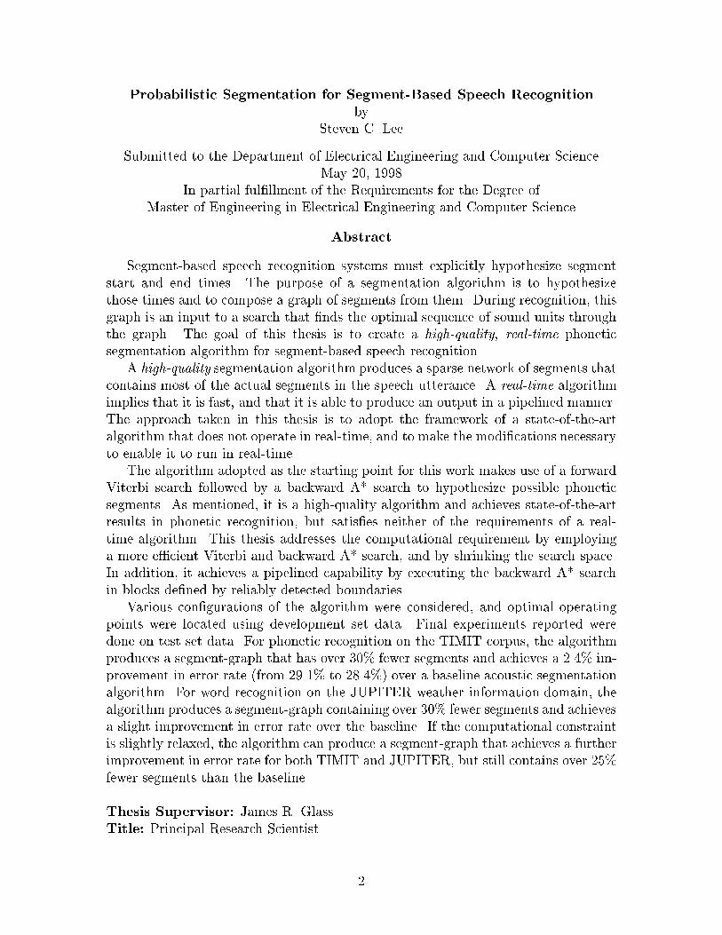
An example segment-graph is shown in the middle of Figure 1-2. On top is a speech

spectrogram, and on the bottom is the reference word and phone transcriptions. Each

rectangle in the segment-graph corresponds to a possible segment, which in this case

is a phonetic unit. The graph can be traversed from the beginning of the utterance to

the end in many di�erent ways; one way is highlighted in black. During recognition,

the search �nds the optimal segment sequence and the phonetic identity of each

segment. The segmentation algorithm is essential to the success of a segment-based

speech recognizer. If the algorithm outputs a graph with too many segments, the

search space may become too large, and the recognizer may not be able to �nish

computation in a reasonable amount of time. If the algorithm hypothesizes too few

segments and misses one, the recognizer has no chance at recognizing that segment,

and recognition errors will likely result.

This thesis deals with the creation of a new phonetic segmentation algorithm for

segment-based speech recognition systems.

1.1 Previous Work

Until recently work on segmentation has been focused mainly on creating a linear

sequence of segments. However, for use in segment-based speech recognition systems,

10

Figure 1-2: On top, a speech spectrogram; in the middle, a segment-graph; on thebottom, the reference phonetic and word transcriptions. The segment-graph is theoutput of the segmentation algorithm and constrains the way the recognizer can dividethe speech signal into phonetic units. In the segment-graph, each gray box representsa possible segment. One possible sequence of segments through the graph is denotedby the black boxes.

a linear sequence of segments o�ers only one choice of segmentation with no alter-

natives. Needless to say, the segmentation algorithm must be extremely accurate, as

any mistakes can be costly. Because linear segmentation algorithms are typically not

perfect, graphs of segments are becoming prevalent in segment-based speech recog-

nition systems. A graph segmentation algorithm provides a segment-based search

with numerous ways to segment the utterance. The output of the algorithm is the

segment-graph previously illustrated in Figure 1-2. This section discusses previous

work in linear and graph segmentation.

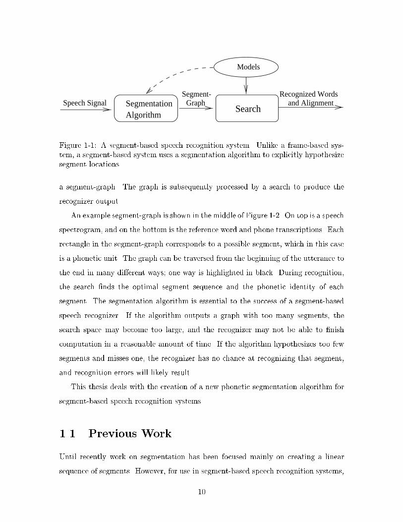
1.1.1 Segmentation using Broad-Class Classi�cation

In [4], Cole and Fanty use a frame-based broad-class classi�er to locate phonetic

boundaries. They construct a linear segmentation using a neural network to classify

each frame in the speech utterance as one of 22 broad-phonetic classes. The segmen-

tation is used in an alphabet recognition system. Processing subsequent to segmenta-

tion uses features extracted from sections of segments that discriminate most between

certain phones. They achieved 95% accuracy in isolated alphabet recognition.

11

1.1.2 Acoustic Segmentation

In acoustic segmentation [6], segment boundaries are located by detecting local max-

ima of spectral change in the speech signal. Segment-graphs are created by fully

connecting these boundaries within acoustically stable regions. Although this algo-

rithm is fast, and recognizers using its segment-graphs perform competitively, the

belief is that these graphs unnecessarily hypothesize too many segments.

1.1.3 Probabilistic Segmentation

In probabilistic segmentation [2], the segment-graph is constructed by combining the

segmentation of the N-best paths produced by a frame-based phonetic recognizer.

N is a variable that can be used to vary the thickness of the segment-graph. This

framework is shown in Figure 1-3. The algorithm makes use of a forward Viterbi and

backward A* search to produce the N-best paths, as shown in Figure 1-4. Recogniz-

ers using this algorithm achieve state-of-the-art results in phonetic recognition while

using segment-graphs half the size of those produced by the acoustic segmentation.

However, one major drawback of this algorithm is that it cannot run in real-time. It

cannot do so because it is computationally intensive, and because the two-pass search

disallows the algorithm from running in a left-to-right pipelined manner.

1.2 Thesis Objective

Because of the success of the probabilistic segmentation algorithm in reducing error

rate while hypothesizing fewer segments, the approach taken in this thesis is to adopt

that framework and to make the modi�cations necessary to enable a real-time capa-

bility. More speci�cally, the goal of this thesis is to modify probabilistic segmentation

to lower its computational requirements and to enable a pipeline capability.

Since the acoustic segmentation is so cheap computationally, creating a segmen-

tation algorithm with even lower computational requirements would be di�cult. In-

stead, the aim is to create a probabilistic algorithm that produces fewer segments

12

speech signal

recognizer

frame-based

N best paths:

h# skcl k

sh#

h# tcl t

segment-based

search

segment graph:

recognized wordsand alignment

segmentation

recognition

Figure 1-3: The probabilistic segmentation framework. The speech signal is passed toa frame-based recognizer, and the segment-graph is constructed by taking the unionof the segmentation in the N-best paths.

forwardViterbisearch

A*search

backwardspeech signal upper-bound scoreslook-aheadlattice of

N best paths

frame-based recognizer

Figure 1-4: The frame-based recognizer used in the probabilistic segmentation frame-work. Because the recognizer uses a forward search followed by a backward search, theprobabilistic segmentation algorithm cannot run in a pipelined manner as requiredby a real-time algorithm.

13

than the acoustic segmentation and is fast enough that the overall recognition sys-

tem, processing a smaller segment-graph, runs faster than one using the acoustic

segmentation, and performs competitively in terms of error rate.

Figure 1-5 illustrates this goal. In a segmentation algorithm, the number of seg-

ments in the segment-graph can usually be controlled by one or more parameters,

such as the variable N in probabilistic segmentation. A general trend is that as the

number of segments increases, segment-based recognition improves because the rec-

ognizer has more alternative segmentations with which to work. This trend for a

hypothetical segmentation algorithm is plotted on the left. The plot shows number

of segments per second versus error rate. The acoustic segmentation baseline is rep-

resented simply by a point on this graph because an optimal point has presumably

been chosen taking into account the relevant tradeo�s. This thesis seeks to develop

an algorithm, like the hypothetical one shown, that can produce an improvement in

error rate with signi�cantly fewer segments than the acoustic segmentation baseline.

Another trend in segmentation is that as the number of segments increases, the

amount of computation necessary to produce the segment-graph also increases. This

trend is illustrated for the same hypothetical segmentation algorithm in the plot on

the right of Figure 1-5. The plot shows number of segments per second versus overall

recognition computation. This thesis seeks to develop an algorithm that requires

less computation than the baseline at the operating points that provide better error

rate with signi�cantly fewer segments, similar to the one shown in the plots. The

regions of the curves shown in bold satisfy the desired characteristics. E�ectively

the amount of extra computation needed to compute a higher quality segment graph

must be lower than the computational savings attained by searching through a smaller

segment network.

The rest of this thesis is divided as follows. Chapter 2 describes the experimental

framework in this work. In particular, it describes the two corpora used and the

baseline con�guration of the recognizer. Chapter 3 describes the changes made to

the forward Viterbi search. These changes allow the frame-based recognizer in prob-

abilistic segmentation to run much more e�ciently. Chapter 4 presents the backward

14

computation

overallrecognizer

*

*

ba a bnumber of segments per secondnumber of segments per second

e

c

* baseline * baseline- desired algorithm - desired algorithm

errorrate

Figure 1-5: Plots showing the desired characteristics of a segmentation algorithm.The algorithm should be able to produce an improvement in error rate as depictedby the plot on the left. It should also use less overall computation than the acousticsegmentation baseline, as shown on the right. The bold regions of the curves satisfyboth of these goal.

A* search used to compute the N-best paths of the frame-based recognizer. Chapter

5 describes how a pipelining capability was incorporated into the algorithm. Chapter

6 concludes by summarizing the accomplishments of this thesis and discussing future

work.

15

Chapter 2

Experimental Framework

2.1 Introduction

This thesis conducts experiments in both phonetic recognition and word recognition.

This chapter provides an overview for both of these tasks.

2.2 Phonetic Recognition

This section describes TIMIT, the corpus used for phonetic recognition experiments

in this thesis. In addition, performance of the baseline TIMIT recognizer is presented.

2.2.1 The TIMIT Corpus

The TIMIT acoustic-phonetic corpus [11] is widely used in the research community

to benchmark phonetic recognition experiments. It contains 6300 utterances from

630 American speakers. The speakers were selected from 8 prede�ned dialect regions

of the United States, and the male to female ratio of the speakers is approximately

two to one. The corpus contains 10 sentences from each speaker composed of the

following:

� 2 sa sentences identical for all speakers.

16

� 5 sx sentences drawn from 450 phonetically compact sentences developed at

MIT [11]. These sentences were designed to cover a wide range of phonetic

contexts. Each of the 450 sx sentences were spoken 7 times each.

� 3 si sentences chosen at random from the Brown corpus [5].

Each utterance in the corpus was hand-transcribed by acoustic-phonetic experts,

both at the phonetic level and at the word level. At the phonetic level, the corpus

uses a set of 61 phones, shown in Table 2-1. The word transcriptions are not used in

this thesis.

The sa sentences were excluded from all training and recognition experiments

because they have orthographies identical for all speakers and therefore contain an

unfair amount of information about the phones in those sentences. The remaining

sentences were divided into 3 sets:

� a train set of 3696 utterances from 462 speakers, used for training. This set is

identical to the training set de�ned by NIST.

� a test set of 192 utterances from 24 speakers composed of 2 males and 1 female

from each dialect region, used for �nal evaluation. This set is identical to the

core test set de�ned by NIST.

� a dev set of 400 utterances from 50 speakers, used for tuning parameters.

Because of the enormous amount of computation necessary to process the full dev

and test sets, experiments on them were run in a distributed mode across several

machines. Unfortunately, it is di�cult to obtain a measure of computation in a

distributed task. To deal with this problem, the following small sets were constructed

to allow computational experiments to be run on the local machine in a reasonable

amount of time:

� a small-test set of 7 random utterances taken from the full test set, used for

measuring computation on the test set.

17

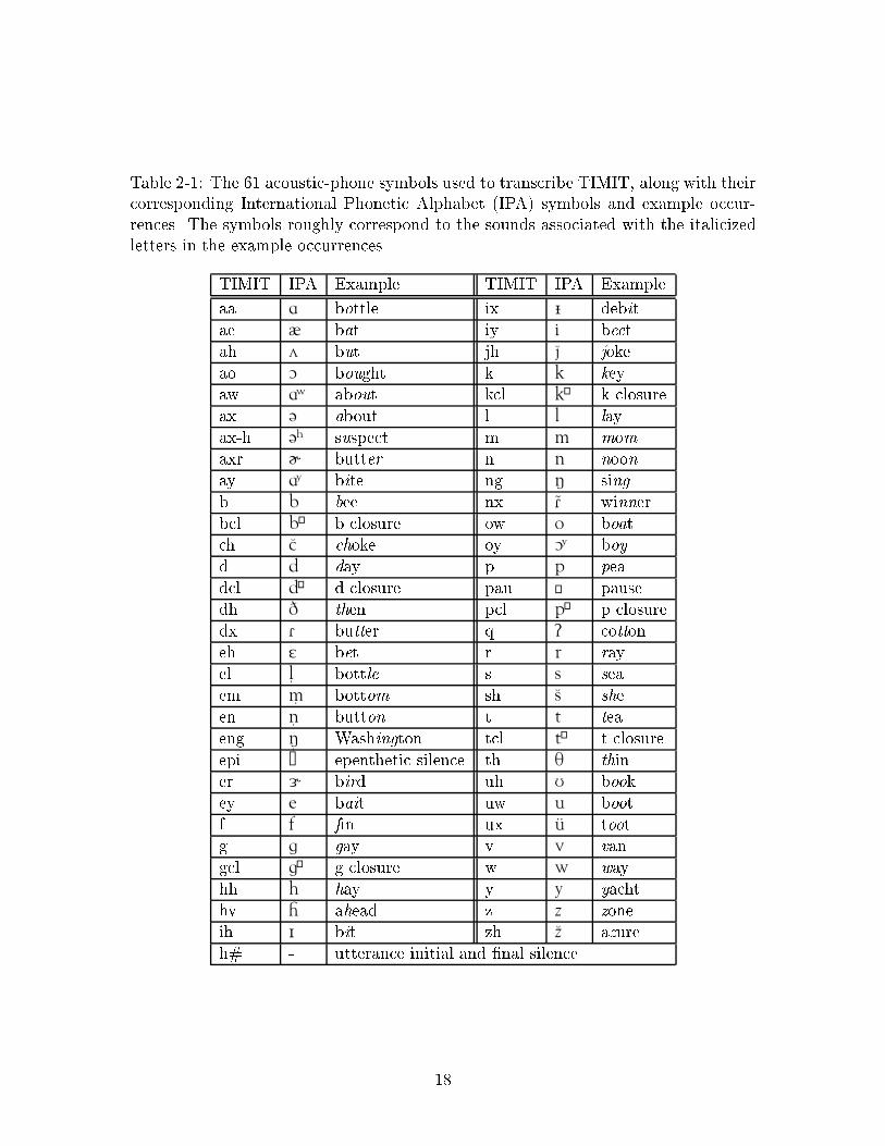
Table 2-1: The 61 acoustic-phone symbols used to transcribe TIMIT, along with theircorresponding International Phonetic Alphabet (IPA) symbols and example occur-rences. The symbols roughly correspond to the sounds associated with the italicizedletters in the example occurrences.

TIMIT IPA Example TIMIT IPA Example

aa a bottle ix | debitae @ bat iy i beetah ^ but jh J jokeao O bought k k keyaw a⁄  about kcl k› k closureax { about l l layax-h {‡  suspect m m momaxr } butter n n noonay a¤  bite ng 4 singb b bee nx FÊ winnerbcl b› b closure ow o boatch C choke oy O¤  boyd d day p p peadcl d› d closure pau √ pausedh D then pcl p› p closuredx F butter q ? cottoneh E bet r r rayel lÍ bottle s s seaem mÍ bottom sh S sheen nÍ button t t teaeng 4Í Washington tcl t› t closureepi ∑ epenthetic silence th T thiner 5 bird uh U bookey e bait uw u bootf f fin ux uÚ tootg g gay v v vangcl g› g closure w w wayhh h hay y y yachthv H ahead z z zoneih I bit zh Z azureh# - utterance initial and �nal silence

18

� a small-dev set of 7 random utterances taken from the full dev set, used for

measuring computation on the dev set.

To ensure fair experimental conditions, the utterances in the train, dev, and test

sets never overlap, and they re ect a balanced representation of speakers in the corpus.

In addition, the sets are identical to those used by many others in the speech recogni-

tion community, so results can be directly compared to those of others [6, 7, 10, 12, 15].

2.2.2 Baseline Recognizer Con�guration and Performance

The baseline recognizer for TIMIT was previously reported in [6]. Utterances are rep-

resented by 14 Mel-frequency cepstral coe�cients (MFCCs) and log energy computed

at 5ms intervals. Segment-graphs are generated using the acoustic segmentation al-

gorithm described in Chapter 1.

As is frequently done by others to report recognition results, acoustic models are

constructed on the train set using 39 labels collapsed from the set of 61 labels shown

in Figure 2-1 [6, 7, 12, 19]. Both frame-based boundary models and segment-based

models are used. The context-dependent diphone boundary models are mixtures of

diagonal Gaussians based on measurements taken at various times within a 150ms

window centered around the boundary time. This window of measurements allows the

models to capture contextual information. The segment models are also mixtures of

diagonal Gaussians, based on measurements taken over segment thirds; delta energy

and delta MFCCs at segment boundaries; segment duration; and the number of

boundaries within a segment. Language constraints are provided by a bigram.

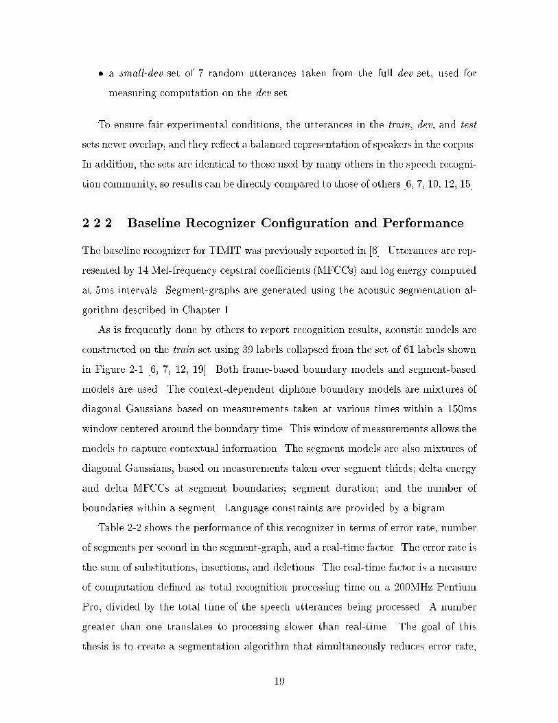
Table 2-2 shows the performance of this recognizer in terms of error rate, number

of segments per second in the segment-graph, and a real-time factor. The error rate is

the sum of substitutions, insertions, and deletions. The real-time factor is a measure

of computation de�ned as total recognition processing time on a 200MHz Pentium

Pro, divided by the total time of the speech utterances being processed. A number

greater than one translates to processing slower than real-time. The goal of this

thesis is to create a segmentation algorithm that simultaneously reduces error rate,

19

Table 2-2: TIMIT baseline recognizer results, using the acoustic segmentation.

Set Error Rate (%) Segments/Second Real-Time Factor

dev 27.7 86.2 2.64test 29.1 87.2 3.02

segment-graph size, and computation.

2.3 Word Recognition

This section describes JUPITER, the corpus used for word recognition experiments in

this thesis. In addition, performance of the baseline JUPITER recognizer is presented.

2.3.1 The JUPITER Corpus

The JUPITER corpus is composed of spontaneous speech data from a live telephone-

based weather information system [20]. The corpus used for this thesis contains

over 12,000 utterances spoken by random speakers calling into the system. Unlike

TIMIT, whose reference transcriptions were hand-transcribed, JUPITER's reference

transcriptions were created by a recognizer performing forced alignment.

The words found in the corpus include proper names such as that of cities, coun-

tries, airports, states, and regions; basic words such as articles and verbs; support

words such as numbers, months, and days; and weather related-words, such as humid-

ity and temperature. Some sentences in the JUPITER corpus are shown in Table 2-3.

As was done for TIMIT, the utterances in the corpus were divided into 3 sets:

� a train set of 11,405 utterances

� a test set of 480 utterances

� a dev set of 502 utterances

In addition, the following smaller sets were created for computational experiments:

20

� a small-test set of 11 utterances

� a small-dev set of 13 utterances

2.3.2 Baseline Recognizer Con�guration and Performance

The baseline JUPITER recognizer is based on a phonetic recognizer that only con-

siders phone sequences allowed by a pronunciation network. This network de�nes the

legal phonetic sequences for all words in the lexicon, and accounts for variability in

speaking style by de�ning multiple possible phone sequences for each word and for

each word pair boundary.

Utterances are represented by 14 MFCCs computed at 5ms intervals. Segment-

graphs are generated using the acoustic segmentation algorithm described in Chap-

ter 1.

The lexicon of 1345 words is built from a set of 68 phones very similar to the

TIMIT phones shown in Table 2-1. Only context-dependent diphone boundary models

are used in this recognizer. These models are similar to the ones used in TIMIT

and are composed of mixtures of diagonal Gaussians trained on the train set using

measurements taken at various times within a 150ms window centered around the

boundary time. In addition to constraints de�ned by the pronunciation network, the

recognizer uses a bigram language model.

Table 2-3: Sample Sentences from the JUPITER corpus.

What cities do you know about in California?How about in France?What will the temperature be in Boston tomorrow?What about the humidity?Are there any ood warnings in the United States?Where is it sunny in the Caribbean?What's the wind speed in Chicago?How about London?Can you give me the forecast for Seattle?Will it rain tomorrow in Denver?

21

Table 2-4: JUPITER baseline recognizer results, using the acoustic segmentation.

Set Error Rate (%) Segments/Second Real-Time Factor

dev 12.7 100.1 1.03test 10.6 99.7 0.89

Table 2-4 shows the performance of this recognizer, in terms of error rate, num-

ber of segments per second, and the real-time factor. In terms of error rate and

computation, these results are better than the phonetic recognition results shown

in Table 2-2. This is the case because the TIMIT baseline recognizer is tuned to

optimize recognition error rate while the JUPITER baseline recognizer is tuned for

real-time performance. As in TIMIT, the goal of this thesis is to create a segmen-

tation algorithm that lowers error rate while using smaller segment-graphs and less

computation.

22

Chapter 3

Viterbi Search

3.1 Introduction

The key component of the probabilistic segmentation framework is the phonetic recog-

nizer used to compute the N-best paths. Although any recognizer, be it frame-based

or segment-based, can be used for this purpose, a frame-based recognizer was chosen

to free the �rst pass recognizer from any dependence on segment-graphs. Consid-

ering that Phillips et al achieved competitive results on phonetic recognition using

boundary models only [14], those models were chosen to be used with this recognizer.

As illustrated in Figure 1-4, the phonetic recognizer is made up of a forward

Viterbi and a backward A* search. When a single best sequence is required, the

Viterbi search is su�cient. However, when the top N-best hypotheses are needed, as

is the case in this work, an alternative is required. In this thesis, the N-best hypotheses

are produced by using a forward Viterbi with a backward A* search. The backward

A* search uses the lattice of scores created by the Viterbi search as look-ahead upper

bounds to produce the N-best paths in order of their likelihoods.

This chapter describes the Viterbi search used to �nd the single best path. How

the Viterbi lattice can be used with a backward A* search to produce the N-best

paths is deferred to Chapter 4. This chapter focuses on the modi�cations made to

the Viterbi search to improve its computational e�ciency.

23

3.2 Mathematical Formulation

Let A be a sequence of acoustic observations; let W be a sequence of phonetic units;

and let S be a set of segments de�ning a segmentation:

A = f~a1; ~a2; :::; ~aTg

W = fw1; w2; :::; wNg

S = fs1; s2; :::; sNg

Most speech recognizers �nd the most likely phone sequence by searching for W �

with the highest posterior probability P (W j A):

W � = argmaxW

P (W j A)

Because P (W jA) is di�cult to model directly, it is often expanded into several

terms. Taking into account the segmentation, the above equation can be rewritten:

P (W j A) =X

S

P (WS j A)

W � = argmaxW

X

S

P (WS j A)

The right hand side of the above equations is adding up the probability of a

phonetic sequence W for every possible partition of the speech utterance as de�ned

by a segment sequence S. The result of this summation is the total probability of the

phonetic sequence. In a Viterbi search, this summation is often approximated with a

maximization to simplify implementation [13]:

P (W j A) � maxS

P (WS j A)

W � = argmaxWS

P (WS j A)

Using Bayes' formula, P (WS j A) can be further expanded:

24

P (WS j A) =P (A j WS)P (S jW )P (W )

P (A)

W � = argmaxWS

P (A jWS)P (S j W )P (W )

P (A)

Since P (A) is a constant for a given utterance, it can be ignored in the maximizing

function. The remaining three terms being maximized above are the three scoring

components in the Viterbi search.

3.2.1 Acoustic Model Score

P (A j WS) is the acoustic component of the maximizing function. In the probabilis-

tic segmentation used in this thesis, the acoustic score is derived from frame-based

boundary models. While segment models are not used in probabilistic segmentation,

they are used in the segment-based search subsequent to segmentation. They will be

relevant in the forthcoming discussion on the segment-based search.

In this thesis, the context-dependent diphone boundary models are mixtures of

diagonal Gaussians based on measurements taken at various times within a 150ms

window centered around the boundary time. The segment models are also mixtures of

diagonal Gaussians, based on measurements taken over segment thirds; delta energy

and delta MFCCs at segment boundaries; segment duration; and the number of

boundaries within a segment.

3.2.2 Duration Model Score

P (S j W ) is the duration component of the maximizing function. It is frequently

approximated as P (S) and computed under the independence assumption:

P (S jW ) � P (S) �NY

i=0

P (si)

In this work, the duration score is modeled by a segment transition weight (stw) that

adjusts between insertions and deletions.

25

3.2.3 Language Model Score

P (W ) is the language component of the maximizing function. In this thesis, the

language score is approximated using a bigram that conditions the probability of

each successive word only on the probability of the preceding word:

P (W ) = P (w1; :::; wN) =NY

i=1

P (wi j wi�1)

3.3 Frame-Based Search

Normally a frame-based recognizer uses a frame-based Viterbi search to solve the

maximization problem described in the previous section. The Viterbi search can be

visualized as one that �nds the best path through a lattice. This lattice for a frame-

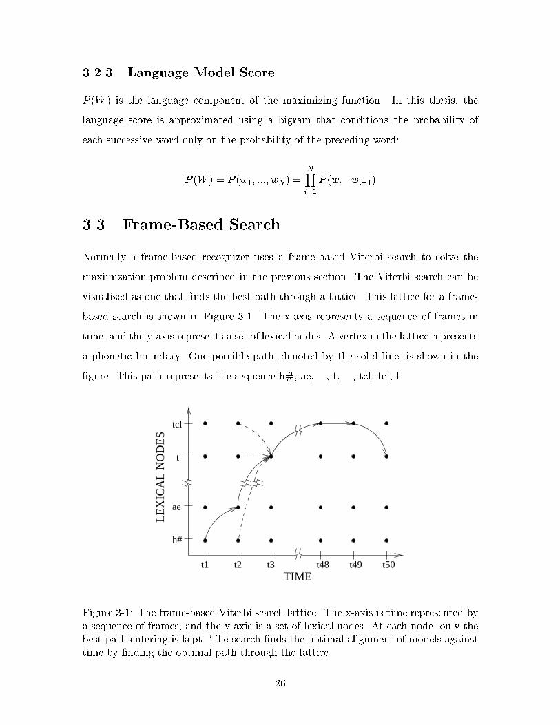
based search is shown in Figure 3-1. The x-axis represents a sequence of frames in

time, and the y-axis represents a set of lexical nodes. A vertex in the lattice represents

a phonetic boundary. One possible path, denoted by the solid line, is shown in the

�gure. This path represents the sequence h#, ae, ..., t, ..., tcl, tcl, t.

TIME

ae

tcl

t

LE

XIC

AL

NO

DE

S

h#

t1 t2 t3 t48 t49 t50

Figure 3-1: The frame-based Viterbi search lattice. The x-axis is time represented bya sequence of frames, and the y-axis is a set of lexical nodes. At each node, only thebest path entering is kept. The search �nds the optimal alignment of models againsttime by �nding the optimal path through the lattice.

26

To �nd the optimal path, the Viterbi search processes input frames in a time-

synchronous manner. For each node at a given frame, the active lexical nodes at the

previous frame are retrieved. The path to each of these active nodes is extended to

the current node if the extension is allowed by the pronunciation network. For each

extended path, the appropriate boundary, segment transition, and bigram model

scores are added to the path score. Only the best arriving path to each node is kept.

This Viterbi maximization is illustrated at node (t3, t) of Figure 3-1. Four paths

are shown entering the node. The one with the best score, denoted by the solid line,

originates from node (t2, ae); therefore, only a pointer to (t2, ae) is kept at (t3, t).

When all the frames have been processed, the Viterbi lattice contains the best path

and its associated score from the initial node to every node. The overall best path

can then be retrieved from the lattice by looking for the node with the best score at

the last frame and performing a back-trace.

To reduce computational and memory requirements, beam pruning is usually done

after each frame has been processed. Paths that do not have scores within a threshold

of the best scoring path at the current analysis frame are declared inactive and can

no longer be extended.

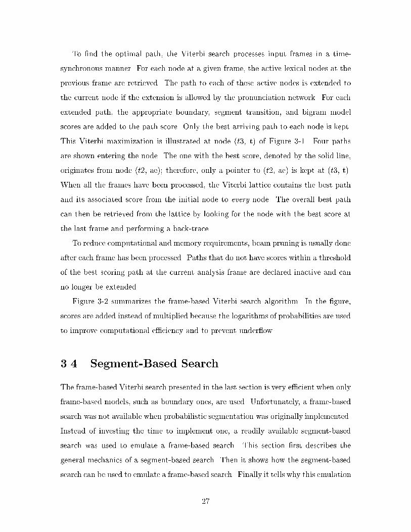
Figure 3-2 summarizes the frame-based Viterbi search algorithm. In the �gure,

scores are added instead of multiplied because the logarithms of probabilities are used

to improve computational e�ciency and to prevent under ow.

3.4 Segment-Based Search

The frame-based Viterbi search presented in the last section is very e�cient when only

frame-based models, such as boundary ones, are used. Unfortunately, a frame-based

search was not available when probabilistic segmentation was originally implemented.

Instead of investing the time to implement one, a readily available segment-based

search was used to emulate a frame-based search. This section �rst describes the

general mechanics of a segment-based search. Then it shows how the segment-based

search can be used to emulate a frame-based search. Finally it tells why this emulation

27

for each frame fto in the utterancelet best score(fto) = �1let flast be the frame preceding ftolet ~y be the measurement vector for boundary flast

for each node nto in the pronunciation networkfor each pronunciation arc a arriving at node nto

let nfrom be the source node of arc alet b be the pronunciation arc arriving at node nfromif (nfrom; ffrom) has not been pruned from the Viterbi lattice

let � be the label for the transition b! a

let acoustic score = p(~y j �)let duration score = stw if b 6= a, or 0 if b = a

let language score = p(�)let score = acoustic score+ duration score+ language score

if (score(nfrom; ffrom) + score > score(nto; fto))score(nto; fto) = score(nfrom; ffrom) + score

make a back pointer from (nto; fto) to (nfrom; ffrom)if score(nto; fto) > best score(fto)

let best score(fto) = score(nto; fto)for each node nto in the pronunciation network

if best score(fto)� score(nto; fto) > thresh

prune node (nto; fto) from the Viterbi lattice

Figure 3-2: Pseudocode for the frame-based Viterbi algorithm.

28

is ine�cient.

The lattice for the segment-based Viterbi search is shown in Figure 3-3. It is

similar to the frame-based lattice, with one exception. The time axis of the segment-

based lattice is represented by a graph of segments in addition to a series of frames.

A vertex in the lattice represents a phonetic boundary. The solid line through the

�gure shows one possible path through the lattice.

ae

tcl

t

LE

XIC

AL

NO

DE

S

h#

t1 t2 t3 t48 t49 t50

TIME

Figure 3-3: The segment-based Viterbi search lattice. The x-axis is time representedby a sequence of frames and segments; and the y-axis is a set of lexical nodes. As inthe frame-based case, only the best path entering a node is kept, and the search �ndsthe optimal alignment of models against time by �nding the optimal path throughthe lattice.

To �nd the optimal path, the search processes segment boundaries in a time-

synchronous fashion. For each segment ending at a boundary, the search computes

the normalized segment scores of all possible phonetic units that can go within that

segment. It also computes the boundary scores for all frames spanning the segment,

the duration score, and the bigram score. Only models that have not been pruned

out and those that are allowed by the pronunciation network are scored. As before,

29

only the best path to a node is kept, and the best path at the end of processing can

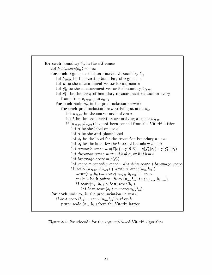
be retrieved by performing a back-trace. Figure 3-4 summarizes the segment-based

search.

The segment-based search can emulate a frame-based one if it uses boundary

models only on a segment graph that contains every segmentation considered by a

frame-based search. Since a frame-based search considers every possible segmentation

that can be created from the input frames, such a segment-graph can be obtained by

creating a set of boundaries at the desired frame-rate and connecting every boundary

pair. Figure 3-5 illustrates the construction of such a graph.

To keep the size of the segment-graph manageable, the maximum length of a

segment formed by connecting a boundary pair is set to be 500ms. This limit has no

e�ect on performance, as the true frame-based search is unlikely to �nd an optimal

path with a segment longer than 500ms.

Using the segment-based search as a frame-based search is computationally inef-

�cient. Whereas in the true frame-based search each model is scored only once per

time, each model can be scored multiple times in the segment-based emulation. This

redundant scoring occurs whenever multiple segments are attached to either side of

a frame. Because every boundary pair is connected in the segment-graph used in the

simulated search, numerous models are needlessly re-scored in this framework.

3.5 Reducing Computation

To do away with the ine�ciencies of the emulation, a true frame-based search as

described in Section 3.3 was implemented. In addition, computation was further

reduced by shrinking the search space of the Viterbi search. In time, instead of

scoring at every frame, only landmarks that have been detected by a spectral change

algorithm were scored. The landmarks used have been successfully applied previously

to the acoustic segmentation algorithm, and eliminate large amounts of computation

spent considering sections of speech unlikely to be segments. Along the lexical-space,

the full set of phone models was collapsed into a set of broad classes. Phones with

30

for each boundary bto in the utterancelet best score(bto) = �1for each segment s that terminates at boundary bto

let bfrom be the starting boundary of segment slet ~x be the measurement vector for segment slet ~yb be the measurement vector for boundary bfromlet ~yi[] be the array of boundary measurement vectors for every

frame from bfrom+1 to bto�1for each node nto in the pronunciation network

for each pronunciation arc a arriving at node ntolet nfrom be the source node of arc alet b be the pronunciation arc arriving at node nfromif (nfrom; bfrom) has not been pruned from the Viterbi lattice

let � be the label on arc alet �� be the anti-phone labellet �b be the label for the transition boundary b! a

let �i be the label for the internal boundary a! a

let acoustic score = p(~xj�)� p(~xj��) + p( ~ybj�b) + p(~yi[]j�i)let duration score = stw if b 6= a, or 0 if b = a

let language score = p(�b)let score = acoustic score+ duration score+ language score

if (score(nfrom; bfrom) + score > score(nto; bto))score(nto; bto) = score(nfrom; bfrom) + score

make a back pointer from (nto; bto) to (nfrom; bfrom)if score(nto; bto) > best score(bto)

let best score(bto) = score(nto; bto)for each node nto in the pronunciation network

if best score(bto)� score(nto; bto) > thresh

prune node (nto; bto) from the Viterbi lattice

Figure 3-4: Pseudocode for the segment-based Viterbi algorithm.

31

Figure 3-5: The construction of a segment-graph used to emulate a frame-basedsearch. Every boundary pair on the left are connected to create the segment-graphshown on the right.

similar spectral properties, such as the two fricatives shown on the left and the two

vowels shown on the right of Figure 3-6, were grouped into a single class. This can

be done because the identities of the segments are irrelevant for segmentation.

Figure 3-6: From left to right, spectrograms of [f], [s], [{], and [o]. To save compu-tation, phones with similar spectral properties, such as the two fricatives on the leftand the two vowels on the right, were grouped together to form broad-classes.

3.6 Experiments

This section presents the performance of various versions of the Viterbi search. The

best path from the search is evaluated on phonetic recognition error rate and on the

computation needed to produce the path. Even though probabilistic segmentation

does not use the best path directly, these recognition results were examined because

they should be correlated to the quality of the segments produced by the probabilistic

segmentation algorithm.

32

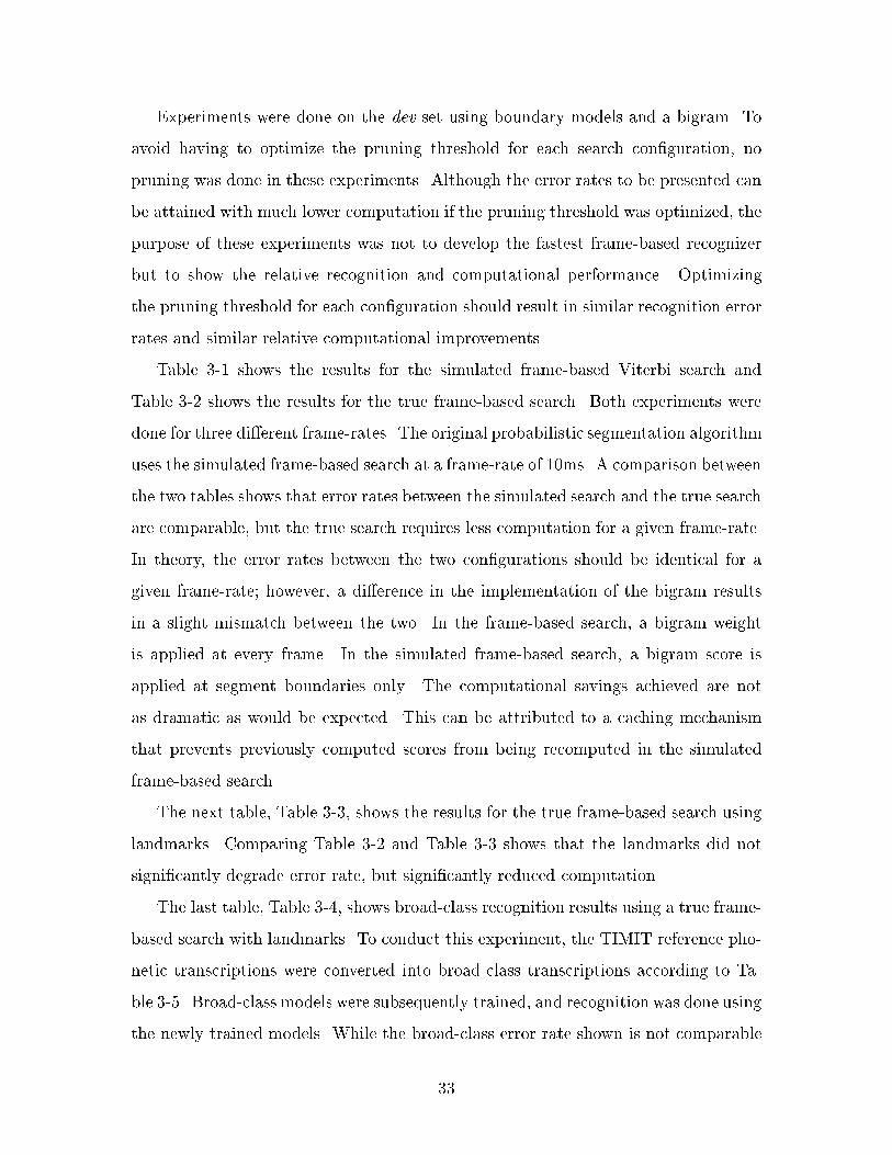
Experiments were done on the dev set using boundary models and a bigram. To

avoid having to optimize the pruning threshold for each search con�guration, no

pruning was done in these experiments. Although the error rates to be presented can

be attained with much lower computation if the pruning threshold was optimized, the

purpose of these experiments was not to develop the fastest frame-based recognizer

but to show the relative recognition and computational performance. Optimizing

the pruning threshold for each con�guration should result in similar recognition error

rates and similar relative computational improvements.

Table 3-1 shows the results for the simulated frame-based Viterbi search and

Table 3-2 shows the results for the true frame-based search. Both experiments were

done for three di�erent frame-rates. The original probabilistic segmentation algorithm

uses the simulated frame-based search at a frame-rate of 10ms. A comparison between

the two tables shows that error rates between the simulated search and the true search

are comparable, but the true search requires less computation for a given frame-rate.

In theory, the error rates between the two con�gurations should be identical for a

given frame-rate; however, a di�erence in the implementation of the bigram results

in a slight mismatch between the two. In the frame-based search, a bigram weight

is applied at every frame. In the simulated frame-based search, a bigram score is

applied at segment boundaries only. The computational savings achieved are not

as dramatic as would be expected. This can be attributed to a caching mechanism

that prevents previously computed scores from being recomputed in the simulated

frame-based search.

The next table, Table 3-3, shows the results for the true frame-based search using

landmarks. Comparing Table 3-2 and Table 3-3 shows that the landmarks did not

signi�cantly degrade error rate, but signi�cantly reduced computation.

The last table, Table 3-4, shows broad-class recognition results using a true frame-

based search with landmarks. To conduct this experiment, the TIMIT reference pho-

netic transcriptions were converted into broad-class transcriptions according to Ta-

ble 3-5. Broad-class models were subsequently trained, and recognition was done using

the newly trained models. While the broad-class error rate shown is not comparable

33

Table 3-1: TIMIT dev set recognition results, using the frame-based search simulatedwith a segment-based search.

Frame-rate Error Rate (%) Real-Time Factor

10ms 28.7 4.0520ms 28.0 1.7330ms 29.0 1.09

Table 3-2: TIMIT dev set recognition results, using the true frame-based search.

Frame-rate Error Rate (%) Real-Time Factor

10ms 28.9 3.0120ms 28.2 1.5230ms 29.4 1.01

Table 3-3: TIMIT dev set recognition results, using the true frame-based search withlandmarks.

Frame-rate Error Rate (%) Real-Time Factor

Landmarks 28.5 0.92

Table 3-4: TIMIT dev set recognition results on broad classes, using the true frame-based search with landmarks.

Frame-rate Error Rate (%) Real-Time Factor

Landmarks 24.1 0.44

34

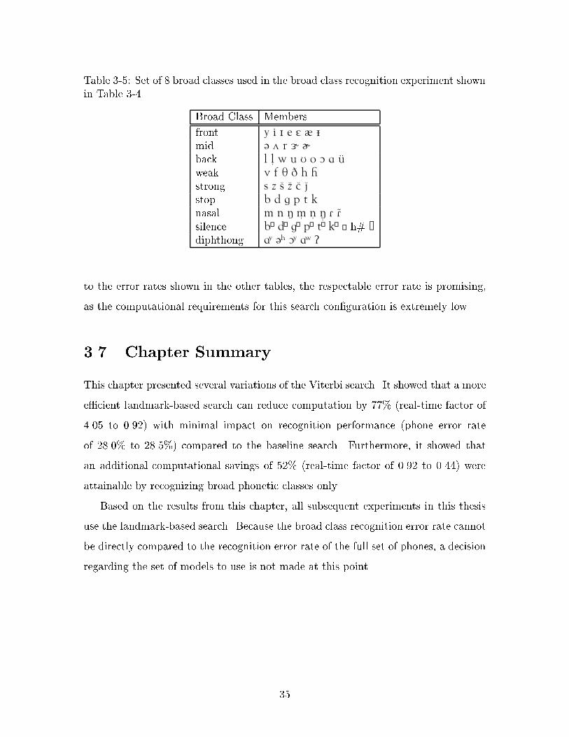
Table 3-5: Set of 8 broad classes used in the broad class recognition experiment shownin Table 3-4.

Broad Class Members

front y i I e E @ |mid { ^ r 5 }back l lÍ w u U o O a uÚweak v f T D h Hstrong s z S Z C Jstop b d g p t knasal m n 4 mÍ nÍ 4Í F FÊsilence b› d› g› p› t› k› √ h# ∑diphthong a¤  {‡  O¤  a⁄  ?

to the error rates shown in the other tables, the respectable error rate is promising,

as the computational requirements for this search con�guration is extremely low.

3.7 Chapter Summary

This chapter presented several variations of the Viterbi search. It showed that a more

e�cient landmark-based search can reduce computation by 77% (real-time factor of

4.05 to 0.92) with minimal impact on recognition performance (phone error rate

of 28.0% to 28.5%) compared to the baseline search. Furthermore, it showed that

an additional computational savings of 52% (real-time factor of 0.92 to 0.44) were

attainable by recognizing broad phonetic classes only.

Based on the results from this chapter, all subsequent experiments in this thesis

use the landmark-based search. Because the broad class recognition error rate cannot

be directly compared to the recognition error rate of the full set of phones, a decision

regarding the set of models to use is not made at this point.

35

Chapter 4

A* Search

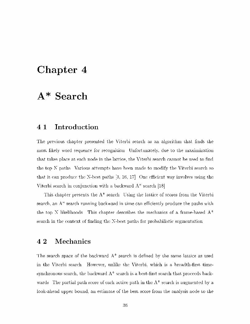
4.1 Introduction

The previous chapter presented the Viterbi search as an algorithm that �nds the

most likely word sequence for recognition. Unfortunately, due to the maximization

that takes place at each node in the lattice, the Viterbi search cannot be used to �nd

the top N paths. Various attempts have been made to modify the Viterbi search so

that it can produce the N-best paths [3, 16, 17]. One e�cient way involves using the

Viterbi search in conjunction with a backward A* search [18].

This chapter presents the A* search. Using the lattice of scores from the Viterbi

search, an A* search running backward in time can e�ciently produce the paths with

the top N likelihoods. This chapter describes the mechanics of a frame-based A*

search in the context of �nding the N-best paths for probabilistic segmentation.

4.2 Mechanics

The search space of the backward A* search is de�ned by the same lattice as used

in the Viterbi search. However, unlike the Viterbi, which is a breadth-�rst time-

synchronous search, the backward A* search is a best-�rst search that proceeds back-

wards. The partial path score of each active path in the A* search is augmented by a

look-ahead upper bound, an estimate of the best score from the analysis node to the

36

beginning of the utterance.

Typically, the A* search is implemented using a stack to maintain a list of active

paths sorted by their path scores. At each iteration of the search, the best path is

popped o� the stack and extended backward by one frame. The lexical nodes to

which a path can extend are de�ned by the pronunciation network. When a path

is extended, the appropriate boundary, segment transition, and bigram model scores

are added to the partial path score and a look-ahead upper bound to create the

new path score. After extension, incomplete paths are inserted back into the stack,

and complete paths that span the entire utterance are passed on as the next N-best

output. The search completes when it has produced N complete paths. To improve

e�ciency, paths in the stack not within a threshold of the best are pruned away.

In addition to the pruning, the e�ciency of the A* search is also controlled by

the tightness of the upper bound added to the partial path score. At one extreme

is an upper bound of zero. In this case, the path at the top of the stack changes

after almost every iteration, and the search spends a lot of time extending paths that

are ultimately not the best. At the other extreme is an upper bound that is the

exact score of the best path from the start of the partial path to the beginning of the

utterance node. With such an upper bound, the scoring function always produces

the score of the best complete path through the node at the start of the partial path.

Hence the partial path of the best overall path is always at the top of the stack, and

it is continuously extended until it is complete.

To make the A* search as e�cient as possible, the Viterbi search is used to provide

the upper bound in the look-ahead score, as the Viterbi lattice contains the score of

the best path to each lattice node. Because the A* search uses the Viterbi lattice,

pruning during the Viterbi search must be done with care. Pruning too aggressively

will result in paths that do not have the best scores.

Figure 4-1 summarizes in detail the A* search. It is best understood by going

through an example. Consider Table 4-1, which shows the boundary scores for a hy-

pothetical utterance, and Figure 4-2, which shows a Viterbi lattice that has processed

those scores. The scores in the table follow the convention that lower is better. The

37

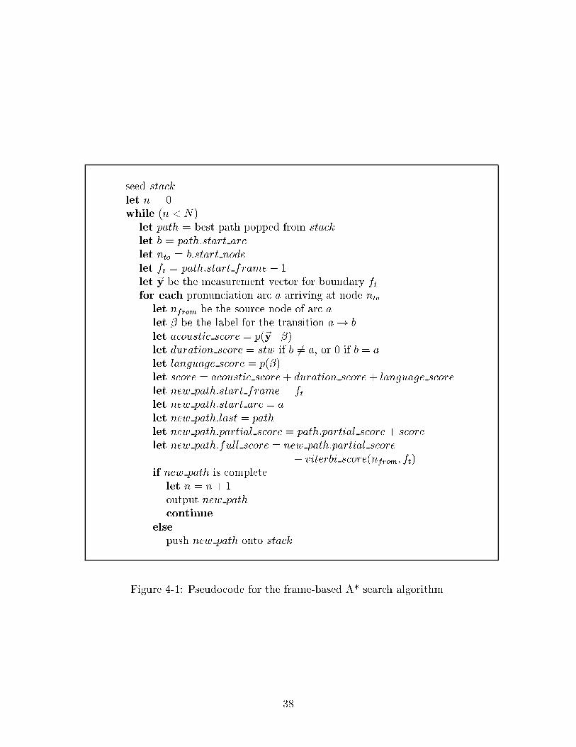
seed stack

let n = 0while (n < N)

let path = best path popped from stack

let b = path:start arc

let nto = b:start node

let ft = path:start frame� 1let ~y be the measurement vector for boundary ftfor each pronunciation arc a arriving at node nto

let nfrom be the source node of arc alet � be the label for the transition a! b

let acoustic score = p(~y j �)let duration score = stw if b 6= a, or 0 if b = a

let language score = p(�)let score = acoustic score+ duration score+ language score

let new path:start frame = ftlet new path:start arc = a

let new path:last = path

let new path:partial score = path:partial score+ score

let new path:full score = new path:partial score

+ viterbi score(nfrom; ft)if new path is complete

let n = n+ 1output new path

continue

elsepush new path onto stack

Figure 4-1: Pseudocode for the frame-based A* search algorithm.

38

lattice contains the overall best path, represented by a solid line. It also contains

the best path and its associated score to each lattice node. Only the model h# is

scored at time t1 and t4 because the pronunciation network constrains the start and

end of the utterance to h#. The pronunciation network does not impose any other

constraints.

Table 4-2 shows the evolution of the stack as the A* search processes the hypo-

thetical utterance. Each path in the stack is associated with two scores. One is the

partial score of the path from the end of the utterance to the start of the path. The

other is a full path score that is the sum of the partial path score and the look-ahead

upper bound from the Viterbi lattice. The paths in the stack are sorted by the full

path score, but the partial score is needed to compute the full path score for future

extensions.

In the example, the stack is seeded with an end-of-utterance model, h#, as re-

quired by the pronunciation network. This single path is popped from the stack and

extended to the left, from the end to the beginning. During extension, the look-ahead

estimate is obtained from the appropriate node in the Viterbi lattice. The new partial

score is the sum of the old partial score and the boundary score of the new boundary

in the path. The new full path score is the sum of the estimate and the new partial

score. Each of the extended paths is inserted back into the stack, and the best path

is popped again. This process continues until the desired number of paths have been

completely expanded. In the example shown, two paths are found. They are shown

in bold in the �gure.

The example presented highlights the e�ciency of the A* search when it uses an

exact look-ahead estimate to compute the top paths. In particular, the top of the

stack always contains the partial path of the next best path. The search never wastes

any computation expanding an unwanted path.

In probabilistic segmentation, the segment-graph is simply constructed by taking

the union of the segmentations in the N-best paths. In the above example, the

segment-graph resulting from the two best paths found is shown in Figure 4-3.

39

Table 4-1: The boundary scores for a hypothetical utterance. Because the pronunci-ation network constrains the beginning and end of the utterance to be h#, only h#models are scored at t1 and t4.

t1 t2 t3 t4Label Score Label Score Label Score Label Scoreh# ! aa 3 aa ! aa 1 aa ! aa 2 aa ! h# 3h# ! ae 4 aa ! ae 3 aa ! ae 1 ae ! h# 1h# ! h# 5 aa ! h# 3 aa ! h# 2 h# ! h# 4

ae ! aa 2 ae ! aa 3ae ! ae 4 ae ! ae 4ae ! h# 3 ae ! h# 4h# ! aa 4 h# ! aa 3h# ! ae 2 h# ! ae 2h# ! h# 3 h# ! h# 4

t1 t2 t3 t4 t5

h#

ae

aa

TIME

LE

XIC

AL

NO

DE

S

0 5

4

4

6

6

6

5

6 6

3

Figure 4-2: A processed Viterbi lattice showing the best path to each node and thescore associated with the path.

40

Table 4-2: The evolution of the A* search stack in a hypothetical utterance. Pathsare popped from the stack on the left, extended on the right, and pushed back onthe stack on the left of the next row, until the desired number of paths is completelyexpanded. In this example, the top two paths are found, and they are shown in boldin the �gure.

Stack ExtensionsFull Partial New New Partial New Path

Path Score Score Score Estimate Score Scoreh# 6 0 aa/h# 6 3 9

ae/h# 5 1 6h#/h# 6 4 10

ae/h# 6 1 aa/ae/h# 4 2 6aa/h# 9 3 ae/ae/h# 6 5 11h#/h# 10 4 h#/ae/h# 6 3 9aa/ae/h# 6 2 aa/aa/ae/h# 3 3 6h#/ae/h# 9 3 ae/aa/ae/h# 4 4 8aa/h# 9 3 h#/aa/ae/h# 5 6 11h#/h# 10 4ae/ae/h# 11 5

aa/aa/ae/h# 6 3 h#/aa/aa/ae/h# 0 6 6ae/aa/ae/h# 8 4h#/ae/h# 9 3aa/h# 9 3h#/h# 10 4

h#/aa/ae/h# 11 6ae/ae/h# 11 5

ae/aa/ae/h# 8 4 h#/ae/aa/ae/h# 0 8 8h#/ae/h# 9 3aa/h# 9 3h#/h# 10 4

h#/aa/ae/h# 11 6ae/ae/h# 11 5

+ =h#

h# h#

h#

ae

ae

ae

aa

aa

Figure 4-3: The construction of a segment-graph from the two best paths in the A*search example.

41

4.3 Experiments

A frame-based A* search was implemented in this thesis to work with the frame-

based Viterbi search discussed in Chapter 3. This section presents recognition results

and computational requirements of a segment-based phonetic recognizer using the

A* search for probabilistic segmentation. The di�erence between the implementation

presented here and the implementation presented in [2] is the improved e�ciency of

the Viterbi and A* searches. In addition, experiments on JUPITER and on broad-

class segmentation are presented for the �rst time.

In these experiments, only boundary models were used for segmentation. For the

subsequent segment-based search, both boundary and segment models were used. In

addition, both recognition passes used a bigram language model.

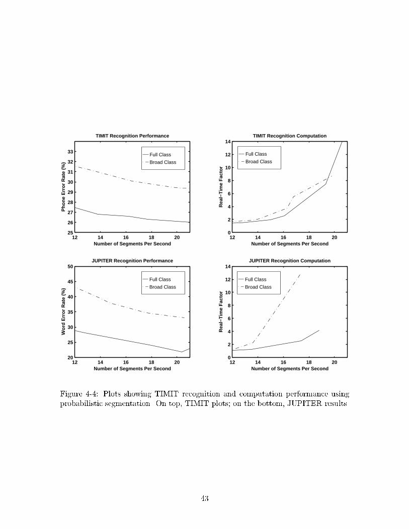
The results are shown in Figure 4-4. TIMIT results are on top, and JUPITER re-

sults are on the bottom. The recognition plots on the left show the number of segments

per second in the segment-graph versus recognition error rate. The computation plots

on the right show the number of segments per second in the segment-graph versus

overall recognition computation. The number of segments per second is controlled

by N, the number of path segmentations used to construct the segment-graph. To

further evaluate the tradeo� between broad-class and full-class models left unresolved

in Chapter 3, experiments were performed using both sets of models for segmenta-

tion. Results on broad-class segmentation are shown as broken lines, and results on

full-class segmentation are shown as solid lines. The set of broad-classes used was

shown in Figure 3-5. Experiments were conducted on the dev sets.

This section �rst discusses general trends seen in both TIMIT and JUPITER,

then discusses some trends unique to each corpus.

4.3.1 General Trends

The plots in Figure 4-4 shows several general trends:

� The recognition plots show that as the number of segments in the segment-graph

increase, recognition error rate improves but asymptotes at some point. The

42

Full Class

Broad Class

Full Class

Broad Class

Full Class

Broad Class

Full Class

Broad Class

12 14 16 18 200

2

4

6

8

10

12

14

Number of Segments Per Second

Rea

l−T

ime

Fac

tor

JUPITER Recognition Computation

12 14 16 18 2020

25

30

35

40

45

50

Number of Segments Per Second

Wor

d E

rror

Rat

e (%

)

JUPITER Recognition Performance

12 14 16 18 2025

26

27

28

29

30

31

32

33

Number of Segments Per Second

Pho

ne E

rror

Rat

e (%

)

TIMIT Recognition Performance

12 14 16 18 200

2

4

6

8

10

12

14

Number of Segments Per Second

Rea

l−T

ime

Fac

tor

TIMIT Recognition Computation

Figure 4-4: Plots showing TIMIT recognition and computation performance usingprobabilistic segmentation. On top, TIMIT plots; on the bottom, JUPITER results.

43

initial improvement stems from the fact that the segmentation is not perfect at

N = 1, and the search bene�ts from having more segmentation choices. The

error rate asymptotes because the average quality of the segments added to the

segment-graph degrades as N increases. At some point, increasing N does not

add any more viable segments to the segment-graph.

� The computation plots show that as the number of segments in the segment-

graph increases, computation also increases. This is due to two e�ects. First,

a bigger segment-graph translates into a bigger search space for the segment-

based search, and hence more computation. Second, the A* search requires

more computation to produce a bigger segment-graph. The latter e�ect is com-

pounded by the fact that as N increases, the A* search is less likely to produce

a path with a segmentation not already in the segment-graph.

� The recognition error rate for broad-class segmentation is worse than for full-

class segmentation. Furthermore, for a given segment-graph size, the broad-

class segmentation leads to greater computational requirements for the overall

recognizer. The computation result is surprising, but can be explained by the

fact that with so few models, the space of all possible paths is much smaller,

and the chances of duplicate segments in the top N paths are much higher.

Therefore, a greater N is needed to provide the same number of segments. The

computation needed to compute the segment-graph for a higher N dominates

over the computational savings from having a smaller search space. The plots

in Figure 4-5 show that this is indeed the case. Both TIMIT plots, on top, and

JUPITER plots, on the bottom, are shown, but they show the same pattern.

The plots on the left, N versus the overall recognition computation, show that

the broad-class segmentation requires less computation for a given N, the ex-

pected result of having a smaller search space. However, the plots on the right,

N versus segments per second, show that broad-class models result in much

fewer segments at a given N. Overall, these results show that using broad-class

models in this segmentation framework is not bene�cial. In the rest of this

44

Full Class

Broad Class

Full Class

Broad Class

Full Class

Broad Class

Full Class

Broad Class

0 200 400 600 800 10000.5

1

1.5

2

2.5

3

3.5

4

4.5

N

Re

al−

Tim

e F

act

or

JUPITER

0 200 400 600 800 10000

5

10

15

N

Re

al−

Tim

e F

act

or

TIMIT

0 200 400 600 800 10008

10

12

14

16

18

20

N

Nu

mb

er

of S

eg

me

nts

Pe

r S

eco

nd

JUPITER

0 200 400 600 800 100010

12

14

16

18

20

22

N

Nu

mb

er

of S

eg

me

nts

Pe

r S

eco

nd

TIMIT

Figure 4-5: Plots showing real-time factor and number of segments per second versusN in probabilistic segmentation. On top, the plots for TIMIT; on the bottom, theplots for JUPITER.

chapter, only the full-class results are considered.

4.3.2 Dissenting Trends

Recall from Table 2-2 that the baseline for the TIMIT dev set is a 27.7% error rate

achieved using a segment-graph with 86.2 segments per second, at 2.64 times real-

time. The JUPITER dev set baseline from Table 2-4 is a 12.7% error rate, achieved

with a segment-graph containing 100.1 segments per second, at 1.03 times real-time.

For TIMIT, this segmentation framework achieves an improvement in recogni-

45

tion error rate with so few segments that overall computational requirements also

improve over the baseline. The story is entirely di�erent for JUPITER, however.

In JUPITER, recognition error rate is far from that of the baseline. This may be

caused by the large di�erence between the number of segments produced in these

experiments and the number of segments produced by the baseline. In an ideal situ-

ation the x-axes in Figure 4-4 should extend to the baseline number of segments so

that direct comparisons can be made. Unfortunately limited computational resources

prevented those experiments. Regardless, the algorithm has no problems beating the

baseline in TIMIT with such small segment-graphs.

One possible explanation for the algorithm's poor performance on JUPITER is

a pronunciation network mismatch, and illustrates the importance of the network

even in segmentation. For TIMIT, the pronunciation network used in probabilistic

segmentation and in the subsequent segment-based search is the same. As is typical

in phonetic recognition, this network allows any phone to follow any other phone. For

JUPITER, the pronunciation network used in probabilistic segmentation allows any

phone to follow any other phone, but the network used in the subsequent segment-

based search contains tight word-level phonetic constraints.

Since the focus of this thesis is on phonetic segmentation, word constraints are

not used even if the segment-graph is being used in word recognition. However, the

results here seem to indicate that the segmentation algorithm could bene�t from such

constraints.

4.4 Chapter Summary

This chapter described the backward A* search that produces the N-best paths used

to construct the segment-graph in probabilistic segmentation. It presented results in

phonetic and word recognition using segment-graphs produced using the algorithm.

The results demonstrate several trends. First, as the number of segments in the

segment-graph increases, recognition accuracy improves but asymptotes at a point.

Second, the amount of computation necessary to perform recognition grows as the

46

number of segments increases. Third, the broad-class segmentation results in poor

recognition and computation performance.

The segment-graphs produced by probabilistic segmentation result in much better

performance for TIMIT than for JUPITER. This can be attributed to the fact that

the segmentation algorithm does not use word constraints even for word recognition.

Since the focus of this thesis is on phonetic segmentation, higher level constraints

such as word constraints are not used.

47

Chapter 5

Block Processing

5.1 Introduction

Recall from Chapter 1 that the original probabilistic segmentation implementation

could not run in real-time for two reasons. One is that it required too much com-

putation. Chapter 3 showed that switching to a frame-based search using landmarks

helped to relieve that problem. The other reason is that the algorithm cannot pro-

duce an output in a pipeline, as the forward Viterbi search must complete before the

backward A* search can begin. This chapter addresses this problem and describes a

block probabilistic segmentation algorithm in which the Viterbi and A* searches run

in blocks de�ned by reliably detected boundaries. In addition, this chapter introduces

the concept of soft boundaries to allow the A* search to recover from mistakes by the

boundary detection algorithm.

5.2 Mechanics

Figure 5-1 illustrates the block probabilistic segmentation algorithm. As the speech

signal is being processed, probable segment boundaries are located. As soon as one

is detected, the algorithm runs the forward Viterbi and backward A* searches in

the block de�ned by the two most recently detected boundaries. The A* search

outputs the N-best paths for the interval of speech spanned by the block, and the

48

Figure 5-1: Illustration of block processing using hard boundaries. The two-pass N-best algorithm executes in blocks de�ned by reliably detected segment boundaries,producing the N-best paths and the segment-graph in a left-to-right manner.

segment-graph for that section is subsequently constructed. The algorithm continues

by processing the next detected block. The end result is that the segment-graph is

produced in a pipelined left-to-right manner as the input is being streamed into the

algorithm.

5.3 Boundary Detection Algorithms

This section introduces the boundary detection algorithms used to detect the probable

segment boundaries that de�ne the blocks to be processed. In general, the bound-

ary detection algorithm must have two properties. First, the boundaries detected

must be very reliable, as the N-best algorithm running in each block cannot possibly

produce a segment that crosses a block. Because the probabilistic segmentation al-

gorithm running within each block produces segment boundaries inside the block, a

missed boundary by the boundary detection algorithm is much preferred to one that is

wrongly detected. Second, the boundary detection algorithm should produce bound-

aries at a reasonable frequency so that the latency for the segmentation algorithm is

49

not too long.

In this thesis, two di�erent boundary detection algorithms were examined. They

are described separately below.

5.3.1 Acoustic Boundaries

The acoustic boundary detection algorithm detects probable segment boundaries

based on acoustic change. Boundaries are placed at major peaks of spectral change

in the speech signal. These boundaries are a subset of the landmarks used to save

computation in the Viterbi search presented in Chapter 3. A threshold on the height

of the peaks controls the frequency of the boundaries. In this thesis, the threshold is

set such that a boundary is detected on average every 200ms.

Experiments show that the boundaries detected by this algorithm have the desired

characteristics. Approximately 85% of the detected boundaries in TIMIT are within

10ms of an actual segment boundary in the phonetic transcription. For JUPITER,

the number rises to about 96%. This di�erence between TIMIT and JUPITER can

be attributed to two factors. First, the algorithm may be better suited for tele-

phone speech. Second, and likely the dominating factor, is that the TIMIT reference

transcription is neutral and hand-transcribed, whereas the JUPITER reference tran-

scription is based on forced paths. Since even humans frequently disagree about the

precise placement of segment boundaries, this di�erence is not signi�cant.

5.3.2 Viterbi Boundaries

The Viterbi boundary detection algorithm is based on statistics in the Viterbi search.

Boundaries are placed at frames where all active nodes above a threshold are transition

nodes. The threshold controls the frequency of the boundaries. In this work, it was

set to produce a boundary on average every 200ms.

The performance of this algorithm is similar to that of the acoustic boundary

detection algorithm. Experiments show that approximately 85% of the detected

boundaries in TIMIT are within 10ms of an actual segment boundary in the pho-

50

netic transcription. For JUPITER, the number rises to about 94% for the same

possible reasons as given for the acoustic boundaries.

5.4 Recovery from Errors

The statistics presented for each of the boundary detection algorithms show that they

are generally reliable. However, they are not perfect. In particular, they do occasion-

ally detect a boundary where a boundary does not exist. When this occurs, the N-best

algorithm running between the boundaries cannot hypothesize actual segments that

cross the boundary.

To counter this problem, soft boundaries were introduced. Figure 5-2 illustrates

this concept. In contrast to Figure 5-1, where the N-best algorithm runs between ev-

ery neighboring hard boundary, the N-best algorithm runs between every other soft

boundary. This allows the N-best algorithm to recover from mistakes in the bound-

ary detection algorithm by hypothesizing segments that span parts of two blocks.

Unfortunately, this bene�t comes at a cost. An algorithm using soft boundaries re-

quires more computation than one using hard boundaries because some sections of

the speech signal are processed twice. In addition, an algorithm based on soft bound-

aries has a higher latency because the output lags the latest input data by at least

one block.

Figure 5-2: Illustration of block processing using soft boundaries. The N-best algo-rithm runs between every other boundary, allowing the N-best algorithm to correctmistakes by the boundary detection algorithm.

51

5.5 Experiments

This section presents experiments performed to study the performance of the block

probabilistic segmentation algorithm. Experiments on the dev sets were performed to

study the tradeo�s between several con�gurations of the algorithm. Optimal operat-

ing points were picked based on data from those experiments, and �nal experiments

were run on the test set. In all these experiments, only boundary models were used

for segmentation. For the subsequent segment-based search, both boundary and seg-

ment models were used. In addition, both recognition passes used a bigram language

model. The development and �nal experiments are discussed separately below.

5.5.1 Development Experiments

The development experiments were conducted to examine the e�ect of three variables

on the performance of the block probabilistic segmentation algorithm in terms of both

overall recognition accuracy and computation. The variables examined are acoustic

versus Viterbi boundaries; soft versus hard boundaries; and broad-class models versus

full-class models.

The e�ect of each of these is assumed to be independent, so that the e�ect of one

variable can be examined by holding the others constant. Experiments were done

on the dev set, for both TIMIT and JUPITER. In the plots to be presented, the

TIMIT results are on top and the JUPITER results are on the bottom. Recognition

performance, that is, number of segments per second versus error rate, is plotted on

the left, and computation performance, shown as the number of segments per second

versus the real-time factor, is plotted on the right.

Acoustic versus Viterbi Boundaries

In this experiment, the di�erence in performance between acoustic and Viterbi bound-

aries was examined. The segmentation algorithm used soft boundaries with a full set

of models.

The results are shown in Figure 5-3. The acoustic boundaries are represented

52

by the broken lines, and the Viterbi boundaries are represented by the solid lines.

The computation plots on the right show that they both require about the same

amount of computation. However, the recognition plot on the top left shows that for

TIMIT, the Viterbi boundaries clearly outperform the acoustic boundaries in terms

of recognition error rate. Therefore, all subsequent TIMIT experiments use Viterbi

boundaries. The recognition plot on the bottom left shows that for JUPITER, the

Viterbi boundaries are better at some operating points while the acoustic boundaries

are better at other operating points. Because the segmentation algorithm runs at the

operating point where the acoustic boundaries are better, all subsequent JUPITER

experiments use acoustic boundaries.

Soft versus Hard Boundaries

In this experiment, the performance di�erence between soft and hard boundaries

was examined. The segmentation algorithm used Viterbi boundaries for TIMIT and

acoustic boundaries for JUPITER. In addition, the algorithm used a full set of models.

The results are shown in Figure 5-4. The soft boundaries are represented by

the broken lines, and the hard boundaries are represented by the solid lines. The

left recognition plots show that the soft boundaries in general outperform the hard

boundaries in terms of error rate, but the right computation plots show that this

performance comes at a cost of greater computation, as expected. This is one trade-

o� to be taken into account when looking for an optimal operating point for the

segmentation algorithm.

Broad-Class versus Full-Class

Chapter 4 presented poor results from experiments in which broad-class models were

used for probabilistic segmentation processing the entire utterance. This was ex-

plained by the fact that with so few models, the space of all possible paths is much

smaller, and the chances of duplicate segments in the top N paths are much higher.

However, because the space of all possible paths grows exponentially with the length

of the piece of speech being processed, the e�ect of broad classes on this space is

53

Viterbi

Acoustic

Viterbi

Acoustic

Viterbi

Acoustic

Viterbi

Acoustic

20 30 40 50 60 70 80 9025

30

35

40

Number of Segments Per Second

Pho

ne E

rror

Rat

e

TIMIT Recognition Performance

20 30 40 50 60 70 80 901

2

3

4

5

6

7

Number of Segments Per Second

Rea

l−T

ime

Fac

tor

TIMIT Recognition Computation

20 30 40 50 60 70 80 9010

15

20

25

30

35

40

Number of Segments Per Second

Wor

d E

rror

Rat

e

JUPITER Recognition Performance

20 30 40 50 60 70 80 900

1

2

3

4

5

Number of Segments Per Second

Rea

l−T

ime

Fac

tor

JUPITER Recognition Computation

Figure 5-3: Plots showing recognition performance on the left and computation per-formance on the right, for acoustic and Viterbi boundaries. TIMIT plots are on top,and JUPITER plots are on the bottom. For TIMIT, Viterbi boundaries outperformacoustic boundaries. For JUPITER, however, the optimal set of boundaries variesdepending on the operating point.

54

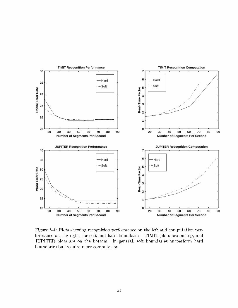
Hard

Soft

Hard

Soft

Hard

Soft

Hard

Soft

20 30 40 50 60 70 80 9025

26

27

28

29

30

Number of Segments Per Second

Pho

ne E

rror

Rat

e

TIMIT Recognition Performance

20 30 40 50 60 70 80 9010

15

20

25

30

35

40

Number of Segments Per Second

Wor

d E

rror

Rat

e

JUPITER Recognition Performance

20 30 40 50 60 70 80 900

1

2

3

4

5

6

7

Number of Segments Per Second

Rea

l−T

ime

Fac

tor

JUPITER Recognition Computation

20 30 40 50 60 70 80 900

1

2

3

4

5

6

7

Number of Segments Per SecondR

eal−

Tim

e F

acto

r

TIMIT Recognition Computation

Figure 5-4: Plots showing recognition performance on the left and computation per-formance on the right, for soft and hard boundaries. TIMIT plots are on top, andJUPITER plots are on the bottom. In general, soft boundaries outperform hardboundaries but require more computation.

55

much smaller on blocks than on the entire utterance. Therefore, the phenomenon

seen in Chapter 4, where broad-class segmentation failed to bring any computational

savings, may not apply to the algorithm processing small blocks. This experiment

examines whether broad-class models used on small blocks can boost computational

performance at a reasonable cost to recognition performance.

The set of broad-class models used in this experiment is the one shown in Fig-

ure 3-5. The segmentation algorithm uses Viterbi soft boundaries for TIMIT and

acoustic soft boundaries for JUPITER. The results are shown in Figure 5-5. Unlike

in Chapter 4, using broad-class models on the block algorithm can achieve com-

putational savings over the full-class models. In particular, broad-class models are

computationally cheaper for some operating points in TIMIT and all operating points

in JUPITER. However, as seen in Chapter 4, the full-class models perform better than

the broad-class models in terms of error rate. This is another tradeo� to be taken into

account when looking for an optimal operating point for the segmentation algorithm.

5.5.2 Final Experiments

Based on the results from the development experiments, �nal experiments on TIMIT

used Viterbi boundaries, and �nal experiments on JUPITER used acoustic bound-

aries. They were conducted on their respective test sets.

For TIMIT, an improvement over the baseline in terms of error rate, number of

segments, and computation was attained using soft Viterbi boundaries with full-class

models. In addition, when the recognizer was allowed to run without any computa-

tional constraints, a further error rate reduction was achieved by simply increasing

the size of the segment-graph. This result is shown in Table 5-2.

For JUPITER, the new segmentation algorithm achieved an improvement in terms

of error rate and number of segments using acoustic soft boundaries and full-class

models. However, the algorithm at that operating point required signi�cantly more

computation than the baseline. Using the set of 8 broad-classes shown in Figure 3-5

resulted in an algorithm that achieved an improvement in computation and number

of segments, but not in error rate. As a compromise between the two, experiments

56

Full−Class

Broad−Class

20 30 40 50 60 70 80 9025

26

27

28

29

30

Number of Segments Per Second

Pho

ne E

rror

Rat

e

TIMIT Recognition Performance

Full−Class

Broad−Class

20 30 40 50 60 70 80 900

1

2

3

4

5

6

Number of Segments Per SecondR

eal−

Tim

e F

acto

r

TIMIT Recognition Computation

Full−Class

Broad−Class

20 30 40 50 60 70 80 9010

15

20

25

30

35

40

Number of Segments Per Second

Wor

d E

rror

Rat

e

JUPITER Recognition Performance

Full−Class

Broad−Class

20 30 40 50 60 70 80 900

1

2

3

4

5

6

7

Number of Segments Per Second

Rea

l−T

ime

Fac

tor

JUPITER Recognition Computation

Figure 5-5: Plots showing recognition performance on the left and computation per-formance on the right, for broad-class and full-class segmentation. TIMIT plots are ontop, and JUPITER plots are on the bottom. In general, full-class models outperformbroad-class models, but the broad-class models require less computation.

57

Table 5-1: Set of 21 broad classes used for �nal JUPITER experiments.

Broad Class Members

1 y i e2 I E @ |3 ^ U { U4 a al ol o lÍ a⁄ 5 r rr rx6 l w ll7 u yu8 5 ir9 or ar10 a¤  O¤ 11 v D H12 f T h13 s z14 S Z J C15 b p16 d t17 g k18 m n 4 mm nn19 F tx20 b› d› g› p› t› ∑ k› h# h#1 h#221 ? iwt

using a set of 20 broad-classes shown in Table 5-1 were run. This con�guration of

the algorithm achieved an improvement in word error rate and number of segments

at a much more reasonable level of computation. Table 5-3 summarizes the test set

results for JUPITER. In the table, the result with the computational constraint used

the set of 20 broad-class models, and the result without the computational constraint

used the full set of models.

5.6 Chapter Summary

This chapter presented several modi�cations to the probabilistic segmentation algo-

rithm to enable it to run in a pipelined manner. The revised algorithm executes the

N-best algorithm in blocks de�ned by probable segment boundaries. These bound-

58

Table 5-2: Final TIMIT recognition results on the test set.

Error Rate (%) Segments/SecondBaseline 29.1 87.2With Computation Constraint 28.4 56.6Without Computation Constraint 28.1 61.3

Table 5-3: Final JUPITER recognition results on the test set.

Error Rate (%) Segments/SecondBaseline 10.6 99.7With Computation Constraint 10.5 65.2Without Computation Constraint 10.0 76.3

aries are de�ned by a boundary detection algorithm, two of which were explored in

this chapter. To allow the N-best algorithm to correct for mistakes in the bound-

ary detection algorithm, soft boundaries were introduced. These boundaries allow

the N-best algorithm to produce a path with a segment that crosses over a detected

boundary.

Experimental results on various versions of the block segmentation algorithm

were presented. These experiments show that the Viterbi boundaries work better

for TIMIT, and the acoustic boundaries work better for JUPITER. They also show

that, as expected, the choice between soft and hard boundaries involves a tradeo�

between recognition performance and computation. The same tradeo� is true for the

choice between broad-class and full-class models.

When optimal operating points were chosen for experiments on test data, improve-

ments in both TIMIT and JUPITER were attained. For TIMIT, at the same com-

putation level as the baseline, recognition error rate improved from 29.1% to 28.4%,

and size of the segment graph decreased from 87.2 to 61.3 segments per second. For

JUPITER, at a similar computation level as the baseline, error rates improved from

10.6% to 10.5% and segment-graph size decreased from 99.7 to 76.3 segments per

second. When no constraints were placed on computation, further error rate gains

were achieved with slightly larger segment-graphs. In TIMIT, recognition error rate

59

declined to 28.1% at 61.3 segments per second, and for JUPITER error rate declined

to 10.0% at 76.3 segments per second.

60

Chapter 6

Conclusion

6.1 Accomplishments

In this thesis, various modi�cations to the probabilistic segmentation algorithm pre-

sented in [2] were explored, with the goal of creating an algorithm that is fast, runs

in a pipeline, and results in competitive recognition error rate.

Computational savings were attained by replacing the segment-based search us-

ing only boundary-models with a much more e�cient frame-based search. Further

computational savings were attained by using acoustic landmarks located at irregu-

lar intervals rather than regularly spaced frames. A pipeline capability was achieved

by running the probabilistic segmentation algorithm in blocks de�ned by probable

segment boundaries.

Experiments were performed to study the computation and recognition tradeo�s

for several con�gurations of the algorithm. In particular, the di�erence in performance

between acoustic and Viterbi boundaries; soft and hard boundaries; and full-class and

broad-class segmentation were examined. Optimal operating points picked from these

experiments result in a segmentation algorithm that can produce an improvement in

error rate with signi�cantly fewer segments than the baseline acoustic segmentation.

The error rate improvement is greater when the recognizer is allowed to use signi�-

cantly more computation than the baseline recognizer.

61

6.2 Algorithm Advantages

The algorithm developed in this thesis has several attractive attributes. First, the

algorithm allows for a tradeo� between accuracy and computation as determined

by the number of segments produced. If computation is an important factor for

an application, the algorithm can be tuned to run faster than the baseline while still

producing a competitive error rate. If error rate is more important than computation,

the algorithm can be tuned to produce an optimal error rate signi�cantly better than

the baseline.

More importantly, the algorithm outputs a smaller segment-graph containing more

relevant segments than that produced by the baseline acoustic segmentation. This

allows more sophisticated segment-based modeling techniques to be explored. For

example, Chang has developed a novel segment-based acoustic modeling technique,

termed near-miss modeling, that relies on a quality segment-graph [1].

Finally, the algorithm produces information in the �rst pass recognizer that can

be reused to guide acoustic modeling in the subsequent segment-based search. For

example, if the �rst-pass recognizer identi�es a segment to be a fricative, then the

segment-based search can use features and models tailored for distinguishing between

phones within the fricative class. Heterogeneous measurements that improve within-

class classi�cation performance have been developed by Halberstadt [8]. They can

easily be applied to this framework.

6.3 Future Work

Possible extensions to this work include:

� Using a dynamic N tuned to the characteristics of each block. Currently the

number of segments in the segment-graph is controlled by N, the number of

paths used to produce the segment-graph. This N is a constant, regardless of

the size of the block being processed, or the con�dence that the segments in

the block are correct. Allocating a larger N to bigger blocks or blocks with low

62

con�dence should help to distribute segments to areas of the speech signal with

more uncertainty.

� Using word or syllable constraints in the probabilistic segmentation recognizer.

As discussed in Chapter 4, the segmentation algorithm can bene�t from such

constraints when the overall task of the segment-based recognizer is word recog-

nition.

� Investigating the tradeo� between memory and computation. This thesis con-

centrated on the tradeo� between recognition performance and computation,

without regard to memory requirements. However, memory can a�ect the speed

of execution as well if the memory requirements are so enormous that time spent

swapping memory dominates over time spent computing. This phenomenon is

seen at very large N in this thesis.

� Investigating the use of the A* word graph search instead of the A* N-best

search [9]. The word graph search directly computes a graph and should reduce

redundant computation used to expand previously seen segmentations in the

N-best search.

63

Bibliography

[1] J. Chang. Near-Miss Modeling: A Segment-Based Approach to Speech Recogni-

tion. PhD thesis, Massachusetts Institute of Technology, Department of Electri-

cal Engineering and Computer Science, 1998.

[2] J. Chang and J. Glass. Segmentation and modeling in segment-based recognition.

In Proc. Eurospeech, pages 1199{1202, Rhodes, Greece, 1997.

[3] Y. Chow and R. Schwartz. The N-best algorithm. In Proc. DARPA Speech and

Natural Language Workshop, pages 199{202, Cape Cod, MA, 1989.

[4] R. Cole and M. Fanty. Spoken letter recognition. In Proc. Third DARPA Speech

and Natural Language Workshop, pages 385{390, Hidden Valley, PA, 1990.

[5] W. Francis and H. Kucera. Frequency Analysis of English Usage: Lexicon and

Grammar. Houghton Mi�in, Boston, MA, 1982.

[6] J. Glass, J. Chang, and M. McCandless. A probabilistic framework for feature-

based speech recognition. In Proc. ICSLP, pages 2277{2280, Philadelphia, PA,

1996.

[7] W. Goldenthal. Statistical Trajectory Models for Phonetic Recognition. PhD

thesis, Massachusetts Institute of Technology, Department of Aeronautics and

Astronautics, 1994.

[8] A. Halberstadt and J. Glass. Heterogeneous acoustic measurements for phonetic

classi�cation. In Proc. Eurospeech, pages 401{404, Rhodes, Greece, 1997.

64

[9] I. Hetherington, M. Phillips, J. Glass, and V. Zue. A* word network search for

continuous speech recognition. In Proc. Eurospeech, pages 1533{1536, Berlin,

Germany, 1993.

[10] L. Lamel and J. Gauvain. High performance speaker-independent phone recogni-

tion using cdhmm. In Proc. Eurospeech, pages 121{124, Berlin, Germany, 1993.

[11] L. Lamel, R. Kassel, and S. Sene�. Speech database development: Design and

analysis of the acoustic-phonetic corpus. In Proc. DARPA Speech Recognition

Workshop, pages 100{109, Palo Alto, CA, 1986.

[12] J. Mari, D. Fohr, and J. Junqua. A second-order hmm for high performance word

and phoneme-based continuous speech recognition. In Proc. ICASSP, pages 435{

438, Berlin, Germany, 1996.

[13] N. Merhav and Y. Ephraim. Hidden markov modeling using the most likely state

sequence. In Proc. ICASSP, pages 469{472, Toronto, Canada, 1991.

[14] M. Phillips and J. Glass. Phonetic transition modelling for continuous speech

recognition. Journal of the Acoustical Society of America, 95(5):2877, 1994.

[15] A. Robinson. An application of recurrent nets to phone probability estimation.

IEEE Transactions on Neural Networks, 5(2):298{305, 1994.

[16] R. Schwartz and S. Austin. The N-best algorithm: An e�cient and exact proce-

dure for �nding the N most likely sentence hypothesis. In Proc. ICASSP, pages

81{84, Tokyo, Japan, 1990.

[17] R. Schwartz and S. Austin. A comparison of several approximate algorithms for

�nding multiple (N-best) sentence hypotheses. In Proc. ICASSP, pages 81{84,

Toronto, Canada, 1991.

[18] F. Soong and E. Huang. A tree-trellis based fast search for �nding the N best

sentence hypothesis in continuous speech recognition. In Proc. ICASSP, pages

705{708, Albuqueque, NM, 1990.

65

[19] S. Young and P. Woodland. State clustering in hidden markov model-based

continuous speech recognition. Computer Speech and Language, 8(4):369{383,

1994.

[20] V. Zue, S. Sene�, J. Glass, L. Hetherington, E. Hurley, H. Meng, C. Pao, J. Po-

lifroni, R. Schloming, and P. Schmid. From interface to content: Translingual

access and delivery of on-line information. In Proc. Eurospeech, pages 2047{2050,

Rhodes, Greece, 1997.

66