Probabilistic Robust Motion Planning for UAVs

Mangal KothariAssistant Professor

Department of Aerospace EngineeringIndian Institute of Technology Kanpur

Kanpur 208016mangal@iitk.ac.in

Finding a path is not enough !!!

Successful execution requires robust planning.

Challenges

• Localization uncertainty

• Modelling uncertainty

• Perception uncertainty

• Wind disturbance

• Situation awareness

• Motion constraints (e.g.

turn radius)

Problem Formulation

Consider the following stochastic system

subject to

Goal

Probability of leaving configuration space

Minimum time problem

Nonlinear Gaussian system

(e.g. turn radii constraint)

Path Planning Algorithms

Overview

• Cell decomposition method

• Potential Field

• Voronoi Diagram

• Visibility Line (VL)

• Probabilistic Roadmap (PRM)

• Rapidly-exploring Random Tree (RRT)

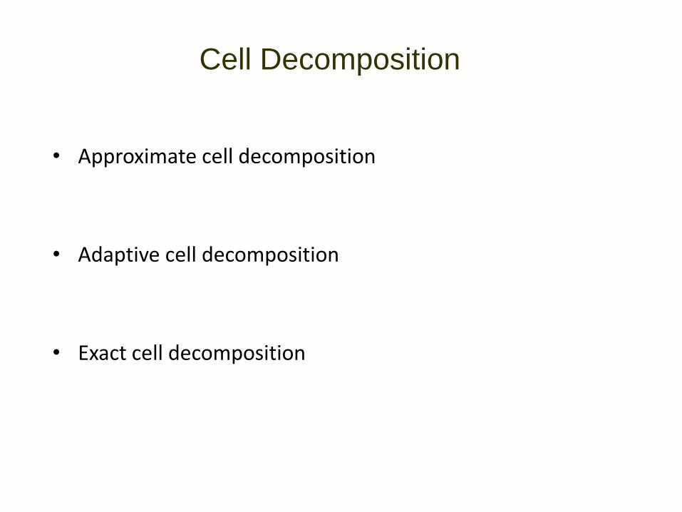
• Approximate cell decomposition

• Adaptive cell decomposition

• Exact cell decomposition

Cell Decomposition

Approximate Cell Decomposition

Start point

Target point

Adaptive Cell Decomposition

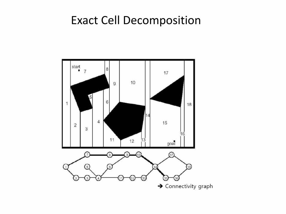
Exact Cell Decomposition

Potential Field

Start

point

Target

point

Voronoi Diagram

0 20 40 60 80 100 120 140 160 180 2000

20

40

60

80

100

120

140

160

180

200

1

2

3

45

X-Range (km)

Y-R

ange (

km

)

Start point

Target point

Visibility Line

Randomly chosen point

Path searched by algorithm

Probabilistic roadmap (PRM)

Start Point Target Point

Rapidly-exploring Random Tree (RRT)

1. Breadth-First Search (BFS)

2. Depth-First Search (DFS)

3. Dijkstra’s Algorithm

4. Best-First Search

5. A star (A*)

Search Algorithms

StartA

B DC

E GF H

Goal

Step 1: Explore paths A B

(Goal not found) A C

A D

Step 2: Explore paths A B E

(Goal not found) A B F

A C G

A D H

Step 3 : Explore paths ACGGoal

(Goal found)

In the event of tie, the left node is chosen

first.

Breadth-First Search (BFS)

StartA

B DC

E GF H

Goal

Step 1: Explore paths A B

(Goal not found)

Step 2: Explore paths A B E

(Goal not found) A B F

Step 3: Explore paths A C

(Goal not found)

Step 4 : Explore paths A C G

(Goal not found)

Step 5 : Explore paths A C G Goal

(Goal found)

In the event of tie, the left node is chosen first.

Depth-First Search (DFS)

• Dijkstra algorithm is used in graphs with varying costs of traversal.

• The cost is usually the length of the edge.

• Using this algorithm, one can find the shortest paths from a start node to all points in a graph if the cost is minimum.

• Dijkstra algorithm is guaranteed to find the shortest path.

Dijkstra Algorithm

A Star (A*)

• Use Best-First search (similar to Depth-First algorithm along with a heuristic to determine the next move)

• Use Best-First search and Dijkstra algorithm to estimate the distance to goal and distance to start, respectively

• The cost function can be expressed as follows:

f(n) = h(n) + g(n)

where f(n) is the total cost of the node, h(n) is theheuristic value of the node (from the goal), and g(n) isthe cost from the start position to the node

20

Motion planning problem (MPP)

Consider a linear time-invariant system (LTI)

Subject to

Physical constraints

Environmental constraints

21

Evaluating Constraint for Collision Avoidance

Collision with the jth obstacle (conjunction):

In order to avoid collision (disjunctions):

When the vehicle state is a random variable !!!

These constraints are not applicable

Another approach need to be considered

Stochastic Environments

In the probabilistic framework, compute

Joint chance constraint

Enforce

Evaluation of the Probabilistic Constraint

Simplify the joint chance constraint for the jth obstalce

If then

For probabilistic satisfaction, it is enough to show that one of surfaces

satisfies the above inequality.

Converting into the Equivalent Deterministic Constraint

Change of variable

Converted constraint

Chance constraint

Conversion: Constraint Tightening

The equivalent deterministic constraint

The constraint tightening depends on uncertainty in the position and on

the value of .

Condition: Multiple Obstacles

From Boole’s bound, we can write

By limiting

It can be ensured

Let be an event

Risk allocation can be done!!!

Problem Statement: Linear Systems

Find a sequence of control input that minimizes:

subject to

Kalman Filter theory

27MDP/POMDP

Problem Statement: Nonlinear Systems

Find a sequence of control input that minimizes:

subject to

Prediction step of EKF: belief

update (a priori distribution)

MDP: consider every reachable belief state28

Chance constrained RRT (CC-RRT) Algorithm

• Grow a tree of state distributions for a given time

• sample reference path (similar to waypoint selection)

• generate trajectory for the sampled path (use a control/guidance law to generate trajectory)

• evaluate the feasibility of the generated trajectory (using chance constraint)

• include the path in the existing tree if it is feasible

CC-RRT: Tree expansion

Closed-loop prediction (a priori distribution)

29

Trajectory Generation: Path Following

Fixed-wing UAV kinematic model

Path following law: pursuit and LOS

componentsPath following geometry

Error dynamics

Predicted trajectory

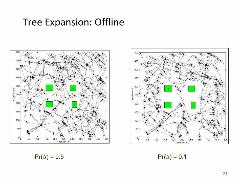
Tree Expansion: Offline

Pr(∆) = 0.5 Pr(∆) = 0.1

31

Numerical Results: Offline

Paths with different Pr(∆)

32

Online Implementation

• Employ a look-ahead strategy

• Expansion – grow the tree for the given time window

• with emphasis on exploration and optimization heuristics

• branch and bound method to keep only promising nodes

• Execution – choose the best path for execution and update the information (pop-up and dynamic obstacles)

• re-evaluate feasibility of the tree when new measurements are received

33

Numerical Results: Online

Sample tree after 1 sec Sample tree after execution of the first segment

Complete tracked path

34

Incorporation of a Sensor Model

Consider the following nonlinear Gaussian system

Let be the error between the nominal and actual systems. The

linearized error dynamics is given as

Nominal system

Compute a priori closed-loop distribution

Closed-loop DistributionsThe measurement step of Kalman Filter is given by

The augmented system

where

Closed-loop Update: Most likely Measurements

A priori distribution of the augmented system

Closed-loop belief update

Closed-loop prediction (with most likely future measurements)

Numerical Results: A Single Agent System

A Two Agent System

Thank You