PROBABILISTIC ROADMAP BASED PATH PLANNING FOR … · PROBABILISTIC ROADMAP BASED PATH PLANNING FOR...
34
PROBABILISTIC ROADMAP BASED PATH PLANNING FOR MOBILE ROBOTS NURUL FADZLINA BINTI JAMIN A project report submitted in partial fulfillment of the requirements for the award of the Degree of Master of Electrical Engineering Faculty of Electrical & Electronics Engineering Universiti Tun Hussein Onn Malaysia JANUARY 2014
Transcript of PROBABILISTIC ROADMAP BASED PATH PLANNING FOR … · PROBABILISTIC ROADMAP BASED PATH PLANNING FOR...

PROBABILISTIC ROADMAP BASED PATH PLANNING FOR MOBILE
ROBOTS
NURUL FADZLINA BINTI JAMIN
A project report submitted in partial
fulfillment of the requirements for the award of the
Degree of Master of Electrical Engineering
Faculty of Electrical & Electronics Engineering Universiti Tun Hussein Onn
Malaysia
JANUARY 2014

ABSTRACT
Probabilistic Road Map (PRM) is one of the well-known or common solution
methods used to solve the motion planning problem for mobile robot where the
initial point and target point (goal) are chosen or fixed by user on the robot
configuration workspace. In this study, the configuration space defined by static
random obstacles. Furthermore, the PRM method has been used to find a feasible
path between the start and the goal of the mobile robot. The PRM planner consists of
two phases: a construction and a query phases. In the construction phase, a roadmap
(graph) is built, approximating the motions that can be made in the environment.
First, a random configuration is created. Then, it is connected to some neighbors,
typically either the nearest neighbors or all neighbors less than some predetermined
distance. Configurations and connections are then added to the graph until the
roadmap is dense enough. In the query phase, the start and goal configurations are
connected to the graph, and a path is obtained by a Dijkstra's shortest path query. In
order to achieve a shorter path, the path pruning was applied in the system. The
system was analyzed and simulated using MATLAB software.

vii
ABSTRAK
Probabilistic Road Map (PRM) adalah salah satu kaedah penyelesaian yang
terkenal atau umum yang digunakan untuk menyelesaikan masalah perancangan
gerakan di mana titik permulaan dan titik sasaran (matlamat) dipilih atau ditetapkan
oleh pengguna pada ruang kerja konfigurasi robot. Dalam kajian ini, ruang
konfigurasi yang ditakrifkan oleh halangan statik secara rawak. Tambahan pula,
kaedah PRM itu telah digunakan untuk mencari laluan yang boleh dilaksanakan
antara titik permulaan dan matlamat mobile robot. Perancang PRM terdiri daripada
dua fasa iaitu fasa pembinaan dan fasa pertanyaan. Dalam fasa pembinaan, pelan
tindakan (graf) dibina, menghampiri pergerakan yang boleh dibuat dalam alam
sekitar. Pertama, konfigurasi rawak dicipta. Kemudian, ia akan dihubungkan atau
disambungkan dengan beberapa jiran, biasanya ia disambungkan kepada jiran
terdekat atau semua jiran dalam jarak yang telah ditetapkan. Konfigurasi dan
sambungan akan ditambahkan kepada graf sehingga laluan itu sempurna. Dalam fasa
pertanyaan pula, permulaan dan matlamat konfigurasi disambungkan kepada graf,
dan laluan yang diperolehi dengan laluan terpendek ditentukan oleh Dijkstra. Dalam
usaha untuk mencapai laluan yang lebih pendek, path pruning telah digunakan di
dalam sistem ini. Sistem ini telah dianalisis dan simulasi dengan menggunakan
perisian MATLAB.
CONTENT
CHAPTER CONTENT PAGE
SUPERVISOR'S DECLARATION
STUDENT'S DECLARATION
DEDICATION
ACKNOWLEDGEMENT
ABSTRACT
ABSTRAK
CONTENT
LIST OF TABLES
LIST OF FIGURES
LIST OF SYMBOLS AND ABBREVIATIONS
1 INTRODUCTION
1.0 Overview of Project
1.1 Problem Statement
1.2 Objectives of Project
1.3 Scope of the Project
1.4 Summary
1.5 Project Outline
2 LITE,RATURE REVIEW
2.0 Introduction
2.1 Two Wheels Mobile Robot
2.2 Path Planning Approaches
2.3 Global Path Planning
ii
iii
iv
v
vi
vii
viii
xi
xii
xvi

2.4 Local Path Planning
2.5 Classification of Robot Path Planning Method
2.6 Metric Maps
2.6.1 Path Planning on Metric Maps
2.7 Motion Planning
2.7.1 b Configuration Space
2.8 Shortest Path
2.9 Dijkstra's Algorithm
2.10 Summary
3 METHODOLOGY
3.0 Introduction
3.1 Project Methodology
3.2 Method and Approach
3.2.1 Roadmap
3.2.2 Voronoi Diagram
3.2.3 Probabilistic Roadmap
3.3 Djikstra's Algorithm
3.4 Software Implementation
4 RESULT AND DISCUSSIONS
4.0 Introduction
4.1 World Dimension
4.2 Initial Position and Goal Position
4.3 Dijkstra's Algorithm
4.4 Simulation of Path Planning Using PRM Method
4.5 Result of the Total Path and Computational Time
4.6 Result of the Graphical Using Interface (GUI)
4.7 Comparison
4.8 , Summary

5 CONCLUSION AND RECOMMENDATIONS
5.0 Introduction
5.1 Limitation
5.2 Recommendation
5.3 Conclusion
I
REFERENCES
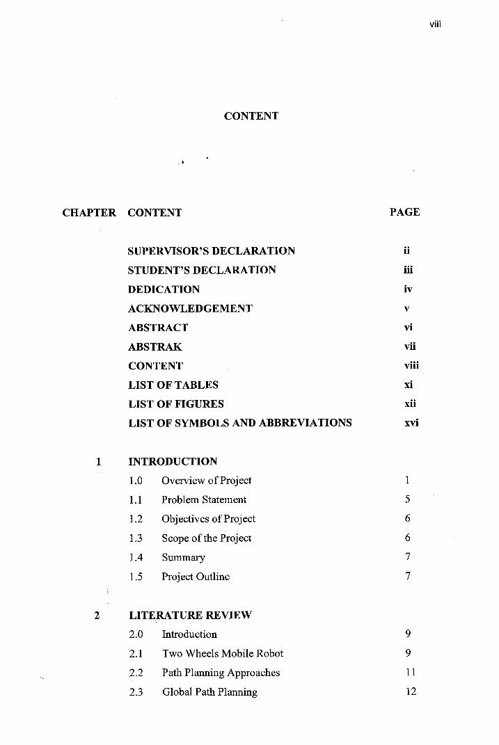
LIST OF TABLES
TABLE TITLE PAGE
4.1 The source code for creating the workspace 37
4.2 The source code for starting point and target point 39
4.3 The source code for Djikstra's Algorithm 40
4.4 The source code for path pruning 41
4.5 The result of computational time and total path taken 43
4.6 The number of obstacles fixed to 10 and number of
samples is varied 47
4.7 The number of samples fixed to 20 and number of
obstacles is varied

xii
LIST OF FIGURES
FIGURE TITLE PAGE
1.1 The path planning from initial point A to desired point B 2
1.2 The example of a valid path 2
1.3 The example of an invalid path 3
1.4 The example of a road map 4
2.1 The Mobile robot Dala as a car-like robot:
a non-holonomic system of dimension 4 with
two non holonomic constraints
2.2 The implementation of robot (a) Joe, (b) nBot and
(c) EMIEW 11
2.3 The diagram of the classification for robot path planning
method 15
The example of the workspace 18
2.5 The configuration space of a point-sized robot
(where white is Ckee and gray is Cobs) 19
CHAPTER 1 I
INTRODUCTION
1.0 Overview of Project
Generally, path planning is an important primitive for mobile robots that lets
robots find the shortest or otherwise optimal path between two points. In fact, path
planning is a core problem in robotics. In its basic version, the path planning problem
consists in the definition of the optimal sequence of rotations and translations needed in
order to move an object of a given geometry from an initial to a target configuration
while avoiding collisions with obstacles.
If the constraints on the motion depend only on the environment's obstacles and
on the relative position of the moving object, the problem is holonomic. On the other
hand, dynamic constraints are considered in planning the non-holonomic motion.
Typically, each of the programs that have been implemented on the robots is
fixed and difficult to be modified again. Modifications can solely be done on the sensor
of a robot or a machine that had been used. Due from that, the path planning should be
carried out appropriately in helping the robot to detect and avoid any obstacles around
them.

The robots will move smoothly by avoiding any obstacle to reach the desired
point using the shortest way if the correct path planning been applied as shown in Figure
1 .I [29]. Whereas Figure 1.2 and Figure 1.3 shown the example of the valid path and the
example of invalid path from the starting point to the ending point [30].
Figure 1.1 : The path planning from initial point A to desired point B
Figure 1.2: The example of a valid path

Figure 1.3: The example of an invalid path
Path planning, in fact, is an important issue in making a robot to get fi-om point A
to point B. Path planning algorithms are measured by their computational complexity.
The feasibility of real-time motion planning is depend on the accuracy of the map (or
floor plan), on robot localization and on the number of obstacles.
Topologically, the problem of path planning is related to the shortest path
problem of finding a route between two nodes in a graph. Planning is a term that gives
different meaning to different groups of people. Robotics addresses the automation of
mechanical systems that have sensing, actuation, and computation capabilities which are
the similar terms, such as autonomous systems.
The fundamental need in robotics is to have algorithms that convert high-level
specifications of tasks from humans into low-level descriptions of how to move. The
terms motion planning or path planning and trajectory planning are often used for these
kinds of problems [ 1 1.

Normally, the path planning is a core problem in robotics. In its basic version, the
path planning problem consists in the definition of the optimal sequence of rotations and
translations were needed in moving an object of a given geometry from an initial to a
target configuration while avoiding collisions with obstacles [I]. I
If the constraints on the motion depend solely on the environment's obstacles and
on the relative position of the moving object, the problem is holonomic. In non-
holonomic motions planning also dynamic constraints are considered.
Generally, the Probabilistic Roadmap (PRM) planner is one of a motion planning
algorithm in robotics field. This is used to solve the problem of find a path between a
starting point (starting configuration) of the robot and a desired point (goal
configuration) of the robot while avoiding the obstacle. The basic idea behind PRM is to
take random samples from the configuration space of the robot.
After that, testing them for whether they are in the free space and use a local
planner to attempt to connect these configurations to other nearby configurations as
example of road map- that was shown in Figure 1.4. In addition, the starting and goal
configurations are added in, and a graph search algorithm is applied to the resulting
graph to determine a path between the starting and goal configurations [2].

Figure 1.4: The example of a road map
1.1 Problem Statement
The main problem encountered in the motion of a robot is there are obstacles in
the field. This problem happens especially when having lots of obstacles that are
disturbing the movement of the robots in that field. As mentioned before, most of the
programs installed on the robot are fixed and difficult to be modified. Normally, the path
of the robot that has been programmed need to modified if the obstacles properties
changed from the original position. Besides, the robot might have a difficulty if the
obstacles move to new locations.
In order to solve the above-mentioned problem, a path planning method called
PRM is implemented so that the robot will be able move from an initial point to the
desired point by avoiding any obstacles standing in the field. As PRM is a method that
generates points randomly, it is computationally efficient and produces path that is
probabilistically complete.

One of the drawbacks of PRM method is the resulting path length is not optimal.
To address the issue, path pruning is applied in which the planned path is further tuned
as to make it shorter.
The impact of this prdject $ to help the robot developer or robot creator to have a
good technique for robot movement in the field or workspace by avoiding any
surrounding obstacles. The project is intended to improve the efficiency of the robot
motion by taking the shortest path from the initial point to achieve the desired point.
1.2 Objectives of Project
The main purpose of the project as listed:
a) To implement probabilistic roadmap (PRM) method for mobile robot path
planning.
b) To apply path pruning technique in order to shorten the planned path.
c) To analyze the efficiency of the path planning using PRM and path pruning
technique.
1.3 Scope of the Project
In order to achieve the objectives, the project is focus on implementation of path
planning using PRM method for the algorithm development. The project has also
focused on two wheels mobile robot. On the other hand, the number of sample is defined
randomly as well as the number of obstacle. The path planning will be implemented on

two wheels robot in order to avoid non-holonomic constraint such as minimum turning
radius. In addition, the system will be simulated and analyzed using MATLAB software.
1.4 Summary . *
This chapter has discussed about the overview of the project which includes the
objectives designation, as well as the scope of the project in order to give an insight and
idea of the project. On the other hand, it also comes out with a problem statement of the
project. Next chapter will discuss about the literature review on the functions, principles
and application on each component of this project.
1.5 Project Outline
The thesis comprises of 5 chapters altogether. Chapter 1 is on introduction,
Chapter 2 is literature review, Chapter 3 contains methodology, Chapter 4 is on result
and discussion followed by last chapter which is Chapter 5 is conclusion.
Chapter 1 is the section where the introduction of the thesis of project will be
discussed. The overview of the project will be outlined including problem statement, the
projects' objective, the project scope and also impact and significant of the research.
Chapter 2 there will be discussing the literature review of previous works from
thesis, journals, conference paper and experiments that related to the project. The review
includes Path Planning Approaches, Global Path Planning, Local Path Planning,
Classification of Robot Path Planning Method, Metric Maps, Path Planning on Metric
Maps and Configuration Space.

Chapter 3 represents the research methodology of this project. The step by step
procedure use to run this project from the beginning till end will be explained in detail.
This will also include the procedures or flow chart and processes involved for the
software development of the entire project. *
Chapter 4 consists of the experimental results and its respective analysis. The
result obtained will be discussed and explained here with the aid of figures. The
comparison of the every case will be discussed here.
In Chapter 5, here would be the summarized of the thesis and further
recommendation for the research.

CHAPTER 2 . *
LITERATURE REVIEW
2.0 Introduction
In order to design the path planning for the robot using PRM method, a research
needs to be conducted. The understanding about the path planning will be provided in
this literature review. The references for this project had been taken from journals,
conferences paper and articles which had been cited directly from the reliable internet
source.
2.1 Two Wheels Mobile Robot
A Virtual Wheel on a Two-Wheel Robot had integrated the method on the
mobile robot Dala as shown in Figure 2.1. The rotation is performed by applying
different velocities to the right and left wheels because this mobile robot is a differential-
driven robot. In spite of its four wheels, it has the same kinematic as a two-wheel robot
which virtual axle will be located in the middle of the real axles. In order to avoid too
much slipping and unnatural trajectories robot Dala had been considered as a car-like
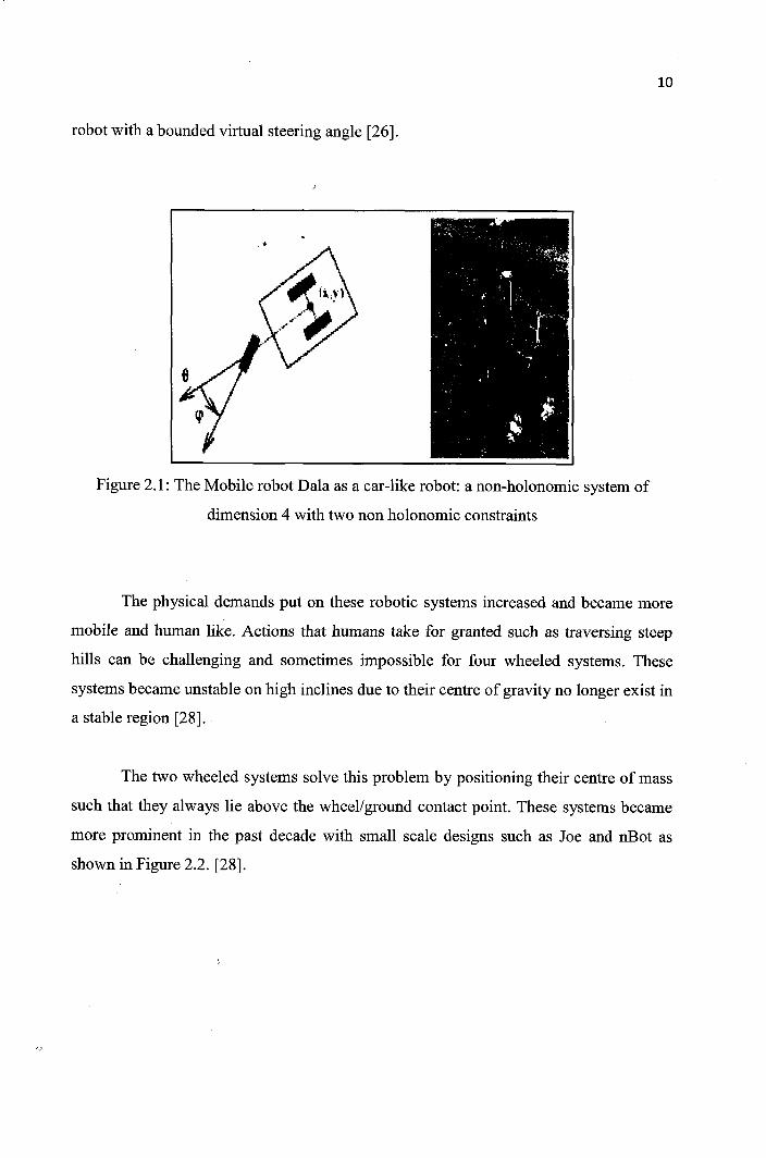
robot with a bounded virtual steering angle [26].
Figure 2.1 : The Mobile robot Dala as a car-like robot: a non-holonomic system of
dimension 4 with two non holonomic constraints
The physical demands put on these robotic systems increased and became more
mobile and human like. Actions that humans take for granted such as traversing steep
hills can be challenging and sometimes impossible for four wheeled systems. These
systems became unstable on high inclines due to their centre of gravity no longer exist in
a stable region [28].
The two wheeled systems solve this problem by positioning their centre of mass
such that they always lie above the wheellground contact point. These systems became
more prominent in the past decade with small scale designs such as Joe and nBot as
shown in Figure 2.2. [28].

Figure 2.2: The implementation of robot (a) Joe, (b) nBot and (c) EMIEW
2.2 Path Planning Approaches
Basically, various approaches have been introduced in order to implement the
path planning for a robot. The approaches based on the environment, type of sensor and
robot capabilities. Besides, they gradually contributed towards better performance in
term of time, distance, cost and complexity [3].
On the other hand, the plan is really needed between starting point and ending
point in creating a path that free from collision and satisfied certain optimization criteria
such as shortest path. It is because, the categorized path planning as an optimization
problem according to definition that, in a given mobile robot and a description of an
environment [4].
This definition is true if the purpose of solving path planning problem is only for
the shortest path because most new approaches are introduced toward shorter path. It is
because, by looking for the shorter path does not guarantee the time taken is shorter
because sometime the shorter path needs complex algorithm making the calculation to
generate output is longer [4].

The path planning problem can be grouped into global path planning and local
path planning. Global path planning requires complete knowledge about the
environment and a static terrain. In that setting a collision-free path from the start to the
destination configuration is generated before the vehicle starts its motion [19]. *
In addition, the global path planning problem had been addressed by many
researchers with common solutions being PRM methods and rapidly-expanding Random
Tree (RRT) methods. On the other hand, local path planning is executed in real-time
during flight. The basic idea is to sense the obstacles in the environment first and then
determines a collision-free path [20].
2.3 Global Path Planning
The global path planning is a path planning that requires robot to move with
prior information of environment. The information that derived from this algorithm was
about the environment first loaded into the robot path planning program before
determining the path to take from starting point to a target point. In this approach the
algorithm generates a complete path from the start point to the destination point before
the robot starts its motion [ 5 ] .
On the other hand, global path planning also is one of the processes for
deliberatively deciding the best way to move the robot from a start location to a goal
location. Thus for global path planning, the decision of moving robot from a starting
point to a goal is already made and then robotics released into the specified environment.
One of the early global path planning models that extensively studied is Piano's Mover
problem where full information is assumed to be available on the geometry, positions of
the obstacles and the moving object [5] .

In this model, the full complexity of the path generation problem has been
investigated, and a number of heuristic and non-heuristic approaches involving moving
rigid or hinged bodies in two or three dimensional space have been considered [5].
A few common appr'oaches are used in global path planning are Roadmap such
as Visibility Graph, Voronoi Graph and Silhouette, Cell Decomposition such as Exact
Decomposition, Approximate decomposition and Hierarchical Decomposition and also
new modern approaches such as Genetic Algorithm, Neural Network and Ant Colony
Optimization (ACO) [6].
2.4 Local Path Planning
The local path planning is a path planning that requires robot to move in
unknown environment or dynamic environment where the algorithm is used for the path
planning will response to the obstacle and the change of environment. Besides, the local
path planning also can be defined as real time obstacle avoidance by using sensory based
information regarding contingency measures that affect the save navigation of the robot
~71.
Normally in local path planning, a robot is guided with one straight line from
starting point to the target point which is the shortest path and robot follows the line till
it sense obstacle. Then the robot performs obstacle avoidance by deviating from the line
and in the same time update some important information such as new distance from
current position to the target point, obstacle leaving point and etc. In this type of path
planning, the robot must always know the position of target point from its current
position to ensure that robot can reach the destination accurately.
The potential field method is one of the well-known local paths planning
technique. In this path planning method, the robot is considered as a particle moving
under the influence of an artificial potential produced by the goal configuration and the
obstacles. The value of a potential function can be viewed as energy and the gradient of
the potential is force. The goal configuration is an attractive potential and the obstacles
are all repulsive potential [8]. I
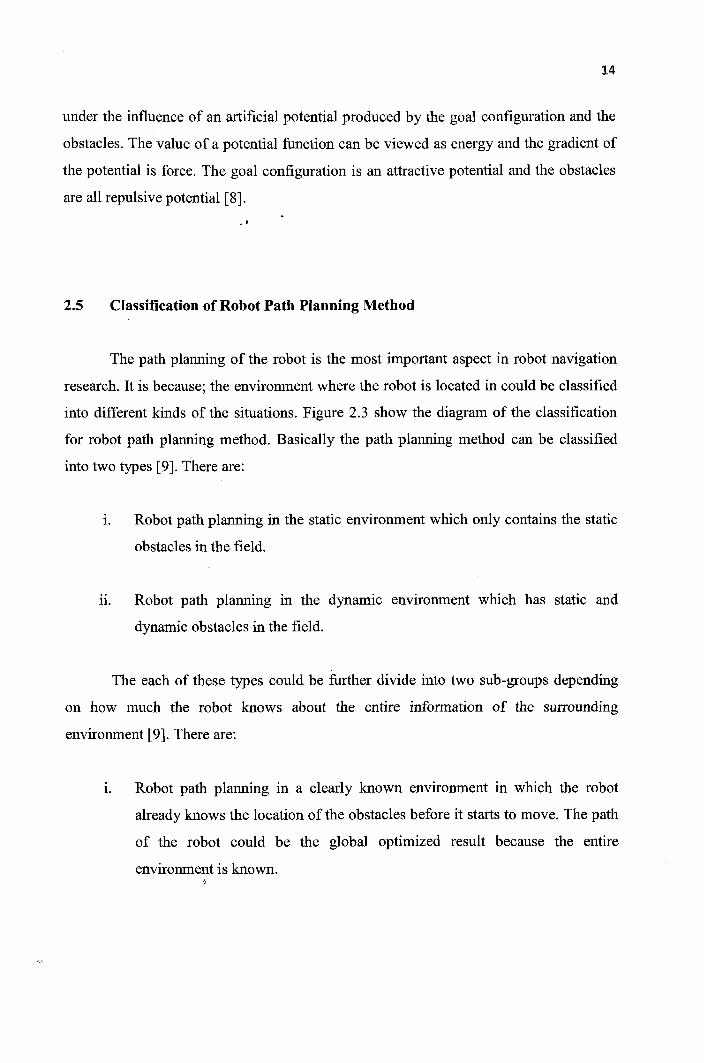
2.5 Classification of Robot Path Planning Method
The path planning of the robot is the most important aspect in robot navigation
research. It is because; the environment where the robot is located in could be classified
into different kinds of the situations. Figure 2.3 show the diagram of the classification
for robot path planning method. Basically the path planning method can be classified
into two types [9]. There are:
i. Robot path planning in the static environment which only contains the static
obstacles in the field.
. . 11. Robot path planning in the dynamic environment which has static and
dynamic obstacles in the field.
The each of these types could be fiuther divide into two sub-groups depending
on how much the robot knows about the entire information of the surrounding
environment [9]. There are:
i. Robot path planning in a clearly known environment in which the robot
already knows the location of the obstacles before it starts to move. The path
of the robot could be the global optimized result because the entire
environment is known.

. . 11. Robot path planning in a partly known or uncertain environment in which the
robot probes the environment using sensors to acquire the local information
of the location, shape and size of the obstacles. Then uses the information to
proceed the local path planning.
*
Figure 2.3: The diagram of the classification for robot path planning method
2.6 Metric Maps
The metric maps capture geometric properties of the environment are the number
of different map representations is very large, which none of them is dominant.
Basically, the regular grid is a two-dimensional array of square elements which called as
pixels.
It is also often called as occupancy grid, because each element in the grid will
hold a value representing whether the location in space is occupied or empty. On a

coarse grid, path planning is faster but obstacles are expanded on the grid and narrow
corridors can disappear [lo].
. *
2.6.1 Path Planning on Metric Maps
The A* algorithm finds a path as good as found by Dijkstra's algorithm but does
it much more efficiently using an additional heuristic to guide itself to the goal.
Dijkstra's algorithm uses a best first approach.
It works by visiting nodes in the graph starting from the start point and
repeatedly examining the closest not-yet examined node until it reaches the goal. A*
always first expands the node with the best cost calculated by the equation (2.1).
Where g(n) represents the cost of the path from the starting point to the node n ,
while h(n) represents the heuristic estimated cost from the node n to the goal. Usually,
for calculating the heuristic cost, the Manhattan or the Euclidean distance is used [l 11.
The D* algorithm is the dynamic version of A* producing the same result but
much faster in dynamic environments. In a sense of re-planning A* is computationally
expensive because it must re-plan the entire path to the goal every time new information
is added.
In contrast, D;Y: does not require complete re-planning since it adjusts optimal
path costs by increasing and lowering the cost only locally and incrementally as needed.

Expansions of D* algorithm, like Focused D*, D* Lite and Delayed D* are accordingly
even more efficient [I 1 1. i
The potential field planners are extremely easy to implement so it is very widely
represented. It treats the r d o t as a point under the influence of an artificial potential
field. The goal acts as an attractive force on the robot and the obstacles act as repulsive
forces. Such an artificial potential field smoothly guides the robot to the goal while
simultaneously avoiding known obstacles [12].
While potential field planners follow the gradient descent of the field to the goal
they always find the shortest path from every possible start point. Potential fields have
become a common tool in mobile robot application in spite of the local minima problem
[12]. The harmonic functions can be used to advantage for potential field path planning,
since they do not exhibit spurious local minima [13].
2.7 Motion Planning
A basic motion planning problem is to produce a continuous motion that
connects a start configuration S and a goal configuration G, while avoiding collision
with known obstacles. The robot and obstacle geometry is described in a 2-Dimensional
(2D) or 3-Dimensional (3D) workspace as shown in Figure 2.4, while the motion is
represented as a path in (possibly higher-dimensional) configuration space.

Figure 2.4: The example of the workspace
2.7.1 Configuration Space
A configuration describes the pose of the robot, and the configuration space C is
the set of all possible configurations. If the robot is a single point (zero-sized) translating
in a 2-dimensional (2D) plane (the workspace), C is a plane, and a configuration can be
represented using two parameters (x, y). Besides, if the robot is a 2D shape that can
translate and rotate, the workspace is still 2-dimensional.
However, C is the special Euclidean group SE(2) = R2 X SO(2) (where SO(2) is
the special orthogonal group of 2D rotations), and a configuration can be represented
using 3 parameters (x, y, 8). If the robot is solid 3D shape that can translate and rotate,
the workspace is 3-dimensional, but C is the special Euclidean group SE(3) = R3 X
S0(3), and a configuration requires 6 parameters: (x, y, z) for translation, and Euler
angles (a, P, y).
The last is, if the robot is a fixed-base manipulator with N revolute joints (and no
closed-loops), C is N-dimensional. The configuration space of a point-sized robot is

shown in Figure 2.5 and the configuration space for a rectangular translating robot was
shown in Figure 2.6.
Figure 2.5: The configuration space of a point-sized robot (where white is Cfiee and gray
is cobs)
Figure 2.6: The configuration space for a rectangular translating robot in red (where
white is Ck,, gray is Cobs, dark gray is the objects and light gray is configurations where
the robot would touch an object or leave the workspace)

The valid path between a start and a goal configuration for a movable object or
robot was found as a motion planning problem. A configuration is defined as an n-tuple
of values that determine the position of every point of the object. The workspace is the
place in which the robot moves [14].
I
In traditional robotics and animation applications, the workspace is composed of
one or more obstacles. The configuration space (C-space) is an n-dimensional space
where n being the number of degrees of freedom (DOF) of the robot consisting of all
robot configurations [14].
Providing coverage of wide-open regions of C-space, and representing the
connectivity of C-space is the main difficulties in constructing appropriate roadmaps for
PRM even in the presence of narrow passages. Respectively, the wide-open regions of
C-space would properly cover in order to generate milestones. [15].
More recently, a hybrid strategy combining a bridge test with a Gaussian
probability density function along narrow passages, and a uniform probability density
function in wide-open region of C-space was proposed in order to construct appropriate
roadmaps for workspaces with both characteristics. The bridge test is based on the
observation that a narrow passage in C has at least one restricted direction between C-
obstacles that can be identified by a short straight-line segment or bridge with endpoints
on two C-obstacles [15].
2.8 Shortest Path
As know, basically in the graph theory, the problem of finding a path between
two vertices or nodes in a graph we called the shortest path problem. It means the sum of
the weights of its constituent edges is minimized as shown in Figure 2.7. This is
analogous to the problem of finding the shortest path between two intersections on a
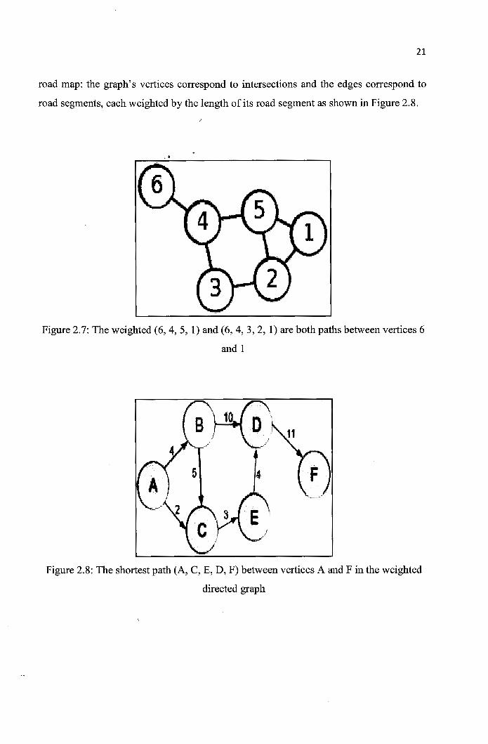
road map: the graph's vertices correspond to intersections and the edges correspond to
road segments, each weighted by the length of its road segment as shown in Figure 2.8.
Figure 2.7: The weighted (6,4, 5, 1) and (6,4, 3,2, 1) are both paths between vertices 6
and 1
Figure 2.8: The shortest path (A, C, E, D, F) between vertices A and F in the weighted
directed graph

The road network can be considered as a graph with positive weights. The nodes
represent road junctions and each edge of the graph is associated with a road segment
between two junctions. The weiglit of an edge may correspond to the length of the
associated road segment, the time needed to traverse the segment or the cost of
traversing the segment. Usin'g directed edges it is also possible to model one-way streets.
Such graphs are special in the sense that some edges are more important than others for
long distance travel such as highways [21]
This property has been formalized using the notion of highway dimension. There
are great numbers of algorithms that exploit this property and therefore able to compute
the shortest path a lot quicker than would be possible on general graphs [21].
The shortest path algorithms work in two phases. In the first phase, the graph is
preprocessed without knowing the source or target node. This phase may take several
days for realistic data and some techniques. The second phase is the query phase. In this
phase, source and target node are known. The running time of the second phase is
generally less than a second 1221
The idea is that the road network is static, so the preprocessing phase can be done
once and used for a large number of queries on the same road network. The algorithm
with the fastest known query time is called hub labeling and is able to compute shortest
path on the road networks of Europe or the USA in a fraction of a microsecond [22].
2.9 Dijkstra's Algorithm
The Dijkstra's Algorithm is a Graph Search Algorithm that solves the problem
for the shortest path with a positive edge and indirectly will result in the shortest path.
Dijkstra's algorithm is often used to create all the routes by calculating the distance and
aggregating data to obtain the lowest or shortest distance as shown in Figure 2.9. This
algorithm is often used in routing and as a subroutine in other graph algorithms [23].
The given source node in the graph, the algorithm finds the path with lowest cost
or the shortest path betweeii that node and every other node. It can also be used for
finding costs of shortest paths from a single node to a single destination node by
stopping the algorithm once the shortest path to the destination node has been
determined.
For example, if the nodes of the graph represent cities and edge path costs
represent driving distances between pairs of cities connected by a direct road, Dijkstra's
algorithm can be used to find the shortest route between one city and all other cities. As
a result, the shortest path first is widely used in network routing protocols, most notably
Open Shortest Path First (OSPF) [24].
In addition, the Dijkstra's original algorithm does not use a min-priority
queue and runs I 0(1vl2); where IVI is the number of nodes. They said, the idea of this
algorithm is also given by another researcher [25]. The implementation based on a min-
priority queue implemented by a Fibonacci heap and running in O(IEJ+IVI log IVI);
where IEI is the number of edges. This is asymptotically the fastest known single-source
shortest-path algorithm for arbitrary directed graphs with unbounded non-negative
weights [24].

Figure 2.9: The example of Dijkstra's Algorithm (It picks the unvisited vertex with the
lowest-distance, calculates the distance through it to each unvisited neighbor, and
updates the neighbor's distance if smaller. Mark visited set to red when done with
neighbors)
2.10 Summary
All the references for this literature review of this project have helped the author
to generate ideas in order to execute this project successfblly. Based on the knowledge
and understanding after reading each reference, most of the papers of the others
researchers used similar method with this project but applied on a different kind of
robot. Due to that, researcher can get several ideas from other researchers' paper in order
to implement the PRh4 method for path planning of the ground robot.

REFERENCES i
[l] LaValle S.M. (2006), "Planning Algorithms", University of Illinois,
Published by Cambridge University Press.
[2] Kavraki L.E., Svestka P., Latombe J.C. and Overmars M.H. (1996),
"Probabilistic Roadmaps For Path Planning In High-Dimensional
Configuration Spaces ", IEEE Transactions on Robotics and Automation.
[3] Sariff N. and Buniyamin N. (2010), "Ant Colony System for Robot Path
Planning In Global Static Environment", in 9th WSEAS International
Conference on System Science and Simulation in Engineering.
[4] Al-Tahanva I., Sheta A., Al-Weshah M. (2008), "A Mobile Robot Path
Planning Using Genetic Algorithm In Static Environment", Journal of
Computer Science.
[ 5 ] Sedighi K., Ashenay H., Manikas K., Wainwright T.W. and Tai R.L. (2004),
l!Autonomous Local Path Planning For A Mobile Robot Using A Genetic
Algorithm ", in Congress on Evolutionary Computation.
[6] Xiong L., Xiao-ping F., Sheng Y. and Heng Z. (2004), "A Novel Genetic
Algorithm for Robot Path Planning In Environment Containing Large
Numbers Of Irregular Obstacles ", ROBOT.
[7] Kumar E.V., Aneja M. and Deodhare D. (2008), "Solving A Path Planning
Problem In A Partially Known Environment Using A Swaim Algorithm", in
IEEE International Symposium on Measurements and Control in Robotics
Bangalore, India. /
[8] Khatib 0. (1998), "Real-Time Obstacle Avoidance for Manipulators and .
Mobile Robots ", the International Journal of Robotics Research: p. 90-98.
[9] Hui Miao (2009), "Robot Path Planning in Dynamic Environments Using a
Simulated Annealing Based Approach ", Faculty of Science and Technology,
Queensland University of Technology.
[ lo ] Elfes A. (2000), "Using Occupancy Grids for Mobile Robot Perception and
Navigation ", journal of Robotic System, IEEE Computer.
[I 11 Kristo H. (2006), "Path Planning and Learning Strategies for Mobile Robots
In Dynamic Partially Unknown Environments ", Faculty of Mathematics and
Computer Science, University of Tartu, Estonia.
[12] Choset H., Lynch K.M., Hutchinson S., Kantor G., Burgard W., Kavraki L.E.,
Thrun S. (2005), "Principles of Robot Motion", the MIT Press.
[13] Connolly C.I. and Grupen R.A. (1992), "The Application of Harmonic
Functions To Robotics ", Journal of Robotic Systems.
[14] Latombe J.C. (1991), "Robot Motion Planning", Boston, MA: Kluwer
Academic Publishers.
[15] Zhang G., Ferrari S. and Qian M. (2009), "An Information Roadmap Method
for Robotic Sensor Path Planning", Department of Mechanical Engineering
and Materials Science, Duke University, Durham.