Probabilistic multifactorial grammar and lexicology · Chapter 12. Probabilistic multifactorial...

chapter 12

Probabilistic multifactorial grammar and lexicology

Binomial logistic regression

What you will learn from this chapter:

In this chapter you will learn how to model the speaker’s choice between two near synonymous words or constructions on the basis of contextual features. The most popular statistical tool that is used to create such models is logistic regression. The approach is illustrated by a case study of two Dutch causative auxiliaries. As in the case of linear regression, you will learn how to create, test and interpret a logistic model with the help of different R tools.

12.1 Introduction to logistic regression

Logistic regression models the relationships between a categorical response variable with two or more possible values and one or more explanatory variables, or predictors. This technique is particularly popular in probabilistic multifactorial models that explain and predict the speaker’s choice between two or more near synonyms or variants on the basis of conceptual, geographic, social, pragmatic and other factors. If there are two possible outcomes (i.e. near synonyms), the logistic model is called binomial, or dichotomous. In case of three and more outcomes, we deal with multinomial, or polytomous regression. This chapter will discuss binomial models. Multinomial models will be introduced in the next chapter.

The structure of a logistic regression model is very similar to that of a linear regression model. It can be represented by the following equation:

g(x) = b0 + b1x1 + b2x2 + …

where g(x) is called the logit (or log odds) of the outcome (i.e. construction A or B). It is a value that reflects the chances of one outcome compared with the other outcome for a given configuration of values of the predictors. In multifactorial grammar, the logit repre-sents the chances of construction A to be chosen in a particular type of context compared with the chances of construction B to be used in the same type of context. These chances

254 How to do Linguistics with R

depend on the predictors shown in the right part of the equation. For example, one can expect that the chances that the speaker will choose the modal verb may as opposed to might to express probability depend on the degree of (un)certainty. The chances of choos-ing the word gown as opposed to dress may depend on the degree of formality of the event and length of the clothing item. The chances of windshield compared with windscreen may depend on the variety of English used by the speaker.

The remaining components of the formula are identical to the basic components of linear regression discussed in Chapter 7. The first term, b0, is the intercept. It is the value that determines the chances of an outcome when all predictors are equal to zero (for quan-titative variables) or the reference value (for categorical variables).1 The terms b1, b2, and so on, are the estimates of the effect of x1, x2, etc. They show by how much the chances of a particular outcome will increase or decrease when the value of the predictor (e.g. certainty, formality, language variety, etc.) changes.

Fitting a model means finding the values of all coefficients b0, b1, b2, etc. The main method for fitting regression models is called maximum likelihood. When fitting a logis-tic regression model, the algorithm tries again and again different sets of values of the model parameters and returns the combination which maximally closely models the actual outcomes.

However, after R returns you a fitted model with specific values of the coefficients, this is only a beginning of your analysis. As in linear regression, one has to carry out model diagnostics and evaluation. These steps will be considered in the remaining part of the chapter and illustrated in a case study of the Dutch causative constructions with doen ‘do’ and laten ‘let’.

12.2 Logistic regression model of Dutch causative auxiliaries doen and laten

12.2.1 Theoretical background and data

To reproduce the code in this case study, you will need the following add-on packages that should be installed (if you have not installed them yet) and loaded:

> install.packages(c("rms", "visreg", "car"))> library(Rling); library(rms); library(visreg); library(car)

Causative constructions with doen and laten in Dutch, similar to the English constructions make/have/get/cause X (to) do Y, refer to complex causative events, which normally involve

1. This holds for the treatment coding, when one level is chosen as the reference level (see Chapter 7). This is the default coding of categorical and binary variables in R, and also the most convenient one for fitting and interpreting logistic regression models.

Chapter 12. Probabilistic multifactorial grammar and lexicology 255

the causing event, the effected event, the Causer (the entity that initiates the causation) and the Causee (the entity that actually carries out the effected event). Consider the following example:

(1) Hij deed me denken aan mijn vader. He did me think at my father “He reminded me of my father.”

In this example, hij ‘he’ is the Causer and me ‘me’ is the Causee. The auxiliary deed (the past form of doen) relates to the causing event, and the infinitive denken ‘think’ designates the effected event, i.e. what happened as the result of the causing event. As in all analytic causatives, the causing event (what the Causer actually did to bring about the effected event) is left unspecified.

The differences between the constructions with doen and laten have been explored extensively (e.g. Verhagen & Kemmer 1997; Levshina 2011). Most researchers agree that the construction with doen denotes direct causation, whereas the laten-construction refers to indirect causation. Direct causation means that “there is no intervening energy source ‘downstream’ from the initiator: if the energy is put in, the effect is the inevitable result” (Verhagen & Kemmer 1997: 70). Indirect causation, which also includes the situations of enablement and permission, emerges when the situation “can be conceptualized in such a way that it is recognized that some other force besides the initiator is the most immediate source of energy in the effected event” (Verhagen & Kemmer 1997: 67).

Compare (1) with (2). While in (1) the causation is construed as involuntary, not con-trolled by the Causee, who is the affected entity, in (2) the main source of energy is the Causee, who acts deliberately. Thus, in (2) the causation is less direct than in (1):

(2) Ik liet hem mijn huis schilderen. I let him my house paint “I had him paint my house.”

One could think of several ways of operationalizing this difference in a corpus-based quantitative study. First, as Verhagen & Kemmer (1997) show, (in)directness is closely related to the semantic characteristics of the main participants. Four types of causation are distinguished:

– inducive: a mental Causer acts upon a mental Causee – volitional: a mental Causer acts upon an non-mental Causee – affective: a non-mental Causer acts upon a mental Causee – physical: a non-mental Causer acts upon a non-mental Causee

Verhagen & Kemmer (1997) demonstrate that inducive causation ‘favours’ laten, since a human entity normally does not act upon another human mind directly (except for telepathy). In contrast, affective and physical causation ‘prefer’ doen because an inanimate


Causer usually produces direct effect, as in (1). There are no theory-driven expectations about volitional causation; it can be both direct and indirect.

Another operationalization of directness and indirectness is (in)transitivity of the effected predicate (denken ‘think’ in the first example, and schilderen ‘paint’ in the second one). If the effected predicate is intransitive, the causation chain is short, and the causation can be seen as more direct. If the predicate is transitive, and there is a third entity, which is affected by the causation, like the house in (2), the causation chain is longer and the causa-tion is less direct.

In addition to the conceptual factors related to (in)directness of causation, we should take into account a geographic factor, namely, Netherlandic or Belgian (Flemish) variety of Dutch. As was mentioned in the previous chapter, the decrease in the use of causative doen has been especially dramatic in Netherlandic Dutch.

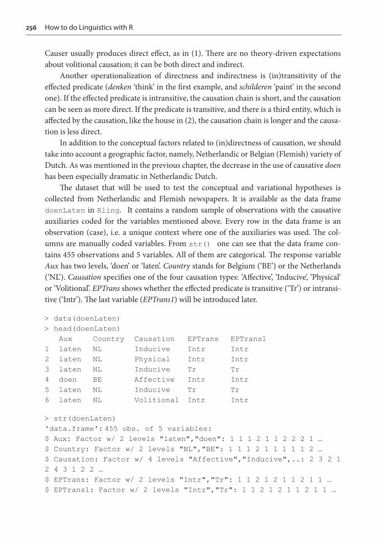
The dataset that will be used to test the conceptual and variational hypotheses is collected from Netherlandic and Flemish newspapers. It is available as the data frame doenLaten in Rling. It contains a random sample of observations with the causative auxiliaries coded for the variables mentioned above. Every row in the data frame is an observation (case), i.e. a unique context where one of the auxiliaries was used. The col-umns are manually coded variables. From str() one can see that the data frame con-tains 455 observations and 5 variables. All of them are categorical. The response variable Aux has two levels, ‘doen’ or ‘laten’. Country stands for Belgium (‘BE’) or the Netherlands (‘NL’). Causation specifies one of the four causation types: ‘Affective’, ‘Inducive’, ‘Physical’ or ‘Volitional’. EPTrans shows whether the effected predicate is transitive (‘Tr’) or intransi-tive (‘Intr’). The last variable (EPTrans1) will be introduced later.

> data(doenLaten)> head(doenLaten) Aux Country Causation EPTrans EPTrans11 laten NL Inducive Intr Intr2 laten NL Physical Intr Intr3 laten NL Inducive Tr Tr4 doen BE Affective Intr Intr5 laten NL Inducive Tr Tr6 laten NL Volitional Intr Intr

> str(doenLaten)'data.frame': 455 obs. of 5 variables:$ Aux: Factor w/ 2 levels "laten","doen": 1 1 1 2 1 1 2 2 2 1 …$ Country: Factor w/ 2 levels "NL","BE": 1 1 1 2 1 1 1 1 1 2 …$ Causation: Factor w/ 4 levels "Affective","Inducive",..: 2 3 2 1 2 4 3 1 2 2 …$ EPTrans: Factor w/ 2 levels "Intr","Tr": 1 1 2 1 2 1 1 2 1 1 …$ EPTrans1: Factor w/ 2 levels "Intr","Tr": 1 1 2 1 2 1 1 2 1 1 …


The frequencies of doen and laten are as follows:

> summary(doenLaten$Aux)laten doen277 178

How many observations are needed for logistic regression?

There exist different rules of thumb for logistic regression. According to one of them, the maximal number of parameters (i.e. all b-values in the formula) in a logistic regres-sion model is approximately equal to the frequency of the less frequent outcome divided by 10 (Hosmer & Lemeshow 2000: 346–347). In our case, the less frequent auxiliary is doen. It occurs 178 times. Therefore, the maximum number of regression parameters is 178/10 ≈ 18. As you can see from the tables of regression coefficients presented below, the number of parameters in different models tested in this chapter is much lower.

12.2.2 Fitting a binary logistic regression model: Main functions

The main function in this analysis is lrm() from the add-on package rms. We will be using lrm() most of the time because it returns many useful statistics. However, for some purposes you will also need glm()for generalized linear models from the base package. The use of these functions is similar but not identical. The main arguments of the func-tions are the formula and the data. In the formula, the response variable should be on the left side of the tilde sign, and all the predictors of interest should be on the right. An important difference between the functions is that the glm() function requires that you specify the type of the model (i.e. binomial logistic) by adding the argument family = binomial.

To fit a logistic regression model with lrm(), you can use the following template:

> yourModel1 <- lrm(Outcome ~ PredictorX + PredictorY + …, data = yourData)

To create a logistic model with glm(), use the following:

> yourModel2 <- glm(Outcome ~ PredictorX + PredictorY + …, family = binomial, data = yourData)


To see the coefficients and other statistics of the model fitted with lrm(), you can simply type in the name of the model:

> yourModel1

To do the same with glm(), you should use the summary() function:

> summary(yourModel2)

Let us illustrate this by fitting a model with Aux as the response and three predictors with the help of lrm():

> m.lrm <- lrm(Aux ~ Causation + EPTrans + Country, data = doenLaten)> m.lrm

Logistic Regression Model

lrm(formula = Aux ~ Causation + EPTrans + Country, data = doenLaten) Model Likelihood Discrimination Rank Discrim. Ratio Test Indexes IndexesObs 455 LR chi2 271.35 R2 0.609 C 0.894laten 277 d.f. 5 g 2.296 Dxy 0.787doen 178 Pr(>chi2) <0.0001 gr 9.935 gamma 0.817max |deriv| 1e-07 gp 0.378 tau-a 0.376 Brier 0.112 Coef S.E. Wald Z Pr(>|Z|)Intercept 1.8631 0.3771 4.94 <0.0001Causation=Inducive -3.3725 0.3741 -9.01 <0.0001Causation=Physical 0.4661 0.6275 0.74 0.4576Causation=Volitional -3.7373 0.4278 -8.74 <0.0001EPTrans=Tr -1.2952 0.3394 -3.82 0.0001Country=BE 0.7085 0.2841 2.49 0.0126

After the line with the formula, the output contains several columns with different statis-tics. The column on the left reports the total number of observations and the frequency of each outcome.

The column ‘Model Likelihood Ratio Test’ says whether the model is significant in general. This is an omnibus test, similar to the F-test in linear regression and ANOVA. In this column, one can find the Likelihood Ratio test statistic, the number of degrees of freedom and the p-value. The null hypothesis of the test is that the deviance (a term for unexplained variation in logistic regression) of the current model does not differ from the deviance of a model without any predictors. In such a model, which is called the intercept-only model, the probability of each outcome is kept constant for all observations. Since the p-value is smaller than 0.05, our model is significant, i.e. at least one predictor significantly deviates from zero.


The two columns on the right contain various goodness-of-fit statistics. The most fre-quently reported statistics for logistic regression are the concordance index C, also known as the area under the ROC-curve, and the Nagelkerke pseudo-R2. If you take all possible pairs that contain a sentence with doen and a sentence with laten, and try all combinations, the statistic C will be the proportion of the times when the model predicts a higher prob-ability of doen for the sentence with doen, and a higher probability of laten for the sentence with laten (see below on how these probabilities are computed). For this model, C = 0.894. This means that for 89.4% of the pairs of doen and laten examples, the predicted prob-ability of doen is higher for the sentence where the speaker actually used doen than for the example where laten occurred. How good is this result? Hosmer & Lemeshow (2000: 162) propose the following scale:

C = 0.5 no discrimination 0.7 ≤ C < 0.8 acceptable discrimination 0.8 ≤ C < 0.9 excellent discrimination C ≥ 0.9 outstanding discrimination

It seems that our model discriminates well.The second important measure is the Nagelkerke pseudo-R2 (R2). It ranges from 0

(no predictive power) to 1 (perfect prediction). However, in logistic regression R2 tends to be lower than in linear regression models, where this statistic originates from, even if the quality of models is comparable. This is why Hosmer & Lemeshow (2000: 167) do not rec-ommend reporting the statistic. Another reason is that it is less conceptually clear than its linear regression counterpart, which shows the proportion of total variance in the response explained by the model (see Chapter 7).

Next, let us have a look at the table of coefficients. The first estimate belongs to the inter-cept. This value (1.8631) is the estimated log odds of the outcome when all predictors are at their reference levels (for categorical variables) or are equal to zero (for quantitative vari-ables). The reference levels of each variable correspond to affective causation, intransitive Effected Predicate and Netherlandic Dutch. Note that this holds only for the treatment cod-ing of categorical variables, which is the default in R. But which outcome is meant here, doen or laten? The algorithm compares the second level of the factor that represents the outcome with the first, or reference level. To check the order of levels, you can type in the following:

> levels(doenLaten$Aux)[1] "laten" "doen"

Thus, the algorithm compares the second level (‘doen’) with the reference level (‘laten’). To obtain simple odds, one should exponentiate the coefficient with the help of exp(), which is the opposite of log():

> exp(1.8631)[1] 6.443681


Compare:

> log(6.443681)[1] 1.8631

This means that the odds of doen vs. laten in affective causation contexts with intransi-tive Effected Predicates and in the Netherlandic variety are approximately 6.44. Recall that odds greater than 1 mean that the probability of the first outcome is greater than the prob-ability of the second outcome (see Chapter 9). If odds are between 0 and 1, the probability of the first outcome is smaller than that of the second outcome. The odds of 6.44 mean that the chances of doen are 6.44 times greater than those of laten for this type of context (affec-tive causation, intransitive verb, Netherlandic newspapers).

Next, let us interpret the coefficients of the predictors, which are represented as log odds ratios. What do they indicate? A log odds ratio compares the odds of the outcome for each level of a predictor with the reference level (the default option). The Causation variable has four levels, but only three are shown in the table of coefficient. ‘Affective’ is the reference level. EPTrans has two levels, but only EPTrans = ‘Tr’ is shown. The Country variable has two levels (‘NL’ and ‘BE’), but the table shows only the coefficient of Country = ‘BE’. If the reference value is not specified by the user, the program selects the one that comes first alphabetically: EPTrans = ‘Intr’ and Causation = ‘Affective’. As for Country with the values ‘BE’ and ‘NL’, the reference level ‘NL’ has been selected manually. Which value of a predictor is selected as the reference level, is not important statistically. However, for the purposes of interpretation you might wish to choose the reference level manually (see Chapter 4).

After this introduction, let us interpret the coefficients. Unlike simple odds and odds ratios, where equal probabilities correspond to 1, log odds and log odds ratios are centred around zero. If the coefficient is positive, the level specified in the table boosts the chances of doen (and therefore decreases the odds of laten). If the coefficient is negative, the speci-fied level decreases the odds of doen (and boosts the chances of laten). For Causation, the reference level is ‘Affective’. We see that inducive and volitional causation types have nega-tive coefficients. That means that they decrease the odds of doen (and, conversely, boost the chances of laten) in comparison with affective causation. Physical causation has a positive estimate, so it seems to boost the chances of doen in comparison with the reference level. Transitive Effected Predicates seem to ‘disfavour’ doen (or ‘favour’ laten) when compared with intransitives. The odds of doen in the Belgian variety of Dutch are higher than those in the Netherlandic variety.

The log odds ratios, like odds ratios, represent the effect size. To transform log odds ratios into simple odds ratios, one can use exponentiation. For example, if the log odds ratio of doen in the Belgian variety vs. the Netherlandic variety is 0.7085, the simple odds ratio is computed as follows:


> exp(0.7085)[1] 2.030943

Therefore, the odds of doen vs. laten in the Belgian variety of Dutch are approximately 2.03 times higher than those in the Netherlandic variety, other variables being con-trolled for.

This model contains only categorical predictors. In case of quantitative independent variables, their coefficients will show the change in the probability of a given outcome per measure unit (per word, per second, etc.).

Odds, log odds, odds ratios and log odds ratios

These notions are very important for understanding of logistic regression and interpre-tation of its results. Although odds and odds ratios have been already introduced (see Chapter 9), this box provides an overview of the old and new terms together.

Odds are a simple ratio of the probability of one event to the probability of another event, which can be expressed in a simplified form as a ratio of the frequency of out-come X to the frequency of non-X. The odds of doen vs. laten can be calculated as the ratio of occurrences of the causative doen to the frequency of laten, 178/277 ≈ 0.64. If odds equal 1, the probabilities of the outcomes are equal. If odds are greater than 1, the chances of the first event to happen are greater. If odds are between 0 and 1, as the odds of doen in this case study, the other outcome (laten) is expected to be used more frequently.

Odds should not be confused with probabilities, which are normally expressed as proportions or percentages. The proportion of doen in our data is equal to the number of occurrences of doen divided by the total number of observations: 178/455 ≈ 0.39, or 39%. If the chances of two events are equal, the probability of either outcome is 0.5, or 50%. Probabilities range from 0 to 1 (or from 0% to 100%).

Log odds are logarithmically transformed odds. We will be speaking about the natural logarithm (ln, or log() in R) everywhere in this chapter. Log odds have a nice property of being centred around 0 because the natural logarithm of 1 (when the odds of two outcomes are equal) is 0. The log odds of doen in our data are then ln(0.64) ≈ –0.45. The negative log odds show that this outcome is less probable than the other one (laten). The value of log odds can range from -Infinity (the natural logarithm of 0) to Infinity. Another name for log odds is logit.

(Continued)


Odds ratio is the ratio of two odds. Consider the odds of doen in the Belgian and Netherlandic varieties of newspaper Dutch. The odds ratio will look as follows:

doenin BElatenin BEOR doeninNLlateninNL

=

Similar to simple odds, an OR of 1 would mean that there is no difference between the odds of doen in the two varieties. If an OR is greater than 1, the odds of doen vs. laten in Belgian Dutch are higher than those in Netherlandic Dutch. If an OR is between 0 and 1, the odds of doen vs. laten in Belgian Dutch is smaller than in Netherlandic Dutch. To compute the actual odds ratio, one needs the frequencies of the auxiliaries in both varieties of Dutch:

> table(doenLaten$Aux, doenLaten$Country)

NL BElaten 162 115doen 71 107

The odds of doen vs. laten in the Belgian data are 107/115 ≈ 0.93. The value is close to 1 because doen is almost as frequent as laten in the Belgian sample. The odds of doen vs. laten in the Netherlandic newspapers are much lower: 71/162 ≈ 0.44. The odds ratio is then 0.93/0.44 ≈ 2.12. This means that the odds of doen in the Belgian newspapers are about twice as high as those in the Netherlandic newspapers.

Finally, a logarithm of an odds ratio is called the log odds ratio. In our case, ln(2.12) ≈ 0.75. In fact, this is the coefficient of Country = ‘BE’ in a model with Country as the only predictor:

> m.Country <- lrm(Aux ~ Country, data = doenLaten)> m.Country[output omitted]

Coef S.E. Wald Z Pr(>|Z|)Intercept -0.8249 0.1423 -5.80 <0.0001Country=BE 0.7528 0.1957 3.85 0.0001

Thus, the coefficients of predictors are log odds ratios. Recall that the log odds ratio will be close to 0 if there is no difference between the levels of the predictor with regard to the choice between the synonyms. If a log odds ratio is positive, the specified level (e.g. Country = ‘BE’ in the model) boosts the chances of the selected outcome (doen) in comparison with the reference level (Country = ‘NL’). If a log odds ratio is negative, the chances of the specified outcome decrease in comparison with the reference level.


Let us now have a look at the remaining columns in the table of coefficients. The column S.E. shows the standard errors. Unusually high standard errors may signal data sparse-ness or multicollinearity (see Section 12.2.6). Wald is the Wald test statistic, a ratio of the estimate and the standard error. It is used to obtain the p-values. The latter can be found in the last column. Note that some other packages may use other tests to compute p-values, such as the likelihood ratio test or the Score test. The p-values of coefficients show how confident one can be about the estimate and whether the null hypothesis of no difference between the given value and the reference value of the predictors (e.g. Country = ‘BE’ and Country = ‘NL’) can be rejected. If the p-value is smaller than 0.05, the null hypothesis of no difference can be rejected.

All p-values in this example are smaller than the conventional level of significance 0.05, except for Causation = ‘Physical’. This means that there is no significant difference between physical causation and affective causation (the reference level) with regard to the odds of doen vs. laten. This result ties in with the previous hypotheses, where affective and physical causation were regarded as two manifestations of direct causation.

As in linear regression, it is useful to compute the 95% confidence intervals of the estimated coefficients. This can be done with a glm object:

> m.glm <- glm(Aux ~ Causation + EPTrans + Country, data = doenLaten, family = binomial)>�FRQ¿QW�P�JOP�:DLWLQJ�IRU�SUR¿OLQJ�WR�EH�GRQH« 2.5% 97.5%(Intercept) 1.1596659 2.6449674CausationInducive -4.1408874 -2.6683830CausationPhysical -0.7012840 1.8170992CausationVolitional -4.6187118 -2.9362799EPTransTr -1.9819904 -0.6446563CountryBE 0.1566746 1.2746268

If a 95% confidence interval contains zero, this indicates that the corresponding effect is not significant. To obtain simple odds ratios, you can use exponentiation:

!�H[S�FRQ¿QW�P�JOP��:DLWLQJ�IRU�SUR¿OLQJ�WR�EH�GRQH«

One can easily obtain a simple odds ratio from a logistic regression coefficient (i.e. the log odds ratio) by using exp().

> exp(0.7528)[1] 2.122936


2.5% 97.5%(Intercept) 3.188867846 14.08298573CausationInducive 0.015908728 0.06936430CausationPhysical 0.495948081 6.15398090CausationVolitional 0.009865497 0.05306276EPTransTr 0.137794692 0.52484288CountryBE 1.169615002 3.57736608

In case of simple odds ratios, the confidence interval of a significant effect should not include 1.Similar to linear regression, the coefficients of the predictors and the intercept can be

used to compute the fitted values, or the probabilities of the outcomes as predicted by the model. They can be obtained from the logit value, which is calculated by multiplying the regression coefficients by the actual values of the variables according to the logistic regres-sion formula and summing up the results. To illustrate the procedure, let us take one of the observations from the dataset:

(3) Dit doet denken aan de onzalige tijden van de junta van This does think at the wretched times of the junta of de partijvoorzitters. the party chairmen. ‘This reminds of the wretched times of the junta of party chairmen.’

This context is an example of affective causation with intransitive effected predicate denken ‘think’. It comes from a Belgian newspaper. To calculate the predicted probability of doen for this context, we will need all coefficients in the model, including the intercept. Recall the structure of the logistic regression model:

g(x) = b0 + b1x1 + b2x2 + …

To compute the logit of doen, one needs to sum up all coefficients in m.lrm multiplied by the values of the relevant predictors. If a value of a categorical variable is not true in this context (e.g. Causation = ‘Inducive’), the corresponding coefficient is multiplied by 0. If it is true (e.g. Causation = ‘Affective’ in this example), the coefficient is multiplied by 1. The result looks as follows:

g(x) = 1.8631+ (– 3.3725) × 0 + 0.4661 × 0 + (– 3.7373) × 0 + (– 1.2952) × 0 + 0.7085 × 1 = 2.5716

The sum 2.57 is the logit, or the log odds of the outcome (doen). The value is positive, so the chances of doen are estimated higher than those of laten in this context. In simple odds, it can be expressed as follows:

> exp(2.5716)[1] 13.08675


This means that doen has approximately 13.09 times more chances to occur in this context than laten, according to the model. Predicted values are usually reported as probabilities. One can transform logits (log odds) into probabilities by using the following formula:

( )

( )1

g x

g xp ee+

=

where P is the probability of a given outcome, and g(x) is the logit value. In our case, the probability of doen can be computed as follows:

> exp(2.5716)/(1 + exp(2.5716))[1] 0.9290113

The predicted probability of doen in this context is around 0.929, or 92.9%. Conversely, one can get the logit from probability P as follows:

( ) 1

Pg log odds logP

= =−

In this example, this would look as follows:

!�ORJ��í��[1] 2.5716

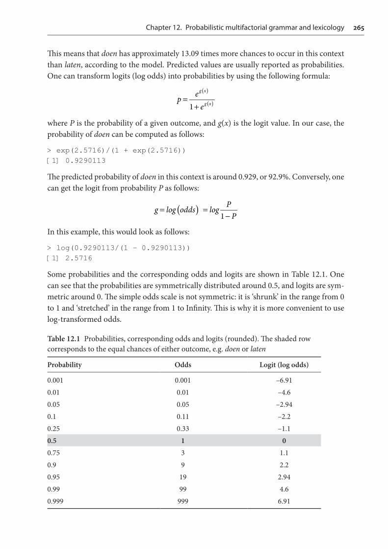
Some probabilities and the corresponding odds and logits are shown in Table 12.1. One can see that the probabilities are symmetrically distributed around 0.5, and logits are sym-metric around 0. The simple odds scale is not symmetric: it is ‘shrunk’ in the range from 0 to 1 and ‘stretched’ in the range from 1 to Infinity. This is why it is more convenient to use log-transformed odds.

Table 12.1 Probabilities, corresponding odds and logits (rounded). The shaded row corresponds to the equal chances of either outcome, e.g. doen or laten

Probability Odds Logit (log odds)

0.001 0.001 –6.910.01 0.01 –4.60.05 0.05 –2.940.1 0.11 –2.20.25 0.33 –1.10.5 1 00.75 3 1.10.9 9 2.20.95 19 2.940.99 99 4.60.999 999 6.91


To obtain the predicted probabilities for all or one observation automatically, you can use SUHGLFW�PRGHO�OUP��W\SH� ��¿WWHG��for lrm models or predict(model.glm, type = "response") for glm models. The row number of the observation in our data was 27:

!�SUHGLFW�P�OUP��W\SH� ��¿WWHG��>��@ 270.9290074

Since the probability is close to 1, this context is highly typical of doen.

Why not use linear regression instead of logistic regression?

Indeed, one could simply compute probabilities (proportions) of doen and laten for all possible combinations of predictors and run a linear regression with the probabilities as the response variable. However, this is not a very good idea. First, if you use linear regression, the regression line will be an endless straight line. As a result, the probabil-ity of an outcome may become greater than 1 or smaller than 0, which is impossible. The logit transformation of probabilities solves this problem. Second, such use of linear regression may result in violations of linear regression assumptions, such as homosce-dasticity and normally distributed residuals.

12.2.3 Selection of variables

There are two strategies of variable selection available for logistic regression: fitting a model with all predictors of interest and stepwise selection (see Chapter 7). You will need to use a glm()object for stepwise selection. For example, to run forward selection, you can do the following:

> m0.glm <- glm(Aux ~ 1, data = doenLaten, family = binomial)> m.fw <- step(m0.glm, direction = "forward", scope = ~ Causation + EPTrans + Country)[output omitted]

Backward stepwise selection is the safest option if you really need a stepwise solution. To run it, you should enter the model with all predictors and add direction = "backward":

> m.bw <- step(m.glm, direction = "backward")Start: AIC=349.7Aux ~ Causation + EPTrans + Country


Df Deviance AIC⟨none⟩ 337.70 349.70- Country 1 344.05 354.05- EPTrans 1 353.36 363.36- Causation 3 550.58 556.58

Finally, one can use the default bidirectional selection (direction = "both"). In all three cases, the stepwise algorithm picks all three variables that were in the first model.

In case you fit a model and find out that some p-values are above the 0.05 threshold, this is not a sufficient reason to discard the variable. When a predictor has more than two values, not all comparisons are shown in the table. In the model presented above, for example, the difference between inducive and volitional causation is not shown in the table of coefficients. This is why it is useful to perform an ANOVA to test if the model that includes this variable tells us more about the outcome than the model without this vari-able. For illustration, one can check if the variable Causation is worth including in the final model as follows:

> m.glm1 <- glm(Aux ~ EPTrans + Country, data = doenLaten, family = binomial)> anova(m.glm1, m.glm, test = "Chisq")Analysis of Deviance Table

Model 1: Aux ~ EPTrans + CountryModel 2: Aux ~ Causation + EPTrans + CountryResid. Df Resid. Dev Df Deviance Pr(>Chi)1 452 550.582 449 337.70 3 212.88 < 2.2e-16 ***

If the greater model reduces the deviance significantly in comparison with the model with-out a predictor, this is a sign that the predictor is worth keeping in the model. A useful function is drop1(), which removes each term from the model, one at a time, and tests the changes in the model’s fit:

> drop1(m.glm, test = "Chisq")Single term deletions

Model:Aux ~ Causation + EPTrans + Country Df Deviance AIC LRT Pr(>Chi)⟨none⟩ 337.70 349.70Causation 3 550.58 556.58 212.878 < 2.2e-16 ***EPTrans 1 353.36 363.36 15.661 7.579e-05 ***Country 1 344.05 354.05 6.348 0.01175 *–-Signif. codes: 0 '***' 0.001 '**' 0.01 '*' 0.05 '.' 0.1 ' ' 1

The results indicate that all predictors are useful.


12.2.4 Testing possible interactions

As has been already explained in connection with linear regression and ANOVA, interac-tions are observed when the effect of one predictor on the outcome depends on the value of another variable. A commonly observed type of interactions in multifactorial models of grammar and lexicon is different effect of contextual variables on the choice between the constructions in different language varieties. An example is the loosening of the ani-macy constraint on the semantics of the possessor/recipient in the genitive and dative alternations from late Modern English on (Wolk et al. 2013). Such differences may also be detected in geographic varieties and registers (e.g. Bresnan & Hay 2008; Szmrecsanyi 2010).

Let us test if there are interactions between the variable Country and the other predictors.

> m.glm.int <- glm(Aux ~ Causation + EPTrans*Country, data = doenLaten, family = binomial)

The significance of the interaction can be estimated with the help of ANOVA:

> anova(m.glm, m.glm.int, test = "Chisq")

Analysis of Deviance Table

Model 1: Aux ~ Causation + EPTrans + CountryModel 2: Aux ~ Causation + EPTrans *CountryResid. Df Resid. Dev Df Deviance Pr(>Chi)1 449 337.702 448 334.58 1 3.1151 0.07757.–-Signif. codes: 0 '***' 0.001 '**' 0.01 '*' 0.05 '.' 0.1 ' ' 1

The model with the interaction is not significantly better than the model with the main effects only (p = 0.078). Still, it is worth considering for didactic purposes. There are three terms in the table of coefficients that need interpretation:

> summary(m.glm.int)[output omitted]EPTransTr -1.8825 0.4919 -3.827 0.00013 ***CountryBE 0.3693 0.3416 1.081 0.27966EPTransTr:CountryBE 1.0827 0.6215 1.742 0.08149.[output omitted]

As you may remember from previous discussions of interactions in Chapters 7 and 8, the coefficient of EPTrans no longer corresponds to the independent effect of EPTrans as it was in the initial model. Instead, it shows the conditional effect of transitive Effected Predicates only if Country = ‘NL’ (the reference level). This effect is significant and negative. Likewise,


CountryBE is not an independent effect of Country any more. It is the effect of Country when the Effected Predicate is intransitive (again, this is the reference level). It is positive but not significant. Finally, EPTransTr: CountryBE is the interaction term. It reflects the difference in the effect of transitive Effected Predicates in the Belgian and Netherlandic data. The estimate is positive. This means that transitive Effected Predicates increase the chances of doen in Belgian Dutch in comparison with the Netherlandic variety, although this effect is only marginally significant.

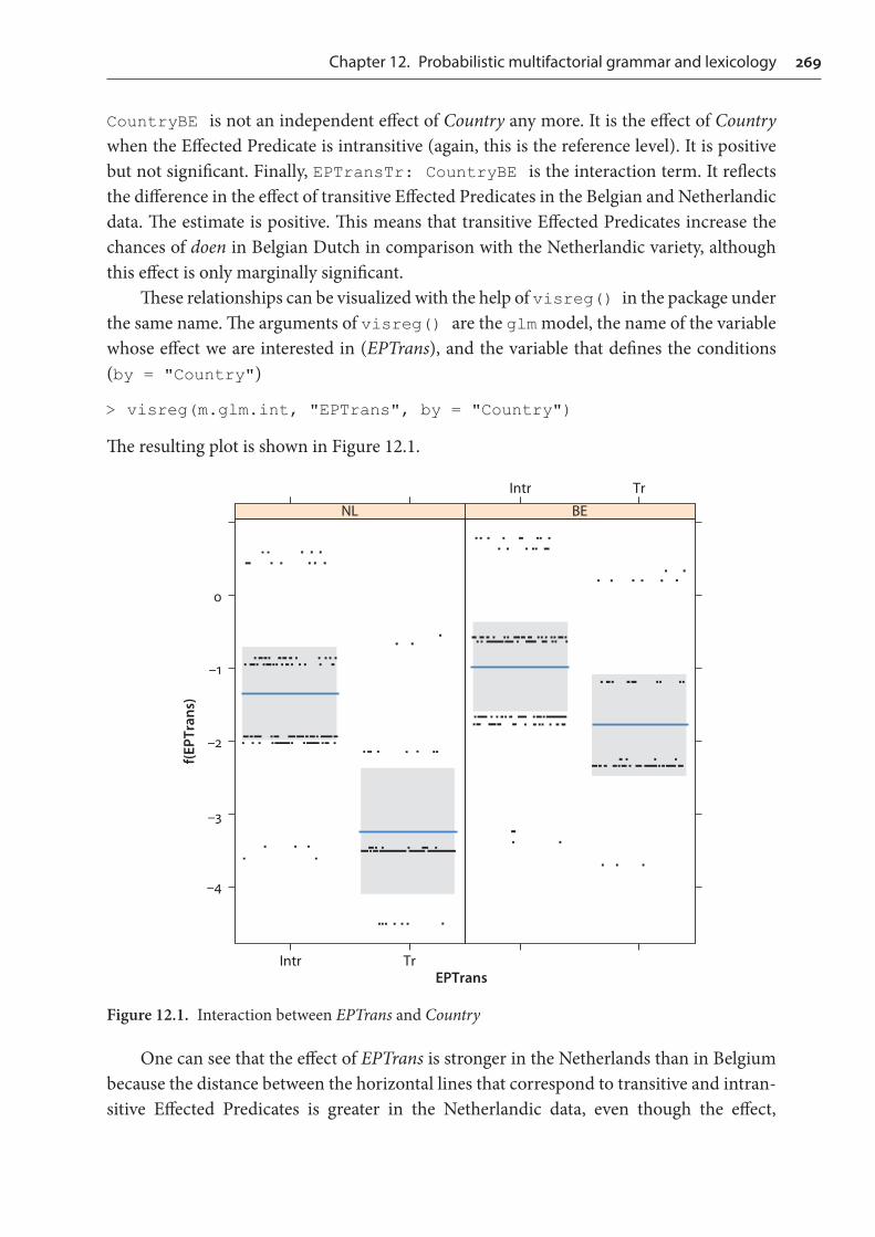
These relationships can be visualized with the help of visreg() in the package under the same name. The arguments of visreg() are the glm model, the name of the variable whose effect we are interested in (EPTrans), and the variable that defines the conditions (by = "Country")

> visreg(m.glm.int, "EPTrans", by = "Country")

The resulting plot is shown in Figure 12.1.

Intr

–4

–3

–2

–1

0

TrEPTrans

f(EPT

rans

)

NL BEIntr Tr

Figure 12.1. Interaction between EPTrans and Country

One can see that the effect of EPTrans is stronger in the Netherlands than in Belgium because the distance between the horizontal lines that correspond to transitive and intran-sitive Effected Predicates is greater in the Netherlandic data, even though the effect,


essentially, remains the same: intransitive predicates are more pro-doen than transitive ones. As additional research in Levshina at al. (2013) has demonstrated, there seems to be lexical factors at play: in the Netherlandic data, there are very many observations with constructions laten zien ‘show, let see’, laten weten ‘let know’ and laten horen ‘let hear’. All of them contain transitive Effected Predicates. Why these expressions are preponder-ant in the Dutch newspapers and much less frequent in the Belgian data requires further investigation.

12.2.5 Identifying outliers and overly influential observations

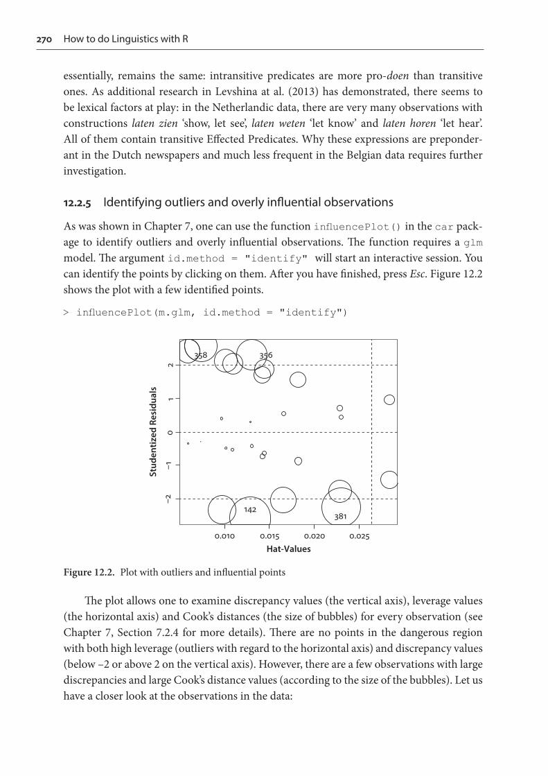
As was shown in Chapter 7, one can use the function LQÀXHQFH3ORW�� in the car pack-age to identify outliers and overly influential observations. The function requires a glm model. The argument id.method = "identify" will start an interactive session. You can identify the points by clicking on them. After you have finished, press Esc. Figure 12.2 shows the plot with a few identified points.

!�LQÀXHQFH3ORW�P�JOP��LG�PHWKRG� ��LGHQWLI\��

0.010

–2–1

01

2

0.015Hat-Values

0.020 0.025

Stud

entiz

ed R

esid

uals

358 356

142381

Figure 12.2. Plot with outliers and influential points

The plot allows one to examine discrepancy values (the vertical axis), leverage values (the horizontal axis) and Cook’s distances (the size of bubbles) for every observation (see Chapter 7, Section 7.2.4 for more details). There are no points in the dangerous region with both high leverage (outliers with regard to the horizontal axis) and discrepancy values (below –2 or above 2 on the vertical axis). However, there are a few observations with large discrepancies and large Cook’s distance values (according to the size of the bubbles). Let us have a closer look at the observations in the data:


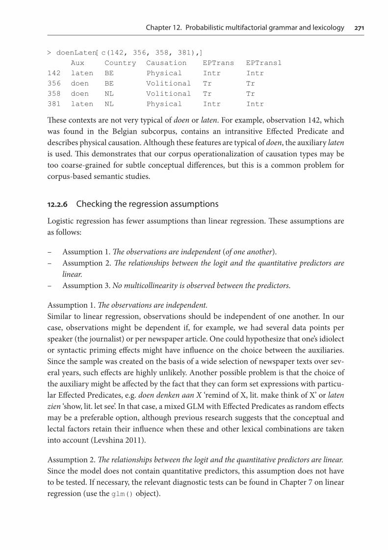
> doenLaten[c(142, 356, 358, 381),] Aux Country Causation EPTrans EPTrans1142 laten BE Physical Intr Intr356 doen BE Volitional Tr Tr358 doen NL Volitional Tr Tr381 laten NL Physical Intr Intr

These contexts are not very typical of doen or laten. For example, observation 142, which was found in the Belgian subcorpus, contains an intransitive Effected Predicate and describes physical causation. Although these features are typical of doen, the auxiliary laten is used. This demonstrates that our corpus operationalization of causation types may be too coarse-grained for subtle conceptual differences, but this is a common problem for corpus-based semantic studies.

12.2.6 Checking the regression assumptions

Logistic regression has fewer assumptions than linear regression. These assumptions are as follows:

– Assumption 1. The observations are independent (of one another). – Assumption 2. The relationships between the logit and the quantitative predictors are

linear. – Assumption 3. No multicollinearity is observed between the predictors.

Assumption 1. The observations are independent.Similar to linear regression, observations should be independent of one another. In our case, observations might be dependent if, for example, we had several data points per speaker (the journalist) or per newspaper article. One could hypothesize that one’s idiolect or syntactic priming effects might have influence on the choice between the auxiliaries. Since the sample was created on the basis of a wide selection of newspaper texts over sev-eral years, such effects are highly unlikely. Another possible problem is that the choice of the auxiliary might be affected by the fact that they can form set expressions with particu-lar Effected Predicates, e.g. doen denken aan X ‘remind of X, lit. make think of X’ or laten zien ‘show, lit. let see’. In that case, a mixed GLM with Effected Predicates as random effects may be a preferable option, although previous research suggests that the conceptual and lectal factors retain their influence when these and other lexical combinations are taken into account (Levshina 2011).

Assumption 2. The relationships between the logit and the quantitative predictors are linear.Since the model does not contain quantitative predictors, this assumption does not have to be tested. If necessary, the relevant diagnostic tests can be found in Chapter 7 on linear regression (use the glm() object).


Assumption 3. No multicollinearity is observed between the predictors.As in linear regression diagnostics (see Section 7.2.5 in Chapter 7), one can use the func-tion vif() in the rms package, which computes VIF (Variance Inflation Factor) scores for each term in the lrm() object. The package car also contains such a function, which can be used with a glm() object, if necessary.

> rms::vif(m.lrm)Causation=Inducive Causation=Physical Causation=Volitional1.699064 1.356411 1.959948EPTrans=Tr Country=BE1.270669 1.017354

As was already mentioned in Chapter 7, there exist different rules of thumb to detect the scores that are too high and therefore indicate the presence of multicollinearity. The thresh-olds of 5 or 10 are the most commonly used. Overall, logistic regression is quite robust with regard to some correlation between predictors.

The presence of multicollinearity is accompanied by large standard errors and p- values. The original model seems to contain no traces of serious multicollinearity, but we can model a situation when multicollinearity is obvious for illustration purposes, similar to what we did in Chapter 7 to illustrate multicollinearity in linear regression. Let us add another variable to the model, named EPTrans1, which is very similar to EPTrans, with the exception of a few values. See what happens with the coefficients, p-values and VIF-scores for EPTrans and EPTrans1:

> m.test <- lrm(Aux~Causation + EPTrans + EPTrans1 + Country, data = doenLaten)> m.test[output omitted]

Coef S.E. Wald Z Pr(>|Z|)Intercept 1.8749 0.3780 4.96 <0.0001Causation=Inducive -3.3661 0.3742 -9.00 <0.0001Causation=Physical 0.5027 0.6336 0.79 0.4275Causation=Volitional -3.7178 0.4282 -8.68 <0.0001EPTrans=Tr -0.0889 1.6257 -0.05 0.9564EPTrans1=Tr -1.2153 1.5972 -0.76 0.4467Country=BE 0.6936 0.2848 2.44 0.0149

> rms::vif(m.test)Causation=Inducive Causation=Physical Causation=Volitional1.697379 1.373455 1.959740EPTrans=Tr EPTrans1=Tr Country=BE29.170101 28.516853 1.021357


The VIF-scores of EPTrans and EPTrans1 are almost 30. This is a sign of strong multi-collinearity. The estimates of these two predictors in the model are unreliable, and the p-values are now much greater than 0.05. However, the predictive power of the model does not suffer: the C-index is even slightly higher than in the previous model (0.895 compared to 0.894).

Most traditional linguistic categories, like transitivity or animacy, with their prototyp-ically organized structure and fuzzy boundaries allow for many different operationaliza-tions in a corpus-linguistic study. Although logistic regression is quite robust with regard to small amounts of multicollinearity, in situations of very similar operationalizations it is advisable to select one variable that is the most justified theoretically. Alternatively, one can use dimensionality-reduction techniques presented in Chapters 17 to 19.

Complete and quasi-complete separation

Complete and quasi-complete separation occurs when some values of a predictor or a combination of several predictors can perfectly predict the outcome. Imagine you want to predict the use of the definite and indefinite article in English and include the gram-matical number of the head noun as a predictor. If you cross-tabulate the predictor and the response, the table will contain a zero in the cell that corresponds to plural nouns and the indefinite article, as shown below. This is called quasi-complete separation. If the frequency of the definite article in the singular were zero, that would be an example of complete separation.

Definite Indefinite Singular 18 15 Plural 12 0

Complete and quasi-complete separation should be avoided because the model either becomes unreliable (one can usually tell that from huge standard errors), or it simply may not converge and you will receive an error message. To solve the problem, you can recode the predictor (e.g. by conflating its levels) or use a model with a correction, such as the Firth penalized regression (see, for instance, the package logistf and the func-tion under the same name). It is always useful to do cross-tabulation of all categorical predictors and the response before beginning your analysis in order to detect configura-tions with zero frequencies or a large number of cells with very low frequencies.


12.2.7 Testing for overfitting

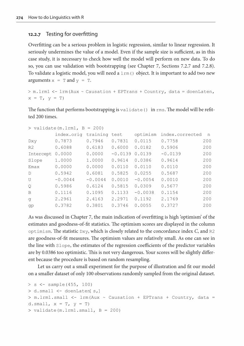
Overfitting can be a serious problem in logistic regression, similar to linear regression. It seriously undermines the value of a model. Even if the sample size is sufficient, as in this case study, it is necessary to check how well the model will perform on new data. To do so, you can use validation with bootstrapping (see Chapter 7, Sections 7.2.7 and 7.2.8). To validate a logistic model, you will need a lrm() object. It is important to add two new arguments x = T and y = T.

> m.lrm1 <- lrm(Aux ~ Causation + EPTrans + Country, data = doenLaten, x = T, y = T)

The function that performs bootstrapping is validate() in rms. The model will be refit-ted 200 times.

> validate(m.lrm1, B = 200) index.orig training test optimism index.corrected nDxy 0.7873 0.7946 0.7831 0.0115 0.7758 200R2 0.6088 0.6183 0.6000 0.0182 0.5906 200Intercept 0.0000 0.0000 -0.0139 0.0139 -0.0139 200Slope 1.0000 1.0000 0.9614 0.0386 0.9614 200Emax 0.0000 0.0000 0.0110 0.0110 0.0110 200D 0.5942 0.6081 0.5825 0.0255 0.5687 200U -0.0044 -0.0044 0.0010 -0.0054 0.0010 200Q 0.5986 0.6124 0.5815 0.0309 0.5677 200B 0.1116 0.1095 0.1133 -0.0038 0.1154 200g 2.2961 2.4163 2.2971 0.1192 2.1769 200gp 0.3782 0.3801 0.3746 0.0055 0.3727 200

As was discussed in Chapter 7, the main indication of overfitting is high ‘optimism’ of the estimates and goodness-of-fit statistics. The optimism scores are displayed in the column optimism. The statistic Dxy, which is closely related to the concordance index C, and R2 are goodness-of-fit measures. The optimism values are relatively small. As one can see in the line with Slope, the estimates of the regression coefficients of the predictor variables are by 0.0386 too optimistic. This is not very dangerous. Your scores will be slightly differ-ent because the procedure is based on random resampling.

Let us carry out a small experiment for the purpose of illustration and fit our model on a smaller dataset of only 100 observations randomly sampled from the original dataset.

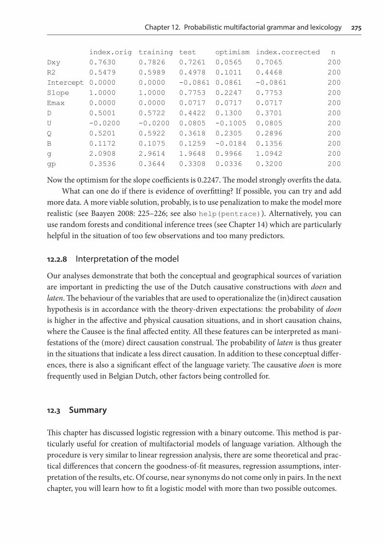
> s <- sample(455, 100)> d.small <- doenLaten[s,]> m.lrm1.small <- lrm(Aux ~ Causation + EPTrans + Country, data = d.small, x = T, y = T)> validate(m.lrm1.small, B = 200)


index.orig training test optimism index.corrected nDxy 0.7630 0.7826 0.7261 0.0565 0.7065 200R2 0.5479 0.5989 0.4978 0.1011 0.4468 200Intercept 0.0000 0.0000 -0.0861 0.0861 -0.0861 200Slope 1.0000 1.0000 0.7753 0.2247 0.7753 200Emax 0.0000 0.0000 0.0717 0.0717 0.0717 200D 0.5001 0.5722 0.4422 0.1300 0.3701 200U -0.0200 -0.0200 0.0805 -0.1005 0.0805 200Q 0.5201 0.5922 0.3618 0.2305 0.2896 200B 0.1172 0.1075 0.1259 -0.0184 0.1356 200g 2.0908 2.9614 1.9648 0.9966 1.0942 200gp 0.3536 0.3644 0.3308 0.0336 0.3200 200

Now the optimism for the slope coefficients is 0.2247. The model strongly overfits the data.What can one do if there is evidence of overfitting? If possible, you can try and add

more data. A more viable solution, probably, is to use penalization to make the model more realistic (see Baayen 2008: 225–226; see also help(pentrace)). Alternatively, you can use random forests and conditional inference trees (see Chapter 14) which are particularly helpful in the situation of too few observations and too many predictors.

12.2.8 Interpretation of the model

Our analyses demonstrate that both the conceptual and geographical sources of variation are important in predicting the use of the Dutch causative constructions with doen and laten. The behaviour of the variables that are used to operationalize the (in)direct causation hypothesis is in accordance with the theory-driven expectations: the probability of doen is higher in the affective and physical causation situations, and in short causation chains, where the Causee is the final affected entity. All these features can be interpreted as mani-festations of the (more) direct causation construal. The probability of laten is thus greater in the situations that indicate a less direct causation. In addition to these conceptual differ-ences, there is also a significant effect of the language variety. The causative doen is more frequently used in Belgian Dutch, other factors being controlled for.

12.3 Summary

This chapter has discussed logistic regression with a binary outcome. This method is par-ticularly useful for creation of multifactorial models of language variation. Although the procedure is very similar to linear regression analysis, there are some theoretical and prac-tical differences that concern the goodness-of-fit measures, regression assumptions, inter-pretation of the results, etc. Of course, near synonyms do not come only in pairs. In the next chapter, you will learn how to fit a logistic model with more than two possible outcomes.


How to write up the results of logistic regression analysis

Logistic regression is reported similarly to linear regression. For a model with one pre-dictor, you can provide the intercept b0, the estimate b, standard error SE and p-value. To report the results of multiple logistic regression, you can make a table with these statistics. The asterisk system (***, **, *) can be used to indicate the significance of p-values. In both cases, it is necessary to provide some general goodness-of-fit sta-tistic, preferably the concordance index C. Interactions are best represented visually. Although not strictly necessary, it is also useful to provide 95% confidence intervals, as well as to convert log odds ratios into simple odds ratios.

Probabilistic multifactorial grammar and lexicology · Chapter 12. Probabilistic multifactorial...

Documents

Transcript of Probabilistic multifactorial grammar and lexicology · Chapter 12. Probabilistic multifactorial...