Probabilistic Modeling and Statistical Characteristics of

Probabilistic Modeling and StatisticalCharacteristics of Aggregate Wind Power

H. Louie and J. M. Sloughter

Abstract The stochasticity of the electrical power output by wind turbines posesspecial challenges to power system operation and planning. Increasing penetrationlevels of wind and other weather-driven renewable resources exacerbate theuncertainty and variability that must be managed. This chapter focuses on theprobabilistic modeling and statistical characteristics of aggregated wind power inlarge electrical systems. The mathematical framework for probabilistic models—accounting for geographic diversity and the smoothing effect—is developed, andthe selection and application of parametric models is discussed. Statistical char-acteristics from several real systems with high levels of wind power penetrationare provided and analyzed.

Keywords Copulas � Correlation � Geographic diversity � Smoothing effect �Wind generators � Wind power modeling

1 Introduction

Wind turbines are classified as weather-driven renewable resources due to thedependency of their power output on local meteorological conditions [1]. Theseconditions are inherently transient and often erratic. Consequently, the poweroutput by wind turbines—hereafter also simply referred to as ‘‘wind power’’—isappropriately characterized as being variable and uncertain. Variability refers to

H. Louie (&)Department of Electrical and Computer Engineering, Seattle University, 901 12th Ave,Seattle WA 98122, USAe-mail: [email protected]

J. M. SloughterDepartment of Mathematics, Seattle University, 901 12th Ave, Seattle WA 98122, USAe-mail: [email protected]

J. Hossain and A. Mahmud (eds.), Large Scale Renewable Power Generation,Green Energy and Technology, DOI: 10.1007/978-981-4585-30-9_2,� Springer Science+Business Media Singapore 2014

19

the unintentional tendency for wind power to change—perhaps rapidly—from onemoment to the next, whereas uncertainty refers to the wide range of unknownfuture values of wind power.

The stochasticity of wind power is a concern for system operators, as the legacyelectric grid was designed to be operated with primarily deterministic sources[2, 3]. Although stochastic, wind power often exhibits identifiable patterns andquantifiable statistical distributions, which can be modeled and exploited to bettermanage the system. These models, whether mathematically formalized or tacitlyunderstood, have applications in several areas, including wind power forecastsystems, stochastic unit-commitment programs, risk analysis, and Monte Carlo-based simulations for resource planning and research [4–6].

This chapter focuses on the aggregate system-wide wind power, rather than thewind power from individual wind plants or turbines. We are motivated to take thismacro-level view because for many system operators it is the aggregate—notindividual—wind power that is of utmost concern. Our goal is to identify anddevelop probabilistic models of aggregate wind power and analyze its statisticalcharacteristics. More specifically, we use parametric distributions—probabilitydensity functions (pdf) and cumulative distribution functions (cdf)—to model theinstantaneous and moment-to-moment variations of aggregate wind power.

The remainder of this chapter is organized as follows. Section 2 describes thegeneral characteristics of aggregate wind power. Section 3 formulates an idealizedprobabilistic model of wind power output from an individual wind plant. Aspectsof geographic diversity including correlation, dependency structures, and practicalconsiderations are discussed in Sect. 4, leading to probabilistic models forinstantaneous and moment-to-moment wind power variation in Sect. 5. Aggregatewind power data from four large systems are analyzed and discussed in Sect. 6.The concluding remarks are given in Sect. 7.

2 General Characteristics of Aggregate Wind Power

Aggregate wind power is defined as the sum of the real power delivered by allwind plants in a system as measured at their point of interconnection with the grid.We are concerned with both the instantaneous and moment-to-moment variationsof aggregate wind power. The statistical characteristics of instantaneous aggregatewind power provide information about the uncertainty, whereas the statisticalcharacteristics of moment-to-moment variation of aggregate wind power provideinformation about the variability. Rather than formulating models in the powerdomain, it is more useful to do so in the normalized power domain. This facilitateseasier comparison and allows the models to be scaled to the desired capacity level,increasing their applicability. The units in the normalized power domain are per-unit (p.u.), where the normalization is done with respect to the total capacity of thewind plants in the system.

20 H. Louie and J. M. Sloughter

The characteristics of aggregate wind power are derived from—but differentthan—the characteristics of wind power from individual wind plants. Aggregatewind power is strongly influenced by the geographic diversity of the wind plants inthe system. Geographic diversity is a term describing the tendency for wind plantsin different wind regimes and separated by large distances to exhibit low corre-lation in their instantaneous wind power and moment-to-moment variations.

Many aspects of geographic diversity have been widely explored in the liter-ature [7–21]. All other things being equal, a system with high geographic diversityhas lower variability and uncertainty than one with low geographic diversity. Thereduction of variability caused by geographic diversity is also known as thesmoothing effect. The benefits of high geographic diversity include less frequentoccurrences of extremely high and low power output; less frequent ramp events;and improved accuracy of wind power forecasts. The results are greater economyand reliability, decreased reserve requirements, and more efficient commit-ment and dispatch of generators [22].

2.1 Uncertainty of Aggregate Wind Power

We first consider the uncertainty characteristics of aggregate wind power. Thedefinition of uncertainty can be subjective, with several appropriate interpretationspossible, depending on the application or situation. For example, a system operatormay be concerned about the probability of extremely high or low aggregate windpower. In this case uncertainty is best measured using quantiles. Another operatormay be interested in the general spread of potential values of aggregate windpower, in which case the standard deviation is an appropriate measure. Rather thanstrictly defining uncertainty, our approach is to recognize that the uncertaintyinformation of aggregate wind power is contained in its probability densityfunction, from which the quantiles, standard deviation, and other metrics ofuncertainty can be measured or computed.

The shape of the probability density function can be approximated by con-structing an empirical histogram of instantaneous aggregate wind power. Figure 1ashows a typical histogram of wind power from an individual wind plant and isprovided for comparison purposes. Figure 1b–d shows aggregate wind power fromthree large systems. We will discuss the specific details of these systems and othersin greater detail in Sect. 6. For now it suffices to know that each system has over4 GW of installed wind capacity—a considerable amount. The computed standarddeviation is provided with each plot. From inspection of Fig. 1, we make twoimportant observations: (1) the modality of the wind power from an individualwind plant is different from that of wind power aggregated across a large system,and (2) different systems exhibit different uncertainty characteristics.

By most measures, the system corresponding to Fig. 1b has higher uncertaintythan other systems. The standard deviation is greater than in other systems, andthere are more frequent occurrences of zero and near rated (1.0 p.u.) power

Probabilistic Modeling and Statistical Characteristics 21

production. These characteristics are similar to those of the individual wind plant,and as such the system can be described as having low geographic diversity. Thewind plants in systems with low geographic diversity are often in close proxim-ity—perhaps separated by 200 km or less—and are in the same or similar windregime. The Bonneville Power Administration (BPA) is an example of a systemwith low geographic diversity.

The system corresponding to Fig. 1c exhibits less uncertainty than Fig. 1b. Thestandard deviation and occurrences of low output are reduced, and the maximumpower output rarely exceeds 0.75 p.u. Figure 1d exhibits the lowest uncertainty ofthe systems, which is characteristic of a system with appreciable geographicdiversity. Episodes of extremely low and high production are rare, and the standarddeviation is lower than the others. Systems with this level of geographic diversitytend to have wind plants spread over very large territories. The Midwest ISO(MISO) and PJM systems are examples of systems with higher geographicdiversity.

It is evident that there is no proto-typical histogram or probability densityfunction of instantaneous aggregate wind power, and so the uncertainty will varydepending on system specifics—mainly the level of geographic diversity. Ourapproach, therefore, is to seek a flexible multi-parametric model capable of rep-resenting the commonly exhibited probability density function shapes by systemswith various levels of geographic diversity.

(a) (b)

(c) (d)

Fig. 1 Histograms of normalized wind power from an individual wind plant (a), and from largesystems (b–d) with standard deviation displayed. a Single wind plant, b Lower diversity,c Medium diversity and d Higher diversity


2.2 Variability of Aggregate Wind Power

Instantaneous wind power values provide us with information on uncertainty, butwe are also interested in wind power variability. The variability of wind power isexamined through the statistical characteristics of wind power variation. Windpower variation is defined as the difference in instantaneous wind power at twopoints in time, usually 1 h: DP t½ � ¼ P t½ � � P t � q½ � where DP is the variation ofwind power, t is the time, and q is the variation period. Similar to our approachwith uncertainty, the variability of aggregate wind power is assessed by consid-ering the probability density function of DP, as well as its statistical characteristicssuch as standard deviation and quantiles. We will see that variability in aggregatewind power is strongly influenced by geographic diversity.

Figure 2 shows typical normalized hour-to-hour wind power variation in anindividual wind plant (a) and system (b) over a period of 1 year. Note that forclarity the ordinate is logarithmically scaled. The trace for the individual windplant is much broader than for the system aggregate, indicating more frequentextreme variability. Aggregation, therefore, tends to smooth wind power vari-ability. In Fig. 2a, b, the nearly linear decrease in occurrences on the logarith-mically scaled ordinate suggests that an appropriate parametric model will have anexponential form. The slope of the decrease is influenced by the geographicdiversity of the system, as well as the variation period, with shorter periods havingsteeper slopes.

In the above we have briefly described typical uncertainty and variabilitycharacteristics of aggregate wind power. These characteristics depend on thegeographic diversity in a system, as well as the characteristics of the constituentindividual wind plants. Therefore in order to thoughtfully propose aggregate windpower models, we must begin by modeling individual wind plants and thenestablishing the mathematical framework for geographic diversity’s effect onuncertainty and variability.

(a) (b)

Fig. 2 Normalized hourly variability in wind power from an individual wind plant (a) anda large system (b) over the course of 1 year


3 Individual Wind Plant Model

The characteristics of aggregate wind power—especially at low levels of geo-graphic diversity—depend on the characteristics of the system’s constituent windplants. We first derive an analytic model of wind plant power output under ide-alized conditions: that the wind speed follows a parametric probability densityfunction and the energy conversion process is deterministic, among otherassumptions. We conclude the section by considering non-idealities in wind plantpower production.

The power delivered by a wind plant Pi is the sum of the real power producedby its constituent wind turbines, less collector system losses:

Pi ¼XM

j¼1

PWT; j � PL; i ð1Þ

where M is the number of wind turbines in the wind plant, PWT, j is the real powergenerated by the jth wind turbine and PL,i is the ith wind plant’s collector systemlosses at the current operating state.

Although (1) appears straightforward, wind turbines are nonlinear energyconversion devices whose power output is primarily dependent on wind speed,which is a random variable. This implies that Pi will be stochastic, and that aprobabilistic model of Pi can be derived by transforming the probability densityfunction of the wind speed.

3.1 Probabilistic Wind Speed Model

Let ~v be a random variable representing the wind speed at a certain wind turbinewith corresponding probability density function fv ~vð Þ. The presence of the tildeindicates that the variable is random. We can approximate fv ~vð Þ by the repeatedindependent sampling of ~v. These samples can be binned into a histogram andscaled to approximate fv ~vð Þ. Two typical, yet specific, scaled histograms of windspeed are shown in Fig. 3.

Although histograms are helpful visual approximations of probability densityfunctions, it is often desirable to represent them using a parametric function. Let

fv ~v; hð Þ be the model of fv ~vð Þ with parameters arranged in the vector H. For thesake of brevity, we will suppress H in all distributions hereafter, so that, for

example, fvð~vÞ represents the parametric model of fv ~vð Þ.Returning to Fig. 3, we see that each histogram is asymmetric with a distinctly

positive skewness, indicating that high wind speeds are less frequent than lowwind speeds. These characteristics can be modeled using the three-parameterGeneralized Gamma distribution [23]. However, estimating the parameters of thisdistribution can be difficult. Instead, the two-parameter Weibull distribution, which


is a special case of the Generalized Gamma distribution, is commonly used. TheWeibull probability density function [24] is

fv ~vð Þ ¼ 0 ~v\0kk

~vk

� �k�1e� ~v=kð Þk ~v� 0

�ð2Þ

where k and k are the shape and scale parameters, respectively. The parameters can beestimated from sampled data using the maximum likelihood estimation (MLE)method or the method of moments, though for the Weibull distribution these methodscan be mathematically cumbersome [25, 26]. Examples of Weibull distributions withparameters estimated using MLE are shown as the solid traces in Fig. 3. In each case,the parametric function is a reasonable approximation to the data.

The two-parameter Weibull model can often be simplified to a single parametermodel without appreciably sacrificing accuracy. For locations with wind regimessuitable for wind plant development, the estimated shape parameter of the Weibulldistribution is often near 2.0. Therefore, the Weibull distribution can be reduced tothe Rayleigh distribution [24]. A useful feature of the Rayleigh distribution is thatits parameter can be estimated with the method of moments using only the mean ofthe wind speed, which is sometimes the only quantity available.

3.2 Idealized Wind Turbine Power Curve

We next examine the effect of the wind turbine in shaping the wind powerprobability density function. Wind turbines convert a portion of the kinetic energyinto a mass of moving air to electrical energy by way of electric generator. Theelectrical power output by a wind turbine is computed from:

~PWT ¼12

CpAq~v3 ð3Þ

(a) (b)

Fig. 3 Histograms of wind speed from two locations with fit Weibull probability densityfunctions. a wind speed distribution for location 1, b wind speed distribution for location 2


where Cp is the dimensionless power coefficient, A is the area swept by the rotorblades in m2, and q and ~v are the density and velocity of the air mass incident to thewind turbine, in kg/m3 and m/s, respectively [27]. The power coefficient representsthe overall efficiency of the energy conversion process, which depends on turbinedesign and operating state. If a constant Cp can be maintained, then the wind speedand wind power are cubically related. Under low or high wind speed conditions thewind turbine is operated such that Cp is zero, for reasons discussed later. Although(3) is useful, a more common and illustrative way to show the relationship betweenwind speed and wind turbine power output is with the power curve.

A power curve deterministically maps each wind speed to the correspondingpower output of a wind turbine. An example of an idealized power curve is shownin Fig. 4. In general, there are four regions of operation.

3.2.1 Below Cut-in Wind Speed v\vcið Þ

At low wind speeds no electrical power is produced and Cp is zero. The power inthe wind is not enough to either overcome the friction of the drivetrain, or to resultin positive net power production. The threshold wind speed at which powergeneration begins is known as the cut-in wind speed (vci).

3.2.2 Between Cut-in and Rated Wind Speed vci� v\vrð Þ

When the wind speed is between the cut-in and rated wind speed (vr), the windturbine generates power. In this region, the turbine is designed or controlled tomaximize Cp, and a nearly cubic wind speed-turbine power relationship isobserved. This relationship can be approximated as

PWT ¼ av3 � bPr ð4Þ

where a and b are coefficients and Pr is the rated power of the wind turbine [27].The coefficients can be determined by enforcing Pr ¼ av3

r � bPr and 0 ¼av3

ci � bPr and then numerically solving the resulting set of equations.

Fig. 4 Idealized powercurve of a 2.5 MW windturbine with cut-in speed of2.5 m/s, rated wind speed of3 m/s, and cut-out wind speedof 25 m/s


3.2.3 Between Rated and Cut-out Wind Speed vr � v\vcoð Þ

At wind speeds above rated and below cut-out (vco), the wind turbine is controlledto maintain constant power production. As the wind speed increases over thisregion constant power is maintained by reducing Cp through active pitch control orpassive stall design.

3.2.4 At and Above Cut-out Wind Speed vco� vð Þ

At excessively high wind speeds, the wind turbine is in danger of mechanicalfailure. The turbine is aerodynamically slowed and stopped, and then mechanicallylocked into place to prevent rotation. Cp is zero over this region.

The effect of the varying power coefficient can be implicitly accounted for byexpressing (3) as the piecewise function PWT = g(v), where g(v):

PWT ¼ g vð Þ ¼

0 v\vci

av3 � bPr vci� v\vr

Pr vr� v\vco

0 vco� v

8>><

>>:ð5Þ

As previously mentioned, the power curve in Fig. 4 and expressed as (5) areidealized. Most utility-scale wind turbine manufacturers develop the power curvefor a particular wind turbine model under carefully controlled conditions accordingto accepted standards [28]. Field performance of wind turbines can be inconsistentand appreciably differ from the manufacturer-supplied power curve. These non-idealities are discussed in detail in Sect. 3.4.

3.3 Idealized Wind Plant Model

A basic model of power from a wind plant is

~Pi ¼ M~PWT ¼ Mg ~vð Þ ð6Þ

where ~Pi is the total real power from the M wind turbines of wind plant i. Thismodel makes several assumptions, such as all wind turbines experience the samewind speed and have the same power curve. We will discuss the reasonableness ofthese assumptions in Sect. 3.4. However, for the following, we will assume that (6)holds. Since ~Pi is a random variable, we can characterize it with a probabilitydensity function or cumulative distribution function (cdf).

Let the cdf of the wind speed be Fv ~vð Þ and let the cdf of the wind power fromthe wind plant be FP ~Pi

� �. The cdf of the power from the wind plant is the

piecewise function:


FP ~Pi

� �¼

Fv vcið Þ þ 1� Fv vcoð Þ ~Pi ¼ 0

Fv g�1 ~Pi�M

� �� þ 1� Fv vcoð Þ 0\~Pi\MPr

1 ~Pi ¼ MPr

8><

>:ð7Þ

where g-1(PWT) is the inverse power curve.We can see that this gives us the following probabilities:

Prf~Pi ¼ 0g ¼ Fv vcið Þ þ 1� Fv vcoð ÞPrf0\~Pi\MPrg ¼ Fv vrð Þ � Fv vcið Þ

Prf~Pi ¼ MPrg ¼ Fv vcoð Þ � Fv vrð Þð8Þ

As there is a measurable probability of wind power being exactly equal to either0 or MPr, we do not have a purely continuous distribution function. We insteadhave a mixed discrete/continuous distribution function.

Our pdf for wind power, then, will need to use the Dirac delta function dð�Þ toaddress the probabilities of wind power being exactly equal to either 0 or MPr. Forall other values of wind power, we can calculate the pdf using the traditionalchange-of-variables method. Using (5), the inverse power curve for the regionbetween 0 and MPr is

v ¼ g�1ðPWTÞ ¼PWT þ bPr

a

� 1=3ð9Þ

The corresponding probability density function of wind power for this region isfound by taking the derivative of (7) with respect to ~Pi so that:

fP ~Pi

� �¼

dFP ~Pi

� �

d~Pi¼

dFv g�1 ~Pi�M

� ��

d~Pi¼

dFv g�1 ~Pi�M

� ��

dg�1 ~Pi�M

� � �dg�1 ~Pi

�M

� �

d~Pi

¼ dFv ~vð Þd~v

�dg�1 ~Pi

�M

� �

d~Pi

ð10Þ

We note that dFv ~vð Þd~v

is just the pdf of the wind speed fv ~vð Þ evaluated at ~v ¼

g�1 ~Pi�M

� �and that

dg�1 ~Pi�M

� �

d~Pi¼

~Pi=MþbPra

0@

1A�2=3

3aMð11Þ

For the specific case of a Weibull wind speed distribution (10) becomes:


fp ~Pi

� �¼ k

k

g�1 ~Pi�M

� �

k

0@

1A

k�1

e�

g�1 ~Pi=M� �

k

� k0BB@

1CCA

~Pi=MþbPra

0

@

1

A�2=3

3aM: ð12Þ

We now have closed-form algebraic expressions for the probability densityfunction of wind power when 0\~Pi\MPr.

Applying (6), the idealized individual wind plant model for a Weibull distri-bution of wind speed is therefore:

fp ~Pi

� �¼ k

k

g�1 ~Pi�M

� �

k

0

@

1

Ak�1

e�

g�1 ~Pi=M� �

k

� k0

BB@

1

CCA

~Pi=MþbPra

0@

1A�2=3

3aM

þ Fv vcið Þ þ 1� Fv vcoð Þð Þd ~Pi

� �þ Fv vcoð Þ � Fv vrð Þð Þd ~Pi �MPr

� �

ð13Þ

For 0� ~Pi�MPr, and 0 everywhere else. For a Rayleigh distribution of windspeed:

fp ~Pi

� �¼

g�1 ~Pi�M

� �

k2

0

@

1

Ae�

g�1 ~Pi=M� �2

2k2

� 0BB@

1CCA

~Pi=MþbPra

0@

1A�2=3

3aM

þ Fv vcið Þ þ 1� Fv vcoð Þð Þd ~Pi

� �þ Fv vcoð Þ � Fv vrð Þð Þd ~Pi �MPr

� �

ð14Þ

again for 0� ~Pi�MPr, and 0 everywhere else.The models of individual wind plant power output in (13) and (14) were ana-

lytically derived and are dependent only on a small number of wind speed andpower curve parameters. Figure 5 shows an example of the pdf and cdf of a windplant. We note that the pdf shown is similar in appearance to that of Fig. 1a, whichis reassuring. However, there are differences, particularly near rated power. Ouranalytic model overestimates the probability of rated power production from thewind plant. This discrepancy is an artifact of the idealized assumptions implied by(6). Despite the differences the derived model has utility—it serves as a reasonablestarting point in the absence of additional data, and it allows for further analyticmanipulation, as we will see later.


3.4 Non-idealized Wind Plant Modeling

The derived probability density functions in (14) and (15) are idealized models ofwind power under several assumptions implied by (6), including:

1. the collector system is lossless;2. all wind turbines are in service;3. the power curves are deterministic for each wind turbine;4. the wind speed and air density are the same at each wind turbine.

The first and second assumptions allow the wind plant to reach 100 % ratedoutput. However, collector system losses are nonzero—usually between 1 and 5 %[29]—and wind turbines are routinely taken out of service due to scheduledmaintenance or malfunction. A typical wind turbine requires regularly scheduledmaintenance at 6 month intervals, although online condition monitoring may yieldmore optimal schedules [30]. Maintenance and malfunction-related outages canlast several hours or longer, with offshore wind turbines generally requiring longeroutages. For these reasons, a large wind plant may have one or more wind turbinesout of service at any given time. Although rated power is not achieved, occur-rences of near rated power may be common, as shown in Fig. 1a.

The third assumption, while greatly simplifying the model, is not substantiatedby empirical data. Even after correcting for air density, power production straysfrom the manufacturer-supplied power curve for several reasons, including:dependency of power output on wind direction; forced curtailment; wind shear andturbulence; manufacturing and installation defects; efficiency degradation overtime; and internal power consumption for control systems, lighting, pumps, andother functions. These effects are illustrated by an empirical power curve. Anempirical power curve is constructed by plotting repeated in situ simultaneousmeasurements of wind speed and wind power, as shown in Fig. 6. It is clear fromthis figure that the idealized power curve model in (5) does not capture the truein situ relationship between wind speed and wind power.

(a) (b)

Fig. 5 Analytic pdf (a) and cdf (b) of wind power from an individual wind plant with powercurve in Fig. 4 and a Rayleigh distribution of wind speed with scale parameter k = 5


The fourth assumption implied by (6) is naïve, though often used. In reality,wind turbines can be separated by several kilometres and installed in varyingterrain. The wind turbines almost never simultaneously experience the same windspeed. In other words, there is geographic diversity within each wind plant thatmust be accounted for. Over the years, several approaches to more realisticallyaccount for non-idealities in power curves have been proposed [32–34]. Someinvolve creating sub-groups of wind turbines, where each sub-group has its ownwind speed. Other methods involve creating data-driven wind plant power curvesusing statistical methods. Provided they are well-defined, wind plant power curvescan be used in place of (5) to analytically derive a probabilistic model of windpower using the same steps detailed in Sect. 3.3.

To summarize our progress, we started by identifying suitable parametricprobabilistic models of wind speed: Rayleigh or Weibull. We then developed pdfsand cdfs for individual wind plant power output by transforming the wind speedmodels using an idealized power curve, as in (13) and (14). This method can beused to account for non-idealities using a wind plant power curve if desired. Weare now poised to consider the aggregate power production from a fleet of windplants in a common system. To do this, we must model the correlation anddependency of wind power among the wind plants. In other words, we must modelthe geographic diversity.

4 Geographic Diversity

The most important influencer of the uncertainty and variability of aggregate windpower is the geographic diversity of the system. A system’s geographic diversity isa reference to the general level of dependence between the wind power from its

Fig. 6 Empirical powercurve of a wind turbineshowing effects of non-idealities � 2007 IEEE.Reprinted, with permission,from [31]


constituent wind plants. Dependence is often quantified using a correlation coef-ficient, with lower correlation generally resulting in decreased uncertainty andvariability. The goal of this section is to formulate the mathematic basis for thisphenomenon, discuss factors influencing correlation and dependency, as well as tocomment on practical considerations.

4.1 Theoretical Basis

Aggregate wind power can mathematically be represented as

~Pagg ¼1N

XN

i¼1

~Pi

Cið15Þ

where ~Pagg is the normalized aggregate wind power, N is the number of windplants considered, and Ci and Pi are the capacity and real power delivered by theith wind plant.

Hereafter, subscripts are used to associate a variable with a specific wind plant,so that xn pertains to the nth wind plant. We start with the idealized assumptionthat the wind speed at each wind plant ~v1; . . .;~vN are independent random vari-ables. Consequently, ~P1; . . .; ~PN will also be independent random variables, andare therefore uncorrelated.

As a result of the assumption of independence, the probability distribution ofthe aggregate power output is found through convolution and change-of-variables:

fPagg~Pagg

� �¼ N

XN

i¼1

Ci

!fP1

~P1� �

� � � � � fPN~PN

� �ð16Þ

where * is the convolution operator.By the Central Limit Theorem, as N increases fPagg

~Pagg

� �will approach the

Gaussian distribution so that:

fPagg~Pagg

� �¼ 1

ragg

ffiffiffiffiffiffi2pp e

�~Pagg�laggð Þ2

2r2agg N ! inf ð17Þ

where lagg and ragg are the mean and standard deviation of fPagg~Pagg

� �. The

transformation of the probability density function to a Gaussian distributionaccording to the Central Limit Theorem has important implications to theuncertainty of aggregate wind power.


4.2 Uncertainty and Variability Reduction

The normalized aggregate wind power’s statistical variance will decrease as morewind plants are added to the system according to

r2agg ¼

1N2

XN

i¼1

r2i ð18Þ

where r2i is the variance of the normalized power output of the ith wind plant. The

decrease in variance causes the Gaussian distribution to contract, which can beinterpreted as a decrease in the uncertainty of the wind power.

The evolution of fPagg~Pagg

� �to a Gaussian distribution can be noticeable even

for small values of N. This is illustrated in Fig. 7 where fPagg~Pagg

� �for N = 2, 4, 6,

and 8 are plotted using numerical convolution based on the pdf in Fig. 5a andassuming independence in power output. Note how the distribution contracts asmore wind plants are aggregated, resulting in decreased standard deviation anddecreased probability of extremely high or low power output. In other words, theuncertainty decreases.

The effects of geographic diversity also apply to the moment-to-moment var-iation in aggregate wind power: under the assumption of independence, as morewind plants are aggregated the moment-to-moment variation approaches aGaussian distribution with decreasing variance.

(a) (b)

(c) (d)

Fig. 7 Probability density functions of normalized aggregate wind power for systems with 2 (a),4 (b), 6 (c) and 8 (d) wind plants under assumption of independence


The preceding derivation showed the mathematical mechanism by whichgeographic diversity reduces uncertainty and variability in aggregate wind power.Its foundation is the assumption that the wind speed (and power) at all N windplants are independent, and hence not correlated, but how realistic and restrictiveis this assumption? It is intuitive that a pair of wind plants in close proximity willexperience similar wind conditions. However, if they are separated by severalhundred kilometres, the same claim becomes unreasonable. In other words, windpower tends to exhibit high spatial dependency of its correlation. It is these fea-tures that ultimately determine the geographic diversity of a system.

4.3 Correlation of Instantaneous Wind Power

The dependency of two random variables can be quantified by correlation coef-ficients. The correlation coefficient does not fully capture the underlying depen-dency structure between the variables as the joint distribution would, butnonetheless it is useful in quantifying the dependency. Among the most usedcorrelation coefficients are Pearson’s q and Kendall’s s. Pearson’s q measureslinear correlation, whereas Kendall’s s measures rank correlation [35]. There is nocompelling reason to believe that wind power would be linearly correlated, and ithas been argued that Kendall’s s is a more suitable metric for wind speed or power[36]. Nonetheless, many studies to date have focused strictly on Pearson’s q.Whichever metric is used, it is widely recognized that there exists a strong rela-tionship between separation distance and correlation coefficient [10–16].

Empirical studies have shown that the relationship between separation distanceand correlation coefficient can be modeled as

s ¼ e�rds ð19Þ

where r is the so-called decay constant, s is the stretching coefficient, and d is thedistance between wind plants in kilometers [7, 16]. Figure 8 shows the computedKendall’s s for various randomly sampled wind plant pairings obtained from theNREL Eastern Wind Integration Data Set [37]. Similar traces have been reportedfor Pearson’s q [7, 14]. The solid trace is for hourly averaged data; the dashedtrace is for daily-averaged data. The decay and stretching coefficients for thehourly averaged data are 0.0037 and 0.92, respectively; and 0.0096 and 0.81 forthe daily averaged data, respectively. In general, longer averaging periods result inlarger correlation coefficients. Zero correlation in wind power among wind plantpairs does occur but is rare, and when it does occur it is usually at separationdistances greater than 1,000 km.


4.4 Correlation of Wind Power Variation

Geographic diversity tends to have more pronounced effect on the moment-to-moment variation of wind power than on instantaneous wind power. Figure 9shows the rank correlation coefficient for variation periods of 1 h (solid) and 6 h(dashed) for the same 100 wind plant pairs that were considered in the previoussection. As before, an equation of the form of (19) suitably fits the data. The decayand stretching coefficients are 0.108 and 0.532 for the hourly variation, and 0.029and 0.692 for the 6-hourly variation, respectively. From Fig. 9, and in general,longer variation periods tend to have higher correlation than short ones.

When compared to instantaneous power, the correlation coefficients of windpower variations are smaller and decay faster with distance. Near-zero correlationis exhibited at closer distances, around 750 km. The reduction of variation(smoothing effect), therefore, is noticeable in many systems.

4.5 Other Factors Influencing Correlation

Correlation of wind power is not solely dependent on separation distance. Othervariables influencing correlation of wind power are:

• Terrain. Wind plants located close to each other but in different terrain mayexperience different wind regimes, which may decrease correlation.

Fig. 8 Kendall’s s computedfor 100 samples with hourlyaveraging (solid) and dailyaveraging (dashed). Only thedata points for hourlyaveraging are shown for thesake of clarity

Fig. 9 Kendall’s s computedfor 100 samples of aggregatewind power variation withhourly variation periods(solid) and 6-hourly variationperiods (dashed). Only thedata points for hourlyvariation periods are shownfor the sake of clarity


• Averaging and variation period. Shorter periods tend to exhibit less correlation.Compare, for example, the solid and dashed lines in Figs. 8 and 9.

• Direction of the separation. For example, many North America wind plants withEast–West separation have greater correlation than those with North–Southseparation [38].

• Number of wind turbines. Correlation between aggregate wind power in systemstends to be higher than the correlation between wind plants of individual windturbines [16]. High frequency fluctuations tend to be uncorrelated and are fil-tered by dispersed wind turbines.

It is also notable that the correlation coefficient itself may exhibit erratic var-iation. Wind plant pairs may exhibit high correlation one day, and low correlationthe next [15, 18].

4.6 Wind Power Dependency Structures

The correlation coefficient, while useful in quantifying dependence, does notprovide sufficient information to construct the pdf of aggregate wind power from apair of wind plants. Rather, information on the dependency structure of the windpower contained in the pair’s joint distribution is needed.

The dependency structure of wind power is best explained visually and byconsidering the bi-variate case. Figure 10 shows typical, yet specific, contour plotsof joint probability density functions for four different wind plant pairs, each withdifferent rank correlation coefficients. The darker shading indicates greater density.The marginal histograms are shown on the top and right side of each plot.

Inspecting Fig. 10 shows how rank correlation tends to influence the jointdistribution of wind power. At the lowest levels of correlation (Fig. 10a), mutuallyhigh power output is rare. Mutually low power output does occur, but that is anartifact of the marginal distributions having increased density at low power output.

At correlation levels in Fig. 10b—around 0.25—a concentration of higherdensity appears in the area of mutually high power output, but the density atmutually lower power remains. As correlation increases (Fig. 10c, d), the densitybegins to align along the diagonal, with areas of increased density at the extremes.

The normalized power output from each wind plant pair can be summed toexamine the aggregate wind power in each of the four cases. The resulting his-tograms of aggregate power are shown in Fig. 11. Note that the power has been re-normalized by dividing the aggregate power by two, using a simplifyingassumption that the capacities of each wind plant are identical.

As can be expected from its near-zero correlation, Fig. 11a resembles a systemwith higher geographic diversity. The standard deviation is lower than the others,and there is decreased probability of extreme power output. As correlationincreases in Fig. 11b–d, so does the standard deviation and propensity for extremepower output. In Fig. 11d, the histogram appears similar to that of an individualwind plant, which is a signature of low geographic diversity.


(a) (b)

(d)(c)

Fig. 10 Joint probability density function contours for wind plant pairs with increasing rankcorrelation. Darker shading indicates greater density. a s = 0.01, b s = 0.25, c s = 0.52 andd s = 0.76

(a) (b)

(c) (d)

Fig. 11 Histograms of aggregate wind power for increasing rank correlation coefficients.a s = 0.01, b s = 0.25, c s = 0.52 and d s = 0.76


Figure 11 also illustrates that the wind plants in a system do not need beuncorrelated to realize the benefits of geographic diversity. Rather, uncertainty andvariability are decreased even if the wind plants exhibit higher correlation—although not as noticeably as if the wind plants are uncorrelated.

4.7 Multivariate Models and Simulation

In the special case that aggregate and individual wind power need to be modeled orsimulated, a multivariate model is required. For example, a Monte Carlo simu-lation can be performed by sampling from the joint distribution of the power fromthe wind plants. However, a proper joint distribution model must be identified.

Returning to Fig. 10, we see that the joint distributions do not obviously con-form to any common parametric functions, and are certainly not Gaussian. Onereason for this is that the marginal distributions add complexity to the overallstructure. It is possible to decouple the influence of the marginal distributions fromthe joint by transforming the data from the wind power domain to the rank/uniformdomain by way of the cdf of the individual wind plants. The result is uniformmarginal distributions, with a joint distribution that is more amenable to para-metric modeling. The resulting dependency structure can be modeled using cop-ulas [39]. Though beyond the scope of this chapter, other works have shown thatGumbel and Gaussian copulas are appropriate for multi-variate wind powerdependency modeling [40, 41]. The selection of a specific copula depends on thenumber of wind plants and the desired rank correlation.

One method of Monte Carlo simulation of wind power using copulas is: (1)identify the separation distances of the wind plants to be modeled; (2) using (19),compute the corresponding rank correlation matrix; (3) select an appropriate multi-variate copula to model the dependency structure, using the correlation coefficientto determine the copula’s parameters; (4) randomly draw the desired number ofsamples from the copula in the rank/uniform domain; (5) transform the samples tothe wind power domain using the inverse cdf of (7). See [40, 41] for additionalimplementation details.

4.8 Practical Considerations

Geographic diversity can theoretically reduce uncertainty and variability of aggre-gate wind power. However, in many systems, the perceived benefits of geographicdiversity have failed to materialize. There are four main reasons for this [16]:

1. In many electricity markets, the system-wide benefits of reduced uncertaintyand variability do not directly translate into gains for individual wind plants—they do not have compelling economic reasons to seek geographic diversity.


2. Wind plants tend to have greater capacities, resulting in high concentrations ofwind turbines.

3. There is limited access to suitable transmission limits the number of geo-graphically diverse regions that can be interconnected.

4. There is only so much geographic diversity that can be had. In a given region,as wind plants are added, the benefits of geographic diversity saturate. Addi-tionally, large-scale forces such as insolation similarly influence very wideareas (e.g., the continental United States).

In this section we have shown that geographic diversity, particularly in theseparation distance between wind plants, reduces dependency and correlation. Thisin turn leads to a transformation of the probability density function of instanta-neous and moment-to-moment variations in aggregate wind power toward aGaussian distribution, with decreased standard deviation, and hence less uncer-tainty and variability. However, geographic diversity can and should not be viewedas a panacea for eliminating variability and uncertainty. Wind plants exhibit sta-tistically significant correlation at large separation distances, and there are severalpractical reasons for geographic diversity not to occur. The prospects for vari-ability reduction, however, are better as the correlation of wind power variabilityrapidly decreases with separation distance.

5 Aggregate Wind Power Models

In many cases, especially in the absence of transmission congestion, we are lessconcerned about the power from individual wind plants, and more concerned aboutthe aggregate wind power. In these cases, we need not model the individual windplants, and instead focus only on the aggregate wind power.

In this section we identify appropriate parametric models of the probabilitydensity functions of aggregate instantaneous wind power and wind power varia-tion. Parametric approximation has several advantages including: fewer datapoints are needed to ‘‘fill out’’ the distribution; analytic calculations are moretractable; and the model can be expressed with fewer pieces of information—hopefully just one or two parameters.

5.1 Instantaneous Aggregate Wind Power Model

The shape of the histograms of aggregate wind power in Fig. 1 suggests that weseek a model with two parameters—one controlling the shape at low wind power,the other at high wind power.

One promising candidate is the Beta probability density function:


fP ~Pagg

� �¼

~Pa�1agg � 1� ~Pagg

� �b�1

B a; bð Þ ð20Þ

where B(a, b) is the Beta function:

Bða; bÞ ¼Z1

0

ua�1 � ð1� uÞb�1du ð21Þ

and a and b are shape parameters and u is the variable of integration. The domainof the Beta pdf is [0, 1], thereby necessitating the use of normalized aggregatewind power values. A wide range of shapes are possible by careful selection of aand b, as shown in Fig. 12.

5.2 Beta Distribution Parameter Selection

An important advantage of using the Beta pdf to model aggregate wind power isthat its parameters lend themselves to meaningful interpretation [42]. Values of athat are less than 1 indicate an increasing probability density of 0 or near-zeropower output; whereas a values greater than 1 indicate decreasing probabilitydensity over this range. The b values have a similar interpretation. If b is greater

(a) (b)

(d)(c)

Fig. 12 Examples of Beta probability density functions with various a and b parameters


than 1, then the probability density decreases toward full power output; whereas ifit is less than 1, there is increasing probability density.

In the absence of specific information, heuristic guides can be followed formodeling aggregate wind power. For low diversity, a and b are both greater than 1;for medium diversity a[ 1 and b\ 1; and for higher diversity a\ 1, b\ 1 or aGaussian distribution can be used. Specific values for the parameters can beselected from estimations of the mean and variance.

The shape parameters are related to the mean as

l ¼ aaþ b

ð22Þ

The mean wind power considered over a length of time is also known as thecapacity factor, which ranges between 20 and 40 % for most systems. Thereforethe ratio of a to b from 1:1.5 to 1:4 is reasonable. The parameters are related to thevariance as

r2 ¼ ab

aþ bð Þ2 aþ bþ 1ð Þð23Þ

Typical variance values range from about 0.02 to 0.10.The parameters of the Beta pdf can be estimated using the method of moments

according to

a ¼ ll 1� lð Þ

r2� 1

� ð24Þ

b ¼ 1� lð Þ l 1� lð Þr2

� 1

� ð25Þ

where l and r2 are the sampled mean and variance of the wind power data. There

is no closed-form MLE of a and b, but numerical methods can be used to computethem [43].

Traces of the Beta pdf with parameters fit using MLE to aggregate wind powerdata from four large systems in different years are found in Figs. 13 and 14. Ineach case the Beta pdf is able to reasonably approximate the data. A rigorousevaluation of the fit of Beta distributions to aggregate wind power is found in [42].

5.3 Aggregate Wind Power Variation Model

Wind speed and wind power tend to exhibit large autocorrelation coefficients atshort time lags. As such D~P tends to be near-zero, with only rare occurrences ofextreme deviations. The trend is that of symmetric and exponential decay.


(a) (b)

(c) (d)

Fig. 13 Normalized aggregate wind power histograms in 2012 with fit Beta probability densityfunctions. a BPA, b MISO, c PJM and d 50 Hz

(a) (b)

(c) (d)

Fig. 14 Normalized aggregate wind power histograms in 2008 with fit Beta probability densityfunctions. a BPA, b MISO, c PJM and d 50 Hz


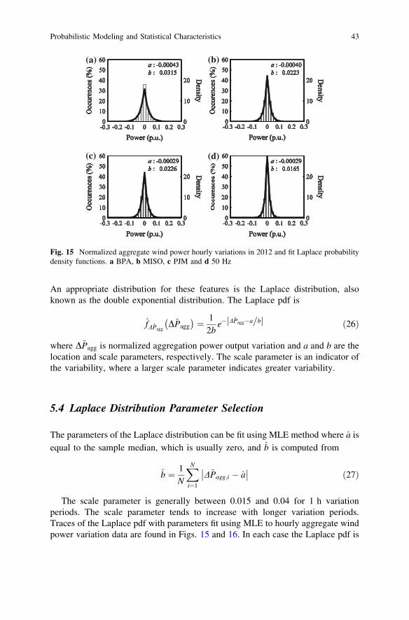
An appropriate distribution for these features is the Laplace distribution, alsoknown as the double exponential distribution. The Laplace pdf is

fD~PaggD~Pagg

� �¼ 1

2be� D~Pagg�a=bj j ð26Þ

where D~Pagg is normalized aggregation power output variation and a and b are thelocation and scale parameters, respectively. The scale parameter is an indicator ofthe variability, where a larger scale parameter indicates greater variability.

5.4 Laplace Distribution Parameter Selection

The parameters of the Laplace distribution can be fit using MLE method where a is

equal to the sample median, which is usually zero, and b is computed from

b ¼ 1N

XN

i¼1

D~Pagg;i � a�� ð27Þ

The scale parameter is generally between 0.015 and 0.04 for 1 h variationperiods. The scale parameter tends to increase with longer variation periods.Traces of the Laplace pdf with parameters fit using MLE to hourly aggregate windpower variation data are found in Figs. 15 and 16. In each case the Laplace pdf is

(a) (b)

(c) (d)

Fig. 15 Normalized aggregate wind power hourly variations in 2012 and fit Laplace probabilitydensity functions. a BPA, b MISO, c PJM and d 50 Hz


able to reasonably approximate the data. A rigorous evaluation of the fit of Laplacedistributions to aggregate wind power is found in [44].

5.5 Influence of Variation Period

An important factor influencing the pdf of wind power variation is the variationperiod. As discussed in Sect. 4.4, the variation in wind power from wind plantsexhibits greater correlation as the variation period increases. Additionally, there isalso more time for the wind power to change, so there is greater potential forextreme variation. Figure 17 shows histograms and fit Laplace pdfs for hourly and4-hourly variation periods. It is clear that a longer variation period results in abroader distribution, and hence, more variability that must be managed. TheLaplace distribution is able to reasonably fit the data at both variation periodsmainly by adjusting its scale parameter.

6 Statistical Characteristics of Aggregate Wind Power

It has only been within the last several years that aggregate wind power data setshave been made widely available to the research community. In this section weanalyze several data sets with the goal of documenting and discussing statistical

(a) (b)

(c) (d)

Fig. 16 Normalized aggregate wind power hourly variations in 2008 and fit Laplace probabilitydensity functions. a BPA, b MISO, c PJM and d 50 Hz


characteristics of aggregate wind power, as well as seeking additional insight intogeographic diversity.

6.1 Data Set Descriptions

Four data sets of aggregate wind power are considered: Bonneville Power Adminis-tration (BPA), Midwest ISO (MISO),PJM Interconnection (PJM),and50 Hz[45–48].BPA’s territory is located in the Pacific Northwest of the United States, primarily inWashington State and Oregon. MISO has territory in 12 states in the midwest of theUnited States and in the Canadian province of Manitoba. PJM’s territory covers all orpartsof13states in theeasternportionof theU.S.50Hz’s territory is in thenorthernandeastern portion of Germany. Each system has a large amount of wind plant capacity.

The data correspond to hourly averages for the years 2008 and 2012. The datahave been normalized to reported system-wide wind capacity. However, thesereports are infrequently issued. To overcome this, linear interpolation betweenreporting dates was used. This inherently introduces some error in the analysis, andso the reported statistics must be interpreted with this in mind. The capacities atthe start and end of 2008 and 2012 are provided in Table 1.

(a) (b)

Fig. 17 Normalized aggregate wind power variation histograms and fit Laplace distributions for1-h (a) and 4-h variation periods (b)

Table 1 Data set descriptions

System 2008 startcapacity (MW)

2008 endcapacity (MW)

2012 startcapacity (MW)

2012 endcapacity (MW)

BPA 1,301 1,671 4,131 4,711MISO 2,462 4,327 10,514 12,270PJM 1,150 1,277 5,318 6,45750 Hz 9,091 9,493 11,570 12,420


6.2 Statistical Analysis of Uncertainty

Several statistical quantities of instantaneous aggregate wind power for eachsystem for 2012 and 2008 are provided in Tables 2 and 3, respectively. In additionto the mean and standard deviation, several quantiles were computed, where, forexample, Q(50) refers to the median.

The mean values range between 0.18 and 0.33 p.u., and the standard deviationranges from 0.17 to 0.29 p.u. These typical ranges of mean and standard deviationcan be used to construct models of aggregate wind power, as discussed inSect. 5.2. The Q(99) quantiles indicates the magnitude of rare wind power events.For example, for BPA in 2012, in 99 % of the hours the aggregate wind power wasless than or equal to 85 % of the rated capacity. This means that 1 % of year—approximately 88 h—the power was greater than 0.85 p.u. For all systems, thevalues corresponding to the 99 % quantile ranged between 0.68 and 0.88 p.u.Extremely low values were common: the 10 % quantile is 0.08 p.u. or less in allcases. In other words, in each system the power output is less than 8 % of ratedcapacity for nearly 876 h each year. The relatively high frequency of low poweroutput has system-wide generation capacity implications. In general, the systemshave very different levels of uncertainty that must be managed by their operators.By several measures, MISO, PJM, and 50 Hz have less uncertainty than BPA.

6.3 Statistical Analysis of Variability

The statistics for hour-to-hour variation for each system in 2012 and 2008 areprovided in Tables 4 and 5, respectively. The variations of aggregate wind power

Table 2 Instantaneous aggregate wind power statistical information for 2012

System Mean (p.u.) Standarddeviation (p.u.)

Q(1)(p.u.)

Q(10)(p.u.)

Q(20)(p.u.)

Q(50)(p.u.)

Q(80)(p.u.)

Q(90)(p.u.)

Q(99)(p.u.)

BPA 0.26 0.26 0.00 0.01 0.02 0.16 0.52 0.68 0.85MISO 0.31 0.19 0.02 0.08 0.13 0.28 0.51 0.58 0.72PJM 0.25 0.17 0.01 0.05 0.09 0.21 0.39 0.50 0.6850 Hz 0.18 0.17 0.00 0.02 0.04 0.12 0.28 0.41 0.78

Table 3 Instantaneous aggregate wind power statistical information for 2008

System Mean(p.u.)

Standarddeviation (p.u.)

Q(1)(p.u.)

Q(10)(p.u.)

Q(20)(p.u.)

Q(50)(p.u.)

Q(80)(p.u.)

Q(90)(p.u.)

Q(99)(p.u.)

BPA 0.32 0.29 0.00 0.01 0.03 0.25 0.64 0.76 0.88MISO 0.30 0.19 0.02 0.08 0.12 0.27 0.49 0.58 0.71PJM 0.33 0.22 0.01 0.07 0.12 0.30 0.53 0.64 0.8950 Hz 0.20 0.20 0.01 0.03 0.05 0.13 0.35 0.52 0.80


in large systems tend to be symmetric, with near-zero mean and median. In mostsystem, the variations are less than 0.06 p.u. in magnitude for over 80 % of thehours. Extreme outliers corresponding to changes of 0:08 to 0.17 p.u. do occur,but are rare. The standard deviations range from 0.024 to 0.054 p.u. In eachsystem, the variations are leptokurtic, indicating a higher occurrence of ‘‘tailevent’’ variations. In general, MISO, PJM, and 50 Hz have less variability thanBPA.

6.4 Effect of Capacity on Uncertainty and Variability

The effect of capacity and capacity increases on aggregate wind power uncertaintyand variability are often of interest as system operators anticipate and plan forincreased amounts of wind plants in their system. The specifics of how theuncertainty and variability associated with aggregate wind power are related tocapacity depend on the build-out of the wind plants in the system, and are difficultto analytically derive. However, based on the available data and past experience,there are several general observations that can be made:

1. Systems with larger installed capacities do not necessarily exhibit less uncer-tainty and variability in aggregate wind power than systems with smallercapacities.

2. Additions of wind plant capacity to a system tend reduce uncertainty andvariability.

3. Within a given system, the benefits of geographic diversity can become satu-rated and insensitive to increases in capacity.

Table 4 Aggregate wind power hourly variation for 2012

System Standarddeviation(p.u.)

Kurtosis Q(1)(p.u.)

Q(10)(p.u.)

Q(20)(p.u.)

Q(50)(p.u.)

Q(80)(p.u.)

Q(90)(p.u.)

Q(99)(p.u.)

BPA 0.048 7.0 -0.130 -0.053 -0.029 0.00 0.026 0.057 0.144MISO 0.030 4.4 -0.79 -0.036 -0.022 0.00 0.021 0.036 0.083PJM 0.032 28.2 -0.84 -0.035 -0.022 0.00 0.021 0.037 0.08350 Hz 0.024 6.5 -0.66 -0.027 -0.015 0.00 0.014 0.027 0.072

Table 5 Instantaneous aggregate wind power hourly variation for 2008

System Standarddeviation(p.u.)

Kurtosis Q(1)(p.u.)

Q(10)(p.u.)

Q(20)(p.u.)

Q(50)(p.u.)

Q(80)(p.u.)

Q(90)(p.u.)

Q(99)(p.u.)

BPA 0.054 8.2 -0.138 -0.061 -0.034 0.00 0.030 0.061 0.167MISO 0.034 5.0 -0.093 -0.041 -0.024 0.00 0.024 0.040 0.089PJM 0.049 7.3 -0.128 -0.055 -0.032 0.00 0.031 0.055 0.13150 Hz 0.026 7.0 -0.075 -0.027 -0.015 0.00 0.015 0.029 0.073


As an example of the first observation, we compare the statistics of instantaneouspower in PJM and BPA. At the end of 2012, there was 4.7 GW of installed windcapacity in BPA. At the end of 2008 in PJM there was 1.3 GW of installed windcapacity. It would seem that BPA should have less uncertainty given its muchhigher installed capacity and therefore greater opportunity for geographic diversity.However, the standard deviation of PJM (0.22 p.u.) was less than that of BPA(26 p.u.). BPA also generally exhibited more occurrences of extremely low andhigh power production, as shown by the quantiles in Tables 2 and 3. A similarexample for variability can be made by comparing 2008 MISO data with 2008 BPAdata. These cases should not be misinterpreted as evidence that systems with highercapacities of wind plants have greater uncertainty and variability than those withlower capacities. Rather, they are simply examples that the contrary is not alwaysthe case. The important concept is that different systems experience different build-outs of wind plants—some lead to appreciable geographic diversity, others do not.

The second observation—that additions of wind plant capacity to a system tendreduce uncertainty and variability—is observed by comparing the statistics of eachsystem in 2008–2012. In each system, the standard deviation of the instantaneouspower and power variation decreased from 2008 to 2012. The exception is MISO,whose standard deviation of instantaneous power remained the same. Regardless,the data support the general notion that wind plant capacity additions decreaseuncertainty and variability.

The final observation—that the benefits of uncertainty and variability reductioncan become saturated—is supported by examining the sensitivity of uncertainty andvariability to capacity addition. For BPA, PJM and 50 Hz, for every 1 GW of newwind plant installations, the standard deviation of instantaneous wind powerdecreased by just one percentage point, based upon year-end capacity values. ForMISO, the standard deviation did not change, despite an increase in 8 GW of windpower. The quantiles in many systems also showed modest changes despite largecapacity additions. The modest effects of capacity additions on uncertainty can beseen by inspecting Figs. 13 and 14. The histograms and approximated probabilitydensity functions of the system do not appear appreciably different in 2012 thanthey did in 2008, despite several thousand megawatts of wind plant installations ineach system. The histograms and probability density functions of variations inFigs. 15 and 16, however, have more noticeable differences.

The sensitivity of variability to changes in capacity are mixed. The standarddeviation of wind power variability in BPA and PJM decreased by approximately0.25 % point for each 1 GW of new capacity. A change in percentage point of thismagnitude is appreciable since the standard deviations of variation are all less than6 %. However, both MISO and 50 Hz exhibited small changes to their standarddeviation between 2008 and 2012.


7 Conclusions

Many power systems around the world now have total installed wind plantcapacities in excess of several gigawatts. System operators must manage theinherent uncertainty and variability of the aggregate wind power in their systemsin order to maintain reliability and economic efficiency. The characteristics ofaggregate wind power can be quite different from individual wind plants,depending on the level of geographic diversity in the system. Tools such as windpower forecast systems, stochastic unit commitment, and resource planningrequire reasonable and practical probabilistic models of aggregate wind power andwind power variation as inputs.

This chapter demonstrated that the uncertainty and variability exhibited byaggregate wind power can be reasonably represented using parsimonious para-metric models. More specifically, the two-parameter Beta distribution is wellsuited for modeling instantaneous aggregate wind power and the two-parameterLaplace distribution is well suited for modeling moment-to-moment variation.

Several aspects of geographic diversity were explored. Among the main con-clusions are that geographic diversity should not be viewed as a panacea for thechallenges of wind integration. Reduction in variability—the smoothing effect—isnoticeable, but reduction in uncertainty requires exceedingly large geographicareas. Appreciable correlation of instantaneous power amongst wind plants canexist at distances approaching 1,000 km. Clustering and other practical consid-erations also limit the amount of geographic diversity that occurs in many systems.Analysis of several systems showed that the effects of geographic diversity, par-ticularly on uncertainty, saturate when installations of wind plants reach severalgigawatts in total.

References

1. Burton T, Sharpe D, Jenkins N, Bossanyi E (2001) Wind energy handbook. Wiley, WestSussex

2. Smith JC, Milligan M, DeMeo EA, Parsons B (2007) Utility wind integration and operatingimpact state of the art. IEEE Trans Power Syst 22:900–908. doi:10.1109/TPWRS.2007.901598

3. Smith JC, Thresher R, Zavadil R, DeMeo EA, Piwko R, Ernst B, Ackerman T (2009) Amighty wind. IEEE Power Energy Mag 7:41–51. doi:10.1109/MPE.2008.931492

4. Tuohy A, Meibom P, Denny E, O’Malley M (2009) Unit commitment for systems withsignificant wind penetration. IEEE Trans Power Syst 24:592–601. doi:10.1109/TPWRS.2009.2016470

5. Ruiz P, Philbrick CR, Zak E, Cheung K, Sauer P (2008) Applying stochastic programming tothe unit commitment problem. In: Probabilistic methods applied to power systems; 2008

6. Pinson P, Kariniotakis G (2010) Conditional prediction intervals of wind power generation.IEEE Trans Power Syst 25:1845–1856

7. Hasche B (2010) General statistics of geographically dispersed wind power. Wind Energy13:773–784. doi:10.1002/we.397


http://dx.doi.org/10.1109/TPWRS.2007.901598


http://dx.doi.org/10.1109/MPE.2008.931492



http://dx.doi.org/10.1002/we.397

8. EnerNex Corporation (2011) Eastern wind integration and transmission study. Technicalreport NREL/SR-5500-47078, NREL, Golden, CO, USA

9. GE Energy (2010) Western wind and solar integration study. Technical report NREL/SR-550-47434, NREL, Golden, CO, USA 2010

10. McNerney G, Richardson R (1992) The statistical smoothing of power delivered to utilitiesby multiple wind turbines. IEEE Trans Energy Convers 7(4):644–647. doi:10.1109/60.182646

11. Archer C, Jacobson M (2003) Spatial and temporal distributions of U.S. winds and windpower at 80 m derived from measurements. J Geophys Res 108(D9):10–1–10–20

12. Wan Y (2004) Wind power plant behaviors: analyses of long-term wind power data.Technical report NREL/TP-500-36551

13. Holttinen H (2005) Hourly wind power variations in the Nordic countries. Wind Energy8:173–195

14. Ernst B, Wan Y, Kirby B (1999) Short-term power fluctuation of wind turbines: analyzingdata from the German 250-MW measurement program from the ancillary services viewpoint.Technical report NREL/CP-500-26722

15. Wan Y, Milligan M, Parsons B (2003) Output power correlation between adjacent windpower plants. J Sol Energy Eng 125:551–555

16. Louie H (2013) Correlation and statistical characteristics of aggregate wind power in largetranscontinental systems. Wind Energy. doi:10.1002/we.1597

17. Tastu J, Pinson P, Kotwa E, Madsen H, Nielsen H (2011) Spatio-temporal analysis andmodeling of short-term wind power forecast errors. Wind Energy 14:43–60. doi:10.1002/we.401

18. Nanahara T, Asari M, Maejima T, Sato T, Yamaguchi K, Shibata M (2004) Smoothingeffects of distributed wind turbines. Part 2. Coherence among power output of distant windturbines. Wind Energy 7:75–85. doi:10.1002/we.108

19. Krich A, Milligan M (2005) The impact of wind energy on hourly load followingrequirements: an hourly and seasonal analysis. Technical report NREL/CP-500-38061

20. Wan Y (2011) Analysis of wind power ramping behavior in ERCOT. Technical reportNREL/TP-5500-49218 2011

21. Gibescu M, Brand A, Kling W (2008) Estimation of variability and predictability of large-scale wind energy in the Netherlands. Wind Energy 12:241–260. doi:10.1002/we.291

22. Milligan M (2000) Modelling utility-scale wind power plants. Part 2: Capacity credit. WindEnergy 3:167–206. doi:10.1002/we.36

23. Sloughter JM, Gneiting T, Raftery AE (2010) Probabilistic wind speed forecasting usingensembles and Bayesian model averaging. J Am Stat Assoc 105:25–35. doi:10.1198/jasa.2009.ap08615

24. Papoulis A, Pillai SU (2002) Probability, random variables and stochastic processes, 4th edn.McGraw-Hill, New York

25. Justus CG, Hargraves WR, Mikhail A, Graber D (1978) Methods for estimating wind speedfrequency distributions. J Appl Meteorol 17:350–353

26. Tuzuner A, Yu Z (2008) A theoretical analysis on parameter estimation for the weibull windspeed distribution. IEEE PES General Meeting 2008

27. Twidell J, Weir T (2006) Renew Energy Res, 2nd edn. Taylor & Francis, London28. International Electrotechnical Commission (2005), Power performance measurements of

electricity producing wind turbines. Standard 61400-12-129. Camm EH, Behnke MR, Bolado O et al (2009) Wind power plant substation and collector

system redundancy, reliability and economics. IEEE PES general meeting 200930. Fischer K, Besnard F, Bertling L (2012) Reliability-centered maintenance for wind turbines

based on statistical analysis and practical experience. IEEE Trans Energy Convers27(184):195. doi:10.1109/TEC.2011.2176129

31. Potter CW, Gil H, McCaa J (2007) Wind power data for grid integration studies. IEEE PESgeneral meeting


http://dx.doi.org/10.1109/60.182646

http://dx.doi.org/10.1109/60.182646







http://dx.doi.org/10.1198/jasa.2009.ap08615

http://dx.doi.org/10.1198/jasa.2009.ap08615

http://dx.doi.org/10.1109/TEC.2011.2176129

32. Hayes B, Ilie I, Porpodas A, Djokic S, Chicco G. Equivalent power curve model of a windfarm based on field measurement data. In: IEEE PowerTech; 2011

33. Jin T, Tian Z (2010) Uncertainty analysis for wind energy production with dynamic powercurves. In: Probabilistic methods applied to power systems; 2010

34. Collins J, Parkes J, Tindal A (2009) Forecasting for utility-scale wind farms—the powermodel challenge. In: CIGRE/IEEE joint symposium on integration of wide-scale renewableresources into the power delivery system 2009

35. Kendall M (1938) A new measure of rank correlation. Biometrika 30:81–8936. Louie H (2012) Evaluating Archimedean copula models of wind speed for wind power

modeling. Power Africa 2012:1–5. doi:10.1109/PowerAfrica.649861037. Wind integration datasets (2011) National Renewable Energy Laboratory. http://www.nrel.

gov/wind/integrationdatasets. Accessed 1 July 201338. Osborn D, Hendersen M, Nickell B, Lasher W, Liebold C, Adams J, Caspary J (2011)

Driving forces behind wind. Power Energy Mag 9:60–7439. Nelsen R (2006) An introduction to copulas, 2nd edn. Springer, New York40. Louie H (2012) Evaluation of bivariate Archimedean and elliptical copulas to model wind

power dependency structures. Wind Energy. doi:10.1002/we.157141. Díaz G (2013) A note on the multivariate Archimedean dependence structure in small wind

generation sites. Wind Energy. doi:10.1002/we.163342. Louie H (2010) Characterizing and modelling aggregate wind plant power output in large

systems. IEEE PES general meeting; 2010, pp 1–843. Beckman RJ, Tietjen GL. Maximum likelihood estimation for the beta distribution. J Stat

Comput Simul 7:253–25844. Louie H (2010) Evaluation of probabilistic models of wind plant power output

characteristics. In: Probabilistic methods applied to power systems; 2010, pp 442–447, doi:10.1109/PMAPS.2010.5528963

45. McManus B (2013) Wind generation & total load in the BPA balancing authority. BonnevillePower Administration. http://www.transmission.bpa.gov/Business/Operations/Wind/default.aspx. Accessed 1 July 2013

46. Market reports (2013). MISO. https://www.midwestiso.org/Library/MarketReports/. Acces-sed 1 July 2013

47. Operational analysis (2013). PJM interconnection www.pjm.com/markets-and-operations/ops-analysis.aspx. Accessed 1 July 2013

48. Archive wind power (2013). 50 Hertz. http://www.50hertz.com/en/1983.htm. Accessed 1July 2013


http://dx.doi.org/10.1109/PowerAfrica.6498610

http://www.nrel.gov/wind/integrationdatasets

http://www.nrel.gov/wind/integrationdatasets



http://dx.doi.org/10.1109/PMAPS.2010.5528963

http://www.transmission.bpa.gov/Business/Operations/Wind/default.aspx

http://www.transmission.bpa.gov/Business/Operations/Wind/default.aspx

https://www.midwestiso.org/Library/MarketReports/

http://www.pjm.com/markets-and-operations/ops-analysis.aspx

http://www.pjm.com/markets-and-operations/ops-analysis.aspx

http://www.50hertz.com/en/1983.htm

Probabilistic Modeling and Statistical Characteristics of

Documents

Transcript of Probabilistic Modeling and Statistical Characteristics of