Probabilistic Democracy

Muhammet A. BasDepartment of Government

Harvard University

Randall StoneDepartment of Political Science

University of Rochester

Abstract

Democracy is an important concept that is difficult to measure, and all existing measureshave well-known weaknesses. We propose a minimalist definition—a democratic governmentis one in which the incumbent steps down if she loses a competitive election (Przeworski,2000)—and an algorithm for estimating the conditional probability of democracy using a struc-tural model. The model allows for strategic voting, and we find that leaders are often reelectedbecause the voters fear the conflict that might ensue if they were defeated. Ratification of theConvention Against Torture by the country in question emboldens voters, while ratificationby third parties, close relations with the United States and the incumbent’s military experi-ence increase voter intimidation. Our estimated democracy scores are highly correlated withPolity and ACLP. They diverge from Polity because they capture different concepts, and fromACLP because the latter underestimates the uncertainty inherent in cases that are difficult tocode. Comparisons of these variables using the democratic peace and the relationship betweendemocracy and development underscore the fact that even relatively small perturbations indemocracy codings can have substantively important effects.

A minimalist definition of democracy is that competitive elections are held, and the incum-

bent steps down if she loses (Przeworski, 1991, 2000). This does not capture everything that is

commonly thought to be important about democratic institutions, but it does capture a necessary

condition. The credibility of electoral sanctions is essential for the operation of democratic insti-

tutions, and it is an important dimension along which contemporary electoral systems vary. This

definition has an advantage over the multidimensional conceptions of democracy behind the com-

monly employed quantitative measures, because it is objective and does not require aggregation

of diverse indicators. However, this is a measure that cannot be coded; it must be estimated. The

effectiveness of electoral sanctions is inherently uncertain, because it represents the probability

that the incumbent steps down, conditional on losing.

To illustrate the point, consider a hypothetical situation. Presidential elections are held in 2018

in Russia, and Vladimir Putin is declared the winner. Were electoral sanctions in place? Critics

will charge that the election was not “free and fair,” because the incumbent had a number of extra-

constitutional advantages. He controlled the mass media, intimidated his opponents, controlled an

impressive system of patronage, and employed various forms of electoral misconduct. Supporters

will point out that Putin remains highly popular in Russia despite all of the things his Western

detractors say about him, and he almost certainly won a majority of the votes. The problem is that

we do not observe an outcome that would allow us to judge with certainty: it may be the case that

Putin won, but would have refused to step down had he lost. Since we only observe the decision

whether to accept an unfavorable electoral outcome when such an outcome occurs, we are left to

draw uncertain inferences.

Przeworski (2000) attempt to get around this problem by using a conservative coding rule, and

judging a political system to be democratic only after a peaceful transfer of power to the opposition

has taken place. This purchases a low frequency of type I errors (false democracies) at the cost

of a high frequency of type II errors (false non-democracies). In addition, it does not allow for

1

the existence of borderline cases, or for the possibility that the probability of compliance varies

between elections. In what follows, we introduce a method to estimate the probability of stepping

down, conditional on losing an election. The model allows for partial observability — we may

only know for certain that the election was lost if we observe that the incumbent steps down —

but also allows us to incorporate more detailed information that we have about particular cases

to improve the efficiency of our estimates. Our estimates of democracy differ in interesting ways

from the codings by Przeworski et al. and by Polity, which is consistent with the interpretation

that uncertainty about the efficacy of electoral sanctions is generally greater than it appears to the

analyst in retrospect. In the case of Russia, we find that it is unlikely that Putin would comply if

he were voted down.1 We can say more than this, however; we have a point estimate that changes

over time and a confidence interval, and we think both of these tell us something important about

Russia’s political system.

The model is strategic, as we explain below, which in this case means that voters can take into

account their expectations about whether the leader will comply when they decide how to vote.

This allows for a novel explanation for elections in authoritarian regimes: leaders are willing to

hold elections because they rely on a portion of the population to vote for them strategically in order

to avoid the conflict and disorder that would follow if the leader lost and repudiated the election.

We find that voter intimidation is an important substantive explanation for electoral outcomes in

semi-competitive political systems. Ratification of the Convention Against Torture by the country

in question emboldens voters, while ratification by third parties, close relations with the United

States, and the incumbent’s military experience increase voter intimidation. We are able to directly

test the hypothesis that vote choices depend on the expected probability that the incumbent steps

down when faced with electoral defeat by using a comparative model test.

1The estimated probability was 0.36 in 2000 and 0.44 in 2004.

2

We go on to apply our estimates of democracy to two of the key empirical puzzles in political

science, the democratic peace and the effect of democracy on development. The effects of our mea-

sure of democracy are qualitatively similar to those of Polity and of the Przeworski et al. measure,

but there are some important differences. Our measure supports the democratic peace hypothesis

more robustly than the Przeworski et al. measure, and an interactive model that disentangles the

decisions of initiators and targets suggests that it best fits the intuition that the democratic peace

holds because democracies are reluctant to fight other democracies. Only our measure contains

enough over-time variation to provide evidence for the democratic peace even with country fixed

effects. All three measures support the finding that democracy retards growth, but only in relatively

prosperous countries, but they differ with respect to the threshold of wealth necessary for the effect

to take hold. Our measure indicates that this is a concern only in high-income countries, while

the others suggest that it is a problem for middle-income countries as well. Our measure has the

advantage that it comes with an estimate of its own uncertainty, so the estimates of these effects

have been corrected for the uncertainty of the measure.

1 A Minimalist Conception of Democracy

The conception of democracy advanced in Przeworski (1991) and Przeworski (2000) is based on

the effectiveness of electoral sanctions. In order for democratically elected leaders to represent

the preferences of the citizenry and safeguard their liberty, it must be the case that the electorate

can replace an unsatisfactory leader. It is a necessary condition for the operation of democracy,

then, that leaders are subject to competitive elections, and that when they lose, they step down. As

Przeworski (1991) puts it, in order for democracy to be a self-enforcing equilibrium, it must be the

case that opposition candidates have incentives to challenge the incumbent, that the outcome of the

election be uncertain, and that the incumbent prefers to concede defeat if she loses.

3

This way of posing the question focuses on the credibility of elections, which is a key empirical

issue facing contemporary electoral systems. Elections have become ubiquitous features of even

authoritarian political systems. Authoritarian leaders use plebiscites and semi-competitive elec-

tions as ways to cement their legitimacy and demonstrate their popularity to rivals and to foreign

and domestic audiences. Indeed, the benefits of international recognition spur “pseudo-democrats”

to invite international monitors to oversee their elections, even when they intend to cheat (Hyde,

2011). In many cases, the ranks of potential challengers are screened to prevent the emergence of

real threats, either through legal maneuvers or through intimidation. The media may be closely

controlled and biased in favor of the incumbent. Vote buying, ballot stuffing and electoral repres-

sion tilt the competition in the incumbent’s favor. It might seem that interfering with electoral

outcomes so overtly would defeat the purpose of holding elections in order to demonstrate the dic-

tator’s popularity, but recent work suggests that insecure authoritarian leaders benefit from holding

unfair elections because their opponents are left uncertain about how much support they have

(Rozenas, 2016). However, even rigged elections can be lost, and this has become one of the more

common routes to democratization. Meanwhile, some of the same tactics are used to advantage

incumbents in a wide range of democratic states, although the more overt forms of manipulation

are most common in developing countries (Stokes et al., 2013). Consequently, the dividing line be-

tween democracy and authoritarianism has become blurred, and the key feature that distinguishes

between the two is the probability that the incumbent, if defeated, would in fact step down.

This conception is minimalist in the sense that it identifies only a necessary condition for

democracy, and not a sufficient condition. It remains an empirical question whether competi-

tive elections and effective electoral sanctions guarantee the representation of voter preferences,

the flourishing of an independent media, or the free exercise of a wide range of rights and liber-

ties. According to the Freedom House scale, in contrast, these rights and liberties are the defining

features of democracy. These conditions, and additional institutional features such as division of

powers, constraints on the executive, and an independent judiciary, may also be necessary for elec-

4

toral sanctions to be effective. However, these other features of a democratic political system that

correlate with effective electoral sanctions are not part of the definition. In contrast, these institu-

tional features are the key defining features of democracy according to the polity project (Jaggers

and Gurr, 1995).

Similarly, this definition does not incorporate political participation. While eschewing the term

democracy, Dahl (1973) argued that polyarchy was defined along two dimensions, contestation and

participation. Similarly, Barber (2003) argued that the quality of democracy depended critically

on the breadth and depth of participation. The notion that participation is central to democratic

governance and depends on a supportive political culture goes back to De Tocqueville (2003),

and finds expression in a long line of comparative behavioral studies of political culture (Verba

and Almond, 1963). This notion of democracy is often invoked to criticize ambitious democracy-

promotion efforts abroad. Along similar lines, Robert Putnam argues that effective performance of

democratic institutions depends upon a supportive political culture, which may have deep historical

roots (Putnam, Leonardi and Nanetti, 1994).

Moreover, our definition does not impose restrictions on the membership of the electorate,

which is often held to be a key defining feature of democracy. In the literature on the democratic

peace, for example, cases of wars between democracies are sometimes excluded on the grounds

that one country or the other had a restrictive franchise. For example, was Britain a democracy in

1812? An institutional view of democracy proposed by De Mesquita and Smith (2005) argues that

the defining features of political systems are the size of the selectorate that chooses the leader and

the size of the necessary winning coalition.

More broadly, the minimalist definition of democracy does not make any claims about repre-

sentation. This may be regarded as a theoretical advantage, because electoral sanctions have more

secure game-theoretic micro-foundations than representation. Representative notions of democ-

racy run into difficulties because diverse preferences of members of society have to be aggregated

5

by institutions. For example, electoral institutions based on single-member districts tend to fa-

vor the preferences of the median voter, while proportional-representation systems provide better

representation for extreme preferences, but make elected officials less responsive to changes in

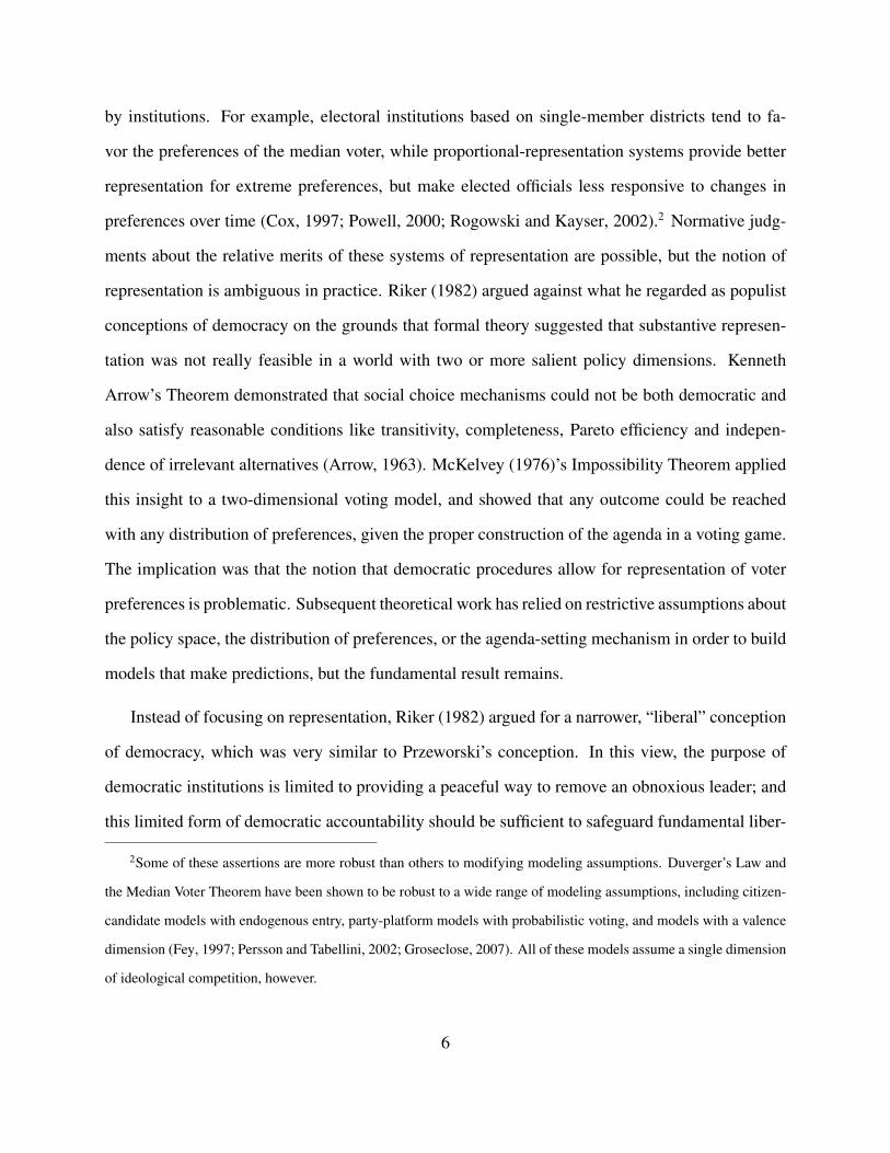
preferences over time (Cox, 1997; Powell, 2000; Rogowski and Kayser, 2002).2 Normative judg-

ments about the relative merits of these systems of representation are possible, but the notion of

representation is ambiguous in practice. Riker (1982) argued against what he regarded as populist

conceptions of democracy on the grounds that formal theory suggested that substantive represen-

tation was not really feasible in a world with two or more salient policy dimensions. Kenneth

Arrow’s Theorem demonstrated that social choice mechanisms could not be both democratic and

also satisfy reasonable conditions like transitivity, completeness, Pareto efficiency and indepen-

dence of irrelevant alternatives (Arrow, 1963). McKelvey (1976)’s Impossibility Theorem applied

this insight to a two-dimensional voting model, and showed that any outcome could be reached

with any distribution of preferences, given the proper construction of the agenda in a voting game.

The implication was that the notion that democratic procedures allow for representation of voter

preferences is problematic. Subsequent theoretical work has relied on restrictive assumptions about

the policy space, the distribution of preferences, or the agenda-setting mechanism in order to build

models that make predictions, but the fundamental result remains.

Instead of focusing on representation, Riker (1982) argued for a narrower, “liberal” conception

of democracy, which was very similar to Przeworski’s conception. In this view, the purpose of

democratic institutions is limited to providing a peaceful way to remove an obnoxious leader; and

this limited form of democratic accountability should be sufficient to safeguard fundamental liber-

2Some of these assertions are more robust than others to modifying modeling assumptions. Duverger’s Law and

the Median Voter Theorem have been shown to be robust to a wide range of modeling assumptions, including citizen-

candidate models with endogenous entry, party-platform models with probabilistic voting, and models with a valence

dimension (Fey, 1997; Persson and Tabellini, 2002; Groseclose, 2007). All of these models assume a single dimension

of ideological competition, however.

6

ties and to prevent the leader from pursuing policies that antagonize the overwhelming majority of

voters. This is consistent with the view taken by early democratic theorists, whose chief concern

was to prevent the usurpation of power by a tyrant. For Calvin, Calvin and Battles (1995) and

Locke (2014), rebellion was justified to overthrow tyranny, but not in order to ensure that gov-

ernment policies reflected majority preferences. De Montesquieu (1989) justified the division of

powers as a device to prevent tyranny. Similarly, the Federalists argued for the division of powers,

and more specifically for a bicameral legislature, a presidential veto and an independent judiciary,

on grounds that these institutions created the means and provided the incentives for the incumbents

of various offices to hold each other in check. Institutional design was chiefly useful in order to

ensure that democracy was a self-enforcing equilibrium. On the other hand, the Federalists were

suspicious of factions that represented diverse interests, because they might undermine the pursuit

of the general interest in preventing the consolidation of tyrannical power.

This limited conception of democracy is consistent with Ferejohn (1986)’s model of incum-

bent quality and electoral control, which points to a fundamental tension between efforts to use

democratic institutions to constrain opportunistic leaders and the ambition to use them to repre-

sent the full range of voter preferences. In this model, the electorate has only general interests in

good governance, and the incumbent may be competent or incompetent, but has the opportunity

to improve outcomes by exerting costly effort. The key result of the model is that voters can use

retrospective voting to discipline the incumbent and induce her to exert effort, although there is

a trade-off between creating strong incentives for the incumbent to exert effort and taking advan-

tage of opportunities to replace incompetent incumbents. In an extension of the model to the case

where voters have heterogeneous interests, however, this virtuous equilibrium unravels. If voters

have diverse preferences, the incumbent can play segments of the electorate off against each other

and escape effective control.

7

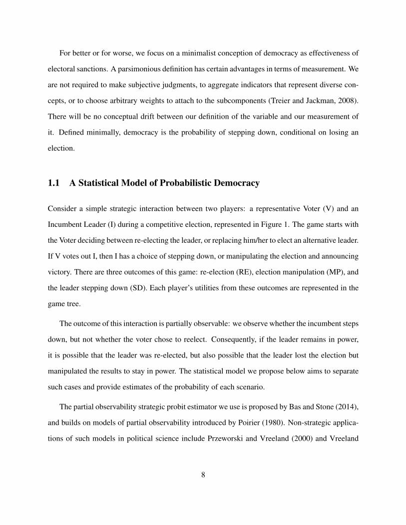
For better or for worse, we focus on a minimalist conception of democracy as effectiveness of

electoral sanctions. A parsimonious definition has certain advantages in terms of measurement. We

are not required to make subjective judgments, to aggregate indicators that represent diverse con-

cepts, or to choose arbitrary weights to attach to the subcomponents (Treier and Jackman, 2008).

There will be no conceptual drift between our definition of the variable and our measurement of

it. Defined minimally, democracy is the probability of stepping down, conditional on losing an

election.

1.1 A Statistical Model of Probabilistic Democracy

Consider a simple strategic interaction between two players: a representative Voter (V) and an

Incumbent Leader (I) during a competitive election, represented in Figure 1. The game starts with

the Voter deciding between re-electing the leader, or replacing him/her to elect an alternative leader.

If V votes out I, then I has a choice of stepping down, or manipulating the election and announcing

victory. There are three outcomes of this game: re-election (RE), election manipulation (MP), and

the leader stepping down (SD). Each player’s utilities from these outcomes are represented in the

game tree.

The outcome of this interaction is partially observable: we observe whether the incumbent steps

down, but not whether the voter chose to reelect. Consequently, if the leader remains in power,

it is possible that the leader was re-elected, but also possible that the leader lost the election but

manipulated the results to stay in power. The statistical model we propose below aims to separate

such cases and provide estimates of the probability of each scenario.

The partial observability strategic probit estimator we use is proposed by Bas and Stone (2014),

and builds on models of partial observability introduced by Poirier (1980). Non-strategic applica-

tions of such models in political science include Przeworski and Vreeland (2000) and Vreeland

8

Incumbent

Voters

replace

manipulate step down

Incumbent wins

Incumbentsteps down

re-elect

Incumbentwins

I

V

replace

manipulate step down

UV(MP)UI(MP)

UV(SD)UI(SD)

re-elect

UV(RE)UI(RE)

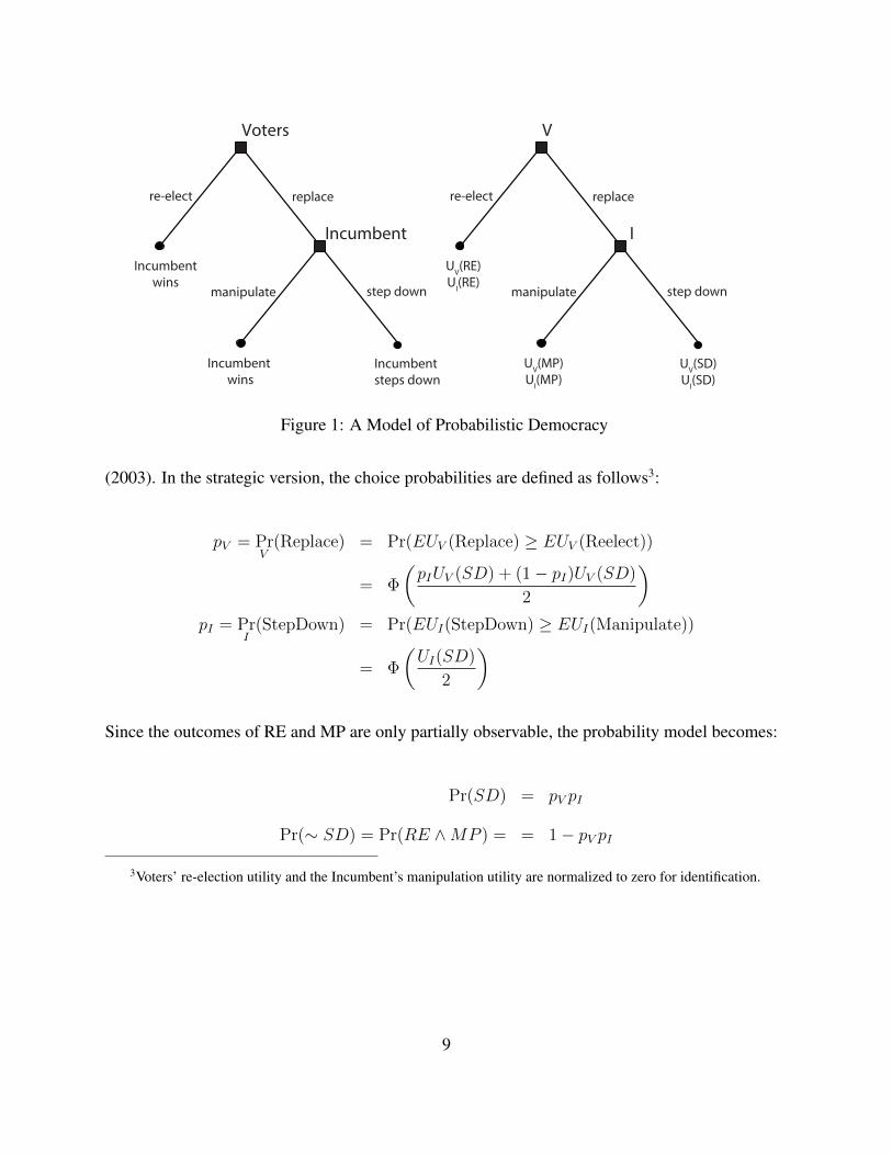
Figure 1: A Model of Probabilistic Democracy

(2003). In the strategic version, the choice probabilities are defined as follows3:

pV = PrV

(Replace) = Pr(EUV (Replace) ≥ EUV (Reelect))

= Φ

(pIUV (SD) + (1− pI)UV (SD)

2

)pI = Pr

I(StepDown) = Pr(EUI(StepDown) ≥ EUI(Manipulate))

= Φ

(UI(SD)

2

)

Since the outcomes of RE and MP are only partially observable, the probability model becomes:

Pr(SD) = pV pI

Pr(∼ SD) = Pr(RE ∧MP ) = = 1− pV pI

3Voters’ re-election utility and the Incumbent’s manipulation utility are normalized to zero for identification.

9

The remaining utilities are estimated with regressors. The corresponding likelihood function that

is maximized is

ln(L) =N∑i

ISD(ln(pV ) + ln(pI)) + (1− ISD) ln(1− pV pI)

where ISD is an indicator function recording whether the leader stepped down after the election.

1.2 Estimating Democracy

To identify competitive elections, we use the National Elections Across Democracy and Autocracy

(NELDA) Data Set (Hyde, 2011). We focus on elections for the office of the national leader

during the years 1945 to 2008. In presidential systems, only presidential elections are included in

our sample, while only parliamentary elections are included in parliamentary systems. We define

competitive elections as ones in which multiple parties were legal, at least one opposition party

competed, and multiple candidates appeared on the ballot.

These competitive elections constitute our sample for estimation. Our dependent variable,

Stepdown, answers the question, “did the incumbent leader step down after the election?” We used

information from NELDA to identify those elections in which the incumbent was replaced, and

stepped down because the vote count gave victory to another political actor. In our coding, we did

not count cases as the incumbent stepping down in which a successor was chosen by the previous

incumbent who replaced the incumbent leader after the elections. Thus, among the competitive

elections in our sample, Stepdown takes a value 1 if the incumbent lost the election and stepped

down based on the above criteria, and 0 otherwise. In terms of our theoretical model, the 0s reflect

partial observability: they include cases in which the incumbent won fair elections, and also cases

in which the incumbent would have lost a fair election, but was able to manipulate the election to

avoid stepping down.

10

In order to assist with the identification of the partial observability model, we incorporate

information about a few cases in which we can confidently code the outcome either as competitive

elections in which the incumbent leader won or as manipulated elections in which the incumbent

did not have sufficient support to win fairly. We create a revised dependent variable Stepdown2

by adding two more categories to Stepdown. In the former group, we include the elections in the

United States, Canada, UK, France (after 1947), Germany, Sweden, Finland, Norway, Denmark,

Netherlands, and Belgium. We assign a new category Stepdown2=3 for these cases. For elections

in our sample in which we believe the incumbent manipulated the outcome (Stepdown2=2), we

include Iran in 2009; Zimbabwe in 2008; Ukraine 2004 (first election); Ethiopia in 2005; Guyana

in 1980; Philippines in 1986; Zambia in 2001; Haiti in 1995 and 2000; and Togo in 2003 and 2005

(identified by Hyde).4

Our measure of democracy is the estimated probability that the leader steps down, conditional

on losing the election (Pr(StepDown|ElectionLoss)). Because this is an estimated quantity, we

are able to provide standard errors and confidence intervals for the point estimates of the proba-

bility of stepping down, and to incorporate estimation uncertainty when we use the measure as a

regressor. Since our sample only includes election years, we extend the measure to years without

elections for countries in the sample by making out-of-sample predictions based on the values of

the regressors in those years. For instance, for the United States post-2000, while our estimation

sample only includes 2000 and 2004, we calculate the measure for years 2001-03 as well. We

also extend the measure to countries that do not appear in our sample because they did not hold

competitive elections based on the criteria described above (e.g. North Korea). For these coun-

tries, we assign a Democracy score of 0. Finally, for countries in which the incumbent leader steps

down after losing the election in a given year, we code Democracy = 1, because our definition of

democracy is satisfied.

4The log-likelihood of this resulting model is ln(L) =∑N

i SD0 ln(1−pV pI)+SD1(ln pV +ln pI)+SD2(ln pV +

ln(1− pI)) + SD3 ln(1− pV ), where SDi are indicator variables representing the possible values of Stepdown2.

11

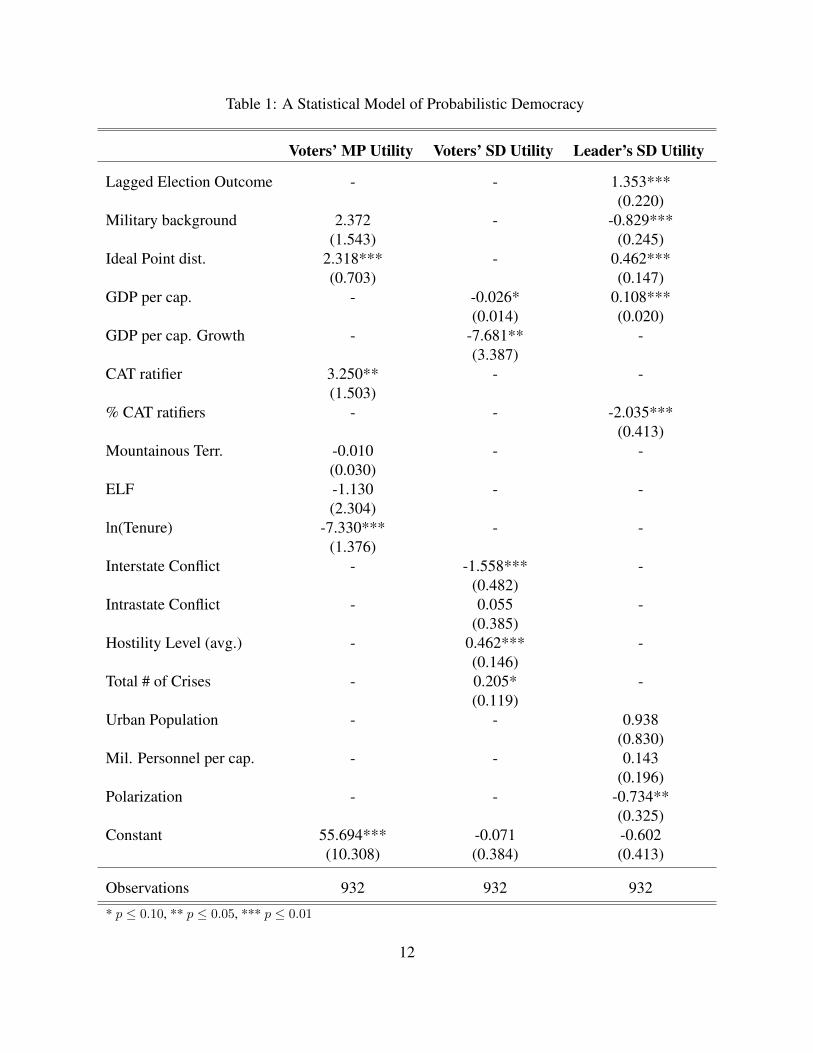
Table 1: A Statistical Model of Probabilistic Democracy

Voters’ MP Utility Voters’ SD Utility Leader’s SD Utility

Lagged Election Outcome - - 1.353***(0.220)

Military background 2.372 - -0.829***(1.543) (0.245)

Ideal Point dist. 2.318*** - 0.462***(0.703) (0.147)

GDP per cap. - -0.026* 0.108***(0.014) (0.020)

GDP per cap. Growth - -7.681** -(3.387)

CAT ratifier 3.250** - -(1.503)

% CAT ratifiers - - -2.035***(0.413)

Mountainous Terr. -0.010 - -(0.030)

ELF -1.130 - -(2.304)

ln(Tenure) -7.330*** - -(1.376)

Interstate Conflict - -1.558*** -(0.482)

Intrastate Conflict - 0.055 -(0.385)

Hostility Level (avg.) - 0.462*** -(0.146)

Total # of Crises - 0.205* -(0.119)

Urban Population - - 0.938(0.830)

Mil. Personnel per cap. - - 0.143(0.196)

Polarization - - -0.734**(0.325)

Constant 55.694*** -0.071 -0.602(10.308) (0.384) (0.413)

Observations 932 932 932

* p ≤ 0.10, ** p ≤ 0.05, *** p ≤ 0.01

12

The results of our analysis are presented in Table 1, and the coefficients in each column repre-

sent the effects of covariates on a particular actor‘s utility for a particular outcome. The marginal

effects of each variable and their confidence intervals are presented in Table 2. Because the model

is strategic, any variable that appears in both the voters’ and the leader’s utility function has a

compound effect on the vote choice; it influences the voters’ valuation of outcomes and the voters’

assessment of the probability that the leader will step down if defeated. Consequently, the statisti-

cal significance of coefficients may not coincide with statistical significance of marginal effects.5

The model is one of partial observability, and the inferential problem for the analyst is determin-

ing whether the voters in fact reelected the leader when the leader fails to step down following an

election. In order to generate credible estimates, therefore, we need to make identifying assump-

tions that pin down the voters‘ utilities for these distinct outcomes. Without loss of generality, we

normalize the voters‘ utility for reelecting the leader to zero, so our estimates for the effects of

covariates on the utility of the leader stepping down (SD) or remaining in power by manipulating

the election (MP) are measured relative to that baseline.

Consequently, the estimated utility for SD (second column) represents the difference between

the utility of reelecting a leader and the utility of removing the leader peacefully. We assume that

two sets of factors may influence this choice: economic well-being (GDP per capita, economic

growth, and the occurrence of an economic crisis) and armed conflict (interstate war, intrastate or

civil war, and severity of conflict). The economic variables have the results that are expected from

the economic voting literature. GDP per capita has the strongest effect; a one-standard deviation

increase in GDP per capita, or $10,000, decreases the probability that the electorate chooses to

5In addition, for the same reason, the model effectively interacts all of the variables in the leader’s utility with

all of the variables in the voters’ utility when calculating the voters’ choice, so the usual caveats about the statistical

significance of interactive estimates apply. We only discuss this when it plays an important role in the interpretation

of particular variables, however, and generally confine our discussion to the case where the interacting variables are at

their means or modes.

13

replace the leader by 33.7 percentage points. The level of economic growth has a weaker effect

in the same direction—a one-standard-deviation increase in growth decreases the probability by

7.6 percentage points—and economic crises have a marginally significant effect of encouraging

replacement of the leader.6 Economic crises, as defined by Reinhart and Rogoff (2009), include fi-

nancial crises, banking crises, exchange rate crises, sovereign debt crises or repudiation of domestic

debt. Their effect is only marginally significant in the main specification, but is highly significant

in specifications that do not include economic growth. Interstate conflict has a strong effect that

discourages replacing the leader. The probability of voting the leader out of office during a conflict

is reduced by 27.6 percentage points, which is consistent with behavioral arguments about a “rally

around the flag” effect and with strategic arguments about “gambling for resurrection” or diver-

sionary war (Downs and Rocke, 1995; Chiozza and Goemans, 2011; Debs and Goemans, 2010).

Civil war has no significant effect. In contrast, the severity of international conflict is associated

with significantly increased probability of replacing the leader, which is consistent with the result

in the public opinion literature that casualties have cumulative effects that undermine support for

war (Mueller, 1994).

On the other hand, the estimated utility for MP (first column) represents the difference in utili-

ties between retaining the leader through political manipulation or by reelection, and the quality of

leadership is irrelevant to this choice, because the leader remains in power either way. Instead, the

relevant variables are ones that make a political struggle over the succession more or less attrac-

tive from the point of view of the electorate. We assume that there are three sets of such factors:

personal characteristics of the leader that are relevant to regime stability (duration of tenure and

military background), international factors (ideal point distance from the United States measured

in terms of UN voting and ratification of the Convention Against Torture), and the feasibility of

6Note that GDP per capita, while only marginally significant in the voters’ utility, also plays a role in the leader’s

utility, and the net marginal effect of a one-standard deviation increase in GDP per capita has a 95% confidence interval

of a (-21.3, -46.2) percentage point reduction in the probability of voting the incumbent out of office.

14

waging a civil war (mountainous terrain and ethno-linguistic fractionalization). Only one leader

characteristic, the length of tenure, has a significant coefficient in the voters’ utility, but both have

significant marginal effects. The model estimates that with other variables at their means or modes,

voters prefer to reelect the leader rather than have the leader retain office through electoral manip-

ulation if the leader’s tenure is above average (approximately eight years). Increasing the length

of tenure by one standard deviation (to 26 years six months) reduces the estimated probability of

voting against the leader by 11 percentage points. The leader’s military background increases the

probability of voting against the leader by 21 percentage points.

Two international factors have striking effects. Voters appear to be more assertive if their gov-

ernments have ratified the Convention Against Torture (CAT), voting against the leader approxi-

mately 9 percentage points more often. This could be because adopting the CAT increases the cost

of using politically repressive tactics, or because ratification facilitates collective action against

the regime by creating a focal point for protest (Simmons, 2009). Alternatively, we could observe

this because countries that are unlikely to employ torture against the opposition are more likely to

ratify the CAT, and this knowledge emboldens the opposition. In any case, we find no evidence

to support the hypothesis that repressive dictators sign the CAT in order to signal their type and

deter the opposition (Vreeland, 2008); in that case, we would expect CAT ratifiers to experience

less opposition, rather than more.

In addition, we find a significant coefficient of close political relations with the United States,

measured in terms of similarity of ideal points estimated from United Nations voting records (Bai-

ley, Strezhnev and Voeten, 2017). The marginal effect of ideal point distance on vote choice is

insignificant when all variables are at their means, because there is a compound effect: ideal point

distance also affects the leader’s choice, and this in turn affects the voter’s choice. However, the

significant coefficient suggests that voters in countries that are closely aligned with the United

States are deterred from voting against their leaders; conversely, voters in countries that are further

15

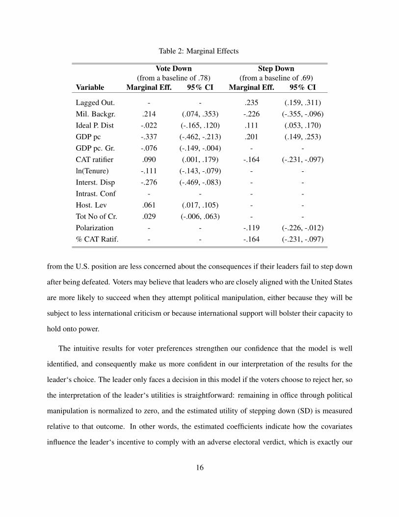
Table 2: Marginal Effects

Vote Down Step Down(from a baseline of .78) (from a baseline of .69)

Variable Marginal Eff. 95% CI Marginal Eff. 95% CI

Lagged Out. - - .235 (.159, .311)Mil. Backgr. .214 (.074, .353) -.226 (-.355, -.096)Ideal P. Dist -.022 (-.165, .120) .111 (.053, .170)GDP pc -.337 (-.462, -.213) .201 (.149, .253)GDP pc. Gr. -.076 (-.149, -.004) - -CAT ratifier .090 (.001, .179) -.164 (-.231, -.097)ln(Tenure) -.111 (-.143, -.079) - -Interst. Disp -.276 (-.469, -.083) - -Intrast. Conf - - - -Host. Lev .061 (.017, .105) - -Tot No of Cr. .029 (-.006, .063) - -Polarization - - -.119 (-.226, -.012)% CAT Ratif. - - -.164 (-.231, -.097)

from the U.S. position are less concerned about the consequences if their leaders fail to step down

after being defeated. Voters may believe that leaders who are closely aligned with the United States

are more likely to succeed when they attempt political manipulation, either because they will be

subject to less international criticism or because international support will bolster their capacity to

hold onto power.

The intuitive results for voter preferences strengthen our confidence that the model is well

identified, and consequently make us more confident in our interpretation of the results for the

leader‘s choice. The leader only faces a decision in this model if the voters choose to reject her, so

the interpretation of the leader‘s utilities is straightforward: remaining in office through political

manipulation is normalized to zero, and the estimated utility of stepping down (SD) is measured

relative to that outcome. In other words, the estimated coefficients indicate how the covariates

influence the leader‘s incentive to comply with an adverse electoral verdict, which is exactly our

16

minimal definition of democracy. We allow four sets of factors to influence this decision: char-

acteristics of the political system (previous electoral outcome, GDP per capita, and polarization),

leader characteristics (military background), factors associated with the technology of repression

(urbanization, military personnel), and international factors (alignment with the United States and

ratification of the CAT in the rest of the world). Only the variables associated with the means of

repression were insignificant.

Three systemic variables play a key role in predicting democracy. The previous electoral out-

come is a significant covariate that captures the idea of democratic consolidation. As Przeworski

(1991) argued, democratic institutions function properly when they represent a self-enforcing equi-

librium: the incumbent is willing to step down after losing an election because there is confidence

that the next incumbent will do the same; alternation in office in the long run makes electoral

defeat in the short run tolerable for major interest groups; and elite strategies ensure that compli-

ance is incentive compatible. The best indicator that this is the case is that the previous incumbent

surrendered power voluntarily, and we find that this is associated with a 23.5 percentage point in-

crease in compliance. Second, we find that the level of economic development (per capita GDP)

is a strong predictor of compliance. This is consistent with the finding of Przeworski (2000) that

democracies that had achieved a high enough level of per capita income were unlikely to revert to

authoritarianism. Highly developed economies have educated populations that tend to be politi-

cally engaged and efficacious, and they provide resources for social groups to mobilize politically.

The increased strength of popular opposition makes electoral manipulation less attractive and less

likely to succeed. On the other hand, rich countries provide attractive options to former politi-

cians outside politics, which increases the incentive to comply. We find that increasing per capita

GDP by one standard deviation increases the probability of compliance by 20.1 percentage points.

Third, political polarization decreases the incentive to comply. As political elites become increas-

ingly polarized, compliance in the future becomes more uncertain, which undermines the incentive

17

to comply in the present. A one-standard-deviation increase in the polarization index is associated

with an 11.9 percentage point decrease in the probability of compliance.

Leaders with a military background have a significantly decreased probability of complying.

Military leaders have access to networks of military supporters, which make military coups in

support of the opposition less likely and makes repression easier to organize. In addition, of

course, military leaders are more likely to arise under dictatorships, so there is an endogeneity

concern. However, these estimates are conditional on elections being held, and are also condi-

tional on whether the previous incumbent stepped down voluntarily. Consequently, it appears to be

the case that compliance is less likely when the incumbent has a military background. According

to our estimates, military background is associated with a 22.6 percentage point decrease in the

probability of compliance.

International factors again have striking effects. We assumed that voters were concerned about

whether their own country had ratified the CAT, because this is what the literature suggests provides

protection of human rights. From the perspective of leaders, however, what is more important is the

number of other countries that have ratified, because the CAT is enforceable against foreign citizens

(including expatriate former dictators) regardless of whether their countries of origin have ratified

it. Authoritarian leaders are frequently subject to punishment when they lose office (Chiozza and

Goemans, 2011), so they usually flee abroad, and their ability to enjoy a comfortable retirement

depends on legal immunity. As the number of CAT ratifiers has expanded and the human rights

regime has become more legalized, dictators’ outside options have narrowed. Our estimates indi-

cate that this trend has made authoritarian leaders who hold elections significantly less willing to

comply when they are defeated at the polls. Increasing the percentage of countries that have rati-

fied the CAT from the average level of 24% by one standard deviation, to 53%, is associated with

a decrease of 16.4 percentage points in the probability of compliance. By 2016, 140 countries, or

18

72.5% of UN member states, had ratified the CAT, representing 1.7 standard deviations, a level that

is associated with an estimated decrease in the probability of compliance of 37 percentage points.

Finally, alignment with the United States strongly influences the choices of leaders, as it does

those of voters. Leaders of countries with UN voting records similar to that of the United States are

less likely to comply when they lose elections – again, presumably, because they are more likely

to be shielded from international criticism and provided with material support that strengthens

their capacity to repress the opposition. A decrease of one standard deviation in the distance

between a country’s estimated ideal point and that of the United States is associated with a decrease

in the probability of compliance of 11 percentage points. It appears that leaders draw the same

inference as voters from close relations with the United States: they are less likely to be subjected

to sanctions if they attempt to manipulate elections, and may be able to draw on U.S. assistance to

repress domestic dissent. This is consistent with findings that U.S. foreign aid was associated with

longer tenure of authoritarian leaders, at least during the Cold War (De Mesquita and Smith, 2009;

Morrison, 2009; Bermeo, 2016). Consistent with the findings of Bermeo (2016), the coefficients of

voting alignment become insignificant in both the voter’s and the leader’s utilities when the sample

is limited to the post-Cold War era, which suggests that the effect is attributable to the efforts the

United States made to bolster regimes regarded as opposing communism during the Cold War.

This interpretation is supported by the results of alternative specifications that used U.S. alliances

as a substitute for UN voting alignments, and found similar, but somewhat weaker, effects.

So far, we have considered the non-strategic preferences of leaders and voters, but the strategic

model also allows us to consider a second-order effect: voters may be deterred from voting to re-

move the incumbent leader if they anticipate that she will refuse to step down. The consequences

of electoral manipulation are generally inferior to the outcome in which the leader is reelected

legally, because manipulation may involve repression and civil conflict. Consequently, factors that

make it less likely that the incumbent steps down may also have the perverse effect of deterring

19

voters from expressing their true preferences; dictators may be able to masquerade as democrat-

ically elected leaders because the voters are afraid of the consequences if they prove otherwise.

Leaders of poor, polarized countries that lack a recent experience with a peaceful transition of

power, particularly if they have a military background and close relations with the United States,

are likely to be reelected simply because the population fears the consequences if they lost. This

recalls Machiavelli‘s famous advice to the prince: it is good to be loved, but it is better to be feared.

In order to test whether strategic voting plays an important role in our model, we compare

it with an alternative model that allows for the same distribution of outcomes and employs the

same covariates, but assumes that voters are not strategic. Consider a scenario in which voters

vote expressively, rather than strategically. This would be equivalent to a strategic model in which

voters believe that the leader will step down for certain upon losing the election. In other words,

at their decision node, the voters compare their utility from re-electing the leader to their utility

from the leader stepping down, and ignore the possibility that the leader will try to remain in power

after losing the election.7 To compare our model with this non-strategic version, we conduct two

non-nested model comparison tests proposed by Vuong (1989) and Clarke (2007). Both test results

reject the null hypothesis that the non-strategic model fits the data as well as our strategic election

model to a high degree of confidence.8 This is a direct test of the hypothesis that voters are strategic,

and it indicates that voters are deterred from voting against the incumbent when they believe that

she will not step down if she loses.9

7Voters reelect the leader if U(SQ) > U(SD).

8For our comparison, the Vuong test statistic takes a value 3.04, which implies a p-value of .002. Similarly, the

Clarke test results in a value of 541 (out of 932 observations), which implies a p-value less than .0001.

9The unrestricted structural model contains more reduced-form parameters than the restricted version, and the

additional parameters are interaction terms that represent strategic anticipation. Consequently, the unrestricted model

should fit the data better, but the tests are fair because they appropriately penalize models that are more complex. If

the effects of strategic voting do not improve fit enough to overcome the penalty, the test will fail to reject the null

hypothesis.

20

The comparative test, furthermore, allows us to explore the circumstances under which strategic

voting takes place. Our estimates indicate that the strategic model outperforms the non-strategic

version in approximately 60% of observations, but the percentage increases when the probability

that the leader complies with the electoral outcome declines. The strategic model outperforms the

non-strategic one in 63% of observations if the leader has a military background, compared to only

51% if the leader does not have a military background. In the poorest decile of countries, where

GDP per capita is less than $1,000 per year in 2005 dollars, the strategic version outperforms the

non-strategic one in 65% of observations, compared to 60% of observations in all other countries.

The strategic model outperforms the non-strategic model in 64% of observations in countries with

the lowest quartile of ideal point differences with the United States, compared to 59% of observa-

tions in other countries.

The effect of strategic interaction on vote choices becomes clear when we plot the marginal

probabilities of outcomes. Because decisions made further up the tree (by the voter, in this case)

take into account the choice probabilities attributed to actions further down the tree (made by the

leader), the predicted choice probabilities depend on the covariates that enter the leader’s util-

ity function. As a result, the reduced form equation to be estimated includes interaction effects

between the variables that affect voter choice and the variables that affect the leader’s choice. In

general, these sorts of strategic interactions lead to non-monotonic effects of covariates on outcome

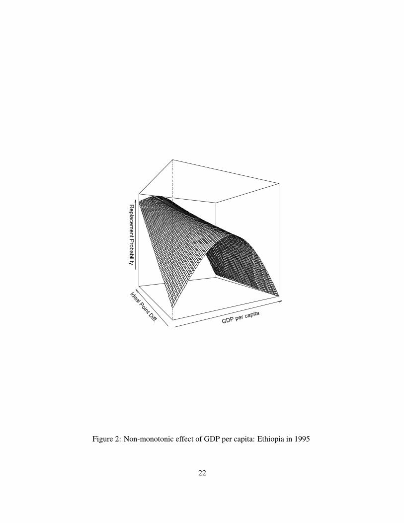
probabilities. Figure 2 provides an illustration of how the probability that the leader is replaced

changes as a function of GDP per capita and ideal point distance from the United States. All other

variables are fixed, and we chose the values they took during the Ethiopian general election in

1995, so this can be thought of as a counterfactual analysis of how that election would have been

different if we were able to vary two parameters.

Focus first on the foreground of the figure, where the ideal-point distance from the United

States is small. In this region, the probability of replacement is very low when GDP per capita is

21

GDP per capita

Ideal Point Diff.

Replacem

ent Probability

Figure 2: Non-monotonic effect of GDP per capita: Ethiopia in 1995

22

near its minimum, because in that case the leader refuses to step down when she loses an election,

and is also very low when GDP per capita is near its maximum, because the voters are highly

likely to reelect the leader. The probability of replacement is maximized at an intermediate level

of national wealth. The ideal point distance from the United States increases as we move towards

the back of the figure, and the replacement probability increases because defeated leaders are more

likely to step down. This effect is very steep when GDP per capita is low, because in that case

voters are likely to vote the incumbent down, so the leader is frequently confronted with the choice

of stepping down. The effect of ideal-point distance becomes almost imperceptible when GDP per

capita is high, however, because voters rarely vote the leader out of office. The most democratic

counterfactual Ethiopia is in the right-rear corner, where GDP per capita and ideal-point distance

are both high, and the least democratic case is in the left-front corner, where both are low. The

predicted probability of leader replacement is almost identical in these two cases; all of the action

occurs in between.

1.2.1 Democracies with Hegemonic Parties: Japan and India

The most difficult regimes to classify are those that appear to conduct competitive multiparty elec-

tions, but in which one party always wins over long periods of time. As Przeworski et al. put

it, if one party consistently wins, “we cannot know whether it would have held elections when

facing the prospect of losing or if it would have yielded office had it in fact lost.” Their coding

rule therefore faces a dilemma. “Err we must; the question is which way” (Przeworski et al. 2000,

23). Their solution is to apply a retrospective coding rule: if a hegemonic party ever gives up

power after losing an election, it is coded retrospectively as a democracy for its entire history; if it

ever repudiates an electoral defeat, it is coded retrospectively as a dictatorship for its entire history.

They acknowledge, however, that this does not really solve the problem. “This clearly is not a

very satisfactory solution: One might easily imagine that even if certain incumbents were willing

23

to allow a peaceful alternation in office later on, they might not have been willing to tolerate it

earlier; conversely, even if they suppressed the opposition later on, they might not have done so

earlier” (Przeworski et al. 2000, 24). Nevertheless, by this coding rule, India and Japan are treated

as democracies from the moment of independence, in spite of the fact that decades passed before

either country experienced a transfer of power to the opposition.

Our estimates tell a different story, and suggest that there was a substantial degree of uncer-

tainty about democratic institutions in both countries, particularly in the early years. The Japanese

political system was competitive under the American occupation, which ended in 1952, and in-

volved several transitions of power, but Japan was ruled continuously by governments led by the

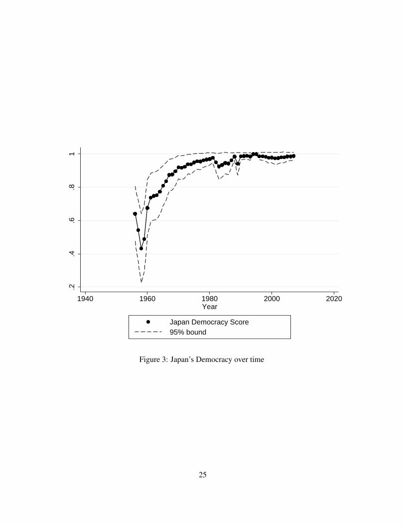
Liberal Democratic Party (LDP) from its formation in 1955 until 1993. By the end of this period,

our estimates (see Figure 3) confirm the conventional wisdom that the Japanese government was

democratic and the LDP was continuously reelected because it enjoyed broad public support, but

the estimated probability that the LDP would actually give up power if it lost an election did not

come to exceed 90% until the 1980s.

Our estimates show a sharp drop in probabilistic democracy in 1957, when Nobusuke Kishi

became Prime Minister, and the estimated probability of conceding an electoral defeat remains be-

low 50% until he leaves office in 1960. This drop is driven largely by Kishi’s military background,

and in this case the leader’s personal characteristics appear to justify skepticism. Kishi was Minis-

ter of Commerce and Industry in the Tojo government during the Second World War, responsible

for wartime mobilization, and was subsequently imprisoned as a Class A war criminal. Before

the war, he had been an outspoken nationalist and had been responsible for the notorious economic

management of Manchuria. As Prime Minister, Kishi attempted to rebuild Japan’s international in-

fluence and pushed a deeply unpopular security treaty with the United States through parliament,

replacing the one adopted during the U.S. occupation. This provoked the largest post-war political

demonstrations in Japan, which eventually compelled him to resign. At the same time, other U.S.

24

.2.4

.6.8

1

1940 1960 1980 2000 2020Year

Japan Democracy Score95% bound

Figure 3: Japan’s Democracy over time

25

allies in East Asia were authoritarian (Taiwan, South Vietnam) or moving in that direction (Korea).

Jung-hee Park, for example, led a coup in South Korea in 1961, was elected president in 1963, and

declared martial law in 1972 when he lost the next election. It appears plausible that Kishi might

have led Japan in the same direction, had circumstances been different. By the 1980s, however,

Japanese society had been transformed by rapid economic growth, and the incentive to play by the

rules of electoral democracy had become compelling.

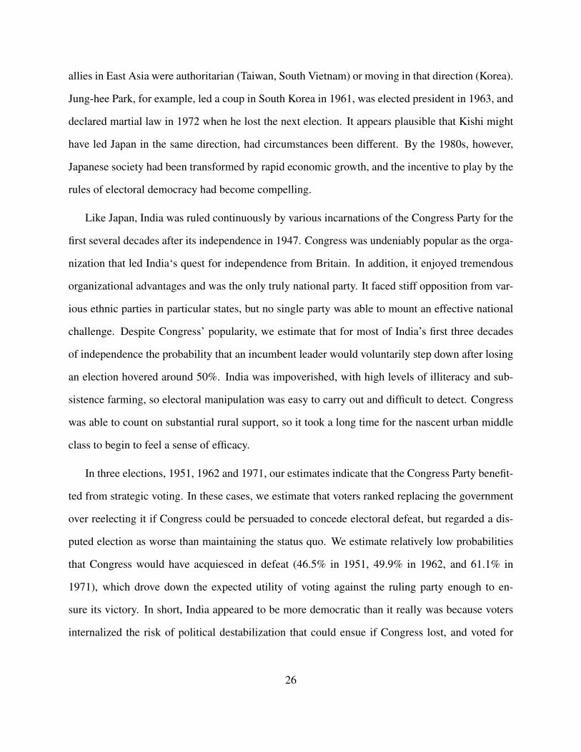
Like Japan, India was ruled continuously by various incarnations of the Congress Party for the

first several decades after its independence in 1947. Congress was undeniably popular as the orga-

nization that led India‘s quest for independence from Britain. In addition, it enjoyed tremendous

organizational advantages and was the only truly national party. It faced stiff opposition from var-

ious ethnic parties in particular states, but no single party was able to mount an effective national

challenge. Despite Congress’ popularity, we estimate that for most of India’s first three decades

of independence the probability that an incumbent leader would voluntarily step down after losing

an election hovered around 50%. India was impoverished, with high levels of illiteracy and sub-

sistence farming, so electoral manipulation was easy to carry out and difficult to detect. Congress

was able to count on substantial rural support, so it took a long time for the nascent urban middle

class to begin to feel a sense of efficacy.

In three elections, 1951, 1962 and 1971, our estimates indicate that the Congress Party benefit-

ted from strategic voting. In these cases, we estimate that voters ranked replacing the government

over reelecting it if Congress could be persuaded to concede electoral defeat, but regarded a dis-

puted election as worse than maintaining the status quo. We estimate relatively low probabilities

that Congress would have acquiesced in defeat (46.5% in 1951, 49.9% in 1962, and 61.1% in

1971), which drove down the expected utility of voting against the ruling party enough to en-

sure its victory. In short, India appeared to be more democratic than it really was because voters

internalized the risk of political destabilization that could ensue if Congress lost, and voted for

26

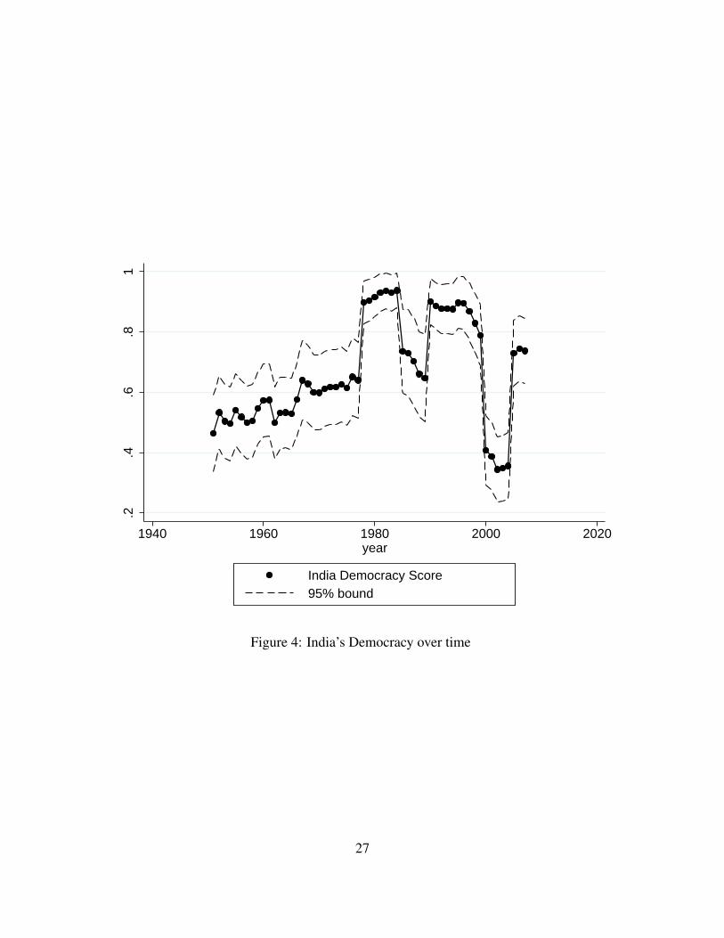
.2.4

.6.8

1

1940 1960 1980 2000 2020year

India Democracy Score95% bound

Figure 4: India’s Democracy over time

27

Congress because they did not trust it to step down if it were defeated. The risks of political unrest,

external threats and internal insurgencies were never distant. India fought Portugal in 1954 and

1961, China in 1962, and Pakistan in 1965 and 1971; it faced insurgencies in Northeast India, in

the Naxalite rebellion, and in Kashmir; and it faced numerous separatist claims and demands by

ethnic minorities to redraw state boundaries (Lacina, N.d.).

The most dramatic event to underscore the weak rule of law in India was the declaration of

martial law from 1975 to 1977. The crisis was provoked when an Indian court ruled Prime Minister

Indira Gandhi’s election to parliament to be illegal on grounds of electoral malpractice for using

government resources for campaigning, effectively stripping her of her position as Prime Minister.

She refused to resign, and when the opposition protested, she asked the President of India to

declare martial law, and then proceeded to rule by decree, imprison opposition leaders, dissolve

the opposition-led governments of two Indian states, and impose press censorship. She ruled

under the state of emergency for two years, and then called elections that she expected to win.

The opposition slogan was that this was the last chance to choose “democracy or dictatorship.”

It was a surprise when the opposition prevailed, and Indira Gandhi stepped down. Our estimates

of Indian probabilistic democracy increase substantially after 1977, because lagged alternation in

office predicts compliance with electoral outcomes; in conventional terms, precedents contribute

to the norm of compliance.

The opposition Janata government was united only in opposition to Indira Gandhi, and it col-

lapsed after a few years, allowing her to win reelection in 1980. This allowed another peaceful

transition of power, which further strengthened our estimate of Indian democracy, and those esti-

mates remained substantially higher for the following decades, which is consistent with a general

consensus that Indian democracy has become more consolidated. The volatility of our estimates

remained high, however, and was mainly driven by the outcome of particular elections; those that

replaced an incumbent government moved the estimate higher, and those that retained an incum-

28

bent, as in 1984 and 1999, lowered the estimate, sometimes dramatically. During this time, India

developed a vibrant multi-party system and elections became considerably less predictable. Per

capita GDP increased and a large urban middle class emerged that was politically sophisticated.

However, India remained a very poor country, with hundreds of millions of subsistence farmers

living below the international poverty line, and the volatility of its democracy estimates reflects the

fact that it is anomalous for a country this poor to be a stable democracy.

1.2.2 Mexico

Our estimates for Mexico are counterintuitive, but on closer examination the strategic model ap-

pears to be picking up important characteristics of the case. Przeworski et al. code Mexico as

an autocracy because it never had a democratic transfer of power during their estimation window,

which ended in 1990. Similarly, polity codes Mexico as authoritarian until the 2000 election,

when the opposition National Action Party (PAN) captured the presidency, and democratic there-

after. The polity score reflects Mexico’s gradual transition to democracy: it ticks upwards (-6 to

-4) when President Portillo introduces his electoral reforms, reaches zero during the competitive

1988 presidential election, rises to 4 after the much cleaner 1994 election, and rises to 6 in 1998

and to 8 in 2000. Throughout this period, two opposition parties gained strength, captured state

governorships, gained control of state assemblies, and acquired substantial strength in Congress.

Meanwhile, political freedom expanded, political participation surged, and elections became more

competitive.

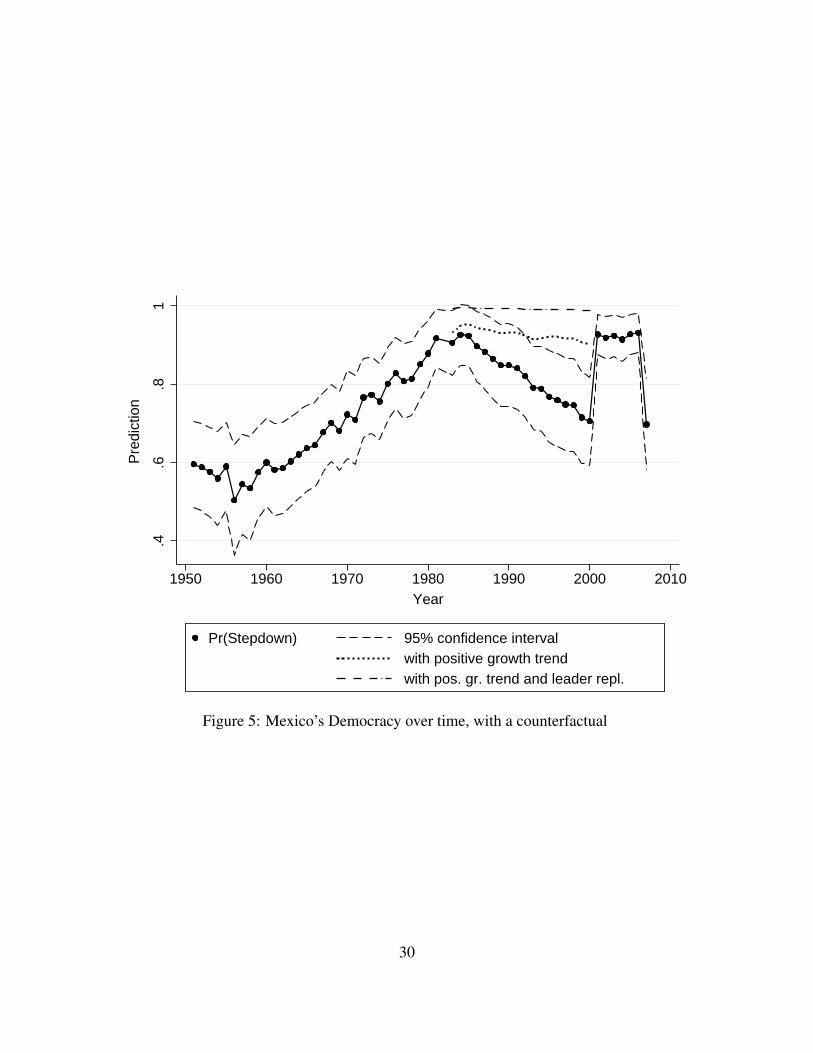
The strategic estimates of Mexican democracy move differently and underscore a different as-

pect of the changing political landscape.10 The strategic estimates rise rapidly during the 1970s, at

a time when very little was happening in Mexican politics. Indeed, the PAN, which was the only

effective opposition party at the time, embarrassed the ruling Institutional Revolutionary Party

10The discussion that follows of the Mexican case draws heavily on Chand (2001).

29

.4.6

.81

Pre

dict

ion

1950 1960 1970 1980 1990 2000 2010Year

Pr(Stepdown) 95% confidence intervalwith positive growth trendwith pos. gr. trend and leader repl.

Figure 5: Mexico’s Democracy over time, with a counterfactual

30

(PRI) by refusing to field a candidate in the 1976 presidential election. Meanwhile, however, rapid

changes were occurring in Mexican society. Per capita income rose rapidly as Mexico integrated

into the world economy, began to export oil, and borrowed heavily to finance industrial devel-

opment. The population became more urbanized, literate, and politically aware, and a growing

middle class began to demand services from the state. Contemporary survey research indicates

that Mexican political attitudes were evolving from those of “subjects” towards those of citizens.

Our estimates suggest that these circumstances make it more likely that the ruling party would in

fact cede power, if it lost an election, and rising per capita GDP drove up our estimates of Mex-

ican democracy. This trend abruptly reversed, however, in 1982, when the Mexican government

defaulted on its foreign debt and suspended convertibility of the peso. Per capita incomes fell

drastically. Growth stagnated for a decade, resumed, and then collapsed again with the second

peso crisis in 1994. To illustrate the role of per capita income in driving the strategic estimates

of democracy, Figure 4 compares the predicted values from the model with those from a counter-

factual in which the trend of rising GDP per capita continued steadily after 1982, and in that case

democracy stabilizes during the 1980s and 1990s a bit below the level actually reached in 2000

after a successful power transition.

So, which set of estimates is right? As we have emphasized above, this is not the right question

to ask, because polity and probabilistic democracy measure different concepts. Polity emphasizes

electoral competitiveness and pluralism, while probabilistic democracy emphasizes the choice of

the incumbent to concede defeat, and in Mexico, competitiveness rose while the incumbent became

more determined to stay in power by whatever means were necessary. Rising per capita GDP did

not immediately change Mexican political institutions, but it did lead to what Vikram Chand has

termed “Mexico‘s political awakening” (Chand, 2001). The PAN was primarily a middle class

political movement, whose early strength was concentrated in the northern states that bordered the

United States and benefitted the most from U.S. foreign investment. The first state to challenge

the hegemony of the PRI was Chihuahua, which was the state with the highest per capita income,

31

and PAN’s strength was always concentrated in urban areas, while the PRI polled most strongly in

the countryside. The PRI’s lock on a corrupt electoral system, furthermore, could not have been

broken without the engagement of a vibrant civil society and the mobilization of tens of thousands

of election monitors.

The year 1982 was a turning point in Mexico’s democratization because the financial crisis

discredited the PRI government and forced it to embrace austerity programs that undermined the

corporatist bargains that kept workers and peasants quiet. As our model predicts, economic growth

is a strong predictor of support for the incumbent government. When incomes fell, opposition to

the PRI surged, and the PAN won the governorship of Chihuahua and the mayoralties of the ma-

jor cities. It is probable that PRI candidates actually won most of the elections before 1982, but

after that, the PRI was forced to resort to a wide range of electoral misconduct in order to prevail.

As opposition grew, voters were struck from election rolls, rural districts reported 100% turnout,

and in some states results were simply falsified. Protests against electoral fraud in Chihuahua in

1986 led to protest marches, hunger strikes, a suspension of services by the Archbishop, and civil

disobedience that blocked the border bridges leading to El Paso. The PRI may have actually won

the presidential election in 1988 as it claimed—it was a close, three-way race—but, facing a de-

termined opposition and mounting international pressure, it ceded governorships and a substantial

bloc of votes in Congress. In short, elections became less fair as they became more competi-

tive. Our model picks this up because it estimates that it was unlikely that the PRI continued to

win under conditions of economic crisis, so it became more likely that the elections were heavily

manipulated. In this sense, our model is correct to pick 1982 as a local maximum for Mexican

democracy: those were the only fair elections that President de la Madrid (1982-1988) tolerated.

Thereafter, the opposition would be forced to fight against extralegal maneuvers for every step

forwards, and the cheating intensified as elections became more competitive.

32

2 Empirical Applications

2.1 Democracy and Conflict

One of the most robust findings in the quantitative study of conflict is that democratic states are

unlikely to fight wars with each other, a pattern that has become known as the “democratic peace”

(Russett and Oneal, 2001).11 While scholars disagree about the theoretical sources of the associa-

tion (see, for instance, Lake (1992); De Mesquita et al. (1999); Schultz (2001); Cederman (2001);

Gartzke (2007)), the democratic peace is regarded as a broadly accepted empirical regularity. We

conduct a series of tests of the democratic peace hypothesis using our measure of probabilistic

democracy, and compare the results to those obtained with ACLP and Polity scores.12

Joint democracy in a dyad of states can be operationalized in several ways. We consider three

alternatives: (i) both states in the dyad have a democracy score above a specified threshold; (ii)

minimum democracy score in the dyad; and (iii) an interactive model. To ensure comparability,

we limit our analyses to the period after 1950. We focus on politically relevant directed dyads

as the unit of analysis. Depending on the specification, we use either logistic regression or a

penalized MLE alternative (Firth, 1993; Heinze and Schemper, 2002) as specified in tables. We

cluster standard errors at the directed dyadic level. Our dependent variable is War Onset, capturing

whether the initiator launches a war against the target state in a given directed dyad year, based on

the Correlates of War (COW) interstate war data set (Sarkees and Wayman, 2010). Our analyses

include a set of control variables that are commonly employed in conflict regressions.13

11For skeptics, see (Rosato, 2003).

12The Online Appendix also includes additional results using the Freedom House score and a factor analysis mea-

sure combining probabilistic democracy, Polity, ACLP, and Freedom House scores.

13The control variables are as follows: Rel. Capabilities (the initiator’s share of military capabilities in the dyad);

Contiguity (an indicator variable capturing whether states share a common border); Rivalry (the existence of rivalry

between the two states defined in terms of past conflict) (Thompson, 2001); S Score (alliance portfolio similarity

33

In our first specification, we create a dichotomous variable capturing cases in which both states

in the dyad have a democracy score above a specified threshold.14 The results from this analysis

are presented in Table 3. According to all three measures, a dyad with two democratic states is

significantly less likely to experience war. To evaluate the size of the estimated effect, consider a

contiguous dyad that involves two rival states that are at parity, have an average alliance portfolio

similarity score, and have experienced a conflict in the prior year. When this dyad involves two

democratic states according to probabilistic democracy, the probability of war drops by .015 (-

.026, -.005) from .021. Similarly, according to the model that employs the Polity coding, the war

likelihood decreases by -.018 (-.028, -.009) from .020. With the ACLP coding, the probability

change is -.018 (-.027, -.009) from a baseline of .019.

Next, we parameterize joint democracy by the minimum democracy score in the dyad, using

probabilistic democracy, Polity, and ACLP scores. Table 4 presents these results. In this opera-

tionalization as well, all three measures are significant. As above, to assess substantive effects, we

consider a contiguous, rivalrous dyad that is at parity, has an average alliance portfolio similarity

score, and has experienced a conflict in the prior year. For this dyad, when we shift the minimum

probabilistic democracy score from 0 (both countries are dictatorships) to 1 (both countries are

perfect democracies), the probability of war drops by .019 (-.030, -.010) from .022. For the same

dyad, increasing the minimum polity score from -10 to 10 results in a -.025 change (-.038, -.016)

between the two states) (Signorino and Ritter, 1999); and Peace Years (polynomials of time since the last conflict,

used to control for duration dependence) (Carter and Signorino, 2010).

14We code both countries as democracies when probabilistic democracy > .5; Polity > 6, and ACLP> 0 (which

is trivial because the ACLP measure is dichotomous) for both states in the dyad. For Polity, a cutoff of 6 is most

commonly used in the literature. For our probabilistic democracy measure, we use .5 because it is intuitive as a

probability cutoff. This is also the level that maximizes the tetrachoric correlation with the ACLP and dichotomous

Polity measures, as presented in Figure 6.

34

in the overall probability of war from a baseline value of .027. Lastly, increasing the minimum

ACLP score in the dyad from 0 to 1 shifts the probability of war by -.018 (-.027, -.009) from .019.

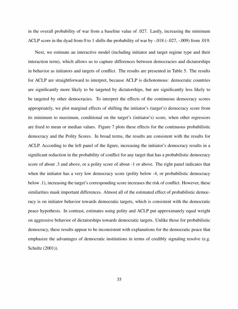
Next, we estimate an interactive model (including initiator and target regime type and their

interaction term), which allows us to capture differences between democracies and dictatorships

in behavior as initiators and targets of conflict. The results are presented in Table 5. The results

for ACLP are straightforward to interpret, because ACLP is dichotomous: democratic countries

are significantly more likely to be targeted by dictatorships, but are significantly less likely to

be targeted by other democracies. To interpret the effects of the continuous democracy scores

appropriately, we plot marginal effects of shifting the initiator’s (target’s) democracy score from

its minimum to maximum, conditional on the target’s (initiator’s) score, when other regressors

are fixed to mean or median values. Figure 7 plots these effects for the continuous probabilistic

democracy and the Polity Scores. In broad terms, the results are consistent with the results for

ACLP. According to the left panel of the figure, increasing the initiator’s democracy results in a

significant reduction in the probability of conflict for any target that has a probabilistic democracy

score of about .3 and above, or a polity score of about -1 or above. The right panel indicates that

when the initiator has a very low democracy score (polity below -4, or probabilistic democracy

below .1), increasing the target’s corresponding score increases the risk of conflict. However, these

similarities mask important differences. Almost all of the estimated effect of probabilistic democ-

racy is on initiator behavior towards democratic targets, which is consistent with the democratic

peace hypothesis. In contrast, estimates using polity and ACLP put approximately equal weight

on aggressive behavior of dictatorships towards democratic targets. Unlike those for probabilistic

democracy, these results appear to be inconsistent with explanations for the democratic peace that

emphasize the advantages of democratic institutions in terms of credibly signaling resolve (e.g.

Schultz (2001)).

35

A final comparison probes the robustness of the above results. There has been some controversy

about whether the democratic peace should be tested using fixed effects (Green, Kim and Yoon,

2001), and the general consensus appears to be that this is inappropriate because many dyads never

experience war, and they will be dropped from the analysis when fixed effects are used (Beck and

Katz, 2001). This, coupled with the fact that accepted measures of democracy do not vary enough

over time, makes it very difficult to reject the null hypothesis in such tests. Probabilistic democracy

offers a potential remedy for scholars who insist on using fixed effects, because it has substantially

more over-time variation than ACLP or Polity. Whereas 98% of ACLP observations and 90% of

polity observations do not vary between any two consecutive years, the corresponding figure for

probabilistic democracy is only 37%. Most of the unchanging observations in our measure are

due to the zeroes that are imputed for regimes that never hold multiparty elections. We have repli-

cated all of the above results using dyadic and country-level (initiator) fixed effects. None of the

democracy variables has any significant effect in any of the models that use dyadic fixed effects.

However, using country fixed effects for initiators, we were able to find significant effects of prob-

abilistic democracy consistent with the democratic peace hypothesis in the minimum democracy

and interactive specifications, while ACLP and polity were consistently insignificant. The results

are reported in the online appendix.

2.2 Democracy and Economic Growth

A long-running concern in political economy of development is that democracy may retard eco-

nomic growth. This worry took on political significance in the 1960s, as the Cold War cast eco-

nomic growth as a competition between markets and central planning. During the 1980s, the

superior economic performance of Pinochet’s Chile compared to other Latin American countries

encouraged the notion that authoritarian governments might enjoy an advantage in implement-

ing growth-friendly economic reforms. The debate became acute again in the 1990s, as post-

36

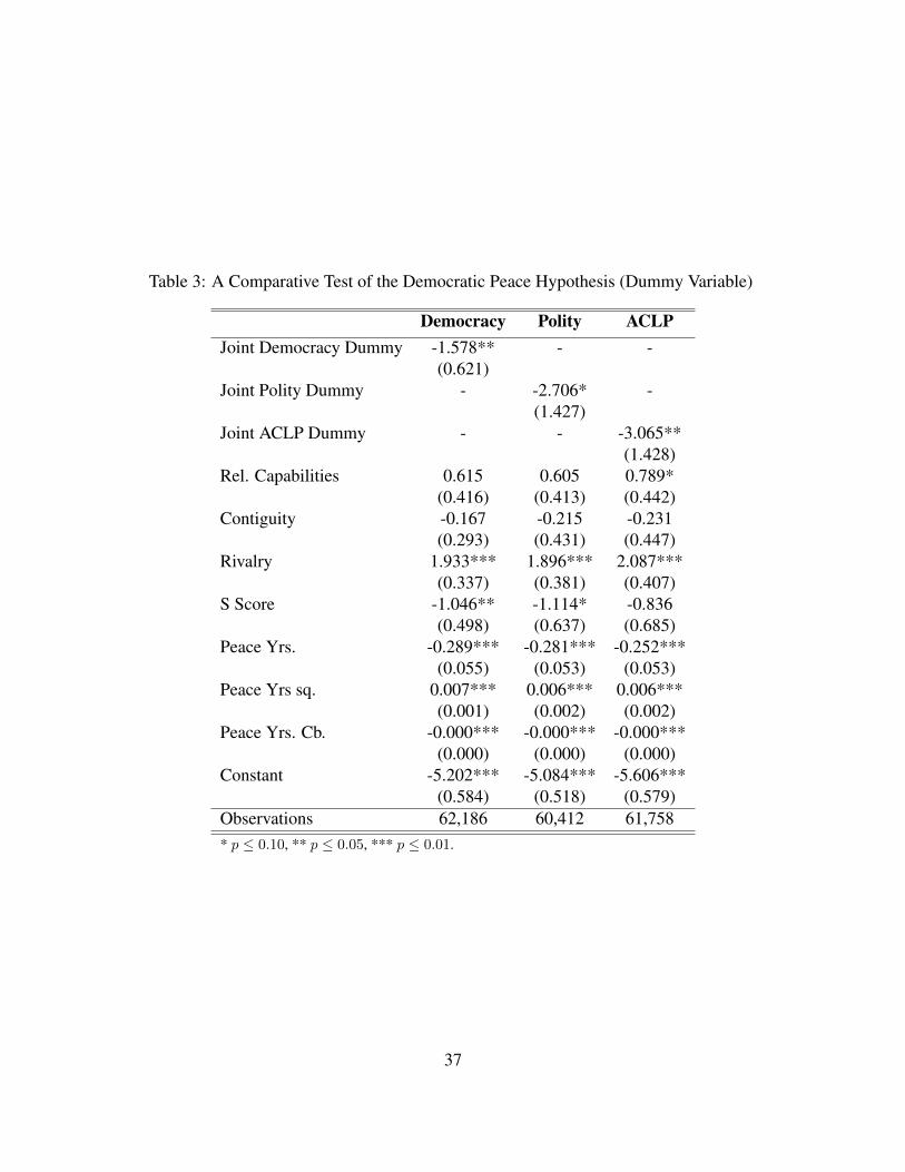
Table 3: A Comparative Test of the Democratic Peace Hypothesis (Dummy Variable)

Democracy Polity ACLPJoint Democracy Dummy -1.578** - -

(0.621)Joint Polity Dummy - -2.706* -

(1.427)Joint ACLP Dummy - - -3.065**

(1.428)Rel. Capabilities 0.615 0.605 0.789*

(0.416) (0.413) (0.442)Contiguity -0.167 -0.215 -0.231

(0.293) (0.431) (0.447)Rivalry 1.933*** 1.896*** 2.087***

(0.337) (0.381) (0.407)S Score -1.046** -1.114* -0.836

(0.498) (0.637) (0.685)Peace Yrs. -0.289*** -0.281*** -0.252***

(0.055) (0.053) (0.053)Peace Yrs sq. 0.007*** 0.006*** 0.006***

(0.001) (0.002) (0.002)Peace Yrs. Cb. -0.000*** -0.000*** -0.000***

(0.000) (0.000) (0.000)Constant -5.202*** -5.084*** -5.606***

(0.584) (0.518) (0.579)Observations 62,186 60,412 61,758* p ≤ 0.10, ** p ≤ 0.05, *** p ≤ 0.01.

37

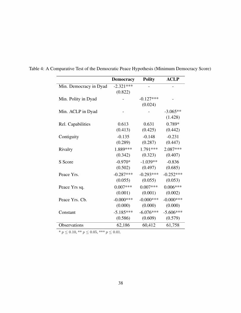
Table 4: A Comparative Test of the Democratic Peace Hypothesis (Minimum Democracy Score)

Democracy Polity ACLPMin. Democracy in Dyad -2.321*** - -

(0.822)Min. Polity in Dyad - -0.127*** -

(0.024)Min. ACLP in Dyad - - -3.065**

(1.428)Rel. Capabilities 0.613 0.631 0.789*

(0.413) (0.425) (0.442)Contiguity -0.135 -0.148 -0.231

(0.289) (0.287) (0.447)Rivalry 1.889*** 1.791*** 2.087***

(0.342) (0.323) (0.407)S Score -0.970* -1.039** -0.836

(0.502) (0.497) (0.685)Peace Yrs. -0.287*** -0.293*** -0.252***

(0.055) (0.055) (0.053)Peace Yrs sq. 0.007*** 0.007*** 0.006***

(0.001) (0.001) (0.002)Peace Yrs. Cb. -0.000*** -0.000*** -0.000***

(0.000) (0.000) (0.000)Constant -5.185*** -6.076*** -5.606***

(0.586) (0.609) (0.579)Observations 62,186 60,412 61,758* p ≤ 0.10, ** p ≤ 0.05, *** p ≤ 0.01.

38

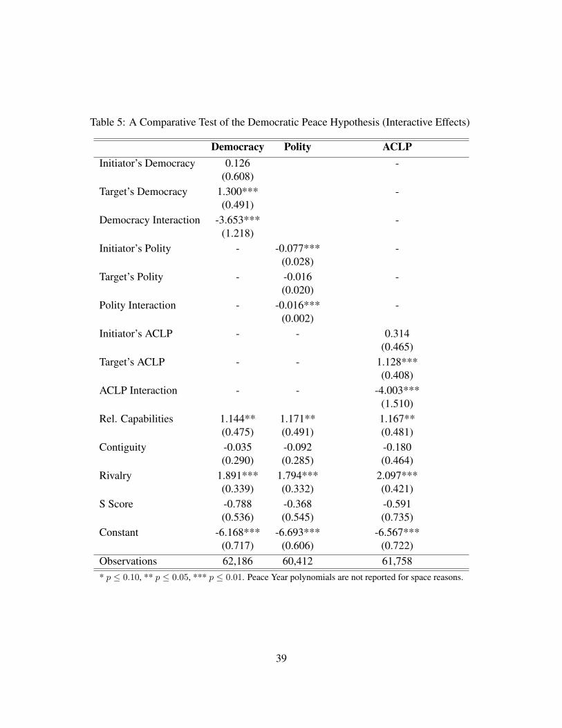
Table 5: A Comparative Test of the Democratic Peace Hypothesis (Interactive Effects)

Democracy Polity ACLPInitiator’s Democracy 0.126 -

(0.608)Target’s Democracy 1.300*** -

(0.491)Democracy Interaction -3.653*** -

(1.218)Initiator’s Polity - -0.077*** -

(0.028)Target’s Polity - -0.016 -

(0.020)Polity Interaction - -0.016*** -

(0.002)Initiator’s ACLP - - 0.314

(0.465)Target’s ACLP - - 1.128***

(0.408)ACLP Interaction - - -4.003***

(1.510)Rel. Capabilities 1.144** 1.171** 1.167**

(0.475) (0.491) (0.481)Contiguity -0.035 -0.092 -0.180

(0.290) (0.285) (0.464)Rivalry 1.891*** 1.794*** 2.097***

(0.339) (0.332) (0.421)S Score -0.788 -0.368 -0.591

(0.536) (0.545) (0.735)Constant -6.168*** -6.693*** -6.567***

(0.717) (0.606) (0.722)Observations 62,186 60,412 61,758* p ≤ 0.10, ** p ≤ 0.05, *** p ≤ 0.01. Peace Year polynomials are not reported for space reasons.

39

Communist countries experimented with simultaneous economic and political transformations

which seemed to imperil each other. In the prominent case of Russia, a fractious parliament frus-

trated efforts at economic reform, international observers called for strengthening the presidency,

and the IMF pushed President Yeltsin to legislate unconstitutionally by decree (Stone, 2002). Rus-

sia’s economic recovery followed Putin’s rise to power.

The literature in political science has yielded a mixed verdict. Studies published at different

times have largely followed the experience of prominent contemporaneous examples. Theoreti-

cal arguments against democracy generally followed the logic of veto players: the profusion of

institutional choke points at which policy reform could be blocked in democracies prevents them

to responding effectively to crises and changing inefficient policies. Moreover, elections lead to

inefficient political budget cycles. Theoretical arguments in favor of democracy were possible as

well: electoral control by the median voter tends to reward policies that promote general interests,

rather than narrow ones (De Mesquita and Smith, 2005).

A simple cross-tabulation using all of the available data indicates a negative association be-

tween democracy and economic growth, which holds regardless of which measure of democracy

we choose. Democracies experience a higher percentage of low-growth years than dictatorships,

and they enjoy a lower average growth rate. These differences may not be due to democracy,

however. The most likely alternative explanation seems to be that it has something to do with

the process of economic development itself. It might be the case, for example, that high-income

countries are likely to be democracies and that high-income countries grow more slowly than low-

income countries. If this is the case, it might be misguided to advise low-income countries to adopt

authoritarian institutions in order to improve their growth prospects. To explore this possibility, we

estimate growth regressions that interact democracy with GDP per capita, and we compare the

results across our three measures of democracy.

40

Our findings, presented in Table 7, confirm that all three democracy measures are associated

with slower growth, and that this effect holds only for wealthy countries. However, the results

using the three measures yield very different conclusions about how wealthy countries have to be

to experience a growth-retarding effect. According to our measure of probabilistic democracy,

the effect is only significant for highly developed economies with GDP per capita of $12,000

per year or more in 2005 dollars. This means that the association between democracy and slow

growth is driven by the experience of the OECD countries. In contrast, the results using the Polity

and ACLP measures of democracy indicate that the negative association between democracy and

growth is significant for middle-income countries as well (economies with GDP per capita of

$8,000 or more using Polity, or $6,000 using ACLP). This has an important policy implication:

according to our measure, authoritarianism is not an effective instrument for increasing growth

for developing countries, while the results for the other measures would suggest that it is. The

more limited scope for democracy to retard growth using our measure of probabilistic democracy

suggests that the mechanism that drives the effect is specific to advanced countries. For example,

welfare-state policies, labor market distortions due to unionism or high levels of redistribution are

potential culprits that would not be present in developing countries. Alternatively, slower growth

may be driven by demographic changes that set in when countries become wealthy, the population

enjoys longer lifespans, and fertility declines.15

3 Conclusions

Democracy is a critically important concept in political science, and measures of democracy are

involved in most quantitative studies in comparative politics and international relations. Neverthe-

less, we are unsettled both on conceptual and empirical grounds. Conceptually, we have no clear

15We have controlled for population growth, which is strongly associated with GDP growth, but not for the age

structure of the population.

41

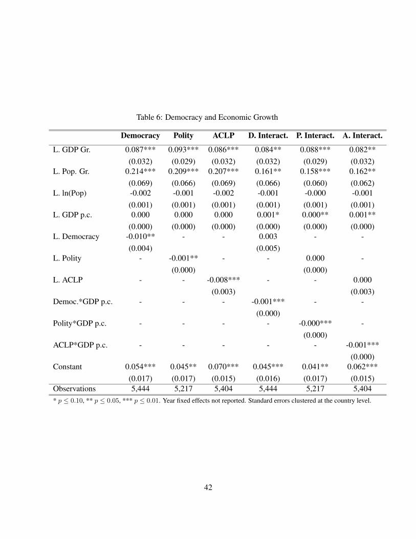
Table 6: Democracy and Economic Growth

Democracy Polity ACLP D. Interact. P. Interact. A. Interact.

L. GDP Gr. 0.087*** 0.093*** 0.086*** 0.084** 0.088*** 0.082**(0.032) (0.029) (0.032) (0.032) (0.029) (0.032)

L. Pop. Gr. 0.214*** 0.209*** 0.207*** 0.161** 0.158*** 0.162**(0.069) (0.066) (0.069) (0.066) (0.060) (0.062)

L. ln(Pop) -0.002 -0.001 -0.002 -0.001 -0.000 -0.001(0.001) (0.001) (0.001) (0.001) (0.001) (0.001)

L. GDP p.c. 0.000 0.000 0.000 0.001* 0.000** 0.001**(0.000) (0.000) (0.000) (0.000) (0.000) (0.000)

L. Democracy -0.010** - - 0.003 - -(0.004) (0.005)

L. Polity - -0.001** - - 0.000 -(0.000) (0.000)

L. ACLP - - -0.008*** - - 0.000(0.003) (0.003)

Democ.*GDP p.c. - - - -0.001*** - -(0.000)

Polity*GDP p.c. - - - - -0.000*** -(0.000)

ACLP*GDP p.c. - - - - - -0.001***(0.000)

Constant 0.054*** 0.045** 0.070*** 0.045*** 0.041** 0.062***(0.017) (0.017) (0.015) (0.016) (0.017) (0.015)

Observations 5,444 5,217 5,404 5,444 5,217 5,404* p ≤ 0.10, ** p ≤ 0.05, *** p ≤ 0.01. Year fixed effects not reported. Standard errors clustered at the country level.

42

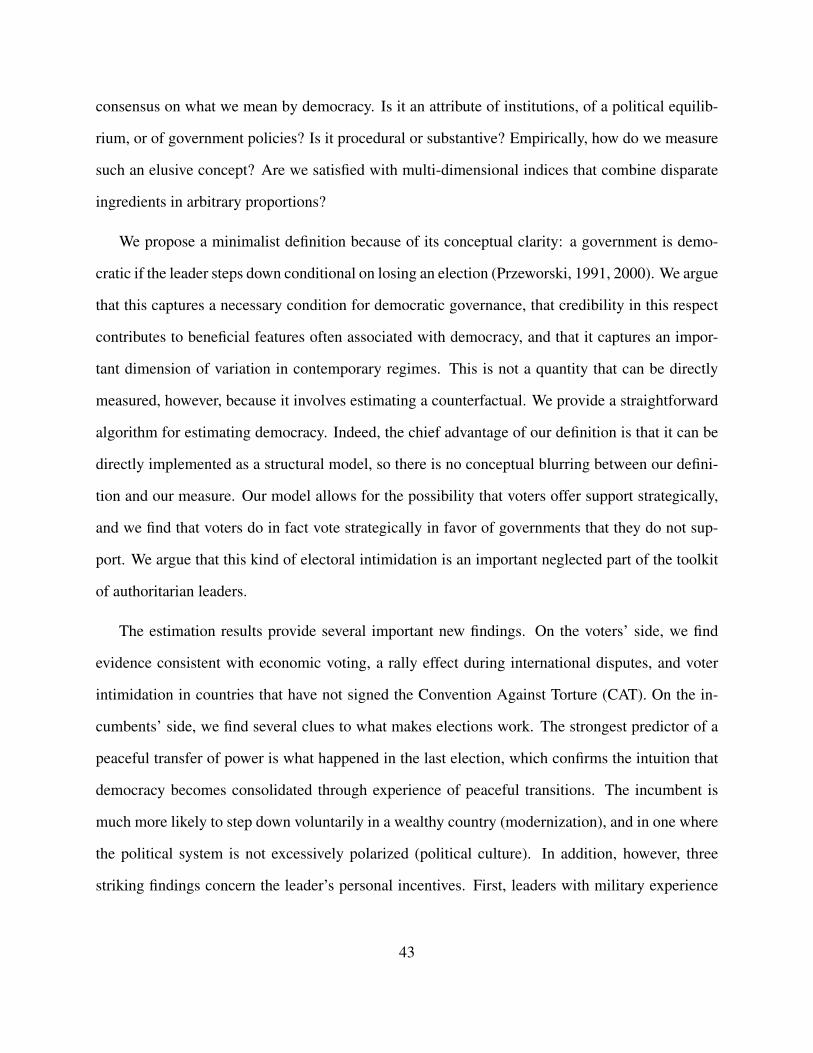
consensus on what we mean by democracy. Is it an attribute of institutions, of a political equilib-

rium, or of government policies? Is it procedural or substantive? Empirically, how do we measure

such an elusive concept? Are we satisfied with multi-dimensional indices that combine disparate

ingredients in arbitrary proportions?

We propose a minimalist definition because of its conceptual clarity: a government is demo-

cratic if the leader steps down conditional on losing an election (Przeworski, 1991, 2000). We argue

that this captures a necessary condition for democratic governance, that credibility in this respect

contributes to beneficial features often associated with democracy, and that it captures an impor-

tant dimension of variation in contemporary regimes. This is not a quantity that can be directly

measured, however, because it involves estimating a counterfactual. We provide a straightforward

algorithm for estimating democracy. Indeed, the chief advantage of our definition is that it can be

directly implemented as a structural model, so there is no conceptual blurring between our defini-

tion and our measure. Our model allows for the possibility that voters offer support strategically,

and we find that voters do in fact vote strategically in favor of governments that they do not sup-

port. We argue that this kind of electoral intimidation is an important neglected part of the toolkit

of authoritarian leaders.

The estimation results provide several important new findings. On the voters’ side, we find

evidence consistent with economic voting, a rally effect during international disputes, and voter

intimidation in countries that have not signed the Convention Against Torture (CAT). On the in-

cumbents’ side, we find several clues to what makes elections work. The strongest predictor of a

peaceful transfer of power is what happened in the last election, which confirms the intuition that

democracy becomes consolidated through experience of peaceful transitions. The incumbent is

much more likely to step down voluntarily in a wealthy country (modernization), and in one where

the political system is not excessively polarized (political culture). In addition, however, three

striking findings concern the leader’s personal incentives. First, leaders with military experience

43

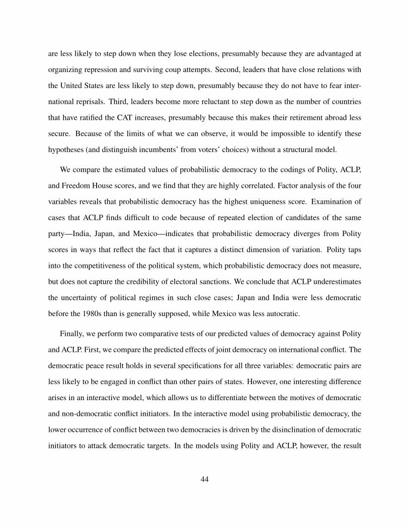
are less likely to step down when they lose elections, presumably because they are advantaged at

organizing repression and surviving coup attempts. Second, leaders that have close relations with

the United States are less likely to step down, presumably because they do not have to fear inter-

national reprisals. Third, leaders become more reluctant to step down as the number of countries

that have ratified the CAT increases, presumably because this makes their retirement abroad less

secure. Because of the limits of what we can observe, it would be impossible to identify these

hypotheses (and distinguish incumbents’ from voters’ choices) without a structural model.

We compare the estimated values of probabilistic democracy to the codings of Polity, ACLP,

and Freedom House scores, and we find that they are highly correlated. Factor analysis of the four

variables reveals that probabilistic democracy has the highest uniqueness score. Examination of

cases that ACLP finds difficult to code because of repeated election of candidates of the same

party—India, Japan, and Mexico—indicates that probabilistic democracy diverges from Polity

scores in ways that reflect the fact that it captures a distinct dimension of variation. Polity taps

into the competitiveness of the political system, which probabilistic democracy does not measure,

but does not capture the credibility of electoral sanctions. We conclude that ACLP underestimates

the uncertainty of political regimes in such close cases; Japan and India were less democratic

before the 1980s than is generally supposed, while Mexico was less autocratic.

Finally, we perform two comparative tests of our predicted values of democracy against Polity

and ACLP. First, we compare the predicted effects of joint democracy on international conflict. The

democratic peace result holds in several specifications for all three variables: democratic pairs are

less likely to be engaged in conflict than other pairs of states. However, one interesting difference

arises in an interactive model, which allows us to differentiate between the motives of democratic

and non-democratic conflict initiators. In the interactive model using probabilistic democracy, the

lower occurrence of conflict between two democracies is driven by the disinclination of democratic

initiators to attack democratic targets. In the models using Polity and ACLP, however, the result

44

is driven primarily by the increased tendency of non-democratic initiators to target democratic

states. This implies a rather different mechanism than theorists of the democratic peace generally

maintain.

Second, we compare the predicted effects of democracy on economic growth, conditional on

GDP per capita. According to all three measures, democracy reduces economic growth, but only in

relatively wealthy countries. The differences between the measures regard the level of wealth that

is necessary for democracy to impede growth. According to probabilistic democracy, only high-

income countries (GDP per capita of $12,000 or more in 2005 dollars) are subject to the effect.

According to Polity and ACLP, in contrast, middle-income countries also grow more slowly under

democracy. These differences imply different inferences about what mechanisms might be at work

to cause the effect and different inferences about what kinds of institutions are most likely to help

poor countries to develop their economies.

As long as democracy has to be coded, it will be miscoded. The coding rules for Polity and

ACLP lead to different pitfalls, but each has characteristic failings that are well known in the liter-

ature. In contrast, an estimation procedure is more transparent and more amenable to improvement

as knowledge accumulates. In addition, the process of estimating the model creates new knowl-

edge and better understanding of the means by which elections are manipulated in authoritarian

countries. Finally, we have demonstrated that although our estimates track the two most widely

used measures of democracy pretty closely, even marginal changes in the specification of a variable

as important as democracy can have non-trivial substantive implications.

45

.7.7

5.8

.85

.9

.5 .6 .7 .8 .9 1

Democracy Cutpoint for Measure

Tetrachoric Correlation with ACLP 95% Bound

Polity Cuto�

5

6

7

8

9

Measure Cuto

�

0.5

0.6

0.7

0.8

0.9

Tetrachoric Correlaton

0.65

0.70

0.75

0.80

0.85

Figure 6: Comparison of cutpoints to construct binary measures of Democracy

46

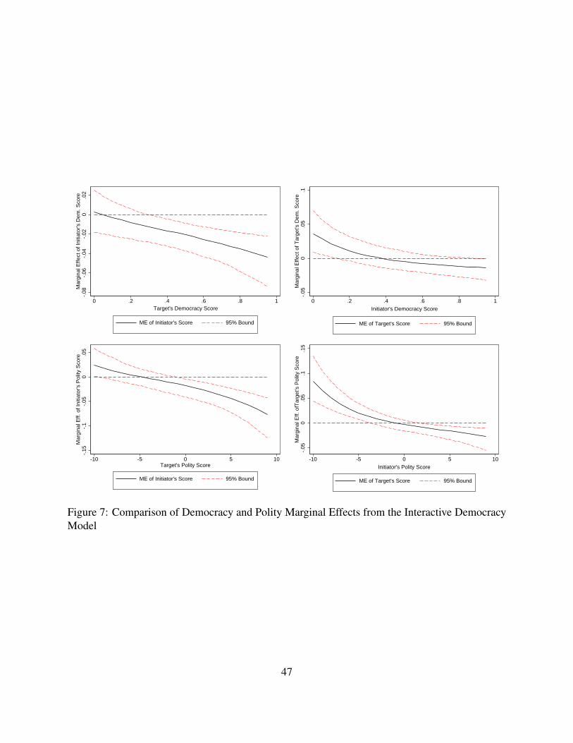
-.08

-.06

-.04

-.02

0.0

2M

argi

nal E

ffect

of I

nitia

tor's

Dem

. Sco

re

0 .2 .4 .6 .8 1Target's Democracy Score

ME of Initiator's Score 95% Bound

-.05

0.0

5.1

Mar

gina

l Effe

ct o

f Tar

get's

Dem

. Sco

re0 .2 .4 .6 .8 1

Initiator's Democracy Score

ME of Target's Score 95% Bound

-.15

-.1

-.05

0.0

5M

argi

nal E

ff. o

f Ini

tiato

r's P

olity

Sco

re

-10 -5 0 5 10Target's Polity Score

ME of Initiator's Score 95% Bound

-.05

0.0

5.1

.15

Mar

gina

l Eff.

ofT

arge

t's P

olity

Sco

re

-10 -5 0 5 10Initiator's Polity Score

ME of Target's Score 95% Bound

Figure 7: Comparison of Democracy and Polity Marginal Effects from the Interactive DemocracyModel

47

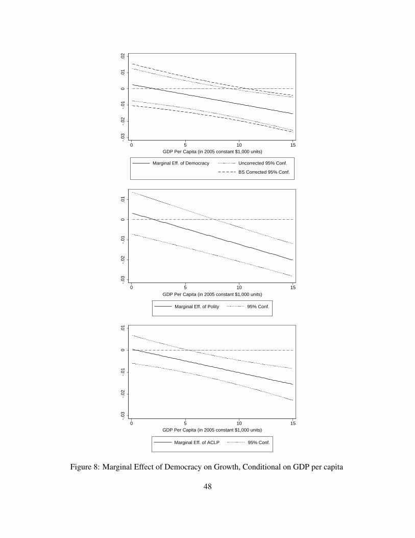
-.03

-.02

-.01

0.0

1.0

2

0 5 10 15GDP Per Capita (in 2005 constant $1,000 units)

Marginal Eff. of Democracy Uncorrected 95% Conf.

BS Corrected 95% Conf.

-.03

-.02

-.01

0.0

1

0 5 10 15

GDP Per Capita (in 2005 constant $1,000 units)

Marginal Eff. of Polity 95% Conf.

-.03

-.02

-.01

0.0

1

0 5 10 15GDP Per Capita (in 2005 constant $1,000 units)

Marginal Eff. of ACLP 95% Conf.

Figure 8: Marginal Effect of Democracy on Growth, Conditional on GDP per capita

48

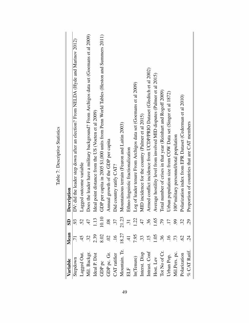
Tabl

e7:

Des

crip

tive

Stat

istic

s

Vari

able

Mea

nSD

Des

crip

tion

Step

dow

n.7

1.9

3D

V:d

idth

ele

ader

step

dow

naf

tera

nel

ectio

n?Fr

omN

EL

DA

(Hyd

ean

dM

arin

ov20

12)

Lag

ged

Out

..4

5.5

2L

agge

dou

tcom

eva

riab

leM

il.B

ackg

r..3

2.4

7D

oes

the

lead

erha

vea

mili

tary

back

grou

nd?

From

Arc

higo

sda

tase

t(G

oem

ans

etal

2009

)Id

ealP

.Dis

t2.

391.

13Id

ealp

oint

dist

ance

from

the

US

(Voe

ten

etal

2009

)G

DP

pc8.

0210

.10

GD

Ppe

rcap

itain

2005

$1,0

00un

itsfr

omPe

nnW

orld

Tabl

es(H

esto

nan

dSu

mm

ers

2011

)G

DP

pc.G

r..0

2.0

8A

nnua

lgro

wth

ofth

eG

DP

perc

apita

CA

Tra

tifier

.16

.37

Did

coun

try

ratif

yC

AT

?M

ount

ain.

Tr.

18.2

721

.23

Mou

ntai

nous

terr

ain

(Fea

ron

and

Lai

tin20

03)

EL

F.4

1.3

1E

thno

-lin

guis

ticfr

actio

naliz

atio

nln

(Ten

ure)

7.95

1.22

Log

ofle

ader

tenu

reFr

omA

rchi

gos

data

set(

Goe

man

set

al20

09)

Inte

rst.

Dis

p.3

3.4

7M

IDin

cide

nce

fort

heco

untr

y(P

alm

eret

al20

15)

Intr

ast.

Con

f.1

5.3

6A

rmed

confl

icti

ncid

ence

from

UC

DP/

PRIO

Dat

aset

(Gle

ditc

het

al20

02)

Hos

t.L

ev1.

051.

65A

vera

geho

stili

tyle

velf

rom

invo

lved

MID

disp

utes

(Pal

mer

etal

2015

)To

tNo

ofC

r..3

6.7

9To

taln

umbe

rofc

rise

sin

that

year

(Rei

nhar

tand

Rog

off2

009)

Urb

anPo

p..1

6.1

7U

rban

popu

latio

nsi

zefr

omC

OW

Dat

ase

t(Si

nger

etal

1872

)M

il.Pe

rs.p

c..7

3.9

910

0*m

ilita

rype

rson

nel/t

otal

popu

latio

nPo

lari

zatio

n.6

2.3

2Po

lari

zatio

nin

dex

from

EPR

Dat

aset

(Ced

erm

anet

al20

10)

%C

AT

Rat

if.

.24

.29

Prop

ortio

nof

coun

trie

sth

atar

eC

AT

mem

bers

49

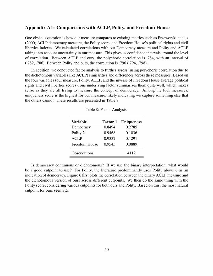
Appendix A1: Comparisons with ACLP, Polity, and Freedom House

One obvious question is how our measure compares to existing metrics such as Przeworski et al.’s(2000) ACLP democracy measure, the Polity score, and Freedom House’s political rights and civilliberties indexes. We calculated correlations with our Democracy measure and Polity and ACLPtaking into account uncertainty in our measure. This gives us confidence intervals around the levelof correlation. Between ACLP and ours, the polychoric correlation is .784, with an interval of(.782, .786). Between Polity and ours, the correlation is .796 (.794, .798).

In addition, we conducted factor analysis to further assess (using polychoric correlation due tothe dichotomous variables like ACLP) similarities and differences across these measures. Based onthe four variables (our measure, Polity, ACLP, and the inverse of Freedom House average politicalrights and civil liberties scores), one underlying factor summarizes them quite well, which makessense as they are all trying to measure the concept of democracy. Among the four measures,uniqueness score is the highest for our measure, likely indicating we capture something else thatthe others cannot. These results are presented in Table 8.

Table 8: Factor Analysis

Variable Factor 1 UniquenessDemocracy 0.8494 0.2785Polity 2 0.9468 0.1036ACLP 0.9332 0.1291Freedom House 0.9545 0.0889

Observations 4112

Is democracy continuous or dichotomous? If we use the binary interpretation, what wouldbe a good cutpoint to use? For Polity, the literature predominantly uses Polity above 6 as anindication of democracy. Figure 6 first plots the correlation between the binary ACLP measure andthe dichotomous version of ours across different cutpoints. We then do the same thing with thePolity score, considering various cutpoints for both ours and Polity. Based on this, the most naturalcutpoint for ours seems .5.

50

ReferencesArrow, Kenneth Joseph. 1963. Social Choice and Individual Values. Number 12 Yale University

Press.

Bailey, Michael A, Anton Strezhnev and Erik Voeten. 2017. “Estimating Dynamic State Prefer-ences from United Nations Voting Data.” Journal of Conflict Resolution pp. 430–456.

Barber, Benjamin R. 2003. Strong Democracy: Participatory Politics for a New Age. Univ ofCalifornia Press.

Bas, Muhammet A and Randall W Stone. 2014. “Adverse Selection and Growth under IMF Pro-grams.” The Review of International Organizations 9(1):1–28.

Beck, Nathaniel and Jonathan N Katz. 2001. “Throwing Out the Baby with the Bath Water: AComment on Green, Kim, and Yoon.” International Organization 55(02):487–495.

Bermeo, Sarah Blodgett. 2016. “Aid is not Oil: Donor Utility, Heterogeneous Aid, and the Aid-Democratization Relationship.” International Organization 70(01):1–32.

Calvin, Jean, John Calvin and Ford Lewis Battles. 1995. Institutes of the Christian Religion: 1536Edition. Vol. 1 Wm. B. Eerdmans Publishing.

Carter, David B and Curtis S Signorino. 2010. “Back to the Future: Modeling Time Dependencein Binary Data.” Political Analysis 18(3):271–292.

Cederman, Lars-Erik. 2001. “Back to Kant: Reinterpreting the Democratic Peace as a Macrohis-torical Learning Process.” The American Political Science Review 95(1):15–31.

Chand, Vikram K. 2001. Mexico’s Political Awakening. University of Notre Dame Press.

Chiozza, Giacomo and Hein Erich Goemans. 2011. Leaders and International Conflict. CambridgeUniversity Press.

Clarke, Kevin A. 2007. “A Simple Distribution-free Test for Non-nested Model Selection.” Politi-cal Analysis 15(3):347–363.

Cox, Gary W. 1997. Making Votes Count: Strategic Coordination in the World’s Electoral Systems.Cambridge University Press.

Dahl, Robert Alan. 1973. Polyarchy: Participation and Opposition. Yale University Press.

De Mesquita, Bruce Bueno and Alastair Smith. 2005. The Logic of Political Survival. MIT press.

De Mesquita, Bruce Bueno and Alastair Smith. 2009. “A Political Economy of Aid.” InternationalOrganization 63(02):309–340.

51

De Mesquita, Bruce Bueno, James D Morrow, Randolph M Siverson and Alastair Smith. 1999. “AnInstitutional Explanation of the Democratic Peace.” American Political Science Review pp. 791–807.

De Montesquieu, Charles. 1989. Montesquieu: The Spirit of the Laws. Cambridge UniversityPress.

De Tocqueville, Alexis. 2003. Democracy in America. Vol. 10 Regnery Publishing.

Debs, Alexandre and Hein E Goemans. 2010. “Regime Type, the Fate of Leaders, and War.”American Political Science Review 104(03):430–445.

Downs, George W and David M Rocke. 1995. Optimal Imperfection?: Domestic Uncertainty andInstitutions in International Relations. Princeton University Press.

Ferejohn, John. 1986. “Incumbent Performance and Electoral Control.” Public Choice 50(1-3):5–25.

Fey, Mark. 1997. “Stability and Coordination in Duverger’s Law: A Formal Model of Pre-electionPolls and Strategic Voting.” American Political Science Review 91(01):135–147.

Firth, David. 1993. “Bias Reduction of Maximum Likelihood Estimates.” Biometrika 80(1):27–38.

Gartzke, Erik. 2007. “The Capitalist Peace.” American Journal of Political Science 51(1):166–191.

Green, Donald P, Soo Yeon Kim and David H Yoon. 2001. “Dirty Pool.” International Organiza-tion 55(02):441–468.

Groseclose, Tim. 2007. “’One and a Half Dimensional’ Preferences and Majority Rule.” SocialChoice and Welfare 28:321–335.

Heinze, Georg and Michael Schemper. 2002. “A Solution to the Problem of Separation in LogisticRegression.” Statistics in medicine 21(16):2409–2419.

Hyde, Susan D. 2011. The Pseudo-Democrat’s Dilemma: Why Election Observation Became anInternational Norm. Cornell University Press.

Jaggers, Keith and Ted Robert Gurr. 1995. “Tracking Democracy’s Third Wave with the Polity IIIData.” Journal of Peace Research 32(4):469–482.

Lacina, Bethany. N.d. Rival Claims: Ethnic Competition and Territorial Autonomy under IndianFederalism. University of Michigan Press.

Lake, David A. 1992. “Powerful Pacifists: Democratic States and War.” American Political ScienceReview 86(01):24–37.

Locke, John. 2014. Second Treatise of Government: An Essay Concerning the True Original,Extent and End of Civil Government. John Wiley & Sons.

52

McKelvey, Richard D. 1976. “Intransitivities in Multidimensional Voting Models and Some Im-plications for Agenda Control.” Journal of Economic Theory 12(3):472–482.

Morrison, Kevin M. 2009. “Oil, Nontax Revenue, and the Redistributional Foundations of RegimeStability.” International Organization 63(01):107–138.

Mueller, John. 1994. Policy and Opinion in the Gulf War. University of Chicago Press.

Persson, Torsten and Guido Enrico Tabellini. 2002. Political Economics: Explaining EconomicPolicy. MIT press.

Poirier, Dale J. 1980. “Partial Observability in Bivariate Probit Models.” Journal of Econometrics12(2):209–217.

Powell, G Bingham. 2000. Elections as Instruments of Democracy: Majoritarian and ProportionalVisions. Yale University Press.

Przeworski, Adam. 1991. Democracy and the Market: Political and Economic Reforms in EasternEurope and Latin America. Cambridge University Press.

Przeworski, Adam. 2000. Democracy and Development: Political Institutions and Well-being inthe World, 1950-1990. Vol. 3 Cambridge University Press.

Przeworski, Adam and James Raymond Vreeland. 2000. “The Effect of IMF Programs on Eco-nomic Growth.” Journal of development Economics 62(2):385–421.

Putnam, Robert D, Robert Leonardi and Raffaella Y Nanetti. 1994. Making Democracy Work:Civic Traditions in Modern Italy. Princeton University Press.

Reinhart, Carmen M and Kenneth S Rogoff. 2009. This Time is Different: Eight Centuries ofFinancial Folly. Princeton University Press.

Riker, William H. 1982. Liberalism against Populism: A Confrontation between the Theory ofDemocracy and the Theory of Social Choice. Waveland Press.

Rogowski, Ronald and Mark Andreas Kayser. 2002. “Majoritarian Electoral Systems and Con-sumer Power: Price-level Evidence from the OECD Countries.” American Journal of PoliticalScience pp. 526–539.

Rosato, Sebastian. 2003. “The Flawed Logic of Democratic Peace Theory.” American PoliticalScience Review 97(04):585–602.

Rozenas, Arturas. 2016. “Office Insecurity and Electoral Manipulation.” The Journal of Politics78(1):232–248.

Russett, Bruce M and John R Oneal. 2001. Triangulating Peace: Democracy, Interdependence,and International Organizations. Norton.

53

Sarkees, Meredith Reid and Frank Whelon Wayman. 2010. Resort to War: 1816-2007. CQ Press.

Schultz, Kenneth A. 2001. Democracy and Coercive Diplomacy. Vol. 76 Cambridge UniversityPress.

Signorino, Curtis S and Jeffrey M Ritter. 1999. “Tau-b or not Tau-b: Measuring the Similarity ofForeign Policy Positions.” International Studies Quarterly 43(1):115–144.

Simmons, Beth A. 2009. Mobilizing for Human Rights: International Law in Domestic Politics.Cambridge University Press.

Stokes, Susan C, Thad Dunning, Marcelo Nazareno and Valeria Brusco. 2013. Brokers, Voters,and Clientelism: The Puzzle of Distributive Politics. Cambridge University Press.

Stone, Randall W. 2002. Lending Credibility: The International Monetary Fund and the Post-Communist Transition. Princeton University Press.

Thompson, William R. 2001. “Identifying Rivals and Rivalries in World Politics.” InternationalStudies Quarterly 45(4):557–586.

Treier, Shawn and Simon Jackman. 2008. “Democracy as a Latent Variable.” American Journal ofPolitical Science 52(1):201–217.

Verba, Sidney and Gabriel A Almond. 1963. “The Civic Culture: Political Attitudes and Democ-racy in Five Nations.”.

Vreeland, James Raymond. 2003. The IMF and Economic Development. Cambridge UniversityPress.

Vreeland, James Raymond. 2008. “Political Institutions and Human Rights: Why Dictator-ships Enter into the United Nations Convention Against Torture.” International Organization62(01):65–101.

Vuong, Quang H. 1989. “Likelihood Ratio Tests for Model Selection and Non-nested Hypotheses.”Econometrica: Journal of the Econometric Society pp. 307–333.

54