HAL Id: hal-02400732https://hal-upec-upem.archives-ouvertes.fr/hal-02400732

Submitted on 17 Dec 2019

HAL is a multi-disciplinary open accessarchive for the deposit and dissemination of sci-entific research documents, whether they are pub-lished or not. The documents may come fromteaching and research institutions in France orabroad, or from public or private research centers.

L’archive ouverte pluridisciplinaire HAL, estdestinée au dépôt et à la diffusion de documentsscientifiques de niveau recherche, publiés ou non,émanant des établissements d’enseignement et derecherche français ou étrangers, des laboratoirespublics ou privés.

Probabilistic analysis of the effect of the combination oftraffic and wind actions on a cable-stayed bridge

Mariia Nesterova, Franziska Schmidt, Christian Soize

To cite this version:Mariia Nesterova, Franziska Schmidt, Christian Soize. Probabilistic analysis of the effect of the com-bination of traffic and wind actions on a cable-stayed bridge. Bridge Structures, 2019, 15 (3), pp.121-138. 10.3233/BRS-190151. hal-02400732

Probabilistic analysis of the effect of the

combination of traffic and wind actions on a

cable-stayed bridge

M. Nesterova1, F. Schmidt1∗, C. Soize2

1Universite Paris-Est, EMGCU, MAST, IFSTTAR, Marne-la-Vallee, France

2Universite Paris-Est, MSME UMR 8208, UPEM, Marne-la-Vallee, France

Abstract

At the design stage of bridges, all possible actions and their com-

binations are to be considered. In certain cases, the influence of the

environment must be taken into account in addition to design val-

ues of traffic loads. In order to assess the current state of an exist-

ing bridge, actual applied actions must be considered: updated traffic

situation, monitored climatic actions, and their unfavorable combina-

tions. Therefore, monitoring all actions makes it possible to adequately

study a structure. Since only limited data are generally available, the

important question is how the quality and the duration of monitoring

influence the assessment of the structure. In the current study applied

to the Millau viaduct, effects from monitored traffic and wind actions

are evaluated. The statistical analysis of applied actions and caused ef-

fects is done according to the Peaks Over Threshold (POT) approach.

∗Corresponding author: franziska.schmidt@ifsttar.fr

1

Results include the comparison between confidence intervals of predic-

tions, for each studied load case and for various periods of monitoring.

In addition, this paper presents study of the influence of the length of

monitoring data on predictions of future extreme load cases, and also

proposes an alternative efficient algorithm for threshold choice in the

POT approach.

Keywords— cable-state bridges, orthotropic deck, Extreme Values Theory, Peaks

Over Threshold, wind actions, traffic actions, combination of actions, BWIM

1 Introduction

The complexity of predicting the residual life of large complex unique bridges such

as the Millau viaduct is an important topic for the modern civil engineering work.

Due to the fact that many European bridges, as well as bridges all over the world,

are coming to the end of the design life, the question of the extension of their oper-

ational life is essential [1]. Moreover, some bridges were not designed to the current

loading and have to be re-assessed. Studying such structures allows for improv-

ing the assessment of existing structures and possibly, gaining some profit from an

economic point of view by avoiding unnecessary over-design or strengthening.

Usually, in bridge engineering and development of standards or norms, such as

background works on the Eurocodes [2], the Extreme Value Theory (EVT) is used

[3] for forecasting of return levels of actions for the period of the interest. One

of the most efficient approaches to be used is the Peaks Over Threshold (POT)

method, that was not used during the mentioned background works, but which has

proven to work well in diverse fields: wind engineering [4], precipitation predictions

with non-stationary data [5], electricity demand estimation with a time-varying

threshold [6], etc. Here, it is used for two types of loading − loading from heavy

vehicles and wind loading, and their combination.

2

Concerning bridges, EVT has been successfully used to envision the forthcoming

situation of structures [7, 8] based on the long-term monitoring of traffic actions.

For the proper use of EVT, usually, only extreme actions (meaning the highest in

absolute value) are considered. More precisely, heavy (even over-weighted) trucks

are taken into account without paying attention to lighter vehicles.

Usually, bridges are designed against wind according to standards [9], consid-

ering the specific area of the location of the structure. As for effects of the wind on

existing bridges, where applicable, much research have been made, and even more

research are needed. For instance, the study of the aeroelastic behavior of long-span

suspension bridges [10] shows the importance of wind effects, which can endanger

the life of a bridge. Combining wind actions with vehicles as mass points [11] shows

that higher wind speed actions do not necessarily cause a shorter life. However,

the combination with trucks induces large stresses in the structure. In the current

work, only static wind loads [12] are studied that simplifies the calculation process

but makes it possible to observe conclusions based on available weather data. The

considered direction of the wind (perpendicular to the deck) has been chosen after

analyzing wind roses for the area.

The present work is devoted to the Millau viaduct, France, with the main aim in

finding probabilities and effects of the combination of high velocity winds with heavy

traffic for the most unfavorable cases. In order to use available monitoring data and

to avoid additional assumptions, only static loads are considered without accounting

for accelerations of traffic or dynamic wind effects. Based on techniques developed

in the field of finance [13] and risk management [14], an updated algorithm is

proposed for the threshold choice in the POT approach applied to traffic and wind

actions that gives the best level of confidence for results. As well, the observation of

the influence of a monitoring duration on load effects predictions is made to evaluate

the validity of predicting critical load cases using limited monitoring information.

In this current paper, the following monitoring systems have been used: Bridge

3

Weigh In Motion (BWIM), the principle of which was firstly proposed by Fred Moses

[15, 16], installed underneath the deck slab, and the weather station information

for the wind velocity. Following cases (and their combinations) are presented here:

• Traffic actions based on two months of BWIM data,

• Traffic actions based on six months of BWIM data,

• Wind actions based on the same period of monitoring as traffic,

• Wind actions based on historical data for the period of existence of the bridge.

Abbreviations:

EVT Extreme Value Theory

POT Peaks Over Threshold

BWIM Bridge-Weigh-In-Motion

GPD Generalized Pareto Distribution

LE(s) Load Effect(s)

MRLP Mean Residual Life Plot

RL(s) Return Level(s)

CI(s) Confidence Interval(s)

BM(s) Bending Moment(s)

PE Probability of Exceedance

SHM Structural Health Monitoring

BMS Bridge Management System

GVW Gross Vehicle Weight

ULS Ultimate Limit State

SLS Serviceability Limit State

LM Load Model

4

2 Millau Viaduct

2.1 Overview

The Millau viaduct is crossing the valley of the Tarn river in Southern France. It is

one of the highest cable-stayed bridges in the world, with piles of heights between

77 and 245 m, and pylons of almost 90 m of height (Figure 1). Its steel orthotropic

deck is composed of 342 m long spans with the total length 2460 m. Each span is

suspended by 11 cables and provided with extension joints at the abutments [17],

which permit openings up to 80 cm in the longitudinal direction. It is necessary

to mention that span lengths (over 200 m) require specific studies, as their lengths

are beyond those covered by the load models of the Eurocodes [18].

At the design stage of the viaduct, extreme wind actions were considered with

a respect to site characteristics and the aerodynamic behavior of bridge elements.

The possible effects are taken into account by safety factors obtained by both static

and dynamic calculations [19]. One of the design deformed shapes: tower-lateral

with some torsion in the deck (Figure 2) brings attention to the combination of

traffic and wind loads. Therefore, the case of congestion of heavy trucks and the

static wind coming from unfavorable direction is studied further in the paper.

2.2 Objectives

The main aspect covered in this study is the prediction of extreme load effects based

on monitored actions caused by the wind and traffic, both separately and combined

together. These two loads are assumed to be statistically independent due to the

absence of any recorded data on their dependency.

It should be noted that due to the safety regulations on traffic, the Millau

viaduct is closed if the wind speed crosses 39 m/s (140 km/h), and lorry caravans are

prohibited for wind velocities over 30.5 m/s (110 km/h). Therefore, the combination

of traffic and wind is studied up to these values.

5

One of the objectives of this paper is the comparison between the probabilities

of occurrence of extreme load effects for given return periods, based on various

monitoring periods.

Let L1 and L2 be the statistically independent random variables of load effects,

caused by two types of independent actions, which occur simultaneously. For k =

1, 2, ... let Ik = l1k, ..., lnk be the set of n independent realizations of Lk and let be

lmaxk = maxj=1,...,nljk. Since L1 and L2 are two independent random variables, if

B1 is any part of I1 and B2 is any part of I2, then:

Pr((L1 ∈ B1) ∩ (L2 ∈ B2)) = Pr(L1 ∈ B1)× Pr(L2 ∈ B2). (1)

In this work, random variables L1 and L2 are chosen to be the bending moment

(BM) of the pylon P2 at the level of the deck caused by wind and traffic actions,

respectively. The load effect L2 is given by a single heavy lorry or a group of several

vehicles in order to find the most critical and the most probable cases.

Different traffic scenarios can be simulated to use measured traffic data and

take into account various traffic situations, as it was done before by Monte-Carlo

simulations [20] and traffic microsimulation [21]. Nevertheless, only lines of lorries

are considered here as the comparison made in the current study covers static

loading for both traffic and wind actions.

The static wind was chosen for the probabilistic model in order to observe the

possibility of making such analysis if only simple data from a weather station is

available: hourly wind speeds and directions. Therefore, results should not affect

the Millau viaduct but allow to use it as a case study. The idea is to show, even if

the information on the wind is not precise or not complete, that the probability for

the combination of extreme cases of traffic and static wind actions is low compared

to probabilities of extreme cases for each load separately.

6

2.3 Monitoring of traffic

The deck of the Millau viaduct was equipped with a BWIM system for two short

periods during years 2016 and 2017, in the same way as it has been done before

[22]. Recorded data include information about every truck passing the bridge: type

of vehicle, weights of each axle, distances between them, and speed.

The system itself was located in the middle of the first span (Figure 1), inside

the orthotropic deck, underneath the deck plate. The deck of the viaduct has two

lanes in each direction, a slow and a high-speed lane. Monitoring has been done in

the most loaded direction, which permits using recorded data for the mathematical

model and theoretical predictions of traffic actions.

Figure 4 shows gross vehicle weight (GVW) of all recorded heavy trucks on both

lanes. There are several interruptions in recordings, therefore, two sets of data are

used here:

• October - December 2016 (43 days), called BWIM-I hereafter,

• February - July 2017, called BWIM-II hereafter (26, 67 and 40 days are con-

sidered as one measured period, and short pauses in monitoring during the

year 2017 are not taken into account, assuming that the traffic was continu-

ously being observed).

The advantage of the BWIM system is that it counts, weights and records all

vehicle passing over the instrumented section. The statistical distribution depends

on many factors such as location, country regulations, time of the day, day of the

week, and economical aspects. Changes in the economical situation cause increases

or drops in traffic volume and brings doubts into the assumption of stationarity of

traffic over time [23]. Nevertheless, the traffic growth is neglected here due to the

fact that longer monitored data are not available. Moreover, weekly stationarity

of traffic is assumed based on testing of time series for recorded traffic. It can be

clearly observed from Figure 4 that the distribution of vehicles weights and numbers

7

repeat itself every week with slight seasonal change.

For the considered period, the most common type of vehicles is a 5-axles truck

”113” (composed of two single axles and a group of three axles), which is common

in France. The second popular type is a two-axles van ”11” (two single axles),

followed by four-axles ”112” (two single axles followed by a tandem) and a few

more (”111”,”12”,”1111”,”1211”). The proportion of each type is shown in the

pie-chart of Figure 5.

For the extreme value analysis using POT approach, only the highest values

are considered. All data are presented in Table 1. The fourth column shows the

limit for GVW in France for a given number of axles [24], and the sixth and eighth

columns give the proportion of overloaded trucks.

2.4 Data collection for the wind

In order to observe the influence of some climatic conditions (here, the wind), the

global effects on the entire structure are considered. The wind profile is formed

according to the wind data at four different heights of the pile P2 with its pylon

collected by the Bridge Management System (BMS) and a national weather station

located nearby.

First of all, data from the Structural Health Monitoring (SHM) system installed

in the structure is used. It includes measurements of wind speeds and directions

at the level of the deck and at the top of the highest tower. The SHM system

is operating only if the wind speed upcrosses the value of 25 m/s [25], which is

not sufficient for the statistical analysis and for making predictions. For research

purposes, during one week (16-20 May 2017) the SHM system was turned on during

working hours to observe the values of the wind near the bridge structure (the

example of recorded signal is shown in Figure 6) and compare these values with

those of the weather station. The following conclusions can be made based on

provided results:

8

• The values of hourly mean or maximum of wind speeds are used in the

further predictions: according to experience [26], these values are considered

as independent observations of the wind speed.

• One of the most frequent directions is perpendicular to the longitudinal di-

rection of the bridge deck (winds from North-West, Figure 7), that brings

attention to both limit states – ultimate (ULS) and serviceability (SLS), of

the deck of the viaduct (Figure 2) including possible torsion in the deck.

• The wind speed at the top of the tower is about 20% higher than at the level

of the deck (Figure 8), which makes it necessary to take this difference into

account in calculations.

Secondly, weather data for wind velocities in the area are coming from the

climatic station located nearby, in Creissels, and comprise values of wind speeds

and directions for each hour at the height of 80 m above the ground. To obtain

values of the wind speed at the level of the deck (249 m height) and at the top of P2

(339 m height) of the viaduct, a simplified calibration has been done depending on

the mean values of differences between wind velocities at several heights. Monitored

wind velocities for certain hours between 16th and 20th of May, 2017 (Figure 8)

are compared with wind velocities from the Creissels weather station.

Figure 8 shows that the ”peaks” of velocities arrive approximately at the same

time. The random variables represent the differences of wind speeds between several

heights (the Creissels weather station, the deck and the top of the pylon P2 of the

Millau viaduct). From the measurements, the statistical estimation of their prob-

ability distribution functions show that these random variables are approximately

Gaussian. Only velocities of more than 30 km/h are considered.

The period of weather data is chosen to be the same as for the monitoring of

traffic: (11/10/2016 − 21/06/2017). The obtained histograms of wind speeds for

the given period are shown in Figure 9. In the considered direction, the maximum

9

wind speed recorded during this period is 55 km/h. The 95%-estimate of the

confidence interval of wind speed is 74.6 ± 10.4 km/h at the top of the pylon and

68.6± 8.4 km/h at the deck level. The values of the wind force as a function of the

wind speed are summarized in Table 8 in Appendix D.

In addition, due to the availability of data and for statistical calculations, these

data were updated twice: one with the period of bridge operation (16/12/2004 −

01/03/2018) and one with the entire period of available climatic data at the Creissels

weather station (01/01/1985 − 01/03/2018) in order to observe the influence of

monitored duration on results.

3 Prediction of load effects

3.1 Methodology

3.1.1 Calculation of Load Effects

Two available periods of traffic measurements allow for comparing predictions made

by using short time (43 days) BWIM-I monitoring with results based on a longer

period BWIM-II (176 days). The action of the wind is taken into account as a

separate static load coming from the most unfavorable direction. Three periods

are considered: WS-I - the same period as BWIM-II (2016-2017) and WS-II - the

operating life of the bridge at the moment (2004-2018). In addition, the entire

available statistical data for wind WS-III (1985-2008) is used to compare results

obtained for various lengths of monitoring duration. Both types of actions have

been combined, based on the period from October 2016 until June 2017.

These measurements provide sets of values that form vectors of load effects

(LEs), which are used in the EVT, based on the block and the threshold models

[3], where only extreme effects are considered. Data are fitted to the generalized

Pareto distribution (GPD). The confidence intervals (CIs) of return levels (RLs)

10

are compared. Figure 10 represents the different steps of the procedure that are

used for each case. The return levels are estimated for the guaranteed lifetime of

the bridge of 120 years [27].

The methodology for the application of POT (Figure 11) to recorded load effects

and for the calculation of the return levels is given in Appendix A. The evaluation of

confidence intervals is detailed in Appendix B. The main drawback of the approach

is the choice of a threshold, therefore, an updated algorithm is provided based on

previous works in other fields [13], [14].

3.1.2 Updated methodology for threshold choice

One of the most used ways to estimate the threshold is the mean residual life plot.

The idea is to choose a sufficiently high limit so that values exceeding it are well

fitted to the GPD with corresponding shape and scale parameters. To reach that,

the threshold is usually taken at the tail of the Mean Residual Life plot (MRLP)

when the function of the mean value excesses begins to be less curvy and has a

tendency to be linear. Basically, the mean residual life plot (MRLP) is given by

the set ζ of the ”locus of points” (2) such that for an element xi of the load effect,

which exceeds a threshold u, with i = 1, ..., Ne and Ne the total number of excesses,

ζ = (u, 1

Ne

Ne∑i=1

(xi − u)) : u < xmax (2)

Another solution used is checking several different thresholds by evaluating of

confidence intervals for return levels.

Let U = Uo, ..., Uk, ..., Up be the sequence of thresholds with Uo correspond-

ing to the value of 90%-quantile (as it was concluded to be the most appropriate

choice, for instance, in the recent study for temperatures [28]) and Up correspond-

ing to the value of 99%-quantile (as higher values of threshold would lead to an

insufficient number of excesses Ne,k to fit GPD). By substituting U into Eq. (13)

11

of Appendix A, we obtain a sequence of confidence intervals C(U) and for each Uk,

the probability of exceedance is written as

ζu,k =Ne,kNtot

, (3)

in which Ntot is the total number of load effects.

Then, both C(U) and ζu(U) are plotted in the one graph in order to choose the

threshold that gives the smallest value of the confident intervals.

In the current section, the methodology according to the EVT is described.

However, the motivation for the choice of a threshold level comes also from the

design and serviceability purposes. For instance, the choice of a threshold for traffic

can be also explained by traffic regulations in France, where the value of the gross

vehicle weight for 5-axles vehicles should not exceed 44 tons [24].

3.2 Return levels for traffic

3.2.1 Case of a critical single vehicle

It is necessary to take into account that 5-axles vehicles are often transporting

goods in groups of two, three or four trucks. Analyzing time-series data available

from the BWIM monitoring and recorded speeds of vehicles, situations with the

presence of several heavy vehicles on one span at the same time were detected.

This allows for assessing probabilities of occurrence (Table 2) of such situation that

can lead to larger values of overall load effects. As 90.5% of time, a passage of a

single vehicle takes place, the results are obtained, first of all, for this case.

The distribution of single vehicles is made for each group (Figure 5), separately

and for all vehicles together. Calculations are made using the algorithm explained

in Section 1 (Figure 12).

1. The first difficulty of the POT approach is finding a correct threshold. It is

12

done here by different procedures:

(a) observing the MRLP [3] according to Eq. (2) in Section 3.1.2 and

Appendix A, an example is given in Figure 13 for axle type ’1111’.

(b) checking several different thresholds with corresponding model check-

ing and evaluating the confidence intervals for return levels, as it is

explained in Section 3.1.2. The algorithm has been programmed in

MATLAB and the same example (axle type ’1111’) is presented in Fig-

ure 14. This figure shows two curves: confidence intervals and probabil-

ity of exceedance as a function of a TH (threshold). The best value of a

TH is where the confidence interval has a minimum value and the prob-

ability of exceedance stays inside an accepted range [90...99%] yielding

TH=34.

2. At the next step, the GPD defined by Eq. (11) in Appendix A, is estimated

as to the distribution of ”extreme” load effects − effects that lay over chosen

TH − with the corresponding (fitted) parameters.

3. The analysis of the quality of the estimation is done by probability and

quantile plots (e.g. Figure 15). Empirical points (cross symbols in Figure 15)

are placed in order and they should tend to be linear following the theoretical

curve (dashed line in Figure 15). This is followed by ks-tests [29] based on

differences between empirical and theoretical distributions.

4. Return levels are assessed according to Eq. (12) in Appendix A for the return

period equal to the design life of the bridge using estimated GPD shape and

scale parameters.

5. The last step is the calculation of 95% confidence intervals for the computed

return level (e.g. Fig. 15, dashed lines) according to Eqs. (13) to (17) in

Appendix B.

13

For the first part of the study BWIM-I, only 43 days of data were available.

The calculations were done according to the presented algorithm and the results

are summarized in Table 3. For each type of vehicles, allowed weight and maximum

recorded are provided, as well as the number of monitored trucks per day. Table

3 also includes TH chosen by proposed alternative method for each axle type and

the percentage of vehicles weights over this TH. Moreover, the return levels and the

confidence intervals are presented for the return period of 120 years - the guaranteed

lifetime of Millau viaduct - as it was mentioned in Section 2.1. It is more difficult to

fit the distribution when there are not much data available as, for example, ”1211”

with only 6 trucks per day. Therefore, the confidence intervals are too large to

rely on values of the return levels. Comparing the column ”113” with ”ALL”, it is

obvious that the heaviest and most frequent type of trucks is contributing the most

into the entire picture, since the value of both the return levels and the confidence

intervals is approximately the same for both cases.

The second part of the work, BWIM-II, includes all data available after the

second installation, in total, 176 days. The same procedure is applied in order

to obtain the return levels and the confidence intervals for GVW of all types of

trucks. Results allow for updating the value of the confidence intervals. Table 4

shows that adding more data (longer period of measurements) permits to decrease

the values of the return levels with the corresponding confidence intervals if the

recorded maximum stays the same.

3.2.2 Case of a queue of lorries

All calculations are shown for a passage of a single truck. As for queues of lorries,

for predictions of return levels, the mean value of the vehicle mass is used in each

case according to Table 2. Table 2 gives numbers of occurrence of single 5-axles

vehicles, groups of two, three, four and five 5-axles vehicles, as well as the mean and

total mass for each case. The expected GVW in 120 years, caused bending moment

14

and the corresponding probability are computed. Bending moments caused in the

structure are shown in Table 9 in D.

3.3 Return levels for wind

The procedure explained in Section 3.2 (see Figure 12), is also applied to the wind

loading. Table 5 represents values of the return levels and the confidence intervals

for the wind. The wind pressure is calculated with the wind speeds. As described

in Section 2.3, wind speeds have been measured in two elevations: one at the level

of the deck and one at the top of the pylon of the highest pile P2. In this work,

the main objective is to analyze the influence of the combination of the wind load

and the traffic load. The probability of occurrence of the wind NW direction,

considering only four possible directions, is given in the second column of Table 5.

Even if the measured values are not so high, it is possible to combine strong

winds occurring in the perpendicular direction to the deck with heavy trucks passing

in lane I (slow lane, Figure 3) that is closer to the edge of the deck. Therefore, the

next step is the combination of effects caused by both loads together.

3.4 Combination of the wind and traffic actions

3.4.1 Bending moments

Prediction of traffic weights and wind velocities has been done in previous sections.

In order to pass from actions to their effects, the bending moments (BM) at the level

of the deck are found for both types of actions, as well as for their combination.

Figure 2 displays a schematic view of the deformation (see Section 2.1) for the

highest pile of the bridge. To obtain the response of the part of the bridge (see

Figure 16, left), a static linear 2D beam finite element model of the pile P2 with

its pylon has been developed using Matlab (see Figure 16, middle). Traffic forces

are directly obtained from known weights coming from BWIM data. The wind

15

forces are calculated according to the general formula proposed in standards [9],

see Annex C. Both monitored maximum actions and predicted actions at the end

of the lifetime are applied to this part of the structure.

Figure 16 (right) shows how the wind load is transferred from the real 3D model

to the 2D computational model. The result wind forces for all the elements of the

considered part of the bridge (the pylon, pile, deck, and cables) are shown in Table

8. The wind pressure used in calculations is obtained from the measurements for

the known wind velocities at different levels. The reference areas used in calcu-

lations correspond to actual dimensions of the studied Millau viaduct. Table 10

in Appendix D shows the values of the bending moments at the deck level of the

bridge that are caused by wind forces applied to the 2D computational model for

various wind speeds.

3.4.2 Probabilistic model

Let Mmaxt = mt(W

maxt ) and Mmax

w = mw(V maxz ) be the random variables that

model the bending moments in the same section at the level of the deck induced

by the extreme values Wmaxt of the random vehicle weight and the extreme val-

ues V maxz of the random wind speed. The probability distributions of the extreme

values Wmaxt and V maxz correspond to the same period of measurements. The de-

terministic function mt is linear that is an increasing function (for positive moment)

and the function mw is also an increasing function (for positive moment). These

two functions are associated with the 2D computational model. Let Ωmax be the

event defined by:

Ωmax = Mmaxt ∈ Ct) ∩ Mmax

w ∈ CW ), (4)

in which Ct and Cw are any given intervals. Since Wmaxt and V maxz are assumed

16

to be independent random variables, we have:

PrΩmax = PrMmaxt ∈ Ct × PrMmax

w ∈ Cw (5)

For weekly duration, for 120 years return level, and for 13 weeks duration,

Table 6 displays the probabilities of the extreme wind actions, the extreme traffic

actions, and the combination of the simultaneous occurrence of these two extreme

actions. Values of the bending moment provided for traffic (Table 9, Appendix D)

contribute to the resulting bending moment three times less than the wind. As well,

the combination that brings very high values of the bending moment, is probable

extremely rare.

3.4.3 Design load model

Calculations of design traffic actions Ft are made according to the load model LM1

of European Norms, [18], that consists of two parts: the concentrated axle load

FTS and the uniformly distributed load FUDL. Results are shown in the last row of

Table 9. According to standards [30], the design value of an action can be crossed

in 10% of cases every 100 years in case of traffic on bridges.

The design model for wind actions FW is based on the procedure explained in

[9] for the case of wind loads on bridges. Methodology is shortly explained in Annex

C, and results are shown in the last row of Table 10. According to standards [30],

the design value of an action can be crossed in 2% of cases every year for the wind

(as a climatic action).

The design combination of both loads is computed for ultimate limit state (ULS)

and serviceability limit state (SLS) respecting formulations proposed in standards

[30]. Considering G to be the value of self-weight of the structure and the wind to

17

be a leading action, design combinations Ed can be written as following:

ULS : Ed = G+ γw(FW )lead + γt(ψ0Ft)accomp, (6)

SLS : Ed = G+ FW,lead + (ψ0Ft)accomp, (7)

where: ψ0 are factors for combination value of accompanying variable traffic

actions, ψ0,TS = 0.75 – for the concentrated axle load (LM1, [18]) and ψ0,UDL = 0.4

– for the uniformly distributed load (LM1, [18]). Considering values of partial

factors for the wind (γw = 1.5) and traffic (γt = 1.35), Eq. (6) and Eq. (7) take

the following form:

ULS : Ed = G+ 1.5FW + 1.35(0.75FTS + 0.4FUDL), (8)

SLS : Ed = G+ FW + 0.75FTS + 0.4FUDL, (9)

Results for combination of extreme wind and extreme traffic actions and proba-

bility of their simultaneous occurrence are represented in Table 6. The table shows

both, ULS and SLS for each case. In the case of monitored traffic actions, the

combination coefficient is taken ψ0 = 1. It can be observed from the table that de-

sign values of actions, even using reduction coefficients are much higher than values

predicted based on monitoring. This confirms that the structure has extra capacity

even in the worth case that can probably arrive during the design operational life.

4 Conclusions

The relevance of combining traffic loads with the wind load in the case of cable-

stayed bridges is an important question. Even though all unfavorable combinations

18

are considered at the design stage, it is interesting to reanalize the extreme values

combination in a probabilistic framework.

Monitoring of traffic and wind loads at any period of the operational life of

a bridge allows for updating the design expected life of the structure. Due to

economical and practical reasons, measurements of applied actions are often limited,

which require studying the influence of monitoring duration on the quality of results.

In order to assess global extreme load effects, a probabilistic approach is proposed

in this paper on the base of available data and EVT.

This work has been carried out on the data from the Millau viaduct. Traffic

is represented by most frequent types of heavy vehicles and based on BWIM data

of 43 days, updated after 176 days of monitoring. Hourly wind data from the

weather station near the viaduct have been treated for the same time period. As

the combination of both types of loads, their superposition has been carried out.

The analysis that has been made for both wind and traffic actions, proves the

efficiency of the POT approach in cases where the number of events for load effects

is sufficient to have at least one exceedance of the threshold per day. Moreover, the

main drawback of the method — the choice of a threshold — has been addressed.

For instance, choice of a threshold value in the MRLP method introduces an uncer-

tainty. Therefore, an updated algorithm (plotting confidence intervals computed

for all possible values of a threshold against the threshold with following choosing

the best TH with a respect to probabilities of exceedance) is suggested in this study.

It shows to be efficient enough and less time-consuming.

The predictions are made for weights of passing vehicles of each type and for

wind velocities at different levels of height. The results of obtained approach show

that the longer period of monitoring positively influences confidence intervals for

long-term predictions. For example, for vehicle weights of the most frequent type,

four times longer monitoring duration decreases the value of the confidence interval

by 65%.

19

Another conclusion is the importance of the most frequent type of heavy vehicles

as it contributes the most to the entire number of trucks. It means that for long-

term extreme events predictions, there are only most frequent of heavy vehicles

need to be observed, ignoring frequent light cars, which brings a lot of value, for

instance, in the fatigue limit state. This allows for making such type of analysis

based on just statistical data that are often available.

In a case of the wind, although it gives good model fitting, the confidence

intervals for the return levels are quite high due to the assumption of stationarity

of load effects. Predicted wind speeds based on data for the entire life of the Millau

viaduct since its opening, do not upcross the value of 110 km/h that would cause

traffic limitations, which allows for assessing probabilities of the combination of

extreme cases for both loads as statistically independent variables.

In order to assess the combination of both actions, the part of the bridge con-

taining the highest pylon is studied. Both, wind and traffic actions give bending

moments at the level of the deck around its longitudinal axis. The contribution of

each load is significantly high, therefore probabilities of occurrence of extreme cases

are studied separately and combined together. Single over-weighted trucks (with

the weekly mean of around 600 kN) are frequent, however, their contribution to

the overall bending moment is not as significant as a passage of a queue of lorries

that happen rare enough (twice a month for a group of four or 4 times per year for

a queue of five lorries).

The probability calculation that has been carried out, shows that the high

values of the bending moment could cause some torsion in the deck with the fol-

lowing consequences on the behavior of trucks with a large trailer, but this event

is sufficiently rare.

The further work should include extreme value analysis based on longer sta-

tistical data for traffic. The dynamic induced by the wind action should be taken

into account for more precise conclusions. Moreover, fatigue of deck elements and

20

cables, which has not been mentioned here, could be considered as it can bring

contribution to the reliability level of the structure.

5 Acknowledgement

This project has received funding from the European Unions Horizon 2020 research

and innovation programme under the Marie Sklodowska-Curie grant agreement No

676139. The grant is gratefully acknowledged.

The BWIM measurements for the Millau viaduct were obtained with the help

from CESTEL, Slovenia and EIFFAGE, France, which is highly appreciated.

References

[1] P.B.R. Dissanayake and P.A.K. Karunananda. Reliability Index for Structural

Health Monitoring of Aging Bridges. Structural Health Monitoring: An In-

ternational Journal, 7:175–183, March 2008. doi: 10.1177/1475921708090555.

URL http://journals.sagepub.com/doi/10.1177/1475921708090555.

[2] Bertram Kuhn. Assessment of Existing Steel Structures Recommendations

for Estimation of the Remaining Fatigue Life. Procedia Engineering, 66:3–

11, 2013. ISSN 18777058. doi: 10.1016/j.proeng.2013.12.057. URL http:

//linkinghub.elsevier.com/retrieve/pii/S1877705813018900.

[3] Stuart Coles. An Introduction to Statistical Modeling of Extreme Values.

Springer Science & Business Media, August 2001. ISBN 978-1-85233-459-8.

Google-Books-ID: 2nugUEaKqFEC.

[4] Puneet Agarwal and Lance Manuel. Simulation of offshore wind turbine re-

sponse for long-term extreme load prediction. Engineering Structures, 31

(10):2236–2246, October 2009. ISSN 0141-0296. doi: 10.1016/j.engstruct.

21

2009.04.002. URL http://www.sciencedirect.com/science/article/pii/

S0141029609001436.

[5] M. Roth, T. A. Buishand, G. Jongbloed, A. M. G. Klein Tank, and

J. H. van Zanten. Projections of precipitation extremes based on a re-

gional, non-stationary peaks-over-threshold approach: A case study for the

Netherlands and north-western Germany. Weather and Climate Extremes, 4

(Supplement C):1–10, August 2014. ISSN 2212-0947. doi: 10.1016/j.wace.

2014.01.001. URL http://www.sciencedirect.com/science/article/pii/

S2212094714000024.

[6] Caston Sigauke and Alphonce Bere. Modelling non-stationary time se-

ries using a peaks over threshold distribution with time varying covari-

ates and threshold: An application to peak electricity demand. Energy,

119(Supplement C):152–166, January 2017. ISSN 0360-5442. doi: 10.

1016/j.energy.2016.12.027. URL http://www.sciencedirect.com/science/

article/pii/S0360544216318321.

[7] Mark A. Treacy, Eugen Brhwiler, and Colin C. Caprani. Monitoring of traffic

action local effects in highway bridge deck slabs and the influence of mea-

surement duration on extreme value estimates. Structure and Infrastruc-

ture Engineering, 10(12):1555–1572, December 2014. ISSN 1573-2479. doi:

10.1080/15732479.2013.835327. URL https://doi.org/10.1080/15732479.

2013.835327.

[8] Xiao Yi Zhou. Statistical analysis of traffic loads and their effects on

bridges. phdthesis, Universit Paris-Est, May 2013. URL https://tel.

archives-ouvertes.fr/tel-00862408/document.

[9] EN 1991-1-4: Eurocode 1: Actions on structures - Part 1-4: General actions

22

- Wind actions. European Committee for Standardisation, 2005. URL http:

//archive.org/details/en.1991.1.4.2005.

[10] A. Arena, W. Lacarbonara, D.T. Valentine, and P. Marzocca. Aeroe-

lastic behavior of long-span suspension bridges under arbitrary wind pro-

files. Journal of Fluids and Structures, 50:105–119, October 2014. ISSN

08899746. doi: 10.1016/j.jfluidstructs.2014.06.018. URL http://linkinghub.

elsevier.com/retrieve/pii/S0889974614001364.

[11] Wei Zhang, C. S. Cai, Fang Pan, and Ye Zhang. Fatigue life estimation of

existing bridges under vehicle and non-stationary hurricane wind. Journal of

Wind Engineering and Industrial Aerodynamics, 133(Supplement C):135–145,

October 2014. ISSN 0167-6105. doi: 10.1016/j.jweia.2014.06.008. URL http:

//www.sciencedirect.com/science/article/pii/S0167610514001159.

[12] A.G. Davenport. The generalization and simplification of wind loads and

implications for computational methods. Journal of Wind Engineering and

Industrial Aerodynamics, 46:409–417, 1993.

[13] T. Mikosch P. Embrechts, C. Kluppelberg. Modelling Extremal Events for

Insurance and Finance. Springer Verlag Berlin Heidelberg, February 2012.

[14] Rudiger Frey Alexander J. McNeil, Paul Embrechts. Quantitative Risk Man-

agement: Concepts, Techniques, and Tools. Princeton University Press,

September 2005.

[15] Torbjorn Haugen, Jorunn R. Levy, Erlend Aakre, and Maria Elena Palma

Tello. Weigh-in-Motion Equipment Experiences and Challenges. Transporta-

tion Research Procedia, 14:1423–1432, 2016. ISSN 23521465. doi: 10.1016/j.

trpro.2016.05.215. URL http://linkinghub.elsevier.com/retrieve/pii/

S2352146516302174.

23

[16] Jim Richardson, Steven Jones, and Alan Brown. On the use of bridge weigh-

in-motion for overweight truck enforcement. International Journal of Heavy

Vehicle Systems, 21:83–104, 2014.

[17] Emmanuel Cachot, Thierry Vayssade, Michel Virlogeux, Herve Lancon, Ziad

Hajar, and Claude Servant. The Millau Viaduct: Ten Years of Struc-

tural Monitoring. Structural Engineering International, 25:375–380, Novem-

ber 2015. doi: 10.2749/101686615x14355644770776. URL http://www.

ingentaconnect.com/content/10.2749/101686615X14355644770776.

[18] EN 1991-1-2: Eurocode 1: Actions on structures - Part 2: Traffic loads on

bridges. European Committee for Standardisation, 2003.

[19] Marc Buonomo, Claude Servant, Michel Virlogeux, and Jean-Marie Cremer.

The design and the construction of the Millau Viaduct. Steelbridge 2004, 2004.

[20] Eugene J. OBrien and Bernard Enright. Modeling same-direction two-lane

traffic for bridge loading. Structural Safety, 33(4):296 – 304, 2011. ISSN

0167-4730. doi: https://doi.org/10.1016/j.strusafe.2011.04.004. URL http:

//www.sciencedirect.com/science/article/pii/S0167473011000427.

[21] Colin C. Caprani, Eugene J. OBrien, and Alessandro Lipari. Long-span

bridge traffic loading based on multi-lane traffic micro-simulation. Engi-

neering Structures, 115:207 – 219, 2016. ISSN 0141-0296. doi: https://doi.

org/10.1016/j.engstruct.2016.01.045. URL http://www.sciencedirect.com/

science/article/pii/S0141029616000614.

[22] Franziska Schmidt, Bernard Jacob, Claude Servant, and Yves Marchadour.

Experimentation of a bridge WIM system in France and applications for

bridge monitoring and overload detection. In International Conference on

Weigh-In-Motion ICWIM6, page 8p, France, June 2012. URL https://hal.

archives-ouvertes.fr/hal-00950245.

24

[23] Isaac Farreras Alcover. Data-based models for assessment and life prediction of

monitored civil infrastructure assets. PhD thesis, University of Surrey, January

2014. URL http://epubs.surrey.ac.uk/807811/.

[24] Code de la route - Article R312-4, 2018.

[25] Gallice, Sylvestre and Lancon, Herv. Dix annees de monitoring structurel du

viaduc de Millau. Travaux (Paris), (896):108–117, 2013. ISSN 0041-1906. URL

http://www.refdoc.fr/Detailnotice?idarticle.

[26] P. Kree and C. Soize. Mathematics of Random Phenomena: Random Vibra-

tions of Mechanical Structures (Mathematics and Its Applications). Springer,

1986.

[27] Christian Cremona. Structural Performance: Probability-based Assessment.

John Wiley & Sons, Inc., Hoboken, NJ, USA, February 2013. ISBN 978-

1-118-60117-4 978-1-84821-236-7. URL http://doi.wiley.com/10.1002/

9781118601174. DOI: 10.1002/9781118601174.

[28] Esther Bommier. Peaks-over-threshold modelling of environmental data. Mas-

ter’s thesis, Uppsala University, Applied Mathematics and Statistics, 2014.

[29] F. J Massey. The kolmogorov-smirnov test for goodness of fit. Jour-

nal of the American Statistical Association 253, 46:68 – 78, 1951. URL

https://r-forge.r-project.org/scm/viewvc.php/*checkout*/pkg/

literature/1951-jamsta-massey-kolmsmirntest.pdf?root=glogis.

[30] EN 1990: Eurocode: Basis of structural design. European Committee for

Standardisation, 2002.

[31] Xiao-Yi Zhou, Franziska Schmidt, Franois Toutlemonde, and Bernard Ja-

cob. A mixture peaks over threshold approach for predicting extreme bridge

25

traffic load effects. Probabilistic Engineering Mechanics, 43(Supplement C):

121–131, January 2016. ISSN 0266-8920. doi: 10.1016/j.probengmech.

2015.12.004. URL http://www.sciencedirect.com/science/article/pii/

S0266892015300680.

[32] James Pickands. Statistical Inference Using Extreme Order Statistics. The

Annals of Statistics, 3(1):119–131, 1975. ISSN 0090-5364. URL http://www.

jstor.org/stable/2958083.

[33] Csar Crespo-Minguilln and Juan R. Casas. A comprehensive traffic load model

for bridge safety checking. Structural Safety, 19(4):339–359, January 1997.

ISSN 0167-4730. doi: 10.1016/S0167-4730(97)00016-7. URL http://www.

sciencedirect.com/science/article/pii/S0167473097000167.

[34] E.J. OBrien, F. Schmidt, D. Hajializadeh, B. Zhou, X.-Y.; Enright, C.C.

Caprani, S. Wilson, and E. Sheils. A review of probabilistic methods of as-

sessment of load effects in bridges. Structural Safety, 53:44–56, 2015.

[35] J. R. Hosking, J. R. M.; Wallis. Parameter and quantile estimation for the

generalized pareto distribution. Technometrics 29, 339, 1987.

[36] Thomas Schendel and Rossukon Thongwichian. Confidence intervals for

return levels for the peaks-over-threshold approach. Advances in Wa-

ter Resources, 99:53–59, January 2017. ISSN 03091708. doi: 10.1016/j.

advwatres.2016.11.011. URL http://linkinghub.elsevier.com/retrieve/

pii/S0309170816306960.

26

Appendix

A Peaks Over Threshold approach

This approach has been recently proved to be a good solution for predictions of

extreme traffic actions [8, 31]. As a time-series process, peak values of LEs, that

lay above a certain threshold, are fitted to the GPD (Figure 11).

Let X = (X1, ..., Xi, ..., Xn) to be the sequence of random variables representing

LEs with the distribution function F . Let Y = (Y1, ..., Yj , ..., Ym) to be the sequence

of random variables representing exceedances of a threshold u and defined by Y =

X −u, for every threshold excess Xj ∈ X so that Xj > u. A few assumptions have

to be made for the application of the EVT :

• identical distribution of random variables Xi,

• random variables Xi are independent,

• threshold u is sufficiently high.

The cumulative distribution function Fu of Yj , can be expressed as:

Fu(Yj) = FYj |Xj(Yj ;u) = P [Y ≤ Yj |Xi > u] =

F (Yj + u)− F (u)

1− F (u)(10)

The main principle of the POT approach is described a few decades ago [32]

and it is based on the following expression: Fu(Yj) tends to the upper tail of a

GPD, Eq. (11), with shape and scale parameters (σ and ξ). Certain conditions

have to be respected in order to apply this approach: i) Yj = Xj−u ≥ 0, ii) Xj ≥ u

for ξ ≥ 0 and u ≤ Yj ≤ u− σ/ξ for ξ < 0, iii) σ > 0.

G(Yj ; ξ;σ;u) =

(1− [1 + ξ(

Yj

σ )]−1/ξ, ξ 6= 0

1− exp(−Yj

σ ), ξ = 0

(11)

27

For a long period, observations can be based on the cumulative distribution

function of extreme values over a shorter period [33]. Provided, for instance, in

[3], for the probability P [X ≤ Xi|Xi > u] with the probability of exceedance

ζu = PXi > u, the solution to the function is the following:

RL(p) =

(u+ σ

ξ [(pζu)−ξ − 1], ξ 6= 0

u+ σlog(pζu), ξ = 0

(12)

where RL(p) is p-observation return level a quantile that exceeds once every

p observations with large enough p to provide RL(p) > u. The POT approach has

also its issues, such as selecting of an optimized threshold [34]. On one side, it

should be reasonably high, so, that extreme event types are not mixed, in order

to avoid their convergence. On the other side, the threshold must be low enough

to provide a necessary number of peaks for obtaining reliable results. The correct

choice of parameter estimators σ, ξ for the GPD is also a drawback of the approach

[8].

B Confidence Intervals

The means of comparison between several load cases in this paper is the value of the

statistical uncertainty represented by CIs for RLs. Here, 95% confidence intervals

are used for return levels and they depend on the value of variance:

CI = ±1.96√V ar(RL) (13)

The variance is assessed here based on the delta method [35] and given by:

V ar(RL) = 5RTL × V ×5RL (14)

The value of variance for RL depends on variance of GPD parameters ξ, σ and

28

on probability of exceedance ζu. All three parameters have maximum likelihood

estimates: ξ, σ and ζu [3], as the number of exceedances over threshold follow the

Binominal distribution with (Ntot, ζu) and its natural estimator can be expressed

as:

ζu =NeNtot

(15)

If vi,j represents values of variance-covariance matrix of GPD parameters ξ and

σ, the complete variance-covariance matrix for all parameters is found as:

V =

ζu(1− ζu)/Ntot 0 0

0 v1,1 v1,2

0 v2,1 v2,2

(16)

For a p-observations RL Eq. (17) gives the 5RTL evaluated with parameters

estimates (ξ, σ, ζu).

5RTL =

∂RL/∂ζu

∂RL/∂σ

∂RL/∂ξ

=

σpξζξ−1u

ξ−1(pζu)ξ − 1

−σξ−2(pζu)ξ − 1+ σξ−1(pζu)ξlog(pζu)

(17)

It was recently concluded [36] that the efficiency of the described method is high

enough under the assumption of normal distribution of return levels estimators.

Therefore, it is used further in the current research.

C Design values of wind force

The general expression of a wind force Fw acting on a structure:

Fw = 0.5ρv2b cecfAref , (18)

29

Where:

ρ is the air density, ρ = 1.25 kg m−3 is the recommended value,

vb is the basic wind velocity, , see Eq. (22),

ce is the exposure factor, that can be found from Eq. (19),

cf is the force coefficient wind actions on bridge decks in the x-direction, rec-

ommended value cf = 1.3),

Aref is the reference area reference area of all the elements of the considered part

of the bridge (the pylon, pile, deck, and cables) correspond to actual dimensions of

the studied Millau viaduct.

ce =(1 + 7Iv(z))0.5ρV

2m(z)

0.5ρv2b(19)

where:

Vm is the mean wind velocity at a height z above the ground, see Eq. (21).

Iv(z) is the turbulence intensity at height z:

Iv(z) =σv

vm(z)=

k1c0(z)ln(z/z0)

(20)

k1 is the turbulence factor, recommended value is 1.0,

c0(z) is the oreography factor,

z0 is the roughness length.

The mean wind velocity:

Vm(z) = cr(z)c0(z)vb, (21)

where: cr(z) = 0.19(z0/z0,II)0.07 × ln(z/z0) is the roughness factor with z0 -

the roughness length, z0 = z0,II = 0.05m in the case of Millau, zmin = 2m,

30

The basic wind velocity:

vb = cprobcdircseasonvb,0 (22)

vb,0 is the fundamental value of the basic wind velocity, defined as the charac-

teristic 10 minutes mean wind velocity at 10 m above ground level in open country

with low vegetation and few isolated obstacles (distant at least 20 obstacle heights),

in the area of Millau the value vb,0 = 24m/s as it is stated in National Annex, [9].

cdir and cseason are the directional and seasonal factors, with recommended

values 1.0,

cprob is a probability factor that should be used as the return period for the

design of the Millau viaduct defers from T = 50 years. Considering a 2-% value

of annual probability p of exceedance, parameters K = 0.2 and n = 0.5, then,

cprob = 1.33.

D Calculations

Supporting information on the computational process for traffic and wind actions

can be found in the following tables:

• Details of recorded vehicles types by BWIM system − Table 7,

• Computation of wind loads from wind speeds at different levels − Table 8,

• BM and probability of its occurrence for traffic and wind actions, respectively

in Tables 9 and 10.

31

Table 1: Monitored data for different types of trucksAxletype

Image %AllowedGVW,(×103kg)

I - 43 days II - 176 dayTotalrecorded

GVW overlimit (%)

Totalrecorded

GVW overlimit (%)

”113” 47 44 17611 12.1 76754 7.0

”11” 35 19 12781 1.1 57442 0.7

”112” 9 38 3489 1.2 14658 1.0

”111” 2 26 878 2.9 3827 3.0

”12” 2 26 589 11.4 2908 8.7

”1111” 1 32 518 7.9 2211 8.8

”1211” 1 44 264 3.4 1084 3.3

32

Table 2: Occurrence of 5-axles trucksNumber of5-axlestrucks inthe queue

Totalnumberofoccurrences

Perweek

Mean massof onevehicle(×103kg)

Totalmass(×103kg)

% ofoccurrences

1 70412 2708 32.6 32.6 90.460%

2 7024 270 33.0 66.0 9.024%

3 389 15 32.7 98.1 0.500%

4 11 0.5 29.2 116.8 0.014%

5 2 0.08 29.9 149.5 0.002%

33

Table 3: Return levels with confident intervals based on BWIM of 43 daysAxle Type ”11” ”12” ”111” ”112” ”113” ”1111” ”1211” ALL

Allowed GVW(×103kg)

19 26 26 38 44 32 44 44

Max recorded(×103kg)

32.8 41.2 35.7 47.8 86.7 45.3 62.5 86.7

Trucksper day

297 14 20 81 410 12 6 841

Threshold 17 29 26 35 44 34 41 44

Pr(X>TH) 3% 4% 3% 3% 12% 6% 9% 6%

RL, 120 years(×103kg)

39 47 37 54 169 55 162 169

CI(×103kg)

36 222 56 59 78 65 1119 78

RL+CI(×103kg

75 269 93 112 246 120 1281 248

34

Table 4: Updated return level with confidence interval based on BWIM-IIof 176 days with same thresholds

PeriodMaximumrecorded(×103kg)

Trucksper day

TH(×103kg)

Pr(X>TH)RL(×103kg)

CI(×103kg)

RL+CI(×103kg)

43 days 86.7 841 44 6% 169 78 248

176 days 86.7 903 44 3% 113 28 141

35

Table 5: Results for return levels and confidence interval for the wind datacollected at Creissels

Based ondata at80mheight

Probability ofoccurrence of the windNW direction, for 4possible directions

Wind speed (×0.278m/s) OverTH(%)

Max TH RL CI

1985-2018,12113 days

0.378 119 55 134 219 1

2004-2018,4824 days

0.387 103 55 110 203 0.4

2016-2017,254 days

0.305 69 55 70 119 0.6

36

Table 6: Combination of extreme wind and extreme traffic actions and prob-ability to their simultaneous occurrence

CaseTraffic only Wind only Combinationµmaxt ,

(kNm)P (Mmax

t

> µmaxt )

µmaxw ,

(kNm)P (Mmax

w

> µmaxw )

ωmaxSLS ,

(kNm)ωmaxULS ,

(kNm)P (Ωmax

> ωmax)

Weekly max,”113”

8661 8.3× 10−2 13411 5.9× 10−3 22072 31809 4.8× 10−4

Return level,120 years

12450 9.5× 10−7 167140 9.5× 10−7 179590 267518 9.1× 10−13

5 x ”113”,13 weeks

12099 8× 10−2 32524 3.5× 10−4 44624 65120 2.8× 10−5

Design,[30]

1764900.1 per100 years

2764100.02 per1 year

363056 531587 -

37

Table 7: Example of vehicles typesType(axles)

Distance between axles (m) Axlegroup

Weight of each axle (kN)1 - 2 2 - 3 3 - 4 4 - 5 1 2 3 4 5

113 (5) 3.64 5.50 1.27 1.23 113 15 22 17 17 17

40 (2) 5.27 - - - 11 41 119

61 (4) 3.69 6.73 1.31 - 112 32 139 34 34 -

100 (3) 8.7 3.61 5.1 - 111 46 65 5 - -

56 (3) 6.8 1.46 - - 12 78 142 142 - -

38

Table 8: Wind load as a function of wind speed

Bridgeelement

Windspeed

Windpressure

Height Width AreaWindforce

Windload Comment

(m/s) (Pa) (m) (m) (m2) (kN) (kN/m)

Pier,bottom

28.6 528.8 155 17 2635 1393 9.0

Pier,top

31.7 647.8 90 17 1530 991 11.0two columnsof 8.5m height

Deck 34.7 778.8 7 342 2394 1865 266.4+ windbarrier 3m height

Pylon,bottom

34.7 778.8 36 10 360 280 7.8two columnsof 5m height

Pylon,middle

35.8 829.5 36 8.2 295.2 245 6.8

Pylon,top

36.9 881.7 15 2.9 43.5 38 2.6

Cablesto pylon

35.8 829.5 1330 0.5 665 552 27.6Distributedalong 20m height

Cablesto deck

34.7 778.5 1330 0.5 665 518 -From11 cables

39

Table 9: Bending moments for traffic actions and their occurrence

caseGVW(×103kg)

Load(kN)

Bendingmoment(kN ×m)

Occurrenceevery

Maximumrecorded ”113”

86.7 850.5 7017 26 weeks

Mean ofweekly max

59.5 583.7 4815 1 week

2 x ”113” 66.0 647.5 5341 40 min

3 x ”113” 98.1 962.4 7939 12 hours

4 x ”113” 116.8 1145.8 9453 2 weeks

5 x ”113” 149.5 1466.6 12099 13 weeks

RL + CIsingle ”113”

113+27 1383.2 11411 120 years

RL + CI5 trucks

565+56 6092.0 50260 107 years

Design load,[18]

- LM1 176490 1000 years

40

Table 10: Wind speed and associated wind force applied to the 2D compu-tational model and computed bending moments

caseWeekly max Max recorded RL, 120 years Design, [9]Windspeed(m/s)

Force(kN)

Windspeed(m/s)

Force(kN)

Windspeed(m/s)

Force(kN)

Windspeed(m/s)

Force(kN)

Pile, bottom 9.8 161.8 19.2 625.3 52.5 4691 32 9544

Pile, top 12.8 162.1 22.2 488.1 55.6 3051 32 5814

Deck 15.9 389.1 25.3 988.2 58.6 5313 32 9097

Pylon, bottom 15.9 58.5 25.3 148.6 58.6 799 32 1368

Pylon, middle 17.0 54.9 26.4 132.8 59.7 680 32 1122

Pylon, top 18.1 9.2 27.5 21.3 60.8 104 32 165

Cables 17.0 123.7 26.4 299.2 59.7 1532 32 2527

Bendingmoment,deck (kN ×m)

13411 32524 167140 276410

41

List of Figures

1 Scheme of the Millau Viaduct . . . . . . . . . . . . . . . . . . . . . . 43

2 Schematic view of one of the deformation modes of the deck for the

considered part of the bridge, [19] . . . . . . . . . . . . . . . . . . . . 43

3 Cross section of the deck and traffic lanes . . . . . . . . . . . . . . . 43

4 GVW of all vehicles recorded by BWIM system . . . . . . . . . . . . 44

5 Most frequent axles combinations . . . . . . . . . . . . . . . . . . . . 44

6 Recorded wind speeds at the top of P2 of the Millau viaduct . . . . 45

7 Wind roses for the top of the pylon P2 and for the weather station

in Creissels . . . . . . . . . . . . . . . . . . . . . . . . . . . . . . . . 45

8 Wind speeds at different levels based on different recorded data for

Millau viaduct . . . . . . . . . . . . . . . . . . . . . . . . . . . . . . 46

9 Histogram of the wind speeds at different levels for the period Oct

2016 June 2017 . . . . . . . . . . . . . . . . . . . . . . . . . . . . . . 46

10 Extreme value assessment procedure . . . . . . . . . . . . . . . . . . 46

11 Representation of the POT approach . . . . . . . . . . . . . . . . . . 47

12 Steps to be taken in POT approach . . . . . . . . . . . . . . . . . . . 47

13 Threshold choice (a) by MRLP for the mass of traffic . . . . . . . . . 47

14 Threshold choice (b) depending on confidence intervals and the prob-

ability of exceedance . . . . . . . . . . . . . . . . . . . . . . . . . . . 48

15 Analysis of the quality of the estimation . . . . . . . . . . . . . . . . 49

16 Part of the bridge considered for the 2D computational model (left),

scheme of the pile with its pylon P2 (middle), 2D computational

model (right) . . . . . . . . . . . . . . . . . . . . . . . . . . . . . . . 50

42

Figure 1: Scheme of the Millau Viaduct

Figure 2: Schematic view of one of the deformation modes of the deck forthe considered part of the bridge, [19]

Figure 3: Cross section of the deck and traffic lanes

43

Figure 4: GVW of all vehicles recorded by BWIM system

Figure 5: Most frequent axles combinations

44

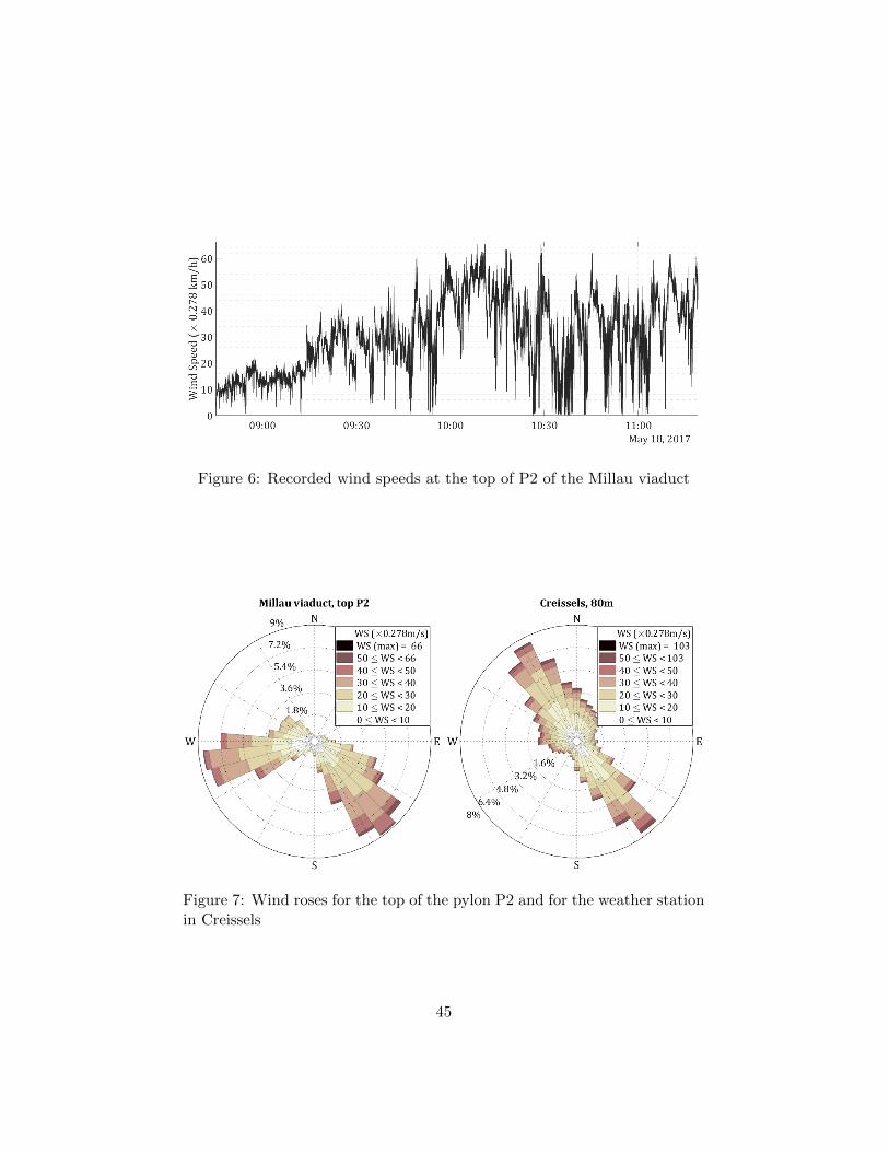
Figure 6: Recorded wind speeds at the top of P2 of the Millau viaduct

Figure 7: Wind roses for the top of the pylon P2 and for the weather stationin Creissels

45

Figure 8: Wind speeds at different levels based on different recorded datafor Millau viaduct

Figure 9: Histogram of the wind speeds at different levels for the period Oct2016 June 2017

Monitoring Distribution EVT Comparison

BWIM-I Heavy vehicles TH choice Confidence

BWIM-II Traffic queues GPD fitting intervals

WS-I Wind effects Model check

Return levelsWS-II

WS-III

Figure 10: Extreme value assessment procedure

46

time

LE

TH

X

Pr(X)

GPD

Figure 11: Representation of the POT approach

THchoice

GPDfitting

Modelcheck

ReturnLevel

CI Update

Figure 12: Steps to be taken in POT approach

Figure 13: Threshold choice (a) by MRLP for the mass of traffic

47

Figure 14: Threshold choice (b) depending on confidence intervals and theprobability of exceedance

48

Figure 15: Analysis of the quality of the estimation

49

Figure 16: Part of the bridge considered for the 2D computational model(left), scheme of the pile with its pylon P2 (middle), 2D computational model(right)

50