PROBABILISTIC ANALYSIS OF AIR VOID STRUCTURE AND ITS ...

PROBABILISTIC ANALYSIS OF AIR VOID STRUCTURE AND ITS

RELATIONSHIP TO PERMEABILITY AND MOISTURE DAMAGE OF HOT

MIX ASPHALT

A Thesis

by

ADHARA CASTELBLANCO TORRES

Submitted to the Office of Graduate Studies of Texas A&M University

in partial fulfillment of the requirements for the degree of

MASTER OF SCIENCE

December 2004

Major Subject: Civil Engineering

PROBABILISTIC ANALYSIS OF AIR VOID STRUCTURE AND ITS

RELATIONSHIP TO PERMEABILITY AND MOISTURE DAMAGE OF HOT

MIX ASPHALT

A Thesis

by

ADHARA CASTELBLANCO TORRES

Submitted to Texas A&M University in partial fulfillment of the requirements

for the degree of

MASTER OF SCIENCE

Approved as to style and content by:

Eyad Masad Roger Smith (Chair of Committee) (Member)

Charles Glover Paul N. Roschke (Member) (Head of Department)

December 2004

Major Subject: Civil Engineering

iii

ABSTRACT

Probabilistic Analysis of Air Void Structure and Its Relationship to Permeability and

Moisture Damage of Hot Mix Asphalt. (December 2004)

Adhara Castelblanco Torres, B.S., Universidad Nacional de Colombia

Chair of Advisory Committee: Dr. Eyad Masad

The permeability of hot mix asphalt (HMA) is of special interest to engineers and

researchers due to the effects that water has on asphalt pavement performance.

Significant research has been done to study HMA permeability. However, most of the

studies primarily focused on relating permeability to the average percent air voids in the

mix. Such relationships cannot predict permeability accurately due to the different

distributions of air void structures at a given average percent of air voids. Air void

distribution is a function of many factors such as mix design, compaction method, and

aggregate properties. Recent advances in X-ray computed tomography and image

analysis techniques offer a unique opportunity to better quantify the air void structure

and, consequently, predict HMA permeability.

This study is focused on portraying permeability as a function of air void size

distribution by using a probabilistic approach that was previously developed by Garcia

Bengochea for soils. This approach expresses permeability as a function of the

probability density function (pdf) of the air void size distribution. Equations are derived

in this thesis to describe this relationship for laboratory specimens compacted using the

iv

linear kneading compactor (LKC) and SuperaveTM gyratory compactor (SGC) as well as

for field cores (labeled as MS). A good correlation exists between permeability and the

pdf of the air voids that formed the flow paths (i.e. connected voids).

The relationship between moisture damage, air void structure, and cohesive and

adhesive bond energy is also investigated in this study. Moisture damage is evaluated by

monitoring changes in mechanical properties due to moisture conditioning. The

influence of air void structure on pore pressure is studied using a recently developed

program at Texas A&M University that simulates fluid flow and pore pressure in a

porous medium. The surface free energy of the aggregates and asphalt are calculated

from laboratory measurements using the Universal Sorption Device (USD) and the

Wilhelmy Plate method, respectively, in order to test the compatibility of the aggregates

with the asphalt in the presence of water.

v

DEDICATION

To my beloved parents, Jose Ignacio and Flor Lucia

vi

ACKNOWLEDGMENTS

I would like to express my immense gratitude to my advisor and committee chair, Dr.

Eyad Masad, for providing me with the opportunity of participating as a research

assistant in this study, and most of all for teaching me and guiding me in the process.

His particular enthusiasm and thoughtfulness encouraged me all the way through.

My gratitude is extended to Dr. Roger Smith and Dr. Charles Glover for taking

part as my committee members. I give special thanks to Dr. Robert Lytton for his

valuable contributions. Their feedback in the final completion of this thesis is greatly

appreciated.

I would like to thank Dr. Birgisson from the University of Florida for sharing his

results from the experimental measurements of HMA mechanical properties that were

conducted at the University of Florida, and most of all, for his useful discussions about

these measurements. I would also like to thank my colleagues from TTI from whom I

received important feedback.

I am especially grateful with my parents for their support and encouragement.

This effort is dedicated to them. Bellatrix and Hector, thanks for standing always by my

side.

vii

TABLE OF CONTENTS

Page

ABSTRACT ..................................................................................................................... iii

DEDICATION ...................................................................................................................v

ACKNOWLEDGMENTS.................................................................................................vi

TABLE OF CONTENTS .................................................................................................vii

LIST OF FIGURES...........................................................................................................ix

LIST OF TABLES ...........................................................................................................xii CHAPTER

I INTRODUCTION.....................................................................................................1

Problem Statement ........................................................................................2 Objective and Scope......................................................................................3 Organization of the Study .............................................................................3

II LITERATURE REVIEW..........................................................................................5

Description of HMA Internal Structure ........................................................5 Permeability of Porous Media.......................................................................5 Permeability Models for Porous Media ........................................................6

Serial Type Models .................................................................................8 Network Models ......................................................................................8 Probabilistic Models................................................................................9

Permeability Anisotropy .............................................................................12 Moisture Damage ........................................................................................12

III MICROSTRUCTURAL ANALYSIS TO CHARACTERIZE AIR VOID SIZE asdfffDISTRIBUTION ....................................................................................................14

Introduction .................................................................................................14 Overview of X-Ray Computed Tomography (CT) Imaging.......................15 Description of Mixes...................................................................................17

viii

CHAPTER Page

Laboratory Specimens Compacted Using Linear Kneading Compactor (LKC) ..........................................................................................................17 Field Cores ..................................................................................................18 Laboratory Specimens Compacted Using SuperpaveTM Gyratory Compactor (SGC)........................................................................................20 Air Void Distribution Results Using X-ray CT Imaging ............................24 Probabilistic Analysis of Air Void Size and Permeability ..........................29 Summary .....................................................................................................50

IV THE RELATIONSHIP BETWEEN AIR VOID DISTRIBUTION, klkjMATERIAL SURFACE PROPERTIES AND MOISTURE DAMAGE...............52

Introduction .................................................................................................52 Measurements of HMA Moisture Damage .................................................53 Relationship between Air Void Size, Pore Pressure Distribution and Moisture Damage ........................................................................................58

Energy Ratio..........................................................................................58 Number of Load Cycles to Failure Ratio ..............................................62

Air Void Analysis........................................................................................63 Pressure Distribution ...................................................................................74 Surface Energy and Bond Strength .............................................................78

Asphalt……………………………………………………………….. 83 Aggregates.............................................................................................86 Adhesive and Cohesive Bond Energies ................................................89

Summary .....................................................................................................92

V CONCLUSIONS.....................................................................................................95 Conclusions .................................................................................................95

REFERENCES.................................................................................................................99

APPENDIX A ................................................................................................................103

VITA ..............................................................................................................................106

ix

LIST OF FIGURES

FIGURE Page

1 Schematic of the X-ray CT scanner. .....................................................................16

2 X-ray CT images of an LKC specimen: (a) grey scale image, and (b) thresholded image...........................................................................................25

3 Difference in air void content with thickness for LKC cores...............................26

4 Difference in air void content with thickness for field cores. ..............................27

5 Difference in air void content with thickness for SGC limestone cores. .............28

6 Difference in air void content with thickness for SGC granite cores...................29

7 Examples of probability plots for an LKC core: a) Weibull distribution, and b) Lognormal distribution. ...................................................................................32

8 Permeability vs. PSP using Lognormal distribution for LKC specimens. ...........35

9 Permeability vs. PSP using Weibull distribution for LKC specimens. ................35

10 Permeability vs. PSP using Lognormal distribution for field specimens.............36

11 Permeability vs. PSP using Weibull distribution for field specimens..................36

12 Flow paths in a LKC specimen. ...........................................................................39

13 Flow paths in a field specimen. ............................................................................40

14 Permeability vs. PSP using Lognormal distribution for LKC flow paths. ...........41

15 Permeability vs. PSP using Weibull distribution for LKC flow paths.................41

16 Permeability vs. PSP using Lognormal distribution for field flow paths.............42

17 Permeability vs. PSP using Weibull distribution for field flow paths. ................42

18 Permeability vs. PSP using Lognormal distribution for SGC granite cores. .......46

19 Permeability vs. PSP using Weibull distribution for SGC granite cores. ............46

x

FIGURE Page

20 Permeability vs. PSP using Lognormal distribution for SGC limestone cores. ...47

21 Permeability vs. PSP using Weibull distribution for SGC limestone cores.........47

22 Determination of DCSE. ......................................................................................54

23 Conditioned vs. unconditioned energy ratios (ER) for granite SGC mixes (17).............................................................................................................61

24 Conditioned vs. unconditioned energy ratios (ER) for limestone SGC mixes (2)...............................................................................................................61

25 Comparison between SGC granite and limestone ER ratios................................62

26 Comparison between SGC granite and limestone N ratios (2). ...........................63

27 Air void quartile difference between granite and limestone gradations...............64

28 Three dimensional air voids of SGC specimen section for mixtures: (a) GA-C1, and (b) WR-C1..................................................................................66

29 Three dimensional air void of SGC specimen section for mixtures: (a) GA-C2, (b) GA-F2..........................................................................................67

30 Air Void distribution for SGC granite specimens. ...............................................68

31 Air void distributions for SGC limestone specimens...........................................69

32 Average diameter vs. N ratio for SGC granite specimens. ..................................70

33 Average diameter vs. ER ratio for SGC granite specimens. ................................71

34 Average diameter vs. N ratio for SGC limestone specimens. ..............................72

35 Average diameter vs. ER ratio for SGC limestone specimens.............................72

36 Dependence of relative strength of mixtures on access to water in void system (28). ..........................................................................................................73

37 Pressure distributions for SGC granite specimens. ..............................................76

38 Pressure distributions for SGC limestone specimens...........................................77

xi

FIGURE Page

39 Comparison of average air void pressure between SGC specimens with different aggregates. .............................................................................................78

40 Wilhelmy Plate method procedure. .......................................................................83

41 Surface energy components of asphalt PG67-22. ................................................86

42 Cohesive bond strength of asphalt with and without water. ................................91

43 Granite coarse gradation mixes, NMAS=12.5 mm. ...........................................104

44 Granite fine gradation mixes, NMAS=12.5 mm. ...............................................104

45 Limestone coarse gradation mixes, NMAS=12.5 mm. ......................................105

46 Limestone fine gradation mixes, NMAS=12.5 mm. ..........................................105

xii

LIST OF TABLES

TABLE Page

1 Description of permeability analytical models (5) .................................................7

2 Properties of LKC mixes......................................................................................18

3 Permeability and percent air voids of laboratory LKC specimens......................18

4 Properties of field core mixes...............................................................................19

5 Volumetric properties of limestone SGC specimens ...........................................21

6 Volumetric properties of granite specimens.........................................................21

7 Mechanical properties of limestone SGC specimens ...........................................23

8 Mechanical properties of granite SGC specimens ...............................................23

9 PSP calculation for Lognormal distribution and laboratory specimens ...............37

10 PSP calculation for Weibull distribution and laboratory specimens....................37

11 PSP calculation for Lognormal distribution and field specimens ........................38

12 PSP calculation for Weibull distribution and field specimens .............................38

13 PSP calculation for Lognormal distribution and flow paths of laboratory LKC specimens ....................................................................................................43

14 PSP calculation for Weibull distribution and flow paths of laboratory specimens .............................................................................................................43

15 PSP calculation for Lognormal distribution and flow paths of field specimens .............................................................................................................43

16 PSP calculation for Weibull distribution and flow paths of field specimens.......44

17 Degree of saturation of SGC specimens ..............................................................45

18 PSP calculation for Lognormal distribution and limestone specimens................48

19 PSP calculation for Weibull distribution and limestone specimens.....................48

xiii

TABLE Page

20 PSP calculation for Lognormal distribution and granite specimens ....................48

21 PSP calculation for Weibull distribution and granite specimens .........................48

22 Regression equations for permeability .................................................................49

23 Permeability equations with Lognormal distribution...........................................50

24 Mechanical data for conditioned and unconditioned granite SGC specimens, (17).....................................................................................................59

25 Mechanical data for conditioned and unconditioned limestone SGC specimens, (2).......................................................................................................60

26 Aggregate angularity measurements ....................................................................65

27 Surface free energy components of solvent liquids (ergs/cm2)............................84

28 Advancing and receding contact angles measured with the Wilhelmy Plate method..................................................................................................................85

29 Healing and fracture energy components of the asphalt ......................................85

30 Surface energy components of gas solvents.........................................................87

31 Spreading pressures and specific surface areas for SGC granite samples ...........88

32 Spreading pressures and specific surface areas for SGC limestone samples .......88

33 Surface energy components of aggregates ...........................................................88

34 Cohesive bond strength of asphalt without water ................................................90

35 Cohesive bond strength of asphalt with water .....................................................90

36 Adhesive bond strength without water (ergs/cm2) ...............................................91

37 Adhesive bond strength with water (ergs/cm2) ....................................................92

38 Gradation of granite mixes .................................................................................103

39 Gradation of limestone mixes ............................................................................103

1

CHAPTER I

INTRODUCTION

The permeability of hot mix asphalt (HMA) is of special interest to engineers and

researchers due to the effects that water has on asphalt pavement performance. Water

infiltration within the HMA can cause moisture damage that is manifested in the

stripping of the binder from the aggregate. Consequently, it is important to take this

property into account to better control the factors that may adversely affect HMA

performance.

Al Omari et al. (1), indicated that many empirical relationships have been

developed to predict permeability of HMA as a function of percent of air voids only.

However, the predictions vary considerably among these models due to the wide

variability in the air void structure among these mixes have. Therefore, permeability of

HMA would be better predicted if the air void size distribution is taken into

consideration. In this study, a probabilistic approach is used to quantify the air void

structure and relate it to HMA permeability for different types of mixtures. The air void

structure is captured using X-ray computed tomography and analyzed using imaging

techniques.

____________________

This thesis follows the style of the Transportation Research Record.

2

The influence of air void structure on moisture damage is also investigated in this

study. A fracture mechanics framework (2) is used to determine the damage that asphalt

mixes experience when they are moisture conditioned. A three dimensional program,

that was developed recently at Texas A&M University, is used to simulate fluid flow in

three dimensional images of HMA and assess pore pressure distribution. Moisture

damage is also attributed to an adhesive and/or a cohesive failure of the pavement

structure. Therefore, these cohesive and adhesive bond strengths are measured to have a

better understanding of the moisture damage and the factors that can cause it.

Problem Statement

Permeability has significant effects on HMA performance. A number of research

studies have been completed to study permeability and many empirical models have

been developed to relate permeability to the average percent air voids. However, HMA

mixes involve a wide range of aggregate size, and a complex distribution of air voids.

Therefore, these models cannot accurately predict permeability based on the average

percent of air voids only.

A probabilistic approach for the analysis of air void structure leads to a better

understanding of how air void distribution influences permeability of asphalt mixtures.

This analysis can be achieved through capturing the microstructure of HMA mixes using

X-Ray Computed Tomography (CT) imaging.

Moisture damage in HMA is related to air void structure and surface properties

of aggregates and binder. Such relationship needs to be established in order to design

asphalt mixes with optimum air void distribution and the least moisture damage.

3

Objective and Scope

The first objective of this study is to portray permeability as a function of air void size

distribution and percent air voids using a probabilistic approach. This objective is

achieved by using the Capillary Model developed by Garcia-Bengochea which

introduces a pore size parameter that can be calculated from continuous data obtained

using X-Ray CT imaging (3).

The second objective is to determine the relationship between the air void

distribution, pore pressure distribution, material surface properties and moisture damage.

This objective is achieved through (1) measurements of surface energy of mixture

components to analyze their adhesive and cohesive properties, (2) simulation of pore

pressure in the HMA microstructure, and (3) measurements of HMA mechanical

properties before and after moisture conditioning.

Organization of the Study

Chapter II documents a review of the empirical and analytical models that have been

developed to predict permeability of porous media, and the limitations of these models

in predicting HMA permeability. This chapter also includes a description of the X-Ray

CT imaging technique that was used in this study to capture HMA microstructure of the

specimens used in this research.

Chapter III includes the development of a probabilistic permeability model for

HMA. The air void size distribution was characterized for laboratory specimens that

were compacted using the Linear Kneading Compactor (LKC) and SuperpaveTM

gyratory compactor (SGC), as well as for field cores. The relationship that exists

4

between different air void distributions and permeability measurements is presented.

This is accomplished based on the Capillary model developed by Garcia-Bengochea (3).

Two different analyses are considered for this purpose; the first one is taking all the

voids into account while the second one is considering the connected voids only.

Chapter IV discusses the influence that air void distribution and pressure

distribution have on moisture damage. The analysis in this chapter is done on SGC

specimens that were prepared with granite and limestone obtained from the University

of Florida. Measurements of their mechanical properties before and after conditioning

were used to assess their resistance to moisture damage. A three dimensional program

for the simulation of fluid flow was used to calculate pore pressure that water exhorts

within the microstructure. Furthermore, results of surface energy testing are presented

in order to assess the cohesive and adhesive bonding.

Chapter V summarizes the results of the relationship between permeability and

air void size distribution. Also, a summary of the findings in regard to the relation

between air void size, pore pressure, material surface properties, and moisture damage of

HMA is presented. Recommendations are given in regard to the factors that might affect

these results.

5

CHAPTER II

LITERATURE REVIEW

Description of HMA Internal Structure

An asphalt mixture is a composite material that consists of asphalt binder, aggregates,

and air voids. The internal structure (or microstructure) refers to the spatial and

directional distribution of these constituents in the mix. The internal structure of an

asphalt mixture is influenced by aggregate shape and gradation, asphalt binder content,

and the degree and method of compaction.

The internal structure determines the ability of water to infiltrate into the mix,

and it also controls the retention of moisture within the mix. Therefore, it is important to

capture and quantify the internal structure distribution. They were measured in this

study using X-ray computed tomography (CT) and image analysis techniques.

Permeability of Porous Media

Different empirical and analytical models have been developed to describe the

permeability of porous media. Usually, permeability is described using the Darcy’s

coefficient of permeability k. This coefficient is derived from Darcy’s Law which

implies that there is a linear relationship between the discharge velocity and the

hydraulic gradient, when the flow is laminar (4). Darcy (1856) observed that the

discharge velocity of water through a saturated granular soil can be calculated through

the empirical expression (4):

6

(1)

where

v = discharge velocity,

i = hydraulic gradient,

k = coefficient of permeability

Essentially, the discharge velocity v represents the quantity of water that

percolates per unit of time across a unit area of a section that is normal to the direction

of the flow. The coefficient of permeability k is a measure of the ability of water to

infiltrate the porous medium. The hydraulic gradient i is the rate of loss of total head h,

between two points that are separated an apparent flow distance s, and can be calculated

using the following equation (4):

dsdhi −= (2)

It has been recognized that the Darcy’s coefficient of permeability of porous

media can be calculated based on the assumption of laminar flow (4). This has been

confirmed in different numerical simulations of various porous media, and hence it has

been implied to be applicable to HMA (1).

Permeability Models for Porous Media

Analytical models have been developed to describe flow through porous media. Bear (5)

summarized these analytical models into four categories: capillary tube models, fissure

models, hydraulic radius models, and resistant to flow models. These models are based

on simplified assumptions regarding the distributions of solids and voids, and shape of

kiv =

7

air voids. Therefore, they relate permeability to average parameters that describe the

internal structure, such as porosity and average aggregate size, and insert a constant

shape factor to fit the data. Consequently, they do not really represent the wide range of

void and aggregate sizes that exist and that influence permeability.

These models can be expressed in the following general form, (1):

2sDCf(n)K ⋅⋅= (3)

Where, K is the absolute permeability, f(n) is a function of porosity or percent air

voids, C is an empirical factor that accounts for the air void distribution, and Ds is the

average size of particles in a porous medium. A summary of these models is presented

in Table 1. At the same time, the absolute permeability K is related to the Darcy’s

permeability coefficient k as (1):

µγKk = (4)

Where, γ is the unit weight of the fluid and µ is fluid viscosity.

TABLE 1 Description of permeability analytical models (5) Model Permeability Constants Remarks

C=1/32 for 1-D tubeC=1/96 for 3-D tube

n: porosity, δ: air void diameter, λ: factor of packing, D: average particle size

k=Cn2D2/[(1-n)λ]λ=3π for single sphere in infinite

fluid, C=π/6 for spherical particlesBased on Stockes' Equation for

dragResistance to Flow

k=Cn3D2/(1-n)2C=1/180 for spherical particles

Kozeny-Carman equation based on Hydraulic RadiusHydraulic Radius

Applicable to fissured rockk= Cnb2

C=1/96 for capillarity in orthogonal direction

Fissure C=1/12 for parallel fissures of width b

Based on Haggen-Poiseuille's EquationCapillary tubes

k=Cnδ2

k=CnD2∫δ2α(δ)dδ Tubes are distributed equally in each orthogonal direction

8

xsnP 2

43 δπ⋅=

Serial Type Models

In order to overcome the assumption that the pore size is constant throughout the porous

medium and also that the capillary tubes are uniformly organized, these models intend to

include an additional factor known as tortuosity. The tortuosity factor is the ratio

between the length of a flow channel with respect to the length of a straight line distance

that goes from the inlet to the outlet of a porous medium. Scheidegger (6) included this

tortuosity factor into a model that calculates permeability as:

2

2

961

TPk δ

⋅= (5)

Where, δ is the average pore diameter, T is a tortuosity factor and P is the

porosity of the model. Also, according to the model, the porosity factor is defined as:

(6)

Where the factor 3 is introduced by considering that each spatial dimension has n

capillaries per unit area; x is the length of the model, and s is the length of the capillary

tube. This tortuosity factor was also used by Al-Omari et al (1) in a model that

calculated HMA permeability which was determined using X-ray CT.

Network Models

None of the models that have been already mentioned take into account the fact that

water can branch out by taking different paths and then converge into the same flow path

again. The voids in these networks are represented by the nodes on the network.

However, this is not a very accurate representation due to the lack of knowledge of the

9

microstructure distribution. As such, these models were not successful in obtaining

reasonable approximations of permeability. Another shortcoming of these network

models is the difficulty of replicating the actual microstructure using an idealized

network of channels (6).

Probabilistic Models

All the models that have been described above employ average parameters to describe

the internal structure and predict permeability. However, Scheidegger (6) established

that the correlation between average parameters with permeability is complex because of

the strong dependence of flow rate on the area connectivity, shape and tortuosity of pore

paths.

Childs and Collis-George (7), proposed a probabilistic based flow model to

quantify the distribution of pores which was later modified by Marshall (8). The model

uses pore size distribution to calculate permeability through simplified assumptions in

regard to connectivity between adjacent sections: 1) Pore size is considered to be a

random variable that can be characterized with a known probability distribution. 2) The

overall flow between adjacent sections of the porous media is a function of the number

of void pairs that are interconnected, and their sizes. 3) The quantity of flow through

the pair of connected voids is restricted by the one with the narrower size; and 4) the

connection between any pair of pores in two adjacent sections is totally random. Garcia-

Bengochea (3) defined empirical correlations that related a pore size parameter based on

probability principles to permeability. Under these assumptions the equation that Childs

and Collis-George developed for permeability becomes:

10

jjii

Rx

x

Rx

xxxfxxfxgck

i

i

j

j

∆⋅∆⋅= ∑ ∑=

=

=

=

)()(0 0

_2

µρ

PSPCk s ⋅=

(7)

Where, k is the coefficient of permeability, c is an empirical matching factor that

is needed to correct the permeability calculated with the model to the measurement at

full saturation; ρ is the density of water, g is the gravitational acceleration, µ is the

coefficient of absolute viscosity of water, xi and xj are void radii, and x is the narrowest

radii between xi and xj. The terms f(xi) ∆ xi and f(xj) ∆ xj are the fraction of pore space

occupied by pores with radii between xi and xi +∆ xi and between xj and xj +∆ xj

respectively.

Garcia-Bengochea, defined a pore size parameter (PSP) based on probability

principles (3):

)()(_2

ji

n

i

n

jxPxPxPSP ∑∑= (8)

Where, n is the total number of pores, xi and xj are random pore diameters, x is

the smaller pore diameter between xi and xj, and P(x) is the volumetric frequency of

occurrence of pores with diameter within x and x+∆x.

Following this, an empirical correlation between permeability k and PSP was defined by

inserting a shape factor Cs (3).

(9)

To overcome the empiricism of this expression, Juang and Holtz (9), developed a

new model for permeability as a function of the pore size density function, which was

11

jijiji dx dx )f(x )f(x ) x,P(x =

)(dx )f(x ) x,P(xor )P(xdx )f(x ) x,P(x jjjiiiiji jxP====

∫ ∫∞ ∞

⋅⋅⋅⋅⋅=0 0

___2

2

)()(),,(32 jijiji dxdxxfxfxxygxgnk

µρ

measured from mercury intrusion. By considering a section of a porous medium with

thickness ∆y, and assuming that its cross sections have identical pore size density

functions then, the probability P(xi, xj), that pores within diameters xi to x+dxi on cross

section i, are connected to pores on cross section j within diameters xj to x+dxj, has two

extreme cases:

1) If ∆y>>x, the connection of voids on the adjacent cross sections can be assumed as

being completely random. Therefore:

(10)

2) If ∆y→0, the connection of voids on the adjacent cross sections is assumed to be

completely correlated. Thus:

(11)

Where, f(x) is the pore size density function of the porous medium. Juang and

Holts (9) developed Equation 12, for the intermediate case between completely

correlated and uncorrelated cases:

(12)

Where g(y,xi,xj) is a connecting function, y is a variable that accounts for

tortuosity of flow and x is the smallest between xi,xj; and f(x)dx represents the

proportion of the total pore volume of voids within a diameter range of x and x+dx.

12

Permeability Anisotropy

Permeability anisotropy indicates that the material exhibits different permeability values

depending on direction. Permeability anisotropy occurs in a porous medium such as

HMA, due to the directional distribution of aggregates and air voids.

Al-Omari and Masad (10) developed a three dimensional fluid flow model to

calculate HMA permeability by capturing the microstructure using X-ray CT images.

The anisotropy of permeability can be calculated by applying pressure gradients in

different directions and calculating the permeability coefficients in these directions.

Moisture Damage

HMA moisture damage is caused by the infiltration of water into the internal structure

and moisture susceptibility of the mixture. Moisture damage can be caused by a

cohesive failure when the asphalt binder separates or by an adhesive failure when the

linkage between the aggregate and the asphalt binder breaks down (2).

The adhesive resistance of a mix depends on the bonding strength between the

aggregate and the asphalt binder. If this bond is weak, a failure will occur at the

aggregate-asphalt interface; this is commonly known as stripping (11). There are

different ways to mitigate stripping of asphalt pavements. Firstly it is important to

provide adequate drainage to the pavement structure so that moisture will not remain

within the internal structure. Poor compaction is another issue that should be addressed

because it can facilitate the penetration of moisture into the mix (11).

In order to obtain a mixture that is not susceptible to stripping, there has to be

chemical compatibility between the aggregate and the asphalt binder. Some aggregates

13

are more susceptible to stripping because of their chemical composition. Siliceous

aggregates such as granite and sandstone have been categorized as hydrophilic because

they tend to strip much more easily than carbonate aggregates such as limestone (12).

Lytton (13) reported on the surface energy of different binders and aggregates.

He demonstrated the importance of selecting aggregates and binder that are compatible

in terms of surface energy in order to provide adequate cohesive and adhesive bond

strengths in the mix. Lytton (13) presented the methods to calculate the bond energy

necessary to resist fracture and the bond energy needed for crack healing. Lytton (13)

also linked moisture damage to the asphalt film thickness which is a function of the

aggregate properties and mix design.

14

CHAPTER III

MICROSTRUCTURAL ANALYSIS TO CHARACTERIZE AIR VOID SIZE

DISTRIBUTION

Introduction

Scheiddeger (6) developed a definition for the air void size at a given point of the

microstructure that could be used to mathematically interpret the pore size distribution

as well as its density function. He believed that the pore diameter at any point within the

pore space is a random variable and considered it as the largest sphere that holds this

point and nonetheless remains entirely inside the pore space. In this way, a pore

diameter x, could be assigned to each point within the pore space, and the air void

diameter distribution can be established by determining the respective fraction of the

pore space that is composed of air void diameters between x and x + dx.

Numerous methodologies have been used to characterize the air void size

distribution of porous media. These methods include: a) application of probability

theory to indirectly determine the air void distribution from a representative grain size

distribution; b) scanning electron microscopy techniques; c) capillary suction methods;

and d) mercury intrusion techniques. However, the latter was most frequently used to

determine the pore size distribution because of its appropriateness (9). This procedure

consisted of intruding a non-wetting liquid (mercury) into the porous medium. The

surface tension of this liquid resists the entry of the liquid into the pores. Washburn (14)

15

noticed that this tension could be overcome by an external pressure that is inversely

proportional to the diameter size of the pore being intruded. With the powerful features

of X-Ray CT imaging techniques, the microstructure of porous media such as HMA can

be digitally captured in a three dimensional fashion (15).

Overview of X-Ray Computed Tomography (CT) Imaging

The X-Ray CT imaging technique consists of studying the interior of opaque solid

objects in a non-destructive fashion. Two dimensional images or most commonly

known as “slices” can be obtained through this process. Each slice reveals the interior

of the object on a plane, and if stacked together, the slices can build a three dimensional

image of the object. These slices are generally about 1 mm in thickness with an overlap

of 0.2 mm in between (15).

The X-Ray system is composed of an X-ray source, a turntable to hold the

sample, and a detector. 1 shows a schematic of the system. The source emits X-rays

that pass through the solid object while it rotates horizontally. After each complete

rotation, an image is produced from the different density measurements that are

registered, and are represented by a grey scale.

16

X-Ray Source

Detector

Specimen

Collimator(window)

X-Ray Source

Detector

Specimen

Collimator(window)

Figure 1 Schematic of the X-ray CT scanner.

Subsequent to scanning each slice, the turntable is shifted downwards, by a fixed

distance which is equivalent to the resolution in that direction. The whole procedure is

repeated once again to produce the next image, until the whole solid is scanned.

An important issue to take into account when using X-ray CT images is the

resolution at which they are taken (number of pixels per unit length of the longitudinal

image dimension). The resolution is affected by several factors such as the type and size

of the X-ray source and detectors, the distance between the source, the solid and the

detector, and the method used for image reconstruction. The image reconstruction

consists of representing the object in a grid of picture elements (pixels) if using two

dimensions, or volume elements (voxels) if using three dimensions.

The images that were analyzed varied in resolution. The images of the

laboratory LKC cores were taken at a resolution in the range of 0.146 to 0.195

mm/pixel. The resolution of the field cores was not the same for all specimens due to

17

the difference in size (i.e. 0.092, 0.142, 0.186, and 0.195 mm/pixel), and the SGC cores

were scanned with a resolution of 0.195 mm/pixel. These images are captured in a grey

scale that consists of 256 levels; each level corresponds to a density within the core. Air

voids have the lowest intensity of all and are shown in black, which corresponds to level

zero.

Description of Mixes

Three sets of specimens were used to find the relationship between the pore size

distribution and the permeability. These specimens were categorized as: 1) laboratory

specimens compacted using Linear Kneading Compactor (LKC), 2) field cores (MS),

and 3) laboratory specimens compacted using SuperpaveTM Gyratory Compactor (SGC).

Details about these mixtures are described in the following sections.

Laboratory Specimens Compacted Using Linear Kneading Compactor (LKC)

The laboratory specimens were prepared with two different types of aggregates, gravel

and limestone. The gravel mix had a nominal maximum aggregate size (NMAS) of 12.5

mm, whereas three different mixes were prepared with the limestone having NMAS of

12.5 mm, 19.0 mm, and 25.0 mm, respectively. The samples were cored from slabs with

different thicknesses prepared with the Linear Kneading Compactor (LKC).

Permeability measurements for these mixes were obtained using the Karol Warner

permeameter which is based on the falling head method (16). The properties of these

mixes are summarized in Table 2 and Table 3.

18

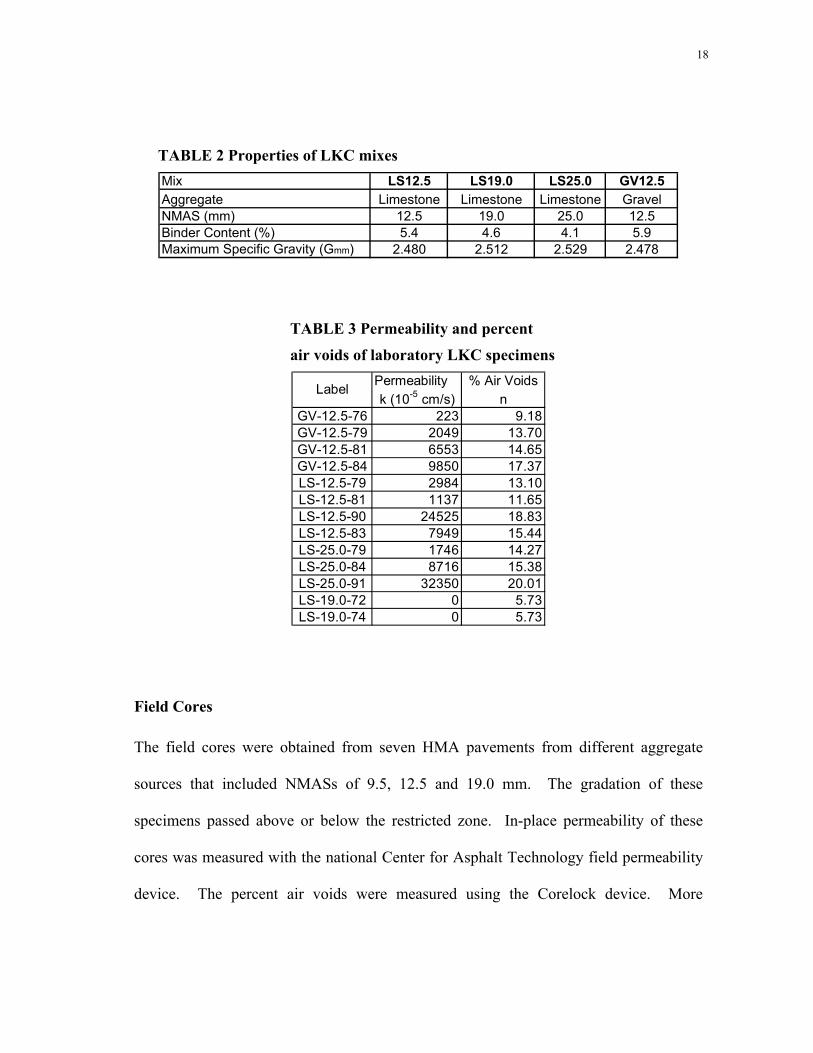
TABLE 2 Properties of LKC mixes Mix LS12.5 LS19.0 LS25.0 GV12.5Aggregate Limestone Limestone Limestone GravelNMAS (mm) 12.5 19.0 25.0 12.5Binder Content (%) 5.4 4.6 4.1 5.9Maximum Specific Gravity (Gmm) 2.480 2.512 2.529 2.478

TABLE 3 Permeability and percent

air voids of laboratory LKC specimens Permeability % Air Voidsk (10-5 cm/s) n

GV-12.5-76 223 9.18GV-12.5-79 2049 13.70GV-12.5-81 6553 14.65GV-12.5-84 9850 17.37LS-12.5-79 2984 13.10LS-12.5-81 1137 11.65LS-12.5-90 24525 18.83LS-12.5-83 7949 15.44LS-25.0-79 1746 14.27LS-25.0-84 8716 15.38LS-25.0-91 32350 20.01LS-19.0-72 0 5.73LS-19.0-74 0 5.73

Label

Field Cores

The field cores were obtained from seven HMA pavements from different aggregate

sources that included NMASs of 9.5, 12.5 and 19.0 mm. The gradation of these

specimens passed above or below the restricted zone. In-place permeability of these

cores was measured with the national Center for Asphalt Technology field permeability

device. The percent air voids were measured using the Corelock device. More

19

information on these measurements is given by Al-Omari et al. (1). The properties of

these mixes are summarized in Table 4 including the percent air voids and permeability

data.

TABLE 4 Properties of field core mixes Permeability % Air Voidsk (10-5 cm/s) n

MS1 - 1 Above 12.5 697 13.90MS1 - 4 Above 12.5 10 6.60MS1 - 6 Above 12.5 37 7.00MS1 - 7 Above 12.5 1 4.40MS1 - 8 Above 12.5 1 5.60MS2 - 6 Below 12.5 0 5.30MS2 - 7 Below 12.5 49 9.50MS2 - 9 Below 12.5 76 7.10MS2 - 11 Below 12.5 119 6.90MS4 - 7 Below 9.5 120 8.80MS4 - 11 Below 9.5 54 8.20MS4 - 14 Below 9.5 291 9.00MS5 - 1 Below 19.0 3333 7.40MS5 - 3 Below 19.0 30 5.40MS5 - 4 Below 19.0 348 8.50MS5 - 11 Below 19.0 4960 10.60MS5 - 12 Below 19.0 244 7.20MS6 - 6 Above 19.0 269 8.70MS6 - 7 Above 19.0 1386 11.00MS6 - 8 Above 19.0 656 9.60MS6 - 13 Above 19.0 1 6.00MS6 - 14 Above 19.0 178 7.50MS7 - 3 Below 9.5 0 4.70MS7 - 6 Below 9.5 28 7.20MS7 - 9 Below 9.5 527 10.60MS7 - 13 Below 9.5 327 9.50MS8 - 10 Below 19.0 13477 10.60MS8 - 11 Below 19.0 16307 9.60MS8 - 12 Below 19.0 1619 7.60MS8 - 13 Below 19.0 17789 12.60

NMAS (mm)GradationLabel

20

Laboratory Specimens Compacted Using SuperpaveTM Gyratory Compactor

(SGC)

These specimens were obtained from two different studies on moisture susceptibility

conducted at the University of Florida by Birgisson, Roque and Page (2), (17). The

specimens were prepared using granite aggregate from Georgia and limestone aggregate

from Florida. These two types of aggregates are commonly used throughout Florida.

Experience has shown that the limestone does not have significant potential for stripping

whereas the granite does. The limestone and granite mixes will be denoted hereafter as

WR and GA, respectively.

Both types of mixes were prepared with coarse aggregate, fine aggregate,

screenings, and mineral filler that were blended together in different proportions to make

six different HMA mixtures, respectively. A limestone mixture that was previously

designed by Florida Department of Transportation (FDOT) was used to produce a

coarse-graded (C1) and fine-graded mixtures (F1). The coarse gradation refers to

passing below the restricted zone, while the fine gradation refers to passing above the

restricted zone. Two more gradation designs were used by varying the coarse and fine

proportions of the original mixture. Hence, six limestone mixtures of 12.5-mm nominal

maximum aggregate size were prepared, three of them from the coarse gradation (C),

and the other three from the fine gradation (F): C1, C2, C3, F1, F2, F3/C4. The dual

designation of F3/C4 was used to indicate that the gradation was adjusted to fall under

the restricted zone with the purpose of having a higher permeability. The volumetric

properties of these mixtures are summarized in Table 5. The six granite mixtures were

21

of 12.5-mm nominal maximum aggregate size, three of them have coarse gradations

(GA-C1, GA-C2, GA-C3), and the other three, have fine gradation, (GA-F1, GA-F2,

GA-F3). All specimens were prepared to 7% target percent air voids. The properties of

these mixtures are given in Table 6.

TABLE 5 Volumetric properties of limestone SGC specimens Specimen WR-C1 WR-C2 WR-C3 WR-F1 WR-F2 WR-F3/C4Binder Content 6.5 5.8 5.3 6.3 5.4 5.6Specific gravity of Asphalt 1.035 1.035 1.035 1.035 1.035 1.035Bulk Specific Gravity 2.235 2.255 2.254 2.244 2.281 2.244Voids in Mineral Aggregate (%) 15.4 13.8 13.6 15.6 13.2 14Voids filled with Asphalt (%) 74.1 71.6 70.2 74.2 70.1 71.9Effective specific gravity of aggregate 2.549 2.545 2.528 2.554 2.565 2.537Effective asphalt (%) 5.3 4.6 4.5 5.3 4.2 5.5Theoretical Film Thickness (microns) 11.2 10.1 8.0 9.0 6.9 8.1Percent of air voids 4.0 3.9 4.0 4.0 3.9 3.9Permeability (10-5 cm/s) 72.37 64.24 29.39 69.63 17.81 9.68Surface area (m2/kg) 4.87 4.64 5.68 6.05 6.31 5.64

TABLE 6 Volumetric properties of granite specimens

Specimen GA-C1 GA-C2 GA-C3 GA-F1 GA-F2 GA-F3Binder Content 6.6 5.3 5.3 5.7 4.6 5.1Specific gravity of Asphalt 1.035 1.035 1.035 1.035 1.035 1.035Bulk Specific Gravity 2.345 2.399 2.391 2.374 2.433 2.404Voids in Mineral Aggregate (%) 18.5 15.4 15.7 16.6 13.6 15.1Voids filled with Asphalt (%) 78.5 73.8 74.2 75.9 71.2 73.3Effective specific gravity of aggregate 2.710 2.719 2.709 2.706 2.725 2.720Effective asphalt (%) 6.3 4.9 5.0 5.4 4.1 4.6Theoretical Film Thickness (microns) 19.9 14.3 12.1 13.4 7.7 9.9Percent of air voids 4.0 4.0 4.1 4.0 3.9 4.0Permeability (10-5 cm/s) 67.50 59.00 56.00 25.33 9.33 34.25Surface area (m2/kg) 3.30 3.50 4.20 4.10 5.30 4.90

Overall, the six mixtures of each type of aggregate can be categorized as fine

uniformly-graded and fine dense-graded to coarse uniformly-graded and coarse gap-

22

graded; the corresponding nomenclature of the limestone and granite specimens,

coincides with approximately the same gradation (2), (17). The purpose of varying the

gradation was to obtain mixtures of different permeability and other volumetric

properties but with the same aggregate type, to test the influence of these factors on

moisture damage. Following SuperpaveTM volumetric mix design specifications, the

content of asphalt was determined for each mixture by targeting the air void content to

4% at Ndesign of 109 gyrations. The asphalt used was determined to be PG 67-22 (AC-

30).

For each mixture, 3 samples were conditioned, according to AASHTO T-283.

The SuperPaveTM IDT was used to test unconditioned (U) and conditioned (C) samples

to measure resilient modulus, creep compliance, and strength. The tensile strength,

resilient modulus, fracture energy limit (FE), and creep properties (D1 and m-value)

were determined from these tests. All this data is summarized in Tables 7 and 8. More

details about these tests are given in references (2) and (17).

23

TABLE 7 Mechanical properties of limestone SGC specimens

Resilient Modulus

(Gpa)

Creep compliance at 100 seconds

(1/Gpa)

Tensile Strength

(Mpa)

Fracture Energy (kJ/m3)

Failure Strain (10-6)

m-value D1

WR-C1 (C) 7.00 1.71 1.33 2.20 2017.0 0.44 1.50E-06WR-C2 (C) 7.35 2.45 1.27 1.90 1766.0 0.59 1.03E-06WR-C3 (C) 9.96 1.09 1.62 1.60 1259.0 0.54 5.75E-07WR-C1 (U) 8.53 1.74 1.59 2.50 1939.0 0.54 9.51E-07WR-C2 (U) 8.66 2.46 1.28 1.90 1702.0 0.67 7.65E-07WR-C3 (U) 10.97 0.78 1.92 2.00 1320.0 0.43 7.84E-07WR-F1 (C) 6.17 3.68 1.56 4.20 3270.0 0.73 9.13E-07WR-F2 (C) 5.59 3.02 1.56 3.10 2674.7 0.67 9.49E-07WR-F3 (C) 9.45 1.44 1.77 1.90 1366.0 0.69 4.08E-07WR-F1 (U) 6.08 3.42 1.57 4.20 3269.0 0.60 1.16E-06WR-F2 (U) 8.13 1.74 1.81 3.10 2114.0 0.54 1.01E-06WR-F3/C4 (U) 9.67 1.28 1.98 2.70 1685.0 0.53 7.08E-07

Property

Temperature: 10 oC

Label

TABLE 8 Mechanical properties of granite SGC specimens

Resilient Modulus

(Gpa)

Creep compliance at 100 seconds

(1/Gpa)

Tensile Strength

(Mpa)

Fracture Energy (kJ/m3)

Failure Strain (10-6)

m-value D1

GA-C1 (C) 4.08 4.42 1.12 2.90 3350.1 0.66 1.54E-06GA-C2 (C) 8.35 2.84 1.84 2.80 2055.8 0.65 1.03E-06GA-C3 (C) 9.07 2.75 1.77 2.10 1610.9 0.6 9.10E-07GA-C1 (U) 5.1 4.12 1.44 6.00 4763.8 0.62 1.74E-06GA-C2 (U) 8.79 2.16 2.00 5.00 3122.0 0.59 1.06E-06GA-C3 (U) 9.99 1.47 1.99 3.80 2406.3 0.57 8.70E-07GA-F1 (C) 7.05 2.89 1.59 2.80 2145.1 0.63 1.52E-06GA-F2 (C) 10.1 1.92 1.96 2.30 1351.3 0.56 1.24E-06GA-F3 (C) 8.14 2.28 1.75 2.10 1638.4 0.6 1.44E-06GA-F1 (U) 8.45 1.93 1.93 3.70 2428.4 0.57 1.30E-06GA-F2 (U) 10.2 2.52 2.52 3.60 1803.8 0.48 1.58E-06GA-F3 (U) 9.95 2.14 2.14 2.80 1757.2 0.56 8.97E-07

Label

Property

Temperature: 10 oC

24

Air Void Distribution Results Using X-ray CT Imaging

As described in the previous section, X-ray CT images are produced in a grey scale. To

analyze the images, they have to be transformed into a binary format such that the voids

can be isolated from the rest of the solids (mastic and aggregates). By doing so, the grey

images were transformed such that air voids appeared in black, and all other phases

appeared in white. This procedure was done by setting a threshold value of grey

intensity such that every pixel with an intensity value above threshold is turned to black

and every pixel with an intensity value below the threshold is turned to white.

This threshold was chosen by finding an intensity value such that the percent air

voids calculated from the 3-D image matches the measured one. The air void content

was measured using the Corelock device for the field and LKC laboratory specimens,

and the AASHTO T166 method was used for the SGC granite and limestone specimens.

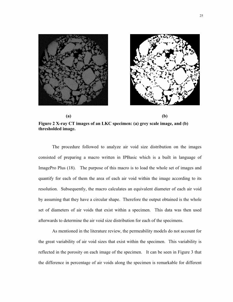
Figure 2 shows a sample of how a thresholded image on the right looks in

comparison to the original grey scale image on the left. It is remarkable how close the

air voids can be identified in the binary format. Hence, it is important to rely on

accurate measurements of percent air voids as that will affect the appearance of the

transformed image and, the calculations based one on the images will be influenced as

well.

25

(a) (b)

Figure 2 X-ray CT images of an LKC specimen: (a) grey scale image, and (b) thresholded image.

The procedure followed to analyze air void size distribution on the images

consisted of preparing a macro written in IPBasic which is a built in language of

ImagePro Plus (18). The purpose of this macro is to load the whole set of images and

quantify for each of them the area of each air void within the image according to its

resolution. Subsequently, the macro calculates an equivalent diameter of each air void

by assuming that they have a circular shape. Therefore the output obtained is the whole

set of diameters of air voids that exist within a specimen. This data was then used

afterwards to determine the air void size distribution for each of the specimens.

As mentioned in the literature review, the permeability models do not account for

the great variability of air void sizes that exist within the specimen. This variability is

reflected in the porosity on each image of the specimen. It can be seen in Figure 3 that

the difference in percentage of air voids along the specimen is remarkable for different

26

aggregate types (gravel GV and limestone LS), having different nominal maximum

aggregate size (NMAS), even though both were compacted with LKC. When

comparing these air void distributions with their respective percentage of air voids

consigned in Table 3, it becomes meaningful that disaggregate data about the air void

content is more significant than an aggregate value for the specimen.

0

10

20

30

40

50

60

70

80

0% 5% 10% 15% 20% 25%Air void content

Thic

knes

s (m

m)

LS-19.0-74 GV-12.5-79 LS-25.0-79

Figure 3 Difference in air void content with thickness for LKC cores.

Figure 4 shows that the porosity of the field cores changes greatly along the

thickness of the specimen in regard to the NMAS as observed with the LKC cores,

having in particular more air voids toward the top and bottom parts of the specimen.

Even though MS5-4 and MS4-7 have a similar percentage of air voids, (i.e. 8.5% and

27

8.8% respectively), their distribution is different. On the other hand, MS1-1 is shifted to

the right because its air void content is greater (13.9%). These details are difficult to

capture with a measurement of air void content only.

0

10

20

30

40

50

60

70

0% 5% 10% 15% 20% 25%Air void content

Thic

knes

s (m

m)

MS5-4 MS4-7 MS1-1

Figure 4 Difference in air void content with thickness for field cores.

The variability of the air void distribution along the thickness of the SGC

specimens is also remarkable, as shown in Figures 5 and 6. Even though, these mixtures

were compacted using the same method, and they exhibit a common profile distribution

of air void content (i.e. more air voids in the top and in the bottom, with generally lower

values in the remainder of the specimen), the type of gradation makes a difference.

This can be seen in Figures 5 and 6 which show a comparison between the air void

28

distribution profile for a coarse gradation and a fine gradation for limestone and granite

respectively.

0

10

20

30

40

50

60

70

80

90

0% 2% 4% 6% 8% 10% 12% 14% 16% 18%Air void content

Thic

knes

s (m

m)

WR-C2WR-F2

Figure 5 Difference in air void content with thickness for SGC limestone cores.

29

0

20

40

60

80

100

120

0% 2% 4% 6% 8% 10% 12% 14% 16% 18%Air void content

Thic

knes

s (m

m)

GA-C1GA-F1

Figure 6 Difference in air void content with thickness for SGC granite cores.

Probabilistic Analysis of Air Void Size and Permeability

The variable diameter capillary model developed by Garcia-Bengochea was used

to predict the permeability of the LKC and the field specimens respectively (3). This

model is based on a probabilistic approach because it relates the air void size distribution

to permeability. Garcia-Bengochea approximated the air void size distribution in a

discrete form by measuring the volume of void space occupied by voids within a certain

size range. These measurements were conducted using the mercury intrusion technique

(3).

This model was applied using the assumption that the probability that air voids

on two adjacent sections, or slices of the specimen, are connected is completely

30

∑=i

iis xxPnCk 2)(

)nE(x PSP PSP,C k 2s ==

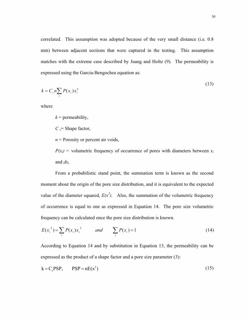
correlated. This assumption was adopted because of the very small distance (i.e. 0.8

mm) between adjacent sections that were captured in the testing. This assumption

matches with the extreme case described by Juang and Holtz (9). The permeability is

expressed using the Garcia-Bengochea equation as:

(13)

where

k = permeability,

C s= Shape factor,

n = Porosity or percent air voids,

P(xi) = volumetric frequency of occurrence of pores with diameters between xi

and dxi.

From a probabilistic stand point, the summation term is known as the second

moment about the origin of the pore size distribution, and it is equivalent to the expected

value of the diameter squared, E(x2). Also, the summation of the volumetric frequency

of occurrence is equal to one as expressed in Equation 14. The pore size volumetric

frequency can be calculated once the pore size distribution is known.

1)()()( 22 == ∑∑i

iii

ii xPandxxPxE (14)

According to Equation 14 and by substitution in Equation 13, the permeability can be

expressed as the product of a shape factor and a pore size parameter (3):

(15)

31

dxxnECdxxfxnCk si

d

dis )()( 22

max

min

== ∫

Where, PSP is the pore size parameter that is related to the pore size distribution.

X-ray CT Image analysis allows performing air void measurements in a precise

way by measuring continuous data. Hence, the summation in Equation 14 is replaced by

an integral over all the diameter sizes. It corresponds to the area under the curve of the

product of the diameter squared and the probability density function f(xi), of a known

distribution that fits the pore size data. This can be mathematically expressed as:

(16)

The probability density function was determined by plotting the pore size

cumulative probability versus the cumulative probability of a test distribution. These

plots are most commonly known as “probability plots” and are available from statistical

packages (19). Figure 7 shows an example of the probability plots for an LKC core

tested using Weibull and Lognormal distributions. If the distribution of the data

matched the test distribution, the data points should cluster around the equality line.

32

( )

⋅−−

⋅⋅⋅

= 2

2

2lnexp

21)(

σµ

πσx

xxf

Weibull P-P Plot of LS2591

Observed Cum Prob

1.00.75.50.250.00

Expe

cted

Cum

Pro

b1.00

.75

.50

.25

0.00

Lognormal P-P Plot of LS2591

Observed Cum Prob

1.00.75.50.250.00

Expe

cted

Cum

Pro

b

1.00

.75

.50

.25

0.00

(a) (b)

Figure 7 Examples of probability plots for an LKC core: a) Weibull distribution, and b) Lognormal distribution.

The Pearson correlation coefficient was used to establish the degree of linearity

between the cumulative probability of the data and the test distribution. The closer this

coefficient is to one, the better the correlation between the two cumulative probabilities

is, and thus, the distribution fits the data (19).

According to the probability plots and the Pearson correlation coefficients, there

were two distributions that fitted the data the best, Lognormal and Weibull distributions

with Pearson correlation coefficients between 0.94 and 0.99. Both of these density

functions were used thereafter for the analysis.

The density function of the lognormal distribution is expressed as (20):

(17)

33

))/(exp()( 1 βββ α

αβ xxxf −⋅⋅= −

where

x = air void diameter,

µ = location parameter,

σ = scale parameter

A lognormally-distributed random variable implies that the logarithm of it is

normally-distributed. The location parameter µ can be any real number whereas the

scale parameter σ can only be a positive real number. This type of distribution is

commonly used to model continuous random data when the distribution is thought to be

skewed. The form of the lognormal distribution is skewed to the right; and for a given µ

the skewness increases as σ increases.

The density function of the Weibull distribution expression is (20):

(18)

where

α = Scale parameter,

β = Shape parameter

As the shape parameter, β, increases, the peak at the mode becomes larger.

Similarly, the random variable x has this distribution if xβ is exponentially distributed.

Both of these distributions are commonly used to model continuous data, and they are

broadly used because of the wide range of shapes that they can take.

The density functions of these distributions were multiplied by the pore diameter

squared xi2 and integrated to calculate the expected value of the diameter squared as it is

34

b PSP log m k Log +=

mb (PSP) 10 k =

expressed in Equation 16. This integration was numerically calculated by using a macro

written in Maple (21). The input to the macro are the parameters of the probability

density function (i.e. location, µ, scale, σ, or shape, β) and the minimum and maximum

pore diameters (xmin, xmax) extracted from the image analysis software Image-Pro Plus

(18). Consequently, the pore size parameters were calculated by multiplying the

integral results by the percent air voids of each core as shown in Equation 15.

Garcia-Bengochea (3) found that when plotting the permeability and the pore

size parameter on a logarithmic scale with the permeability as the dependent variable, a

linear trend could fit the data. Hence, the relation between permeability and pore size

parameter could be expressed as:

(19)

Thus, this is the equation of a straight line with Log k as the dependent variable, and

regression parameters m, and b, obtained from the fitted curve. Equation 19 can also be

written as:

(20)

Equation 20 is equivalent to Equation 15 when Cs = 10b and m=1. The shape

factor, Cs, is included in order to account for the effect of the fluid properties, as well as

the shape of the voids. This can be seen from the Hagen-Poiseuille equation (4).

Figures 8 to 11 show the results of the regression analysis for the LKC and field

specimens for the two types of distributions.

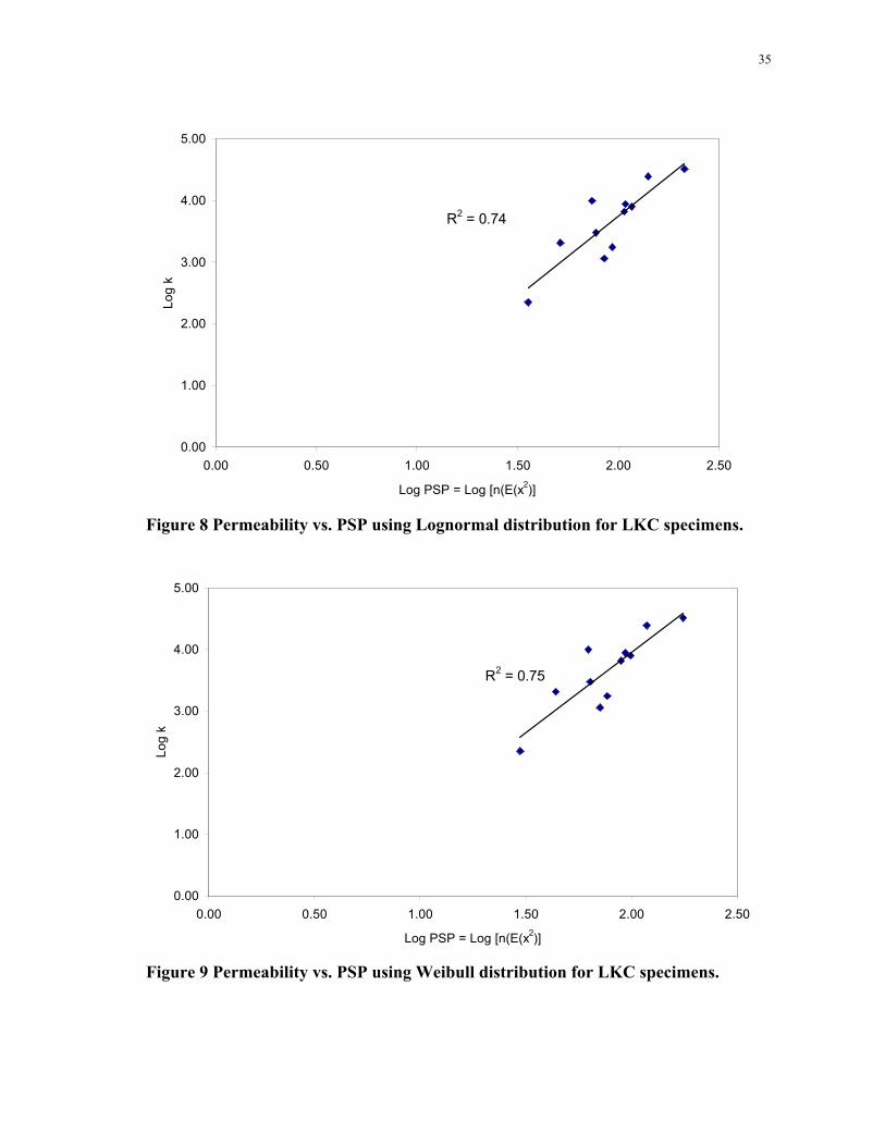
35

R2 = 0.74

0.00

1.00

2.00

3.00

4.00

5.00

0.00 0.50 1.00 1.50 2.00 2.50

Log PSP = Log [n(E(x2)]

Log

k

Figure 8 Permeability vs. PSP using Lognormal distribution for LKC specimens.

R2 = 0.75

0.00

1.00

2.00

3.00

4.00

5.00

0.00 0.50 1.00 1.50 2.00 2.50


Log

k

Figure 9 Permeability vs. PSP using Weibull distribution for LKC specimens.

36

R2 = 0.48

0.00

1.00

2.00

3.00

4.00

5.00

0.00 0.50 1.00 1.50 2.00


Log

k

Figure 10 Permeability vs. PSP using Lognormal distribution for field specimens.

R2 = 0.22

0.00

1.00

2.00

3.00

4.00

5.00

0.00 0.20 0.40 0.60 0.80 1.00 1.20 1.40 1.60 1.80 2.00


Log

k

Figure 11 Permeability vs. PSP using Weibull distribution for field specimens.

37

The correlation coefficients from the regression analysis between the

permeability and the pore size parameter in Logarithmic scale are fairly good for the

LKC specimens (74% and 75% for lognormal and Weibull distributions, respectively).

However, the results are not compelling for the field cores (48% and 22% for Lognormal

and Weibull distributions respectively).

Tables 9 and 10 include the summarized data for the two distributions when

analyzing LKC specimens while Tables 11 and 12 include the same data for the field

specimens.

TABLE 9 PSP calculation for Lognormal distribution and laboratory specimens Measured Distribution Parameters E(x2) Air voids PSP Log (PSP)

Permeability (k) location scale10-5 cm/s µ σ

GV-12.5-76 223 0.150 0.745 0.17 11.84 3.9 9.2 35.7 1.6 2.35GV-12.5-79 2049 0.105 0.762 0.17 12.73 3.8 13.7 51.5 1.7 3.31GV-12.5-81 6553 0.451 0.779 0.17 13.33 7.3 14.7 107.2 2.0 3.82GV-12.5-84 9850 0.156 0.777 0.17 12.64 4.3 17.4 74.2 1.9 3.99LS-12.5-79 2984 0.331 0.772 0.17 13.99 5.9 13.1 77.4 1.9 3.47LS-12.5-81 1137 0.451 0.779 0.17 13.33 7.3 11.7 85.3 1.9 3.06LS-12.5-90 24525 0.433 0.792 0.17 14.67 7.5 18.8 140.7 2.1 4.39LS-12.5-83 7949 0.477 0.775 0.17 13.11 7.6 15.4 116.6 2.1 3.90LS-25.0-79 1746 0.356 0.787 0.17 15.91 6.6 14.3 93.5 2.0 3.24LS-25.0-84 8716 0.425 0.783 0.17 13.32 7.1 15.4 108.5 2.0 3.94LS-25.0-91 32350 0.511 0.854 0.17 20.70 10.7 20.0 213.7 2.3 4.51

Calculated Log kn[E(x2)]

Log n[E(x2)]

x min x max ∫x2f(x)dx

Diameters

n (%)Label

TABLE 10 PSP calculation for Weibull distribution and laboratory specimens Measured Distribution Parameters E(x2) Air voids PSP Log (PSP)

Permeability (k) scale shape10-5 cm/s α β


Label Calculated Log k

Diameters

x min x max ∫x2f(x)dx n (%) n[E(x2)]Log

n[E(x2)]

38

TABLE 11 PSP calculation for Lognormal distribution and field specimens Measured Distribution Parameters E(x2) Air voids PSP Log (PSP)


MS1 - 1 697 0.267 0.785 0.16 16.62 5.6 13.9 77.4 1.9 2.84MS1 - 4 10 -0.358 0.572 0.32 13.08 0.9 6.6 6.2 0.8 1.00MS1 - 6 37 -0.227 0.609 0.32 9.31 1.3 7.0 9.3 1.0 1.57MS1 - 7 1 -0.393 0.568 0.32 8.61 0.9 4.4 3.8 0.6 0.00MS2 - 7 49 -0.024 0.631 0.16 15.44 2.1 9.5 20.1 1.3 1.69MS2 - 9 76 0.135 0.672 0.17 7.26 3.0 7.1 21.1 1.3 1.88MS2 - 11 119 -0.065 0.969 0.16 13.35 4.5 6.9 31.3 1.5 2.08MS4 - 11 54 -0.049 0.854 0.32 6.48 2.7 8.2 22.5 1.4 1.73MS4 - 7 120 0.010 0.883 0.32 8.31 3.5 8.8 31.2 1.5 2.08MS4 - 14 291 -0.072 0.928 0.16 12.97 4.1 9.0 36.5 1.6 2.46MS5 - 1 3333 -0.022 0.782 0.22 16.51 3.2 7.4 23.5 1.4 3.52MS5 - 3 30 0.113 0.806 0.22 16.88 4.4 5.4 23.8 1.4 1.48MS5 - 4 348 0.031 0.810 0.22 12.45 3.7 8.5 31.2 1.5 2.54MS5 - 11 4960 0.261 0.736 0.22 13.91 4.8 10.6 50.7 1.7 3.70MS5 - 12 244 0.362 0.702 0.22 14.66 5.4 7.2 38.7 1.6 2.39MS6 - 6 269 0.036 0.750 0.22 9.69 3.1 8.7 26.8 1.4 2.43MS6 - 7 1386 -0.343 0.568 0.22 9.38 1.0 11.0 10.6 1.0 3.14MS6 - 8 656 -0.314 0.615 0.22 12.43 1.1 9.6 10.9 1.0 2.82MS6 - 13 1 -0.131 0.697 0.22 10.21 2.0 6.0 12.0 1.1 0.00MS6 - 14 178 -0.515 0.899 0.22 10.05 1.6 7.5 12.2 1.1 2.25MS7 - 6 28 -0.084 0.696 0.32 7.74 2.1 7.2 15.3 1.2 1.45MS7 - 9 527 -0.092 0.892 0.32 11.74 3.5 10.6 37.2 1.6 2.72MS8 - 10 13477 0.130 0.716 0.21 11.75 3.5 10.6 37.0 1.6 4.13MS8 - 11 16307 0.318 0.745 0.21 11.25 5.2 9.6 50.0 1.7 4.21MS8 - 12 1619 0.195 0.717 0.21 10.42 3.9 7.6 29.5 1.5 3.21MS8 - 13 17789 0.276 0.730 0.21 11.78 4.7 12.6 59.6 1.8 4.25

LabelDiameters

Calculated Log kx min x max ∫x2f(x)dx n (%) n[E(x2)]

Log n[E(x2)]

TABLE 12 PSP calculation for Weibull distribution and field specimens Measured E(x2) Air voids PSP Log (PSP)

Permeability (k) scale shape10-5 cm/s α β

MS1 - 1 697 1.908 1.411 0.16 16.62 4.6 13.9 63.5 1.8 2.84MS1 - 4 10 0.937 1.655 0.32 13.08 1.0 6.6 6.4 0.8 1.00MS1 - 6 37 1.035 1.589 0.32 9.31 1.2 7.0 8.5 0.9 1.57MS1 - 7 1 0.906 1.645 0.32 8.61 0.9 4.4 4.0 0.6 0.00MS2 - 7 49 1.963 1.479 0.16 15.44 4.6 9.5 44.1 1.6 1.69MS2 - 9 76 1.716 1.562 0.17 7.26 3.4 7.1 24.1 1.4 1.88MS2 - 11 119 1.874 1.493 0.16 13.35 4.2 6.9 29.0 1.5 2.08MS4 - 11 54 1.335 1.680 0.32 6.48 1.9 8.2 16.0 1.2 1.73MS4 - 7 120 1.367 1.661 0.32 8.31 2.1 8.8 18.1 1.3 2.08MS4 - 14 291 1.577 1.619 0.16 12.97 3.0 9.0 27.0 1.4 2.46MS5 - 1 3333 1.516 1.102 0.22 16.51 3.9 7.4 28.9 1.5 3.52MS5 - 3 30 1.556 1.233 0.22 16.88 3.5 5.4 19.0 1.3 1.48MS5 - 4 348 1.447 1.287 0.22 12.45 2.9 8.5 24.6 1.4 2.54MS5 - 11 4960 1.477 1.141 0.22 13.91 3.5 10.6 37.2 1.6 3.70MS5 - 12 244 1.443 1.317 0.22 14.66 2.8 7.2 20.2 1.3 2.39MS6 - 6 269 1.641 1.453 0.22 9.69 3.3 8.7 28.6 1.5 2.43MS6 - 7 1386 1.523 1.402 0.22 9.38 2.9 11.0 32.2 1.5 3.14MS6 - 8 656 1.842 1.549 0.22 12.43 3.9 9.6 37.8 1.6 2.82MS6 - 13 1 2.003 1.655 0.22 10.21 4.4 6.0 26.6 1.4 0.00MS6 - 14 178 1.483 1.522 0.22 10.05 2.6 7.5 19.4 1.3 2.25MS7 - 6 28 1.003 1.539 0.32 7.74 1.2 7.2 8.4 0.9 1.45MS7 - 9 527 1.255 1.393 0.32 11.74 2.0 10.6 21.2 1.3 2.72MS8 - 10 13477 0.947 1.107 0.21 11.75 1.5 10.6 16.0 1.2 4.13MS8 - 11 16307 0.940 1.082 0.21 11.25 1.5 9.6 14.8 1.2 4.21MS8 - 12 1619 1.296 1.509 0.21 10.42 2.0 7.6 15.1 1.2 3.21MS8 - 13 17789 1.423 1.178 0.21 11.78 3.1 12.6 39.3 1.6 4.25

Distribution ParametersLabel

Diameters Calculated Log kn[E(x2)] Log n[E(x2)]x min x max ∫x2f(x)dx n (%)

39

Al-Omari et al. (1) reported that for these mixtures, the air void connectivity

varies considerably in the field cores compared with the LKC specimens. Figures 12

and 13 are examples of flow paths that were captured on the LKC specimens and field

cores. In addition, Masad et al. (15) showed that a number of field cores do not have

connected flow paths across the full depth and, that the measured permeability was in

some cases only due to the flow in a small part of the core near the surface. Therefore,

it was decided to study the relationship between permeability and air void distribution

only in the connected flow paths that contribute to permeability. Also, only cores that

have connected flow paths were used in the analysis. A macro was developed to

identify and analyze the connected voids while eliminating the stagnant regions and

isolated air voids, etc.

Figure 12 Flow paths in a LKC specimen.

40

Figure 13 Flow paths in a field specimen.

The regression analysis results for Lognormal and Weibull distributions for both

sets of specimens when taking into consideration only the connected flow paths are

shown in Figures 14 to 17. The respective data is included in Tables 13 to 16.

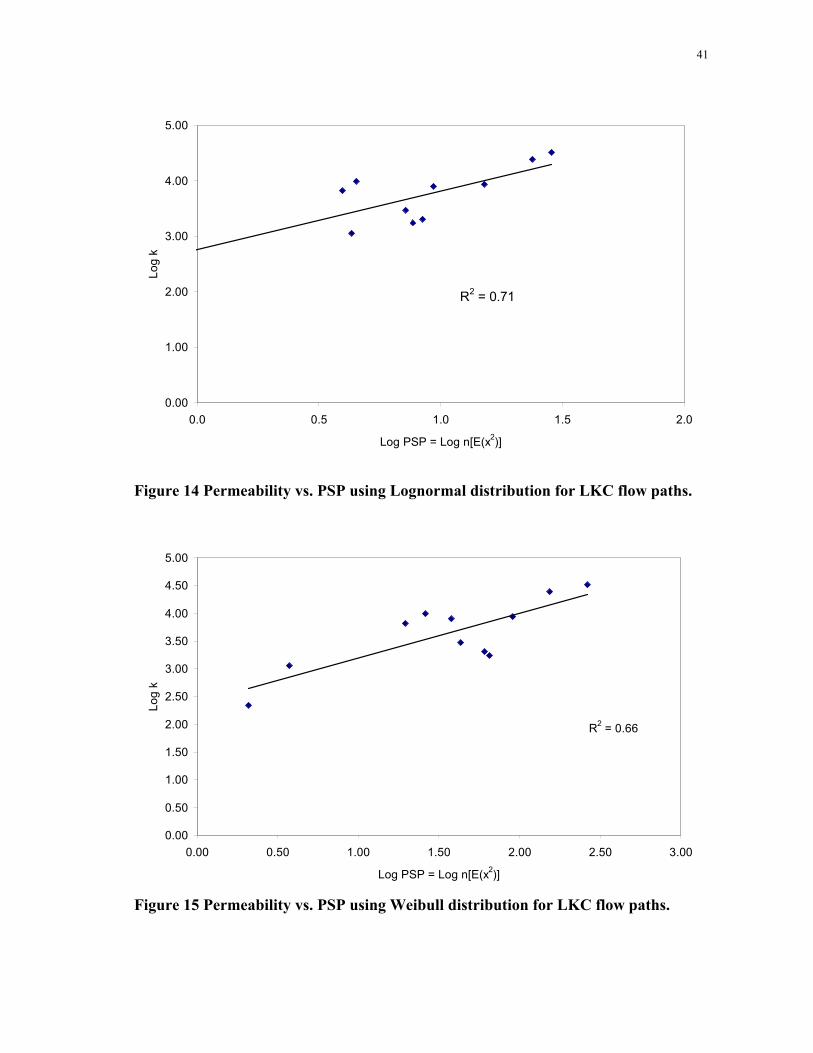
41

R2 = 0.71

0.00

1.00

2.00

3.00

4.00

5.00

0.0 0.5 1.0 1.5 2.0

Log PSP = Log n[E(x2)]

Log

k

Figure 14 Permeability vs. PSP using Lognormal distribution for LKC flow paths.

R2 = 0.66

0.00

0.50

1.00

1.50

2.00

2.50

3.00

3.50

4.00

4.50

5.00

0.00 0.50 1.00 1.50 2.00 2.50 3.00

Log PSP = Log n[E(x2)]

Log

k

Figure 15 Permeability vs. PSP using Weibull distribution for LKC flow paths.

42

R2 = 0.88

0.00

1.00

2.00

3.00

4.00

5.00

0.0 0.5 1.0 1.5 2.0


Log

k

Figure 16 Permeability vs. PSP using Lognormal distribution for field flow paths.

R2 = 0.85

0.00

1.00

2.00

3.00

4.00

5.00

0.0 0.5 1.0 1.5 2.0Log PSP = Log [n(E(d2)]

Log

k

Figure 17 Permeability vs. PSP using Weibull distribution for field flow paths.

43

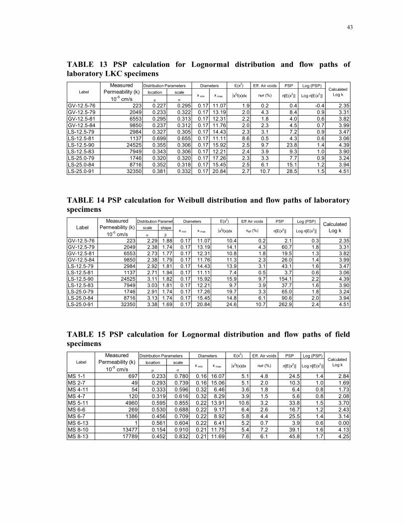
TABLE 13 PSP calculation for Lognormal distribution and flow paths of laboratory LKC specimens

Measured Distribution Parameters E(x2) Eff. Air voids PSP Log (PSP)Permeability (k) location scale

10-5 cm/s µ σ

GV-12.5-76 223 0.227 0.295 0.17 11.07 1.9 0.2 0.4 -0.4 2.35GV-12.5-79 2049 0.233 0.322 0.17 13.19 2.0 4.3 8.4 0.9 3.31GV-12.5-81 6553 0.295 0.313 0.17 12.31 2.2 1.8 4.0 0.6 3.82GV-12.5-84 9850 0.237 0.312 0.17 11.76 2.0 2.3 4.5 0.7 3.99LS-12.5-79 2984 0.327 0.305 0.17 14.43 2.3 3.1 7.2 0.9 3.47LS-12.5-81 1137 0.699 0.655 0.17 11.11 8.6 0.5 4.3 0.6 3.06LS-12.5-90 24525 0.355 0.306 0.17 15.92 2.5 9.7 23.8 1.4 4.39LS-12.5-83 7949 0.343 0.306 0.17 12.21 2.4 3.9 9.3 1.0 3.90LS-25.0-79 1746 0.320 0.320 0.17 17.26 2.3 3.3 7.7 0.9 3.24LS-25.0-84 8716 0.352 0.318 0.17 15.45 2.5 6.1 15.1 1.2 3.94LS-25.0-91 32350 0.381 0.332 0.17 20.84 2.7 10.7 28.5 1.5 4.51

LabelDiameters

Calculated Log kx min x max ∫x2f(x)dx neff (%) n[E(x2)] Log n[E(x2)]

TABLE 14 PSP calculation for Weibull distribution and flow paths of laboratory specimens

Measured Distribution Paramete E(x2) Eff Air voids PSP Log (PSP)Permeability (k) scale shape

10-5 cm/s α β


Label Calculated Log k

Diameters

x min x max ∫x2f(x)dx neff (%) n[E(x2)] Log n[E(x2)]

TABLE 15 PSP calculation for Lognormal distribution and flow paths of field specimens

Measured Distribution Parameters E(x2) Eff. Air voids PSP Log (PSP)Permeability (k) location scale

10-5 cm/s µ σ

MS 1-1 697 0.233 0.780 0.16 16.07 5.1 4.8 24.5 1.4 2.84MS 2-7 49 0.293 0.739 0.16 15.06 5.1 2.0 10.3 1.0 1.69MS 4-11 54 0.333 0.596 0.32 6.46 3.6 1.8 6.4 0.8 1.73MS 4-7 120 0.319 0.616 0.32 8.29 3.9 1.5 5.6 0.8 2.08MS 5-11 4960 0.595 0.855 0.22 13.91 10.6 3.2 33.8 1.5 3.70MS 6-6 269 0.530 0.688 0.22 9.17 6.4 2.6 16.7 1.2 2.43MS 6-7 1386 0.456 0.709 0.22 8.92 5.8 4.4 25.5 1.4 3.14MS 6-13 1 0.561 0.604 0.22 6.41 5.2 0.7 3.9 0.6 0.00MS 8-10 13477 0.154 0.910 0.21 11.75 5.4 7.2 39.1 1.6 4.13MS 8-13 17789 0.452 0.832 0.21 11.69 7.6 6.1 45.8 1.7 4.25

LabelDiameters

Calculated Log kx min x max ∫x2f(x)dx neff (%) n[E(x2)] Log n[E(x2)]

44

TABLE 16 PSP calculation for Weibull distribution and flow paths of field specimens

Measured Distribution Parameters E(x2) Eff. Porosity PSP Log (PSP)Permeability (k) scale shape

10-5 cm/s α β

MS 1-1 697 1.787 1.663 0.16 16.07 3.5 4.8 16.9 1.2 2.84MS 2-7 49 1.867 1.743 0.16 15.06 3.7 2.0 7.5 0.9 1.69MS 4-11 54 1.819 2.176 0.32 6.46 3.2 1.8 5.7 0.8 1.73MS 4-7 120 1.807 2.115 0.32 8.29 3.2 1.5 4.6 0.7 2.08MS 5-11 4960 2.663 1.500 0.22 13.91 8.4 3.2 26.8 1.4 3.70MS 6-6 269 2.320 1.852 0.22 9.17 5.6 2.6 14.5 1.2 2.43MS 6-7 1386 2.172 1.804 0.22 8.92 5.0 4.4 21.8 1.3 3.14MS 6-13 1 2.313 2.071 0.22 6.41 5.3 0.7 3.9 0.6 0.00MS 8-10 13477 1.742 1.438 0.21 11.75 3.7 7.2 27.1 1.4 4.13MS 8-13 17789 2.279 1.552 0.21 11.69 6.0 6.1 36.4 1.6 4.25

LabelDiameters

Calculated Log kx min x max ∫x2f(x)dx neff (%) n[E(x2)]

Log n[E(x2)]

Figures 14-17 show that the correlation coefficient R2 notably increased when

analyzing solely the flow paths for the field samples for which the R2 increased from

48% to 88% and from 22% to 85% using Lognormal and Weibull distributions

respectively. On the other hand, the R2 values were slightly decreased (74% to 71% and

75% to 66%) for the LKC specimens.

The analysis was performed for the SGC granite and limestone specimens by

considering all voids regardless of their connectivity. The relationship between the pore

size parameter and the permeability of these cores was done using two different

permeability measurement procedures. The constant head method gave higher

permeability values than the falling head method that was used in Florida. The

saturation procedure that was followed in the Florida method was based on AASHTO T-

283. Following this procedure, a target saturation of 65 to 80 percent has to be achieved

by allowing vacuum saturation during 15 minutes. Next, the specimen is placed in water

bath without vacuum for an additional 15 min. If the minimum saturation is not

achieved, another cycle is done until the target is attained. Finally, the core is placed in a

45

water bath at 60C for 24 hours and is allowed to drain 36 hours; then the specimen is

located on a dehumidify chamber for 48 hours prior to the permeability measurement.

On the other hand, for measuring the permeability with the constant head method, the

cores were saturated for 24 hours and then they were vacuum saturated during 10

minutes with a pressure of 28in Hg. The percentage of saturation varied from core to

core as shown in Table 17 as well as the permeabilities measured with the two methods.

The results for the relationships between the constant head and falling head

permeabilities and the pore size parameter are shown in Figures 19 to 22, and the

corresponding data is summarized in Tables 18 to 21. This was done taking into account

all the air voids.

TABLE 17 Degree of saturation of SGC specimens

GA-C1 89.8 67.50 228.13GA-C2 78.3 59.00 271.18GA-C3 76.5 56.00 93.00GA-F1 97.4 25.33 76.66GA-F2 78.1 9.33 74.35GA-F3 74.7 34.25 172.91WR-C1 82.4 72.37 301.98WR-C2 85.2 64.24 367.49WR-C3 97.7 29.39 379.60WR-F1 98.4 69.63 226.41WR-F2 92.2 17.81 177.69

WR-F3/C4 98.4 9.68 298.12

Falling head permeability (10-5 cm/s)

Constant head permeability (10-5 cm/s)

Degree of Saturation, S%Specimen

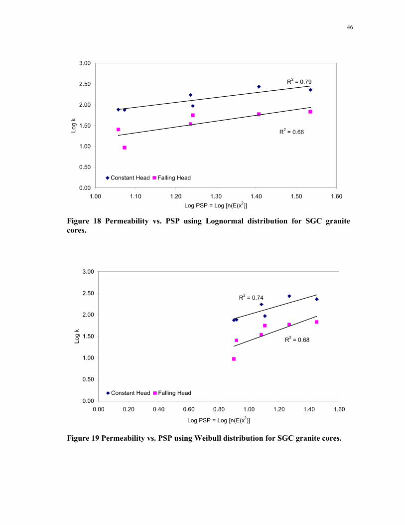
46

R2 = 0.79

R2 = 0.66

0.00

0.50

1.00

1.50

2.00

2.50

3.00

1.00 1.10 1.20 1.30 1.40 1.50 1.60Log PSP = Log [n(E(x2)]

Log

k

Constant Head Falling Head

Figure 18 Permeability vs. PSP using Lognormal distribution for SGC granite cores.

R2 = 0.68

R2 = 0.74

0.00

0.50

1.00

1.50

2.00

2.50

3.00

0.00 0.20 0.40 0.60 0.80 1.00 1.20 1.40 1.60


Log

k


Figure 19 Permeability vs. PSP using Weibull distribution for SGC granite cores.

47

R2 = 0.68

R2 = 0.88

0.00

0.50

1.00

1.50

2.00

2.50

3.00

0.00 0.20 0.40 0.60 0.80 1.00 1.20 1.40 1.60Log PSP = Log [n(E(x2)]

Log

k


Figure 20 Permeability vs. PSP using Lognormal distribution for SGC limestone cores.

R2 = 0.66

R2 = 0.89

0.00

0.50

1.00

1.50

2.00

2.50

3.00

0.00 0.20 0.40 0.60 0.80 1.00 1.20 1.40 1.60


Log

k


Figure 21 Permeability vs. PSP using Weibull distribution for SGC limestone cores.

48

TABLE 18 PSP calculation for Lognormal distribution and limestone specimens Constant Head Distribution Parameters E(x2) Eff Air voids PSP Log (PSP)


WR-C1 301.98 -0.001 0.703 0.22 8.40 2.5 6.6 16.8 1.2 2.48WR-C2 367.49 -0.046 0.730 0.22 11.21 2.6 6.6 16.9 1.2 2.57WR-C3 379.60 -0.185 0.718 0.22 10.98 1.9 6.9 13.3 1.1 2.58WR-F1 226.41 -0.324 0.691 0.22 8.67 1.3 7.0 9.3 1.0 2.35WR-F2 177.69 -0.390 0.739 0.22 11.09 1.4 6.9 9.4 1.0 2.25

WR-F3/C4 298.12 -0.184 0.725 0.22 11.08 2.0 7.3 14.4 1.2 2.47

CoreDiameters

Calculated Log kx min x max ∫x2f(x)dx neff (%) n[E(x2)]

Log n[E(x2)]

TABLE 19 PSP calculation for Weibull distribution and limestone specimens Constant Head Distribution Parameters E(x2) Eff Air voids PSP Log (PSP)Permeability (k) scale shape

10-5 cm/s α β

WR-C1 301.98 1.360 1.872 0.22 8.40 1.9 6.6 12.6 1.1 2.48WR-C2 367.49 1.312 1.816 0.22 11.21 1.8 6.6 11.9 1.1 2.57WR-C3 379.60 1.133 1.864 0.22 10.98 1.3 6.9 9.2 1.0 2.58WR-F1 226.41 0.972 1.949 0.22 8.67 1.0 7.0 6.7 0.8 2.35WR-F2 177.69 0.925 1.854 0.22 11.09 0.9 6.9 6.1 0.8 2.25

WR-F3/C4 298.12 1.137 1.845 0.22 11.08 1.3 7.3 9.8 1.0 2.47

x min x max neff (%) ∫x2f(x)dx n[E(x2)] Log n[E(x2)]Core

DiametersCalculated

Log k

TABLE 20 PSP calculation for Lognormal distribution and granite specimens Constant Head Distribution Parameters E(x2) Eff Air voids PSP Log (PSP) Permeability (k) location scale

10-5 cm/s µ σ

GA-C1 228.13 0.301 0.701 0.22 8.40 4.319 7.9 34.29 1.54 2.36GA-C2 271.18 0.147 0.728 0.22 11.21 3.684 6.9 25.53 1.41 2.43GA-C3 93.00 -0.021 0.696 0.22 10.98 2.478 7.1 17.50 1.24 1.97GA-F1 76.66 -0.266 0.683 0.22 8.67 1.472 7.8 11.41 1.06 1.88GA-F2 74.35 -0.295 0.732 0.22 11.09 1.594 7.4 11.83 1.07 1.87GA-F3 172.91 -0.093 0.723 0.22 11.08 2.309 7.5 17.27 1.24 2.24

Calculated Log kx min x max

CoreDiameters

Log n[E(x2)]

neff (%) ∫x2f(x)dx n[E(x2)]

TABLE 21 PSP calculation for Weibull distribution and granite specimens Constant Head Distribution Parameters E(x2) Eff Air voids PSP Log (PSP)Permeability (k) scale shape

10-5 cm/s α β

GA-C1 228.13 1.849 1.840 0.22 8.40 3.6 7.9 28.2 1.5 2.36GA-C2 271.18 1.596 1.799 0.22 11.21 2.7 6.9 18.6 1.3 2.43GA-C3 93.00 1.329 1.892 0.22 10.98 1.8 7.1 12.8 1.1 1.97GA-F1 76.66 1.029 1.957 0.22 8.67 1.1 7.8 8.3 0.9 1.88GA-F2 74.35 1.017 1.851 0.22 11.09 1.1 7.4 7.9 0.9 1.87GA-F3 172.91 1.247 1.838 0.22 11.08 1.6 7.5 12.1 1.1 2.24

x min x maxCore

DiametersCalculated

Log kneff (%) ∫x2f(x)dx n[E(x2)] Log n[E(x2)]

49

According to the R2 values, the distribution that most closely represents the

relationship of permeability and air void size distribution is Lognormal. The derived

equations for permeability obtained from the regression analysis, and their

corresponding correlation coefficients are found in Table 22. These equations have the

form of Equation 19. The transformations of these equations, to the form expressed in

Equation 20 are included in Table 23. It was considered that the permeability

measurements of the constant head method were more reliable, because this method is

best suited for samples that contain no more than 10% particles passing the 75-µm (No.

200) sieve (22). The gradations of these specimens are included in appendix A.

TABLE 22 Regression equations for permeability Specimen Lognormal Weibull

LKC Log k=2.5834 Log (PSP)-1.4228 Log k=2.6192 Log (PSP)-1.2912

(All voids) R2 = 0.74 R2 = 0.75LKC Log k=1.0489 Log (PSP)+2.7664 Log k=0.805 Log (PSP)+2.3931

(Flow paths) R2 = 0.71 R2 = 0.66MSD Log k=2.5002 Log (PSP)-1.0183 Log k=1.9664 Log (PSP)-0.2168

(All voids) R2 = 0.48 R2 = 0.22MSD Log k=3.1997 Log (PSP)-1.2298 Log k=3.4067 Log (PSP)-1.1618

(Flow paths) R2 = 0.88 R2 = 0.85SGC Granite Log k=1.1813 Log (PSP)+0.6386 Log k=1.0137 Log (PSP)+0.9891(All voids), constant head method R2 = 0.78 R2 = 0.74

SGC Limestone Log k=0.8901Log (PSP)+1.4598 Log k=0.8074Log (PSP)+1.6779(All voids), constant head method R2 = 0.68 R2 = 0.66

50

TABLE 23 Permeability equations with Lognormal distribution

Specimen PermeabilityLKC (All voids)LKC (Flow paths)Field Cores(All voids)Field Cores(Flow paths)SGC Granite (All voids), constant head methodSGC Limestone(All voids), constant head method

k=4.35PSP1.1813

k=28.83 PSP0.8901

k=0.04 PSP2.5834

k=584 PSP1.0489

k=0.10PSP2.5002

k=0.06 PSP3.1997

Summary

Several studies have demonstrated that HMA permeability is highly related to percent

air voids. However, this relationship can not be generalized because the air void size

distribution has significant influence on HMA permeability. X-ray CT made it possible

to capture and analyze air void distribution in HMA.

Three sets of specimens were analyzed: LKC laboratory specimens, field cores,

and SGC laboratory specimens. A relationship is developed between permeability and

parameters that represent air void distribution. The probability density functions that

best fit the size distribution were determined. This was done by using probability plots

and relying on the Pearson correlation coefficient to judge the accuracy of the fitting.

The Lognormal and the Weibull distribution were found as the most suitable probability

distributions to fit the data, having coefficients of determination between 68% and 88%.

51

The capillary model established by Garcia-Bengochea was used to relate

permeability to the pore size parameter (PSP) that was determined using probabilistic

approach for the analysis of air voids. This PSP was calculated using the assumption

that the probability of having two air voids on adjacent sections connected is totally

correlated, since the distance between sections is very small.

The results obtained from the regression analyses were very good for the

laboratory LKC and SGC specimens. However, this was not the case for the field cores

when all voids were considered. An alternative approach was followed where only the

connected voids in field cores were analyzed. Consequently, there was a significant

improvement between the permeability and air void size distribution in the field cores.

52

CHAPTER IV

THE RELATIONSHIP BETWEEN AIR VOID DISTRIBUTION, MATERIAL

SURFACE PROPERTIES AND MOISTURE DAMAGE

Introduction

The durability of a pavement throughout its design life can be achieved when the

pavement is resistant to weathering, cracking, and traffic abrasion (23). Weathering

consists of the effects provoked by oxidation or hardening of the asphalt, moisture

damage and changes in the aggregate soundness due to freezing and thawing. Moisture

can deteriorate asphalt dramatically by affecting the stiffness and the strength (loss of

cohesion) of the asphalt film, and also by breaking the adhesive bond between

aggregates and asphalt. Loss of adhesion can lead to stripping and raveling whereas

loss of cohesion can lessen the load carrying capacity of the pavement leading to

premature cracking.

This chapter documents the results of studying the relationship between moisture

damage, air void distribution, material surface properties and pore pressure. The

resistance to moisture damage is assessed by measuring the mechanical properties of

HMA specimens before and after moisture conditioning. These mechanical properties

were measured at the University of Florida and were made available to this study by Dr.

Birgisson. The surface energy of the aggregates and asphalt binder were measured in

order to assess the fracture and healing capabilities of the mixes with and without the

presence of moisture.

53

Measurements of HMA Moisture Damage

Zhang et al (24) developed a viscoelastic fracture mechanics-based framework to

describe the fracture properties of HMA. These researchers demonstrated that there are

two fracture thresholds that define the type of damage that can take place in an asphalt

mixture: micro-damage and macro-damage. Micro-damage is not related to crack

initiation or crack growth and is totally healable after a resting period. On the other

hand, macro-damage is associated with crack growth and the damage provoked is

irreversible.

It was found that the dissipated creep strain energy (DCSE) and the fracture

energy (FE) define the two threshold values under cyclic and continuously increasing

loading, respectively. These limits can be determined from the stress-strain response of

a tensile strength test and resilient modulus test using the SuperPaveTM Indirect Tensile

test (24). The DCSE corresponds to the area under the tensile strength/strain curve that

is not recoverable and can be calculated as the total area under the curve (i.e. fracture

energy), minus the area that corresponds to the elastic energy. The elastic energy (EE) is

equal to the area under this curve limited by a line with slope equal to the resilient

modulus, and a vertical line that crosses the x-axis at the strain at failure. A

representation of the elastic energy (EE) and dissipated creep strain energy (DCSE)

components of the fracture energy can be seen in Figure 22, (24). To determine the

elastic energy at fracture the elastic modulus of the mix must be measured. Therefore,

these limits account ultimately for the effects of strength, stiffness, strain to failure, and

the viscoelastic response of the mixture.

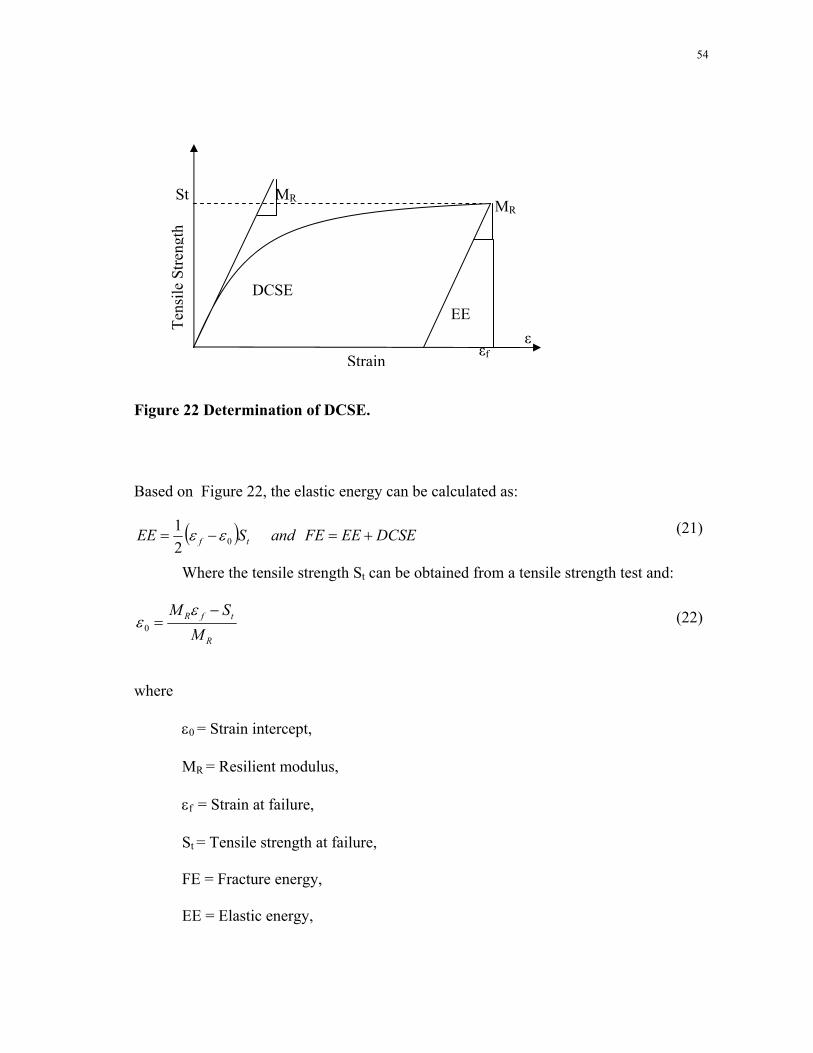
54

( ) DCSEEEFEandSEE tf +=−= 021 εε

R

tfR

MSM −

=ε

ε 0

Figure 22 Determination of DCSE.

Based on Figure 22, the elastic energy can be calculated as:

(21)

Where the tensile strength St can be obtained from a tensile strength test and:

(22)

where

ε0 = Strain intercept,

MR = Resilient modulus,

εf = Strain at failure,

St = Tensile strength at failure,

FE = Fracture energy,

EE = Elastic energy,

Tens

ile S

treng

th

ε

MR

DCSE

St

EE

εf

MR

Strain

55

∫=1.0

0max )10sin()10sin(/ dtttcycleDCSE avg πξπσ

DCSE = Dissipated creep strain energy

Birgisson, et al. (2) found that it was necessary to account for the effects that

moisture damage causes to key mechanical properties. They demonstrated through the

determination of the SuperpaveTM Indirect Tension Test fracture parameters (i.e. creep,

resilient modulus, and tensile strength, tests) on conditioned and unconditioned

mixtures, that the effects of moisture damage on the multiple parameters associated with

the fracture resistance of mixtures could be summarized into one single number. This

number corresponded to the ratio between the number of cycles to failure for

conditioned and unconditioned specimens. The calculation of the number of cycles is

based on the crack growth law (2, 24), which is based on the dissipated creep strain

energy threshold concept as well. This calculation is based on the determination of the

stress distribution near the crack tip, as it evolves through the crack length and the

damage that occurs while DCSE is building up. This accumulation takes place in small

zones of the process zones in front of the crack tip.

The procedure consists of determining the DCSE per cycle and the accumulated

DCSE on each zone due to the number of cycles N to fail the previous zone, and so forth

until a determined crack size is formed. The accumulated DCSE can be calculated using

creep compliance parameters for a specified type of load. For a harversine load that is

applied during 0.1 seconds and 0.9 seconds of rest period, the DCSE per cycle is

calculated as (2, 24):

(23)

56

mtDDtD 10)( +=

)()( tDt aveσε =

11max

)()( −=== maveave mtD

dttD

dtt σσεξ

11

2 )100(201/ −= m

avg mDcycleDCSE σ

Where σavg is the average stress in the zone of interest, and ξmax is the maximum

creep strain rate. The damage rate of an asphalt mixture under constant loading is

considered to correspond to its creep compliance. Under the DCSE threshold, this rate

of damage is controlled by the creep properties of the mix. The creep compliance can be

expressed with a power function of the form (2):

(24)

Where, D(t) is the creep compliance, Do is the glassy compliance of the material, D1 is

the compliance coefficient of time, m is the compliance exponent, and t is the time of

loading.

Also, the strain, and creep compliance are related as (2):

(25)

Therefore the creep strain rate can be formulated by deriving Equation 25 with

respect to time, as follows:

(26)

And by substitution of Equation 26 in Equation 23, the DCSE per cycle for a

100-second SuperPaveTM IDT creep test is calculated as:

(27)

From Equation 27 the number of cycles to fail zone i (Nfi), can be obtained. This

equation is used for the rest of the zones that form the process zone until a crack of the

57

198.2

min DmDCSEa

DCSEDCSE

ER ff

⋅⋅

==

length of the process zone is formed. By doing so, the DCSE that is accumulated along

the crack is calculated. Finally, when the DCSE limit is reached, the crack length that

was originally specified is produced. As a result, the number of loads to propagate a

determined crack length is predicted.

As a consequence, following the fracture mechanics threshold principles, the key

parameters that appear to control cracking performance of HMA are: DCSE, m-value

and D1. The m-value is the parameter that controls the creep strain rate at low

temperatures. A lower m-value is desirable because the lower the rate of accumulation

of DCSE will be, hence the less fast the threshold value will be reached. Besides these

parameters, the tensile stress governs the location and how fast a crack initiates and

propagates depending on the pavement configuration. Therefore, it is reasonable to

account for all these factors when determining the moisture damage of a mix, rather than

solely focusing on one property (2, 17).

Birgisson, Roque, and Page (17) proposed the use of the “Energy Ratio” (ER), as

a parameter to assess the mix resistance to moisture damage. Jajliardo (25) was able to

determine a minimum DCSE for adequate cracking performance and also proposed a

minimum required ER for different traffic levels. This ratio was developed based on

forensic research of 36 field pavement sections of known cracking performance and is a

function of the parameters that were previously mentioned:

(28)

where

58

DCSEf = Dissipated creep strain energy to fracture (KJ/m3),

DCSEmin= Minimum dissipated creep strain energy for adequate cracking

performance (KJ/m3),

D1 and m = parameters obtained from creep test (1/psi),

a = 0.0299 σ-3.1 (6.36-St) + 2.46 x 10-8 ,

σ = tensile stress of asphalt layer (psi),

St = tensile strength (MPa)

The rationale behind the HMA fracture mechanics framework for studying water

damage is to account for different key mixture properties that are affected by moisture.

Hence this framework demonstrates that moisture damage can not be assessed based

only on one property such as the resilient modulus itself.

Relationship between Air Void Size, Pore Pressure Distribution and Moisture

Damage

The air void distribution and pore pressure distribution were studied in order to

determine their relationship to moisture damage. Moisture damage was assessed by the

change in energy ratio (ER) and number of cycles to failure due to moisture

conditioning.

Energy Ratio

As previously explained, the energy ratio can be used to determine the moisture

sensitivity of asphalt mixes that is reflected in their cracking performance. Therefore,

the energy ratio (ER) was calculated using Equation 28 with an average tensile stress of

59

the asphalt layer equal to 120 psi. This tensile stress is a common value obtained for

Florida pavements which have a thin layer of HMA and a stiff base. Tables 24 and 25

show the calculated ratios.

TABLE 24 Mechanical data for conditioned and unconditioned granite SGC specimens, (17)

Label m-value D1DCSE (kJ/m3)

ER a

GA-C1 (C) 0.66 1.54E-06 2.75 0.50 8.08E-08GA-C2 (C) 0.65 1.03E-06 2.60 0.67 7.31E-08GA-C3 (C) 0.6 9.10E-07 1.93 0.62 7.38E-08GA-C1 (U) 0.62 1.74E-06 5.80 1.07 7.73E-08GA-C2 (U) 0.59 1.06E-06 4.77 1.57 7.13E-08GA-C3 (U) 0.57 8.70E-07 3.60 1.55 7.14E-08GA-F1 (C) 0.63 1.52E-06 2.62 0.53 7.57E-08GA-F2 (C) 0.56 1.24E-06 2.11 0.70 7.18E-08GA-F3 (C) 0.6 1.44E-06 1.91 0.42 7.40E-08GA-F1 (U) 0.57 1.30E-06 3.48 1.06 7.21E-08GA-F2 (U) 0.48 1.58E-06 3.29 1.22 6.58E-08GA-F3 (U) 0.56 8.97E-07 2.57 1.16 6.98E-08

60

TABLE 25 Mechanical data for conditioned and unconditioned limestone SGC specimens, (2)

Label m-value D1DCSE (kJ/m3)

ER a

WR-C1 (C) 0.44 1.50E-06 2.07 1.25 7.9E-08WR-C2 (C) 0.59 1.03E-06 1.79 0.65 7.9E-08WR-C3 (C) 0.54 5.75E-07 1.47 1.19 7.5E-08WR-C1 (U) 0.54 9.51E-07 2.35 1.18 7.6E-08WR-C2 (U) 0.67 7.65E-07 1.81 0.62 7.9E-08WR-C3 (U) 0.43 7.84E-07 1.83 2.09 7.2E-08WR-F1 (C) 0.73 9.13E-07 4.00 0.85 7.6E-08WR-F2 (C) 0.67 9.49E-07 2.88 0.77 7.6E-08WR-F3 (C) 0.69 4.08E-07 1.73 0.97 7.4E-08WR-F1 (U) 0.60 1.16E-06 4.00 1.20 7.6E-08WR-F2 (U) 0.54 1.01E-06 2.90 1.31 7.3E-08WR-F3/C4 (U) 0.53 7.08E-07 2.50 1.65 7.2E-08

Figures 23 and 24 show the differences between the ER of the conditioned and

unconditioned SGC specimens. As pointed out by Birgisson et al (2), it can be inferred

from these graphs that the change in the ER from a wet to a dry stage is more dramatic

for the granite than for the limestone. Even though the ER of gradation C2 for the

granite was better than for the limestone in a dried condition, it turned to be worse when

conditioned because it decreases dramatically while the ER of the limestone remains

about the same.

According to the ER ratio of the conditioned ER to the unconditioned ER

overall, the granite is more susceptible to moisture damage than the limestone is, as it

can be seen in Figure 25.

61

0.00

0.50

1.00

1.50

2.00

2.50

GA-C1 GA-C2 GA-C3 GA-F1 GA-F2 GA-F3

Ene

rgy

Rat

io (

ER

)Conditioned Unconditioned

Figure 23 Conditioned vs. unconditioned energy ratios (ER) for granite SGC mixes (17).

0.00

0.50

1.00

1.50

2.00

2.50

WR-C1 WR-C2 WR-C3 WR-F1 WR-F2 WR-F3/C4

Ene

rgy

Rat

io (E

R)

Conditioned Unconditioned

Figure 24 Conditioned vs. unconditioned energy ratios (ER) for limestone SGC mixes (2).

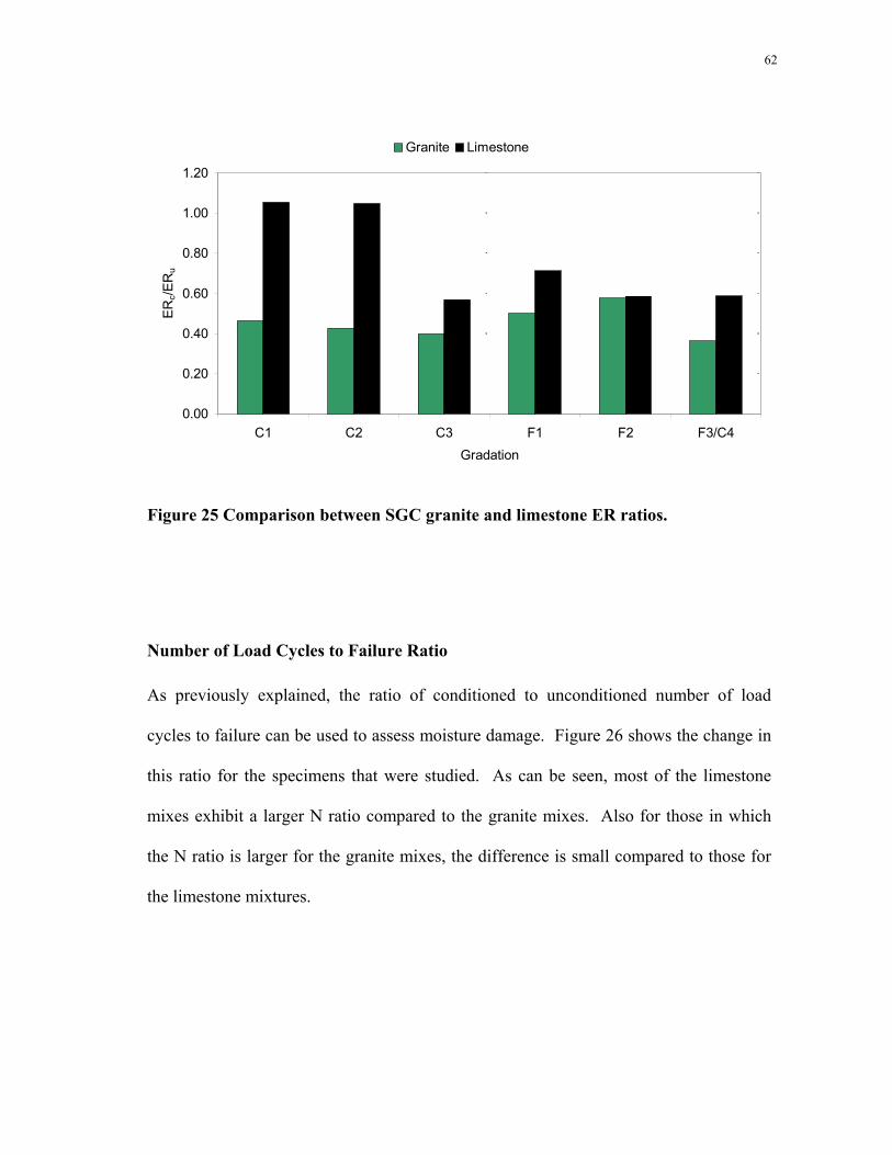
62

0.00

0.20

0.40

0.60

0.80

1.00

1.20

C1 C2 C3 F1 F2 F3/C4Gradation

ERc/E

Ru

Granite Limestone

Figure 25 Comparison between SGC granite and limestone ER ratios.

Number of Load Cycles to Failure Ratio

As previously explained, the ratio of conditioned to unconditioned number of load

cycles to failure can be used to assess moisture damage. Figure 26 shows the change in

this ratio for the specimens that were studied. As can be seen, most of the limestone

mixes exhibit a larger N ratio compared to the granite mixes. Also for those in which

the N ratio is larger for the granite mixes, the difference is small compared to those for

the limestone mixtures.

63

0.00

0.20

0.40

0.60

0.80

1.00

1.20

C1 C2 C3 F1 F2 F3/C4Gradation

Nc/N

u

Granite Limestone

Figure 26 Comparison between SGC granite and limestone N ratios (2).

Air Void Analysis

The air void distribution for the granite and limestone specimens were determined from

square images that were extracted from the original circular section which had a

diameter of 100 mm. These square sections were obtained by using a macro that cuts

most of the area of the specimen that could be covered. The resulting images had a side

of 70.3 mm but its resolution was kept as the original image so that better results could

be obtained.

Even though the mix design of the mixtures was the same, the air void

distribution shows that there is a significant difference among the corresponding

specimens when analyzing the quartiles. The differences in the quartiles of each pair of

F3 & F3/C4

64

analogous gradations of the SGC granite and limestone specimens (Granite air void Size

– Limestone Air Void Size) are shown in Figure 27. The difference is always positive

indicating larger voids in the granite mixes. It can be inferred from this figure that even

though the corresponding coarse and fine gradations are approximately the same, their

air void distribution is not identical. This is especially true for the coarse gradations.

0.00

0.20

0.40

0.60

0.80

1.00

C1 C2 C3 F1 F2 C4Gradation

Diff

eren

ce in

air

void

dia

met

er (m

m)

(gra

nite

-lim

esto

ne)

1st Quartile 2nd Quartile 3rd Quartile

Figure 27 Air void quartile difference between granite and limestone gradations.

Figure 28 shows how the three dimensional air voids differ for the SGC granite

and limestone specimen that have similar gradations (i.e. GA-C1 and WR-C1).

Consequently an additional analysis was done using the AIMS software to study the

angularity of particles that passed sieve #4 and that were retained in sieve #8. This

F3 & F3/C4

65

software analyses the angularity on black and white images of aggregate particles using

two methods: the gradient method and the radius method (26). The results from the

gradient method were considered in this study due to the fact that it captures a wider

range of measurements in comparison to the radius method. The principle behind the

gradient method consists on measuring the gradient vector direction for adjacent points

on the outline of the particles. The gradient values for all the corners is determined and

accumulated in order to calculate the angularity gradient for the particle. More details

about this method are given by Chandan et al (27).

Three measurements were done for each aggregate. The average results are

included in Table 26. It can be inferred from these measurements that the limestone has

less rounded particles than the granite does. Hence, the interlocking of the limestone

particles is greater, leading to form air voids that are smaller than the voids that are

formed with the granite. Angularity could be therefore, a good explanation for having

larger air voids for all the SGC granite specimens than for the SGC limestone specimens

even though both were prepared with the same gradation.

TABLE 26 Aggregate angularity measurements Particles Granite Limestone

Mean 3493.38 3736.82% Rounded Particles 19.63 11.22% Sub-Rounded Particles 47.61 48.81% Sub-Angular Particles 20.40 26.48% Angular Particles 12.37 13.48

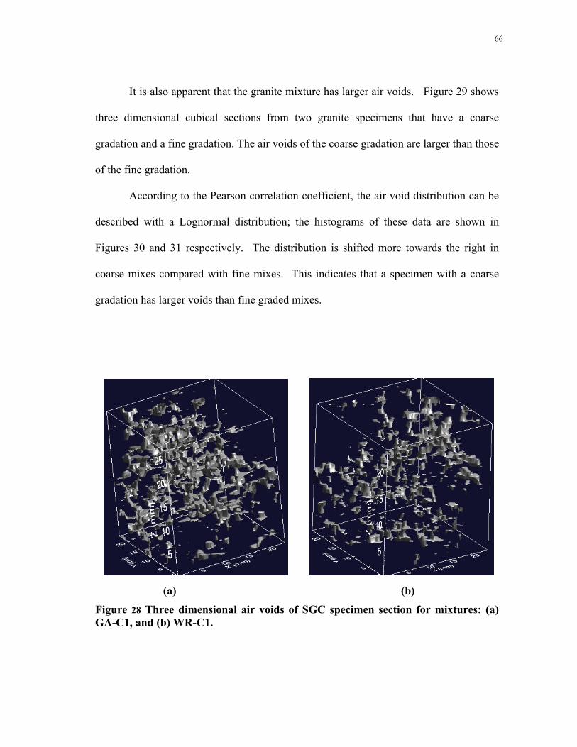
66

It is also apparent that the granite mixture has larger air voids. Figure 29 shows

three dimensional cubical sections from two granite specimens that have a coarse

gradation and a fine gradation. The air voids of the coarse gradation are larger than those

of the fine gradation.

According to the Pearson correlation coefficient, the air void distribution can be

described with a Lognormal distribution; the histograms of these data are shown in

Figures 30 and 31 respectively. The distribution is shifted more towards the right in

coarse mixes compared with fine mixes. This indicates that a specimen with a coarse

gradation has larger voids than fine graded mixes.

(a) (b)

Figure 28 Three dimensional air voids of SGC specimen section for mixtures: (a) GA-C1, and (b) WR-C1.

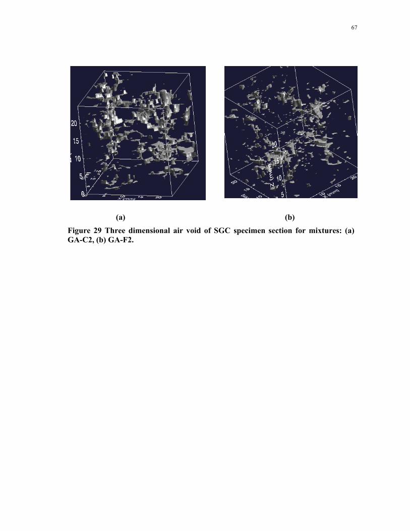
67

(a) (b)

Figure 29 Three dimensional air void of SGC specimen section for mixtures: (a) GA-C2, (b) GA-F2.

68

2.50 5.00 7.50 10.00gac1

0%

10%

20%

30%

Perc

ent

2.50 5.00 7.50 10.00gac2

0%

10%

20%

30%

Perc

ent

2.50 5.00 7.50 10.00gac3

0%

10%

20%

30%

Perc

ent

2.50 5.00 7.50 10.00gaf1

0%

10%

20%

30%

Perc

ent

2.50 5.00 7.50 10.00gaf2

0%

10%

20%

30%

Perc

ent

2.50 5.00 7.50 10.00gaf3

0%

10%

20%

30%

Perc

ent

FIGURE 30 Air Void distribution for SGC granite specimens.

Air void diameter (mm) Air void diameter (mm)



69

2.50 5.00 7.50 10.00wrc1

0%

10%

20%

30%Pe

rcen

t

2.50 5.00 7.50 10.00wrc2

0%

10%

20%

30%

Perc

ent

2.50 5.00 7.50 10.00wrc3

0%

10%

20%

30%

Perc

ent

2.50 5.00 7.50 10.00wrf1

0%

10%

20%

30%

Perc

ent

2.50 5.00 7.50 10.00wrf2

0%

10%

20%

30%

Perc

ent

2.50 5.00 7.50 10.00wrf3

0%

10%

20%

30%

Perc

ent

Figure 31 Air void distributions for SGC limestone specimens.




70

In order to relate the air void distribution to moisture damage, the mean diameter

size was compared to ratios of the number of cycles to failure and energy ratios of the

conditioned to the unconditioned specimen. A polynomial regression trend line was

used to fit the data because it gave a better correlation coefficient than other regression

types. The relationships found between the average air void diameter and ER and N

ratios, for the granite SGC specimens are shown in Figures 32 and 33. For the granite

specimens, the N and ER ratios decrease with an increase in void size until they reach a

“pessimum” point after which these ratios start to increase with an increase in void size.

Figure 32 Average diameter vs. N ratio for SGC granite specimens.

Dam

age

decr

ease

s R2 = 0.91

0.00

0.20

0.40

0.60

0.80

1.00

0.00 0.20 0.40 0.60 0.80 1.00 1.20 1.40 1.60 1.80

average diameter (mm)

Nc/N

u R2=0.91

Nc/

Nu

Average Diameter E(x)

Dam

age

decr

ease

s R2 = 0.91

0.00

0.20

0.40

0.60

0.80

1.00

0.00 0.20 0.40 0.60 0.80 1.00 1.20 1.40 1.60 1.80


Nc/N

u R2=0.91

Nc/

Nu


R2 = 0.91

0.00

0.20

0.40

0.60

0.80

1.00

0.00 0.20 0.40 0.60 0.80 1.00 1.20 1.40 1.60 1.80


Nc/N

u R2=0.91

Nc/

Nu


Dam

age

decr

ease

sD

amag

e de

crea

ses

71

Figure 33 Average diameter vs. ER ratio for SGC granite specimens.

The relationships between the N and ER ratios and the air void size for SGC

limestone mixes are shown in Figures 34 and 35. The relationship has the same form, as

the SGC granite mixes, but, it is not as clear as distinct as the granite mixes.

R2 = 0.82

0.00

0.20

0.40

0.60

0.80

1.00

0.00 0.20 0.40 0.60 0.80 1.00 1.20 1.40 1.60 1.80average diameter (mm)

ERc/E

Ru

Dam

age

decr

ease

sR2=0.82


ER

c/E

Ru R2 = 0.82

0.00

0.20

0.40

0.60

0.80

1.00


ERc/E

Ru

Dam

age

decr

ease

sD

amag

e de

crea

ses

R2=0.82


ER

c/E

Ru

72

Figure 34 Average diameter vs. N ratio for SGC limestone specimens.

Figure 35 Average diameter vs. ER ratio for SGC limestone specimens.

R2 = 0.89

0.00

0.20

0.40

0.60

0.80

1.00

1.20

0.00 0.20 0.40 0.60 0.80 1.00 1.20 1.40 1.60 1.80


Nc/N

u

R2=0.89


Nc/

Nu

Dam

age

decr

ease

s

R2 = 0.89

0.00

0.20

0.40

0.60

0.80

1.00

1.20

0.00 0.20 0.40 0.60 0.80 1.00 1.20 1.40 1.60 1.80


Nc/N

u

R2=0.89


Nc/

Nu

R2 = 0.89

0.00

0.20

0.40

0.60

0.80

1.00

1.20

0.00 0.20 0.40 0.60 0.80 1.00 1.20 1.40 1.60 1.80


Nc/N

u

R2=0.89


Nc/

Nu

Dam

age

decr

ease

sD

amag

e de

crea

ses

R2 = 0.84

0.00

0.20

0.40

0.60

0.80

1.00

1.20


ER

c/ER

u

R2=0.84

ER

c/E

Ru


Dam

age

decr

ease

s

R2 = 0.84

0.00

0.20

0.40

0.60

0.80

1.00

1.20


ER

c/ER

u

R2=0.84

ER

c/E

Ru


R2 = 0.84

0.00

0.20

0.40

0.60

0.80

1.00

1.20


ER

c/ER

u

R2=0.84

ER

c/E

Ru


Dam

age

decr

ease

sD

amag

e de

crea

ses

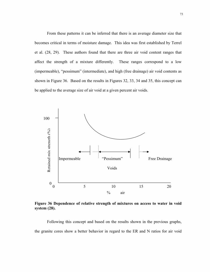
73

From these patterns it can be inferred that there is an average diameter size that

becomes critical in terms of moisture damage. This idea was first established by Terrel

et al. (28, 29). These authors found that there are three air void content ranges that

affect the strength of a mixture differently. These ranges correspond to a low

(impermeable), “pessimum” (intermediate), and high (free drainage) air void contents as

shown in Figure 36. Based on the results in Figures 32, 33, 34 and 35, this concept can

be applied to the average size of air void at a given percent air voids.

Figure 36 Dependence of relative strength of mixtures on access to water in void system (28).

Following this concept and based on the results shown in the previous graphs,

the granite cores show a better behavior in regard to the ER and N ratios for air void

05 10 15 20 0

100

Impermeable “Pessimum”

Voids

Free Drainage

Ret

aine

dm

ixst

reng

th(%

)

% air

74

sizes that are outside the range between 1.2 and 1.4 mm; whereas for the limestone

cores, the performance improves when the average diameter of the voids is away from

the range between 0.8 and 1.0 mm.

Pressure Distribution

Pore fluid plays an important role in the failure of porous media. If fluid is not present,

the medium will fail like a solid when the acting stress exceeds a certain limit.

However, due to the presence of interstitial fluid, the mode of failure that can happen has

been recognized by Terzaghi as “splitting” failure. This type of failure originates the

tensile breakdown of the medium, due to the effect of the fluid pressure (4).

Furthermore, one of mechanisms theorized for stripping suggests that pore

pressure causes the asphalt film to strip from the aggregate because during the initial

densification of the pavement structure due to traffic loading, the percolating water can

get trapped in impermeable voids. Hence, stripping can be generated due to high pore

water pressure that may develop as a consequence of further loading and environmental

cycling.

The pressure distribution was determined through the use of a three dimensional

fluid flow model developed by Al-Omari and Masad (10). The main purpose of this

model is to determine the fluid flow characteristics and permeability when a fixed stress

is applied to the specimen in a particular direction under saturated condition.

Furthermore, it records the pressure at each point of the microstructure where water

percolates. This model runs in a Fortran code that uses as input the bitmap from the

image analysis of square sections that are taken from the original images, because it

75

works with a finite difference numerical scheme in which the control volume is chosen

to have square images (10). Also, a hydraulic gradient is introduced so that water could

flow from the inlet to the outlet of the microstructure.

The statistical analysis of the pore pressure distribution showed that there is

difference in the developed pressure distribution among specimens as shown in Figures

37 and 38. However, there was apparent no relationship between the calculated N and

ER ratios and pressure distribution. This is not surprising given that the measurements

associated with the calculation of these ratios were conducted after pore pressure was

released, (2).

Nonetheless, the results show that different pore pressure distributions can result

due to the difference in mixes in terms of aggregate size distribution and aggregate type.

As a matter of fact, it was reported that the limestone mixes took a long time to release

the pore water. This was found by determining the time lapsed for the conditioned

modulus to recover 95 percent of the unconditioned small strain modulus which usually

increases when the saturation level decreases (2).

As can be seen in Figure 39, the difference between the average air void

pressures among corresponding gradations was always greater for the limestone cores

than for the granite cores, except for the mix F1. Therefore, generally more pressure is

associated with longer time of retention of the interstitial water.

76

0.02 0.04 0.06 0.08 0.10gac1

0%

5%

10%

15%

20%

Perc

ent

0.02 0.04 0.06 0.08 0.10gac2

0%

5%

10%

15%

20%

Perc

ent

0.02 0.04 0.06 0.08 0.10gac3

0%

5%

10%

15%

20%

Perc

ent

0.02 0.04 0.06 0.08 0.10gaf1

0%

5%

10%

15%

20%Pe

rcen

t

0.02 0.04 0.06 0.08 0.10gaf2

0%

5%

10%

15%

20%

Perc

ent

0.02 0.04 0.06 0.08 0.10

gaf3

0%

5%

10%

15%

20%

Perc

ent

Figure 37 Pressure distributions for SGC granite specimens.

σ = 0.029 σ = 0.031

σ = 0.031 σ = 0.032

σ = 0.033 σ = 0.029

Pressure Pressure

Pressure Pressure

Pressure Pressure

77

0.02 0.04 0.06 0.08 0.10wrc1

0%

5%

10%

15%

20%

Perc

ent

0.02 0.04 0.06 0.08 0.10

wrc2

0%

5%

10%

15%

20%

Perc

ent

0.02 0.04 0.06 0.08 0.10wrc3

0%

5%

10%

15%

20%

Perc

ent

0.02 0.04 0.06 0.08 0.10

wrf1

0%

5%

10%

15%

20%Pe

rcen

t

0.02 0.04 0.06 0.08 0.10wrf2

0%

5%

10%

15%

20%

Perc

ent

0.02 0.04 0.06 0.08 0.10

wrf3

0%

5%

10%

15%

20%

Perc

ent

Figure 38 Pressure distributions for SGC limestone specimens.

σ = 0.030 σ = 0.031

σ = 0.032 σ = 0.034

Pressure Pressure

Pressure Pressure

Pressure Pressure

78

0

0.01

0.02

0.03

0.04

0.05

0.06

0.07

C1 C2 C3 F1 F2 F3 & F3/C4

Gradation

Ave

rage

pre

ssur

e (N

/m2)

Granite Limestone

Figure 39 Comparison of average air void pressure between SGC specimens with different aggregates.

Surface Energy and Bond Strength

The surface energy can be defined as the energy that is required to create a new unit area

of surface of the same material under a vacuum (13). In summary, it requires surface

energy to initiate and propagate a microcrack through the HMA structure. If the energy

needed to cause that fatigue damage is relatively high, then the HMA is considerably

resistant to fracture. Conversely, if the HMA does not have much energy to heal then it

can be said, that the HMA does not have sufficient potential to self heal.

Schapery’s fundamental law of fracture explains this surface energy as a balance

between the strain energy that is released when a crack propagates and the energy that is

necessary to surmount the viscous resistance of the material where the energy is released

Pressure Pressure

79

ABLW G G G ∆+∆=∆

LWj

LWi

LWij

LWG Γ+Γ+Γ−=∆

( )2LWj

LWi

LWij Γ−Γ=Γ

ABj

ABi

ABij

ABG Γ+Γ+Γ−=∆

(13). Additionally, the surface energy of a material is always formed by two

components regardless if its fracture is adhesive or cohesive: an apolar component

(Lifshitz-van der Waals component) and a polar component (acid-base component).

Therefore, the total surface energy that governs the fracture of the material can be

expressed as (13):

(29)

where

∆G= total surface free energy of the asphalt or aggregate,

∆G LW= Lifshitz-van der Waals apolar component of the total surface free

energy,

∆GAB= Acid-base polar component of the total surface free energy

For adhesion and without the presence of water, the LW component is calculated as:

(30)

Where,

(31)

with

ΓLWi= Lifshitz-van der Waals component of Gibbs free energy of the asphalt

ΓLWj= Lifshitz-van der Waals component of Gibbs free energy of the aggregate

And the acid-basic component is calculated as follows:

(32)

80

( )( )−−++ Γ−ΓΓ−Γ=Γ jijiAB

ij 2

−+−+ ΓΓ=ΓΓΓ=Γ jjABjii

ABi and 22

ABi

LWii G G G ∆+∆=∆

LWi

LW Γ=∆ 2Gi

ABi

AB Γ=∆ 2G i

LWk

LWj

LWk

LWi

LWj

LWi

LWk ikj

LW 222 2 G ΓΓ−ΓΓ−ΓΓ+Γ=∆

( ) ( ) −++−−−+++−+ ΓΓ+ΓΓ+Γ+ΓΓ−Γ+ΓΓ−ΓΓ=∆ jijijikjikikjABG 22224 k

-k

(33)

Additionally the acid-basic component of the material i and j, ΓiAB and Γj

AB are

expressed as:

(34)

Where, Γ+ is the acid component and Γ- the basic component. The sub indices i

and j stand for asphalt and aggregate respectively.

The cohesive surface energy of the asphalt, when no water is present is expressed as

(13):

(35)

where

(36)

(37)

When water (k) is present between the interface of asphalt and aggregate, the

apolar and polar components of the adhesive surface energy on the interface can be

calculated as (13):

(38)

(39)

81

G G G ABikj

LWikj ikj ∆+∆=∆

Therefore the total Gibbs adhesive bond strength is (13):

(40)

Additionally, the cohesive surface energy on the interface when water is present

can be calculated as expressed in Equations 38 and 39 by replacing Γj for Γi.

The Wilhelmy plate method is used to measure the contact angles that a film of

asphalt forms with three different solvents (30). On the other hand, the surface energy

of the aggregate are indirectly measured with the Universal Sorption Device (USD)

method that is based on the equilibrium spreading pressure of the adsorbed vapor, on the

aggregate surface (30). From these procedures it is possible to calculate the energy

components, ΓLW, Γ+, and Γ- of the asphalt and the aggregate. These two procedures will

be described in the following sections.

Every material has two different sets of surface energy components, depending

on the process. The wetting energy predicts the healing capacity of the material while

the dewetting energy predicts fracture. These energy components can be calculated

applying the theory of surface energies and contact angles developed by Good and van

Oss (1991) for both, adhesive and/or cohesive fractures. Present research by Little et al.

(30), demonstrated that the acid base components of surface energy affect healing in a

positive way, meaning that the higher this component is, the more healable the material

is. On the other hand, the Lifshitz-van der Waals component affects healing negatively.

The surface free energies of the Georgia granite, the Florida limestone, and the

asphalt used to prepare the mixtures, were measured to better understand the damage

that the mixtures experience due to the presence of water.

82

−++− ΓΓ+ΓΓ+ΓΓ=+Γ sisiLW

sLW

iis 222)cos1( θ

Asphalt

The asphalt used to prepare both types of mixes was a PG 67-22. The Wilhelmy Plate

method was used to measure the dynamic contact angles between a film of asphalt and

four different solvents of known surface energy components: diiodomethane, distilled

water, formamide, and glycerol. These solvents were chosen because of their fairly large

surface energies, immiscibility with asphalt, and different surface energy components.

Young-Dupre’s equation (Equation 41) can be used in order to calculate the

surface free energy of the asphalt from the dynamic contact angles, under the

assumption that the equilibrium film pressure can be neglected for asphalt (26):

(41)

In this equation, θi is the contact angle that is formed between the asphalt and the

solvent, s. θi, is related to two different sets of surface energy processes, (i.e. wetting

and dewetting) which are used to predict healing and fracture respectively. When the

asphalt film is introduced into the solvent, the advancing angle is measured and the

wetting surface energy can be calculated. On the other hand, the dewetting surface

energy is associated with the receding angle that the asphalt film forms with the solvent

when it is withdrawn. Figure 40 shows a schematic of the Wilhemy plate method.

83

=

3

2

1

3

2

1

333231

232221

131211

YYY

xxx

aaaaaaaaa

s

si

s

si

s

LWs

i aaaΓΓ

=ΓΓ

=ΓΓ

=−+

2 ,2 ,2 321

−+ Γ=Γ=Γ= aaLW

a xxx 321 , ,

( ) ii CosxY θ+= 1

θ

Figure 40 Wilhelmy Plate method procedure.

As can be seen in Equation 41, there are three unknowns (i.e. ΓLW, Γ+, and Γ-).

Therefore at least three different solvents of known surface energies must be used so that

the different components of the asphalt surface energy can be determined from solving

the linear system of equations. This can be more clearly represented through a matrix

as shown below:

(42)

where

(43)

(44)

(45)

84

with

ani = Known surface energy components of the solvent i,

xi = Unknown surface energy components of the asphalt,

Yi(x)= Known Function of the measured contact angles (θi), between asphalt and

solvent i.

From the four solvents that were initially used to measure the contact angles,

only three were chosen because they gave the least variation in the surface energy of the

asphalt. These were diiodomethane, distilled water and glycerol. The surface energy

components of the solvents that were used are summarized in Table 27.

TABLE 27 Surface free energy components of solvent liquids (ergs/cm2)

Solvent Γ LW Γ + Γ - ΓDiidomethane 50.8 0 0 50.8Glycerol 34 3.92 57.4 64Distilled Water 21.8 25.5 25.5 72.8

As seen in Table 28, the accuracy of the measurements taken with the Wilhelmy

Plate is very good based on the standard deviation calculated from three measurements.

Also, the coefficient of variation demonstrates that the assurance on the measurements is

good for a 95 percent level of confidence.

85

TABLE 28 Advancing and receding contact angles measured with the Wilhelmy Plate method

Average 95.32 68.66 88.53 59.83 72.14 35.05Standard Deviation 2.13 1.16 2.14 2.02 2.97 2.17Coefficient of variation 0.02 0.02 0.02 0.03 0.04 0.06

methylene iodideAdvancing

AngleReceding

Angle

WATER GLYCEROLReceding

AngleAdvancing

AngleReceding

AngleAdvancing

Angle

The calculation of the linear system of equations was done by using a program

developed by Della Volpe and Siboni (31) that uses the original scale with variable

errors of contact angles, developed by van Oss, Chaudury and Good. These values are

included in Table 29 and are displayed in Figure 41.

.

TABLE 29 Healing and fracture energy components of the asphalt

(ergs/cm2) S.D. (ergs/cm2) S.D.Γ LW 21.68 0.65 42.01 0.91Γ + 0.05 0.07 0.23 0.16Γ - 4.05 0.44 11.28 0.73Γ AB 0.9 3.22Γ 22.58 2.05 45.23 3.29

Wetting DewettingComponent

From these energy components, it can be inferred that the non polar (LW)

component is much larger than the polar component (acid-base). The high value of the

non polar component can be explained by aging of the asphalt. However, there is no

information about this effect.

86

LWAcid

BaseAcid-Base

Total

Healing

Fracture0

5

10

15

20

25

30

35

40

45

50

ergs

/cm

2

Figure 41 Surface energy components of asphalt PG67-22.

It is noted that the acidic component Γ+ is practically zero given that standard

deviation. It is important to recall that it is not appropriate to directly compare the acidic

and basic components of asphalt. Each acidic or basic component should be compared

to the reference solvent or with other asphalt’s acidic or basic components because the

scale of measurement is relative, not absolute. In fact, there is no absolute scale.

Aggregates

The universal sorption device (USD) was used to quantify the surface energy of the

aggregates. This method consists of measuring the absorption of a particular gas solvent

of known surface energy components through the surface of an aggregate. The

aggregate size that is tested consists of particles that pass sieve No. 4 (4.75 mm) but are

87

( )LW

l

leLWs Γ

Γ⋅+Π=Γ

42 2

( )−

+

ΓΓΓ−Γ+Π

=Γlm

LWlm

LWslme

s 42

2

( )+

−++

ΓΓΓ−ΓΓ−Γ+Π

=Γlb

lbsLW

lbLWslbe

s 4222

2

−+ΓΓ+Γ=Γ 2LWxs

retained on sieve No. 8 (2.36 mm). Three different types of gas solvents of known

surface energy components must be used to measure the surface energy of the

aggregates: n-Hexane (apolar), the monopolar Methyl Propyl Ketone (MPK), and

distilled water (bipolar). The surface energies of these gas solvents are included in

Table 30.

TABLE 30 Surface energy components of gas solvents

Solvent Γ LW Γ + Γ - Γ AB Γn-hexane 18.4 0 0 0 18.4MPK 24.7 0 19.6 0 24.7Distilled Water 21.8 25.5 25.5 51 72.8

The Brunauer, Emmett and Teller theory (BET) is applied to calculate the

specific surface area of the aggregate that corresponds to the surface area per unit mass

of absorbent (30). Following this, the spreading pressure at saturation vapor pressure,

πe, is measured for each solvent. Having πe plus the surface energies of the three gas

solvents, the following equations can be solved in the following order to obtain the

surface energy components of the aggregate (30):

(46)

(47)

(48)

(49)

88

where

Γl = Surface energy of the apolar liquid (n-hexane),

Γlm = Surface energy of the monopolar liquid (MPK),

Γlb = Surface energy of the bipolar liquid (distilled water),

Γs = Total surface energy of the aggregate

The spreading pressures for the granite and the limestone and the specific surface

areas that were obtained using the USD are presented in Tables 31 and 32 respectively.

TABLE 31 Spreading pressures and specific surface areas for SGC granite samples

Πe SSA Πe SSA Πe SSA1 30.25 0.12 39.42 0.47 125.34 0.88

n-hexane MPK waterGranite Sample #

TABLE 32 Spreading pressures and specific surface areas for SGC limestone samples

Πe SSA Πe SSA Πe SSA1 43.89 0.2975 40.9 0.76 132.5 0.722 41.9 0.86 129.8 0.56

average : 43.89 0.2975 41.4 0.81 131.15 0.64

Limestone Sample #

n-hexane MPK water

With these measurements the surface energy components of the aggregates are

calculated as it was previously described and the results are shown in Table 33.

TABLE 33 Surface energy components of aggregates

AGGREGATE Γ ΓLW ΓAB Γ+ Γ-

Georgia Granite 218.63 61.08 157.55 31.86 194.78Florida Limestone 223.77 88.46 135.30 24.76 184.87

89

Adhesive and Cohesive Bond Energies

The fatigue of HMA can be characterized by loss of adhesive bond strength or loss of

cohesive bond strength. An adhesive fracture is characterized by loss of attraction

between the molecules at the interface between the asphalt and the aggregate. When the

fracture is cohesive, the cracks take place within the asphalt mastic itself. By knowing

these cohesion and adhesion characteristics of the mix, it is possible to evaluate water

susceptibility in terms of healing and fatigue cracking properties.

The adhesive surface energy corresponds to the creation of a unit crack area at

the interface between the asphalt and the aggregate under a vacuum condition (13). In

addition, the cohesive bond surface energy consists of the formation of a cohesive unit

area formed by the combination of two asphalt pieces under a vacuum condition (13).

It is important to point out that an asphalt-aggregate combination is compatible when no

water is present if the cohesive or the adhesive surface energies are positive; hence the

lower magnitude of these two governs the mode of fracture. Therefore the ideal

situation is to have a mix with high adhesive and cohesive surface energies. However,

as mentioned previously, the adhesive surface energy should preferably have a larger

acid-base component rather than with a large LW component because this improves

healing in the presence of water.

The cohesive bond strength of the asphalt with and without the presence of water

was calculated using Equations 35 and 40 respectively; Tables 34 and 35 include the

calculated values. Figure 42 shows the difference between these two conditions. As can

be seen, water increases the asphalt ability to heal (higher acid base component) and

90

reduces its resistance to fracture. This is because the hydrogen atoms in the water

have good interaction or affinity with those of the AB component of the asphalt; hence,

water makes the hydrogen bonds stronger and enhances the healing capability. This

reinforces the fact that, it is beneficial to have a greater AB component and a low LW

component. However, the bonding of these hydrogen atoms, takes time and therefore it

is associated with the long term healing of the asphalt.

TABLE 34 Cohesive bond strength of asphalt without water Fracture

∆Gh LW ∆Gh

AB ∆Gf

43.36 1.80 90.5

HealingASPHALT TYPE

PG 67-22

TABLE 35 Cohesive bond strength of asphalt with water Fracture

∆Gh LW ∆Gh

AB ∆Gf

0.00 58.63 37.49PG 67-22

HealingASPHALT TYPE

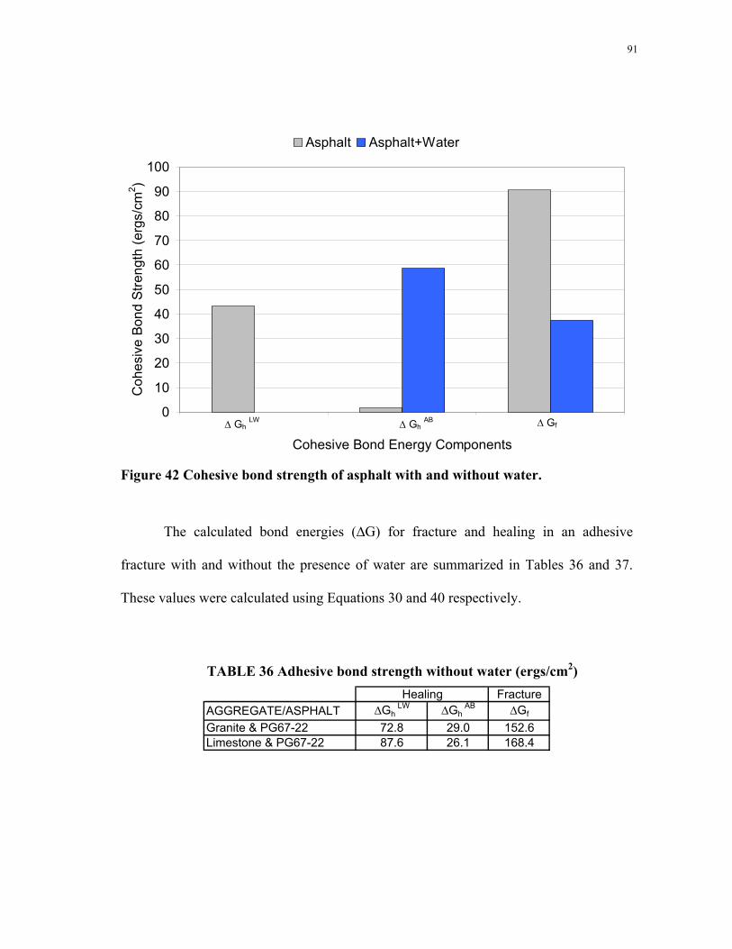
91

0

10

20

30

40

50

60

70

80

90

100

∆Gh LW ∆Gh AB ∆Gf

Cohesive Bond Energy Components

Coh

esiv

e Bo

nd S

treng

th (e

rgs/

cm2 )

Asphalt Asphalt+Water

∆ Gh LW ∆ Gh

AB ∆ Gf

Figure 42 Cohesive bond strength of asphalt with and without water.

The calculated bond energies (∆G) for fracture and healing in an adhesive

fracture with and without the presence of water are summarized in Tables 36 and 37.

These values were calculated using Equations 30 and 40 respectively.

TABLE 36 Adhesive bond strength without water (ergs/cm2) Fracture

∆Gh LW ∆Gh

AB ∆Gf

Granite & PG67-22 72.8 29.0 152.6Limestone & PG67-22 87.6 26.1 168.4

AGGREGATE/ASPHALTHealing

92

TABLE 37 Adhesive bond strength with water (ergs/cm2) Fracture

AGGREGATE/ASPHALT ∆Gh LW ∆Gh

AB ∆Gf

Granite & PG67-22 -0.08 -89.58 -72.0Limestone & PG67-22 -0.12 -82.05 -60.7

Healing

Limestone has better resistance to fracture than granite under dry conditions as

indicated by the higher fracture energy in Table 36. Also, it can be inferred from the

bond strength energies that the limestone has better resistance to fracture when water is

present because its energy components are less negative compared to the granite. On the

other hand, when water is in the interface, the limestone has a better capability to heal

because its acid-base component is less negative, thus there is less detachment of the

asphalt from the aggregate, as it can be seen in Table 37.

These results are in accordance to the observations that were carried out on the

specimens by Birgisson et al (2). When opening the core, they found that even though

the limestone specimens did not exhibit much stripping, they were susceptible to

moisture damage due to a reduced cohesion.

Summary

The moisture damage parameters that were selected to relate pore size distribution and

pressure distribution were the energy ratio (ER) and the number of cycles to failure (N).

These parameters were studied as a ratio that reflected the change from a wet to a dry

condition. Therefore, the higher these ratios are the lesser damage takes place.

The specimens analyzed in this chapter consisted of limestone and granite

specimens from the SGC mixtures that were prepared using corresponding gradations.

93

The air void distribution was calculated from the image analysis that registered the size

of all pores within the specimens. The pore pressure distribution was calculated from a

three dimensional fluid flow model for HMA under saturated conditions.

When comparing the granite and the limestone cores based on the ER, it was

evident that the change in this parameter from a wet condition to a dry condition for

granite mixtures was larger than for the limestone mixtures. This indicates that the

granite mixes are more vulnerable to moisture damage than the limestone mixes. This

ratio encompasses key mechanical properties (i.e. DCSE, tensile stress, creep

compliance, m-value) that change with moisture. The trend was similar when the

limestone and granite mixes were compared based on the N ratio.

The N and ER ratios showed that there is a “pessimum” air void size range for

which the damage is higher. A similar idea of this qualification was first declared by

Terrel et al. (28, 29) who found that there is a “pessimum” air void content for which the

strength of a mix is worse than otherwise would be. The limestone cores displayed this

same pattern of minimum performance. However, the ranges differ, being

approximately from 1.2 to 1.4 mm for the granite cores, and from 0.8 to 1.0 mm for the

limestone cores.

The pressure distribution was different within the specimens of each type of

aggregate and between mixes with similar gradations but different types of aggregates.

There was no meaningful relationship between the pressure distribution and these

parameters. This was not surprising because the measurements associated with the

determination of N and ER were conducted after pore pressure was released.

94

The universal sorption device (USD) and the Wilhelmy plate methods were used

to measure the surface energies of the aggregates and the asphalt respectively. From

these measurements the cohesive and adhesive bond strengths without and in the

presence of water were calculated. According to the measurements and calculations,

this asphalt has a better healing ability when water is present; however, its fracture

energy is lower under this condition. Also, the granite is more susceptible to moisture

damage as it has less ability to heal and is more prone to fracture than the limestone

under wet conditions.

95

CHAPTER V

CONCLUSIONS

Conclusions

The current design methods of HMA include permanent deformation, low temperature

cracking, and fatigue cracking. Moisture sensitivity is only considered to determine if

the final design mixture is susceptible to damage due to the action of water. Moisture

damage is directly related to permeability. In spite of the influence of moisture damage

on stripping, excessive deflection, cracking and reduction of load carrying capacity, the

mix microstructure characteristics and material properties that affect moisture damage

are not directly considered.

X-ray CT was used to capture the microstructure and image analysis techniques

were utilized to analyze the air void distribution. The use of X-ray CT image is

considered a major improvement over previous studies that attempted to link the air void

distribution of granular materials to permeability. X-ray CT enhanced the ability of

obtaining continuous data about the air void distribution at the microstructure level.

This was done in the past by analyzing discrete data using mercury intrusion techniques

which might cause disturbance to the microstructure.

This study established the relationship between the air void size distribution and

HMA permeability through the analysis of three sets of HMA specimens. These sets

included laboratory specimens compacted using the linear kneading compactor,

96

laboratory specimens compacted using the SuperpaveTM gyratory compactor, and field

cores. The influence of air void size distribution on permeability was established using

the assumption that the probability of having two voids connected to each other on

adjacent slices (X-ray CT images) is completely correlated. This assumption was

adopted due to the small HMA slice thicknesses. The air void size distribution was

considered to be Lognormal based on the Pearson correlation coefficient and probability

plots that showed linearity between the data and the tested distribution.

There was a strong correlation between the air void size distribution and

permeability for laboratory compacted specimens. However, weak correlation was

found between air void distribution in field cores and permeability field measurements.

This was attributed to the fact that in field permeability measurements, fluid tends to

flow in the top one inch of a core due to the high percent of air voids in the top

compared with the rest of the core. In other words, the measured field permeability is

not associated with all air voids in the pavement. In fact, some field permeability

measurements can be high while X-ray CT shows that there is no air void connectivity

across the core. Therefore, it was decided to only include the cores that have connected

voids in studying the correlation between air void distribution and field permeability.

This step lead to significant improvement in correlation between air void distribution in

field cores and permeability field measurements.

This study also related moisture damage to air void distribution and pore

pressure distribution in HMA microstructure. The air void distribution was calculated

from the image analysis that registered the size of all the air voids within the specimens.

97

The pore pressure distribution was calculated from a three dimensional fluid flow model

for HMA under saturated conditions. The resistance of HMA to moisture damage was

evaluated using two parameters that were derived based on fracture mechanics

principles. These parameters are energy ratio (ER) and the number of cycles to failure

(N). The ratio of the parameter determined under dry conditions to the same parameter

under wet conditions was taken as indication of resistance to moisture damage.

Therefore, the higher these ratios are the lesser damage takes place.

The moisture damage was assessed for limestone and granite specimens that

were prepared using similar gradations. However, the gradation within each mix type

was varied to obtain different air void distributions. The granite mixes had larger air

voids than their limestone counterparts even though they were designed to have similar

gradations.

When comparing the granite and the limestone cores based on the ER and N

ratios, it was evident that the change in this parameter from a dry condition to a wet

condition was larger for granite specimens than for the limestone specimens.

The N and ER ratios showed that there is a “pessimum” air void size range, for

each of the granite and limestone mixes, where moisture damage is at maximum.

However, the ranges differ, being approximately from 1.2 to 1.4 mm for the granite

cores, and from 0.8 to 1.0 mm for the limestone cores. A similar idea of this

qualification was first declared by Terrel et al. (28, 29), who found that there is a

“pessimum” air void content for which the resistance to moisture damage is worst than

98

otherwise would be. The limestone cores displayed this same pattern of minimum

performance.

The pressure distribution was different within specimens from each type of mix,

and between mixes with similar gradations but different types of aggregates. There was

no meaningful relationship between the pressure distribution and the moisture damage

parameters. This was not surprising because after all, the measurements associated with

the determination of N and ER, were conducted after pore pressure was released.

The moisture damage was also related to the chemical properties aggregates and

binder. The universal sorption device (USD) and the Wilhelmy plate methods were used

to measure the surface energies of the aggregates and the asphalt, respectively. From

these measurements, the cohesive and adhesive bond strengths without and in the

presence of water were calculated. According to the measurements and calculations,

this asphalt has a better healing ability when water is present; however, its fracture

energy is lower under this condition. Also, the granite is more susceptible to moisture

damage as it has less ability to heal and is more prone to fracture than the limestone

under wet conditions. The current asphalt mix design methods need to account for the

cohesive and adhesive properties of asphalt mixtures that are highly affected by

moisture.

99

REFERENCES

1. Al-Omari, A., L. Tashman, E. Masad, A. Cooley, and T. Harman. Proposed

Methodology for Predicting HMA Permeability. Journal of the Association of Asphalt

Paving Technologists, Vol. 71, 2002, pp. 30-58.

2. Birgisson, B., R. Roque, and G. Page. Evaluation of Water Damage Using Hot Mix

Asphalt Fracture Mechanics. Journal of the Association of Asphalt Paving

Technologists, Vol. 72, 2003, pp. 424-462.

3. Garcia-Bengochea, I. The Relation between Permeability and Pore Size Distribution

of Compacted Clayey Silts. M.S. thesis. Purdue University, Lafayette, IN, 1978.

4. Terzaghi, K., R. Peck, and G. Mesri. Soil Mechanics in Engineering Practice. John

Wiley & Sons, New York, 1996.

5. Bear, J. Dynamics of Fluids in Porous Media, American Elsevier Publishing Co.,

New York, 1972.

6. Scheidegger, A.E. The Physics of Flow Through Porous Media, University of Toronto

Press, Toronto, Canada, 1957.

7. Childs, E.C., and N. Collis-George. The Permeability of Porous Materials. Proc. Roy.

Soc. Lond., Vol. A201, 1950, pp. 392-405.

8. Marshall, T.J. A Relation between Permeability and Size Distribution of Pores. J.

Soil Sci., Vol. 9, No. 1, 1958, pp. 1-8.

9. Juang, C.H., and R.D. Holtz. A Probabilistic Permeability Model and the Pore Size

Density Function. International Journal for Numerical and Analytical Methods in

Geomechanics, Vol. 10, 1986, pp. 543-553.

100

10. Al-Omari, A., and E. Masad. Three Dimensional Simulation of Fluid Flow in X-ray

CT Images of Porous Media. International Journal for Numerical and Analytical

Methods in Geomechanics, Vol. 28, Issue 13, 2004, pp. 1327-1360.

11. Roberts, F., P. Kandhal, E. Brown, D. Lee, and T. Kennedy. Hot Mix Asphalt

Materials, Mixture Design and Construction. NAPA Educational Foundation, Lanham,

Maryland, 1996.

12. Barksdale, R. The Aggregate Handbook. National Stone, Sand and Gravel

Association, Arlington, VA., 2001.

13. Lytton, R. “Adhesive Fracture in Asphalt Concrete Mixtures”, 2004.

http://ceprofs.tamu.edu/lytton/ADHESIVE%20FRACTURE%20IN%20ASPHALT%20

CONCRETE%20MIXTURES.doc.

14. E.W. Washburn. Note on a Method of Determining the Distribution of Pore Sizes in

a Porous Material, Proc.Nat.Acad.Sci., Vol. 7, 1921, pp. 115-116.

15. Masad, E., V. K. Jandhyala, J. Dasgupta, N. Somadevan, and N. Shashidhar.

Characterization of Air Void Distribution in Asphalt Mixes Using X-Ray CT. Journal

of Materials in Civil Engineering, ASCE, Vol. 14, No. 2, 2002, pp. 122-129.

16. ASTM D 5084-00 Standard Test Methods for Measurement of Hydraulic

Conductivity of Saturated Porous Materials Using a Flexible Wall Permeameter. ASTM

International, West Conshohocken, PA, 2002.

17. Birgisson, B., R. Roque, and G. Page. The Use of a Performance-Based Fracture

Criterion for the Evaluation of Moisture Susceptibility in Hot Mix Asphalt. Presented at

101

the 83rd Annual Meeting of the Transportation Research Board, Washington, DC, Jan.

11-15, 2004, [available on CD].

18. Image Pro Plus, Version, 4.1, Media Cybernetics, L.P, Georgia, MD (1999).

19. SPSS for Windows - Release 10.0.7. SPSS Inc. Business Intelligence Division,

Chicago, IL, 2002.

20. Minitab Release 13.1. BCIS Lab, St. Cloud, MN, 2000.

21. Maple 9.01. Waterloo Maple Inc., Waterloo, Canada, 2003.

22. ASTM D 2434-68 Standard Test Method for Permeability of Granular Soils

(Constant Head) ASTM International. West Conshohocken, PA, 2000.

23. Lavin, P. Asphalt Pavements. Spon Press, New York, 2003.

24. Zhang, Z., R. Roque, B. Birgisson, and B. Sangpetngam. Identification and

Verification of a Suitable Crack Growth Law for Asphalt Mixtures. Journal of the

Association of Asphalt Paving Technologists (Symposium), Vol. 70, 2001, pp. 206-241.

25. Jajliardo, A. Development of Specification Criteria to Mitigate Top-Down

Cracking. M.S. thesis. University of Florida, Gainesville, 2003.

26. Masad, E., S. Saadeh, T. Al-Rousan, E. Garboczi, and D. Little. Computations Of

Particle Surface Characteristics Using Optical and X-Ray CT Images. Journal of

Computational Geosciences, 2004, (in press).

27. Chandan, C., K. Sivakumar, T. Fletcher, and E. Masad. Geometry Analysis of

Aggregate Particles Using Imaging Techniques. Journal of Computing in Civil

Engineering, ASCE. Vol. 18, No. 1, 2002, pp. 75-82.

102

28. Terrel, R. and S. Al-Swailmi. Role of Pessimum Voids Concept in Understanding

Moisture Damage to Asphalt Concrete Mixtures. In Transportation Research Record

1386, TRB, National Research Council, Washington, DC, 1993, pp.31-37.

29. Terrel, R., and S. Al-Sqailmi. Evaluation of Water Damage of Asphalt Concrete

Mixtures Using the Environmental Conditioning System (ECS). Journal of the

Association of Asphalt Paving Technologists (Symposium), Vol. 61, 1992, pp. 405-445.

30. Cheng, D., D. Little, R. Lytton, and J. Holste. Use of Surface Free Energy

Properties of the Asphalt- Aggregate System to Predict Moisture Damage Potential.

Journal of the Association of Asphalt Paving Technologists. Vol. 71, 2002, pp. 59-88

31. Della Volpe, C., and S. Siboni. Calculations of Acid-Base Surface Tension

Components. Trento, Italy. http://devilmac.ing.unitn.it:8080/

103

APPENDIX A

TABLE 38 Gradation of granite mixes

GA-C1 GA-C2 GA-C3 GA-F1 GA-F2 GA-F319 mm (3/4) 100.0 100.0 100.0 100.0 100.0 100.012.5 mm (1/2) 97.4 90.9 97.3 94.7 90.5 94.69.5 mm (3/8) 89.0 72.9 89.5 84.0 77.4 85.14.75 mm (#4) 55.5 45.9 55.4 66.4 60.3 65.12.36 mm (#8) 29.6 28.1 33.9 49.2 43.2 34.81.18 mm (#16) 19.2 18.9 23.0 32.7 34.0 26.0600 mm (#30) 13.3 13.2 16.0 21.0 23.0 18.1300 mm (#30) 9.3 9.2 11.2 12.9 15.3 12.5150 mm (#100) 5.4 5.6 6.8 5.9 8.7 7.775 mm (#200) 3.5 3.9 4.7 3.3 5.4 5.8

Sieve Size Granite Specimens: Percent Passing

TABLE 39 Gradation of limestone mixes

WR-C1 WR-C2 WR-C3 WR-F1 WR-F2 WR-F3/C419 mm (3/4) 100.0 100.0 100.0 100.0 100.0 100.012.5 mm (1/2) 97.0 91.0 98.0 96.0 91.0 95.09.5 mm (3/8) 90.0 74.0 89.0 85.0 78.0 85.04.75 mm (#4) 60.0 47.0 57.0 69.0 61.0 67.02.36 mm (#8) 33.0 30.0 36.0 53.0 44.0 37.01.18 mm (#16) 20.0 20.0 24.0 34.0 35.0 26.0600 mm (#30) 15.0 14.0 18.0 23.0 24.0 20.0300 mm (#30) 11.0 10.0 13.0 15.0 16.0 14.0150 mm (#100) 7.6 6.7 9.2 9.6 9.1 8.675 mm (#200) 4.8 4.8 6.3 4.8 6.3 5.8

Sieve Size Limestone Specimens: Percent Passing

104

0.0

10.0

20.0

30.0

40.0

50.0

60.0

70.0

80.0

90.0

100.0

Sieve Size (0.45 power), mm

Per

cent

Pas

sing

C1 C2 C3

0.30.60.07 0.15 1.18 2.36 4.7 9.5 12.5 19.0

Figure 43 Granite Coarse Gradation Mixes, NMAS=12.5 mm.

0.0

10.0

20.0

30.0

40.0

50.0

60.0

70.0

80.0

90.0

100.0


Per

cent

Pas

sing

F1 F2 F3

0.30.60.07 0.15 1.18 2.36 4.75 9.5 12.5 19.0

Figure 44 Granite fine gradation mixes, NMAS=12.5 mm.

105

0.0

10.0

20.0

30.0

40.0

50.0

60.0

70.0

80.0

90.0

100.0


Per

cent

Pas

sing

C1 C2 C3

0.30.60.07 0.15 1.18 2.36 4.7 9.5 12.5 19.0

Figure 45 Limestone coarse gradation mixes, NMAS=12.5 mm.

Limestone Fine Gradation Mixes NMAS=12.5mm

0.0

10.0

20.0

30.0

40.0

50.0

60.0

70.0

80.0

90.0

100.0


Per

cent

Pas

sing

F1 F2 F3/C4

0.30.60.07 0.15 1.18 2.36 4.7 9.5 12.5 19.0

Figure 46 Limestone fine gradation mixes, NMAS=12.5 mm.

106

VITA

Adhara Castelblanco Torres was born in Bogotá, Colombia, in 1977. She received her

Bachelor of Science degree in civil engineering from Universidad Nacional de Colombia

in April 2002. In the fall of 2002, she started her master’s degree at Texas A&M

University, and she graduated in December 2004, with a Master of Science in civil

engineering. She can be contacted at the following address:

8708 Duncanson Dr.

Bakersfield, CA 93309

PROBABILISTIC ANALYSIS OF AIR VOID STRUCTURE AND ITS ...

Documents

Transcript of PROBABILISTIC ANALYSIS OF AIR VOID STRUCTURE AND ITS ...