HAL Id: hal-01007202https://hal.archives-ouvertes.fr/hal-01007202

Submitted on 13 Apr 2018

HAL is a multi-disciplinary open accessarchive for the deposit and dissemination of sci-entific research documents, whether they are pub-lished or not. The documents may come fromteaching and research institutions in France orabroad, or from public or private research centers.

L’archive ouverte pluridisciplinaire HAL, estdestinée au dépôt et à la diffusion de documentsscientifiques de niveau recherche, publiés ou non,émanant des établissements d’enseignement et derecherche français ou étrangers, des laboratoirespublics ou privés.

Probabilistic analysis and design of strip foundationsresting on rocks obeying Hoek-Brown failure criterion

Nut Mao, Tamara Al-Bittar, Abdul-Hamid Soubra

To cite this version:Nut Mao, Tamara Al-Bittar, Abdul-Hamid Soubra. Probabilistic analysis and design of strip founda-tions resting on rocks obeying Hoek-Brown failure criterion. International Journal of Rock Mechanicsand Mining Sciences, Pergamon and Elsevier, 2012, 49 (1), pp.45-58. �10.1016/j.ijrmms.2011.11.005�.�hal-01007202�

n Corr

E-m

ng

Probabilistic analysis and design of strip foundations resting on rocks obeyiHoek–Brown failure criterion

Nut Mao, Tamara Al-Bittar, Abdul-Hamid Soubra

University of Nantes, Bd. de l’universite, BP 152, 44603 Saint-Nazaire Cedex, France

babilist

g capac

Hoek–

study,

e poly

meters

These a), the i

cal load

increas

he non

bearin

In this paper, a pro

the ultimate bearin

follow the modified

the analysis. In this

analysis theory. Th

analysis. Four para

random variables.

the intact rock (sc

results of the verti

increases with the

greater effect, (ii) t

PDF of the ultimate

out PDF, (iv) the probabilis

or smaller than the determ

Finally, it was shown in t

decreases with the increas

esponding author. Tel.: þ33 240 905 108; fax

ail address: abed.soubra@univ-nantes.fr (A.-H

ic analysis is presented to compute the probability density function (PDF) of

ity of a shallow strip footing resting on a rock mass. The rock is assumed to

Brown failure criterion. Vertical and inclined loading cases are considered in

the deterministic models are based on the kinematic approach of the limit

nomial chaos expansion (PCE) methodology is used for the probabilistic

related to the modified Hoek–Brown failure criterion are considered as

re the geological strength index (GSI), the uniaxial compressive strength ofntact rock material constant (mi) and the disturbance coefficient (D). The

case have shown that (i) the variability of the ultimate bearing capacity

e in the coefficients of variation of the random variables; GSI and sc being of

-normality of the input variables has a significant effect on the shape of the

g capacity, (iii) a negative correlation between GSI and sc leads to less spread

tic footing breadth based on a reliability-based design (RBD) may be greater

inistic breadth depending on the values of the input statistical parameters.

he inclined load case that the variability of the ultimate bearing capacity

e of the footing load inclination.

1. Introduction

Traditionally, stability analysis and design of shallow foundationsresting on soils or rocks is based on deterministic approaches [1–4].In this paper, the behavior of shallow foundations resting on a rockmass is studied using a probabilistic approach. The probabilisticapproaches allow one to consider the propagation of the uncertain-ties from the input parameters to the system responses. Mostprobabilistic analyses existing in literature consider the ultimatelimit state of foundations resting on a soil mass [5–12]. To the bestof the authors’ knowledge, there are no probabilistic studies on theultimate limit state of shallow foundations resting on rock masses.The present paper fills this gap; it aims at determining the ultimatebearing capacity of a shallow strip footing resting on a rock massusing a probabilistic approach. The footing rests on a rock mass thatfollows the modified Hoek–Brown failure criterion. In this criterion,only intact rocks or heavily jointed rocks masses (i.e. with suffi-ciently dense and randomly distributed joints) can be considered.A central (vertical or inclined) footing load is considered in theanalysis. The deterministic models are based on the kinematic

: þ33 240 905 109.

. Soubra).

1

approach of limit analysis theory using translational multiblockfailure mechanisms. Four uncertain parameters related to the mod-ified Hoek–Brown failure criterion are modeled as random variables.These are the geological strength index (GSI), the uniaxial compres-sive strength of the intact rock (sc), the intact rock material constant(mi) and the disturbance coefficient (D). Notice that the systemresponse considered in this paper is the ultimate bearing capacity ofthe footing. This response is related to the failure of the footing byrock punching.

As for the probabilistic studies, the classical Monte Carlo simu-lation (MCS) methodology is generally used to compute eitherthe probability density function (PDF) of the system response orthe failure probability Pf. In spite of being a rigorous and a robustmethodology, MCS requires a great number of calls to the determi-nistic model (about 1,000,000 samples for a failure probability of10�5). This is not convenient in case where the computation of thesystem response is not given by a simple analytical formula. In thepresent paper, a more efficient method based on the polynomialchaos expansion (PCE) is used [13–16]. The PCE methodology aims atreplacing the deterministic model (for which the uncertain inputparameters are modeled by random variables) by an approximatesimple analytical equation called meta-model. Thus, one can easilycalculate the system response when performing Monte Carlo simula-tions. In this paper, the meta-model is used to perform both

Table 1Usual probability density functions and their cor-

responding families of orthogonal polynomials.

Probability density functions Polynomials

Gaussian Hermite

Gamma Laguerre

Beta Jacobi

Uniform Legendre

probabilistic and reliability-based analyses. It is also used to performa reliability-based design.

In the probabilistic analysis, a parametric study was performed.The PDF of the system response (ultimate bearing capacity) wasdetermined for normal and non-normal random variables and fordifferent values of the statistical parameters of the random variables(i.e. coefficient of variation and correlation between random vari-ables). Also, a global sensitivity analysis based on Sobol indices wasperformed. These indices give the contribution of each randomvariable or combination of random variables in the variability ofthe system response. This is important because it helps engineers indetecting the uncertain parameters that have a significant influencein the variability of the system response. Concerning the reliability-based analysis, the meta-model determined by the probabilisticanalysis was used to compute the Hasofer–Lind reliability indexand the corresponding failure probability for different values of theapplied footing load. In addition to the reliability-based analysis, areliability-based design (RBD) was performed to determine (for givenvalues of the statistical parameters of the input random variables)the footing breadth corresponding to a target failure probability.

The paper is organized as follows: The next section aims atpresenting the basic idea of the polynomial chaos expansion (PCE)methodology. It is followed by a presentation of the deterministicmodel used for the computation of the ultimate bearing capacity ofa centrally loaded strip footing (vertical or inclined load) resting on arock mass. Finally, the probabilistic and reliability-based results arepresented and discussed for both cases of vertical and inclinedloadings. The paper ends with a conclusion.

2. Polynomial chaos expansion (PCE) methodology

The polynomial chaos expansion methodology allows one torepresent by an analytical equation (meta-model) the response ofa mechanical system whose input uncertain parameters aremodeled by random variables. The main advantage of a PCEmethodology is that the PDF of the system response can be easilyobtained by applying MCS on the meta-model. Another importantadvantage of the meta-model is that it can be used to perform aglobal sensitivity analysis based on Sobol indices. These indicesgive the contribution of each random variable or combination ofrandom variables in the variability of the system response. Itshould be noticed that the meta-model aims at presenting therandom model response by a set of coefficients in a suitable (so-called polynomial chaos) basis. These coefficients may be effi-ciently computed using a non-intrusive technique where thedeterministic model does not need to be modified; it is treatedas a black box. Two non-intrusive approaches have been proposedin literature: the projection and the regression approach. In thispaper, the regression approach [13–16] is used. Once theunknown coefficients of the PCE are determined, this PCE willbe called ‘‘meta-model’’ and it will be used for further post-treatment in the probabilistic analysis. Thus, the PDF of theresponse can be derived with no cost since one makes use ofthe simple analytical formula. In this section, the main idea of thePCE methodology is first described. It is followed by a presenta-tion of (i) the regression method used to determine the unknownPCE coefficients, (ii) the statistical analyses (determination of thePDF of the system response and the Sobol indices) by using themeta-model and (iii) the numerical implementation of the PCEmethodology.

2.1. System output

Consider a deterministic model with M input uncertain para-meters gathered in a vector X ¼ fX1,. . .,XMg. The different elements

2

of this vector can have different types of the probability densityfunction. In order to represent our mechanical system response by aPCE, all the uncertain parameters should be represented by a uniquechosen PDF. Table 1 presents the usual probability density functionsand their corresponding families of orthogonal polynomials. In thispaper, the independent standard normal space is used. Thus, thesuitable corresponding basis is the multidimensional Hermite poly-nomials. The expressions of the multi-dimensional Hermite poly-nomials are given in [16] among others.

Based on the Gaussian PDF chosen in this paper, Xiu andKarniadakis [17] have shown that the system response can beexpanded onto an orthogonal polynomial basis as follows:

GPCEðxÞ ¼X1b ¼ 0

abCbðxÞffiXP�1

b ¼ 0

abCbðxÞ ð1Þ

where x is the vector resulting from the transformation of therandom vector X into an independent standard normal space, ab arethe unknown coefficients to be computed and Cb are the multi-dimensional Hermite polynomials. The PCE representation shouldbe truncated by retaining only the multivariate polynomials ofdegree less than or equal to the PCE order p. This truncation schemeleads to a number P of unknown coefficients given by

P¼ðMþpÞ!

M!p!ð2Þ

For the determination of the PCE unknown coefficients, it isrequired to evaluate the system response at a set of collocationpoints (i.e. sampling points). As suggested by several authors[13–16], the roots of the one-dimensional Hermite polynomial (ofone degree higher than the PCE order p) are used for each randomvariable. The collocation points are the result of all possiblecombinations of these roots. Thus, the number N of the availablecollocation points depends on the number M of the randomvariables and the PCE order p as follows:

N¼ ðpþ1ÞM ð3Þ

As proposed in [13–16], this number of collocation points shouldbe increased by one when using a PCE of an odd order since in thiscase the number of collocation points does not include the origin.The origin should be included since it represents the point with thehighest failure probability.

It should be mentioned here that in order to perform thedeterministic calculations, one should transform the independentstandard normal random variables of a given collocation point to thephysical correlated non-normal space (if the physical variables arecorrelated and non-normal). This is done by first correlating theindependent standard normal random variables of a given colloca-tion point, by multiplying these independent standard variables bythe Cholesky transform CH of the standard covariance matrix (i.e.correlation matrix) as follows:

xc¼ CHUx ð4Þ

where xc is the correlated standard normal random vector andx is the independent standard normal random vector. Thestandard correlated normal vector has now to be transformed

into the non-normal space using the following equation:

X ¼ F�1½Fðxc

Þ� ð5Þ

where X is the physical random vector, F(.) is the cumulativedensity function (CDF) in the non-normal space and F(.) is thenormal CDF. The next section is devoted to the presentation of theregression approach used to calculate the coefficients ab ofthe PCE.

2.2. Regression approach

As may be seen from Eq. (3), the number of the availablecollocation points dramatically increases as p or M increases. Thisnumber is always higher than the number P of the unknowncoefficients (given by Eq. (2)) when MZ2. This leads to a linearsystem of equations whose number of equations N is greater thanthe number of unknowns P. Based on the regression approach, thevector of the unknown coefficients can be obtained by solving thefollowing equation:

ab ¼ ðOTOÞ�1OT Y ð6Þ

where Y ¼ fY1,. . .,YNg is the vector of the model response values

(computed via the deterministic model for the N collocationpoints) and O is the matrix of dimensions N� P. It is given by:

O¼

c10ðxÞ c1

1ðxÞ � � � c1P�1ðxÞ

c20ðxÞ c2

1ðxÞ � � � c2P�1ðxÞ

^ ^ & ^

cN0 ðxÞ cN

1 ðxÞ � � � cNP�1ðxÞ

2666664

3777775 ð7Þ

Several attempts have been made in literature to select themost efficient collocation points among the N available ones toreduce the number of calls of the deterministic model. Websteret al. [18] selected a number K of collocation points among the N

available points based on the empirical equation K¼(Pþ1).Isukapalli et al. [13] proposed another empirical equation K¼2P.In both approaches, the collocation points are chosen to be thenearest ones to the origin of the standard space of randomvariables. More recently, Sudret [19] proposed a more rationalmethodology for the determination of the necessary number ofcollocation points. This method is used in this paper. It is based onthe invertibility of the information matrix A¼OTO. It can bedescribed by the following steps: (a) the N available collocationpoints are ordered in a list according to increasing norm, (b) theinformation matrix A is first constructed using the first P colloca-tion points of the ordered list, i.e. the P collocation points that arethe closest ones to the origin of the standard space of the randomvariables and finally (c) this matrix is successively increased byadding each time another collocation point from the ordered listuntil the matrix becomes invertible. This leads to a number K ofcollocation points smaller than the number N of the availablecollocation points.

It should be noticed here that the quality of the outputapproximation via a PCE closely depends on the PCE order p. Letus consider K realizations fxð1Þ ¼ ðxð1Þ1 ,. . .,xð1ÞM Þ,. . .,x

ðKÞ¼ ðxðKÞ1 ,. . .,

xðKÞM Þg of the standard normal random vector x, and noteG¼ fGðxð1ÞÞ,. . .,GðxðKÞÞg the corresponding values of the modelresponse determined by deterministic calculations. To ensure agood fit between the meta-model and the true deterministic model(i.e. to obtain the optimal PCE order), the simplest error estimate isthe well-known coefficient of determination R2 given by:

R2¼ 1�

DPCE

VarðGÞð8Þ

3

where DPCE is the empirical error given by:

DPCE ¼1

K

XK

i ¼ 1

½GðxðiÞÞ�GPCEðxðiÞÞ� ð9Þ

and

VarðGÞ ¼1

K�1

XK

i ¼ 1

½GðxðiÞÞ�G�2 ð10Þ

G¼1

K

XK

i ¼ 1

GðxðiÞÞ ð11Þ

The value R2¼ 1 indicates a perfect fit of the true model response

G, whereas R2¼ 0 indicates a nonlinear relationship between the

true model G and the PCE model GPCE. This coefficient may be abiased estimate since it does not take into account the robustness ofthe meta-model (i.e. its capability of correctly predicting the modelresponse at any point which does not belong to the experimentaldesign). As a consequence, one makes use of a more reliable andrigorous error estimate, namely the leave-one-out error estimate[20]. This error estimate consists in sequentially removing a pointfrom the K collocation points. Let Gx\i be the meta-model that hasbeen built from the K collocation points after removing the ithobservation from these collocation points and let Di

¼GðxðiÞÞ�Gx\i

ðxðiÞÞ be the predicted residual between the model evaluation atpoint xðiÞand its prediction based on Gx\i. The empirical error is thusgiven as follows:

Dn

PCE ¼1

K

XK

i ¼ 1

ðDiÞ2

ð12Þ

The corresponding coefficient of determination of the empiri-cal error given by Eq. (12) is often denoted by Q2:

Q2¼ 1�

Dn

PCE

Var½G�ð13Þ

2.3. Statistical analysis

Once the output approximation via a PCE is obtained, this PCEwill be called meta-model and will be employed for the prob-abilistic and the reliability-based analyses. The PDF of the systemresponse and the corresponding statistical moments (i.e. mean m,standard deviation s, skewness d and kurtosis k) can be easilyestimated. This can be done by simulating a large number ofrealizations of the standard normal variables on the meta-modelusing Monte Carlo technique. Another important advantage of themeta-model is that it can be used to perform a global sensitivityanalysis (GSA). The GSA is generally based on the decompositionof the response variance as a sum of contributions of the differentrandom variables or combinations of random variables (the sumof all Sobol indices is equal to 1). In this framework, Sobol indicesgive the contribution of each random variable or combination ofrandom variables to the variability of the system response [19].This is important because it helps engineers in detecting theuncertain input parameters which have a significant influence inthe variability of the system response.

2.4. Numerical implementation of the PCE methodology

For the implementation of the PCE methodology, a computerprogram was developed in the commercial software Matlab 7.6.For each input random variable, the code first computes the rootsof the one-dimensional Hermite polynomial (of one degree higherthan the prescribed PCE order p) and then it provides the collocationpoints in the standard space of normal random variables. In a second

Fig. 1. Failure envelope of the Mohr–Coulomb and the Hoek–Brown failure

criterion in the (s, t) plan.

step, the program uses isoprobabilistic transformation and Choleskytransformation of the standard covariance matrix to transform thecollocation points to the corresponding physical space (in case ofnon-normal and correlated variables) in order to calculate thecorresponding system response(s) using the deterministic model.Finally, the program computes the unknown coefficients of the PCEusing the regression approach presented above. A probabilisticanalysis can thus be performed using this code. The PDF of thesystem response and the corresponding statistical moments can beobtained by simulating a large number of standard normal randomvariables on the meta-model using the Monte Carlo technique. TheSobol indices for each random variable or a combination of randomvariables can also be determined using the coefficients of the PCE.On the other hand, the program can also be employed to perform areliability analysis on the meta-model. This can be done easily sincethe obtained PCE is given in the standard space of the normaluncorrelated random variables. Thus, one can determine the relia-bility index and the corresponding design point for different valuesof the applied footing load. A reliability-based design based on themeta-model can also be performed to obtain the footing breadth fora target reliability index.

Fig. 2. Failure mechanisms for the computation of the ultimate bearing capacity of

(a) vertically loaded foundation (M1 mechanism) and (b) obliquely loaded

foundation (M2 mechanism).

3. Deterministic bearing capacity of a centrally loaded stripfooting

In this section, one first presents a brief description of themodified Hoek–Brown failure criterion. This is followed by apresentation of the two deterministic models used to computethe ultimate bearing capacity of a centrally loaded shallow stripfooting (i.e. a footing subjected to a vertical or an inclined load).

3.1. Modified Hoek–Brown failure criterion

The modified Hoek–Brown failure criterion only deals with intactrocks or heavily jointed rock masses. A heavily jointed rock massinvolves sufficiently dense and randomly distributed joints so that inthe scale of the problem, it can be regarded as an isotropic assemblyof interlocking particles. Consequently, rocks with few discontinu-ities cannot be considered in this framework [21–23]. The modifiedHoek–Brown failure criterion can be described by the followingequation [24]:

s1�s3 ¼ sc ms3

scþs

� �n

ð14Þ

where s1 and s3 are, respectively, the major and minor principalstresses at failure and sc is the uniaxial compressive strength of theintact rock material. The parameters m, s and n are given by thefollowing equations:

m¼mi expGSI�100

28�14D

� �ð15Þ

s¼ expGSI�100

9�3D

� �ð16Þ

n¼1

2þ

1

6exp �

GSI

15

� ��exp �

20

3

� �� �ð17Þ

In these equations, the geological strength index (GSI) char-acterizes the quality of the rock mass and depends on its structureand its joints surface conditions [25]. On the other hand, theparameter mi is the value of parameter m for intact rock and canbe obtained from experimental tests. The parameter mi variesfrom 4 for very fine weak rock like claystone to 33 for coarseigneous light-colored rock like granite. Finally, D is the distur-bance coefficient. It varies from 0.0 for undisturbed in situ rockmasses to 1.0 for very disturbed rock masses. Fig. 1 presents the

4

nonlinear modified Hoek–Brown failure criterion in the (t, s)plane.

3.2. Limit analysis models

Two kinematically admissible failure mechanisms M1 and M2based on the upper-bound theorem of limit analysis are usedherein. These mechanisms were firstly presented by Soubra [1]for the computation of the ultimate bearing capacity of a stripfooting resting on a soil mass. Later on, the M1 mechanism wasused by Yang and Yin [3] and Saada et al. [4] for the case of a stripfooting resting on a rock mass obeying Hoek–Brown failurecriterion.

M1 is a translational symmetrical multiblock failure mechan-ism (Fig. 2a) and is used for the computation of the ultimatebearing capacity of a vertically loaded strip footing. It is composedof 2kþ1 triangular rigid blocks (a central symmetrical blockunder the footing and 2k symmetrical rigid blocks at both sidesof the footing). This mechanism can be completely described by2k angular parameters which are ai (i¼1, y, k�1), bi (i¼1, y, k)and y. On the other hand, M2 is a translational non-symmetricalmultiblock failure mechanism (Fig. 2b) and is suitable for thecalculation of the ultimate bearing capacity of an obliquely loadedstrip foundation. This mechanism is composed of k triangularrigid blocks. It can be completely described by 2k�1 angular

Fig. 3. Velocity field of M1 mechanism as given by (a) Yang and Yin [3]; (b) Saada

et al. [4]; (c) present approach.

parameters which are ai (i¼1, y, k�1) and bi (i¼1, y, k).The computation of the ultimate bearing capacity is performed byequating the total rate of work of the external forces _W to the totalrate of energy dissipation _D along the lines of velocity disconti-nuities. For more details on these mechanisms, the reader can referto [1].

The above mechanisms were used by Soubra [1] in the case of aMohr–Coulomb material (i.e. a soil mass) where the failure envelopeis linear. For a rock mass obeying the modified Hoek–Brown failurecriterion, the failure envelope is nonlinear (see Fig. 1). Yang and Yin[3] replaced the nonlinear modified Hoek–Brown failure criterion bya linear Mohr–Coulomb failure criterion represented by a tangentialline (see Fig. 1) where P is the tangent point. This criterion isgiven by

t¼ ctþsntan jt ð18Þ

where jt is the tangential friction angle and ct is the intercept ofthe tangential line with the t-axis in the (t, s) plan. Thistechnique has also been used in [26] among others. For thetangent point P, the cohesion ct can be expressed in terms of(i) the tangential friction angle jt and (ii) the parameters m, s, n ofthe Hoek–Brown failure criterion as follows:

ct

sc¼

cos jt

2

mn 1�sin jt

� �2 sin jt

� �ð1=ð1�nÞÞ

�tan jt

m1þ

sin jt

n

� �mnð1�sin jtÞ

2 sin jt

� �ð1=ð1�nÞÞ

þs

mtan jt

ð19Þ

Notice that the location of the tangent point P is obtained byoptimization as will be shown later. By using the tangential linemethod, the rate of energy dissipation per unit area along a givenvelocity discontinuity surface remains essentially the same asthat of the linear Mohr–Coulomb criterion but with ct and jt

instead of c and j as follows:

_D ¼ ctv:cos jt ð20Þ

where n is the velocity along a given velocity discontinuitysurface. Notice that in this approach, all the block velocities ni

and all the inter-block velocities vi,iþ1 are assumed to be inclinedat a constant angle jt (the tangential friction angle) with respect totheir corresponding velocity discontinuity surfaces as shown inFig. 3a for the case of a symmetrical mechanism. Since the strengthgiven by the tangential line (for a given value of the normal stress) iseither equal or exceeds that of the nonlinear failure criterion (seeFig. 1), the solution obtained using the tangential line method iscertainly greater than that of a nonlinear failure criterion and thus, itremains a strict upper-bound to the exact solution.

Recently, a more rigorous and efficient approach, which pre-serves the original nonlinear form of the modified Hoek–Brownfailure criterion, was proposed by Saada et al. [4]. Contrary to thetangential line method where a single tangential friction angle jt

was used; in the method by Sadaa et al. [4], each wedge i (i¼1, y, k)is assumed to move with a velocity ni (i¼1, y, k) inclined at angleji with respect to line di. As for the relative velocity vi,iþ1, it wasarbitrarily considered to be inclined at the same angle as that ofline diþ1 (i.e. ji,iþ1¼jiþ1) (Fig. 3b). Although the approach bySaada et al. [4] constitutes a significant improvement with respectto the method by Yang and Yin [3] (since these authors make useof several tangential friction angles and not only of a singletangential friction angle everywhere in the rock mass), theirassumption concerning the inclination of the relative velocityvi,iþ1 is a shortcoming. This shortcoming will be removed in thepresent paper. Thus, the velocity vi,iþ1 will be assumed herein asbeing inclined at an angle ji,iþ1 to line liþ1 where ji,iþ1 will bedifferent along the different lines liþ1 (Fig. 3c). By using this

5

approach, a higher number of degree of freedom will be added tothe failure mechanism.

Notice that the numerical results have shown that the increase inthe number of blocks decreases (i.e. improves) the ultimate bearingcapacity. However, the increase from seven blocks to eight blocksdecreases (i.e. improves) the solution by a small percentage (o0.8%).Thus only seven blocks will be used hereafter. Notice also that theimprovement induced by the present approach with respect to thatby Saada et al. [4] (where ji,iþ1¼jiþ1) was found equal to 0.9% forseven blocks. Although, this improvement is very small, the presentapproach will be used hereafter with seven rigid blocks, the increasein the computation time with the present approach being notsignificant (only few seconds). It should be emphasized here thatby using several tangential friction angles (as is the case in theapproach of [4] and by the present approach), the modified Hoek–Brown failure criterion will be implicitly represented by a series oftangential lines to the nonlinear failure criterion. The rate of energydissipation _D used in this case is given as follows [4]:

_D ¼ssc

mvðnÞ þsc nðn=ðn�1ÞÞ�nð1=ðn�1ÞÞ

� mðn=ðn�1ÞÞ 1

vðnÞv�vðnÞ

2

� �1=n !ðn=ðn�1ÞÞ

ð21Þ

where n(n) is the normal component of a velocity n along a givenvelocity discontinuity surface.

For both M1 and M2 mechanisms, it was found, after somesimplifications, that an upper-bound of the ultimate bearing capacityis given by

qu ¼1

2gB0NgþqNqþscNsc ð22Þ

where Ng, Nq and Nsc are non-dimensional parameters. They can beexpressed in terms of (i) the mechanism geometrical parameters and(ii) the different tangential friction angles jiþ1 and ji,iþ1. These non-dimensional parameters are given in Appendices A and B for both theM1 and M2 failure mechanisms, respectively. For each failuremechanism, the ultimate bearing capacity is obtained by minimiza-tion with respect to the angular parameters of the failure mechanismand with respect to the different tangential friction angles jiþ1 andji,iþ1 of that failure mechanism.

Table 3Coefficients of determination R2 and Q2 of the different PCE orders.

Order of PCE Coefficients of determination

R2 Q2

2 0.9990050287 0.9956879877

3 0.9999903833 0.9996685645

4 0.9999996619 0.9999977432

5 0.9999999945 0.9999999791

100

10-1

10-2

10-3

10-4

10-50.00 1.00 2.00 3.00 4.00

qu (MPa)

CD

F

PCE Order 2PCE Order 3

PCE Order 4

PCE Order 5PCE Order 6

Fig. 4. Influence of the PCE order on the CDF of the ultimate bearing capacity.

4. Probabilistic and reliability-based numerical results

A strip footing of width B0¼1 m placed on a weightless (g¼0)rock mass, with no surcharge loading on the ground surface (q¼0) isconsidered in the analysis. As mentioned before, the four parameters(GSI, sc, mi, D) related to the modified Hoek–Brown failure criterionare considered as random variables. In order to incorporate thepossible dependence between the parameters GSI and sc, a correla-tion coefficient was considered herein. In this paper, the illustrativevalues used for the coefficient of correlation and for the statisticalmoments of the different random variables are given in Table 2.However, other values of these parameters were considered in theframework of the parametric study. It should be mentioned herethat the values of the statistical parameters of GSI, mi and sc wereproposed in [27]. As for the disturbance coefficient D, the practicalvalues used in rock engineering problems are within a range of0–0.6 [3,4,24]. Since there is no information about the coefficientof variation of the disturbance coefficient D and the correlationcoefficient, the illustrative values presented in Table 2 were adoptedin this study. The deterministic models are based on the two failuremechanisms M1 and M2. The results are presented first for the caseof a vertically loaded footing and then for the case of an obliquelyloaded footing.

4.1. Case of a vertically loaded footing

4.1.1. Optimal PCE order and Sobol indices

This section aims at determining the optimal PCE order p and theSobol indices. To determine the optimal PCE order p, two alternativemethods are used herein. The first one aims at determining the twocoefficients of determination R2 and Q2 given respectively by Eqs.(8) and (13) although the computation of only Q2 is sufficient since itis more restrictive than R2. As mentioned before, a value of R2 and Q2

close to one indicates a good fit between the meta-model and thetrue model. The coefficients of determination R2 and Q2 werecalculated for the different PCE orders (i.e. PCEs of order 2, 3,4 and 5). Table 3 shows that R2 and Q2 of order 4 and order 5 areclose to 1 (higher than 0.99999). Consequently, a PCE of order p¼4provides a good fit between the meta-model and the true model.The second method consists in verifying the two following condi-tions: (i) the absolute difference between the coefficients corre-sponding to the same terms in two PCEs of successive orders (p andpþ1) becomes smaller than a prescribed tolerance (er10�3 forexample) and (ii) the coefficients of the new terms of the PCE oforder pþ1 tend to be negligible. The numerical results (results not

Table 2Input random variables and their statistical characteristics.

Variables Mean m Coefficient of

variation COV (%)

GSI [–] 25 10

mi [–] 8 12.5

sc [MPa] 10 25

D [–] 0.3 10

6

provided herein) have shown that the absolute differences betweenthe coefficients of the common terms of the PCEs of order 4 and5 are less than 10�3. These results have also shown that thecoefficients of the new terms in the PCE of order 5 are all less than10�3. These two observations confirm the adequacy of the choicedone (i.e. p¼4) with the method based on the coefficients ofdetermination. Thus, a PCE of order p¼4 will be used for allprobabilistic calculations performed in this paper.

It should be mentioned here that the above two methods allowone to check the adequacy of the PCE order for the accuratecomputation of the statistical moments of the system response. Tocheck the adequacy of the PCE order at the tail distribution (for thecomputation of the failure probability), Fig. 4 presents the CDF of theultimate bearing capacity provided by the PCEs of orders 2, 3, 4,5 and 6. From this figure, one can see that the PCEs of orders 4, 5 and6 can be considered as adequate since there is no difference betweenthe CDFs of these PCEs in the zone of small failure probability.Notice that the distance from the origin of the standard space that iscovered by the sampling zone is equal to 3.1623, 3.4917 and 3.9241for the PCEs of orders 4, 5 and 6, respectively. Since the reliability

Type of the probability

density function

Coefficient of

correlation r

Log-normal �0.75rr(GSI, sc) rþ0.75

Log-normal

Log-normal

Log-normal

index used in the (RBD) is equal to 3.8 (as will be shown later), a PCEof order 6 is thus necessary because the corresponding samplingzone covers a distance larger than 3.8. Thus, the reliability analysis

0.00

0.20

0.40

0.60

0.80

1.00

1.20

0.00 1.00 2.00 3.00 4.00

qu (MPa)

PD

F

COV(GSI) = 5%

COV(GSI) = 7.5%COV(GSI) = 10%COV(GSI) = 12.5%COV(GSI) = 15%

COV(m ) = 12.5%, COV( ) = 25%, COV(D) = 10%

0.00

0.20

0.40

0.60

0.80

1.00

1.20

0.00 1.00 2.00 3.00 4.00

qu (MPa)

PD

F

COV(σc) = 12.5%

COV(σc) = 18.75%

COV(σc) = 25%

COV(σc) = 31.25%

COV(σc) = 37.5%

COV(GSI) = 10%, COV(mi) = 12.5%, COV(D) = 10%

Fig. 5. Influence of the coefficients of variation of the input random variables on the

COV(mi); (c) influence of COV(sc); (d) influence of COV(D).

Table 4Sobol’ indices for a fourth order PCE.

SU(GSI) 0.3141

SU(mi) 0.0866

SU(sc) 0.5378

SU(D) 0.0308

SU(GSI, mi) 2.62�10�3

SU(GSI, sc) 0.0196

SU(GSI, D) 5.91�10�4

SU(mi, sc) 5.41�10�3

SU(mi, D) 3.23�10�4

SU(sc, D) 1.92�10�3

SU(GSI, mi, sc) 1.56�10�3

SU(GSI, mi, D) 4.71�10�6

SU(GSI, sc, D) 3.57�10�5

SU(mi, sc, D) 1.97�10�5

SU(GSI, mi, sc, D) 2.70�10�7

Summation 1.0000

7

will be performed using a PCE of order 6 while all the probabilisticanalyses will be performed using a PCE of order 4.

Table 4 presents the Sobol indices (denoted by SU) of thedifferent random variables or combinations of random variablesobtained using a fourth order PCE. As mentioned previously, theSobol indices provide the contribution of each random variable or acombination of random variables to the response variability. FromTable 4, one can observe that the Sobol index of the parameter sc ishigher than that of all the other parameters. Consequently, sc hasthe most important contribution in the variability of the systemresponse (i.e. the ultimate bearing capacity). Another influencingparameter is GSI which has a Sobol index of 0.3141. As for the tworemaining parameters (i.e. mi and D), their contribution is lessimportant due to the small values of their Sobol indices. Also, theSobol indices of all combinations of random variables are negligible.This study is important because it helps engineers in detectingthe uncertain parameters which have a significant weight in thevariability of the system response. For a given rock mass, a thoroughexperimental investigation on the variability of the input para-meters will thus be required by the engineer for only the influentialparameters [i.e. the geological strength index (GSI) and the uniaxial

0.00

0.20

0.40

0.60

0.80

1.00

1.20

0.00 1.00 2.00 3.00 4.00

qu (MPa)

PD

F

COV(mi) = 6.25%COV(mi) = 9.375%

COV(mi) = 12.5%

COV(mi) = 15.625%

COV(mi) = 18.75%

COV(GSI) = 10%, COV( ) = 25%, COV(D) = 10%

0.00

0.20

0.40

0.60

0.80

1.00

1.20

0.00 1.00 2.00 3.00 4.00

qu (MPa)

PD

F

COV(D) = 5%

COV(D) = 7.5%

COV(D) = 10%

COV(D) = 12.5%

COV(D) = 15%

COV(GSI) = 10%, COV(mi) = 12.5%, COV(σc) = 25%

PDF of the ultimate bearing capacity: (a) influence of COV(GSI); (b) influence of

Table 5Effect of the coefficients of variation of the input random variables on the statistical moments of the ultimate bearing capacity.

Coefficient

of variation

%

m s COV% d k Deterministic

value of qu

COV(GSI)

5 1.5037 0.4395 29.4 0.9017 1.4701

1.4889

10 1.5056 0.5129 34.1 1.0624 2.0664

15 1.5054 0.6258 41.0 1.3388 3.3512

COV(mi)

6.25 1.5059 0.4948 32.9 1.0264 1.9290

12.5 1.5056 0.5129 34.1 1.0624 2.0664

18.75 1.5050 0.5426 36.1 1.1310 2.3422

COV(sc)

12.5 1.5052 0.3895 25.9 0.7980 1.1747

25 1.5056 0.5129 34.1 1.0624 2.0664

37.5 1.5051 0.6700 44.5 1.4223 3.7569

COV(D)

5 1.5042 0.5062 33.7 1.0553 2.0389

10 1.5056 0.5129 34.1 1.0624 2.0664

15 1.5070 0.5239 34.8 1.0677 2.0846

0.10

0.21

0.31

0.42

0.51

0.12

0.10

0.09

0.07

0.06

0.72

0.63

0.54

0.45

0.37

0.04

0.04

0.03

0.03

0.02

0.00

0.10

0.20

0.30

0.40

0.50

0.60

0.70

0.80

0.90

1.00

5.00 7.50 10.00 12.50 15.00

COV(GSI) (%)

Sobo

l ind

ices

SU(GSI) SU(mi)

SU( c) SU(D)

COV(m ) = 12.5%, COV( ) = 25%, COV(D) = 10%

0.34

0.33

0.31

0.30

0.28

0.02 0.

05 0.09 0.

13 0.17

0.58

0.56

0.54

0.51

0.48

0.03

0.03

0.03

0.03

0.03

0.00

0.10

0.20

0.30

0.40

0.50

0.60

0.70

0.80

0.90

1.00

6.250 9.375 12.500 15.625 18.750

COV(mi) (%)

Sobo

l ind

ices

SU(GSI) SU(mi)SU( c) SU(D)

COV(GSI) = 10%, COV( ) = 25%, COV(D) = 10%

0.55

0.42

0.31

0.24

0.18

0.15

0.12

0.09

0.07

0.05

0.23

0.40

0.54

0.64

0.71

0.05

0.04

0.03

0.02

0.02

0.00

0.10

0.20

0.30

0.40

0.50

0.60

0.70

0.80

0.90

1.00

12.50 18.75 25.00 31.25 37.50

Sobo

l ind

ices

SU(GSI) SU(mi)SU(σc) SU(D)

COV(GSI) = 10%, COV(mi) = 12.5%, COV(D) = 10%

0.32

0.32

0.31

0.31

0.30

0.09

0.09

0.09

0.09

0.08

0.55

0.55

0.54

0.53

0.52

0.01 0.02 0.03 0.05 0.07

0.00

0.10

0.20

0.30

0.40

0.50

0.60

0.70

0.80

0.90

1.00

5.00 7.50 10.00 12.50 15.00COV(D) (%)

Sobo

l ind

ices

SU(GSI) SU(mi)SU(σc) SU(D)

COV(GSI) = 10%, COV(mi) = 12.5%, COV(σc) = 25%

COV( c) (%)σ

Fig. 6. Influence of the coefficients of variation of the input random variables on the Sobol’ indices: (a) influence of COV(GSI); (b) influence of COV(mi); (c) Influence of

COV(sc); (d) influence of COV(D).

8

compressive strength of the intact rock (sc)] to obtain reliableresults of the system response.

4.1.2. Parametric study

The aim of this section is to study the effect of the statisticalcharacteristics of the random variables (the coefficient of

Table 6Influence of the probability density function type of the input random v

two sets of the coefficients of variation.

m

Standard COVs and non-normal variables 1.5055

Standard COVs and normal variables 1.5056

High COVs and non-normal variables 1.5212

High COVs and normal variables 1.5203

0.00

0.20

0.40

0.60

0.80

1.00

1.20

0.00 1.00 2.00 3.00 4.00

qu (MPa)

PD

F

Standard COVs - Non-normal variablesHigh COVs - Non-normal variables

Standard COVs- Normal variablesHigh COVs - Normal variables

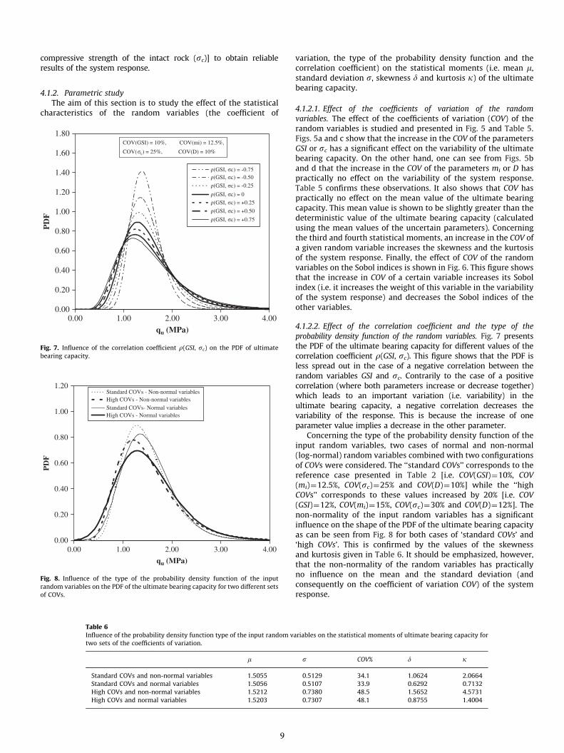
Fig. 8. Influence of the type of the probability density function of the input

random variables on the PDF of the ultimate bearing capacity for two different sets

of COVs.

0.00

0.20

0.40

0.60

0.80

1.00

1.20

1.40

1.60

1.80

0.00 1.00 2.00 3.00 4.00qu (MPa)

PD

F

(GSI, c) = -0.75(GSI, c) = -0.50

(GSI, c) = -0.25

(GSI, c) = 0

(GSI, c) = +0.25

(GSI, c) = +0.50

(GSI, c) = +0.75

COV(GSI) = 10%, COV(mi) = 12.5%,

COV( ) = 25%, COV(D) = 10%

Fig. 7. Influence of the correlation coefficient r(GSI, sc) on the PDF of ultimate

bearing capacity.

9

variation, the type of the probability density function and thecorrelation coefficient) on the statistical moments (i.e. mean m,standard deviation s, skewness d and kurtosis k) of the ultimatebearing capacity.

4.1.2.1. Effect of the coefficients of variation of the random

variables. The effect of the coefficients of variation (COV) of therandom variables is studied and presented in Fig. 5 and Table 5.Figs. 5a and c show that the increase in the COV of the parametersGSI or sc has a significant effect on the variability of the ultimatebearing capacity. On the other hand, one can see from Figs. 5band d that the increase in the COV of the parameters mi or D haspractically no effect on the variability of the system response.Table 5 confirms these observations. It also shows that COV haspractically no effect on the mean value of the ultimate bearingcapacity. This mean value is shown to be slightly greater than thedeterministic value of the ultimate bearing capacity (calculatedusing the mean values of the uncertain parameters). Concerningthe third and fourth statistical moments, an increase in the COV ofa given random variable increases the skewness and the kurtosisof the system response. Finally, the effect of COV of the randomvariables on the Sobol indices is shown in Fig. 6. This figure showsthat the increase in COV of a certain variable increases its Sobolindex (i.e. it increases the weight of this variable in the variabilityof the system response) and decreases the Sobol indices of theother variables.

4.1.2.2. Effect of the correlation coefficient and the type of the

probability density function of the random variables. Fig. 7 presentsthe PDF of the ultimate bearing capacity for different values of thecorrelation coefficient r(GSI, sc). This figure shows that the PDF isless spread out in the case of a negative correlation between therandom variables GSI and sc. Contrarily to the case of a positivecorrelation (where both parameters increase or decrease together)which leads to an important variation (i.e. variability) in theultimate bearing capacity, a negative correlation decreases thevariability of the response. This is because the increase of oneparameter value implies a decrease in the other parameter.

Concerning the type of the probability density function of theinput random variables, two cases of normal and non-normal(log-normal) random variables combined with two configurationsof COVs were considered. The ‘‘standard COVs’’ corresponds to thereference case presented in Table 2 [i.e. COV(GSI)¼10%, COV

(mi)¼12.5%, COV(sc)¼25% and COV(D)¼10%] while the ‘‘highCOVs’’ corresponds to these values increased by 20% [i.e. COV

(GSI)¼12%, COV(mi)¼15%, COV(sc)¼30% and COV(D)¼12%]. Thenon-normality of the input random variables has a significantinfluence on the shape of the PDF of the ultimate bearing capacityas can be seen from Fig. 8 for both cases of ‘standard COVs’ and‘high COVs’. This is confirmed by the values of the skewnessand kurtosis given in Table 6. It should be emphasized, however,that the non-normality of the random variables has practicallyno influence on the mean and the standard deviation (andconsequently on the coefficient of variation COV) of the systemresponse.

ariables on the statistical moments of ultimate bearing capacity for

s COV% d k

0.5129 34.1 1.0624 2.0664

0.5107 33.9 0.6292 0.7132

0.7380 48.5 1.5652 4.5731

0.7307 48.1 0.8755 1.4004

0.00

0.50

1.00

1.50

2.00

2.50

3.00

3.50

-0.75 -0.50 -0.25 0.00 0.25 0.50 0.75

(GSI, c)

B0

(m)

High COVsStandard COVsLow COVsDeterministic design

Fig. 9. Comparison between the probabilistic and the deterministic design.

0.00

0.05

0.10

0.15

0.20

0.25

0.30

0.00 0.50 1.00 1.50

H (

MN

/m)

H = 0.267MN/m( = 23°)

Table 7Reliability index, design point and failure probability for different values of the applied footing load.

Ps (MN/m) F bHL GSIn min sc

n (MPa) Dn Pf (FORM) Pf (MCS) COV (%) (MCS)

0.40 3.75 3.86 20.10 6.87 4.79 0.32 5.77�10�5 5.94�10�5 5.80

0.43 3.50 3.65 20.32 6.92 4.98 0.32 1.32�10�4 1.35�10�4 3.85

0.46 3.25 3.42 20.56 6.98 5.19 0.32 3.08�10�4 3.06�10�4 2.55

0.50 3.00 3.18 20.83 7.04 5.43 0.32 7.27�10�4 7.73�10�4 1.61

0.54 2.75 2.92 21.14 7.11 5.68 0.32 1.74�10�3 1.76�10�3 1.06

0.60 2.50 2.63 21.47 7.19 5.99 0.32 4.21�10�3 4.25�10�3 0.68

0.66 2.25 2.32 21.85 7.27 6.35 0.31 1.02�10�2 1.03�10�2 0.44

0.74 2.00 1.96 22.28 7.37 6.77 0.31 2.48�10�2 2.51�10�2 0.28

0.85 1.75 1.56 22.79 7.49 7.29 0.31 5.94�10�2 5.98�10�2 0.18

0.99 1.50 1.09 23.39 7.62 7.94 0.30 1.37�10�1 1.38�10�1 0.11

1.19 1.25 0.54 24.12 7.78 8.78 0.30 2.93�10�1 2.95�10�1 6.92�10�2

1.49 1.00 �0.13 25.06 7.98 9.93 0.30 5.52�10�1 5.53�10�1 4.02�10�2

1.99 0.75 �1.00 26.33 8.24 11.65 0.29 8.41�10�1 8.42�10�1 1.94�10�2

2.98 0.50 �2.22 28.26 8.62 14.57 0.29 9.87�10�1 9.87�10�1 5.13�10�3

4.96 0.30 �3.76 30.98 9.12 19.26 0.28 1.00 1.00 4.25�10�4

4.1.3. Reliability analysis

This section aims at performing a reliability analysis using themeta-model of the ultimate bearing capacity deduced from a PCEof order 6. Table 7 presents the Hasofer–Lind reliability index bHL,the corresponding design point (GSIn, mi

n, scn and Dn) and the

probability of failure Pf computed by FORM for different values ofthe applied footing load Ps. This table also presents the probabilityof failure Pf computed by Monte Carlo Simulation (MCS) on themeta-model and the corresponding coefficient of variation for anumber of simulations NMCS¼5,000,000 samples. All these resultsare presented for the case of uncorrelated and lognormal randomvariables. Notice that the performance function used in this sectionis G¼Pu�Ps, where Pu and Ps are, respectively, the ultimate footingload (Pu¼quB) and the applied footing load.

From Table 7, one can notice that the reliability index bHL

decreases and consequently, the probability of failure Pf increases,when the value of the applied footing load increases (i.e. when thesafety factor F¼Pu/Ps decreases). When the applied footing load Ps

is equal to the ultimate footing load (i.e. F¼1), the values of therandom variables at the design point are very close (not exactlyequal because the input random variables are non-normal) totheir mean values, and the corresponding probability of failure isnearly equal to 50%. In fact, the value of the design point is exactlyequal to the equivalent normal mean point. Concerning the failureprobability Pf computed by FORM and MCS, Table 7 shows that aslong as the failure probability is small, the corresponding coeffi-cient of variation is important which indicates the inaccuracy ofthe estimated Pf (i.e. a greater number of samples is required).However, concerning the high failure probabilities correspondingto great values of the applied footing load, they seem to be wellestimated by the current MCS with a very small coefficient ofvariation. For the practical case F¼3, the failure probability isequal to 7.73�10�4 and the corresponding COV is 1.61% which issmaller than the commonly adopted value used in the literature(i.e. 10%). Finally, notice that the failure probability computed via

FORM approximation is found to have a good agreement with theone obtained from MCS for different values of the applied footingload Ps. This explains that the limit state surface in this case isalmost linear around the design point, which allows one to obtaina good approximation by using FORM.

V (MN/m)

Fig. 10. Interaction diagram (H, V) for the case of an inclined loading.

4.1.4. Reliability-based design

The conventional deterministic approach used in the design of avertically loaded foundation consists in prescribing a target safetyfactor (generally F¼3) regardless of the uncertainties involved in theinput parameters. Recently, a reliability-based design (RBD) approach

10

has been used by several authors [28 among others]. This approachwas used in this section since it allows one to take into account theinherent uncertainties of the input parameters in a rational way.

The ‘‘probabilistic foundation breadth’’ B0 in this case is computedaccording to a target reliability index of 3.8. Note that this value isthat suggested in the head Eurocode (EN 1990:2002 – Eurocode:Basis of Design) upon which Eurocode 7 and the other Eurocodes arebased [29] for the ultimate limit states. The performance functionused in this section is G¼qu�A where A is equal to one-third of theultimate bearing capacity computed using the mean values of therandom variables. The meta-model of the ultimate bearing capacitydeduced from the PCE of order 6 is used and the Hasofer–Lindreliability index bHL is employed to compute the reliability of thefoundation. For a given set of the statistical parameters of therandom variables, the Hasofer–Lind reliability index is computedfor different values of footing breadth by minimization with respectto the different random variables. The breadth of the footing

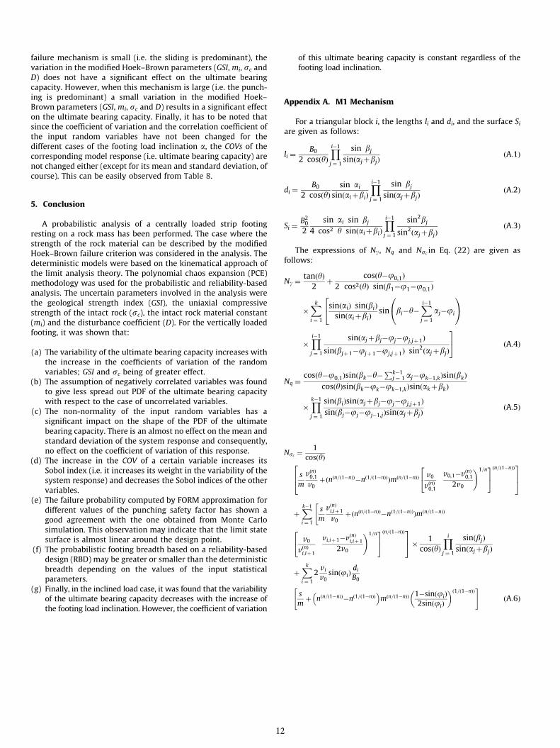
Fig. 12. Failure mechanisms for different

Table 8Statistical moments of the ultimate bearing capacity for different cases

Load inclination

a (1)

5 10 15

m 1.3032 1.1004 0.9090

s 0.4443 0.3758 0.3104

COV% 34.1 34.2 34.2

k 1.0627 1.0672 1.0693

d 2.0710 2.0928 2.1113

0.0

1.0

2.0

3.0

4.0

5.0

6.0

0.00 0.50 1.00 1.50 2.00 2.50 3.00

qu (MPa)

PD

F

α = 5°α = 10°α = 15°α = 23°α = 30°α = 35°α = 40°

COV(GSI) = 10%, COV(σc) = 25% COV(mi) = 12.5%, COV(D) = 10%

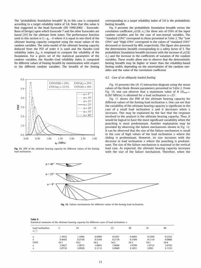
Fig. 11. PDF of the ultimate bearing capacity for different values of the footing

load inclination.

11

corresponding to a target reliability index of 3.8 is the probabilisticfooting breadth.

Fig. 9 presents the probabilistic foundation breadth versus thecorrelation coefficient r(GSI, sc) for three sets of COVs of the inputrandom variables and for the case of non-normal variables. The‘‘standard COVs’’ correspond to those presented in Table 2. The ‘‘LowCOVs’’ and ‘‘High COVs’’ correspond to the values of ‘‘standard COVs’’decreased or increased by 40%, respectively. This figure also presentsthe deterministic breadth corresponding to a safety factor of 3. Theprobabilistic foundation breadth increases with the increase of r(GSI,sc) and the increase in the coefficients of variation of the randomvariables. These results allow one to observe that the deterministicfooting breadth may be higher or lower than the reliability-basedfooting width, depending on the uncertainties of the random vari-ables and the value of the correlation coefficient.

4.2. Case of an obliquely loaded footing

Fig. 10 presents the (H, V) interaction diagram using the meanvalues of the Hoek–Brown parameters presented in Table 2. FromFig. 10, one can observe that a maximum value of H (Hmax¼

0.267 MN/m) is obtained for a load inclination a¼231.Fig. 11 shows the PDF of the ultimate bearing capacity for

different values of the footing load inclination a. One can see thatthe variability of the ultimate bearing capacity is significant in thecase of a small load inclination a and it decreases when aincreases. This may be explained by the fact that the responseinvolved in the analysis is the ultimate bearing capacity. Thus, itwould be logical to have the most significant variability when thepunching is most predominant. Another explanation may beprovided by observing the failure mechanisms shown in Fig. 12.It can be observed that the size of the failure mechanism is smallin the case of high values of the load inclination a where thesliding is predominant. However, its size increases with thedecrease in load inclination a where the punching is predomi-nant. The size of the failure mechanism is maximal in the verticalload case. As expected, the ultimate bearing capacity increaseswith the size of the failure mechanism. Therefore, when the

values of the footing load inclination.

of load inclination a.

23 30 35 40

0.6367 0.4405 0.3260 0.2325

0.2178 0.1509 0.1119 0.0800

34.2 34.3 34.3 34.4

1.0698 1.0709 1.0712 1.0742

2.0969 2.1051 2.095 2.1153

failure mechanism is small (i.e. the sliding is predominant), thevariation in the modified Hoek–Brown parameters (GSI, mi, sc andD) does not have a significant effect on the ultimate bearingcapacity. However, when this mechanism is large (i.e. the punch-ing is predominant) a small variation in the modified Hoek–Brown parameters (GSI, mi, sc and D) results in a significant effecton the ultimate bearing capacity. Finally, it has to be noted thatsince the coefficient of variation and the correlation coefficient ofthe input random variables have not been changed for thedifferent cases of the footing load inclination a, the COVs of thecorresponding model response (i.e. ultimate bearing capacity) arenot changed either (except for its mean and standard deviation, ofcourse). This can be easily observed from Table 8.

5. Conclusion

A probabilistic analysis of a centrally loaded strip footingresting on a rock mass has been performed. The case where thestrength of the rock material can be described by the modifiedHoek–Brown failure criterion was considered in the analysis. Thedeterministic models were based on the kinematical approach ofthe limit analysis theory. The polynomial chaos expansion (PCE)methodology was used for the probabilistic and reliability-basedanalysis. The uncertain parameters involved in the analysis werethe geological strength index (GSI), the uniaxial compressivestrength of the intact rock (sc), the intact rock material constant(mi) and the disturbance coefficient (D). For the vertically loadedfooting, it was shown that:

(a)

The variability of the ultimate bearing capacity increases withthe increase in the coefficients of variation of the randomvariables; GSI and sc being of greater effect.

(b)

The assumption of negatively correlated variables was foundto give less spread out PDF of the ultimate bearing capacitywith respect to the case of uncorrelated variables.

(c)

The non-normality of the input random variables has asignificant impact on the shape of the PDF of the ultimatebearing capacity. There is an almost no effect on the mean andstandard deviation of the system response and consequently,no effect on the coefficient of variation of this response.

(d)

The increase in the COV of a certain variable increases itsSobol index (i.e. it increases its weight in the variability of thesystem response) and decreases the Sobol indices of the othervariables.

(e)

The failure probability computed by FORM approximation fordifferent values of the punching safety factor has shown agood agreement with the one obtained from Monte Carlosimulation. This observation may indicate that the limit statesurface is almost linear around the design point.

(f)

The probabilistic footing breadth based on a reliability-baseddesign (RBD) may be greater or smaller than the deterministicbreadth depending on the values of the input statisticalparameters.

(g)

Finally, in the inclined load case, it was found that the variabilityof the ultimate bearing capacity decreases with the increase ofthe footing load inclination. However, the coefficient of variation

12

of this ultimate bearing capacity is constant regardless of thefooting load inclination.

Appendix A. M1 Mechanism

For a triangular block i, the lengths li and di, and the surface Si

are given as follows:

li ¼B0

2 cosðyÞ

Yi�1

j ¼ 1

sin bj

sinðajþbjÞðA:1Þ

di ¼B0

2 cosðyÞsin ai

sinðaiþbiÞ

Yi�1

j ¼ 1

sin bj

sinðajþbjÞðA:2Þ

Si ¼B2

0

2

sin ai sin bj

4 cos2 y sinðaiþbiÞ

Yi�1

j ¼ 1

sin2bj

sin2ðajþbjÞ

ðA:3Þ

The expressions of Ng, Nq and Nsc in Eq. (22) are given asfollows:

Ng ¼tanðyÞ

2þ

cosðy�j0,1Þ

2 cos2ðyÞ sinðb1�j1�j0,1Þ

�Xk

i ¼ 1

sinðaiÞ sinðbiÞ

sinðaiþbiÞsin bi�y�

Xi�1

j ¼ 1

aj�ji

0@

1A

24

�Yi�1

j ¼ 1

sinðajþbj�jj�jj,jþ1Þ

sinðbjþ1�jjþ1�jj,jþ1Þ sin2ðajþbjÞ

35 ðA:4Þ

Nq ¼cosðy�j0,1Þsinðbk�y�

Pk�1j ¼ 1 aj�jk�1,kÞsinðbkÞ

cosðyÞsinðbk�jk�jk�1,kÞsinðakþbkÞ

�Yk�1

j ¼ 1

sinðbiÞsinðajþbj�jj�jj,jþ1Þ

sinðbj�jj�jj�1,jÞsinðajþbjÞðA:5Þ

Nsc ¼1

cosðyÞ

s

m

vðnÞ0,1

v0þðnðn=ð1�nÞÞ�nð1=ð1�nÞÞÞmðn=ð1�nÞÞ v0

vðnÞ0,1

v0,1�vðnÞ0,1

2v0

!1=n24

35ðn=ð1�nÞÞ

264

375

þXk�1

i ¼ 1

s

m

vðnÞi,iþ1

v0þðnðn=ð1�nÞÞ�nð1=ð1�nÞÞÞmðn=ð1�nÞÞ

"

v0

vðnÞi,iþ1

vi,iþ1�vðnÞi,iþ1

2v0

!1=n24

35ðn=ð1�nÞÞ35� 1

cosðyÞ

Yi

j ¼ 1

sinðbjÞ

sinðajþbjÞ

þXk

i ¼ 1

2vi

v0sinðjiÞ

di

B0

s

mþ nðn=ð1�nÞÞ�nð1=ð1�nÞÞ�

mðn=ð1�nÞÞ 1�sinðjiÞ

2sinðjiÞ

� �ð1=ð1�nÞÞ" #

ðA:6Þ

Appendix B. M2 Mechanism

For a triangular block i, the lengths li and di, and the surface Si

are given as follows:

li ¼ B0sin b1

sinða1þb1Þ

Yi

j ¼ 2

sin bj

sinðajþbjÞðB:1Þ

di ¼ B0sin b1

sinða1þb1Þ

sin ai

sin bi

Yi sin bj

sinðajþbjÞðB:2Þ

j ¼ 2

G6¼Xk�1

i ¼ 1

s

m

vðnÞi,iþ1

v1

sin b1

sinða1þb1Þ

Yi

j ¼ 2

sin bj

sinðajþbjÞ

þðnn=ð1�nÞ�n1=ð1�nÞÞmn=ð1�nÞ

24 v1

vðnÞi,iþ1

vi,iþ1�vðnÞi,iþ1

2v1

!1=n35n=ð1�nÞ

sin b1

sinða1þb1Þ

Yi

j ¼ 2

sin bj

sinðajþbjÞ

37777777775

266666666664

ðB:12Þ

Si ¼B2

0

2

sin2 b1

sin2ða1þb1Þ

sin aisinðaiþbiÞ

sin bj

Yi

j ¼ 2

sin2 bj

sin2ðajþbjÞ

ðB:3Þ

The expressions of Ng, Nq and Nsc in Eq. (22) are given asfollows:

Ng ¼�1

sinðb1�j1Þþtana cosðb1�j1ÞðG1þtan a:G2Þ ðB:4Þ

Nq ¼�1

sinðb1�j1Þþtan a cosðb1�j1ÞðG3þtan a:G4Þ ðB:5Þ

Nsc ¼1

sinðb1�j1Þþtan a cosðb1�j1ÞðG5þtan a:G6Þ ðB:6Þ

where

G1¼sin2 b1

sin2ða1þb1Þ

Xk

i ¼ 1

sin ai sinðaiþbiÞ

sin bi

sin bi�ji�Xi�1

j ¼ 1

aj

0@

1A

�Yi

j ¼ 2

sin2 bj

sin2ðajþbjÞ

Yi�1

j ¼ 1

sinðajþbj�jj�jj�1,jÞ

sinðbjþ1�jjþ1�jj�1,jÞ

26666664

37777775

ðB:7Þ

G2¼sin2 b1

sin2ða1þb1Þ

Xk

i ¼ 1

sin ai sinðaiþbiÞ

sin bi

cos bi�ji�Xi�1

j ¼ 1

aj

0@

1A

�Yi

j ¼ 2

sin2 bj

sin2ðajþbjÞ

Yi�1

j ¼ 1

sinðajþbj�jj�jj�1,jÞ

sinðbjþ1�jjþ1�jj�1,jÞ

26666664

37777775

ðB:8Þ

G3¼sin b1

sinða1þb1Þsin bk�jk�

Xk�1

j ¼ 1

aj

0@

1A

�Yk

j ¼ 2

sin bj

sinðajþbjÞ

Yk�1

j ¼ 1

sinðajþbj�jj�jj�1,jÞ

sinðbjþ1�jjþ1�jj�1,jÞðB:9Þ

G4¼sinb1

sinða1þb1Þcos bk�jk�

Xk�1

j ¼ 1

aj

0@

1A

13

�Yk

j ¼ 2

sinbj

sinðajþbjÞ

Yk�1

j ¼ 1

sinðajþbj�jj�jj�1,jÞ

sinðbjþ1�jjþ1�jj�1,jÞðB:10Þ

G5¼Xk

i ¼ 1

s

m

vðnÞi

v1

sin ai

sin bi

sin b1

sinða1þb1Þ

Yi

j ¼ 2

sin bj

sinðajþbjÞ

24

þðnn=ð1�nÞ�n1=ð1�nÞÞmn=ð1�nÞ v1

vðnÞi,iþ1

vi,iþ1�vðnÞi,iþ1

2v1

!1=n24

35

n=ð1�nÞ

sin ai

sin bi

sin b1

sinða1þb1Þ

Yi

j ¼ 2

sin bj

sinðajþbjÞ

35 ðB:11Þ

References

[1] Soubra AH. Upper-bound solutions for bearing capacity of foundations.J Geotech Geoenviron Eng ASCE 1999;125(1):59–68.

[2] Maghous S, de Buhan P, Bekaert A. Failure design of jointed rock structures bymeans of a homogenization approach. Mech Cohesive-Frictional Mater1998;3:207–28.

[3] Yang XL, Yin JH. Upper bound solution for ultimate bearing capacity with amodified Hoek–Brown failure criterion. Int J Rock Mech Min Sci 2005;42:550–60.

[4] Saada Z, Maghous S, Garnier D. Bearing capacity of shallow foundations onrocks obeying a modified Hoek–Brown failure criterion. Comput Geotech2008;35:144–54.

[5] Griffiths DV, Fenton GA. Bearing capacity of spatially random soil: theundrained clay Prandtl problem revisited. Geotechnique 2001;51(4):351–9.

[6] Fenton GA, Griffiths DV. Bearing-capacity prediction of spatially random c–jsoils. Can Geotech J 2003;40:64–5.

[7] Przewlocki J. A stochastic approach to the problem of bearing capacity by themethod of characteristics. Comput Geotech 2005;32:370–6.

[8] Popescu R, Deodatis G, Nobahar A. Effects of random heterogeneity of soilproperties on bearing capacity. Probab Eng Mech 2005;20:324–41.

[9] Youssef Abdel Massih DS, Soubra AH, Low BK. Reliability-based analysis anddesign of strip footings against bearing capacity failure. J Geotech GeoenvironEng ASCE 2008;134(7):917–28.

[10] Youssef Abdel Massih DS, Soubra AH. Reliability-based analysis of stripfootings using response surface methodology. Int J Geomech ASCE 2008;8(2):134–43.

[11] Soubra AH, Youssef Abdel Massih DS. Probabilistic analysis and design at theultimate limit state of obliquely loaded strip footings. Geotechnique2010;60(4):275–85.

[12] Cho SE, Park HC. Effect of spatial variability of cross-correlated soil propertieson bearing capacity of strip footing. Int J Numer Anal Meth Geomech2010;34:1–26.

[13] Isukapalli SS, Roy A, Georgopoulos PG. Stochastic response surface methods(SRSMs) for uncertainty propagation: application to environmental andbiological systems. Risk Anal 1998;18(3):357–63.

[14] Phoon KK, Haung SP. Geotechnical probabilistic analysis using collocation-based stochastic response surface method. In: Kanda J, Takada T, Furuta H,editors. Applications of statistics and probability in civil engineering,Tokyo, 2007.

[15] Huang SP, Liang B, Phoon KK. Geotechnical probabilistic analysis by colloca-tion-based stochastic response surface method: an EXCEL add-in implemen-tation. Georisk 2009;3(2):75–86.

[16] Isukapalli SS. An uncertainty analysis of transport-transformation models.PhD thesis, Rutgers Univ, New Jersey, 1999.

[17] Xiu D, Karniadakis GE. The Wiener–Askey polynomial chaos for stochasticdifferential equations. J Sci Comput 2002;24(2):619–44.

[18] Webster M, Tatang M, McRae G. Application of the probabilistic collocationmethod for an uncertainty analysis of a simple ocean model. Technicalreport, MIT joint program on the science and policy of global change, Reportsseries no. 4. Cambridge, MA: MIT; 1996.

[19] Sudret B. Global sensitivity analysis using polynomial chaos expansion.Reliab Eng System Saf 2008;93:964–79.

[20] Blatman G, Sudret B. An adaptive algorithm to build up sparse polynomialchaos expansions for stochastic finite element analysis. Probab Eng Mech2010;25:183–97.

[21] Hoek E, Brown E. Empirical strength criterion for rock masses. J Geotech EngDiv 1980;106(GT9):1013–35.

[22] Hoek E, Marinos P. A brief history of the development of the Hoek–Brownfailure criterion. Soils Rocks 2007;30(2):85–92.

[23] Brown ET. Estimating the mechanical properties of rock masses. In: Potvin Y,Carter J, Dyskin A, Jeffrey R, Editors. Proc 1st southern hemisphere int rockmech symp, Perth, vol. 1; 2008, pp. 3–21.

[24] Hoek E, Carranze-Torres C, Corkum B. Hoek–Brown failure criterion-2002edition. In: Proc North Am rock mech symp, Toronto, July 2002, p. 267–73.

14

[25] Hoek E, Brown ET. Practical estimates of rock mass strength. Int J Rock MechMin Sci 1997;34(8):1165–86.

[26] Collins IF, Gunn CIM, Pender MJ, Yan W. Slope stability analyses for materialswith a nonlinear failure envelope. Int J Num Anal Meth Geomech 1988;12:533–50.

[27] Hoek E. Reliability of Hoek–Brown estimates of rock mass properties andtheir impact on design. Technical note. Int J Rock Mech Min Sci 1998;35:63–8.

[28] Phoon KK, Kulhawy FH, Grigoriu MD. Multiple resistance factor design forshallow transmission line structure foundations. J Geotech Geoenviron Eng2003;129:807–18.

[29] Orr TL, Breysse D. Eurocode 7 and reliability based design. In: Phoon KK,editor. Reliability-based design in geotechnical engineering: computationsand applications. London: Taylor & Francis; 2008 [Chapter8].