1

Probabilistic AHP and TOPSIS for Multi-Attribute Decision-Making under Uncertainty

Jarret M. Lafleur

Daniel Guggenheim School of Aerospace Engineering Georgia Institute of Technology

270 Ferst Drive Atlanta, GA 30332

404-894-7783 jarret.m.lafleur@gatech.edu

Abstract—One challenging aspect in designing complex engineering systems is the task of making informed design decisions in the face of uncertainty.1,2 This paper presents a probabilistic methodology to facilitate such decision-making, in particular under uncertainty in decision-maker preferences. This methodology builds on the frequently-used multi-attribute decision-making techniques of the Analytic Hierarchy Process (AHP) and Technique for Order Preference by Similarity to Ideal Solution (TOPSIS), and it overcomes some typical limitations that exist in relying on these deterministic techniques. The methodology is divided into three segments, each of which consists of multiple steps. The first segment (steps 1-4) involves setting up the problem by defining objectives, priorities, uncertainties, design attributes, and candidate designs. The second segment (steps 5-8) involves applications of AHP and TOPSIS using AHP prioritization matrices generated from probability density functions. The third segment (steps 9-10) involves visualization of results to assist in selecting a final design. A key characteristic measured in these final steps is the consistency with which a design ranks among the top several alternatives. An example satellite orbit and launch vehicle selection problem illustrates the methodology throughout the paper.

TABLE OF CONTENTS

1. INTRODUCTION .................................................................1 2. METHODOLOGY ...............................................................4 3. CONCLUSION ..................................................................16 ACKNOWLEDGEMENTS ......................................................16 APPENDIX: NOMENCLATURE ............................................17 REFERENCES ......................................................................17 BIOGRAPHY ........................................................................18

1. INTRODUCTION

One challenging aspect in designing complex engineering systems is the task of making informed design decisions in the face of uncertainty. Typically, uncertainty about system performance and cost is high in early design phases since little hardware has yet been produced. Moreover, during these early design phases, the engineer is faced with the 1978-1-4244-7351-9/11/$26.00 ©2011 IEEE. 2 IEEEAC paper #1135, Version 2, Updated January 9, 2011

challenge of trading system performance and cost objectives against each other, and the decision-maker’s preferences for one objective over another (e.g., how much he or she prefers high performance over low cost) are also uncertain.

The study of multi-attribute decision-making has made significant strides over the past several decades in developing approaches to informing decisions that depend on trades among multiple deterministic attributes. Developments have also been made in incorporating uncertainty into the estimation of system attributes (for example, through Monte Carlo simulation). The work presented here combines these probabilistic methods with the multi-attribute decision-making techniques of the Analytic Hierarchy Process (AHP) and Technique for Order Preference by Similarity to Ideal Solution (TOPSIS) in order to facilitate informed decisions under uncertainty in decision-maker preferences. Provided are a description of the decision-making methodology, application to a sample practical engineering scenario, and sample visualization of results.

Brief Overview of AHP and TOPSIS

The primary contributions of this paper are in (1) combining probabilistic versions of the AHP and TOPSIS tools, (2) visualizing and summarizing the resulting data in a meaningful way, and (3) demonstrating this method for a practical engineering scenario. Since this requires the reader to be familiar with AHP and TOPSIS in advance, provided here is a brief overview of these tools and previous work incorporating uncertainty information.

Analytic Hierarchy Process (AHP) — Developed by Saaty in the mid-1970s [1-3], the Analytic Hierarchy Process (AHP) is a multi-attribute decision-making technique that allows for the prioritization of objectives and selection of alternatives based on a set of pairwise comparisons. Objectives are prioritized by first populating a matrix of pairwise comparisons describing each objective’s importance relative to each other objective.3 The pairwise

3 There is a subtle distinction between the terms “attribute” and “objective”, which is that an objective is an attribute with direction. For example, “cost” is an attribute while “low cost” is an objective. Despite AHP’s classification as a multi-attribute decision-making (MADM) technique, the

2

comparison matrix consists of elements aij and is reciprocal, i.e., such that aji = 1/aij. This matrix is then reduced to a vector of weights describing the relative importance of each objective. If multiple alternative concepts are to be evaluated according to these weights, each concept is compared to each other concept in a pairwise manner in terms of each objective category. Using the objective weights vector, scores from each single-objective concept comparison matrix are then aggregated into a single score vector describing the relative desirability of each concept. From here, the user may either select the highest-scoring concept or distribute resources to all concepts according to the weights [2]. A diagram of the AHP hierarchy is shown in Fig. 1.

Over the past three decades, AHP has become a common tool for decision-making. One advantage is its versatility in that it can be used for both objective prioritization and concept selection. While a number of multi-attribute decision-making techniques address the concept selection procedure assuming that objective weights are known, AHP is distinct in its simple but structured approach for obtaining these weights. The pairwise comparison method is straightforward, and its internal consistency can be notion of direction (and therefore objectives) is essential in order for decisions to be made. Confusion can exist because multi-objective decision-making (MODM) is a classification of techniques distinct from MADM, but the distinction does not lie in the use of objectives over attributes. Rather, MADM deals with concept selection from a list of possible solutions while MODM deals with concept design when a list of solutions does not exist. To be clear, this paper deals only with MADM techniques.

evaluated through methods proposed by Saaty [1-3]. AHP is also flexible in its ability to handle both qualitative and quantitative (ratio-scale) judgement inputs. However, disadvantages exist in that pairwise comparisons become time-consuming as the number of objectives and alternatives increases.4 Furthermore, the conventional use of AHP is deterministic, which hinders the user’s ability to generate confidence estimates in the final results.

Pertinent to this paper is the history of probabilistic modifications to the original deterministic version of AHP. One of the earliest analyses in this area by Vargas, one of Saaty’s colleagues, in 1982 considered the implications of assuming that the ½ · (n² – n) pairwise comparisons in the AHP matrices are independent gamma-distributed random variables [5]. A 1991 study by Zahir suggested beta distributions for each pairwise comparison but introduced a distribution-neutral uncertainty analysis, assuming only an uncertainty Δaij in each comparison. The 1991 study developed analytic expressions for priority uncertainties in the case of n = 2 and n = 3 items and suggested that it is possible to have consistency but still have uncertainty within an AHP matrix [6]. Around the same time, Rahman and Shrestha showed that uncertainty could be approximated through the inconsistency of the pairwise comparison matrix [7-9],5 and some recent papers have

4 The number of pairwise comparisons required for an AHP matrix is ½ · (n² – n), where n is the number of items to be compared. It is the n² dependence that drives the unmanageability of the comparisons as n becomes large.

5 This clearly conflicts with the finding of Zahir that inconsistency and

Objective#n

Des

ign

#1

Des

ign

#2

Des

ign

#3

Des

ign

#4

Des

ign

#k

Design #1 1 1 7 3 1/7Design #2 1 1 3 2 3Design #3 1/7 1/3 1 1/9 1/2Design #4 1/3 1/2 9 1 5Design #k 7 1/3 2 1/5 1

Objective#2

Des

ign

#1

Des

ign

#2

Des

ign

#3

Des

ign

#4

Des

ign

#k

Design #1 1 5 8 2 1/2Design #2 1/5 1 9 3 5Design #3 1/8 1/9 1 1/2 1/9Design #4 1/2 1/3 2 1 2Design #k 2 1/5 9 1/2 1

Objective#1

Des

ign

#1

Des

ign

#2

Des

ign

#3

Des

ign

#4

Des

ign

#k

Design #1 1 3 7 4 1/5Design #2 1/3 1 8 2 3Design #3 1/7 1/8 1 1/2 1/9Design #4 1/4 1/2 2 1 1Design #k 5 1/3 9 1 1

Obj

ect

ive

#1

Obj

ect

ive

#2

Obj

ect

ive

#3

Obj

ect

ive

#4

Obj

ect

ive

#n

Objective #1 1 2 5 2 1/3Objective #2 1/2 1 7 1 1Objective #3 1/5 1/7 1 1/5 1/8Objective #4 1/2 1 5 1 1Objective #n 3 1 8 1 1

G1G1

O1O1

D2D2

Level IOverall Goal

Level IIAttributes/Objectives

Level IIIAlternatives/Designs

O2O2 OnOn

D1D1 D3D3 DkDk

Objective#n

Des

ign

#1

Des

ign

#2

Des

ign

#3

Des

ign

#4

Des

ign

#k

Design #1 1 1 7 3 1/7Design #2 1 1 3 2 3Design #3 1/7 1/3 1 1/9 1/2Design #4 1/3 1/2 9 1 5Design #k 7 1/3 2 1/5 1

Objective#2

Des

ign

#1

Des

ign

#2

Des

ign

#3

Des

ign

#4

Des

ign

#k

Design #1 1 5 8 2 1/2Design #2 1/5 1 9 3 5Design #3 1/8 1/9 1 1/2 1/9Design #4 1/2 1/3 2 1 2Design #k 2 1/5 9 1/2 1

Objective#1

Des

ign

#1

Des

ign

#2

Des

ign

#3

Des

ign

#4

Des

ign

#k

Design #1 1 3 7 4 1/5Design #2 1/3 1 8 2 3Design #3 1/7 1/8 1 1/2 1/9Design #4 1/4 1/2 2 1 1Design #k 5 1/3 9 1 1

Obj

ect

ive

#1

Obj

ect

ive

#2

Obj

ect

ive

#3

Obj

ect

ive

#4

Obj

ect

ive

#n

Objective #1 1 2 5 2 1/3Objective #2 1/2 1 7 1 1Objective #3 1/5 1/7 1 1/5 1/8Objective #4 1/2 1 5 1 1Objective #n 3 1 8 1 1

G1G1

O1O1

D2D2

Level IOverall Goal

Level IIAttributes/Objectives

Level IIIAlternatives/Designs

O2O2 OnOn

D1D1 D3D3 DkDk

Figure 1 – Schematic depiction of AHP hierarchy (adapted from [4]). Pairwise comparisons are performed among attributes/objectives at the overall goal level and among alternatives/designs at the attribute/objective level.

3

developed the idea of estimating uncertainties without explicitly requiring the user to provide additional information [10-11]. The more traditional approach (of which the present work is one) of requiring users to provide information on the uncertainty of the individual pairwise comparisons is employed by studies by Hauser and Tadikamalla, Rosenbloom, and Hihn and Lum [12-14].

Technique for Order Preference by Similarity to Ideal Solution (TOPSIS) — The Technique for Order Preference by Similarity to Ideal Solution (TOPSIS) is a multi-attribute decision-making technique developed around 1980 by Yoon and Hwang [15-16] that allows for scoring of alternatives based on their euclidean distances from positive and negative ideal solutions. As Fig. 2 illustrates, the TOPSIS positive ideal design is an imaginary design representing the combination of the best performance attributes of the entire set of designs considered. This design probably does not exist in the actual space of alternatives, but the decision-maker would prefer to select a solution “as close as possible” [17] to it. Similarly, the negative ideal design is an imaginary design representing the combined worst attributes of the entire set of designs considered. Presumably, the decision-maker would prefer an alternative “as far as possible” from the negative ideal, and the need for consideration of both negative and positive ideal designs becomes clear for scenarios in which a series of designs has identical distances to the positive ideal but varying distances to the negative ideal.

TOPSIS too has found broad use for decision-making applications over the past few decades. Advantages include its fairly intuitive physical meaning based on consideration of distances from ideal solutions (e.g., see Fig. 2), the fact that it reflects the empirical phenomenon of diminishing marginal rates of substitution [15, 18], and its consideration of performance characteristics directly, rather than through pairwise comparisons. The latter makes it particularly useful for scenarios in which dozens, hundreds, or thousands of alternative designs are considered (i.e., where pairwise comparisons become impractical) and for scenarios in which performance metrics can be computed directly rather than rated in a qualitative fashion.

However, TOPSIS still requires the specification of weightings on objectives (e.g., to determine the scaling or “stretching” of the axes in Fig. 2). Thus, a method like AHP is still required in order to determine proper objective weightings.6 Additionally, like AHP, TOPSIS in its standard form is deterministic and does not consider uncertainty in weightings. Much of the literature on overcoming this limitation focuses on the application of

uncertainty are conceptually different, and the issue seems to be unresolved in the literature.

6 For this reason, deterministic combinations of AHP and TOPSIS are somewhat common in the literature, such as in [19-21].

fuzzy logic [22-25], whereas this paper focuses on the use of longer-established probabilistic techniques.

Example Application: Orbit and Launch Vehicle Decision for a Small Reconnaissance Satellite

Integrated throughout this paper is an example application of this method to the scenario of choosing a launch vehicle and circular orbit for a small, responsive military reconnaissance satellite. In this scenario, a 400 kg satellite is to be launched to monitor activity at an unfriendly missile launch site at 40.85°N latitude, and the decision-maker must choose the orbit in which to place the satellite as well as what launch vehicle to use. The on-board targeted sensor is assumed to have a total field of view angle of 1° and a nadir ground sample distance of 1.0 m at a reference altitude of 400 km. The satellite’s ballistic coefficient is assumed to be 110 kg/m², a representative average for satellites [26, 27], and minimal propellant is available for orbit maintenance.

This class of mission and spacecraft is similar in some respects to the 2006 TacSat-2 project, a joint effort among Department of Defense organizations and NASA. TacSat-2 was launched on December 16, 2006 from Wallops Flight Facility in Virginia with the mission of both demonstrating responsive space capabilities and delivering 11 onboard instrument packages and experiments [28-29]. The mass of TacSat-2 was 370 kg, and it was launched aboard a Minotaur I rocket to a 40° inclined circular orbit with an altitude of approximately 410 km [28-29]. The imager carried aboard TacSat-2 had a 1º field of view and an expected ground sample distance resolution of 1 m.7

7 M.P. Kleiman, Kirtland AFB, Personal Communication, 26 Oct. 2009.

Objective #1

Obj

ectiv

e #2

Better Worse

Bet

ter

Wor

se

Objective Space

Positive Ideal Design

Negative Ideal Design

Objective #1

Obj

ectiv

e #2

Better Worse

Bet

ter

Wor

se

Objective Space

Positive Ideal DesignPositive Ideal Design

Negative Ideal DesignNegative Ideal Design

Figure 2 – Depiction of TOPSIS in two dimensions. Small black circles represent alternatives represented in terms of how they perform with respect to Objectives #1

and #2.

4

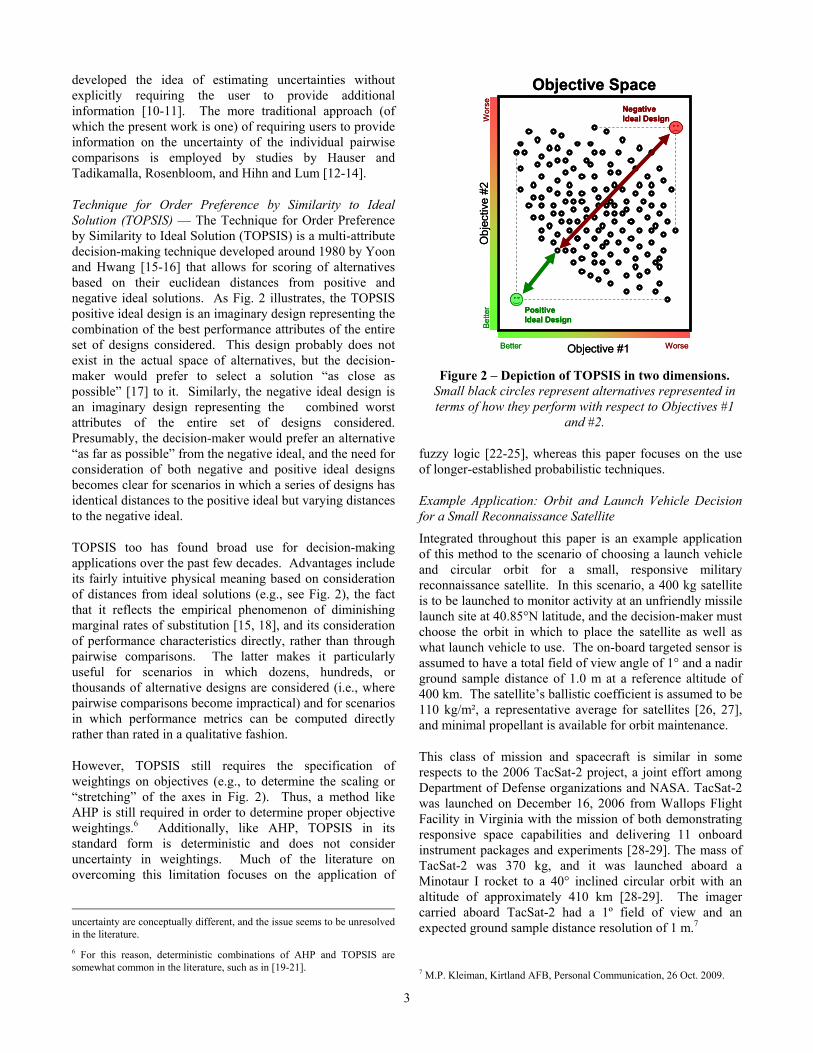
2. METHODOLOGY

Figure 3 summarizes the basic steps of the probabilistic AHP and TOPSIS methodology introduced in this paper. Each step is covered in detail in this section and is illustrated using the satellite application defined in Section 1. Overall, the methodology is divided into three segments, each of which consists of multiple steps. The first segment, consisting of steps 1-4 and to the left in Fig. 3, involves setting up the problem by defining objectives, priorities, uncertainties, design attributes, and alternatives (candidate designs). This segment also involves the evaluation of each candidate design with respect to the defined attributes. Most of these steps, with the exception of the specification of uncertainties in step 4, would normally be required even in a deterministic decision process. The second segment, which consists of steps 5-8 in Fig. 3 and is easily automated, involves several thousand applications of AHP and TOPSIS under different (random) AHP prioritization matrices based on probability density functions (PDFs) assigned in step 4. The third segment, consisting of steps 9-10 and to the right in Fig. 3, involves visualization of the results to assist in making a final design selection.

Setting up the Problem

Detailed next are the first four steps of the methodology outlined in Fig. 3. These steps are focused on setting up the decision problem in terms of objectives, priorities, uncertainties, design attributes, and alternatives. Most of these steps would normally be required in a deterministic decision process, and step 4 describes the additional inputs required for the desired probabilistic process.

Step 1: Generate List of Objectives/Attributes — As shown in Fig. 3, the first step in this methodology is the specification of objectives and attributes for consideration

in the design problem. These objectives and attributes are application-specific, and brainstorming exercises may be required to determine the relevant objectives for a particular application; however, for this methodology to be effective, attributes must be quantifiable. In the case of inherently qualitative attributes, the user may decide to use a quantitative scale to convert a qualitative degree to a number (common choices include, for example, mapping “low/medium/high” ratings to a 1-3-5 or 1-3-9 scale).

Table 1 lists the objectives for the example satellite application used throughout this paper. In this particular application, all attributes are quantifiable. One objective is high launch margin, defined as the difference between actual and required payload capability divided by the required capability. Since satellite mass is given in this example (400 kg), this attribute is governed by the selection of launch vehicle. Two additional objectives, low launch cost and high launch reliability, are also governed by the selection of launch vehicle. Image field of view (FOV) and nadir ground sample distance (GSD) are measures of the breadth and resolution of the resulting reconnaissance images, both of which depend on the altitude of the selected orbit. Higher orbits produce greater the fields of view but also lower resolution (i.e., larger ground sample distance). Mean worst-case daily data latency refers to the maximum time a user must wait between image acquisition and downlink to the ground, averaged over a range of dates and assuming use of the Schriever Air Force Base Air Force Satellite Control Network (AFSCN) node in Colorado for downlink. Mean daily coverage time refers to the average amount of time per day that the target site is visible from the satellite. Both the data latency and daily coverage attributes depend on orbit altitude and inclination. Finally, orbit lifetime is an estimate of the amount of time the satellite can remain in orbit assuming no reboost maneuvers. Since this attribute depends on atmospheric drag, it is altitude-dependent.

Generate list of objectives/

attributes

Populate AHP objectives pairwisecomparison matrix, including PDFs on

each element

Repeated Sub-Process

Monte Carlo Simulation

Select* an AHP objectives pairwise comparison matrix, based on PDFs for each element

*Selections in this step are automated as part of the Monte Carlo simulation.

Determine traditional deterministic AHPobjectives priority vector (weightings)

Apply traditional deterministic TOPSIS

Record scores and rank order of alternatives

Visualize and Review Results

Select Alternative(s)

Evaluate and record each design’s performance with respect to each attribute

1

4

5

6

7

8

10

3

Generate list of candidate

designs

2

9

Generate list of objectives/

attributes

Populate AHP objectives pairwisecomparison matrix, including PDFs on

each element

Repeated Sub-Process

Monte Carlo Simulation

Select* an AHP objectives pairwise comparison matrix, based on PDFs for each element

*Selections in this step are automated as part of the Monte Carlo simulation.

Determine traditional deterministic AHPobjectives priority vector (weightings)

Apply traditional deterministic TOPSIS

Record scores and rank order of alternatives

Visualize and Review Results

Select Alternative(s)

Evaluate and record each design’s performance with respect to each attribute

1

4

5

6

7

8

10

3

Generate list of candidate

designs

2

9

Figure 3 – Probabilistic AHP and TOPSIS Flowchart.

5

Step 2: Generate List of Candidate Designs — The second step in this methodology is the specification of all candidate designs to be evaluated. If the set of possible designs is small (e.g., a dozen or less), candidate designs may be enumerated manually. If the trade space is large and unmanageable (e.g., consisting of billions or trillions of designs), themed or otherwise brainstormed designs may generated with the assistance of a morphological matrix [30-31]. If the trade space is large but manageable (e.g., consisting of dozens to millions of designs), it is likely feasible to enumerate every possible design within the design variable ranges and resolutions of interest; this more rigorous approach is used in the example application here.

Table 2 lists the three design variables defined for this application. These are the variables for which values can be chosen by the decision maker. The launch vehicle can be selected from one of twelve domestic options that are well-suited to launching small payloads. Orbit altitude can take on seven values between 200 and 2000 km, and orbit inclination can take one of ten values between 0° and 90°. Overall, this represents 840 discrete design options.

Step 3: Evaluate each Design’s Performance with respect to each Attribute — In this third step, each candidate design from the second step is evaluated according to the attributes of the first step. The methods by which these evaluations are made are application-specific, ideally using validated engineering models and tools. In the satellite example application, launch vehicle cost and reliability are estimated from available data [32], and margin is estimated from launch vehicle payload capacity models [33]. Image field of view area and ground sample distance are estimated using analytic relationships to scale the baseline capability (1° field of view and 1.0 m resolution at 400 km altitude) to

different altitudes. Data latency and coverage time statistics are based on simulations using the Satellite Tool Kit (STK) software package, and orbit lifetime is based on interpolated estimates conservatively assuming launch during a solar maximum period [27].

The initial result of step 3 is a table of performance with respect to each of the eight attributes for each of the 840 candidate designs, similar in format to Table 3. In some cases, however, it may be realized that some designs can be easily eliminated from consideration. In the satellite example, filters are applied to eliminate any designs with negative launch margins, with no coverage of the reconnaissance target, or with orbit lifetimes less than three months. Any such designs would either never realistically launch or would be of negligible operational value once launched. In addition, designs with more than 100% launch margin are eliminated since mass growth and practical launch margins of this order are rare. After these filters are applied, 59 candidate designs remain. These designs are shown in Table 3. Note that the format of Table 3 is such that a row is dedicated to each candidate design. In each row, the design is defined (by altitude, inclination, and launch vehicle), and the performance of that design with respect to each attribute is recorded. A table of this format is the primary result of step 3.

Table 2. Design Variables for Satellite Example.

Design Variable Options Considered

Launch Vehicle Falcon 1, Falcon 1e, Pegasus XL, Pegasus XL with HAPS, Taurus 2110, Taurus 2210,

Taurus 3110, Taurus 3210, Minotaur I, Minotaur IV, Athena I, Athena II Orbit Altitude (km) 200, 300, 400, 600, 1000, 1500, 2000 Orbit Inclination (deg.) 0, 10, 20, 30, 40, 50, 60, 70, 80, 90

Table 1. Objectives for Satellite Example.

Attribute Units Preferred Value

Launch Margin percent High Launch Cost $FY2009M Low Launch Reliability percent High Image Field of View Area km² High Image Nadir Ground Sample Distance km Low Mean Worst-Case Daily Data Latency hours Low Mean Daily Coverage Time hours High Orbit Lifetime years High

6

Table 3. Evaluation of the 59 designs that remain after applying filters.

Design Definition Design Attributes

Design No.

Orbit Alt. (km)

Orbit Inclin. (deg.)

Launch Vehicle

Launch Margin

(percent)

Launch Cost

($FY09M)

Launch Reliability(percent)

Image FOV Area (km²)

Image Nadir GSD (m)

Mean Worst-Case Daily Data

Latency (hrs)

Mean Daily

Coverage Time (hrs)

Orbit Lifetime

(yrs)

1 400 30 Pegasus XL 0.1 22.4 93.6 38.3 1.0 14.8 0.62 0.52 400 30 Minotaur I 31.9 22.4 97.9 38.3 1.0 14.8 0.62 0.53 400 30 Athena I 86.4 42.4 95.2 38.3 1.0 14.8 0.62 0.54 400 40 Minotaur I 27.4 22.4 97.9 38.3 1.0 14.1 1.00 0.55 400 40 Athena I 76.9 42.4 95.2 38.3 1.0 14.1 1.00 0.56 400 50 Minotaur I 22.8 22.4 97.9 38.3 1.0 12.8 1.18 0.57 400 50 Athena I 67.1 42.4 95.2 38.3 1.0 12.8 1.18 0.58 400 60 Minotaur I 18.0 22.4 97.9 38.3 1.0 11.7 1.10 0.59 400 60 Athena I 56.9 42.4 95.2 38.3 1.0 11.7 1.10 0.5

10 400 70 Falcon 1e 91.5 10.2 93.1 38.3 1.0 6.3 0.80 0.511 400 70 Minotaur I 13.1 22.4 97.9 38.3 1.0 6.3 0.80 0.512 400 70 Athena I 46.4 42.4 95.2 38.3 1.0 6.3 0.80 0.513 400 80 Falcon 1e 80.9 10.2 93.1 38.3 1.0 4.7 0.72 0.514 400 80 Minotaur I 8.0 22.4 97.9 38.3 1.0 4.7 0.72 0.515 400 80 Athena I 35.5 42.4 95.2 38.3 1.0 4.7 0.72 0.516 400 90 Falcon 1e 69.4 10.2 93.1 38.3 1.0 3.7 0.72 0.517 400 90 Taurus 2210 88.8 28.6 97.6 38.3 1.0 3.7 0.72 0.518 400 90 Minotaur I 2.8 22.4 97.9 38.3 1.0 3.7 0.72 0.519 400 90 Athena I 24.3 42.4 95.2 38.3 1.0 3.7 0.72 0.520 600 30 Minotaur I 18.6 22.4 97.9 86.1 1.5 14.8 0.94 20.421 600 30 Athena I 70.0 42.4 95.2 86.1 1.5 14.8 0.94 20.422 600 40 Minotaur I 14.4 22.4 97.9 86.1 1.5 13.2 1.31 20.423 600 40 Athena I 61.1 42.4 95.2 86.1 1.5 13.2 1.31 20.424 600 50 Falcon 1e 96.3 10.2 93.1 86.1 1.5 11.9 1.51 20.425 600 50 Minotaur I 10.0 22.4 97.9 86.1 1.5 11.9 1.51 20.426 600 50 Athena I 51.8 42.4 95.2 86.1 1.5 11.9 1.51 20.427 600 60 Falcon 1e 87.8 10.2 93.1 86.1 1.5 11.0 1.52 20.428 600 60 Minotaur I 5.5 22.4 97.9 86.1 1.5 11.0 1.52 20.429 600 60 Athena I 42.2 42.4 95.2 86.1 1.5 11.0 1.52 20.430 600 70 Falcon 1e 78.4 10.2 93.1 86.1 1.5 6.5 1.16 20.431 600 70 Taurus 2210 95.4 28.6 97.6 86.1 1.5 6.5 1.16 20.432 600 70 Minotaur I 0.9 22.4 97.9 86.1 1.5 6.5 1.16 20.433 600 70 Athena I 32.2 42.4 95.2 86.1 1.5 6.5 1.16 20.434 600 80 Falcon 1e 68.2 10.2 93.1 86.1 1.5 4.8 1.04 20.435 600 80 Taurus 2210 84.3 28.6 97.6 86.1 1.5 4.8 1.04 20.436 600 80 Athena I 21.9 42.4 95.2 86.1 1.5 4.8 1.04 20.437 600 90 Falcon 1e 57.0 10.2 93.1 86.1 1.5 3.9 1.00 20.438 600 90 Taurus 2210 72.5 28.6 97.6 86.1 1.5 3.9 1.00 20.439 600 90 Athena I 11.3 42.4 95.2 86.1 1.5 3.9 1.00 20.440 1000 20 Taurus 2210 98.8 28.6 97.6 239.3 2.5 14.7 0.94 2050.141 1000 30 Taurus 2210 92.7 28.6 97.6 239.3 2.5 12.7 1.48 2050.142 1000 30 Athena I 39.8 42.4 95.2 239.3 2.5 12.7 1.48 2050.143 1000 40 Taurus 2210 85.8 28.6 97.6 239.3 2.5 11.8 1.84 2050.144 1000 40 Athena I 32.0 42.4 95.2 239.3 2.5 11.8 1.84 2050.145 1000 50 Taurus 2210 78.2 28.6 97.6 239.3 2.5 10.6 2.07 2050.146 1000 50 Athena I 23.9 42.4 95.2 239.3 2.5 10.6 2.07 2050.147 1000 60 Taurus 2210 69.9 28.6 97.6 239.3 2.5 9.7 2.14 2050.148 1000 60 Athena I 15.5 42.4 95.2 239.3 2.5 9.7 2.14 2050.149 1000 70 Taurus 2110 99.5 28.6 97.6 239.3 2.5 8.9 2.00 2050.150 1000 70 Taurus 2210 60.7 28.6 97.6 239.3 2.5 8.9 2.00 2050.151 1000 70 Athena I 6.7 42.4 95.2 239.3 2.5 8.9 2.00 2050.152 1000 80 Taurus 2110 89.0 28.6 97.6 239.3 2.5 5.0 1.64 2050.153 1000 80 Taurus 2210 50.8 28.6 97.6 239.3 2.5 5.0 1.64 2050.154 1000 80 Taurus 3210 88.4 31.6 97.6 239.3 2.5 5.0 1.64 2050.155 1000 90 Taurus 2110 77.6 28.6 97.6 239.3 2.5 4.0 1.58 2050.156 1000 90 Taurus 2210 40.2 28.6 97.6 239.3 2.5 4.0 1.58 2050.157 1000 90 Taurus 3210 75.6 31.6 97.6 239.3 2.5 4.0 1.58 2050.158 1500 30 Athena I 7.2 42.4 95.2 538.3 3.8 11.2 2.08 28984.759 1500 40 Athena I 0.9 42.4 95.2 538.3 3.8 10.3 2.40 28984.7

7

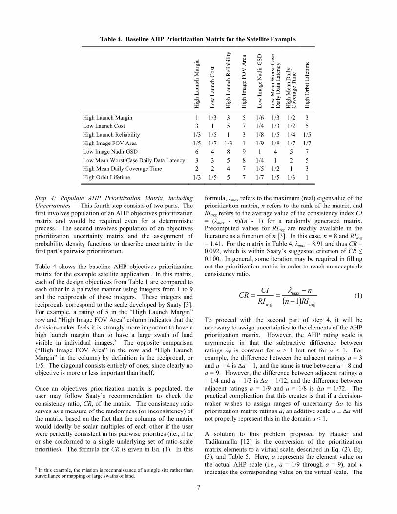
Step 4: Populate AHP Prioritization Matrix, including Uncertainties — This fourth step consists of two parts. The first involves population of an AHP objectives prioritization matrix and would be required even for a deterministic process. The second involves population of an objectives prioritization uncertainty matrix and the assignment of probability density functions to describe uncertainty in the first part’s pairwise prioritization.

Table 4 shows the baseline AHP objectives prioritization matrix for the example satellite application. In this matrix, each of the design objectives from Table 1 are compared to each other in a pairwise manner using integers from 1 to 9 and the reciprocals of those integers. These integers and reciprocals correspond to the scale developed by Saaty [3]. For example, a rating of 5 in the “High Launch Margin” row and “High Image FOV Area” column indicates that the decision-maker feels it is strongly more important to have a high launch margin than to have a large swath of land visible in individual images.8 The opposite comparison (“High Image FOV Area” in the row and “High Launch Margin” in the column) by definition is the reciprocal, or 1/5. The diagonal consists entirely of ones, since clearly no objective is more or less important than itself.

Once an objectives prioritization matrix is populated, the user may follow Saaty’s recommendation to check the consistency ratio, CR, of the matrix. The consistency ratio serves as a measure of the randomness (or inconsistency) of the matrix, based on the fact that the columns of the matrix would ideally be scalar multiples of each other if the user were perfectly consistent in his pairwise priorities (i.e., if he or she conformed to a single underlying set of ratio-scale priorities). The formula for CR is given in Eq. (1). In this

8 In this example, the mission is reconnaissance of a single site rather than surveillance or mapping of large swaths of land.

formula, λmax refers to the maximum (real) eigenvalue of the prioritization matrix, n refers to the rank of the matrix, and RIavg refers to the average value of the consistency index CI = (λmax - n)/(n - 1) for a randomly generated matrix. Precomputed values for RIavg are readily available in the literature as a function of n [3]. In this case, n = 8 and RIavg = 1.41. For the matrix in Table 4, λmax = 8.91 and thus CR = 0.092, which is within Saaty’s suggested criterion of CR ≤ 0.100. In general, some iteration may be required in filling out the prioritization matrix in order to reach an acceptable consistency ratio.

( ) avgavg RIn

n

RI

CICR

1max

−−== λ

(1)

To proceed with the second part of step 4, it will be necessary to assign uncertainties to the elements of the AHP prioritization matrix. However, the AHP rating scale is asymmetric in that the subtractive difference between ratings aij is constant for a > 1 but not for a < 1. For example, the difference between the adjacent ratings a = 3 and a = 4 is Δa = 1, and the same is true between a = 8 and a = 9. However, the difference between adjacent ratings a = 1/4 and a = 1/3 is Δa = 1/12, and the difference between adjacent ratings a = 1/9 and a = 1/8 is Δa = 1/72. The practical complication that this creates is that if a decision-maker wishes to assign ranges of uncertainty Δa to his prioritization matrix ratings a, an additive scale a ± Δa will not properly represent this in the domain a < 1.

A solution to this problem proposed by Hauser and Tadikamalla [12] is the conversion of the prioritization matrix elements to a virtual scale, described in Eq. (2), Eq. (3), and Table 5. Here, a represents the element value on the actual AHP scale (i.e., a = 1/9 through a = 9), and v indicates the corresponding value on the virtual scale. The

Table 4. Baseline AHP Prioritization Matrix for the Satellite Example.

Hig

h L

aunc

h M

argi

n

Low

Lau

nch

Cos

t

Hig

h L

aunc

h R

elia

bili

ty

Hig

h Im

age

FO

V A

rea

Low

Im

age

Nad

ir G

SD

Low

Mea

n W

orst

-Cas

e D

aily

Dat

a L

aten

cy

Hig

h M

ean

Dai

ly

Cov

erag

e T

ime

Hig

h O

rbit

Lif

etim

e

High Launch Margin 1 1/3 3 5 1/6 1/3 1/2 3 Low Launch Cost 3 1 5 7 1/4 1/3 1/2 5 High Launch Reliability 1/3 1/5 1 3 1/8 1/5 1/4 1/5 High Image FOV Area 1/5 1/7 1/3 1 1/9 1/8 1/7 1/7 Low Image Nadir GSD 6 4 8 9 1 4 5 7 Low Mean Worst-Case Daily Data Latency 3 3 5 8 1/4 1 2 5 High Mean Daily Coverage Time 2 2 4 7 1/5 1/2 1 3 High Orbit Lifetime 1/3 1/5 5 7 1/7 1/5 1/3 1

8

basic idea of this approach is to convert the prioritization matrix to the virtual scale in order to assign and interpret uncertainties, and then to convert the matrix back to the actual scale to compute the AHP priority vector.

( )

≥

<−=

1 if

1 if 12

aa

aa

a

av (2)

( )

≥

<−=

1 if

1 if 2

1

vv

vvva (3)

Table 6 shows the resulting conversion of Table 4 to the virtual scale. By definition, the matrix is no longer reciprocal, but because the a(1) = v(1) = 1, the diagonal is still made up entirely of ones.

The next part of step 4 requires the assignment of uncertainties. The example application used in this paper assumes that AHP prioritization matrix ratings on the virtual scale are independently distributed as symmetric triangular random variables. These distributions are simple to construct (requiring just two parameters), and the use of triangular distributions for early project planning applications is well supported in the literature [12, 14, 34-36] Using the baseline AHP ratings (the vij’s in Table 6) as

the modes of the triangular distributions9 captures the notion that the baseline rating is more likely to be the true rating than is any other value. As a result, just one additional piece of information is needed to specify the distributions for each element. This additional piece of information is the width of the tail of the distribution, or the maximum uncertainty in the baseline virtual-scale rating. This information is recorded by the user (or by the group of users among whom vij estimates differ) in the uij elements of a matrix such as in Table 7. These uij uncertainties need not be integers, since the original AHP rating scale (and by extension, the new virtual scale) is valid for any ratio scale.10 Note that these uncertainties are only defined at and to the upper right of the matrix diagonal, since the lower-left entries of an AHP prioritization matrix are correlated with those in the upper right. Thus, in more formal terms, a matrix of random variables Xij on the virtual scale is formed as in Table 8. Each Xij is distributed as a triangular random variable, where the entries to the upper right of the diagonal are independently distributed as in Eq. (4). Entries to the lower left of the diagonal are dependent on the upper right as described by Eq. (5). By definition, the diagonal itself consists of deterministic values of unity (i.e., it is always certain that an objective is as important as itself).

9 Since the triangular distributions are symmetric, the modes also correspond to the mean and median values.

10 The primary caveat to this is that if one wishes to find the consistency ratio of an AHP prioritization matrix that has been populated based on a continuous ratio scale (rather than the traditional discrete scale in the first row of Table 5), the random indices that are available in most published tables are invalid and must be recomputed.

Table 6. Baseline AHP Prioritization Matrix converted to Virtual Scale.

Hig

h L

aunc

h M

argi

n

Low

Lau

nch

Cos

t

Hig

h L

aunc

h R

elia

bili

ty

Hig

h Im

age

FO

V A

rea

Low

Im

age

Nad

ir G

SD

Low

Mea

n W

orst

-Cas

e D

aily

Dat

a L

aten

cy

Hig

h M

ean

Dai

ly

Cov

erag

e T

ime

Hig

h O

rbit

Lif

etim

e

High Launch Margin 1 -1 3 5 -4 -1 0 3 Low Launch Cost 3 1 5 7 -2 -1 0 5 High Launch Reliability -1 -3 1 3 -6 -3 -2 -3 High Image FOV Area -3 -5 -1 1 -7 -6 -5 -5 Low Image Nadir GSD 6 4 8 9 1 4 5 7 Low Mean Worst-Case Daily Data Latency 3 3 5 8 -2 1 2 5 High Mean Daily Coverage Time 2 2 4 7 -3 0 1 3 High Orbit Lifetime -1 -3 5 7 -5 -3 -1 1

Table 5. Actual-to-Virtual Scale Conversion Chart.

Actual AHP Scale, a 1/9 1/8 1/7 1/6 1/5 1/4 1/3 1/2 1 2 3 4 5 6 7 8 9Virtual AHP Scale, v -7 -6 -5 -4 -3 -2 -1 0 1 2 3 4 5 6 7 8 9

9

( )ijijijijijij uvvuvTriangularX +− ,,~ (4)

ijji XX −= 2 (5)

Monte Carlo Simulation

Detailed next are steps 5-8 of the methodology outlined in Fig. 3. These steps are focused on executing the Monte Carlo simulation and acquiring the data which will be analyzed in the final segment. Since all relevant aspects of the problem have been set up in the first segment, steps 5-8 are easily automated. In the example application, steps 5-8 are repeated 10,000 times, taking only a few minutes of time on a standard personal computer, to produce statistically significant results.

Step 5: Select an AHP Prioritization Matrix — The first step in the Monte Carlo simulation is the selection of an AHP prioritization matrix by sampling from the random matrix generated in step 4 (e.g., Table 8). This can be accomplished by independently sampling from ½ · (n² – n) virtual-scale triangular distributions as defined in step 4, assigning those values to the proper elements in the upper right of the matrix, computing the lower-left elements based on Eq. (5), and then converting the resulting sample matrix to the actual AHP scale based on Eq. (3). The resulting matrix is one possible AHP prioritization matrix based on the uncertainties the user assigned in step 4.

Step 6: Determine AHP Priority Vector — The next step in the Monte Carlo simulation is the conversion of the AHP prioritization matrix selected in step 5 into a single vector of objective weights. This is a standard step in AHP, although

Table 8. Probabilistic Prioritization Matrix on the Virtual Scale.

Hig

h L

aunc

h M

argi

n

Low

Lau

nch

Cos

t

Hig

h L

aunc

h R

elia

bili

ty

Hig

h Im

age

FO

V A

rea

Low

Im

age

Nad

ir G

SD

Low

Mea

n W

orst

-Cas

e D

aily

Dat

a L

aten

cy

Hig

h M

ean

Dai

ly

Cov

erag

e T

ime

Hig

h O

rbit

Lif

etim

e

High Launch Margin 1 X1,2 X1,3 X1,4 X1,5 X1,6 X1,7 X1,8 Low Launch Cost 2-X1,2 1 X2,3 X2,4 X2,5 X2,6 X2,7 X2,8 High Launch Reliability 2-X1,3 2-X2,3 1 X3,4 X3,5 X3,6 X3,7 X3,8 High Image FOV Area 2-X1,4 2-X2,4 2-X3,4 1 X4,5 X4,6 X4,7 X4,8 Low Image Nadir GSD 2-X1,5 2-X2,5 2-X3,5 2-X4,5 1 X5,6 X5,7 X5,8 Low Mean Worst-Case Daily Data Latency 2-X1,6 2-X2,6 2-X3,6 2-X4,6 2-X5,6 1 X6,7 X6,8 High Mean Daily Coverage Time 2-X1,7 2-X2,7 2-X3,7 2-X4,7 2-X5,7 2-X6,7 1 X7,8 High Orbit Lifetime 2-X1,8 2-X2,8 2-X3,8 2-X4,8 2-X5,8 2-X6,8 2-X7,8 1

Table 7. Uncertainty Matrix in the Virtual Scale.

Hig

h L

aunc

h M

argi

n

Low

Lau

nch

Cos

t

Hig

h L

aunc

h R

elia

bili

ty

Hig

h Im

age

FO

V A

rea

Low

Im

age

Nad

ir G

SD

Low

Mea

n W

orst

-Cas

e D

aily

Dat

a L

aten

cy

Hig

h M

ean

Dai

ly

Cov

erag

e T

ime

Hig

h O

rbit

Lif

etim

e

High Launch Margin 0 3 1.5 2 2 2.5 2.5 2.5 Low Launch Cost 0 1.5 2 2 3 3.5 4 High Launch Reliability 0 3 1 1.5 1.5 5.5 High Image FOV Area 0 0 0.5 0.5 1.5 Low Image Nadir GSD 0 2 2 1.5 Low Mean Worst-Case Daily Data Latency 0 0.5 0.5 High Mean Daily Coverage Time 0 1.5 High Orbit Lifetime 0

10

the literature contains some debate about the best way to execute it. In his original book on AHP, Saaty proposes the vector of weights is the principal right eigenvector of the prioritization matrix. However, he also posits that a normalized arithmetic mean over the columns, an arithmetic mean over the normalized columns, or a normalized geometric mean over the columns would also approximate this vector for computationally-constrained applications [3]. In 1988, Hihn and Johnson [37] evaluated 16 such conversion techniques against several numerical criteria and concluded that Saaty’s eigenvector technique is generally inferior. A recent textbook by Winston [38] suggests using the arithmetic mean of the normalized columns, which is one of the approximations Saaty suggests. This is the convention used here; if applied to the baseline matrix of Table 4, it yields the priority vector in Table 9. However, it is worth noting that if a user desires, any of the methods listed above may be used in this step in lieu of the arithmetic mean of the normalized columns.

Note that the priority vector on the right in Table 9 indicates that by far the highest priority for this mission is low (or small) image ground sample distance. This reflects the fact that the primary mission of this satellite is reconnaissance of a specific ground target. The second-highest priority according to Table 9 is low data latency, which is also to be expected for a responsive reconnaissance mission. The lowest priority is for the mission to have a high (or long) orbit lifetime, as in this scenario the focus is on a short-term threat from a particular location.

Recall that in each of the 10,000 Monte Carlo runs, a new prioritization matrix is selected. A new priority vector is thus computed each time a new prioritization matrix is selected, and the vector in Table 9 represents just one such priority vector considered throughout this methodology.

Step 7: Apply Traditional Deterministic TOPSIS — With computation of the priority vector complete, TOPSIS may be used to score the various alternative designs (e.g., each of the 59 options in Table 3) in terms of how well they fulfill the prioritized objectives. This proceeds as a standard implementation of TOPSIS, whereby closeness for design i, Ci, is computed as in Eq. (6). Here, Si

- is the euclidean distance between the normalized and weighted design attribute vector di and the normalized and weighted negative ideal design attribute vector d-. The quantity Si

+ indicates the euclidean distance between the normalized and weighted design attribute vector di and the normalized and weighted positive ideal design attribute vector d+. Details on the TOPSIS computation process are available in [4,15-16].

−+

−

−+

−

−+−

−=

+=

dddd

dd

SS

SC

ii

i

ii

ii

(6)

Step 8: Record Scores and Rank Order of Alternatives — The closeness scores Ci from step 7 indicate, in a weighted sense, how distant each design is from the negative ideal. By definition, these values range from zero to unity, with unity most desirable. Thus, designs may be ranked by their Ci values. Table 10 shows the closeness scores and ranks for each of the 59 designs under consideration in the satellite example, assuming the baseline priority vector in Table 9. On each of the 10,000 iterations of step 8, a table like Table 10 is recorded. The resulting tables are then used in the next segment of analysis.

Results Visualization and Decision-Making

Steps 9 and 10 of this methodology involve (1) the visualization of the results of the 10,000 Monte Carlo simulations run in steps 5-8 and (2) the interpretation of

Table 9. Baseline Prioritization Matrix with Normalized Columns and Priority Vector.

Hig

h L

aunc

h M

argi

n

Low

Lau

nch

Cos

t

Hig

h L

aunc

h R

elia

bili

ty

Hig

h Im

age

FO

V A

rea

Low

Im

age

Nad

ir G

SD

Low

Mea

n W

orst

-Cas

e D

aily

Dat

a L

aten

cy

Hig

h M

ean

Dai

ly

Cov

erag

e T

ime

Hig

h O

rbit

Lif

etim

e

Pri

orit

y V

ecto

r

High Launch Margin 0.063 0.031 0.096 0.106 0.074 0.050 0.051 0.123 0.074Low Launch Cost 0.189 0.092 0.160 0.149 0.111 0.050 0.051 0.205 0.126High Launch Reliability 0.021 0.018 0.032 0.064 0.056 0.030 0.026 0.008 0.032High Image FOV Area 0.013 0.013 0.011 0.021 0.049 0.019 0.015 0.006 0.018Low Image Nadir GSD 0.378 0.368 0.255 0.191 0.445 0.598 0.514 0.288 0.380Low Mean Worst-Case Daily Data Latency 0.189 0.276 0.160 0.170 0.111 0.149 0.206 0.205 0.183High Mean Daily Coverage Time 0.126 0.184 0.128 0.149 0.089 0.075 0.103 0.123 0.122High Orbit Lifetime 0.021 0.018 0.160 0.149 0.064 0.030 0.034 0.041 0.065

11

these results in order to down-select to a single design or, alternatively, a handful of designs for more detailed analysis.

Step 9: Visualize and Review Results — The visualization of results suggested here involves four parts. In the first part, the resulting TOPSIS scores from the Monte Carlo runs are plotted as a function of design number and Monte Carlo case number. In the example satellite application, each of the 59 designs in Table 3 was evaluated according to 10,000 different possible AHP prioritization matrices. Thus, the plot in Fig. 4 displays 590,000 TOPSIS scores on the color axis. Red indicates high (desirable) TOPSIS scores, and blue indicates low scores.

Notice that in Fig. 4, colors occur in distinct vertical stripes. For example, designs 10, 13, 16, and 17 have distinct red-orange stripes, and design 42 has the most distinct dark blue stripe. Thus, this simple plot of the raw TOPSIS scores provides a first glance of which designs are likely to emerge as top candidates. In addition, the plot provides some information on the variability of the TOPSIS scores for particular designs. For example, design 55 has a more consistent color across all Monte Carlo cases than design 30, suggesting that the TOPSIS score for design 55 is relatively insensitive to the prescribed uncertainty in the AHP prioritization matrix.

The next part consists of visualizing the rank-order of alternatives, as opposed to the TOPSIS score itself as was done in Fig. 4. As described earlier, the rank-order of the alternatives has been recorded for each of the 10,000 Monte Carlo runs, and what remains is to plot this data in a meaningful way. One question that this data can answer is, “In the 10,000 Monte Carlo runs, how often does a particular design appear as the best alternative?” In other words, this data allows a decision-maker to compute the probability that any particular design (e.g., any of designs 1 through 59) will be the highest-scoring alternative. By extension, this data can also answer the question, “In the 10,000 Monte Carlos runs, how often does a particular design appear among the top five alternatives?” or “How often does any particular design appear among the top ten alternatives?” These questions are slightly different, since it is possible that one may encounter a situation where Design A is the top design 70% of the time and Design B is the top design 20% of the time, but Design B may be among the top five designs 90% of the time while Design A is in the top five only 80% of the time. The N-value of the “Top N” threshold will depend in part on whether the goal of the decision process is to select a single candidate (N = 1) or instead to downselect to a family of candidates for further study (N > 1).

Table 10. Closeness Scores and Ranks of the 59 example designs under consideration, according to

the baseline priority vector in Table 9.

Design Definition Scores according to

Baseline Prioritization

Design No.

Orbit Alt. (km)

Orbit Inclin.(deg.)

Launch Vehicle

Closeness, Ci Rank

1 400 30 Pegasus XL 0.5546 272 400 30 Minotaur I 0.5603 233 400 30 Athena I 0.5574 254 400 40 Minotaur I 0.5694 185 400 40 Athena I 0.5657 216 400 50 Minotaur I 0.5783 127 400 50 Athena I 0.5739 168 400 60 Minotaur I 0.5817 119 400 60 Athena I 0.5765 14

10 400 70 Falcon 1e 0.6166 311 400 70 Minotaur I 0.5979 712 400 70 Athena I 0.5918 1013 400 80 Falcon 1e 0.6183 214 400 80 Minotaur I 0.6000 615 400 80 Athena I 0.5931 916 400 90 Falcon 1e 0.6194 117 400 90 Taurus 2210 0.6134 418 400 90 Minotaur I 0.6017 519 400 90 Athena I 0.5939 820 600 30 Minotaur I 0.5089 3821 600 30 Athena I 0.5063 3922 600 40 Minotaur I 0.5228 3623 600 40 Athena I 0.5190 3724 600 50 Falcon 1e 0.5557 2625 600 50 Minotaur I 0.5320 3326 600 50 Athena I 0.5272 3527 600 60 Falcon 1e 0.5594 2428 600 60 Minotaur I 0.5359 3229 600 60 Athena I 0.5302 3430 600 70 Falcon 1e 0.5732 1731 600 70 Taurus 2210 0.5653 2232 600 70 Minotaur I 0.5503 2833 600 70 Athena I 0.5435 3134 600 80 Falcon 1e 0.5761 1535 600 80 Taurus 2210 0.5683 2036 600 80 Athena I 0.5465 3037 600 90 Falcon 1e 0.5768 1338 600 90 Taurus 2210 0.5692 1939 600 90 Athena I 0.5473 2940 1000 20 Taurus 2210 0.3634 5841 1000 30 Taurus 2210 0.3807 5542 1000 30 Athena I 0.3533 5943 1000 40 Taurus 2210 0.3931 5144 1000 40 Athena I 0.3672 5745 1000 50 Taurus 2210 0.4042 4946 1000 50 Athena I 0.3796 5647 1000 60 Taurus 2210 0.4092 4748 1000 60 Athena I 0.3858 5349 1000 70 Taurus 2110 0.4206 4650 1000 70 Taurus 2210 0.4082 4851 1000 70 Athena I 0.3859 5252 1000 80 Taurus 2110 0.4359 4253 1000 80 Taurus 2210 0.4253 4554 1000 80 Taurus 3210 0.4334 4355 1000 90 Taurus 2110 0.4391 4056 1000 90 Taurus 2210 0.4295 4457 1000 90 Taurus 3210 0.4363 4158 1500 30 Athena I 0.3842 5659 1500 40 Athena I 0.3938 53

12

Figure 5 shows such rank-order results for the satellite example application. The top graph of Fig. 5 indicates the probability that the indicated designs (16, 10, 13, and 17) rank as the top alternative in the TOPSIS evaluation. This graph shows that design 16 (i.e., launching the satellite of interest on a Falcon 1e rocket to a 400 km altitude, 90° inclination orbit) ranks as the top design in 88.7% of the 10,000 Monte Carlo runs. Next in line is design 10 (top design 5.8% of the time), design 13 (top design 5.4% of the time11), and design 17 (top design 0.05% of the time). No other designs have positive probabilities; that is, in none of the 10,000 Monte Carlo runs do other candidate designs rank as the top design. A reasonable conclusion to draw from this data is that design 16 is a clear winner; however, it is worth noting that the first three of the four designs in this graph are very similar, differing only in their orbital inclinations. As a result, this may suggest that further trade studies are warranted for inclination (e.g., to resolve the “best” inclination to the level of 1-5° rather than increments of 10°). In this case, a useful result of this probabilistic analysis is the identification of a family of potential solutions for further study.

In support of identification of such a family of potential solutions, a user may generate graphs such as at the bottom of Fig. 5. The bottom left graph in Fig. 5 shows the probabilities that particular designs rank among the top five alternatives among the 10,000 Monte Carlo runs. Notice

11 Interestingly, design 10 is the top design more frequently than design 13 even though design 13 has the higher baseline TOPSIS score (see Table 10).

that designs 10, 13, 16, and 17 always fall within the top five, and design 18 falls within the top five 96.4% of the time. Eight additional designs with small probabilities are plotted in the top-five graph of Fig. 5; no other designs had positive probabilities of falling within the top five.

The bottom right graph of Fig. 5 shows the probabilities that particular designs rank among the top ten alternatives among the 10,000 Monte Carlo runs. Notice that ten designs (17, 16, 13, 10, 11, 14, 18, 19, 15, and 12) nearly always fall within the top ten, while another eleven designs (8, 37, 34, 6, 30, 4, 7, 9, 27, 5, and 24) rank in the top ten only occasionally. Furthermore, notice that among the ten most frequent top ten designs, only four launch vehicles are used (Falcon 1e, Taurus 2210, Minotaur I, and Athena I), only one altitude appears (400 km), and just three inclinations occur (70°, 80°, and 90°). Thus, if the goal of this decision process is to narrow the scope of future trade studies, the graphs at the bottom of Fig. 5 provide a rigorous basis for such a downselection.

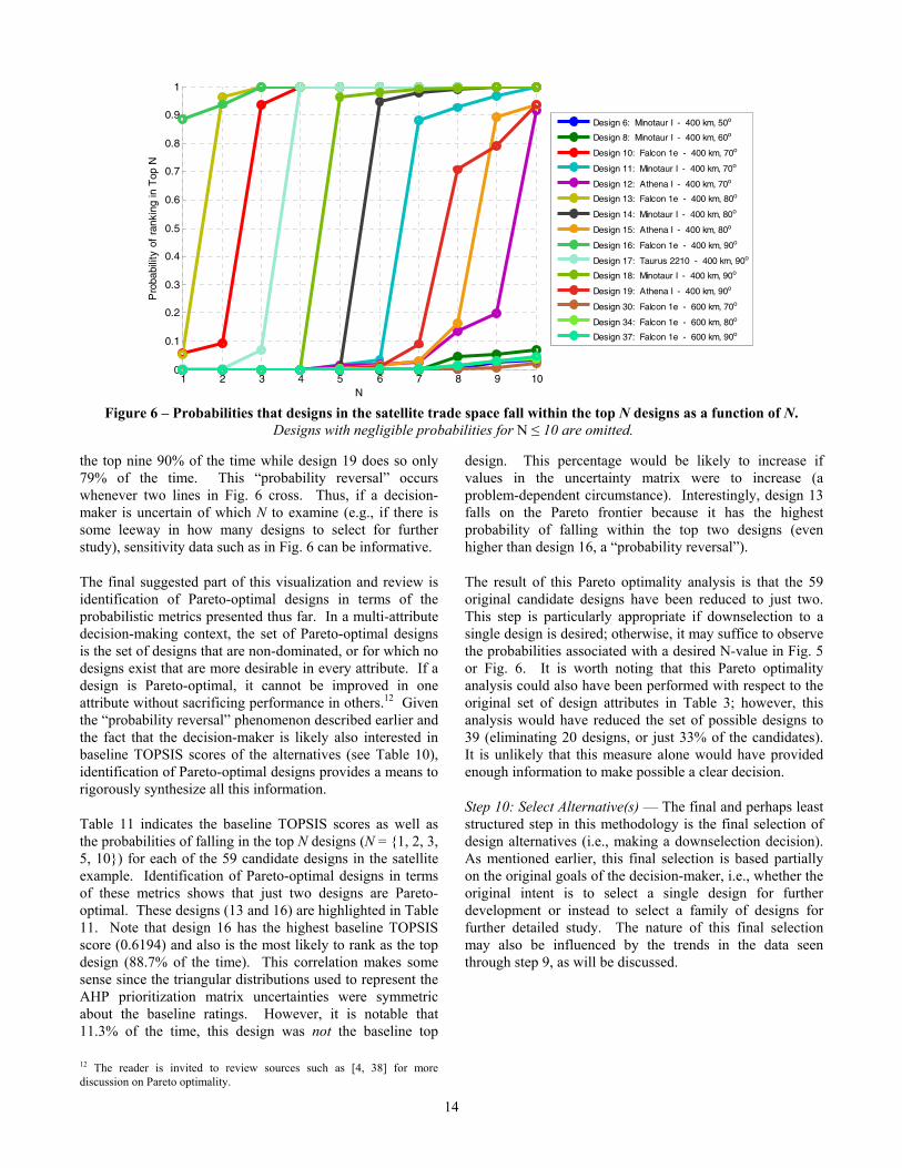
The data in Fig. 5 can also be visualized as the line graph of Fig. 6. The y-axis of Fig. 6 indicates the probability that a particular design, indicated by a particular line on the graph, will rank within the top N designs in an AHP and TOPSIS evaluation. The x-axis of Fig. 6 indicates the value of N. Thus, for example, Fig. 6 shows that design 16 (the lime-green line) has an 89% probability of being the top design (N = 1) and a nearly 100% probability of falling within the top three, four, five, etc. designs (N > 2). Design 13 (the light olive line) has only a 5% probability of being the top design but has a 100% probability of falling within the top

Figure 4 – TOPSIS Score as a function of Design Number (1-59) and Monte Carlo Case Number (1-10,000) for the Satellite Example Application.

13

three, four, five, etc. designs. Thus, each graph in Fig. 5 corresponds to a particular vertical slice of Fig. 6 (in particular, the N = 1, N = 5, and N = 10 vertical slices).

One characteristic Fig. 6 highlights well is the presence of “probability reversal” scenarios. The hypothetical example presented earlier is a scenario in which Design A is the top design 70% of the time and Design B is the top design 20%

of the time, but Design B is among the top five designs 90% of the time while Design A is in the top five only 80% of the time. In such a scenario, the apparent desirability of a design depends on the selected value of N. In Fig. 6, this occurs between designs 13 and 16 as well as between designs 15 and 19: In the latter example, design 19 falls within the top eight designs 71% of the time and design 15 does so 16% of the time. However, design 15 falls within

0 0.2 0.4 0.6 0.8 1

17

13

10

16

Taurus 2210 - 400 km, 90o

Falcon 1e - 400 km, 80o

Falcon 1e - 400 km, 70o

Falcon 1e - 400 km, 90o

Probability of being the Top Design

Des

ign

Num

ber

0 0.2 0.4 0.6 0.8 1

7

34

30

19

15

14

12

11

18

10

13

16

17

Athena I - 400 km, 50o

Falcon 1e - 600 km, 80o

Falcon 1e - 600 km, 70o

Athena I - 400 km, 90o

Athena I - 400 km, 80o

Minotaur I - 400 km, 80o

Athena I - 400 km, 70o

Minotaur I - 400 km, 70o

Minotaur I - 400 km, 90o

Falcon 1e - 400 km, 70o

Falcon 1e - 400 km, 80o

Falcon 1e - 400 km, 90o

Taurus 2210 - 400 km, 90o

Probability of being within the Top 5 Designs

Des

ign

Num

ber

0 0.2 0.4 0.6 0.8 1

24

5

27

9

7

4

30

6

34

37

8

12

15

19

18

14

11

10

13

16

17

Falcon 1e - 600 km, 50o

Athena I - 400 km, 40o

Falcon 1e - 600 km, 60o

Athena I - 400 km, 60o

Athena I - 400 km, 50o

Minotaur I - 400 km, 40o

Falcon 1e - 600 km, 70o

Minotaur I - 400 km, 50o

Falcon 1e - 600 km, 80o

Falcon 1e - 600 km, 90o

Minotaur I - 400 km, 60o

Athena I - 400 km, 70o

Athena I - 400 km, 80o

Athena I - 400 km, 90o

Minotaur I - 400 km, 90o

Minotaur I - 400 km, 80o

Minotaur I - 400 km, 70o

Falcon 1e - 400 km, 70o

Falcon 1e - 400 km, 80o

Falcon 1e - 400 km, 90o

Taurus 2210 - 400 km, 90o

Probability of being within the Top 10 Designs

Des

ign

Num

ber

Figure 5 – Probabilities that designs in the satellite trade space fall within the top one (top graph), top five (bottom left graph), or top ten (bottom right graph). Only designs with positive probabilities are shown.

14

the top nine 90% of the time while design 19 does so only 79% of the time. This “probability reversal” occurs whenever two lines in Fig. 6 cross. Thus, if a decision-maker is uncertain of which N to examine (e.g., if there is some leeway in how many designs to select for further study), sensitivity data such as in Fig. 6 can be informative.

The final suggested part of this visualization and review is identification of Pareto-optimal designs in terms of the probabilistic metrics presented thus far. In a multi-attribute decision-making context, the set of Pareto-optimal designs is the set of designs that are non-dominated, or for which no designs exist that are more desirable in every attribute. If a design is Pareto-optimal, it cannot be improved in one attribute without sacrificing performance in others.12 Given the “probability reversal” phenomenon described earlier and the fact that the decision-maker is likely also interested in baseline TOPSIS scores of the alternatives (see Table 10), identification of Pareto-optimal designs provides a means to rigorously synthesize all this information.

Table 11 indicates the baseline TOPSIS scores as well as the probabilities of falling in the top N designs (N = {1, 2, 3, 5, 10}) for each of the 59 candidate designs in the satellite example. Identification of Pareto-optimal designs in terms of these metrics shows that just two designs are Pareto-optimal. These designs (13 and 16) are highlighted in Table 11. Note that design 16 has the highest baseline TOPSIS score (0.6194) and also is the most likely to rank as the top design (88.7% of the time). This correlation makes some sense since the triangular distributions used to represent the AHP prioritization matrix uncertainties were symmetric about the baseline ratings. However, it is notable that 11.3% of the time, this design was not the baseline top

12 The reader is invited to review sources such as [4, 38] for more discussion on Pareto optimality.

design. This percentage would be likely to increase if values in the uncertainty matrix were to increase (a problem-dependent circumstance). Interestingly, design 13 falls on the Pareto frontier because it has the highest probability of falling within the top two designs (even higher than design 16, a “probability reversal”).

The result of this Pareto optimality analysis is that the 59 original candidate designs have been reduced to just two. This step is particularly appropriate if downselection to a single design is desired; otherwise, it may suffice to observe the probabilities associated with a desired N-value in Fig. 5 or Fig. 6. It is worth noting that this Pareto optimality analysis could also have been performed with respect to the original set of design attributes in Table 3; however, this analysis would have reduced the set of possible designs to 39 (eliminating 20 designs, or just 33% of the candidates). It is unlikely that this measure alone would have provided enough information to make possible a clear decision.

Step 10: Select Alternative(s) — The final and perhaps least structured step in this methodology is the final selection of design alternatives (i.e., making a downselection decision). As mentioned earlier, this final selection is based partially on the original goals of the decision-maker, i.e., whether the original intent is to select a single design for further development or instead to select a family of designs for further detailed study. The nature of this final selection may also be influenced by the trends in the data seen through step 9, as will be discussed.

1 2 3 4 5 6 7 8 9 100

0.1

0.2

0.3

0.4

0.5

0.6

0.7

0.8

0.9

1

N

Pro

babi

lity

of r

anki

ng in

Top

N

Design 6: Minotaur I - 400 km, 50o

Design 8: Minotaur I - 400 km, 60o

Design 10: Falcon 1e - 400 km, 70o

Design 11: Minotaur I - 400 km, 70o

Design 12: Athena I - 400 km, 70o

Design 13: Falcon 1e - 400 km, 80o

Design 14: Minotaur I - 400 km, 80o

Design 15: Athena I - 400 km, 80o

Design 16: Falcon 1e - 400 km, 90o

Design 17: Taurus 2210 - 400 km, 90o

Design 18: Minotaur I - 400 km, 90o

Design 19: Athena I - 400 km, 90o

Design 30: Falcon 1e - 600 km, 70o

Design 34: Falcon 1e - 600 km, 80o

Design 37: Falcon 1e - 600 km, 90o

Figure 6 – Probabilities that designs in the satellite trade space fall within the top N designs as a function of N.

Designs with negligible probabilities for N ≤ 10 are omitted.

15

Table 11. Probabilistic AHP/TOPSIS Attributes considered for identification of Pareto-optimal designs for the example satellite application. Pareto-optimal designs are bold and highlighted.

Design Definition Probabilistic AHP/TOPSIS Attributes

Design No.

Orbit Alt. (km)

Orbit Inclin. (deg.)

Launch Vehicle

Baseline Closeness,

Ci

Probability of ranking in the Top N designs

N = 1 N = 2 N = 3 N = 5 N = 10

1 400 30 Pegasus XL 0.5546 0 0 0 0 0 2 400 30 Minotaur I 0.5603 0 0 0 0 0 3 400 30 Athena I 0.5574 0 0 0 0 0 4 400 40 Minotaur I 0.5694 0 0 0 0 0.0018 5 400 40 Athena I 0.5657 0 0 0 0 0.0002 6 400 50 Minotaur I 0.5783 0 0 0 0 0.0320 7 400 50 Athena I 0.5739 0 0 0 0.0001 0.0010 8 400 60 Minotaur I 0.5817 0 0 0 0 0.0669 9 400 60 Athena I 0.5765 0 0 0 0 0.0004

10 400 70 Falcon 1e 0.6166 0.0582 0.0940 0.9343 1.0000 1.0000 11 400 70 Minotaur I 0.5979 0 0 0 0.0150 0.9998 12 400 70 Athena I 0.5918 0 0 0 0.0133 0.9154 13 400 80 Falcon 1e 0.6183 0.0542 0.9645 1.0000 1.0000 1.0000 14 400 80 Minotaur I 0.6000 0 0 0 0.0045 0.9996 15 400 80 Athena I 0.5931 0 0 0 0.0022 0.9355 16 400 90 Falcon 1e 0.6194 0.8871 0.9382 0.9992 1.0000 1.0000 17 400 90 Taurus 2210 0.6134 0.0005 0.0033 0.0665 1.0000 1.0000 18 400 90 Minotaur I 0.6017 0 0 0 0.9636 0.9995 19 400 90 Athena I 0.5939 0 0 0 0.0009 0.9393 20 600 30 Minotaur I 0.5089 0 0 0 0 0 21 600 30 Athena I 0.5063 0 0 0 0 0 22 600 40 Minotaur I 0.5228 0 0 0 0 0 23 600 40 Athena I 0.5190 0 0 0 0 0 24 600 50 Falcon 1e 0.5557 0 0 0 0 0.0001 25 600 50 Minotaur I 0.5320 0 0 0 0 0 26 600 50 Athena I 0.5272 0 0 0 0 0 27 600 60 Falcon 1e 0.5594 0 0 0 0 0.0003 28 600 60 Minotaur I 0.5359 0 0 0 0 0 29 600 60 Athena I 0.5302 0 0 0 0 0 30 600 70 Falcon 1e 0.5732 0 0 0 0.0003 0.0219 31 600 70 Taurus 2210 0.5653 0 0 0 0 0 32 600 70 Minotaur I 0.5503 0 0 0 0 0 33 600 70 Athena I 0.5435 0 0 0 0 0 34 600 80 Falcon 1e 0.5761 0 0 0 0.0001 0.0393 35 600 80 Taurus 2210 0.5683 0 0 0 0 0 36 600 80 Athena I 0.5465 0 0 0 0 0 37 600 90 Falcon 1e 0.5768 0 0 0 0 0.0470 38 600 90 Taurus 2210 0.5692 0 0 0 0 0 39 600 90 Athena I 0.5473 0 0 0 0 0 40 1000 20 Taurus 2210 0.3634 0 0 0 0 0 41 1000 30 Taurus 2210 0.3807 0 0 0 0 0 42 1000 30 Athena I 0.3533 0 0 0 0 0 43 1000 40 Taurus 2210 0.3931 0 0 0 0 0 44 1000 40 Athena I 0.3672 0 0 0 0 0 45 1000 50 Taurus 2210 0.4042 0 0 0 0 0 46 1000 50 Athena I 0.3796 0 0 0 0 0 47 1000 60 Taurus 2210 0.4092 0 0 0 0 0 48 1000 60 Athena I 0.3858 0 0 0 0 0 49 1000 70 Taurus 2110 0.4206 0 0 0 0 0 50 1000 70 Taurus 2210 0.4082 0 0 0 0 0 51 1000 70 Athena I 0.3859 0 0 0 0 0 52 1000 80 Taurus 2110 0.4359 0 0 0 0 0 53 1000 80 Taurus 2210 0.4253 0 0 0 0 0 54 1000 80 Taurus 3210 0.4334 0 0 0 0 0 55 1000 90 Taurus 2110 0.4391 0 0 0 0 0 56 1000 90 Taurus 2210 0.4295 0 0 0 0 0 57 1000 90 Taurus 3210 0.4363 0 0 0 0 0 58 1500 30 Athena I 0.3842 0 0 0 0 0 59 1500 40 Athena I 0.3938 0 0 0 0 0

16

In terms of the example satellite application, the data through step 9 indicates a strong preference for design 16, which involves launch on a Falcon 1e rocket to a 400 km altitude, 90° inclination orbit. Design 16 has favorable performance in terms of several important attributes, such as a 1-meter ground sample distance, 3.7-hour mean worst-case daily data latency, and $10.2 million launch cost (all three of which are the lowest and best possible values among all 59 designs considered). However, Fig. 5 also indicates that launch on a Taurus 2210, Minotaur I, or Athena I, or an orbit inclination lower than 90° (but higher than 70°) is not unreasonable. Although designs with 600 km orbits do not stand out, they do appear with positive probabilities in the top five and top ten designs (see Fig. 5) and may be worth some consideration. A key point in this example application is that two of the design variables (orbit altitude and inclination) are discretized versions of continuous variables. Thus, the fact that inclinations of the top designs tended to be in the 70-90° range and that altitudes tended to be 400-600 km suggests that a second iteration of this procedure within this narrower domain may be warranted with higher resolution on altitude and inclination (e.g., 20 km instead of 200 km on altitude and 1° instead of 10° on inclination). An additional iteration such as this would provide a higher confidence level in the optimality of the top designs identified in this first iteration.

If a single best solution is required of the decision-maker after the first iteration (e.g., due to time or budget constraints), this procedure does identify a clear best solution given the resolution of the study and given the decision-maker’s preferences and preference uncertainty. In this scenario, the recommended design is design 16, launch on a Falcon 1e rocket to a 400 km altitude, 90° inclination orbit. This design ranked as the top design in 89% of Monte Carlo simulations, 15 times more frequently than the next most frequent top design. This design also happens to possess the highest baseline TOPSIS score.

3. CONCLUSION

In summary, this paper has presented a probabilistic methodology to facilitate informed engineering decisions under uncertainty, building on the deterministic multi-attribute decision-making techniques of AHP and TOPSIS. As shown previously in Fig. 3, the methodology is divided into three segments, each of which consists of multiple steps. The first segment, consisting of steps 1-4, involves setting up the problem by defining objectives, priorities, uncertainties, design attributes, and alternatives (candidate designs). This segment also involves the evaluation of each candidate design with respect to the defined attributes. The second segment, which consists of steps 5-8, involves several thousand applications of AHP and TOPSIS under different (random) AHP prioritization matrices based on probability density functions (PDFs) assigned in step 4. The third segment, consisting of steps 9-10, involves

visualization of the results to assist in making a final design selection. An example satellite orbit and launch vehicle selection problem has been used to illustrate the methodology throughout this paper.

The contributions of this paper fall into three categories. First, this paper has introduced and outlined the coupling of probabilistic AHP with TOPSIS. This distinguishes the present work from previous works which have combined deterministic versions of these tools [19-21] or which have covered probabilistic AHP only [5-14]. Second, this paper has introduced several ways of visualizing and analyzing this method’s probabilistic results, useful for efficiently and clearly understanding the data. Third, this work has illustrated its probabilistic decision support process using a practical engineering application.

Several avenues exist for future expansion of the basic methodology presented here. Among them is inclusion of uncertainties on the attributes in the TOPSIS scoring. At present, it has been assumed that uncertainty in a design’s attributes (e.g., cost, reliability, ground sample distance, data latency statistics) is small compared to the uncertainty in decision-maker preferences (i.e., the AHP priority vector). Uncertainty in attributes, e.g., due to uncertainty in the models used to estimate them, can be accommodated within this framework by assigning PDFs to the attributes and drawing from those PDFs in the Monte Carlo simulation (steps 5-8). Another area for expansion or customization is use of nonsymmetric or non-triangular distributions to describe uncertainty in AHP prioritization matrices. Such distributions would require more decision-maker inputs to specify their additional parameters, but they may be more accurate, particularly in situations in which uncertainty is skewed to the left or right.

Overall, this paper is intended to provide a useful engineering framework and tool for facilitating design decisions under uncertainty. Like all engineering tools (including AHP and TOPSIS in their original deterministic forms), this method is meant to inform, but not make, the decision which is the ultimate responsibility of the decision-maker himself. Thus, this tool is most useful in scenarios where large numbers of alternatives need to be reduced to a manageable few, or where it yields a statistically significant “best” design subject to little dispute. In instances where two or more designs rank similarly, further study is warranted. In closing, it is hoped that the methods and ideas presented here find broad use with systems engineers and decision-makers in the future.

ACKNOWLEDGEMENTS

The author would like to thank Dr. Joseph Saleh for his guidance through the course of this work. Great thanks are also due to Joy Brathwaite and Greg Dubos, who were pivotal in developing an early version of this methodology.

17

The author would also like to acknowledge the support of the Department of Defense through the National Defense Science and Engineering Graduate (NDSEG) Fellowship. Finally, the author would like to thank the Gerald A. Soffen Fund for the Advancement of Space Science Education for its generosity in providing travel support to allow this paper to be presented at the IEEE Aerospace Conference.

APPENDIX: NOMENCLATURE

aij = element of AHP prioritization matrix Ci = TOPSIS closeness score for design i CI = AHP consistency index CR = AHP consistency ratio d- = negative ideal design attribute vector d+ = positive ideal design attribute vector di = design attribute vector of design i Di = design alternative i Gi = overall goal i n = number of objectives N = number of top designs considered Oi = objective i RIavg = AHP random index Si

- = euclidean distance between di and d- Si

+ = euclidean distance between di and d+ uij = element of virtual-scale uncertainty matrix vij = element of virtual-scale prioritization matrix Xij = element of random virtual-scale prioritiz. matrix λmax = maximum eigenvalue of AHP prioritization matrix

REFERENCES

[1] T.L. Saaty, Hierarchies and Priorities – Eigenvalue Analysis, Philadelphia: Univ. of Pennsylvania, 1977.

[2] T.L. Saaty, “A Scaling Method for Priorities in Hierarchical Structures,” Journal of Mathematical Psychology, Vol. 15, No. 3, 1977, pp. 234-281.

[3] T.L. Saaty, The Analytic Hierarchy Process, New York: McGraw-Hill, 1980.

[4] P. Sen and J. Yang, Multiple Criteria Decision Support in Engineering Design, London: Springer, 1998.

[5] L.G. Vargas, “Reciprocal Matrices with Random Coefficients,” Mathematical Modelling, Vol. 3, No. 1, 1982, pp. 69-81.

[6] M.S. Zahir, “Incorporating the uncertainty of decision judgements in the analytic hierarchy process,” European Journal of Op. Res., Vol. 53, No. 2, 1991, pp. 206-216.

[7] S. Rahman and G. Shrestha, “A Method to Estimate the Reliability of Expert Judgement,” Session 10C2, IEEE Southeastcon ’89 Proceedings: Energy and Information Technologies in the Southeast, Columbia, 9-12 April 1989.

[8] S. Rahman and G. Shrestha, “Analysis of Inconsistent Data in Power Planning,” IEEE Transactions on Power Systems, Vol. 6, No. 1, 1991, pp. 225-230.

[9] S. Rahman and G. Shrestha, “A Technique to Incorporate New Information in Evaluating Generation Alternatives,” IEEE Transactions on Power Systems, Vol. 7, No. 2, 1992, pp. 900-906.

[10] H. Eskandari and L. Rabelo, “Handling Uncertainty in the Analytic Hierarchy Process,” International Journal of Information Technology & Decision Making, Vol. 6, No. 1, 2007, pp. 177-189.

[11] M.J. Scott, “Quantifying uncertainty in multicriteria concept selection methods,” Research in Engineering Design, Vol. 17, No. 4, 2007, pp. 175-187.

[12] D. Hauser and P. Tadikamalla, “The Analytic Hierarchy Process in an uncertain environment: A simulation approach,” European Journal of Op. Res., Vol. 91, No. 1, 1996, pp. 27-37.

[13] E.S. Rosenbloom, “A probabilistic interpretation of the final rankings in AHP,” European Journal of Op. Res., Vol. 96, No. 2, 1996, pp. 371-378.

[14] J. Hihn and K.T. Lum, “Improving Software Size Estimates by using Probabilistic Pairwise Comparison Matrices,” IEEE 10th International Symposium on Software Metrics, Chicago, 14-16 Sept. 2004.

[15] C. Hwang and K. Yoon, Multiple Attribute Decision Making, Berlin: Springer-Verlag, 1981.

[16] K. Yoon, “Systems Selection by Multiple Attribute Decision Making,” Ph.D. Dissertation, Department of Industrial Engineering, Kansas State University, Manhattan, 1980.

[17] M. Zeleny, Linear Multiobjective Programming, Berlin: Springer-Verlag, 1974.

[18] K.R. MacCrimmon and M. Toda, “The Experimental Determination of Indifference Curves,” The Review of Economic Studies, Vol. 36, No. 4, 1969, pp. 433-451.

[19] N.D. Chakladar and S. Chakraborty, “A combined TOPSIS-AHP-method-based approach for non-traditional machining processes selection,” Proceedings of the Institution of Mechanical Engineers, Part B: Journal of Engineering Manufacture, Vol. 222, No. 12, 2008, pp. 1613-1623.

[20] M. Yurdakul and Y.T. İç, “Development of a performance measurement model for manufacturing companies using the AHP and TOPSIS approaches,” International Journal of Production Research, Vol. 43, No. 21, 2005, pp. 4609-4641.

18

[21] M. Lin, C. Wang, M. Chen, and C.A. Chang, “Using AHP and TOPSIS approaches in customer-driven product design process,” Computers in Industry, Vol. 59, No. 1, 2008, pp. 17-31.

[22] B. Ashtiani, F. Haghighirad, A. Makui, and G. Montazer, “Extension of fuzzy TOPSIS method based on interval-valued fuzzy sets,” Applied Soft Computing, Vol. 9, No. 2, 2009, pp. 457-461.

[23] C. Chen, “Extensions of the TOPSIS for group decision-making under fuzzy environment,” Fuzzy Sets and Systems, Vol. 114, No. 1, 2000, pp. 1-9.

[24] S. Tsaur, T. Chang, and C. Yen, “The evaluation of airline service quality by fuzzy MCDM,” Tourism Management, Vol. 23, No. 2, 2002, pp. 107-115.

[25] T. Chu and Y. Lin, “A Fuzzy TOPSIS Method for Robot Selection,” Int’l Journal of Adv. Manufacturing Technology, Vol. 21, No. 4, 2003, pp. 284-290.

[26] J.M. Lafleur and J.H. Saleh, “GT-FAST: A Point Design Tool for Rapid Fractionated Spacecraft Sizing and Synthesis,” AIAA 2009-6563, Space 2009 Conference, Pasadena, 14-17 Sept. 2009.

[27] W.J. Larson and J.R. Wertz (eds.), Space Mission Analysis and Design, 3rd ed., El Segundo: Microcosm Press and Kluwer Academic Publishers, 1999.

[28] Air Force Research Laboratory Space Vehicles Directorate, TacSat-2 Micro Satellite Fact Sheet, Kirtland Air Force Base, Sept. 2006.

[29] NASA Goddard Space Flight Center, National Space Science Data Center Spacecraft Query [database], http://nssdc.gsfc.nasa.gov/nmc/SpacecraftQuery.jsp [retrieved 3 Aug. 2009].

[30] G.E. Dieter, Engineering Design, 3rd ed., Boston: McGraw-Hill, 2000.

[31] J.M. Lafleur, G. Lantoine, A.L. Hensley, et. al., “A Systematic Concept Exploration Methodology Applied to Venus In Situ Explorer,” 6th International Planetary Probe Workshop, Atlanta, 23-27 June 2008.

[32] O. Brown, “Common Launch Vehicle Data for Econometric Analysis,” DARPA/TTO Memorandum, 10 April 2008.

[33] E.S. Fleming, J.M. Lafleur, and J.H. Saleh, “Response Surface Equations for Expendable Launch Vehicle Payload Capability,” AIAA 2009-6656, Space 2009 Conference, Pasadena, 14-17 Sept. 2009.

[34] T.S. Glickman and F. Xu, “The distribution of the product of two triangular random variables,” Statistics and Probability Letters, Vol. 78, No. 16, 2008, pp. 2821-2826.

[35] D. Johnson, “Triangular approximations for continuous random variables in risk analysis,” Journal of the Operational Research Society, Vol. 53, No. 4, 2002, pp. 457-467.

[36] T.M. Williams, “Practical Use of Distributions in Network Analysis,” Journal of the Operational Research Society, Vol. 43, No. 3, 1992, pp. 265-270.

[37] J.M. Hihn and C.R. Johnson, “Evaluation Techniques for Paired Ratio-Comparison Matrices in a Hierarchical Decision Model,” Measurement in Economics: Theory and Applications of Economic Indices, Heidelberg: Physica-Verlag, 1988, pp. 269-288.

[38] W.L. Winston, Operations Research: Applications and Algorithms, 4th ed., Belmon: Brooks/Cole, 2004.

BIOGRAPHY

Jarret Lafleur is a Ph.D. Candidate in the Space Systems Design Lab (SSDL) at the Georgia Institute of Technology, where he has been supported in his studies on flexibility in space systems design by a National Defense Science and Engineering Graduate Fellowship and National Science Foundation Graduate Research Fellowship. As part of his graduate

studies, from 2007-2009 he actively supported work on the Defense Advanced Research Projects Agency (DARPA) System F6 fractionated spacecraft program. During 2009-2010, he was one of ten Sam Nunn Security Program fellows at the institute, focusing on policy aspects of space infrastructure security. Since 2007, Jarret has also spent summers at NASA Johnson Space Center in the Flight Mechanics and Trajectory Design Branch, frequently supporting Mars aerocapture, entry, descent, and landing trajectory assessments for strategic planning of future human-class missions. He holds a B.S. in Aerospace Engineering and M.S. in Aerospace Engineering from the Georgia Institute of Technology.