Principles of Wireless Sensor Networks - kth.se · Principles of Wireless Sensor Networks https:...

Principles of Wireless Sensor Networks

https://www.kth.se/social/course/EL2745/

Lecture 3 January 24, 2013

Carlo Fischione Associate Professor of Sensor Networks

e-mail: [email protected] http://www.ee.kth.se/~carlofi/

KTH Royal Institute of Technology Stockholm, Sweden

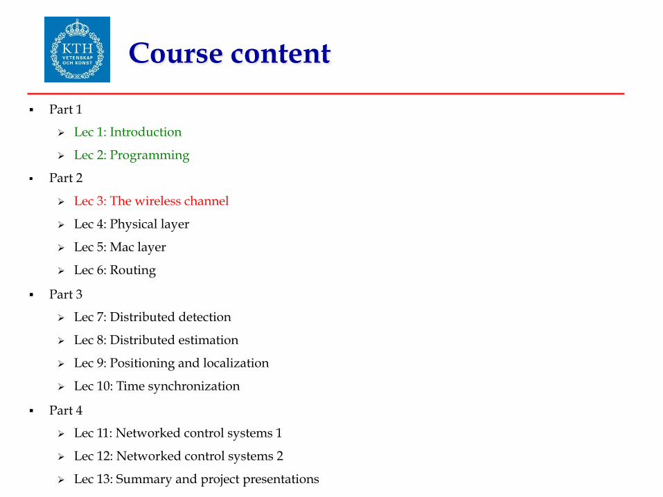
Course content

§  Part 1

Ø  Lec 1: Introduction

Ø  Lec 2: Programming

§  Part 2

Ø  Lec 3: The wireless channel

Ø  Lec 4: Physical layer

Ø  Lec 5: Mac layer

Ø  Lec 6: Routing

§  Part 3

Ø  Lec 7: Distributed detection

Ø  Lec 8: Distributed estimation

Ø  Lec 9: Positioning and localization

Ø  Lec 10: Time synchronization

§  Part 4

Ø  Lec 11: Networked control systems 1

Ø  Lec 12: Networked control systems 2

Ø  Lec 13: Summary and project presentations

•  Suppose that a node has permission to transmit messages over

wireless •  How the signals carrying the messages are treated by the wireless

channel?

Where we are

Process Controller Phy MAC

Routing

Transport

Session

Application Presentation

Today’s learning goals

§  What is the AWGN channel?

§  How the channel attenuates (fades) the transmit power?

§  What is the slow fading?

§  What is the fast fading?

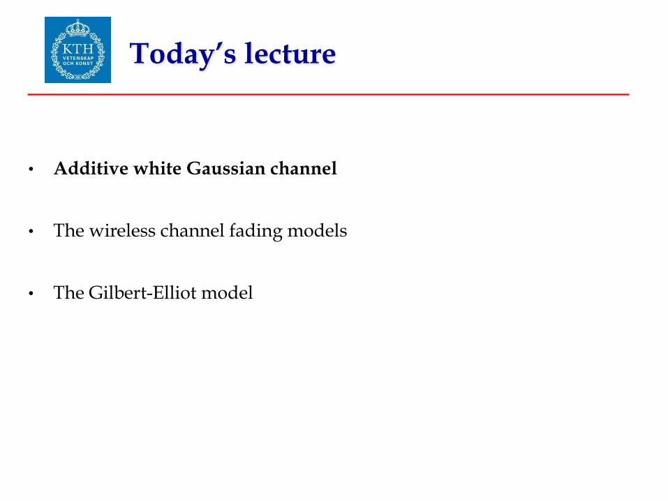
Today’s lecture

•  Additive white Gaussian channel

•  The wireless channel fading models

•  The Gilbert-Elliot model

Digital communications over wireless channels

m = source message, e.g., video, sounds, temperature

s = vector “quantized” source

s(t) = modulated signal transmitter over the wireless channel

r(t) = received signal

x = demodulated signal

= decoded signal

Message Source

Vector Modulator

Modulator Channel Receiver Decision Device

m s s(t) r(t) x m̂

!

m̂

AWGN wireless channels

AWGN channel: the transmitted signal is received together with an Additive White Gaussian Noise

1

Material for lecturesCarlo Fischione

Automatic Control Lab

KTH Royal Institute of Technology

10044, Stockholm, Sweden

[email protected]

r(t) = s(t) + n0

(t)

n0

(t) 2 N(0, N0

)

Pe,0|1 =

Z0

�1

1p2⇡N

0

e�(

x� 2ET

s

)

2

2N0 dx = Q

r2E

N0

Ts

!

Pe,1|0 =

Z �1

0

1p2⇡N

0

e�(

x+2ET

s

)

2

2N0 dx = Q

r2E

N0

Ts

!

Pe

=

1

2

Pe,0|1 +

1

2

Pe,1|0 = Q

r2E

N0

Ts

!

ai

(t) =

8><

>:

cos(2⇡fc

t) if bit 0 ,

cos(2⇡fc

t+ ⇡) if bit 1.

g(t) =

r2E

T, 0 t T

s

s(t) =

1X

k=0

ai

g(t� kTs

)

G(f) = �r

2E

Ts

ej⇡fTs � e�j⇡fT

s

j2⇡f= �

r2E

Ts

Ts

sin(⇡fTs

)

⇡fTs

= �r

2E

Ts

Ts

sinc(fTs

)

�

s

(f) = 2ETs

sinc

2

(fTs

)

G(f) =

ZT

s

0

a0

g(t)e�2⇡ftdt

1





[email protected]

r(t) = s(t) + n0

(t)

n0

(t) 2 N

✓0,�2

=

N0

2Ts

◆

Pe,0|1 =

Z0

�1

1p2⇡�2

e�(

x�p

E

T

s

)

2

2�2 dx = Q

r2E

N0

!

Pe,1|0 =

Z �1

0

1p2⇡�2

e�(

x+p

E

T

s

)

2

2�2 dx = Q

r2E

N0

!

Pe

=

1

2

Pe,0|1 +

1

2

Pe,1|0 = Q

r2E

N0

!

ai

(t) =

8><

>:

cos(2⇡fc

t) if bit 0 ,

cos(2⇡fc

t+ ⇡) if bit 1.

g(t) =

r2E

T, 0 t T

s

s(t) =

1X

k=0

ai

g(t� kTs

)

G(f) = �r

2E

Ts


s

j2⇡f= �

r2E

Ts

Ts

sin(⇡fTs

)

⇡fTs

= �r

2E

Ts

Ts

sinc(fTs

)

�

s

(f) = 2ETs

sinc

2

(fTs

)

G(f) =

ZT

s

0

a0

g(t)e�2⇡ftdt

Message Source

Vector Modulator

Modulator Channel Receiver Decision Device

m s s(t) r(t) x

€

ˆ m

!

Example: binary phase shift keying modulation

•  To fix ideas, let us consider a basic modulation format: BPSK

•  = carrier frequency over which the signal is transmitted

•  is around 2.4GHz for many low data rate and low power WSNs

•  The presence of AWGN noise can determine an erroneous detection of the signal. See next lecture.

More real wireless channels

•  In AWGN channels, the transmitted signal s(t) is received corrupted by additive noise

•  In real wireless channels it is also multiplicatively attenuated

•  The power of s(t)

which, due to antennas and wireless channel, is attenuated by

•  The received power is

•  Let’s see how can be modeled

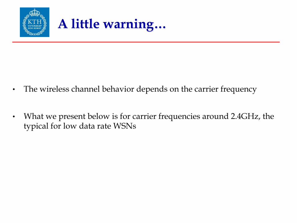
A little warning…

•  The wireless channel behavior depends on the carrier frequency

•  What we present below is for carrier frequencies around 2.4GHz, the typical for low data rate WSNs

Today’s lecture



•  Path-loss

•  Slow fading

•  Fast fading


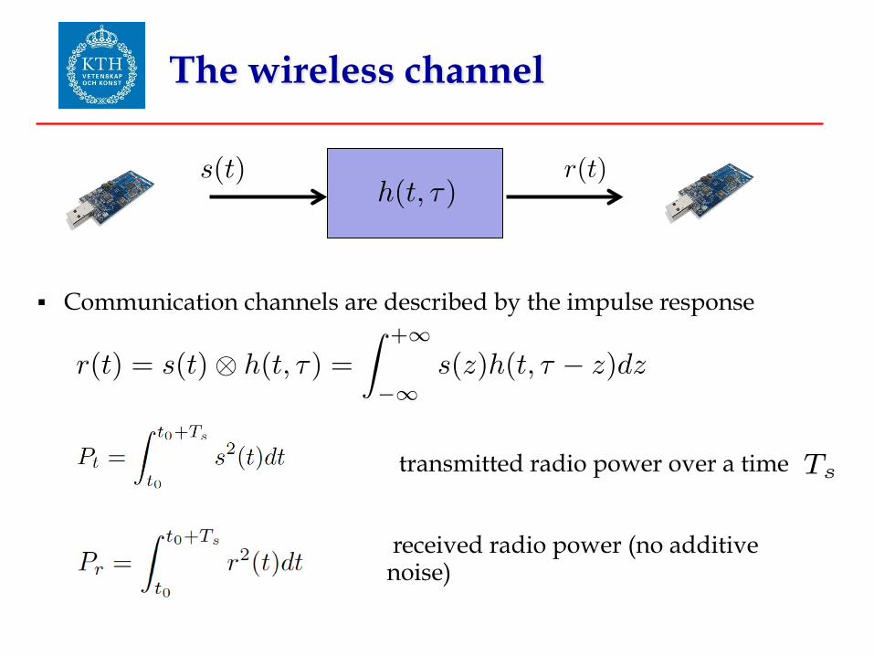
The wireless channel

§  Communication channels are described by the impulse response

transmitted radio power over a time

received radio power (no additive noise)

1





[email protected]

s(t)

h(t, ⌧)

r(t) = s(t)⌦ h(t, ⌧) =

Z+1

�1s(z)h(t, ⌧ � z)dz

Pt

=

Zt0+Ts

t0

r2(t)dt

SNR =

Pr

N0

Pr

= Pt

Gt

(✓t

, t

)Gr

(✓r

, r

)

�2

4⇡r

�

N0

r

G(✓t

, t

)

v(t)

1





[email protected]

s(t)

h(t, ⌧)

r(t) = s(t)⌦ h(t, ⌧) =

Z+1

�1s(z)h(t, ⌧ � z)dz

Pt

=

Zt0+Ts

t0

r2(t)dt

SNR =

Pr

N0

Pr

= Pt

Gt

(✓t

, t

)Gr

(✓r

, r

)

�2

4⇡r

�

N0

r

G(✓t

, t

)

v(t)

1





[email protected]

s(t)

h(t, ⌧)

r(t) = s(t)⌦ h(t, ⌧) =

Z+1

�1s(z)h(t, ⌧ � z)dz

Pt

=

Zt0+Ts

t0

r2(t)dt

SNR =

Pr

N0

Pr

= Pt

Gt

(✓t

, t

)Gr

(✓r

, r

)

�2

4⇡r

�

N0

r

G(✓t

, t

)

v(t)

1





[email protected]

s(t)

h(t, ⌧)

r(t) = s(t)⌦ h(t, ⌧) =

Z+1

�1s(z)h(t, ⌧ � z)dz

Pt

=

Zt0+Ts

t0

r2(t)dt

SNR =

Pr

N0

Pr

= Pt

Gt

(✓t

, t

)Gr

(✓r

, r

)

�2

4⇡r

�

N0

r

G(✓t

, t

)

v(t)

1





[email protected]

s(t)

h(t, ⌧)

r(t) = s(t)⌦ h(t, ⌧) =

Z+1

�1s(z)h(t, ⌧ � z)dz

Pt

=

Zt0+Ts

t0

r2(t)dt

SNR =

Pr

N0

Pr

= Pt

Gt

(✓t

, t

)Gr

(✓r

, r

)

�2

4⇡r

�

N0

r

G(✓t

, t

)

v(t)

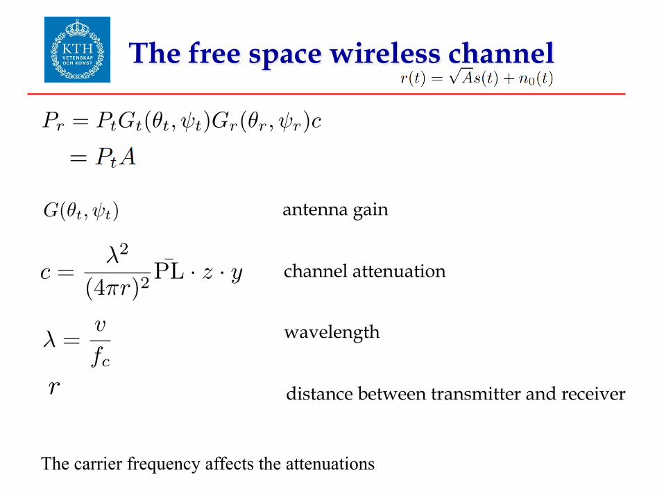
The free space wireless channel

antenna gain

channel attenuation

wavelength

distance between transmitter and receiver

1





[email protected]

Pr

= Pt

Gt

(✓t

, t

)Gr

(✓r

, r

)

�2

4⇡r

�

N0

r

G(✓t

, t

)

v(t)

P =

Z 1

�1v2(t)dt =

Z 1

�1V (f)V ⇤

(f)df

V (f) =

Z 1

�1v(t)ej2⇡ftdt

V (f)V ⇤(f)

Vn

(f) = V0

s

1 +

fc

f

R(f) =

��D

a

�� =s

1

(!2

0

� !2

)

2

+

(!

20!

2)

2

Q

2

[V/m/s2]

1





[email protected]

Pr

= Pt

Gt

(✓t

, t

)Gr

(✓r

, r

)

�2

4⇡r

�

N0

r

G(✓t

, t

)

v(t)

P =

Z 1

�1v2(t)dt =

Z 1

�1V (f)V ⇤

(f)df

V (f) =

Z 1

�1v(t)ej2⇡ftdt

V (f)V ⇤(f)

Vn

(f) = V0

s

1 +

fc

f

R(f) =

��D

a

�� =s

1

(!2

0

� !2

)

2

+

(!

20!

2)

2

Q

2

[V/m/s2]

1





[email protected]

s(t)

h(t, ⌧)

r(t) = s(t)⌦ h(t, ⌧) =

Z+1

�1s(z)h(t, ⌧ � z)dz

Pt

=

Zt0+Ts

t0

r2(t)dt

SNR =

Pr

N0

Pr

= Pt

Gt

(✓t

, t

)Gr

(✓r

, r

)c

c =�2

4⇡rPL · z · s

�

N0

r

G(✓t

, t

)

1





[email protected]

� =

v

fc

r(t) =pAs(t) + n

0

(t)

Pt

=

E

Ts

Pe

= 10

�6

Pe

= Q(

p2�⇤

)

SNR = z2E

b

N0

p(�) =1

�⇤ e�

�

⇤

� = z2

�⇤= E z2

Eb

N0

Pe

=

Z 1

0

Pe

(�)p(�)d� =

1

2

1�

r�⇤

1 + �⇤

�

Pe

' 1

4�⇤

5

Pt

=

Zt0+T

s

t0

r2(t)dt

SNR =

Pr

N0

Pr

= Pt

Gt

(✓t

, t

)Gr

(✓r

, r

)c

Pr

= Pt

Gt

(✓t

, t

)Gr

(✓r

, r

)

�2

(4⇡r)2¯

PL · z · y

c =�2

(4⇡r)2¯

PL · z · y

�

N0

r

G(✓t

, t

)

v(t)

P =

Z 1

�1v2(t)dt =

Z 1

�1V (f)V ⇤

(f)df

V (f) =

Z 1

�1v(t)ej2⇡ftdt

V (f)V ⇤(f)

Vn

(f) = V0

s

1 +

fc

f

R(f) =

��D

a

�� =s

1

(!2

0

� !2

)

2

+

(!

20!

2)

2

Q

2

[V/m/s2]

The carrier frequency affects the attenuations

The antenna

•  The antenna determines the attenuations of the transmitted signals

•  Let’s see how

Antennas

•  Antennas are transducers to transmit and receive radio signals

•  Variable currents within antenna conductors induce radiation of electromagnetic waves

•  Efficiency of energy capture to a receiver depends on 1.  the antenna geometry 2.  how impedance is matched between the antenna and the

medium and between the antenna and the electronics

•  Due to the reciprocity between transmission and reception, an antenna that is efficient in transmission is also efficient in reception

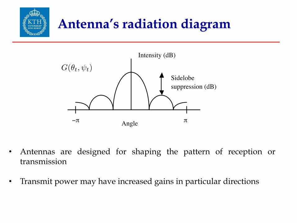
Antenna’s radiation diagram

•  Antennas are designed for shaping the pattern of reception or

transmission

•  Transmit power may have increased gains in particular directions

−π π

Intensity (dB)

Sidelobe suppression (dB)

Angle

1





[email protected]

Pr

= Pt

Gt

(✓t

, t

)Gr

(✓r

, r

)

�2

4⇡r

�

N0

r

G(✓t

, t

)

v(t)

P =

Z 1

�1v2(t)dt =

Z 1

�1V (f)V ⇤

(f)df

V (f) =

Z 1

�1v(t)ej2⇡ftdt

V (f)V ⇤(f)

Vn

(f) = V0

s

1 +

fc

f

R(f) =

��D

a

�� =s

1

(!2

0

� !2

)

2

+

(!

20!

2)

2

Q

2

[V/m/s2]

Antenna’s figure of merit

Efficiency: the fraction of input energy that is radiated. By reciprocity, the fraction of incident radiation that is captured Gain: the ratio of the intensity in the pattern to that of an isotropic antenna Beamwidth: the angle between the 3 dB points of the main antenna lobe (set of angles with largest intensity). Sidelobe suppression: the ratio of the peak intensity to the intensity of the largest sidelobe The environment in which the antennas operates—the packaging of the radio receiver, and the presence of nearby conductive entities (e.g., people) can alter the antenna efficiency and beam pattern

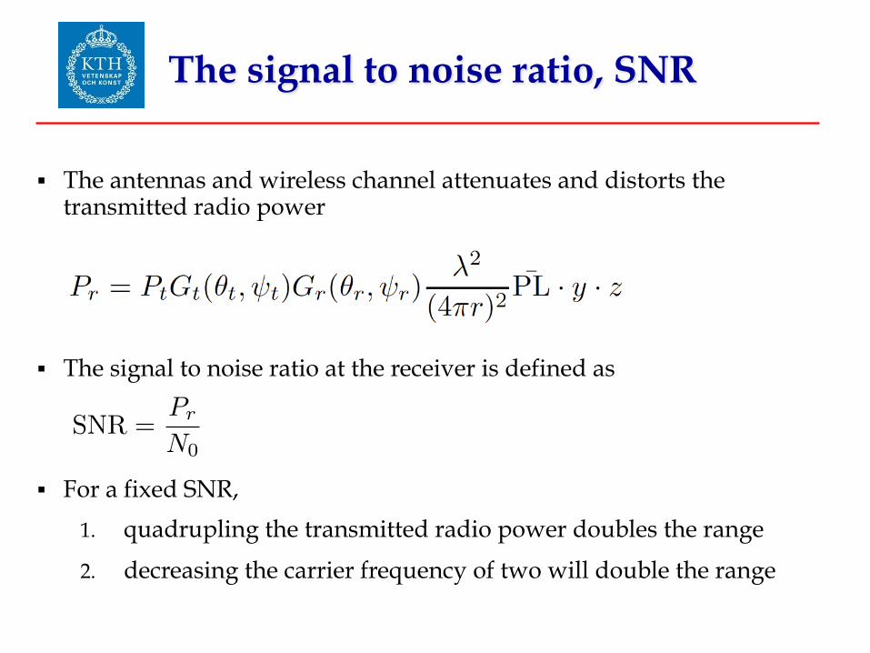
The signal to noise ratio, SNR

§  The antennas and wireless channel attenuates and distorts the transmitted radio power

§  The signal to noise ratio at the receiver is defined as

§  For a fixed SNR,

1.  quadrupling the transmitted radio power doubles the range

2.  decreasing the carrier frequency of two will double the range

1





[email protected]

SNR =

Pr

N0

Pr

= Pt

Gt

(✓t

, t

)Gr

(✓r

, r

)

�2

4⇡r

�

N0

r

G(✓t

, t

)

v(t)

P =

Z 1

�1v2(t)dt =

Z 1

�1V (f)V ⇤

(f)df

V (f) =

Z 1

�1v(t)ej2⇡ftdt

V (f)V ⇤(f)

Vn

(f) = V0

s

1 +

fc

f

Channel attenuation vs distance

r, distance TX-RX

Distance loss

Slow fading

Fast fading

+

+

5

Pt

=

Zt0+T

s

t0

r2(t)dt

SNR =

Pr

N0

Pr

= Pt

Gt

(✓t

, t

)Gr

(✓r

, r

)c

Pr

= Pt

Gt

(✓t

, t

)Gr

(✓r

, r

)

�2

(4⇡r)2¯

PL · z · y

c =�2

(4⇡r)2¯

PL · z · y

�

N0

r

G(✓t

, t

)

v(t)

P =

Z 1

�1v2(t)dt =

Z 1

�1V (f)V ⇤

(f)df

V (f) =

Z 1

�1v(t)ej2⇡ftdt

V (f)V ⇤(f)

Vn

(f) = V0

s

1 +

fc

f

R(f) =

��D

a

�� =s

1

(!2

0

� !2

)

2

+

(!

20!

2)

2

Q

2

[V/m/s2]

Path loss

§  The path loss power depends on the distance transmitter receiver

•  The dB of the path loss power is often called Received Signal Strength (RSS) and provided by TelosB motes as RSSI, for indoor scenarios is

4

g(t) =

r2E

Ts

, 0 t Ts

s(t) =1X

k=0

ai

g(t� kTs

)

G(f) = �r

2E

Ts


s

j2⇡f= �

r2E

Ts

Ts

sin(⇡fTs

)

⇡fTs

= �r

2E

Ts

Ts

sinc(fTs

)

�

s

(f) = 2ETs

sinc

2

(fTs

)

G(f) =

ZT

s

0

a0

g(t)e�2⇡ftdt

�

s

(f) = �2

0

|G(f)|2

T

PL

dB

(r) = 10 log

10

PL(r) = PL(d0

) + 10nSF

log

✓d

d0

◆+ FAF +

X

j

PAF

j

PL =

�2

(4⇡r)2¯

PL

h(t, ⌧) =pG

t

G

r

PLyX

i

↵i

(t)ej✓i(t)�(⌧ � ⌧i

(t))

|↵i

(t)ej✓i(t)| = zi

f(z) =z

�2

e�z

2

2�2

X = N(µ,�2

)

y = ex

10

s(t)

h(t, ⌧)

5

Pt

=

Zt0+T

s

t0

r2(t)dt

SNR =

Pr

N0

Pr

= Pt

Gt

(✓t

, t

)Gr

(✓r

, r

)c

Pr

= Pt

Gt

(✓t

, t

)Gr

(✓r

, r

)

�2

(4⇡r)2¯

PL · z · y

c =�2

(4⇡r)2¯

PL · z · y

�

N0

r

G(✓t

, t

)

v(t)

P =

Z 1

�1v2(t)dt =

Z 1

�1V (f)V ⇤

(f)df

V (f) =

Z 1

�1v(t)ej2⇡ftdt

V (f)V ⇤(f)

Vn

(f) = V0

s

1 +

fc

f

R(f) =

��D

a

�� =s

1

(!2

0

� !2

)

2

+

(!

20!

2)

2

Q

2

[V/m/s2]

distance

Distance loss

Shadowing

Multipath

+

+

floor attenuation factor path attenuation factor per obstacle within a room

path loss exponent

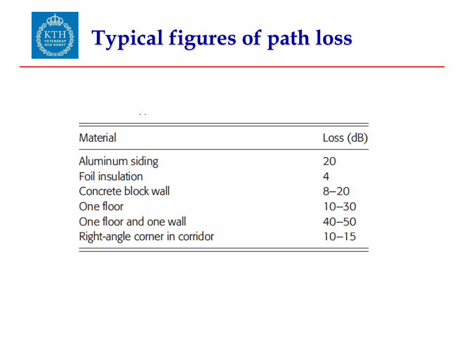
Typical figures of path loss

Shadow fading

The shadow fading often follows a lognormal probability distribution function

1





[email protected]

X = N(µ,�2

)

y = ex

10

s(t)

h(t, ⌧)

r(t) = s(t)⌦ h(t, ⌧) =

Z+1

�1s(z)h(t, ⌧ � z)dz

Pt

=

Zt0+T

s

t0

r2(t)dt

SNR =

Pr

N0

Pr

= Pt

Gt

(✓t

, t

)Gr

(✓r

, r

)c

c =�2

4⇡rPL · z · y

�

N0

1





[email protected]

X = N(µ,�2

)

y = ex

10

s(t)

h(t, ⌧)

r(t) = s(t)⌦ h(t, ⌧) =

Z+1

�1s(z)h(t, ⌧ � z)dz

Pt

=

Zt0+T

s

t0

r2(t)dt

SNR =

Pr

N0

Pr

= Pt

Gt

(✓t

, t

)Gr

(✓r

, r

)c

c =�2

4⇡rPL · z · y

�

N0

distance

Distance loss

Shadowing

Multipath

+

+

4

g(t) =

r2E

Ts

, 0 t Ts

s(t) =1X

k=0

ai

g(t� kTs

)

G(f) = �r

2E

Ts


s

j2⇡f= �

r2E

Ts

Ts

sin(⇡fTs

)

⇡fTs

= �r

2E

Ts

Ts

sinc(fTs

)

�

s

(f) = 2ETs

sinc

2

(fTs

)

G(f) =

ZT

s

0

a0

g(t)e�2⇡ftdt

�

s

(f) = �2

0

|G(f)|2

T

PL

dB

= 10 log

10

PL = PL(d0

) + 10nSF

log

✓r

r0

◆+ FAF +

X

j

PAF

j

PL =

�2

(4⇡r)2¯

PL

h(t, ⌧) =pG

t

G

r

PLyX

i

↵i

(t)ej✓i(t)�(⌧ � ⌧i

(t))

|↵i

(t)ej✓i(t)| = zi

f(z) =z

�2

e�z

2

2�2

X = N(µ,�2

)

y = ex

10

s(t)

h(t, ⌧)

4

g(t) =

r2E

Ts

, 0 t Ts

s(t) =1X

k=0

ai

g(t� kTs

)

G(f) = �r

2E

Ts


s

j2⇡f= �

r2E

Ts

Ts

sin(⇡fTs

)

⇡fTs

= �r

2E

Ts

Ts

sinc(fTs

)

�

s

(f) = 2ETs

sinc

2

(fTs

)

G(f) =

ZT

s

0

a0

g(t)e�2⇡ftdt

�

s

(f) = �2

0

|G(f)|2

T

PL

dB

= 10 log

10

PL = PL(d0

) + 10nSF

log

✓r

r0

◆+ FAF +

X

j

PAF

j

PL =

�2

(4⇡r)2¯

PL

h(t, ⌧) =pG

t

G

r

PLyX

i

↵i

(t)ej✓i(t)�(⌧ � ⌧i

(t))

|↵i

(t)ej✓i(t)| = zi

f(z) =z

�2

e�z

2

2�2

X = N(µ,�2

)

y = ex

10

s(t)

h(t, ⌧)

4

g(t) =

r2E

Ts

, 0 t Ts

s(t) =1X

k=0

ai

g(t� kTs

)

G(f) = �r

2E

Ts


s

j2⇡f= �

r2E

Ts

Ts

sin(⇡fTs

)

⇡fTs

= �r

2E

Ts

Ts

sinc(fTs

)

�

s

(f) = 2ETs

sinc

2

(fTs

)

G(f) =

ZT

s

0

a0

g(t)e�2⇡ftdt

�

s

(f) = �2

0

|G(f)|2

T

PL

dB

= 10 log

10

PL = PL(d0

) + 10nSF

log

✓r

r0

◆+ FAF +

X

j

PAF

j

PL =

�2

(4⇡r)2¯

PL

h(t, ⌧) =pG

t

G

r

PLyX

i

↵i

(t)ej✓i(t)�(⌧ � ⌧i

(t))

|↵i

(t)ej✓i(t)| = zi

f(z) =z

�2

e�z

2

2�2

X = N(µ,�2

)

y = ex

10

s(t)

h(t, ⌧)

4

g(t) =

r2E

Ts

, 0 t Ts

s(t) =1X

k=0

ai

g(t� kTs

)

G(f) = �r

2E

Ts


s

j2⇡f= �

r2E

Ts

Ts

sin(⇡fTs

)

⇡fTs

= �r

2E

Ts

Ts

sinc(fTs

)

�

s

(f) = 2ETs

sinc

2

(fTs

)

G(f) =

ZT

s

0

a0

g(t)e�2⇡ftdt

�

s

(f) = �2

0

|G(f)|2

T

PL

dB

= 10 log

10

PL = PL(d0

) + 10nSF

log

✓r

r0

◆+ FAF +

X

j

PAF

j

PL =

�2

(4⇡r)2¯

PL

h(t, ⌧) =pG

t

G

r

PLyX

i

↵i

(t)ej✓i(t)�(⌧ � ⌧i

(t))

|↵i

(t)ej✓i(t)| = zi

f(z) =z

�2

e�z

2

2�2

X = N(µ,�2

)

y = ex

10

s(t)

h(t, ⌧)

4

g(t) =

r2E

Ts

, 0 t Ts

s(t) =1X

k=0

ai

g(t� kTs

)

G(f) = �r

2E

Ts


s

j2⇡f= �

r2E

Ts

Ts

sin(⇡fTs

)

⇡fTs

= �r

2E

Ts

Ts

sinc(fTs

)

�

s

(f) = 2ETs

sinc

2

(fTs

)

G(f) =

ZT

s

0

a0

g(t)e�2⇡ftdt

�

s

(f) = �2

0

|G(f)|2

T

PL

dB

= 10 log

10

PL = PL(d0

) + 10nSF

log

✓r

r0

◆+ FAF +

X

j

PAF

j

PL =

�2

(4⇡r)2¯

PL

h(t, ⌧) =pG

t

G

r

PLyX

i

↵i

(t)ej✓i(t)�(⌧ � ⌧i

(t))

|↵i

(t)ej✓i(t)| = zi

f(z) =z

�2

e�z

2

2�2

X = N(µ,�2

)

y = ex

10

s(t)

h(t, ⌧)

4

g(t) =

r2E

Ts

, 0 t Ts

s(t) =1X

k=0

ai

g(t� kTs

)

G(f) = �r

2E

Ts


s

j2⇡f= �

r2E

Ts

Ts

sin(⇡fTs

)

⇡fTs

= �r

2E

Ts

Ts

sinc(fTs

)

�

s

(f) = 2ETs

sinc

2

(fTs

)

G(f) =

ZT

s

0

a0

g(t)e�2⇡ftdt

�

s

(f) = �2

0

|G(f)|2

T

PL

dB

= 10 log

10

PL = PL(d0

) + 10nSF

log

✓r

r0

◆+ FAF +

X

j

PAF

j

PL =

�2

(4⇡r)2¯

PL

h(t, ⌧) =pG

t

G

r

PLyX

i

↵i

(t)ej✓i(t)�(⌧ � ⌧i

(t))

|↵i

(t)ej✓i(t)| = zi

f(z) =z

�2

e�z

2

2�2

X = N(µ,�2

)

y = ex

10

s(t)

h(t, ⌧)

5

Pt

=

Zt0+T

s

t0

r2(t)dt

SNR =

Pr

N0

Pr

= Pt

Gt

(✓t

, t

)Gr

(✓r

, r

)c

Pr

= Pt

Gt

(✓t

, t

)Gr

(✓r

, r

)

�2

(4⇡r)2¯

PL · z · y

c =�2

(4⇡r)2¯

PL · z · y

�

N0

r

G(✓t

, t

)

v(t)

P =

Z 1

�1v2(t)dt =

Z 1

�1V (f)V ⇤

(f)df

V (f) =

Z 1

�1v(t)ej2⇡ftdt

V (f)V ⇤(f)

Vn

(f) = V0

s

1 +

fc

f

R(f) =

��D

a

�� =s

1

(!2

0

� !2

)

2

+

(!

20!

2)

2

Q

2

[V/m/s2]

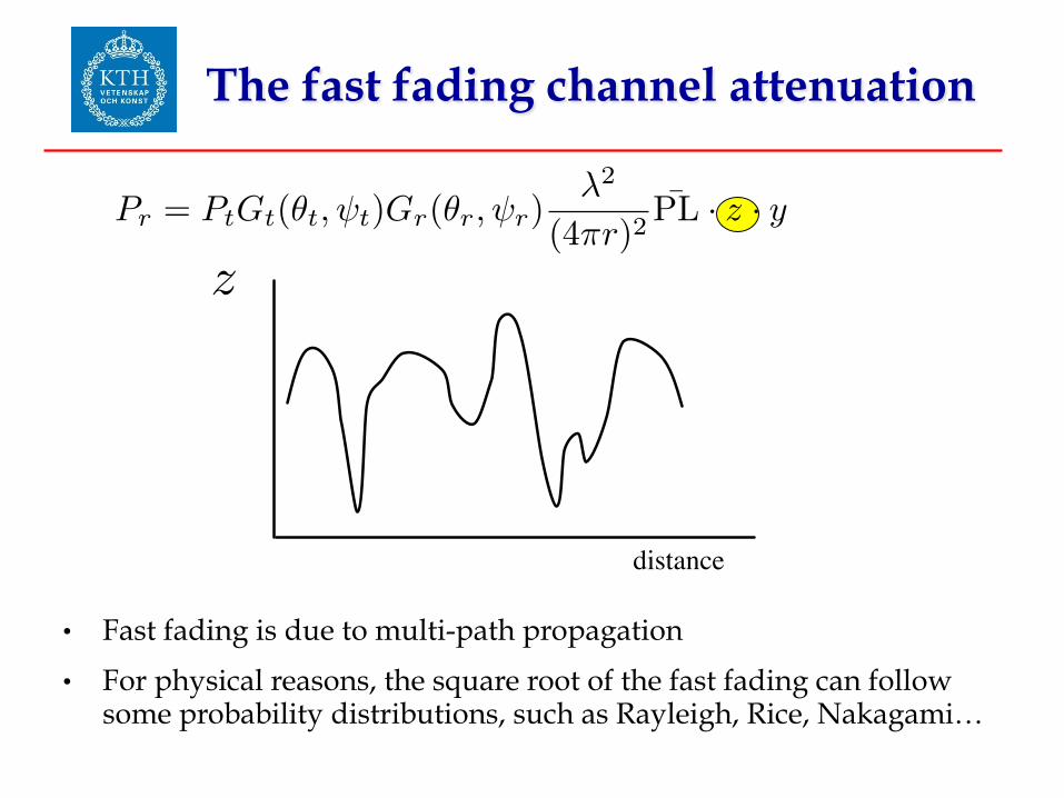
•  Fast fading is due to multi-path propagation

•  For physical reasons, the square root of the fast fading can follow some probability distributions, such as Rayleigh, Rice, Nakagami…

The fast fading channel attenuation

distance

1





[email protected]

s(t)

h(t, ⌧)

r(t) = s(t)⌦ h(t, ⌧) =

Z+1

�1s(z)h(t, ⌧ � z)dz

Pt

=

Zt0+Ts

t0

r2(t)dt

SNR =

Pr

N0

Pr

= Pt

Gt

(✓t

, t

)Gr

(✓r

, r

)c

c =�2

4⇡rPL · z · s

�

N0

r

G(✓t

, t

)

5

Pt

=

Zt0+T

s

t0

r2(t)dt

SNR =

Pr

N0

Pr

= Pt

Gt

(✓t

, t

)Gr

(✓r

, r

)c

Pr

= Pt

Gt

(✓t

, t

)Gr

(✓r

, r

)

�2

(4⇡r)2¯

PL · z · y

c =�2

(4⇡r)2¯

PL · z · y

�

N0

r

G(✓t

, t

)

v(t)

P =

Z 1

�1v2(t)dt =

Z 1

�1V (f)V ⇤

(f)df

V (f) =

Z 1

�1v(t)ej2⇡ftdt

V (f)V ⇤(f)

Vn

(f) = V0

s

1 +

fc

f

R(f) =

��D

a

�� =s

1

(!2

0

� !2

)

2

+

(!

20!

2)

2

Q

2

[V/m/s2]

•  Fast fading may follow a Rayleigh distribution (if x is a Rayleigh random variable, z is and exponential random variable)

Rayleigh fast fading

distance

Distance loss

Shadowing

Multipath

+

+

5

Pt

=

Zt0+T

s

t0

r2(t)dt

SNR =

Pr

N0

Pr

= Pt

Gt

(✓t

, t

)Gr

(✓r

, r

)c

Pr

= Pt

Gt

(✓t

, t

)Gr

(✓r

, r

)

�2

(4⇡r)2¯

PL · z · y

c =�2

(4⇡r)2¯

PL · z · y

�

N0

r

G(✓t

, t

)

v(t)

P =

Z 1

�1v2(t)dt =

Z 1

�1V (f)V ⇤

(f)df

V (f) =

Z 1

�1v(t)ej2⇡ftdt

V (f)V ⇤(f)

Vn

(f) = V0

s

1 +

fc

f

R(f) =

��D

a

�� =s

1

(!2

0

� !2

)

2

+

(!

20!

2)

2

Q

2

[V/m/s2]

Multi-path Rayleigh fading

§  The channel impulse response may spread the transmitted signal over time due to multiple reflectors

4

g(t) =

r2E

Ts

, 0 t Ts

s(t) =1X

k=0

ai

g(t� kTs

)

G(f) = �r

2E

Ts


s

j2⇡f= �

r2E

Ts

Ts

sin(⇡fTs

)

⇡fTs

= �r

2E

Ts

Ts

sinc(fTs

)

�

s

(f) = 2ETs

sinc

2

(fTs

)

G(f) =

ZT

s

0

a0

g(t)e�2⇡ftdt

�

s

(f) = �2

0

|G(f)|2

T

PL

dB

(r) = 10 log

10

PL(r) = PL(d0

) + 10nSF

log

✓d

d0

◆+ FAF +

X

j

PAF

j

PL =

�2

(4⇡r)2¯

PL

h(t, ⌧) =pG

t

G

r

PLyX

i

↵i

(t)ej✓i(t)�(⌧ � ⌧i

(t))

|↵i

(t)ej✓i(t)| = zi

f(z) =z

�2

e�z

2

2�2

X = N(µ,�2

)

y = ex

10

s(t)

h(t, ⌧)

random variable with uniform distribution

random variable with Rayleigh distribution

imaginary number

delay of path i

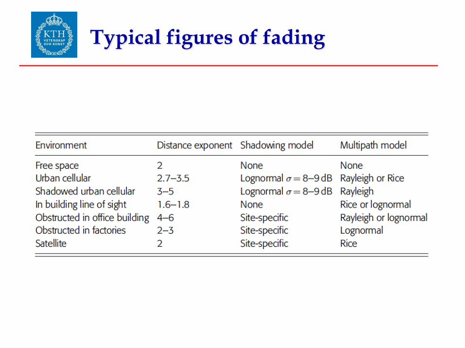
Typical figures of fading

Today’s lecture



•  Path-loss

•  Slow fading

•  Fast fading


•  It is a simple way to describe the behavior of the wireless channel in two states: Bad and Good

•  probability of bad state

•  probability of good state

•  probability to go from the good state to the bad

•  probability to go from the bad state to the good

Gilbert-Elliot model

•  We studied the wireless channel attenuates the transmit power

•  AWGN •  Path loss •  Slow fading •  Fast fading

•  Next lecture, we study the probability of erroneously decoding bits

Conclusions

Phy MAC

Routing

Transport

Session

Application Presentation

Project

•  The project is a 10-15 pages single column written report •  Must contain experimental results of your proposal •  Time line:

1.  Jan 21: every group communicates to [email protected] the preferences on the topic

2.  Jan 25: Carlo sends out the study material with detailed instructions

3.  Feb 4: every group e-mails to [email protected] the proposal for report table of content

4.  Feb 5: Carlo sends feedback on the proposal 5.  Feb 6: The groups start working on the writing and experiments 6.  Feb 6-Mar 4: groups work and ask feedback if needed to the

teaching assistants and Carlo 7.  Feb 28: peer-review of the project report by two other groups 8.  March 4: every group gives a 10 minutes presentation on the

project and submits the final project report

Principles of Wireless Sensor Networks - kth.se · Principles of Wireless Sensor Networks https:...

Documents

Transcript of Principles of Wireless Sensor Networks - kth.se · Principles of Wireless Sensor Networks https:...