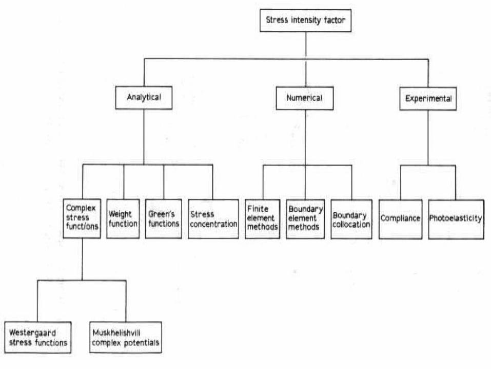
Principle of Superposition For a linear elastic system, the individual components of stress, strain,...
39
Principle of Superposition For a linear elastic system, the individual components of stress, strain, displacement are additive. For example, two normal stress in x direction caused by two different external load can be added to get total stress P M P M P M P M a M M P P a x total I I a b total I a P M y A I O n sim illarlinesstressintensity factorscan also added K K (a) K (b) = Y a Y a K K (a) 0 = Y a 0
-
Upload
heather-hodge -
Category
Documents
-
view
221 -
download
1
Transcript of Principle of Superposition For a linear elastic system, the individual components of stress, strain,...

Principle of Superposition
For a linear elastic system, the individual components of stress, strain, displacement are additive. For example, two normal stress in x direction caused by two different external load can be added to get total stress
P
M
P
M
P
M
P
M a
MM
PP
a
x
total I I
a b
total I
a
P My
A I
On simillar lines stress intensity
factors can also added
K K (a) K (b)
= Y a Y a
K K (a) 0
= Y a 0

Principle of SuperpositionFor example consider a plate having semicircular crack subjected to an internal pressure
I
1/42 22 2
2 2
1.12 aK g( )
3 a a, g( ) sin cos
8 8 c c
a
2c
I I I
For Semi circular crack
, g( ) 12
K (total) K (b) K (c)
2 1.12 p a 0
2.24 = p a

Crack Tip PlasticityLEFM assumes a sharp crack tip, inducing infinite stress at the crack tip. But in real materials, the crack tip radius is finite and hence the crack tip stresses are also finite. In addition, inelastic deformations due to plasticity in metals, crazing in polymers leads to further relaxation of stresses.
For metals with yielding, LEFM solutions are not accurate. A small region around the crack tip yields leading to a small plastic zone around it.
For moderately yielding metals, LEFM solutions can be used with simple correction.For extensively yielding metals, alternative fracture parameters like CTOD, J-integral are to be used taking into account material non-linearity.

Small Scale PlasticityIrwin’s ApproachNormal stress yy based on elastic analysis is given by
On the crack plane = 0
As a first approximation yielding occurs when yy = ys
ry = first order estimate of plastic zone size. This is approximate estimate, because of the fact that yy is based on elastic analysis
Iyy
K 3cos 1 sin sin
2 2 22 r
Iyy
K
2 r
2 2
I Iys y y
ys ysy
K 1 K a, r , or r
2 22 r

Irwin’s ApproachWhen yielding occurs, stresses redistribute in order to satisfy equilibrium conditions. The cross hatched regions represents forces active in the elastic analysis that cannot be carried in elasto-plastic analysis, because of the reason that the stresses cannot exceed ys.To redistribute this excessive force, the plastic zone size must increase. This is possible if the material immediately ahead of plastic zone carries more stress.
Irwin proposed that plasticity makes the crack behave as if it were larger than actual physical size.Let the effective crack size be aeff , such that aeff = a+whereis the correction.
or

To permit redistribution of stresses , the areas A and B must be the same
2
I
ys
2
Ieff y
ys
I eff
Kplastic constraint factor
1 Keffective crack size = a a 2r = a+
Effective stress in tensity factor K Y a

A long rectangular plate has a width of 100 mm, thickness of 5 mm and an axial load of 50 kN. If the plate is made of titanium Ti-6AL-4V,(KIC=115 MPa-m1/2, ys=p10 MPa) what is the factor of safety against crack growth for a crack of length a = 20 mm.
1/ 2 2 4
eff
1/ 22 4
sec 1 0.025 0.062
1. a = a = 0.01m
0.2Y= sec 1 0.025 0.2 0.06 0.2
2
1.02448
150 1000300
5 100
I effK Y a
a a aY
b b b
trial
X
XMPa
X
2a=20mm
2b=100mm
150KN

1/ 2
IC
I
2 2
eff
1.02448 300 0.01
54.525
K 115Factor of Safety without plastic correction = 2.11
K 54.525
2.
1 1 54.5252 = 0.00114275
910
effective crack size = a 2 = 0.
I
Iy
ys
y
K X X
MPa m
trial
Kr
a r
eff
01 0.00114275 0.1114275
1.3007
1.0307 300 0.01114275 57.85
3.
2 0.001286
a 2 = 0.011286
s in 58.25
Factor of Safety with plastic
I eff
y
y
I
Y
Effective SIF K Y a X X X
trial
r
a r
Effective stres tensity factor K
IC
I
K 115 correction = 1.975
K 58.25

Strip Yield Method (Proposed by Dugdale and Barrenblatt)They assumed a narrow long slender plastic zone ahead of crack tip in a non-hardening (ideal plastic) material in plane stress for a through crack in a infinite plate.
The strip yield plastic zone assumes a crack length of 2a + 2Whereis length of plastic zone.Approximate elasto-plastic behavior is obtained by superimposing two elastic solutions (a) a through crack under remote tension (b) a through crack under crack closure stress.
Concept: stress at the crack tip is no more a singular and it is a finite value (ys), hence stress singularity term is zero. I.e. the length of the plastic zone is such that the stress intensity factor due to remote tension cancels with crack closure.

x P
P
2a
Strip Yield MethodSIF due to crack closure stress can be estimated by considering a normal force P applied to the crack at a distance x from the center line of crack
SIF for two crack tips are given by
ys
( )
( )
Crack closure force = P = -
I
I
P a xK a
a xa
P a xK a
a xadx
ys
a+ys
For the problem considered
SIF is obtained by replacing P by
- and a by a+ , and adding the two
- a+ a+( )
a+ a+a+
I
a
dx
x xK closure dx
x x

1ys
ys
a+( ) -2 cos (A)
a+
SIF due to remote tension
( ) a+ (B)
(A) = (B)
cosa+ 2
Expanding right hand side using
I
I
aK closure
K tension
a
2 4
ys ys
22 2
2ys
Taylor's series
1 11
a+ 2! 2 4! 2
Considering first two term of the Taylor's series
= ...... length of the plastic zone8 8
I
ys
a
a K
Strip Yield Method
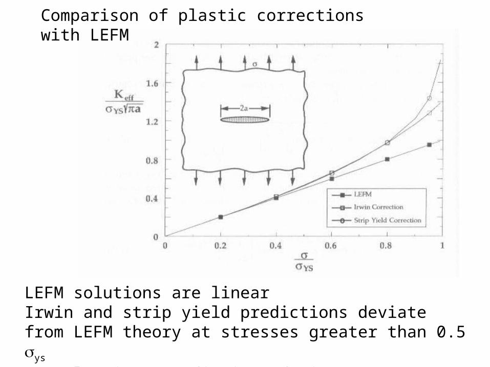
Comparison of plastic corrections with LEFM
LEFM solutions are linearIrwin and strip yield predictions deviate from LEFM theory at stresses greater than 0.5 ys
Two plasticty predictions deviate at 0.85 ys

Plastic Zone ShapeIn the earlier calculation plastic zone size was calculated for = 0(along the crack plane), the plastic zone shape will be quite different when all angles are considered. Plasticity are based on von Mises and Tresca’s yield criteria. For mode I problem stress field are obtained using Westergaard’ stress function., then principal stresses are given by
1/ 22
21 2,
2 2
and hence
xx yy xx yyxy

Using the principal stresses in von Mises yield criteria
max
1 2 1 3max
1 2 1max max
Tresca:
/ 2
or : for PSN2 2
: for PSS2 2
ys

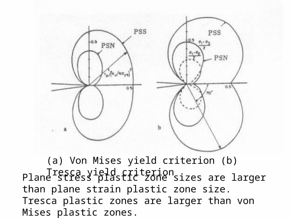
(a) Von Mises yield criterion (b) Tresca yield criterion
Plane stress plastic zone sizes are larger than plane strain plastic zone size. Tresca plastic zones are larger than von Mises plastic zones.
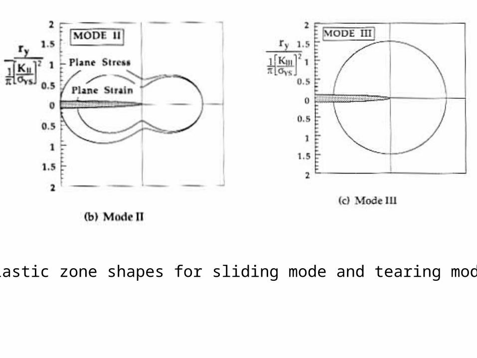
Plastic zone shapes for sliding mode and tearing modes

Plane strain or plane stress
In general, the conditions ahead of a crack tip are neither plane stress nor plane strain. There are limiting cases where a two dimensional assumptions are valid, or at least provides a good approximation.The nature of the plastic zone that is formed ahead of a crack tip plays a very important role in the determination of the type of failure that occurs. Since the plastic region is larger in PSS than in PSN, plane stress failure will, in general, be ductile, while, on the other hand, plane strain fracture will be brittle, even in a material that is generally ductile. This phenomenon explains the peculiar thickness effect, observed in all fracture experiments, that thin samples exhibit a higher value of fracture toughness than thicker samples made of the same material and operating at the same temperature. From this it can be surmised that the plane stress fracture toughness is relatedto both metallurgical parameters and specimen geometry while the plane strain fracture toughness depends more on metallurgical factors than on the others.

Due to presence of crack tip, stress in a direction to normal to crack plane yy
will be large near the crack tip. This stress would in turn tries to contract in x and z direction. But the material surrounding it will constraint it, inducing stresses in x and z direction, there by a triaxial state of stress exists near the crack tip. This leads to plane strain condition at interior.At the plate surface zz is zero and zz is maximum. This leads to plane stress condition at exterior.

The state of stress is also dependent on size of plate thickness.If the plastic zone size is small compared to the plate thickness, plane strain condition exists. If the plastic zone size is larger than the plate thickness, plane stress condition prevails.As the loading is increased, plastic zone size also increases leading to plane stress conditions.

Effect of plate thickness on fracture toughness
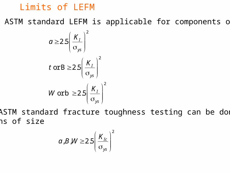
Limits of LEFM
As per ASTM standard LEFM is applicable for components of size2
2
2
2.5
or B 2.5
or b 2.5
I
ys
I
ys
I
ys
Ka
Kt
KW
As per ASTM standard fracture toughness testing can be done on Specimens of size
2
, , 2.5
Ic
ys
Ka B W

Concept of Isoparametric Elements
(-1,1)
(1,1)
(1,-1)(-1,-1)
Y
X
(x1, y
1)
(1,1)
(1,-1)(x5, y
5)
(x2, y
2)
(x6, y
6)
(x3, y
3)
(x4, y
4)
(x7, y
7)
(x8, y
8)
(-1,-1)
(-1,1)
Elements are defined in local coordinate system () with straight well defined edges. Elements defined in local coordinates have advantage that numerical integration limits vary –1 to +1 Elements from local coordinated when mapped on to global cartesian coordinates, it can be distorted to a new curvilinear set as shown in the figure. In Isop. Formulation, with distorted elements, numerical integration are still carried with limits of local coorinates i.e. –1 to +1
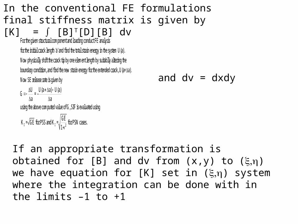
In the conventional FE formulations final stiffness matrix is given by [K] = [B]T[D][B] dv
For the given structural component and loading conduct FE analysis
for the initial crack length 'a' and find the total strain energy in the system U(a).
Now physically shift the crack tip by one element length by suitablly altering the
boundary condition, and find the new strain energy for the extended crack, U(a+ a).
Now SE release rate is given by
U U(a a) U(a)G = -
a ausing the above computed va
I I 2
lue of G, SIF is evaluated using
GE K = GE for PSS and K = for PSN cases.
1-
and dv = dxdy
If an appropriate transformation is obtained for [B] and dv from (x,y) to () we have equation for [K] set in () system where the integration can be done with in the limits –1 to +1

In order to achieve such a transformation ( [B] and dv) two sets of nodes ate defined for each element.
One set of nodes (marked as )are used to interpolate coordinates of a point with in the element using nodal coordinates. For exampleIf N1, N2, N3…… are the interpolation function used to interpolate shape variation, such thatX = N1 X1+ N2 X2 + N3 X3 +………Y = N1 Y1+ N2 Y2 + N3 Y3 +………
For an eight node quadratic elementN1 = - ¼ .()N5 = - ½ .(
Theinterpolation functions N1, N2, N3…… are generally called here as ‘Shape function’ as they define the shape/distortions
Nodes to define shape (coordinate interpolation with in the element)
X (x,y)
4 7 3
8 6
1 5 2

Nodes to define displacement (displacement interpolation with in the element)
4 7 3
X (u,v)8 6
1 5 2
Another set of nodes (marked as )are used to interpolate displacements of a point with in the element using nodal displacements. For example if N1, N2, N3…… are the interpolation function used to interpolate shape variation, such thatu = N1 u1+ N2 u2 + N3 u3 +………v = N1 v1+ N2 v2 + N3 v3 +………
For a four node bilinear elementN1 = - ¼ .(N2 = - ½ .(
Theinterpolation functions N1, N2, N3…… are generally called here as ‘Displacement function’ as they define the displacement variation with in the element.

If number of nodes used to define shape (identified by and Ni ) and the number of nodes used to define the displacement variation (identified by and Ni ) are equal, say for example 8 nodes for shape and 8 nodes for displacement, then such elements are called ISOPARAMETRIC ELEMENTS.
If number of nodes used to define shape are more than the number of nodes used to define the displacement variation say for example 8 nodes for shape and 4 nodes for displacement, then such elements are called SUPERPARAMETRIC ELEMENTS.
If number of nodes used to define shape are less than the number of nodes used to define the displacement variation say for example 4 nodes for shape and 8 nodes for displacement, then such elements are called SUBPARAMETRIC ELEMENTS.
4 7 3
8 6
1 5 2Isoparametric element
4 7 3
8 6
1 5 2Superparametric element
4 7 3
8 6
1 5 2Subparametric element

i i
i i
x y
where Jx y
J is called Jacobian matrix
i i
i i
N N
N N
(A)
i i i
i i i
i i
ii
i i
ii
N N x N y
x y
N N x N y
x y
N x y N
xNN x yy
N N
xJ
NNy
For any curved element formulations (iso, super or sub) [J] is obtained using shape functions (defined for shapes)

1
Re writing eqn. (A)
note that is obtained by displacement functions
The terms of strain-displacement matrix [B] are given by
ii
i i
i
i
NN
xJ
N Ny
N
N
of the prvious equation and det
i
i
N
xN
y
dv dxdy J d d
0
note B 0
i
i
i i
N
xN
y
N N
y x

Crack tip singular elementsUse of conventional elements near the crack tip, even with very fine mesh near would not simulate the stress field conditions of the crack tip ( ) . Barsoum showed that by moving mid-side nodes of a 8 node isoparametric element to quarter points induced singularity and improved the performance of the analysis enormously.
1/ r
1/ r Crack tip
12
34
5
6
7
8
Move mid-sideNodes at points4
1
Crack tip
12
34
5
7
8 6
Crack tip
1,8,4
5
2
6
3
7
Move mid-sideNodes at points
41
Crack tip
1,8,4
Collapseside
5
6
3
7
2

1
-1
In the FEM formulations strain vector
is given by
J ,
J = jacobian matrix
, parametric coordinates of a point
on an element
The strain vector can be singular if either J or B is sigular
i
i
uB
v
-1 (x,y)J can be sigular when det J = = 0
( , )
consider the quadratic element as shown
let us evaluate the boundary nodes
between 1 and 2 in x direction
0
where B 0
i
i
i i
N
N
N N
Crack tip
12
34
5
6
7
8
Move mid-sideNodes at points4
1

21 1 1
1 1 2 2 5 5
21 2 5
1 2 5
2
1 1(1 ), (1 ), (1 )
2 2
1 1(1 ) (1 ) (1 )
2 20, , / 4
1(1 ) (1 )
2 4
solving 1 2
Jacobian J (1 )2
as x 0; det J 0....
N N N
x N x N x N x
x x x x
x x L x L
Lx L
x
L
x L x
L
..leading to singularity
1 25 xy
LL/4

21 1 2 2 5 5 1 2 5
1 2
5
1
Let us evaluate the strain
1 1(1 ) (1 ) (1 )
2 2
using 1 2
1 11 2 2 2 1 2 2
2 2
4
1 3 4 1 1
2 2x
u N u N u N u u u u
x
L
x x x xu u u
L L L L
x xu
L L
uu
x LxL xL
2 5
4 2 4
1 1 ......leading to 1/ singularity
u uL LxL
rx r

Virtual Crack Extension Method to Evaluate SIF
For a two-dimensional cracked body in mode I, the total potential in terms of FE solutions is given byU = ½ {u}T[K]{u}- {u}T[F]The strain energy release rateIs defined as
UG = -
u K F1 = -
2
TT T
a
K u F u u ua a a
crack tip FE mesh
The first term in above expression is zero (equilibrium condition). In the absence of traction on crack face the third term is also zero.

aa
2
2
Hence
KU 1G = -
2 for plane stress
E = for plane strain
1-
TIKu u
a E awhere E E
For a given FE mesh for a body with crack length a, and to extend the crack length by a it is not necessary to alter entire mesh. This can be achieved by moving a few elements near the crack tip and keeping rest intact. If N number of elements that are effected then
The strain energy release rate is proportional to the derivative of the stiff ness matrix with respect to crack length.
1
K1 G =
2
NT
i
u ua

Stress Approach to Evaluate SIF
r1 r2 r3 r4
r1 r2 r3 r4
y1 y2 y3 y4
Iyy
K 3cos 1 sin sin
2 2 22 r
On the crack plane = 0I
yy
I yy
1 2 y1 y2
I 1 I 2
K
2 rRearranging
K 2 r
At various points r , r ...measure , ..
Hence a set of K (r ),K (r )...
can be calculated.
Plot these values againist r/a.
Extend the best fit line to meet
abcissa to get
Ithe required K for
the given structural conponent
and loading.
xx
x xx
xx
KI
r/a

Displacement Approach to Evaluate SIF
xx
x xx
xx
KI
r/a
r1
r2r3
r4
r
v1 v2v3
v4
= 1
2I
2(1 ) r 1v K sin cos
E 2 2 2 2
1
I 1
where v = displacements in y directions
3(3 4 ) for PSS and for PSN
1
At some given angle =
2K (r) f v(r)
r
1 2 1 2
I 1 I 2
I
At various points r , r ...measure v ,v ..
Hence a set of K (r ),K (r )...can be
calculated. Plot these values againist r/a.
Extend the best fit line to meet abcissa to
get the required K for the given structural
conponent and loading.

Strain Energy Release Rate to Evaluate SIF
a + a
1 2
a
1 2
F o r a s t e e l b e a m s h o w n b e l o w , a c r a c k o f l e n g t h 7 . 5 m m i s d e t e c t e d b y N D T . F i n d t h e b e a m t h i c k n e s s t o p r o v i d e a f a c t o r o f s a f e t y o f 2 ( 1 ) b y i g n o r i n g p l a s t i c z o n e ( 2 ) b y t a k i n g p l a s t i c z o n e i n t o a c c o u n t . y s = 1 0 0 0 M P a , K I C = 9 0 M P a - m 1 / 2
I 2
2
2 4
3 P L aK x
2 b e
a a 1 . 9 6 2 . 7 5 1 3 . 6 6
b b
a a 2 3 . 9 8 2 5 . 2 2
b b
P = 2 0 K N
e = ?
b = 5 0 m m
6
I 2
2 2 4
I g n o r i n g p l a s t i c i t y
2 0 x 1 0 0 03 0 . 9 0 . 0 0 7 5
1 x 1 0K x
2 0 . 0 5 e
1 . 9 6 2 . 7 5 0 . 1 5 1 3 . 6 6 0 . 1 5 2 3 . 9 8 0 . 1 5 2 5 . 2 2 0 . 1 5


![Superposition rules, Lie theorem, and partial differential ... · Superposition rules, Lie theorem, and partial differential equations ... [15] he was able to ... superposition](https://static.fdocuments.us/doc/165x107/5b51ae327f8b9a7b648c4dfc/superposition-rules-lie-theorem-and-partial-dierential-superposition.jpg)


![5 Superposition [Repaired]](https://static.fdocuments.us/doc/165x107/577cc6931a28aba7119e9b56/5-superposition-repaired.jpg)