Principal Neighbourhood Aggregation for Graph Nets

Gabriele Corso∗University of Cambridgegc579@cam.ac.uk

Luca Cavalleri∗University of Cambridgelc737@cam.ac.uk

Dominique BeainiInVivo AI

dominique@invivoai.com

Pietro LiòUniversity of Cambridge

pietro.lio@cst.cam.ac.uk

Petar VelickovicDeepMind

petarv@google.com

Abstract

Graph Neural Networks (GNNs) have been shown to be effective models fordifferent predictive tasks on graph-structured data. Recent work on their expressivepower has focused on isomorphism tasks and countable feature spaces. We extendthis theoretical framework to include continuous features—which occur regularlyin real-world input domains and within the hidden layers of GNNs—and wedemonstrate the requirement for multiple aggregation functions in this context.Accordingly, we propose Principal Neighbourhood Aggregation (PNA), a novelarchitecture combining multiple aggregators with degree-scalers (which generalizethe sum aggregator). Finally, we compare the capacity of different models tocapture and exploit the graph structure via a novel benchmark containing multipletasks taken from classical graph theory, alongside existing benchmarks from real-world domains, all of which demonstrate the strength of our model. With this work,we hope to steer some of the GNN research towards new aggregation methodswhich we believe are essential in the search for powerful and robust models.

1 Introduction

Graph Neural Networks (GNNs) have been an active research field for the last ten years withsignificant advancements in graph representation learning [1, 2, 3, 4]. However, it is difficult tounderstand the effectiveness of new GNNs due to the lack of standardized benchmarks [5] and oftheoretical frameworks for their expressive power.

In fact, most work in this domain has focused on improving the GNN architectures on a set of graphbenchmarks, without evaluating the capacity of their network to accurately characterize the graphs’structural properties. Only recently there have been significant studies on the expressive power ofvarious GNN models [6, 7, 8, 9, 10]. However, these have mainly focused on the isomorphism taskin domains with countable features spaces, and little work has been done on understanding theircapacity to capture and exploit the underlying properties of the graph structure.

We hypothesize that the aggregation layers of current GNNs are unable to extract enough informationfrom the nodes’ neighbourhoods in a single layer, which limits their expressive power and learningabilities.

We first mathematically prove the need for multiple aggregators and propose a solution for theuncountable multiset injectivity problem introduced by [6]. Then, we propose the concept of degree-scalers as a generalization to the sum aggregation, which allow the network to amplify or attenuatesignals based on the degree of each node. Combining the above, we design the proposed Principal

∗Equal contribution.

34th Conference on Neural Information Processing Systems (NeurIPS 2020), Vancouver, Canada.

Neighbourhood Aggregation (PNA) model and demonstrate empirically that multiple aggregationstrategies improve the performance of the GNN.

Dehmamy et al. [11] have also empirically found that using multiple aggregators (mean, sum andnormalized mean), which extract similar statistics from the input message, improves the performanceof GNNs on the task of graph moments. In contrast, our work extends the theoretical framework byderiving the necessity to use complementary aggregators. Accordingly, we propose the use of differentstatistical aggregations to allow each node to better understand the distribution of the messages itreceives, and we generalize the mean as the first of a set of possible n-moment aggregators. In thesetting of graph kernels, Cai et al. [12] constructed a simple baseline using multiple aggregators. Inthe field of computer vision, Lee et al. [13] empirically showed the benefits of combining mean andmax pooling. These give us further confidence in the validity of our theoretical analysis.

We present a consistently well-performing and parameter efficient encode-process-decode architecture[14] for GNNs. This differs from traditional GNNs by allowing a variable number of convolutionswith shared parameters. Using this model, we compare the performances of some of the most diffusedmodels in the literature (GCN [15], GAT [16], GIN [6] and MPNN [17]) with our PNA.

Previous work on tasks taken from classical graph theory focuses on evaluating the performance ofGNN models on a single task such as shortest paths [18, 19, 20], graph moments [11] or travellingsalesman problem [5, 21]. Instead, we took a different approach by developing a multi-task benchmarkcontaining problems both on the node level and the graph level. Many of the tasks are based ondynamic programming algorithms and are, therefore, expected to be well suited for GNNs [19]. Webelieve this multi-task approach ensures that the GNNs are able to understand multiple propertiessimultaneously, which is fundamental for solving complex graph problems. Moreover, efficientlysharing parameters between the tasks suggests a deeper understanding of the structural features of thegraphs. Furthermore, we explore the generalization ability of the networks by testing on graphs oflarger sizes than those present in the training set.

To further demonstrate the performance of our model, we also run tests on recently proposed real-world GNN benchmark datasets [5, 22] with tasks taken from molecular chemistry and computervision. Results show the PNA outperforms the other models in the literature in most of the taskshence further supporting our theoretical findings.

The code for all the aggregators, scalers, models (in PyTorch, DGL and PyTorch Geometric frame-works), architectures, multi-task dataset generation and real-world benchmarks is available here.

2 Principal Neighbourhood Aggregation

In this section, we first explain the motivation behind using multiple aggregators concurrently. Wethen present the idea of degree-based scalers, linking to prior related work on GNN expressiveness.Finally, we detail the design of graph convolutional layers which leverage the proposed PrincipalNeighbourhood Aggregation.

2.1 Proposed aggregators

Most work in the literature uses only a single aggregation method, with mean, sum and max aggrega-tors being the most used in the state-of-the-art models [6, 15, 17, 18]. In Figure 1, we observe howdifferent aggregators fail to discriminate between different messages when using a single GNN layer.

We formalize our observations in the theorem below:Theorem 1 (Number of aggregators needed). In order to discriminate between multisets of size nwhose underlying set is R, at least n aggregators are needed.

Proposition 1 (Moments of the multiset). The moments of a multiset (as defined in Equation 4)exhibit a valid example using n aggregators.

We prove Theorem 1 in Appendix A and Proposition 1 in Appendix B. Note that unlike Xu et al. [6],we consider a continuous input feature space; this better represents many real-world tasks where theobserved values have uncertainty, and better models the latent node features within a neural network’srepresentations. Continuous features make the space uncountable, and void the injectivity proof ofthe sum aggregation presented by Xu et al. [6].

2

Simple aggregators that can differen�ate graph 1 and 2:

Graph 1:

Graph 2:

2

2 𝑢2

𝑢1v

4

0𝑢2

𝑢1v

MeanMinMaxSTD

Node receiving the message

Message of neighbour node #1

Message ofneighbour node #2

VS

Aggregators that fail:

0

2 2𝑢2

𝑢1v

𝑢3

2

0 0𝑢2

𝑢1v

𝑢3

VS

MeanMinMaxSTD

1

4 1𝑢2

𝑢1v

𝑢3

0

3 3𝑢2

𝑢1v

𝑢3

VS

MeanMinMaxSTD

0

42

2 𝑢2

𝑢1v

𝑢3𝑢4

VS

MeanMinMaxSTD

4

04

0 𝑢2

𝑢1v

𝑢3𝑢4

Figure 1: Examples where, for a single GNN layer and continuous input feature spaces, someaggregators fail to differentiate between neighbourhood messages.

Hence, we redefine aggregators as continuous functions of multisets which compute a statistic onthe neighbouring nodes, such as mean, max or standard deviation. The continuity is important withcontinuous input spaces, as small variations in the input should result in small variations of theaggregators’ output.

Theorem 1 proves that the number of independent aggregators used is a limiting factor of theexpressiveness of GNNs. To empirically demonstrate this, we leverage four aggregators, namelymean, maximum, minimum and standard deviation. Furthermore, we note that this can be extended tothe normalized moment aggregators, which allow advanced distribution information to be extractedwhenever the degree of the nodes is high.

The following paragraphs will describe the aggregators we leveraged in our architectures.

Mean aggregation µ(X l) The most common message aggregator in the literature, wherein eachnode computes a weighted average or sum of its incoming messages. Equation 1 presents, on theleft, the general mean equation, and, on the right, the direct neighbour formulation, where X is anymultiset, X l are the nodes’ features at layer l, N(i) is the neighbourhood of node i and di = |N(i)|.For clarity we use E[f(X)] whereX is a multiset of size d to be defined as E[f(X)] = 1

d

∑x∈X f(x).

µ(X) = E[X] , µi(Xl) =

1

di

∑j∈N(i)

X lj (1)

Maximum and minimum aggregations max(X l), min(X l) Also often used in literature, theyare very useful for discrete tasks, for domains where credit assignment is important and whenextrapolating to unseen distributions of graphs [18]. Alternatively, we present the softmax andsoftmin aggregators in Appendix E, which are differentiable and work for weighted graphs, but don’tperform as well on our benchmarks.

maxi(X l) = maxj∈N(i)

X lj , mini(X l) = min

j∈N(i)X lj (2)

Standard deviation aggregation σ(X l) The standard deviation (STD or σ) is used to quantifythe spread of neighbouring nodes features, such that a node can assess the diversity of the signals itreceives. Equation 3 presents, on the left, the standard deviation formulation and, on the right, theSTD of a graph-neighbourhood. ReLU is the rectified linear unit used to avoid negative values causedby numerical errors and ε is a small positive number to ensure σ is differentiable.

σ(X) =√E[X2]− E[X]2 , σi(X

l) =

√ReLU

(µi(X l2)− µi(X l)

2)

+ ε (3)

Normalized moments aggregation Mn(X l) The mean and standard deviation are the first andsecond normalized moments of the multiset (n = 1, n = 2). Additional moments, such as the

3

skewness (n = 3), the kurtosis (n = 4), or higher moments, could be useful to better describe theneighbourhood. These become even more important when the degree of a node is high because fouraggregators are insufficient to describe the neighbourhood accurately. As described in Appendix D,we choose the nth root normalization, as presented in Equation 4, because it gives a statistic that scaleslinearly with the size of the individual elements (as the other aggregators); this gives the trainingadequate numerical stability. Once again we add an ε to the absolute value of the expectation beforeapplying the nth root for numerical stability of the gradient.

Mn(X) = n√

E [(X − µ)n] , n > 1 (4)

2.2 Degree-based scalers

We introduce scalers as functions of the number of messages being aggregated (usually the nodedegree), which are multiplied with the aggregated value to perform either an amplification or anattenuation of the incoming messages.

Xu et al. [6] show that the use of mean and max aggregators by themselves fail to distinguish betweenneighbourhoods with identical features but with differing cardinalities, and the same applies to all theaggregators described above. They propose the use of the sum aggregator to discriminate betweensuch multisets. We generalise their approach by expressing the sum aggregator as the composition ofa mean aggregator and a linear-degree amplifying scaler Samp(d) = d.

Theorem 2 (Injective functions on countable multisets). The mean aggregation composed with anyscaling linear to an injective function on the neighbourhood size can generate injective functions onbounded multisets of countable elements.

We formalize and prove Theorem 2 in Appendix C; the results proven in [6] about the sum aggregatorbecome then a particular case of this theorem, and we can use any kind of injective scaler todiscriminate between multisets of various sizes.

Recent work shows that summation aggregation doesn’t generalize well to unseen graphs [18],especially when larger. One reason is that a small change of the degree will cause the message andgradients to be amplified/attenuated exponentially (a linear amplification at each layer will causean exponential amplification after multiple layers). Although there are different strategies to dealwith this problem, we propose using a logarithmic amplification S ∝ log(d+ 1) to reduce this effect.Note that the logarithm is injective for positive values, and d is defined non-negative.

Further motivation for using logarithmic scalers is to better describe the neighbourhood influence ofa given node. Suppose we have a social network where nodes A, B and C have respectively 5 million,1 million and 100 followers: on a linear scale, nodes B and C are closer than A and B; however, thisdoes not accurately model their relative influence. This scenario exhibits how a logarithmic scale candiscriminate better between messages received by influencer and follower nodes.

We propose the logarithmic scaler Samp presented in Equation 5, where δ is a normalization parametercomputed over the training set, and d is the degree of the node receiving the message.

Samp(d) =log(d+ 1)

δ, δ =

1

|train|∑i∈ train

log(di + 1) (5)

We further generalize this scaler in Equation 6, where α is a variable parameter that is negativefor attenuation, positive for amplification or zero for no scaling. Other definitions of S(d) can beused—such as a linear scaling—as long as the function is injective for d > 0.

S(d, α) =

(log(d+ 1)

δ

)α, d > 0, −1 ≤ α ≤ 1 (6)

2.3 Combined aggregation

We combine the aggregators and scalers presented in previous sections obtaining the PrincipalNeighbourhood Aggregation (PNA). This is a general and flexible architecture, which in our tests weused with four neighbour-aggregations with three degree-scalers each, as summarized in Equation 7.

4

The aggregators are defined in Equations 1–3, while the scalers are defined in Equation 6, with ⊗being the tensor product. ⊕

=

[I

S(D,α = 1)S(D,α = −1)

]︸ ︷︷ ︸

scalers

⊗

µσ

maxmin

︸ ︷︷ ︸aggregators

(7)

As mentioned earlier, higher degree graphs such as social networks could benefit from furtheraggregators (e.g. using the moments proposed in Equation 4). We insert the PNA operator within theframework of a message passing neural network [17], obtaining the following GNN layer:

X(t+1)i = U

X(t)i ,

⊕(j,i)∈E

M(X

(t)i , Ej→i, X

(t)j

) (8)

where Ej→i is the feature (if present) of the edge (j, i), M and U are neural networks (for ourbenchmarks, a linear layer was enough). U reduces the size of the concatenated message (in spaceR13F ) back to RF where F is the dimension of the hidden features in the network. As in the MPNNpaper [17], we employ multiple towers to improve computational complexity and generalizationperformance.

𝑖𝑑𝑒𝑛𝑡𝑖𝑡𝑦𝑎𝑚𝑝𝑙𝑖𝑓𝑖𝑐𝑎𝑡𝑖𝑜𝑛𝑎𝑡𝑡𝑒𝑛𝑢𝑎𝑡𝑖𝑜𝑛

scalers

𝑚𝑒𝑎𝑛𝑚𝑎𝑥𝑚𝑖𝑛𝑠𝑡𝑑

multipleaggregators MLP

Figure 2: Diagram for the Principal Neighbourhood Aggregation or PNA.

Using twelve operations per kernel will require the usage of additional weights per input feature inthe U function, which could seem to be just quantitatively—not qualitatively—more powerful thanan ordinary MPNN with a single aggregator [17]. However, the overall increase in parameters in theGNN model is modest and, as per our theoretical analysis above, a limiting factor of GNNs is likelytheir usage of a single aggregation.

This is comparable to convolutional neural networks (CNN) where a simple 3 × 3 convolutionalkernel requires 9 weights per feature (1 weight per neighbour). Using a CNN with a single weightper 3× 3 kernel will reduce the computational capacity since the feedforward network won’t be ableto compute derivatives or the Laplacian operator. Hence, it is intuitive that the GNNs should alsorequire multiple weights per node, as previously demonstrated in Theorem 1. In Appendix K, wewill demonstrate this observation empirically, by running experiments on baseline models with largerdimensions of the hidden features (and, therefore, more parameters).

3 Architecture

We compare the performance of the PNA layer against some of the most popular models in theliterature, namely GCN [15], GAT [16], GIN [6] and MPNN [17] on a common architecture. InAppendix F, we present the details of these graph convolutional layers.

For the multi-task experiments, we used an architecture, represented in Figure 3, withM convolutionsfollowed by three fully-connected layers for node labels and a set2set (S2S)[23] readout function forgraph labels. In particular, we want to highlight:

5

Gated Recurrent Units (GRU) [24] applied after the update function of each layer, as in [17, 25].Their ability to retain information from previous layers proved effective when increasing the numberof convolutional layersM.

Weight sharing in all the GNN layers but the first makes the architecture follow an encode-process-decode configuration [3, 14]. This is a strong prior which works well on all our experimental tasks,yields a parameter-efficient architecture, and allows the model to have a variable numberM of layers.

Variable depth M, decided at inference time (based on the size of the input graph and/or otherheuristics), is important when using models over high variance graph distributions. In our experimentswe have only used heuristics dependant on the number of nodes N (M = f(N)) and, for thearchitectures in the results below, we settled with M = bN/2c. It would be interesting to testheuristics based on properties of the graph, such as the diameter, or an adaptive computation timeheuristic [26, 27] based on, for example, the convergence of the nodes features [18]. We leave theseanalyses to future work.

GC1GRU GCm

GRU

⨯ ( 𝓜 − 1)

MLP

S2S MLP

inputfeatures

nodeslabels

graphlabels

Figure 3: Layout of the architecture used. When comparing different models, the difference lies onlyin the type of graph convolution used in place of GC1 and GCm.

This architecture layout was chosen for its performance and parameter efficiency. We note that allarchitectural attempts yielded similar comparative performance of GNN layers and in Appendix I weprovide the results for a more standard architecture.

4 Multi-task benchmark

The benchmark consists of classical graph theory tasks on artificially generated graphs.

Random graph generation Following previous work [18, 28], the benchmark contains undirectedunweighted randomly generated graphs of a wide variety of types. In Appendix G, we detail thesetypes, and we describe the random toggling used to increase graph diversity. For the presentedmulti-task results, we used graphs of small sizes (15 to 50 nodes) as they were already sufficient todemonstrate clear differences between the models.

Multi-task graph properties In the multi-task benchmark, we consider three node labels and threegraph labels based on standard graph theory problems. The node properties tasks are the single-sourceshortest-path lengths, the eccentricity and the Laplacian features (LX where L = (D − A) is theLaplacian matrix and X the node feature vector). The graph properties tasks are whether the graph isconnected, the diameter and the spectral radius.

Input features As input features, the network is provided with two vectors of size N , a one-hotvector (representing the source for the shortest-path task) and a feature vector X where each elementis i.i.d. sampled as Xi ∼ U [0, 1]. Apart from taking part in the Laplacian features task, this randomfeature vector also provides a unique identifier for the nodes in other tasks. Similar strengthening viarandom features was also concurrently discovered by [29]. This allows for addressing some of theproblems highlighted in [7, 30]; e.g. the task of whether a graph is connected could be performed bycontinually aggregating the maximum feature of the neighbourhood and then checking whether theyare all equal in the readout.

Model training While having clear differences, these tasks also share related subroutines (suchas graph traversals). While we do not take this sharing of subroutines as prior as in [18], we expectmodels to pick up on these commonalities and efficiently share parameters between the tasks, whichreinforce each other during the training.

6

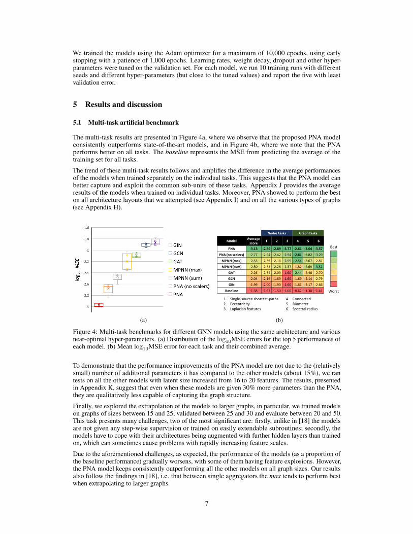
We trained the models using the Adam optimizer for a maximum of 10,000 epochs, using earlystopping with a patience of 1,000 epochs. Learning rates, weight decay, dropout and other hyper-parameters were tuned on the validation set. For each model, we run 10 training runs with differentseeds and different hyper-parameters (but close to the tuned values) and report the five with leastvalidation error.

5 Results and discussion

5.1 Multi-task artificial benchmark

The multi-task results are presented in Figure 4a, where we observe that the proposed PNA modelconsistently outperforms state-of-the-art models, and in Figure 4b, where we note that the PNAperforms better on all tasks. The baseline represents the MSE from predicting the average of thetraining set for all tasks.

The trend of these multi-task results follows and amplifies the difference in the average performancesof the models when trained separately on the individual tasks. This suggests that the PNA model canbetter capture and exploit the common sub-units of these tasks. Appendix J provides the averageresults of the models when trained on individual tasks. Moreover, PNA showed to perform the beston all architecture layouts that we attempted (see Appendix I) and on all the various types of graphs(see Appendix H).

(a)

Nodes tasks Graph tasks

ModelAverage

score1 2 3 4 5 6

PNA -3.13 -2.89 -2.89 -3.77 -2.61 -3.04 -3.57

PNA (no scalers) -2.77 -2.54 -2.42 -2.94 -2.61 -2.82 -3.29

MPNN (max) -2.53 -2.36 -2.16 -2.59 -2.54 -2.67 -2.87

MPNN (sum) -2.50 -2.33 -2.26 -2.37 -1.82 -2.69 -3.52

GAT -2.26 -2.34 -2.09 -1.60 -2.44 -2.40 -2.70

GCN -2.04 -2.16 -1.89 -1.60 -1.69 -2.14 -2.79

GIN -1.99 -2.00 -1.90 -1.60 -1.61 -2.17 -2.66

Baseline -1.38 -1.87 -1.50 -1.60 -0.62 -1.30 -1.41

1. Single-source shortest-paths2. Eccentricity3. Laplacian features

4. Connected 5. Diameter6. Spectral radius

Best

Worst

(b)

Figure 4: Multi-task benchmarks for different GNN models using the same architecture and variousnear-optimal hyper-parameters. (a) Distribution of the log10MSE errors for the top 5 performances ofeach model. (b) Mean log10MSE error for each task and their combined average.

To demonstrate that the performance improvements of the PNA model are not due to the (relativelysmall) number of additional parameters it has compared to the other models (about 15%), we rantests on all the other models with latent size increased from 16 to 20 features. The results, presentedin Appendix K, suggest that even when these models are given 30% more parameters than the PNA,they are qualitatively less capable of capturing the graph structure.

Finally, we explored the extrapolation of the models to larger graphs, in particular, we trained modelson graphs of sizes between 15 and 25, validated between 25 and 30 and evaluate between 20 and 50.This task presents many challenges, two of the most significant are: firstly, unlike in [18] the modelsare not given any step-wise supervision or trained on easily extendable subroutines; secondly, themodels have to cope with their architectures being augmented with further hidden layers than trainedon, which can sometimes cause problems with rapidly increasing feature scales.

Due to the aforementioned challenges, as expected, the performance of the models (as a proportion ofthe baseline performance) gradually worsens, with some of them having feature explosions. However,the PNA model keeps consistently outperforming all the other models on all graph sizes. Our resultsalso follow the findings in [18], i.e. that between single aggregators the max tends to perform bestwhen extrapolating to larger graphs.

7

-2

-1.5

-1

-0.5

0

log 1

0 r

atio

MSE

mo

del

an

d M

SE b

asel

ine

Size of the graphs in the test set

PNA

MPNN (sum)

MPNN (max)

GIN

GAT

GCN

Baseline

20-25 25-30 30-35 35-40 40-45 45-50

Figure 5: Multi-task log10 of the ratio of the MSE for different GNN models and the MSE of thebaseline.

5.2 Real-world benchmarks

The recent works by Dwivedi et al. [5] and Hu et al. [22] have shown problems with manybenchmarks used for GNNs in recent years and proposed a new range of datasets across differentartificial and real-world tasks. To test the capacity of the PNA model in real-world domains, weassessed it on their chemical (ZINC and MolHIV) and computer vision (CIFAR10 and MNIST)datasets.

To ensure a fair comparison of the different convolutional layers, we followed their method for trainingprocedure (data splits, optimizer, etc.) and GNN structure (layers, normalization and approximatenumber of parameters). For the MolHIV dataset, we used the same GNN structure as in [31].

ZINC CIFAR10 MNIST MolHIV

Model

No edge features

Edge featuresNo edge features

Edge featuresNo edge features

Edge featuresNo edge features

MAE MAE Acc Acc Acc Acc % ROC-AUC

Dwivedi et al.

and Xu et al.

papers

MLP 0.710±0.001 56.01±0.90 94.46±0.28

GCN 0.469±0.002 54.46±0.10 89.99±0.15 76.06±0.97

GIN 0.408±0.008 53.28±3.70 93.96±1.30 75.58±1.40

DiffPoll 0.466±0.006 57.99±0.45 95.02±0.42

GAT 0.463±0.002 65.48±0.33 95.62±0.13

MoNet 0.407±0.007 53.42±0.43 90.36±0.47

GatedGCN 0.422±0.006 0.363±0.009 69.19±0.28 69.37±0.48 97.37±0.06 97.47±0.13

Our experi-ments

MPNN (sum) 0.381±0.005 0.288±0.002* 65.39±0.47 65.61±0.30 96.72±0.17 96.90±0.15

MPNN (max) 0.468±0.002 0.328±0.008* 69.70±0.55 70.86±0.27 97.37±0.11 97.82±0.08

PNA (no scalers) 0.413±0.006 0.247±0.036* 70.46±0.44 70.47±0.72 97.41±0.16 97.94±0.12 78.76±1.04

PNA 0.320±0.032 0.188±0.004* 70.21±0.15 70.35±0.63 97.19±0.08 97.69±0.22 79.05±1.32

Figure 6: Results of the PNA and MPNN models in comparison with those analysed by Dwivedi etal. and Xu et al. (GCN[15], GIN[6], DiffPool[32], GAT[16], MoNet[33] and GatedGCN[34]). *indicates the training was conducted with additional patience to ensure convergence.

To better understand the results in the table, we need to take into account how graphs differ amongthe four datasets. In the chemical benchmarks, graphs are diverse and individual edges (bonds) cansignificantly impact the properties of the graphs (molecules). This contrasts with computer visiondatasets made of graphs with a regular topology (every node has 8 edges) and where the graphstructure of the representation is not crucial (the good performance of the MLP is evidence).

8

With this and our theoretical analysis in mind, it is understandable why the PNA has a strongperformance in the chemical datasets, as it was designed to understand the graph structure and betterretain neighbourhood information. At the same time, the version without scalers suffers from thefact it cannot distinguish between neighbourhoods of different size. Instead, in the computer visiondatasets the average improvement of the PNA on SOTA was lower due to the smaller importance ofthe graph structure and the version of the PNA without scalers performs better as the constant degreeof these graphs makes scalers redundant (and it is better to ’spend’ parameters for larger hiddensizes).

6 Conclusion

We have extended the theoretical framework in which GNNs are analyzed to continuous features andproven the need for multiple aggregators in such circumstances. We also have generalized the sumaggregation by presenting degree-scalers and proposed the use of a logarithmic scaling. Taking theabove into consideration, we have presented a method, Principal Neighbourhood Aggregation, con-sisting of the composition of multiple aggregators and degree-scalers. With the goal of understandingthe ability of GNNs to capture graph structures, we have proposed a novel multi-task benchmarkand an encode-process-decode architecture for approaching it. Empirical results from synthetic andreal-world domains support our theoretical evidence. We believe that our findings constitute a steptowards establishing a hierarchy of models w.r.t. their expressive power, where the PNA modelappears to outperform the prior art in GNN layer design.

Broader Impact

Our work focuses mainly on theoretically analyzing the expressive power of Graph Neural Networksand can, therefore, play an indirect role in the (positive or negative) impacts that the field of graphrepresentation learning might have on the domains where it will be applied.

More directly, our contribution in proving the limitations of existing GNNs on continuous featurespaces should help to provide an insight into their behaviour. We believe this is a significant resultwhich might motivate future research aimed at overcoming such limitations, yielding more reliablemodels. However, we also recognize that, in the short-term, proofs of such weaknesses might sparkmistrust against applications of these systems or steer adversarial attacks towards existing GNNarchitectures.

In an effort to overcome some of these short-term negative impacts and contribute to the searchfor more reliable models, we propose the Principal Neighbourhood Aggregation, a method thatovercomes some of these theoretical limitations. Our tests demonstrate the higher capacity of thePNA compared to the prior art on both synthetic and real-world tasks; however, we recognize that ourtests are not exhaustive and that our proofs do not allow for generating “optimal” aggregators forany task. As such, we do not rule out sub-optimal performance when applying the exact architectureproposed here to novel domains.

We propose the usage of aggregation functions, such as standard deviation and higher-order moments,and logarithmic scalers. To the best of our knowledge, these have not been used before in GNNliterature. To further test their behaviour, we conducted out-of-distribution experiments, testing ourmodels on graphs much larger than those in the training set. While the PNA model consistentlyoutperformed other models and baselines, there was still a noticeable drop in performance. Wetherefore strongly encourage future work on analyzing the stability and efficacy of these novelaggregation methods on new domains and, in general, on finding GNN architectures that bettergeneralize to graphs from unseen distributions, as this will be essential for the transition to industrialapplications.

Acknowledgements

The authors thank Saro Passaro for the valuable insights and discussion for the mathematical proofs.

9

Funding Disclosure

Dominique Beaini is currently a Machine Learning Researcher at InVivo AI. Pietro Liò is a FullProfessor at the Department of Computer Science and Technology of the University of Cambridge.Petar Velickovic is a Research Scientist at DeepMind.

References[1] F. Scarselli, M. Gori, A. C. Tsoi, M. Hagenbuchner, and G. Monfardini. The graph neural

network model. IEEE Transactions on Neural Networks, 20(1):61–80, 2009.

[2] Michael M. Bronstein, Joan Bruna, Yann LeCun, Arthur Szlam, and Pierre Vandergheynst.Geometric deep learning: Going beyond euclidean data. IEEE Signal Processing Magazine,34(4):18–42, Jul 2017.

[3] Peter W Battaglia, Jessica B Hamrick, Victor Bapst, Alvaro Sanchez-Gonzalez, ViniciusZambaldi, Mateusz Malinowski, Andrea Tacchetti, David Raposo, Adam Santoro, RyanFaulkner, et al. Relational inductive biases, deep learning, and graph networks. arXiv preprintarXiv:1806.01261, 2018.

[4] William L Hamilton, Rex Ying, and Jure Leskovec. Representation learning on graphs: Methodsand applications. arXiv preprint arXiv:1709.05584, 2017.

[5] Vijay Prakash Dwivedi, Chaitanya K Joshi, Thomas Laurent, Yoshua Bengio, and XavierBresson. Benchmarking graph neural networks. arXiv preprint arXiv:2003.00982, 2020.

[6] Keyulu Xu, Weihua Hu, Jure Leskovec, and Stefanie Jegelka. How powerful are graph neuralnetworks? arXiv preprint arXiv:1810.00826, 2018.

[7] Vikas K Garg, Stefanie Jegelka, and Tommi Jaakkola. Generalization and representationallimits of graph neural networks. arXiv preprint arXiv:2002.06157, 2020.

[8] Christopher Morris, Martin Ritzert, Matthias Fey, William L Hamilton, Jan Eric Lenssen,Gaurav Rattan, and Martin Grohe. Weisfeiler and leman go neural: Higher-order graph neuralnetworks. In Proceedings of the AAAI Conference on Artificial Intelligence, volume 33, pages4602–4609, 2019.

[9] Ryan L Murphy, Balasubramaniam Srinivasan, Vinayak Rao, and Bruno Ribeiro. Relationalpooling for graph representations. arXiv preprint arXiv:1903.02541, 2019.

[10] Ryoma Sato. A survey on the expressive power of graph neural networks. arXiv preprintarXiv:2003.04078, 2020.

[11] Nima Dehmamy, Albert-László Barabási, and Rose Yu. Understanding the representationpower of graph neural networks in learning graph topology. In Advances in Neural InformationProcessing Systems, pages 15387–15397, 2019.

[12] Chen Cai and Yusu Wang. A simple yet effective baseline for non-attributed graph classification.arXiv preprint arXiv:1811.03508, 2018.

[13] Chen-Yu Lee, Patrick W Gallagher, and Zhuowen Tu. Generalizing pooling functions inconvolutional neural networks: Mixed, gated, and tree. In Artificial intelligence and statistics,pages 464–472, 2016.

[14] Jessica B Hamrick, Kelsey R Allen, Victor Bapst, Tina Zhu, Kevin R McKee, Joshua BTenenbaum, and Peter W Battaglia. Relational inductive bias for physical construction inhumans and machines. arXiv preprint arXiv:1806.01203, 2018.

[15] Thomas N Kipf and Max Welling. Semi-supervised classification with graph convolutionalnetworks. arXiv preprint arXiv:1609.02907, 2016.

[16] Petar Velickovic, Guillem Cucurull, Arantxa Casanova, Adriana Romero, Pietro Lio, and YoshuaBengio. Graph attention networks. arXiv preprint arXiv:1710.10903, 2017.

10

[17] Justin Gilmer, Samuel S Schoenholz, Patrick F Riley, Oriol Vinyals, and George E Dahl. Neuralmessage passing for quantum chemistry. In Proceedings of the 34th International Conferenceon Machine Learning-Volume 70, pages 1263–1272. JMLR. org, 2017.

[18] Petar Velickovic, Rex Ying, Matilde Padovano, Raia Hadsell, and Charles Blundell. Neuralexecution of graph algorithms. arXiv preprint arXiv:1910.10593, 2019.

[19] Keyulu Xu, Jingling Li, Mozhi Zhang, Simon S Du, Ken-ichi Kawarabayashi, and StefanieJegelka. What can neural networks reason about? arXiv preprint arXiv:1905.13211, 2019.

[20] Alex Graves, Greg Wayne, Malcolm Reynolds, Tim Harley, Ivo Danihelka, Agnieszka Grabska-Barwinska, Sergio Gómez Colmenarejo, Edward Grefenstette, Tiago Ramalho, John Agapiou,Adrià Puigdomènech Badia, Karl Moritz Hermann, Yori Zwols, Georg Ostrovski, Adam Cain,Helen King, Christopher Summerfield, Phil Blunsom, Koray Kavukcuoglu, and Demis Has-sabis. Hybrid computing using a neural network with dynamic external memory. Nature,538(7626):471–476, 2016.

[21] Chaitanya K Joshi, Thomas Laurent, and Xavier Bresson. An efficient graph convolutionalnetwork technique for the travelling salesman problem. arXiv preprint arXiv:1906.01227, 2019.

[22] Weihua Hu, Matthias Fey, Marinka Zitnik, Yuxiao Dong, Hongyu Ren, Bowen Liu, MicheleCatasta, and Jure Leskovec. Open graph benchmark: Datasets for machine learning on graphs.arXiv preprint arXiv:2005.00687, 2020.

[23] Oriol Vinyals, Samy Bengio, and Manjunath Kudlur. Order matters: Sequence to sequence forsets. arXiv preprint arXiv:1511.06391, 2015.

[24] Kyunghyun Cho, Bart Van Merriënboer, Caglar Gulcehre, Dzmitry Bahdanau, Fethi Bougares,Holger Schwenk, and Yoshua Bengio. Learning phrase representations using rnn encoder-decoder for statistical machine translation. arXiv preprint arXiv:1406.1078, 2014.

[25] Yujia Li, Daniel Tarlow, Marc Brockschmidt, and Richard Zemel. Gated graph sequence neuralnetworks. arXiv preprint arXiv:1511.05493, 2015.

[26] Alex Graves. Adaptive computation time for recurrent neural networks. arXiv preprintarXiv:1603.08983, 2016.

[27] Indro Spinelli, Simone Scardapane, and Aurelio Uncini. Adaptive propagation graph convolu-tional network. arXiv preprint arXiv:2002.10306, 2020.

[28] Jiaxuan You, Rex Ying, and Jure Leskovec. Position-aware graph neural networks. arXivpreprint arXiv:1906.04817, 2019.

[29] Ryoma Sato, Makoto Yamada, and Hisashi Kashima. Random features strengthen graph neuralnetworks. arXiv preprint arXiv:2002.03155, 2020.

[30] Zhengdao Chen, Lei Chen, Soledad Villar, and Joan Bruna. Can graph neural networks countsubstructures? arXiv preprint arXiv:2002.04025, 2020.

[31] Dominique Beaini, Saro Passaro, Vincent Létourneau, William L Hamilton, Gabriele Corso,and Pietro Liò. Directional graph networks. arXiv preprint arXiv:2010.02863, 2020.

[32] Zhitao Ying, Jiaxuan You, Christopher Morris, Xiang Ren, Will Hamilton, and Jure Leskovec.Hierarchical graph representation learning with differentiable pooling. In Advances in neuralinformation processing systems, pages 4800–4810, 2018.

[33] Federico Monti, Davide Boscaini, Jonathan Masci, Emanuele Rodola, Jan Svoboda, andMichael M Bronstein. Geometric deep learning on graphs and manifolds using mixture modelcnns. In Proceedings of the IEEE Conference on Computer Vision and Pattern Recognition,pages 5115–5124, 2017.

[34] Xavier Bresson and Thomas Laurent. Residual gated graph convnets. arXiv preprintarXiv:1711.07553, 2017.

11

[35] Joseph J. Rotman. An Introduction to Algebraic Topology, volume 119 of Graduate Texts inMathematics. Springer New York.

[36] Karol Borsuk. Drei sätze über die n-dimensionale euklidische sphäre. Fundamenta Mathemati-cae, (20):177–190, 1933.

[37] Richard P. Stanley. Enumerative Combinatorics Volume 2. Cambridge Studies in AdvancedMathematics no. 62. Cambridge University Press, Cambridge, 2001.

[38] M Hazewinkel. Encyclopaedia of mathematics. Volume 9, STO-ZYG. Encyclopaedia ofmathematics ; vol 9: STO-ZYG. Kluwer Academic, Dordecht, 1988.

[39] P. Erdos and A Rényi. On the evolution of random graphs. pages 17–61, 1960.

[40] Réka Albert and Albert-László Barabási. Statistical mechanics of complex networks. Reviewsof Modern Physics, 74(1):47–97, Jan 2002.

[41] Duncan J. Watts. Networks, dynamics, and the small-world phenomenon. American Journal ofSociology, 105(2):493–527, 1999.

12