
Primordial Magnetic Fields And Early Structure Formation...
107
Primordial Magnetic Fields And Early Structure Formation In The Universe Thesis submitted to Jawaharlal Nehru University, New Delhi (India) for award of the degree of Kanhaiya Lal Pandey Raman Research Institute Bangalore - 560 080 (India) (2013)
Transcript of Primordial Magnetic Fields And Early Structure Formation...
Primordial Magnetic Fields AndEarly Structure Formation
In The Universe
Thesis submitted to
Jawaharlal Nehru University, New Delhi (India)
for award of the degree of
Do tor of Philosophy
Kanhaiya Lal Pandey
Raman Research InstituteBangalore - 560 080 (India)
(2013)

bc
Primordial Magnetic Fields AndEarly Structure Formation
In The Universe
by
Kanhaiya Lal Pandeyunder the supervision of
Prof. Shiv K. Sethi
A Thesis for the degree of
Do tor of Philosophy
Raman Research InstituteBangalore - 560 080 (India)
(2013)bc

DECLARATION
I hereby declare that the work reported in this thesis entitled “Primordial Magnetic
Fields And Early Structure Formation In The Universe” has been independently car-
ried out by me at theRaman Research Institute, Bangalore, under the supervision ofProf.
Shiv K. Sethi. The subject matter presented in this thesis has not previously formed the
basis of the award of any degree, diploma, associateship, fellowship or any other similar
title.
Prof. Shiv K. Sethi Kanhaiya L. Pandey
(Thesis Supervisor) (The Candidate)
Astronomy & Astrophysics Group
Raman Research Institute
Bangalore 560 080
India.
[\
i

CERTIFICATE
This is to certify that the thesis entitled “Primordial Magnetic Fields And Early
Structure Formation In The Universe”, submitted byKanhaiya L. Pandey for the award
of the degree of Doctor of Philosophy of Jawaharlal Nehru University, is his original work.
This has not been published or submitted to any other University for any other degree or
diploma.
Prof. Ravi Subrahmanyan Prof. Shiv K. Sethi
(Director) (Thesis Supervisor)
Astronomy & Astrophysics Group
Raman Research Institute
Bangalore 560 080
India.
[\
iii


Acknowledgements
I believe that the success of any project depends largely on the encouragement and
guidance of many, and I must admit that this thesis would not have been possible without
the kind support and help of many individuals and organizations. I am writing this section
to take an opportunity to express my gratitude to all those people who have been helpful
in the successful completion of this thesis work.
First of all I would like to thank RRI as an organization for providing me a place and
a nice healthy academic atmosphere to work here as a PhD student. It has been a really
good experience to be in RRI. I express my gratitude to all of them who have / had been
involved in the establishment and nurturing of this institute.
My Special thanks of gratitude to Shiv for being my thesis adviser and giving me timely
suggestions and support. He has been a great teacher all along, I benefited immensely
from his constructive criticism and suggestions. I have learnt a lot from him and most
importantly how to be patient. He has always encouraged me tothink in new ways and
gave me a lot of freedom. I would like to convey my sincere regards and respect for his
valuable involvement during the period of my graduate research. I would also like to thank
Bhargavi for her kind hospitality and delicious food, whichI get whenever I go to Shiv’s
home.
I thank the members of my supervisory committee, Biman, Sam,Ravi and Dwarka for
the fruitful academic discussions, and practical advices which helped me a lot all along.
I must also thank all the faculty members of our astro floor, Sridhar, Biswajit, Ramesh,
Uday, Shukre, CRS and Laxmi for all the help, support, encouragement and several valu-
able scientific discussions on various occasions.
I would also like to express my gratitude to Desh, Sesh and Srikanth for all their
support, help and encouragement, for many valuable academic / non-academic discussions
and even more importantly for their friendly gesture all along.
I thank all my collaborators, especially Dr. Zoltan & Dr. Kahniashvili for all the
scientific discussions, help and encouragement.
Thanks to Vidya for her support and care, her immense patience, and prompt and
timely help for any administrative issue. I must thank Laxamamma and Hanumatappa
also for 3 o’clock tea and all other assistance. Thanks to thevery supportive RRI admin-
istration, Krishna, Marisa and Radha for being very proactive in their help, the computer
department, Jacob, Krishnamurthy, Nandu and Sridhar for their timely assistance with
the computer related problems, our canteen people for providing healthy food, our very
friendly library staff members for maintaining the libraryin a very efficient manner, es-[\
v

Acknowledgements
pecially Kiran, Nagraj, Manjunath, Meera, Geetha and Vrinda for all the help in library
related matters. Many thanks to the housekeeping staff of RRI for making my stay in
RRI a pleasant and enjoyable experience. I thank our hostel-mess cooks Yashodamma,
Ratnamma, Padmaji, Mangalaji and other staff for healthy food and environment at the
hostel.
I must also thank all my friends at RRI who made my stay in RRI memorable. I really
enjoyed their company all along. Many many thanks to my old friend Laxmi Narayan
Tripathi (IISc), who has been like a family member for me herein Bangalore, for all his
help and support. I thank Yogesh, Wasim, Peyush, Ruta, Kshitij, Shashikant, Poonam,
Siddharth, Chetana, Raman, Harsha, Samarth, Sharanya, Nithya, and Harshal for various
valuable discussions with them through which I developed myunderstanding of various
topics in astrophysics and other related subjects. I thank Nishant, Mamta, Giri, Pragya,
Madhukar, Chandreyee, Nipanjana, Mahavir, Jagdish, Lijo and Nazma for all the help
and companionship. I would also like to thank my hostel friends Satyam, Rakesh, Bharat,
Suresh, RK and JK for introducing sports into my daily routine and also thanks to Radhika,
Renu and Santosh especially for letting me grab some of theirfood on many Sundays, what
they cooked for themselves. Let me thank all my old, new, Facebook and non-Facebook
friends here collectively, for all the wishes, comments, tagging, liking & sharing, which
made my leisure times happy and joyful.
Last, but certainly not the least, I wish to thank and expressmy gratitude towards
my beloved parents. They took care of all the family responsibilities on their own so
that I can concentrate fully on my research work without any hassle. I must also thank
Gayatri bua for taking care of my parents, whenever they needed it, during my absence at
home. Without their moral and practical support throughout, I would not have been able
to complete this task.
Now finally, in memory of my grandfather who, to me, was a very simple, easy going,
down to earth, a thoughtful person, and who was a great admirer of the slogan “Jai Jawan,
Jai Kisan, Jai Vigyan”, I would like to dedicate this thesis to the whole community of the
farmers, whose contribution to the humanity is immense but ironically the least rewarded.
[\
vi
Preface
This thesis contains the study of the implications of the primordial magnetic fields for
early structure formation in the Universe and the bounds on primordial magnetic field pa-
rameters coming from various cosmological observables such as, cosmic microwave back-
ground polarization, large scale structure formation, weaklensing shear, and Lyα opacity.
Based on recent observations of magnetic fields in the cosmos, indicating their pres-
ence in clusters, super-clusters, even in the intergalactic medium and high redshift galax-
ies, it is now commonly believed that magnetic fields exist inthe whole universe quite
ubiquitosly. These cosmic magnetic fields in turn indicatesthe existence of magnetic
fields in the early universe, which would have been generatedin the very early universe,
possibly during the inflation or other early phase transitions in the Universe. The exis-
tence of magnetic fields in the early universe can alter the course of structure formation in
several ways. One of those is the extra matter perturbations(over and above inflationary
matter perturbations) sourced by the existence of these primordial magnetic fields during
recombination era. After recombination these matter perturbations also would grow and
take part in the structure formation. This can lead to extra power in the matter power
spectrum at scales around∼ 1–10 h Mpc−1. At the other hand presnce of sufficiently
strong magnetic fields can even lead to heating of the ambientmedium via decay of mag-
netic field energy due to ambipolar diffusion and decaying turbulence in the medium, and
therefore affect the structure formation as thermal history plays an important role in this
process. Thus we see that the existence of the primordial magnetic fields can influence the
matter distribution in the univesre. And therefore the cosmological probes of the matter
distribution in the universe are expected to have signatures of the existence of primordial
magnetic fields. Using these observables we can actually probe the existence of primordial
magnetic fields and put bounds on the physical parameters related to them. These were
the main motivation behind this thesis work.
Following is the summary of the actual thesis work,
∗ Implications of primordial magnetic fields for early struct ure formation
• Formation of supermassive black holes (SMBH) at very high redshifts: This work
is about the investigation of possible role of primordial magnetic field to solve the
puzzle of the formation of early super massive black holes posed by some SDSS
observations of early (z≃ 6) bright quasars. Many models have been proposed to
solve this mystery based on super-Eddington accretion or hierarchal merger models.
[\
vii
Preface
All the models make very optimistic assumptions and have their own share of prob-
lems. Presence of magnetic field also affects the course of thermal and dynamical
evolution of collapsing gas because of the dissipation of the magnetic field energy in
the medium. Our work suggests that if the magnetic field strength is above a critical
value (∼ 3.5 nG), it can actually lead to the formation of more massivestars≃ 104
M⊙. The black holes left behind after the death of these stars will have enough time
to accrete gas to become a108 M⊙ SMBH by the redshift of 6–8. This model avoids
many of the odd assumptions which are required in other models. Though this model
requires a larger magnetic field value than the available bounds on primordial mag-
netic fields and relies on metal-free primordial gas, these value of magnetic fields
are allowed under∼ 2–3 σ upward fluctuation of the Gaussian random primordial
magnetic fields which is sufficient to account for the number of high redshift quasars
observed. Metal-free gas is not a bad assumption for the primordial gas at the redshift
of z ∼ 15. Over all this model presents a plausible novel mechanismto form high
redshift supermassive black holes.
∗ Bounds on primordial magnetic fields coming from various cosmological parame-
ters
• Cosmic Microwave Background Polarization & Large Scale Structure forma-
tion: In this work we have studied the limits on primordial magnetic field coming
from various cosmological probes such as, Faraday rotationof Cosmic Microwave
Background (CMB) polarization plane and statistics of large scale structures in the
universe. The presence of primordial magnetic field during recombination causes a
rotation of the CMB polarization plane due to the Faraday effect. The rotation angle is
proportional to the magnetic field strength. Primordial magnetic field can also induce
formation of structures in the Universe. Unlike theΛCDM matter power spectrum,
the magnetic field induced matter power spectrum increases at small scales (up till a
cut-off at magnetic Jeans scale) and it plays an important role in the formation of the
first structures in the Universe also. The smallest structure to collapse atz ≃ 10 in the
ΛCDM model are 2.5σ fluctuations of the density field as opposed to the magnetic
field case where 1σ collapse is possible. This means the number of collapsed halo
is more abundant in the later case. This result is crucial in finding the bounds on the
strength of primordial magnetic field, since the WMAP results suggests that the Uni-
verse reionized at z = 10, combining these two one can put bounds on the primordial
magnetic field strength. From the analysis in this work we findthat the range of the
acceptable values of magnetic field strength is below 1-3 nG.
[\
viii
Preface
• Cosmological weak lensing shear:In this work we have calculated a theoretical
estimate of shear power spectrum and the shear correlation functions, taking into ac-
count the effect of primordial magnetic fields on matter power spectrum. Comparing
this result with the CFHTLS weak lensing data (Fu et al., 2008), we have found limits
on primordial magnetic fields which are much stronger (∼ 0.5 nG for the spectral in-
dex valuenB = −2.8 under the confidence level of 5σ) in comparison to the existing
limits on primordial magnetic fields coming from CMB data.
• Lyα effective optical opacity: This work is an extension of the previous work, with
the same motive but this time the observable is the line of sight distribution of Lyα
clouds. We have simulated one dimensional distribution of Lyα absorbers along the
line of sight and calculated effective Lyα opacity as function of redshift. Using ob-
served data of effective Lyα opacity from Faucher-Giguere et al. (2008) we have
calculated bounds on primordial magnetic field, which turned out to be even stronger
than our previous estimates (B0 ∼ 0.2 – 0.3 nG for nB = -2.8 with the confidence
level of 5σ). In this analysis we have considered two cases, one when themagnetic
field induced perturbations are uncorrelated with inflationary perturbations, and the
other is when they are correlated, though the final results (bounds onB0) are not very
different for both the cases.
The work presented in this Thesis has been already published, the details of which are
as following :
Publications
1. Supermassive Black Hole Formation At High Redshifts Through A Primordial Mag-
netic Field, Shiv K. Sethi, Zoltan Haiman, Kanhaiya L. Pandey 2010,ApJ 721, 615
2. Primordial Magnetic Field Limits From Cosmological Data, Tina Kahniashivili,
Alexander G. Tevzadze, Shiv K. Sethi, Kanhaiya L. Pandey, Bharat Ratra 2010,
PRD 82, 083005
3. Theoretical Estimates Of Two-point Shear Correlation Functions Using Tangled
Magnetic Fields, Kanhaiya L. Pandey, Shiv K. Sethi 2012,ApJ 748, 27
4. Probing Primordial Magnetic Fields Using Lyα Clouds, Kanhaiya L. Pandey, Shiv
K. Sethi 2012,ApJ 762, 15
[\
ix

Contents
Declaration i
Certificate iii
Acknowledgement v
Synopsis vii
List of Figures xv
List of Tables xvii
1 Introduction 1
1.1 Magnetic Fields In The Universe. . . . . . . . . . . . . . . . . . . . . 1
1.2 Large Scale Magnetic Fields . . . . . . . . . . . . . . . . . . . . . . . 2
1.3 Origin Of Large Scale Magnetic Fields . . . . . . . . . . . . . . . . . 6
1.4 Modelling The Primordial Magnetic Fields . . . . . . . . . . . . . . . 10
1.5 Role Of Primordial Magnetic Fields In Early Structure Forma tion . . 12
1.5.1 Magnetic field induced density & velocity perturbations . . . . 12
1.5.2 Matter power spectrum of density field induced by primordial
magnetic fields . . . . . . . . . . . . . . . . . . . . . . . . . . 13
1.6 This Thesis . . . . . . . . . . . . . . . . . . . . . . . . . . . . . . . . 15
2 Early Formation Of Supermassive Black Holes (SMBHs) : Role Of
Primordial Magnetic Fields 17
2.1 Formation Of SMBHs At High Redshifts . . . . . . . . . . . . . . . . 17
[\
xi
Table of Content
2.2 The Role Of Primordial Magnetic Fields . . . . . . . . . . . . . . . . 18
2.3 Chemistry And The Thermo-dynamical Evolution Of Collapsing Pri-
mordial Gas . . . . . . . . . . . . . . . . . . . . . . . . . . . . . . . . 19
2.3.1 Formation of molecular hydrogen . . . . . . . . . . . . . . . . 19
2.3.2 Density evolution of the collapsing halo . . . . . . . . . . . . . 20
2.3.3 Thermal evolution of the collapsing gas . . . . . . . . . . . . . 22
2.4 Results . . . . . . . . . . . . . . . . . . . . . . . . . . . . . . . . . . . 24
2.5 The Mass Of The Central Object . . . . . . . . . . . . . . . . . . . . 28
2.6 Discussion . . . . . . . . . . . . . . . . . . . . . . . . . . . . . . . . . 30
3 Primordial Magnetic Field Limits From Cosmological Data 31
3.1 Introduction . . . . . . . . . . . . . . . . . . . . . . . . . . . . . . . . 31
3.2 Modeling The Primordial Magnetic Fields (Concept of Beff) . . . . . . 32
3.3 CMB Polarization Plane Rotation . . . . . . . . . . . . . . . . . . . . 33
3.4 Large Scale Structures . . . . . . . . . . . . . . . . . . . . . . . . . . 36
3.5 Discussion . . . . . . . . . . . . . . . . . . . . . . . . . . . . . . . . . 39
4 Probing Primordial Magnetic Fields Using Weak Lensing 43
4.1 Introduction . . . . . . . . . . . . . . . . . . . . . . . . . . . . . . . . 43
4.2 Weak Lensing & Cosmic Shear . . . . . . . . . . . . . . . . . . . . . 43
4.2.1 Gravitational lensing in general . . . . . . . . . . . . . . . . . 43
4.2.2 Weak lensing theory & cosmic shear. . . . . . . . . . . . . . . 45
4.3 Shear Power Spectrum From Tangled Magnetic Field Power Spectrum 48
4.4 Results . . . . . . . . . . . . . . . . . . . . . . . . . . . . . . . . . . . 49
4.5 Discussion . . . . . . . . . . . . . . . . . . . . . . . . . . . . . . . . . 51
5 Probing Primordial Magnetic Fields Using Lyα Clouds 57
5.1 Introduction . . . . . . . . . . . . . . . . . . . . . . . . . . . . . . . . 57
5.2 Lyα Clouds . . . . . . . . . . . . . . . . . . . . . . . . . . . . . . . . 59
5.3 The Simulation: Density Fluctuation Along The Line-Of-Sight: Dis-
tribution Of Ly α Clouds . . . . . . . . . . . . . . . . . . . . . . . . . 60
5.4 Calculation Of Lyα Opacity . . . . . . . . . . . . . . . . . . . . . . . 62
5.5 Results . . . . . . . . . . . . . . . . . . . . . . . . . . . . . . . . . . . 64
5.6 Discussion . . . . . . . . . . . . . . . . . . . . . . . . . . . . . . . . . 68
6 Conclusion 73
6.1 The Motivation And The Groundworks . . . . . . . . . . . . . . . . . 73
[\
xii
Table of Content
6.2 Thesis Work . . . . . . . . . . . . . . . . . . . . . . . . . . . . . . . . 74
6.2.1 Early formation of supermassive black holes . . . . . . . . . . 74
6.2.2 Primordial magnetic field limits from cosmological data . . . . 75
6.2.3 Probing primordial magnetic fields using weak lensing. . . . . 75
6.2.4 Probing primordial magnetic fields using Lyα clouds . . . . . . 75
Bibliography 79
[\
xiii


List of Figures
1.1 Galactic magnetic fields . . . . . . . . . . . . . . . . . . . . . . . . . 4
1.2 ASS & BSS configurations of galactic magnetic field . . . . . . . . . . 5
1.3 Symmetric & Antisymmetric configurations of galactic magnetic fields 6
1.4 Magnetic-field-induced matter power spectrum . . . . . . . . . . . . . 14
2.1 Temperature evolution of collapsing gas for various values magnetic
fields . . . . . . . . . . . . . . . . . . . . . . . . . . . . . . . . . . . . 25
2.2 Evolution of H2 fraction in the collapsing gas . . . . . . . . . . . . . . 26
2.3 Evolution of ionized fraction in the collapsing gas . . . . . . . . . . . 27
2.4 Various heating and cooling rates involved in the process for B = 1 nG 28
2.5 Various heating and cooling rates involved in the process for B = 4 nG 29
3.1 Rms rotation angle αrms as a function of spectral index nB for the
case when Beff = 1nG and ν0 = 100GHz. Circles correspond to the
computed values. . . . . . . . . . . . . . . . . . . . . . . . . . . . . . 34
3.2 Effective magnetic field limits set by the measurement of the rotation
angle αrms for different spectral index (nB = −3,−2,−1, 0, 1, 2, from
bottom to top). The horizontal solid line shows the upper limit set by
BBN. Vertical dashed lines correspond to the angles αrms = 3.16 that
is set by the BBN limit on the effective magnetic field with spectral
index nB = 2 and αrms = 4.4 set by the WMAP 7-year data. The
numerical values of the effective magnetic field constraints (in nG at
100 GHz) from the αrms = 4.4 limit are shown on the graph for each
spectral index value. . . . . . . . . . . . . . . . . . . . . . . . . . . . 35
[\
xv
List of Figures
3.3 The mass dispersion at z = 10 for Beff = 6nG as a function of mag-
netic field power spectral index nB. From top to bottom (at the left
hand side of the plot), the curves correspond to nB = 2, 1, 0,−1,−2,−2.8. 38
3.4 Constraint on the magnetic field strength Beff as a function of the
power spectral index nB. . . . . . . . . . . . . . . . . . . . . . . . . . 39
3.5 The squared spherical Bessel functions j2l (x) for l = 5000 (top) and
l = 10000 (bottom). Clearly j2l (x) peaks at x ≈ l. . . . . . . . . . . . 42
3.6 The sum of the squared spherical Bessel function∑lC
l=0(2l + 1)j2l (x)
for lC = xS ≃ 16000. The sum converges to 1 (horizontal solid line). . 42
4.1 The inflationary λCDM matter power spectrum . . . . . . . . . . . . 44
4.2 deflection of a light ray by intervening large scale structure . . . . . . 45
4.3 Deflection of light rays coming from a distant source by a gravitational
potential fluctuation φ. . . . . . . . . . . . . . . . . . . . . . . . . . . 46
4.4 Magnetic field induced matter power spectrum . . . . . . . . . . . . . 50
4.5 Shear power spectra for the magnetic and the ΛCDM models. . . . . 52
4.6 2-point shear correlation functions . . . . . . . . . . . . . . . . . . . . 53
4.7 The χ2 analysis of our results against CFHTLS data; bounds on PMF 54
5.1 Formation of Lyα lines in quasar spectra . . . . . . . . . . . . . . . . 58
5.2 Quasar spectra; Lyα forest. . . . . . . . . . . . . . . . . . . . . . . . 59
5.3 magnetic field induced matter power spectrum . . . . . . . . . . . . . 64
5.4 Evolution of 〈τ〉 for the uncorrelated δinfl and δpmf case. . . . . . . . 65
5.5 Evolution of τeff for the uncorrelated δinfl and δpmf case. . . . . . . . 66
5.6 Evolution of 〈τ〉 for the correlated δinfl and δpmf case. . . . . . . . . . 67
5.7 Evolution of τeff for the correlated δinfl and δpmf case. . . . . . . . . . 68
5.8 Distribution of τi (1.5 nG) vs dτi (= τi (1.5 nG)−τi (0 nG)) at redshift
z = 4. . . . . . . . . . . . . . . . . . . . . . . . . . . . . . . . . . . . 69
5.9 χ2 analysis of τeff against the data from FG et al.(2008); bounds on
PMF . . . . . . . . . . . . . . . . . . . . . . . . . . . . . . . . . . . 70
5.10 to compare results from our previous analysis . . . . . . . . . . . . . 71
[\
xvi

List of Tables
5.1 Typical values of some physical properties of Lyα clouds . . . . . . . 60
[\
xvii

1Introduction
1.1 Magnetic Fields In The Universe
Magnetic field is another manifestation of electromagneticforce field, which is one of the
four fundamental forces (others are gravitational, weak & strong nuclear forces) in the
universe known to humankind by now, and after strong nuclearforce the second strongest
amongst them. Since the universe as we know it today, is charge neutral globally as well
as locally, we do not need to worry about the electrical forces but, whenever we encounter
plasmas, which is very common in astrophysical systems, magnetic field effects come into
the picture. In most of the cases these magnetic fields are strong enough to influence the
dynamics of the system significantly. No wonder magnetic fields play an important role in
almost every area of astrophysics. Formation of planetary and stellar objects, production
of jets and outflows, synchrotron sources like radio galaxies and neutron stars, accretion
disks, inter stellar medium (ISM), supernovae and gamma raybursts (GRBs) are just a few
examples.
From observations, we know that the magnetic fields are present quite ubiquitously
in the universe. Small scale objects like planets and stars,at large scale tenuous gas in
the inter stellar medium of galaxies and even more tenuous intracluster medium are all
magnetized. The first extraterrestrial magnetic field were observed in sunspots by Hale
1908. Starting from 1949, microgauss strength magnetic fields have been observed in
several galaxies coherent over galactic sizes≃ 10 - 100 kpc, weaker magnetic fields have
been observed with coherence length scales up to cluster sizes, and there is evidence of
supercluster scale magnetic fields also. Origin and the maintenance of magnetic fields
coherent over such cosmological scales is still an unresolved issue in astrophysics.
How did the Universe get magnetized at the first place? Is magnetic fields in the
universe a result of top-down process, ie. a weak uniform magnetic field formed during
[\
1
2 Chapter 1. Introduction
very early universe and propagated to small scale objects asthey collapsed, or bottom-up
process like structure formation in theΛCDM, in which it would have been created in
small scale objects like stars and accretion disks first and then propagated to large scales
through outflows and bursts. The two leading theories for theorigin and the maintenance
of the galactic magnetic fields representing the above two scenarios are the dynamo model
(bottom-up) and the primordial magnetic field model (top-down). These two theories are
quite different from each other in the sense of the initial conditions and what they predict
about the galactic magnetic fields. The concept of primordial magnetic theory initially
came as an attempt to understand the galactic/cosmic magnetic fields, as battery mecha-
nisms to generate magnetic fields were unable to explainµG level of galactic magnetic
fields. Dynamo theories came later.
According to primordial magnetic field theory the cosmic magnetic fields (magnetic
fields with very large coherence length) were generated in the very early universe (possibly
during inflation). These cosmic magnetic fields got amplifiedby flux freezing and got
twisted around the galactic center, along with the process of galaxy formation and this is
what we see as galactic magnetic fields. The magnetic diffusivity of galaxy was assumed
to be very low and in this case there is no need of any mechanismto maintain the magnetic
fields once it got created.
Later it was realized that, the magnetic field diffusivity could be very high inside a
galaxy because of the turbulent nature of the galactic medium, and the magnetic field
would quickly decay at all scales. Therefore the galactic magnetic field has to be main-
tained by continuous regeneration of magnetic field by fluid motion. And thus people
started approaching the problem using dynamo theory.
1.2 Large Scale Magnetic Fields
While analyzing MHD problems in the astrophysical context the usual practice is to di-
vide the total magnetic field into two components (known as two-scale theory first used
by Steenback, Krause & Radler (1966)), the uniform large scale componentBu and a ran-
dom componentbr which is such as〈br〉 = 0, the total field becomesB = Bu + b with
〈B〉 = Bu and 〈B2〉 = B2u + 〈b2〉. Among large scale magnetic fields, galactic mag-
netic fields have been studied in quite detail. Our own galaxythe Milky Way provides us
with the spatial detail of galactic magnetic field, whereas large number of external galax-
ies give us the global field structure that is unattainable from the Milky Way. Though
there are several observational tracers to probe the magnetic fields, they respond only to
either the plane of the sky componentB⊥ or the line of sight componentB‖. The total
[\
1.2. Large Scale Magnetic Fields 3
magnetic field in a galaxy can be estimated from the nonthermal radio emission, assum-
ing equipartition between the magnetic field energy and kinetic energy of the relativistic
particles. Intensity and polarization of observed synchrotron radiation, polarization of star
light and polarization of infrared emission from the interstellar dust are the main probes of
B⊥, Faraday rotation and Zeeman splitting are used to probeB‖. Based on the these obser-
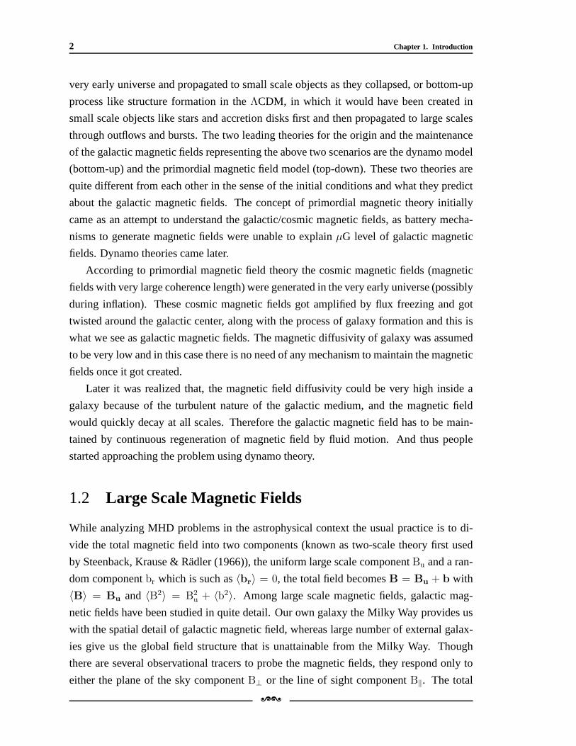
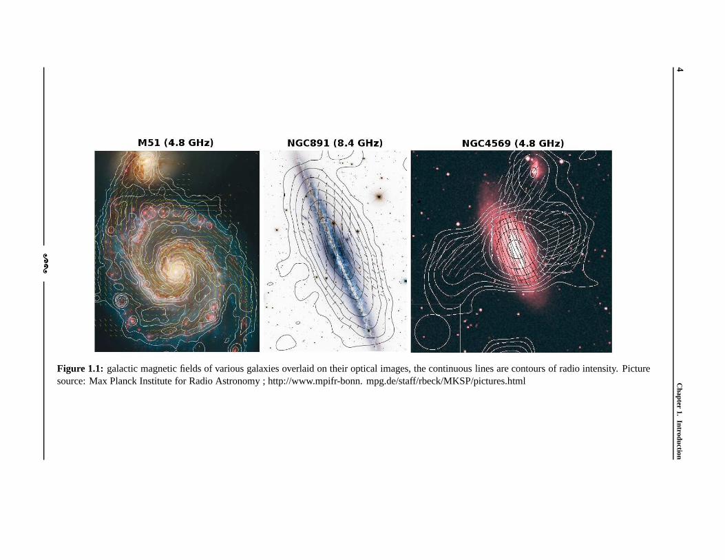
vational tracers, magnetic fields have been mapped for several galaxies. The morphology
and the symmetry features of the galactic magnetic fields constrain theory of its origin and
evolution. In spiral galaxies the magnetic fields have been found to be mostly parallel to
the galactic plane and field lines closely follow the opticalspiral arms of the galaxy. There
are cases when we do not see a well defined material spiral arms(flocculant and irregular
galaxies) but we see a definite spiral magnetic field lines. The total magnetic field strength
is generally highest at the position of optical spiral arms,whereas the highest regular fields
are found in the interarm region of the spiral galaxy. The mean equipartition value of the
total magnetic field is around 10µG, the strength of the regular field is of the order of 1-5
µG in the interarm region. From the measurements of polarization of synchrotron radia-
tion at high radio frequencies coming from external galaxies one can estimate the relative
energies in uniform and random component of the magnetic field and it is found that the
energy in uniform component is about two-thirds of that of random component, and it
can go to as low as 5% in the regions of heavy star formation. There are feeble evidence
for magnetic fields in elliptical galaxies also Greenfield, Roberts & Bruke (1985); Moss
& Shukurov (1996), the total field strength is similar to thatof spiral galaxies but there
are positive detection of polarized synchrotron emission,indicating almost zero uniform
component of the magnetic field.
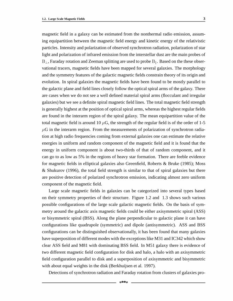
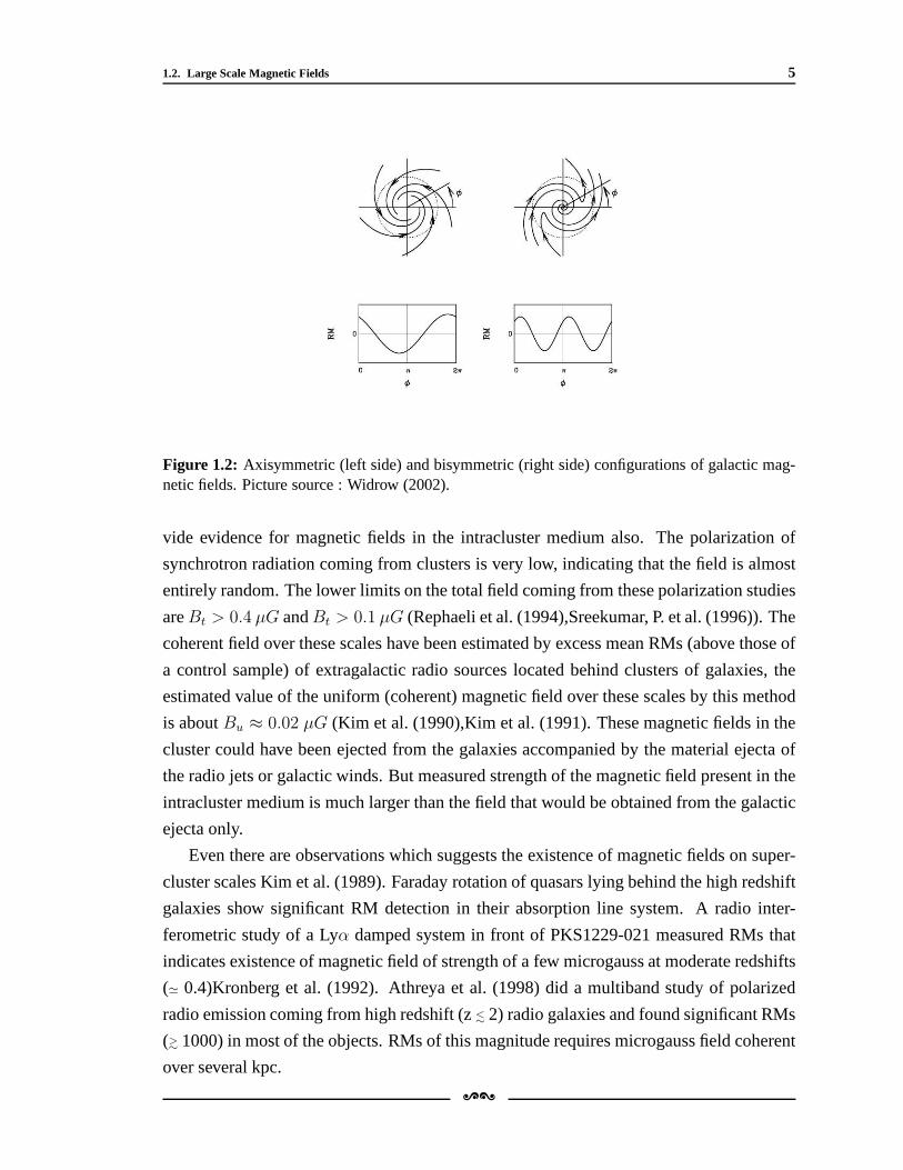
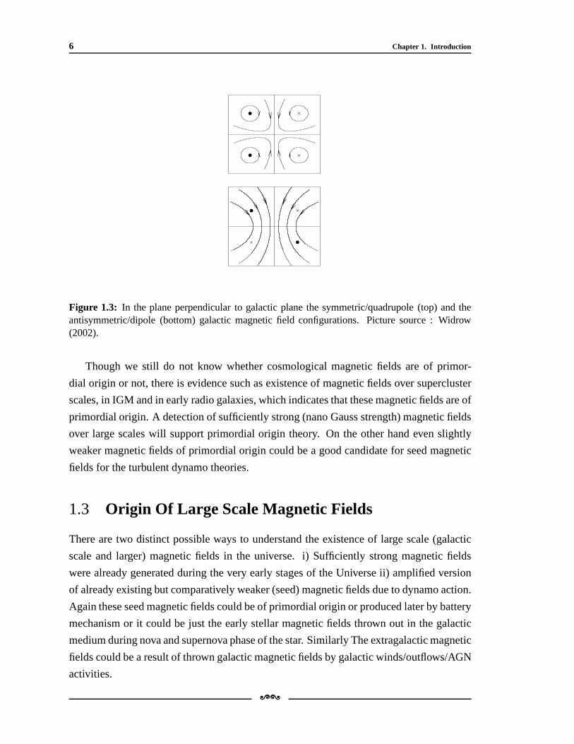
Large scale magnetic fields in galaxies can be categorized into several types based
on their symmetry properties of their structure. Figure 1.2and 1.3 shows such various
possible configurations of the large scale galactic magnetic fields. On the basis of sym-
metry around the galactic axis magnetic fields could be either axisymmetric spiral (ASS)
or bisymmetric spiral (BSS). Along the plane perpendicularto galactic plane it can have
configurations like quadrupole (symmetric) and dipole (antisymmetric). ASS and BSS
configurations can be distinguished observationally, it has been found that many galaxies
have superposition of different modes with the exceptions like M31 and IC342 which show
clear ASS field and M81 with dominating BSS field. In M51 galaxythere is evidence of
two different magnetic field configuration for disk and halo,a halo with an axisymmetric
field configuration parallel to disk and a superposition of axisymmetric and bisymmetric
with about equal weights in the disk (Berkhuijsen et al. 1997).
Detections of synchrotron radiation and Faraday rotation from clusters of galaxies pro-
[\
4C
hapter1.
Introduction
Figure 1.1: galactic magnetic fields of various galaxies overlaid on their optical images, the continuous lines are contours of radio intensity. Picturesource: Max Planck Institute for Radio Astronomy ; http://www.mpifr-bonn. mpg.de/staff/rbeck/MKSP/pictures.html
[\
1.2. Large Scale Magnetic Fields 5
Figure 1.2: Axisymmetric (left side) and bisymmetric (right side) configurations of galactic mag-netic fields. Picture source : Widrow (2002).
vide evidence for magnetic fields in the intracluster mediumalso. The polarization of
synchrotron radiation coming from clusters is very low, indicating that the field is almost
entirely random. The lower limits on the total field coming from these polarization studies
areBt > 0.4 µG andBt > 0.1 µG (Rephaeli et al. (1994),Sreekumar, P. et al. (1996)). The
coherent field over these scales have been estimated by excess mean RMs (above those of
a control sample) of extragalactic radio sources located behind clusters of galaxies, the
estimated value of the uniform (coherent) magnetic field over these scales by this method
is aboutBu ≈ 0.02 µG (Kim et al. (1990),Kim et al. (1991). These magnetic fields inthe
cluster could have been ejected from the galaxies accompanied by the material ejecta of
the radio jets or galactic winds. But measured strength of the magnetic field present in the
intracluster medium is much larger than the field that would be obtained from the galactic
ejecta only.
Even there are observations which suggests the existence ofmagnetic fields on super-
cluster scales Kim et al. (1989). Faraday rotation of quasars lying behind the high redshift
galaxies show significant RM detection in their absorption line system. A radio inter-
ferometric study of a Lyα damped system in front of PKS1229-021 measured RMs that
indicates existence of magnetic field of strength of a few microgauss at moderate redshifts
(≃ 0.4)Kronberg et al. (1992). Athreya et al. (1998) did a multiband study of polarized
radio emission coming from high redshift (z. 2) radio galaxies and found significant RMs
(& 1000) in most of the objects. RMs of this magnitude requires microgauss field coherent
over several kpc.
[\
6 Chapter 1. Introduction
Figure 1.3: In the plane perpendicular to galactic plane the symmetric/quadrupole (top) and theantisymmetric/dipole (bottom) galactic magnetic field configurations. Picture source : Widrow(2002).
Though we still do not know whether cosmological magnetic fields are of primor-
dial origin or not, there is evidence such as existence of magnetic fields over supercluster
scales, in IGM and in early radio galaxies, which indicates that these magnetic fields are of
primordial origin. A detection of sufficiently strong (nanoGauss strength) magnetic fields
over large scales will support primordial origin theory. Onthe other hand even slightly
weaker magnetic fields of primordial origin could be a good candidate for seed magnetic
fields for the turbulent dynamo theories.
1.3 Origin Of Large Scale Magnetic Fields
There are two distinct possible ways to understand the existence of large scale (galactic
scale and larger) magnetic fields in the universe. i) Sufficiently strong magnetic fields
were already generated during the very early stages of the Universe ii) amplified version
of already existing but comparatively weaker (seed) magnetic fields due to dynamo action.
Again these seed magnetic fields could be of primordial origin or produced later by battery
mechanism or it could be just the early stellar magnetic fields thrown out in the galactic
medium during nova and supernova phase of the star. Similarly The extragalactic magnetic
fields could be a result of thrown galactic magnetic fields by galactic winds/outflows/AGN
activities.
[\
1.3. Origin Of Large Scale Magnetic Fields 7
It has been suggested that the primordial magnetic fields could have been generated
during various early phases of the universe like the inflation, the electroweak phase tran-
sition, the quark-hadron phase transition, during the formation of the first objects or even
during reionization Turner & Widrow (1988); Widrow (2002);Gnedin et al. (2000). As a
matter of fact we do not have any observation which can confirmthese theories, but still
we can put theoretical limits on the strength of these primordial (cosmological) magnetic
fields and probe it indirectly using some other cosmologicalobservables. Several con-
straints of this kind have already been derived using Faraday rotation estimates of high
redshift sources, estimates of anisotropy of the CMB causedby these cosmological mag-
netic fields, predictions of light elements abundance from big-bang nucleosynthesis (BBN)
in the presence magnetic fields etc. For example based on 4-year Cosmic Background Ex-
plorer (COBE) data, Barrow (1997) suggested an upper limit on cosmological magnetic
field which isB . 5 × 10⁻⁹h75Ω1/2G and coherent over scales larger than the present
horizon size. Constraints from BBN suggests an upper limit of B < 10−6 G. These values
are scaled to present epoch values, assuming the scaling relation asBt = a(t)2B0.
Other than primordial origin of magnetic fields there are battery mechanisms which
can generate seed magnetic fields from zero magnetic field conditions. This process was
first discovered by Biermann in 1950. The Biermann battery works on basis of relative
motion of electrons and ions (since electrons are much lighter than their positively charged
counterparts, the ions, and respond much more to a pressure gradient (force) in a medium)
that give rise to a net electric field (Eb = −∇pe/ene) in the medium, if this electric field
has a curl it can give rise to magnetic field. Sincepe = nekBT , the condition∇× Eb 6= 0
indicates∇ne × ∇T 6= 0 for this whole thing to happen, ie. the gradients∇ne and∇T
are not parallel to each other. Such scenario are not very rare in astrophysics the example
could be the ionization fronts where the temperature gradient is normal to the front but the
density gradient can have different direction as the ionization front is sweeping across the
arbitrarily distributed density fluctuations. This mechanism can produce a seed magnetic
field of strength of the order of∼ 10−20.
Since the magnetic fields over larger scales than the galactic scales have not been ob-
served in good details because of several observational limitations, the present day avail-
able detailed observations of galactic magnetic fields in our own Milky Way and other
galaxies can provide a good probe to distinguish between themodels. The salient features
of the two models, the dynamo theory and the primordial theory are as given below
Dynamo theories : Magnetic field in a conducting medium can be amplified by the
inductive effects associated with the motions of the medium, this process is generally re-
ferred to as dynamo. In the dynamo process the kinetic energyassociated with the motions
[\
8 Chapter 1. Introduction
in the medium is converted into magnetic energy. The medium inside galaxy or cluster is
very turbulent and the dynamo action happening in these systems are commonly known
as turbulent dynamo. Turbulent dynamos are conveniently divided into fluctuation (small
scale) dynamo and the mean field (large scale) dynamo. Fluctuation dynamo produces
magnetic fields that are correlated only over the scales which are comparable (or smaller)
than the scales of energy carrying random/turbulent motions.
The fluctuation dynamo are generic to any random flow where magnetic Reynold’s
numberRm is greater than a critical valueRm,crit ∼ 30 − 100, depending on the form
of velocity correlation function. The field grows exponentially roughly on the eddy turn
over time scalel0/v0, wherev0 is the typical variation in velocity over the scalel0 with the
magnetic field scalelB ∼ l0/R1/2m . In the context of galaxy clusters turbulence are mainly
be driven by the merging of subclusters and the typical values for the largest turbulent
scales and the turbulent velocity would bel0 ∼ 100 kpc ; v0 ∼ 300 kms−1, leading
to a growth timeτ0 ∼ l0/v0 ∼ 3 × 10⁸ yr; thus for a cluster lifetime of a few Gyr,
one could then have significant amplification by the fluctuation dynamo. And in the case
of galactic interstellar turbulence driven by supernovae,if we take typical values to be
l0 ∼ 100 pc, v0 ∼ 10 kms−1 one getsτ0 ∼ 107 yr. Again the fluctuation dynamo would
rapidly grow the magnetic field even for very young high redshift protogalaxies.
If the turbulence are helical theαΩ mean field dynamo mechanism can play a role and
produce magnetic fields at even larger scales (by inverse cascade of magnetic-energy/helicity).
The interstellar medium is assumed to become turbulent, dueto for example the effect of
supernovae randomly going off in different regions. In a rotating, stratified (in density and
pressure) medium like a disk galaxy, such turbulence becomes helical and thusαΩ mean
field dynamo can actually work in these kinds of system. In spiral galaxies large scale
differential rotation (mean velocity) can stretch the radial field into azimuthal toroidal
fields (Ω-effect), whereas small scale helical turbulence can convert the toroidal fields into
poloidal fields (α-effect). In this also the magneto-fluid dynamics equationsgives expo-
nentially growth of magnetic fields as a solution for conditions which can be easily met in
the spiral galaxies. The mean field grows typically on time-scales a few times the rotation
time scales, of order 3-10×108 yr. Unlike primordial origin theory this model can accom-
modate various shorts of galactic magnetic field configurations and can give explanations
for them, This model also has gotten its own share of problems, validity of FOSA (first or-
der smoothing assumption, on which theory relies) in the galactic medium is one of them.
In the linear limit this theory is well worked out and works quite fine, but in the non-linear
regime it becomes a very complex and complicated.
According to the simplest version of mean field dynamo theory, when the governing
[\
1.3. Origin Of Large Scale Magnetic Fields 9
equations are linear inBu, the mean fieldBu can grow exponentially in the low (but non-
zero) resistivity limit. In the nonlinear regime whenBu becomes significant and its back
reaction on the fluid motion becomes important, quenching ofthe magnetic field happens.
It inhibits the dynamo action and the magnetic field gets saturated at some value. This
happens when the magnetic field energy becomes of the order ofthe turbulent energy and
thusBu saturates at about its equipartition value. Early quenching of magnetic fields (α
quenching problem) is one of the problems with this dynamo theory for galactic magnetic
fields, though various theories have been already proposed and an active research is still
going on to resolve these problems, because of complexity ofthe problem there are still
some open questions to be answered.
Primordial origin theory : Just after the discovery of galactic magnetic fields Hoyle,
F. (1958) came up with the idea of primordial magnetic fields to understand the existence
of magnetic fields over galactic scales, as battery mechanisms can not produce such mag-
netic fields, dynamo theories were not known at that time. Later Piddington (1964, 1972),
Howard & Kulsurd (1997) took forward this hypothesis. In this theory it is assumed that
the large scale magnetic fields are of primordial origin and sufficiently strong magnetic
field was already present before the formation of galaxies started and the present (large
scale) galactic magnetic fields are just the primordial magnetic fields twisted by the differ-
ential rotation in the galaxy. This theory rely on low magnetic diffusivity of the galaxies
and therefore there have not been any significant decay of thegalactic magnetic fields.
The primordial magnetic fields could have been generated during various early universe
phase transitions. The exponential stretching of the vacuum fluctuations of the electro-
magnetic fields during inflation could produce magnetic fields coherent over very large
scale. Other mechanisms like electroweak transition or QCDtransition produce magnetic
fields coherent over smaller scales and thus very tiny magnetic fields over galactic scales,
unless helicity is also generated, in which case the inversecascade of the energy to larger
scales is possible. The problem with the inflationary model is that the electromagnetism
is conformally coupled to gravity and therefore, in a spatially flat FLRW cosmology, the
magnetic field generated during inflation will decay adiabatically (B ∼ 1/a(t)2, where a
is the expansion factor), Turner & Widrow (1988) suggested that one need to break the
conformal and gauge invariance of the electromagnetic action to get away with this effect.
Various authors have attempted to find an effective and natural way to break conformal
invariance and still research is going on in this field. In these modelsB ∼ 1/a(t)ǫ with
typically ǫ ≪ 1 for getting a strong field. Sincea is exponentially increasing during the
inflation the predicted field strength is exponentially sensitive to any changes of the param-
eters of the model which affects theǫ, and therefore these model of primordial magnetic
[\
10 Chapter 1. Introduction
field generation can lead to a wide range of magnetic field strength based on the values of
cosmological parameters used. The strongest field which canbe generated by these mech-
anism is estimated to be around10−9 G (redshifted to present epoch). A magnetic field
of the strength∼ 10−9 can also be sheared and amplified due to flux freezing, during the
collapse to form a galaxy and lead to a microgauss field observed in several galaxies. The
differential rotation wraps the field in a bisymmetric spiral, none of the field component
reverses across the galactic mid plane, unless the field was initially nearly vertical in that
case the field would be axisymmetric but with odd parity aboutthe galactic mid plane.
Primordial magnetic field strength of a few nG coherent over Mpc scales could strongly
influence several astrophysical processes which occurred during the early phases of the
universe, and therefore signature of the primordial magnetic fields can be found in several
cosmological observables like in CMBR temperature and polarization anisotropies have
extensively been investigated. These fields have several implications in the process of early
structure formation also. These effects of the primordial magnetic field will be discussed
in detail in the following sections.
In summary, both the models have got their own share of difficulties in understanding
of the origin of large scale magnetic fields, and explaining the observations, the dynamo
theory of galactic magnetic field favours ASS configuration and even parity (quadrupole)
structure along verticalBuz direction, whereas primordial theory favours the BSS configu-
ration with odd parity (dipole) structure along the vertical direction, a careful observation
of these features in galactic magnetic fields can reveal which model is more close to reality.
In observations we see most of the spiral galaxies have a mixture of ASS and BSS config-
uration of magnetic fields, though recent observation of quadrupole (even) symmetry of
magnetic field in the Milky Way favours the dynamo model, since in the primordial theory
it is difficult to sustain a quadrupole symmetric magnetic field which comes naturally as
a favored solution in the dynamo theory. But again the existence of microgauss strength
magnetic fields in disk galaxies at high redshift such as z≈ 2 is a challenge for dynamo
theory as they have very less time for amplification. A good understanding of magnetic
field diffusion in the galaxies is also crucial for all these models and a better understanding
of this process is needed to resolve the problem.
1.4 Modelling The Primordial Magnetic Fields
For the calculations the primordial magnetic field is assumed to be statistically homoge-
neous and isotropic Gaussian vector random process, in thiscase for this field the two
[\
1.4. Modelling The Primordial Magnetic Fields 11
point correlation function in Fourier space can be written as,
〈Bi(q)B∗j (k)〉 = δ3D(q− k)(δi,j − qiqj/q
2)B2(q) (1.1)
where the first term in RHS assures the statistical isotropy and homogeneity, and the sec-
ond term (known as transverse plane projector) is to assure that the field is divergence-less.
The third term says that the magnetic field is assumed to follow a power law,B2(k) = Akn
for kmin ≤ k ≤ kmax. WhereA ≃ π2(n + 3)〈B20〉/k
(n+3)max , n is the spectral index.B0 is
given by following expression (Kim et al. (1996))
B20 ≡ 〈Bi(q)B
∗j (k)〉 =
1
π2
∫ kc
0
dk k2B2(k) (1.2)
wherekc is the coherence length (smoothing scale, which is usually taken to be 1 Mpc).
kmin is the scale which is set by the scales which crossed the horizon during inflation, if
the number of e-folding during the inflation is very largekmin → 0, in this thesis we will
takekmin = 0 throughout. kmax is the scale at which damping of magnetic fields due
to radiative viscosity (before recombination) becomes important, numerically this scale is
given by (Sethi & Subramanian (2005))
kmax = 235Mpc−1
(
B0
10−9 G
)−1 (Ωm
0.3
)(
Ωbh2
0.02
)1/2(h
0.7
)1/4
(1.3)
The energy density of the magnetic field is given by (Kahniashvili & Ratra, 2007)
ρB(λ) =B2
λ(kDλ)nB+3
8πΓ(nB/2 + 5/2). (1.4)
this Eqn tells us that the magnetic field energy goes ask−(nB+3), and asnB → −3 the
magnetic field energy spectrum becomes scale invariant. This case is actually favored by
many primordial magnetic field origin theories such as (inflationary origin) and is ideal
for a model of large scale primordial magnetic fields. In thisthesis work we have mostly
considered the spectral indexnB values close to -3.
[\
12 Chapter 1. Introduction
1.5 Role Of Primordial Magnetic Fields In Early Struc-
ture Formation
1.5.1 Magnetic field induced density & velocity perturbations
In the linearized Newtonian theory, the magneto-hydrodynamic equations takes the fol-
lowing form in comoving coordinates,
d(avb)
dt= −∇φ+
(∇×B)×B
4πρb(1.5)
∇ · vb = −aδb (1.6)
∇2φ = 4πGa2(ρDMδDM + ρbδb) (1.7)∂(a2B)
∂t=
∇× (vb × a2B)
a(1.8)
∇ ·B = 0 (1.9)
as our interest here is the scales over which perturbations are linear at present epoch
(k . 0.2 h Mpc−1),in equation (1.4) the pressure gradient term is neglectedbecause it
is important for length scales smaller than Jeans length (> k ≃ 1 Mpc−1). Again in
equation (1.7) the resistivity term has been dropped assuming that the medium has infinite
conductivity, further neglecting the right hand side (RHS)in equation (1.7) we get
B(x, t)a2 = constant (1.10)
that means in the linear regimeB simply redshifts as(1 + z)2.
Combining equations (1.4) and (1.5) gives,
∂2δb∂t2
+ 2a
a
∂δbδt
− 4πG(ρDMδDM + ρbδb) =∇ · [(∇×B)×B]
4πa2ρb(1.11)
here the subscripts ‘b’ refers to baryonic and ‘DM’ refers todark matter component. The
above equation (eq 1.10) contains two source terms: dark matter + baryonic perturbations
and the magnetic fields. The RHS in the equation (1.10) acts asan additional source term
for density perturbations in the mhd fluid coming through themagnetic fields. If we drop
the magnetic field terms in the above equations (eq 1.4-1.8 and 1.10) we get the fluid
equations for the evolution of dark matter perturbations (eq 1.11).
∂2δDM
∂t2= −2
a
a
∂δDM
δt+ 4πG(ρDMδDM + ρbδb) (1.12)
[\
1.5. Role Of Primordial Magnetic Fields In Early Structure Formation 13
The evolution dark matter component is not directly affected by the magnetic fields but
does get affected indirectly through the baryonic component (eq 1.12).
∂2δm∂t2
= −2a
a
∂δmδt
+ 4πGρmδm +ρbρm
S(t, x) (1.13)
whereδm = (ρDMδDM + ρbδb)/ρm andρm = (ρDM + ρb). S(t, x) is the source term from
the magnetic fields (RHS of eq 1.7). The above equation can be easily solved using Green’s
function methods. Wasserman (1978) showed that the equation (1.12) admits a growing
solution too, i.e., tangled magnetic fields can provide initial conditions for the growth
of density perturbations. Furthermore the tangled magnetic fields give rise to both the
divergence (compressional) and curl part of the velocity field (for details see Gopal &
Sethi 2003).
1.5.2 Matter power spectrum of density field induced by primordial
magnetic fields
The real space spatial density contrast and peculiar velocity component (induced by mag-
netic fields) along the line of sight can be given as (Wasserman 1978),
δ(x) = ∇ · [B× (∇×B)] (1.14)
v(x) · z = ∇ · [B× (∇×B)] · z (1.15)
HereB ≡ B(x, t0), i.e., the value of magnetic field at the present epoch. In Fourier space
the above expression becomes,
δ(k) =
∫
d3k1[(k1 ·B(k− k1))(k ·B(k1))− (k1 · k)(B(k1) ·B(k− k1))] (1.16)
v(k) = −i
∫
d3k1[(B(k1) ·B(k− k1))k1 − (k1 ·B(k− k1))B(k1)] (1.17)
by choosingk to lie along thez-axis andn to lie in thex− z plane, we have,
∫
d3k1 =
∫
dk1k21
∫
dµ
∫
dφ (1.18)
whereµ ≡ cosθ (θ is the angle betweenk1 and thez-axis) andφ is the azimuthal angle.
In the integralk1 ranges fromkmin to kmax, µ from -1 to +1 andφ from 0 to 2π. Since
µ depends onk1 (µ = k · k1/(kk1)), care needs to be taken while evaluating the above
[\
14 Chapter 1. Introduction
integral, in fact the above integral can be computed by splitting it in three parts as following
∫
d3k1 =
∫ k
0
dk1
∫ +1
−1
dµ+
∫ kmax−k
k
dk1
∫ +1
−1
dµ+
∫ kmax
kmax−k
dk1
∫ 1
µmax
dµ (1.19)
whereµmax = (k2 + k21 − k2
max)/(2kk1). Now P (k) can be computed as〈δ2(k)〉, using
equation (1.1) and simplifying we get the following expression for P (k) (Gopal & Sethi
(2003)),
P (k) =
∫ kmax
kmin
dk1
∫ +1
−1
dµB2(k1)B
2(|k− k1|)|k− k1|2
(1.20)
× [2k5k31µ+ k4k4
1(1− 5µ2) + 2k3k51µ
3]
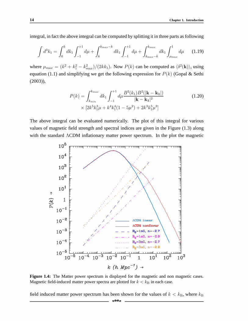
The above integral can be evaluated numerically. The plot ofthis integral for various
values of magnetic field strength and spectral indices are given in the Figure (1.3) along
with the standardΛCDM inflationary matter power spectrum. In the plot the magnetic
Figure 1.4: The Matter power spectrum is displayed for the magnetic and non magnetic cases.Magnetic field-induced matter power spectra are plotted fork < kB in each case.
field induced matter power spectrum has been shown for the values ofk < kB, wherekB[\
1.6. This Thesis 15
is magnetic Jeans scale. In analogous to thermal Jeans scaleλJ = vs(π/ρG)1/2 this scale
is given asλB = vA(π/ρG)1/2 wherevA is Alfven speed. Using the appropriate form
of Alfven speedvA (≡ B/(4πρ)1/2), we get the following formula to compute magnetic
Jeans scale (Sethi & Subramanian (2005)),
kJ ≃ 14.8 Mpc−1
(
Ωm
0.3
)−1(h
0.7
)(
BJ
10−9 G
)−1
(1.21)
where
BJ(a) = B(kJ, a)a2(t) and BJ = Bc(kB/kc)
n+3
2 (1.22)
In the plot we can see that at smaller scales (k > 0.1hMpc−1) there is appreciable en-
hancement in the matter power spectrum due to magnetic field generated perturbations, at
these scales it is almost comparable to standard inflationary (λCDM) matter power spec-
trum, whereas at larger scales (k << 0.1hMpc−1) it is almost negligible in comparison
to inflationary matter power spectrum. Thus we see the existence of primordial magnetic
fields can have implications in the matter distribution in the universe at smaller scales.
Apart from this these primordial magnetic fields can have other implications also in early
structure formation, for example decay of these fields via turbulence and ambipolar diffu-
sion can heat the surrounding medium and this can affect several astrophysical processes
including star formation etc., in the first chapter we will see how can this phenomenon
have a role in understanding the early formation of super massive black holes.
1.6 This Thesis
The aim of this chapter was to set up the stage for the rest of the chapters which discuss my
actual thesis work. In this chapter we learned that, there are some indications which sug-
gests that there was some amount of magnetic field which existed during the primordial
ages of the universe, and the existence of these primordial magnetic fields could influ-
ence the structure formation process in the universe. A quantitative knowledge of these
effects can actually help us probing these primordial magnetic fields through various cos-
mological observables. The next chapter,Chapter Two of this thesis covers my first
thesis project which was to study the possible role of primordial magnetic fields in un-
derstanding the puzzle posed by observations of very early (z = 6 - 8) but bright quasars
(M ≃ 104−5M⊙). The strength of the primordial magnetic fields play a key role in the
analysis given in the chapter two. In the literature there are several bounds primordial
magnetic field parameters (strength and coherence scale) have been proposed based on
[\
16 Chapter 1. Introduction
various kinds of observations and theories but still we havevery limited knowledge about
them. Further chapters,Chapter Three, Four andFive discuss our work towards deriv-
ing constraints on primordial magnetic field strength coming from various cosmological
observables. In theThird Chapter we discuss the large scale imprints of cosmological
magnetic fields, such as, their effects on the formation of the first bound structures in the
universe and the rotation of CMB polarization plane. As we saw in this chapter, the ex-
istence of primordial magnetic fields could produce extra matter perturbations over and
above the inflationary matter perturbations, at very early stage of the universe. This would
influence the matter distribution in the universe favorablyat the scales which are smaller
than (k ∼ 0.1Mpc−1), these are the scales which are mainly probed by weak lensing and
Lyα distribution. TheFourth and theFifth Chapter is about the exercise of constraining
the primordial magnetic field parameters using weak lensingshear analysis and the effec-
tive opacity of Lyα distribution along the line of sight. Finally the last chapter, Chapter
Six is a brief discussion and conclusion about this whole thesiswork.
[\
2Early Formation Of Supermassive Black Holes
(SMBHs) : Role Of Primordial Magnetic Fields
2.1 Formation Of SMBHs At High Redshifts
With the advent of Sloan Digital Sky Survey (SDSS) and the other large area surveys dis-
covery of very bright quasars with luminosity> 1047 erg-s−1) at high redshiftsz & 6
suggests that some supermassive object as massive as109M⊙ were already present when
the universe was very young Fan (2006). Formation of such high mass objects at such an
early stage of the universe poses a puzzle for astrophysics.Early population III stars of
masses∼ 100 M⊙ are expected by the time of redshiftz & 25 (Abel et al., 2002; Bromm
et al., 2002; Yoshida et al., 2008). Even if these stars leavebehind similar mass black holes
after they die out, the Eddington time for growing these seedblack holes to the mass of
108−9M⊙ is of the order of the age of the universe. Thus we see that it isdifficult to gener-
ate a SMBH of mass108−9M⊙ from the given102M⊙ seed black holes unless considering
a phase of super-Eddington accretion or using some very optimistic assumptions in hier-
archical merger models (Haiman & Loeb, 2001; Yoo & Miralda-Escude, 2004; Bromley
et al., 2004; Shapiro, 2005; Volonteri & Rees, 2006; Li et al., 2007; Tanaka & Haiman,
2009).
In the models involving rapid (super-Eddingtopn) collapsethe primordial gas rapidly
gets accreted onto a pre-existing seed BH and collapses intoa SMBH as massive as
104−6M⊙ (Oh & Haiman, 2002; Bromm & Loeb, 2003; Lodato & Natarajan, 2006; Spaans
& Silk, 2006; Begelman et al., 2006; Volonteri et al., 2008; Wise et al., 2008; Regan &
Haehnelt, 2009; Shang et al., 2010). These so called direct collapse models involve metal-
free gas in relatively massive (& 108M⊙) dark matter halos at redshiftz & 10, with virial
temperatureTvir & 104K. The collapsing gas which collapse as it cools and sheds its
angular momentum, must avoid fragmentation and collapse rapidly. These conditions are[\
17
18 Chapter 2. Formation Of SMBHs At High Redshifts
very difficult to be satisfied simultaneously unless the gas remains warm i.e., at temper-
atureTvir ∼ 104 K. An efficient formation of H2 gas in such collapsing halos can cool
the gas to the temperature of T∼ 300 K (Shang et al., 2010), even if the fragmentation is
avoided the inward flow of this cold gas is quite slow∼ 2-3 km s−1 with a corresponding
low accretion rate of∼ 0.01M⊙ yr−1. We can get away with the H2 cooling also in these
models provided the gas is exposed to an intense UV fluxJ . The UV flux slows down the
formation of H2 by either directly photo-dissociating H2 or photo-dissociating the inter-
mediary H−. To inhibit the formation of H2 the photo-dissociation timescale,tdiss ∝ J−1,
has to be shorter than H2 formation time scale,tform ∝ ρ−1. This leads to a critical UV
flux density needed to inhibit the H2 formation which is directly proportional to the den-
sity, Jcrit ∝ ρ for these halos the critical flux is high,J ≈ 102 − 105 (Shang et al., 2010),
at high redshifts only a small fraction of halos which are unusually close to UV bright
sources may see this kind of flux, on the other hand, to avoid fragmentation the gas must
remain metal/dust free (Omukai et al., 2008), which is not possible if the gas is nearby
such luminous galaxies.
2.2 The Role Of Primordial Magnetic Fields
Magnetic heating can play an important role in keeping the collapsing gas warm. If we
consider the existence of background primordial magnetic fields of strength (comoving)≈1 nG (Widrow (2002) and references therein), it can be strongly amplified by flux-freezing
inside the collapsing gas. This in turn will affect the H2 formation and cooling. Sethi
et al. (2008) have shown that 0.2 - 2 nG fields can significantlyenhance the H2 fraction
during the early stages of the collapse, later Schleicher etal. (2009) found similar results,
and emphasized that the magnetic heating from 0.1 - 1 nG fieldscan result in significantly
high temperatures in halos with high densitiesn & 108 cm−3, which can be achieved
during later stages of the collapse.
This work is an extension of Sethi et al. (2008) & Schleicher et al. (2009) with higher
particle density in the collapsing halo and the higher magnetic field. The main result of
this work is that, there exist a critical densityncrit ≈ 103 cm−3 above which H2 cooling
is inefficient, and the temperature stays near∼ 104 K, even as the gas collapse further,
for B < Bcrit, though H2 cooling is delayed, the gas eventually cools down below∼1000 K. Though the critical magnetic field value is higher than the existing upper limits
on primordial magnetic field strength, it can be realized in the rare& 2−3σ regions of the
spatially fluctuatingB field. The abundance of the halos located in these high magnetic
field regions is sufficient to explain the number of quasars observed atz ≈ 6 in the SDSS
[\
2.3. Chemistry And The Thermo-dynamical Evolution Of Collapsing Primordial Gas 19
observations.
2.3 Chemistry And The Thermo-dynamical Evolution Of
Collapsing Primordial Gas
2.3.1 Formation of molecular hydrogen
In the context of formation of the first objects in the universe, H2 has an important role as
a coolant. Elements heavier than Lithium were first formed inside during stellar evolution
and supernova events, and hence when the first structure werebeing formed there was
no better coolant than H2 molecule for temperatures below. 10000 K. In the context of
primordial universe when there were no dust grains, the formation of molecular hydrogen
progresses through two channels with either H− or H2+ in the intermediate stage. In the
first process an electron attaches to a neutral hydrogen atomradiatively to form H−,
H + e−k9−→ H− + γ (2.1)
which in turn form H2 molecule by the reaction:
H− +Hk10−→ H2 + e− (2.2)
At the same time H− ion can also be destroyed by energetic CMB photons, or used upin
some non H2 productive reactions, following are some of the important reactions of such
kind which we have taken into account (k’s are the corresponding reaction rates (Shang et
al., 2010; Sethi et al., 2008)),
H− + γcmbkγ−→ H + e− (2.3)
H− +H+ k13−→ H+2 + e− (2.4)
H− + e−k19−→ H + 2e− (2.5)
H− +Hk20−→ 2H + e− (2.6)
H− +H+ k21−→ 2H (2.7)
The alternative channel through the formation of H2+ occurs when a proton acts as a
catalyst:
H +H+ ↔ H+2 + γ, H+
2 +H → H2 +H+ (2.8)
[\
20 Chapter 2. Formation Of SMBHs At High Redshifts
There is also a third channel through the formation of HeH+. Recently, Hirata & Pad-
manabhan have shown that the H− channel dominates the production of the H2 molecule,
with only∼ 1 per cent contribution from the H2 + channel, and∼ 0.004 per cent from the
HeH+ channel. Therefore in this work H− channel has been used in the calculations. The
net rate of formation ofH2 through theH− channel is given by:
km =k9k10xHInb
k10xHInb + kγ + (k13 + k21)xpnb + k19xenb + k20xHInb. (2.9)
The notation of the reaction rates follows the appendix of Shang et al. (2010), except the
kγ which is the rate of destruction ofH− by CMB photons (eq. 8 in Sethi et al. (2008)).
The net destruction rate ofH2, kdes, is:
kdes = k15xHI + k17xp + k18xe. (2.10)
rate of formation of molecular hydrogen is then given by,
dxH2
dt= kmnbxe(1− xe − 2xH2
)− kdesnbxH2(2.11)
where symbols have there usual meaning.
2.3.2 Density evolution of the collapsing halo
The density from the equation of motion of a bound shell collapsing under gravity (for
details see e.g. Peebles 1980; Padmanabhan 1993):
r = −GM
r2(2.12)
(ignoring the effect of cosmological constant at high redshift). The parametric solutions
of this equation are given by
r = 2rvir[(1− cosθ)/2] (2.13)
t = tc[(θ − sinθ)/2π] (2.14)
Here,tc is the age of the universe at the collapse redshiftzvir andrvir = rmax/2 =12[(2GMt2c)/π
2]1/3 is the radius at virialization. The collapse of the cold darkmatter (cdm)
part of the halo halts at the point of virialization and the overdensity of the region at this
[\
2.3. Chemistry And The Thermo-dynamical Evolution Of Collapsing Primordial Gas 21
point of time is given by(∼ 18π2 in the spherical top-hat model of gravitational collapse
in the cosmological settings of Einstein d’Sitter universe. In this case, the gas density
first decreases due to universal expansion, and then slowly increases prior to the collapse
redshift to reach an overdensity of 18π2 at zvir. The temperature reached by the gas after
virialization depends on the mass of the object, M, through the virial condition (Sethi et
al., 2008):
Tvir ≃ 800K
(
M
106 M⊙
)2/3(1 + z
20
)(
Ωm
0.3
)1/3(h
0.7
)2/3( µ
1.22
)
(2.15)
Even though the dark matter part of halo stops collapsing, the gas part still continues to
collapse as it cools, to follow the evolution of the gas to higher densities beyond the stage
of virialization, we have followed a prescription given thepaper Birnboim & Dekel (2003).
Under this prescription we follow a spherical shell of gas asit collapse down inside
the fixed dark matter halo using energy conservation arguments. We have taken the dark
matter profile as of a fixed isothermal sphere, and it is assumed that the shells do not cross
each other as they contract. The total mass inside a shell at radiusr, which originally (at
zvir) containing a total massMvir is,
M(r) = fbMvir + (1 + fb)Mvirr
rvir(2.16)
wherefb is the baryonic fraction, gravitational potential atr can be given by,
φ(r) = −GM(r)
r− (1− fb)
GMvir
rvirln(rvir
r
)
(2.17)
now we can calculate the evolution of the shell in time in the step ofdt by increasingr to
r + udt, whereu is the velocity of the shell at radiusr and then recalculating the velocity
of the shellu(r + dr) using the energy conservation,
1
2u2 + φ(r) =
1
2v2vir + φ(rvir) = constant (2.18)
vvir is the velocity of the shell at virialization, and is relatedto Mvir andrvir by v2vir =
GMvir/rvir, using this method we have followed the infalling gas to the densities up to
108 cm−3.
[\
22 Chapter 2. Formation Of SMBHs At High Redshifts
2.3.3 Thermal evolution of the collapsing gas
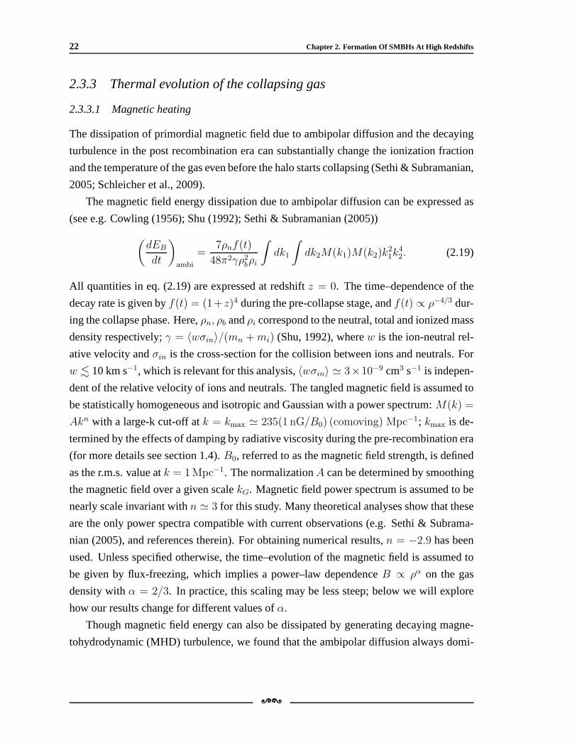
2.3.3.1 Magnetic heating
The dissipation of primordial magnetic field due to ambipolar diffusion and the decaying
turbulence in the post recombination era can substantiallychange the ionization fraction
and the temperature of the gas even before the halo starts collapsing (Sethi & Subramanian,
2005; Schleicher et al., 2009).
The magnetic field energy dissipation due to ambipolar diffusion can be expressed as
(see e.g. Cowling (1956); Shu (1992); Sethi & Subramanian (2005))
(
dEB
dt
)
ambi
=7ρnf(t)
48π2γρ2bρi
∫
dk1
∫
dk2M(k1)M(k2)k21k
42. (2.19)
All quantities in eq. (2.19) are expressed at redshiftz = 0. The time–dependence of the
decay rate is given byf(t) = (1+z)4 during the pre-collapse stage, andf(t) ∝ ρ−4/3 dur-
ing the collapse phase. Here,ρn, ρb andρi correspond to the neutral, total and ionized mass
density respectively;γ = 〈wσin〉/(mn +mi) (Shu, 1992), wherew is the ion-neutral rel-
ative velocity andσin is the cross-section for the collision between ions and neutrals. For
w . 10 km s−1, which is relevant for this analysis,〈wσin〉 ≃ 3×10⁻⁹ cm3 s−1 is indepen-
dent of the relative velocity of ions and neutrals. The tangled magnetic field is assumed to
be statistically homogeneous and isotropic and Gaussian with a power spectrum:M(k) =
Akn with a large-k cut-off atk = kmax ≃ 235(1 nG/B0) (comoving) Mpc−1; kmax is de-
termined by the effects of damping by radiative viscosity during the pre-recombination era
(for more details see section 1.4).B0, referred to as the magnetic field strength, is defined
as the r.m.s. value atk = 1Mpc−1. The normalizationA can be determined by smoothing
the magnetic field over a given scalekG. Magnetic field power spectrum is assumed to be
nearly scale invariant withn ≃ 3 for this study. Many theoretical analyses show that these
are the only power spectra compatible with current observations (e.g. Sethi & Subrama-
nian (2005), and references therein). For obtaining numerical results,n = −2.9 has been
used. Unless specified otherwise, the time–evolution of themagnetic field is assumed to
be given by flux-freezing, which implies a power–law dependenceB ∝ ρα on the gas
density withα = 2/3. In practice, this scaling may be less steep; below we will explore
how our results change for different values ofα.
Though magnetic field energy can also be dissipated by generating decaying magne-
tohydrodynamic (MHD) turbulence, we found that the ambipolar diffusion always domi-
[\
2.3. Chemistry And The Thermo-dynamical Evolution Of Collapsing Primordial Gas 23
nates for our case The evolution of magnetic field energy density can be written as
dEB
dt=
4
3
ρ
ρ−(
dEB
dt
)
turb
−(
dEB
dt
)
ambi
(2.20)
The first term on the right-hand side takes into account the change in the magnetic field
energy due to adiabatic expansion (in the early stages of theevolution of a halo) and
compression (during the halo collapse). The heatingLheat can be expressed as,
Lheat =
(
dEB
dt
)
turb
+
(
dEB
dt
)
ambi
(2.21)
2.3.3.2 Other cooling (heating) processes
The cooling (heating) processes that dominate in primordial gas in the density and temper-
ature range we consider for this problem, are: (a) Compton cooling (heating)kiC (eq. 15
in SBK08), (b) atomic H cooling (eq. 16 in SBK08), and (c)H2 molecular cooling (Galli
& Palla 1998) and (d) the adiabatic cooling (heating) due to expansion (collapse) of the
system. In the following section,
Lcool ≡ atomic H cooling + molecular H2 cooling (2.22)
2.3.3.3 Evolution of density (n), temperature (T ) and other related quantities
Following Sethi et al. (2008), the evolution of the ionization fraction (xe), magnetic field
energy density (EB), temperature (T ), andH2 molecule fraction (xH2) are described by
the equations
xe =[
βe(1− xe) exp (−hνα/(kBTcbr))− αenbx2e
]
C +
+ γenb(1− xe)xe (2.23)dEB
dt=
4
3
ρ
ρ−(
dEB
dt
)
turb
−(
dEB
dt
)
ambi
(2.24)
dT
dt=
2
3
nb
nbT + kiCxe(Tcbr − T ) +
2
3nbkB(Lheat − Lcool) , (2.25)
dxH2
dt= kmnbxe(1− xe − 2xH2
)− kdesnbxH2. (2.26)
The symbols here have their usual meaning. Eq. 2.24 and 2.26 are just the Eq. 2.20 and
2.11 described in the previous subsections, Eq. 2.25 is for the temperature evolution of
the collapsing gas, in which the first term correspond to adiabatic cooling (or heating),
second term is accounting for inverse Compton cooling (heating),Lcool,Lheat are the other[\
24 Chapter 2. Formation Of SMBHs At High Redshifts
heating and cooling (volume) rates, described in the previous sections. Eq. 2.23 describes
the evolution of the ionized fraction, the first two terms arethe terms for the recombination
of the primordial plasma (for details and notation see Peebles 1968, 1993), the third term
on the right-hand side of the equation corresponds to the collisional ionization (for details
see Sethi et al. (2008)).
2.4 Results
In Figure 2.1, 2.2, and 2.3 the evolution of the temperature,theH2 fraction (nH2/nH), and
the ionized fraction for a single halo fromz ≃ 800 (corresponding to the initial number
densityn ≃ 100 cm−3 on the left of Figures 2.1, 2.2, and 2.3), down to a maximum density
of n ≃ 106 cm−3 in the collapsed halo. The evolution on these figures is monotonically
to the right: the x–axis shows the density decreasing to the right (until the turnaround
redshift), and then increasing again as the halo collapses.
These figures show an interplay between several physical effects. First, the magnetic
field decay directly increases the temperature. This increases the electron fraction (due to
more rapid collisional ionization), the larger electron fraction in turn tends to increase the
molecular hydrogen fraction, but at the same time high temperature increases the colli-
sional destruction rate of molecular hydrogen. Thus the molecular hydrogen cooling rate
depends on the temperature directly. As the temperature reaches& 8, 000K, atomic cool-
ing dominates, which, again, is governed by the ionized fraction. A higher magnetic field
strength generally results in more rapid heating, and therefore a higher temperature. This,
in turn results in higher ionized fractions, higher H2 fraction but controlled by its destruc-
tion again due to high temperature. In the collapsing stage when HI cooling is not efficient
because of low temperature, molecular hydrogen becomes thedominant coolant, and thus
play an important role during the collapsing phase of the halo.
Figures 2.4 and 2.5 show the variation of various kind of heating and cooling functions
as the halo collapse for magnetic field strengthB0 = 1 nG and4 nG respectively. In both
the Figures we see that during the collapse phase, adiabaticheating or Compton cooling
rates are much lower than the magnetic heating, H2 cooling or HI cooling, and therefore
they do not play an important role in this whole process. ForB0 = 1 nG case, (Figure 2.4)
we see that the atomic HI cooling becomes unimportant soon after the start of the collapse
phase, as the magnetic heating is not sufficient to keep the temperature above 8000 K, as
a consequence temperature goes down below 8000 K and atomic cooling rate decreases
sharply. But H2 cooling quickly becomes more important, dominating the magnetic heat-
ing for a short period of time when the density is around 0.1 - 0.2 cm−3, resulting in a
[\
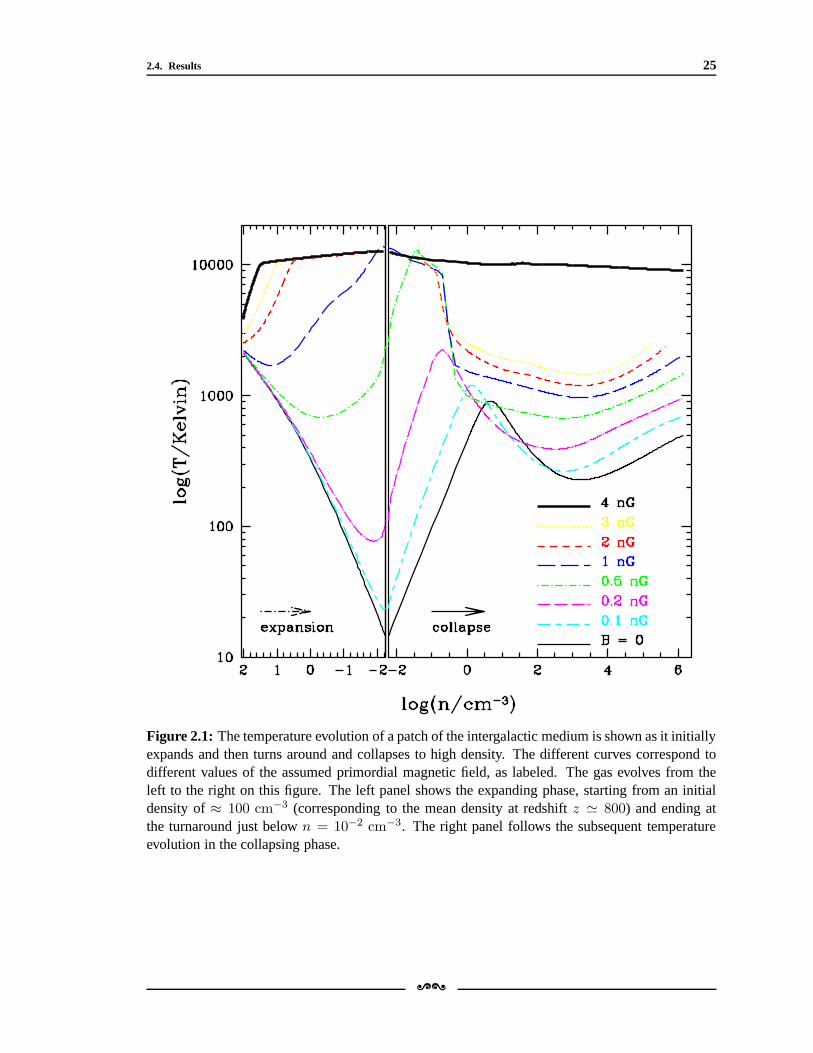
2.4. Results 25
Figure 2.1: The temperature evolution of a patch of the intergalactic medium is shown as it initiallyexpands and then turns around and collapses to high density.The different curves correspond todifferent values of the assumed primordial magnetic field, as labeled. The gas evolves from theleft to the right on this figure. The left panel shows the expanding phase, starting from an initialdensity of≈ 100 cm−3 (corresponding to the mean density at redshiftz ≃ 800) and ending atthe turnaround just belown = 10−2 cm−3. The right panel follows the subsequent temperatureevolution in the collapsing phase.
[\
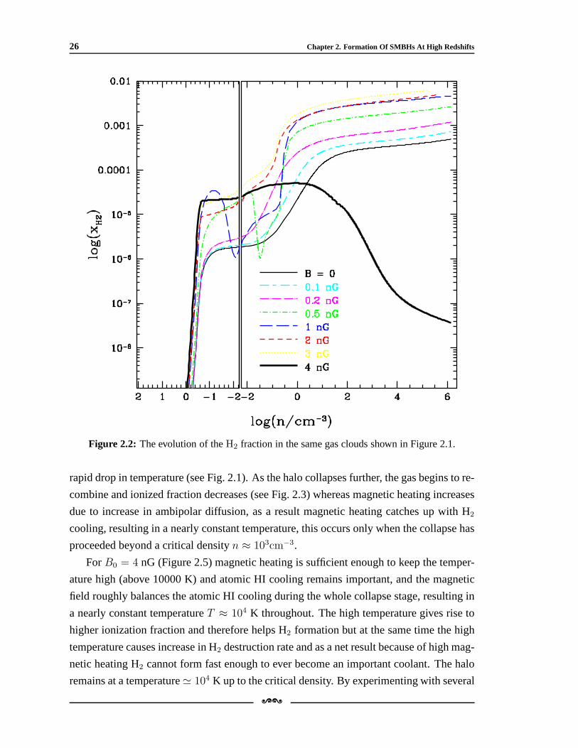
26 Chapter 2. Formation Of SMBHs At High Redshifts
Figure 2.2: The evolution of theH2 fraction in the same gas clouds shown in Figure 2.1.
rapid drop in temperature (see Fig. 2.1). As the halo collapses further, the gas begins to re-
combine and ionized fraction decreases (see Fig. 2.3) whereas magnetic heating increases
due to increase in ambipolar diffusion, as a result magneticheating catches up with H2cooling, resulting in a nearly constant temperature, this occurs only when the collapse has
proceeded beyond a critical densityn ≈ 103cm−3.
ForB0 = 4 nG (Figure 2.5) magnetic heating is sufficient enough to keepthe temper-
ature high (above 10000 K) and atomic HI cooling remains important, and the magnetic
field roughly balances the atomic HI cooling during the wholecollapse stage, resulting in
a nearly constant temperatureT ≈ 104 K throughout. The high temperature gives rise to
higher ionization fraction and therefore helps H2 formation but at the same time the high
temperature causes increase in H2 destruction rate and as a net result because of high mag-
netic heating H2 cannot form fast enough to ever become an important coolant.The halo
remains at a temperature≃ 104 K up to the critical density. By experimenting with several
[\
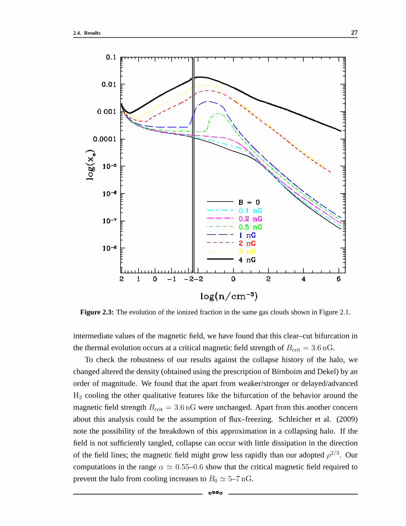
2.4. Results 27
Figure 2.3: The evolution of the ionized fraction in the same gas clouds shown in Figure 2.1.
intermediate values of the magnetic field, we have found thatthis clear–cut bifurcation in
the thermal evolution occurs at a critical magnetic field strength ofBcrit = 3.6 nG.
To check the robustness of our results against the collapse history of the halo, we
changed altered the density (obtained using the prescription of Birnboim and Dekel) by an
order of magnitude. We found that the apart from weaker/stronger or delayed/advanced
H2 cooling the other qualitative features like the bifurcation of the behavior around the
magnetic field strengthBcrit = 3.6 nG were unchanged. Apart from this another concern
about this analysis could be the assumption of flux–freezing. Schleicher et al. (2009)
note the possibility of the breakdown of this approximationin a collapsing halo. If the
field is not sufficiently tangled, collapse can occur with little dissipation in the direction
of the field lines; the magnetic field might grow less rapidly than our adoptedρ2/3. Our
computations in the rangeα ≃ 0.55–0.6 show that the critical magnetic field required to
prevent the halo from cooling increases toB0 ≃ 5–7 nG.
[\
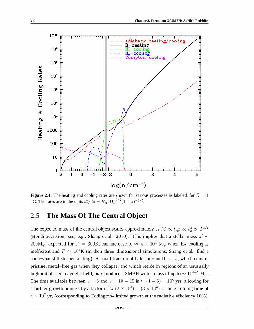
28 Chapter 2. Formation Of SMBHs At High Redshifts
Figure 2.4: The heating and cooling rates are shown for various processes as labeled, forB = 1
nG. The rates are in the unitsdt/dz = H−10 Ω
−1/2m (1 + z)−5/2.
2.5 The Mass Of The Central Object
The expected mass of the central object scales approximately asM ∝ t−1acc ∝ c3s ∝ T 3/2
(Bondi accretion; see, e.g., Shang et al. 2010). This implies that a stellar mass of∼200M⊙, expected forT = 300K, can increase to≈ 4 × 10⁴ M⊙ whenH2–cooling is
inefficient andT ≈ 104K (in their three–dimensional simulations, Shang et al. finda
somewhat still steeper scaling). A small fraction of halos at z = 10 − 15, which contain
pristine, metal–free gas when they collapse, and which reside in regions of an unusually
high initial seed magnetic field, may produce a SMBH with a mass of up to∼ 104−5 M⊙.
The time available betweenz = 6 andz = 10 − 15 is ≈ (4 − 6) × 108 yrs, allowing for
a further growth in mass by a factor of≈ (2 × 10⁴) − (3 × 10⁶) at the e–folding time of
4 × 10⁷ yr, (corresponding to Eddington–limited growth at the radiative efficiency 10%).
[\
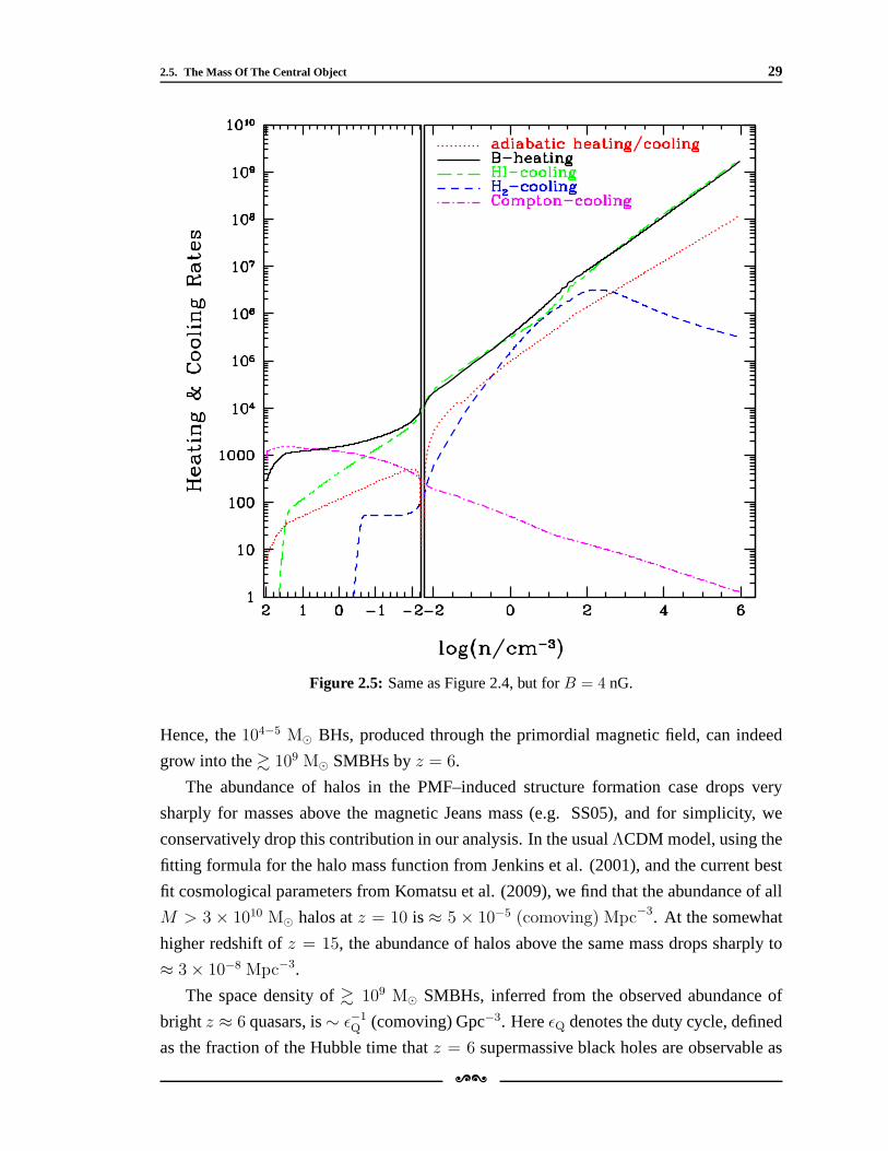
2.5. The Mass Of The Central Object 29
Figure 2.5: Same as Figure 2.4, but forB = 4 nG.
Hence, the104−5 M⊙ BHs, produced through the primordial magnetic field, can indeed
grow into the& 109 M⊙ SMBHs byz = 6.
The abundance of halos in the PMF–induced structure formation case drops very
sharply for masses above the magnetic Jeans mass (e.g. SS05), and for simplicity, we
conservatively drop this contribution in our analysis. In the usualΛCDM model, using the
fitting formula for the halo mass function from Jenkins et al.(2001), and the current best
fit cosmological parameters from Komatsu et al. (2009), we find that the abundance of all
M > 3 × 10¹⁰ M⊙ halos atz = 10 is ≈ 5 × 10⁻⁵ (comoving) Mpc−3. At the somewhat
higher redshift ofz = 15, the abundance of halos above the same mass drops sharply to
≈ 3× 10⁻⁸ Mpc−3.
The space density of& 109 M⊙ SMBHs, inferred from the observed abundance of
brightz ≈ 6 quasars, is∼ ǫ−1Q (comoving) Gpc−3. HereǫQ denotes the duty cycle, defined
as the fraction of the Hubble time thatz = 6 supermassive black holes are observable as
[\
30 Chapter 2. Formation Of SMBHs At High Redshifts
luminous quasars. Assuming a quasar lifetime of∼ 50 Myr (e.g. Martini 2004), we have
ǫQ ∼ 0.05, and the space density ofz = 6 SMBHs is∼ 20 Gpc−3. Therefore, at redshift
z = 10, a fraction as low asf ∼ (20 Gpc−3)/(5× 10−5 Mpc−3) = 3× 10⁻³ of the whole
population ofM & 3×10¹⁰ M⊙ halos is sufficient to account for the presence of these rare
z ≈ 6 SMBHs. Such a small fraction would correspond to∼ 2.8σ upward fluctuations of
a Gaussian random PMF.
2.6 Discussion
In this work we have investigated the role of primordial magnetic fields in the formation
of SMBHs at high redshifts. Calculations showed that the direct gas collapse in the early
dark matter halos, aided by heating from the dissipation of aprimordial magnetic field
can lead to the formation of high mass objects which in turn can grow into a SMBH by
the redshifts of 6-8. This model avoids many of the odd assumptions required in earlier
models (such as an extremely high UV flux and the absence ofH2 and of other molecules
and metals). But at the same time this model requires a large primordial magnetic field,
and relies on metal-free primordial gas. From this analysis, in general, it seems that any
other heating mechanism, which could compete with atomic HIcooling in the collapsing
halo, down to a density ofn ∼ 103 cm−3, would produce similar effect as the magnetic
field produced here.
[\
3Primordial Magnetic Field Limits
From Cosmological Data
3.1 Introduction
In the previous chapter we saw that, presence of magnetic fields can play an important
role in the formation of early collapsed halos . If the magnetic field strength around the
collapsing halo is strong enough (Bcrit = 3.6 nG), it can drastically change the course
of thermal and dynamical evolution of the halo, and as a result more massive stars can
form and consequently it can lead to formation of early supermassive black holes. The
abundance of such objects will depend on the value of primordial magnetic field at those
high red shifts, which is still not a well probed quantity. This chapter is about the study of
limits on primordial magnetic field coming from various cosmological observables. The
aim of this work was to investigate the limits on primordial magnetic fields coming from
the observational constraint on the Farady rotation of CMB polarization plane and the
Large Scale Structures (LSS) in the universe.
A quadrupole anisotropy in the temperature inhomogeneity can lead to polarization
of CMB photons. This quadrupole anisotropy could arise fromthe following 3 types of
perturbations,
1 Scalar (due to density fluctuations)
2 Vector (due to vorticity)
3 Tensor (due to gravity waves)
To study the polarization pattern in the CMB, the CMB polarization can be decomposed
into two components:
1 Curl free component : E-mode or gradient-mode[\
31
32 Chapter 3. Primordial Magnetic Field Limits From Cosmological Data
2 Grad free component : B-mode or curl-mode
the E-mode may arise due to both the scalar and the tensor perturbations (the contribution
from vector perturbations is expected to be negligible), but the B-mode could arise due to
only vector or tensor perturbations. In fact a cosmologicalmagnetic field also can source a
B-mode in CMB polarization and CMB B-polarization measurement can be a crucial test
to limit the primordial magnetic field strength. In this analysis we are not going to take
this into account.
Presence of magnetic field during recombination causes a rotation in CMB polarization
plane due to Faraday effect. The same field could cause additional density perturbations
and thus affect the structure formation scenario and the LSSstatistics (Section 1.5).
3.2 Modeling The Primordial Magnetic Fields (Concept
of Beff)
Assuming primordial magnetic field as a stochastic Gaussianmagnetic field it can be fully
described by its two-point correlation function . For simplicity we consider here the case of
the non-helical magnetic field, in this case the two-point correlation function in wavenum-
ber space can be written as (Section 1.4, equation 1.1)
〈B⋆i (k)Bj(k
′)〉 = (2π)3δ(3)(k− k′)Pij(k)PB(k). (3.1)
Herei andj are spatial indices,i, j ∈ (1, 2, 3), ki = ki/k a unit wave vector,Pij(k) =
δij − kikj the transverse plane projector,δ(3)(k− k′) the Dirac delta function, andPB(k)
is the power spectrum of the magnetic field.
We define the smoothed magnetic fieldBλ through the mean-square magnetic field
(Mack et al., 2002)
Bλ2 = 〈B(x) ·B(x)〉|λ, (3.2)
where the smoothing is done on a comoving lengthλ with a Gaussian smoothing ker-
nel function∝ exp[−x2/λ2]. Corresponding to the smoothing lengthλ is the smoothing
wavenumberkλ = 2π/λ. The power spectrumPB(k) is assumed to be a simple power law
on large scales,k < kD (wherekD is the cutoff wavenumber),
PB(k) = PB0knB =
2π2λ3B2λ
Γ(nB/2 + 3/2)(λk)nB , (3.3)
and assumed to vanish on small scales wherek > kD.
[\
3.3. CMB Polarization Plane Rotation 33
The energy density of the magnetic field is given by (Kahniashvili & Ratra, 2007)
ρB(λ) =B2
λ(kDλ)nB+3
8πΓ(nB/2 + 5/2). (3.4)
For this work we define an effective magnetic fieldBeff such thatρB = B2eff/(8π). For the
scale-invariant spectrum (nB = −3 ; (Ratra, 1992)) we getBeff = Bλ for all values ofλ.
The scale-invariant case is the only case where the values ofthe effective and smoothed
fields coincide.
The cut-off scalekD (≡ kmax Section 1.4, equation 1.3) is determined by the Alfven
wave damping scalek−1D ∼ vALS wherevA is the Alfven velocity andLS the Silk damping
scale (Jedamzik et al., 1998). This description is more appropriate when we are dealing
with an homogeneous magnetic field and the Alfven waves are the fluctuationsB1(x) with
respect to a background homogeneous magnetic fieldB0 (|B1| ≪ |B0|). In the case of
the stochastic magnetic field we generalize the Alfven velocity definition, see Ref. Mack
et al. (2002), by referring to the analogy between the effective magnetic field and the
homogeneous magnetic field. Assuming that the Alfven velocity is determined byBeff , a
simple computation gives the expression ofkD in terms ofBeff (Kahniashvili et al., 2011):
kD
1Mpc−1 = 1.4
√
(2π)nB+3h
Γ(nB/2 + 5/2)
(
10−7G
Beff
)
. (3.5)
Hereh is the Hubble constant in units of 100 km s−1 Mpc−1. The BBN limit on the
effective magnetic field strength,Beff ≤ 8.4× 10⁻⁷ G (Kahniashvili et al., 2011), gives an
upper limit on the cut-off wavenumberkD,
kBBND ≥ 0.17h1/2 (2π)(nB+3)/2
Γ1/2(nB/2 + 5/2)Mpc−1. (3.6)
In the case of an extremely large magnetic field it is possibleto haveλD > 1 Mpc. At this
point it would seem unreasonable (unjustified) to consider asmoothing scaleλ = 1 Mpc
as is conventionally done.
3.3 CMB Polarization Plane Rotation
The presence of (primordial) magnetic field during recombination causes a rotation of the
CMB polarization plane through the Faraday effect (Kosowsky & Loeb, 1996). The rms
rotation angleαrms = (〈α2〉)1/2 induced by a stochastic magnetic field with smoothed
[\
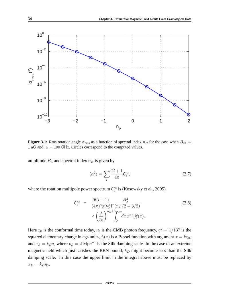
34 Chapter 3. Primordial Magnetic Field Limits From Cosmological Data
−3 −2 −1 0 1 210
−10
10−8
10−6
10−4
10−2
100
nB
α rms (
°)
Figure 3.1: Rms rotation angleαrms as a function of spectral indexnB for the case whenBeff =1nG andν0 = 100GHz. Circles correspond to the computed values.
amplitudeBλ and spectral indexnB is given by
〈α2〉 =∑
l
2l + 1
4πCα
l , (3.7)
where the rotation multipole power spectrumCαl is (Kosowsky et al., 2005)
Cαl ≃ 9l(l + 1)
(4π)3q2ν40
B2λ
Γ (nB/2 + 3/2)(3.8)
×(
λ
η0
)nB+3∫ xS
0
dx xnBj2l (x).
Hereη0 is the conformal time today,ν0 is the CMB photon frequency,q2 = 1/137 is the
squared elementary charge in cgs units,jl(x) is a Bessel function with argumentx = kη0,
andxS = kSη0 wherekS = 2 Mpc−1 is the Silk damping scale. In the case of an extreme
magnetic field which just satisfies the BBN bound,kD might become less than the Silk
damping scale. In this case the upper limit in the integral above must be replaced by
xD = kDη0.
[\
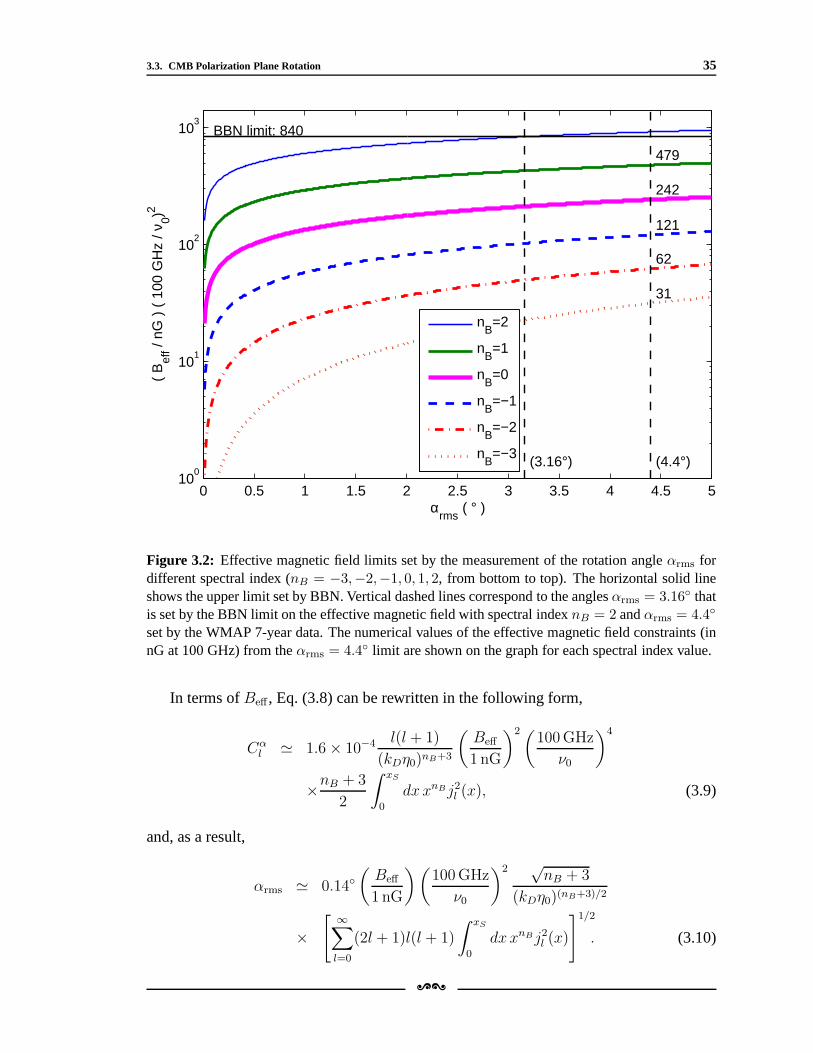
3.3. CMB Polarization Plane Rotation 35
0 0.5 1 1.5 2 2.5 3 3.5 4 4.5 510
0
101
102
103
αrms
( ° )
( B
eff /
nG )
( 1
00 G
Hz
/ ν0)2
(3.16°) (4.4°)
BBN limit: 840
479
242
121
62
31
nB=2
nB=1
nB=0
nB=−1
nB=−2
nB=−3
Figure 3.2: Effective magnetic field limits set by the measurement of therotation angleαrms fordifferent spectral index (nB = −3,−2,−1, 0, 1, 2, from bottom to top). The horizontal solid lineshows the upper limit set by BBN. Vertical dashed lines correspond to the anglesαrms = 3.16 thatis set by the BBN limit on the effective magnetic field with spectral indexnB = 2 andαrms = 4.4
set by the WMAP 7-year data. The numerical values of the effective magnetic field constraints (innG at 100 GHz) from theαrms = 4.4 limit are shown on the graph for each spectral index value.
In terms ofBeff , Eq. (3.8) can be rewritten in the following form,
Cαl ≃ 1.6× 10⁻⁴ l(l + 1)
(kDη0)nB+3
(
Beff
1 nG
)2(100GHz
ν0
)4
×nB + 3
2
∫ xS
0
dx xnBj2l (x), (3.9)
and, as a result,
αrms ≃ 0.14(
Beff
1 nG
)(
100GHz
ν0
)2 √nB + 3
(kDη0)(nB+3)/2
×[
∞∑
l=0
(2l + 1)l(l + 1)
∫ xS
0
dx xnBj2l (x)
]1/2
. (3.10)
[\
36 Chapter 3. Primordial Magnetic Field Limits From Cosmological Data
It is of interest to compare Eq. (3.10) with the corresponding result, Eq. (2) of Ref.
(Kosowsky & Loeb, 1996), derived for a homogeneous magneticfield and at frequency
ν0 = 30 GHz,
αrms ≃ 1.6(
B0
1 nG
)(
30GHz
ν0
)2
(3.11)
Both expressions agree fornB → −3 after accounting for∑
l(2l + 1)j2l (x) = 1 and the
fact that Bessel functions peak atx ∼ l for givenl (see Appendix A).
Figure 3.1 shows the rms rotation angleαrms, Eq. (3.10), as a function of the spectral
indexnB when the effective magnetic field is normalized to be10−9 G. The WMAP 7-year
data limits the rms rotation angle to be less then4.4 at95% C. L. (Komatsu et al., 2011).
This allows us to limit the effective magnetic field as shown in Fig. 3.2.
3.4 Large Scale Structures
A primordial tangled magnetic field can also induce the formation of structures in the
Universe. In particular, these fields can play an important role in the formation of first
structures (see, e.g. Refs. Wasserman (1978); Kim et al. (1996); Subramanian & Barrow
(1998); Gopal & Sethi (2005); Sethi & Subramanian (2005); Sethi et al. (2008); Yamazaki
et al. (2008); Sethi, Haiman, Pandey (2010)).
The magnetic-field-induced matter power spectrumP (k) is ∝ k4 for nB > −1.5 and
∝ k2nB+7 for nB ≤ −1.5 (Kim et al., 1996; Gopal & Sethi, 2005). The cut-off scale of
the power spectrum is determined by the larger of the magnetic Jeans’ wavenumberkJ and
the thermal Jeans’ wavenumberktherm (for a detailed discussion, see, e.g. Ref. Sethi et al.
(2008)). Here the magnetic Jeans’ wavenumber is (see, e.g. Ref. Kim et al. (1996))
kJ ≃ (230(nB+3)/2 × 13.8)2/(nB+5)
(
1 nG
Beff
)
Mpc−1. (3.12)
Unlike theΛCDM matter power spectrum, the magnetic-field-induced matter power spec-
trum increases at small scales and can exceed theΛCDM matter one at small scales (for a
comparison of these two spectra, see, e.g. Fig. 3 of Ref. Gopal & Sethi (2005)). And, there-
fore, one of the more important contributions of the additional power induced by magnetic
fields is to the formation of the first structures in the Universe (e.g. Refs. Sethi & Sub-
ramanian (2005); Sethi, Haiman, Pandey (2010); Yamazaki etal. (2008) and references
therein).
In Fig. 3.3 we show the linear mass dispersionσ(M) for matter power spectra induced
by a primordial magnetic field withBeff = 6nG at z = 10 for different values ofnB.
[\
3.4. Large Scale Structures 37
Notable features of Fig. 3.3 are: (a) the mass dispersion on small scales is larger for a
larger value ofnB; and, (b) fornB ≥ −1.5, the mass dispersion drops more sharply at
larger scales than fornB ≤ −1.5. We focus here on the mass dispersion on the smallest
scales, as these scales are more relevant for the formation of the first structures in the
Universe. These first structures were responsible for the reionization of the Universe at
z ≃ 10. To obtain meaningful constraints onBeff from the formation of first structures, we
need to know how the curves shown in Fig. 3.3 vary asBeff is changed and as the Universe
evolves.
The mass dispersionσ(M, z) evolves with the time dependence of the growing mode of
the linear density perturbations sourced by the primordialmagnetic field (Kim et al., 1996;
Gopal & Sethi, 2005). The growing mode is∝ a(t), the scale factor, at high redshifts,
the same as in the “standard”ΛCDM case without a magnetic field. To account for this
evolution the curves corresponding toσ in Fig. 3.3 must be scaled by roughly a factor of
≃ 11/(1 + z) for redshiftsz ≫ 1.
It can be shown that the value ofσ at the smallest scales (M ≃ 106M⊙) is invariant
under a change inBeff if the cut-off scale is determined bykJ: an increase/decrease in the
value ofBeff is compensated by a decrease/increase in the value ofkJ. However, ifBeff is
decreased to a value at whichktherm ≤ kJ, then the value ofσ decreases with a decrease
in Beff , as the cut-off scale becomes independent of the value ofBeff .
It has been shown that the dissipation of magnetic fields in the post-recombination era
can substantially alter the thermal and ionization historyof the universe (Yamazaki et al.,
2008; Sethi & Subramanian, 2005; Sethi et al., 2008). In particular, this dissipation raises
the matter temperature and therefore the Jeans’ scale in theIGM. For Beff ≥ 1 nG the
matter temperature rises to≃ 104K as early asz ≥ 100, (Sethi & Subramanian, 2005),
resulting in a steep rise in the Jeans’ scale as compared to the usual case. The Jeans’ wave
number corresponding to this temperature isktherm ≃ 10Mpc−1 (see, e.g. Fig. 4 of Ref.
Sethi et al. (2008)).
WMAP results show that the Universe reionized atz ≃ 10. This reionization was
caused by the non-linear collapse of the first structures, followed by star formation and
the emission of UV photons from the collapsed halos. For a virialized structure in the
spherical collapse model, the linear mass dispersionσ ≃ 1.7. This implies that the value
of σ at the scales of interest atz ≃ 10 is not expected to be much higher than1.7. Consider
thenB = 2 model in Fig. 3.3; the value of mass dispersion at the smallest scales is≃ 100,
which means that the first structures formed atz ≃ 650 in this case (the redshift of the
collapse of first structures is≃ 6.5σmax, whereσmax is the maximum value ofσ atz ≃ 10),
which can certainly be ruled out by the WMAP data on CMB anisotropies. A similar
[\
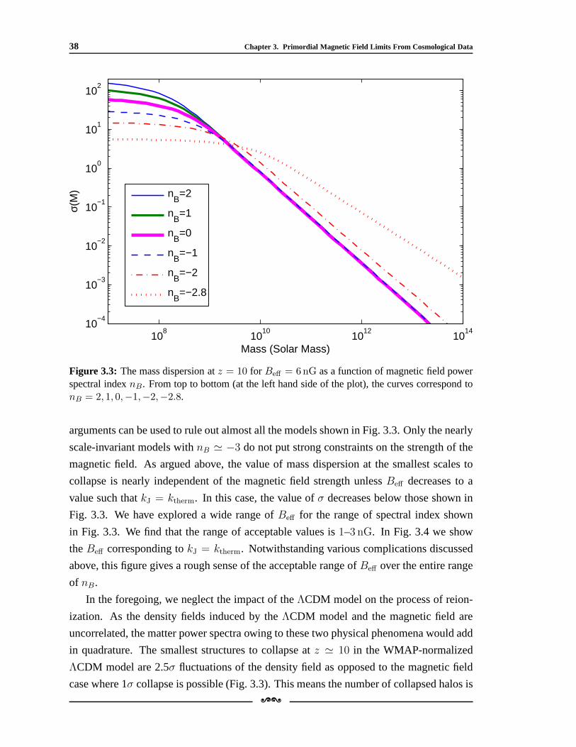
38 Chapter 3. Primordial Magnetic Field Limits From Cosmological Data
108
1010
1012
1014
10−4
10−3
10−2
10−1
100
101
102
Mass (Solar Mass)
σ(M
)
nB=2
nB=1
nB=0
nB=−1
nB=−2
nB=−2.8
Figure 3.3: The mass dispersion atz = 10 for Beff = 6nG as a function of magnetic field powerspectral indexnB. From top to bottom (at the left hand side of the plot), the curves correspond tonB = 2, 1, 0,−1,−2,−2.8.
arguments can be used to rule out almost all the models shown in Fig. 3.3. Only the nearly
scale-invariant models withnB ≃ −3 do not put strong constraints on the strength of the
magnetic field. As argued above, the value of mass dispersionat the smallest scales to
collapse is nearly independent of the magnetic field strength unlessBeff decreases to a
value such thatkJ = ktherm. In this case, the value ofσ decreases below those shown in
Fig. 3.3. We have explored a wide range ofBeff for the range of spectral index shown
in Fig. 3.3. We find that the range of acceptable values is1–3 nG. In Fig. 3.4 we show
theBeff corresponding tokJ = ktherm. Notwithstanding various complications discussed
above, this figure gives a rough sense of the acceptable rangeof Beff over the entire range
of nB.
In the foregoing, we neglect the impact of theΛCDM model on the process of reion-
ization. As the density fields induced by theΛCDM model and the magnetic field are
uncorrelated, the matter power spectra owing to these two physical phenomena would add
in quadrature. The smallest structures to collapse atz ≃ 10 in the WMAP-normalized
ΛCDM model are 2.5σ fluctuations of the density field as opposed to the magnetic field
case where 1σ collapse is possible (Fig. 3.3). This means the number of collapsed halos is[\
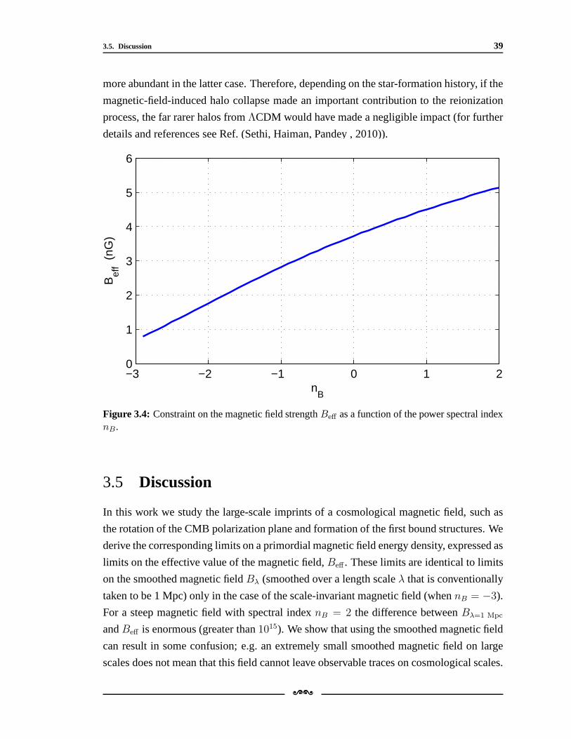
3.5. Discussion 39
more abundant in the latter case. Therefore, depending on the star-formation history, if the
magnetic-field-induced halo collapse made an important contribution to the reionization
process, the far rarer halos fromΛCDM would have made a negligible impact (for further
details and references see Ref. (Sethi, Haiman, Pandey , 2010)).
−3 −2 −1 0 1 20
1
2
3
4
5
6
nB
Bef
f (nG
)
Figure 3.4: Constraint on the magnetic field strengthBeff as a function of the power spectral indexnB.
3.5 Discussion
In this work we study the large-scale imprints of a cosmological magnetic field, such as
the rotation of the CMB polarization plane and formation of the first bound structures. We
derive the corresponding limits on a primordial magnetic field energy density, expressed as
limits on the effective value of the magnetic field,Beff . These limits are identical to limits
on the smoothed magnetic fieldBλ (smoothed over a length scaleλ that is conventionally
taken to be 1 Mpc) only in the case of the scale-invariant magnetic field (whennB = −3).
For a steep magnetic field with spectral indexnB = 2 the difference betweenBλ=1 Mpc
andBeff is enormous (greater than1015). We show that using the smoothed magnetic field
can result in some confusion; e.g. an extremely small smoothed magnetic field on large
scales does not mean that this field cannot leave observable traces on cosmological scales.
[\
40 Chapter 3. Primordial Magnetic Field Limits From Cosmological Data
An intergalactic magnetic field of effective value larger than 1-10 nG (with, depending
on magnetic spectral index, corresponding values ofBλ=1 Mpc in the range10−8 − 10−26
G) is ruled out by cosmological data. These limits of 1-10 nG are consistent with recent
observational bounds on the intergalactic magnetic field (Neronov & Vovk, 2010; Tavec-
chio et al., 2010; Ando & Kusenko, 2010) if the field was generated in the early Universe
with spectral shapenB ≤ 1. This favors the inflationary magnetogenesis scenario.
[\
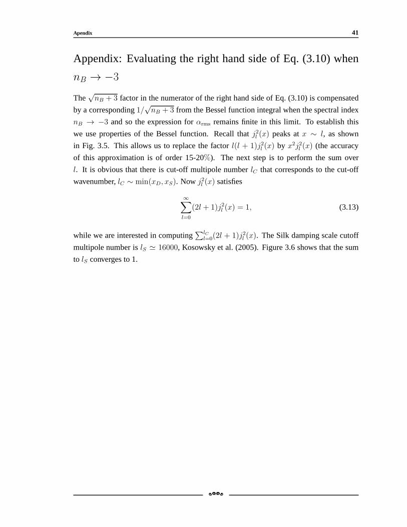
Apendix 41
Appendix: Evaluating the right hand side of Eq. (3.10) when
nB → −3
The√nB + 3 factor in the numerator of the right hand side of Eq. (3.10) iscompensated
by a corresponding1/√nB + 3 from the Bessel function integral when the spectral index
nB → −3 and so the expression forαrms remains finite in this limit. To establish this
we use properties of the Bessel function. Recall thatj2l (x) peaks atx ∼ l, as shown
in Fig. 3.5. This allows us to replace the factorl(l + 1)j2l (x) by x2j2l (x) (the accuracy
of this approximation is of order 15-20%). The next step is to perform the sum over
l. It is obvious that there is cut-off multipole numberlC that corresponds to the cut-off
wavenumber,lC ∼ min(xD, xS). Now j2l (x) satisfies
∞∑
l=0
(2l + 1)j2l (x) = 1, (3.13)
while we are interested in computing∑lC
l=0(2l + 1)j2l (x). The Silk damping scale cutoff
multipole number islS ≃ 16000, Kosowsky et al. (2005). Figure 3.6 shows that the sum
to lS converges to 1.
[\
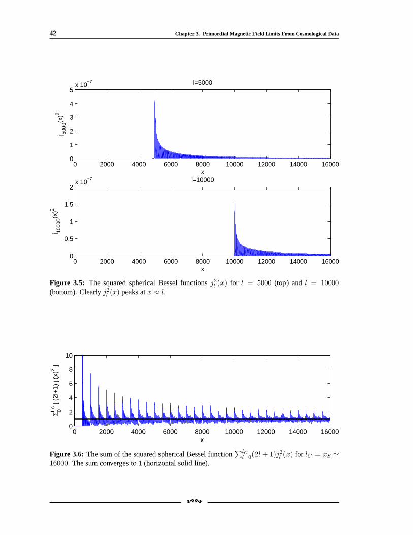
42 Chapter 3. Primordial Magnetic Field Limits From Cosmological Data
0 2000 4000 6000 8000 10000 12000 14000 160000
1
2
3
4
5x 10
−7
x
j 5000
(x)2
l=5000
0 2000 4000 6000 8000 10000 12000 14000 160000
0.5
1
1.5
2x 10
−7
x
j 1000
0(x)2
l=10000
Figure 3.5: The squared spherical Bessel functionsj2l (x) for l = 5000 (top) andl = 10000(bottom). Clearlyj2l (x) peaks atx ≈ l.
0 2000 4000 6000 8000 10000 12000 14000 160000
2
4
6
8
10
x
Σ 0Lc [
(2l+
1) j l(x
)2 ]
Figure 3.6: The sum of the squared spherical Bessel function∑lC
l=0(2l + 1)j2l (x) for lC = xS ≃16000. The sum converges to 1 (horizontal solid line).
[\
4Probing Primordial Magnetic Fields
Using Weak Lensing
4.1 Introduction
In recent years, weak gravitational lensing has proved to beone of best probes of the matter
power spectrum of the universe. In particular, this method can reliably estimate the matter
power spectrum at small scales which are not directly accessible to other methods e.g.
galaxy surveys (for details and further references see e.g.Munshi et al. (2008); Hoekstra
& Jain (2008); Refregier (2003); Bartelmann & Schneider (2001)) (Figure 4.1). These are
the scale which are affected by the existence of primordial magnetic fields (see Figures 1.4
or 4.4) and thus a careful analysis of the cosmological observables which probe these small
scale density distribution in the Universe such as weak lensing shear and Lyα distribution
can actually provide information about primordial magnetic fields also.
In this work we attempt to constrain primordial magnetic fields within the framework
of the two-point shear correlation function induced by gravitational lensing, including the
contribution of matter perturbations induced by these magnetic fields. We compare our
results with the CFHTLS (Canada-France-Hawaii Telescope Legacy Survey) Wide data
(Fu et al., 2008).
4.2 Weak Lensing & Cosmic Shear
4.2.1 Gravitational lensing in general
From Einstein’s general theory of relativity we know that light rays passing close to a
massive object are bent by the object’s gravitational field.The bending of light rays be-
cause of the intervening massive object give rise to the phenomenon which is known as
[\
43
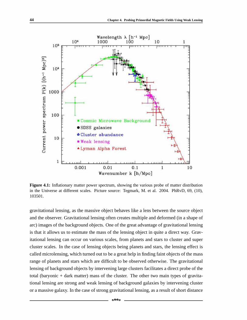
44 Chapter 4. Probing Primordial Magnetic Fields Using Weak Lensing
Figure 4.1: Inflationary matter power spectrum, showing the various probe of matter distributionin the Universe at different scales. Picture source: Tegmark, M. et al. 2004. PhRvD, 69, (10),103501.
gravitational lensing, as the massive object behaves like alens between the source object
and the observer. Gravitational lensing often creates multiple and deformed (in a shape of
arc) images of the background objects. One of the great advantage of gravitational lensing
is that it allows us to estimate the mass of the lensing objectin quite a direct way. Grav-
itational lensing can occur on various scales, from planetsand stars to cluster and super
cluster scales. In the case of lensing objects being planetsand stars, the lensing effect is
called microlensing, which turned out to be a great help in finding faint objects of the mass
range of planets and stars which are difficult to be observed otherwise. The gravitational
lensing of background objects by intervening large clusters facilitates a direct probe of the
total (baryonic + dark matter) mass of the cluster. The othertwo main types of gravita-
tional lensing are strong and weak lensing of background galaxies by intervening cluster
or a massive galaxy. In the case of strong gravitational lensing, as a result of short distance
[\
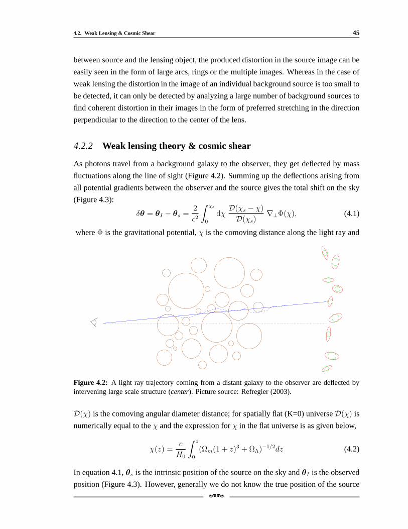
4.2. Weak Lensing & Cosmic Shear 45
between source and the lensing object, the produced distortion in the source image can be
easily seen in the form of large arcs, rings or the multiple images. Whereas in the case of
weak lensing the distortion in the image of an individual background source is too small to
be detected, it can only be detected by analyzing a large number of background sources to
find coherent distortion in their images in the form of preferred stretching in the direction
perpendicular to the direction to the center of the lens.
4.2.2 Weak lensing theory & cosmic shear
As photons travel from a background galaxy to the observer, they get deflected by mass
fluctuations along the line of sight (Figure 4.2). Summing upthe deflections arising from
all potential gradients between the observer and the sourcegives the total shift on the sky
(Figure 4.3):
δθ = θI − θs =2
c2
∫ χs
0
dχD(χs − χ)
D(χs)∇⊥Φ(χ), (4.1)
whereΦ is the gravitational potential,χ is the comoving distance along the light ray and
Figure 4.2: A light ray trajectory coming from a distant galaxy to the observer are deflected byintervening large scale structure (center). Picture source: Refregier (2003).
D(χ) is the comoving angular diameter distance; for spatially flat (K=0) universeD(χ) is
numerically equal to theχ and the expression forχ in the flat universe is as given below,
χ(z) =c
H0
∫ z
0
(Ωm(1 + z)3 + ΩΛ)−1/2dz (4.2)
In equation 4.1,θs is the intrinsic position of the source on the sky andθI is the observed
position (Figure 4.3). However, generally we do not know thetrue position of the source[\
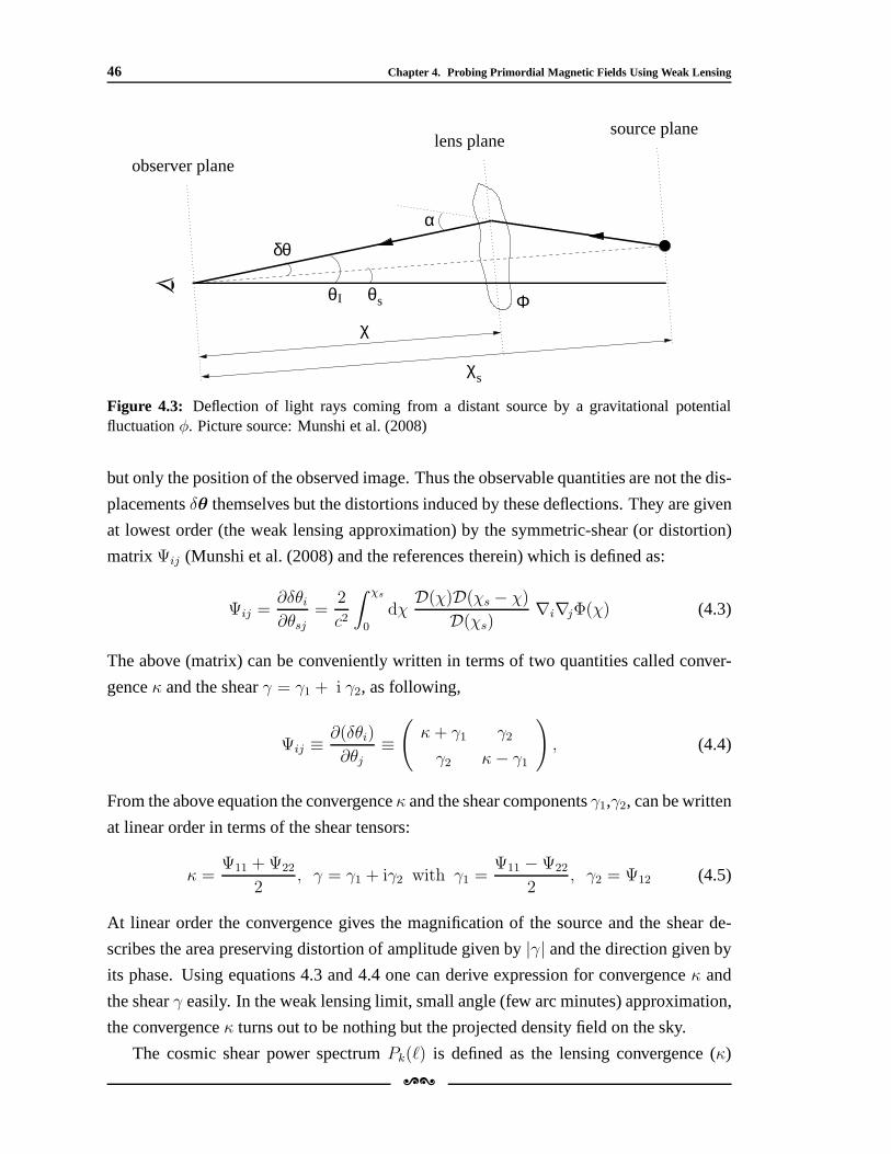
46 Chapter 4. Probing Primordial Magnetic Fields Using Weak Lensing
χ
χ
α
δθ
θ
s
observer plane
lens planesource plane
I θs Φ
Figure 4.3: Deflection of light rays coming from a distant source by a gravitational potentialfluctuationφ. Picture source: Munshi et al. (2008)
but only the position of the observed image. Thus the observable quantities are not the dis-
placementsδθ themselves but the distortions induced by these deflections. They are given
at lowest order (the weak lensing approximation) by the symmetric-shear (or distortion)
matrixΨij (Munshi et al. (2008) and the references therein) which is defined as:
Ψij =∂δθi∂θsj
=2
c2
∫ χs
0
dχD(χ)D(χs − χ)
D(χs)∇i∇jΦ(χ) (4.3)
The above (matrix) can be conveniently written in terms of two quantities called conver-
genceκ and the shearγ = γ1 + i γ2, as following,
Ψij ≡∂(δθi)
∂θj≡(
κ+ γ1 γ2
γ2 κ− γ1
)
, (4.4)
From the above equation the convergenceκ and the shear componentsγ1,γ2, can be written
at linear order in terms of the shear tensors:
κ =Ψ11 +Ψ22
2, γ = γ1 + iγ2 with γ1 =
Ψ11 −Ψ22
2, γ2 = Ψ12 (4.5)
At linear order the convergence gives the magnification of the source and the shear de-
scribes the area preserving distortion of amplitude given by |γ| and the direction given by
its phase. Using equations 4.3 and 4.4 one can derive expression for convergenceκ and
the shearγ easily. In the weak lensing limit, small angle (few arc minutes) approximation,
the convergenceκ turns out to be nothing but the projected density field on the sky.
The cosmic shear power spectrumPk(ℓ) is defined as the lensing convergence (κ)
[\
4.2. Weak Lensing & Cosmic Shear 47
power spectrum as a function of multipole momentℓ (or inverse angular scaleθ) Pκ, and
is a measure of the projection of matter power spectrumPδ on the sky plane,
〈κ(ℓ)κ∗(ℓ)〉 = (2π)2δD(ℓ− ℓ′)Pκ(ℓ) (4.6)
From equation 4.5,κ(ℓ) andγ(ℓ) can be written as (Munshi et al., 2008),
κ(ℓ) = −1
2(ℓ2x + ℓ2y)φ(ℓ) (4.7)
γ(ℓ) = −1
2(ℓx + iℓy)
2φ(ℓ) =ℓ2x − ℓ2y + 2iℓxℓy
ℓ2x + ℓ2yκ(ℓ) = ei2βκ(ℓ) (4.8)
whereφ is called lensing potential defined asΨij = φ,ij, β is the polar angle ofℓ;
tanβ = ℓy/ℓx, andℓ = (ℓx, ℓy). From the above it is obvious thatPκ(ℓ) = Pγ(ℓ).
Putting the value ofφ(ℓ) in terms of density contrastδ(k, z) (using Poission’s equation
∇2Φ = (3/2)ΩmH20 (1 + z)δ, Ψij = φ,ij and Eq. 4.3) in the above equation and using
Limber’s approximationk2 ≃ k2⊥ (herek = (k‖,k
x,y⊥ ) with kx,y
⊥ = ℓ/D) one can get the
expression forκ andγ in terms ofδ, further using the obtained expression for the conver-
genceκ(ℓ) in equation 4.6 one can easily get the following relation forthe cosmic shear
power spectrum, which essentially relates the 3d matter power spectrumPδ(k, z) to the
shear power spectrumPγ(ℓ) (= Pκ(ℓ)) and commonly known as Limber’s equation,
Pγ(ℓ) =9
4Ω2
m
(
H0
c
)4 ∫ χlim
0
dχ
a2(χ)Pδ
(
ℓ
D(χ);χ
)
×[∫ χlim
χ
dχ′n(χ′)D(χ′ − χ)
D(χ′)
]2
(4.9)
whereχlim is the limiting comoving distance of the survey; n(z) is the redshift distribution
of the sources andℓ is the modulus of a two dimensional wave vector perpendicular to the
line of sight.Pδ is the matter power spectrum.
The correlation functionξ(θ) of the complex shearγ can be computed as,
〈γγ∗〉θ =∫
d2ℓ
(2π)2Pγ(ℓ) e
iℓ.θ =
∫
ℓdℓ
(2π)2Pγ(ℓ)e
iℓθ cosϕdϕ (4.10)
=
∫
dℓ
2πℓPγ(ℓ)J0(ℓθ).
The cosmological shear field induced by density perturbations is a curl-free quantity
and is donated as an E-type field. One can decompose the observed shear signal into E
[\
48 Chapter 4. Probing Primordial Magnetic Fields Using Weak Lensing
(non-rotational) and B (rotational) components. Detection of non-zero B-modes indicates
a non-gravitational contribution to the shear field, which might be caused by systematic
contamination to the lensing signal.1
These decomposed shear correlation functions can be expressed as:
ξE,B(θ) =ξ+(θ)± ξ′(θ)
2(4.11)
whereξ′ is given by
ξ′(θ) = ξ−(θ) +
∫ ∞
θ
dϑ
ϑξ−(ϑ)
(
4− 12
(
θ
ϑ
)2)
(4.12)
ξ+ andξ− are two-point shear correlation functions which are related to the matter power
spectrum according to the following relation,
ξ±(θ) =1
2π
∫ ∞
0
dℓ ℓPγ(ℓ)J0,4(ℓθ) (4.13)
θ is the angular separation between the galaxy pairs, andJ0,4 are Bessel functions of the
first kind.
4.3 Shear Power Spectrum From Tangled Magnetic Field
Power Spectrum
We have used the magnetic field induced matter power spectrumPδ (equation 1.19) to
compute the shear power spectrumPγ(ℓ) which in turn is used to calculateξ+, ξ−, ξE and
ξB using Eqs (4.11), (4.12) & (4.13). We have used the same source redshift distribution
as in Fu et al. (2008):
n(z) = Aza + zab
zb + c; A =
(∫ zmax
0
za + zab
zb + cdz
)−1
(4.14)
wherezmax = 6. Values of the parameters a, b, c & A we have taken from the same paper
Fu et al. (2008). Values of these parameters as quoted in the paper are as, a = 0.612±0.043 ; b = 8.125± 0.871 ; c = 0.620± 0.065 & A = 1.555. To evaluate the integral (4.9)
1The presence of primordial magnetic fields will also generate the B-modes of the shear power spectrum.Both the vector and tensor modes generated by magnetic fieldscould sources these modes. Vector modesare likely to play a more dominant role at angular scales of interest in this work.
[\
4.4. Results 49
we changed the variable fromχ to z using (4.2).
Pγ(ℓ) =9
4Ω2
m
(
H0
c
)4 ∫ zlim
0
dz
a2(z)Pδ (k, z)
×[∫ zlim
z
dz′ n(z′)χ(z′ − z)
χ(z′)
]2
(4.15)
wherek = ℓ/χ(z). AgainPδ (k,z) can be written as,
Pδ(k, z) = Pδ(k)×D2(z) (4.16)
where D(z) is growth factor, which as noted above is the same as for the flatΛCDM mode
and is given by Peebles (1993):
D(z) =5Ωm
2[Ωm(1 + z)3 + ΩΛ]
1/2
∫ ∞
z
1 + z
(Ωm(1 + z)3 + ΩΛ)3/2dz (4.17)
We tookzlim = 2.5 for our calculations as in Fu et al. (2008).
For comparison, we also compute all the relevant quantitiesfor the linear and non-
linearΛCDM models. ForΛCDM linear power spectrum we usedP (k, z) = AkT 2(k)D2(z),
where the transfer functionT (k) is given by Bond & Efstathiou (1984). For nonlinear
ΛCDM we followed prescription given in Peacock & Dodds (1996). For all the calcula-
tions we have used flat (k=0)ΛCDM universe withΩm = 0.24,Ωb = 0.044,h = 0.73 and
σ8 = 0.77.
4.4 Results
In Figure 4.4 we show the tangled magnetic field induced matter power spectra for a range
of spectral indexn and magnetic field strengths,B0 atz = 0. The matter power spectra are
plotted fork < kJ ; a sharp cut-off below this scale is assumed for our computation. For
comparison, we have also displayed the linear and non-linear ΛCDM matter power spectra
(the non-linear power spectrum is obtained following the method introduced by Peacock
& Dodds (1996)). The figure shows that the magnetic field induced matter power spectra
can dominate over theΛCDM case at small scales. Possible implications of this excess
have already been studied for early formation of structures, reionization, and the HI signal
from the epoch of reionization (Sethi & Subramanian, 2005; Tashiro & Sugiyama, 2006;
Schliecher, Banerjee, Klessen , 2009; Sethi & Subramanian,2009; Sethi, Haiman, Pandey
[\
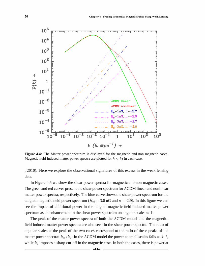
50 Chapter 4. Probing Primordial Magnetic Fields Using Weak Lensing
Figure 4.4: The Matter power spectrum is displayed for the magnetic and non magnetic cases.Magnetic field-induced matter power spectra are plotted fork < kJ in each case.
, 2010). Here we explore the observational signatures of this excess in the weak lensing
data.
In Figure 4.5 we show the shear power spectra for magnetic andnon-magnetic cases.
The green and red curves present the shear power spectrum forΛCDM linear and nonlinear
matter power spectra, respectively. The blue curve shows the shear power spectrum for the
tangled magnetic field power spectrum (Beff = 3.0 nG andn = -2.9). In this figure we can
see the impact of additional power in the tangled magnetic field-induced matter power
spectrum as an enhancement in the shear power spectrum on angular scales≃ 1′.
The peak of the matter power spectra of both theΛCDM model and the magnetic-
field induced matter power spectra are also seen in the shear power spectra. The ratio of
angular scales at the peak of the two cases correspond to the ratio of these peaks of the
matter power spectra:keq/kJ . In theΛCDM model the power at small scales falls ask−3,
while kJ imposes a sharp cut-off in the magnetic case. In both the cases, there is power at
[\
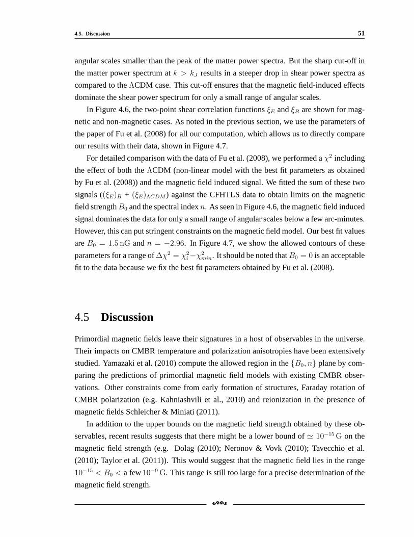
4.5. Discussion 51
angular scales smaller than the peak of the matter power spectra. But the sharp cut-off in
the matter power spectrum atk > kJ results in a steeper drop in shear power spectra as
compared to theΛCDM case. This cut-off ensures that the magnetic field-induced effects
dominate the shear power spectrum for only a small range of angular scales.
In Figure 4.6, the two-point shear correlation functionsξE andξB are shown for mag-
netic and non-magnetic cases. As noted in the previous section, we use the parameters of
the paper of Fu et al. (2008) for all our computation, which allows us to directly compare
our results with their data, shown in Figure 4.7.
For detailed comparison with the data of Fu et al. (2008), we performed aχ2 including
the effect of both theΛCDM (non-linear model with the best fit parameters as obtained
by Fu et al. (2008)) and the magnetic field induced signal. We fitted the sum of these two
signals ((ξE)B + (ξE)ΛCDM ) against the CFHTLS data to obtain limits on the magnetic
field strengthB0 and the spectral indexn. As seen in Figure 4.6, the magnetic field induced
signal dominates the data for only a small range of angular scales below a few arc-minutes.
However, this can put stringent constraints on the magneticfield model. Our best fit values
areB0 = 1.5 nG andn = −2.96. In Figure 4.7, we show the allowed contours of these
parameters for a range of∆χ2 = χ2i−χ2
min. It should be noted thatB0 = 0 is an acceptable
fit to the data because we fix the best fit parameters obtained byFu et al. (2008).
4.5 Discussion
Primordial magnetic fields leave their signatures in a host of observables in the universe.
Their impacts on CMBR temperature and polarization anisotropies have been extensively
studied. Yamazaki et al. (2010) compute the allowed region in theB0, n plane by com-
paring the predictions of primordial magnetic field models with existing CMBR obser-
vations. Other constraints come from early formation of structures, Faraday rotation of
CMBR polarization (e.g. Kahniashvili et al., 2010) and reionization in the presence of
magnetic fields Schleicher & Miniati (2011).
In addition to the upper bounds on the magnetic field strengthobtained by these ob-
servables, recent results suggests that there might be a lower bound of≃ 10−15G on the
magnetic field strength (e.g. Dolag (2010); Neronov & Vovk (2010); Tavecchio et al.
(2010); Taylor et al. (2011)). This would suggest that the magnetic field lies in the range
10−15 < B0 < a few10−9G. This range is still too large for a precise determination ofthe
magnetic field strength.
[\
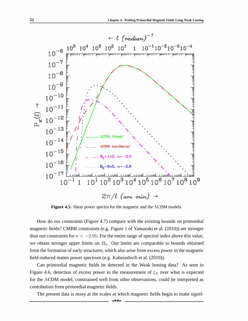
52 Chapter 4. Probing Primordial Magnetic Fields Using Weak Lensing
Figure 4.5: Shear power spectra for the magnetic and theΛCDM models.
How do our constraints (Figure 4.7) compare with the existing bounds on primordial
magnetic fields? CMBR constraints (e.g. Figure 1 of Yamazakiet al. (2010)) are stronger
than our constraints forn < −2.95. For the entire range of spectral index above this value,
we obtain stronger upper limits onB0. Our limits are comparable to bounds obtained
from the formation of early structures, which also arise from excess power in the magnetic
field-induced matter power spectrum (e.g. Kahniashvili et al. (2010)).
Can primordial magnetic fields be detected in the Weak lensing data? As seen in
Figure 4.6, detection of excess power in the measurement ofξE over what is expected
for theΛCDM model, constrained well from other observations, couldbe interpreted as
contribution from primordial magnetic fields.
The present data is noisy at the scales at which magnetic fields begin to make signif-[\
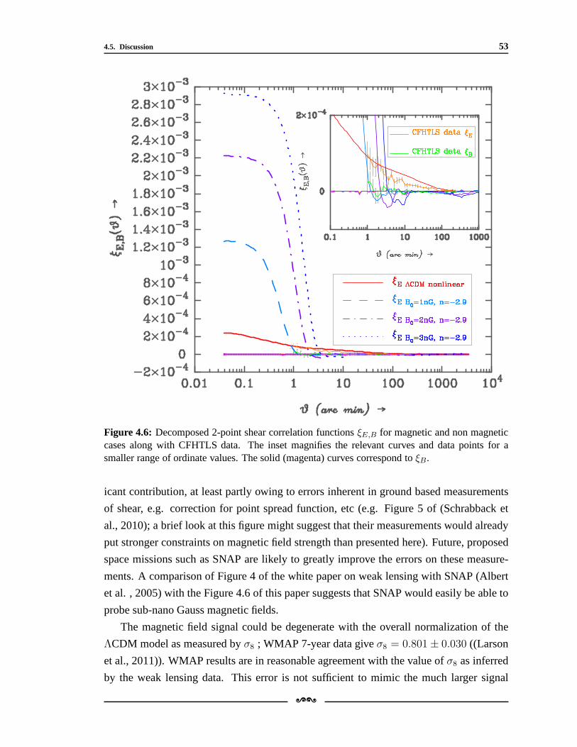
4.5. Discussion 53
Figure 4.6: Decomposed 2-point shear correlation functionsξE,B for magnetic and non magneticcases along with CFHTLS data. The inset magnifies the relevant curves and data points for asmaller range of ordinate values. The solid (magenta) curves correspond toξB.
icant contribution, at least partly owing to errors inherent in ground based measurements
of shear, e.g. correction for point spread function, etc (e.g. Figure 5 of (Schrabback et
al., 2010); a brief look at this figure might suggest that their measurements would already
put stronger constraints on magnetic field strength than presented here). Future, proposed
space missions such as SNAP are likely to greatly improve theerrors on these measure-
ments. A comparison of Figure 4 of the white paper on weak lensing with SNAP (Albert
et al. , 2005) with the Figure 4.6 of this paper suggests that SNAP would easily be able to
probe sub-nano Gauss magnetic fields.
The magnetic field signal could be degenerate with the overall normalization of the
ΛCDM model as measured byσ8 ; WMAP 7-year data giveσ8 = 0.801± 0.030 ((Larson
et al., 2011)). WMAP results are in reasonable agreement with the value ofσ8 as inferred
by the weak lensing data. This error is not sufficient to mimicthe much larger signal
[\
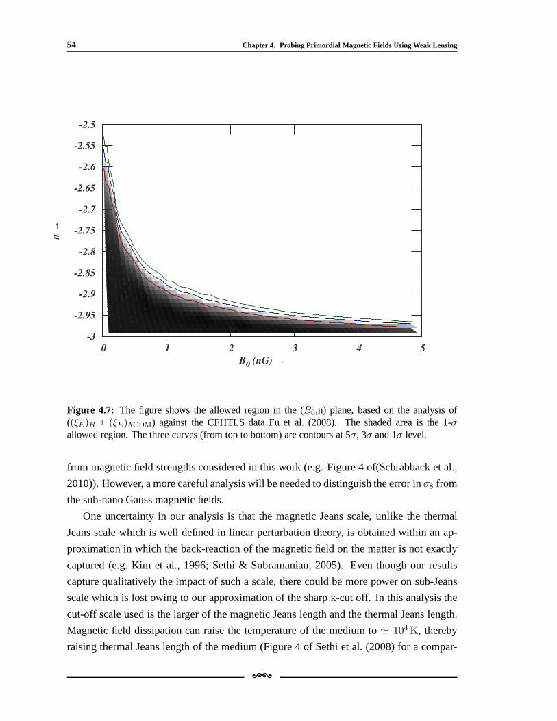
54 Chapter 4. Probing Primordial Magnetic Fields Using Weak Lensing
0 1 2 3 4 5
B0 (nG) →
-3
-2.95
-2.9
-2.85
-2.8
-2.75
-2.7
-2.65
-2.6
-2.55
-2.5
n →
Figure 4.7: The figure shows the allowed region in the (B0,n) plane, based on the analysis of((ξE)B + (ξE)ΛCDM) against the CFHTLS data Fu et al. (2008). The shaded area is the 1-σallowed region. The three curves (from top to bottom) are contours at 5σ, 3σ and 1σ level.
from magnetic field strengths considered in this work (e.g. Figure 4 of(Schrabback et al.,
2010)). However, a more careful analysis will be needed to distinguish the error inσ8 from
the sub-nano Gauss magnetic fields.
One uncertainty in our analysis is that the magnetic Jeans scale, unlike the thermal
Jeans scale which is well defined in linear perturbation theory, is obtained within an ap-
proximation in which the back-reaction of the magnetic fieldon the matter is not exactly
captured (e.g. Kim et al., 1996; Sethi & Subramanian, 2005).Even though our results
capture qualitatively the impact of such a scale, there could be more power on sub-Jeans
scale which is lost owing to our approximation of the sharp k-cut off. In this analysis the
cut-off scale used is the larger of the magnetic Jeans lengthand the thermal Jeans length.
Magnetic field dissipation can raise the temperature of the medium to≃ 104K, thereby
raising thermal Jeans length of the medium (Figure 4 of Sethiet al. (2008) for a compar-
[\
4.5. Discussion 55
ison between the two scales for different magnetic field strengths). ForB0 & 10−9G,
the magnetic Jeans scale is the larger of the two scales, as the maximum temperature of
the medium reached owing to this process doesn’t exceed104K. In the more general case
also this would be true as photoionization of the medium by other sources, e.g. the sources
which could have cause reionization of the universe atz ≃ 10, also results in comparable
temperatures. For magnetic field strengths smaller than considered in the work, the cut-off
scale is likely to be determined by thermal Jeans scale, caused by the photoionization of
the medium by sources other than the magnetic field dissipation. Our approximation al-
lows us to identify important length and angular scales for our study (Figure 4.5 and 4.6).
However, further work along these lines could extend our analysis by taking into account
the physical effects of sub-magnetic Jeans scales.
The analysis of Lyman-α forest in the redshift range2 . z . 4 is another powerful
probe of the matter power spectrum of at small scales (e.g. Croft et al., 2002). Primordial
magnetic field can alter this interpretation in many ways: (a) more small scale power
owing to magnetic field induced matter power spectrum (Figure 4.4), (b) dissipation of
magnetic field can change the thermal state of Lyman-α clouds (Sethi, Haiman, Pandey ,
2010; Sethi & Subramanian, 2005, e.g.), (c) magnetic Jeans length can reduce the power
at the smallest probable scale. In the next chapter we will look into and discuss some of
these effects in detail.
[\

5Probing Primordial Magnetic Fields
Using Lyα Clouds
5.1 Introduction
In the past 10 years, cosmological weak lensing and the studyof Lyα clouds in the redshift
range2 . z . 5 have emerged as reliable methods to precisely determine thematter
power spectrum on scales below10 h−1Mpc (Figure 4.1). In particular, these methods can
estimate the matter power spectrum at small scales which arenot directly accessible to
other methods e.g. galaxy surveys (for details and further references see e.g. Munshi et al.
(2008); Hoekstra & Jain (2008); Croft et al. (1998, 1999, 2002)). Since these are the scales
which are highly affected by the existence of primordial magnetic fields (see Figures 1.4
or 5.3), a careful analysis of these cosmological variablescan actually probe the existence
of these magnetic fields.
In this work we attempt to constrain primordial magnetic fields within the framework
of the distribution of Lyα clouds in the intergalactic medium (IGM) in the redshift range
2 . z . 5. These clouds have been shown to originate in the mildly non-linear density
regions of the IGM (Cen & Ostriker (1994)). This has allowed development of detailed
semi-analytic methods to understand the observed properties of these clouds (e.g. Bi et al.,
1995; Hui et al., 1997; Choudhury et al., 2001a,b). Adoptinga semi-analytic approach,
we simulate density fluctuation along the line-of-sight, including the contribution of matter
perturbations induced by these magnetic fields. We compute effective Lyα opacity of the
IGM for this computed Lyα cloud distribution and compare our results with the existing
data (e.g. Faucher-Giguere et al., 2008).
In the previous analysis, the density perturbations induced by magnetic fields are as-
sumed to be uncorrelated to the density field generated by theusualΛCDM model. Re-
[\
57
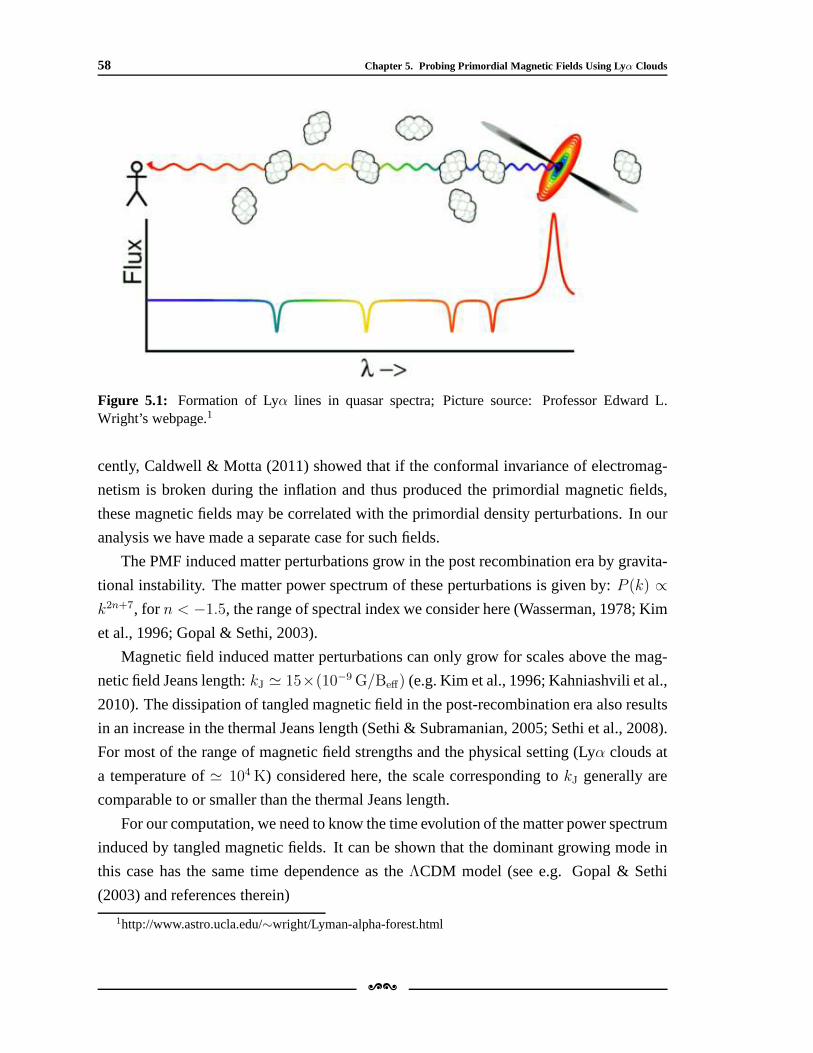
58 Chapter 5. Probing Primordial Magnetic Fields Using Lyα Clouds
Figure 5.1: Formation of Lyα lines in quasar spectra; Picture source: Professor Edward L.Wright’s webpage.1
cently, Caldwell & Motta (2011) showed that if the conformalinvariance of electromag-
netism is broken during the inflation and thus produced the primordial magnetic fields,
these magnetic fields may be correlated with the primordial density perturbations. In our
analysis we have made a separate case for such fields.
The PMF induced matter perturbations grow in the post recombination era by gravita-
tional instability. The matter power spectrum of these perturbations is given by:P (k) ∝k2n+7, for n < −1.5, the range of spectral index we consider here (Wasserman, 1978; Kim
et al., 1996; Gopal & Sethi, 2003).
Magnetic field induced matter perturbations can only grow for scales above the mag-
netic field Jeans length:kJ ≃ 15×(10−9G/Beff) (e.g. Kim et al., 1996; Kahniashvili et al.,
2010). The dissipation of tangled magnetic field in the post-recombination era also results
in an increase in the thermal Jeans length (Sethi & Subramanian, 2005; Sethi et al., 2008).
For most of the range of magnetic field strengths and the physical setting (Lyα clouds at
a temperature of≃ 104K) considered here, the scale corresponding tokJ generally are
comparable to or smaller than the thermal Jeans length.
For our computation, we need to know the time evolution of thematter power spectrum
induced by tangled magnetic fields. It can be shown that the dominant growing mode in
this case has the same time dependence as theΛCDM model (see e.g. Gopal & Sethi
(2003) and references therein)
1http://www.astro.ucla.edu/∼wright/Lyman-alpha-forest.html
[\
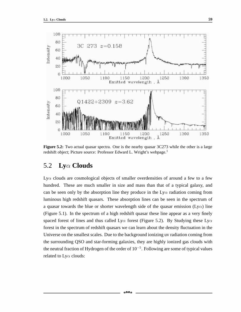
5.2. Lyα Clouds 59
Figure 5.2: Two actual quasar spectra. One is the nearby quasar 3C273 while the other is a largeredshift object; Picture source: Professor Edward L. Wright’s webpage.1
5.2 Lyα Clouds
Lyα clouds are cosmological objects of smaller overdensities of around a few to a few
hundred. These are much smaller in size and mass than that of atypical galaxy, and
can be seen only by the absorption line they produce in the Lyα radiation coming from
luminous high redshift quasars. These absorption lines canbe seen in the spectrum of
a quasar towards the blue or shorter wavelength side of the quasar emission (Lyα) line
(Figure 5.1). In the spectrum of a high redshift quasar theseline appear as a very finely
spaced forest of lines and thus called Lyα forest (Figure 5.2). By Studying these Lyα
forest in the spectrum of redshift quasars we can learn aboutthe density fluctuation in the
Universe on the smallest scales. Due to the background ionizing uv radiation coming from
the surrounding QSO and star-forming galaxies, they are highly ionized gas clouds with
the neutral fraction of Hydrogen of the order of 10−5. Following are some of typical values
related to Lyα clouds:
[\
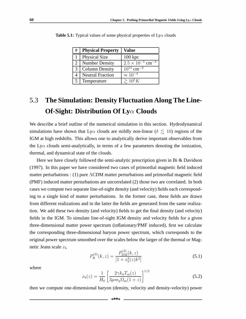
60 Chapter 5. Probing Primordial Magnetic Fields Using Lyα Clouds
Table 5.1: Typical values of some physical properties of Lyα clouds
# Physical Property Value1 Physical Size 100 kpc2 Number Density 2.5× 10⁻⁵ cm−3
3 Column Density 1014 cm−2
4 Neutral Fraction ≈ 10−4
5 Temperature & 105K
5.3 The Simulation: Density Fluctuation Along The Line-
Of-Sight: Distribution Of Ly α Clouds
We describe a brief outline of the numerical simulation in this section. Hydrodynamical
simulations have shown that Lyα clouds are mildly non-linear (δ . 10) regions of the
IGM at high redshifts. This allows one to analytically derive important observables from
the Lyα clouds semi-analytically, in terms of a few parameters denoting the ionization,
thermal, and dynamical state of the clouds.
Here we have closely followed the semi-analytic prescription given in Bi & Davidson
(1997). In this paper we have considered two cases of primordial magnetic field induced
matter perturbations : (1) pureΛCDM matter perturbations and primordial magnetic field
(PMF) induced matter perturbations are uncorrelated (2) those two are correlated. In both
cases we compute two separate line-of-sight density (and velocity) fields each correspond-
ing to a single kind of matter perturbations. In the former case, these fields are drawn
from different realizations and in the latter the fields are generated from the same realiza-
tion. We add these two density (and velocity) fields to get thefinal density (and velocity)
fields in the IGM. To simulate line-of-sight IGM density and velocity fields for a given
three-dimensional matter power spectrum (inflationary/PMF induced), first we calculate
the corresponding three-dimensional baryon power spectrum, which corresponds to the
original power spectrum smoothed over the scales below the larger of the thermal or Mag-
netic Jeans scalexb
P(3)B (k, z) =
P(3)DM(k, z)
[1 + x2b(z)k
2](5.1)
where
xb(z) =1
H0
[
2γkBTm(z)
3µmpΩm(1 + z)
]1/2
(5.2)
then we compute one-dimensional baryon (density, velocityand density-velocity) power
[\
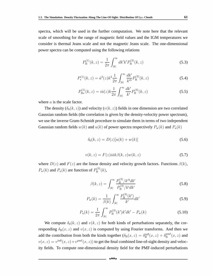
5.3. The Simulation: Density Fluctuation Along The Line-Of-Sight: Distribution Of Ly α Clouds 61
spectra, which will be used in the further computation. We note here that the relevant
scale of smoothing for the range of magnetic field values and the IGM temperatures we
consider is thermal Jeans scale and not the magnetic Jeans scale. The one-dimensional
power spectra can be computed using the following relations
P(1)B (k, z) =
1
2π
∫ ∞
|k|
dk′k′P(3)B (k, z) (5.3)
P (1)v (k, z) = a2(z)k2 1
2π
∫ ∞
|k|
dk′
k′3P
(3)B (k, z) (5.4)
P(1)Bv (k, z) = ia(z)k
1
2π
∫ ∞
|k|
dk′
k′P
(3)B (k, z) (5.5)
wherea is the scale factor.
The density (δ0(k, z)) and velocity (v(k, z)) fields in one dimension are two correlated
Gaussian random fields (the correlation is given by the density-velocity power spectrum),
we use the inverse Gram-Schmidt procedure to simulate them in terms of two independent
Gaussian random fieldsw(k) andu(k) of power spectra respectivelyPw(k) andPu(k)
δ0(k, z) = D(z)[u(k) + w(k)] (5.6)
v(k, z) = F (z)iakβ(k, z)w(k, z) (5.7)
whereD(z) andF (z) are the linear density and velocity growth factors. Functionsβ(k),
Pw(k) andPu(k) are function ofP (3)B (k),
β(k, z) =
∫ ∞
|k|
P(3)B /k′3dk′
P(3)B /k′dk′
(5.8)
Pw(k) =1
β(k)
∫ ∞
|k|
P(3)B (k′)
k′dk′ (5.9)
Pu(k) =1
2π
∫ ∞
|k|
P(3)B (k′)k′dk′ − Pw(k) (5.10)
We computeδ0(k, z) andv(k, z) for both kinds of perturbations separately, the cor-
respondingδB(x, z) andv(x, z) is computed by using Fourier transforms. And then we
add the contribution from both the kinds together (δB(x, z) = δinflB (x, z) + δpmfB (x, z) and
v(x, z) = vinfl(x, z)+vpmf(x, z)) to get the final combined line-of-sight density and veloc-
ity fields. To compute one-dimensional density field for the PMF-induced perturbations
[\
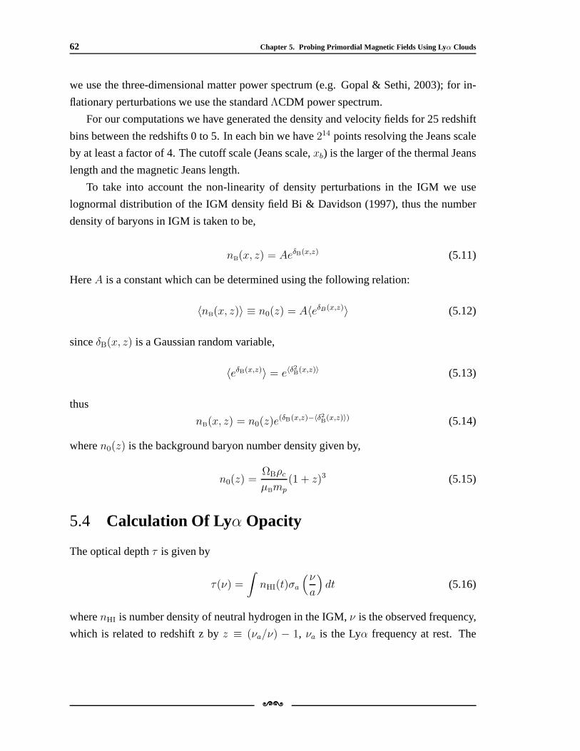
62 Chapter 5. Probing Primordial Magnetic Fields Using Lyα Clouds
we use the three-dimensional matter power spectrum (e.g. Gopal & Sethi, 2003); for in-
flationary perturbations we use the standardΛCDM power spectrum.
For our computations we have generated the density and velocity fields for 25 redshift
bins between the redshifts 0 to 5. In each bin we have214 points resolving the Jeans scale
by at least a factor of 4. The cutoff scale (Jeans scale,xb) is the larger of the thermal Jeans
length and the magnetic Jeans length.
To take into account the non-linearity of density perturbations in the IGM we use
lognormal distribution of the IGM density field Bi & Davidson(1997), thus the number
density of baryons in IGM is taken to be,
nB(x, z) = AeδB(x,z) (5.11)
HereA is a constant which can be determined using the following relation:
〈nB(x, z)〉 ≡ n0(z) = A〈eδB(x,z)〉 (5.12)
sinceδB(x, z) is a Gaussian random variable,
〈eδB(x,z)〉 = e〈δ2B(x,z)〉 (5.13)
thus
nB(x, z) = n0(z)e(δB(x,z)−〈δ2
B(x,z)〉) (5.14)
wheren0(z) is the background baryon number density given by,
n0(z) =ΩBρcµBmp
(1 + z)3 (5.15)
5.4 Calculation Of Lyα Opacity
The optical depthτ is given by
τ(ν) =
∫
nHI(t)σa
(ν
a
)
dt (5.16)
wherenHI is number density of neutral hydrogen in the IGM,ν is the observed frequency,
which is related to redshift z byz ≡ (νa/ν) − 1, νa is the Lyα frequency at rest. The
[\
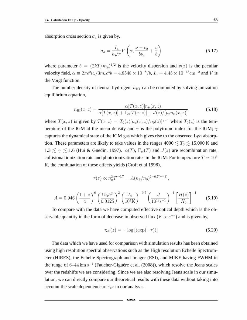
5.4. Calculation Of Lyα Opacity 63
absorption cross sectionσa is given by,
σa =Iab√πV
(
α,ν − νabνa
+v
b
)
(5.17)
where parameterb = (2kT/mp)1/2 is the velocity dispersion andv(x) is the peculiar
velocity field,α ≡ 2πe2νa/3mec3b = 4.8548× 10⁻⁸/b, Iα = 4.45× 10⁻¹⁸cm−2 andV is
the Voigt function.
The number density of neutral hydrogen,nHI can be computed by solving ionization
equilibrium equation,
nHI(x, z) =α[T (x, z)]nB(x, z)
α[T (x, z)] + Γci[T (x, z)] + J(z)/[µenB(x, z)](5.18)
whereT (x, z) is given byT (x, z) = T0(z)[nB(x, z)/n0(z)]γ−1 whereT0(z) is the tem-
perature of the IGM at the mean density andγ is the polytropic index for the IGM;γ
captures the dynamical state of the IGM gas which gives rise to the observed Lyα absorp-
tion. These parameters are likely to take values in the ranges 4000. T0 . 15,000 K and
1.3 . γ . 1.6 (Hui & Gnedin, 1997).α(T ), Γci(T ) andJ(z) are recombination rate,
collisional ionization rate and photo ionization rates in the IGM. For temperatureT ≃ 104
K, the combination of these effects yields (Croft et al.1998),
τ(z) ∝ n2BT−0.7 = A(nB/n0)
2−0.7(γ−1),
A = 0.946
(
1 + z
4
)6(ΩBh
2
0.0125
)2(T0
104K
)−0.7(J
1012s−1
)−1 [H(z)
H0
]−1
(5.19)
To compare with the data we have computed effective optical depth which is the ob-
servable quantity in the form of decrease in observed flux (F ∝ e−τ ) and is given by,
τeff(z) = − log [〈exp(−τ )〉] (5.20)
The data which we have used for comparison with simulation results has been obtained
using high resolution spectral observations such as the High resolution Echelle Spectrom-
eter (HIRES), the Echelle Spectrograph and Imager (ESI), and MIKE having FWHM in
the range of6–44 km s−1 (Faucher-Giguere et al. (2008)), which resolve the Jeans scales
over the redshifts we are considering. Since we are also resolving Jeans scale in our simu-
lation, we can directly compare our theoretical results with these data without taking into
account the scale dependence ofτeff in our analysis.
[\
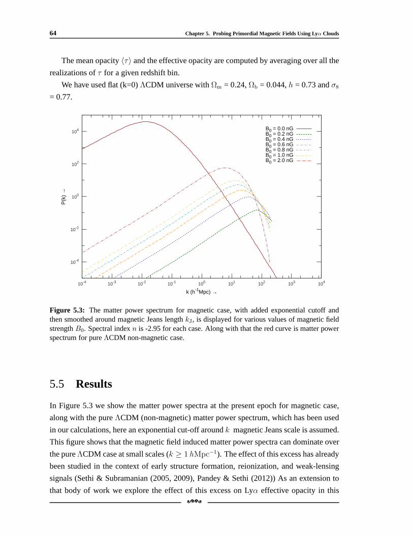
64 Chapter 5. Probing Primordial Magnetic Fields Using Lyα Clouds
The mean opacity〈τ〉 and the effective opacity are computed by averaging over allthe
realizations ofτ for a given redshift bin.
We have used flat (k=0)ΛCDM universe withΩm = 0.24,Ωb = 0.044,h = 0.73 andσ8
= 0.77.
10-4
10-2
100
102
104
10-4 10-3 10-2 10-1 100 101 102 103 104
P(k
) →
k (h-1Mpc) →
B0 = 0.0 nGB0 = 0.2 nGB0 = 0.4 nGB0 = 0.6 nGB0 = 0.8 nGB0 = 1.0 nGB0 = 2.0 nG
Figure 5.3: The matter power spectrum for magnetic case, with added exponential cutoff andthen smoothed around magnetic Jeans lengthkJ, is displayed for various values of magnetic fieldstrengthB0. Spectral indexn is -2.95 for each case. Along with that the red curve is matterpowerspectrum for pureΛCDM non-magnetic case.
5.5 Results
In Figure 5.3 we show the matter power spectra at the present epoch for magnetic case,
along with the pureΛCDM (non-magnetic) matter power spectrum, which has been used
in our calculations, here an exponential cut-off aroundk magnetic Jeans scale is assumed.
This figure shows that the magnetic field induced matter powerspectra can dominate over
the pureΛCDM case at small scales (k ≥ 1 hMpc−1). The effect of this excess has already
been studied in the context of early structure formation, reionization, and weak-lensing
signals (Sethi & Subramanian (2005, 2009), Pandey & Sethi (2012)) As an extension to
that body of work we explore the effect of this excess on Lyα effective opacity in this[\
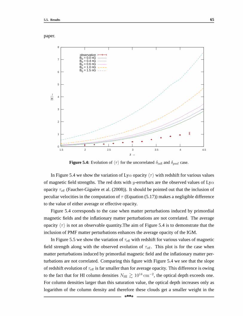
5.5. Results 65
paper.
0
1
2
3
4
5
6
7
8
1.5 2 2.5 3 3.5 4 4.5
⟨τ⟩ →
z →
observationB0 = 0.0 nGB0 = 0.4 nGB0 = 0.6 nGB0 = 1.0 nGB0 = 1.5 nG
Figure 5.4: Evolution of〈τ〉 for the uncorrelatedδinfl andδpmf case.
In Figure 5.4 we show the variation of Lyα opacity〈τ〉 with redshift for various values
of magnetic field strengths. The red dots withy-errorbars are the observed values of Lyα
opacityτeff (Faucher-Giguere et al. (2008)). It should be pointed out that the inclusion of
peculiar velocities in the computation ofτ (Equation (5.17)) makes a negligible difference
to the value of either average or effective opacity.
Figure 5.4 corresponds to the case when matter perturbations induced by primordial
magnetic fields and the inflationary matter perturbations are not correlated. The average
opacity〈τ〉 is not an observable quantity.The aim of Figure 5.4 is to demonstrate that the
inclusion of PMF matter perturbations enhances the averageopacity of the IGM.
In Figure 5.5 we show the variation ofτeff with redshift for various values of magnetic
field strength along with the observed evolution ofτeff . This plot is for the case when
matter perturbations induced by primordial magnetic field and the inflationary matter per-
turbations are not correlated. Comparing this figure with Figure 5.4 we see that the slope
of redshift evolution ofτeff is far smaller than for average opacity. This difference is owing
to the fact that for HI column densitiesNHI & 1014 cm−2, the optical depth exceeds one.
For column densities larger than this saturation value, theoptical depth increases only as
logarithm of the column density and therefore these clouds get a smaller weight in the[\
66 Chapter 5. Probing Primordial Magnetic Fields Using Lyα Clouds
0
0.2
0.4
0.6
0.8
1
1.2
1.4
1.5 2 2.5 3 3.5 4 4.5
τ eff
→
z →
observationB0 = 0.0 nGB0 = 0.4 nGB0 = 0.6 nGB0 = 1.0 nGB0 = 1.5 nG
Figure 5.5: Evolution ofτeff for the uncorrelatedδinfl andδpmf case.
computation ofτeff . As the average opacity of the IGM increases sharply with increasing
redshift (Equation (5.19)), this effect is more enhanced athigher redshifts.
A comparison between Figures 5.4 and 5.5 shows that an increase in〈τ〉 doesn’t nec-
essarily lead to an increase inτeff . In Figure 5.5 it is seen thatτeff is greater than the usual
ΛCDM case forz . 3 but falls below the predictions of this model for larger redshifts.
We can understand this behavior by the following set of arguments. The change in
the effective optical depthdτeff ∝∑
i exp(−τi)dτi, whereτi refers to optical depths of
individual clouds. On the other hand,d〈τ〉 ∝∑
i dτi. As seen in Figure 5.4, the inclusion
of PMF density perturbations increase〈τ〉 or∑
i dτi > 0, but∑
i exp(−τi)dτi could be
negative ifdτi is negative whereverτi is smallest. To elaborate this point, In Figure 5.8
we have plotted the distribution of optical depthsτis for the 1.5 nG case (z = 4), against
thedτi = τi (2 nG) − τi (0 nG); (z = 4). It is clear from this figure thatτi values are
small whendτi is more negative, or this can make∑
i exp(−τi)dτi negative, and thus it
explains the decrease ofτeff even when there is increase in〈τ〉 with increasing magnetic
field values. It should be pointed out that this behavior ofτeff cannot be mimicked by a
change inJ , γ (Equation (5.19)) or by a scaling of the power spectrum by changing the
value ofσ8.
The Figures 5.6 and 5.7 are for the same analysis as Figures 5.4 and 5.5 respectively,
[\
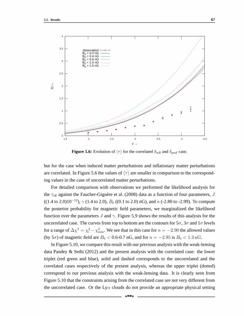
5.5. Results 67
0
0.5
1
1.5
2
2.5
3
3.5
4
1.5 2 2.5 3 3.5 4 4.5
⟨τ⟩ →
z →
observationB0 = 0.0 nGB0 = 0.4 nGB0 = 0.6 nGB0 = 1.0 nGB0 = 1.5 nG
Figure 5.6: Evolution of〈τ〉 for the correlatedδinfl andδpmf case.
but for the case when induced matter perturbations and inflationary matter perturbations
are correlated. In Figure 5.6 the values of〈τ〉 are smaller in comparison to the correspond-
ing values in the case of uncorrelated matter perturbations.
For detailed comparison with observations we performed thelikelihood analysis for
theτeff against the Faucher-Giguere et al. (2008) data as a function of four parameters,J
((1.4 to 2.0)10−12), γ (1.4 to 2.0),B0 ((0.1 to 2.0) nG), andn (-2.80 to -2.99). To compute
the posterior probability for magnetic field parameters, wemarginalized the likelihood
function over the parametersJ andγ. Figure 5.9 shows the results of this analysis for the
uncorrelated case. The curves from top to bottom are the contours for 5σ, 3σ and 1σ levels
for a range of∆χ2 = χ2i −χ2
min. We see that in this case forn = −2.90 the allowed values
(by 5σ) of magnetic field areB0 < 0.6-0.7 nG, and forn = −2.95 isB0 < 1.3 nG.
In Figure 5.10, we compare this result with our previous analysis with the weak-lensing
data Pandey & Sethi (2012) and the present analysis with the correlated case: the lower
triplet (red green and blue), solid and dashed corresponds to the uncorrelated and the
correlated cases respectively of the present analysis, whereas the upper triplet (dotted)
correspond to our previous analysis with the weak-lensing data. It is clearly seen from
Figure 5.10 that the constraints arising from the correlated case are not very different from
the uncorrelated case. Or the Lyα clouds do not provide an appropriate physical setting
[\
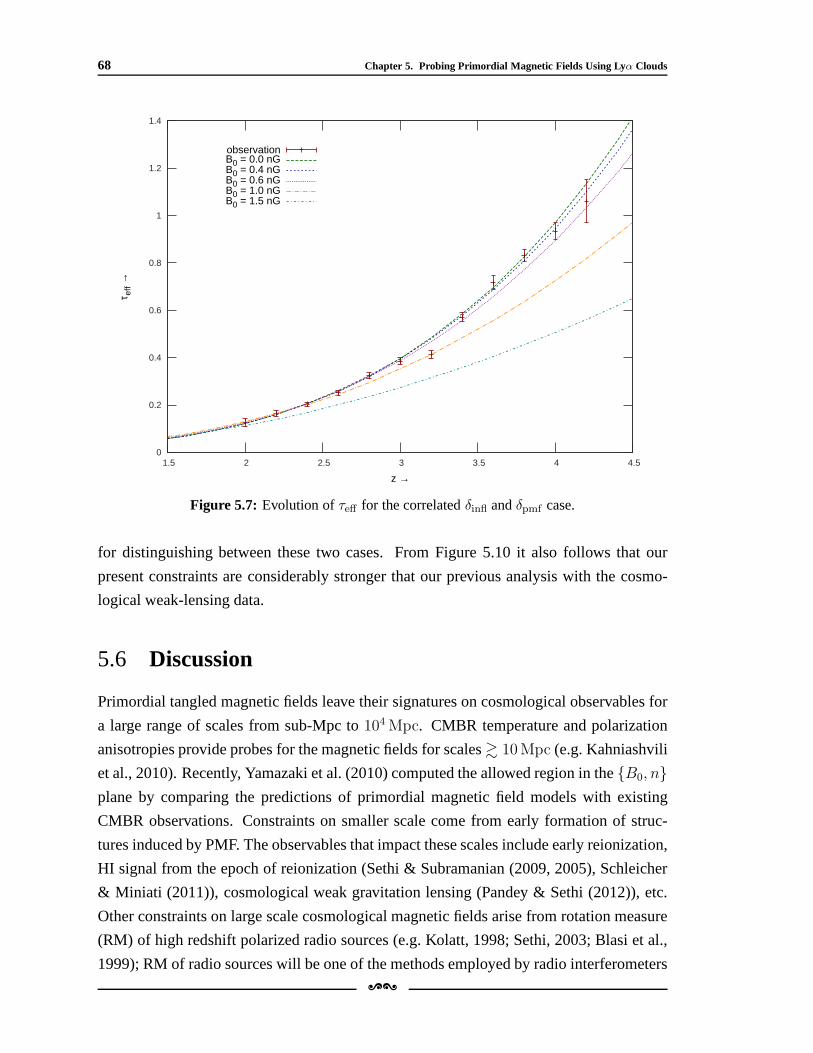
68 Chapter 5. Probing Primordial Magnetic Fields Using Lyα Clouds
0
0.2
0.4
0.6
0.8
1
1.2
1.4
1.5 2 2.5 3 3.5 4 4.5
τ eff
→
z →
observationB0 = 0.0 nGB0 = 0.4 nGB0 = 0.6 nGB0 = 1.0 nGB0 = 1.5 nG
Figure 5.7: Evolution ofτeff for the correlatedδinfl andδpmf case.
for distinguishing between these two cases. From Figure 5.10 it also follows that our
present constraints are considerably stronger that our previous analysis with the cosmo-
logical weak-lensing data.
5.6 Discussion
Primordial tangled magnetic fields leave their signatures on cosmological observables for
a large range of scales from sub-Mpc to104Mpc. CMBR temperature and polarization
anisotropies provide probes for the magnetic fields for scales& 10Mpc (e.g. Kahniashvili
et al., 2010). Recently, Yamazaki et al. (2010) computed theallowed region in theB0, nplane by comparing the predictions of primordial magnetic field models with existing
CMBR observations. Constraints on smaller scale come from early formation of struc-
tures induced by PMF. The observables that impact these scales include early reionization,
HI signal from the epoch of reionization (Sethi & Subramanian (2009, 2005), Schleicher
& Miniati (2011)), cosmological weak gravitation lensing (Pandey & Sethi (2012)), etc.
Other constraints on large scale cosmological magnetic fields arise from rotation measure
(RM) of high redshift polarized radio sources (e.g. Kolatt,1998; Sethi, 2003; Blasi et al.,
1999); RM of radio sources will be one of the methods employedby radio interferometers[\
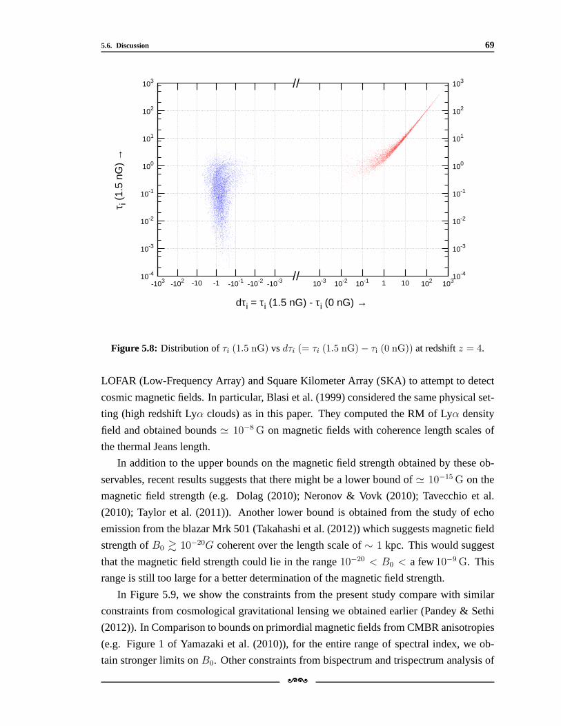
5.6. Discussion 69
10-4
10-3
10-2
10-1
100
101
102
103
-10-3-10-2-10-1-1-10-102-103
τ i (1
.5 n
G)
→
dτi = τi (1.5 nG) - τi (0 nG) →
//
//10-3 10-2 10-1 1 10 102 103
10-4
10-3
10-2
10-1
100
101
102
103
Figure 5.8: Distribution ofτi (1.5 nG) vsdτi (= τi (1.5 nG)− τi (0 nG)) at redshiftz = 4.
LOFAR (Low-Frequency Array) and Square Kilometer Array (SKA) to attempt to detect
cosmic magnetic fields. In particular, Blasi et al. (1999) considered the same physical set-
ting (high redshift Lyα clouds) as in this paper. They computed the RM of Lyα density
field and obtained bounds≃ 10−8G on magnetic fields with coherence length scales of
the thermal Jeans length.
In addition to the upper bounds on the magnetic field strengthobtained by these ob-
servables, recent results suggests that there might be a lower bound of≃ 10−15G on the
magnetic field strength (e.g. Dolag (2010); Neronov & Vovk (2010); Tavecchio et al.
(2010); Taylor et al. (2011)). Another lower bound is obtained from the study of echo
emission from the blazar Mrk 501 (Takahashi et al. (2012)) which suggests magnetic field
strength ofB0 & 10−20G coherent over the length scale of∼ 1 kpc. This would suggest
that the magnetic field strength could lie in the range10−20 < B0 < a few10−9G. This
range is still too large for a better determination of the magnetic field strength.
In Figure 5.9, we show the constraints from the present studycompare with similar
constraints from cosmological gravitational lensing we obtained earlier (Pandey & Sethi
(2012)). In Comparison to bounds on primordial magnetic fields from CMBR anisotropies
(e.g. Figure 1 of Yamazaki et al. (2010)), for the entire range of spectral index, we ob-
tain stronger limits onB0. Other constraints from bispectrum and trispectrum analysis of
[\
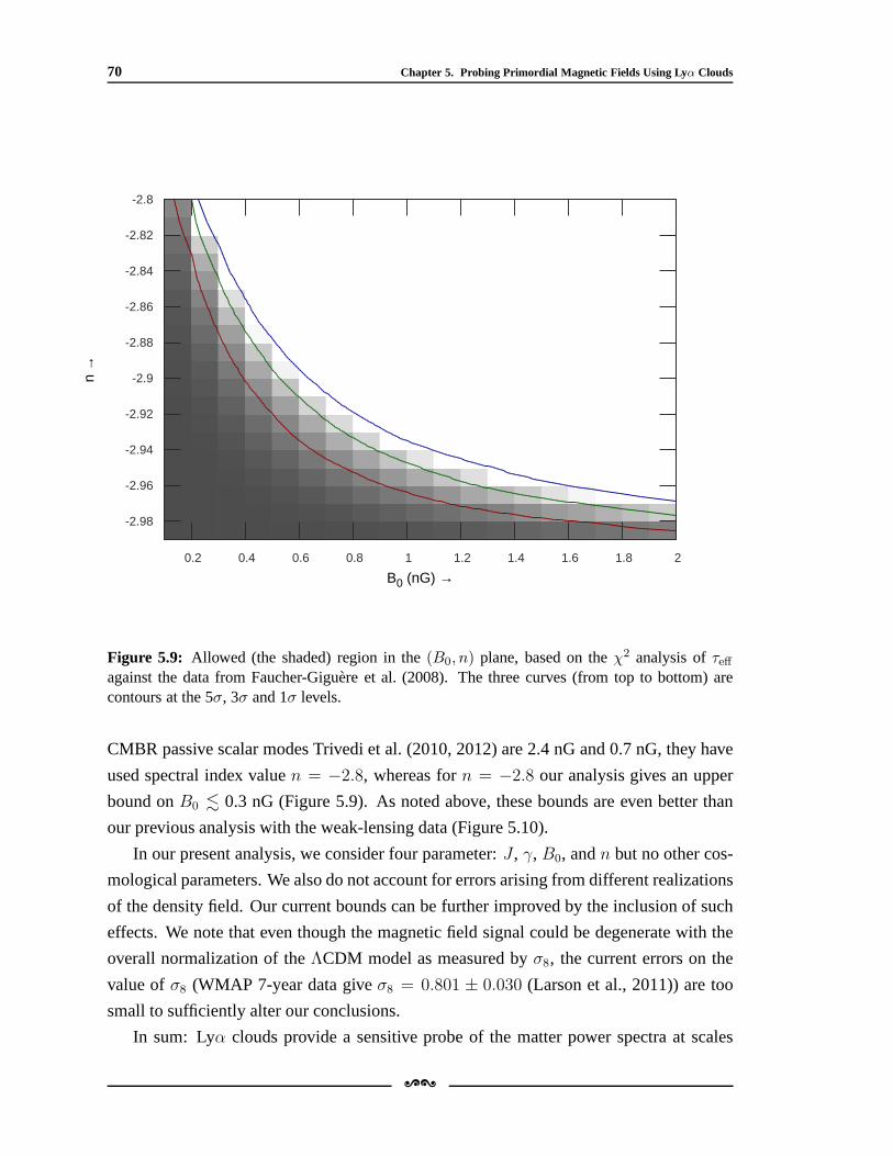
70 Chapter 5. Probing Primordial Magnetic Fields Using Lyα Clouds
0.2 0.4 0.6 0.8 1 1.2 1.4 1.6 1.8 2
B0 (nG) →
-2.98
-2.96
-2.94
-2.92
-2.9
-2.88
-2.86
-2.84
-2.82
-2.8
n →
Figure 5.9: Allowed (the shaded) region in the(B0, n) plane, based on theχ2 analysis ofτeffagainst the data from Faucher-Giguere et al. (2008). The three curves (from top to bottom) arecontours at the 5σ, 3σ and 1σ levels.
CMBR passive scalar modes Trivedi et al. (2010, 2012) are 2.4nG and 0.7 nG, they have
used spectral index valuen = −2.8, whereas forn = −2.8 our analysis gives an upper
bound onB0 . 0.3 nG (Figure 5.9). As noted above, these bounds are even better than
our previous analysis with the weak-lensing data (Figure 5.10).
In our present analysis, we consider four parameter:J , γ, B0, andn but no other cos-
mological parameters. We also do not account for errors arising from different realizations
of the density field. Our current bounds can be further improved by the inclusion of such
effects. We note that even though the magnetic field signal could be degenerate with the
overall normalization of theΛCDM model as measured byσ8, the current errors on the
value ofσ8 (WMAP 7-year data giveσ8 = 0.801 ± 0.030 (Larson et al., 2011)) are too
small to sufficiently alter our conclusions.
In sum: Lyα clouds provide a sensitive probe of the matter power spectraat scales
[\
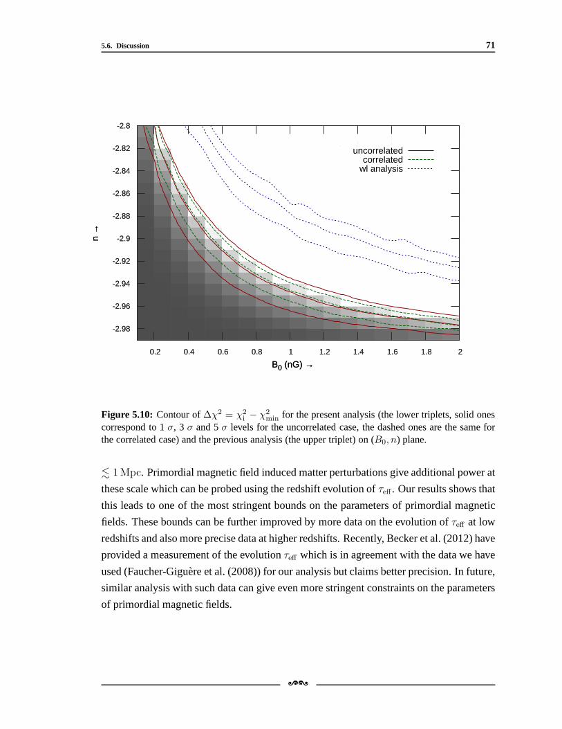
5.6. Discussion 71
"chisq_uc.dat" u 1:2:3uncorrelated
correlatedwl analysis
0.2 0.4 0.6 0.8 1 1.2 1.4 1.6 1.8 2
B0 (nG) →
-2.98
-2.96
-2.94
-2.92
-2.9
-2.88
-2.86
-2.84
-2.82
-2.8
n →
"chisq_uc.dat" u 1:2:3uncorrelated
correlatedwl analysis
0.2 0.4 0.6 0.8 1 1.2 1.4 1.6 1.8 2
B0 (nG) →
-2.98
-2.96
-2.94
-2.92
-2.9
-2.88
-2.86
-2.84
-2.82
-2.8
n →
Figure 5.10: Contour of∆χ2 = χ2i − χ2
min for the present analysis (the lower triplets, solid onescorrespond to 1σ, 3 σ and 5σ levels for the uncorrelated case, the dashed ones are the same forthe correlated case) and the previous analysis (the upper triplet) on (B0, n) plane.
. 1Mpc. Primordial magnetic field induced matter perturbations give additional power at
these scale which can be probed using the redshift evolutionof τeff . Our results shows that
this leads to one of the most stringent bounds on the parameters of primordial magnetic
fields. These bounds can be further improved by more data on the evolution ofτeff at low
redshifts and also more precise data at higher redshifts. Recently, Becker et al. (2012) have
provided a measurement of the evolutionτeff which is in agreement with the data we have
used (Faucher-Giguere et al. (2008)) for our analysis but claims better precision. In future,
similar analysis with such data can give even more stringentconstraints on the parameters
of primordial magnetic fields.
[\

6Conclusion
The Following sections briefly describe the motivation, thegroundworks, the main results
of this thesis work and their relevance. This chapter also discuss the current status of this
field of research and in particular the contribution and possible future prospects of this
thesis work.
6.1 The Motivation And The Groundworks
From previous studies it is known that the presence of primordial magnetic fields during
pre-recombination era could generate extra matter perturbations (over and above inflation-
ary matter perturbations) in the universe. In the matter power spectrum this contributes
appreciably as an additional power at smaller scales (k∼ 1 - 10 h/Mpc) (Wasserman,
1978; Kim et al., 1996; Gopal & Sethi, 2003). Presence of sufficiently strong magnetic
fields can even lead to heating of the ambient medium via ambipolar diffusion and mag-
netic field decay due to decaying turbulence (Sethi & Subramanian, 2005) and therefore
affect the structure formation as thermal history plays a crucial role in structure formation
processes. In other words primordial magnetic fields could play an important role in the
formation of the first structures in the universe. The formation of the first structures in
the universe has several other implications also, such as reionization Sethi & Subramanian
(2005) of the universe. Moreover, since the existence of theprimordial magnetic fields
can influence the matter distribution in the universe, the cosmological probes of the matter
distribution in the universe are expected to have signatures of the existence of primordial
magnetic fields. Using these observables we can actually probe the existence of primor-
dial magnetic fields or put bounds on the physical parametersrelated to them. To study
[\
73
74 Chapter 6. Conclusion
the effects of primordial magnetic fields quantitatively, one needs to know the strength
and the other parameters of primordial magnetic fields with certain amount of accuracy.
Therefore it is necessary to probe the magnetic fields with more and more accuracy. These
were some of the main motivations behind this thesis work.
This thesis work is mostly based on the earlier works in this field of cosmology (effects
of primordial magnetic fields on early structure formation)such as Wasserman (1978);
Kim et al. (1996); Sethi (2003); Gopal & Sethi (2003, 2005); Sethi et al. (2008); Sethi &
Subramanian (2005). My first project was to investigate the possible role of PMF in the
formation of supermassive black holes (Chapter 2 of this thesis). Rest of thesis work was
towards finding bounds on PMF from various cosmological observables (Chapter 3, 4 and
5 of this thesis). Chapter wise summary and results of my thesis work is as follows,
6.2 Thesis Work
6.2.1 Early formation of supermassive black holes
This work is about the investigation of possible role of primordial magnetic field to solve
the puzzle of the formation of early super massive black holes posed by some SDSS ob-
servations of early (z≃ 6) bright quasars. Many models have been proposed to solve this
mystery based on super-Eddington accretion or hierarchal merger models. All the mod-
els make very optimistic assumptions and have their own share of problems. Presence of
magnetic field also affects the course of thermal and dynamical evolution of collapsing gas
because of ambipolar diffusion and dissipation of the magnetic fields. Our work suggests
that if the magnetic field strength is above a critical value (∼ 3.5 nG), it can actually lead
to the formation of more massive stars≃ 104 M⊙. The black holes left behind after the
death of these stars will have enough time to accrete gas to become a108 M⊙ SMBH by
the redshift of 6-8. This model avoids many of the odd assumptions which are required in
other models (Chapter 2). Though this model requires a larger magnetic field value than
the available bounds on primordial magnetic fields and relies on metal-free primordial
gas, these value of magnetic fields are allowed under∼ 2-3 σ upward fluctuation of the
Gaussian random PMF which is sufficient to account for the number high redshift quasars
observed. Metal-free gas is not a bad assumption for the primordial gas at the redshift of
z ∼ 15. Over all this model presents a plausible novel mechanismto form high redshift
supermassive black holes.
[\
6.2. Thesis Work 75
6.2.2 Primordial magnetic field limits from cosmological data
In this work we have studied the limits on primordial magnetic field coming from various
cosmological probes such as, Faraday rotation of Cosmic Microwave Background (CMB)
polarization plane and statistics of large scale structures in the universe. The presence of
primordial magnetic field during recombination causes a rotation of the CMB polarization
plane through the Faraday effect. The rotation angle is proportional to the magnetic field
strength. Primordial magnetic field can also induce formation of structures in the Uni-
verse. Unlike theΛCDM matter power spectrum, the magnetic field induced matterpower
spectrum increases at small scales (until a cut-off at magnetic Jeans scale) and it plays an
important role in the formation of the first structures in theUniverse also. The smallest
structure to collapse atz ≃ 10 in theΛCDM model are 2.5σ fluctuations of the density
field as opposed to the magnetic field case where 1σ collapse is possible (Figure 3.3). This
means the number of collapsed halo is more abundant in the later case. WMAP results
suggests that the Universe reionized at z = 10. Comparing this with the results shown in
the Figure 3.3 most of the model with different spectral index can be ruled out. Only the
nearly scale invariant models withnB ≃ −3 do not put strong constraint on the magnetic
field strength. After doing all these analysis in this work wefind that the range of the
acceptable values of magnetic field strength is 1-3 nG. Figure 3.4 gives a rough sense of
the acceptable range of Beff over the entire range ofnB.
6.2.3 Probing primordial magnetic fields using weak lensing
In this work we have calculated a theoretical estimate of shear power spectrum and the
shear correlation functions, taking into account the effect of primordial magnetic fields
on matter power spectrum. Comparing this result with the CFHTLS weak lensing data
(Fu et al., 2008), we have found limits on primordial magnetic fields which are much
stronger (∼ 0.5 nG for the spectral index valuenB = −2.8 under the confidence level of
5σ, Figure 4.7) in comparison to the existing limits on primordial magnetic fields coming
from CMB data. Future proposed space missions are likely to improve the errors on these
measurements, given that we can hope that SNAP would easily be able to probe magnetic
fields with even greater precision.
6.2.4 Probing primordial magnetic fields using Lyα clouds
This work is an extension of the previous work, with the same motive but this time the ob-
servable is the line of sight distribution of Lyα clouds. We have simulated one dimensional
[\
76 Chapter 6. Conclusion
distribution of Lyα absorbers along the line of sight and calculated effective Lyα opacity as
function of redshift. Using observed data of effective Lyα opacity from Faucher-Giguere
et al. (2008) we have calculated bounds on primordial magnetic field, which turned out
to be even stronger than our previous estimates (B0 ∼ 0.2 − 0.3 nG for nB = -2.8 with
the confidence level of 5σ). In this analysis we have considered two cases, one when the
magnetic field induced perturbations are uncorrelated withinflationary perturbations, and
the other is when they are correlated, though the final results (bounds onB0) are not very
different for both the cases (Figure 5.10). These bounds canbe further improved by more
data on the evolution ofτeff at low redshifts and also more precise data at high redshift.In
this analysis we have consider four parameters namely, photoionization fluxJ , polytropic
indexγ, B0 & nB.
Overall this thesis investigates the possible role of primordial magnetic fields in
early structure formation and attempts to constrain the primordial magnetic fields using
several kinds of cosmological observables. The bounds coming from weak lensing and
Lyα observables are stronger than the other bounds available inliterature e.g., the bounds
coming from the study of CMB anisotropies (Yamazaki et al., 2010; Kahniashvili & Ratra
, 2005; Kahniashvili et al., 2010; Seshadri & Subramanian, 2009; Trivedi et al., 2010,
2012), and the bounds coming from the rotation measure (RM) of high redshift polarized
radio sources (Kolatt, 1998; Sethi, 2003; Blasi et al., 1999). Most of these bounds are in the
range of a few to a few tens of nano-Gauss, for example if we seethe CMBR constraints
shown in Figure 10 of Yamazaki et al. (2010) for entire range of spectral indexnB > −2.95
we obtain stronger upper limits onB0. Similarly bispectrum and trispectrum analysis of
CMBR passive scalar modes Trivedi et al. (2010, 2012) give upper bound values 2.4 nG
and 0.7 nG (nB = −2.8) respectively, whereas our weak lensing and Lyα analysis give
stronger bounds such as 0.5 nG and 0.2 nG respectively.
In addition to the upper bounds on the magnetic field strengthobtained by these ob-
servables, recent results suggests that there might be a lower bound of≃ 10−15G on the
magnetic field strength (e.g. Dolag (2010); Neronov & Vovk (2010); Tavecchio et al.
(2010); Taylor et al. (2011)). Another lower bound is obtained from the study of echo
emission from the blazar Mrk 501 (Takahashi et al., 2012) which suggests magnetic field
strength ofB0 & 10−20G coherent over the length scale of∼ 1 kpc. This gives the cosmic
magnetic field strength is in the range10−20 < B0 < a few10−9G. This range is still too
large for a better quantitative determination of the impactof primordial magnetic field on
cosmology.
A better understanding and measurement of early magnetic field is needed. We expect
[\

6.2. Thesis Work 77
that in future RM of radio sources obtained using the radio interferometers such as LOFAR
and SKA will provide a better measurement of these magnetic fields Arshakian & Beck
(2009). Future space missions such as SNAP can help providing better measurement of
weak lensing shear and thus may provide a better probe for early magnetic fields. Similarly
a better measurement ofτeff also can help improving the bounds on these magnetic fields.
[\


Bibliography
Abel, T., Bryan, G. L., & Norman, M. L. 2002, Science, 295, 93
Albert, J. et al. 2005, astro-ph/0507460
Ando, S., & Kusenko, A. 2010, Astrophys. J. Lett., 722, L39
Arshakian, T. G., & Beck, R. 2009, The Low-Frequency Radio Universe, 407, 33
Athreya, R. M., Kapahi, V. K., McCarthy, P. J., & van Breugel,W. 1998, A&A, 329, 809
Barkana, R., Haiman, Z., & Ostriker, J. P. 2001, Astrophys. J., 558, 482
Barrow, J. D., Ferreira, P.G., & Silk, J. 1997, Phys. Rev. Lett., 78, 3610
Bartelmann, M., Schneider, P. 2001, Physics Reports, 340, 291-472
Beck, R. Brandenburg, A. Moss D., Shukurow, A., Ruzmaikin, A., & Skoloff, D. D. 1996,
AARA, 34, 155
Becker, G. D., Hewett, P. C., Worseck, G., & Prochaska, J. X. 2012, arXiv:1208.2584
Begelman, M. C. 2002, Astrophys. J., 568, L97
Begelman, M. C., Volonteri, M., & Rees, M. J. 2006, MNRAS, 370, 289
Begelman, M. C., Rossi, E. M., & Armitage, P. J. 2008, MNRAS, 387, 1649
Bi, H., Ge, J., & Fang, L.-Z. 1995, Astrophys. J., 452, 90
Bi, H., Davidson, Arthur F. 1997, Astrophys. J.497, 523[\
79
80 Bibliography
Birnboim, Y. & Dekel, A. 2003, MNRAS, 345, 349
Blasi, P., Burles, S., & Olinto, A. V. 1999, Astrophys. J. Lett., 514, L79
Bond, J. R., Efstathiou, G. 1984, ApJ, 285, L45-L48.
Bromm, V., Coppi, P. S., & Larson, R. B. 2002, Astrophys. J., 564, 23
Bromm, V., & Loeb, A. 2003, Astrophys. J., 596, 34
Bromley, J. M., Somerville, R. S., & Fabian, A. C. 2004, MNRAS, 350, 456
Caldwell, Robert R. & Motta, Leonardo 2011, Phys. Rev. D, 84,123525
Capitelli, M., Coppola, C. M., Diomede, P., & Longo, S. 2007,A&A, 470, 811
Cattaneo, F. & Vainshtein, S. I. 1991, Astrophys. J.376, L21
Cen, R., & Ostriker, J. P. 1994, Astrophys. J., 431, 451
Choudhury, T. R., Srianand, R., & Padmanabhan, T. 2001, Astrophys. J., 559, 29
Choudhury, T. R., Padmanabhan, T., & Srianand, R. 2001, MNRAS, 322, 561
Cowling, T. G. 1956, MNRAS, 116, 114
Croft, R. A. C., Weinberg, D. H., Katz, Neal et al. 1998, Astrophys. J., 495, 44
Croft, R. A. C., Weinberg, D. H., Pettini, Max et al. 1999, Astrophys. J., 520, 1
Croft, R. A. C., Weinberg, D. H., Bolte, M., et al. 2002, Astrophys. J., 581, 20
Demozzi, V., Mukhanov, V., & Rubinstein, H. 2009, JCAP, 8, 25
Dijkstra, M., Haiman, Z., Mesinger, A., & Wyithe, J. S. B. 2008, MNRAS, 391, 1961
Dolag, K. 2010, Highlights of Astronomy, 15, 461
Durrer, R., Ferreira, P. G., & Kahniashvili, T. 2000, Phys. Rev. D, 61, 043001
Fan, X. 2006, New Astron. Rev., 50, 665
Faucher-Giguere, C.-A., Prochaska, J. X., Lidz, A., Hernquist, L., & Zaldarriaga, M. 2008,
Astrophys. J., 681, 831
Finelli, F., Paci, F., & Paoletti, D. 2008, Phys. Rev. D, 78, 023510
[\
Bibliography 81
Fu, L., Semboloni, E., Hoekstra, H., et al. 2008, A&A, 479, 9
Galli, D., & Palla, F. 1998, A&A, 335, 403
Giovannini, M., & Kunze, K. E. 2008, Phys. Rev. D, 77, 063003
Gnedin, N. Y., Ferrara, A., & Zweibel, E. G. 2000, Astrophys.J., 539, 505
Gopal, R., & Sethi, S. K. 2003, J. Astrophys. Astron., 24, 51
Gopal, R., & Sethi, S. K. 2005, MNRAS, 363, 521
Greenfield, P. E., Roberts, D. H., & Bruke, B. F. 1985, Astrophys. J., 293, 370
Haiman, Z., & Loeb, A. 2001, Astrophys. J., 552, 459
Heger, A., Fryer, C. L., Woosley, S. E., Langer, N., & Hartmann, D. H. 2003, Astrophys.
J., 591, 288
Hoekstra, H., & Jain, B. 2008, Annual Review of Nuclear and Particle Science, 58, 99
Howard, A. M., & Kulsurd, R. M. 1997, Astrophys. J., 483, 648
Hoyle, F. 1958,La Structure et L’evolution de L’universe, 53
Hui, L., Gnedin, N. Y., & Zhang, Y. 1997, Astrophys. J., 486, 599
Jedamzik, K., Katalinic, V., & Olinto, A. V. 1998, Phys. Rev. D, 57, 3264
Jenkins, A., Frenk, C. S., White, S. D. M., et al. 2001, MNRAS,321, 372
Kahniashvili, T., & Ratra, B. 2005, Phys. Rev. D, 71, 103006
Kahniashvili, T., & Ratra, B. 2007, Phys. Rev. D, 75, 023002
Kahniashvili, Tina; Ratra, Bharat 2005, Phys. Rev. D, 71, 103006.
Kahniashvili, Tina; Tevzadze, Alexander G.; Sethi, Shiv K.; Pandey, Kanhaiya; Ratra,
Bharat 2011, Phys. Rev. D, 82, 083005
Kahniashvili, T., Tevzadze, A. G., & Ratra, B. 2011, Astrophys. J., 726, 78
Kim, K.-T., Kronberg, P. P., Dewdney, Giovannini, G., & Venturi, T. 1989, Nature, 341,
720
[\
82 Bibliography
Kim, K.-T., Kronberg, P. P., Dewdney, P. E., Landecker . T. L.1990, Astrophys. J., 355,
29
Kim, K.-T., Tribble, P. C., & Kronberg, P. P. 1991, Astrophys. J., 379, 80
Kim, E.-J., Olinto, A. V., & Rosner, R. 1996, Astrophys. J., 468, 28
Kolatt, T. 1998, Astrophys. J., 495, 564
Komatsu, E., Dunkley, J., Nolta, M. R., et al. 2009, ApJS, 180, 330
Komatsu, E., Smith, K. M., Dunkley, J., et al. 2011, ApJS, 192, 18
Kosowsky, A., & Loeb, A. 1996, Astrophys. J., 469, 1
Kosowsky, A., Kahniashvili, T., Lavrelashvili, G., & Ratra, B. 2005, Phys. Rev. D, 71,
043006
Koushiappas, S. M., Bullock, J. S., & Dekel, A. 2004, MNRAS, 354, 292
Krause, F. & Radler, K.-H. 1980, ”Mean Field Magnetohydrodynamics and Dynamo The-
ory” (Pergmon Press, Oxford)
Kronberg, P. P., Perry, J. P., & Zukowski, E. L. H. 1991, Astrophys. J., 379, 80
Kulsurd, R. M. 1999, AARA, 37, 37
Larson, D., Dunkley, J., Hinshaw, G., et al. 2011, ApJS, 192,16
Lewis, A. 2004, Phys. Rev. D, 70, 043011
Li, Y., Hernquist, L., Robertson, B., et al. 2007, Astrophys. J., 665, 187
Lodato, G., & Natarajan, P. 2006, MNRAS, 371, 1813
Mack, A., Kahniashvili, T., & Kosowsky, A. 2002, Phys. Rev. D, 65, 123004
Maki, H., & Susa, H. 2004, Astrophys. J., 609, 467
Maki, H., & Susa, H. 2007, PASJ, 59, 787
Martin, P. G., Schwarz, D. H., & Mandy, M. E. 1996, Astrophys.J., 461, 265
Martini, P. 2004, Coevolution of Black Holes and Galaxies, 169
[\
Bibliography 83
Mofatt, H. K. 1978, ”Magnetic Field Generation in Electrically Conducting Fluids, Cam-
bridge Univ. Press, Cambridge”
Moss, D., & Shukurov, A. 1996, MNRAS, 279, 229
Munshi, D., Valageas, P., van Waerbeke, L., & Heavens, A. 2008, Phys. Rep., 462, 67
Neronov, A., & Vovk, I. 2010, Science, 328, 73
Oh, S. P., & Haiman, Z. 2002, Astrophys. J., 569, 558
Ohsuga, K., Mori, M., Nakamoto, T., & Mineshige, S. 2005, Astrophys. J., 628, 368
Omukai, K., Schneider, R., & Haiman, Z. 2008, Astrophys. J.,686, 801
Omukai, K. 2001, Astrophys. J., 546, 635
Pandey, Kanhaiya L. & Sethi, Shiv K. 2012, Astrophys. J., 748, 1
Parker, E. N. 1979, Cosmical Magnetic Fields (Oxford: Clarendon)
Piddington, J. H. 1964, MNRAS, 128, 345
Piddington, J. H. 1972, Cosmic Electrodynamics, 128, 345
Peacock, J. A., Dodds, S. J. 1996, MNRAS, 280, L19-L26.
Principles of Physical Cosmology by P.J.E. Peebles. Princeton University Press, 1993.
ISBN: 978-0-691-01933-8
Ratra, B. 1992, Astrophys. J. Lett., 391, L1
Regan, J. A., & Haehnelt, M. G. 2009, MNRAS, 396, 343
Rephaeli, Y. Ulmer, M. & Gruber, D. 1994 Astrophys. J., 429, 554
Refregier, A. 2003, ARAA, 41, 645
Ruzmaikin, A. A., Shukurow, A. M., & Sokoloff, D. D. 1988, Magnetic Fields in Galaxies
(Dordrecht: Kluwer)
Schaerer, D. 2002, A&A, 382, 28
Schleicher, D. R. G., Banerjee, R., Klessen R. S. 2009, ApJ, 692, 236
Schleicher, D. R. G., Galli, D., Glover, S. C. O., et al. 2009,Astrophys. J., 703, 1096[\
84 Bibliography
Schrabback, T., et al. 2010, A&A, 516, A63.
Schleicher, D. R. G., & Miniati, F. 2011, MNRAS, 418, L143
Seshadri, T. R., & Subramanian, K. 2001, Physical Review Letters, 87, 101301
Seshadri, T. R., Subramanian, K. 2009, Phys. Rev. Lett.103,081303.
Sethi, S. K. 2003, MNRAS, 342, 962
Sethi, S. K. 2003, MNRAS, 342, 962
Sethi, S. K., & Subramanian, K. 2005, MNRAS, 356, 778
Sethi, S. K., Nath, B. B., Subramanian, K. 2008, MNRAS, 387, 1589.
Sethi, S. K., Subramanian, K. 2009, JCAP, 11, 21.
Sethi, Shiv, Haiman, Zoltan, Pandey, Kanhaiya 2010, ApJ, 721, 615.
Shang, C., Bryan, G. L., & Haiman, Z. 2010, MNRAS, 402, 1249
Shapiro, S. L. 2005, Astrophys. J., 620, 59
Shu, F. H. 1992, The physics of astrophysics. Volume II: Gas dynamics., by Shu,
F. H.. University Science Books, Mill Valley, CA (USA), 1992, 493 p., ISBN 0-935702-
65-2
Spaans, M., & Silk, J. 2006, Astrophys. J., 652, 902
Sreekumar, P. et al.1996, Astrophys. J., 464, 629
Steenback, M., Krause, F., & Radler, K.-H. 1966,Zs. f. Naturforschung 21, 369
Subramanian, K. , & Barrow, J. D. 1998, Phys. Rev. D, 58, 083502
Subramanian, K., & Barrow, J. D. 2002, MNRAS, 335, L57
Takahashi, K., Mori, M., Ichiki, K., Inoue, S. 2012, Astrophys. J., 744, L7.
Tanaka, T., & Haiman, Z. 2009, Astrophys. J., 696, 1798
Tashiro, H., Sugiyama, N. 2006, MNRAS, 368, 965.
Tavecchio, F., Ghisellini, G., Foschini, L., et al. 2010, MNRAS, 406, L70
[\
6.2. Thesis Work 85
Taylor, A. M., Vovk, I., & Neronov, A. 2011, A&A, 529, A144
Trivedi, Pranjal, Subramaniyan, K., Seshadri, T. R. 2010, Phys. Rev. D, 82, 123006
Trivedi, Pranjal, Seshadri, T. R., Subramaniyan, K. 2012, Phys. Rev. Lett., 108, 23
Turk, M. J., Abel, T., & O’Shea, B. 2009, Science, 325, 601
Turner, M. S., & Widrow, L. M. 1988, Phys. Rev. D, 37, 2743
Volonteri, M., & Rees, M. J. 2005, Astrophys. J., 633, 624
Volonteri, M., & Rees, M. J. 2006, Astrophys. J., 650, 669
Volonteri, M., Lodato, G., & Natarajan, P. 2008, MNRAS, 383,1079
Volonteri, M. 2010, A&A Rev., 18, 279
Wasserman, I. 1978, Astrophys. J., 224, 337
Widrow, L. M. 2002, Reviews of Modern Physics, 74, 775
Wise, J. H., Turk, M. J., & Abel, T. 2008, Astrophys. J., 682, 745
Yamazaki, D. G., Ichiki, K., Kajino, T., & Mathews, G. J. 2006, Astrophys. J., 646, 719
Yamazaki, D. G., Ichiki, K., Kajino, T., & Mathews, G. J. 2008, Phys. Rev. D, 77, 043005
Yamazaki, D. G., Ichiki, K., Kajino, T., & Mathews, G. J. 2008, Phys. Rev. D, 78, 123001
Yamazaki, D. G., Ichiki, K., Kajino, T., & Mathews, G. J. 2010, Phys. Rev. D, 81, 023008
Yamazaki, D. G., Ichiki, K., Kajino, T., Mathews, G. J. 2010,Advances in Astronomy,
2010, 586590
Yoo, J., & Miralda-Escude, J. 2004, Astrophys. J. Lett., 614, L25
Yoshida, N., Omukai, K., & Hernquist, L. 2008, Science, 321,669
Zel’dovich, Ya. B., Ruzmaikin, A. A., & Sokoloff, D. D. 1983,”Magnetic Fields in Astro-
physics, Gordon & Breach, New York
Zweibel, E. G., & Heiles, C. 1997, Nature, 385, 131
[\