
Primordial Gravitational Waves from Cosmic Inflationsw664.user.srcf.net/Part_III_Essay/Primordial...
35
Mathematical Tripos Part III Essay #75 (colour in electronic version) Submied 5th May 2017, updated 26th August 2017 P G W C I Mike S. Wang DAMTP, University of Cambridge Abstract. Cosmic inflation generates primordial gravitational waves (PGWs) through the same physical process that seeds all structure formation in the observable universe. We will demonstrate this mechanism in detail and relate it to the distinctive signatures PGWs could leave in the observable temperature anisotropies and polarisation of the cosmic microwave background (CMB). The detection of primordial gravitational waves is of great significance to validating and understanding inflationary physics, and we shall see why CMB polarisation oers a promising path. In the end, we will remark on the unique observational challenges and prospects of probing primordial gravitational waves in future experiments. Keywords. Inflation, primordial gravitational waves (theory), gravitational waves and CMBR polarisation, power spectrum, gravitational waves / experiments. Contents I A Brief Overview 1 II The Inflation Paradigm and Generation of Gravitational Waves 1 II.1 Dynamics of single-field slow-roll inflation ............................... 1 II.2 antum fluctuations and the primordial power spectrum ...................... 2 II.3 Scalar, vector and tensor perturbations in the FLRW background ................... 3 III CMB Signatures from Primordial Gravitational Waves 5 III.1 Temperature anisotropies from PGWs .................................. 5 III.2 Polarisation from PGWs .......................................... 9 IV B-Mode Polarisation: A Promising Route for Detecting PGWs? 12 IV.1 Cosmological sources of B-mode polarisation .............................. 12 IV.2 Statistical aspects of B-mode polarisation ................................ 13 V A “Smoking Gun”: Physical Significance of PGW Discovery 14 V.1 Alternatives to inflation .......................................... 14 V.2 Energy scale and the inflaton field excursion .............................. 15 V.3 Constraining models of inflation ..................................... 16 VI Future Experiments: Challenges and Prospects 17 VI.1 Challenges in detecting PGWs ...................................... 19 VI.2 Future prospects and concluding remarks ................................ 19 Appendices 23
Transcript of Primordial Gravitational Waves from Cosmic Inflationsw664.user.srcf.net/Part_III_Essay/Primordial...
Mathematical Tripos Part III Essay 75 (colour in electronic version)Submied 5th May 2017 updated 26th August 2017
Primordial Gravitational Waves from Cosmic Inflation
Mike S WangDAMTP University of Cambridge
Abstract Cosmic inflation generates primordial gravitational waves (PGWs) through the same physicalprocess that seeds all structure formation in the observable universe We will demonstrate this mechanism indetail and relate it to the distinctive signatures PGWs could leave in the observable temperature anisotropiesand polarisation of the cosmic microwave background (CMB) The detection of primordial gravitational wavesis of great significance to validating and understanding inflationary physics and we shall see why CMBpolarisation oers a promising path In the end we will remark on the unique observational challenges andprospects of probing primordial gravitational waves in future experiments
Keywords Inflation primordial gravitational waves (theory) gravitational waves and CMBR polarisationpower spectrum gravitational waves experiments
Contents
I A Brief Overview 1
II The Inflation Paradigm and Generation of Gravitational Waves 1II1 Dynamics of single-field slow-roll inflation 1
II2 antum fluctuations and the primordial power spectrum 2
II3 Scalar vector and tensor perturbations in the FLRW background 3
III CMB Signatures from Primordial Gravitational Waves 5III1 Temperature anisotropies from PGWs 5
III2 Polarisation from PGWs 9
IV B-Mode Polarisation A Promising Route for Detecting PGWs 12IV1 Cosmological sources of B-mode polarisation 12
IV2 Statistical aspects of B-mode polarisation 13
V A ldquoSmoking Gunrdquo Physical Significance of PGW Discovery 14V1 Alternatives to inflation 14
V2 Energy scale and the inflaton field excursion 15
V3 Constraining models of inflation 16
VI Future Experiments Challenges and Prospects 17VI1 Challenges in detecting PGWs 19
VI2 Future prospects and concluding remarks 19
Appendices 23
1
I A Brief Overview
Technological advances in the past decade have ush-
ered cosmology into an exciting era where theory and
observations are directly confronted Increasing preci-
sion by orders of magnitude in measurements of the
cosmological parameters enables us to further probe
conditions of the very early universe thus deepening
our understanding of fundamental physics Currently
the ination paradigm has been successful in solving
numerous puzzles in the standard Big Bang cosmol-
ogy such as the horizon problem the atness problem
and the relic problem however evidence for its hap-
pening is yet to be found and its energy scales to be
determined [1]
The cosmic microwave background (CMB) is a power-
ful utility for discovering evidence of ination primor-
dial gravitational waves (PGWs) generated from the
same inationary mechanism that seeds large struc-
ture formation leave observable imprints in the CMB
In Sec II and Sec III we will explore in detail this mech-
anism and the related physical observables Sec IV
demonstrates why CMB polarisation oers a promis-
ing route for PGW detections The signicance of such
a detection for understanding fundamental physics in
the very early universe is discussed in Sec V before
we nally remark on the obstacles as well as positive
outlooks of future experimental eorts in Sec VI
Unless otherwise noted the conventions adopted in
this paper are 1) mostly-plus Lorentzian signature
(minus+++) 2) natural units in which ~ = c = 1 and the
reduced Planck mass MPl = 1radic
8πG 3) Latin alphabet
for spatial indices and Greek alphabet for spacetime in-
dices 4) the Hubble parameter denoted byH equiv aa and
the comoving Hubble parameter denoted by H equiv a
with a being the scale factor
II The Inflation Paradigm and Genera-tion of Gravitational Waves
The theory of ination postulates a brief period (within
10minus34
s) of quasi-exponential accelerated expansion dur-
ing which the scale factor increased by over 60 e-folds
The intense expansion is sourced by a negative pres-
sure component in energy-momentum of the matter
contents and drives the universe towards almost per-
fect homogeneity isotropy and atness [2]
A key prediction of ination which does not exist in
non-inationary physics is the generation of primor-
dial gravitational waves resulting from tensor pertur-
bations in the geometry of the very early universe as
such PGWs are often said to be a ldquosmoking gunrdquo for
validating the ination theory [1]
II1 Dynamics of single-field slow-roll inflation
As an entry point we rst consider a simple model in
which ination is driven by a single scalar eld ϕ (t x)known as the inaton with an interaction potential
V (ϕ) Its energy density and pressure
ρ equiv minusT 0
0=
1
2
˙ϕ2 +V (ϕ)
P equiv1
3
T ii =
1
2
˙ϕ2 minusV (ϕ)(1)
can be calculated from the energy-momentum tensor
Tmicroν = partmicroϕpartνϕ minus дmicroν
[1
2
partλϕpartλϕ +V (ϕ)
] (2)
The Friedman equations
H 2 =1
3M2
Pl
ρ (3)
H + H 2 = minus1
6M2
Pl
(ρ + 3P ) (4)
are obtained from the Einstein eld equation applied
to the most general metric for an expanding universe
assuming the cosmological principlemdashthe FriedmannndashLemaicirctrendashRobertsonndashWalker (FLRW) metric The un-
perturbed form of the FLRW metric can be taken as
ds2 = a(τ )2(minus dτ 2 + dx middot dx
) (5)
From the Friedman equations it is easy to see that
the condition of ination a gt 0 is equivalent to˙ϕ2 lt
V (ϕ) Further dierentiating Eqn (3) with respect
to time and employing Eqns (1) and (4) lead to the
KleinndashGordon equation governing the scalar inaton
dynamics
umlϕ + 3H ˙ϕ +Vϕ = 0 (6)
where the subscript ldquoϕrdquo denotes ϕ-derivatives
A simple approximate case is the slow-roll model the
inaton rolls down a region of small gradients in the
potential with its potential energy dominating over
kinetic energy |V | ˙ϕ2 Dierentiating this condition
with respect to time shows that this process is sustained
if
umlϕ
Vϕ
2
Two slow-roll parameters dened for general ination-
ary models gauge this process
ϵ B minusd lnH
d lnaequiv minus
H
H 2
η Bd ln ϵ
d lnaequiv
ϵ
Hϵ
(7)
In the slow-roll model these parameters are both 1
in magnitude
ϵ equiv1
2M2
Pl
˙ϕ2
H 2asymp ϵV equiv
M2
Pl
2
(Vϕ
V
)2
η asymp 4ϵV minus 2ηV ηV equiv M2
Pl
Vϕϕ
V
(8)
Here ϵV ηV are the potential slow-roll parameters which
are often more convenient to use in slow-roll scenar-
ios [2] Their linear relations above with the slow-roll
parameters follow from the Friedman equation (3) and
the KleinndashGordon equation (6) in the slow-roll approx-
imation
II2 antum fluctuations and the primordialpower spectrum
The background inaton eldmacrϕ (t ) is only time-
dependent and acts as a ldquoclockrdquo during the inationary
period However as quantum eects are important
in the early universe by the uncertainty principle the
inaton eld locally uctuates around its background
value ϕ (t x) = macrϕ (t ) + δϕ (t x) This means dier-
ent amounts of ination occur at dierent locations in
spacetime leading to density inhomogeneities in the
universe from which structure ultimately forms
We start our quantisation procedure from the inatonaction [2] assuming the unperturbed FLRW metric (5)
S =
intdτ d
3xradicminusд
[minus
1
2
дmicroν partmicroϕpartνϕ minusV (ϕ)
]
=
intdτ d
3x1
2
a2
[ϕ prime2 minus
(nablaϕ
)2
minus 2a2V (ϕ)] (9)
where we denote the derivative of ϕ with respect to
conformal time τ by ϕ prime to distinguish from the deriva-
tive˙ϕ with respect to cosmic time t Introducing the
eld re-denition f (τ x) = a(τ ) δϕ (τ x) and ignoring
metric uctuations in the inationary background1 we
expand the action (9) to second order
(2)S =
intdτ d
3x1
2
a2
(f prime
aminusH f
a
)2
minus
(nablaf
a
)2
minus a2Vϕϕ
(f
a
)2
=1
2
intdτ d
3x[f prime2 minus
(nablaf
)2
minusH ( f 2)prime+ (H 2 minus a2Vϕϕ ) f
2
]
=1
2
intdτ d
3x[f prime2 minus
(nablaf
)2
+(H prime +H 2 minus a2Vϕϕ
)f 2
]
=1
2
intdτ d
3xf prime2 minus
(nablaf
)2
+
(aprimeprime
aminus a2Vϕϕ
)f 2
We note that in slow-roll approximations H asymp const
and ρ asymp V so by Eqn (3)
aprimeprime
aasymp 2a2H 2 asymp
2
3ηVa2Vϕϕ a2Vϕϕ
as η 1 Therefore
(2)S asymp
intdτ d
3x1
2
[f prime2 minus
(nablaf
)2
+aprimeprime
af 2
] (10)
By considering the associated EulerndashLagrange equa-
1A more rigorous treatment can be found in [3] but for our
purposes the analysis below is sucient for de Sitter expansion
tion for the Lagrangian
L =1
2
[f prime2 minus
(nablaf
)2
+aprimeprime
af 2
](11)
we arrive at the MukhanovndashSasaki equation
f primeprime minus nabla2 f minusaprimeprime
af 2 = 0 (12)
In canonical quantisation f (τ x) as well as its conju-
gate momentum π (τ x) equiv partLpart f prime = f prime are promoted
to be operators obeying the equal-time canonical com-
mutation relation (CCR)
[ˆf (τ x) π (τ xprime)
]= iδ (x minus xprime) (13)
3
We expandˆf (τ x) and π (τ x) in Fourier space as
ˆf (τ x) =int
d3k
(2π )32
(f lowastk a
dagger
k eminusikmiddotx + fkak e
ikmiddotx)
π (τ x) =int
d3k
(2π )32
(f primeklowastadaggerk e
minusikmiddotx + f primekak eikmiddotx
) (14)
where ak adaggerk are the time-independent annihilation and
creation operators for each mode satisfying
[aka
dagger
kprime]= δ (k minus kprime) (15)
and fk satises Eqn (12) in Fourier space
f primeprimek + ω2
k (τ ) fk = 0 (16)
with ω2
k B k2 minus aprimeprimea k equiv k Now Eqns (13) and (15)
demand that the Wronskian
W ( f lowastk fk ) equiv f lowastk fprimek minus fk f
lowastkprime= minusi (17)
Since the expansion is quasi-de Sitter during ination
ie a asymp eHt
and H asymp const we have
τ (t ) = minus
int infin
t
dt prime
a(t prime)asymp minus
int infin
tdt prime e
minusHt prime = minus1
aH
and Eqn (16) specialises to
f primeprimek +
(k2 minus
2
τ 2
)fk = 0 (18)
The exact solution to this is given by
fk (τ ) = Aeminusikτradic
2k
(1 minus
i
kτ
)+ B
eikτradic
2k
(1 +
i
kτ
)
but we must choose the positive-frequency solu-
tion suitably normalised such that limτrarrminusinfin fk (τ ) =eminusikτ
radic2k This ensures that Eqn (17) is satised and
the vacuum state is the ground state of the Hamilto-
nian [2] Hence we adopt
fk =eminusikτradic
2k
(1 minus
i
kτ
) (19)
We are ready now to determine the power spectrum for
a physical observable qlangq(k)qlowast (kprime)
rangequiv
2π 2
k3Pq (k )δ (k minus kprime) (20)
in the case of the inaton eld q = δϕ = f a Using
Eqn (14) we can calculate the zero-point uctuationlang0
ˆf (τ 0) ˆf dagger (τ 0)0
rang=
intd
3k
(2π )32
d3k prime
(2π )32
fk flowastk prime
lang0
[aka
dagger
kprime] 0
rang=
intd lnk
k3
2π 2
fk2
and read o Pf =(k32π
) fk (τ )2
By solution (19)
Pδϕ (k ) = aminus2Pf (k )
= (minusHτ )2k3
2π 2
1
2k
[1 +
1
(kτ )2
]
=
(H
2π
)2
1 +
k2
a2H 2
+-
(21)
rarr
(H
2π
)2
on super-horizon scales k aH
Now we arrive at an important result sinceH is slowly
varying we approximate the inaton power spectrum
by evaluating at horizon crossing k = aH
Pδϕ (k ) asymp
(Hk
2π
)2
where Hk equivk
a (22)
II3 Scalar vector and tensor perturbations in theFLRW background
For later comparison and completeness we will de-
scribe briey scalar and vector perturbations as well as
tensor perturbations in the FLRW background space-
time The general perturbed FLRW metric takes the
form
ds2 = a(τ )2minus (1 + 2A) dτ 2 + 2Bi dx i dτ
+[(1 + 2C )δi j + 2Ei j
]dx i dx j
(23)
where Ei j is traceless and spatial indices are raised and
lowered using δi j
Scalar perturbations mdash Scalar density inhomogeneities
from cosmic ination grow through gravitational insta-
bility which explains large structure formation seen
in the observable universe [4] Gauge freedom allows
us to push scalar perturbations into the curvature in
comoving gauge where δϕ = 0 the spatial metric
дi j = a(t )2 e2
˜ζ δi j (24)
˜ζ is the gauge-invariant comoving curvature perturba-tion ζ evaluated in this gauge In spatially-at gauge
ζ takes the form [2]
ζ = minusHδϕ
˙ϕ (25)
By comparing with the inaton power spectrum (22)
we nd the scalar perturbation power spectrum
Pζ =1
2M2
Plϵ
(Hk
2π
)2
(26)
4
Scale-dependence of the power spectrum is measured
by the scalar spectral index or tilt
ns B 1 +d lnPζ
d lnk(27)
where a value of unity corresponds to scale-invariance
The power spectrum could be approximated by a
power-law with some reference scale [1] k
Pζ (k ) = As (k)
(k
k
)nsminus1
(28)
Vector perturbations mdash Primordial vector perturbations
are negligible after ination since they are associated
with vorticity which by conservation of angular mo-
mentum is diluted with the scale factor (see [5])
[To avoid clustering of superscripts we adopt the fol-
lowing convention in the context of tensor perturba-
tions (gravitational waves) an overdot ldquo ˙ rdquo represents
derivatives with respect to the conformal time now de-
noted by η rather than the cosmic time t ]
Tensor perturbations mdash Primordial gravitational waves
are mathematically speaking tensor perturbations to
the spacetime metric In the FLRW background we
can write the perturbation as
ds2 = a(η)2[minus dη2 +
(δi j + hi j
)dx i dx j
](29)
where hi j is symmetric traceless and transverse ie
hii = 0 and partihij = 0 since we can always absorb the
other parts of the tensor into scalar or vector perturba-
tions which decouple from true tensor perturbations
at the linear order [1] These conditions imply that
hi j has only two degrees of freedom which we shall
denote as the helicity p = plusmn2
It is helpful to decompose hi j in Fourier modes
hi j =sump=plusmn2
intd
3k
(2π )32
h(p )i j (ηk) eikmiddotx (30)
For k along the z-axis we choose a set of basis tensors
m(plusmn2) (z) =1
2
(x plusmn iy) otimes (x plusmn iy) (31)
satisfying the orthogonality and reality conditions [6]
m(p )i j (k)
[m(q )i j (k)
]lowast= δpq (32)
[m
(p )i j (k)
]lowast=m
(minusp )i j (k) =m(p )
i j (minusk) (33)
In such a basis we have
h (plusmn2)i j (ηk) =
1
radic2
m(plusmn2)i j (k)h (plusmn2) (ηk) (34)
As in the inaton case we start from the combined
EinsteinndashHilbert action and the matter action
S =M2
Pl
2
intd
4xradicminusдR
+
intd
4xradicminusд
[minus
1
2
partmicroϕpartmicroϕ minusV (ϕ)
](35)
where R is the Ricci scalar and expand to second order
to nd
(2)S =M2
Pl
8
intdη d
3x a2
(˙hi j ˙hi j minus partihjk part
ihjk) (36)
This laborious calculation can be found in Appendix A
Using Eqns (30) (32) (33) and (34) we could rewrite
terms in the second order action in the Fourier space
as follows
intd
3x ˙hi j ˙hi j =sum
pq=plusmn2
intd
3k
(2π )32
d3k prime
(2π )32
1
2
˙h (p ) (ηk) ˙h (q ) (ηkprime)m(p )i j (k)m(q )i j (kprime)
intd
3x ei(k+kprime)middotx
=1
2
sumpq=plusmn2
intd
3k
(2π )32
d3k prime
(2π )32
˙h (p ) (ηk) ˙h (q ) (ηkprime)m(p )i j (k)m(q )i j (kprime) (2π )3δ (k + kprime)
=1
2
sump=plusmn2
intd
3k[
˙h (p ) (ηk)]
2
and similarlyintd
3x partihjk partihjk = minus
1
2
sump=plusmn2
intd
3k k2
[h (p ) (ηk)
]2
so that
(2)S =M2
Pl
16
sump=plusmn2
intdη d
3k a2
[(˙h (p )
)2
+ k2
(h (p )
)2
] (37)
5
By comparing Eqn (37) with the action (9) in Fourier
space we see that following the same quantisa-
tion procedure with δϕ rarr (MPlradic
8)h (p )for each
independently-evolving helicity state one can derive
the power spectrum as dened in the two-point corre-
latorlangh (p ) (k)
[h (p ) (kprime)
]lowastrangequiv
2π 2
k3Ph (k )δ (k minus kprime) (38)
to be (at horizon crossing)
Ph (k ) =8
M2
Pl
(Hk
2π
)2
(39)
As in the case of scalar perturbations we can dene
the tensor spectral index
nt Bd lnPh (k )
d lnk(40)
so that the tensor perturbation power spectrum (39)
can be approximated by a power law
Ph (k ) = At (k)
(k
k
)nt
(41)
in analogy with Eqn (28)
II31 A consistency condition
Comparing the scalar and tensor power spectra (26)
(39) and their power-law approximations (28) (41) we
see that the tensor-to-scalar ratio dened below is
r BAt
As
= 16ϵ (42)
We shall see later the CMB polarisation measurements
are sensitive to this value and it contains critical infor-
mation about inationary physics [1]
We have from Eqns (7) (39) and (40)
nt =d lnPh
d lna
d lna
d lnk
= 2
d lnH
d lna
(d lnk
d lna
)minus1k=aH= minus2ϵ (1 minus ϵ )minus1
asymp minus2ϵ (43)
where we have used lnk = lna + lnH at horizon cross-
ing so d lnkd lna = 1 minus ϵ Therefore a consistency
condition is obtained for canonical single-eld slow-rollination
r asymp minus8nt (44)
II32 Evolution of gravitational waves
In the absence of anisotropic stress the traceless part
of the ij-component of the Einstein eld equation gives
umlh (plusmn2) + 2H ˙h (plusmn2) + k2h (plusmn2) = 0 (45)
with solutions h (plusmn2) prop eplusmnikηa Details of the deriva-
tion may be found in Appendix B
III CMB Signatures from PrimordialGravitational Waves
Observational and precision cosmology has been mak-
ing remarkable leaps in recent times and since its dis-
covery the cosmic microwave background has been an
indispensable utility directly probing the very early uni-
verse Local uctuations in physical properties such as
temperature and density were imprinted into the CMB
at the time of recombination when photons decoupled
from the primordial plasma and became essentially
free-streaming presenting an almost perfect blackbody
thermal spectrum Angular variance in CMB radiation
thus encodes the information of perturbations gener-
ated during the hypothetical inationary era lending
us insights into the geometry and matter contents of
the early universe [7]
Two key observables of the CMB are the temperatureanisotropy and polarisation We will discuss the dis-
tinctive signatures of PGWs in these observables and
explain why the latter gives a particularly promising
route in the detection of PGWs in the next section
III1 Temperature anisotropies from PGWs
III11 Concepts and notions
The blackbody spectrum mdash The Lorentz-invariant dis-
tribution function of CMB photons in the phase space
is isotropic and homogeneous in the rest frame but
Doppler-shifted relativistically for an observer with
relative velocity v to the background
macrf (pmicro ) prop1
exp
[Eγ (1 + e middot v)TCMB
]minus 1
where e is the direction of the incoming photon and
E its observed energy γ equiv (1 minus v middot v)minus12 and TCMB
27255 K is the isotropic CMB temperature This is a
blackbody spectrum with temperature varying with
6
direction e as T (e) asymp TCMB (1 minus e middot v) |v| 1 we see
here a dipole anisotropymdashwhich along with kinematicquadrupole and multipole anisotropies at order |v|2
or highermdashmust be subtracted to give the cosmologicalanisotropies [6]
Optical depth and visibility mdash Along a line of sight x =x0minus (η0minusη)e between conformal times η and η0 where
the observation takes place at position x0 the optical
depth is dened by
τ B
int η0
ηdη aneσT (46)
and the visibility function is dened by
д(η) B minusτ eminusτ (47)
Here eminusτ
is interpreted as the probability that a photon
does not get scattered in the interval (ηη0) and д(η)is the probability density that a photon last-scattered
at time η They satisfy the integral relation [6]int η0
ηdηprimeд(ηprime) = 1 minus e
minusτ (η) (48)
Rotations of a random eld mdash Rotational transforma-
tions of a scalar random eld f (n) on the sphere can
be performed by acting on the spherical multipole co-
ecients f`m via the Wigner D-matrices The relevant
mathematics is found in Appendix C
Angular power spectrum mdash The two-point correlator
of a scalar random eld f (n) is rotationally-invariant
if [7] langf`m f lowast`primemprime
rang= C`δ``primeδmmprime (49)
where C` is the angular power spectrum associated
with the random eld f
III12 The Boltzmann equation for anisotropies
In what follows in this section it is useful to express
3-vectors in terms of an orthonormal tetrad with com-
ponents (E0)micro (Ei )
microsuch that
дmicroν (E0)micro (E0)
ν = minus1 дmicroν (E0)micro (Ei )
ν = 0
дmicroν (Ei )micro (Ej )
ν = δi j
We denote the tetrad components of the direction of
propagation vector e by e ı then the 4-momentum of a
photon with energy E is(Epı
)=ϵ
a
(1e ı
)(50)
where ϵ equiv aE is the comoving photon energy
We write
f (ηexϵ ) = macrf (ϵ )1 minus Θ(ηxe)
d lnmacrf
d ln ϵ
(51)
where Θ is the fractional temperature uctuation On
physical grounds
df
dη
path
=df
dη
scatt
where the LHS is a total derivative along the photon
path and the RHS describes scattering eects This
leads to the linearised Boltzmann equation for Θ(ηxe)
partΘ
partη+ e middot nablaΘ minus
d ln ϵ
dη= minusaneσTΘ + aneσTe middot vb
+3aneσT
16π
intdmΘ(m)
[1 + (e middotm)2
](52)
where at linear order d
dη = part
partη + e middot nabla along a
line of sight ne is the average electron density σT is
the cross-section for Thomson scattering and vb is the
velocity of baryons and electrons tightly coupled by
Coulomb scattering [6]
Multipole expansion and normal modes mdash We can ex-
pand the fractional temperature uctuation in Fourier
space in the basis of the Legendre polynomials P` (x )
Θ(ηke) =sum`gt0
(minusi)`Θ` (ηk)P` (k middot e) (53)
or in the basis of the spherical harmonics
Θ(ηke) =sum`m
Θ`m (ηk)Y`m (e) (54)
Then by the addition formula [6]
P` (k middot e) =sum|m |6`
4π
2` + 1
Y lowast`m (k)Y`m (e)
we have
Θ`m (ηk) = (minusi)`4π
2` + 1
Θ` (ηk)Y lowast`m (k) (55)
III13 Linear anisotropies from gravitational waves
We will temporarily suppress the polarisation label
(p) p = plusmn2 for readability It is useful to work in an
orthonormal tetrad whose components are given by
(E0)micro = aminus1δ
micro0 (Ei )
micro = aminus1
(δmicroi minus
1
2
h ji δ
microj
) (56)
7
The time-component of the geodesic equation at linear
order for the metric (29) gives then an equation [7]
satised by ϵ (see Appendix D)
1
ϵ
dϵ
dη+
1
2
˙hi jeıe = 0 (57)
For tensor perturbations there are no perturbed scalars
or 3-vectors so vb = 0 and the monopoleintdmΘ(m) = 0
Using Eqn (57) and the integrating factor eminusτ
in the
linearised Boltzmann equation (52) we obtain
d
dη
(eminusτΘ
)= minusτ e
minusτΘ minus eminusτaneσTΘ
minus1
2
eminusτ ˙hi je
ıe = minus1
2
eminusτ ˙hi je
ıe
which can be integrated to
Θ(η0x0e) asymp minus1
2
int η0
0
dη eminusτ ˙hi je
ıe (58)
Note here we have 1) recognised τ = minusaneσT from
denition (46) 2) evaluated τ (η0) = 0 τ (0) = infin and
3) neglected the temperature quadrupole at last-scatter-
ing on large scales as it has not had the time grow
The physical interpretation of this is that˙hi j is the shear
of the gravitational waves and˙hi je
ıe contributes to
the temperature anisotropies as a local quadrupole as
h is traceless [6]
We shall now attempt to evaluate the integral expres-
sion First take a Fourier mode of hi j given in Eqn (34)
along the z-axis
˙h (plusmn2)i j (ηk z)e ıe =
1
2
radic2
˙h (plusmn2) (ηk z)[(x plusmn iy) middot e
]2
=1
2
radic2
˙h (plusmn2) (ηk z) sin2 θ e
plusmn2iϕ
=
radic4π
15
˙h (plusmn2) (ηk z)Y2plusmn2 (e) (59)
where θ ϕ are the spherical polar coordinates of e and
we have recalled the explicit form of the (l m) = (2plusmn2)spherical harmonic
Y2plusmn2 (e) =
radic15
32πeplusmn2iϕ
sin2 θ
The contribution from the integrand in Eqn (58) at a
particular time η = η0minusχ where χ is the comoving dis-
tance from the observer now is modulated by a phase
factor due to the spatial dependence of gravitational
waves After some algebraic manipulations with the
Rayleigh expansion and the Wigner 3j-symbols (see
Appendix E) we have the result
˙h (plusmn2)i j (ηk z)e ıe eminusikχ cos θ = minus
radicπ
2
˙h (plusmn2) (ηk z)
timessum`
(minusi)`radic
2` + 1
radic(` + 2)
(` minus 2)
j` (kχ)
(kχ)2Y`plusmn2 (e) (60)
We are now ready to extend this result to Fourier modes
with k along a general direction by a rotation via the
Wigner D-matrix
˙h (plusmn2)i j (ηk)e ıe eminusikχkmiddote = minus
radicπ
2
˙h (plusmn2) (ηk)
timessum`m
(minusi)`radic
2` + 1
radic(` + 2)
(` minus 2)
j` (kχ)
(kχ)2
times D`mplusmn2
(ϕkθk0)Y`m (e) (61)
where explicitly
D`mplusmn2
(ϕkθk0) =
radic4π
2` + 1∓2Y lowast`m (k)
In analogy with Eqns (54) and (55) we expand the frac-
tional temperature uctuation in spherical multipoles
Θ`m (η0x0) =1
radic2
sump=plusmn2
intd
3k
(2π )32
(minusi)`Θ(p )`
(η0k)
times
radic4π
2` + 1
D`mp (ϕkθk0) e
ikmiddotx0 (62)
Θ(p )`
(η0k) =2` + 1
4
int η0
0
dηprime eminusτ ˙h (p ) (ηprimek)
times
radic(` + 2)
(` minus 2)
j` (kχ)
(kχ)2(63)
where inside the integral χ = η0 minus ηprime
III14 Angular power spectrum of temperatureanisotropies
To make contact with observations we shall now
compute the two-point correlator for the temperature
anisotropies induced by gravitational waves
8
langΘ`mΘ
lowast`primemprime
rang=
1
radic2
+-
2
(minusi)` (minusi)minus`prime
radic4π
2` + 1
radic4π
2`prime + 1
sumpq=plusmn2
intd
3k
(2π )32
d3k prime
(2π )32
langh (p ) (k)h (q )lowast (kprime)
rangtimesΘ
(p )`
(η0k)
h (p ) (k)
Θ(q )`
(η0kprime)
h (q ) (kprime)D`mp (ϕkθk0)D
`prime
mprimeq (ϕkprimeθkprime0) ei(kminuskprime)middotx0
=(minusi)`minus`
primeradic(2` + 1) (2`prime + 1)
1
4π 2
sumpq=plusmn2
intd
3k d3k prime
2π 2
k3Ph (k )δ (k minus kprime)δpq
timesΘ
(p )`
(η0k)
h (p ) (k)
Θ(q )`
(η0kprime)
h (q ) (kprime)D`mp (ϕkθk0)D
`prime
mprimeq (ϕkprimeθkprime0) ei(kminuskprime)middotx0
=(minusi)`minus`
prime
2
radic(2` + 1) (2`prime + 1)
sump=plusmn2
intd lnk Ph (k )
Θ(p )`
(η0k)
h (p ) (k)
2 intdkD`
mp (ϕkθk0)D`prime
mprimep (ϕkθk0)︸ ︷︷ ︸= 4π
2`+1δ``primeδmmprime
=(minusi)`minus`
primeradic(2` + 1) (2`prime + 1)
intd lnk Ph (k )
Θ(p )`
(η0k)
h (p ) (k)
2
4π
2` + 1
δ``primeδmmprime
=4π
(2` + 1)2δ``primeδmmprime
intd lnk
Θ(p )`
(η0k)
h (p ) (k)
2
Ph (k )
where formally d3k = k2
dk dk and in the third to
the fourth lines the Wigner D-matrix orthogonality
condition has been used [6]
Comparing with Eqn (49) we see that the angular
power spectrum for temperature anisotropies gener-
ated by gravitational waves is simply
C` =4π
(2` + 1)2
intd lnk
Θ(p )`
(η0k)
h (p ) (k)
2
Ph (k ) (64)
A crude approximation mdash To gain an intuitive under-
standing and make use of C` we assume that [6]
1) the shear in gravitational waves is impulsive at
horizon entry
2) the visibility function is sharply peaked at the
time of recombination ηlowast so τ ηgtηlowast = 0
3) the primordial power spectrum Ph (k ) is scale-
invariant
This means that we can write
˙h (plusmn2) (ηk) sim minusδ (η minus kminus1)h (plusmn2) (k) (65)
and substitute this into Eqns (63) and (64)
C` sim4π
(2` + 1)2Ph
int ηminus1
lowast
ηminus1
0
d lnk
times
2` + 1
4
radic(` + 2)
(` minus 2)
j` (kη0 minus 1)
(kη0 minus 1)2
2
=π
4
(` + 2)
(` minus 2)Ph
int ηminus1
lowast
ηminus1
0
d lnkj2`(kη0 minus 1)
(kη0 minus 1)4
=π
4
(` + 2)
(` minus 2)Ph
int η0ηlowastminus1
0
dx
1 + x
j2`(x )
x4
asympπ
4
(` + 2)
(` minus 2)Ph
int infin
0
dxj2`(x )
x5
To arrive at the last line we note that for 1 `
η0ηlowast asymp 60 the integral is dominated by x asymp l Finally
using the numerical formula [6]int infin
0
dxj2`(x )
x5=
4
15
(` minus 1)
(` + 3)
we have
C` simπ
15
1
(` minus 2) (` + 2)Ph (66)
Because of our approximation this scale-invariant an-
gular power spectrum is only valid for gravitational
waves on scales ` isin (160) which enter the horizon
after last-scattering (ηlowast lt kminus1 lt η0)
9
III2 Polarisation from PGWs
III21 Concepts and notions
Stokes parameters mdash In analogy with electromagnetism
where the correlation matrix of the electric elds for a
plane wave propagating in direction z are captured by
the 4 real parameters I Q U and V
langExE
lowastx
rang langExE
lowasty
ranglangEyE
lowastx
rang langEyE
lowasty
rang+-equiv
1
2
I +Q U + iVU minus iV I minusQ
+- (67)
we could also characterise the polarisation of the CMB
using these Stokes parameters2
The trace is the total
intensity I the dierence between intensities in x- and
y-directions is Q and U the dierence when x y-axes
are rotated by 45deg V describes circular polarisation
which vanishes for Thomson scattering [6]
Spin mdash Locally the propagation direction e of the ob-
served photon and its associated spherical polar unit
vectorsˆθ
ˆφ form a right-handed basis In the plane
spanned byˆθ
ˆφ we dene the complex null basis
mplusmn B ˆθ plusmn iˆφ (68)
with respect to which the linear Stokes parameters
are determined Under a left-handed rotation through
angleψ about e
mplusmn minusrarr eplusmniψmplusmn
a quantity on the 2-sphere sη is said to be spin s if it
correspondingly transforms as
sη minusrarr eisψ
sη (69)
eg Q plusmn iU has spin plusmn2
Spin-weighted spherical harmonics mdash The spin-raising
and spin-lowering operators eth andmacreth act on a spin-s
quantitysη as
ethsη = minus sins θ (partθ + i cosecθ partϕ ) sin
minuss θ sη
macrethsη = minus sinminuss θ (partθ minus i cosecθ partϕ ) sin
s θ sη(70)
We can now dene the spin-weighted spherical har-
monics
Ys `m =
radic(` minus |s |)
(` + |s |)eths Y`m (71)
2The average is taken over a time span longer than the wave
period but shorter in comparison with amplitude variations In
analogy with Eqn (51) these parameters are dened for the fre-
quency independent fractional thermodynamic equivalent temper-
atures [7]
where [7] ethminus|s | equiv (minus1)s macreth|s |
Numerous Ys `m proper-
ties which are useful in subsequent calculations are
listed in Appendix F
Linear polarisation tensor mdash In the coordinate basis we
can write the complex null basis vectorsmplusmn as
maplusmn = (partθ )
a plusmn i cosecθ (partϕ )a (72)
The linear polarisation tensor can then be expressed
as
Pab =1
4
[(Q + iU )ma
minusmbminus + (Q minus iU )ma
+mb+
] (73)
This relates to the symmetric traceless part of Eqn (67)
the projection of Pab onto the complex null basis gives
Q plusmn iU =maplusmnm
bplusmnPab (74)
E- and B-modes mdash We can decompose the symmetric
traceless linear polarisation tensor as
Pab = nabla〈anablab〉PE + εc(anablab )nablacPB (75)
for some real scalar potentials PE PB Here ε is the
alternating tensor and 〈 〉 denotes the symmetric trace-
less part of a tensor ie nabla〈anablab〉 = nabla(anablab ) minus дabnabla
22
Then (see derivations in Appendix G)
Q + iU = eth eth(PE + iPB )
Q minus iU = macreth macreth(PE minus iPB )(76)
As in the case for temperature anisotropies we may
expand in spherical harmonics the elds
PE (e) =sum`m
radic(` minus 2)
(` + 2)E`mY`m (e)
PB (e) =sum`m
radic(` minus 2)
(` + 2)B`mY`m (e)
(77)
so that
(Q plusmn iU ) (e) =sum`m
(E`m plusmn iB`m ) Yplusmn2 `m (e) (78)
These coecients E`m and B`m are associated with
what are known as E- and B-mode CMB polarisation
induced by (primordial) gravitational waves
III22 The Boltzmann equation for polarisation
Pre-recombination polarisation is negligible since e-
cient Thomson scattering isotropises CMB radiation
10
Towards recombination the mean-free path of pho-
tons increases until they can free-stream over an ap-
preciable distance (compared with the wavelength
associated with perturbations) between scatterings
such that a temperature quadrupole is generated [6]
The linear polarisation observed today is directly re-
lated to quadrupole anisotropies at the time of last-
scattering [8] and standard results in scattering theory
give the Boltzmann equation for linear polarisation
d(Q plusmn iU ) (e)dη
= τ (Q plusmn iU ) (e)
minus3
5
τsum|m |62
E2m minus
1
radic6
Θ2m+-
Yplusmn2 2m (e) (79)
where d
dη is along the background lightcone [7]
By using the integrating factor eminusτ
again as we did for
deriving Eqn (58) we obtain a line-of-sight integral
solution to the polarisation observed today
(Q plusmn iU ) (η0x0e) = minusradic
6
10
sum|m |62
int η0
0
dη д(η)
times(Θ2m minus
radic6E2m
)(ηx0 minus χe) Yplusmn2 2m (e) (80)
where χ = η0 minus η
Note that if reionisation is absent the integral mainly
receives contributions from the time of recombination
III23 Linear polarisation from gravitational waves
We shall now consider the generation of linear polarisa-
tion from gravitational waves and thus restore the po-
larisation labels (p) If we neglect reionisation and treat
last-scattering as instantaneous [6] ie д(η) asymp δ (ηminusηlowast)where we have reused ηlowast to denote the conformal time
at last-scattering which takes place close to recombi-
nation then the integral solution (80) above becomes
(Q plusmn iU ) (η0x0e) = minusradic
6
10
timessum|m |62
(Θ2m minus
radic6E2m
)(ηlowastxlowast) Yplusmn2 2m (e) (81)
where xlowast = x0 minus χlowaste and χlowast = η0 minus ηlowast Now Eqn (62)
says in Fourier space
Θ(p )`m (ηk) =
1
radic2
(minusi)`Θ(p )`
(ηk)
times
radic4π
2` + 1
D`mp (ϕkθk0)
and similar expressions hold for E`m and B`m With
the substitution of the equation above set to ` = 2
taking the Fourier transform of Eqn (81) (with respect
to x0) yields the polarisation generated by a single
helicity-p state
(Q plusmn iU ) (η0ke) = minus
radic6
10
+-
1
radic2
(minusi)2radic
4π
5
(Θ
(p )2minusradic
6E(p )2
)(ηlowastk) eminusikχlowastkmiddote
sum|m |62
D2
mp (ϕkθk0) Yplusmn2 2m (e)
=1
10
radic12π
5
(Θ
(p )2minusradic
6E(p )2
)(ηlowastk) eminusikχlowastkmiddote
sum|m |62
D2
mp (ϕkθk0) Yplusmn2 2m (e) (82)
where we have used the translation property of Fourier
transform resulting in the modulation by a phase fac-
tor
To determine the angular power spectra associated
withE- andB-modes we must evaluate the polarisation
contribution above from gravitational waves First
taking k = z we obtain the following expression (see
calculations in Appendix H)
(Q plusmn iU ) (η0k ze) prop minusradic
5
sum`
(minusi)`radic
2` + 1
times Yplusmn2 `p (e)
[ϵ` (kχlowast) plusmn
p
2
iβ` (kχlowast)]
(83)
where the projection functions are
ϵ` (x ) B1
4
d2j`
dx2+
4
x
dj`dx+
(2
x2minus 1
)j`
β` (x ) B1
2
(dj`dx+
2
xj`
)
(84)
By comparing results Eqns (83) and (84) with Eqn (78)
we act with D`mplusmn2
(ϕkθk0) to nd for general direc-
11
tions k
E (plusmn2)`m (η0k)
B (plusmn2)`m (η0k)
= minus
radic5
10
radic12π
5
(minusi)`radic
2` + 1
(Θ(plusmn2)
2minusradic
6E (plusmn2)2
)(ηlowastk)
times
ϵ` (kχlowast)plusmnβ` (kχlowast)
D`mplusmn2
(ϕkθk0)
= minus
radic12π
10
(minusi)`radic
2` + 1
(Θ(plusmn2)
2minusradic
6E (plusmn2)2
)(ηlowastk)
times
ϵ` (kχlowast)plusmnβ` (kχlowast)
D`mplusmn2
(ϕkθk0) (85)
where the pre-factors have been restored
Now we can write down the E- and B-mode power
spectra using the orthogonality condition of Wigner
D-matrices since it is analogous to calculating the
temperature anisotropy power spectrum
CE`CB`
=
6π
25
intd lnk Ph (k )
times
(Θ
(p )2minusradic
6E(p )2
)(ηlowastk)
h (p ) (k)
2
ϵ2
`(kχlowast)
β2
`(kχlowast)
(86)
where h (p ) (k) is primordial
(Θ
(p )2minusradic
6E(p )2
)h (p )
is
independent of the polarisation state and we have
summed over the helicity states p = plusmn2
Tight-coupling and large-angle behaviour mdash Physically
we expect a temperature quadrupole to build up over a
scattering time scale due to the shear of gravitational
waves Θ(e) sim minus(lp2) ˙hi jeie j where lp is the photon
mean-free path close to recombination [7] A more
in-depth treatment using the tight-coupling approxi-
mation and polarisation-dependent scattering shows
that [6](Θ
(p )2minusradic
6E(p )2
)(ηk) asymp
5
3
radic3
lp ˙h (p ) (ηk) (87)
Substitution of this into Eqn (86) gives
CE`CB`
=
2π
9
l2
pPh
intd lnk
times
˙h (p ) (ηlowastk)h (p ) (k)
2
ϵ2
`(kχlowast)
β2
`(kχlowast)
(88)
On scales outside the horizon at matterndashradiation
equality the form of the gravitational wave shear in
the matter-dominated era is derived in Appendix B
˙h (p ) (ηk) = minus3h (p ) (k)j2 (kη)
η (89)
where h (p ) (k) is the primordial value Thus the inte-
grand here contains the product of factors j22(kηlowast) and
ϵ2
`(kχlowast) (or β2
`) The rst factor peaks around kηlowast asymp 2
whereas the second factor peaks aroundkχlowast asymp l Hence
for large-angle behaviour l χlowastηlowast the integral is
dominated by modes with kχlowast l at the right tails of
ϵ2
`(or β2
`)
The explicit forms (84) of ϵ` and β` and the asymp-
totic expression for spherical Bessel functions j` (x ) simxminus1
sin(x minus `π2) give
ϵ` (x ) sim minus1
2xsin
(x minus`π
2
)
β` (x ) sim1
2xcos
(x minus`π
2
)
ϵ2
`(x ) and β2
`(x ) are rapidly oscillating and thus can
be replaced by their averages in the integral ie
ϵ` (x )β` (x ) rarr 18x2 so we are left with
CE` CB` asymp
πPh4
lp
χlowast+-
2 int infin
0
dx
x3j22(x )
asympπPh288
lp
χlowast+-
2
We see therefore the E- and B-mode polarisation gener-
ated by gravitational waves has roughly equal powers
on large scales
III24 Statistics of the CMB polarisation
Cross-correlation mdash The angular power spectrum en-
codes the auto-correlation of an observable obeying
rotational invariance but we can also have cross-
correlations between dierent observables eg the
two-point correlation between E- and B-modeslangE`mB
lowast`primemprime
rang= CEB` δ``primeδmmprime (90)
or between temperature anisotropies and polarisa-
tion [9] langΘ`mE
lowast`primemprime
rang= CΘE` δ``primeδmmprimelang
Θ`mBlowast`primemprime
rang= CΘB` δ``primeδmmprime
(91)
Parity symmetry mdash A possible further constraint on the
polarisation statistics is parity invariance The E- and
12
B-modes possess electric parity and magnetic parityrespectively
3that is under a parity transformation [7]
E`m minusrarr (minus1)`E`m B`m minusrarr (minus1)`+1B`m (92)
Non-violation of statistical isotropy and parity symme-
try necessarily implies zero cross-correlation between
B and Θ or E
Cosmic variance mdash As the confrontation between the-
ory and observations often lies between the predictions
for the probability distribution and the measurements
of the physical variables it is impossible to avoid men-
tioning estimators and statistical variance In observa-
tional cosmology the intrinsic cosmic variance arises
as one attempts to estimate ensemble expectations with
only one realisation of the universe which contributes
to the overall experimental errors [6]
Given a general zero-mean random eld f (n) on the
2-sphere we measure the spherical multipoles f`m and
construct the unbiased estimator
ˆC` =1
2` + 1
summ
f`m f lowast`m (93)
for the corresponding true angular power spectrum C`
This has a variance [6]
varˆC` =
2
2` + 1
C2
` (94)
due to the fact that we only have 2` + 1 independent
modes for any given multipole
Therefore an estimator for cross-correlation may be
for example [9]
ˆCEB` =1
2` + 1
summ
E`mBlowast`m
the cosmic variance for auto-correlations may be for
example
varˆCE` =
2
2` + 1
CE` CE`
and for cross-correlations [7]
varˆCΘE` =
1
2` + 1
(CΘE` C
ΘE` + CΘ` C
E`
)
varˆCΘB` =
1
2` + 1
(CΘB` C
ΘB` + CΘ` C
B`
)
3This follows from that under a parity transformation erarr minuse
butˆθ(minuse) = ˆθ(e) and
ˆφ(minuse) = minus ˆφ(e) so (Q plusmn iU ) (e) rarr (Q ∓iU ) (minuse)
IV B-Mode Polarisation A PromisingRoute for Detecting PGWs
The measurements of CMB polarisation will soon be of
critical importance in modern cosmology the polari-
sation signal and the cross-correlations provide consis-
tency checks for standard cosmology and complement
the cosmological information encoded in temperature
anisotropies which are ultimately bound by cosmic
variance the denitive detection of B-mode would
indicate non-scalar perturbations distinguishing dif-
ferent types of primordial uctuations and imposing
signicant constraints on cosmological models [1 6]
In particular for our purposes the measurements of
B-mode polarisation oers a promising route for de-
tecting primordial gravitational waves
IV1 Cosmological sources of B-mode polarisa-tion
(Primordial) perturbations in background spacetime
may be decomposed into scalar vector and tensor
types which crucially decouple at linear order [1] The
E- and B-mode split of CMB polarisation has impli-
cations on what type of uctuations may be present
during the inationary period [9 10]
1) scalar perturbations create only E- not B-mode
polarisation
2) vector perturbations create mostly B-mode polar-
isation
3) tensor perturbations create both E- and B-mode
polarisation
We have proved the last claim in sectsect III23 and as for
the rst claim one can intuitively see that scalar per-
turbations do not possess any handedness so they can-
not create any B-modes which are associated with the
ldquocurlrdquo patterns in CMB temperature maps but vector
and tensor perturbations can [9]
Although we can show this directly just as in sectsect III23
but for scalar perturbations we will instead argue from
the Boltzmann equation (79) for linear polarisation by
showing that (see details in Appendix I)
E` + k
radic(` + 1)2 minus 4
2` + 3
E`+1 minus
radic`2 minus 4
2` minus 1
E`minus1
= τE` minus
3
5
δ`2E2 minus
1
radic6
Θ2+-
(95)
13
B` + k
radic(` + 1)2 minus 4
2` + 3
B`+1
minus
radic`2 minus 4
2` minus 1
B`minus1
= τB` (96)
We see that the B-mode equation (96) does not have a
source term from temperature quadrupoles so scalar
perturbations do not produce B-mode polarisation
For B-mode polarisation to truly vindicate the exis-
tence of primordial gravitational waves we must con-
sider other cosmological sources of B-modes These
include 1) topological defects 2) global phase tran-
sition 3) primordial inhomogeneous magnetic elds
4) gravitational lensing
Topological defects mdash We have remarked in sect II3 that
primordial vector modes are diluted away with expan-
sion However topological defects such as cosmic
strings which are often found in grand unication
models actively and eciently produce vector pertur-
bations which in turn create B-mode polarisation [1]
Nonetheless the presence of topological defects alone
poorly accounts for the polarisation signals seen in the
data of the BICEP2 Collaboration4
[11] The peaks pro-
duced by cosmic strings in the polarisation spectrum
if they are formed are at high ` sim 600ndash1000 (gener-
ated at last-scattering) and at low ` sim 10 (generated at
reionisation)
Global phase transitions mdash It has been shown on dimen-
sional grounds and by simulations that the symmetry-
breaking phase transition of a self-ordering scalar eld
could causally produce a scale-invariant spectrum of
gravitational waves [12] However similar to topologi-
cal defects global phase transitions of self-order scalar
eld do not reproduce the BICEP2 data [13]
The key physical point is that in these two alter-
native cosmological models of B-mode polarisation
the causally-produced uctuations are on sub-horizon
scales only the inationary model alters the causal
structure of the very early universe and accounts for
correlations on super-horizon scales [13 14] The dis-
tinctive signature of an anti-correlation between CMB
temperature and polarisation imprinted by adiabatic
uctuations at recombination and seen on large scales
` sim 50ndash150 in WMAP5
data is convincing evidence
for the ination theory [7]
4Acronym for Background Imaging of Cosmic Extragalactic
Polarisation
5Acronym for the Wilkinson Microwave Anisotropy Probe
Primordial inhomogeneous magnetic elds mdash In the
early universe magnetic anisotropic stress can gen-
erate both vorticity and gravitational waves and leave
signatures in the CMB temperature anisotropy and
polarisation (including B-modes) However these pri-
mordial elds are not well-motivated by theoretical
models which predict either very small eld ampli-
tudes or a blue tilt in ns Furthermore they can be
distinguished from primordial gravitational waves by
their non-Gaussianity or detection of the Faraday ef-
fect [15] (interaction between light and magnetic elds
in a medium)
Gravitational lensing mdash This deforms the polarisation
pattern on the sky by shifting the positions of photons
relative to the last-scattering surface Some E-mode
polarisation is consequently converted to B-modes as
the geometric relation between polarisation direction
and angular variations in the E-mode amplitude is not
preserved [7] More in-depth investigations of lens-
ing eects and careful de-lensing work are needed to
remove its contamination of the primordial B-mode
signal (see further discussions in sect VI1)
IV2 Statistical aspects of B-mode polarisation
The observational importance of CMB polarisation also
stems from the exhaustion of information that could
ever be extracted from CMB temperature anisotropies
(and E-mode polarisation) Soon the cosmic variance
intrinsic to the latter would fundamentally limit our
ability to achieve much greater accuracies [16] in par-
ticular we see that the weighting factor (2` + 1)minus1in
Eqn (94) attributes greater variances at lower ` ie on
large scales of our interests where gravitational waves
(GWs) contribute signicantly to anisotropies6
To demonstrate this point we turn to the tensor-to-
scalar ratio r introduced in sectsect II31 as an example
imagine that r is the only unknown variable and our
measurements of large-scale temperature anisotropies
are noise-free We saw in sectsect III14 that C` sim Ph sim At
for gravitational waves and similarly for curvature
perturbations C` sim As so we can estimate r as the
excess power over C`
r` =ˆC` minus C`
CGW
`(r = 1)
(97)
using a set of angular power spectrum estimators [6]
6In Appendix B we show that as the universe expands gravi-
tational waves are damped by the scale factor within the Hubble
horizon
14
ˆC` given in sectsect III24 Here C` is the true angular power
spectrum from curvature perturbations and CGW
`(r =
1) is the true angular power spectrum from GWs if rwere equal to 1
Amongst all weighted averages the inverse-variance
weighting gives the least variance so one can make
a prediction on the error σ (r ) in the null hypothesis
H0 r = 0
1
σ 2 (r )=
sum`
2` + 1
2
CGW
`(r = 1)
C`
2
(98)
Approximating CGW
`(r = 1)C` asymp 04 as constant for
` lt 60 we obtain a rough estimate
1
σ 2 (r )asymp
042
2
times (60 + 1)2 =rArr σ (r ) asymp 006
Using the actual spectra observed gives σ (r ) = 008
which is not far from our rough estimate [6] The latest
Planck data puts an upper bound r lt 010 minus 011 at
95 condence level (CL) [17] consistent with r = 0
We thus see that the scope of detecting PGWs within
temperature anisotropies alone is slim
On the other hand the CMB B-mode polarisation may
circumvent this problem it receives no scalar contribu-
tions and is unlike the temperature anisotropies and
E-mode polarisation to which the gravitation wave con-
tribution is sub-dominant [6] The peak location and
the peak height of the polarisation power spectrum are
sensitive to the epoch of last-scattering when pertur-
bation theory is still in the linear regime they depend
respectively on the horizon size at last-scattering and
its duration this signature is not limited by cosmic
variance until late reionisation [8] In contrast temper-
ature uctuations can alter between last-scattering and
today eg through the integrated SachsndashWolfe eect
of an evolving gravitational potential Therefore B-
mode polarisation complements information extracted
from temperature anisotropies and already-detected
E-mode polarisation [18] and oers a promising route
for primordial gravitational wave detection
V A ldquoSmoking Gunrdquo Physical Signifi-cance of PGW Discovery
Having discussed the causal mechanism the cosmolog-
ical imprints and the practical detection of primordial
gravitational waves we now turn to the signicance of
a PGW discovery As we mentioned earlier in this pa-
per the theory of ination solves a number of puzzles in
standard Big Bang cosmology quantum uctuations in
the very early universe are amplied and subsequently
frozen in on super-horizon scales seeding large-scale
structure formation Detecting PGWs provides strong
evidence for the existence of ination and in addition
it will reveal to us
the energy scale of ination and thus that of the
very early universe
the amplitude of the inaton eld excursion which
constrains models of ination
any violation of the various consistency condi-
tions for testing ination models
clues about modied gravity and particle physics
beyond the Standard Model
The last point is anticipated as the validation of ina-
tion theory inevitably involves the testing of all fun-
damental theories upon which it is built The links
between primordial gravitational waves and modied
gravity and eective eld theory are explored in some
recent literature [19] We shall here consider the other
points in turn
V1 Alternatives to inflation
To validate the ination theory we must consider
competing cosmological models which chiey in-
clude [1] 1) ekpyrotic cosmology 2) string gas cosmol-
ogy 3) pre-Big Bang cosmology
Ekpyrotic cosmology mdash In this model the universe
starts from a cold beginning followed by slow con-
traction and then a bounce returning to the standard
FLRW cosmology Its cyclic extension presents a sce-
nario where the ekpyrotic phase recurs indenitely It
has been shown that in this model not only quantum
uctuations but inhomogeneities are also exponentially
amplied without ne-tuning [20] during the bounc-
ing phase the null energy condition is violatedmdasha sign
usually associated with instabilities [1] furthermore
taking gravitational back-reaction into account the
curvature spectrum is strongly scale-dependent [21]
In the new ekpyrotic models some of these issues
are resolved however a substantial amount of non-
Gaussianity is now predicted [22] and more impor-
tantly the absence of detectable levels of PGWs makes
it very distinguishable from ination
String gas cosmology mdash This model assumes a hot Big
Bang start of the universe with energies at the string
scale and with compact dimensions The dynamics
15
of interacting strings means three spatial dimensions
are expected to de-compactify but this requires ne-
tuning Also a smooth transition from the string gas
phase to the standard radiation phase violates the
null energy condition believed to be important in
ultraviolet-complete (UV-complete) theories or the
scale-inversion symmetry believed to be fundamental
to string theory in addition the production of a nearly
scale-invariant power spectrum requires a blue-tilted
scalar spectral index [1 23 24]
Pre-Big Bang cosmology mdash Motivated by string gas cos-
mology this scenario describes a cold empty at initial
state of the universe Dilatons drive a period of ldquosuper-
inationrdquo until the string scale is reached after which
the radiation-dominated era initiates [1 25] However
the issue of string phase exit to the radiation phase is
poorly understood and some literature claims that the
horizon atness and isotropy problems in standard
cosmology are not explained [26]
To summarise the key obstacles of current alternative
theories to competing with ination include 1) failure
of a smooth transition to the standard Big Bang evolu-
tion 2) absence of a signicant amplitude of primordial
gravitational waves The latter means primordial grav-
itational waves and thus B-mode polarisation are a
ldquosmoking gunrdquo of ination [1]
V2 Energy scale and the inflaton field excursion
Energy scale of the early universe mdash Recall that for slow-
roll ination˙ϕ2 V so Eqns (1) (3) (39) and (42)
together lead to a relation between the energy scale of
ination V 14and the tensor-to-scalar ration r
V 14 asymp
3π 2
2
rPs+-
14
MPl (99)
For ducial values at r = 001 k = 005 Mpcminus1
and
ln
(10
10As
)= 3089 (the value given in [17]) we have
calculated that V 14
asymp 103 times 1016
GeV using MPl =
243 times 1018
GeV ie
V 14 =
( r
001
)14
106 times 1016
GeV
We see that the energy scale during ination reaches
that of Grand Unication theories just a few orders of
magnitude below the Planck scale It is dicult to over-
state the huge implications this has for high-energy
particle physics To date the only hints about physics
at such enormous energies are the apparent unica-
tion of gauge couplings and the lower bounds on the
proton lifetimemdashsuch energy scales are forever beyond
the reach of human-made ground particle colliders [7]
in comparison the Large Hadron Collider currently
operates at up to 13 TeV [27] lower by O(10
13
)
Lyth bound mdash We can relate the inaton eld excursion
∆ϕ to the tensor-to-scalar ratio r Recall in sectsect II31 we
have derived that r = 16ϵ equiv(8M2
Pl
) (˙ϕH
)2
which
can be written using the number of e-folds dN = H dtas
r
8
=
(1
MPl
dϕ
dN
)2
Integration gives
∆ϕ
MPl
=
int N
0
dN
radicr (N )
8
equiv Ne
radicr8
(100)
where N is the number of e-folds between the end of
ination and the horizon exit of the CMB pivot scale
and the eective number of e-folds
Ne B
int N
0
dN
radicr (N )
r(101)
is model-dependent as r evolves [19] In slow-roll ina-
tion we can treat ϵ as approximately constant so r also
is giving a lower bound on the inaton eld excursion
∆ϕ
MPl
amp
radicr8
N asympN
60
radicr
0002
(102)
Hence we see that if at least 60 e-folds are required to
solve the atness and the horizon problems [1] emis-
sion of a substantial amount of gravitational waves
would mean a super-Planckian eld excursion (A
more conservative bound of Ne = 30 gives instead
∆ϕMPl amp 106
radicr001 but the conclusion is unal-
tered)
Super-Planckian eld variation has consequences for
ination model-building For instance in the context
of supergravity one may expect the inaton potential
to have an innite power series say
V = V0 +m2
2
ϕ2 + λ4ϕ4 +
λ6
M2
Pl
ϕ6 +λ8
M4
Pl
ϕ8 + middot middot middot
Standard eld theories would truncate such series af-
ter the rst few terms as is the case in the Standard
Model its minimal supersymmetric extensions and
many others [28] However for more generic eld theo-
ries the coupling coecients λ arising from integrated-
out elds at higher energies may be large eg at
16
O (1) in which case the series diverges A detectable rcould place us in an uncharted territory of high-energy
physics propelling advances in beyond-the-Standard-
Model UV-complete theories
V3 Constraining models of inflation
Broadly speaking ination models are classied as
1) single-eld of which single-eld slow-roll ination
is a simple case but including some apparently multindash
eld models such as hybrid ination or 2) multi-eld
where more than one scalar eld is invoked [1]
Generic single-eld ination mdash Single-eld ination
may be large or small according to the inaton eld
excursion and blue (ns gt 1) or red (ns lt 1) depending
on the tilt ns Non-canonical kinetic eects may appear
in general single-eld models given by an action of the
form (MPl = 1 here)
S =1
2
intd
4xradicminusд
[R + 2P (X ϕ)
](103)
where X equiv minusдmicroν partmicroϕpartνϕ2 P is the pressure of the
scalar uid and ρ = 2XPX minus P its energy density For
instance slow-roll ination has P (X ϕ) = X minus V (ϕ)These models are characterised by a speed of sound
cs B
radicPXρX
(104)
where cs = 1 for a canonical kinetic term and cs 1
signals a signicant departure from that In addition
a time-varying speed of sound cs (t ) would alter the
prediction for the scalar spectral index as ns = minus2ϵ minusη minus s where
s Bcs
Hcs
(105)
measures its time-dependence [1]
Multi-eld ination mdash Multi-eld models produce
novel features such as large non-Gaussianities with
dierent shapes and amplitudes and isocurvature
perturbations which could leave imprints on CMB
anisotropies However the extension to ordinary
single-eld models to include more scalar degrees of
freedom also diminishes the predictive power of ina-
tion Diagnostics beyond the B-mode polarisation may
be needed for such models [1]
V31 Model features
Shape of the ination potential mdash For single-eld slow-
roll ination we merely say the inaton potential V
remains ldquoatrdquo ie ϵV 1 andηV
1 In addition to
ϵV and ηV the family of potential slow-roll parameters
include [17] [cf Eqn (8)]
ξV B M2
Pl
VϕVϕϕϕ
V 2
12
etc (106)
which encode derivatives of the inaton potential at
increasing orders so they control the shape of the po-
tential V (ϕ) Often in literature (eg [1 7]) the Hubbleslow-roll parameters dened analogously to the above
are adopted with the potential variable V (ϕ) replaced
by the Hubble parameter H (ϕ)
Deviation from scale-invariance mdash A perfectly scale-
invariant spectrum ie the HarrisonndashZelrsquodovichndash
Peebles spectrum has ns = 1 Deviations from scale-
invariance may be captured by the scalar spectral index
and its running
αs Bdns
d lnk (107)
which parametrise the scalar power spectrum as [cf
Eqn (28)]
Ps = As
(k
k
)nsminus1+ 1
2αs ln
(kk
) (108)
αs may be small even for strong scale-dependence as
it only arises at second order in slow-roll A signi-
cant value of αs would mean that the third potential
slow-roll parameter ξV plays an important role in in-
ationary dynamics [1 7]
V32 Significance of the tensor power spectrum
To link the model features above to the detection of
PGWs we observe that the spectral indices are related
to the potential slow-roll parameters (in the case of
canonical single-eld ination P = X minusV ) by
ns minus 1 = 2ηV minus 6ϵV
nt = minus2ϵV
at rst order The second equation is Eqn (43) and the
rst comes from Eqns (8) and (26)
ns minus 1 = 2
d lnH
d lnkminus
d ln ϵ
d lnk
asymp2
H
d lnH
dtminus
1
H
d ln ϵ
d ln t= minus2ϵ minus η
asymp 2ηV minus 6ϵV
17
where we have replaced d lnk = (1 minus ϵ )H dt asymp H dtat horizon crossing k = aH The runnings αs and
αt (dened analogously for tensor perturbations) can
also be linked to potential slow-roll parameters so the
measurements of r spectral indices ns nt and runnings
αs αt can break the degeneracy in (potential) slow-
roll parameters and control the shape of the inaton
potential thus constraining inationary models
Consistency conditions mdash The measurements of PGW
signals can be used to test consistency of dierent ina-
tion models (see Tab 1) and therefore lter out single-
eld ination through the sound speed and on multi-
eld ination through cos∆ which is the directly mea-
surable correlation between adiabatic and isocurvature
perturbations for two-eld ination or more generally
through sin2 ∆ which parametrises the ratio between
the adiabatic power spectrum at horizon exit during
ination and the observed power spectrum [1]
Table 1 Consistency conditions for inflation models
model consistency conditions
single-eld slow-roll r = minus8nt
generic single-eld r = minus8ntcs
multi-eld r = minus8nt sin2 ∆
Symmetries in fundamental physics mdash Sensitivity of in-
ation to the UV-completion of gravity is a crux in its
model-building but also creates excitement over exper-
imental probes of fundamental physics as the very early
universe is the ultimate laboratory for high energy phe-
nomena Many inationary models are motivated by
string theory which is by far the best-studied theory of
quantum gravity and supersymmetry is a fundamental
spacetime symmetry of that (and others) [1]
Controlling the shape of the inaton potential over
super-Planckian ranges requires an approximate shift-symmetry ϕ rarr ϕ + const in the ultraviolet limit of
the underlying particle theory for ination The con-
struction of controlled large-eld ination models with
approximate shift symmetries in string theory has been
realised recently Therefore the inaton eld excur-
sion as inferred from PGW signals could probe the
symmetries in fundamental physics and serve as a se-
lection principle in string-theoretical ination models
[1 7]
VI Future Experiments Challenges andProspects
70 years ago the cosmic microwave background was
predicted by Alpher and Hermann 53 years ago the
CMB was ldquoaccidentallyrdquo discovered by Penzias and
Wilson 25 years ago the CMB anisotropy was rst
observed by the COBE DMR7 What marked the gaps
of many years in between was not our ignorance of
the signatures encoded in the CMB but the lack of
necessary technology to make precise measurements
[16]
Now that has all changed within the last decade or
so observational cosmology has beneted from leaps
in precision technology and many may refer to the
present time as the ldquogolden age of cosmologyrdquo in im-
plicit parallelism with the golden age of exploration
when new continents were discovered and mapped out
[1]
Bounds from current CMB observations mdash Various cos-
mological parameters related to ination [17] have
been measured including but not limited to
1) a red tilt of ns = 09645ndash09677 at 68 CL de-
pending on the types of data included The scale-
invariant HarrisonndashZelrsquodovichndashPeebles spectrum
is 56σ away
2) a value of running for scalar perturbations con-
sistent with zero αs = minus00033 plusmn 00074 with the
Planck 2015 full mission temperature data high-
` polarisation and lensing
3) an upper bound at 95 CL for the tensor-to-scalar
ratio r0002 lt 010ndash011 or r0002 lt 018 assuming
nonzero αs and αt The subscript denotes the pivot
scale k in units of Mpcminus1
Therefore our current observations disfavour models
with a blue tilt eg hybrid ination and suggests a
negative curvature of the potential Vϕϕ lt 0 Models
predicting large tensor amplitudes are also virtually
ruled out eg the cubic and quartic power law poten-
tials [7] For the testing of select inationary models
and the reconstruction of a smooth inaton potential
see [17]
Graphic presentation of current CMB observations mdash
Constraints on the tensor-to-scalar ratio r0002 in
the ΛCDM model with B-mode polarisation results
7Acronyms for the Cosmic Background Explorer and Dieren-
tial Microwave Radiometers
18
added to existing Planck 2015 results from the BI-
CEP2Keck Array+Planck default conguration are
shown in Fig 1 (see [29]) The Planck 2015 re-
sults have conrmed measurements of temperature
anisotropies and E-mode polarisation The (re-dened)
angular power spectra CEE`
and
DTT` B
`(` + 1)
2πCTT` D
T E` B
`(` + 1)
2πCT E`
are shown in Fig 2 (see [30]) A full-sky map of CMB
polarisation ltered at around 5deg is shown in Fig 3 (see
[31])
Figure 1 Constraints (68 and 95 CL) on the tensor-to-scalar ratio r0002 in the ΛCDM model with B-modepolarisation results added to existing Planck data fromthe BICEP2Keck Array+Planck (BKP) default likelihoodconfiguration Zero running and consistency relationsare assumed Solid lines show the approximate ns-r rela-tion for quadratic and linear potentials to first order inslow roll the laer separates concave and convex poten-tials Doed lines show loci of approximately constantnumbers of e-folds N (from the horizon exit to the endof inflation) for power-law single-field inflation Creditcopy ESAPlanck Collaboration
As it currently stands the observations of r are not sig-
nicant enough for the null hypothesis H0 r = 0 to be
rejected The constraints placed by CMB temperature
data on the tensor perturbation amplitude although
improved by the inclusion of Type IA supernova lumi-
nosities and baryon acoustic oscillations (BAO)8
[7]
are close to the cosmic variance limit
Since B-mode polarisation as we have explained ear-
lier is a powerful route for vindicating gravitational
8Through more precise values of the matter density and ns
Figure 2 Planck 2015 CMB spectra with the baseΛCDM model fit to full temperature-only and low-`polarisation data The upper panels show the spectraand the lower panels the residuals The horizontal scalechanges from logarithmic to linear at the ldquohybridisa-tionrdquo scale ` = 29 Also note the change in verticalscales in lower panels on either side of ` = 29 Credit copyESAPlanck Collaboration
waves and thus ination experimental eorts directed
at detecting B-mode signals more sensitively have been
driving more stringent constraints on tensor perturba-
tions recently We shall now present an overview of
the experimental challenges and prospects lying ahead
in detecting PGWs
19
Figure 3 Planck 2015 CMB polarisation filtered ataround 5deg Credit copy ESAPlanck Collaboration
VI1 Challenges in detecting PGWs
The main challenge in detecting PGWs is that the pri-
mordial B-mode polarisation signal is faint The CMB
polarisation anisotropy is only a few percent of the tem-
perature anisotropy in the standard thermal history
and B-mode polarisation is at least an order of mag-
nitude lower than the E-mode polarisation [4] What
complicates the picture are reionisation (weak) gravi-
tational lensing and foreground contamination such as
polarised galactic emission (in particular thermal dust
emission)
Reionisation mdash When intergalactic medium begins to
reionise the emitted free electrons re-scatter CMB pho-
tons so polarisation signals from last-scattering are
suppressed but there is instead a slight increase in po-
larisation power on large angular scales9
This eect
controlled by the epoch of reionisation is small and can
be analysed by determining the corresponding optical
depth τreion [7]
Gravitational lensing10mdash We have mentioned gravi-
tational lensing as a cosmological source of B-mode
polarisation in sect IV1 As polarisation receives contri-
butions from gradients of the baryon velocity but tem-
perature uctuations from both velocity and density
of the photon-baryon plasma which are out of phase
acoustic oscillations are narrower for polarisation spec-
tra than for the temperature anisotropy and therefore
gravitational lensing eects are more signicant for
the former
A careful analysis reveals that the converted extrin-
sic B-mode from intrinsic E-mode is small in generic
models with a peak (sim 10 relative change to the undis-
torted spectra) at angular scales around ` sim 1000 Re-
9Reionisation also screens temperature anisotropiesmdashuniform
screening is important on virtually all scales
10The following discussions on gravitational lensing eects are
mostly based on [32]
cently gravitational lensing in B-mode polarisation has
been detected by multiple experiments in particular
in the range 30 lt ` lt 150 which includes the re-
combination peak [33 34] Therefore contamination
from lensing could be especially signicant for small
r 001 and accurate de-lensing work is needed for
very high sensitivity measurements in the future
Instrumentation and astrophysical foregrounds mdash Cur-
rent and future CMB experiments should reach a sensi-
tive level that gravitational lensing noise is comparable
to instrumental noise but eorts for improving sen-
sitivity is only sensible if foreground contamination
can be removed coherently [7] The main astrophysicalforegrounds include the following [8]
1) free-free although intrinsically unpolarised free-
free emission from ionised hydrogen clouds can
be partially polarised due to Thomson scattering
The eect is small and does not dominate at any
frequencies
2) dust this may be the dominant foreground at high
frequencies Interstellar dust causes microwave
thermal emission which generates EB-mode po-
larisation if galactic magnetic elds are present
[19] Recently the much-reported detection of B-
mode polarisation from BICEP2Keck Array was
due to bright dust emission at 353 GHz [35]
3) point sources these are likely to be negligible
except possibly for satellite missions
4) synchrotron this is a major concern at low fre-
quencies as it is highly polarised
There is some scope in exploiting the EB-mode po-
larisation nature of foregrounds for their removal but
the technique may be compromised if the foreground
produce the two modes unequally However multi-
frequency coverage in CMB measurements may be
able to remove these polarised foregrounds [8]
Looking ahead the power of any future experiment
endeavouring to detect PGWs lies upon three crucial el-
ements [36] 1) instrumental sensitivity 2) foreground
removal 3) size of the survey (eg angular range of
view number of detectors)
VI2 Future prospects and concluding remarks
Although the primordial B-mode polarisation signals
are weak there are no fundamental technological or
cosmological barriers to achieving great levels sensi-
tivities The Planck mission has already obtained a
20
sensitivity level of r sim 01 (not for B-modes though)
Next generation of ground-based and balloon experi-
ments surveying smaller regions of the sky with known
low-foreground contamination may achieve r sim 001
and a dedicated polarisation satellite surveying the full
sky such as CMBPol may bring this down to r sim 0001
Levels of such sensitivity would mark a qualitative shift
in our capability to test the ination theory [7 37]
Satellite missions mdash Forecasts for a speculative future
satellite mission using the Fisher methodology have
been made in a concept study where the theoretical
angular power spectra are split into a primordial con-
tribution a residual foreground contribution and an
instrumental noise contribution For a ducial model
with r = 001 without foreground contamination the
forecast errors are ∆r = 54 times 10minus4
and ∆nt = 0076 for
a low-cost mission aimed at detecting B-mode polarisa-
tion on scales above about 2deg A graphic representation
of the forecast constraints in the ns-r plane with a pes-
simistic foreground assumption (contamination with
residual amplitude 10 in C`) is shown in Fig 4 More
forecast details can be found in the concept study for
the CMBPol mission [1]
Figure 4 Forecasts of future constraints in the ns-rplane for a low-cost mission with pessimistic foregroundThe contours shown are for 683 (1σ ) and 954 (2σ )CL Results for WMAP (5-year analysis) Planck andCMBPol are compared (coloured) Large-field and small-field regimes are distinguished at r = 001 Credit copyCMBPol Study Team
Direct detection11mdash The CMB has provided a powerful
window into the very early universe yet it alone is still
not sucient One obstacle arises from the tensor spec-
tral index nt which is cosmic-variance limited (eg it
receives residual signals from gravitational lensing) its
determination also requires a measurement of the GW
11The following discussions are mostly based on [19 38]
amplitudes on dierent scales Currently a value of
nt determined from a full-sky polarisation map when
extrapolated to much smaller wavelengths has a signif-
icant error Thus to provide even stronger constraints
on tensor modes one must look for other observational
channels such as direct detection eg small scale mea-
surements could be performed in laser interferometer
experiments Information from direct detection and
from B-mode polarisation can complement each other
There have already been proposals and concept stud-
ies of space-based interferometers such as the Laser
Interferometer Space Antenna (LISA) and the Big Bang
Observer (BBO) Although the tensor energy density
could be very low BBO may still be able detect its
signal at certain frequencies with a high signicance
level To separate stochastic PGWs from other cosmo-
logical contributions such as global phase transitions
these sources must either be precisely modelled or ex-
periments with even greater sensitivity (eg Ultimate
DECIGO12
) are called for similarly astrophysical fore-
grounds would also need to be better studied and their
contamination must be carefully removed
Cosmic ination was hypothesised to solve a series of
puzzles in standard Big Bang cosmology but it also
provides the causal mechanism for large structure for-
mation The same mechanism generates a background
of stochastic gravitational waves with a nearly scale-
invariant spectrum which leave relatively clean im-
prints in CMB observables when cosmological pertur-
bations were still in the linear regime
As it currently stands the ination paradigm is still
incomplete without a denitive proof of its existence
However the arrival of precision cosmology has en-
hanced detection sensitivity to B-mode polarisation
by many orders of magnitude provided we can utilise
CMB probes with direct detection and remove fore-
ground contamination with in-depth study of galactic
emissions there is a hopeful prospect that we may ob-
serve primordial gravitational waves in the foreseeable
future The conrmed observation would not only vin-
dicate the ination theory but also open up a path to
uncharted territories in fundamental physics at ultra-
high energies The features of the signal can tell us fur-
ther about non-Gaussianities or even parity-violation
of Nature On the other hand non-detection could
still constrain tensor perturbations ruling out many
12Acronym for the Deci-Hertz Interferometer Gravitational
Wave Observatory
21
large-eld inationary models
History is often viewed in retrospect we believe the
Golden Age of Cosmology is still ahead of us
Acknowledgement
The author thanks Anthony Challinor at the Depart-
ment of Applied Mathematics and Theoretical Physics
and the Institute of Astronomy University of Cam-
bridge for insightful discussions and valuable guid-
ance
References
[1] CMBPol Study Team Collaboration D Baumann
et al ldquoCMBPol Mission Concept Study Probing
Ination with CMB Polarizationrdquo AIP Conf Proc 1141(2009) 10ndash120 arXiv08113919 [astro-ph]
[2] D Baumann ldquoCosmology - Part III Mathematical
Triposrdquo Lecture notes University of Cambridge
damtpcamacukuserdb275CosmologyLecturespdf
[3] D Baumann ldquoInationrdquo in Physics of the large and thesmall TASI 09 proceedings of the Theoretical AdvancedStudy Institute in Elementary Particle Physicspp 523ndash686 2011 arXiv09075424 [hep-th]
[4] D Baumann and H V Peiris ldquoCosmological Ination
Theory and Observationsrdquo Adv Sci Lett 2 (2009)
105ndash120 arXiv08103022 [astro-ph]
[5] W Hu and M J White ldquocmb anisotropies Total
angular momentum methodrdquo Phys Rev D56 (1997)
596ndash615 arXivastro-ph9702170 [astro-ph]
[6] A Challinor ldquoPart-III Advanced Cosmology Lecture
notes Physics of the cosmic microwave backgroundrdquo
Lecture notes University of Cambridge 2017
Available upon request
[7] A Challinor and H Peiris ldquoLecture notes on the
physics of cosmic microwave background
anisotropiesrdquo in American Institute of PhysicsConference Series vol 1132 pp 86ndash140 2009
arXiv09035158 [astro-phCO]
[8] W Hu and M J White ldquoA CMB polarization primerrdquo
New Astron 2 (1997) 323 arXivastro-ph9706147[astro-ph]
[9] M Kamionkowski A Kosowsky and A Stebbins ldquoA
Probe of primordial gravity waves and vorticityrdquo PhysRev Lett 78 (1997) 2058ndash2061
arXivastro-ph9609132 [astro-ph]
[10] U Seljak and M Zaldarriaga ldquoSignature of gravity
waves in polarization of the microwave backgroundrdquo
Phys Rev Lett 78 (1997) 2054ndash2057
arXivastro-ph9609169 [astro-ph]
[11] J Lizarraga J Urrestilla D Daverio M Hindmarsh
M Kunz and A R Liddle ldquoConstraining topological
defects with temperature and polarization
anisotropiesrdquo Phys Rev D90 no 10 (2014) 103504
arXiv14084126 [astro-phCO]
[12] K Jones-Smith L M Krauss and H Mathur ldquoA
Nearly Scale Invariant Spectrum of Gravitational
Radiation from Global Phase Transitionsrdquo Phys RevLett 100 (2008) 131302 arXiv07120778[astro-ph]
[13] R Durrer D G Figueroa and M Kunz ldquoCan
Self-Ordering Scalar Fields explain the BICEP2
B-mode signalrdquo JCAP 1408 (2014) 029
arXiv14043855 [astro-phCO]
[14] D N Spergel and M Zaldarriaga ldquoCMB polarization
as a direct test of inationrdquo Phys Rev Lett 79 (1997)
2180ndash2183 arXivastro-ph9705182 [astro-ph]
[15] A Lewis ldquoCMB anisotropies from primordial
inhomogeneous magnetic eldsrdquo Phys Rev D70(2004) 043011 arXivastro-ph0406096 [astro-ph]
[16] M Bucher ldquoStatus of CMB observations in 2015rdquo IntJ Mod Phys Conf Ser 43 (2016) 1660188
arXiv160603375 [astro-phCO]
[17] Planck Collaboration P A R Ade et al ldquoPlanck
2015 results XX Constraints on inationrdquo AstronAstrophys 594 (2016) A20 arXiv150202114[astro-phCO]
[18] E M Leitch J M Kovac C Pryke B Reddall E S
Sandberg M Dragovan J E Carlstrom N W
Halverson and W L Holzapfel ldquoMeasuring
polarization with DASIrdquo Nature 420 (2002) 763ndash771
arXivastro-ph0209476 [astro-ph]
[19] C Guzzetti M N Bartolo M Liguori and
S Matarrese ldquoGravitational waves from inationrdquo RivNuovo Cim 39 no 9 (2016) 399ndash495
arXiv160501615 [astro-phCO]
[20] R Kallosh L Kofman and A D Linde ldquoPyrotechnic
universerdquo Phys Rev D64 (2001) 123523
arXivhep-th0104073 [hep-th]
[21] D H Lyth ldquoThe Primordial curvature perturbation in
the ekpyrotic universerdquo Phys Lett B524 (2002) 1ndash4
arXivhep-ph0106153 [hep-ph]
[22] E I Buchbinder J Khoury and B A Ovrut
ldquoNon-Gaussianities in new ekpyrotic cosmologyrdquo PhysRev Lett 100 (2008) 171302 arXiv07105172[hep-th]
[23] R H Brandenberger S Kanno J Soda D A Easson
J Khoury P Martineau A Nayeri and S P Patil
ldquoMore on the spectrum of perturbations in string gas
22
cosmologyrdquo JCAP 0611 (2006) 009
arXivhep-th0608186 [hep-th]
[24] N Kaloper L Kofman A D Linde and V Mukhanov
ldquoOn the new string theory inspired mechanism of
generation of cosmological perturbationsrdquo JCAP 0610(2006) 006 arXivhep-th0608200 [hep-th]
[25] M Gasperini and G Veneziano ldquoThe Pre - big bang
scenario in string cosmologyrdquo Phys Rept 373 (2003)
1ndash212 arXivhep-th0207130 [hep-th]
[26] N Kaloper A D Linde and R Bousso ldquoPre - big bang
requires the universe to be exponentially large from
the very beginningrdquo Phys Rev D59 (1999) 043508
arXivhep-th9801073 [hep-th]
[27] ldquoThe Acclerator Complexrdquo [Online] CERN webpage
httphomecernaboutaccelerators
[28] D H Lyth ldquoWhat would we learn by detecting a
gravitational wave signal in the cosmic microwave
background anisotropyrdquo Phys Rev Lett 78 (1997)
1861ndash1863 arXivhep-ph9606387 [hep-ph]
[29] Planck Collaboration P A R Ade et al ldquoPlanck
2015 results XIII Cosmological parametersrdquo AstronAstrophys 594 (2016) A13 arXiv150201589[astro-phCO]
[30] Planck Collaboration N Aghanim et al ldquoPlanck
2015 results XI CMB power spectra likelihoods and
robustness of parametersrdquo Astron Astrophys 594(2016) A11 arXiv150702704 [astro-phCO]
[31] ldquoPlanck Mission Picture Galleryrdquo [Online] ESA
webpapage Feb 2015 httpswwwcosmosesaintwebplanckpicture-gallery
[32] M Zaldarriaga and U Seljak ldquoGravitational lensing
eect on cosmic microwave background polarizationrdquo
Phys Rev D58 (1998) 023003
arXivastro-ph9803150 [astro-ph]
[33] SPTpol Collaboration D Hanson et al ldquoDetection of
B-mode Polarization in the Cosmic Microwave
Background with Data from the South Pole Telescoperdquo
Phys Rev Lett 111 no 14 (2013) 141301
arXiv13075830 [astro-phCO]
[34] BICEP2 Collaboration P A R Ade et al ldquodetection
of b-mode polarization at degree angular scales by
bicep2rdquo Phys Rev Lett 112 no 24 (2014) 241101
arXiv14033985 [astro-phCO]
[35] BICEP2 Planck Collaboration P A R Ade et alldquoJoint Analysis of BICEP2Keck Array and Planck
Datardquo Phys Rev Lett 114 (2015) 101301
arXiv150200612 [astro-phCO]
[36] L Krauss S Dodelson and S Meyer ldquoPrimordial
Gravitational Waves and Cosmologyrdquo Science 328(2010) 989ndash992 arXiv10042504 [astro-phCO]
[37] W H Kinney ldquoTASI Lectures on Inationrdquo ArXive-prints (2009) arXiv09021529 [astro-phCO]
[38] J Caligiuri and A Kosowsky ldquoInationary Tensor
Perturbations After BICEP2rdquo Phys Rev Lett 112(2014) 191302 arXiv14035324 [astro-phCO]
23
Appendices
We are reminded that in these appendices the convention adopted in sect II3 is in place an overdot denotes a
conformal time η-derivative
A Second Order Action for Gravitational Waves
A1 Statement of the problem and set-ups
Problem mdash The action governing gravitational waves is the second order expansion of the full action
S = SEH + Sϕ (109)
where the EinsteinndashHilbert action is
SEH =M2
Pl
2
intd
4xradicminusдR (110)
and the matter action is
Sϕ =
intd
4xradicminusдLϕ (111)
with the scalar-eld Lagrangian
Lϕ = minus1
2
partmicroϕpartmicroϕ minusV (ϕ) (112)
Set-up mdash The perturbed at FLRW metric дmicroν is conformally equivalent to the perturbed Minkowski metric
дmicroν = a(η)2дmicroν = a(η)2(ηmicroν + hmicroν
)(113)
where the pure tensor perturbation hmicroν is spatial h0micro equiv 0 traceless ηmicroνhmicroν = 0 and transverse
macrpartmicrohmicroν = 0 We will
temporarily set MPl = 1 The pre-superscript denotes the order of the quantity Barred quantities are associated
with the perturbed Minkowski metric and unbarred associated with the perturbed FLRW metric egmacrpart0 = minuspartη
but part0 = minusaminus2partη
A2 Preliminary results
In deriving these results we bear in mind that hmicroν is symmetric purely-spatial traceless and transverse its indices
are raised with the unperturbed Minkowski metric
Result 1 The perturbed inverse Minkowski metric is
дab = ηab minus hab + O(h2
) (114)
and the perturbed inverse FLRW metric is дab = aminus2дab
Result 2 For conformally equivalent metrices дab = Ω2дab the associated Ricci scalars are related by
R = Ωminus2
(R minus 6nabla2
ln Ω minus 6nablaa ln Ωnablaa ln Ω) (115)
Proof Since дab = Ωminus2дab direct computation gives
Γabc =1
2
дad(partb дcd + partc дbd minus partd дbc
)= Γabc +
1
2
Ωminus2дad(дcd partbΩ + дbd partcΩ minus дbcΩpartd
)= Γabc + δ
ac partb ln Ω + δab partc ln Ω minus дbcnabla
aln Ω
24
Hence
Rab = partc Γcab + partb Γ
cac + Γcab Γ
dcd minus Γcad Γ
dbc
= Rab minus partc(дabnabla
cln Ω
)minus 2parta partb ln Ω + 2parta ln Ωpartb ln Ω
+ 2Γcab partc ln Ω minus 2дab partc ln Ωpartc ln Ω
minus дab Γdcd nabla
cln Ω + дbc Γ
cad nabla
dln Ω + дac Γ
cbd nabla
dln Ω
But
partc(дabnabla
cln Ω
)= nablac
(дabnabla
cln Ω
)+ дbd Γ
dac nabla
cln Ω + дad Γ
dbc nabla
cln Ω minus дab Γ
ccd nabla
dln Ω
parta partb ln Ω = nablaanablab ln Ω + Γcab partc
ln Ω
so we have
Rab = Rab minus 2nablaanablab ln Ω + 2nablaa ln Ωnablab ln Ω minus 2дabnablac ln Ωnablac ln Ω minus дabnabla2
ln Ω
Therefore
R = Ωminus2дab Rab
= Ωminus2
(R minus 6nabla2
ln Ω minus 6nablaa ln Ωnablaa ln Ω)
Result 3 Using the formula
det(X + ϵA) = detX det(I + ϵB) = detX1 + ϵ trB +
ϵ2
2
[(trB)2 minus tr
(B2
)]+-+ O
(ϵ3
) B equiv Xminus1A
we have the perturbed FLRW metric determinant up to second order
(0)д = minusa8
(1)д = (0)д tr
((0)дmicroν a2hν ρ
)= (0)д tr
(aminus2ηmicroνa2hν ρ
)= 0
(2)д =1
2
(0)д[0
2 minus tr
((0)дmicroν a2hν ρ
(0)дρσ a2hσλ)]=a8
2
hmicroνhmicroν
Thus using binomial expansion
radicminus(д + δд) =
radicminusд
radic1 + дminus1 δд =
radicminusд
[1 + 1
2дminus1 δд minus 1
8дminus2 δд2 + O
(δд3
)]
(0)radicminusд = a4 (116)
(1)radicminusд =
1
2
(0)radicminusд
(0)дminus1 (1)д = 0 (117)
(2)radicminusд =
1
2
(0)radicminusд
(0)дminus1 (2)д = minus
a4
4
hmicroνhmicroν (118)
Result 4 The perturbed Minkowski metric Christoel symbols up to second order are
Γ0
i j =1
2
˙hi j
Γij0 =1
2
(˙hi j minus h
ik ˙hk j)+ O
(h3
)
Γijk =1
2
(macrpartjh
ik +
macrpartkhij minus
macrpartihjk minus hil macrpartjhlk minus h
il macrpartkhl j + hil macrpartlhjk
)+ O
(h3
) (119)
and all others are identically zero to all orders
25
Result 5 We compute the following quantities up to second order
дmicroν macrpartρ Γρmicroν = minus
1
2
hi j umlhi j +1
2
hjk macrparti macrpartihjk
minusдmicroν macrpartν Γρmicroρ = minus
1
2
partη(hi jpartηhi j
)+
1
2
umlhi j +1
2
macrpartk(hi j macrpartkhi j
)
дmicroν Γρmicroν Γ
σρσ = 0
minusдmicroν Γσmicroρ Γρνσ = minus
1
4
˙hi j˙hi j +
1
4
macrpartihjkmacrpartihjk
which add up to give the perturbed Minkowski metric Ricci scalar up to second order
R = minushi j umlhi j minus1
4
macrpartihjkmacrpartihjk minus
3
4
˙hi j˙hi j (120)
Result 6 Combining Result 2 using the conformal factor Ω = a Result 4 and Result 5 we extract the perturbed
FLRW metric Ricci scalar up to second order
(0)R = minus6
a2
(minuspart2
η lna minus aminus2a2
)=
6
a2(H prime +H ) (121)
(1)R = 0 (122)
(2)R = minusaminus2
(hi j umlhi j +
1
4
macrpartihjkmacrpartihjk +
3
4
˙hi j˙hi j
)minus 6aminus2 (2)
Γii0macrpart0
lna
= minusaminus2
(hi j umlhi j +
1
4
macrpartihjkmacrpartihjk +
3
4
˙hi j˙hi j
)minus 3aminus2Hhi j ˙hi j (123)
A3 Full calculations
EinsteinndashHilbert action mdash We need to calculate the second order quantity which by Eqn (117) is just
(2) (radicminusдR
)=
(0)radicminusд (2)R +
(2)radicminusд (0)R
By Eqns (116) and (123)
(0)radicminusд (2)R = minusa2
(hi j umlhi j +
1
4
macrpartihjkmacrpartihjk +
3
4
˙hi j˙hi j
)minus 3a2Hhi j ˙hi j
Integrating the rst term by parts
minus
intd
4x a2hi j umlhi j =
intd
4x 2a2Hhi j ˙hi j +
intd
4x a2 ˙hi j ˙hi j
we nd the integralintd
4x(0)radicminusд (2)R =
1
4
intd
4x a2 ˙hi j ˙hi j minus1
4
intd
4x a2 macrpartihjkmacrpartihjk minus
intd
4x a2Hhi j ˙hi j
Integrate the last term by parts
minus
intd
4x a2Hhi j ˙hi j =1
2
intd
4x partη(a2H
)hi jhi j
=1
2
intd
4x a2
(˙H + 2H 2
)
Next we have from Eqns (118) and (121)
(2)radicminusд (0)R = minus
3
2
intd
4x a2 ( ˙H +H 2)hi jhi j
26
We now arrive at
(2)SEH =1
8
intd
4x a2 ˙hi j˙hi j minus
1
8
intd
4x a2 macrpartihjkmacrpartihjk minus
1
4
intd
4x a2
(H 2 + 2
˙H)hi jh
i j (124)
Matter action mdash We need to calculate the second order quantity which by Eqn (117) is just
(2)(radicminusдLϕ ) =
(2)radicminusд (0)Lϕ +
(0)radicminusд (2)Lϕ
Since ϕ equiv ϕ (t )
(2)Lϕ equiv
(2) [minus
1
2
дmicroν partmicroϕpartν ϕ minusV (ϕ)
]= minus
1
2
(2)дmicroν partmicroϕpartν ϕ = minusaminus4
2
hikhjkpartiϕpartjϕ = 0
and we have from Eqn (118)
(2)(radicminusдLϕ ) =
(2)radicminusд (0)Lϕ = minus
a4
4
hi jhi j
[1
2
aminus2 ˙ϕ2 minusV (ϕ)
]
But by the Friedman equations (3) written in terms of conformal time
3H 2 = a2ρ
minus6˙H = a2 (ρ + 3P )
where ρ = ˙ϕ2(2a2) +V and P = ˙ϕ2(2a2) minusV we have
(2)(radicminusдLϕ ) =
(2)radicminusд (0)Lϕ = minus
a4
4
hi jhi jP =
a2
4
hi jhi j(H 2 + 2
˙H)
Therefore we arrive at
(2)Sϕ =1
4
intd
4x a2
(H 2 + 2
˙H)hi jh
i j (125)
Finally adding the two sectors [Eqns (124) and (125)] together and restoring MPl we obtain
(2)S =M2
Pl
8
intdη d
3x a2
(˙hi j
˙hi j minus macrpartihjkmacrpartihjk
) (126)
This is precisely Eqn (36) where the derivatives are taken with respect to the Minkowski metric
A4 Extension
In general the energy-momentum tensor for a single scalar eld is
T microν = partmicroϕpartνϕ + дmicroνLϕ (127)
so Eqn (1) gives P = (0)Lϕ as we saw above Equivalently the matter action (111) can be recast as [1]
Lϕ =
intd
4xradicminusдP (X ϕ) (128)
where pressure P is a function of both the inaton eld and the kinetic term X equiv minusдmicroν partmicroϕpartν ϕ2 Proceeding as
above with the substitution of the Friedman equations yields the same second order action for gravitational waves
in FLRW background spacetime but now valid for more general single-eld ination minimally coupled to gravity
where the kinetic terms include only rst derivatives
27
B Evolution of Gravitational Waves
The non-zero Christoel symbols for the perturbed metric (29) are to rst order
Γ0
00= H
Γ0
i j = H(δi j + hi j
)+
1
2
˙hi j
Γij0 = Hδ ij +1
2
˙hi j
Γijk =1
2
(partjh
ik + partkh
ij minus part
ihjk)
(129)
Observing that the Ricci scalar R = дmicroνRmicroν does not receive linear-order contributions from tensor perturbations
as hi j is transverse we have
R =6
a2
(˙H +H 2
)equal to its value for the unperturbed FLRW metric For convenience we rst compute the following results
Γρ0ρ = 4H Γ
ρiρ = 0
so that the Ricci tensor is
Ri j = part0Γ0
i j + partkΓki j minus partjΓ
ρiρ + Γ0
i j Γρ0ρ minus Γ0
ik Γkj0 minus Γki0 Γ
0
jk minus Γkil Γljk
=(
˙H + 2H 2
) (δi j + hi j
)+
1
2
(umlhi j minus nabla
2hi j + 2H ˙hi j)+ (H prime + 2H 2)hi j
and the Einstein tensor is
Gi j equiv Ri j minus1
2
дi jR = minus(2
˙H +H 2
)δi j +
1
2
(umlhi j minus nabla
2hi j + 2H ˙hi j)minus
(2
˙H +H 2
)hi j︸ ︷︷ ︸
=δGi j
(130)
all at the linear order
On the other hand we must also calculate the tensor perturbation to the energy-momentum contribution
which for a perfect uid is
Tmicroν = (ρ + P )UmicroUν + Pдmicroν + a2Πi j
where ρP and Πi j are the density pressure and anisotropic stress of the uid and U microits 4-velocity (a rst order
quantity) Substitution of the perturbations ρ = ρ +δρ P = P +δP into the energy-momentum tensor above yields
the rst order perturbation
δTi j = a2Phi j + a2Πi j (131)
Applying the Einstein eld equation to quantities (130) and (131) employing the background Friedman equation
[see Eqns (3) and (4)] 2˙H +H 2 = minusMminus2
Pla2P and ignoring anisotropic stress Πi j we obtain the ij-component of
the Einstein equation for the evolution of gravitational waves
umlhi j + 2H ˙hi j minus nabla2hi j = 0
which in Fourier space is precisely Eqn (45) for each polarisation state
Example 1 (Evolution in the matter-dominated era) During matter domination H = 2η so the equation
above becomes
umlh (p ) +4
η˙h (p ) + k2h (p ) = 0 (132)
which we recognise as a (spherical) Bessel equation after making the change of variables x equiv kη h equiv f (x )x
x2d
2 f
dx2+ 2x
df
dx+ (x2 minus 2) f = 0
28
so the solution is simply the spherical Bessel function f (x ) = j1 (x ) Thus the solution is
h (p ) (ηk) = 3h (p ) (k)j1 (kη)
kη (133)
Either by dierentiating Eqn (132) above to obtain a new Bessel equation or using the Bessel function property
jn+1 (x ) = minus(minusx )n d
dx(minusx )minusn jn (x )
we obtain the gravitational wave shear
˙h (p ) (ηk) = minus3h (p ) (k)j2 (kη)
η
Example 2 (Asymptotic features for general a(η)) Outside the Hubble horizon k H it is straight-forward
to see h (plusmn2) = const is the growing solution for Eqn (45) Since we can rewrite Eqn (45) as
part2
η
(ah (plusmn2)
)+
(k2 minus
a
a
)ah (plusmn2) = 0 (134)
for modes well inside the Hubble horizon k H we can neglect aa k2 thus obtaining
h (plusmn2) prope
ikη
a
This is interpreted as the usual gravitational waves in at Minkowski spacetime but with a damping factor a the
radiation nature of gravitons means the energy density averaged over many oscillations aminus2
langumlhi j umlhi j
rangprop aminus4
so that
we have adiabatic decay hi j prop aminus1
C Rotations via the Wigner D-Matrix
A 3-dimensional rotation can be completely specied by the Euler angles (α β γ ) For a general rotation of the
spherical harmonics we act with the operator
D (α β γ ) = eminusiα Lz
eminusiβ Ly
eminusiγ Lz
where Li are the angular momentum operators (generators of the rotation) so that DY`m =summprime D
`mprimemY`mprime is
an expansion in the basis of the spherical harmonics The coecients D`mprimem are the components of the Wigner
D-matricesThe rotation operators are unitary
DdaggerD = I =rArrsumn
D`lowastnmD
`nmprime = δmmprime
and under an active rotation the spherical multipole coecients of a random eld on a sphere transform as
f`m minusrarr
intdnY lowast`mD
sum`primemprime
f`primemprimeY`primemprime
=
intdnY lowast`m
sum`primemprimenprime
f`primemprimeD`prime
nprimemprimeY`primenprime
=summprime
D`mmprime f`mprime
by the orthogonality relation of the spherical harmonicsintdnY`mY lowast`primemprime = δ``primeδmmprime
An explicit result for the Wigner D-matrix is that
D`m 0
(ϕθ 0) =
radic4π
2` + 1
Y lowast`m (n)
which could be derived from Y`m (z) =radic(2` + 1)(4π )δm0 [6]
29
D The Geodesic Equation for Tensor Perturbations
The rst order metric connections can be found in Eqn (129) in Appendix B
With the tetrad given in Eqn (56) we have
dx micro
dλ= pmicro =
ϵ
a2
(1e ı minus
1
2
hi je)
where λ is the ane parameter so that
dη
dλ=
ϵ
a2
dx i
dη= e ı minus
1
2
hi je
to linear order The time-component of the geodesic equation
ϵ
a2
dpmicro
dη+ Γ
microν ρ p
νpρ = 0
is then
ϵ
a2
d
dη
ϵ
a2+
( ϵa2
)2
H +H
(δi j + hi j +
1
2
˙hi j
) (e ı minus
1
2
hikeˆk) (e minus
1
2
hjleˆl)= 0
from which the linear-order terms can be extracted
d ln ϵ
dη+
(Hhi j +
1
2
˙hi j
)e ıe minusHhi je
ıe = 0
which is precisely Eqn (57)
E Calculation of the Gravitational Shear Contribution to Temperature Anisotropies
The calculations in this appendix primarily follows that in [6] To derive Eqn (60) from Eqn (59) modulated by a
plane wave due to the evolution of gravitational waves we rst use the Rayleigh plane-wave expansion
eminusiχkmiddote =
sumLgt0
(minusi)L (2L + 1)jL (kχ)PL (cosθ ) (135)
and PL (cosθ ) =radic
4π(2L + 1)YL0 (e) to rewrite it asradic4π
15
˙h (plusmn2) (ηk z)Y2plusmn2 (e) eminusikχ cos θ =4πradic
15
˙h (plusmn2) (ηk z)sumLgt0
(minusi)Lradic
2L + 1jL (kχ)Y2plusmn2 (e)YL0 (e)
The product of two spherical harmonics can be expanded in the basis of spherical harmonics with Wigner 3j-symbol
valued coecients
Y2plusmn2 (e)YL0 (e) =sum`m
radic5(2L + 1) (2` + 1)
4π
2 L `
plusmn2 0 m+-
2 L `
0 0 0
+-Y lowast`m (e)
but for temperature anisotropiesm = plusmn2 and thus ` gt 2 soradic4π
15
˙h (plusmn2) (ηk z)Y2plusmn2 (e) eminusikχ cos θ =radic4π
3
˙h (plusmn2) (ηk z)sumLgt0
(minusi)L (2L + 1)jL (kχ)sum`gt2
radic2` + 1
2 L `
∓2 0 plusmn2
+-
2 L `
0 0 0
+-Y`plusmn2 (e)
where we have used the reality condition Y lowast`plusmn2= (minus1)plusmn2Y`∓2
30
We shall concentrate on the summation over L ie the expressionsumLgt0
(minusi)L (2L + 1)jL (kχ)
2 L `
∓2 0 plusmn2
+-
2 L `
0 0 0
+-
The Wigner 3j-symbol2 L `
0 0 0
+-
is non-vanishing only for L + ` isin 2Z by the time-reversal formula
a b cminusd minuse minusf
+-= (minus1)a+b+c
a b cd e f
+- (136)
hence the summation in L is only over L = ``plusmn2 by triangle inequalitya minus b 6 c 6 a+b of the Wigner 3j-symbol
a b cd e f
+- We receive the following contributions
A B (minusi)`+2 (2` + 5)j`+2 (x )
2 ` + 2 `
∓2 0 plusmn2
+-
2 ` + 2 `
0 0 0
+-= minus(minusi)`
radic3
8
radic(` + 2)
(` minus 2)
1
(2` + 3) (2` + 1)j`+2 (x )
and similarly
B B minus(minusi)`radic
3
8
radic(` + 2)
(` minus 2)
1
(2` + 1) (2` minus 1)j`minus2 (x ) C B minus(minusi)`
radic3
8
radic(` + 2)
(` minus 2)
2
(2` + 3) (2` minus 1)j` (x )
where x equiv kχ and we have used the following results
2 ` + 2 `
plusmn2 0 ∓2
+-
2 ` + 2 `
0 0 0
+-=
radic3
8
radic(` + 2)
(` minus 2)
1
(2` + 5) (2` + 3) (2` + 1)
2 ` minus 2 `
plusmn2 0 ∓2
+-
2 ` minus 2 `
0 0 0
+-=
radic3
8
radic(` + 2)
(` minus 2)
1
(2` + 1) (2` minus 1) (2` minus 3)
2 ` `
plusmn2 0 ∓2
+-
2 ` `
0 0 0
+-= minus
radic3
2
radic(` + 2)
(` minus 2)
1
(2` + 3) (2` + 1) (2` minus 1)
We utilise the recursion relation for j` (x )
j` =x
2` + 1
(j`+1 + j`minus1
)=
x
2` + 1
[ x
2` + 3
(j`+2 + j`
)+
x
2` minus 1
(j` + j`minus2
)]
=x2
(2` + 1) (2` + 3)j`+2 +
x2
(2` minus 1) (2` + 1)j`minus2 +
x2
2` + 1
(1
2` + 3
+1
2` minus 1
)j` (137)
so (2` + 3) (2` + 1) (2` minus 1)j` = x2[(2` minus 1)j`+2 + (2` + 3)j`minus2 + (4` + 2)j`
] Therefore the total contribution of A
B and C gives
˙h (plusmn2)i j (ηk z)e ıe eminusikχ cos θ = minus
radicπ
2
˙h (plusmn2) (ηk z)sum`gt2
(minusi)`radic
2` + 1
radic(` + 2)
(` minus 2)
j` (kχ)
(kχ)2Y`plusmn2 (e)
F Properties of Spin Spherical Harmonics
We list below a number of properties of the spin spherical harmonics
Orthogonality relation intdn Ys `m Y lowasts `primemprime = δ``primeδmmprime (138)
31
Conjugation relation
Y lowasts `m = (minus1)s+m Yminuss `minusm (139)
Parity relation
Ys `m (minusn) = (minus1)` Yminuss `m (n) (140)
Wigner D-matrix relation
D`minusms (ϕθ 0) = (minus1)m
radic4π
2` + 1
Ys `m (θ ϕ) (141)
Product formula
Ys1 `1m1
Ys2 `2m2
=sumLMS
(minus1)`1+`2+L
radic(2`1 + 1) (2`2 + 1) (2L + 1)
4π`1 `2 Lm1 m2 M
+-
`1 `2 Ls1 s2 S
+-
YS LM (142)
G Tensor Calculus on the 2-Sphere
This mathematical introduction to tensor calculus on the 2-sphere may be found in literatures such as [6] In a
basis of complex null vectors on the 2-sphere we decompose the metric tensor and the alternating tensor as
дab =1
2
(m+amminusb +mminusam+b ) εab =i
2
(m+amminusb minusmminusam+b ) (143)
The action of the alternating tensor on the null basis vectors is a rotation by π2
ε ba mplusmnb = plusmnimplusmna (144)
We can express maplusmn in the spherical polar coordinate basis as Eqn (72) They satisfy the parallel transport
equations
ma+nablaam
bplusmn = plusmn cotθmb
plusmn maminusnablaam
bplusmn = ∓ cotθmb
plusmn (145)
To derive Eqn (76) from Eqns (74) and (75) we write
Q plusmn iU =maplusmnm
bplusmn
[nabla〈anablab〉PE + ε
c(anablab )nablacPB
]
=maplusmnm
bplusmnnablaanablab (PE plusmn iPB )
=
[(maplusmnnablaa
)2
minusmaplusmn
(nablaam
bplusmn
)︸ ︷︷ ︸=cot θmb
plusmn
nablab
](PE plusmn iPB )
=[(partθ plusmn i cosecθpartϕ )
2 minus cotθ (partθ plusmn i cosecθpartϕ )](PE plusmn iPB )
= sinθ (partθ plusmn i cosecθpartϕ )[(sinθ )minus1 (partθ plusmn i cosecθpartϕ ) (PE plusmn iPB )
]
which we recognise by Eqn (70) as
Q + iU = eth eth(PE + iPB ) Q minus iU = macreth macreth(PE minus iPB )
32
H Calculation of the Gravitational Shear Contribution to Temperature Anisotropies
The calculations in this appendix primarily follows that in [6] To derive Eqn (83) from Eqn (82) we note only
m = p summands survive in Eqn (82) Employing the Rayleigh plane-wave expansion [cf Eqn (135)]
(Q plusmn iU ) (η0k ze)
prop eminusikχlowast cos θ Yplusmn2 2p (e)
= Yplusmn2 2p (e)sumL
radic4π (2L + 1) (minusi)L jL (kχlowast)YL0 (e)
=sumL
radic4π (2L + 1) (minusi)L jL (kχlowast)
sum`ms
(minus1)2+L+`radic
5(2L + 1) (2` + 1)
4π2 L `
p 0 m+-
2 L `
plusmn2 0 s+-
Y lowasts `m (e)
=radic
5
sumL
iL (2L + 1)jL (kχlowast)
sum`ms
(minus1)`radic
2` + 1(minus1)2+L+`
2 L `
minusp 0 m+-
2 L `
plusmn2 0 minuss+-(minus1)minussminusm Ys `m (e)
=radic
5
sumL
(minusi)L (2L + 1)jL (kχlowast)sum`
radic2` + 1
2 L `
minusp 0 p+-
2 L `
plusmn2 0 ∓2
+-
Yplusmn2 `p (e)
where we have used in the second line the product formula (142) and in the third line the conjugation relation (139)
for spin-weighted spherical harmonics (see Appendix F) as well as relabelledms rarr minusmminuss and employed in the
third line the time-reversal formula (136) for the Wigner 3j-symbols (see Appendix E) Furthermore in the last
line the only terms that survive in thems summations arem = p and s = plusmn2 summands (Q plusmn iU is spin plusmn2 and
m = p as argued earlier)
We follow a similar procedure to the one in Appendix E The summation is over ` minus 2 6 L 6 ` + 2 by the
triangle inequality of the Wigner 3j-symbols and we have the results below
2 ` + 2 `
∓2 0 plusmn2
+-
2 ` + 2 `
plusmn2 0 ∓2
+-=
1
4
`(` minus 1)
(2` + 1) (2` + 3) (2` + 5)
2 ` + 1 `
∓2 0 plusmn2
+-
2 ` + 1 `
plusmn2 0 ∓2
+-= ∓
` minus 1
2(2` + 1) (2` + 3)
2 ` `
∓2 0 plusmn2
+-
2 ` `
plusmn2 0 ∓2
+-=
3
2
(` minus 1) (` + 2)
(2` minus 1) (2` + 1) (2` + 3)
2 ` minus 1 `
∓2 0 plusmn2
+-
2 ` minus 1 `
plusmn2 0 ∓2
+-= ∓
` + 2
2(2` minus 1) (2` + 1)
2 ` minus 2 `
∓2 0 plusmn2
+-
2 ` minus 2 `
plusmn2 0 ∓2
+-=
1
4
(` + 1) (` + 2)
(2` minus 3) (2` minus 1) (2` + 1)
Hence the sum
sumL (minusi)L (2L + 1)jL (x )
2 L `
minusp 0 p+-
2 L `
plusmn2 0 ∓2
+-
becomes
(minusi)`
1
4
[minus
`(` minus 1)
(2` + 1) (2` + 3)j`+2 +
6(` minus 1) (` + 2)
(2` minus 1) (2` + 3)j` minus
(` + 1) (` + 2)
(2` minus 1) (2` + 1)j`minus2
]
+i
2
(` minus 1
2` + 1
j`+1 minus` + 2
2` + 1
j`minus1
)
Now the result (83) can be derived using the following recursion relations for the spherical Bessel functions
j` (x )
x=
1
2` + 1
[j`minus1 (x ) + j`+1 (x )
] (2` + 1)j prime` (x ) = `j`minus1 (x ) minus (` + 1)j`+1 (x )
from which we identify
2β` (x ) =1
2` + 1
[(` + 2)j`minus1 minus (` minus 1)j`+1
]
33
as well as
j prime`
x=
`
(2` + 1) (2` minus 1)(j`minus2 + j` ) minus
` + 1
(2` + 1) (2` + 3)(j` + j`+2)
j primeprime` =`
2` + 1
(` minus 1
2` minus 1
j`minus2 minus`
2` minus 1
j`
)minus
` + 1
(2` + 1) (2` + 3)
[(` + 1)j` minus (` + 2)j`+2
]and Eqn (137) so that
4ϵ` (x ) =`(` minus 1)
(2` + 1) (2` + 3)j`+2 minus
6(` minus 1) (` + 2)
(2` minus 1) (2` + 3)j` +
(` + 1) (` + 2)
(2` minus 1) (2` + 1)j`minus2
I Polarisation from Scalar Perturbations
We prove here that scalar perturbations do not generate B-mode polarisation Expanding the Fourier transform of
Q plusmn iU in normal modes
(Q plusmn iU ) (ηke) =sum`m
(minusi)`4π
2` + 1
(E` plusmn iB` ) (ηk)Y lowast`m (k) Yplusmn2 `m (e) (146)
we substitute this into the Boltzmann equation (79) for linear polarisation If we take k = k z then the result is
a + b = c where the quantities to be examined separately are
a equivsum`m
(minusi)`4π
2` + 1
(E` plusmn iB` )Ylowast`m (k) Yplusmn2 2m (e) =
sum`
(minusi)`radic
4π
2` + 1
(E` plusmn iB` )Y`0 (e)
b equivsum`m
(minusi)`4π
2` + 1
ie middot k(E` plusmn iB` )Ylowast`m (k) Y
plusmn2 `m (e)
= minussum`m
(minusi)`+14π
2` + 1
k (E` plusmn iB` )Ylowast`m (k)
1
` + 1
radic[(` + 1)2 minusm2
][(` + 1)2 minus 4]
4(` + 1)2 minus 1
Yplusmn2 `+1m (e)
∓2m
`(` + 1)Y
plusmn2 `m (e) +1
`
radic(`2 minusm2) (`2 minus 4)
4`2 minus 1
Yplusmn2 `minus1m (e)
= minus4πksum`m
(minusi)`
1
2` minus 1
(E`minus1 plusmn iB`minus1)Ylowast`minus1m (k)
1
`
radic(`2 minusm2) (`2 minus 4)
4`2 minus 1
Yplusmn2 `m (e)
plusmni
2` + 1
(E` plusmn iB` )Ylowast`m (k)
2m
`(` + 1)Y
plusmn2 `m (e)
minus1
2` + 3
(E`+1 plusmn iB`+1)Ylowast`+1m (k)
1
` + 1
radic[(` + 1)2 minusm2
][(` + 1)2 minus 4]
4(` + 1)2 minus 1
Yplusmn2 `m (e)
= minusradic
4πksum`
(minusi)`
1
2` minus 1
radic`2 minus 4
2` + 1
(E`minus1 plusmn iB`minus1) minus1
2` + 3
radic[(` + 1)2 minus 4]
2` + 1
(E`+1 plusmn iB`+1)
Y
plusmn2 `0(e)
and
c equivsum`m
(minusi)`4π
2` + 1
τ (E` plusmn iB` )Ylowast`m (k) Y
plusmn2 `m (e) minus3
5
τsum|m |62
E2m minus
1
radic6
Θ2m+-
Yplusmn2 2m (e)
=sum`
(minusi)`radic
4π
2` + 1
τ (E` plusmn iB` ) Yplusmn2 `0
(e) minus3
5
τsum`
δ`2
sum|m |62
E`m minus
1
radic6
Θ`m+-
Yplusmn2 `m (e)
34
The following results have been used in the derivation above 1) Y lowast`m (z) =
radic(2` + 1)(4π )δm0 2) the recursion
relation
cosθ Ys `m =1
` + 1
radic[(` + 1)2 minusm2
][(` + 1)2 minus s2]
4(` + 1)2 minus 1
Ys `+1m minussm
`(` + 1)Ys `m +
1
`
radic(`2 minusm2) (`2 minus s2)
4`2 minus 1
Ys `minus1m
We have now arrived at
sum`
(minusi)`radic
4π
2` + 1
(E` plusmn iB` ) + k
radic(` + 1)2 minus 4
2` + 3
(E`+1 plusmn iB`+1) minus
radic`2 minus 4
2` minus 1
(E`minus1 plusmn iB`minus1)
Yplusmn2 `0
(e)
=sum`
(minusi)`radic
4π
2` + 1
τ (E` plusmn iB` ) Yplusmn2 `0
(e) minus3
5
τsum`
δ`2
sum|m |62
E`m minus
1
radic6
Θ`m+-
Yplusmn2 `m (e) (147)
Adding and subtracting this equation with dierent plusmn signs we obtain
E` + k
radic(` + 1)2 minus 4
2` + 3
E`+1 minus
radic`2 minus 4
2` minus 1
E`minus1
= τ
E` minus
3
5
δ`2E2 minus
1
radic6
Θ2+-
B` + k
radic(` + 1)2 minus 4
2` + 3
B`+1 minus
radic`2 minus 4
2` minus 1
B`minus1
= τB`
- I A Brief Overview
- II The Inflation Paradigm and Generation of Gravitational Waves
-
- II1 Dynamics of single-field slow-roll inflation
- II2 Quantum fluctuations and the primordial power spectrum
- II3 Quantum fluctuations and the primordial power spectrum
-
- II31 A consistency condition
- II32 Evolution of gravitational waves
-
- III CMB Signatures from Primordial Gravitational Waves
-
- III1 Temperature anisotropies from PGWs
-
- III11 Concepts and notions
- III12 The Boltzmann equation for anisotropies
- III13 Linear anisotropies from gravitational waves
- III14 Angular power spectrum of temperature anisotropies
-
- III2 Polarisation from PGWs
-
- III21 Concepts and notions
- III22 The Boltzmann equation for polarisation
- III23 Linear polarisation from gravitational waves
- III24 Statistics of the CMB polarisation
-
- IV B-Mode Polarisation A Promising Route for Detecting PGWs
-
- IV1 Cosmological sources of B-mode polarisation
- IV2 Statistical aspects of B-mode polarisation
-
- V A Smoking Gun Physical Significance of PGW Discovery
-
- V1 Alternatives to inflation
- V2 Energy scale and field excursion in inflation
- V3 Constraints on models of inflation
-
- V31 Model features
- V32 Significance of the tensor power spectrum
-
- VI Future Experiments Challenges and Prospects
-
- VI1 Challenges in detecting PGWs
- VI2 Future prospects and concluding remarks
-
- Appendices
-
- A Second Order Action for Gravitational Waves
- B Evolution of Gravitational Waves
- C Rotations via the Wigner D-Matrix
- D The Geodesic Equation for Tensor Perturbations
- E Calculation of the Gravitational Shear Contribution to Temperature Anisotropies
- F Properties of Spin Spherical Harmonics
- G Tensor Calculus on the 2-Sphere
- H Calculation of the Gravitational Shear Contribution to Temperature Anisotropies
- I Polarisation from Scalar Perturbations
-
1
I A Brief Overview
Technological advances in the past decade have ush-
ered cosmology into an exciting era where theory and
observations are directly confronted Increasing preci-
sion by orders of magnitude in measurements of the
cosmological parameters enables us to further probe
conditions of the very early universe thus deepening
our understanding of fundamental physics Currently
the ination paradigm has been successful in solving
numerous puzzles in the standard Big Bang cosmol-
ogy such as the horizon problem the atness problem
and the relic problem however evidence for its hap-
pening is yet to be found and its energy scales to be
determined [1]
The cosmic microwave background (CMB) is a power-
ful utility for discovering evidence of ination primor-
dial gravitational waves (PGWs) generated from the
same inationary mechanism that seeds large struc-
ture formation leave observable imprints in the CMB
In Sec II and Sec III we will explore in detail this mech-
anism and the related physical observables Sec IV
demonstrates why CMB polarisation oers a promis-
ing route for PGW detections The signicance of such
a detection for understanding fundamental physics in
the very early universe is discussed in Sec V before
we nally remark on the obstacles as well as positive
outlooks of future experimental eorts in Sec VI
Unless otherwise noted the conventions adopted in
this paper are 1) mostly-plus Lorentzian signature
(minus+++) 2) natural units in which ~ = c = 1 and the
reduced Planck mass MPl = 1radic
8πG 3) Latin alphabet
for spatial indices and Greek alphabet for spacetime in-
dices 4) the Hubble parameter denoted byH equiv aa and
the comoving Hubble parameter denoted by H equiv a
with a being the scale factor
II The Inflation Paradigm and Genera-tion of Gravitational Waves
The theory of ination postulates a brief period (within
10minus34
s) of quasi-exponential accelerated expansion dur-
ing which the scale factor increased by over 60 e-folds
The intense expansion is sourced by a negative pres-
sure component in energy-momentum of the matter
contents and drives the universe towards almost per-
fect homogeneity isotropy and atness [2]
A key prediction of ination which does not exist in
non-inationary physics is the generation of primor-
dial gravitational waves resulting from tensor pertur-
bations in the geometry of the very early universe as
such PGWs are often said to be a ldquosmoking gunrdquo for
validating the ination theory [1]
II1 Dynamics of single-field slow-roll inflation
As an entry point we rst consider a simple model in
which ination is driven by a single scalar eld ϕ (t x)known as the inaton with an interaction potential
V (ϕ) Its energy density and pressure
ρ equiv minusT 0
0=
1
2
˙ϕ2 +V (ϕ)
P equiv1
3
T ii =
1
2
˙ϕ2 minusV (ϕ)(1)
can be calculated from the energy-momentum tensor
Tmicroν = partmicroϕpartνϕ minus дmicroν
[1
2
partλϕpartλϕ +V (ϕ)
] (2)
The Friedman equations
H 2 =1
3M2
Pl
ρ (3)
H + H 2 = minus1
6M2
Pl
(ρ + 3P ) (4)
are obtained from the Einstein eld equation applied
to the most general metric for an expanding universe
assuming the cosmological principlemdashthe FriedmannndashLemaicirctrendashRobertsonndashWalker (FLRW) metric The un-
perturbed form of the FLRW metric can be taken as
ds2 = a(τ )2(minus dτ 2 + dx middot dx
) (5)
From the Friedman equations it is easy to see that
the condition of ination a gt 0 is equivalent to˙ϕ2 lt
V (ϕ) Further dierentiating Eqn (3) with respect
to time and employing Eqns (1) and (4) lead to the
KleinndashGordon equation governing the scalar inaton
dynamics
umlϕ + 3H ˙ϕ +Vϕ = 0 (6)
where the subscript ldquoϕrdquo denotes ϕ-derivatives
A simple approximate case is the slow-roll model the
inaton rolls down a region of small gradients in the
potential with its potential energy dominating over
kinetic energy |V | ˙ϕ2 Dierentiating this condition
with respect to time shows that this process is sustained
if
umlϕ
Vϕ
2
Two slow-roll parameters dened for general ination-
ary models gauge this process
ϵ B minusd lnH
d lnaequiv minus
H
H 2
η Bd ln ϵ
d lnaequiv
ϵ
Hϵ
(7)
In the slow-roll model these parameters are both 1
in magnitude
ϵ equiv1
2M2
Pl
˙ϕ2
H 2asymp ϵV equiv
M2
Pl
2
(Vϕ
V
)2
η asymp 4ϵV minus 2ηV ηV equiv M2
Pl
Vϕϕ
V
(8)
Here ϵV ηV are the potential slow-roll parameters which
are often more convenient to use in slow-roll scenar-
ios [2] Their linear relations above with the slow-roll
parameters follow from the Friedman equation (3) and
the KleinndashGordon equation (6) in the slow-roll approx-
imation
II2 antum fluctuations and the primordialpower spectrum
The background inaton eldmacrϕ (t ) is only time-
dependent and acts as a ldquoclockrdquo during the inationary
period However as quantum eects are important
in the early universe by the uncertainty principle the
inaton eld locally uctuates around its background
value ϕ (t x) = macrϕ (t ) + δϕ (t x) This means dier-
ent amounts of ination occur at dierent locations in
spacetime leading to density inhomogeneities in the
universe from which structure ultimately forms
We start our quantisation procedure from the inatonaction [2] assuming the unperturbed FLRW metric (5)
S =
intdτ d
3xradicminusд
[minus
1
2
дmicroν partmicroϕpartνϕ minusV (ϕ)
]
=
intdτ d
3x1
2
a2
[ϕ prime2 minus
(nablaϕ
)2
minus 2a2V (ϕ)] (9)
where we denote the derivative of ϕ with respect to
conformal time τ by ϕ prime to distinguish from the deriva-
tive˙ϕ with respect to cosmic time t Introducing the
eld re-denition f (τ x) = a(τ ) δϕ (τ x) and ignoring
metric uctuations in the inationary background1 we
expand the action (9) to second order
(2)S =
intdτ d
3x1
2
a2
(f prime
aminusH f
a
)2
minus
(nablaf
a
)2
minus a2Vϕϕ
(f
a
)2
=1
2
intdτ d
3x[f prime2 minus
(nablaf
)2
minusH ( f 2)prime+ (H 2 minus a2Vϕϕ ) f
2
]
=1
2
intdτ d
3x[f prime2 minus
(nablaf
)2
+(H prime +H 2 minus a2Vϕϕ
)f 2
]
=1
2
intdτ d
3xf prime2 minus
(nablaf
)2
+
(aprimeprime
aminus a2Vϕϕ
)f 2
We note that in slow-roll approximations H asymp const
and ρ asymp V so by Eqn (3)
aprimeprime
aasymp 2a2H 2 asymp
2
3ηVa2Vϕϕ a2Vϕϕ
as η 1 Therefore
(2)S asymp
intdτ d
3x1
2
[f prime2 minus
(nablaf
)2
+aprimeprime
af 2
] (10)
By considering the associated EulerndashLagrange equa-
1A more rigorous treatment can be found in [3] but for our
purposes the analysis below is sucient for de Sitter expansion
tion for the Lagrangian
L =1
2
[f prime2 minus
(nablaf
)2
+aprimeprime
af 2
](11)
we arrive at the MukhanovndashSasaki equation
f primeprime minus nabla2 f minusaprimeprime
af 2 = 0 (12)
In canonical quantisation f (τ x) as well as its conju-
gate momentum π (τ x) equiv partLpart f prime = f prime are promoted
to be operators obeying the equal-time canonical com-
mutation relation (CCR)
[ˆf (τ x) π (τ xprime)
]= iδ (x minus xprime) (13)
3
We expandˆf (τ x) and π (τ x) in Fourier space as
ˆf (τ x) =int
d3k
(2π )32
(f lowastk a
dagger
k eminusikmiddotx + fkak e
ikmiddotx)
π (τ x) =int
d3k
(2π )32
(f primeklowastadaggerk e
minusikmiddotx + f primekak eikmiddotx
) (14)
where ak adaggerk are the time-independent annihilation and
creation operators for each mode satisfying
[aka
dagger
kprime]= δ (k minus kprime) (15)
and fk satises Eqn (12) in Fourier space
f primeprimek + ω2
k (τ ) fk = 0 (16)
with ω2
k B k2 minus aprimeprimea k equiv k Now Eqns (13) and (15)
demand that the Wronskian
W ( f lowastk fk ) equiv f lowastk fprimek minus fk f
lowastkprime= minusi (17)
Since the expansion is quasi-de Sitter during ination
ie a asymp eHt
and H asymp const we have
τ (t ) = minus
int infin
t
dt prime
a(t prime)asymp minus
int infin
tdt prime e
minusHt prime = minus1
aH
and Eqn (16) specialises to
f primeprimek +
(k2 minus
2
τ 2
)fk = 0 (18)
The exact solution to this is given by
fk (τ ) = Aeminusikτradic
2k
(1 minus
i
kτ
)+ B
eikτradic
2k
(1 +
i
kτ
)
but we must choose the positive-frequency solu-
tion suitably normalised such that limτrarrminusinfin fk (τ ) =eminusikτ
radic2k This ensures that Eqn (17) is satised and
the vacuum state is the ground state of the Hamilto-
nian [2] Hence we adopt
fk =eminusikτradic
2k
(1 minus
i
kτ
) (19)
We are ready now to determine the power spectrum for
a physical observable qlangq(k)qlowast (kprime)
rangequiv
2π 2
k3Pq (k )δ (k minus kprime) (20)
in the case of the inaton eld q = δϕ = f a Using
Eqn (14) we can calculate the zero-point uctuationlang0
ˆf (τ 0) ˆf dagger (τ 0)0
rang=
intd
3k
(2π )32
d3k prime
(2π )32
fk flowastk prime
lang0
[aka
dagger
kprime] 0
rang=
intd lnk
k3
2π 2
fk2
and read o Pf =(k32π
) fk (τ )2
By solution (19)
Pδϕ (k ) = aminus2Pf (k )
= (minusHτ )2k3
2π 2
1
2k
[1 +
1
(kτ )2
]
=
(H
2π
)2
1 +
k2
a2H 2
+-
(21)
rarr
(H
2π
)2
on super-horizon scales k aH
Now we arrive at an important result sinceH is slowly
varying we approximate the inaton power spectrum
by evaluating at horizon crossing k = aH
Pδϕ (k ) asymp
(Hk
2π
)2
where Hk equivk
a (22)
II3 Scalar vector and tensor perturbations in theFLRW background
For later comparison and completeness we will de-
scribe briey scalar and vector perturbations as well as
tensor perturbations in the FLRW background space-
time The general perturbed FLRW metric takes the
form
ds2 = a(τ )2minus (1 + 2A) dτ 2 + 2Bi dx i dτ
+[(1 + 2C )δi j + 2Ei j
]dx i dx j
(23)
where Ei j is traceless and spatial indices are raised and
lowered using δi j
Scalar perturbations mdash Scalar density inhomogeneities
from cosmic ination grow through gravitational insta-
bility which explains large structure formation seen
in the observable universe [4] Gauge freedom allows
us to push scalar perturbations into the curvature in
comoving gauge where δϕ = 0 the spatial metric
дi j = a(t )2 e2
˜ζ δi j (24)
˜ζ is the gauge-invariant comoving curvature perturba-tion ζ evaluated in this gauge In spatially-at gauge
ζ takes the form [2]
ζ = minusHδϕ
˙ϕ (25)
By comparing with the inaton power spectrum (22)
we nd the scalar perturbation power spectrum
Pζ =1
2M2
Plϵ
(Hk
2π
)2
(26)
4
Scale-dependence of the power spectrum is measured
by the scalar spectral index or tilt
ns B 1 +d lnPζ
d lnk(27)
where a value of unity corresponds to scale-invariance
The power spectrum could be approximated by a
power-law with some reference scale [1] k
Pζ (k ) = As (k)
(k
k
)nsminus1
(28)
Vector perturbations mdash Primordial vector perturbations
are negligible after ination since they are associated
with vorticity which by conservation of angular mo-
mentum is diluted with the scale factor (see [5])
[To avoid clustering of superscripts we adopt the fol-
lowing convention in the context of tensor perturba-
tions (gravitational waves) an overdot ldquo ˙ rdquo represents
derivatives with respect to the conformal time now de-
noted by η rather than the cosmic time t ]
Tensor perturbations mdash Primordial gravitational waves
are mathematically speaking tensor perturbations to
the spacetime metric In the FLRW background we
can write the perturbation as
ds2 = a(η)2[minus dη2 +
(δi j + hi j
)dx i dx j
](29)
where hi j is symmetric traceless and transverse ie
hii = 0 and partihij = 0 since we can always absorb the
other parts of the tensor into scalar or vector perturba-
tions which decouple from true tensor perturbations
at the linear order [1] These conditions imply that
hi j has only two degrees of freedom which we shall
denote as the helicity p = plusmn2
It is helpful to decompose hi j in Fourier modes
hi j =sump=plusmn2
intd
3k
(2π )32
h(p )i j (ηk) eikmiddotx (30)
For k along the z-axis we choose a set of basis tensors
m(plusmn2) (z) =1
2
(x plusmn iy) otimes (x plusmn iy) (31)
satisfying the orthogonality and reality conditions [6]
m(p )i j (k)
[m(q )i j (k)
]lowast= δpq (32)
[m
(p )i j (k)
]lowast=m
(minusp )i j (k) =m(p )
i j (minusk) (33)
In such a basis we have
h (plusmn2)i j (ηk) =
1
radic2
m(plusmn2)i j (k)h (plusmn2) (ηk) (34)
As in the inaton case we start from the combined
EinsteinndashHilbert action and the matter action
S =M2
Pl
2
intd
4xradicminusдR
+
intd
4xradicminusд
[minus
1
2
partmicroϕpartmicroϕ minusV (ϕ)
](35)
where R is the Ricci scalar and expand to second order
to nd
(2)S =M2
Pl
8
intdη d
3x a2
(˙hi j ˙hi j minus partihjk part
ihjk) (36)
This laborious calculation can be found in Appendix A
Using Eqns (30) (32) (33) and (34) we could rewrite
terms in the second order action in the Fourier space
as follows
intd
3x ˙hi j ˙hi j =sum
pq=plusmn2
intd
3k
(2π )32
d3k prime
(2π )32
1
2
˙h (p ) (ηk) ˙h (q ) (ηkprime)m(p )i j (k)m(q )i j (kprime)
intd
3x ei(k+kprime)middotx
=1
2
sumpq=plusmn2
intd
3k
(2π )32
d3k prime
(2π )32
˙h (p ) (ηk) ˙h (q ) (ηkprime)m(p )i j (k)m(q )i j (kprime) (2π )3δ (k + kprime)
=1
2
sump=plusmn2
intd
3k[
˙h (p ) (ηk)]
2
and similarlyintd
3x partihjk partihjk = minus
1
2
sump=plusmn2
intd
3k k2
[h (p ) (ηk)
]2
so that
(2)S =M2
Pl
16
sump=plusmn2
intdη d
3k a2
[(˙h (p )
)2
+ k2
(h (p )
)2
] (37)
5
By comparing Eqn (37) with the action (9) in Fourier
space we see that following the same quantisa-
tion procedure with δϕ rarr (MPlradic
8)h (p )for each
independently-evolving helicity state one can derive
the power spectrum as dened in the two-point corre-
latorlangh (p ) (k)
[h (p ) (kprime)
]lowastrangequiv
2π 2
k3Ph (k )δ (k minus kprime) (38)
to be (at horizon crossing)
Ph (k ) =8
M2
Pl
(Hk
2π
)2
(39)
As in the case of scalar perturbations we can dene
the tensor spectral index
nt Bd lnPh (k )
d lnk(40)
so that the tensor perturbation power spectrum (39)
can be approximated by a power law
Ph (k ) = At (k)
(k
k
)nt
(41)
in analogy with Eqn (28)
II31 A consistency condition
Comparing the scalar and tensor power spectra (26)
(39) and their power-law approximations (28) (41) we
see that the tensor-to-scalar ratio dened below is
r BAt
As
= 16ϵ (42)
We shall see later the CMB polarisation measurements
are sensitive to this value and it contains critical infor-
mation about inationary physics [1]
We have from Eqns (7) (39) and (40)
nt =d lnPh
d lna
d lna
d lnk
= 2
d lnH
d lna
(d lnk
d lna
)minus1k=aH= minus2ϵ (1 minus ϵ )minus1
asymp minus2ϵ (43)
where we have used lnk = lna + lnH at horizon cross-
ing so d lnkd lna = 1 minus ϵ Therefore a consistency
condition is obtained for canonical single-eld slow-rollination
r asymp minus8nt (44)
II32 Evolution of gravitational waves
In the absence of anisotropic stress the traceless part
of the ij-component of the Einstein eld equation gives
umlh (plusmn2) + 2H ˙h (plusmn2) + k2h (plusmn2) = 0 (45)
with solutions h (plusmn2) prop eplusmnikηa Details of the deriva-
tion may be found in Appendix B
III CMB Signatures from PrimordialGravitational Waves
Observational and precision cosmology has been mak-
ing remarkable leaps in recent times and since its dis-
covery the cosmic microwave background has been an
indispensable utility directly probing the very early uni-
verse Local uctuations in physical properties such as
temperature and density were imprinted into the CMB
at the time of recombination when photons decoupled
from the primordial plasma and became essentially
free-streaming presenting an almost perfect blackbody
thermal spectrum Angular variance in CMB radiation
thus encodes the information of perturbations gener-
ated during the hypothetical inationary era lending
us insights into the geometry and matter contents of
the early universe [7]
Two key observables of the CMB are the temperatureanisotropy and polarisation We will discuss the dis-
tinctive signatures of PGWs in these observables and
explain why the latter gives a particularly promising
route in the detection of PGWs in the next section
III1 Temperature anisotropies from PGWs
III11 Concepts and notions
The blackbody spectrum mdash The Lorentz-invariant dis-
tribution function of CMB photons in the phase space
is isotropic and homogeneous in the rest frame but
Doppler-shifted relativistically for an observer with
relative velocity v to the background
macrf (pmicro ) prop1
exp
[Eγ (1 + e middot v)TCMB
]minus 1
where e is the direction of the incoming photon and
E its observed energy γ equiv (1 minus v middot v)minus12 and TCMB
27255 K is the isotropic CMB temperature This is a
blackbody spectrum with temperature varying with
6
direction e as T (e) asymp TCMB (1 minus e middot v) |v| 1 we see
here a dipole anisotropymdashwhich along with kinematicquadrupole and multipole anisotropies at order |v|2
or highermdashmust be subtracted to give the cosmologicalanisotropies [6]
Optical depth and visibility mdash Along a line of sight x =x0minus (η0minusη)e between conformal times η and η0 where
the observation takes place at position x0 the optical
depth is dened by
τ B
int η0
ηdη aneσT (46)
and the visibility function is dened by
д(η) B minusτ eminusτ (47)
Here eminusτ
is interpreted as the probability that a photon
does not get scattered in the interval (ηη0) and д(η)is the probability density that a photon last-scattered
at time η They satisfy the integral relation [6]int η0
ηdηprimeд(ηprime) = 1 minus e
minusτ (η) (48)
Rotations of a random eld mdash Rotational transforma-
tions of a scalar random eld f (n) on the sphere can
be performed by acting on the spherical multipole co-
ecients f`m via the Wigner D-matrices The relevant
mathematics is found in Appendix C
Angular power spectrum mdash The two-point correlator
of a scalar random eld f (n) is rotationally-invariant
if [7] langf`m f lowast`primemprime
rang= C`δ``primeδmmprime (49)
where C` is the angular power spectrum associated
with the random eld f
III12 The Boltzmann equation for anisotropies
In what follows in this section it is useful to express
3-vectors in terms of an orthonormal tetrad with com-
ponents (E0)micro (Ei )
microsuch that
дmicroν (E0)micro (E0)
ν = minus1 дmicroν (E0)micro (Ei )
ν = 0
дmicroν (Ei )micro (Ej )
ν = δi j
We denote the tetrad components of the direction of
propagation vector e by e ı then the 4-momentum of a
photon with energy E is(Epı
)=ϵ
a
(1e ı
)(50)
where ϵ equiv aE is the comoving photon energy
We write
f (ηexϵ ) = macrf (ϵ )1 minus Θ(ηxe)
d lnmacrf
d ln ϵ
(51)
where Θ is the fractional temperature uctuation On
physical grounds
df
dη
path
=df
dη
scatt
where the LHS is a total derivative along the photon
path and the RHS describes scattering eects This
leads to the linearised Boltzmann equation for Θ(ηxe)
partΘ
partη+ e middot nablaΘ minus
d ln ϵ
dη= minusaneσTΘ + aneσTe middot vb
+3aneσT
16π
intdmΘ(m)
[1 + (e middotm)2
](52)
where at linear order d
dη = part
partη + e middot nabla along a
line of sight ne is the average electron density σT is
the cross-section for Thomson scattering and vb is the
velocity of baryons and electrons tightly coupled by
Coulomb scattering [6]
Multipole expansion and normal modes mdash We can ex-
pand the fractional temperature uctuation in Fourier
space in the basis of the Legendre polynomials P` (x )
Θ(ηke) =sum`gt0
(minusi)`Θ` (ηk)P` (k middot e) (53)
or in the basis of the spherical harmonics
Θ(ηke) =sum`m
Θ`m (ηk)Y`m (e) (54)
Then by the addition formula [6]
P` (k middot e) =sum|m |6`
4π
2` + 1
Y lowast`m (k)Y`m (e)
we have
Θ`m (ηk) = (minusi)`4π
2` + 1
Θ` (ηk)Y lowast`m (k) (55)
III13 Linear anisotropies from gravitational waves
We will temporarily suppress the polarisation label
(p) p = plusmn2 for readability It is useful to work in an
orthonormal tetrad whose components are given by
(E0)micro = aminus1δ
micro0 (Ei )
micro = aminus1
(δmicroi minus
1
2
h ji δ
microj
) (56)
7
The time-component of the geodesic equation at linear
order for the metric (29) gives then an equation [7]
satised by ϵ (see Appendix D)
1
ϵ
dϵ
dη+
1
2
˙hi jeıe = 0 (57)
For tensor perturbations there are no perturbed scalars
or 3-vectors so vb = 0 and the monopoleintdmΘ(m) = 0
Using Eqn (57) and the integrating factor eminusτ
in the
linearised Boltzmann equation (52) we obtain
d
dη
(eminusτΘ
)= minusτ e
minusτΘ minus eminusτaneσTΘ
minus1
2
eminusτ ˙hi je
ıe = minus1
2
eminusτ ˙hi je
ıe
which can be integrated to
Θ(η0x0e) asymp minus1
2
int η0
0
dη eminusτ ˙hi je
ıe (58)
Note here we have 1) recognised τ = minusaneσT from
denition (46) 2) evaluated τ (η0) = 0 τ (0) = infin and
3) neglected the temperature quadrupole at last-scatter-
ing on large scales as it has not had the time grow
The physical interpretation of this is that˙hi j is the shear
of the gravitational waves and˙hi je
ıe contributes to
the temperature anisotropies as a local quadrupole as
h is traceless [6]
We shall now attempt to evaluate the integral expres-
sion First take a Fourier mode of hi j given in Eqn (34)
along the z-axis
˙h (plusmn2)i j (ηk z)e ıe =
1
2
radic2
˙h (plusmn2) (ηk z)[(x plusmn iy) middot e
]2
=1
2
radic2
˙h (plusmn2) (ηk z) sin2 θ e
plusmn2iϕ
=
radic4π
15
˙h (plusmn2) (ηk z)Y2plusmn2 (e) (59)
where θ ϕ are the spherical polar coordinates of e and
we have recalled the explicit form of the (l m) = (2plusmn2)spherical harmonic
Y2plusmn2 (e) =
radic15
32πeplusmn2iϕ
sin2 θ
The contribution from the integrand in Eqn (58) at a
particular time η = η0minusχ where χ is the comoving dis-
tance from the observer now is modulated by a phase
factor due to the spatial dependence of gravitational
waves After some algebraic manipulations with the
Rayleigh expansion and the Wigner 3j-symbols (see
Appendix E) we have the result
˙h (plusmn2)i j (ηk z)e ıe eminusikχ cos θ = minus
radicπ
2
˙h (plusmn2) (ηk z)
timessum`
(minusi)`radic
2` + 1
radic(` + 2)
(` minus 2)
j` (kχ)
(kχ)2Y`plusmn2 (e) (60)
We are now ready to extend this result to Fourier modes
with k along a general direction by a rotation via the
Wigner D-matrix
˙h (plusmn2)i j (ηk)e ıe eminusikχkmiddote = minus
radicπ
2
˙h (plusmn2) (ηk)
timessum`m
(minusi)`radic
2` + 1
radic(` + 2)
(` minus 2)
j` (kχ)
(kχ)2
times D`mplusmn2
(ϕkθk0)Y`m (e) (61)
where explicitly
D`mplusmn2
(ϕkθk0) =
radic4π
2` + 1∓2Y lowast`m (k)
In analogy with Eqns (54) and (55) we expand the frac-
tional temperature uctuation in spherical multipoles
Θ`m (η0x0) =1
radic2
sump=plusmn2
intd
3k
(2π )32
(minusi)`Θ(p )`
(η0k)
times
radic4π
2` + 1
D`mp (ϕkθk0) e
ikmiddotx0 (62)
Θ(p )`
(η0k) =2` + 1
4
int η0
0
dηprime eminusτ ˙h (p ) (ηprimek)
times
radic(` + 2)
(` minus 2)
j` (kχ)
(kχ)2(63)
where inside the integral χ = η0 minus ηprime
III14 Angular power spectrum of temperatureanisotropies
To make contact with observations we shall now
compute the two-point correlator for the temperature
anisotropies induced by gravitational waves
8
langΘ`mΘ
lowast`primemprime
rang=
1
radic2
+-
2
(minusi)` (minusi)minus`prime
radic4π
2` + 1
radic4π
2`prime + 1
sumpq=plusmn2
intd
3k
(2π )32
d3k prime
(2π )32
langh (p ) (k)h (q )lowast (kprime)
rangtimesΘ
(p )`
(η0k)
h (p ) (k)
Θ(q )`
(η0kprime)
h (q ) (kprime)D`mp (ϕkθk0)D
`prime
mprimeq (ϕkprimeθkprime0) ei(kminuskprime)middotx0
=(minusi)`minus`
primeradic(2` + 1) (2`prime + 1)
1
4π 2
sumpq=plusmn2
intd
3k d3k prime
2π 2
k3Ph (k )δ (k minus kprime)δpq
timesΘ
(p )`
(η0k)
h (p ) (k)
Θ(q )`
(η0kprime)
h (q ) (kprime)D`mp (ϕkθk0)D
`prime
mprimeq (ϕkprimeθkprime0) ei(kminuskprime)middotx0
=(minusi)`minus`
prime
2
radic(2` + 1) (2`prime + 1)
sump=plusmn2
intd lnk Ph (k )
Θ(p )`
(η0k)
h (p ) (k)
2 intdkD`
mp (ϕkθk0)D`prime
mprimep (ϕkθk0)︸ ︷︷ ︸= 4π
2`+1δ``primeδmmprime
=(minusi)`minus`
primeradic(2` + 1) (2`prime + 1)
intd lnk Ph (k )
Θ(p )`
(η0k)
h (p ) (k)
2
4π
2` + 1
δ``primeδmmprime
=4π
(2` + 1)2δ``primeδmmprime
intd lnk
Θ(p )`
(η0k)
h (p ) (k)
2
Ph (k )
where formally d3k = k2
dk dk and in the third to
the fourth lines the Wigner D-matrix orthogonality
condition has been used [6]
Comparing with Eqn (49) we see that the angular
power spectrum for temperature anisotropies gener-
ated by gravitational waves is simply
C` =4π
(2` + 1)2
intd lnk
Θ(p )`
(η0k)
h (p ) (k)
2
Ph (k ) (64)
A crude approximation mdash To gain an intuitive under-
standing and make use of C` we assume that [6]
1) the shear in gravitational waves is impulsive at
horizon entry
2) the visibility function is sharply peaked at the
time of recombination ηlowast so τ ηgtηlowast = 0
3) the primordial power spectrum Ph (k ) is scale-
invariant
This means that we can write
˙h (plusmn2) (ηk) sim minusδ (η minus kminus1)h (plusmn2) (k) (65)
and substitute this into Eqns (63) and (64)
C` sim4π
(2` + 1)2Ph
int ηminus1
lowast
ηminus1
0
d lnk
times
2` + 1
4
radic(` + 2)
(` minus 2)
j` (kη0 minus 1)
(kη0 minus 1)2
2
=π
4
(` + 2)
(` minus 2)Ph
int ηminus1
lowast
ηminus1
0
d lnkj2`(kη0 minus 1)
(kη0 minus 1)4
=π
4
(` + 2)
(` minus 2)Ph
int η0ηlowastminus1
0
dx
1 + x
j2`(x )
x4
asympπ
4
(` + 2)
(` minus 2)Ph
int infin
0
dxj2`(x )
x5
To arrive at the last line we note that for 1 `
η0ηlowast asymp 60 the integral is dominated by x asymp l Finally
using the numerical formula [6]int infin
0
dxj2`(x )
x5=
4
15
(` minus 1)
(` + 3)
we have
C` simπ
15
1
(` minus 2) (` + 2)Ph (66)
Because of our approximation this scale-invariant an-
gular power spectrum is only valid for gravitational
waves on scales ` isin (160) which enter the horizon
after last-scattering (ηlowast lt kminus1 lt η0)
9
III2 Polarisation from PGWs
III21 Concepts and notions
Stokes parameters mdash In analogy with electromagnetism
where the correlation matrix of the electric elds for a
plane wave propagating in direction z are captured by
the 4 real parameters I Q U and V
langExE
lowastx
rang langExE
lowasty
ranglangEyE
lowastx
rang langEyE
lowasty
rang+-equiv
1
2
I +Q U + iVU minus iV I minusQ
+- (67)
we could also characterise the polarisation of the CMB
using these Stokes parameters2
The trace is the total
intensity I the dierence between intensities in x- and
y-directions is Q and U the dierence when x y-axes
are rotated by 45deg V describes circular polarisation
which vanishes for Thomson scattering [6]
Spin mdash Locally the propagation direction e of the ob-
served photon and its associated spherical polar unit
vectorsˆθ
ˆφ form a right-handed basis In the plane
spanned byˆθ
ˆφ we dene the complex null basis
mplusmn B ˆθ plusmn iˆφ (68)
with respect to which the linear Stokes parameters
are determined Under a left-handed rotation through
angleψ about e
mplusmn minusrarr eplusmniψmplusmn
a quantity on the 2-sphere sη is said to be spin s if it
correspondingly transforms as
sη minusrarr eisψ
sη (69)
eg Q plusmn iU has spin plusmn2
Spin-weighted spherical harmonics mdash The spin-raising
and spin-lowering operators eth andmacreth act on a spin-s
quantitysη as
ethsη = minus sins θ (partθ + i cosecθ partϕ ) sin
minuss θ sη
macrethsη = minus sinminuss θ (partθ minus i cosecθ partϕ ) sin
s θ sη(70)
We can now dene the spin-weighted spherical har-
monics
Ys `m =
radic(` minus |s |)
(` + |s |)eths Y`m (71)
2The average is taken over a time span longer than the wave
period but shorter in comparison with amplitude variations In
analogy with Eqn (51) these parameters are dened for the fre-
quency independent fractional thermodynamic equivalent temper-
atures [7]
where [7] ethminus|s | equiv (minus1)s macreth|s |
Numerous Ys `m proper-
ties which are useful in subsequent calculations are
listed in Appendix F
Linear polarisation tensor mdash In the coordinate basis we
can write the complex null basis vectorsmplusmn as
maplusmn = (partθ )
a plusmn i cosecθ (partϕ )a (72)
The linear polarisation tensor can then be expressed
as
Pab =1
4
[(Q + iU )ma
minusmbminus + (Q minus iU )ma
+mb+
] (73)
This relates to the symmetric traceless part of Eqn (67)
the projection of Pab onto the complex null basis gives
Q plusmn iU =maplusmnm
bplusmnPab (74)
E- and B-modes mdash We can decompose the symmetric
traceless linear polarisation tensor as
Pab = nabla〈anablab〉PE + εc(anablab )nablacPB (75)
for some real scalar potentials PE PB Here ε is the
alternating tensor and 〈 〉 denotes the symmetric trace-
less part of a tensor ie nabla〈anablab〉 = nabla(anablab ) minus дabnabla
22
Then (see derivations in Appendix G)
Q + iU = eth eth(PE + iPB )
Q minus iU = macreth macreth(PE minus iPB )(76)
As in the case for temperature anisotropies we may
expand in spherical harmonics the elds
PE (e) =sum`m
radic(` minus 2)
(` + 2)E`mY`m (e)
PB (e) =sum`m
radic(` minus 2)
(` + 2)B`mY`m (e)
(77)
so that
(Q plusmn iU ) (e) =sum`m
(E`m plusmn iB`m ) Yplusmn2 `m (e) (78)
These coecients E`m and B`m are associated with
what are known as E- and B-mode CMB polarisation
induced by (primordial) gravitational waves
III22 The Boltzmann equation for polarisation
Pre-recombination polarisation is negligible since e-
cient Thomson scattering isotropises CMB radiation
10
Towards recombination the mean-free path of pho-
tons increases until they can free-stream over an ap-
preciable distance (compared with the wavelength
associated with perturbations) between scatterings
such that a temperature quadrupole is generated [6]
The linear polarisation observed today is directly re-
lated to quadrupole anisotropies at the time of last-
scattering [8] and standard results in scattering theory
give the Boltzmann equation for linear polarisation
d(Q plusmn iU ) (e)dη
= τ (Q plusmn iU ) (e)
minus3
5
τsum|m |62
E2m minus
1
radic6
Θ2m+-
Yplusmn2 2m (e) (79)
where d
dη is along the background lightcone [7]
By using the integrating factor eminusτ
again as we did for
deriving Eqn (58) we obtain a line-of-sight integral
solution to the polarisation observed today
(Q plusmn iU ) (η0x0e) = minusradic
6
10
sum|m |62
int η0
0
dη д(η)
times(Θ2m minus
radic6E2m
)(ηx0 minus χe) Yplusmn2 2m (e) (80)
where χ = η0 minus η
Note that if reionisation is absent the integral mainly
receives contributions from the time of recombination
III23 Linear polarisation from gravitational waves
We shall now consider the generation of linear polarisa-
tion from gravitational waves and thus restore the po-
larisation labels (p) If we neglect reionisation and treat
last-scattering as instantaneous [6] ie д(η) asymp δ (ηminusηlowast)where we have reused ηlowast to denote the conformal time
at last-scattering which takes place close to recombi-
nation then the integral solution (80) above becomes
(Q plusmn iU ) (η0x0e) = minusradic
6
10
timessum|m |62
(Θ2m minus
radic6E2m
)(ηlowastxlowast) Yplusmn2 2m (e) (81)
where xlowast = x0 minus χlowaste and χlowast = η0 minus ηlowast Now Eqn (62)
says in Fourier space
Θ(p )`m (ηk) =
1
radic2
(minusi)`Θ(p )`
(ηk)
times
radic4π
2` + 1
D`mp (ϕkθk0)
and similar expressions hold for E`m and B`m With
the substitution of the equation above set to ` = 2
taking the Fourier transform of Eqn (81) (with respect
to x0) yields the polarisation generated by a single
helicity-p state
(Q plusmn iU ) (η0ke) = minus
radic6
10
+-
1
radic2
(minusi)2radic
4π
5
(Θ
(p )2minusradic
6E(p )2
)(ηlowastk) eminusikχlowastkmiddote
sum|m |62
D2
mp (ϕkθk0) Yplusmn2 2m (e)
=1
10
radic12π
5
(Θ
(p )2minusradic
6E(p )2
)(ηlowastk) eminusikχlowastkmiddote
sum|m |62
D2
mp (ϕkθk0) Yplusmn2 2m (e) (82)
where we have used the translation property of Fourier
transform resulting in the modulation by a phase fac-
tor
To determine the angular power spectra associated
withE- andB-modes we must evaluate the polarisation
contribution above from gravitational waves First
taking k = z we obtain the following expression (see
calculations in Appendix H)
(Q plusmn iU ) (η0k ze) prop minusradic
5
sum`
(minusi)`radic
2` + 1
times Yplusmn2 `p (e)
[ϵ` (kχlowast) plusmn
p
2
iβ` (kχlowast)]
(83)
where the projection functions are
ϵ` (x ) B1
4
d2j`
dx2+
4
x
dj`dx+
(2
x2minus 1
)j`
β` (x ) B1
2
(dj`dx+
2
xj`
)
(84)
By comparing results Eqns (83) and (84) with Eqn (78)
we act with D`mplusmn2
(ϕkθk0) to nd for general direc-
11
tions k
E (plusmn2)`m (η0k)
B (plusmn2)`m (η0k)
= minus
radic5
10
radic12π
5
(minusi)`radic
2` + 1
(Θ(plusmn2)
2minusradic
6E (plusmn2)2
)(ηlowastk)
times
ϵ` (kχlowast)plusmnβ` (kχlowast)
D`mplusmn2
(ϕkθk0)
= minus
radic12π
10
(minusi)`radic
2` + 1
(Θ(plusmn2)
2minusradic
6E (plusmn2)2
)(ηlowastk)
times
ϵ` (kχlowast)plusmnβ` (kχlowast)
D`mplusmn2
(ϕkθk0) (85)
where the pre-factors have been restored
Now we can write down the E- and B-mode power
spectra using the orthogonality condition of Wigner
D-matrices since it is analogous to calculating the
temperature anisotropy power spectrum
CE`CB`
=
6π
25
intd lnk Ph (k )
times
(Θ
(p )2minusradic
6E(p )2
)(ηlowastk)
h (p ) (k)
2
ϵ2
`(kχlowast)
β2
`(kχlowast)
(86)
where h (p ) (k) is primordial
(Θ
(p )2minusradic
6E(p )2
)h (p )
is
independent of the polarisation state and we have
summed over the helicity states p = plusmn2
Tight-coupling and large-angle behaviour mdash Physically
we expect a temperature quadrupole to build up over a
scattering time scale due to the shear of gravitational
waves Θ(e) sim minus(lp2) ˙hi jeie j where lp is the photon
mean-free path close to recombination [7] A more
in-depth treatment using the tight-coupling approxi-
mation and polarisation-dependent scattering shows
that [6](Θ
(p )2minusradic
6E(p )2
)(ηk) asymp
5
3
radic3
lp ˙h (p ) (ηk) (87)
Substitution of this into Eqn (86) gives
CE`CB`
=
2π
9
l2
pPh
intd lnk
times
˙h (p ) (ηlowastk)h (p ) (k)
2
ϵ2
`(kχlowast)
β2
`(kχlowast)
(88)
On scales outside the horizon at matterndashradiation
equality the form of the gravitational wave shear in
the matter-dominated era is derived in Appendix B
˙h (p ) (ηk) = minus3h (p ) (k)j2 (kη)
η (89)
where h (p ) (k) is the primordial value Thus the inte-
grand here contains the product of factors j22(kηlowast) and
ϵ2
`(kχlowast) (or β2
`) The rst factor peaks around kηlowast asymp 2
whereas the second factor peaks aroundkχlowast asymp l Hence
for large-angle behaviour l χlowastηlowast the integral is
dominated by modes with kχlowast l at the right tails of
ϵ2
`(or β2
`)
The explicit forms (84) of ϵ` and β` and the asymp-
totic expression for spherical Bessel functions j` (x ) simxminus1
sin(x minus `π2) give
ϵ` (x ) sim minus1
2xsin
(x minus`π
2
)
β` (x ) sim1
2xcos
(x minus`π
2
)
ϵ2
`(x ) and β2
`(x ) are rapidly oscillating and thus can
be replaced by their averages in the integral ie
ϵ` (x )β` (x ) rarr 18x2 so we are left with
CE` CB` asymp
πPh4
lp
χlowast+-
2 int infin
0
dx
x3j22(x )
asympπPh288
lp
χlowast+-
2
We see therefore the E- and B-mode polarisation gener-
ated by gravitational waves has roughly equal powers
on large scales
III24 Statistics of the CMB polarisation
Cross-correlation mdash The angular power spectrum en-
codes the auto-correlation of an observable obeying
rotational invariance but we can also have cross-
correlations between dierent observables eg the
two-point correlation between E- and B-modeslangE`mB
lowast`primemprime
rang= CEB` δ``primeδmmprime (90)
or between temperature anisotropies and polarisa-
tion [9] langΘ`mE
lowast`primemprime
rang= CΘE` δ``primeδmmprimelang
Θ`mBlowast`primemprime
rang= CΘB` δ``primeδmmprime
(91)
Parity symmetry mdash A possible further constraint on the
polarisation statistics is parity invariance The E- and
12
B-modes possess electric parity and magnetic parityrespectively
3that is under a parity transformation [7]
E`m minusrarr (minus1)`E`m B`m minusrarr (minus1)`+1B`m (92)
Non-violation of statistical isotropy and parity symme-
try necessarily implies zero cross-correlation between
B and Θ or E
Cosmic variance mdash As the confrontation between the-
ory and observations often lies between the predictions
for the probability distribution and the measurements
of the physical variables it is impossible to avoid men-
tioning estimators and statistical variance In observa-
tional cosmology the intrinsic cosmic variance arises
as one attempts to estimate ensemble expectations with
only one realisation of the universe which contributes
to the overall experimental errors [6]
Given a general zero-mean random eld f (n) on the
2-sphere we measure the spherical multipoles f`m and
construct the unbiased estimator
ˆC` =1
2` + 1
summ
f`m f lowast`m (93)
for the corresponding true angular power spectrum C`
This has a variance [6]
varˆC` =
2
2` + 1
C2
` (94)
due to the fact that we only have 2` + 1 independent
modes for any given multipole
Therefore an estimator for cross-correlation may be
for example [9]
ˆCEB` =1
2` + 1
summ
E`mBlowast`m
the cosmic variance for auto-correlations may be for
example
varˆCE` =
2
2` + 1
CE` CE`
and for cross-correlations [7]
varˆCΘE` =
1
2` + 1
(CΘE` C
ΘE` + CΘ` C
E`
)
varˆCΘB` =
1
2` + 1
(CΘB` C
ΘB` + CΘ` C
B`
)
3This follows from that under a parity transformation erarr minuse
butˆθ(minuse) = ˆθ(e) and
ˆφ(minuse) = minus ˆφ(e) so (Q plusmn iU ) (e) rarr (Q ∓iU ) (minuse)
IV B-Mode Polarisation A PromisingRoute for Detecting PGWs
The measurements of CMB polarisation will soon be of
critical importance in modern cosmology the polari-
sation signal and the cross-correlations provide consis-
tency checks for standard cosmology and complement
the cosmological information encoded in temperature
anisotropies which are ultimately bound by cosmic
variance the denitive detection of B-mode would
indicate non-scalar perturbations distinguishing dif-
ferent types of primordial uctuations and imposing
signicant constraints on cosmological models [1 6]
In particular for our purposes the measurements of
B-mode polarisation oers a promising route for de-
tecting primordial gravitational waves
IV1 Cosmological sources of B-mode polarisa-tion
(Primordial) perturbations in background spacetime
may be decomposed into scalar vector and tensor
types which crucially decouple at linear order [1] The
E- and B-mode split of CMB polarisation has impli-
cations on what type of uctuations may be present
during the inationary period [9 10]
1) scalar perturbations create only E- not B-mode
polarisation
2) vector perturbations create mostly B-mode polar-
isation
3) tensor perturbations create both E- and B-mode
polarisation
We have proved the last claim in sectsect III23 and as for
the rst claim one can intuitively see that scalar per-
turbations do not possess any handedness so they can-
not create any B-modes which are associated with the
ldquocurlrdquo patterns in CMB temperature maps but vector
and tensor perturbations can [9]
Although we can show this directly just as in sectsect III23
but for scalar perturbations we will instead argue from
the Boltzmann equation (79) for linear polarisation by
showing that (see details in Appendix I)
E` + k
radic(` + 1)2 minus 4
2` + 3
E`+1 minus
radic`2 minus 4
2` minus 1
E`minus1
= τE` minus
3
5
δ`2E2 minus
1
radic6
Θ2+-
(95)
13
B` + k
radic(` + 1)2 minus 4
2` + 3
B`+1
minus
radic`2 minus 4
2` minus 1
B`minus1
= τB` (96)
We see that the B-mode equation (96) does not have a
source term from temperature quadrupoles so scalar
perturbations do not produce B-mode polarisation
For B-mode polarisation to truly vindicate the exis-
tence of primordial gravitational waves we must con-
sider other cosmological sources of B-modes These
include 1) topological defects 2) global phase tran-
sition 3) primordial inhomogeneous magnetic elds
4) gravitational lensing
Topological defects mdash We have remarked in sect II3 that
primordial vector modes are diluted away with expan-
sion However topological defects such as cosmic
strings which are often found in grand unication
models actively and eciently produce vector pertur-
bations which in turn create B-mode polarisation [1]
Nonetheless the presence of topological defects alone
poorly accounts for the polarisation signals seen in the
data of the BICEP2 Collaboration4
[11] The peaks pro-
duced by cosmic strings in the polarisation spectrum
if they are formed are at high ` sim 600ndash1000 (gener-
ated at last-scattering) and at low ` sim 10 (generated at
reionisation)
Global phase transitions mdash It has been shown on dimen-
sional grounds and by simulations that the symmetry-
breaking phase transition of a self-ordering scalar eld
could causally produce a scale-invariant spectrum of
gravitational waves [12] However similar to topologi-
cal defects global phase transitions of self-order scalar
eld do not reproduce the BICEP2 data [13]
The key physical point is that in these two alter-
native cosmological models of B-mode polarisation
the causally-produced uctuations are on sub-horizon
scales only the inationary model alters the causal
structure of the very early universe and accounts for
correlations on super-horizon scales [13 14] The dis-
tinctive signature of an anti-correlation between CMB
temperature and polarisation imprinted by adiabatic
uctuations at recombination and seen on large scales
` sim 50ndash150 in WMAP5
data is convincing evidence
for the ination theory [7]
4Acronym for Background Imaging of Cosmic Extragalactic
Polarisation
5Acronym for the Wilkinson Microwave Anisotropy Probe
Primordial inhomogeneous magnetic elds mdash In the
early universe magnetic anisotropic stress can gen-
erate both vorticity and gravitational waves and leave
signatures in the CMB temperature anisotropy and
polarisation (including B-modes) However these pri-
mordial elds are not well-motivated by theoretical
models which predict either very small eld ampli-
tudes or a blue tilt in ns Furthermore they can be
distinguished from primordial gravitational waves by
their non-Gaussianity or detection of the Faraday ef-
fect [15] (interaction between light and magnetic elds
in a medium)
Gravitational lensing mdash This deforms the polarisation
pattern on the sky by shifting the positions of photons
relative to the last-scattering surface Some E-mode
polarisation is consequently converted to B-modes as
the geometric relation between polarisation direction
and angular variations in the E-mode amplitude is not
preserved [7] More in-depth investigations of lens-
ing eects and careful de-lensing work are needed to
remove its contamination of the primordial B-mode
signal (see further discussions in sect VI1)
IV2 Statistical aspects of B-mode polarisation
The observational importance of CMB polarisation also
stems from the exhaustion of information that could
ever be extracted from CMB temperature anisotropies
(and E-mode polarisation) Soon the cosmic variance
intrinsic to the latter would fundamentally limit our
ability to achieve much greater accuracies [16] in par-
ticular we see that the weighting factor (2` + 1)minus1in
Eqn (94) attributes greater variances at lower ` ie on
large scales of our interests where gravitational waves
(GWs) contribute signicantly to anisotropies6
To demonstrate this point we turn to the tensor-to-
scalar ratio r introduced in sectsect II31 as an example
imagine that r is the only unknown variable and our
measurements of large-scale temperature anisotropies
are noise-free We saw in sectsect III14 that C` sim Ph sim At
for gravitational waves and similarly for curvature
perturbations C` sim As so we can estimate r as the
excess power over C`
r` =ˆC` minus C`
CGW
`(r = 1)
(97)
using a set of angular power spectrum estimators [6]
6In Appendix B we show that as the universe expands gravi-
tational waves are damped by the scale factor within the Hubble
horizon
14
ˆC` given in sectsect III24 Here C` is the true angular power
spectrum from curvature perturbations and CGW
`(r =
1) is the true angular power spectrum from GWs if rwere equal to 1
Amongst all weighted averages the inverse-variance
weighting gives the least variance so one can make
a prediction on the error σ (r ) in the null hypothesis
H0 r = 0
1
σ 2 (r )=
sum`
2` + 1
2
CGW
`(r = 1)
C`
2
(98)
Approximating CGW
`(r = 1)C` asymp 04 as constant for
` lt 60 we obtain a rough estimate
1
σ 2 (r )asymp
042
2
times (60 + 1)2 =rArr σ (r ) asymp 006
Using the actual spectra observed gives σ (r ) = 008
which is not far from our rough estimate [6] The latest
Planck data puts an upper bound r lt 010 minus 011 at
95 condence level (CL) [17] consistent with r = 0
We thus see that the scope of detecting PGWs within
temperature anisotropies alone is slim
On the other hand the CMB B-mode polarisation may
circumvent this problem it receives no scalar contribu-
tions and is unlike the temperature anisotropies and
E-mode polarisation to which the gravitation wave con-
tribution is sub-dominant [6] The peak location and
the peak height of the polarisation power spectrum are
sensitive to the epoch of last-scattering when pertur-
bation theory is still in the linear regime they depend
respectively on the horizon size at last-scattering and
its duration this signature is not limited by cosmic
variance until late reionisation [8] In contrast temper-
ature uctuations can alter between last-scattering and
today eg through the integrated SachsndashWolfe eect
of an evolving gravitational potential Therefore B-
mode polarisation complements information extracted
from temperature anisotropies and already-detected
E-mode polarisation [18] and oers a promising route
for primordial gravitational wave detection
V A ldquoSmoking Gunrdquo Physical Signifi-cance of PGW Discovery
Having discussed the causal mechanism the cosmolog-
ical imprints and the practical detection of primordial
gravitational waves we now turn to the signicance of
a PGW discovery As we mentioned earlier in this pa-
per the theory of ination solves a number of puzzles in
standard Big Bang cosmology quantum uctuations in
the very early universe are amplied and subsequently
frozen in on super-horizon scales seeding large-scale
structure formation Detecting PGWs provides strong
evidence for the existence of ination and in addition
it will reveal to us
the energy scale of ination and thus that of the
very early universe
the amplitude of the inaton eld excursion which
constrains models of ination
any violation of the various consistency condi-
tions for testing ination models
clues about modied gravity and particle physics
beyond the Standard Model
The last point is anticipated as the validation of ina-
tion theory inevitably involves the testing of all fun-
damental theories upon which it is built The links
between primordial gravitational waves and modied
gravity and eective eld theory are explored in some
recent literature [19] We shall here consider the other
points in turn
V1 Alternatives to inflation
To validate the ination theory we must consider
competing cosmological models which chiey in-
clude [1] 1) ekpyrotic cosmology 2) string gas cosmol-
ogy 3) pre-Big Bang cosmology
Ekpyrotic cosmology mdash In this model the universe
starts from a cold beginning followed by slow con-
traction and then a bounce returning to the standard
FLRW cosmology Its cyclic extension presents a sce-
nario where the ekpyrotic phase recurs indenitely It
has been shown that in this model not only quantum
uctuations but inhomogeneities are also exponentially
amplied without ne-tuning [20] during the bounc-
ing phase the null energy condition is violatedmdasha sign
usually associated with instabilities [1] furthermore
taking gravitational back-reaction into account the
curvature spectrum is strongly scale-dependent [21]
In the new ekpyrotic models some of these issues
are resolved however a substantial amount of non-
Gaussianity is now predicted [22] and more impor-
tantly the absence of detectable levels of PGWs makes
it very distinguishable from ination
String gas cosmology mdash This model assumes a hot Big
Bang start of the universe with energies at the string
scale and with compact dimensions The dynamics
15
of interacting strings means three spatial dimensions
are expected to de-compactify but this requires ne-
tuning Also a smooth transition from the string gas
phase to the standard radiation phase violates the
null energy condition believed to be important in
ultraviolet-complete (UV-complete) theories or the
scale-inversion symmetry believed to be fundamental
to string theory in addition the production of a nearly
scale-invariant power spectrum requires a blue-tilted
scalar spectral index [1 23 24]
Pre-Big Bang cosmology mdash Motivated by string gas cos-
mology this scenario describes a cold empty at initial
state of the universe Dilatons drive a period of ldquosuper-
inationrdquo until the string scale is reached after which
the radiation-dominated era initiates [1 25] However
the issue of string phase exit to the radiation phase is
poorly understood and some literature claims that the
horizon atness and isotropy problems in standard
cosmology are not explained [26]
To summarise the key obstacles of current alternative
theories to competing with ination include 1) failure
of a smooth transition to the standard Big Bang evolu-
tion 2) absence of a signicant amplitude of primordial
gravitational waves The latter means primordial grav-
itational waves and thus B-mode polarisation are a
ldquosmoking gunrdquo of ination [1]
V2 Energy scale and the inflaton field excursion
Energy scale of the early universe mdash Recall that for slow-
roll ination˙ϕ2 V so Eqns (1) (3) (39) and (42)
together lead to a relation between the energy scale of
ination V 14and the tensor-to-scalar ration r
V 14 asymp
3π 2
2
rPs+-
14
MPl (99)
For ducial values at r = 001 k = 005 Mpcminus1
and
ln
(10
10As
)= 3089 (the value given in [17]) we have
calculated that V 14
asymp 103 times 1016
GeV using MPl =
243 times 1018
GeV ie
V 14 =
( r
001
)14
106 times 1016
GeV
We see that the energy scale during ination reaches
that of Grand Unication theories just a few orders of
magnitude below the Planck scale It is dicult to over-
state the huge implications this has for high-energy
particle physics To date the only hints about physics
at such enormous energies are the apparent unica-
tion of gauge couplings and the lower bounds on the
proton lifetimemdashsuch energy scales are forever beyond
the reach of human-made ground particle colliders [7]
in comparison the Large Hadron Collider currently
operates at up to 13 TeV [27] lower by O(10
13
)
Lyth bound mdash We can relate the inaton eld excursion
∆ϕ to the tensor-to-scalar ratio r Recall in sectsect II31 we
have derived that r = 16ϵ equiv(8M2
Pl
) (˙ϕH
)2
which
can be written using the number of e-folds dN = H dtas
r
8
=
(1
MPl
dϕ
dN
)2
Integration gives
∆ϕ
MPl
=
int N
0
dN
radicr (N )
8
equiv Ne
radicr8
(100)
where N is the number of e-folds between the end of
ination and the horizon exit of the CMB pivot scale
and the eective number of e-folds
Ne B
int N
0
dN
radicr (N )
r(101)
is model-dependent as r evolves [19] In slow-roll ina-
tion we can treat ϵ as approximately constant so r also
is giving a lower bound on the inaton eld excursion
∆ϕ
MPl
amp
radicr8
N asympN
60
radicr
0002
(102)
Hence we see that if at least 60 e-folds are required to
solve the atness and the horizon problems [1] emis-
sion of a substantial amount of gravitational waves
would mean a super-Planckian eld excursion (A
more conservative bound of Ne = 30 gives instead
∆ϕMPl amp 106
radicr001 but the conclusion is unal-
tered)
Super-Planckian eld variation has consequences for
ination model-building For instance in the context
of supergravity one may expect the inaton potential
to have an innite power series say
V = V0 +m2
2
ϕ2 + λ4ϕ4 +
λ6
M2
Pl
ϕ6 +λ8
M4
Pl
ϕ8 + middot middot middot
Standard eld theories would truncate such series af-
ter the rst few terms as is the case in the Standard
Model its minimal supersymmetric extensions and
many others [28] However for more generic eld theo-
ries the coupling coecients λ arising from integrated-
out elds at higher energies may be large eg at
16
O (1) in which case the series diverges A detectable rcould place us in an uncharted territory of high-energy
physics propelling advances in beyond-the-Standard-
Model UV-complete theories
V3 Constraining models of inflation
Broadly speaking ination models are classied as
1) single-eld of which single-eld slow-roll ination
is a simple case but including some apparently multindash
eld models such as hybrid ination or 2) multi-eld
where more than one scalar eld is invoked [1]
Generic single-eld ination mdash Single-eld ination
may be large or small according to the inaton eld
excursion and blue (ns gt 1) or red (ns lt 1) depending
on the tilt ns Non-canonical kinetic eects may appear
in general single-eld models given by an action of the
form (MPl = 1 here)
S =1
2
intd
4xradicminusд
[R + 2P (X ϕ)
](103)
where X equiv minusдmicroν partmicroϕpartνϕ2 P is the pressure of the
scalar uid and ρ = 2XPX minus P its energy density For
instance slow-roll ination has P (X ϕ) = X minus V (ϕ)These models are characterised by a speed of sound
cs B
radicPXρX
(104)
where cs = 1 for a canonical kinetic term and cs 1
signals a signicant departure from that In addition
a time-varying speed of sound cs (t ) would alter the
prediction for the scalar spectral index as ns = minus2ϵ minusη minus s where
s Bcs
Hcs
(105)
measures its time-dependence [1]
Multi-eld ination mdash Multi-eld models produce
novel features such as large non-Gaussianities with
dierent shapes and amplitudes and isocurvature
perturbations which could leave imprints on CMB
anisotropies However the extension to ordinary
single-eld models to include more scalar degrees of
freedom also diminishes the predictive power of ina-
tion Diagnostics beyond the B-mode polarisation may
be needed for such models [1]
V31 Model features
Shape of the ination potential mdash For single-eld slow-
roll ination we merely say the inaton potential V
remains ldquoatrdquo ie ϵV 1 andηV
1 In addition to
ϵV and ηV the family of potential slow-roll parameters
include [17] [cf Eqn (8)]
ξV B M2
Pl
VϕVϕϕϕ
V 2
12
etc (106)
which encode derivatives of the inaton potential at
increasing orders so they control the shape of the po-
tential V (ϕ) Often in literature (eg [1 7]) the Hubbleslow-roll parameters dened analogously to the above
are adopted with the potential variable V (ϕ) replaced
by the Hubble parameter H (ϕ)
Deviation from scale-invariance mdash A perfectly scale-
invariant spectrum ie the HarrisonndashZelrsquodovichndash
Peebles spectrum has ns = 1 Deviations from scale-
invariance may be captured by the scalar spectral index
and its running
αs Bdns
d lnk (107)
which parametrise the scalar power spectrum as [cf
Eqn (28)]
Ps = As
(k
k
)nsminus1+ 1
2αs ln
(kk
) (108)
αs may be small even for strong scale-dependence as
it only arises at second order in slow-roll A signi-
cant value of αs would mean that the third potential
slow-roll parameter ξV plays an important role in in-
ationary dynamics [1 7]
V32 Significance of the tensor power spectrum
To link the model features above to the detection of
PGWs we observe that the spectral indices are related
to the potential slow-roll parameters (in the case of
canonical single-eld ination P = X minusV ) by
ns minus 1 = 2ηV minus 6ϵV
nt = minus2ϵV
at rst order The second equation is Eqn (43) and the
rst comes from Eqns (8) and (26)
ns minus 1 = 2
d lnH
d lnkminus
d ln ϵ
d lnk
asymp2
H
d lnH
dtminus
1
H
d ln ϵ
d ln t= minus2ϵ minus η
asymp 2ηV minus 6ϵV
17
where we have replaced d lnk = (1 minus ϵ )H dt asymp H dtat horizon crossing k = aH The runnings αs and
αt (dened analogously for tensor perturbations) can
also be linked to potential slow-roll parameters so the
measurements of r spectral indices ns nt and runnings
αs αt can break the degeneracy in (potential) slow-
roll parameters and control the shape of the inaton
potential thus constraining inationary models
Consistency conditions mdash The measurements of PGW
signals can be used to test consistency of dierent ina-
tion models (see Tab 1) and therefore lter out single-
eld ination through the sound speed and on multi-
eld ination through cos∆ which is the directly mea-
surable correlation between adiabatic and isocurvature
perturbations for two-eld ination or more generally
through sin2 ∆ which parametrises the ratio between
the adiabatic power spectrum at horizon exit during
ination and the observed power spectrum [1]
Table 1 Consistency conditions for inflation models
model consistency conditions
single-eld slow-roll r = minus8nt
generic single-eld r = minus8ntcs
multi-eld r = minus8nt sin2 ∆
Symmetries in fundamental physics mdash Sensitivity of in-
ation to the UV-completion of gravity is a crux in its
model-building but also creates excitement over exper-
imental probes of fundamental physics as the very early
universe is the ultimate laboratory for high energy phe-
nomena Many inationary models are motivated by
string theory which is by far the best-studied theory of
quantum gravity and supersymmetry is a fundamental
spacetime symmetry of that (and others) [1]
Controlling the shape of the inaton potential over
super-Planckian ranges requires an approximate shift-symmetry ϕ rarr ϕ + const in the ultraviolet limit of
the underlying particle theory for ination The con-
struction of controlled large-eld ination models with
approximate shift symmetries in string theory has been
realised recently Therefore the inaton eld excur-
sion as inferred from PGW signals could probe the
symmetries in fundamental physics and serve as a se-
lection principle in string-theoretical ination models
[1 7]
VI Future Experiments Challenges andProspects
70 years ago the cosmic microwave background was
predicted by Alpher and Hermann 53 years ago the
CMB was ldquoaccidentallyrdquo discovered by Penzias and
Wilson 25 years ago the CMB anisotropy was rst
observed by the COBE DMR7 What marked the gaps
of many years in between was not our ignorance of
the signatures encoded in the CMB but the lack of
necessary technology to make precise measurements
[16]
Now that has all changed within the last decade or
so observational cosmology has beneted from leaps
in precision technology and many may refer to the
present time as the ldquogolden age of cosmologyrdquo in im-
plicit parallelism with the golden age of exploration
when new continents were discovered and mapped out
[1]
Bounds from current CMB observations mdash Various cos-
mological parameters related to ination [17] have
been measured including but not limited to
1) a red tilt of ns = 09645ndash09677 at 68 CL de-
pending on the types of data included The scale-
invariant HarrisonndashZelrsquodovichndashPeebles spectrum
is 56σ away
2) a value of running for scalar perturbations con-
sistent with zero αs = minus00033 plusmn 00074 with the
Planck 2015 full mission temperature data high-
` polarisation and lensing
3) an upper bound at 95 CL for the tensor-to-scalar
ratio r0002 lt 010ndash011 or r0002 lt 018 assuming
nonzero αs and αt The subscript denotes the pivot
scale k in units of Mpcminus1
Therefore our current observations disfavour models
with a blue tilt eg hybrid ination and suggests a
negative curvature of the potential Vϕϕ lt 0 Models
predicting large tensor amplitudes are also virtually
ruled out eg the cubic and quartic power law poten-
tials [7] For the testing of select inationary models
and the reconstruction of a smooth inaton potential
see [17]
Graphic presentation of current CMB observations mdash
Constraints on the tensor-to-scalar ratio r0002 in
the ΛCDM model with B-mode polarisation results
7Acronyms for the Cosmic Background Explorer and Dieren-
tial Microwave Radiometers
18
added to existing Planck 2015 results from the BI-
CEP2Keck Array+Planck default conguration are
shown in Fig 1 (see [29]) The Planck 2015 re-
sults have conrmed measurements of temperature
anisotropies and E-mode polarisation The (re-dened)
angular power spectra CEE`
and
DTT` B
`(` + 1)
2πCTT` D
T E` B
`(` + 1)
2πCT E`
are shown in Fig 2 (see [30]) A full-sky map of CMB
polarisation ltered at around 5deg is shown in Fig 3 (see
[31])
Figure 1 Constraints (68 and 95 CL) on the tensor-to-scalar ratio r0002 in the ΛCDM model with B-modepolarisation results added to existing Planck data fromthe BICEP2Keck Array+Planck (BKP) default likelihoodconfiguration Zero running and consistency relationsare assumed Solid lines show the approximate ns-r rela-tion for quadratic and linear potentials to first order inslow roll the laer separates concave and convex poten-tials Doed lines show loci of approximately constantnumbers of e-folds N (from the horizon exit to the endof inflation) for power-law single-field inflation Creditcopy ESAPlanck Collaboration
As it currently stands the observations of r are not sig-
nicant enough for the null hypothesis H0 r = 0 to be
rejected The constraints placed by CMB temperature
data on the tensor perturbation amplitude although
improved by the inclusion of Type IA supernova lumi-
nosities and baryon acoustic oscillations (BAO)8
[7]
are close to the cosmic variance limit
Since B-mode polarisation as we have explained ear-
lier is a powerful route for vindicating gravitational
8Through more precise values of the matter density and ns
Figure 2 Planck 2015 CMB spectra with the baseΛCDM model fit to full temperature-only and low-`polarisation data The upper panels show the spectraand the lower panels the residuals The horizontal scalechanges from logarithmic to linear at the ldquohybridisa-tionrdquo scale ` = 29 Also note the change in verticalscales in lower panels on either side of ` = 29 Credit copyESAPlanck Collaboration
waves and thus ination experimental eorts directed
at detecting B-mode signals more sensitively have been
driving more stringent constraints on tensor perturba-
tions recently We shall now present an overview of
the experimental challenges and prospects lying ahead
in detecting PGWs
19
Figure 3 Planck 2015 CMB polarisation filtered ataround 5deg Credit copy ESAPlanck Collaboration
VI1 Challenges in detecting PGWs
The main challenge in detecting PGWs is that the pri-
mordial B-mode polarisation signal is faint The CMB
polarisation anisotropy is only a few percent of the tem-
perature anisotropy in the standard thermal history
and B-mode polarisation is at least an order of mag-
nitude lower than the E-mode polarisation [4] What
complicates the picture are reionisation (weak) gravi-
tational lensing and foreground contamination such as
polarised galactic emission (in particular thermal dust
emission)
Reionisation mdash When intergalactic medium begins to
reionise the emitted free electrons re-scatter CMB pho-
tons so polarisation signals from last-scattering are
suppressed but there is instead a slight increase in po-
larisation power on large angular scales9
This eect
controlled by the epoch of reionisation is small and can
be analysed by determining the corresponding optical
depth τreion [7]
Gravitational lensing10mdash We have mentioned gravi-
tational lensing as a cosmological source of B-mode
polarisation in sect IV1 As polarisation receives contri-
butions from gradients of the baryon velocity but tem-
perature uctuations from both velocity and density
of the photon-baryon plasma which are out of phase
acoustic oscillations are narrower for polarisation spec-
tra than for the temperature anisotropy and therefore
gravitational lensing eects are more signicant for
the former
A careful analysis reveals that the converted extrin-
sic B-mode from intrinsic E-mode is small in generic
models with a peak (sim 10 relative change to the undis-
torted spectra) at angular scales around ` sim 1000 Re-
9Reionisation also screens temperature anisotropiesmdashuniform
screening is important on virtually all scales
10The following discussions on gravitational lensing eects are
mostly based on [32]
cently gravitational lensing in B-mode polarisation has
been detected by multiple experiments in particular
in the range 30 lt ` lt 150 which includes the re-
combination peak [33 34] Therefore contamination
from lensing could be especially signicant for small
r 001 and accurate de-lensing work is needed for
very high sensitivity measurements in the future
Instrumentation and astrophysical foregrounds mdash Cur-
rent and future CMB experiments should reach a sensi-
tive level that gravitational lensing noise is comparable
to instrumental noise but eorts for improving sen-
sitivity is only sensible if foreground contamination
can be removed coherently [7] The main astrophysicalforegrounds include the following [8]
1) free-free although intrinsically unpolarised free-
free emission from ionised hydrogen clouds can
be partially polarised due to Thomson scattering
The eect is small and does not dominate at any
frequencies
2) dust this may be the dominant foreground at high
frequencies Interstellar dust causes microwave
thermal emission which generates EB-mode po-
larisation if galactic magnetic elds are present
[19] Recently the much-reported detection of B-
mode polarisation from BICEP2Keck Array was
due to bright dust emission at 353 GHz [35]
3) point sources these are likely to be negligible
except possibly for satellite missions
4) synchrotron this is a major concern at low fre-
quencies as it is highly polarised
There is some scope in exploiting the EB-mode po-
larisation nature of foregrounds for their removal but
the technique may be compromised if the foreground
produce the two modes unequally However multi-
frequency coverage in CMB measurements may be
able to remove these polarised foregrounds [8]
Looking ahead the power of any future experiment
endeavouring to detect PGWs lies upon three crucial el-
ements [36] 1) instrumental sensitivity 2) foreground
removal 3) size of the survey (eg angular range of
view number of detectors)
VI2 Future prospects and concluding remarks
Although the primordial B-mode polarisation signals
are weak there are no fundamental technological or
cosmological barriers to achieving great levels sensi-
tivities The Planck mission has already obtained a
20
sensitivity level of r sim 01 (not for B-modes though)
Next generation of ground-based and balloon experi-
ments surveying smaller regions of the sky with known
low-foreground contamination may achieve r sim 001
and a dedicated polarisation satellite surveying the full
sky such as CMBPol may bring this down to r sim 0001
Levels of such sensitivity would mark a qualitative shift
in our capability to test the ination theory [7 37]
Satellite missions mdash Forecasts for a speculative future
satellite mission using the Fisher methodology have
been made in a concept study where the theoretical
angular power spectra are split into a primordial con-
tribution a residual foreground contribution and an
instrumental noise contribution For a ducial model
with r = 001 without foreground contamination the
forecast errors are ∆r = 54 times 10minus4
and ∆nt = 0076 for
a low-cost mission aimed at detecting B-mode polarisa-
tion on scales above about 2deg A graphic representation
of the forecast constraints in the ns-r plane with a pes-
simistic foreground assumption (contamination with
residual amplitude 10 in C`) is shown in Fig 4 More
forecast details can be found in the concept study for
the CMBPol mission [1]
Figure 4 Forecasts of future constraints in the ns-rplane for a low-cost mission with pessimistic foregroundThe contours shown are for 683 (1σ ) and 954 (2σ )CL Results for WMAP (5-year analysis) Planck andCMBPol are compared (coloured) Large-field and small-field regimes are distinguished at r = 001 Credit copyCMBPol Study Team
Direct detection11mdash The CMB has provided a powerful
window into the very early universe yet it alone is still
not sucient One obstacle arises from the tensor spec-
tral index nt which is cosmic-variance limited (eg it
receives residual signals from gravitational lensing) its
determination also requires a measurement of the GW
11The following discussions are mostly based on [19 38]
amplitudes on dierent scales Currently a value of
nt determined from a full-sky polarisation map when
extrapolated to much smaller wavelengths has a signif-
icant error Thus to provide even stronger constraints
on tensor modes one must look for other observational
channels such as direct detection eg small scale mea-
surements could be performed in laser interferometer
experiments Information from direct detection and
from B-mode polarisation can complement each other
There have already been proposals and concept stud-
ies of space-based interferometers such as the Laser
Interferometer Space Antenna (LISA) and the Big Bang
Observer (BBO) Although the tensor energy density
could be very low BBO may still be able detect its
signal at certain frequencies with a high signicance
level To separate stochastic PGWs from other cosmo-
logical contributions such as global phase transitions
these sources must either be precisely modelled or ex-
periments with even greater sensitivity (eg Ultimate
DECIGO12
) are called for similarly astrophysical fore-
grounds would also need to be better studied and their
contamination must be carefully removed
Cosmic ination was hypothesised to solve a series of
puzzles in standard Big Bang cosmology but it also
provides the causal mechanism for large structure for-
mation The same mechanism generates a background
of stochastic gravitational waves with a nearly scale-
invariant spectrum which leave relatively clean im-
prints in CMB observables when cosmological pertur-
bations were still in the linear regime
As it currently stands the ination paradigm is still
incomplete without a denitive proof of its existence
However the arrival of precision cosmology has en-
hanced detection sensitivity to B-mode polarisation
by many orders of magnitude provided we can utilise
CMB probes with direct detection and remove fore-
ground contamination with in-depth study of galactic
emissions there is a hopeful prospect that we may ob-
serve primordial gravitational waves in the foreseeable
future The conrmed observation would not only vin-
dicate the ination theory but also open up a path to
uncharted territories in fundamental physics at ultra-
high energies The features of the signal can tell us fur-
ther about non-Gaussianities or even parity-violation
of Nature On the other hand non-detection could
still constrain tensor perturbations ruling out many
12Acronym for the Deci-Hertz Interferometer Gravitational
Wave Observatory
21
large-eld inationary models
History is often viewed in retrospect we believe the
Golden Age of Cosmology is still ahead of us
Acknowledgement
The author thanks Anthony Challinor at the Depart-
ment of Applied Mathematics and Theoretical Physics
and the Institute of Astronomy University of Cam-
bridge for insightful discussions and valuable guid-
ance
References
[1] CMBPol Study Team Collaboration D Baumann
et al ldquoCMBPol Mission Concept Study Probing
Ination with CMB Polarizationrdquo AIP Conf Proc 1141(2009) 10ndash120 arXiv08113919 [astro-ph]
[2] D Baumann ldquoCosmology - Part III Mathematical
Triposrdquo Lecture notes University of Cambridge
damtpcamacukuserdb275CosmologyLecturespdf
[3] D Baumann ldquoInationrdquo in Physics of the large and thesmall TASI 09 proceedings of the Theoretical AdvancedStudy Institute in Elementary Particle Physicspp 523ndash686 2011 arXiv09075424 [hep-th]
[4] D Baumann and H V Peiris ldquoCosmological Ination
Theory and Observationsrdquo Adv Sci Lett 2 (2009)
105ndash120 arXiv08103022 [astro-ph]
[5] W Hu and M J White ldquocmb anisotropies Total
angular momentum methodrdquo Phys Rev D56 (1997)
596ndash615 arXivastro-ph9702170 [astro-ph]
[6] A Challinor ldquoPart-III Advanced Cosmology Lecture
notes Physics of the cosmic microwave backgroundrdquo
Lecture notes University of Cambridge 2017
Available upon request
[7] A Challinor and H Peiris ldquoLecture notes on the
physics of cosmic microwave background
anisotropiesrdquo in American Institute of PhysicsConference Series vol 1132 pp 86ndash140 2009
arXiv09035158 [astro-phCO]
[8] W Hu and M J White ldquoA CMB polarization primerrdquo
New Astron 2 (1997) 323 arXivastro-ph9706147[astro-ph]
[9] M Kamionkowski A Kosowsky and A Stebbins ldquoA
Probe of primordial gravity waves and vorticityrdquo PhysRev Lett 78 (1997) 2058ndash2061
arXivastro-ph9609132 [astro-ph]
[10] U Seljak and M Zaldarriaga ldquoSignature of gravity
waves in polarization of the microwave backgroundrdquo
Phys Rev Lett 78 (1997) 2054ndash2057
arXivastro-ph9609169 [astro-ph]
[11] J Lizarraga J Urrestilla D Daverio M Hindmarsh
M Kunz and A R Liddle ldquoConstraining topological
defects with temperature and polarization
anisotropiesrdquo Phys Rev D90 no 10 (2014) 103504
arXiv14084126 [astro-phCO]
[12] K Jones-Smith L M Krauss and H Mathur ldquoA
Nearly Scale Invariant Spectrum of Gravitational
Radiation from Global Phase Transitionsrdquo Phys RevLett 100 (2008) 131302 arXiv07120778[astro-ph]
[13] R Durrer D G Figueroa and M Kunz ldquoCan
Self-Ordering Scalar Fields explain the BICEP2
B-mode signalrdquo JCAP 1408 (2014) 029
arXiv14043855 [astro-phCO]
[14] D N Spergel and M Zaldarriaga ldquoCMB polarization
as a direct test of inationrdquo Phys Rev Lett 79 (1997)
2180ndash2183 arXivastro-ph9705182 [astro-ph]
[15] A Lewis ldquoCMB anisotropies from primordial
inhomogeneous magnetic eldsrdquo Phys Rev D70(2004) 043011 arXivastro-ph0406096 [astro-ph]
[16] M Bucher ldquoStatus of CMB observations in 2015rdquo IntJ Mod Phys Conf Ser 43 (2016) 1660188
arXiv160603375 [astro-phCO]
[17] Planck Collaboration P A R Ade et al ldquoPlanck
2015 results XX Constraints on inationrdquo AstronAstrophys 594 (2016) A20 arXiv150202114[astro-phCO]
[18] E M Leitch J M Kovac C Pryke B Reddall E S
Sandberg M Dragovan J E Carlstrom N W
Halverson and W L Holzapfel ldquoMeasuring
polarization with DASIrdquo Nature 420 (2002) 763ndash771
arXivastro-ph0209476 [astro-ph]
[19] C Guzzetti M N Bartolo M Liguori and
S Matarrese ldquoGravitational waves from inationrdquo RivNuovo Cim 39 no 9 (2016) 399ndash495
arXiv160501615 [astro-phCO]
[20] R Kallosh L Kofman and A D Linde ldquoPyrotechnic
universerdquo Phys Rev D64 (2001) 123523
arXivhep-th0104073 [hep-th]
[21] D H Lyth ldquoThe Primordial curvature perturbation in
the ekpyrotic universerdquo Phys Lett B524 (2002) 1ndash4
arXivhep-ph0106153 [hep-ph]
[22] E I Buchbinder J Khoury and B A Ovrut
ldquoNon-Gaussianities in new ekpyrotic cosmologyrdquo PhysRev Lett 100 (2008) 171302 arXiv07105172[hep-th]
[23] R H Brandenberger S Kanno J Soda D A Easson
J Khoury P Martineau A Nayeri and S P Patil
ldquoMore on the spectrum of perturbations in string gas
22
cosmologyrdquo JCAP 0611 (2006) 009
arXivhep-th0608186 [hep-th]
[24] N Kaloper L Kofman A D Linde and V Mukhanov
ldquoOn the new string theory inspired mechanism of
generation of cosmological perturbationsrdquo JCAP 0610(2006) 006 arXivhep-th0608200 [hep-th]
[25] M Gasperini and G Veneziano ldquoThe Pre - big bang
scenario in string cosmologyrdquo Phys Rept 373 (2003)
1ndash212 arXivhep-th0207130 [hep-th]
[26] N Kaloper A D Linde and R Bousso ldquoPre - big bang
requires the universe to be exponentially large from
the very beginningrdquo Phys Rev D59 (1999) 043508
arXivhep-th9801073 [hep-th]
[27] ldquoThe Acclerator Complexrdquo [Online] CERN webpage
httphomecernaboutaccelerators
[28] D H Lyth ldquoWhat would we learn by detecting a
gravitational wave signal in the cosmic microwave
background anisotropyrdquo Phys Rev Lett 78 (1997)
1861ndash1863 arXivhep-ph9606387 [hep-ph]
[29] Planck Collaboration P A R Ade et al ldquoPlanck
2015 results XIII Cosmological parametersrdquo AstronAstrophys 594 (2016) A13 arXiv150201589[astro-phCO]
[30] Planck Collaboration N Aghanim et al ldquoPlanck
2015 results XI CMB power spectra likelihoods and
robustness of parametersrdquo Astron Astrophys 594(2016) A11 arXiv150702704 [astro-phCO]
[31] ldquoPlanck Mission Picture Galleryrdquo [Online] ESA
webpapage Feb 2015 httpswwwcosmosesaintwebplanckpicture-gallery
[32] M Zaldarriaga and U Seljak ldquoGravitational lensing
eect on cosmic microwave background polarizationrdquo
Phys Rev D58 (1998) 023003
arXivastro-ph9803150 [astro-ph]
[33] SPTpol Collaboration D Hanson et al ldquoDetection of
B-mode Polarization in the Cosmic Microwave
Background with Data from the South Pole Telescoperdquo
Phys Rev Lett 111 no 14 (2013) 141301
arXiv13075830 [astro-phCO]
[34] BICEP2 Collaboration P A R Ade et al ldquodetection
of b-mode polarization at degree angular scales by
bicep2rdquo Phys Rev Lett 112 no 24 (2014) 241101
arXiv14033985 [astro-phCO]
[35] BICEP2 Planck Collaboration P A R Ade et alldquoJoint Analysis of BICEP2Keck Array and Planck
Datardquo Phys Rev Lett 114 (2015) 101301
arXiv150200612 [astro-phCO]
[36] L Krauss S Dodelson and S Meyer ldquoPrimordial
Gravitational Waves and Cosmologyrdquo Science 328(2010) 989ndash992 arXiv10042504 [astro-phCO]
[37] W H Kinney ldquoTASI Lectures on Inationrdquo ArXive-prints (2009) arXiv09021529 [astro-phCO]
[38] J Caligiuri and A Kosowsky ldquoInationary Tensor
Perturbations After BICEP2rdquo Phys Rev Lett 112(2014) 191302 arXiv14035324 [astro-phCO]
23
Appendices
We are reminded that in these appendices the convention adopted in sect II3 is in place an overdot denotes a
conformal time η-derivative
A Second Order Action for Gravitational Waves
A1 Statement of the problem and set-ups
Problem mdash The action governing gravitational waves is the second order expansion of the full action
S = SEH + Sϕ (109)
where the EinsteinndashHilbert action is
SEH =M2
Pl
2
intd
4xradicminusдR (110)
and the matter action is
Sϕ =
intd
4xradicminusдLϕ (111)
with the scalar-eld Lagrangian
Lϕ = minus1
2
partmicroϕpartmicroϕ minusV (ϕ) (112)
Set-up mdash The perturbed at FLRW metric дmicroν is conformally equivalent to the perturbed Minkowski metric
дmicroν = a(η)2дmicroν = a(η)2(ηmicroν + hmicroν
)(113)
where the pure tensor perturbation hmicroν is spatial h0micro equiv 0 traceless ηmicroνhmicroν = 0 and transverse
macrpartmicrohmicroν = 0 We will
temporarily set MPl = 1 The pre-superscript denotes the order of the quantity Barred quantities are associated
with the perturbed Minkowski metric and unbarred associated with the perturbed FLRW metric egmacrpart0 = minuspartη
but part0 = minusaminus2partη
A2 Preliminary results
In deriving these results we bear in mind that hmicroν is symmetric purely-spatial traceless and transverse its indices
are raised with the unperturbed Minkowski metric
Result 1 The perturbed inverse Minkowski metric is
дab = ηab minus hab + O(h2
) (114)
and the perturbed inverse FLRW metric is дab = aminus2дab
Result 2 For conformally equivalent metrices дab = Ω2дab the associated Ricci scalars are related by
R = Ωminus2
(R minus 6nabla2
ln Ω minus 6nablaa ln Ωnablaa ln Ω) (115)
Proof Since дab = Ωminus2дab direct computation gives
Γabc =1
2
дad(partb дcd + partc дbd minus partd дbc
)= Γabc +
1
2
Ωminus2дad(дcd partbΩ + дbd partcΩ minus дbcΩpartd
)= Γabc + δ
ac partb ln Ω + δab partc ln Ω minus дbcnabla
aln Ω
24
Hence
Rab = partc Γcab + partb Γ
cac + Γcab Γ
dcd minus Γcad Γ
dbc
= Rab minus partc(дabnabla
cln Ω
)minus 2parta partb ln Ω + 2parta ln Ωpartb ln Ω
+ 2Γcab partc ln Ω minus 2дab partc ln Ωpartc ln Ω
minus дab Γdcd nabla
cln Ω + дbc Γ
cad nabla
dln Ω + дac Γ
cbd nabla
dln Ω
But
partc(дabnabla
cln Ω
)= nablac
(дabnabla
cln Ω
)+ дbd Γ
dac nabla
cln Ω + дad Γ
dbc nabla
cln Ω minus дab Γ
ccd nabla
dln Ω
parta partb ln Ω = nablaanablab ln Ω + Γcab partc
ln Ω
so we have
Rab = Rab minus 2nablaanablab ln Ω + 2nablaa ln Ωnablab ln Ω minus 2дabnablac ln Ωnablac ln Ω minus дabnabla2
ln Ω
Therefore
R = Ωminus2дab Rab
= Ωminus2
(R minus 6nabla2
ln Ω minus 6nablaa ln Ωnablaa ln Ω)
Result 3 Using the formula
det(X + ϵA) = detX det(I + ϵB) = detX1 + ϵ trB +
ϵ2
2
[(trB)2 minus tr
(B2
)]+-+ O
(ϵ3
) B equiv Xminus1A
we have the perturbed FLRW metric determinant up to second order
(0)д = minusa8
(1)д = (0)д tr
((0)дmicroν a2hν ρ
)= (0)д tr
(aminus2ηmicroνa2hν ρ
)= 0
(2)д =1
2
(0)д[0
2 minus tr
((0)дmicroν a2hν ρ
(0)дρσ a2hσλ)]=a8
2
hmicroνhmicroν
Thus using binomial expansion
radicminus(д + δд) =
radicminusд
radic1 + дminus1 δд =
radicminusд
[1 + 1
2дminus1 δд minus 1
8дminus2 δд2 + O
(δд3
)]
(0)radicminusд = a4 (116)
(1)radicminusд =
1
2
(0)radicminusд
(0)дminus1 (1)д = 0 (117)
(2)radicminusд =
1
2
(0)radicminusд
(0)дminus1 (2)д = minus
a4
4
hmicroνhmicroν (118)
Result 4 The perturbed Minkowski metric Christoel symbols up to second order are
Γ0
i j =1
2
˙hi j
Γij0 =1
2
(˙hi j minus h
ik ˙hk j)+ O
(h3
)
Γijk =1
2
(macrpartjh
ik +
macrpartkhij minus
macrpartihjk minus hil macrpartjhlk minus h
il macrpartkhl j + hil macrpartlhjk
)+ O
(h3
) (119)
and all others are identically zero to all orders
25
Result 5 We compute the following quantities up to second order
дmicroν macrpartρ Γρmicroν = minus
1
2
hi j umlhi j +1
2
hjk macrparti macrpartihjk
minusдmicroν macrpartν Γρmicroρ = minus
1
2
partη(hi jpartηhi j
)+
1
2
umlhi j +1
2
macrpartk(hi j macrpartkhi j
)
дmicroν Γρmicroν Γ
σρσ = 0
minusдmicroν Γσmicroρ Γρνσ = minus
1
4
˙hi j˙hi j +
1
4
macrpartihjkmacrpartihjk
which add up to give the perturbed Minkowski metric Ricci scalar up to second order
R = minushi j umlhi j minus1
4
macrpartihjkmacrpartihjk minus
3
4
˙hi j˙hi j (120)
Result 6 Combining Result 2 using the conformal factor Ω = a Result 4 and Result 5 we extract the perturbed
FLRW metric Ricci scalar up to second order
(0)R = minus6
a2
(minuspart2
η lna minus aminus2a2
)=
6
a2(H prime +H ) (121)
(1)R = 0 (122)
(2)R = minusaminus2
(hi j umlhi j +
1
4
macrpartihjkmacrpartihjk +
3
4
˙hi j˙hi j
)minus 6aminus2 (2)
Γii0macrpart0
lna
= minusaminus2
(hi j umlhi j +
1
4
macrpartihjkmacrpartihjk +
3
4
˙hi j˙hi j
)minus 3aminus2Hhi j ˙hi j (123)
A3 Full calculations
EinsteinndashHilbert action mdash We need to calculate the second order quantity which by Eqn (117) is just
(2) (radicminusдR
)=
(0)radicminusд (2)R +
(2)radicminusд (0)R
By Eqns (116) and (123)
(0)radicminusд (2)R = minusa2
(hi j umlhi j +
1
4
macrpartihjkmacrpartihjk +
3
4
˙hi j˙hi j
)minus 3a2Hhi j ˙hi j
Integrating the rst term by parts
minus
intd
4x a2hi j umlhi j =
intd
4x 2a2Hhi j ˙hi j +
intd
4x a2 ˙hi j ˙hi j
we nd the integralintd
4x(0)radicminusд (2)R =
1
4
intd
4x a2 ˙hi j ˙hi j minus1
4
intd
4x a2 macrpartihjkmacrpartihjk minus
intd
4x a2Hhi j ˙hi j
Integrate the last term by parts
minus
intd
4x a2Hhi j ˙hi j =1
2
intd
4x partη(a2H
)hi jhi j
=1
2
intd
4x a2
(˙H + 2H 2
)
Next we have from Eqns (118) and (121)
(2)radicminusд (0)R = minus
3
2
intd
4x a2 ( ˙H +H 2)hi jhi j
26
We now arrive at
(2)SEH =1
8
intd
4x a2 ˙hi j˙hi j minus
1
8
intd
4x a2 macrpartihjkmacrpartihjk minus
1
4
intd
4x a2
(H 2 + 2
˙H)hi jh
i j (124)
Matter action mdash We need to calculate the second order quantity which by Eqn (117) is just
(2)(radicminusдLϕ ) =
(2)radicminusд (0)Lϕ +
(0)radicminusд (2)Lϕ
Since ϕ equiv ϕ (t )
(2)Lϕ equiv
(2) [minus
1
2
дmicroν partmicroϕpartν ϕ minusV (ϕ)
]= minus
1
2
(2)дmicroν partmicroϕpartν ϕ = minusaminus4
2
hikhjkpartiϕpartjϕ = 0
and we have from Eqn (118)
(2)(radicminusдLϕ ) =
(2)radicminusд (0)Lϕ = minus
a4
4
hi jhi j
[1
2
aminus2 ˙ϕ2 minusV (ϕ)
]
But by the Friedman equations (3) written in terms of conformal time
3H 2 = a2ρ
minus6˙H = a2 (ρ + 3P )
where ρ = ˙ϕ2(2a2) +V and P = ˙ϕ2(2a2) minusV we have
(2)(radicminusдLϕ ) =
(2)radicminusд (0)Lϕ = minus
a4
4
hi jhi jP =
a2
4
hi jhi j(H 2 + 2
˙H)
Therefore we arrive at
(2)Sϕ =1
4
intd
4x a2
(H 2 + 2
˙H)hi jh
i j (125)
Finally adding the two sectors [Eqns (124) and (125)] together and restoring MPl we obtain
(2)S =M2
Pl
8
intdη d
3x a2
(˙hi j
˙hi j minus macrpartihjkmacrpartihjk
) (126)
This is precisely Eqn (36) where the derivatives are taken with respect to the Minkowski metric
A4 Extension
In general the energy-momentum tensor for a single scalar eld is
T microν = partmicroϕpartνϕ + дmicroνLϕ (127)
so Eqn (1) gives P = (0)Lϕ as we saw above Equivalently the matter action (111) can be recast as [1]
Lϕ =
intd
4xradicminusдP (X ϕ) (128)
where pressure P is a function of both the inaton eld and the kinetic term X equiv minusдmicroν partmicroϕpartν ϕ2 Proceeding as
above with the substitution of the Friedman equations yields the same second order action for gravitational waves
in FLRW background spacetime but now valid for more general single-eld ination minimally coupled to gravity
where the kinetic terms include only rst derivatives
27
B Evolution of Gravitational Waves
The non-zero Christoel symbols for the perturbed metric (29) are to rst order
Γ0
00= H
Γ0
i j = H(δi j + hi j
)+
1
2
˙hi j
Γij0 = Hδ ij +1
2
˙hi j
Γijk =1
2
(partjh
ik + partkh
ij minus part
ihjk)
(129)
Observing that the Ricci scalar R = дmicroνRmicroν does not receive linear-order contributions from tensor perturbations
as hi j is transverse we have
R =6
a2
(˙H +H 2
)equal to its value for the unperturbed FLRW metric For convenience we rst compute the following results
Γρ0ρ = 4H Γ
ρiρ = 0
so that the Ricci tensor is
Ri j = part0Γ0
i j + partkΓki j minus partjΓ
ρiρ + Γ0
i j Γρ0ρ minus Γ0
ik Γkj0 minus Γki0 Γ
0
jk minus Γkil Γljk
=(
˙H + 2H 2
) (δi j + hi j
)+
1
2
(umlhi j minus nabla
2hi j + 2H ˙hi j)+ (H prime + 2H 2)hi j
and the Einstein tensor is
Gi j equiv Ri j minus1
2
дi jR = minus(2
˙H +H 2
)δi j +
1
2
(umlhi j minus nabla
2hi j + 2H ˙hi j)minus
(2
˙H +H 2
)hi j︸ ︷︷ ︸
=δGi j
(130)
all at the linear order
On the other hand we must also calculate the tensor perturbation to the energy-momentum contribution
which for a perfect uid is
Tmicroν = (ρ + P )UmicroUν + Pдmicroν + a2Πi j
where ρP and Πi j are the density pressure and anisotropic stress of the uid and U microits 4-velocity (a rst order
quantity) Substitution of the perturbations ρ = ρ +δρ P = P +δP into the energy-momentum tensor above yields
the rst order perturbation
δTi j = a2Phi j + a2Πi j (131)
Applying the Einstein eld equation to quantities (130) and (131) employing the background Friedman equation
[see Eqns (3) and (4)] 2˙H +H 2 = minusMminus2
Pla2P and ignoring anisotropic stress Πi j we obtain the ij-component of
the Einstein equation for the evolution of gravitational waves
umlhi j + 2H ˙hi j minus nabla2hi j = 0
which in Fourier space is precisely Eqn (45) for each polarisation state
Example 1 (Evolution in the matter-dominated era) During matter domination H = 2η so the equation
above becomes
umlh (p ) +4
η˙h (p ) + k2h (p ) = 0 (132)
which we recognise as a (spherical) Bessel equation after making the change of variables x equiv kη h equiv f (x )x
x2d
2 f
dx2+ 2x
df
dx+ (x2 minus 2) f = 0
28
so the solution is simply the spherical Bessel function f (x ) = j1 (x ) Thus the solution is
h (p ) (ηk) = 3h (p ) (k)j1 (kη)
kη (133)
Either by dierentiating Eqn (132) above to obtain a new Bessel equation or using the Bessel function property
jn+1 (x ) = minus(minusx )n d
dx(minusx )minusn jn (x )
we obtain the gravitational wave shear
˙h (p ) (ηk) = minus3h (p ) (k)j2 (kη)
η
Example 2 (Asymptotic features for general a(η)) Outside the Hubble horizon k H it is straight-forward
to see h (plusmn2) = const is the growing solution for Eqn (45) Since we can rewrite Eqn (45) as
part2
η
(ah (plusmn2)
)+
(k2 minus
a
a
)ah (plusmn2) = 0 (134)
for modes well inside the Hubble horizon k H we can neglect aa k2 thus obtaining
h (plusmn2) prope
ikη
a
This is interpreted as the usual gravitational waves in at Minkowski spacetime but with a damping factor a the
radiation nature of gravitons means the energy density averaged over many oscillations aminus2
langumlhi j umlhi j
rangprop aminus4
so that
we have adiabatic decay hi j prop aminus1
C Rotations via the Wigner D-Matrix
A 3-dimensional rotation can be completely specied by the Euler angles (α β γ ) For a general rotation of the
spherical harmonics we act with the operator
D (α β γ ) = eminusiα Lz
eminusiβ Ly
eminusiγ Lz
where Li are the angular momentum operators (generators of the rotation) so that DY`m =summprime D
`mprimemY`mprime is
an expansion in the basis of the spherical harmonics The coecients D`mprimem are the components of the Wigner
D-matricesThe rotation operators are unitary
DdaggerD = I =rArrsumn
D`lowastnmD
`nmprime = δmmprime
and under an active rotation the spherical multipole coecients of a random eld on a sphere transform as
f`m minusrarr
intdnY lowast`mD
sum`primemprime
f`primemprimeY`primemprime
=
intdnY lowast`m
sum`primemprimenprime
f`primemprimeD`prime
nprimemprimeY`primenprime
=summprime
D`mmprime f`mprime
by the orthogonality relation of the spherical harmonicsintdnY`mY lowast`primemprime = δ``primeδmmprime
An explicit result for the Wigner D-matrix is that
D`m 0
(ϕθ 0) =
radic4π
2` + 1
Y lowast`m (n)
which could be derived from Y`m (z) =radic(2` + 1)(4π )δm0 [6]
29
D The Geodesic Equation for Tensor Perturbations
The rst order metric connections can be found in Eqn (129) in Appendix B
With the tetrad given in Eqn (56) we have
dx micro
dλ= pmicro =
ϵ
a2
(1e ı minus
1
2
hi je)
where λ is the ane parameter so that
dη
dλ=
ϵ
a2
dx i
dη= e ı minus
1
2
hi je
to linear order The time-component of the geodesic equation
ϵ
a2
dpmicro
dη+ Γ
microν ρ p
νpρ = 0
is then
ϵ
a2
d
dη
ϵ
a2+
( ϵa2
)2
H +H
(δi j + hi j +
1
2
˙hi j
) (e ı minus
1
2
hikeˆk) (e minus
1
2
hjleˆl)= 0
from which the linear-order terms can be extracted
d ln ϵ
dη+
(Hhi j +
1
2
˙hi j
)e ıe minusHhi je
ıe = 0
which is precisely Eqn (57)
E Calculation of the Gravitational Shear Contribution to Temperature Anisotropies
The calculations in this appendix primarily follows that in [6] To derive Eqn (60) from Eqn (59) modulated by a
plane wave due to the evolution of gravitational waves we rst use the Rayleigh plane-wave expansion
eminusiχkmiddote =
sumLgt0
(minusi)L (2L + 1)jL (kχ)PL (cosθ ) (135)
and PL (cosθ ) =radic
4π(2L + 1)YL0 (e) to rewrite it asradic4π
15
˙h (plusmn2) (ηk z)Y2plusmn2 (e) eminusikχ cos θ =4πradic
15
˙h (plusmn2) (ηk z)sumLgt0
(minusi)Lradic
2L + 1jL (kχ)Y2plusmn2 (e)YL0 (e)
The product of two spherical harmonics can be expanded in the basis of spherical harmonics with Wigner 3j-symbol
valued coecients
Y2plusmn2 (e)YL0 (e) =sum`m
radic5(2L + 1) (2` + 1)
4π
2 L `
plusmn2 0 m+-
2 L `
0 0 0
+-Y lowast`m (e)
but for temperature anisotropiesm = plusmn2 and thus ` gt 2 soradic4π
15
˙h (plusmn2) (ηk z)Y2plusmn2 (e) eminusikχ cos θ =radic4π
3
˙h (plusmn2) (ηk z)sumLgt0
(minusi)L (2L + 1)jL (kχ)sum`gt2
radic2` + 1
2 L `
∓2 0 plusmn2
+-
2 L `
0 0 0
+-Y`plusmn2 (e)
where we have used the reality condition Y lowast`plusmn2= (minus1)plusmn2Y`∓2
30
We shall concentrate on the summation over L ie the expressionsumLgt0
(minusi)L (2L + 1)jL (kχ)
2 L `
∓2 0 plusmn2
+-
2 L `
0 0 0
+-
The Wigner 3j-symbol2 L `
0 0 0
+-
is non-vanishing only for L + ` isin 2Z by the time-reversal formula
a b cminusd minuse minusf
+-= (minus1)a+b+c
a b cd e f
+- (136)
hence the summation in L is only over L = ``plusmn2 by triangle inequalitya minus b 6 c 6 a+b of the Wigner 3j-symbol
a b cd e f
+- We receive the following contributions
A B (minusi)`+2 (2` + 5)j`+2 (x )
2 ` + 2 `
∓2 0 plusmn2
+-
2 ` + 2 `
0 0 0
+-= minus(minusi)`
radic3
8
radic(` + 2)
(` minus 2)
1
(2` + 3) (2` + 1)j`+2 (x )
and similarly
B B minus(minusi)`radic
3
8
radic(` + 2)
(` minus 2)
1
(2` + 1) (2` minus 1)j`minus2 (x ) C B minus(minusi)`
radic3
8
radic(` + 2)
(` minus 2)
2
(2` + 3) (2` minus 1)j` (x )
where x equiv kχ and we have used the following results
2 ` + 2 `
plusmn2 0 ∓2
+-
2 ` + 2 `
0 0 0
+-=
radic3
8
radic(` + 2)
(` minus 2)
1
(2` + 5) (2` + 3) (2` + 1)
2 ` minus 2 `
plusmn2 0 ∓2
+-
2 ` minus 2 `
0 0 0
+-=
radic3
8
radic(` + 2)
(` minus 2)
1
(2` + 1) (2` minus 1) (2` minus 3)
2 ` `
plusmn2 0 ∓2
+-
2 ` `
0 0 0
+-= minus
radic3
2
radic(` + 2)
(` minus 2)
1
(2` + 3) (2` + 1) (2` minus 1)
We utilise the recursion relation for j` (x )
j` =x
2` + 1
(j`+1 + j`minus1
)=
x
2` + 1
[ x
2` + 3
(j`+2 + j`
)+
x
2` minus 1
(j` + j`minus2
)]
=x2
(2` + 1) (2` + 3)j`+2 +
x2
(2` minus 1) (2` + 1)j`minus2 +
x2
2` + 1
(1
2` + 3
+1
2` minus 1
)j` (137)
so (2` + 3) (2` + 1) (2` minus 1)j` = x2[(2` minus 1)j`+2 + (2` + 3)j`minus2 + (4` + 2)j`
] Therefore the total contribution of A
B and C gives
˙h (plusmn2)i j (ηk z)e ıe eminusikχ cos θ = minus
radicπ
2
˙h (plusmn2) (ηk z)sum`gt2
(minusi)`radic
2` + 1
radic(` + 2)
(` minus 2)
j` (kχ)
(kχ)2Y`plusmn2 (e)
F Properties of Spin Spherical Harmonics
We list below a number of properties of the spin spherical harmonics
Orthogonality relation intdn Ys `m Y lowasts `primemprime = δ``primeδmmprime (138)
31
Conjugation relation
Y lowasts `m = (minus1)s+m Yminuss `minusm (139)
Parity relation
Ys `m (minusn) = (minus1)` Yminuss `m (n) (140)
Wigner D-matrix relation
D`minusms (ϕθ 0) = (minus1)m
radic4π
2` + 1
Ys `m (θ ϕ) (141)
Product formula
Ys1 `1m1
Ys2 `2m2
=sumLMS
(minus1)`1+`2+L
radic(2`1 + 1) (2`2 + 1) (2L + 1)
4π`1 `2 Lm1 m2 M
+-
`1 `2 Ls1 s2 S
+-
YS LM (142)
G Tensor Calculus on the 2-Sphere
This mathematical introduction to tensor calculus on the 2-sphere may be found in literatures such as [6] In a
basis of complex null vectors on the 2-sphere we decompose the metric tensor and the alternating tensor as
дab =1
2
(m+amminusb +mminusam+b ) εab =i
2
(m+amminusb minusmminusam+b ) (143)
The action of the alternating tensor on the null basis vectors is a rotation by π2
ε ba mplusmnb = plusmnimplusmna (144)
We can express maplusmn in the spherical polar coordinate basis as Eqn (72) They satisfy the parallel transport
equations
ma+nablaam
bplusmn = plusmn cotθmb
plusmn maminusnablaam
bplusmn = ∓ cotθmb
plusmn (145)
To derive Eqn (76) from Eqns (74) and (75) we write
Q plusmn iU =maplusmnm
bplusmn
[nabla〈anablab〉PE + ε
c(anablab )nablacPB
]
=maplusmnm
bplusmnnablaanablab (PE plusmn iPB )
=
[(maplusmnnablaa
)2
minusmaplusmn
(nablaam
bplusmn
)︸ ︷︷ ︸=cot θmb
plusmn
nablab
](PE plusmn iPB )
=[(partθ plusmn i cosecθpartϕ )
2 minus cotθ (partθ plusmn i cosecθpartϕ )](PE plusmn iPB )
= sinθ (partθ plusmn i cosecθpartϕ )[(sinθ )minus1 (partθ plusmn i cosecθpartϕ ) (PE plusmn iPB )
]
which we recognise by Eqn (70) as
Q + iU = eth eth(PE + iPB ) Q minus iU = macreth macreth(PE minus iPB )
32
H Calculation of the Gravitational Shear Contribution to Temperature Anisotropies
The calculations in this appendix primarily follows that in [6] To derive Eqn (83) from Eqn (82) we note only
m = p summands survive in Eqn (82) Employing the Rayleigh plane-wave expansion [cf Eqn (135)]
(Q plusmn iU ) (η0k ze)
prop eminusikχlowast cos θ Yplusmn2 2p (e)
= Yplusmn2 2p (e)sumL
radic4π (2L + 1) (minusi)L jL (kχlowast)YL0 (e)
=sumL
radic4π (2L + 1) (minusi)L jL (kχlowast)
sum`ms
(minus1)2+L+`radic
5(2L + 1) (2` + 1)
4π2 L `
p 0 m+-
2 L `
plusmn2 0 s+-
Y lowasts `m (e)
=radic
5
sumL
iL (2L + 1)jL (kχlowast)
sum`ms
(minus1)`radic
2` + 1(minus1)2+L+`
2 L `
minusp 0 m+-
2 L `
plusmn2 0 minuss+-(minus1)minussminusm Ys `m (e)
=radic
5
sumL
(minusi)L (2L + 1)jL (kχlowast)sum`
radic2` + 1
2 L `
minusp 0 p+-
2 L `
plusmn2 0 ∓2
+-
Yplusmn2 `p (e)
where we have used in the second line the product formula (142) and in the third line the conjugation relation (139)
for spin-weighted spherical harmonics (see Appendix F) as well as relabelledms rarr minusmminuss and employed in the
third line the time-reversal formula (136) for the Wigner 3j-symbols (see Appendix E) Furthermore in the last
line the only terms that survive in thems summations arem = p and s = plusmn2 summands (Q plusmn iU is spin plusmn2 and
m = p as argued earlier)
We follow a similar procedure to the one in Appendix E The summation is over ` minus 2 6 L 6 ` + 2 by the
triangle inequality of the Wigner 3j-symbols and we have the results below
2 ` + 2 `
∓2 0 plusmn2
+-
2 ` + 2 `
plusmn2 0 ∓2
+-=
1
4
`(` minus 1)
(2` + 1) (2` + 3) (2` + 5)
2 ` + 1 `
∓2 0 plusmn2
+-
2 ` + 1 `
plusmn2 0 ∓2
+-= ∓
` minus 1
2(2` + 1) (2` + 3)
2 ` `
∓2 0 plusmn2
+-
2 ` `
plusmn2 0 ∓2
+-=
3
2
(` minus 1) (` + 2)
(2` minus 1) (2` + 1) (2` + 3)
2 ` minus 1 `
∓2 0 plusmn2
+-
2 ` minus 1 `
plusmn2 0 ∓2
+-= ∓
` + 2
2(2` minus 1) (2` + 1)
2 ` minus 2 `
∓2 0 plusmn2
+-
2 ` minus 2 `
plusmn2 0 ∓2
+-=
1
4
(` + 1) (` + 2)
(2` minus 3) (2` minus 1) (2` + 1)
Hence the sum
sumL (minusi)L (2L + 1)jL (x )
2 L `
minusp 0 p+-
2 L `
plusmn2 0 ∓2
+-
becomes
(minusi)`
1
4
[minus
`(` minus 1)
(2` + 1) (2` + 3)j`+2 +
6(` minus 1) (` + 2)
(2` minus 1) (2` + 3)j` minus
(` + 1) (` + 2)
(2` minus 1) (2` + 1)j`minus2
]
+i
2
(` minus 1
2` + 1
j`+1 minus` + 2
2` + 1
j`minus1
)
Now the result (83) can be derived using the following recursion relations for the spherical Bessel functions
j` (x )
x=
1
2` + 1
[j`minus1 (x ) + j`+1 (x )
] (2` + 1)j prime` (x ) = `j`minus1 (x ) minus (` + 1)j`+1 (x )
from which we identify
2β` (x ) =1
2` + 1
[(` + 2)j`minus1 minus (` minus 1)j`+1
]
33
as well as
j prime`
x=
`
(2` + 1) (2` minus 1)(j`minus2 + j` ) minus
` + 1
(2` + 1) (2` + 3)(j` + j`+2)
j primeprime` =`
2` + 1
(` minus 1
2` minus 1
j`minus2 minus`
2` minus 1
j`
)minus
` + 1
(2` + 1) (2` + 3)
[(` + 1)j` minus (` + 2)j`+2
]and Eqn (137) so that
4ϵ` (x ) =`(` minus 1)
(2` + 1) (2` + 3)j`+2 minus
6(` minus 1) (` + 2)
(2` minus 1) (2` + 3)j` +
(` + 1) (` + 2)
(2` minus 1) (2` + 1)j`minus2
I Polarisation from Scalar Perturbations
We prove here that scalar perturbations do not generate B-mode polarisation Expanding the Fourier transform of
Q plusmn iU in normal modes
(Q plusmn iU ) (ηke) =sum`m
(minusi)`4π
2` + 1
(E` plusmn iB` ) (ηk)Y lowast`m (k) Yplusmn2 `m (e) (146)
we substitute this into the Boltzmann equation (79) for linear polarisation If we take k = k z then the result is
a + b = c where the quantities to be examined separately are
a equivsum`m
(minusi)`4π
2` + 1
(E` plusmn iB` )Ylowast`m (k) Yplusmn2 2m (e) =
sum`
(minusi)`radic
4π
2` + 1
(E` plusmn iB` )Y`0 (e)
b equivsum`m
(minusi)`4π
2` + 1
ie middot k(E` plusmn iB` )Ylowast`m (k) Y
plusmn2 `m (e)
= minussum`m
(minusi)`+14π
2` + 1
k (E` plusmn iB` )Ylowast`m (k)
1
` + 1
radic[(` + 1)2 minusm2
][(` + 1)2 minus 4]
4(` + 1)2 minus 1
Yplusmn2 `+1m (e)
∓2m
`(` + 1)Y
plusmn2 `m (e) +1
`
radic(`2 minusm2) (`2 minus 4)
4`2 minus 1
Yplusmn2 `minus1m (e)
= minus4πksum`m
(minusi)`
1
2` minus 1
(E`minus1 plusmn iB`minus1)Ylowast`minus1m (k)
1
`
radic(`2 minusm2) (`2 minus 4)
4`2 minus 1
Yplusmn2 `m (e)
plusmni
2` + 1
(E` plusmn iB` )Ylowast`m (k)
2m
`(` + 1)Y
plusmn2 `m (e)
minus1
2` + 3
(E`+1 plusmn iB`+1)Ylowast`+1m (k)
1
` + 1
radic[(` + 1)2 minusm2
][(` + 1)2 minus 4]
4(` + 1)2 minus 1
Yplusmn2 `m (e)
= minusradic
4πksum`
(minusi)`
1
2` minus 1
radic`2 minus 4
2` + 1
(E`minus1 plusmn iB`minus1) minus1
2` + 3
radic[(` + 1)2 minus 4]
2` + 1
(E`+1 plusmn iB`+1)
Y
plusmn2 `0(e)
and
c equivsum`m
(minusi)`4π
2` + 1
τ (E` plusmn iB` )Ylowast`m (k) Y
plusmn2 `m (e) minus3
5
τsum|m |62
E2m minus
1
radic6
Θ2m+-
Yplusmn2 2m (e)
=sum`
(minusi)`radic
4π
2` + 1
τ (E` plusmn iB` ) Yplusmn2 `0
(e) minus3
5
τsum`
δ`2
sum|m |62
E`m minus
1
radic6
Θ`m+-
Yplusmn2 `m (e)
34
The following results have been used in the derivation above 1) Y lowast`m (z) =
radic(2` + 1)(4π )δm0 2) the recursion
relation
cosθ Ys `m =1
` + 1
radic[(` + 1)2 minusm2
][(` + 1)2 minus s2]
4(` + 1)2 minus 1
Ys `+1m minussm
`(` + 1)Ys `m +
1
`
radic(`2 minusm2) (`2 minus s2)
4`2 minus 1
Ys `minus1m
We have now arrived at
sum`
(minusi)`radic
4π
2` + 1
(E` plusmn iB` ) + k
radic(` + 1)2 minus 4
2` + 3
(E`+1 plusmn iB`+1) minus
radic`2 minus 4
2` minus 1
(E`minus1 plusmn iB`minus1)
Yplusmn2 `0
(e)
=sum`
(minusi)`radic
4π
2` + 1
τ (E` plusmn iB` ) Yplusmn2 `0
(e) minus3
5
τsum`
δ`2
sum|m |62
E`m minus
1
radic6
Θ`m+-
Yplusmn2 `m (e) (147)
Adding and subtracting this equation with dierent plusmn signs we obtain
E` + k
radic(` + 1)2 minus 4
2` + 3
E`+1 minus
radic`2 minus 4
2` minus 1
E`minus1
= τ
E` minus
3
5
δ`2E2 minus
1
radic6
Θ2+-
B` + k
radic(` + 1)2 minus 4
2` + 3
B`+1 minus
radic`2 minus 4
2` minus 1
B`minus1
= τB`
- I A Brief Overview
- II The Inflation Paradigm and Generation of Gravitational Waves
-
- II1 Dynamics of single-field slow-roll inflation
- II2 Quantum fluctuations and the primordial power spectrum
- II3 Quantum fluctuations and the primordial power spectrum
-
- II31 A consistency condition
- II32 Evolution of gravitational waves
-
- III CMB Signatures from Primordial Gravitational Waves
-
- III1 Temperature anisotropies from PGWs
-
- III11 Concepts and notions
- III12 The Boltzmann equation for anisotropies
- III13 Linear anisotropies from gravitational waves
- III14 Angular power spectrum of temperature anisotropies
-
- III2 Polarisation from PGWs
-
- III21 Concepts and notions
- III22 The Boltzmann equation for polarisation
- III23 Linear polarisation from gravitational waves
- III24 Statistics of the CMB polarisation
-
- IV B-Mode Polarisation A Promising Route for Detecting PGWs
-
- IV1 Cosmological sources of B-mode polarisation
- IV2 Statistical aspects of B-mode polarisation
-
- V A Smoking Gun Physical Significance of PGW Discovery
-
- V1 Alternatives to inflation
- V2 Energy scale and field excursion in inflation
- V3 Constraints on models of inflation
-
- V31 Model features
- V32 Significance of the tensor power spectrum
-
- VI Future Experiments Challenges and Prospects
-
- VI1 Challenges in detecting PGWs
- VI2 Future prospects and concluding remarks
-
- Appendices
-
- A Second Order Action for Gravitational Waves
- B Evolution of Gravitational Waves
- C Rotations via the Wigner D-Matrix
- D The Geodesic Equation for Tensor Perturbations
- E Calculation of the Gravitational Shear Contribution to Temperature Anisotropies
- F Properties of Spin Spherical Harmonics
- G Tensor Calculus on the 2-Sphere
- H Calculation of the Gravitational Shear Contribution to Temperature Anisotropies
- I Polarisation from Scalar Perturbations
-
2
Two slow-roll parameters dened for general ination-
ary models gauge this process
ϵ B minusd lnH
d lnaequiv minus
H
H 2
η Bd ln ϵ
d lnaequiv
ϵ
Hϵ
(7)
In the slow-roll model these parameters are both 1
in magnitude
ϵ equiv1
2M2
Pl
˙ϕ2
H 2asymp ϵV equiv
M2
Pl
2
(Vϕ
V
)2
η asymp 4ϵV minus 2ηV ηV equiv M2
Pl
Vϕϕ
V
(8)
Here ϵV ηV are the potential slow-roll parameters which
are often more convenient to use in slow-roll scenar-
ios [2] Their linear relations above with the slow-roll
parameters follow from the Friedman equation (3) and
the KleinndashGordon equation (6) in the slow-roll approx-
imation
II2 antum fluctuations and the primordialpower spectrum
The background inaton eldmacrϕ (t ) is only time-
dependent and acts as a ldquoclockrdquo during the inationary
period However as quantum eects are important
in the early universe by the uncertainty principle the
inaton eld locally uctuates around its background
value ϕ (t x) = macrϕ (t ) + δϕ (t x) This means dier-
ent amounts of ination occur at dierent locations in
spacetime leading to density inhomogeneities in the
universe from which structure ultimately forms
We start our quantisation procedure from the inatonaction [2] assuming the unperturbed FLRW metric (5)
S =
intdτ d
3xradicminusд
[minus
1
2
дmicroν partmicroϕpartνϕ minusV (ϕ)
]
=
intdτ d
3x1
2
a2
[ϕ prime2 minus
(nablaϕ
)2
minus 2a2V (ϕ)] (9)
where we denote the derivative of ϕ with respect to
conformal time τ by ϕ prime to distinguish from the deriva-
tive˙ϕ with respect to cosmic time t Introducing the
eld re-denition f (τ x) = a(τ ) δϕ (τ x) and ignoring
metric uctuations in the inationary background1 we
expand the action (9) to second order
(2)S =
intdτ d
3x1
2
a2
(f prime
aminusH f
a
)2
minus
(nablaf
a
)2
minus a2Vϕϕ
(f
a
)2
=1
2
intdτ d
3x[f prime2 minus
(nablaf
)2
minusH ( f 2)prime+ (H 2 minus a2Vϕϕ ) f
2
]
=1
2
intdτ d
3x[f prime2 minus
(nablaf
)2
+(H prime +H 2 minus a2Vϕϕ
)f 2
]
=1
2
intdτ d
3xf prime2 minus
(nablaf
)2
+
(aprimeprime
aminus a2Vϕϕ
)f 2
We note that in slow-roll approximations H asymp const
and ρ asymp V so by Eqn (3)
aprimeprime
aasymp 2a2H 2 asymp
2
3ηVa2Vϕϕ a2Vϕϕ
as η 1 Therefore
(2)S asymp
intdτ d
3x1
2
[f prime2 minus
(nablaf
)2
+aprimeprime
af 2
] (10)
By considering the associated EulerndashLagrange equa-
1A more rigorous treatment can be found in [3] but for our
purposes the analysis below is sucient for de Sitter expansion
tion for the Lagrangian
L =1
2
[f prime2 minus
(nablaf
)2
+aprimeprime
af 2
](11)
we arrive at the MukhanovndashSasaki equation
f primeprime minus nabla2 f minusaprimeprime
af 2 = 0 (12)
In canonical quantisation f (τ x) as well as its conju-
gate momentum π (τ x) equiv partLpart f prime = f prime are promoted
to be operators obeying the equal-time canonical com-
mutation relation (CCR)
[ˆf (τ x) π (τ xprime)
]= iδ (x minus xprime) (13)
3
We expandˆf (τ x) and π (τ x) in Fourier space as
ˆf (τ x) =int
d3k
(2π )32
(f lowastk a
dagger
k eminusikmiddotx + fkak e
ikmiddotx)
π (τ x) =int
d3k
(2π )32
(f primeklowastadaggerk e
minusikmiddotx + f primekak eikmiddotx
) (14)
where ak adaggerk are the time-independent annihilation and
creation operators for each mode satisfying
[aka
dagger
kprime]= δ (k minus kprime) (15)
and fk satises Eqn (12) in Fourier space
f primeprimek + ω2
k (τ ) fk = 0 (16)
with ω2
k B k2 minus aprimeprimea k equiv k Now Eqns (13) and (15)
demand that the Wronskian
W ( f lowastk fk ) equiv f lowastk fprimek minus fk f
lowastkprime= minusi (17)
Since the expansion is quasi-de Sitter during ination
ie a asymp eHt
and H asymp const we have
τ (t ) = minus
int infin
t
dt prime
a(t prime)asymp minus
int infin
tdt prime e
minusHt prime = minus1
aH
and Eqn (16) specialises to
f primeprimek +
(k2 minus
2
τ 2
)fk = 0 (18)
The exact solution to this is given by
fk (τ ) = Aeminusikτradic
2k
(1 minus
i
kτ
)+ B
eikτradic
2k
(1 +
i
kτ
)
but we must choose the positive-frequency solu-
tion suitably normalised such that limτrarrminusinfin fk (τ ) =eminusikτ
radic2k This ensures that Eqn (17) is satised and
the vacuum state is the ground state of the Hamilto-
nian [2] Hence we adopt
fk =eminusikτradic
2k
(1 minus
i
kτ
) (19)
We are ready now to determine the power spectrum for
a physical observable qlangq(k)qlowast (kprime)
rangequiv
2π 2
k3Pq (k )δ (k minus kprime) (20)
in the case of the inaton eld q = δϕ = f a Using
Eqn (14) we can calculate the zero-point uctuationlang0
ˆf (τ 0) ˆf dagger (τ 0)0
rang=
intd
3k
(2π )32
d3k prime
(2π )32
fk flowastk prime
lang0
[aka
dagger
kprime] 0
rang=
intd lnk
k3
2π 2
fk2
and read o Pf =(k32π
) fk (τ )2
By solution (19)
Pδϕ (k ) = aminus2Pf (k )
= (minusHτ )2k3
2π 2
1
2k
[1 +
1
(kτ )2
]
=
(H
2π
)2
1 +
k2
a2H 2
+-
(21)
rarr
(H
2π
)2
on super-horizon scales k aH
Now we arrive at an important result sinceH is slowly
varying we approximate the inaton power spectrum
by evaluating at horizon crossing k = aH
Pδϕ (k ) asymp
(Hk
2π
)2
where Hk equivk
a (22)
II3 Scalar vector and tensor perturbations in theFLRW background
For later comparison and completeness we will de-
scribe briey scalar and vector perturbations as well as
tensor perturbations in the FLRW background space-
time The general perturbed FLRW metric takes the
form
ds2 = a(τ )2minus (1 + 2A) dτ 2 + 2Bi dx i dτ
+[(1 + 2C )δi j + 2Ei j
]dx i dx j
(23)
where Ei j is traceless and spatial indices are raised and
lowered using δi j
Scalar perturbations mdash Scalar density inhomogeneities
from cosmic ination grow through gravitational insta-
bility which explains large structure formation seen
in the observable universe [4] Gauge freedom allows
us to push scalar perturbations into the curvature in
comoving gauge where δϕ = 0 the spatial metric
дi j = a(t )2 e2
˜ζ δi j (24)
˜ζ is the gauge-invariant comoving curvature perturba-tion ζ evaluated in this gauge In spatially-at gauge
ζ takes the form [2]
ζ = minusHδϕ
˙ϕ (25)
By comparing with the inaton power spectrum (22)
we nd the scalar perturbation power spectrum
Pζ =1
2M2
Plϵ
(Hk
2π
)2
(26)
4
Scale-dependence of the power spectrum is measured
by the scalar spectral index or tilt
ns B 1 +d lnPζ
d lnk(27)
where a value of unity corresponds to scale-invariance
The power spectrum could be approximated by a
power-law with some reference scale [1] k
Pζ (k ) = As (k)
(k
k
)nsminus1
(28)
Vector perturbations mdash Primordial vector perturbations
are negligible after ination since they are associated
with vorticity which by conservation of angular mo-
mentum is diluted with the scale factor (see [5])
[To avoid clustering of superscripts we adopt the fol-
lowing convention in the context of tensor perturba-
tions (gravitational waves) an overdot ldquo ˙ rdquo represents
derivatives with respect to the conformal time now de-
noted by η rather than the cosmic time t ]
Tensor perturbations mdash Primordial gravitational waves
are mathematically speaking tensor perturbations to
the spacetime metric In the FLRW background we
can write the perturbation as
ds2 = a(η)2[minus dη2 +
(δi j + hi j
)dx i dx j
](29)
where hi j is symmetric traceless and transverse ie
hii = 0 and partihij = 0 since we can always absorb the
other parts of the tensor into scalar or vector perturba-
tions which decouple from true tensor perturbations
at the linear order [1] These conditions imply that
hi j has only two degrees of freedom which we shall
denote as the helicity p = plusmn2
It is helpful to decompose hi j in Fourier modes
hi j =sump=plusmn2
intd
3k
(2π )32
h(p )i j (ηk) eikmiddotx (30)
For k along the z-axis we choose a set of basis tensors
m(plusmn2) (z) =1
2
(x plusmn iy) otimes (x plusmn iy) (31)
satisfying the orthogonality and reality conditions [6]
m(p )i j (k)
[m(q )i j (k)
]lowast= δpq (32)
[m
(p )i j (k)
]lowast=m
(minusp )i j (k) =m(p )
i j (minusk) (33)
In such a basis we have
h (plusmn2)i j (ηk) =
1
radic2
m(plusmn2)i j (k)h (plusmn2) (ηk) (34)
As in the inaton case we start from the combined
EinsteinndashHilbert action and the matter action
S =M2
Pl
2
intd
4xradicminusдR
+
intd
4xradicminusд
[minus
1
2
partmicroϕpartmicroϕ minusV (ϕ)
](35)
where R is the Ricci scalar and expand to second order
to nd
(2)S =M2
Pl
8
intdη d
3x a2
(˙hi j ˙hi j minus partihjk part
ihjk) (36)
This laborious calculation can be found in Appendix A
Using Eqns (30) (32) (33) and (34) we could rewrite
terms in the second order action in the Fourier space
as follows
intd
3x ˙hi j ˙hi j =sum
pq=plusmn2
intd
3k
(2π )32
d3k prime
(2π )32
1
2
˙h (p ) (ηk) ˙h (q ) (ηkprime)m(p )i j (k)m(q )i j (kprime)
intd
3x ei(k+kprime)middotx
=1
2
sumpq=plusmn2
intd
3k
(2π )32
d3k prime
(2π )32
˙h (p ) (ηk) ˙h (q ) (ηkprime)m(p )i j (k)m(q )i j (kprime) (2π )3δ (k + kprime)
=1
2
sump=plusmn2
intd
3k[
˙h (p ) (ηk)]
2
and similarlyintd
3x partihjk partihjk = minus
1
2
sump=plusmn2
intd
3k k2
[h (p ) (ηk)
]2
so that
(2)S =M2
Pl
16
sump=plusmn2
intdη d
3k a2
[(˙h (p )
)2
+ k2
(h (p )
)2
] (37)
5
By comparing Eqn (37) with the action (9) in Fourier
space we see that following the same quantisa-
tion procedure with δϕ rarr (MPlradic
8)h (p )for each
independently-evolving helicity state one can derive
the power spectrum as dened in the two-point corre-
latorlangh (p ) (k)
[h (p ) (kprime)
]lowastrangequiv
2π 2
k3Ph (k )δ (k minus kprime) (38)
to be (at horizon crossing)
Ph (k ) =8
M2
Pl
(Hk
2π
)2
(39)
As in the case of scalar perturbations we can dene
the tensor spectral index
nt Bd lnPh (k )
d lnk(40)
so that the tensor perturbation power spectrum (39)
can be approximated by a power law
Ph (k ) = At (k)
(k
k
)nt
(41)
in analogy with Eqn (28)
II31 A consistency condition
Comparing the scalar and tensor power spectra (26)
(39) and their power-law approximations (28) (41) we
see that the tensor-to-scalar ratio dened below is
r BAt
As
= 16ϵ (42)
We shall see later the CMB polarisation measurements
are sensitive to this value and it contains critical infor-
mation about inationary physics [1]
We have from Eqns (7) (39) and (40)
nt =d lnPh
d lna
d lna
d lnk
= 2
d lnH
d lna
(d lnk
d lna
)minus1k=aH= minus2ϵ (1 minus ϵ )minus1
asymp minus2ϵ (43)
where we have used lnk = lna + lnH at horizon cross-
ing so d lnkd lna = 1 minus ϵ Therefore a consistency
condition is obtained for canonical single-eld slow-rollination
r asymp minus8nt (44)
II32 Evolution of gravitational waves
In the absence of anisotropic stress the traceless part
of the ij-component of the Einstein eld equation gives
umlh (plusmn2) + 2H ˙h (plusmn2) + k2h (plusmn2) = 0 (45)
with solutions h (plusmn2) prop eplusmnikηa Details of the deriva-
tion may be found in Appendix B
III CMB Signatures from PrimordialGravitational Waves
Observational and precision cosmology has been mak-
ing remarkable leaps in recent times and since its dis-
covery the cosmic microwave background has been an
indispensable utility directly probing the very early uni-
verse Local uctuations in physical properties such as
temperature and density were imprinted into the CMB
at the time of recombination when photons decoupled
from the primordial plasma and became essentially
free-streaming presenting an almost perfect blackbody
thermal spectrum Angular variance in CMB radiation
thus encodes the information of perturbations gener-
ated during the hypothetical inationary era lending
us insights into the geometry and matter contents of
the early universe [7]
Two key observables of the CMB are the temperatureanisotropy and polarisation We will discuss the dis-
tinctive signatures of PGWs in these observables and
explain why the latter gives a particularly promising
route in the detection of PGWs in the next section
III1 Temperature anisotropies from PGWs
III11 Concepts and notions
The blackbody spectrum mdash The Lorentz-invariant dis-
tribution function of CMB photons in the phase space
is isotropic and homogeneous in the rest frame but
Doppler-shifted relativistically for an observer with
relative velocity v to the background
macrf (pmicro ) prop1
exp
[Eγ (1 + e middot v)TCMB
]minus 1
where e is the direction of the incoming photon and
E its observed energy γ equiv (1 minus v middot v)minus12 and TCMB
27255 K is the isotropic CMB temperature This is a
blackbody spectrum with temperature varying with
6
direction e as T (e) asymp TCMB (1 minus e middot v) |v| 1 we see
here a dipole anisotropymdashwhich along with kinematicquadrupole and multipole anisotropies at order |v|2
or highermdashmust be subtracted to give the cosmologicalanisotropies [6]
Optical depth and visibility mdash Along a line of sight x =x0minus (η0minusη)e between conformal times η and η0 where
the observation takes place at position x0 the optical
depth is dened by
τ B
int η0
ηdη aneσT (46)
and the visibility function is dened by
д(η) B minusτ eminusτ (47)
Here eminusτ
is interpreted as the probability that a photon
does not get scattered in the interval (ηη0) and д(η)is the probability density that a photon last-scattered
at time η They satisfy the integral relation [6]int η0
ηdηprimeд(ηprime) = 1 minus e
minusτ (η) (48)
Rotations of a random eld mdash Rotational transforma-
tions of a scalar random eld f (n) on the sphere can
be performed by acting on the spherical multipole co-
ecients f`m via the Wigner D-matrices The relevant
mathematics is found in Appendix C
Angular power spectrum mdash The two-point correlator
of a scalar random eld f (n) is rotationally-invariant
if [7] langf`m f lowast`primemprime
rang= C`δ``primeδmmprime (49)
where C` is the angular power spectrum associated
with the random eld f
III12 The Boltzmann equation for anisotropies
In what follows in this section it is useful to express
3-vectors in terms of an orthonormal tetrad with com-
ponents (E0)micro (Ei )
microsuch that
дmicroν (E0)micro (E0)
ν = minus1 дmicroν (E0)micro (Ei )
ν = 0
дmicroν (Ei )micro (Ej )
ν = δi j
We denote the tetrad components of the direction of
propagation vector e by e ı then the 4-momentum of a
photon with energy E is(Epı
)=ϵ
a
(1e ı
)(50)
where ϵ equiv aE is the comoving photon energy
We write
f (ηexϵ ) = macrf (ϵ )1 minus Θ(ηxe)
d lnmacrf
d ln ϵ
(51)
where Θ is the fractional temperature uctuation On
physical grounds
df
dη
path
=df
dη
scatt
where the LHS is a total derivative along the photon
path and the RHS describes scattering eects This
leads to the linearised Boltzmann equation for Θ(ηxe)
partΘ
partη+ e middot nablaΘ minus
d ln ϵ
dη= minusaneσTΘ + aneσTe middot vb
+3aneσT
16π
intdmΘ(m)
[1 + (e middotm)2
](52)
where at linear order d
dη = part
partη + e middot nabla along a
line of sight ne is the average electron density σT is
the cross-section for Thomson scattering and vb is the
velocity of baryons and electrons tightly coupled by
Coulomb scattering [6]
Multipole expansion and normal modes mdash We can ex-
pand the fractional temperature uctuation in Fourier
space in the basis of the Legendre polynomials P` (x )
Θ(ηke) =sum`gt0
(minusi)`Θ` (ηk)P` (k middot e) (53)
or in the basis of the spherical harmonics
Θ(ηke) =sum`m
Θ`m (ηk)Y`m (e) (54)
Then by the addition formula [6]
P` (k middot e) =sum|m |6`
4π
2` + 1
Y lowast`m (k)Y`m (e)
we have
Θ`m (ηk) = (minusi)`4π
2` + 1
Θ` (ηk)Y lowast`m (k) (55)
III13 Linear anisotropies from gravitational waves
We will temporarily suppress the polarisation label
(p) p = plusmn2 for readability It is useful to work in an
orthonormal tetrad whose components are given by
(E0)micro = aminus1δ
micro0 (Ei )
micro = aminus1
(δmicroi minus
1
2
h ji δ
microj
) (56)
7
The time-component of the geodesic equation at linear
order for the metric (29) gives then an equation [7]
satised by ϵ (see Appendix D)
1
ϵ
dϵ
dη+
1
2
˙hi jeıe = 0 (57)
For tensor perturbations there are no perturbed scalars
or 3-vectors so vb = 0 and the monopoleintdmΘ(m) = 0
Using Eqn (57) and the integrating factor eminusτ
in the
linearised Boltzmann equation (52) we obtain
d
dη
(eminusτΘ
)= minusτ e
minusτΘ minus eminusτaneσTΘ
minus1
2
eminusτ ˙hi je
ıe = minus1
2
eminusτ ˙hi je
ıe
which can be integrated to
Θ(η0x0e) asymp minus1
2
int η0
0
dη eminusτ ˙hi je
ıe (58)
Note here we have 1) recognised τ = minusaneσT from
denition (46) 2) evaluated τ (η0) = 0 τ (0) = infin and
3) neglected the temperature quadrupole at last-scatter-
ing on large scales as it has not had the time grow
The physical interpretation of this is that˙hi j is the shear
of the gravitational waves and˙hi je
ıe contributes to
the temperature anisotropies as a local quadrupole as
h is traceless [6]
We shall now attempt to evaluate the integral expres-
sion First take a Fourier mode of hi j given in Eqn (34)
along the z-axis
˙h (plusmn2)i j (ηk z)e ıe =
1
2
radic2
˙h (plusmn2) (ηk z)[(x plusmn iy) middot e
]2
=1
2
radic2
˙h (plusmn2) (ηk z) sin2 θ e
plusmn2iϕ
=
radic4π
15
˙h (plusmn2) (ηk z)Y2plusmn2 (e) (59)
where θ ϕ are the spherical polar coordinates of e and
we have recalled the explicit form of the (l m) = (2plusmn2)spherical harmonic
Y2plusmn2 (e) =
radic15
32πeplusmn2iϕ
sin2 θ
The contribution from the integrand in Eqn (58) at a
particular time η = η0minusχ where χ is the comoving dis-
tance from the observer now is modulated by a phase
factor due to the spatial dependence of gravitational
waves After some algebraic manipulations with the
Rayleigh expansion and the Wigner 3j-symbols (see
Appendix E) we have the result
˙h (plusmn2)i j (ηk z)e ıe eminusikχ cos θ = minus
radicπ
2
˙h (plusmn2) (ηk z)
timessum`
(minusi)`radic
2` + 1
radic(` + 2)
(` minus 2)
j` (kχ)
(kχ)2Y`plusmn2 (e) (60)
We are now ready to extend this result to Fourier modes
with k along a general direction by a rotation via the
Wigner D-matrix
˙h (plusmn2)i j (ηk)e ıe eminusikχkmiddote = minus
radicπ
2
˙h (plusmn2) (ηk)
timessum`m
(minusi)`radic
2` + 1
radic(` + 2)
(` minus 2)
j` (kχ)
(kχ)2
times D`mplusmn2
(ϕkθk0)Y`m (e) (61)
where explicitly
D`mplusmn2
(ϕkθk0) =
radic4π
2` + 1∓2Y lowast`m (k)
In analogy with Eqns (54) and (55) we expand the frac-
tional temperature uctuation in spherical multipoles
Θ`m (η0x0) =1
radic2
sump=plusmn2
intd
3k
(2π )32
(minusi)`Θ(p )`
(η0k)
times
radic4π
2` + 1
D`mp (ϕkθk0) e
ikmiddotx0 (62)
Θ(p )`
(η0k) =2` + 1
4
int η0
0
dηprime eminusτ ˙h (p ) (ηprimek)
times
radic(` + 2)
(` minus 2)
j` (kχ)
(kχ)2(63)
where inside the integral χ = η0 minus ηprime
III14 Angular power spectrum of temperatureanisotropies
To make contact with observations we shall now
compute the two-point correlator for the temperature
anisotropies induced by gravitational waves
8
langΘ`mΘ
lowast`primemprime
rang=
1
radic2
+-
2
(minusi)` (minusi)minus`prime
radic4π
2` + 1
radic4π
2`prime + 1
sumpq=plusmn2
intd
3k
(2π )32
d3k prime
(2π )32
langh (p ) (k)h (q )lowast (kprime)
rangtimesΘ
(p )`
(η0k)
h (p ) (k)
Θ(q )`
(η0kprime)
h (q ) (kprime)D`mp (ϕkθk0)D
`prime
mprimeq (ϕkprimeθkprime0) ei(kminuskprime)middotx0
=(minusi)`minus`
primeradic(2` + 1) (2`prime + 1)
1
4π 2
sumpq=plusmn2
intd
3k d3k prime
2π 2
k3Ph (k )δ (k minus kprime)δpq
timesΘ
(p )`
(η0k)
h (p ) (k)
Θ(q )`
(η0kprime)
h (q ) (kprime)D`mp (ϕkθk0)D
`prime
mprimeq (ϕkprimeθkprime0) ei(kminuskprime)middotx0
=(minusi)`minus`
prime
2
radic(2` + 1) (2`prime + 1)
sump=plusmn2
intd lnk Ph (k )
Θ(p )`
(η0k)
h (p ) (k)
2 intdkD`
mp (ϕkθk0)D`prime
mprimep (ϕkθk0)︸ ︷︷ ︸= 4π
2`+1δ``primeδmmprime
=(minusi)`minus`
primeradic(2` + 1) (2`prime + 1)
intd lnk Ph (k )
Θ(p )`
(η0k)
h (p ) (k)
2
4π
2` + 1
δ``primeδmmprime
=4π
(2` + 1)2δ``primeδmmprime
intd lnk
Θ(p )`
(η0k)
h (p ) (k)
2
Ph (k )
where formally d3k = k2
dk dk and in the third to
the fourth lines the Wigner D-matrix orthogonality
condition has been used [6]
Comparing with Eqn (49) we see that the angular
power spectrum for temperature anisotropies gener-
ated by gravitational waves is simply
C` =4π
(2` + 1)2
intd lnk
Θ(p )`
(η0k)
h (p ) (k)
2
Ph (k ) (64)
A crude approximation mdash To gain an intuitive under-
standing and make use of C` we assume that [6]
1) the shear in gravitational waves is impulsive at
horizon entry
2) the visibility function is sharply peaked at the
time of recombination ηlowast so τ ηgtηlowast = 0
3) the primordial power spectrum Ph (k ) is scale-
invariant
This means that we can write
˙h (plusmn2) (ηk) sim minusδ (η minus kminus1)h (plusmn2) (k) (65)
and substitute this into Eqns (63) and (64)
C` sim4π
(2` + 1)2Ph
int ηminus1
lowast
ηminus1
0
d lnk
times
2` + 1
4
radic(` + 2)
(` minus 2)
j` (kη0 minus 1)
(kη0 minus 1)2
2
=π
4
(` + 2)
(` minus 2)Ph
int ηminus1
lowast
ηminus1
0
d lnkj2`(kη0 minus 1)
(kη0 minus 1)4
=π
4
(` + 2)
(` minus 2)Ph
int η0ηlowastminus1
0
dx
1 + x
j2`(x )
x4
asympπ
4
(` + 2)
(` minus 2)Ph
int infin
0
dxj2`(x )
x5
To arrive at the last line we note that for 1 `
η0ηlowast asymp 60 the integral is dominated by x asymp l Finally
using the numerical formula [6]int infin
0
dxj2`(x )
x5=
4
15
(` minus 1)
(` + 3)
we have
C` simπ
15
1
(` minus 2) (` + 2)Ph (66)
Because of our approximation this scale-invariant an-
gular power spectrum is only valid for gravitational
waves on scales ` isin (160) which enter the horizon
after last-scattering (ηlowast lt kminus1 lt η0)
9
III2 Polarisation from PGWs
III21 Concepts and notions
Stokes parameters mdash In analogy with electromagnetism
where the correlation matrix of the electric elds for a
plane wave propagating in direction z are captured by
the 4 real parameters I Q U and V
langExE
lowastx
rang langExE
lowasty
ranglangEyE
lowastx
rang langEyE
lowasty
rang+-equiv
1
2
I +Q U + iVU minus iV I minusQ
+- (67)
we could also characterise the polarisation of the CMB
using these Stokes parameters2
The trace is the total
intensity I the dierence between intensities in x- and
y-directions is Q and U the dierence when x y-axes
are rotated by 45deg V describes circular polarisation
which vanishes for Thomson scattering [6]
Spin mdash Locally the propagation direction e of the ob-
served photon and its associated spherical polar unit
vectorsˆθ
ˆφ form a right-handed basis In the plane
spanned byˆθ
ˆφ we dene the complex null basis
mplusmn B ˆθ plusmn iˆφ (68)
with respect to which the linear Stokes parameters
are determined Under a left-handed rotation through
angleψ about e
mplusmn minusrarr eplusmniψmplusmn
a quantity on the 2-sphere sη is said to be spin s if it
correspondingly transforms as
sη minusrarr eisψ
sη (69)
eg Q plusmn iU has spin plusmn2
Spin-weighted spherical harmonics mdash The spin-raising
and spin-lowering operators eth andmacreth act on a spin-s
quantitysη as
ethsη = minus sins θ (partθ + i cosecθ partϕ ) sin
minuss θ sη
macrethsη = minus sinminuss θ (partθ minus i cosecθ partϕ ) sin
s θ sη(70)
We can now dene the spin-weighted spherical har-
monics
Ys `m =
radic(` minus |s |)
(` + |s |)eths Y`m (71)
2The average is taken over a time span longer than the wave
period but shorter in comparison with amplitude variations In
analogy with Eqn (51) these parameters are dened for the fre-
quency independent fractional thermodynamic equivalent temper-
atures [7]
where [7] ethminus|s | equiv (minus1)s macreth|s |
Numerous Ys `m proper-
ties which are useful in subsequent calculations are
listed in Appendix F
Linear polarisation tensor mdash In the coordinate basis we
can write the complex null basis vectorsmplusmn as
maplusmn = (partθ )
a plusmn i cosecθ (partϕ )a (72)
The linear polarisation tensor can then be expressed
as
Pab =1
4
[(Q + iU )ma
minusmbminus + (Q minus iU )ma
+mb+
] (73)
This relates to the symmetric traceless part of Eqn (67)
the projection of Pab onto the complex null basis gives
Q plusmn iU =maplusmnm
bplusmnPab (74)
E- and B-modes mdash We can decompose the symmetric
traceless linear polarisation tensor as
Pab = nabla〈anablab〉PE + εc(anablab )nablacPB (75)
for some real scalar potentials PE PB Here ε is the
alternating tensor and 〈 〉 denotes the symmetric trace-
less part of a tensor ie nabla〈anablab〉 = nabla(anablab ) minus дabnabla
22
Then (see derivations in Appendix G)
Q + iU = eth eth(PE + iPB )
Q minus iU = macreth macreth(PE minus iPB )(76)
As in the case for temperature anisotropies we may
expand in spherical harmonics the elds
PE (e) =sum`m
radic(` minus 2)
(` + 2)E`mY`m (e)
PB (e) =sum`m
radic(` minus 2)
(` + 2)B`mY`m (e)
(77)
so that
(Q plusmn iU ) (e) =sum`m
(E`m plusmn iB`m ) Yplusmn2 `m (e) (78)
These coecients E`m and B`m are associated with
what are known as E- and B-mode CMB polarisation
induced by (primordial) gravitational waves
III22 The Boltzmann equation for polarisation
Pre-recombination polarisation is negligible since e-
cient Thomson scattering isotropises CMB radiation
10
Towards recombination the mean-free path of pho-
tons increases until they can free-stream over an ap-
preciable distance (compared with the wavelength
associated with perturbations) between scatterings
such that a temperature quadrupole is generated [6]
The linear polarisation observed today is directly re-
lated to quadrupole anisotropies at the time of last-
scattering [8] and standard results in scattering theory
give the Boltzmann equation for linear polarisation
d(Q plusmn iU ) (e)dη
= τ (Q plusmn iU ) (e)
minus3
5
τsum|m |62
E2m minus
1
radic6
Θ2m+-
Yplusmn2 2m (e) (79)
where d
dη is along the background lightcone [7]
By using the integrating factor eminusτ
again as we did for
deriving Eqn (58) we obtain a line-of-sight integral
solution to the polarisation observed today
(Q plusmn iU ) (η0x0e) = minusradic
6
10
sum|m |62
int η0
0
dη д(η)
times(Θ2m minus
radic6E2m
)(ηx0 minus χe) Yplusmn2 2m (e) (80)
where χ = η0 minus η
Note that if reionisation is absent the integral mainly
receives contributions from the time of recombination
III23 Linear polarisation from gravitational waves
We shall now consider the generation of linear polarisa-
tion from gravitational waves and thus restore the po-
larisation labels (p) If we neglect reionisation and treat
last-scattering as instantaneous [6] ie д(η) asymp δ (ηminusηlowast)where we have reused ηlowast to denote the conformal time
at last-scattering which takes place close to recombi-
nation then the integral solution (80) above becomes
(Q plusmn iU ) (η0x0e) = minusradic
6
10
timessum|m |62
(Θ2m minus
radic6E2m
)(ηlowastxlowast) Yplusmn2 2m (e) (81)
where xlowast = x0 minus χlowaste and χlowast = η0 minus ηlowast Now Eqn (62)
says in Fourier space
Θ(p )`m (ηk) =
1
radic2
(minusi)`Θ(p )`
(ηk)
times
radic4π
2` + 1
D`mp (ϕkθk0)
and similar expressions hold for E`m and B`m With
the substitution of the equation above set to ` = 2
taking the Fourier transform of Eqn (81) (with respect
to x0) yields the polarisation generated by a single
helicity-p state
(Q plusmn iU ) (η0ke) = minus
radic6
10
+-
1
radic2
(minusi)2radic
4π
5
(Θ
(p )2minusradic
6E(p )2
)(ηlowastk) eminusikχlowastkmiddote
sum|m |62
D2
mp (ϕkθk0) Yplusmn2 2m (e)
=1
10
radic12π
5
(Θ
(p )2minusradic
6E(p )2
)(ηlowastk) eminusikχlowastkmiddote
sum|m |62
D2
mp (ϕkθk0) Yplusmn2 2m (e) (82)
where we have used the translation property of Fourier
transform resulting in the modulation by a phase fac-
tor
To determine the angular power spectra associated
withE- andB-modes we must evaluate the polarisation
contribution above from gravitational waves First
taking k = z we obtain the following expression (see
calculations in Appendix H)
(Q plusmn iU ) (η0k ze) prop minusradic
5
sum`
(minusi)`radic
2` + 1
times Yplusmn2 `p (e)
[ϵ` (kχlowast) plusmn
p
2
iβ` (kχlowast)]
(83)
where the projection functions are
ϵ` (x ) B1
4
d2j`
dx2+
4
x
dj`dx+
(2
x2minus 1
)j`
β` (x ) B1
2
(dj`dx+
2
xj`
)
(84)
By comparing results Eqns (83) and (84) with Eqn (78)
we act with D`mplusmn2
(ϕkθk0) to nd for general direc-
11
tions k
E (plusmn2)`m (η0k)
B (plusmn2)`m (η0k)
= minus
radic5
10
radic12π
5
(minusi)`radic
2` + 1
(Θ(plusmn2)
2minusradic
6E (plusmn2)2
)(ηlowastk)
times
ϵ` (kχlowast)plusmnβ` (kχlowast)
D`mplusmn2
(ϕkθk0)
= minus
radic12π
10
(minusi)`radic
2` + 1
(Θ(plusmn2)
2minusradic
6E (plusmn2)2
)(ηlowastk)
times
ϵ` (kχlowast)plusmnβ` (kχlowast)
D`mplusmn2
(ϕkθk0) (85)
where the pre-factors have been restored
Now we can write down the E- and B-mode power
spectra using the orthogonality condition of Wigner
D-matrices since it is analogous to calculating the
temperature anisotropy power spectrum
CE`CB`
=
6π
25
intd lnk Ph (k )
times
(Θ
(p )2minusradic
6E(p )2
)(ηlowastk)
h (p ) (k)
2
ϵ2
`(kχlowast)
β2
`(kχlowast)
(86)
where h (p ) (k) is primordial
(Θ
(p )2minusradic
6E(p )2
)h (p )
is
independent of the polarisation state and we have
summed over the helicity states p = plusmn2
Tight-coupling and large-angle behaviour mdash Physically
we expect a temperature quadrupole to build up over a
scattering time scale due to the shear of gravitational
waves Θ(e) sim minus(lp2) ˙hi jeie j where lp is the photon
mean-free path close to recombination [7] A more
in-depth treatment using the tight-coupling approxi-
mation and polarisation-dependent scattering shows
that [6](Θ
(p )2minusradic
6E(p )2
)(ηk) asymp
5
3
radic3
lp ˙h (p ) (ηk) (87)
Substitution of this into Eqn (86) gives
CE`CB`
=
2π
9
l2
pPh
intd lnk
times
˙h (p ) (ηlowastk)h (p ) (k)
2
ϵ2
`(kχlowast)
β2
`(kχlowast)
(88)
On scales outside the horizon at matterndashradiation
equality the form of the gravitational wave shear in
the matter-dominated era is derived in Appendix B
˙h (p ) (ηk) = minus3h (p ) (k)j2 (kη)
η (89)
where h (p ) (k) is the primordial value Thus the inte-
grand here contains the product of factors j22(kηlowast) and
ϵ2
`(kχlowast) (or β2
`) The rst factor peaks around kηlowast asymp 2
whereas the second factor peaks aroundkχlowast asymp l Hence
for large-angle behaviour l χlowastηlowast the integral is
dominated by modes with kχlowast l at the right tails of
ϵ2
`(or β2
`)
The explicit forms (84) of ϵ` and β` and the asymp-
totic expression for spherical Bessel functions j` (x ) simxminus1
sin(x minus `π2) give
ϵ` (x ) sim minus1
2xsin
(x minus`π
2
)
β` (x ) sim1
2xcos
(x minus`π
2
)
ϵ2
`(x ) and β2
`(x ) are rapidly oscillating and thus can
be replaced by their averages in the integral ie
ϵ` (x )β` (x ) rarr 18x2 so we are left with
CE` CB` asymp
πPh4
lp
χlowast+-
2 int infin
0
dx
x3j22(x )
asympπPh288
lp
χlowast+-
2
We see therefore the E- and B-mode polarisation gener-
ated by gravitational waves has roughly equal powers
on large scales
III24 Statistics of the CMB polarisation
Cross-correlation mdash The angular power spectrum en-
codes the auto-correlation of an observable obeying
rotational invariance but we can also have cross-
correlations between dierent observables eg the
two-point correlation between E- and B-modeslangE`mB
lowast`primemprime
rang= CEB` δ``primeδmmprime (90)
or between temperature anisotropies and polarisa-
tion [9] langΘ`mE
lowast`primemprime
rang= CΘE` δ``primeδmmprimelang
Θ`mBlowast`primemprime
rang= CΘB` δ``primeδmmprime
(91)
Parity symmetry mdash A possible further constraint on the
polarisation statistics is parity invariance The E- and
12
B-modes possess electric parity and magnetic parityrespectively
3that is under a parity transformation [7]
E`m minusrarr (minus1)`E`m B`m minusrarr (minus1)`+1B`m (92)
Non-violation of statistical isotropy and parity symme-
try necessarily implies zero cross-correlation between
B and Θ or E
Cosmic variance mdash As the confrontation between the-
ory and observations often lies between the predictions
for the probability distribution and the measurements
of the physical variables it is impossible to avoid men-
tioning estimators and statistical variance In observa-
tional cosmology the intrinsic cosmic variance arises
as one attempts to estimate ensemble expectations with
only one realisation of the universe which contributes
to the overall experimental errors [6]
Given a general zero-mean random eld f (n) on the
2-sphere we measure the spherical multipoles f`m and
construct the unbiased estimator
ˆC` =1
2` + 1
summ
f`m f lowast`m (93)
for the corresponding true angular power spectrum C`
This has a variance [6]
varˆC` =
2
2` + 1
C2
` (94)
due to the fact that we only have 2` + 1 independent
modes for any given multipole
Therefore an estimator for cross-correlation may be
for example [9]
ˆCEB` =1
2` + 1
summ
E`mBlowast`m
the cosmic variance for auto-correlations may be for
example
varˆCE` =
2
2` + 1
CE` CE`
and for cross-correlations [7]
varˆCΘE` =
1
2` + 1
(CΘE` C
ΘE` + CΘ` C
E`
)
varˆCΘB` =
1
2` + 1
(CΘB` C
ΘB` + CΘ` C
B`
)
3This follows from that under a parity transformation erarr minuse
butˆθ(minuse) = ˆθ(e) and
ˆφ(minuse) = minus ˆφ(e) so (Q plusmn iU ) (e) rarr (Q ∓iU ) (minuse)
IV B-Mode Polarisation A PromisingRoute for Detecting PGWs
The measurements of CMB polarisation will soon be of
critical importance in modern cosmology the polari-
sation signal and the cross-correlations provide consis-
tency checks for standard cosmology and complement
the cosmological information encoded in temperature
anisotropies which are ultimately bound by cosmic
variance the denitive detection of B-mode would
indicate non-scalar perturbations distinguishing dif-
ferent types of primordial uctuations and imposing
signicant constraints on cosmological models [1 6]
In particular for our purposes the measurements of
B-mode polarisation oers a promising route for de-
tecting primordial gravitational waves
IV1 Cosmological sources of B-mode polarisa-tion
(Primordial) perturbations in background spacetime
may be decomposed into scalar vector and tensor
types which crucially decouple at linear order [1] The
E- and B-mode split of CMB polarisation has impli-
cations on what type of uctuations may be present
during the inationary period [9 10]
1) scalar perturbations create only E- not B-mode
polarisation
2) vector perturbations create mostly B-mode polar-
isation
3) tensor perturbations create both E- and B-mode
polarisation
We have proved the last claim in sectsect III23 and as for
the rst claim one can intuitively see that scalar per-
turbations do not possess any handedness so they can-
not create any B-modes which are associated with the
ldquocurlrdquo patterns in CMB temperature maps but vector
and tensor perturbations can [9]
Although we can show this directly just as in sectsect III23
but for scalar perturbations we will instead argue from
the Boltzmann equation (79) for linear polarisation by
showing that (see details in Appendix I)
E` + k
radic(` + 1)2 minus 4
2` + 3
E`+1 minus
radic`2 minus 4
2` minus 1
E`minus1
= τE` minus
3
5
δ`2E2 minus
1
radic6
Θ2+-
(95)
13
B` + k
radic(` + 1)2 minus 4
2` + 3
B`+1
minus
radic`2 minus 4
2` minus 1
B`minus1
= τB` (96)
We see that the B-mode equation (96) does not have a
source term from temperature quadrupoles so scalar
perturbations do not produce B-mode polarisation
For B-mode polarisation to truly vindicate the exis-
tence of primordial gravitational waves we must con-
sider other cosmological sources of B-modes These
include 1) topological defects 2) global phase tran-
sition 3) primordial inhomogeneous magnetic elds
4) gravitational lensing
Topological defects mdash We have remarked in sect II3 that
primordial vector modes are diluted away with expan-
sion However topological defects such as cosmic
strings which are often found in grand unication
models actively and eciently produce vector pertur-
bations which in turn create B-mode polarisation [1]
Nonetheless the presence of topological defects alone
poorly accounts for the polarisation signals seen in the
data of the BICEP2 Collaboration4
[11] The peaks pro-
duced by cosmic strings in the polarisation spectrum
if they are formed are at high ` sim 600ndash1000 (gener-
ated at last-scattering) and at low ` sim 10 (generated at
reionisation)
Global phase transitions mdash It has been shown on dimen-
sional grounds and by simulations that the symmetry-
breaking phase transition of a self-ordering scalar eld
could causally produce a scale-invariant spectrum of
gravitational waves [12] However similar to topologi-
cal defects global phase transitions of self-order scalar
eld do not reproduce the BICEP2 data [13]
The key physical point is that in these two alter-
native cosmological models of B-mode polarisation
the causally-produced uctuations are on sub-horizon
scales only the inationary model alters the causal
structure of the very early universe and accounts for
correlations on super-horizon scales [13 14] The dis-
tinctive signature of an anti-correlation between CMB
temperature and polarisation imprinted by adiabatic
uctuations at recombination and seen on large scales
` sim 50ndash150 in WMAP5
data is convincing evidence
for the ination theory [7]
4Acronym for Background Imaging of Cosmic Extragalactic
Polarisation
5Acronym for the Wilkinson Microwave Anisotropy Probe
Primordial inhomogeneous magnetic elds mdash In the
early universe magnetic anisotropic stress can gen-
erate both vorticity and gravitational waves and leave
signatures in the CMB temperature anisotropy and
polarisation (including B-modes) However these pri-
mordial elds are not well-motivated by theoretical
models which predict either very small eld ampli-
tudes or a blue tilt in ns Furthermore they can be
distinguished from primordial gravitational waves by
their non-Gaussianity or detection of the Faraday ef-
fect [15] (interaction between light and magnetic elds
in a medium)
Gravitational lensing mdash This deforms the polarisation
pattern on the sky by shifting the positions of photons
relative to the last-scattering surface Some E-mode
polarisation is consequently converted to B-modes as
the geometric relation between polarisation direction
and angular variations in the E-mode amplitude is not
preserved [7] More in-depth investigations of lens-
ing eects and careful de-lensing work are needed to
remove its contamination of the primordial B-mode
signal (see further discussions in sect VI1)
IV2 Statistical aspects of B-mode polarisation
The observational importance of CMB polarisation also
stems from the exhaustion of information that could
ever be extracted from CMB temperature anisotropies
(and E-mode polarisation) Soon the cosmic variance
intrinsic to the latter would fundamentally limit our
ability to achieve much greater accuracies [16] in par-
ticular we see that the weighting factor (2` + 1)minus1in
Eqn (94) attributes greater variances at lower ` ie on
large scales of our interests where gravitational waves
(GWs) contribute signicantly to anisotropies6
To demonstrate this point we turn to the tensor-to-
scalar ratio r introduced in sectsect II31 as an example
imagine that r is the only unknown variable and our
measurements of large-scale temperature anisotropies
are noise-free We saw in sectsect III14 that C` sim Ph sim At
for gravitational waves and similarly for curvature
perturbations C` sim As so we can estimate r as the
excess power over C`
r` =ˆC` minus C`
CGW
`(r = 1)
(97)
using a set of angular power spectrum estimators [6]
6In Appendix B we show that as the universe expands gravi-
tational waves are damped by the scale factor within the Hubble
horizon
14
ˆC` given in sectsect III24 Here C` is the true angular power
spectrum from curvature perturbations and CGW
`(r =
1) is the true angular power spectrum from GWs if rwere equal to 1
Amongst all weighted averages the inverse-variance
weighting gives the least variance so one can make
a prediction on the error σ (r ) in the null hypothesis
H0 r = 0
1
σ 2 (r )=
sum`
2` + 1
2
CGW
`(r = 1)
C`
2
(98)
Approximating CGW
`(r = 1)C` asymp 04 as constant for
` lt 60 we obtain a rough estimate
1
σ 2 (r )asymp
042
2
times (60 + 1)2 =rArr σ (r ) asymp 006
Using the actual spectra observed gives σ (r ) = 008
which is not far from our rough estimate [6] The latest
Planck data puts an upper bound r lt 010 minus 011 at
95 condence level (CL) [17] consistent with r = 0
We thus see that the scope of detecting PGWs within
temperature anisotropies alone is slim
On the other hand the CMB B-mode polarisation may
circumvent this problem it receives no scalar contribu-
tions and is unlike the temperature anisotropies and
E-mode polarisation to which the gravitation wave con-
tribution is sub-dominant [6] The peak location and
the peak height of the polarisation power spectrum are
sensitive to the epoch of last-scattering when pertur-
bation theory is still in the linear regime they depend
respectively on the horizon size at last-scattering and
its duration this signature is not limited by cosmic
variance until late reionisation [8] In contrast temper-
ature uctuations can alter between last-scattering and
today eg through the integrated SachsndashWolfe eect
of an evolving gravitational potential Therefore B-
mode polarisation complements information extracted
from temperature anisotropies and already-detected
E-mode polarisation [18] and oers a promising route
for primordial gravitational wave detection
V A ldquoSmoking Gunrdquo Physical Signifi-cance of PGW Discovery
Having discussed the causal mechanism the cosmolog-
ical imprints and the practical detection of primordial
gravitational waves we now turn to the signicance of
a PGW discovery As we mentioned earlier in this pa-
per the theory of ination solves a number of puzzles in
standard Big Bang cosmology quantum uctuations in
the very early universe are amplied and subsequently
frozen in on super-horizon scales seeding large-scale
structure formation Detecting PGWs provides strong
evidence for the existence of ination and in addition
it will reveal to us
the energy scale of ination and thus that of the
very early universe
the amplitude of the inaton eld excursion which
constrains models of ination
any violation of the various consistency condi-
tions for testing ination models
clues about modied gravity and particle physics
beyond the Standard Model
The last point is anticipated as the validation of ina-
tion theory inevitably involves the testing of all fun-
damental theories upon which it is built The links
between primordial gravitational waves and modied
gravity and eective eld theory are explored in some
recent literature [19] We shall here consider the other
points in turn
V1 Alternatives to inflation
To validate the ination theory we must consider
competing cosmological models which chiey in-
clude [1] 1) ekpyrotic cosmology 2) string gas cosmol-
ogy 3) pre-Big Bang cosmology
Ekpyrotic cosmology mdash In this model the universe
starts from a cold beginning followed by slow con-
traction and then a bounce returning to the standard
FLRW cosmology Its cyclic extension presents a sce-
nario where the ekpyrotic phase recurs indenitely It
has been shown that in this model not only quantum
uctuations but inhomogeneities are also exponentially
amplied without ne-tuning [20] during the bounc-
ing phase the null energy condition is violatedmdasha sign
usually associated with instabilities [1] furthermore
taking gravitational back-reaction into account the
curvature spectrum is strongly scale-dependent [21]
In the new ekpyrotic models some of these issues
are resolved however a substantial amount of non-
Gaussianity is now predicted [22] and more impor-
tantly the absence of detectable levels of PGWs makes
it very distinguishable from ination
String gas cosmology mdash This model assumes a hot Big
Bang start of the universe with energies at the string
scale and with compact dimensions The dynamics
15
of interacting strings means three spatial dimensions
are expected to de-compactify but this requires ne-
tuning Also a smooth transition from the string gas
phase to the standard radiation phase violates the
null energy condition believed to be important in
ultraviolet-complete (UV-complete) theories or the
scale-inversion symmetry believed to be fundamental
to string theory in addition the production of a nearly
scale-invariant power spectrum requires a blue-tilted
scalar spectral index [1 23 24]
Pre-Big Bang cosmology mdash Motivated by string gas cos-
mology this scenario describes a cold empty at initial
state of the universe Dilatons drive a period of ldquosuper-
inationrdquo until the string scale is reached after which
the radiation-dominated era initiates [1 25] However
the issue of string phase exit to the radiation phase is
poorly understood and some literature claims that the
horizon atness and isotropy problems in standard
cosmology are not explained [26]
To summarise the key obstacles of current alternative
theories to competing with ination include 1) failure
of a smooth transition to the standard Big Bang evolu-
tion 2) absence of a signicant amplitude of primordial
gravitational waves The latter means primordial grav-
itational waves and thus B-mode polarisation are a
ldquosmoking gunrdquo of ination [1]
V2 Energy scale and the inflaton field excursion
Energy scale of the early universe mdash Recall that for slow-
roll ination˙ϕ2 V so Eqns (1) (3) (39) and (42)
together lead to a relation between the energy scale of
ination V 14and the tensor-to-scalar ration r
V 14 asymp
3π 2
2
rPs+-
14
MPl (99)
For ducial values at r = 001 k = 005 Mpcminus1
and
ln
(10
10As
)= 3089 (the value given in [17]) we have
calculated that V 14
asymp 103 times 1016
GeV using MPl =
243 times 1018
GeV ie
V 14 =
( r
001
)14
106 times 1016
GeV
We see that the energy scale during ination reaches
that of Grand Unication theories just a few orders of
magnitude below the Planck scale It is dicult to over-
state the huge implications this has for high-energy
particle physics To date the only hints about physics
at such enormous energies are the apparent unica-
tion of gauge couplings and the lower bounds on the
proton lifetimemdashsuch energy scales are forever beyond
the reach of human-made ground particle colliders [7]
in comparison the Large Hadron Collider currently
operates at up to 13 TeV [27] lower by O(10
13
)
Lyth bound mdash We can relate the inaton eld excursion
∆ϕ to the tensor-to-scalar ratio r Recall in sectsect II31 we
have derived that r = 16ϵ equiv(8M2
Pl
) (˙ϕH
)2
which
can be written using the number of e-folds dN = H dtas
r
8
=
(1
MPl
dϕ
dN
)2
Integration gives
∆ϕ
MPl
=
int N
0
dN
radicr (N )
8
equiv Ne
radicr8
(100)
where N is the number of e-folds between the end of
ination and the horizon exit of the CMB pivot scale
and the eective number of e-folds
Ne B
int N
0
dN
radicr (N )
r(101)
is model-dependent as r evolves [19] In slow-roll ina-
tion we can treat ϵ as approximately constant so r also
is giving a lower bound on the inaton eld excursion
∆ϕ
MPl
amp
radicr8
N asympN
60
radicr
0002
(102)
Hence we see that if at least 60 e-folds are required to
solve the atness and the horizon problems [1] emis-
sion of a substantial amount of gravitational waves
would mean a super-Planckian eld excursion (A
more conservative bound of Ne = 30 gives instead
∆ϕMPl amp 106
radicr001 but the conclusion is unal-
tered)
Super-Planckian eld variation has consequences for
ination model-building For instance in the context
of supergravity one may expect the inaton potential
to have an innite power series say
V = V0 +m2
2
ϕ2 + λ4ϕ4 +
λ6
M2
Pl
ϕ6 +λ8
M4
Pl
ϕ8 + middot middot middot
Standard eld theories would truncate such series af-
ter the rst few terms as is the case in the Standard
Model its minimal supersymmetric extensions and
many others [28] However for more generic eld theo-
ries the coupling coecients λ arising from integrated-
out elds at higher energies may be large eg at
16
O (1) in which case the series diverges A detectable rcould place us in an uncharted territory of high-energy
physics propelling advances in beyond-the-Standard-
Model UV-complete theories
V3 Constraining models of inflation
Broadly speaking ination models are classied as
1) single-eld of which single-eld slow-roll ination
is a simple case but including some apparently multindash
eld models such as hybrid ination or 2) multi-eld
where more than one scalar eld is invoked [1]
Generic single-eld ination mdash Single-eld ination
may be large or small according to the inaton eld
excursion and blue (ns gt 1) or red (ns lt 1) depending
on the tilt ns Non-canonical kinetic eects may appear
in general single-eld models given by an action of the
form (MPl = 1 here)
S =1
2
intd
4xradicminusд
[R + 2P (X ϕ)
](103)
where X equiv minusдmicroν partmicroϕpartνϕ2 P is the pressure of the
scalar uid and ρ = 2XPX minus P its energy density For
instance slow-roll ination has P (X ϕ) = X minus V (ϕ)These models are characterised by a speed of sound
cs B
radicPXρX
(104)
where cs = 1 for a canonical kinetic term and cs 1
signals a signicant departure from that In addition
a time-varying speed of sound cs (t ) would alter the
prediction for the scalar spectral index as ns = minus2ϵ minusη minus s where
s Bcs
Hcs
(105)
measures its time-dependence [1]
Multi-eld ination mdash Multi-eld models produce
novel features such as large non-Gaussianities with
dierent shapes and amplitudes and isocurvature
perturbations which could leave imprints on CMB
anisotropies However the extension to ordinary
single-eld models to include more scalar degrees of
freedom also diminishes the predictive power of ina-
tion Diagnostics beyond the B-mode polarisation may
be needed for such models [1]
V31 Model features
Shape of the ination potential mdash For single-eld slow-
roll ination we merely say the inaton potential V
remains ldquoatrdquo ie ϵV 1 andηV
1 In addition to
ϵV and ηV the family of potential slow-roll parameters
include [17] [cf Eqn (8)]
ξV B M2
Pl
VϕVϕϕϕ
V 2
12
etc (106)
which encode derivatives of the inaton potential at
increasing orders so they control the shape of the po-
tential V (ϕ) Often in literature (eg [1 7]) the Hubbleslow-roll parameters dened analogously to the above
are adopted with the potential variable V (ϕ) replaced
by the Hubble parameter H (ϕ)
Deviation from scale-invariance mdash A perfectly scale-
invariant spectrum ie the HarrisonndashZelrsquodovichndash
Peebles spectrum has ns = 1 Deviations from scale-
invariance may be captured by the scalar spectral index
and its running
αs Bdns
d lnk (107)
which parametrise the scalar power spectrum as [cf
Eqn (28)]
Ps = As
(k
k
)nsminus1+ 1
2αs ln
(kk
) (108)
αs may be small even for strong scale-dependence as
it only arises at second order in slow-roll A signi-
cant value of αs would mean that the third potential
slow-roll parameter ξV plays an important role in in-
ationary dynamics [1 7]
V32 Significance of the tensor power spectrum
To link the model features above to the detection of
PGWs we observe that the spectral indices are related
to the potential slow-roll parameters (in the case of
canonical single-eld ination P = X minusV ) by
ns minus 1 = 2ηV minus 6ϵV
nt = minus2ϵV
at rst order The second equation is Eqn (43) and the
rst comes from Eqns (8) and (26)
ns minus 1 = 2
d lnH
d lnkminus
d ln ϵ
d lnk
asymp2
H
d lnH
dtminus
1
H
d ln ϵ
d ln t= minus2ϵ minus η
asymp 2ηV minus 6ϵV
17
where we have replaced d lnk = (1 minus ϵ )H dt asymp H dtat horizon crossing k = aH The runnings αs and
αt (dened analogously for tensor perturbations) can
also be linked to potential slow-roll parameters so the
measurements of r spectral indices ns nt and runnings
αs αt can break the degeneracy in (potential) slow-
roll parameters and control the shape of the inaton
potential thus constraining inationary models
Consistency conditions mdash The measurements of PGW
signals can be used to test consistency of dierent ina-
tion models (see Tab 1) and therefore lter out single-
eld ination through the sound speed and on multi-
eld ination through cos∆ which is the directly mea-
surable correlation between adiabatic and isocurvature
perturbations for two-eld ination or more generally
through sin2 ∆ which parametrises the ratio between
the adiabatic power spectrum at horizon exit during
ination and the observed power spectrum [1]
Table 1 Consistency conditions for inflation models
model consistency conditions
single-eld slow-roll r = minus8nt
generic single-eld r = minus8ntcs
multi-eld r = minus8nt sin2 ∆
Symmetries in fundamental physics mdash Sensitivity of in-
ation to the UV-completion of gravity is a crux in its
model-building but also creates excitement over exper-
imental probes of fundamental physics as the very early
universe is the ultimate laboratory for high energy phe-
nomena Many inationary models are motivated by
string theory which is by far the best-studied theory of
quantum gravity and supersymmetry is a fundamental
spacetime symmetry of that (and others) [1]
Controlling the shape of the inaton potential over
super-Planckian ranges requires an approximate shift-symmetry ϕ rarr ϕ + const in the ultraviolet limit of
the underlying particle theory for ination The con-
struction of controlled large-eld ination models with
approximate shift symmetries in string theory has been
realised recently Therefore the inaton eld excur-
sion as inferred from PGW signals could probe the
symmetries in fundamental physics and serve as a se-
lection principle in string-theoretical ination models
[1 7]
VI Future Experiments Challenges andProspects
70 years ago the cosmic microwave background was
predicted by Alpher and Hermann 53 years ago the
CMB was ldquoaccidentallyrdquo discovered by Penzias and
Wilson 25 years ago the CMB anisotropy was rst
observed by the COBE DMR7 What marked the gaps
of many years in between was not our ignorance of
the signatures encoded in the CMB but the lack of
necessary technology to make precise measurements
[16]
Now that has all changed within the last decade or
so observational cosmology has beneted from leaps
in precision technology and many may refer to the
present time as the ldquogolden age of cosmologyrdquo in im-
plicit parallelism with the golden age of exploration
when new continents were discovered and mapped out
[1]
Bounds from current CMB observations mdash Various cos-
mological parameters related to ination [17] have
been measured including but not limited to
1) a red tilt of ns = 09645ndash09677 at 68 CL de-
pending on the types of data included The scale-
invariant HarrisonndashZelrsquodovichndashPeebles spectrum
is 56σ away
2) a value of running for scalar perturbations con-
sistent with zero αs = minus00033 plusmn 00074 with the
Planck 2015 full mission temperature data high-
` polarisation and lensing
3) an upper bound at 95 CL for the tensor-to-scalar
ratio r0002 lt 010ndash011 or r0002 lt 018 assuming
nonzero αs and αt The subscript denotes the pivot
scale k in units of Mpcminus1
Therefore our current observations disfavour models
with a blue tilt eg hybrid ination and suggests a
negative curvature of the potential Vϕϕ lt 0 Models
predicting large tensor amplitudes are also virtually
ruled out eg the cubic and quartic power law poten-
tials [7] For the testing of select inationary models
and the reconstruction of a smooth inaton potential
see [17]
Graphic presentation of current CMB observations mdash
Constraints on the tensor-to-scalar ratio r0002 in
the ΛCDM model with B-mode polarisation results
7Acronyms for the Cosmic Background Explorer and Dieren-
tial Microwave Radiometers
18
added to existing Planck 2015 results from the BI-
CEP2Keck Array+Planck default conguration are
shown in Fig 1 (see [29]) The Planck 2015 re-
sults have conrmed measurements of temperature
anisotropies and E-mode polarisation The (re-dened)
angular power spectra CEE`
and
DTT` B
`(` + 1)
2πCTT` D
T E` B
`(` + 1)
2πCT E`
are shown in Fig 2 (see [30]) A full-sky map of CMB
polarisation ltered at around 5deg is shown in Fig 3 (see
[31])
Figure 1 Constraints (68 and 95 CL) on the tensor-to-scalar ratio r0002 in the ΛCDM model with B-modepolarisation results added to existing Planck data fromthe BICEP2Keck Array+Planck (BKP) default likelihoodconfiguration Zero running and consistency relationsare assumed Solid lines show the approximate ns-r rela-tion for quadratic and linear potentials to first order inslow roll the laer separates concave and convex poten-tials Doed lines show loci of approximately constantnumbers of e-folds N (from the horizon exit to the endof inflation) for power-law single-field inflation Creditcopy ESAPlanck Collaboration
As it currently stands the observations of r are not sig-
nicant enough for the null hypothesis H0 r = 0 to be
rejected The constraints placed by CMB temperature
data on the tensor perturbation amplitude although
improved by the inclusion of Type IA supernova lumi-
nosities and baryon acoustic oscillations (BAO)8
[7]
are close to the cosmic variance limit
Since B-mode polarisation as we have explained ear-
lier is a powerful route for vindicating gravitational
8Through more precise values of the matter density and ns
Figure 2 Planck 2015 CMB spectra with the baseΛCDM model fit to full temperature-only and low-`polarisation data The upper panels show the spectraand the lower panels the residuals The horizontal scalechanges from logarithmic to linear at the ldquohybridisa-tionrdquo scale ` = 29 Also note the change in verticalscales in lower panels on either side of ` = 29 Credit copyESAPlanck Collaboration
waves and thus ination experimental eorts directed
at detecting B-mode signals more sensitively have been
driving more stringent constraints on tensor perturba-
tions recently We shall now present an overview of
the experimental challenges and prospects lying ahead
in detecting PGWs
19
Figure 3 Planck 2015 CMB polarisation filtered ataround 5deg Credit copy ESAPlanck Collaboration
VI1 Challenges in detecting PGWs
The main challenge in detecting PGWs is that the pri-
mordial B-mode polarisation signal is faint The CMB
polarisation anisotropy is only a few percent of the tem-
perature anisotropy in the standard thermal history
and B-mode polarisation is at least an order of mag-
nitude lower than the E-mode polarisation [4] What
complicates the picture are reionisation (weak) gravi-
tational lensing and foreground contamination such as
polarised galactic emission (in particular thermal dust
emission)
Reionisation mdash When intergalactic medium begins to
reionise the emitted free electrons re-scatter CMB pho-
tons so polarisation signals from last-scattering are
suppressed but there is instead a slight increase in po-
larisation power on large angular scales9
This eect
controlled by the epoch of reionisation is small and can
be analysed by determining the corresponding optical
depth τreion [7]
Gravitational lensing10mdash We have mentioned gravi-
tational lensing as a cosmological source of B-mode
polarisation in sect IV1 As polarisation receives contri-
butions from gradients of the baryon velocity but tem-
perature uctuations from both velocity and density
of the photon-baryon plasma which are out of phase
acoustic oscillations are narrower for polarisation spec-
tra than for the temperature anisotropy and therefore
gravitational lensing eects are more signicant for
the former
A careful analysis reveals that the converted extrin-
sic B-mode from intrinsic E-mode is small in generic
models with a peak (sim 10 relative change to the undis-
torted spectra) at angular scales around ` sim 1000 Re-
9Reionisation also screens temperature anisotropiesmdashuniform
screening is important on virtually all scales
10The following discussions on gravitational lensing eects are
mostly based on [32]
cently gravitational lensing in B-mode polarisation has
been detected by multiple experiments in particular
in the range 30 lt ` lt 150 which includes the re-
combination peak [33 34] Therefore contamination
from lensing could be especially signicant for small
r 001 and accurate de-lensing work is needed for
very high sensitivity measurements in the future
Instrumentation and astrophysical foregrounds mdash Cur-
rent and future CMB experiments should reach a sensi-
tive level that gravitational lensing noise is comparable
to instrumental noise but eorts for improving sen-
sitivity is only sensible if foreground contamination
can be removed coherently [7] The main astrophysicalforegrounds include the following [8]
1) free-free although intrinsically unpolarised free-
free emission from ionised hydrogen clouds can
be partially polarised due to Thomson scattering
The eect is small and does not dominate at any
frequencies
2) dust this may be the dominant foreground at high
frequencies Interstellar dust causes microwave
thermal emission which generates EB-mode po-
larisation if galactic magnetic elds are present
[19] Recently the much-reported detection of B-
mode polarisation from BICEP2Keck Array was
due to bright dust emission at 353 GHz [35]
3) point sources these are likely to be negligible
except possibly for satellite missions
4) synchrotron this is a major concern at low fre-
quencies as it is highly polarised
There is some scope in exploiting the EB-mode po-
larisation nature of foregrounds for their removal but
the technique may be compromised if the foreground
produce the two modes unequally However multi-
frequency coverage in CMB measurements may be
able to remove these polarised foregrounds [8]
Looking ahead the power of any future experiment
endeavouring to detect PGWs lies upon three crucial el-
ements [36] 1) instrumental sensitivity 2) foreground
removal 3) size of the survey (eg angular range of
view number of detectors)
VI2 Future prospects and concluding remarks
Although the primordial B-mode polarisation signals
are weak there are no fundamental technological or
cosmological barriers to achieving great levels sensi-
tivities The Planck mission has already obtained a
20
sensitivity level of r sim 01 (not for B-modes though)
Next generation of ground-based and balloon experi-
ments surveying smaller regions of the sky with known
low-foreground contamination may achieve r sim 001
and a dedicated polarisation satellite surveying the full
sky such as CMBPol may bring this down to r sim 0001
Levels of such sensitivity would mark a qualitative shift
in our capability to test the ination theory [7 37]
Satellite missions mdash Forecasts for a speculative future
satellite mission using the Fisher methodology have
been made in a concept study where the theoretical
angular power spectra are split into a primordial con-
tribution a residual foreground contribution and an
instrumental noise contribution For a ducial model
with r = 001 without foreground contamination the
forecast errors are ∆r = 54 times 10minus4
and ∆nt = 0076 for
a low-cost mission aimed at detecting B-mode polarisa-
tion on scales above about 2deg A graphic representation
of the forecast constraints in the ns-r plane with a pes-
simistic foreground assumption (contamination with
residual amplitude 10 in C`) is shown in Fig 4 More
forecast details can be found in the concept study for
the CMBPol mission [1]
Figure 4 Forecasts of future constraints in the ns-rplane for a low-cost mission with pessimistic foregroundThe contours shown are for 683 (1σ ) and 954 (2σ )CL Results for WMAP (5-year analysis) Planck andCMBPol are compared (coloured) Large-field and small-field regimes are distinguished at r = 001 Credit copyCMBPol Study Team
Direct detection11mdash The CMB has provided a powerful
window into the very early universe yet it alone is still
not sucient One obstacle arises from the tensor spec-
tral index nt which is cosmic-variance limited (eg it
receives residual signals from gravitational lensing) its
determination also requires a measurement of the GW
11The following discussions are mostly based on [19 38]
amplitudes on dierent scales Currently a value of
nt determined from a full-sky polarisation map when
extrapolated to much smaller wavelengths has a signif-
icant error Thus to provide even stronger constraints
on tensor modes one must look for other observational
channels such as direct detection eg small scale mea-
surements could be performed in laser interferometer
experiments Information from direct detection and
from B-mode polarisation can complement each other
There have already been proposals and concept stud-
ies of space-based interferometers such as the Laser
Interferometer Space Antenna (LISA) and the Big Bang
Observer (BBO) Although the tensor energy density
could be very low BBO may still be able detect its
signal at certain frequencies with a high signicance
level To separate stochastic PGWs from other cosmo-
logical contributions such as global phase transitions
these sources must either be precisely modelled or ex-
periments with even greater sensitivity (eg Ultimate
DECIGO12
) are called for similarly astrophysical fore-
grounds would also need to be better studied and their
contamination must be carefully removed
Cosmic ination was hypothesised to solve a series of
puzzles in standard Big Bang cosmology but it also
provides the causal mechanism for large structure for-
mation The same mechanism generates a background
of stochastic gravitational waves with a nearly scale-
invariant spectrum which leave relatively clean im-
prints in CMB observables when cosmological pertur-
bations were still in the linear regime
As it currently stands the ination paradigm is still
incomplete without a denitive proof of its existence
However the arrival of precision cosmology has en-
hanced detection sensitivity to B-mode polarisation
by many orders of magnitude provided we can utilise
CMB probes with direct detection and remove fore-
ground contamination with in-depth study of galactic
emissions there is a hopeful prospect that we may ob-
serve primordial gravitational waves in the foreseeable
future The conrmed observation would not only vin-
dicate the ination theory but also open up a path to
uncharted territories in fundamental physics at ultra-
high energies The features of the signal can tell us fur-
ther about non-Gaussianities or even parity-violation
of Nature On the other hand non-detection could
still constrain tensor perturbations ruling out many
12Acronym for the Deci-Hertz Interferometer Gravitational
Wave Observatory
21
large-eld inationary models
History is often viewed in retrospect we believe the
Golden Age of Cosmology is still ahead of us
Acknowledgement
The author thanks Anthony Challinor at the Depart-
ment of Applied Mathematics and Theoretical Physics
and the Institute of Astronomy University of Cam-
bridge for insightful discussions and valuable guid-
ance
References
[1] CMBPol Study Team Collaboration D Baumann
et al ldquoCMBPol Mission Concept Study Probing
Ination with CMB Polarizationrdquo AIP Conf Proc 1141(2009) 10ndash120 arXiv08113919 [astro-ph]
[2] D Baumann ldquoCosmology - Part III Mathematical
Triposrdquo Lecture notes University of Cambridge
damtpcamacukuserdb275CosmologyLecturespdf
[3] D Baumann ldquoInationrdquo in Physics of the large and thesmall TASI 09 proceedings of the Theoretical AdvancedStudy Institute in Elementary Particle Physicspp 523ndash686 2011 arXiv09075424 [hep-th]
[4] D Baumann and H V Peiris ldquoCosmological Ination
Theory and Observationsrdquo Adv Sci Lett 2 (2009)
105ndash120 arXiv08103022 [astro-ph]
[5] W Hu and M J White ldquocmb anisotropies Total
angular momentum methodrdquo Phys Rev D56 (1997)
596ndash615 arXivastro-ph9702170 [astro-ph]
[6] A Challinor ldquoPart-III Advanced Cosmology Lecture
notes Physics of the cosmic microwave backgroundrdquo
Lecture notes University of Cambridge 2017
Available upon request
[7] A Challinor and H Peiris ldquoLecture notes on the
physics of cosmic microwave background
anisotropiesrdquo in American Institute of PhysicsConference Series vol 1132 pp 86ndash140 2009
arXiv09035158 [astro-phCO]
[8] W Hu and M J White ldquoA CMB polarization primerrdquo
New Astron 2 (1997) 323 arXivastro-ph9706147[astro-ph]
[9] M Kamionkowski A Kosowsky and A Stebbins ldquoA
Probe of primordial gravity waves and vorticityrdquo PhysRev Lett 78 (1997) 2058ndash2061
arXivastro-ph9609132 [astro-ph]
[10] U Seljak and M Zaldarriaga ldquoSignature of gravity
waves in polarization of the microwave backgroundrdquo
Phys Rev Lett 78 (1997) 2054ndash2057
arXivastro-ph9609169 [astro-ph]
[11] J Lizarraga J Urrestilla D Daverio M Hindmarsh
M Kunz and A R Liddle ldquoConstraining topological
defects with temperature and polarization
anisotropiesrdquo Phys Rev D90 no 10 (2014) 103504
arXiv14084126 [astro-phCO]
[12] K Jones-Smith L M Krauss and H Mathur ldquoA
Nearly Scale Invariant Spectrum of Gravitational
Radiation from Global Phase Transitionsrdquo Phys RevLett 100 (2008) 131302 arXiv07120778[astro-ph]
[13] R Durrer D G Figueroa and M Kunz ldquoCan
Self-Ordering Scalar Fields explain the BICEP2
B-mode signalrdquo JCAP 1408 (2014) 029
arXiv14043855 [astro-phCO]
[14] D N Spergel and M Zaldarriaga ldquoCMB polarization
as a direct test of inationrdquo Phys Rev Lett 79 (1997)
2180ndash2183 arXivastro-ph9705182 [astro-ph]
[15] A Lewis ldquoCMB anisotropies from primordial
inhomogeneous magnetic eldsrdquo Phys Rev D70(2004) 043011 arXivastro-ph0406096 [astro-ph]
[16] M Bucher ldquoStatus of CMB observations in 2015rdquo IntJ Mod Phys Conf Ser 43 (2016) 1660188
arXiv160603375 [astro-phCO]
[17] Planck Collaboration P A R Ade et al ldquoPlanck
2015 results XX Constraints on inationrdquo AstronAstrophys 594 (2016) A20 arXiv150202114[astro-phCO]
[18] E M Leitch J M Kovac C Pryke B Reddall E S
Sandberg M Dragovan J E Carlstrom N W
Halverson and W L Holzapfel ldquoMeasuring
polarization with DASIrdquo Nature 420 (2002) 763ndash771
arXivastro-ph0209476 [astro-ph]
[19] C Guzzetti M N Bartolo M Liguori and
S Matarrese ldquoGravitational waves from inationrdquo RivNuovo Cim 39 no 9 (2016) 399ndash495
arXiv160501615 [astro-phCO]
[20] R Kallosh L Kofman and A D Linde ldquoPyrotechnic
universerdquo Phys Rev D64 (2001) 123523
arXivhep-th0104073 [hep-th]
[21] D H Lyth ldquoThe Primordial curvature perturbation in
the ekpyrotic universerdquo Phys Lett B524 (2002) 1ndash4
arXivhep-ph0106153 [hep-ph]
[22] E I Buchbinder J Khoury and B A Ovrut
ldquoNon-Gaussianities in new ekpyrotic cosmologyrdquo PhysRev Lett 100 (2008) 171302 arXiv07105172[hep-th]
[23] R H Brandenberger S Kanno J Soda D A Easson
J Khoury P Martineau A Nayeri and S P Patil
ldquoMore on the spectrum of perturbations in string gas
22
cosmologyrdquo JCAP 0611 (2006) 009
arXivhep-th0608186 [hep-th]
[24] N Kaloper L Kofman A D Linde and V Mukhanov
ldquoOn the new string theory inspired mechanism of
generation of cosmological perturbationsrdquo JCAP 0610(2006) 006 arXivhep-th0608200 [hep-th]
[25] M Gasperini and G Veneziano ldquoThe Pre - big bang
scenario in string cosmologyrdquo Phys Rept 373 (2003)
1ndash212 arXivhep-th0207130 [hep-th]
[26] N Kaloper A D Linde and R Bousso ldquoPre - big bang
requires the universe to be exponentially large from
the very beginningrdquo Phys Rev D59 (1999) 043508
arXivhep-th9801073 [hep-th]
[27] ldquoThe Acclerator Complexrdquo [Online] CERN webpage
httphomecernaboutaccelerators
[28] D H Lyth ldquoWhat would we learn by detecting a
gravitational wave signal in the cosmic microwave
background anisotropyrdquo Phys Rev Lett 78 (1997)
1861ndash1863 arXivhep-ph9606387 [hep-ph]
[29] Planck Collaboration P A R Ade et al ldquoPlanck
2015 results XIII Cosmological parametersrdquo AstronAstrophys 594 (2016) A13 arXiv150201589[astro-phCO]
[30] Planck Collaboration N Aghanim et al ldquoPlanck
2015 results XI CMB power spectra likelihoods and
robustness of parametersrdquo Astron Astrophys 594(2016) A11 arXiv150702704 [astro-phCO]
[31] ldquoPlanck Mission Picture Galleryrdquo [Online] ESA
webpapage Feb 2015 httpswwwcosmosesaintwebplanckpicture-gallery
[32] M Zaldarriaga and U Seljak ldquoGravitational lensing
eect on cosmic microwave background polarizationrdquo
Phys Rev D58 (1998) 023003
arXivastro-ph9803150 [astro-ph]
[33] SPTpol Collaboration D Hanson et al ldquoDetection of
B-mode Polarization in the Cosmic Microwave
Background with Data from the South Pole Telescoperdquo
Phys Rev Lett 111 no 14 (2013) 141301
arXiv13075830 [astro-phCO]
[34] BICEP2 Collaboration P A R Ade et al ldquodetection
of b-mode polarization at degree angular scales by
bicep2rdquo Phys Rev Lett 112 no 24 (2014) 241101
arXiv14033985 [astro-phCO]
[35] BICEP2 Planck Collaboration P A R Ade et alldquoJoint Analysis of BICEP2Keck Array and Planck
Datardquo Phys Rev Lett 114 (2015) 101301
arXiv150200612 [astro-phCO]
[36] L Krauss S Dodelson and S Meyer ldquoPrimordial
Gravitational Waves and Cosmologyrdquo Science 328(2010) 989ndash992 arXiv10042504 [astro-phCO]
[37] W H Kinney ldquoTASI Lectures on Inationrdquo ArXive-prints (2009) arXiv09021529 [astro-phCO]
[38] J Caligiuri and A Kosowsky ldquoInationary Tensor
Perturbations After BICEP2rdquo Phys Rev Lett 112(2014) 191302 arXiv14035324 [astro-phCO]
23
Appendices
We are reminded that in these appendices the convention adopted in sect II3 is in place an overdot denotes a
conformal time η-derivative
A Second Order Action for Gravitational Waves
A1 Statement of the problem and set-ups
Problem mdash The action governing gravitational waves is the second order expansion of the full action
S = SEH + Sϕ (109)
where the EinsteinndashHilbert action is
SEH =M2
Pl
2
intd
4xradicminusдR (110)
and the matter action is
Sϕ =
intd
4xradicminusдLϕ (111)
with the scalar-eld Lagrangian
Lϕ = minus1
2
partmicroϕpartmicroϕ minusV (ϕ) (112)
Set-up mdash The perturbed at FLRW metric дmicroν is conformally equivalent to the perturbed Minkowski metric
дmicroν = a(η)2дmicroν = a(η)2(ηmicroν + hmicroν
)(113)
where the pure tensor perturbation hmicroν is spatial h0micro equiv 0 traceless ηmicroνhmicroν = 0 and transverse
macrpartmicrohmicroν = 0 We will
temporarily set MPl = 1 The pre-superscript denotes the order of the quantity Barred quantities are associated
with the perturbed Minkowski metric and unbarred associated with the perturbed FLRW metric egmacrpart0 = minuspartη
but part0 = minusaminus2partη
A2 Preliminary results
In deriving these results we bear in mind that hmicroν is symmetric purely-spatial traceless and transverse its indices
are raised with the unperturbed Minkowski metric
Result 1 The perturbed inverse Minkowski metric is
дab = ηab minus hab + O(h2
) (114)
and the perturbed inverse FLRW metric is дab = aminus2дab
Result 2 For conformally equivalent metrices дab = Ω2дab the associated Ricci scalars are related by
R = Ωminus2
(R minus 6nabla2
ln Ω minus 6nablaa ln Ωnablaa ln Ω) (115)
Proof Since дab = Ωminus2дab direct computation gives
Γabc =1
2
дad(partb дcd + partc дbd minus partd дbc
)= Γabc +
1
2
Ωminus2дad(дcd partbΩ + дbd partcΩ minus дbcΩpartd
)= Γabc + δ
ac partb ln Ω + δab partc ln Ω minus дbcnabla
aln Ω
24
Hence
Rab = partc Γcab + partb Γ
cac + Γcab Γ
dcd minus Γcad Γ
dbc
= Rab minus partc(дabnabla
cln Ω
)minus 2parta partb ln Ω + 2parta ln Ωpartb ln Ω
+ 2Γcab partc ln Ω minus 2дab partc ln Ωpartc ln Ω
minus дab Γdcd nabla
cln Ω + дbc Γ
cad nabla
dln Ω + дac Γ
cbd nabla
dln Ω
But
partc(дabnabla
cln Ω
)= nablac
(дabnabla
cln Ω
)+ дbd Γ
dac nabla
cln Ω + дad Γ
dbc nabla
cln Ω minus дab Γ
ccd nabla
dln Ω
parta partb ln Ω = nablaanablab ln Ω + Γcab partc
ln Ω
so we have
Rab = Rab minus 2nablaanablab ln Ω + 2nablaa ln Ωnablab ln Ω minus 2дabnablac ln Ωnablac ln Ω minus дabnabla2
ln Ω
Therefore
R = Ωminus2дab Rab
= Ωminus2
(R minus 6nabla2
ln Ω minus 6nablaa ln Ωnablaa ln Ω)
Result 3 Using the formula
det(X + ϵA) = detX det(I + ϵB) = detX1 + ϵ trB +
ϵ2
2
[(trB)2 minus tr
(B2
)]+-+ O
(ϵ3
) B equiv Xminus1A
we have the perturbed FLRW metric determinant up to second order
(0)д = minusa8
(1)д = (0)д tr
((0)дmicroν a2hν ρ
)= (0)д tr
(aminus2ηmicroνa2hν ρ
)= 0
(2)д =1
2
(0)д[0
2 minus tr
((0)дmicroν a2hν ρ
(0)дρσ a2hσλ)]=a8
2
hmicroνhmicroν
Thus using binomial expansion
radicminus(д + δд) =
radicminusд
radic1 + дminus1 δд =
radicminusд
[1 + 1
2дminus1 δд minus 1
8дminus2 δд2 + O
(δд3
)]
(0)radicminusд = a4 (116)
(1)radicminusд =
1
2
(0)radicminusд
(0)дminus1 (1)д = 0 (117)
(2)radicminusд =
1
2
(0)radicminusд
(0)дminus1 (2)д = minus
a4
4
hmicroνhmicroν (118)
Result 4 The perturbed Minkowski metric Christoel symbols up to second order are
Γ0
i j =1
2
˙hi j
Γij0 =1
2
(˙hi j minus h
ik ˙hk j)+ O
(h3
)
Γijk =1
2
(macrpartjh
ik +
macrpartkhij minus
macrpartihjk minus hil macrpartjhlk minus h
il macrpartkhl j + hil macrpartlhjk
)+ O
(h3
) (119)
and all others are identically zero to all orders
25
Result 5 We compute the following quantities up to second order
дmicroν macrpartρ Γρmicroν = minus
1
2
hi j umlhi j +1
2
hjk macrparti macrpartihjk
minusдmicroν macrpartν Γρmicroρ = minus
1
2
partη(hi jpartηhi j
)+
1
2
umlhi j +1
2
macrpartk(hi j macrpartkhi j
)
дmicroν Γρmicroν Γ
σρσ = 0
minusдmicroν Γσmicroρ Γρνσ = minus
1
4
˙hi j˙hi j +
1
4
macrpartihjkmacrpartihjk
which add up to give the perturbed Minkowski metric Ricci scalar up to second order
R = minushi j umlhi j minus1
4
macrpartihjkmacrpartihjk minus
3
4
˙hi j˙hi j (120)
Result 6 Combining Result 2 using the conformal factor Ω = a Result 4 and Result 5 we extract the perturbed
FLRW metric Ricci scalar up to second order
(0)R = minus6
a2
(minuspart2
η lna minus aminus2a2
)=
6
a2(H prime +H ) (121)
(1)R = 0 (122)
(2)R = minusaminus2
(hi j umlhi j +
1
4
macrpartihjkmacrpartihjk +
3
4
˙hi j˙hi j
)minus 6aminus2 (2)
Γii0macrpart0
lna
= minusaminus2
(hi j umlhi j +
1
4
macrpartihjkmacrpartihjk +
3
4
˙hi j˙hi j
)minus 3aminus2Hhi j ˙hi j (123)
A3 Full calculations
EinsteinndashHilbert action mdash We need to calculate the second order quantity which by Eqn (117) is just
(2) (radicminusдR
)=
(0)radicminusд (2)R +
(2)radicminusд (0)R
By Eqns (116) and (123)
(0)radicminusд (2)R = minusa2
(hi j umlhi j +
1
4
macrpartihjkmacrpartihjk +
3
4
˙hi j˙hi j
)minus 3a2Hhi j ˙hi j
Integrating the rst term by parts
minus
intd
4x a2hi j umlhi j =
intd
4x 2a2Hhi j ˙hi j +
intd
4x a2 ˙hi j ˙hi j
we nd the integralintd
4x(0)radicminusд (2)R =
1
4
intd
4x a2 ˙hi j ˙hi j minus1
4
intd
4x a2 macrpartihjkmacrpartihjk minus
intd
4x a2Hhi j ˙hi j
Integrate the last term by parts
minus
intd
4x a2Hhi j ˙hi j =1
2
intd
4x partη(a2H
)hi jhi j
=1
2
intd
4x a2
(˙H + 2H 2
)
Next we have from Eqns (118) and (121)
(2)radicminusд (0)R = minus
3
2
intd
4x a2 ( ˙H +H 2)hi jhi j
26
We now arrive at
(2)SEH =1
8
intd
4x a2 ˙hi j˙hi j minus
1
8
intd
4x a2 macrpartihjkmacrpartihjk minus
1
4
intd
4x a2
(H 2 + 2
˙H)hi jh
i j (124)
Matter action mdash We need to calculate the second order quantity which by Eqn (117) is just
(2)(radicminusдLϕ ) =
(2)radicminusд (0)Lϕ +
(0)radicminusд (2)Lϕ
Since ϕ equiv ϕ (t )
(2)Lϕ equiv
(2) [minus
1
2
дmicroν partmicroϕpartν ϕ minusV (ϕ)
]= minus
1
2
(2)дmicroν partmicroϕpartν ϕ = minusaminus4
2
hikhjkpartiϕpartjϕ = 0
and we have from Eqn (118)
(2)(radicminusдLϕ ) =
(2)radicminusд (0)Lϕ = minus
a4
4
hi jhi j
[1
2
aminus2 ˙ϕ2 minusV (ϕ)
]
But by the Friedman equations (3) written in terms of conformal time
3H 2 = a2ρ
minus6˙H = a2 (ρ + 3P )
where ρ = ˙ϕ2(2a2) +V and P = ˙ϕ2(2a2) minusV we have
(2)(radicminusдLϕ ) =
(2)radicminusд (0)Lϕ = minus
a4
4
hi jhi jP =
a2
4
hi jhi j(H 2 + 2
˙H)
Therefore we arrive at
(2)Sϕ =1
4
intd
4x a2
(H 2 + 2
˙H)hi jh
i j (125)
Finally adding the two sectors [Eqns (124) and (125)] together and restoring MPl we obtain
(2)S =M2
Pl
8
intdη d
3x a2
(˙hi j
˙hi j minus macrpartihjkmacrpartihjk
) (126)
This is precisely Eqn (36) where the derivatives are taken with respect to the Minkowski metric
A4 Extension
In general the energy-momentum tensor for a single scalar eld is
T microν = partmicroϕpartνϕ + дmicroνLϕ (127)
so Eqn (1) gives P = (0)Lϕ as we saw above Equivalently the matter action (111) can be recast as [1]
Lϕ =
intd
4xradicminusдP (X ϕ) (128)
where pressure P is a function of both the inaton eld and the kinetic term X equiv minusдmicroν partmicroϕpartν ϕ2 Proceeding as
above with the substitution of the Friedman equations yields the same second order action for gravitational waves
in FLRW background spacetime but now valid for more general single-eld ination minimally coupled to gravity
where the kinetic terms include only rst derivatives
27
B Evolution of Gravitational Waves
The non-zero Christoel symbols for the perturbed metric (29) are to rst order
Γ0
00= H
Γ0
i j = H(δi j + hi j
)+
1
2
˙hi j
Γij0 = Hδ ij +1
2
˙hi j
Γijk =1
2
(partjh
ik + partkh
ij minus part
ihjk)
(129)
Observing that the Ricci scalar R = дmicroνRmicroν does not receive linear-order contributions from tensor perturbations
as hi j is transverse we have
R =6
a2
(˙H +H 2
)equal to its value for the unperturbed FLRW metric For convenience we rst compute the following results
Γρ0ρ = 4H Γ
ρiρ = 0
so that the Ricci tensor is
Ri j = part0Γ0
i j + partkΓki j minus partjΓ
ρiρ + Γ0
i j Γρ0ρ minus Γ0
ik Γkj0 minus Γki0 Γ
0
jk minus Γkil Γljk
=(
˙H + 2H 2
) (δi j + hi j
)+
1
2
(umlhi j minus nabla
2hi j + 2H ˙hi j)+ (H prime + 2H 2)hi j
and the Einstein tensor is
Gi j equiv Ri j minus1
2
дi jR = minus(2
˙H +H 2
)δi j +
1
2
(umlhi j minus nabla
2hi j + 2H ˙hi j)minus
(2
˙H +H 2
)hi j︸ ︷︷ ︸
=δGi j
(130)
all at the linear order
On the other hand we must also calculate the tensor perturbation to the energy-momentum contribution
which for a perfect uid is
Tmicroν = (ρ + P )UmicroUν + Pдmicroν + a2Πi j
where ρP and Πi j are the density pressure and anisotropic stress of the uid and U microits 4-velocity (a rst order
quantity) Substitution of the perturbations ρ = ρ +δρ P = P +δP into the energy-momentum tensor above yields
the rst order perturbation
δTi j = a2Phi j + a2Πi j (131)
Applying the Einstein eld equation to quantities (130) and (131) employing the background Friedman equation
[see Eqns (3) and (4)] 2˙H +H 2 = minusMminus2
Pla2P and ignoring anisotropic stress Πi j we obtain the ij-component of
the Einstein equation for the evolution of gravitational waves
umlhi j + 2H ˙hi j minus nabla2hi j = 0
which in Fourier space is precisely Eqn (45) for each polarisation state
Example 1 (Evolution in the matter-dominated era) During matter domination H = 2η so the equation
above becomes
umlh (p ) +4
η˙h (p ) + k2h (p ) = 0 (132)
which we recognise as a (spherical) Bessel equation after making the change of variables x equiv kη h equiv f (x )x
x2d
2 f
dx2+ 2x
df
dx+ (x2 minus 2) f = 0
28
so the solution is simply the spherical Bessel function f (x ) = j1 (x ) Thus the solution is
h (p ) (ηk) = 3h (p ) (k)j1 (kη)
kη (133)
Either by dierentiating Eqn (132) above to obtain a new Bessel equation or using the Bessel function property
jn+1 (x ) = minus(minusx )n d
dx(minusx )minusn jn (x )
we obtain the gravitational wave shear
˙h (p ) (ηk) = minus3h (p ) (k)j2 (kη)
η
Example 2 (Asymptotic features for general a(η)) Outside the Hubble horizon k H it is straight-forward
to see h (plusmn2) = const is the growing solution for Eqn (45) Since we can rewrite Eqn (45) as
part2
η
(ah (plusmn2)
)+
(k2 minus
a
a
)ah (plusmn2) = 0 (134)
for modes well inside the Hubble horizon k H we can neglect aa k2 thus obtaining
h (plusmn2) prope
ikη
a
This is interpreted as the usual gravitational waves in at Minkowski spacetime but with a damping factor a the
radiation nature of gravitons means the energy density averaged over many oscillations aminus2
langumlhi j umlhi j
rangprop aminus4
so that
we have adiabatic decay hi j prop aminus1
C Rotations via the Wigner D-Matrix
A 3-dimensional rotation can be completely specied by the Euler angles (α β γ ) For a general rotation of the
spherical harmonics we act with the operator
D (α β γ ) = eminusiα Lz
eminusiβ Ly
eminusiγ Lz
where Li are the angular momentum operators (generators of the rotation) so that DY`m =summprime D
`mprimemY`mprime is
an expansion in the basis of the spherical harmonics The coecients D`mprimem are the components of the Wigner
D-matricesThe rotation operators are unitary
DdaggerD = I =rArrsumn
D`lowastnmD
`nmprime = δmmprime
and under an active rotation the spherical multipole coecients of a random eld on a sphere transform as
f`m minusrarr
intdnY lowast`mD
sum`primemprime
f`primemprimeY`primemprime
=
intdnY lowast`m
sum`primemprimenprime
f`primemprimeD`prime
nprimemprimeY`primenprime
=summprime
D`mmprime f`mprime
by the orthogonality relation of the spherical harmonicsintdnY`mY lowast`primemprime = δ``primeδmmprime
An explicit result for the Wigner D-matrix is that
D`m 0
(ϕθ 0) =
radic4π
2` + 1
Y lowast`m (n)
which could be derived from Y`m (z) =radic(2` + 1)(4π )δm0 [6]
29
D The Geodesic Equation for Tensor Perturbations
The rst order metric connections can be found in Eqn (129) in Appendix B
With the tetrad given in Eqn (56) we have
dx micro
dλ= pmicro =
ϵ
a2
(1e ı minus
1
2
hi je)
where λ is the ane parameter so that
dη
dλ=
ϵ
a2
dx i
dη= e ı minus
1
2
hi je
to linear order The time-component of the geodesic equation
ϵ
a2
dpmicro
dη+ Γ
microν ρ p
νpρ = 0
is then
ϵ
a2
d
dη
ϵ
a2+
( ϵa2
)2
H +H
(δi j + hi j +
1
2
˙hi j
) (e ı minus
1
2
hikeˆk) (e minus
1
2
hjleˆl)= 0
from which the linear-order terms can be extracted
d ln ϵ
dη+
(Hhi j +
1
2
˙hi j
)e ıe minusHhi je
ıe = 0
which is precisely Eqn (57)
E Calculation of the Gravitational Shear Contribution to Temperature Anisotropies
The calculations in this appendix primarily follows that in [6] To derive Eqn (60) from Eqn (59) modulated by a
plane wave due to the evolution of gravitational waves we rst use the Rayleigh plane-wave expansion
eminusiχkmiddote =
sumLgt0
(minusi)L (2L + 1)jL (kχ)PL (cosθ ) (135)
and PL (cosθ ) =radic
4π(2L + 1)YL0 (e) to rewrite it asradic4π
15
˙h (plusmn2) (ηk z)Y2plusmn2 (e) eminusikχ cos θ =4πradic
15
˙h (plusmn2) (ηk z)sumLgt0
(minusi)Lradic
2L + 1jL (kχ)Y2plusmn2 (e)YL0 (e)
The product of two spherical harmonics can be expanded in the basis of spherical harmonics with Wigner 3j-symbol
valued coecients
Y2plusmn2 (e)YL0 (e) =sum`m
radic5(2L + 1) (2` + 1)
4π
2 L `
plusmn2 0 m+-
2 L `
0 0 0
+-Y lowast`m (e)
but for temperature anisotropiesm = plusmn2 and thus ` gt 2 soradic4π
15
˙h (plusmn2) (ηk z)Y2plusmn2 (e) eminusikχ cos θ =radic4π
3
˙h (plusmn2) (ηk z)sumLgt0
(minusi)L (2L + 1)jL (kχ)sum`gt2
radic2` + 1
2 L `
∓2 0 plusmn2
+-
2 L `
0 0 0
+-Y`plusmn2 (e)
where we have used the reality condition Y lowast`plusmn2= (minus1)plusmn2Y`∓2
30
We shall concentrate on the summation over L ie the expressionsumLgt0
(minusi)L (2L + 1)jL (kχ)
2 L `
∓2 0 plusmn2
+-
2 L `
0 0 0
+-
The Wigner 3j-symbol2 L `
0 0 0
+-
is non-vanishing only for L + ` isin 2Z by the time-reversal formula
a b cminusd minuse minusf
+-= (minus1)a+b+c
a b cd e f
+- (136)
hence the summation in L is only over L = ``plusmn2 by triangle inequalitya minus b 6 c 6 a+b of the Wigner 3j-symbol
a b cd e f
+- We receive the following contributions
A B (minusi)`+2 (2` + 5)j`+2 (x )
2 ` + 2 `
∓2 0 plusmn2
+-
2 ` + 2 `
0 0 0
+-= minus(minusi)`
radic3
8
radic(` + 2)
(` minus 2)
1
(2` + 3) (2` + 1)j`+2 (x )
and similarly
B B minus(minusi)`radic
3
8
radic(` + 2)
(` minus 2)
1
(2` + 1) (2` minus 1)j`minus2 (x ) C B minus(minusi)`
radic3
8
radic(` + 2)
(` minus 2)
2
(2` + 3) (2` minus 1)j` (x )
where x equiv kχ and we have used the following results
2 ` + 2 `
plusmn2 0 ∓2
+-
2 ` + 2 `
0 0 0
+-=
radic3
8
radic(` + 2)
(` minus 2)
1
(2` + 5) (2` + 3) (2` + 1)
2 ` minus 2 `
plusmn2 0 ∓2
+-
2 ` minus 2 `
0 0 0
+-=
radic3
8
radic(` + 2)
(` minus 2)
1
(2` + 1) (2` minus 1) (2` minus 3)
2 ` `
plusmn2 0 ∓2
+-
2 ` `
0 0 0
+-= minus
radic3
2
radic(` + 2)
(` minus 2)
1
(2` + 3) (2` + 1) (2` minus 1)
We utilise the recursion relation for j` (x )
j` =x
2` + 1
(j`+1 + j`minus1
)=
x
2` + 1
[ x
2` + 3
(j`+2 + j`
)+
x
2` minus 1
(j` + j`minus2
)]
=x2
(2` + 1) (2` + 3)j`+2 +
x2
(2` minus 1) (2` + 1)j`minus2 +
x2
2` + 1
(1
2` + 3
+1
2` minus 1
)j` (137)
so (2` + 3) (2` + 1) (2` minus 1)j` = x2[(2` minus 1)j`+2 + (2` + 3)j`minus2 + (4` + 2)j`
] Therefore the total contribution of A
B and C gives
˙h (plusmn2)i j (ηk z)e ıe eminusikχ cos θ = minus
radicπ
2
˙h (plusmn2) (ηk z)sum`gt2
(minusi)`radic
2` + 1
radic(` + 2)
(` minus 2)
j` (kχ)
(kχ)2Y`plusmn2 (e)
F Properties of Spin Spherical Harmonics
We list below a number of properties of the spin spherical harmonics
Orthogonality relation intdn Ys `m Y lowasts `primemprime = δ``primeδmmprime (138)
31
Conjugation relation
Y lowasts `m = (minus1)s+m Yminuss `minusm (139)
Parity relation
Ys `m (minusn) = (minus1)` Yminuss `m (n) (140)
Wigner D-matrix relation
D`minusms (ϕθ 0) = (minus1)m
radic4π
2` + 1
Ys `m (θ ϕ) (141)
Product formula
Ys1 `1m1
Ys2 `2m2
=sumLMS
(minus1)`1+`2+L
radic(2`1 + 1) (2`2 + 1) (2L + 1)
4π`1 `2 Lm1 m2 M
+-
`1 `2 Ls1 s2 S
+-
YS LM (142)
G Tensor Calculus on the 2-Sphere
This mathematical introduction to tensor calculus on the 2-sphere may be found in literatures such as [6] In a
basis of complex null vectors on the 2-sphere we decompose the metric tensor and the alternating tensor as
дab =1
2
(m+amminusb +mminusam+b ) εab =i
2
(m+amminusb minusmminusam+b ) (143)
The action of the alternating tensor on the null basis vectors is a rotation by π2
ε ba mplusmnb = plusmnimplusmna (144)
We can express maplusmn in the spherical polar coordinate basis as Eqn (72) They satisfy the parallel transport
equations
ma+nablaam
bplusmn = plusmn cotθmb
plusmn maminusnablaam
bplusmn = ∓ cotθmb
plusmn (145)
To derive Eqn (76) from Eqns (74) and (75) we write
Q plusmn iU =maplusmnm
bplusmn
[nabla〈anablab〉PE + ε
c(anablab )nablacPB
]
=maplusmnm
bplusmnnablaanablab (PE plusmn iPB )
=
[(maplusmnnablaa
)2
minusmaplusmn
(nablaam
bplusmn
)︸ ︷︷ ︸=cot θmb
plusmn
nablab
](PE plusmn iPB )
=[(partθ plusmn i cosecθpartϕ )
2 minus cotθ (partθ plusmn i cosecθpartϕ )](PE plusmn iPB )
= sinθ (partθ plusmn i cosecθpartϕ )[(sinθ )minus1 (partθ plusmn i cosecθpartϕ ) (PE plusmn iPB )
]
which we recognise by Eqn (70) as
Q + iU = eth eth(PE + iPB ) Q minus iU = macreth macreth(PE minus iPB )
32
H Calculation of the Gravitational Shear Contribution to Temperature Anisotropies
The calculations in this appendix primarily follows that in [6] To derive Eqn (83) from Eqn (82) we note only
m = p summands survive in Eqn (82) Employing the Rayleigh plane-wave expansion [cf Eqn (135)]
(Q plusmn iU ) (η0k ze)
prop eminusikχlowast cos θ Yplusmn2 2p (e)
= Yplusmn2 2p (e)sumL
radic4π (2L + 1) (minusi)L jL (kχlowast)YL0 (e)
=sumL
radic4π (2L + 1) (minusi)L jL (kχlowast)
sum`ms
(minus1)2+L+`radic
5(2L + 1) (2` + 1)
4π2 L `
p 0 m+-
2 L `
plusmn2 0 s+-
Y lowasts `m (e)
=radic
5
sumL
iL (2L + 1)jL (kχlowast)
sum`ms
(minus1)`radic
2` + 1(minus1)2+L+`
2 L `
minusp 0 m+-
2 L `
plusmn2 0 minuss+-(minus1)minussminusm Ys `m (e)
=radic
5
sumL
(minusi)L (2L + 1)jL (kχlowast)sum`
radic2` + 1
2 L `
minusp 0 p+-
2 L `
plusmn2 0 ∓2
+-
Yplusmn2 `p (e)
where we have used in the second line the product formula (142) and in the third line the conjugation relation (139)
for spin-weighted spherical harmonics (see Appendix F) as well as relabelledms rarr minusmminuss and employed in the
third line the time-reversal formula (136) for the Wigner 3j-symbols (see Appendix E) Furthermore in the last
line the only terms that survive in thems summations arem = p and s = plusmn2 summands (Q plusmn iU is spin plusmn2 and
m = p as argued earlier)
We follow a similar procedure to the one in Appendix E The summation is over ` minus 2 6 L 6 ` + 2 by the
triangle inequality of the Wigner 3j-symbols and we have the results below
2 ` + 2 `
∓2 0 plusmn2
+-
2 ` + 2 `
plusmn2 0 ∓2
+-=
1
4
`(` minus 1)
(2` + 1) (2` + 3) (2` + 5)
2 ` + 1 `
∓2 0 plusmn2
+-
2 ` + 1 `
plusmn2 0 ∓2
+-= ∓
` minus 1
2(2` + 1) (2` + 3)
2 ` `
∓2 0 plusmn2
+-
2 ` `
plusmn2 0 ∓2
+-=
3
2
(` minus 1) (` + 2)
(2` minus 1) (2` + 1) (2` + 3)
2 ` minus 1 `
∓2 0 plusmn2
+-
2 ` minus 1 `
plusmn2 0 ∓2
+-= ∓
` + 2
2(2` minus 1) (2` + 1)
2 ` minus 2 `
∓2 0 plusmn2
+-
2 ` minus 2 `
plusmn2 0 ∓2
+-=
1
4
(` + 1) (` + 2)
(2` minus 3) (2` minus 1) (2` + 1)
Hence the sum
sumL (minusi)L (2L + 1)jL (x )
2 L `
minusp 0 p+-
2 L `
plusmn2 0 ∓2
+-
becomes
(minusi)`
1
4
[minus
`(` minus 1)
(2` + 1) (2` + 3)j`+2 +
6(` minus 1) (` + 2)
(2` minus 1) (2` + 3)j` minus
(` + 1) (` + 2)
(2` minus 1) (2` + 1)j`minus2
]
+i
2
(` minus 1
2` + 1
j`+1 minus` + 2
2` + 1
j`minus1
)
Now the result (83) can be derived using the following recursion relations for the spherical Bessel functions
j` (x )
x=
1
2` + 1
[j`minus1 (x ) + j`+1 (x )
] (2` + 1)j prime` (x ) = `j`minus1 (x ) minus (` + 1)j`+1 (x )
from which we identify
2β` (x ) =1
2` + 1
[(` + 2)j`minus1 minus (` minus 1)j`+1
]
33
as well as
j prime`
x=
`
(2` + 1) (2` minus 1)(j`minus2 + j` ) minus
` + 1
(2` + 1) (2` + 3)(j` + j`+2)
j primeprime` =`
2` + 1
(` minus 1
2` minus 1
j`minus2 minus`
2` minus 1
j`
)minus
` + 1
(2` + 1) (2` + 3)
[(` + 1)j` minus (` + 2)j`+2
]and Eqn (137) so that
4ϵ` (x ) =`(` minus 1)
(2` + 1) (2` + 3)j`+2 minus
6(` minus 1) (` + 2)
(2` minus 1) (2` + 3)j` +
(` + 1) (` + 2)
(2` minus 1) (2` + 1)j`minus2
I Polarisation from Scalar Perturbations
We prove here that scalar perturbations do not generate B-mode polarisation Expanding the Fourier transform of
Q plusmn iU in normal modes
(Q plusmn iU ) (ηke) =sum`m
(minusi)`4π
2` + 1
(E` plusmn iB` ) (ηk)Y lowast`m (k) Yplusmn2 `m (e) (146)
we substitute this into the Boltzmann equation (79) for linear polarisation If we take k = k z then the result is
a + b = c where the quantities to be examined separately are
a equivsum`m
(minusi)`4π
2` + 1
(E` plusmn iB` )Ylowast`m (k) Yplusmn2 2m (e) =
sum`
(minusi)`radic
4π
2` + 1
(E` plusmn iB` )Y`0 (e)
b equivsum`m
(minusi)`4π
2` + 1
ie middot k(E` plusmn iB` )Ylowast`m (k) Y
plusmn2 `m (e)
= minussum`m
(minusi)`+14π
2` + 1
k (E` plusmn iB` )Ylowast`m (k)
1
` + 1
radic[(` + 1)2 minusm2
][(` + 1)2 minus 4]
4(` + 1)2 minus 1
Yplusmn2 `+1m (e)
∓2m
`(` + 1)Y
plusmn2 `m (e) +1
`
radic(`2 minusm2) (`2 minus 4)
4`2 minus 1
Yplusmn2 `minus1m (e)
= minus4πksum`m
(minusi)`
1
2` minus 1
(E`minus1 plusmn iB`minus1)Ylowast`minus1m (k)
1
`
radic(`2 minusm2) (`2 minus 4)
4`2 minus 1
Yplusmn2 `m (e)
plusmni
2` + 1
(E` plusmn iB` )Ylowast`m (k)
2m
`(` + 1)Y
plusmn2 `m (e)
minus1
2` + 3
(E`+1 plusmn iB`+1)Ylowast`+1m (k)
1
` + 1
radic[(` + 1)2 minusm2
][(` + 1)2 minus 4]
4(` + 1)2 minus 1
Yplusmn2 `m (e)
= minusradic
4πksum`
(minusi)`
1
2` minus 1
radic`2 minus 4
2` + 1
(E`minus1 plusmn iB`minus1) minus1
2` + 3
radic[(` + 1)2 minus 4]
2` + 1
(E`+1 plusmn iB`+1)
Y
plusmn2 `0(e)
and
c equivsum`m
(minusi)`4π
2` + 1
τ (E` plusmn iB` )Ylowast`m (k) Y
plusmn2 `m (e) minus3
5
τsum|m |62
E2m minus
1
radic6
Θ2m+-
Yplusmn2 2m (e)
=sum`
(minusi)`radic
4π
2` + 1
τ (E` plusmn iB` ) Yplusmn2 `0
(e) minus3
5
τsum`
δ`2
sum|m |62
E`m minus
1
radic6
Θ`m+-
Yplusmn2 `m (e)
34
The following results have been used in the derivation above 1) Y lowast`m (z) =
radic(2` + 1)(4π )δm0 2) the recursion
relation
cosθ Ys `m =1
` + 1
radic[(` + 1)2 minusm2
][(` + 1)2 minus s2]
4(` + 1)2 minus 1
Ys `+1m minussm
`(` + 1)Ys `m +
1
`
radic(`2 minusm2) (`2 minus s2)
4`2 minus 1
Ys `minus1m
We have now arrived at
sum`
(minusi)`radic
4π
2` + 1
(E` plusmn iB` ) + k
radic(` + 1)2 minus 4
2` + 3
(E`+1 plusmn iB`+1) minus
radic`2 minus 4
2` minus 1
(E`minus1 plusmn iB`minus1)
Yplusmn2 `0
(e)
=sum`
(minusi)`radic
4π
2` + 1
τ (E` plusmn iB` ) Yplusmn2 `0
(e) minus3
5
τsum`
δ`2
sum|m |62
E`m minus
1
radic6
Θ`m+-
Yplusmn2 `m (e) (147)
Adding and subtracting this equation with dierent plusmn signs we obtain
E` + k
radic(` + 1)2 minus 4
2` + 3
E`+1 minus
radic`2 minus 4
2` minus 1
E`minus1
= τ
E` minus
3
5
δ`2E2 minus
1
radic6
Θ2+-
B` + k
radic(` + 1)2 minus 4
2` + 3
B`+1 minus
radic`2 minus 4
2` minus 1
B`minus1
= τB`
- I A Brief Overview
- II The Inflation Paradigm and Generation of Gravitational Waves
-
- II1 Dynamics of single-field slow-roll inflation
- II2 Quantum fluctuations and the primordial power spectrum
- II3 Quantum fluctuations and the primordial power spectrum
-
- II31 A consistency condition
- II32 Evolution of gravitational waves
-
- III CMB Signatures from Primordial Gravitational Waves
-
- III1 Temperature anisotropies from PGWs
-
- III11 Concepts and notions
- III12 The Boltzmann equation for anisotropies
- III13 Linear anisotropies from gravitational waves
- III14 Angular power spectrum of temperature anisotropies
-
- III2 Polarisation from PGWs
-
- III21 Concepts and notions
- III22 The Boltzmann equation for polarisation
- III23 Linear polarisation from gravitational waves
- III24 Statistics of the CMB polarisation
-
- IV B-Mode Polarisation A Promising Route for Detecting PGWs
-
- IV1 Cosmological sources of B-mode polarisation
- IV2 Statistical aspects of B-mode polarisation
-
- V A Smoking Gun Physical Significance of PGW Discovery
-
- V1 Alternatives to inflation
- V2 Energy scale and field excursion in inflation
- V3 Constraints on models of inflation
-
- V31 Model features
- V32 Significance of the tensor power spectrum
-
- VI Future Experiments Challenges and Prospects
-
- VI1 Challenges in detecting PGWs
- VI2 Future prospects and concluding remarks
-
- Appendices
-
- A Second Order Action for Gravitational Waves
- B Evolution of Gravitational Waves
- C Rotations via the Wigner D-Matrix
- D The Geodesic Equation for Tensor Perturbations
- E Calculation of the Gravitational Shear Contribution to Temperature Anisotropies
- F Properties of Spin Spherical Harmonics
- G Tensor Calculus on the 2-Sphere
- H Calculation of the Gravitational Shear Contribution to Temperature Anisotropies
- I Polarisation from Scalar Perturbations
-

3
We expandˆf (τ x) and π (τ x) in Fourier space as
ˆf (τ x) =int
d3k
(2π )32
(f lowastk a
dagger
k eminusikmiddotx + fkak e
ikmiddotx)
π (τ x) =int
d3k
(2π )32
(f primeklowastadaggerk e
minusikmiddotx + f primekak eikmiddotx
) (14)
where ak adaggerk are the time-independent annihilation and
creation operators for each mode satisfying
[aka
dagger
kprime]= δ (k minus kprime) (15)
and fk satises Eqn (12) in Fourier space
f primeprimek + ω2
k (τ ) fk = 0 (16)
with ω2
k B k2 minus aprimeprimea k equiv k Now Eqns (13) and (15)
demand that the Wronskian
W ( f lowastk fk ) equiv f lowastk fprimek minus fk f
lowastkprime= minusi (17)
Since the expansion is quasi-de Sitter during ination
ie a asymp eHt
and H asymp const we have
τ (t ) = minus
int infin
t
dt prime
a(t prime)asymp minus
int infin
tdt prime e
minusHt prime = minus1
aH
and Eqn (16) specialises to
f primeprimek +
(k2 minus
2
τ 2
)fk = 0 (18)
The exact solution to this is given by
fk (τ ) = Aeminusikτradic
2k
(1 minus
i
kτ
)+ B
eikτradic
2k
(1 +
i
kτ
)
but we must choose the positive-frequency solu-
tion suitably normalised such that limτrarrminusinfin fk (τ ) =eminusikτ
radic2k This ensures that Eqn (17) is satised and
the vacuum state is the ground state of the Hamilto-
nian [2] Hence we adopt
fk =eminusikτradic
2k
(1 minus
i
kτ
) (19)
We are ready now to determine the power spectrum for
a physical observable qlangq(k)qlowast (kprime)
rangequiv
2π 2
k3Pq (k )δ (k minus kprime) (20)
in the case of the inaton eld q = δϕ = f a Using
Eqn (14) we can calculate the zero-point uctuationlang0
ˆf (τ 0) ˆf dagger (τ 0)0
rang=
intd
3k
(2π )32
d3k prime
(2π )32
fk flowastk prime
lang0
[aka
dagger
kprime] 0
rang=
intd lnk
k3
2π 2
fk2
and read o Pf =(k32π
) fk (τ )2
By solution (19)
Pδϕ (k ) = aminus2Pf (k )
= (minusHτ )2k3
2π 2
1
2k
[1 +
1
(kτ )2
]
=
(H
2π
)2
1 +
k2
a2H 2
+-
(21)
rarr
(H
2π
)2
on super-horizon scales k aH
Now we arrive at an important result sinceH is slowly
varying we approximate the inaton power spectrum
by evaluating at horizon crossing k = aH
Pδϕ (k ) asymp
(Hk
2π
)2
where Hk equivk
a (22)
II3 Scalar vector and tensor perturbations in theFLRW background
For later comparison and completeness we will de-
scribe briey scalar and vector perturbations as well as
tensor perturbations in the FLRW background space-
time The general perturbed FLRW metric takes the
form
ds2 = a(τ )2minus (1 + 2A) dτ 2 + 2Bi dx i dτ
+[(1 + 2C )δi j + 2Ei j
]dx i dx j
(23)
where Ei j is traceless and spatial indices are raised and
lowered using δi j
Scalar perturbations mdash Scalar density inhomogeneities
from cosmic ination grow through gravitational insta-
bility which explains large structure formation seen
in the observable universe [4] Gauge freedom allows
us to push scalar perturbations into the curvature in
comoving gauge where δϕ = 0 the spatial metric
дi j = a(t )2 e2
˜ζ δi j (24)
˜ζ is the gauge-invariant comoving curvature perturba-tion ζ evaluated in this gauge In spatially-at gauge
ζ takes the form [2]
ζ = minusHδϕ
˙ϕ (25)
By comparing with the inaton power spectrum (22)
we nd the scalar perturbation power spectrum
Pζ =1
2M2
Plϵ
(Hk
2π
)2
(26)
4
Scale-dependence of the power spectrum is measured
by the scalar spectral index or tilt
ns B 1 +d lnPζ
d lnk(27)
where a value of unity corresponds to scale-invariance
The power spectrum could be approximated by a
power-law with some reference scale [1] k
Pζ (k ) = As (k)
(k
k
)nsminus1
(28)
Vector perturbations mdash Primordial vector perturbations
are negligible after ination since they are associated
with vorticity which by conservation of angular mo-
mentum is diluted with the scale factor (see [5])
[To avoid clustering of superscripts we adopt the fol-
lowing convention in the context of tensor perturba-
tions (gravitational waves) an overdot ldquo ˙ rdquo represents
derivatives with respect to the conformal time now de-
noted by η rather than the cosmic time t ]
Tensor perturbations mdash Primordial gravitational waves
are mathematically speaking tensor perturbations to
the spacetime metric In the FLRW background we
can write the perturbation as
ds2 = a(η)2[minus dη2 +
(δi j + hi j
)dx i dx j
](29)
where hi j is symmetric traceless and transverse ie
hii = 0 and partihij = 0 since we can always absorb the
other parts of the tensor into scalar or vector perturba-
tions which decouple from true tensor perturbations
at the linear order [1] These conditions imply that
hi j has only two degrees of freedom which we shall
denote as the helicity p = plusmn2
It is helpful to decompose hi j in Fourier modes
hi j =sump=plusmn2
intd
3k
(2π )32
h(p )i j (ηk) eikmiddotx (30)
For k along the z-axis we choose a set of basis tensors
m(plusmn2) (z) =1
2
(x plusmn iy) otimes (x plusmn iy) (31)
satisfying the orthogonality and reality conditions [6]
m(p )i j (k)
[m(q )i j (k)
]lowast= δpq (32)
[m
(p )i j (k)
]lowast=m
(minusp )i j (k) =m(p )
i j (minusk) (33)
In such a basis we have
h (plusmn2)i j (ηk) =
1
radic2
m(plusmn2)i j (k)h (plusmn2) (ηk) (34)
As in the inaton case we start from the combined
EinsteinndashHilbert action and the matter action
S =M2
Pl
2
intd
4xradicminusдR
+
intd
4xradicminusд
[minus
1
2
partmicroϕpartmicroϕ minusV (ϕ)
](35)
where R is the Ricci scalar and expand to second order
to nd
(2)S =M2
Pl
8
intdη d
3x a2
(˙hi j ˙hi j minus partihjk part
ihjk) (36)
This laborious calculation can be found in Appendix A
Using Eqns (30) (32) (33) and (34) we could rewrite
terms in the second order action in the Fourier space
as follows
intd
3x ˙hi j ˙hi j =sum
pq=plusmn2
intd
3k
(2π )32
d3k prime
(2π )32
1
2
˙h (p ) (ηk) ˙h (q ) (ηkprime)m(p )i j (k)m(q )i j (kprime)
intd
3x ei(k+kprime)middotx
=1
2
sumpq=plusmn2
intd
3k
(2π )32
d3k prime
(2π )32
˙h (p ) (ηk) ˙h (q ) (ηkprime)m(p )i j (k)m(q )i j (kprime) (2π )3δ (k + kprime)
=1
2
sump=plusmn2
intd
3k[
˙h (p ) (ηk)]
2
and similarlyintd
3x partihjk partihjk = minus
1
2
sump=plusmn2
intd
3k k2
[h (p ) (ηk)
]2
so that
(2)S =M2
Pl
16
sump=plusmn2
intdη d
3k a2
[(˙h (p )
)2
+ k2
(h (p )
)2
] (37)
5
By comparing Eqn (37) with the action (9) in Fourier
space we see that following the same quantisa-
tion procedure with δϕ rarr (MPlradic
8)h (p )for each
independently-evolving helicity state one can derive
the power spectrum as dened in the two-point corre-
latorlangh (p ) (k)
[h (p ) (kprime)
]lowastrangequiv
2π 2
k3Ph (k )δ (k minus kprime) (38)
to be (at horizon crossing)
Ph (k ) =8
M2
Pl
(Hk
2π
)2
(39)
As in the case of scalar perturbations we can dene
the tensor spectral index
nt Bd lnPh (k )
d lnk(40)
so that the tensor perturbation power spectrum (39)
can be approximated by a power law
Ph (k ) = At (k)
(k
k
)nt
(41)
in analogy with Eqn (28)
II31 A consistency condition
Comparing the scalar and tensor power spectra (26)
(39) and their power-law approximations (28) (41) we
see that the tensor-to-scalar ratio dened below is
r BAt
As
= 16ϵ (42)
We shall see later the CMB polarisation measurements
are sensitive to this value and it contains critical infor-
mation about inationary physics [1]
We have from Eqns (7) (39) and (40)
nt =d lnPh
d lna
d lna
d lnk
= 2
d lnH
d lna
(d lnk
d lna
)minus1k=aH= minus2ϵ (1 minus ϵ )minus1
asymp minus2ϵ (43)
where we have used lnk = lna + lnH at horizon cross-
ing so d lnkd lna = 1 minus ϵ Therefore a consistency
condition is obtained for canonical single-eld slow-rollination
r asymp minus8nt (44)
II32 Evolution of gravitational waves
In the absence of anisotropic stress the traceless part
of the ij-component of the Einstein eld equation gives
umlh (plusmn2) + 2H ˙h (plusmn2) + k2h (plusmn2) = 0 (45)
with solutions h (plusmn2) prop eplusmnikηa Details of the deriva-
tion may be found in Appendix B
III CMB Signatures from PrimordialGravitational Waves
Observational and precision cosmology has been mak-
ing remarkable leaps in recent times and since its dis-
covery the cosmic microwave background has been an
indispensable utility directly probing the very early uni-
verse Local uctuations in physical properties such as
temperature and density were imprinted into the CMB
at the time of recombination when photons decoupled
from the primordial plasma and became essentially
free-streaming presenting an almost perfect blackbody
thermal spectrum Angular variance in CMB radiation
thus encodes the information of perturbations gener-
ated during the hypothetical inationary era lending
us insights into the geometry and matter contents of
the early universe [7]
Two key observables of the CMB are the temperatureanisotropy and polarisation We will discuss the dis-
tinctive signatures of PGWs in these observables and
explain why the latter gives a particularly promising
route in the detection of PGWs in the next section
III1 Temperature anisotropies from PGWs
III11 Concepts and notions
The blackbody spectrum mdash The Lorentz-invariant dis-
tribution function of CMB photons in the phase space
is isotropic and homogeneous in the rest frame but
Doppler-shifted relativistically for an observer with
relative velocity v to the background
macrf (pmicro ) prop1
exp
[Eγ (1 + e middot v)TCMB
]minus 1
where e is the direction of the incoming photon and
E its observed energy γ equiv (1 minus v middot v)minus12 and TCMB
27255 K is the isotropic CMB temperature This is a
blackbody spectrum with temperature varying with
6
direction e as T (e) asymp TCMB (1 minus e middot v) |v| 1 we see
here a dipole anisotropymdashwhich along with kinematicquadrupole and multipole anisotropies at order |v|2
or highermdashmust be subtracted to give the cosmologicalanisotropies [6]
Optical depth and visibility mdash Along a line of sight x =x0minus (η0minusη)e between conformal times η and η0 where
the observation takes place at position x0 the optical
depth is dened by
τ B
int η0
ηdη aneσT (46)
and the visibility function is dened by
д(η) B minusτ eminusτ (47)
Here eminusτ
is interpreted as the probability that a photon
does not get scattered in the interval (ηη0) and д(η)is the probability density that a photon last-scattered
at time η They satisfy the integral relation [6]int η0
ηdηprimeд(ηprime) = 1 minus e
minusτ (η) (48)
Rotations of a random eld mdash Rotational transforma-
tions of a scalar random eld f (n) on the sphere can
be performed by acting on the spherical multipole co-
ecients f`m via the Wigner D-matrices The relevant
mathematics is found in Appendix C
Angular power spectrum mdash The two-point correlator
of a scalar random eld f (n) is rotationally-invariant
if [7] langf`m f lowast`primemprime
rang= C`δ``primeδmmprime (49)
where C` is the angular power spectrum associated
with the random eld f
III12 The Boltzmann equation for anisotropies
In what follows in this section it is useful to express
3-vectors in terms of an orthonormal tetrad with com-
ponents (E0)micro (Ei )
microsuch that
дmicroν (E0)micro (E0)
ν = minus1 дmicroν (E0)micro (Ei )
ν = 0
дmicroν (Ei )micro (Ej )
ν = δi j
We denote the tetrad components of the direction of
propagation vector e by e ı then the 4-momentum of a
photon with energy E is(Epı
)=ϵ
a
(1e ı
)(50)
where ϵ equiv aE is the comoving photon energy
We write
f (ηexϵ ) = macrf (ϵ )1 minus Θ(ηxe)
d lnmacrf
d ln ϵ
(51)
where Θ is the fractional temperature uctuation On
physical grounds
df
dη
path
=df
dη
scatt
where the LHS is a total derivative along the photon
path and the RHS describes scattering eects This
leads to the linearised Boltzmann equation for Θ(ηxe)
partΘ
partη+ e middot nablaΘ minus
d ln ϵ
dη= minusaneσTΘ + aneσTe middot vb
+3aneσT
16π
intdmΘ(m)
[1 + (e middotm)2
](52)
where at linear order d
dη = part
partη + e middot nabla along a
line of sight ne is the average electron density σT is
the cross-section for Thomson scattering and vb is the
velocity of baryons and electrons tightly coupled by
Coulomb scattering [6]
Multipole expansion and normal modes mdash We can ex-
pand the fractional temperature uctuation in Fourier
space in the basis of the Legendre polynomials P` (x )
Θ(ηke) =sum`gt0
(minusi)`Θ` (ηk)P` (k middot e) (53)
or in the basis of the spherical harmonics
Θ(ηke) =sum`m
Θ`m (ηk)Y`m (e) (54)
Then by the addition formula [6]
P` (k middot e) =sum|m |6`
4π
2` + 1
Y lowast`m (k)Y`m (e)
we have
Θ`m (ηk) = (minusi)`4π
2` + 1
Θ` (ηk)Y lowast`m (k) (55)
III13 Linear anisotropies from gravitational waves
We will temporarily suppress the polarisation label
(p) p = plusmn2 for readability It is useful to work in an
orthonormal tetrad whose components are given by
(E0)micro = aminus1δ
micro0 (Ei )
micro = aminus1
(δmicroi minus
1
2
h ji δ
microj
) (56)
7
The time-component of the geodesic equation at linear
order for the metric (29) gives then an equation [7]
satised by ϵ (see Appendix D)
1
ϵ
dϵ
dη+
1
2
˙hi jeıe = 0 (57)
For tensor perturbations there are no perturbed scalars
or 3-vectors so vb = 0 and the monopoleintdmΘ(m) = 0
Using Eqn (57) and the integrating factor eminusτ
in the
linearised Boltzmann equation (52) we obtain
d
dη
(eminusτΘ
)= minusτ e
minusτΘ minus eminusτaneσTΘ
minus1
2
eminusτ ˙hi je
ıe = minus1
2
eminusτ ˙hi je
ıe
which can be integrated to
Θ(η0x0e) asymp minus1
2
int η0
0
dη eminusτ ˙hi je
ıe (58)
Note here we have 1) recognised τ = minusaneσT from
denition (46) 2) evaluated τ (η0) = 0 τ (0) = infin and
3) neglected the temperature quadrupole at last-scatter-
ing on large scales as it has not had the time grow
The physical interpretation of this is that˙hi j is the shear
of the gravitational waves and˙hi je
ıe contributes to
the temperature anisotropies as a local quadrupole as
h is traceless [6]
We shall now attempt to evaluate the integral expres-
sion First take a Fourier mode of hi j given in Eqn (34)
along the z-axis
˙h (plusmn2)i j (ηk z)e ıe =
1
2
radic2
˙h (plusmn2) (ηk z)[(x plusmn iy) middot e
]2
=1
2
radic2
˙h (plusmn2) (ηk z) sin2 θ e
plusmn2iϕ
=
radic4π
15
˙h (plusmn2) (ηk z)Y2plusmn2 (e) (59)
where θ ϕ are the spherical polar coordinates of e and
we have recalled the explicit form of the (l m) = (2plusmn2)spherical harmonic
Y2plusmn2 (e) =
radic15
32πeplusmn2iϕ
sin2 θ
The contribution from the integrand in Eqn (58) at a
particular time η = η0minusχ where χ is the comoving dis-
tance from the observer now is modulated by a phase
factor due to the spatial dependence of gravitational
waves After some algebraic manipulations with the
Rayleigh expansion and the Wigner 3j-symbols (see
Appendix E) we have the result
˙h (plusmn2)i j (ηk z)e ıe eminusikχ cos θ = minus
radicπ
2
˙h (plusmn2) (ηk z)
timessum`
(minusi)`radic
2` + 1
radic(` + 2)
(` minus 2)
j` (kχ)
(kχ)2Y`plusmn2 (e) (60)
We are now ready to extend this result to Fourier modes
with k along a general direction by a rotation via the
Wigner D-matrix
˙h (plusmn2)i j (ηk)e ıe eminusikχkmiddote = minus
radicπ
2
˙h (plusmn2) (ηk)
timessum`m
(minusi)`radic
2` + 1
radic(` + 2)
(` minus 2)
j` (kχ)
(kχ)2
times D`mplusmn2
(ϕkθk0)Y`m (e) (61)
where explicitly
D`mplusmn2
(ϕkθk0) =
radic4π
2` + 1∓2Y lowast`m (k)
In analogy with Eqns (54) and (55) we expand the frac-
tional temperature uctuation in spherical multipoles
Θ`m (η0x0) =1
radic2
sump=plusmn2
intd
3k
(2π )32
(minusi)`Θ(p )`
(η0k)
times
radic4π
2` + 1
D`mp (ϕkθk0) e
ikmiddotx0 (62)
Θ(p )`
(η0k) =2` + 1
4
int η0
0
dηprime eminusτ ˙h (p ) (ηprimek)
times
radic(` + 2)
(` minus 2)
j` (kχ)
(kχ)2(63)
where inside the integral χ = η0 minus ηprime
III14 Angular power spectrum of temperatureanisotropies
To make contact with observations we shall now
compute the two-point correlator for the temperature
anisotropies induced by gravitational waves
8
langΘ`mΘ
lowast`primemprime
rang=
1
radic2
+-
2
(minusi)` (minusi)minus`prime
radic4π
2` + 1
radic4π
2`prime + 1
sumpq=plusmn2
intd
3k
(2π )32
d3k prime
(2π )32
langh (p ) (k)h (q )lowast (kprime)
rangtimesΘ
(p )`
(η0k)
h (p ) (k)
Θ(q )`
(η0kprime)
h (q ) (kprime)D`mp (ϕkθk0)D
`prime
mprimeq (ϕkprimeθkprime0) ei(kminuskprime)middotx0
=(minusi)`minus`
primeradic(2` + 1) (2`prime + 1)
1
4π 2
sumpq=plusmn2
intd
3k d3k prime
2π 2
k3Ph (k )δ (k minus kprime)δpq
timesΘ
(p )`
(η0k)
h (p ) (k)
Θ(q )`
(η0kprime)
h (q ) (kprime)D`mp (ϕkθk0)D
`prime
mprimeq (ϕkprimeθkprime0) ei(kminuskprime)middotx0
=(minusi)`minus`
prime
2
radic(2` + 1) (2`prime + 1)
sump=plusmn2
intd lnk Ph (k )
Θ(p )`
(η0k)
h (p ) (k)
2 intdkD`
mp (ϕkθk0)D`prime
mprimep (ϕkθk0)︸ ︷︷ ︸= 4π
2`+1δ``primeδmmprime
=(minusi)`minus`
primeradic(2` + 1) (2`prime + 1)
intd lnk Ph (k )
Θ(p )`
(η0k)
h (p ) (k)
2
4π
2` + 1
δ``primeδmmprime
=4π
(2` + 1)2δ``primeδmmprime
intd lnk
Θ(p )`
(η0k)
h (p ) (k)
2
Ph (k )
where formally d3k = k2
dk dk and in the third to
the fourth lines the Wigner D-matrix orthogonality
condition has been used [6]
Comparing with Eqn (49) we see that the angular
power spectrum for temperature anisotropies gener-
ated by gravitational waves is simply
C` =4π
(2` + 1)2
intd lnk
Θ(p )`
(η0k)
h (p ) (k)
2
Ph (k ) (64)
A crude approximation mdash To gain an intuitive under-
standing and make use of C` we assume that [6]
1) the shear in gravitational waves is impulsive at
horizon entry
2) the visibility function is sharply peaked at the
time of recombination ηlowast so τ ηgtηlowast = 0
3) the primordial power spectrum Ph (k ) is scale-
invariant
This means that we can write
˙h (plusmn2) (ηk) sim minusδ (η minus kminus1)h (plusmn2) (k) (65)
and substitute this into Eqns (63) and (64)
C` sim4π
(2` + 1)2Ph
int ηminus1
lowast
ηminus1
0
d lnk
times
2` + 1
4
radic(` + 2)
(` minus 2)
j` (kη0 minus 1)
(kη0 minus 1)2
2
=π
4
(` + 2)
(` minus 2)Ph
int ηminus1
lowast
ηminus1
0
d lnkj2`(kη0 minus 1)
(kη0 minus 1)4
=π
4
(` + 2)
(` minus 2)Ph
int η0ηlowastminus1
0
dx
1 + x
j2`(x )
x4
asympπ
4
(` + 2)
(` minus 2)Ph
int infin
0
dxj2`(x )
x5
To arrive at the last line we note that for 1 `
η0ηlowast asymp 60 the integral is dominated by x asymp l Finally
using the numerical formula [6]int infin
0
dxj2`(x )
x5=
4
15
(` minus 1)
(` + 3)
we have
C` simπ
15
1
(` minus 2) (` + 2)Ph (66)
Because of our approximation this scale-invariant an-
gular power spectrum is only valid for gravitational
waves on scales ` isin (160) which enter the horizon
after last-scattering (ηlowast lt kminus1 lt η0)
9
III2 Polarisation from PGWs
III21 Concepts and notions
Stokes parameters mdash In analogy with electromagnetism
where the correlation matrix of the electric elds for a
plane wave propagating in direction z are captured by
the 4 real parameters I Q U and V
langExE
lowastx
rang langExE
lowasty
ranglangEyE
lowastx
rang langEyE
lowasty
rang+-equiv
1
2
I +Q U + iVU minus iV I minusQ
+- (67)
we could also characterise the polarisation of the CMB
using these Stokes parameters2
The trace is the total
intensity I the dierence between intensities in x- and
y-directions is Q and U the dierence when x y-axes
are rotated by 45deg V describes circular polarisation
which vanishes for Thomson scattering [6]
Spin mdash Locally the propagation direction e of the ob-
served photon and its associated spherical polar unit
vectorsˆθ
ˆφ form a right-handed basis In the plane
spanned byˆθ
ˆφ we dene the complex null basis
mplusmn B ˆθ plusmn iˆφ (68)
with respect to which the linear Stokes parameters
are determined Under a left-handed rotation through
angleψ about e
mplusmn minusrarr eplusmniψmplusmn
a quantity on the 2-sphere sη is said to be spin s if it
correspondingly transforms as
sη minusrarr eisψ
sη (69)
eg Q plusmn iU has spin plusmn2
Spin-weighted spherical harmonics mdash The spin-raising
and spin-lowering operators eth andmacreth act on a spin-s
quantitysη as
ethsη = minus sins θ (partθ + i cosecθ partϕ ) sin
minuss θ sη
macrethsη = minus sinminuss θ (partθ minus i cosecθ partϕ ) sin
s θ sη(70)
We can now dene the spin-weighted spherical har-
monics
Ys `m =
radic(` minus |s |)
(` + |s |)eths Y`m (71)
2The average is taken over a time span longer than the wave
period but shorter in comparison with amplitude variations In
analogy with Eqn (51) these parameters are dened for the fre-
quency independent fractional thermodynamic equivalent temper-
atures [7]
where [7] ethminus|s | equiv (minus1)s macreth|s |
Numerous Ys `m proper-
ties which are useful in subsequent calculations are
listed in Appendix F
Linear polarisation tensor mdash In the coordinate basis we
can write the complex null basis vectorsmplusmn as
maplusmn = (partθ )
a plusmn i cosecθ (partϕ )a (72)
The linear polarisation tensor can then be expressed
as
Pab =1
4
[(Q + iU )ma
minusmbminus + (Q minus iU )ma
+mb+
] (73)
This relates to the symmetric traceless part of Eqn (67)
the projection of Pab onto the complex null basis gives
Q plusmn iU =maplusmnm
bplusmnPab (74)
E- and B-modes mdash We can decompose the symmetric
traceless linear polarisation tensor as
Pab = nabla〈anablab〉PE + εc(anablab )nablacPB (75)
for some real scalar potentials PE PB Here ε is the
alternating tensor and 〈 〉 denotes the symmetric trace-
less part of a tensor ie nabla〈anablab〉 = nabla(anablab ) minus дabnabla
22
Then (see derivations in Appendix G)
Q + iU = eth eth(PE + iPB )
Q minus iU = macreth macreth(PE minus iPB )(76)
As in the case for temperature anisotropies we may
expand in spherical harmonics the elds
PE (e) =sum`m
radic(` minus 2)
(` + 2)E`mY`m (e)
PB (e) =sum`m
radic(` minus 2)
(` + 2)B`mY`m (e)
(77)
so that
(Q plusmn iU ) (e) =sum`m
(E`m plusmn iB`m ) Yplusmn2 `m (e) (78)
These coecients E`m and B`m are associated with
what are known as E- and B-mode CMB polarisation
induced by (primordial) gravitational waves
III22 The Boltzmann equation for polarisation
Pre-recombination polarisation is negligible since e-
cient Thomson scattering isotropises CMB radiation
10
Towards recombination the mean-free path of pho-
tons increases until they can free-stream over an ap-
preciable distance (compared with the wavelength
associated with perturbations) between scatterings
such that a temperature quadrupole is generated [6]
The linear polarisation observed today is directly re-
lated to quadrupole anisotropies at the time of last-
scattering [8] and standard results in scattering theory
give the Boltzmann equation for linear polarisation
d(Q plusmn iU ) (e)dη
= τ (Q plusmn iU ) (e)
minus3
5
τsum|m |62
E2m minus
1
radic6
Θ2m+-
Yplusmn2 2m (e) (79)
where d
dη is along the background lightcone [7]
By using the integrating factor eminusτ
again as we did for
deriving Eqn (58) we obtain a line-of-sight integral
solution to the polarisation observed today
(Q plusmn iU ) (η0x0e) = minusradic
6
10
sum|m |62
int η0
0
dη д(η)
times(Θ2m minus
radic6E2m
)(ηx0 minus χe) Yplusmn2 2m (e) (80)
where χ = η0 minus η
Note that if reionisation is absent the integral mainly
receives contributions from the time of recombination
III23 Linear polarisation from gravitational waves
We shall now consider the generation of linear polarisa-
tion from gravitational waves and thus restore the po-
larisation labels (p) If we neglect reionisation and treat
last-scattering as instantaneous [6] ie д(η) asymp δ (ηminusηlowast)where we have reused ηlowast to denote the conformal time
at last-scattering which takes place close to recombi-
nation then the integral solution (80) above becomes
(Q plusmn iU ) (η0x0e) = minusradic
6
10
timessum|m |62
(Θ2m minus
radic6E2m
)(ηlowastxlowast) Yplusmn2 2m (e) (81)
where xlowast = x0 minus χlowaste and χlowast = η0 minus ηlowast Now Eqn (62)
says in Fourier space
Θ(p )`m (ηk) =
1
radic2
(minusi)`Θ(p )`
(ηk)
times
radic4π
2` + 1
D`mp (ϕkθk0)
and similar expressions hold for E`m and B`m With
the substitution of the equation above set to ` = 2
taking the Fourier transform of Eqn (81) (with respect
to x0) yields the polarisation generated by a single
helicity-p state
(Q plusmn iU ) (η0ke) = minus
radic6
10
+-
1
radic2
(minusi)2radic
4π
5
(Θ
(p )2minusradic
6E(p )2
)(ηlowastk) eminusikχlowastkmiddote
sum|m |62
D2
mp (ϕkθk0) Yplusmn2 2m (e)
=1
10
radic12π
5
(Θ
(p )2minusradic
6E(p )2
)(ηlowastk) eminusikχlowastkmiddote
sum|m |62
D2
mp (ϕkθk0) Yplusmn2 2m (e) (82)
where we have used the translation property of Fourier
transform resulting in the modulation by a phase fac-
tor
To determine the angular power spectra associated
withE- andB-modes we must evaluate the polarisation
contribution above from gravitational waves First
taking k = z we obtain the following expression (see
calculations in Appendix H)
(Q plusmn iU ) (η0k ze) prop minusradic
5
sum`
(minusi)`radic
2` + 1
times Yplusmn2 `p (e)
[ϵ` (kχlowast) plusmn
p
2
iβ` (kχlowast)]
(83)
where the projection functions are
ϵ` (x ) B1
4
d2j`
dx2+
4
x
dj`dx+
(2
x2minus 1
)j`
β` (x ) B1
2
(dj`dx+
2
xj`
)
(84)
By comparing results Eqns (83) and (84) with Eqn (78)
we act with D`mplusmn2
(ϕkθk0) to nd for general direc-
11
tions k
E (plusmn2)`m (η0k)
B (plusmn2)`m (η0k)
= minus
radic5
10
radic12π
5
(minusi)`radic
2` + 1
(Θ(plusmn2)
2minusradic
6E (plusmn2)2
)(ηlowastk)
times
ϵ` (kχlowast)plusmnβ` (kχlowast)
D`mplusmn2
(ϕkθk0)
= minus
radic12π
10
(minusi)`radic
2` + 1
(Θ(plusmn2)
2minusradic
6E (plusmn2)2
)(ηlowastk)
times
ϵ` (kχlowast)plusmnβ` (kχlowast)
D`mplusmn2
(ϕkθk0) (85)
where the pre-factors have been restored
Now we can write down the E- and B-mode power
spectra using the orthogonality condition of Wigner
D-matrices since it is analogous to calculating the
temperature anisotropy power spectrum
CE`CB`
=
6π
25
intd lnk Ph (k )
times
(Θ
(p )2minusradic
6E(p )2
)(ηlowastk)
h (p ) (k)
2
ϵ2
`(kχlowast)
β2
`(kχlowast)
(86)
where h (p ) (k) is primordial
(Θ
(p )2minusradic
6E(p )2
)h (p )
is
independent of the polarisation state and we have
summed over the helicity states p = plusmn2
Tight-coupling and large-angle behaviour mdash Physically
we expect a temperature quadrupole to build up over a
scattering time scale due to the shear of gravitational
waves Θ(e) sim minus(lp2) ˙hi jeie j where lp is the photon
mean-free path close to recombination [7] A more
in-depth treatment using the tight-coupling approxi-
mation and polarisation-dependent scattering shows
that [6](Θ
(p )2minusradic
6E(p )2
)(ηk) asymp
5
3
radic3
lp ˙h (p ) (ηk) (87)
Substitution of this into Eqn (86) gives
CE`CB`
=
2π
9
l2
pPh
intd lnk
times
˙h (p ) (ηlowastk)h (p ) (k)
2
ϵ2
`(kχlowast)
β2
`(kχlowast)
(88)
On scales outside the horizon at matterndashradiation
equality the form of the gravitational wave shear in
the matter-dominated era is derived in Appendix B
˙h (p ) (ηk) = minus3h (p ) (k)j2 (kη)
η (89)
where h (p ) (k) is the primordial value Thus the inte-
grand here contains the product of factors j22(kηlowast) and
ϵ2
`(kχlowast) (or β2
`) The rst factor peaks around kηlowast asymp 2
whereas the second factor peaks aroundkχlowast asymp l Hence
for large-angle behaviour l χlowastηlowast the integral is
dominated by modes with kχlowast l at the right tails of
ϵ2
`(or β2
`)
The explicit forms (84) of ϵ` and β` and the asymp-
totic expression for spherical Bessel functions j` (x ) simxminus1
sin(x minus `π2) give
ϵ` (x ) sim minus1
2xsin
(x minus`π
2
)
β` (x ) sim1
2xcos
(x minus`π
2
)
ϵ2
`(x ) and β2
`(x ) are rapidly oscillating and thus can
be replaced by their averages in the integral ie
ϵ` (x )β` (x ) rarr 18x2 so we are left with
CE` CB` asymp
πPh4
lp
χlowast+-
2 int infin
0
dx
x3j22(x )
asympπPh288
lp
χlowast+-
2
We see therefore the E- and B-mode polarisation gener-
ated by gravitational waves has roughly equal powers
on large scales
III24 Statistics of the CMB polarisation
Cross-correlation mdash The angular power spectrum en-
codes the auto-correlation of an observable obeying
rotational invariance but we can also have cross-
correlations between dierent observables eg the
two-point correlation between E- and B-modeslangE`mB
lowast`primemprime
rang= CEB` δ``primeδmmprime (90)
or between temperature anisotropies and polarisa-
tion [9] langΘ`mE
lowast`primemprime
rang= CΘE` δ``primeδmmprimelang
Θ`mBlowast`primemprime
rang= CΘB` δ``primeδmmprime
(91)
Parity symmetry mdash A possible further constraint on the
polarisation statistics is parity invariance The E- and
12
B-modes possess electric parity and magnetic parityrespectively
3that is under a parity transformation [7]
E`m minusrarr (minus1)`E`m B`m minusrarr (minus1)`+1B`m (92)
Non-violation of statistical isotropy and parity symme-
try necessarily implies zero cross-correlation between
B and Θ or E
Cosmic variance mdash As the confrontation between the-
ory and observations often lies between the predictions
for the probability distribution and the measurements
of the physical variables it is impossible to avoid men-
tioning estimators and statistical variance In observa-
tional cosmology the intrinsic cosmic variance arises
as one attempts to estimate ensemble expectations with
only one realisation of the universe which contributes
to the overall experimental errors [6]
Given a general zero-mean random eld f (n) on the
2-sphere we measure the spherical multipoles f`m and
construct the unbiased estimator
ˆC` =1
2` + 1
summ
f`m f lowast`m (93)
for the corresponding true angular power spectrum C`
This has a variance [6]
varˆC` =
2
2` + 1
C2
` (94)
due to the fact that we only have 2` + 1 independent
modes for any given multipole
Therefore an estimator for cross-correlation may be
for example [9]
ˆCEB` =1
2` + 1
summ
E`mBlowast`m
the cosmic variance for auto-correlations may be for
example
varˆCE` =
2
2` + 1
CE` CE`
and for cross-correlations [7]
varˆCΘE` =
1
2` + 1
(CΘE` C
ΘE` + CΘ` C
E`
)
varˆCΘB` =
1
2` + 1
(CΘB` C
ΘB` + CΘ` C
B`
)
3This follows from that under a parity transformation erarr minuse
butˆθ(minuse) = ˆθ(e) and
ˆφ(minuse) = minus ˆφ(e) so (Q plusmn iU ) (e) rarr (Q ∓iU ) (minuse)
IV B-Mode Polarisation A PromisingRoute for Detecting PGWs
The measurements of CMB polarisation will soon be of
critical importance in modern cosmology the polari-
sation signal and the cross-correlations provide consis-
tency checks for standard cosmology and complement
the cosmological information encoded in temperature
anisotropies which are ultimately bound by cosmic
variance the denitive detection of B-mode would
indicate non-scalar perturbations distinguishing dif-
ferent types of primordial uctuations and imposing
signicant constraints on cosmological models [1 6]
In particular for our purposes the measurements of
B-mode polarisation oers a promising route for de-
tecting primordial gravitational waves
IV1 Cosmological sources of B-mode polarisa-tion
(Primordial) perturbations in background spacetime
may be decomposed into scalar vector and tensor
types which crucially decouple at linear order [1] The
E- and B-mode split of CMB polarisation has impli-
cations on what type of uctuations may be present
during the inationary period [9 10]
1) scalar perturbations create only E- not B-mode
polarisation
2) vector perturbations create mostly B-mode polar-
isation
3) tensor perturbations create both E- and B-mode
polarisation
We have proved the last claim in sectsect III23 and as for
the rst claim one can intuitively see that scalar per-
turbations do not possess any handedness so they can-
not create any B-modes which are associated with the
ldquocurlrdquo patterns in CMB temperature maps but vector
and tensor perturbations can [9]
Although we can show this directly just as in sectsect III23
but for scalar perturbations we will instead argue from
the Boltzmann equation (79) for linear polarisation by
showing that (see details in Appendix I)
E` + k
radic(` + 1)2 minus 4
2` + 3
E`+1 minus
radic`2 minus 4
2` minus 1
E`minus1
= τE` minus
3
5
δ`2E2 minus
1
radic6
Θ2+-
(95)
13
B` + k
radic(` + 1)2 minus 4
2` + 3
B`+1
minus
radic`2 minus 4
2` minus 1
B`minus1
= τB` (96)
We see that the B-mode equation (96) does not have a
source term from temperature quadrupoles so scalar
perturbations do not produce B-mode polarisation
For B-mode polarisation to truly vindicate the exis-
tence of primordial gravitational waves we must con-
sider other cosmological sources of B-modes These
include 1) topological defects 2) global phase tran-
sition 3) primordial inhomogeneous magnetic elds
4) gravitational lensing
Topological defects mdash We have remarked in sect II3 that
primordial vector modes are diluted away with expan-
sion However topological defects such as cosmic
strings which are often found in grand unication
models actively and eciently produce vector pertur-
bations which in turn create B-mode polarisation [1]
Nonetheless the presence of topological defects alone
poorly accounts for the polarisation signals seen in the
data of the BICEP2 Collaboration4
[11] The peaks pro-
duced by cosmic strings in the polarisation spectrum
if they are formed are at high ` sim 600ndash1000 (gener-
ated at last-scattering) and at low ` sim 10 (generated at
reionisation)
Global phase transitions mdash It has been shown on dimen-
sional grounds and by simulations that the symmetry-
breaking phase transition of a self-ordering scalar eld
could causally produce a scale-invariant spectrum of
gravitational waves [12] However similar to topologi-
cal defects global phase transitions of self-order scalar
eld do not reproduce the BICEP2 data [13]
The key physical point is that in these two alter-
native cosmological models of B-mode polarisation
the causally-produced uctuations are on sub-horizon
scales only the inationary model alters the causal
structure of the very early universe and accounts for
correlations on super-horizon scales [13 14] The dis-
tinctive signature of an anti-correlation between CMB
temperature and polarisation imprinted by adiabatic
uctuations at recombination and seen on large scales
` sim 50ndash150 in WMAP5
data is convincing evidence
for the ination theory [7]
4Acronym for Background Imaging of Cosmic Extragalactic
Polarisation
5Acronym for the Wilkinson Microwave Anisotropy Probe
Primordial inhomogeneous magnetic elds mdash In the
early universe magnetic anisotropic stress can gen-
erate both vorticity and gravitational waves and leave
signatures in the CMB temperature anisotropy and
polarisation (including B-modes) However these pri-
mordial elds are not well-motivated by theoretical
models which predict either very small eld ampli-
tudes or a blue tilt in ns Furthermore they can be
distinguished from primordial gravitational waves by
their non-Gaussianity or detection of the Faraday ef-
fect [15] (interaction between light and magnetic elds
in a medium)
Gravitational lensing mdash This deforms the polarisation
pattern on the sky by shifting the positions of photons
relative to the last-scattering surface Some E-mode
polarisation is consequently converted to B-modes as
the geometric relation between polarisation direction
and angular variations in the E-mode amplitude is not
preserved [7] More in-depth investigations of lens-
ing eects and careful de-lensing work are needed to
remove its contamination of the primordial B-mode
signal (see further discussions in sect VI1)
IV2 Statistical aspects of B-mode polarisation
The observational importance of CMB polarisation also
stems from the exhaustion of information that could
ever be extracted from CMB temperature anisotropies
(and E-mode polarisation) Soon the cosmic variance
intrinsic to the latter would fundamentally limit our
ability to achieve much greater accuracies [16] in par-
ticular we see that the weighting factor (2` + 1)minus1in
Eqn (94) attributes greater variances at lower ` ie on
large scales of our interests where gravitational waves
(GWs) contribute signicantly to anisotropies6
To demonstrate this point we turn to the tensor-to-
scalar ratio r introduced in sectsect II31 as an example
imagine that r is the only unknown variable and our
measurements of large-scale temperature anisotropies
are noise-free We saw in sectsect III14 that C` sim Ph sim At
for gravitational waves and similarly for curvature
perturbations C` sim As so we can estimate r as the
excess power over C`
r` =ˆC` minus C`
CGW
`(r = 1)
(97)
using a set of angular power spectrum estimators [6]
6In Appendix B we show that as the universe expands gravi-
tational waves are damped by the scale factor within the Hubble
horizon
14
ˆC` given in sectsect III24 Here C` is the true angular power
spectrum from curvature perturbations and CGW
`(r =
1) is the true angular power spectrum from GWs if rwere equal to 1
Amongst all weighted averages the inverse-variance
weighting gives the least variance so one can make
a prediction on the error σ (r ) in the null hypothesis
H0 r = 0
1
σ 2 (r )=
sum`
2` + 1
2
CGW
`(r = 1)
C`
2
(98)
Approximating CGW
`(r = 1)C` asymp 04 as constant for
` lt 60 we obtain a rough estimate
1
σ 2 (r )asymp
042
2
times (60 + 1)2 =rArr σ (r ) asymp 006
Using the actual spectra observed gives σ (r ) = 008
which is not far from our rough estimate [6] The latest
Planck data puts an upper bound r lt 010 minus 011 at
95 condence level (CL) [17] consistent with r = 0
We thus see that the scope of detecting PGWs within
temperature anisotropies alone is slim
On the other hand the CMB B-mode polarisation may
circumvent this problem it receives no scalar contribu-
tions and is unlike the temperature anisotropies and
E-mode polarisation to which the gravitation wave con-
tribution is sub-dominant [6] The peak location and
the peak height of the polarisation power spectrum are
sensitive to the epoch of last-scattering when pertur-
bation theory is still in the linear regime they depend
respectively on the horizon size at last-scattering and
its duration this signature is not limited by cosmic
variance until late reionisation [8] In contrast temper-
ature uctuations can alter between last-scattering and
today eg through the integrated SachsndashWolfe eect
of an evolving gravitational potential Therefore B-
mode polarisation complements information extracted
from temperature anisotropies and already-detected
E-mode polarisation [18] and oers a promising route
for primordial gravitational wave detection
V A ldquoSmoking Gunrdquo Physical Signifi-cance of PGW Discovery
Having discussed the causal mechanism the cosmolog-
ical imprints and the practical detection of primordial
gravitational waves we now turn to the signicance of
a PGW discovery As we mentioned earlier in this pa-
per the theory of ination solves a number of puzzles in
standard Big Bang cosmology quantum uctuations in
the very early universe are amplied and subsequently
frozen in on super-horizon scales seeding large-scale
structure formation Detecting PGWs provides strong
evidence for the existence of ination and in addition
it will reveal to us
the energy scale of ination and thus that of the
very early universe
the amplitude of the inaton eld excursion which
constrains models of ination
any violation of the various consistency condi-
tions for testing ination models
clues about modied gravity and particle physics
beyond the Standard Model
The last point is anticipated as the validation of ina-
tion theory inevitably involves the testing of all fun-
damental theories upon which it is built The links
between primordial gravitational waves and modied
gravity and eective eld theory are explored in some
recent literature [19] We shall here consider the other
points in turn
V1 Alternatives to inflation
To validate the ination theory we must consider
competing cosmological models which chiey in-
clude [1] 1) ekpyrotic cosmology 2) string gas cosmol-
ogy 3) pre-Big Bang cosmology
Ekpyrotic cosmology mdash In this model the universe
starts from a cold beginning followed by slow con-
traction and then a bounce returning to the standard
FLRW cosmology Its cyclic extension presents a sce-
nario where the ekpyrotic phase recurs indenitely It
has been shown that in this model not only quantum
uctuations but inhomogeneities are also exponentially
amplied without ne-tuning [20] during the bounc-
ing phase the null energy condition is violatedmdasha sign
usually associated with instabilities [1] furthermore
taking gravitational back-reaction into account the
curvature spectrum is strongly scale-dependent [21]
In the new ekpyrotic models some of these issues
are resolved however a substantial amount of non-
Gaussianity is now predicted [22] and more impor-
tantly the absence of detectable levels of PGWs makes
it very distinguishable from ination
String gas cosmology mdash This model assumes a hot Big
Bang start of the universe with energies at the string
scale and with compact dimensions The dynamics
15
of interacting strings means three spatial dimensions
are expected to de-compactify but this requires ne-
tuning Also a smooth transition from the string gas
phase to the standard radiation phase violates the
null energy condition believed to be important in
ultraviolet-complete (UV-complete) theories or the
scale-inversion symmetry believed to be fundamental
to string theory in addition the production of a nearly
scale-invariant power spectrum requires a blue-tilted
scalar spectral index [1 23 24]
Pre-Big Bang cosmology mdash Motivated by string gas cos-
mology this scenario describes a cold empty at initial
state of the universe Dilatons drive a period of ldquosuper-
inationrdquo until the string scale is reached after which
the radiation-dominated era initiates [1 25] However
the issue of string phase exit to the radiation phase is
poorly understood and some literature claims that the
horizon atness and isotropy problems in standard
cosmology are not explained [26]
To summarise the key obstacles of current alternative
theories to competing with ination include 1) failure
of a smooth transition to the standard Big Bang evolu-
tion 2) absence of a signicant amplitude of primordial
gravitational waves The latter means primordial grav-
itational waves and thus B-mode polarisation are a
ldquosmoking gunrdquo of ination [1]
V2 Energy scale and the inflaton field excursion
Energy scale of the early universe mdash Recall that for slow-
roll ination˙ϕ2 V so Eqns (1) (3) (39) and (42)
together lead to a relation between the energy scale of
ination V 14and the tensor-to-scalar ration r
V 14 asymp
3π 2
2
rPs+-
14
MPl (99)
For ducial values at r = 001 k = 005 Mpcminus1
and
ln
(10
10As
)= 3089 (the value given in [17]) we have
calculated that V 14
asymp 103 times 1016
GeV using MPl =
243 times 1018
GeV ie
V 14 =
( r
001
)14
106 times 1016
GeV
We see that the energy scale during ination reaches
that of Grand Unication theories just a few orders of
magnitude below the Planck scale It is dicult to over-
state the huge implications this has for high-energy
particle physics To date the only hints about physics
at such enormous energies are the apparent unica-
tion of gauge couplings and the lower bounds on the
proton lifetimemdashsuch energy scales are forever beyond
the reach of human-made ground particle colliders [7]
in comparison the Large Hadron Collider currently
operates at up to 13 TeV [27] lower by O(10
13
)
Lyth bound mdash We can relate the inaton eld excursion
∆ϕ to the tensor-to-scalar ratio r Recall in sectsect II31 we
have derived that r = 16ϵ equiv(8M2
Pl
) (˙ϕH
)2
which
can be written using the number of e-folds dN = H dtas
r
8
=
(1
MPl
dϕ
dN
)2
Integration gives
∆ϕ
MPl
=
int N
0
dN
radicr (N )
8
equiv Ne
radicr8
(100)
where N is the number of e-folds between the end of
ination and the horizon exit of the CMB pivot scale
and the eective number of e-folds
Ne B
int N
0
dN
radicr (N )
r(101)
is model-dependent as r evolves [19] In slow-roll ina-
tion we can treat ϵ as approximately constant so r also
is giving a lower bound on the inaton eld excursion
∆ϕ
MPl
amp
radicr8
N asympN
60
radicr
0002
(102)
Hence we see that if at least 60 e-folds are required to
solve the atness and the horizon problems [1] emis-
sion of a substantial amount of gravitational waves
would mean a super-Planckian eld excursion (A
more conservative bound of Ne = 30 gives instead
∆ϕMPl amp 106
radicr001 but the conclusion is unal-
tered)
Super-Planckian eld variation has consequences for
ination model-building For instance in the context
of supergravity one may expect the inaton potential
to have an innite power series say
V = V0 +m2
2
ϕ2 + λ4ϕ4 +
λ6
M2
Pl
ϕ6 +λ8
M4
Pl
ϕ8 + middot middot middot
Standard eld theories would truncate such series af-
ter the rst few terms as is the case in the Standard
Model its minimal supersymmetric extensions and
many others [28] However for more generic eld theo-
ries the coupling coecients λ arising from integrated-
out elds at higher energies may be large eg at
16
O (1) in which case the series diverges A detectable rcould place us in an uncharted territory of high-energy
physics propelling advances in beyond-the-Standard-
Model UV-complete theories
V3 Constraining models of inflation
Broadly speaking ination models are classied as
1) single-eld of which single-eld slow-roll ination
is a simple case but including some apparently multindash
eld models such as hybrid ination or 2) multi-eld
where more than one scalar eld is invoked [1]
Generic single-eld ination mdash Single-eld ination
may be large or small according to the inaton eld
excursion and blue (ns gt 1) or red (ns lt 1) depending
on the tilt ns Non-canonical kinetic eects may appear
in general single-eld models given by an action of the
form (MPl = 1 here)
S =1
2
intd
4xradicminusд
[R + 2P (X ϕ)
](103)
where X equiv minusдmicroν partmicroϕpartνϕ2 P is the pressure of the
scalar uid and ρ = 2XPX minus P its energy density For
instance slow-roll ination has P (X ϕ) = X minus V (ϕ)These models are characterised by a speed of sound
cs B
radicPXρX
(104)
where cs = 1 for a canonical kinetic term and cs 1
signals a signicant departure from that In addition
a time-varying speed of sound cs (t ) would alter the
prediction for the scalar spectral index as ns = minus2ϵ minusη minus s where
s Bcs
Hcs
(105)
measures its time-dependence [1]
Multi-eld ination mdash Multi-eld models produce
novel features such as large non-Gaussianities with
dierent shapes and amplitudes and isocurvature
perturbations which could leave imprints on CMB
anisotropies However the extension to ordinary
single-eld models to include more scalar degrees of
freedom also diminishes the predictive power of ina-
tion Diagnostics beyond the B-mode polarisation may
be needed for such models [1]
V31 Model features
Shape of the ination potential mdash For single-eld slow-
roll ination we merely say the inaton potential V
remains ldquoatrdquo ie ϵV 1 andηV
1 In addition to
ϵV and ηV the family of potential slow-roll parameters
include [17] [cf Eqn (8)]
ξV B M2
Pl
VϕVϕϕϕ
V 2
12
etc (106)
which encode derivatives of the inaton potential at
increasing orders so they control the shape of the po-
tential V (ϕ) Often in literature (eg [1 7]) the Hubbleslow-roll parameters dened analogously to the above
are adopted with the potential variable V (ϕ) replaced
by the Hubble parameter H (ϕ)
Deviation from scale-invariance mdash A perfectly scale-
invariant spectrum ie the HarrisonndashZelrsquodovichndash
Peebles spectrum has ns = 1 Deviations from scale-
invariance may be captured by the scalar spectral index
and its running
αs Bdns
d lnk (107)
which parametrise the scalar power spectrum as [cf
Eqn (28)]
Ps = As
(k
k
)nsminus1+ 1
2αs ln
(kk
) (108)
αs may be small even for strong scale-dependence as
it only arises at second order in slow-roll A signi-
cant value of αs would mean that the third potential
slow-roll parameter ξV plays an important role in in-
ationary dynamics [1 7]
V32 Significance of the tensor power spectrum
To link the model features above to the detection of
PGWs we observe that the spectral indices are related
to the potential slow-roll parameters (in the case of
canonical single-eld ination P = X minusV ) by
ns minus 1 = 2ηV minus 6ϵV
nt = minus2ϵV
at rst order The second equation is Eqn (43) and the
rst comes from Eqns (8) and (26)
ns minus 1 = 2
d lnH
d lnkminus
d ln ϵ
d lnk
asymp2
H
d lnH
dtminus
1
H
d ln ϵ
d ln t= minus2ϵ minus η
asymp 2ηV minus 6ϵV
17
where we have replaced d lnk = (1 minus ϵ )H dt asymp H dtat horizon crossing k = aH The runnings αs and
αt (dened analogously for tensor perturbations) can
also be linked to potential slow-roll parameters so the
measurements of r spectral indices ns nt and runnings
αs αt can break the degeneracy in (potential) slow-
roll parameters and control the shape of the inaton
potential thus constraining inationary models
Consistency conditions mdash The measurements of PGW
signals can be used to test consistency of dierent ina-
tion models (see Tab 1) and therefore lter out single-
eld ination through the sound speed and on multi-
eld ination through cos∆ which is the directly mea-
surable correlation between adiabatic and isocurvature
perturbations for two-eld ination or more generally
through sin2 ∆ which parametrises the ratio between
the adiabatic power spectrum at horizon exit during
ination and the observed power spectrum [1]
Table 1 Consistency conditions for inflation models
model consistency conditions
single-eld slow-roll r = minus8nt
generic single-eld r = minus8ntcs
multi-eld r = minus8nt sin2 ∆
Symmetries in fundamental physics mdash Sensitivity of in-
ation to the UV-completion of gravity is a crux in its
model-building but also creates excitement over exper-
imental probes of fundamental physics as the very early
universe is the ultimate laboratory for high energy phe-
nomena Many inationary models are motivated by
string theory which is by far the best-studied theory of
quantum gravity and supersymmetry is a fundamental
spacetime symmetry of that (and others) [1]
Controlling the shape of the inaton potential over
super-Planckian ranges requires an approximate shift-symmetry ϕ rarr ϕ + const in the ultraviolet limit of
the underlying particle theory for ination The con-
struction of controlled large-eld ination models with
approximate shift symmetries in string theory has been
realised recently Therefore the inaton eld excur-
sion as inferred from PGW signals could probe the
symmetries in fundamental physics and serve as a se-
lection principle in string-theoretical ination models
[1 7]
VI Future Experiments Challenges andProspects
70 years ago the cosmic microwave background was
predicted by Alpher and Hermann 53 years ago the
CMB was ldquoaccidentallyrdquo discovered by Penzias and
Wilson 25 years ago the CMB anisotropy was rst
observed by the COBE DMR7 What marked the gaps
of many years in between was not our ignorance of
the signatures encoded in the CMB but the lack of
necessary technology to make precise measurements
[16]
Now that has all changed within the last decade or
so observational cosmology has beneted from leaps
in precision technology and many may refer to the
present time as the ldquogolden age of cosmologyrdquo in im-
plicit parallelism with the golden age of exploration
when new continents were discovered and mapped out
[1]
Bounds from current CMB observations mdash Various cos-
mological parameters related to ination [17] have
been measured including but not limited to
1) a red tilt of ns = 09645ndash09677 at 68 CL de-
pending on the types of data included The scale-
invariant HarrisonndashZelrsquodovichndashPeebles spectrum
is 56σ away
2) a value of running for scalar perturbations con-
sistent with zero αs = minus00033 plusmn 00074 with the
Planck 2015 full mission temperature data high-
` polarisation and lensing
3) an upper bound at 95 CL for the tensor-to-scalar
ratio r0002 lt 010ndash011 or r0002 lt 018 assuming
nonzero αs and αt The subscript denotes the pivot
scale k in units of Mpcminus1
Therefore our current observations disfavour models
with a blue tilt eg hybrid ination and suggests a
negative curvature of the potential Vϕϕ lt 0 Models
predicting large tensor amplitudes are also virtually
ruled out eg the cubic and quartic power law poten-
tials [7] For the testing of select inationary models
and the reconstruction of a smooth inaton potential
see [17]
Graphic presentation of current CMB observations mdash
Constraints on the tensor-to-scalar ratio r0002 in
the ΛCDM model with B-mode polarisation results
7Acronyms for the Cosmic Background Explorer and Dieren-
tial Microwave Radiometers
18
added to existing Planck 2015 results from the BI-
CEP2Keck Array+Planck default conguration are
shown in Fig 1 (see [29]) The Planck 2015 re-
sults have conrmed measurements of temperature
anisotropies and E-mode polarisation The (re-dened)
angular power spectra CEE`
and
DTT` B
`(` + 1)
2πCTT` D
T E` B
`(` + 1)
2πCT E`
are shown in Fig 2 (see [30]) A full-sky map of CMB
polarisation ltered at around 5deg is shown in Fig 3 (see
[31])
Figure 1 Constraints (68 and 95 CL) on the tensor-to-scalar ratio r0002 in the ΛCDM model with B-modepolarisation results added to existing Planck data fromthe BICEP2Keck Array+Planck (BKP) default likelihoodconfiguration Zero running and consistency relationsare assumed Solid lines show the approximate ns-r rela-tion for quadratic and linear potentials to first order inslow roll the laer separates concave and convex poten-tials Doed lines show loci of approximately constantnumbers of e-folds N (from the horizon exit to the endof inflation) for power-law single-field inflation Creditcopy ESAPlanck Collaboration
As it currently stands the observations of r are not sig-
nicant enough for the null hypothesis H0 r = 0 to be
rejected The constraints placed by CMB temperature
data on the tensor perturbation amplitude although
improved by the inclusion of Type IA supernova lumi-
nosities and baryon acoustic oscillations (BAO)8
[7]
are close to the cosmic variance limit
Since B-mode polarisation as we have explained ear-
lier is a powerful route for vindicating gravitational
8Through more precise values of the matter density and ns
Figure 2 Planck 2015 CMB spectra with the baseΛCDM model fit to full temperature-only and low-`polarisation data The upper panels show the spectraand the lower panels the residuals The horizontal scalechanges from logarithmic to linear at the ldquohybridisa-tionrdquo scale ` = 29 Also note the change in verticalscales in lower panels on either side of ` = 29 Credit copyESAPlanck Collaboration
waves and thus ination experimental eorts directed
at detecting B-mode signals more sensitively have been
driving more stringent constraints on tensor perturba-
tions recently We shall now present an overview of
the experimental challenges and prospects lying ahead
in detecting PGWs
19
Figure 3 Planck 2015 CMB polarisation filtered ataround 5deg Credit copy ESAPlanck Collaboration
VI1 Challenges in detecting PGWs
The main challenge in detecting PGWs is that the pri-
mordial B-mode polarisation signal is faint The CMB
polarisation anisotropy is only a few percent of the tem-
perature anisotropy in the standard thermal history
and B-mode polarisation is at least an order of mag-
nitude lower than the E-mode polarisation [4] What
complicates the picture are reionisation (weak) gravi-
tational lensing and foreground contamination such as
polarised galactic emission (in particular thermal dust
emission)
Reionisation mdash When intergalactic medium begins to
reionise the emitted free electrons re-scatter CMB pho-
tons so polarisation signals from last-scattering are
suppressed but there is instead a slight increase in po-
larisation power on large angular scales9
This eect
controlled by the epoch of reionisation is small and can
be analysed by determining the corresponding optical
depth τreion [7]
Gravitational lensing10mdash We have mentioned gravi-
tational lensing as a cosmological source of B-mode
polarisation in sect IV1 As polarisation receives contri-
butions from gradients of the baryon velocity but tem-
perature uctuations from both velocity and density
of the photon-baryon plasma which are out of phase
acoustic oscillations are narrower for polarisation spec-
tra than for the temperature anisotropy and therefore
gravitational lensing eects are more signicant for
the former
A careful analysis reveals that the converted extrin-
sic B-mode from intrinsic E-mode is small in generic
models with a peak (sim 10 relative change to the undis-
torted spectra) at angular scales around ` sim 1000 Re-
9Reionisation also screens temperature anisotropiesmdashuniform
screening is important on virtually all scales
10The following discussions on gravitational lensing eects are
mostly based on [32]
cently gravitational lensing in B-mode polarisation has
been detected by multiple experiments in particular
in the range 30 lt ` lt 150 which includes the re-
combination peak [33 34] Therefore contamination
from lensing could be especially signicant for small
r 001 and accurate de-lensing work is needed for
very high sensitivity measurements in the future
Instrumentation and astrophysical foregrounds mdash Cur-
rent and future CMB experiments should reach a sensi-
tive level that gravitational lensing noise is comparable
to instrumental noise but eorts for improving sen-
sitivity is only sensible if foreground contamination
can be removed coherently [7] The main astrophysicalforegrounds include the following [8]
1) free-free although intrinsically unpolarised free-
free emission from ionised hydrogen clouds can
be partially polarised due to Thomson scattering
The eect is small and does not dominate at any
frequencies
2) dust this may be the dominant foreground at high
frequencies Interstellar dust causes microwave
thermal emission which generates EB-mode po-
larisation if galactic magnetic elds are present
[19] Recently the much-reported detection of B-
mode polarisation from BICEP2Keck Array was
due to bright dust emission at 353 GHz [35]
3) point sources these are likely to be negligible
except possibly for satellite missions
4) synchrotron this is a major concern at low fre-
quencies as it is highly polarised
There is some scope in exploiting the EB-mode po-
larisation nature of foregrounds for their removal but
the technique may be compromised if the foreground
produce the two modes unequally However multi-
frequency coverage in CMB measurements may be
able to remove these polarised foregrounds [8]
Looking ahead the power of any future experiment
endeavouring to detect PGWs lies upon three crucial el-
ements [36] 1) instrumental sensitivity 2) foreground
removal 3) size of the survey (eg angular range of
view number of detectors)
VI2 Future prospects and concluding remarks
Although the primordial B-mode polarisation signals
are weak there are no fundamental technological or
cosmological barriers to achieving great levels sensi-
tivities The Planck mission has already obtained a
20
sensitivity level of r sim 01 (not for B-modes though)
Next generation of ground-based and balloon experi-
ments surveying smaller regions of the sky with known
low-foreground contamination may achieve r sim 001
and a dedicated polarisation satellite surveying the full
sky such as CMBPol may bring this down to r sim 0001
Levels of such sensitivity would mark a qualitative shift
in our capability to test the ination theory [7 37]
Satellite missions mdash Forecasts for a speculative future
satellite mission using the Fisher methodology have
been made in a concept study where the theoretical
angular power spectra are split into a primordial con-
tribution a residual foreground contribution and an
instrumental noise contribution For a ducial model
with r = 001 without foreground contamination the
forecast errors are ∆r = 54 times 10minus4
and ∆nt = 0076 for
a low-cost mission aimed at detecting B-mode polarisa-
tion on scales above about 2deg A graphic representation
of the forecast constraints in the ns-r plane with a pes-
simistic foreground assumption (contamination with
residual amplitude 10 in C`) is shown in Fig 4 More
forecast details can be found in the concept study for
the CMBPol mission [1]
Figure 4 Forecasts of future constraints in the ns-rplane for a low-cost mission with pessimistic foregroundThe contours shown are for 683 (1σ ) and 954 (2σ )CL Results for WMAP (5-year analysis) Planck andCMBPol are compared (coloured) Large-field and small-field regimes are distinguished at r = 001 Credit copyCMBPol Study Team
Direct detection11mdash The CMB has provided a powerful
window into the very early universe yet it alone is still
not sucient One obstacle arises from the tensor spec-
tral index nt which is cosmic-variance limited (eg it
receives residual signals from gravitational lensing) its
determination also requires a measurement of the GW
11The following discussions are mostly based on [19 38]
amplitudes on dierent scales Currently a value of
nt determined from a full-sky polarisation map when
extrapolated to much smaller wavelengths has a signif-
icant error Thus to provide even stronger constraints
on tensor modes one must look for other observational
channels such as direct detection eg small scale mea-
surements could be performed in laser interferometer
experiments Information from direct detection and
from B-mode polarisation can complement each other
There have already been proposals and concept stud-
ies of space-based interferometers such as the Laser
Interferometer Space Antenna (LISA) and the Big Bang
Observer (BBO) Although the tensor energy density
could be very low BBO may still be able detect its
signal at certain frequencies with a high signicance
level To separate stochastic PGWs from other cosmo-
logical contributions such as global phase transitions
these sources must either be precisely modelled or ex-
periments with even greater sensitivity (eg Ultimate
DECIGO12
) are called for similarly astrophysical fore-
grounds would also need to be better studied and their
contamination must be carefully removed
Cosmic ination was hypothesised to solve a series of
puzzles in standard Big Bang cosmology but it also
provides the causal mechanism for large structure for-
mation The same mechanism generates a background
of stochastic gravitational waves with a nearly scale-
invariant spectrum which leave relatively clean im-
prints in CMB observables when cosmological pertur-
bations were still in the linear regime
As it currently stands the ination paradigm is still
incomplete without a denitive proof of its existence
However the arrival of precision cosmology has en-
hanced detection sensitivity to B-mode polarisation
by many orders of magnitude provided we can utilise
CMB probes with direct detection and remove fore-
ground contamination with in-depth study of galactic
emissions there is a hopeful prospect that we may ob-
serve primordial gravitational waves in the foreseeable
future The conrmed observation would not only vin-
dicate the ination theory but also open up a path to
uncharted territories in fundamental physics at ultra-
high energies The features of the signal can tell us fur-
ther about non-Gaussianities or even parity-violation
of Nature On the other hand non-detection could
still constrain tensor perturbations ruling out many
12Acronym for the Deci-Hertz Interferometer Gravitational
Wave Observatory
21
large-eld inationary models
History is often viewed in retrospect we believe the
Golden Age of Cosmology is still ahead of us
Acknowledgement
The author thanks Anthony Challinor at the Depart-
ment of Applied Mathematics and Theoretical Physics
and the Institute of Astronomy University of Cam-
bridge for insightful discussions and valuable guid-
ance
References
[1] CMBPol Study Team Collaboration D Baumann
et al ldquoCMBPol Mission Concept Study Probing
Ination with CMB Polarizationrdquo AIP Conf Proc 1141(2009) 10ndash120 arXiv08113919 [astro-ph]
[2] D Baumann ldquoCosmology - Part III Mathematical
Triposrdquo Lecture notes University of Cambridge
damtpcamacukuserdb275CosmologyLecturespdf
[3] D Baumann ldquoInationrdquo in Physics of the large and thesmall TASI 09 proceedings of the Theoretical AdvancedStudy Institute in Elementary Particle Physicspp 523ndash686 2011 arXiv09075424 [hep-th]
[4] D Baumann and H V Peiris ldquoCosmological Ination
Theory and Observationsrdquo Adv Sci Lett 2 (2009)
105ndash120 arXiv08103022 [astro-ph]
[5] W Hu and M J White ldquocmb anisotropies Total
angular momentum methodrdquo Phys Rev D56 (1997)
596ndash615 arXivastro-ph9702170 [astro-ph]
[6] A Challinor ldquoPart-III Advanced Cosmology Lecture
notes Physics of the cosmic microwave backgroundrdquo
Lecture notes University of Cambridge 2017
Available upon request
[7] A Challinor and H Peiris ldquoLecture notes on the
physics of cosmic microwave background
anisotropiesrdquo in American Institute of PhysicsConference Series vol 1132 pp 86ndash140 2009
arXiv09035158 [astro-phCO]
[8] W Hu and M J White ldquoA CMB polarization primerrdquo
New Astron 2 (1997) 323 arXivastro-ph9706147[astro-ph]
[9] M Kamionkowski A Kosowsky and A Stebbins ldquoA
Probe of primordial gravity waves and vorticityrdquo PhysRev Lett 78 (1997) 2058ndash2061
arXivastro-ph9609132 [astro-ph]
[10] U Seljak and M Zaldarriaga ldquoSignature of gravity
waves in polarization of the microwave backgroundrdquo
Phys Rev Lett 78 (1997) 2054ndash2057
arXivastro-ph9609169 [astro-ph]
[11] J Lizarraga J Urrestilla D Daverio M Hindmarsh
M Kunz and A R Liddle ldquoConstraining topological
defects with temperature and polarization
anisotropiesrdquo Phys Rev D90 no 10 (2014) 103504
arXiv14084126 [astro-phCO]
[12] K Jones-Smith L M Krauss and H Mathur ldquoA
Nearly Scale Invariant Spectrum of Gravitational
Radiation from Global Phase Transitionsrdquo Phys RevLett 100 (2008) 131302 arXiv07120778[astro-ph]
[13] R Durrer D G Figueroa and M Kunz ldquoCan
Self-Ordering Scalar Fields explain the BICEP2
B-mode signalrdquo JCAP 1408 (2014) 029
arXiv14043855 [astro-phCO]
[14] D N Spergel and M Zaldarriaga ldquoCMB polarization
as a direct test of inationrdquo Phys Rev Lett 79 (1997)
2180ndash2183 arXivastro-ph9705182 [astro-ph]
[15] A Lewis ldquoCMB anisotropies from primordial
inhomogeneous magnetic eldsrdquo Phys Rev D70(2004) 043011 arXivastro-ph0406096 [astro-ph]
[16] M Bucher ldquoStatus of CMB observations in 2015rdquo IntJ Mod Phys Conf Ser 43 (2016) 1660188
arXiv160603375 [astro-phCO]
[17] Planck Collaboration P A R Ade et al ldquoPlanck
2015 results XX Constraints on inationrdquo AstronAstrophys 594 (2016) A20 arXiv150202114[astro-phCO]
[18] E M Leitch J M Kovac C Pryke B Reddall E S
Sandberg M Dragovan J E Carlstrom N W
Halverson and W L Holzapfel ldquoMeasuring
polarization with DASIrdquo Nature 420 (2002) 763ndash771
arXivastro-ph0209476 [astro-ph]
[19] C Guzzetti M N Bartolo M Liguori and
S Matarrese ldquoGravitational waves from inationrdquo RivNuovo Cim 39 no 9 (2016) 399ndash495
arXiv160501615 [astro-phCO]
[20] R Kallosh L Kofman and A D Linde ldquoPyrotechnic
universerdquo Phys Rev D64 (2001) 123523
arXivhep-th0104073 [hep-th]
[21] D H Lyth ldquoThe Primordial curvature perturbation in
the ekpyrotic universerdquo Phys Lett B524 (2002) 1ndash4
arXivhep-ph0106153 [hep-ph]
[22] E I Buchbinder J Khoury and B A Ovrut
ldquoNon-Gaussianities in new ekpyrotic cosmologyrdquo PhysRev Lett 100 (2008) 171302 arXiv07105172[hep-th]
[23] R H Brandenberger S Kanno J Soda D A Easson
J Khoury P Martineau A Nayeri and S P Patil
ldquoMore on the spectrum of perturbations in string gas
22
cosmologyrdquo JCAP 0611 (2006) 009
arXivhep-th0608186 [hep-th]
[24] N Kaloper L Kofman A D Linde and V Mukhanov
ldquoOn the new string theory inspired mechanism of
generation of cosmological perturbationsrdquo JCAP 0610(2006) 006 arXivhep-th0608200 [hep-th]
[25] M Gasperini and G Veneziano ldquoThe Pre - big bang
scenario in string cosmologyrdquo Phys Rept 373 (2003)
1ndash212 arXivhep-th0207130 [hep-th]
[26] N Kaloper A D Linde and R Bousso ldquoPre - big bang
requires the universe to be exponentially large from
the very beginningrdquo Phys Rev D59 (1999) 043508
arXivhep-th9801073 [hep-th]
[27] ldquoThe Acclerator Complexrdquo [Online] CERN webpage
httphomecernaboutaccelerators
[28] D H Lyth ldquoWhat would we learn by detecting a
gravitational wave signal in the cosmic microwave
background anisotropyrdquo Phys Rev Lett 78 (1997)
1861ndash1863 arXivhep-ph9606387 [hep-ph]
[29] Planck Collaboration P A R Ade et al ldquoPlanck
2015 results XIII Cosmological parametersrdquo AstronAstrophys 594 (2016) A13 arXiv150201589[astro-phCO]
[30] Planck Collaboration N Aghanim et al ldquoPlanck
2015 results XI CMB power spectra likelihoods and
robustness of parametersrdquo Astron Astrophys 594(2016) A11 arXiv150702704 [astro-phCO]
[31] ldquoPlanck Mission Picture Galleryrdquo [Online] ESA
webpapage Feb 2015 httpswwwcosmosesaintwebplanckpicture-gallery
[32] M Zaldarriaga and U Seljak ldquoGravitational lensing
eect on cosmic microwave background polarizationrdquo
Phys Rev D58 (1998) 023003
arXivastro-ph9803150 [astro-ph]
[33] SPTpol Collaboration D Hanson et al ldquoDetection of
B-mode Polarization in the Cosmic Microwave
Background with Data from the South Pole Telescoperdquo
Phys Rev Lett 111 no 14 (2013) 141301
arXiv13075830 [astro-phCO]
[34] BICEP2 Collaboration P A R Ade et al ldquodetection
of b-mode polarization at degree angular scales by
bicep2rdquo Phys Rev Lett 112 no 24 (2014) 241101
arXiv14033985 [astro-phCO]
[35] BICEP2 Planck Collaboration P A R Ade et alldquoJoint Analysis of BICEP2Keck Array and Planck
Datardquo Phys Rev Lett 114 (2015) 101301
arXiv150200612 [astro-phCO]
[36] L Krauss S Dodelson and S Meyer ldquoPrimordial
Gravitational Waves and Cosmologyrdquo Science 328(2010) 989ndash992 arXiv10042504 [astro-phCO]
[37] W H Kinney ldquoTASI Lectures on Inationrdquo ArXive-prints (2009) arXiv09021529 [astro-phCO]
[38] J Caligiuri and A Kosowsky ldquoInationary Tensor
Perturbations After BICEP2rdquo Phys Rev Lett 112(2014) 191302 arXiv14035324 [astro-phCO]
23
Appendices
We are reminded that in these appendices the convention adopted in sect II3 is in place an overdot denotes a
conformal time η-derivative
A Second Order Action for Gravitational Waves
A1 Statement of the problem and set-ups
Problem mdash The action governing gravitational waves is the second order expansion of the full action
S = SEH + Sϕ (109)
where the EinsteinndashHilbert action is
SEH =M2
Pl
2
intd
4xradicminusдR (110)
and the matter action is
Sϕ =
intd
4xradicminusдLϕ (111)
with the scalar-eld Lagrangian
Lϕ = minus1
2
partmicroϕpartmicroϕ minusV (ϕ) (112)
Set-up mdash The perturbed at FLRW metric дmicroν is conformally equivalent to the perturbed Minkowski metric
дmicroν = a(η)2дmicroν = a(η)2(ηmicroν + hmicroν
)(113)
where the pure tensor perturbation hmicroν is spatial h0micro equiv 0 traceless ηmicroνhmicroν = 0 and transverse
macrpartmicrohmicroν = 0 We will
temporarily set MPl = 1 The pre-superscript denotes the order of the quantity Barred quantities are associated
with the perturbed Minkowski metric and unbarred associated with the perturbed FLRW metric egmacrpart0 = minuspartη
but part0 = minusaminus2partη
A2 Preliminary results
In deriving these results we bear in mind that hmicroν is symmetric purely-spatial traceless and transverse its indices
are raised with the unperturbed Minkowski metric
Result 1 The perturbed inverse Minkowski metric is
дab = ηab minus hab + O(h2
) (114)
and the perturbed inverse FLRW metric is дab = aminus2дab
Result 2 For conformally equivalent metrices дab = Ω2дab the associated Ricci scalars are related by
R = Ωminus2
(R minus 6nabla2
ln Ω minus 6nablaa ln Ωnablaa ln Ω) (115)
Proof Since дab = Ωminus2дab direct computation gives
Γabc =1
2
дad(partb дcd + partc дbd minus partd дbc
)= Γabc +
1
2
Ωminus2дad(дcd partbΩ + дbd partcΩ minus дbcΩpartd
)= Γabc + δ
ac partb ln Ω + δab partc ln Ω minus дbcnabla
aln Ω
24
Hence
Rab = partc Γcab + partb Γ
cac + Γcab Γ
dcd minus Γcad Γ
dbc
= Rab minus partc(дabnabla
cln Ω
)minus 2parta partb ln Ω + 2parta ln Ωpartb ln Ω
+ 2Γcab partc ln Ω minus 2дab partc ln Ωpartc ln Ω
minus дab Γdcd nabla
cln Ω + дbc Γ
cad nabla
dln Ω + дac Γ
cbd nabla
dln Ω
But
partc(дabnabla
cln Ω
)= nablac
(дabnabla
cln Ω
)+ дbd Γ
dac nabla
cln Ω + дad Γ
dbc nabla
cln Ω minus дab Γ
ccd nabla
dln Ω
parta partb ln Ω = nablaanablab ln Ω + Γcab partc
ln Ω
so we have
Rab = Rab minus 2nablaanablab ln Ω + 2nablaa ln Ωnablab ln Ω minus 2дabnablac ln Ωnablac ln Ω minus дabnabla2
ln Ω
Therefore
R = Ωminus2дab Rab
= Ωminus2
(R minus 6nabla2
ln Ω minus 6nablaa ln Ωnablaa ln Ω)
Result 3 Using the formula
det(X + ϵA) = detX det(I + ϵB) = detX1 + ϵ trB +
ϵ2
2
[(trB)2 minus tr
(B2
)]+-+ O
(ϵ3
) B equiv Xminus1A
we have the perturbed FLRW metric determinant up to second order
(0)д = minusa8
(1)д = (0)д tr
((0)дmicroν a2hν ρ
)= (0)д tr
(aminus2ηmicroνa2hν ρ
)= 0
(2)д =1
2
(0)д[0
2 minus tr
((0)дmicroν a2hν ρ
(0)дρσ a2hσλ)]=a8
2
hmicroνhmicroν
Thus using binomial expansion
radicminus(д + δд) =
radicminusд
radic1 + дminus1 δд =
radicminusд
[1 + 1
2дminus1 δд minus 1
8дminus2 δд2 + O
(δд3
)]
(0)radicminusд = a4 (116)
(1)radicminusд =
1
2
(0)radicminusд
(0)дminus1 (1)д = 0 (117)
(2)radicminusд =
1
2
(0)radicminusд
(0)дminus1 (2)д = minus
a4
4
hmicroνhmicroν (118)
Result 4 The perturbed Minkowski metric Christoel symbols up to second order are
Γ0
i j =1
2
˙hi j
Γij0 =1
2
(˙hi j minus h
ik ˙hk j)+ O
(h3
)
Γijk =1
2
(macrpartjh
ik +
macrpartkhij minus
macrpartihjk minus hil macrpartjhlk minus h
il macrpartkhl j + hil macrpartlhjk
)+ O
(h3
) (119)
and all others are identically zero to all orders
25
Result 5 We compute the following quantities up to second order
дmicroν macrpartρ Γρmicroν = minus
1
2
hi j umlhi j +1
2
hjk macrparti macrpartihjk
minusдmicroν macrpartν Γρmicroρ = minus
1
2
partη(hi jpartηhi j
)+
1
2
umlhi j +1
2
macrpartk(hi j macrpartkhi j
)
дmicroν Γρmicroν Γ
σρσ = 0
minusдmicroν Γσmicroρ Γρνσ = minus
1
4
˙hi j˙hi j +
1
4
macrpartihjkmacrpartihjk
which add up to give the perturbed Minkowski metric Ricci scalar up to second order
R = minushi j umlhi j minus1
4
macrpartihjkmacrpartihjk minus
3
4
˙hi j˙hi j (120)
Result 6 Combining Result 2 using the conformal factor Ω = a Result 4 and Result 5 we extract the perturbed
FLRW metric Ricci scalar up to second order
(0)R = minus6
a2
(minuspart2
η lna minus aminus2a2
)=
6
a2(H prime +H ) (121)
(1)R = 0 (122)
(2)R = minusaminus2
(hi j umlhi j +
1
4
macrpartihjkmacrpartihjk +
3
4
˙hi j˙hi j
)minus 6aminus2 (2)
Γii0macrpart0
lna
= minusaminus2
(hi j umlhi j +
1
4
macrpartihjkmacrpartihjk +
3
4
˙hi j˙hi j
)minus 3aminus2Hhi j ˙hi j (123)
A3 Full calculations
EinsteinndashHilbert action mdash We need to calculate the second order quantity which by Eqn (117) is just
(2) (radicminusдR
)=
(0)radicminusд (2)R +
(2)radicminusд (0)R
By Eqns (116) and (123)
(0)radicminusд (2)R = minusa2
(hi j umlhi j +
1
4
macrpartihjkmacrpartihjk +
3
4
˙hi j˙hi j
)minus 3a2Hhi j ˙hi j
Integrating the rst term by parts
minus
intd
4x a2hi j umlhi j =
intd
4x 2a2Hhi j ˙hi j +
intd
4x a2 ˙hi j ˙hi j
we nd the integralintd
4x(0)radicminusд (2)R =
1
4
intd
4x a2 ˙hi j ˙hi j minus1
4
intd
4x a2 macrpartihjkmacrpartihjk minus
intd
4x a2Hhi j ˙hi j
Integrate the last term by parts
minus
intd
4x a2Hhi j ˙hi j =1
2
intd
4x partη(a2H
)hi jhi j
=1
2
intd
4x a2
(˙H + 2H 2
)
Next we have from Eqns (118) and (121)
(2)radicminusд (0)R = minus
3
2
intd
4x a2 ( ˙H +H 2)hi jhi j
26
We now arrive at
(2)SEH =1
8
intd
4x a2 ˙hi j˙hi j minus
1
8
intd
4x a2 macrpartihjkmacrpartihjk minus
1
4
intd
4x a2
(H 2 + 2
˙H)hi jh
i j (124)
Matter action mdash We need to calculate the second order quantity which by Eqn (117) is just
(2)(radicminusдLϕ ) =
(2)radicminusд (0)Lϕ +
(0)radicminusд (2)Lϕ
Since ϕ equiv ϕ (t )
(2)Lϕ equiv
(2) [minus
1
2
дmicroν partmicroϕpartν ϕ minusV (ϕ)
]= minus
1
2
(2)дmicroν partmicroϕpartν ϕ = minusaminus4
2
hikhjkpartiϕpartjϕ = 0
and we have from Eqn (118)
(2)(radicminusдLϕ ) =
(2)radicminusд (0)Lϕ = minus
a4
4
hi jhi j
[1
2
aminus2 ˙ϕ2 minusV (ϕ)
]
But by the Friedman equations (3) written in terms of conformal time
3H 2 = a2ρ
minus6˙H = a2 (ρ + 3P )
where ρ = ˙ϕ2(2a2) +V and P = ˙ϕ2(2a2) minusV we have
(2)(radicminusдLϕ ) =
(2)radicminusд (0)Lϕ = minus
a4
4
hi jhi jP =
a2
4
hi jhi j(H 2 + 2
˙H)
Therefore we arrive at
(2)Sϕ =1
4
intd
4x a2
(H 2 + 2
˙H)hi jh
i j (125)
Finally adding the two sectors [Eqns (124) and (125)] together and restoring MPl we obtain
(2)S =M2
Pl
8
intdη d
3x a2
(˙hi j
˙hi j minus macrpartihjkmacrpartihjk
) (126)
This is precisely Eqn (36) where the derivatives are taken with respect to the Minkowski metric
A4 Extension
In general the energy-momentum tensor for a single scalar eld is
T microν = partmicroϕpartνϕ + дmicroνLϕ (127)
so Eqn (1) gives P = (0)Lϕ as we saw above Equivalently the matter action (111) can be recast as [1]
Lϕ =
intd
4xradicminusдP (X ϕ) (128)
where pressure P is a function of both the inaton eld and the kinetic term X equiv minusдmicroν partmicroϕpartν ϕ2 Proceeding as
above with the substitution of the Friedman equations yields the same second order action for gravitational waves
in FLRW background spacetime but now valid for more general single-eld ination minimally coupled to gravity
where the kinetic terms include only rst derivatives
27
B Evolution of Gravitational Waves
The non-zero Christoel symbols for the perturbed metric (29) are to rst order
Γ0
00= H
Γ0
i j = H(δi j + hi j
)+
1
2
˙hi j
Γij0 = Hδ ij +1
2
˙hi j
Γijk =1
2
(partjh
ik + partkh
ij minus part
ihjk)
(129)
Observing that the Ricci scalar R = дmicroνRmicroν does not receive linear-order contributions from tensor perturbations
as hi j is transverse we have
R =6
a2
(˙H +H 2
)equal to its value for the unperturbed FLRW metric For convenience we rst compute the following results
Γρ0ρ = 4H Γ
ρiρ = 0
so that the Ricci tensor is
Ri j = part0Γ0
i j + partkΓki j minus partjΓ
ρiρ + Γ0
i j Γρ0ρ minus Γ0
ik Γkj0 minus Γki0 Γ
0
jk minus Γkil Γljk
=(
˙H + 2H 2
) (δi j + hi j
)+
1
2
(umlhi j minus nabla
2hi j + 2H ˙hi j)+ (H prime + 2H 2)hi j
and the Einstein tensor is
Gi j equiv Ri j minus1
2
дi jR = minus(2
˙H +H 2
)δi j +
1
2
(umlhi j minus nabla
2hi j + 2H ˙hi j)minus
(2
˙H +H 2
)hi j︸ ︷︷ ︸
=δGi j
(130)
all at the linear order
On the other hand we must also calculate the tensor perturbation to the energy-momentum contribution
which for a perfect uid is
Tmicroν = (ρ + P )UmicroUν + Pдmicroν + a2Πi j
where ρP and Πi j are the density pressure and anisotropic stress of the uid and U microits 4-velocity (a rst order
quantity) Substitution of the perturbations ρ = ρ +δρ P = P +δP into the energy-momentum tensor above yields
the rst order perturbation
δTi j = a2Phi j + a2Πi j (131)
Applying the Einstein eld equation to quantities (130) and (131) employing the background Friedman equation
[see Eqns (3) and (4)] 2˙H +H 2 = minusMminus2
Pla2P and ignoring anisotropic stress Πi j we obtain the ij-component of
the Einstein equation for the evolution of gravitational waves
umlhi j + 2H ˙hi j minus nabla2hi j = 0
which in Fourier space is precisely Eqn (45) for each polarisation state
Example 1 (Evolution in the matter-dominated era) During matter domination H = 2η so the equation
above becomes
umlh (p ) +4
η˙h (p ) + k2h (p ) = 0 (132)
which we recognise as a (spherical) Bessel equation after making the change of variables x equiv kη h equiv f (x )x
x2d
2 f
dx2+ 2x
df
dx+ (x2 minus 2) f = 0
28
so the solution is simply the spherical Bessel function f (x ) = j1 (x ) Thus the solution is
h (p ) (ηk) = 3h (p ) (k)j1 (kη)
kη (133)
Either by dierentiating Eqn (132) above to obtain a new Bessel equation or using the Bessel function property
jn+1 (x ) = minus(minusx )n d
dx(minusx )minusn jn (x )
we obtain the gravitational wave shear
˙h (p ) (ηk) = minus3h (p ) (k)j2 (kη)
η
Example 2 (Asymptotic features for general a(η)) Outside the Hubble horizon k H it is straight-forward
to see h (plusmn2) = const is the growing solution for Eqn (45) Since we can rewrite Eqn (45) as
part2
η
(ah (plusmn2)
)+
(k2 minus
a
a
)ah (plusmn2) = 0 (134)
for modes well inside the Hubble horizon k H we can neglect aa k2 thus obtaining
h (plusmn2) prope
ikη
a
This is interpreted as the usual gravitational waves in at Minkowski spacetime but with a damping factor a the
radiation nature of gravitons means the energy density averaged over many oscillations aminus2
langumlhi j umlhi j
rangprop aminus4
so that
we have adiabatic decay hi j prop aminus1
C Rotations via the Wigner D-Matrix
A 3-dimensional rotation can be completely specied by the Euler angles (α β γ ) For a general rotation of the
spherical harmonics we act with the operator
D (α β γ ) = eminusiα Lz
eminusiβ Ly
eminusiγ Lz
where Li are the angular momentum operators (generators of the rotation) so that DY`m =summprime D
`mprimemY`mprime is
an expansion in the basis of the spherical harmonics The coecients D`mprimem are the components of the Wigner
D-matricesThe rotation operators are unitary
DdaggerD = I =rArrsumn
D`lowastnmD
`nmprime = δmmprime
and under an active rotation the spherical multipole coecients of a random eld on a sphere transform as
f`m minusrarr
intdnY lowast`mD
sum`primemprime
f`primemprimeY`primemprime
=
intdnY lowast`m
sum`primemprimenprime
f`primemprimeD`prime
nprimemprimeY`primenprime
=summprime
D`mmprime f`mprime
by the orthogonality relation of the spherical harmonicsintdnY`mY lowast`primemprime = δ``primeδmmprime
An explicit result for the Wigner D-matrix is that
D`m 0
(ϕθ 0) =
radic4π
2` + 1
Y lowast`m (n)
which could be derived from Y`m (z) =radic(2` + 1)(4π )δm0 [6]
29
D The Geodesic Equation for Tensor Perturbations
The rst order metric connections can be found in Eqn (129) in Appendix B
With the tetrad given in Eqn (56) we have
dx micro
dλ= pmicro =
ϵ
a2
(1e ı minus
1
2
hi je)
where λ is the ane parameter so that
dη
dλ=
ϵ
a2
dx i
dη= e ı minus
1
2
hi je
to linear order The time-component of the geodesic equation
ϵ
a2
dpmicro
dη+ Γ
microν ρ p
νpρ = 0
is then
ϵ
a2
d
dη
ϵ
a2+
( ϵa2
)2
H +H
(δi j + hi j +
1
2
˙hi j
) (e ı minus
1
2
hikeˆk) (e minus
1
2
hjleˆl)= 0
from which the linear-order terms can be extracted
d ln ϵ
dη+
(Hhi j +
1
2
˙hi j
)e ıe minusHhi je
ıe = 0
which is precisely Eqn (57)
E Calculation of the Gravitational Shear Contribution to Temperature Anisotropies
The calculations in this appendix primarily follows that in [6] To derive Eqn (60) from Eqn (59) modulated by a
plane wave due to the evolution of gravitational waves we rst use the Rayleigh plane-wave expansion
eminusiχkmiddote =
sumLgt0
(minusi)L (2L + 1)jL (kχ)PL (cosθ ) (135)
and PL (cosθ ) =radic
4π(2L + 1)YL0 (e) to rewrite it asradic4π
15
˙h (plusmn2) (ηk z)Y2plusmn2 (e) eminusikχ cos θ =4πradic
15
˙h (plusmn2) (ηk z)sumLgt0
(minusi)Lradic
2L + 1jL (kχ)Y2plusmn2 (e)YL0 (e)
The product of two spherical harmonics can be expanded in the basis of spherical harmonics with Wigner 3j-symbol
valued coecients
Y2plusmn2 (e)YL0 (e) =sum`m
radic5(2L + 1) (2` + 1)
4π
2 L `
plusmn2 0 m+-
2 L `
0 0 0
+-Y lowast`m (e)
but for temperature anisotropiesm = plusmn2 and thus ` gt 2 soradic4π
15
˙h (plusmn2) (ηk z)Y2plusmn2 (e) eminusikχ cos θ =radic4π
3
˙h (plusmn2) (ηk z)sumLgt0
(minusi)L (2L + 1)jL (kχ)sum`gt2
radic2` + 1
2 L `
∓2 0 plusmn2
+-
2 L `
0 0 0
+-Y`plusmn2 (e)
where we have used the reality condition Y lowast`plusmn2= (minus1)plusmn2Y`∓2
30
We shall concentrate on the summation over L ie the expressionsumLgt0
(minusi)L (2L + 1)jL (kχ)
2 L `
∓2 0 plusmn2
+-
2 L `
0 0 0
+-
The Wigner 3j-symbol2 L `
0 0 0
+-
is non-vanishing only for L + ` isin 2Z by the time-reversal formula
a b cminusd minuse minusf
+-= (minus1)a+b+c
a b cd e f
+- (136)
hence the summation in L is only over L = ``plusmn2 by triangle inequalitya minus b 6 c 6 a+b of the Wigner 3j-symbol
a b cd e f
+- We receive the following contributions
A B (minusi)`+2 (2` + 5)j`+2 (x )
2 ` + 2 `
∓2 0 plusmn2
+-
2 ` + 2 `
0 0 0
+-= minus(minusi)`
radic3
8
radic(` + 2)
(` minus 2)
1
(2` + 3) (2` + 1)j`+2 (x )
and similarly
B B minus(minusi)`radic
3
8
radic(` + 2)
(` minus 2)
1
(2` + 1) (2` minus 1)j`minus2 (x ) C B minus(minusi)`
radic3
8
radic(` + 2)
(` minus 2)
2
(2` + 3) (2` minus 1)j` (x )
where x equiv kχ and we have used the following results
2 ` + 2 `
plusmn2 0 ∓2
+-
2 ` + 2 `
0 0 0
+-=
radic3
8
radic(` + 2)
(` minus 2)
1
(2` + 5) (2` + 3) (2` + 1)
2 ` minus 2 `
plusmn2 0 ∓2
+-
2 ` minus 2 `
0 0 0
+-=
radic3
8
radic(` + 2)
(` minus 2)
1
(2` + 1) (2` minus 1) (2` minus 3)
2 ` `
plusmn2 0 ∓2
+-
2 ` `
0 0 0
+-= minus
radic3
2
radic(` + 2)
(` minus 2)
1
(2` + 3) (2` + 1) (2` minus 1)
We utilise the recursion relation for j` (x )
j` =x
2` + 1
(j`+1 + j`minus1
)=
x
2` + 1
[ x
2` + 3
(j`+2 + j`
)+
x
2` minus 1
(j` + j`minus2
)]
=x2
(2` + 1) (2` + 3)j`+2 +
x2
(2` minus 1) (2` + 1)j`minus2 +
x2
2` + 1
(1
2` + 3
+1
2` minus 1
)j` (137)
so (2` + 3) (2` + 1) (2` minus 1)j` = x2[(2` minus 1)j`+2 + (2` + 3)j`minus2 + (4` + 2)j`
] Therefore the total contribution of A
B and C gives
˙h (plusmn2)i j (ηk z)e ıe eminusikχ cos θ = minus
radicπ
2
˙h (plusmn2) (ηk z)sum`gt2
(minusi)`radic
2` + 1
radic(` + 2)
(` minus 2)
j` (kχ)
(kχ)2Y`plusmn2 (e)
F Properties of Spin Spherical Harmonics
We list below a number of properties of the spin spherical harmonics
Orthogonality relation intdn Ys `m Y lowasts `primemprime = δ``primeδmmprime (138)
31
Conjugation relation
Y lowasts `m = (minus1)s+m Yminuss `minusm (139)
Parity relation
Ys `m (minusn) = (minus1)` Yminuss `m (n) (140)
Wigner D-matrix relation
D`minusms (ϕθ 0) = (minus1)m
radic4π
2` + 1
Ys `m (θ ϕ) (141)
Product formula
Ys1 `1m1
Ys2 `2m2
=sumLMS
(minus1)`1+`2+L
radic(2`1 + 1) (2`2 + 1) (2L + 1)
4π`1 `2 Lm1 m2 M
+-
`1 `2 Ls1 s2 S
+-
YS LM (142)
G Tensor Calculus on the 2-Sphere
This mathematical introduction to tensor calculus on the 2-sphere may be found in literatures such as [6] In a
basis of complex null vectors on the 2-sphere we decompose the metric tensor and the alternating tensor as
дab =1
2
(m+amminusb +mminusam+b ) εab =i
2
(m+amminusb minusmminusam+b ) (143)
The action of the alternating tensor on the null basis vectors is a rotation by π2
ε ba mplusmnb = plusmnimplusmna (144)
We can express maplusmn in the spherical polar coordinate basis as Eqn (72) They satisfy the parallel transport
equations
ma+nablaam
bplusmn = plusmn cotθmb
plusmn maminusnablaam
bplusmn = ∓ cotθmb
plusmn (145)
To derive Eqn (76) from Eqns (74) and (75) we write
Q plusmn iU =maplusmnm
bplusmn
[nabla〈anablab〉PE + ε
c(anablab )nablacPB
]
=maplusmnm
bplusmnnablaanablab (PE plusmn iPB )
=
[(maplusmnnablaa
)2
minusmaplusmn
(nablaam
bplusmn
)︸ ︷︷ ︸=cot θmb
plusmn
nablab
](PE plusmn iPB )
=[(partθ plusmn i cosecθpartϕ )
2 minus cotθ (partθ plusmn i cosecθpartϕ )](PE plusmn iPB )
= sinθ (partθ plusmn i cosecθpartϕ )[(sinθ )minus1 (partθ plusmn i cosecθpartϕ ) (PE plusmn iPB )
]
which we recognise by Eqn (70) as
Q + iU = eth eth(PE + iPB ) Q minus iU = macreth macreth(PE minus iPB )
32
H Calculation of the Gravitational Shear Contribution to Temperature Anisotropies
The calculations in this appendix primarily follows that in [6] To derive Eqn (83) from Eqn (82) we note only
m = p summands survive in Eqn (82) Employing the Rayleigh plane-wave expansion [cf Eqn (135)]
(Q plusmn iU ) (η0k ze)
prop eminusikχlowast cos θ Yplusmn2 2p (e)
= Yplusmn2 2p (e)sumL
radic4π (2L + 1) (minusi)L jL (kχlowast)YL0 (e)
=sumL
radic4π (2L + 1) (minusi)L jL (kχlowast)
sum`ms
(minus1)2+L+`radic
5(2L + 1) (2` + 1)
4π2 L `
p 0 m+-
2 L `
plusmn2 0 s+-
Y lowasts `m (e)
=radic
5
sumL
iL (2L + 1)jL (kχlowast)
sum`ms
(minus1)`radic
2` + 1(minus1)2+L+`
2 L `
minusp 0 m+-
2 L `
plusmn2 0 minuss+-(minus1)minussminusm Ys `m (e)
=radic
5
sumL
(minusi)L (2L + 1)jL (kχlowast)sum`
radic2` + 1
2 L `
minusp 0 p+-
2 L `
plusmn2 0 ∓2
+-
Yplusmn2 `p (e)
where we have used in the second line the product formula (142) and in the third line the conjugation relation (139)
for spin-weighted spherical harmonics (see Appendix F) as well as relabelledms rarr minusmminuss and employed in the
third line the time-reversal formula (136) for the Wigner 3j-symbols (see Appendix E) Furthermore in the last
line the only terms that survive in thems summations arem = p and s = plusmn2 summands (Q plusmn iU is spin plusmn2 and
m = p as argued earlier)
We follow a similar procedure to the one in Appendix E The summation is over ` minus 2 6 L 6 ` + 2 by the
triangle inequality of the Wigner 3j-symbols and we have the results below
2 ` + 2 `
∓2 0 plusmn2
+-
2 ` + 2 `
plusmn2 0 ∓2
+-=
1
4
`(` minus 1)
(2` + 1) (2` + 3) (2` + 5)
2 ` + 1 `
∓2 0 plusmn2
+-
2 ` + 1 `
plusmn2 0 ∓2
+-= ∓
` minus 1
2(2` + 1) (2` + 3)
2 ` `
∓2 0 plusmn2
+-
2 ` `
plusmn2 0 ∓2
+-=
3
2
(` minus 1) (` + 2)
(2` minus 1) (2` + 1) (2` + 3)
2 ` minus 1 `
∓2 0 plusmn2
+-
2 ` minus 1 `
plusmn2 0 ∓2
+-= ∓
` + 2
2(2` minus 1) (2` + 1)
2 ` minus 2 `
∓2 0 plusmn2
+-
2 ` minus 2 `
plusmn2 0 ∓2
+-=
1
4
(` + 1) (` + 2)
(2` minus 3) (2` minus 1) (2` + 1)
Hence the sum
sumL (minusi)L (2L + 1)jL (x )
2 L `
minusp 0 p+-
2 L `
plusmn2 0 ∓2
+-
becomes
(minusi)`
1
4
[minus
`(` minus 1)
(2` + 1) (2` + 3)j`+2 +
6(` minus 1) (` + 2)
(2` minus 1) (2` + 3)j` minus
(` + 1) (` + 2)
(2` minus 1) (2` + 1)j`minus2
]
+i
2
(` minus 1
2` + 1
j`+1 minus` + 2
2` + 1
j`minus1
)
Now the result (83) can be derived using the following recursion relations for the spherical Bessel functions
j` (x )
x=
1
2` + 1
[j`minus1 (x ) + j`+1 (x )
] (2` + 1)j prime` (x ) = `j`minus1 (x ) minus (` + 1)j`+1 (x )
from which we identify
2β` (x ) =1
2` + 1
[(` + 2)j`minus1 minus (` minus 1)j`+1
]
33
as well as
j prime`
x=
`
(2` + 1) (2` minus 1)(j`minus2 + j` ) minus
` + 1
(2` + 1) (2` + 3)(j` + j`+2)
j primeprime` =`
2` + 1
(` minus 1
2` minus 1
j`minus2 minus`
2` minus 1
j`
)minus
` + 1
(2` + 1) (2` + 3)
[(` + 1)j` minus (` + 2)j`+2
]and Eqn (137) so that
4ϵ` (x ) =`(` minus 1)
(2` + 1) (2` + 3)j`+2 minus
6(` minus 1) (` + 2)
(2` minus 1) (2` + 3)j` +
(` + 1) (` + 2)
(2` minus 1) (2` + 1)j`minus2
I Polarisation from Scalar Perturbations
We prove here that scalar perturbations do not generate B-mode polarisation Expanding the Fourier transform of
Q plusmn iU in normal modes
(Q plusmn iU ) (ηke) =sum`m
(minusi)`4π
2` + 1
(E` plusmn iB` ) (ηk)Y lowast`m (k) Yplusmn2 `m (e) (146)
we substitute this into the Boltzmann equation (79) for linear polarisation If we take k = k z then the result is
a + b = c where the quantities to be examined separately are
a equivsum`m
(minusi)`4π
2` + 1
(E` plusmn iB` )Ylowast`m (k) Yplusmn2 2m (e) =
sum`
(minusi)`radic
4π
2` + 1
(E` plusmn iB` )Y`0 (e)
b equivsum`m
(minusi)`4π
2` + 1
ie middot k(E` plusmn iB` )Ylowast`m (k) Y
plusmn2 `m (e)
= minussum`m
(minusi)`+14π
2` + 1
k (E` plusmn iB` )Ylowast`m (k)
1
` + 1
radic[(` + 1)2 minusm2
][(` + 1)2 minus 4]
4(` + 1)2 minus 1
Yplusmn2 `+1m (e)
∓2m
`(` + 1)Y
plusmn2 `m (e) +1
`
radic(`2 minusm2) (`2 minus 4)
4`2 minus 1
Yplusmn2 `minus1m (e)
= minus4πksum`m
(minusi)`
1
2` minus 1
(E`minus1 plusmn iB`minus1)Ylowast`minus1m (k)
1
`
radic(`2 minusm2) (`2 minus 4)
4`2 minus 1
Yplusmn2 `m (e)
plusmni
2` + 1
(E` plusmn iB` )Ylowast`m (k)
2m
`(` + 1)Y
plusmn2 `m (e)
minus1
2` + 3
(E`+1 plusmn iB`+1)Ylowast`+1m (k)
1
` + 1
radic[(` + 1)2 minusm2
][(` + 1)2 minus 4]
4(` + 1)2 minus 1
Yplusmn2 `m (e)
= minusradic
4πksum`
(minusi)`
1
2` minus 1
radic`2 minus 4
2` + 1
(E`minus1 plusmn iB`minus1) minus1
2` + 3
radic[(` + 1)2 minus 4]
2` + 1
(E`+1 plusmn iB`+1)
Y
plusmn2 `0(e)
and
c equivsum`m
(minusi)`4π
2` + 1
τ (E` plusmn iB` )Ylowast`m (k) Y
plusmn2 `m (e) minus3
5
τsum|m |62
E2m minus
1
radic6
Θ2m+-
Yplusmn2 2m (e)
=sum`
(minusi)`radic
4π
2` + 1
τ (E` plusmn iB` ) Yplusmn2 `0
(e) minus3
5
τsum`
δ`2
sum|m |62
E`m minus
1
radic6
Θ`m+-
Yplusmn2 `m (e)
34
The following results have been used in the derivation above 1) Y lowast`m (z) =
radic(2` + 1)(4π )δm0 2) the recursion
relation
cosθ Ys `m =1
` + 1
radic[(` + 1)2 minusm2
][(` + 1)2 minus s2]
4(` + 1)2 minus 1
Ys `+1m minussm
`(` + 1)Ys `m +
1
`
radic(`2 minusm2) (`2 minus s2)
4`2 minus 1
Ys `minus1m
We have now arrived at
sum`
(minusi)`radic
4π
2` + 1
(E` plusmn iB` ) + k
radic(` + 1)2 minus 4
2` + 3
(E`+1 plusmn iB`+1) minus
radic`2 minus 4
2` minus 1
(E`minus1 plusmn iB`minus1)
Yplusmn2 `0
(e)
=sum`
(minusi)`radic
4π
2` + 1
τ (E` plusmn iB` ) Yplusmn2 `0
(e) minus3
5
τsum`
δ`2
sum|m |62
E`m minus
1
radic6
Θ`m+-
Yplusmn2 `m (e) (147)
Adding and subtracting this equation with dierent plusmn signs we obtain
E` + k
radic(` + 1)2 minus 4
2` + 3
E`+1 minus
radic`2 minus 4
2` minus 1
E`minus1
= τ
E` minus
3
5
δ`2E2 minus
1
radic6
Θ2+-
B` + k
radic(` + 1)2 minus 4
2` + 3
B`+1 minus
radic`2 minus 4
2` minus 1
B`minus1
= τB`
- I A Brief Overview
- II The Inflation Paradigm and Generation of Gravitational Waves
-
- II1 Dynamics of single-field slow-roll inflation
- II2 Quantum fluctuations and the primordial power spectrum
- II3 Quantum fluctuations and the primordial power spectrum
-
- II31 A consistency condition
- II32 Evolution of gravitational waves
-
- III CMB Signatures from Primordial Gravitational Waves
-
- III1 Temperature anisotropies from PGWs
-
- III11 Concepts and notions
- III12 The Boltzmann equation for anisotropies
- III13 Linear anisotropies from gravitational waves
- III14 Angular power spectrum of temperature anisotropies
-
- III2 Polarisation from PGWs
-
- III21 Concepts and notions
- III22 The Boltzmann equation for polarisation
- III23 Linear polarisation from gravitational waves
- III24 Statistics of the CMB polarisation
-
- IV B-Mode Polarisation A Promising Route for Detecting PGWs
-
- IV1 Cosmological sources of B-mode polarisation
- IV2 Statistical aspects of B-mode polarisation
-
- V A Smoking Gun Physical Significance of PGW Discovery
-
- V1 Alternatives to inflation
- V2 Energy scale and field excursion in inflation
- V3 Constraints on models of inflation
-
- V31 Model features
- V32 Significance of the tensor power spectrum
-
- VI Future Experiments Challenges and Prospects
-
- VI1 Challenges in detecting PGWs
- VI2 Future prospects and concluding remarks
-
- Appendices
-
- A Second Order Action for Gravitational Waves
- B Evolution of Gravitational Waves
- C Rotations via the Wigner D-Matrix
- D The Geodesic Equation for Tensor Perturbations
- E Calculation of the Gravitational Shear Contribution to Temperature Anisotropies
- F Properties of Spin Spherical Harmonics
- G Tensor Calculus on the 2-Sphere
- H Calculation of the Gravitational Shear Contribution to Temperature Anisotropies
- I Polarisation from Scalar Perturbations
-
4
Scale-dependence of the power spectrum is measured
by the scalar spectral index or tilt
ns B 1 +d lnPζ
d lnk(27)
where a value of unity corresponds to scale-invariance
The power spectrum could be approximated by a
power-law with some reference scale [1] k
Pζ (k ) = As (k)
(k
k
)nsminus1
(28)
Vector perturbations mdash Primordial vector perturbations
are negligible after ination since they are associated
with vorticity which by conservation of angular mo-
mentum is diluted with the scale factor (see [5])
[To avoid clustering of superscripts we adopt the fol-
lowing convention in the context of tensor perturba-
tions (gravitational waves) an overdot ldquo ˙ rdquo represents
derivatives with respect to the conformal time now de-
noted by η rather than the cosmic time t ]
Tensor perturbations mdash Primordial gravitational waves
are mathematically speaking tensor perturbations to
the spacetime metric In the FLRW background we
can write the perturbation as
ds2 = a(η)2[minus dη2 +
(δi j + hi j
)dx i dx j
](29)
where hi j is symmetric traceless and transverse ie
hii = 0 and partihij = 0 since we can always absorb the
other parts of the tensor into scalar or vector perturba-
tions which decouple from true tensor perturbations
at the linear order [1] These conditions imply that
hi j has only two degrees of freedom which we shall
denote as the helicity p = plusmn2
It is helpful to decompose hi j in Fourier modes
hi j =sump=plusmn2
intd
3k
(2π )32
h(p )i j (ηk) eikmiddotx (30)
For k along the z-axis we choose a set of basis tensors
m(plusmn2) (z) =1
2
(x plusmn iy) otimes (x plusmn iy) (31)
satisfying the orthogonality and reality conditions [6]
m(p )i j (k)
[m(q )i j (k)
]lowast= δpq (32)
[m
(p )i j (k)
]lowast=m
(minusp )i j (k) =m(p )
i j (minusk) (33)
In such a basis we have
h (plusmn2)i j (ηk) =
1
radic2
m(plusmn2)i j (k)h (plusmn2) (ηk) (34)
As in the inaton case we start from the combined
EinsteinndashHilbert action and the matter action
S =M2
Pl
2
intd
4xradicminusдR
+
intd
4xradicminusд
[minus
1
2
partmicroϕpartmicroϕ minusV (ϕ)
](35)
where R is the Ricci scalar and expand to second order
to nd
(2)S =M2
Pl
8
intdη d
3x a2
(˙hi j ˙hi j minus partihjk part
ihjk) (36)
This laborious calculation can be found in Appendix A
Using Eqns (30) (32) (33) and (34) we could rewrite
terms in the second order action in the Fourier space
as follows
intd
3x ˙hi j ˙hi j =sum
pq=plusmn2
intd
3k
(2π )32
d3k prime
(2π )32
1
2
˙h (p ) (ηk) ˙h (q ) (ηkprime)m(p )i j (k)m(q )i j (kprime)
intd
3x ei(k+kprime)middotx
=1
2
sumpq=plusmn2
intd
3k
(2π )32
d3k prime
(2π )32
˙h (p ) (ηk) ˙h (q ) (ηkprime)m(p )i j (k)m(q )i j (kprime) (2π )3δ (k + kprime)
=1
2
sump=plusmn2
intd
3k[
˙h (p ) (ηk)]
2
and similarlyintd
3x partihjk partihjk = minus
1
2
sump=plusmn2
intd
3k k2
[h (p ) (ηk)
]2
so that
(2)S =M2
Pl
16
sump=plusmn2
intdη d
3k a2
[(˙h (p )
)2
+ k2
(h (p )
)2
] (37)
5
By comparing Eqn (37) with the action (9) in Fourier
space we see that following the same quantisa-
tion procedure with δϕ rarr (MPlradic
8)h (p )for each
independently-evolving helicity state one can derive
the power spectrum as dened in the two-point corre-
latorlangh (p ) (k)
[h (p ) (kprime)
]lowastrangequiv
2π 2
k3Ph (k )δ (k minus kprime) (38)
to be (at horizon crossing)
Ph (k ) =8
M2
Pl
(Hk
2π
)2
(39)
As in the case of scalar perturbations we can dene
the tensor spectral index
nt Bd lnPh (k )
d lnk(40)
so that the tensor perturbation power spectrum (39)
can be approximated by a power law
Ph (k ) = At (k)
(k
k
)nt
(41)
in analogy with Eqn (28)
II31 A consistency condition
Comparing the scalar and tensor power spectra (26)
(39) and their power-law approximations (28) (41) we
see that the tensor-to-scalar ratio dened below is
r BAt
As
= 16ϵ (42)
We shall see later the CMB polarisation measurements
are sensitive to this value and it contains critical infor-
mation about inationary physics [1]
We have from Eqns (7) (39) and (40)
nt =d lnPh
d lna
d lna
d lnk
= 2
d lnH
d lna
(d lnk
d lna
)minus1k=aH= minus2ϵ (1 minus ϵ )minus1
asymp minus2ϵ (43)
where we have used lnk = lna + lnH at horizon cross-
ing so d lnkd lna = 1 minus ϵ Therefore a consistency
condition is obtained for canonical single-eld slow-rollination
r asymp minus8nt (44)
II32 Evolution of gravitational waves
In the absence of anisotropic stress the traceless part
of the ij-component of the Einstein eld equation gives
umlh (plusmn2) + 2H ˙h (plusmn2) + k2h (plusmn2) = 0 (45)
with solutions h (plusmn2) prop eplusmnikηa Details of the deriva-
tion may be found in Appendix B
III CMB Signatures from PrimordialGravitational Waves
Observational and precision cosmology has been mak-
ing remarkable leaps in recent times and since its dis-
covery the cosmic microwave background has been an
indispensable utility directly probing the very early uni-
verse Local uctuations in physical properties such as
temperature and density were imprinted into the CMB
at the time of recombination when photons decoupled
from the primordial plasma and became essentially
free-streaming presenting an almost perfect blackbody
thermal spectrum Angular variance in CMB radiation
thus encodes the information of perturbations gener-
ated during the hypothetical inationary era lending
us insights into the geometry and matter contents of
the early universe [7]
Two key observables of the CMB are the temperatureanisotropy and polarisation We will discuss the dis-
tinctive signatures of PGWs in these observables and
explain why the latter gives a particularly promising
route in the detection of PGWs in the next section
III1 Temperature anisotropies from PGWs
III11 Concepts and notions
The blackbody spectrum mdash The Lorentz-invariant dis-
tribution function of CMB photons in the phase space
is isotropic and homogeneous in the rest frame but
Doppler-shifted relativistically for an observer with
relative velocity v to the background
macrf (pmicro ) prop1
exp
[Eγ (1 + e middot v)TCMB
]minus 1
where e is the direction of the incoming photon and
E its observed energy γ equiv (1 minus v middot v)minus12 and TCMB
27255 K is the isotropic CMB temperature This is a
blackbody spectrum with temperature varying with
6
direction e as T (e) asymp TCMB (1 minus e middot v) |v| 1 we see
here a dipole anisotropymdashwhich along with kinematicquadrupole and multipole anisotropies at order |v|2
or highermdashmust be subtracted to give the cosmologicalanisotropies [6]
Optical depth and visibility mdash Along a line of sight x =x0minus (η0minusη)e between conformal times η and η0 where
the observation takes place at position x0 the optical
depth is dened by
τ B
int η0
ηdη aneσT (46)
and the visibility function is dened by
д(η) B minusτ eminusτ (47)
Here eminusτ
is interpreted as the probability that a photon
does not get scattered in the interval (ηη0) and д(η)is the probability density that a photon last-scattered
at time η They satisfy the integral relation [6]int η0
ηdηprimeд(ηprime) = 1 minus e
minusτ (η) (48)
Rotations of a random eld mdash Rotational transforma-
tions of a scalar random eld f (n) on the sphere can
be performed by acting on the spherical multipole co-
ecients f`m via the Wigner D-matrices The relevant
mathematics is found in Appendix C
Angular power spectrum mdash The two-point correlator
of a scalar random eld f (n) is rotationally-invariant
if [7] langf`m f lowast`primemprime
rang= C`δ``primeδmmprime (49)
where C` is the angular power spectrum associated
with the random eld f
III12 The Boltzmann equation for anisotropies
In what follows in this section it is useful to express
3-vectors in terms of an orthonormal tetrad with com-
ponents (E0)micro (Ei )
microsuch that
дmicroν (E0)micro (E0)
ν = minus1 дmicroν (E0)micro (Ei )
ν = 0
дmicroν (Ei )micro (Ej )
ν = δi j
We denote the tetrad components of the direction of
propagation vector e by e ı then the 4-momentum of a
photon with energy E is(Epı
)=ϵ
a
(1e ı
)(50)
where ϵ equiv aE is the comoving photon energy
We write
f (ηexϵ ) = macrf (ϵ )1 minus Θ(ηxe)
d lnmacrf
d ln ϵ
(51)
where Θ is the fractional temperature uctuation On
physical grounds
df
dη
path
=df
dη
scatt
where the LHS is a total derivative along the photon
path and the RHS describes scattering eects This
leads to the linearised Boltzmann equation for Θ(ηxe)
partΘ
partη+ e middot nablaΘ minus
d ln ϵ
dη= minusaneσTΘ + aneσTe middot vb
+3aneσT
16π
intdmΘ(m)
[1 + (e middotm)2
](52)
where at linear order d
dη = part
partη + e middot nabla along a
line of sight ne is the average electron density σT is
the cross-section for Thomson scattering and vb is the
velocity of baryons and electrons tightly coupled by
Coulomb scattering [6]
Multipole expansion and normal modes mdash We can ex-
pand the fractional temperature uctuation in Fourier
space in the basis of the Legendre polynomials P` (x )
Θ(ηke) =sum`gt0
(minusi)`Θ` (ηk)P` (k middot e) (53)
or in the basis of the spherical harmonics
Θ(ηke) =sum`m
Θ`m (ηk)Y`m (e) (54)
Then by the addition formula [6]
P` (k middot e) =sum|m |6`
4π
2` + 1
Y lowast`m (k)Y`m (e)
we have
Θ`m (ηk) = (minusi)`4π
2` + 1
Θ` (ηk)Y lowast`m (k) (55)
III13 Linear anisotropies from gravitational waves
We will temporarily suppress the polarisation label
(p) p = plusmn2 for readability It is useful to work in an
orthonormal tetrad whose components are given by
(E0)micro = aminus1δ
micro0 (Ei )
micro = aminus1
(δmicroi minus
1
2
h ji δ
microj
) (56)
7
The time-component of the geodesic equation at linear
order for the metric (29) gives then an equation [7]
satised by ϵ (see Appendix D)
1
ϵ
dϵ
dη+
1
2
˙hi jeıe = 0 (57)
For tensor perturbations there are no perturbed scalars
or 3-vectors so vb = 0 and the monopoleintdmΘ(m) = 0
Using Eqn (57) and the integrating factor eminusτ
in the
linearised Boltzmann equation (52) we obtain
d
dη
(eminusτΘ
)= minusτ e
minusτΘ minus eminusτaneσTΘ
minus1
2
eminusτ ˙hi je
ıe = minus1
2
eminusτ ˙hi je
ıe
which can be integrated to
Θ(η0x0e) asymp minus1
2
int η0
0
dη eminusτ ˙hi je
ıe (58)
Note here we have 1) recognised τ = minusaneσT from
denition (46) 2) evaluated τ (η0) = 0 τ (0) = infin and
3) neglected the temperature quadrupole at last-scatter-
ing on large scales as it has not had the time grow
The physical interpretation of this is that˙hi j is the shear
of the gravitational waves and˙hi je
ıe contributes to
the temperature anisotropies as a local quadrupole as
h is traceless [6]
We shall now attempt to evaluate the integral expres-
sion First take a Fourier mode of hi j given in Eqn (34)
along the z-axis
˙h (plusmn2)i j (ηk z)e ıe =
1
2
radic2
˙h (plusmn2) (ηk z)[(x plusmn iy) middot e
]2
=1
2
radic2
˙h (plusmn2) (ηk z) sin2 θ e
plusmn2iϕ
=
radic4π
15
˙h (plusmn2) (ηk z)Y2plusmn2 (e) (59)
where θ ϕ are the spherical polar coordinates of e and
we have recalled the explicit form of the (l m) = (2plusmn2)spherical harmonic
Y2plusmn2 (e) =
radic15
32πeplusmn2iϕ
sin2 θ
The contribution from the integrand in Eqn (58) at a
particular time η = η0minusχ where χ is the comoving dis-
tance from the observer now is modulated by a phase
factor due to the spatial dependence of gravitational
waves After some algebraic manipulations with the
Rayleigh expansion and the Wigner 3j-symbols (see
Appendix E) we have the result
˙h (plusmn2)i j (ηk z)e ıe eminusikχ cos θ = minus
radicπ
2
˙h (plusmn2) (ηk z)
timessum`
(minusi)`radic
2` + 1
radic(` + 2)
(` minus 2)
j` (kχ)
(kχ)2Y`plusmn2 (e) (60)
We are now ready to extend this result to Fourier modes
with k along a general direction by a rotation via the
Wigner D-matrix
˙h (plusmn2)i j (ηk)e ıe eminusikχkmiddote = minus
radicπ
2
˙h (plusmn2) (ηk)
timessum`m
(minusi)`radic
2` + 1
radic(` + 2)
(` minus 2)
j` (kχ)
(kχ)2
times D`mplusmn2
(ϕkθk0)Y`m (e) (61)
where explicitly
D`mplusmn2
(ϕkθk0) =
radic4π
2` + 1∓2Y lowast`m (k)
In analogy with Eqns (54) and (55) we expand the frac-
tional temperature uctuation in spherical multipoles
Θ`m (η0x0) =1
radic2
sump=plusmn2
intd
3k
(2π )32
(minusi)`Θ(p )`
(η0k)
times
radic4π
2` + 1
D`mp (ϕkθk0) e
ikmiddotx0 (62)
Θ(p )`
(η0k) =2` + 1
4
int η0
0
dηprime eminusτ ˙h (p ) (ηprimek)
times
radic(` + 2)
(` minus 2)
j` (kχ)
(kχ)2(63)
where inside the integral χ = η0 minus ηprime
III14 Angular power spectrum of temperatureanisotropies
To make contact with observations we shall now
compute the two-point correlator for the temperature
anisotropies induced by gravitational waves
8
langΘ`mΘ
lowast`primemprime
rang=
1
radic2
+-
2
(minusi)` (minusi)minus`prime
radic4π
2` + 1
radic4π
2`prime + 1
sumpq=plusmn2
intd
3k
(2π )32
d3k prime
(2π )32
langh (p ) (k)h (q )lowast (kprime)
rangtimesΘ
(p )`
(η0k)
h (p ) (k)
Θ(q )`
(η0kprime)
h (q ) (kprime)D`mp (ϕkθk0)D
`prime
mprimeq (ϕkprimeθkprime0) ei(kminuskprime)middotx0
=(minusi)`minus`
primeradic(2` + 1) (2`prime + 1)
1
4π 2
sumpq=plusmn2
intd
3k d3k prime
2π 2
k3Ph (k )δ (k minus kprime)δpq
timesΘ
(p )`
(η0k)
h (p ) (k)
Θ(q )`
(η0kprime)
h (q ) (kprime)D`mp (ϕkθk0)D
`prime
mprimeq (ϕkprimeθkprime0) ei(kminuskprime)middotx0
=(minusi)`minus`
prime
2
radic(2` + 1) (2`prime + 1)
sump=plusmn2
intd lnk Ph (k )
Θ(p )`
(η0k)
h (p ) (k)
2 intdkD`
mp (ϕkθk0)D`prime
mprimep (ϕkθk0)︸ ︷︷ ︸= 4π
2`+1δ``primeδmmprime
=(minusi)`minus`
primeradic(2` + 1) (2`prime + 1)
intd lnk Ph (k )
Θ(p )`
(η0k)
h (p ) (k)
2
4π
2` + 1
δ``primeδmmprime
=4π
(2` + 1)2δ``primeδmmprime
intd lnk
Θ(p )`
(η0k)
h (p ) (k)
2
Ph (k )
where formally d3k = k2
dk dk and in the third to
the fourth lines the Wigner D-matrix orthogonality
condition has been used [6]
Comparing with Eqn (49) we see that the angular
power spectrum for temperature anisotropies gener-
ated by gravitational waves is simply
C` =4π
(2` + 1)2
intd lnk
Θ(p )`
(η0k)
h (p ) (k)
2
Ph (k ) (64)
A crude approximation mdash To gain an intuitive under-
standing and make use of C` we assume that [6]
1) the shear in gravitational waves is impulsive at
horizon entry
2) the visibility function is sharply peaked at the
time of recombination ηlowast so τ ηgtηlowast = 0
3) the primordial power spectrum Ph (k ) is scale-
invariant
This means that we can write
˙h (plusmn2) (ηk) sim minusδ (η minus kminus1)h (plusmn2) (k) (65)
and substitute this into Eqns (63) and (64)
C` sim4π
(2` + 1)2Ph
int ηminus1
lowast
ηminus1
0
d lnk
times
2` + 1
4
radic(` + 2)
(` minus 2)
j` (kη0 minus 1)
(kη0 minus 1)2
2
=π
4
(` + 2)
(` minus 2)Ph
int ηminus1
lowast
ηminus1
0
d lnkj2`(kη0 minus 1)
(kη0 minus 1)4
=π
4
(` + 2)
(` minus 2)Ph
int η0ηlowastminus1
0
dx
1 + x
j2`(x )
x4
asympπ
4
(` + 2)
(` minus 2)Ph
int infin
0
dxj2`(x )
x5
To arrive at the last line we note that for 1 `
η0ηlowast asymp 60 the integral is dominated by x asymp l Finally
using the numerical formula [6]int infin
0
dxj2`(x )
x5=
4
15
(` minus 1)
(` + 3)
we have
C` simπ
15
1
(` minus 2) (` + 2)Ph (66)
Because of our approximation this scale-invariant an-
gular power spectrum is only valid for gravitational
waves on scales ` isin (160) which enter the horizon
after last-scattering (ηlowast lt kminus1 lt η0)
9
III2 Polarisation from PGWs
III21 Concepts and notions
Stokes parameters mdash In analogy with electromagnetism
where the correlation matrix of the electric elds for a
plane wave propagating in direction z are captured by
the 4 real parameters I Q U and V
langExE
lowastx
rang langExE
lowasty
ranglangEyE
lowastx
rang langEyE
lowasty
rang+-equiv
1
2
I +Q U + iVU minus iV I minusQ
+- (67)
we could also characterise the polarisation of the CMB
using these Stokes parameters2
The trace is the total
intensity I the dierence between intensities in x- and
y-directions is Q and U the dierence when x y-axes
are rotated by 45deg V describes circular polarisation
which vanishes for Thomson scattering [6]
Spin mdash Locally the propagation direction e of the ob-
served photon and its associated spherical polar unit
vectorsˆθ
ˆφ form a right-handed basis In the plane
spanned byˆθ
ˆφ we dene the complex null basis
mplusmn B ˆθ plusmn iˆφ (68)
with respect to which the linear Stokes parameters
are determined Under a left-handed rotation through
angleψ about e
mplusmn minusrarr eplusmniψmplusmn
a quantity on the 2-sphere sη is said to be spin s if it
correspondingly transforms as
sη minusrarr eisψ
sη (69)
eg Q plusmn iU has spin plusmn2
Spin-weighted spherical harmonics mdash The spin-raising
and spin-lowering operators eth andmacreth act on a spin-s
quantitysη as
ethsη = minus sins θ (partθ + i cosecθ partϕ ) sin
minuss θ sη
macrethsη = minus sinminuss θ (partθ minus i cosecθ partϕ ) sin
s θ sη(70)
We can now dene the spin-weighted spherical har-
monics
Ys `m =
radic(` minus |s |)
(` + |s |)eths Y`m (71)
2The average is taken over a time span longer than the wave
period but shorter in comparison with amplitude variations In
analogy with Eqn (51) these parameters are dened for the fre-
quency independent fractional thermodynamic equivalent temper-
atures [7]
where [7] ethminus|s | equiv (minus1)s macreth|s |
Numerous Ys `m proper-
ties which are useful in subsequent calculations are
listed in Appendix F
Linear polarisation tensor mdash In the coordinate basis we
can write the complex null basis vectorsmplusmn as
maplusmn = (partθ )
a plusmn i cosecθ (partϕ )a (72)
The linear polarisation tensor can then be expressed
as
Pab =1
4
[(Q + iU )ma
minusmbminus + (Q minus iU )ma
+mb+
] (73)
This relates to the symmetric traceless part of Eqn (67)
the projection of Pab onto the complex null basis gives
Q plusmn iU =maplusmnm
bplusmnPab (74)
E- and B-modes mdash We can decompose the symmetric
traceless linear polarisation tensor as
Pab = nabla〈anablab〉PE + εc(anablab )nablacPB (75)
for some real scalar potentials PE PB Here ε is the
alternating tensor and 〈 〉 denotes the symmetric trace-
less part of a tensor ie nabla〈anablab〉 = nabla(anablab ) minus дabnabla
22
Then (see derivations in Appendix G)
Q + iU = eth eth(PE + iPB )
Q minus iU = macreth macreth(PE minus iPB )(76)
As in the case for temperature anisotropies we may
expand in spherical harmonics the elds
PE (e) =sum`m
radic(` minus 2)
(` + 2)E`mY`m (e)
PB (e) =sum`m
radic(` minus 2)
(` + 2)B`mY`m (e)
(77)
so that
(Q plusmn iU ) (e) =sum`m
(E`m plusmn iB`m ) Yplusmn2 `m (e) (78)
These coecients E`m and B`m are associated with
what are known as E- and B-mode CMB polarisation
induced by (primordial) gravitational waves
III22 The Boltzmann equation for polarisation
Pre-recombination polarisation is negligible since e-
cient Thomson scattering isotropises CMB radiation
10
Towards recombination the mean-free path of pho-
tons increases until they can free-stream over an ap-
preciable distance (compared with the wavelength
associated with perturbations) between scatterings
such that a temperature quadrupole is generated [6]
The linear polarisation observed today is directly re-
lated to quadrupole anisotropies at the time of last-
scattering [8] and standard results in scattering theory
give the Boltzmann equation for linear polarisation
d(Q plusmn iU ) (e)dη
= τ (Q plusmn iU ) (e)
minus3
5
τsum|m |62
E2m minus
1
radic6
Θ2m+-
Yplusmn2 2m (e) (79)
where d
dη is along the background lightcone [7]
By using the integrating factor eminusτ
again as we did for
deriving Eqn (58) we obtain a line-of-sight integral
solution to the polarisation observed today
(Q plusmn iU ) (η0x0e) = minusradic
6
10
sum|m |62
int η0
0
dη д(η)
times(Θ2m minus
radic6E2m
)(ηx0 minus χe) Yplusmn2 2m (e) (80)
where χ = η0 minus η
Note that if reionisation is absent the integral mainly
receives contributions from the time of recombination
III23 Linear polarisation from gravitational waves
We shall now consider the generation of linear polarisa-
tion from gravitational waves and thus restore the po-
larisation labels (p) If we neglect reionisation and treat
last-scattering as instantaneous [6] ie д(η) asymp δ (ηminusηlowast)where we have reused ηlowast to denote the conformal time
at last-scattering which takes place close to recombi-
nation then the integral solution (80) above becomes
(Q plusmn iU ) (η0x0e) = minusradic
6
10
timessum|m |62
(Θ2m minus
radic6E2m
)(ηlowastxlowast) Yplusmn2 2m (e) (81)
where xlowast = x0 minus χlowaste and χlowast = η0 minus ηlowast Now Eqn (62)
says in Fourier space
Θ(p )`m (ηk) =
1
radic2
(minusi)`Θ(p )`
(ηk)
times
radic4π
2` + 1
D`mp (ϕkθk0)
and similar expressions hold for E`m and B`m With
the substitution of the equation above set to ` = 2
taking the Fourier transform of Eqn (81) (with respect
to x0) yields the polarisation generated by a single
helicity-p state
(Q plusmn iU ) (η0ke) = minus
radic6
10
+-
1
radic2
(minusi)2radic
4π
5
(Θ
(p )2minusradic
6E(p )2
)(ηlowastk) eminusikχlowastkmiddote
sum|m |62
D2
mp (ϕkθk0) Yplusmn2 2m (e)
=1
10
radic12π
5
(Θ
(p )2minusradic
6E(p )2
)(ηlowastk) eminusikχlowastkmiddote
sum|m |62
D2
mp (ϕkθk0) Yplusmn2 2m (e) (82)
where we have used the translation property of Fourier
transform resulting in the modulation by a phase fac-
tor
To determine the angular power spectra associated
withE- andB-modes we must evaluate the polarisation
contribution above from gravitational waves First
taking k = z we obtain the following expression (see
calculations in Appendix H)
(Q plusmn iU ) (η0k ze) prop minusradic
5
sum`
(minusi)`radic
2` + 1
times Yplusmn2 `p (e)
[ϵ` (kχlowast) plusmn
p
2
iβ` (kχlowast)]
(83)
where the projection functions are
ϵ` (x ) B1
4
d2j`
dx2+
4
x
dj`dx+
(2
x2minus 1
)j`
β` (x ) B1
2
(dj`dx+
2
xj`
)
(84)
By comparing results Eqns (83) and (84) with Eqn (78)
we act with D`mplusmn2
(ϕkθk0) to nd for general direc-
11
tions k
E (plusmn2)`m (η0k)
B (plusmn2)`m (η0k)
= minus
radic5
10
radic12π
5
(minusi)`radic
2` + 1
(Θ(plusmn2)
2minusradic
6E (plusmn2)2
)(ηlowastk)
times
ϵ` (kχlowast)plusmnβ` (kχlowast)
D`mplusmn2
(ϕkθk0)
= minus
radic12π
10
(minusi)`radic
2` + 1
(Θ(plusmn2)
2minusradic
6E (plusmn2)2
)(ηlowastk)
times
ϵ` (kχlowast)plusmnβ` (kχlowast)
D`mplusmn2
(ϕkθk0) (85)
where the pre-factors have been restored
Now we can write down the E- and B-mode power
spectra using the orthogonality condition of Wigner
D-matrices since it is analogous to calculating the
temperature anisotropy power spectrum
CE`CB`
=
6π
25
intd lnk Ph (k )
times
(Θ
(p )2minusradic
6E(p )2
)(ηlowastk)
h (p ) (k)
2
ϵ2
`(kχlowast)
β2
`(kχlowast)
(86)
where h (p ) (k) is primordial
(Θ
(p )2minusradic
6E(p )2
)h (p )
is
independent of the polarisation state and we have
summed over the helicity states p = plusmn2
Tight-coupling and large-angle behaviour mdash Physically
we expect a temperature quadrupole to build up over a
scattering time scale due to the shear of gravitational
waves Θ(e) sim minus(lp2) ˙hi jeie j where lp is the photon
mean-free path close to recombination [7] A more
in-depth treatment using the tight-coupling approxi-
mation and polarisation-dependent scattering shows
that [6](Θ
(p )2minusradic
6E(p )2
)(ηk) asymp
5
3
radic3
lp ˙h (p ) (ηk) (87)
Substitution of this into Eqn (86) gives
CE`CB`
=
2π
9
l2
pPh
intd lnk
times
˙h (p ) (ηlowastk)h (p ) (k)
2
ϵ2
`(kχlowast)
β2
`(kχlowast)
(88)
On scales outside the horizon at matterndashradiation
equality the form of the gravitational wave shear in
the matter-dominated era is derived in Appendix B
˙h (p ) (ηk) = minus3h (p ) (k)j2 (kη)
η (89)
where h (p ) (k) is the primordial value Thus the inte-
grand here contains the product of factors j22(kηlowast) and
ϵ2
`(kχlowast) (or β2
`) The rst factor peaks around kηlowast asymp 2
whereas the second factor peaks aroundkχlowast asymp l Hence
for large-angle behaviour l χlowastηlowast the integral is
dominated by modes with kχlowast l at the right tails of
ϵ2
`(or β2
`)
The explicit forms (84) of ϵ` and β` and the asymp-
totic expression for spherical Bessel functions j` (x ) simxminus1
sin(x minus `π2) give
ϵ` (x ) sim minus1
2xsin
(x minus`π
2
)
β` (x ) sim1
2xcos
(x minus`π
2
)
ϵ2
`(x ) and β2
`(x ) are rapidly oscillating and thus can
be replaced by their averages in the integral ie
ϵ` (x )β` (x ) rarr 18x2 so we are left with
CE` CB` asymp
πPh4
lp
χlowast+-
2 int infin
0
dx
x3j22(x )
asympπPh288
lp
χlowast+-
2
We see therefore the E- and B-mode polarisation gener-
ated by gravitational waves has roughly equal powers
on large scales
III24 Statistics of the CMB polarisation
Cross-correlation mdash The angular power spectrum en-
codes the auto-correlation of an observable obeying
rotational invariance but we can also have cross-
correlations between dierent observables eg the
two-point correlation between E- and B-modeslangE`mB
lowast`primemprime
rang= CEB` δ``primeδmmprime (90)
or between temperature anisotropies and polarisa-
tion [9] langΘ`mE
lowast`primemprime
rang= CΘE` δ``primeδmmprimelang
Θ`mBlowast`primemprime
rang= CΘB` δ``primeδmmprime
(91)
Parity symmetry mdash A possible further constraint on the
polarisation statistics is parity invariance The E- and
12
B-modes possess electric parity and magnetic parityrespectively
3that is under a parity transformation [7]
E`m minusrarr (minus1)`E`m B`m minusrarr (minus1)`+1B`m (92)
Non-violation of statistical isotropy and parity symme-
try necessarily implies zero cross-correlation between
B and Θ or E
Cosmic variance mdash As the confrontation between the-
ory and observations often lies between the predictions
for the probability distribution and the measurements
of the physical variables it is impossible to avoid men-
tioning estimators and statistical variance In observa-
tional cosmology the intrinsic cosmic variance arises
as one attempts to estimate ensemble expectations with
only one realisation of the universe which contributes
to the overall experimental errors [6]
Given a general zero-mean random eld f (n) on the
2-sphere we measure the spherical multipoles f`m and
construct the unbiased estimator
ˆC` =1
2` + 1
summ
f`m f lowast`m (93)
for the corresponding true angular power spectrum C`
This has a variance [6]
varˆC` =
2
2` + 1
C2
` (94)
due to the fact that we only have 2` + 1 independent
modes for any given multipole
Therefore an estimator for cross-correlation may be
for example [9]
ˆCEB` =1
2` + 1
summ
E`mBlowast`m
the cosmic variance for auto-correlations may be for
example
varˆCE` =
2
2` + 1
CE` CE`
and for cross-correlations [7]
varˆCΘE` =
1
2` + 1
(CΘE` C
ΘE` + CΘ` C
E`
)
varˆCΘB` =
1
2` + 1
(CΘB` C
ΘB` + CΘ` C
B`
)
3This follows from that under a parity transformation erarr minuse
butˆθ(minuse) = ˆθ(e) and
ˆφ(minuse) = minus ˆφ(e) so (Q plusmn iU ) (e) rarr (Q ∓iU ) (minuse)
IV B-Mode Polarisation A PromisingRoute for Detecting PGWs
The measurements of CMB polarisation will soon be of
critical importance in modern cosmology the polari-
sation signal and the cross-correlations provide consis-
tency checks for standard cosmology and complement
the cosmological information encoded in temperature
anisotropies which are ultimately bound by cosmic
variance the denitive detection of B-mode would
indicate non-scalar perturbations distinguishing dif-
ferent types of primordial uctuations and imposing
signicant constraints on cosmological models [1 6]
In particular for our purposes the measurements of
B-mode polarisation oers a promising route for de-
tecting primordial gravitational waves
IV1 Cosmological sources of B-mode polarisa-tion
(Primordial) perturbations in background spacetime
may be decomposed into scalar vector and tensor
types which crucially decouple at linear order [1] The
E- and B-mode split of CMB polarisation has impli-
cations on what type of uctuations may be present
during the inationary period [9 10]
1) scalar perturbations create only E- not B-mode
polarisation
2) vector perturbations create mostly B-mode polar-
isation
3) tensor perturbations create both E- and B-mode
polarisation
We have proved the last claim in sectsect III23 and as for
the rst claim one can intuitively see that scalar per-
turbations do not possess any handedness so they can-
not create any B-modes which are associated with the
ldquocurlrdquo patterns in CMB temperature maps but vector
and tensor perturbations can [9]
Although we can show this directly just as in sectsect III23
but for scalar perturbations we will instead argue from
the Boltzmann equation (79) for linear polarisation by
showing that (see details in Appendix I)
E` + k
radic(` + 1)2 minus 4
2` + 3
E`+1 minus
radic`2 minus 4
2` minus 1
E`minus1
= τE` minus
3
5
δ`2E2 minus
1
radic6
Θ2+-
(95)
13
B` + k
radic(` + 1)2 minus 4
2` + 3
B`+1
minus
radic`2 minus 4
2` minus 1
B`minus1
= τB` (96)
We see that the B-mode equation (96) does not have a
source term from temperature quadrupoles so scalar
perturbations do not produce B-mode polarisation
For B-mode polarisation to truly vindicate the exis-
tence of primordial gravitational waves we must con-
sider other cosmological sources of B-modes These
include 1) topological defects 2) global phase tran-
sition 3) primordial inhomogeneous magnetic elds
4) gravitational lensing
Topological defects mdash We have remarked in sect II3 that
primordial vector modes are diluted away with expan-
sion However topological defects such as cosmic
strings which are often found in grand unication
models actively and eciently produce vector pertur-
bations which in turn create B-mode polarisation [1]
Nonetheless the presence of topological defects alone
poorly accounts for the polarisation signals seen in the
data of the BICEP2 Collaboration4
[11] The peaks pro-
duced by cosmic strings in the polarisation spectrum
if they are formed are at high ` sim 600ndash1000 (gener-
ated at last-scattering) and at low ` sim 10 (generated at
reionisation)
Global phase transitions mdash It has been shown on dimen-
sional grounds and by simulations that the symmetry-
breaking phase transition of a self-ordering scalar eld
could causally produce a scale-invariant spectrum of
gravitational waves [12] However similar to topologi-
cal defects global phase transitions of self-order scalar
eld do not reproduce the BICEP2 data [13]
The key physical point is that in these two alter-
native cosmological models of B-mode polarisation
the causally-produced uctuations are on sub-horizon
scales only the inationary model alters the causal
structure of the very early universe and accounts for
correlations on super-horizon scales [13 14] The dis-
tinctive signature of an anti-correlation between CMB
temperature and polarisation imprinted by adiabatic
uctuations at recombination and seen on large scales
` sim 50ndash150 in WMAP5
data is convincing evidence
for the ination theory [7]
4Acronym for Background Imaging of Cosmic Extragalactic
Polarisation
5Acronym for the Wilkinson Microwave Anisotropy Probe
Primordial inhomogeneous magnetic elds mdash In the
early universe magnetic anisotropic stress can gen-
erate both vorticity and gravitational waves and leave
signatures in the CMB temperature anisotropy and
polarisation (including B-modes) However these pri-
mordial elds are not well-motivated by theoretical
models which predict either very small eld ampli-
tudes or a blue tilt in ns Furthermore they can be
distinguished from primordial gravitational waves by
their non-Gaussianity or detection of the Faraday ef-
fect [15] (interaction between light and magnetic elds
in a medium)
Gravitational lensing mdash This deforms the polarisation
pattern on the sky by shifting the positions of photons
relative to the last-scattering surface Some E-mode
polarisation is consequently converted to B-modes as
the geometric relation between polarisation direction
and angular variations in the E-mode amplitude is not
preserved [7] More in-depth investigations of lens-
ing eects and careful de-lensing work are needed to
remove its contamination of the primordial B-mode
signal (see further discussions in sect VI1)
IV2 Statistical aspects of B-mode polarisation
The observational importance of CMB polarisation also
stems from the exhaustion of information that could
ever be extracted from CMB temperature anisotropies
(and E-mode polarisation) Soon the cosmic variance
intrinsic to the latter would fundamentally limit our
ability to achieve much greater accuracies [16] in par-
ticular we see that the weighting factor (2` + 1)minus1in
Eqn (94) attributes greater variances at lower ` ie on
large scales of our interests where gravitational waves
(GWs) contribute signicantly to anisotropies6
To demonstrate this point we turn to the tensor-to-
scalar ratio r introduced in sectsect II31 as an example
imagine that r is the only unknown variable and our
measurements of large-scale temperature anisotropies
are noise-free We saw in sectsect III14 that C` sim Ph sim At
for gravitational waves and similarly for curvature
perturbations C` sim As so we can estimate r as the
excess power over C`
r` =ˆC` minus C`
CGW
`(r = 1)
(97)
using a set of angular power spectrum estimators [6]
6In Appendix B we show that as the universe expands gravi-
tational waves are damped by the scale factor within the Hubble
horizon
14
ˆC` given in sectsect III24 Here C` is the true angular power
spectrum from curvature perturbations and CGW
`(r =
1) is the true angular power spectrum from GWs if rwere equal to 1
Amongst all weighted averages the inverse-variance
weighting gives the least variance so one can make
a prediction on the error σ (r ) in the null hypothesis
H0 r = 0
1
σ 2 (r )=
sum`
2` + 1
2
CGW
`(r = 1)
C`
2
(98)
Approximating CGW
`(r = 1)C` asymp 04 as constant for
` lt 60 we obtain a rough estimate
1
σ 2 (r )asymp
042
2
times (60 + 1)2 =rArr σ (r ) asymp 006
Using the actual spectra observed gives σ (r ) = 008
which is not far from our rough estimate [6] The latest
Planck data puts an upper bound r lt 010 minus 011 at
95 condence level (CL) [17] consistent with r = 0
We thus see that the scope of detecting PGWs within
temperature anisotropies alone is slim
On the other hand the CMB B-mode polarisation may
circumvent this problem it receives no scalar contribu-
tions and is unlike the temperature anisotropies and
E-mode polarisation to which the gravitation wave con-
tribution is sub-dominant [6] The peak location and
the peak height of the polarisation power spectrum are
sensitive to the epoch of last-scattering when pertur-
bation theory is still in the linear regime they depend
respectively on the horizon size at last-scattering and
its duration this signature is not limited by cosmic
variance until late reionisation [8] In contrast temper-
ature uctuations can alter between last-scattering and
today eg through the integrated SachsndashWolfe eect
of an evolving gravitational potential Therefore B-
mode polarisation complements information extracted
from temperature anisotropies and already-detected
E-mode polarisation [18] and oers a promising route
for primordial gravitational wave detection
V A ldquoSmoking Gunrdquo Physical Signifi-cance of PGW Discovery
Having discussed the causal mechanism the cosmolog-
ical imprints and the practical detection of primordial
gravitational waves we now turn to the signicance of
a PGW discovery As we mentioned earlier in this pa-
per the theory of ination solves a number of puzzles in
standard Big Bang cosmology quantum uctuations in
the very early universe are amplied and subsequently
frozen in on super-horizon scales seeding large-scale
structure formation Detecting PGWs provides strong
evidence for the existence of ination and in addition
it will reveal to us
the energy scale of ination and thus that of the
very early universe
the amplitude of the inaton eld excursion which
constrains models of ination
any violation of the various consistency condi-
tions for testing ination models
clues about modied gravity and particle physics
beyond the Standard Model
The last point is anticipated as the validation of ina-
tion theory inevitably involves the testing of all fun-
damental theories upon which it is built The links
between primordial gravitational waves and modied
gravity and eective eld theory are explored in some
recent literature [19] We shall here consider the other
points in turn
V1 Alternatives to inflation
To validate the ination theory we must consider
competing cosmological models which chiey in-
clude [1] 1) ekpyrotic cosmology 2) string gas cosmol-
ogy 3) pre-Big Bang cosmology
Ekpyrotic cosmology mdash In this model the universe
starts from a cold beginning followed by slow con-
traction and then a bounce returning to the standard
FLRW cosmology Its cyclic extension presents a sce-
nario where the ekpyrotic phase recurs indenitely It
has been shown that in this model not only quantum
uctuations but inhomogeneities are also exponentially
amplied without ne-tuning [20] during the bounc-
ing phase the null energy condition is violatedmdasha sign
usually associated with instabilities [1] furthermore
taking gravitational back-reaction into account the
curvature spectrum is strongly scale-dependent [21]
In the new ekpyrotic models some of these issues
are resolved however a substantial amount of non-
Gaussianity is now predicted [22] and more impor-
tantly the absence of detectable levels of PGWs makes
it very distinguishable from ination
String gas cosmology mdash This model assumes a hot Big
Bang start of the universe with energies at the string
scale and with compact dimensions The dynamics
15
of interacting strings means three spatial dimensions
are expected to de-compactify but this requires ne-
tuning Also a smooth transition from the string gas
phase to the standard radiation phase violates the
null energy condition believed to be important in
ultraviolet-complete (UV-complete) theories or the
scale-inversion symmetry believed to be fundamental
to string theory in addition the production of a nearly
scale-invariant power spectrum requires a blue-tilted
scalar spectral index [1 23 24]
Pre-Big Bang cosmology mdash Motivated by string gas cos-
mology this scenario describes a cold empty at initial
state of the universe Dilatons drive a period of ldquosuper-
inationrdquo until the string scale is reached after which
the radiation-dominated era initiates [1 25] However
the issue of string phase exit to the radiation phase is
poorly understood and some literature claims that the
horizon atness and isotropy problems in standard
cosmology are not explained [26]
To summarise the key obstacles of current alternative
theories to competing with ination include 1) failure
of a smooth transition to the standard Big Bang evolu-
tion 2) absence of a signicant amplitude of primordial
gravitational waves The latter means primordial grav-
itational waves and thus B-mode polarisation are a
ldquosmoking gunrdquo of ination [1]
V2 Energy scale and the inflaton field excursion
Energy scale of the early universe mdash Recall that for slow-
roll ination˙ϕ2 V so Eqns (1) (3) (39) and (42)
together lead to a relation between the energy scale of
ination V 14and the tensor-to-scalar ration r
V 14 asymp
3π 2
2
rPs+-
14
MPl (99)
For ducial values at r = 001 k = 005 Mpcminus1
and
ln
(10
10As
)= 3089 (the value given in [17]) we have
calculated that V 14
asymp 103 times 1016
GeV using MPl =
243 times 1018
GeV ie
V 14 =
( r
001
)14
106 times 1016
GeV
We see that the energy scale during ination reaches
that of Grand Unication theories just a few orders of
magnitude below the Planck scale It is dicult to over-
state the huge implications this has for high-energy
particle physics To date the only hints about physics
at such enormous energies are the apparent unica-
tion of gauge couplings and the lower bounds on the
proton lifetimemdashsuch energy scales are forever beyond
the reach of human-made ground particle colliders [7]
in comparison the Large Hadron Collider currently
operates at up to 13 TeV [27] lower by O(10
13
)
Lyth bound mdash We can relate the inaton eld excursion
∆ϕ to the tensor-to-scalar ratio r Recall in sectsect II31 we
have derived that r = 16ϵ equiv(8M2
Pl
) (˙ϕH
)2
which
can be written using the number of e-folds dN = H dtas
r
8
=
(1
MPl
dϕ
dN
)2
Integration gives
∆ϕ
MPl
=
int N
0
dN
radicr (N )
8
equiv Ne
radicr8
(100)
where N is the number of e-folds between the end of
ination and the horizon exit of the CMB pivot scale
and the eective number of e-folds
Ne B
int N
0
dN
radicr (N )
r(101)
is model-dependent as r evolves [19] In slow-roll ina-
tion we can treat ϵ as approximately constant so r also
is giving a lower bound on the inaton eld excursion
∆ϕ
MPl
amp
radicr8
N asympN
60
radicr
0002
(102)
Hence we see that if at least 60 e-folds are required to
solve the atness and the horizon problems [1] emis-
sion of a substantial amount of gravitational waves
would mean a super-Planckian eld excursion (A
more conservative bound of Ne = 30 gives instead
∆ϕMPl amp 106
radicr001 but the conclusion is unal-
tered)
Super-Planckian eld variation has consequences for
ination model-building For instance in the context
of supergravity one may expect the inaton potential
to have an innite power series say
V = V0 +m2
2
ϕ2 + λ4ϕ4 +
λ6
M2
Pl
ϕ6 +λ8
M4
Pl
ϕ8 + middot middot middot
Standard eld theories would truncate such series af-
ter the rst few terms as is the case in the Standard
Model its minimal supersymmetric extensions and
many others [28] However for more generic eld theo-
ries the coupling coecients λ arising from integrated-
out elds at higher energies may be large eg at
16
O (1) in which case the series diverges A detectable rcould place us in an uncharted territory of high-energy
physics propelling advances in beyond-the-Standard-
Model UV-complete theories
V3 Constraining models of inflation
Broadly speaking ination models are classied as
1) single-eld of which single-eld slow-roll ination
is a simple case but including some apparently multindash
eld models such as hybrid ination or 2) multi-eld
where more than one scalar eld is invoked [1]
Generic single-eld ination mdash Single-eld ination
may be large or small according to the inaton eld
excursion and blue (ns gt 1) or red (ns lt 1) depending
on the tilt ns Non-canonical kinetic eects may appear
in general single-eld models given by an action of the
form (MPl = 1 here)
S =1
2
intd
4xradicminusд
[R + 2P (X ϕ)
](103)
where X equiv minusдmicroν partmicroϕpartνϕ2 P is the pressure of the
scalar uid and ρ = 2XPX minus P its energy density For
instance slow-roll ination has P (X ϕ) = X minus V (ϕ)These models are characterised by a speed of sound
cs B
radicPXρX
(104)
where cs = 1 for a canonical kinetic term and cs 1
signals a signicant departure from that In addition
a time-varying speed of sound cs (t ) would alter the
prediction for the scalar spectral index as ns = minus2ϵ minusη minus s where
s Bcs
Hcs
(105)
measures its time-dependence [1]
Multi-eld ination mdash Multi-eld models produce
novel features such as large non-Gaussianities with
dierent shapes and amplitudes and isocurvature
perturbations which could leave imprints on CMB
anisotropies However the extension to ordinary
single-eld models to include more scalar degrees of
freedom also diminishes the predictive power of ina-
tion Diagnostics beyond the B-mode polarisation may
be needed for such models [1]
V31 Model features
Shape of the ination potential mdash For single-eld slow-
roll ination we merely say the inaton potential V
remains ldquoatrdquo ie ϵV 1 andηV
1 In addition to
ϵV and ηV the family of potential slow-roll parameters
include [17] [cf Eqn (8)]
ξV B M2
Pl
VϕVϕϕϕ
V 2
12
etc (106)
which encode derivatives of the inaton potential at
increasing orders so they control the shape of the po-
tential V (ϕ) Often in literature (eg [1 7]) the Hubbleslow-roll parameters dened analogously to the above
are adopted with the potential variable V (ϕ) replaced
by the Hubble parameter H (ϕ)
Deviation from scale-invariance mdash A perfectly scale-
invariant spectrum ie the HarrisonndashZelrsquodovichndash
Peebles spectrum has ns = 1 Deviations from scale-
invariance may be captured by the scalar spectral index
and its running
αs Bdns
d lnk (107)
which parametrise the scalar power spectrum as [cf
Eqn (28)]
Ps = As
(k
k
)nsminus1+ 1
2αs ln
(kk
) (108)
αs may be small even for strong scale-dependence as
it only arises at second order in slow-roll A signi-
cant value of αs would mean that the third potential
slow-roll parameter ξV plays an important role in in-
ationary dynamics [1 7]
V32 Significance of the tensor power spectrum
To link the model features above to the detection of
PGWs we observe that the spectral indices are related
to the potential slow-roll parameters (in the case of
canonical single-eld ination P = X minusV ) by
ns minus 1 = 2ηV minus 6ϵV
nt = minus2ϵV
at rst order The second equation is Eqn (43) and the
rst comes from Eqns (8) and (26)
ns minus 1 = 2
d lnH
d lnkminus
d ln ϵ
d lnk
asymp2
H
d lnH
dtminus
1
H
d ln ϵ
d ln t= minus2ϵ minus η
asymp 2ηV minus 6ϵV
17
where we have replaced d lnk = (1 minus ϵ )H dt asymp H dtat horizon crossing k = aH The runnings αs and
αt (dened analogously for tensor perturbations) can
also be linked to potential slow-roll parameters so the
measurements of r spectral indices ns nt and runnings
αs αt can break the degeneracy in (potential) slow-
roll parameters and control the shape of the inaton
potential thus constraining inationary models
Consistency conditions mdash The measurements of PGW
signals can be used to test consistency of dierent ina-
tion models (see Tab 1) and therefore lter out single-
eld ination through the sound speed and on multi-
eld ination through cos∆ which is the directly mea-
surable correlation between adiabatic and isocurvature
perturbations for two-eld ination or more generally
through sin2 ∆ which parametrises the ratio between
the adiabatic power spectrum at horizon exit during
ination and the observed power spectrum [1]
Table 1 Consistency conditions for inflation models
model consistency conditions
single-eld slow-roll r = minus8nt
generic single-eld r = minus8ntcs
multi-eld r = minus8nt sin2 ∆
Symmetries in fundamental physics mdash Sensitivity of in-
ation to the UV-completion of gravity is a crux in its
model-building but also creates excitement over exper-
imental probes of fundamental physics as the very early
universe is the ultimate laboratory for high energy phe-
nomena Many inationary models are motivated by
string theory which is by far the best-studied theory of
quantum gravity and supersymmetry is a fundamental
spacetime symmetry of that (and others) [1]
Controlling the shape of the inaton potential over
super-Planckian ranges requires an approximate shift-symmetry ϕ rarr ϕ + const in the ultraviolet limit of
the underlying particle theory for ination The con-
struction of controlled large-eld ination models with
approximate shift symmetries in string theory has been
realised recently Therefore the inaton eld excur-
sion as inferred from PGW signals could probe the
symmetries in fundamental physics and serve as a se-
lection principle in string-theoretical ination models
[1 7]
VI Future Experiments Challenges andProspects
70 years ago the cosmic microwave background was
predicted by Alpher and Hermann 53 years ago the
CMB was ldquoaccidentallyrdquo discovered by Penzias and
Wilson 25 years ago the CMB anisotropy was rst
observed by the COBE DMR7 What marked the gaps
of many years in between was not our ignorance of
the signatures encoded in the CMB but the lack of
necessary technology to make precise measurements
[16]
Now that has all changed within the last decade or
so observational cosmology has beneted from leaps
in precision technology and many may refer to the
present time as the ldquogolden age of cosmologyrdquo in im-
plicit parallelism with the golden age of exploration
when new continents were discovered and mapped out
[1]
Bounds from current CMB observations mdash Various cos-
mological parameters related to ination [17] have
been measured including but not limited to
1) a red tilt of ns = 09645ndash09677 at 68 CL de-
pending on the types of data included The scale-
invariant HarrisonndashZelrsquodovichndashPeebles spectrum
is 56σ away
2) a value of running for scalar perturbations con-
sistent with zero αs = minus00033 plusmn 00074 with the
Planck 2015 full mission temperature data high-
` polarisation and lensing
3) an upper bound at 95 CL for the tensor-to-scalar
ratio r0002 lt 010ndash011 or r0002 lt 018 assuming
nonzero αs and αt The subscript denotes the pivot
scale k in units of Mpcminus1
Therefore our current observations disfavour models
with a blue tilt eg hybrid ination and suggests a
negative curvature of the potential Vϕϕ lt 0 Models
predicting large tensor amplitudes are also virtually
ruled out eg the cubic and quartic power law poten-
tials [7] For the testing of select inationary models
and the reconstruction of a smooth inaton potential
see [17]
Graphic presentation of current CMB observations mdash
Constraints on the tensor-to-scalar ratio r0002 in
the ΛCDM model with B-mode polarisation results
7Acronyms for the Cosmic Background Explorer and Dieren-
tial Microwave Radiometers
18
added to existing Planck 2015 results from the BI-
CEP2Keck Array+Planck default conguration are
shown in Fig 1 (see [29]) The Planck 2015 re-
sults have conrmed measurements of temperature
anisotropies and E-mode polarisation The (re-dened)
angular power spectra CEE`
and
DTT` B
`(` + 1)
2πCTT` D
T E` B
`(` + 1)
2πCT E`
are shown in Fig 2 (see [30]) A full-sky map of CMB
polarisation ltered at around 5deg is shown in Fig 3 (see
[31])
Figure 1 Constraints (68 and 95 CL) on the tensor-to-scalar ratio r0002 in the ΛCDM model with B-modepolarisation results added to existing Planck data fromthe BICEP2Keck Array+Planck (BKP) default likelihoodconfiguration Zero running and consistency relationsare assumed Solid lines show the approximate ns-r rela-tion for quadratic and linear potentials to first order inslow roll the laer separates concave and convex poten-tials Doed lines show loci of approximately constantnumbers of e-folds N (from the horizon exit to the endof inflation) for power-law single-field inflation Creditcopy ESAPlanck Collaboration
As it currently stands the observations of r are not sig-
nicant enough for the null hypothesis H0 r = 0 to be
rejected The constraints placed by CMB temperature
data on the tensor perturbation amplitude although
improved by the inclusion of Type IA supernova lumi-
nosities and baryon acoustic oscillations (BAO)8
[7]
are close to the cosmic variance limit
Since B-mode polarisation as we have explained ear-
lier is a powerful route for vindicating gravitational
8Through more precise values of the matter density and ns
Figure 2 Planck 2015 CMB spectra with the baseΛCDM model fit to full temperature-only and low-`polarisation data The upper panels show the spectraand the lower panels the residuals The horizontal scalechanges from logarithmic to linear at the ldquohybridisa-tionrdquo scale ` = 29 Also note the change in verticalscales in lower panels on either side of ` = 29 Credit copyESAPlanck Collaboration
waves and thus ination experimental eorts directed
at detecting B-mode signals more sensitively have been
driving more stringent constraints on tensor perturba-
tions recently We shall now present an overview of
the experimental challenges and prospects lying ahead
in detecting PGWs
19
Figure 3 Planck 2015 CMB polarisation filtered ataround 5deg Credit copy ESAPlanck Collaboration
VI1 Challenges in detecting PGWs
The main challenge in detecting PGWs is that the pri-
mordial B-mode polarisation signal is faint The CMB
polarisation anisotropy is only a few percent of the tem-
perature anisotropy in the standard thermal history
and B-mode polarisation is at least an order of mag-
nitude lower than the E-mode polarisation [4] What
complicates the picture are reionisation (weak) gravi-
tational lensing and foreground contamination such as
polarised galactic emission (in particular thermal dust
emission)
Reionisation mdash When intergalactic medium begins to
reionise the emitted free electrons re-scatter CMB pho-
tons so polarisation signals from last-scattering are
suppressed but there is instead a slight increase in po-
larisation power on large angular scales9
This eect
controlled by the epoch of reionisation is small and can
be analysed by determining the corresponding optical
depth τreion [7]
Gravitational lensing10mdash We have mentioned gravi-
tational lensing as a cosmological source of B-mode
polarisation in sect IV1 As polarisation receives contri-
butions from gradients of the baryon velocity but tem-
perature uctuations from both velocity and density
of the photon-baryon plasma which are out of phase
acoustic oscillations are narrower for polarisation spec-
tra than for the temperature anisotropy and therefore
gravitational lensing eects are more signicant for
the former
A careful analysis reveals that the converted extrin-
sic B-mode from intrinsic E-mode is small in generic
models with a peak (sim 10 relative change to the undis-
torted spectra) at angular scales around ` sim 1000 Re-
9Reionisation also screens temperature anisotropiesmdashuniform
screening is important on virtually all scales
10The following discussions on gravitational lensing eects are
mostly based on [32]
cently gravitational lensing in B-mode polarisation has
been detected by multiple experiments in particular
in the range 30 lt ` lt 150 which includes the re-
combination peak [33 34] Therefore contamination
from lensing could be especially signicant for small
r 001 and accurate de-lensing work is needed for
very high sensitivity measurements in the future
Instrumentation and astrophysical foregrounds mdash Cur-
rent and future CMB experiments should reach a sensi-
tive level that gravitational lensing noise is comparable
to instrumental noise but eorts for improving sen-
sitivity is only sensible if foreground contamination
can be removed coherently [7] The main astrophysicalforegrounds include the following [8]
1) free-free although intrinsically unpolarised free-
free emission from ionised hydrogen clouds can
be partially polarised due to Thomson scattering
The eect is small and does not dominate at any
frequencies
2) dust this may be the dominant foreground at high
frequencies Interstellar dust causes microwave
thermal emission which generates EB-mode po-
larisation if galactic magnetic elds are present
[19] Recently the much-reported detection of B-
mode polarisation from BICEP2Keck Array was
due to bright dust emission at 353 GHz [35]
3) point sources these are likely to be negligible
except possibly for satellite missions
4) synchrotron this is a major concern at low fre-
quencies as it is highly polarised
There is some scope in exploiting the EB-mode po-
larisation nature of foregrounds for their removal but
the technique may be compromised if the foreground
produce the two modes unequally However multi-
frequency coverage in CMB measurements may be
able to remove these polarised foregrounds [8]
Looking ahead the power of any future experiment
endeavouring to detect PGWs lies upon three crucial el-
ements [36] 1) instrumental sensitivity 2) foreground
removal 3) size of the survey (eg angular range of
view number of detectors)
VI2 Future prospects and concluding remarks
Although the primordial B-mode polarisation signals
are weak there are no fundamental technological or
cosmological barriers to achieving great levels sensi-
tivities The Planck mission has already obtained a
20
sensitivity level of r sim 01 (not for B-modes though)
Next generation of ground-based and balloon experi-
ments surveying smaller regions of the sky with known
low-foreground contamination may achieve r sim 001
and a dedicated polarisation satellite surveying the full
sky such as CMBPol may bring this down to r sim 0001
Levels of such sensitivity would mark a qualitative shift
in our capability to test the ination theory [7 37]
Satellite missions mdash Forecasts for a speculative future
satellite mission using the Fisher methodology have
been made in a concept study where the theoretical
angular power spectra are split into a primordial con-
tribution a residual foreground contribution and an
instrumental noise contribution For a ducial model
with r = 001 without foreground contamination the
forecast errors are ∆r = 54 times 10minus4
and ∆nt = 0076 for
a low-cost mission aimed at detecting B-mode polarisa-
tion on scales above about 2deg A graphic representation
of the forecast constraints in the ns-r plane with a pes-
simistic foreground assumption (contamination with
residual amplitude 10 in C`) is shown in Fig 4 More
forecast details can be found in the concept study for
the CMBPol mission [1]
Figure 4 Forecasts of future constraints in the ns-rplane for a low-cost mission with pessimistic foregroundThe contours shown are for 683 (1σ ) and 954 (2σ )CL Results for WMAP (5-year analysis) Planck andCMBPol are compared (coloured) Large-field and small-field regimes are distinguished at r = 001 Credit copyCMBPol Study Team
Direct detection11mdash The CMB has provided a powerful
window into the very early universe yet it alone is still
not sucient One obstacle arises from the tensor spec-
tral index nt which is cosmic-variance limited (eg it
receives residual signals from gravitational lensing) its
determination also requires a measurement of the GW
11The following discussions are mostly based on [19 38]
amplitudes on dierent scales Currently a value of
nt determined from a full-sky polarisation map when
extrapolated to much smaller wavelengths has a signif-
icant error Thus to provide even stronger constraints
on tensor modes one must look for other observational
channels such as direct detection eg small scale mea-
surements could be performed in laser interferometer
experiments Information from direct detection and
from B-mode polarisation can complement each other
There have already been proposals and concept stud-
ies of space-based interferometers such as the Laser
Interferometer Space Antenna (LISA) and the Big Bang
Observer (BBO) Although the tensor energy density
could be very low BBO may still be able detect its
signal at certain frequencies with a high signicance
level To separate stochastic PGWs from other cosmo-
logical contributions such as global phase transitions
these sources must either be precisely modelled or ex-
periments with even greater sensitivity (eg Ultimate
DECIGO12
) are called for similarly astrophysical fore-
grounds would also need to be better studied and their
contamination must be carefully removed
Cosmic ination was hypothesised to solve a series of
puzzles in standard Big Bang cosmology but it also
provides the causal mechanism for large structure for-
mation The same mechanism generates a background
of stochastic gravitational waves with a nearly scale-
invariant spectrum which leave relatively clean im-
prints in CMB observables when cosmological pertur-
bations were still in the linear regime
As it currently stands the ination paradigm is still
incomplete without a denitive proof of its existence
However the arrival of precision cosmology has en-
hanced detection sensitivity to B-mode polarisation
by many orders of magnitude provided we can utilise
CMB probes with direct detection and remove fore-
ground contamination with in-depth study of galactic
emissions there is a hopeful prospect that we may ob-
serve primordial gravitational waves in the foreseeable
future The conrmed observation would not only vin-
dicate the ination theory but also open up a path to
uncharted territories in fundamental physics at ultra-
high energies The features of the signal can tell us fur-
ther about non-Gaussianities or even parity-violation
of Nature On the other hand non-detection could
still constrain tensor perturbations ruling out many
12Acronym for the Deci-Hertz Interferometer Gravitational
Wave Observatory
21
large-eld inationary models
History is often viewed in retrospect we believe the
Golden Age of Cosmology is still ahead of us
Acknowledgement
The author thanks Anthony Challinor at the Depart-
ment of Applied Mathematics and Theoretical Physics
and the Institute of Astronomy University of Cam-
bridge for insightful discussions and valuable guid-
ance
References
[1] CMBPol Study Team Collaboration D Baumann
et al ldquoCMBPol Mission Concept Study Probing
Ination with CMB Polarizationrdquo AIP Conf Proc 1141(2009) 10ndash120 arXiv08113919 [astro-ph]
[2] D Baumann ldquoCosmology - Part III Mathematical
Triposrdquo Lecture notes University of Cambridge
damtpcamacukuserdb275CosmologyLecturespdf
[3] D Baumann ldquoInationrdquo in Physics of the large and thesmall TASI 09 proceedings of the Theoretical AdvancedStudy Institute in Elementary Particle Physicspp 523ndash686 2011 arXiv09075424 [hep-th]
[4] D Baumann and H V Peiris ldquoCosmological Ination
Theory and Observationsrdquo Adv Sci Lett 2 (2009)
105ndash120 arXiv08103022 [astro-ph]
[5] W Hu and M J White ldquocmb anisotropies Total
angular momentum methodrdquo Phys Rev D56 (1997)
596ndash615 arXivastro-ph9702170 [astro-ph]
[6] A Challinor ldquoPart-III Advanced Cosmology Lecture
notes Physics of the cosmic microwave backgroundrdquo
Lecture notes University of Cambridge 2017
Available upon request
[7] A Challinor and H Peiris ldquoLecture notes on the
physics of cosmic microwave background
anisotropiesrdquo in American Institute of PhysicsConference Series vol 1132 pp 86ndash140 2009
arXiv09035158 [astro-phCO]
[8] W Hu and M J White ldquoA CMB polarization primerrdquo
New Astron 2 (1997) 323 arXivastro-ph9706147[astro-ph]
[9] M Kamionkowski A Kosowsky and A Stebbins ldquoA
Probe of primordial gravity waves and vorticityrdquo PhysRev Lett 78 (1997) 2058ndash2061
arXivastro-ph9609132 [astro-ph]
[10] U Seljak and M Zaldarriaga ldquoSignature of gravity
waves in polarization of the microwave backgroundrdquo
Phys Rev Lett 78 (1997) 2054ndash2057
arXivastro-ph9609169 [astro-ph]
[11] J Lizarraga J Urrestilla D Daverio M Hindmarsh
M Kunz and A R Liddle ldquoConstraining topological
defects with temperature and polarization
anisotropiesrdquo Phys Rev D90 no 10 (2014) 103504
arXiv14084126 [astro-phCO]
[12] K Jones-Smith L M Krauss and H Mathur ldquoA
Nearly Scale Invariant Spectrum of Gravitational
Radiation from Global Phase Transitionsrdquo Phys RevLett 100 (2008) 131302 arXiv07120778[astro-ph]
[13] R Durrer D G Figueroa and M Kunz ldquoCan
Self-Ordering Scalar Fields explain the BICEP2
B-mode signalrdquo JCAP 1408 (2014) 029
arXiv14043855 [astro-phCO]
[14] D N Spergel and M Zaldarriaga ldquoCMB polarization
as a direct test of inationrdquo Phys Rev Lett 79 (1997)
2180ndash2183 arXivastro-ph9705182 [astro-ph]
[15] A Lewis ldquoCMB anisotropies from primordial
inhomogeneous magnetic eldsrdquo Phys Rev D70(2004) 043011 arXivastro-ph0406096 [astro-ph]
[16] M Bucher ldquoStatus of CMB observations in 2015rdquo IntJ Mod Phys Conf Ser 43 (2016) 1660188
arXiv160603375 [astro-phCO]
[17] Planck Collaboration P A R Ade et al ldquoPlanck
2015 results XX Constraints on inationrdquo AstronAstrophys 594 (2016) A20 arXiv150202114[astro-phCO]
[18] E M Leitch J M Kovac C Pryke B Reddall E S
Sandberg M Dragovan J E Carlstrom N W
Halverson and W L Holzapfel ldquoMeasuring
polarization with DASIrdquo Nature 420 (2002) 763ndash771
arXivastro-ph0209476 [astro-ph]
[19] C Guzzetti M N Bartolo M Liguori and
S Matarrese ldquoGravitational waves from inationrdquo RivNuovo Cim 39 no 9 (2016) 399ndash495
arXiv160501615 [astro-phCO]
[20] R Kallosh L Kofman and A D Linde ldquoPyrotechnic
universerdquo Phys Rev D64 (2001) 123523
arXivhep-th0104073 [hep-th]
[21] D H Lyth ldquoThe Primordial curvature perturbation in
the ekpyrotic universerdquo Phys Lett B524 (2002) 1ndash4
arXivhep-ph0106153 [hep-ph]
[22] E I Buchbinder J Khoury and B A Ovrut
ldquoNon-Gaussianities in new ekpyrotic cosmologyrdquo PhysRev Lett 100 (2008) 171302 arXiv07105172[hep-th]
[23] R H Brandenberger S Kanno J Soda D A Easson
J Khoury P Martineau A Nayeri and S P Patil
ldquoMore on the spectrum of perturbations in string gas
22
cosmologyrdquo JCAP 0611 (2006) 009
arXivhep-th0608186 [hep-th]
[24] N Kaloper L Kofman A D Linde and V Mukhanov
ldquoOn the new string theory inspired mechanism of
generation of cosmological perturbationsrdquo JCAP 0610(2006) 006 arXivhep-th0608200 [hep-th]
[25] M Gasperini and G Veneziano ldquoThe Pre - big bang
scenario in string cosmologyrdquo Phys Rept 373 (2003)
1ndash212 arXivhep-th0207130 [hep-th]
[26] N Kaloper A D Linde and R Bousso ldquoPre - big bang
requires the universe to be exponentially large from
the very beginningrdquo Phys Rev D59 (1999) 043508
arXivhep-th9801073 [hep-th]
[27] ldquoThe Acclerator Complexrdquo [Online] CERN webpage
httphomecernaboutaccelerators
[28] D H Lyth ldquoWhat would we learn by detecting a
gravitational wave signal in the cosmic microwave
background anisotropyrdquo Phys Rev Lett 78 (1997)
1861ndash1863 arXivhep-ph9606387 [hep-ph]
[29] Planck Collaboration P A R Ade et al ldquoPlanck
2015 results XIII Cosmological parametersrdquo AstronAstrophys 594 (2016) A13 arXiv150201589[astro-phCO]
[30] Planck Collaboration N Aghanim et al ldquoPlanck
2015 results XI CMB power spectra likelihoods and
robustness of parametersrdquo Astron Astrophys 594(2016) A11 arXiv150702704 [astro-phCO]
[31] ldquoPlanck Mission Picture Galleryrdquo [Online] ESA
webpapage Feb 2015 httpswwwcosmosesaintwebplanckpicture-gallery
[32] M Zaldarriaga and U Seljak ldquoGravitational lensing
eect on cosmic microwave background polarizationrdquo
Phys Rev D58 (1998) 023003
arXivastro-ph9803150 [astro-ph]
[33] SPTpol Collaboration D Hanson et al ldquoDetection of
B-mode Polarization in the Cosmic Microwave
Background with Data from the South Pole Telescoperdquo
Phys Rev Lett 111 no 14 (2013) 141301
arXiv13075830 [astro-phCO]
[34] BICEP2 Collaboration P A R Ade et al ldquodetection
of b-mode polarization at degree angular scales by
bicep2rdquo Phys Rev Lett 112 no 24 (2014) 241101
arXiv14033985 [astro-phCO]
[35] BICEP2 Planck Collaboration P A R Ade et alldquoJoint Analysis of BICEP2Keck Array and Planck
Datardquo Phys Rev Lett 114 (2015) 101301
arXiv150200612 [astro-phCO]
[36] L Krauss S Dodelson and S Meyer ldquoPrimordial
Gravitational Waves and Cosmologyrdquo Science 328(2010) 989ndash992 arXiv10042504 [astro-phCO]
[37] W H Kinney ldquoTASI Lectures on Inationrdquo ArXive-prints (2009) arXiv09021529 [astro-phCO]
[38] J Caligiuri and A Kosowsky ldquoInationary Tensor
Perturbations After BICEP2rdquo Phys Rev Lett 112(2014) 191302 arXiv14035324 [astro-phCO]
23
Appendices
We are reminded that in these appendices the convention adopted in sect II3 is in place an overdot denotes a
conformal time η-derivative
A Second Order Action for Gravitational Waves
A1 Statement of the problem and set-ups
Problem mdash The action governing gravitational waves is the second order expansion of the full action
S = SEH + Sϕ (109)
where the EinsteinndashHilbert action is
SEH =M2
Pl
2
intd
4xradicminusдR (110)
and the matter action is
Sϕ =
intd
4xradicminusдLϕ (111)
with the scalar-eld Lagrangian
Lϕ = minus1
2
partmicroϕpartmicroϕ minusV (ϕ) (112)
Set-up mdash The perturbed at FLRW metric дmicroν is conformally equivalent to the perturbed Minkowski metric
дmicroν = a(η)2дmicroν = a(η)2(ηmicroν + hmicroν
)(113)
where the pure tensor perturbation hmicroν is spatial h0micro equiv 0 traceless ηmicroνhmicroν = 0 and transverse
macrpartmicrohmicroν = 0 We will
temporarily set MPl = 1 The pre-superscript denotes the order of the quantity Barred quantities are associated
with the perturbed Minkowski metric and unbarred associated with the perturbed FLRW metric egmacrpart0 = minuspartη
but part0 = minusaminus2partη
A2 Preliminary results
In deriving these results we bear in mind that hmicroν is symmetric purely-spatial traceless and transverse its indices
are raised with the unperturbed Minkowski metric
Result 1 The perturbed inverse Minkowski metric is
дab = ηab minus hab + O(h2
) (114)
and the perturbed inverse FLRW metric is дab = aminus2дab
Result 2 For conformally equivalent metrices дab = Ω2дab the associated Ricci scalars are related by
R = Ωminus2
(R minus 6nabla2
ln Ω minus 6nablaa ln Ωnablaa ln Ω) (115)
Proof Since дab = Ωminus2дab direct computation gives
Γabc =1
2
дad(partb дcd + partc дbd minus partd дbc
)= Γabc +
1
2
Ωminus2дad(дcd partbΩ + дbd partcΩ minus дbcΩpartd
)= Γabc + δ
ac partb ln Ω + δab partc ln Ω minus дbcnabla
aln Ω
24
Hence
Rab = partc Γcab + partb Γ
cac + Γcab Γ
dcd minus Γcad Γ
dbc
= Rab minus partc(дabnabla
cln Ω
)minus 2parta partb ln Ω + 2parta ln Ωpartb ln Ω
+ 2Γcab partc ln Ω minus 2дab partc ln Ωpartc ln Ω
minus дab Γdcd nabla
cln Ω + дbc Γ
cad nabla
dln Ω + дac Γ
cbd nabla
dln Ω
But
partc(дabnabla
cln Ω
)= nablac
(дabnabla
cln Ω
)+ дbd Γ
dac nabla
cln Ω + дad Γ
dbc nabla
cln Ω minus дab Γ
ccd nabla
dln Ω
parta partb ln Ω = nablaanablab ln Ω + Γcab partc
ln Ω
so we have
Rab = Rab minus 2nablaanablab ln Ω + 2nablaa ln Ωnablab ln Ω minus 2дabnablac ln Ωnablac ln Ω minus дabnabla2
ln Ω
Therefore
R = Ωminus2дab Rab
= Ωminus2
(R minus 6nabla2
ln Ω minus 6nablaa ln Ωnablaa ln Ω)
Result 3 Using the formula
det(X + ϵA) = detX det(I + ϵB) = detX1 + ϵ trB +
ϵ2
2
[(trB)2 minus tr
(B2
)]+-+ O
(ϵ3
) B equiv Xminus1A
we have the perturbed FLRW metric determinant up to second order
(0)д = minusa8
(1)д = (0)д tr
((0)дmicroν a2hν ρ
)= (0)д tr
(aminus2ηmicroνa2hν ρ
)= 0
(2)д =1
2
(0)д[0
2 minus tr
((0)дmicroν a2hν ρ
(0)дρσ a2hσλ)]=a8
2
hmicroνhmicroν
Thus using binomial expansion
radicminus(д + δд) =
radicminusд
radic1 + дminus1 δд =
radicminusд
[1 + 1
2дminus1 δд minus 1
8дminus2 δд2 + O
(δд3
)]
(0)radicminusд = a4 (116)
(1)radicminusд =
1
2
(0)radicminusд
(0)дminus1 (1)д = 0 (117)
(2)radicminusд =
1
2
(0)radicminusд
(0)дminus1 (2)д = minus
a4
4
hmicroνhmicroν (118)
Result 4 The perturbed Minkowski metric Christoel symbols up to second order are
Γ0
i j =1
2
˙hi j
Γij0 =1
2
(˙hi j minus h
ik ˙hk j)+ O
(h3
)
Γijk =1
2
(macrpartjh
ik +
macrpartkhij minus
macrpartihjk minus hil macrpartjhlk minus h
il macrpartkhl j + hil macrpartlhjk
)+ O
(h3
) (119)
and all others are identically zero to all orders
25
Result 5 We compute the following quantities up to second order
дmicroν macrpartρ Γρmicroν = minus
1
2
hi j umlhi j +1
2
hjk macrparti macrpartihjk
minusдmicroν macrpartν Γρmicroρ = minus
1
2
partη(hi jpartηhi j
)+
1
2
umlhi j +1
2
macrpartk(hi j macrpartkhi j
)
дmicroν Γρmicroν Γ
σρσ = 0
minusдmicroν Γσmicroρ Γρνσ = minus
1
4
˙hi j˙hi j +
1
4
macrpartihjkmacrpartihjk
which add up to give the perturbed Minkowski metric Ricci scalar up to second order
R = minushi j umlhi j minus1
4
macrpartihjkmacrpartihjk minus
3
4
˙hi j˙hi j (120)
Result 6 Combining Result 2 using the conformal factor Ω = a Result 4 and Result 5 we extract the perturbed
FLRW metric Ricci scalar up to second order
(0)R = minus6
a2
(minuspart2
η lna minus aminus2a2
)=
6
a2(H prime +H ) (121)
(1)R = 0 (122)
(2)R = minusaminus2
(hi j umlhi j +
1
4
macrpartihjkmacrpartihjk +
3
4
˙hi j˙hi j
)minus 6aminus2 (2)
Γii0macrpart0
lna
= minusaminus2
(hi j umlhi j +
1
4
macrpartihjkmacrpartihjk +
3
4
˙hi j˙hi j
)minus 3aminus2Hhi j ˙hi j (123)
A3 Full calculations
EinsteinndashHilbert action mdash We need to calculate the second order quantity which by Eqn (117) is just
(2) (radicminusдR
)=
(0)radicminusд (2)R +
(2)radicminusд (0)R
By Eqns (116) and (123)
(0)radicminusд (2)R = minusa2
(hi j umlhi j +
1
4
macrpartihjkmacrpartihjk +
3
4
˙hi j˙hi j
)minus 3a2Hhi j ˙hi j
Integrating the rst term by parts
minus
intd
4x a2hi j umlhi j =
intd
4x 2a2Hhi j ˙hi j +
intd
4x a2 ˙hi j ˙hi j
we nd the integralintd
4x(0)radicminusд (2)R =
1
4
intd
4x a2 ˙hi j ˙hi j minus1
4
intd
4x a2 macrpartihjkmacrpartihjk minus
intd
4x a2Hhi j ˙hi j
Integrate the last term by parts
minus
intd
4x a2Hhi j ˙hi j =1
2
intd
4x partη(a2H
)hi jhi j
=1
2
intd
4x a2
(˙H + 2H 2
)
Next we have from Eqns (118) and (121)
(2)radicminusд (0)R = minus
3
2
intd
4x a2 ( ˙H +H 2)hi jhi j
26
We now arrive at
(2)SEH =1
8
intd
4x a2 ˙hi j˙hi j minus
1
8
intd
4x a2 macrpartihjkmacrpartihjk minus
1
4
intd
4x a2
(H 2 + 2
˙H)hi jh
i j (124)
Matter action mdash We need to calculate the second order quantity which by Eqn (117) is just
(2)(radicminusдLϕ ) =
(2)radicminusд (0)Lϕ +
(0)radicminusд (2)Lϕ
Since ϕ equiv ϕ (t )
(2)Lϕ equiv
(2) [minus
1
2
дmicroν partmicroϕpartν ϕ minusV (ϕ)
]= minus
1
2
(2)дmicroν partmicroϕpartν ϕ = minusaminus4
2
hikhjkpartiϕpartjϕ = 0
and we have from Eqn (118)
(2)(radicminusдLϕ ) =
(2)radicminusд (0)Lϕ = minus
a4
4
hi jhi j
[1
2
aminus2 ˙ϕ2 minusV (ϕ)
]
But by the Friedman equations (3) written in terms of conformal time
3H 2 = a2ρ
minus6˙H = a2 (ρ + 3P )
where ρ = ˙ϕ2(2a2) +V and P = ˙ϕ2(2a2) minusV we have
(2)(radicminusдLϕ ) =
(2)radicminusд (0)Lϕ = minus
a4
4
hi jhi jP =
a2
4
hi jhi j(H 2 + 2
˙H)
Therefore we arrive at
(2)Sϕ =1
4
intd
4x a2
(H 2 + 2
˙H)hi jh
i j (125)
Finally adding the two sectors [Eqns (124) and (125)] together and restoring MPl we obtain
(2)S =M2
Pl
8
intdη d
3x a2
(˙hi j
˙hi j minus macrpartihjkmacrpartihjk
) (126)
This is precisely Eqn (36) where the derivatives are taken with respect to the Minkowski metric
A4 Extension
In general the energy-momentum tensor for a single scalar eld is
T microν = partmicroϕpartνϕ + дmicroνLϕ (127)
so Eqn (1) gives P = (0)Lϕ as we saw above Equivalently the matter action (111) can be recast as [1]
Lϕ =
intd
4xradicminusдP (X ϕ) (128)
where pressure P is a function of both the inaton eld and the kinetic term X equiv minusдmicroν partmicroϕpartν ϕ2 Proceeding as
above with the substitution of the Friedman equations yields the same second order action for gravitational waves
in FLRW background spacetime but now valid for more general single-eld ination minimally coupled to gravity
where the kinetic terms include only rst derivatives
27
B Evolution of Gravitational Waves
The non-zero Christoel symbols for the perturbed metric (29) are to rst order
Γ0
00= H
Γ0
i j = H(δi j + hi j
)+
1
2
˙hi j
Γij0 = Hδ ij +1
2
˙hi j
Γijk =1
2
(partjh
ik + partkh
ij minus part
ihjk)
(129)
Observing that the Ricci scalar R = дmicroνRmicroν does not receive linear-order contributions from tensor perturbations
as hi j is transverse we have
R =6
a2
(˙H +H 2
)equal to its value for the unperturbed FLRW metric For convenience we rst compute the following results
Γρ0ρ = 4H Γ
ρiρ = 0
so that the Ricci tensor is
Ri j = part0Γ0
i j + partkΓki j minus partjΓ
ρiρ + Γ0
i j Γρ0ρ minus Γ0
ik Γkj0 minus Γki0 Γ
0
jk minus Γkil Γljk
=(
˙H + 2H 2
) (δi j + hi j
)+
1
2
(umlhi j minus nabla
2hi j + 2H ˙hi j)+ (H prime + 2H 2)hi j
and the Einstein tensor is
Gi j equiv Ri j minus1
2
дi jR = minus(2
˙H +H 2
)δi j +
1
2
(umlhi j minus nabla
2hi j + 2H ˙hi j)minus
(2
˙H +H 2
)hi j︸ ︷︷ ︸
=δGi j
(130)
all at the linear order
On the other hand we must also calculate the tensor perturbation to the energy-momentum contribution
which for a perfect uid is
Tmicroν = (ρ + P )UmicroUν + Pдmicroν + a2Πi j
where ρP and Πi j are the density pressure and anisotropic stress of the uid and U microits 4-velocity (a rst order
quantity) Substitution of the perturbations ρ = ρ +δρ P = P +δP into the energy-momentum tensor above yields
the rst order perturbation
δTi j = a2Phi j + a2Πi j (131)
Applying the Einstein eld equation to quantities (130) and (131) employing the background Friedman equation
[see Eqns (3) and (4)] 2˙H +H 2 = minusMminus2
Pla2P and ignoring anisotropic stress Πi j we obtain the ij-component of
the Einstein equation for the evolution of gravitational waves
umlhi j + 2H ˙hi j minus nabla2hi j = 0
which in Fourier space is precisely Eqn (45) for each polarisation state
Example 1 (Evolution in the matter-dominated era) During matter domination H = 2η so the equation
above becomes
umlh (p ) +4
η˙h (p ) + k2h (p ) = 0 (132)
which we recognise as a (spherical) Bessel equation after making the change of variables x equiv kη h equiv f (x )x
x2d
2 f
dx2+ 2x
df
dx+ (x2 minus 2) f = 0
28
so the solution is simply the spherical Bessel function f (x ) = j1 (x ) Thus the solution is
h (p ) (ηk) = 3h (p ) (k)j1 (kη)
kη (133)
Either by dierentiating Eqn (132) above to obtain a new Bessel equation or using the Bessel function property
jn+1 (x ) = minus(minusx )n d
dx(minusx )minusn jn (x )
we obtain the gravitational wave shear
˙h (p ) (ηk) = minus3h (p ) (k)j2 (kη)
η
Example 2 (Asymptotic features for general a(η)) Outside the Hubble horizon k H it is straight-forward
to see h (plusmn2) = const is the growing solution for Eqn (45) Since we can rewrite Eqn (45) as
part2
η
(ah (plusmn2)
)+
(k2 minus
a
a
)ah (plusmn2) = 0 (134)
for modes well inside the Hubble horizon k H we can neglect aa k2 thus obtaining
h (plusmn2) prope
ikη
a
This is interpreted as the usual gravitational waves in at Minkowski spacetime but with a damping factor a the
radiation nature of gravitons means the energy density averaged over many oscillations aminus2
langumlhi j umlhi j
rangprop aminus4
so that
we have adiabatic decay hi j prop aminus1
C Rotations via the Wigner D-Matrix
A 3-dimensional rotation can be completely specied by the Euler angles (α β γ ) For a general rotation of the
spherical harmonics we act with the operator
D (α β γ ) = eminusiα Lz
eminusiβ Ly
eminusiγ Lz
where Li are the angular momentum operators (generators of the rotation) so that DY`m =summprime D
`mprimemY`mprime is
an expansion in the basis of the spherical harmonics The coecients D`mprimem are the components of the Wigner
D-matricesThe rotation operators are unitary
DdaggerD = I =rArrsumn
D`lowastnmD
`nmprime = δmmprime
and under an active rotation the spherical multipole coecients of a random eld on a sphere transform as
f`m minusrarr
intdnY lowast`mD
sum`primemprime
f`primemprimeY`primemprime
=
intdnY lowast`m
sum`primemprimenprime
f`primemprimeD`prime
nprimemprimeY`primenprime
=summprime
D`mmprime f`mprime
by the orthogonality relation of the spherical harmonicsintdnY`mY lowast`primemprime = δ``primeδmmprime
An explicit result for the Wigner D-matrix is that
D`m 0
(ϕθ 0) =
radic4π
2` + 1
Y lowast`m (n)
which could be derived from Y`m (z) =radic(2` + 1)(4π )δm0 [6]
29
D The Geodesic Equation for Tensor Perturbations
The rst order metric connections can be found in Eqn (129) in Appendix B
With the tetrad given in Eqn (56) we have
dx micro
dλ= pmicro =
ϵ
a2
(1e ı minus
1
2
hi je)
where λ is the ane parameter so that
dη
dλ=
ϵ
a2
dx i
dη= e ı minus
1
2
hi je
to linear order The time-component of the geodesic equation
ϵ
a2
dpmicro
dη+ Γ
microν ρ p
νpρ = 0
is then
ϵ
a2
d
dη
ϵ
a2+
( ϵa2
)2
H +H
(δi j + hi j +
1
2
˙hi j
) (e ı minus
1
2
hikeˆk) (e minus
1
2
hjleˆl)= 0
from which the linear-order terms can be extracted
d ln ϵ
dη+
(Hhi j +
1
2
˙hi j
)e ıe minusHhi je
ıe = 0
which is precisely Eqn (57)
E Calculation of the Gravitational Shear Contribution to Temperature Anisotropies
The calculations in this appendix primarily follows that in [6] To derive Eqn (60) from Eqn (59) modulated by a
plane wave due to the evolution of gravitational waves we rst use the Rayleigh plane-wave expansion
eminusiχkmiddote =
sumLgt0
(minusi)L (2L + 1)jL (kχ)PL (cosθ ) (135)
and PL (cosθ ) =radic
4π(2L + 1)YL0 (e) to rewrite it asradic4π
15
˙h (plusmn2) (ηk z)Y2plusmn2 (e) eminusikχ cos θ =4πradic
15
˙h (plusmn2) (ηk z)sumLgt0
(minusi)Lradic
2L + 1jL (kχ)Y2plusmn2 (e)YL0 (e)
The product of two spherical harmonics can be expanded in the basis of spherical harmonics with Wigner 3j-symbol
valued coecients
Y2plusmn2 (e)YL0 (e) =sum`m
radic5(2L + 1) (2` + 1)
4π
2 L `
plusmn2 0 m+-
2 L `
0 0 0
+-Y lowast`m (e)
but for temperature anisotropiesm = plusmn2 and thus ` gt 2 soradic4π
15
˙h (plusmn2) (ηk z)Y2plusmn2 (e) eminusikχ cos θ =radic4π
3
˙h (plusmn2) (ηk z)sumLgt0
(minusi)L (2L + 1)jL (kχ)sum`gt2
radic2` + 1
2 L `
∓2 0 plusmn2
+-
2 L `
0 0 0
+-Y`plusmn2 (e)
where we have used the reality condition Y lowast`plusmn2= (minus1)plusmn2Y`∓2
30
We shall concentrate on the summation over L ie the expressionsumLgt0
(minusi)L (2L + 1)jL (kχ)
2 L `
∓2 0 plusmn2
+-
2 L `
0 0 0
+-
The Wigner 3j-symbol2 L `
0 0 0
+-
is non-vanishing only for L + ` isin 2Z by the time-reversal formula
a b cminusd minuse minusf
+-= (minus1)a+b+c
a b cd e f
+- (136)
hence the summation in L is only over L = ``plusmn2 by triangle inequalitya minus b 6 c 6 a+b of the Wigner 3j-symbol
a b cd e f
+- We receive the following contributions
A B (minusi)`+2 (2` + 5)j`+2 (x )
2 ` + 2 `
∓2 0 plusmn2
+-
2 ` + 2 `
0 0 0
+-= minus(minusi)`
radic3
8
radic(` + 2)
(` minus 2)
1
(2` + 3) (2` + 1)j`+2 (x )
and similarly
B B minus(minusi)`radic
3
8
radic(` + 2)
(` minus 2)
1
(2` + 1) (2` minus 1)j`minus2 (x ) C B minus(minusi)`
radic3
8
radic(` + 2)
(` minus 2)
2
(2` + 3) (2` minus 1)j` (x )
where x equiv kχ and we have used the following results
2 ` + 2 `
plusmn2 0 ∓2
+-
2 ` + 2 `
0 0 0
+-=
radic3
8
radic(` + 2)
(` minus 2)
1
(2` + 5) (2` + 3) (2` + 1)
2 ` minus 2 `
plusmn2 0 ∓2
+-
2 ` minus 2 `
0 0 0
+-=
radic3
8
radic(` + 2)
(` minus 2)
1
(2` + 1) (2` minus 1) (2` minus 3)
2 ` `
plusmn2 0 ∓2
+-
2 ` `
0 0 0
+-= minus
radic3
2
radic(` + 2)
(` minus 2)
1
(2` + 3) (2` + 1) (2` minus 1)
We utilise the recursion relation for j` (x )
j` =x
2` + 1
(j`+1 + j`minus1
)=
x
2` + 1
[ x
2` + 3
(j`+2 + j`
)+
x
2` minus 1
(j` + j`minus2
)]
=x2
(2` + 1) (2` + 3)j`+2 +
x2
(2` minus 1) (2` + 1)j`minus2 +
x2
2` + 1
(1
2` + 3
+1
2` minus 1
)j` (137)
so (2` + 3) (2` + 1) (2` minus 1)j` = x2[(2` minus 1)j`+2 + (2` + 3)j`minus2 + (4` + 2)j`
] Therefore the total contribution of A
B and C gives
˙h (plusmn2)i j (ηk z)e ıe eminusikχ cos θ = minus
radicπ
2
˙h (plusmn2) (ηk z)sum`gt2
(minusi)`radic
2` + 1
radic(` + 2)
(` minus 2)
j` (kχ)
(kχ)2Y`plusmn2 (e)
F Properties of Spin Spherical Harmonics
We list below a number of properties of the spin spherical harmonics
Orthogonality relation intdn Ys `m Y lowasts `primemprime = δ``primeδmmprime (138)
31
Conjugation relation
Y lowasts `m = (minus1)s+m Yminuss `minusm (139)
Parity relation
Ys `m (minusn) = (minus1)` Yminuss `m (n) (140)
Wigner D-matrix relation
D`minusms (ϕθ 0) = (minus1)m
radic4π
2` + 1
Ys `m (θ ϕ) (141)
Product formula
Ys1 `1m1
Ys2 `2m2
=sumLMS
(minus1)`1+`2+L
radic(2`1 + 1) (2`2 + 1) (2L + 1)
4π`1 `2 Lm1 m2 M
+-
`1 `2 Ls1 s2 S
+-
YS LM (142)
G Tensor Calculus on the 2-Sphere
This mathematical introduction to tensor calculus on the 2-sphere may be found in literatures such as [6] In a
basis of complex null vectors on the 2-sphere we decompose the metric tensor and the alternating tensor as
дab =1
2
(m+amminusb +mminusam+b ) εab =i
2
(m+amminusb minusmminusam+b ) (143)
The action of the alternating tensor on the null basis vectors is a rotation by π2
ε ba mplusmnb = plusmnimplusmna (144)
We can express maplusmn in the spherical polar coordinate basis as Eqn (72) They satisfy the parallel transport
equations
ma+nablaam
bplusmn = plusmn cotθmb
plusmn maminusnablaam
bplusmn = ∓ cotθmb
plusmn (145)
To derive Eqn (76) from Eqns (74) and (75) we write
Q plusmn iU =maplusmnm
bplusmn
[nabla〈anablab〉PE + ε
c(anablab )nablacPB
]
=maplusmnm
bplusmnnablaanablab (PE plusmn iPB )
=
[(maplusmnnablaa
)2
minusmaplusmn
(nablaam
bplusmn
)︸ ︷︷ ︸=cot θmb
plusmn
nablab
](PE plusmn iPB )
=[(partθ plusmn i cosecθpartϕ )
2 minus cotθ (partθ plusmn i cosecθpartϕ )](PE plusmn iPB )
= sinθ (partθ plusmn i cosecθpartϕ )[(sinθ )minus1 (partθ plusmn i cosecθpartϕ ) (PE plusmn iPB )
]
which we recognise by Eqn (70) as
Q + iU = eth eth(PE + iPB ) Q minus iU = macreth macreth(PE minus iPB )
32
H Calculation of the Gravitational Shear Contribution to Temperature Anisotropies
The calculations in this appendix primarily follows that in [6] To derive Eqn (83) from Eqn (82) we note only
m = p summands survive in Eqn (82) Employing the Rayleigh plane-wave expansion [cf Eqn (135)]
(Q plusmn iU ) (η0k ze)
prop eminusikχlowast cos θ Yplusmn2 2p (e)
= Yplusmn2 2p (e)sumL
radic4π (2L + 1) (minusi)L jL (kχlowast)YL0 (e)
=sumL
radic4π (2L + 1) (minusi)L jL (kχlowast)
sum`ms
(minus1)2+L+`radic
5(2L + 1) (2` + 1)
4π2 L `
p 0 m+-
2 L `
plusmn2 0 s+-
Y lowasts `m (e)
=radic
5
sumL
iL (2L + 1)jL (kχlowast)
sum`ms
(minus1)`radic
2` + 1(minus1)2+L+`
2 L `
minusp 0 m+-
2 L `
plusmn2 0 minuss+-(minus1)minussminusm Ys `m (e)
=radic
5
sumL
(minusi)L (2L + 1)jL (kχlowast)sum`
radic2` + 1
2 L `
minusp 0 p+-
2 L `
plusmn2 0 ∓2
+-
Yplusmn2 `p (e)
where we have used in the second line the product formula (142) and in the third line the conjugation relation (139)
for spin-weighted spherical harmonics (see Appendix F) as well as relabelledms rarr minusmminuss and employed in the
third line the time-reversal formula (136) for the Wigner 3j-symbols (see Appendix E) Furthermore in the last
line the only terms that survive in thems summations arem = p and s = plusmn2 summands (Q plusmn iU is spin plusmn2 and
m = p as argued earlier)
We follow a similar procedure to the one in Appendix E The summation is over ` minus 2 6 L 6 ` + 2 by the
triangle inequality of the Wigner 3j-symbols and we have the results below
2 ` + 2 `
∓2 0 plusmn2
+-
2 ` + 2 `
plusmn2 0 ∓2
+-=
1
4
`(` minus 1)
(2` + 1) (2` + 3) (2` + 5)
2 ` + 1 `
∓2 0 plusmn2
+-
2 ` + 1 `
plusmn2 0 ∓2
+-= ∓
` minus 1
2(2` + 1) (2` + 3)
2 ` `
∓2 0 plusmn2
+-
2 ` `
plusmn2 0 ∓2
+-=
3
2
(` minus 1) (` + 2)
(2` minus 1) (2` + 1) (2` + 3)
2 ` minus 1 `
∓2 0 plusmn2
+-
2 ` minus 1 `
plusmn2 0 ∓2
+-= ∓
` + 2
2(2` minus 1) (2` + 1)
2 ` minus 2 `
∓2 0 plusmn2
+-
2 ` minus 2 `
plusmn2 0 ∓2
+-=
1
4
(` + 1) (` + 2)
(2` minus 3) (2` minus 1) (2` + 1)
Hence the sum
sumL (minusi)L (2L + 1)jL (x )
2 L `
minusp 0 p+-
2 L `
plusmn2 0 ∓2
+-
becomes
(minusi)`
1
4
[minus
`(` minus 1)
(2` + 1) (2` + 3)j`+2 +
6(` minus 1) (` + 2)
(2` minus 1) (2` + 3)j` minus
(` + 1) (` + 2)
(2` minus 1) (2` + 1)j`minus2
]
+i
2
(` minus 1
2` + 1
j`+1 minus` + 2
2` + 1
j`minus1
)
Now the result (83) can be derived using the following recursion relations for the spherical Bessel functions
j` (x )
x=
1
2` + 1
[j`minus1 (x ) + j`+1 (x )
] (2` + 1)j prime` (x ) = `j`minus1 (x ) minus (` + 1)j`+1 (x )
from which we identify
2β` (x ) =1
2` + 1
[(` + 2)j`minus1 minus (` minus 1)j`+1
]
33
as well as
j prime`
x=
`
(2` + 1) (2` minus 1)(j`minus2 + j` ) minus
` + 1
(2` + 1) (2` + 3)(j` + j`+2)
j primeprime` =`
2` + 1
(` minus 1
2` minus 1
j`minus2 minus`
2` minus 1
j`
)minus
` + 1
(2` + 1) (2` + 3)
[(` + 1)j` minus (` + 2)j`+2
]and Eqn (137) so that
4ϵ` (x ) =`(` minus 1)
(2` + 1) (2` + 3)j`+2 minus
6(` minus 1) (` + 2)
(2` minus 1) (2` + 3)j` +
(` + 1) (` + 2)
(2` minus 1) (2` + 1)j`minus2
I Polarisation from Scalar Perturbations
We prove here that scalar perturbations do not generate B-mode polarisation Expanding the Fourier transform of
Q plusmn iU in normal modes
(Q plusmn iU ) (ηke) =sum`m
(minusi)`4π
2` + 1
(E` plusmn iB` ) (ηk)Y lowast`m (k) Yplusmn2 `m (e) (146)
we substitute this into the Boltzmann equation (79) for linear polarisation If we take k = k z then the result is
a + b = c where the quantities to be examined separately are
a equivsum`m
(minusi)`4π
2` + 1
(E` plusmn iB` )Ylowast`m (k) Yplusmn2 2m (e) =
sum`
(minusi)`radic
4π
2` + 1
(E` plusmn iB` )Y`0 (e)
b equivsum`m
(minusi)`4π
2` + 1
ie middot k(E` plusmn iB` )Ylowast`m (k) Y
plusmn2 `m (e)
= minussum`m
(minusi)`+14π
2` + 1
k (E` plusmn iB` )Ylowast`m (k)
1
` + 1
radic[(` + 1)2 minusm2
][(` + 1)2 minus 4]
4(` + 1)2 minus 1
Yplusmn2 `+1m (e)
∓2m
`(` + 1)Y
plusmn2 `m (e) +1
`
radic(`2 minusm2) (`2 minus 4)
4`2 minus 1
Yplusmn2 `minus1m (e)
= minus4πksum`m
(minusi)`
1
2` minus 1
(E`minus1 plusmn iB`minus1)Ylowast`minus1m (k)
1
`
radic(`2 minusm2) (`2 minus 4)
4`2 minus 1
Yplusmn2 `m (e)
plusmni
2` + 1
(E` plusmn iB` )Ylowast`m (k)
2m
`(` + 1)Y
plusmn2 `m (e)
minus1
2` + 3
(E`+1 plusmn iB`+1)Ylowast`+1m (k)
1
` + 1
radic[(` + 1)2 minusm2
][(` + 1)2 minus 4]
4(` + 1)2 minus 1
Yplusmn2 `m (e)
= minusradic
4πksum`
(minusi)`
1
2` minus 1
radic`2 minus 4
2` + 1
(E`minus1 plusmn iB`minus1) minus1
2` + 3
radic[(` + 1)2 minus 4]
2` + 1
(E`+1 plusmn iB`+1)
Y
plusmn2 `0(e)
and
c equivsum`m
(minusi)`4π
2` + 1
τ (E` plusmn iB` )Ylowast`m (k) Y
plusmn2 `m (e) minus3
5
τsum|m |62
E2m minus
1
radic6
Θ2m+-
Yplusmn2 2m (e)
=sum`
(minusi)`radic
4π
2` + 1
τ (E` plusmn iB` ) Yplusmn2 `0
(e) minus3
5
τsum`
δ`2
sum|m |62
E`m minus
1
radic6
Θ`m+-
Yplusmn2 `m (e)
34
The following results have been used in the derivation above 1) Y lowast`m (z) =
radic(2` + 1)(4π )δm0 2) the recursion
relation
cosθ Ys `m =1
` + 1
radic[(` + 1)2 minusm2
][(` + 1)2 minus s2]
4(` + 1)2 minus 1
Ys `+1m minussm
`(` + 1)Ys `m +
1
`
radic(`2 minusm2) (`2 minus s2)
4`2 minus 1
Ys `minus1m
We have now arrived at
sum`
(minusi)`radic
4π
2` + 1
(E` plusmn iB` ) + k
radic(` + 1)2 minus 4
2` + 3
(E`+1 plusmn iB`+1) minus
radic`2 minus 4
2` minus 1
(E`minus1 plusmn iB`minus1)
Yplusmn2 `0
(e)
=sum`
(minusi)`radic
4π
2` + 1
τ (E` plusmn iB` ) Yplusmn2 `0
(e) minus3
5
τsum`
δ`2
sum|m |62
E`m minus
1
radic6
Θ`m+-
Yplusmn2 `m (e) (147)
Adding and subtracting this equation with dierent plusmn signs we obtain
E` + k
radic(` + 1)2 minus 4
2` + 3
E`+1 minus
radic`2 minus 4
2` minus 1
E`minus1
= τ
E` minus
3
5
δ`2E2 minus
1
radic6
Θ2+-
B` + k
radic(` + 1)2 minus 4
2` + 3
B`+1 minus
radic`2 minus 4
2` minus 1
B`minus1
= τB`
- I A Brief Overview
- II The Inflation Paradigm and Generation of Gravitational Waves
-
- II1 Dynamics of single-field slow-roll inflation
- II2 Quantum fluctuations and the primordial power spectrum
- II3 Quantum fluctuations and the primordial power spectrum
-
- II31 A consistency condition
- II32 Evolution of gravitational waves
-
- III CMB Signatures from Primordial Gravitational Waves
-
- III1 Temperature anisotropies from PGWs
-
- III11 Concepts and notions
- III12 The Boltzmann equation for anisotropies
- III13 Linear anisotropies from gravitational waves
- III14 Angular power spectrum of temperature anisotropies
-
- III2 Polarisation from PGWs
-
- III21 Concepts and notions
- III22 The Boltzmann equation for polarisation
- III23 Linear polarisation from gravitational waves
- III24 Statistics of the CMB polarisation
-
- IV B-Mode Polarisation A Promising Route for Detecting PGWs
-
- IV1 Cosmological sources of B-mode polarisation
- IV2 Statistical aspects of B-mode polarisation
-
- V A Smoking Gun Physical Significance of PGW Discovery
-
- V1 Alternatives to inflation
- V2 Energy scale and field excursion in inflation
- V3 Constraints on models of inflation
-
- V31 Model features
- V32 Significance of the tensor power spectrum
-
- VI Future Experiments Challenges and Prospects
-
- VI1 Challenges in detecting PGWs
- VI2 Future prospects and concluding remarks
-
- Appendices
-
- A Second Order Action for Gravitational Waves
- B Evolution of Gravitational Waves
- C Rotations via the Wigner D-Matrix
- D The Geodesic Equation for Tensor Perturbations
- E Calculation of the Gravitational Shear Contribution to Temperature Anisotropies
- F Properties of Spin Spherical Harmonics
- G Tensor Calculus on the 2-Sphere
- H Calculation of the Gravitational Shear Contribution to Temperature Anisotropies
- I Polarisation from Scalar Perturbations
-

5
By comparing Eqn (37) with the action (9) in Fourier
space we see that following the same quantisa-
tion procedure with δϕ rarr (MPlradic
8)h (p )for each
independently-evolving helicity state one can derive
the power spectrum as dened in the two-point corre-
latorlangh (p ) (k)
[h (p ) (kprime)
]lowastrangequiv
2π 2
k3Ph (k )δ (k minus kprime) (38)
to be (at horizon crossing)
Ph (k ) =8
M2
Pl
(Hk
2π
)2
(39)
As in the case of scalar perturbations we can dene
the tensor spectral index
nt Bd lnPh (k )
d lnk(40)
so that the tensor perturbation power spectrum (39)
can be approximated by a power law
Ph (k ) = At (k)
(k
k
)nt
(41)
in analogy with Eqn (28)
II31 A consistency condition
Comparing the scalar and tensor power spectra (26)
(39) and their power-law approximations (28) (41) we
see that the tensor-to-scalar ratio dened below is
r BAt
As
= 16ϵ (42)
We shall see later the CMB polarisation measurements
are sensitive to this value and it contains critical infor-
mation about inationary physics [1]
We have from Eqns (7) (39) and (40)
nt =d lnPh
d lna
d lna
d lnk
= 2
d lnH
d lna
(d lnk
d lna
)minus1k=aH= minus2ϵ (1 minus ϵ )minus1
asymp minus2ϵ (43)
where we have used lnk = lna + lnH at horizon cross-
ing so d lnkd lna = 1 minus ϵ Therefore a consistency
condition is obtained for canonical single-eld slow-rollination
r asymp minus8nt (44)
II32 Evolution of gravitational waves
In the absence of anisotropic stress the traceless part
of the ij-component of the Einstein eld equation gives
umlh (plusmn2) + 2H ˙h (plusmn2) + k2h (plusmn2) = 0 (45)
with solutions h (plusmn2) prop eplusmnikηa Details of the deriva-
tion may be found in Appendix B
III CMB Signatures from PrimordialGravitational Waves
Observational and precision cosmology has been mak-
ing remarkable leaps in recent times and since its dis-
covery the cosmic microwave background has been an
indispensable utility directly probing the very early uni-
verse Local uctuations in physical properties such as
temperature and density were imprinted into the CMB
at the time of recombination when photons decoupled
from the primordial plasma and became essentially
free-streaming presenting an almost perfect blackbody
thermal spectrum Angular variance in CMB radiation
thus encodes the information of perturbations gener-
ated during the hypothetical inationary era lending
us insights into the geometry and matter contents of
the early universe [7]
Two key observables of the CMB are the temperatureanisotropy and polarisation We will discuss the dis-
tinctive signatures of PGWs in these observables and
explain why the latter gives a particularly promising
route in the detection of PGWs in the next section
III1 Temperature anisotropies from PGWs
III11 Concepts and notions
The blackbody spectrum mdash The Lorentz-invariant dis-
tribution function of CMB photons in the phase space
is isotropic and homogeneous in the rest frame but
Doppler-shifted relativistically for an observer with
relative velocity v to the background
macrf (pmicro ) prop1
exp
[Eγ (1 + e middot v)TCMB
]minus 1
where e is the direction of the incoming photon and
E its observed energy γ equiv (1 minus v middot v)minus12 and TCMB
27255 K is the isotropic CMB temperature This is a
blackbody spectrum with temperature varying with
6
direction e as T (e) asymp TCMB (1 minus e middot v) |v| 1 we see
here a dipole anisotropymdashwhich along with kinematicquadrupole and multipole anisotropies at order |v|2
or highermdashmust be subtracted to give the cosmologicalanisotropies [6]
Optical depth and visibility mdash Along a line of sight x =x0minus (η0minusη)e between conformal times η and η0 where
the observation takes place at position x0 the optical
depth is dened by
τ B
int η0
ηdη aneσT (46)
and the visibility function is dened by
д(η) B minusτ eminusτ (47)
Here eminusτ
is interpreted as the probability that a photon
does not get scattered in the interval (ηη0) and д(η)is the probability density that a photon last-scattered
at time η They satisfy the integral relation [6]int η0
ηdηprimeд(ηprime) = 1 minus e
minusτ (η) (48)
Rotations of a random eld mdash Rotational transforma-
tions of a scalar random eld f (n) on the sphere can
be performed by acting on the spherical multipole co-
ecients f`m via the Wigner D-matrices The relevant
mathematics is found in Appendix C
Angular power spectrum mdash The two-point correlator
of a scalar random eld f (n) is rotationally-invariant
if [7] langf`m f lowast`primemprime
rang= C`δ``primeδmmprime (49)
where C` is the angular power spectrum associated
with the random eld f
III12 The Boltzmann equation for anisotropies
In what follows in this section it is useful to express
3-vectors in terms of an orthonormal tetrad with com-
ponents (E0)micro (Ei )
microsuch that
дmicroν (E0)micro (E0)
ν = minus1 дmicroν (E0)micro (Ei )
ν = 0
дmicroν (Ei )micro (Ej )
ν = δi j
We denote the tetrad components of the direction of
propagation vector e by e ı then the 4-momentum of a
photon with energy E is(Epı
)=ϵ
a
(1e ı
)(50)
where ϵ equiv aE is the comoving photon energy
We write
f (ηexϵ ) = macrf (ϵ )1 minus Θ(ηxe)
d lnmacrf
d ln ϵ
(51)
where Θ is the fractional temperature uctuation On
physical grounds
df
dη
path
=df
dη
scatt
where the LHS is a total derivative along the photon
path and the RHS describes scattering eects This
leads to the linearised Boltzmann equation for Θ(ηxe)
partΘ
partη+ e middot nablaΘ minus
d ln ϵ
dη= minusaneσTΘ + aneσTe middot vb
+3aneσT
16π
intdmΘ(m)
[1 + (e middotm)2
](52)
where at linear order d
dη = part
partη + e middot nabla along a
line of sight ne is the average electron density σT is
the cross-section for Thomson scattering and vb is the
velocity of baryons and electrons tightly coupled by
Coulomb scattering [6]
Multipole expansion and normal modes mdash We can ex-
pand the fractional temperature uctuation in Fourier
space in the basis of the Legendre polynomials P` (x )
Θ(ηke) =sum`gt0
(minusi)`Θ` (ηk)P` (k middot e) (53)
or in the basis of the spherical harmonics
Θ(ηke) =sum`m
Θ`m (ηk)Y`m (e) (54)
Then by the addition formula [6]
P` (k middot e) =sum|m |6`
4π
2` + 1
Y lowast`m (k)Y`m (e)
we have
Θ`m (ηk) = (minusi)`4π
2` + 1
Θ` (ηk)Y lowast`m (k) (55)
III13 Linear anisotropies from gravitational waves
We will temporarily suppress the polarisation label
(p) p = plusmn2 for readability It is useful to work in an
orthonormal tetrad whose components are given by
(E0)micro = aminus1δ
micro0 (Ei )
micro = aminus1
(δmicroi minus
1
2
h ji δ
microj
) (56)
7
The time-component of the geodesic equation at linear
order for the metric (29) gives then an equation [7]
satised by ϵ (see Appendix D)
1
ϵ
dϵ
dη+
1
2
˙hi jeıe = 0 (57)
For tensor perturbations there are no perturbed scalars
or 3-vectors so vb = 0 and the monopoleintdmΘ(m) = 0
Using Eqn (57) and the integrating factor eminusτ
in the
linearised Boltzmann equation (52) we obtain
d
dη
(eminusτΘ
)= minusτ e
minusτΘ minus eminusτaneσTΘ
minus1
2
eminusτ ˙hi je
ıe = minus1
2
eminusτ ˙hi je
ıe
which can be integrated to
Θ(η0x0e) asymp minus1
2
int η0
0
dη eminusτ ˙hi je
ıe (58)
Note here we have 1) recognised τ = minusaneσT from
denition (46) 2) evaluated τ (η0) = 0 τ (0) = infin and
3) neglected the temperature quadrupole at last-scatter-
ing on large scales as it has not had the time grow
The physical interpretation of this is that˙hi j is the shear
of the gravitational waves and˙hi je
ıe contributes to
the temperature anisotropies as a local quadrupole as
h is traceless [6]
We shall now attempt to evaluate the integral expres-
sion First take a Fourier mode of hi j given in Eqn (34)
along the z-axis
˙h (plusmn2)i j (ηk z)e ıe =
1
2
radic2
˙h (plusmn2) (ηk z)[(x plusmn iy) middot e
]2
=1
2
radic2
˙h (plusmn2) (ηk z) sin2 θ e
plusmn2iϕ
=
radic4π
15
˙h (plusmn2) (ηk z)Y2plusmn2 (e) (59)
where θ ϕ are the spherical polar coordinates of e and
we have recalled the explicit form of the (l m) = (2plusmn2)spherical harmonic
Y2plusmn2 (e) =
radic15
32πeplusmn2iϕ
sin2 θ
The contribution from the integrand in Eqn (58) at a
particular time η = η0minusχ where χ is the comoving dis-
tance from the observer now is modulated by a phase
factor due to the spatial dependence of gravitational
waves After some algebraic manipulations with the
Rayleigh expansion and the Wigner 3j-symbols (see
Appendix E) we have the result
˙h (plusmn2)i j (ηk z)e ıe eminusikχ cos θ = minus
radicπ
2
˙h (plusmn2) (ηk z)
timessum`
(minusi)`radic
2` + 1
radic(` + 2)
(` minus 2)
j` (kχ)
(kχ)2Y`plusmn2 (e) (60)
We are now ready to extend this result to Fourier modes
with k along a general direction by a rotation via the
Wigner D-matrix
˙h (plusmn2)i j (ηk)e ıe eminusikχkmiddote = minus
radicπ
2
˙h (plusmn2) (ηk)
timessum`m
(minusi)`radic
2` + 1
radic(` + 2)
(` minus 2)
j` (kχ)
(kχ)2
times D`mplusmn2
(ϕkθk0)Y`m (e) (61)
where explicitly
D`mplusmn2
(ϕkθk0) =
radic4π
2` + 1∓2Y lowast`m (k)
In analogy with Eqns (54) and (55) we expand the frac-
tional temperature uctuation in spherical multipoles
Θ`m (η0x0) =1
radic2
sump=plusmn2
intd
3k
(2π )32
(minusi)`Θ(p )`
(η0k)
times
radic4π
2` + 1
D`mp (ϕkθk0) e
ikmiddotx0 (62)
Θ(p )`
(η0k) =2` + 1
4
int η0
0
dηprime eminusτ ˙h (p ) (ηprimek)
times
radic(` + 2)
(` minus 2)
j` (kχ)
(kχ)2(63)
where inside the integral χ = η0 minus ηprime
III14 Angular power spectrum of temperatureanisotropies
To make contact with observations we shall now
compute the two-point correlator for the temperature
anisotropies induced by gravitational waves
8
langΘ`mΘ
lowast`primemprime
rang=
1
radic2
+-
2
(minusi)` (minusi)minus`prime
radic4π
2` + 1
radic4π
2`prime + 1
sumpq=plusmn2
intd
3k
(2π )32
d3k prime
(2π )32
langh (p ) (k)h (q )lowast (kprime)
rangtimesΘ
(p )`
(η0k)
h (p ) (k)
Θ(q )`
(η0kprime)
h (q ) (kprime)D`mp (ϕkθk0)D
`prime
mprimeq (ϕkprimeθkprime0) ei(kminuskprime)middotx0
=(minusi)`minus`
primeradic(2` + 1) (2`prime + 1)
1
4π 2
sumpq=plusmn2
intd
3k d3k prime
2π 2
k3Ph (k )δ (k minus kprime)δpq
timesΘ
(p )`
(η0k)
h (p ) (k)
Θ(q )`
(η0kprime)
h (q ) (kprime)D`mp (ϕkθk0)D
`prime
mprimeq (ϕkprimeθkprime0) ei(kminuskprime)middotx0
=(minusi)`minus`
prime
2
radic(2` + 1) (2`prime + 1)
sump=plusmn2
intd lnk Ph (k )
Θ(p )`
(η0k)
h (p ) (k)
2 intdkD`
mp (ϕkθk0)D`prime
mprimep (ϕkθk0)︸ ︷︷ ︸= 4π
2`+1δ``primeδmmprime
=(minusi)`minus`
primeradic(2` + 1) (2`prime + 1)
intd lnk Ph (k )
Θ(p )`
(η0k)
h (p ) (k)
2
4π
2` + 1
δ``primeδmmprime
=4π
(2` + 1)2δ``primeδmmprime
intd lnk
Θ(p )`
(η0k)
h (p ) (k)
2
Ph (k )
where formally d3k = k2
dk dk and in the third to
the fourth lines the Wigner D-matrix orthogonality
condition has been used [6]
Comparing with Eqn (49) we see that the angular
power spectrum for temperature anisotropies gener-
ated by gravitational waves is simply
C` =4π
(2` + 1)2
intd lnk
Θ(p )`
(η0k)
h (p ) (k)
2
Ph (k ) (64)
A crude approximation mdash To gain an intuitive under-
standing and make use of C` we assume that [6]
1) the shear in gravitational waves is impulsive at
horizon entry
2) the visibility function is sharply peaked at the
time of recombination ηlowast so τ ηgtηlowast = 0
3) the primordial power spectrum Ph (k ) is scale-
invariant
This means that we can write
˙h (plusmn2) (ηk) sim minusδ (η minus kminus1)h (plusmn2) (k) (65)
and substitute this into Eqns (63) and (64)
C` sim4π
(2` + 1)2Ph
int ηminus1
lowast
ηminus1
0
d lnk
times
2` + 1
4
radic(` + 2)
(` minus 2)
j` (kη0 minus 1)
(kη0 minus 1)2
2
=π
4
(` + 2)
(` minus 2)Ph
int ηminus1
lowast
ηminus1
0
d lnkj2`(kη0 minus 1)
(kη0 minus 1)4
=π
4
(` + 2)
(` minus 2)Ph
int η0ηlowastminus1
0
dx
1 + x
j2`(x )
x4
asympπ
4
(` + 2)
(` minus 2)Ph
int infin
0
dxj2`(x )
x5
To arrive at the last line we note that for 1 `
η0ηlowast asymp 60 the integral is dominated by x asymp l Finally
using the numerical formula [6]int infin
0
dxj2`(x )
x5=
4
15
(` minus 1)
(` + 3)
we have
C` simπ
15
1
(` minus 2) (` + 2)Ph (66)
Because of our approximation this scale-invariant an-
gular power spectrum is only valid for gravitational
waves on scales ` isin (160) which enter the horizon
after last-scattering (ηlowast lt kminus1 lt η0)
9
III2 Polarisation from PGWs
III21 Concepts and notions
Stokes parameters mdash In analogy with electromagnetism
where the correlation matrix of the electric elds for a
plane wave propagating in direction z are captured by
the 4 real parameters I Q U and V
langExE
lowastx
rang langExE
lowasty
ranglangEyE
lowastx
rang langEyE
lowasty
rang+-equiv
1
2
I +Q U + iVU minus iV I minusQ
+- (67)
we could also characterise the polarisation of the CMB
using these Stokes parameters2
The trace is the total
intensity I the dierence between intensities in x- and
y-directions is Q and U the dierence when x y-axes
are rotated by 45deg V describes circular polarisation
which vanishes for Thomson scattering [6]
Spin mdash Locally the propagation direction e of the ob-
served photon and its associated spherical polar unit
vectorsˆθ
ˆφ form a right-handed basis In the plane
spanned byˆθ
ˆφ we dene the complex null basis
mplusmn B ˆθ plusmn iˆφ (68)
with respect to which the linear Stokes parameters
are determined Under a left-handed rotation through
angleψ about e
mplusmn minusrarr eplusmniψmplusmn
a quantity on the 2-sphere sη is said to be spin s if it
correspondingly transforms as
sη minusrarr eisψ
sη (69)
eg Q plusmn iU has spin plusmn2
Spin-weighted spherical harmonics mdash The spin-raising
and spin-lowering operators eth andmacreth act on a spin-s
quantitysη as
ethsη = minus sins θ (partθ + i cosecθ partϕ ) sin
minuss θ sη
macrethsη = minus sinminuss θ (partθ minus i cosecθ partϕ ) sin
s θ sη(70)
We can now dene the spin-weighted spherical har-
monics
Ys `m =
radic(` minus |s |)
(` + |s |)eths Y`m (71)
2The average is taken over a time span longer than the wave
period but shorter in comparison with amplitude variations In
analogy with Eqn (51) these parameters are dened for the fre-
quency independent fractional thermodynamic equivalent temper-
atures [7]
where [7] ethminus|s | equiv (minus1)s macreth|s |
Numerous Ys `m proper-
ties which are useful in subsequent calculations are
listed in Appendix F
Linear polarisation tensor mdash In the coordinate basis we
can write the complex null basis vectorsmplusmn as
maplusmn = (partθ )
a plusmn i cosecθ (partϕ )a (72)
The linear polarisation tensor can then be expressed
as
Pab =1
4
[(Q + iU )ma
minusmbminus + (Q minus iU )ma
+mb+
] (73)
This relates to the symmetric traceless part of Eqn (67)
the projection of Pab onto the complex null basis gives
Q plusmn iU =maplusmnm
bplusmnPab (74)
E- and B-modes mdash We can decompose the symmetric
traceless linear polarisation tensor as
Pab = nabla〈anablab〉PE + εc(anablab )nablacPB (75)
for some real scalar potentials PE PB Here ε is the
alternating tensor and 〈 〉 denotes the symmetric trace-
less part of a tensor ie nabla〈anablab〉 = nabla(anablab ) minus дabnabla
22
Then (see derivations in Appendix G)
Q + iU = eth eth(PE + iPB )
Q minus iU = macreth macreth(PE minus iPB )(76)
As in the case for temperature anisotropies we may
expand in spherical harmonics the elds
PE (e) =sum`m
radic(` minus 2)
(` + 2)E`mY`m (e)
PB (e) =sum`m
radic(` minus 2)
(` + 2)B`mY`m (e)
(77)
so that
(Q plusmn iU ) (e) =sum`m
(E`m plusmn iB`m ) Yplusmn2 `m (e) (78)
These coecients E`m and B`m are associated with
what are known as E- and B-mode CMB polarisation
induced by (primordial) gravitational waves
III22 The Boltzmann equation for polarisation
Pre-recombination polarisation is negligible since e-
cient Thomson scattering isotropises CMB radiation
10
Towards recombination the mean-free path of pho-
tons increases until they can free-stream over an ap-
preciable distance (compared with the wavelength
associated with perturbations) between scatterings
such that a temperature quadrupole is generated [6]
The linear polarisation observed today is directly re-
lated to quadrupole anisotropies at the time of last-
scattering [8] and standard results in scattering theory
give the Boltzmann equation for linear polarisation
d(Q plusmn iU ) (e)dη
= τ (Q plusmn iU ) (e)
minus3
5
τsum|m |62
E2m minus
1
radic6
Θ2m+-
Yplusmn2 2m (e) (79)
where d
dη is along the background lightcone [7]
By using the integrating factor eminusτ
again as we did for
deriving Eqn (58) we obtain a line-of-sight integral
solution to the polarisation observed today
(Q plusmn iU ) (η0x0e) = minusradic
6
10
sum|m |62
int η0
0
dη д(η)
times(Θ2m minus
radic6E2m
)(ηx0 minus χe) Yplusmn2 2m (e) (80)
where χ = η0 minus η
Note that if reionisation is absent the integral mainly
receives contributions from the time of recombination
III23 Linear polarisation from gravitational waves
We shall now consider the generation of linear polarisa-
tion from gravitational waves and thus restore the po-
larisation labels (p) If we neglect reionisation and treat
last-scattering as instantaneous [6] ie д(η) asymp δ (ηminusηlowast)where we have reused ηlowast to denote the conformal time
at last-scattering which takes place close to recombi-
nation then the integral solution (80) above becomes
(Q plusmn iU ) (η0x0e) = minusradic
6
10
timessum|m |62
(Θ2m minus
radic6E2m
)(ηlowastxlowast) Yplusmn2 2m (e) (81)
where xlowast = x0 minus χlowaste and χlowast = η0 minus ηlowast Now Eqn (62)
says in Fourier space
Θ(p )`m (ηk) =
1
radic2
(minusi)`Θ(p )`
(ηk)
times
radic4π
2` + 1
D`mp (ϕkθk0)
and similar expressions hold for E`m and B`m With
the substitution of the equation above set to ` = 2
taking the Fourier transform of Eqn (81) (with respect
to x0) yields the polarisation generated by a single
helicity-p state
(Q plusmn iU ) (η0ke) = minus
radic6
10
+-
1
radic2
(minusi)2radic
4π
5
(Θ
(p )2minusradic
6E(p )2
)(ηlowastk) eminusikχlowastkmiddote
sum|m |62
D2
mp (ϕkθk0) Yplusmn2 2m (e)
=1
10
radic12π
5
(Θ
(p )2minusradic
6E(p )2
)(ηlowastk) eminusikχlowastkmiddote
sum|m |62
D2
mp (ϕkθk0) Yplusmn2 2m (e) (82)
where we have used the translation property of Fourier
transform resulting in the modulation by a phase fac-
tor
To determine the angular power spectra associated
withE- andB-modes we must evaluate the polarisation
contribution above from gravitational waves First
taking k = z we obtain the following expression (see
calculations in Appendix H)
(Q plusmn iU ) (η0k ze) prop minusradic
5
sum`
(minusi)`radic
2` + 1
times Yplusmn2 `p (e)
[ϵ` (kχlowast) plusmn
p
2
iβ` (kχlowast)]
(83)
where the projection functions are
ϵ` (x ) B1
4
d2j`
dx2+
4
x
dj`dx+
(2
x2minus 1
)j`
β` (x ) B1
2
(dj`dx+
2
xj`
)
(84)
By comparing results Eqns (83) and (84) with Eqn (78)
we act with D`mplusmn2
(ϕkθk0) to nd for general direc-
11
tions k
E (plusmn2)`m (η0k)
B (plusmn2)`m (η0k)
= minus
radic5
10
radic12π
5
(minusi)`radic
2` + 1
(Θ(plusmn2)
2minusradic
6E (plusmn2)2
)(ηlowastk)
times
ϵ` (kχlowast)plusmnβ` (kχlowast)
D`mplusmn2
(ϕkθk0)
= minus
radic12π
10
(minusi)`radic
2` + 1
(Θ(plusmn2)
2minusradic
6E (plusmn2)2
)(ηlowastk)
times
ϵ` (kχlowast)plusmnβ` (kχlowast)
D`mplusmn2
(ϕkθk0) (85)
where the pre-factors have been restored
Now we can write down the E- and B-mode power
spectra using the orthogonality condition of Wigner
D-matrices since it is analogous to calculating the
temperature anisotropy power spectrum
CE`CB`
=
6π
25
intd lnk Ph (k )
times
(Θ
(p )2minusradic
6E(p )2
)(ηlowastk)
h (p ) (k)
2
ϵ2
`(kχlowast)
β2
`(kχlowast)
(86)
where h (p ) (k) is primordial
(Θ
(p )2minusradic
6E(p )2
)h (p )
is
independent of the polarisation state and we have
summed over the helicity states p = plusmn2
Tight-coupling and large-angle behaviour mdash Physically
we expect a temperature quadrupole to build up over a
scattering time scale due to the shear of gravitational
waves Θ(e) sim minus(lp2) ˙hi jeie j where lp is the photon
mean-free path close to recombination [7] A more
in-depth treatment using the tight-coupling approxi-
mation and polarisation-dependent scattering shows
that [6](Θ
(p )2minusradic
6E(p )2
)(ηk) asymp
5
3
radic3
lp ˙h (p ) (ηk) (87)
Substitution of this into Eqn (86) gives
CE`CB`
=
2π
9
l2
pPh
intd lnk
times
˙h (p ) (ηlowastk)h (p ) (k)
2
ϵ2
`(kχlowast)
β2
`(kχlowast)
(88)
On scales outside the horizon at matterndashradiation
equality the form of the gravitational wave shear in
the matter-dominated era is derived in Appendix B
˙h (p ) (ηk) = minus3h (p ) (k)j2 (kη)
η (89)
where h (p ) (k) is the primordial value Thus the inte-
grand here contains the product of factors j22(kηlowast) and
ϵ2
`(kχlowast) (or β2
`) The rst factor peaks around kηlowast asymp 2
whereas the second factor peaks aroundkχlowast asymp l Hence
for large-angle behaviour l χlowastηlowast the integral is
dominated by modes with kχlowast l at the right tails of
ϵ2
`(or β2
`)
The explicit forms (84) of ϵ` and β` and the asymp-
totic expression for spherical Bessel functions j` (x ) simxminus1
sin(x minus `π2) give
ϵ` (x ) sim minus1
2xsin
(x minus`π
2
)
β` (x ) sim1
2xcos
(x minus`π
2
)
ϵ2
`(x ) and β2
`(x ) are rapidly oscillating and thus can
be replaced by their averages in the integral ie
ϵ` (x )β` (x ) rarr 18x2 so we are left with
CE` CB` asymp
πPh4
lp
χlowast+-
2 int infin
0
dx
x3j22(x )
asympπPh288
lp
χlowast+-
2
We see therefore the E- and B-mode polarisation gener-
ated by gravitational waves has roughly equal powers
on large scales
III24 Statistics of the CMB polarisation
Cross-correlation mdash The angular power spectrum en-
codes the auto-correlation of an observable obeying
rotational invariance but we can also have cross-
correlations between dierent observables eg the
two-point correlation between E- and B-modeslangE`mB
lowast`primemprime
rang= CEB` δ``primeδmmprime (90)
or between temperature anisotropies and polarisa-
tion [9] langΘ`mE
lowast`primemprime
rang= CΘE` δ``primeδmmprimelang
Θ`mBlowast`primemprime
rang= CΘB` δ``primeδmmprime
(91)
Parity symmetry mdash A possible further constraint on the
polarisation statistics is parity invariance The E- and
12
B-modes possess electric parity and magnetic parityrespectively
3that is under a parity transformation [7]
E`m minusrarr (minus1)`E`m B`m minusrarr (minus1)`+1B`m (92)
Non-violation of statistical isotropy and parity symme-
try necessarily implies zero cross-correlation between
B and Θ or E
Cosmic variance mdash As the confrontation between the-
ory and observations often lies between the predictions
for the probability distribution and the measurements
of the physical variables it is impossible to avoid men-
tioning estimators and statistical variance In observa-
tional cosmology the intrinsic cosmic variance arises
as one attempts to estimate ensemble expectations with
only one realisation of the universe which contributes
to the overall experimental errors [6]
Given a general zero-mean random eld f (n) on the
2-sphere we measure the spherical multipoles f`m and
construct the unbiased estimator
ˆC` =1
2` + 1
summ
f`m f lowast`m (93)
for the corresponding true angular power spectrum C`
This has a variance [6]
varˆC` =
2
2` + 1
C2
` (94)
due to the fact that we only have 2` + 1 independent
modes for any given multipole
Therefore an estimator for cross-correlation may be
for example [9]
ˆCEB` =1
2` + 1
summ
E`mBlowast`m
the cosmic variance for auto-correlations may be for
example
varˆCE` =
2
2` + 1
CE` CE`
and for cross-correlations [7]
varˆCΘE` =
1
2` + 1
(CΘE` C
ΘE` + CΘ` C
E`
)
varˆCΘB` =
1
2` + 1
(CΘB` C
ΘB` + CΘ` C
B`
)
3This follows from that under a parity transformation erarr minuse
butˆθ(minuse) = ˆθ(e) and
ˆφ(minuse) = minus ˆφ(e) so (Q plusmn iU ) (e) rarr (Q ∓iU ) (minuse)
IV B-Mode Polarisation A PromisingRoute for Detecting PGWs
The measurements of CMB polarisation will soon be of
critical importance in modern cosmology the polari-
sation signal and the cross-correlations provide consis-
tency checks for standard cosmology and complement
the cosmological information encoded in temperature
anisotropies which are ultimately bound by cosmic
variance the denitive detection of B-mode would
indicate non-scalar perturbations distinguishing dif-
ferent types of primordial uctuations and imposing
signicant constraints on cosmological models [1 6]
In particular for our purposes the measurements of
B-mode polarisation oers a promising route for de-
tecting primordial gravitational waves
IV1 Cosmological sources of B-mode polarisa-tion
(Primordial) perturbations in background spacetime
may be decomposed into scalar vector and tensor
types which crucially decouple at linear order [1] The
E- and B-mode split of CMB polarisation has impli-
cations on what type of uctuations may be present
during the inationary period [9 10]
1) scalar perturbations create only E- not B-mode
polarisation
2) vector perturbations create mostly B-mode polar-
isation
3) tensor perturbations create both E- and B-mode
polarisation
We have proved the last claim in sectsect III23 and as for
the rst claim one can intuitively see that scalar per-
turbations do not possess any handedness so they can-
not create any B-modes which are associated with the
ldquocurlrdquo patterns in CMB temperature maps but vector
and tensor perturbations can [9]
Although we can show this directly just as in sectsect III23
but for scalar perturbations we will instead argue from
the Boltzmann equation (79) for linear polarisation by
showing that (see details in Appendix I)
E` + k
radic(` + 1)2 minus 4
2` + 3
E`+1 minus
radic`2 minus 4
2` minus 1
E`minus1
= τE` minus
3
5
δ`2E2 minus
1
radic6
Θ2+-
(95)
13
B` + k
radic(` + 1)2 minus 4
2` + 3
B`+1
minus
radic`2 minus 4
2` minus 1
B`minus1
= τB` (96)
We see that the B-mode equation (96) does not have a
source term from temperature quadrupoles so scalar
perturbations do not produce B-mode polarisation
For B-mode polarisation to truly vindicate the exis-
tence of primordial gravitational waves we must con-
sider other cosmological sources of B-modes These
include 1) topological defects 2) global phase tran-
sition 3) primordial inhomogeneous magnetic elds
4) gravitational lensing
Topological defects mdash We have remarked in sect II3 that
primordial vector modes are diluted away with expan-
sion However topological defects such as cosmic
strings which are often found in grand unication
models actively and eciently produce vector pertur-
bations which in turn create B-mode polarisation [1]
Nonetheless the presence of topological defects alone
poorly accounts for the polarisation signals seen in the
data of the BICEP2 Collaboration4
[11] The peaks pro-
duced by cosmic strings in the polarisation spectrum
if they are formed are at high ` sim 600ndash1000 (gener-
ated at last-scattering) and at low ` sim 10 (generated at
reionisation)
Global phase transitions mdash It has been shown on dimen-
sional grounds and by simulations that the symmetry-
breaking phase transition of a self-ordering scalar eld
could causally produce a scale-invariant spectrum of
gravitational waves [12] However similar to topologi-
cal defects global phase transitions of self-order scalar
eld do not reproduce the BICEP2 data [13]
The key physical point is that in these two alter-
native cosmological models of B-mode polarisation
the causally-produced uctuations are on sub-horizon
scales only the inationary model alters the causal
structure of the very early universe and accounts for
correlations on super-horizon scales [13 14] The dis-
tinctive signature of an anti-correlation between CMB
temperature and polarisation imprinted by adiabatic
uctuations at recombination and seen on large scales
` sim 50ndash150 in WMAP5
data is convincing evidence
for the ination theory [7]
4Acronym for Background Imaging of Cosmic Extragalactic
Polarisation
5Acronym for the Wilkinson Microwave Anisotropy Probe
Primordial inhomogeneous magnetic elds mdash In the
early universe magnetic anisotropic stress can gen-
erate both vorticity and gravitational waves and leave
signatures in the CMB temperature anisotropy and
polarisation (including B-modes) However these pri-
mordial elds are not well-motivated by theoretical
models which predict either very small eld ampli-
tudes or a blue tilt in ns Furthermore they can be
distinguished from primordial gravitational waves by
their non-Gaussianity or detection of the Faraday ef-
fect [15] (interaction between light and magnetic elds
in a medium)
Gravitational lensing mdash This deforms the polarisation
pattern on the sky by shifting the positions of photons
relative to the last-scattering surface Some E-mode
polarisation is consequently converted to B-modes as
the geometric relation between polarisation direction
and angular variations in the E-mode amplitude is not
preserved [7] More in-depth investigations of lens-
ing eects and careful de-lensing work are needed to
remove its contamination of the primordial B-mode
signal (see further discussions in sect VI1)
IV2 Statistical aspects of B-mode polarisation
The observational importance of CMB polarisation also
stems from the exhaustion of information that could
ever be extracted from CMB temperature anisotropies
(and E-mode polarisation) Soon the cosmic variance
intrinsic to the latter would fundamentally limit our
ability to achieve much greater accuracies [16] in par-
ticular we see that the weighting factor (2` + 1)minus1in
Eqn (94) attributes greater variances at lower ` ie on
large scales of our interests where gravitational waves
(GWs) contribute signicantly to anisotropies6
To demonstrate this point we turn to the tensor-to-
scalar ratio r introduced in sectsect II31 as an example
imagine that r is the only unknown variable and our
measurements of large-scale temperature anisotropies
are noise-free We saw in sectsect III14 that C` sim Ph sim At
for gravitational waves and similarly for curvature
perturbations C` sim As so we can estimate r as the
excess power over C`
r` =ˆC` minus C`
CGW
`(r = 1)
(97)
using a set of angular power spectrum estimators [6]
6In Appendix B we show that as the universe expands gravi-
tational waves are damped by the scale factor within the Hubble
horizon
14
ˆC` given in sectsect III24 Here C` is the true angular power
spectrum from curvature perturbations and CGW
`(r =
1) is the true angular power spectrum from GWs if rwere equal to 1
Amongst all weighted averages the inverse-variance
weighting gives the least variance so one can make
a prediction on the error σ (r ) in the null hypothesis
H0 r = 0
1
σ 2 (r )=
sum`
2` + 1
2
CGW
`(r = 1)
C`
2
(98)
Approximating CGW
`(r = 1)C` asymp 04 as constant for
` lt 60 we obtain a rough estimate
1
σ 2 (r )asymp
042
2
times (60 + 1)2 =rArr σ (r ) asymp 006
Using the actual spectra observed gives σ (r ) = 008
which is not far from our rough estimate [6] The latest
Planck data puts an upper bound r lt 010 minus 011 at
95 condence level (CL) [17] consistent with r = 0
We thus see that the scope of detecting PGWs within
temperature anisotropies alone is slim
On the other hand the CMB B-mode polarisation may
circumvent this problem it receives no scalar contribu-
tions and is unlike the temperature anisotropies and
E-mode polarisation to which the gravitation wave con-
tribution is sub-dominant [6] The peak location and
the peak height of the polarisation power spectrum are
sensitive to the epoch of last-scattering when pertur-
bation theory is still in the linear regime they depend
respectively on the horizon size at last-scattering and
its duration this signature is not limited by cosmic
variance until late reionisation [8] In contrast temper-
ature uctuations can alter between last-scattering and
today eg through the integrated SachsndashWolfe eect
of an evolving gravitational potential Therefore B-
mode polarisation complements information extracted
from temperature anisotropies and already-detected
E-mode polarisation [18] and oers a promising route
for primordial gravitational wave detection
V A ldquoSmoking Gunrdquo Physical Signifi-cance of PGW Discovery
Having discussed the causal mechanism the cosmolog-
ical imprints and the practical detection of primordial
gravitational waves we now turn to the signicance of
a PGW discovery As we mentioned earlier in this pa-
per the theory of ination solves a number of puzzles in
standard Big Bang cosmology quantum uctuations in
the very early universe are amplied and subsequently
frozen in on super-horizon scales seeding large-scale
structure formation Detecting PGWs provides strong
evidence for the existence of ination and in addition
it will reveal to us
the energy scale of ination and thus that of the
very early universe
the amplitude of the inaton eld excursion which
constrains models of ination
any violation of the various consistency condi-
tions for testing ination models
clues about modied gravity and particle physics
beyond the Standard Model
The last point is anticipated as the validation of ina-
tion theory inevitably involves the testing of all fun-
damental theories upon which it is built The links
between primordial gravitational waves and modied
gravity and eective eld theory are explored in some
recent literature [19] We shall here consider the other
points in turn
V1 Alternatives to inflation
To validate the ination theory we must consider
competing cosmological models which chiey in-
clude [1] 1) ekpyrotic cosmology 2) string gas cosmol-
ogy 3) pre-Big Bang cosmology
Ekpyrotic cosmology mdash In this model the universe
starts from a cold beginning followed by slow con-
traction and then a bounce returning to the standard
FLRW cosmology Its cyclic extension presents a sce-
nario where the ekpyrotic phase recurs indenitely It
has been shown that in this model not only quantum
uctuations but inhomogeneities are also exponentially
amplied without ne-tuning [20] during the bounc-
ing phase the null energy condition is violatedmdasha sign
usually associated with instabilities [1] furthermore
taking gravitational back-reaction into account the
curvature spectrum is strongly scale-dependent [21]
In the new ekpyrotic models some of these issues
are resolved however a substantial amount of non-
Gaussianity is now predicted [22] and more impor-
tantly the absence of detectable levels of PGWs makes
it very distinguishable from ination
String gas cosmology mdash This model assumes a hot Big
Bang start of the universe with energies at the string
scale and with compact dimensions The dynamics
15
of interacting strings means three spatial dimensions
are expected to de-compactify but this requires ne-
tuning Also a smooth transition from the string gas
phase to the standard radiation phase violates the
null energy condition believed to be important in
ultraviolet-complete (UV-complete) theories or the
scale-inversion symmetry believed to be fundamental
to string theory in addition the production of a nearly
scale-invariant power spectrum requires a blue-tilted
scalar spectral index [1 23 24]
Pre-Big Bang cosmology mdash Motivated by string gas cos-
mology this scenario describes a cold empty at initial
state of the universe Dilatons drive a period of ldquosuper-
inationrdquo until the string scale is reached after which
the radiation-dominated era initiates [1 25] However
the issue of string phase exit to the radiation phase is
poorly understood and some literature claims that the
horizon atness and isotropy problems in standard
cosmology are not explained [26]
To summarise the key obstacles of current alternative
theories to competing with ination include 1) failure
of a smooth transition to the standard Big Bang evolu-
tion 2) absence of a signicant amplitude of primordial
gravitational waves The latter means primordial grav-
itational waves and thus B-mode polarisation are a
ldquosmoking gunrdquo of ination [1]
V2 Energy scale and the inflaton field excursion
Energy scale of the early universe mdash Recall that for slow-
roll ination˙ϕ2 V so Eqns (1) (3) (39) and (42)
together lead to a relation between the energy scale of
ination V 14and the tensor-to-scalar ration r
V 14 asymp
3π 2
2
rPs+-
14
MPl (99)
For ducial values at r = 001 k = 005 Mpcminus1
and
ln
(10
10As
)= 3089 (the value given in [17]) we have
calculated that V 14
asymp 103 times 1016
GeV using MPl =
243 times 1018
GeV ie
V 14 =
( r
001
)14
106 times 1016
GeV
We see that the energy scale during ination reaches
that of Grand Unication theories just a few orders of
magnitude below the Planck scale It is dicult to over-
state the huge implications this has for high-energy
particle physics To date the only hints about physics
at such enormous energies are the apparent unica-
tion of gauge couplings and the lower bounds on the
proton lifetimemdashsuch energy scales are forever beyond
the reach of human-made ground particle colliders [7]
in comparison the Large Hadron Collider currently
operates at up to 13 TeV [27] lower by O(10
13
)
Lyth bound mdash We can relate the inaton eld excursion
∆ϕ to the tensor-to-scalar ratio r Recall in sectsect II31 we
have derived that r = 16ϵ equiv(8M2
Pl
) (˙ϕH
)2
which
can be written using the number of e-folds dN = H dtas
r
8
=
(1
MPl
dϕ
dN
)2
Integration gives
∆ϕ
MPl
=
int N
0
dN
radicr (N )
8
equiv Ne
radicr8
(100)
where N is the number of e-folds between the end of
ination and the horizon exit of the CMB pivot scale
and the eective number of e-folds
Ne B
int N
0
dN
radicr (N )
r(101)
is model-dependent as r evolves [19] In slow-roll ina-
tion we can treat ϵ as approximately constant so r also
is giving a lower bound on the inaton eld excursion
∆ϕ
MPl
amp
radicr8
N asympN
60
radicr
0002
(102)
Hence we see that if at least 60 e-folds are required to
solve the atness and the horizon problems [1] emis-
sion of a substantial amount of gravitational waves
would mean a super-Planckian eld excursion (A
more conservative bound of Ne = 30 gives instead
∆ϕMPl amp 106
radicr001 but the conclusion is unal-
tered)
Super-Planckian eld variation has consequences for
ination model-building For instance in the context
of supergravity one may expect the inaton potential
to have an innite power series say
V = V0 +m2
2
ϕ2 + λ4ϕ4 +
λ6
M2
Pl
ϕ6 +λ8
M4
Pl
ϕ8 + middot middot middot
Standard eld theories would truncate such series af-
ter the rst few terms as is the case in the Standard
Model its minimal supersymmetric extensions and
many others [28] However for more generic eld theo-
ries the coupling coecients λ arising from integrated-
out elds at higher energies may be large eg at
16
O (1) in which case the series diverges A detectable rcould place us in an uncharted territory of high-energy
physics propelling advances in beyond-the-Standard-
Model UV-complete theories
V3 Constraining models of inflation
Broadly speaking ination models are classied as
1) single-eld of which single-eld slow-roll ination
is a simple case but including some apparently multindash
eld models such as hybrid ination or 2) multi-eld
where more than one scalar eld is invoked [1]
Generic single-eld ination mdash Single-eld ination
may be large or small according to the inaton eld
excursion and blue (ns gt 1) or red (ns lt 1) depending
on the tilt ns Non-canonical kinetic eects may appear
in general single-eld models given by an action of the
form (MPl = 1 here)
S =1
2
intd
4xradicminusд
[R + 2P (X ϕ)
](103)
where X equiv minusдmicroν partmicroϕpartνϕ2 P is the pressure of the
scalar uid and ρ = 2XPX minus P its energy density For
instance slow-roll ination has P (X ϕ) = X minus V (ϕ)These models are characterised by a speed of sound
cs B
radicPXρX
(104)
where cs = 1 for a canonical kinetic term and cs 1
signals a signicant departure from that In addition
a time-varying speed of sound cs (t ) would alter the
prediction for the scalar spectral index as ns = minus2ϵ minusη minus s where
s Bcs
Hcs
(105)
measures its time-dependence [1]
Multi-eld ination mdash Multi-eld models produce
novel features such as large non-Gaussianities with
dierent shapes and amplitudes and isocurvature
perturbations which could leave imprints on CMB
anisotropies However the extension to ordinary
single-eld models to include more scalar degrees of
freedom also diminishes the predictive power of ina-
tion Diagnostics beyond the B-mode polarisation may
be needed for such models [1]
V31 Model features
Shape of the ination potential mdash For single-eld slow-
roll ination we merely say the inaton potential V
remains ldquoatrdquo ie ϵV 1 andηV
1 In addition to
ϵV and ηV the family of potential slow-roll parameters
include [17] [cf Eqn (8)]
ξV B M2
Pl
VϕVϕϕϕ
V 2
12
etc (106)
which encode derivatives of the inaton potential at
increasing orders so they control the shape of the po-
tential V (ϕ) Often in literature (eg [1 7]) the Hubbleslow-roll parameters dened analogously to the above
are adopted with the potential variable V (ϕ) replaced
by the Hubble parameter H (ϕ)
Deviation from scale-invariance mdash A perfectly scale-
invariant spectrum ie the HarrisonndashZelrsquodovichndash
Peebles spectrum has ns = 1 Deviations from scale-
invariance may be captured by the scalar spectral index
and its running
αs Bdns
d lnk (107)
which parametrise the scalar power spectrum as [cf
Eqn (28)]
Ps = As
(k
k
)nsminus1+ 1
2αs ln
(kk
) (108)
αs may be small even for strong scale-dependence as
it only arises at second order in slow-roll A signi-
cant value of αs would mean that the third potential
slow-roll parameter ξV plays an important role in in-
ationary dynamics [1 7]
V32 Significance of the tensor power spectrum
To link the model features above to the detection of
PGWs we observe that the spectral indices are related
to the potential slow-roll parameters (in the case of
canonical single-eld ination P = X minusV ) by
ns minus 1 = 2ηV minus 6ϵV
nt = minus2ϵV
at rst order The second equation is Eqn (43) and the
rst comes from Eqns (8) and (26)
ns minus 1 = 2
d lnH
d lnkminus
d ln ϵ
d lnk
asymp2
H
d lnH
dtminus
1
H
d ln ϵ
d ln t= minus2ϵ minus η
asymp 2ηV minus 6ϵV
17
where we have replaced d lnk = (1 minus ϵ )H dt asymp H dtat horizon crossing k = aH The runnings αs and
αt (dened analogously for tensor perturbations) can
also be linked to potential slow-roll parameters so the
measurements of r spectral indices ns nt and runnings
αs αt can break the degeneracy in (potential) slow-
roll parameters and control the shape of the inaton
potential thus constraining inationary models
Consistency conditions mdash The measurements of PGW
signals can be used to test consistency of dierent ina-
tion models (see Tab 1) and therefore lter out single-
eld ination through the sound speed and on multi-
eld ination through cos∆ which is the directly mea-
surable correlation between adiabatic and isocurvature
perturbations for two-eld ination or more generally
through sin2 ∆ which parametrises the ratio between
the adiabatic power spectrum at horizon exit during
ination and the observed power spectrum [1]
Table 1 Consistency conditions for inflation models
model consistency conditions
single-eld slow-roll r = minus8nt
generic single-eld r = minus8ntcs
multi-eld r = minus8nt sin2 ∆
Symmetries in fundamental physics mdash Sensitivity of in-
ation to the UV-completion of gravity is a crux in its
model-building but also creates excitement over exper-
imental probes of fundamental physics as the very early
universe is the ultimate laboratory for high energy phe-
nomena Many inationary models are motivated by
string theory which is by far the best-studied theory of
quantum gravity and supersymmetry is a fundamental
spacetime symmetry of that (and others) [1]
Controlling the shape of the inaton potential over
super-Planckian ranges requires an approximate shift-symmetry ϕ rarr ϕ + const in the ultraviolet limit of
the underlying particle theory for ination The con-
struction of controlled large-eld ination models with
approximate shift symmetries in string theory has been
realised recently Therefore the inaton eld excur-
sion as inferred from PGW signals could probe the
symmetries in fundamental physics and serve as a se-
lection principle in string-theoretical ination models
[1 7]
VI Future Experiments Challenges andProspects
70 years ago the cosmic microwave background was
predicted by Alpher and Hermann 53 years ago the
CMB was ldquoaccidentallyrdquo discovered by Penzias and
Wilson 25 years ago the CMB anisotropy was rst
observed by the COBE DMR7 What marked the gaps
of many years in between was not our ignorance of
the signatures encoded in the CMB but the lack of
necessary technology to make precise measurements
[16]
Now that has all changed within the last decade or
so observational cosmology has beneted from leaps
in precision technology and many may refer to the
present time as the ldquogolden age of cosmologyrdquo in im-
plicit parallelism with the golden age of exploration
when new continents were discovered and mapped out
[1]
Bounds from current CMB observations mdash Various cos-
mological parameters related to ination [17] have
been measured including but not limited to
1) a red tilt of ns = 09645ndash09677 at 68 CL de-
pending on the types of data included The scale-
invariant HarrisonndashZelrsquodovichndashPeebles spectrum
is 56σ away
2) a value of running for scalar perturbations con-
sistent with zero αs = minus00033 plusmn 00074 with the
Planck 2015 full mission temperature data high-
` polarisation and lensing
3) an upper bound at 95 CL for the tensor-to-scalar
ratio r0002 lt 010ndash011 or r0002 lt 018 assuming
nonzero αs and αt The subscript denotes the pivot
scale k in units of Mpcminus1
Therefore our current observations disfavour models
with a blue tilt eg hybrid ination and suggests a
negative curvature of the potential Vϕϕ lt 0 Models
predicting large tensor amplitudes are also virtually
ruled out eg the cubic and quartic power law poten-
tials [7] For the testing of select inationary models
and the reconstruction of a smooth inaton potential
see [17]
Graphic presentation of current CMB observations mdash
Constraints on the tensor-to-scalar ratio r0002 in
the ΛCDM model with B-mode polarisation results
7Acronyms for the Cosmic Background Explorer and Dieren-
tial Microwave Radiometers
18
added to existing Planck 2015 results from the BI-
CEP2Keck Array+Planck default conguration are
shown in Fig 1 (see [29]) The Planck 2015 re-
sults have conrmed measurements of temperature
anisotropies and E-mode polarisation The (re-dened)
angular power spectra CEE`
and
DTT` B
`(` + 1)
2πCTT` D
T E` B
`(` + 1)
2πCT E`
are shown in Fig 2 (see [30]) A full-sky map of CMB
polarisation ltered at around 5deg is shown in Fig 3 (see
[31])
Figure 1 Constraints (68 and 95 CL) on the tensor-to-scalar ratio r0002 in the ΛCDM model with B-modepolarisation results added to existing Planck data fromthe BICEP2Keck Array+Planck (BKP) default likelihoodconfiguration Zero running and consistency relationsare assumed Solid lines show the approximate ns-r rela-tion for quadratic and linear potentials to first order inslow roll the laer separates concave and convex poten-tials Doed lines show loci of approximately constantnumbers of e-folds N (from the horizon exit to the endof inflation) for power-law single-field inflation Creditcopy ESAPlanck Collaboration
As it currently stands the observations of r are not sig-
nicant enough for the null hypothesis H0 r = 0 to be
rejected The constraints placed by CMB temperature
data on the tensor perturbation amplitude although
improved by the inclusion of Type IA supernova lumi-
nosities and baryon acoustic oscillations (BAO)8
[7]
are close to the cosmic variance limit
Since B-mode polarisation as we have explained ear-
lier is a powerful route for vindicating gravitational
8Through more precise values of the matter density and ns
Figure 2 Planck 2015 CMB spectra with the baseΛCDM model fit to full temperature-only and low-`polarisation data The upper panels show the spectraand the lower panels the residuals The horizontal scalechanges from logarithmic to linear at the ldquohybridisa-tionrdquo scale ` = 29 Also note the change in verticalscales in lower panels on either side of ` = 29 Credit copyESAPlanck Collaboration
waves and thus ination experimental eorts directed
at detecting B-mode signals more sensitively have been
driving more stringent constraints on tensor perturba-
tions recently We shall now present an overview of
the experimental challenges and prospects lying ahead
in detecting PGWs
19
Figure 3 Planck 2015 CMB polarisation filtered ataround 5deg Credit copy ESAPlanck Collaboration
VI1 Challenges in detecting PGWs
The main challenge in detecting PGWs is that the pri-
mordial B-mode polarisation signal is faint The CMB
polarisation anisotropy is only a few percent of the tem-
perature anisotropy in the standard thermal history
and B-mode polarisation is at least an order of mag-
nitude lower than the E-mode polarisation [4] What
complicates the picture are reionisation (weak) gravi-
tational lensing and foreground contamination such as
polarised galactic emission (in particular thermal dust
emission)
Reionisation mdash When intergalactic medium begins to
reionise the emitted free electrons re-scatter CMB pho-
tons so polarisation signals from last-scattering are
suppressed but there is instead a slight increase in po-
larisation power on large angular scales9
This eect
controlled by the epoch of reionisation is small and can
be analysed by determining the corresponding optical
depth τreion [7]
Gravitational lensing10mdash We have mentioned gravi-
tational lensing as a cosmological source of B-mode
polarisation in sect IV1 As polarisation receives contri-
butions from gradients of the baryon velocity but tem-
perature uctuations from both velocity and density
of the photon-baryon plasma which are out of phase
acoustic oscillations are narrower for polarisation spec-
tra than for the temperature anisotropy and therefore
gravitational lensing eects are more signicant for
the former
A careful analysis reveals that the converted extrin-
sic B-mode from intrinsic E-mode is small in generic
models with a peak (sim 10 relative change to the undis-
torted spectra) at angular scales around ` sim 1000 Re-
9Reionisation also screens temperature anisotropiesmdashuniform
screening is important on virtually all scales
10The following discussions on gravitational lensing eects are
mostly based on [32]
cently gravitational lensing in B-mode polarisation has
been detected by multiple experiments in particular
in the range 30 lt ` lt 150 which includes the re-
combination peak [33 34] Therefore contamination
from lensing could be especially signicant for small
r 001 and accurate de-lensing work is needed for
very high sensitivity measurements in the future
Instrumentation and astrophysical foregrounds mdash Cur-
rent and future CMB experiments should reach a sensi-
tive level that gravitational lensing noise is comparable
to instrumental noise but eorts for improving sen-
sitivity is only sensible if foreground contamination
can be removed coherently [7] The main astrophysicalforegrounds include the following [8]
1) free-free although intrinsically unpolarised free-
free emission from ionised hydrogen clouds can
be partially polarised due to Thomson scattering
The eect is small and does not dominate at any
frequencies
2) dust this may be the dominant foreground at high
frequencies Interstellar dust causes microwave
thermal emission which generates EB-mode po-
larisation if galactic magnetic elds are present
[19] Recently the much-reported detection of B-
mode polarisation from BICEP2Keck Array was
due to bright dust emission at 353 GHz [35]
3) point sources these are likely to be negligible
except possibly for satellite missions
4) synchrotron this is a major concern at low fre-
quencies as it is highly polarised
There is some scope in exploiting the EB-mode po-
larisation nature of foregrounds for their removal but
the technique may be compromised if the foreground
produce the two modes unequally However multi-
frequency coverage in CMB measurements may be
able to remove these polarised foregrounds [8]
Looking ahead the power of any future experiment
endeavouring to detect PGWs lies upon three crucial el-
ements [36] 1) instrumental sensitivity 2) foreground
removal 3) size of the survey (eg angular range of
view number of detectors)
VI2 Future prospects and concluding remarks
Although the primordial B-mode polarisation signals
are weak there are no fundamental technological or
cosmological barriers to achieving great levels sensi-
tivities The Planck mission has already obtained a
20
sensitivity level of r sim 01 (not for B-modes though)
Next generation of ground-based and balloon experi-
ments surveying smaller regions of the sky with known
low-foreground contamination may achieve r sim 001
and a dedicated polarisation satellite surveying the full
sky such as CMBPol may bring this down to r sim 0001
Levels of such sensitivity would mark a qualitative shift
in our capability to test the ination theory [7 37]
Satellite missions mdash Forecasts for a speculative future
satellite mission using the Fisher methodology have
been made in a concept study where the theoretical
angular power spectra are split into a primordial con-
tribution a residual foreground contribution and an
instrumental noise contribution For a ducial model
with r = 001 without foreground contamination the
forecast errors are ∆r = 54 times 10minus4
and ∆nt = 0076 for
a low-cost mission aimed at detecting B-mode polarisa-
tion on scales above about 2deg A graphic representation
of the forecast constraints in the ns-r plane with a pes-
simistic foreground assumption (contamination with
residual amplitude 10 in C`) is shown in Fig 4 More
forecast details can be found in the concept study for
the CMBPol mission [1]
Figure 4 Forecasts of future constraints in the ns-rplane for a low-cost mission with pessimistic foregroundThe contours shown are for 683 (1σ ) and 954 (2σ )CL Results for WMAP (5-year analysis) Planck andCMBPol are compared (coloured) Large-field and small-field regimes are distinguished at r = 001 Credit copyCMBPol Study Team
Direct detection11mdash The CMB has provided a powerful
window into the very early universe yet it alone is still
not sucient One obstacle arises from the tensor spec-
tral index nt which is cosmic-variance limited (eg it
receives residual signals from gravitational lensing) its
determination also requires a measurement of the GW
11The following discussions are mostly based on [19 38]
amplitudes on dierent scales Currently a value of
nt determined from a full-sky polarisation map when
extrapolated to much smaller wavelengths has a signif-
icant error Thus to provide even stronger constraints
on tensor modes one must look for other observational
channels such as direct detection eg small scale mea-
surements could be performed in laser interferometer
experiments Information from direct detection and
from B-mode polarisation can complement each other
There have already been proposals and concept stud-
ies of space-based interferometers such as the Laser
Interferometer Space Antenna (LISA) and the Big Bang
Observer (BBO) Although the tensor energy density
could be very low BBO may still be able detect its
signal at certain frequencies with a high signicance
level To separate stochastic PGWs from other cosmo-
logical contributions such as global phase transitions
these sources must either be precisely modelled or ex-
periments with even greater sensitivity (eg Ultimate
DECIGO12
) are called for similarly astrophysical fore-
grounds would also need to be better studied and their
contamination must be carefully removed
Cosmic ination was hypothesised to solve a series of
puzzles in standard Big Bang cosmology but it also
provides the causal mechanism for large structure for-
mation The same mechanism generates a background
of stochastic gravitational waves with a nearly scale-
invariant spectrum which leave relatively clean im-
prints in CMB observables when cosmological pertur-
bations were still in the linear regime
As it currently stands the ination paradigm is still
incomplete without a denitive proof of its existence
However the arrival of precision cosmology has en-
hanced detection sensitivity to B-mode polarisation
by many orders of magnitude provided we can utilise
CMB probes with direct detection and remove fore-
ground contamination with in-depth study of galactic
emissions there is a hopeful prospect that we may ob-
serve primordial gravitational waves in the foreseeable
future The conrmed observation would not only vin-
dicate the ination theory but also open up a path to
uncharted territories in fundamental physics at ultra-
high energies The features of the signal can tell us fur-
ther about non-Gaussianities or even parity-violation
of Nature On the other hand non-detection could
still constrain tensor perturbations ruling out many
12Acronym for the Deci-Hertz Interferometer Gravitational
Wave Observatory
21
large-eld inationary models
History is often viewed in retrospect we believe the
Golden Age of Cosmology is still ahead of us
Acknowledgement
The author thanks Anthony Challinor at the Depart-
ment of Applied Mathematics and Theoretical Physics
and the Institute of Astronomy University of Cam-
bridge for insightful discussions and valuable guid-
ance
References
[1] CMBPol Study Team Collaboration D Baumann
et al ldquoCMBPol Mission Concept Study Probing
Ination with CMB Polarizationrdquo AIP Conf Proc 1141(2009) 10ndash120 arXiv08113919 [astro-ph]
[2] D Baumann ldquoCosmology - Part III Mathematical
Triposrdquo Lecture notes University of Cambridge
damtpcamacukuserdb275CosmologyLecturespdf
[3] D Baumann ldquoInationrdquo in Physics of the large and thesmall TASI 09 proceedings of the Theoretical AdvancedStudy Institute in Elementary Particle Physicspp 523ndash686 2011 arXiv09075424 [hep-th]
[4] D Baumann and H V Peiris ldquoCosmological Ination
Theory and Observationsrdquo Adv Sci Lett 2 (2009)
105ndash120 arXiv08103022 [astro-ph]
[5] W Hu and M J White ldquocmb anisotropies Total
angular momentum methodrdquo Phys Rev D56 (1997)
596ndash615 arXivastro-ph9702170 [astro-ph]
[6] A Challinor ldquoPart-III Advanced Cosmology Lecture
notes Physics of the cosmic microwave backgroundrdquo
Lecture notes University of Cambridge 2017
Available upon request
[7] A Challinor and H Peiris ldquoLecture notes on the
physics of cosmic microwave background
anisotropiesrdquo in American Institute of PhysicsConference Series vol 1132 pp 86ndash140 2009
arXiv09035158 [astro-phCO]
[8] W Hu and M J White ldquoA CMB polarization primerrdquo
New Astron 2 (1997) 323 arXivastro-ph9706147[astro-ph]
[9] M Kamionkowski A Kosowsky and A Stebbins ldquoA
Probe of primordial gravity waves and vorticityrdquo PhysRev Lett 78 (1997) 2058ndash2061
arXivastro-ph9609132 [astro-ph]
[10] U Seljak and M Zaldarriaga ldquoSignature of gravity
waves in polarization of the microwave backgroundrdquo
Phys Rev Lett 78 (1997) 2054ndash2057
arXivastro-ph9609169 [astro-ph]
[11] J Lizarraga J Urrestilla D Daverio M Hindmarsh
M Kunz and A R Liddle ldquoConstraining topological
defects with temperature and polarization
anisotropiesrdquo Phys Rev D90 no 10 (2014) 103504
arXiv14084126 [astro-phCO]
[12] K Jones-Smith L M Krauss and H Mathur ldquoA
Nearly Scale Invariant Spectrum of Gravitational
Radiation from Global Phase Transitionsrdquo Phys RevLett 100 (2008) 131302 arXiv07120778[astro-ph]
[13] R Durrer D G Figueroa and M Kunz ldquoCan
Self-Ordering Scalar Fields explain the BICEP2
B-mode signalrdquo JCAP 1408 (2014) 029
arXiv14043855 [astro-phCO]
[14] D N Spergel and M Zaldarriaga ldquoCMB polarization
as a direct test of inationrdquo Phys Rev Lett 79 (1997)
2180ndash2183 arXivastro-ph9705182 [astro-ph]
[15] A Lewis ldquoCMB anisotropies from primordial
inhomogeneous magnetic eldsrdquo Phys Rev D70(2004) 043011 arXivastro-ph0406096 [astro-ph]
[16] M Bucher ldquoStatus of CMB observations in 2015rdquo IntJ Mod Phys Conf Ser 43 (2016) 1660188
arXiv160603375 [astro-phCO]
[17] Planck Collaboration P A R Ade et al ldquoPlanck
2015 results XX Constraints on inationrdquo AstronAstrophys 594 (2016) A20 arXiv150202114[astro-phCO]
[18] E M Leitch J M Kovac C Pryke B Reddall E S
Sandberg M Dragovan J E Carlstrom N W
Halverson and W L Holzapfel ldquoMeasuring
polarization with DASIrdquo Nature 420 (2002) 763ndash771
arXivastro-ph0209476 [astro-ph]
[19] C Guzzetti M N Bartolo M Liguori and
S Matarrese ldquoGravitational waves from inationrdquo RivNuovo Cim 39 no 9 (2016) 399ndash495
arXiv160501615 [astro-phCO]
[20] R Kallosh L Kofman and A D Linde ldquoPyrotechnic
universerdquo Phys Rev D64 (2001) 123523
arXivhep-th0104073 [hep-th]
[21] D H Lyth ldquoThe Primordial curvature perturbation in
the ekpyrotic universerdquo Phys Lett B524 (2002) 1ndash4
arXivhep-ph0106153 [hep-ph]
[22] E I Buchbinder J Khoury and B A Ovrut
ldquoNon-Gaussianities in new ekpyrotic cosmologyrdquo PhysRev Lett 100 (2008) 171302 arXiv07105172[hep-th]
[23] R H Brandenberger S Kanno J Soda D A Easson
J Khoury P Martineau A Nayeri and S P Patil
ldquoMore on the spectrum of perturbations in string gas
22
cosmologyrdquo JCAP 0611 (2006) 009
arXivhep-th0608186 [hep-th]
[24] N Kaloper L Kofman A D Linde and V Mukhanov
ldquoOn the new string theory inspired mechanism of
generation of cosmological perturbationsrdquo JCAP 0610(2006) 006 arXivhep-th0608200 [hep-th]
[25] M Gasperini and G Veneziano ldquoThe Pre - big bang
scenario in string cosmologyrdquo Phys Rept 373 (2003)
1ndash212 arXivhep-th0207130 [hep-th]
[26] N Kaloper A D Linde and R Bousso ldquoPre - big bang
requires the universe to be exponentially large from
the very beginningrdquo Phys Rev D59 (1999) 043508
arXivhep-th9801073 [hep-th]
[27] ldquoThe Acclerator Complexrdquo [Online] CERN webpage
httphomecernaboutaccelerators
[28] D H Lyth ldquoWhat would we learn by detecting a
gravitational wave signal in the cosmic microwave
background anisotropyrdquo Phys Rev Lett 78 (1997)
1861ndash1863 arXivhep-ph9606387 [hep-ph]
[29] Planck Collaboration P A R Ade et al ldquoPlanck
2015 results XIII Cosmological parametersrdquo AstronAstrophys 594 (2016) A13 arXiv150201589[astro-phCO]
[30] Planck Collaboration N Aghanim et al ldquoPlanck
2015 results XI CMB power spectra likelihoods and
robustness of parametersrdquo Astron Astrophys 594(2016) A11 arXiv150702704 [astro-phCO]
[31] ldquoPlanck Mission Picture Galleryrdquo [Online] ESA
webpapage Feb 2015 httpswwwcosmosesaintwebplanckpicture-gallery
[32] M Zaldarriaga and U Seljak ldquoGravitational lensing
eect on cosmic microwave background polarizationrdquo
Phys Rev D58 (1998) 023003
arXivastro-ph9803150 [astro-ph]
[33] SPTpol Collaboration D Hanson et al ldquoDetection of
B-mode Polarization in the Cosmic Microwave
Background with Data from the South Pole Telescoperdquo
Phys Rev Lett 111 no 14 (2013) 141301
arXiv13075830 [astro-phCO]
[34] BICEP2 Collaboration P A R Ade et al ldquodetection
of b-mode polarization at degree angular scales by
bicep2rdquo Phys Rev Lett 112 no 24 (2014) 241101
arXiv14033985 [astro-phCO]
[35] BICEP2 Planck Collaboration P A R Ade et alldquoJoint Analysis of BICEP2Keck Array and Planck
Datardquo Phys Rev Lett 114 (2015) 101301
arXiv150200612 [astro-phCO]
[36] L Krauss S Dodelson and S Meyer ldquoPrimordial
Gravitational Waves and Cosmologyrdquo Science 328(2010) 989ndash992 arXiv10042504 [astro-phCO]
[37] W H Kinney ldquoTASI Lectures on Inationrdquo ArXive-prints (2009) arXiv09021529 [astro-phCO]
[38] J Caligiuri and A Kosowsky ldquoInationary Tensor
Perturbations After BICEP2rdquo Phys Rev Lett 112(2014) 191302 arXiv14035324 [astro-phCO]
23
Appendices
We are reminded that in these appendices the convention adopted in sect II3 is in place an overdot denotes a
conformal time η-derivative
A Second Order Action for Gravitational Waves
A1 Statement of the problem and set-ups
Problem mdash The action governing gravitational waves is the second order expansion of the full action
S = SEH + Sϕ (109)
where the EinsteinndashHilbert action is
SEH =M2
Pl
2
intd
4xradicminusдR (110)
and the matter action is
Sϕ =
intd
4xradicminusдLϕ (111)
with the scalar-eld Lagrangian
Lϕ = minus1
2
partmicroϕpartmicroϕ minusV (ϕ) (112)
Set-up mdash The perturbed at FLRW metric дmicroν is conformally equivalent to the perturbed Minkowski metric
дmicroν = a(η)2дmicroν = a(η)2(ηmicroν + hmicroν
)(113)
where the pure tensor perturbation hmicroν is spatial h0micro equiv 0 traceless ηmicroνhmicroν = 0 and transverse
macrpartmicrohmicroν = 0 We will
temporarily set MPl = 1 The pre-superscript denotes the order of the quantity Barred quantities are associated
with the perturbed Minkowski metric and unbarred associated with the perturbed FLRW metric egmacrpart0 = minuspartη
but part0 = minusaminus2partη
A2 Preliminary results
In deriving these results we bear in mind that hmicroν is symmetric purely-spatial traceless and transverse its indices
are raised with the unperturbed Minkowski metric
Result 1 The perturbed inverse Minkowski metric is
дab = ηab minus hab + O(h2
) (114)
and the perturbed inverse FLRW metric is дab = aminus2дab
Result 2 For conformally equivalent metrices дab = Ω2дab the associated Ricci scalars are related by
R = Ωminus2
(R minus 6nabla2
ln Ω minus 6nablaa ln Ωnablaa ln Ω) (115)
Proof Since дab = Ωminus2дab direct computation gives
Γabc =1
2
дad(partb дcd + partc дbd minus partd дbc
)= Γabc +
1
2
Ωminus2дad(дcd partbΩ + дbd partcΩ minus дbcΩpartd
)= Γabc + δ
ac partb ln Ω + δab partc ln Ω minus дbcnabla
aln Ω
24
Hence
Rab = partc Γcab + partb Γ
cac + Γcab Γ
dcd minus Γcad Γ
dbc
= Rab minus partc(дabnabla
cln Ω
)minus 2parta partb ln Ω + 2parta ln Ωpartb ln Ω
+ 2Γcab partc ln Ω minus 2дab partc ln Ωpartc ln Ω
minus дab Γdcd nabla
cln Ω + дbc Γ
cad nabla
dln Ω + дac Γ
cbd nabla
dln Ω
But
partc(дabnabla
cln Ω
)= nablac
(дabnabla
cln Ω
)+ дbd Γ
dac nabla
cln Ω + дad Γ
dbc nabla
cln Ω minus дab Γ
ccd nabla
dln Ω
parta partb ln Ω = nablaanablab ln Ω + Γcab partc
ln Ω
so we have
Rab = Rab minus 2nablaanablab ln Ω + 2nablaa ln Ωnablab ln Ω minus 2дabnablac ln Ωnablac ln Ω minus дabnabla2
ln Ω
Therefore
R = Ωminus2дab Rab
= Ωminus2
(R minus 6nabla2
ln Ω minus 6nablaa ln Ωnablaa ln Ω)
Result 3 Using the formula
det(X + ϵA) = detX det(I + ϵB) = detX1 + ϵ trB +
ϵ2
2
[(trB)2 minus tr
(B2
)]+-+ O
(ϵ3
) B equiv Xminus1A
we have the perturbed FLRW metric determinant up to second order
(0)д = minusa8
(1)д = (0)д tr
((0)дmicroν a2hν ρ
)= (0)д tr
(aminus2ηmicroνa2hν ρ
)= 0
(2)д =1
2
(0)д[0
2 minus tr
((0)дmicroν a2hν ρ
(0)дρσ a2hσλ)]=a8
2
hmicroνhmicroν
Thus using binomial expansion
radicminus(д + δд) =
radicminusд
radic1 + дminus1 δд =
radicminusд
[1 + 1
2дminus1 δд minus 1
8дminus2 δд2 + O
(δд3
)]
(0)radicminusд = a4 (116)
(1)radicminusд =
1
2
(0)radicminusд
(0)дminus1 (1)д = 0 (117)
(2)radicminusд =
1
2
(0)radicminusд
(0)дminus1 (2)д = minus
a4
4
hmicroνhmicroν (118)
Result 4 The perturbed Minkowski metric Christoel symbols up to second order are
Γ0
i j =1
2
˙hi j
Γij0 =1
2
(˙hi j minus h
ik ˙hk j)+ O
(h3
)
Γijk =1
2
(macrpartjh
ik +
macrpartkhij minus
macrpartihjk minus hil macrpartjhlk minus h
il macrpartkhl j + hil macrpartlhjk
)+ O
(h3
) (119)
and all others are identically zero to all orders
25
Result 5 We compute the following quantities up to second order
дmicroν macrpartρ Γρmicroν = minus
1
2
hi j umlhi j +1
2
hjk macrparti macrpartihjk
minusдmicroν macrpartν Γρmicroρ = minus
1
2
partη(hi jpartηhi j
)+
1
2
umlhi j +1
2
macrpartk(hi j macrpartkhi j
)
дmicroν Γρmicroν Γ
σρσ = 0
minusдmicroν Γσmicroρ Γρνσ = minus
1
4
˙hi j˙hi j +
1
4
macrpartihjkmacrpartihjk
which add up to give the perturbed Minkowski metric Ricci scalar up to second order
R = minushi j umlhi j minus1
4
macrpartihjkmacrpartihjk minus
3
4
˙hi j˙hi j (120)
Result 6 Combining Result 2 using the conformal factor Ω = a Result 4 and Result 5 we extract the perturbed
FLRW metric Ricci scalar up to second order
(0)R = minus6
a2
(minuspart2
η lna minus aminus2a2
)=
6
a2(H prime +H ) (121)
(1)R = 0 (122)
(2)R = minusaminus2
(hi j umlhi j +
1
4
macrpartihjkmacrpartihjk +
3
4
˙hi j˙hi j
)minus 6aminus2 (2)
Γii0macrpart0
lna
= minusaminus2
(hi j umlhi j +
1
4
macrpartihjkmacrpartihjk +
3
4
˙hi j˙hi j
)minus 3aminus2Hhi j ˙hi j (123)
A3 Full calculations
EinsteinndashHilbert action mdash We need to calculate the second order quantity which by Eqn (117) is just
(2) (radicminusдR
)=
(0)radicminusд (2)R +
(2)radicminusд (0)R
By Eqns (116) and (123)
(0)radicminusд (2)R = minusa2
(hi j umlhi j +
1
4
macrpartihjkmacrpartihjk +
3
4
˙hi j˙hi j
)minus 3a2Hhi j ˙hi j
Integrating the rst term by parts
minus
intd
4x a2hi j umlhi j =
intd
4x 2a2Hhi j ˙hi j +
intd
4x a2 ˙hi j ˙hi j
we nd the integralintd
4x(0)radicminusд (2)R =
1
4
intd
4x a2 ˙hi j ˙hi j minus1
4
intd
4x a2 macrpartihjkmacrpartihjk minus
intd
4x a2Hhi j ˙hi j
Integrate the last term by parts
minus
intd
4x a2Hhi j ˙hi j =1
2
intd
4x partη(a2H
)hi jhi j
=1
2
intd
4x a2
(˙H + 2H 2
)
Next we have from Eqns (118) and (121)
(2)radicminusд (0)R = minus
3
2
intd
4x a2 ( ˙H +H 2)hi jhi j
26
We now arrive at
(2)SEH =1
8
intd
4x a2 ˙hi j˙hi j minus
1
8
intd
4x a2 macrpartihjkmacrpartihjk minus
1
4
intd
4x a2
(H 2 + 2
˙H)hi jh
i j (124)
Matter action mdash We need to calculate the second order quantity which by Eqn (117) is just
(2)(radicminusдLϕ ) =
(2)radicminusд (0)Lϕ +
(0)radicminusд (2)Lϕ
Since ϕ equiv ϕ (t )
(2)Lϕ equiv
(2) [minus
1
2
дmicroν partmicroϕpartν ϕ minusV (ϕ)
]= minus
1
2
(2)дmicroν partmicroϕpartν ϕ = minusaminus4
2
hikhjkpartiϕpartjϕ = 0
and we have from Eqn (118)
(2)(radicminusдLϕ ) =
(2)radicminusд (0)Lϕ = minus
a4
4
hi jhi j
[1
2
aminus2 ˙ϕ2 minusV (ϕ)
]
But by the Friedman equations (3) written in terms of conformal time
3H 2 = a2ρ
minus6˙H = a2 (ρ + 3P )
where ρ = ˙ϕ2(2a2) +V and P = ˙ϕ2(2a2) minusV we have
(2)(radicminusдLϕ ) =
(2)radicminusд (0)Lϕ = minus
a4
4
hi jhi jP =
a2
4
hi jhi j(H 2 + 2
˙H)
Therefore we arrive at
(2)Sϕ =1
4
intd
4x a2
(H 2 + 2
˙H)hi jh
i j (125)
Finally adding the two sectors [Eqns (124) and (125)] together and restoring MPl we obtain
(2)S =M2
Pl
8
intdη d
3x a2
(˙hi j
˙hi j minus macrpartihjkmacrpartihjk
) (126)
This is precisely Eqn (36) where the derivatives are taken with respect to the Minkowski metric
A4 Extension
In general the energy-momentum tensor for a single scalar eld is
T microν = partmicroϕpartνϕ + дmicroνLϕ (127)
so Eqn (1) gives P = (0)Lϕ as we saw above Equivalently the matter action (111) can be recast as [1]
Lϕ =
intd
4xradicminusдP (X ϕ) (128)
where pressure P is a function of both the inaton eld and the kinetic term X equiv minusдmicroν partmicroϕpartν ϕ2 Proceeding as
above with the substitution of the Friedman equations yields the same second order action for gravitational waves
in FLRW background spacetime but now valid for more general single-eld ination minimally coupled to gravity
where the kinetic terms include only rst derivatives
27
B Evolution of Gravitational Waves
The non-zero Christoel symbols for the perturbed metric (29) are to rst order
Γ0
00= H
Γ0
i j = H(δi j + hi j
)+
1
2
˙hi j
Γij0 = Hδ ij +1
2
˙hi j
Γijk =1
2
(partjh
ik + partkh
ij minus part
ihjk)
(129)
Observing that the Ricci scalar R = дmicroνRmicroν does not receive linear-order contributions from tensor perturbations
as hi j is transverse we have
R =6
a2
(˙H +H 2
)equal to its value for the unperturbed FLRW metric For convenience we rst compute the following results
Γρ0ρ = 4H Γ
ρiρ = 0
so that the Ricci tensor is
Ri j = part0Γ0
i j + partkΓki j minus partjΓ
ρiρ + Γ0
i j Γρ0ρ minus Γ0
ik Γkj0 minus Γki0 Γ
0
jk minus Γkil Γljk
=(
˙H + 2H 2
) (δi j + hi j
)+
1
2
(umlhi j minus nabla
2hi j + 2H ˙hi j)+ (H prime + 2H 2)hi j
and the Einstein tensor is
Gi j equiv Ri j minus1
2
дi jR = minus(2
˙H +H 2
)δi j +
1
2
(umlhi j minus nabla
2hi j + 2H ˙hi j)minus
(2
˙H +H 2
)hi j︸ ︷︷ ︸
=δGi j
(130)
all at the linear order
On the other hand we must also calculate the tensor perturbation to the energy-momentum contribution
which for a perfect uid is
Tmicroν = (ρ + P )UmicroUν + Pдmicroν + a2Πi j
where ρP and Πi j are the density pressure and anisotropic stress of the uid and U microits 4-velocity (a rst order
quantity) Substitution of the perturbations ρ = ρ +δρ P = P +δP into the energy-momentum tensor above yields
the rst order perturbation
δTi j = a2Phi j + a2Πi j (131)
Applying the Einstein eld equation to quantities (130) and (131) employing the background Friedman equation
[see Eqns (3) and (4)] 2˙H +H 2 = minusMminus2
Pla2P and ignoring anisotropic stress Πi j we obtain the ij-component of
the Einstein equation for the evolution of gravitational waves
umlhi j + 2H ˙hi j minus nabla2hi j = 0
which in Fourier space is precisely Eqn (45) for each polarisation state
Example 1 (Evolution in the matter-dominated era) During matter domination H = 2η so the equation
above becomes
umlh (p ) +4
η˙h (p ) + k2h (p ) = 0 (132)
which we recognise as a (spherical) Bessel equation after making the change of variables x equiv kη h equiv f (x )x
x2d
2 f
dx2+ 2x
df
dx+ (x2 minus 2) f = 0
28
so the solution is simply the spherical Bessel function f (x ) = j1 (x ) Thus the solution is
h (p ) (ηk) = 3h (p ) (k)j1 (kη)
kη (133)
Either by dierentiating Eqn (132) above to obtain a new Bessel equation or using the Bessel function property
jn+1 (x ) = minus(minusx )n d
dx(minusx )minusn jn (x )
we obtain the gravitational wave shear
˙h (p ) (ηk) = minus3h (p ) (k)j2 (kη)
η
Example 2 (Asymptotic features for general a(η)) Outside the Hubble horizon k H it is straight-forward
to see h (plusmn2) = const is the growing solution for Eqn (45) Since we can rewrite Eqn (45) as
part2
η
(ah (plusmn2)
)+
(k2 minus
a
a
)ah (plusmn2) = 0 (134)
for modes well inside the Hubble horizon k H we can neglect aa k2 thus obtaining
h (plusmn2) prope
ikη
a
This is interpreted as the usual gravitational waves in at Minkowski spacetime but with a damping factor a the
radiation nature of gravitons means the energy density averaged over many oscillations aminus2
langumlhi j umlhi j
rangprop aminus4
so that
we have adiabatic decay hi j prop aminus1
C Rotations via the Wigner D-Matrix
A 3-dimensional rotation can be completely specied by the Euler angles (α β γ ) For a general rotation of the
spherical harmonics we act with the operator
D (α β γ ) = eminusiα Lz
eminusiβ Ly
eminusiγ Lz
where Li are the angular momentum operators (generators of the rotation) so that DY`m =summprime D
`mprimemY`mprime is
an expansion in the basis of the spherical harmonics The coecients D`mprimem are the components of the Wigner
D-matricesThe rotation operators are unitary
DdaggerD = I =rArrsumn
D`lowastnmD
`nmprime = δmmprime
and under an active rotation the spherical multipole coecients of a random eld on a sphere transform as
f`m minusrarr
intdnY lowast`mD
sum`primemprime
f`primemprimeY`primemprime
=
intdnY lowast`m
sum`primemprimenprime
f`primemprimeD`prime
nprimemprimeY`primenprime
=summprime
D`mmprime f`mprime
by the orthogonality relation of the spherical harmonicsintdnY`mY lowast`primemprime = δ``primeδmmprime
An explicit result for the Wigner D-matrix is that
D`m 0
(ϕθ 0) =
radic4π
2` + 1
Y lowast`m (n)
which could be derived from Y`m (z) =radic(2` + 1)(4π )δm0 [6]
29
D The Geodesic Equation for Tensor Perturbations
The rst order metric connections can be found in Eqn (129) in Appendix B
With the tetrad given in Eqn (56) we have
dx micro
dλ= pmicro =
ϵ
a2
(1e ı minus
1
2
hi je)
where λ is the ane parameter so that
dη
dλ=
ϵ
a2
dx i
dη= e ı minus
1
2
hi je
to linear order The time-component of the geodesic equation
ϵ
a2
dpmicro
dη+ Γ
microν ρ p
νpρ = 0
is then
ϵ
a2
d
dη
ϵ
a2+
( ϵa2
)2
H +H
(δi j + hi j +
1
2
˙hi j
) (e ı minus
1
2
hikeˆk) (e minus
1
2
hjleˆl)= 0
from which the linear-order terms can be extracted
d ln ϵ
dη+
(Hhi j +
1
2
˙hi j
)e ıe minusHhi je
ıe = 0
which is precisely Eqn (57)
E Calculation of the Gravitational Shear Contribution to Temperature Anisotropies
The calculations in this appendix primarily follows that in [6] To derive Eqn (60) from Eqn (59) modulated by a
plane wave due to the evolution of gravitational waves we rst use the Rayleigh plane-wave expansion
eminusiχkmiddote =
sumLgt0
(minusi)L (2L + 1)jL (kχ)PL (cosθ ) (135)
and PL (cosθ ) =radic
4π(2L + 1)YL0 (e) to rewrite it asradic4π
15
˙h (plusmn2) (ηk z)Y2plusmn2 (e) eminusikχ cos θ =4πradic
15
˙h (plusmn2) (ηk z)sumLgt0
(minusi)Lradic
2L + 1jL (kχ)Y2plusmn2 (e)YL0 (e)
The product of two spherical harmonics can be expanded in the basis of spherical harmonics with Wigner 3j-symbol
valued coecients
Y2plusmn2 (e)YL0 (e) =sum`m
radic5(2L + 1) (2` + 1)
4π
2 L `
plusmn2 0 m+-
2 L `
0 0 0
+-Y lowast`m (e)
but for temperature anisotropiesm = plusmn2 and thus ` gt 2 soradic4π
15
˙h (plusmn2) (ηk z)Y2plusmn2 (e) eminusikχ cos θ =radic4π
3
˙h (plusmn2) (ηk z)sumLgt0
(minusi)L (2L + 1)jL (kχ)sum`gt2
radic2` + 1
2 L `
∓2 0 plusmn2
+-
2 L `
0 0 0
+-Y`plusmn2 (e)
where we have used the reality condition Y lowast`plusmn2= (minus1)plusmn2Y`∓2
30
We shall concentrate on the summation over L ie the expressionsumLgt0
(minusi)L (2L + 1)jL (kχ)
2 L `
∓2 0 plusmn2
+-
2 L `
0 0 0
+-
The Wigner 3j-symbol2 L `
0 0 0
+-
is non-vanishing only for L + ` isin 2Z by the time-reversal formula
a b cminusd minuse minusf
+-= (minus1)a+b+c
a b cd e f
+- (136)
hence the summation in L is only over L = ``plusmn2 by triangle inequalitya minus b 6 c 6 a+b of the Wigner 3j-symbol
a b cd e f
+- We receive the following contributions
A B (minusi)`+2 (2` + 5)j`+2 (x )
2 ` + 2 `
∓2 0 plusmn2
+-
2 ` + 2 `
0 0 0
+-= minus(minusi)`
radic3
8
radic(` + 2)
(` minus 2)
1
(2` + 3) (2` + 1)j`+2 (x )
and similarly
B B minus(minusi)`radic
3
8
radic(` + 2)
(` minus 2)
1
(2` + 1) (2` minus 1)j`minus2 (x ) C B minus(minusi)`
radic3
8
radic(` + 2)
(` minus 2)
2
(2` + 3) (2` minus 1)j` (x )
where x equiv kχ and we have used the following results
2 ` + 2 `
plusmn2 0 ∓2
+-
2 ` + 2 `
0 0 0
+-=
radic3
8
radic(` + 2)
(` minus 2)
1
(2` + 5) (2` + 3) (2` + 1)
2 ` minus 2 `
plusmn2 0 ∓2
+-
2 ` minus 2 `
0 0 0
+-=
radic3
8
radic(` + 2)
(` minus 2)
1
(2` + 1) (2` minus 1) (2` minus 3)
2 ` `
plusmn2 0 ∓2
+-
2 ` `
0 0 0
+-= minus
radic3
2
radic(` + 2)
(` minus 2)
1
(2` + 3) (2` + 1) (2` minus 1)
We utilise the recursion relation for j` (x )
j` =x
2` + 1
(j`+1 + j`minus1
)=
x
2` + 1
[ x
2` + 3
(j`+2 + j`
)+
x
2` minus 1
(j` + j`minus2
)]
=x2
(2` + 1) (2` + 3)j`+2 +
x2
(2` minus 1) (2` + 1)j`minus2 +
x2
2` + 1
(1
2` + 3
+1
2` minus 1
)j` (137)
so (2` + 3) (2` + 1) (2` minus 1)j` = x2[(2` minus 1)j`+2 + (2` + 3)j`minus2 + (4` + 2)j`
] Therefore the total contribution of A
B and C gives
˙h (plusmn2)i j (ηk z)e ıe eminusikχ cos θ = minus
radicπ
2
˙h (plusmn2) (ηk z)sum`gt2
(minusi)`radic
2` + 1
radic(` + 2)
(` minus 2)
j` (kχ)
(kχ)2Y`plusmn2 (e)
F Properties of Spin Spherical Harmonics
We list below a number of properties of the spin spherical harmonics
Orthogonality relation intdn Ys `m Y lowasts `primemprime = δ``primeδmmprime (138)
31
Conjugation relation
Y lowasts `m = (minus1)s+m Yminuss `minusm (139)
Parity relation
Ys `m (minusn) = (minus1)` Yminuss `m (n) (140)
Wigner D-matrix relation
D`minusms (ϕθ 0) = (minus1)m
radic4π
2` + 1
Ys `m (θ ϕ) (141)
Product formula
Ys1 `1m1
Ys2 `2m2
=sumLMS
(minus1)`1+`2+L
radic(2`1 + 1) (2`2 + 1) (2L + 1)
4π`1 `2 Lm1 m2 M
+-
`1 `2 Ls1 s2 S
+-
YS LM (142)
G Tensor Calculus on the 2-Sphere
This mathematical introduction to tensor calculus on the 2-sphere may be found in literatures such as [6] In a
basis of complex null vectors on the 2-sphere we decompose the metric tensor and the alternating tensor as
дab =1
2
(m+amminusb +mminusam+b ) εab =i
2
(m+amminusb minusmminusam+b ) (143)
The action of the alternating tensor on the null basis vectors is a rotation by π2
ε ba mplusmnb = plusmnimplusmna (144)
We can express maplusmn in the spherical polar coordinate basis as Eqn (72) They satisfy the parallel transport
equations
ma+nablaam
bplusmn = plusmn cotθmb
plusmn maminusnablaam
bplusmn = ∓ cotθmb
plusmn (145)
To derive Eqn (76) from Eqns (74) and (75) we write
Q plusmn iU =maplusmnm
bplusmn
[nabla〈anablab〉PE + ε
c(anablab )nablacPB
]
=maplusmnm
bplusmnnablaanablab (PE plusmn iPB )
=
[(maplusmnnablaa
)2
minusmaplusmn
(nablaam
bplusmn
)︸ ︷︷ ︸=cot θmb
plusmn
nablab
](PE plusmn iPB )
=[(partθ plusmn i cosecθpartϕ )
2 minus cotθ (partθ plusmn i cosecθpartϕ )](PE plusmn iPB )
= sinθ (partθ plusmn i cosecθpartϕ )[(sinθ )minus1 (partθ plusmn i cosecθpartϕ ) (PE plusmn iPB )
]
which we recognise by Eqn (70) as
Q + iU = eth eth(PE + iPB ) Q minus iU = macreth macreth(PE minus iPB )
32
H Calculation of the Gravitational Shear Contribution to Temperature Anisotropies
The calculations in this appendix primarily follows that in [6] To derive Eqn (83) from Eqn (82) we note only
m = p summands survive in Eqn (82) Employing the Rayleigh plane-wave expansion [cf Eqn (135)]
(Q plusmn iU ) (η0k ze)
prop eminusikχlowast cos θ Yplusmn2 2p (e)
= Yplusmn2 2p (e)sumL
radic4π (2L + 1) (minusi)L jL (kχlowast)YL0 (e)
=sumL
radic4π (2L + 1) (minusi)L jL (kχlowast)
sum`ms
(minus1)2+L+`radic
5(2L + 1) (2` + 1)
4π2 L `
p 0 m+-
2 L `
plusmn2 0 s+-
Y lowasts `m (e)
=radic
5
sumL
iL (2L + 1)jL (kχlowast)
sum`ms
(minus1)`radic
2` + 1(minus1)2+L+`
2 L `
minusp 0 m+-
2 L `
plusmn2 0 minuss+-(minus1)minussminusm Ys `m (e)
=radic
5
sumL
(minusi)L (2L + 1)jL (kχlowast)sum`
radic2` + 1
2 L `
minusp 0 p+-
2 L `
plusmn2 0 ∓2
+-
Yplusmn2 `p (e)
where we have used in the second line the product formula (142) and in the third line the conjugation relation (139)
for spin-weighted spherical harmonics (see Appendix F) as well as relabelledms rarr minusmminuss and employed in the
third line the time-reversal formula (136) for the Wigner 3j-symbols (see Appendix E) Furthermore in the last
line the only terms that survive in thems summations arem = p and s = plusmn2 summands (Q plusmn iU is spin plusmn2 and
m = p as argued earlier)
We follow a similar procedure to the one in Appendix E The summation is over ` minus 2 6 L 6 ` + 2 by the
triangle inequality of the Wigner 3j-symbols and we have the results below
2 ` + 2 `
∓2 0 plusmn2
+-
2 ` + 2 `
plusmn2 0 ∓2
+-=
1
4
`(` minus 1)
(2` + 1) (2` + 3) (2` + 5)
2 ` + 1 `
∓2 0 plusmn2
+-
2 ` + 1 `
plusmn2 0 ∓2
+-= ∓
` minus 1
2(2` + 1) (2` + 3)
2 ` `
∓2 0 plusmn2
+-
2 ` `
plusmn2 0 ∓2
+-=
3
2
(` minus 1) (` + 2)
(2` minus 1) (2` + 1) (2` + 3)
2 ` minus 1 `
∓2 0 plusmn2
+-
2 ` minus 1 `
plusmn2 0 ∓2
+-= ∓
` + 2
2(2` minus 1) (2` + 1)
2 ` minus 2 `
∓2 0 plusmn2
+-
2 ` minus 2 `
plusmn2 0 ∓2
+-=
1
4
(` + 1) (` + 2)
(2` minus 3) (2` minus 1) (2` + 1)
Hence the sum
sumL (minusi)L (2L + 1)jL (x )
2 L `
minusp 0 p+-
2 L `
plusmn2 0 ∓2
+-
becomes
(minusi)`
1
4
[minus
`(` minus 1)
(2` + 1) (2` + 3)j`+2 +
6(` minus 1) (` + 2)
(2` minus 1) (2` + 3)j` minus
(` + 1) (` + 2)
(2` minus 1) (2` + 1)j`minus2
]
+i
2
(` minus 1
2` + 1
j`+1 minus` + 2
2` + 1
j`minus1
)
Now the result (83) can be derived using the following recursion relations for the spherical Bessel functions
j` (x )
x=
1
2` + 1
[j`minus1 (x ) + j`+1 (x )
] (2` + 1)j prime` (x ) = `j`minus1 (x ) minus (` + 1)j`+1 (x )
from which we identify
2β` (x ) =1
2` + 1
[(` + 2)j`minus1 minus (` minus 1)j`+1
]
33
as well as
j prime`
x=
`
(2` + 1) (2` minus 1)(j`minus2 + j` ) minus
` + 1
(2` + 1) (2` + 3)(j` + j`+2)
j primeprime` =`
2` + 1
(` minus 1
2` minus 1
j`minus2 minus`
2` minus 1
j`
)minus
` + 1
(2` + 1) (2` + 3)
[(` + 1)j` minus (` + 2)j`+2
]and Eqn (137) so that
4ϵ` (x ) =`(` minus 1)
(2` + 1) (2` + 3)j`+2 minus
6(` minus 1) (` + 2)
(2` minus 1) (2` + 3)j` +
(` + 1) (` + 2)
(2` minus 1) (2` + 1)j`minus2
I Polarisation from Scalar Perturbations
We prove here that scalar perturbations do not generate B-mode polarisation Expanding the Fourier transform of
Q plusmn iU in normal modes
(Q plusmn iU ) (ηke) =sum`m
(minusi)`4π
2` + 1
(E` plusmn iB` ) (ηk)Y lowast`m (k) Yplusmn2 `m (e) (146)
we substitute this into the Boltzmann equation (79) for linear polarisation If we take k = k z then the result is
a + b = c where the quantities to be examined separately are
a equivsum`m
(minusi)`4π
2` + 1
(E` plusmn iB` )Ylowast`m (k) Yplusmn2 2m (e) =
sum`
(minusi)`radic
4π
2` + 1
(E` plusmn iB` )Y`0 (e)
b equivsum`m
(minusi)`4π
2` + 1
ie middot k(E` plusmn iB` )Ylowast`m (k) Y
plusmn2 `m (e)
= minussum`m
(minusi)`+14π
2` + 1
k (E` plusmn iB` )Ylowast`m (k)
1
` + 1
radic[(` + 1)2 minusm2
][(` + 1)2 minus 4]
4(` + 1)2 minus 1
Yplusmn2 `+1m (e)
∓2m
`(` + 1)Y
plusmn2 `m (e) +1
`
radic(`2 minusm2) (`2 minus 4)
4`2 minus 1
Yplusmn2 `minus1m (e)
= minus4πksum`m
(minusi)`
1
2` minus 1
(E`minus1 plusmn iB`minus1)Ylowast`minus1m (k)
1
`
radic(`2 minusm2) (`2 minus 4)
4`2 minus 1
Yplusmn2 `m (e)
plusmni
2` + 1
(E` plusmn iB` )Ylowast`m (k)
2m
`(` + 1)Y
plusmn2 `m (e)
minus1
2` + 3
(E`+1 plusmn iB`+1)Ylowast`+1m (k)
1
` + 1
radic[(` + 1)2 minusm2
][(` + 1)2 minus 4]
4(` + 1)2 minus 1
Yplusmn2 `m (e)
= minusradic
4πksum`
(minusi)`
1
2` minus 1
radic`2 minus 4
2` + 1
(E`minus1 plusmn iB`minus1) minus1
2` + 3
radic[(` + 1)2 minus 4]
2` + 1
(E`+1 plusmn iB`+1)
Y
plusmn2 `0(e)
and
c equivsum`m
(minusi)`4π
2` + 1
τ (E` plusmn iB` )Ylowast`m (k) Y
plusmn2 `m (e) minus3
5
τsum|m |62
E2m minus
1
radic6
Θ2m+-
Yplusmn2 2m (e)
=sum`
(minusi)`radic
4π
2` + 1
τ (E` plusmn iB` ) Yplusmn2 `0
(e) minus3
5
τsum`
δ`2
sum|m |62
E`m minus
1
radic6
Θ`m+-
Yplusmn2 `m (e)
34
The following results have been used in the derivation above 1) Y lowast`m (z) =
radic(2` + 1)(4π )δm0 2) the recursion
relation
cosθ Ys `m =1
` + 1
radic[(` + 1)2 minusm2
][(` + 1)2 minus s2]
4(` + 1)2 minus 1
Ys `+1m minussm
`(` + 1)Ys `m +
1
`
radic(`2 minusm2) (`2 minus s2)
4`2 minus 1
Ys `minus1m
We have now arrived at
sum`
(minusi)`radic
4π
2` + 1
(E` plusmn iB` ) + k
radic(` + 1)2 minus 4
2` + 3
(E`+1 plusmn iB`+1) minus
radic`2 minus 4
2` minus 1
(E`minus1 plusmn iB`minus1)
Yplusmn2 `0
(e)
=sum`
(minusi)`radic
4π
2` + 1
τ (E` plusmn iB` ) Yplusmn2 `0
(e) minus3
5
τsum`
δ`2
sum|m |62
E`m minus
1
radic6
Θ`m+-
Yplusmn2 `m (e) (147)
Adding and subtracting this equation with dierent plusmn signs we obtain
E` + k
radic(` + 1)2 minus 4
2` + 3
E`+1 minus
radic`2 minus 4
2` minus 1
E`minus1
= τ
E` minus
3
5
δ`2E2 minus
1
radic6
Θ2+-
B` + k
radic(` + 1)2 minus 4
2` + 3
B`+1 minus
radic`2 minus 4
2` minus 1
B`minus1
= τB`
- I A Brief Overview
- II The Inflation Paradigm and Generation of Gravitational Waves
-
- II1 Dynamics of single-field slow-roll inflation
- II2 Quantum fluctuations and the primordial power spectrum
- II3 Quantum fluctuations and the primordial power spectrum
-
- II31 A consistency condition
- II32 Evolution of gravitational waves
-
- III CMB Signatures from Primordial Gravitational Waves
-
- III1 Temperature anisotropies from PGWs
-
- III11 Concepts and notions
- III12 The Boltzmann equation for anisotropies
- III13 Linear anisotropies from gravitational waves
- III14 Angular power spectrum of temperature anisotropies
-
- III2 Polarisation from PGWs
-
- III21 Concepts and notions
- III22 The Boltzmann equation for polarisation
- III23 Linear polarisation from gravitational waves
- III24 Statistics of the CMB polarisation
-
- IV B-Mode Polarisation A Promising Route for Detecting PGWs
-
- IV1 Cosmological sources of B-mode polarisation
- IV2 Statistical aspects of B-mode polarisation
-
- V A Smoking Gun Physical Significance of PGW Discovery
-
- V1 Alternatives to inflation
- V2 Energy scale and field excursion in inflation
- V3 Constraints on models of inflation
-
- V31 Model features
- V32 Significance of the tensor power spectrum
-
- VI Future Experiments Challenges and Prospects
-
- VI1 Challenges in detecting PGWs
- VI2 Future prospects and concluding remarks
-
- Appendices
-
- A Second Order Action for Gravitational Waves
- B Evolution of Gravitational Waves
- C Rotations via the Wigner D-Matrix
- D The Geodesic Equation for Tensor Perturbations
- E Calculation of the Gravitational Shear Contribution to Temperature Anisotropies
- F Properties of Spin Spherical Harmonics
- G Tensor Calculus on the 2-Sphere
- H Calculation of the Gravitational Shear Contribution to Temperature Anisotropies
- I Polarisation from Scalar Perturbations
-
6
direction e as T (e) asymp TCMB (1 minus e middot v) |v| 1 we see
here a dipole anisotropymdashwhich along with kinematicquadrupole and multipole anisotropies at order |v|2
or highermdashmust be subtracted to give the cosmologicalanisotropies [6]
Optical depth and visibility mdash Along a line of sight x =x0minus (η0minusη)e between conformal times η and η0 where
the observation takes place at position x0 the optical
depth is dened by
τ B
int η0
ηdη aneσT (46)
and the visibility function is dened by
д(η) B minusτ eminusτ (47)
Here eminusτ
is interpreted as the probability that a photon
does not get scattered in the interval (ηη0) and д(η)is the probability density that a photon last-scattered
at time η They satisfy the integral relation [6]int η0
ηdηprimeд(ηprime) = 1 minus e
minusτ (η) (48)
Rotations of a random eld mdash Rotational transforma-
tions of a scalar random eld f (n) on the sphere can
be performed by acting on the spherical multipole co-
ecients f`m via the Wigner D-matrices The relevant
mathematics is found in Appendix C
Angular power spectrum mdash The two-point correlator
of a scalar random eld f (n) is rotationally-invariant
if [7] langf`m f lowast`primemprime
rang= C`δ``primeδmmprime (49)
where C` is the angular power spectrum associated
with the random eld f
III12 The Boltzmann equation for anisotropies
In what follows in this section it is useful to express
3-vectors in terms of an orthonormal tetrad with com-
ponents (E0)micro (Ei )
microsuch that
дmicroν (E0)micro (E0)
ν = minus1 дmicroν (E0)micro (Ei )
ν = 0
дmicroν (Ei )micro (Ej )
ν = δi j
We denote the tetrad components of the direction of
propagation vector e by e ı then the 4-momentum of a
photon with energy E is(Epı
)=ϵ
a
(1e ı
)(50)
where ϵ equiv aE is the comoving photon energy
We write
f (ηexϵ ) = macrf (ϵ )1 minus Θ(ηxe)
d lnmacrf
d ln ϵ
(51)
where Θ is the fractional temperature uctuation On
physical grounds
df
dη
path
=df
dη
scatt
where the LHS is a total derivative along the photon
path and the RHS describes scattering eects This
leads to the linearised Boltzmann equation for Θ(ηxe)
partΘ
partη+ e middot nablaΘ minus
d ln ϵ
dη= minusaneσTΘ + aneσTe middot vb
+3aneσT
16π
intdmΘ(m)
[1 + (e middotm)2
](52)
where at linear order d
dη = part
partη + e middot nabla along a
line of sight ne is the average electron density σT is
the cross-section for Thomson scattering and vb is the
velocity of baryons and electrons tightly coupled by
Coulomb scattering [6]
Multipole expansion and normal modes mdash We can ex-
pand the fractional temperature uctuation in Fourier
space in the basis of the Legendre polynomials P` (x )
Θ(ηke) =sum`gt0
(minusi)`Θ` (ηk)P` (k middot e) (53)
or in the basis of the spherical harmonics
Θ(ηke) =sum`m
Θ`m (ηk)Y`m (e) (54)
Then by the addition formula [6]
P` (k middot e) =sum|m |6`
4π
2` + 1
Y lowast`m (k)Y`m (e)
we have
Θ`m (ηk) = (minusi)`4π
2` + 1
Θ` (ηk)Y lowast`m (k) (55)
III13 Linear anisotropies from gravitational waves
We will temporarily suppress the polarisation label
(p) p = plusmn2 for readability It is useful to work in an
orthonormal tetrad whose components are given by
(E0)micro = aminus1δ
micro0 (Ei )
micro = aminus1
(δmicroi minus
1
2
h ji δ
microj
) (56)
7
The time-component of the geodesic equation at linear
order for the metric (29) gives then an equation [7]
satised by ϵ (see Appendix D)
1
ϵ
dϵ
dη+
1
2
˙hi jeıe = 0 (57)
For tensor perturbations there are no perturbed scalars
or 3-vectors so vb = 0 and the monopoleintdmΘ(m) = 0
Using Eqn (57) and the integrating factor eminusτ
in the
linearised Boltzmann equation (52) we obtain
d
dη
(eminusτΘ
)= minusτ e
minusτΘ minus eminusτaneσTΘ
minus1
2
eminusτ ˙hi je
ıe = minus1
2
eminusτ ˙hi je
ıe
which can be integrated to
Θ(η0x0e) asymp minus1
2
int η0
0
dη eminusτ ˙hi je
ıe (58)
Note here we have 1) recognised τ = minusaneσT from
denition (46) 2) evaluated τ (η0) = 0 τ (0) = infin and
3) neglected the temperature quadrupole at last-scatter-
ing on large scales as it has not had the time grow
The physical interpretation of this is that˙hi j is the shear
of the gravitational waves and˙hi je
ıe contributes to
the temperature anisotropies as a local quadrupole as
h is traceless [6]
We shall now attempt to evaluate the integral expres-
sion First take a Fourier mode of hi j given in Eqn (34)
along the z-axis
˙h (plusmn2)i j (ηk z)e ıe =
1
2
radic2
˙h (plusmn2) (ηk z)[(x plusmn iy) middot e
]2
=1
2
radic2
˙h (plusmn2) (ηk z) sin2 θ e
plusmn2iϕ
=
radic4π
15
˙h (plusmn2) (ηk z)Y2plusmn2 (e) (59)
where θ ϕ are the spherical polar coordinates of e and
we have recalled the explicit form of the (l m) = (2plusmn2)spherical harmonic
Y2plusmn2 (e) =
radic15
32πeplusmn2iϕ
sin2 θ
The contribution from the integrand in Eqn (58) at a
particular time η = η0minusχ where χ is the comoving dis-
tance from the observer now is modulated by a phase
factor due to the spatial dependence of gravitational
waves After some algebraic manipulations with the
Rayleigh expansion and the Wigner 3j-symbols (see
Appendix E) we have the result
˙h (plusmn2)i j (ηk z)e ıe eminusikχ cos θ = minus
radicπ
2
˙h (plusmn2) (ηk z)
timessum`
(minusi)`radic
2` + 1
radic(` + 2)
(` minus 2)
j` (kχ)
(kχ)2Y`plusmn2 (e) (60)
We are now ready to extend this result to Fourier modes
with k along a general direction by a rotation via the
Wigner D-matrix
˙h (plusmn2)i j (ηk)e ıe eminusikχkmiddote = minus
radicπ
2
˙h (plusmn2) (ηk)
timessum`m
(minusi)`radic
2` + 1
radic(` + 2)
(` minus 2)
j` (kχ)
(kχ)2
times D`mplusmn2
(ϕkθk0)Y`m (e) (61)
where explicitly
D`mplusmn2
(ϕkθk0) =
radic4π
2` + 1∓2Y lowast`m (k)
In analogy with Eqns (54) and (55) we expand the frac-
tional temperature uctuation in spherical multipoles
Θ`m (η0x0) =1
radic2
sump=plusmn2
intd
3k
(2π )32
(minusi)`Θ(p )`
(η0k)
times
radic4π
2` + 1
D`mp (ϕkθk0) e
ikmiddotx0 (62)
Θ(p )`
(η0k) =2` + 1
4
int η0
0
dηprime eminusτ ˙h (p ) (ηprimek)
times
radic(` + 2)
(` minus 2)
j` (kχ)
(kχ)2(63)
where inside the integral χ = η0 minus ηprime
III14 Angular power spectrum of temperatureanisotropies
To make contact with observations we shall now
compute the two-point correlator for the temperature
anisotropies induced by gravitational waves
8
langΘ`mΘ
lowast`primemprime
rang=
1
radic2
+-
2
(minusi)` (minusi)minus`prime
radic4π
2` + 1
radic4π
2`prime + 1
sumpq=plusmn2
intd
3k
(2π )32
d3k prime
(2π )32
langh (p ) (k)h (q )lowast (kprime)
rangtimesΘ
(p )`
(η0k)
h (p ) (k)
Θ(q )`
(η0kprime)
h (q ) (kprime)D`mp (ϕkθk0)D
`prime
mprimeq (ϕkprimeθkprime0) ei(kminuskprime)middotx0
=(minusi)`minus`
primeradic(2` + 1) (2`prime + 1)
1
4π 2
sumpq=plusmn2
intd
3k d3k prime
2π 2
k3Ph (k )δ (k minus kprime)δpq
timesΘ
(p )`
(η0k)
h (p ) (k)
Θ(q )`
(η0kprime)
h (q ) (kprime)D`mp (ϕkθk0)D
`prime
mprimeq (ϕkprimeθkprime0) ei(kminuskprime)middotx0
=(minusi)`minus`
prime
2
radic(2` + 1) (2`prime + 1)
sump=plusmn2
intd lnk Ph (k )
Θ(p )`
(η0k)
h (p ) (k)
2 intdkD`
mp (ϕkθk0)D`prime
mprimep (ϕkθk0)︸ ︷︷ ︸= 4π
2`+1δ``primeδmmprime
=(minusi)`minus`
primeradic(2` + 1) (2`prime + 1)
intd lnk Ph (k )
Θ(p )`
(η0k)
h (p ) (k)
2
4π
2` + 1
δ``primeδmmprime
=4π
(2` + 1)2δ``primeδmmprime
intd lnk
Θ(p )`
(η0k)
h (p ) (k)
2
Ph (k )
where formally d3k = k2
dk dk and in the third to
the fourth lines the Wigner D-matrix orthogonality
condition has been used [6]
Comparing with Eqn (49) we see that the angular
power spectrum for temperature anisotropies gener-
ated by gravitational waves is simply
C` =4π
(2` + 1)2
intd lnk
Θ(p )`
(η0k)
h (p ) (k)
2
Ph (k ) (64)
A crude approximation mdash To gain an intuitive under-
standing and make use of C` we assume that [6]
1) the shear in gravitational waves is impulsive at
horizon entry
2) the visibility function is sharply peaked at the
time of recombination ηlowast so τ ηgtηlowast = 0
3) the primordial power spectrum Ph (k ) is scale-
invariant
This means that we can write
˙h (plusmn2) (ηk) sim minusδ (η minus kminus1)h (plusmn2) (k) (65)
and substitute this into Eqns (63) and (64)
C` sim4π
(2` + 1)2Ph
int ηminus1
lowast
ηminus1
0
d lnk
times
2` + 1
4
radic(` + 2)
(` minus 2)
j` (kη0 minus 1)
(kη0 minus 1)2
2
=π
4
(` + 2)
(` minus 2)Ph
int ηminus1
lowast
ηminus1
0
d lnkj2`(kη0 minus 1)
(kη0 minus 1)4
=π
4
(` + 2)
(` minus 2)Ph
int η0ηlowastminus1
0
dx
1 + x
j2`(x )
x4
asympπ
4
(` + 2)
(` minus 2)Ph
int infin
0
dxj2`(x )
x5
To arrive at the last line we note that for 1 `
η0ηlowast asymp 60 the integral is dominated by x asymp l Finally
using the numerical formula [6]int infin
0
dxj2`(x )
x5=
4
15
(` minus 1)
(` + 3)
we have
C` simπ
15
1
(` minus 2) (` + 2)Ph (66)
Because of our approximation this scale-invariant an-
gular power spectrum is only valid for gravitational
waves on scales ` isin (160) which enter the horizon
after last-scattering (ηlowast lt kminus1 lt η0)
9
III2 Polarisation from PGWs
III21 Concepts and notions
Stokes parameters mdash In analogy with electromagnetism
where the correlation matrix of the electric elds for a
plane wave propagating in direction z are captured by
the 4 real parameters I Q U and V
langExE
lowastx
rang langExE
lowasty
ranglangEyE
lowastx
rang langEyE
lowasty
rang+-equiv
1
2
I +Q U + iVU minus iV I minusQ
+- (67)
we could also characterise the polarisation of the CMB
using these Stokes parameters2
The trace is the total
intensity I the dierence between intensities in x- and
y-directions is Q and U the dierence when x y-axes
are rotated by 45deg V describes circular polarisation
which vanishes for Thomson scattering [6]
Spin mdash Locally the propagation direction e of the ob-
served photon and its associated spherical polar unit
vectorsˆθ
ˆφ form a right-handed basis In the plane
spanned byˆθ
ˆφ we dene the complex null basis
mplusmn B ˆθ plusmn iˆφ (68)
with respect to which the linear Stokes parameters
are determined Under a left-handed rotation through
angleψ about e
mplusmn minusrarr eplusmniψmplusmn
a quantity on the 2-sphere sη is said to be spin s if it
correspondingly transforms as
sη minusrarr eisψ
sη (69)
eg Q plusmn iU has spin plusmn2
Spin-weighted spherical harmonics mdash The spin-raising
and spin-lowering operators eth andmacreth act on a spin-s
quantitysη as
ethsη = minus sins θ (partθ + i cosecθ partϕ ) sin
minuss θ sη
macrethsη = minus sinminuss θ (partθ minus i cosecθ partϕ ) sin
s θ sη(70)
We can now dene the spin-weighted spherical har-
monics
Ys `m =
radic(` minus |s |)
(` + |s |)eths Y`m (71)
2The average is taken over a time span longer than the wave
period but shorter in comparison with amplitude variations In
analogy with Eqn (51) these parameters are dened for the fre-
quency independent fractional thermodynamic equivalent temper-
atures [7]
where [7] ethminus|s | equiv (minus1)s macreth|s |
Numerous Ys `m proper-
ties which are useful in subsequent calculations are
listed in Appendix F
Linear polarisation tensor mdash In the coordinate basis we
can write the complex null basis vectorsmplusmn as
maplusmn = (partθ )
a plusmn i cosecθ (partϕ )a (72)
The linear polarisation tensor can then be expressed
as
Pab =1
4
[(Q + iU )ma
minusmbminus + (Q minus iU )ma
+mb+
] (73)
This relates to the symmetric traceless part of Eqn (67)
the projection of Pab onto the complex null basis gives
Q plusmn iU =maplusmnm
bplusmnPab (74)
E- and B-modes mdash We can decompose the symmetric
traceless linear polarisation tensor as
Pab = nabla〈anablab〉PE + εc(anablab )nablacPB (75)
for some real scalar potentials PE PB Here ε is the
alternating tensor and 〈 〉 denotes the symmetric trace-
less part of a tensor ie nabla〈anablab〉 = nabla(anablab ) minus дabnabla
22
Then (see derivations in Appendix G)
Q + iU = eth eth(PE + iPB )
Q minus iU = macreth macreth(PE minus iPB )(76)
As in the case for temperature anisotropies we may
expand in spherical harmonics the elds
PE (e) =sum`m
radic(` minus 2)
(` + 2)E`mY`m (e)
PB (e) =sum`m
radic(` minus 2)
(` + 2)B`mY`m (e)
(77)
so that
(Q plusmn iU ) (e) =sum`m
(E`m plusmn iB`m ) Yplusmn2 `m (e) (78)
These coecients E`m and B`m are associated with
what are known as E- and B-mode CMB polarisation
induced by (primordial) gravitational waves
III22 The Boltzmann equation for polarisation
Pre-recombination polarisation is negligible since e-
cient Thomson scattering isotropises CMB radiation
10
Towards recombination the mean-free path of pho-
tons increases until they can free-stream over an ap-
preciable distance (compared with the wavelength
associated with perturbations) between scatterings
such that a temperature quadrupole is generated [6]
The linear polarisation observed today is directly re-
lated to quadrupole anisotropies at the time of last-
scattering [8] and standard results in scattering theory
give the Boltzmann equation for linear polarisation
d(Q plusmn iU ) (e)dη
= τ (Q plusmn iU ) (e)
minus3
5
τsum|m |62
E2m minus
1
radic6
Θ2m+-
Yplusmn2 2m (e) (79)
where d
dη is along the background lightcone [7]
By using the integrating factor eminusτ
again as we did for
deriving Eqn (58) we obtain a line-of-sight integral
solution to the polarisation observed today
(Q plusmn iU ) (η0x0e) = minusradic
6
10
sum|m |62
int η0
0
dη д(η)
times(Θ2m minus
radic6E2m
)(ηx0 minus χe) Yplusmn2 2m (e) (80)
where χ = η0 minus η
Note that if reionisation is absent the integral mainly
receives contributions from the time of recombination
III23 Linear polarisation from gravitational waves
We shall now consider the generation of linear polarisa-
tion from gravitational waves and thus restore the po-
larisation labels (p) If we neglect reionisation and treat
last-scattering as instantaneous [6] ie д(η) asymp δ (ηminusηlowast)where we have reused ηlowast to denote the conformal time
at last-scattering which takes place close to recombi-
nation then the integral solution (80) above becomes
(Q plusmn iU ) (η0x0e) = minusradic
6
10
timessum|m |62
(Θ2m minus
radic6E2m
)(ηlowastxlowast) Yplusmn2 2m (e) (81)
where xlowast = x0 minus χlowaste and χlowast = η0 minus ηlowast Now Eqn (62)
says in Fourier space
Θ(p )`m (ηk) =
1
radic2
(minusi)`Θ(p )`
(ηk)
times
radic4π
2` + 1
D`mp (ϕkθk0)
and similar expressions hold for E`m and B`m With
the substitution of the equation above set to ` = 2
taking the Fourier transform of Eqn (81) (with respect
to x0) yields the polarisation generated by a single
helicity-p state
(Q plusmn iU ) (η0ke) = minus
radic6
10
+-
1
radic2
(minusi)2radic
4π
5
(Θ
(p )2minusradic
6E(p )2
)(ηlowastk) eminusikχlowastkmiddote
sum|m |62
D2
mp (ϕkθk0) Yplusmn2 2m (e)
=1
10
radic12π
5
(Θ
(p )2minusradic
6E(p )2
)(ηlowastk) eminusikχlowastkmiddote
sum|m |62
D2
mp (ϕkθk0) Yplusmn2 2m (e) (82)
where we have used the translation property of Fourier
transform resulting in the modulation by a phase fac-
tor
To determine the angular power spectra associated
withE- andB-modes we must evaluate the polarisation
contribution above from gravitational waves First
taking k = z we obtain the following expression (see
calculations in Appendix H)
(Q plusmn iU ) (η0k ze) prop minusradic
5
sum`
(minusi)`radic
2` + 1
times Yplusmn2 `p (e)
[ϵ` (kχlowast) plusmn
p
2
iβ` (kχlowast)]
(83)
where the projection functions are
ϵ` (x ) B1
4
d2j`
dx2+
4
x
dj`dx+
(2
x2minus 1
)j`
β` (x ) B1
2
(dj`dx+
2
xj`
)
(84)
By comparing results Eqns (83) and (84) with Eqn (78)
we act with D`mplusmn2
(ϕkθk0) to nd for general direc-
11
tions k
E (plusmn2)`m (η0k)
B (plusmn2)`m (η0k)
= minus
radic5
10
radic12π
5
(minusi)`radic
2` + 1
(Θ(plusmn2)
2minusradic
6E (plusmn2)2
)(ηlowastk)
times
ϵ` (kχlowast)plusmnβ` (kχlowast)
D`mplusmn2
(ϕkθk0)
= minus
radic12π
10
(minusi)`radic
2` + 1
(Θ(plusmn2)
2minusradic
6E (plusmn2)2
)(ηlowastk)
times
ϵ` (kχlowast)plusmnβ` (kχlowast)
D`mplusmn2
(ϕkθk0) (85)
where the pre-factors have been restored
Now we can write down the E- and B-mode power
spectra using the orthogonality condition of Wigner
D-matrices since it is analogous to calculating the
temperature anisotropy power spectrum
CE`CB`
=
6π
25
intd lnk Ph (k )
times
(Θ
(p )2minusradic
6E(p )2
)(ηlowastk)
h (p ) (k)
2
ϵ2
`(kχlowast)
β2
`(kχlowast)
(86)
where h (p ) (k) is primordial
(Θ
(p )2minusradic
6E(p )2
)h (p )
is
independent of the polarisation state and we have
summed over the helicity states p = plusmn2
Tight-coupling and large-angle behaviour mdash Physically
we expect a temperature quadrupole to build up over a
scattering time scale due to the shear of gravitational
waves Θ(e) sim minus(lp2) ˙hi jeie j where lp is the photon
mean-free path close to recombination [7] A more
in-depth treatment using the tight-coupling approxi-
mation and polarisation-dependent scattering shows
that [6](Θ
(p )2minusradic
6E(p )2
)(ηk) asymp
5
3
radic3
lp ˙h (p ) (ηk) (87)
Substitution of this into Eqn (86) gives
CE`CB`
=
2π
9
l2
pPh
intd lnk
times
˙h (p ) (ηlowastk)h (p ) (k)
2
ϵ2
`(kχlowast)
β2
`(kχlowast)
(88)
On scales outside the horizon at matterndashradiation
equality the form of the gravitational wave shear in
the matter-dominated era is derived in Appendix B
˙h (p ) (ηk) = minus3h (p ) (k)j2 (kη)
η (89)
where h (p ) (k) is the primordial value Thus the inte-
grand here contains the product of factors j22(kηlowast) and
ϵ2
`(kχlowast) (or β2
`) The rst factor peaks around kηlowast asymp 2
whereas the second factor peaks aroundkχlowast asymp l Hence
for large-angle behaviour l χlowastηlowast the integral is
dominated by modes with kχlowast l at the right tails of
ϵ2
`(or β2
`)
The explicit forms (84) of ϵ` and β` and the asymp-
totic expression for spherical Bessel functions j` (x ) simxminus1
sin(x minus `π2) give
ϵ` (x ) sim minus1
2xsin
(x minus`π
2
)
β` (x ) sim1
2xcos
(x minus`π
2
)
ϵ2
`(x ) and β2
`(x ) are rapidly oscillating and thus can
be replaced by their averages in the integral ie
ϵ` (x )β` (x ) rarr 18x2 so we are left with
CE` CB` asymp
πPh4
lp
χlowast+-
2 int infin
0
dx
x3j22(x )
asympπPh288
lp
χlowast+-
2
We see therefore the E- and B-mode polarisation gener-
ated by gravitational waves has roughly equal powers
on large scales
III24 Statistics of the CMB polarisation
Cross-correlation mdash The angular power spectrum en-
codes the auto-correlation of an observable obeying
rotational invariance but we can also have cross-
correlations between dierent observables eg the
two-point correlation between E- and B-modeslangE`mB
lowast`primemprime
rang= CEB` δ``primeδmmprime (90)
or between temperature anisotropies and polarisa-
tion [9] langΘ`mE
lowast`primemprime
rang= CΘE` δ``primeδmmprimelang
Θ`mBlowast`primemprime
rang= CΘB` δ``primeδmmprime
(91)
Parity symmetry mdash A possible further constraint on the
polarisation statistics is parity invariance The E- and
12
B-modes possess electric parity and magnetic parityrespectively
3that is under a parity transformation [7]
E`m minusrarr (minus1)`E`m B`m minusrarr (minus1)`+1B`m (92)
Non-violation of statistical isotropy and parity symme-
try necessarily implies zero cross-correlation between
B and Θ or E
Cosmic variance mdash As the confrontation between the-
ory and observations often lies between the predictions
for the probability distribution and the measurements
of the physical variables it is impossible to avoid men-
tioning estimators and statistical variance In observa-
tional cosmology the intrinsic cosmic variance arises
as one attempts to estimate ensemble expectations with
only one realisation of the universe which contributes
to the overall experimental errors [6]
Given a general zero-mean random eld f (n) on the
2-sphere we measure the spherical multipoles f`m and
construct the unbiased estimator
ˆC` =1
2` + 1
summ
f`m f lowast`m (93)
for the corresponding true angular power spectrum C`
This has a variance [6]
varˆC` =
2
2` + 1
C2
` (94)
due to the fact that we only have 2` + 1 independent
modes for any given multipole
Therefore an estimator for cross-correlation may be
for example [9]
ˆCEB` =1
2` + 1
summ
E`mBlowast`m
the cosmic variance for auto-correlations may be for
example
varˆCE` =
2
2` + 1
CE` CE`
and for cross-correlations [7]
varˆCΘE` =
1
2` + 1
(CΘE` C
ΘE` + CΘ` C
E`
)
varˆCΘB` =
1
2` + 1
(CΘB` C
ΘB` + CΘ` C
B`
)
3This follows from that under a parity transformation erarr minuse
butˆθ(minuse) = ˆθ(e) and
ˆφ(minuse) = minus ˆφ(e) so (Q plusmn iU ) (e) rarr (Q ∓iU ) (minuse)
IV B-Mode Polarisation A PromisingRoute for Detecting PGWs
The measurements of CMB polarisation will soon be of
critical importance in modern cosmology the polari-
sation signal and the cross-correlations provide consis-
tency checks for standard cosmology and complement
the cosmological information encoded in temperature
anisotropies which are ultimately bound by cosmic
variance the denitive detection of B-mode would
indicate non-scalar perturbations distinguishing dif-
ferent types of primordial uctuations and imposing
signicant constraints on cosmological models [1 6]
In particular for our purposes the measurements of
B-mode polarisation oers a promising route for de-
tecting primordial gravitational waves
IV1 Cosmological sources of B-mode polarisa-tion
(Primordial) perturbations in background spacetime
may be decomposed into scalar vector and tensor
types which crucially decouple at linear order [1] The
E- and B-mode split of CMB polarisation has impli-
cations on what type of uctuations may be present
during the inationary period [9 10]
1) scalar perturbations create only E- not B-mode
polarisation
2) vector perturbations create mostly B-mode polar-
isation
3) tensor perturbations create both E- and B-mode
polarisation
We have proved the last claim in sectsect III23 and as for
the rst claim one can intuitively see that scalar per-
turbations do not possess any handedness so they can-
not create any B-modes which are associated with the
ldquocurlrdquo patterns in CMB temperature maps but vector
and tensor perturbations can [9]
Although we can show this directly just as in sectsect III23
but for scalar perturbations we will instead argue from
the Boltzmann equation (79) for linear polarisation by
showing that (see details in Appendix I)
E` + k
radic(` + 1)2 minus 4
2` + 3
E`+1 minus
radic`2 minus 4
2` minus 1
E`minus1
= τE` minus
3
5
δ`2E2 minus
1
radic6
Θ2+-
(95)
13
B` + k
radic(` + 1)2 minus 4
2` + 3
B`+1
minus
radic`2 minus 4
2` minus 1
B`minus1
= τB` (96)
We see that the B-mode equation (96) does not have a
source term from temperature quadrupoles so scalar
perturbations do not produce B-mode polarisation
For B-mode polarisation to truly vindicate the exis-
tence of primordial gravitational waves we must con-
sider other cosmological sources of B-modes These
include 1) topological defects 2) global phase tran-
sition 3) primordial inhomogeneous magnetic elds
4) gravitational lensing
Topological defects mdash We have remarked in sect II3 that
primordial vector modes are diluted away with expan-
sion However topological defects such as cosmic
strings which are often found in grand unication
models actively and eciently produce vector pertur-
bations which in turn create B-mode polarisation [1]
Nonetheless the presence of topological defects alone
poorly accounts for the polarisation signals seen in the
data of the BICEP2 Collaboration4
[11] The peaks pro-
duced by cosmic strings in the polarisation spectrum
if they are formed are at high ` sim 600ndash1000 (gener-
ated at last-scattering) and at low ` sim 10 (generated at
reionisation)
Global phase transitions mdash It has been shown on dimen-
sional grounds and by simulations that the symmetry-
breaking phase transition of a self-ordering scalar eld
could causally produce a scale-invariant spectrum of
gravitational waves [12] However similar to topologi-
cal defects global phase transitions of self-order scalar
eld do not reproduce the BICEP2 data [13]
The key physical point is that in these two alter-
native cosmological models of B-mode polarisation
the causally-produced uctuations are on sub-horizon
scales only the inationary model alters the causal
structure of the very early universe and accounts for
correlations on super-horizon scales [13 14] The dis-
tinctive signature of an anti-correlation between CMB
temperature and polarisation imprinted by adiabatic
uctuations at recombination and seen on large scales
` sim 50ndash150 in WMAP5
data is convincing evidence
for the ination theory [7]
4Acronym for Background Imaging of Cosmic Extragalactic
Polarisation
5Acronym for the Wilkinson Microwave Anisotropy Probe
Primordial inhomogeneous magnetic elds mdash In the
early universe magnetic anisotropic stress can gen-
erate both vorticity and gravitational waves and leave
signatures in the CMB temperature anisotropy and
polarisation (including B-modes) However these pri-
mordial elds are not well-motivated by theoretical
models which predict either very small eld ampli-
tudes or a blue tilt in ns Furthermore they can be
distinguished from primordial gravitational waves by
their non-Gaussianity or detection of the Faraday ef-
fect [15] (interaction between light and magnetic elds
in a medium)
Gravitational lensing mdash This deforms the polarisation
pattern on the sky by shifting the positions of photons
relative to the last-scattering surface Some E-mode
polarisation is consequently converted to B-modes as
the geometric relation between polarisation direction
and angular variations in the E-mode amplitude is not
preserved [7] More in-depth investigations of lens-
ing eects and careful de-lensing work are needed to
remove its contamination of the primordial B-mode
signal (see further discussions in sect VI1)
IV2 Statistical aspects of B-mode polarisation
The observational importance of CMB polarisation also
stems from the exhaustion of information that could
ever be extracted from CMB temperature anisotropies
(and E-mode polarisation) Soon the cosmic variance
intrinsic to the latter would fundamentally limit our
ability to achieve much greater accuracies [16] in par-
ticular we see that the weighting factor (2` + 1)minus1in
Eqn (94) attributes greater variances at lower ` ie on
large scales of our interests where gravitational waves
(GWs) contribute signicantly to anisotropies6
To demonstrate this point we turn to the tensor-to-
scalar ratio r introduced in sectsect II31 as an example
imagine that r is the only unknown variable and our
measurements of large-scale temperature anisotropies
are noise-free We saw in sectsect III14 that C` sim Ph sim At
for gravitational waves and similarly for curvature
perturbations C` sim As so we can estimate r as the
excess power over C`
r` =ˆC` minus C`
CGW
`(r = 1)
(97)
using a set of angular power spectrum estimators [6]
6In Appendix B we show that as the universe expands gravi-
tational waves are damped by the scale factor within the Hubble
horizon
14
ˆC` given in sectsect III24 Here C` is the true angular power
spectrum from curvature perturbations and CGW
`(r =
1) is the true angular power spectrum from GWs if rwere equal to 1
Amongst all weighted averages the inverse-variance
weighting gives the least variance so one can make
a prediction on the error σ (r ) in the null hypothesis
H0 r = 0
1
σ 2 (r )=
sum`
2` + 1
2
CGW
`(r = 1)
C`
2
(98)
Approximating CGW
`(r = 1)C` asymp 04 as constant for
` lt 60 we obtain a rough estimate
1
σ 2 (r )asymp
042
2
times (60 + 1)2 =rArr σ (r ) asymp 006
Using the actual spectra observed gives σ (r ) = 008
which is not far from our rough estimate [6] The latest
Planck data puts an upper bound r lt 010 minus 011 at
95 condence level (CL) [17] consistent with r = 0
We thus see that the scope of detecting PGWs within
temperature anisotropies alone is slim
On the other hand the CMB B-mode polarisation may
circumvent this problem it receives no scalar contribu-
tions and is unlike the temperature anisotropies and
E-mode polarisation to which the gravitation wave con-
tribution is sub-dominant [6] The peak location and
the peak height of the polarisation power spectrum are
sensitive to the epoch of last-scattering when pertur-
bation theory is still in the linear regime they depend
respectively on the horizon size at last-scattering and
its duration this signature is not limited by cosmic
variance until late reionisation [8] In contrast temper-
ature uctuations can alter between last-scattering and
today eg through the integrated SachsndashWolfe eect
of an evolving gravitational potential Therefore B-
mode polarisation complements information extracted
from temperature anisotropies and already-detected
E-mode polarisation [18] and oers a promising route
for primordial gravitational wave detection
V A ldquoSmoking Gunrdquo Physical Signifi-cance of PGW Discovery
Having discussed the causal mechanism the cosmolog-
ical imprints and the practical detection of primordial
gravitational waves we now turn to the signicance of
a PGW discovery As we mentioned earlier in this pa-
per the theory of ination solves a number of puzzles in
standard Big Bang cosmology quantum uctuations in
the very early universe are amplied and subsequently
frozen in on super-horizon scales seeding large-scale
structure formation Detecting PGWs provides strong
evidence for the existence of ination and in addition
it will reveal to us
the energy scale of ination and thus that of the
very early universe
the amplitude of the inaton eld excursion which
constrains models of ination
any violation of the various consistency condi-
tions for testing ination models
clues about modied gravity and particle physics
beyond the Standard Model
The last point is anticipated as the validation of ina-
tion theory inevitably involves the testing of all fun-
damental theories upon which it is built The links
between primordial gravitational waves and modied
gravity and eective eld theory are explored in some
recent literature [19] We shall here consider the other
points in turn
V1 Alternatives to inflation
To validate the ination theory we must consider
competing cosmological models which chiey in-
clude [1] 1) ekpyrotic cosmology 2) string gas cosmol-
ogy 3) pre-Big Bang cosmology
Ekpyrotic cosmology mdash In this model the universe
starts from a cold beginning followed by slow con-
traction and then a bounce returning to the standard
FLRW cosmology Its cyclic extension presents a sce-
nario where the ekpyrotic phase recurs indenitely It
has been shown that in this model not only quantum
uctuations but inhomogeneities are also exponentially
amplied without ne-tuning [20] during the bounc-
ing phase the null energy condition is violatedmdasha sign
usually associated with instabilities [1] furthermore
taking gravitational back-reaction into account the
curvature spectrum is strongly scale-dependent [21]
In the new ekpyrotic models some of these issues
are resolved however a substantial amount of non-
Gaussianity is now predicted [22] and more impor-
tantly the absence of detectable levels of PGWs makes
it very distinguishable from ination
String gas cosmology mdash This model assumes a hot Big
Bang start of the universe with energies at the string
scale and with compact dimensions The dynamics
15
of interacting strings means three spatial dimensions
are expected to de-compactify but this requires ne-
tuning Also a smooth transition from the string gas
phase to the standard radiation phase violates the
null energy condition believed to be important in
ultraviolet-complete (UV-complete) theories or the
scale-inversion symmetry believed to be fundamental
to string theory in addition the production of a nearly
scale-invariant power spectrum requires a blue-tilted
scalar spectral index [1 23 24]
Pre-Big Bang cosmology mdash Motivated by string gas cos-
mology this scenario describes a cold empty at initial
state of the universe Dilatons drive a period of ldquosuper-
inationrdquo until the string scale is reached after which
the radiation-dominated era initiates [1 25] However
the issue of string phase exit to the radiation phase is
poorly understood and some literature claims that the
horizon atness and isotropy problems in standard
cosmology are not explained [26]
To summarise the key obstacles of current alternative
theories to competing with ination include 1) failure
of a smooth transition to the standard Big Bang evolu-
tion 2) absence of a signicant amplitude of primordial
gravitational waves The latter means primordial grav-
itational waves and thus B-mode polarisation are a
ldquosmoking gunrdquo of ination [1]
V2 Energy scale and the inflaton field excursion
Energy scale of the early universe mdash Recall that for slow-
roll ination˙ϕ2 V so Eqns (1) (3) (39) and (42)
together lead to a relation between the energy scale of
ination V 14and the tensor-to-scalar ration r
V 14 asymp
3π 2
2
rPs+-
14
MPl (99)
For ducial values at r = 001 k = 005 Mpcminus1
and
ln
(10
10As
)= 3089 (the value given in [17]) we have
calculated that V 14
asymp 103 times 1016
GeV using MPl =
243 times 1018
GeV ie
V 14 =
( r
001
)14
106 times 1016
GeV
We see that the energy scale during ination reaches
that of Grand Unication theories just a few orders of
magnitude below the Planck scale It is dicult to over-
state the huge implications this has for high-energy
particle physics To date the only hints about physics
at such enormous energies are the apparent unica-
tion of gauge couplings and the lower bounds on the
proton lifetimemdashsuch energy scales are forever beyond
the reach of human-made ground particle colliders [7]
in comparison the Large Hadron Collider currently
operates at up to 13 TeV [27] lower by O(10
13
)
Lyth bound mdash We can relate the inaton eld excursion
∆ϕ to the tensor-to-scalar ratio r Recall in sectsect II31 we
have derived that r = 16ϵ equiv(8M2
Pl
) (˙ϕH
)2
which
can be written using the number of e-folds dN = H dtas
r
8
=
(1
MPl
dϕ
dN
)2
Integration gives
∆ϕ
MPl
=
int N
0
dN
radicr (N )
8
equiv Ne
radicr8
(100)
where N is the number of e-folds between the end of
ination and the horizon exit of the CMB pivot scale
and the eective number of e-folds
Ne B
int N
0
dN
radicr (N )
r(101)
is model-dependent as r evolves [19] In slow-roll ina-
tion we can treat ϵ as approximately constant so r also
is giving a lower bound on the inaton eld excursion
∆ϕ
MPl
amp
radicr8
N asympN
60
radicr
0002
(102)
Hence we see that if at least 60 e-folds are required to
solve the atness and the horizon problems [1] emis-
sion of a substantial amount of gravitational waves
would mean a super-Planckian eld excursion (A
more conservative bound of Ne = 30 gives instead
∆ϕMPl amp 106
radicr001 but the conclusion is unal-
tered)
Super-Planckian eld variation has consequences for
ination model-building For instance in the context
of supergravity one may expect the inaton potential
to have an innite power series say
V = V0 +m2
2
ϕ2 + λ4ϕ4 +
λ6
M2
Pl
ϕ6 +λ8
M4
Pl
ϕ8 + middot middot middot
Standard eld theories would truncate such series af-
ter the rst few terms as is the case in the Standard
Model its minimal supersymmetric extensions and
many others [28] However for more generic eld theo-
ries the coupling coecients λ arising from integrated-
out elds at higher energies may be large eg at
16
O (1) in which case the series diverges A detectable rcould place us in an uncharted territory of high-energy
physics propelling advances in beyond-the-Standard-
Model UV-complete theories
V3 Constraining models of inflation
Broadly speaking ination models are classied as
1) single-eld of which single-eld slow-roll ination
is a simple case but including some apparently multindash
eld models such as hybrid ination or 2) multi-eld
where more than one scalar eld is invoked [1]
Generic single-eld ination mdash Single-eld ination
may be large or small according to the inaton eld
excursion and blue (ns gt 1) or red (ns lt 1) depending
on the tilt ns Non-canonical kinetic eects may appear
in general single-eld models given by an action of the
form (MPl = 1 here)
S =1
2
intd
4xradicminusд
[R + 2P (X ϕ)
](103)
where X equiv minusдmicroν partmicroϕpartνϕ2 P is the pressure of the
scalar uid and ρ = 2XPX minus P its energy density For
instance slow-roll ination has P (X ϕ) = X minus V (ϕ)These models are characterised by a speed of sound
cs B
radicPXρX
(104)
where cs = 1 for a canonical kinetic term and cs 1
signals a signicant departure from that In addition
a time-varying speed of sound cs (t ) would alter the
prediction for the scalar spectral index as ns = minus2ϵ minusη minus s where
s Bcs
Hcs
(105)
measures its time-dependence [1]
Multi-eld ination mdash Multi-eld models produce
novel features such as large non-Gaussianities with
dierent shapes and amplitudes and isocurvature
perturbations which could leave imprints on CMB
anisotropies However the extension to ordinary
single-eld models to include more scalar degrees of
freedom also diminishes the predictive power of ina-
tion Diagnostics beyond the B-mode polarisation may
be needed for such models [1]
V31 Model features
Shape of the ination potential mdash For single-eld slow-
roll ination we merely say the inaton potential V
remains ldquoatrdquo ie ϵV 1 andηV
1 In addition to
ϵV and ηV the family of potential slow-roll parameters
include [17] [cf Eqn (8)]
ξV B M2
Pl
VϕVϕϕϕ
V 2
12
etc (106)
which encode derivatives of the inaton potential at
increasing orders so they control the shape of the po-
tential V (ϕ) Often in literature (eg [1 7]) the Hubbleslow-roll parameters dened analogously to the above
are adopted with the potential variable V (ϕ) replaced
by the Hubble parameter H (ϕ)
Deviation from scale-invariance mdash A perfectly scale-
invariant spectrum ie the HarrisonndashZelrsquodovichndash
Peebles spectrum has ns = 1 Deviations from scale-
invariance may be captured by the scalar spectral index
and its running
αs Bdns
d lnk (107)
which parametrise the scalar power spectrum as [cf
Eqn (28)]
Ps = As
(k
k
)nsminus1+ 1
2αs ln
(kk
) (108)
αs may be small even for strong scale-dependence as
it only arises at second order in slow-roll A signi-
cant value of αs would mean that the third potential
slow-roll parameter ξV plays an important role in in-
ationary dynamics [1 7]
V32 Significance of the tensor power spectrum
To link the model features above to the detection of
PGWs we observe that the spectral indices are related
to the potential slow-roll parameters (in the case of
canonical single-eld ination P = X minusV ) by
ns minus 1 = 2ηV minus 6ϵV
nt = minus2ϵV
at rst order The second equation is Eqn (43) and the
rst comes from Eqns (8) and (26)
ns minus 1 = 2
d lnH
d lnkminus
d ln ϵ
d lnk
asymp2
H
d lnH
dtminus
1
H
d ln ϵ
d ln t= minus2ϵ minus η
asymp 2ηV minus 6ϵV
17
where we have replaced d lnk = (1 minus ϵ )H dt asymp H dtat horizon crossing k = aH The runnings αs and
αt (dened analogously for tensor perturbations) can
also be linked to potential slow-roll parameters so the
measurements of r spectral indices ns nt and runnings
αs αt can break the degeneracy in (potential) slow-
roll parameters and control the shape of the inaton
potential thus constraining inationary models
Consistency conditions mdash The measurements of PGW
signals can be used to test consistency of dierent ina-
tion models (see Tab 1) and therefore lter out single-
eld ination through the sound speed and on multi-
eld ination through cos∆ which is the directly mea-
surable correlation between adiabatic and isocurvature
perturbations for two-eld ination or more generally
through sin2 ∆ which parametrises the ratio between
the adiabatic power spectrum at horizon exit during
ination and the observed power spectrum [1]
Table 1 Consistency conditions for inflation models
model consistency conditions
single-eld slow-roll r = minus8nt
generic single-eld r = minus8ntcs
multi-eld r = minus8nt sin2 ∆
Symmetries in fundamental physics mdash Sensitivity of in-
ation to the UV-completion of gravity is a crux in its
model-building but also creates excitement over exper-
imental probes of fundamental physics as the very early
universe is the ultimate laboratory for high energy phe-
nomena Many inationary models are motivated by
string theory which is by far the best-studied theory of
quantum gravity and supersymmetry is a fundamental
spacetime symmetry of that (and others) [1]
Controlling the shape of the inaton potential over
super-Planckian ranges requires an approximate shift-symmetry ϕ rarr ϕ + const in the ultraviolet limit of
the underlying particle theory for ination The con-
struction of controlled large-eld ination models with
approximate shift symmetries in string theory has been
realised recently Therefore the inaton eld excur-
sion as inferred from PGW signals could probe the
symmetries in fundamental physics and serve as a se-
lection principle in string-theoretical ination models
[1 7]
VI Future Experiments Challenges andProspects
70 years ago the cosmic microwave background was
predicted by Alpher and Hermann 53 years ago the
CMB was ldquoaccidentallyrdquo discovered by Penzias and
Wilson 25 years ago the CMB anisotropy was rst
observed by the COBE DMR7 What marked the gaps
of many years in between was not our ignorance of
the signatures encoded in the CMB but the lack of
necessary technology to make precise measurements
[16]
Now that has all changed within the last decade or
so observational cosmology has beneted from leaps
in precision technology and many may refer to the
present time as the ldquogolden age of cosmologyrdquo in im-
plicit parallelism with the golden age of exploration
when new continents were discovered and mapped out
[1]
Bounds from current CMB observations mdash Various cos-
mological parameters related to ination [17] have
been measured including but not limited to
1) a red tilt of ns = 09645ndash09677 at 68 CL de-
pending on the types of data included The scale-
invariant HarrisonndashZelrsquodovichndashPeebles spectrum
is 56σ away
2) a value of running for scalar perturbations con-
sistent with zero αs = minus00033 plusmn 00074 with the
Planck 2015 full mission temperature data high-
` polarisation and lensing
3) an upper bound at 95 CL for the tensor-to-scalar
ratio r0002 lt 010ndash011 or r0002 lt 018 assuming
nonzero αs and αt The subscript denotes the pivot
scale k in units of Mpcminus1
Therefore our current observations disfavour models
with a blue tilt eg hybrid ination and suggests a
negative curvature of the potential Vϕϕ lt 0 Models
predicting large tensor amplitudes are also virtually
ruled out eg the cubic and quartic power law poten-
tials [7] For the testing of select inationary models
and the reconstruction of a smooth inaton potential
see [17]
Graphic presentation of current CMB observations mdash
Constraints on the tensor-to-scalar ratio r0002 in
the ΛCDM model with B-mode polarisation results
7Acronyms for the Cosmic Background Explorer and Dieren-
tial Microwave Radiometers
18
added to existing Planck 2015 results from the BI-
CEP2Keck Array+Planck default conguration are
shown in Fig 1 (see [29]) The Planck 2015 re-
sults have conrmed measurements of temperature
anisotropies and E-mode polarisation The (re-dened)
angular power spectra CEE`
and
DTT` B
`(` + 1)
2πCTT` D
T E` B
`(` + 1)
2πCT E`
are shown in Fig 2 (see [30]) A full-sky map of CMB
polarisation ltered at around 5deg is shown in Fig 3 (see
[31])
Figure 1 Constraints (68 and 95 CL) on the tensor-to-scalar ratio r0002 in the ΛCDM model with B-modepolarisation results added to existing Planck data fromthe BICEP2Keck Array+Planck (BKP) default likelihoodconfiguration Zero running and consistency relationsare assumed Solid lines show the approximate ns-r rela-tion for quadratic and linear potentials to first order inslow roll the laer separates concave and convex poten-tials Doed lines show loci of approximately constantnumbers of e-folds N (from the horizon exit to the endof inflation) for power-law single-field inflation Creditcopy ESAPlanck Collaboration
As it currently stands the observations of r are not sig-
nicant enough for the null hypothesis H0 r = 0 to be
rejected The constraints placed by CMB temperature
data on the tensor perturbation amplitude although
improved by the inclusion of Type IA supernova lumi-
nosities and baryon acoustic oscillations (BAO)8
[7]
are close to the cosmic variance limit
Since B-mode polarisation as we have explained ear-
lier is a powerful route for vindicating gravitational
8Through more precise values of the matter density and ns
Figure 2 Planck 2015 CMB spectra with the baseΛCDM model fit to full temperature-only and low-`polarisation data The upper panels show the spectraand the lower panels the residuals The horizontal scalechanges from logarithmic to linear at the ldquohybridisa-tionrdquo scale ` = 29 Also note the change in verticalscales in lower panels on either side of ` = 29 Credit copyESAPlanck Collaboration
waves and thus ination experimental eorts directed
at detecting B-mode signals more sensitively have been
driving more stringent constraints on tensor perturba-
tions recently We shall now present an overview of
the experimental challenges and prospects lying ahead
in detecting PGWs
19
Figure 3 Planck 2015 CMB polarisation filtered ataround 5deg Credit copy ESAPlanck Collaboration
VI1 Challenges in detecting PGWs
The main challenge in detecting PGWs is that the pri-
mordial B-mode polarisation signal is faint The CMB
polarisation anisotropy is only a few percent of the tem-
perature anisotropy in the standard thermal history
and B-mode polarisation is at least an order of mag-
nitude lower than the E-mode polarisation [4] What
complicates the picture are reionisation (weak) gravi-
tational lensing and foreground contamination such as
polarised galactic emission (in particular thermal dust
emission)
Reionisation mdash When intergalactic medium begins to
reionise the emitted free electrons re-scatter CMB pho-
tons so polarisation signals from last-scattering are
suppressed but there is instead a slight increase in po-
larisation power on large angular scales9
This eect
controlled by the epoch of reionisation is small and can
be analysed by determining the corresponding optical
depth τreion [7]
Gravitational lensing10mdash We have mentioned gravi-
tational lensing as a cosmological source of B-mode
polarisation in sect IV1 As polarisation receives contri-
butions from gradients of the baryon velocity but tem-
perature uctuations from both velocity and density
of the photon-baryon plasma which are out of phase
acoustic oscillations are narrower for polarisation spec-
tra than for the temperature anisotropy and therefore
gravitational lensing eects are more signicant for
the former
A careful analysis reveals that the converted extrin-
sic B-mode from intrinsic E-mode is small in generic
models with a peak (sim 10 relative change to the undis-
torted spectra) at angular scales around ` sim 1000 Re-
9Reionisation also screens temperature anisotropiesmdashuniform
screening is important on virtually all scales
10The following discussions on gravitational lensing eects are
mostly based on [32]
cently gravitational lensing in B-mode polarisation has
been detected by multiple experiments in particular
in the range 30 lt ` lt 150 which includes the re-
combination peak [33 34] Therefore contamination
from lensing could be especially signicant for small
r 001 and accurate de-lensing work is needed for
very high sensitivity measurements in the future
Instrumentation and astrophysical foregrounds mdash Cur-
rent and future CMB experiments should reach a sensi-
tive level that gravitational lensing noise is comparable
to instrumental noise but eorts for improving sen-
sitivity is only sensible if foreground contamination
can be removed coherently [7] The main astrophysicalforegrounds include the following [8]
1) free-free although intrinsically unpolarised free-
free emission from ionised hydrogen clouds can
be partially polarised due to Thomson scattering
The eect is small and does not dominate at any
frequencies
2) dust this may be the dominant foreground at high
frequencies Interstellar dust causes microwave
thermal emission which generates EB-mode po-
larisation if galactic magnetic elds are present
[19] Recently the much-reported detection of B-
mode polarisation from BICEP2Keck Array was
due to bright dust emission at 353 GHz [35]
3) point sources these are likely to be negligible
except possibly for satellite missions
4) synchrotron this is a major concern at low fre-
quencies as it is highly polarised
There is some scope in exploiting the EB-mode po-
larisation nature of foregrounds for their removal but
the technique may be compromised if the foreground
produce the two modes unequally However multi-
frequency coverage in CMB measurements may be
able to remove these polarised foregrounds [8]
Looking ahead the power of any future experiment
endeavouring to detect PGWs lies upon three crucial el-
ements [36] 1) instrumental sensitivity 2) foreground
removal 3) size of the survey (eg angular range of
view number of detectors)
VI2 Future prospects and concluding remarks
Although the primordial B-mode polarisation signals
are weak there are no fundamental technological or
cosmological barriers to achieving great levels sensi-
tivities The Planck mission has already obtained a
20
sensitivity level of r sim 01 (not for B-modes though)
Next generation of ground-based and balloon experi-
ments surveying smaller regions of the sky with known
low-foreground contamination may achieve r sim 001
and a dedicated polarisation satellite surveying the full
sky such as CMBPol may bring this down to r sim 0001
Levels of such sensitivity would mark a qualitative shift
in our capability to test the ination theory [7 37]
Satellite missions mdash Forecasts for a speculative future
satellite mission using the Fisher methodology have
been made in a concept study where the theoretical
angular power spectra are split into a primordial con-
tribution a residual foreground contribution and an
instrumental noise contribution For a ducial model
with r = 001 without foreground contamination the
forecast errors are ∆r = 54 times 10minus4
and ∆nt = 0076 for
a low-cost mission aimed at detecting B-mode polarisa-
tion on scales above about 2deg A graphic representation
of the forecast constraints in the ns-r plane with a pes-
simistic foreground assumption (contamination with
residual amplitude 10 in C`) is shown in Fig 4 More
forecast details can be found in the concept study for
the CMBPol mission [1]
Figure 4 Forecasts of future constraints in the ns-rplane for a low-cost mission with pessimistic foregroundThe contours shown are for 683 (1σ ) and 954 (2σ )CL Results for WMAP (5-year analysis) Planck andCMBPol are compared (coloured) Large-field and small-field regimes are distinguished at r = 001 Credit copyCMBPol Study Team
Direct detection11mdash The CMB has provided a powerful
window into the very early universe yet it alone is still
not sucient One obstacle arises from the tensor spec-
tral index nt which is cosmic-variance limited (eg it
receives residual signals from gravitational lensing) its
determination also requires a measurement of the GW
11The following discussions are mostly based on [19 38]
amplitudes on dierent scales Currently a value of
nt determined from a full-sky polarisation map when
extrapolated to much smaller wavelengths has a signif-
icant error Thus to provide even stronger constraints
on tensor modes one must look for other observational
channels such as direct detection eg small scale mea-
surements could be performed in laser interferometer
experiments Information from direct detection and
from B-mode polarisation can complement each other
There have already been proposals and concept stud-
ies of space-based interferometers such as the Laser
Interferometer Space Antenna (LISA) and the Big Bang
Observer (BBO) Although the tensor energy density
could be very low BBO may still be able detect its
signal at certain frequencies with a high signicance
level To separate stochastic PGWs from other cosmo-
logical contributions such as global phase transitions
these sources must either be precisely modelled or ex-
periments with even greater sensitivity (eg Ultimate
DECIGO12
) are called for similarly astrophysical fore-
grounds would also need to be better studied and their
contamination must be carefully removed
Cosmic ination was hypothesised to solve a series of
puzzles in standard Big Bang cosmology but it also
provides the causal mechanism for large structure for-
mation The same mechanism generates a background
of stochastic gravitational waves with a nearly scale-
invariant spectrum which leave relatively clean im-
prints in CMB observables when cosmological pertur-
bations were still in the linear regime
As it currently stands the ination paradigm is still
incomplete without a denitive proof of its existence
However the arrival of precision cosmology has en-
hanced detection sensitivity to B-mode polarisation
by many orders of magnitude provided we can utilise
CMB probes with direct detection and remove fore-
ground contamination with in-depth study of galactic
emissions there is a hopeful prospect that we may ob-
serve primordial gravitational waves in the foreseeable
future The conrmed observation would not only vin-
dicate the ination theory but also open up a path to
uncharted territories in fundamental physics at ultra-
high energies The features of the signal can tell us fur-
ther about non-Gaussianities or even parity-violation
of Nature On the other hand non-detection could
still constrain tensor perturbations ruling out many
12Acronym for the Deci-Hertz Interferometer Gravitational
Wave Observatory
21
large-eld inationary models
History is often viewed in retrospect we believe the
Golden Age of Cosmology is still ahead of us
Acknowledgement
The author thanks Anthony Challinor at the Depart-
ment of Applied Mathematics and Theoretical Physics
and the Institute of Astronomy University of Cam-
bridge for insightful discussions and valuable guid-
ance
References
[1] CMBPol Study Team Collaboration D Baumann
et al ldquoCMBPol Mission Concept Study Probing
Ination with CMB Polarizationrdquo AIP Conf Proc 1141(2009) 10ndash120 arXiv08113919 [astro-ph]
[2] D Baumann ldquoCosmology - Part III Mathematical
Triposrdquo Lecture notes University of Cambridge
damtpcamacukuserdb275CosmologyLecturespdf
[3] D Baumann ldquoInationrdquo in Physics of the large and thesmall TASI 09 proceedings of the Theoretical AdvancedStudy Institute in Elementary Particle Physicspp 523ndash686 2011 arXiv09075424 [hep-th]
[4] D Baumann and H V Peiris ldquoCosmological Ination
Theory and Observationsrdquo Adv Sci Lett 2 (2009)
105ndash120 arXiv08103022 [astro-ph]
[5] W Hu and M J White ldquocmb anisotropies Total
angular momentum methodrdquo Phys Rev D56 (1997)
596ndash615 arXivastro-ph9702170 [astro-ph]
[6] A Challinor ldquoPart-III Advanced Cosmology Lecture
notes Physics of the cosmic microwave backgroundrdquo
Lecture notes University of Cambridge 2017
Available upon request
[7] A Challinor and H Peiris ldquoLecture notes on the
physics of cosmic microwave background
anisotropiesrdquo in American Institute of PhysicsConference Series vol 1132 pp 86ndash140 2009
arXiv09035158 [astro-phCO]
[8] W Hu and M J White ldquoA CMB polarization primerrdquo
New Astron 2 (1997) 323 arXivastro-ph9706147[astro-ph]
[9] M Kamionkowski A Kosowsky and A Stebbins ldquoA
Probe of primordial gravity waves and vorticityrdquo PhysRev Lett 78 (1997) 2058ndash2061
arXivastro-ph9609132 [astro-ph]
[10] U Seljak and M Zaldarriaga ldquoSignature of gravity
waves in polarization of the microwave backgroundrdquo
Phys Rev Lett 78 (1997) 2054ndash2057
arXivastro-ph9609169 [astro-ph]
[11] J Lizarraga J Urrestilla D Daverio M Hindmarsh
M Kunz and A R Liddle ldquoConstraining topological
defects with temperature and polarization
anisotropiesrdquo Phys Rev D90 no 10 (2014) 103504
arXiv14084126 [astro-phCO]
[12] K Jones-Smith L M Krauss and H Mathur ldquoA
Nearly Scale Invariant Spectrum of Gravitational
Radiation from Global Phase Transitionsrdquo Phys RevLett 100 (2008) 131302 arXiv07120778[astro-ph]
[13] R Durrer D G Figueroa and M Kunz ldquoCan
Self-Ordering Scalar Fields explain the BICEP2
B-mode signalrdquo JCAP 1408 (2014) 029
arXiv14043855 [astro-phCO]
[14] D N Spergel and M Zaldarriaga ldquoCMB polarization
as a direct test of inationrdquo Phys Rev Lett 79 (1997)
2180ndash2183 arXivastro-ph9705182 [astro-ph]
[15] A Lewis ldquoCMB anisotropies from primordial
inhomogeneous magnetic eldsrdquo Phys Rev D70(2004) 043011 arXivastro-ph0406096 [astro-ph]
[16] M Bucher ldquoStatus of CMB observations in 2015rdquo IntJ Mod Phys Conf Ser 43 (2016) 1660188
arXiv160603375 [astro-phCO]
[17] Planck Collaboration P A R Ade et al ldquoPlanck
2015 results XX Constraints on inationrdquo AstronAstrophys 594 (2016) A20 arXiv150202114[astro-phCO]
[18] E M Leitch J M Kovac C Pryke B Reddall E S
Sandberg M Dragovan J E Carlstrom N W
Halverson and W L Holzapfel ldquoMeasuring
polarization with DASIrdquo Nature 420 (2002) 763ndash771
arXivastro-ph0209476 [astro-ph]
[19] C Guzzetti M N Bartolo M Liguori and
S Matarrese ldquoGravitational waves from inationrdquo RivNuovo Cim 39 no 9 (2016) 399ndash495
arXiv160501615 [astro-phCO]
[20] R Kallosh L Kofman and A D Linde ldquoPyrotechnic
universerdquo Phys Rev D64 (2001) 123523
arXivhep-th0104073 [hep-th]
[21] D H Lyth ldquoThe Primordial curvature perturbation in
the ekpyrotic universerdquo Phys Lett B524 (2002) 1ndash4
arXivhep-ph0106153 [hep-ph]
[22] E I Buchbinder J Khoury and B A Ovrut
ldquoNon-Gaussianities in new ekpyrotic cosmologyrdquo PhysRev Lett 100 (2008) 171302 arXiv07105172[hep-th]
[23] R H Brandenberger S Kanno J Soda D A Easson
J Khoury P Martineau A Nayeri and S P Patil
ldquoMore on the spectrum of perturbations in string gas
22
cosmologyrdquo JCAP 0611 (2006) 009
arXivhep-th0608186 [hep-th]
[24] N Kaloper L Kofman A D Linde and V Mukhanov
ldquoOn the new string theory inspired mechanism of
generation of cosmological perturbationsrdquo JCAP 0610(2006) 006 arXivhep-th0608200 [hep-th]
[25] M Gasperini and G Veneziano ldquoThe Pre - big bang
scenario in string cosmologyrdquo Phys Rept 373 (2003)
1ndash212 arXivhep-th0207130 [hep-th]
[26] N Kaloper A D Linde and R Bousso ldquoPre - big bang
requires the universe to be exponentially large from
the very beginningrdquo Phys Rev D59 (1999) 043508
arXivhep-th9801073 [hep-th]
[27] ldquoThe Acclerator Complexrdquo [Online] CERN webpage
httphomecernaboutaccelerators
[28] D H Lyth ldquoWhat would we learn by detecting a
gravitational wave signal in the cosmic microwave
background anisotropyrdquo Phys Rev Lett 78 (1997)
1861ndash1863 arXivhep-ph9606387 [hep-ph]
[29] Planck Collaboration P A R Ade et al ldquoPlanck
2015 results XIII Cosmological parametersrdquo AstronAstrophys 594 (2016) A13 arXiv150201589[astro-phCO]
[30] Planck Collaboration N Aghanim et al ldquoPlanck
2015 results XI CMB power spectra likelihoods and
robustness of parametersrdquo Astron Astrophys 594(2016) A11 arXiv150702704 [astro-phCO]
[31] ldquoPlanck Mission Picture Galleryrdquo [Online] ESA
webpapage Feb 2015 httpswwwcosmosesaintwebplanckpicture-gallery
[32] M Zaldarriaga and U Seljak ldquoGravitational lensing
eect on cosmic microwave background polarizationrdquo
Phys Rev D58 (1998) 023003
arXivastro-ph9803150 [astro-ph]
[33] SPTpol Collaboration D Hanson et al ldquoDetection of
B-mode Polarization in the Cosmic Microwave
Background with Data from the South Pole Telescoperdquo
Phys Rev Lett 111 no 14 (2013) 141301
arXiv13075830 [astro-phCO]
[34] BICEP2 Collaboration P A R Ade et al ldquodetection
of b-mode polarization at degree angular scales by
bicep2rdquo Phys Rev Lett 112 no 24 (2014) 241101
arXiv14033985 [astro-phCO]
[35] BICEP2 Planck Collaboration P A R Ade et alldquoJoint Analysis of BICEP2Keck Array and Planck
Datardquo Phys Rev Lett 114 (2015) 101301
arXiv150200612 [astro-phCO]
[36] L Krauss S Dodelson and S Meyer ldquoPrimordial
Gravitational Waves and Cosmologyrdquo Science 328(2010) 989ndash992 arXiv10042504 [astro-phCO]
[37] W H Kinney ldquoTASI Lectures on Inationrdquo ArXive-prints (2009) arXiv09021529 [astro-phCO]
[38] J Caligiuri and A Kosowsky ldquoInationary Tensor
Perturbations After BICEP2rdquo Phys Rev Lett 112(2014) 191302 arXiv14035324 [astro-phCO]
23
Appendices
We are reminded that in these appendices the convention adopted in sect II3 is in place an overdot denotes a
conformal time η-derivative
A Second Order Action for Gravitational Waves
A1 Statement of the problem and set-ups
Problem mdash The action governing gravitational waves is the second order expansion of the full action
S = SEH + Sϕ (109)
where the EinsteinndashHilbert action is
SEH =M2
Pl
2
intd
4xradicminusдR (110)
and the matter action is
Sϕ =
intd
4xradicminusдLϕ (111)
with the scalar-eld Lagrangian
Lϕ = minus1
2
partmicroϕpartmicroϕ minusV (ϕ) (112)
Set-up mdash The perturbed at FLRW metric дmicroν is conformally equivalent to the perturbed Minkowski metric
дmicroν = a(η)2дmicroν = a(η)2(ηmicroν + hmicroν
)(113)
where the pure tensor perturbation hmicroν is spatial h0micro equiv 0 traceless ηmicroνhmicroν = 0 and transverse
macrpartmicrohmicroν = 0 We will
temporarily set MPl = 1 The pre-superscript denotes the order of the quantity Barred quantities are associated
with the perturbed Minkowski metric and unbarred associated with the perturbed FLRW metric egmacrpart0 = minuspartη
but part0 = minusaminus2partη
A2 Preliminary results
In deriving these results we bear in mind that hmicroν is symmetric purely-spatial traceless and transverse its indices
are raised with the unperturbed Minkowski metric
Result 1 The perturbed inverse Minkowski metric is
дab = ηab minus hab + O(h2
) (114)
and the perturbed inverse FLRW metric is дab = aminus2дab
Result 2 For conformally equivalent metrices дab = Ω2дab the associated Ricci scalars are related by
R = Ωminus2
(R minus 6nabla2
ln Ω minus 6nablaa ln Ωnablaa ln Ω) (115)
Proof Since дab = Ωminus2дab direct computation gives
Γabc =1
2
дad(partb дcd + partc дbd minus partd дbc
)= Γabc +
1
2
Ωminus2дad(дcd partbΩ + дbd partcΩ minus дbcΩpartd
)= Γabc + δ
ac partb ln Ω + δab partc ln Ω minus дbcnabla
aln Ω
24
Hence
Rab = partc Γcab + partb Γ
cac + Γcab Γ
dcd minus Γcad Γ
dbc
= Rab minus partc(дabnabla
cln Ω
)minus 2parta partb ln Ω + 2parta ln Ωpartb ln Ω
+ 2Γcab partc ln Ω minus 2дab partc ln Ωpartc ln Ω
minus дab Γdcd nabla
cln Ω + дbc Γ
cad nabla
dln Ω + дac Γ
cbd nabla
dln Ω
But
partc(дabnabla
cln Ω
)= nablac
(дabnabla
cln Ω
)+ дbd Γ
dac nabla
cln Ω + дad Γ
dbc nabla
cln Ω minus дab Γ
ccd nabla
dln Ω
parta partb ln Ω = nablaanablab ln Ω + Γcab partc
ln Ω
so we have
Rab = Rab minus 2nablaanablab ln Ω + 2nablaa ln Ωnablab ln Ω minus 2дabnablac ln Ωnablac ln Ω minus дabnabla2
ln Ω
Therefore
R = Ωminus2дab Rab
= Ωminus2
(R minus 6nabla2
ln Ω minus 6nablaa ln Ωnablaa ln Ω)
Result 3 Using the formula
det(X + ϵA) = detX det(I + ϵB) = detX1 + ϵ trB +
ϵ2
2
[(trB)2 minus tr
(B2
)]+-+ O
(ϵ3
) B equiv Xminus1A
we have the perturbed FLRW metric determinant up to second order
(0)д = minusa8
(1)д = (0)д tr
((0)дmicroν a2hν ρ
)= (0)д tr
(aminus2ηmicroνa2hν ρ
)= 0
(2)д =1
2
(0)д[0
2 minus tr
((0)дmicroν a2hν ρ
(0)дρσ a2hσλ)]=a8
2
hmicroνhmicroν
Thus using binomial expansion
radicminus(д + δд) =
radicminusд
radic1 + дminus1 δд =
radicminusд
[1 + 1
2дminus1 δд minus 1
8дminus2 δд2 + O
(δд3
)]
(0)radicminusд = a4 (116)
(1)radicminusд =
1
2
(0)radicminusд
(0)дminus1 (1)д = 0 (117)
(2)radicminusд =
1
2
(0)radicminusд
(0)дminus1 (2)д = minus
a4
4
hmicroνhmicroν (118)
Result 4 The perturbed Minkowski metric Christoel symbols up to second order are
Γ0
i j =1
2
˙hi j
Γij0 =1
2
(˙hi j minus h
ik ˙hk j)+ O
(h3
)
Γijk =1
2
(macrpartjh
ik +
macrpartkhij minus
macrpartihjk minus hil macrpartjhlk minus h
il macrpartkhl j + hil macrpartlhjk
)+ O
(h3
) (119)
and all others are identically zero to all orders
25
Result 5 We compute the following quantities up to second order
дmicroν macrpartρ Γρmicroν = minus
1
2
hi j umlhi j +1
2
hjk macrparti macrpartihjk
minusдmicroν macrpartν Γρmicroρ = minus
1
2
partη(hi jpartηhi j
)+
1
2
umlhi j +1
2
macrpartk(hi j macrpartkhi j
)
дmicroν Γρmicroν Γ
σρσ = 0
minusдmicroν Γσmicroρ Γρνσ = minus
1
4
˙hi j˙hi j +
1
4
macrpartihjkmacrpartihjk
which add up to give the perturbed Minkowski metric Ricci scalar up to second order
R = minushi j umlhi j minus1
4
macrpartihjkmacrpartihjk minus
3
4
˙hi j˙hi j (120)
Result 6 Combining Result 2 using the conformal factor Ω = a Result 4 and Result 5 we extract the perturbed
FLRW metric Ricci scalar up to second order
(0)R = minus6
a2
(minuspart2
η lna minus aminus2a2
)=
6
a2(H prime +H ) (121)
(1)R = 0 (122)
(2)R = minusaminus2
(hi j umlhi j +
1
4
macrpartihjkmacrpartihjk +
3
4
˙hi j˙hi j
)minus 6aminus2 (2)
Γii0macrpart0
lna
= minusaminus2
(hi j umlhi j +
1
4
macrpartihjkmacrpartihjk +
3
4
˙hi j˙hi j
)minus 3aminus2Hhi j ˙hi j (123)
A3 Full calculations
EinsteinndashHilbert action mdash We need to calculate the second order quantity which by Eqn (117) is just
(2) (radicminusдR
)=
(0)radicminusд (2)R +
(2)radicminusд (0)R
By Eqns (116) and (123)
(0)radicminusд (2)R = minusa2
(hi j umlhi j +
1
4
macrpartihjkmacrpartihjk +
3
4
˙hi j˙hi j
)minus 3a2Hhi j ˙hi j
Integrating the rst term by parts
minus
intd
4x a2hi j umlhi j =
intd
4x 2a2Hhi j ˙hi j +
intd
4x a2 ˙hi j ˙hi j
we nd the integralintd
4x(0)radicminusд (2)R =
1
4
intd
4x a2 ˙hi j ˙hi j minus1
4
intd
4x a2 macrpartihjkmacrpartihjk minus
intd
4x a2Hhi j ˙hi j
Integrate the last term by parts
minus
intd
4x a2Hhi j ˙hi j =1
2
intd
4x partη(a2H
)hi jhi j
=1
2
intd
4x a2
(˙H + 2H 2
)
Next we have from Eqns (118) and (121)
(2)radicminusд (0)R = minus
3
2
intd
4x a2 ( ˙H +H 2)hi jhi j
26
We now arrive at
(2)SEH =1
8
intd
4x a2 ˙hi j˙hi j minus
1
8
intd
4x a2 macrpartihjkmacrpartihjk minus
1
4
intd
4x a2
(H 2 + 2
˙H)hi jh
i j (124)
Matter action mdash We need to calculate the second order quantity which by Eqn (117) is just
(2)(radicminusдLϕ ) =
(2)radicminusд (0)Lϕ +
(0)radicminusд (2)Lϕ
Since ϕ equiv ϕ (t )
(2)Lϕ equiv
(2) [minus
1
2
дmicroν partmicroϕpartν ϕ minusV (ϕ)
]= minus
1
2
(2)дmicroν partmicroϕpartν ϕ = minusaminus4
2
hikhjkpartiϕpartjϕ = 0
and we have from Eqn (118)
(2)(radicminusдLϕ ) =
(2)radicminusд (0)Lϕ = minus
a4
4
hi jhi j
[1
2
aminus2 ˙ϕ2 minusV (ϕ)
]
But by the Friedman equations (3) written in terms of conformal time
3H 2 = a2ρ
minus6˙H = a2 (ρ + 3P )
where ρ = ˙ϕ2(2a2) +V and P = ˙ϕ2(2a2) minusV we have
(2)(radicminusдLϕ ) =
(2)radicminusд (0)Lϕ = minus
a4
4
hi jhi jP =
a2
4
hi jhi j(H 2 + 2
˙H)
Therefore we arrive at
(2)Sϕ =1
4
intd
4x a2
(H 2 + 2
˙H)hi jh
i j (125)
Finally adding the two sectors [Eqns (124) and (125)] together and restoring MPl we obtain
(2)S =M2
Pl
8
intdη d
3x a2
(˙hi j
˙hi j minus macrpartihjkmacrpartihjk
) (126)
This is precisely Eqn (36) where the derivatives are taken with respect to the Minkowski metric
A4 Extension
In general the energy-momentum tensor for a single scalar eld is
T microν = partmicroϕpartνϕ + дmicroνLϕ (127)
so Eqn (1) gives P = (0)Lϕ as we saw above Equivalently the matter action (111) can be recast as [1]
Lϕ =
intd
4xradicminusдP (X ϕ) (128)
where pressure P is a function of both the inaton eld and the kinetic term X equiv minusдmicroν partmicroϕpartν ϕ2 Proceeding as
above with the substitution of the Friedman equations yields the same second order action for gravitational waves
in FLRW background spacetime but now valid for more general single-eld ination minimally coupled to gravity
where the kinetic terms include only rst derivatives
27
B Evolution of Gravitational Waves
The non-zero Christoel symbols for the perturbed metric (29) are to rst order
Γ0
00= H
Γ0
i j = H(δi j + hi j
)+
1
2
˙hi j
Γij0 = Hδ ij +1
2
˙hi j
Γijk =1
2
(partjh
ik + partkh
ij minus part
ihjk)
(129)
Observing that the Ricci scalar R = дmicroνRmicroν does not receive linear-order contributions from tensor perturbations
as hi j is transverse we have
R =6
a2
(˙H +H 2
)equal to its value for the unperturbed FLRW metric For convenience we rst compute the following results
Γρ0ρ = 4H Γ
ρiρ = 0
so that the Ricci tensor is
Ri j = part0Γ0
i j + partkΓki j minus partjΓ
ρiρ + Γ0
i j Γρ0ρ minus Γ0
ik Γkj0 minus Γki0 Γ
0
jk minus Γkil Γljk
=(
˙H + 2H 2
) (δi j + hi j
)+
1
2
(umlhi j minus nabla
2hi j + 2H ˙hi j)+ (H prime + 2H 2)hi j
and the Einstein tensor is
Gi j equiv Ri j minus1
2
дi jR = minus(2
˙H +H 2
)δi j +
1
2
(umlhi j minus nabla
2hi j + 2H ˙hi j)minus
(2
˙H +H 2
)hi j︸ ︷︷ ︸
=δGi j
(130)
all at the linear order
On the other hand we must also calculate the tensor perturbation to the energy-momentum contribution
which for a perfect uid is
Tmicroν = (ρ + P )UmicroUν + Pдmicroν + a2Πi j
where ρP and Πi j are the density pressure and anisotropic stress of the uid and U microits 4-velocity (a rst order
quantity) Substitution of the perturbations ρ = ρ +δρ P = P +δP into the energy-momentum tensor above yields
the rst order perturbation
δTi j = a2Phi j + a2Πi j (131)
Applying the Einstein eld equation to quantities (130) and (131) employing the background Friedman equation
[see Eqns (3) and (4)] 2˙H +H 2 = minusMminus2
Pla2P and ignoring anisotropic stress Πi j we obtain the ij-component of
the Einstein equation for the evolution of gravitational waves
umlhi j + 2H ˙hi j minus nabla2hi j = 0
which in Fourier space is precisely Eqn (45) for each polarisation state
Example 1 (Evolution in the matter-dominated era) During matter domination H = 2η so the equation
above becomes
umlh (p ) +4
η˙h (p ) + k2h (p ) = 0 (132)
which we recognise as a (spherical) Bessel equation after making the change of variables x equiv kη h equiv f (x )x
x2d
2 f
dx2+ 2x
df
dx+ (x2 minus 2) f = 0
28
so the solution is simply the spherical Bessel function f (x ) = j1 (x ) Thus the solution is
h (p ) (ηk) = 3h (p ) (k)j1 (kη)
kη (133)
Either by dierentiating Eqn (132) above to obtain a new Bessel equation or using the Bessel function property
jn+1 (x ) = minus(minusx )n d
dx(minusx )minusn jn (x )
we obtain the gravitational wave shear
˙h (p ) (ηk) = minus3h (p ) (k)j2 (kη)
η
Example 2 (Asymptotic features for general a(η)) Outside the Hubble horizon k H it is straight-forward
to see h (plusmn2) = const is the growing solution for Eqn (45) Since we can rewrite Eqn (45) as
part2
η
(ah (plusmn2)
)+
(k2 minus
a
a
)ah (plusmn2) = 0 (134)
for modes well inside the Hubble horizon k H we can neglect aa k2 thus obtaining
h (plusmn2) prope
ikη
a
This is interpreted as the usual gravitational waves in at Minkowski spacetime but with a damping factor a the
radiation nature of gravitons means the energy density averaged over many oscillations aminus2
langumlhi j umlhi j
rangprop aminus4
so that
we have adiabatic decay hi j prop aminus1
C Rotations via the Wigner D-Matrix
A 3-dimensional rotation can be completely specied by the Euler angles (α β γ ) For a general rotation of the
spherical harmonics we act with the operator
D (α β γ ) = eminusiα Lz
eminusiβ Ly
eminusiγ Lz
where Li are the angular momentum operators (generators of the rotation) so that DY`m =summprime D
`mprimemY`mprime is
an expansion in the basis of the spherical harmonics The coecients D`mprimem are the components of the Wigner
D-matricesThe rotation operators are unitary
DdaggerD = I =rArrsumn
D`lowastnmD
`nmprime = δmmprime
and under an active rotation the spherical multipole coecients of a random eld on a sphere transform as
f`m minusrarr
intdnY lowast`mD
sum`primemprime
f`primemprimeY`primemprime
=
intdnY lowast`m
sum`primemprimenprime
f`primemprimeD`prime
nprimemprimeY`primenprime
=summprime
D`mmprime f`mprime
by the orthogonality relation of the spherical harmonicsintdnY`mY lowast`primemprime = δ``primeδmmprime
An explicit result for the Wigner D-matrix is that
D`m 0
(ϕθ 0) =
radic4π
2` + 1
Y lowast`m (n)
which could be derived from Y`m (z) =radic(2` + 1)(4π )δm0 [6]
29
D The Geodesic Equation for Tensor Perturbations
The rst order metric connections can be found in Eqn (129) in Appendix B
With the tetrad given in Eqn (56) we have
dx micro
dλ= pmicro =
ϵ
a2
(1e ı minus
1
2
hi je)
where λ is the ane parameter so that
dη
dλ=
ϵ
a2
dx i
dη= e ı minus
1
2
hi je
to linear order The time-component of the geodesic equation
ϵ
a2
dpmicro
dη+ Γ
microν ρ p
νpρ = 0
is then
ϵ
a2
d
dη
ϵ
a2+
( ϵa2
)2
H +H
(δi j + hi j +
1
2
˙hi j
) (e ı minus
1
2
hikeˆk) (e minus
1
2
hjleˆl)= 0
from which the linear-order terms can be extracted
d ln ϵ
dη+
(Hhi j +
1
2
˙hi j
)e ıe minusHhi je
ıe = 0
which is precisely Eqn (57)
E Calculation of the Gravitational Shear Contribution to Temperature Anisotropies
The calculations in this appendix primarily follows that in [6] To derive Eqn (60) from Eqn (59) modulated by a
plane wave due to the evolution of gravitational waves we rst use the Rayleigh plane-wave expansion
eminusiχkmiddote =
sumLgt0
(minusi)L (2L + 1)jL (kχ)PL (cosθ ) (135)
and PL (cosθ ) =radic
4π(2L + 1)YL0 (e) to rewrite it asradic4π
15
˙h (plusmn2) (ηk z)Y2plusmn2 (e) eminusikχ cos θ =4πradic
15
˙h (plusmn2) (ηk z)sumLgt0
(minusi)Lradic
2L + 1jL (kχ)Y2plusmn2 (e)YL0 (e)
The product of two spherical harmonics can be expanded in the basis of spherical harmonics with Wigner 3j-symbol
valued coecients
Y2plusmn2 (e)YL0 (e) =sum`m
radic5(2L + 1) (2` + 1)
4π
2 L `
plusmn2 0 m+-
2 L `
0 0 0
+-Y lowast`m (e)
but for temperature anisotropiesm = plusmn2 and thus ` gt 2 soradic4π
15
˙h (plusmn2) (ηk z)Y2plusmn2 (e) eminusikχ cos θ =radic4π
3
˙h (plusmn2) (ηk z)sumLgt0
(minusi)L (2L + 1)jL (kχ)sum`gt2
radic2` + 1
2 L `
∓2 0 plusmn2
+-
2 L `
0 0 0
+-Y`plusmn2 (e)
where we have used the reality condition Y lowast`plusmn2= (minus1)plusmn2Y`∓2
30
We shall concentrate on the summation over L ie the expressionsumLgt0
(minusi)L (2L + 1)jL (kχ)
2 L `
∓2 0 plusmn2
+-
2 L `
0 0 0
+-
The Wigner 3j-symbol2 L `
0 0 0
+-
is non-vanishing only for L + ` isin 2Z by the time-reversal formula
a b cminusd minuse minusf
+-= (minus1)a+b+c
a b cd e f
+- (136)
hence the summation in L is only over L = ``plusmn2 by triangle inequalitya minus b 6 c 6 a+b of the Wigner 3j-symbol
a b cd e f
+- We receive the following contributions
A B (minusi)`+2 (2` + 5)j`+2 (x )
2 ` + 2 `
∓2 0 plusmn2
+-
2 ` + 2 `
0 0 0
+-= minus(minusi)`
radic3
8
radic(` + 2)
(` minus 2)
1
(2` + 3) (2` + 1)j`+2 (x )
and similarly
B B minus(minusi)`radic
3
8
radic(` + 2)
(` minus 2)
1
(2` + 1) (2` minus 1)j`minus2 (x ) C B minus(minusi)`
radic3
8
radic(` + 2)
(` minus 2)
2
(2` + 3) (2` minus 1)j` (x )
where x equiv kχ and we have used the following results
2 ` + 2 `
plusmn2 0 ∓2
+-
2 ` + 2 `
0 0 0
+-=
radic3
8
radic(` + 2)
(` minus 2)
1
(2` + 5) (2` + 3) (2` + 1)
2 ` minus 2 `
plusmn2 0 ∓2
+-
2 ` minus 2 `
0 0 0
+-=
radic3
8
radic(` + 2)
(` minus 2)
1
(2` + 1) (2` minus 1) (2` minus 3)
2 ` `
plusmn2 0 ∓2
+-
2 ` `
0 0 0
+-= minus
radic3
2
radic(` + 2)
(` minus 2)
1
(2` + 3) (2` + 1) (2` minus 1)
We utilise the recursion relation for j` (x )
j` =x
2` + 1
(j`+1 + j`minus1
)=
x
2` + 1
[ x
2` + 3
(j`+2 + j`
)+
x
2` minus 1
(j` + j`minus2
)]
=x2
(2` + 1) (2` + 3)j`+2 +
x2
(2` minus 1) (2` + 1)j`minus2 +
x2
2` + 1
(1
2` + 3
+1
2` minus 1
)j` (137)
so (2` + 3) (2` + 1) (2` minus 1)j` = x2[(2` minus 1)j`+2 + (2` + 3)j`minus2 + (4` + 2)j`
] Therefore the total contribution of A
B and C gives
˙h (plusmn2)i j (ηk z)e ıe eminusikχ cos θ = minus
radicπ
2
˙h (plusmn2) (ηk z)sum`gt2
(minusi)`radic
2` + 1
radic(` + 2)
(` minus 2)
j` (kχ)
(kχ)2Y`plusmn2 (e)
F Properties of Spin Spherical Harmonics
We list below a number of properties of the spin spherical harmonics
Orthogonality relation intdn Ys `m Y lowasts `primemprime = δ``primeδmmprime (138)
31
Conjugation relation
Y lowasts `m = (minus1)s+m Yminuss `minusm (139)
Parity relation
Ys `m (minusn) = (minus1)` Yminuss `m (n) (140)
Wigner D-matrix relation
D`minusms (ϕθ 0) = (minus1)m
radic4π
2` + 1
Ys `m (θ ϕ) (141)
Product formula
Ys1 `1m1
Ys2 `2m2
=sumLMS
(minus1)`1+`2+L
radic(2`1 + 1) (2`2 + 1) (2L + 1)
4π`1 `2 Lm1 m2 M
+-
`1 `2 Ls1 s2 S
+-
YS LM (142)
G Tensor Calculus on the 2-Sphere
This mathematical introduction to tensor calculus on the 2-sphere may be found in literatures such as [6] In a
basis of complex null vectors on the 2-sphere we decompose the metric tensor and the alternating tensor as
дab =1
2
(m+amminusb +mminusam+b ) εab =i
2
(m+amminusb minusmminusam+b ) (143)
The action of the alternating tensor on the null basis vectors is a rotation by π2
ε ba mplusmnb = plusmnimplusmna (144)
We can express maplusmn in the spherical polar coordinate basis as Eqn (72) They satisfy the parallel transport
equations
ma+nablaam
bplusmn = plusmn cotθmb
plusmn maminusnablaam
bplusmn = ∓ cotθmb
plusmn (145)
To derive Eqn (76) from Eqns (74) and (75) we write
Q plusmn iU =maplusmnm
bplusmn
[nabla〈anablab〉PE + ε
c(anablab )nablacPB
]
=maplusmnm
bplusmnnablaanablab (PE plusmn iPB )
=
[(maplusmnnablaa
)2
minusmaplusmn
(nablaam
bplusmn
)︸ ︷︷ ︸=cot θmb
plusmn
nablab
](PE plusmn iPB )
=[(partθ plusmn i cosecθpartϕ )
2 minus cotθ (partθ plusmn i cosecθpartϕ )](PE plusmn iPB )
= sinθ (partθ plusmn i cosecθpartϕ )[(sinθ )minus1 (partθ plusmn i cosecθpartϕ ) (PE plusmn iPB )
]
which we recognise by Eqn (70) as
Q + iU = eth eth(PE + iPB ) Q minus iU = macreth macreth(PE minus iPB )
32
H Calculation of the Gravitational Shear Contribution to Temperature Anisotropies
The calculations in this appendix primarily follows that in [6] To derive Eqn (83) from Eqn (82) we note only
m = p summands survive in Eqn (82) Employing the Rayleigh plane-wave expansion [cf Eqn (135)]
(Q plusmn iU ) (η0k ze)
prop eminusikχlowast cos θ Yplusmn2 2p (e)
= Yplusmn2 2p (e)sumL
radic4π (2L + 1) (minusi)L jL (kχlowast)YL0 (e)
=sumL
radic4π (2L + 1) (minusi)L jL (kχlowast)
sum`ms
(minus1)2+L+`radic
5(2L + 1) (2` + 1)
4π2 L `
p 0 m+-
2 L `
plusmn2 0 s+-
Y lowasts `m (e)
=radic
5
sumL
iL (2L + 1)jL (kχlowast)
sum`ms
(minus1)`radic
2` + 1(minus1)2+L+`
2 L `
minusp 0 m+-
2 L `
plusmn2 0 minuss+-(minus1)minussminusm Ys `m (e)
=radic
5
sumL
(minusi)L (2L + 1)jL (kχlowast)sum`
radic2` + 1
2 L `
minusp 0 p+-
2 L `
plusmn2 0 ∓2
+-
Yplusmn2 `p (e)
where we have used in the second line the product formula (142) and in the third line the conjugation relation (139)
for spin-weighted spherical harmonics (see Appendix F) as well as relabelledms rarr minusmminuss and employed in the
third line the time-reversal formula (136) for the Wigner 3j-symbols (see Appendix E) Furthermore in the last
line the only terms that survive in thems summations arem = p and s = plusmn2 summands (Q plusmn iU is spin plusmn2 and
m = p as argued earlier)
We follow a similar procedure to the one in Appendix E The summation is over ` minus 2 6 L 6 ` + 2 by the
triangle inequality of the Wigner 3j-symbols and we have the results below
2 ` + 2 `
∓2 0 plusmn2
+-
2 ` + 2 `
plusmn2 0 ∓2
+-=
1
4
`(` minus 1)
(2` + 1) (2` + 3) (2` + 5)
2 ` + 1 `
∓2 0 plusmn2
+-
2 ` + 1 `
plusmn2 0 ∓2
+-= ∓
` minus 1
2(2` + 1) (2` + 3)
2 ` `
∓2 0 plusmn2
+-
2 ` `
plusmn2 0 ∓2
+-=
3
2
(` minus 1) (` + 2)
(2` minus 1) (2` + 1) (2` + 3)
2 ` minus 1 `
∓2 0 plusmn2
+-
2 ` minus 1 `
plusmn2 0 ∓2
+-= ∓
` + 2
2(2` minus 1) (2` + 1)
2 ` minus 2 `
∓2 0 plusmn2
+-
2 ` minus 2 `
plusmn2 0 ∓2
+-=
1
4
(` + 1) (` + 2)
(2` minus 3) (2` minus 1) (2` + 1)
Hence the sum
sumL (minusi)L (2L + 1)jL (x )
2 L `
minusp 0 p+-
2 L `
plusmn2 0 ∓2
+-
becomes
(minusi)`
1
4
[minus
`(` minus 1)
(2` + 1) (2` + 3)j`+2 +
6(` minus 1) (` + 2)
(2` minus 1) (2` + 3)j` minus
(` + 1) (` + 2)
(2` minus 1) (2` + 1)j`minus2
]
+i
2
(` minus 1
2` + 1
j`+1 minus` + 2
2` + 1
j`minus1
)
Now the result (83) can be derived using the following recursion relations for the spherical Bessel functions
j` (x )
x=
1
2` + 1
[j`minus1 (x ) + j`+1 (x )
] (2` + 1)j prime` (x ) = `j`minus1 (x ) minus (` + 1)j`+1 (x )
from which we identify
2β` (x ) =1
2` + 1
[(` + 2)j`minus1 minus (` minus 1)j`+1
]
33
as well as
j prime`
x=
`
(2` + 1) (2` minus 1)(j`minus2 + j` ) minus
` + 1
(2` + 1) (2` + 3)(j` + j`+2)
j primeprime` =`
2` + 1
(` minus 1
2` minus 1
j`minus2 minus`
2` minus 1
j`
)minus
` + 1
(2` + 1) (2` + 3)
[(` + 1)j` minus (` + 2)j`+2
]and Eqn (137) so that
4ϵ` (x ) =`(` minus 1)
(2` + 1) (2` + 3)j`+2 minus
6(` minus 1) (` + 2)
(2` minus 1) (2` + 3)j` +
(` + 1) (` + 2)
(2` minus 1) (2` + 1)j`minus2
I Polarisation from Scalar Perturbations
We prove here that scalar perturbations do not generate B-mode polarisation Expanding the Fourier transform of
Q plusmn iU in normal modes
(Q plusmn iU ) (ηke) =sum`m
(minusi)`4π
2` + 1
(E` plusmn iB` ) (ηk)Y lowast`m (k) Yplusmn2 `m (e) (146)
we substitute this into the Boltzmann equation (79) for linear polarisation If we take k = k z then the result is
a + b = c where the quantities to be examined separately are
a equivsum`m
(minusi)`4π
2` + 1
(E` plusmn iB` )Ylowast`m (k) Yplusmn2 2m (e) =
sum`
(minusi)`radic
4π
2` + 1
(E` plusmn iB` )Y`0 (e)
b equivsum`m
(minusi)`4π
2` + 1
ie middot k(E` plusmn iB` )Ylowast`m (k) Y
plusmn2 `m (e)
= minussum`m
(minusi)`+14π
2` + 1
k (E` plusmn iB` )Ylowast`m (k)
1
` + 1
radic[(` + 1)2 minusm2
][(` + 1)2 minus 4]
4(` + 1)2 minus 1
Yplusmn2 `+1m (e)
∓2m
`(` + 1)Y
plusmn2 `m (e) +1
`
radic(`2 minusm2) (`2 minus 4)
4`2 minus 1
Yplusmn2 `minus1m (e)
= minus4πksum`m
(minusi)`
1
2` minus 1
(E`minus1 plusmn iB`minus1)Ylowast`minus1m (k)
1
`
radic(`2 minusm2) (`2 minus 4)
4`2 minus 1
Yplusmn2 `m (e)
plusmni
2` + 1
(E` plusmn iB` )Ylowast`m (k)
2m
`(` + 1)Y
plusmn2 `m (e)
minus1
2` + 3
(E`+1 plusmn iB`+1)Ylowast`+1m (k)
1
` + 1
radic[(` + 1)2 minusm2
][(` + 1)2 minus 4]
4(` + 1)2 minus 1
Yplusmn2 `m (e)
= minusradic
4πksum`
(minusi)`
1
2` minus 1
radic`2 minus 4
2` + 1
(E`minus1 plusmn iB`minus1) minus1
2` + 3
radic[(` + 1)2 minus 4]
2` + 1
(E`+1 plusmn iB`+1)
Y
plusmn2 `0(e)
and
c equivsum`m
(minusi)`4π
2` + 1
τ (E` plusmn iB` )Ylowast`m (k) Y
plusmn2 `m (e) minus3
5
τsum|m |62
E2m minus
1
radic6
Θ2m+-
Yplusmn2 2m (e)
=sum`
(minusi)`radic
4π
2` + 1
τ (E` plusmn iB` ) Yplusmn2 `0
(e) minus3
5
τsum`
δ`2
sum|m |62
E`m minus
1
radic6
Θ`m+-
Yplusmn2 `m (e)
34
The following results have been used in the derivation above 1) Y lowast`m (z) =
radic(2` + 1)(4π )δm0 2) the recursion
relation
cosθ Ys `m =1
` + 1
radic[(` + 1)2 minusm2
][(` + 1)2 minus s2]
4(` + 1)2 minus 1
Ys `+1m minussm
`(` + 1)Ys `m +
1
`
radic(`2 minusm2) (`2 minus s2)
4`2 minus 1
Ys `minus1m
We have now arrived at
sum`
(minusi)`radic
4π
2` + 1
(E` plusmn iB` ) + k
radic(` + 1)2 minus 4
2` + 3
(E`+1 plusmn iB`+1) minus
radic`2 minus 4
2` minus 1
(E`minus1 plusmn iB`minus1)
Yplusmn2 `0
(e)
=sum`
(minusi)`radic
4π
2` + 1
τ (E` plusmn iB` ) Yplusmn2 `0
(e) minus3
5
τsum`
δ`2
sum|m |62
E`m minus
1
radic6
Θ`m+-
Yplusmn2 `m (e) (147)
Adding and subtracting this equation with dierent plusmn signs we obtain
E` + k
radic(` + 1)2 minus 4
2` + 3
E`+1 minus
radic`2 minus 4
2` minus 1
E`minus1
= τ
E` minus
3
5
δ`2E2 minus
1
radic6
Θ2+-
B` + k
radic(` + 1)2 minus 4
2` + 3
B`+1 minus
radic`2 minus 4
2` minus 1
B`minus1
= τB`
- I A Brief Overview
- II The Inflation Paradigm and Generation of Gravitational Waves
-
- II1 Dynamics of single-field slow-roll inflation
- II2 Quantum fluctuations and the primordial power spectrum
- II3 Quantum fluctuations and the primordial power spectrum
-
- II31 A consistency condition
- II32 Evolution of gravitational waves
-
- III CMB Signatures from Primordial Gravitational Waves
-
- III1 Temperature anisotropies from PGWs
-
- III11 Concepts and notions
- III12 The Boltzmann equation for anisotropies
- III13 Linear anisotropies from gravitational waves
- III14 Angular power spectrum of temperature anisotropies
-
- III2 Polarisation from PGWs
-
- III21 Concepts and notions
- III22 The Boltzmann equation for polarisation
- III23 Linear polarisation from gravitational waves
- III24 Statistics of the CMB polarisation
-
- IV B-Mode Polarisation A Promising Route for Detecting PGWs
-
- IV1 Cosmological sources of B-mode polarisation
- IV2 Statistical aspects of B-mode polarisation
-
- V A Smoking Gun Physical Significance of PGW Discovery
-
- V1 Alternatives to inflation
- V2 Energy scale and field excursion in inflation
- V3 Constraints on models of inflation
-
- V31 Model features
- V32 Significance of the tensor power spectrum
-
- VI Future Experiments Challenges and Prospects
-
- VI1 Challenges in detecting PGWs
- VI2 Future prospects and concluding remarks
-
- Appendices
-
- A Second Order Action for Gravitational Waves
- B Evolution of Gravitational Waves
- C Rotations via the Wigner D-Matrix
- D The Geodesic Equation for Tensor Perturbations
- E Calculation of the Gravitational Shear Contribution to Temperature Anisotropies
- F Properties of Spin Spherical Harmonics
- G Tensor Calculus on the 2-Sphere
- H Calculation of the Gravitational Shear Contribution to Temperature Anisotropies
- I Polarisation from Scalar Perturbations
-
8
langΘ`mΘ
lowast`primemprime
rang=
1
radic2
+-
2
(minusi)` (minusi)minus`prime
radic4π
2` + 1
radic4π
2`prime + 1
sumpq=plusmn2
intd
3k
(2π )32
d3k prime
(2π )32
langh (p ) (k)h (q )lowast (kprime)
rangtimesΘ
(p )`
(η0k)
h (p ) (k)
Θ(q )`
(η0kprime)
h (q ) (kprime)D`mp (ϕkθk0)D
`prime
mprimeq (ϕkprimeθkprime0) ei(kminuskprime)middotx0
=(minusi)`minus`
primeradic(2` + 1) (2`prime + 1)
1
4π 2
sumpq=plusmn2
intd
3k d3k prime
2π 2
k3Ph (k )δ (k minus kprime)δpq
timesΘ
(p )`
(η0k)
h (p ) (k)
Θ(q )`
(η0kprime)
h (q ) (kprime)D`mp (ϕkθk0)D
`prime
mprimeq (ϕkprimeθkprime0) ei(kminuskprime)middotx0
=(minusi)`minus`
prime
2
radic(2` + 1) (2`prime + 1)
sump=plusmn2
intd lnk Ph (k )
Θ(p )`
(η0k)
h (p ) (k)
2 intdkD`
mp (ϕkθk0)D`prime
mprimep (ϕkθk0)︸ ︷︷ ︸= 4π
2`+1δ``primeδmmprime
=(minusi)`minus`
primeradic(2` + 1) (2`prime + 1)
intd lnk Ph (k )
Θ(p )`
(η0k)
h (p ) (k)
2
4π
2` + 1
δ``primeδmmprime
=4π
(2` + 1)2δ``primeδmmprime
intd lnk
Θ(p )`
(η0k)
h (p ) (k)
2
Ph (k )
where formally d3k = k2
dk dk and in the third to
the fourth lines the Wigner D-matrix orthogonality
condition has been used [6]
Comparing with Eqn (49) we see that the angular
power spectrum for temperature anisotropies gener-
ated by gravitational waves is simply
C` =4π
(2` + 1)2
intd lnk
Θ(p )`
(η0k)
h (p ) (k)
2
Ph (k ) (64)
A crude approximation mdash To gain an intuitive under-
standing and make use of C` we assume that [6]
1) the shear in gravitational waves is impulsive at
horizon entry
2) the visibility function is sharply peaked at the
time of recombination ηlowast so τ ηgtηlowast = 0
3) the primordial power spectrum Ph (k ) is scale-
invariant
This means that we can write
˙h (plusmn2) (ηk) sim minusδ (η minus kminus1)h (plusmn2) (k) (65)
and substitute this into Eqns (63) and (64)
C` sim4π
(2` + 1)2Ph
int ηminus1
lowast
ηminus1
0
d lnk
times
2` + 1
4
radic(` + 2)
(` minus 2)
j` (kη0 minus 1)
(kη0 minus 1)2
2
=π
4
(` + 2)
(` minus 2)Ph
int ηminus1
lowast
ηminus1
0
d lnkj2`(kη0 minus 1)
(kη0 minus 1)4
=π
4
(` + 2)
(` minus 2)Ph
int η0ηlowastminus1
0
dx
1 + x
j2`(x )
x4
asympπ
4
(` + 2)
(` minus 2)Ph
int infin
0
dxj2`(x )
x5
To arrive at the last line we note that for 1 `
η0ηlowast asymp 60 the integral is dominated by x asymp l Finally
using the numerical formula [6]int infin
0
dxj2`(x )
x5=
4
15
(` minus 1)
(` + 3)
we have
C` simπ
15
1
(` minus 2) (` + 2)Ph (66)
Because of our approximation this scale-invariant an-
gular power spectrum is only valid for gravitational
waves on scales ` isin (160) which enter the horizon
after last-scattering (ηlowast lt kminus1 lt η0)
9
III2 Polarisation from PGWs
III21 Concepts and notions
Stokes parameters mdash In analogy with electromagnetism
where the correlation matrix of the electric elds for a
plane wave propagating in direction z are captured by
the 4 real parameters I Q U and V
langExE
lowastx
rang langExE
lowasty
ranglangEyE
lowastx
rang langEyE
lowasty
rang+-equiv
1
2
I +Q U + iVU minus iV I minusQ
+- (67)
we could also characterise the polarisation of the CMB
using these Stokes parameters2
The trace is the total
intensity I the dierence between intensities in x- and
y-directions is Q and U the dierence when x y-axes
are rotated by 45deg V describes circular polarisation
which vanishes for Thomson scattering [6]
Spin mdash Locally the propagation direction e of the ob-
served photon and its associated spherical polar unit
vectorsˆθ
ˆφ form a right-handed basis In the plane
spanned byˆθ
ˆφ we dene the complex null basis
mplusmn B ˆθ plusmn iˆφ (68)
with respect to which the linear Stokes parameters
are determined Under a left-handed rotation through
angleψ about e
mplusmn minusrarr eplusmniψmplusmn
a quantity on the 2-sphere sη is said to be spin s if it
correspondingly transforms as
sη minusrarr eisψ
sη (69)
eg Q plusmn iU has spin plusmn2
Spin-weighted spherical harmonics mdash The spin-raising
and spin-lowering operators eth andmacreth act on a spin-s
quantitysη as
ethsη = minus sins θ (partθ + i cosecθ partϕ ) sin
minuss θ sη
macrethsη = minus sinminuss θ (partθ minus i cosecθ partϕ ) sin
s θ sη(70)
We can now dene the spin-weighted spherical har-
monics
Ys `m =
radic(` minus |s |)
(` + |s |)eths Y`m (71)
2The average is taken over a time span longer than the wave
period but shorter in comparison with amplitude variations In
analogy with Eqn (51) these parameters are dened for the fre-
quency independent fractional thermodynamic equivalent temper-
atures [7]
where [7] ethminus|s | equiv (minus1)s macreth|s |
Numerous Ys `m proper-
ties which are useful in subsequent calculations are
listed in Appendix F
Linear polarisation tensor mdash In the coordinate basis we
can write the complex null basis vectorsmplusmn as
maplusmn = (partθ )
a plusmn i cosecθ (partϕ )a (72)
The linear polarisation tensor can then be expressed
as
Pab =1
4
[(Q + iU )ma
minusmbminus + (Q minus iU )ma
+mb+
] (73)
This relates to the symmetric traceless part of Eqn (67)
the projection of Pab onto the complex null basis gives
Q plusmn iU =maplusmnm
bplusmnPab (74)
E- and B-modes mdash We can decompose the symmetric
traceless linear polarisation tensor as
Pab = nabla〈anablab〉PE + εc(anablab )nablacPB (75)
for some real scalar potentials PE PB Here ε is the
alternating tensor and 〈 〉 denotes the symmetric trace-
less part of a tensor ie nabla〈anablab〉 = nabla(anablab ) minus дabnabla
22
Then (see derivations in Appendix G)
Q + iU = eth eth(PE + iPB )
Q minus iU = macreth macreth(PE minus iPB )(76)
As in the case for temperature anisotropies we may
expand in spherical harmonics the elds
PE (e) =sum`m
radic(` minus 2)
(` + 2)E`mY`m (e)
PB (e) =sum`m
radic(` minus 2)
(` + 2)B`mY`m (e)
(77)
so that
(Q plusmn iU ) (e) =sum`m
(E`m plusmn iB`m ) Yplusmn2 `m (e) (78)
These coecients E`m and B`m are associated with
what are known as E- and B-mode CMB polarisation
induced by (primordial) gravitational waves
III22 The Boltzmann equation for polarisation
Pre-recombination polarisation is negligible since e-
cient Thomson scattering isotropises CMB radiation
10
Towards recombination the mean-free path of pho-
tons increases until they can free-stream over an ap-
preciable distance (compared with the wavelength
associated with perturbations) between scatterings
such that a temperature quadrupole is generated [6]
The linear polarisation observed today is directly re-
lated to quadrupole anisotropies at the time of last-
scattering [8] and standard results in scattering theory
give the Boltzmann equation for linear polarisation
d(Q plusmn iU ) (e)dη
= τ (Q plusmn iU ) (e)
minus3
5
τsum|m |62
E2m minus
1
radic6
Θ2m+-
Yplusmn2 2m (e) (79)
where d
dη is along the background lightcone [7]
By using the integrating factor eminusτ
again as we did for
deriving Eqn (58) we obtain a line-of-sight integral
solution to the polarisation observed today
(Q plusmn iU ) (η0x0e) = minusradic
6
10
sum|m |62
int η0
0
dη д(η)
times(Θ2m minus
radic6E2m
)(ηx0 minus χe) Yplusmn2 2m (e) (80)
where χ = η0 minus η
Note that if reionisation is absent the integral mainly
receives contributions from the time of recombination
III23 Linear polarisation from gravitational waves
We shall now consider the generation of linear polarisa-
tion from gravitational waves and thus restore the po-
larisation labels (p) If we neglect reionisation and treat
last-scattering as instantaneous [6] ie д(η) asymp δ (ηminusηlowast)where we have reused ηlowast to denote the conformal time
at last-scattering which takes place close to recombi-
nation then the integral solution (80) above becomes
(Q plusmn iU ) (η0x0e) = minusradic
6
10
timessum|m |62
(Θ2m minus
radic6E2m
)(ηlowastxlowast) Yplusmn2 2m (e) (81)
where xlowast = x0 minus χlowaste and χlowast = η0 minus ηlowast Now Eqn (62)
says in Fourier space
Θ(p )`m (ηk) =
1
radic2
(minusi)`Θ(p )`
(ηk)
times
radic4π
2` + 1
D`mp (ϕkθk0)
and similar expressions hold for E`m and B`m With
the substitution of the equation above set to ` = 2
taking the Fourier transform of Eqn (81) (with respect
to x0) yields the polarisation generated by a single
helicity-p state
(Q plusmn iU ) (η0ke) = minus
radic6
10
+-
1
radic2
(minusi)2radic
4π
5
(Θ
(p )2minusradic
6E(p )2
)(ηlowastk) eminusikχlowastkmiddote
sum|m |62
D2
mp (ϕkθk0) Yplusmn2 2m (e)
=1
10
radic12π
5
(Θ
(p )2minusradic
6E(p )2
)(ηlowastk) eminusikχlowastkmiddote
sum|m |62
D2
mp (ϕkθk0) Yplusmn2 2m (e) (82)
where we have used the translation property of Fourier
transform resulting in the modulation by a phase fac-
tor
To determine the angular power spectra associated
withE- andB-modes we must evaluate the polarisation
contribution above from gravitational waves First
taking k = z we obtain the following expression (see
calculations in Appendix H)
(Q plusmn iU ) (η0k ze) prop minusradic
5
sum`
(minusi)`radic
2` + 1
times Yplusmn2 `p (e)
[ϵ` (kχlowast) plusmn
p
2
iβ` (kχlowast)]
(83)
where the projection functions are
ϵ` (x ) B1
4
d2j`
dx2+
4
x
dj`dx+
(2
x2minus 1
)j`
β` (x ) B1
2
(dj`dx+
2
xj`
)
(84)
By comparing results Eqns (83) and (84) with Eqn (78)
we act with D`mplusmn2
(ϕkθk0) to nd for general direc-
11
tions k
E (plusmn2)`m (η0k)
B (plusmn2)`m (η0k)
= minus
radic5
10
radic12π
5
(minusi)`radic
2` + 1
(Θ(plusmn2)
2minusradic
6E (plusmn2)2
)(ηlowastk)
times
ϵ` (kχlowast)plusmnβ` (kχlowast)
D`mplusmn2
(ϕkθk0)
= minus
radic12π
10
(minusi)`radic
2` + 1
(Θ(plusmn2)
2minusradic
6E (plusmn2)2
)(ηlowastk)
times
ϵ` (kχlowast)plusmnβ` (kχlowast)
D`mplusmn2
(ϕkθk0) (85)
where the pre-factors have been restored
Now we can write down the E- and B-mode power
spectra using the orthogonality condition of Wigner
D-matrices since it is analogous to calculating the
temperature anisotropy power spectrum
CE`CB`
=
6π
25
intd lnk Ph (k )
times
(Θ
(p )2minusradic
6E(p )2
)(ηlowastk)
h (p ) (k)
2
ϵ2
`(kχlowast)
β2
`(kχlowast)
(86)
where h (p ) (k) is primordial
(Θ
(p )2minusradic
6E(p )2
)h (p )
is
independent of the polarisation state and we have
summed over the helicity states p = plusmn2
Tight-coupling and large-angle behaviour mdash Physically
we expect a temperature quadrupole to build up over a
scattering time scale due to the shear of gravitational
waves Θ(e) sim minus(lp2) ˙hi jeie j where lp is the photon
mean-free path close to recombination [7] A more
in-depth treatment using the tight-coupling approxi-
mation and polarisation-dependent scattering shows
that [6](Θ
(p )2minusradic
6E(p )2
)(ηk) asymp
5
3
radic3
lp ˙h (p ) (ηk) (87)
Substitution of this into Eqn (86) gives
CE`CB`
=
2π
9
l2
pPh
intd lnk
times
˙h (p ) (ηlowastk)h (p ) (k)
2
ϵ2
`(kχlowast)
β2
`(kχlowast)
(88)
On scales outside the horizon at matterndashradiation
equality the form of the gravitational wave shear in
the matter-dominated era is derived in Appendix B
˙h (p ) (ηk) = minus3h (p ) (k)j2 (kη)
η (89)
where h (p ) (k) is the primordial value Thus the inte-
grand here contains the product of factors j22(kηlowast) and
ϵ2
`(kχlowast) (or β2
`) The rst factor peaks around kηlowast asymp 2
whereas the second factor peaks aroundkχlowast asymp l Hence
for large-angle behaviour l χlowastηlowast the integral is
dominated by modes with kχlowast l at the right tails of
ϵ2
`(or β2
`)
The explicit forms (84) of ϵ` and β` and the asymp-
totic expression for spherical Bessel functions j` (x ) simxminus1
sin(x minus `π2) give
ϵ` (x ) sim minus1
2xsin
(x minus`π
2
)
β` (x ) sim1
2xcos
(x minus`π
2
)
ϵ2
`(x ) and β2
`(x ) are rapidly oscillating and thus can
be replaced by their averages in the integral ie
ϵ` (x )β` (x ) rarr 18x2 so we are left with
CE` CB` asymp
πPh4
lp
χlowast+-
2 int infin
0
dx
x3j22(x )
asympπPh288
lp
χlowast+-
2
We see therefore the E- and B-mode polarisation gener-
ated by gravitational waves has roughly equal powers
on large scales
III24 Statistics of the CMB polarisation
Cross-correlation mdash The angular power spectrum en-
codes the auto-correlation of an observable obeying
rotational invariance but we can also have cross-
correlations between dierent observables eg the
two-point correlation between E- and B-modeslangE`mB
lowast`primemprime
rang= CEB` δ``primeδmmprime (90)
or between temperature anisotropies and polarisa-
tion [9] langΘ`mE
lowast`primemprime
rang= CΘE` δ``primeδmmprimelang
Θ`mBlowast`primemprime
rang= CΘB` δ``primeδmmprime
(91)
Parity symmetry mdash A possible further constraint on the
polarisation statistics is parity invariance The E- and
12
B-modes possess electric parity and magnetic parityrespectively
3that is under a parity transformation [7]
E`m minusrarr (minus1)`E`m B`m minusrarr (minus1)`+1B`m (92)
Non-violation of statistical isotropy and parity symme-
try necessarily implies zero cross-correlation between
B and Θ or E
Cosmic variance mdash As the confrontation between the-
ory and observations often lies between the predictions
for the probability distribution and the measurements
of the physical variables it is impossible to avoid men-
tioning estimators and statistical variance In observa-
tional cosmology the intrinsic cosmic variance arises
as one attempts to estimate ensemble expectations with
only one realisation of the universe which contributes
to the overall experimental errors [6]
Given a general zero-mean random eld f (n) on the
2-sphere we measure the spherical multipoles f`m and
construct the unbiased estimator
ˆC` =1
2` + 1
summ
f`m f lowast`m (93)
for the corresponding true angular power spectrum C`
This has a variance [6]
varˆC` =
2
2` + 1
C2
` (94)
due to the fact that we only have 2` + 1 independent
modes for any given multipole
Therefore an estimator for cross-correlation may be
for example [9]
ˆCEB` =1
2` + 1
summ
E`mBlowast`m
the cosmic variance for auto-correlations may be for
example
varˆCE` =
2
2` + 1
CE` CE`
and for cross-correlations [7]
varˆCΘE` =
1
2` + 1
(CΘE` C
ΘE` + CΘ` C
E`
)
varˆCΘB` =
1
2` + 1
(CΘB` C
ΘB` + CΘ` C
B`
)
3This follows from that under a parity transformation erarr minuse
butˆθ(minuse) = ˆθ(e) and
ˆφ(minuse) = minus ˆφ(e) so (Q plusmn iU ) (e) rarr (Q ∓iU ) (minuse)
IV B-Mode Polarisation A PromisingRoute for Detecting PGWs
The measurements of CMB polarisation will soon be of
critical importance in modern cosmology the polari-
sation signal and the cross-correlations provide consis-
tency checks for standard cosmology and complement
the cosmological information encoded in temperature
anisotropies which are ultimately bound by cosmic
variance the denitive detection of B-mode would
indicate non-scalar perturbations distinguishing dif-
ferent types of primordial uctuations and imposing
signicant constraints on cosmological models [1 6]
In particular for our purposes the measurements of
B-mode polarisation oers a promising route for de-
tecting primordial gravitational waves
IV1 Cosmological sources of B-mode polarisa-tion
(Primordial) perturbations in background spacetime
may be decomposed into scalar vector and tensor
types which crucially decouple at linear order [1] The
E- and B-mode split of CMB polarisation has impli-
cations on what type of uctuations may be present
during the inationary period [9 10]
1) scalar perturbations create only E- not B-mode
polarisation
2) vector perturbations create mostly B-mode polar-
isation
3) tensor perturbations create both E- and B-mode
polarisation
We have proved the last claim in sectsect III23 and as for
the rst claim one can intuitively see that scalar per-
turbations do not possess any handedness so they can-
not create any B-modes which are associated with the
ldquocurlrdquo patterns in CMB temperature maps but vector
and tensor perturbations can [9]
Although we can show this directly just as in sectsect III23
but for scalar perturbations we will instead argue from
the Boltzmann equation (79) for linear polarisation by
showing that (see details in Appendix I)
E` + k
radic(` + 1)2 minus 4
2` + 3
E`+1 minus
radic`2 minus 4
2` minus 1
E`minus1
= τE` minus
3
5
δ`2E2 minus
1
radic6
Θ2+-
(95)
13
B` + k
radic(` + 1)2 minus 4
2` + 3
B`+1
minus
radic`2 minus 4
2` minus 1
B`minus1
= τB` (96)
We see that the B-mode equation (96) does not have a
source term from temperature quadrupoles so scalar
perturbations do not produce B-mode polarisation
For B-mode polarisation to truly vindicate the exis-
tence of primordial gravitational waves we must con-
sider other cosmological sources of B-modes These
include 1) topological defects 2) global phase tran-
sition 3) primordial inhomogeneous magnetic elds
4) gravitational lensing
Topological defects mdash We have remarked in sect II3 that
primordial vector modes are diluted away with expan-
sion However topological defects such as cosmic
strings which are often found in grand unication
models actively and eciently produce vector pertur-
bations which in turn create B-mode polarisation [1]
Nonetheless the presence of topological defects alone
poorly accounts for the polarisation signals seen in the
data of the BICEP2 Collaboration4
[11] The peaks pro-
duced by cosmic strings in the polarisation spectrum
if they are formed are at high ` sim 600ndash1000 (gener-
ated at last-scattering) and at low ` sim 10 (generated at
reionisation)
Global phase transitions mdash It has been shown on dimen-
sional grounds and by simulations that the symmetry-
breaking phase transition of a self-ordering scalar eld
could causally produce a scale-invariant spectrum of
gravitational waves [12] However similar to topologi-
cal defects global phase transitions of self-order scalar
eld do not reproduce the BICEP2 data [13]
The key physical point is that in these two alter-
native cosmological models of B-mode polarisation
the causally-produced uctuations are on sub-horizon
scales only the inationary model alters the causal
structure of the very early universe and accounts for
correlations on super-horizon scales [13 14] The dis-
tinctive signature of an anti-correlation between CMB
temperature and polarisation imprinted by adiabatic
uctuations at recombination and seen on large scales
` sim 50ndash150 in WMAP5
data is convincing evidence
for the ination theory [7]
4Acronym for Background Imaging of Cosmic Extragalactic
Polarisation
5Acronym for the Wilkinson Microwave Anisotropy Probe
Primordial inhomogeneous magnetic elds mdash In the
early universe magnetic anisotropic stress can gen-
erate both vorticity and gravitational waves and leave
signatures in the CMB temperature anisotropy and
polarisation (including B-modes) However these pri-
mordial elds are not well-motivated by theoretical
models which predict either very small eld ampli-
tudes or a blue tilt in ns Furthermore they can be
distinguished from primordial gravitational waves by
their non-Gaussianity or detection of the Faraday ef-
fect [15] (interaction between light and magnetic elds
in a medium)
Gravitational lensing mdash This deforms the polarisation
pattern on the sky by shifting the positions of photons
relative to the last-scattering surface Some E-mode
polarisation is consequently converted to B-modes as
the geometric relation between polarisation direction
and angular variations in the E-mode amplitude is not
preserved [7] More in-depth investigations of lens-
ing eects and careful de-lensing work are needed to
remove its contamination of the primordial B-mode
signal (see further discussions in sect VI1)
IV2 Statistical aspects of B-mode polarisation
The observational importance of CMB polarisation also
stems from the exhaustion of information that could
ever be extracted from CMB temperature anisotropies
(and E-mode polarisation) Soon the cosmic variance
intrinsic to the latter would fundamentally limit our
ability to achieve much greater accuracies [16] in par-
ticular we see that the weighting factor (2` + 1)minus1in
Eqn (94) attributes greater variances at lower ` ie on
large scales of our interests where gravitational waves
(GWs) contribute signicantly to anisotropies6
To demonstrate this point we turn to the tensor-to-
scalar ratio r introduced in sectsect II31 as an example
imagine that r is the only unknown variable and our
measurements of large-scale temperature anisotropies
are noise-free We saw in sectsect III14 that C` sim Ph sim At
for gravitational waves and similarly for curvature
perturbations C` sim As so we can estimate r as the
excess power over C`
r` =ˆC` minus C`
CGW
`(r = 1)
(97)
using a set of angular power spectrum estimators [6]
6In Appendix B we show that as the universe expands gravi-
tational waves are damped by the scale factor within the Hubble
horizon
14
ˆC` given in sectsect III24 Here C` is the true angular power
spectrum from curvature perturbations and CGW
`(r =
1) is the true angular power spectrum from GWs if rwere equal to 1
Amongst all weighted averages the inverse-variance
weighting gives the least variance so one can make
a prediction on the error σ (r ) in the null hypothesis
H0 r = 0
1
σ 2 (r )=
sum`
2` + 1
2
CGW
`(r = 1)
C`
2
(98)
Approximating CGW
`(r = 1)C` asymp 04 as constant for
` lt 60 we obtain a rough estimate
1
σ 2 (r )asymp
042
2
times (60 + 1)2 =rArr σ (r ) asymp 006
Using the actual spectra observed gives σ (r ) = 008
which is not far from our rough estimate [6] The latest
Planck data puts an upper bound r lt 010 minus 011 at
95 condence level (CL) [17] consistent with r = 0
We thus see that the scope of detecting PGWs within
temperature anisotropies alone is slim
On the other hand the CMB B-mode polarisation may
circumvent this problem it receives no scalar contribu-
tions and is unlike the temperature anisotropies and
E-mode polarisation to which the gravitation wave con-
tribution is sub-dominant [6] The peak location and
the peak height of the polarisation power spectrum are
sensitive to the epoch of last-scattering when pertur-
bation theory is still in the linear regime they depend
respectively on the horizon size at last-scattering and
its duration this signature is not limited by cosmic
variance until late reionisation [8] In contrast temper-
ature uctuations can alter between last-scattering and
today eg through the integrated SachsndashWolfe eect
of an evolving gravitational potential Therefore B-
mode polarisation complements information extracted
from temperature anisotropies and already-detected
E-mode polarisation [18] and oers a promising route
for primordial gravitational wave detection
V A ldquoSmoking Gunrdquo Physical Signifi-cance of PGW Discovery
Having discussed the causal mechanism the cosmolog-
ical imprints and the practical detection of primordial
gravitational waves we now turn to the signicance of
a PGW discovery As we mentioned earlier in this pa-
per the theory of ination solves a number of puzzles in
standard Big Bang cosmology quantum uctuations in
the very early universe are amplied and subsequently
frozen in on super-horizon scales seeding large-scale
structure formation Detecting PGWs provides strong
evidence for the existence of ination and in addition
it will reveal to us
the energy scale of ination and thus that of the
very early universe
the amplitude of the inaton eld excursion which
constrains models of ination
any violation of the various consistency condi-
tions for testing ination models
clues about modied gravity and particle physics
beyond the Standard Model
The last point is anticipated as the validation of ina-
tion theory inevitably involves the testing of all fun-
damental theories upon which it is built The links
between primordial gravitational waves and modied
gravity and eective eld theory are explored in some
recent literature [19] We shall here consider the other
points in turn
V1 Alternatives to inflation
To validate the ination theory we must consider
competing cosmological models which chiey in-
clude [1] 1) ekpyrotic cosmology 2) string gas cosmol-
ogy 3) pre-Big Bang cosmology
Ekpyrotic cosmology mdash In this model the universe
starts from a cold beginning followed by slow con-
traction and then a bounce returning to the standard
FLRW cosmology Its cyclic extension presents a sce-
nario where the ekpyrotic phase recurs indenitely It
has been shown that in this model not only quantum
uctuations but inhomogeneities are also exponentially
amplied without ne-tuning [20] during the bounc-
ing phase the null energy condition is violatedmdasha sign
usually associated with instabilities [1] furthermore
taking gravitational back-reaction into account the
curvature spectrum is strongly scale-dependent [21]
In the new ekpyrotic models some of these issues
are resolved however a substantial amount of non-
Gaussianity is now predicted [22] and more impor-
tantly the absence of detectable levels of PGWs makes
it very distinguishable from ination
String gas cosmology mdash This model assumes a hot Big
Bang start of the universe with energies at the string
scale and with compact dimensions The dynamics
15
of interacting strings means three spatial dimensions
are expected to de-compactify but this requires ne-
tuning Also a smooth transition from the string gas
phase to the standard radiation phase violates the
null energy condition believed to be important in
ultraviolet-complete (UV-complete) theories or the
scale-inversion symmetry believed to be fundamental
to string theory in addition the production of a nearly
scale-invariant power spectrum requires a blue-tilted
scalar spectral index [1 23 24]
Pre-Big Bang cosmology mdash Motivated by string gas cos-
mology this scenario describes a cold empty at initial
state of the universe Dilatons drive a period of ldquosuper-
inationrdquo until the string scale is reached after which
the radiation-dominated era initiates [1 25] However
the issue of string phase exit to the radiation phase is
poorly understood and some literature claims that the
horizon atness and isotropy problems in standard
cosmology are not explained [26]
To summarise the key obstacles of current alternative
theories to competing with ination include 1) failure
of a smooth transition to the standard Big Bang evolu-
tion 2) absence of a signicant amplitude of primordial
gravitational waves The latter means primordial grav-
itational waves and thus B-mode polarisation are a
ldquosmoking gunrdquo of ination [1]
V2 Energy scale and the inflaton field excursion
Energy scale of the early universe mdash Recall that for slow-
roll ination˙ϕ2 V so Eqns (1) (3) (39) and (42)
together lead to a relation between the energy scale of
ination V 14and the tensor-to-scalar ration r
V 14 asymp
3π 2
2
rPs+-
14
MPl (99)
For ducial values at r = 001 k = 005 Mpcminus1
and
ln
(10
10As
)= 3089 (the value given in [17]) we have
calculated that V 14
asymp 103 times 1016
GeV using MPl =
243 times 1018
GeV ie
V 14 =
( r
001
)14
106 times 1016
GeV
We see that the energy scale during ination reaches
that of Grand Unication theories just a few orders of
magnitude below the Planck scale It is dicult to over-
state the huge implications this has for high-energy
particle physics To date the only hints about physics
at such enormous energies are the apparent unica-
tion of gauge couplings and the lower bounds on the
proton lifetimemdashsuch energy scales are forever beyond
the reach of human-made ground particle colliders [7]
in comparison the Large Hadron Collider currently
operates at up to 13 TeV [27] lower by O(10
13
)
Lyth bound mdash We can relate the inaton eld excursion
∆ϕ to the tensor-to-scalar ratio r Recall in sectsect II31 we
have derived that r = 16ϵ equiv(8M2
Pl
) (˙ϕH
)2
which
can be written using the number of e-folds dN = H dtas
r
8
=
(1
MPl
dϕ
dN
)2
Integration gives
∆ϕ
MPl
=
int N
0
dN
radicr (N )
8
equiv Ne
radicr8
(100)
where N is the number of e-folds between the end of
ination and the horizon exit of the CMB pivot scale
and the eective number of e-folds
Ne B
int N
0
dN
radicr (N )
r(101)
is model-dependent as r evolves [19] In slow-roll ina-
tion we can treat ϵ as approximately constant so r also
is giving a lower bound on the inaton eld excursion
∆ϕ
MPl
amp
radicr8
N asympN
60
radicr
0002
(102)
Hence we see that if at least 60 e-folds are required to
solve the atness and the horizon problems [1] emis-
sion of a substantial amount of gravitational waves
would mean a super-Planckian eld excursion (A
more conservative bound of Ne = 30 gives instead
∆ϕMPl amp 106
radicr001 but the conclusion is unal-
tered)
Super-Planckian eld variation has consequences for
ination model-building For instance in the context
of supergravity one may expect the inaton potential
to have an innite power series say
V = V0 +m2
2
ϕ2 + λ4ϕ4 +
λ6
M2
Pl
ϕ6 +λ8
M4
Pl
ϕ8 + middot middot middot
Standard eld theories would truncate such series af-
ter the rst few terms as is the case in the Standard
Model its minimal supersymmetric extensions and
many others [28] However for more generic eld theo-
ries the coupling coecients λ arising from integrated-
out elds at higher energies may be large eg at
16
O (1) in which case the series diverges A detectable rcould place us in an uncharted territory of high-energy
physics propelling advances in beyond-the-Standard-
Model UV-complete theories
V3 Constraining models of inflation
Broadly speaking ination models are classied as
1) single-eld of which single-eld slow-roll ination
is a simple case but including some apparently multindash
eld models such as hybrid ination or 2) multi-eld
where more than one scalar eld is invoked [1]
Generic single-eld ination mdash Single-eld ination
may be large or small according to the inaton eld
excursion and blue (ns gt 1) or red (ns lt 1) depending
on the tilt ns Non-canonical kinetic eects may appear
in general single-eld models given by an action of the
form (MPl = 1 here)
S =1
2
intd
4xradicminusд
[R + 2P (X ϕ)
](103)
where X equiv minusдmicroν partmicroϕpartνϕ2 P is the pressure of the
scalar uid and ρ = 2XPX minus P its energy density For
instance slow-roll ination has P (X ϕ) = X minus V (ϕ)These models are characterised by a speed of sound
cs B
radicPXρX
(104)
where cs = 1 for a canonical kinetic term and cs 1
signals a signicant departure from that In addition
a time-varying speed of sound cs (t ) would alter the
prediction for the scalar spectral index as ns = minus2ϵ minusη minus s where
s Bcs
Hcs
(105)
measures its time-dependence [1]
Multi-eld ination mdash Multi-eld models produce
novel features such as large non-Gaussianities with
dierent shapes and amplitudes and isocurvature
perturbations which could leave imprints on CMB
anisotropies However the extension to ordinary
single-eld models to include more scalar degrees of
freedom also diminishes the predictive power of ina-
tion Diagnostics beyond the B-mode polarisation may
be needed for such models [1]
V31 Model features
Shape of the ination potential mdash For single-eld slow-
roll ination we merely say the inaton potential V
remains ldquoatrdquo ie ϵV 1 andηV
1 In addition to
ϵV and ηV the family of potential slow-roll parameters
include [17] [cf Eqn (8)]
ξV B M2
Pl
VϕVϕϕϕ
V 2
12
etc (106)
which encode derivatives of the inaton potential at
increasing orders so they control the shape of the po-
tential V (ϕ) Often in literature (eg [1 7]) the Hubbleslow-roll parameters dened analogously to the above
are adopted with the potential variable V (ϕ) replaced
by the Hubble parameter H (ϕ)
Deviation from scale-invariance mdash A perfectly scale-
invariant spectrum ie the HarrisonndashZelrsquodovichndash
Peebles spectrum has ns = 1 Deviations from scale-
invariance may be captured by the scalar spectral index
and its running
αs Bdns
d lnk (107)
which parametrise the scalar power spectrum as [cf
Eqn (28)]
Ps = As
(k
k
)nsminus1+ 1
2αs ln
(kk
) (108)
αs may be small even for strong scale-dependence as
it only arises at second order in slow-roll A signi-
cant value of αs would mean that the third potential
slow-roll parameter ξV plays an important role in in-
ationary dynamics [1 7]
V32 Significance of the tensor power spectrum
To link the model features above to the detection of
PGWs we observe that the spectral indices are related
to the potential slow-roll parameters (in the case of
canonical single-eld ination P = X minusV ) by
ns minus 1 = 2ηV minus 6ϵV
nt = minus2ϵV
at rst order The second equation is Eqn (43) and the
rst comes from Eqns (8) and (26)
ns minus 1 = 2
d lnH
d lnkminus
d ln ϵ
d lnk
asymp2
H
d lnH
dtminus
1
H
d ln ϵ
d ln t= minus2ϵ minus η
asymp 2ηV minus 6ϵV
17
where we have replaced d lnk = (1 minus ϵ )H dt asymp H dtat horizon crossing k = aH The runnings αs and
αt (dened analogously for tensor perturbations) can
also be linked to potential slow-roll parameters so the
measurements of r spectral indices ns nt and runnings
αs αt can break the degeneracy in (potential) slow-
roll parameters and control the shape of the inaton
potential thus constraining inationary models
Consistency conditions mdash The measurements of PGW
signals can be used to test consistency of dierent ina-
tion models (see Tab 1) and therefore lter out single-
eld ination through the sound speed and on multi-
eld ination through cos∆ which is the directly mea-
surable correlation between adiabatic and isocurvature
perturbations for two-eld ination or more generally
through sin2 ∆ which parametrises the ratio between
the adiabatic power spectrum at horizon exit during
ination and the observed power spectrum [1]
Table 1 Consistency conditions for inflation models
model consistency conditions
single-eld slow-roll r = minus8nt
generic single-eld r = minus8ntcs
multi-eld r = minus8nt sin2 ∆
Symmetries in fundamental physics mdash Sensitivity of in-
ation to the UV-completion of gravity is a crux in its
model-building but also creates excitement over exper-
imental probes of fundamental physics as the very early
universe is the ultimate laboratory for high energy phe-
nomena Many inationary models are motivated by
string theory which is by far the best-studied theory of
quantum gravity and supersymmetry is a fundamental
spacetime symmetry of that (and others) [1]
Controlling the shape of the inaton potential over
super-Planckian ranges requires an approximate shift-symmetry ϕ rarr ϕ + const in the ultraviolet limit of
the underlying particle theory for ination The con-
struction of controlled large-eld ination models with
approximate shift symmetries in string theory has been
realised recently Therefore the inaton eld excur-
sion as inferred from PGW signals could probe the
symmetries in fundamental physics and serve as a se-
lection principle in string-theoretical ination models
[1 7]
VI Future Experiments Challenges andProspects
70 years ago the cosmic microwave background was
predicted by Alpher and Hermann 53 years ago the
CMB was ldquoaccidentallyrdquo discovered by Penzias and
Wilson 25 years ago the CMB anisotropy was rst
observed by the COBE DMR7 What marked the gaps
of many years in between was not our ignorance of
the signatures encoded in the CMB but the lack of
necessary technology to make precise measurements
[16]
Now that has all changed within the last decade or
so observational cosmology has beneted from leaps
in precision technology and many may refer to the
present time as the ldquogolden age of cosmologyrdquo in im-
plicit parallelism with the golden age of exploration
when new continents were discovered and mapped out
[1]
Bounds from current CMB observations mdash Various cos-
mological parameters related to ination [17] have
been measured including but not limited to
1) a red tilt of ns = 09645ndash09677 at 68 CL de-
pending on the types of data included The scale-
invariant HarrisonndashZelrsquodovichndashPeebles spectrum
is 56σ away
2) a value of running for scalar perturbations con-
sistent with zero αs = minus00033 plusmn 00074 with the
Planck 2015 full mission temperature data high-
` polarisation and lensing
3) an upper bound at 95 CL for the tensor-to-scalar
ratio r0002 lt 010ndash011 or r0002 lt 018 assuming
nonzero αs and αt The subscript denotes the pivot
scale k in units of Mpcminus1
Therefore our current observations disfavour models
with a blue tilt eg hybrid ination and suggests a
negative curvature of the potential Vϕϕ lt 0 Models
predicting large tensor amplitudes are also virtually
ruled out eg the cubic and quartic power law poten-
tials [7] For the testing of select inationary models
and the reconstruction of a smooth inaton potential
see [17]
Graphic presentation of current CMB observations mdash
Constraints on the tensor-to-scalar ratio r0002 in
the ΛCDM model with B-mode polarisation results
7Acronyms for the Cosmic Background Explorer and Dieren-
tial Microwave Radiometers
18
added to existing Planck 2015 results from the BI-
CEP2Keck Array+Planck default conguration are
shown in Fig 1 (see [29]) The Planck 2015 re-
sults have conrmed measurements of temperature
anisotropies and E-mode polarisation The (re-dened)
angular power spectra CEE`
and
DTT` B
`(` + 1)
2πCTT` D
T E` B
`(` + 1)
2πCT E`
are shown in Fig 2 (see [30]) A full-sky map of CMB
polarisation ltered at around 5deg is shown in Fig 3 (see
[31])
Figure 1 Constraints (68 and 95 CL) on the tensor-to-scalar ratio r0002 in the ΛCDM model with B-modepolarisation results added to existing Planck data fromthe BICEP2Keck Array+Planck (BKP) default likelihoodconfiguration Zero running and consistency relationsare assumed Solid lines show the approximate ns-r rela-tion for quadratic and linear potentials to first order inslow roll the laer separates concave and convex poten-tials Doed lines show loci of approximately constantnumbers of e-folds N (from the horizon exit to the endof inflation) for power-law single-field inflation Creditcopy ESAPlanck Collaboration
As it currently stands the observations of r are not sig-
nicant enough for the null hypothesis H0 r = 0 to be
rejected The constraints placed by CMB temperature
data on the tensor perturbation amplitude although
improved by the inclusion of Type IA supernova lumi-
nosities and baryon acoustic oscillations (BAO)8
[7]
are close to the cosmic variance limit
Since B-mode polarisation as we have explained ear-
lier is a powerful route for vindicating gravitational
8Through more precise values of the matter density and ns
Figure 2 Planck 2015 CMB spectra with the baseΛCDM model fit to full temperature-only and low-`polarisation data The upper panels show the spectraand the lower panels the residuals The horizontal scalechanges from logarithmic to linear at the ldquohybridisa-tionrdquo scale ` = 29 Also note the change in verticalscales in lower panels on either side of ` = 29 Credit copyESAPlanck Collaboration
waves and thus ination experimental eorts directed
at detecting B-mode signals more sensitively have been
driving more stringent constraints on tensor perturba-
tions recently We shall now present an overview of
the experimental challenges and prospects lying ahead
in detecting PGWs
19
Figure 3 Planck 2015 CMB polarisation filtered ataround 5deg Credit copy ESAPlanck Collaboration
VI1 Challenges in detecting PGWs
The main challenge in detecting PGWs is that the pri-
mordial B-mode polarisation signal is faint The CMB
polarisation anisotropy is only a few percent of the tem-
perature anisotropy in the standard thermal history
and B-mode polarisation is at least an order of mag-
nitude lower than the E-mode polarisation [4] What
complicates the picture are reionisation (weak) gravi-
tational lensing and foreground contamination such as
polarised galactic emission (in particular thermal dust
emission)
Reionisation mdash When intergalactic medium begins to
reionise the emitted free electrons re-scatter CMB pho-
tons so polarisation signals from last-scattering are
suppressed but there is instead a slight increase in po-
larisation power on large angular scales9
This eect
controlled by the epoch of reionisation is small and can
be analysed by determining the corresponding optical
depth τreion [7]
Gravitational lensing10mdash We have mentioned gravi-
tational lensing as a cosmological source of B-mode
polarisation in sect IV1 As polarisation receives contri-
butions from gradients of the baryon velocity but tem-
perature uctuations from both velocity and density
of the photon-baryon plasma which are out of phase
acoustic oscillations are narrower for polarisation spec-
tra than for the temperature anisotropy and therefore
gravitational lensing eects are more signicant for
the former
A careful analysis reveals that the converted extrin-
sic B-mode from intrinsic E-mode is small in generic
models with a peak (sim 10 relative change to the undis-
torted spectra) at angular scales around ` sim 1000 Re-
9Reionisation also screens temperature anisotropiesmdashuniform
screening is important on virtually all scales
10The following discussions on gravitational lensing eects are
mostly based on [32]
cently gravitational lensing in B-mode polarisation has
been detected by multiple experiments in particular
in the range 30 lt ` lt 150 which includes the re-
combination peak [33 34] Therefore contamination
from lensing could be especially signicant for small
r 001 and accurate de-lensing work is needed for
very high sensitivity measurements in the future
Instrumentation and astrophysical foregrounds mdash Cur-
rent and future CMB experiments should reach a sensi-
tive level that gravitational lensing noise is comparable
to instrumental noise but eorts for improving sen-
sitivity is only sensible if foreground contamination
can be removed coherently [7] The main astrophysicalforegrounds include the following [8]
1) free-free although intrinsically unpolarised free-
free emission from ionised hydrogen clouds can
be partially polarised due to Thomson scattering
The eect is small and does not dominate at any
frequencies
2) dust this may be the dominant foreground at high
frequencies Interstellar dust causes microwave
thermal emission which generates EB-mode po-
larisation if galactic magnetic elds are present
[19] Recently the much-reported detection of B-
mode polarisation from BICEP2Keck Array was
due to bright dust emission at 353 GHz [35]
3) point sources these are likely to be negligible
except possibly for satellite missions
4) synchrotron this is a major concern at low fre-
quencies as it is highly polarised
There is some scope in exploiting the EB-mode po-
larisation nature of foregrounds for their removal but
the technique may be compromised if the foreground
produce the two modes unequally However multi-
frequency coverage in CMB measurements may be
able to remove these polarised foregrounds [8]
Looking ahead the power of any future experiment
endeavouring to detect PGWs lies upon three crucial el-
ements [36] 1) instrumental sensitivity 2) foreground
removal 3) size of the survey (eg angular range of
view number of detectors)
VI2 Future prospects and concluding remarks
Although the primordial B-mode polarisation signals
are weak there are no fundamental technological or
cosmological barriers to achieving great levels sensi-
tivities The Planck mission has already obtained a
20
sensitivity level of r sim 01 (not for B-modes though)
Next generation of ground-based and balloon experi-
ments surveying smaller regions of the sky with known
low-foreground contamination may achieve r sim 001
and a dedicated polarisation satellite surveying the full
sky such as CMBPol may bring this down to r sim 0001
Levels of such sensitivity would mark a qualitative shift
in our capability to test the ination theory [7 37]
Satellite missions mdash Forecasts for a speculative future
satellite mission using the Fisher methodology have
been made in a concept study where the theoretical
angular power spectra are split into a primordial con-
tribution a residual foreground contribution and an
instrumental noise contribution For a ducial model
with r = 001 without foreground contamination the
forecast errors are ∆r = 54 times 10minus4
and ∆nt = 0076 for
a low-cost mission aimed at detecting B-mode polarisa-
tion on scales above about 2deg A graphic representation
of the forecast constraints in the ns-r plane with a pes-
simistic foreground assumption (contamination with
residual amplitude 10 in C`) is shown in Fig 4 More
forecast details can be found in the concept study for
the CMBPol mission [1]
Figure 4 Forecasts of future constraints in the ns-rplane for a low-cost mission with pessimistic foregroundThe contours shown are for 683 (1σ ) and 954 (2σ )CL Results for WMAP (5-year analysis) Planck andCMBPol are compared (coloured) Large-field and small-field regimes are distinguished at r = 001 Credit copyCMBPol Study Team
Direct detection11mdash The CMB has provided a powerful
window into the very early universe yet it alone is still
not sucient One obstacle arises from the tensor spec-
tral index nt which is cosmic-variance limited (eg it
receives residual signals from gravitational lensing) its
determination also requires a measurement of the GW
11The following discussions are mostly based on [19 38]
amplitudes on dierent scales Currently a value of
nt determined from a full-sky polarisation map when
extrapolated to much smaller wavelengths has a signif-
icant error Thus to provide even stronger constraints
on tensor modes one must look for other observational
channels such as direct detection eg small scale mea-
surements could be performed in laser interferometer
experiments Information from direct detection and
from B-mode polarisation can complement each other
There have already been proposals and concept stud-
ies of space-based interferometers such as the Laser
Interferometer Space Antenna (LISA) and the Big Bang
Observer (BBO) Although the tensor energy density
could be very low BBO may still be able detect its
signal at certain frequencies with a high signicance
level To separate stochastic PGWs from other cosmo-
logical contributions such as global phase transitions
these sources must either be precisely modelled or ex-
periments with even greater sensitivity (eg Ultimate
DECIGO12
) are called for similarly astrophysical fore-
grounds would also need to be better studied and their
contamination must be carefully removed
Cosmic ination was hypothesised to solve a series of
puzzles in standard Big Bang cosmology but it also
provides the causal mechanism for large structure for-
mation The same mechanism generates a background
of stochastic gravitational waves with a nearly scale-
invariant spectrum which leave relatively clean im-
prints in CMB observables when cosmological pertur-
bations were still in the linear regime
As it currently stands the ination paradigm is still
incomplete without a denitive proof of its existence
However the arrival of precision cosmology has en-
hanced detection sensitivity to B-mode polarisation
by many orders of magnitude provided we can utilise
CMB probes with direct detection and remove fore-
ground contamination with in-depth study of galactic
emissions there is a hopeful prospect that we may ob-
serve primordial gravitational waves in the foreseeable
future The conrmed observation would not only vin-
dicate the ination theory but also open up a path to
uncharted territories in fundamental physics at ultra-
high energies The features of the signal can tell us fur-
ther about non-Gaussianities or even parity-violation
of Nature On the other hand non-detection could
still constrain tensor perturbations ruling out many
12Acronym for the Deci-Hertz Interferometer Gravitational
Wave Observatory
21
large-eld inationary models
History is often viewed in retrospect we believe the
Golden Age of Cosmology is still ahead of us
Acknowledgement
The author thanks Anthony Challinor at the Depart-
ment of Applied Mathematics and Theoretical Physics
and the Institute of Astronomy University of Cam-
bridge for insightful discussions and valuable guid-
ance
References
[1] CMBPol Study Team Collaboration D Baumann
et al ldquoCMBPol Mission Concept Study Probing
Ination with CMB Polarizationrdquo AIP Conf Proc 1141(2009) 10ndash120 arXiv08113919 [astro-ph]
[2] D Baumann ldquoCosmology - Part III Mathematical
Triposrdquo Lecture notes University of Cambridge
damtpcamacukuserdb275CosmologyLecturespdf
[3] D Baumann ldquoInationrdquo in Physics of the large and thesmall TASI 09 proceedings of the Theoretical AdvancedStudy Institute in Elementary Particle Physicspp 523ndash686 2011 arXiv09075424 [hep-th]
[4] D Baumann and H V Peiris ldquoCosmological Ination
Theory and Observationsrdquo Adv Sci Lett 2 (2009)
105ndash120 arXiv08103022 [astro-ph]
[5] W Hu and M J White ldquocmb anisotropies Total
angular momentum methodrdquo Phys Rev D56 (1997)
596ndash615 arXivastro-ph9702170 [astro-ph]
[6] A Challinor ldquoPart-III Advanced Cosmology Lecture
notes Physics of the cosmic microwave backgroundrdquo
Lecture notes University of Cambridge 2017
Available upon request
[7] A Challinor and H Peiris ldquoLecture notes on the
physics of cosmic microwave background
anisotropiesrdquo in American Institute of PhysicsConference Series vol 1132 pp 86ndash140 2009
arXiv09035158 [astro-phCO]
[8] W Hu and M J White ldquoA CMB polarization primerrdquo
New Astron 2 (1997) 323 arXivastro-ph9706147[astro-ph]
[9] M Kamionkowski A Kosowsky and A Stebbins ldquoA
Probe of primordial gravity waves and vorticityrdquo PhysRev Lett 78 (1997) 2058ndash2061
arXivastro-ph9609132 [astro-ph]
[10] U Seljak and M Zaldarriaga ldquoSignature of gravity
waves in polarization of the microwave backgroundrdquo
Phys Rev Lett 78 (1997) 2054ndash2057
arXivastro-ph9609169 [astro-ph]
[11] J Lizarraga J Urrestilla D Daverio M Hindmarsh
M Kunz and A R Liddle ldquoConstraining topological
defects with temperature and polarization
anisotropiesrdquo Phys Rev D90 no 10 (2014) 103504
arXiv14084126 [astro-phCO]
[12] K Jones-Smith L M Krauss and H Mathur ldquoA
Nearly Scale Invariant Spectrum of Gravitational
Radiation from Global Phase Transitionsrdquo Phys RevLett 100 (2008) 131302 arXiv07120778[astro-ph]
[13] R Durrer D G Figueroa and M Kunz ldquoCan
Self-Ordering Scalar Fields explain the BICEP2
B-mode signalrdquo JCAP 1408 (2014) 029
arXiv14043855 [astro-phCO]
[14] D N Spergel and M Zaldarriaga ldquoCMB polarization
as a direct test of inationrdquo Phys Rev Lett 79 (1997)
2180ndash2183 arXivastro-ph9705182 [astro-ph]
[15] A Lewis ldquoCMB anisotropies from primordial
inhomogeneous magnetic eldsrdquo Phys Rev D70(2004) 043011 arXivastro-ph0406096 [astro-ph]
[16] M Bucher ldquoStatus of CMB observations in 2015rdquo IntJ Mod Phys Conf Ser 43 (2016) 1660188
arXiv160603375 [astro-phCO]
[17] Planck Collaboration P A R Ade et al ldquoPlanck
2015 results XX Constraints on inationrdquo AstronAstrophys 594 (2016) A20 arXiv150202114[astro-phCO]
[18] E M Leitch J M Kovac C Pryke B Reddall E S
Sandberg M Dragovan J E Carlstrom N W
Halverson and W L Holzapfel ldquoMeasuring
polarization with DASIrdquo Nature 420 (2002) 763ndash771
arXivastro-ph0209476 [astro-ph]
[19] C Guzzetti M N Bartolo M Liguori and
S Matarrese ldquoGravitational waves from inationrdquo RivNuovo Cim 39 no 9 (2016) 399ndash495
arXiv160501615 [astro-phCO]
[20] R Kallosh L Kofman and A D Linde ldquoPyrotechnic
universerdquo Phys Rev D64 (2001) 123523
arXivhep-th0104073 [hep-th]
[21] D H Lyth ldquoThe Primordial curvature perturbation in
the ekpyrotic universerdquo Phys Lett B524 (2002) 1ndash4
arXivhep-ph0106153 [hep-ph]
[22] E I Buchbinder J Khoury and B A Ovrut
ldquoNon-Gaussianities in new ekpyrotic cosmologyrdquo PhysRev Lett 100 (2008) 171302 arXiv07105172[hep-th]
[23] R H Brandenberger S Kanno J Soda D A Easson
J Khoury P Martineau A Nayeri and S P Patil
ldquoMore on the spectrum of perturbations in string gas
22
cosmologyrdquo JCAP 0611 (2006) 009
arXivhep-th0608186 [hep-th]
[24] N Kaloper L Kofman A D Linde and V Mukhanov
ldquoOn the new string theory inspired mechanism of
generation of cosmological perturbationsrdquo JCAP 0610(2006) 006 arXivhep-th0608200 [hep-th]
[25] M Gasperini and G Veneziano ldquoThe Pre - big bang
scenario in string cosmologyrdquo Phys Rept 373 (2003)
1ndash212 arXivhep-th0207130 [hep-th]
[26] N Kaloper A D Linde and R Bousso ldquoPre - big bang
requires the universe to be exponentially large from
the very beginningrdquo Phys Rev D59 (1999) 043508
arXivhep-th9801073 [hep-th]
[27] ldquoThe Acclerator Complexrdquo [Online] CERN webpage
httphomecernaboutaccelerators
[28] D H Lyth ldquoWhat would we learn by detecting a
gravitational wave signal in the cosmic microwave
background anisotropyrdquo Phys Rev Lett 78 (1997)
1861ndash1863 arXivhep-ph9606387 [hep-ph]
[29] Planck Collaboration P A R Ade et al ldquoPlanck
2015 results XIII Cosmological parametersrdquo AstronAstrophys 594 (2016) A13 arXiv150201589[astro-phCO]
[30] Planck Collaboration N Aghanim et al ldquoPlanck
2015 results XI CMB power spectra likelihoods and
robustness of parametersrdquo Astron Astrophys 594(2016) A11 arXiv150702704 [astro-phCO]
[31] ldquoPlanck Mission Picture Galleryrdquo [Online] ESA
webpapage Feb 2015 httpswwwcosmosesaintwebplanckpicture-gallery
[32] M Zaldarriaga and U Seljak ldquoGravitational lensing
eect on cosmic microwave background polarizationrdquo
Phys Rev D58 (1998) 023003
arXivastro-ph9803150 [astro-ph]
[33] SPTpol Collaboration D Hanson et al ldquoDetection of
B-mode Polarization in the Cosmic Microwave
Background with Data from the South Pole Telescoperdquo
Phys Rev Lett 111 no 14 (2013) 141301
arXiv13075830 [astro-phCO]
[34] BICEP2 Collaboration P A R Ade et al ldquodetection
of b-mode polarization at degree angular scales by
bicep2rdquo Phys Rev Lett 112 no 24 (2014) 241101
arXiv14033985 [astro-phCO]
[35] BICEP2 Planck Collaboration P A R Ade et alldquoJoint Analysis of BICEP2Keck Array and Planck
Datardquo Phys Rev Lett 114 (2015) 101301
arXiv150200612 [astro-phCO]
[36] L Krauss S Dodelson and S Meyer ldquoPrimordial
Gravitational Waves and Cosmologyrdquo Science 328(2010) 989ndash992 arXiv10042504 [astro-phCO]
[37] W H Kinney ldquoTASI Lectures on Inationrdquo ArXive-prints (2009) arXiv09021529 [astro-phCO]
[38] J Caligiuri and A Kosowsky ldquoInationary Tensor
Perturbations After BICEP2rdquo Phys Rev Lett 112(2014) 191302 arXiv14035324 [astro-phCO]
23
Appendices
We are reminded that in these appendices the convention adopted in sect II3 is in place an overdot denotes a
conformal time η-derivative
A Second Order Action for Gravitational Waves
A1 Statement of the problem and set-ups
Problem mdash The action governing gravitational waves is the second order expansion of the full action
S = SEH + Sϕ (109)
where the EinsteinndashHilbert action is
SEH =M2
Pl
2
intd
4xradicminusдR (110)
and the matter action is
Sϕ =
intd
4xradicminusдLϕ (111)
with the scalar-eld Lagrangian
Lϕ = minus1
2
partmicroϕpartmicroϕ minusV (ϕ) (112)
Set-up mdash The perturbed at FLRW metric дmicroν is conformally equivalent to the perturbed Minkowski metric
дmicroν = a(η)2дmicroν = a(η)2(ηmicroν + hmicroν
)(113)
where the pure tensor perturbation hmicroν is spatial h0micro equiv 0 traceless ηmicroνhmicroν = 0 and transverse
macrpartmicrohmicroν = 0 We will
temporarily set MPl = 1 The pre-superscript denotes the order of the quantity Barred quantities are associated
with the perturbed Minkowski metric and unbarred associated with the perturbed FLRW metric egmacrpart0 = minuspartη
but part0 = minusaminus2partη
A2 Preliminary results
In deriving these results we bear in mind that hmicroν is symmetric purely-spatial traceless and transverse its indices
are raised with the unperturbed Minkowski metric
Result 1 The perturbed inverse Minkowski metric is
дab = ηab minus hab + O(h2
) (114)
and the perturbed inverse FLRW metric is дab = aminus2дab
Result 2 For conformally equivalent metrices дab = Ω2дab the associated Ricci scalars are related by
R = Ωminus2
(R minus 6nabla2
ln Ω minus 6nablaa ln Ωnablaa ln Ω) (115)
Proof Since дab = Ωminus2дab direct computation gives
Γabc =1
2
дad(partb дcd + partc дbd minus partd дbc
)= Γabc +
1
2
Ωminus2дad(дcd partbΩ + дbd partcΩ minus дbcΩpartd
)= Γabc + δ
ac partb ln Ω + δab partc ln Ω minus дbcnabla
aln Ω
24
Hence
Rab = partc Γcab + partb Γ
cac + Γcab Γ
dcd minus Γcad Γ
dbc
= Rab minus partc(дabnabla
cln Ω
)minus 2parta partb ln Ω + 2parta ln Ωpartb ln Ω
+ 2Γcab partc ln Ω minus 2дab partc ln Ωpartc ln Ω
minus дab Γdcd nabla
cln Ω + дbc Γ
cad nabla
dln Ω + дac Γ
cbd nabla
dln Ω
But
partc(дabnabla
cln Ω
)= nablac
(дabnabla
cln Ω
)+ дbd Γ
dac nabla
cln Ω + дad Γ
dbc nabla
cln Ω minus дab Γ
ccd nabla
dln Ω
parta partb ln Ω = nablaanablab ln Ω + Γcab partc
ln Ω
so we have
Rab = Rab minus 2nablaanablab ln Ω + 2nablaa ln Ωnablab ln Ω minus 2дabnablac ln Ωnablac ln Ω minus дabnabla2
ln Ω
Therefore
R = Ωminus2дab Rab
= Ωminus2
(R minus 6nabla2
ln Ω minus 6nablaa ln Ωnablaa ln Ω)
Result 3 Using the formula
det(X + ϵA) = detX det(I + ϵB) = detX1 + ϵ trB +
ϵ2
2
[(trB)2 minus tr
(B2
)]+-+ O
(ϵ3
) B equiv Xminus1A
we have the perturbed FLRW metric determinant up to second order
(0)д = minusa8
(1)д = (0)д tr
((0)дmicroν a2hν ρ
)= (0)д tr
(aminus2ηmicroνa2hν ρ
)= 0
(2)д =1
2
(0)д[0
2 minus tr
((0)дmicroν a2hν ρ
(0)дρσ a2hσλ)]=a8
2
hmicroνhmicroν
Thus using binomial expansion
radicminus(д + δд) =
radicminusд
radic1 + дminus1 δд =
radicminusд
[1 + 1
2дminus1 δд minus 1
8дminus2 δд2 + O
(δд3
)]
(0)radicminusд = a4 (116)
(1)radicminusд =
1
2
(0)radicminusд
(0)дminus1 (1)д = 0 (117)
(2)radicminusд =
1
2
(0)radicminusд
(0)дminus1 (2)д = minus
a4
4
hmicroνhmicroν (118)
Result 4 The perturbed Minkowski metric Christoel symbols up to second order are
Γ0
i j =1
2
˙hi j
Γij0 =1
2
(˙hi j minus h
ik ˙hk j)+ O
(h3
)
Γijk =1
2
(macrpartjh
ik +
macrpartkhij minus
macrpartihjk minus hil macrpartjhlk minus h
il macrpartkhl j + hil macrpartlhjk
)+ O
(h3
) (119)
and all others are identically zero to all orders
25
Result 5 We compute the following quantities up to second order
дmicroν macrpartρ Γρmicroν = minus
1
2
hi j umlhi j +1
2
hjk macrparti macrpartihjk
minusдmicroν macrpartν Γρmicroρ = minus
1
2
partη(hi jpartηhi j
)+
1
2
umlhi j +1
2
macrpartk(hi j macrpartkhi j
)
дmicroν Γρmicroν Γ
σρσ = 0
minusдmicroν Γσmicroρ Γρνσ = minus
1
4
˙hi j˙hi j +
1
4
macrpartihjkmacrpartihjk
which add up to give the perturbed Minkowski metric Ricci scalar up to second order
R = minushi j umlhi j minus1
4
macrpartihjkmacrpartihjk minus
3
4
˙hi j˙hi j (120)
Result 6 Combining Result 2 using the conformal factor Ω = a Result 4 and Result 5 we extract the perturbed
FLRW metric Ricci scalar up to second order
(0)R = minus6
a2
(minuspart2
η lna minus aminus2a2
)=
6
a2(H prime +H ) (121)
(1)R = 0 (122)
(2)R = minusaminus2
(hi j umlhi j +
1
4
macrpartihjkmacrpartihjk +
3
4
˙hi j˙hi j
)minus 6aminus2 (2)
Γii0macrpart0
lna
= minusaminus2
(hi j umlhi j +
1
4
macrpartihjkmacrpartihjk +
3
4
˙hi j˙hi j
)minus 3aminus2Hhi j ˙hi j (123)
A3 Full calculations
EinsteinndashHilbert action mdash We need to calculate the second order quantity which by Eqn (117) is just
(2) (radicminusдR
)=
(0)radicminusд (2)R +
(2)radicminusд (0)R
By Eqns (116) and (123)
(0)radicminusд (2)R = minusa2
(hi j umlhi j +
1
4
macrpartihjkmacrpartihjk +
3
4
˙hi j˙hi j
)minus 3a2Hhi j ˙hi j
Integrating the rst term by parts
minus
intd
4x a2hi j umlhi j =
intd
4x 2a2Hhi j ˙hi j +
intd
4x a2 ˙hi j ˙hi j
we nd the integralintd
4x(0)radicminusд (2)R =
1
4
intd
4x a2 ˙hi j ˙hi j minus1
4
intd
4x a2 macrpartihjkmacrpartihjk minus
intd
4x a2Hhi j ˙hi j
Integrate the last term by parts
minus
intd
4x a2Hhi j ˙hi j =1
2
intd
4x partη(a2H
)hi jhi j
=1
2
intd
4x a2
(˙H + 2H 2
)
Next we have from Eqns (118) and (121)
(2)radicminusд (0)R = minus
3
2
intd
4x a2 ( ˙H +H 2)hi jhi j
26
We now arrive at
(2)SEH =1
8
intd
4x a2 ˙hi j˙hi j minus
1
8
intd
4x a2 macrpartihjkmacrpartihjk minus
1
4
intd
4x a2
(H 2 + 2
˙H)hi jh
i j (124)
Matter action mdash We need to calculate the second order quantity which by Eqn (117) is just
(2)(radicminusдLϕ ) =
(2)radicminusд (0)Lϕ +
(0)radicminusд (2)Lϕ
Since ϕ equiv ϕ (t )
(2)Lϕ equiv
(2) [minus
1
2
дmicroν partmicroϕpartν ϕ minusV (ϕ)
]= minus
1
2
(2)дmicroν partmicroϕpartν ϕ = minusaminus4
2
hikhjkpartiϕpartjϕ = 0
and we have from Eqn (118)
(2)(radicminusдLϕ ) =
(2)radicminusд (0)Lϕ = minus
a4
4
hi jhi j
[1
2
aminus2 ˙ϕ2 minusV (ϕ)
]
But by the Friedman equations (3) written in terms of conformal time
3H 2 = a2ρ
minus6˙H = a2 (ρ + 3P )
where ρ = ˙ϕ2(2a2) +V and P = ˙ϕ2(2a2) minusV we have
(2)(radicminusдLϕ ) =
(2)radicminusд (0)Lϕ = minus
a4
4
hi jhi jP =
a2
4
hi jhi j(H 2 + 2
˙H)
Therefore we arrive at
(2)Sϕ =1
4
intd
4x a2
(H 2 + 2
˙H)hi jh
i j (125)
Finally adding the two sectors [Eqns (124) and (125)] together and restoring MPl we obtain
(2)S =M2
Pl
8
intdη d
3x a2
(˙hi j
˙hi j minus macrpartihjkmacrpartihjk
) (126)
This is precisely Eqn (36) where the derivatives are taken with respect to the Minkowski metric
A4 Extension
In general the energy-momentum tensor for a single scalar eld is
T microν = partmicroϕpartνϕ + дmicroνLϕ (127)
so Eqn (1) gives P = (0)Lϕ as we saw above Equivalently the matter action (111) can be recast as [1]
Lϕ =
intd
4xradicminusдP (X ϕ) (128)
where pressure P is a function of both the inaton eld and the kinetic term X equiv minusдmicroν partmicroϕpartν ϕ2 Proceeding as
above with the substitution of the Friedman equations yields the same second order action for gravitational waves
in FLRW background spacetime but now valid for more general single-eld ination minimally coupled to gravity
where the kinetic terms include only rst derivatives
27
B Evolution of Gravitational Waves
The non-zero Christoel symbols for the perturbed metric (29) are to rst order
Γ0
00= H
Γ0
i j = H(δi j + hi j
)+
1
2
˙hi j
Γij0 = Hδ ij +1
2
˙hi j
Γijk =1
2
(partjh
ik + partkh
ij minus part
ihjk)
(129)
Observing that the Ricci scalar R = дmicroνRmicroν does not receive linear-order contributions from tensor perturbations
as hi j is transverse we have
R =6
a2
(˙H +H 2
)equal to its value for the unperturbed FLRW metric For convenience we rst compute the following results
Γρ0ρ = 4H Γ
ρiρ = 0
so that the Ricci tensor is
Ri j = part0Γ0
i j + partkΓki j minus partjΓ
ρiρ + Γ0
i j Γρ0ρ minus Γ0
ik Γkj0 minus Γki0 Γ
0
jk minus Γkil Γljk
=(
˙H + 2H 2
) (δi j + hi j
)+
1
2
(umlhi j minus nabla
2hi j + 2H ˙hi j)+ (H prime + 2H 2)hi j
and the Einstein tensor is
Gi j equiv Ri j minus1
2
дi jR = minus(2
˙H +H 2
)δi j +
1
2
(umlhi j minus nabla
2hi j + 2H ˙hi j)minus
(2
˙H +H 2
)hi j︸ ︷︷ ︸
=δGi j
(130)
all at the linear order
On the other hand we must also calculate the tensor perturbation to the energy-momentum contribution
which for a perfect uid is
Tmicroν = (ρ + P )UmicroUν + Pдmicroν + a2Πi j
where ρP and Πi j are the density pressure and anisotropic stress of the uid and U microits 4-velocity (a rst order
quantity) Substitution of the perturbations ρ = ρ +δρ P = P +δP into the energy-momentum tensor above yields
the rst order perturbation
δTi j = a2Phi j + a2Πi j (131)
Applying the Einstein eld equation to quantities (130) and (131) employing the background Friedman equation
[see Eqns (3) and (4)] 2˙H +H 2 = minusMminus2
Pla2P and ignoring anisotropic stress Πi j we obtain the ij-component of
the Einstein equation for the evolution of gravitational waves
umlhi j + 2H ˙hi j minus nabla2hi j = 0
which in Fourier space is precisely Eqn (45) for each polarisation state
Example 1 (Evolution in the matter-dominated era) During matter domination H = 2η so the equation
above becomes
umlh (p ) +4
η˙h (p ) + k2h (p ) = 0 (132)
which we recognise as a (spherical) Bessel equation after making the change of variables x equiv kη h equiv f (x )x
x2d
2 f
dx2+ 2x
df
dx+ (x2 minus 2) f = 0
28
so the solution is simply the spherical Bessel function f (x ) = j1 (x ) Thus the solution is
h (p ) (ηk) = 3h (p ) (k)j1 (kη)
kη (133)
Either by dierentiating Eqn (132) above to obtain a new Bessel equation or using the Bessel function property
jn+1 (x ) = minus(minusx )n d
dx(minusx )minusn jn (x )
we obtain the gravitational wave shear
˙h (p ) (ηk) = minus3h (p ) (k)j2 (kη)
η
Example 2 (Asymptotic features for general a(η)) Outside the Hubble horizon k H it is straight-forward
to see h (plusmn2) = const is the growing solution for Eqn (45) Since we can rewrite Eqn (45) as
part2
η
(ah (plusmn2)
)+
(k2 minus
a
a
)ah (plusmn2) = 0 (134)
for modes well inside the Hubble horizon k H we can neglect aa k2 thus obtaining
h (plusmn2) prope
ikη
a
This is interpreted as the usual gravitational waves in at Minkowski spacetime but with a damping factor a the
radiation nature of gravitons means the energy density averaged over many oscillations aminus2
langumlhi j umlhi j
rangprop aminus4
so that
we have adiabatic decay hi j prop aminus1
C Rotations via the Wigner D-Matrix
A 3-dimensional rotation can be completely specied by the Euler angles (α β γ ) For a general rotation of the
spherical harmonics we act with the operator
D (α β γ ) = eminusiα Lz
eminusiβ Ly
eminusiγ Lz
where Li are the angular momentum operators (generators of the rotation) so that DY`m =summprime D
`mprimemY`mprime is
an expansion in the basis of the spherical harmonics The coecients D`mprimem are the components of the Wigner
D-matricesThe rotation operators are unitary
DdaggerD = I =rArrsumn
D`lowastnmD
`nmprime = δmmprime
and under an active rotation the spherical multipole coecients of a random eld on a sphere transform as
f`m minusrarr
intdnY lowast`mD
sum`primemprime
f`primemprimeY`primemprime
=
intdnY lowast`m
sum`primemprimenprime
f`primemprimeD`prime
nprimemprimeY`primenprime
=summprime
D`mmprime f`mprime
by the orthogonality relation of the spherical harmonicsintdnY`mY lowast`primemprime = δ``primeδmmprime
An explicit result for the Wigner D-matrix is that
D`m 0
(ϕθ 0) =
radic4π
2` + 1
Y lowast`m (n)
which could be derived from Y`m (z) =radic(2` + 1)(4π )δm0 [6]
29
D The Geodesic Equation for Tensor Perturbations
The rst order metric connections can be found in Eqn (129) in Appendix B
With the tetrad given in Eqn (56) we have
dx micro
dλ= pmicro =
ϵ
a2
(1e ı minus
1
2
hi je)
where λ is the ane parameter so that
dη
dλ=
ϵ
a2
dx i
dη= e ı minus
1
2
hi je
to linear order The time-component of the geodesic equation
ϵ
a2
dpmicro
dη+ Γ
microν ρ p
νpρ = 0
is then
ϵ
a2
d
dη
ϵ
a2+
( ϵa2
)2
H +H
(δi j + hi j +
1
2
˙hi j
) (e ı minus
1
2
hikeˆk) (e minus
1
2
hjleˆl)= 0
from which the linear-order terms can be extracted
d ln ϵ
dη+
(Hhi j +
1
2
˙hi j
)e ıe minusHhi je
ıe = 0
which is precisely Eqn (57)
E Calculation of the Gravitational Shear Contribution to Temperature Anisotropies
The calculations in this appendix primarily follows that in [6] To derive Eqn (60) from Eqn (59) modulated by a
plane wave due to the evolution of gravitational waves we rst use the Rayleigh plane-wave expansion
eminusiχkmiddote =
sumLgt0
(minusi)L (2L + 1)jL (kχ)PL (cosθ ) (135)
and PL (cosθ ) =radic
4π(2L + 1)YL0 (e) to rewrite it asradic4π
15
˙h (plusmn2) (ηk z)Y2plusmn2 (e) eminusikχ cos θ =4πradic
15
˙h (plusmn2) (ηk z)sumLgt0
(minusi)Lradic
2L + 1jL (kχ)Y2plusmn2 (e)YL0 (e)
The product of two spherical harmonics can be expanded in the basis of spherical harmonics with Wigner 3j-symbol
valued coecients
Y2plusmn2 (e)YL0 (e) =sum`m
radic5(2L + 1) (2` + 1)
4π
2 L `
plusmn2 0 m+-
2 L `
0 0 0
+-Y lowast`m (e)
but for temperature anisotropiesm = plusmn2 and thus ` gt 2 soradic4π
15
˙h (plusmn2) (ηk z)Y2plusmn2 (e) eminusikχ cos θ =radic4π
3
˙h (plusmn2) (ηk z)sumLgt0
(minusi)L (2L + 1)jL (kχ)sum`gt2
radic2` + 1
2 L `
∓2 0 plusmn2
+-
2 L `
0 0 0
+-Y`plusmn2 (e)
where we have used the reality condition Y lowast`plusmn2= (minus1)plusmn2Y`∓2
30
We shall concentrate on the summation over L ie the expressionsumLgt0
(minusi)L (2L + 1)jL (kχ)
2 L `
∓2 0 plusmn2
+-
2 L `
0 0 0
+-
The Wigner 3j-symbol2 L `
0 0 0
+-
is non-vanishing only for L + ` isin 2Z by the time-reversal formula
a b cminusd minuse minusf
+-= (minus1)a+b+c
a b cd e f
+- (136)
hence the summation in L is only over L = ``plusmn2 by triangle inequalitya minus b 6 c 6 a+b of the Wigner 3j-symbol
a b cd e f
+- We receive the following contributions
A B (minusi)`+2 (2` + 5)j`+2 (x )
2 ` + 2 `
∓2 0 plusmn2
+-
2 ` + 2 `
0 0 0
+-= minus(minusi)`
radic3
8
radic(` + 2)
(` minus 2)
1
(2` + 3) (2` + 1)j`+2 (x )
and similarly
B B minus(minusi)`radic
3
8
radic(` + 2)
(` minus 2)
1
(2` + 1) (2` minus 1)j`minus2 (x ) C B minus(minusi)`
radic3
8
radic(` + 2)
(` minus 2)
2
(2` + 3) (2` minus 1)j` (x )
where x equiv kχ and we have used the following results
2 ` + 2 `
plusmn2 0 ∓2
+-
2 ` + 2 `
0 0 0
+-=
radic3
8
radic(` + 2)
(` minus 2)
1
(2` + 5) (2` + 3) (2` + 1)
2 ` minus 2 `
plusmn2 0 ∓2
+-
2 ` minus 2 `
0 0 0
+-=
radic3
8
radic(` + 2)
(` minus 2)
1
(2` + 1) (2` minus 1) (2` minus 3)
2 ` `
plusmn2 0 ∓2
+-
2 ` `
0 0 0
+-= minus
radic3
2
radic(` + 2)
(` minus 2)
1
(2` + 3) (2` + 1) (2` minus 1)
We utilise the recursion relation for j` (x )
j` =x
2` + 1
(j`+1 + j`minus1
)=
x
2` + 1
[ x
2` + 3
(j`+2 + j`
)+
x
2` minus 1
(j` + j`minus2
)]
=x2
(2` + 1) (2` + 3)j`+2 +
x2
(2` minus 1) (2` + 1)j`minus2 +
x2
2` + 1
(1
2` + 3
+1
2` minus 1
)j` (137)
so (2` + 3) (2` + 1) (2` minus 1)j` = x2[(2` minus 1)j`+2 + (2` + 3)j`minus2 + (4` + 2)j`
] Therefore the total contribution of A
B and C gives
˙h (plusmn2)i j (ηk z)e ıe eminusikχ cos θ = minus
radicπ
2
˙h (plusmn2) (ηk z)sum`gt2
(minusi)`radic
2` + 1
radic(` + 2)
(` minus 2)
j` (kχ)
(kχ)2Y`plusmn2 (e)
F Properties of Spin Spherical Harmonics
We list below a number of properties of the spin spherical harmonics
Orthogonality relation intdn Ys `m Y lowasts `primemprime = δ``primeδmmprime (138)
31
Conjugation relation
Y lowasts `m = (minus1)s+m Yminuss `minusm (139)
Parity relation
Ys `m (minusn) = (minus1)` Yminuss `m (n) (140)
Wigner D-matrix relation
D`minusms (ϕθ 0) = (minus1)m
radic4π
2` + 1
Ys `m (θ ϕ) (141)
Product formula
Ys1 `1m1
Ys2 `2m2
=sumLMS
(minus1)`1+`2+L
radic(2`1 + 1) (2`2 + 1) (2L + 1)
4π`1 `2 Lm1 m2 M
+-
`1 `2 Ls1 s2 S
+-
YS LM (142)
G Tensor Calculus on the 2-Sphere
This mathematical introduction to tensor calculus on the 2-sphere may be found in literatures such as [6] In a
basis of complex null vectors on the 2-sphere we decompose the metric tensor and the alternating tensor as
дab =1
2
(m+amminusb +mminusam+b ) εab =i
2
(m+amminusb minusmminusam+b ) (143)
The action of the alternating tensor on the null basis vectors is a rotation by π2
ε ba mplusmnb = plusmnimplusmna (144)
We can express maplusmn in the spherical polar coordinate basis as Eqn (72) They satisfy the parallel transport
equations
ma+nablaam
bplusmn = plusmn cotθmb
plusmn maminusnablaam
bplusmn = ∓ cotθmb
plusmn (145)
To derive Eqn (76) from Eqns (74) and (75) we write
Q plusmn iU =maplusmnm
bplusmn
[nabla〈anablab〉PE + ε
c(anablab )nablacPB
]
=maplusmnm
bplusmnnablaanablab (PE plusmn iPB )
=
[(maplusmnnablaa
)2
minusmaplusmn
(nablaam
bplusmn
)︸ ︷︷ ︸=cot θmb
plusmn
nablab
](PE plusmn iPB )
=[(partθ plusmn i cosecθpartϕ )
2 minus cotθ (partθ plusmn i cosecθpartϕ )](PE plusmn iPB )
= sinθ (partθ plusmn i cosecθpartϕ )[(sinθ )minus1 (partθ plusmn i cosecθpartϕ ) (PE plusmn iPB )
]
which we recognise by Eqn (70) as
Q + iU = eth eth(PE + iPB ) Q minus iU = macreth macreth(PE minus iPB )
32
H Calculation of the Gravitational Shear Contribution to Temperature Anisotropies
The calculations in this appendix primarily follows that in [6] To derive Eqn (83) from Eqn (82) we note only
m = p summands survive in Eqn (82) Employing the Rayleigh plane-wave expansion [cf Eqn (135)]
(Q plusmn iU ) (η0k ze)
prop eminusikχlowast cos θ Yplusmn2 2p (e)
= Yplusmn2 2p (e)sumL
radic4π (2L + 1) (minusi)L jL (kχlowast)YL0 (e)
=sumL
radic4π (2L + 1) (minusi)L jL (kχlowast)
sum`ms
(minus1)2+L+`radic
5(2L + 1) (2` + 1)
4π2 L `
p 0 m+-
2 L `
plusmn2 0 s+-
Y lowasts `m (e)
=radic
5
sumL
iL (2L + 1)jL (kχlowast)
sum`ms
(minus1)`radic
2` + 1(minus1)2+L+`
2 L `
minusp 0 m+-
2 L `
plusmn2 0 minuss+-(minus1)minussminusm Ys `m (e)
=radic
5
sumL
(minusi)L (2L + 1)jL (kχlowast)sum`
radic2` + 1
2 L `
minusp 0 p+-
2 L `
plusmn2 0 ∓2
+-
Yplusmn2 `p (e)
where we have used in the second line the product formula (142) and in the third line the conjugation relation (139)
for spin-weighted spherical harmonics (see Appendix F) as well as relabelledms rarr minusmminuss and employed in the
third line the time-reversal formula (136) for the Wigner 3j-symbols (see Appendix E) Furthermore in the last
line the only terms that survive in thems summations arem = p and s = plusmn2 summands (Q plusmn iU is spin plusmn2 and
m = p as argued earlier)
We follow a similar procedure to the one in Appendix E The summation is over ` minus 2 6 L 6 ` + 2 by the
triangle inequality of the Wigner 3j-symbols and we have the results below
2 ` + 2 `
∓2 0 plusmn2
+-
2 ` + 2 `
plusmn2 0 ∓2
+-=
1
4
`(` minus 1)
(2` + 1) (2` + 3) (2` + 5)
2 ` + 1 `
∓2 0 plusmn2
+-
2 ` + 1 `
plusmn2 0 ∓2
+-= ∓
` minus 1
2(2` + 1) (2` + 3)
2 ` `
∓2 0 plusmn2
+-
2 ` `
plusmn2 0 ∓2
+-=
3
2
(` minus 1) (` + 2)
(2` minus 1) (2` + 1) (2` + 3)
2 ` minus 1 `
∓2 0 plusmn2
+-
2 ` minus 1 `
plusmn2 0 ∓2
+-= ∓
` + 2
2(2` minus 1) (2` + 1)
2 ` minus 2 `
∓2 0 plusmn2
+-
2 ` minus 2 `
plusmn2 0 ∓2
+-=
1
4
(` + 1) (` + 2)
(2` minus 3) (2` minus 1) (2` + 1)
Hence the sum
sumL (minusi)L (2L + 1)jL (x )
2 L `
minusp 0 p+-
2 L `
plusmn2 0 ∓2
+-
becomes
(minusi)`
1
4
[minus
`(` minus 1)
(2` + 1) (2` + 3)j`+2 +
6(` minus 1) (` + 2)
(2` minus 1) (2` + 3)j` minus
(` + 1) (` + 2)
(2` minus 1) (2` + 1)j`minus2
]
+i
2
(` minus 1
2` + 1
j`+1 minus` + 2
2` + 1
j`minus1
)
Now the result (83) can be derived using the following recursion relations for the spherical Bessel functions
j` (x )
x=
1
2` + 1
[j`minus1 (x ) + j`+1 (x )
] (2` + 1)j prime` (x ) = `j`minus1 (x ) minus (` + 1)j`+1 (x )
from which we identify
2β` (x ) =1
2` + 1
[(` + 2)j`minus1 minus (` minus 1)j`+1
]
33
as well as
j prime`
x=
`
(2` + 1) (2` minus 1)(j`minus2 + j` ) minus
` + 1
(2` + 1) (2` + 3)(j` + j`+2)
j primeprime` =`
2` + 1
(` minus 1
2` minus 1
j`minus2 minus`
2` minus 1
j`
)minus
` + 1
(2` + 1) (2` + 3)
[(` + 1)j` minus (` + 2)j`+2
]and Eqn (137) so that
4ϵ` (x ) =`(` minus 1)
(2` + 1) (2` + 3)j`+2 minus
6(` minus 1) (` + 2)
(2` minus 1) (2` + 3)j` +
(` + 1) (` + 2)
(2` minus 1) (2` + 1)j`minus2
I Polarisation from Scalar Perturbations
We prove here that scalar perturbations do not generate B-mode polarisation Expanding the Fourier transform of
Q plusmn iU in normal modes
(Q plusmn iU ) (ηke) =sum`m
(minusi)`4π
2` + 1
(E` plusmn iB` ) (ηk)Y lowast`m (k) Yplusmn2 `m (e) (146)
we substitute this into the Boltzmann equation (79) for linear polarisation If we take k = k z then the result is
a + b = c where the quantities to be examined separately are
a equivsum`m
(minusi)`4π
2` + 1
(E` plusmn iB` )Ylowast`m (k) Yplusmn2 2m (e) =
sum`
(minusi)`radic
4π
2` + 1
(E` plusmn iB` )Y`0 (e)
b equivsum`m
(minusi)`4π
2` + 1
ie middot k(E` plusmn iB` )Ylowast`m (k) Y
plusmn2 `m (e)
= minussum`m
(minusi)`+14π
2` + 1
k (E` plusmn iB` )Ylowast`m (k)
1
` + 1
radic[(` + 1)2 minusm2
][(` + 1)2 minus 4]
4(` + 1)2 minus 1
Yplusmn2 `+1m (e)
∓2m
`(` + 1)Y
plusmn2 `m (e) +1
`
radic(`2 minusm2) (`2 minus 4)
4`2 minus 1
Yplusmn2 `minus1m (e)
= minus4πksum`m
(minusi)`
1
2` minus 1
(E`minus1 plusmn iB`minus1)Ylowast`minus1m (k)
1
`
radic(`2 minusm2) (`2 minus 4)
4`2 minus 1
Yplusmn2 `m (e)
plusmni
2` + 1
(E` plusmn iB` )Ylowast`m (k)
2m
`(` + 1)Y
plusmn2 `m (e)
minus1
2` + 3
(E`+1 plusmn iB`+1)Ylowast`+1m (k)
1
` + 1
radic[(` + 1)2 minusm2
][(` + 1)2 minus 4]
4(` + 1)2 minus 1
Yplusmn2 `m (e)
= minusradic
4πksum`
(minusi)`
1
2` minus 1
radic`2 minus 4
2` + 1
(E`minus1 plusmn iB`minus1) minus1
2` + 3
radic[(` + 1)2 minus 4]
2` + 1
(E`+1 plusmn iB`+1)
Y
plusmn2 `0(e)
and
c equivsum`m
(minusi)`4π
2` + 1
τ (E` plusmn iB` )Ylowast`m (k) Y
plusmn2 `m (e) minus3
5
τsum|m |62
E2m minus
1
radic6
Θ2m+-
Yplusmn2 2m (e)
=sum`
(minusi)`radic
4π
2` + 1
τ (E` plusmn iB` ) Yplusmn2 `0
(e) minus3
5
τsum`
δ`2
sum|m |62
E`m minus
1
radic6
Θ`m+-
Yplusmn2 `m (e)
34
The following results have been used in the derivation above 1) Y lowast`m (z) =
radic(2` + 1)(4π )δm0 2) the recursion
relation
cosθ Ys `m =1
` + 1
radic[(` + 1)2 minusm2
][(` + 1)2 minus s2]
4(` + 1)2 minus 1
Ys `+1m minussm
`(` + 1)Ys `m +
1
`
radic(`2 minusm2) (`2 minus s2)
4`2 minus 1
Ys `minus1m
We have now arrived at
sum`
(minusi)`radic
4π
2` + 1
(E` plusmn iB` ) + k
radic(` + 1)2 minus 4
2` + 3
(E`+1 plusmn iB`+1) minus
radic`2 minus 4
2` minus 1
(E`minus1 plusmn iB`minus1)
Yplusmn2 `0
(e)
=sum`
(minusi)`radic
4π
2` + 1
τ (E` plusmn iB` ) Yplusmn2 `0
(e) minus3
5
τsum`
δ`2
sum|m |62
E`m minus
1
radic6
Θ`m+-
Yplusmn2 `m (e) (147)
Adding and subtracting this equation with dierent plusmn signs we obtain
E` + k
radic(` + 1)2 minus 4
2` + 3
E`+1 minus
radic`2 minus 4
2` minus 1
E`minus1
= τ
E` minus
3
5
δ`2E2 minus
1
radic6
Θ2+-
B` + k
radic(` + 1)2 minus 4
2` + 3
B`+1 minus
radic`2 minus 4
2` minus 1
B`minus1
= τB`
- I A Brief Overview
- II The Inflation Paradigm and Generation of Gravitational Waves
-
- II1 Dynamics of single-field slow-roll inflation
- II2 Quantum fluctuations and the primordial power spectrum
- II3 Quantum fluctuations and the primordial power spectrum
-
- II31 A consistency condition
- II32 Evolution of gravitational waves
-
- III CMB Signatures from Primordial Gravitational Waves
-
- III1 Temperature anisotropies from PGWs
-
- III11 Concepts and notions
- III12 The Boltzmann equation for anisotropies
- III13 Linear anisotropies from gravitational waves
- III14 Angular power spectrum of temperature anisotropies
-
- III2 Polarisation from PGWs
-
- III21 Concepts and notions
- III22 The Boltzmann equation for polarisation
- III23 Linear polarisation from gravitational waves
- III24 Statistics of the CMB polarisation
-
- IV B-Mode Polarisation A Promising Route for Detecting PGWs
-
- IV1 Cosmological sources of B-mode polarisation
- IV2 Statistical aspects of B-mode polarisation
-
- V A Smoking Gun Physical Significance of PGW Discovery
-
- V1 Alternatives to inflation
- V2 Energy scale and field excursion in inflation
- V3 Constraints on models of inflation
-
- V31 Model features
- V32 Significance of the tensor power spectrum
-
- VI Future Experiments Challenges and Prospects
-
- VI1 Challenges in detecting PGWs
- VI2 Future prospects and concluding remarks
-
- Appendices
-
- A Second Order Action for Gravitational Waves
- B Evolution of Gravitational Waves
- C Rotations via the Wigner D-Matrix
- D The Geodesic Equation for Tensor Perturbations
- E Calculation of the Gravitational Shear Contribution to Temperature Anisotropies
- F Properties of Spin Spherical Harmonics
- G Tensor Calculus on the 2-Sphere
- H Calculation of the Gravitational Shear Contribution to Temperature Anisotropies
- I Polarisation from Scalar Perturbations
-

9
III2 Polarisation from PGWs
III21 Concepts and notions
Stokes parameters mdash In analogy with electromagnetism
where the correlation matrix of the electric elds for a
plane wave propagating in direction z are captured by
the 4 real parameters I Q U and V
langExE
lowastx
rang langExE
lowasty
ranglangEyE
lowastx
rang langEyE
lowasty
rang+-equiv
1
2
I +Q U + iVU minus iV I minusQ
+- (67)
we could also characterise the polarisation of the CMB
using these Stokes parameters2
The trace is the total
intensity I the dierence between intensities in x- and
y-directions is Q and U the dierence when x y-axes
are rotated by 45deg V describes circular polarisation
which vanishes for Thomson scattering [6]
Spin mdash Locally the propagation direction e of the ob-
served photon and its associated spherical polar unit
vectorsˆθ
ˆφ form a right-handed basis In the plane
spanned byˆθ
ˆφ we dene the complex null basis
mplusmn B ˆθ plusmn iˆφ (68)
with respect to which the linear Stokes parameters
are determined Under a left-handed rotation through
angleψ about e
mplusmn minusrarr eplusmniψmplusmn
a quantity on the 2-sphere sη is said to be spin s if it
correspondingly transforms as
sη minusrarr eisψ
sη (69)
eg Q plusmn iU has spin plusmn2
Spin-weighted spherical harmonics mdash The spin-raising
and spin-lowering operators eth andmacreth act on a spin-s
quantitysη as
ethsη = minus sins θ (partθ + i cosecθ partϕ ) sin
minuss θ sη
macrethsη = minus sinminuss θ (partθ minus i cosecθ partϕ ) sin
s θ sη(70)
We can now dene the spin-weighted spherical har-
monics
Ys `m =
radic(` minus |s |)
(` + |s |)eths Y`m (71)
2The average is taken over a time span longer than the wave
period but shorter in comparison with amplitude variations In
analogy with Eqn (51) these parameters are dened for the fre-
quency independent fractional thermodynamic equivalent temper-
atures [7]
where [7] ethminus|s | equiv (minus1)s macreth|s |
Numerous Ys `m proper-
ties which are useful in subsequent calculations are
listed in Appendix F
Linear polarisation tensor mdash In the coordinate basis we
can write the complex null basis vectorsmplusmn as
maplusmn = (partθ )
a plusmn i cosecθ (partϕ )a (72)
The linear polarisation tensor can then be expressed
as
Pab =1
4
[(Q + iU )ma
minusmbminus + (Q minus iU )ma
+mb+
] (73)
This relates to the symmetric traceless part of Eqn (67)
the projection of Pab onto the complex null basis gives
Q plusmn iU =maplusmnm
bplusmnPab (74)
E- and B-modes mdash We can decompose the symmetric
traceless linear polarisation tensor as
Pab = nabla〈anablab〉PE + εc(anablab )nablacPB (75)
for some real scalar potentials PE PB Here ε is the
alternating tensor and 〈 〉 denotes the symmetric trace-
less part of a tensor ie nabla〈anablab〉 = nabla(anablab ) minus дabnabla
22
Then (see derivations in Appendix G)
Q + iU = eth eth(PE + iPB )
Q minus iU = macreth macreth(PE minus iPB )(76)
As in the case for temperature anisotropies we may
expand in spherical harmonics the elds
PE (e) =sum`m
radic(` minus 2)
(` + 2)E`mY`m (e)
PB (e) =sum`m
radic(` minus 2)
(` + 2)B`mY`m (e)
(77)
so that
(Q plusmn iU ) (e) =sum`m
(E`m plusmn iB`m ) Yplusmn2 `m (e) (78)
These coecients E`m and B`m are associated with
what are known as E- and B-mode CMB polarisation
induced by (primordial) gravitational waves
III22 The Boltzmann equation for polarisation
Pre-recombination polarisation is negligible since e-
cient Thomson scattering isotropises CMB radiation
10
Towards recombination the mean-free path of pho-
tons increases until they can free-stream over an ap-
preciable distance (compared with the wavelength
associated with perturbations) between scatterings
such that a temperature quadrupole is generated [6]
The linear polarisation observed today is directly re-
lated to quadrupole anisotropies at the time of last-
scattering [8] and standard results in scattering theory
give the Boltzmann equation for linear polarisation
d(Q plusmn iU ) (e)dη
= τ (Q plusmn iU ) (e)
minus3
5
τsum|m |62
E2m minus
1
radic6
Θ2m+-
Yplusmn2 2m (e) (79)
where d
dη is along the background lightcone [7]
By using the integrating factor eminusτ
again as we did for
deriving Eqn (58) we obtain a line-of-sight integral
solution to the polarisation observed today
(Q plusmn iU ) (η0x0e) = minusradic
6
10
sum|m |62
int η0
0
dη д(η)
times(Θ2m minus
radic6E2m
)(ηx0 minus χe) Yplusmn2 2m (e) (80)
where χ = η0 minus η
Note that if reionisation is absent the integral mainly
receives contributions from the time of recombination
III23 Linear polarisation from gravitational waves
We shall now consider the generation of linear polarisa-
tion from gravitational waves and thus restore the po-
larisation labels (p) If we neglect reionisation and treat
last-scattering as instantaneous [6] ie д(η) asymp δ (ηminusηlowast)where we have reused ηlowast to denote the conformal time
at last-scattering which takes place close to recombi-
nation then the integral solution (80) above becomes
(Q plusmn iU ) (η0x0e) = minusradic
6
10
timessum|m |62
(Θ2m minus
radic6E2m
)(ηlowastxlowast) Yplusmn2 2m (e) (81)
where xlowast = x0 minus χlowaste and χlowast = η0 minus ηlowast Now Eqn (62)
says in Fourier space
Θ(p )`m (ηk) =
1
radic2
(minusi)`Θ(p )`
(ηk)
times
radic4π
2` + 1
D`mp (ϕkθk0)
and similar expressions hold for E`m and B`m With
the substitution of the equation above set to ` = 2
taking the Fourier transform of Eqn (81) (with respect
to x0) yields the polarisation generated by a single
helicity-p state
(Q plusmn iU ) (η0ke) = minus
radic6
10
+-
1
radic2
(minusi)2radic
4π
5
(Θ
(p )2minusradic
6E(p )2
)(ηlowastk) eminusikχlowastkmiddote
sum|m |62
D2
mp (ϕkθk0) Yplusmn2 2m (e)
=1
10
radic12π
5
(Θ
(p )2minusradic
6E(p )2
)(ηlowastk) eminusikχlowastkmiddote
sum|m |62
D2
mp (ϕkθk0) Yplusmn2 2m (e) (82)
where we have used the translation property of Fourier
transform resulting in the modulation by a phase fac-
tor
To determine the angular power spectra associated
withE- andB-modes we must evaluate the polarisation
contribution above from gravitational waves First
taking k = z we obtain the following expression (see
calculations in Appendix H)
(Q plusmn iU ) (η0k ze) prop minusradic
5
sum`
(minusi)`radic
2` + 1
times Yplusmn2 `p (e)
[ϵ` (kχlowast) plusmn
p
2
iβ` (kχlowast)]
(83)
where the projection functions are
ϵ` (x ) B1
4
d2j`
dx2+
4
x
dj`dx+
(2
x2minus 1
)j`
β` (x ) B1
2
(dj`dx+
2
xj`
)
(84)
By comparing results Eqns (83) and (84) with Eqn (78)
we act with D`mplusmn2
(ϕkθk0) to nd for general direc-
11
tions k
E (plusmn2)`m (η0k)
B (plusmn2)`m (η0k)
= minus
radic5
10
radic12π
5
(minusi)`radic
2` + 1
(Θ(plusmn2)
2minusradic
6E (plusmn2)2
)(ηlowastk)
times
ϵ` (kχlowast)plusmnβ` (kχlowast)
D`mplusmn2
(ϕkθk0)
= minus
radic12π
10
(minusi)`radic
2` + 1
(Θ(plusmn2)
2minusradic
6E (plusmn2)2
)(ηlowastk)
times
ϵ` (kχlowast)plusmnβ` (kχlowast)
D`mplusmn2
(ϕkθk0) (85)
where the pre-factors have been restored
Now we can write down the E- and B-mode power
spectra using the orthogonality condition of Wigner
D-matrices since it is analogous to calculating the
temperature anisotropy power spectrum
CE`CB`
=
6π
25
intd lnk Ph (k )
times
(Θ
(p )2minusradic
6E(p )2
)(ηlowastk)
h (p ) (k)
2
ϵ2
`(kχlowast)
β2
`(kχlowast)
(86)
where h (p ) (k) is primordial
(Θ
(p )2minusradic
6E(p )2
)h (p )
is
independent of the polarisation state and we have
summed over the helicity states p = plusmn2
Tight-coupling and large-angle behaviour mdash Physically
we expect a temperature quadrupole to build up over a
scattering time scale due to the shear of gravitational
waves Θ(e) sim minus(lp2) ˙hi jeie j where lp is the photon
mean-free path close to recombination [7] A more
in-depth treatment using the tight-coupling approxi-
mation and polarisation-dependent scattering shows
that [6](Θ
(p )2minusradic
6E(p )2
)(ηk) asymp
5
3
radic3
lp ˙h (p ) (ηk) (87)
Substitution of this into Eqn (86) gives
CE`CB`
=
2π
9
l2
pPh
intd lnk
times
˙h (p ) (ηlowastk)h (p ) (k)
2
ϵ2
`(kχlowast)
β2
`(kχlowast)
(88)
On scales outside the horizon at matterndashradiation
equality the form of the gravitational wave shear in
the matter-dominated era is derived in Appendix B
˙h (p ) (ηk) = minus3h (p ) (k)j2 (kη)
η (89)
where h (p ) (k) is the primordial value Thus the inte-
grand here contains the product of factors j22(kηlowast) and
ϵ2
`(kχlowast) (or β2
`) The rst factor peaks around kηlowast asymp 2
whereas the second factor peaks aroundkχlowast asymp l Hence
for large-angle behaviour l χlowastηlowast the integral is
dominated by modes with kχlowast l at the right tails of
ϵ2
`(or β2
`)
The explicit forms (84) of ϵ` and β` and the asymp-
totic expression for spherical Bessel functions j` (x ) simxminus1
sin(x minus `π2) give
ϵ` (x ) sim minus1
2xsin
(x minus`π
2
)
β` (x ) sim1
2xcos
(x minus`π
2
)
ϵ2
`(x ) and β2
`(x ) are rapidly oscillating and thus can
be replaced by their averages in the integral ie
ϵ` (x )β` (x ) rarr 18x2 so we are left with
CE` CB` asymp
πPh4
lp
χlowast+-
2 int infin
0
dx
x3j22(x )
asympπPh288
lp
χlowast+-
2
We see therefore the E- and B-mode polarisation gener-
ated by gravitational waves has roughly equal powers
on large scales
III24 Statistics of the CMB polarisation
Cross-correlation mdash The angular power spectrum en-
codes the auto-correlation of an observable obeying
rotational invariance but we can also have cross-
correlations between dierent observables eg the
two-point correlation between E- and B-modeslangE`mB
lowast`primemprime
rang= CEB` δ``primeδmmprime (90)
or between temperature anisotropies and polarisa-
tion [9] langΘ`mE
lowast`primemprime
rang= CΘE` δ``primeδmmprimelang
Θ`mBlowast`primemprime
rang= CΘB` δ``primeδmmprime
(91)
Parity symmetry mdash A possible further constraint on the
polarisation statistics is parity invariance The E- and
12
B-modes possess electric parity and magnetic parityrespectively
3that is under a parity transformation [7]
E`m minusrarr (minus1)`E`m B`m minusrarr (minus1)`+1B`m (92)
Non-violation of statistical isotropy and parity symme-
try necessarily implies zero cross-correlation between
B and Θ or E
Cosmic variance mdash As the confrontation between the-
ory and observations often lies between the predictions
for the probability distribution and the measurements
of the physical variables it is impossible to avoid men-
tioning estimators and statistical variance In observa-
tional cosmology the intrinsic cosmic variance arises
as one attempts to estimate ensemble expectations with
only one realisation of the universe which contributes
to the overall experimental errors [6]
Given a general zero-mean random eld f (n) on the
2-sphere we measure the spherical multipoles f`m and
construct the unbiased estimator
ˆC` =1
2` + 1
summ
f`m f lowast`m (93)
for the corresponding true angular power spectrum C`
This has a variance [6]
varˆC` =
2
2` + 1
C2
` (94)
due to the fact that we only have 2` + 1 independent
modes for any given multipole
Therefore an estimator for cross-correlation may be
for example [9]
ˆCEB` =1
2` + 1
summ
E`mBlowast`m
the cosmic variance for auto-correlations may be for
example
varˆCE` =
2
2` + 1
CE` CE`
and for cross-correlations [7]
varˆCΘE` =
1
2` + 1
(CΘE` C
ΘE` + CΘ` C
E`
)
varˆCΘB` =
1
2` + 1
(CΘB` C
ΘB` + CΘ` C
B`
)
3This follows from that under a parity transformation erarr minuse
butˆθ(minuse) = ˆθ(e) and
ˆφ(minuse) = minus ˆφ(e) so (Q plusmn iU ) (e) rarr (Q ∓iU ) (minuse)
IV B-Mode Polarisation A PromisingRoute for Detecting PGWs
The measurements of CMB polarisation will soon be of
critical importance in modern cosmology the polari-
sation signal and the cross-correlations provide consis-
tency checks for standard cosmology and complement
the cosmological information encoded in temperature
anisotropies which are ultimately bound by cosmic
variance the denitive detection of B-mode would
indicate non-scalar perturbations distinguishing dif-
ferent types of primordial uctuations and imposing
signicant constraints on cosmological models [1 6]
In particular for our purposes the measurements of
B-mode polarisation oers a promising route for de-
tecting primordial gravitational waves
IV1 Cosmological sources of B-mode polarisa-tion
(Primordial) perturbations in background spacetime
may be decomposed into scalar vector and tensor
types which crucially decouple at linear order [1] The
E- and B-mode split of CMB polarisation has impli-
cations on what type of uctuations may be present
during the inationary period [9 10]
1) scalar perturbations create only E- not B-mode
polarisation
2) vector perturbations create mostly B-mode polar-
isation
3) tensor perturbations create both E- and B-mode
polarisation
We have proved the last claim in sectsect III23 and as for
the rst claim one can intuitively see that scalar per-
turbations do not possess any handedness so they can-
not create any B-modes which are associated with the
ldquocurlrdquo patterns in CMB temperature maps but vector
and tensor perturbations can [9]
Although we can show this directly just as in sectsect III23
but for scalar perturbations we will instead argue from
the Boltzmann equation (79) for linear polarisation by
showing that (see details in Appendix I)
E` + k
radic(` + 1)2 minus 4
2` + 3
E`+1 minus
radic`2 minus 4
2` minus 1
E`minus1
= τE` minus
3
5
δ`2E2 minus
1
radic6
Θ2+-
(95)
13
B` + k
radic(` + 1)2 minus 4
2` + 3
B`+1
minus
radic`2 minus 4
2` minus 1
B`minus1
= τB` (96)
We see that the B-mode equation (96) does not have a
source term from temperature quadrupoles so scalar
perturbations do not produce B-mode polarisation
For B-mode polarisation to truly vindicate the exis-
tence of primordial gravitational waves we must con-
sider other cosmological sources of B-modes These
include 1) topological defects 2) global phase tran-
sition 3) primordial inhomogeneous magnetic elds
4) gravitational lensing
Topological defects mdash We have remarked in sect II3 that
primordial vector modes are diluted away with expan-
sion However topological defects such as cosmic
strings which are often found in grand unication
models actively and eciently produce vector pertur-
bations which in turn create B-mode polarisation [1]
Nonetheless the presence of topological defects alone
poorly accounts for the polarisation signals seen in the
data of the BICEP2 Collaboration4
[11] The peaks pro-
duced by cosmic strings in the polarisation spectrum
if they are formed are at high ` sim 600ndash1000 (gener-
ated at last-scattering) and at low ` sim 10 (generated at
reionisation)
Global phase transitions mdash It has been shown on dimen-
sional grounds and by simulations that the symmetry-
breaking phase transition of a self-ordering scalar eld
could causally produce a scale-invariant spectrum of
gravitational waves [12] However similar to topologi-
cal defects global phase transitions of self-order scalar
eld do not reproduce the BICEP2 data [13]
The key physical point is that in these two alter-
native cosmological models of B-mode polarisation
the causally-produced uctuations are on sub-horizon
scales only the inationary model alters the causal
structure of the very early universe and accounts for
correlations on super-horizon scales [13 14] The dis-
tinctive signature of an anti-correlation between CMB
temperature and polarisation imprinted by adiabatic
uctuations at recombination and seen on large scales
` sim 50ndash150 in WMAP5
data is convincing evidence
for the ination theory [7]
4Acronym for Background Imaging of Cosmic Extragalactic
Polarisation
5Acronym for the Wilkinson Microwave Anisotropy Probe
Primordial inhomogeneous magnetic elds mdash In the
early universe magnetic anisotropic stress can gen-
erate both vorticity and gravitational waves and leave
signatures in the CMB temperature anisotropy and
polarisation (including B-modes) However these pri-
mordial elds are not well-motivated by theoretical
models which predict either very small eld ampli-
tudes or a blue tilt in ns Furthermore they can be
distinguished from primordial gravitational waves by
their non-Gaussianity or detection of the Faraday ef-
fect [15] (interaction between light and magnetic elds
in a medium)
Gravitational lensing mdash This deforms the polarisation
pattern on the sky by shifting the positions of photons
relative to the last-scattering surface Some E-mode
polarisation is consequently converted to B-modes as
the geometric relation between polarisation direction
and angular variations in the E-mode amplitude is not
preserved [7] More in-depth investigations of lens-
ing eects and careful de-lensing work are needed to
remove its contamination of the primordial B-mode
signal (see further discussions in sect VI1)
IV2 Statistical aspects of B-mode polarisation
The observational importance of CMB polarisation also
stems from the exhaustion of information that could
ever be extracted from CMB temperature anisotropies
(and E-mode polarisation) Soon the cosmic variance
intrinsic to the latter would fundamentally limit our
ability to achieve much greater accuracies [16] in par-
ticular we see that the weighting factor (2` + 1)minus1in
Eqn (94) attributes greater variances at lower ` ie on
large scales of our interests where gravitational waves
(GWs) contribute signicantly to anisotropies6
To demonstrate this point we turn to the tensor-to-
scalar ratio r introduced in sectsect II31 as an example
imagine that r is the only unknown variable and our
measurements of large-scale temperature anisotropies
are noise-free We saw in sectsect III14 that C` sim Ph sim At
for gravitational waves and similarly for curvature
perturbations C` sim As so we can estimate r as the
excess power over C`
r` =ˆC` minus C`
CGW
`(r = 1)
(97)
using a set of angular power spectrum estimators [6]
6In Appendix B we show that as the universe expands gravi-
tational waves are damped by the scale factor within the Hubble
horizon
14
ˆC` given in sectsect III24 Here C` is the true angular power
spectrum from curvature perturbations and CGW
`(r =
1) is the true angular power spectrum from GWs if rwere equal to 1
Amongst all weighted averages the inverse-variance
weighting gives the least variance so one can make
a prediction on the error σ (r ) in the null hypothesis
H0 r = 0
1
σ 2 (r )=
sum`
2` + 1
2
CGW
`(r = 1)
C`
2
(98)
Approximating CGW
`(r = 1)C` asymp 04 as constant for
` lt 60 we obtain a rough estimate
1
σ 2 (r )asymp
042
2
times (60 + 1)2 =rArr σ (r ) asymp 006
Using the actual spectra observed gives σ (r ) = 008
which is not far from our rough estimate [6] The latest
Planck data puts an upper bound r lt 010 minus 011 at
95 condence level (CL) [17] consistent with r = 0
We thus see that the scope of detecting PGWs within
temperature anisotropies alone is slim
On the other hand the CMB B-mode polarisation may
circumvent this problem it receives no scalar contribu-
tions and is unlike the temperature anisotropies and
E-mode polarisation to which the gravitation wave con-
tribution is sub-dominant [6] The peak location and
the peak height of the polarisation power spectrum are
sensitive to the epoch of last-scattering when pertur-
bation theory is still in the linear regime they depend
respectively on the horizon size at last-scattering and
its duration this signature is not limited by cosmic
variance until late reionisation [8] In contrast temper-
ature uctuations can alter between last-scattering and
today eg through the integrated SachsndashWolfe eect
of an evolving gravitational potential Therefore B-
mode polarisation complements information extracted
from temperature anisotropies and already-detected
E-mode polarisation [18] and oers a promising route
for primordial gravitational wave detection
V A ldquoSmoking Gunrdquo Physical Signifi-cance of PGW Discovery
Having discussed the causal mechanism the cosmolog-
ical imprints and the practical detection of primordial
gravitational waves we now turn to the signicance of
a PGW discovery As we mentioned earlier in this pa-
per the theory of ination solves a number of puzzles in
standard Big Bang cosmology quantum uctuations in
the very early universe are amplied and subsequently
frozen in on super-horizon scales seeding large-scale
structure formation Detecting PGWs provides strong
evidence for the existence of ination and in addition
it will reveal to us
the energy scale of ination and thus that of the
very early universe
the amplitude of the inaton eld excursion which
constrains models of ination
any violation of the various consistency condi-
tions for testing ination models
clues about modied gravity and particle physics
beyond the Standard Model
The last point is anticipated as the validation of ina-
tion theory inevitably involves the testing of all fun-
damental theories upon which it is built The links
between primordial gravitational waves and modied
gravity and eective eld theory are explored in some
recent literature [19] We shall here consider the other
points in turn
V1 Alternatives to inflation
To validate the ination theory we must consider
competing cosmological models which chiey in-
clude [1] 1) ekpyrotic cosmology 2) string gas cosmol-
ogy 3) pre-Big Bang cosmology
Ekpyrotic cosmology mdash In this model the universe
starts from a cold beginning followed by slow con-
traction and then a bounce returning to the standard
FLRW cosmology Its cyclic extension presents a sce-
nario where the ekpyrotic phase recurs indenitely It
has been shown that in this model not only quantum
uctuations but inhomogeneities are also exponentially
amplied without ne-tuning [20] during the bounc-
ing phase the null energy condition is violatedmdasha sign
usually associated with instabilities [1] furthermore
taking gravitational back-reaction into account the
curvature spectrum is strongly scale-dependent [21]
In the new ekpyrotic models some of these issues
are resolved however a substantial amount of non-
Gaussianity is now predicted [22] and more impor-
tantly the absence of detectable levels of PGWs makes
it very distinguishable from ination
String gas cosmology mdash This model assumes a hot Big
Bang start of the universe with energies at the string
scale and with compact dimensions The dynamics
15
of interacting strings means three spatial dimensions
are expected to de-compactify but this requires ne-
tuning Also a smooth transition from the string gas
phase to the standard radiation phase violates the
null energy condition believed to be important in
ultraviolet-complete (UV-complete) theories or the
scale-inversion symmetry believed to be fundamental
to string theory in addition the production of a nearly
scale-invariant power spectrum requires a blue-tilted
scalar spectral index [1 23 24]
Pre-Big Bang cosmology mdash Motivated by string gas cos-
mology this scenario describes a cold empty at initial
state of the universe Dilatons drive a period of ldquosuper-
inationrdquo until the string scale is reached after which
the radiation-dominated era initiates [1 25] However
the issue of string phase exit to the radiation phase is
poorly understood and some literature claims that the
horizon atness and isotropy problems in standard
cosmology are not explained [26]
To summarise the key obstacles of current alternative
theories to competing with ination include 1) failure
of a smooth transition to the standard Big Bang evolu-
tion 2) absence of a signicant amplitude of primordial
gravitational waves The latter means primordial grav-
itational waves and thus B-mode polarisation are a
ldquosmoking gunrdquo of ination [1]
V2 Energy scale and the inflaton field excursion
Energy scale of the early universe mdash Recall that for slow-
roll ination˙ϕ2 V so Eqns (1) (3) (39) and (42)
together lead to a relation between the energy scale of
ination V 14and the tensor-to-scalar ration r
V 14 asymp
3π 2
2
rPs+-
14
MPl (99)
For ducial values at r = 001 k = 005 Mpcminus1
and
ln
(10
10As
)= 3089 (the value given in [17]) we have
calculated that V 14
asymp 103 times 1016
GeV using MPl =
243 times 1018
GeV ie
V 14 =
( r
001
)14
106 times 1016
GeV
We see that the energy scale during ination reaches
that of Grand Unication theories just a few orders of
magnitude below the Planck scale It is dicult to over-
state the huge implications this has for high-energy
particle physics To date the only hints about physics
at such enormous energies are the apparent unica-
tion of gauge couplings and the lower bounds on the
proton lifetimemdashsuch energy scales are forever beyond
the reach of human-made ground particle colliders [7]
in comparison the Large Hadron Collider currently
operates at up to 13 TeV [27] lower by O(10
13
)
Lyth bound mdash We can relate the inaton eld excursion
∆ϕ to the tensor-to-scalar ratio r Recall in sectsect II31 we
have derived that r = 16ϵ equiv(8M2
Pl
) (˙ϕH
)2
which
can be written using the number of e-folds dN = H dtas
r
8
=
(1
MPl
dϕ
dN
)2
Integration gives
∆ϕ
MPl
=
int N
0
dN
radicr (N )
8
equiv Ne
radicr8
(100)
where N is the number of e-folds between the end of
ination and the horizon exit of the CMB pivot scale
and the eective number of e-folds
Ne B
int N
0
dN
radicr (N )
r(101)
is model-dependent as r evolves [19] In slow-roll ina-
tion we can treat ϵ as approximately constant so r also
is giving a lower bound on the inaton eld excursion
∆ϕ
MPl
amp
radicr8
N asympN
60
radicr
0002
(102)
Hence we see that if at least 60 e-folds are required to
solve the atness and the horizon problems [1] emis-
sion of a substantial amount of gravitational waves
would mean a super-Planckian eld excursion (A
more conservative bound of Ne = 30 gives instead
∆ϕMPl amp 106
radicr001 but the conclusion is unal-
tered)
Super-Planckian eld variation has consequences for
ination model-building For instance in the context
of supergravity one may expect the inaton potential
to have an innite power series say
V = V0 +m2
2
ϕ2 + λ4ϕ4 +
λ6
M2
Pl
ϕ6 +λ8
M4
Pl
ϕ8 + middot middot middot
Standard eld theories would truncate such series af-
ter the rst few terms as is the case in the Standard
Model its minimal supersymmetric extensions and
many others [28] However for more generic eld theo-
ries the coupling coecients λ arising from integrated-
out elds at higher energies may be large eg at
16
O (1) in which case the series diverges A detectable rcould place us in an uncharted territory of high-energy
physics propelling advances in beyond-the-Standard-
Model UV-complete theories
V3 Constraining models of inflation
Broadly speaking ination models are classied as
1) single-eld of which single-eld slow-roll ination
is a simple case but including some apparently multindash
eld models such as hybrid ination or 2) multi-eld
where more than one scalar eld is invoked [1]
Generic single-eld ination mdash Single-eld ination
may be large or small according to the inaton eld
excursion and blue (ns gt 1) or red (ns lt 1) depending
on the tilt ns Non-canonical kinetic eects may appear
in general single-eld models given by an action of the
form (MPl = 1 here)
S =1
2
intd
4xradicminusд
[R + 2P (X ϕ)
](103)
where X equiv minusдmicroν partmicroϕpartνϕ2 P is the pressure of the
scalar uid and ρ = 2XPX minus P its energy density For
instance slow-roll ination has P (X ϕ) = X minus V (ϕ)These models are characterised by a speed of sound
cs B
radicPXρX
(104)
where cs = 1 for a canonical kinetic term and cs 1
signals a signicant departure from that In addition
a time-varying speed of sound cs (t ) would alter the
prediction for the scalar spectral index as ns = minus2ϵ minusη minus s where
s Bcs
Hcs
(105)
measures its time-dependence [1]
Multi-eld ination mdash Multi-eld models produce
novel features such as large non-Gaussianities with
dierent shapes and amplitudes and isocurvature
perturbations which could leave imprints on CMB
anisotropies However the extension to ordinary
single-eld models to include more scalar degrees of
freedom also diminishes the predictive power of ina-
tion Diagnostics beyond the B-mode polarisation may
be needed for such models [1]
V31 Model features
Shape of the ination potential mdash For single-eld slow-
roll ination we merely say the inaton potential V
remains ldquoatrdquo ie ϵV 1 andηV
1 In addition to
ϵV and ηV the family of potential slow-roll parameters
include [17] [cf Eqn (8)]
ξV B M2
Pl
VϕVϕϕϕ
V 2
12
etc (106)
which encode derivatives of the inaton potential at
increasing orders so they control the shape of the po-
tential V (ϕ) Often in literature (eg [1 7]) the Hubbleslow-roll parameters dened analogously to the above
are adopted with the potential variable V (ϕ) replaced
by the Hubble parameter H (ϕ)
Deviation from scale-invariance mdash A perfectly scale-
invariant spectrum ie the HarrisonndashZelrsquodovichndash
Peebles spectrum has ns = 1 Deviations from scale-
invariance may be captured by the scalar spectral index
and its running
αs Bdns
d lnk (107)
which parametrise the scalar power spectrum as [cf
Eqn (28)]
Ps = As
(k
k
)nsminus1+ 1
2αs ln
(kk
) (108)
αs may be small even for strong scale-dependence as
it only arises at second order in slow-roll A signi-
cant value of αs would mean that the third potential
slow-roll parameter ξV plays an important role in in-
ationary dynamics [1 7]
V32 Significance of the tensor power spectrum
To link the model features above to the detection of
PGWs we observe that the spectral indices are related
to the potential slow-roll parameters (in the case of
canonical single-eld ination P = X minusV ) by
ns minus 1 = 2ηV minus 6ϵV
nt = minus2ϵV
at rst order The second equation is Eqn (43) and the
rst comes from Eqns (8) and (26)
ns minus 1 = 2
d lnH
d lnkminus
d ln ϵ
d lnk
asymp2
H
d lnH
dtminus
1
H
d ln ϵ
d ln t= minus2ϵ minus η
asymp 2ηV minus 6ϵV
17
where we have replaced d lnk = (1 minus ϵ )H dt asymp H dtat horizon crossing k = aH The runnings αs and
αt (dened analogously for tensor perturbations) can
also be linked to potential slow-roll parameters so the
measurements of r spectral indices ns nt and runnings
αs αt can break the degeneracy in (potential) slow-
roll parameters and control the shape of the inaton
potential thus constraining inationary models
Consistency conditions mdash The measurements of PGW
signals can be used to test consistency of dierent ina-
tion models (see Tab 1) and therefore lter out single-
eld ination through the sound speed and on multi-
eld ination through cos∆ which is the directly mea-
surable correlation between adiabatic and isocurvature
perturbations for two-eld ination or more generally
through sin2 ∆ which parametrises the ratio between
the adiabatic power spectrum at horizon exit during
ination and the observed power spectrum [1]
Table 1 Consistency conditions for inflation models
model consistency conditions
single-eld slow-roll r = minus8nt
generic single-eld r = minus8ntcs
multi-eld r = minus8nt sin2 ∆
Symmetries in fundamental physics mdash Sensitivity of in-
ation to the UV-completion of gravity is a crux in its
model-building but also creates excitement over exper-
imental probes of fundamental physics as the very early
universe is the ultimate laboratory for high energy phe-
nomena Many inationary models are motivated by
string theory which is by far the best-studied theory of
quantum gravity and supersymmetry is a fundamental
spacetime symmetry of that (and others) [1]
Controlling the shape of the inaton potential over
super-Planckian ranges requires an approximate shift-symmetry ϕ rarr ϕ + const in the ultraviolet limit of
the underlying particle theory for ination The con-
struction of controlled large-eld ination models with
approximate shift symmetries in string theory has been
realised recently Therefore the inaton eld excur-
sion as inferred from PGW signals could probe the
symmetries in fundamental physics and serve as a se-
lection principle in string-theoretical ination models
[1 7]
VI Future Experiments Challenges andProspects
70 years ago the cosmic microwave background was
predicted by Alpher and Hermann 53 years ago the
CMB was ldquoaccidentallyrdquo discovered by Penzias and
Wilson 25 years ago the CMB anisotropy was rst
observed by the COBE DMR7 What marked the gaps
of many years in between was not our ignorance of
the signatures encoded in the CMB but the lack of
necessary technology to make precise measurements
[16]
Now that has all changed within the last decade or
so observational cosmology has beneted from leaps
in precision technology and many may refer to the
present time as the ldquogolden age of cosmologyrdquo in im-
plicit parallelism with the golden age of exploration
when new continents were discovered and mapped out
[1]
Bounds from current CMB observations mdash Various cos-
mological parameters related to ination [17] have
been measured including but not limited to
1) a red tilt of ns = 09645ndash09677 at 68 CL de-
pending on the types of data included The scale-
invariant HarrisonndashZelrsquodovichndashPeebles spectrum
is 56σ away
2) a value of running for scalar perturbations con-
sistent with zero αs = minus00033 plusmn 00074 with the
Planck 2015 full mission temperature data high-
` polarisation and lensing
3) an upper bound at 95 CL for the tensor-to-scalar
ratio r0002 lt 010ndash011 or r0002 lt 018 assuming
nonzero αs and αt The subscript denotes the pivot
scale k in units of Mpcminus1
Therefore our current observations disfavour models
with a blue tilt eg hybrid ination and suggests a
negative curvature of the potential Vϕϕ lt 0 Models
predicting large tensor amplitudes are also virtually
ruled out eg the cubic and quartic power law poten-
tials [7] For the testing of select inationary models
and the reconstruction of a smooth inaton potential
see [17]
Graphic presentation of current CMB observations mdash
Constraints on the tensor-to-scalar ratio r0002 in
the ΛCDM model with B-mode polarisation results
7Acronyms for the Cosmic Background Explorer and Dieren-
tial Microwave Radiometers
18
added to existing Planck 2015 results from the BI-
CEP2Keck Array+Planck default conguration are
shown in Fig 1 (see [29]) The Planck 2015 re-
sults have conrmed measurements of temperature
anisotropies and E-mode polarisation The (re-dened)
angular power spectra CEE`
and
DTT` B
`(` + 1)
2πCTT` D
T E` B
`(` + 1)
2πCT E`
are shown in Fig 2 (see [30]) A full-sky map of CMB
polarisation ltered at around 5deg is shown in Fig 3 (see
[31])
Figure 1 Constraints (68 and 95 CL) on the tensor-to-scalar ratio r0002 in the ΛCDM model with B-modepolarisation results added to existing Planck data fromthe BICEP2Keck Array+Planck (BKP) default likelihoodconfiguration Zero running and consistency relationsare assumed Solid lines show the approximate ns-r rela-tion for quadratic and linear potentials to first order inslow roll the laer separates concave and convex poten-tials Doed lines show loci of approximately constantnumbers of e-folds N (from the horizon exit to the endof inflation) for power-law single-field inflation Creditcopy ESAPlanck Collaboration
As it currently stands the observations of r are not sig-
nicant enough for the null hypothesis H0 r = 0 to be
rejected The constraints placed by CMB temperature
data on the tensor perturbation amplitude although
improved by the inclusion of Type IA supernova lumi-
nosities and baryon acoustic oscillations (BAO)8
[7]
are close to the cosmic variance limit
Since B-mode polarisation as we have explained ear-
lier is a powerful route for vindicating gravitational
8Through more precise values of the matter density and ns
Figure 2 Planck 2015 CMB spectra with the baseΛCDM model fit to full temperature-only and low-`polarisation data The upper panels show the spectraand the lower panels the residuals The horizontal scalechanges from logarithmic to linear at the ldquohybridisa-tionrdquo scale ` = 29 Also note the change in verticalscales in lower panels on either side of ` = 29 Credit copyESAPlanck Collaboration
waves and thus ination experimental eorts directed
at detecting B-mode signals more sensitively have been
driving more stringent constraints on tensor perturba-
tions recently We shall now present an overview of
the experimental challenges and prospects lying ahead
in detecting PGWs
19
Figure 3 Planck 2015 CMB polarisation filtered ataround 5deg Credit copy ESAPlanck Collaboration
VI1 Challenges in detecting PGWs
The main challenge in detecting PGWs is that the pri-
mordial B-mode polarisation signal is faint The CMB
polarisation anisotropy is only a few percent of the tem-
perature anisotropy in the standard thermal history
and B-mode polarisation is at least an order of mag-
nitude lower than the E-mode polarisation [4] What
complicates the picture are reionisation (weak) gravi-
tational lensing and foreground contamination such as
polarised galactic emission (in particular thermal dust
emission)
Reionisation mdash When intergalactic medium begins to
reionise the emitted free electrons re-scatter CMB pho-
tons so polarisation signals from last-scattering are
suppressed but there is instead a slight increase in po-
larisation power on large angular scales9
This eect
controlled by the epoch of reionisation is small and can
be analysed by determining the corresponding optical
depth τreion [7]
Gravitational lensing10mdash We have mentioned gravi-
tational lensing as a cosmological source of B-mode
polarisation in sect IV1 As polarisation receives contri-
butions from gradients of the baryon velocity but tem-
perature uctuations from both velocity and density
of the photon-baryon plasma which are out of phase
acoustic oscillations are narrower for polarisation spec-
tra than for the temperature anisotropy and therefore
gravitational lensing eects are more signicant for
the former
A careful analysis reveals that the converted extrin-
sic B-mode from intrinsic E-mode is small in generic
models with a peak (sim 10 relative change to the undis-
torted spectra) at angular scales around ` sim 1000 Re-
9Reionisation also screens temperature anisotropiesmdashuniform
screening is important on virtually all scales
10The following discussions on gravitational lensing eects are
mostly based on [32]
cently gravitational lensing in B-mode polarisation has
been detected by multiple experiments in particular
in the range 30 lt ` lt 150 which includes the re-
combination peak [33 34] Therefore contamination
from lensing could be especially signicant for small
r 001 and accurate de-lensing work is needed for
very high sensitivity measurements in the future
Instrumentation and astrophysical foregrounds mdash Cur-
rent and future CMB experiments should reach a sensi-
tive level that gravitational lensing noise is comparable
to instrumental noise but eorts for improving sen-
sitivity is only sensible if foreground contamination
can be removed coherently [7] The main astrophysicalforegrounds include the following [8]
1) free-free although intrinsically unpolarised free-
free emission from ionised hydrogen clouds can
be partially polarised due to Thomson scattering
The eect is small and does not dominate at any
frequencies
2) dust this may be the dominant foreground at high
frequencies Interstellar dust causes microwave
thermal emission which generates EB-mode po-
larisation if galactic magnetic elds are present
[19] Recently the much-reported detection of B-
mode polarisation from BICEP2Keck Array was
due to bright dust emission at 353 GHz [35]
3) point sources these are likely to be negligible
except possibly for satellite missions
4) synchrotron this is a major concern at low fre-
quencies as it is highly polarised
There is some scope in exploiting the EB-mode po-
larisation nature of foregrounds for their removal but
the technique may be compromised if the foreground
produce the two modes unequally However multi-
frequency coverage in CMB measurements may be
able to remove these polarised foregrounds [8]
Looking ahead the power of any future experiment
endeavouring to detect PGWs lies upon three crucial el-
ements [36] 1) instrumental sensitivity 2) foreground
removal 3) size of the survey (eg angular range of
view number of detectors)
VI2 Future prospects and concluding remarks
Although the primordial B-mode polarisation signals
are weak there are no fundamental technological or
cosmological barriers to achieving great levels sensi-
tivities The Planck mission has already obtained a
20
sensitivity level of r sim 01 (not for B-modes though)
Next generation of ground-based and balloon experi-
ments surveying smaller regions of the sky with known
low-foreground contamination may achieve r sim 001
and a dedicated polarisation satellite surveying the full
sky such as CMBPol may bring this down to r sim 0001
Levels of such sensitivity would mark a qualitative shift
in our capability to test the ination theory [7 37]
Satellite missions mdash Forecasts for a speculative future
satellite mission using the Fisher methodology have
been made in a concept study where the theoretical
angular power spectra are split into a primordial con-
tribution a residual foreground contribution and an
instrumental noise contribution For a ducial model
with r = 001 without foreground contamination the
forecast errors are ∆r = 54 times 10minus4
and ∆nt = 0076 for
a low-cost mission aimed at detecting B-mode polarisa-
tion on scales above about 2deg A graphic representation
of the forecast constraints in the ns-r plane with a pes-
simistic foreground assumption (contamination with
residual amplitude 10 in C`) is shown in Fig 4 More
forecast details can be found in the concept study for
the CMBPol mission [1]
Figure 4 Forecasts of future constraints in the ns-rplane for a low-cost mission with pessimistic foregroundThe contours shown are for 683 (1σ ) and 954 (2σ )CL Results for WMAP (5-year analysis) Planck andCMBPol are compared (coloured) Large-field and small-field regimes are distinguished at r = 001 Credit copyCMBPol Study Team
Direct detection11mdash The CMB has provided a powerful
window into the very early universe yet it alone is still
not sucient One obstacle arises from the tensor spec-
tral index nt which is cosmic-variance limited (eg it
receives residual signals from gravitational lensing) its
determination also requires a measurement of the GW
11The following discussions are mostly based on [19 38]
amplitudes on dierent scales Currently a value of
nt determined from a full-sky polarisation map when
extrapolated to much smaller wavelengths has a signif-
icant error Thus to provide even stronger constraints
on tensor modes one must look for other observational
channels such as direct detection eg small scale mea-
surements could be performed in laser interferometer
experiments Information from direct detection and
from B-mode polarisation can complement each other
There have already been proposals and concept stud-
ies of space-based interferometers such as the Laser
Interferometer Space Antenna (LISA) and the Big Bang
Observer (BBO) Although the tensor energy density
could be very low BBO may still be able detect its
signal at certain frequencies with a high signicance
level To separate stochastic PGWs from other cosmo-
logical contributions such as global phase transitions
these sources must either be precisely modelled or ex-
periments with even greater sensitivity (eg Ultimate
DECIGO12
) are called for similarly astrophysical fore-
grounds would also need to be better studied and their
contamination must be carefully removed
Cosmic ination was hypothesised to solve a series of
puzzles in standard Big Bang cosmology but it also
provides the causal mechanism for large structure for-
mation The same mechanism generates a background
of stochastic gravitational waves with a nearly scale-
invariant spectrum which leave relatively clean im-
prints in CMB observables when cosmological pertur-
bations were still in the linear regime
As it currently stands the ination paradigm is still
incomplete without a denitive proof of its existence
However the arrival of precision cosmology has en-
hanced detection sensitivity to B-mode polarisation
by many orders of magnitude provided we can utilise
CMB probes with direct detection and remove fore-
ground contamination with in-depth study of galactic
emissions there is a hopeful prospect that we may ob-
serve primordial gravitational waves in the foreseeable
future The conrmed observation would not only vin-
dicate the ination theory but also open up a path to
uncharted territories in fundamental physics at ultra-
high energies The features of the signal can tell us fur-
ther about non-Gaussianities or even parity-violation
of Nature On the other hand non-detection could
still constrain tensor perturbations ruling out many
12Acronym for the Deci-Hertz Interferometer Gravitational
Wave Observatory
21
large-eld inationary models
History is often viewed in retrospect we believe the
Golden Age of Cosmology is still ahead of us
Acknowledgement
The author thanks Anthony Challinor at the Depart-
ment of Applied Mathematics and Theoretical Physics
and the Institute of Astronomy University of Cam-
bridge for insightful discussions and valuable guid-
ance
References
[1] CMBPol Study Team Collaboration D Baumann
et al ldquoCMBPol Mission Concept Study Probing
Ination with CMB Polarizationrdquo AIP Conf Proc 1141(2009) 10ndash120 arXiv08113919 [astro-ph]
[2] D Baumann ldquoCosmology - Part III Mathematical
Triposrdquo Lecture notes University of Cambridge
damtpcamacukuserdb275CosmologyLecturespdf
[3] D Baumann ldquoInationrdquo in Physics of the large and thesmall TASI 09 proceedings of the Theoretical AdvancedStudy Institute in Elementary Particle Physicspp 523ndash686 2011 arXiv09075424 [hep-th]
[4] D Baumann and H V Peiris ldquoCosmological Ination
Theory and Observationsrdquo Adv Sci Lett 2 (2009)
105ndash120 arXiv08103022 [astro-ph]
[5] W Hu and M J White ldquocmb anisotropies Total
angular momentum methodrdquo Phys Rev D56 (1997)
596ndash615 arXivastro-ph9702170 [astro-ph]
[6] A Challinor ldquoPart-III Advanced Cosmology Lecture
notes Physics of the cosmic microwave backgroundrdquo
Lecture notes University of Cambridge 2017
Available upon request
[7] A Challinor and H Peiris ldquoLecture notes on the
physics of cosmic microwave background
anisotropiesrdquo in American Institute of PhysicsConference Series vol 1132 pp 86ndash140 2009
arXiv09035158 [astro-phCO]
[8] W Hu and M J White ldquoA CMB polarization primerrdquo
New Astron 2 (1997) 323 arXivastro-ph9706147[astro-ph]
[9] M Kamionkowski A Kosowsky and A Stebbins ldquoA
Probe of primordial gravity waves and vorticityrdquo PhysRev Lett 78 (1997) 2058ndash2061
arXivastro-ph9609132 [astro-ph]
[10] U Seljak and M Zaldarriaga ldquoSignature of gravity
waves in polarization of the microwave backgroundrdquo
Phys Rev Lett 78 (1997) 2054ndash2057
arXivastro-ph9609169 [astro-ph]
[11] J Lizarraga J Urrestilla D Daverio M Hindmarsh
M Kunz and A R Liddle ldquoConstraining topological
defects with temperature and polarization
anisotropiesrdquo Phys Rev D90 no 10 (2014) 103504
arXiv14084126 [astro-phCO]
[12] K Jones-Smith L M Krauss and H Mathur ldquoA
Nearly Scale Invariant Spectrum of Gravitational
Radiation from Global Phase Transitionsrdquo Phys RevLett 100 (2008) 131302 arXiv07120778[astro-ph]
[13] R Durrer D G Figueroa and M Kunz ldquoCan
Self-Ordering Scalar Fields explain the BICEP2
B-mode signalrdquo JCAP 1408 (2014) 029
arXiv14043855 [astro-phCO]
[14] D N Spergel and M Zaldarriaga ldquoCMB polarization
as a direct test of inationrdquo Phys Rev Lett 79 (1997)
2180ndash2183 arXivastro-ph9705182 [astro-ph]
[15] A Lewis ldquoCMB anisotropies from primordial
inhomogeneous magnetic eldsrdquo Phys Rev D70(2004) 043011 arXivastro-ph0406096 [astro-ph]
[16] M Bucher ldquoStatus of CMB observations in 2015rdquo IntJ Mod Phys Conf Ser 43 (2016) 1660188
arXiv160603375 [astro-phCO]
[17] Planck Collaboration P A R Ade et al ldquoPlanck
2015 results XX Constraints on inationrdquo AstronAstrophys 594 (2016) A20 arXiv150202114[astro-phCO]
[18] E M Leitch J M Kovac C Pryke B Reddall E S
Sandberg M Dragovan J E Carlstrom N W
Halverson and W L Holzapfel ldquoMeasuring
polarization with DASIrdquo Nature 420 (2002) 763ndash771
arXivastro-ph0209476 [astro-ph]
[19] C Guzzetti M N Bartolo M Liguori and
S Matarrese ldquoGravitational waves from inationrdquo RivNuovo Cim 39 no 9 (2016) 399ndash495
arXiv160501615 [astro-phCO]
[20] R Kallosh L Kofman and A D Linde ldquoPyrotechnic
universerdquo Phys Rev D64 (2001) 123523
arXivhep-th0104073 [hep-th]
[21] D H Lyth ldquoThe Primordial curvature perturbation in
the ekpyrotic universerdquo Phys Lett B524 (2002) 1ndash4
arXivhep-ph0106153 [hep-ph]
[22] E I Buchbinder J Khoury and B A Ovrut
ldquoNon-Gaussianities in new ekpyrotic cosmologyrdquo PhysRev Lett 100 (2008) 171302 arXiv07105172[hep-th]
[23] R H Brandenberger S Kanno J Soda D A Easson
J Khoury P Martineau A Nayeri and S P Patil
ldquoMore on the spectrum of perturbations in string gas
22
cosmologyrdquo JCAP 0611 (2006) 009
arXivhep-th0608186 [hep-th]
[24] N Kaloper L Kofman A D Linde and V Mukhanov
ldquoOn the new string theory inspired mechanism of
generation of cosmological perturbationsrdquo JCAP 0610(2006) 006 arXivhep-th0608200 [hep-th]
[25] M Gasperini and G Veneziano ldquoThe Pre - big bang
scenario in string cosmologyrdquo Phys Rept 373 (2003)
1ndash212 arXivhep-th0207130 [hep-th]
[26] N Kaloper A D Linde and R Bousso ldquoPre - big bang
requires the universe to be exponentially large from
the very beginningrdquo Phys Rev D59 (1999) 043508
arXivhep-th9801073 [hep-th]
[27] ldquoThe Acclerator Complexrdquo [Online] CERN webpage
httphomecernaboutaccelerators
[28] D H Lyth ldquoWhat would we learn by detecting a
gravitational wave signal in the cosmic microwave
background anisotropyrdquo Phys Rev Lett 78 (1997)
1861ndash1863 arXivhep-ph9606387 [hep-ph]
[29] Planck Collaboration P A R Ade et al ldquoPlanck
2015 results XIII Cosmological parametersrdquo AstronAstrophys 594 (2016) A13 arXiv150201589[astro-phCO]
[30] Planck Collaboration N Aghanim et al ldquoPlanck
2015 results XI CMB power spectra likelihoods and
robustness of parametersrdquo Astron Astrophys 594(2016) A11 arXiv150702704 [astro-phCO]
[31] ldquoPlanck Mission Picture Galleryrdquo [Online] ESA
webpapage Feb 2015 httpswwwcosmosesaintwebplanckpicture-gallery
[32] M Zaldarriaga and U Seljak ldquoGravitational lensing
eect on cosmic microwave background polarizationrdquo
Phys Rev D58 (1998) 023003
arXivastro-ph9803150 [astro-ph]
[33] SPTpol Collaboration D Hanson et al ldquoDetection of
B-mode Polarization in the Cosmic Microwave
Background with Data from the South Pole Telescoperdquo
Phys Rev Lett 111 no 14 (2013) 141301
arXiv13075830 [astro-phCO]
[34] BICEP2 Collaboration P A R Ade et al ldquodetection
of b-mode polarization at degree angular scales by
bicep2rdquo Phys Rev Lett 112 no 24 (2014) 241101
arXiv14033985 [astro-phCO]
[35] BICEP2 Planck Collaboration P A R Ade et alldquoJoint Analysis of BICEP2Keck Array and Planck
Datardquo Phys Rev Lett 114 (2015) 101301
arXiv150200612 [astro-phCO]
[36] L Krauss S Dodelson and S Meyer ldquoPrimordial
Gravitational Waves and Cosmologyrdquo Science 328(2010) 989ndash992 arXiv10042504 [astro-phCO]
[37] W H Kinney ldquoTASI Lectures on Inationrdquo ArXive-prints (2009) arXiv09021529 [astro-phCO]
[38] J Caligiuri and A Kosowsky ldquoInationary Tensor
Perturbations After BICEP2rdquo Phys Rev Lett 112(2014) 191302 arXiv14035324 [astro-phCO]
23
Appendices
We are reminded that in these appendices the convention adopted in sect II3 is in place an overdot denotes a
conformal time η-derivative
A Second Order Action for Gravitational Waves
A1 Statement of the problem and set-ups
Problem mdash The action governing gravitational waves is the second order expansion of the full action
S = SEH + Sϕ (109)
where the EinsteinndashHilbert action is
SEH =M2
Pl
2
intd
4xradicminusдR (110)
and the matter action is
Sϕ =
intd
4xradicminusдLϕ (111)
with the scalar-eld Lagrangian
Lϕ = minus1
2
partmicroϕpartmicroϕ minusV (ϕ) (112)
Set-up mdash The perturbed at FLRW metric дmicroν is conformally equivalent to the perturbed Minkowski metric
дmicroν = a(η)2дmicroν = a(η)2(ηmicroν + hmicroν
)(113)
where the pure tensor perturbation hmicroν is spatial h0micro equiv 0 traceless ηmicroνhmicroν = 0 and transverse
macrpartmicrohmicroν = 0 We will
temporarily set MPl = 1 The pre-superscript denotes the order of the quantity Barred quantities are associated
with the perturbed Minkowski metric and unbarred associated with the perturbed FLRW metric egmacrpart0 = minuspartη
but part0 = minusaminus2partη
A2 Preliminary results
In deriving these results we bear in mind that hmicroν is symmetric purely-spatial traceless and transverse its indices
are raised with the unperturbed Minkowski metric
Result 1 The perturbed inverse Minkowski metric is
дab = ηab minus hab + O(h2
) (114)
and the perturbed inverse FLRW metric is дab = aminus2дab
Result 2 For conformally equivalent metrices дab = Ω2дab the associated Ricci scalars are related by
R = Ωminus2
(R minus 6nabla2
ln Ω minus 6nablaa ln Ωnablaa ln Ω) (115)
Proof Since дab = Ωminus2дab direct computation gives
Γabc =1
2
дad(partb дcd + partc дbd minus partd дbc
)= Γabc +
1
2
Ωminus2дad(дcd partbΩ + дbd partcΩ minus дbcΩpartd
)= Γabc + δ
ac partb ln Ω + δab partc ln Ω minus дbcnabla
aln Ω
24
Hence
Rab = partc Γcab + partb Γ
cac + Γcab Γ
dcd minus Γcad Γ
dbc
= Rab minus partc(дabnabla
cln Ω
)minus 2parta partb ln Ω + 2parta ln Ωpartb ln Ω
+ 2Γcab partc ln Ω minus 2дab partc ln Ωpartc ln Ω
minus дab Γdcd nabla
cln Ω + дbc Γ
cad nabla
dln Ω + дac Γ
cbd nabla
dln Ω
But
partc(дabnabla
cln Ω
)= nablac
(дabnabla
cln Ω
)+ дbd Γ
dac nabla
cln Ω + дad Γ
dbc nabla
cln Ω minus дab Γ
ccd nabla
dln Ω
parta partb ln Ω = nablaanablab ln Ω + Γcab partc
ln Ω
so we have
Rab = Rab minus 2nablaanablab ln Ω + 2nablaa ln Ωnablab ln Ω minus 2дabnablac ln Ωnablac ln Ω minus дabnabla2
ln Ω
Therefore
R = Ωminus2дab Rab
= Ωminus2
(R minus 6nabla2
ln Ω minus 6nablaa ln Ωnablaa ln Ω)
Result 3 Using the formula
det(X + ϵA) = detX det(I + ϵB) = detX1 + ϵ trB +
ϵ2
2
[(trB)2 minus tr
(B2
)]+-+ O
(ϵ3
) B equiv Xminus1A
we have the perturbed FLRW metric determinant up to second order
(0)д = minusa8
(1)д = (0)д tr
((0)дmicroν a2hν ρ
)= (0)д tr
(aminus2ηmicroνa2hν ρ
)= 0
(2)д =1
2
(0)д[0
2 minus tr
((0)дmicroν a2hν ρ
(0)дρσ a2hσλ)]=a8
2
hmicroνhmicroν
Thus using binomial expansion
radicminus(д + δд) =
radicminusд
radic1 + дminus1 δд =
radicminusд
[1 + 1
2дminus1 δд minus 1
8дminus2 δд2 + O
(δд3
)]
(0)radicminusд = a4 (116)
(1)radicminusд =
1
2
(0)radicminusд
(0)дminus1 (1)д = 0 (117)
(2)radicminusд =
1
2
(0)radicminusд
(0)дminus1 (2)д = minus
a4
4
hmicroνhmicroν (118)
Result 4 The perturbed Minkowski metric Christoel symbols up to second order are
Γ0
i j =1
2
˙hi j
Γij0 =1
2
(˙hi j minus h
ik ˙hk j)+ O
(h3
)
Γijk =1
2
(macrpartjh
ik +
macrpartkhij minus
macrpartihjk minus hil macrpartjhlk minus h
il macrpartkhl j + hil macrpartlhjk
)+ O
(h3
) (119)
and all others are identically zero to all orders
25
Result 5 We compute the following quantities up to second order
дmicroν macrpartρ Γρmicroν = minus
1
2
hi j umlhi j +1
2
hjk macrparti macrpartihjk
minusдmicroν macrpartν Γρmicroρ = minus
1
2
partη(hi jpartηhi j
)+
1
2
umlhi j +1
2
macrpartk(hi j macrpartkhi j
)
дmicroν Γρmicroν Γ
σρσ = 0
minusдmicroν Γσmicroρ Γρνσ = minus
1
4
˙hi j˙hi j +
1
4
macrpartihjkmacrpartihjk
which add up to give the perturbed Minkowski metric Ricci scalar up to second order
R = minushi j umlhi j minus1
4
macrpartihjkmacrpartihjk minus
3
4
˙hi j˙hi j (120)
Result 6 Combining Result 2 using the conformal factor Ω = a Result 4 and Result 5 we extract the perturbed
FLRW metric Ricci scalar up to second order
(0)R = minus6
a2
(minuspart2
η lna minus aminus2a2
)=
6
a2(H prime +H ) (121)
(1)R = 0 (122)
(2)R = minusaminus2
(hi j umlhi j +
1
4
macrpartihjkmacrpartihjk +
3
4
˙hi j˙hi j
)minus 6aminus2 (2)
Γii0macrpart0
lna
= minusaminus2
(hi j umlhi j +
1
4
macrpartihjkmacrpartihjk +
3
4
˙hi j˙hi j
)minus 3aminus2Hhi j ˙hi j (123)
A3 Full calculations
EinsteinndashHilbert action mdash We need to calculate the second order quantity which by Eqn (117) is just
(2) (radicminusдR
)=
(0)radicminusд (2)R +
(2)radicminusд (0)R
By Eqns (116) and (123)
(0)radicminusд (2)R = minusa2
(hi j umlhi j +
1
4
macrpartihjkmacrpartihjk +
3
4
˙hi j˙hi j
)minus 3a2Hhi j ˙hi j
Integrating the rst term by parts
minus
intd
4x a2hi j umlhi j =
intd
4x 2a2Hhi j ˙hi j +
intd
4x a2 ˙hi j ˙hi j
we nd the integralintd
4x(0)radicminusд (2)R =
1
4
intd
4x a2 ˙hi j ˙hi j minus1
4
intd
4x a2 macrpartihjkmacrpartihjk minus
intd
4x a2Hhi j ˙hi j
Integrate the last term by parts
minus
intd
4x a2Hhi j ˙hi j =1
2
intd
4x partη(a2H
)hi jhi j
=1
2
intd
4x a2
(˙H + 2H 2
)
Next we have from Eqns (118) and (121)
(2)radicminusд (0)R = minus
3
2
intd
4x a2 ( ˙H +H 2)hi jhi j
26
We now arrive at
(2)SEH =1
8
intd
4x a2 ˙hi j˙hi j minus
1
8
intd
4x a2 macrpartihjkmacrpartihjk minus
1
4
intd
4x a2
(H 2 + 2
˙H)hi jh
i j (124)
Matter action mdash We need to calculate the second order quantity which by Eqn (117) is just
(2)(radicminusдLϕ ) =
(2)radicminusд (0)Lϕ +
(0)radicminusд (2)Lϕ
Since ϕ equiv ϕ (t )
(2)Lϕ equiv
(2) [minus
1
2
дmicroν partmicroϕpartν ϕ minusV (ϕ)
]= minus
1
2
(2)дmicroν partmicroϕpartν ϕ = minusaminus4
2
hikhjkpartiϕpartjϕ = 0
and we have from Eqn (118)
(2)(radicminusдLϕ ) =
(2)radicminusд (0)Lϕ = minus
a4
4
hi jhi j
[1
2
aminus2 ˙ϕ2 minusV (ϕ)
]
But by the Friedman equations (3) written in terms of conformal time
3H 2 = a2ρ
minus6˙H = a2 (ρ + 3P )
where ρ = ˙ϕ2(2a2) +V and P = ˙ϕ2(2a2) minusV we have
(2)(radicminusдLϕ ) =
(2)radicminusд (0)Lϕ = minus
a4
4
hi jhi jP =
a2
4
hi jhi j(H 2 + 2
˙H)
Therefore we arrive at
(2)Sϕ =1
4
intd
4x a2
(H 2 + 2
˙H)hi jh
i j (125)
Finally adding the two sectors [Eqns (124) and (125)] together and restoring MPl we obtain
(2)S =M2
Pl
8
intdη d
3x a2
(˙hi j
˙hi j minus macrpartihjkmacrpartihjk
) (126)
This is precisely Eqn (36) where the derivatives are taken with respect to the Minkowski metric
A4 Extension
In general the energy-momentum tensor for a single scalar eld is
T microν = partmicroϕpartνϕ + дmicroνLϕ (127)
so Eqn (1) gives P = (0)Lϕ as we saw above Equivalently the matter action (111) can be recast as [1]
Lϕ =
intd
4xradicminusдP (X ϕ) (128)
where pressure P is a function of both the inaton eld and the kinetic term X equiv minusдmicroν partmicroϕpartν ϕ2 Proceeding as
above with the substitution of the Friedman equations yields the same second order action for gravitational waves
in FLRW background spacetime but now valid for more general single-eld ination minimally coupled to gravity
where the kinetic terms include only rst derivatives
27
B Evolution of Gravitational Waves
The non-zero Christoel symbols for the perturbed metric (29) are to rst order
Γ0
00= H
Γ0
i j = H(δi j + hi j
)+
1
2
˙hi j
Γij0 = Hδ ij +1
2
˙hi j
Γijk =1
2
(partjh
ik + partkh
ij minus part
ihjk)
(129)
Observing that the Ricci scalar R = дmicroνRmicroν does not receive linear-order contributions from tensor perturbations
as hi j is transverse we have
R =6
a2
(˙H +H 2
)equal to its value for the unperturbed FLRW metric For convenience we rst compute the following results
Γρ0ρ = 4H Γ
ρiρ = 0
so that the Ricci tensor is
Ri j = part0Γ0
i j + partkΓki j minus partjΓ
ρiρ + Γ0
i j Γρ0ρ minus Γ0
ik Γkj0 minus Γki0 Γ
0
jk minus Γkil Γljk
=(
˙H + 2H 2
) (δi j + hi j
)+
1
2
(umlhi j minus nabla
2hi j + 2H ˙hi j)+ (H prime + 2H 2)hi j
and the Einstein tensor is
Gi j equiv Ri j minus1
2
дi jR = minus(2
˙H +H 2
)δi j +
1
2
(umlhi j minus nabla
2hi j + 2H ˙hi j)minus
(2
˙H +H 2
)hi j︸ ︷︷ ︸
=δGi j
(130)
all at the linear order
On the other hand we must also calculate the tensor perturbation to the energy-momentum contribution
which for a perfect uid is
Tmicroν = (ρ + P )UmicroUν + Pдmicroν + a2Πi j
where ρP and Πi j are the density pressure and anisotropic stress of the uid and U microits 4-velocity (a rst order
quantity) Substitution of the perturbations ρ = ρ +δρ P = P +δP into the energy-momentum tensor above yields
the rst order perturbation
δTi j = a2Phi j + a2Πi j (131)
Applying the Einstein eld equation to quantities (130) and (131) employing the background Friedman equation
[see Eqns (3) and (4)] 2˙H +H 2 = minusMminus2
Pla2P and ignoring anisotropic stress Πi j we obtain the ij-component of
the Einstein equation for the evolution of gravitational waves
umlhi j + 2H ˙hi j minus nabla2hi j = 0
which in Fourier space is precisely Eqn (45) for each polarisation state
Example 1 (Evolution in the matter-dominated era) During matter domination H = 2η so the equation
above becomes
umlh (p ) +4
η˙h (p ) + k2h (p ) = 0 (132)
which we recognise as a (spherical) Bessel equation after making the change of variables x equiv kη h equiv f (x )x
x2d
2 f
dx2+ 2x
df
dx+ (x2 minus 2) f = 0
28
so the solution is simply the spherical Bessel function f (x ) = j1 (x ) Thus the solution is
h (p ) (ηk) = 3h (p ) (k)j1 (kη)
kη (133)
Either by dierentiating Eqn (132) above to obtain a new Bessel equation or using the Bessel function property
jn+1 (x ) = minus(minusx )n d
dx(minusx )minusn jn (x )
we obtain the gravitational wave shear
˙h (p ) (ηk) = minus3h (p ) (k)j2 (kη)
η
Example 2 (Asymptotic features for general a(η)) Outside the Hubble horizon k H it is straight-forward
to see h (plusmn2) = const is the growing solution for Eqn (45) Since we can rewrite Eqn (45) as
part2
η
(ah (plusmn2)
)+
(k2 minus
a
a
)ah (plusmn2) = 0 (134)
for modes well inside the Hubble horizon k H we can neglect aa k2 thus obtaining
h (plusmn2) prope
ikη
a
This is interpreted as the usual gravitational waves in at Minkowski spacetime but with a damping factor a the
radiation nature of gravitons means the energy density averaged over many oscillations aminus2
langumlhi j umlhi j
rangprop aminus4
so that
we have adiabatic decay hi j prop aminus1
C Rotations via the Wigner D-Matrix
A 3-dimensional rotation can be completely specied by the Euler angles (α β γ ) For a general rotation of the
spherical harmonics we act with the operator
D (α β γ ) = eminusiα Lz
eminusiβ Ly
eminusiγ Lz
where Li are the angular momentum operators (generators of the rotation) so that DY`m =summprime D
`mprimemY`mprime is
an expansion in the basis of the spherical harmonics The coecients D`mprimem are the components of the Wigner
D-matricesThe rotation operators are unitary
DdaggerD = I =rArrsumn
D`lowastnmD
`nmprime = δmmprime
and under an active rotation the spherical multipole coecients of a random eld on a sphere transform as
f`m minusrarr
intdnY lowast`mD
sum`primemprime
f`primemprimeY`primemprime
=
intdnY lowast`m
sum`primemprimenprime
f`primemprimeD`prime
nprimemprimeY`primenprime
=summprime
D`mmprime f`mprime
by the orthogonality relation of the spherical harmonicsintdnY`mY lowast`primemprime = δ``primeδmmprime
An explicit result for the Wigner D-matrix is that
D`m 0
(ϕθ 0) =
radic4π
2` + 1
Y lowast`m (n)
which could be derived from Y`m (z) =radic(2` + 1)(4π )δm0 [6]
29
D The Geodesic Equation for Tensor Perturbations
The rst order metric connections can be found in Eqn (129) in Appendix B
With the tetrad given in Eqn (56) we have
dx micro
dλ= pmicro =
ϵ
a2
(1e ı minus
1
2
hi je)
where λ is the ane parameter so that
dη
dλ=
ϵ
a2
dx i
dη= e ı minus
1
2
hi je
to linear order The time-component of the geodesic equation
ϵ
a2
dpmicro
dη+ Γ
microν ρ p
νpρ = 0
is then
ϵ
a2
d
dη
ϵ
a2+
( ϵa2
)2
H +H
(δi j + hi j +
1
2
˙hi j
) (e ı minus
1
2
hikeˆk) (e minus
1
2
hjleˆl)= 0
from which the linear-order terms can be extracted
d ln ϵ
dη+
(Hhi j +
1
2
˙hi j
)e ıe minusHhi je
ıe = 0
which is precisely Eqn (57)
E Calculation of the Gravitational Shear Contribution to Temperature Anisotropies
The calculations in this appendix primarily follows that in [6] To derive Eqn (60) from Eqn (59) modulated by a
plane wave due to the evolution of gravitational waves we rst use the Rayleigh plane-wave expansion
eminusiχkmiddote =
sumLgt0
(minusi)L (2L + 1)jL (kχ)PL (cosθ ) (135)
and PL (cosθ ) =radic
4π(2L + 1)YL0 (e) to rewrite it asradic4π
15
˙h (plusmn2) (ηk z)Y2plusmn2 (e) eminusikχ cos θ =4πradic
15
˙h (plusmn2) (ηk z)sumLgt0
(minusi)Lradic
2L + 1jL (kχ)Y2plusmn2 (e)YL0 (e)
The product of two spherical harmonics can be expanded in the basis of spherical harmonics with Wigner 3j-symbol
valued coecients
Y2plusmn2 (e)YL0 (e) =sum`m
radic5(2L + 1) (2` + 1)
4π
2 L `
plusmn2 0 m+-
2 L `
0 0 0
+-Y lowast`m (e)
but for temperature anisotropiesm = plusmn2 and thus ` gt 2 soradic4π
15
˙h (plusmn2) (ηk z)Y2plusmn2 (e) eminusikχ cos θ =radic4π
3
˙h (plusmn2) (ηk z)sumLgt0
(minusi)L (2L + 1)jL (kχ)sum`gt2
radic2` + 1
2 L `
∓2 0 plusmn2
+-
2 L `
0 0 0
+-Y`plusmn2 (e)
where we have used the reality condition Y lowast`plusmn2= (minus1)plusmn2Y`∓2
30
We shall concentrate on the summation over L ie the expressionsumLgt0
(minusi)L (2L + 1)jL (kχ)
2 L `
∓2 0 plusmn2
+-
2 L `
0 0 0
+-
The Wigner 3j-symbol2 L `
0 0 0
+-
is non-vanishing only for L + ` isin 2Z by the time-reversal formula
a b cminusd minuse minusf
+-= (minus1)a+b+c
a b cd e f
+- (136)
hence the summation in L is only over L = ``plusmn2 by triangle inequalitya minus b 6 c 6 a+b of the Wigner 3j-symbol
a b cd e f
+- We receive the following contributions
A B (minusi)`+2 (2` + 5)j`+2 (x )
2 ` + 2 `
∓2 0 plusmn2
+-
2 ` + 2 `
0 0 0
+-= minus(minusi)`
radic3
8
radic(` + 2)
(` minus 2)
1
(2` + 3) (2` + 1)j`+2 (x )
and similarly
B B minus(minusi)`radic
3
8
radic(` + 2)
(` minus 2)
1
(2` + 1) (2` minus 1)j`minus2 (x ) C B minus(minusi)`
radic3
8
radic(` + 2)
(` minus 2)
2
(2` + 3) (2` minus 1)j` (x )
where x equiv kχ and we have used the following results
2 ` + 2 `
plusmn2 0 ∓2
+-
2 ` + 2 `
0 0 0
+-=
radic3
8
radic(` + 2)
(` minus 2)
1
(2` + 5) (2` + 3) (2` + 1)
2 ` minus 2 `
plusmn2 0 ∓2
+-
2 ` minus 2 `
0 0 0
+-=
radic3
8
radic(` + 2)
(` minus 2)
1
(2` + 1) (2` minus 1) (2` minus 3)
2 ` `
plusmn2 0 ∓2
+-
2 ` `
0 0 0
+-= minus
radic3
2
radic(` + 2)
(` minus 2)
1
(2` + 3) (2` + 1) (2` minus 1)
We utilise the recursion relation for j` (x )
j` =x
2` + 1
(j`+1 + j`minus1
)=
x
2` + 1
[ x
2` + 3
(j`+2 + j`
)+
x
2` minus 1
(j` + j`minus2
)]
=x2
(2` + 1) (2` + 3)j`+2 +
x2
(2` minus 1) (2` + 1)j`minus2 +
x2
2` + 1
(1
2` + 3
+1
2` minus 1
)j` (137)
so (2` + 3) (2` + 1) (2` minus 1)j` = x2[(2` minus 1)j`+2 + (2` + 3)j`minus2 + (4` + 2)j`
] Therefore the total contribution of A
B and C gives
˙h (plusmn2)i j (ηk z)e ıe eminusikχ cos θ = minus
radicπ
2
˙h (plusmn2) (ηk z)sum`gt2
(minusi)`radic
2` + 1
radic(` + 2)
(` minus 2)
j` (kχ)
(kχ)2Y`plusmn2 (e)
F Properties of Spin Spherical Harmonics
We list below a number of properties of the spin spherical harmonics
Orthogonality relation intdn Ys `m Y lowasts `primemprime = δ``primeδmmprime (138)
31
Conjugation relation
Y lowasts `m = (minus1)s+m Yminuss `minusm (139)
Parity relation
Ys `m (minusn) = (minus1)` Yminuss `m (n) (140)
Wigner D-matrix relation
D`minusms (ϕθ 0) = (minus1)m
radic4π
2` + 1
Ys `m (θ ϕ) (141)
Product formula
Ys1 `1m1
Ys2 `2m2
=sumLMS
(minus1)`1+`2+L
radic(2`1 + 1) (2`2 + 1) (2L + 1)
4π`1 `2 Lm1 m2 M
+-
`1 `2 Ls1 s2 S
+-
YS LM (142)
G Tensor Calculus on the 2-Sphere
This mathematical introduction to tensor calculus on the 2-sphere may be found in literatures such as [6] In a
basis of complex null vectors on the 2-sphere we decompose the metric tensor and the alternating tensor as
дab =1
2
(m+amminusb +mminusam+b ) εab =i
2
(m+amminusb minusmminusam+b ) (143)
The action of the alternating tensor on the null basis vectors is a rotation by π2
ε ba mplusmnb = plusmnimplusmna (144)
We can express maplusmn in the spherical polar coordinate basis as Eqn (72) They satisfy the parallel transport
equations
ma+nablaam
bplusmn = plusmn cotθmb
plusmn maminusnablaam
bplusmn = ∓ cotθmb
plusmn (145)
To derive Eqn (76) from Eqns (74) and (75) we write
Q plusmn iU =maplusmnm
bplusmn
[nabla〈anablab〉PE + ε
c(anablab )nablacPB
]
=maplusmnm
bplusmnnablaanablab (PE plusmn iPB )
=
[(maplusmnnablaa
)2
minusmaplusmn
(nablaam
bplusmn
)︸ ︷︷ ︸=cot θmb
plusmn
nablab
](PE plusmn iPB )
=[(partθ plusmn i cosecθpartϕ )
2 minus cotθ (partθ plusmn i cosecθpartϕ )](PE plusmn iPB )
= sinθ (partθ plusmn i cosecθpartϕ )[(sinθ )minus1 (partθ plusmn i cosecθpartϕ ) (PE plusmn iPB )
]
which we recognise by Eqn (70) as
Q + iU = eth eth(PE + iPB ) Q minus iU = macreth macreth(PE minus iPB )
32
H Calculation of the Gravitational Shear Contribution to Temperature Anisotropies
The calculations in this appendix primarily follows that in [6] To derive Eqn (83) from Eqn (82) we note only
m = p summands survive in Eqn (82) Employing the Rayleigh plane-wave expansion [cf Eqn (135)]
(Q plusmn iU ) (η0k ze)
prop eminusikχlowast cos θ Yplusmn2 2p (e)
= Yplusmn2 2p (e)sumL
radic4π (2L + 1) (minusi)L jL (kχlowast)YL0 (e)
=sumL
radic4π (2L + 1) (minusi)L jL (kχlowast)
sum`ms
(minus1)2+L+`radic
5(2L + 1) (2` + 1)
4π2 L `
p 0 m+-
2 L `
plusmn2 0 s+-
Y lowasts `m (e)
=radic
5
sumL
iL (2L + 1)jL (kχlowast)
sum`ms
(minus1)`radic
2` + 1(minus1)2+L+`
2 L `
minusp 0 m+-
2 L `
plusmn2 0 minuss+-(minus1)minussminusm Ys `m (e)
=radic
5
sumL
(minusi)L (2L + 1)jL (kχlowast)sum`
radic2` + 1
2 L `
minusp 0 p+-
2 L `
plusmn2 0 ∓2
+-
Yplusmn2 `p (e)
where we have used in the second line the product formula (142) and in the third line the conjugation relation (139)
for spin-weighted spherical harmonics (see Appendix F) as well as relabelledms rarr minusmminuss and employed in the
third line the time-reversal formula (136) for the Wigner 3j-symbols (see Appendix E) Furthermore in the last
line the only terms that survive in thems summations arem = p and s = plusmn2 summands (Q plusmn iU is spin plusmn2 and
m = p as argued earlier)
We follow a similar procedure to the one in Appendix E The summation is over ` minus 2 6 L 6 ` + 2 by the
triangle inequality of the Wigner 3j-symbols and we have the results below
2 ` + 2 `
∓2 0 plusmn2
+-
2 ` + 2 `
plusmn2 0 ∓2
+-=
1
4
`(` minus 1)
(2` + 1) (2` + 3) (2` + 5)
2 ` + 1 `
∓2 0 plusmn2
+-
2 ` + 1 `
plusmn2 0 ∓2
+-= ∓
` minus 1
2(2` + 1) (2` + 3)
2 ` `
∓2 0 plusmn2
+-
2 ` `
plusmn2 0 ∓2
+-=
3
2
(` minus 1) (` + 2)
(2` minus 1) (2` + 1) (2` + 3)
2 ` minus 1 `
∓2 0 plusmn2
+-
2 ` minus 1 `
plusmn2 0 ∓2
+-= ∓
` + 2
2(2` minus 1) (2` + 1)
2 ` minus 2 `
∓2 0 plusmn2
+-
2 ` minus 2 `
plusmn2 0 ∓2
+-=
1
4
(` + 1) (` + 2)
(2` minus 3) (2` minus 1) (2` + 1)
Hence the sum
sumL (minusi)L (2L + 1)jL (x )
2 L `
minusp 0 p+-
2 L `
plusmn2 0 ∓2
+-
becomes
(minusi)`
1
4
[minus
`(` minus 1)
(2` + 1) (2` + 3)j`+2 +
6(` minus 1) (` + 2)
(2` minus 1) (2` + 3)j` minus
(` + 1) (` + 2)
(2` minus 1) (2` + 1)j`minus2
]
+i
2
(` minus 1
2` + 1
j`+1 minus` + 2
2` + 1
j`minus1
)
Now the result (83) can be derived using the following recursion relations for the spherical Bessel functions
j` (x )
x=
1
2` + 1
[j`minus1 (x ) + j`+1 (x )
] (2` + 1)j prime` (x ) = `j`minus1 (x ) minus (` + 1)j`+1 (x )
from which we identify
2β` (x ) =1
2` + 1
[(` + 2)j`minus1 minus (` minus 1)j`+1
]
33
as well as
j prime`
x=
`
(2` + 1) (2` minus 1)(j`minus2 + j` ) minus
` + 1
(2` + 1) (2` + 3)(j` + j`+2)
j primeprime` =`
2` + 1
(` minus 1
2` minus 1
j`minus2 minus`
2` minus 1
j`
)minus
` + 1
(2` + 1) (2` + 3)
[(` + 1)j` minus (` + 2)j`+2
]and Eqn (137) so that
4ϵ` (x ) =`(` minus 1)
(2` + 1) (2` + 3)j`+2 minus
6(` minus 1) (` + 2)
(2` minus 1) (2` + 3)j` +
(` + 1) (` + 2)
(2` minus 1) (2` + 1)j`minus2
I Polarisation from Scalar Perturbations
We prove here that scalar perturbations do not generate B-mode polarisation Expanding the Fourier transform of
Q plusmn iU in normal modes
(Q plusmn iU ) (ηke) =sum`m
(minusi)`4π
2` + 1
(E` plusmn iB` ) (ηk)Y lowast`m (k) Yplusmn2 `m (e) (146)
we substitute this into the Boltzmann equation (79) for linear polarisation If we take k = k z then the result is
a + b = c where the quantities to be examined separately are
a equivsum`m
(minusi)`4π
2` + 1
(E` plusmn iB` )Ylowast`m (k) Yplusmn2 2m (e) =
sum`
(minusi)`radic
4π
2` + 1
(E` plusmn iB` )Y`0 (e)
b equivsum`m
(minusi)`4π
2` + 1
ie middot k(E` plusmn iB` )Ylowast`m (k) Y
plusmn2 `m (e)
= minussum`m
(minusi)`+14π
2` + 1
k (E` plusmn iB` )Ylowast`m (k)
1
` + 1
radic[(` + 1)2 minusm2
][(` + 1)2 minus 4]
4(` + 1)2 minus 1
Yplusmn2 `+1m (e)
∓2m
`(` + 1)Y
plusmn2 `m (e) +1
`
radic(`2 minusm2) (`2 minus 4)
4`2 minus 1
Yplusmn2 `minus1m (e)
= minus4πksum`m
(minusi)`
1
2` minus 1
(E`minus1 plusmn iB`minus1)Ylowast`minus1m (k)
1
`
radic(`2 minusm2) (`2 minus 4)
4`2 minus 1
Yplusmn2 `m (e)
plusmni
2` + 1
(E` plusmn iB` )Ylowast`m (k)
2m
`(` + 1)Y
plusmn2 `m (e)
minus1
2` + 3
(E`+1 plusmn iB`+1)Ylowast`+1m (k)
1
` + 1
radic[(` + 1)2 minusm2
][(` + 1)2 minus 4]
4(` + 1)2 minus 1
Yplusmn2 `m (e)
= minusradic
4πksum`
(minusi)`
1
2` minus 1
radic`2 minus 4
2` + 1
(E`minus1 plusmn iB`minus1) minus1
2` + 3
radic[(` + 1)2 minus 4]
2` + 1
(E`+1 plusmn iB`+1)
Y
plusmn2 `0(e)
and
c equivsum`m
(minusi)`4π
2` + 1
τ (E` plusmn iB` )Ylowast`m (k) Y
plusmn2 `m (e) minus3
5
τsum|m |62
E2m minus
1
radic6
Θ2m+-
Yplusmn2 2m (e)
=sum`
(minusi)`radic
4π
2` + 1
τ (E` plusmn iB` ) Yplusmn2 `0
(e) minus3
5
τsum`
δ`2
sum|m |62
E`m minus
1
radic6
Θ`m+-
Yplusmn2 `m (e)
34
The following results have been used in the derivation above 1) Y lowast`m (z) =
radic(2` + 1)(4π )δm0 2) the recursion
relation
cosθ Ys `m =1
` + 1
radic[(` + 1)2 minusm2
][(` + 1)2 minus s2]
4(` + 1)2 minus 1
Ys `+1m minussm
`(` + 1)Ys `m +
1
`
radic(`2 minusm2) (`2 minus s2)
4`2 minus 1
Ys `minus1m
We have now arrived at
sum`
(minusi)`radic
4π
2` + 1
(E` plusmn iB` ) + k
radic(` + 1)2 minus 4
2` + 3
(E`+1 plusmn iB`+1) minus
radic`2 minus 4
2` minus 1
(E`minus1 plusmn iB`minus1)
Yplusmn2 `0
(e)
=sum`
(minusi)`radic
4π
2` + 1
τ (E` plusmn iB` ) Yplusmn2 `0
(e) minus3
5
τsum`
δ`2
sum|m |62
E`m minus
1
radic6
Θ`m+-
Yplusmn2 `m (e) (147)
Adding and subtracting this equation with dierent plusmn signs we obtain
E` + k
radic(` + 1)2 minus 4
2` + 3
E`+1 minus
radic`2 minus 4
2` minus 1
E`minus1
= τ
E` minus
3
5
δ`2E2 minus
1
radic6
Θ2+-
B` + k
radic(` + 1)2 minus 4
2` + 3
B`+1 minus
radic`2 minus 4
2` minus 1
B`minus1
= τB`
- I A Brief Overview
- II The Inflation Paradigm and Generation of Gravitational Waves
-
- II1 Dynamics of single-field slow-roll inflation
- II2 Quantum fluctuations and the primordial power spectrum
- II3 Quantum fluctuations and the primordial power spectrum
-
- II31 A consistency condition
- II32 Evolution of gravitational waves
-
- III CMB Signatures from Primordial Gravitational Waves
-
- III1 Temperature anisotropies from PGWs
-
- III11 Concepts and notions
- III12 The Boltzmann equation for anisotropies
- III13 Linear anisotropies from gravitational waves
- III14 Angular power spectrum of temperature anisotropies
-
- III2 Polarisation from PGWs
-
- III21 Concepts and notions
- III22 The Boltzmann equation for polarisation
- III23 Linear polarisation from gravitational waves
- III24 Statistics of the CMB polarisation
-
- IV B-Mode Polarisation A Promising Route for Detecting PGWs
-
- IV1 Cosmological sources of B-mode polarisation
- IV2 Statistical aspects of B-mode polarisation
-
- V A Smoking Gun Physical Significance of PGW Discovery
-
- V1 Alternatives to inflation
- V2 Energy scale and field excursion in inflation
- V3 Constraints on models of inflation
-
- V31 Model features
- V32 Significance of the tensor power spectrum
-
- VI Future Experiments Challenges and Prospects
-
- VI1 Challenges in detecting PGWs
- VI2 Future prospects and concluding remarks
-
- Appendices
-
- A Second Order Action for Gravitational Waves
- B Evolution of Gravitational Waves
- C Rotations via the Wigner D-Matrix
- D The Geodesic Equation for Tensor Perturbations
- E Calculation of the Gravitational Shear Contribution to Temperature Anisotropies
- F Properties of Spin Spherical Harmonics
- G Tensor Calculus on the 2-Sphere
- H Calculation of the Gravitational Shear Contribution to Temperature Anisotropies
- I Polarisation from Scalar Perturbations
-

10
Towards recombination the mean-free path of pho-
tons increases until they can free-stream over an ap-
preciable distance (compared with the wavelength
associated with perturbations) between scatterings
such that a temperature quadrupole is generated [6]
The linear polarisation observed today is directly re-
lated to quadrupole anisotropies at the time of last-
scattering [8] and standard results in scattering theory
give the Boltzmann equation for linear polarisation
d(Q plusmn iU ) (e)dη
= τ (Q plusmn iU ) (e)
minus3
5
τsum|m |62
E2m minus
1
radic6
Θ2m+-
Yplusmn2 2m (e) (79)
where d
dη is along the background lightcone [7]
By using the integrating factor eminusτ
again as we did for
deriving Eqn (58) we obtain a line-of-sight integral
solution to the polarisation observed today
(Q plusmn iU ) (η0x0e) = minusradic
6
10
sum|m |62
int η0
0
dη д(η)
times(Θ2m minus
radic6E2m
)(ηx0 minus χe) Yplusmn2 2m (e) (80)
where χ = η0 minus η
Note that if reionisation is absent the integral mainly
receives contributions from the time of recombination
III23 Linear polarisation from gravitational waves
We shall now consider the generation of linear polarisa-
tion from gravitational waves and thus restore the po-
larisation labels (p) If we neglect reionisation and treat
last-scattering as instantaneous [6] ie д(η) asymp δ (ηminusηlowast)where we have reused ηlowast to denote the conformal time
at last-scattering which takes place close to recombi-
nation then the integral solution (80) above becomes
(Q plusmn iU ) (η0x0e) = minusradic
6
10
timessum|m |62
(Θ2m minus
radic6E2m
)(ηlowastxlowast) Yplusmn2 2m (e) (81)
where xlowast = x0 minus χlowaste and χlowast = η0 minus ηlowast Now Eqn (62)
says in Fourier space
Θ(p )`m (ηk) =
1
radic2
(minusi)`Θ(p )`
(ηk)
times
radic4π
2` + 1
D`mp (ϕkθk0)
and similar expressions hold for E`m and B`m With
the substitution of the equation above set to ` = 2
taking the Fourier transform of Eqn (81) (with respect
to x0) yields the polarisation generated by a single
helicity-p state
(Q plusmn iU ) (η0ke) = minus
radic6
10
+-
1
radic2
(minusi)2radic
4π
5
(Θ
(p )2minusradic
6E(p )2
)(ηlowastk) eminusikχlowastkmiddote
sum|m |62
D2
mp (ϕkθk0) Yplusmn2 2m (e)
=1
10
radic12π
5
(Θ
(p )2minusradic
6E(p )2
)(ηlowastk) eminusikχlowastkmiddote
sum|m |62
D2
mp (ϕkθk0) Yplusmn2 2m (e) (82)
where we have used the translation property of Fourier
transform resulting in the modulation by a phase fac-
tor
To determine the angular power spectra associated
withE- andB-modes we must evaluate the polarisation
contribution above from gravitational waves First
taking k = z we obtain the following expression (see
calculations in Appendix H)
(Q plusmn iU ) (η0k ze) prop minusradic
5
sum`
(minusi)`radic
2` + 1
times Yplusmn2 `p (e)
[ϵ` (kχlowast) plusmn
p
2
iβ` (kχlowast)]
(83)
where the projection functions are
ϵ` (x ) B1
4
d2j`
dx2+
4
x
dj`dx+
(2
x2minus 1
)j`
β` (x ) B1
2
(dj`dx+
2
xj`
)
(84)
By comparing results Eqns (83) and (84) with Eqn (78)
we act with D`mplusmn2
(ϕkθk0) to nd for general direc-
11
tions k
E (plusmn2)`m (η0k)
B (plusmn2)`m (η0k)
= minus
radic5
10
radic12π
5
(minusi)`radic
2` + 1
(Θ(plusmn2)
2minusradic
6E (plusmn2)2
)(ηlowastk)
times
ϵ` (kχlowast)plusmnβ` (kχlowast)
D`mplusmn2
(ϕkθk0)
= minus
radic12π
10
(minusi)`radic
2` + 1
(Θ(plusmn2)
2minusradic
6E (plusmn2)2
)(ηlowastk)
times
ϵ` (kχlowast)plusmnβ` (kχlowast)
D`mplusmn2
(ϕkθk0) (85)
where the pre-factors have been restored
Now we can write down the E- and B-mode power
spectra using the orthogonality condition of Wigner
D-matrices since it is analogous to calculating the
temperature anisotropy power spectrum
CE`CB`
=
6π
25
intd lnk Ph (k )
times
(Θ
(p )2minusradic
6E(p )2
)(ηlowastk)
h (p ) (k)
2
ϵ2
`(kχlowast)
β2
`(kχlowast)
(86)
where h (p ) (k) is primordial
(Θ
(p )2minusradic
6E(p )2
)h (p )
is
independent of the polarisation state and we have
summed over the helicity states p = plusmn2
Tight-coupling and large-angle behaviour mdash Physically
we expect a temperature quadrupole to build up over a
scattering time scale due to the shear of gravitational
waves Θ(e) sim minus(lp2) ˙hi jeie j where lp is the photon
mean-free path close to recombination [7] A more
in-depth treatment using the tight-coupling approxi-
mation and polarisation-dependent scattering shows
that [6](Θ
(p )2minusradic
6E(p )2
)(ηk) asymp
5
3
radic3
lp ˙h (p ) (ηk) (87)
Substitution of this into Eqn (86) gives
CE`CB`
=
2π
9
l2
pPh
intd lnk
times
˙h (p ) (ηlowastk)h (p ) (k)
2
ϵ2
`(kχlowast)
β2
`(kχlowast)
(88)
On scales outside the horizon at matterndashradiation
equality the form of the gravitational wave shear in
the matter-dominated era is derived in Appendix B
˙h (p ) (ηk) = minus3h (p ) (k)j2 (kη)
η (89)
where h (p ) (k) is the primordial value Thus the inte-
grand here contains the product of factors j22(kηlowast) and
ϵ2
`(kχlowast) (or β2
`) The rst factor peaks around kηlowast asymp 2
whereas the second factor peaks aroundkχlowast asymp l Hence
for large-angle behaviour l χlowastηlowast the integral is
dominated by modes with kχlowast l at the right tails of
ϵ2
`(or β2
`)
The explicit forms (84) of ϵ` and β` and the asymp-
totic expression for spherical Bessel functions j` (x ) simxminus1
sin(x minus `π2) give
ϵ` (x ) sim minus1
2xsin
(x minus`π
2
)
β` (x ) sim1
2xcos
(x minus`π
2
)
ϵ2
`(x ) and β2
`(x ) are rapidly oscillating and thus can
be replaced by their averages in the integral ie
ϵ` (x )β` (x ) rarr 18x2 so we are left with
CE` CB` asymp
πPh4
lp
χlowast+-
2 int infin
0
dx
x3j22(x )
asympπPh288
lp
χlowast+-
2
We see therefore the E- and B-mode polarisation gener-
ated by gravitational waves has roughly equal powers
on large scales
III24 Statistics of the CMB polarisation
Cross-correlation mdash The angular power spectrum en-
codes the auto-correlation of an observable obeying
rotational invariance but we can also have cross-
correlations between dierent observables eg the
two-point correlation between E- and B-modeslangE`mB
lowast`primemprime
rang= CEB` δ``primeδmmprime (90)
or between temperature anisotropies and polarisa-
tion [9] langΘ`mE
lowast`primemprime
rang= CΘE` δ``primeδmmprimelang
Θ`mBlowast`primemprime
rang= CΘB` δ``primeδmmprime
(91)
Parity symmetry mdash A possible further constraint on the
polarisation statistics is parity invariance The E- and
12
B-modes possess electric parity and magnetic parityrespectively
3that is under a parity transformation [7]
E`m minusrarr (minus1)`E`m B`m minusrarr (minus1)`+1B`m (92)
Non-violation of statistical isotropy and parity symme-
try necessarily implies zero cross-correlation between
B and Θ or E
Cosmic variance mdash As the confrontation between the-
ory and observations often lies between the predictions
for the probability distribution and the measurements
of the physical variables it is impossible to avoid men-
tioning estimators and statistical variance In observa-
tional cosmology the intrinsic cosmic variance arises
as one attempts to estimate ensemble expectations with
only one realisation of the universe which contributes
to the overall experimental errors [6]
Given a general zero-mean random eld f (n) on the
2-sphere we measure the spherical multipoles f`m and
construct the unbiased estimator
ˆC` =1
2` + 1
summ
f`m f lowast`m (93)
for the corresponding true angular power spectrum C`
This has a variance [6]
varˆC` =
2
2` + 1
C2
` (94)
due to the fact that we only have 2` + 1 independent
modes for any given multipole
Therefore an estimator for cross-correlation may be
for example [9]
ˆCEB` =1
2` + 1
summ
E`mBlowast`m
the cosmic variance for auto-correlations may be for
example
varˆCE` =
2
2` + 1
CE` CE`
and for cross-correlations [7]
varˆCΘE` =
1
2` + 1
(CΘE` C
ΘE` + CΘ` C
E`
)
varˆCΘB` =
1
2` + 1
(CΘB` C
ΘB` + CΘ` C
B`
)
3This follows from that under a parity transformation erarr minuse
butˆθ(minuse) = ˆθ(e) and
ˆφ(minuse) = minus ˆφ(e) so (Q plusmn iU ) (e) rarr (Q ∓iU ) (minuse)
IV B-Mode Polarisation A PromisingRoute for Detecting PGWs
The measurements of CMB polarisation will soon be of
critical importance in modern cosmology the polari-
sation signal and the cross-correlations provide consis-
tency checks for standard cosmology and complement
the cosmological information encoded in temperature
anisotropies which are ultimately bound by cosmic
variance the denitive detection of B-mode would
indicate non-scalar perturbations distinguishing dif-
ferent types of primordial uctuations and imposing
signicant constraints on cosmological models [1 6]
In particular for our purposes the measurements of
B-mode polarisation oers a promising route for de-
tecting primordial gravitational waves
IV1 Cosmological sources of B-mode polarisa-tion
(Primordial) perturbations in background spacetime
may be decomposed into scalar vector and tensor
types which crucially decouple at linear order [1] The
E- and B-mode split of CMB polarisation has impli-
cations on what type of uctuations may be present
during the inationary period [9 10]
1) scalar perturbations create only E- not B-mode
polarisation
2) vector perturbations create mostly B-mode polar-
isation
3) tensor perturbations create both E- and B-mode
polarisation
We have proved the last claim in sectsect III23 and as for
the rst claim one can intuitively see that scalar per-
turbations do not possess any handedness so they can-
not create any B-modes which are associated with the
ldquocurlrdquo patterns in CMB temperature maps but vector
and tensor perturbations can [9]
Although we can show this directly just as in sectsect III23
but for scalar perturbations we will instead argue from
the Boltzmann equation (79) for linear polarisation by
showing that (see details in Appendix I)
E` + k
radic(` + 1)2 minus 4
2` + 3
E`+1 minus
radic`2 minus 4
2` minus 1
E`minus1
= τE` minus
3
5
δ`2E2 minus
1
radic6
Θ2+-
(95)
13
B` + k
radic(` + 1)2 minus 4
2` + 3
B`+1
minus
radic`2 minus 4
2` minus 1
B`minus1
= τB` (96)
We see that the B-mode equation (96) does not have a
source term from temperature quadrupoles so scalar
perturbations do not produce B-mode polarisation
For B-mode polarisation to truly vindicate the exis-
tence of primordial gravitational waves we must con-
sider other cosmological sources of B-modes These
include 1) topological defects 2) global phase tran-
sition 3) primordial inhomogeneous magnetic elds
4) gravitational lensing
Topological defects mdash We have remarked in sect II3 that
primordial vector modes are diluted away with expan-
sion However topological defects such as cosmic
strings which are often found in grand unication
models actively and eciently produce vector pertur-
bations which in turn create B-mode polarisation [1]
Nonetheless the presence of topological defects alone
poorly accounts for the polarisation signals seen in the
data of the BICEP2 Collaboration4
[11] The peaks pro-
duced by cosmic strings in the polarisation spectrum
if they are formed are at high ` sim 600ndash1000 (gener-
ated at last-scattering) and at low ` sim 10 (generated at
reionisation)
Global phase transitions mdash It has been shown on dimen-
sional grounds and by simulations that the symmetry-
breaking phase transition of a self-ordering scalar eld
could causally produce a scale-invariant spectrum of
gravitational waves [12] However similar to topologi-
cal defects global phase transitions of self-order scalar
eld do not reproduce the BICEP2 data [13]
The key physical point is that in these two alter-
native cosmological models of B-mode polarisation
the causally-produced uctuations are on sub-horizon
scales only the inationary model alters the causal
structure of the very early universe and accounts for
correlations on super-horizon scales [13 14] The dis-
tinctive signature of an anti-correlation between CMB
temperature and polarisation imprinted by adiabatic
uctuations at recombination and seen on large scales
` sim 50ndash150 in WMAP5
data is convincing evidence
for the ination theory [7]
4Acronym for Background Imaging of Cosmic Extragalactic
Polarisation
5Acronym for the Wilkinson Microwave Anisotropy Probe
Primordial inhomogeneous magnetic elds mdash In the
early universe magnetic anisotropic stress can gen-
erate both vorticity and gravitational waves and leave
signatures in the CMB temperature anisotropy and
polarisation (including B-modes) However these pri-
mordial elds are not well-motivated by theoretical
models which predict either very small eld ampli-
tudes or a blue tilt in ns Furthermore they can be
distinguished from primordial gravitational waves by
their non-Gaussianity or detection of the Faraday ef-
fect [15] (interaction between light and magnetic elds
in a medium)
Gravitational lensing mdash This deforms the polarisation
pattern on the sky by shifting the positions of photons
relative to the last-scattering surface Some E-mode
polarisation is consequently converted to B-modes as
the geometric relation between polarisation direction
and angular variations in the E-mode amplitude is not
preserved [7] More in-depth investigations of lens-
ing eects and careful de-lensing work are needed to
remove its contamination of the primordial B-mode
signal (see further discussions in sect VI1)
IV2 Statistical aspects of B-mode polarisation
The observational importance of CMB polarisation also
stems from the exhaustion of information that could
ever be extracted from CMB temperature anisotropies
(and E-mode polarisation) Soon the cosmic variance
intrinsic to the latter would fundamentally limit our
ability to achieve much greater accuracies [16] in par-
ticular we see that the weighting factor (2` + 1)minus1in
Eqn (94) attributes greater variances at lower ` ie on
large scales of our interests where gravitational waves
(GWs) contribute signicantly to anisotropies6
To demonstrate this point we turn to the tensor-to-
scalar ratio r introduced in sectsect II31 as an example
imagine that r is the only unknown variable and our
measurements of large-scale temperature anisotropies
are noise-free We saw in sectsect III14 that C` sim Ph sim At
for gravitational waves and similarly for curvature
perturbations C` sim As so we can estimate r as the
excess power over C`
r` =ˆC` minus C`
CGW
`(r = 1)
(97)
using a set of angular power spectrum estimators [6]
6In Appendix B we show that as the universe expands gravi-
tational waves are damped by the scale factor within the Hubble
horizon
14
ˆC` given in sectsect III24 Here C` is the true angular power
spectrum from curvature perturbations and CGW
`(r =
1) is the true angular power spectrum from GWs if rwere equal to 1
Amongst all weighted averages the inverse-variance
weighting gives the least variance so one can make
a prediction on the error σ (r ) in the null hypothesis
H0 r = 0
1
σ 2 (r )=
sum`
2` + 1
2
CGW
`(r = 1)
C`
2
(98)
Approximating CGW
`(r = 1)C` asymp 04 as constant for
` lt 60 we obtain a rough estimate
1
σ 2 (r )asymp
042
2
times (60 + 1)2 =rArr σ (r ) asymp 006
Using the actual spectra observed gives σ (r ) = 008
which is not far from our rough estimate [6] The latest
Planck data puts an upper bound r lt 010 minus 011 at
95 condence level (CL) [17] consistent with r = 0
We thus see that the scope of detecting PGWs within
temperature anisotropies alone is slim
On the other hand the CMB B-mode polarisation may
circumvent this problem it receives no scalar contribu-
tions and is unlike the temperature anisotropies and
E-mode polarisation to which the gravitation wave con-
tribution is sub-dominant [6] The peak location and
the peak height of the polarisation power spectrum are
sensitive to the epoch of last-scattering when pertur-
bation theory is still in the linear regime they depend
respectively on the horizon size at last-scattering and
its duration this signature is not limited by cosmic
variance until late reionisation [8] In contrast temper-
ature uctuations can alter between last-scattering and
today eg through the integrated SachsndashWolfe eect
of an evolving gravitational potential Therefore B-
mode polarisation complements information extracted
from temperature anisotropies and already-detected
E-mode polarisation [18] and oers a promising route
for primordial gravitational wave detection
V A ldquoSmoking Gunrdquo Physical Signifi-cance of PGW Discovery
Having discussed the causal mechanism the cosmolog-
ical imprints and the practical detection of primordial
gravitational waves we now turn to the signicance of
a PGW discovery As we mentioned earlier in this pa-
per the theory of ination solves a number of puzzles in
standard Big Bang cosmology quantum uctuations in
the very early universe are amplied and subsequently
frozen in on super-horizon scales seeding large-scale
structure formation Detecting PGWs provides strong
evidence for the existence of ination and in addition
it will reveal to us
the energy scale of ination and thus that of the
very early universe
the amplitude of the inaton eld excursion which
constrains models of ination
any violation of the various consistency condi-
tions for testing ination models
clues about modied gravity and particle physics
beyond the Standard Model
The last point is anticipated as the validation of ina-
tion theory inevitably involves the testing of all fun-
damental theories upon which it is built The links
between primordial gravitational waves and modied
gravity and eective eld theory are explored in some
recent literature [19] We shall here consider the other
points in turn
V1 Alternatives to inflation
To validate the ination theory we must consider
competing cosmological models which chiey in-
clude [1] 1) ekpyrotic cosmology 2) string gas cosmol-
ogy 3) pre-Big Bang cosmology
Ekpyrotic cosmology mdash In this model the universe
starts from a cold beginning followed by slow con-
traction and then a bounce returning to the standard
FLRW cosmology Its cyclic extension presents a sce-
nario where the ekpyrotic phase recurs indenitely It
has been shown that in this model not only quantum
uctuations but inhomogeneities are also exponentially
amplied without ne-tuning [20] during the bounc-
ing phase the null energy condition is violatedmdasha sign
usually associated with instabilities [1] furthermore
taking gravitational back-reaction into account the
curvature spectrum is strongly scale-dependent [21]
In the new ekpyrotic models some of these issues
are resolved however a substantial amount of non-
Gaussianity is now predicted [22] and more impor-
tantly the absence of detectable levels of PGWs makes
it very distinguishable from ination
String gas cosmology mdash This model assumes a hot Big
Bang start of the universe with energies at the string
scale and with compact dimensions The dynamics
15
of interacting strings means three spatial dimensions
are expected to de-compactify but this requires ne-
tuning Also a smooth transition from the string gas
phase to the standard radiation phase violates the
null energy condition believed to be important in
ultraviolet-complete (UV-complete) theories or the
scale-inversion symmetry believed to be fundamental
to string theory in addition the production of a nearly
scale-invariant power spectrum requires a blue-tilted
scalar spectral index [1 23 24]
Pre-Big Bang cosmology mdash Motivated by string gas cos-
mology this scenario describes a cold empty at initial
state of the universe Dilatons drive a period of ldquosuper-
inationrdquo until the string scale is reached after which
the radiation-dominated era initiates [1 25] However
the issue of string phase exit to the radiation phase is
poorly understood and some literature claims that the
horizon atness and isotropy problems in standard
cosmology are not explained [26]
To summarise the key obstacles of current alternative
theories to competing with ination include 1) failure
of a smooth transition to the standard Big Bang evolu-
tion 2) absence of a signicant amplitude of primordial
gravitational waves The latter means primordial grav-
itational waves and thus B-mode polarisation are a
ldquosmoking gunrdquo of ination [1]
V2 Energy scale and the inflaton field excursion
Energy scale of the early universe mdash Recall that for slow-
roll ination˙ϕ2 V so Eqns (1) (3) (39) and (42)
together lead to a relation between the energy scale of
ination V 14and the tensor-to-scalar ration r
V 14 asymp
3π 2
2
rPs+-
14
MPl (99)
For ducial values at r = 001 k = 005 Mpcminus1
and
ln
(10
10As
)= 3089 (the value given in [17]) we have
calculated that V 14
asymp 103 times 1016
GeV using MPl =
243 times 1018
GeV ie
V 14 =
( r
001
)14
106 times 1016
GeV
We see that the energy scale during ination reaches
that of Grand Unication theories just a few orders of
magnitude below the Planck scale It is dicult to over-
state the huge implications this has for high-energy
particle physics To date the only hints about physics
at such enormous energies are the apparent unica-
tion of gauge couplings and the lower bounds on the
proton lifetimemdashsuch energy scales are forever beyond
the reach of human-made ground particle colliders [7]
in comparison the Large Hadron Collider currently
operates at up to 13 TeV [27] lower by O(10
13
)
Lyth bound mdash We can relate the inaton eld excursion
∆ϕ to the tensor-to-scalar ratio r Recall in sectsect II31 we
have derived that r = 16ϵ equiv(8M2
Pl
) (˙ϕH
)2
which
can be written using the number of e-folds dN = H dtas
r
8
=
(1
MPl
dϕ
dN
)2
Integration gives
∆ϕ
MPl
=
int N
0
dN
radicr (N )
8
equiv Ne
radicr8
(100)
where N is the number of e-folds between the end of
ination and the horizon exit of the CMB pivot scale
and the eective number of e-folds
Ne B
int N
0
dN
radicr (N )
r(101)
is model-dependent as r evolves [19] In slow-roll ina-
tion we can treat ϵ as approximately constant so r also
is giving a lower bound on the inaton eld excursion
∆ϕ
MPl
amp
radicr8
N asympN
60
radicr
0002
(102)
Hence we see that if at least 60 e-folds are required to
solve the atness and the horizon problems [1] emis-
sion of a substantial amount of gravitational waves
would mean a super-Planckian eld excursion (A
more conservative bound of Ne = 30 gives instead
∆ϕMPl amp 106
radicr001 but the conclusion is unal-
tered)
Super-Planckian eld variation has consequences for
ination model-building For instance in the context
of supergravity one may expect the inaton potential
to have an innite power series say
V = V0 +m2
2
ϕ2 + λ4ϕ4 +
λ6
M2
Pl
ϕ6 +λ8
M4
Pl
ϕ8 + middot middot middot
Standard eld theories would truncate such series af-
ter the rst few terms as is the case in the Standard
Model its minimal supersymmetric extensions and
many others [28] However for more generic eld theo-
ries the coupling coecients λ arising from integrated-
out elds at higher energies may be large eg at
16
O (1) in which case the series diverges A detectable rcould place us in an uncharted territory of high-energy
physics propelling advances in beyond-the-Standard-
Model UV-complete theories
V3 Constraining models of inflation
Broadly speaking ination models are classied as
1) single-eld of which single-eld slow-roll ination
is a simple case but including some apparently multindash
eld models such as hybrid ination or 2) multi-eld
where more than one scalar eld is invoked [1]
Generic single-eld ination mdash Single-eld ination
may be large or small according to the inaton eld
excursion and blue (ns gt 1) or red (ns lt 1) depending
on the tilt ns Non-canonical kinetic eects may appear
in general single-eld models given by an action of the
form (MPl = 1 here)
S =1
2
intd
4xradicminusд
[R + 2P (X ϕ)
](103)
where X equiv minusдmicroν partmicroϕpartνϕ2 P is the pressure of the
scalar uid and ρ = 2XPX minus P its energy density For
instance slow-roll ination has P (X ϕ) = X minus V (ϕ)These models are characterised by a speed of sound
cs B
radicPXρX
(104)
where cs = 1 for a canonical kinetic term and cs 1
signals a signicant departure from that In addition
a time-varying speed of sound cs (t ) would alter the
prediction for the scalar spectral index as ns = minus2ϵ minusη minus s where
s Bcs
Hcs
(105)
measures its time-dependence [1]
Multi-eld ination mdash Multi-eld models produce
novel features such as large non-Gaussianities with
dierent shapes and amplitudes and isocurvature
perturbations which could leave imprints on CMB
anisotropies However the extension to ordinary
single-eld models to include more scalar degrees of
freedom also diminishes the predictive power of ina-
tion Diagnostics beyond the B-mode polarisation may
be needed for such models [1]
V31 Model features
Shape of the ination potential mdash For single-eld slow-
roll ination we merely say the inaton potential V
remains ldquoatrdquo ie ϵV 1 andηV
1 In addition to
ϵV and ηV the family of potential slow-roll parameters
include [17] [cf Eqn (8)]
ξV B M2
Pl
VϕVϕϕϕ
V 2
12
etc (106)
which encode derivatives of the inaton potential at
increasing orders so they control the shape of the po-
tential V (ϕ) Often in literature (eg [1 7]) the Hubbleslow-roll parameters dened analogously to the above
are adopted with the potential variable V (ϕ) replaced
by the Hubble parameter H (ϕ)
Deviation from scale-invariance mdash A perfectly scale-
invariant spectrum ie the HarrisonndashZelrsquodovichndash
Peebles spectrum has ns = 1 Deviations from scale-
invariance may be captured by the scalar spectral index
and its running
αs Bdns
d lnk (107)
which parametrise the scalar power spectrum as [cf
Eqn (28)]
Ps = As
(k
k
)nsminus1+ 1
2αs ln
(kk
) (108)
αs may be small even for strong scale-dependence as
it only arises at second order in slow-roll A signi-
cant value of αs would mean that the third potential
slow-roll parameter ξV plays an important role in in-
ationary dynamics [1 7]
V32 Significance of the tensor power spectrum
To link the model features above to the detection of
PGWs we observe that the spectral indices are related
to the potential slow-roll parameters (in the case of
canonical single-eld ination P = X minusV ) by
ns minus 1 = 2ηV minus 6ϵV
nt = minus2ϵV
at rst order The second equation is Eqn (43) and the
rst comes from Eqns (8) and (26)
ns minus 1 = 2
d lnH
d lnkminus
d ln ϵ
d lnk
asymp2
H
d lnH
dtminus
1
H
d ln ϵ
d ln t= minus2ϵ minus η
asymp 2ηV minus 6ϵV
17
where we have replaced d lnk = (1 minus ϵ )H dt asymp H dtat horizon crossing k = aH The runnings αs and
αt (dened analogously for tensor perturbations) can
also be linked to potential slow-roll parameters so the
measurements of r spectral indices ns nt and runnings
αs αt can break the degeneracy in (potential) slow-
roll parameters and control the shape of the inaton
potential thus constraining inationary models
Consistency conditions mdash The measurements of PGW
signals can be used to test consistency of dierent ina-
tion models (see Tab 1) and therefore lter out single-
eld ination through the sound speed and on multi-
eld ination through cos∆ which is the directly mea-
surable correlation between adiabatic and isocurvature
perturbations for two-eld ination or more generally
through sin2 ∆ which parametrises the ratio between
the adiabatic power spectrum at horizon exit during
ination and the observed power spectrum [1]
Table 1 Consistency conditions for inflation models
model consistency conditions
single-eld slow-roll r = minus8nt
generic single-eld r = minus8ntcs
multi-eld r = minus8nt sin2 ∆
Symmetries in fundamental physics mdash Sensitivity of in-
ation to the UV-completion of gravity is a crux in its
model-building but also creates excitement over exper-
imental probes of fundamental physics as the very early
universe is the ultimate laboratory for high energy phe-
nomena Many inationary models are motivated by
string theory which is by far the best-studied theory of
quantum gravity and supersymmetry is a fundamental
spacetime symmetry of that (and others) [1]
Controlling the shape of the inaton potential over
super-Planckian ranges requires an approximate shift-symmetry ϕ rarr ϕ + const in the ultraviolet limit of
the underlying particle theory for ination The con-
struction of controlled large-eld ination models with
approximate shift symmetries in string theory has been
realised recently Therefore the inaton eld excur-
sion as inferred from PGW signals could probe the
symmetries in fundamental physics and serve as a se-
lection principle in string-theoretical ination models
[1 7]
VI Future Experiments Challenges andProspects
70 years ago the cosmic microwave background was
predicted by Alpher and Hermann 53 years ago the
CMB was ldquoaccidentallyrdquo discovered by Penzias and
Wilson 25 years ago the CMB anisotropy was rst
observed by the COBE DMR7 What marked the gaps
of many years in between was not our ignorance of
the signatures encoded in the CMB but the lack of
necessary technology to make precise measurements
[16]
Now that has all changed within the last decade or
so observational cosmology has beneted from leaps
in precision technology and many may refer to the
present time as the ldquogolden age of cosmologyrdquo in im-
plicit parallelism with the golden age of exploration
when new continents were discovered and mapped out
[1]
Bounds from current CMB observations mdash Various cos-
mological parameters related to ination [17] have
been measured including but not limited to
1) a red tilt of ns = 09645ndash09677 at 68 CL de-
pending on the types of data included The scale-
invariant HarrisonndashZelrsquodovichndashPeebles spectrum
is 56σ away
2) a value of running for scalar perturbations con-
sistent with zero αs = minus00033 plusmn 00074 with the
Planck 2015 full mission temperature data high-
` polarisation and lensing
3) an upper bound at 95 CL for the tensor-to-scalar
ratio r0002 lt 010ndash011 or r0002 lt 018 assuming
nonzero αs and αt The subscript denotes the pivot
scale k in units of Mpcminus1
Therefore our current observations disfavour models
with a blue tilt eg hybrid ination and suggests a
negative curvature of the potential Vϕϕ lt 0 Models
predicting large tensor amplitudes are also virtually
ruled out eg the cubic and quartic power law poten-
tials [7] For the testing of select inationary models
and the reconstruction of a smooth inaton potential
see [17]
Graphic presentation of current CMB observations mdash
Constraints on the tensor-to-scalar ratio r0002 in
the ΛCDM model with B-mode polarisation results
7Acronyms for the Cosmic Background Explorer and Dieren-
tial Microwave Radiometers
18
added to existing Planck 2015 results from the BI-
CEP2Keck Array+Planck default conguration are
shown in Fig 1 (see [29]) The Planck 2015 re-
sults have conrmed measurements of temperature
anisotropies and E-mode polarisation The (re-dened)
angular power spectra CEE`
and
DTT` B
`(` + 1)
2πCTT` D
T E` B
`(` + 1)
2πCT E`
are shown in Fig 2 (see [30]) A full-sky map of CMB
polarisation ltered at around 5deg is shown in Fig 3 (see
[31])
Figure 1 Constraints (68 and 95 CL) on the tensor-to-scalar ratio r0002 in the ΛCDM model with B-modepolarisation results added to existing Planck data fromthe BICEP2Keck Array+Planck (BKP) default likelihoodconfiguration Zero running and consistency relationsare assumed Solid lines show the approximate ns-r rela-tion for quadratic and linear potentials to first order inslow roll the laer separates concave and convex poten-tials Doed lines show loci of approximately constantnumbers of e-folds N (from the horizon exit to the endof inflation) for power-law single-field inflation Creditcopy ESAPlanck Collaboration
As it currently stands the observations of r are not sig-
nicant enough for the null hypothesis H0 r = 0 to be
rejected The constraints placed by CMB temperature
data on the tensor perturbation amplitude although
improved by the inclusion of Type IA supernova lumi-
nosities and baryon acoustic oscillations (BAO)8
[7]
are close to the cosmic variance limit
Since B-mode polarisation as we have explained ear-
lier is a powerful route for vindicating gravitational
8Through more precise values of the matter density and ns
Figure 2 Planck 2015 CMB spectra with the baseΛCDM model fit to full temperature-only and low-`polarisation data The upper panels show the spectraand the lower panels the residuals The horizontal scalechanges from logarithmic to linear at the ldquohybridisa-tionrdquo scale ` = 29 Also note the change in verticalscales in lower panels on either side of ` = 29 Credit copyESAPlanck Collaboration
waves and thus ination experimental eorts directed
at detecting B-mode signals more sensitively have been
driving more stringent constraints on tensor perturba-
tions recently We shall now present an overview of
the experimental challenges and prospects lying ahead
in detecting PGWs
19
Figure 3 Planck 2015 CMB polarisation filtered ataround 5deg Credit copy ESAPlanck Collaboration
VI1 Challenges in detecting PGWs
The main challenge in detecting PGWs is that the pri-
mordial B-mode polarisation signal is faint The CMB
polarisation anisotropy is only a few percent of the tem-
perature anisotropy in the standard thermal history
and B-mode polarisation is at least an order of mag-
nitude lower than the E-mode polarisation [4] What
complicates the picture are reionisation (weak) gravi-
tational lensing and foreground contamination such as
polarised galactic emission (in particular thermal dust
emission)
Reionisation mdash When intergalactic medium begins to
reionise the emitted free electrons re-scatter CMB pho-
tons so polarisation signals from last-scattering are
suppressed but there is instead a slight increase in po-
larisation power on large angular scales9
This eect
controlled by the epoch of reionisation is small and can
be analysed by determining the corresponding optical
depth τreion [7]
Gravitational lensing10mdash We have mentioned gravi-
tational lensing as a cosmological source of B-mode
polarisation in sect IV1 As polarisation receives contri-
butions from gradients of the baryon velocity but tem-
perature uctuations from both velocity and density
of the photon-baryon plasma which are out of phase
acoustic oscillations are narrower for polarisation spec-
tra than for the temperature anisotropy and therefore
gravitational lensing eects are more signicant for
the former
A careful analysis reveals that the converted extrin-
sic B-mode from intrinsic E-mode is small in generic
models with a peak (sim 10 relative change to the undis-
torted spectra) at angular scales around ` sim 1000 Re-
9Reionisation also screens temperature anisotropiesmdashuniform
screening is important on virtually all scales
10The following discussions on gravitational lensing eects are
mostly based on [32]
cently gravitational lensing in B-mode polarisation has
been detected by multiple experiments in particular
in the range 30 lt ` lt 150 which includes the re-
combination peak [33 34] Therefore contamination
from lensing could be especially signicant for small
r 001 and accurate de-lensing work is needed for
very high sensitivity measurements in the future
Instrumentation and astrophysical foregrounds mdash Cur-
rent and future CMB experiments should reach a sensi-
tive level that gravitational lensing noise is comparable
to instrumental noise but eorts for improving sen-
sitivity is only sensible if foreground contamination
can be removed coherently [7] The main astrophysicalforegrounds include the following [8]
1) free-free although intrinsically unpolarised free-
free emission from ionised hydrogen clouds can
be partially polarised due to Thomson scattering
The eect is small and does not dominate at any
frequencies
2) dust this may be the dominant foreground at high
frequencies Interstellar dust causes microwave
thermal emission which generates EB-mode po-
larisation if galactic magnetic elds are present
[19] Recently the much-reported detection of B-
mode polarisation from BICEP2Keck Array was
due to bright dust emission at 353 GHz [35]
3) point sources these are likely to be negligible
except possibly for satellite missions
4) synchrotron this is a major concern at low fre-
quencies as it is highly polarised
There is some scope in exploiting the EB-mode po-
larisation nature of foregrounds for their removal but
the technique may be compromised if the foreground
produce the two modes unequally However multi-
frequency coverage in CMB measurements may be
able to remove these polarised foregrounds [8]
Looking ahead the power of any future experiment
endeavouring to detect PGWs lies upon three crucial el-
ements [36] 1) instrumental sensitivity 2) foreground
removal 3) size of the survey (eg angular range of
view number of detectors)
VI2 Future prospects and concluding remarks
Although the primordial B-mode polarisation signals
are weak there are no fundamental technological or
cosmological barriers to achieving great levels sensi-
tivities The Planck mission has already obtained a
20
sensitivity level of r sim 01 (not for B-modes though)
Next generation of ground-based and balloon experi-
ments surveying smaller regions of the sky with known
low-foreground contamination may achieve r sim 001
and a dedicated polarisation satellite surveying the full
sky such as CMBPol may bring this down to r sim 0001
Levels of such sensitivity would mark a qualitative shift
in our capability to test the ination theory [7 37]
Satellite missions mdash Forecasts for a speculative future
satellite mission using the Fisher methodology have
been made in a concept study where the theoretical
angular power spectra are split into a primordial con-
tribution a residual foreground contribution and an
instrumental noise contribution For a ducial model
with r = 001 without foreground contamination the
forecast errors are ∆r = 54 times 10minus4
and ∆nt = 0076 for
a low-cost mission aimed at detecting B-mode polarisa-
tion on scales above about 2deg A graphic representation
of the forecast constraints in the ns-r plane with a pes-
simistic foreground assumption (contamination with
residual amplitude 10 in C`) is shown in Fig 4 More
forecast details can be found in the concept study for
the CMBPol mission [1]
Figure 4 Forecasts of future constraints in the ns-rplane for a low-cost mission with pessimistic foregroundThe contours shown are for 683 (1σ ) and 954 (2σ )CL Results for WMAP (5-year analysis) Planck andCMBPol are compared (coloured) Large-field and small-field regimes are distinguished at r = 001 Credit copyCMBPol Study Team
Direct detection11mdash The CMB has provided a powerful
window into the very early universe yet it alone is still
not sucient One obstacle arises from the tensor spec-
tral index nt which is cosmic-variance limited (eg it
receives residual signals from gravitational lensing) its
determination also requires a measurement of the GW
11The following discussions are mostly based on [19 38]
amplitudes on dierent scales Currently a value of
nt determined from a full-sky polarisation map when
extrapolated to much smaller wavelengths has a signif-
icant error Thus to provide even stronger constraints
on tensor modes one must look for other observational
channels such as direct detection eg small scale mea-
surements could be performed in laser interferometer
experiments Information from direct detection and
from B-mode polarisation can complement each other
There have already been proposals and concept stud-
ies of space-based interferometers such as the Laser
Interferometer Space Antenna (LISA) and the Big Bang
Observer (BBO) Although the tensor energy density
could be very low BBO may still be able detect its
signal at certain frequencies with a high signicance
level To separate stochastic PGWs from other cosmo-
logical contributions such as global phase transitions
these sources must either be precisely modelled or ex-
periments with even greater sensitivity (eg Ultimate
DECIGO12
) are called for similarly astrophysical fore-
grounds would also need to be better studied and their
contamination must be carefully removed
Cosmic ination was hypothesised to solve a series of
puzzles in standard Big Bang cosmology but it also
provides the causal mechanism for large structure for-
mation The same mechanism generates a background
of stochastic gravitational waves with a nearly scale-
invariant spectrum which leave relatively clean im-
prints in CMB observables when cosmological pertur-
bations were still in the linear regime
As it currently stands the ination paradigm is still
incomplete without a denitive proof of its existence
However the arrival of precision cosmology has en-
hanced detection sensitivity to B-mode polarisation
by many orders of magnitude provided we can utilise
CMB probes with direct detection and remove fore-
ground contamination with in-depth study of galactic
emissions there is a hopeful prospect that we may ob-
serve primordial gravitational waves in the foreseeable
future The conrmed observation would not only vin-
dicate the ination theory but also open up a path to
uncharted territories in fundamental physics at ultra-
high energies The features of the signal can tell us fur-
ther about non-Gaussianities or even parity-violation
of Nature On the other hand non-detection could
still constrain tensor perturbations ruling out many
12Acronym for the Deci-Hertz Interferometer Gravitational
Wave Observatory
21
large-eld inationary models
History is often viewed in retrospect we believe the
Golden Age of Cosmology is still ahead of us
Acknowledgement
The author thanks Anthony Challinor at the Depart-
ment of Applied Mathematics and Theoretical Physics
and the Institute of Astronomy University of Cam-
bridge for insightful discussions and valuable guid-
ance
References
[1] CMBPol Study Team Collaboration D Baumann
et al ldquoCMBPol Mission Concept Study Probing
Ination with CMB Polarizationrdquo AIP Conf Proc 1141(2009) 10ndash120 arXiv08113919 [astro-ph]
[2] D Baumann ldquoCosmology - Part III Mathematical
Triposrdquo Lecture notes University of Cambridge
damtpcamacukuserdb275CosmologyLecturespdf
[3] D Baumann ldquoInationrdquo in Physics of the large and thesmall TASI 09 proceedings of the Theoretical AdvancedStudy Institute in Elementary Particle Physicspp 523ndash686 2011 arXiv09075424 [hep-th]
[4] D Baumann and H V Peiris ldquoCosmological Ination
Theory and Observationsrdquo Adv Sci Lett 2 (2009)
105ndash120 arXiv08103022 [astro-ph]
[5] W Hu and M J White ldquocmb anisotropies Total
angular momentum methodrdquo Phys Rev D56 (1997)
596ndash615 arXivastro-ph9702170 [astro-ph]
[6] A Challinor ldquoPart-III Advanced Cosmology Lecture
notes Physics of the cosmic microwave backgroundrdquo
Lecture notes University of Cambridge 2017
Available upon request
[7] A Challinor and H Peiris ldquoLecture notes on the
physics of cosmic microwave background
anisotropiesrdquo in American Institute of PhysicsConference Series vol 1132 pp 86ndash140 2009
arXiv09035158 [astro-phCO]
[8] W Hu and M J White ldquoA CMB polarization primerrdquo
New Astron 2 (1997) 323 arXivastro-ph9706147[astro-ph]
[9] M Kamionkowski A Kosowsky and A Stebbins ldquoA
Probe of primordial gravity waves and vorticityrdquo PhysRev Lett 78 (1997) 2058ndash2061
arXivastro-ph9609132 [astro-ph]
[10] U Seljak and M Zaldarriaga ldquoSignature of gravity
waves in polarization of the microwave backgroundrdquo
Phys Rev Lett 78 (1997) 2054ndash2057
arXivastro-ph9609169 [astro-ph]
[11] J Lizarraga J Urrestilla D Daverio M Hindmarsh
M Kunz and A R Liddle ldquoConstraining topological
defects with temperature and polarization
anisotropiesrdquo Phys Rev D90 no 10 (2014) 103504
arXiv14084126 [astro-phCO]
[12] K Jones-Smith L M Krauss and H Mathur ldquoA
Nearly Scale Invariant Spectrum of Gravitational
Radiation from Global Phase Transitionsrdquo Phys RevLett 100 (2008) 131302 arXiv07120778[astro-ph]
[13] R Durrer D G Figueroa and M Kunz ldquoCan
Self-Ordering Scalar Fields explain the BICEP2
B-mode signalrdquo JCAP 1408 (2014) 029
arXiv14043855 [astro-phCO]
[14] D N Spergel and M Zaldarriaga ldquoCMB polarization
as a direct test of inationrdquo Phys Rev Lett 79 (1997)
2180ndash2183 arXivastro-ph9705182 [astro-ph]
[15] A Lewis ldquoCMB anisotropies from primordial
inhomogeneous magnetic eldsrdquo Phys Rev D70(2004) 043011 arXivastro-ph0406096 [astro-ph]
[16] M Bucher ldquoStatus of CMB observations in 2015rdquo IntJ Mod Phys Conf Ser 43 (2016) 1660188
arXiv160603375 [astro-phCO]
[17] Planck Collaboration P A R Ade et al ldquoPlanck
2015 results XX Constraints on inationrdquo AstronAstrophys 594 (2016) A20 arXiv150202114[astro-phCO]
[18] E M Leitch J M Kovac C Pryke B Reddall E S
Sandberg M Dragovan J E Carlstrom N W
Halverson and W L Holzapfel ldquoMeasuring
polarization with DASIrdquo Nature 420 (2002) 763ndash771
arXivastro-ph0209476 [astro-ph]
[19] C Guzzetti M N Bartolo M Liguori and
S Matarrese ldquoGravitational waves from inationrdquo RivNuovo Cim 39 no 9 (2016) 399ndash495
arXiv160501615 [astro-phCO]
[20] R Kallosh L Kofman and A D Linde ldquoPyrotechnic
universerdquo Phys Rev D64 (2001) 123523
arXivhep-th0104073 [hep-th]
[21] D H Lyth ldquoThe Primordial curvature perturbation in
the ekpyrotic universerdquo Phys Lett B524 (2002) 1ndash4
arXivhep-ph0106153 [hep-ph]
[22] E I Buchbinder J Khoury and B A Ovrut
ldquoNon-Gaussianities in new ekpyrotic cosmologyrdquo PhysRev Lett 100 (2008) 171302 arXiv07105172[hep-th]
[23] R H Brandenberger S Kanno J Soda D A Easson
J Khoury P Martineau A Nayeri and S P Patil
ldquoMore on the spectrum of perturbations in string gas
22
cosmologyrdquo JCAP 0611 (2006) 009
arXivhep-th0608186 [hep-th]
[24] N Kaloper L Kofman A D Linde and V Mukhanov
ldquoOn the new string theory inspired mechanism of
generation of cosmological perturbationsrdquo JCAP 0610(2006) 006 arXivhep-th0608200 [hep-th]
[25] M Gasperini and G Veneziano ldquoThe Pre - big bang
scenario in string cosmologyrdquo Phys Rept 373 (2003)
1ndash212 arXivhep-th0207130 [hep-th]
[26] N Kaloper A D Linde and R Bousso ldquoPre - big bang
requires the universe to be exponentially large from
the very beginningrdquo Phys Rev D59 (1999) 043508
arXivhep-th9801073 [hep-th]
[27] ldquoThe Acclerator Complexrdquo [Online] CERN webpage
httphomecernaboutaccelerators
[28] D H Lyth ldquoWhat would we learn by detecting a
gravitational wave signal in the cosmic microwave
background anisotropyrdquo Phys Rev Lett 78 (1997)
1861ndash1863 arXivhep-ph9606387 [hep-ph]
[29] Planck Collaboration P A R Ade et al ldquoPlanck
2015 results XIII Cosmological parametersrdquo AstronAstrophys 594 (2016) A13 arXiv150201589[astro-phCO]
[30] Planck Collaboration N Aghanim et al ldquoPlanck
2015 results XI CMB power spectra likelihoods and
robustness of parametersrdquo Astron Astrophys 594(2016) A11 arXiv150702704 [astro-phCO]
[31] ldquoPlanck Mission Picture Galleryrdquo [Online] ESA
webpapage Feb 2015 httpswwwcosmosesaintwebplanckpicture-gallery
[32] M Zaldarriaga and U Seljak ldquoGravitational lensing
eect on cosmic microwave background polarizationrdquo
Phys Rev D58 (1998) 023003
arXivastro-ph9803150 [astro-ph]
[33] SPTpol Collaboration D Hanson et al ldquoDetection of
B-mode Polarization in the Cosmic Microwave
Background with Data from the South Pole Telescoperdquo
Phys Rev Lett 111 no 14 (2013) 141301
arXiv13075830 [astro-phCO]
[34] BICEP2 Collaboration P A R Ade et al ldquodetection
of b-mode polarization at degree angular scales by
bicep2rdquo Phys Rev Lett 112 no 24 (2014) 241101
arXiv14033985 [astro-phCO]
[35] BICEP2 Planck Collaboration P A R Ade et alldquoJoint Analysis of BICEP2Keck Array and Planck
Datardquo Phys Rev Lett 114 (2015) 101301
arXiv150200612 [astro-phCO]
[36] L Krauss S Dodelson and S Meyer ldquoPrimordial
Gravitational Waves and Cosmologyrdquo Science 328(2010) 989ndash992 arXiv10042504 [astro-phCO]
[37] W H Kinney ldquoTASI Lectures on Inationrdquo ArXive-prints (2009) arXiv09021529 [astro-phCO]
[38] J Caligiuri and A Kosowsky ldquoInationary Tensor
Perturbations After BICEP2rdquo Phys Rev Lett 112(2014) 191302 arXiv14035324 [astro-phCO]
23
Appendices
We are reminded that in these appendices the convention adopted in sect II3 is in place an overdot denotes a
conformal time η-derivative
A Second Order Action for Gravitational Waves
A1 Statement of the problem and set-ups
Problem mdash The action governing gravitational waves is the second order expansion of the full action
S = SEH + Sϕ (109)
where the EinsteinndashHilbert action is
SEH =M2
Pl
2
intd
4xradicminusдR (110)
and the matter action is
Sϕ =
intd
4xradicminusдLϕ (111)
with the scalar-eld Lagrangian
Lϕ = minus1
2
partmicroϕpartmicroϕ minusV (ϕ) (112)
Set-up mdash The perturbed at FLRW metric дmicroν is conformally equivalent to the perturbed Minkowski metric
дmicroν = a(η)2дmicroν = a(η)2(ηmicroν + hmicroν
)(113)
where the pure tensor perturbation hmicroν is spatial h0micro equiv 0 traceless ηmicroνhmicroν = 0 and transverse
macrpartmicrohmicroν = 0 We will
temporarily set MPl = 1 The pre-superscript denotes the order of the quantity Barred quantities are associated
with the perturbed Minkowski metric and unbarred associated with the perturbed FLRW metric egmacrpart0 = minuspartη
but part0 = minusaminus2partη
A2 Preliminary results
In deriving these results we bear in mind that hmicroν is symmetric purely-spatial traceless and transverse its indices
are raised with the unperturbed Minkowski metric
Result 1 The perturbed inverse Minkowski metric is
дab = ηab minus hab + O(h2
) (114)
and the perturbed inverse FLRW metric is дab = aminus2дab
Result 2 For conformally equivalent metrices дab = Ω2дab the associated Ricci scalars are related by
R = Ωminus2
(R minus 6nabla2
ln Ω minus 6nablaa ln Ωnablaa ln Ω) (115)
Proof Since дab = Ωminus2дab direct computation gives
Γabc =1
2
дad(partb дcd + partc дbd minus partd дbc
)= Γabc +
1
2
Ωminus2дad(дcd partbΩ + дbd partcΩ minus дbcΩpartd
)= Γabc + δ
ac partb ln Ω + δab partc ln Ω minus дbcnabla
aln Ω
24
Hence
Rab = partc Γcab + partb Γ
cac + Γcab Γ
dcd minus Γcad Γ
dbc
= Rab minus partc(дabnabla
cln Ω
)minus 2parta partb ln Ω + 2parta ln Ωpartb ln Ω
+ 2Γcab partc ln Ω minus 2дab partc ln Ωpartc ln Ω
minus дab Γdcd nabla
cln Ω + дbc Γ
cad nabla
dln Ω + дac Γ
cbd nabla
dln Ω
But
partc(дabnabla
cln Ω
)= nablac
(дabnabla
cln Ω
)+ дbd Γ
dac nabla
cln Ω + дad Γ
dbc nabla
cln Ω minus дab Γ
ccd nabla
dln Ω
parta partb ln Ω = nablaanablab ln Ω + Γcab partc
ln Ω
so we have
Rab = Rab minus 2nablaanablab ln Ω + 2nablaa ln Ωnablab ln Ω minus 2дabnablac ln Ωnablac ln Ω minus дabnabla2
ln Ω
Therefore
R = Ωminus2дab Rab
= Ωminus2
(R minus 6nabla2
ln Ω minus 6nablaa ln Ωnablaa ln Ω)
Result 3 Using the formula
det(X + ϵA) = detX det(I + ϵB) = detX1 + ϵ trB +
ϵ2
2
[(trB)2 minus tr
(B2
)]+-+ O
(ϵ3
) B equiv Xminus1A
we have the perturbed FLRW metric determinant up to second order
(0)д = minusa8
(1)д = (0)д tr
((0)дmicroν a2hν ρ
)= (0)д tr
(aminus2ηmicroνa2hν ρ
)= 0
(2)д =1
2
(0)д[0
2 minus tr
((0)дmicroν a2hν ρ
(0)дρσ a2hσλ)]=a8
2
hmicroνhmicroν
Thus using binomial expansion
radicminus(д + δд) =
radicminusд
radic1 + дminus1 δд =
radicminusд
[1 + 1
2дminus1 δд minus 1
8дminus2 δд2 + O
(δд3
)]
(0)radicminusд = a4 (116)
(1)radicminusд =
1
2
(0)radicminusд
(0)дminus1 (1)д = 0 (117)
(2)radicminusд =
1
2
(0)radicminusд
(0)дminus1 (2)д = minus
a4
4
hmicroνhmicroν (118)
Result 4 The perturbed Minkowski metric Christoel symbols up to second order are
Γ0
i j =1
2
˙hi j
Γij0 =1
2
(˙hi j minus h
ik ˙hk j)+ O
(h3
)
Γijk =1
2
(macrpartjh
ik +
macrpartkhij minus
macrpartihjk minus hil macrpartjhlk minus h
il macrpartkhl j + hil macrpartlhjk
)+ O
(h3
) (119)
and all others are identically zero to all orders
25
Result 5 We compute the following quantities up to second order
дmicroν macrpartρ Γρmicroν = minus
1
2
hi j umlhi j +1
2
hjk macrparti macrpartihjk
minusдmicroν macrpartν Γρmicroρ = minus
1
2
partη(hi jpartηhi j
)+
1
2
umlhi j +1
2
macrpartk(hi j macrpartkhi j
)
дmicroν Γρmicroν Γ
σρσ = 0
minusдmicroν Γσmicroρ Γρνσ = minus
1
4
˙hi j˙hi j +
1
4
macrpartihjkmacrpartihjk
which add up to give the perturbed Minkowski metric Ricci scalar up to second order
R = minushi j umlhi j minus1
4
macrpartihjkmacrpartihjk minus
3
4
˙hi j˙hi j (120)
Result 6 Combining Result 2 using the conformal factor Ω = a Result 4 and Result 5 we extract the perturbed
FLRW metric Ricci scalar up to second order
(0)R = minus6
a2
(minuspart2
η lna minus aminus2a2
)=
6
a2(H prime +H ) (121)
(1)R = 0 (122)
(2)R = minusaminus2
(hi j umlhi j +
1
4
macrpartihjkmacrpartihjk +
3
4
˙hi j˙hi j
)minus 6aminus2 (2)
Γii0macrpart0
lna
= minusaminus2
(hi j umlhi j +
1
4
macrpartihjkmacrpartihjk +
3
4
˙hi j˙hi j
)minus 3aminus2Hhi j ˙hi j (123)
A3 Full calculations
EinsteinndashHilbert action mdash We need to calculate the second order quantity which by Eqn (117) is just
(2) (radicminusдR
)=
(0)radicminusд (2)R +
(2)radicminusд (0)R
By Eqns (116) and (123)
(0)radicminusд (2)R = minusa2
(hi j umlhi j +
1
4
macrpartihjkmacrpartihjk +
3
4
˙hi j˙hi j
)minus 3a2Hhi j ˙hi j
Integrating the rst term by parts
minus
intd
4x a2hi j umlhi j =
intd
4x 2a2Hhi j ˙hi j +
intd
4x a2 ˙hi j ˙hi j
we nd the integralintd
4x(0)radicminusд (2)R =
1
4
intd
4x a2 ˙hi j ˙hi j minus1
4
intd
4x a2 macrpartihjkmacrpartihjk minus
intd
4x a2Hhi j ˙hi j
Integrate the last term by parts
minus
intd
4x a2Hhi j ˙hi j =1
2
intd
4x partη(a2H
)hi jhi j
=1
2
intd
4x a2
(˙H + 2H 2
)
Next we have from Eqns (118) and (121)
(2)radicminusд (0)R = minus
3
2
intd
4x a2 ( ˙H +H 2)hi jhi j
26
We now arrive at
(2)SEH =1
8
intd
4x a2 ˙hi j˙hi j minus
1
8
intd
4x a2 macrpartihjkmacrpartihjk minus
1
4
intd
4x a2
(H 2 + 2
˙H)hi jh
i j (124)
Matter action mdash We need to calculate the second order quantity which by Eqn (117) is just
(2)(radicminusдLϕ ) =
(2)radicminusд (0)Lϕ +
(0)radicminusд (2)Lϕ
Since ϕ equiv ϕ (t )
(2)Lϕ equiv
(2) [minus
1
2
дmicroν partmicroϕpartν ϕ minusV (ϕ)
]= minus
1
2
(2)дmicroν partmicroϕpartν ϕ = minusaminus4
2
hikhjkpartiϕpartjϕ = 0
and we have from Eqn (118)
(2)(radicminusдLϕ ) =
(2)radicminusд (0)Lϕ = minus
a4
4
hi jhi j
[1
2
aminus2 ˙ϕ2 minusV (ϕ)
]
But by the Friedman equations (3) written in terms of conformal time
3H 2 = a2ρ
minus6˙H = a2 (ρ + 3P )
where ρ = ˙ϕ2(2a2) +V and P = ˙ϕ2(2a2) minusV we have
(2)(radicminusдLϕ ) =
(2)radicminusд (0)Lϕ = minus
a4
4
hi jhi jP =
a2
4
hi jhi j(H 2 + 2
˙H)
Therefore we arrive at
(2)Sϕ =1
4
intd
4x a2
(H 2 + 2
˙H)hi jh
i j (125)
Finally adding the two sectors [Eqns (124) and (125)] together and restoring MPl we obtain
(2)S =M2
Pl
8
intdη d
3x a2
(˙hi j
˙hi j minus macrpartihjkmacrpartihjk
) (126)
This is precisely Eqn (36) where the derivatives are taken with respect to the Minkowski metric
A4 Extension
In general the energy-momentum tensor for a single scalar eld is
T microν = partmicroϕpartνϕ + дmicroνLϕ (127)
so Eqn (1) gives P = (0)Lϕ as we saw above Equivalently the matter action (111) can be recast as [1]
Lϕ =
intd
4xradicminusдP (X ϕ) (128)
where pressure P is a function of both the inaton eld and the kinetic term X equiv minusдmicroν partmicroϕpartν ϕ2 Proceeding as
above with the substitution of the Friedman equations yields the same second order action for gravitational waves
in FLRW background spacetime but now valid for more general single-eld ination minimally coupled to gravity
where the kinetic terms include only rst derivatives
27
B Evolution of Gravitational Waves
The non-zero Christoel symbols for the perturbed metric (29) are to rst order
Γ0
00= H
Γ0
i j = H(δi j + hi j
)+
1
2
˙hi j
Γij0 = Hδ ij +1
2
˙hi j
Γijk =1
2
(partjh
ik + partkh
ij minus part
ihjk)
(129)
Observing that the Ricci scalar R = дmicroνRmicroν does not receive linear-order contributions from tensor perturbations
as hi j is transverse we have
R =6
a2
(˙H +H 2
)equal to its value for the unperturbed FLRW metric For convenience we rst compute the following results
Γρ0ρ = 4H Γ
ρiρ = 0
so that the Ricci tensor is
Ri j = part0Γ0
i j + partkΓki j minus partjΓ
ρiρ + Γ0
i j Γρ0ρ minus Γ0
ik Γkj0 minus Γki0 Γ
0
jk minus Γkil Γljk
=(
˙H + 2H 2
) (δi j + hi j
)+
1
2
(umlhi j minus nabla
2hi j + 2H ˙hi j)+ (H prime + 2H 2)hi j
and the Einstein tensor is
Gi j equiv Ri j minus1
2
дi jR = minus(2
˙H +H 2
)δi j +
1
2
(umlhi j minus nabla
2hi j + 2H ˙hi j)minus
(2
˙H +H 2
)hi j︸ ︷︷ ︸
=δGi j
(130)
all at the linear order
On the other hand we must also calculate the tensor perturbation to the energy-momentum contribution
which for a perfect uid is
Tmicroν = (ρ + P )UmicroUν + Pдmicroν + a2Πi j
where ρP and Πi j are the density pressure and anisotropic stress of the uid and U microits 4-velocity (a rst order
quantity) Substitution of the perturbations ρ = ρ +δρ P = P +δP into the energy-momentum tensor above yields
the rst order perturbation
δTi j = a2Phi j + a2Πi j (131)
Applying the Einstein eld equation to quantities (130) and (131) employing the background Friedman equation
[see Eqns (3) and (4)] 2˙H +H 2 = minusMminus2
Pla2P and ignoring anisotropic stress Πi j we obtain the ij-component of
the Einstein equation for the evolution of gravitational waves
umlhi j + 2H ˙hi j minus nabla2hi j = 0
which in Fourier space is precisely Eqn (45) for each polarisation state
Example 1 (Evolution in the matter-dominated era) During matter domination H = 2η so the equation
above becomes
umlh (p ) +4
η˙h (p ) + k2h (p ) = 0 (132)
which we recognise as a (spherical) Bessel equation after making the change of variables x equiv kη h equiv f (x )x
x2d
2 f
dx2+ 2x
df
dx+ (x2 minus 2) f = 0
28
so the solution is simply the spherical Bessel function f (x ) = j1 (x ) Thus the solution is
h (p ) (ηk) = 3h (p ) (k)j1 (kη)
kη (133)
Either by dierentiating Eqn (132) above to obtain a new Bessel equation or using the Bessel function property
jn+1 (x ) = minus(minusx )n d
dx(minusx )minusn jn (x )
we obtain the gravitational wave shear
˙h (p ) (ηk) = minus3h (p ) (k)j2 (kη)
η
Example 2 (Asymptotic features for general a(η)) Outside the Hubble horizon k H it is straight-forward
to see h (plusmn2) = const is the growing solution for Eqn (45) Since we can rewrite Eqn (45) as
part2
η
(ah (plusmn2)
)+
(k2 minus
a
a
)ah (plusmn2) = 0 (134)
for modes well inside the Hubble horizon k H we can neglect aa k2 thus obtaining
h (plusmn2) prope
ikη
a
This is interpreted as the usual gravitational waves in at Minkowski spacetime but with a damping factor a the
radiation nature of gravitons means the energy density averaged over many oscillations aminus2
langumlhi j umlhi j
rangprop aminus4
so that
we have adiabatic decay hi j prop aminus1
C Rotations via the Wigner D-Matrix
A 3-dimensional rotation can be completely specied by the Euler angles (α β γ ) For a general rotation of the
spherical harmonics we act with the operator
D (α β γ ) = eminusiα Lz
eminusiβ Ly
eminusiγ Lz
where Li are the angular momentum operators (generators of the rotation) so that DY`m =summprime D
`mprimemY`mprime is
an expansion in the basis of the spherical harmonics The coecients D`mprimem are the components of the Wigner
D-matricesThe rotation operators are unitary
DdaggerD = I =rArrsumn
D`lowastnmD
`nmprime = δmmprime
and under an active rotation the spherical multipole coecients of a random eld on a sphere transform as
f`m minusrarr
intdnY lowast`mD
sum`primemprime
f`primemprimeY`primemprime
=
intdnY lowast`m
sum`primemprimenprime
f`primemprimeD`prime
nprimemprimeY`primenprime
=summprime
D`mmprime f`mprime
by the orthogonality relation of the spherical harmonicsintdnY`mY lowast`primemprime = δ``primeδmmprime
An explicit result for the Wigner D-matrix is that
D`m 0
(ϕθ 0) =
radic4π
2` + 1
Y lowast`m (n)
which could be derived from Y`m (z) =radic(2` + 1)(4π )δm0 [6]
29
D The Geodesic Equation for Tensor Perturbations
The rst order metric connections can be found in Eqn (129) in Appendix B
With the tetrad given in Eqn (56) we have
dx micro
dλ= pmicro =
ϵ
a2
(1e ı minus
1
2
hi je)
where λ is the ane parameter so that
dη
dλ=
ϵ
a2
dx i
dη= e ı minus
1
2
hi je
to linear order The time-component of the geodesic equation
ϵ
a2
dpmicro
dη+ Γ
microν ρ p
νpρ = 0
is then
ϵ
a2
d
dη
ϵ
a2+
( ϵa2
)2
H +H
(δi j + hi j +
1
2
˙hi j
) (e ı minus
1
2
hikeˆk) (e minus
1
2
hjleˆl)= 0
from which the linear-order terms can be extracted
d ln ϵ
dη+
(Hhi j +
1
2
˙hi j
)e ıe minusHhi je
ıe = 0
which is precisely Eqn (57)
E Calculation of the Gravitational Shear Contribution to Temperature Anisotropies
The calculations in this appendix primarily follows that in [6] To derive Eqn (60) from Eqn (59) modulated by a
plane wave due to the evolution of gravitational waves we rst use the Rayleigh plane-wave expansion
eminusiχkmiddote =
sumLgt0
(minusi)L (2L + 1)jL (kχ)PL (cosθ ) (135)
and PL (cosθ ) =radic
4π(2L + 1)YL0 (e) to rewrite it asradic4π
15
˙h (plusmn2) (ηk z)Y2plusmn2 (e) eminusikχ cos θ =4πradic
15
˙h (plusmn2) (ηk z)sumLgt0
(minusi)Lradic
2L + 1jL (kχ)Y2plusmn2 (e)YL0 (e)
The product of two spherical harmonics can be expanded in the basis of spherical harmonics with Wigner 3j-symbol
valued coecients
Y2plusmn2 (e)YL0 (e) =sum`m
radic5(2L + 1) (2` + 1)
4π
2 L `
plusmn2 0 m+-
2 L `
0 0 0
+-Y lowast`m (e)
but for temperature anisotropiesm = plusmn2 and thus ` gt 2 soradic4π
15
˙h (plusmn2) (ηk z)Y2plusmn2 (e) eminusikχ cos θ =radic4π
3
˙h (plusmn2) (ηk z)sumLgt0
(minusi)L (2L + 1)jL (kχ)sum`gt2
radic2` + 1
2 L `
∓2 0 plusmn2
+-
2 L `
0 0 0
+-Y`plusmn2 (e)
where we have used the reality condition Y lowast`plusmn2= (minus1)plusmn2Y`∓2
30
We shall concentrate on the summation over L ie the expressionsumLgt0
(minusi)L (2L + 1)jL (kχ)
2 L `
∓2 0 plusmn2
+-
2 L `
0 0 0
+-
The Wigner 3j-symbol2 L `
0 0 0
+-
is non-vanishing only for L + ` isin 2Z by the time-reversal formula
a b cminusd minuse minusf
+-= (minus1)a+b+c
a b cd e f
+- (136)
hence the summation in L is only over L = ``plusmn2 by triangle inequalitya minus b 6 c 6 a+b of the Wigner 3j-symbol
a b cd e f
+- We receive the following contributions
A B (minusi)`+2 (2` + 5)j`+2 (x )
2 ` + 2 `
∓2 0 plusmn2
+-
2 ` + 2 `
0 0 0
+-= minus(minusi)`
radic3
8
radic(` + 2)
(` minus 2)
1
(2` + 3) (2` + 1)j`+2 (x )
and similarly
B B minus(minusi)`radic
3
8
radic(` + 2)
(` minus 2)
1
(2` + 1) (2` minus 1)j`minus2 (x ) C B minus(minusi)`
radic3
8
radic(` + 2)
(` minus 2)
2
(2` + 3) (2` minus 1)j` (x )
where x equiv kχ and we have used the following results
2 ` + 2 `
plusmn2 0 ∓2
+-
2 ` + 2 `
0 0 0
+-=
radic3
8
radic(` + 2)
(` minus 2)
1
(2` + 5) (2` + 3) (2` + 1)
2 ` minus 2 `
plusmn2 0 ∓2
+-
2 ` minus 2 `
0 0 0
+-=
radic3
8
radic(` + 2)
(` minus 2)
1
(2` + 1) (2` minus 1) (2` minus 3)
2 ` `
plusmn2 0 ∓2
+-
2 ` `
0 0 0
+-= minus
radic3
2
radic(` + 2)
(` minus 2)
1
(2` + 3) (2` + 1) (2` minus 1)
We utilise the recursion relation for j` (x )
j` =x
2` + 1
(j`+1 + j`minus1
)=
x
2` + 1
[ x
2` + 3
(j`+2 + j`
)+
x
2` minus 1
(j` + j`minus2
)]
=x2
(2` + 1) (2` + 3)j`+2 +
x2
(2` minus 1) (2` + 1)j`minus2 +
x2
2` + 1
(1
2` + 3
+1
2` minus 1
)j` (137)
so (2` + 3) (2` + 1) (2` minus 1)j` = x2[(2` minus 1)j`+2 + (2` + 3)j`minus2 + (4` + 2)j`
] Therefore the total contribution of A
B and C gives
˙h (plusmn2)i j (ηk z)e ıe eminusikχ cos θ = minus
radicπ
2
˙h (plusmn2) (ηk z)sum`gt2
(minusi)`radic
2` + 1
radic(` + 2)
(` minus 2)
j` (kχ)
(kχ)2Y`plusmn2 (e)
F Properties of Spin Spherical Harmonics
We list below a number of properties of the spin spherical harmonics
Orthogonality relation intdn Ys `m Y lowasts `primemprime = δ``primeδmmprime (138)
31
Conjugation relation
Y lowasts `m = (minus1)s+m Yminuss `minusm (139)
Parity relation
Ys `m (minusn) = (minus1)` Yminuss `m (n) (140)
Wigner D-matrix relation
D`minusms (ϕθ 0) = (minus1)m
radic4π
2` + 1
Ys `m (θ ϕ) (141)
Product formula
Ys1 `1m1
Ys2 `2m2
=sumLMS
(minus1)`1+`2+L
radic(2`1 + 1) (2`2 + 1) (2L + 1)
4π`1 `2 Lm1 m2 M
+-
`1 `2 Ls1 s2 S
+-
YS LM (142)
G Tensor Calculus on the 2-Sphere
This mathematical introduction to tensor calculus on the 2-sphere may be found in literatures such as [6] In a
basis of complex null vectors on the 2-sphere we decompose the metric tensor and the alternating tensor as
дab =1
2
(m+amminusb +mminusam+b ) εab =i
2
(m+amminusb minusmminusam+b ) (143)
The action of the alternating tensor on the null basis vectors is a rotation by π2
ε ba mplusmnb = plusmnimplusmna (144)
We can express maplusmn in the spherical polar coordinate basis as Eqn (72) They satisfy the parallel transport
equations
ma+nablaam
bplusmn = plusmn cotθmb
plusmn maminusnablaam
bplusmn = ∓ cotθmb
plusmn (145)
To derive Eqn (76) from Eqns (74) and (75) we write
Q plusmn iU =maplusmnm
bplusmn
[nabla〈anablab〉PE + ε
c(anablab )nablacPB
]
=maplusmnm
bplusmnnablaanablab (PE plusmn iPB )
=
[(maplusmnnablaa
)2
minusmaplusmn
(nablaam
bplusmn
)︸ ︷︷ ︸=cot θmb
plusmn
nablab
](PE plusmn iPB )
=[(partθ plusmn i cosecθpartϕ )
2 minus cotθ (partθ plusmn i cosecθpartϕ )](PE plusmn iPB )
= sinθ (partθ plusmn i cosecθpartϕ )[(sinθ )minus1 (partθ plusmn i cosecθpartϕ ) (PE plusmn iPB )
]
which we recognise by Eqn (70) as
Q + iU = eth eth(PE + iPB ) Q minus iU = macreth macreth(PE minus iPB )
32
H Calculation of the Gravitational Shear Contribution to Temperature Anisotropies
The calculations in this appendix primarily follows that in [6] To derive Eqn (83) from Eqn (82) we note only
m = p summands survive in Eqn (82) Employing the Rayleigh plane-wave expansion [cf Eqn (135)]
(Q plusmn iU ) (η0k ze)
prop eminusikχlowast cos θ Yplusmn2 2p (e)
= Yplusmn2 2p (e)sumL
radic4π (2L + 1) (minusi)L jL (kχlowast)YL0 (e)
=sumL
radic4π (2L + 1) (minusi)L jL (kχlowast)
sum`ms
(minus1)2+L+`radic
5(2L + 1) (2` + 1)
4π2 L `
p 0 m+-
2 L `
plusmn2 0 s+-
Y lowasts `m (e)
=radic
5
sumL
iL (2L + 1)jL (kχlowast)
sum`ms
(minus1)`radic
2` + 1(minus1)2+L+`
2 L `
minusp 0 m+-
2 L `
plusmn2 0 minuss+-(minus1)minussminusm Ys `m (e)
=radic
5
sumL
(minusi)L (2L + 1)jL (kχlowast)sum`
radic2` + 1
2 L `
minusp 0 p+-
2 L `
plusmn2 0 ∓2
+-
Yplusmn2 `p (e)
where we have used in the second line the product formula (142) and in the third line the conjugation relation (139)
for spin-weighted spherical harmonics (see Appendix F) as well as relabelledms rarr minusmminuss and employed in the
third line the time-reversal formula (136) for the Wigner 3j-symbols (see Appendix E) Furthermore in the last
line the only terms that survive in thems summations arem = p and s = plusmn2 summands (Q plusmn iU is spin plusmn2 and
m = p as argued earlier)
We follow a similar procedure to the one in Appendix E The summation is over ` minus 2 6 L 6 ` + 2 by the
triangle inequality of the Wigner 3j-symbols and we have the results below
2 ` + 2 `
∓2 0 plusmn2
+-
2 ` + 2 `
plusmn2 0 ∓2
+-=
1
4
`(` minus 1)
(2` + 1) (2` + 3) (2` + 5)
2 ` + 1 `
∓2 0 plusmn2
+-
2 ` + 1 `
plusmn2 0 ∓2
+-= ∓
` minus 1
2(2` + 1) (2` + 3)
2 ` `
∓2 0 plusmn2
+-
2 ` `
plusmn2 0 ∓2
+-=
3
2
(` minus 1) (` + 2)
(2` minus 1) (2` + 1) (2` + 3)
2 ` minus 1 `
∓2 0 plusmn2
+-
2 ` minus 1 `
plusmn2 0 ∓2
+-= ∓
` + 2
2(2` minus 1) (2` + 1)
2 ` minus 2 `
∓2 0 plusmn2
+-
2 ` minus 2 `
plusmn2 0 ∓2
+-=
1
4
(` + 1) (` + 2)
(2` minus 3) (2` minus 1) (2` + 1)
Hence the sum
sumL (minusi)L (2L + 1)jL (x )
2 L `
minusp 0 p+-
2 L `
plusmn2 0 ∓2
+-
becomes
(minusi)`
1
4
[minus
`(` minus 1)
(2` + 1) (2` + 3)j`+2 +
6(` minus 1) (` + 2)
(2` minus 1) (2` + 3)j` minus
(` + 1) (` + 2)
(2` minus 1) (2` + 1)j`minus2
]
+i
2
(` minus 1
2` + 1
j`+1 minus` + 2
2` + 1
j`minus1
)
Now the result (83) can be derived using the following recursion relations for the spherical Bessel functions
j` (x )
x=
1
2` + 1
[j`minus1 (x ) + j`+1 (x )
] (2` + 1)j prime` (x ) = `j`minus1 (x ) minus (` + 1)j`+1 (x )
from which we identify
2β` (x ) =1
2` + 1
[(` + 2)j`minus1 minus (` minus 1)j`+1
]
33
as well as
j prime`
x=
`
(2` + 1) (2` minus 1)(j`minus2 + j` ) minus
` + 1
(2` + 1) (2` + 3)(j` + j`+2)
j primeprime` =`
2` + 1
(` minus 1
2` minus 1
j`minus2 minus`
2` minus 1
j`
)minus
` + 1
(2` + 1) (2` + 3)
[(` + 1)j` minus (` + 2)j`+2
]and Eqn (137) so that
4ϵ` (x ) =`(` minus 1)
(2` + 1) (2` + 3)j`+2 minus
6(` minus 1) (` + 2)
(2` minus 1) (2` + 3)j` +
(` + 1) (` + 2)
(2` minus 1) (2` + 1)j`minus2
I Polarisation from Scalar Perturbations
We prove here that scalar perturbations do not generate B-mode polarisation Expanding the Fourier transform of
Q plusmn iU in normal modes
(Q plusmn iU ) (ηke) =sum`m
(minusi)`4π
2` + 1
(E` plusmn iB` ) (ηk)Y lowast`m (k) Yplusmn2 `m (e) (146)
we substitute this into the Boltzmann equation (79) for linear polarisation If we take k = k z then the result is
a + b = c where the quantities to be examined separately are
a equivsum`m
(minusi)`4π
2` + 1
(E` plusmn iB` )Ylowast`m (k) Yplusmn2 2m (e) =
sum`
(minusi)`radic
4π
2` + 1
(E` plusmn iB` )Y`0 (e)
b equivsum`m
(minusi)`4π
2` + 1
ie middot k(E` plusmn iB` )Ylowast`m (k) Y
plusmn2 `m (e)
= minussum`m
(minusi)`+14π
2` + 1
k (E` plusmn iB` )Ylowast`m (k)
1
` + 1
radic[(` + 1)2 minusm2
][(` + 1)2 minus 4]
4(` + 1)2 minus 1
Yplusmn2 `+1m (e)
∓2m
`(` + 1)Y
plusmn2 `m (e) +1
`
radic(`2 minusm2) (`2 minus 4)
4`2 minus 1
Yplusmn2 `minus1m (e)
= minus4πksum`m
(minusi)`
1
2` minus 1
(E`minus1 plusmn iB`minus1)Ylowast`minus1m (k)
1
`
radic(`2 minusm2) (`2 minus 4)
4`2 minus 1
Yplusmn2 `m (e)
plusmni
2` + 1
(E` plusmn iB` )Ylowast`m (k)
2m
`(` + 1)Y
plusmn2 `m (e)
minus1
2` + 3
(E`+1 plusmn iB`+1)Ylowast`+1m (k)
1
` + 1
radic[(` + 1)2 minusm2
][(` + 1)2 minus 4]
4(` + 1)2 minus 1
Yplusmn2 `m (e)
= minusradic
4πksum`
(minusi)`
1
2` minus 1
radic`2 minus 4
2` + 1
(E`minus1 plusmn iB`minus1) minus1
2` + 3
radic[(` + 1)2 minus 4]
2` + 1
(E`+1 plusmn iB`+1)
Y
plusmn2 `0(e)
and
c equivsum`m
(minusi)`4π
2` + 1
τ (E` plusmn iB` )Ylowast`m (k) Y
plusmn2 `m (e) minus3
5
τsum|m |62
E2m minus
1
radic6
Θ2m+-
Yplusmn2 2m (e)
=sum`
(minusi)`radic
4π
2` + 1
τ (E` plusmn iB` ) Yplusmn2 `0
(e) minus3
5
τsum`
δ`2
sum|m |62
E`m minus
1
radic6
Θ`m+-
Yplusmn2 `m (e)
34
The following results have been used in the derivation above 1) Y lowast`m (z) =
radic(2` + 1)(4π )δm0 2) the recursion
relation
cosθ Ys `m =1
` + 1
radic[(` + 1)2 minusm2
][(` + 1)2 minus s2]
4(` + 1)2 minus 1
Ys `+1m minussm
`(` + 1)Ys `m +
1
`
radic(`2 minusm2) (`2 minus s2)
4`2 minus 1
Ys `minus1m
We have now arrived at
sum`
(minusi)`radic
4π
2` + 1
(E` plusmn iB` ) + k
radic(` + 1)2 minus 4
2` + 3
(E`+1 plusmn iB`+1) minus
radic`2 minus 4
2` minus 1
(E`minus1 plusmn iB`minus1)
Yplusmn2 `0
(e)
=sum`
(minusi)`radic
4π
2` + 1
τ (E` plusmn iB` ) Yplusmn2 `0
(e) minus3
5
τsum`
δ`2
sum|m |62
E`m minus
1
radic6
Θ`m+-
Yplusmn2 `m (e) (147)
Adding and subtracting this equation with dierent plusmn signs we obtain
E` + k
radic(` + 1)2 minus 4
2` + 3
E`+1 minus
radic`2 minus 4
2` minus 1
E`minus1
= τ
E` minus
3
5
δ`2E2 minus
1
radic6
Θ2+-
B` + k
radic(` + 1)2 minus 4
2` + 3
B`+1 minus
radic`2 minus 4
2` minus 1
B`minus1
= τB`
- I A Brief Overview
- II The Inflation Paradigm and Generation of Gravitational Waves
-
- II1 Dynamics of single-field slow-roll inflation
- II2 Quantum fluctuations and the primordial power spectrum
- II3 Quantum fluctuations and the primordial power spectrum
-
- II31 A consistency condition
- II32 Evolution of gravitational waves
-
- III CMB Signatures from Primordial Gravitational Waves
-
- III1 Temperature anisotropies from PGWs
-
- III11 Concepts and notions
- III12 The Boltzmann equation for anisotropies
- III13 Linear anisotropies from gravitational waves
- III14 Angular power spectrum of temperature anisotropies
-
- III2 Polarisation from PGWs
-
- III21 Concepts and notions
- III22 The Boltzmann equation for polarisation
- III23 Linear polarisation from gravitational waves
- III24 Statistics of the CMB polarisation
-
- IV B-Mode Polarisation A Promising Route for Detecting PGWs
-
- IV1 Cosmological sources of B-mode polarisation
- IV2 Statistical aspects of B-mode polarisation
-
- V A Smoking Gun Physical Significance of PGW Discovery
-
- V1 Alternatives to inflation
- V2 Energy scale and field excursion in inflation
- V3 Constraints on models of inflation
-
- V31 Model features
- V32 Significance of the tensor power spectrum
-
- VI Future Experiments Challenges and Prospects
-
- VI1 Challenges in detecting PGWs
- VI2 Future prospects and concluding remarks
-
- Appendices
-
- A Second Order Action for Gravitational Waves
- B Evolution of Gravitational Waves
- C Rotations via the Wigner D-Matrix
- D The Geodesic Equation for Tensor Perturbations
- E Calculation of the Gravitational Shear Contribution to Temperature Anisotropies
- F Properties of Spin Spherical Harmonics
- G Tensor Calculus on the 2-Sphere
- H Calculation of the Gravitational Shear Contribution to Temperature Anisotropies
- I Polarisation from Scalar Perturbations
-
12
B-modes possess electric parity and magnetic parityrespectively
3that is under a parity transformation [7]
E`m minusrarr (minus1)`E`m B`m minusrarr (minus1)`+1B`m (92)
Non-violation of statistical isotropy and parity symme-
try necessarily implies zero cross-correlation between
B and Θ or E
Cosmic variance mdash As the confrontation between the-
ory and observations often lies between the predictions
for the probability distribution and the measurements
of the physical variables it is impossible to avoid men-
tioning estimators and statistical variance In observa-
tional cosmology the intrinsic cosmic variance arises
as one attempts to estimate ensemble expectations with
only one realisation of the universe which contributes
to the overall experimental errors [6]
Given a general zero-mean random eld f (n) on the
2-sphere we measure the spherical multipoles f`m and
construct the unbiased estimator
ˆC` =1
2` + 1
summ
f`m f lowast`m (93)
for the corresponding true angular power spectrum C`
This has a variance [6]
varˆC` =
2
2` + 1
C2
` (94)
due to the fact that we only have 2` + 1 independent
modes for any given multipole
Therefore an estimator for cross-correlation may be
for example [9]
ˆCEB` =1
2` + 1
summ
E`mBlowast`m
the cosmic variance for auto-correlations may be for
example
varˆCE` =
2
2` + 1
CE` CE`
and for cross-correlations [7]
varˆCΘE` =
1
2` + 1
(CΘE` C
ΘE` + CΘ` C
E`
)
varˆCΘB` =
1
2` + 1
(CΘB` C
ΘB` + CΘ` C
B`
)
3This follows from that under a parity transformation erarr minuse
butˆθ(minuse) = ˆθ(e) and
ˆφ(minuse) = minus ˆφ(e) so (Q plusmn iU ) (e) rarr (Q ∓iU ) (minuse)
IV B-Mode Polarisation A PromisingRoute for Detecting PGWs
The measurements of CMB polarisation will soon be of
critical importance in modern cosmology the polari-
sation signal and the cross-correlations provide consis-
tency checks for standard cosmology and complement
the cosmological information encoded in temperature
anisotropies which are ultimately bound by cosmic
variance the denitive detection of B-mode would
indicate non-scalar perturbations distinguishing dif-
ferent types of primordial uctuations and imposing
signicant constraints on cosmological models [1 6]
In particular for our purposes the measurements of
B-mode polarisation oers a promising route for de-
tecting primordial gravitational waves
IV1 Cosmological sources of B-mode polarisa-tion
(Primordial) perturbations in background spacetime
may be decomposed into scalar vector and tensor
types which crucially decouple at linear order [1] The
E- and B-mode split of CMB polarisation has impli-
cations on what type of uctuations may be present
during the inationary period [9 10]
1) scalar perturbations create only E- not B-mode
polarisation
2) vector perturbations create mostly B-mode polar-
isation
3) tensor perturbations create both E- and B-mode
polarisation
We have proved the last claim in sectsect III23 and as for
the rst claim one can intuitively see that scalar per-
turbations do not possess any handedness so they can-
not create any B-modes which are associated with the
ldquocurlrdquo patterns in CMB temperature maps but vector
and tensor perturbations can [9]
Although we can show this directly just as in sectsect III23
but for scalar perturbations we will instead argue from
the Boltzmann equation (79) for linear polarisation by
showing that (see details in Appendix I)
E` + k
radic(` + 1)2 minus 4
2` + 3
E`+1 minus
radic`2 minus 4
2` minus 1
E`minus1
= τE` minus
3
5
δ`2E2 minus
1
radic6
Θ2+-
(95)
13
B` + k
radic(` + 1)2 minus 4
2` + 3
B`+1
minus
radic`2 minus 4
2` minus 1
B`minus1
= τB` (96)
We see that the B-mode equation (96) does not have a
source term from temperature quadrupoles so scalar
perturbations do not produce B-mode polarisation
For B-mode polarisation to truly vindicate the exis-
tence of primordial gravitational waves we must con-
sider other cosmological sources of B-modes These
include 1) topological defects 2) global phase tran-
sition 3) primordial inhomogeneous magnetic elds
4) gravitational lensing
Topological defects mdash We have remarked in sect II3 that
primordial vector modes are diluted away with expan-
sion However topological defects such as cosmic
strings which are often found in grand unication
models actively and eciently produce vector pertur-
bations which in turn create B-mode polarisation [1]
Nonetheless the presence of topological defects alone
poorly accounts for the polarisation signals seen in the
data of the BICEP2 Collaboration4
[11] The peaks pro-
duced by cosmic strings in the polarisation spectrum
if they are formed are at high ` sim 600ndash1000 (gener-
ated at last-scattering) and at low ` sim 10 (generated at
reionisation)
Global phase transitions mdash It has been shown on dimen-
sional grounds and by simulations that the symmetry-
breaking phase transition of a self-ordering scalar eld
could causally produce a scale-invariant spectrum of
gravitational waves [12] However similar to topologi-
cal defects global phase transitions of self-order scalar
eld do not reproduce the BICEP2 data [13]
The key physical point is that in these two alter-
native cosmological models of B-mode polarisation
the causally-produced uctuations are on sub-horizon
scales only the inationary model alters the causal
structure of the very early universe and accounts for
correlations on super-horizon scales [13 14] The dis-
tinctive signature of an anti-correlation between CMB
temperature and polarisation imprinted by adiabatic
uctuations at recombination and seen on large scales
` sim 50ndash150 in WMAP5
data is convincing evidence
for the ination theory [7]
4Acronym for Background Imaging of Cosmic Extragalactic
Polarisation
5Acronym for the Wilkinson Microwave Anisotropy Probe
Primordial inhomogeneous magnetic elds mdash In the
early universe magnetic anisotropic stress can gen-
erate both vorticity and gravitational waves and leave
signatures in the CMB temperature anisotropy and
polarisation (including B-modes) However these pri-
mordial elds are not well-motivated by theoretical
models which predict either very small eld ampli-
tudes or a blue tilt in ns Furthermore they can be
distinguished from primordial gravitational waves by
their non-Gaussianity or detection of the Faraday ef-
fect [15] (interaction between light and magnetic elds
in a medium)
Gravitational lensing mdash This deforms the polarisation
pattern on the sky by shifting the positions of photons
relative to the last-scattering surface Some E-mode
polarisation is consequently converted to B-modes as
the geometric relation between polarisation direction
and angular variations in the E-mode amplitude is not
preserved [7] More in-depth investigations of lens-
ing eects and careful de-lensing work are needed to
remove its contamination of the primordial B-mode
signal (see further discussions in sect VI1)
IV2 Statistical aspects of B-mode polarisation
The observational importance of CMB polarisation also
stems from the exhaustion of information that could
ever be extracted from CMB temperature anisotropies
(and E-mode polarisation) Soon the cosmic variance
intrinsic to the latter would fundamentally limit our
ability to achieve much greater accuracies [16] in par-
ticular we see that the weighting factor (2` + 1)minus1in
Eqn (94) attributes greater variances at lower ` ie on
large scales of our interests where gravitational waves
(GWs) contribute signicantly to anisotropies6
To demonstrate this point we turn to the tensor-to-
scalar ratio r introduced in sectsect II31 as an example
imagine that r is the only unknown variable and our
measurements of large-scale temperature anisotropies
are noise-free We saw in sectsect III14 that C` sim Ph sim At
for gravitational waves and similarly for curvature
perturbations C` sim As so we can estimate r as the
excess power over C`
r` =ˆC` minus C`
CGW
`(r = 1)
(97)
using a set of angular power spectrum estimators [6]
6In Appendix B we show that as the universe expands gravi-
tational waves are damped by the scale factor within the Hubble
horizon
14
ˆC` given in sectsect III24 Here C` is the true angular power
spectrum from curvature perturbations and CGW
`(r =
1) is the true angular power spectrum from GWs if rwere equal to 1
Amongst all weighted averages the inverse-variance
weighting gives the least variance so one can make
a prediction on the error σ (r ) in the null hypothesis
H0 r = 0
1
σ 2 (r )=
sum`
2` + 1
2
CGW
`(r = 1)
C`
2
(98)
Approximating CGW
`(r = 1)C` asymp 04 as constant for
` lt 60 we obtain a rough estimate
1
σ 2 (r )asymp
042
2
times (60 + 1)2 =rArr σ (r ) asymp 006
Using the actual spectra observed gives σ (r ) = 008
which is not far from our rough estimate [6] The latest
Planck data puts an upper bound r lt 010 minus 011 at
95 condence level (CL) [17] consistent with r = 0
We thus see that the scope of detecting PGWs within
temperature anisotropies alone is slim
On the other hand the CMB B-mode polarisation may
circumvent this problem it receives no scalar contribu-
tions and is unlike the temperature anisotropies and
E-mode polarisation to which the gravitation wave con-
tribution is sub-dominant [6] The peak location and
the peak height of the polarisation power spectrum are
sensitive to the epoch of last-scattering when pertur-
bation theory is still in the linear regime they depend
respectively on the horizon size at last-scattering and
its duration this signature is not limited by cosmic
variance until late reionisation [8] In contrast temper-
ature uctuations can alter between last-scattering and
today eg through the integrated SachsndashWolfe eect
of an evolving gravitational potential Therefore B-
mode polarisation complements information extracted
from temperature anisotropies and already-detected
E-mode polarisation [18] and oers a promising route
for primordial gravitational wave detection
V A ldquoSmoking Gunrdquo Physical Signifi-cance of PGW Discovery
Having discussed the causal mechanism the cosmolog-
ical imprints and the practical detection of primordial
gravitational waves we now turn to the signicance of
a PGW discovery As we mentioned earlier in this pa-
per the theory of ination solves a number of puzzles in
standard Big Bang cosmology quantum uctuations in
the very early universe are amplied and subsequently
frozen in on super-horizon scales seeding large-scale
structure formation Detecting PGWs provides strong
evidence for the existence of ination and in addition
it will reveal to us
the energy scale of ination and thus that of the
very early universe
the amplitude of the inaton eld excursion which
constrains models of ination
any violation of the various consistency condi-
tions for testing ination models
clues about modied gravity and particle physics
beyond the Standard Model
The last point is anticipated as the validation of ina-
tion theory inevitably involves the testing of all fun-
damental theories upon which it is built The links
between primordial gravitational waves and modied
gravity and eective eld theory are explored in some
recent literature [19] We shall here consider the other
points in turn
V1 Alternatives to inflation
To validate the ination theory we must consider
competing cosmological models which chiey in-
clude [1] 1) ekpyrotic cosmology 2) string gas cosmol-
ogy 3) pre-Big Bang cosmology
Ekpyrotic cosmology mdash In this model the universe
starts from a cold beginning followed by slow con-
traction and then a bounce returning to the standard
FLRW cosmology Its cyclic extension presents a sce-
nario where the ekpyrotic phase recurs indenitely It
has been shown that in this model not only quantum
uctuations but inhomogeneities are also exponentially
amplied without ne-tuning [20] during the bounc-
ing phase the null energy condition is violatedmdasha sign
usually associated with instabilities [1] furthermore
taking gravitational back-reaction into account the
curvature spectrum is strongly scale-dependent [21]
In the new ekpyrotic models some of these issues
are resolved however a substantial amount of non-
Gaussianity is now predicted [22] and more impor-
tantly the absence of detectable levels of PGWs makes
it very distinguishable from ination
String gas cosmology mdash This model assumes a hot Big
Bang start of the universe with energies at the string
scale and with compact dimensions The dynamics
15
of interacting strings means three spatial dimensions
are expected to de-compactify but this requires ne-
tuning Also a smooth transition from the string gas
phase to the standard radiation phase violates the
null energy condition believed to be important in
ultraviolet-complete (UV-complete) theories or the
scale-inversion symmetry believed to be fundamental
to string theory in addition the production of a nearly
scale-invariant power spectrum requires a blue-tilted
scalar spectral index [1 23 24]
Pre-Big Bang cosmology mdash Motivated by string gas cos-
mology this scenario describes a cold empty at initial
state of the universe Dilatons drive a period of ldquosuper-
inationrdquo until the string scale is reached after which
the radiation-dominated era initiates [1 25] However
the issue of string phase exit to the radiation phase is
poorly understood and some literature claims that the
horizon atness and isotropy problems in standard
cosmology are not explained [26]
To summarise the key obstacles of current alternative
theories to competing with ination include 1) failure
of a smooth transition to the standard Big Bang evolu-
tion 2) absence of a signicant amplitude of primordial
gravitational waves The latter means primordial grav-
itational waves and thus B-mode polarisation are a
ldquosmoking gunrdquo of ination [1]
V2 Energy scale and the inflaton field excursion
Energy scale of the early universe mdash Recall that for slow-
roll ination˙ϕ2 V so Eqns (1) (3) (39) and (42)
together lead to a relation between the energy scale of
ination V 14and the tensor-to-scalar ration r
V 14 asymp
3π 2
2
rPs+-
14
MPl (99)
For ducial values at r = 001 k = 005 Mpcminus1
and
ln
(10
10As
)= 3089 (the value given in [17]) we have
calculated that V 14
asymp 103 times 1016
GeV using MPl =
243 times 1018
GeV ie
V 14 =
( r
001
)14
106 times 1016
GeV
We see that the energy scale during ination reaches
that of Grand Unication theories just a few orders of
magnitude below the Planck scale It is dicult to over-
state the huge implications this has for high-energy
particle physics To date the only hints about physics
at such enormous energies are the apparent unica-
tion of gauge couplings and the lower bounds on the
proton lifetimemdashsuch energy scales are forever beyond
the reach of human-made ground particle colliders [7]
in comparison the Large Hadron Collider currently
operates at up to 13 TeV [27] lower by O(10
13
)
Lyth bound mdash We can relate the inaton eld excursion
∆ϕ to the tensor-to-scalar ratio r Recall in sectsect II31 we
have derived that r = 16ϵ equiv(8M2
Pl
) (˙ϕH
)2
which
can be written using the number of e-folds dN = H dtas
r
8
=
(1
MPl
dϕ
dN
)2
Integration gives
∆ϕ
MPl
=
int N
0
dN
radicr (N )
8
equiv Ne
radicr8
(100)
where N is the number of e-folds between the end of
ination and the horizon exit of the CMB pivot scale
and the eective number of e-folds
Ne B
int N
0
dN
radicr (N )
r(101)
is model-dependent as r evolves [19] In slow-roll ina-
tion we can treat ϵ as approximately constant so r also
is giving a lower bound on the inaton eld excursion
∆ϕ
MPl
amp
radicr8
N asympN
60
radicr
0002
(102)
Hence we see that if at least 60 e-folds are required to
solve the atness and the horizon problems [1] emis-
sion of a substantial amount of gravitational waves
would mean a super-Planckian eld excursion (A
more conservative bound of Ne = 30 gives instead
∆ϕMPl amp 106
radicr001 but the conclusion is unal-
tered)
Super-Planckian eld variation has consequences for
ination model-building For instance in the context
of supergravity one may expect the inaton potential
to have an innite power series say
V = V0 +m2
2
ϕ2 + λ4ϕ4 +
λ6
M2
Pl
ϕ6 +λ8
M4
Pl
ϕ8 + middot middot middot
Standard eld theories would truncate such series af-
ter the rst few terms as is the case in the Standard
Model its minimal supersymmetric extensions and
many others [28] However for more generic eld theo-
ries the coupling coecients λ arising from integrated-
out elds at higher energies may be large eg at
16
O (1) in which case the series diverges A detectable rcould place us in an uncharted territory of high-energy
physics propelling advances in beyond-the-Standard-
Model UV-complete theories
V3 Constraining models of inflation
Broadly speaking ination models are classied as
1) single-eld of which single-eld slow-roll ination
is a simple case but including some apparently multindash
eld models such as hybrid ination or 2) multi-eld
where more than one scalar eld is invoked [1]
Generic single-eld ination mdash Single-eld ination
may be large or small according to the inaton eld
excursion and blue (ns gt 1) or red (ns lt 1) depending
on the tilt ns Non-canonical kinetic eects may appear
in general single-eld models given by an action of the
form (MPl = 1 here)
S =1
2
intd
4xradicminusд
[R + 2P (X ϕ)
](103)
where X equiv minusдmicroν partmicroϕpartνϕ2 P is the pressure of the
scalar uid and ρ = 2XPX minus P its energy density For
instance slow-roll ination has P (X ϕ) = X minus V (ϕ)These models are characterised by a speed of sound
cs B
radicPXρX
(104)
where cs = 1 for a canonical kinetic term and cs 1
signals a signicant departure from that In addition
a time-varying speed of sound cs (t ) would alter the
prediction for the scalar spectral index as ns = minus2ϵ minusη minus s where
s Bcs
Hcs
(105)
measures its time-dependence [1]
Multi-eld ination mdash Multi-eld models produce
novel features such as large non-Gaussianities with
dierent shapes and amplitudes and isocurvature
perturbations which could leave imprints on CMB
anisotropies However the extension to ordinary
single-eld models to include more scalar degrees of
freedom also diminishes the predictive power of ina-
tion Diagnostics beyond the B-mode polarisation may
be needed for such models [1]
V31 Model features
Shape of the ination potential mdash For single-eld slow-
roll ination we merely say the inaton potential V
remains ldquoatrdquo ie ϵV 1 andηV
1 In addition to
ϵV and ηV the family of potential slow-roll parameters
include [17] [cf Eqn (8)]
ξV B M2
Pl
VϕVϕϕϕ
V 2
12
etc (106)
which encode derivatives of the inaton potential at
increasing orders so they control the shape of the po-
tential V (ϕ) Often in literature (eg [1 7]) the Hubbleslow-roll parameters dened analogously to the above
are adopted with the potential variable V (ϕ) replaced
by the Hubble parameter H (ϕ)
Deviation from scale-invariance mdash A perfectly scale-
invariant spectrum ie the HarrisonndashZelrsquodovichndash
Peebles spectrum has ns = 1 Deviations from scale-
invariance may be captured by the scalar spectral index
and its running
αs Bdns
d lnk (107)
which parametrise the scalar power spectrum as [cf
Eqn (28)]
Ps = As
(k
k
)nsminus1+ 1
2αs ln
(kk
) (108)
αs may be small even for strong scale-dependence as
it only arises at second order in slow-roll A signi-
cant value of αs would mean that the third potential
slow-roll parameter ξV plays an important role in in-
ationary dynamics [1 7]
V32 Significance of the tensor power spectrum
To link the model features above to the detection of
PGWs we observe that the spectral indices are related
to the potential slow-roll parameters (in the case of
canonical single-eld ination P = X minusV ) by
ns minus 1 = 2ηV minus 6ϵV
nt = minus2ϵV
at rst order The second equation is Eqn (43) and the
rst comes from Eqns (8) and (26)
ns minus 1 = 2
d lnH
d lnkminus
d ln ϵ
d lnk
asymp2
H
d lnH
dtminus
1
H
d ln ϵ
d ln t= minus2ϵ minus η
asymp 2ηV minus 6ϵV
17
where we have replaced d lnk = (1 minus ϵ )H dt asymp H dtat horizon crossing k = aH The runnings αs and
αt (dened analogously for tensor perturbations) can
also be linked to potential slow-roll parameters so the
measurements of r spectral indices ns nt and runnings
αs αt can break the degeneracy in (potential) slow-
roll parameters and control the shape of the inaton
potential thus constraining inationary models
Consistency conditions mdash The measurements of PGW
signals can be used to test consistency of dierent ina-
tion models (see Tab 1) and therefore lter out single-
eld ination through the sound speed and on multi-
eld ination through cos∆ which is the directly mea-
surable correlation between adiabatic and isocurvature
perturbations for two-eld ination or more generally
through sin2 ∆ which parametrises the ratio between
the adiabatic power spectrum at horizon exit during
ination and the observed power spectrum [1]
Table 1 Consistency conditions for inflation models
model consistency conditions
single-eld slow-roll r = minus8nt
generic single-eld r = minus8ntcs
multi-eld r = minus8nt sin2 ∆
Symmetries in fundamental physics mdash Sensitivity of in-
ation to the UV-completion of gravity is a crux in its
model-building but also creates excitement over exper-
imental probes of fundamental physics as the very early
universe is the ultimate laboratory for high energy phe-
nomena Many inationary models are motivated by
string theory which is by far the best-studied theory of
quantum gravity and supersymmetry is a fundamental
spacetime symmetry of that (and others) [1]
Controlling the shape of the inaton potential over
super-Planckian ranges requires an approximate shift-symmetry ϕ rarr ϕ + const in the ultraviolet limit of
the underlying particle theory for ination The con-
struction of controlled large-eld ination models with
approximate shift symmetries in string theory has been
realised recently Therefore the inaton eld excur-
sion as inferred from PGW signals could probe the
symmetries in fundamental physics and serve as a se-
lection principle in string-theoretical ination models
[1 7]
VI Future Experiments Challenges andProspects
70 years ago the cosmic microwave background was
predicted by Alpher and Hermann 53 years ago the
CMB was ldquoaccidentallyrdquo discovered by Penzias and
Wilson 25 years ago the CMB anisotropy was rst
observed by the COBE DMR7 What marked the gaps
of many years in between was not our ignorance of
the signatures encoded in the CMB but the lack of
necessary technology to make precise measurements
[16]
Now that has all changed within the last decade or
so observational cosmology has beneted from leaps
in precision technology and many may refer to the
present time as the ldquogolden age of cosmologyrdquo in im-
plicit parallelism with the golden age of exploration
when new continents were discovered and mapped out
[1]
Bounds from current CMB observations mdash Various cos-
mological parameters related to ination [17] have
been measured including but not limited to
1) a red tilt of ns = 09645ndash09677 at 68 CL de-
pending on the types of data included The scale-
invariant HarrisonndashZelrsquodovichndashPeebles spectrum
is 56σ away
2) a value of running for scalar perturbations con-
sistent with zero αs = minus00033 plusmn 00074 with the
Planck 2015 full mission temperature data high-
` polarisation and lensing
3) an upper bound at 95 CL for the tensor-to-scalar
ratio r0002 lt 010ndash011 or r0002 lt 018 assuming
nonzero αs and αt The subscript denotes the pivot
scale k in units of Mpcminus1
Therefore our current observations disfavour models
with a blue tilt eg hybrid ination and suggests a
negative curvature of the potential Vϕϕ lt 0 Models
predicting large tensor amplitudes are also virtually
ruled out eg the cubic and quartic power law poten-
tials [7] For the testing of select inationary models
and the reconstruction of a smooth inaton potential
see [17]
Graphic presentation of current CMB observations mdash
Constraints on the tensor-to-scalar ratio r0002 in
the ΛCDM model with B-mode polarisation results
7Acronyms for the Cosmic Background Explorer and Dieren-
tial Microwave Radiometers
18
added to existing Planck 2015 results from the BI-
CEP2Keck Array+Planck default conguration are
shown in Fig 1 (see [29]) The Planck 2015 re-
sults have conrmed measurements of temperature
anisotropies and E-mode polarisation The (re-dened)
angular power spectra CEE`
and
DTT` B
`(` + 1)
2πCTT` D
T E` B
`(` + 1)
2πCT E`
are shown in Fig 2 (see [30]) A full-sky map of CMB
polarisation ltered at around 5deg is shown in Fig 3 (see
[31])
Figure 1 Constraints (68 and 95 CL) on the tensor-to-scalar ratio r0002 in the ΛCDM model with B-modepolarisation results added to existing Planck data fromthe BICEP2Keck Array+Planck (BKP) default likelihoodconfiguration Zero running and consistency relationsare assumed Solid lines show the approximate ns-r rela-tion for quadratic and linear potentials to first order inslow roll the laer separates concave and convex poten-tials Doed lines show loci of approximately constantnumbers of e-folds N (from the horizon exit to the endof inflation) for power-law single-field inflation Creditcopy ESAPlanck Collaboration
As it currently stands the observations of r are not sig-
nicant enough for the null hypothesis H0 r = 0 to be
rejected The constraints placed by CMB temperature
data on the tensor perturbation amplitude although
improved by the inclusion of Type IA supernova lumi-
nosities and baryon acoustic oscillations (BAO)8
[7]
are close to the cosmic variance limit
Since B-mode polarisation as we have explained ear-
lier is a powerful route for vindicating gravitational
8Through more precise values of the matter density and ns
Figure 2 Planck 2015 CMB spectra with the baseΛCDM model fit to full temperature-only and low-`polarisation data The upper panels show the spectraand the lower panels the residuals The horizontal scalechanges from logarithmic to linear at the ldquohybridisa-tionrdquo scale ` = 29 Also note the change in verticalscales in lower panels on either side of ` = 29 Credit copyESAPlanck Collaboration
waves and thus ination experimental eorts directed
at detecting B-mode signals more sensitively have been
driving more stringent constraints on tensor perturba-
tions recently We shall now present an overview of
the experimental challenges and prospects lying ahead
in detecting PGWs
19
Figure 3 Planck 2015 CMB polarisation filtered ataround 5deg Credit copy ESAPlanck Collaboration
VI1 Challenges in detecting PGWs
The main challenge in detecting PGWs is that the pri-
mordial B-mode polarisation signal is faint The CMB
polarisation anisotropy is only a few percent of the tem-
perature anisotropy in the standard thermal history
and B-mode polarisation is at least an order of mag-
nitude lower than the E-mode polarisation [4] What
complicates the picture are reionisation (weak) gravi-
tational lensing and foreground contamination such as
polarised galactic emission (in particular thermal dust
emission)
Reionisation mdash When intergalactic medium begins to
reionise the emitted free electrons re-scatter CMB pho-
tons so polarisation signals from last-scattering are
suppressed but there is instead a slight increase in po-
larisation power on large angular scales9
This eect
controlled by the epoch of reionisation is small and can
be analysed by determining the corresponding optical
depth τreion [7]
Gravitational lensing10mdash We have mentioned gravi-
tational lensing as a cosmological source of B-mode
polarisation in sect IV1 As polarisation receives contri-
butions from gradients of the baryon velocity but tem-
perature uctuations from both velocity and density
of the photon-baryon plasma which are out of phase
acoustic oscillations are narrower for polarisation spec-
tra than for the temperature anisotropy and therefore
gravitational lensing eects are more signicant for
the former
A careful analysis reveals that the converted extrin-
sic B-mode from intrinsic E-mode is small in generic
models with a peak (sim 10 relative change to the undis-
torted spectra) at angular scales around ` sim 1000 Re-
9Reionisation also screens temperature anisotropiesmdashuniform
screening is important on virtually all scales
10The following discussions on gravitational lensing eects are
mostly based on [32]
cently gravitational lensing in B-mode polarisation has
been detected by multiple experiments in particular
in the range 30 lt ` lt 150 which includes the re-
combination peak [33 34] Therefore contamination
from lensing could be especially signicant for small
r 001 and accurate de-lensing work is needed for
very high sensitivity measurements in the future
Instrumentation and astrophysical foregrounds mdash Cur-
rent and future CMB experiments should reach a sensi-
tive level that gravitational lensing noise is comparable
to instrumental noise but eorts for improving sen-
sitivity is only sensible if foreground contamination
can be removed coherently [7] The main astrophysicalforegrounds include the following [8]
1) free-free although intrinsically unpolarised free-
free emission from ionised hydrogen clouds can
be partially polarised due to Thomson scattering
The eect is small and does not dominate at any
frequencies
2) dust this may be the dominant foreground at high
frequencies Interstellar dust causes microwave
thermal emission which generates EB-mode po-
larisation if galactic magnetic elds are present
[19] Recently the much-reported detection of B-
mode polarisation from BICEP2Keck Array was
due to bright dust emission at 353 GHz [35]
3) point sources these are likely to be negligible
except possibly for satellite missions
4) synchrotron this is a major concern at low fre-
quencies as it is highly polarised
There is some scope in exploiting the EB-mode po-
larisation nature of foregrounds for their removal but
the technique may be compromised if the foreground
produce the two modes unequally However multi-
frequency coverage in CMB measurements may be
able to remove these polarised foregrounds [8]
Looking ahead the power of any future experiment
endeavouring to detect PGWs lies upon three crucial el-
ements [36] 1) instrumental sensitivity 2) foreground
removal 3) size of the survey (eg angular range of
view number of detectors)
VI2 Future prospects and concluding remarks
Although the primordial B-mode polarisation signals
are weak there are no fundamental technological or
cosmological barriers to achieving great levels sensi-
tivities The Planck mission has already obtained a
20
sensitivity level of r sim 01 (not for B-modes though)
Next generation of ground-based and balloon experi-
ments surveying smaller regions of the sky with known
low-foreground contamination may achieve r sim 001
and a dedicated polarisation satellite surveying the full
sky such as CMBPol may bring this down to r sim 0001
Levels of such sensitivity would mark a qualitative shift
in our capability to test the ination theory [7 37]
Satellite missions mdash Forecasts for a speculative future
satellite mission using the Fisher methodology have
been made in a concept study where the theoretical
angular power spectra are split into a primordial con-
tribution a residual foreground contribution and an
instrumental noise contribution For a ducial model
with r = 001 without foreground contamination the
forecast errors are ∆r = 54 times 10minus4
and ∆nt = 0076 for
a low-cost mission aimed at detecting B-mode polarisa-
tion on scales above about 2deg A graphic representation
of the forecast constraints in the ns-r plane with a pes-
simistic foreground assumption (contamination with
residual amplitude 10 in C`) is shown in Fig 4 More
forecast details can be found in the concept study for
the CMBPol mission [1]
Figure 4 Forecasts of future constraints in the ns-rplane for a low-cost mission with pessimistic foregroundThe contours shown are for 683 (1σ ) and 954 (2σ )CL Results for WMAP (5-year analysis) Planck andCMBPol are compared (coloured) Large-field and small-field regimes are distinguished at r = 001 Credit copyCMBPol Study Team
Direct detection11mdash The CMB has provided a powerful
window into the very early universe yet it alone is still
not sucient One obstacle arises from the tensor spec-
tral index nt which is cosmic-variance limited (eg it
receives residual signals from gravitational lensing) its
determination also requires a measurement of the GW
11The following discussions are mostly based on [19 38]
amplitudes on dierent scales Currently a value of
nt determined from a full-sky polarisation map when
extrapolated to much smaller wavelengths has a signif-
icant error Thus to provide even stronger constraints
on tensor modes one must look for other observational
channels such as direct detection eg small scale mea-
surements could be performed in laser interferometer
experiments Information from direct detection and
from B-mode polarisation can complement each other
There have already been proposals and concept stud-
ies of space-based interferometers such as the Laser
Interferometer Space Antenna (LISA) and the Big Bang
Observer (BBO) Although the tensor energy density
could be very low BBO may still be able detect its
signal at certain frequencies with a high signicance
level To separate stochastic PGWs from other cosmo-
logical contributions such as global phase transitions
these sources must either be precisely modelled or ex-
periments with even greater sensitivity (eg Ultimate
DECIGO12
) are called for similarly astrophysical fore-
grounds would also need to be better studied and their
contamination must be carefully removed
Cosmic ination was hypothesised to solve a series of
puzzles in standard Big Bang cosmology but it also
provides the causal mechanism for large structure for-
mation The same mechanism generates a background
of stochastic gravitational waves with a nearly scale-
invariant spectrum which leave relatively clean im-
prints in CMB observables when cosmological pertur-
bations were still in the linear regime
As it currently stands the ination paradigm is still
incomplete without a denitive proof of its existence
However the arrival of precision cosmology has en-
hanced detection sensitivity to B-mode polarisation
by many orders of magnitude provided we can utilise
CMB probes with direct detection and remove fore-
ground contamination with in-depth study of galactic
emissions there is a hopeful prospect that we may ob-
serve primordial gravitational waves in the foreseeable
future The conrmed observation would not only vin-
dicate the ination theory but also open up a path to
uncharted territories in fundamental physics at ultra-
high energies The features of the signal can tell us fur-
ther about non-Gaussianities or even parity-violation
of Nature On the other hand non-detection could
still constrain tensor perturbations ruling out many
12Acronym for the Deci-Hertz Interferometer Gravitational
Wave Observatory
21
large-eld inationary models
History is often viewed in retrospect we believe the
Golden Age of Cosmology is still ahead of us
Acknowledgement
The author thanks Anthony Challinor at the Depart-
ment of Applied Mathematics and Theoretical Physics
and the Institute of Astronomy University of Cam-
bridge for insightful discussions and valuable guid-
ance
References
[1] CMBPol Study Team Collaboration D Baumann
et al ldquoCMBPol Mission Concept Study Probing
Ination with CMB Polarizationrdquo AIP Conf Proc 1141(2009) 10ndash120 arXiv08113919 [astro-ph]
[2] D Baumann ldquoCosmology - Part III Mathematical
Triposrdquo Lecture notes University of Cambridge
damtpcamacukuserdb275CosmologyLecturespdf
[3] D Baumann ldquoInationrdquo in Physics of the large and thesmall TASI 09 proceedings of the Theoretical AdvancedStudy Institute in Elementary Particle Physicspp 523ndash686 2011 arXiv09075424 [hep-th]
[4] D Baumann and H V Peiris ldquoCosmological Ination
Theory and Observationsrdquo Adv Sci Lett 2 (2009)
105ndash120 arXiv08103022 [astro-ph]
[5] W Hu and M J White ldquocmb anisotropies Total
angular momentum methodrdquo Phys Rev D56 (1997)
596ndash615 arXivastro-ph9702170 [astro-ph]
[6] A Challinor ldquoPart-III Advanced Cosmology Lecture
notes Physics of the cosmic microwave backgroundrdquo
Lecture notes University of Cambridge 2017
Available upon request
[7] A Challinor and H Peiris ldquoLecture notes on the
physics of cosmic microwave background
anisotropiesrdquo in American Institute of PhysicsConference Series vol 1132 pp 86ndash140 2009
arXiv09035158 [astro-phCO]
[8] W Hu and M J White ldquoA CMB polarization primerrdquo
New Astron 2 (1997) 323 arXivastro-ph9706147[astro-ph]
[9] M Kamionkowski A Kosowsky and A Stebbins ldquoA
Probe of primordial gravity waves and vorticityrdquo PhysRev Lett 78 (1997) 2058ndash2061
arXivastro-ph9609132 [astro-ph]
[10] U Seljak and M Zaldarriaga ldquoSignature of gravity
waves in polarization of the microwave backgroundrdquo
Phys Rev Lett 78 (1997) 2054ndash2057
arXivastro-ph9609169 [astro-ph]
[11] J Lizarraga J Urrestilla D Daverio M Hindmarsh
M Kunz and A R Liddle ldquoConstraining topological
defects with temperature and polarization
anisotropiesrdquo Phys Rev D90 no 10 (2014) 103504
arXiv14084126 [astro-phCO]
[12] K Jones-Smith L M Krauss and H Mathur ldquoA
Nearly Scale Invariant Spectrum of Gravitational
Radiation from Global Phase Transitionsrdquo Phys RevLett 100 (2008) 131302 arXiv07120778[astro-ph]
[13] R Durrer D G Figueroa and M Kunz ldquoCan
Self-Ordering Scalar Fields explain the BICEP2
B-mode signalrdquo JCAP 1408 (2014) 029
arXiv14043855 [astro-phCO]
[14] D N Spergel and M Zaldarriaga ldquoCMB polarization
as a direct test of inationrdquo Phys Rev Lett 79 (1997)
2180ndash2183 arXivastro-ph9705182 [astro-ph]
[15] A Lewis ldquoCMB anisotropies from primordial
inhomogeneous magnetic eldsrdquo Phys Rev D70(2004) 043011 arXivastro-ph0406096 [astro-ph]
[16] M Bucher ldquoStatus of CMB observations in 2015rdquo IntJ Mod Phys Conf Ser 43 (2016) 1660188
arXiv160603375 [astro-phCO]
[17] Planck Collaboration P A R Ade et al ldquoPlanck
2015 results XX Constraints on inationrdquo AstronAstrophys 594 (2016) A20 arXiv150202114[astro-phCO]
[18] E M Leitch J M Kovac C Pryke B Reddall E S
Sandberg M Dragovan J E Carlstrom N W
Halverson and W L Holzapfel ldquoMeasuring
polarization with DASIrdquo Nature 420 (2002) 763ndash771
arXivastro-ph0209476 [astro-ph]
[19] C Guzzetti M N Bartolo M Liguori and
S Matarrese ldquoGravitational waves from inationrdquo RivNuovo Cim 39 no 9 (2016) 399ndash495
arXiv160501615 [astro-phCO]
[20] R Kallosh L Kofman and A D Linde ldquoPyrotechnic
universerdquo Phys Rev D64 (2001) 123523
arXivhep-th0104073 [hep-th]
[21] D H Lyth ldquoThe Primordial curvature perturbation in
the ekpyrotic universerdquo Phys Lett B524 (2002) 1ndash4
arXivhep-ph0106153 [hep-ph]
[22] E I Buchbinder J Khoury and B A Ovrut
ldquoNon-Gaussianities in new ekpyrotic cosmologyrdquo PhysRev Lett 100 (2008) 171302 arXiv07105172[hep-th]
[23] R H Brandenberger S Kanno J Soda D A Easson
J Khoury P Martineau A Nayeri and S P Patil
ldquoMore on the spectrum of perturbations in string gas
22
cosmologyrdquo JCAP 0611 (2006) 009
arXivhep-th0608186 [hep-th]
[24] N Kaloper L Kofman A D Linde and V Mukhanov
ldquoOn the new string theory inspired mechanism of
generation of cosmological perturbationsrdquo JCAP 0610(2006) 006 arXivhep-th0608200 [hep-th]
[25] M Gasperini and G Veneziano ldquoThe Pre - big bang
scenario in string cosmologyrdquo Phys Rept 373 (2003)
1ndash212 arXivhep-th0207130 [hep-th]
[26] N Kaloper A D Linde and R Bousso ldquoPre - big bang
requires the universe to be exponentially large from
the very beginningrdquo Phys Rev D59 (1999) 043508
arXivhep-th9801073 [hep-th]
[27] ldquoThe Acclerator Complexrdquo [Online] CERN webpage
httphomecernaboutaccelerators
[28] D H Lyth ldquoWhat would we learn by detecting a
gravitational wave signal in the cosmic microwave
background anisotropyrdquo Phys Rev Lett 78 (1997)
1861ndash1863 arXivhep-ph9606387 [hep-ph]
[29] Planck Collaboration P A R Ade et al ldquoPlanck
2015 results XIII Cosmological parametersrdquo AstronAstrophys 594 (2016) A13 arXiv150201589[astro-phCO]
[30] Planck Collaboration N Aghanim et al ldquoPlanck
2015 results XI CMB power spectra likelihoods and
robustness of parametersrdquo Astron Astrophys 594(2016) A11 arXiv150702704 [astro-phCO]
[31] ldquoPlanck Mission Picture Galleryrdquo [Online] ESA
webpapage Feb 2015 httpswwwcosmosesaintwebplanckpicture-gallery
[32] M Zaldarriaga and U Seljak ldquoGravitational lensing
eect on cosmic microwave background polarizationrdquo
Phys Rev D58 (1998) 023003
arXivastro-ph9803150 [astro-ph]
[33] SPTpol Collaboration D Hanson et al ldquoDetection of
B-mode Polarization in the Cosmic Microwave
Background with Data from the South Pole Telescoperdquo
Phys Rev Lett 111 no 14 (2013) 141301
arXiv13075830 [astro-phCO]
[34] BICEP2 Collaboration P A R Ade et al ldquodetection
of b-mode polarization at degree angular scales by
bicep2rdquo Phys Rev Lett 112 no 24 (2014) 241101
arXiv14033985 [astro-phCO]
[35] BICEP2 Planck Collaboration P A R Ade et alldquoJoint Analysis of BICEP2Keck Array and Planck
Datardquo Phys Rev Lett 114 (2015) 101301
arXiv150200612 [astro-phCO]
[36] L Krauss S Dodelson and S Meyer ldquoPrimordial
Gravitational Waves and Cosmologyrdquo Science 328(2010) 989ndash992 arXiv10042504 [astro-phCO]
[37] W H Kinney ldquoTASI Lectures on Inationrdquo ArXive-prints (2009) arXiv09021529 [astro-phCO]
[38] J Caligiuri and A Kosowsky ldquoInationary Tensor
Perturbations After BICEP2rdquo Phys Rev Lett 112(2014) 191302 arXiv14035324 [astro-phCO]
23
Appendices
We are reminded that in these appendices the convention adopted in sect II3 is in place an overdot denotes a
conformal time η-derivative
A Second Order Action for Gravitational Waves
A1 Statement of the problem and set-ups
Problem mdash The action governing gravitational waves is the second order expansion of the full action
S = SEH + Sϕ (109)
where the EinsteinndashHilbert action is
SEH =M2
Pl
2
intd
4xradicminusдR (110)
and the matter action is
Sϕ =
intd
4xradicminusдLϕ (111)
with the scalar-eld Lagrangian
Lϕ = minus1
2
partmicroϕpartmicroϕ minusV (ϕ) (112)
Set-up mdash The perturbed at FLRW metric дmicroν is conformally equivalent to the perturbed Minkowski metric
дmicroν = a(η)2дmicroν = a(η)2(ηmicroν + hmicroν
)(113)
where the pure tensor perturbation hmicroν is spatial h0micro equiv 0 traceless ηmicroνhmicroν = 0 and transverse
macrpartmicrohmicroν = 0 We will
temporarily set MPl = 1 The pre-superscript denotes the order of the quantity Barred quantities are associated
with the perturbed Minkowski metric and unbarred associated with the perturbed FLRW metric egmacrpart0 = minuspartη
but part0 = minusaminus2partη
A2 Preliminary results
In deriving these results we bear in mind that hmicroν is symmetric purely-spatial traceless and transverse its indices
are raised with the unperturbed Minkowski metric
Result 1 The perturbed inverse Minkowski metric is
дab = ηab minus hab + O(h2
) (114)
and the perturbed inverse FLRW metric is дab = aminus2дab
Result 2 For conformally equivalent metrices дab = Ω2дab the associated Ricci scalars are related by
R = Ωminus2
(R minus 6nabla2
ln Ω minus 6nablaa ln Ωnablaa ln Ω) (115)
Proof Since дab = Ωminus2дab direct computation gives
Γabc =1
2
дad(partb дcd + partc дbd minus partd дbc
)= Γabc +
1
2
Ωminus2дad(дcd partbΩ + дbd partcΩ minus дbcΩpartd
)= Γabc + δ
ac partb ln Ω + δab partc ln Ω minus дbcnabla
aln Ω
24
Hence
Rab = partc Γcab + partb Γ
cac + Γcab Γ
dcd minus Γcad Γ
dbc
= Rab minus partc(дabnabla
cln Ω
)minus 2parta partb ln Ω + 2parta ln Ωpartb ln Ω
+ 2Γcab partc ln Ω minus 2дab partc ln Ωpartc ln Ω
minus дab Γdcd nabla
cln Ω + дbc Γ
cad nabla
dln Ω + дac Γ
cbd nabla
dln Ω
But
partc(дabnabla
cln Ω
)= nablac
(дabnabla
cln Ω
)+ дbd Γ
dac nabla
cln Ω + дad Γ
dbc nabla
cln Ω minus дab Γ
ccd nabla
dln Ω
parta partb ln Ω = nablaanablab ln Ω + Γcab partc
ln Ω
so we have
Rab = Rab minus 2nablaanablab ln Ω + 2nablaa ln Ωnablab ln Ω minus 2дabnablac ln Ωnablac ln Ω minus дabnabla2
ln Ω
Therefore
R = Ωminus2дab Rab
= Ωminus2
(R minus 6nabla2
ln Ω minus 6nablaa ln Ωnablaa ln Ω)
Result 3 Using the formula
det(X + ϵA) = detX det(I + ϵB) = detX1 + ϵ trB +
ϵ2
2
[(trB)2 minus tr
(B2
)]+-+ O
(ϵ3
) B equiv Xminus1A
we have the perturbed FLRW metric determinant up to second order
(0)д = minusa8
(1)д = (0)д tr
((0)дmicroν a2hν ρ
)= (0)д tr
(aminus2ηmicroνa2hν ρ
)= 0
(2)д =1
2
(0)д[0
2 minus tr
((0)дmicroν a2hν ρ
(0)дρσ a2hσλ)]=a8
2
hmicroνhmicroν
Thus using binomial expansion
radicminus(д + δд) =
radicminusд
radic1 + дminus1 δд =
radicminusд
[1 + 1
2дminus1 δд minus 1
8дminus2 δд2 + O
(δд3
)]
(0)radicminusд = a4 (116)
(1)radicminusд =
1
2
(0)radicminusд
(0)дminus1 (1)д = 0 (117)
(2)radicminusд =
1
2
(0)radicminusд
(0)дminus1 (2)д = minus
a4
4
hmicroνhmicroν (118)
Result 4 The perturbed Minkowski metric Christoel symbols up to second order are
Γ0
i j =1
2
˙hi j
Γij0 =1
2
(˙hi j minus h
ik ˙hk j)+ O
(h3
)
Γijk =1
2
(macrpartjh
ik +
macrpartkhij minus
macrpartihjk minus hil macrpartjhlk minus h
il macrpartkhl j + hil macrpartlhjk
)+ O
(h3
) (119)
and all others are identically zero to all orders
25
Result 5 We compute the following quantities up to second order
дmicroν macrpartρ Γρmicroν = minus
1
2
hi j umlhi j +1
2
hjk macrparti macrpartihjk
minusдmicroν macrpartν Γρmicroρ = minus
1
2
partη(hi jpartηhi j
)+
1
2
umlhi j +1
2
macrpartk(hi j macrpartkhi j
)
дmicroν Γρmicroν Γ
σρσ = 0
minusдmicroν Γσmicroρ Γρνσ = minus
1
4
˙hi j˙hi j +
1
4
macrpartihjkmacrpartihjk
which add up to give the perturbed Minkowski metric Ricci scalar up to second order
R = minushi j umlhi j minus1
4
macrpartihjkmacrpartihjk minus
3
4
˙hi j˙hi j (120)
Result 6 Combining Result 2 using the conformal factor Ω = a Result 4 and Result 5 we extract the perturbed
FLRW metric Ricci scalar up to second order
(0)R = minus6
a2
(minuspart2
η lna minus aminus2a2
)=
6
a2(H prime +H ) (121)
(1)R = 0 (122)
(2)R = minusaminus2
(hi j umlhi j +
1
4
macrpartihjkmacrpartihjk +
3
4
˙hi j˙hi j
)minus 6aminus2 (2)
Γii0macrpart0
lna
= minusaminus2
(hi j umlhi j +
1
4
macrpartihjkmacrpartihjk +
3
4
˙hi j˙hi j
)minus 3aminus2Hhi j ˙hi j (123)
A3 Full calculations
EinsteinndashHilbert action mdash We need to calculate the second order quantity which by Eqn (117) is just
(2) (radicminusдR
)=
(0)radicminusд (2)R +
(2)radicminusд (0)R
By Eqns (116) and (123)
(0)radicminusд (2)R = minusa2
(hi j umlhi j +
1
4
macrpartihjkmacrpartihjk +
3
4
˙hi j˙hi j
)minus 3a2Hhi j ˙hi j
Integrating the rst term by parts
minus
intd
4x a2hi j umlhi j =
intd
4x 2a2Hhi j ˙hi j +
intd
4x a2 ˙hi j ˙hi j
we nd the integralintd
4x(0)radicminusд (2)R =
1
4
intd
4x a2 ˙hi j ˙hi j minus1
4
intd
4x a2 macrpartihjkmacrpartihjk minus
intd
4x a2Hhi j ˙hi j
Integrate the last term by parts
minus
intd
4x a2Hhi j ˙hi j =1
2
intd
4x partη(a2H
)hi jhi j
=1
2
intd
4x a2
(˙H + 2H 2
)
Next we have from Eqns (118) and (121)
(2)radicminusд (0)R = minus
3
2
intd
4x a2 ( ˙H +H 2)hi jhi j
26
We now arrive at
(2)SEH =1
8
intd
4x a2 ˙hi j˙hi j minus
1
8
intd
4x a2 macrpartihjkmacrpartihjk minus
1
4
intd
4x a2
(H 2 + 2
˙H)hi jh
i j (124)
Matter action mdash We need to calculate the second order quantity which by Eqn (117) is just
(2)(radicminusдLϕ ) =
(2)radicminusд (0)Lϕ +
(0)radicminusд (2)Lϕ
Since ϕ equiv ϕ (t )
(2)Lϕ equiv
(2) [minus
1
2
дmicroν partmicroϕpartν ϕ minusV (ϕ)
]= minus
1
2
(2)дmicroν partmicroϕpartν ϕ = minusaminus4
2
hikhjkpartiϕpartjϕ = 0
and we have from Eqn (118)
(2)(radicminusдLϕ ) =
(2)radicminusд (0)Lϕ = minus
a4
4
hi jhi j
[1
2
aminus2 ˙ϕ2 minusV (ϕ)
]
But by the Friedman equations (3) written in terms of conformal time
3H 2 = a2ρ
minus6˙H = a2 (ρ + 3P )
where ρ = ˙ϕ2(2a2) +V and P = ˙ϕ2(2a2) minusV we have
(2)(radicminusдLϕ ) =
(2)radicminusд (0)Lϕ = minus
a4
4
hi jhi jP =
a2
4
hi jhi j(H 2 + 2
˙H)
Therefore we arrive at
(2)Sϕ =1
4
intd
4x a2
(H 2 + 2
˙H)hi jh
i j (125)
Finally adding the two sectors [Eqns (124) and (125)] together and restoring MPl we obtain
(2)S =M2
Pl
8
intdη d
3x a2
(˙hi j
˙hi j minus macrpartihjkmacrpartihjk
) (126)
This is precisely Eqn (36) where the derivatives are taken with respect to the Minkowski metric
A4 Extension
In general the energy-momentum tensor for a single scalar eld is
T microν = partmicroϕpartνϕ + дmicroνLϕ (127)
so Eqn (1) gives P = (0)Lϕ as we saw above Equivalently the matter action (111) can be recast as [1]
Lϕ =
intd
4xradicminusдP (X ϕ) (128)
where pressure P is a function of both the inaton eld and the kinetic term X equiv minusдmicroν partmicroϕpartν ϕ2 Proceeding as
above with the substitution of the Friedman equations yields the same second order action for gravitational waves
in FLRW background spacetime but now valid for more general single-eld ination minimally coupled to gravity
where the kinetic terms include only rst derivatives
27
B Evolution of Gravitational Waves
The non-zero Christoel symbols for the perturbed metric (29) are to rst order
Γ0
00= H
Γ0
i j = H(δi j + hi j
)+
1
2
˙hi j
Γij0 = Hδ ij +1
2
˙hi j
Γijk =1
2
(partjh
ik + partkh
ij minus part
ihjk)
(129)
Observing that the Ricci scalar R = дmicroνRmicroν does not receive linear-order contributions from tensor perturbations
as hi j is transverse we have
R =6
a2
(˙H +H 2
)equal to its value for the unperturbed FLRW metric For convenience we rst compute the following results
Γρ0ρ = 4H Γ
ρiρ = 0
so that the Ricci tensor is
Ri j = part0Γ0
i j + partkΓki j minus partjΓ
ρiρ + Γ0
i j Γρ0ρ minus Γ0
ik Γkj0 minus Γki0 Γ
0
jk minus Γkil Γljk
=(
˙H + 2H 2
) (δi j + hi j
)+
1
2
(umlhi j minus nabla
2hi j + 2H ˙hi j)+ (H prime + 2H 2)hi j
and the Einstein tensor is
Gi j equiv Ri j minus1
2
дi jR = minus(2
˙H +H 2
)δi j +
1
2
(umlhi j minus nabla
2hi j + 2H ˙hi j)minus
(2
˙H +H 2
)hi j︸ ︷︷ ︸
=δGi j
(130)
all at the linear order
On the other hand we must also calculate the tensor perturbation to the energy-momentum contribution
which for a perfect uid is
Tmicroν = (ρ + P )UmicroUν + Pдmicroν + a2Πi j
where ρP and Πi j are the density pressure and anisotropic stress of the uid and U microits 4-velocity (a rst order
quantity) Substitution of the perturbations ρ = ρ +δρ P = P +δP into the energy-momentum tensor above yields
the rst order perturbation
δTi j = a2Phi j + a2Πi j (131)
Applying the Einstein eld equation to quantities (130) and (131) employing the background Friedman equation
[see Eqns (3) and (4)] 2˙H +H 2 = minusMminus2
Pla2P and ignoring anisotropic stress Πi j we obtain the ij-component of
the Einstein equation for the evolution of gravitational waves
umlhi j + 2H ˙hi j minus nabla2hi j = 0
which in Fourier space is precisely Eqn (45) for each polarisation state
Example 1 (Evolution in the matter-dominated era) During matter domination H = 2η so the equation
above becomes
umlh (p ) +4
η˙h (p ) + k2h (p ) = 0 (132)
which we recognise as a (spherical) Bessel equation after making the change of variables x equiv kη h equiv f (x )x
x2d
2 f
dx2+ 2x
df
dx+ (x2 minus 2) f = 0
28
so the solution is simply the spherical Bessel function f (x ) = j1 (x ) Thus the solution is
h (p ) (ηk) = 3h (p ) (k)j1 (kη)
kη (133)
Either by dierentiating Eqn (132) above to obtain a new Bessel equation or using the Bessel function property
jn+1 (x ) = minus(minusx )n d
dx(minusx )minusn jn (x )
we obtain the gravitational wave shear
˙h (p ) (ηk) = minus3h (p ) (k)j2 (kη)
η
Example 2 (Asymptotic features for general a(η)) Outside the Hubble horizon k H it is straight-forward
to see h (plusmn2) = const is the growing solution for Eqn (45) Since we can rewrite Eqn (45) as
part2
η
(ah (plusmn2)
)+
(k2 minus
a
a
)ah (plusmn2) = 0 (134)
for modes well inside the Hubble horizon k H we can neglect aa k2 thus obtaining
h (plusmn2) prope
ikη
a
This is interpreted as the usual gravitational waves in at Minkowski spacetime but with a damping factor a the
radiation nature of gravitons means the energy density averaged over many oscillations aminus2
langumlhi j umlhi j
rangprop aminus4
so that
we have adiabatic decay hi j prop aminus1
C Rotations via the Wigner D-Matrix
A 3-dimensional rotation can be completely specied by the Euler angles (α β γ ) For a general rotation of the
spherical harmonics we act with the operator
D (α β γ ) = eminusiα Lz
eminusiβ Ly
eminusiγ Lz
where Li are the angular momentum operators (generators of the rotation) so that DY`m =summprime D
`mprimemY`mprime is
an expansion in the basis of the spherical harmonics The coecients D`mprimem are the components of the Wigner
D-matricesThe rotation operators are unitary
DdaggerD = I =rArrsumn
D`lowastnmD
`nmprime = δmmprime
and under an active rotation the spherical multipole coecients of a random eld on a sphere transform as
f`m minusrarr
intdnY lowast`mD
sum`primemprime
f`primemprimeY`primemprime
=
intdnY lowast`m
sum`primemprimenprime
f`primemprimeD`prime
nprimemprimeY`primenprime
=summprime
D`mmprime f`mprime
by the orthogonality relation of the spherical harmonicsintdnY`mY lowast`primemprime = δ``primeδmmprime
An explicit result for the Wigner D-matrix is that
D`m 0
(ϕθ 0) =
radic4π
2` + 1
Y lowast`m (n)
which could be derived from Y`m (z) =radic(2` + 1)(4π )δm0 [6]
29
D The Geodesic Equation for Tensor Perturbations
The rst order metric connections can be found in Eqn (129) in Appendix B
With the tetrad given in Eqn (56) we have
dx micro
dλ= pmicro =
ϵ
a2
(1e ı minus
1
2
hi je)
where λ is the ane parameter so that
dη
dλ=
ϵ
a2
dx i
dη= e ı minus
1
2
hi je
to linear order The time-component of the geodesic equation
ϵ
a2
dpmicro
dη+ Γ
microν ρ p
νpρ = 0
is then
ϵ
a2
d
dη
ϵ
a2+
( ϵa2
)2
H +H
(δi j + hi j +
1
2
˙hi j
) (e ı minus
1
2
hikeˆk) (e minus
1
2
hjleˆl)= 0
from which the linear-order terms can be extracted
d ln ϵ
dη+
(Hhi j +
1
2
˙hi j
)e ıe minusHhi je
ıe = 0
which is precisely Eqn (57)
E Calculation of the Gravitational Shear Contribution to Temperature Anisotropies
The calculations in this appendix primarily follows that in [6] To derive Eqn (60) from Eqn (59) modulated by a
plane wave due to the evolution of gravitational waves we rst use the Rayleigh plane-wave expansion
eminusiχkmiddote =
sumLgt0
(minusi)L (2L + 1)jL (kχ)PL (cosθ ) (135)
and PL (cosθ ) =radic
4π(2L + 1)YL0 (e) to rewrite it asradic4π
15
˙h (plusmn2) (ηk z)Y2plusmn2 (e) eminusikχ cos θ =4πradic
15
˙h (plusmn2) (ηk z)sumLgt0
(minusi)Lradic
2L + 1jL (kχ)Y2plusmn2 (e)YL0 (e)
The product of two spherical harmonics can be expanded in the basis of spherical harmonics with Wigner 3j-symbol
valued coecients
Y2plusmn2 (e)YL0 (e) =sum`m
radic5(2L + 1) (2` + 1)
4π
2 L `
plusmn2 0 m+-
2 L `
0 0 0
+-Y lowast`m (e)
but for temperature anisotropiesm = plusmn2 and thus ` gt 2 soradic4π
15
˙h (plusmn2) (ηk z)Y2plusmn2 (e) eminusikχ cos θ =radic4π
3
˙h (plusmn2) (ηk z)sumLgt0
(minusi)L (2L + 1)jL (kχ)sum`gt2
radic2` + 1
2 L `
∓2 0 plusmn2
+-
2 L `
0 0 0
+-Y`plusmn2 (e)
where we have used the reality condition Y lowast`plusmn2= (minus1)plusmn2Y`∓2
30
We shall concentrate on the summation over L ie the expressionsumLgt0
(minusi)L (2L + 1)jL (kχ)
2 L `
∓2 0 plusmn2
+-
2 L `
0 0 0
+-
The Wigner 3j-symbol2 L `
0 0 0
+-
is non-vanishing only for L + ` isin 2Z by the time-reversal formula
a b cminusd minuse minusf
+-= (minus1)a+b+c
a b cd e f
+- (136)
hence the summation in L is only over L = ``plusmn2 by triangle inequalitya minus b 6 c 6 a+b of the Wigner 3j-symbol
a b cd e f
+- We receive the following contributions
A B (minusi)`+2 (2` + 5)j`+2 (x )
2 ` + 2 `
∓2 0 plusmn2
+-
2 ` + 2 `
0 0 0
+-= minus(minusi)`
radic3
8
radic(` + 2)
(` minus 2)
1
(2` + 3) (2` + 1)j`+2 (x )
and similarly
B B minus(minusi)`radic
3
8
radic(` + 2)
(` minus 2)
1
(2` + 1) (2` minus 1)j`minus2 (x ) C B minus(minusi)`
radic3
8
radic(` + 2)
(` minus 2)
2
(2` + 3) (2` minus 1)j` (x )
where x equiv kχ and we have used the following results
2 ` + 2 `
plusmn2 0 ∓2
+-
2 ` + 2 `
0 0 0
+-=
radic3
8
radic(` + 2)
(` minus 2)
1
(2` + 5) (2` + 3) (2` + 1)
2 ` minus 2 `
plusmn2 0 ∓2
+-
2 ` minus 2 `
0 0 0
+-=
radic3
8
radic(` + 2)
(` minus 2)
1
(2` + 1) (2` minus 1) (2` minus 3)
2 ` `
plusmn2 0 ∓2
+-
2 ` `
0 0 0
+-= minus
radic3
2
radic(` + 2)
(` minus 2)
1
(2` + 3) (2` + 1) (2` minus 1)
We utilise the recursion relation for j` (x )
j` =x
2` + 1
(j`+1 + j`minus1
)=
x
2` + 1
[ x
2` + 3
(j`+2 + j`
)+
x
2` minus 1
(j` + j`minus2
)]
=x2
(2` + 1) (2` + 3)j`+2 +
x2
(2` minus 1) (2` + 1)j`minus2 +
x2
2` + 1
(1
2` + 3
+1
2` minus 1
)j` (137)
so (2` + 3) (2` + 1) (2` minus 1)j` = x2[(2` minus 1)j`+2 + (2` + 3)j`minus2 + (4` + 2)j`
] Therefore the total contribution of A
B and C gives
˙h (plusmn2)i j (ηk z)e ıe eminusikχ cos θ = minus
radicπ
2
˙h (plusmn2) (ηk z)sum`gt2
(minusi)`radic
2` + 1
radic(` + 2)
(` minus 2)
j` (kχ)
(kχ)2Y`plusmn2 (e)
F Properties of Spin Spherical Harmonics
We list below a number of properties of the spin spherical harmonics
Orthogonality relation intdn Ys `m Y lowasts `primemprime = δ``primeδmmprime (138)
31
Conjugation relation
Y lowasts `m = (minus1)s+m Yminuss `minusm (139)
Parity relation
Ys `m (minusn) = (minus1)` Yminuss `m (n) (140)
Wigner D-matrix relation
D`minusms (ϕθ 0) = (minus1)m
radic4π
2` + 1
Ys `m (θ ϕ) (141)
Product formula
Ys1 `1m1
Ys2 `2m2
=sumLMS
(minus1)`1+`2+L
radic(2`1 + 1) (2`2 + 1) (2L + 1)
4π`1 `2 Lm1 m2 M
+-
`1 `2 Ls1 s2 S
+-
YS LM (142)
G Tensor Calculus on the 2-Sphere
This mathematical introduction to tensor calculus on the 2-sphere may be found in literatures such as [6] In a
basis of complex null vectors on the 2-sphere we decompose the metric tensor and the alternating tensor as
дab =1
2
(m+amminusb +mminusam+b ) εab =i
2
(m+amminusb minusmminusam+b ) (143)
The action of the alternating tensor on the null basis vectors is a rotation by π2
ε ba mplusmnb = plusmnimplusmna (144)
We can express maplusmn in the spherical polar coordinate basis as Eqn (72) They satisfy the parallel transport
equations
ma+nablaam
bplusmn = plusmn cotθmb
plusmn maminusnablaam
bplusmn = ∓ cotθmb
plusmn (145)
To derive Eqn (76) from Eqns (74) and (75) we write
Q plusmn iU =maplusmnm
bplusmn
[nabla〈anablab〉PE + ε
c(anablab )nablacPB
]
=maplusmnm
bplusmnnablaanablab (PE plusmn iPB )
=
[(maplusmnnablaa
)2
minusmaplusmn
(nablaam
bplusmn
)︸ ︷︷ ︸=cot θmb
plusmn
nablab
](PE plusmn iPB )
=[(partθ plusmn i cosecθpartϕ )
2 minus cotθ (partθ plusmn i cosecθpartϕ )](PE plusmn iPB )
= sinθ (partθ plusmn i cosecθpartϕ )[(sinθ )minus1 (partθ plusmn i cosecθpartϕ ) (PE plusmn iPB )
]
which we recognise by Eqn (70) as
Q + iU = eth eth(PE + iPB ) Q minus iU = macreth macreth(PE minus iPB )
32
H Calculation of the Gravitational Shear Contribution to Temperature Anisotropies
The calculations in this appendix primarily follows that in [6] To derive Eqn (83) from Eqn (82) we note only
m = p summands survive in Eqn (82) Employing the Rayleigh plane-wave expansion [cf Eqn (135)]
(Q plusmn iU ) (η0k ze)
prop eminusikχlowast cos θ Yplusmn2 2p (e)
= Yplusmn2 2p (e)sumL
radic4π (2L + 1) (minusi)L jL (kχlowast)YL0 (e)
=sumL
radic4π (2L + 1) (minusi)L jL (kχlowast)
sum`ms
(minus1)2+L+`radic
5(2L + 1) (2` + 1)
4π2 L `
p 0 m+-
2 L `
plusmn2 0 s+-
Y lowasts `m (e)
=radic
5
sumL
iL (2L + 1)jL (kχlowast)
sum`ms
(minus1)`radic
2` + 1(minus1)2+L+`
2 L `
minusp 0 m+-
2 L `
plusmn2 0 minuss+-(minus1)minussminusm Ys `m (e)
=radic
5
sumL
(minusi)L (2L + 1)jL (kχlowast)sum`
radic2` + 1
2 L `
minusp 0 p+-
2 L `
plusmn2 0 ∓2
+-
Yplusmn2 `p (e)
where we have used in the second line the product formula (142) and in the third line the conjugation relation (139)
for spin-weighted spherical harmonics (see Appendix F) as well as relabelledms rarr minusmminuss and employed in the
third line the time-reversal formula (136) for the Wigner 3j-symbols (see Appendix E) Furthermore in the last
line the only terms that survive in thems summations arem = p and s = plusmn2 summands (Q plusmn iU is spin plusmn2 and
m = p as argued earlier)
We follow a similar procedure to the one in Appendix E The summation is over ` minus 2 6 L 6 ` + 2 by the
triangle inequality of the Wigner 3j-symbols and we have the results below
2 ` + 2 `
∓2 0 plusmn2
+-
2 ` + 2 `
plusmn2 0 ∓2
+-=
1
4
`(` minus 1)
(2` + 1) (2` + 3) (2` + 5)
2 ` + 1 `
∓2 0 plusmn2
+-
2 ` + 1 `
plusmn2 0 ∓2
+-= ∓
` minus 1
2(2` + 1) (2` + 3)
2 ` `
∓2 0 plusmn2
+-
2 ` `
plusmn2 0 ∓2
+-=
3
2
(` minus 1) (` + 2)
(2` minus 1) (2` + 1) (2` + 3)
2 ` minus 1 `
∓2 0 plusmn2
+-
2 ` minus 1 `
plusmn2 0 ∓2
+-= ∓
` + 2
2(2` minus 1) (2` + 1)
2 ` minus 2 `
∓2 0 plusmn2
+-
2 ` minus 2 `
plusmn2 0 ∓2
+-=
1
4
(` + 1) (` + 2)
(2` minus 3) (2` minus 1) (2` + 1)
Hence the sum
sumL (minusi)L (2L + 1)jL (x )
2 L `
minusp 0 p+-
2 L `
plusmn2 0 ∓2
+-
becomes
(minusi)`
1
4
[minus
`(` minus 1)
(2` + 1) (2` + 3)j`+2 +
6(` minus 1) (` + 2)
(2` minus 1) (2` + 3)j` minus
(` + 1) (` + 2)
(2` minus 1) (2` + 1)j`minus2
]
+i
2
(` minus 1
2` + 1
j`+1 minus` + 2
2` + 1
j`minus1
)
Now the result (83) can be derived using the following recursion relations for the spherical Bessel functions
j` (x )
x=
1
2` + 1
[j`minus1 (x ) + j`+1 (x )
] (2` + 1)j prime` (x ) = `j`minus1 (x ) minus (` + 1)j`+1 (x )
from which we identify
2β` (x ) =1
2` + 1
[(` + 2)j`minus1 minus (` minus 1)j`+1
]
33
as well as
j prime`
x=
`
(2` + 1) (2` minus 1)(j`minus2 + j` ) minus
` + 1
(2` + 1) (2` + 3)(j` + j`+2)
j primeprime` =`
2` + 1
(` minus 1
2` minus 1
j`minus2 minus`
2` minus 1
j`
)minus
` + 1
(2` + 1) (2` + 3)
[(` + 1)j` minus (` + 2)j`+2
]and Eqn (137) so that
4ϵ` (x ) =`(` minus 1)
(2` + 1) (2` + 3)j`+2 minus
6(` minus 1) (` + 2)
(2` minus 1) (2` + 3)j` +
(` + 1) (` + 2)
(2` minus 1) (2` + 1)j`minus2
I Polarisation from Scalar Perturbations
We prove here that scalar perturbations do not generate B-mode polarisation Expanding the Fourier transform of
Q plusmn iU in normal modes
(Q plusmn iU ) (ηke) =sum`m
(minusi)`4π
2` + 1
(E` plusmn iB` ) (ηk)Y lowast`m (k) Yplusmn2 `m (e) (146)
we substitute this into the Boltzmann equation (79) for linear polarisation If we take k = k z then the result is
a + b = c where the quantities to be examined separately are
a equivsum`m
(minusi)`4π
2` + 1
(E` plusmn iB` )Ylowast`m (k) Yplusmn2 2m (e) =
sum`
(minusi)`radic
4π
2` + 1
(E` plusmn iB` )Y`0 (e)
b equivsum`m
(minusi)`4π
2` + 1
ie middot k(E` plusmn iB` )Ylowast`m (k) Y
plusmn2 `m (e)
= minussum`m
(minusi)`+14π
2` + 1
k (E` plusmn iB` )Ylowast`m (k)
1
` + 1
radic[(` + 1)2 minusm2
][(` + 1)2 minus 4]
4(` + 1)2 minus 1
Yplusmn2 `+1m (e)
∓2m
`(` + 1)Y
plusmn2 `m (e) +1
`
radic(`2 minusm2) (`2 minus 4)
4`2 minus 1
Yplusmn2 `minus1m (e)
= minus4πksum`m
(minusi)`
1
2` minus 1
(E`minus1 plusmn iB`minus1)Ylowast`minus1m (k)
1
`
radic(`2 minusm2) (`2 minus 4)
4`2 minus 1
Yplusmn2 `m (e)
plusmni
2` + 1
(E` plusmn iB` )Ylowast`m (k)
2m
`(` + 1)Y
plusmn2 `m (e)
minus1
2` + 3
(E`+1 plusmn iB`+1)Ylowast`+1m (k)
1
` + 1
radic[(` + 1)2 minusm2
][(` + 1)2 minus 4]
4(` + 1)2 minus 1
Yplusmn2 `m (e)
= minusradic
4πksum`
(minusi)`
1
2` minus 1
radic`2 minus 4
2` + 1
(E`minus1 plusmn iB`minus1) minus1
2` + 3
radic[(` + 1)2 minus 4]
2` + 1
(E`+1 plusmn iB`+1)
Y
plusmn2 `0(e)
and
c equivsum`m
(minusi)`4π
2` + 1
τ (E` plusmn iB` )Ylowast`m (k) Y
plusmn2 `m (e) minus3
5
τsum|m |62
E2m minus
1
radic6
Θ2m+-
Yplusmn2 2m (e)
=sum`
(minusi)`radic
4π
2` + 1
τ (E` plusmn iB` ) Yplusmn2 `0
(e) minus3
5
τsum`
δ`2
sum|m |62
E`m minus
1
radic6
Θ`m+-
Yplusmn2 `m (e)
34
The following results have been used in the derivation above 1) Y lowast`m (z) =
radic(2` + 1)(4π )δm0 2) the recursion
relation
cosθ Ys `m =1
` + 1
radic[(` + 1)2 minusm2
][(` + 1)2 minus s2]
4(` + 1)2 minus 1
Ys `+1m minussm
`(` + 1)Ys `m +
1
`
radic(`2 minusm2) (`2 minus s2)
4`2 minus 1
Ys `minus1m
We have now arrived at
sum`
(minusi)`radic
4π
2` + 1
(E` plusmn iB` ) + k
radic(` + 1)2 minus 4
2` + 3
(E`+1 plusmn iB`+1) minus
radic`2 minus 4
2` minus 1
(E`minus1 plusmn iB`minus1)
Yplusmn2 `0
(e)
=sum`
(minusi)`radic
4π
2` + 1
τ (E` plusmn iB` ) Yplusmn2 `0
(e) minus3
5
τsum`
δ`2
sum|m |62
E`m minus
1
radic6
Θ`m+-
Yplusmn2 `m (e) (147)
Adding and subtracting this equation with dierent plusmn signs we obtain
E` + k
radic(` + 1)2 minus 4
2` + 3
E`+1 minus
radic`2 minus 4
2` minus 1
E`minus1
= τ
E` minus
3
5
δ`2E2 minus
1
radic6
Θ2+-
B` + k
radic(` + 1)2 minus 4
2` + 3
B`+1 minus
radic`2 minus 4
2` minus 1
B`minus1
= τB`
- I A Brief Overview
- II The Inflation Paradigm and Generation of Gravitational Waves
-
- II1 Dynamics of single-field slow-roll inflation
- II2 Quantum fluctuations and the primordial power spectrum
- II3 Quantum fluctuations and the primordial power spectrum
-
- II31 A consistency condition
- II32 Evolution of gravitational waves
-
- III CMB Signatures from Primordial Gravitational Waves
-
- III1 Temperature anisotropies from PGWs
-
- III11 Concepts and notions
- III12 The Boltzmann equation for anisotropies
- III13 Linear anisotropies from gravitational waves
- III14 Angular power spectrum of temperature anisotropies
-
- III2 Polarisation from PGWs
-
- III21 Concepts and notions
- III22 The Boltzmann equation for polarisation
- III23 Linear polarisation from gravitational waves
- III24 Statistics of the CMB polarisation
-
- IV B-Mode Polarisation A Promising Route for Detecting PGWs
-
- IV1 Cosmological sources of B-mode polarisation
- IV2 Statistical aspects of B-mode polarisation
-
- V A Smoking Gun Physical Significance of PGW Discovery
-
- V1 Alternatives to inflation
- V2 Energy scale and field excursion in inflation
- V3 Constraints on models of inflation
-
- V31 Model features
- V32 Significance of the tensor power spectrum
-
- VI Future Experiments Challenges and Prospects
-
- VI1 Challenges in detecting PGWs
- VI2 Future prospects and concluding remarks
-
- Appendices
-
- A Second Order Action for Gravitational Waves
- B Evolution of Gravitational Waves
- C Rotations via the Wigner D-Matrix
- D The Geodesic Equation for Tensor Perturbations
- E Calculation of the Gravitational Shear Contribution to Temperature Anisotropies
- F Properties of Spin Spherical Harmonics
- G Tensor Calculus on the 2-Sphere
- H Calculation of the Gravitational Shear Contribution to Temperature Anisotropies
- I Polarisation from Scalar Perturbations
-
13
B` + k
radic(` + 1)2 minus 4
2` + 3
B`+1
minus
radic`2 minus 4
2` minus 1
B`minus1
= τB` (96)
We see that the B-mode equation (96) does not have a
source term from temperature quadrupoles so scalar
perturbations do not produce B-mode polarisation
For B-mode polarisation to truly vindicate the exis-
tence of primordial gravitational waves we must con-
sider other cosmological sources of B-modes These
include 1) topological defects 2) global phase tran-
sition 3) primordial inhomogeneous magnetic elds
4) gravitational lensing
Topological defects mdash We have remarked in sect II3 that
primordial vector modes are diluted away with expan-
sion However topological defects such as cosmic
strings which are often found in grand unication
models actively and eciently produce vector pertur-
bations which in turn create B-mode polarisation [1]
Nonetheless the presence of topological defects alone
poorly accounts for the polarisation signals seen in the
data of the BICEP2 Collaboration4
[11] The peaks pro-
duced by cosmic strings in the polarisation spectrum
if they are formed are at high ` sim 600ndash1000 (gener-
ated at last-scattering) and at low ` sim 10 (generated at
reionisation)
Global phase transitions mdash It has been shown on dimen-
sional grounds and by simulations that the symmetry-
breaking phase transition of a self-ordering scalar eld
could causally produce a scale-invariant spectrum of
gravitational waves [12] However similar to topologi-
cal defects global phase transitions of self-order scalar
eld do not reproduce the BICEP2 data [13]
The key physical point is that in these two alter-
native cosmological models of B-mode polarisation
the causally-produced uctuations are on sub-horizon
scales only the inationary model alters the causal
structure of the very early universe and accounts for
correlations on super-horizon scales [13 14] The dis-
tinctive signature of an anti-correlation between CMB
temperature and polarisation imprinted by adiabatic
uctuations at recombination and seen on large scales
` sim 50ndash150 in WMAP5
data is convincing evidence
for the ination theory [7]
4Acronym for Background Imaging of Cosmic Extragalactic
Polarisation
5Acronym for the Wilkinson Microwave Anisotropy Probe
Primordial inhomogeneous magnetic elds mdash In the
early universe magnetic anisotropic stress can gen-
erate both vorticity and gravitational waves and leave
signatures in the CMB temperature anisotropy and
polarisation (including B-modes) However these pri-
mordial elds are not well-motivated by theoretical
models which predict either very small eld ampli-
tudes or a blue tilt in ns Furthermore they can be
distinguished from primordial gravitational waves by
their non-Gaussianity or detection of the Faraday ef-
fect [15] (interaction between light and magnetic elds
in a medium)
Gravitational lensing mdash This deforms the polarisation
pattern on the sky by shifting the positions of photons
relative to the last-scattering surface Some E-mode
polarisation is consequently converted to B-modes as
the geometric relation between polarisation direction
and angular variations in the E-mode amplitude is not
preserved [7] More in-depth investigations of lens-
ing eects and careful de-lensing work are needed to
remove its contamination of the primordial B-mode
signal (see further discussions in sect VI1)
IV2 Statistical aspects of B-mode polarisation
The observational importance of CMB polarisation also
stems from the exhaustion of information that could
ever be extracted from CMB temperature anisotropies
(and E-mode polarisation) Soon the cosmic variance
intrinsic to the latter would fundamentally limit our
ability to achieve much greater accuracies [16] in par-
ticular we see that the weighting factor (2` + 1)minus1in
Eqn (94) attributes greater variances at lower ` ie on
large scales of our interests where gravitational waves
(GWs) contribute signicantly to anisotropies6
To demonstrate this point we turn to the tensor-to-
scalar ratio r introduced in sectsect II31 as an example
imagine that r is the only unknown variable and our
measurements of large-scale temperature anisotropies
are noise-free We saw in sectsect III14 that C` sim Ph sim At
for gravitational waves and similarly for curvature
perturbations C` sim As so we can estimate r as the
excess power over C`
r` =ˆC` minus C`
CGW
`(r = 1)
(97)
using a set of angular power spectrum estimators [6]
6In Appendix B we show that as the universe expands gravi-
tational waves are damped by the scale factor within the Hubble
horizon
14
ˆC` given in sectsect III24 Here C` is the true angular power
spectrum from curvature perturbations and CGW
`(r =
1) is the true angular power spectrum from GWs if rwere equal to 1
Amongst all weighted averages the inverse-variance
weighting gives the least variance so one can make
a prediction on the error σ (r ) in the null hypothesis
H0 r = 0
1
σ 2 (r )=
sum`
2` + 1
2
CGW
`(r = 1)
C`
2
(98)
Approximating CGW
`(r = 1)C` asymp 04 as constant for
` lt 60 we obtain a rough estimate
1
σ 2 (r )asymp
042
2
times (60 + 1)2 =rArr σ (r ) asymp 006
Using the actual spectra observed gives σ (r ) = 008
which is not far from our rough estimate [6] The latest
Planck data puts an upper bound r lt 010 minus 011 at
95 condence level (CL) [17] consistent with r = 0
We thus see that the scope of detecting PGWs within
temperature anisotropies alone is slim
On the other hand the CMB B-mode polarisation may
circumvent this problem it receives no scalar contribu-
tions and is unlike the temperature anisotropies and
E-mode polarisation to which the gravitation wave con-
tribution is sub-dominant [6] The peak location and
the peak height of the polarisation power spectrum are
sensitive to the epoch of last-scattering when pertur-
bation theory is still in the linear regime they depend
respectively on the horizon size at last-scattering and
its duration this signature is not limited by cosmic
variance until late reionisation [8] In contrast temper-
ature uctuations can alter between last-scattering and
today eg through the integrated SachsndashWolfe eect
of an evolving gravitational potential Therefore B-
mode polarisation complements information extracted
from temperature anisotropies and already-detected
E-mode polarisation [18] and oers a promising route
for primordial gravitational wave detection
V A ldquoSmoking Gunrdquo Physical Signifi-cance of PGW Discovery
Having discussed the causal mechanism the cosmolog-
ical imprints and the practical detection of primordial
gravitational waves we now turn to the signicance of
a PGW discovery As we mentioned earlier in this pa-
per the theory of ination solves a number of puzzles in
standard Big Bang cosmology quantum uctuations in
the very early universe are amplied and subsequently
frozen in on super-horizon scales seeding large-scale
structure formation Detecting PGWs provides strong
evidence for the existence of ination and in addition
it will reveal to us
the energy scale of ination and thus that of the
very early universe
the amplitude of the inaton eld excursion which
constrains models of ination
any violation of the various consistency condi-
tions for testing ination models
clues about modied gravity and particle physics
beyond the Standard Model
The last point is anticipated as the validation of ina-
tion theory inevitably involves the testing of all fun-
damental theories upon which it is built The links
between primordial gravitational waves and modied
gravity and eective eld theory are explored in some
recent literature [19] We shall here consider the other
points in turn
V1 Alternatives to inflation
To validate the ination theory we must consider
competing cosmological models which chiey in-
clude [1] 1) ekpyrotic cosmology 2) string gas cosmol-
ogy 3) pre-Big Bang cosmology
Ekpyrotic cosmology mdash In this model the universe
starts from a cold beginning followed by slow con-
traction and then a bounce returning to the standard
FLRW cosmology Its cyclic extension presents a sce-
nario where the ekpyrotic phase recurs indenitely It
has been shown that in this model not only quantum
uctuations but inhomogeneities are also exponentially
amplied without ne-tuning [20] during the bounc-
ing phase the null energy condition is violatedmdasha sign
usually associated with instabilities [1] furthermore
taking gravitational back-reaction into account the
curvature spectrum is strongly scale-dependent [21]
In the new ekpyrotic models some of these issues
are resolved however a substantial amount of non-
Gaussianity is now predicted [22] and more impor-
tantly the absence of detectable levels of PGWs makes
it very distinguishable from ination
String gas cosmology mdash This model assumes a hot Big
Bang start of the universe with energies at the string
scale and with compact dimensions The dynamics
15
of interacting strings means three spatial dimensions
are expected to de-compactify but this requires ne-
tuning Also a smooth transition from the string gas
phase to the standard radiation phase violates the
null energy condition believed to be important in
ultraviolet-complete (UV-complete) theories or the
scale-inversion symmetry believed to be fundamental
to string theory in addition the production of a nearly
scale-invariant power spectrum requires a blue-tilted
scalar spectral index [1 23 24]
Pre-Big Bang cosmology mdash Motivated by string gas cos-
mology this scenario describes a cold empty at initial
state of the universe Dilatons drive a period of ldquosuper-
inationrdquo until the string scale is reached after which
the radiation-dominated era initiates [1 25] However
the issue of string phase exit to the radiation phase is
poorly understood and some literature claims that the
horizon atness and isotropy problems in standard
cosmology are not explained [26]
To summarise the key obstacles of current alternative
theories to competing with ination include 1) failure
of a smooth transition to the standard Big Bang evolu-
tion 2) absence of a signicant amplitude of primordial
gravitational waves The latter means primordial grav-
itational waves and thus B-mode polarisation are a
ldquosmoking gunrdquo of ination [1]
V2 Energy scale and the inflaton field excursion
Energy scale of the early universe mdash Recall that for slow-
roll ination˙ϕ2 V so Eqns (1) (3) (39) and (42)
together lead to a relation between the energy scale of
ination V 14and the tensor-to-scalar ration r
V 14 asymp
3π 2
2
rPs+-
14
MPl (99)
For ducial values at r = 001 k = 005 Mpcminus1
and
ln
(10
10As
)= 3089 (the value given in [17]) we have
calculated that V 14
asymp 103 times 1016
GeV using MPl =
243 times 1018
GeV ie
V 14 =
( r
001
)14
106 times 1016
GeV
We see that the energy scale during ination reaches
that of Grand Unication theories just a few orders of
magnitude below the Planck scale It is dicult to over-
state the huge implications this has for high-energy
particle physics To date the only hints about physics
at such enormous energies are the apparent unica-
tion of gauge couplings and the lower bounds on the
proton lifetimemdashsuch energy scales are forever beyond
the reach of human-made ground particle colliders [7]
in comparison the Large Hadron Collider currently
operates at up to 13 TeV [27] lower by O(10
13
)
Lyth bound mdash We can relate the inaton eld excursion
∆ϕ to the tensor-to-scalar ratio r Recall in sectsect II31 we
have derived that r = 16ϵ equiv(8M2
Pl
) (˙ϕH
)2
which
can be written using the number of e-folds dN = H dtas
r
8
=
(1
MPl
dϕ
dN
)2
Integration gives
∆ϕ
MPl
=
int N
0
dN
radicr (N )
8
equiv Ne
radicr8
(100)
where N is the number of e-folds between the end of
ination and the horizon exit of the CMB pivot scale
and the eective number of e-folds
Ne B
int N
0
dN
radicr (N )
r(101)
is model-dependent as r evolves [19] In slow-roll ina-
tion we can treat ϵ as approximately constant so r also
is giving a lower bound on the inaton eld excursion
∆ϕ
MPl
amp
radicr8
N asympN
60
radicr
0002
(102)
Hence we see that if at least 60 e-folds are required to
solve the atness and the horizon problems [1] emis-
sion of a substantial amount of gravitational waves
would mean a super-Planckian eld excursion (A
more conservative bound of Ne = 30 gives instead
∆ϕMPl amp 106
radicr001 but the conclusion is unal-
tered)
Super-Planckian eld variation has consequences for
ination model-building For instance in the context
of supergravity one may expect the inaton potential
to have an innite power series say
V = V0 +m2
2
ϕ2 + λ4ϕ4 +
λ6
M2
Pl
ϕ6 +λ8
M4
Pl
ϕ8 + middot middot middot
Standard eld theories would truncate such series af-
ter the rst few terms as is the case in the Standard
Model its minimal supersymmetric extensions and
many others [28] However for more generic eld theo-
ries the coupling coecients λ arising from integrated-
out elds at higher energies may be large eg at
16
O (1) in which case the series diverges A detectable rcould place us in an uncharted territory of high-energy
physics propelling advances in beyond-the-Standard-
Model UV-complete theories
V3 Constraining models of inflation
Broadly speaking ination models are classied as
1) single-eld of which single-eld slow-roll ination
is a simple case but including some apparently multindash
eld models such as hybrid ination or 2) multi-eld
where more than one scalar eld is invoked [1]
Generic single-eld ination mdash Single-eld ination
may be large or small according to the inaton eld
excursion and blue (ns gt 1) or red (ns lt 1) depending
on the tilt ns Non-canonical kinetic eects may appear
in general single-eld models given by an action of the
form (MPl = 1 here)
S =1
2
intd
4xradicminusд
[R + 2P (X ϕ)
](103)
where X equiv minusдmicroν partmicroϕpartνϕ2 P is the pressure of the
scalar uid and ρ = 2XPX minus P its energy density For
instance slow-roll ination has P (X ϕ) = X minus V (ϕ)These models are characterised by a speed of sound
cs B
radicPXρX
(104)
where cs = 1 for a canonical kinetic term and cs 1
signals a signicant departure from that In addition
a time-varying speed of sound cs (t ) would alter the
prediction for the scalar spectral index as ns = minus2ϵ minusη minus s where
s Bcs
Hcs
(105)
measures its time-dependence [1]
Multi-eld ination mdash Multi-eld models produce
novel features such as large non-Gaussianities with
dierent shapes and amplitudes and isocurvature
perturbations which could leave imprints on CMB
anisotropies However the extension to ordinary
single-eld models to include more scalar degrees of
freedom also diminishes the predictive power of ina-
tion Diagnostics beyond the B-mode polarisation may
be needed for such models [1]
V31 Model features
Shape of the ination potential mdash For single-eld slow-
roll ination we merely say the inaton potential V
remains ldquoatrdquo ie ϵV 1 andηV
1 In addition to
ϵV and ηV the family of potential slow-roll parameters
include [17] [cf Eqn (8)]
ξV B M2
Pl
VϕVϕϕϕ
V 2
12
etc (106)
which encode derivatives of the inaton potential at
increasing orders so they control the shape of the po-
tential V (ϕ) Often in literature (eg [1 7]) the Hubbleslow-roll parameters dened analogously to the above
are adopted with the potential variable V (ϕ) replaced
by the Hubble parameter H (ϕ)
Deviation from scale-invariance mdash A perfectly scale-
invariant spectrum ie the HarrisonndashZelrsquodovichndash
Peebles spectrum has ns = 1 Deviations from scale-
invariance may be captured by the scalar spectral index
and its running
αs Bdns
d lnk (107)
which parametrise the scalar power spectrum as [cf
Eqn (28)]
Ps = As
(k
k
)nsminus1+ 1
2αs ln
(kk
) (108)
αs may be small even for strong scale-dependence as
it only arises at second order in slow-roll A signi-
cant value of αs would mean that the third potential
slow-roll parameter ξV plays an important role in in-
ationary dynamics [1 7]
V32 Significance of the tensor power spectrum
To link the model features above to the detection of
PGWs we observe that the spectral indices are related
to the potential slow-roll parameters (in the case of
canonical single-eld ination P = X minusV ) by
ns minus 1 = 2ηV minus 6ϵV
nt = minus2ϵV
at rst order The second equation is Eqn (43) and the
rst comes from Eqns (8) and (26)
ns minus 1 = 2
d lnH
d lnkminus
d ln ϵ
d lnk
asymp2
H
d lnH
dtminus
1
H
d ln ϵ
d ln t= minus2ϵ minus η
asymp 2ηV minus 6ϵV
17
where we have replaced d lnk = (1 minus ϵ )H dt asymp H dtat horizon crossing k = aH The runnings αs and
αt (dened analogously for tensor perturbations) can
also be linked to potential slow-roll parameters so the
measurements of r spectral indices ns nt and runnings
αs αt can break the degeneracy in (potential) slow-
roll parameters and control the shape of the inaton
potential thus constraining inationary models
Consistency conditions mdash The measurements of PGW
signals can be used to test consistency of dierent ina-
tion models (see Tab 1) and therefore lter out single-
eld ination through the sound speed and on multi-
eld ination through cos∆ which is the directly mea-
surable correlation between adiabatic and isocurvature
perturbations for two-eld ination or more generally
through sin2 ∆ which parametrises the ratio between
the adiabatic power spectrum at horizon exit during
ination and the observed power spectrum [1]
Table 1 Consistency conditions for inflation models
model consistency conditions
single-eld slow-roll r = minus8nt
generic single-eld r = minus8ntcs
multi-eld r = minus8nt sin2 ∆
Symmetries in fundamental physics mdash Sensitivity of in-
ation to the UV-completion of gravity is a crux in its
model-building but also creates excitement over exper-
imental probes of fundamental physics as the very early
universe is the ultimate laboratory for high energy phe-
nomena Many inationary models are motivated by
string theory which is by far the best-studied theory of
quantum gravity and supersymmetry is a fundamental
spacetime symmetry of that (and others) [1]
Controlling the shape of the inaton potential over
super-Planckian ranges requires an approximate shift-symmetry ϕ rarr ϕ + const in the ultraviolet limit of
the underlying particle theory for ination The con-
struction of controlled large-eld ination models with
approximate shift symmetries in string theory has been
realised recently Therefore the inaton eld excur-
sion as inferred from PGW signals could probe the
symmetries in fundamental physics and serve as a se-
lection principle in string-theoretical ination models
[1 7]
VI Future Experiments Challenges andProspects
70 years ago the cosmic microwave background was
predicted by Alpher and Hermann 53 years ago the
CMB was ldquoaccidentallyrdquo discovered by Penzias and
Wilson 25 years ago the CMB anisotropy was rst
observed by the COBE DMR7 What marked the gaps
of many years in between was not our ignorance of
the signatures encoded in the CMB but the lack of
necessary technology to make precise measurements
[16]
Now that has all changed within the last decade or
so observational cosmology has beneted from leaps
in precision technology and many may refer to the
present time as the ldquogolden age of cosmologyrdquo in im-
plicit parallelism with the golden age of exploration
when new continents were discovered and mapped out
[1]
Bounds from current CMB observations mdash Various cos-
mological parameters related to ination [17] have
been measured including but not limited to
1) a red tilt of ns = 09645ndash09677 at 68 CL de-
pending on the types of data included The scale-
invariant HarrisonndashZelrsquodovichndashPeebles spectrum
is 56σ away
2) a value of running for scalar perturbations con-
sistent with zero αs = minus00033 plusmn 00074 with the
Planck 2015 full mission temperature data high-
` polarisation and lensing
3) an upper bound at 95 CL for the tensor-to-scalar
ratio r0002 lt 010ndash011 or r0002 lt 018 assuming
nonzero αs and αt The subscript denotes the pivot
scale k in units of Mpcminus1
Therefore our current observations disfavour models
with a blue tilt eg hybrid ination and suggests a
negative curvature of the potential Vϕϕ lt 0 Models
predicting large tensor amplitudes are also virtually
ruled out eg the cubic and quartic power law poten-
tials [7] For the testing of select inationary models
and the reconstruction of a smooth inaton potential
see [17]
Graphic presentation of current CMB observations mdash
Constraints on the tensor-to-scalar ratio r0002 in
the ΛCDM model with B-mode polarisation results
7Acronyms for the Cosmic Background Explorer and Dieren-
tial Microwave Radiometers
18
added to existing Planck 2015 results from the BI-
CEP2Keck Array+Planck default conguration are
shown in Fig 1 (see [29]) The Planck 2015 re-
sults have conrmed measurements of temperature
anisotropies and E-mode polarisation The (re-dened)
angular power spectra CEE`
and
DTT` B
`(` + 1)
2πCTT` D
T E` B
`(` + 1)
2πCT E`
are shown in Fig 2 (see [30]) A full-sky map of CMB
polarisation ltered at around 5deg is shown in Fig 3 (see
[31])
Figure 1 Constraints (68 and 95 CL) on the tensor-to-scalar ratio r0002 in the ΛCDM model with B-modepolarisation results added to existing Planck data fromthe BICEP2Keck Array+Planck (BKP) default likelihoodconfiguration Zero running and consistency relationsare assumed Solid lines show the approximate ns-r rela-tion for quadratic and linear potentials to first order inslow roll the laer separates concave and convex poten-tials Doed lines show loci of approximately constantnumbers of e-folds N (from the horizon exit to the endof inflation) for power-law single-field inflation Creditcopy ESAPlanck Collaboration
As it currently stands the observations of r are not sig-
nicant enough for the null hypothesis H0 r = 0 to be
rejected The constraints placed by CMB temperature
data on the tensor perturbation amplitude although
improved by the inclusion of Type IA supernova lumi-
nosities and baryon acoustic oscillations (BAO)8
[7]
are close to the cosmic variance limit
Since B-mode polarisation as we have explained ear-
lier is a powerful route for vindicating gravitational
8Through more precise values of the matter density and ns
Figure 2 Planck 2015 CMB spectra with the baseΛCDM model fit to full temperature-only and low-`polarisation data The upper panels show the spectraand the lower panels the residuals The horizontal scalechanges from logarithmic to linear at the ldquohybridisa-tionrdquo scale ` = 29 Also note the change in verticalscales in lower panels on either side of ` = 29 Credit copyESAPlanck Collaboration
waves and thus ination experimental eorts directed
at detecting B-mode signals more sensitively have been
driving more stringent constraints on tensor perturba-
tions recently We shall now present an overview of
the experimental challenges and prospects lying ahead
in detecting PGWs
19
Figure 3 Planck 2015 CMB polarisation filtered ataround 5deg Credit copy ESAPlanck Collaboration
VI1 Challenges in detecting PGWs
The main challenge in detecting PGWs is that the pri-
mordial B-mode polarisation signal is faint The CMB
polarisation anisotropy is only a few percent of the tem-
perature anisotropy in the standard thermal history
and B-mode polarisation is at least an order of mag-
nitude lower than the E-mode polarisation [4] What
complicates the picture are reionisation (weak) gravi-
tational lensing and foreground contamination such as
polarised galactic emission (in particular thermal dust
emission)
Reionisation mdash When intergalactic medium begins to
reionise the emitted free electrons re-scatter CMB pho-
tons so polarisation signals from last-scattering are
suppressed but there is instead a slight increase in po-
larisation power on large angular scales9
This eect
controlled by the epoch of reionisation is small and can
be analysed by determining the corresponding optical
depth τreion [7]
Gravitational lensing10mdash We have mentioned gravi-
tational lensing as a cosmological source of B-mode
polarisation in sect IV1 As polarisation receives contri-
butions from gradients of the baryon velocity but tem-
perature uctuations from both velocity and density
of the photon-baryon plasma which are out of phase
acoustic oscillations are narrower for polarisation spec-
tra than for the temperature anisotropy and therefore
gravitational lensing eects are more signicant for
the former
A careful analysis reveals that the converted extrin-
sic B-mode from intrinsic E-mode is small in generic
models with a peak (sim 10 relative change to the undis-
torted spectra) at angular scales around ` sim 1000 Re-
9Reionisation also screens temperature anisotropiesmdashuniform
screening is important on virtually all scales
10The following discussions on gravitational lensing eects are
mostly based on [32]
cently gravitational lensing in B-mode polarisation has
been detected by multiple experiments in particular
in the range 30 lt ` lt 150 which includes the re-
combination peak [33 34] Therefore contamination
from lensing could be especially signicant for small
r 001 and accurate de-lensing work is needed for
very high sensitivity measurements in the future
Instrumentation and astrophysical foregrounds mdash Cur-
rent and future CMB experiments should reach a sensi-
tive level that gravitational lensing noise is comparable
to instrumental noise but eorts for improving sen-
sitivity is only sensible if foreground contamination
can be removed coherently [7] The main astrophysicalforegrounds include the following [8]
1) free-free although intrinsically unpolarised free-
free emission from ionised hydrogen clouds can
be partially polarised due to Thomson scattering
The eect is small and does not dominate at any
frequencies
2) dust this may be the dominant foreground at high
frequencies Interstellar dust causes microwave
thermal emission which generates EB-mode po-
larisation if galactic magnetic elds are present
[19] Recently the much-reported detection of B-
mode polarisation from BICEP2Keck Array was
due to bright dust emission at 353 GHz [35]
3) point sources these are likely to be negligible
except possibly for satellite missions
4) synchrotron this is a major concern at low fre-
quencies as it is highly polarised
There is some scope in exploiting the EB-mode po-
larisation nature of foregrounds for their removal but
the technique may be compromised if the foreground
produce the two modes unequally However multi-
frequency coverage in CMB measurements may be
able to remove these polarised foregrounds [8]
Looking ahead the power of any future experiment
endeavouring to detect PGWs lies upon three crucial el-
ements [36] 1) instrumental sensitivity 2) foreground
removal 3) size of the survey (eg angular range of
view number of detectors)
VI2 Future prospects and concluding remarks
Although the primordial B-mode polarisation signals
are weak there are no fundamental technological or
cosmological barriers to achieving great levels sensi-
tivities The Planck mission has already obtained a
20
sensitivity level of r sim 01 (not for B-modes though)
Next generation of ground-based and balloon experi-
ments surveying smaller regions of the sky with known
low-foreground contamination may achieve r sim 001
and a dedicated polarisation satellite surveying the full
sky such as CMBPol may bring this down to r sim 0001
Levels of such sensitivity would mark a qualitative shift
in our capability to test the ination theory [7 37]
Satellite missions mdash Forecasts for a speculative future
satellite mission using the Fisher methodology have
been made in a concept study where the theoretical
angular power spectra are split into a primordial con-
tribution a residual foreground contribution and an
instrumental noise contribution For a ducial model
with r = 001 without foreground contamination the
forecast errors are ∆r = 54 times 10minus4
and ∆nt = 0076 for
a low-cost mission aimed at detecting B-mode polarisa-
tion on scales above about 2deg A graphic representation
of the forecast constraints in the ns-r plane with a pes-
simistic foreground assumption (contamination with
residual amplitude 10 in C`) is shown in Fig 4 More
forecast details can be found in the concept study for
the CMBPol mission [1]
Figure 4 Forecasts of future constraints in the ns-rplane for a low-cost mission with pessimistic foregroundThe contours shown are for 683 (1σ ) and 954 (2σ )CL Results for WMAP (5-year analysis) Planck andCMBPol are compared (coloured) Large-field and small-field regimes are distinguished at r = 001 Credit copyCMBPol Study Team
Direct detection11mdash The CMB has provided a powerful
window into the very early universe yet it alone is still
not sucient One obstacle arises from the tensor spec-
tral index nt which is cosmic-variance limited (eg it
receives residual signals from gravitational lensing) its
determination also requires a measurement of the GW
11The following discussions are mostly based on [19 38]
amplitudes on dierent scales Currently a value of
nt determined from a full-sky polarisation map when
extrapolated to much smaller wavelengths has a signif-
icant error Thus to provide even stronger constraints
on tensor modes one must look for other observational
channels such as direct detection eg small scale mea-
surements could be performed in laser interferometer
experiments Information from direct detection and
from B-mode polarisation can complement each other
There have already been proposals and concept stud-
ies of space-based interferometers such as the Laser
Interferometer Space Antenna (LISA) and the Big Bang
Observer (BBO) Although the tensor energy density
could be very low BBO may still be able detect its
signal at certain frequencies with a high signicance
level To separate stochastic PGWs from other cosmo-
logical contributions such as global phase transitions
these sources must either be precisely modelled or ex-
periments with even greater sensitivity (eg Ultimate
DECIGO12
) are called for similarly astrophysical fore-
grounds would also need to be better studied and their
contamination must be carefully removed
Cosmic ination was hypothesised to solve a series of
puzzles in standard Big Bang cosmology but it also
provides the causal mechanism for large structure for-
mation The same mechanism generates a background
of stochastic gravitational waves with a nearly scale-
invariant spectrum which leave relatively clean im-
prints in CMB observables when cosmological pertur-
bations were still in the linear regime
As it currently stands the ination paradigm is still
incomplete without a denitive proof of its existence
However the arrival of precision cosmology has en-
hanced detection sensitivity to B-mode polarisation
by many orders of magnitude provided we can utilise
CMB probes with direct detection and remove fore-
ground contamination with in-depth study of galactic
emissions there is a hopeful prospect that we may ob-
serve primordial gravitational waves in the foreseeable
future The conrmed observation would not only vin-
dicate the ination theory but also open up a path to
uncharted territories in fundamental physics at ultra-
high energies The features of the signal can tell us fur-
ther about non-Gaussianities or even parity-violation
of Nature On the other hand non-detection could
still constrain tensor perturbations ruling out many
12Acronym for the Deci-Hertz Interferometer Gravitational
Wave Observatory
21
large-eld inationary models
History is often viewed in retrospect we believe the
Golden Age of Cosmology is still ahead of us
Acknowledgement
The author thanks Anthony Challinor at the Depart-
ment of Applied Mathematics and Theoretical Physics
and the Institute of Astronomy University of Cam-
bridge for insightful discussions and valuable guid-
ance
References
[1] CMBPol Study Team Collaboration D Baumann
et al ldquoCMBPol Mission Concept Study Probing
Ination with CMB Polarizationrdquo AIP Conf Proc 1141(2009) 10ndash120 arXiv08113919 [astro-ph]
[2] D Baumann ldquoCosmology - Part III Mathematical
Triposrdquo Lecture notes University of Cambridge
damtpcamacukuserdb275CosmologyLecturespdf
[3] D Baumann ldquoInationrdquo in Physics of the large and thesmall TASI 09 proceedings of the Theoretical AdvancedStudy Institute in Elementary Particle Physicspp 523ndash686 2011 arXiv09075424 [hep-th]
[4] D Baumann and H V Peiris ldquoCosmological Ination
Theory and Observationsrdquo Adv Sci Lett 2 (2009)
105ndash120 arXiv08103022 [astro-ph]
[5] W Hu and M J White ldquocmb anisotropies Total
angular momentum methodrdquo Phys Rev D56 (1997)
596ndash615 arXivastro-ph9702170 [astro-ph]
[6] A Challinor ldquoPart-III Advanced Cosmology Lecture
notes Physics of the cosmic microwave backgroundrdquo
Lecture notes University of Cambridge 2017
Available upon request
[7] A Challinor and H Peiris ldquoLecture notes on the
physics of cosmic microwave background
anisotropiesrdquo in American Institute of PhysicsConference Series vol 1132 pp 86ndash140 2009
arXiv09035158 [astro-phCO]
[8] W Hu and M J White ldquoA CMB polarization primerrdquo
New Astron 2 (1997) 323 arXivastro-ph9706147[astro-ph]
[9] M Kamionkowski A Kosowsky and A Stebbins ldquoA
Probe of primordial gravity waves and vorticityrdquo PhysRev Lett 78 (1997) 2058ndash2061
arXivastro-ph9609132 [astro-ph]
[10] U Seljak and M Zaldarriaga ldquoSignature of gravity
waves in polarization of the microwave backgroundrdquo
Phys Rev Lett 78 (1997) 2054ndash2057
arXivastro-ph9609169 [astro-ph]
[11] J Lizarraga J Urrestilla D Daverio M Hindmarsh
M Kunz and A R Liddle ldquoConstraining topological
defects with temperature and polarization
anisotropiesrdquo Phys Rev D90 no 10 (2014) 103504
arXiv14084126 [astro-phCO]
[12] K Jones-Smith L M Krauss and H Mathur ldquoA
Nearly Scale Invariant Spectrum of Gravitational
Radiation from Global Phase Transitionsrdquo Phys RevLett 100 (2008) 131302 arXiv07120778[astro-ph]
[13] R Durrer D G Figueroa and M Kunz ldquoCan
Self-Ordering Scalar Fields explain the BICEP2
B-mode signalrdquo JCAP 1408 (2014) 029
arXiv14043855 [astro-phCO]
[14] D N Spergel and M Zaldarriaga ldquoCMB polarization
as a direct test of inationrdquo Phys Rev Lett 79 (1997)
2180ndash2183 arXivastro-ph9705182 [astro-ph]
[15] A Lewis ldquoCMB anisotropies from primordial
inhomogeneous magnetic eldsrdquo Phys Rev D70(2004) 043011 arXivastro-ph0406096 [astro-ph]
[16] M Bucher ldquoStatus of CMB observations in 2015rdquo IntJ Mod Phys Conf Ser 43 (2016) 1660188
arXiv160603375 [astro-phCO]
[17] Planck Collaboration P A R Ade et al ldquoPlanck
2015 results XX Constraints on inationrdquo AstronAstrophys 594 (2016) A20 arXiv150202114[astro-phCO]
[18] E M Leitch J M Kovac C Pryke B Reddall E S
Sandberg M Dragovan J E Carlstrom N W
Halverson and W L Holzapfel ldquoMeasuring
polarization with DASIrdquo Nature 420 (2002) 763ndash771
arXivastro-ph0209476 [astro-ph]
[19] C Guzzetti M N Bartolo M Liguori and
S Matarrese ldquoGravitational waves from inationrdquo RivNuovo Cim 39 no 9 (2016) 399ndash495
arXiv160501615 [astro-phCO]
[20] R Kallosh L Kofman and A D Linde ldquoPyrotechnic
universerdquo Phys Rev D64 (2001) 123523
arXivhep-th0104073 [hep-th]
[21] D H Lyth ldquoThe Primordial curvature perturbation in
the ekpyrotic universerdquo Phys Lett B524 (2002) 1ndash4
arXivhep-ph0106153 [hep-ph]
[22] E I Buchbinder J Khoury and B A Ovrut
ldquoNon-Gaussianities in new ekpyrotic cosmologyrdquo PhysRev Lett 100 (2008) 171302 arXiv07105172[hep-th]
[23] R H Brandenberger S Kanno J Soda D A Easson
J Khoury P Martineau A Nayeri and S P Patil
ldquoMore on the spectrum of perturbations in string gas
22
cosmologyrdquo JCAP 0611 (2006) 009
arXivhep-th0608186 [hep-th]
[24] N Kaloper L Kofman A D Linde and V Mukhanov
ldquoOn the new string theory inspired mechanism of
generation of cosmological perturbationsrdquo JCAP 0610(2006) 006 arXivhep-th0608200 [hep-th]
[25] M Gasperini and G Veneziano ldquoThe Pre - big bang
scenario in string cosmologyrdquo Phys Rept 373 (2003)
1ndash212 arXivhep-th0207130 [hep-th]
[26] N Kaloper A D Linde and R Bousso ldquoPre - big bang
requires the universe to be exponentially large from
the very beginningrdquo Phys Rev D59 (1999) 043508
arXivhep-th9801073 [hep-th]
[27] ldquoThe Acclerator Complexrdquo [Online] CERN webpage
httphomecernaboutaccelerators
[28] D H Lyth ldquoWhat would we learn by detecting a
gravitational wave signal in the cosmic microwave
background anisotropyrdquo Phys Rev Lett 78 (1997)
1861ndash1863 arXivhep-ph9606387 [hep-ph]
[29] Planck Collaboration P A R Ade et al ldquoPlanck
2015 results XIII Cosmological parametersrdquo AstronAstrophys 594 (2016) A13 arXiv150201589[astro-phCO]
[30] Planck Collaboration N Aghanim et al ldquoPlanck
2015 results XI CMB power spectra likelihoods and
robustness of parametersrdquo Astron Astrophys 594(2016) A11 arXiv150702704 [astro-phCO]
[31] ldquoPlanck Mission Picture Galleryrdquo [Online] ESA
webpapage Feb 2015 httpswwwcosmosesaintwebplanckpicture-gallery
[32] M Zaldarriaga and U Seljak ldquoGravitational lensing
eect on cosmic microwave background polarizationrdquo
Phys Rev D58 (1998) 023003
arXivastro-ph9803150 [astro-ph]
[33] SPTpol Collaboration D Hanson et al ldquoDetection of
B-mode Polarization in the Cosmic Microwave
Background with Data from the South Pole Telescoperdquo
Phys Rev Lett 111 no 14 (2013) 141301
arXiv13075830 [astro-phCO]
[34] BICEP2 Collaboration P A R Ade et al ldquodetection
of b-mode polarization at degree angular scales by
bicep2rdquo Phys Rev Lett 112 no 24 (2014) 241101
arXiv14033985 [astro-phCO]
[35] BICEP2 Planck Collaboration P A R Ade et alldquoJoint Analysis of BICEP2Keck Array and Planck
Datardquo Phys Rev Lett 114 (2015) 101301
arXiv150200612 [astro-phCO]
[36] L Krauss S Dodelson and S Meyer ldquoPrimordial
Gravitational Waves and Cosmologyrdquo Science 328(2010) 989ndash992 arXiv10042504 [astro-phCO]
[37] W H Kinney ldquoTASI Lectures on Inationrdquo ArXive-prints (2009) arXiv09021529 [astro-phCO]
[38] J Caligiuri and A Kosowsky ldquoInationary Tensor
Perturbations After BICEP2rdquo Phys Rev Lett 112(2014) 191302 arXiv14035324 [astro-phCO]
23
Appendices
We are reminded that in these appendices the convention adopted in sect II3 is in place an overdot denotes a
conformal time η-derivative
A Second Order Action for Gravitational Waves
A1 Statement of the problem and set-ups
Problem mdash The action governing gravitational waves is the second order expansion of the full action
S = SEH + Sϕ (109)
where the EinsteinndashHilbert action is
SEH =M2
Pl
2
intd
4xradicminusдR (110)
and the matter action is
Sϕ =
intd
4xradicminusдLϕ (111)
with the scalar-eld Lagrangian
Lϕ = minus1
2
partmicroϕpartmicroϕ minusV (ϕ) (112)
Set-up mdash The perturbed at FLRW metric дmicroν is conformally equivalent to the perturbed Minkowski metric
дmicroν = a(η)2дmicroν = a(η)2(ηmicroν + hmicroν
)(113)
where the pure tensor perturbation hmicroν is spatial h0micro equiv 0 traceless ηmicroνhmicroν = 0 and transverse
macrpartmicrohmicroν = 0 We will
temporarily set MPl = 1 The pre-superscript denotes the order of the quantity Barred quantities are associated
with the perturbed Minkowski metric and unbarred associated with the perturbed FLRW metric egmacrpart0 = minuspartη
but part0 = minusaminus2partη
A2 Preliminary results
In deriving these results we bear in mind that hmicroν is symmetric purely-spatial traceless and transverse its indices
are raised with the unperturbed Minkowski metric
Result 1 The perturbed inverse Minkowski metric is
дab = ηab minus hab + O(h2
) (114)
and the perturbed inverse FLRW metric is дab = aminus2дab
Result 2 For conformally equivalent metrices дab = Ω2дab the associated Ricci scalars are related by
R = Ωminus2
(R minus 6nabla2
ln Ω minus 6nablaa ln Ωnablaa ln Ω) (115)
Proof Since дab = Ωminus2дab direct computation gives
Γabc =1
2
дad(partb дcd + partc дbd minus partd дbc
)= Γabc +
1
2
Ωminus2дad(дcd partbΩ + дbd partcΩ minus дbcΩpartd
)= Γabc + δ
ac partb ln Ω + δab partc ln Ω minus дbcnabla
aln Ω
24
Hence
Rab = partc Γcab + partb Γ
cac + Γcab Γ
dcd minus Γcad Γ
dbc
= Rab minus partc(дabnabla
cln Ω
)minus 2parta partb ln Ω + 2parta ln Ωpartb ln Ω
+ 2Γcab partc ln Ω minus 2дab partc ln Ωpartc ln Ω
minus дab Γdcd nabla
cln Ω + дbc Γ
cad nabla
dln Ω + дac Γ
cbd nabla
dln Ω
But
partc(дabnabla
cln Ω
)= nablac
(дabnabla
cln Ω
)+ дbd Γ
dac nabla
cln Ω + дad Γ
dbc nabla
cln Ω minus дab Γ
ccd nabla
dln Ω
parta partb ln Ω = nablaanablab ln Ω + Γcab partc
ln Ω
so we have
Rab = Rab minus 2nablaanablab ln Ω + 2nablaa ln Ωnablab ln Ω minus 2дabnablac ln Ωnablac ln Ω minus дabnabla2
ln Ω
Therefore
R = Ωminus2дab Rab
= Ωminus2
(R minus 6nabla2
ln Ω minus 6nablaa ln Ωnablaa ln Ω)
Result 3 Using the formula
det(X + ϵA) = detX det(I + ϵB) = detX1 + ϵ trB +
ϵ2
2
[(trB)2 minus tr
(B2
)]+-+ O
(ϵ3
) B equiv Xminus1A
we have the perturbed FLRW metric determinant up to second order
(0)д = minusa8
(1)д = (0)д tr
((0)дmicroν a2hν ρ
)= (0)д tr
(aminus2ηmicroνa2hν ρ
)= 0
(2)д =1
2
(0)д[0
2 minus tr
((0)дmicroν a2hν ρ
(0)дρσ a2hσλ)]=a8
2
hmicroνhmicroν
Thus using binomial expansion
radicminus(д + δд) =
radicminusд
radic1 + дminus1 δд =
radicminusд
[1 + 1
2дminus1 δд minus 1
8дminus2 δд2 + O
(δд3
)]
(0)radicminusд = a4 (116)
(1)radicminusд =
1
2
(0)radicminusд
(0)дminus1 (1)д = 0 (117)
(2)radicminusд =
1
2
(0)radicminusд
(0)дminus1 (2)д = minus
a4
4
hmicroνhmicroν (118)
Result 4 The perturbed Minkowski metric Christoel symbols up to second order are
Γ0
i j =1
2
˙hi j
Γij0 =1
2
(˙hi j minus h
ik ˙hk j)+ O
(h3
)
Γijk =1
2
(macrpartjh
ik +
macrpartkhij minus
macrpartihjk minus hil macrpartjhlk minus h
il macrpartkhl j + hil macrpartlhjk
)+ O
(h3
) (119)
and all others are identically zero to all orders
25
Result 5 We compute the following quantities up to second order
дmicroν macrpartρ Γρmicroν = minus
1
2
hi j umlhi j +1
2
hjk macrparti macrpartihjk
minusдmicroν macrpartν Γρmicroρ = minus
1
2
partη(hi jpartηhi j
)+
1
2
umlhi j +1
2
macrpartk(hi j macrpartkhi j
)
дmicroν Γρmicroν Γ
σρσ = 0
minusдmicroν Γσmicroρ Γρνσ = minus
1
4
˙hi j˙hi j +
1
4
macrpartihjkmacrpartihjk
which add up to give the perturbed Minkowski metric Ricci scalar up to second order
R = minushi j umlhi j minus1
4
macrpartihjkmacrpartihjk minus
3
4
˙hi j˙hi j (120)
Result 6 Combining Result 2 using the conformal factor Ω = a Result 4 and Result 5 we extract the perturbed
FLRW metric Ricci scalar up to second order
(0)R = minus6
a2
(minuspart2
η lna minus aminus2a2
)=
6
a2(H prime +H ) (121)
(1)R = 0 (122)
(2)R = minusaminus2
(hi j umlhi j +
1
4
macrpartihjkmacrpartihjk +
3
4
˙hi j˙hi j
)minus 6aminus2 (2)
Γii0macrpart0
lna
= minusaminus2
(hi j umlhi j +
1
4
macrpartihjkmacrpartihjk +
3
4
˙hi j˙hi j
)minus 3aminus2Hhi j ˙hi j (123)
A3 Full calculations
EinsteinndashHilbert action mdash We need to calculate the second order quantity which by Eqn (117) is just
(2) (radicminusдR
)=
(0)radicminusд (2)R +
(2)radicminusд (0)R
By Eqns (116) and (123)
(0)radicminusд (2)R = minusa2
(hi j umlhi j +
1
4
macrpartihjkmacrpartihjk +
3
4
˙hi j˙hi j
)minus 3a2Hhi j ˙hi j
Integrating the rst term by parts
minus
intd
4x a2hi j umlhi j =
intd
4x 2a2Hhi j ˙hi j +
intd
4x a2 ˙hi j ˙hi j
we nd the integralintd
4x(0)radicminusд (2)R =
1
4
intd
4x a2 ˙hi j ˙hi j minus1
4
intd
4x a2 macrpartihjkmacrpartihjk minus
intd
4x a2Hhi j ˙hi j
Integrate the last term by parts
minus
intd
4x a2Hhi j ˙hi j =1
2
intd
4x partη(a2H
)hi jhi j
=1
2
intd
4x a2
(˙H + 2H 2
)
Next we have from Eqns (118) and (121)
(2)radicminusд (0)R = minus
3
2
intd
4x a2 ( ˙H +H 2)hi jhi j
26
We now arrive at
(2)SEH =1
8
intd
4x a2 ˙hi j˙hi j minus
1
8
intd
4x a2 macrpartihjkmacrpartihjk minus
1
4
intd
4x a2
(H 2 + 2
˙H)hi jh
i j (124)
Matter action mdash We need to calculate the second order quantity which by Eqn (117) is just
(2)(radicminusдLϕ ) =
(2)radicminusд (0)Lϕ +
(0)radicminusд (2)Lϕ
Since ϕ equiv ϕ (t )
(2)Lϕ equiv
(2) [minus
1
2
дmicroν partmicroϕpartν ϕ minusV (ϕ)
]= minus
1
2
(2)дmicroν partmicroϕpartν ϕ = minusaminus4
2
hikhjkpartiϕpartjϕ = 0
and we have from Eqn (118)
(2)(radicminusдLϕ ) =
(2)radicminusд (0)Lϕ = minus
a4
4
hi jhi j
[1
2
aminus2 ˙ϕ2 minusV (ϕ)
]
But by the Friedman equations (3) written in terms of conformal time
3H 2 = a2ρ
minus6˙H = a2 (ρ + 3P )
where ρ = ˙ϕ2(2a2) +V and P = ˙ϕ2(2a2) minusV we have
(2)(radicminusдLϕ ) =
(2)radicminusд (0)Lϕ = minus
a4
4
hi jhi jP =
a2
4
hi jhi j(H 2 + 2
˙H)
Therefore we arrive at
(2)Sϕ =1
4
intd
4x a2
(H 2 + 2
˙H)hi jh
i j (125)
Finally adding the two sectors [Eqns (124) and (125)] together and restoring MPl we obtain
(2)S =M2
Pl
8
intdη d
3x a2
(˙hi j
˙hi j minus macrpartihjkmacrpartihjk
) (126)
This is precisely Eqn (36) where the derivatives are taken with respect to the Minkowski metric
A4 Extension
In general the energy-momentum tensor for a single scalar eld is
T microν = partmicroϕpartνϕ + дmicroνLϕ (127)
so Eqn (1) gives P = (0)Lϕ as we saw above Equivalently the matter action (111) can be recast as [1]
Lϕ =
intd
4xradicminusдP (X ϕ) (128)
where pressure P is a function of both the inaton eld and the kinetic term X equiv minusдmicroν partmicroϕpartν ϕ2 Proceeding as
above with the substitution of the Friedman equations yields the same second order action for gravitational waves
in FLRW background spacetime but now valid for more general single-eld ination minimally coupled to gravity
where the kinetic terms include only rst derivatives
27
B Evolution of Gravitational Waves
The non-zero Christoel symbols for the perturbed metric (29) are to rst order
Γ0
00= H
Γ0
i j = H(δi j + hi j
)+
1
2
˙hi j
Γij0 = Hδ ij +1
2
˙hi j
Γijk =1
2
(partjh
ik + partkh
ij minus part
ihjk)
(129)
Observing that the Ricci scalar R = дmicroνRmicroν does not receive linear-order contributions from tensor perturbations
as hi j is transverse we have
R =6
a2
(˙H +H 2
)equal to its value for the unperturbed FLRW metric For convenience we rst compute the following results
Γρ0ρ = 4H Γ
ρiρ = 0
so that the Ricci tensor is
Ri j = part0Γ0
i j + partkΓki j minus partjΓ
ρiρ + Γ0
i j Γρ0ρ minus Γ0
ik Γkj0 minus Γki0 Γ
0
jk minus Γkil Γljk
=(
˙H + 2H 2
) (δi j + hi j
)+
1
2
(umlhi j minus nabla
2hi j + 2H ˙hi j)+ (H prime + 2H 2)hi j
and the Einstein tensor is
Gi j equiv Ri j minus1
2
дi jR = minus(2
˙H +H 2
)δi j +
1
2
(umlhi j minus nabla
2hi j + 2H ˙hi j)minus
(2
˙H +H 2
)hi j︸ ︷︷ ︸
=δGi j
(130)
all at the linear order
On the other hand we must also calculate the tensor perturbation to the energy-momentum contribution
which for a perfect uid is
Tmicroν = (ρ + P )UmicroUν + Pдmicroν + a2Πi j
where ρP and Πi j are the density pressure and anisotropic stress of the uid and U microits 4-velocity (a rst order
quantity) Substitution of the perturbations ρ = ρ +δρ P = P +δP into the energy-momentum tensor above yields
the rst order perturbation
δTi j = a2Phi j + a2Πi j (131)
Applying the Einstein eld equation to quantities (130) and (131) employing the background Friedman equation
[see Eqns (3) and (4)] 2˙H +H 2 = minusMminus2
Pla2P and ignoring anisotropic stress Πi j we obtain the ij-component of
the Einstein equation for the evolution of gravitational waves
umlhi j + 2H ˙hi j minus nabla2hi j = 0
which in Fourier space is precisely Eqn (45) for each polarisation state
Example 1 (Evolution in the matter-dominated era) During matter domination H = 2η so the equation
above becomes
umlh (p ) +4
η˙h (p ) + k2h (p ) = 0 (132)
which we recognise as a (spherical) Bessel equation after making the change of variables x equiv kη h equiv f (x )x
x2d
2 f
dx2+ 2x
df
dx+ (x2 minus 2) f = 0
28
so the solution is simply the spherical Bessel function f (x ) = j1 (x ) Thus the solution is
h (p ) (ηk) = 3h (p ) (k)j1 (kη)
kη (133)
Either by dierentiating Eqn (132) above to obtain a new Bessel equation or using the Bessel function property
jn+1 (x ) = minus(minusx )n d
dx(minusx )minusn jn (x )
we obtain the gravitational wave shear
˙h (p ) (ηk) = minus3h (p ) (k)j2 (kη)
η
Example 2 (Asymptotic features for general a(η)) Outside the Hubble horizon k H it is straight-forward
to see h (plusmn2) = const is the growing solution for Eqn (45) Since we can rewrite Eqn (45) as
part2
η
(ah (plusmn2)
)+
(k2 minus
a
a
)ah (plusmn2) = 0 (134)
for modes well inside the Hubble horizon k H we can neglect aa k2 thus obtaining
h (plusmn2) prope
ikη
a
This is interpreted as the usual gravitational waves in at Minkowski spacetime but with a damping factor a the
radiation nature of gravitons means the energy density averaged over many oscillations aminus2
langumlhi j umlhi j
rangprop aminus4
so that
we have adiabatic decay hi j prop aminus1
C Rotations via the Wigner D-Matrix
A 3-dimensional rotation can be completely specied by the Euler angles (α β γ ) For a general rotation of the
spherical harmonics we act with the operator
D (α β γ ) = eminusiα Lz
eminusiβ Ly
eminusiγ Lz
where Li are the angular momentum operators (generators of the rotation) so that DY`m =summprime D
`mprimemY`mprime is
an expansion in the basis of the spherical harmonics The coecients D`mprimem are the components of the Wigner
D-matricesThe rotation operators are unitary
DdaggerD = I =rArrsumn
D`lowastnmD
`nmprime = δmmprime
and under an active rotation the spherical multipole coecients of a random eld on a sphere transform as
f`m minusrarr
intdnY lowast`mD
sum`primemprime
f`primemprimeY`primemprime
=
intdnY lowast`m
sum`primemprimenprime
f`primemprimeD`prime
nprimemprimeY`primenprime
=summprime
D`mmprime f`mprime
by the orthogonality relation of the spherical harmonicsintdnY`mY lowast`primemprime = δ``primeδmmprime
An explicit result for the Wigner D-matrix is that
D`m 0
(ϕθ 0) =
radic4π
2` + 1
Y lowast`m (n)
which could be derived from Y`m (z) =radic(2` + 1)(4π )δm0 [6]
29
D The Geodesic Equation for Tensor Perturbations
The rst order metric connections can be found in Eqn (129) in Appendix B
With the tetrad given in Eqn (56) we have
dx micro
dλ= pmicro =
ϵ
a2
(1e ı minus
1
2
hi je)
where λ is the ane parameter so that
dη
dλ=
ϵ
a2
dx i
dη= e ı minus
1
2
hi je
to linear order The time-component of the geodesic equation
ϵ
a2
dpmicro
dη+ Γ
microν ρ p
νpρ = 0
is then
ϵ
a2
d
dη
ϵ
a2+
( ϵa2
)2
H +H
(δi j + hi j +
1
2
˙hi j
) (e ı minus
1
2
hikeˆk) (e minus
1
2
hjleˆl)= 0
from which the linear-order terms can be extracted
d ln ϵ
dη+
(Hhi j +
1
2
˙hi j
)e ıe minusHhi je
ıe = 0
which is precisely Eqn (57)
E Calculation of the Gravitational Shear Contribution to Temperature Anisotropies
The calculations in this appendix primarily follows that in [6] To derive Eqn (60) from Eqn (59) modulated by a
plane wave due to the evolution of gravitational waves we rst use the Rayleigh plane-wave expansion
eminusiχkmiddote =
sumLgt0
(minusi)L (2L + 1)jL (kχ)PL (cosθ ) (135)
and PL (cosθ ) =radic
4π(2L + 1)YL0 (e) to rewrite it asradic4π
15
˙h (plusmn2) (ηk z)Y2plusmn2 (e) eminusikχ cos θ =4πradic
15
˙h (plusmn2) (ηk z)sumLgt0
(minusi)Lradic
2L + 1jL (kχ)Y2plusmn2 (e)YL0 (e)
The product of two spherical harmonics can be expanded in the basis of spherical harmonics with Wigner 3j-symbol
valued coecients
Y2plusmn2 (e)YL0 (e) =sum`m
radic5(2L + 1) (2` + 1)
4π
2 L `
plusmn2 0 m+-
2 L `
0 0 0
+-Y lowast`m (e)
but for temperature anisotropiesm = plusmn2 and thus ` gt 2 soradic4π
15
˙h (plusmn2) (ηk z)Y2plusmn2 (e) eminusikχ cos θ =radic4π
3
˙h (plusmn2) (ηk z)sumLgt0
(minusi)L (2L + 1)jL (kχ)sum`gt2
radic2` + 1
2 L `
∓2 0 plusmn2
+-
2 L `
0 0 0
+-Y`plusmn2 (e)
where we have used the reality condition Y lowast`plusmn2= (minus1)plusmn2Y`∓2
30
We shall concentrate on the summation over L ie the expressionsumLgt0
(minusi)L (2L + 1)jL (kχ)
2 L `
∓2 0 plusmn2
+-
2 L `
0 0 0
+-
The Wigner 3j-symbol2 L `
0 0 0
+-
is non-vanishing only for L + ` isin 2Z by the time-reversal formula
a b cminusd minuse minusf
+-= (minus1)a+b+c
a b cd e f
+- (136)
hence the summation in L is only over L = ``plusmn2 by triangle inequalitya minus b 6 c 6 a+b of the Wigner 3j-symbol
a b cd e f
+- We receive the following contributions
A B (minusi)`+2 (2` + 5)j`+2 (x )
2 ` + 2 `
∓2 0 plusmn2
+-
2 ` + 2 `
0 0 0
+-= minus(minusi)`
radic3
8
radic(` + 2)
(` minus 2)
1
(2` + 3) (2` + 1)j`+2 (x )
and similarly
B B minus(minusi)`radic
3
8
radic(` + 2)
(` minus 2)
1
(2` + 1) (2` minus 1)j`minus2 (x ) C B minus(minusi)`
radic3
8
radic(` + 2)
(` minus 2)
2
(2` + 3) (2` minus 1)j` (x )
where x equiv kχ and we have used the following results
2 ` + 2 `
plusmn2 0 ∓2
+-
2 ` + 2 `
0 0 0
+-=
radic3
8
radic(` + 2)
(` minus 2)
1
(2` + 5) (2` + 3) (2` + 1)
2 ` minus 2 `
plusmn2 0 ∓2
+-
2 ` minus 2 `
0 0 0
+-=
radic3
8
radic(` + 2)
(` minus 2)
1
(2` + 1) (2` minus 1) (2` minus 3)
2 ` `
plusmn2 0 ∓2
+-
2 ` `
0 0 0
+-= minus
radic3
2
radic(` + 2)
(` minus 2)
1
(2` + 3) (2` + 1) (2` minus 1)
We utilise the recursion relation for j` (x )
j` =x
2` + 1
(j`+1 + j`minus1
)=
x
2` + 1
[ x
2` + 3
(j`+2 + j`
)+
x
2` minus 1
(j` + j`minus2
)]
=x2
(2` + 1) (2` + 3)j`+2 +
x2
(2` minus 1) (2` + 1)j`minus2 +
x2
2` + 1
(1
2` + 3
+1
2` minus 1
)j` (137)
so (2` + 3) (2` + 1) (2` minus 1)j` = x2[(2` minus 1)j`+2 + (2` + 3)j`minus2 + (4` + 2)j`
] Therefore the total contribution of A
B and C gives
˙h (plusmn2)i j (ηk z)e ıe eminusikχ cos θ = minus
radicπ
2
˙h (plusmn2) (ηk z)sum`gt2
(minusi)`radic
2` + 1
radic(` + 2)
(` minus 2)
j` (kχ)
(kχ)2Y`plusmn2 (e)
F Properties of Spin Spherical Harmonics
We list below a number of properties of the spin spherical harmonics
Orthogonality relation intdn Ys `m Y lowasts `primemprime = δ``primeδmmprime (138)
31
Conjugation relation
Y lowasts `m = (minus1)s+m Yminuss `minusm (139)
Parity relation
Ys `m (minusn) = (minus1)` Yminuss `m (n) (140)
Wigner D-matrix relation
D`minusms (ϕθ 0) = (minus1)m
radic4π
2` + 1
Ys `m (θ ϕ) (141)
Product formula
Ys1 `1m1
Ys2 `2m2
=sumLMS
(minus1)`1+`2+L
radic(2`1 + 1) (2`2 + 1) (2L + 1)
4π`1 `2 Lm1 m2 M
+-
`1 `2 Ls1 s2 S
+-
YS LM (142)
G Tensor Calculus on the 2-Sphere
This mathematical introduction to tensor calculus on the 2-sphere may be found in literatures such as [6] In a
basis of complex null vectors on the 2-sphere we decompose the metric tensor and the alternating tensor as
дab =1
2
(m+amminusb +mminusam+b ) εab =i
2
(m+amminusb minusmminusam+b ) (143)
The action of the alternating tensor on the null basis vectors is a rotation by π2
ε ba mplusmnb = plusmnimplusmna (144)
We can express maplusmn in the spherical polar coordinate basis as Eqn (72) They satisfy the parallel transport
equations
ma+nablaam
bplusmn = plusmn cotθmb
plusmn maminusnablaam
bplusmn = ∓ cotθmb
plusmn (145)
To derive Eqn (76) from Eqns (74) and (75) we write
Q plusmn iU =maplusmnm
bplusmn
[nabla〈anablab〉PE + ε
c(anablab )nablacPB
]
=maplusmnm
bplusmnnablaanablab (PE plusmn iPB )
=
[(maplusmnnablaa
)2
minusmaplusmn
(nablaam
bplusmn
)︸ ︷︷ ︸=cot θmb
plusmn
nablab
](PE plusmn iPB )
=[(partθ plusmn i cosecθpartϕ )
2 minus cotθ (partθ plusmn i cosecθpartϕ )](PE plusmn iPB )
= sinθ (partθ plusmn i cosecθpartϕ )[(sinθ )minus1 (partθ plusmn i cosecθpartϕ ) (PE plusmn iPB )
]
which we recognise by Eqn (70) as
Q + iU = eth eth(PE + iPB ) Q minus iU = macreth macreth(PE minus iPB )
32
H Calculation of the Gravitational Shear Contribution to Temperature Anisotropies
The calculations in this appendix primarily follows that in [6] To derive Eqn (83) from Eqn (82) we note only
m = p summands survive in Eqn (82) Employing the Rayleigh plane-wave expansion [cf Eqn (135)]
(Q plusmn iU ) (η0k ze)
prop eminusikχlowast cos θ Yplusmn2 2p (e)
= Yplusmn2 2p (e)sumL
radic4π (2L + 1) (minusi)L jL (kχlowast)YL0 (e)
=sumL
radic4π (2L + 1) (minusi)L jL (kχlowast)
sum`ms
(minus1)2+L+`radic
5(2L + 1) (2` + 1)
4π2 L `
p 0 m+-
2 L `
plusmn2 0 s+-
Y lowasts `m (e)
=radic
5
sumL
iL (2L + 1)jL (kχlowast)
sum`ms
(minus1)`radic
2` + 1(minus1)2+L+`
2 L `
minusp 0 m+-
2 L `
plusmn2 0 minuss+-(minus1)minussminusm Ys `m (e)
=radic
5
sumL
(minusi)L (2L + 1)jL (kχlowast)sum`
radic2` + 1
2 L `
minusp 0 p+-
2 L `
plusmn2 0 ∓2
+-
Yplusmn2 `p (e)
where we have used in the second line the product formula (142) and in the third line the conjugation relation (139)
for spin-weighted spherical harmonics (see Appendix F) as well as relabelledms rarr minusmminuss and employed in the
third line the time-reversal formula (136) for the Wigner 3j-symbols (see Appendix E) Furthermore in the last
line the only terms that survive in thems summations arem = p and s = plusmn2 summands (Q plusmn iU is spin plusmn2 and
m = p as argued earlier)
We follow a similar procedure to the one in Appendix E The summation is over ` minus 2 6 L 6 ` + 2 by the
triangle inequality of the Wigner 3j-symbols and we have the results below
2 ` + 2 `
∓2 0 plusmn2
+-
2 ` + 2 `
plusmn2 0 ∓2
+-=
1
4
`(` minus 1)
(2` + 1) (2` + 3) (2` + 5)
2 ` + 1 `
∓2 0 plusmn2
+-
2 ` + 1 `
plusmn2 0 ∓2
+-= ∓
` minus 1
2(2` + 1) (2` + 3)
2 ` `
∓2 0 plusmn2
+-
2 ` `
plusmn2 0 ∓2
+-=
3
2
(` minus 1) (` + 2)
(2` minus 1) (2` + 1) (2` + 3)
2 ` minus 1 `
∓2 0 plusmn2
+-
2 ` minus 1 `
plusmn2 0 ∓2
+-= ∓
` + 2
2(2` minus 1) (2` + 1)
2 ` minus 2 `
∓2 0 plusmn2
+-
2 ` minus 2 `
plusmn2 0 ∓2
+-=
1
4
(` + 1) (` + 2)
(2` minus 3) (2` minus 1) (2` + 1)
Hence the sum
sumL (minusi)L (2L + 1)jL (x )
2 L `
minusp 0 p+-
2 L `
plusmn2 0 ∓2
+-
becomes
(minusi)`
1
4
[minus
`(` minus 1)
(2` + 1) (2` + 3)j`+2 +
6(` minus 1) (` + 2)
(2` minus 1) (2` + 3)j` minus
(` + 1) (` + 2)
(2` minus 1) (2` + 1)j`minus2
]
+i
2
(` minus 1
2` + 1
j`+1 minus` + 2
2` + 1
j`minus1
)
Now the result (83) can be derived using the following recursion relations for the spherical Bessel functions
j` (x )
x=
1
2` + 1
[j`minus1 (x ) + j`+1 (x )
] (2` + 1)j prime` (x ) = `j`minus1 (x ) minus (` + 1)j`+1 (x )
from which we identify
2β` (x ) =1
2` + 1
[(` + 2)j`minus1 minus (` minus 1)j`+1
]
33
as well as
j prime`
x=
`
(2` + 1) (2` minus 1)(j`minus2 + j` ) minus
` + 1
(2` + 1) (2` + 3)(j` + j`+2)
j primeprime` =`
2` + 1
(` minus 1
2` minus 1
j`minus2 minus`
2` minus 1
j`
)minus
` + 1
(2` + 1) (2` + 3)
[(` + 1)j` minus (` + 2)j`+2
]and Eqn (137) so that
4ϵ` (x ) =`(` minus 1)
(2` + 1) (2` + 3)j`+2 minus
6(` minus 1) (` + 2)
(2` minus 1) (2` + 3)j` +
(` + 1) (` + 2)
(2` minus 1) (2` + 1)j`minus2
I Polarisation from Scalar Perturbations
We prove here that scalar perturbations do not generate B-mode polarisation Expanding the Fourier transform of
Q plusmn iU in normal modes
(Q plusmn iU ) (ηke) =sum`m
(minusi)`4π
2` + 1
(E` plusmn iB` ) (ηk)Y lowast`m (k) Yplusmn2 `m (e) (146)
we substitute this into the Boltzmann equation (79) for linear polarisation If we take k = k z then the result is
a + b = c where the quantities to be examined separately are
a equivsum`m
(minusi)`4π
2` + 1
(E` plusmn iB` )Ylowast`m (k) Yplusmn2 2m (e) =
sum`
(minusi)`radic
4π
2` + 1
(E` plusmn iB` )Y`0 (e)
b equivsum`m
(minusi)`4π
2` + 1
ie middot k(E` plusmn iB` )Ylowast`m (k) Y
plusmn2 `m (e)
= minussum`m
(minusi)`+14π
2` + 1
k (E` plusmn iB` )Ylowast`m (k)
1
` + 1
radic[(` + 1)2 minusm2
][(` + 1)2 minus 4]
4(` + 1)2 minus 1
Yplusmn2 `+1m (e)
∓2m
`(` + 1)Y
plusmn2 `m (e) +1
`
radic(`2 minusm2) (`2 minus 4)
4`2 minus 1
Yplusmn2 `minus1m (e)
= minus4πksum`m
(minusi)`
1
2` minus 1
(E`minus1 plusmn iB`minus1)Ylowast`minus1m (k)
1
`
radic(`2 minusm2) (`2 minus 4)
4`2 minus 1
Yplusmn2 `m (e)
plusmni
2` + 1
(E` plusmn iB` )Ylowast`m (k)
2m
`(` + 1)Y
plusmn2 `m (e)
minus1
2` + 3
(E`+1 plusmn iB`+1)Ylowast`+1m (k)
1
` + 1
radic[(` + 1)2 minusm2
][(` + 1)2 minus 4]
4(` + 1)2 minus 1
Yplusmn2 `m (e)
= minusradic
4πksum`
(minusi)`
1
2` minus 1
radic`2 minus 4
2` + 1
(E`minus1 plusmn iB`minus1) minus1
2` + 3
radic[(` + 1)2 minus 4]
2` + 1
(E`+1 plusmn iB`+1)
Y
plusmn2 `0(e)
and
c equivsum`m
(minusi)`4π
2` + 1
τ (E` plusmn iB` )Ylowast`m (k) Y
plusmn2 `m (e) minus3
5
τsum|m |62
E2m minus
1
radic6
Θ2m+-
Yplusmn2 2m (e)
=sum`
(minusi)`radic
4π
2` + 1
τ (E` plusmn iB` ) Yplusmn2 `0
(e) minus3
5
τsum`
δ`2
sum|m |62
E`m minus
1
radic6
Θ`m+-
Yplusmn2 `m (e)
34
The following results have been used in the derivation above 1) Y lowast`m (z) =
radic(2` + 1)(4π )δm0 2) the recursion
relation
cosθ Ys `m =1
` + 1
radic[(` + 1)2 minusm2
][(` + 1)2 minus s2]
4(` + 1)2 minus 1
Ys `+1m minussm
`(` + 1)Ys `m +
1
`
radic(`2 minusm2) (`2 minus s2)
4`2 minus 1
Ys `minus1m
We have now arrived at
sum`
(minusi)`radic
4π
2` + 1
(E` plusmn iB` ) + k
radic(` + 1)2 minus 4
2` + 3
(E`+1 plusmn iB`+1) minus
radic`2 minus 4
2` minus 1
(E`minus1 plusmn iB`minus1)
Yplusmn2 `0
(e)
=sum`
(minusi)`radic
4π
2` + 1
τ (E` plusmn iB` ) Yplusmn2 `0
(e) minus3
5
τsum`
δ`2
sum|m |62
E`m minus
1
radic6
Θ`m+-
Yplusmn2 `m (e) (147)
Adding and subtracting this equation with dierent plusmn signs we obtain
E` + k
radic(` + 1)2 minus 4
2` + 3
E`+1 minus
radic`2 minus 4
2` minus 1
E`minus1
= τ
E` minus
3
5
δ`2E2 minus
1
radic6
Θ2+-
B` + k
radic(` + 1)2 minus 4
2` + 3
B`+1 minus
radic`2 minus 4
2` minus 1
B`minus1
= τB`
- I A Brief Overview
- II The Inflation Paradigm and Generation of Gravitational Waves
-
- II1 Dynamics of single-field slow-roll inflation
- II2 Quantum fluctuations and the primordial power spectrum
- II3 Quantum fluctuations and the primordial power spectrum
-
- II31 A consistency condition
- II32 Evolution of gravitational waves
-
- III CMB Signatures from Primordial Gravitational Waves
-
- III1 Temperature anisotropies from PGWs
-
- III11 Concepts and notions
- III12 The Boltzmann equation for anisotropies
- III13 Linear anisotropies from gravitational waves
- III14 Angular power spectrum of temperature anisotropies
-
- III2 Polarisation from PGWs
-
- III21 Concepts and notions
- III22 The Boltzmann equation for polarisation
- III23 Linear polarisation from gravitational waves
- III24 Statistics of the CMB polarisation
-
- IV B-Mode Polarisation A Promising Route for Detecting PGWs
-
- IV1 Cosmological sources of B-mode polarisation
- IV2 Statistical aspects of B-mode polarisation
-
- V A Smoking Gun Physical Significance of PGW Discovery
-
- V1 Alternatives to inflation
- V2 Energy scale and field excursion in inflation
- V3 Constraints on models of inflation
-
- V31 Model features
- V32 Significance of the tensor power spectrum
-
- VI Future Experiments Challenges and Prospects
-
- VI1 Challenges in detecting PGWs
- VI2 Future prospects and concluding remarks
-
- Appendices
-
- A Second Order Action for Gravitational Waves
- B Evolution of Gravitational Waves
- C Rotations via the Wigner D-Matrix
- D The Geodesic Equation for Tensor Perturbations
- E Calculation of the Gravitational Shear Contribution to Temperature Anisotropies
- F Properties of Spin Spherical Harmonics
- G Tensor Calculus on the 2-Sphere
- H Calculation of the Gravitational Shear Contribution to Temperature Anisotropies
- I Polarisation from Scalar Perturbations
-
14
ˆC` given in sectsect III24 Here C` is the true angular power
spectrum from curvature perturbations and CGW
`(r =
1) is the true angular power spectrum from GWs if rwere equal to 1
Amongst all weighted averages the inverse-variance
weighting gives the least variance so one can make
a prediction on the error σ (r ) in the null hypothesis
H0 r = 0
1
σ 2 (r )=
sum`
2` + 1
2
CGW
`(r = 1)
C`
2
(98)
Approximating CGW
`(r = 1)C` asymp 04 as constant for
` lt 60 we obtain a rough estimate
1
σ 2 (r )asymp
042
2
times (60 + 1)2 =rArr σ (r ) asymp 006
Using the actual spectra observed gives σ (r ) = 008
which is not far from our rough estimate [6] The latest
Planck data puts an upper bound r lt 010 minus 011 at
95 condence level (CL) [17] consistent with r = 0
We thus see that the scope of detecting PGWs within
temperature anisotropies alone is slim
On the other hand the CMB B-mode polarisation may
circumvent this problem it receives no scalar contribu-
tions and is unlike the temperature anisotropies and
E-mode polarisation to which the gravitation wave con-
tribution is sub-dominant [6] The peak location and
the peak height of the polarisation power spectrum are
sensitive to the epoch of last-scattering when pertur-
bation theory is still in the linear regime they depend
respectively on the horizon size at last-scattering and
its duration this signature is not limited by cosmic
variance until late reionisation [8] In contrast temper-
ature uctuations can alter between last-scattering and
today eg through the integrated SachsndashWolfe eect
of an evolving gravitational potential Therefore B-
mode polarisation complements information extracted
from temperature anisotropies and already-detected
E-mode polarisation [18] and oers a promising route
for primordial gravitational wave detection
V A ldquoSmoking Gunrdquo Physical Signifi-cance of PGW Discovery
Having discussed the causal mechanism the cosmolog-
ical imprints and the practical detection of primordial
gravitational waves we now turn to the signicance of
a PGW discovery As we mentioned earlier in this pa-
per the theory of ination solves a number of puzzles in
standard Big Bang cosmology quantum uctuations in
the very early universe are amplied and subsequently
frozen in on super-horizon scales seeding large-scale
structure formation Detecting PGWs provides strong
evidence for the existence of ination and in addition
it will reveal to us
the energy scale of ination and thus that of the
very early universe
the amplitude of the inaton eld excursion which
constrains models of ination
any violation of the various consistency condi-
tions for testing ination models
clues about modied gravity and particle physics
beyond the Standard Model
The last point is anticipated as the validation of ina-
tion theory inevitably involves the testing of all fun-
damental theories upon which it is built The links
between primordial gravitational waves and modied
gravity and eective eld theory are explored in some
recent literature [19] We shall here consider the other
points in turn
V1 Alternatives to inflation
To validate the ination theory we must consider
competing cosmological models which chiey in-
clude [1] 1) ekpyrotic cosmology 2) string gas cosmol-
ogy 3) pre-Big Bang cosmology
Ekpyrotic cosmology mdash In this model the universe
starts from a cold beginning followed by slow con-
traction and then a bounce returning to the standard
FLRW cosmology Its cyclic extension presents a sce-
nario where the ekpyrotic phase recurs indenitely It
has been shown that in this model not only quantum
uctuations but inhomogeneities are also exponentially
amplied without ne-tuning [20] during the bounc-
ing phase the null energy condition is violatedmdasha sign
usually associated with instabilities [1] furthermore
taking gravitational back-reaction into account the
curvature spectrum is strongly scale-dependent [21]
In the new ekpyrotic models some of these issues
are resolved however a substantial amount of non-
Gaussianity is now predicted [22] and more impor-
tantly the absence of detectable levels of PGWs makes
it very distinguishable from ination
String gas cosmology mdash This model assumes a hot Big
Bang start of the universe with energies at the string
scale and with compact dimensions The dynamics
15
of interacting strings means three spatial dimensions
are expected to de-compactify but this requires ne-
tuning Also a smooth transition from the string gas
phase to the standard radiation phase violates the
null energy condition believed to be important in
ultraviolet-complete (UV-complete) theories or the
scale-inversion symmetry believed to be fundamental
to string theory in addition the production of a nearly
scale-invariant power spectrum requires a blue-tilted
scalar spectral index [1 23 24]
Pre-Big Bang cosmology mdash Motivated by string gas cos-
mology this scenario describes a cold empty at initial
state of the universe Dilatons drive a period of ldquosuper-
inationrdquo until the string scale is reached after which
the radiation-dominated era initiates [1 25] However
the issue of string phase exit to the radiation phase is
poorly understood and some literature claims that the
horizon atness and isotropy problems in standard
cosmology are not explained [26]
To summarise the key obstacles of current alternative
theories to competing with ination include 1) failure
of a smooth transition to the standard Big Bang evolu-
tion 2) absence of a signicant amplitude of primordial
gravitational waves The latter means primordial grav-
itational waves and thus B-mode polarisation are a
ldquosmoking gunrdquo of ination [1]
V2 Energy scale and the inflaton field excursion
Energy scale of the early universe mdash Recall that for slow-
roll ination˙ϕ2 V so Eqns (1) (3) (39) and (42)
together lead to a relation between the energy scale of
ination V 14and the tensor-to-scalar ration r
V 14 asymp
3π 2
2
rPs+-
14
MPl (99)
For ducial values at r = 001 k = 005 Mpcminus1
and
ln
(10
10As
)= 3089 (the value given in [17]) we have
calculated that V 14
asymp 103 times 1016
GeV using MPl =
243 times 1018
GeV ie
V 14 =
( r
001
)14
106 times 1016
GeV
We see that the energy scale during ination reaches
that of Grand Unication theories just a few orders of
magnitude below the Planck scale It is dicult to over-
state the huge implications this has for high-energy
particle physics To date the only hints about physics
at such enormous energies are the apparent unica-
tion of gauge couplings and the lower bounds on the
proton lifetimemdashsuch energy scales are forever beyond
the reach of human-made ground particle colliders [7]
in comparison the Large Hadron Collider currently
operates at up to 13 TeV [27] lower by O(10
13
)
Lyth bound mdash We can relate the inaton eld excursion
∆ϕ to the tensor-to-scalar ratio r Recall in sectsect II31 we
have derived that r = 16ϵ equiv(8M2
Pl
) (˙ϕH
)2
which
can be written using the number of e-folds dN = H dtas
r
8
=
(1
MPl
dϕ
dN
)2
Integration gives
∆ϕ
MPl
=
int N
0
dN
radicr (N )
8
equiv Ne
radicr8
(100)
where N is the number of e-folds between the end of
ination and the horizon exit of the CMB pivot scale
and the eective number of e-folds
Ne B
int N
0
dN
radicr (N )
r(101)
is model-dependent as r evolves [19] In slow-roll ina-
tion we can treat ϵ as approximately constant so r also
is giving a lower bound on the inaton eld excursion
∆ϕ
MPl
amp
radicr8
N asympN
60
radicr
0002
(102)
Hence we see that if at least 60 e-folds are required to
solve the atness and the horizon problems [1] emis-
sion of a substantial amount of gravitational waves
would mean a super-Planckian eld excursion (A
more conservative bound of Ne = 30 gives instead
∆ϕMPl amp 106
radicr001 but the conclusion is unal-
tered)
Super-Planckian eld variation has consequences for
ination model-building For instance in the context
of supergravity one may expect the inaton potential
to have an innite power series say
V = V0 +m2
2
ϕ2 + λ4ϕ4 +
λ6
M2
Pl
ϕ6 +λ8
M4
Pl
ϕ8 + middot middot middot
Standard eld theories would truncate such series af-
ter the rst few terms as is the case in the Standard
Model its minimal supersymmetric extensions and
many others [28] However for more generic eld theo-
ries the coupling coecients λ arising from integrated-
out elds at higher energies may be large eg at
16
O (1) in which case the series diverges A detectable rcould place us in an uncharted territory of high-energy
physics propelling advances in beyond-the-Standard-
Model UV-complete theories
V3 Constraining models of inflation
Broadly speaking ination models are classied as
1) single-eld of which single-eld slow-roll ination
is a simple case but including some apparently multindash
eld models such as hybrid ination or 2) multi-eld
where more than one scalar eld is invoked [1]
Generic single-eld ination mdash Single-eld ination
may be large or small according to the inaton eld
excursion and blue (ns gt 1) or red (ns lt 1) depending
on the tilt ns Non-canonical kinetic eects may appear
in general single-eld models given by an action of the
form (MPl = 1 here)
S =1
2
intd
4xradicminusд
[R + 2P (X ϕ)
](103)
where X equiv minusдmicroν partmicroϕpartνϕ2 P is the pressure of the
scalar uid and ρ = 2XPX minus P its energy density For
instance slow-roll ination has P (X ϕ) = X minus V (ϕ)These models are characterised by a speed of sound
cs B
radicPXρX
(104)
where cs = 1 for a canonical kinetic term and cs 1
signals a signicant departure from that In addition
a time-varying speed of sound cs (t ) would alter the
prediction for the scalar spectral index as ns = minus2ϵ minusη minus s where
s Bcs
Hcs
(105)
measures its time-dependence [1]
Multi-eld ination mdash Multi-eld models produce
novel features such as large non-Gaussianities with
dierent shapes and amplitudes and isocurvature
perturbations which could leave imprints on CMB
anisotropies However the extension to ordinary
single-eld models to include more scalar degrees of
freedom also diminishes the predictive power of ina-
tion Diagnostics beyond the B-mode polarisation may
be needed for such models [1]
V31 Model features
Shape of the ination potential mdash For single-eld slow-
roll ination we merely say the inaton potential V
remains ldquoatrdquo ie ϵV 1 andηV
1 In addition to
ϵV and ηV the family of potential slow-roll parameters
include [17] [cf Eqn (8)]
ξV B M2
Pl
VϕVϕϕϕ
V 2
12
etc (106)
which encode derivatives of the inaton potential at
increasing orders so they control the shape of the po-
tential V (ϕ) Often in literature (eg [1 7]) the Hubbleslow-roll parameters dened analogously to the above
are adopted with the potential variable V (ϕ) replaced
by the Hubble parameter H (ϕ)
Deviation from scale-invariance mdash A perfectly scale-
invariant spectrum ie the HarrisonndashZelrsquodovichndash
Peebles spectrum has ns = 1 Deviations from scale-
invariance may be captured by the scalar spectral index
and its running
αs Bdns
d lnk (107)
which parametrise the scalar power spectrum as [cf
Eqn (28)]
Ps = As
(k
k
)nsminus1+ 1
2αs ln
(kk
) (108)
αs may be small even for strong scale-dependence as
it only arises at second order in slow-roll A signi-
cant value of αs would mean that the third potential
slow-roll parameter ξV plays an important role in in-
ationary dynamics [1 7]
V32 Significance of the tensor power spectrum
To link the model features above to the detection of
PGWs we observe that the spectral indices are related
to the potential slow-roll parameters (in the case of
canonical single-eld ination P = X minusV ) by
ns minus 1 = 2ηV minus 6ϵV
nt = minus2ϵV
at rst order The second equation is Eqn (43) and the
rst comes from Eqns (8) and (26)
ns minus 1 = 2
d lnH
d lnkminus
d ln ϵ
d lnk
asymp2
H
d lnH
dtminus
1
H
d ln ϵ
d ln t= minus2ϵ minus η
asymp 2ηV minus 6ϵV
17
where we have replaced d lnk = (1 minus ϵ )H dt asymp H dtat horizon crossing k = aH The runnings αs and
αt (dened analogously for tensor perturbations) can
also be linked to potential slow-roll parameters so the
measurements of r spectral indices ns nt and runnings
αs αt can break the degeneracy in (potential) slow-
roll parameters and control the shape of the inaton
potential thus constraining inationary models
Consistency conditions mdash The measurements of PGW
signals can be used to test consistency of dierent ina-
tion models (see Tab 1) and therefore lter out single-
eld ination through the sound speed and on multi-
eld ination through cos∆ which is the directly mea-
surable correlation between adiabatic and isocurvature
perturbations for two-eld ination or more generally
through sin2 ∆ which parametrises the ratio between
the adiabatic power spectrum at horizon exit during
ination and the observed power spectrum [1]
Table 1 Consistency conditions for inflation models
model consistency conditions
single-eld slow-roll r = minus8nt
generic single-eld r = minus8ntcs
multi-eld r = minus8nt sin2 ∆
Symmetries in fundamental physics mdash Sensitivity of in-
ation to the UV-completion of gravity is a crux in its
model-building but also creates excitement over exper-
imental probes of fundamental physics as the very early
universe is the ultimate laboratory for high energy phe-
nomena Many inationary models are motivated by
string theory which is by far the best-studied theory of
quantum gravity and supersymmetry is a fundamental
spacetime symmetry of that (and others) [1]
Controlling the shape of the inaton potential over
super-Planckian ranges requires an approximate shift-symmetry ϕ rarr ϕ + const in the ultraviolet limit of
the underlying particle theory for ination The con-
struction of controlled large-eld ination models with
approximate shift symmetries in string theory has been
realised recently Therefore the inaton eld excur-
sion as inferred from PGW signals could probe the
symmetries in fundamental physics and serve as a se-
lection principle in string-theoretical ination models
[1 7]
VI Future Experiments Challenges andProspects
70 years ago the cosmic microwave background was
predicted by Alpher and Hermann 53 years ago the
CMB was ldquoaccidentallyrdquo discovered by Penzias and
Wilson 25 years ago the CMB anisotropy was rst
observed by the COBE DMR7 What marked the gaps
of many years in between was not our ignorance of
the signatures encoded in the CMB but the lack of
necessary technology to make precise measurements
[16]
Now that has all changed within the last decade or
so observational cosmology has beneted from leaps
in precision technology and many may refer to the
present time as the ldquogolden age of cosmologyrdquo in im-
plicit parallelism with the golden age of exploration
when new continents were discovered and mapped out
[1]
Bounds from current CMB observations mdash Various cos-
mological parameters related to ination [17] have
been measured including but not limited to
1) a red tilt of ns = 09645ndash09677 at 68 CL de-
pending on the types of data included The scale-
invariant HarrisonndashZelrsquodovichndashPeebles spectrum
is 56σ away
2) a value of running for scalar perturbations con-
sistent with zero αs = minus00033 plusmn 00074 with the
Planck 2015 full mission temperature data high-
` polarisation and lensing
3) an upper bound at 95 CL for the tensor-to-scalar
ratio r0002 lt 010ndash011 or r0002 lt 018 assuming
nonzero αs and αt The subscript denotes the pivot
scale k in units of Mpcminus1
Therefore our current observations disfavour models
with a blue tilt eg hybrid ination and suggests a
negative curvature of the potential Vϕϕ lt 0 Models
predicting large tensor amplitudes are also virtually
ruled out eg the cubic and quartic power law poten-
tials [7] For the testing of select inationary models
and the reconstruction of a smooth inaton potential
see [17]
Graphic presentation of current CMB observations mdash
Constraints on the tensor-to-scalar ratio r0002 in
the ΛCDM model with B-mode polarisation results
7Acronyms for the Cosmic Background Explorer and Dieren-
tial Microwave Radiometers
18
added to existing Planck 2015 results from the BI-
CEP2Keck Array+Planck default conguration are
shown in Fig 1 (see [29]) The Planck 2015 re-
sults have conrmed measurements of temperature
anisotropies and E-mode polarisation The (re-dened)
angular power spectra CEE`
and
DTT` B
`(` + 1)
2πCTT` D
T E` B
`(` + 1)
2πCT E`
are shown in Fig 2 (see [30]) A full-sky map of CMB
polarisation ltered at around 5deg is shown in Fig 3 (see
[31])
Figure 1 Constraints (68 and 95 CL) on the tensor-to-scalar ratio r0002 in the ΛCDM model with B-modepolarisation results added to existing Planck data fromthe BICEP2Keck Array+Planck (BKP) default likelihoodconfiguration Zero running and consistency relationsare assumed Solid lines show the approximate ns-r rela-tion for quadratic and linear potentials to first order inslow roll the laer separates concave and convex poten-tials Doed lines show loci of approximately constantnumbers of e-folds N (from the horizon exit to the endof inflation) for power-law single-field inflation Creditcopy ESAPlanck Collaboration
As it currently stands the observations of r are not sig-
nicant enough for the null hypothesis H0 r = 0 to be
rejected The constraints placed by CMB temperature
data on the tensor perturbation amplitude although
improved by the inclusion of Type IA supernova lumi-
nosities and baryon acoustic oscillations (BAO)8
[7]
are close to the cosmic variance limit
Since B-mode polarisation as we have explained ear-
lier is a powerful route for vindicating gravitational
8Through more precise values of the matter density and ns
Figure 2 Planck 2015 CMB spectra with the baseΛCDM model fit to full temperature-only and low-`polarisation data The upper panels show the spectraand the lower panels the residuals The horizontal scalechanges from logarithmic to linear at the ldquohybridisa-tionrdquo scale ` = 29 Also note the change in verticalscales in lower panels on either side of ` = 29 Credit copyESAPlanck Collaboration
waves and thus ination experimental eorts directed
at detecting B-mode signals more sensitively have been
driving more stringent constraints on tensor perturba-
tions recently We shall now present an overview of
the experimental challenges and prospects lying ahead
in detecting PGWs
19
Figure 3 Planck 2015 CMB polarisation filtered ataround 5deg Credit copy ESAPlanck Collaboration
VI1 Challenges in detecting PGWs
The main challenge in detecting PGWs is that the pri-
mordial B-mode polarisation signal is faint The CMB
polarisation anisotropy is only a few percent of the tem-
perature anisotropy in the standard thermal history
and B-mode polarisation is at least an order of mag-
nitude lower than the E-mode polarisation [4] What
complicates the picture are reionisation (weak) gravi-
tational lensing and foreground contamination such as
polarised galactic emission (in particular thermal dust
emission)
Reionisation mdash When intergalactic medium begins to
reionise the emitted free electrons re-scatter CMB pho-
tons so polarisation signals from last-scattering are
suppressed but there is instead a slight increase in po-
larisation power on large angular scales9
This eect
controlled by the epoch of reionisation is small and can
be analysed by determining the corresponding optical
depth τreion [7]
Gravitational lensing10mdash We have mentioned gravi-
tational lensing as a cosmological source of B-mode
polarisation in sect IV1 As polarisation receives contri-
butions from gradients of the baryon velocity but tem-
perature uctuations from both velocity and density
of the photon-baryon plasma which are out of phase
acoustic oscillations are narrower for polarisation spec-
tra than for the temperature anisotropy and therefore
gravitational lensing eects are more signicant for
the former
A careful analysis reveals that the converted extrin-
sic B-mode from intrinsic E-mode is small in generic
models with a peak (sim 10 relative change to the undis-
torted spectra) at angular scales around ` sim 1000 Re-
9Reionisation also screens temperature anisotropiesmdashuniform
screening is important on virtually all scales
10The following discussions on gravitational lensing eects are
mostly based on [32]
cently gravitational lensing in B-mode polarisation has
been detected by multiple experiments in particular
in the range 30 lt ` lt 150 which includes the re-
combination peak [33 34] Therefore contamination
from lensing could be especially signicant for small
r 001 and accurate de-lensing work is needed for
very high sensitivity measurements in the future
Instrumentation and astrophysical foregrounds mdash Cur-
rent and future CMB experiments should reach a sensi-
tive level that gravitational lensing noise is comparable
to instrumental noise but eorts for improving sen-
sitivity is only sensible if foreground contamination
can be removed coherently [7] The main astrophysicalforegrounds include the following [8]
1) free-free although intrinsically unpolarised free-
free emission from ionised hydrogen clouds can
be partially polarised due to Thomson scattering
The eect is small and does not dominate at any
frequencies
2) dust this may be the dominant foreground at high
frequencies Interstellar dust causes microwave
thermal emission which generates EB-mode po-
larisation if galactic magnetic elds are present
[19] Recently the much-reported detection of B-
mode polarisation from BICEP2Keck Array was
due to bright dust emission at 353 GHz [35]
3) point sources these are likely to be negligible
except possibly for satellite missions
4) synchrotron this is a major concern at low fre-
quencies as it is highly polarised
There is some scope in exploiting the EB-mode po-
larisation nature of foregrounds for their removal but
the technique may be compromised if the foreground
produce the two modes unequally However multi-
frequency coverage in CMB measurements may be
able to remove these polarised foregrounds [8]
Looking ahead the power of any future experiment
endeavouring to detect PGWs lies upon three crucial el-
ements [36] 1) instrumental sensitivity 2) foreground
removal 3) size of the survey (eg angular range of
view number of detectors)
VI2 Future prospects and concluding remarks
Although the primordial B-mode polarisation signals
are weak there are no fundamental technological or
cosmological barriers to achieving great levels sensi-
tivities The Planck mission has already obtained a
20
sensitivity level of r sim 01 (not for B-modes though)
Next generation of ground-based and balloon experi-
ments surveying smaller regions of the sky with known
low-foreground contamination may achieve r sim 001
and a dedicated polarisation satellite surveying the full
sky such as CMBPol may bring this down to r sim 0001
Levels of such sensitivity would mark a qualitative shift
in our capability to test the ination theory [7 37]
Satellite missions mdash Forecasts for a speculative future
satellite mission using the Fisher methodology have
been made in a concept study where the theoretical
angular power spectra are split into a primordial con-
tribution a residual foreground contribution and an
instrumental noise contribution For a ducial model
with r = 001 without foreground contamination the
forecast errors are ∆r = 54 times 10minus4
and ∆nt = 0076 for
a low-cost mission aimed at detecting B-mode polarisa-
tion on scales above about 2deg A graphic representation
of the forecast constraints in the ns-r plane with a pes-
simistic foreground assumption (contamination with
residual amplitude 10 in C`) is shown in Fig 4 More
forecast details can be found in the concept study for
the CMBPol mission [1]
Figure 4 Forecasts of future constraints in the ns-rplane for a low-cost mission with pessimistic foregroundThe contours shown are for 683 (1σ ) and 954 (2σ )CL Results for WMAP (5-year analysis) Planck andCMBPol are compared (coloured) Large-field and small-field regimes are distinguished at r = 001 Credit copyCMBPol Study Team
Direct detection11mdash The CMB has provided a powerful
window into the very early universe yet it alone is still
not sucient One obstacle arises from the tensor spec-
tral index nt which is cosmic-variance limited (eg it
receives residual signals from gravitational lensing) its
determination also requires a measurement of the GW
11The following discussions are mostly based on [19 38]
amplitudes on dierent scales Currently a value of
nt determined from a full-sky polarisation map when
extrapolated to much smaller wavelengths has a signif-
icant error Thus to provide even stronger constraints
on tensor modes one must look for other observational
channels such as direct detection eg small scale mea-
surements could be performed in laser interferometer
experiments Information from direct detection and
from B-mode polarisation can complement each other
There have already been proposals and concept stud-
ies of space-based interferometers such as the Laser
Interferometer Space Antenna (LISA) and the Big Bang
Observer (BBO) Although the tensor energy density
could be very low BBO may still be able detect its
signal at certain frequencies with a high signicance
level To separate stochastic PGWs from other cosmo-
logical contributions such as global phase transitions
these sources must either be precisely modelled or ex-
periments with even greater sensitivity (eg Ultimate
DECIGO12
) are called for similarly astrophysical fore-
grounds would also need to be better studied and their
contamination must be carefully removed
Cosmic ination was hypothesised to solve a series of
puzzles in standard Big Bang cosmology but it also
provides the causal mechanism for large structure for-
mation The same mechanism generates a background
of stochastic gravitational waves with a nearly scale-
invariant spectrum which leave relatively clean im-
prints in CMB observables when cosmological pertur-
bations were still in the linear regime
As it currently stands the ination paradigm is still
incomplete without a denitive proof of its existence
However the arrival of precision cosmology has en-
hanced detection sensitivity to B-mode polarisation
by many orders of magnitude provided we can utilise
CMB probes with direct detection and remove fore-
ground contamination with in-depth study of galactic
emissions there is a hopeful prospect that we may ob-
serve primordial gravitational waves in the foreseeable
future The conrmed observation would not only vin-
dicate the ination theory but also open up a path to
uncharted territories in fundamental physics at ultra-
high energies The features of the signal can tell us fur-
ther about non-Gaussianities or even parity-violation
of Nature On the other hand non-detection could
still constrain tensor perturbations ruling out many
12Acronym for the Deci-Hertz Interferometer Gravitational
Wave Observatory
21
large-eld inationary models
History is often viewed in retrospect we believe the
Golden Age of Cosmology is still ahead of us
Acknowledgement
The author thanks Anthony Challinor at the Depart-
ment of Applied Mathematics and Theoretical Physics
and the Institute of Astronomy University of Cam-
bridge for insightful discussions and valuable guid-
ance
References
[1] CMBPol Study Team Collaboration D Baumann
et al ldquoCMBPol Mission Concept Study Probing
Ination with CMB Polarizationrdquo AIP Conf Proc 1141(2009) 10ndash120 arXiv08113919 [astro-ph]
[2] D Baumann ldquoCosmology - Part III Mathematical
Triposrdquo Lecture notes University of Cambridge
damtpcamacukuserdb275CosmologyLecturespdf
[3] D Baumann ldquoInationrdquo in Physics of the large and thesmall TASI 09 proceedings of the Theoretical AdvancedStudy Institute in Elementary Particle Physicspp 523ndash686 2011 arXiv09075424 [hep-th]
[4] D Baumann and H V Peiris ldquoCosmological Ination
Theory and Observationsrdquo Adv Sci Lett 2 (2009)
105ndash120 arXiv08103022 [astro-ph]
[5] W Hu and M J White ldquocmb anisotropies Total
angular momentum methodrdquo Phys Rev D56 (1997)
596ndash615 arXivastro-ph9702170 [astro-ph]
[6] A Challinor ldquoPart-III Advanced Cosmology Lecture
notes Physics of the cosmic microwave backgroundrdquo
Lecture notes University of Cambridge 2017
Available upon request
[7] A Challinor and H Peiris ldquoLecture notes on the
physics of cosmic microwave background
anisotropiesrdquo in American Institute of PhysicsConference Series vol 1132 pp 86ndash140 2009
arXiv09035158 [astro-phCO]
[8] W Hu and M J White ldquoA CMB polarization primerrdquo
New Astron 2 (1997) 323 arXivastro-ph9706147[astro-ph]
[9] M Kamionkowski A Kosowsky and A Stebbins ldquoA
Probe of primordial gravity waves and vorticityrdquo PhysRev Lett 78 (1997) 2058ndash2061
arXivastro-ph9609132 [astro-ph]
[10] U Seljak and M Zaldarriaga ldquoSignature of gravity
waves in polarization of the microwave backgroundrdquo
Phys Rev Lett 78 (1997) 2054ndash2057
arXivastro-ph9609169 [astro-ph]
[11] J Lizarraga J Urrestilla D Daverio M Hindmarsh
M Kunz and A R Liddle ldquoConstraining topological
defects with temperature and polarization
anisotropiesrdquo Phys Rev D90 no 10 (2014) 103504
arXiv14084126 [astro-phCO]
[12] K Jones-Smith L M Krauss and H Mathur ldquoA
Nearly Scale Invariant Spectrum of Gravitational
Radiation from Global Phase Transitionsrdquo Phys RevLett 100 (2008) 131302 arXiv07120778[astro-ph]
[13] R Durrer D G Figueroa and M Kunz ldquoCan
Self-Ordering Scalar Fields explain the BICEP2
B-mode signalrdquo JCAP 1408 (2014) 029
arXiv14043855 [astro-phCO]
[14] D N Spergel and M Zaldarriaga ldquoCMB polarization
as a direct test of inationrdquo Phys Rev Lett 79 (1997)
2180ndash2183 arXivastro-ph9705182 [astro-ph]
[15] A Lewis ldquoCMB anisotropies from primordial
inhomogeneous magnetic eldsrdquo Phys Rev D70(2004) 043011 arXivastro-ph0406096 [astro-ph]
[16] M Bucher ldquoStatus of CMB observations in 2015rdquo IntJ Mod Phys Conf Ser 43 (2016) 1660188
arXiv160603375 [astro-phCO]
[17] Planck Collaboration P A R Ade et al ldquoPlanck
2015 results XX Constraints on inationrdquo AstronAstrophys 594 (2016) A20 arXiv150202114[astro-phCO]
[18] E M Leitch J M Kovac C Pryke B Reddall E S
Sandberg M Dragovan J E Carlstrom N W
Halverson and W L Holzapfel ldquoMeasuring
polarization with DASIrdquo Nature 420 (2002) 763ndash771
arXivastro-ph0209476 [astro-ph]
[19] C Guzzetti M N Bartolo M Liguori and
S Matarrese ldquoGravitational waves from inationrdquo RivNuovo Cim 39 no 9 (2016) 399ndash495
arXiv160501615 [astro-phCO]
[20] R Kallosh L Kofman and A D Linde ldquoPyrotechnic
universerdquo Phys Rev D64 (2001) 123523
arXivhep-th0104073 [hep-th]
[21] D H Lyth ldquoThe Primordial curvature perturbation in
the ekpyrotic universerdquo Phys Lett B524 (2002) 1ndash4
arXivhep-ph0106153 [hep-ph]
[22] E I Buchbinder J Khoury and B A Ovrut
ldquoNon-Gaussianities in new ekpyrotic cosmologyrdquo PhysRev Lett 100 (2008) 171302 arXiv07105172[hep-th]
[23] R H Brandenberger S Kanno J Soda D A Easson
J Khoury P Martineau A Nayeri and S P Patil
ldquoMore on the spectrum of perturbations in string gas
22
cosmologyrdquo JCAP 0611 (2006) 009
arXivhep-th0608186 [hep-th]
[24] N Kaloper L Kofman A D Linde and V Mukhanov
ldquoOn the new string theory inspired mechanism of
generation of cosmological perturbationsrdquo JCAP 0610(2006) 006 arXivhep-th0608200 [hep-th]
[25] M Gasperini and G Veneziano ldquoThe Pre - big bang
scenario in string cosmologyrdquo Phys Rept 373 (2003)
1ndash212 arXivhep-th0207130 [hep-th]
[26] N Kaloper A D Linde and R Bousso ldquoPre - big bang
requires the universe to be exponentially large from
the very beginningrdquo Phys Rev D59 (1999) 043508
arXivhep-th9801073 [hep-th]
[27] ldquoThe Acclerator Complexrdquo [Online] CERN webpage
httphomecernaboutaccelerators
[28] D H Lyth ldquoWhat would we learn by detecting a
gravitational wave signal in the cosmic microwave
background anisotropyrdquo Phys Rev Lett 78 (1997)
1861ndash1863 arXivhep-ph9606387 [hep-ph]
[29] Planck Collaboration P A R Ade et al ldquoPlanck
2015 results XIII Cosmological parametersrdquo AstronAstrophys 594 (2016) A13 arXiv150201589[astro-phCO]
[30] Planck Collaboration N Aghanim et al ldquoPlanck
2015 results XI CMB power spectra likelihoods and
robustness of parametersrdquo Astron Astrophys 594(2016) A11 arXiv150702704 [astro-phCO]
[31] ldquoPlanck Mission Picture Galleryrdquo [Online] ESA
webpapage Feb 2015 httpswwwcosmosesaintwebplanckpicture-gallery
[32] M Zaldarriaga and U Seljak ldquoGravitational lensing
eect on cosmic microwave background polarizationrdquo
Phys Rev D58 (1998) 023003
arXivastro-ph9803150 [astro-ph]
[33] SPTpol Collaboration D Hanson et al ldquoDetection of
B-mode Polarization in the Cosmic Microwave
Background with Data from the South Pole Telescoperdquo
Phys Rev Lett 111 no 14 (2013) 141301
arXiv13075830 [astro-phCO]
[34] BICEP2 Collaboration P A R Ade et al ldquodetection
of b-mode polarization at degree angular scales by
bicep2rdquo Phys Rev Lett 112 no 24 (2014) 241101
arXiv14033985 [astro-phCO]
[35] BICEP2 Planck Collaboration P A R Ade et alldquoJoint Analysis of BICEP2Keck Array and Planck
Datardquo Phys Rev Lett 114 (2015) 101301
arXiv150200612 [astro-phCO]
[36] L Krauss S Dodelson and S Meyer ldquoPrimordial
Gravitational Waves and Cosmologyrdquo Science 328(2010) 989ndash992 arXiv10042504 [astro-phCO]
[37] W H Kinney ldquoTASI Lectures on Inationrdquo ArXive-prints (2009) arXiv09021529 [astro-phCO]
[38] J Caligiuri and A Kosowsky ldquoInationary Tensor
Perturbations After BICEP2rdquo Phys Rev Lett 112(2014) 191302 arXiv14035324 [astro-phCO]
23
Appendices
We are reminded that in these appendices the convention adopted in sect II3 is in place an overdot denotes a
conformal time η-derivative
A Second Order Action for Gravitational Waves
A1 Statement of the problem and set-ups
Problem mdash The action governing gravitational waves is the second order expansion of the full action
S = SEH + Sϕ (109)
where the EinsteinndashHilbert action is
SEH =M2
Pl
2
intd
4xradicminusдR (110)
and the matter action is
Sϕ =
intd
4xradicminusдLϕ (111)
with the scalar-eld Lagrangian
Lϕ = minus1
2
partmicroϕpartmicroϕ minusV (ϕ) (112)
Set-up mdash The perturbed at FLRW metric дmicroν is conformally equivalent to the perturbed Minkowski metric
дmicroν = a(η)2дmicroν = a(η)2(ηmicroν + hmicroν
)(113)
where the pure tensor perturbation hmicroν is spatial h0micro equiv 0 traceless ηmicroνhmicroν = 0 and transverse
macrpartmicrohmicroν = 0 We will
temporarily set MPl = 1 The pre-superscript denotes the order of the quantity Barred quantities are associated
with the perturbed Minkowski metric and unbarred associated with the perturbed FLRW metric egmacrpart0 = minuspartη
but part0 = minusaminus2partη
A2 Preliminary results
In deriving these results we bear in mind that hmicroν is symmetric purely-spatial traceless and transverse its indices
are raised with the unperturbed Minkowski metric
Result 1 The perturbed inverse Minkowski metric is
дab = ηab minus hab + O(h2
) (114)
and the perturbed inverse FLRW metric is дab = aminus2дab
Result 2 For conformally equivalent metrices дab = Ω2дab the associated Ricci scalars are related by
R = Ωminus2
(R minus 6nabla2
ln Ω minus 6nablaa ln Ωnablaa ln Ω) (115)
Proof Since дab = Ωminus2дab direct computation gives
Γabc =1
2
дad(partb дcd + partc дbd minus partd дbc
)= Γabc +
1
2
Ωminus2дad(дcd partbΩ + дbd partcΩ minus дbcΩpartd
)= Γabc + δ
ac partb ln Ω + δab partc ln Ω minus дbcnabla
aln Ω
24
Hence
Rab = partc Γcab + partb Γ
cac + Γcab Γ
dcd minus Γcad Γ
dbc
= Rab minus partc(дabnabla
cln Ω
)minus 2parta partb ln Ω + 2parta ln Ωpartb ln Ω
+ 2Γcab partc ln Ω minus 2дab partc ln Ωpartc ln Ω
minus дab Γdcd nabla
cln Ω + дbc Γ
cad nabla
dln Ω + дac Γ
cbd nabla
dln Ω
But
partc(дabnabla
cln Ω
)= nablac
(дabnabla
cln Ω
)+ дbd Γ
dac nabla
cln Ω + дad Γ
dbc nabla
cln Ω minus дab Γ
ccd nabla
dln Ω
parta partb ln Ω = nablaanablab ln Ω + Γcab partc
ln Ω
so we have
Rab = Rab minus 2nablaanablab ln Ω + 2nablaa ln Ωnablab ln Ω minus 2дabnablac ln Ωnablac ln Ω minus дabnabla2
ln Ω
Therefore
R = Ωminus2дab Rab
= Ωminus2
(R minus 6nabla2
ln Ω minus 6nablaa ln Ωnablaa ln Ω)
Result 3 Using the formula
det(X + ϵA) = detX det(I + ϵB) = detX1 + ϵ trB +
ϵ2
2
[(trB)2 minus tr
(B2
)]+-+ O
(ϵ3
) B equiv Xminus1A
we have the perturbed FLRW metric determinant up to second order
(0)д = minusa8
(1)д = (0)д tr
((0)дmicroν a2hν ρ
)= (0)д tr
(aminus2ηmicroνa2hν ρ
)= 0
(2)д =1
2
(0)д[0
2 minus tr
((0)дmicroν a2hν ρ
(0)дρσ a2hσλ)]=a8
2
hmicroνhmicroν
Thus using binomial expansion
radicminus(д + δд) =
radicminusд
radic1 + дminus1 δд =
radicminusд
[1 + 1
2дminus1 δд minus 1
8дminus2 δд2 + O
(δд3
)]
(0)radicminusд = a4 (116)
(1)radicminusд =
1
2
(0)radicminusд
(0)дminus1 (1)д = 0 (117)
(2)radicminusд =
1
2
(0)radicminusд
(0)дminus1 (2)д = minus
a4
4
hmicroνhmicroν (118)
Result 4 The perturbed Minkowski metric Christoel symbols up to second order are
Γ0
i j =1
2
˙hi j
Γij0 =1
2
(˙hi j minus h
ik ˙hk j)+ O
(h3
)
Γijk =1
2
(macrpartjh
ik +
macrpartkhij minus
macrpartihjk minus hil macrpartjhlk minus h
il macrpartkhl j + hil macrpartlhjk
)+ O
(h3
) (119)
and all others are identically zero to all orders
25
Result 5 We compute the following quantities up to second order
дmicroν macrpartρ Γρmicroν = minus
1
2
hi j umlhi j +1
2
hjk macrparti macrpartihjk
minusдmicroν macrpartν Γρmicroρ = minus
1
2
partη(hi jpartηhi j
)+
1
2
umlhi j +1
2
macrpartk(hi j macrpartkhi j
)
дmicroν Γρmicroν Γ
σρσ = 0
minusдmicroν Γσmicroρ Γρνσ = minus
1
4
˙hi j˙hi j +
1
4
macrpartihjkmacrpartihjk
which add up to give the perturbed Minkowski metric Ricci scalar up to second order
R = minushi j umlhi j minus1
4
macrpartihjkmacrpartihjk minus
3
4
˙hi j˙hi j (120)
Result 6 Combining Result 2 using the conformal factor Ω = a Result 4 and Result 5 we extract the perturbed
FLRW metric Ricci scalar up to second order
(0)R = minus6
a2
(minuspart2
η lna minus aminus2a2
)=
6
a2(H prime +H ) (121)
(1)R = 0 (122)
(2)R = minusaminus2
(hi j umlhi j +
1
4
macrpartihjkmacrpartihjk +
3
4
˙hi j˙hi j
)minus 6aminus2 (2)
Γii0macrpart0
lna
= minusaminus2
(hi j umlhi j +
1
4
macrpartihjkmacrpartihjk +
3
4
˙hi j˙hi j
)minus 3aminus2Hhi j ˙hi j (123)
A3 Full calculations
EinsteinndashHilbert action mdash We need to calculate the second order quantity which by Eqn (117) is just
(2) (radicminusдR
)=
(0)radicminusд (2)R +
(2)radicminusд (0)R
By Eqns (116) and (123)
(0)radicminusд (2)R = minusa2
(hi j umlhi j +
1
4
macrpartihjkmacrpartihjk +
3
4
˙hi j˙hi j
)minus 3a2Hhi j ˙hi j
Integrating the rst term by parts
minus
intd
4x a2hi j umlhi j =
intd
4x 2a2Hhi j ˙hi j +
intd
4x a2 ˙hi j ˙hi j
we nd the integralintd
4x(0)radicminusд (2)R =
1
4
intd
4x a2 ˙hi j ˙hi j minus1
4
intd
4x a2 macrpartihjkmacrpartihjk minus
intd
4x a2Hhi j ˙hi j
Integrate the last term by parts
minus
intd
4x a2Hhi j ˙hi j =1
2
intd
4x partη(a2H
)hi jhi j
=1
2
intd
4x a2
(˙H + 2H 2
)
Next we have from Eqns (118) and (121)
(2)radicminusд (0)R = minus
3
2
intd
4x a2 ( ˙H +H 2)hi jhi j
26
We now arrive at
(2)SEH =1
8
intd
4x a2 ˙hi j˙hi j minus
1
8
intd
4x a2 macrpartihjkmacrpartihjk minus
1
4
intd
4x a2
(H 2 + 2
˙H)hi jh
i j (124)
Matter action mdash We need to calculate the second order quantity which by Eqn (117) is just
(2)(radicminusдLϕ ) =
(2)radicminusд (0)Lϕ +
(0)radicminusд (2)Lϕ
Since ϕ equiv ϕ (t )
(2)Lϕ equiv
(2) [minus
1
2
дmicroν partmicroϕpartν ϕ minusV (ϕ)
]= minus
1
2
(2)дmicroν partmicroϕpartν ϕ = minusaminus4
2
hikhjkpartiϕpartjϕ = 0
and we have from Eqn (118)
(2)(radicminusдLϕ ) =
(2)radicminusд (0)Lϕ = minus
a4
4
hi jhi j
[1
2
aminus2 ˙ϕ2 minusV (ϕ)
]
But by the Friedman equations (3) written in terms of conformal time
3H 2 = a2ρ
minus6˙H = a2 (ρ + 3P )
where ρ = ˙ϕ2(2a2) +V and P = ˙ϕ2(2a2) minusV we have
(2)(radicminusдLϕ ) =
(2)radicminusд (0)Lϕ = minus
a4
4
hi jhi jP =
a2
4
hi jhi j(H 2 + 2
˙H)
Therefore we arrive at
(2)Sϕ =1
4
intd
4x a2
(H 2 + 2
˙H)hi jh
i j (125)
Finally adding the two sectors [Eqns (124) and (125)] together and restoring MPl we obtain
(2)S =M2
Pl
8
intdη d
3x a2
(˙hi j
˙hi j minus macrpartihjkmacrpartihjk
) (126)
This is precisely Eqn (36) where the derivatives are taken with respect to the Minkowski metric
A4 Extension
In general the energy-momentum tensor for a single scalar eld is
T microν = partmicroϕpartνϕ + дmicroνLϕ (127)
so Eqn (1) gives P = (0)Lϕ as we saw above Equivalently the matter action (111) can be recast as [1]
Lϕ =
intd
4xradicminusдP (X ϕ) (128)
where pressure P is a function of both the inaton eld and the kinetic term X equiv minusдmicroν partmicroϕpartν ϕ2 Proceeding as
above with the substitution of the Friedman equations yields the same second order action for gravitational waves
in FLRW background spacetime but now valid for more general single-eld ination minimally coupled to gravity
where the kinetic terms include only rst derivatives
27
B Evolution of Gravitational Waves
The non-zero Christoel symbols for the perturbed metric (29) are to rst order
Γ0
00= H
Γ0
i j = H(δi j + hi j
)+
1
2
˙hi j
Γij0 = Hδ ij +1
2
˙hi j
Γijk =1
2
(partjh
ik + partkh
ij minus part
ihjk)
(129)
Observing that the Ricci scalar R = дmicroνRmicroν does not receive linear-order contributions from tensor perturbations
as hi j is transverse we have
R =6
a2
(˙H +H 2
)equal to its value for the unperturbed FLRW metric For convenience we rst compute the following results
Γρ0ρ = 4H Γ
ρiρ = 0
so that the Ricci tensor is
Ri j = part0Γ0
i j + partkΓki j minus partjΓ
ρiρ + Γ0
i j Γρ0ρ minus Γ0
ik Γkj0 minus Γki0 Γ
0
jk minus Γkil Γljk
=(
˙H + 2H 2
) (δi j + hi j
)+
1
2
(umlhi j minus nabla
2hi j + 2H ˙hi j)+ (H prime + 2H 2)hi j
and the Einstein tensor is
Gi j equiv Ri j minus1
2
дi jR = minus(2
˙H +H 2
)δi j +
1
2
(umlhi j minus nabla
2hi j + 2H ˙hi j)minus
(2
˙H +H 2
)hi j︸ ︷︷ ︸
=δGi j
(130)
all at the linear order
On the other hand we must also calculate the tensor perturbation to the energy-momentum contribution
which for a perfect uid is
Tmicroν = (ρ + P )UmicroUν + Pдmicroν + a2Πi j
where ρP and Πi j are the density pressure and anisotropic stress of the uid and U microits 4-velocity (a rst order
quantity) Substitution of the perturbations ρ = ρ +δρ P = P +δP into the energy-momentum tensor above yields
the rst order perturbation
δTi j = a2Phi j + a2Πi j (131)
Applying the Einstein eld equation to quantities (130) and (131) employing the background Friedman equation
[see Eqns (3) and (4)] 2˙H +H 2 = minusMminus2
Pla2P and ignoring anisotropic stress Πi j we obtain the ij-component of
the Einstein equation for the evolution of gravitational waves
umlhi j + 2H ˙hi j minus nabla2hi j = 0
which in Fourier space is precisely Eqn (45) for each polarisation state
Example 1 (Evolution in the matter-dominated era) During matter domination H = 2η so the equation
above becomes
umlh (p ) +4
η˙h (p ) + k2h (p ) = 0 (132)
which we recognise as a (spherical) Bessel equation after making the change of variables x equiv kη h equiv f (x )x
x2d
2 f
dx2+ 2x
df
dx+ (x2 minus 2) f = 0
28
so the solution is simply the spherical Bessel function f (x ) = j1 (x ) Thus the solution is
h (p ) (ηk) = 3h (p ) (k)j1 (kη)
kη (133)
Either by dierentiating Eqn (132) above to obtain a new Bessel equation or using the Bessel function property
jn+1 (x ) = minus(minusx )n d
dx(minusx )minusn jn (x )
we obtain the gravitational wave shear
˙h (p ) (ηk) = minus3h (p ) (k)j2 (kη)
η
Example 2 (Asymptotic features for general a(η)) Outside the Hubble horizon k H it is straight-forward
to see h (plusmn2) = const is the growing solution for Eqn (45) Since we can rewrite Eqn (45) as
part2
η
(ah (plusmn2)
)+
(k2 minus
a
a
)ah (plusmn2) = 0 (134)
for modes well inside the Hubble horizon k H we can neglect aa k2 thus obtaining
h (plusmn2) prope
ikη
a
This is interpreted as the usual gravitational waves in at Minkowski spacetime but with a damping factor a the
radiation nature of gravitons means the energy density averaged over many oscillations aminus2
langumlhi j umlhi j
rangprop aminus4
so that
we have adiabatic decay hi j prop aminus1
C Rotations via the Wigner D-Matrix
A 3-dimensional rotation can be completely specied by the Euler angles (α β γ ) For a general rotation of the
spherical harmonics we act with the operator
D (α β γ ) = eminusiα Lz
eminusiβ Ly
eminusiγ Lz
where Li are the angular momentum operators (generators of the rotation) so that DY`m =summprime D
`mprimemY`mprime is
an expansion in the basis of the spherical harmonics The coecients D`mprimem are the components of the Wigner
D-matricesThe rotation operators are unitary
DdaggerD = I =rArrsumn
D`lowastnmD
`nmprime = δmmprime
and under an active rotation the spherical multipole coecients of a random eld on a sphere transform as
f`m minusrarr
intdnY lowast`mD
sum`primemprime
f`primemprimeY`primemprime
=
intdnY lowast`m
sum`primemprimenprime
f`primemprimeD`prime
nprimemprimeY`primenprime
=summprime
D`mmprime f`mprime
by the orthogonality relation of the spherical harmonicsintdnY`mY lowast`primemprime = δ``primeδmmprime
An explicit result for the Wigner D-matrix is that
D`m 0
(ϕθ 0) =
radic4π
2` + 1
Y lowast`m (n)
which could be derived from Y`m (z) =radic(2` + 1)(4π )δm0 [6]
29
D The Geodesic Equation for Tensor Perturbations
The rst order metric connections can be found in Eqn (129) in Appendix B
With the tetrad given in Eqn (56) we have
dx micro
dλ= pmicro =
ϵ
a2
(1e ı minus
1
2
hi je)
where λ is the ane parameter so that
dη
dλ=
ϵ
a2
dx i
dη= e ı minus
1
2
hi je
to linear order The time-component of the geodesic equation
ϵ
a2
dpmicro
dη+ Γ
microν ρ p
νpρ = 0
is then
ϵ
a2
d
dη
ϵ
a2+
( ϵa2
)2
H +H
(δi j + hi j +
1
2
˙hi j
) (e ı minus
1
2
hikeˆk) (e minus
1
2
hjleˆl)= 0
from which the linear-order terms can be extracted
d ln ϵ
dη+
(Hhi j +
1
2
˙hi j
)e ıe minusHhi je
ıe = 0
which is precisely Eqn (57)
E Calculation of the Gravitational Shear Contribution to Temperature Anisotropies
The calculations in this appendix primarily follows that in [6] To derive Eqn (60) from Eqn (59) modulated by a
plane wave due to the evolution of gravitational waves we rst use the Rayleigh plane-wave expansion
eminusiχkmiddote =
sumLgt0
(minusi)L (2L + 1)jL (kχ)PL (cosθ ) (135)
and PL (cosθ ) =radic
4π(2L + 1)YL0 (e) to rewrite it asradic4π
15
˙h (plusmn2) (ηk z)Y2plusmn2 (e) eminusikχ cos θ =4πradic
15
˙h (plusmn2) (ηk z)sumLgt0
(minusi)Lradic
2L + 1jL (kχ)Y2plusmn2 (e)YL0 (e)
The product of two spherical harmonics can be expanded in the basis of spherical harmonics with Wigner 3j-symbol
valued coecients
Y2plusmn2 (e)YL0 (e) =sum`m
radic5(2L + 1) (2` + 1)
4π
2 L `
plusmn2 0 m+-
2 L `
0 0 0
+-Y lowast`m (e)
but for temperature anisotropiesm = plusmn2 and thus ` gt 2 soradic4π
15
˙h (plusmn2) (ηk z)Y2plusmn2 (e) eminusikχ cos θ =radic4π
3
˙h (plusmn2) (ηk z)sumLgt0
(minusi)L (2L + 1)jL (kχ)sum`gt2
radic2` + 1
2 L `
∓2 0 plusmn2
+-
2 L `
0 0 0
+-Y`plusmn2 (e)
where we have used the reality condition Y lowast`plusmn2= (minus1)plusmn2Y`∓2
30
We shall concentrate on the summation over L ie the expressionsumLgt0
(minusi)L (2L + 1)jL (kχ)
2 L `
∓2 0 plusmn2
+-
2 L `
0 0 0
+-
The Wigner 3j-symbol2 L `
0 0 0
+-
is non-vanishing only for L + ` isin 2Z by the time-reversal formula
a b cminusd minuse minusf
+-= (minus1)a+b+c
a b cd e f
+- (136)
hence the summation in L is only over L = ``plusmn2 by triangle inequalitya minus b 6 c 6 a+b of the Wigner 3j-symbol
a b cd e f
+- We receive the following contributions
A B (minusi)`+2 (2` + 5)j`+2 (x )
2 ` + 2 `
∓2 0 plusmn2
+-
2 ` + 2 `
0 0 0
+-= minus(minusi)`
radic3
8
radic(` + 2)
(` minus 2)
1
(2` + 3) (2` + 1)j`+2 (x )
and similarly
B B minus(minusi)`radic
3
8
radic(` + 2)
(` minus 2)
1
(2` + 1) (2` minus 1)j`minus2 (x ) C B minus(minusi)`
radic3
8
radic(` + 2)
(` minus 2)
2
(2` + 3) (2` minus 1)j` (x )
where x equiv kχ and we have used the following results
2 ` + 2 `
plusmn2 0 ∓2
+-
2 ` + 2 `
0 0 0
+-=
radic3
8
radic(` + 2)
(` minus 2)
1
(2` + 5) (2` + 3) (2` + 1)
2 ` minus 2 `
plusmn2 0 ∓2
+-
2 ` minus 2 `
0 0 0
+-=
radic3
8
radic(` + 2)
(` minus 2)
1
(2` + 1) (2` minus 1) (2` minus 3)
2 ` `
plusmn2 0 ∓2
+-
2 ` `
0 0 0
+-= minus
radic3
2
radic(` + 2)
(` minus 2)
1
(2` + 3) (2` + 1) (2` minus 1)
We utilise the recursion relation for j` (x )
j` =x
2` + 1
(j`+1 + j`minus1
)=
x
2` + 1
[ x
2` + 3
(j`+2 + j`
)+
x
2` minus 1
(j` + j`minus2
)]
=x2
(2` + 1) (2` + 3)j`+2 +
x2
(2` minus 1) (2` + 1)j`minus2 +
x2
2` + 1
(1
2` + 3
+1
2` minus 1
)j` (137)
so (2` + 3) (2` + 1) (2` minus 1)j` = x2[(2` minus 1)j`+2 + (2` + 3)j`minus2 + (4` + 2)j`
] Therefore the total contribution of A
B and C gives
˙h (plusmn2)i j (ηk z)e ıe eminusikχ cos θ = minus
radicπ
2
˙h (plusmn2) (ηk z)sum`gt2
(minusi)`radic
2` + 1
radic(` + 2)
(` minus 2)
j` (kχ)
(kχ)2Y`plusmn2 (e)
F Properties of Spin Spherical Harmonics
We list below a number of properties of the spin spherical harmonics
Orthogonality relation intdn Ys `m Y lowasts `primemprime = δ``primeδmmprime (138)
31
Conjugation relation
Y lowasts `m = (minus1)s+m Yminuss `minusm (139)
Parity relation
Ys `m (minusn) = (minus1)` Yminuss `m (n) (140)
Wigner D-matrix relation
D`minusms (ϕθ 0) = (minus1)m
radic4π
2` + 1
Ys `m (θ ϕ) (141)
Product formula
Ys1 `1m1
Ys2 `2m2
=sumLMS
(minus1)`1+`2+L
radic(2`1 + 1) (2`2 + 1) (2L + 1)
4π`1 `2 Lm1 m2 M
+-
`1 `2 Ls1 s2 S
+-
YS LM (142)
G Tensor Calculus on the 2-Sphere
This mathematical introduction to tensor calculus on the 2-sphere may be found in literatures such as [6] In a
basis of complex null vectors on the 2-sphere we decompose the metric tensor and the alternating tensor as
дab =1
2
(m+amminusb +mminusam+b ) εab =i
2
(m+amminusb minusmminusam+b ) (143)
The action of the alternating tensor on the null basis vectors is a rotation by π2
ε ba mplusmnb = plusmnimplusmna (144)
We can express maplusmn in the spherical polar coordinate basis as Eqn (72) They satisfy the parallel transport
equations
ma+nablaam
bplusmn = plusmn cotθmb
plusmn maminusnablaam
bplusmn = ∓ cotθmb
plusmn (145)
To derive Eqn (76) from Eqns (74) and (75) we write
Q plusmn iU =maplusmnm
bplusmn
[nabla〈anablab〉PE + ε
c(anablab )nablacPB
]
=maplusmnm
bplusmnnablaanablab (PE plusmn iPB )
=
[(maplusmnnablaa
)2
minusmaplusmn
(nablaam
bplusmn
)︸ ︷︷ ︸=cot θmb
plusmn
nablab
](PE plusmn iPB )
=[(partθ plusmn i cosecθpartϕ )
2 minus cotθ (partθ plusmn i cosecθpartϕ )](PE plusmn iPB )
= sinθ (partθ plusmn i cosecθpartϕ )[(sinθ )minus1 (partθ plusmn i cosecθpartϕ ) (PE plusmn iPB )
]
which we recognise by Eqn (70) as
Q + iU = eth eth(PE + iPB ) Q minus iU = macreth macreth(PE minus iPB )
32
H Calculation of the Gravitational Shear Contribution to Temperature Anisotropies
The calculations in this appendix primarily follows that in [6] To derive Eqn (83) from Eqn (82) we note only
m = p summands survive in Eqn (82) Employing the Rayleigh plane-wave expansion [cf Eqn (135)]
(Q plusmn iU ) (η0k ze)
prop eminusikχlowast cos θ Yplusmn2 2p (e)
= Yplusmn2 2p (e)sumL
radic4π (2L + 1) (minusi)L jL (kχlowast)YL0 (e)
=sumL
radic4π (2L + 1) (minusi)L jL (kχlowast)
sum`ms
(minus1)2+L+`radic
5(2L + 1) (2` + 1)
4π2 L `
p 0 m+-
2 L `
plusmn2 0 s+-
Y lowasts `m (e)
=radic
5
sumL
iL (2L + 1)jL (kχlowast)
sum`ms
(minus1)`radic
2` + 1(minus1)2+L+`
2 L `
minusp 0 m+-
2 L `
plusmn2 0 minuss+-(minus1)minussminusm Ys `m (e)
=radic
5
sumL
(minusi)L (2L + 1)jL (kχlowast)sum`
radic2` + 1
2 L `
minusp 0 p+-
2 L `
plusmn2 0 ∓2
+-
Yplusmn2 `p (e)
where we have used in the second line the product formula (142) and in the third line the conjugation relation (139)
for spin-weighted spherical harmonics (see Appendix F) as well as relabelledms rarr minusmminuss and employed in the
third line the time-reversal formula (136) for the Wigner 3j-symbols (see Appendix E) Furthermore in the last
line the only terms that survive in thems summations arem = p and s = plusmn2 summands (Q plusmn iU is spin plusmn2 and
m = p as argued earlier)
We follow a similar procedure to the one in Appendix E The summation is over ` minus 2 6 L 6 ` + 2 by the
triangle inequality of the Wigner 3j-symbols and we have the results below
2 ` + 2 `
∓2 0 plusmn2
+-
2 ` + 2 `
plusmn2 0 ∓2
+-=
1
4
`(` minus 1)
(2` + 1) (2` + 3) (2` + 5)
2 ` + 1 `
∓2 0 plusmn2
+-
2 ` + 1 `
plusmn2 0 ∓2
+-= ∓
` minus 1
2(2` + 1) (2` + 3)
2 ` `
∓2 0 plusmn2
+-
2 ` `
plusmn2 0 ∓2
+-=
3
2
(` minus 1) (` + 2)
(2` minus 1) (2` + 1) (2` + 3)
2 ` minus 1 `
∓2 0 plusmn2
+-
2 ` minus 1 `
plusmn2 0 ∓2
+-= ∓
` + 2
2(2` minus 1) (2` + 1)
2 ` minus 2 `
∓2 0 plusmn2
+-
2 ` minus 2 `
plusmn2 0 ∓2
+-=
1
4
(` + 1) (` + 2)
(2` minus 3) (2` minus 1) (2` + 1)
Hence the sum
sumL (minusi)L (2L + 1)jL (x )
2 L `
minusp 0 p+-
2 L `
plusmn2 0 ∓2
+-
becomes
(minusi)`
1
4
[minus
`(` minus 1)
(2` + 1) (2` + 3)j`+2 +
6(` minus 1) (` + 2)
(2` minus 1) (2` + 3)j` minus
(` + 1) (` + 2)
(2` minus 1) (2` + 1)j`minus2
]
+i
2
(` minus 1
2` + 1
j`+1 minus` + 2
2` + 1
j`minus1
)
Now the result (83) can be derived using the following recursion relations for the spherical Bessel functions
j` (x )
x=
1
2` + 1
[j`minus1 (x ) + j`+1 (x )
] (2` + 1)j prime` (x ) = `j`minus1 (x ) minus (` + 1)j`+1 (x )
from which we identify
2β` (x ) =1
2` + 1
[(` + 2)j`minus1 minus (` minus 1)j`+1
]
33
as well as
j prime`
x=
`
(2` + 1) (2` minus 1)(j`minus2 + j` ) minus
` + 1
(2` + 1) (2` + 3)(j` + j`+2)
j primeprime` =`
2` + 1
(` minus 1
2` minus 1
j`minus2 minus`
2` minus 1
j`
)minus
` + 1
(2` + 1) (2` + 3)
[(` + 1)j` minus (` + 2)j`+2
]and Eqn (137) so that
4ϵ` (x ) =`(` minus 1)
(2` + 1) (2` + 3)j`+2 minus
6(` minus 1) (` + 2)
(2` minus 1) (2` + 3)j` +
(` + 1) (` + 2)
(2` minus 1) (2` + 1)j`minus2
I Polarisation from Scalar Perturbations
We prove here that scalar perturbations do not generate B-mode polarisation Expanding the Fourier transform of
Q plusmn iU in normal modes
(Q plusmn iU ) (ηke) =sum`m
(minusi)`4π
2` + 1
(E` plusmn iB` ) (ηk)Y lowast`m (k) Yplusmn2 `m (e) (146)
we substitute this into the Boltzmann equation (79) for linear polarisation If we take k = k z then the result is
a + b = c where the quantities to be examined separately are
a equivsum`m
(minusi)`4π
2` + 1
(E` plusmn iB` )Ylowast`m (k) Yplusmn2 2m (e) =
sum`
(minusi)`radic
4π
2` + 1
(E` plusmn iB` )Y`0 (e)
b equivsum`m
(minusi)`4π
2` + 1
ie middot k(E` plusmn iB` )Ylowast`m (k) Y
plusmn2 `m (e)
= minussum`m
(minusi)`+14π
2` + 1
k (E` plusmn iB` )Ylowast`m (k)
1
` + 1
radic[(` + 1)2 minusm2
][(` + 1)2 minus 4]
4(` + 1)2 minus 1
Yplusmn2 `+1m (e)
∓2m
`(` + 1)Y
plusmn2 `m (e) +1
`
radic(`2 minusm2) (`2 minus 4)
4`2 minus 1
Yplusmn2 `minus1m (e)
= minus4πksum`m
(minusi)`
1
2` minus 1
(E`minus1 plusmn iB`minus1)Ylowast`minus1m (k)
1
`
radic(`2 minusm2) (`2 minus 4)
4`2 minus 1
Yplusmn2 `m (e)
plusmni
2` + 1
(E` plusmn iB` )Ylowast`m (k)
2m
`(` + 1)Y
plusmn2 `m (e)
minus1
2` + 3
(E`+1 plusmn iB`+1)Ylowast`+1m (k)
1
` + 1
radic[(` + 1)2 minusm2
][(` + 1)2 minus 4]
4(` + 1)2 minus 1
Yplusmn2 `m (e)
= minusradic
4πksum`
(minusi)`
1
2` minus 1
radic`2 minus 4
2` + 1
(E`minus1 plusmn iB`minus1) minus1
2` + 3
radic[(` + 1)2 minus 4]
2` + 1
(E`+1 plusmn iB`+1)
Y
plusmn2 `0(e)
and
c equivsum`m
(minusi)`4π
2` + 1
τ (E` plusmn iB` )Ylowast`m (k) Y
plusmn2 `m (e) minus3
5
τsum|m |62
E2m minus
1
radic6
Θ2m+-
Yplusmn2 2m (e)
=sum`
(minusi)`radic
4π
2` + 1
τ (E` plusmn iB` ) Yplusmn2 `0
(e) minus3
5
τsum`
δ`2
sum|m |62
E`m minus
1
radic6
Θ`m+-
Yplusmn2 `m (e)
34
The following results have been used in the derivation above 1) Y lowast`m (z) =
radic(2` + 1)(4π )δm0 2) the recursion
relation
cosθ Ys `m =1
` + 1
radic[(` + 1)2 minusm2
][(` + 1)2 minus s2]
4(` + 1)2 minus 1
Ys `+1m minussm
`(` + 1)Ys `m +
1
`
radic(`2 minusm2) (`2 minus s2)
4`2 minus 1
Ys `minus1m
We have now arrived at
sum`
(minusi)`radic
4π
2` + 1
(E` plusmn iB` ) + k
radic(` + 1)2 minus 4
2` + 3
(E`+1 plusmn iB`+1) minus
radic`2 minus 4
2` minus 1
(E`minus1 plusmn iB`minus1)
Yplusmn2 `0
(e)
=sum`
(minusi)`radic
4π
2` + 1
τ (E` plusmn iB` ) Yplusmn2 `0
(e) minus3
5
τsum`
δ`2
sum|m |62
E`m minus
1
radic6
Θ`m+-
Yplusmn2 `m (e) (147)
Adding and subtracting this equation with dierent plusmn signs we obtain
E` + k
radic(` + 1)2 minus 4
2` + 3
E`+1 minus
radic`2 minus 4
2` minus 1
E`minus1
= τ
E` minus
3
5
δ`2E2 minus
1
radic6
Θ2+-
B` + k
radic(` + 1)2 minus 4
2` + 3
B`+1 minus
radic`2 minus 4
2` minus 1
B`minus1
= τB`
- I A Brief Overview
- II The Inflation Paradigm and Generation of Gravitational Waves
-
- II1 Dynamics of single-field slow-roll inflation
- II2 Quantum fluctuations and the primordial power spectrum
- II3 Quantum fluctuations and the primordial power spectrum
-
- II31 A consistency condition
- II32 Evolution of gravitational waves
-
- III CMB Signatures from Primordial Gravitational Waves
-
- III1 Temperature anisotropies from PGWs
-
- III11 Concepts and notions
- III12 The Boltzmann equation for anisotropies
- III13 Linear anisotropies from gravitational waves
- III14 Angular power spectrum of temperature anisotropies
-
- III2 Polarisation from PGWs
-
- III21 Concepts and notions
- III22 The Boltzmann equation for polarisation
- III23 Linear polarisation from gravitational waves
- III24 Statistics of the CMB polarisation
-
- IV B-Mode Polarisation A Promising Route for Detecting PGWs
-
- IV1 Cosmological sources of B-mode polarisation
- IV2 Statistical aspects of B-mode polarisation
-
- V A Smoking Gun Physical Significance of PGW Discovery
-
- V1 Alternatives to inflation
- V2 Energy scale and field excursion in inflation
- V3 Constraints on models of inflation
-
- V31 Model features
- V32 Significance of the tensor power spectrum
-
- VI Future Experiments Challenges and Prospects
-
- VI1 Challenges in detecting PGWs
- VI2 Future prospects and concluding remarks
-
- Appendices
-
- A Second Order Action for Gravitational Waves
- B Evolution of Gravitational Waves
- C Rotations via the Wigner D-Matrix
- D The Geodesic Equation for Tensor Perturbations
- E Calculation of the Gravitational Shear Contribution to Temperature Anisotropies
- F Properties of Spin Spherical Harmonics
- G Tensor Calculus on the 2-Sphere
- H Calculation of the Gravitational Shear Contribution to Temperature Anisotropies
- I Polarisation from Scalar Perturbations
-
15
of interacting strings means three spatial dimensions
are expected to de-compactify but this requires ne-
tuning Also a smooth transition from the string gas
phase to the standard radiation phase violates the
null energy condition believed to be important in
ultraviolet-complete (UV-complete) theories or the
scale-inversion symmetry believed to be fundamental
to string theory in addition the production of a nearly
scale-invariant power spectrum requires a blue-tilted
scalar spectral index [1 23 24]
Pre-Big Bang cosmology mdash Motivated by string gas cos-
mology this scenario describes a cold empty at initial
state of the universe Dilatons drive a period of ldquosuper-
inationrdquo until the string scale is reached after which
the radiation-dominated era initiates [1 25] However
the issue of string phase exit to the radiation phase is
poorly understood and some literature claims that the
horizon atness and isotropy problems in standard
cosmology are not explained [26]
To summarise the key obstacles of current alternative
theories to competing with ination include 1) failure
of a smooth transition to the standard Big Bang evolu-
tion 2) absence of a signicant amplitude of primordial
gravitational waves The latter means primordial grav-
itational waves and thus B-mode polarisation are a
ldquosmoking gunrdquo of ination [1]
V2 Energy scale and the inflaton field excursion
Energy scale of the early universe mdash Recall that for slow-
roll ination˙ϕ2 V so Eqns (1) (3) (39) and (42)
together lead to a relation between the energy scale of
ination V 14and the tensor-to-scalar ration r
V 14 asymp
3π 2
2
rPs+-
14
MPl (99)
For ducial values at r = 001 k = 005 Mpcminus1
and
ln
(10
10As
)= 3089 (the value given in [17]) we have
calculated that V 14
asymp 103 times 1016
GeV using MPl =
243 times 1018
GeV ie
V 14 =
( r
001
)14
106 times 1016
GeV
We see that the energy scale during ination reaches
that of Grand Unication theories just a few orders of
magnitude below the Planck scale It is dicult to over-
state the huge implications this has for high-energy
particle physics To date the only hints about physics
at such enormous energies are the apparent unica-
tion of gauge couplings and the lower bounds on the
proton lifetimemdashsuch energy scales are forever beyond
the reach of human-made ground particle colliders [7]
in comparison the Large Hadron Collider currently
operates at up to 13 TeV [27] lower by O(10
13
)
Lyth bound mdash We can relate the inaton eld excursion
∆ϕ to the tensor-to-scalar ratio r Recall in sectsect II31 we
have derived that r = 16ϵ equiv(8M2
Pl
) (˙ϕH
)2
which
can be written using the number of e-folds dN = H dtas
r
8
=
(1
MPl
dϕ
dN
)2
Integration gives
∆ϕ
MPl
=
int N
0
dN
radicr (N )
8
equiv Ne
radicr8
(100)
where N is the number of e-folds between the end of
ination and the horizon exit of the CMB pivot scale
and the eective number of e-folds
Ne B
int N
0
dN
radicr (N )
r(101)
is model-dependent as r evolves [19] In slow-roll ina-
tion we can treat ϵ as approximately constant so r also
is giving a lower bound on the inaton eld excursion
∆ϕ
MPl
amp
radicr8
N asympN
60
radicr
0002
(102)
Hence we see that if at least 60 e-folds are required to
solve the atness and the horizon problems [1] emis-
sion of a substantial amount of gravitational waves
would mean a super-Planckian eld excursion (A
more conservative bound of Ne = 30 gives instead
∆ϕMPl amp 106
radicr001 but the conclusion is unal-
tered)
Super-Planckian eld variation has consequences for
ination model-building For instance in the context
of supergravity one may expect the inaton potential
to have an innite power series say
V = V0 +m2
2
ϕ2 + λ4ϕ4 +
λ6
M2
Pl
ϕ6 +λ8
M4
Pl
ϕ8 + middot middot middot
Standard eld theories would truncate such series af-
ter the rst few terms as is the case in the Standard
Model its minimal supersymmetric extensions and
many others [28] However for more generic eld theo-
ries the coupling coecients λ arising from integrated-
out elds at higher energies may be large eg at
16
O (1) in which case the series diverges A detectable rcould place us in an uncharted territory of high-energy
physics propelling advances in beyond-the-Standard-
Model UV-complete theories
V3 Constraining models of inflation
Broadly speaking ination models are classied as
1) single-eld of which single-eld slow-roll ination
is a simple case but including some apparently multindash
eld models such as hybrid ination or 2) multi-eld
where more than one scalar eld is invoked [1]
Generic single-eld ination mdash Single-eld ination
may be large or small according to the inaton eld
excursion and blue (ns gt 1) or red (ns lt 1) depending
on the tilt ns Non-canonical kinetic eects may appear
in general single-eld models given by an action of the
form (MPl = 1 here)
S =1
2
intd
4xradicminusд
[R + 2P (X ϕ)
](103)
where X equiv minusдmicroν partmicroϕpartνϕ2 P is the pressure of the
scalar uid and ρ = 2XPX minus P its energy density For
instance slow-roll ination has P (X ϕ) = X minus V (ϕ)These models are characterised by a speed of sound
cs B
radicPXρX
(104)
where cs = 1 for a canonical kinetic term and cs 1
signals a signicant departure from that In addition
a time-varying speed of sound cs (t ) would alter the
prediction for the scalar spectral index as ns = minus2ϵ minusη minus s where
s Bcs
Hcs
(105)
measures its time-dependence [1]
Multi-eld ination mdash Multi-eld models produce
novel features such as large non-Gaussianities with
dierent shapes and amplitudes and isocurvature
perturbations which could leave imprints on CMB
anisotropies However the extension to ordinary
single-eld models to include more scalar degrees of
freedom also diminishes the predictive power of ina-
tion Diagnostics beyond the B-mode polarisation may
be needed for such models [1]
V31 Model features
Shape of the ination potential mdash For single-eld slow-
roll ination we merely say the inaton potential V
remains ldquoatrdquo ie ϵV 1 andηV
1 In addition to
ϵV and ηV the family of potential slow-roll parameters
include [17] [cf Eqn (8)]
ξV B M2
Pl
VϕVϕϕϕ
V 2
12
etc (106)
which encode derivatives of the inaton potential at
increasing orders so they control the shape of the po-
tential V (ϕ) Often in literature (eg [1 7]) the Hubbleslow-roll parameters dened analogously to the above
are adopted with the potential variable V (ϕ) replaced
by the Hubble parameter H (ϕ)
Deviation from scale-invariance mdash A perfectly scale-
invariant spectrum ie the HarrisonndashZelrsquodovichndash
Peebles spectrum has ns = 1 Deviations from scale-
invariance may be captured by the scalar spectral index
and its running
αs Bdns
d lnk (107)
which parametrise the scalar power spectrum as [cf
Eqn (28)]
Ps = As
(k
k
)nsminus1+ 1
2αs ln
(kk
) (108)
αs may be small even for strong scale-dependence as
it only arises at second order in slow-roll A signi-
cant value of αs would mean that the third potential
slow-roll parameter ξV plays an important role in in-
ationary dynamics [1 7]
V32 Significance of the tensor power spectrum
To link the model features above to the detection of
PGWs we observe that the spectral indices are related
to the potential slow-roll parameters (in the case of
canonical single-eld ination P = X minusV ) by
ns minus 1 = 2ηV minus 6ϵV
nt = minus2ϵV
at rst order The second equation is Eqn (43) and the
rst comes from Eqns (8) and (26)
ns minus 1 = 2
d lnH
d lnkminus
d ln ϵ
d lnk
asymp2
H
d lnH
dtminus
1
H
d ln ϵ
d ln t= minus2ϵ minus η
asymp 2ηV minus 6ϵV
17
where we have replaced d lnk = (1 minus ϵ )H dt asymp H dtat horizon crossing k = aH The runnings αs and
αt (dened analogously for tensor perturbations) can
also be linked to potential slow-roll parameters so the
measurements of r spectral indices ns nt and runnings
αs αt can break the degeneracy in (potential) slow-
roll parameters and control the shape of the inaton
potential thus constraining inationary models
Consistency conditions mdash The measurements of PGW
signals can be used to test consistency of dierent ina-
tion models (see Tab 1) and therefore lter out single-
eld ination through the sound speed and on multi-
eld ination through cos∆ which is the directly mea-
surable correlation between adiabatic and isocurvature
perturbations for two-eld ination or more generally
through sin2 ∆ which parametrises the ratio between
the adiabatic power spectrum at horizon exit during
ination and the observed power spectrum [1]
Table 1 Consistency conditions for inflation models
model consistency conditions
single-eld slow-roll r = minus8nt
generic single-eld r = minus8ntcs
multi-eld r = minus8nt sin2 ∆
Symmetries in fundamental physics mdash Sensitivity of in-
ation to the UV-completion of gravity is a crux in its
model-building but also creates excitement over exper-
imental probes of fundamental physics as the very early
universe is the ultimate laboratory for high energy phe-
nomena Many inationary models are motivated by
string theory which is by far the best-studied theory of
quantum gravity and supersymmetry is a fundamental
spacetime symmetry of that (and others) [1]
Controlling the shape of the inaton potential over
super-Planckian ranges requires an approximate shift-symmetry ϕ rarr ϕ + const in the ultraviolet limit of
the underlying particle theory for ination The con-
struction of controlled large-eld ination models with
approximate shift symmetries in string theory has been
realised recently Therefore the inaton eld excur-
sion as inferred from PGW signals could probe the
symmetries in fundamental physics and serve as a se-
lection principle in string-theoretical ination models
[1 7]
VI Future Experiments Challenges andProspects
70 years ago the cosmic microwave background was
predicted by Alpher and Hermann 53 years ago the
CMB was ldquoaccidentallyrdquo discovered by Penzias and
Wilson 25 years ago the CMB anisotropy was rst
observed by the COBE DMR7 What marked the gaps
of many years in between was not our ignorance of
the signatures encoded in the CMB but the lack of
necessary technology to make precise measurements
[16]
Now that has all changed within the last decade or
so observational cosmology has beneted from leaps
in precision technology and many may refer to the
present time as the ldquogolden age of cosmologyrdquo in im-
plicit parallelism with the golden age of exploration
when new continents were discovered and mapped out
[1]
Bounds from current CMB observations mdash Various cos-
mological parameters related to ination [17] have
been measured including but not limited to
1) a red tilt of ns = 09645ndash09677 at 68 CL de-
pending on the types of data included The scale-
invariant HarrisonndashZelrsquodovichndashPeebles spectrum
is 56σ away
2) a value of running for scalar perturbations con-
sistent with zero αs = minus00033 plusmn 00074 with the
Planck 2015 full mission temperature data high-
` polarisation and lensing
3) an upper bound at 95 CL for the tensor-to-scalar
ratio r0002 lt 010ndash011 or r0002 lt 018 assuming
nonzero αs and αt The subscript denotes the pivot
scale k in units of Mpcminus1
Therefore our current observations disfavour models
with a blue tilt eg hybrid ination and suggests a
negative curvature of the potential Vϕϕ lt 0 Models
predicting large tensor amplitudes are also virtually
ruled out eg the cubic and quartic power law poten-
tials [7] For the testing of select inationary models
and the reconstruction of a smooth inaton potential
see [17]
Graphic presentation of current CMB observations mdash
Constraints on the tensor-to-scalar ratio r0002 in
the ΛCDM model with B-mode polarisation results
7Acronyms for the Cosmic Background Explorer and Dieren-
tial Microwave Radiometers
18
added to existing Planck 2015 results from the BI-
CEP2Keck Array+Planck default conguration are
shown in Fig 1 (see [29]) The Planck 2015 re-
sults have conrmed measurements of temperature
anisotropies and E-mode polarisation The (re-dened)
angular power spectra CEE`
and
DTT` B
`(` + 1)
2πCTT` D
T E` B
`(` + 1)
2πCT E`
are shown in Fig 2 (see [30]) A full-sky map of CMB
polarisation ltered at around 5deg is shown in Fig 3 (see
[31])
Figure 1 Constraints (68 and 95 CL) on the tensor-to-scalar ratio r0002 in the ΛCDM model with B-modepolarisation results added to existing Planck data fromthe BICEP2Keck Array+Planck (BKP) default likelihoodconfiguration Zero running and consistency relationsare assumed Solid lines show the approximate ns-r rela-tion for quadratic and linear potentials to first order inslow roll the laer separates concave and convex poten-tials Doed lines show loci of approximately constantnumbers of e-folds N (from the horizon exit to the endof inflation) for power-law single-field inflation Creditcopy ESAPlanck Collaboration
As it currently stands the observations of r are not sig-
nicant enough for the null hypothesis H0 r = 0 to be
rejected The constraints placed by CMB temperature
data on the tensor perturbation amplitude although
improved by the inclusion of Type IA supernova lumi-
nosities and baryon acoustic oscillations (BAO)8
[7]
are close to the cosmic variance limit
Since B-mode polarisation as we have explained ear-
lier is a powerful route for vindicating gravitational
8Through more precise values of the matter density and ns
Figure 2 Planck 2015 CMB spectra with the baseΛCDM model fit to full temperature-only and low-`polarisation data The upper panels show the spectraand the lower panels the residuals The horizontal scalechanges from logarithmic to linear at the ldquohybridisa-tionrdquo scale ` = 29 Also note the change in verticalscales in lower panels on either side of ` = 29 Credit copyESAPlanck Collaboration
waves and thus ination experimental eorts directed
at detecting B-mode signals more sensitively have been
driving more stringent constraints on tensor perturba-
tions recently We shall now present an overview of
the experimental challenges and prospects lying ahead
in detecting PGWs
19
Figure 3 Planck 2015 CMB polarisation filtered ataround 5deg Credit copy ESAPlanck Collaboration
VI1 Challenges in detecting PGWs
The main challenge in detecting PGWs is that the pri-
mordial B-mode polarisation signal is faint The CMB
polarisation anisotropy is only a few percent of the tem-
perature anisotropy in the standard thermal history
and B-mode polarisation is at least an order of mag-
nitude lower than the E-mode polarisation [4] What
complicates the picture are reionisation (weak) gravi-
tational lensing and foreground contamination such as
polarised galactic emission (in particular thermal dust
emission)
Reionisation mdash When intergalactic medium begins to
reionise the emitted free electrons re-scatter CMB pho-
tons so polarisation signals from last-scattering are
suppressed but there is instead a slight increase in po-
larisation power on large angular scales9
This eect
controlled by the epoch of reionisation is small and can
be analysed by determining the corresponding optical
depth τreion [7]
Gravitational lensing10mdash We have mentioned gravi-
tational lensing as a cosmological source of B-mode
polarisation in sect IV1 As polarisation receives contri-
butions from gradients of the baryon velocity but tem-
perature uctuations from both velocity and density
of the photon-baryon plasma which are out of phase
acoustic oscillations are narrower for polarisation spec-
tra than for the temperature anisotropy and therefore
gravitational lensing eects are more signicant for
the former
A careful analysis reveals that the converted extrin-
sic B-mode from intrinsic E-mode is small in generic
models with a peak (sim 10 relative change to the undis-
torted spectra) at angular scales around ` sim 1000 Re-
9Reionisation also screens temperature anisotropiesmdashuniform
screening is important on virtually all scales
10The following discussions on gravitational lensing eects are
mostly based on [32]
cently gravitational lensing in B-mode polarisation has
been detected by multiple experiments in particular
in the range 30 lt ` lt 150 which includes the re-
combination peak [33 34] Therefore contamination
from lensing could be especially signicant for small
r 001 and accurate de-lensing work is needed for
very high sensitivity measurements in the future
Instrumentation and astrophysical foregrounds mdash Cur-
rent and future CMB experiments should reach a sensi-
tive level that gravitational lensing noise is comparable
to instrumental noise but eorts for improving sen-
sitivity is only sensible if foreground contamination
can be removed coherently [7] The main astrophysicalforegrounds include the following [8]
1) free-free although intrinsically unpolarised free-
free emission from ionised hydrogen clouds can
be partially polarised due to Thomson scattering
The eect is small and does not dominate at any
frequencies
2) dust this may be the dominant foreground at high
frequencies Interstellar dust causes microwave
thermal emission which generates EB-mode po-
larisation if galactic magnetic elds are present
[19] Recently the much-reported detection of B-
mode polarisation from BICEP2Keck Array was
due to bright dust emission at 353 GHz [35]
3) point sources these are likely to be negligible
except possibly for satellite missions
4) synchrotron this is a major concern at low fre-
quencies as it is highly polarised
There is some scope in exploiting the EB-mode po-
larisation nature of foregrounds for their removal but
the technique may be compromised if the foreground
produce the two modes unequally However multi-
frequency coverage in CMB measurements may be
able to remove these polarised foregrounds [8]
Looking ahead the power of any future experiment
endeavouring to detect PGWs lies upon three crucial el-
ements [36] 1) instrumental sensitivity 2) foreground
removal 3) size of the survey (eg angular range of
view number of detectors)
VI2 Future prospects and concluding remarks
Although the primordial B-mode polarisation signals
are weak there are no fundamental technological or
cosmological barriers to achieving great levels sensi-
tivities The Planck mission has already obtained a
20
sensitivity level of r sim 01 (not for B-modes though)
Next generation of ground-based and balloon experi-
ments surveying smaller regions of the sky with known
low-foreground contamination may achieve r sim 001
and a dedicated polarisation satellite surveying the full
sky such as CMBPol may bring this down to r sim 0001
Levels of such sensitivity would mark a qualitative shift
in our capability to test the ination theory [7 37]
Satellite missions mdash Forecasts for a speculative future
satellite mission using the Fisher methodology have
been made in a concept study where the theoretical
angular power spectra are split into a primordial con-
tribution a residual foreground contribution and an
instrumental noise contribution For a ducial model
with r = 001 without foreground contamination the
forecast errors are ∆r = 54 times 10minus4
and ∆nt = 0076 for
a low-cost mission aimed at detecting B-mode polarisa-
tion on scales above about 2deg A graphic representation
of the forecast constraints in the ns-r plane with a pes-
simistic foreground assumption (contamination with
residual amplitude 10 in C`) is shown in Fig 4 More
forecast details can be found in the concept study for
the CMBPol mission [1]
Figure 4 Forecasts of future constraints in the ns-rplane for a low-cost mission with pessimistic foregroundThe contours shown are for 683 (1σ ) and 954 (2σ )CL Results for WMAP (5-year analysis) Planck andCMBPol are compared (coloured) Large-field and small-field regimes are distinguished at r = 001 Credit copyCMBPol Study Team
Direct detection11mdash The CMB has provided a powerful
window into the very early universe yet it alone is still
not sucient One obstacle arises from the tensor spec-
tral index nt which is cosmic-variance limited (eg it
receives residual signals from gravitational lensing) its
determination also requires a measurement of the GW
11The following discussions are mostly based on [19 38]
amplitudes on dierent scales Currently a value of
nt determined from a full-sky polarisation map when
extrapolated to much smaller wavelengths has a signif-
icant error Thus to provide even stronger constraints
on tensor modes one must look for other observational
channels such as direct detection eg small scale mea-
surements could be performed in laser interferometer
experiments Information from direct detection and
from B-mode polarisation can complement each other
There have already been proposals and concept stud-
ies of space-based interferometers such as the Laser
Interferometer Space Antenna (LISA) and the Big Bang
Observer (BBO) Although the tensor energy density
could be very low BBO may still be able detect its
signal at certain frequencies with a high signicance
level To separate stochastic PGWs from other cosmo-
logical contributions such as global phase transitions
these sources must either be precisely modelled or ex-
periments with even greater sensitivity (eg Ultimate
DECIGO12
) are called for similarly astrophysical fore-
grounds would also need to be better studied and their
contamination must be carefully removed
Cosmic ination was hypothesised to solve a series of
puzzles in standard Big Bang cosmology but it also
provides the causal mechanism for large structure for-
mation The same mechanism generates a background
of stochastic gravitational waves with a nearly scale-
invariant spectrum which leave relatively clean im-
prints in CMB observables when cosmological pertur-
bations were still in the linear regime
As it currently stands the ination paradigm is still
incomplete without a denitive proof of its existence
However the arrival of precision cosmology has en-
hanced detection sensitivity to B-mode polarisation
by many orders of magnitude provided we can utilise
CMB probes with direct detection and remove fore-
ground contamination with in-depth study of galactic
emissions there is a hopeful prospect that we may ob-
serve primordial gravitational waves in the foreseeable
future The conrmed observation would not only vin-
dicate the ination theory but also open up a path to
uncharted territories in fundamental physics at ultra-
high energies The features of the signal can tell us fur-
ther about non-Gaussianities or even parity-violation
of Nature On the other hand non-detection could
still constrain tensor perturbations ruling out many
12Acronym for the Deci-Hertz Interferometer Gravitational
Wave Observatory
21
large-eld inationary models
History is often viewed in retrospect we believe the
Golden Age of Cosmology is still ahead of us
Acknowledgement
The author thanks Anthony Challinor at the Depart-
ment of Applied Mathematics and Theoretical Physics
and the Institute of Astronomy University of Cam-
bridge for insightful discussions and valuable guid-
ance
References
[1] CMBPol Study Team Collaboration D Baumann
et al ldquoCMBPol Mission Concept Study Probing
Ination with CMB Polarizationrdquo AIP Conf Proc 1141(2009) 10ndash120 arXiv08113919 [astro-ph]
[2] D Baumann ldquoCosmology - Part III Mathematical
Triposrdquo Lecture notes University of Cambridge
damtpcamacukuserdb275CosmologyLecturespdf
[3] D Baumann ldquoInationrdquo in Physics of the large and thesmall TASI 09 proceedings of the Theoretical AdvancedStudy Institute in Elementary Particle Physicspp 523ndash686 2011 arXiv09075424 [hep-th]
[4] D Baumann and H V Peiris ldquoCosmological Ination
Theory and Observationsrdquo Adv Sci Lett 2 (2009)
105ndash120 arXiv08103022 [astro-ph]
[5] W Hu and M J White ldquocmb anisotropies Total
angular momentum methodrdquo Phys Rev D56 (1997)
596ndash615 arXivastro-ph9702170 [astro-ph]
[6] A Challinor ldquoPart-III Advanced Cosmology Lecture
notes Physics of the cosmic microwave backgroundrdquo
Lecture notes University of Cambridge 2017
Available upon request
[7] A Challinor and H Peiris ldquoLecture notes on the
physics of cosmic microwave background
anisotropiesrdquo in American Institute of PhysicsConference Series vol 1132 pp 86ndash140 2009
arXiv09035158 [astro-phCO]
[8] W Hu and M J White ldquoA CMB polarization primerrdquo
New Astron 2 (1997) 323 arXivastro-ph9706147[astro-ph]
[9] M Kamionkowski A Kosowsky and A Stebbins ldquoA
Probe of primordial gravity waves and vorticityrdquo PhysRev Lett 78 (1997) 2058ndash2061
arXivastro-ph9609132 [astro-ph]
[10] U Seljak and M Zaldarriaga ldquoSignature of gravity
waves in polarization of the microwave backgroundrdquo
Phys Rev Lett 78 (1997) 2054ndash2057
arXivastro-ph9609169 [astro-ph]
[11] J Lizarraga J Urrestilla D Daverio M Hindmarsh
M Kunz and A R Liddle ldquoConstraining topological
defects with temperature and polarization
anisotropiesrdquo Phys Rev D90 no 10 (2014) 103504
arXiv14084126 [astro-phCO]
[12] K Jones-Smith L M Krauss and H Mathur ldquoA
Nearly Scale Invariant Spectrum of Gravitational
Radiation from Global Phase Transitionsrdquo Phys RevLett 100 (2008) 131302 arXiv07120778[astro-ph]
[13] R Durrer D G Figueroa and M Kunz ldquoCan
Self-Ordering Scalar Fields explain the BICEP2
B-mode signalrdquo JCAP 1408 (2014) 029
arXiv14043855 [astro-phCO]
[14] D N Spergel and M Zaldarriaga ldquoCMB polarization
as a direct test of inationrdquo Phys Rev Lett 79 (1997)
2180ndash2183 arXivastro-ph9705182 [astro-ph]
[15] A Lewis ldquoCMB anisotropies from primordial
inhomogeneous magnetic eldsrdquo Phys Rev D70(2004) 043011 arXivastro-ph0406096 [astro-ph]
[16] M Bucher ldquoStatus of CMB observations in 2015rdquo IntJ Mod Phys Conf Ser 43 (2016) 1660188
arXiv160603375 [astro-phCO]
[17] Planck Collaboration P A R Ade et al ldquoPlanck
2015 results XX Constraints on inationrdquo AstronAstrophys 594 (2016) A20 arXiv150202114[astro-phCO]
[18] E M Leitch J M Kovac C Pryke B Reddall E S
Sandberg M Dragovan J E Carlstrom N W
Halverson and W L Holzapfel ldquoMeasuring
polarization with DASIrdquo Nature 420 (2002) 763ndash771
arXivastro-ph0209476 [astro-ph]
[19] C Guzzetti M N Bartolo M Liguori and
S Matarrese ldquoGravitational waves from inationrdquo RivNuovo Cim 39 no 9 (2016) 399ndash495
arXiv160501615 [astro-phCO]
[20] R Kallosh L Kofman and A D Linde ldquoPyrotechnic
universerdquo Phys Rev D64 (2001) 123523
arXivhep-th0104073 [hep-th]
[21] D H Lyth ldquoThe Primordial curvature perturbation in
the ekpyrotic universerdquo Phys Lett B524 (2002) 1ndash4
arXivhep-ph0106153 [hep-ph]
[22] E I Buchbinder J Khoury and B A Ovrut
ldquoNon-Gaussianities in new ekpyrotic cosmologyrdquo PhysRev Lett 100 (2008) 171302 arXiv07105172[hep-th]
[23] R H Brandenberger S Kanno J Soda D A Easson
J Khoury P Martineau A Nayeri and S P Patil
ldquoMore on the spectrum of perturbations in string gas
22
cosmologyrdquo JCAP 0611 (2006) 009
arXivhep-th0608186 [hep-th]
[24] N Kaloper L Kofman A D Linde and V Mukhanov
ldquoOn the new string theory inspired mechanism of
generation of cosmological perturbationsrdquo JCAP 0610(2006) 006 arXivhep-th0608200 [hep-th]
[25] M Gasperini and G Veneziano ldquoThe Pre - big bang
scenario in string cosmologyrdquo Phys Rept 373 (2003)
1ndash212 arXivhep-th0207130 [hep-th]
[26] N Kaloper A D Linde and R Bousso ldquoPre - big bang
requires the universe to be exponentially large from
the very beginningrdquo Phys Rev D59 (1999) 043508
arXivhep-th9801073 [hep-th]
[27] ldquoThe Acclerator Complexrdquo [Online] CERN webpage
httphomecernaboutaccelerators
[28] D H Lyth ldquoWhat would we learn by detecting a
gravitational wave signal in the cosmic microwave
background anisotropyrdquo Phys Rev Lett 78 (1997)
1861ndash1863 arXivhep-ph9606387 [hep-ph]
[29] Planck Collaboration P A R Ade et al ldquoPlanck
2015 results XIII Cosmological parametersrdquo AstronAstrophys 594 (2016) A13 arXiv150201589[astro-phCO]
[30] Planck Collaboration N Aghanim et al ldquoPlanck
2015 results XI CMB power spectra likelihoods and
robustness of parametersrdquo Astron Astrophys 594(2016) A11 arXiv150702704 [astro-phCO]
[31] ldquoPlanck Mission Picture Galleryrdquo [Online] ESA
webpapage Feb 2015 httpswwwcosmosesaintwebplanckpicture-gallery
[32] M Zaldarriaga and U Seljak ldquoGravitational lensing
eect on cosmic microwave background polarizationrdquo
Phys Rev D58 (1998) 023003
arXivastro-ph9803150 [astro-ph]
[33] SPTpol Collaboration D Hanson et al ldquoDetection of
B-mode Polarization in the Cosmic Microwave
Background with Data from the South Pole Telescoperdquo
Phys Rev Lett 111 no 14 (2013) 141301
arXiv13075830 [astro-phCO]
[34] BICEP2 Collaboration P A R Ade et al ldquodetection
of b-mode polarization at degree angular scales by
bicep2rdquo Phys Rev Lett 112 no 24 (2014) 241101
arXiv14033985 [astro-phCO]
[35] BICEP2 Planck Collaboration P A R Ade et alldquoJoint Analysis of BICEP2Keck Array and Planck
Datardquo Phys Rev Lett 114 (2015) 101301
arXiv150200612 [astro-phCO]
[36] L Krauss S Dodelson and S Meyer ldquoPrimordial
Gravitational Waves and Cosmologyrdquo Science 328(2010) 989ndash992 arXiv10042504 [astro-phCO]
[37] W H Kinney ldquoTASI Lectures on Inationrdquo ArXive-prints (2009) arXiv09021529 [astro-phCO]
[38] J Caligiuri and A Kosowsky ldquoInationary Tensor
Perturbations After BICEP2rdquo Phys Rev Lett 112(2014) 191302 arXiv14035324 [astro-phCO]
23
Appendices
We are reminded that in these appendices the convention adopted in sect II3 is in place an overdot denotes a
conformal time η-derivative
A Second Order Action for Gravitational Waves
A1 Statement of the problem and set-ups
Problem mdash The action governing gravitational waves is the second order expansion of the full action
S = SEH + Sϕ (109)
where the EinsteinndashHilbert action is
SEH =M2
Pl
2
intd
4xradicminusдR (110)
and the matter action is
Sϕ =
intd
4xradicminusдLϕ (111)
with the scalar-eld Lagrangian
Lϕ = minus1
2
partmicroϕpartmicroϕ minusV (ϕ) (112)
Set-up mdash The perturbed at FLRW metric дmicroν is conformally equivalent to the perturbed Minkowski metric
дmicroν = a(η)2дmicroν = a(η)2(ηmicroν + hmicroν
)(113)
where the pure tensor perturbation hmicroν is spatial h0micro equiv 0 traceless ηmicroνhmicroν = 0 and transverse
macrpartmicrohmicroν = 0 We will
temporarily set MPl = 1 The pre-superscript denotes the order of the quantity Barred quantities are associated
with the perturbed Minkowski metric and unbarred associated with the perturbed FLRW metric egmacrpart0 = minuspartη
but part0 = minusaminus2partη
A2 Preliminary results
In deriving these results we bear in mind that hmicroν is symmetric purely-spatial traceless and transverse its indices
are raised with the unperturbed Minkowski metric
Result 1 The perturbed inverse Minkowski metric is
дab = ηab minus hab + O(h2
) (114)
and the perturbed inverse FLRW metric is дab = aminus2дab
Result 2 For conformally equivalent metrices дab = Ω2дab the associated Ricci scalars are related by
R = Ωminus2
(R minus 6nabla2
ln Ω minus 6nablaa ln Ωnablaa ln Ω) (115)
Proof Since дab = Ωminus2дab direct computation gives
Γabc =1
2
дad(partb дcd + partc дbd minus partd дbc
)= Γabc +
1
2
Ωminus2дad(дcd partbΩ + дbd partcΩ minus дbcΩpartd
)= Γabc + δ
ac partb ln Ω + δab partc ln Ω minus дbcnabla
aln Ω
24
Hence
Rab = partc Γcab + partb Γ
cac + Γcab Γ
dcd minus Γcad Γ
dbc
= Rab minus partc(дabnabla
cln Ω
)minus 2parta partb ln Ω + 2parta ln Ωpartb ln Ω
+ 2Γcab partc ln Ω minus 2дab partc ln Ωpartc ln Ω
minus дab Γdcd nabla
cln Ω + дbc Γ
cad nabla
dln Ω + дac Γ
cbd nabla
dln Ω
But
partc(дabnabla
cln Ω
)= nablac
(дabnabla
cln Ω
)+ дbd Γ
dac nabla
cln Ω + дad Γ
dbc nabla
cln Ω minus дab Γ
ccd nabla
dln Ω
parta partb ln Ω = nablaanablab ln Ω + Γcab partc
ln Ω
so we have
Rab = Rab minus 2nablaanablab ln Ω + 2nablaa ln Ωnablab ln Ω minus 2дabnablac ln Ωnablac ln Ω minus дabnabla2
ln Ω
Therefore
R = Ωminus2дab Rab
= Ωminus2
(R minus 6nabla2
ln Ω minus 6nablaa ln Ωnablaa ln Ω)
Result 3 Using the formula
det(X + ϵA) = detX det(I + ϵB) = detX1 + ϵ trB +
ϵ2
2
[(trB)2 minus tr
(B2
)]+-+ O
(ϵ3
) B equiv Xminus1A
we have the perturbed FLRW metric determinant up to second order
(0)д = minusa8
(1)д = (0)д tr
((0)дmicroν a2hν ρ
)= (0)д tr
(aminus2ηmicroνa2hν ρ
)= 0
(2)д =1
2
(0)д[0
2 minus tr
((0)дmicroν a2hν ρ
(0)дρσ a2hσλ)]=a8
2
hmicroνhmicroν
Thus using binomial expansion
radicminus(д + δд) =
radicminusд
radic1 + дminus1 δд =
radicminusд
[1 + 1
2дminus1 δд minus 1
8дminus2 δд2 + O
(δд3
)]
(0)radicminusд = a4 (116)
(1)radicminusд =
1
2
(0)radicminusд
(0)дminus1 (1)д = 0 (117)
(2)radicminusд =
1
2
(0)radicminusд
(0)дminus1 (2)д = minus
a4
4
hmicroνhmicroν (118)
Result 4 The perturbed Minkowski metric Christoel symbols up to second order are
Γ0
i j =1
2
˙hi j
Γij0 =1
2
(˙hi j minus h
ik ˙hk j)+ O
(h3
)
Γijk =1
2
(macrpartjh
ik +
macrpartkhij minus
macrpartihjk minus hil macrpartjhlk minus h
il macrpartkhl j + hil macrpartlhjk
)+ O
(h3
) (119)
and all others are identically zero to all orders
25
Result 5 We compute the following quantities up to second order
дmicroν macrpartρ Γρmicroν = minus
1
2
hi j umlhi j +1
2
hjk macrparti macrpartihjk
minusдmicroν macrpartν Γρmicroρ = minus
1
2
partη(hi jpartηhi j
)+
1
2
umlhi j +1
2
macrpartk(hi j macrpartkhi j
)
дmicroν Γρmicroν Γ
σρσ = 0
minusдmicroν Γσmicroρ Γρνσ = minus
1
4
˙hi j˙hi j +
1
4
macrpartihjkmacrpartihjk
which add up to give the perturbed Minkowski metric Ricci scalar up to second order
R = minushi j umlhi j minus1
4
macrpartihjkmacrpartihjk minus
3
4
˙hi j˙hi j (120)
Result 6 Combining Result 2 using the conformal factor Ω = a Result 4 and Result 5 we extract the perturbed
FLRW metric Ricci scalar up to second order
(0)R = minus6
a2
(minuspart2
η lna minus aminus2a2
)=
6
a2(H prime +H ) (121)
(1)R = 0 (122)
(2)R = minusaminus2
(hi j umlhi j +
1
4
macrpartihjkmacrpartihjk +
3
4
˙hi j˙hi j
)minus 6aminus2 (2)
Γii0macrpart0
lna
= minusaminus2
(hi j umlhi j +
1
4
macrpartihjkmacrpartihjk +
3
4
˙hi j˙hi j
)minus 3aminus2Hhi j ˙hi j (123)
A3 Full calculations
EinsteinndashHilbert action mdash We need to calculate the second order quantity which by Eqn (117) is just
(2) (radicminusдR
)=
(0)radicminusд (2)R +
(2)radicminusд (0)R
By Eqns (116) and (123)
(0)radicminusд (2)R = minusa2
(hi j umlhi j +
1
4
macrpartihjkmacrpartihjk +
3
4
˙hi j˙hi j
)minus 3a2Hhi j ˙hi j
Integrating the rst term by parts
minus
intd
4x a2hi j umlhi j =
intd
4x 2a2Hhi j ˙hi j +
intd
4x a2 ˙hi j ˙hi j
we nd the integralintd
4x(0)radicminusд (2)R =
1
4
intd
4x a2 ˙hi j ˙hi j minus1
4
intd
4x a2 macrpartihjkmacrpartihjk minus
intd
4x a2Hhi j ˙hi j
Integrate the last term by parts
minus
intd
4x a2Hhi j ˙hi j =1
2
intd
4x partη(a2H
)hi jhi j
=1
2
intd
4x a2
(˙H + 2H 2
)
Next we have from Eqns (118) and (121)
(2)radicminusд (0)R = minus
3
2
intd
4x a2 ( ˙H +H 2)hi jhi j
26
We now arrive at
(2)SEH =1
8
intd
4x a2 ˙hi j˙hi j minus
1
8
intd
4x a2 macrpartihjkmacrpartihjk minus
1
4
intd
4x a2
(H 2 + 2
˙H)hi jh
i j (124)
Matter action mdash We need to calculate the second order quantity which by Eqn (117) is just
(2)(radicminusдLϕ ) =
(2)radicminusд (0)Lϕ +
(0)radicminusд (2)Lϕ
Since ϕ equiv ϕ (t )
(2)Lϕ equiv
(2) [minus
1
2
дmicroν partmicroϕpartν ϕ minusV (ϕ)
]= minus
1
2
(2)дmicroν partmicroϕpartν ϕ = minusaminus4
2
hikhjkpartiϕpartjϕ = 0
and we have from Eqn (118)
(2)(radicminusдLϕ ) =
(2)radicminusд (0)Lϕ = minus
a4
4
hi jhi j
[1
2
aminus2 ˙ϕ2 minusV (ϕ)
]
But by the Friedman equations (3) written in terms of conformal time
3H 2 = a2ρ
minus6˙H = a2 (ρ + 3P )
where ρ = ˙ϕ2(2a2) +V and P = ˙ϕ2(2a2) minusV we have
(2)(radicminusдLϕ ) =
(2)radicminusд (0)Lϕ = minus
a4
4
hi jhi jP =
a2
4
hi jhi j(H 2 + 2
˙H)
Therefore we arrive at
(2)Sϕ =1
4
intd
4x a2
(H 2 + 2
˙H)hi jh
i j (125)
Finally adding the two sectors [Eqns (124) and (125)] together and restoring MPl we obtain
(2)S =M2
Pl
8
intdη d
3x a2
(˙hi j
˙hi j minus macrpartihjkmacrpartihjk
) (126)
This is precisely Eqn (36) where the derivatives are taken with respect to the Minkowski metric
A4 Extension
In general the energy-momentum tensor for a single scalar eld is
T microν = partmicroϕpartνϕ + дmicroνLϕ (127)
so Eqn (1) gives P = (0)Lϕ as we saw above Equivalently the matter action (111) can be recast as [1]
Lϕ =
intd
4xradicminusдP (X ϕ) (128)
where pressure P is a function of both the inaton eld and the kinetic term X equiv minusдmicroν partmicroϕpartν ϕ2 Proceeding as
above with the substitution of the Friedman equations yields the same second order action for gravitational waves
in FLRW background spacetime but now valid for more general single-eld ination minimally coupled to gravity
where the kinetic terms include only rst derivatives
27
B Evolution of Gravitational Waves
The non-zero Christoel symbols for the perturbed metric (29) are to rst order
Γ0
00= H
Γ0
i j = H(δi j + hi j
)+
1
2
˙hi j
Γij0 = Hδ ij +1
2
˙hi j
Γijk =1
2
(partjh
ik + partkh
ij minus part
ihjk)
(129)
Observing that the Ricci scalar R = дmicroνRmicroν does not receive linear-order contributions from tensor perturbations
as hi j is transverse we have
R =6
a2
(˙H +H 2
)equal to its value for the unperturbed FLRW metric For convenience we rst compute the following results
Γρ0ρ = 4H Γ
ρiρ = 0
so that the Ricci tensor is
Ri j = part0Γ0
i j + partkΓki j minus partjΓ
ρiρ + Γ0
i j Γρ0ρ minus Γ0
ik Γkj0 minus Γki0 Γ
0
jk minus Γkil Γljk
=(
˙H + 2H 2
) (δi j + hi j
)+
1
2
(umlhi j minus nabla
2hi j + 2H ˙hi j)+ (H prime + 2H 2)hi j
and the Einstein tensor is
Gi j equiv Ri j minus1
2
дi jR = minus(2
˙H +H 2
)δi j +
1
2
(umlhi j minus nabla
2hi j + 2H ˙hi j)minus
(2
˙H +H 2
)hi j︸ ︷︷ ︸
=δGi j
(130)
all at the linear order
On the other hand we must also calculate the tensor perturbation to the energy-momentum contribution
which for a perfect uid is
Tmicroν = (ρ + P )UmicroUν + Pдmicroν + a2Πi j
where ρP and Πi j are the density pressure and anisotropic stress of the uid and U microits 4-velocity (a rst order
quantity) Substitution of the perturbations ρ = ρ +δρ P = P +δP into the energy-momentum tensor above yields
the rst order perturbation
δTi j = a2Phi j + a2Πi j (131)
Applying the Einstein eld equation to quantities (130) and (131) employing the background Friedman equation
[see Eqns (3) and (4)] 2˙H +H 2 = minusMminus2
Pla2P and ignoring anisotropic stress Πi j we obtain the ij-component of
the Einstein equation for the evolution of gravitational waves
umlhi j + 2H ˙hi j minus nabla2hi j = 0
which in Fourier space is precisely Eqn (45) for each polarisation state
Example 1 (Evolution in the matter-dominated era) During matter domination H = 2η so the equation
above becomes
umlh (p ) +4
η˙h (p ) + k2h (p ) = 0 (132)
which we recognise as a (spherical) Bessel equation after making the change of variables x equiv kη h equiv f (x )x
x2d
2 f
dx2+ 2x
df
dx+ (x2 minus 2) f = 0
28
so the solution is simply the spherical Bessel function f (x ) = j1 (x ) Thus the solution is
h (p ) (ηk) = 3h (p ) (k)j1 (kη)
kη (133)
Either by dierentiating Eqn (132) above to obtain a new Bessel equation or using the Bessel function property
jn+1 (x ) = minus(minusx )n d
dx(minusx )minusn jn (x )
we obtain the gravitational wave shear
˙h (p ) (ηk) = minus3h (p ) (k)j2 (kη)
η
Example 2 (Asymptotic features for general a(η)) Outside the Hubble horizon k H it is straight-forward
to see h (plusmn2) = const is the growing solution for Eqn (45) Since we can rewrite Eqn (45) as
part2
η
(ah (plusmn2)
)+
(k2 minus
a
a
)ah (plusmn2) = 0 (134)
for modes well inside the Hubble horizon k H we can neglect aa k2 thus obtaining
h (plusmn2) prope
ikη
a
This is interpreted as the usual gravitational waves in at Minkowski spacetime but with a damping factor a the
radiation nature of gravitons means the energy density averaged over many oscillations aminus2
langumlhi j umlhi j
rangprop aminus4
so that
we have adiabatic decay hi j prop aminus1
C Rotations via the Wigner D-Matrix
A 3-dimensional rotation can be completely specied by the Euler angles (α β γ ) For a general rotation of the
spherical harmonics we act with the operator
D (α β γ ) = eminusiα Lz
eminusiβ Ly
eminusiγ Lz
where Li are the angular momentum operators (generators of the rotation) so that DY`m =summprime D
`mprimemY`mprime is
an expansion in the basis of the spherical harmonics The coecients D`mprimem are the components of the Wigner
D-matricesThe rotation operators are unitary
DdaggerD = I =rArrsumn
D`lowastnmD
`nmprime = δmmprime
and under an active rotation the spherical multipole coecients of a random eld on a sphere transform as
f`m minusrarr
intdnY lowast`mD
sum`primemprime
f`primemprimeY`primemprime
=
intdnY lowast`m
sum`primemprimenprime
f`primemprimeD`prime
nprimemprimeY`primenprime
=summprime
D`mmprime f`mprime
by the orthogonality relation of the spherical harmonicsintdnY`mY lowast`primemprime = δ``primeδmmprime
An explicit result for the Wigner D-matrix is that
D`m 0
(ϕθ 0) =
radic4π
2` + 1
Y lowast`m (n)
which could be derived from Y`m (z) =radic(2` + 1)(4π )δm0 [6]
29
D The Geodesic Equation for Tensor Perturbations
The rst order metric connections can be found in Eqn (129) in Appendix B
With the tetrad given in Eqn (56) we have
dx micro
dλ= pmicro =
ϵ
a2
(1e ı minus
1
2
hi je)
where λ is the ane parameter so that
dη
dλ=
ϵ
a2
dx i
dη= e ı minus
1
2
hi je
to linear order The time-component of the geodesic equation
ϵ
a2
dpmicro
dη+ Γ
microν ρ p
νpρ = 0
is then
ϵ
a2
d
dη
ϵ
a2+
( ϵa2
)2
H +H
(δi j + hi j +
1
2
˙hi j
) (e ı minus
1
2
hikeˆk) (e minus
1
2
hjleˆl)= 0
from which the linear-order terms can be extracted
d ln ϵ
dη+
(Hhi j +
1
2
˙hi j
)e ıe minusHhi je
ıe = 0
which is precisely Eqn (57)
E Calculation of the Gravitational Shear Contribution to Temperature Anisotropies
The calculations in this appendix primarily follows that in [6] To derive Eqn (60) from Eqn (59) modulated by a
plane wave due to the evolution of gravitational waves we rst use the Rayleigh plane-wave expansion
eminusiχkmiddote =
sumLgt0
(minusi)L (2L + 1)jL (kχ)PL (cosθ ) (135)
and PL (cosθ ) =radic
4π(2L + 1)YL0 (e) to rewrite it asradic4π
15
˙h (plusmn2) (ηk z)Y2plusmn2 (e) eminusikχ cos θ =4πradic
15
˙h (plusmn2) (ηk z)sumLgt0
(minusi)Lradic
2L + 1jL (kχ)Y2plusmn2 (e)YL0 (e)
The product of two spherical harmonics can be expanded in the basis of spherical harmonics with Wigner 3j-symbol
valued coecients
Y2plusmn2 (e)YL0 (e) =sum`m
radic5(2L + 1) (2` + 1)
4π
2 L `
plusmn2 0 m+-
2 L `
0 0 0
+-Y lowast`m (e)
but for temperature anisotropiesm = plusmn2 and thus ` gt 2 soradic4π
15
˙h (plusmn2) (ηk z)Y2plusmn2 (e) eminusikχ cos θ =radic4π
3
˙h (plusmn2) (ηk z)sumLgt0
(minusi)L (2L + 1)jL (kχ)sum`gt2
radic2` + 1
2 L `
∓2 0 plusmn2
+-
2 L `
0 0 0
+-Y`plusmn2 (e)
where we have used the reality condition Y lowast`plusmn2= (minus1)plusmn2Y`∓2
30
We shall concentrate on the summation over L ie the expressionsumLgt0
(minusi)L (2L + 1)jL (kχ)
2 L `
∓2 0 plusmn2
+-
2 L `
0 0 0
+-
The Wigner 3j-symbol2 L `
0 0 0
+-
is non-vanishing only for L + ` isin 2Z by the time-reversal formula
a b cminusd minuse minusf
+-= (minus1)a+b+c
a b cd e f
+- (136)
hence the summation in L is only over L = ``plusmn2 by triangle inequalitya minus b 6 c 6 a+b of the Wigner 3j-symbol
a b cd e f
+- We receive the following contributions
A B (minusi)`+2 (2` + 5)j`+2 (x )
2 ` + 2 `
∓2 0 plusmn2
+-
2 ` + 2 `
0 0 0
+-= minus(minusi)`
radic3
8
radic(` + 2)
(` minus 2)
1
(2` + 3) (2` + 1)j`+2 (x )
and similarly
B B minus(minusi)`radic
3
8
radic(` + 2)
(` minus 2)
1
(2` + 1) (2` minus 1)j`minus2 (x ) C B minus(minusi)`
radic3
8
radic(` + 2)
(` minus 2)
2
(2` + 3) (2` minus 1)j` (x )
where x equiv kχ and we have used the following results
2 ` + 2 `
plusmn2 0 ∓2
+-
2 ` + 2 `
0 0 0
+-=
radic3
8
radic(` + 2)
(` minus 2)
1
(2` + 5) (2` + 3) (2` + 1)
2 ` minus 2 `
plusmn2 0 ∓2
+-
2 ` minus 2 `
0 0 0
+-=
radic3
8
radic(` + 2)
(` minus 2)
1
(2` + 1) (2` minus 1) (2` minus 3)
2 ` `
plusmn2 0 ∓2
+-
2 ` `
0 0 0
+-= minus
radic3
2
radic(` + 2)
(` minus 2)
1
(2` + 3) (2` + 1) (2` minus 1)
We utilise the recursion relation for j` (x )
j` =x
2` + 1
(j`+1 + j`minus1
)=
x
2` + 1
[ x
2` + 3
(j`+2 + j`
)+
x
2` minus 1
(j` + j`minus2
)]
=x2
(2` + 1) (2` + 3)j`+2 +
x2
(2` minus 1) (2` + 1)j`minus2 +
x2
2` + 1
(1
2` + 3
+1
2` minus 1
)j` (137)
so (2` + 3) (2` + 1) (2` minus 1)j` = x2[(2` minus 1)j`+2 + (2` + 3)j`minus2 + (4` + 2)j`
] Therefore the total contribution of A
B and C gives
˙h (plusmn2)i j (ηk z)e ıe eminusikχ cos θ = minus
radicπ
2
˙h (plusmn2) (ηk z)sum`gt2
(minusi)`radic
2` + 1
radic(` + 2)
(` minus 2)
j` (kχ)
(kχ)2Y`plusmn2 (e)
F Properties of Spin Spherical Harmonics
We list below a number of properties of the spin spherical harmonics
Orthogonality relation intdn Ys `m Y lowasts `primemprime = δ``primeδmmprime (138)
31
Conjugation relation
Y lowasts `m = (minus1)s+m Yminuss `minusm (139)
Parity relation
Ys `m (minusn) = (minus1)` Yminuss `m (n) (140)
Wigner D-matrix relation
D`minusms (ϕθ 0) = (minus1)m
radic4π
2` + 1
Ys `m (θ ϕ) (141)
Product formula
Ys1 `1m1
Ys2 `2m2
=sumLMS
(minus1)`1+`2+L
radic(2`1 + 1) (2`2 + 1) (2L + 1)
4π`1 `2 Lm1 m2 M
+-
`1 `2 Ls1 s2 S
+-
YS LM (142)
G Tensor Calculus on the 2-Sphere
This mathematical introduction to tensor calculus on the 2-sphere may be found in literatures such as [6] In a
basis of complex null vectors on the 2-sphere we decompose the metric tensor and the alternating tensor as
дab =1
2
(m+amminusb +mminusam+b ) εab =i
2
(m+amminusb minusmminusam+b ) (143)
The action of the alternating tensor on the null basis vectors is a rotation by π2
ε ba mplusmnb = plusmnimplusmna (144)
We can express maplusmn in the spherical polar coordinate basis as Eqn (72) They satisfy the parallel transport
equations
ma+nablaam
bplusmn = plusmn cotθmb
plusmn maminusnablaam
bplusmn = ∓ cotθmb
plusmn (145)
To derive Eqn (76) from Eqns (74) and (75) we write
Q plusmn iU =maplusmnm
bplusmn
[nabla〈anablab〉PE + ε
c(anablab )nablacPB
]
=maplusmnm
bplusmnnablaanablab (PE plusmn iPB )
=
[(maplusmnnablaa
)2
minusmaplusmn
(nablaam
bplusmn
)︸ ︷︷ ︸=cot θmb
plusmn
nablab
](PE plusmn iPB )
=[(partθ plusmn i cosecθpartϕ )
2 minus cotθ (partθ plusmn i cosecθpartϕ )](PE plusmn iPB )
= sinθ (partθ plusmn i cosecθpartϕ )[(sinθ )minus1 (partθ plusmn i cosecθpartϕ ) (PE plusmn iPB )
]
which we recognise by Eqn (70) as
Q + iU = eth eth(PE + iPB ) Q minus iU = macreth macreth(PE minus iPB )
32
H Calculation of the Gravitational Shear Contribution to Temperature Anisotropies
The calculations in this appendix primarily follows that in [6] To derive Eqn (83) from Eqn (82) we note only
m = p summands survive in Eqn (82) Employing the Rayleigh plane-wave expansion [cf Eqn (135)]
(Q plusmn iU ) (η0k ze)
prop eminusikχlowast cos θ Yplusmn2 2p (e)
= Yplusmn2 2p (e)sumL
radic4π (2L + 1) (minusi)L jL (kχlowast)YL0 (e)
=sumL
radic4π (2L + 1) (minusi)L jL (kχlowast)
sum`ms
(minus1)2+L+`radic
5(2L + 1) (2` + 1)
4π2 L `
p 0 m+-
2 L `
plusmn2 0 s+-
Y lowasts `m (e)
=radic
5
sumL
iL (2L + 1)jL (kχlowast)
sum`ms
(minus1)`radic
2` + 1(minus1)2+L+`
2 L `
minusp 0 m+-
2 L `
plusmn2 0 minuss+-(minus1)minussminusm Ys `m (e)
=radic
5
sumL
(minusi)L (2L + 1)jL (kχlowast)sum`
radic2` + 1
2 L `
minusp 0 p+-
2 L `
plusmn2 0 ∓2
+-
Yplusmn2 `p (e)
where we have used in the second line the product formula (142) and in the third line the conjugation relation (139)
for spin-weighted spherical harmonics (see Appendix F) as well as relabelledms rarr minusmminuss and employed in the
third line the time-reversal formula (136) for the Wigner 3j-symbols (see Appendix E) Furthermore in the last
line the only terms that survive in thems summations arem = p and s = plusmn2 summands (Q plusmn iU is spin plusmn2 and
m = p as argued earlier)
We follow a similar procedure to the one in Appendix E The summation is over ` minus 2 6 L 6 ` + 2 by the
triangle inequality of the Wigner 3j-symbols and we have the results below
2 ` + 2 `
∓2 0 plusmn2
+-
2 ` + 2 `
plusmn2 0 ∓2
+-=
1
4
`(` minus 1)
(2` + 1) (2` + 3) (2` + 5)
2 ` + 1 `
∓2 0 plusmn2
+-
2 ` + 1 `
plusmn2 0 ∓2
+-= ∓
` minus 1
2(2` + 1) (2` + 3)
2 ` `
∓2 0 plusmn2
+-
2 ` `
plusmn2 0 ∓2
+-=
3
2
(` minus 1) (` + 2)
(2` minus 1) (2` + 1) (2` + 3)
2 ` minus 1 `
∓2 0 plusmn2
+-
2 ` minus 1 `
plusmn2 0 ∓2
+-= ∓
` + 2
2(2` minus 1) (2` + 1)
2 ` minus 2 `
∓2 0 plusmn2
+-
2 ` minus 2 `
plusmn2 0 ∓2
+-=
1
4
(` + 1) (` + 2)
(2` minus 3) (2` minus 1) (2` + 1)
Hence the sum
sumL (minusi)L (2L + 1)jL (x )
2 L `
minusp 0 p+-
2 L `
plusmn2 0 ∓2
+-
becomes
(minusi)`
1
4
[minus
`(` minus 1)
(2` + 1) (2` + 3)j`+2 +
6(` minus 1) (` + 2)
(2` minus 1) (2` + 3)j` minus
(` + 1) (` + 2)
(2` minus 1) (2` + 1)j`minus2
]
+i
2
(` minus 1
2` + 1
j`+1 minus` + 2
2` + 1
j`minus1
)
Now the result (83) can be derived using the following recursion relations for the spherical Bessel functions
j` (x )
x=
1
2` + 1
[j`minus1 (x ) + j`+1 (x )
] (2` + 1)j prime` (x ) = `j`minus1 (x ) minus (` + 1)j`+1 (x )
from which we identify
2β` (x ) =1
2` + 1
[(` + 2)j`minus1 minus (` minus 1)j`+1
]
33
as well as
j prime`
x=
`
(2` + 1) (2` minus 1)(j`minus2 + j` ) minus
` + 1
(2` + 1) (2` + 3)(j` + j`+2)
j primeprime` =`
2` + 1
(` minus 1
2` minus 1
j`minus2 minus`
2` minus 1
j`
)minus
` + 1
(2` + 1) (2` + 3)
[(` + 1)j` minus (` + 2)j`+2
]and Eqn (137) so that
4ϵ` (x ) =`(` minus 1)
(2` + 1) (2` + 3)j`+2 minus
6(` minus 1) (` + 2)
(2` minus 1) (2` + 3)j` +
(` + 1) (` + 2)
(2` minus 1) (2` + 1)j`minus2
I Polarisation from Scalar Perturbations
We prove here that scalar perturbations do not generate B-mode polarisation Expanding the Fourier transform of
Q plusmn iU in normal modes
(Q plusmn iU ) (ηke) =sum`m
(minusi)`4π
2` + 1
(E` plusmn iB` ) (ηk)Y lowast`m (k) Yplusmn2 `m (e) (146)
we substitute this into the Boltzmann equation (79) for linear polarisation If we take k = k z then the result is
a + b = c where the quantities to be examined separately are
a equivsum`m
(minusi)`4π
2` + 1
(E` plusmn iB` )Ylowast`m (k) Yplusmn2 2m (e) =
sum`
(minusi)`radic
4π
2` + 1
(E` plusmn iB` )Y`0 (e)
b equivsum`m
(minusi)`4π
2` + 1
ie middot k(E` plusmn iB` )Ylowast`m (k) Y
plusmn2 `m (e)
= minussum`m
(minusi)`+14π
2` + 1
k (E` plusmn iB` )Ylowast`m (k)
1
` + 1
radic[(` + 1)2 minusm2
][(` + 1)2 minus 4]
4(` + 1)2 minus 1
Yplusmn2 `+1m (e)
∓2m
`(` + 1)Y
plusmn2 `m (e) +1
`
radic(`2 minusm2) (`2 minus 4)
4`2 minus 1
Yplusmn2 `minus1m (e)
= minus4πksum`m
(minusi)`
1
2` minus 1
(E`minus1 plusmn iB`minus1)Ylowast`minus1m (k)
1
`
radic(`2 minusm2) (`2 minus 4)
4`2 minus 1
Yplusmn2 `m (e)
plusmni
2` + 1
(E` plusmn iB` )Ylowast`m (k)
2m
`(` + 1)Y
plusmn2 `m (e)
minus1
2` + 3
(E`+1 plusmn iB`+1)Ylowast`+1m (k)
1
` + 1
radic[(` + 1)2 minusm2
][(` + 1)2 minus 4]
4(` + 1)2 minus 1
Yplusmn2 `m (e)
= minusradic
4πksum`
(minusi)`
1
2` minus 1
radic`2 minus 4
2` + 1
(E`minus1 plusmn iB`minus1) minus1
2` + 3
radic[(` + 1)2 minus 4]
2` + 1
(E`+1 plusmn iB`+1)
Y
plusmn2 `0(e)
and
c equivsum`m
(minusi)`4π
2` + 1
τ (E` plusmn iB` )Ylowast`m (k) Y
plusmn2 `m (e) minus3
5
τsum|m |62
E2m minus
1
radic6
Θ2m+-
Yplusmn2 2m (e)
=sum`
(minusi)`radic
4π
2` + 1
τ (E` plusmn iB` ) Yplusmn2 `0
(e) minus3
5
τsum`
δ`2
sum|m |62
E`m minus
1
radic6
Θ`m+-
Yplusmn2 `m (e)
34
The following results have been used in the derivation above 1) Y lowast`m (z) =
radic(2` + 1)(4π )δm0 2) the recursion
relation
cosθ Ys `m =1
` + 1
radic[(` + 1)2 minusm2
][(` + 1)2 minus s2]
4(` + 1)2 minus 1
Ys `+1m minussm
`(` + 1)Ys `m +
1
`
radic(`2 minusm2) (`2 minus s2)
4`2 minus 1
Ys `minus1m
We have now arrived at
sum`
(minusi)`radic
4π
2` + 1
(E` plusmn iB` ) + k
radic(` + 1)2 minus 4
2` + 3
(E`+1 plusmn iB`+1) minus
radic`2 minus 4
2` minus 1
(E`minus1 plusmn iB`minus1)
Yplusmn2 `0
(e)
=sum`
(minusi)`radic
4π
2` + 1
τ (E` plusmn iB` ) Yplusmn2 `0
(e) minus3
5
τsum`
δ`2
sum|m |62
E`m minus
1
radic6
Θ`m+-
Yplusmn2 `m (e) (147)
Adding and subtracting this equation with dierent plusmn signs we obtain
E` + k
radic(` + 1)2 minus 4
2` + 3
E`+1 minus
radic`2 minus 4
2` minus 1
E`minus1
= τ
E` minus
3
5
δ`2E2 minus
1
radic6
Θ2+-
B` + k
radic(` + 1)2 minus 4
2` + 3
B`+1 minus
radic`2 minus 4
2` minus 1
B`minus1
= τB`
- I A Brief Overview
- II The Inflation Paradigm and Generation of Gravitational Waves
-
- II1 Dynamics of single-field slow-roll inflation
- II2 Quantum fluctuations and the primordial power spectrum
- II3 Quantum fluctuations and the primordial power spectrum
-
- II31 A consistency condition
- II32 Evolution of gravitational waves
-
- III CMB Signatures from Primordial Gravitational Waves
-
- III1 Temperature anisotropies from PGWs
-
- III11 Concepts and notions
- III12 The Boltzmann equation for anisotropies
- III13 Linear anisotropies from gravitational waves
- III14 Angular power spectrum of temperature anisotropies
-
- III2 Polarisation from PGWs
-
- III21 Concepts and notions
- III22 The Boltzmann equation for polarisation
- III23 Linear polarisation from gravitational waves
- III24 Statistics of the CMB polarisation
-
- IV B-Mode Polarisation A Promising Route for Detecting PGWs
-
- IV1 Cosmological sources of B-mode polarisation
- IV2 Statistical aspects of B-mode polarisation
-
- V A Smoking Gun Physical Significance of PGW Discovery
-
- V1 Alternatives to inflation
- V2 Energy scale and field excursion in inflation
- V3 Constraints on models of inflation
-
- V31 Model features
- V32 Significance of the tensor power spectrum
-
- VI Future Experiments Challenges and Prospects
-
- VI1 Challenges in detecting PGWs
- VI2 Future prospects and concluding remarks
-
- Appendices
-
- A Second Order Action for Gravitational Waves
- B Evolution of Gravitational Waves
- C Rotations via the Wigner D-Matrix
- D The Geodesic Equation for Tensor Perturbations
- E Calculation of the Gravitational Shear Contribution to Temperature Anisotropies
- F Properties of Spin Spherical Harmonics
- G Tensor Calculus on the 2-Sphere
- H Calculation of the Gravitational Shear Contribution to Temperature Anisotropies
- I Polarisation from Scalar Perturbations
-
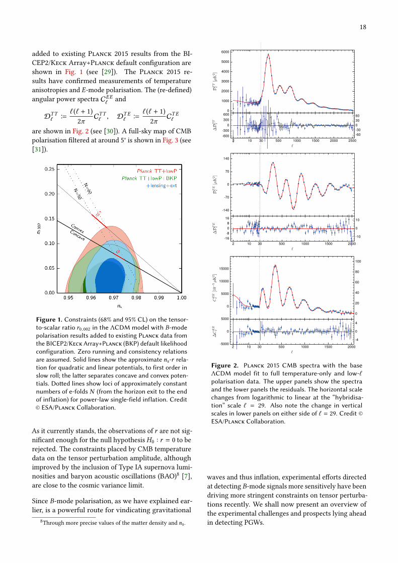
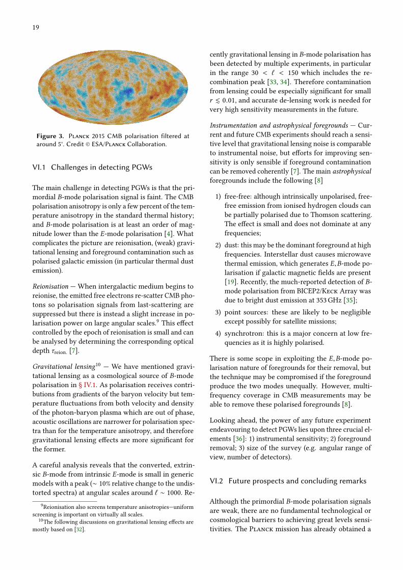
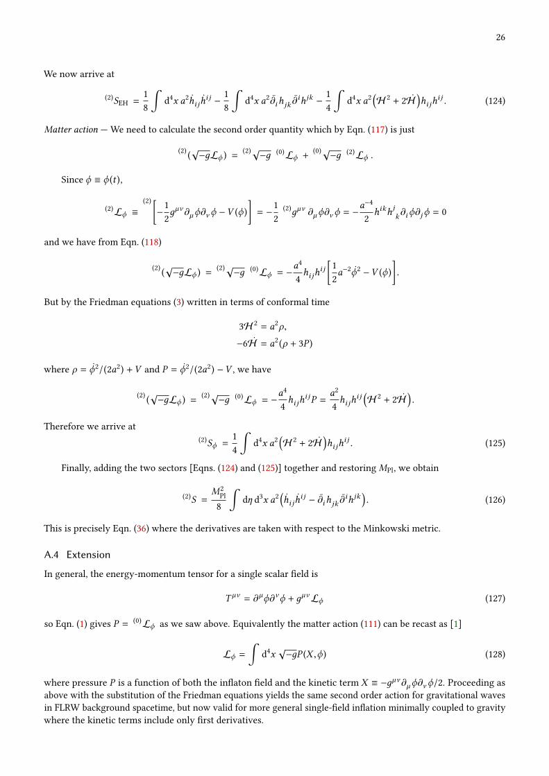
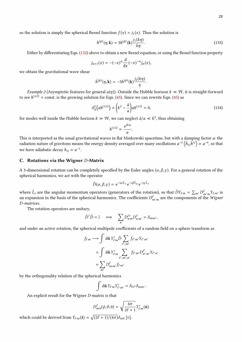
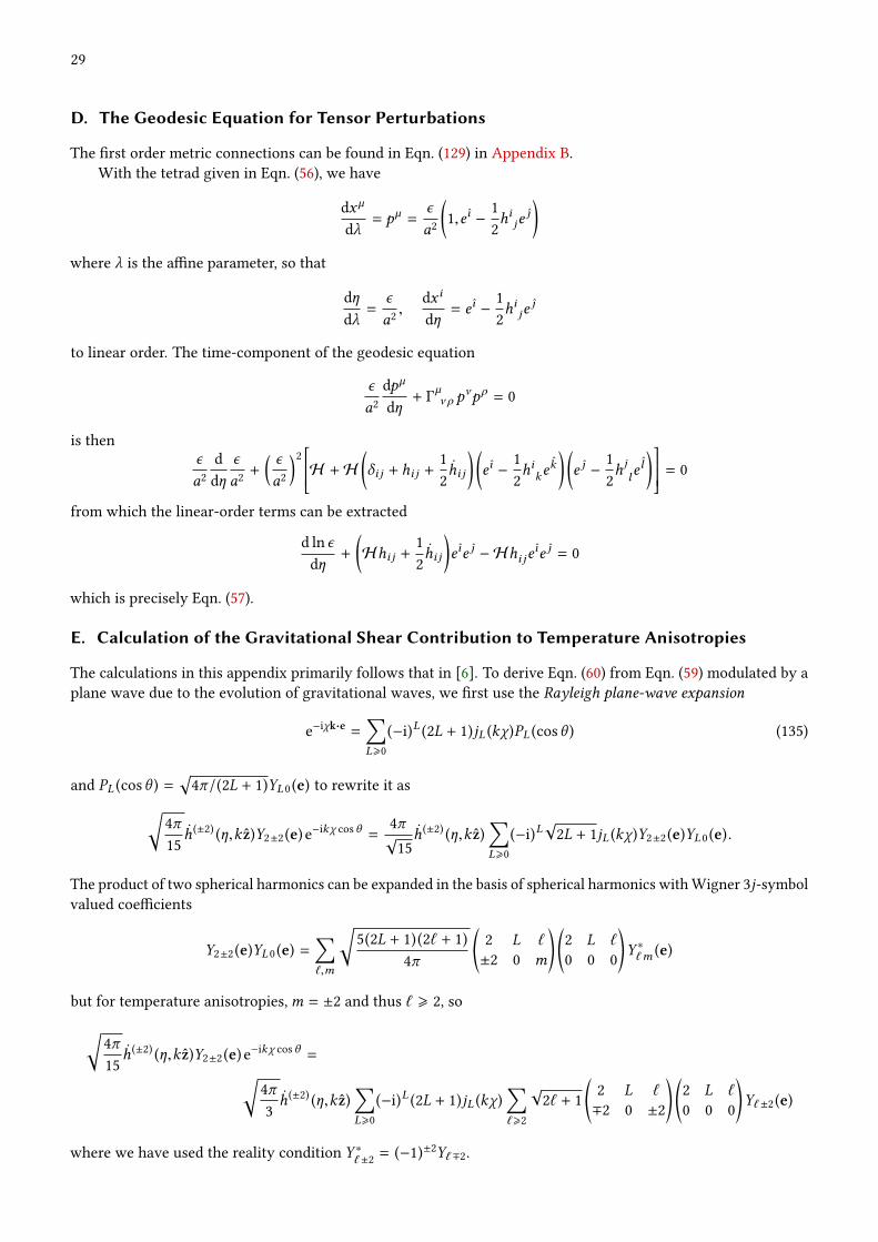
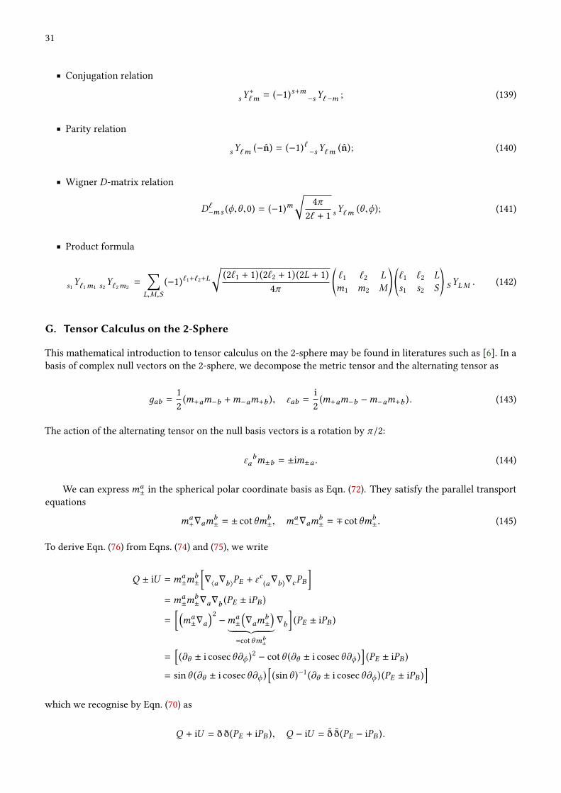
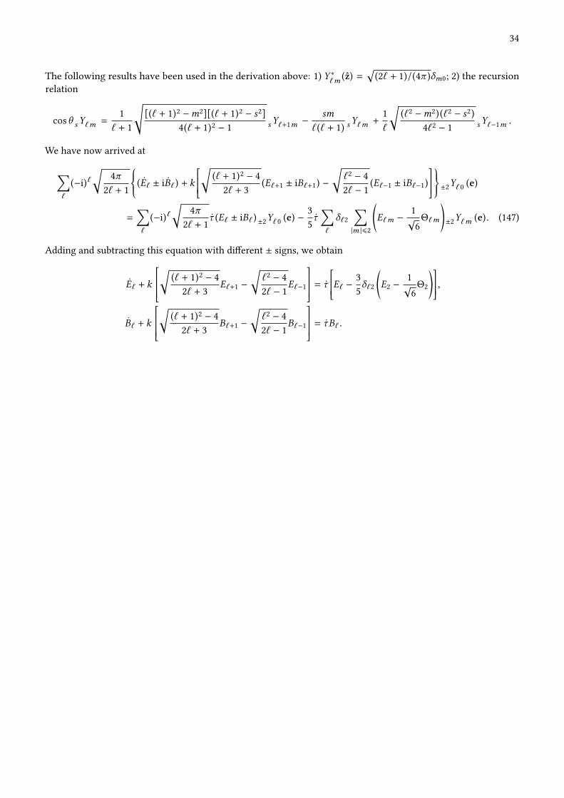