Pricing, Variety, and Inventory Decisions in Retail ...

Pricing, Variety, and Inventory Decisions

in Retail Operations Management

Bacel Maddah

Dissertation submitted to the Faculty of

Virginia Polytechnic Institute and State University

in partial fulfillment of the requirements for the degree of

Doctor of Philosophy

in

Industrial and Systems Engineering

Dr. Ebru K. Bish, Chair

Dr. Kyle Y. Lin

Dr. Russell D. Meller

Dr. Joel A. Nachlas

Dr. Subhash C. Sarin

February 11, 2005

Blacksburg, Virginia

Keywords: Product variety; Joint pricing and inventory; Discrete choice models; Bundling/Tying;

Multi-item multi-location newsvendor.

Copyright c© 2005, Bacel Maddah

Pricing, Variety, and Inventory Decisions

in Retail Operations Management

Bacel Maddah

(ABSTRACT)

This dissertation is concerned with decision making in retail operations management. Specifically,

we focus on pricing, variety, and inventory decisions, which are at the interface of the marketing and

operations functions of a retail firm. We consider two problems that relate to two major types of

retail goods. First, we study joint pricing, variety, and inventory decisions for a set of “substitutable”

items that serve the same need for the consumer (commonly referred to as a “retailer’s product line”).

Second, we present a novel model of a selling strategy for “complementary” items that we refer to

as “convenience tying,” and focus on analyzing the effect of this selling strategy on pricing and

profitability. We also study inventory decisions under convenience tying and exogenous pricing.

For a product line of substitutable items, the retailer’s objective is to jointly determine the set of

variants to include in her product line (assortment), together with their prices and inventory levels,

so as to maximize her expected profit. We model the consumer choice process using a multinomial

logit choice model and consider a newsvendor type inventory setting. We derive the structure of

the optimal assortment for a special case where the non-ascending order of items in mean consumer

valuation and the non-descending order of items in unit cost agree. For this special case, we find that

an optimal assortment has a limited number of items with the largest values of the mean consumer

valuation (equivalently, the items with the smallest values of the unit cost). For the general case, we

propose a dominance rule that significantly reduces the number of different subsets to be considered

when searching for an optimal assortment. We also present bounds on the optimal prices that can

be obtained by solving single variable equations. Finally, we combine several observations from our

analytical and numerical study to develop an efficient heuristic procedure, which is shown to perform

well on many numerical tests.

With the objective of gaining further insights into the structure of the retailer’s optimal decisions,

we study a special case of the product line problem with “similar items” having equal unit costs and

identical reservation price distributions. We also assume that all items in a product line are sold at the

same price. We focus on two situations: (i) the assortment size is exogenously fixed, while the retailer

jointly determines the pricing and inventory levels of items in her product line; and (ii) the pricing

is exogenously set, while the retailer jointly determines the assortment size and inventory levels. We

also briefly discuss the joint pricing/variety/inventory problem where the pricing, assortment size,

and inventory levels are all decision variables.

In the first setting, we characterize the structure of the retailer’s optimal pricing and inventory

decisions. We then study the effect of limited inventory on the optimal pricing by comparing our

results (in the “risky case” with limited inventory) with the “riskless case,” which assumes infinite

inventory levels. In addition, we gain insights on how the optimal price changes with product line

variety as well as demand and cost parameters, and show that the behavior of the optimal price in

the risky case can be quite different from that in the riskless case.

In the second setting, we characterize the retailer’s optimal assortment size considering the trade-

off between sales revenue and inventory costs. Our stylized model allows us to obtain strong structural

and monotonicity results. In particular, we find that the expected profit at optimal inventory levels

is unimodal in the assortment size, which implies that the optimal assortment size is finite. By

comparison to the riskless case, we find that this finite variety level is due to inventory costs. Finally,

iii

for the joint pricing/variety/inventory problem, we find that even when the retailer has control over

the price, finite inventories still restrict the variety level. We also propose several bounds that can

be useful in solving the joint problem.

We then study a convenience tying strategy for two complementary items that we denote by

“primary” and “secondary.” The retailer sells the primary item in an appropriate department of her

store. In addition, to stimulate demand, the secondary item is offered in two locations: its appropri-

ate department and the primary item’s department where it is displayed in very close proximity to

the primary item. We analyze the profitability of this selling practice by comparing it to the tradi-

tional independent components strategy, where the two items are sold independently (each in its own

department). We focus on understanding the effect of convenience tying on pricing. We also briefly

discuss inventory considerations. First, assuming infinite inventory levels, we show that convenience

tying decreases the price of the primary item and adjusts the price of the secondary item up or down

depending on its popularity in the primary item’s department. We also derive several structural and

monotonicity properties of the optimal prices, and provide sufficient conditions for the profitability

of convenience tying. Then, under exogenous pricing, we find that convenience tying is profitable

only if it generates enough demand to cover the increase in inventory costs due to decentralizing the

sales of the secondary item.

iv

Special thanks to

• My advisor, Dr. Ebru Bish, for her outstanding support and guidance. The completion of thisdissertation would not have been possible without Ebru’s patience, kindness, and encourage-ment on both professional and personal levels. I could not ask for a better mentor.

• My committee members, Dr. Kyle Lin, Dr. Russell Meller, Dr. Joel Nachlas, and Dr. SubhashSarin, for their helpful suggestions that have enhanced the quality of this monograph andfor valuable coursework. I’m particularly grateful to Dr. Nachlas for useful comments andencouragement on the material in Chapter 5.

• The nice people at Hannaford Bros. who introduced me to retail management practices duringtwo summer internships. They provided me with experience that has been vital to this dis-sertation. In particular, I would like to thank Andrea Manning, Brenda Munroe, and BernieOuellette.

• Dr. Michael Williams for course work on real analysis that has been very useful.

• Mrs. Lovedia Cole for helping me find my way through the lengthy process of graduating fromVirginia Tech.

• My former advisors, Dr. Nadim Abboud and Dr. Muhammad El-Taha, for introducing meto Operations Research, helping me come to the States, and continuing to provide valuablesupport and advice throughout the years. I have also greatly benefited from joint researchworks with Nadim and Muhammad.

• My friends, especially, Bachir Baeni and Tony El-Nachar for making my undergraduate studyworthwhile, Rana Sfeir for writing countless e-mails of encouragement and support the last fewyears, Tony Atallah and Charlie Thieme for valuable advice on many personal and professionalmatters, and my current classmates, Ahmed Ghoneim, Walid Nasr, and Javier Rueda, foruseful discussions and helpful suggestions on resolving many of the difficulties I faced whileworking on this dissertation.

• My family, especially my mom and dad, for their love and for cutting me loose from all the“conventions” that disable creative ideas.

v

Contents

1 Introduction 1

1.1 Motivations and Objectives . . . . . . . . . . . . . . . . . . . . . . . . . . . . . . . . . 1

1.2 Joint Pricing, Assortment, and Inventory Decisions for a Retailer’s Product Line . . . 4

1.3 Joint Pricing, Assortment, and Inventory Decisions for a Retailer’s Product Line: A

Special Case . . . . . . . . . . . . . . . . . . . . . . . . . . . . . . . . . . . . . . . . . . 6

1.4 Pricing and Inventory Decisions under Convenience Tying . . . . . . . . . . . . . . . . 8

2 Literature Review 12

2.1 Review of the Literature on Product Line Pricing, Variety, and Inventory Decisions . . 12

2.2 Review of the Literature Related to Convenience Tying . . . . . . . . . . . . . . . . . 16

3 Joint Pricing, Inventory, and Assortment Decisions for a Retailer’s Product Line 19

3.1 Model and Assumptions . . . . . . . . . . . . . . . . . . . . . . . . . . . . . . . . . . . 19

3.2 Structure of the Optimal Assortment . . . . . . . . . . . . . . . . . . . . . . . . . . . . 24

3.3 Properties and Bounds on the Optimal Prices . . . . . . . . . . . . . . . . . . . . . . . 29

3.4 Numerical Results and a Heuristic Procedure . . . . . . . . . . . . . . . . . . . . . . . 30

4 Joint Pricing, Assortment, and Inventory Decisions for a Retailer’s Product Line:

A Stylized Model with Similar Items 37


vi

4.2 On the Optimal Price when the Assortment Size is Fixed . . . . . . . . . . . . . . . . 39

4.2.1 Comparative Statics on the Optimal Price . . . . . . . . . . . . . . . . . . . . . 40

4.2.2 Comparison to the Riskless Case . . . . . . . . . . . . . . . . . . . . . . . . . . 42

4.3 On the Optimal Assortment Size when the Price is Fixed . . . . . . . . . . . . . . . . 45

4.3.1 Comparative Statics on the Optimal Assortment Size . . . . . . . . . . . . . . 47

4.4 Bounds and the Joint Variety/Pricing/Inventory Problem . . . . . . . . . . . . . . . . 49

5 Pricing and Inventory Decisions under Convenience Tying 52


5.2 Pricing under Convenience Tying and Independent Components Strategies . . . . . . . 57

5.2.1 Structure of the Optimal Prices under CT . . . . . . . . . . . . . . . . . . . . . 58

5.2.2 Comparison of the Optimal Prices under IC and CT . . . . . . . . . . . . . . . 60

5.2.3 Comparative Statics on the Optimal Prices under CT . . . . . . . . . . . . . . 61

5.2.4 Comparison of the Optimal Profits under IC and CT . . . . . . . . . . . . . . . 63

5.3 A Special Case with Limited Inventory and Exogenous Pricing . . . . . . . . . . . . . 65

5.3.1 The Effect of Stockouts of P on CT . . . . . . . . . . . . . . . . . . . . . . . . 68

6 Conclusions and Suggestions for Further Research 71

6.1 The Retailer’s Product Line Problem . . . . . . . . . . . . . . . . . . . . . . . . . . . . 71

6.2 The Convenience Tying Problem . . . . . . . . . . . . . . . . . . . . . . . . . . . . . . 75

References 78

Appendix 87

vii

List of Figures

4.1 Independent components (IC) and convenience tying (CT) strategies . . . . . . . . . . . 54

A.1 Approximation for φ(Φ−1(1− x)) . . . . . . . . . . . . . . . . . . . . . . . . . . . . . . 87

A.2 Graphical comparison of the exact and the approximate expected profits . . . . . . . . 89

A.3 Graphical comparison of the exact and the approximate expected profits . . . . . . . . 90

viii

List of Tables

3.1 Optimal solution (n = 3) . . . . . . . . . . . . . . . . . . . . . . . . . . . . . . . . . . . 32

3.2 Optimal solution (n = 4) . . . . . . . . . . . . . . . . . . . . . . . . . . . . . . . . . . . 33

3.3 Optimal solution (n = 3), small λ . . . . . . . . . . . . . . . . . . . . . . . . . . . . . . . 33

3.4 EMH solution (n = 3) . . . . . . . . . . . . . . . . . . . . . . . . . . . . . . . . . . . . . 35

3.5 EMH solution (n = 4) . . . . . . . . . . . . . . . . . . . . . . . . . . . . . . . . . . . . . 36

3.6 EMH solution (n = 3), small λ . . . . . . . . . . . . . . . . . . . . . . . . . . . . . . . . 36

5.1 Testing the Normal approximation to XTSP . . . . . . . . . . . . . . . . . . . . . . . . . 70

K.1 Example of p∗k being decreasing in k . . . . . . . . . . . . . . . . . . . . . . . . . . . . . 110

K.2. Example of p∗k being decreasing in c . . . . . . . . . . . . . . . . . . . . . . . . . . . . 110

K.3. Example of p∗k being increasing in λ . . . . . . . . . . . . . . . . . . . . . . . . . . . . 110

K.4. Example of p∗k being decreasing in λ . . . . . . . . . . . . . . . . . . . . . . . . . . . . 111

K.5. Example of pEk and pP

k being decreasing in k . . . . . . . . . . . . . . . . . . . . . . . . 111

K.6. Example of pEk and pP

k being nonincreasing in c . . . . . . . . . . . . . . . . . . . . . . 112

ix

Chapter 1

Introduction

1.1 Motivations and Objectives

Integrating operations and marketing decisions is an important objective for firms in today’s com-

petitive environment. The interaction between operations management (OM) and marketing is clear.

Marketing decisions drive the consumer demand, which is an input to the OM models that address

issues such as capacity planning and inventory control. On the other hand, the Marketing De-

partment of a firm relies on the OM cost estimates in making decisions concerning pricing, variety,

promotions, etc. Therefore, developing joint operations and marketing models is a research objective

that arises naturally. The interest in joint marketing/OM models is reflected in many works in the

literature (see, for example, Eliashberg and Steinberg [23], Griffin and Hauser [35], Karmarkar [46],

and Porteus and Whang [78]). In this dissertation, we study pricing, variety, and inventory decisions

in retail operations management. Deciding on the prices and the breadth of items to be offered in a

retail store is among the main functions of marketing. Moreover, inventory decisions that take into

account the uncertainty in demand are the responsibility of OM. Our work thus contributes to the

growing literature on joint marketing/OM models.

Within the spirit of an integrated marketing/OM approach, one of our main contributions is to

1

2

study the aforementioned pricing, assortment, and inventory decisions jointly. Under this integrative

framework, the retailer sets two or more of the above decisions simultaneously. This seems to be

a successful business practice for many retailers. For example, JCPenney received the “Fusion

Award” in supply chain management for “its innovation in integrating upstream to merchandising

and allocation systems and then downstream to suppliers and sourcing.” A JCPenney vice president

attributes this success to the fact that, at JCPenney, “assortments, allocations, markdown pricing are

all linked and optimized together” (Frantz [28]). Northern Group, the Canadian retailer, managed

to get out of an unprofitable situation by implementing a merchandise optimization tool. Northern

Group’s CFO credits this turnaround to “assortment planning” and the attempt to “sell out of every

product in every quantity for full price” (Okun [71]).

More specifically, an important contribution of this research is to include inventory costs within

pricing and assortment optimization models. Most of the previous literature along this avenue as-

sumes infinite inventory levels and, therefore, excludes inventory considerations (see, for example,

Aydin and Ryan [6], Dobson and Kalish [20], Green and Krieger [32], Kaul and Rao [48], and the

references therein). We believe that this is due in part to the complexities introduced by inventory

modeling. For example, the review paper by Petruzzi and Dada [76] indicates a high level of diffi-

culty associated with joint pricing and inventory optimization even for the single item case. These

difficulties do not, however, justify ignoring inventory effects in modeling. For example, in 2003

the average End-of-Month capital invested in inventory of food retailers (grocery and liquor stores)

in the U.S. was approximately 34.5 Billion dollars, with an inventory/sales ratio of approximately

82% (U.S. Census Bureau [87]). On the other hand, the net 2003 profit margin in food retailing is

estimated to be 0.95% (Food Marketing Institute [29]). With an inventory cost of capital commonly

estimated at 20% (annually) or higher, these numbers indicate that food retailers can significantly

3

increase their profitability by reducing inventory costs.

We develop models that reflect the actual way consumer demand is generated in practice. For

this purpose, we adopt state of the art demand models from the marketing and economics literature,

which reflect the central role of pricing in consumer purchase decisions. We develop two models for

a family of substitutable items that serve the same need for the consumer (commonly referred to as

a “product line” or a “category”). In both models, consumer demand is generated based on the

classical utility maximization principle. The consumer choice process is modeled by a Multinomial

Logit Choice Model (MNL), which leads to a demand function where the demand for an item depends

on its own price and consumer valuation as well as those of other items in the product line. This

reflects the price/quality based substitution that the consumer is engaged in upon every visit to a

retail store. We note that the MNL can be estimated from actual store sales data with relative ease,

especially with the wide availability of business information software that dynamically tracks store

operations (see, for example, Guadagni and Little [36]).

Finally, we present a third model for pricing and inventory decisions under convenience tying,

where we perform a novel analysis of a selling strategy for complementary items. Complementary

goods are on the other extreme of product lines of substitutable items. Thus, we intend to gain

insights by comparing these extreme situations in future research. We note that the demand function

for the convenience tying model is also developed in a realistic manner by aggregating consumer

preferences with customers acting to maximize their surplus (utility).

In the remainder of this chapter, we provide details on the specific research problems that we

consider in this dissertation.

4

1.2 Joint Pricing, Assortment, and Inventory Decisions for a Retailer’s Product

Line

Retailers display their goods in sets of items referred to as product lines or categories. The items in

each product line serve the same basic need for the consumer (e.g., drinking coffee), but are different

in some secondary features (e.g., flavor, aroma, color). These distinctions lead to different consumer

valuation of each item in the product line. When faced with a purchase decision from a product

line, a consumer selects her most preferred item, given the trade-off between price and quality. She

may also choose not to buy any of the displayed items and postpone her purchase, or seek a different

retailer. Pricing has a major impact on the consumer’s choice among the available alternatives.

However, other factors are also important. Such factors include the assortment size or variety level,

in terms of which items are offered in the product line, and the shelf inventory levels of items in the

product line.

We analyze the joint pricing, inventory, and assortment size decisions for a retailer’s product

line. Our objective is to characterize the structure of the retailer’s optimal assortment and to

gain insights into the combined effect of pricing, inventory, and variety on the profitability of a

product line. We are also interested in developing easily implementable and effective methods for

practical applications that generate profitable solutions for the retailer’s product line problem. For

this purpose, we develop a multi-item inventory model with stochastic and price-dependent demand.

The randomness of the demand in our model is due to uncertainty in both the number of customers

arriving and the valuations of those customers for the offered products.

Our model is developed with the following assumptions. Consumers arrive at the retailer’s store

during a selling period. A consumer chooses at most one item from the product line based on price

and quality only, independently of the inventory status at the time of her arrival. This assumption

5

implies that if a consumer’s most preferred item is out of stock, then the consumer leaves the store

empty handed, without considering the purchase of other available items. That is, we consider a

“static choice model” with no stockout based substitution. This assumption is mainly for analytical

tractability and is common in the literature (see Mahajan and van Ryzin [57] for a discussion of this

assumption and other aspects of the inventory and consumer choice problem).

Consumers act to maximize their surplus (utility) defined as the difference between the consumer

reservation price (valuation) and the retail price of an item. The consumer surplus is determined

based on the well-known Multinomial Logit Choice Model (MNL) (see, for example, Anderson and

de Palma [2], Ben-Akiva and Lerman [10], Manski and McFadden [61], and McFadden [64]).) The

MNL is widely utilized as a consumer choice model due to the following reasons: (i) The MNL yields

closed-form expressions of the purchase probabilities of items in the product line, leading to tractable

analytical models; and (ii) it is easy to statistically estimate the parameters (and test the goodness

of fit) of the MNL based on data from actual store transactions, especially with the wide spread of

technology that tracks such transactions (see, for example, Guadagni and Little [36], Hauser [41],

McFadden [64], and McFadden et al. [65]). We point out that these references indicate that the

MNL predicts product line demand with high accuracy. The interest in the MNL is reflected in

many recent works on variety, inventory, and pricing models. Examples of these works include Aydin

and Ryan [6], Aydin and Porteus [7], Besanko et al. [11], Cattani et al. [15], Hanson and Martin [39],

Hopp and Xu [43], and van Ryzin and Mahajan [80]. By utilizing the MNL, we derive the demand

distribution for items in a product line in a realistic fashion by aggregating the individual consumer

choices.

To model the inventory costs, we consider a newsvendor type setting where the items in a product

line are to be sold within a single time period with leftover inventory not carried to subsequent

6

periods. This type of inventory models is utilized in many works similar to ours. Examples include

Aydin and Porteus [7], Cattani et al. [15], Gaur and Honhon [31], Netessine and Rudi [70], Smith

and Agrawal [85], and van Ryzin and Mahajan [80]. Moreover, Smith and Agrawal [85] cite several

studies which indicate that the newsvendor model is suitable for many retail systems that utilize

Electronic Data Interchange. We note finally that the newsvendor type model provides a basis that

can be built on to extend our work to more sophisticated (multi-period) inventory models.

Under the above assumptions, we derive the structure of the optimal assortment for a special case

where the non-ascending order of items in mean consumer valuation and the non-descending order

of items in unit cost agree. For this special case, we find that an optimal assortment has a limited

number of items with the largest values of the mean consumer valuation (equivalently, the items

with the smallest values of the unit cost). For the general case, we propose a dominance rule that

significantly reduces the number of different subsets to be analyzed when searching for an optimal

assortment. We also present bounds on the optimal prices that can be obtained by solving single

variable equations. Finally, we combine several observations from our analytical and numerical study

to develop an efficient heuristic procedure, which is shown to perform well on many numerical tests.

Chapter 3 of this dissertation studies the above problem in detail.

1.3 Joint Pricing, Assortment, and Inventory Decisions for a Retailer’s Product

Line: A Special Case

In the second part of this dissertation, we make certain simplifications to the model presented above

to allow for the analysis of the complex effects of variety, pricing, and limited shelf inventory within

a simplified framework. Our objective is to gain insights through the analysis of this stylized model.

In particular, we consider a situation where all the items that may be included in the product line

7

have the equal unit costs and identical consumer reservation prices. In this stylized model, variety

and profitability are determined only by the number of items in an assortment.

Although stylized, this model may nevertheless apply to certain situations where the items of

a product line are distinguishable by a minor attribute. For example, in a product line of clothing

items belonging to the same broad color group (such as the reds or the greens, etc.), it is likely that

the items will have the same cost structure and similar consumer valuations.

All the assumptions made in Section 1.2 hold here. We make the following additional assumptions.

We assume that all the items in the product line are to be sold at the same price. This assump-

tion serves to simplify the problem further. We note that our extensive numerical experimentation

suggests that such a pricing structure is optimal (although an analytical proof is lacking).

We focus on two situations: (i) the assortment size is exogenously fixed, while the retailer jointly

determines the pricing and inventory levels of items in her product line; and (ii) the pricing is

exogenously set, while the retailer jointly determines the assortment size and inventory levels. We

also briefly discuss the joint pricing/variety/inventory problem where the pricing, assortment size,

and inventory levels are all decision variables.

The first setting allows us to characterize the structure of the retailer’s optimal pricing and

inventory decisions for a given assortment. We then study the effect of limited inventory on the

optimal pricing by comparing our results (the “risky case”) with the “riskless case,” which assumes

infinite inventory levels. In addition, we gain insights on how the optimal price changes with product

line variety as well as demand and cost parameters, and show that the behavior of the optimal price

in the risky case can be quite different from that in the riskless case.

Considering the second setting, we characterize the retailer’s optimal assortment size (variety

level) considering the trade-off between sales revenue and inventory costs: While a high variety

8

increases the overall demand for the retailer’s product line, it also leads to thinning of demand for

each individual item (due to cannibalization), resulting in possibly higher inventory costs (van Ryzin

and Mahajan [80]). Our stylized model allows us to obtain strong results on the finiteness of the

optimal assortment size and on how demand and cost parameters and the market price affect the

retailer’s optimal variety level.

Finally, we briefly discuss the joint pricing/variety/inventory problem and find that even when

the retailer has control over both the price and the variety level, finite inventories still restrict the

variety level. We also propose several bounds that can be useful in solving the joint problem.


1.4 Pricing and Inventory Decisions under Convenience Tying

Retailers utilize various selling strategies to benefit from the complementarity in consumption of

some items. Among the widely studied techniques are those involving “bundling” where one item is

packaged with one or more complementary items and the whole package is sold for one price (see,

for example, Eppen et al. [24]). However, retailers often “tie” two complementary items together

by physically displaying them in near proximity in order to induce customers to buy the two item

s together (and hence expand the demand). More specifically, a “secondary” item (e.g., cakes) is

“tied-in” to a primary item (e.g., berries) by displaying it next to the primary item in the appropriate

location of the latter (e.g., the produce department). In addition, the secondary item is also sold in

its own appropriate location (e.g., the bakery department) for customers who do not consume it in

conjunction with the primary item. We refer to this selling strategy as convenience tying.1

1The economics literature defines tying as the situation where a firm “makes the sales (or price) of one of its productsconditional upon the purchaser also buying some other product from it” (Whinston [89], see also, Burstein [14] andBowman [13] ). This is also known as line forcing. The selling strategy we consider does not require such line forcingsince the customer freely chooses to buy the tied-in item at her own convenience (hence, the term “convenience tying”).

9

The convenience tying practice seems to be gaining a wide popularity among retailers. For ex-

ample, while walking through the aisles of our local Wal-Mart or Kroger stores, we notice several

items tied together. Examples include beer (primary) and lemon (secondary) displayed in overhang-

ing baskets, chips (primary) and dippings (secondary) placed on small shelves encastrated in the

chips shelves, milk (primary) and cereals (secondary) offered in separate shelves just next to the

fridges where milk is sold, etc. Moreover, many retailers are showing interest in understanding and

profitably implementing convenience tying. In fact, this part of the dissertation is motivated by the

author’s work on a berries and cakes pricing and demand forecasting problem for a large chain of

grocery stores in New England.

Important questions facing a retailer engaging in the convenience tying practice include selecting

which items to tie together and deciding on the prices and the inventory levels for these items. To

the best of our knowledge, the above questions (and apparently the entire concept of convenience

tying), have not been studied in the academic literature. In this dissertation, we take the first step

in this research direction. Our objectives are (i) to gain insights into the convenience tying practice

through an analytical model, and (ii) to provide possible answers to the foregoing questions.

Our model is developed with the following assumptions. Consumers arrive to the retailer store

and choose to buy the primary item only, the secondary item only, both items, or neither, in a way

as to maximize their surplus (utility) similar to the aforementioned models on retail product lines.

Consumer reservation prices are random and, to simplify the analysis, are uniformly distributed.

This allows us to develop the demand distribution by aggregating consumer preferences in a realistic

manner. The secondary item is sold at the same price in both locations where it is offered. Moreover,

customers who buy it in the primary item’s location are those willing to buy the primary item first.

Hence, the demand for the secondary item in the primary item’s location is a fraction of the demand

10

of the latter (and therefore it depends on the price of the primary item in addition to its own price).

This leads to “cross-price elasticity effects” between the primary and secondary items. As a result,

their prices (that maximize the retailer’s profit) should be determined jointly.

We focus our analysis on the pricing implications of convenience tying under the assumption that

inventory levels of both the primary and the secondary item are infinite.2 This setting is common

in the related literature on bundling of complementary items (see the references in Section 2.2). In

addition, this assumption holds in certain practical situations, when, for example, the inventory levels

are always sufficiently high due to the marketing requirements of a full shelf. To gain insights into

the inventory implications of convenience tying, we briefly study another situation, where the prices

of both the primary and secondary items are exogenous and the inventory levels are set optimally

within a newsvendor type inventory model. In both situations, we compare convenience tying to the

classical “independent components” strategy where the two items are sold independently each in its

appropriate department.

In the first setting with ample inventories, we find that convenience tying leads to a lower price

(than under independent components) of the primary item in order to increase the demand volume

for the secondary item. On the other hand, the change in the price of the secondary item depends

on how its consumer valuation shifts when it is tied-in to the primary item. This may be understood

by thinking of an overall (system) consumer valuation that dictates the price of the secondary item

(which is sold at the same price in the two echelons of the system). We also derive sufficient conditions

for the profitability of convenience tying, and perform a detailed comparative statics analysis on the

effect of changing demand and cost parameters on the optimal prices. Even though the problem of

finding the optimal prices generally has no closed-form solution, we show that this problem is “well-

2Since, apparently, convenience tying was not analyzed in the previous literature, we believe that this is a necessarystep to initiate its study.

11

behaved” in the sense that the optimal prices are the unique solutions to the first-order optimality

conditions under some reasonable assumptions.

In the second situation with exogenous prices and limited inventory, we find that convenience

tying is profitable only if it leads to a higher total demand volume relative to independent components.

Specifically, the increase in total demand should be large enough to cover the additional inventory

costs, which arise as a consequence of demand decentralization under convenience tying (see, for

example, Eppen [25]). We also discuss the effect of the primary item stockouts on the demand

function under convenience tying.


Chapter 2

Literature Review

In this chapter, we provide a brief overview of the literature that is most relevant to the problems

of interest in this dissertation. Specifically, Section 2.1 presents a brief literature review on product

line pricing, inventory, and variety decisions, while Section 2.2 surveys some of the well-known

quantitative works on bundling (which relates to our convenience tying model).

2.1 Review of the Literature on Product Line Pricing, Variety, and Inventory

Decisions

The literature on this area is at the interface of economics, marketing, and operations management

(OM). Mahajan and van Ryzin [57] present a comprehensive review of this literature. The economics

literature approaches this topic from the point of view of product differentiation (see Lancaster [50]

for a review). The focus of this literature is on developing consumer choice models that reflect the

way consumers make their purchase decisions from a set of differentiated products (see, for example,

Hoteling [45], Lancaster [51], and McFadden [64]). The Multinomial Logit Choice Model (MNL)

that we utilize is among the most popular consumer choice models (see, for example, Anderson and

de Palma [2] and Ben-Akiva and Lerman [10]). Apparently, the MNL has its roots in Mathematical

12

13

Psychology (see, for example, Luce [55] and Luce and Suppes [56]). It has also been widely used to

model travel demand in transportation systems (see, for example, Domencich and McFadden [22]).

The economics literature also utilizes the MNL and other consumer choice models in modeling variety

within a market-equilibrium framework in a market with many firms selling different products (see,

for example, Anderson and de Palma [3] and [4]).

The marketing literature emphasizes data collection and model fitting issues (see, for example,

Besanko et al. [11], Guadagni and Little [36], and Jain et al. [37]). The data is usually collected

based on actual consumer behavior compiled from scanner data (log of all sales transactions in a

store) and panel data (obtained by tracking the buying habits of a selected group of customers).

A popular technique for measuring consumer utilities from store data is conjoint analysis (see, for

example, Green and Krieger [34]). Several works in the marketing literature address the problem of

product line design (in terms of what items to offer to consumers, i.e., variety decisions) and pricing

utilizing data obtained from conjoint analysis (see Green and Krieger [32] and Kaul and Rao [48] for

reviews). A typical approach is to utilize deterministic estimates of utilities of the consumer segments

and formulate the resulting problem as a mixed integer program with the objective of maximizing

the firm’s profit subject to consumer utility maximization constraints (see, for example, Dobson and

Kalish [20] and [21] and Green and Krieger [33]). Other works on product line design and pricing

include Hanson and Martin [39], Moorthy [68], Mussa and Rosen [69], and Oren et al. [72].

In the following, we review with some detail the recent works on product line pricing, variety,

and inventory decisions that are mostly related to our work. Van Ryzin and Mahajan [80] consider

the problem of inventory and assortment decisions for a product line under an MNL consumer choice

process, while assuming that the prices are exogenously determined. They demonstrate that the

optimal assortment has a simple structure having items with the largest mean consumers valuations.

14

Van Ryzin and Mahajan find that a large assortment size (high variety level) is desired if either

the price, or the no-purchase utility, or the sales volume are sufficiently high. Aydin and Ryan [6]

consider the problem of pricing and assortment size decisions for a product line in the riskless case

(i.e., assuming infinite inventory levels) under an MNL consumer choice process. They show that the

optimal prices can be characterized by equal profit margins, with the expected profit being unimodal

in the common margin. They further find that the optimal profit margin and the expected profit are

increasing in the average margin of an item in the product line, where the average margin is defined

as the difference between the mean consumer valuation of an item and its unit cost. Our work may

be seen as an extension of van Ryzin and Mahajan [80] and Aydin and Ryan [6] in the sense that we

study the problem of joint inventory, pricing, and assortment size decisions for a product line under

MNL choice. Hanson and Martin [39] consider a model similar to that of Aydin and Ryan [6] under

a fairly general form of the MNL choice model. They show that the expected profit function is not,

in general, concave or even quasiconcave in the prices of items in an assortment, and they propose a

numerical search technique to determine the optimal prices.

We are also aware of many very recent works that are closely related to ours. Aydin and Porteus [7]

consider a model similar to ours (see Section 1.2), with MNL purchase probabilities and a newsvendor

type inventory model. They show that the problem of finding the optimal prices is well-behaved in the

sense that the first-order optimality conditions have a unique solution, and derive some monotonicity

properties of the optimal prices and inventory levels. Aydin and Porteus also prove that the optimal

price of an item is increasing in the item’s own unit cost and decreasing in the unit costs of the

other items in an assortment. The results in Aydin and Porteus [7] do not apply to our model

because of differences in demand assumptions. Aydin and Porteus consider a multiplicative demand

model where the total (stochastic) demand is deterministically split between the products according

15

to the MNL purchase probabilities. This implies that the coefficient of variation of the demand for

an item is independent of the pricing. Our model is different in the sense that the total demand

is split between the different products in a probabilistic way leading to a demand function with a

coefficient of variation that depends on the prices of all items in the assortment in a complex form.

Moreover, Aydin and Porteus do not address the optimal assortment problem that we consider in

detail. Despite the complex nature of our demand function, we derive some important structural

properties of the optimal assortment as detailed in Chapter 3.

Cattani et al. [15] consider two products (custom and standard) under an MNL consumer choice

process with the objective of determining the optimal product prices and capacity levels for a dedi-

cated and a flexible resource. Through a set of assumptions, the problem is reduced to the problem

of finding the optimal prices and inventory levels for two products in a newsvendor setting under

price dependent demand, similar to our model (see Section 1.2). They propose a heuristic solution

procedure to determine the optimal prices and inventory levels for the two products. Their heuristic

iterates between a marketing (riskless) model that sets the prices (assuming infinite inventory levels)

and an operations model that sets the inventory levels (assuming prices are fixed). The approach

of Cattani et al. [15] is mostly numerical. Moreover, they do not address the optimal assortment

problem like we do.

Hopp and Xu [43] consider an MNL-based model for a product line with the expected profit

consisting of sales revenues minus operations cost, where the latter is modeled as an increasing

function of the number of items in an assortment. Under these assumptions, they derive several

properties of the optimal prices and assortment size. They further discuss risk attitudes of the

retailer and markets with multiple segments of consumers. They find that, in the case of a market

with a single customer segment, both the optimal variety level and the optimal price increase if

16

either the fixed cost or variable cost of an item is reduced. Hopp and Xu also conclude that risk

averse firms should not offer a high variety level. Gaur and Honhon [31] consider a problem similar

to that of Van Ryzin and Mahajan [80], but utilize the Lancaster consumer choice model instead of

the MNL.

Several authors study the problem of pricing and/or inventory decisions of a product line con-

sidering competition between retailers under consumer choice processes (see, for example, Anderson

and de Palma [3], Besanko et al. [11], Hopp and Xu [44], and Mahajan and van Ryzin [59]). The

problem of determining inventory levels considering stockout based substitution in a product line

has also received considerable attention in the recent literature (see, for example, Agrawal and Smith

[85], Netessine and Rudi [70], and Mahajan and van Ryzin [58]).

Finally, the works on single item inventory models with price dependent demand are also relevant

to our research. Examples of these works include Chen and Simchi-Levi [17], Federgruen and Heching

[27], Karlin and Carr [47], Mills [67], Petruzzi and Dada [76], Whitin [90], and Young [91].

2.2 Review of the Literature Related to Convenience Tying

The literature on bundling (i.e., the sales of items jointly as a bundle or a package) is broadly

related to the convenience tying problem described in Section 1.4. Most of the quantitative literature

deals with bundling as a price discrimination tool that allows the retailer to extract more consumer

surplus (see, for example, Adams and Yellen [1] and Stigler [86]). Adams and Yellen (AY) consider the

following selling strategies for two items which are independent in demand: (i) pure components, when

the two items are sold separately; (ii) pure bundling, if the two items are sold as a package only; and

(iii) mixed bundling, when the items are offered both separately and as a package. The convenience

tying strategy we study in this dissertation may be seen as an additional selling alternative to the

17

these strategies. AY find that mixed bundling is more profitable than the two other forms of sales

in most situations, and that negative correlation of reservation prices of the two items encourages

some form of bundling.

Several papers extend the work of AY. In particular, Schmalensee [83] applies the AY framework to

the case where one of the products is sold competitively, while the other is controlled by a monopolist.

Dansby and Conard [18] and Lewbel [52] extend the AY model to handle items that are substitutable

or complementary in demand. Paroush and Peles [75] consider a model with linear, price dependent

demand, and compare the pure components and the pure bundling strategies. Schmalensee [82]

considers the AY model with the reservation prices following a bivariate Normal distribution and

derive conditions under which bundling is more profitable than pure components. Long [54] and

McAffee et al. [62] derive conditions under which mixed bundling is more profitable than pure

components for any reservation price distribution. Pierce and Winter [77] illustrate analytically

and empirically that pure bundling may be more profitable than mixed bundling. Salinger [81]

compares pure bundling and pure components under somewhat general settings.

More recently, Bakos and Brynjolfsson [8] consider the problem of bundling information goods,

with zero marginal costs for each good, and prove that pure bundling is asymptotically optimal as

the number of bundled goods increases. Hanson and Martin [40] analyze bundles of two or more

components, while assuming that consumer reservation prices are well-known (deterministic). They

formulate the problem as an integer program and propose an efficient solution procedure. Ansari and

Weinberg [5] and Venkatesh and Mahajan [88] study the profitability of bundling in the entertainment

sector, with season tickets and single-event tickets being sold for a series of performances.

In terms of cost side implications of bundling, very limited work has been done. In a recent

paper, Ernst and Kouvelis [26] investigate the effect of bundling on inventory costs. They argue that

18

the benefits of bundling stem from its ability to allow demand substitution at stockout situations.

In another recent work, McCardle et al. [63] propose a joint inventory and pricing model for pure

bundling assuming uniformly distributed reservation prices. We also note that Hanson and Martin

[40] and Salinger [81] briefly discuss some cost aspects of bundling.

Other works that are also related to convenience tying are on the “loss leader” selling practice

(see, for example, Hess and Gerstner [42], Lal and Matutes [49], and the references therein). Loss

leader pricing is a strategy where a retailer sells an item at or below cost in order to increase store

traffic and, consequently, generate high profits from other items that can be sold at sufficiently large

profit margins. Convenience tying can be seen as a loss leader strategy if the primary item is priced

below its unit cost (in Chapter 5, we show that such situations may indeed be profitable). Hess and

Gerstner [42] study a loss leader strategy with rain checks. In this strategy, a customer who finds

an advertised loss leader item out of stock is given a rain check which entitles her to buy the item

at the same reduced price in a future date. They utilize a game theoretic model with multiple firms

in the market competing for the sales of one “shopping good” (candidate to be a loss leader) and

a set of “impulse goods” (defined as items bought on the spot without price comparison with other

stores). Hess and Gerstner show that retailers offering rain checks may deliberately run out of stock

on loss leaders in order to have customers visit their stores a second time.

Lal and Matutes [49] consider a duopoly model with two competing firms selling two products

one or both of which could be advertised (and the customers become aware of prices of the advertised

items before visiting the store). They model the competition between the two firms as a multi-stage

game that includes advertising and pricing decisions of the retailer as well as the customer’s rational

for choosing one store over the other. Lal and Matutes show that a loss leader strategy could exist

in market equilibrium.

Chapter 3

Joint Pricing, Inventory, and Assortment

Decisions for a Retailer’s Product Line

In this chapter we consider the problem of joint pricing, inventory and assortment decisions for a

retailer’s product line as introduced in Section 1.2. This chapter is organized as follows. Section

3.1 introduces the basic model and assumptions. Section 3.2 presents structural properties of the

optimal assortment. Section 3.3 discusses structural properties and bounds on the optimal prices.

Finally, Section 3.4 presents an efficient heuristic procedure that is suited for practical applications.

3.1 Model and Assumptions

Let Ω = 1, 2, . . . , n be the set of possible variants from which the retailer can compose her product

line. Let S ⊆ Ω denote the set of items stocked by the store. Demand for items in S is generated

from customers arriving to the retailer’s store during a single selling period. A customer chooses

to purchase at most one item from set S so as to maximize her “surplus,” which is the difference

between her reservation price and the retail price of an item. We adopt a Multinomial Logit Choice

Model (MNL) with the consumer surplus (utility) for item i ∈ S given by Ui = αi − pi + εi, and

19

20

the utility of the no-purchase option given by U0 = u0 + ε0, where pi and αi respectively denote the

retail price and the mean reservation price (consumer valuation) of item i ∈ S, u0 is the mean utility

for the no-purchase option, and εi, i ∈ S ∪ 0, are independent and identically distributed Gumbel

random variables with mean 0 and shape factor µ.1 (See Johnson et al. [38] and Patel et al. [74] for

details on the Gumbel distribution.)

The probability that a consumer buys item i ∈ S is given by qi(S,p) = PrUi = maxj∈S∪0Uj,

and the no-purchase probability is given by q0(S,p) = 1 −∑j∈S qj(S,p), where p = (p1, . . . , p|S|) is

the price vector corresponding to items in S, with |S| denoting the cardinality of set S. Utilizing

the expression for the Gumbel distribution function and simplifying (see, for example, Anderson et

al. [2], pp. 29-42), it can be shown that qi(S,p), i ∈ S ∪ 0, can be expressed as

qi(S,p) =e(αi−pi)/µ

v0 +∑

j∈S e(αj−pj )/µ

, i ∈ S, q0(S,p) =v0

v0 +∑

j∈S e(αj−pj )/µ

, (3.1)

where v0 = eu0/µ.

We adopt a demand model similar to that in Cattani et al. [15] and van Ryzin and Mahajan

[80]. Denote by λ the mean number of customers arriving during the selling period. Under the

assumptions that (i) consumers make their purchasing decisions independently of the inventory status

at the moment of their arrival, and (ii) they will leave the store empty-handed if their preferred

item (in S) is out of stock (i.e., there is no stockout based substitution), the expected demand

for item i ∈ S is λqi(S,p). Then, the demand for item i ∈ S, Xi, is assumed to be a Normal

1The model parameters are commonly estimated by assuming αi =∑

j∈Tiβjixji, i ∈ Ω, where Ti is the set of

“attributes” corresponding to item i, xji is the observed value of attribute j for item i (as measured from actualconsumer behavior data), and βji is the “utility weight” of attribute j for item i. The coefficients βji are evaluatedusing maximum likelihood estimation. See Guadagni and Little [36] and McFadden [64] for details. Guadagni andLittle [36] further indicate that parameters such as u0 and µ can be “absorbed” into estimates of the αi by adequatelyscaling the model. In this dissertation, we assume that the MNL parameters have been estimated accurately, andaddress the retailer’s problem of making operational decisions based on these estimates.

21

random variable with mean λqi(S,p) and standard deviation√λqi(S,p), which represents a Normal

approximation to demand generated from customers arriving according to a Poisson process with

rate λ per selling period. We note that all the subsequent results would also extend to the case where

Xi is a Normal random variable with mean λqi(S,p) and standard deviation σ(λqi(S,p))β, where

σ > 0 and 0 ≤ β < 1, with the coefficient of variation of Xi being decreasing in λ (as in van Ryzin

and Mahajan [80]).

In our model, the coefficient of variation and standard deviation of Xi are given by 1/√λqi(S,p)

and√λqi(S,p), respectively. That is, both the demand standard deviation and coefficient of variation

are functions of the price vector of the product line. Most of the literature on joint inventory and

pricing models assumes that the demand is either “additive,” with the demand standard deviation

being independent of the price, or “multiplicative,” with the demand coefficient of variation not

depending on the price (see, for example, Petruzzi and Dada [76]). In that sense, our demand model

may be seen as “mixed multiplicative/additive.” This follows from the fact that Xi = λqi(S,p) +

√λqi(S,p)Zi, where Zi are independent and identically distributed random variables with a standard

Normal distribution. Young [91] considers a demand with a similar multiplicative/additive structure

for the case of a single item. However, even for the single item case, none of Young’s results are

applicable to our model because Young makes restrictive assumptions on the range of cost and

demand parameters.

Our model may be seen as a multi-item newsvendor model with items having Normal demands,

under the additional complexities of pricing and assortment decisions. On the cost side, we assume

that items of the product line do not have a salvage value and no additional holding or shortage

costs apply (as in Aydin and Porteus [7] and van Ryzin and Mahajan [80]). We note that the essence

of inventory costs in terms of overage and underage costs are captured here. In addition, these

22

assumptions can be easily relaxed to include holding and shortage costs and salvage values without

changing the structure of our results. By utilizing the well-known results for the newsvendor model

under Normal demand (see, for example, Silver et al. [84], pp. 404-408), we can write the optimal

inventory level for item i ∈ S, y∗i (S,p), and the expected profit from S at optimal inventory levels,

Π(S,p), as:

y∗i (S,p) = λqi(S,p) + Φ−1(1 − ci/pi)√λqi(S,p), i ∈ S, (3.2)

Π(S,p) =∑j∈S

[λqj(S,p)(pj − cj) − pj

√λqj(S,p)φ(Φ−1(1 − cj/pj))

], (3.3)

where ci < pi is the unit cost of item i ∈ S, and φ(·) and Φ(·) are the probability density function

and the cumulative distribution function of the standard Normal distribution, respectively. Observe

that in (3.3), the first term is the “riskless” expected profit (assuming an infinite supply of items),

while the second term involving the demand standard deviation represents the inventory costs.

The optimal prices that maximize the expected profit from S can be obtained via a multiple

variable search on Π(S,p) in (3.3). The optimal inventory levels can then obtained using (3.2).

However, no closed-form expression exists for the term Φ−1(1−ci/pi) which complicates the analysis

of Π(S,p). Furthermore, approximate expressions for Φ−1(·) are quite cumbersome and are not

promising in obtaining a simplified expression for Π(S,p) (see, for example, Patel and Read [73], pp.

66-70). Consequently, we propose the following simple approximation for φ(Φ−1(1− x)), 0 ≤ x ≤ 1:

φ(Φ−1(1− x)) ≈ −ax(x− 1), (3.4)

23

where a > 02; see Appendix A. With this approximation, Π(S,p) in (3.3) simplifies to the following:

Π(S,p) =∑j∈S

(pj − cj)[λqj(S,p)− a

cjpj

√λqj(S,p)

]. (3.5)

That is, Π(S,p) =∑

j∈S Πj(S,p), where Πj(S,p) = (pj − cj)[λqj(S,p) − a

cj

pj

√λqj(S,p)

]is the

expected profit from item j ∈ S.

Our objective is to find the assortment yielding the maximum profit, Π∗:

Π∗ = Π(S∗,p∗) = maxS⊆Ω

maxp∈ΓS

Π(S,p), (3.6)

where S∗ is an optimal assortment, p∗ is the corresponding optimal price vector, and

ΓS = (p1, . . . , p|S|) | p1 > c1, . . . , p|S| > c|S|.

We use the expression of Π(S,p) in (3.5) in the remainder of this chapter. We observe, through an

extensive numerical study, that the approximate expected profit in (3.5) behaves in a similar fashion

to the exact expected profit in (3.3). We also observe that, for a given assortment, the optimal prices

under the approximate expected profit are very close to their counterparts under the exact expected

profit. In summary, our numerical study indicates that our approximation does not change the main

structural properties of the optimal solution (see Appendix A for details of the numerical study).

The following assumption guarantees that the retailer will not be better off not selling anything

(hence, the optimal expected profit is positive).

(A1): Let i be the item in Ω such that αi−ci = maxj∈Ωαj−cj. The expected profit from assortment

i is increasing in pi at pi = ci. That is, ∂Π(i,pi)

∂pi

∣∣∣p

i=c

i

> 0, or equivalently,

2We find that with a = 1.66, the approximation is reasonably accurate with an average error of 8.6%. However, oursubsequent analytic results hold for any positive constant a.

24

λ > a2(1 + v0e

−(αi−c

i)/µ).3

Assumption (A1) implies that in an optimal assortment, S∗, the contribution of each item in S∗

to the expected profit is positive, and that the optimal price vector, p∗, for S∗ is an internal point

solution. The following lemma states these results formally.

Lemma 3.1.1 Assume that (A1) holds. Then, the contribution of each item in an optimal assort-

ment to the expected profit is positive, i.e., Πi(S∗,p∗) > 0, i ∈ S∗. In addition, the optimal price

vector, p∗, satisfies ci < p∗i <∞, with ∂Π(S∗,p)∂pi

∣∣∣p=p∗= 0, i ∈ S∗.

Proof. See Appendix B.

In the remainder of this chapter, we assume that (A1) holds. When a result involves changing

the values of the model parameters, we assume that the change is restricted to the range where (A1)

holds.

3.2 Structure of the Optimal Assortment

Our main structural result allows us to determine whether a given item “dominates” another item.

The dominance relationship that we consider is quite intuitive as it requires the dominating item to

have a lower or equal unit cost and a higher or equal mean reservation price than the dominated item

(with one of the two inequalities being strict). We show that an optimal assortment cannot contain

the dominated item and not contain the dominating item. While this type of a dominance relationship

can considerably reduce the computational effort needed to determine the optimal assortment, it also

3In fact, our results hold under a weaker assumption than (A1). However, we choose to report (A1) here because(i) it is easy to verify whether (A1) holds or not; (ii) (A1) guarantees that an item’s mean demand is reasonably large,which leads to a low probability of negative demand under the Normal demand distribution; and (iii) (A1) is not toorestrictive, e.g., if (αi − ci) >> 0, then (A1) holds if λ > a2 ≈ 3 when a = 1.66.

25

allows us to derive the structure of the optimal assortment for a special case that may apply to many

practical situations. We present below some important lemmas that are utilized to derive our main

result. Other supporting lemmas are presented in Appendix C.

Lemma 3.2.1 Consider an assortment S ⊆ Ω. Assume that prices of items in S are fixed at some

price vector p. Then, the expected profit from S, Π(S,p, αi), is strictly pseudoconvex in αi, the mean

reservation price of item i ∈ S.

Proof. See Appendix C.

Lemma 3.2.1 extends a similar result in van Ryzin and Mahajan [80]. The intuition behind

Lemma 3.2.1 is as follows. Recall that the demand coefficient of variation and standard deviation

of item i ∈ S are 1/√λqi(S,p) and

√λqi(S,p), respectively. Then, it can be easily shown that (i)

the demand coefficient of variation of item j = i, j ∈ S, is increasing in αi, while that of item i

is decreasing in αi; (ii) the demand standard deviation of item j ∈ S, j = i, is decreasing in αi,

while that of item i is increasing in αi;4 and (iii) the total expected demand for the product line,

λ(1− q0(S,p)), is increasing in αi. With the inventory costs being increasing in demand variability

and sales revenues being increasing in the total expected demand (at fixed prices), these conflicting

effects of αi explain the pseudoconvexity result in Lemma 3.2.1.

The following lemma studies the effect of changing the mean reservation price of an item in an

optimal assortment.

Lemma 3.2.2 Consider an optimal assortment S∗ ⊆ Ω. Let p∗ be the optimal price vector when

αi = α′i, for some i ∈ S∗. Assume that prices of items in S∗ are fixed at p∗. Then, the expected

profit from S∗,Π(S∗,p∗, αi), is increasing in αi for αi ≥ α′i.

4Here we are measuring demand variability by both the standard deviation and the coefficient of variation of thedemand, similar to Petruzzi and Dada [76].

26


Lemma 3.2.2 states that increasing the mean reservation price, αi, of an item in an optimal

assortment increases the expected profit from the assortment when the prices of items in the assort-

ment are unchanged. Clearly, this implies that the optimal profit (with prices adjusted optimally

and possibly a new optimal assortment obtained as αi changes) also increases in αi, i ∈ S∗.

Another key parameter that drives the profitability of an item is its unit cost. The following

lemma studies the effect of changing the unit cost of an item on the profitability of a product line.

Lemma 3.2.3 Consider an assortment S ⊆ Ω. Assume that prices of items in S are fixed at some

price vector p and that Πi(S,p, ci) > 0 when ci = c′i, for some i ∈ S. Then, the expected profit from

S, Π(S,p, ci), increases if ci is decreased below c′i.


Lemma 3.2.3 states that decreasing the unit cost of an item returning a positive expected profit

will increase the expected profit from an assortment. It can be easily seen that this results also

extends to the case of an optimal assortment. That is, decreasing the unit cost of an item in

the optimal assortment increases the optimal profit. A question that arises naturally is whether

increasing the mean reservation price of an item (by perhaps an advertisement campaign) is more

profitable than decreasing the item’s unit cost, or vice versa. We numerically observe, in Section 3.4,

that decreasing the unit cost is slightly more profitable.

Next, we present our main dominance result.

Lemma 3.2.4 Consider two items i, k ∈ Ω such that αi ≤ αk and ci ≥ ck, with at least one of the

two inequalities being strict, that is, item k “dominates” item i. Then, an optimal assortment cannot

contain item i and not contain item k.

27


Observe that the number of assortments to be considered in the search for an optimal assortment

can be significantly reduced if there are few dominance relations like the one described in Lemma

3.2.4. For example, with exactly one pair of items satisfying the dominance relation in the lemma,

the number of assortments to be considered is reduced by∑n−1

r=1

(n−2r−1

)= 2n−2, which leads to more

than 25% reduction in computational effort since the total number of subsets of Ω to be considered

in an exhaustive search is 2n − 1. (Under (A1), the empty set, i.e., the option of selling nothing,

cannot be optimal.) In addition, Lemma 3.2.4 allows the development of the structure of an optimal

assortment in a special case which may be commonly encountered in practice. This is stated in the

following theorem.

Theorem 3.2.1 Assume that the items in Ω are such that α1 ≥ α2 ≥ . . . αn, and c1 ≤ c2 ≤ . . . cn.

Then, an optimal assortment is S∗ = 1, 2, . . . , k, for some k ≤ n.

Proof. The proof follows directly from Lemma 3.2.4. Lemma 3.2.4 implies that if the optimal

assortment is of cardinality 1, then 1 is an optimal assortment. Similarly, if the optimal assortment

is of cardinality 2, then 1, 2 is an optimal assortment, and so on.

In the special case of a product line with all items having the same unit cost, Theorem 3.2.1

implies that an optimal assortment has the k, k ≤ n, items with the largest values of αi. Van Ryzin

and Mahajan [80] prove a similar result when, in addition to having the same unit cost, all items have

the same price (or same price to unit cost ratio) which is exogenously determined. Thus, Theorem

3.2.1 extends the result of van Ryzin and Mahajan to a product line with items having distinct

endogenous prices. Another special case of Theorem 3.2.1 is a product line with items having the

same mean reservation prices; in this case, an optimal assortment has the k, k ≤ n, items with the

28

smallest values of ci.

Theorem 3.2.1 is quite intuitive: An optimal assortment simply contains either the most popular

item (with the least possible cost), or the two most popular items (with the least costs), and so on.

Furthermore, Theorem 3.2.1 greatly simplifies the search for an optimal assortment in the special

case where it applies, as it suffices to consider only n assortments out of (2n−1) possible assortments.

We point out that in many cases, the economies of scale in the supply of popular items may lead

to a structure of reservation prices/unit costs that is similar to that in the theorem. That is, high

customer demand for popular items implies larger order size for these items, which tends to decrease

the unit cost per item with business practices such as quantity discounts.

For cases where Theorem 3.2.1 does not apply, one may expect an optimal assortment to have

the k, k ≤ n, items with the largest “average margins,” αi−ci, similar to the structure of the optimal

assortment in Theorem 3.2.1. In fact, a somewhat similar result holds in the riskless case (which

assumes infinite inventory levels), where it can be shown that while the optimal assortment is Ω (i.e.,

there is no limit on variety), the optimal assortment of size k has the k items with the largest average

margins; see, for example, Aydin and Ryan [6]. However, in Section 3.4, we find several counter-

examples of optimal assortments not having items with the largest average margin, indicating that a

result similar to Theorem 3.2.1 does not hold in general. Nevertheless, we observe that assortments

consisting of items with the largest average margins return expected profits that are very close to

the optimal profit. This last observation is one of the main motivations for our heuristic procedure,

discussed in Section 3.4, which can be utilized in cases where Theorem 3.2.1 does not hold.

29

3.3 Properties and Bounds on the Optimal Prices

We first exploit the optimality conditions to gain insight into the structure of the optimal prices.

The following lemma is a consequence of the first-order optimality conditions.

Lemma 3.3.1 Consider an optimal assortment S∗ ⊆ Ω. Then, the optimal prices of any two items

i, j ∈ S∗ satisfy the following equation:

1µ(p∗i−ci)

(1 − a

2cip∗i

1√λqi(S∗,p∗)

)+a c2i

p∗i2

1√λqi(S∗,p∗)

= 1µ(p∗j−cj)

(1− a

2cj

p∗j1√

λqj(S∗,p)

)+a

c2jp∗j

21√

λqj(S∗,p∗) .


Lemma 3.3.1 has several important implications. First, note that for λ large enough (λ → ∞),

and with the optimal prices being finite (as shown in Lemma 3.1.1), the optimal profit margins for

all items in S∗ will be exactly equal, i.e., p∗i − ci = p∗j − cj, i, j ∈ S∗. This is due to the fact that for

large λ our problem converges to the “riskless case,” as it can be easily shown that for finite prices

Π(S∗,p) in (3.5) converges to∑

j∈S(pj − cj)λqj(S∗,p), the expected profit for the riskless case. For

the riskless case, many authors indeed show that the optimal prices are characterized by “equal profit

margins” (see, for example, Anderson et al. [2], Aydin and Ryan [6], and Cattani et al. [15]).

Second, Lemma 3.3.1 shows that with finite inventory levels (i.e., in the “risky” case), the “equal

margins” property is no longer guaranteed to hold at optimality. However, Lemma 3.3.1 suggests

that for large mean demands, λqi(S∗,p∗) and λqj(S∗,p∗), items i and j will have approximately

equal profit margins, i.e., p∗i − ci ≈ p∗j − cj, i, j ∈ S∗. We observe, through an extensive numerical

study, that the optimal profit margins are indeed quite close (see Section 3.4 for details). Finally,

Lemma 3.3.1 may be useful in numerically solving for the optimal prices.

Next, in Lemma 3.3.2 and Corollary 3.3.1, we develop bounds on the optimal prices that can be

obtained by solving single variable equations. These bounds are useful in the numerical search for

30

the optimal prices of an assortment. Moreover, in practice, product lines may have a handful of “fast

movers” that attract most of the demand and numerous “slow movers,” each attracting only a thin

fraction of the demand. Lemma 3.3.2 can identify highly unprofitable slow movers and eliminate these

items from consideration. Define πi(pi) ≡ λp2i qi(i, pi) − a2c2i and hmax

i ≡ maxpi>0p2i qi(i, pi).

Lemma 3.3.2 Consider item i ∈ Ω. Then,

(i) If hmaxi > a2c2i /λ and pi > ci then p∗i ∈ (maxc, pi, pi) in any assortment containing i,

where pi and pi are such that πi(pi) = πi(pi) = 0 with pi < pi.5

(ii) Otherwise, item i must not be included in an optimal assortment.

Proof. See Appendix D.

Note that the bounds in Lemma 3.3.2 apply to the optimal price of an item i ∈ Ω in any

assortment S ⊆ Ω containing i. Finally, bounds on the optimal prices of all items (in all possible

assortments) can be obtained by solving one simple equation, as indicated in the following result.

Corollary 3.3.1 Consider item i ∈ Ω. Then, p∗i ∈ (maxci, p, p) in any assortment containing

i, where p and p are such that πi(p) = π

i(p) = 0 with p < p, and item i is characterized by

ci= minj∈Ωcj, and α

i= maxj∈Ωαj.

Proof. See Appendix D.

3.4 Numerical Results and a Heuristic Procedure

The objectives of our numerical study in this section are twofold: (i) To study the properties of

an optimal solution for the general case (when Theorem 3.2.1 does not hold); and (ii) to develop a

5The condition that hmaxi > a2c2

i /λ guarantees that there are exactly two solutions of πi(pi) = 0; see Appendix D.

31

simple effective heuristic for the problem at hand, motivated mainly by our analytical results and

numerical observations.

Table 3.1 presents the numerical results for a three-item case. The optimal assortment, S∗,

is obtained by enumerating over all subsets of Ω = 1, 2, 3 and determining the corresponding

optimal profit (together with optimal prices and inventory levels) for each subset. In addition to the

optimal assortment, S∗, and its expected profit, Π∗, Table 3.1 reports the optimal profit margins,

p∗i − ci, i ∈ Ω, and the no-purchase probability, q0(S∗,p∗) (the fraction of customers who leave the

store empty-handed). Note that an infinite profit margin indicates that the item is not included in

S∗. The second column of Table 3.1 shows the modification from the “base case,” described in the

table heading. Each modification involves changing the parameters given in the second column of

the table only, while keeping other parameters at their base values.

Table 3.1 reveals three important insights. First, items in S∗ have approximately equal profit

margins, p∗i − ci, i ∈ S∗. This finding is not surprising given our discussion of Lemma 3.3.1. Second,

an optimal assortment need not have the items with the largest values of αi − ci (which shows that

a result similar to Theorem 3.2.1 does not hold in general). For example, in Case 8 the two items

with the largest values of αi − ci are items 1 and 2, while the optimal assortment contains items 1

and 3 only. A similar observation holds for Case 9.6 We observe, however, (on Cases 8 and 9, and

many other cases) that assortments containing items with the largest values of αi − ci yield expected

profits that are very close to the optimal expected profits. (This will be further discussed within the

context of our proposed heuristic procedure.) Third, we observe that reducing an item’s unit cost by

a certain amount is slightly more profitable than increasing its mean reservation price by the same

6We have verified that similar counter-examples exist under the exact expected profit in (3.3) as well as under theexact expected profit obtained based on a Poisson arrival process, which indicates that the counter-examples are notdue to our approximations.

32

amount. For example, while item 1 has the same value of α1 − c1 = 3 in Cases 2 and 3 (with items

2 and 3 having the same parameters in both cases), Case 3 (where ci is smaller) yields a slightly

higher expected profit than Case 2. The same observation is valid when comparing Cases 4 and 5,

or Cases 6 and 7.

Table 3.2 presents the results for a four-item case, which confirm the three main insights observed

in Table 3.1. In particular, a similar observation on decreasing ci being more profitable than increas-

ing αi can be made by comparing Cases 2 and 3, or 4 and 5, or 6 and 7 in Table 3.2. In addition,

Cases 8 and 9 in Table 3.2 furnish more examples on optimal assortments not having the items with

the largest values of αi − ci. Moreover, it can be observed throughout Table 3.2 that optimal profit

margins for items in S∗ are approximately equal.

Table 3.1. Optimal solution (n = 3)Base case: λ = 100, α1 = 11, α2 = 10, α3 = 9, c1 = 9, c2 = 8, c3 = 7, v0 = 1, µ = 1.

Case Modification p∗1 − c1 p∗2 − c2 p∗3 − c3 q0(S∗,p∗) S∗ Π∗

1 None 2.531 2.534 2.536 0.362 1, 2, 3 117.4532 α1 = 12 2.790 2.904 2.904 0.329 1, 2, 3 142.5283 c1 = 8 2.795 2.909 2.908 0.330 1, 2, 3 143.1754 α1 = 12.75 3.066 ∞ 3.331 0.308 1, 3 173.9505 c1 = 7.25 3.075 ∞ 3.345 0.310 1, 3 175.6676 α1 = 15 4.673 ∞ ∞ 0.210 1 323.9357 c1 = 5 4.692 ∞ ∞ 0.213 1 333.6948 α1 = 12.8, c2 = 7.98 3.096 ∞ 3.379 0.305 1, 3 176.6609 c1 = 7.25, c2 = 7.98 3.075 ∞ 3.343 0.310 1, 3 175.667

33

Table 3.2. Optimal solution (n = 4)Base case: λ = 150, α1 = 20, α2 = 22, α3 = 24, α4 = 26, c1 = 18, c2 = 20, c3 = 22, c4 = 24,v0 = 1, µ = 1.

Case Modification p∗1 − c1 p∗2 − c2 p∗3 − c3 p∗4 − c4 q0(S∗,p∗) S∗ Π∗

1 None 2.663 2.661 2.659 2.658 0.326 1, 2, 3, 4 190.2002 α1 = 21.6 3.027 3.215 3.214 ∞ 0.297 1, 2, 3 252.2863 c1 = 16.4 3.029 3.217 3.216 ∞ 0.297 1, 2, 3 252.8164 α1 = 21.8 3.078 3.299 ∞ ∞ 0.300 1, 2 267.3385 c1 = 16.2 3.081 3.302 ∞ ∞ 0.300 1, 2 268.0096 α1 = 22 3.155 ∞ ∞ ∞ 0.300 1 285.4007 c1 = 16 3.158 ∞ ∞ ∞ 0.301 1 286.2368 α1 = 21.6, α4 = 26.015 3.027 3.215 3.214 ∞ 0.297 1, 2, 3 252.2869 α1 = 21.6, c4 = 23.98 3.027 3.215 3.214 ∞ 0.297 1, 2, 3 252.286

Table 3.3. Optimal solution (n = 3), small λBase case: λ = 100, α1 = 11, α2 = 10, α3 = 9, c1 = 9, c2 = 8, c3 = 7, v0 = 1, µ = 1.

Case Modification p∗1 − c1 p∗2 − c2 p∗3 − c3 q0(S∗,p∗) S∗ Π∗

1 λ = 30 2.425 2.534 2.536 0.339 1, 2, 3 24.3792 λ = 30, α1 = 11.75 2.467 ∞ 2.598 0.348 1, 3 29.5483 λ = 30, α1 = 11.75, α2 = 10.07 2.467 ∞ 2.598 0.348 1, 3 29.5484 λ = 10 ∞ ∞ 1.751 0.438 3 4.3285 λ = 10, α1 = 11.08 ∞ ∞ 1.751 0.438 3 4.3286 λ = 4 ∞ ∞ 1.400 0.354 3 0.503

As discussed in Section 3.3, the optimal profit margins are exactly equal for λ large enough.

However, how the optimal margins compare for small λ is not clear. This is studied in Table 3.3,

which indicates that the optimal margins remain approximately equal even for small λ, with the

number of items in S∗ decreasing as λ decreases. Note also that Cases 3 and 5 in Table 3.3 provide

more examples of optimal assortments with items not having the largest value of αi − ci.

The analytical and numerical results presented thus far suggest that a solution with equal profit

margins and having some assortment of items with the largest values of αi − ci is expected to yield

an expected profit which is quite close to the optimal profit. This is the main motivation behind our

proposed heuristic solution procedure, referred to as the “Equal Margins Heuristic (EMH).” Details

of the EMH procedure are as follows.

34

Equal Margins Heuristic (EMH)

Step 0: Eliminate any item i ∈ Ω that cannot return a positive expected profit (assuming equalprofit margins, with a common margin m). That is, eliminate any item such thatλ(ci +m)2 e(αi−ci−m)/µ

v0+e(αi−ci−m)/µ − a2c2i < 0, for all m > 0. Let Ω ⊆ Ω, with cardinality n ≤ n, be theset of items which are not eliminated in this step.

Step 1: Sort items in Ω in nonincreasing order of αi − ci. Break ties according to the smallervalue of ci. Number items in Ω such that item 1 is the item with the largest αi − ci, item 2 isthe item with the second largest αi − ci, and so on.

Step 2: Assuming equal profit margins, find the common margin, mk, that would yield thehighest profit from Sk = 1, 2, . . . , k, k = 1, 2, . . . n. That is, find

ΠHk (Sk, mk) = max

m>0m∑i∈Sk

[λqi(Sk, m)− a

cici +m

√λqi(Sk, m)

],

where qi(Sk, m) = e(αi−ci−m)/µ

v0+∑

j∈Sk

e(αj−cj−m)/µ .

Step 3: Find kH such that kH = arg maxk=1,...,n

ΠHk (Sk, mk). Set SH = SkH , mH = mkH , and

ΠH = ΠHkH (SkH , mkH). Set prices and inventory levels of items in SH to

pHi = ci +mH ,

yHi = λqi(SH, mH) + Φ−1(1 − ci/(ci +mH))

√λqi(SH , mH).

In the EMH Algorithm, Step 0 is a direct consequence of Lemma 3.3.2. The tie breaking rule

in Step 1 is motivated by the observation that decreasing ci is more profitable than increasing αi,

as discussed above. The remaining steps then find the most profitable assortment consisting of the

k ≤ n items with the largest values of αi − ci, and under the restriction of equal profit margins.

The advantage of EMH is that it requires little computational effort relative to the effort required

to find the optimal solution: The EMH generates at most n assortments, each requiring a single

variable search (over the common margin), while determining the optimal solution requires generating

up to 2n − 1 assortments (when Theorem 3.2.1 does not hold), with a multiple variable search (over

the price vector) for each assortment. Moreover, our numerical study suggests that EMH generates

35

solutions that are very close to the optimal solution, with the ratio of heuristic expected profit to

the optimal expected profit, ΠH/Π∗, being larger than 99.5% in all tested cases; see the last column

in Tables 3.4, 3.5, and 3.6, which report this ratio for the examples in Tables 3.1, 3.2, and 3.3,

respectively. These results indicate an excellent performance for the EMH, which is not surprising

given the analytical motivations upon which it is founded. Tables 3.4, 3.5, and 3.6 also report the best

heuristic assortment, SH , together with the corresponding common margin, mH , the no-purchase

probability, q0(SH, mH), and the expected profit, ΠH . Observe that the no-purchase probabilities

for the heuristic and the optimal solution are quite close (see Tables 3.1-3.6). This suggests that

the heuristic solution exhibits a similar performance to the optimal solution in satisfying secondary

objectives such as the service level.

Table 3.4. EMH solution (n = 3)Base case: λ = 100, α1 = 11, α2 = 10, α3 = 9, c1 = 9, c2 = 8, c3 = 7, v0 = 1, µ = 1.

Case Modification mH q0(SH , mH) SH ΠH ΠH/Π∗

1 None 2.534 0.362 1, 2, 3 117.453 100.00 %2 α1 = 12 2.839 0.328 1, 2, 3 142.446 99.94%3 c1 = 8 2.839 0.329 1, 2, 3 143.094 99.94%4 α1 = 12.75 3.184 0.317 1, 3 173.760 99.98%5 c1 = 7.25 3.192 0.319 1, 3 175.472 99.89%6 α1 = 15 4.673 0.210 1 323.935 100.00%7 c1 = 5 4.692 0.213 1 333.694 100.00%8 α1 = 12.8, c2 = 7.98 3.125 0.294 1, 2 176.00 99.63%9 c1 = 7.25, c2 = 7.98 3.194 0.300 1, 2 175.144 99.70%

36

Table 3.5. EMH solution (n = 4)Base case: λ = 150, α1 = 20, α2 = 22, α3 = 24, α4 = 26, c1 = 18, c2 = 20, c3 = 22,

c4 = 24, v0 = 1, µ = 1.


1 None 2.66 0.326 1, 2, 3, 4 190.200 100.00%2 α1 = 21.6 3.027 0.297 1, 2, 3 252.021 99.89%3 c1 = 16.4 3.074 0.296 1, 2, 3 252.551 99.90%4 α1 = 21.8 3.103 0.299 1, 2 267.138 99.92%5 c1 = 16.2 3.106 0.300 1, 2 267.809 99.92%6 α1 = 22 3.155 0.300 1 285.400 100.00%7 c1 = 16 3.158 0.301 1 286.236 100%8 α1 = 21.6, α4 = 26.015 3.073 0.295 1, 2, 4 251.972 99.87%9 α1 = 21.6, c4 = 23.98 3.073 0.295 1, 2, 4 252.018 99.89%

Table 3.6. EMH solution (n = 3) small λBase case: λ = 100, α1 = 11, α2 = 10, α3 = 9, c1 = 9, c2 = 8, c3 = 7, v0 = 1, µ = 1.


1 λ = 30 2.432 0.339 1, 2, 3 24.378 100.00%2 λ = 30, α1 = 11.75 2.504 0.347 1, 3 29.525 99.92%3 λ = 30, α1 = 11.75, α2 = 10.07 2.504 0.343 1, 2 29.522 99.91%4 λ = 10 1.751 0.438 3 4.328 100.00%5 λ = 10, α1 = 11.08 1.744 0.417 1 4.315 99.70%6 λ = 4 1.400 0.354 3 0.503 100.00%

Chapter 4

Joint Pricing, Assortment, and Inventory

Decisions for a Retailer’s Product Line: A

Stylized Model with Similar Items

In this chapter, we consider a special case of the model presented in Chapter 3 by requiring that

all items that may be included in the product line have the same unit cost and identical consumer

reservation price distributions. The resulting stylized model is amenable to analytical study, and

the optimal pricing, inventory, and assortment decisions can be characterized with stronger results

than in Chapter 3. These results allow us to gain more insight into the product line problem that

we introduced in Chapter 3.

This chapter is organized as follows. In Section 4.1, we introduce our model and assumptions. In

Section 4.2, we study the optimal pricing problem when the assortment size is fixed. Then in Section

4.3, we analyze the optimal assortment size problem when the price is exogenously determined.

Finally, in Section 4.4, we present bounds on the optimal price and variety level, and discuss the

joint pricing/variety/inventory problem.

37

38


We study the joint pricing, inventory, and assortment size decisions of a retailer’s product line,

considering the framework of Section 3.1. However, we make the simplifying assumption that all

items in Ω have equal mean reservation prices (consumer valuations) and unit costs, denoted by α

and c, respectively. Let Sk ⊆ Ω denote a subset of any k ∈ Z+ items in Ω, stocked by the store.

Under the above assumption, all subsets of Ω with cardinality k (Sk) will be equally profitable. We

also assume that all items in an assortment Sk are to be sold at the same price p > c, as discussed

in Section 1.3.

Considering the MNL consumer choice model described in Section 3.1, the probability that a

consumer buys an item i ∈ Sk reduces to the following in our stylized model

q(p, k) =e(α−p)/µ

v0 + ke(α−p)/µ, (4.1)

where v0 = eu0/µ.

In addition, the optimal inventory level, y∗(p, k), and the expected profit at optimal inventory

levels, Π(p, k), for item i ∈ Sk are given by

y∗(p, k) = λq(p, k) + Φ−1(1 − c/p)√λq(p, k), and (4.2)

Π(p, k) = k(p− c)[λq(p, k)− a

c

p

√λq(p, k)

]. (4.3)

We use the expression of Π(p, k) in (4.3) in the remainder of this chapter. Note that (4.3) indicates

that the profitability of the product line depends on the price of the items and the assortment size, k,

only, while in the general model of Section 3.1 the profitability of an assortment depends in a complex

39

way on the individual characteristics of each item in the assortment. The simplified objective function

in (4.3) allows us to provide a more explicit characterization of the optimal solution as shown below.

4.2 On the Optimal Price when the Assortment Size is Fixed

In this section, we assume that the assortment size, k, is fixed, and analyze properties of the optimal

price, p∗k = arg maxp>c Π(p, k), where Π(p, k) is as given in (4.3). The analysis here is useful when

the assortment size is imposed by space constraints or by other, possibly, marketing considerations.

In addition, the analysis in this section allows the determination of an optimal solution for the joint

variety/pricing/inventory problem by enumerating over all possible values of k. We discuss the joint

variety/pricing/inventory problem in Section 4.4.

Similar to Assumption (A1) in the previous chapter, we make the following assumption through-

out this section, which ensures that the retailer will not be better off by not selling anything.

(A2): The expected profit, Π(p, k), is increasing in p at p = c, that is, ∂Π(p,k)∂p

∣∣∣p=c


λ > a2(k + v0e−(α−c)/µ).1

It can be easily shown that limp→∞ Π(p, k) → 0−. This, together with (A2), ensures that

the optimal price, p∗k, is an internal point solution satisfying the first- and second-order optimality

conditions. In addition, our extensive numerical study suggests that Π(p, k) > 0 is pseudoconcave in

p. In fact, we have failed to find a counter-example. However, this result does not seem to lend itself

to an analytical proof easily. The following lemma indicates that under a somewhat weak condition,

Π(p, k) > 0 is pseudoconcave in p.

1Note that (A2) is equivalent to (A1) when all items in Ω have equal mean reservation prices and unit costs.However, we include (A2) here for completeness.

40

Lemma 4.2.1 The expected profit Π(p, k) is pseudoconcave in p ≥ c in the region where Π(p, k) > 0

and q(p, k) ≥ 1/3.

Proof. See Appendix E.

Note that the item purchase probability, q(p, k), is decreasing in p, with a maximum value of

q(c, k). Thus, if q(c, k) > 1/3, then Lemma 4.2.1 will determine an interval to the right of c where

Π(p, k) > 0 is pseudoconcave in p. (We show that under (A2), Π(p, k) > 0 on exactly one interval

to the right of c; see Appendix J.)

4.2.1 Comparative Statics on the Optimal Price

Next we analyze the behavior of p∗k as a function of problem parameters. The following theorem

summarizes our comparative statics analysis on p∗k.

Theorem 4.2.1 For a fixed assortment size k, the optimal price p∗k is:

(i) Increasing in the assortment size, k, if p∗k ≥ 32c;

(ii) Increasing in the expected store volume, λ, if p∗k < 2c; and decreasing in λ, otherwise;

(iii) Increasing in the unit cost per item, c, if p∗k > 2c.

Proof. See Appendix F.

Theorem 4.2.1 has important consequences as indicated in the two corollaries below as well as in

some results in the next section.

Corollary 4.2.1 If p∗k ≥ 32c for some k ∈ Z+, then p∗k is increasing in k for all k ≥ k. In particular,

if p∗1 ≥ 32c, then p∗k is increasing in k for all k ∈ Z+.

41

Proof. Follows directly from Theorem 4.2.1.

Corollary 4.2.2 If p∗k > 2c (p∗k < 2c) at some λ = λ0, then p∗k is almost everywhere decreasing

(increasing) in λ for all λ with limλ→∞ p∗k(λ) ≥ 2c (limλ→∞ p∗k(λ) ≤ 2c).

Proof. Consider that p∗k > 2c at some λ = λ0. Then by Theorem 4.2.1 p∗k is decreasing in λ for

all λ ≤ λ0. Next we analyze the behavior of p∗k in λ ≥ λ0. Theorem 4.2.1 also implies that as λ

increases from λ0, p∗k decreases to the extent that p∗k may approach 2c from above. In this case, if

λ increases further by an infinitesimal amount and p∗k drops below the 2c threshold, then Theorem

4.2.1 implies that p∗k becomes increasing in λ, and eventually approaches 2c from below, and may

exceed 2c to decrease again, and so on. Thus, we conclude that p∗k is almost everywhere decreasing

in λ for all λ. A similar argument holds if p∗k < 2c at some λ0.

We note that in Corollary 4.2.2 we use the term “almost everywhere decreasing (increasing),”

because if p∗k approaches 2c from above (below), then it might be increasing (decreasing) in λ on

some interval of λ with an infinitely small length (see Rudin [79], p. 317, for a precise definition of

the term “almost everywhere”).

Corollary 4.2.1 states that if the optimal price is relatively high (p∗k ≥ 3c/2) at a given variety

level, then increasing variety will also increase the optimal price. The condition, p∗k ≥ 3c/2, can be

seen as an indicator that consumers tolerate high prices well so that the retailer is induced to increase

the price if the breadth of the assortment is enlarged. This could be the case of a store located in an

upscale neighborhood. Our numerical study suggests that in environments where consumers do not

tolerate high prices well (with p∗k < 3c/2), the retailer may expand the breadth of the assortment,

while decreasing the price (see Appendix K). In such cases, the retailer may achieve a higher profit

due to the increase in sales volume as a result of the higher variety and the price drop. This could

42

be the case of a large discount store where a wide array of brands are sold at low prices.

Corollary 4.2.2 asserts that the optimal price as a function of the expected store volume moves

in one direction only, all else held constant (see Appendix K for some numerical examples). This

might be the case of an expensive store with a low volume where the price decreases as a result of

an increase in volume, or the case of a low-price high-volume store where the price increases with

volume. The condition, p∗k > 2c, may be seen as an indicator of the nature of the marketplace and

the store. It would be interesting to test the validity of the threshold-based results of Corollaries

4.2.1 and 4.2.2 in more complex situations (such as a product line with items having different unit

costs and reservation price distributions).

Unfortunately, we have little to say on p∗k as a function of c, except for the result in Theorem

4.2.1 (iii). However, we have found interesting counter-intuitive examples where p∗k is decreasing in

c for cases not covered by Theorem 4.2.1 (iii) (see Appendix K).

We note, finally, that we have verified that our findings that p∗k can be decreasing in k or nonin-

creasing in c continue to hold for the optimal price obtained from the exact expected profit function in

(3.3) as well as from the exact profit function generated from a Poisson arrival process (see Appendix

K). Thus, we believe that these findings are not due to our approximation in (4.3).

4.2.2 Comparison to the Riskless Case

Our objective, in this section, is to better understand the implications of limited inventory on the

optimal pricing of a product line. For this purpose, we relax the limited inventory assumption and

assume that there is an ample supply of inventory. Since the expected profit function under this

assumption becomes independent of demand variability (see (4.4) below), we refer to this case as

the “riskless case” (like many researches do, e.g., Petruzzi and Dada [76]). This case is extensively

43

studied in the economics and marketing literature. In the remainder of this section, we assume that

the assortment size (k) is given and analyze the optimal pricing problem.

Formally, in the riskless case the expected profit in (3.3) reduces to:

Π0(p, k) = k(p− c)λq(p, k). (4.4)

The following result indicates that Π0(p, k) attains a unique maximum that we denote by p0k.

Corollary 4.2.3 The expected riskless profit Π0(p, k) is unimodal in p.

Proof. Follows as a special case of the results in Anderson et al. [2] or Cattani et al. [15].

In the following theorem, we present a comparative statics analysis on p0k, similar to that on p∗k

in Section 4.2.1.

Theorem 4.2.2 For a fixed assortment size k, the optimal riskless price p0k is:

(i) Increasing in the assortment size, k;

(ii) Increasing in the unit cost per item, c;

(iii) Increasing in the mean reservation price, α.

Proof. See Appendix G.

The intuitions behind Theorem 4.2.2 are clear: (i) Higher variety increases the overall demand

for the product line, so the retailer can afford increasing the price and losing some of the demand to

achieve higher profits; (ii) a higher unit cost requires a higher price to maintain a reasonable profit

margin; and (iii) if consumers are willing to pay more, on average, then the price should be raised to

increase the profit. More importantly, by comparing Theorem 4.2.2 to Theorem 4.2.1, we get another

44

interpretation of the effect of limited inventory on pricing. Recall that we were able to show that

the risky price, p∗k, is increasing in k or c above certain threshold values only (see Theorem 4.2.1).

Indeed, we observe, numerically, that p∗k can be decreasing in k or c at advanced stages of thinning

of demand (characterized by a large value of k; see Appendix K), when the inventory costs are high.

In these cases, p∗k decreases with k or c to sustain a level of demand yielding a sales revenue that

covers the inventory cost. On the other hand, when inventory is not a factor, the riskless price, p0k,

is always increasing in k and c, as stated in Theorem 4.2.2.

An important question in the literature on the single item joint pricing and inventory problem

is how the risky price, p∗, compares with the riskless price, p0. For an additive demand function,

Mills [67] finds that p∗ ≤ p0. On the other hand, for the multiplicative demand case, Karlin and

Carr [47] prove that p∗ ≥ p0. Young [91] generalizes these two results by proving that (i) p∗ ≤ p0,

if the demand variance is nondecreasing in the price, p, and the demand coefficient of variation is

increasing in p; and (ii) p∗ ≥ p0, if the demand variance is decreasing in p and the demand coefficient

of variation is nonincreasing in p. In our case, the demand variance (λq(p, k)) is decreasing in p,

while the demand coefficient of variation (1/√λq(p, k)) is increasing in p: a case which does not fit

into the framework of Young’s results. In fact, for cases like ours, Petruzzi and Dada [76] conjecture,

on the relationship between p∗ and p0, that “either the price dependency of demand variance or

of demand coefficient of variation will take precedence, thereby ensuring a determinable direction

for the relationship.” The following result confirms Petruzzi and Dada’s conjecture and suggests the

criterion, p0k < 2c, with which to determine the direction of the relationship.

Lemma 4.2.2 If p0k < 2c, then p∗k ≤ p0

k. Otherwise, p∗k ≥ p0k.

Proof. Observe that limλ→∞ Π(p, k) = Π0(p, k) and hence limλ→∞ p∗k = p0k. Then, applying Corol-

lary 4.2.2 with λ0 = ∞ completes the proof.

45

We observe that there exists cases where p0k < 2c as well as cases where p0

k > 2c, depending on

the value of α (see the examples in Appendix K). In particular, by Theorem 5 (iii) we expect to

have p∗k ≤ p0k for small values of α and p∗k ≥ p0

k for large values of α. The interpretation of these

findings follows the reasoning by Petruzzi and Dada [76] detailed above. For small α, the coefficient

of variation of the demand(1/√λq(p, k)

)is large, while the variance (λq(p, k)) is small. Therefore,

p∗k is decreased below p0k to decrease the demand coefficient of variation (which takes precedence over

the demand variance). A similar interpretation applies to the case of large α, where p∗k is increased

over p0k to reduce the somewhat large variance in this case.

4.3 On the Optimal Assortment Size when the Price is Fixed

In this section, we consider a retailer who is a “price-taker” in the market. With the market price of

p > c, the retailer determines the optimal assortment size, k∗p = arg maxk>0 Π(p, k), for her product

line, where Π(p, k) is as given in (4.3). (Note that we assume here that the cardinality of Ω is infinite;

that is, there is no upper bound on the variety level, k.) This case applies to items for which the

retailer’s pricing flexibility is quite limited due to factors such as high market competition. We note

that our model in this section can be seen as a special case of the model in van Ryzin and Mahajan

[80]. Our simplified model, with all items having identical reservation price distributions, allows us to

obtain somewhat stronger results than those in [80], especially when analyzing the effect of changing

model parameters on the optimal assortment size.

We make the following assumption throughout this section, which guarantees that the optimal

assortment set is not empty, i.e., the retailer will not be better off by not selling anything.

(A3): The expected profit, Π(p, k), is increasing in k at k = 1, that is, ∂Π(p,k)∂k

∣∣∣k=1


λ > a2c2

p2 (1 + v0e−(α−p)/µ)

(1 + e(α−p)/µ

2v0

)2.

46

(A side benefit of (A3) is that it reduces the probability of negative demand by requiring the

mean of the Normal demand to be above a certain value.)

As discussed above, a large assortment size, k, leads to a higher expected total demand (and,

therefore, to a higher sales revenue when the price is exogenously determined as in this section). On

the other hand, a large k may also lead to higher inventory costs due to the thinning of demand

per item. Even though we consider no direct costs for adding items to the optimal assortment, as a

result of this trade-off one would expect the optimal assortment size, k∗p, to be neither too small nor

too large. The following result confirms this intuition.

Theorem 4.3.1 The expected profit Π(p, k) is strictly pseudoconcave and unimodal in k.

Proof. See Appendix H.

Theorem 4.3.1 states that the expected profit increases with variety (k) up to k = k∗p. For k > k∗p,

adding more items to the product line will only diminish the expected profit. Thus, Theorem 4.3.1

implies that k∗p < ∞ (i.e., there exists an upper limit on the variety level). On the other hand, in

the riskless case (which assumes infinite inventory levels), the expected profit, k(p − c)λq(p, k), is

increasing in k, and there is no upper bound on variety in the product line (Aydin and Ryan [6]

prove a similar result for the riskless case). That is, inventory costs limit the variety level of the

product line.

Theorem 4.3.1 leads to the following optimality condition for determining k∗p when the assortment

size, k, is treated as a continuous variable.

Corollary 4.3.1 Assume that (A3) holds. Then, the first-order optimality condition, ∂Π(p,k)∂k

∣∣∣k=k∗

p

=

0, is necessary and sufficient to determine k∗p.

Proof. Follows directly from Theorem 4.3.1.

47

Note that the optimal assortment size with integral value is given by kp∗

= argmaxk∈ k∗p,k∗

pΠ(p, k),

where x (x) is the largest (smallest) integer ≤ (≥) x.

4.3.1 Comparative Statics on the Optimal Assortment Size

We next analyze the effect of changing various model parameters on k∗p. In all the subsequent results,

we assume that the parameters change within the range where (A3) holds. The following theorem

states that k∗p is monotone in the unit cost per item, c, and the total mean demand, λ.

Theorem 4.3.2 For a fixed price p, the optimal assortment size k∗p is:

(i) Decreasing in the unit cost per item, c;

(ii) Increasing in the expected store volume (arrival rate), λ.

Proof. See Appendix I.

Theorem 4.3.2 states that the higher the unit cost per item, the lower the optimal variety level.

That is, retailers selling expensive items should not offer a wide variety. On the other hand, retailers

with low cost items should diversify their assortments. This kind of practice is adopted by many

retailers. For example, a grocery store offers several types of the relatively low cost ordinary produce,

while offering only a few types of the more expensive organic produce. A popular clothing retailer

offers relatively few expensive models (possibly from reputable fashion brands) along with a wide

array of the low quality/price brands. Theorem 4.3.2 also indicates that a higher store volume allows

the retailer to offer a wide variety. Van Ryzin and Mahajan [80] prove that a similar result holds

asymptotically (for λ large) in a more general case where items in the product line do not need to

have the same mean consumer valuation. Our result is stronger (as it holds for any λ) for the special

case that we consider. Van Ryzin and Mahajan [80] offer an excellent interpretation of this finding

48

and utilize it to justify the fact that “Super Stores” carry a much higher level of variety than small

stores. The interested reader is referred to van Ryzin and Mahajan [80] for details.

In general, similar monotonicity properties do not seem to hold for the behavior of k∗p as a function

of other model parameters. However, the following theorem establishes monotonicity results under

a fairly mild condition.

Theorem 4.3.3 For a fixed price p, if q(p, 1) > 12 (equivalently, u0 < α − p), then the optimal

assortment size k∗p is:

(i) Increasing in the price, p (in the range where p < α− u0);

(ii) Decreasing in the mean reservation price, α (in the range where α > u0 + p);

(iii) Increasing in the utility of the no-purchase option, u0 (in the range where u0 < α− p).

Proof. See Appendix I.

The condition in Theorem 4.3.3 simply states that, on average, the no-purchase option is less

appealing than buying from the retailer’s product line even when it consists of a single item (observe

that kq(p, k) ≥ q(p, 1), for k ≥ 1). Clearly, for relatively high quality and/or low-priced items, this

condition is expected to hold (since α− p would be large). Theorem 4.3.3 (i) indicates that a higher

price increases the cost of underage, so variety is increased to reduce the risk of losing a customer.

We note that van Ryzin and Mahajan [80] show that such a result holds for a price that is high

enough. Thus, Theorem 4.3.3 (i) complements van Ryzin and Mahajan’s Result since it holds for

a relatively low price (p < α − u0). Theorem 4.3.3 (ii) indicates that as the quality of the items

increases, there will be less need for variety. This is, for example, the case of a sandwich shop that

is recognized by customers for offering a few good sandwiches. Theorem 4.3.3 states that the shop

will not gain much by offering a more diversified menu. Finally, Theorem 4.3.3 (iii) also states that

49

a high no-purchase utility (possibly indicating a fierce competitive environment) forces the retailer

to increase the breadth of her product line in order to reduce the number of unsatisfied customers.

Van Ryzin and Mahajan [80] also present a weaker asymptotic version of Theorem 4.3.3 (iii) in a

more general case and provide a detailed discussion. Their discussion also applies to our case.

4.4 Bounds and the Joint Variety/Pricing/Inventory Problem

In this section, we first present bounds on the optimal price, p∗k, when the variety level is fixed. We

then briefly discuss the joint variety/pricing/inventory problem. The following lemma presents an

upper bound on p∗k, which can be obtained by solving a simple equation.

Lemma 4.4.1 Assume (A2) holds. Then, for a fixed assortment size k, an upper bound on p∗k is

given by pk, which is the largest solution to the following equation:

λp2q(p, k)− a2c2 = 0. (4.5)

Proof. See Appendix J.

We note here that under (A2), (4.5) has exactly one solution in (c,∞) and Π(p, k) > 0 for

p ∈ (c, pk); see Appendix J. Lemma 4.4.1 also allows the development of an upper bound on p∗k for

any assortment size k, as given in the following result.

Corollary 4.4.1 Assume (A2) holds. Then, for any assortment size k ∈ Z+, an upper bound on

p∗k is given by p1, which is the largest solution to (4.5) with k = 1.


50

Other bounds on p∗k may be obtained by applying the first-order optimality conditions as indicated

in the following lemma.

Lemma 4.4.2 Assume (A2) holds. Then, for a fixed assortment size k, let pki , i = 1, 2, denote the

(unique) solution to wi(p, k) = 0, where w1(p, k) = 1 − (p−c)µ (1− kq(p, k)) and

w2(p, k) = 2cp − (p−c)

µ (1− kq(p, k)). Let pk(1) = min(pk

1, pk2) and pk

(2) = max(pk1, p

k2). Then,

p∗k /∈ (pk(1), p

k(2)).


Next we discuss the joint variety/pricing/inventoryproblem in which the retailer has the flexibility

to jointly determine the price, assortment size, and inventory level in a way as to maximize her

expected profit. Formally, the objective of the joint problem is as follows:

Π(p∗∗, k∗∗) = maxk∈Z+

maxp≥c

Π(p, k). (4.6)

The joint optimal price and assortment size may be determined by enumerating over all possible

values of the assortment size k ∈ Z+ and performing a single variable search on p for each value of

k. (The bounds on p∗k given in Lemmas 4.4.1 and 4.4.2 and Corollary 4.4.1 can be useful in this

search.) Then, the value k∗∗ yielding the maximum expected profit is the optimal assortment size

and the corresponding p∗∗ ≡ p∗k∗∗ is the optimal price.

Note that p1 in Corollary 4.4.1 determines an upper bound on p∗∗. The following lemma deter-

mines an upper bound on k∗∗.

Lemma 4.4.3 The set K =k∣∣∣Π(p, k) < 0 for p ∈ (c,∞), k ≥ k

is not empty. Moreover, let

k ≡ infK. Then k∗∗ < k <∞.


51

Therefore, the total enumeration on k in the joint variety/pricing/inventory problem can be done

on finite values of k = 1, 2, . . . , k. More importantly, Lemma 4.4.3 implies that in the joint problem

the optimal assortment size is finite, while the optimal assortment size for the riskless case is infinite.

That is, even when the retailer has control over the price, inventory costs impose an upper limit on

variety beyond which adding more items to the product line is not profitable.

Chapter 5

Pricing and Inventory Decisions under

Convenience Tying

In this chapter, we study the pricing and inventory decisions for the convenience tying strategy

described in Section 1.4. The remainder of this chapter is organized as follows. Section 5.1 in-

troduces our model and assumptions. Section 5.2 studies the optimal pricing problem (assuming

infinite inventory levels) and analyzes the effect of convenience tying on pricing and profitability (by

comparing it to the independent components strategy). Finally, Section 5.3 analyzes the profitability

of convenience tying when the inventory levels are set optimally, while the prices are exogenously

determined.


Consider two complementary items that we denote by the “primary” (or tying) item, P , and the

“secondary” (or tied-in) item, S, that can be sold according to two different strategies in a retail

store. Under the “independent components strategy (IC),” items P and S are sold independently

in two different locations of the store, denoted by EP and ES, respectively. Under the “convenience

52

53

tying strategy (CT),” P is sold in locationEP , while S is sold in both locations ES and EP , where we

refer to the latter selling practice of S as “tying S to P” or making “S tied-in to P ;” see Figure 4.1 for

a representation of these strategies, where λJi and RJ

i respectively denote the arrival rate per selling

period and the corresponding consumer reservation price for item i ∈ P, S, SP, SP under selling

strategy J ∈ 0, T. The subscripts “SP” and “SP” refer to customers who buy both S and P and

customers who buy S and do not buy P , respectively, while the subscripts “P” and “S” respectively

refer to customers who buy P and who buy S. The superscripts “0” and “T” respectively denote the

IC and CT strategies. We omit these superscripts when the corresponding parameter is the same

under both IC and CT. In addition, let pi, i ∈ P, S, denote the selling price of item i, and let

qP (pP ) denote the purchase probability of the primary item P .

We consider the following demand model.

• All demand is generated from customers arriving in a single selling period.

• The arrival process for customers who purchase P has a rate λP (per selling period) under

both IC and CT.

• The arrival process to ES for customers who buy S and not buy P has a rate λSP under both

IC and CT.

• Under IC, the arrival process to ES for customers who buy both P and S has a rate λ0SP , and

this arrival process will vanish under CT.1

• Under CT, a customer will buy S in EP only if she is willing to buy P first, which implies that

the “effective” arrival rate for customers who buy S in EP is given by λPqP (pP ).

1This is a reasonable assumption, since customers who buy S to consume it with P will most likely buy S in EP

under CT. We believe that from a psychological point of view a consumer will buy the primary item, P , first, and thenconsider buying the secondary item, S, that will be consumed with P .

EP

P

ES

S Pλ

0SPλPλ S

EP

P

P Pqλ

S

a) IC Strategy

ES

S Pλ

S Pλ

b) CT Strategy

~ ( , )l uP P PR U r r

~ ( , )~ ( , 1)

l uP P PTSP

R U r rR U δ δ +

~ (0,1)SR U

~ (0,1)SR U

Figure 4.1. Independent components (IC) and convenience tying (CT) strategies

Bacel

54

55

In practice, arrival rates λSP and λ0SP can be estimated from a “basket analysis,” which tracks

the items bought by each customer on every shopping occasion.

Purchase probabilities for items P and S are determined as follows. Consumers act to maximize

their surplus, with a no-purchase utility equal to zero (this is a common assumption in the bundling

literature; see, for example, Schmalensee [82]). The reservation prices (consumer valuations) for P

and S (in locations ES and EP ) have the following uniform distributions.

• The consumer reservation price for P , RP , is uniformly distributed on [rlP , r

uP ], i.e.,

RP ∼ U(rlP , r

uP ), under both IC and CT.

• The reservation price for S among customers who visit ES is RS ∼ U(0, 1) (without loss of

generality) under both IC and CT.

• The reservation price for S under CT among customers who visit EP is RTSP ∼ U(δ, δ + 1).

The parameter δ represents the shift in the consumer valuation for S as a result of tying. If δ ≥ 0,

then customers who visit EP are willing to pay for S at least as much as those customers who

visit ES. This could be the case of a “strong complementarity” between P and S, e.g., salads and

dressings, business suits and shirts or ties, etc. Otherwise, if δ < 0, then customers who visit EP

value S less than those who visit ES. This may be the case where only a small fraction of the

consumers in EP values highly the consumption of S in conjuction with P , e.g., a mobile phone and

expensive accessories such as a wireless headset. Then the purchase probabilities for P in EP (under

both IC and CT), S in ES (under both IC and CT), and S in EP under CT are given by

qP (pP ) =

(ruP − pP + (pP − rl

P )−)+

ruP − rl

P

, (5.1)

qTSP (pS) =

(δ + 1 − pS + (pS − δ)−

)+, (5.2)

56

qS(pS) =(1− pS + p−S

)+, (5.3)

where x+ ≡ max(0, x) and x− ≡ min(0, x).

We assume infinite inventory levels of items throughout the system, which allows us to focus

on the pricing aspect of CT. Moreover, this assumption applies in certain practical situations as

discussed in Section 1.4. We note that in Section 5.3 we relax this assumption and study a variation

of our model under limited inventories.

Define Π0S(pS) and ΠP (pP ) as the expected profit from S under IC, and that from P under both

IC and CT. Define also ΠTSP

(pS) and ΠTSP (pS, pP ) as the expected profits from S under CT in ES

and EP , respectively. Then, the expected profits under IC and CT can be written as

Π0(pS, pP ) = Π0S(pS) + ΠP (pP ) = (λSP + λ0

SP )(pS − cS)qS(pS) + λP (pP − cP )qP (pP ), (5.4)

= (λSP + λ0SP )(pS − cS)

(1 − pS + p−S

)++ λP (pP − cP )


P )−)+

ruP − rl

P

,

ΠT (pS, pP ) = ΠTSP (pS) + ΠT

SP (pS, pP ) + ΠP (pP ), (5.5)

= λSP (pS − cS)qS(pS) + λP qP (pP )(pS − cS)qTSP (pS) + λP (pP − cP )qP (pP ),

= λSP (pS − cS)(1 − pS + p−S

)++ λP qP (pP )(pS − cS)

(δ + 1 − pS + (pS − δ)−

)+

+λP (pP − cP )


P )−)+

ruP − rl

P

.

Then, the retailer’s objective of maximizing the expected profit is given by

Π∗ = maxJ∈0,T

maxpS ,pP

ΠJ (pS, pP )

.

57

5.2 Pricing under Convenience Tying and Independent Components Strategies

In this section we study the problem of optimal pricing under both IC and CT. This study is within

the same spirit of the conventional analysis of bundling in the economics literature. We make the

following assumptions throughout this section.

Assumption (A4): δ+ < cS < 1 + δ−, and rlP < cP < ru

P .

Assumption (A5): δ+ ≤ 1− cS, and δ− ≥ −(1 − cS)/2.

Assumption (A4) imposes realistic ranges on the unit costs of S and P , while Assumption (A5)

states that the shift in the reservation price of S, |δ|, should not be too large, ensuring that S is

demanded at both ES and EP , which seems to be the case in practice.2

Under IC, the solution to the pricing problem is straightforward as indicated by the following

theorem.

Theorem 5.2.1 The optimal prices under IC, (p0S, p

0p) ≡ arg maxpS ,pp Π0(pS, pp), are given by

p0S =

1 + cS2

, p0P =

ruP + cP

2.

Proof. It can be easily shown from (5.4) that an optimal price, (p0S, p

0P ), must satisfy p0

S ∈ (cS, 1)

and p0P ∈ (cP , ru

P ). Under these restrictions, the expected profit under IC reduces to

Π0(pS, pP ) = (λSP + λ0SP )(pS − cS)(1− pS) + λP (pP − cP )

(ruP − pP )ruP − rl

P

,

which is differentiable everywhere in this range. The proof then follows from the first- and second-

2Specifically, (A5) implies that when δ < 0 (δ > 0), |δ| is not too large leading to a high optimal price of S relativeto customers who demand it in EP (ES), to the extent that none of these customers could buy it.

58

order optimality conditions.

Next we characterize the structure of the optimal prices under CT.

5.2.1 Structure of the Optimal Prices under CT

This section focuses on the problem of determining the optimal prices under CT given by (pTS , p

TP ) ≡

argmax ΠT (pS, pP ), where ΠT (pS, pP ) is given in (5.5). The following lemma shows that under

assumption (A4) the optimal prices under CT are restricted to a bounded domain.

Lemma 5.2.1 Under CT, the optimal prices (pTS , p

TP ) ∈ D, where

D = (pS, pP )|cS < pS < 1 + δ+ and rlP ≤ pP < ru

P.

Proof. It can be easily shown, by enumerating the different cases for δ > 0 and δ ≤ 0, that for every

point (p′S, p′P ) /∈ D, there exists an improving direction that leads to a point (p′′S, p

′′P ) ∈ D such that

ΠT (p′′S, p′′P ) > ΠT (p′S, p

′P ). This implies that (pT

S , pTP ) ∈ D.

Lemma 5.2.1 is intuitive. If S is priced below its unit cost, then the profit could be improved by

increasing pS, while if S is priced too high (i.e., pS ≥ 1 + δ+), then no consumer buys S, and the

profit can be improved by decreasing pS. The same reasoning applies when the price of P is too high

(i.e., pP ≥ ruP ). However, the price of P may be set below its unit cost (when rl

P ≤ pP < cP ) if this

generates enough revenue from the sales of S that could cover the loss from P ; see Example 1 below

for such a case.

The following theorem characterizes the structure of the optimal prices under CT.

59

Theorem 5.2.2 The optimal prices under CT, (pTS , p

TP ), are the unique local maximum of ΠT (pS, pP )

on G = (pS, pP )|cS < pS < 1 + δ− and rlP ≤ pP < ru

P, and are determined as follows:

(i) If the first-order optimality conditions have a solution on G, then this solution is unique,

and the optimal prices can be determined by solving the following equations:

pTS =

λP (δ + 1 + cS)(ruP − pT

P ) + λSP (1 + cS)(ruP − rl

P )2(λSP (ru

P − rlP ) + λP (ru

P − pTP )) , (5.6)

pTP =

−(pTS − cS)(δ + 1 − pT

S ) + ruP + cP

2. (5.7)

(ii) Otherwise, pTP = rl

P and pTS = (1+cS )

2 + δ λP2(λSP+λP ) .

Proof. See Appendix L.

As stated above, we can have interesting situations where P is sold below its unit cost. Such a

situation is illustrated in the following example.

Example 1.

If δ = 0, then (5.6) and (5.7) have closed-form solutions given by

pS =1 + cS

2, pP =

ruP + cP

2− (1 − cS)2

8.

If pP > rlP , i.e., 4(ru

P + cP − 2rlP ) − (1 − cS)2 > 0, then (pT

S , pTP ) = (pS, pP ). Otherwise, if pP < rl

P ,

i.e., 4(ruP + cP − 2rl

P ) − (1 − cS)2 < 0, then (pTS , p

TP ) = ( 1+cS

2 , rlP ).

In Example 1, P is priced below its unit cost, at rlP , if 4(ru

P + cP − 2rlP )− (1− cS)2 < 0, which is

more likely to hold if the range of the reservation price of P (ruP −rl

P ) is small (leading to a low profit

margin for P ), or the unit cost of S (cS) is low (allowing a higher profit margin on S). Example 1

60

also reveals another situation where P is priced below its unit cost. Specifically, this case happens

when 4(ruP +cP −2rl

P )−(1−cS)2 > 0, and pP = ruP +cP

2 − (1−cS )2

8 < cP . This is the case of a relatively

high unit cost of P . In these cases, P may be seen as a “loss leader” priced below its unit cost in

order to increase the demand for S (see, for example, Hess and Gerstner [42] and Lal and Matutes

[49]).

5.2.2 Comparison of the Optimal Prices under IC and CT

The following lemma investigates the effect of convenience tying on pricing.

Lemma 5.2.2 The optimal prices under CT, (pTS , pT

P ), compare to the optimal prices under IC,

(p0S, p0

P ), as follows:

(i) pTS > p0

S if and only if δ > 0;

(ii) pTS < p0

S if and only if δ < 0;

(iii) pTS = p0

S if and only if δ = 0;

(iv) pTP < p0

P .

Proof. See Appendix M.

Lemma 5.2.2 states that convenience tying will increase the price of S (the tied-in item) if S

is more “popular” among consumers who visit EP than among those who visit ES. This can be

explained by considering a “system-wide” reservation price of S which dictates its price. This system

reservation price is similar to a weighted average of the reservation prices of S in ES and in EP ,

with the weights being the demand volumes for S in ES (λSP ) and in EP (λPqP (pP )). If δ > 0, then

the system reservation price of S under CT is higher than its reservation price under IC, and hence

61

the price of S is increased. The converse happens if δ < 0 (and if δ = 0 the price of S is the same

under both IC and CT). Lemma 5.2.2 also states that convenience tying always decreases the price

of P (the tying item). This can be interpreted by the fact that under convenience tying P generates

more demand to the “system,” which allows the reduction of its profit margin in exchange for an

additional profit from S.

5.2.3 Comparative Statics on the Optimal Prices under CT

The optimal prices under CT do not have closed-form expressions in most cases as shown above.

Moreover, these cases (with δ = 0 indicating a change of consumer taste in EP , and pP > rlP ,

implying that some customers will not buy P ) seem to be the most reasonable in practice. The

following lemmas perform comparative statics analysis on the effect of changing demand and cost

parameters on the optimal prices under CT in such cases.

Lemma 5.2.3 Assume that δ = 0 and pTP > rl

P . Then, pTS is:

(i) decreasing (increasing) in λSP , the mean demand of S in ES, if δ > 0 (δ < 0);

(ii) increasing (decreasing) in λP , the mean demand of P in EP , if δ > 0 (δ < 0);

(iii) increasing (decreasing) in rlP if δ > 0 (δ < 0);

(iv) increasing in δ if δ > 0;

(v) decreasing (increasing) in cP , the unit cost of P , if δ > 0 (δ < 0).

Proof. See Appendix N.

The results in Lemma 5.2.3 can be explained by utilizing the system reservation price concept for

S explained above. For example, if δ > 0, then increasing λSP will decrease the system reservation

62

price of S, and the converse happens if δ < 0. The opposite happens if λP or rlP increases (which

will increase the volume for S in EP , λP qP (pP )). Increasing δ > 0 increases the valuation of S in

ES, and hence leads to a higher system reservation price for S. Finally, increasing the unit cost of P

leads to a higher optimal price of P (see Lemma 5.2.4 below), and hence results in a lower demand

volume for S in EP (since qP (pP ) is decreasing in pP ), which results in similar effects as the above.

Lemma 5.2.4 Assume that δ = 0, and pTP > rl

P . Then, pTP is:

(i) increasing in λSP , the mean demand of S in ES;

(ii) decreasing in λP , the mean demand of P in EP ;

(iii) decreasing in δ if δ > 0;

(iv) decreasing in rlP ;

(v) increasing in cP , the unit cost of P .

Proof. See Appendix N.

Lemma 5.2.4 indicates that any change in the model parameters that could increase the revenue

from S in EP (when the price of P is fixed) is “amplified” by a further decrease in the price of P .

That is due to the fact that a higher volume of S in EP allows the retailer to forfeit some of her

revenues from P in exchange for higher returns from S. For example, decreasing λSP increases the

system reservation price of S as explained above, and hence leads to a higher price for S in EP (if

the price of P is unchanged), which leads to a lower price of P . Similarly, increasing λP , δ > 0,

or rlP works to increase the volume of S, and, hence, decreases the price of P . We note here that

the result on rlP is interesting and may appear counter-intuitive, since it indicates that increasing

the consumer valuation for P decreases its price. Finally, changing the unit cost of P does not have

63

a “direct” effect on the sales of S (but rather an indirect one as explained above), and hence the

corresponding change in the price of P confirms with the conventional intuition and varies in the

same direction as its unit cost.

5.2.4 Comparison of the Optimal Profits under IC and CT

The following lemma studies the profitability of CT when the price of one of the items is exogenous

(that is, the price of one of the items is fixed at the same value under both IC and CT). This applies

in cases where the retailer has control over the price of only one of the items. Define ΠT ∗ and Π0∗

as the optimal expected profits under CT and IC respectively.

Lemma 5.2.5 CT is more profitable than IC, i.e., ΠT ∗> Π0∗, if

(i) The price of P is fixed at pP ∈ (rlP , r

uP ) and

−γ(pP )2λSP +(λP qP (pP ) − λ0

SP

)(1 − cS2

)2

+λP qP (pP )[δ(1 − cS)

2+ γ(pP )2α(pP )(1 + 1/α(pP ))

]> 0,

where γ(pP ) ≡ δ α(pP )1+2α(pP ) and α(pP ) ≡ λP qP (pP )

2λSP.

(ii) The price of S is fixed at pS ∈ (cS, 1 + δ−), pTP = p0

P − β(pS)2 > rl

P , and

λPβ(pS)

2(ruP − rl

P )

(ruP − cP +

β(pS)2

)− λ0

SP (1− pS)(pS − cS) > 0,

where β(pS) ≡ (δ + 1− pS)(pS − cS).

Proof. See Appendix O.

Lemma 5.2.5 has the following corollary which provides sufficient profitability conditions that are

easy to verify.

64

Corollary 5.2.1 CT is more profitable than IC, i.e., ΠT ∗> Π0∗, if

(i) The price of P is fixed at pP ∈ (rlP , r

uP ), δ > 0, and λP qP (pP ) > λSP + λ0

SP .

(ii) The price of P is fixed at pP ∈ (rlP , r

uP ), δ < 0, and λP qp(pP )(1+2δ/(1−cS)) > λSP /4+λ0

SP .

Proof. Follows by noting that, under (A5), the first term of the condition in Lemma 5.2.5 (i) is

bounded below by −(

1−cS2

)2λSP if δ > 0, and by −

(1−cS

4

)2λSP if δ < 0.

Corollary 5.2.1 (i) states that CT is profitable if the demand volume for S in EP under CT is

larger than its demand volume in ES under IC. This is intuitive. Corollary 5.2.1 (ii) presents a

similar result and it also indicates that a smaller unit cost of S improves the profitability of CT

(relative to that of IC).

The following corollary presents a necessary condition for the profitability of CT when the price

of S is fixed.

Corollary 5.2.2 When the price of S is fixed at pS ∈ (cS, 1 + δ−) and pTP = p0

P − β(pS)2 > rl

P , CT

is more profitable than IC, i.e., ΠT ∗> Π0∗, only if λP qP (pT

P )qTSP (pS) > 2λ0

SP qS(pS).

Proof. Follows by noting that the condition in Lemma 5.2.5 (ii) may be rewritten as

λP qP (pTP )qT

SP (pS) − λP

2qTSP (pS)2

(pS − cS)2(ru

P − rlP )

− 2λ0SP qS(pS) > 0.

Corollary 5.2.2 states that CT is profitable only if it increases the mean demand for S by at least

two fold. This indicates that when the price of S is fixed, CT is unlikely to be profitable.

Finally, the following corollary utilizes Lemma 5.2.5 to provide sufficient conditions for the prof-

itability of CT when the prices of S and P are both decision variables.

65

Corollary 5.2.3 CT is more profitable than IC, i.e., ΠT ∗> Π0∗, if

(i) There exists pP ∈ (rlP , r

uP ) such that

− γ(pP )2λSP +(λP qP (pP ) − λ0

SP

) (1−cS2

)2+ +λP qP (pP )

[δ (1−cS )

2 + γ(pP )2α(pP )(1 + 1/α(pP ))]

+ λP

[qP (pP )(pP − cP ) −

(ruP−cP

2(ruP−rl

P )

)2]> 0.

(ii) There exists pS ∈ (cS, 1 + δ−) such that pTP = p0

P − β(pS)2 > rl

P and

λPβ(pS)

2

(ruP − cP

(ruP − rl

P )+

β(pS)2(ru

P − rlP )

)+ (λSP − λ0

SP )(1 − pS)(pS − cS)− λSP

(1 − cS

2

)2

> 0.

Proof. Follows from Lemma 5.2.5 by noting that

ΠT ∗ − Π0∗ = ΠTS (pT

S , pTP ) − Π0

S(p0S, p

0P ) ≥ ΠT

S (pS, pP ) − Π0S(p0

S, p0P ),

for all (pS, pP ) ∈ G.

5.3 A Special Case with Limited Inventory and Exogenous Pricing

In this section, we assume that prices of P and S are fixed (under both IC and CT), and study a cost

side aspect of convenience tying. Specifically, we relax the assumption of infinite inventory levels of

Section 5.1, and assume that inventory levels are finite and set optimally in a way so as to maximize

the retailer’s profit (equivalently, so as to reduce the inventory costs). We assume, similar to the

models in Chapters 3 and 4, that all the inventory is to be sold in a single selling period with leftover

inventory not being carried to subsequent periods within a newsvendor type inventory setting. We

adopt the following demand model:

66

• The demand for P in EP , XP , has a Normal distribution with mean µP ≡ λPqP (pP ) and

standard deviation√µP , i.e., XP ∼ N

(µP ,

√µP

), under both IC and CT.

• The demand in ES of customers who buy S and not buy P is XSP ∼ N(µSP ,

√µSP

)under

both IC and CT, where µSP ≡ λSP qS(pS).

• Under IC, the demand in ES of customers who buy both S and P is X0SP ∼ N

(µ0

SP ,√µ0

SP

),

where µ0SP ≡ λ0

SP qS(pS).

• Under CT, the demand for S inEP isXTSP ∼ N

(µT

SP ,√µT

SP

), where µT

SP ≡ λP qP (pP )qTSP (pS).

This demand model is based on assuming that all arrival processes to the system are Poisson processes

and then utilizing the well-known Normal approximation to the Poisson distribution similar to the

approach in Chapters 3 and 4. Note that the total demand for S in ES under IC is X0S ≡ XSP +X0

SP .

Therefore, X0S ∼ N

(µSP + µ0

SP ,√µSP + µ0

SP

).

Our model may be seen as a two-location two-item newsvendor model with items having Normal

demands, under the additional complexity of tying decisions. Adopting a cost structure similar to that

used in Chapters 3 and 4, and assuming pi > ci, i = S, P, the expected profits at optimal inventory

levels under IC and CT in (5.4) and (5.5) can be written as Π0 = Π0S +ΠP and ΠT = ΠT

SP+ΠT

SP +ΠP ,

or equivalently

Π0 = (pS − cS)(µSP + µ0SP ) − pSθS

√µSP + µ0

SP + (pP − cP )µP − pP θP√µP , (5.8)

ΠT = (pS − cS)(µSP + µTSP ) − pSθS

(√µSP +

√µT

SP

)+ (pP − cP )µP − pP θP

√µP , (5.9)

where θi = φ(Φ−1 (1 − ci/pi)

), i = S, P , and φ(·) and Φ(·) respectively denote the probability

density function and the cumulative distribution function of the standard Normal distribution.

67

Note first that the problem of finding the optimal inventory levels (under both IC and CT) is

straightforward within our newsvendor setting. Specifically, the optimal inventory level for an item

i with demand Xi ∼ N (µXi , σXi) is given by

y∗i = µXi + Φ−1(1− ci/pi)σXi , (5.10)

where ci and pi respectively denote the unit cost and the price of item i. We therefore focus on

comparing IC and CT in the remainder of this section. Note also that since the demand for P is

the same under both IC and CT, the inventory level and the expected profit from P will not change

under IC and CT. Therefore, in the remaining analysis we focus on S. We make the following

assumption that guarantees that the retailer will not be better off not selling any of item S at either

location under both IC and CT.

Assumption (A6): Π0S > 0, ΠT

SP> 0, and ΠT

SP > 0, or equivalently, min(√µSP ,√µT

SP ) > θSpS

pS−cS.

The following lemma compares the optimal profits under IC and CT.

Lemma 5.3.1 CT is more profitable than IC if and only if

µTSP − µ0

SP > θSpS

pS − cS

(√µT

SP +√µSP −

√µ0

SP + µSP

)> 0.

Proof. See Appendix O.

Lemma 5.3.1 states that in order for convenience tying to be profitable, the mean demand of S

should increase to an extent that generates enough revenue to cover the additional inventory costs

incurred due to decentralizing the sales of S. This is due to the well-known result that demand

variability (and hence inventory costs) are lower in centralized systems due to risk pooling; see, for

68

example, Eppen [25].

Next, we compare the optimal inventory levels under IC and CT.

Lemma 5.3.2 Let yTS and y0

S respectively denote the optimal inventory level of S under CT and IC.

Then, we have

yTS − y0

S = µTSP − µ0

SP + Φ−1(1 − cS/pS)(√

µTSP +

√µSP −

√µ0

SP + µSP

).

Proof. Follows from (5.10).

Lemmas 5.3.1 and 5.3.2 indicate that, when CT is profitable, the optimal inventory level under

CT is higher than that under IC for a wide range of cases. Specifically, a conservative condition

is that the inventory level of S will increase for any “critical ratio” (1 − cS/pS) larger than 0.5

(corresponding to Φ−1(1 − cS/pS) > 0).

5.3.1 The Effect of Stockouts of P on CT

The above analysis is under the approximate assumption that a customer who is willing to buy

P may buy S even if P is out of stock. This assumption is justified if the stockouts of P occur

sporadically. In reality, a customer may not buy S in EP if P is stocked out (even if she has the

willingness to do so when P is in-stock). The above analysis, therefore, provides an upper bound

on the profitability of CT. In the following, we discuss the development of a lower bound on this

profitability which allows the retailer to gauge the effect of stockouts of P .

The lower bound is developed based on the assumption that if P is stocked out then no customer

buys S. This case differs from the above in the distribution of XTSP , the demand for S in EP . For

example, assume that the demand for P , XP , has a discrete distribution with mean λP qP (pP ). By

69

conditioning on the demand for P , the probability mass function of XTSP is given by

PrXTSP = i =

yP∑j=i

PrXP = j(j

i

)qTSP (pS)

i(1− qT

SP (pS))j−i (5.11)

+PrXP > yP (yP

i

)qTSP (pS)

i(1 − qT

SP (pS))yP −i,

i = 0, . . . , yP ,

where yP is the inventory level of P . With this demand model, the optimal inventory levels for P

and S in EP can be determined jointly via discrete optimization on expected newsvendor type profits

under integral demands.

An approximate approach, which is expected to perform well if XP has a Poisson distribution,

is to utilize Normal approximations to XP and XTSP . This approximation significantly reduces the

computational effort. We approximate XP by a Normal random variable XP with mean λP qP (pP )

and standard deviation√λP qP (pP ). We then approximateXT

SP by another Normal random variable

with mean

µTSP =

yP∫

0

xP fXP(xP )dxP + yP FXP

(yP )

qT

SP (pS), (5.12)

and standard deviation σTSP =

√µT

SP , where fXP(·) is the density function of XP and FXP

(yp) =

∫∞yPfXP

(xP )dxP . Our numerical study suggests that this approximation is reasonably accurate, but

it tends to slightly overestimate the standard deviation, of XTSP (see Table 5.1 below). This will lead

to a conservative lower bound on the profitability of CT and a minor overstock of S in EP in most

cases.

Table 5.1 below tests the accuracy of the Normal approximation to XTSP . In this table, the exact

mean and standard deviation of XTSP , µT

SP and σTSP , are evaluated from (5.11) with XP having a

70

Poisson distribution with mean λP qP (pP ), while the approximate ones, µTSP and σT

SP , are estimated

from (5.12). The inventory level of P , yP , is set optimally based on the Poisson distribution of XP .

Table 5.1. Testing the Normal approximation to XTSP (qT

SP (pS) = 0.400)

cp/pP = 0.300 cp/pP = 0.450λP qP (pP ) yP µT

SP σTSP µT

SP σTSP yP µT

SP σTSP µT

SP σTSP

30.000 33.000 11.588 3.094 11.598 3.406 31.000 11.309 2.943 11.311 3.36340.000 44.000 15.584 3.619 15.595 3.949 41.000 15.176 3.401 15.178 3.89650.000 54.000 19.485 4.021 19.496 4.415 51.000 19.058 3.804 19.060 4.366

Chapter 6

Conclusions and Suggestions for Further

Research

In this dissertation, we study the retailer’s pricing, variety, and inventory decisions considering sub-

stitutable as well as complementary items. Specifically, we first study the joint pricing, assortment,

and inventory decisions for a retailer’s product line comprised of a set of substitutable items. Then,

we study the effectiveness of a selling strategy for complementary items. In this chapter, we present

conclusions and suggestions for future research on these two types of problems.

6.1 The Retailer’s Product Line Problem

For the retailer’s product line problem we utilize the multinomial logit choice model for consumer

behavior, which allows a realistic and analytically tractable framework for analyzing pricing and

assortment decisions. We also consider a newsvendor type setting, which allows us to capture the

essence of inventory costs in terms of the risks of understocking and overstoking, and, in addition,

provides a building block for more complex multi-period (stochastic) inventory models.

Our work reveals several important insights and provides decision tools that can be applied in

71

72

practice as well. In particular, we find that an optimal assortment consists of items with the largest

values of the mean reservation price, αi (equivalently, the smallest unit cost, ci, or the largest average

margin, αi − ci), for the special case where the non-ascending order of αi’s and the non-descending

order of ci’s are the same. We also propose a dominance relationship for the general case, which

could significantly reduce the number of assortments to be analyzed in the search for an optimal

assortment. We show, through counter-examples, that the optimal assortment does not, in general,

consist of the items with the largest average margins (which indicates that a related result in the

riskless case, which assumes infinite inventory levels, does not extend to the finite inventory case).

However, we observe, via many numerical tests, that assortments having items with the largest

average margins yield expected profits that are quite close to the optimal profits.

Furthermore, we show that the “equal profit margins” property of the riskless case no longer

holds in our model with finite inventory. (In fact, the equal profit margins result in the riskless case

can be deduced asymptotically from our model.) Nonetheless, we argue, based on the optimality

conditions, that the profit margins in our model would be approximately equal at optimality. Our

numerical study confirms this argument. In addition, we propose “easy-to-compute” bounds on the

optimal prices. Finally, based on our analytical results and observations from our numerical study,

we propose a simple heuristic that performs quite well on many numerical tests.

Next, we study a “stylized” version of this problem with similar items having equal unit costs and

identical reservation prices, which leads to many interesting insights. We consider two variations of

this stylized model: (i) the retailer is a “price-taker,” while the assortment size and inventory levels

are decision variables; and (ii) the assortment size is exogenously determined, while the retailer

controls the price and inventory levels. We also briefly discuss the joint problem where the price,

assortment size, and inventory levels are decision variables. We demonstrate that the expected

73

profit function at optimal inventory levels is well-behaved in the sense that many unimodularity and

monotonicity results hold. However, we also show, via numerical examples, that for a given variety

level, the optimal price can behave in a somewhat counter-intuitive way (for example, we find that

the optimal price can be decreasing in the variety level or in the unit cost). In addition, we analyze

the effect of limited inventory on variety and pricing. We conclude that finite inventories restrict the

assortment size (variety level) even when the retailer has control over the price. We also find that

with finite inventory, the optimal price is adjusted up or down from the riskless price (which assumes

infinite inventory levels) in such a way as to reduce demand uncertainty (measured in terms of both

demand variance and coefficient of variation).

Several extensions to our work deserve further analysis. In particular, one may be able to utilize

the conceptual results for the stylized similar items case to develop insights and bounds on the

optimal solution in the general case. For example, the insight that the optimal assortment size is

finite for the similar items case seems to be also valid for the general items case. The proof of this

observation appears to be possible but definitely not trivial. Similarly, it may be possible to develop

a tighter upper bound on the optimal assortment size for the general items case based on results

from the similar items case.

While our work has been developed with retail applications in mind, it might have applications

in other areas such as the choice of manufacturing technology. For example, Bish and Wang [12]

study the technology choice decision of a two-product firm: The firm can invest in a flexible resource

that can manufacture both products as well as two dedicated cheaper resources, each of which can

manufacture a single product. Considering that demand of each product is a function of its own

price only, they characterize the structure of the firm’s optimal “resource investment portfolio” (i.e.,

resources mix and capacities of flexible and dedicated resources). Incorporating realistic MNL-based

74

demand models (similar to what we consider in this dissertation) into the firm’s technology choice

decision can be a promising avenue for future research.

Important extensions of our work are those that will broaden the scope of practical problems

covered by our analysis. For example, our customer choice model is based on a subtle “Independence

from Irrelevant Alternatives” (IIA) property, which implies that the ratio of the purchase probabilities

of two items is independent of the assortment containing them (see, for example, Debreu [19] and

Luce [55]). That is, adding a new item, k, to an assortment containing items i and j will not affect

the ratio of the purchase probabilities of i and j. While this assumption is valid in many situations

and there exists statistical tests to validate it (see, for example, McFadded et al. [65]), there can

also be situations where certain items in a product line share more similarities with each other than

with other items. For example, introducing a new flavor of chocolate ice-cream to a diversified

line of ice-cream (e.g., a line of Ben & Jerry’s brands) will most likely affect other chocolate-based

flavors more than strawberry-based flavors. Fortunately, the consumer choice theory offers an elegant

solution to the violation of the IIA property through an enhanced choice model referred to as the

“nested logit model” (see, for example, Anderson et al. [2] and McFadden [66]). We believe that

the nested logit will not only rectify such shortcomings of the MNL but can also capture important

inter-store dynamics such as the cannibalization between the different categories in a store (e.g.,

between ordinary produce and organic produce, ready baked cakes and cakes mix, fresh seafood and

frozen seafood).

Another problem that deserves further study is to consider “dynamic” stockout based substitution

between items in the product line. The exact solution to this problem is quite difficult (especially

with the additional complexities of pricing and variety decisions) as indicated in the recent papers

by Mahajan and van Ryzin [58], Netessine and Rudi [70], and Smith and Aggrawal [85]. However,

75

certain heuristic procedures may perform very well on this problem. For example, when the profit

margins are equal, Mahajan and van Ryzin [58] report the excellent performance of a simple “pulled

newsboy” heuristic. With the profit margins being approximately equal in our current model, such

a heuristic may work very well.

Finally, considering a multi-period inventory setting, where leftover inventory is carried from one

period to the next, and new inventory is introduced as needed is also worthy of further investigation.

This will lead our research to the widely studied area of “dynamic pricing,” which is crucial for

many industries such as airlines and sports organizations (see, for example, Gallego and van Ryzin

[30]). While most work on dynamic pricing involves a single commodity, this extension of our work

involves dynamic pricing of multiple substitutable items and “dynamic assortment” decisions (see,

for example, Caro and Gallien [16] and Lin and Li [53]). Although this is an analytically challenging

problem, there have been some recent advances on joint pricing and inventory models within a multi-

period setting. These works may prove to be useful to us. In particular, Chen and Simchi-Levi [17]

and Federgruen and Heching [27] utilize a similar mixed multiplicative/additive demand structure

and develop interesting results for single-item dynamic pricing problems.

6.2 The Convenience Tying Problem

In this dissertation, we present an original model and analysis for the convenience tying strategy

(CT). Our study focuses on the pricing and inventory implications of this strategy. When compared

with the conventional strategy in which items are sold separately in different locations (IC), CT

decreases the price of the tying item and adjusts up or down the price of the tied-in item based on its

popularity in the tying item’s department. Moreover, when the prices are fixed, CT must generate a

sufficiently higher demand than IC to be profitable due to decentralizing the sales of S (which leads

76

to higher stock levels in most cases).

Our analysis exploits two facets of CT. First, we incorporate the cross-price elasticity effects into

our model, reflecting the dependence of the demand of one item on the price of the other item (in

addition to its own price). This appears to be a realistic phenomenon that we observed in a data set

we obtained from a retailer adopting CT. Second, our model considers the concept of risk pooling or

demand consolidation, which allows us to assess the inventory costs and demand variability effects

of CT. In that sense, our work introduces a new dimension to risk pooling modeling by exploiting

a situation where decentralization could lead to a larger demand volume that covers additional

inventory costs and improves profitability.

As aforementioned, our work is a first step in studying CT. It can be extended (and enhanced)

in several directions. Different reservation price distributions may be utilized in the pricing anal-

ysis. Perhaps the Normal or another smooth unimodal distribution may be more applicable than

the Uniform distribution that we utilize here. However, we expect that the analysis will be more

complicated with these distributions. In addition, our modeling of the change in the reservation

price of the tied-in item (when it is sold with the primary item) by a simple shift in the distribution

support could be enhanced by a more elaborate formulation that takes into account various measur-

able attributes such as search costs and visual effects. The same is true for our second model that

considers a single-period inventory cost structure. A worthwhile extension would be to consider the

possibility of replenishing the tied-in item in the tied item’s department from its original department,

which seems to be the case in some practical situations, especially with limited display space. The

effect of stockouts of the tying item that we discuss briefly may also merit further study. Finally, the

problem of joint pricing and inventory decisions under CT, where the retailer decides on both the

prices and inventory levels simultaneously, is an important area for further research. For example,

77

it is of interest to investigate how the pricing effects of CT (such as decreasing the price of the tying

item) would change if the inventory levels were finite.

78

References

[1] Adams, W. J. and J. Yellen. Commodity Bundling and the Burden of Monopoly. The Quarterly

Journal of Economics, 90: 475-498, 1976.

[2] Anderson, S. P., A. de Palma, and J. Thisse. Discrete Choice Theory of Product Differentiation.

MIT Press, Cambridge, MA, 1992.

[3] Anderson, S. P. and A. de Palma. The Logit as a Model of Product Differentiation. Oxford

Economic Papers, 44: 51-67, 1992.

[4] Anderson, S. P. and A. de Palma. Multiproduct Firms: A Nested Logit Approach. The Journal

of Industrial Economics, 40: 264-276, 1992.

[5] Ansari, A. and C. B. Weinberg. Pricing a Bundle of Products or Services: The Case of Non-

profits. Journal of Marketing Research, 33: 86-93, 1996.

[6] Aydin, G. and J. Ryan. Product Line Selection and Pricing under the Multinomial Logit Choice

Model. Working paper, Purdue University, 2002.

[7] Aydin, G. and E. L. Porteus. Inventory, Pricing and Supply Chain Coordination for Multiple

Competing Products under Logit Demand. Working paper, Stanford University, 2003.

[8] Bakos, Y. and E. Brynjolfsson. Bundling Information Goods, Pricing, Profits, and Efficiency.

Management Science, 45: 1613-1630, 1999.

[9] Bazaraa M. S., H. D. Sherali, and C. M. Shetty. Nonlinear Programming: Theory and Algo-

rithms. Second Edition. Wiley, NY, 1993.

[10] Ben-Akiva, M. and S. R. Lerman. Discrete Choice Analysis. MIT Press, Cambridge, MA, 1985.

79

[11] Besanko, D., S. Gupta, and D. Jain. Logit Demand Estimation under Competitive Pricing

Behavior: An Equilibrium Framework. Management Science, 44: 1533-1547, 1998.

[12] Bish, E. K. and Q. Wang. Optimal Investment Strategies for Flexible Resources, Considering

Pricing and Correlated Demands. Operations Research, 52: 954-964, 2004.

[13] Bowman, W. S. Tying Arrangements and the Leverage Problem. Yale Law Journal, 67: 19-36,

1957.

[14] Burstein, M. L. The Economics of Tie-In Sales. Review of Economic and Statistics, 42: 68-73,

1960.

[15] Cattani, K., E. Dahan, and G. Schmidt. Spackling: Smoothing Make-to-Order Production of

Custom Products with Make-To-Stock Production of Standard Items. Working paper, University

of North Carolina, Chapel Hill, 2003.

[16] Caro, F. and J. Gallien. Dynamic Assortment with Demand Learning for Seasonal Consumer

Goods. Working paper, Massachusetts Institute of Technology, 2004.

[17] Chen, X. and D. Simchi-Levi. Coordinating Inventory Control and Pricing Strategies with

Random Demand and Fixed Ordering Cost: The Finite Horizon Case. Operations Research, 52:

887-896, 2004.

[18] Dansby, R. and C. Conrad. Commodity Bundling. American Economic Review, 74: 377-381,

1984.

[19] Debreu, G. Review of R. Luce’s Individual Choice Behavior: A Theoretical Analysis. American

Economic Review, 50: 186-188, 1960.

80

[20] Dobson, G. and S. Kalish. Heuristics for Pricing and Positioning a Product Line Using Conjoint

and Cost Data. Management Science, 39: 160-175, 1993.

[21] Dobson, G. and S. Kalish. Positioning and Pricing of a Product Line: Formulation and Heuris-

tics. Marketing Science, 7: 107-125, 1988.

[22] Domencich, T. A. and D. McFadden. Urban Travel Demand – A Behavioral Analysis. Elsevier,

New York, 1975.

[23] Eliashberg, J. and J. Steinberg. Marketing Production Joint Decision Making. In Handbooks

in Operations Research and Management Science, Volume 5. J. Eliashberg and G. L. Lilien

(Editors). Elsevier, NY, 1993.

[24] Eppen, G., W. Hanson, and R. Martin. Bundling New Products, New Markets, Low Risk. Sloan

Management Review, 32: 7-14, 1991.

[25] Eppen, G. Effects of Centralization on Expected Costs in a Multi-Location Newsboy Problem.


[26] Ernst, R. and P. Kouvelis. The Effect of Selling Packaged Goods on Inventory Decisions.


[27] Federgruen, A. and A. Heching. Combined Pricing and Inventory Control under Uncertainty.

Operations Research, 47: 454-475, 1999.

[28] Frantz, M. RIS News Recognizes JCPenney in 1st Annual Fusion Awards. RIS News, October,

2004.

[29] Food Marketing Institute. Food Retailing in the 21st Century: Riding a Consumer Revolution.

Available online at http://www.fmi.org/media/bg/FoodRetailing2003.pdf.

81

[30] Gallego, G. and G. van Ryzin. Optimal Dynamic Pricing of Inventories with Stochastic Demand

over Finite Horizons. Management Science, 40: 999-1020, 1994.

[31] Gaur, V. and D. Honhon. Product Variety and Inventory Decisions Under the Lancaster Demand

Model. Working paper, New York University, 2004.

[32] Green, P. E. and A. M. Krieger. Recent Contributions to Optimal Product Positioning and

Buyer Segmentation. European Journal of Operational Research, 41: 127-141, 1989.

[33] Green, P. E. and A. M. Krieger. Models and Heuristics for Product Line Selection. Marketing

Science, 4: 1-19, 1985.

[34] Green, P. E., A. M. Krieger, and Y. Wind. Thirty Years of Conjoint Analysis: Reflections and

Prospects. Interfaces, 31: 56-73, 2001.

[35] Griffin, A. and J. R. Hauser. Patterns of Communication among Marketing, Engineering and

Manufacturing - A Comparison Between Two New Product Teams. Management Science, 38:

360-373, 1992.

[36] Guadagni, P. M. and J. D. C. Little. A Logit Model of Brand Choice Calibrated on Scanner

Data. Marketing Science, 2: 203-238, 1983.

[37] Jain, D., N. Vilcassim, and P. Chintagunta. A Random-Coefficients Logit Brand-Choice Model

Applied to Panel Data. Journal of Business and Economic Statistics, 12: 317-328, 1994.

[38] Johnson, N. L., S. Kotz, and N. Balakrishman. Continuous Univariate Distributions, Volume

2. Second Edition. Wiley, NY, 1995.

[39] Hanson, W. and K. Martin. Optimizing Multinomial Logit Profit Functions. Management

Science, 42: 992-1003, 1996.

82

[40] Hanson, W. and K. Martin. Optimal Bundling Pricing. Management Science, 36: 155-174,

1990.

[41] Hauser, J. R. Testing the Accuracy, Usefulness, and Significance of Probabilistic Choice Models:

An Information Theoretic Approach. Operations Research, 26: 406-421, 1978.

[42] Hess, J. D. and E. Gerstner. Loss Leader Pricing and Rain Check Policy. Marketing Science, 6:

358-374, 1987.

[43] Hopp, W. J. and X. Xu. A Joint Marketing/Operations Model of Differentiated Product Deci-

sions. Working paper, Northwestern University, 2003.

[44] Hopp, W. J. and X. Xu. A Competitive Marketing/Operations Model of Differentiated Product

Decisions. Working paper, Northwestern University, 2003.

[45] Hotelling, H. Stability in Competition. Economic Journal, 39: 41-57, 1929.

[46] Karmarkar, U. S. Integrative Research in Marketing and Operations Management. Journal of

Marketing Research, 33: 125-133, 1996.

[47] Karlin, S. and C. R. Carr. Prices and Optimal Inventory Policy. In Studies in Applied Probability

and Management Science. K. J. Arrow, S. Karlin, and H. Scarf (Editors). Stanford University

Press, Stanford, CA, 1962.

[48] Kaul, A. and V. R. Rao. Research for Product Positioning and Design Decisions: An Integrative

Review. International Journal of Research in Marketing, 12: 293-320, 1995.

[49] Lal, R. and C. Matutes. Retail Pricing and Advertising Strategies. Journal of Business, 67:

345-370, 1994.

83

[50] Lancaster, K. The Economics of Product Variety: A Survey. Marketing Science, 9: 189-206,

1990.

[51] Lancaster, K. A New Approach to Consumer Theory. Journal of Political Economics, 74:

132-157, 1966.

[52] Lewbel, A. Bundling of Substitutes or Complements. International Journal of Industrial Orga-

nization, 3: 101-107, 1985.

[53] Lin, K. Y. and F. Li. Optimal Dynamic Pricing for a Line of Substitutable Products. Working

paper, Virginia Tech, 2004.

[54] Long, J. B. Jr. Comments on Gaussian Demand and Commodity Bundling. Journal of Business,

57: 235-246, 1984.

[55] Luce, R. Individual Choice Behavior: A Theoretical Analyis. Wiley, New York, 1959.

[56] Luce, R. and P. Suppes. Preference, Utility, and Subjective Probability. In Handbook of Math-

ematical Psychology. R. Luce, R. Bush, and E. Galanter (Editors). Wiley, New York, 1965.

[57] Mahajan, S. and G. van Ryzin. Retail Inventories and Consumer Choice. In Quantitative Models

for Supply Chain Management. S. Tayur , R. Ganeshan, and M. J. Magazine (Editors). Kluwer

Academic Publishing, Boston, 1999.

[58] Mahajan, S. and G. van Ryzin. Stocking Retail Assortments under Dynamic Consumer Choice.


[59] Mahajan, S. and G. van Ryzin. Inventory Competition under Dynamic Consumer Choice.


84

[60] Mangasarian, O. L. Nonlinear Programming. McGraw-Hill, NY, 1969.

[61] Manski, C. F. and D. McFadden (Editors). Structural Analysis of Discrete Data and Econometric

Applications. MIT Press, Cambridge, MA, 1981.

[62] McAfee, R., J. McMillan, and M. Whinston. Multiproduct Monopoly, Commodity Bundling,

and Correlation of Values. The Quarterly Journal of Economics, 114: 371-383, 1989.

[63] McCardle, K., K. Rajaram, and C. S. Tang. Bundling Retail Products: Models and Analysis.

Working Paper, UCLA, 2004.

[64] McFadden, D. Conditional Logit Analysis of Qualitative Choice Behavior. In Frontiers in Econo-

metrics. P. Zarembka (Editor). Academic Press, New York, 1974.

[65] McFadden, D., K. Train, and W. B. Tye. An Application of Diagnostic Tests for the Indepen-

dence from Irrelevant Alternatives Property of the Multinomial Logit Model. Transportation

Research Record: Forecasting Passenger and Fright Travel, 637:39-46, 1978.

[66] McFadden, D. Modeling the Choice of Residential Location. In Spatial Interaction Theory and

Planning Models. L. Karlqvist, L. Lundqvist, F. Snickars, and J. Weibull (Editors), North

Holland, Amsterdam, 1978.

[67] Mills, E. S. Uncertainty and Price Theory. Quarterly Journal of Economics, 73: 116-130, 1959.

[68] Moorthy, K. S. Market Segmentation, Self-Selection, and Product Line Design. Marketing

Science, 3: 288-307, 1984.

[69] Mussa, M. and S. Rosen. Monopoly and Product Quality. Journal of Economic Theory, 18:

301-317, 1978.

85

[70] Netessine, S. and N. Rudi. Centralized and Competitive Inventory Models with Demand Sub-

stitution. Operations Research, 51: 329-335, 2003.

[71] Okun, A. Assortment Agility. RIS News, October, 2004.

[72] Oren, S., S. Smith, and R. Wilson. Pricing a Product Line. Journal of Business, 57: s73-s99,

1984.

[73] Patel, J. K. and C. Read. Handbook of the Normal Distribution. Second Edition. Marcel Dekker,

NY, 1996.

[74] Patel, J. K., C. H. Kapadia, and D. B. Owen. Handbook of Statistical Distributions. Marcel

Dekker, NY, 1976.

[75] Paroush, J. and Y. Peles. A Combined Monopoly and Optimal Packaging. European Economic

Review, 15: 373-383, 1981.

[76] Petruzzi, N. C. and M. Dada. Pricing and the Newsvendor Problem: A Review with Extensions.


[77] Pierce, B. and H. Winter. Pure vs. Mixed Commodity Bundling. Review of Industrial Organi-

zation, 11: 811-821, 1996.

[78] Porteus, E. L. and S. J. Whang. On Manufacturing/Marketing Incentives. Management Science,

37: 1166-1181, 1991.

[79] Rudin, W. Principles of Mathematical Analysis. Third Edition. McGraw-Hill, NY, 1976.

[80] Van Ryzin, G. and S. Mahajan. On the Relationship between Inventory Costs and Variety

Benefits in Retail Assortments. Management Science, 45: 1496-1509, 1999.

86

[81] Salinger, M. A Graphical Analysis of Bundling. Journal of Business, 68: 85-98, 1995.

[82] Schmalensee, R. Pricing of Product Bundles. Journal of Business, 57: 211-229, 1984.

[83] Schmalensee, R. Commodity Bundling by a Single Product Monopolist. Journal of Law and

Economics, 25: 67-71, 1982.

[84] Silver, E. A., D. F. Pyke, and R. Peterson. Inventory Management and Production Planning

and Scheduling. Third edition. John Wiley & Sons , NY, 1998.

[85] Smith, S. A. and N. Agrawal. Management of Multi-Item Retail Inventory System with Demand

Substitution. Operations Research, 48: 50-64, 2000.

[86] Stigler, G. United States vs. Loews, Inc.: A Note on Block Booking. Supreme Court Rev.,

152-157, 1963.

[87] U.S. Census Bureau. Annual Benchmark Report for Retail Trade and Food Services: January

1992 through February 2004. Available online at http://www.census.gov/prod/2003pubs/br02-

a.pdf.

[88] Venkatesh, R. and V. Mahajan. A Probabilistic Approach to Pricing a Bundle of Products or

Services. Journal of Marketing Research, 30: 494-508, 1993.

[89] Whinston, D. Tying, Foreclosure, and Exclusion. American Economic Review, 80: 837-859,

1990.

[90] Whitin, T. M. Inventory Control and Price Theory. Management Science, 2: 61-80, 1955.

[91] Young, L. Price, Inventory and the Structure of Uncertain Demand. New Zealand Operations

Research, 6: 157-177, 1978.

87

Appendix

Appendix A. Approximation for φ(Φ−1(1 − x)), 0 ≤ x ≤ 1.

This approximation is developed by fitting a quadratic function to φ(Φ−1(1−x)), as shown in Figure

A.1. To simplify the expression for Π(S,p), we let the quadratic pass through points (0,0) and

(0,1). This leads to a quadratic of the form u(x) = −ax(x − 1). The value of a is chosen so as

to minimize the sum of squared deviations from the actual function, i.e., mina

∫ 10 [φ(Φ−1(1 − x)) −

u(x)]2dx. Solving for a numerically, we find that a ≈ 1.66, for which the average relative error,

∫ 10 |φ(Φ−1(1− x))− u(x)|/φ(Φ−1(1− x))dx, is approximately 8.6% and the maximum absolute error

is 0.027 at x = 0.101 and x = 0.890.

Figure A.1. Approximation for φ(Φ−1(1−x)).

In the following we present a graphical comparison between the exact expected profit function in

(3.3) and the expected profit with the above approximation in (3.5) for the case of a single item.

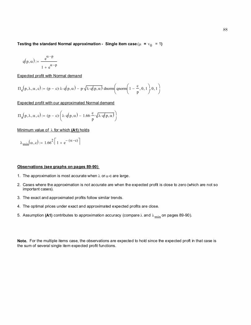
Testing the standard Normal approximation - Single item case (µ = v0 = 1)

q p α,( ) eα p−

1 eα p−+

:=

Expected profit with Normal demand

Πe p λ, α, c,( ) p c−( ) λ⋅ q p α,( )⋅ p λ q p α,( )⋅⋅ dnorm qnorm 1cp

− 0, 1,

0, 1,

⋅−:=

Expected profit with our approximated Normal demand

Πa p λ, α, c,( ) p c−( ) λ q p α,( )⋅ 1.66cp

⋅ λ q p α,( )⋅⋅−

⋅:=

Minimum value of λ for which (A1) holds

λmin α c,( ) 1.662 1 e α c−( )−+ ⋅:=

Observations (see graphs on pages 89-90)

1. The approximation is most accurate when λ or α-c are large.

2. Cases where the approximation is not accurate are when the expected profit is close to zero (which are not so important cases).

3. The exact and approximated profits follow similar trends.

4. The optimal prices under exact and approximated expected profits are close.

5. Assumption (A1) contributes to approximation accuracy (compare λ and λmin on pages 89-90).

Note. For the multiple items case, the observations are expected to hold since the expected proft in that case isthe sum of several single item expected profit functions.

Bacel

88

10 15 200

50Πe p 100, 10, 8,( )

Πa p 100, 10, 8,( )

p10 15 20

0

10

20

Πe p 30, 10, 8,( )

Πa p 30, 10, 8,( )

p

λmin 10 8,( ) 3.129=λmin 10 8,( ) 3.129=

10 15 20

0

2

4

Πe p 10, 10, 8,( )

Πa p 10, 10, 8,( )

p10 15 20

1

0.5

0

0.5

Πe p 4, 10, 8,( )

Πa p 4, 10, 8,( )

p

λmin 10 8,( ) 3.129=

λmin 10 8,( ) 3.129=

10 15 20

0

5

Πe p 30, 8.5, 8,( )

Πa p 30, 8.5, 8,( )

p10 15 20

1

0

1

Πe p 10, 8.5, 8,( )

Πa p 10, 8.5, 8,( )

p

λmin 8.5 8,( ) 4.427=λmin 8.5 8,( ) 4.427=

Bacel

Bacel

Bacel

Bacel

Bacel

Figure A.2. Graphical Comparison of the exact and the approximate expected profits.

Bacel

89

Bacel

0

10 15 20

1

0.5

0

Πe p 5, 8.5, 8,( )

Πa p 5, 8.5, 8,( )

p10 15 20

0

2

4

6

Πe p 30, 8.1, 8,( )

Πa p 30, 8.1, 8,( )

p

λmin 8.1 8,( ) 5.249=λmin 8.5 8,( ) 4.427=

10 15 20

1

0.5

0

0.5

Πe p 10, 8.1, 8,( )

Πa p 10, 8.1, 8,( )

p10 15 20

1

0.5

0

Πe p 6, 8.1, 8,( )

Πa p 6, 8.1, 8,( )

p

λmin 8.1 8,( ) 5.249=λmin 8.1 8,( ) 5.249=

10 15 20

1

0

1

2

Πe p 100, 6, 8,( )

Πa p 100, 6, 8,( )

p10 15 20

1

0

1

Πe p 60, 6, 8,( )

Πa p 60, 6, 8,( )

p

λmin 6 8,( ) 23.117=λmin 6 8,( ) 23.117=

Bacel

Bacel

Bacel

Figure A.3. Graphical Comparison of the exact and the approximate expected profits.

Bacel

90

91

Appendix B. Proof of Lemma 3.1.1

The proof is by contradiction. Consider an optimal assortment S∗, and let S+ ⊂ S∗ and S− ⊂

S∗ denote the subsets of items having positive contribution and nonpositive contribution to the

expected profit, respectively. Under Assumption (A1), Π(i, c+i) > 0 and, consequently, S+ is not

empty. By contradiction, assume that S− is also not empty. Noting that Πi(S∗,p∗, αj) = (p∗i −

ci)[λqi(S∗,p∗, αj) − a ci

p∗i

√λqi(S∗,p∗, αj)

]and ∂qi(S

∗,p∗,αj)∂αj

= −(1/µ)qi(S∗,p∗, αj)qj(S∗,p∗, αj) < 0

for i, j ∈ S∗, i = j, we derive

∂Πi(S∗,p∗, αj)∂αj

= (p∗i − ci)∂qi(S∗,p∗, αj)

∂αj(1/qi(S∗,p∗, αj)

[λqi(S∗,p∗, αj) − a

2cip∗i

√λqi(S∗,p∗, αj)

]

< (1/qi(S∗,p∗, αj))∂qi(S∗,p∗, αj)

∂αjΠi(S∗,p∗, αj), by definition of Πi(S∗,p∗, αj),

< 0, in the range where Πi(S∗,p∗, αj) > 0. (6.1)

Since, by definition, Πi(S∗,p∗, αj) > 0 for i ∈ S+, (6.1) implies that ∂Πi(S∗,p∗,αj)∂αj

< 0 in the

decreasing direction of αj . Hence, Πi(S∗,p∗, αj) remains positive and increases as αj decreases.

Next consider an assortment S ′ = S∗ \ j, where j ∈ S−. Let p∗−j = (p∗1, . . . , p∗j−1, p

∗j+1, . . . p

∗|S∗|),

denote the optimal price vector for S∗, corresponding to the items in S ′. Noting that S ′ is equivalent

to S∗ with αj = −∞ (since limαj→−∞ qj(S∗,p∗, αj) → 0), it follows that

Πi(S ′,p∗−j) > Πi(S∗,p∗), i, j ∈ S∗, i = j, (by (6.1)),

which implies that Π(S ′,p∗−j) > Π(S∗,p∗). This contradicts with the optimality of S∗. Therefore,

S− must be empty. This proves the first part of the lemma.

Now we can show that p∗ is an internal point solution. Denote by Πi(S∗, pi,p∗−i), the expected

92

contribution of i ∈ S∗ when the prices of other items are fixed at their optimal values in S∗. It

can be easily shown that Πi(S∗, ci,p∗−i) = 0 and limpi→∞ Πi(S∗, pi,p∗

−i) → 0−. Moreover, as proved

above, under (A1) Πi(S∗, p∗i ,p∗−i) = Πi(S∗,p∗) > 0, for all i ∈ S∗. Thus, it must be true that

ci < p∗i <∞, i ∈ S∗, and, therefore, ∂Π(S∗,p∗)∂pi

∣∣∣p=p∗= 0.

Appendix C. Structure of the optimal assortment

The following lemmas are utilized to support the proofs of the results in Section 3.2.

Lemma 6.2.1 below is presented as an exercise in Mangasarian [60] (p. 148) and Bazaraa et al. [9] (p. 123).

In the following, we provide a proof for it for the sake of completeness.

Lemma 6.2.1 Consider the function π(x) = θ(x)/δ(x) defined over an open set Γ ⊂ . If θ(x) is a

strictly convex function and δ(x) is a positive linear function, then π(x) is strictly pseudoconvex.

Proof. We need to show that for all x1, x2 ∈ Γ, if ∇π(x1)(x2 − x1) ≥ 0, then π(x2) > π(x1), where

∇π(x1) = ∂π(x)∂x

∣∣∣x=x1

, (see, for example, Bazaraa et al. [9], pp. 113-114). Note that

∇π(x1) =∇θ(x1)δ(x1) − θ(x1)∇δ(x1)

(δ(x1))2 .

Note also that since θ(x) is a convex function, then θ(x2)− θ(x1) > ∇θ(x1) (x2 − x1). Furthermore,

since δ(x) is linear, then ∇δ(x1) (x2 − x1) = δ(x2) − δ(x1). Upon replacement and simplification, it

follows that if ∇π(x1)(x2 − x1) ≥ 0, then

δ(x2)δ(x1)

(θ(x2)δ(x2)

− θ(x1)δ(x1)

)> 0,

which implies that π(x2) > π(x1).

93

Lemma 6.2.2 Consider an assortment S ⊆ Ω. Assume that prices of items in S are fixed at

some price vector p. Then, the expected profit from S, Π(S,p, vi), is strictly pseudoconvex in vi ≡

e(αi−pi)/µ, i ∈ S.

Proof. Note that qi(S,p) = vi/(v0 +∑

j∈S vj), i ∈ S. Then, Π(S,p) can be written as Π(vi) =

θ(vi)/δ(vi), i ∈ S,where θ(vi) = (K1+K2vi)−(K3+K4v1/2i )(K5+vi)1/2 , with K1 =

∑j =i,j∈S

(pj − cj)λvj

> 0, K2 = (pi − ci)λ > 0, K3 =∑

j =i,j∈S(pj − cj)a

cj

pj

√λ√vj > 0, K4 = (pi − ci)a ci

pi

√λ > 0, K5 =

∑j =i,j∈S

vj + v0 > 0, and δ(vi) =∑

j =i,j∈Svj + v0 + vi. Upon differentiation and simplification, it follows

that ∂2θ(vi)∂v2

i= 1

4(K5 + vi)−3/2(K4K25v

−3/2i +K3) > 0. Therefore, θ(vi) is strictly convex in vi. On the

other hand, δ(vi) is linear in vi. Applying Lemma 6.2.1, it follows that Π(vi) is strictly pseudoconvex

in vi, i ∈ S.

Lemma 6.2.3 Consider two real functions v(x) and π(x) defined on . If v(x) is increasing in x

and π(v(x)) is strictly pseudoconvex in v(x), then π(v(x)) is strictly pseudoconvex in x.

We need to show that for all x1, x2, if ∇π(v(x1))(x2 − x1) ≥ 0, then π(v(x2)) > π(v(x1)). Since v is

increasing in x, then x2−x1 is of the same sign as v(x2)−v(x1). Therefore, if ∇π(v(x1))(x2−x1) ≥ 0,

then ∇π(v(x1))(v(x2)− v(x1)) ≥ 0. Since π is strictly pseudoconvex in v, the last inequality implies

that π(v(x2)) > π(v(x1)).

Lemma 6.2.4 Consider an assortment S ⊆ Ω. Assume that the prices of items in S are fixed at

some price vector p and Πi(S,p, αi) > 0 when αi = α′i, for some i ∈ S. Then, Πi(S,p, αi) is

increasing in αi for αi ≥ α′i.

Proof. Similar to the proof of Lemma 3.1.1, the derivative of Πi(S,p, αi) with respect to αi, i ∈ S,

94

is given by

∂Πi(S,p, αi)∂αi

= (pi − ci)∂qi(S,p, αi)

∂αi(1/qi(S,p, αi))

[λqi(S,p, αi) − a

2cipi

√λqi(S,p, αi)

]

> (1/qi(S,p, αi))∂qi(S,p, αi)

∂αiΠi(S,p, αi),

where the inequality follows by definition of Πi(S,p, αi) and since ∂qi(S,p,αi)∂αi

= (1/µ)qi(S,p, αi)(1 −

qi(S,p, αi)) > 0. Using an argument similar to that in the proof of Lemma 3.1.1, it follows that

∂Πi(S,p,αi)∂αi

> 0, in the increasing direction of αi. That is, Πi(S,p, αi) remains positive and increases

as αi increases.

Next, we present proofs for the results in Section 3.2.

Proof of Lemma 3.2.1. For any fixed price vector p, Π(S,p, vi) is strictly pseudoconvex in vi

by Lemma 6.2.2, and vi is increasing in αi. Then, Lemma 6.2.3 implies that Π(S,p, αi) is strictly

pseudoconvex in αi, i ∈ S.

Proof of Lemma 3.2.2. Lemma 3.2.1 implies that Π(S∗,p∗, αi) is strictly pseudoconvex in αi, i ∈

S∗, when prices of items in S∗ are fixed at p∗. Therefore, it is sufficient to show that Π(S∗,p∗, αi) is

increasing in αi at αi = α′i. By contradiction, assume that Π(S∗,p∗, αi) is nonincreasing in αi at αi =

α′i. Then, the strict pseudoconvexity of Π(S∗,p∗, αi) in αi implies that Π(S∗,p∗, αi) is decreasing in

αi, for αi < α′i, and hence Π(S∗,p∗,−∞) > Π(S∗,p∗, α′

i), or equivalently Π(S∗\i,p∗−i) > Π(S∗,p∗)

(since setting αi = −∞ is equivalent to removing i from S∗), which contradicts with the optimality

of S∗.

Proof of Lemma 3.2.3. Note that ∂Π(S,p,ci)∂ci

= ∂Πi(S,p,ci)∂ci

= −Πi(S,p,ci)pi−ci

+ a√λqi(S,p)

(cipi

− 1).

Therefore, if Πi(S,p, c′i) > 0, then it can be shown, in a similar way to the proof of Lemma 3.1.1,

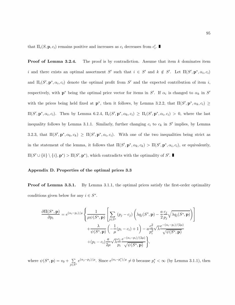
95

that Πi(S,p, ci) remains positive and increases as ci decreases from c′i.

Proof of Lemma 3.2.4. The proof is by contradiction. Assume that item k dominates item

i and there exists an optimal assortment S ′ such that i ∈ S ′ and k /∈ S ′. Let Π(S ′,p∗, αi, ci)

and Πi(S ′,p∗, αi, ci) denote the optimal profit from S ′ and the expected contribution of item i,

respectively, with p∗ being the optimal price vector for items in S ′. If αi is changed to αk in S ′

with the prices being held fixed at p∗, then it follows, by Lemma 3.2.2, that Π(S ′,p∗, αk, ci) ≥

Π(S ′,p∗, αi, ci). Then by Lemma 6.2.4, Πi(S ′,p∗, αk, ci) ≥ Πi(S ′,p∗, αi, ci) > 0, where the last

inequality follows by Lemma 3.1.1. Similarly, further changing ci to ck in S ′ implies, by Lemma

3.2.3, that Π(S ′,p∗, αk, ck) ≥ Π(S ′,p∗, αi, ci). With one of the two inequalities being strict as

in the statement of the lemma, it follows that Π(S ′,p∗, αk, ck) > Π(S ′,p∗, αi, ci), or equivalently,

Π(S ′ ∪ k \ i,p∗) > Π(S ′,p∗), which contradicts with the optimality of S ′.

Appendix D. Properties of the optimal prices 3.3

Proof of Lemma 3.3.1. By Lemma 3.1.1, the optimal prices satisfy the first-order optimality

conditions given below for any i ∈ S∗.

∂Π(S∗,p)∂pi

= e(αi−pi)/µ

1µψ(S∗,p)

∑

j∈S∗(pj − cj)

(λqj(S∗,p)− a

2cjpj

√λqj(S∗,p)

)

+λ

ψ(S∗,p)

(−1µ

(pi − ci) + 1)− a

c2ip2

i

√λe−(αi−pi)/(2µ)√

ψ(S∗,p)

+(pi − ci)a

2µ

√λcipi

e−(αi−pi)/(2µ)√ψ(S∗,p)

,

where ψ(S∗,p) = v0 +∑

j∈S∗e(αj−pj)/µ. Since e(αi−p∗i )/µ = 0 because p∗i <∞ (by Lemma 3.1.1), then

96

setting ∂Π(S∗,p)∂pi

= 0 and dividing by (λ/ψ(S∗,p)) yields

1µ

(p∗i − ci)

(1 − a

2cip∗i

1√λqi(S∗,p∗)

)+ a

c2ip∗i

2

1√λqi(S∗,p∗)

= Υ(S∗,p∗),

where Υ(S∗,p∗) = 1 + 1µλ

∑j∈S∗

(p∗j − cj)(λqj(S∗,p∗)− a

2cj

p∗j

√λqj(S∗,p∗)

). Noting that Υ(S∗,p∗) is

the same for all i ∈ S∗ yields the result in the lemma.

The following result is utilized in the proof of Lemma 3.3.2.

Lemma 6.2.5 Consider item i ∈ Ω. Then, either Πi(i, pi) > 0 on exactly one interval of pi ∈

(ci,∞), or Πi(i, pi) ≤ 0 for all pi ∈ (ci,∞).

Proof. Setting Πi(i, pi) = 0 for pi ∈ (ci,∞), implies that

hi(pi) =a2c2iλ

, (6.2)

where hi(pi) ≡ p2i qi(i, pi) (or, equivalently, πi(pi) = 0). In the following, we prove that hi(pi) is

unimodal in pi ≥ 0. Note that hi(0) = 0, hi(pi) > 0 for 0 < pi < ∞, and limpi→+∞ hi(pi) → 0+.

Therefore, hi(pi) attains a maximum in (0,∞). Next we show that this maximum is unique by

showing that ∂hi(pi)∂pi

has a single zero in (0,∞). Note that ∂hi(pi)∂pi

= 2piqi(i, pi) − p2iµ qi(i, pi)(1 −

qi(i, pi)). Setting ∂hi(pi)∂pi

= 0 yields pi(1 − qi(i, pi) = 2µ. It can be easily shown that the left

hand side of this equation is increasing in pi. Therefore, the equation has a unique solution. Hence,

it follows that hi(pi) is unimodal in pi ≥ 0. This, together with the fact that the right hand side of

(6.2) is constant in pi, implies that Πi(i, pi) has at most two zeroes on in (ci,∞). (Observe that a

unimodal function can take on the same value at most twice.)

Define hmaxi ≡ maxpi>0 hi(pi). Note that it can be easily shown that for pi large enough (pi → ∞),

97

Πi(i, pi) < 0. Therefore, (1) if hmaxi ≤ a2c2i /λ, then (6.2) has at most one solution (equivalently,

Πi(i, pi) has at most one zero in pi ∈ (ci,∞)). Then, Πi(i, pi) ≤ 0 for all pi ∈ (ci,∞); (2) if

hmaxi > a2c2i /λ, then (6.2) has two solutions, pi and pi with pi < pi. Then, (2.a) if pi < pi ≤ ci, then

Πi(i, pi) ≤ 0 for all pi ∈ (ci,∞); (2.b) if ci < pi < pi, then Πi(i, pi) > 0 for pi ∈ (pi, pi), and

Πi(i, pi) ≤ 0 otherwise (within the (ci,∞) region); (2.c) if pi ≤ ci < pi, then Πi(i, pi) > 0 for

pi ∈ (ci, pi), and Πi(i, pi) ≤ 0 otherwise (within the (ci,∞) region).

Proof of Lemma 3.3.2. Recall that (6.2) is equivalent to Πi(i, pi) = 0 for pi ∈ (ci,∞). Note

also that Πi(i, pi) > Πi(S, pi,p−i), for all pi > ci in the region where Πi(S, pi,p−i) > 0, since

Πi(S, pi,p−i) > 0 increases as αj decreases, j = i, j ∈ S, as shown in the proof of Lemma 3.1.1, and

Πi(i, pi) is equivalent to Πi(S, pi,p−i) with αj = −∞, j = i, j ∈ S. This, together with Lemma

6.2.5, yields the desired result.

Proof of Corollary 3.3.1. Lemmas 3.2.3 and 6.2.4 imply that Πi(i, pi) ≥ Πi(i, pi) for all

pi > ci in the region where Πi(i, pi) > 0. This, together with Lemma 3.3.2, yields the desired

result. Note that by Assumption (A1), Πi(i, pi) > 0 for pi ∈ (maxc

i, p, p).

Appendix E. Structural results on p∗k

Proof of Lemma 4.2.1. Let γ1(p, k) =√λq(p, k) − a c

p . It can be shown that γ1(p) is concave

when q(p, k) ≥ 1/3 as

∂2γ1(p, k)∂p2

=1

4µ2

√λq(p, k)(1− kq(p, k))(1− 3kq(p, k))− 2a

c

p3< 0.

98

Let γ2(p, k) = k(p− c)√λq(p, k). Then for q(p, k) ≥ 1/3,

∂2γ2(p, k)∂p2

= −kµ

√λq(p, k)(1− kq(p, k)) + k(p− c)

14µ2

√λq(p, k)(1 − kq(p, k))(1− 3kq(p, k)) < 0.

Thus, γ2(p, k) is also concave for q(p, k) ≥ 1/3. A result in Mangasarian [60] (p. 149), which can be

proven in a similar way to Lemma 6.2.1, states that the product of two positive concave functions is

pseudoconcave. Therefore, Π(p, k) = γ2(p, k)γ1(p, k) is pseudoconcave in p in the range q(p, k) ≥ 1/3

and Π(p, k) > 0. (Note that if Π(p, k) > 0, then γ1(p, k) > 0.)

Appendix F. Monotonicity results on p∗k

Proof of Theorem 4.2.1. Since under (A2) p∗k is an internal point solution, ∂Π(p,k)∂p

∣∣∣p=p∗k

= 0 and

∂2Π(p,k)∂p2

∣∣∣p=p∗k

< 0. To prove part (i), differentiate ∂Π(p,k)∂p

∣∣∣p=p∗k

with respect to k. Then by implicit

differentiation, we can obtain

∂

∂k

(∂Π(p, k)∂p

∣∣∣∣p=p∗k

)=∂2Π(k, p)∂p2

∣∣∣∣∣p=p∗

k

∂p∗k∂k

+∂2Π(k, p)∂k∂p

∣∣∣∣∣p=p∗

k

= 0.

Therefore, ∂p∗k∂k = −

(∂2Π(k,p)

∂k∂p

∣∣∣p=p∗

k

)/(∂2Π(k,p)

∂p2

∣∣∣p=p∗

k

), and ∂p∗k

∂k is of the same sign as ∂2Π(k,p)∂k∂p

∣∣∣p=p∗

k

.

In the following we show that ∂2Π(k,p)∂k∂p

∣∣∣p=p∗

k

> 0 if p∗k ≥ 3c2 , which completes the proof of (i).

We have

∂Π(p, k)∂p

=Π(p, k)p− c

+ k(p− c)

(λ∂q(p, k)∂p

+ ac

p2

√λq(p, k)− a

c

2p

√λ

q(p, k)∂q(p, k)∂p

). (6.3)

99

Setting ∂Π(p,k)∂p = 0 implies that

λ∂q(p, k)∂p

− ac

p2

√λ

(12q(p, k)−

12 p∂q(p, k)∂p

− q(p, k)12

)= − Π(p, k)

k(p− c)2. (6.4)

Differentiating (6.3) with respect to k, we have

∂2Π(p, k)∂k∂p

=1k

(Π(p, k)p− c

+ k(p− c)

(λ∂q(p, k)∂p

+ ac

p2

√λq(p, k)− a

c

2p

√λ


))

+k(λ∂q(p, k)∂k

− a√λc

2pq(p, k)−

12∂q(p, k)∂k

)+ k(p− c)λ

∂2q(p, k)∂p∂k

−k(p− c)ac

p2

√λ

(−p

4q(p, k)−

32∂q(p, k)∂k

∂q(p, k)∂p

+p

2q(p, k)−

12∂2q(p, k)∂p∂k

−12q(p, k)−

12∂q(p, k)∂k

).

Recall that ∂Π(p,k)∂p

∣∣∣p=p∗k

= 0. Note also that ∂q(p,k)∂k = −q(p, k)2 and ∂2q(p,k)

∂p∂k = −2q(p, k)∂q(p,k)∂p .

Applying (6.3) with the fact that ∂Π(p,k)∂p

∣∣∣p=p∗k

= 0 and simplifying leads to

∂2Π(p, k)∂k∂p

∣∣∣∣∣p=p∗

k

= k

(−λq(p∗k, k)2 + a

c

2p∗k

√λq(p∗k, k)

32

)

−k(p∗k − c)q(p∗k, k)

2λ∂q(p∗k, k)

∂p− a

c

p∗k2

√λ

(34p∗kq(p

∗k, k)

− 12∂q(p∗k, k)

∂p− 1

2q(p∗k, k)

12

).

Applying (6.4) to the term in the curly brackets and simplifying yields

∂2Π(p, k)∂k∂p

∣∣∣∣∣p=p∗k

= k

(−λq(p∗k, k)2 + a

c

2p∗k

√λq(p∗k, k)

32

)+ 2

Π(p∗k, k)p∗k − c

+k(p∗k − c)q(p∗k, k)ac

p∗k2

√λ

(−1

4p∗kq(p

∗k, k)

− 12∂q(p∗k, k)

∂p+

32q(p∗k, k)

12

).

100

Replacing Π(p∗k, k) by its expression in (4.3) and simplifying yields

∂2Π(p, k)∂k∂p

∣∣∣∣∣p=p∗

k

= kλq(p∗k, k)2 + k

√λa

c

p∗k

(−(p∗k − c)

4q(p∗k, k)

12∂q(p∗k, k)

∂p− 3

2c

p∗kq(p∗k, k)

32

).

Utilizing the fact that ∂q(p∗k,k)

∂p = − 1µq(p

∗k, k)(1− kq(p∗k, k)) and further simplifying gives

∂2Π(p, k)∂k∂p

∣∣∣∣∣p=p∗k

= kq(p∗k, k)

(λq(p∗k, k)− a

c

4p∗k

√λq(p∗k, k)

(6c

p∗k− 1µ

(p∗k − c)(1− kq(p∗k, k)

)).

Thus, it follows that ∂p∗k∂k is of the same sign as

W (p, k) = λq(p∗k, k) − ac

4p∗kt(p∗k, k)

√λq(p, k),

where t(p∗k, k) = 6 cp∗

k− 1

µ(p∗k − c)(1− kq(p∗k, k). Observe that since Π(p∗k, k) > 0, we have λq(p∗k, k)−

a cp

√λq(p, k) > 0. Then, W (p, k) > 0 if t(p∗k, k) ≤ 4. Observe also that t(p, k) is decreasing in p ≥ c

with a maximizer p = c and a maximum value of t(c, k) = 6. Then, there exists pck such that for p∗k >

pck, t(p

∗k, k) < 4 (i.e., t(pc

k, k) = 4). Note finally that t( 3c2 , k) = 4 − 1

µc2 (1 − kq( 3c

2 , k)) < S(pck, k) = 4,

which implies that pck <

3c2 . Therefore, if p∗k ≥ 3c

2 , then p∗k > pck and W (p, k) > 0, which also imply

that ∂p∗k∂k > 0.

The proof of (ii) is more straightforward. Denote Π(p, k) as Π(p, λ). Similar to the above, ∂p∗k∂λ is

of the same sign as ∂2Π(p,λ)∂p∂λ

∣∣∣p=p∗

k

. Setting ∂Π(p,λ)∂p = 0 implies that

∂q(p)∂p

∣∣∣∣p=p∗

k

= −λq(p∗k) − a c2

p2

√λq(p∗k)

(p∗k − c)(λ− a c

2p∗k

√λ

q(p∗k)

) . (6.5)

101

Differentiating Π(p, λ) with respect to λ, we have

∂Π(p, λ)∂λ

= (p− c)

(q(p)− ac

2p√λ

√q(p)

)=

Π(p, λ)λ

+(p− c)λ

ac

2p

√λq(p).

Differentiating the last equation with respect to p, we have

∂2Π(p, λ)∂p∂λ

=1λ

(∂Π(p, λ)∂p

+ac2

2p2

√λq(p) + (p− c)

ac

4p

√λ

q(p)∂q(p)∂p

).

Therefore, since ∂Π(p,λ)∂p

∣∣∣p=p∗

k

= 0, then ∂2Π(p,λ)∂p∂λ

∣∣∣p=p∗

k

is of the same sign as

W1(p∗k, λ) =ac2

2p∗k2

√λq(p∗k) + (p∗k − c)

ac

4p∗k

√λ

q(p∗k)∂q(p)∂p

∣∣∣∣p=p∗k

.

Utilizing (6.5), we have

W1(p∗k, k) =λ ac

2p

√λq(p∗k)

(2c−p∗k2p∗

k

)(λ− a c

2p∗k

√λ

q(p∗k)

) ,

where(λ− a c

2p∗k

√λ

q(p∗k)

)> 0 since Π(p∗k, λ) > 0. Therefore, W1(p∗k, k) > 0 if p∗k < 2c and W1(p∗k, k) <

0 if p∗k > 2c. This completes the proof of (ii).

The proof of (iii) is similar to that of (ii). Denote Π(p, k) as Π(p, c). Similar to the above, ∂p∗k

∂c is

of the same sign as ∂2Π(p,c)∂p∂c

∣∣∣p=p∗

k

. Differentiation implies that

∂Π(p, c)∂c

= −Π(p, c)p− c

− k(p− c)a

p

√λq(p),

∂2Π(p, c)∂p∂c

= − 1p − c

∂Π(p, c)∂p

+Π(p, c)(p− c)2

− ka

p

√λq(p) + k(p− c)

a

p2

√λq(p)

−k(p− c)a

2p

√λ

q(p)∂q(p)∂p

.

102

The facts that Π(p∗k, c) > 0 and ∂Π(p,c)∂p

∣∣∣∣∣p=p∗

k

= 0 imply that ∂Π(p,c)∂p∂c

∣∣∣p=p∗

k

> 0 if W2(p∗k, c) > 0, where

W2(p∗k, c) = −ka c

p∗k2

√λq(p∗k) − k(p∗k − c)

a

2p∗k

√λ

q(p∗k)∂q(p)∂p

∣∣∣∣p=p∗k

.

Utilizing (6.5), we have

W2(p∗k, c) = kλa

2p∗k2

√λq(p∗k)

p∗k − 2c

λ− a c2p∗

k

√λ

q(p∗k)

.

Therefore, W2(p∗k, c) > 0 if p∗k > 2c, which completes the proof of (iii).

Appendix G. Riskless Case

Proof of Theorem 4.2.2. Parts (i) and (ii) follow directly by setting a = 0 in the proof of

Theorem 4.2.1. To prove (iii), we adopt a more direct approach. Note that ∂p0k

∂α is of the same sign

as ∂2Π0(p,α)∂α∂p

∣∣∣p=p0

k

. The fact that ∂Π0(p,α)∂p

∣∣∣p=p0

k

= 0 (from Corollary 4.2.3) implies that

q(p0k) = −(p0

k − c)∂q(p, α)∂p

∣∣∣∣p=p0

k

.

In addition, it can be shown that

∂2Π0(p, α)∂α∂p

= kλ∂q(p, α)∂α

+ kλ(p− c)∂2q(p, α)∂α∂p

,

where ∂q(p,α)∂α = 1

µq(p, α)(1− kq(p, α)) and ∂2q(p,α)∂α∂p = 1

µ∂q(p,α)

∂p (1 − 2kq(p, α)). Then,

∂2Π0(p, α)∂α∂p

∣∣∣∣∣p=p0

k

=kλ

µ

(q(p0

k, α))2> 0,

103

which completes the proof.

Appendix H. Structural results on k∗p

Proof of Theorem 4.3.1. Assume k is a continuous variable. Rewrite (3.5) as Π(p, k) = θ(p, k)/δ(p, k),

where

θ(p, k) = (p− c)(λe(α−p)/µk − a

c

pk√λe(α−p)/µ

(1 + ke(α−p)/µ

)1/2),

and δ(p, k) = 1 + ke(α−p)/µ. Clearly, δ(p, k) is linear in k. Moreover, θ(p, k) is strictly concave in k

as

∂2θ(p, k)∂k2

= −(p− c)ac

pλ

12

(e(α−p)/µ

)32(1 + ke(α−p)/µ

)− 32

(1 +

34ke(α−p)/µ

)< 0.

A result in Mangasarian [60] (p. 149) implies that the function obtained by dividing a concave function

by a linear positive function is pseuodoconcave. (It can be easily verified, utilizing arguments like

those in the proof of Lemma 6.2.1, that a similar result holds under strict concavity.) Therefore,

Π(p, k) = θ(p, k)/δ(p, k) is strictly pseudoconcave in k. To prove that Π(p, k) is unimodal in k (since

a pseudoconcave function can be either unimodal or monotone), it is sufficient to show that Π(p, k)

attains a maximum in k ∈ (1,∞); see, for example, Bazaraa et al., p. 116 and 123. Note that Π(p, k)

is increasing in k at k = 1 under (A3) with Π(p, 1) > 0. In addition, it can be easily shown that

limk→∞ Π(p, k) → 0−. Thus, it follows that Π(p, k) starts as an increasing function at k = 1 and

becomes decreasing at some k > 1. Therefore, Π(p, k) attains a local maximum in k ∈ (1,∞), which

is the unique global maximum due to the strict pseudoconcavity of Π(p, k). This completes the proof.

104

Appendix I. Monotonicity results on k∗p

Proof of Theorem 4.3.2. Theorem 4.3.1 implies that ∂Π(p,k)∂k

∣∣∣k=k∗

p

= 0 and ∂2Π(p,k)∂k2

∣∣∣k=k∗

p

< 0. To

prove part (i), denote Π(p, k) as Π(k, c) and note that ∂k∗p

∂c is of the same sign as ∂2Π(k,c)∂c∂k

∣∣∣k=k∗p

(similar

to the proof of Theorem 4.2.1). We have

∂Π(k, c)∂k

= (p− c)

λq(k)− a

c

p

√λq(k) + k

∂q(k)∂k

(λ− a

c

2p

√λ

q(k)

). (6.6)

Then,

λq(k)− ac

p

√λq(k) + k

∂q(k)∂k

(λ− a

c

2p

√λ

q(k)

)∣∣∣∣∣k=k∗

p

= 0, (6.7)

which also implies that

∂q(k)∂k

∣∣∣∣k=k∗

p

= −(λq(k)− a c

p

√λq(k)

)k(λ− a c

2p

√λ

q(k)

)∣∣∣∣∣∣k=k∗

p

. (6.8)

Differentiating (6.6) with respect to c at k = k∗p yields

∂2Π(k,c)∂c∂k

∣∣∣k=k∗

p

= −(λq(k)− a c

p

√λq(k)

)+ k ∂q(k)

∂k

(λ− a c

2p

√λ

q(k)

) ∣∣∣∣k=k∗

p

+ (p− c)(−a

p

√λq(k)− a

2pk∂q(k)∂k

√λ

q(k)

)∣∣∣k=k∗

p

.

Applying (6.7) and (6.8),

∂2Π(k,c)∂c∂k

∣∣∣k=k∗

p

= −ap (p− c)

√λq(k∗p) −

(λq(k∗

p)−a cp

√λq(k∗

p))√

λq(k∗p)

2

(λ−a c

2p

√λ

q(k∗p)

)

= −ap (p− c)

λ

√λq(k∗

p)

2

(λ−a c

2p

√λ

q(k∗p)

) < 0,

where the last inequality follows since λ− a c2p

√λ

q(k∗p) > λ− a c

p

√λ

q(k∗p) = Π(k∗

p ,c)

k∗p(p−c)q(k∗

p) , and Π(k∗p, c) > 0

105

under (A2). This completes the proof of (i).

The proof of (ii) is similar. ∂k∗p

∂λ is of the same sign as ∂2Π(k,λ)∂λ∂k

∣∣∣k=k∗p

. Differentiating (6.6) with

respect to λ at k = k∗p and simplifying yields

∂Π(k, λ)∂λ∂k

∣∣∣∣k=k∗

p

=(p− c)

2λ

(λq(k)− a

c

p

√λq(k)

)+ k

∂q(k)∂k

(λ− a

c

2p

√λ

q(k)

) ∣∣∣k=k∗

p

+(p− c)

2

(q(k) + k

∂q(k)∂k

)∣∣∣∣k=k∗

p

.

Applying (6.7) and (6.8),

∂Π(k, λ)∂λ∂k

∣∣∣∣k=k∗

p

=(p− c)

2

q(k∗p) −

(λq(k∗p) − a c

p

√λq(k∗p)

)(λ− a c

2p

√λ

q(k∗p)

)=

(p− c)a cp

√λq(k∗p)

4(λ− a c

2p

√λ

q(k∗p)

) > 0,

which completes the proof.

Proof of Theorem 4.3.3. To prove (i), note that ∂k∗p

∂p is of the same sign as ∂2Π(p,k)∂k∂p

∣∣∣k=k∗p

. Note

also that (6.8) implies that

1k∗p

(λq(p, k∗p)−

ac

p

√λq(p, k∗p)

)= λ(q(p, k∗p))

2 − ac

2p

√λ(q(p, k∗p))

3/2. (6.9)

By differentiating Π(p, k) with respect to p then with respect to k and simplifying, it follows that

∂2Π(p, k)∂k∂p

=1

p− c

∂Π(p, k)∂k

+ (p− c)

(λ∂q(p, k)∂p

+ac

p2

√λq(p, k)− ac

2p

√λ


)

+ k(p− c)[−2λq(p, k)

∂q(p, k)∂p

− ac

2p2

√λ (q(p, k))3/2 +

34ac

p

√λq(p, k)

∂q(p, k)∂p

].

106

Then, ∂2Π(p,k)∂k∂p

∣∣∣k=k∗p


∆1(p, k∗p) =

λ∂q(p, k)∂p

+ac

p2

√λq(p, k)− ac

2p

√λ


+ k

[−2λq(p, k)

∂q(p, k)∂p

− ac

2p2

√λ (q(p, k))3/2 +

34ac

p

√λq(p, k)

∂q(p, k)∂p

]∣∣∣∣∣k=k∗

p

=

∂q(p, k)∂p

[(λ (q(p, k))2 − ac

2p

√λ (q(p, k))3/2

)(1

(q(p, k))2− 2

k

q(p, k)

)− k

ac

4p

√λq(p, k)

]

+ac

p2

√λq(p, k)

(1 − kq(p, k)

2

)∣∣∣∣∣k=k∗

p

.

Utilizing (6.9) and the fact that kq(p, k) ≤ 1, it follows that

∆1(p, k∗p) ≥∂q(p, k)∂p

[1k

(λq(p, k)− ac

p

√λq(p, k)

)(1

(q(p, k))2− 2

k

q(p, k)

)− k

ac

4p

√λq(p, k)

] ∣∣∣∣∣k=k∗

p

=∂q(p, k)∂p

(1 − 2kq(p, k)k(q(p, k))2

)[λq(p, k)− ac

p

√λq(p, k)

(1 +

k2(q(p, k))2

4(1− 2kq(p, k))

)] ∣∣∣∣∣k=k∗

p

.

Observe that kq(p, k) is increasing in k. Then, k∗p(p, k∗p) > q(p, 1). Therefore, if q(p, 1) > 1/2, then

k∗pq(p, k∗p) > 1/2. It follows that ∆1(p, k∗p) is of the same sign as

λq(p, k∗p) −ac

p

√λq(p, k∗p)

(1 +

k∗p2(q(p, k∗p))2

4(1− 2k∗pq(p, k∗p))

)> λq(p, k∗p)−

ac

p

√λq(p, k∗p) > 0,

where the last inequality follows since Π(p, k∗p) > 0 under (A3). This proves (i).

To prove (ii), it can be shown, similar to the proof of Theorem 4.3.2, that ∂k∗∂α is of the same sign

as ∂2Π(k,α)∂k∂α

∣∣∣k=k∗p

, where

∂Π(k, α)∂α

= k(p− c)∂q(k, α)∂α

(λ− a

c

2p

√λ

q(k, α)

),

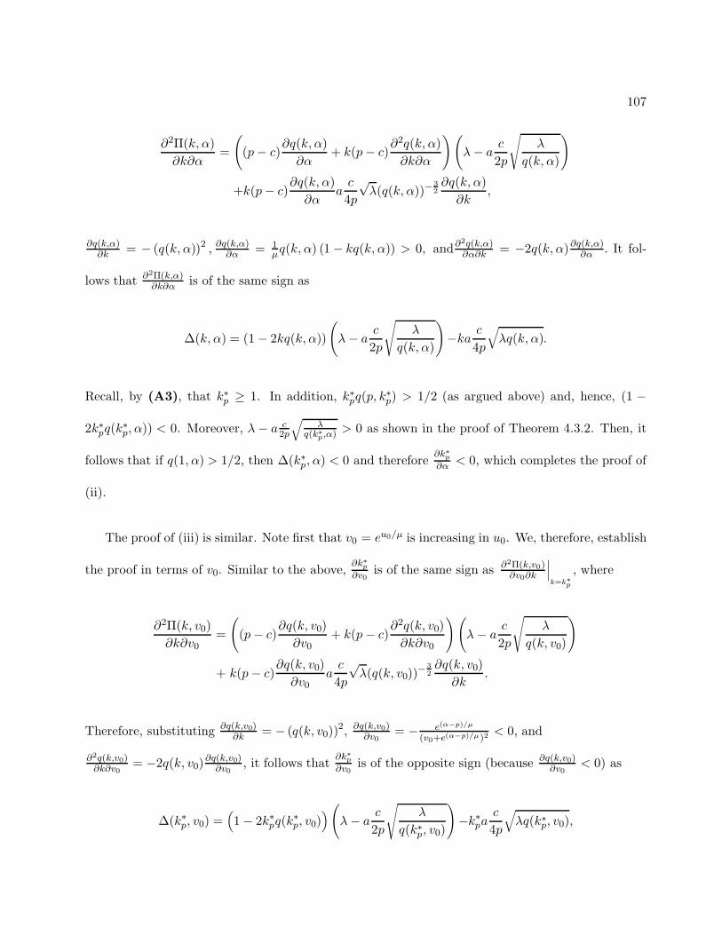
107

∂2Π(k, α)∂k∂α

=

((p− c)

∂q(k, α)∂α

+ k(p− c)∂2q(k, α)∂k∂α

)(λ− a

c

2p

√λ

q(k, α)

)

+k(p− c)∂q(k, α)∂α

ac

4p

√λ(q(k, α))−

32∂q(k, α)∂k

,

∂q(k,α)∂k = − (q(k, α))2 , ∂q(k,α)

∂α = 1µq(k, α) (1 − kq(k, α)) > 0, and∂2q(k,α)

∂α∂k = −2q(k, α)∂q(k,α)∂α . It fol-

lows that ∂2Π(k,α)∂k∂α is of the same sign as

∆(k, α) = (1 − 2kq(k, α))

(λ− a

c

2p

√λ

q(k, α)

)−ka c

4p

√λq(k, α).

Recall, by (A3), that k∗p ≥ 1. In addition, k∗pq(p, k∗p) > 1/2 (as argued above) and, hence, (1 −

2k∗pq(k∗p, α)) < 0. Moreover, λ− a c2p

√λ

q(k∗p ,α) > 0 as shown in the proof of Theorem 4.3.2. Then, it

follows that if q(1, α) > 1/2, then ∆(k∗p, α) < 0 and therefore ∂k∗p

∂α < 0, which completes the proof of

(ii).

The proof of (iii) is similar. Note first that v0 = eu0/µ is increasing in u0. We, therefore, establish

the proof in terms of v0. Similar to the above, ∂k∗p

∂v0is of the same sign as ∂2Π(k,v0)

∂v0∂k

∣∣∣k=k∗p

, where

∂2Π(k, v0)∂k∂v0

=

((p− c)

∂q(k, v0)∂v0

+ k(p− c)∂2q(k, v0)∂k∂v0

)(λ− a

c

2p

√λ

q(k, v0)

)

+ k(p− c)∂q(k, v0)∂v0

ac

4p

√λ(q(k, v0))−

32∂q(k, v0)

∂k.

Therefore, substituting ∂q(k,v0)∂k = − (q(k, v0))

2, ∂q(k,v0)∂v0

= − e(α−p)/µ

(v0+e(α−p)/µ)2< 0, and

∂2q(k,v0)∂k∂v0

= −2q(k, v0)∂q(k,v0)

∂v0, it follows that ∂k∗

p

∂v0is of the opposite sign (because ∂q(k,v0)

∂v0< 0) as

∆(k∗p, v0) =(1 − 2k∗pq(k

∗p, v0))(

λ− ac

2p

√λ

q(k∗p, v0)

)−k∗pa

c

4p

√λq(k∗p, v0),

108

where ∆(k∗p, v0) < 0 under (A3) and the condition that q(1, v0) > 1/2, as discussed above.

Appendix J. Bounds on p∗k

Proof of Lemma 4.4.1. Setting Π(p, k) = 0 for p ∈ (c,∞) implies that

p2q(p, k) =a2c2

λ. (6.10)

Let h(p, k) ≡ p2q(p, k). In the following we first prove that h(p, k) is unimodal in p for p ≥ 0. Note

that h(0, k) = 0, h(p, k) > 0 for 0 < p <∞, and limp→+∞ h(p, k) → 0+. Therefore, h(p, k) attains a

maximum on (0,∞). Next we prove that this maximum is unique by showing that the first derivative

of h(p, k) has a single zero on (0,∞). Note that

∂h(p, k)∂p

= 2pq(p, k) + p2 ∂q(p, k)∂p

= 2pq(p, k)− p2

µq(p, k)(1− kq(p, k)).

Setting ∂h(p,k)∂p = 0 yields

p(1− kq(p, k)) = 2µ.

It can be easily shown that the left hand side of this equation is increasing in p. Therefore, the

equation has a unique solution and hence it follows that h(p, k) is unimodal in p for p ∈ (0,∞).

Thus, the function γ1(p, k) =√λq(p, k)− a c

p has at most two zeroes in p ∈ (0,∞). (Observe that a

unimodal function can take on the same value at most twice.)

Note that Π(c, k) = 0, and (A2) implies that Π(p, k) > 0 for p to the right of c. In addition,

it can be easily shown that for p large enough (p → ∞), Π(p, k) < 0. Therefore, under (A2)

Π(p, k) = k(p−c)√λq(p, k)γ1(p, k) has two zeroes at points pk and pk, with pk ∈ (0, c] and pk ∈ (c,∞).

Then, it follows that Π(p, k) is positive for p ∈ (c, pk), and is negative otherwise (within the range

109

p > c), which implies that pk constitutes an upper bound on p∗k.

Proof of Corollary 4.4.1. Follows since it can be shown that Π(p, 1) > Π(p, k)/k for all p ∈ (c,∞)

and k = 2, 3, . . .. Then, p1 > pk for all k = 2, 3, . . ..

Proof of Lemma 4.4.2. The first derivative of Π(p, k) is given by

∂Π(p, k)∂p

= k

(λq(p, k)− a

c

p

√λq(p, k)

)

+ k(p− c)

(λ∂q(p, k)∂p

+ ac

p2

√λq(p, k)− a

c

2p

√λ


),

where ∂q(p,k)∂p = − 1

µq(p, k) (1 − kq(p, k)). Setting ∂Π(p,k)∂p = 0 and simplifying leads to

√λq(p, k)

(1 − (p− c)

µ(1− kq(p, k))

)= a

c

2p

(2cp

− (p− c)µ

(1 − kq(p, k))).

Letting w1(p, k) ≡ 1 − (p−c)µ (1 − kq(p, k)) and w2(p, k) ≡ 2c

p − (p−c)µ (1− kq(p, k)), it follows that

√λq(p∗k, k)w1(p∗k, k) = a c

2pw2(p∗k, k). Therefore, w1(p∗k, k) and w2(p∗k, k) must be of the same sign.

Note that both w1(p, k) and w2(p, k) are decreasing in p. In addition, w1(c, k) = 1 > 0, w2(c, k) =

2 > 0, limp→∞w1(p, k) → −∞, and limp→∞w2(p, k) → −∞. Therefore, the equation wi(p, k) =

0, i = 1, 2, has a single solution for p ∈ (c,∞), denoted by pki . The fact that w1(p∗k, k) and w2(p∗k, k)

are of the same sign then implies the result in the lemma.

Proof of Lemma 4.4.3. The proof follows by noting that there exists k <∞ such that p2q(p, k) <

a2c2 for all p (since p2q(p, k) is decreasing in k with limk→∞ p2q(p, k) → 0), which implies that

Π(p, k) < 0 for all p > c and k ≥ k based on the results above. This proves that K is not empty.

Since, Π(p∗∗, k∗∗) should be positive (otherwise, the retailer makes at least the same expected profit

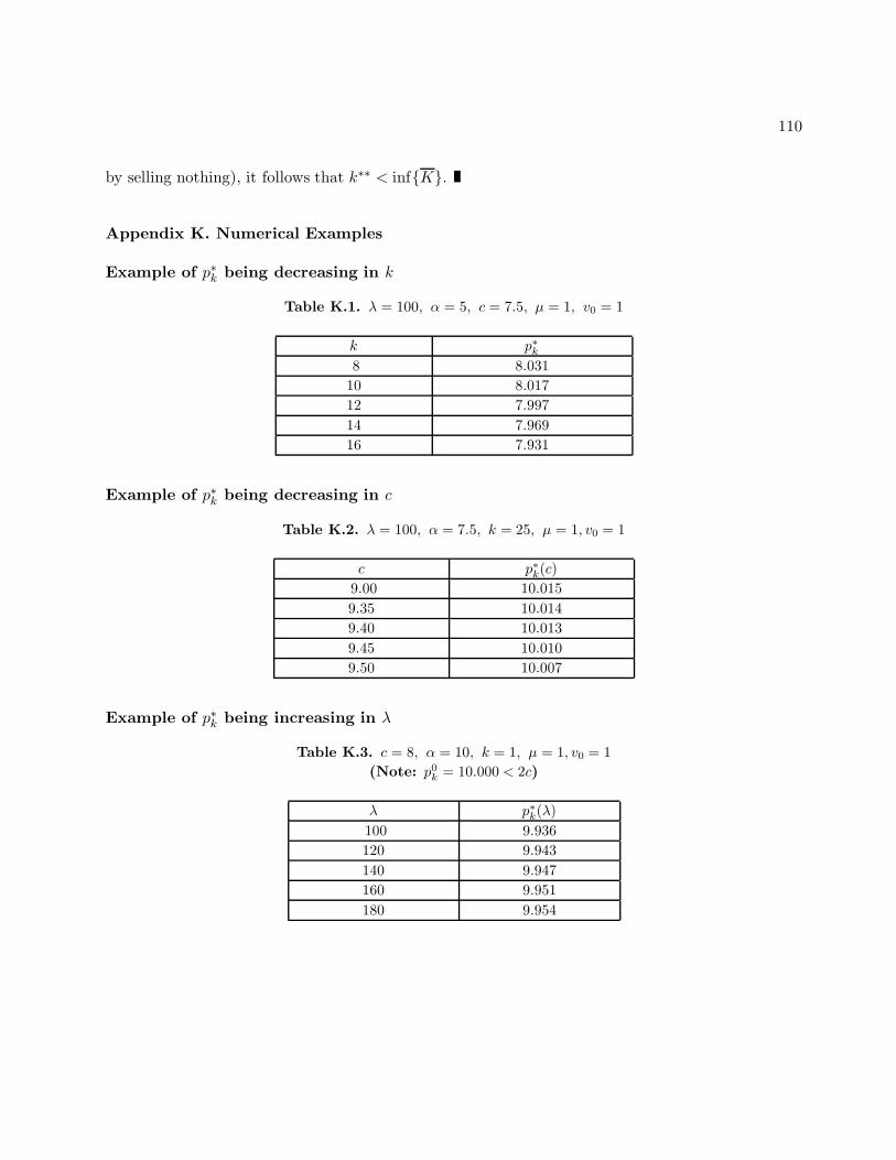
110

by selling nothing), it follows that k∗∗ < infK.

Appendix K. Numerical Examples

Example of p∗k being decreasing in k

Table K.1. λ = 100, α = 5, c = 7.5, µ = 1, v0 = 1

k p∗k8 8.031

10 8.01712 7.99714 7.96916 7.931

Example of p∗k being decreasing in c

Table K.2. λ = 100, α = 7.5, k = 25, µ = 1, v0 = 1

c p∗k(c)9.00 10.0159.35 10.0149.40 10.0139.45 10.0109.50 10.007

Example of p∗k being increasing in λ

Table K.3. c = 8, α = 10, k = 1, µ = 1, v0 = 1(Note: p0

k = 10.000 < 2c)

λ p∗k(λ)100 9.936120 9.943140 9.947160 9.951180 9.954

111

Example of p∗k being decreasing in λ

Table K.4. c = 8, α = 50, k = 1, µ = 1, v0 = 1(Note: p0

k = 46.379 > 2c)

λ p∗k(λ)100 46.388150 46.387200 46.386250 46.385300 46.384

To show that the fact that p∗k may be decreasing in k and nondecreasing c is not due to our approx-

imation in (3.4), we present numerical examples on the behavior of the optimal price based on the

exact expected profit in (3.3), pEk , and the optimal price based on the exact expected profit from

Poisson demands, pPk . The expected profit under Poisson demands is based on the assumption that

the arrival process is a Poisson process with rate λ, then it follows that the demand for item i ∈ Sk,

Xi, has a Poisson distribution with mean λq(p, k), and the expected profit from Poisson demands is

given by

ΠP (p, k) = k

p y∗∑

r=0

rfXi(r) + y∗(1− FXi(r))

− cy∗

,

where fXi(r) = (λq(p,k))r

r! e−λq(p,k) is the density function of Xi, FXi(r) =r∑

l=0g(l) is the corresponding

cumulative density function, and y∗ = F−1Xi

(1 − c/p) is the optimal inventory level for i ∈ Sk. Some

Numerical examples on the behavior of pEk and pP

k follow.

Example of pEk and pP

k being decreasing in k

Table K.5. λ = 105, α = 5, c = 7.5, µ = 1, v0 = 1

k pEk pP

k

5 8.082 8.3446 8.079 8.3277 8.074 8.310

112

Example of pEk and pP

k being nonincreasing in c

Table K.6. λ = 115, α = 8.09, k = 30, µ = 1, v0 = 1

c pEk (c) pP

k (c)9.3015 10.8908297674 10.98888150789.3045 10.8908297674 10.98888150789.3075 10.8908297674 10.9888815078

Appendix L. Structure of the optimal prices under CT

Proof of Theorem 5.2.2. For (pS, pP ) ∈ D, the expected profit is given by

ΠT (pS, pP ) =

ΠT1 (pS, pP ), if cS < pS < 1 + δ− ((pS, pP ) ∈ G),

ΠT2 (pS, pP ), if δ > 0 and 1 ≤ pS < 1 + δ ((pS, pP ) ∈ D \G),

ΠT3 (pS, pP ), if δ ≤ 0 and 1 + δ ≤ pS < 1 ((pS, pP ) ∈ D \G),

where ΠT1 (pS, pP ) = λSP (pS − cS)(1− pS) + λP

ruP − pP

ruP − rl

P

(pS − cS)(δ + 1 − pS) + λPruP − pP

ruP − rl

P

(pP − cP ),

ΠT2 (pS, pP ) = λP

ruP − pP

ruP − rl

P

(pS − cS)(δ + 1 − pS) + λPruP − pP

ruP − rl

P

(pP − cP ),

ΠT3 (pS, pP ) = λSP (pS − cS)(1− pS) + λP

ruP − pP

ruP − rl

P

(pP − cP ).

Observe that the function ΠT (pS, pP ) is everywhere continuous, and everywhere differentiable except

for the lines defined by pP = rlP (cS < pS < 1 + δ+) and pS = 1 + δ− (rl

P ≤ pP < ruP ) (these are the

boundaries of D and G not eliminated by Lemma 5.2.1).

In the following, we show that an optimal price cannot be in D \G, i.e., (pTS , p

TP ) /∈ D \G.

Case 1: δ > 0. In this case, setting ∂ΠT2 (pS ,pP )∂pP

= 0 and solving for pP yields

113

pTP (pS) ≡ −(pS−cS )(δ+1−pS)+ru

P +cP

2 . Now define ΠT2 (pS) ≡ ΠT

2 (pS, pTP (pS)). Then,

ΠT2 (pS) =

λP

4(ruP − rl

P )[(pS − cS)(δ + 1 − pS) + ru

P − cP ]2 .

Observe that a price of S corresponding to a local minimum/maximum of ΠT2 (pS, pP ) is a local

minimum/maximum of ΠT2 (pS). Note that under (A4) and (A5),

(i) limpS→±∞ ΠT2 (pS) = ∞,

(ii) ∂ΠT2 (pS)∂pS

∣∣∣∣pS=cS

= λP

2(ruP−rl

P )(δ + 1− cS)(ru

P − cP ) > 0,

(iii) ∂ΠT2 (pS)∂pS

∣∣∣∣pS=1

= λP

2(ruP−rl

P )(δ − 1 + cS)[δ(1− cS) + ru

P − cP ] < 0, and

(iv) ∂ΠT2 (pS)∂pS

∣∣∣∣pS=δ+1

= − λP

2(ruP−rl

P )(δ + 1 − cS)(ru

P − cP ) < 0.

These imply, since ΠT2 (pS) is a fourth degree polynomial, that ΠT

2 (pS) admits one local minimum, for

pS ∈ (−∞, cS), one local maximum for pS ∈ (cS, 1), another local minimum for pS ∈ (δ+1,∞) and no

local minima/maxima elsewhere. In particular, ΠT2 (pS) has no local minimum/maximum in (1, δ+1),

and, therefore, ΠT (pS, pP ) admits no internal point local maxima onD\G. Then, ΠT (pS, pP ) achieves

its maximum within the boundaries of D \ G (either on the line pS = 1 or on the line pP = rlP ) or

within the interior of G. However, note that ∂ΠT1 (pT

S ,pTP )

∂pS

∣∣∣∣pS=1

= λSP (−1+cS)+λPruP −pP

ruP−rl

P

(δ−1+cS) <

0, which implies that there exists an improving direction (along the direction of pS) from any point

in D \ G on the line pS = 1 leading to the interior of G (because Π(pS, pP ) is continous). Then, it

follows that (pTS , p

TP ) cannot be on the line pS = 1. Similarly, if pP = rl

P , then it can be easily shown

that ΠT2 (pS, r

lP ) is decreasing in pS for all pS > (δ + 1 + cS)/2 < 1, which implies that ΠT

2 (pS, rlP )

is decreasing for pS > 1, and, consequently, there exists an improving direction from any point in

D \G on the line pP = rlP leading to the point (1, rl

P ) (and from there to the interior of G based on

the argument above). This proves that (pTS , p

TP ) /∈ D \G if δ > 0.

114

Case 2: δ < 0. In this case, it can be easily shown that ΠT3 (pS, pP ) admits a unique local maximum

((1+cS)/2, (ruP +cp)/2) /∈ D \G. Therefore, an optimal price (pT

S , pTP ) can only be on the boundaries

of D \ G, and similar to the above case with δ > 0, on the boundary lines pS = δ + 1 or pP = rlP .

An argument similar to the above shows that (pTS , p

TP ) cannot be on the line pS = δ + 1 (since

∂ΠT1 (pT

S ,pTP )

∂pS

∣∣∣∣pS=δ+1

= λSP (−2δ− 1 + cS)+λPruP−pP

ruP−rl

P

(−δ− 1+ cS) < 0). It can be also shown that the

function ΠT (pS, rlP ) is decreasing for pS > δ+1 (since ΠT (pS, r

lP ) is decreasing for pS > (1+cS)/2 =

1 − (1 − cS)/2 < 1 + δ), and then similar to the above, (pTS , p

TP ) cannot be on the line pP = rl

P in

D \G. Therefore, (pTS , p

TP ) /∈ D \G if δ ≤ 0.

Next we show that ΠT1 (pS, pP ) has at most one local maximum on G. Similar to the above, define

ΠT1 (pS) ≡ ΠT

1 (pS, pTP (pS)). Then,

ΠT1 (pS) = λSP (1 − pS)(pS − cS) +

λP

4(ruP − rl

P )[(pS − cS)(δ + 1− pS) + ru

P − cP )]2 .

Then, it can be shown that

(i) limpS→±∞ ΠT1 (pS) = ∞,

(ii) ∂ΠT1 (pS)∂pS

∣∣∣∣pS=cS

= λSP (1 − cS) + λP

2(ruP−rl

P )(δ + 1 − cS)(ru

P − cP ) > 0.

(iii) If δ > 0, then ∂ΠT1 (pS)∂pS

∣∣∣∣pS=1

= −λSP (1 − cS) + λP

2(ruP−rl

P )(δ − 1 + cS)[δ(1− cS) + ru

P − cP ] < 0.

(iv) Otherwise, if δ ≤ 0, then dΠT1 (pS)dpS

∣∣∣∣pS=δ+1

= λSP (−2δ−1+cS)− λP

2(ruP−rl

P )(δ+1−cS)(ru

P −cP ) < 0.

It follows that ΠT1 (pS) admits one local minimum for pS ∈ (−∞, cS) and another one for pS ∈

(1+δ−,∞). The fact that ΠT1 (pS) is a fourth degree polynomial then implies that it will admit exactly

one local maximum for pS ∈ (cS, 1+δ−). There are two cases to consider. Either this local maximum

of ΠT1 (pS) will correspond to a unique internal point local maximum of ΠT (pS, pP ) withinG ( given by

the solution to the first order optimality conditions in (5.6) and (5.7)), or, otherwise, ΠT (pS, pP ) will

115

admit a local maximum on its boundaries (because Lemma 5.2.1 gurantees that ΠT (pS, pP ) admits

a local maximum in D). In the latter case, Lemma 5.2.1 and the above imply that a boundary

point local maximum of ΠT (pS, pP ) within G will only be on the line pP = rlP . Then, it can be

seen by maximizing the function Π1(pS, rlP ) that this local maximum is (1+cS

2 +δ λP2(λSP +λP ) , r

lP ) ∈ G.

(Observe that this solution is in G because under (A4) and (A5), if δ > 0, then cS < 1+cS2 <

1+cS2 +δ λP

2(λSP+λP ) <1+cS

2 + 1−cS2 = 1. If δ ≤ 0, then 1+cS

2 +δ λP2(λSP +λP ) ≥ 1+cS

2 +δ/2 ≥ 1+cS2 − (1−cS)

4 =

14 + 3cS

4 > cS4 + 3cS

4 = cS, and 1+cS2 + δ λP

2(λSP +λP ) <1+cS

2 = 1− (1−cS)2 ≤ 1 + δ.)

Appendix M. Comparison of the optimal prices under IC and CT

Proof of Lemma 5.2.2. Recall that p0S = 1+cS

2 . Then, Theorem 5.2.2 implies that either pTS =

p0S + δ λP

2λSP +λP, or pT

S = p0S + α

1+2αδ, where α = λP2λSP

(rup−pT

P )

rup−rl

p> 0. This proves (i).

To prove (ii), recall that p0P = ru

P +cP

2 . Then, Theorem 5.2.2 implies that either pTP = rl

P < p0P , or

pTP = p0

P − β2 , where β = (δ + 1 − pT

S )(pTS − cS) > 0 (by Theorem 5.2.2). This completes the proof.

Appendix N. Monotonicity results on the optimal prices under CT

Proof of Lemma 5.2.3. To prove (i), note that it can be shown, by implicit differentiation (in the

light of Theorem 5.2.2), that ∂pTS (λSP )∂λSP

is of the same sign as ∂2ΠT1 (pS ,λSP )

∂λSP ∂pS

∣∣∣∣pS=pT

S

. We derive

∂ΠT1 (pS)∂pS

= −λSP (pS − cS) + λSP (1− pS)

+ λP

2(ruP−rl

P )[(δ + 1− pS) − (pS − cS)] [(δ + 1− pS)(pS − cS) + ru

P − cP ] .

Then, ∂2ΠT1 (pS ,λSP )

∂λSP ∂pS

∣∣∣∣pS=pT

S

= −(pTS −cS)+(1−pT

S) = −2(pTS −p0

S). Then the result follows by Lemma

5.2.2.

116

Similarly, ∂pTS (λP )

∂λPis of the same sign as

∂2ΠT1 (pS, λP )∂λP∂pS

∣∣∣∣∣pS=pT

S

=1

2(ruP − rl

P )

[(δ + 1 − pT

S ) − (pTS − cS)

] [(δ + 1 − pT

S )(pTS − cS) + ru

P − cP],

where (δ + 1− pTS ) > 0 since pT

S ∈ G, and therefore ∂pTS (λP )∂λP


(δ + 1 − pTS ) − (pT

S − cS) = −2(pTS − p0

S − δ/2). Observe, from the proof of Lemma 5.2.2, that

pTS − p0

S = α(1+2α)δ < δ/2 if δ > 0 (and > δ/2 if δ < 0). This proves (ii).

By the same reasoning, ∂pTS (rl

P )

∂rlP


∂2ΠT1 (pS, r

lP )

∂rlP∂pS


S

=λP

2(ruP − rl

P )2[(δ + 1 − pT

S )− (pTS − cS)

] [(δ + 1 − pT


P − cP]> 0,

if δ > 0 (and < 0 if δ < 0), which proves (iii).

Similarly, ∂pTS (δ)∂δ is of the same sign as

∂2ΠT (pS, δ)∂δ∂pS


S

=λP

2(ruP − rl

P )

(δ + 1 − pT

S ) − (pTS − cS) + (δ + 1 − pT


P − cP> 0,

if δ > 0, which proves (iv).

Finally, ∂pTS (cP )

∂cPis of the same sign as

∂2ΠT1 (pS, cP )∂cP∂pS


S

= − λP

2(ruP − rl

P )

[(δ + 1 − pT

S ) − (pTS − cS)

]< 0,

if δ > 0 (and > 0 if δ < 0).

Proof of Lemma 5.2.4. By Theorem 5.2.2, we have that pTP = −(pT

S−cS )(δ+1−pTS )+ru

P +cP

2 . Therefore,

pTP is decreasing in pT

S if pTS < (δ+cS +1)/2 (or equivalently, pT

S −p0S < δ/2), and otherwise increasing

117

in pTS . Moreover, as shown in Lemma 5.2.3, pT

S − p0S < δ/2, if δ > 0 (and < δ/2 if δ < 0). The proof

then follows from Lemma 5.2.3.

Appendix O. Comparison of optimal profits under IC and CT

Proof of Lemma 5.2.5. To prove (i), note that when pP is fixed, ΠT ∗ − Π0∗ = ΠTS (pT

S , pP ) −

Π0S(p0

S), ΠTS (pT

S , pP ) is the expected profit from S under CT. Note also that the first-order optimality

conditions imply that pTS = p0

S + γ(pP ) where γ(pP ) is as defined above (similar to equation (5.6) in

Theorem 5.2.2). Then, it can be shown that

ΠT ∗ − Π0∗ = λSP [(1− p0S− γ(pP ))(p0

S+ γ(pP ) − cS)− (1− p0

S)(p0

S− cS)]

+ λP qP (pP )(δ + 1− p0S− γ(pP ))(p0

S+ γ(pP ) − cS)− λ0

SP (1 − p0S)(p0

S − cS).

Utilizing the identity that p0S = 1+cS

2 and simplifying yields the desired result.

Similarly, to prove (ii) note that with pS fixed,

ΠT ∗ − Π0∗ = ΠP (pTP ) + ΠT

SP (pS, pTP )− ΠP (p0

P ) − Π0SP (pS),

where Π0SP (pS) = λ0

SP (pS − cS)qS(pS), pTP = p0

P − β(pS)2 and β(pS) ≡ (δ+ 1− pS)(pS − cS). Then, it

can be shown that

ΠT ∗ − Π0∗ = λPqP (p0P )β(ps)

2+ λP

β(ps)2(ru

P − rlP )

(β(ps)

2+ p0

P − cP

)− λ0

SP (1− ps)(ps − cS),

and the result follows by utilizing the identity that p0P = ru

P +cP

2 and simplifying.

Appendix P. Comparison of CT and IC under exogenous pricing and finite inventories

Proof of Lemma 5.3.1. CT is more profitable than IC if and only if ΠT − Π0 > 0, where ΠT and

118

Π0 are as given in (5.8) and (5.9). Then

ΠT − Π0 = (pS − cS)µT

SP − µ0SP − θS

pS

pS − cS

(√µT

SP +√µSP −

√µ0

SP + µSP

).

Next we show that ΠT −Π0 > 0 only if µTSP −µ0

SP > 0. By contradiction, assume that µTSP −µ0

SP ≤ 0

and ΠT − Π0 > 0. Then the fact that√µ0

SP + µSP <√µ0

SP + √µSP implies that

ΠT − Π0 <

(√µT

SP −√µ0

SP

)(√µT

SP +√µ0

SP − θSps

ps − cS

).

Therefore, ΠT − Π0 > 0 only if√µT

SP +√µ0

SP − θSpS

pS−cS< 0. However,

√µT

SP > θSpS

pS−cSfrom

(A6). This completes the contradiction proof. Note finally that when µTSP − µ0

SP > 0,√µT

SP + √µSP −

√µ0

SP + µSP > 0 .

119

Vita

Bacel Maddah was born in Mimess, South Lebanon on December 7, 1976. He obtained a Bachelor

degree in Civil Engineering from the Lebanese University and a Masters degree in Engineering

Management from the American University of Beirut. He moved from Lebanon to the U.S. in

August 2000 and joined Virginia Tech in August 2001. Bacel research interests are in retail operations

management, queueing theory, and inventory control. He has authored several research articles on

these topics. Bacel has also been active in developing software tools for both practical and academic

purposes, and has had several internships with the industry. He will work as a senior analyst with

United Airlines upon graduating from Virginia Tech. His long-term goals are to continue research

work and to someday go back to Lebanon and contribute to ongoing efforts of social reform.

Pricing, Variety, and Inventory Decisions in Retail ...

Documents

Transcript of Pricing, Variety, and Inventory Decisions in Retail ...